(e book math) pdf - an introduction to complex analysis for engineers
TRANSCRIPT

An Introduction to Complex Analysis for
Engineers
Michael D. Alder
June 3, 1997

1
Preface
These notes are intended to be of use to Third year Electrical and Elec-
tronic Engineers at the University of Western Australia coming to grips with
Complex Function Theory.
There are many text books for just this purpose, and I have insu�cient time
to write a text book, so this is not a substitute for, say, Matthews and How-
ell's Complex Analysis for Mathematics and Engineering,[1], but perhaps a
complement to it. At the same time, knowing how reluctant students are to
use a textbook (except as a talisman to ward o� evil) I have tried to make
these notes su�cient, in that a student who reads them, understands them,
and does the exercises in them, will be able to use the concepts and tech-niques in later years. It will also get the student comfortably through theexamination. The shortness of the course, 20 lectures, for covering Complex
Analysis, either presupposes genius ( 90% perspiration) on the part of thestudents or material skipped. These notes are intended to �ll in some of the
gaps that will inevitably occur in lectures. It is a source of some disappoint-ment to me that I can cover so little of what is a beautiful subject, rich inapplications and connections with other areas of mathematics. This is, then,
a sort of sampler, and only touches the elements.
Styles of Mathematical presentation change over the years, and what wasdeemed acceptable rigour by Euler and Gauss fails to keep modern puristscontent. McLachlan, [2], clearly smarted under the criticisms of his presen-
tation, and he goes to some trouble to explain in later editions that the book
is intended for a di�erent audience from the purists who damned him. My
experience leads me to feel that the need for rigour has been developed tothe point where the intuitive and geometric has been stunted. Both have apart in mathematics, which grows out of the con ict between them. But it
seems to me more important to penetrate to the ideas in a sloppy, scru�y
but serviceable way, than to reduce a subject to predicate calculus and omitthe whole reason for studying it. There is no known means of persuading a
hardheaded engineer that a subject merits his time and energy when it hasbeen turned into an elaborate game. He, or increasingly she, wants to see two
elements at an early stage: procedures for solving problems which make a
di�erence and concepts which organise the procedures into something intelli-gible. Carried to excess this leads to avoidance of abstraction and consequent

2
loss of power later; there is a good reason for the purist's desire for rigour.
But it asks too much of a third year student to focus on the underlying logic
and omit the geometry.
I have deliberately erred in the opposite direction. It is easy enough for the
student with a taste for rigour to clarify the ideas by consulting other books,
and to wind up as a logician if that is his choice. But it is hard to �nd in
the literature any explicit commitment to getting the student to draw lots
of pictures. It used to be taken for granted that a student would do that
sort of thing, but now that the school syllabus has had Euclid expunged, the
undergraduates cannot be expected to see drawing pictures or visualising sur-
faces as a natural prelude to calculation. There is a school of thought which
considers geometric visualisation as immoral; and another which sanctions it
only if done in private (and wash your hands before and afterwards). To my
mind this imposes sterility, and constitutes an attempt by the bureaucrat tostrangle the artist. 1 While I do not want to impose my informal images on
anybody, if no mention is made of informal, intuitive ideas, many studentsnever realise that there are any. All the good mathematicians I know have arich supply of informal models which they use to think about mathematics,
and it were as well to show students how this may be done. Since this seemsto be the respect in which most of the text books are weakest, I have perhapsgone too far in the other direction, but then, I do not o�er this as a text
book. More of an antidote to some of the others.
I have talked to Electrical Engineers about Mathematics teaching, and theyare strikingly consistent in what they want. Prior to talking to them, I
feared that I'd �nd Engineers saying things like `Don't bother with the ideas,
forget about the pictures, just train them to do the sums'. There are, alas,Mathematicians who are convinced that this is how Engineers see the world,
and I had supposed that there might be something in this belief. Silly me.
In fact, it is simply quite wrong.
The Engineers I spoke to want Mathematicians to get across the abstract
ideas in terms the students can grasp and use, so that the Engineers can
subsequently rely on the student having those ideas as part of his or her
1The bureaucratic temper is attracted to mathematics while still at school, because it
appears to be all about following rules, something the bureaucrat cherishes as the solution
to the problems of life. Human beings on the other hand �nd this su�ciently repellant
to be put o� mathematics permanently, which is one of the ironies of education. My own
attitude to the bureaucratic temper is rather that of Dave Allen's feelings about politicians.
He has a soft spot for them. It's a bog in the West of Ireland.

3
thinking. Above all, they want the students to have clear pictures in their
heads of what is happening in the mathematics. Since this is exactly what
any competent Mathematician also wants his students to have, I haven't felt
any need to change my usual style of presentation. This is informal and
user-friendly as far as possible, with (because I am a Topologist by training
and work with Engineers by choice) a strong geometric avour.
I introduce Complex Numbers in a way which was new to me; I point out
that a certain subspace of 2� 2 matrices can be identifed with the plane R2 ,
thus giving a simple rule for multiplying two points in R2 : turn them into
matrices, multiply the matrices, then turn the answer back into a point. I
do it this way because (a) it demysti�es the business of imaginary numbers,
(b) it gives the Cauchy-Riemann conditions in a conceptually transparent
manner, and (c) it emphasises that multiplication by a complex number is a
similarity together with a rotation, a matter which is at the heart of muchof the applicability of the complex number system. There are a few other
advantages of this approach, as will be seen later on. After I had done it thisway, Malcolm Hood pointed out to me that Copson, [3], had taken the sameapproach.2
Engineering students lead a fairly busy life in general, and the Sparkies have
a particularly demanding load. They are also very practical, rightly so, andimpatient of anything which they suspect is academic window-dressing. Sofar, I am with them all the way. They are, however, the main source of
the belief among some mathematicians that peddling recipes is the only wayto teach them. They do not feel comfortable with abstractions. Their goal
tends to be examination passing. So there is some basic opposition between
the students and me: I want them to be able to use the material in lateryears, they want to memorise the minimum required to pass the exam (and
then forget it).
I exaggerate of course. For reasons owing to geography and history, this
University is particularly fortunate in the quality of its students, and most
of them respond well to the discovery that Mathematics makes sense. I hope
that these notes will turn out to be enjoyable as well as useful, at least inretrospect.
But be warned:
2I am most grateful to Malcolm for running an editorial eye over these notes, but even
more grateful for being a model of sanity and decency in a world that sometimes seems
bereft of both.

4
` Well of course I didn't do any at �rst ... then someone suggested I try just
a little sum or two, and I thought \Why not? ... I can handle it". Then
one day someone said \Hey, man, that's kidstu� - try some calculus" ... so I
tried some di�erentials ... then I went on to integrals ... even the occasional
volume of revolution ... but I can stop any time I want to ... I know I can.
OK, so I do the odd bit of complex analysis, but only a few times ... that
stu� can really screw your head up for days ... but I can handle it ... it's OK
really ... I can stop any time I want ...' ( [email protected] (Tim
Bierman))
Contents
1 Fundamentals 9
1.1 A Little History . . . . . . . . . . . . . . . . . . . . . . . . . . 9
1.2 Why Bother With Complex Numbers and Functions? . . . . . 11
1.3 What are Complex Numbers? . . . . . . . . . . . . . . . . . . 12
1.4 Some Soothing Exercises . . . . . . . . . . . . . . . . . . . . . 18
1.5 Some Classical Jargon . . . . . . . . . . . . . . . . . . . . . . 22
1.6 The Geometry of Complex Numbers . . . . . . . . . . . . . . 26
1.7 Conclusions . . . . . . . . . . . . . . . . . . . . . . . . . . . . 29
2 Examples of Complex Functions 33
2.1 A Linear Map . . . . . . . . . . . . . . . . . . . . . . . . . . . 34
2.2 The function w = z2 . . . . . . . . . . . . . . . . . . . . . . . 36
2.3 The Square Root: w = z1
2 . . . . . . . . . . . . . . . . . . . . 46
2.3.1 Branch Cuts . . . . . . . . . . . . . . . . . . . . . . . . 49
2.3.2 Digression: Sliders . . . . . . . . . . . . . . . . . . . . 51
2.4 Squares and Square roots: Summary . . . . . . . . . . . . . . 58
2.5 The function f(z) = 1z
. . . . . . . . . . . . . . . . . . . . . 58
5

6 CONTENTS
2.6 The M�obius Transforms . . . . . . . . . . . . . . . . . . . . . 66
2.7 The Exponential Function . . . . . . . . . . . . . . . . . . . . 69
2.7.1 Digression: In�nite Series . . . . . . . . . . . . . . . . 70
2.7.2 Back to Real exp . . . . . . . . . . . . . . . . . . . . . 73
2.7.3 Back to Complex exp and Complex ln . . . . . . . . . 76
2.8 Other powers . . . . . . . . . . . . . . . . . . . . . . . . . . . 81
2.9 Trigonometric Functions . . . . . . . . . . . . . . . . . . . . . 82
3 C - Di�erentiable Functions 89
3.1 Two sorts of Di�erentiability . . . . . . . . . . . . . . . . . . . 89
3.2 Harmonic Functions . . . . . . . . . . . . . . . . . . . . . . . 97
3.2.1 Applications . . . . . . . . . . . . . . . . . . . . . . . . 100
3.3 Conformal Maps . . . . . . . . . . . . . . . . . . . . . . . . . 102
4 Integration 105
4.1 Discussion . . . . . . . . . . . . . . . . . . . . . . . . . . . . . 105
4.2 The Complex Integral . . . . . . . . . . . . . . . . . . . . . . 107
4.3 Contour Integration . . . . . . . . . . . . . . . . . . . . . . . . 113
4.4 Some Inequalities . . . . . . . . . . . . . . . . . . . . . . . . . 119
4.5 Some Solid and Useful Theorems . . . . . . . . . . . . . . . . 120
5 Taylor and Laurent Series 131
5.1 Fundamentals . . . . . . . . . . . . . . . . . . . . . . . . . . . 131
5.2 Taylor Series . . . . . . . . . . . . . . . . . . . . . . . . . . . . 134

CONTENTS 7
5.3 Laurent Series . . . . . . . . . . . . . . . . . . . . . . . . . . . 138
5.4 Some Sums . . . . . . . . . . . . . . . . . . . . . . . . . . . . 140
5.5 Poles and Zeros . . . . . . . . . . . . . . . . . . . . . . . . . . 143
6 Residues 149
6.1 Trigonometric Integrals . . . . . . . . . . . . . . . . . . . . . . 153
6.2 In�nite Integrals of rational functions . . . . . . . . . . . . . . 154
6.3 Trigonometric and Polynomial functions . . . . . . . . . . . . 159
6.4 Poles on the Real Axis . . . . . . . . . . . . . . . . . . . . . . 161
6.5 More Complicated Functions . . . . . . . . . . . . . . . . . . . 164
6.6 The Argument Principle; Rouch�e's Theorem . . . . . . . . . . 168
6.7 Concluding Remarks . . . . . . . . . . . . . . . . . . . . . . . 174

8 CONTENTS
Chapter 1
Fundamentals
1.1 A Little History
If Complex Numbers had been invented thirty years ago instead of over
three hundred, they wouldn't have been called `Complex Numbers' at all.They'd have been called `Planar Numbers', or `Two-dimensional Numbers'or something similar, and there would have been none of this nonsense about
`imaginary' numbers. The square root of negative one is no more and no lessimaginary than the square root of two. Or two itself, for that matter. All of
them are just bits of language used for various purposes.
`Two' was invented for counting sheep. All the positive integers (whole num-bers) were invented so we could count things, and that's all they were in-vented for. The negative integers were introduced so it would be easy to
count money when you owed more than you had.
The rational numbers were invented for measuring lengths. Since we cantransduce things like voltages and times to lengths, we can measure other
things using the rational numbers, too.
The Real numbers were invented for wholly mathematical reasons: it was
found that there were lengths such as the diagonal of the unit square which,in principle, couldn't be measured by the rational numbers. This is of not
the slightest practical importance, because in real life you can measure onlyto some limited precision, but some people like their ideas to be clean and
cool, so they went o� and invented the real numbers, which included the
9

10 CHAPTER 1. FUNDAMENTALS
rationals but also �lled in the holes. So practical people just went on doing
what they'd always done, but Pure Mathematicians felt better about them
doing it. Daft, you might say, but let us be tolerant.
This has been put in the form of a story:
A (male) Mathematician and a (male) Engineer who knew each other, had
both been invited to the same party. They were standing at one corner of the
room and eyeing a particularly attractive girl in the opposite corner. `Wow,
she looks pretty good,' said the Engineer. `I think I'll go over there and try
my luck.'
`Impossible, and out of the question!' said the Mathematician, who was
thinking much the same but wasn't as forthright.
`And why is it impossible?' asked the Engineer belligerently.
`Because,' said the Mathematician, thinking quickly, `In order to get to her,you will �rst have to get halfway. And then you will have to get half of the
rest of the distance, and then half of that. And so on; in short, you can neverget there in a �nite number of moves.'
The Engineer gave a cheerful grin.
`Maybe so,' he replied, `But in a �nite number of moves, I can get as closeas I need to be for all practical purposes.'
And he made his moves.
***
The Complex Numbers were invented for purely mathematical reasons, just
like the Reals, and were intended to make things neat and tidy in solving
equations. They were regarded with deep suspicion by the more conservativefolk for a century or so.
It turns out that they are very cool things to have for `measuring' such things
as periodic waveforms. Also, the functions which arise between them are very
useful for talking about solutions of some Partial Di�erential Equations. Sodon't look down on Pure Mathematicians for wanting to have things clean
and cool. It pays o� in very unexpected ways. The Universe also seemsto like things clean and cool. And most supersmart people, such as Gauss,
like �nding out about Electricity and Magnetism, working out how to handle

1.2. WHY BOTHERWITH COMPLEX NUMBERS AND FUNCTIONS?11
calculations of orbits of asteroids and doing Pure Mathematics.
In these notes, I am going to rewrite history and give you the story about
Complex Numbers and Functions as if they had been developed for the appli-
cations we now know they have. This will short-circuit some of the mystery,
but will be regarded as shocking by the more conservative. The same sort of
person who three hundred years ago wanted to ban them, is now trying to
keep the confusion. It's a funny old world, and no mistake.
Your text books often have an introductory chapter explaining a bit of the
historical development, and you should read this in order to be educated,
but it isn't in the exam.
1.2 Why BotherWith Complex Numbers and
Functions?
In mastering the material in this book, you are going to have to do a lot of
work. This will consist mainly of chewing a pencil or pen as you struggle todo some sums. Maths is like that. Hours of your life will pass doing this,when you could be watching the X-�les or playing basketball, or whatever.
There had better be some point to this, right?
There is, but it isn't altogether easy to tell you exactly what it is, becauseyou can only really see the advantages in hindsight. You are probably quite
glad now that you learnt to read when you were small, but it might have
seemed a drag at the time. Trust me. It will all be worth it in the end.
If this doesn't altogether convince you, then talk to the Engineering Lec-turers about what happens in their courses. Generally, the more modern
and intricate the material, the more Mathematics it uses. Communication
Engineering and Power Transmission both use Complex Functions; Filtering
Theory in particular needs it. Control Theory uses the subject extensively.Whatever you think about Mathematicians, your lecturers in Engineeringare practical people who wouldn't have you do this course if they thought
they could use the time for teaching you more important things.
Another reason for doing it is that it is fun. You may �nd this hard to believe,but solving problems is like doing exercise. It keeps you �t and healthy and
has its own satisfactions. I mean, on the face of it, someone who runs three

12 CHAPTER 1. FUNDAMENTALS
kilometres every morning has to be potty: they could get there faster in a
car, right? But some people do it and feel good about themselves because
they've done it. Well, what works for your heart and lungs also applies to
your brain. Exercising it will make you feel better. And Complex Analysis is
one of the tougher and meatier bits of Mathematics. Tough minded people
usually like it. But like physical exercise, it hurts the �rst time you do it,
and to get the bene�ts you have to keep at it for a while.
I don't expect you to buy the last argument very easily. You're kept busy
with the engineering courses which are much more obviously relevant, and
I'm aware of the pressure you are under. Your main concern is making sure
you pass the examination. So I am deliberately keeping the core material
minimal.
I am going to start o� by assuming that you have never seen any complexnumbers in your life. In order to explain what they are I am going to do a
bit of very easy linear algebra. The reasons for this will become clear fairlyquickly.
1.3 What are Complex Numbers?
Complex numbers are points in the plane, together with a rule telling you
how to multiply them. They are two-dimensional, whereas the Real numbersare one dimensional, they form a line. The fact that complex numbers form
a plane is probably the most important thing to know about them.
Remember from �rst year that 2� 2 matrices transform points in the plane.
To be de�nite, take �x
y
�
for a point, or if you prefer vector in R2 and let
�a c
b d
�
be a 2� 2 matrix. Placing the matrix to the left of the vector:
�a c
b d
� �x
y
�

1.3. WHAT ARE COMPLEX NUMBERS? 13
and doing matrix multiplication gives a new vector:�ax + cy
bx + dy
�
This is all old stu� which you ought to be good at by now1.
Now I am going to look at a subset of the whole collection of 2� 2 matrices:
those of the form �a �bb a
�
for any real numbers a; b.
The following remarks should be carefully checked out:
� These matrices form a linear subspace of the four dimensional space ofall 2� 2 matrices. If you add two such matrices, the result still has the
same form, the zero matrix is in the collection, and if you multiply anymatrix by a real number, you get another matrix in the set.
� These matrices are also closed under multiplication: If you multiplyany two such matrices, say�
a �bb a
�and
�c �dd c
�
then the resulting matrix is still antisymmetric and has the top leftentry equal to the bottom right entry, which puts it in our set.
� The identity matrix is in the set.
� Every such matrix has an inverse except when both a and b are zero,
and the inverse is also in the set.
� The matrices in the set commute under multiplication. It doesn't mat-ter which order you multiply them in.
� All the rotation matrices: �cos � � sin �sin � cos �
�
are in the set.
1If you are not very con�dent about this, (a) admit it to yourself and (b) dig out some
old Linear Algebra books and practise a bit.

14 CHAPTER 1. FUNDAMENTALS
� The columns of any matrix in the set are orthogonal
� This subset of all 2� 2 matrices is two dimensional.
Exercise 1.3.1 Before going any further, go through every item on this list
and check out that it is correct. This is important, because you are going to
have to know every one of them, and verifying them is or ought to be easy.
This particular collection of matrices IS the set of Complex Numbers. I de�ne
the complex numbers this way:
De�nition 1.3.1 C is the name of the two dimensional subspace of the four
dimensional space of 2� 2 matrices having entries of the form
�a �bb a
�
for any real numbers a; b. Points of C are called, for historical reasons,
complex numbers.
There is nothing mysterious or mystical about them, they behave in a thor-oughly straightforward manner, and all the properties of any other complexnumbers you might have come across are all properties of my complex num-
bers, too.
You might be feeling slightly gobsmacked by this; where are all the imaginarynumbers? Where is
p�1? Have patience. We shall now gradually recover
all the usual hocus-pocus.
First, the fact that the set of matrices is a two dimensional vector space
means that we can treat it as if it were R2 for many purposes. To nail thisidea down, de�ne:
C : R2 �! C
by �a
b
�;
�a �bb a
�
This sets up a one to one correspondence between the points of the planeand the matrices in C . It is easy to check out:

1.3. WHAT ARE COMPLEX NUMBERS? 15
Proposition 1.3.1 C is a linear map
It is clearly onto, one-one and an isomorphism. What this means is that there
is no di�erence between the two objects as far as the linear space properties
are concerned. Or to put it in an intuitive and dramatic manner: You can
think of points in the plane
�a
b
�or you can think of matrices
�a �bb a
�and
it makes no practical di�erence which you choose- at least as far as adding,
subtracting or scaling them is concerned. To drive this point home, if you
choose the vector representation for a couple of points, and I translate them
into matrix notation, and if you add your vectors and I add my matrices,
then your result translates to mine. Likewise if we take 3 times the �rst and
add it to 34 times the second, it won't make a blind bit of di�erence if you
do it with vectors or I do it with matrices, so long as we stick to the sametranslation rules. This is the force of the term isomorphism, which is derivedfrom a Greek word meaning `the same shape'. To say that two things are
isomorphic is to say that they are basically the same, only the names have
been changed. If you think of a vector
�a
b
�as being a `name' of a point
in R2 , and a two by two matrix
�a �bb a
�as being just a di�erent name
for the same point, you will have understood the very important idea of anisomorphism.
You might have an emotional attachment to one of these ways of representing
points in R2 , but that is your problem. It won't actually matter which you
choose.
Of course, the matrix form uses up twice as much ink and space, so you'd bea bit weird to prefer the matrix form, but as far as the sums are concerned,
it doesn't make any di�erence.
Except that you can multiply the matrices as well as add and subtract and
scale them.
And what THIS means is that we have a way of multiplying points of R2 .
Given the points
�a
b
�and
�c
d
�in R
2 , I decide that I prefer to think of
them as matrices
�a �bb a
�and
�c �dd c
�, then I multiply these together
16 CHAPTER 1. FUNDAMENTALS
to get (check this on a piece of paper)
�ac� bd �(ad + bc)
ad+ bc ac� bd
�
Now, if you have a preference for the more compressed form, you can't mul-
tiply your vectors, Or can you? Well, all you have to do is to translate your
vectors into my matrices, multiply them and change them back to vectors.
Alternatively, you can work out what the rules are once and store them in a
safe place:
�a
b
���c
d
�=
�ac� bd
ad+ bc
�
Exercise 1.3.2 Work through this carefully by translating the vectors into
matrices then multiply the matrices, then translate back to vectors.
Now there are lots of ways of multiplying points of R2 , but this particular
way is very cool and does some nice things. It isn't the most obvious wayfor multiplying points of the plane, but it is a zillion times as useful as the
others. The rest of this book after this chapter will try to sell that idea.
First however, for those who are still worried sick that this seems to have
nothing to do with (a + ib), we need to invent a more compressed notation.I de�ne:
De�nition 1.3.2 For all a; b 2 R; a + ib =
�a �bb a
�
So you now have three choices.
1. You can write a+ ib for a complex number; a is called the real part andb is called the imaginary part. This is just ancient history and faintly
weird. I shall call this the classical representation of a complex number.
The i is not a number, it is a sort of tag to keep the two components(a,b) separated.

1.3. WHAT ARE COMPLEX NUMBERS? 17
2. You can write
�a
b
�for a complex number. I shall call this the point
representation of a complex number. It emphasises the fact that the
complex numbers form a plane.
3. You can write �a �bb a
�
for the complex number. I shall call this the matrix representation for
the complex number.
If we go the �rst route, then in order to get the right answer when we multiply
(a + ib) � (c+ id) = ((ac� bd) + i(bc + ad))
(which has to be the right answer from doing the sum with matrices) we cansort of pretend that i is a number but that i2 = �1. I suggest that you might
feel better about this if you think of the matrix representation as the basicone, and the other two as shorthand versions of it designed to save ink and
space.
Exercise 1.3.3 Translate the complex numbers (a+ib) and (c+id) into ma-
trix form, multiply them out and translate the answer back into the classical
form.
Now pretend that i is just an ordinary number with the property that i2 = �1.Multiply out (a + ib) � (c + id) as if everything is an ordinary real number,
put i2 = �1, and collect up the real and imaginary parts, now using the i as
a tag. Verify that you get the same answer.
This certainly is one way to do things, and indeed it is traditional. But it
requires the student to tell himself or herself that there is something deeplymysterious going on, and it is better not to ask too many questions. Actually,
all that is going on is muddle and confusion, which is never a good idea unless
you are a politician.
The only thing that can be said about these three notations is that they each
have their own place in the scheme of things.
The �rst, (a + ib), is useful when reading old fashioned books. It has the
advantage of using least ink and taking up least space. Another advantage

18 CHAPTER 1. FUNDAMENTALS
is that it is easy to remember the rule for multiplying the points: you just
carry on as if they were real numbers and remember that i2 = �1. It has thedisadvantage that it leaves you with a feeling that something inscrutable is
going on, which is not the case.
The second is useful when looking at the geometry of complex numbers,
something we shall do a lot. The way in which some of them are close to
others, and how they move under transformations or maps, is best done by
thinking of points in the plane.
The third is helpful when thinking about the multiplication aspects of com-
plex numbers. Matrix multiplication is something you should be quite com-
fortable with.
Which is the right way to think of complex numbers? The answer is: All
of the above, simultaneously. To focus on the geometry and ignore thealgebra is a blunder, to focus on the algebra and forget the geometry is aneven bigger blunder. To use a compact notation but to forget what it means
is a sure way to disaster.
If you can be able to ip between all three ways of looking at the complexnumbers and choose whichever is easiest and most helpful, then the subject
is complicated but fairly easy. Try to �nd the one true way and cling to itand you will get marmelised. Which is most uncomfortable.
1.4 Some Soothing Exercises
You will probably be feeling a bit gobsmacked still. This is quite normal,and is cured by the following procedure: Do the next lot of exercises slowly
and carefully. Afterwards, you will see that everything I have said so far isdead obvious and you will wonder why it took so long to say it. If, on the
other hand you decide to skip them in the hope that light will dawn at a
later stage, you risk getting more and more muddled about the subject. Thiswould be a pity, because it is really rather neat.
There is a good chance you will try to convince yourself that it will be enough
to put o� doing these exercises until about a week before the exam. This
will mean that you will not know what is going on for the rest of the course,but will spend the lectures copying down the notes with your brain out of

1.4. SOME SOOTHING EXERCISES 19
gear. You won't enjoy this, you really won't.
So sober up, get yourself a pile of scrap paper and a pen, put a chair some-
where quiet and make sure the distractions are somewhere else. Some people
are too dumb to see where their best interests lie, but you are smarter than
that. Right?
Exercise 1.4.1 Translate the complex numbers (1+i0), (0 +i1), (3-i2) into
the other two forms. The �rst is often written 1, the second as i.
Exercise 1.4.2 Translate the complex numbers
�2 0
0 2
�;
�0 1
�1 0
�;
�0 �11 0
�;
and
�2 �11 2
�into the other two forms.
Exercise 1.4.3 Multiply the complex number
�0
1
�
by itself. Express in all three forms.
Exercise 1.4.4 Multiply the complex numbers
�2
3
�and
�2
�3
�
Now do it for �a
b
�and
�a
�b
�
Translate this into the (a+ib) notation.
Exercise 1.4.5 It is usual to de�ne the norm of a point as its distance from
the origin. The convention is to write
k�a
b
�k =
pa2 + b2

20 CHAPTER 1. FUNDAMENTALS
In the classical notation, we call it the modulus and write
ja+ ibj =pa2 + b2
There is not the slightest reason to have two di�erent names except that this
is what we have always done.
Find a description of the complex numbers of modulus 1 in the point and
matrix forms. Draw a picture in the �rst case.
Exercise 1.4.6 You can also represent points in the plane by using polar
coordinates. Work out the rules for multiplying (r; �) by (s; �). This is a
fourth representation, and in some ways the best. How many more, you may
ask.
Exercise 1.4.7 Show that if you have two complex numbers of modulus 1,
their product is of modulus 1. (Hint: This is very obvious in one represen-
tation and an amazing coincidence in another. Choose a representation for
which it is obvious.)
Exercise 1.4.8 What can you say about the polar representation of a com-
plex number of modulus 1?
Exercise 1.4.9 What can you say about the e�ect of multiplying by a com-
plex number of modulus 1?
Exercise 1.4.10 Take a piece of graph paper, put axes in the centre and
mark on some units along the axes so you go from about
��5�5
�in the
bottom left corner to about
�5
5
�in the top right corner. We are going to
see what happens to the complex plane when we multiply everything in it by
a �xed complex number.
I shall choose the complex number 1p2+ i 1p
2for reasons you will see later.
Choose a point in the plane,
�a
b
�(make the numbers easy) and mark it
with a red blob. Now calculate (a + ib) � (1=p2 + i=
p2) and plot the result

1.4. SOME SOOTHING EXERCISES 21
in green. Draw an arrow from the red point to the green one so you can see
what goes where,
Now repeat for half a dozen points (a+ib). Can you explain what the map
from C to C does?
Repeat using the complex number 2+0i (2 for short) as the multiplier.
Exercise 1.4.11 By analogy with the real numbers, we can write the above
map as
w = (1=p2 + i=
p2)z
which is similar to
y = (1=p2) x
but is now a function from C to C instead of from R to R.
Note that in functions from R to R we can draw the graph of the function
and get a picture of it. For functions from C to C we cannot draw a graph!We have to have other ways of visualising complex functions, which is where
the subject gets interesting. Most of this course is about such functions.
Work out what the simple (!) function w = z2 does to a few points. This is
about the simplest non-linear function you could have, and visualising what it
does in the complex plane is very important. The fact that the real function
y = x2 has graph a parabola will turn out to be absolutely no help at all.
Sort this one out, and you will be in good shape for the more complicated
cases to follow.
Warning: This will take you a while to �nish. It's harder than it looks.
Exercise 1.4.12 The rotation matrices
�cos � � sin �sin � cos �
�
are the complex numbers of modulus one. If we think about the point repre-
sentation of them, we get the points
�cos �sin �
�or cos � + i sin � in classical
notation.

22 CHAPTER 1. FUNDAMENTALS
The fact that such a matrix rotates the plane by the angle � means that
multiplying by a complex number of the form cos � + i sin � just rotates the
plane by an angle �. This has a strong bearing on an earlier question.
If you multiply the complex number cos �+i sin � by itself, you just get cos 2�+
i sin 2�. Check this carefully.
What does this tell you about taking square roots of these complex numbers?
Exercise 1.4.13 Write out the complex numberp3=2+ i in polar form, and
check to see what happens when you multiply a few complex numbers by it. It
will be easier if you put everything in polar form, and do the multiplications
also in polars.
Remember, I am giving you these di�erent forms in order to make your life
easier, not to complicate it. Get used to hopping between di�erent represen-
tations and all will be well.
1.5 Some Classical Jargon
We write 1 + i0 as 1, a+ i0 as a, 0 + ib as ib. In particular, the origin 0 + i0is written 0.
You will often �nd 4 + 3i written when strictly speaking it should be 4 + i3.
This is one of the di�erences that don't make a di�erence.
We use the following notation: <(x + iy) = x which is read: `The real partof the complex number x+iy is x.'
And
=(x + iy) = y which is read : `The imaginary part of the complex numberx+iy is y.' The = sign is a letter I in a font derived from German Blackletter.
Some books use `Re(x+iy)' in place of <(x + iy) and `Im(x+iy)' in place of=(x+ iy).
We also write
x+ iy = x�iy, and call �z the complex conjugate of z for any complex number
z.

1.5. SOME CLASSICAL JARGON 23
Notice that the complex conjugate of a complex number in matrix form is
just the transpose of the matrix; re ect about the principal diagonal.
The following `fact' will make some computations shorter:
jzj2 = z�z
Verify it by writing out z as x+ iy and doing the multiplication.
Exercise 1.5.1 Draw the triangle obtained by taking a line from the origin
to the complex number x+iy, drawing a line from the origin along the X axis
of length x, and a vertical line from (x,0) up to x+iy. Mark on this triangle
the values jx + iyj, <(x + iy) and =(x + iy).
Exercise 1.5.2 Mark on the plane a point z = x + iy. Also mark on �zand �z.
Exercise 1.5.3 Verify that ��z = z for any z.
The exercises will have shown you that it is easy to write out a complex
number in Polar form. We can write
z = x+ iy = r(cos � + i sin �)
where � = arccos x = arcsin y, and r = jzj.
We write:
arg(z) = � in this case. There is the usual problem about adding multiples
of 2�, we take the principal value of � as you would expect. arg(0 + 0i) is
not de�ned.
Exercise 1.5.4 Calculate arg(1 + i)
I apologise for this jargon; it does help to make the calculations shorter aftera bit of practice, and given that there have been four centuries of history to
accumulate the stu�, it could be a lot worse.

24 CHAPTER 1. FUNDAMENTALS
In general, I am more concerned with getting the ideas across than the jargon,
which often obscures the ideas for beginners. Jargon is usually used to keep
people from understanding what you are doing, which is childish, but the
method only works on those who haven't seen it before. Once you �gure out
what it actually means, it is pretty simple stu�.
Exercise 1.5.5 Show that1
z=
�z
z�z
Do it the long way by expanding z as x + iy and the short way by cross
multiplying. Is cross multiplying a respectable thing to do? Explain your
position.
Note that z�z is always real (the i component is zero). Use this for calculating
1
4 + 3iand
1
5 + 12i
Express your answers in the classical form a+ib.
Exercise 1.5.6 Find 1zwhen z = r(cos � + i sin �) and express the answers
in polar form.
Exercise 1.5.7 Find 1zwhen
z =
�a �bb a
�
Express your answer in classical, point, polar and matrix forms.
Exercise 1.5.8 Calculate2� i3
5 + i12
Express your answer in classical, point, polar and matrix forms.
It should be clear from doing the exercises, that you can �nd a multiplicativeinverse for any complex number except 0. Hence you can divide z by w for
any complex numbers z and w except when w = 0.
This is most easily seen in the matrix form:

1.5. SOME CLASSICAL JARGON 25
Exercise 1.5.9 Calculate the inverse matrix to
z =
�a �bb a
�
and show it exists except when both a and b are zero
The classical jargon leads to some short and neat arguments which can all
be worked out by longer calculations. Here is an example:
Proposition 1.5.1 (The Triangle Inequality) For any two complex num-
bers z, w:
jz + wj � jzj+ jwj
Proof:
jz + wj2 = (z + w)(z + w)
= (z + w)(�z + �w)
= z�z + z �w + w�z + w �w
= jzj2 + z �w + w�z + jwj2
= jzj2 + z �w + z �w + jwj2
= jzj2 + 2<(z �w) + jwj2� jzj2 + 2j<(z �w)j+ jwj2� jzj2 + 2jz �wj+ jwj2
� (jzj+ j �wj)2
Hence
jz + wj � jzj+ jwj
since jwj = j �wj. 2
Check through the argument carefully to justify each stage.
Exercise 1.5.10 Prove that for any two complex numbers z; w; jzwj = jzjjwj.

26 CHAPTER 1. FUNDAMENTALS
1.6 The Geometry of Complex Numbers
The �rst thing to note is that as far as addition and scaling are concerned,
we are in R2 , so there is nothing new. You can easily draw the line segment
t(2� i3) + (1� t)(7 + i4); t 2 [0; 1]
and if you do this in the point notation, you are just doing �rst year linear
algebra again. I shall assume that you can do this and don't �nd it very
exciting.
Life starts to get more interesting if we look at the geometry of multiplication.
For this, the matrix form is going to make our life simpler.
First, note that any complex number can be put in the form r(cos �+ i sin �),
which is a real number multiplying a complex number of modulus 1. Thismeans that it is a multiple of some point lying on the unit circle, if we thinkin terms of points in the plane. If we take r positive, then this expression is
unique up to multiples of 2�; if r is zero then it isn't. I shall NEVER taker negative in this course, and it is better to have nothing to do with those
low-life who have been seen doing it after dark.
If we write this in matrix form, we get a much clearer picture of what ishappening: the complex number comes out as the matrix:
r
�cos � � sin �
sin � cos �
�
If you stop to think about what this matrix does, you can see that the r part
merely stretches everything by a factor of r. If r = 2 then distances fromthe origin get doubled. Of course, if 0 < r < 1 then the stretch is actually a
compression, but I shall use the word `stretch' in general.
The �cos � � sin �sin � cos �
�
part of the complex number merely rotates by an angle of � in the positive
(anti-clockwise) sense.
It follows that multiplying by a complex number is a mixture of a stretching
by the modulus of the number, and a rotation by the argument of the number.

1.6. THE GEOMETRY OF COMPLEX NUMBERS 27
θ
3+4i
Figure 1.1: Extracting Roots
And this is all that happens, but it is enough to give us some quite pretty
results, as you will see.
Example 1.6.1 Find the �fth root of 3+i4
Solution The complex number can be drawn in the usual way as in �gure 1.1,
or written as the matrix
5
�cos � � sin �sin � cos �
�
where � = arcsin 4=5. The simplest representation is probably in polars,
(5; arcsin 4=5), or if you prefer
5(cos � + i sin �)
A �fth root can be extracted by �rst taking the �fth root of 5. This takes care
of the stretching. The rotation part or angular part is just one �fth of the
angle. There are actually �ve distinct solutions:
51=5(cos�+ i sin�)
for � = �=5; (�+2�)=5; (�+4�)=5; (�+6�)=5; (�+8�)=5 , and � = arcsin 4=5 =arccos 3=5.

28 CHAPTER 1. FUNDAMENTALS
I have hopped into the polar and classical forms quite cheerfully. Practice
does it.
Exercise 1.6.1 Draw the �fth roots on the �gure (or a copy of it).
Example 1.6.2 Draw two straight lines at right angles to each other in the
complex plane. Now choose a complex number, z, not equal to zero, and
multiply every point on each line by z. I claim that the result has to be two
straight lines, still cutting at right angles.
Solution The smart way is to point out that a scaling of the points along
a straight line by a positive real number takes it to a straight line still, and
rotating a straight line leaves it as a straight line. So the lines are still lines
after the transformation. A rigid rotation won't change an angle, nor will a
uniform scaling. So the claim has to be correct. In fact multiplication by a
non-zero complex number, being just a uniform scaling and a rotation, must
leave any angle between lines unchanged, not just right angles.
The dumb way is to use algebra.
Let one line be the set of points
L = fw 2 C : w = w0 + tw1; 9t 2 Rg
for w0 and w1 some �xed complex numbers, and t 2 R. Then transforming
this set by multiplying everything in it by z gives
zL = fw 2 C : w = zw0 + tzw1; 9t 2 Rg
which is still a straight line (through zw0 in the direction of zw1).
If the other line is
L0 = fw 2 C : w = w00 + tw01; 9t 2 Rg
then the same applies to this line too.
If the lines L; L0 are at right angles, then the directions w1; w01 are at right
angles. If we take
w1 = u+ iv and w01 = u0 + iv0

1.7. CONCLUSIONS 29
then this means that we must have
uu0 + vv0 = 0
We need to show that zw1 and zw01 are also at right angles. if z = x + iy,
then we need to show
uu0 + vv0 = 0 ) (xu� yv)(xu0 � yv0) + (xv + yu)(xv0 + yu0) = 0
The right hand side simpli�es to
(x2 + y2)(uu0 + vv0)
so it is true.
The above problem and the two solutions that go with it carry an importantmoral. It is this: If you can see what is going on, you can solve some problemsinstantly just by looking at them. And if you can't, then you just have to
plug away doing algebra, with a serious risk of making a slip and wastinghours of your time as well as getting the wrong answer.
Seeing the patterns that make things happen the way they do is quite inter-
esting, and it is boring to just plug away at algebra. So it is worth a bit oftrouble trying to understand the stu� as opposed to just memorising rulesfor doing the sums.
If you can cheerfully hop to the matrix representation of complex numbers,
some things are blindingly obvious that are completely obscure if you justlearn the rules for multiplying complex numbers in the classical form. This isgenerally true in Mathematics, if you have several di�erent ways of thinking
about something, then you can often �nd one which makes your problems
very easy. If you try to cling to the one true way, then you make a lot of
work for yourself.
1.7 Conclusions
I have gone over the fundamentals of Complex Numbers from a somewhat
di�erent point of view from the usual one which can be found in many text

30 CHAPTER 1. FUNDAMENTALS
books. My reasons for this are starting to emerge already: the insight that
you get into why things are the way they are will help solve some practical
problems later.
There are lots of books on the subject which you might feel better about
consulting, particularly if my breezy style of writing leaves you cold. The
recommended text for the course is [1], and it contains everything I shall do,
and in much the same order. It also contains more, and because you are
doing this course to prepare you to handle other applications I am leaving
to your lecturers in Engineering, it is worth buying for that reason alone.
These notes are very speci�c to the course I am giving, and there's a lot of
the subject that I shan't mention.
I found [4] a very intelligent book, indeed a very exciting book, but ratherdensely written. The authors, Carrier, Krook and Pearson, assume that youare extremely smart and willing to work very hard. This may not be an
altogether plausible model of third year students. The book [3] by Copsonis rather old fashioned but well organised. Jameson's book, [5], is short
and more modern and is intended for those with more of a taste for rigour.Phillips, [6], gets through the material e�ciently and fast, I liked Kodaira,[7], for its attention to the topological aspects of the subject, it does it more
carefully than I do, but runs into the fundamental problems of rigour inthe area: it is very, very di�cult. McLachlan's book, [2], has lots of goodapplications and Esterman's [8] is a middle of the road sort of book which
might suit some of you. It does the course, and it claims to be rigorous,using the rather debatable standards of the sixties. The book [9] by Jerrold
Marsden is a bit more modern in approach, but not very di�erent from thetraditional. Finally, [10] by Ahlfors is a classic, with all that implies.
There are lots more in the library; �nd one that suits you.
The following is a proposition about Mathematics rather than in Mathemat-
ics:
Proposition 1.7.1 (Alder's Law about Learning Maths) Confusion prop-
agates. If you are confused to start with, things can only get worse.
You will get more confused as things pile up on you. So it is necessary to get
very clear about the basics.
The converse to Mike Alder's law about confusion is that if you sort out the

1.7. CONCLUSIONS 31
basics, then you have a much easier life than if you don't.
So do the exercises, and su�er less.

32 CHAPTER 1. FUNDAMENTALS

Chapter 2
Functions from C to C : Some
Easy Examples
The complex numbers form what Mathematicians call (for no very goodreason) a �eld, which is a collection of things you can add, subtract, multiply
and (except in the case of 0) divide. There are some rules saying preciselywhat this means, for instance the associativity `laws', but they are just therules you already know for the real numbers. So every operation you can do
on real numbers makes sense for complex numbers too.
After you learnt about the real numbers at school, you went on to discussfunctions such as y = mx + c and y = x2. You may have started o� by
discussing functions as input-output machines, like slot machines that giveyou a bottle of coke in exchange for some coins, but you pretty quickly went
on to discuss functions by looking at their graphs. This is the main way of
thinking about functions, and for many people it is the only way they evermeet.
Which is a pity, because with complex functions it doesn't much help.
The graph of a function from R to R is a subset of R�R or R2 . The graph of
a function from C to C will be a two-dimensional subset of C � C which is asurface sitting in four dimensions. Your chances with four dimensional spaces
are not good. It is true that we can visualise the real part and imaginary
part separately, because each of these is a function from R2 to R and has
graph a surface. But this loses the relationship between the two components.
So we need to go back to the input-output idea if we are to visualise complex
33
34 CHAPTER 2. EXAMPLES OF COMPLEX FUNCTIONS
Figure 2.1: The random points in a square
functions.
2.1 A Linear Map
I have written a program which draws some random dots inside the square
fx+ iy 2 C : �1 � x � 1;�1 � y � 1g
which is shown in �gure 2.1.
The second �gure 2.2 shows what happens when each of the points is mul-
tiplied by the complex number 0:7 + i0:1. The set is clearly stretched by a
number less than 1 and rotated clockwise through a small angle.
This is about as close as we can get to visualising the map
w = (0:7 + i0:1)z
This is analogous to, say, y = 0:7x, which shrinks the line segment [-1,1]
down to [-0.7,0.7] in a similar sort of way. We don't usually think of such amap as shrinking the real line, we usually think of a graph.

2.1. A LINEAR MAP 35
Figure 2.2: After multiplication
Figure 2.3: After multiplication and shifting

36 CHAPTER 2. EXAMPLES OF COMPLEX FUNCTIONS
And this is about as simple a function as you could ask for.
For a slightly more complicated case, the next �gure 2.3 shows the e�ect of
w = (0:7 + i0:1)z + (0:2� i0:3)
which is rather predictable.
Functions of the form f(z) = wz for some �xed w are the linear maps from C
to C . Functions of the form f(z) = w1z+w2 for �xed w1; w2 are called a�ne
maps. Old fashioned engineers still call the latter `linear'; they shouldn't.
The distinction is often important in engineering. The adding of some con-
stant vector to every vector in the plane used to be called a translation. I
prefer the term shift. So an a�ne map is just a linear map with a shift.
The terms `function', `transformation', `map', `mapping' all mean the same
thing. I recommend map. It is shorter, and all important and much usedterms should be short. I shall defer to tradition and call them complex
functions much of the time. This is shorter than `map from C to C ', which isnecessary in general because you do need to tell people where you are comingfrom and where you are going to.
2.2 The function w = z2
We can get some idea of what the function w = z2 does by the same process.
I have put rather more dots in the before picture, �gure 2.4 and also made
it smaller so you could see the `after' picture at the same scale.
The picture in �gure 2.5 shows what happens to the data points after wesquare them. Note the greater concentration in the centre.
Exercise 2.2.1 Can you explain the greater concentration towards the ori-
gin?
Exercise 2.2.2 Can you work out where the sharp ends came from? Why
are there only two pointy bits? Why are they along the Y-axis? How pointy
are they? What is the angle between the opposite curves?

2.2. THE FUNCTION W = Z2 37
Figure 2.4: The square again
Figure 2.5: After Squaring the square

38 CHAPTER 2. EXAMPLES OF COMPLEX FUNCTIONS
Figure 2.6: A sector of the unit disk
Exercise 2.2.3 Try to get a clearer picture of what w = z2 does by calcu-
lating some values. I suggest you look at the unit circle for a start, and see
what happens there. Then check out to see how the radial distance from the
origin (the modulus) of the points enters into the mapping.
It is possible to give you some help with the last exercise: in �gure 2.6 I haveshown some points placed in a sector of the unit disk, and in �gure 2.7 I
have shown what happens when each point is squared. You should be ableto calculate the squares for enough points on a calculator to see what is going
on.
Your calculations can sometimes be much simpli�ed by doing them in polars,
and your points should be chosen judiciously rather than randomly.
As an alternative, those of you who can program a computer can do what I
have done, and write a little program to do it for you. If you cannot program,
you should learn how to do so, preferably in C or PASCAL. MATLAB canalso do this sort of thing, I am told, but it seems to take longer to do easy
things like this. An engineer who can't program is an anomaly. It isn't
di�cult, and it's a useful skill.
Exercise 2.2.4 Can you see what would happen under the function w = z2

2.2. THE FUNCTION W = Z2 39
Figure 2.7: After Squaring the Sector
if we took a sector of the disk in the second quadrant instead of the �rst?
Exercise 2.2.5 Can you see what would happen to a sector in the �rst seg-
ment which had a radius from zero up to 2 instead of up to 1? If it only went
up to 0.5?
Example 2.2.1 Can you see what happens to the X-axis under the same
function? The Y-axis? A coordinate grid of horizontal and vertical lines?
Solution
The program has been modi�ed a bit to draw the grid points as shown in
�gure 2.8. (If you are viewing this on the screen, the picture may be grottied
up a bit. It looks OK at high enough resolution). The squared grid points are
shown in �gure 2.9.
The rectangular grid gets transformed into a parabolic grid, and we can use
this for specifying coordinates just as well as a rectangular one. There are
some problems where this is a very smart move.
Note that the curves intersect at what looks suspiciously like a right angle. Is
it?

40 CHAPTER 2. EXAMPLES OF COMPLEX FUNCTIONS
Figure 2.8: The usual Coordinate Grid
Figure 2.9: The result of squaring all the grid points: A NEW coordinateGrid

2.2. THE FUNCTION W = Z2 41
Exercise 2.2.6 Can you work out what would happen if we took instead the
function w = z3? For the case of a sector of the unit disk, or of a grid of
points?
It is rather important that you develop a feel for what simple functions do
to the complex plane or bits of it. You are going to need as much expertise
with Complex functions as you have with real functions, and so far we have
only looked at a few of them.
In working out what they do, you have a choice: either learn to program so
that you can do all the sums the easy way, or get very fast at doing them on a
calculator, or use a lot of intelligence and thought in deciding how to choose
some points that will tell you the most about the function. It is the lastmethod which is best; you can fail to get much enlightenment from lookingat a bunch of dots, but the process of �guring out what happens to lines and
curves is very informative.
Example 2.2.2 What is the image under the map f(z) = z2 of the strip of
width 1.0 and height 2.0 bounded by the X-axis and the Y-axis on two sides,
and having the origin in the lower left corner and the point 1 + i 2 at the
top right corner?
Solution
Let's �rst draw a picture of the strip so we have a grasp of the before situation.
I show this with dots in �gure 2.10. I have changed the scale so that the
answer will �t on the page.
Look at the bounding edges of our strip: there is a part of the X-axis between
0 and 1 for a start. Where does this go?
Well, the points are all of the form x + i0 for 0 � x � 1. If you square a
complex number with zero imaginary part, the result is real, and if you square
a number between 0 and 1, it stays between 0 and 1, although it moves closer
to 0. So this part of the edge stays in position, although it gets deformed
towards the origin.
Now look at the vertical line which is on the Y-axis. These are the points:
fiy : 0 � y � 2g

42 CHAPTER 2. EXAMPLES OF COMPLEX FUNCTIONS
Figure 2.10: A vertical strip
If you square iy you get �y2, and if 0 � y � 2 you get the part of the X
axis between �4 and 0. So the left and bottom edges of the strip have been
straightened out to both lie along the X-axis.
We now look at the opposite edge, the points:
f1 + iy : 0 � y � 2g
We have
(1 + iy)(1 + iy) = (1� y2) + i(2y)
and if we write the result as u+ iv we get that u = 1� y2 and v = 2y. This
is a parametric representation of a curve: eliminating y = v=2 we get
u = 1� v2
4
which is a parabola. Well, at last we get a parabola in there somewhere!
We only get the bit of it which has u lying between 1 and -3, with v lying
between 0 and 4.
Draw the bits we have got so far!

2.2. THE FUNCTION W = Z2 43
Finally, what happens to the top edge of the strip? This is:
fx+ i2 : 0 � x � 1g
which when squared gives
fu+ iv : u = x2 � 4; v = 4x; 0 � x � 1g
which is a part of the parabola
u =v2
16� 4
with one end at �4 + i0 and the other at �3 + i4.
Check that it all joins up to give a region with three bounding curves, two of
them parabolic and one linear.
Note how points get `sucked in' towards the origin, and explain it to yourself.
The points inside the strip go inside the region, and everything inside the
unit disk gets pulled in towards the origin, because the modulus of a square is
smaller than the modulus of a point, when the latter is less than 1. Everything
outside the unit disk gets shifted away from the origin for the same reason,
and everything on the unit circle stays on it.
The output of the program is shown in �gure 2.11 It should con�rm your
expectations based on a little thought.
Suppose I had asked what happens to the unit disk under the map f(z) = z2?
You should be able to see fairly quickly that it goes to the unit disk, but in
a rather peculiar way: far from being the identity map, the perimeter isstretched out to twice its length and wrapped around the unit circle twice.
Some people �nd this hard to visualise, which gives them a lot of trouble;
fortunately you are engineers and good at visualising things.
Looking just at the unit circle to see where that goes: imagine a loop madeof chewing gum circling a can of beans.
If we take the loop, stretch it to twice its length and then put it back aroundthe can, circling it twice, then we have performed the squaring map on it.
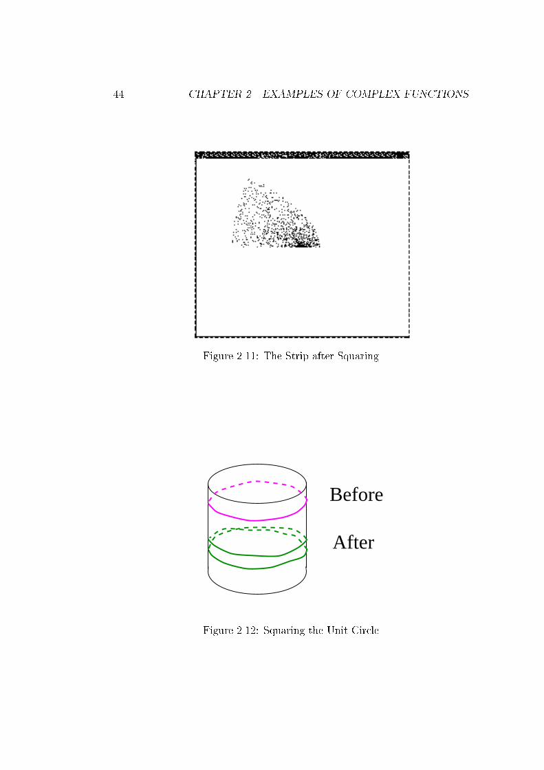
44 CHAPTER 2. EXAMPLES OF COMPLEX FUNCTIONS
Figure 2.11: The Strip after Squaring
Before
After
Figure 2.12: Squaring the Unit Circle

2.2. THE FUNCTION W = Z2 45
This is shown rather crudely in the `after' part of �gure 2.12. You have to
imagine that we look at it from above to get the loop around the unit circle.
Also, it should be smoother than my drawing. Don't shoot the artist, he's
doing his best.
If you tried to `do' the squaring function on a circular carpet representing
the unit disk, you would have to �rst cut the carpet along the X-axis from
the origin to 1+ i0. You need to take the top part of the cut, and push points
close to the origin even closer. Then nail the top half of the cut section to
the oor, and drag the rest of the carpet with you as you walk around the
boundary. The carpet needs to be made of something stretchy, like chewing-
gum1. When you have got back to your starting point, join up the tear you
made and you have a double covering of every point under the carpet.
It is worth trying hard to visualise this, chewing-gum carpet and all.
Notice that there are two points which get sent to any point on the unit circleby the squaring map, which is simply an angle doubling. The same sort of
thing is true for points inside and outside the disk: there are two points sentto a + ib for any a; b. The only exception is 0, which has a unique square
root, itself.
This is telling you that any non-zero complex number has two square roots.In particular, -1 has i and �i as square roots. You should be able to visualisethe squaring function taking a carpet made of chewing-gum and sending two
points to every point.
This isn't exactly a formal proof of the claim that every non-zero complex
number has precisely two distinct square roots; there is one, and it is long
and subtle, because formalising our intuitions about carpets made of chewing-
gum is quite tricky. This is done honestly in Topology courses. But the ideaof the proof is as outlined.
I have tried to sketch the resulting surface just before it gets nailed down. It
is impossible to draw it without it intersecting itself, which is an unfortunateproperty of R3 rather than any intrinsic feature of the surface itself. It ismost easily thought of as follows; take two disks and glue them together at
the centres. In �gure 2.13, my disks have turned into cones touching at thevertices. Cut each disk from the centre to a single point on the perimeter
in a straight line. This is the cut OP and OP' on the top disk, and the cut
1You need a quite horrid imagination to be good at maths.

46 CHAPTER 2. EXAMPLES OF COMPLEX FUNCTIONS
O
P P’
Q Q’Figure 2.13: Squaring the Unit Disk
OQ, OQ' on the lower disk. Now join up the cuts, but instead of joining thebits on the same disks, join the opposite edges on opposite disks. So glue
OP to OQ' and OP' to OQ. The fact that you cannot make it without itintersecting itself is because you are a poor, inadequate three dimensional
being. If you were four dimensional, you could do it. See:
http://maths.uwa.edu.au/~mike/PURE/
and go to the fun pages. If you don't know what this means, you have never
done any net sur�ng, and you need to.
This surface ought to extend to in�nity radially; rather than being made
from two disks, it should be made from two copies of the complex planeitself, with the gluings as described. It is known as a Riemann Surface.
2.3 The Square Root: w = z12
The square root function, f(z) = z1
2 is another function it pays to get a
handle on. It is inverse to the square function, in the sense that if you square

2.3. THE SQUARE ROOT: W = Z1
2 47
the square root of a a number you get the number back. This certainly works
for the real numbers, although you may not have a square root if the number
is negative. We have just convinced ourselves (by thinking about carpets)
that every complex number except zero has precisely two square roots. So
how do we get a well de�ned function from C to itself that takes a complex
number to a square root?
In the case of the real numbers, we have that there are precisely two square
roots, one positive and one negative, except when they coincide at zero. The
square root is taken to be the positive one. The situation for the complex
plane is not nearly so neat, and the reason is that as we go around the circle,
looking for square roots, we go continuously from one solution to another.
Start o� at 1 + i0 and you will surely agree that the obvious value for itssquare root is itself. Proceed smoothly around the unit circle. To take asquare root, simply halve the angle you have gone through.
By the time you get back, you have gone through 2� radians, and the pre-
ferred square root is now �1 + i0. So whereas the two solutions formed twobranches in the case of the reals, and you could only get from one to the
other by passing through zero, for C there are continuous paths from onesolution to another which can go just about anywhere.
Remember that a function is an input-output machine, and if we input onevalue, we want a single value out. We might settle for a vector output in
C � C , but that doesn't work either, because the order won't stay �xed. Weinsist that a function should have a single unique output for every input,because all hell breaks loose if we try to have multiple outputs. Such things
are studied by Mathematicians, who will do anything for a laugh, but itmakes ideas such as continuity and di�erentiability horribly complicated. So
the complications I have outlined to force the square root to be a proper
function are designed to make your life simpler. In the real case, we can
simply choosepx and �px to be two neat functions that do what we want,
at least when x is non-negative. In the complex plane, things are morecomplicated.
The solution proposed by Riemann was to say that the square root function
should not be from C to C , but should be de�ned on the Riemann surface
illustrated in �gure 2.13. This is cheating, but it cheats in a constructive
and useful manner, so mathematicians don't complain that Riemann broke
the rules and they won't play with him any more, they rather admire him

48 CHAPTER 2. EXAMPLES OF COMPLEX FUNCTIONS
O
Q Q’
P P’
Figure 2.14: The Square function through the Riemann Surface
for pulling such a line2.
If you build yourself a surface for the square function, then you project itdown and squash the two sheets (cones in my picture) together to map itinto C , then you can see that there is a one-one, onto, continuous map from
C to the surface, S, and then there is a projection of S on C which is two-one(except at the origin). So there is an inverse to the square function, but it
goes from S to C . This is Riemann's idea, and it is generally considered verycool by the smart money.
I have drawn the pictures again in �gure 2.14; you can see the line in thelower left copy of C (or a bit of it) where I have glued OP to OQ' and OP'
to OQ, and then both lines got glued together by the projection. The black
arrow going down sends each copy of C to C by what amounts to the identity
map. This is the projection map from S. The black arrow going from rightto left and slightly uphill is the square function onto S. The top half of the
complex plane is mapped by the square function to the top cone of S, and
the bottom half of C is mapped to the lower cone.
2Well, the good mathematicians feel that way. They like style. Bad mathematicians
don't like this sort of thing, but life is hard and unkind to bad mathematicians who spend
a lot of the time feeling stupid and hating themselves for it. We should not add to their
problems.

2.3. THE SQUARE ROOT: W = Z1
2 49
The last black arrow going left to right is the square root function, and it
is a perfectly respectable function now, precisely the inverse of the square
function.
So when you write f(z) = z2, you MUST be clear in your own mind whether
you are talking about f : C �! C or f : C �! S. The second has an inverse
square root function, and the former does not.
2.3.1 Branch Cuts
Although the square function to the Riemann surface followed by the projec-
tion to C doesn't have a proper inverse, we can do the following: take half a
plane in C , map it to the Riemann surface, remove the boundary of the halfplane, and project it down to C . This has image a whole plane (the anglehas been doubled), with a cut in it where the edge of the plane has been
taken away. For example, if we take the region from 0 to �, but without theend angles 0 and �, the squaring map sends this to the whole complex planewith the positive X-axis removed. This map has an inverse, (r; �); (r1=2; �
2)
which pulls it back to the half plane above the X-axis.
Another possibility is to take the half plane with positive real part, andsquare that. This gives us a branch cut along the negative real axis. We can
then write
f1(z) = f1(r; �) = (r1=2;�
2)
for the inverse, which is called the Principal Square Root. It is called a
branch of the square root function, thus confusing things in a way which istraditional. We say that this is de�ned for �� < � < �.
Suppose we take the half-plane with strictly negative real part: this also gets
sent to the complex plane with the negative real axis removed. (We have to
think of the angles, � as being between �=2 and 3�=2.) Now we get a squareroot of (r; �) which is the negative of its value for the principal branch. I
shall call this the negative of the Principal branch.
Exercise 2.3.1 Draw the pictures of the before and after squaring, for the
two branches just described. Con�rm that (1; �=4) is the unique square root
of (1; �=2) for the Principal branch, and that (1; 5�=4) is the unique square
root of (1; �=2) for the negative of the Principal branch. Note that (1; �=4) =�(1; 5�=4).

50 CHAPTER 2. EXAMPLES OF COMPLEX FUNCTIONS
Taking branches by choosing any half plane you want is possible, and for
every such branch there is a branch cut, and a unique square root, For every
such branch there is a negative branch obtained by squaring the opposite
half plane, and having the same branch cut. This ensures that in one sense
every complex number has two square roots, and yet forces us to restrict the
domain to ensure that we only get them one at a time.
The point at the origin is called a branch point; I �nd the whole terminology
of `branches' unhelpful. It suggests rather that the Riemann surface comes
in di�erent lumps and you can go one way or the other, getting to di�erent
parts of the surface. For the Riemann surface associated with squaring and
square rooting, it should be clear that there is no such thing. It certainly
behaves in a rather odd way for those of us who are used to moving in three
dimensions. It is rather like driving up one of those carp parks where you go
upward in a spiral around some central column, only instead of going up tothe top, if you go up twice you discover that, SPUNG! you are back where
you started. Such behaviour in a car park would worry anyone except Dr.Who. The origin does have something special about it, but it is the onlypoint that does.
The attempt to choose regions which are restricted in angular extent so
that you can get a one-one map for the squaring function and so choose aparticular square root is harmless, but it seems odd to call the resulting bits`branches'. (Some books call them `sheets', which is at least a bit closer to
the picture of them in my mind.)
It is entirely up to you how you choose to do this cutting up of the space intobits. Of course, once you have taken a region, squared it, con�rmed that the
squaring map is one-one and taken your inverse, you still have to reckon withthe fact that someone else could have taken a di�erent region, squared that,and got the same set as you did. He would also have a square root, and it
could be di�erent from yours. If it was di�erent, it would be the negative of
yours.
Instead of di�erent `branches', you could think of there being two `levels',
corresponding to di�erent levels of the car park, but it is completely up toyou where you start a level, and you can go smoothly from one level to the
next, and anyway levels 1 and 3 are the same.
This must be hard to get clear, because the explanations of it usually strike
me as hopelessly muddled. I hope this one is better. The basic idea is fairly

2.3. THE SQUARE ROOT: W = Z1
2 51
easy. Work through it carefully with a pencil and paper and draw lots of
pictures.
2.3.2 Digression: Sliders
Things can and do get more complicated. Contemplate the following ques-
tion:
Is w =p(z2) the same function as w = z?
The simplest answer is `well it jolly well ought to be', but if you take z = 1
and square it and then take the square root, there is no particular reason to
insist on taking the positive value. On the other hand, suppose we adopt theconvention that we mean the positive square root for positive real numbers,in other words, on the positive reals, square root means what it used to mean.
Are we forced to take the negative square root for negative numbers? No,we can take any one we please. But suppose I apply two rules:
1. For positive real values of z take the (positive) real root
2. If possible, make the function continuous
then there are no longer any choices at all. Because if we take a number suchas ei� for some small positive �, the square is ei2� and the only possibilitiesfor the square root are �ei�, which since r cannot be negative means ei� or
ei(�+�, and we will have to choose the former value to get continuity when� = 0. We can go around the unit circle and at each point we get a unique
result: in particularp(�1)2) = �1.
I could equally well have chosen the negative value everywhere, but with both
the above conventions, I can say cheerfully that
pz2 = z
If I drop the continuity convention, then I can get a terrible mess, with signs
selected any old way.
The argument for
(pz)2

52 CHAPTER 2. EXAMPLES OF COMPLEX FUNCTIONS
is simpler. If you take z and look at its square roots, you are going up from
C to the Riemann surface that is the double level spiral car-park space. you
can go up to either level from any point (except the origin for which there is
only one level). If I square the answer I will get back to my starting point,
whatever it was. So
z = (pz)2
is unambiguously true, although it is expressing the identity function as a
composite of a genuine function and a relation or `multi-valued' function.
Now look at
w =pz2 + 1
Again the square root will give an ambiguity, but I adopt the same two rules.So if z = 1, w =
p2. At large enough values of z, we have that w is close to
z. The same argument about going around a circle, this time a BIG circle,gives us a unique answer. 100i will have to go to about 100i and �100 will
have to go to about �100.
It is by no means clear however that we can make the function continuouscloser in to the origin. f(0) = 1 would seem to be forced if we approach zerofrom the right, but if we approach it from the left, we ought to get �1. Sothe two rules given above cannot both hold. Likewise, �i both get sent tozero; If we have continuity far enough out, then we can send 10i to i timesthe positive value of
p99. But what do we do for 0:5i? Do we send it top
3=4 or �p3=4? Or do we just shrug our shoulders and say it is multivalued
hereabouts?
If we just chop out the part of the imaginary axis between i and �i, we havea perfectly respectable map which is continuous, and sends i(1 + �) into i�when � > 0, sends �1 to �
p2, 1 to +
p2. It has image the whole complex
plane except for the part of the real axis between �1 and 1. Call this map
f . You can visualise it quite clearly as pulling the real axis apart at theorigin, with points close to zero on the right getting sent (almost) to 1 and
points close to zero on the left getting sent (almost) to �1. The two points
�i get sucked in towards zero. Because of the slit in the plane, this is now acontinuous map, although we haven't de�ned it on the points we threw out.
There is also a perfectly respectable map �f which sends z to �f(z). Thishas exactly the same domain and range space, C with a vertical slit in it,
between �i and i, and it has the same range space, C with a horizontal slitin it, between �1 and 1. It is just f followed by a rotation by 180o.

2.3. THE SQUARE ROOT: W = Z1
2 53
We now ask for a description of the Riemann surface forpz2 + 1. You might
think that asking about Riemann surfaces is an idle question prompted by
nothing more than a desire to draw complicated surfaces, but it turns out
to be important and very practical to try to construct these surfaces. The
main reason is that we shall want to be able to integrate along curves in due
course, and we don't want the curve torn apart.
The Riemann surface associated with the square and square root function
was a surface which we pictured as sitting over the domain of the square root
function, C , and which projected down to it. Then we split the squaring
map up so that it was made up of another map into the Riemann surface
followed by the projection. Actually, the Riemann surface is just the graph
of w = z2, but instead of trying to picture it in four dimensions, we put it
in three dimensions and tried not to think about the self-intersection this
caused.
We could construct the above surface as follows: �rst think of the squareroot function. Take a sector of the plane, say the positive real axis and the
angle between 0 and �=2. Now move it vertically up above the base plane.I choose one particular square root for the points in this sector, say I startwith the ordinary real square root on the positive real line. This determines
uniquely the value of the square root on the sector, since w = z2 is one-onehere, so the square root is just half the sector. I can do the same for anothersector on which the square is still one-one, say the part where the imaginary
component is positive. This will overlap the quarter plane I already have;I make sure that everything agrees with the values on the overlap. I keep
going, but when I get back to the positive real axis, I discover that I have
changed the value of the square root, so instead of joining the points, I liftthe new edge up. I keep going around, and now I get di�erent answers from
before, but I can continue gluing bits together on the overlap. When I have
gone around twice, I discover that the top edge now really ought to be joined
up to the starting edge. So I do my Dr. Who act and identify the two edges.
The other way to look at it is to take two copies of the complex plane, andglue them together as in �gure 2.14. We know there are two because of the
square root, and we know that they are joined at the origin because there is
only one square root of zero. We clearly pass from one plane to another at abranch cut, which can be anywhere, and then we go back again a full circuit
later.
Now I shall do the same thing withpz2 + 1. But before tackling this case,

54 CHAPTER 2. EXAMPLES OF COMPLEX FUNCTIONS
a short digression.
Example 2.3.1 In the television series `Sliders', the hero generated a disk
shaped region which identi�ed two di�erent universes. Suppose there are two
people intending to slide into a new universe and they see this disk opening
into a tunnel in front of them. One of them walks around the back of the
disk. If this one sees the other side of the disk and steps through it, and if
the other person goes through the other side of the disk at the same time, is
it true that they must come out in the same place? Do they bump into each
other?
Solution
It is probably easiest to think of this a dimension lower down. Take two sheets
of paper, two universes. Draw a line segment on each. This is the `door into
Summer', the Stargate.
What we do is to identify the one edge of the line segment in one universe with
the opposite edge in the other universe. To make this precise, take universe
A to be the plane (x; y; 1) for any pair of numbers x; y, and universe B to be
the set of points (x; y; 0). I shall make my `gateway' the interval (0; y; n) for�1 � y � 1, for both n = 0; 1.
Now I �rst cut out the interval of points in the `stargate',
(0; y; n); �1 � y � 1; n = 1; 2
I do this in both universes.
Now I pull the two edges of the slits apart a little bit. Then I put new bound-
aries on, one on each side. I have doubled up on points on the edge now,
so there are two origins, a little way apart, in each universe. I call them
0 and 00 respectively, so I have duplicate points (0; y; n) and (00; y; n) for
�1 � y � 1; n = 1; 2. A crude sketch is shown in �gure 2.15. Now I glue
the left hand edge of the slit in one universe to the right hand edge of the slit
in the other universe, and vice versa. So
(0; y; 0) = (00; y; 1) & (0; y; 1) = (00; y; 0) � 1 � y � 1
This will make the path shown by the dotted line in �gure 2.16 continuous.
I joined up the opposite two sides of the cut in each universe in the same
way, but I don't have to. One thing I can do is to have another universe,

2.3. THE SQUARE ROOT: W = Z1
2 55
0 0
Figure 2.15: The construction of the Stargate
World A
World B
Figure 2.16: The Dotted line is a continuous path in the twin universes
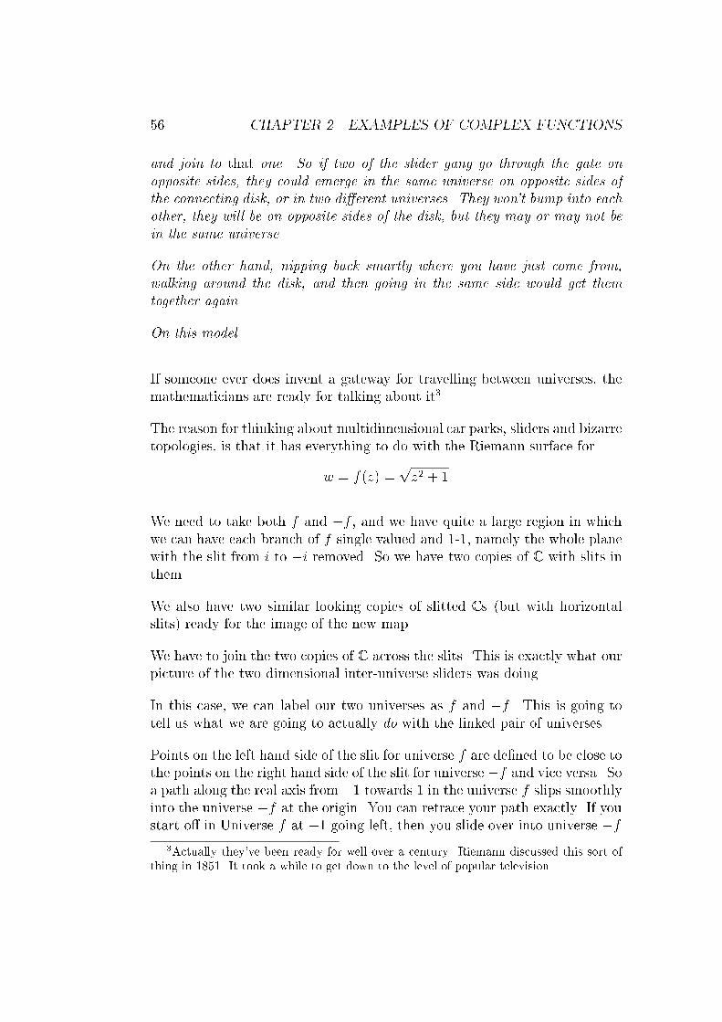
56 CHAPTER 2. EXAMPLES OF COMPLEX FUNCTIONS
and join to that one. So if two of the slider gang go through the gate on
opposite sides, they could emerge in the same universe on opposite sides of
the connecting disk, or in two di�erent universes. They won't bump into each
other, they will be on opposite sides of the disk, but they may or may not be
in the same universe.
On the other hand, nipping back smartly where you have just come from,
walking around the disk, and then going in the same side would get them
together again.
On this model.
If someone ever does invent a gateway for travelling between universes, themathematicians are ready for talking about it3.
The reason for thinking about multidimensional car parks, sliders and bizarre
topologies, is that it has everything to do with the Riemann surface for
w = f(z) =pz2 + 1
We need to take both f and �f , and we have quite a large region in which
we can have each branch of f single valued and 1-1, namely the whole planewith the slit from i to �i removed. So we have two copies of C with slits in
them.
We also have two similar looking copies of slitted C s (but with horizontalslits) ready for the image of the new map.
We have to join the two copies of C across the slits. This is exactly what ourpicture of the two dimensional inter-universe sliders was doing.
In this case, we can label our two universes as f and �f . This is going to
tell us what we are going to actually do with the linked pair of universes.
Points on the left hand side of the slit for universe f are de�ned to be close tothe points on the right hand side of the slit for universe �f and vice versa. So
a path along the real axis from �1 towards 1 in the universe f slips smoothly
into the universe �f at the origin. You can retrace your path exactly. If you
start o� in Universe f at +1 going left, then you slide over into universe �f3Actually they've been ready for well over a century. Riemann discussed this sort of
thing in 1851. It took a while to get down to the level of popular television.

2.3. THE SQUARE ROOT: W = Z1
2 57
at the origin. So in this case, it doesn't matter which way you go into the
`gate', you wind up in the same universe- there are only two. If you are a
long way from the gate in either universe, you don't get to �nd out about
the other universe at all. Continuous paths which don't go through the gate
have to stay in the same universe.
Exercise 2.3.2 Construct a complex function needing three `universes' for
the construction of its Riemann surface.
To see that this is the Riemann surface, observe that if we travel in any path
on the surface, the value ofpz2 + 1 varies continuously along the path.
Exercise 2.3.3 Choose a path in the Riemann surface and con�rm that the
value ofpz2 + 1 varies continuously along the path. Do this for a few paths,
some passing through the `gate' described above.
Exercise 2.3.4 Describe the surface associated with the inverse function.
Show that there is a one-one continuous map going in both directions between
the two surfaces.
It is worth pointing out that the Riemann surface can be constructed inseveral ways: there is nothing unique about the choice of branch cuts, for
example. It is not so obvious that the Riemann surface is unique in the sense
that there is always a way of deforming one into another. You don't have
the background to go into this, so I shan't. But the text books often give theimpression that branch cuts come automatically with the problem, whereasthey are much less clear cut4 than that.
It is clear that the z2 cut along the positive real axis can be replaced by any
ray from the origin. It might seem however that the slit between i and �i isforced. This isn't so, but the proper investigation of these matters is quite
di�cult.
I have avoided de�ning Riemann surfaces, and simply considered them in
rather special cases, because it needs some powerful ideas from Topology to
do the job properly. This seems to be traditional in Complex Analysis, and it
4Aaaagh!

58 CHAPTER 2. EXAMPLES OF COMPLEX FUNCTIONS
leaves students rather puzzled as to how to handle them in new cases. There
isn't time in this course to do more than introduce them, but I hope you
can see two things: �rst that quite simple real functions generalise to rather
complicated complex functions, and second that the investigation of them is
full of ideas that take you outside the universe you are used to. The fact that
this is actually useful is one you will have to take for granted for a while.
2.4 Squares and Square roots: Summary
I have gone into the business of examining the square function and the square
root function in agonising detail, because they illustrate many of the problems
and opportunities of complex functions. They show that the little sweetiesare (a) surprisingly complicated even when the real version of the function
is boringly familiar, and (b) they are not so bad we can't make sense ofthem. Many hours of innocent fun can be had by exploring the behaviour of
complex functions the real versions of which are simple and uninteresting. Itis recommended that you play around with some yourself.
It makes sense to look at functions such as f(z) = z2 because we havethat C is a �eld, so we can do with C everything we could do with R. So
polynomials make sense. And so do in�nite series, as we shall see later, sothe trigonometric and exponential functions make sense, and just as we canask for a square root of �1, so we can ask for a logarithm of it.
Exercise 2.4.1 What would you expect to be the value of ln(�1)?
This is weird stu� by comparison with the innocent functions from R to R,
and it is a good idea to get the basics clear, which is the main reason for
doing to death the square function. We can now move on to a few more easy
functions to �nd out what they do. This should be approached in a spirit of
fun and innocence. Who knows what bizarre things we shall �nd?
2.5 The function f(z) = 1z
The real function f(x) = 1=x is a perfectly straightforward function which
is de�ned everywhere except, of course, at x = 0. Since you can do in C

2.5. THE FUNCTION F (Z) = 1Z
59
everything that you can do in R, the function f(z) = 1=z must also make
sense except at z = 0.
We can say immediately that f(z) = 1=z = �z=z�z, so 1=z does two things:
�rst it takes the conjugate of z, and then it scales by dividing by the square
of the modulus. If this is 1, then the only e�ect is to re ect z in the X-axis.
In order to make our lives easier, we decompose f into these two parts, the
inversion map inv(z) = z=z�z and the conjugation map�(z) = �z. and look at
these separately.
To start to get a grip on the inv function, notice that in polar form, (r; �)
gets sent to (1=r; �). A point on the unit circle will stay �xed, points on the
axes stay on the axes. The origin gets sent o� to in�nity, points close to the
origin get sent far away but preserve the angle. If we take the unit square in
the plane, the point
�11
�gets sent to
�0:50:5
�.
The top edge of the unit square, y = 1; 0 � x � 1, gets sent to a curve joining�0:5
0:5
� �0
1
�which is left �xed by the map as it lies on the unit circle. The
equation of the curve is given by
u = x=(x2 + 1); v = 1=(x2 + 1)
which can be written as
u = vp1=v � 1
The right edge behaves similarly.
The left edge is sent to the Y-axis for values greater than 1, the bottom edgeto the X-axis with values from 1 to in�nity.
The before and after pictures are �gure 2.17 and �gure 2.18 respectively.
Note that the point density is greatest closest to the origin. You should be
able to see why this is so. (Hint: think of the derivative of 1=r.)
If we take a disk, it can be discovered experimentally that the image is alsoa disk in most cases. Some before and after pictures are �gure 2.19 and
�gure 2.20 respectively.
This is a harder one to calculate:

60 CHAPTER 2. EXAMPLES OF COMPLEX FUNCTIONS
Figure 2.17: The Unit Square
Figure 2.18: The Inversion of the unit square

2.5. THE FUNCTION F (Z) = 1Z
61
Figure 2.19: A disk
Figure 2.20: The Inversion of the disk

62 CHAPTER 2. EXAMPLES OF COMPLEX FUNCTIONS
Exercise 2.5.1 Can you �nd an expression for the inversion of the boundary
of the disk?
If you do some experimenting with a program that does inversions, you will
discover that it looks very much as if the inversion of a circle is a circle
except in the degenerate case where the circle passes through the origin.
This is indeed the case.
In order to see this, write the circle with centre
�a
b
�and radius R in polar
coordinates to get the equation
r2 � 2ar cos � � 2br sin � = R2 � a2 � b2
Now the angle is unchanged, so the inversion is the set of (s; �) satisfying
1=s2 � 2a cos �=s� 2b sin �=s = R2 � a2 � b2
which after some rearrangement gives
s2 � 2a cos �=(a2 + b2 �R2)� 2b sin �=(a2 + b2 � R2) = �1=((a2 + b2 � R2)
This is a circle with centre at
�a=(a2 + b2 �R2)b=(a2 + b2 � R2)
�and radius a rather hor-
rible value which can be written down with some patience. If the originalcircle goes through the origin, the radius of the inverted circle is in�nite, and
its centre is also shifted o� to in�nity. This actually gives a straight line.
Exercise 2.5.2 Verify the claim that the equation degenerates to a straight
line when R2 = a2 + b2.
Sneaky Alternative Methods
There is a somewhat neater way of proving that inversions take circles to
circles; it requires that we �nd a way of describing circles which is di�erent
from the usual one.
Suppose we writejz � ajjz � bj = r
for some positive real r, and complex a; b. If r = 1 this just gives the straightline bisecting the line segment from a to b. If r 6= 1, it gives a circle cutting

2.5. THE FUNCTION F (Z) = 1Z
63
the line segment between a and b and it is easy to write down its equation
in more standard forms. Also, any circle can be written in this form.
Now putting w = 1=z in this equation and doing a bit of messing around
with algebra gives a new equation in the same form. Which is also a circle,
or maybe a straight line.
Exercise 2.5.3 Do the algebra to show that the representation is really that
of a circle (or straight line if r = 1).
Do the algebra to show that w = 1=z in this equation gives a new circle (or
possibly a straight line).
Exercise 2.5.4 Show that the unit circle can be represented in the sneaky
form with r = 2. Show that any circle can be written in this form with r = 2.
Another way of representing any circle is in the form
A �Az�z +Bz + �B�z + C �C = 0
for complex numbers A;B;C.
If A = 0 this is a straight line, if C = 0 it passes through the origin.
For this form also, it is easy to con�rm that inversion takes circles to circles,
where a straight line is just a rather extremal case of a circle. Malcolm Hoodtold me this one.
These representations are sneaky and probably cheating, but it is telling
you something important, namely, some representations for things will makesome problems dead easy, and others make it horribly di�cult. Thinkingabout this early on can save you a lot of grief.
Exercise 2.5.5 Can you see why a parametric representation of the circle
of the form z = a+ r cos �+ i(b+ r sin �) could be a serious blunder in trying
to show that inversions take circles to circles?
Remark:

64 CHAPTER 2. EXAMPLES OF COMPLEX FUNCTIONS
The moral we draw from this little excursion is that being true and faithful
to a human being is, possibly, a �ne and splendid thing; being faithful and
true to a principle or ideology might be a �ne and splendid thing, or it might
be a sign of a sentimental nature gone wild. But being faithful and true to
a brand of beans or a choice of representation of an object is to confuse the
�nger pointing at the moon with the moon itself, and a sure sign of total
fatheadedness. The poor devil who believes deeply that the only true and
proper way to represent a circle in the plane is by writing down
(x� a)2 + (y � b)2 = r2
is to be pitied as someone who has confused the language with the thing being
talked about, and is �t only for politics. The more ways you have of talking
and thinking about things, the easier it is to draw conclusions, and the harder
it is to be led astray. It is also a lot more fun.
The converse is also true: the inversion of a straight line is a circle throughthe origin.
To see this, let ax + by + c = 0 be the equation of a straight line. Turn this
into polars to getar cos � + br sin � + c = 0
Now put r = 1=s to get the inversion:
(a=s) cos � + (b=s) sin � + c = 0
and rearrange to get
s2 + (as=c) cos � + (bs=c) sin � = 0
which is a circle passing through the origin with centre at
��a=2c�b=2c
�.
It is easy to see that the `points at in�nity' on each end of the line get sent
to the origin.
This suggests that we could simplify the description by working not in the
plane but in the space we would get by adjoining a `point at in�nity'.
We do this by putting a sphere of radius 1=2 sitting on the origin of R3 , andidentify the z = 0 plane with C . Now to map from the sphere to the plane,
take a line from the north pole of the sphere which is at the point
24 0
0
1
35

2.5. THE FUNCTION F (Z) = 1Z
65
P’
PQ
Q’
Figure 2.21: The Riemann Sphere
and draw it so it cuts the sphere in P and the plane at P 0. Now this sets up
a one-one correspondence between the points of the sphere other than thenorth pole and the points of the plane. The unit circle in the plane is sentto the equator of the sphere.
Now we put the `point at in�nity' of the plane in- at the north pole of the
sphere.
An inversion of the plane now gives an inversion of the sphere, which sendsthe South pole (the origin) to the North pole: all we do is to project down
so that the point Q goes directly to the point Q0 vertically below it, and
vice-versa. In other words, we re ect in the plane of the equator.
Exercise 2.5.6 Verify that this rule ensures that a point in the plane is sent
to its inversion when we go from the point up to the sphere, then re ect in
the plane of the equator, then go back to the plane.
Exercise 2.5.7 Suppose we have a disk which contains the origin on its
boundary. What would you expect the inversion of the disk to look like?
Suppose we have a disk which contains the origin in its interior. What would
you expect the inversion to look like?

66 CHAPTER 2. EXAMPLES OF COMPLEX FUNCTIONS
Sketches of the general situation should take you only a few minutes to work
out; it is probably easiest to visualise it on the Riemann Sphere.
Exercise 2.5.8 What would you expect to get, qualitatively, if you invert a
triangle shaped region of C ? Does it make a di�erence if the triangle contains
the origin?
Draw some pictures of some triangles and what you think their inversions
would look like.
Note that if you do an inversion and then invert the result, you get back to
where you started. In other words, the inversion is its own inverse map. Since
the same is true of conjugation, the map f(z) = 1=z also has this property.
Exercise 2.5.9 What happens if you invert a half-plane made by taking all
the points on one side of a line through the origin? What if the half-plane is
the set of points on one side of a line not through the origin?
I haven't said anything much about the conjugation because it is really verytrivial: just re ect everything in the X-axis.
2.6 The M�obius Transforms
The reciprocal transformation is a special case of a general class of complexfunctions called the Fractional linear or M�obius transforms. In the old days,
they also were called bilinear, but this word now means something else and
is no longer used by the even marginally fashionable.
The general form of the M�obius functions is:
w = f(z) =az + b
cz + d
where a; b; c; d are complex numbers. If c = 0; d = 1, we have the a�ne maps,and if a = 0; b = 1; c = 1; d = 0 we have the reciprocal map. It is tempting
to represent each M�obius function by the corresponding matrix:
az + b
cz + d��a b
c d
�

2.6. THE M�OBIUS TRANSFORMS 67
which makes the identity matrix correspond nicely to the identity map w = z.
One reason it is tempting is that if we compose two M�obius functions we get
another M�obius function and the matrix multiplication gives the correspond-
ing coe�cients. This is easily veri�ed, and shows that providing ad 6= bc the
M�obius functionaz + b
cz + d
has an inverse, and indeed it tells us what it is.
The sneaky argument for the inversion also goes through for M�obius func-
tions, i.e. they take circles on the Riemann Sphere to other circles. It is clear
that the Riemann Sphere is the natural place to discuss the M�obius functions
since the point at 1 is handled straightforwardly.
Exercise 2.6.1 Verify that if ad 6= bc the M�obius function can be de�ned
for 1 in a sensible manner. What if ad = bc?
Exercise 2.6.2 Con�rm that any M�obius function takes circles to circles.
What happens when ad = bc?
A rather special case is when the image by a M�obius function of a circle isa straight line. It follows that the image of the interior of the disk bounded
by the circle is a half-plane.
Example 2.6.1 Find the image of the interior of the unit disk by the map
w = f(z) =z � 1
z + 1
Solution
We see immediately that z = �1 goes to in�nity, and so the bounding circle
must be sent to a straight line, and the interior to a half-plane.
A quick check shows that the real axis stays real, and that 1 ; 0, 0 ;
�1;�0:5 ; �3, and the intersection of the real axis with the unit disk is
sent to the negative real axis. It is easy to verify that i; i;�i; �i.
68 CHAPTER 2. EXAMPLES OF COMPLEX FUNCTIONS
The inverse can be written down at sight (using the matrix representation!)
and is
z = f�1w =w + 1
�w + 1
which tells us that for w = iv we have
z =1 + iv
1� iv=
(1� v2) + 2iv
1 + v2
which point lies on the unit circle. In other words, the inverse takes the
imaginary axis to the unit circle, so the image by f of the unit circle is the
imaginary axis. And since 0 ; �1 we conclude that the image by f of the
interior of the unit disk has to be the half-plane having negative real part.
Any M�obius function has to be determined by its value at three points: itlooks at �rst sight as though 4 will be required, but one could scale top andbottom by any complex number and still have the same function. This must
be true, since if we have z1 ; w1; z2 ; w2, and z3 ; w3 we have three linearequations in a; b; c; d and we can put a = 1 without loss of generality.
It follows that if you are given three points and their images you can deter-mine the M�obius function which takes the three points where you now they
need to go. There is a sneaky way of doing this which you will �nd in thebooks, but the method is not actually shorter than solving the linear equa-
tions in general, so I shall not burden your memory with it. It is possible,however, to use some intelligence in selecting the points:
Example 2.6.2 Find a M�obius function which takes the interior of the unit
disk to the half plane with positive imaginary part.
Solution
We have to have the unit circle going to the real axis, so we might as well
send 1 to 0. We can also send �1 to 1. Finally, if we send 0 to i we have
our three points.
The �1 ; 1 condition means that we have cz + d = c(z + 1) and 0 ; i
means we have az + b = az + i while 1 ; 0 forces a = �i. So a suitable
function is
f(z) =i(1� z)
z + 1

2.7. THE EXPONENTIAL FUNCTION 69
Exercise 2.6.3 Find a M�obius function which takes the interior of the disk
jz � (1 + 2i)j < 3
to the half-plane with positive imaginary part.
Exercise 2.6.4 Draw the images of the rays from the origin under the func-
tion
w =z
z � 1= 1 +
1
z � 1
Exercise 2.6.5 Investigate the e�ect of composing some of the maps you
have met so far. Show that a M�obius function can be written as a suitable
composite of inversions and a�ne maps, and deduce directly that it has to
take circles to circles.
Exercise 2.6.6 Calculate the image of the lines having imaginary part con-
stant under the map
f(z) = (z2 � 1)1=2
Exercise 2.6.7 What is the Riemann surface for the above map?
The M�obius functions are of some interest because they are closed undercomposition, and also for historical reasons. All books on Complex Analysis
mention them. I should have been excommunicated if I had left them out,and I am already regarded as having heretical tendencies, so I have put them
in. You are strongly encouraged to do the above exercises so that (a) you
will be able to make an informed guess at some of the applications and (b) so
that when you meet them in the examination you will approach them with
con�dence and a clear conscience.
2.7 The Exponential Function
The real exponential function is de�ned by
exp(x) = 1 + x + x2=2! + x3=3! + x4=4! + � � �

70 CHAPTER 2. EXAMPLES OF COMPLEX FUNCTIONS
or more formally as the in�nite sum:
exp(x) =
1Xn=0
xn=n!
We write
exp(x) as ex
for reasons which will become apparent shortly.
2.7.1 Digression: In�nite Series
Expressing functions by in�nite series is something you must get used to; the
thing you need to realise is that almost all the functions that you use otherthan polynomials and ratios of polynomials are given by these in�nite series
(called power series in the above case, because they have di�erent powers ofx in them). When you calculate sin(12o) or
p768:3 or ln(35:4) by pressing
the buttons on your calculator, it produces a number on the display. It gets
it from taking the �rst k terms in a power series for the function. A bettercalculator will take more terms; you get the k you pay for.
It is very convenient to have a formula for sin, cos, ex and all the other
functions as an in�nite series, because it is easy to add on some numberof terms, and to stop when the increment is so small it doesn't make anydi�erence to the answer. There is, however, a fundamental problem with this
approach.
If you add the terms:
1 + 1=2 + 1=4 + 1=8 + 1=16 + � � �
or more formally if you calculate
1Xn=0
1=2n
you rapidly get something pretty close to 2. Ten terms gets you to within
one tenth of a percent of the answer, which is, of course, 2.
Suppose you add up the �rst few terms of the series
1 + 1=2 + 1=3 + 1=4 + 1=5 + � � �

2.7. THE EXPONENTIAL FUNCTION 71
or more explicitly you try to compute a �nite number of terms of
1Xn=1
1=n
You �nd that you seem to be getting to the answer rather slowly, but it
is easy enough to put it on a computer and �nd a few thousand terms very
quickly. If you do this, you discover that after about ten thousand terms, you
are only getting increments in the fourth decimal place (of course!) and after
a million terms, you get increments only in the sixth place. If your calculator
is working to single precision and it does this sort of thing, it will conclude
that the series sums to 16.695311. This is what I get on my computer if I
sum ten million terms, which takes less than ten seconds. The question is:
how far out is the result? Could it get up to 20 if we kept going on a higher
precision machine?
The answer is that the result is about as far out after ten million terms as itis after two. The series actually diverges and goes o� to in�nity.
If you didn't know whether a series converged or diverged, it would be possi-ble for you to calculate a number to six places of decimals in a few seconds,
and to get a result which is absolutely and totally wrong, by assuming itconverges because the increments have fallen below the precision of your ma-
chine. For this reason, it is of very considerable practical importance to beable to decide if a series converges. It is also useful to work out how fastit converges by getting a bound on the error as a function of the number of
terms used in the sum.
If you have a power series expansion for a (real) function, then it will, ofcourse have an x in it, and when you plug in a value for the x and add upthe series, you get the value of f(x). It may happen that the series converges
nicely for some values of x and goes o� its head for others. To see the kind
of thing that could happen, take a look at the function
f(x) =1
1 + x
You would have to be crazy to evaluate this by a power series, but there
might be other functions which behave the way this one does, so bear with
me.
It is not too hard to persuade yourself that the equation
1
1 + x= 1� x + x2 � x3 + x4 � x5 + � � �

72 CHAPTER 2. EXAMPLES OF COMPLEX FUNCTIONS
holds for at least some x. If you do the `multiplication':
(1 + x)(1� x + x2 � x3 + x4 � x5 + � � �)
you get
(1� x + x2 � x3 + x4 � x5 + � � �) + (x� x2 + x3 � x4 + � � �)
and it certainly looks plausible that all terms cancel except for the initial 1.
So cross multiplication seems to work. What more could you want?
If you put x = 1=2 you �nd, if you investigate the matter carefully, that the
series does converge. If you put x = �1 the sum goes o� to in�nity, but it
should anyway. If you put x = 1 you get
1� 1 + 1� 1 + 1� 1 + � � �
which is supposed to sum to 1=2. There would seem to be some reasonabledoubt about this.
Exercise 2.7.1 Put x = 2. How do you feel about the resulting series con-
verging to 1=3?
I am, I hope, reminding you of �rst and second year material, and I hopeeven more that you have some recollections of how to test for convergence of
in�nite series. If not, look it up in a good book.
The best sort of result we can hope for is that a power series converges forevery value of x, and that we can get a handle on estimating a bound for theerror after n terms. This bound will usually depend on the x.
The situation for exp(x) is fairly good: the Taylor-MacLaurin theorem tells
us that the error at the stage n is not bigger than the (n + 1)th term, fornegative x. This can, indeed, be made as small as desired by making n big
enough. You can satisfy yourself by some heavy thought that the situationfor positive x is also under control. So the formula
exp(x) = 1 + x+ x2=2! + x3=3! + x4=4! + � � �
is one we can feel relatively secure about.
Exercise 2.7.2 How many terms would you need to calculate exp(100) to
four places of decimals? How about exp(-100)?

2.7. THE EXPONENTIAL FUNCTION 73
2.7.2 Back to Real exp
The following exercise is important and will explain why we write exp(x) as
ex.
Exercise 2.7.3 Write down the �rst four terms of exp(x) and the �rst four
terms of exp(y). Multiply them together and collect up to show you have
rather more than the �rst four terms of exp(x + y).
Produce an argument to convince a sceptical friend that you can say with
con�dence that
8x; y 2 R exp(x) exp(y) = exp(x + y)
Another thing we can do is to show that if we di�erentiate the function
exp(x), we recover the function. This assumes that if we have an in�niteseries and we di�erentiate it term by term, the resulting series will converge
to the derivative of the function. You might like to brood on this to decidewhether you think this is going to happen (a) always (b) sometimes (c)never. The answer cannot be (c) because the exponential function actually
IS di�erentiable, and is indeed its own derivative, just as you would hopefrom di�erentiating the series termwise.
Exercise 2.7.4 You recall, I hope, computing the Fourier series for a square
wave. The series consists of di�erentiable functions, so you can di�erentiate
the series expansion termwise. But you clearly can't di�erentiate the square
wave at the discontinuities.
What do you get if you di�erentiate the series termwise and take limits?
I said earlier that everything you could do for R you could also do for C . You
can certainly add and multiply complex numbers, and you can divide them
except by zero. So the terms in the series
1 + z + z2=2! + z3=3! + z4=4! + � � �
are all respectable complex numbers. We can ask if the series converges to
some complex number when we stick a particular value of z in.
We know that it works if the value of z is a real number. What if it isn't?

74 CHAPTER 2. EXAMPLES OF COMPLEX FUNCTIONS
The answer is that all the arguments go through, and the series converges
for every value of z. I am not going to give a formal proof of this as it is a
fair amount of work and anyway, you are probably not much of a mind to
do formal proofs. But it is instructive to work it out in a few cases. Let us
therefore calculate exp(i).
We get the series:
exp(i) = 1 + i+ (�1)=2!� i=3! + 1=4!� i=5!� 1=6! + � � �
Separating the real and imaginary parts we get:
exp(i) = 1� 1=2! + 1=4!� 1=6! + � � �+ i� i=3! + i=5!� i=7! + � � �or
exp(i) = (1� 1=2! + 1=4!� 1=6! + � � �) + i(1� 1=3! + 1=5!� 1=7! + � � �)
You may or may not recognise the separate series as representing terms you
know. If you calculate the Taylor-MacLaurin expansions by
f(x) = f(0) + xf 0(0)=1! + x2f 00(0)=2! + x3f 000(0)=3! + � � �for the functions cos(x); sin(x) you will immediately recognise
exp(i) = cos 1 + i sin 1
By putting ix in place of i you get:
exp(ix) = cos(x) + i sin(x)
This gives us, when x = �, Euler's Formula:
ei� + 1 = 0
This links up the �ve most interesting numbers in Mathematics, 0; 1; e; i; �,
in the most remarkable formula there is. Since e seems to be all about what
you get if you want a function f satisfying f 0 = f , and � is all about circles,it is decidedly mysterious.
Thinking about this gives you a creepy feeling up the back of the spine: it isas though you went exploring the Mandelbrot set and found a picture of an
old bloke with a stern look and long white whiskers looking out at you. It
might incline you to be better behaved henceforth. I have, therefore, somereservations about the next exercise:

2.7. THE EXPONENTIAL FUNCTION 75
Exercise 2.7.5 (Don't do this if you watch the X-Files)
Euler's formula might either (a) be in no need of an explanation, just a
proof, or (b) be explained by God having a silly sense of humour, just like
most intelligent people or (c) have a more prosaic explanation.
The exponential function is a procedure for turning vector �elds into ows;
if you take the vector �eld which is given by
V
�x
y
�=
�0 �11 0
� �x
y
�
you call the matrix A and then the ow is given as
etA
This is basic to the theory of systems of ODE's. You can verify this particular
case by exponentiating the matrix tA using the standard power series formula
for the exponential of a real number x and replace x by tA. Since all you
have to do with x is to multiply it by itself, divide by a non-zero real number,
add a �nite set of these things and take limits, and since all of these can be
done with matrices, this all makes sense.
Draw a picture of the vector �eld and the resulting ow.
Identify the matrix as a complex number.
Deduce that eit = cos t + i sin t is little more than the observation that a
tangent to a circle is always orthogonal to the radius, together with the ob-
servation that exponentiation is about solving ODE's by Euler's method taken
to the limit.
If you watch the X-Files (The Truth is out there, the Lies are in the pro-
gramme), you might prefer to have the mystery preserved. Actually, there is
still heaps of mystery left, indeed it's the charm of Mathematics5.
Since the argument that exp(x + y) = exp(x) exp(y) (the `index law') goes
through for the complex numbers just as it does for the reals, we can write
exp(x + iy) = exp(x)(cos(y) + i sin(y))
5Engineers who want to preserve mystery are a bit of a worry.

76 CHAPTER 2. EXAMPLES OF COMPLEX FUNCTIONS
And the index law justi�es our writing
ex+iy = ex(cos y + i sin y)
If we write our complex number out in Polar form, z = (r; �) we have that
z = x+ iy = r cos � + ir sin � = rei�
This is a quite common notation; it needs a bit of explanation and I have
just given you one.
2.7.3 Back to Complex exp and Complex ln
We are now ready to look at the exponential map
exp : C �! C
It is certainly much more complicated that the real exponential, and theextra complications will turn out to be very useful.
To see what it does, notice that exp takes the real axis to the positive realnumbers. 0 goes to 1, and all the negative real numbers get squashed into
the space between 0 and 1. It takes the imaginary axis and wraps it aroundthe unit circle. The map eiy is a periodic function: think of the imaginary
axis as a long line made out of chewing gum, and note that the chewing gumline is picked up by exp and wrapped (without stretching) in the positive(anticlockwise) direction around the unit circle. The negative imaginary
numbers are wrapped around in the opposite direction.
I have indicated the start of this process on the axes, as if we have almostgot the exponential function but not quite, restricted to the axes. This is
�gure 2.22.
What happens to the rest of the plane? The image by exp of the axes will
cover only the positive real axis and the unit circle, but the unit circle getscovered in�nitely often. The number 1 + 0i also has an in�nite number of
points sent to it. Does anything at all get sent to the origin? To -2? Theseare all good questions to ask.
I start o� to answer some of them in the following example of how to compute
the e�ect of the complex exponential.

2.7. THE EXPONENTIAL FUNCTION 77
Figure 2.22: The start of the exponential function, restricted to the axes
Example 2.7.1 What is the image by the exponential map of the unit square?
Solution The lower edge, the point x + 0i for 0 � x � 1 gets sent to the
line segment ex + 0i since cos 0 + i sin 0 = 1. The top edge gets sent to
ex(cos 1 + i sin 1) Since 1 is 1 radian, this goes to a line at about 570 and of
radii from 1 to e. The left hand edge, the part of the imaginary axis between
0 and 1, goes to the corresponding arc of the unit circle, and the right hand
edge of the unit square, the points 1+iy, for 0 � y � 1 goes to e(cos y+i sin y)which is an arc of a circle of radius e. The result is shown in �gure 2.23
The �gure following shows the results of applying the exponential map tothe bigger square centred on the origin of side 2 units:
Exercise 2.7.6 Mark in the image of the axes on �gure 2.24
The image by exp of the unit disk is shown in �gure 2.25
I have marked on the X and Y axes to make it clearer where it is.
Exercise 2.7.7 What is the inverse of exp of a point in the spotty region of
�gure 2.25 which is closest to the origin?

78 CHAPTER 2. EXAMPLES OF COMPLEX FUNCTIONS
Figure 2.23: The image by the exponential function of the unit square
Figure 2.24: The image by the exponential function of the 4 times unit square

2.7. THE EXPONENTIAL FUNCTION 79
Figure 2.25: The image by the exponential function of the unit disk
Note that this is taking the complex logarithm of the point!
A little experimenting is called for, and is quite fun; strips which are vertical
and big enough, get mapped onto disks about the origin with a hole at thecentre. If the height of the strips is too small, they get mapped into sectorsof disks with a hole at the centre. You can easily see that there is no way to
actually get any point to cover the origin, although you can get as close asyou like to it. If the strip is very high, you go around several times.
Suppose you wanted a logarithm for �1 + i which is sitting in the second
quadrant. That is to say, you want something, anything which is mapped to
it by exp. Then we have that
ex(cos y + i sin y) = (�1 + i)
It is easier to express (-1+i) in polars as (p2; 3�=4). Then we have
ex(cos y + i sin y) =p2(cos(3�=4) + i sin(3�=4))
which tells us that
x = ln(p2); y = 3�=4
does the job.

80 CHAPTER 2. EXAMPLES OF COMPLEX FUNCTIONS
So does
x = ln(p2); y = (2n� + 3�=4)
for every integer n. There is a vertical line of points in C , at x value ln(p2)
and y values separated by 2� which all get sent to the same point, �1 + i.
If we want the logarithm of �2, we write it as 2(cos � + i sin �) and see that
ln 2 + i� does it nicely. So does ln 2 + i(2n+ 1)� for every integer n.
Exercise 2.7.8 Check this claim by exponentiating ln 2 + i(2n + 1)�
The conclusion that we come to is that every point in C except 0 has an
in�nite number of logarithms, so we have the same problem as for z2, only
much worse, if we insist on having a logarithm function. Our Riemann surface
for the exponential and logarithm functions has not just two but an in�nitenumber of leaves, joined together like an in�nite ascending spiral staircase.The leaves all have their centres joined together: this one is a little di�cult
to draw. Think of a set of cones, one for each integer, all with a commonvertex, nested inside each other, with cuts as in the diagram for z2 giving apath from each cone to the one lower down- for ever.
Exercise 2.7.9 Draw a bit of the Riemann surface for the exponential and
logarithm functions. Show how you can make some branch cuts to get a piece
of it which maps to C with the negative real axis removed. Show that there
are in�nitely many such pieces.
It is common to de�ne a Principal Branch of the logarithm, often called Log,by insisting that we restrict attention to answers which lie in the horizontalstrip with �� < y < �. Alternatively, think of what exp does to such a strip.
The word `branch' suggests to me either trees or banks, and neither seems
to have much to do with a piece of the plane which is mapped to a piece of athing like an in�nite ascending spiral staircase, the central column of which is
non-existent. It is, as explained earlier for the squaring function, rather oldfashioned terminology. The exponential function onto the Riemann surface
is a good test of your ability to visualise things. You know you are getting
close when you feel dizzy just thinking about it.
The log function is a proper inverse to exp providing we regard exp as going
from C to this Riemann surface. And if we don't, we get the usual mess, asseen in the case of the square function.

2.8. OTHER POWERS 81
Exercise 2.7.10 Show that the function Log(1+z1�z ) takes the interior of the
unit disk to the horizontal strip ��=2 < y < �=2.
2.8 Other powers
I can now de�ne zw for complex numbers z and w by
zw = exp(w log(z))
which is `multi-valued', i.e. not a function but an in�nite family of them.
Taking the Principal Branch makes this a function. This agrees with the
ordinary de�nition when w is an integer.
Exercise 2.8.1 Prove that last remark. Does it work for w any real number?
Exercise 2.8.2 Calculate �1i.
Since we can do in C anything we can do in R of an algebraic sort, we can
�nd more exotic powers. The following exercise should be done in your headwhile walking to prove that you know your way around:
Exercise 2.8.3 Calculate ii.
The next one can also be done internally if your concentration is in good
nick:
Exercise 2.8.4 Calculate (1�ip2)2i
This is good, clean fun. I have tried watching television and doing these
sorts of calculations, and in my view the sums are more fun, although they
may keep you awake at nights. You may be able to see why Gauss and
Euler, two of the brightest men who ever lived, spent some time playing with
the complex numbers a long, long time before they were really much usefor anything. It's just nice to know that something like the square root of
negative one raised to the power of itself is a perfectly respectable number.
Actually a lot of perfectly respectable numbers. Find them all. One of themis a smidgin over 0:2.

82 CHAPTER 2. EXAMPLES OF COMPLEX FUNCTIONS
2.9 Trigonometric Functions
The argument through in�nite series that showed that
ei� = cos � + i sin �
and the argument that we can replace the usual series for the real exponential
by simply putting in complex values, is asking to be carried the extra mile.
Suppose we put a complex value in place of a real value for the functions sin
and cos? Would we get respectable complex functions out? Yes indeed we
do.
I de�ne the complex trig functions as follows:
De�nition 2.9.1
eiz = cos z + i sin z
for any complex number z.
It follows immediately that
cos z =1
2(eiz + e�iz)
and putting z = x + iy and hence iz = �y + ix, �iz = y � ix we get
cos z =1
2
�e�y(cos x+ i sin x) + ey(cos x� i sinx)
�or
cos(x + iy) = cos(x) cosh(y)� i sin(x) sinh(y)
Similarly we obtain:
sin(x + iy) = sin(x) cosh(y) + i cos(x) sinh(y)
Example 2.9.1 Solve: sin z = i.
Solution We have sin x cosh y = 0, and since cosh y � 1 it follows that
x = n� for some integer n.
We also have cos x sinh y = 1, hence sinh y = �1 follows.
So x = n�; y = sinh�1�1 with the positive value when n is even and the
negative when it is odd. x = 0; y = ln(1 +p2) is a solution.
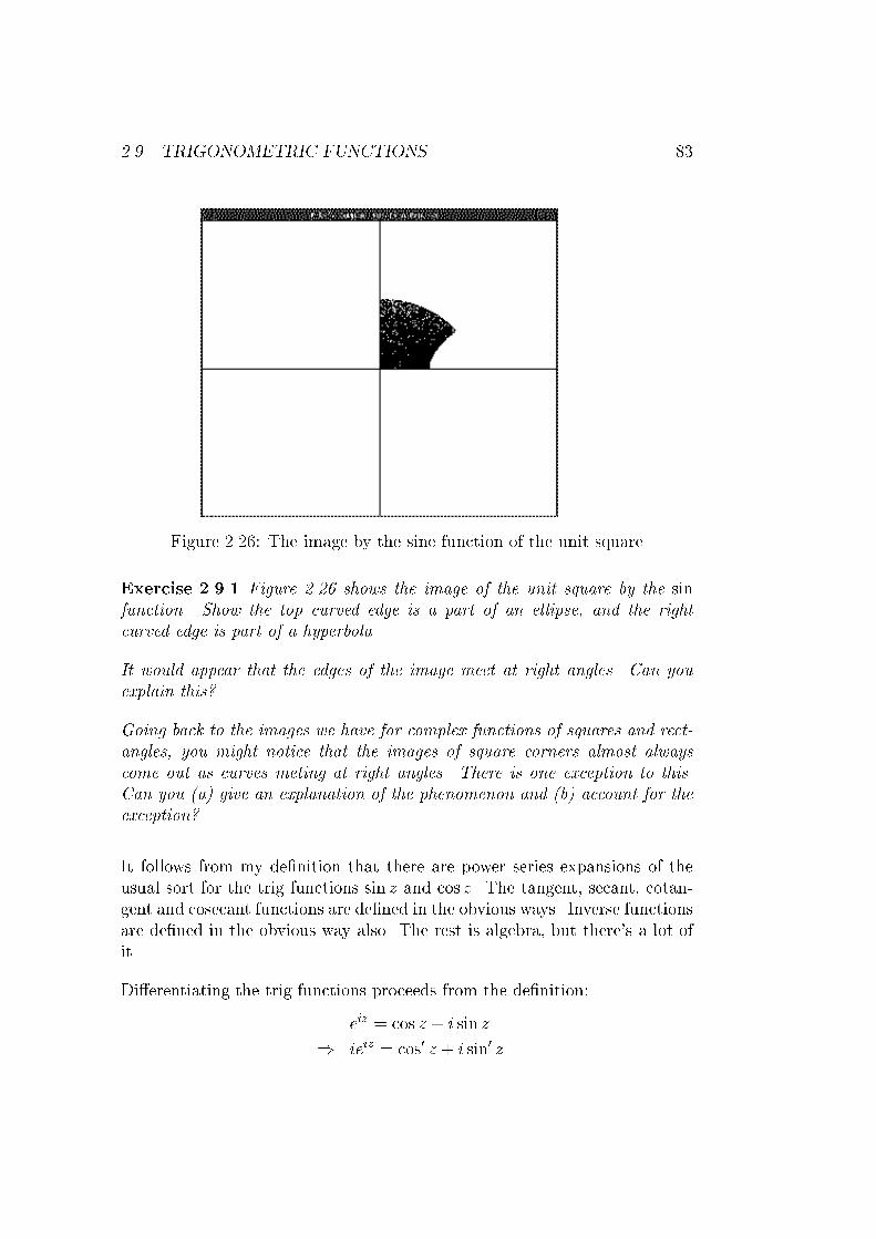
2.9. TRIGONOMETRIC FUNCTIONS 83
Figure 2.26: The image by the sine function of the unit square
Exercise 2.9.1 Figure 2.26 shows the image of the unit square by the sinfunction. Show the top curved edge is a part of an ellipse, and the right
curved edge is part of a hyperbola.
It would appear that the edges of the image meet at right angles. Can you
explain this?
Going back to the images we have for complex functions of squares and rect-
angles, you might notice that the images of square corners almost always
come out as curves meting at right angles. There is one exception to this.
Can you (a) give an explanation of the phenomenon and (b) account for the
exception?
It follows from my de�nition that there are power series expansions of the
usual sort for the trig functions sin z and cos z. The tangent, secant, cotan-gent and cosecant functions are de�ned in the obvious ways. Inverse functions
are de�ned in the obvious way also. The rest is algebra, but there's a lot ofit.
Di�erentiating the trig functions proceeds from the de�nition:
eiz = cos z + i sin z
) ieiz = cos0 z + i sin0 z

84 CHAPTER 2. EXAMPLES OF COMPLEX FUNCTIONS
= � sin z + i cos z
where the second line is obtained by di�erentiating the top line, and the
last line is obtained by multiplying the top line by i. This tells us that the
derivative of cos is � sin and the derivative of sin is cos, as in the real case.
The de�nitions also imply that cos z is just the usual function when z is real,
and likewise for sin.
The inverse trig functions can be obtained from the de�nitions:
Example 2.9.2 If w = arccos z, obtain an expression for w in terms of the
functions de�ned earlier.
Solution
We have
z = cosw =eiw + e�iw
2or
e2iw � 2zeiw + 1 = 0
Solving the quadratic (over C !)
eiw =2z +
p4z2 � 4
2= z +
pz2 � 1
Hence
w = �i log(z +pz2 � 1)
We have all the problems of multiple values in both the square root and the
log functions.
Exercise 2.9.2 Find arcsin 3.
It is worth exploring the derivatives of these functions, if only so as to be able
to do some nasty integrals later by knowing they have easy antiderivatives6.
6This sort of thing used to be a cottage industry in the seventeenth and eighteenth
centuries: mathematicians would issue public challenges to solve horrible integration prob-
lems which they made up by doing a lot of di�erentiations. This is cheating, something
Mathematicians are good at.

2.9. TRIGONOMETRIC FUNCTIONS 85
E(t)
L
C
R
C
LV
V
VR
Figure 2.27: A simple LCR circuit
Exercise 2.9.3 Compute the derivatives of as many of the trig functions
and their inverses as you can.
There is a standard application of the use of complex functions to LCRcircuits which it would be a pity to pass up:
Example 2.9.3 (LCR circuits)
The �gure shows a series LCR circuit with applied EMF E(t); the voltage
drop across each component is shown by VR; VC; VL respectively. We have
E(t) = VR + VC + VL (2.1)
at every time t.
It is well known that the current I in a resistance satis�es Ohms Law, so we
have immediately
VR = IR (2.2)
and since what goes in must come out, the current I through each component
is the same.

86 CHAPTER 2. EXAMPLES OF COMPLEX FUNCTIONS
The current and voltage drop across an inductance or choke is given by
VL = L _I (2.3)
since the impedance is due to the self induced magnetic �eld which by Fara-
day's Laws is proportional to the rate of change of current.
Finally, the voltage drop across a capacitor or condenser is proportional to
the charge on the plates, so we have
VC =1
C
Z t
0
I(�)d� (2.4)
If we have a periodic driving EMF as would arise naturally from any gener-
ator, we can write
I(t) = I0 cos(!t) (2.5)
where ! is the frequency.
I now assume that the current is the real part of a complex current I�, whichwill make keeping track of things simpler.
Then
I�(t) = I0ei(!t) (2.6)
and similarly for complex voltages:
V �R = I�R; V �
L = i!LI�; V �C =
1
i!CI�
Adding up the voltages of equation 2.1 we get:
E� =
�R + i
�!L� 1
!C
��I�
and the quantity
R + i
�!L� 1
!C
�
is called the complex impedance usually denoted by Z.
Then Ohm's Law holds for complex voltages and currents.
2.9. TRIGONOMETRIC FUNCTIONS 87
This notation may seem puzzling; it is little more than a notation, but it al-
lows us to carry through phase information (since the phase of the voltage is
changed by inductances or capacitances) which is of very considerable prac-
tical signi�cance in Power distribution, for example. But I shall leave this to
your Engineering lecturers to develop.
Since you ought to be getting the idea by now as to what to look for, I shall
�nish the chapter in a spirit of optimism, believing that you have sorted
out at least a few functions from C to C and that you have some ideas
of how to go about investigating others if they are sprung on you in an
examination. I leave you to think about some possibilities by working out
which real functions have not yet been extended to complex functions. There
is a lot of room for some experimenting here to investigate the behaviour oflots of functions I haven't mentioned as well as lots that I have. Life being
short, I have to leave it to you to do some investigation. You will �nd itmore fun than most of what's on television.
In the next chapter we continue to work out parallels between R and C andthe functions between them, but we take a big jump in generality. We ask
what it would mean to di�erentiate a complex function.

88 CHAPTER 2. EXAMPLES OF COMPLEX FUNCTIONS
Chapter 3
C - Di�erentiable Functions
3.1 Two sorts of Di�erentiability
Suppose f : C �! C is a function, taking x + iy to u+ iv. We know that ifit is di�erentiable regarded as a map from R
2 to R2 , then the derivative is a
matrix of partial derivatives:� @u
@x@u@y
@v@x
@v@y
�
If you learnt nothing else from second year Mathematics, you may still be
able to hold your head up high if you grasped the idea that the above matrix
is the two dimensional version of the slope of the tangent line in dimensionone. It gives the linear part (corresponding to the slope) of the a�ne map
which best approximates f at each point.
If f : R �! R is a di�erentiable function, then df=dx at any value of t is somereal number,m. Well, what we really mean is that the map y = mx+f(t)�mtis the a�ne map which is the best approximation to f at t. It has slope m,
and the constants have been �xed up to ensure that it passes through the
point (t; f(t)).
This is the old diagram from school-days, �gure 3.1.
In a precisely parallel way, the matrix of partial derivatives gives the linearpart of the best a�ne approximation to the map f : R2 �! R
2 . But at
89

90 CHAPTER 3. C - DIFFERENTIABLE FUNCTIONS
t
f(t)
dydx t = m
y=mx+f(t)-mt
y=f(x)
Figure 3.1: The Best A�ne Approximation to a (real) di�erentiable function
any point x+ iy, if f is di�erentiable in the complex sense, this must be just
a linear complex map, i.e. it multiplies by some complex number. So thematrix must be in our set of complex numbers. In other words, for every
value of x, it looks like �a �bb a
�
for some real numbers a,b, which change with x.
This forces us to have the famous Cauchy Riemann equations:
@u=@x = @v=@y and @u=@y = �@v=@x
It is important to understand what they are saying; there are plenty of maps
from R2 to R2 which are real di�erentiable and will have the matrix of partial
derivatives not satisfying the CR conditions. But these will not correspond
to being a linear approximation in the sense of complex numbers. There
is no complex derivative in this case. For the complex derivative to existin strict analogy with the real case, the matrix must be antisymmetric and
have the top left and bottom right values equal. This is a very considerablerestriction, and means that many real di�erentiable functions will fail to be
complex di�erentiable.

3.1. TWO SORTS OF DIFFERENTIABILITY 91
Exercise 3.1.1 Let � denote the conjugation map which takes z to �z. This
is a very di�erentiable map from R2 to R2 . Write down its derivative matrix.
Is conjugation complex di�erentiable anywhere?
On the other hand, the de�nition of the derivative for a real function such
as f(x) = x2 in the real case was
dy
dxjt = lim
�!0
f(t+�)� f(t)
�
We know that at t = 1 and f(x) = x2 we have
dy
dxj1 = lim
�!0
(1 + �)2 � 12
�
and of course
lim�!0
(1 + �)2 � 12
�
= lim�!0
2� +�2
�= lim
�!02 + �
= 2
Now all this makes sense in the complex numbers. So if we want the derivative
of f(z) = z2 at 1 + i, we have
f 0(1 + i) = lim�!0
(1 + i +�)2 � (1 + i)2
�
= lim�!0
(1 + i)2 +�2 + 2�(1 + i)� (1 + i)2
�= lim
�!02(1 + i) + �
= 2(1 + i)
Here, � is some complex number, but this has no e�ect on the argument. By
going through the above reasoning with z in place of 1 + i, you can see that
the derivative of f(z) = z2 is 2z, regardless of whether z is real or complex.

92 CHAPTER 3. C - DIFFERENTIABLE FUNCTIONS
If we write the function f(z) = z2 as
x+ iy ; u+ iv = x2 � y2 + i(2xy)
we see that @u=@x = @v=@y = 2x and @u=@y = �@v=@x, so the CR equations
are satis�ed. And the derivative is�2x �2y2y 2x
�
as a matrix, and hence 2x + i2y as a complex number. So everything �ts
together neatly.
Moreover, the same argument holds for all polynomial functions. The argu-
ments to show the rules for the derivative of sums, di�erences, products andquotients all still work. You can either go back, dig in your memories and
check, or take my word for it if you are the naturally credulous sort thatschool-teachers and con-men approve so heartily.
It might be worth pointing out that the reason Mathematicians like abstrac-tion, and talk of doing vector spaces over arbitrary �elds for instance, is that
they are lazy. If you do it once and �nd out exactly what properties yourarguments depend upon, you won't have to go over it all again a little later
when you come to a new case. I have just done exactly that bit of unnec-essary repetition with my investigation of the derivative of z2, but had youbeen prepared to buy the abstraction, we could have worked over arbitrary
�elds in �rst year, and you would have known exactly what properties wereneeded to get these results. The belief that Mathematicians (particularly
Pure Mathematicians) are impractical dreamers is held only by those toodumb to grasp the practicality of not wasting your time repeating the sameidea in new words1.
Virtually everything that works for R also works for C then. This includes
such tricks as L'Hopital's rule for �nding limits:
Example 3.1.1 Find
limz!i
z4 � 1
z � i
1It is quite common for stupid people to claim that they have oodles of `common sense'
or `practicality'. My father assured me that I was much less practical and sensible than he
was when he found he couldn't do my Maths homework. I believed him until one day in
my teens I found he had �xed a blown fuse by replacing it with a six inch nail. I concluded
that if this was common sense, I'd rather have the uncommon sort.

3.1. TWO SORTS OF DIFFERENTIABILITY 93
Solution
If z = i we get the indeterminate form 0/0 so we take the derivative of both
numerator and denominator to get
limz!i
4z3
1= 4i3 = �4i
which we can con�rm by putting z4 � 1 = (z � i)(z + i)(z2 � 1).
The Cauchy Riemann equations are necessary for a function to be complex
di�erentiable, but they are not su�cient. As with the case of R di�erentiable
maps, we need the partial derivatives to be continuous, and for complex
di�erentiability they must also be continuous and satisfy the CR conditions.
Example 3.1.2 Is f(z) = jzj2 di�erentiable anywhere?
Solution
The R-derivative is the matrix: �2x 00 2y
�
This cannot satisfy the CR conditions except at the origin. So f is not
di�erentiable except possibly at the origin. If it were di�erentiable at the
origin it would have to be with derivative the zero matrix. Taking
lim�!0
f(�)� f(0)
�
we get
limx+iy!0
x2 + y2
x + iy
= limx+iy!0
x� iy
= 0
Since if x + iy is getting closer to zero, so is its conjugate. Hence f has a
derivative, zero, at the origin but nowhere else.
The function f(z) = jzj2 is of course a very nice real valued function, which
is to say it has zero imaginary part regarded as a complex function. And as

94 CHAPTER 3. C - DIFFERENTIABLE FUNCTIONS
a complex function, it fails to be di�erentiable except at a single point. As
a map f : R2 �! R2 , it has u(x; y) = x2 + y2 and v(x; y) = 0, both of which
are as di�erentiable as you can get. This should persuade you that complex
di�erentiability is something altogether more than real di�erentiability.
What does it mean to have an expression like
lim�!w
f(�) = z
over the complex numbers? That is, are there any new problems associated
with �, z and w being points in the plane? The only issue is that of the
direction in which we approach the critical point w. In one dimension, we
have the same issue: the limit from the left and the limit from the right can
be di�erent, in which case we say that the limit does not exist. Similarly, if
the limit as � ! w depends on which way we choose to home in on w, we
say that there is no limit. In particular problems, coming in to zero downthe Y-axis can give a di�erent answer from coming in along the X-axis, oralong the line y = x. There are some very bizarre functions, few of which
arise in real life, but you need to know that the functions you are familiarwith are not the only ones there are. You have led sheltered lives.
In the case where the CR equations for some function f : C �! C are
satis�ed, and the partial derivatives not only exist but are continuous, wehave that the complex derivative of f exists and is given by
f 0(z) =@u
@x+ i
@u
@y
in classical form.
There is a polar form of the CR equations. It is fairly easy to work it out, I
give it as a pair of exercises:
Exercise 3.1.2 By writing
@u=@r = (@u=@x) (@x=@r) + (@u=@y) (@y=@r)
And similarly for @u=@�, @v=@r and @v=@�, Show the CR equations require:
@v=@� = r @u=@r; @u=@� = �r @v=@r
Exercise 3.1.3 Verify that @�=@x = sin �=r; derive the corresponding ex-
pression for @�=@y and deduce that
@u=@x + i @v=@x = (cos � � i sin �)(@u=@r + i @v=@r)

3.1. TWO SORTS OF DIFFERENTIABILITY 95
which is the partial derivative in polars.
Exercise 3.1.4 Find the other form of the derivative in polars involving �
instead of r in the partial derivatives.
Exercise 3.1.5 We can argue that the formulae:
@v=@� = r @u=@r; @u=@� = �r @v=@r
are `obvious' by writing @x � @r and @y � r @� on the basis that r; � are
just rotated versions of any coordinate frame locally, and regarding @v and
@u as in�nitesimals obtained by taking in�nitesimal independent increments
@r and r@�. Perhaps for this reason it is common to write the polar form as:
1
r
@v
@�=@u
@r;
1
r
@u
@�= �@v
@r
This is the sort of reasoning that Euler or Gauss would have thought useful
and gives some Pure Mathematicians the screaming ab-dabs. It can be re-
garded as a convenient heuristic for remembering the polar form, or it can be
regarded as showing that in�nitesimals ought to have a place in Mathematics
because they work. Although, to be fair to Pure Mathematicians, second rate,
sloppy thinking with in�nitesimals can lead to total garbage. For example, if
you had tried to put @x � r @� and @y � @r you would have got the wrong
answer. Can you see why this is not a good idea?
It is possible, as we have seen, to have a function which is complex dif-ferentiable at only one point, This is rather a bizarre case. Functions likef(z) = z2 are di�erentiable everywhere. If a function f is di�erentiable at
every point in an open ball centred on some point z0, then it is a particularly
well behaved function at that point:
De�nition 3.1.1 If f : C �! C is (complex) di�erentiable at every point
in a ball centred on z0, we say that f is analytic or holomorphic at z0.
De�nition 3.1.2 A function f : C �! C is said to be entire if it is analyticat every point of C .

96 CHAPTER 3. C - DIFFERENTIABLE FUNCTIONS
De�nition 3.1.3 A function f : C �! C is said to have a singularity at z1if it is not analytic at this point. This includes the case when it is not de�ned
there.
De�nition 3.1.4 A function f : C �! C is said to be meromorphic if it
is analytic on its domain and this domain is C except for a discrete set of
singular points.
There is a somewhat tighter de�nition of meromorphic given in many texts,
which I shall come to later.
I hate to load you down with jargon, but this is long standing terminology,and you need to know it so that you don't panic when it is sprung on you
in later years. Very often the singularities of a complex function tell you anawful lot about it, and they come up in Engineering and Physics repeatedly.
There is another de�nition of the term `analytic' which makes sense for real
valued functions, and is concerned with them agreeing with their Taylor ex-pansions at every point. The two de�nitions are in fact very closely related,but this is a little too advanced for me to get into here. I mention it in
case you have come across the other de�nition and are confused. The term`complex analytic' is sometimes used for the form I have given. Some authorsinsist on using `holomorphic' until they have shown that holomorphic func-
tions are in fact analytic in the sense of agreeing with their Taylor expansion(a Theorem of some importance). Then the theorem states that holomorphic
complex functions are analytic.
The following results are mostly obvious or easy to prove and are exact
analogues of the real case:
Proposition 3.1.1 If f and g are functions analytic on a domain E, (i.e.
analytic at every point of E) then
1. f+g is analytic on E
2. f-g is analytic on E
3. wf is analytic on E for any complex or real number w
4. fg is analytic on E

3.2. HARMONIC FUNCTIONS 97
5. f/g is analytic on E except at the zeros of g
2
Proposition 3.1.2 If f; g : C �! C are analytic functions, then the com-
posite function f � g : C �! C is analytic. 2
If f or g have point singularities but are otherwise analytic, then the compos-
ite is analytic except at the obvious singularities. These results will be used
extensively, and because analytic functions have some remarkable properties
they need to be absorbed.
3.2 Harmonic Functions
The fact that a function f from R2 to R2 is complex di�erentiable puts some
very strong conditions on it. These conditions turn out to have connectionswith Laplace's equation which must be the most important Partial Di�eren-
tial Equation (PDE) there is.
Recall the various PDE's you came across last year, in particular the di�usionor heat equation and the wave equation. In steady state cases you hadfunctions satisfying Laplace's Equation arising in many cases. For those in
doubt, go to
http://maths.uwa.edu.au/~mike/m252alder.html
for some notes on second year calculus and PDE material. You should down-load the vector calculus notes which have a part on Stoke's Theorem, and a
smaller part on PDEs at the end. I haven't the time to explain PDEs to you
again, so you should read this stu� if you are confused and muddled aboutPDEs.
I remind you that a function f : R2 �! R is said to be harmonic or to satisfy
Laplace's Equation, if@2f
@x2+@2f
@y2= 0
98 CHAPTER 3. C - DIFFERENTIABLE FUNCTIONS
Thus x2�y2 is harmonic, while x2+y2 is not. Notice that harmonic functions
on R2 have graphs which have opposite curvature in orthogonal directions. So
hyperboloids are in there with a chance of being harmonic, while paraboloids
can't ever be. Harmonic functions have the remarkable property that if you
draw a circle around a point and �nd the average value of the function around
the circle, it is always equal to the value of the function at the centre of the
circle. This holds true for every circle which has f de�ned everywhere inside
it and on its boundary. This gives a neat way of solving Laplace's equation
for f on some region of the plane when we are given the values of f on the
boundary (a Dirichlet Problem for the region). All we do is to �x f on the
boundary, give it random values on the interior, and then go through a cycle
of replacing the value at points inside the region with an average of the values
of neighbouring points on some �nite grid. This only gives an approximation,
but that is all you ever get anyway.
One of the ways of trying to understand functions from R2 to R2 is to think
of them as a pair of functions from R2 to R, the �rst giving the function
u(x; y) and the second v(x; y). This means that we can draw the graphs ofeach function. While not entirely useless, this is not always illuminating. It
does have its merits however, when considering harmonic functions.
The reason is simple: if @u=@x = @v=@y then @2u=@x2 = @2v=@x@y, whichis equal to @2v=@y@x providing the mixed partial derivatives are equal. Thiswill be the case if f is analytic.
And if @u=@y = �@v=@x then @2u=@y2 = �@2v=@y@x.
Hence provided f is analytic we have:
@2u=@x2 + @2u=@y2 = 0
which is to say, u is harmonic.
It is trivial to check that v is harmonic by the same argument applied to v.
Not only are both functions harmonic, they are said to be conjugate har-monic functions because they are related by the CR equations. For conjugate
harmonic functions a number of special properties hold: for example, their
product, and the di�erence of their squares, are also harmonic.
The argument is rather neat: If f is analytic, so is f 2. This follows becausethe product of analytic functions is analytic. If f = u + iv then f 2 =
(u2 � v2) + i(2uv). Hence 2uv is harmonic, and so is any multiple of it for

3.2. HARMONIC FUNCTIONS 99
obvious reasons. Similarly u2 � v2 is harmonic, and so is its negative. They
are, of course, conjugate.
It is not true generally that the product of harmonic functions is harmonic.
Exercise 3.2.1 Find two harmonic functions the product of which is not
harmonic.
Quite a lot of investigation has gone on into working out which functions are
harmonic and which aren't. The reason for this is that if you are looking for
a solution to Laplace's Equation, then it helps if you don't have to look too
far, and if you have a `dictionary' of them, you can save yourself some time.
The fact that they come streaming out of complex analytic functions makescompiling such a dictionary easy.
Given a harmonic function, we can easily construct a conjugate harmonic
function to get back to a complex analytic function. Up to an additiveconstant, the conjugate is unique. An example will make the procedure
clear.
Example 3.2.1 It is easy to verify that
u(x; y) = cosh(x) sin(y)
is harmonic.
Di�erentiating with respect to x,
@u=@x = sinh(x) sin(y) = @v=@y
giving, by integration,
v = � sinh(x) cos(y) + �(x)
Repeating this but di�erentiating with respect to y this time, we get:
v = � sinh(x) cos(y) + (y)
From which we deduce that
v = � sinh(x) cos(y) + C
is a conjugate (for any real number C), and u+iv is easily seen to be analytic.

100 CHAPTER 3. C - DIFFERENTIABLE FUNCTIONS
Exercise 3.2.2 If f : C �! R is harmonic and g : C �! C is analytic,
show that f � g is harmonic. We say that analytic maps preserve solutions
to Laplace's Equation, or Laplace's Equation is invariant under analytic
transforms.
3.2.1 Applications
Let us think about uid ow. (The uid might be the ` ux' of an electric
�eld, so don't imagine this has nothing to do with your �eld of study!)
We write a vector �eld in the plane as
V
�x
y
�=
�u
w
�
where u and w are the components of some vector attached to
�x
y
�.
Now if the uid is irrotational, the `curl' of u dx+ w dy is zero:
(@w=@x� @u=@y) = 0
that is:@w=@x = @u=@y (3.1)
This tells us that there is a potential function � : R2 �! R with u = @�=@x
and w = @�=@y
If there are no sources or sinks, then we also have that the divergence is zero:
@u=@x + @w=@y = 0
or
@u=@x = �@w=@y (3.2)
If you have trouble with this, take it out of two dimensions into three by
going to R3 where this makes more sense and assuming the dz component ofthe vector �eld is zero.
Now equations 3.1 and 3.2 look rather like the CR conditions, but a sign has
gone wrong. This explains why I used w. I �x things up by saying that V is

3.2. HARMONIC FUNCTIONS 101
the wrong function to be concerned with, I really need �V , the conjugate. I
can then let
f : C �! C
be de�ned as
f(x+ iy) = u+ iv
where v = �w. Now we get
@v=@x = �@u=@y (3.3)
and
@u=@x = @v=@y (3.4)
This tells us that if V is an irrotational vector �eld with no sources andsinks, then f = �V is a di�erentiable complex function, and indeed an ana-lytic complex function if V is di�erentiable and the partial derivatives are
continuous.
This in turn tells us that the components of f are harmonic.
The function � is the real part of an antiderivative of f There is an imaginarypart as well, for later reference.
Example 3.2.2 Suppose V (x + iy) is the vector �eld 2x � i2y. Find the
potential function.
Solution
�V = f(x+ iy) = 2(x+ iy), i.e.
f(z) = 2z
This is well known to be the derivative of
F (z) = z2
This has real part x2 � y2 (and imaginary part 2xy). So
�(x+ iy) = x2 � y2
is the required potential function.

102 CHAPTER 3. C - DIFFERENTIABLE FUNCTIONS
Of course, we could have got the same answer by standard methods, but this
is rather neat.
We shall discover later that the curves �(x + iy) = C, the equipotentials
decompose the plane into a family of curves for various values of C, which
are orthogonal to the curves (x + iy) = D for various values of D. This
means that we can look upon the latter curves as the streamlines of the ow.
It should be obvious to you for physical reasons that the ow should always
be orthogonal to the curves of constant potential. If it isn't obvious, ask.
In other words, the solutions to the vector �eld regarded as a system of ODEs
can be obtained directly from integrating a complex function. Thinking
about this leads to the conclusion that this is not too surprising, but again,
it is rather neat.
3.3 Conformal Maps
There was an exercise in chapter two which invited you to notice that ifyou took any of the functions you had been working with at the time, all ofwhich were analytic almost everywhere, then the image by such a function of
a rectangle gave something which had corners. Moreover, although the edgesof the rectangle were sent to curves, the curves intersected at right angles.
The only exception was the case when f(z) = z2 and the corner was at theorigin.
The question was asked, why is this happening and why is there an exception
in the one case?
If you are really smart you will have seen the answer: if you take a corner
where the edges are lines intersecting at right angles, then if the map f is an-
alytic at the corner, it may be approximated by its derivative there. And this
means that in a su�ciently small neighbourhood, the map is approximable
as an a�ne map, multiplication by a complex number together with a shift.
And multiplication by a complex number is just a rotation and a similarity.
None of these will stop a right angle being a right angle. The only exception
is when the derivative is zero, when all bets are o�.
It is clear that not just right angles are preserved by analytic functions;
any angle is preserved. This is rather a striking restriction, forced by the

3.3. CONFORMAL MAPS 103
properties of complex numbers and derivatives.
This property of a complex function is called isogonality2 or conformality,
with the latter sometimes being restricted to the case where the sense of the
angle is preserved. For our purposes, the term conformal means that angles
are preserved everywhere, which is guaranteed if the map is analytic and has
derivative non-zero everywhere.
Exercise 3.3.1 For which complex numbers w is multiplication by w going
to preserve the sense of two intersecting lines?
Exercise 3.3.2 Give an example of a conformal map in this sense which is
not analytic.
There are a lot of applications of Complex Function Theory which dependon this property; I do not, alas, have time to do more than warn you of what
your lecturers in Engineering may exploit at some later time.
It is very commonly desired to transform some one shape in the plane intosome other shape, by a conformal map. Some very remarkable such trans-forms are known; see [11] for a dictionary of very unlikely looking conformal
maps. See [9] for the Schwartz-Christo�el transformations, which take thehalf plane to any polygon, and are conformal on the interior.
It is a remarkable fact that
Theorem 3.1 ( The Riemann Mapping Theorem)
If U is some connected and simply connected region of the complex plane (i.e.
it is in one piece and has no holes in it), and if it is open (i.e. every point in
the U has a disk centred on it also contained in U) then providing U is not
the whole plane, there is a 1-1 conformal mapping of U onto the interior of
the unit disk. 2
3
2From the greek isos meaning equal and agon an angle, as in pentagon and polygon.3Malcolm suggested that I point out that the selection of the interior of the unit disk is
for ease of stating the theorem. It works for a much larger range of regions; it is particularly
useful on occasion to take a half plane as the `universal' region onto which all manner of
unlikely regions can be taken by conformal maps.

104 CHAPTER 3. C - DIFFERENTIABLE FUNCTIONS
It follows that for any two open regions of C which are connected and simply
connected, there is an invertible conformal map which takes one to the other.
This may seem somewhat unlikely, but it has been proved. See [10] for
details.

Chapter 4
Integration
4.1 Discussion
Since we have discussed di�erentiating complex functions, it is now naturalto turn to the problem of integrating them.
Brooding on what it might mean to integrate a function f : C �! C we
might conclude that there are two factors which need to be considered.
The �rst is that integration ought to still be a one-sided inverse to di�er-entiation; di�erentiating an inde�nite integral of a complex function should
yield the function back again. The second is that integration ought still tobe something to do with adding up numbers associated with little boxes andtaking limits as the boxes get smaller.
We have just been discussing writing out a vector �eld as the conjugate of a
complex function, so there is a good prospect that we can integrate complexfunctions over curves, by thinking of them as vector �elds. In second year you
managed to make sense of integrating vector �elds over curves and surfaces,and should now feel cheerful about doing this in the plane. So your experience
of integration already extends to two and three dimensions, and you recall,
I hope, the planar form of the Fundamental Theorem of Calculus known asGreen's Theorem. If you don't, look it up in your notes, you're going to need
it.
On the other hand, we could just take the real and imaginary parts separately,
105

106 CHAPTER 4. INTEGRATION
and integrate each of these in the usual way as a function of two variables.
This would give us some sort of complex number associated with a function
and a region in C . If we were to try to `integrate' the function 2z in this way,
to get an inde�nite integral, we would get x2y + iy2x, which is not complex
di�erentiable except at the origin. If the FTC is to hold, di�erentiating an
inde�nite integral ought to get us back to the thing integrated, and here it
does no such thing. So we conclude that this is not a particularly useful way
to de�ne a complex integral.
Now the derivative of a complex function is a complex function, so the integral
of a complex function should also be a complex function. So integrating
functions from C to C to get other functions from C to C must be more
like integrating functions from R to R than integrating or vector �elds. This
leads to the issue: what do we integrate over? If we integrate over regions
in C , then any version of the Fundamental Theorem of Calculus has to besome variant of Green's Theorem, and must be concerned with relating the
integral over the region of one function with the integral over the boundaryof another. So we seem to need to integrate complex functions over curves ifwe need to integrate them over regions. And we know how to integrate along
curves, because a complex function f(z) is a vector �eld in an obvious way.
Another argument for thinking that curves are the things to integrate com-plex functions over is that if we have an expression like
Zf(z)dz
then the dz ought surely to be dx+ i dy and this is an in�nitesimal complex
number, representable perhaps as a very, very small arrow. And not as a
very, very small square.
Intuitive arguments of this sort can merely be suggestive, since they are
derived from our experience on a di�erent world, the world of real functions.There is a school of thought which would ban such arguments on the grounds
that they can lead us astray, but it is more useful to go somewhere on the
strength of a risky analogy than to go nowhere because it is safer. Anyway,it isn't.
We therefore investigate to see if integrating a complex function along a curve
is generally a reasonable thing to do.
4.2. THE COMPLEX INTEGRAL 107
4.2 The Complex Integral
Given f(z) = 2z let us try to integrate it along the straight line path from 0
to 1 + i.
As for second year integration along curves, I shall parametrise the curve:
x = t; y = t; t 2 [0; 1] takes us uniformly from 0 to 1+ i. I put dz = dx+ i dy;
then dx = dt = dy so we have
Z 1
0
2(t+ it)(1 + i) dt
which is
(1 + i)2Z 1
0
2tdt = (1 + i)2 = 2i
Note that we could have got the same answer by writing
Z 1+i
0
2z dz = [z2]1+i0 = (1 + i)2 = 2i
This is using the fact that we know that 2z has an antiderivative, and weput our faith in the Fundamental Theorem of Calculus. It seems to work in
this case.
More generally, suppose I gave you a curve in the complex plane, by givingyou a function c : [0; 1] �! C , and a complex function f . It makes sense to
do the usual business of confusing functions with values and write
c(t) = x(t) + i y(t)
I shall assume that both x and y are di�erentiable functions of t.
I can reasonably argue that now I have
dx = _x dt; i dy = i _y dt
and I can de�ne
Zc
f =
Z t=1
t=0
f(x(t) + i y(t))( _x+ i _y) dt

108 CHAPTER 4. INTEGRATION
Example 4.2.1 Integrate the function f(z) = 2x+2iy around the unit circle,
starting and �nishing at 1. Compare with the value of integrating around the
same size circle shifted to have centre a + ib. What happens if the circle is
made bigger or smaller?
Solution
Put z = eit to get the unit circle; dz = ieit dt, so the integral is
Z 2�
0
2eitieit dt
= 2i
Z 2�
0
e2itdt = 0
If the circle is of radius r and centre a + ib we have z = reit + a + ib, and
dz = ireit dt so we obtainZ 2�
0
2(reit + a + ib)ireit dt
= 2ri
Z 2�
0
e2itdt + r(a+ ib)
Z 2�
0
eitdt = 0 + 0 = 0
Exercise 4.2.1 I can integrate along curves which are straight lines and
indeed are along or parallel to the axes. If I integrate along the X-axis, with
the obvious parametrisation x(t) = t, I can calculate things such as
Z �=2
0
eit dt
Do it two ways: �rst by �nding an antiderivative to f and directly.
Explain carefully why you would expect these to agree.
You will recall something (I hope) of the integration of vector �elds over
curves from second year. You may remember that the value of the integral
of a vector �eld along a curve depends only on the set of points on the curve,
and not on the parametrisation of the curve. This is physically obvious:
The idea of integrating a vector �eld along a curve is that of driving along atrack and measuring the extent to which the gravity (Vector Field) helps you

4.2. THE COMPLEX INTEGRAL 109
when you are going down hill and costs you when you are going up hill. You
compute the projection of the force on the direction in which you are going
and multiply the value of the force by the distance you go in a very short
(in�nitesimal) time. Now travelling at di�erent speeds will make a di�erence
to the in�nitesimal distances, but they must all add up to the total distance
along the track. And the value of the assistance given by the force �eld
doesn't depend on the time.
The above argument is heuristic and would put some Pure Mathematicians
in a cold sweat until they noticed that a proof of the theorem can be made
which follows this heuristic argument quite closely.
So if we take ZC
P dx+Q dy
and parametrise C by c : [0; 1] �! R2 with c given by t;
�x(t)
y(t)
�we have
that the integral becomes
Z 1
0
P (x(t); y(t))dx
dt+Q(x(t); y(t))
dy
dtdt
And the answer will not be changed by altering the parametrisation, which
was only introduced to save us the hassle of chopping the curve up into littlebits and calculating the projection of the force on each little bit, and then
adding them all up; and then doing it again (and again!) for smaller, littlerlittle bits and taking the limit.
Now the integration of a complex function u+ iv is in many ways similar tothis.
In integrating a complex valued function along a curve, we have
Zc
(u+ i v)(dx+ i dy)
=
Zc
(u dx� v dy) + i(v dx+ u dy)
=
Z 1
0
[u(x(t) + iy(t)) _x� v(x(t) + iy(t)) _y] dt
+ i
Z 1
0
[v(x(t) + iy(t)) _x+ u(x(t) + iy(t)) _y] dt

110 CHAPTER 4. INTEGRATION
So the real part is the integral of the vector �eld
�u
�v
�over the curve, and
the imaginary part is the integral of the vector �eld
�v
u
�over the curve.
Now since both of these are going to be independent of the parametrisation
of the curve for the same reasons as usual, it follows immediately that the
path integral in C is independent of the parametrisation.
You may also remember from second year that there are `nice' vector �elds
which are derived from a potential �eld and have the much stronger property
that the integral along any curve of the �eld gives a result which depends
only on the end points of the curve, and is hence zero for closed curves.
And there are `nasty' vector �elds where this ain't so. If you write downa vector �eld `at random', then it is `nasty', for any sensible de�nition of
`at random'. It is cheering therefore to be able to tell you that the vector�elds in the plane arising from analytic functions are all nice. This is theCauchy-Goursat Theorem:
Theorem 4.1 (Cauchy-Goursat)
If we integrate a function f which is analytic in a domain E � C around a
piecewise smooth simple closed curve contained in E, the result is zero.
Idea of Proof: If f is analytic, then it satis�es the CR equations. Write
f(x+ iy) = u+ iv.
We want ZC
[u dx� v dy] + i [v dx+ u dy] (4.1)
Now Let D be the region having the simple closed curve as its boundary:
@D = C. From Green's Theorem we have:Z@D
F =
ZD
dF
and if F = u dx� v dy, which is the real part of the complex integral 4.1, we
have ZC
[u dx� v dy] =
ZD
�@v=@x� @u=@y = 0
by the CR equations.

4.2. THE COMPLEX INTEGRAL 111
Similarly, the imaginary part is also zero. 2
It follows immediately that if p : [0; 1] �! C is a piecewise smooth path from
0 to w in C , and if f is a complex function which is analytic on a ball big
enough to contain 0 and w,R 1
0f(p(t))( _x+ i _y) dt gives a result which depends
on w but not p. This is obvious, because if we could �nd a path with the
same end points but a di�erent value for the integral, we could go out along
one path, back along the other, and have a non-zero outcome, contradicting
the last theorem.
We use this to de�ne an inde�nite integral:
Theorem 4.2 (Antiderivatives)
For any f which is analytic on a domain E, de�ne
F : C �! C ; by F (w) =
Z 1
0
f(c(t))( _x+ i _y) dt
where c is any smooth path which has c(0) = 0 and c(1) = w.
Then F is analytic and F 0 = f
Proof
The proof is usually a �ddly argument from �rst principles. Since you will
have done similar things for the existence of the potential function for con-
servative �elds, and this is pretty much the same idea, I shall skip it. 2
Corollary 4.2.1 If f is analytic and c : [0; 1] �! C is any smooth path in
C, then if F is the antiderivative provided by the above theorem,Zc
f(z)dz = F (z(0))� F (z(1))
Proof:
This follows immediately from the construction of F . 2
It should be apparent that there is no need to start my construction of Ffrom the origin; anywhere else would do. The two antiderivatives would di�er
by a (complex) constant.

112 CHAPTER 4. INTEGRATION
P
Q
R
Figure 4.1: A path from i to 1 + i
This has given us a fairly satisfactory idea of what is involved in doing in-tegration for analytic complex functions. The key result is that integratingan analytic function around a simple closed loop C gives zero. This has
implications for evaluating integrals around nasty curves:
Example 4.2.2 Evaluate the contour integral
ZC
1 + 2z2
z
where C is the curve starting at P = i and going to Q = �1 along the unit
circular arc centred at the origin in the anticlockwise direction, followed by a
straight line from Q to R at 1 + i.
Solution
The diagram �gure 4.1 shows the curve we have to integrate over. If we were
to join the endpoints by going to i from 1+ i, the resulting closed curve would
not contain a singularity of the functions, which is analytic (being a ratio
of analytic functions), and the integral around the curve would therefore be
zero.
The integral therefore does not depend on the path, and the straight line path

4.3. CONTOUR INTEGRATION 113
from i to 1 + i given by c : [0; 1] �! C , t ; t + i gives the same answer as
the integral over the much more complicated curve asked for.
In fact we can rewrite the integral asZC
dz
z+
ZC
2z dz (4.2)
and since the path does not do a circuit of a singularity, this is
[Logz]10 + [z2]10
= Log(1 + i)� Log(i) + (1 + i)2 � i2
= Log(1� i) + 1 + 2i
= log(p2)� i�=4 + 1 + 2i
= 1 + log(p2) + i(2� �=4)
2
Exercise 4.2.2 Rework the last solution by substituting z = t + i in equa-
tion 4.2 and integrating along the path to con�rm that we agree on the answer.
Exercise 4.2.3 Suppose instead of going by the anticlockwise route along
the unit circle, the curve went the clockwise route and hence circumnavigated
the origin. How would you evaluate, quickly, the new path integral?
Things can be very di�erent when f stops being analytic, for example when
it has a singularity in the region enclosed by C. For a start, there is no
guarantee that integrating around such a loop will give zero, and it often
does not. For seconds, there is no guarantee that such a function will havean antiderivative.
This is the start of some rather curious phenomena which will be investigated
in a separate section.
4.3 Contour Integration
For some reason known only to historians, the term contour is used in Com-plex Analysis to denote a curve, usually a simple closed curve, almost always

114 CHAPTER 4. INTEGRATION
a piecewise di�erentiable curve, in the plane. The term `simple' means that it
does not cross itself, and we can always integrate over pieces that are smooth,
and add up the results (since integration is just adding up anyway!). So we
can include polygons as among the family of curves we can integrate over.
And integrating around such curves is called contour integration. If you had
to guess what it meant, you might come up with a lot of possibilities before
you hit on the actual meaning according to complex function theorists. More
bloody jargon, in short. Still, I suppose it is useful for frightening Law stu-
dents and other low forms of life who have never performed even the simplest
contour integrals. So that you won't be mistaken for such low life, we shall
now perform one. Watch closely.
Example 4.3.1 (Contour Integral)
Integrate 1=z around the unit circle, starting and �nishing at 1.
Solution
The fact that the function 1=z is not even de�ned at 0 and hence cannot be
di�erentiable there means that we cannot cheerfully claim that the answer is
zero, anyway, it isn't. First we do it the clunky way:
Put x + iy(t) = cos t + i sin t as a parametrisation of the unit circle, with
t 2 [0; 2�].
dx + i dy = � sin t + i cos t, and 1=z = �z=z�z and on the unit circle z�z = 1.
This gives: ZS11=z dz
=
Z 2�
0
(cos t� i sin t)(� sin t+ i cos t) dt
=
Z 2�
0
i(sin2 t+ cos2 t) dt
= 2�i
Next we do it more neatly: z = eit parametrises the circle. dz = ieit dt
follows. SoZS11=z dz

4.3. CONTOUR INTEGRATION 115
A
BC
D
Figure 4.2: Any loop enclosing the (single) singularity has the same integral
=
Z 2�
0
1
eitieit dt
= i
Z 2�
0
dt
= 2�i
2
This result measures some property of the singularity.
To see this, note that if I had gone around the origin in a di�erent loop butin the same direction, once, I should have got exactly the same answer.
Exercise 4.3.1 Just to con�rm this, go around a square with vertices at
�1� i.
And to see this, look at �gure 4.2 which shows another loop going once around
the origin.
If we went around the circle, from A to D, but then went along the line DC,
then around the outer loop clockwise, then in to the circle by BA, we should

116 CHAPTER 4. INTEGRATION
get a value ofRC1=z dz = 0, since the function 1=z is analytic on the curve
and its interior (the region between the circle and the outer curve).
But the line CD and the line AB will cancel out if the two line segments
coincide, since they are traversed in opposite directions. Hence the integral
over the inner circle and the outer loop (traversed clockwise) sum to zero.
So the integral over the circle and over the outer loop traversed in the same
direction must be equal.
Thus I have shown:
Proposition 4.3.1 Let f be an analytic function with a singularity at a
point. Then the integral of f around any loop making one circuit of the
singularity is the same as the integral of f around any other loop making a
single circuit of the singularity in the same direction.
De�nition 4.3.1 We say that 1=z has a pole at the origin. More generally,
f has a pole at w if
limz!w
jf(z)j =1
So 1=(z � 1)(z � i) has a pole at z = 1 and another at z = i. 1=z2 also has
a pole at 0.
Exercise 4.3.2 Find the integral for a loop around the singularity at 0 of
1=z2.
The above exercises should leave you prepared for the following:
Proposition 4.3.2 The function 1=(z� z0) has a pole at z0 and the integral
of any single loop around z0 traversed anticlockwise is 2�i.
For any integer n 6= 1, and any simple closed loop c around z0 traversed
anticlockwise around z0, Zc
1=(z � z0)n dz = 0
Proof:

4.3. CONTOUR INTEGRATION 117
Let c be the loop z0 + eit, so dz = ieit. ThenZc
1=(z � z0)n dz = i
Z 2�
0
eit
eintdt
= 2�i if n = 1
= 0 if n 6= 1
2
This allows us to use partial fractions to work out the integrals for loops
around a range of functions with singularities enclosed by the loops.
Example 4.3.2 Calculate the integral of zz2�1
around the circle centred on
the origin of radius 2, in the anticlockwise direction.
Solutionz
z2 � 1=
1
2
�1
z � 1+
1
z + 1
�
So ZC
z
z2 � 1dz =
1
2
�ZC
1
z � 1+
1
z + 1dz
�
=1
2
ZC
1
z � 1dz +
1
2
ZC
1
z � 1dz
=1
22�i+
1
22�i
= 2�i
Note that the loop contains both the singularities.
Exercise 4.3.3 I claim that the integral of an analytic function around a
loop containing k singularities is the same as the sum of the integrals of loops
around each one separately.
Produce an argument to show that my claim is correct, or produce a counter-
example to show I am blathering.
It is important to realise that all this works for functions which are analyticexcept at a set of discrete singularities. It fails miserably when the function
is not analytic:

118 CHAPTER 4. INTEGRATION
Example 4.3.3 Integrate the function �z anticlockwise around the unit circle
and also around the square with vertices at �1� i, in the same sense.
Solution The circle �rst: z = cos t+ i sin t) dz = i(cos t+ i sin t) so:
Z 2�
0
(cos t� i sin t)i(cos t+ i sin t) dt = 2�i
The right hand edge of the square: z = 1 + ti) dz = i dt:
Z 1
�1
(1� ti)i dt = 2i
The opposite edge: z = �1� ti) dz = �i dt so:Z 1
�1
(�1 + ti)� i dt = 2i
The bottom edge: z = t� i) dz = dt so:
Z 1
�1
(t+ i) dt = 2i
And the top edge: z = �t + i) dz = �dt so:Z 1
�1
�(�t� i)dt = 2i
So the result for the square is 8i and for the circle 2�i 2
It is immediate that the contour integral of a path in one direction is always
the negative of the integral in the opposite direction, and that this worksfor functions which are not analytic as well as for those which are, since theindependence of parametrisation holds for all integrable functions, analytic
or not.
Exercise 4.3.4 Prove that reversing the direction of travel reverses the sign
of the answer for any integrable function.
It is also obvious that the integral along two paths which follow is the sum
of the integrals around each path separately, something we used in the lastexample. This follows from the de�nition of the path integral- we are adding
up lots of little bits anyway.

4.4. SOME INEQUALITIES 119
4.4 Some Inequalities
It is important to be able to obtain rough estimates of path integrals, so as
to be able to decide whether you have got a reasonable sort of answer or have
made a blunder somewhere. For this reason, the following inequalities are
useful:
Proposition 4.4.1 If c : [0; 1]! C is a smooth path in C
����Z 1
0
c(t)dt
���� �Z 1
0
jc(t)jdt (4.3)
Proof:
IfR 1
0c(t)dt = Rei�, the left hand side of 4.3 is just R.
We have that
R =
Z 1
0
e�i�c(t) dt
and since the left hand side is real we have also:
R =
Z 1
0
<[e�i�c(t)] dt
But Z 1
0
<[e�i�c(t)]dt �Z 1
0
je�i�c(t)jdt
since for all t, and any function g, <(g(t)) � jg(t)j.
Then since jzwj = jzjjwj and je�i�j = 1 we have
R =
����Z 1
0
c(t)dt
���� �Z 1
0
jc(t)jdt
2
It is not necessary for the path c to be smooth, but it needs to be continuous.
Note that we are integrating the constant function 1 over the path.
We can strengthen this as follows:

120 CHAPTER 4. INTEGRATION
Proposition 4.4.2 Let c be a smooth path in C and f : C �! C a contin-
uous function. Let L be the length of the path and M be the maximum value
of jf j on c. Then ����Zc
f(z)dz
���� �ML
Proof:
����Zc
f(z)dz
���� =����Z 1
0
f(z) _z dt
����
By the preceding result we have:����Z 1
0
f(z) _z dt
���� �Z 1
0
jf(z) _z dtj =Z 1
0
jf(z)jj _zj dt
And Z 1
0
jf(z)jj _zj dt �M
Z 1
0
j _zj dt =ML
2
This is a rather coarse inequality, and we can get better estimates by parti-tioning c and looking for better bounds on the parts.
Example 4.4.1 Estimate the modulus of the integral of �z from 1� i to 1+ i
We have that the length is 2 and the maximum value of j�zj along the path isp2 at the end points. So ����
Zc
�zdz
���� � 2p2
From an earlier example we know that the actual value is 2. 2
4.5 Some Solid and Useful Theorems
Theorem 4.3 (The Cauchy Integral Formula)
If f is analytic in a region E � C , and if C is any closed simple curve in E,
then for any w 2 E,f(w) =
1
2�i
ZC
f(z)
z � wdz

4.5. SOME SOLID AND USEFUL THEOREMS 121
Proof:
We certainly have that
ZC
f(w)
z � wdz = f(w)
ZC
1
z � wdz = f(w) 2�i
Since the integralRC
f(w)
z�wdz will remain constant no matter how small the
loop is, the limit as C shrinks to zero of the integral exists and is f(w)2�i.
But this is also the limit of ZC
f(z)
z � wdz
which is also independent of the loop size.
Hence ZC
f(z)
z � wdz =
ZC
f(w)
z � wdz = f(w)
ZC
1
z � wdz = f(w) 2�i
and the result is proved. 2
Theorem 4.4 (The Cauchy Integral Formula for Derivatives)
If f is analytic in a region E � C , and if C is a simple closed curve in E
then for any z0 enclosed by C, the nth derivative of f exists and is given by:
fn(z0) =n!
2�i
ZC
f(z)
(z � z0)n+1dz
Proof:
We have for the original Cauchy formula:
f(w) =1
2�i
ZC
f(z)
z � wdz
for any w 2 C .
Parametrising the loop C by z(t), we can write this as
f(w) =1
2�i
Z 1
0
f(z(t)) _z(t)
z � wdt

122 CHAPTER 4. INTEGRATION
We now treat the integral as a function of w and t and use Leibnitz Rule
which says we can di�erentiate through an integral sign to get
f 0(w) =1
2�i
Z 1
0
@
@w
�f(z(t) _z(t)
z � w
�dt
This gives immediately:
f 0(w) =1
2�i
Z 1
0
f(z(t)) _z(t)
(z � w)2dt
We simply carry on doing this to get the required result. 2
An important corollary is:
Corollary 4.4.1 If f is analytic in a region E, then it has derivatives of all
orders in E and every derivative is also analytic in E. 2
This makes it clear that complex analytic functions are very special andquite di�erent from continuously di�erentiable real functions. If you can
di�erentiate a complex function everywhere in a region, you can di�erentiatethe derivative in the region, and so on inde�nitely.
A second corollary follows also:
Corollary 4.4.2 If u : R2 �! R is harmonic, then it has partial derivatives
of all orders, and all are harmonic functions. 2
There is a converse to the Cauchy-Goursat theorem:
Theorem 4.5 (Morera's Theorem)
If f : C �! C is continuous and satis�es the condition that for every closed
loop c Zc
f(z) dz = 0
then f is analytic.

4.5. SOME SOLID AND USEFUL THEOREMS 123
Proof:
We can construct an antiderivative of f , F say, by the usual process of inte-
grating f from the origin (or some other convenient location) to the point w
to de�ne F (w). Then F has derivative f , which is by hypothesis continuous,
so F is analytic. Hence it has derivatives of all orders, each of which is also
analytic; f is the �rst of them. 2
We can also show the mean value theorem that says that for any circle centred
on a point w in the domain of an analytic function f , the mean value of all
the values of f on the circle is the value at the centre:
Theorem 4.6 (Gauss' Mean Value Theorem)
If f is analytic and w is any point, then for the circle w +Rei� we have
f(w) =1
2�
Z 2�
0
f(w +Rei�)d�
Proof:
By Cauchy's integral formula we have
f(w) =1
2�i
Zc
f(z)
z � wdz
where c can be taken to be w + Rei� for � 2 [0; 2�]. Substituting for z and
dz we get
f(w) =1
2�i
Z 2�
0
f(w +Rei�)iRei�
Rei�d�
and some cancelling gives the result. 2
It is important to see that the integralR 2�
0f(w + Rei�)d� is NOT a path
integral. If it were, it would be zero. We are not multiplying by a dz, which
being an in�nitesimal complex number has a direction associated with it, but
by a d� which is a `real in�nitesimal'.
You may have been told that in�nitesimals are wicked. This is obsolete.
Modern mathematicians just take them to be elements of a thing called the`tangent bundle' and treat them pretty much the same way the great classical

124 CHAPTER 4. INTEGRATION
mathematicians did. Since I cannot explain the rationale properly in less than
a lecture course on manifolds, I shall rely on your vague intuitions.
The result of Gauss leads to another important property of analytic functions:
Theorem 4.7 (The Maximum Modulus Principle)
If f is analytic and non-constant in a connected region E, then jf(z)j attainsits maximum on the boundary of E.
Proof: Suppose that jf(z)j has a maximum at an interior point w. Then we
could �nd a circle C = w +Rei� centred on w such that
(0) The disk with boundary C is in E,
(1) for every z 2 C, jf(z)j � jf(w)j, and
(2) jf(w)j =��� 12�
R 2�
0f(w +Rei�)d�
���but we have ���� 12�
Z 2�
0
f(w +Rei�)d�
���� � 1
2�
Z 2�
0
jf(w +Rei�)jd�
But by (1) we have
1
2�
Z 2�
0
jf(w +Rei�)jd� � 1
2�
Z 2�
0
jf(w)jd� = jf(w)j
The two inequalities must mean that
Z 2�
0
jf(w)j � jf(w) + Rei�)jd� = 0
which can only happen if
jf(w)j = jf(w) +Rei�)j
for every point on the circle. But this must hold for every circle centred
on w of smaller radius than R, so jf(z)j must be constant in a disk shaped
neighbourhood of w.
Now we cover E with disks. each disk contained in E, with a disk centred at
every point of E. Since jf(z)j is constant in the �rst disk we can take any
4.5. SOME SOLID AND USEFUL THEOREMS 125
disk C 0 of radius R0 intersecting the �rst disk, and observe that there is a
point w0 inside both disks and if we go through items (0), (1) and (2) above
replacing C by C 0, R by R0 and w by w0 everything still holds. From which
we conclude that jf(z)j must also be constant (with the same value) on the
second disk.
This can be extended for all disks, and so jf(z)j is constant on E. This
contradicts the hypothesis. So jf(z)j cannot have an interior point of E as
its maximum. 2
Example 4.5.1 Find the maximum value of jz2 + 3z � 1j on the unit disk
jzj � 1.
Solution By the Maximum Modulus Principle, the value must be a maximum
on the boundary, jzj = 1. We can therefore put z = cos �+ i sin �, and try to
maximise
(cos 2� + 3 cos � � 1)2 + (sin 2� + 3 sin �)2
since the maximum of a positive function occurs at the same place as the
maximum of its square. This simpli�es by elementary trigonometry to
11� 2 cos 2�
which has a maximum at � = ��=2. So z = �i is the location of the
maximum which has valuep13. This may be con�rmed by plugging z = �i
into the original function and computing the modulus.
Theorem 4.8 (Cauchy's Inequalities)
For f analytic in a region containing the disk D of radius R centered on w,
and jf(z)j � B for all z 2 D being a bound on jf(z)j on D, then the nth
derivative of f , fn has modulus bound:
jfn(w)j � n!B
Rn
for all positive integers n.
Proof:
We have
fn(w) =n!
2�i
ZC
f(z)
(z � w)n+1dz

126 CHAPTER 4. INTEGRATION
Hence
jfn(w)j =���� n!2�i
Z 2�
0
f(w +Rei�(iRei�
Rn+1ei(n+1)�d�
����and
jfn(w)j � n!
2�Rn
Z 2�
0
jf(w +Rei�j d�
and since Z 2�
0
jf(w +Rei�j d� � 2�B
the result follows. 2
The extension of the Maximum Modulus Principle to the whole of C is obvi-
ous; if f is entire (analytic on all of C ), then jf(z)j cannot have a maximumat all, except in the rather uninteresting case where it is constant. Of course,
it might, in principle, be the case that although not achieving any maximum,it `saturates, that is, it gets closer and closer to some least upper bound. Thisdoesn't happen either:
Theorem 4.9 (Liouville's Theorem)
If f is an entire function which has jf(z)j bounded, then f is constant.
Proof: Take a circle of radius R around any point w 2 C .
By Cauchy's inequality for the �rst derivative we have
jf 0(w)j � B
R
where B is the bound for jf(z)j on all of C . Since this holds for all circles of
radius R, we see that
f 0(w) = 0
This has to hold for all w 2 C . So f must be constant.
2
It is clear that these results for complex functions have implications for the
real and complex parts which are harmonic, and since any harmonic function
can be extended to a complex function by computing the conjugate harmonic

4.5. SOME SOLID AND USEFUL THEOREMS 127
function, we can deduce corresponding results for harmonic functions. For
example, we can deduce that the mean of the values on a circle is the value
of the function at the centre, and that the only bounded harmonic functions
de�ned on R2 are constant. When trying to solve Laplace's equation, every
little helps.
Exercise 4.5.1 Show that if u is a harmonic function of two variables, it
has the property that the mean value of u on a circle centred at w is u(w).
Exercise 4.5.2 Show that if u is a harmonic function of two variables and
E is a region in R2 , then the maximum value of ju(x; y)j is attained on the
boundary of E.
(It helps give some insight into the theorems for complex functions to seewhat they say about the harmonic functions which are their components:this makes particular sense with constraints on the modulus.)
Finally, the Fundamental Theorem of Algebra is going back to the roots of
Complex Analysis. It says that every polynomial of degree n has n roots,generally complex, although some may be the same. So we count multiplici-
ties. Another way of putting this is that we can factorise any polynomial ofdegree n into n linear factors (z � r1)(z � r2) � � � (z � rn), where the roots rjare generally complex. Now this is pretty much what the Complex Numbers
were invented for, in particular so that we could always factorise quadratics.
But there is more to the theorem than saying that if we take a real poly-nomial, i.e. one with real coe�cients, then we can factorise it into complex
roots. What if we allow ourselves complex coe�cients? Well, it still works.
We can factorise all polynomials over C into linear factors
This is the Fundamental Theorem of Algebra (FTA):
Theorem 4.10 (Fundamental Theorem of Algebra)
A complex polynomial
P (z) = anzn + an�1z
n�1 + � � �+ a1z + a0
with n � 1 can be factorised, uniquely up to order of terms as
an(z � r1)(z � r2) � � � (z � rn)

128 CHAPTER 4. INTEGRATION
Proof:
We show �rst that P has at least one zero, that is there exists w 2 C such
that P (w) = 0.
If not then 1P (z)
is an entire function.
Now it is easy to see that
limjzj!1j1
P (z)j = 0
since the anzn term of P dominates in C for the same reason that it does in
R. So we can �nd a disk of radius R centred on the origin, such that
jzj > R) j 1
P (z)j � 1
Now on the disk, j 1P (z)
j is a continuous function and the disk is compact so
there is some bound B which is attained by j 1P (z)
j on the disk. Actually on
its boundary.
It follows that j 1P (z)
j is bounded by the larger of B and 1 everywhere on C .
Hence, by Liouville's Theorem, 1P (z)
is constant, which is clearly not the case.
So P (z) has at least one zero, r1. Which means that (z � r1) is a factor of
P (z), for we could certainly divide (z� r1) into P (z) by the usual rules, and
there could not be a non-zero remainder.
So P (z) = (z�r1)Pn�1(z) for a new polynomial of degree n�1. This reduces
the degree of the polynomial by one. But the same argument as above applies
here also. So we can keep reducing the degree of the polynomial until it is
one, when the result is obvious.
2
It is also true that if the coe�cients of P are all real, then the roots must
come in conjugate pairs or be real. This certainly holds for P quadratic, for
if
z2 + az + b = (z � r1)(z � r2)
we have immediately that
r1 + r2 = a; r1r2 = b
4.5. SOME SOLID AND USEFUL THEOREMS 129
and the �rst equation tells us that the imaginary parts of r1; r2 must have
equal and opposite values, and the second implies that the real parts have to
be the same.
It is easy to verify that if we multiply a quadratic with real coe�cients by a
linear term z � r then we can get a cubic with real coe�cients only if r is
real.
Exercise 4.5.3 Complete the argument to show that if a polynomial in z
has real coe�cients, the roots must be real or come in conjugate pairs.
You are getting, in rather a lump, the results of about a century of exploration
of Complex Functions by some of the brightest guys in Europe. The impact ofit all, can be more than a bit mind numbing. Indeed if you don't feel smashedby the weight of it all you have probably missed out on the meaning. This
is very dense, solid stu� that needs a lot of thinking about to really absorb.You are being told a lot of properties of these very special functions.
Exercise 4.5.4 Can you think of a well-known class of real functions which
have the property that they satisfy Liouville's Theorem?
You may be left wondering how they discovered all these results. Well, this
was before television, and mucking about with complex functions is ratherfun if you happen to be brilliant. There was certainly a lot to be found out.
And of all the ways of passing an idle hour known to man, just mucking
about with complex functions to see what happens has turned out to be one
of the most productive.
A very practical problem for people wanting to survive the exam is: how do
you get to know and feel comfortable with all these theorems?
The answer is, (1) you use them for solving problems, and (2) you work
through the proofs to see what the ideas are. Much of it is quite intuitive;
for instance the proof of the Cauchy Integral Formula depends strongly onintegrals around loops not changing as they shrink closer to a point inside theloops. This in turn means that the functions have to be analytic except at the
point we are shrinking towards. This tells you what the assumptions in the
theorem are, which stops you doing something daft with the result. Settlingdown somewhere quiet with a pen and lots of blank paper and making up

130 CHAPTER 4. INTEGRATION
your own problems, or working through a text book and doing the problems
there, is the best and surest way of feeling good about Mathematics. You
discover the reasons why Cauchy and Euler and Gauss did the original work:
there is a sense of triumph in getting something as fundamental as this sorted
out. It isn't easy, but when was anything worthwhile ever easy?
Our present culture is very di�erent from the one which produced the great
results of Mathematics and Science. It has taught you to regard anyone who
enjoys this sort of activity as qualifying for the title of King Nerd. A cynic
might say that the ideals of our culture are designed to reassure thickos, who
believe deeply that being really good at throwing balls in buckets makes you
a hero, while playing around with ideas makes you a nerd. This is because
there are a lot of thickos who are incapable of seeing the point of playing with
ideas, and you don't want a bunch of thickos going around feeling insecure
and inferior. Better by far if they focus their minds on watching other peoplethrow balls in buckets.
For the non-thickos:
Exercise 4.5.5 Show that if f is a non-constant complex function and jf(z)j >1 for all z 2 E, and f is analytic in E, some region in C , then jf(z)j has itsminimum value on the boundary of E.

Chapter 5
Taylor and Laurent Series
5.1 Fundamentals
In chapter 2, section 2.7.1, I mentioned brie y the importance of in�nite
series, particularly power series, in estimating values of functions. What itcomes down to is that we can easily add, subtract, multiply and except in
the case of zero, divide real numbers, and this is essentially all we can dowith them. The same applies to complex numbers. The only operation thatmakes sense otherwise is taking limits, and again this makes sense for com-
plex numbers also. It follows that if we want to calculate sin(2) or some otherfunction value, it must be possible to compute the answer, to increasing ac-
curacy, in terms of some �nite number of repeated additions, multiplications,subtractions and divisions, or there isn't any meaning to the expression. Wecan accept that we may never get an exact answer in a �nite number of op-
erations, but if we can't get an estimate and know the size of the uncertainty
with a �nite number of standard operations, and if we cannot guarantee thatwe can reduce the uncertainty below any amount that is desired by doing
more simple arithmetic, then sin(2) simply doesn't have any meaning. Thesame holds for all the other functions. Even the humble square root of 2 ex-
ists only because we have a means of computing it to any desired precision.
And the only way of doing this must involve only additions, subtractions,multiplications and divisions, because this is all there is. Your calculator or
computer must therefore use some form of truncated in�nite series in orderto compute
p2 or arctan 1=4 or whatever. A more expensive calculator may
use more terms, or it may use a smarter series which converges faster, or it
131

132 CHAPTER 5. TAYLOR AND LAURENT SERIES
may do some preprocessing using properties of the function, such as reducing
trig functions by taking a remainder after subtracting o� multiples of 2� to
evaluate sin(100). But it must come down to in�nite series except for the
cases where it can be calculated exactly in a �nite number of operations.
It follows that series expansions for functions is absolutely fundamental, and
that the question of when they converge is also crucial. A calculator that
tried to compute something by using the series
1 + 1=x+ 1=2x2 + 1=3x3 + � � �
would run into trouble at x = 1, but it would produce an answer- one which
is meaningless. Somebody has to design the calculator and that someone has
to know when garbage is going in if garbage is not to come out.
The idea of an in�nite series representations of a function then is simply that
of always being able to add on an extra little bit which will make the resultcloser to the `true' answer, and knowing something about the precision we
have attained at each step. And that is all in�nite series are about.
This comes out in the jargon as:
f(z) =
1X1
akzk
or something similar, where we have a way of calculating the ak. And what
this means is that if
Sn(z) =
nX1
akzk
is the sum of the �rst n terms, the sequence Sn(z) has a limit for every z.
And what this means is that there is for each z some complex number w suchthat if you stipulate a precision ", a small positive real number, then there
is some N , a critical number of steps, such that after that many steps, the
partial sum Sn for n > N is always within the desired accuracy of the answerw. In algebra:
n > N ) jSn � wj < "
Putting this together, we say that
f(z) =
1X1
akzk , 8" 2 R
+ ; 9N 2 N : n > N ) jf(z)�nX1
akzkj < "

5.1. FUNDAMENTALS 133
This blows the mind at �rst sight, but it only says compactly what the
preceding half page said. Read it as: `f(z) is expressed as the in�nite sumP11 akz
k means that for any accuracy " desired in the answer, we can always
�nd some number of terms N , such that if we calculate the sum to at least
N terms, we are guaranteed to be within " of the answer.'
Note that this makes as much sense for z complex as it does for z real.
What is essential is that you read such expressions for meaning and don't
simply switch o� your brain and goggle at it. It shouldn't be necessary to say
this, it should have come with every small bit of Mathematics that you ever
did, but cruel experience has taught me that too many people stop thinking
about meaning and start trying to memorise lines of symbols instead. I have
been to too many Engineering Honours seminars to have any faith in studentshaving grasped the fundamentals, and without the fundamentals it turns intoritualistic nonsense rather fast.
From the above de�nition, it should be very clear that if I give you a new
function of a complex variable, I must either tell you how to calculate thoseaks, or equivalently I must tell you how to calculate it in terms of other
functions you already know, where you have been given the correspondingaks.
When you �rst met the cos and sin functions, they were probably de�nedin terms of the x and y coordinates of a point on the unit circle. If they
weren't, they should have been. This is all very well, but you ought to haveasked how to calculate them. You cannot expect your hand calculator towork out cos(2) by drawing bloody big circles. At some later stage, you met
the Taylor-MacLaurin series:
sin(x) = x� x3
3!+x5
5!� � � �
and this should have cheered you up somewhat. This is something yourcalculator can do. The �rst question that you should be all agog to �nd out
the answer to is, how did we get the series and is it actually right? And
the second question any reasonably suspicious engineer should ask is, does it
always converge? And the third question is, given that it converges and tothe right answer, how many steps does it take to get a reasonably accurateanswer? How many steps do we need to get within 10�4 of the true result,
for example? This last is a severely practical matter: a computer can do
some millions of oating point operations in a second, and TF1 can do about1012 ops. But the de�nition of convergence only says that an N has to exist

134 CHAPTER 5. TAYLOR AND LAURENT SERIES
for any ", it doesn't say that it has to be some piddling little number like
10100 or less. There must be a function such that when " is 10, N is 101010
.
This means that we would never know the value of f(1) to within an order
of magnitude before the stars turn into black cinders. One would like to do
a little better than that for sin(1).
There are satisfactory answers to these questions for the function sin(x). It
is worth understanding how it was done for sin(x) so you can do the same
thing for other functions, in particular for sin(z) when z is complex. I have
already assured you that there is a power series for sin(z), and you may have
learnt it. But knowing how to get it is rather more useful.
5.2 Taylor Series
De�nition 5.2.1 If f is an in�nitely di�erentiable function at some point
z0, then the Taylor Series for f about z0 is
f(z0) + f 0(z0)(z � z0) +f 2(z0)
2!(z � z0)
2 +f 3(z0)
3!(z � z0)
3 + � � �
or in more condensed notation:1X0
fk(z0)
k!(z � z0)
k
where f 0 = f and 0! = 1! = 1.
Note what I didn't say: I didn't claim that the series was equal to f(z). In
general it isn't. For example, the function might be zero on [�1; 1] and doanything you liked outside that interval. Then if we took z0 = 0 we would
get zero for every coe�cient in the series, which would not tell us anything
about f(2). Why should it? Things are even worse than this however:
Exercise 5.2.1 The real function f is de�ned as follows: for x � 0, f(x) =
0. For all other x, f(x) = e101e�1
x2 .
Verify that f is in�nitely di�erentiable everywhere. Verify that all derivatives
are zero at the origin. Deduce that the series about 0, evaluated at 1 is zero
and the value of f(1), e100, di�ers from it by rather a lot.
Draw the graph.

5.2. TAYLOR SERIES 135
I also didn't claim that the Taylor series for f converges. We have from
contemplating the above exercise the depressing conclusion that even when it
converges, it doesn't necessarily converge to anything of the slightest interest.
Exercise 5.2.2 There is a perfectly respectable function
eex
Compute its Taylor series about the origin. Likewise, investigate the Taylor
Series for
eeex
Does it converge?
The question of whether Taylor Series have to converge could keep you busyfor quite a while, but I shall pass over this issue rather quickly. The situation
for analytic functions of a complex variable is so cheering by comparison thatit needs to be stated quickly as an antidote to the depression brought on bythinking about the real case.
Theorem 5.1 (Taylor's Theorem)
If f is a function of a complex variable which is analytic in a disk of radius
R centred on w, then the Taylor series for f about w converges to f :
f(z) = f(w) + f 0(w)(z � w) +f 2(w)
2!(z � w)2 +
f 3(w)
3!(z � w)3 + � � �
=
1X0
fk(w)
k!(z � w)k
provided jz � wj < R.
No Proof 2
It is usual to tell you that the convergence of the series is uniform on sub-disks of the given disk, which means that the N you �nd for some accuracy
" depends only on " and not on z. Unfortunately, this merely means that
on each subdisk there is for every " a `worst case z' and we can pick theN for that case and it will work for all. Of course, the worst case may be

136 CHAPTER 5. TAYLOR AND LAURENT SERIES
terrible, and the case we actually care about have much smaller N , so this is
of limited practical value sometimes.
Although Taylor's Theorem brings us a ray of cheer, note that it gives us no
practical information about how fast the series converges, although this may
be available in particular cases. I shall skip telling you how to �nd this out;
it is treated in almost all books on Complex Function Theory.
It is worth pointing out that the power series expansion of a function is
unique:
Theorem 5.2 (Uniqueness of Power Series)
1X0
akzk =
1X0
bkzk ) 8k; ak = bk
No Proof. 2
This doesn't mean that the Taylor series for a function about di�erent points
can't look di�erent.
We know that sin z has derivative cos z which in turn has derivative � sin z.We also know the values of sin 0(0) and cos 0(1). This is enough:
sin(z) = sin(0) + sin0(0)z +sin2(0)
2!z2 + � � �
So
sin(z) = z � z3
3!+z5
5!� � � �
as advertised.
The Taylor Series about 0 is often ( but not always) a good choice, and iscalled the MacLaurin Series.
It is normally the case that if a Power series converges in a disk but not at
some point on the boundary, it will diverge for every point outside the disk.
This doesn't mean that there isn't a perfectly good power series about someother point.

5.2. TAYLOR SERIES 137
Example 5.2.1 Take
f(z) =1
1� z
Then it is easy to see that
fk(z) =k!
(1� z)k+1
and hence that fk(0) = k!. It follows that the Taylor series is
f(z) = 1 + z + z2 + z3 + � � � =1X0
zk
Now it is clear that this converges in a disk centred at 0 of radius 1, and
rather obvious that it doesn't converge at z = 1. At z = 2i we get
1 + 2i� 4� 8i+ 16 + � � �
which also diverges. If however we expand about i and evaluate at 2i we get
1
1� z=
1
1� i+ i
1
(1� i)2+ i2
1
(1� i)3+ � � �
which isei�=4p
2+ i
ei2�=4
(p2)2
+ i2ei3�=4
(p2)3
+ � � �
Now if we look at the modulus of each term we get:
1p2+
1
(p2)2
+1
(p2)3
+ � � �
which is a geometric series with ratio less than 1 and hence converges.
If you were to `straighten out' the series of complex numbers being added up
so that they all lay along the positive reals, then we would have a convergent
series. Now if you rotate them back into position a term at a time, you
would have to still have the series converge in the plane. (This is an intuitive
argument to show that absolute convergence implies convergence for series.
It is not hard to make it rigorous.) So the series converges.
Exercise 5.2.3 What is the radius of convergence (i.e. the radius of the
largest disk such that the series converges in the interior of the disk) for the
function sin z expanded about the point i? Draw a picture and take a ying
guess �rst, then prove your guess is correct.

138 CHAPTER 5. TAYLOR AND LAURENT SERIES
It is true that, on any common domain of convergence, power series can be
added, subtracted, multiplied and divided. The last operation may introduce
poles at the zeros of the divisor, just as for polynomials. All the others result
in new (convergent) power series. In fact thinking about power series as
`in�nitely long polynomials where the higher terms matter less and less' is
not a bad start. It clearly goes a bit wrong with division however.
5.3 Laurent Series
You may have noticed a certain interest in functions which are reciprocals
of polynomials. The reason of course is that they are easy to compute,just as polynomials are. It is worth looking at functions which are ratios of
polynomials also, and indeed functions which are ratios of other functions wealready know. We shall come back to this later, but for the moment considera function such as
ez
z2
This is a ratio of analytic functions and is hence analytic except at the zeros
of the denominator. There are two roots, both the same, so we have asingularity at z = 0. We can divide out the power series to get
ez
z2� 1
z2+
1
z+
1
2!+z
3!+ � � �
I haven't wanted to say these are equal: this would beg the question. But
the question more or less raises itself, are these equal? Or to put it anotherway, does the expression on the right converge if jzj > 0, and if so, does it
converge to ez=z2?
The answer is `yes' to both parts.
More generally, suppose we have a function which is analytic in the annulusr < jz � cj < R, for some point c, the centre of the annulus. Then it will in
general have an expansion in terms of integral powers, some or all of which
may be negative. This is called a Laurent Series for the function.
More formally:
De�nition 5.3.1 (Laurent Series)
5.3. LAURENT SERIES 139
For any w, the integer power series
1X�1
ak(z � c)k; k 2 Z
is de�ned to be1X0
ak(z � c)k +
1X1
a�k(1
z � c)k
when both of these series converge.
Theorem 5.3 (Laurent's Theorem)
If f is analytic on the annulus r < jz � cj < R, for some point c, then f is
equal to the Laurent series
f(z) =
1X�1
ak(z � c)k
where the coe�cients ak can be computed from:
ak =1
2�i
IC
f(z)
(z � c)1+kdz
if k is positive or zero, and
ak =1
2�i
IC
f(z)
(z � c)1�kdz
when k is negative. C is any simple closed loop around the centre c which is
contained in the annulus and goes in the positive sense.
No Proof: See Mathews and Howell or any standard text. 2
Exercise 5.3.1 Try showing a similar result for the Taylor series for an an-
alytic function; i.e. try to get an expression for the Taylor series coe�cients
in terms of path integrals.
It is the case that Laurent series about any point, like Power series, areunique when they converge.
The following result is extremely useful:

140 CHAPTER 5. TAYLOR AND LAURENT SERIES
Theorem 5.4 (Di�erentiability of Laurent Series)
The Laurent series for a function analytic in an annulus if di�erentiated
termwise gives the derivative of the function.
No Proof: 2
Since the case where all the negative coe�cients are zero reduces to the case
of the Taylor series, this is also true for Taylor Series. It is not generally
true that if a function is given by a sequence of approximating functions, the
derivative is given by the sequence of derivatives. After all,
1
nsinnx
gets closer and closer to the zero function as n increases. But the derivatives
cosnx certainly do not get closer to anything.
This tells us yet again that the analytic functions are very special and thatthey behave in particularly pleasant ways, all things considered.
5.4 Some Sums
The series1
1 + z= 1� z + z2 � z3 + � � � =
1X0
(�1)nzn
converges if jzj < 1. This is `Well Known fact' number 137 or thereabouts.
We can get a Laurent Series for this as follows: �nd a series for 1=(1 + 1=w)
by the usual trick of doing (very) long division to get
1
1 + 1w
= w � w2 + w3 � w4 + � � � =1X1
(�1)n+1wn
and then put z = 1=w to get:
1
1 + z=
1
z� 1
z2+
1
z3� 1
z4+ � � � =
1X1
(�1)n+1 1
zn

5.4. SOME SUMS 141
This converges for jzj > 1. It clearly goes bung when z = �1, and equally
clearly is a geometric series with ratio less than 1 provided jzj > 1.
There are therefore two di�erent Laurent series for 11+z
, one inside the unit
disk, one outside. One is actually a Taylor Series, which is just a special case.
Suppose we have a function like
1
1� z+
1
z � 2i=
1� 2i
z2 � (1 + 2i)z + 2i
This has singularities at z = 1 and z� 2i, where the modulus of the function
goes through the roof.
The function can be expanded about the origin to get:
1 + z + z2 + z3 + � � �+ i
2� z
4+z2
8+ � � �
which converges inside the unit disk.
In the annulus given by 1 < jzj < 2 it can be written as
�1
z� 1
z2� 1
z3� � � �+ i
2� z
4+z2
8+ � � �
And in the annulus jzj > 2 it can be written:
�1
z� 1
z2� 1
z3� � � �+ 1
z+
2i
z2� 4
z3� 8i
z4+16
z5+ � � �
Exercise 5.4.1 Con�rm the above or �nd my error.
Substitutions for terms are valid providing care is taken about the radius of
convergence of both series.
Laurent series expansions about the origin have been produced by some sim-
ple division. The uniqueness of the Laurent expansions tells us that thesehave to be the right answers. Next we consider some simple tricks for getting
expansions about other points:
Example 5.4.1 Find a Laurent expansion of 11+z
about i

142 CHAPTER 5. TAYLOR AND LAURENT SERIES
We write1
1 + z=
1
(1 + i) + (z � i)= (
1
1 + i)(
1
1 + z�i1+i
)
Then we have the Taylor expansion
1
1 + z�i1+i
= 1� z � i
1 + i+
(z � i)2
(1 + i)2� (z � i)3
(1 + i)3+ � � �
valid for j z�i1+ij < 1 i.e. for jz � ij <
p2. We also have
1
1 + z�i1+i
=1 + i
z � i� (1 + i)2
(z � i)2+ � � �
valid when jz � ij >p2.
Example 5.4.2 Find a Laurent expansion for
(1� z)3
z � 2
about 1.
(1� z)3
z � 2=
(z � 1)3
2� z=
(z � 1)3
1� (z � 1)
Putting w = z � 1 we get
w3 1
1� w= w3(� 1
w� 1
w2� 1
w3� � � �)
To give the �nal result
�((z � 1)2 + (z � 1) + 1 +1
z � 1+
1
(z � 1)2+ � � �)
which is valid for jz � 1j > 1.
A small amount of ingenuity may be required to beat the expressions into
the correct shape; practice does it.

5.5. POLES AND ZEROS 143
Exercise 5.4.2 Find the Laurent expansion for
1� z
z � 3
about 1, valid for jz � 1j > 2.
Exercise 5.4.3 Make up a problem of this type and solve it.
Exercise 5.4.4 Go through the exercises on page 230, 232 of Mathews and
Howell.
5.5 Poles and Zeros
We have been looking at functions which are analytic at all points exceptsome set of `bad' or singular points. In the case where every point in some
neighbourhood of a singular point is analytic, we say that we have an isolated
singularity. Almost all examples have such singularities poles of the function,places where the modulus goes through the roof no matter how high the roof
is: put more formally, points w such that
limz!w
jf(z)j =1
We can distinguish di�erent types of singularity: there are those that looklike 1=z, those that look like 1=z2, those that look like Log (at the origin)
and there are those that are just not de�ned at some point w but could have
been if we wanted to. The last are called removable singularities because wecan remove them. For example, if I give you the real function f(x) = x2=x,you might in a careless mood just cancel the x and assume that it is the
same as the function f(x) = x. This is so easily done, you can do it by
accident, but strictly speaking, you have a new function. It so happens
that it agrees with the old function everywhere except at zero, where theoriginal function is not de�ned. Moreover, the new function is di�erentiableeverywhere, while the old function has a singularity at the origin. But not
the sort of singularity which should worry a reasonable man, the gap can be
plugged in only one way that will make the resulting function smooth andindeed in�nitely di�erentiable. And if I'd made the x a z and said it was
144 CHAPTER 5. TAYLOR AND LAURENT SERIES
a complex function, exactly the same applies. Of course, it may take a bit
more e�ort to see that a singularity of a function is removable. But if there is
a new function which is analytic at w and which agrees with the old function
in a neighbourhood of w, the w is a removable singularity.
To be more formal in our de�nitions, we can say that if w is an isolated
singularity of a function f , then f has a Laurent expansion about w, and the
cases are as follows:
f(z) =
1X�1
ak(z � w)k
1. If ak = 0 for all negative k, then f has a removable singularity.
2. If ak = 0 for all negative k less than negative n, and a�n 6= 0 then wesay that w is a pole of order n. Thus 1=z has a pole of order 1. (ItsLaurent expansion has every other coe�cient zero!)
3. If there are in�nitely many negative k non-zero, then we say that w isa pole of in�nite order. The singularity is said to be essential.
Exercise 5.5.1 Give examples of all types of poles.
Exercise 5.5.2 Verify thatsin z
z
has a removable singularity at 0, and remove it (i.e. de�ne a value1 for the
function at 0).
We can do the same kind of thing with zeros as we have done with poles. If
w is a point such that f(z) is analytic at w then if f(w) = 0 we say that w is
a zero of f . It is an isolated zero if there is a neighbourhood of w such that
f(z) is non zero throughout the neighbourhood except at w. An isolated
zero of f , w is said to be of order n if the Taylor series for f centred on w
f(z) =
1X0
ak(z � w)k
has ak = 0 for every k less than n, and an 6= 0.
1Never forget that cancelling sin6z6z
is a sin.

5.5. POLES AND ZEROS 145
Example 5.5.1 The function z2 cos z has a zero of order 2 at the origin.
We have the following easy theorem:
Theorem 5.5 If f is analytic in a neighbourhood of w and has a zero of
order n at w, then there is a function g which is analytic in the neighbourhood
of w, is non-zero at w and has
f(z) = (z � w)ng(z)
Proof:
Write out the Taylor expansion about w for f and divide by (z�w)n to get a
Laurent expansion for some function g. This will in fact be a Taylor series,
the constant term of which is non-zero, and it must converge everywhere the
original Taylor series converged. 2
Exercise 5.5.3 Show the converse: if f can be expressed as
f(z) = (z � w)ng(z)
for some analytic function g which is non-zero at w, then f has a zero at w
of order n.
Corollary 5.5.1 If f and g are analytic and have zeros at w of n and m,
then the product function has a zero at w of order n+m. 2
Very similar to the above theorem is the corresponding result for poles. I
leave it as an exercise:
Exercise 5.5.4 Prove that if a function f has an isolated pole of order n at
w then there is a neighbourhood W of w and a function g analytic on W and
having g(w) 6= 0 such that
f(z) =g(z)
(z � w)n
I de�ned ameromorphic function earlier as one that had isolated singularities.
I really ought to have said isolated poles, and moreover, isolated poles of �nite
order.

146 CHAPTER 5. TAYLOR AND LAURENT SERIES
Exercise 5.5.5 What is the di�erence?
Because the poles and zeros of a meromorphic function tell us a lot about
the function, it is important to be able to say something about them. (The
correspondence pages of one of the major Electrical Engineering Journals
used to be called `Poles and Zeros'.) In Control Theory for example, knowing
the locations of poles and zeros is critical in coming to conclusions about the
stability of the system.
Example 5.5.2 Locate the poles and zeros of the function
tan z
z2
Solution The poles will be the zeros of cos z together with the origin; writing
sin z = z � z3
3!+z5
5!� z7
7!+ � � �
and
cos z = 1� z2
2!+z4
4!� � � �
we get the ratio of power series:
z � z3
3!+ z5
5!� � � �
z2�1� z2
2!+ z4
4!� � � �
�
=1� z2
3!+ z4
5!� � � �
z � z3
2!+ z5
4!� � � �
Doing the (very) long division:
z � z3
2!+z5
4!� � � �
�1� z2
3!+ z4
5!� � � �
� 1
z
1� z2
2!+ z4
4!� � � ��
0 + z2
3� 4z4
5!+ � � �
� z
3z2
3� z4
3!+ � � �

5.5. POLES AND ZEROS 147
If you can't do long division, check the result by cross multiplication and take
it on faith, or �nd out how to do long division.
This gives the �rst few terms of the Laurent Series:
1
z+z
3+16z3
5!+ � � �
which tells us that there is a pole of order 1 at the origin, which should not
come as a surprise to the even moderately alive.
Away from the origin, we have zeros at the locations of the zeros of sin z,
namely at n� where n is an integer, and poles at the zeros of cos z, i.e. at
n�=2 for n an integer. Each of these poles and zeros will have order one.
This follows by observing that if you di�erentiate sin you get cos and when
sinz = 0; cos z = �1 and vice versa.
You have probably already realised:
Theorem 5.6 If f is analytic and has an isolated zero of order n at w, then
1=f is meromorphic in a neighbourhood of w and has a pole of order n at w.
2
Exercise 5.5.6 Work out the possible poles and zeros and orders thereof,
for the ratio of two meromorphic functions with known poles and zeros and
orders thereof.
Exercise 5.5.7 (Riemann's Singularity Theorem)
f is a function known to be analytic in a punctured disk D centred on w that
has w removed, with a singularity at w, and jf j is bounded on the punctured
disk. Show that the singularity is removable.
[Hint: investigate g(z) = (z � w)2f(z) ]
In conclusion, the trick of writing out Laurent Series for functions is a smartway of learning a lot about their local behaviour, and there are scads of
results you can do which we don't have time in this course to look at. Which
is a little sad, and I hope the other material in your engineering courses is asinteresting to explore as this stu� is.

148 CHAPTER 5. TAYLOR AND LAURENT SERIES
Chapter 6
Residues
De�nition 6.0.1 Given a Laurent Series for the function f about w,
f(z) =
1X�1
ak(z � w)k
the value a�1 is called the residue of f at w.
We write Res[f ,w] for the value a�1.
Example 5.5.2 makes it easy to see that Res[tan z=z2,0] = 1.
There are some nifty tricks for calculating residues. Why we want to calculatethem will appear later, take it that there are good reasons.
For example:
Example 6.0.3 Calculate [Res f ,0] for
f(z) =2
z3 � (i+ 1)z2 + iz
Solution:
We can clearly factorise the denominator easily into
z(z � 1)(z � i)
149

150 CHAPTER 6. RESIDUES
so the coe�cient of 1=z is going to come from
2
(z � 1)(z � i)
which when z = 0 is just2
i= �2i
Exercise 6.0.8 Do the last example the long way around and con�rm that
you get the same answer.
And now one reason why we would like to be able to compute residues:
Theorem 6.1 If f has a singularity at w and is otherwise analytic in a
neighbourhood of w, and if c is a simple closed loop going around w once in
an anticlockwise sense, thenIc
f(z)dz = 2�i Res[f; w]
Proof:
This comes immediately from the de�nition of the Laurent series. 2
And the obvious extension for multiple singularities:
Theorem 6.2 (Cauchy's Residue Theorem)
If c is a simple closed curve in C and the function f is meromorphic on the
region enclosed by c and c itself, with singularities at w1; w2; � � �wn in the
region enclosed by c, then
Ic
f(z)dz = 2�i
nX1
Res[f; wk]
where the integration is taken in the positive sense.
Proof:
The usual argument which replaces the given curve by circuits around each
singularity will do the job. 2

151
There is a clever way to compute residues for poles of order greater than one:
Theorem 6.3 If f has a pole of order k at w,
Res[f; w] =1
(k � 1)!limz!w
[(z � w)kf(z)][k�1]
where the exponent [q] refers to the q-fold derivative.
Proof:
We have
f(z) =a�k
(z � w)k+
a�k+1
(z � w)k�1+� � �+ a�1
(z � w)+ a0 + a1(x�w)+a2(x�w)2+� � �
since f has a pole of order k. Then the function g(z) = (z � w)kf(z) is
analytic at w and has derivatives of all orders, and they go:
g(z) = (z � w)kf(z)
= a�k + a�k+1(z � w) + a�k+2(z � w)2 + � � �+ a�1(z � w)k�1 + a0(z � w)k + � � �g0(z) = a�k+1 + 2a�k+2(z � w) + � � �+ (k � 1)a�1(z � w)k�2 + � � �
...
g[k�1](z) = (k � 1)! a�1 + k! a1(z � w) + � � �
And as z ! w, the higher terms all vanish to give the result 2
Example 6.0.4 Calculate
Ic
dz
z4 + (1� i)z3 � iz2
Where c is the circle centred on the origin of radius 2.
Solution The long way around is fairly long. So we use residues and the
last theorem.
First we rewrite the function f :
f(z) =1
(z2)(z + 1)(z � i)

152 CHAPTER 6. RESIDUES
and observe that it has poles at zero, �1 and i. All are within the circle c.
The (z+1) pole has coe�cient
1
(z2)(z � i)
which at z = �1 is �1=(1 + i) = (i� 1)=2.
The z � i pole has coe�cient
1
(z2)(z + 1)
which at z = i is �1=(1 + i) = (i� 1)=2.
And �nally we compute the residue at 0 which is
limz!0
d
dz
�1
(z + 1)(z � i)
�
= limz!0
�[ 2z + (1� i)
((z + 1)(z � i))2] = 1� i
The integral is therefore
2�i[(1� i) + (i� 1)=2 + (i� 1)=2)] = 0
Exercise 6.0.9 Do it the long way around to convince yourself that I haven't
blundered.
The quick way saves some messing around with partial fractions. In fact we
can use the above results to calculate the partial fractions; it is a neat trick
which you will �nd in Mathews and Howell, pp 249-250. If you ever need tocompute a lot of partial fractions, look it up1.
1Some people love knowing little smart tricks like this. It used to be thought the best
thing about Mathematics: you can use sneaky little tricks for impressing the peasantry.
Some schoolteachers use them to impress teenagers. This tells you a lot about such folk.

6.1. TRIGONOMETRIC INTEGRALS 153
6.1 Trigonometric Integrals
This is something more than just a trick, because it gives a practical method
for solving some very nasty de�nite integrals of trigonometric functions.
What we do is to transform them into path integrals and use residues to
evaluate them. An example will make this clear:
Example 6.1.1 Evaluate
Z 2�
0
d�
3 cos � + 5
We are going to transform into an integral around the unit circle S1. In this
case we have
z = ei�; dz = iz d�; 1=z = e�i�
From which we deduce that
cos � =z + 1=z
2
Substituting in the given integral we get
�iIS1
dz
z[32(z + 1=z) + 5]
This can be rewritten
�iIS1
dz32z2 + 3
2+ 5z
= �2iIS1
dz
(3z + 1)(z + 3)
= �2i
3
IS1
dz
(z + 1=3)(z + 3)
The pole at z = �3 is outside the unit circle so we evaluate the residue at
�1=3 and we know the coe�cient there is 1=(z + 3) = 3=8. The integral is
therefore
�2�i2i3
(3=8) = �=2

154 CHAPTER 6. RESIDUES
The substitution for sin � = 12i(z � 1=z) is obvious.
It is clear that we can reduce a trigonometric integral from 0 to 2� to a
rational function in a great many cases, and thus use the residue theory to
get a result. This is (a) cute and (b) useful.
6.2 In�nite Integrals of rational functions
There is a very nice application of the above ideas to integrating real functions
from�1 to1. These are some of the so called `improper' integrals, so called
because respectable integrals have real numbers at the limits of the integrals,
and functions which are bounded on those bounded intervals.
In �rst year, you did the Riemann Integral, and it was all about chopping
the domain interval up into little bits and taking limits of sums of heightsof functions over the little bits. I remind you that we de�ne, for any real
number b, Z 1
b
f(x) dx = limy!1
Z y
b
f(x) dx
when the limit exists, andZ a
�1f(x) dx = lim
y!�1
Z a
y
f(x) dx
for any real number a. Then the doubly in�nite integral exists if, for some a,
limy!1
Z y
a
f(x) dx
and
limy!�1
Z a
y
f(x) dx
both exist, in which caseZ 1
�1f(x) dx = lim
y!1
Z y
a
f(x) dx+ limy!�1
Z a
y
f(x) dx
This is the Riemann Integral for the case when the domain is unbounded.
There are plenty of cases where it doesn't exist. For example,Z 1
�1x dx

6.2. INFINITE INTEGRALS OF RATIONAL FUNCTIONS 155
clearly does not exist.
On the other hand, there is a case for saying that for the function f(x) = x,
the area above the X-axis on the positive side always cancels out the area
below it on the negative side, so we ought to haveZ 1
�1x dx = 0
There are two approaches to this sort of problem; one is the rather repressive
one favoured by most schoolteachers and all bureaucrats, which is to tell you
what the rules are and to insist that you follow them. The other is favoured
by engineers, mathematicians and all those with a bit of go in them, and it
is to make up a new kind of integral which behaves the way your intuitionsthink is reasonable2.
We therefore de�ne a new improper integral for the case where the functionis bounded and the domain is the whole real line:
C
Z 1
�1f(x) dx = lim
y!1
Z y
�yf(x) dx
This means that CRRx = 0, although
RRx does not exist.
The C stands for Cauchy, but I shan't call this the Cauchy Integral becausethat term could cause confusion. It is often called the Cauchy Principal
Value, but this leads one to think it is something possessed by an integral
which does not exist.
Note that if the integral does exist, then so does the CRand they have the
same value. The converse is obviously false.
In what follows, I shall just use the integral sign, without sticking a C in
front of it, to denote this Cauchy Principal Value. We are using the new,symmetrised integral instead of the Riemann integral: they are the same
when the Riemann integral is de�ned, but the new symmetrised integralexists for functions where there is no Riemann Integral3.
2This may turn out to be impossible, in which case your intuitions need a bit of straight-
ening out. You should not assume that absolutely anything goes; only the things that make
sense work.3This sort of thing happens a good deal more than you might have been led to believe

156 CHAPTER 6. RESIDUES
a b
Figure 6.1: The integral around the outer semicircle tends to zero if f dies
away fast enough
The idea of the application of Complex Analysis to evaluation of such inte-grals is indicated by the diagram �gure 6.1.
The idea is that the integral along the line segment from a to b plus theintegral around the semicircle is a loop integral which can be evaluated by
using residues. But as a gets more negative and b more positive, the lineintegral gets closer to the integral
Z 1
�1f(x) dx
and the arc gets further and further away from the origin. Now if f(z)! 0
fast enough to overcome the arc length getting longer, the integral aroundthe arc tends to zero. So for some functions at least, we can integrate f over
the real line by making f the real part of a complex function and counting
residues in the top half of the plane.
I hope you will agree that this is a very cool idea and deserves to work.
Example 6.2.1 Evaluate the area under the `poor man's gaussian':
Z 1
�1
dx
1 + x2
in �rst year. There are, still to come, Riemann-Stieltjes integrals and Lebesgue integrals,
both of which also extend Riemann integrals in useful ways. But not in this course.

6.2. INFINITE INTEGRALS OF RATIONAL FUNCTIONS 157
Solution 1
The old fashioned way is to substitute x = tan � when we get the inde�nite
integral arctan �, and evaluating from x = 0 to x =1 is to go from � = 0 to
� = �=2. So the answer is just �.
Solution 2
We argue that we the result will be the same asIc
dz
1 + z2
where c is the in�nite semi-circle in the positive plane, because the path length
of the semi-circle will go up linearly with the radius of the semi-circle, but
the value of the integral will go down as the square at each point, so the limit
of the integral around the semi-circle will be zero, and the whole contribution
must come from the part along the real axis.
Now there is a pole at �i, and the pole at �i is outside the region. So we
factorise1
1 + z2= (
1
z + i) (
1
z � i)
whereupon the Laurent expansion about z = i has coe�cient
1
2i
and the integral is
2�i1
2i= �
This gives us the right answer, increasing con�dence in the reasoning.
It is about the same amount of work whichever way you do this particularcase, but the general situation is that you probably won't know what sub-
stitution to make. The contour integral approach means you don't have toknow.
Example 6.2.2 EvaluateZ 1
�1
dx
(x2 � 4x+ 5)2
158 CHAPTER 6. RESIDUES
Solution
First we recognise that this is
IH
dz
(z2 � 4z + 5)2
where H is a semicircle in the upper half plane big enough to contain all poles
of the function with positive imaginary part.
We factorise
1
(z2 � 4z + 5)2=
�1
(z � (2 + i))2
� �1
(z � (2� i))2
�
and note that there is one pole at 2 + i of order 2 in the upper half plane.
We evaluate the residue by taking
limz!2+i
d
dz
�1
(z � (2� i))2
�=
�2((2 + i)� (2� i))3
= �i=4
Then it follows that the integral is 2�i times this, i.e. �=2.
Exercise 6.2.1 Evaluate Z 1
�1
dx
(x2 + 4)3
Exercise 6.2.2 Evaluate Z 1
�1
x dx
(x2 + 1)2
Verify your answer by drawing the graph of the function.
Exercise 6.2.3 Make up a few integrals of this type and solve them. If this
is beyond you, try the problems in Mathews and Howell, p 260.
The ideas should be now su�ciently clear to allow you to see the nature of
the arguments required to prove:

6.3. TRIGONOMETRIC AND POLYNOMIAL FUNCTIONS 159
Theorem 6.4 If
f(x) =P (x)
Q(x)
for real non-zero polynomials P;Q and if the degree of Q is at least two more
than the degree of P , then
Z 1
�1f(z) dz = 2�i
kXj=1
Res[f(z); wj]
where there are k poles w1; � � � ; wk of f(z) in the top half plane of C . 2
6.3 Trigonometric and Polynomial functions
We can also deal with the case of some mixtures of trigonometric and poly-nomials in improper integrals. Expressions such as
Z 1
�1
P (x)
Q(x)cos ax dx;
Z 1
�1
P (x)
Q(x)sin ax dx
can be integrated.
Since cos x = <(eix); sinx = =(eix), we have the result:
Theorem 6.5 When P and Q are real polynomials with degree of Q at least
two greater than the degree of P , the integral of the function
f(x) =P (x)
Q(x)cos(ax)
for a > 0 is given by extending f to the complex plane by putting
f(z) =P (z) eiaz
Q(z)
whereupon
Z 1
�1
P (x)
Q(x)cos(ax) dx = �2�
kXj=1
= (Res[f(z); wj])

160 CHAPTER 6. RESIDUES
and Z 1
�1
P (x)
Q(x)sin(ax) dx = 2�
kXj=1
< (Res[f(z); wj])
where w1; � � � ; wk are the poles in the top half of the complex plane. 2
Example 6.3.1 Evaluate
Z 1
�1
cos x
x2 + 1dx
Solution
We have the solution is
�2� =�Res
�eiz
(z � i)(z + i); i
��
The residue is the coe�cient of 1=(z � i) which is, at z = i,
ei(i)
2i= �i e
�1
2
So the imaginary part is �e�1=2 and multiplying by �2� gives the �nal value
�
e
A sketch of the graph of this function shows that the result is reasonable.
Exercise 6.3.1 Sketch the graph and estimate the above integral.
We can see immediately from a sketch of the graph that the integralZ 1
�1
sin x
x2 + 1dx = 0
From the antisymmetry of the function. This also comes out of the aboveexample immediately.
The restriction that the degree of P has to be at least two less than the degreeof Q looks sensible for the case of polynomials, but for the case of mixtures

6.4. POLES ON THE REAL AXIS 161
with trigonometric functions, we can do better: the integralR a11=x, will grow
without bound as a!1, but the integral of (sin x)=x will not, because the
positive and negative bits will partly cancel. A careful argument shows that
we can in practice get away with the degree of P being only at least one less
than the degree of Q. The problems that are associated with this are that
we can run into trouble with the limits. It is essentially the same problem as
that we experience when summing an in�nite series with alternating terms:
grouping the terms di�erently can give you di�erent results. We can therefore
get away with a di�erence of one in the degrees of the polynomials provided
we change the de�nition of the improper integral to impose some symmetry
in the way we take limits, in other words we use the Cauchy version of the
integral, or the Cauchy Principal Value.
6.4 Poles on the Real Axis
A problem which can easily arise is when there is a pole actually on thex-axis. We have a di�erent sort of improper integral in this case, and if f(x)
goes o� to in�nity at b in the interval [a; c], we say that the integralR c
ais
de�ned provided that
limy!b�
Z y
a
exists,
limy!b+
Z c
y
exists, and the improper integral over [a; c] is de�ned to be
limy!b�
Z y
a
+ limy!b+
Z c
y
In the same way as we symmetrised the de�nition of the other improper
integrals, we can take a Cauchy Principal Value for these also, and we havethat for a pole at b 2 [a; c]. the Cauchy Principal Value of
Z c
a
f(x) dx
exists and is
lim�!0+
�Z b��
a
f(x) dx+
Z c
b+�
f(x) dx
�

162 CHAPTER 6. RESIDUES
providing the limit exists. Again, the integral may not actually exist, but still
have a Cauchy Principal Value. One could wish for more carefully thought
out terminology. If it does exist, then the Cauchy Principal Value is the
value of the integral. This is rather a drag to keep writing out, so I shall
just go on writing an ordinary integral sign. So mentally, you should adapt
the de�nition of the integral from the Riemann integral to the symmetrised
integral and all will be well.
If the (symmetrised) integral exists, then it can be evaluated as for the case
where the poles are o� the axis, except in one respect: we count the residue
from a pole on the axis as only `half a residue'. We have the more general
case:
Theorem 6.6 If
f(x) =P (x)
Q(x)
for real non-zero polynomials P;Q and if the degree of Q is at least two more
than the degree of P , and if u1; u2; u` are isolated zeros of order one of P ,
then Z 1
�1f(z) dz = 2�i
kXj=1
Res[f(z); wj] + �iX̀j=1
Res[f(z); uj]
where there are k poles w1; � � � ; wk of f(z) in the top half plane of C , and `
poles u1; � � � ; u` of f(z) on the real axis. 2
Similarly for the trigonometric functions:
Theorem 6.7 When P and Q are real polynomials with degree of Q at least
one greater than the degree of P , and when Q has ` isolated zeros of order
one, the integral of the function
f(x) =P (x)
Q(x)cos(ax)
for a > 0 is given by extending f to the complex plane by putting
f(z) =P (z)eiaz
Q(z)

6.4. POLES ON THE REAL AXIS 163
whereupon
Z 1
�1
P (x)
Q(x)cos(ax) dx = �2�
kXj=1
= (Res[f(z); wj])� �X̀j=1
= (Res[f(z); uj])
andZ 1
�1
P (x)
Q(x)sin(ax) dx = 2�
kXj=1
< (Res[f(z); wj]) + �X̀j=1
< (Res[f(z); uj])
where w1; � � � ; wk are the poles in the top half of the complex plane, and
u1; � � � ; u` are the poles on the real axis. 2
Example 6.4.1 Evaluate Z 1
�1
sin x
xdx
Solution
The above theorem tells us that the integral is
�<�Res[
eiz
z; 0]
�
Now at z = 0 the residue is just the coe�cient ei0 = 1 so the result is �.
Example 6.4.2 The same calculation shows thatZ 1
�1
cos x
xdx = 0
It is easy to see that this is true for the Cauchy symmetrised integral, but not
for the unreconstructed Riemann integral, which does not exist.
Exercise 6.4.1 Sketch the graph of
cos x
x
and verify that the integral Z 1
0
cos x
xdx
does not exist.

164 CHAPTER 6. RESIDUES
Figure 6.2: The bites provide half the residues
The last two theorems depend for the proof on taking little bites out of thepath around the poles in the top half plane in the neighbourhood of each of
the singularities on the real axis. The diagram of �gure 6.2 gives the gameaway. Those of you with the persistence should try to prove the results. Forthose without, there are proofs in all the standard texts.
We have to take the limits as the radii of the bites get smaller and the big
semi-circle gets bigger. The reason for the half of the 2�i Res[f,w] should beobvious.
6.5 More Complicated Functions
We can do something for functions which contain square roots and the like.It should, after all, be possible to use the same ideas for:
Z 1
0
px
x2 + 1dx
The problem we face immediately is that the square root function is well
de�ned on the associated Riemann surface, and we have to worry about theproblem of the so called `multi-valued functions'.

6.5. MORE COMPLICATED FUNCTIONS 165
R-R
Figure 6.3: A contour for zq, 0 < q < 1.
We may do this in a variety of ways, but it is convenient to look at thefunction zq for 0 < q < 1, and to observe that if we de�ne this for r > 0 andfor 0 < � < 2�, then
zq = eq log(rei�) = eq log reqi� = rq (cos q� + i sin q�)
It is clear that this is analytic and one-one on the region
r > 0; 0 < � < 2�
We are, in e�ect, introducing a branch cut along the positive real axis. Put
q = 1=2 for the branch of the square root function given in the �rst paragraph
of section 2.3.1. The square root will pull the plane with the positive real axis
removed back to the top half plane, just as the square took the top half planeand wrapped it around to the plane with the positive real axis removed.
Suppose we take a contour which avoids the branch cut as shown in �gure 6.3but which encloses all the poles in the positive half plane of some rational
function (ratio of polynomials)P (z)
Q(z)
I shall divide up the total contour c into four parts:
166 CHAPTER 6. RESIDUES
1. OC, the outer (almost) circle, going from Rei� for � some small posi-
tive real number, to Rei(2���).
2. IC, the inner semi-circle which has some small radius, r, and which is
centred on the origin.
3. T, the top line segment which is just above the positive real axis and
4. B, the line segment just below the real axis.
Now we consider the function
f(z) = zqP (z)
Q(z)
It is clear that if there are k poles w1; � � � ; wk in the entire plane, none of
which are on the positive real axis, then for some value of R and r,
Ic
f(z) dz = 2�i
kXj=1
Res[f; wj]
We can approximate the left hand side by
IRS1
f(z) dz +
Z R
0
xqP (x)
Q(x)dx�
Z R
0
xq eqi2�P (x)
Q(x)dx+
ZIC
f(z) dz
Now as the semi-circle SC gets smaller, the radius goes down, and the valueof zq also goes down; provided that P (z)
Q(z)does not have a pole of order greater
than one, i.e. provided Q(z) has no zero of order greater than one at the
origin, then the reducing size of the circle ensures that the last term goes to
zero.
Similarly, if the degree of Q is at least two more than the degree of P , theintegral over OC will also go to zero.
This gives us the result:
Z 1
0
xqP (x)
Q(x)=
2�i
1� eqi2�
kXj=1
Res[f; wj]
This is the idea of the proof of:

6.5. MORE COMPLICATED FUNCTIONS 167
Theorem 6.8 For any polynomials P (x) and Q(x) with the degree of Q at
least two more than the degree of P , and for any real q : 0 < q < 1, then
provided Q has a zero of at most one at the origin and no zeros on the positive
reals, and if the zeros of Q, i.e. the poles of P=Q are w1; � � � ; wk, we have
that Z 1
0
xqP (x)
Q(x)=
1
1� eqi2�
kXj=1
Res[f; wj]
2
It is easy enough to use this result:
Example 6.5.1 Evaluate Z 1
0
px
1 + x2dx
Solution
There are two poles of the complex function
pz
1 + z2
one at i and one at �i. The residues are, respectivelypi
2i;
p�i�2i
which sum to1
2p2[(1� i)� (�1� i)] =
�ip2
We take care to choose the square roots for the given branch cut. I have
chosen to take the square roots in the top half of the plane in both cases.
We multiply by 2�i and divide by 1� ei� = 2 to get
�p2
Exercise 6.5.1 Solve the above problem by putting x = y2 and using the
earlier method. Con�rm that you get the same answer.

168 CHAPTER 6. RESIDUES
The same ideas can be used to handle other integrals. Some of the regions to
be integrated over and the functions used are far from obvious, and a great
deal of ingenuity and experience is generally required to tackle new cases.
I am reluctant to show you some of the special tricks which work (and which
you wouldn't have thought of in a million years 4 ) because your only possible
response is to ask if you should learn it for an exam. And knowing special
tricks isn't much use in general. Nor do you have the time to spend on
acquiring the general expertise. So if you should ever be told that some
particularly foul integral can be evaluated by contour integration, you can
demand to be told the function and the contour, and you can check it for
yourself, but it is unlikely that you will hit upon some of the known special
results in the time you have available. So I shall stop here, but warn you
that there are many developments which I am leaving out.
6.6 The Argument Principle; Rouch�e's The-
orem
The following results are of some importance in several areas including controltheory.
Recall that f is meromorphic if it has only isolated poles of �nite order and is
otherwise analytic. It follows from classical real analysis that in any boundedregion of C , a meromorphic function has only a �nite number of poles. Theidea is that any in�nite set of poles inside a bounded region would have to
have a limit point which would also have to be a pole, and it wouldn't be
isolated.
If f is not the zero function, then f can have only isolated zeros, since we can
take a Taylor expansion about any zero, w, and get an expression (z�w)nT ,where n is the order of the zero and T is a power series with non-zero leadingterm and hence f is non zero in some punctured disk centred on w. Then
standard compactness arguments give the required result. It follows that
except for the case where f is the zero function, 1=f is also meromorphic
when f is.
It is convenient to think of a pole of order k as k poles of order 1 on top of
4And neither would I

6.6. THE ARGUMENT PRINCIPLE; ROUCH�E'S THEOREM 169
each other. Thus we can regard the order of a pole at w as the multiplicity
of a single pole. Similarly with zeros.
Suppose c is a simple closed curve which does not intersect any poles or zeros
of a meromorphic function f . Then we have the following:
Theorem 6.9 (The Argument Principle)
1
2�i
Ic
f 0(z)
f(z)dz = Z � P
where Z is the number of zeros of f inside c, P is the number of poles inside
c, both counted with their multiplicity, and c has the positive orientation.
Proof:
We can write
f(z) =(z � a1)(z � a2) � � � (z � aZ)
(z � b1)(z � b2) � � � (z � bP )g(z)
for some analytic function g having no zeros in or on c.
Taking logarithms and di�erentiating, or di�erentiating and rearranging if
you have the patience, we get
f 0(z)
f(z)=
1
z � a1+
1
z � a2+� � �+ 1
z � aZ� 1
z � b1� 1
z � b2�� � �� 1
z � bZ+g0(z)
g(z)
Since g and g0 are analytic and g has no zeros on or inside c, the last term
is analytic, and the result follows from the residue theorem. 2
It may not be entirely obvious why this is called `the argument principle', or
in older texts `The Principle of the Argument'. The reason is that we can
write1
2�i
Ic
f 0(z)
f(z)dz
as1
2�i[Log(f(z))]c
where the evaluation means that we put in the same point z twice, for somestarting point on c, and the same �nishing point, say 0 and 2�. Of course

170 CHAPTER 6. RESIDUES
we don't get zero, because Log is multi-valued, which really means that we
are at a di�erent place on the Riemann surface.
Expanding the expression for Logf(z) we get
1
2�i[log jf(z)j+ i arg(f(z))]c
and the log jf(z)j part does return to its original value as we complete the
loop c. But the argument part does not. So we get
Z � P =1
2�[arg(f(z))]c
meaning that the di�erence between Z and P is the number of times f(z)winds around the origin while � goes from 0 to 2� and z winds around c
once.
We note that if f is analytic, then P = 0. So for analytic f and a simpleclosed loop c not intersecting a zero of f we have
1
2�i
Ic
f 0(z)
f(z)dz = Z
Example 6.6.1 If f(z) = z and c is the unit circle, then we wind around
the origin, which is a zero of order 1 once. There are no poles because f is
analytic (!), and the winding number is 1, which is right. If we had f(z) = z2,
with the same c, then the image of c winds around the origin twice, which
gives us a count of 2. Geometrically, what you are doing is standing at the
origin, and looking along the line towards f(z), as z traces around c. When
z returns (for the �rst time) to its starting point, you must be looking in the
same direction. So you count the number of whole turns you have made. We
get a count of two for z2, and this is right is because we have a zero of order
2 at the origin now. So if you think of the original path as doing a single
wind around a region, and f as wrapping the region around itself, you just
count the `winding number' to get a count of the number of zeros (multiplied
by the order).
If you had z � 1 for f(z) then this has a zero at 1. If we take c(z) = 1 + ei�
we go around the zero once with c, and f(c) goes around the origin once. If
we took c to be 1=2 ei� for the same f , we don't contain any zeros of f in c
and the winding number around the origin is also zero- we don't go around

6.6. THE ARGUMENT PRINCIPLE; ROUCH�E'S THEOREM 171
the origin at all, we never get closer than 1=2 to it. So we turn a little way
and then unturn.
If we have two zeros, each of of order one, inside c, then f sends both of
them to the origin. As � goes from 0 to 2� and z goes around c, the angle
or argument of f(z) seen from the origin goes around twice. You have, after
all, something like (z � a)(z � b), and this looks like z2 with wobbly bits.
The wobbly bits don't change the angle you turn through, precisely because c
contains both the zeros.
The following exercise will convince you that this is sensible faster than any
amount of brooding or persuasion (or even logic):
Exercise 6.6.1 Take f(z) = z(z � 1=2) and c the unit circle. Draw f(c),and con�rm that it circumnavigates the origin twice.
Now take f(z) = z(z � 1:5) and the same c. Draw f(c), and con�rm that it
circumnavigates the origin only once.
The pictures obtained from the above exercise will make the next theorem
easy to grasp:
Theorem 6.10 (Rouch�e's Theorem)
If f and g are two functions analytic inside and on a closed simple loop c on
which f has no zeros, and if jg(z)j < jf(z)j on c, then f and f + g have the
same number of zeros inside c.
Idea of Proof:
Suppose c traces out a simple closed curve enclosing some region of C , and
that f has n zeros inside c, and g has, we suppose, m zeros in the same
region enclosed by c. Then
F (z) = 1 +g(z)
f(z)
has m zeros and n poles inside c. It is also analytic on c itself. We therefore
have that n�m is the number of times F winds around the the origin.

172 CHAPTER 6. RESIDUES
But if jg(z)j < jf(z)j, it follows that j1� F (z)j < 1, in other words, F maps
c to a curve which doesn't actually wind around the origin at all. It winds
around 1, and doesn't get too far from it. So n�m = 0 and the result holds.
See �gure 6.4 for the picture. 2
Making the above result rigorous is a little tricky; but actually de�ning care-
fully what we mean by the region enclosed by a simple loop is also tricky.
Even proving that a simple closed curve divides C into two regions, both
of them connected, one inside and the other outside, is also tricky. It takes
quite a chunk of a topology course to do it justice, and the di�erence between
a topologist and a classical mathematician is that the topologist can actually
make his or her intuitions precise if pushed, and the classical mathematician
has to fall back on `you know what I mean' at some point. I am sticking toa classical way of doing things here, indeed I am being even sloppier than
many of the classical mathematicians felt was safe. This is because, having abackground in topology, I have the cool, calm con�dence of a Christian withfour aces, as Mark Twain once put it. Engineers vary a lot in the degree of
faith they can generate for intuitive arguments such as this. Many mathe-maticians cannot stomach them at all because they cannot see how to make
them rigorous. If you are an algebraist and have no geometric intuitions, youare likely to �nd the above argument heretical and a case for burning MikeAlder at the stake. Most statisticians seem to feel the same way. You can
take a vote among the Sparkies, but whichever way it comes out, catchingme will be di�cult: don't think it hasn't been tried.
And now for some applications of the result:
Example 6.6.2 Find the number of zeros of z7�5z3+2z�1 inside the unit
circle
Solution
Put g(z) = z7+2z� 1 and f(z) = �5z3. Now jg(z)j on the unit circle is not
greater than
jz7j+ 2jzj+ j1j = 4
and jf(z)j = 5. So the number of zeros of (f + g)(z) = z7 � 5z3 + 2z � 1
is the same as the number of zeros of f(z) = �5z3. Counting multiplicities,
this is three, which is the answer.

6.6. THE ARGUMENT PRINCIPLE; ROUCH�E'S THEOREM 173
c F(c)
Figure 6.4: A picture to show the winding number of F is zero.
Example 6.6.3 Find the number of poles of
z3 + z2
z7 � 5z3 + 2z � 1
inside the unit circle.
Solution
Since the numerator is analytic, this is just the same as the number of zeros
of z7 � 5z3 + 2z � 1 which is three.
Exercise 6.6.2 Make up some more like this. Find someone who hasn't done
Rouch�e's Theorem and ask them to �nd the answer. Gloat a bit afterwards.
The methods used here are topological, depending on things which can be
deformed, such as the closed loops, providing they do not pass over a poleor zero of the function. This makes them hard to prove properly but very
powerful to use. More modern mathematics has pushed this a very long way,
and it has astonishing applications in some unexpected areas. My favourite
one is to do with �nding lines in images: there is a standard method called
the Hough Transform, which parametrises the space of lines in the plane by

174 CHAPTER 6. RESIDUES
giving m and c for each line, to give a two dimensional space of lines. The
Hough Transform takes a point (a; b) of the image, uses it to get a relation
between m and c, b = �am + c and draws the resulting curve, actually a
straight line, in the line (m� c) space. It then repeats for every other point
of the image; where the curves all intersect you have the m; c belonging to
the line.
The m; c parametrisation fails to �nd vertical lines, and there are two ways
to go: one is to do it twice, once with m; c and once with 1=m;�c=m, as
when x = my + c. This takes twice as long to compute, and it is a rather
slow algorithm anyway.
The other way to go is to �nd a better parametrisation: You can write
x cos � + y sin � = r for an alternative pair of numbers (r; �) to specify theline. This handles the vertical lines perfectly well, but runs into trouble whenthe line passes through the origin. So engineers and computer scientists tried
for other parametrisations of the space of lines which would get them o� thehook.
Well, there isn't one, and this is a matter of the topology of the space of
lines, and is not an easy argument for an engineer (and an impossible onefor a computer scientist). Complex function theory was one of the lines ofthought which developed into topology around the turn of the century.
6.7 Concluding Remarks
I have only scratched the surface of this immensely important area of math-
ematics, as an inspection of the books mentioned below will indicate. What
can be done with PDEs, including the amazing Joukowsky Transform, is
another story and one I cannot say anything about.
Many people have spent their entire lives inside Complex Function Theory
and felt it worthwhile. I suppose some people have spent their entire lives
hitting balls with sticks and thought that worthwhile. The di�erence is thatthe �rst activity tells people how to design aeroplanes and control systems
and build �ltering circuits and a million other things, while hitting balls withsticks doesn't seem to generate much except sweat and an appetite. And, I
suppose, a large income for people who organise the television rights.

6.7. CONCLUDING REMARKS 175
It's a funny old world, and no mistake.

176 CHAPTER 6. RESIDUES

Bibliography
[1] J. Mathews and R. Howell. Complex Analysis for Mathematics and
Engineering. Jones and Bartlett, 1997.
[2] N.W. McLachlan. Complex Variable Theory and Transform Calculus.Cambridge University Press, 1955.
[3] E.T. Copson. Theory of Functions of a Complex Variable. OxfordClarendon Press, 1935.
[4] G. Carrier; M. Krook; C. Pearson. Functions of a Complex Variable.
McGraw-Hill, 1966.
[5] G. J. O. Jameson. A First Course on Complex Functions. Chapman
and Hall, 1970.
[6] E. Phillips. Functions of a Complex variable. Longman/University Mi-cro�lms International, 1986.
[7] K. Kodaira. Introduction to Complex Analysis. Cambridge University
Press, 1978.
[8] T. Esterman. Complex Numbers and Functions. The Athlone Press,
1962.
[9] Jerrold E. Marsden. Basic Complex Analysis. Freeman, 1973.
[10] L.V Ahlfors. Complex Analysis. McGrah Hill, 2nd edition, 1966.
[11] H Kober. Dictionary of conformal representations. Dover Publications
(For the British Admiralty), London, 1952.
177