e1a quantigene

DealingwiththestatisticsofLargeData

(C)AbhilashKannan- tobeusedonlyforeducationalpurposes

E1A dataset

• Adopted from an example by Maarit Suomalainen.

• E1A cytoplasmic intensity was measured in A549 cells infected for with varying amounts of wild Ad5 (0.031ul, 0.0625ul, 0.125ul, 0.25ul).

• Cells were infected for varying amounts of time (11hrs,7hrs, and 4hrs) .

Aim:

• We want to detect association between the Time of infection and the cytoplasmic E1A intensity.

• The values show the E1A cytoplasmic intensity (intensity of the E1A signal obtained from infections with different concentrations of wt Ad5) by the time of infection (11hrs and 7hrs, 7hrs and 4hrs).

• HO : µBB=µ

BA (null hypothesis i.e. No difference between 11hrs and 7hrs infection) •• H

A : µBB≠µBA (alternate hypothesis i.e. there is a significant difference between 11hrs and 7hrs

infection with respect to the E1A cytoplasmic intensity)


WhyE1A??

• Thefirstviralgene tobetranscribed isearlyregion1A(E1A)

• The 13S and 12S mRNAs are the most abundant at early times duringinfection.

• 9SmRNA is the most abundant at late times.

• The 11S and 10S mRNA are minor species that become more abundantat late times after infection.


Mean of11hrsinfection =0.0178718

Mean of7hrsinfection =0.01049993

Difference =-0.007371876


Distributionofthedata - Nonparametric


• Consider the typical observation from the quantigene data (First 9 values for E1A from 11hrs and 7hrsinfection at 0.031ul of Ad5wt virus)

11hrs 0.016735 0.017585 0.031259 0.011706 0.024269 0.016424 0.01321 0.003255 0.0037967hrs 0.006039 0.005799 0.003534 0.003393 0.008359 0.003465 0.013854 0.012815 0.031331difference 0.010696 0.011786 0.027725 0.008313 0.01591 0.012959 -0.00064 -0.00956 -0.02753

• If the time of the virus infection (11hrs and 7hrs) has made no difference, then an outcome of 0.016735for the 11hrs and 0.006039 for the 7hrs treatment might equally well have been 0.006039 for the 11hrsand 0.016735 for the 7hrs

11hrs 0.006039 0.017585 0.031259 0.011706 0.024269 0.016424 0.01321 0.003255 0.0037967hrs 0.016735 0.005799 0.003534 0.003393 0.008359 0.003465 0.013854 0.012815 0.031331difference 0.010696 0.011786 0.027725 0.008313 0.01591 0.012959 -0.00064 -0.00956 -0.02753

difference 0.010696 0.011786 0.027725 0.008313 0.01591 0.012959 -0.00064 -0.00956 -0.02753

• A difference of 0.010696 becomes a difference of −0.010696

• There would be 29= 512 permutations (combinations), and a mean difference associated with each permutation

• We then locate the mean difference for the data that we observed within this permutation distribution.

• The p-value is the proportion of values that are as large in absolute value as, or larger than, the mean for the data.


Parametric Test Assumptions of the parametric test Non-parametric alternativesTwo independent (unpaired) samples Student's t test

1) data from both samples are randomly selected2) data from both samples come from normally distributed populations3) homogeneity of variance (variances are equal)

Resampling methods – Permutation and bootstapping analysis

Two dependent (paired) samples Student's t test

1) the differences (di) must come from a normally distributed population of differences)

Wilcoxon signed rank (paired samples or matched pairs) test

ANOVA 1) data from all samples are randomly selected2) data from all samples come from normally distributed populations3) homogeneity of variance (variances are equal)

Kruskal-Wallis H test

Pearson Product Moment Correlation Coefficient Analysis

1) Y data for each X must be randomly selected from a normal distribution of Y values2) X data for each Y must be randomly selected from a normal distribution of X values

Spearman Rank CorrelationKendall’s rank CorrelationCoefficientAnalysis

Types of Non-parametric Tests


ActualDifference Meanofthedifference0.005516592 -0.027535 -0.00956 -0.00064 0.008313 0.010696 0.011786 0.012959 0.01591 0.027725 0.005516592

0.0275346 -0.00956 -0.00064 0.008313 0.010696 0.011786 0.012959 0.01591 0.027725 0.011635389-0.027535 0.00956 -0.00064 0.008313 0.010696 0.011786 0.012959 0.01591 0.027725 0.007641054-0.027535 -0.00956 0.000644 0.008313 0.010696 0.011786 0.012959 0.01591 0.027725 0.005659747-0.027535 0.00956 0.000644 0.008313 0.010696 0.011786 0.012959 0.01591 0.027725 0.0077842080.0275346 0.00956 -0.00064 0.008313 0.010696 0.011786 0.012959 0.01591 0.027725 0.013759850.0275346 -0.00956 0.000644 0.008313 0.010696 0.011786 0.012959 0.01591 0.027725 0.0117785440.0275346 0.00956 0.000644 0.008313 0.010696 0.011786 0.012959 0.01591 0.027725 0.0139030050.0275346 0.00956 0.000644 0.008313 0.010696 0.011786 0.012959 0.01591 -0.02772 0.0077419980.0275346 0.00956 0.000644 -0.00831 0.010696 0.011786 0.012959 0.01591 -0.02772 0.005894610.0275346 0.00956 0.000644 0.008313 0.010696 0.011786 0.012959 -0.01591 0.027725 0.0103674990.0275346 0.00956 0.000644 0.008313 0.010696 0.011786 -0.01296 -0.01591 0.027725 0.0074877820.0275346 0.00956 0.000644 0.008313 0.010696 -0.01179 -0.01296 0.01591 0.027725 0.008404160.0275346 0.00956 0.000644 0.008313 -0.0107 -0.01179 -0.01296 0.01591 0.027725 0.0060273090.0275346 0.00956 0.000644 -0.00831 -0.0107 -0.01179 0.012959 0.01591 0.027725 0.0070596380.0275346 0.00956 -0.00064 -0.00831 -0.0107 -0.01179 0.012959 0.01591 0.027725 0.0069164830.0275346 0.00956 0.000644 -0.00831 -0.0107 0.011786 0.012959 0.01591 0.027725 0.009678765

Combinations

• In the permutation distribution, these each have an equal probability of taking a positive or a negative sign.

• There are 2^n possibilities, and hence 29 = 512 different values for d¯. (n is the sample size)

• we have a total of 57 possible combinations that give a mean difference that is as large as or larger than in the actual sample, where the value for pair 8 has a negative sign

Difference 0.010696 0.011786 0.027725 0.008313 0.01591 0.012959 -0.00064 -0.00956 -0.02753

• There are another 57 possibilities that give a mean difference that is of the same absolute value, but negative. Hence p = 114/512 = 0.22. (C)AbhilashKannan- tobeusedonlyfor

educationalpurposes

Reality

• Inourdatawehaveatotalof5839completeobservation for11hrsinfectionand6776completeobservation for7hrsinfection.

• Thereforewhenthenumberofpairsislarge,itwillnotbefeasibletousesuchanenumerationapproachtogetinformationonrelevantpartsoftheupperandlowertailsofthedistribution.

• Computationallyexpensive.

• Wetherefore takerepeatedrandomsamplesfromthepermutation.

• Useofalargersamplesizewillofcourseleadtomoreaccuratep-values


Steps

• Compute the difference between the means of two treatments → observed differenceMean(E1A_11hrs) – Mean(E1A_7hrs)

• Combine two conditions into one dataset (to break the association → HO)Pool the data together

• Repeat the following two steps for a large number of times (e.g., 1,000 permutations):

• Sample two samples from combined dataset without replacement• Compute difference between means of the two sampled (i.e., permuted) datasets

• Compute the fraction of how many times the permuted differences ≥ observed difference out of the total number of permutations → p−value


Permutation

Here we combine the two samples (11hrs and 7hrs treatment) into a single dataset such that under the null hypothesis, there is no difference between the two groups.

New dataset with the permuted means after each iterations - one would have 10000 means of permuted samples from each conditions.

.

.


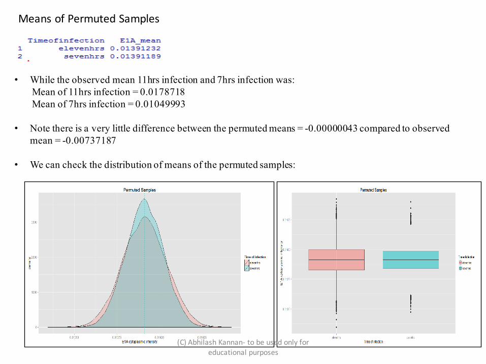
MeansofPermutedSamples

• While the observed mean 11hrs infection and 7hrs infection was:Mean of 11hrs infection = 0.0178718Mean of 7hrs infection = 0.01049993

• Note there is a very little difference between the permuted means = -0.00000043 compared to observed mean = -0.00737187

• We can check the distribution of means of the permuted samples:


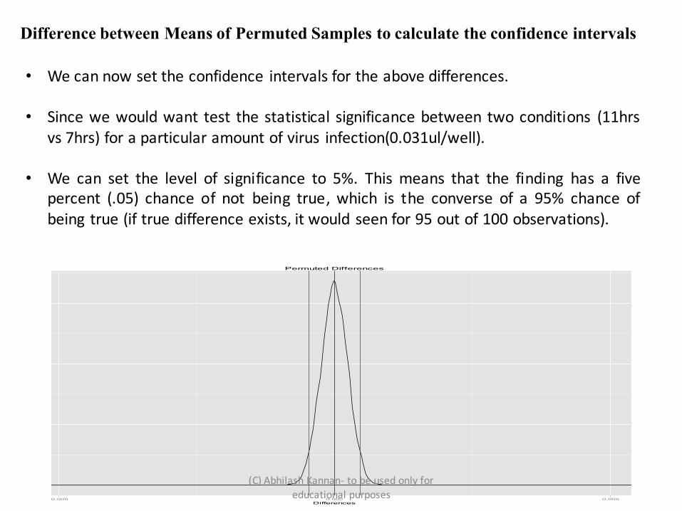
Difference between Means of Permuted Samples to calculate the confidence intervals

• We can now set the confidence intervals for the above differences.

• Since we would want test the statistical significance between two conditions (11hrsvs 7hrs) for a particular amount of virus infection(0.031ul/well).

• We can set the level of significance to 5%. This means that the finding has a fivepercent (.05) chance of not being true, which is the converse of a 95% chance ofbeing true (if true difference exists, it would seen for 95 out of 100 observations).

0

500

1000

1500

-0.005 0.000 0.005Differences

density

Permuted Differences


Computing the p-value

• p-value can be calculated from the distribution of mean differences of 11hrs and 7 hrs treatment from thepermuted sample.

• Since we have already calculated the confidence interval for these differences, we can check if any of thedifference between the two conditions from the our observed samples fall within this computedconfidence interval.

0

500

1000

1500

-0.005 0.000 0.005Differences

dens

ity

Permuted Differences

• The difference is clearly significant.

• It can be clearly seen that observed difference never ovelaps with the confidence intervals (Two red solidintercept) of the permuted differences.

• Thus the number of times the permuted differences ≥ observed difference out of the total number ofpermutations gives the final p-value.

pvalue =sum(abs(diff_permuted) >=abs(diff_observed)) /permutations


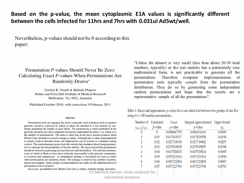
Based on the p-value, the mean cytoplasmic E1A values is significantly differentbetween the cells infected for 11hrs and 7hrs with 0.031ul Ad5wt/well.

Nevertheless, p-values should not be 0 according to this paper:

“Unless the dataset is very small (less than about 20-30 totalnumbers, typically) or the test statistic has a particularly nicemathematical form, is not practicable to generate all thepermutations. Therefore computer implementations ofpermutation tests typically sample from the permutationdistribution. They do so by generating some independentrandom permutations and hope that the results are arepresentative sample of all the permutations”.


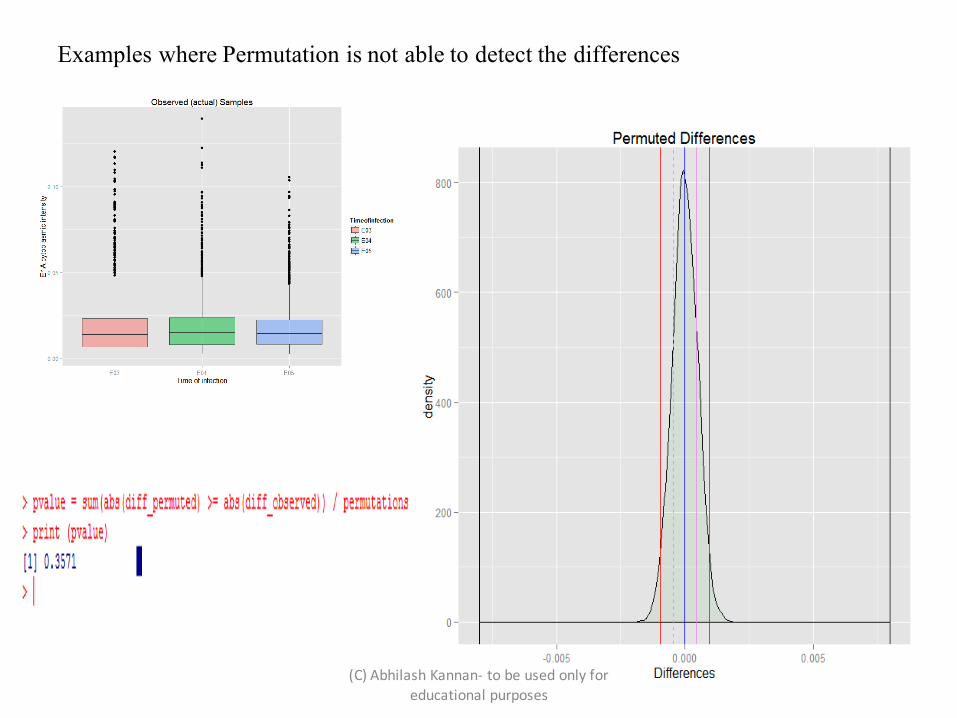
Examples where Permutation is not able to detect the differences


Based on the Permutation resampling analysis:

1. Significant difference in cytoplasmic E1A intensities btween 11hrs, 7hrs and 4 hrs infection with different virus concentration (0.031ul, 0.0625ul, 0.125ul and 0.25ul/well)

2. Some of the technical replicates also show significant differences

Example:

0.031ul virus (4hrs) E09 vs E10 - NSE09 vs E11 - NSE10 vs E11 – S

0.0625ul Virus (11hrs)D03 vs D04 - NSD04 vs D05 - NSD03 vs D05 – S

0.125ulVirus (11hrs)C03 vs C04 - SC04 vs C05 - NSC03 vs C05 - S


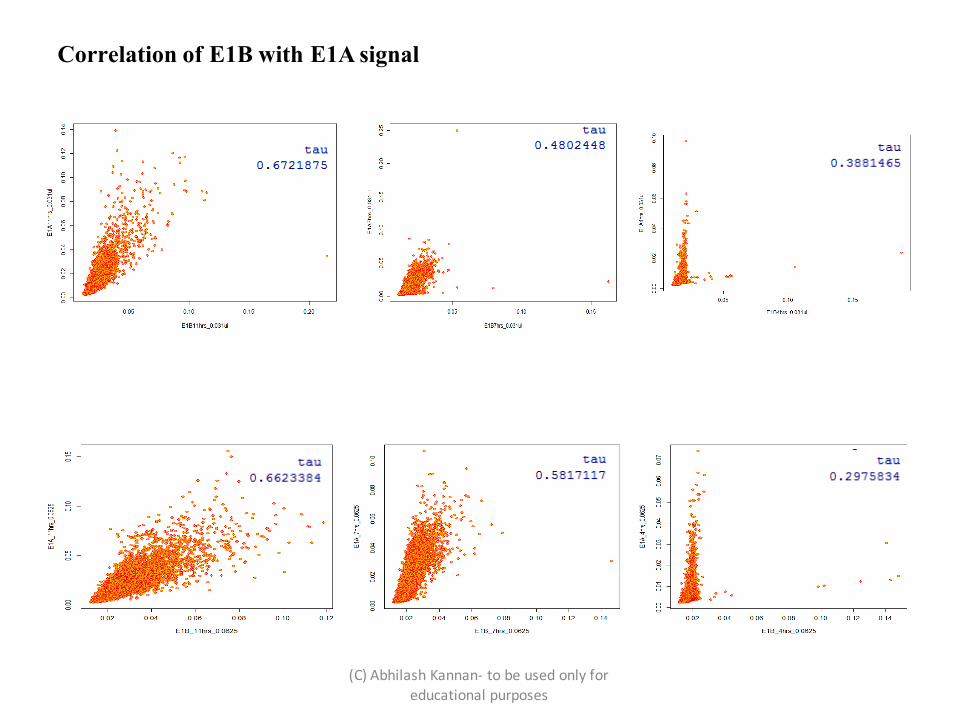
Correlation of E1B with E1A signal


e1a quantigene

Documents