Efficient Resource Allocation Schemes for Search

by

Eran Bashan

A dissertation submitted in partial fulfillmentof the requirements for the degree of

Doctor of Philosophy(Electrical Engineering: Systems)

in The University of Michigan2008

Doctoral Committee:

Professor Alfred O. Hero III, Co-ChairProfessor Jeffrey A. Fessler, Co-ChairProfessor Robert W. KeenerProfessor Demosthenis TeneketzisAssistant Professor Michael Wakin

c© Eran Bashan 2008All Rights Reserved

To my late grandfather, Yehuda Borenstein, a meister who taught me to believe

ii

ACKNOWLEDGEMENTS

This work has seen support from many individuals, and I would like to use this

opportunity to name a few. To begin with, I would like to thank Professor Jeff

Fessler. He convinced me to join the University of Michigan and start this journey

under his wings. I have enjoyed Professor Fessler’s knowledge, inspiration, guidance,

mentorship, and above all friendship and kind words in times of need. Also, I am

in great debt to Professor Hero for his support and help throughout the majority of

this research. Working with Professor Hero is both a challenging and a rewarding

experience. I admire his patience with his students, vast knowledge, and imagination.

This work has benefited from numerous discussions with the rest of my committee

members. I would like to thank Professor Teneketzis, Professor Keener, and Professor

Wakin for their support, input, and helpful comments. At the same time I wish to

thank Raviv Raich with whom I worked closely on a major section of my thesis.

One of the best things that happened to me at Michigan is the exposure to a group

of exceptional individuals whom I was lucky to have as colleagues in both Professors

Fessler and Hero research groups. Specifically, I would like to thank Dan Ruan who

was always there when a tough problem was waiting to be solved. Also, I’d like

to mention Matt Jacobson, Somesh Srivastava, Kim Khalsa, Seyoung Chun, Mark

Kliger, Ami Weisel, Kevin Carter, and Raghuram Rangarajan. I would like to thank

my friends at Michigan: Ioannis Poulakakis, David Shuman, and Petar Momcilovic

and elsewhere Evyatar, Harel, Tani, Oren, Rotem, Amir, Israel, Dikla, Ayelet, and

iii

many others for their support and encouragement throughout the past years.

Finally, and most of all, I have to thank my wife Iris who was there for me to

support and help through the harshest of times. I also wish to thank my parents,

my brothers, and my sister for their distant support of my endeavors. Last but not

least I’m grateful to Herbert and Barbara Goldberg for taking us into their extended

family and creating a place we can call home away from home.

iv

PREFACE

Every journey starts somewhere, and this one started back in March of 1996. After

a few good years with the military and several months in South America, I landed in

Florida and started a long motorcycle journey throughout the United States. Some

25,000 miles and seven months later, I was on my way back to Israel to start my

undergrad education. At that point I knew it is only a matter of time until I will be

back in this magnificent country. Of course, I had no way of knowing that I would

be riding my motorcycle throughout four Michigan winters.

My military education taught me the principles of war, which to a large extent are

suitable for more peaceful situations as well. Two of these principles led me to this

current research: 1) Mass - Bring decisive force to bear at critical times and places. 2)

Economy of Force - Allocate minimum essential combat power to secondary efforts.

This research deals with efficient resource allocation schemes and captures my quest

to create efficient systems.

On the morning of October 6, 2006, I was rushed to the ER at UM Hospital after

an unpleasant encounter I had with a deer on the steering bar of my motorcycle at

approximately 55 mph. Twelve hours and some 400 x-rays later (mainly due to head

and chest CT) it turned out there was nothing wrong with me, I was shaken not

stirred. Recovered from that unorthodox experience it hit me (along with the deer):

there has got to be a better way to do these things. In the time since the accident I

have developed methodology to improve the way we search for needles-in-a-haystack.

v

These methods focus search efforts onto unknown regions of interest, limiting the ef-

forts wasted scanning benign locations. There are numerous applications for which

this may apply, ranging from: air traffic control and missile launch detection to med-

ical imaging and early detection of cancer tumors. It is my sincere hope that this

work will find its way to the real world and help us reduce wasted efforts. Whether

it is in shortening the time we wait through an airport security screening line or by

reducing radiation exposure of healthy tissue, I hope that I made something good

with my time at Michigan.

May 2008

Ann Arbor, MI.

Figure P.1: March 22nd, 2008, I’ve almost made it home. Image taken on Michigan Ave. (US-12).

vi

TABLE OF CONTENTS

DEDICATION . . . . . . . . . . . . . . . . . . . . . . . . . . . . . . . . . . . . . . . . . . ii

ACKNOWLEDGEMENTS . . . . . . . . . . . . . . . . . . . . . . . . . . . . . . . . . . iii

PREFACE . . . . . . . . . . . . . . . . . . . . . . . . . . . . . . . . . . . . . . . . . . . . . v

LIST OF FIGURES . . . . . . . . . . . . . . . . . . . . . . . . . . . . . . . . . . . . . . ix

CHAPTER

I. Introduction . . . . . . . . . . . . . . . . . . . . . . . . . . . . . . . . . . . . . . . 1

1.1 SPECT system design . . . . . . . . . . . . . . . . . . . . . . . . . . . . . . . 41.1.1 Resolution measures . . . . . . . . . . . . . . . . . . . . . . . . . . 6

1.2 Search and dynamic resource allocation . . . . . . . . . . . . . . . . . . . . . 71.2.1 Adaptive sampling . . . . . . . . . . . . . . . . . . . . . . . . . . . 81.2.2 Sensor management . . . . . . . . . . . . . . . . . . . . . . . . . . . 101.2.3 Search theory . . . . . . . . . . . . . . . . . . . . . . . . . . . . . . 121.2.4 Multi-scale hypothesis testing . . . . . . . . . . . . . . . . . . . . . 14

1.3 Applications . . . . . . . . . . . . . . . . . . . . . . . . . . . . . . . . . . . . 16

II. The Two-pinholes problem . . . . . . . . . . . . . . . . . . . . . . . . . . . . . . 18

2.1 Introduction . . . . . . . . . . . . . . . . . . . . . . . . . . . . . . . . . . . . 182.2 Summary of main results and notation borrowed from [20] . . . . . . . . . . 222.3 A two pinhole system . . . . . . . . . . . . . . . . . . . . . . . . . . . . . . . 25

2.3.1 Resolution constraints . . . . . . . . . . . . . . . . . . . . . . . . . 262.3.2 Single pinhole . . . . . . . . . . . . . . . . . . . . . . . . . . . . . . 282.3.3 Two independent pinholes . . . . . . . . . . . . . . . . . . . . . . . 30

2.4 Simulation results . . . . . . . . . . . . . . . . . . . . . . . . . . . . . . . . . 352.4.1 Hard frequency constraint . . . . . . . . . . . . . . . . . . . . . . . 372.4.2 BW-RMS constraint . . . . . . . . . . . . . . . . . . . . . . . . . . 392.4.3 Reconstruction Kernel comparison . . . . . . . . . . . . . . . . . . 41

2.5 Single pinhole with a general reconstruction kernel . . . . . . . . . . . . . . . 432.6 Conclusions and future work . . . . . . . . . . . . . . . . . . . . . . . . . . . 462-A Appendix: Full size reconstructed images of the different systems . . . . . . 48

III. Optimal Two-stage Search for Sparse Targets using Convex Criteria . . . 52

3.1 Introduction . . . . . . . . . . . . . . . . . . . . . . . . . . . . . . . . . . . . 523.2 Problem formulation . . . . . . . . . . . . . . . . . . . . . . . . . . . . . . . 57

3.2.1 Energy allocation with energy constraint . . . . . . . . . . . . . . . 633.3 Search policy . . . . . . . . . . . . . . . . . . . . . . . . . . . . . . . . . . . . 65

3.3.1 Optimal two stage search policy . . . . . . . . . . . . . . . . . . . . 66

vii

3.3.2 Properties of the optimal energy allocation . . . . . . . . . . . . . . 693.3.3 Suboptimal two stage search policy . . . . . . . . . . . . . . . . . . 73

3.4 Comparison of search algorithms . . . . . . . . . . . . . . . . . . . . . . . . . 743.4.1 Estimation post-processing . . . . . . . . . . . . . . . . . . . . . . . 743.4.2 Detection post-processing . . . . . . . . . . . . . . . . . . . . . . . 763.4.3 Achievable cost . . . . . . . . . . . . . . . . . . . . . . . . . . . . . 80

3.5 Application - detecting and estimating a ROI in a SAR image . . . . . . . . 823.6 Conclusions and future work . . . . . . . . . . . . . . . . . . . . . . . . . . . 853-A Appendix: Equivalency of minimizing our cost to minimizing the Cramer-

Rao bound . . . . . . . . . . . . . . . . . . . . . . . . . . . . . . . . . . . . . 883-B Appendix: Chernoff bound on the probability of error and our cost function 883-C Appendix: Showing a global lower bound on our cost . . . . . . . . . . . . . 893-D Appendix: Showing an upper bound on the gain . . . . . . . . . . . . . . . . 903-E Appendix: Minimizing the cost function . . . . . . . . . . . . . . . . . . . . 93

E.1 The case of T = 1 . . . . . . . . . . . . . . . . . . . . . . . . . . . . 93E.2 The case of T = 2 . . . . . . . . . . . . . . . . . . . . . . . . . . . . 94

3-F Convergence of pIi|y(1),θ for the Gaussian case . . . . . . . . . . . . . . . . . 99

IV. The multi-scale search problem . . . . . . . . . . . . . . . . . . . . . . . . . . . 103

4.1 Introduction . . . . . . . . . . . . . . . . . . . . . . . . . . . . . . . . . . . . 1034.2 Problem formulation . . . . . . . . . . . . . . . . . . . . . . . . . . . . . . . 1074.3 Search policy for T = 2 under total effort and time constraints . . . . . . . . 111

4.3.1 First search policy . . . . . . . . . . . . . . . . . . . . . . . . . . . 1134.3.2 Detectability index and asymptotic properties of pIi|Y (1) when ν = 11144.3.3 Second search policy . . . . . . . . . . . . . . . . . . . . . . . . . . 120

4.4 Performance and comparison of search algorithms . . . . . . . . . . . . . . . 1214.4.1 Estimation . . . . . . . . . . . . . . . . . . . . . . . . . . . . . . . . 1214.4.2 Detection . . . . . . . . . . . . . . . . . . . . . . . . . . . . . . . . 1264.4.3 Statistical models approximation . . . . . . . . . . . . . . . . . . . 131

4.5 Conclusions and future work . . . . . . . . . . . . . . . . . . . . . . . . . . . 1344-A Appendix: Mean and variance of Yj(1) given H1 . . . . . . . . . . . . . . . . 1374-B Appendix: Showing pIi|yi(1) → r under Hr . . . . . . . . . . . . . . . . . . . 138

V. Conclusions and Future Work . . . . . . . . . . . . . . . . . . . . . . . . . . . . 141

5.1 Conclusions . . . . . . . . . . . . . . . . . . . . . . . . . . . . . . . . . . . . 1415.2 Future work . . . . . . . . . . . . . . . . . . . . . . . . . . . . . . . . . . . . 143

BIBLIOGRAPHY . . . . . . . . . . . . . . . . . . . . . . . . . . . . . . . . . . . . . . . . 146

viii

LIST OF FIGURES

Figure

P.1 March 22nd, 2008, I’ve almost made it home. Image taken on Michigan Ave. (US-12). vi

2.1 Variance comparison between a single pinhole system (blue, solid) to a two identicalpinholes system (green, dashed) and a two different pinholes system (red, dashed-dot). 32

2.2 A cold spot Derenzo phantom used as an input to our systems. The discs radii are[1.53 2.15 2.45 3.06 4.28 6.12] [mm]. . . . . . . . . . . . . . . . . . . . . . . . . . . 37

2.3 We show samples of reconstructed images of all systems used in the mentionedsimulations. Top left, a standard system. Top right, a new system satisfying thehard frequency constraint. Bottom left, a new system satisfying the BW-RMSconstraint. Bottom right, a new system using a jinc masked reconstruction kernelsatisfying hard frequency constraint. . . . . . . . . . . . . . . . . . . . . . . . . . . 38

2.4 Hard Frequency constraint: Comparison of the two systems frequency responsefunctions showing that both response satisfy the constraint. The solid-blue linerepresents the standard system, while the green-dashed line represents the newsystem. . . . . . . . . . . . . . . . . . . . . . . . . . . . . . . . . . . . . . . . . . . . 39

2.5 Hard Frequency constraint: Comparison of the mean (top row) and variance (bot-tom row) of the two systems. The new system results are presented on the rightcolumn and the standard system on the left. . . . . . . . . . . . . . . . . . . . . . . 40

2.6 Hard Frequency constraint: Variance plots through slices of the Derenzo phantom.We compare the two system performance as well as validating the accuracy of ourvariance approximations. . . . . . . . . . . . . . . . . . . . . . . . . . . . . . . . . . 40

2.7 BW-RMS constraint: In the upper row we plot the search results for βi vs. α, andin the lower row we plot the estimation variance vs. α for the βi’s given in eachupper figure. . . . . . . . . . . . . . . . . . . . . . . . . . . . . . . . . . . . . . . . . 41

2.8 BW-RMS constraint: Comparison of the mean (top row) and variance (bottomrow) of the two systems. The new system results are presented on the right columnand the standard system on the left. . . . . . . . . . . . . . . . . . . . . . . . . . . 42

2.9 BW-RMS constraint: Variance plots through slices of the Derenzo phantom. Wecompare the two system performance as well as validating the accuracy of ourvariance approximations. . . . . . . . . . . . . . . . . . . . . . . . . . . . . . . . . . 42

2.10 BW-RMS constraint: In the upper row we plot the search results for βi vs. α, andin the lower row we plot the estimation variance vs. α for the βi’s given in eachupper figure. . . . . . . . . . . . . . . . . . . . . . . . . . . . . . . . . . . . . . . . . 49

ix

2.11 Standard system, image reconstruction of the Derenzo phantom. . . . . . . . . . . 49

2.12 Hard frequency constraint: New system Gaussian reconstruction kernel, image re-construction of the Derenzo phantom. . . . . . . . . . . . . . . . . . . . . . . . . . 50

2.13 Hard frequency constraint: New system, image reconstructed using jinc maskedkernel. . . . . . . . . . . . . . . . . . . . . . . . . . . . . . . . . . . . . . . . . . . . 50

2.14 BW-RMS constraint: New system, image reconstruction of the Derenzo phantom. . 51

3.1 Gain in MSE for the CME in (3.57) based on an adaptive search compared tothe MSE of the CME for an exhaustive search policy (3.56). Curves with crossescorrespond to ARAP, for p values of 1

100 and 110 , while curves with circles represent

the suboptimal adaptive policy. The MSE gain for ARAP is slightly higher thanthat of the suboptimal mapping. Note that using our methods results in about 6[dB] gain in MSE at SNR value of 12 [dB] for sparsity level of 1%. In addition MSEgain is inversely proportional to the sparsity, hence higher gains can be expectedfor application where |Ψ| ¿ Q. . . . . . . . . . . . . . . . . . . . . . . . . . . . . . 76

3.2 ROC curves for the LRT tests based on an exhaustive search scheme and the twoadaptive policies measurements scheme, for p = 0.1 and p = 0.01 and SNR of 10[dB]. (a) shows the entire ROC curve while (b) zooms in on false alarm probabilityvalues less than 0.5. The simulation suggests that our adaptive search policiesoutperforms an exhaustive search policy in terms of detection probability for falsealarm values lower than 30%. . . . . . . . . . . . . . . . . . . . . . . . . . . . . . . 79

3.3 Detection probability, for a fixed test level, and estimation MSE gain g(·) in (3.58)as a function of ν when SNR is 10 [dB] and p = 0.01. Note that the MSE gainvalues (curve with triangular markers) are given on the r.h.s.of the figure. SinceMSE gain is defined over the true ROI it increases with ν. . . . . . . . . . . . . . . 80

3.4 The cost gain compared to an exhaustive search for both our optimal and subop-timal energy allocation schemes. (a) shows that both algorithms converges to theasymptotic predicted gain, at −10 log p. (b) enhances the difference between ourtwo policies for SNR values in the range of 0− 13 [dB]. . . . . . . . . . . . . . . . . 81

3.5 The proportion of energy invested at the first step for the two algorithms λA andλso. Curves correspond to prior probability values of 0.001, 0.01 and 0.1. As seen,the optimal search policy invest more energy at the first step. However, for SNR> 25 [dB] the two are essentially equivalent. . . . . . . . . . . . . . . . . . . . . . . 82

3.6 The above (13× 13) tank template was used as a matched filter to filter the noisydata X1 and generate y(1). . . . . . . . . . . . . . . . . . . . . . . . . . . . . . . . 84

3.7 SAR imaging example, SNR=4 [dB]. (a) Original image. (b) Image reconstructedusing two exhaustive searches. (c) Effort allocation using ARAP at the secondstage. (d) Image resulted from (3.68) using ARAP. . . . . . . . . . . . . . . . . . . 86

x

3.8 SAR imaging example, SNR=0 [dB]. (a) Image reconstructed using two exhaustivesearches, targets are not easily identifiable. (b) Image resulted from (3.68) usingARAP. Figures (c) and (d) compare a 1D profile going through the targets on thelower left column for 100 different realizations. (c) Profiles of images reconstructedfrom an exhaustive search. (d) Profiles of images reconstructed using ARAP. Thebold bright line on both figures represent the mean profile of the different realiza-tions. Evidently, variations of profiles of images due to ARAP are much smallercompared to variations of profiles of images resulted from an exhaustive scan. . . . 87

4.1 We plot estimation gains as a function of SNR for different contrast levels. Theupper plot show gains for L = 8 while the lower plot show gains for L = 32. Notethat without sufficient contrast (µθ = 1

2 ), λM results in performance loss. However,for high contrast significant gains of 10 [dB] are achieved at SNR values less than15 [dB]. At the same time we only use about 15% of the samples compared to anexhaustive search. Note that the asymptotic lower bound on the gain (4.39) yields22.6 [dB] and 15.3 [dB] for L = 8 and L = 32 respectively. Since in both plots thegains exceed the bound we conclude that the bound is not tight. . . . . . . . . . . 125

4.2 We plot the normalized number of samples N∗ as a function of SNR for L = 8,L = 32, and different contrast levels µθ ∈ 2, 4, 8. These N∗ values are associatedwith estimation gains seen in Fig. 4.1 for SNR values ranging from 0 to 20 [dB](the left half of the SNR axis in Fig 4.1). For example for a relatively low contrastof µθ = 2, SNR of 15 [dB], and L = 8, estimation performance gain of 10 [dB] isachieved with only 14% of the sampling used by exhaustive search. . . . . . . . . . 126

4.3 We plot estimation gains vs. detectability index. Note that for large L (lowerplot) the detectability index can be used to predict performance gain regardless ofthe actual contrast or SNR. This is not the case when L is close to the expectedmaximum target length ξ0 as seen in the upper plot for L = 8. . . . . . . . . . . . 127

4.4 Receiver operating characteristic (ROC) curves for SNR of 0 [dB] and L = 8 ofdata acquired using M-ARAP vs. a non-adaptive exhaustive data acquisition. Theupper plot shows low contrast levels of µθ 6 2, while the lower plot focuses on highcontrast levels. Dash-dot curves represent the ROC of the non-adaptive LRT anddifferent markers represent contrast. In the upper plot we see improved detectionperformance of M-ARAP compared to the non-adaptive scheme. However, this isreversed for the lower plot. . . . . . . . . . . . . . . . . . . . . . . . . . . . . . . . . 131

4.5 Receiver operating characteristic (ROC) curves for SNR of 0 [dB] and L = 32 ofdata acquired using M-ARAP vs. a non-adaptive exhaustive data acquisition. Theupper plot shows low contrast levels of µθ 6 2, while the lower plot focuses onhigh contrast levels. Dash-dot curves represent the ROC of the non-adaptive LRTand different markers represent contrast. The ROC curves due to the non-adaptiveLRT dominate the ROC curves resulting from M-ARAP. . . . . . . . . . . . . . . . 132

4.6 ROC curves for the two tests at SNR of 10 [dB] and low contrast levels of µθ 6 2.In the upper plot we set L = 8, while L = 32 was chosen for the lower plot. Notethat increasing SNR improves test performance of the non-adaptive scheme farbetter than for M-ARAP. This is mainly attributed to the fact that with ν = 1,M-ARAP does not spend enough energy characterizing the alternative and focusesthe sampling energy onto the ROI. . . . . . . . . . . . . . . . . . . . . . . . . . . . 133

xi

4.7 We plot the pdf of the predicted Gaussian mixture (solid blue), simulations his-togram (asterisk red), and the single Gaussian approximation (dash-dot green) withmean and variance given in (4.10) and (4.11). For the upper plot we have L = 8and µθ = 2, while for the lower plot L = 32 and µθ = 8. For both plots SNR is 10[dB] and the detectability index (4.19) is roughly one. . . . . . . . . . . . . . . . . 134

4.8 We plot the cdf of the predicted Gaussian mixture (solid blue), simulations his-togram (asterisk red), and the single Gaussian approximation (dash-dot green)with mean and variance given in (4.10) and (4.11). For the upper plot we haveL = 8 and µθ = 2, while for the lower plot L = 32 and µθ = 8. For both plotsSNR is 10 [dB] and the detectability index (4.19) is roughly one. As one can see,the Gaussian approximation is not far from the true GM distribution. . . . . . . . 135

4.9 We plot the pdf of the predicted Gaussian mixture (solid blue), simulations his-togram (asterisk red), and the single Gaussian approximation (dash-dot green) withmean and variance given in (4.10) and (4.11). For both plots SNR is 20 [dB] andµθ = 4, while L = 8 in the upper plot and L = 32 for the lower plot. Note thatwhile the single Gaussian approximation in the lower plot is still a somewhat rea-sonable approximation of the GM this is not the case for the upper plot. Thisexplains the different behavior exhibited by the curves in Fig. 4.3. . . . . . . . . . 136

xii

ABSTRACT

Efficient Resource Allocation Schemes for Search

byEran Bashan

Co-Chairs: Alfred O. Hero III and Jeffrey A. Fessler

This thesis concerns the problem of efficient resource allocation under constraints.

In many applications a finite budget is used and allocating it efficiently can improve

performance. In the context of medical imaging the constraint is exposure to ioniz-

ing radiation, e.g., computed tomography (CT). In radar and target tracking time

spent searching a particular region before pointing the radar to another location or

transmitted energy level may be limited. In airport security screening the constraint

is screeners’ time. This work addresses both static and dynamic resource allocation

policies where the question is: How a budget should be allocated to maximize a

certain performance criterion.

In addition, many of the above examples correspond to a needle-in-a-haystack

scenario. The goal is to find a small number of details, namely ‘targets’, spread out

in a far greater domain. The set of ‘targets’ is named a region of interest (ROI).

For example, in airport security screening perhaps one in a hundred travelers carry

prohibited item and maybe one in several millions is a terrorist or a real threat.

Nevertheless, in most aforementioned applications the common resource allocation

xiii

policy is exhaustive: all possible locations are searched with equal effort allocation

to spread sensitivity.

A novel framework to deal with the problem of efficient resource allocation is in-

troduced. The framework consists of a cost function trading the proportion of efforts

allocated to the ROI and to its complement. Optimal resource allocation policies

minimizing the cost are derived. These policies result in superior estimation and

detection performance compared to an exhaustive resource allocation policy. More-

over, minimizing the cost has a strong connection to minimizing both probability of

error and the Cramer-Rao bound on estimation mean square error. Furthermore, it

is shown that the allocation policies asymptotically converge to the omniscient allo-

cation policy that knows the location of the ROI in advance. Finally, a multi-scale

allocation policy suitable for scenarios where targets tend to cluster is introduced.

For a sparse scenario exhibiting good contrast between targets and background this

method achieves significant performance gain yet tremendously reduces the number

of samples required compared to an exhaustive search.

xiv

CHAPTER I

Introduction

Consider the problem of efficiently using a given budget to perform a certain

task. By a ‘task’ we generally mean the process of acquiring data and we refer to the

acquisition ‘cost’ as budget. This setting is common to many daily applications where

the question is how to best utilize the budget at hand. In the context of medical

imaging the budget or constraint is the total amount of ionizing radiation a patient

may safely endure, e.g. computed tomography (CT). In radar and target tracking we

are limited by the duration of time we can spend searching a particular region before

moving the radar beam to another location or by the energy level of the transmitted

signal. In airport security screening we are limited by the total amount of screeners

time at any given day. Time is also an issue in medical imaging modalities such as

single photon electron CT (SPECT) or magnetic resonance imaging (MRI) where a

long scan duration may result in either motion blur or a need to keep the patient

inside the scanner for too long.

In addition, in many of the examples discussed above the scanned medium bears

little interest for the actual application. What we are looking for is a small number

of details, namely targets, spread out in a far greater domain. We call the collection

of all targets in a given domain a region of interest (ROI). In medical imaging we

1

2

may look for a small tumor, maybe less than one cubic centimeter, placed somewhere

inside the torso. For target tracking/detection applications the connection may be

more obvious as we are looking for vehicles on the ground, airplanes in the air, or

vessels in the sea. In a general screening process it is also more often than not the

case where the proportion of ‘targets’ within the screened population is relatively

small. For example, percentage of women exhibiting breast cancer is roughly 12%

of the screened population. In airport security screening perhaps one in a hundred

travelers forget a prohibited item in his belonging and maybe one in several million

is a terrorist or a real threat. Nevertheless, in most of the applications mentioned

above the common search/resource allocation scheme is exhaustive where all possible

locations are searched with equal effort allocation to spread sensitivity. For example,

the same energy level is used in each CT projection when we image the torso to

detect lung cancer tumor.

A resource allocation policy may be either static or dynamic. A static allocation

is one where we predetermine how to allocate efforts before any action is taken. In

active radar this is equivalent to predefining the beam pattern and the (angular)

scan speed and trajectory. This way, regardless of finding, the radar beam would

keep scanning the domain in a fix pattern and with a fix resolution. Exhaustive

resource allocation scheme is a special case among static schemes. Dynamic resource

allocation scheme allows the allocation policy to change over time. If this change

is data dependent, then we call such schemes adaptive sensing. In a sense, adaptive

sensing schemes utilize past observation to modify the way some reserved budget is

being deployed to acquire future observations. This thesis considers both static and

dynamic resource allocation schemes. We start by designing a non uniform SPECT

scanner system and move on to derive optimal adaptive allocation schemes.

3

The main contributions of this dissertation are:

i. We design a nonuniform SPECT system to minimize estimation error of a linear

estimator subject to bandwidth constraints. Analytic expression of the expected

estimation variance is given and reduction of up to 70% of estimation variance

is achieved.

ii. We provide a novel framework for the problem of dynamic resource allocation.

This framework utilizes a new cost function that accounts for effort distribution

inside and outside the ROI.

iii. We show that minimizing our cost function is strongly connected to minimizing

both error probability and estimation error.

iv. An optimal Adaptive Resource Allocation Policy, which we call ARAP, is de-

rived for a two stage allocation procedure.

v. We show that ARAP is asymptotically optimal in terms of our cost function.

vi. We derive a multi-scale version of ARAP, namely M-ARAP, utilizing a coarse

scale for the first stage, then refining the data over a small part of the scanned

domain at the second stage.

vii. We show that M-ARAP maintains most of the properties of ARAP, yet signifi-

cantly reducing the total number of measurements used.

viii. A bound on the expected ‘waste’ due to multiscaling is provided.

We suggest that future work would connect our adaptive sensing methods to com-

pressive sensing to yield a new sampling paradigm for sparse signals.

4

The rest of this thesis is organized as follows: We continue with a literature

review of related work for the rest of this chapter. Chapter II propose a method for

designing a nonuniform two-pinhole SPECT system. In Chapter III we formulate

a novel framework for the problem of adaptive resource allocation and derive two

stage optimal effort allocation schemes, namely ARAP. Chapter IV discusses several

benefits in multiscaling and introduces M-ARAP. Finally, in Chapter V we conclude

and point out to possible future work.

1.1 SPECT system design

The first application of the tracer principle was made in 1911 by Hevesy. How-

ever, the bridge to modern nuclear medicine and its emphasis on imaging awaited

the development of imaging devices, which first appeared in the late 1940’s. Cassen

et al. developed the first planar gamma-ray scanning device. Their rectilinear scan-

ner produced a pattern of dots representing the distribution of radiotraces within a

patient body. In the early 1950’s, Anger was the first to use pinhole collimation to

increase resolution in small regions. The image was projected, through the pinhole,

onto a scintillating screen with photographic film behind it. The overall system was

highly inefficient and it required extremely long exposure times (principally due to

losses in the film). These inefficiencies resulted in extremely high radiation doses to

patients. By the end of the 1950’s, Anger had replaced the photographic film with

an array of photomultiplier tubes (PMT). This design becomes the basis for today’s

Anger camera. Kuhl and Edwards were the first to present tomographic images pro-

duced using the Anger Camera in 1963. By 1970’s a series of innovations in rotating

cameras led researchers to look for improved resolution in the reconstructed images.

In 1978 Vogel et al. reported experiments with Anger cameras using a seven-pinhole

5

collimator, but distracting artifacts were present in the images due to limitations in

the reconstruction methods available at that time. It was not until the 1990’s that

researchers were able to use multi-pinhole collimators in Emission Tomography (ET)

scanners. Stationary PET scanners were pioneered by Robertson and Bozzo et al. by

the 1960’s and by Ter-Pogossian et al. in the early 1970’s. Today ET scanners (both

PET and SPECT) are of the most important medical imaging modalities, providing

images that reveal subtle information about physiological processes in humans and

animals.

Since the beginning, the reconstructed image resolution was a constant challenge

for all system designers. In [50] Rogulski et al. showed that improvements in detector

resolution can lead to both improved spatial resolution in the image and improved

counting efficiency, through the design of multiple-pinhole coded-aperture system.

Their group had since been dealing with feasibility issues and had build several such

SPECT systems (see [43, 44, 59]), where optimizing parameters such as number of

pinholes, pinholes geometry and their diameter is essential during the design process.

In [59] they also report on first attempts of using a multi-resolution system, i.e., hav-

ing pinholes with different diameters, where the image is reconstructed using OS-EM

algorithm (Ordered Subsets Expectation Maximization). Unfortunately, no conclu-

sive conclusions regarding this setup are given. Ivanovic et al. had also reported [27]

experiments of a multiple pinhole scanner where they had optimize, among other

system parameters, the number of pinholes their aperture size and their geometry.

In [51] Schramm et al. describe another multiple pinhole SPECT scanner and re-

ports improvements in the system resolution and sensitivity when compared to a

single pinhole system. Meng et al., in [40], describes a study of a Compton scatter-

ing enhanced multiple pinhole imager. They show that scattered detected photons

6

information may be used in addition to photons detected after going through the

pinhole collimator to improve the overall system performance. In [39] Meng and

Clinthorne modified the Uniform Cramer-Rao Bound (UCRB), suggested in [26],

and presented tradeoffs between some resolution constraint and the reconstructed

image variance. They compare the bounds for various multiple pinhole systems and

show that increasing the number of pinholes yield improved system performance.

However, none of the aforementioned papers attempt to analyze a system with dif-

ferent pinhole diameters, and [59] is the only one that even considers such a design.

Intuition leads to consider a system where a wide pinhole, yielding many counts

and improves Signal to Noise Ratio (SNR), is combined with a narrow pinhole that

provides good resolution but a noisy image, to result in a low-noise high-resolution

reconstructed image. In Chapter II we seek to minimize the estimation variance

subject to some constraint on the overall system resolution.

1.1.1 Resolution measures

Among researchers in the imaging science there is a convention that system per-

formance is a task dependent measure. For example, the human vision system deals

very well with “white noises”. Human’s vision automatically averages out zero mean

“salt and pepper” type noises. Therefore, noisy images do not necessarily imply that

the system producing them is not useful. On the other hand, image blur is very

conspicuous for the human eye. Thus, we wish to look at sharp images with as little

spatial bias as possible. As a result, quantifying imaging system performance is not

a trivial task. In [15] den Dekker and van den Bos survey some common resolution

measures. Starting from classical resolution criteria such as Rayleigh’s just resolved

criteria and Houston’s Full Width Half Maximum (FWHM) criteria both considering

7

a noise free system to measure precision effects on system resolution, and compare

the different measures. Evidentially they claim that, since noise free systems are not

of practical interest, all resolution measures should consider SNR. Moreover, they

show similarities between different resolution measures ranging from the image esti-

mated variance to information and decision theory resolution measures, since they

are all deeply affected by SNR. A different approach is taken in [57] where Wang and

Li state 5 axioms that a good resolution measure should obey, then show that any

such measure should be proportional to the standard deviation of the point spread

function of the imaging system. There are several other resolution criteria in the

literature that we are not going to mention here.

In [20] Fessler suggests another approach by minimizing the estimated image

variance subject to a certain constraint on the FWHM of the system. Fessler analyzes

a single pinhole system considering a specific estimation scheme, namely kernel-based

indirect density estimator. For the suggested criteria Fessler shows that the optimal

pinhole diameter should be proportional to the desired system FWHM. Moreover,

for a specific case Fessler provides a close form solution for the problem showing

that the ratio of the optimal pinhole diameter to the system FWHM is constant.

In Chapter II we use that criteria to find the optimal pinhole diameters in a two

pinhole system subject to some constraint on the system frequency response of the

point spread function.

1.2 Search and dynamic resource allocation

The problem of dynamic resource allocation is connected to many different re-

search fields. Although often called by different names and hidden under different

frameworks, the concept of dynamic resource allocation is apparent in: adaptive

8

sensing, Markov decision problems, multi-armed bandit problems, sensor manage-

ment, search, and multi-scale hypothesis testing. Previous work on adaptive sensing

considered the problem of how to spatially distribute samples to recover an underly-

ing signal. In Markov decision problems one is looking to find an action policy that

maximizes a certain reward function depending on the different states and actions.

Multi-Armed Bandit (MAB) problems are a class of sequential resource allocation

problems concerned with allocating one or more resources among several alternative

projects. In search theory the objective is often to find a search sequence (policy)

that maximizes the probability of detecting a target hidden in one of many cells.

Multi-scale hypothesis testing problem concerns with making a multi-hypothesis de-

cision process more efficient by lumping parts of the hypothesis space together.

1.2.1 Adaptive sampling

Most of the previous work on adaptive sampling (AS), which sometimes appears

in the literature as active learning or active sampling, has concentrated on estimat-

ing functions in noise. Castro et al. [13] present asymptotical analysis and shows

that for piecewise constant functions adaptive sampling methods can capitalize on

spatial properties of the function. By focusing samples to the estimated vicinity of

the boundaries, adaptive sampling methods yields nearly optimal convergence rate,

in terms of estimation mean square error (MSE). It is also shown that for spatially

homogeneous functions adaptive sampling has no advantages over passive sampling.

Nowak et al. [42], Castro et al. [12], and Willett et al. [58] consider different ap-

plications characterized by spatially inhomogeneous functions, for which adaptive

sampling methods can be efficiently used. In [11], Castro et al. show that for certain

classes of piecewise constant signals compressed sensing is as efficient as adaptive

9

sampling, in terms of the estimation error convergence rate. Work in the field of

Compressed Sensing (CS) challenges the traditional signal processing sampling re-

quirements. Recent results show that a relatively small number of random projections

of a signal can contain most of its salient information. It follows that if a signal is

compressible in some orthonormal basis, it can be accurately recovered from random

projections even when they are contaminated with noise [9,24]. Candes and Tao [9]

introduce the Dantzig selector (DS) algorithm which solves an l1-norm minimization

problem to reconstruct a sparse signal (defined below) in RQ from a very limited

set of N < Q noisy observations. Their algorithm converges to the true solution as

long as the measurement operator obeys the uniform uncertainty principle (UUP).

They provide an upper bound on the mean squared error (MSE) which, remark-

ably, is proportional up to a C log Q factor of the noise level σ2. Haupt and Nowak

present a similar result but their measurement operator is randomized rather than

following the UUP [24]. Most of the previous work in both AS and CS is limited

to inhomogeneous signals and is of limited usage for the problem considered in this

thesis.

Sparse signals: A signal is considered sparse if its value is zero, or almost zero,

in most places. Strong sparsity is defined when most of the signal elements must be

exactly zero and is quantified by the fraction of nonzero elements. Weak sparsity is

defined when most of the signal elements are very small and is quantified by the rate

at which the sorted nonzero amplitudes decay. Although we consider homogenous

signals, we assume that the support of the ROI is small as compared to the entire

support of the signal. Therefore, we refer to such signals as sparse. Sparsity is used in

a variety of applications: signal compression, reconstruction, approximation, source

10

separation and localization, and target tracking or detection [4,18,23,37,38,41,54,61].

Most of the related research considers post processing tasks. Matching pursuit [38]

use a greedy algorithm to select base elements from the dictionary. Algorithms like

FOCUSS [23] use sparsity to reconstruct a signal from limited samples. Nafie et

al. [41] address the problem of subset selection. Wohlberg [61] provides reconstruc-

tion error bounds for several sparse signal bases. Sparse solutions using l1 penalty

are used in [37] to improve performance in direction-of-arrival estimation. Tropp

lays theoretical foundations for convex relaxation techniques for sparse optimization

problems [54]. Escoda et al. incorporate a priori knowledge of the signal structure

to compensate for a potentially coherent dictionary [18]. An algorithm that adapts a

dictionary to a given training set is given in [4]. In our work, we would like to utilize

the sparsity during the data acquisition phase as a pre-processing task.

1.2.2 Sensor management

Sensor management is a very wide topic with many different applications and we

refer the interested reader to [25]. However, in the context of this work we mention

two questions discussed in the literature that are where to point a sensor and in what

mode to operate a sensor for the next observation. Assume an agile array of sensors

is used to scan a certain domain. At each time step, one chooses which grid point

(cell) to search next and in what mode. Generally, a number of existing targets need

to be tracked while new targets are being looked for. Kastella looks at such porblems

under low SNR [31]. He introduces the discrimination gain based on the Kullback-

Leibler information to quantify the usefulness of the next measurement. Using a

myopic strategy, Kastella shows that pointing the sensor to the cell maximizing the

discrimination gain decreases the probability of incorrectly detecting where a target

11

is. Kreucher et al. [33, 34] show that integrating the sensor management algorithm

with the target tracking algorithm via the posterior joint multi-target probability

density (JMPD), helps to predict which measurement would prove most informative

in terms of increasing the information gain. Our approach differs as we consider

selecting the sensor operation mode from a continuous rather than discrete set of

modes. Krishnamurthy [35, 36] is interested in the problem of how to manage the

sensor to keep track of multiple targets already acquired. He uses a multi-arm bandit

formulation involving hidden Markov models to derive solutions to that problem.

In [36], an optimal algorithm is formulated to track multiple targets. Since the

optimal approach has prohibitive computational complexity, suboptimal methods

are given and numerical examples are presented. In [35], the problem is reversed and

a single target is observed from a collection of sensors. Again, approximate methods

for the optimal solution are formulated due to its intractability.

Adaptive energy allocation is addressed in [47–49]. Rangarajan et al. consider

the problem of adaptive amplitude design for estimating parameters of an unknown

medium under average energy constraints (fix energy constraints in [47]). They treat

an N time-steps design problem and provide an optimal solution for the case of

N = 2 in terms of minimizing estimation MSE. However, they do not consider the

parameter vector of interest to be sparse and as a result only minor gains are possible.

Using our method we show asymptotic gains in MSE inversely proportional to the

sparsity of the scanned domain.

Multi-Armed Bandit problems: In the classical MAB problem (see1 [25] chapter 6)

at each instant of time a single resource is allocated to one of many competing

1Most of the following paragraph is taken from the referred book and was written by Aditya Mahajan and

Demosthenis Teneketzis.

12

projects. The project to which the resource is allocated can change its state; the

remaining projects do not change state. In a variants of the MAB problem one or

more resources are dynamically allocated among several projects; new projects may

arrive; all projects may change state; delays may be incurred by the reallocation

of resources, etc. In general, sequential resource allocation problems can be solved

by dynamic programming. Dynamic programming, which is based on backwards

induction, provides a powerful method for the solution of dynamic optimization

problems, but suffers from the curse of dimensionality. The special structure of the

classical MAB problem has led to the discovery of optimal index-type allocation

policies that can be computed by forward induction (see [22] for more details), which

is computationally less intensive than backward induction. Researchers have also

discovered conditions under which forward induction leads to the discovery of optimal

allocation policies for variants of the classical MAB. In the approach taken here we

assume a different degree of freedom. The action we take affects the way we collect

information regarding certain states, rather than causing a change in the states.

1.2.3 Search theory

The field of Search Theory considers the following problem: a single target is

hidden in one of Q boxes. Each box is equipped with prior, detection, and false

alarm probabilities. A desirable search policy maximizes the probability of correctly

detecting the location of the target. For review of the problem and reference therein

see [6]. From the earlier work of Kadane [30] on “whereabouts search” to a more

recent work of Castanon [10] on “dynamic hypothesis testing”, the question remains

which cell to sample next in order to maximize the probability of detecting the

location of the target. Castanon shows that a myopic strategy is optimal for certain

13

noise characteristics. Although search theory has generated much research for more

than six decades, most of the work has concentrated on searching one box at a

time. In our case, we relax this stringent restriction. Song and Teneketzis [52]

generalize the framework to a search more than one cell at each step. They derive

two condition under which a search policy is optimal for either a fixed horizon or

for any horizon respectively. Most search theory literature considers independent

measurements between neighboring cells and over time. This model enables an offline

calculation of a compact static table listing the probability of detecting the target

while searching a cell at a given time. In turns, the table is used to find an optimal

search policy. Castanon extends this model and consider the case of dependent cells

where the probability table is dynamically updated [10]. This is also the case in our

work, although we introduce dependency between cells in a dual manner: over time

and via a sparsity constraint.

To the best of our knowledge, Posner [46] was the first to consider searching more

than one box at a time. He considers the problem of using a radar to locate a satellite

lost in a region of the sky containing Q cells. His goal is to minimize the expected

total search duration, and the idea is to search the cells where the satellite is most

likely to be first. Assuming a uniform prior, the competing strategy exhaustively

searches each cell for time t1 with an expected search time of t1(Q + 1)/2. Posner

suggests a preliminary search yielding a non-uniform likelihood function, followed by

a search of all cells for a time t1 in a descending likelihood order. For the preliminary

search he allows to widen the radar beam and measure k cells for a time t in each

measurement. Moreover, Posner allows to take as many preliminary searches as

necessary. In his model, the detection probability increases in t and decreases in k.

Posner’s model assumes that the search is stopped as soon as the satellite has been

14

found. Therefore, sequentially searching the cells with the highest likelihood reduces

the overall expected search time. Posner shows that the optimal solution minimizing

the expected search time takes a single preliminary search, in which k = 1 and t is

small (i.e., take a sneak peek at each cell), then uses the returns to sort the cells in a

decreasing likelihood order and finally measure each cell again in the new order. By

minimizing expected search time Posner imposes a ‘soft’ resource constraint on the

total time used in the search process. In the approach taken in this work, we use the

posterior distribution in a similar manner as the likelihood is used in [46], although

we consider a different cost function. The Bayesian framework we use suffice to show

optimality of our search policy.

1.2.4 Multi-scale hypothesis testing

A search problem can be interpreted as a multiple hypothesis testing problem

where we know only one hypothesis out of many is true. A natural extension is

a multiple hypothesis testing were more than one hypothesis is true. Dorfman [16]

considers the problem of detection a defective members of large population. A simple

way of approaching that problem is sampling all members of the population then

testing each sample individually, which is equivalent to an exhaustive search. In

large populations such approach is tedious, e.g. airport security, and may lead to

additional detection errors due to mechanical or human imperfections. Dorfman

considers the problem of weeding out all syphilitic men among a large population

(inductees to the armed forces). Since the test used to detect the presence or absence

of “syphilitic antigen” is very sensitive, Dorfman suggests to pool blood samples

of different individuals together and test the pool rather than testing each sample

individually. If the pool is tested positive (defective) then each one of the pool

15

constituents is tested separately. If the prevalence rate of the syphilitic antigen is

low great savings can be achieved. Dorfman continue by finding the optimal pool size

per a given prevalence rate. Sterrett [53] improves on Dorfman method by suggesting

that individual samples from a defective pool would be retested only until one of them

was found defective. Next the samples yet to be tested are pooled again and retested.

If the prevalence rate is low there is a good chance that the new subgroup would be

cleared and the testing can be stopped. Both Dorfman and Sterrett use a binomial

model (B-model) for the underlying population distribution. Pfeifer and Enis [45]

modify this model (M-model) by considering sampling from two distribution: one is

composed of only zeros while the other contain only positive values. Therefore, each

blood pool sampled results in a number representing the ‘defectiveness’ of that pool

(if zero then the pool is cleared). Under the M-model it is possible to test a subgroup

of the original defective group and still learn about the remaining untested members

of the original group. Thus additional savings are possible compared to the original

Dorfman procedure.

Frakt et al. [21] consider the problem of anomaly detection and localization from

noisy tomographic data. In effort to reduce the problem of testing hypothesis over

a space extremely large in cardinality, they propose a hierarchical framework that

minimize computation and zooms in on the right hypothesis. The main difference

between Frakt work and the previously mentioned papers is that Dorfman proce-

dures are merely a sum of individual samples while Frakt et al. consider a general

affine statistic of the samples. However, the latter requires first sampling the entire

‘population’ on a fine scale. Our goal is to finely sample the population only where

it is needed and therefore is along the line of Dorfman’s procedures.

Abdel-Samad and Tewfik [1–3] consider the problem of maximizing the probabil-

16

ity of correctly detecting a target hidden in M discrete cells given a total of L < M

observations. They suggest using a hierarchical search scheme, i.e. recursively divid-

ing the M cells into m groups until each group contains a single cell, then use l < L

measurements at each step to decide on which group to focus next. Their concern is

how to allocate the L measurements between the different levels of the hierarchical

tree, where SNR is decreasing as the number of cells in each group increases. In [1]

they present one offline solution and two online solution to allocate repeated mea-

surements at each level of the tree, i.e. l is fixed. They conclude that the dynamic

method they call binary look-ahead search performs best at high SNR. That method

use a binary tree, m = 2, but at each stage consider all previous measurement to

decide where to go next. In [2] they continue, analyzing an offline scheme, by estab-

lishing a lower bound on L, for a given error probability, as a function of SNR. In

addition, they now let li, the number of measurement at each step, vary. Again they

conclude that m = 2 is the best choice. Finally, in [3] they resort to a sequential

multi hypothesis testing to provide online enhancement of measurement allocation.

By using sequential hypothesis testing less measurement are needed, on average, to

achieve the same probability of error that an offline batch processing algorithm re-

quires. Hence, the remaining measurements are used to reduce the probability of

error.

1.3 Applications

Different researchers considered different applications for which the above men-

tioned methods have been applied. We are primarily interested in static search

problems. In static search the target location remains unchanged during the search.

Slow or small changes compared to the search duration or the signal support size,

17

respectively, will be considered in future work. Relevant applications are medical

imaging and early tumor detection, static target detection, and screening.

In medical imaging, we are specifically interested in early detection of breast can-

cer tumors. About one out of every eight women will experience breast cancer over

a 90-year life span. If detected at an early stage, the patient stands an excellent

recovery chance. However, detecting early stage tumors is a hard task, especially

among younger women. Microwave imaging technology provides high contrast be-

tween normal breast fatty tissue and tumors and is a promising imaging modality for

this application [7, 14,19,63,64]. Bond et al. [7] suggest an exhaustive search policy

for early detection of breast cancer. Although microwave energy is a non-ionizing

radiation, it generates heat within the scanned tissue, which limits the energy level

that can be safely used for a scan. Additionally, since this is an active radar system,

the SNR depends on the amplitude of the transmitted signal. Hence, a search pol-

icy that would concentrate energy around region of interests should outperform an

exhaustive search for a given total energy budget.

In Section 3.5 we provide an illustrative example of our method when applied to

a synthetic aperture radar (SAR) imaging system. We show we can save time or

improve performance in acquiring the content of an unknown ROI. Another possible

extension of this work is to apply it to the airport security problem.

CHAPTER II

The Two-pinholes problem

2.1 Introduction

A common issue in medical imaging system design is how to optimize certain

parameters to achieve a desired system performance. In [20] Fessler analyzes the

tradeoff between spatial resolution and noise for a simple, single-pinhole, imaging

system with a position sensitive photon-counting detector. This chapter explores

the following problem: in a two-pinholes imaging system, should the pinhole sizes

differ? We follow the work started in [20], and extended it to a two (independent)

pinholes imaging system. We consider image recovery algorithms based on indirect

density estimation methods using kernels that are based on apodized inverse filters.

In [20] Fessler used this method to show that for a single pinhole system the optimal

pinhole diameter ω, in terms of minimum estimation variance, is proportional to the

Kernel function parameter β, which is also the system Full Width Half Maximum.

Moreover, for a Gaussian profile pinhole, a closed form expressions for both the

estimation variance and the proportionality constant was provided. We extend the

expressions given in [20] to hold for an imaging system in which the estimate is

formed by a convex sum of two images recovered from each pinhole independently.

In addition we consider three types of constraints on the system frequency response

18

19

over which we seek the minimum variance. For a Gaussian shape pinhole with a

Gaussian apodizing filter we provide a closed form solution for the problem. We

show that under the first two constraints it is beneficial to design the two pinholes to

have a different diameter. We further show that for the above setting the BW-RMS

(bandwidth root mean square) constraint is not sufficient since it is possible to satisfy

any such constraint with a system that yields zero variance, which basically means a

blank recovered image. Finally, we perform a non-parametric variance minimization

for a single pinhole system considering the same constraints and compare our results

to the one derived for a two pinhole system. Ultimately, when designing medical

imaging systems one would like the system images to be useful (have high-resolution)

for physicians. Unfortunately, minimizing the estimated image variance subject to

the mentioned constraints does not assure that desired property.

Since the beginning, the reconstructed image resolution was a constant challenge

for all system designers. In [50] Rogulski et al. showed that improvements in detector

resolution can lead to both improved spatial resolution in the image and improved

counting efficiency, through the design of multiple-pinhole coded-aperture system.

Their group had since been dealing with feasibility issues and had build several such

SPECT systems (see [43, 44, 59]), where optimizing parameters such as number of

pinholes, pinholes geometry and their diameter is essential during the design process.

In [59] they also report on first attempts of using a multi-resolution system, i.e., hav-

ing pinholes with different diameters, where the image is reconstructed using OS-EM

algorithm (Ordered Subsets Expectation Maximization). Unfortunately, no conclu-

sive conclusions regarding this setup are given. Ivanovic et al. had also reported [27]

experiments of a multiple pinhole scanner where they had optimize, among other

system parameters, the number of pinholes their aperture size and their geometry.

20

In [51] Schramm et al. describe another multiple pinhole SPECT scanner and re-

ports improvements in the system resolution and sensitivity when compared to a

single pinhole system. Meng et al., in [40], describes a study of a Compton scatter-

ing enhanced multiple pinhole imager. They show that scattered detected photons

information may be used in addition to photons detected after going through the

pinhole collimator to improve the overall system performance. In [39] Meng and

Clinthorne modified the Uniform Cramer-Rao Bound (UCRB), suggested in [26],

and presented tradeoffs between some resolution constraint and the reconstructed

image variance. They compare the bounds for various multiple pinhole systems and

show that increasing the number of pinholes yield improved system performance.

However, none of the aforementioned papers attempt to analyze a system with dif-

ferent pinhole diameters, and [59] is the only one that even considers such a design.

In this chapter we analyze a system combining data from two independent pinholes

of different diameters. Intuition leads to consider a system where a wide pinhole,

yielding many counts and improves Signal to Noise Ratio (SNR), is combined with

a narrow pinhole that provides good resolution but a noisy image, to result in a

low-noise high-resolution reconstructed image. Our objective is to minimize the es-

timation variance subject to some constraint on the overall system resolution. We

show that it is not always beneficial to use identical set of pinholes, which is what

current systems use.

Among researchers in the imaging science there is a convention that system per-

formance is a task dependent measure. For example, the human vision system deals

very well with “white noises”. Humans vision automatically average out zero mean

“salt and pepper” type noises. Therefore, noisy images do not necessarily imply that

the system producing them is not useful. On the other hand, image blur is very

21

conspicuous for the human eye. Thus, we wish to look at sharp images with as little

spatial bias as possible. As a result, quantifying imaging system performance is not

a trivial task. In [15] den Dekker and van den Bos survey some common resolution

measures. Starting from classical resolution criteria such as Rayleigh’s just resolved

criteria and Houston’s Full Width Half Maximum (FWHM) criteria both considering

a noise free system to measure precision effects on system resolution, and compare

the different measures. Evidentially they claim that, since noise free systems are not

of practical interest, all resolution measures should consider SNR. Moreover, they

show similarities between different resolution measures ranging from the image esti-

mated variance to information and decision theory resolution measures, since they

are all deeply affected by SNR. A different approach is taken in [57] where Wang and

Li state 5 axioms that a good resolution measure should obey, then show that any

such measure should be proportional to the standard deviation of the point spread

function of the imaging system. There are several other resolution criteria in the

literature that we are not going to mention here.

In [20] Fessler suggests another approach by minimizing the estimated image

variance subject to a certain constraint on the system’s FWHM. Fessler analyzes a

single pinhole system considering a specific estimation scheme, namely kernel-based

indirect density estimator. For the suggested criteria Fessler shows that the optimal

pinhole diameter should be proportional to the desired system FWHM. Moreover, for

a specific case Fessler provides a close form solution for the problem showing that the

ratio of the optimal pinhole diameter to the system FWHM is 1/√

2. In the rest of

this chapter we use the criteria suggested in [20] to find the optimal pinhole diameters

in a two pinhole system subject to some constraint on the system frequency response

of the point spread function.

22

2.2 Summary of main results and notation borrowed from [20]

We first review a one pinhole system. Consider an emitting object with emission-

rate density λ(x) having unit emissions per unit time per unit volume. The emission

rate density λ(x) is defined over a subset Ω of Rd, and we concentrate on d = 2

(planar imaging). We assume that the time-ordered sequence of emissions originated

from statistically independent random spatial locations X1, X2, . . . drawn from

a Poisson spatial point process having rate λ(x). Let s(x) denote the sensitivity

function of the emission system, i.e., s(x) is the probability that a photon emitted

from a location x is detected somewhere by the system. When the system detects an

emission, the probability density that the emission originated from a spatial location

x is given by

(2.1) f(x) =λ(x)s(x)∫

λ(x′)s(x′)dx′=

λ(x)s(x)

r,

where r4=

∫λ(x)s(x)dx is the total rate of detected events, with units of detected

counts per unit time. Let V (i)n N

n=1 be the recorded position of some photon mea-

sured by a position sensitive device, where i = 1, 2, ...Q represents the number of

independent pinholes. We use kernel-based indirect density estimation to estimate

the density, f(x), of the unknown source x. This method can be described, for a

single pinhole system (Q = 1), as

(2.2) f(x) =1

N

N∑n=1

gβ(x, V (1)n ),

23

where we suppose that the imaging system records a total of N events during a

prespecified time t0. By assumption, N is a Poisson random variable with mean

(2.3) EN = t0

∫λ(x)s(x)dx = t0r.

In addition, we must have∫

gβ(x, ·)dx = 1 to assure that f(x) integrate to one. Next

we use (2.1) to estimate λ(x) as

(2.4) λ(x) =f(x)

s(x)r =

f(x)

s(x)

ENt0

=f(x)

s(x)

N

t0,

where N is used as an estimate of EN. In general the recorded measurements

V (i)n are indirectly related to the emitted photons Xn through some conditional

pdf f(v|x). This pdf includes both the pinhole collimator response function as well as

the detector response function. We consider a shift-invariant system1, i.e., f(v|x) =

h(v−x). Since f(v|x) is a conditional pdf in v, it has to integrate to one. In addition

we assume that the kernel function is also shift-invariant, i.e., gβ(x− v). The design

problem is to choose the pinhole diameter ω, where the pinhole response function

is defined by h0(x) = 1ω2 t(x/ω), and t(x) is a transmissivity function, normalized

in such a way that∫

t(x)dx = 1. The Fourier transform of the pinhole response

function is H0(ν) = T (ων). Define the apodized inverse filter

(2.5) Gβ(ν)4=

A(βν)

H0(ν),

where A(βν) is a user-chosen apodizing function, which is also the overall PSF(ν) for

a single pinhole. We further simplify the problem by assuming that the sensitivity

function is space invariant, i.e. s(x) = s0, where s0 depends on the pinhole diameter

1For example a scanner system where the emitting body is being scanned with pinhole detectors.

24

ω. Therefore, in the spatial domain we have the following results, the systems overall

point spread function is given by

(2.6) psf(x, x′) =

∫gβ(x− v)h(v − x′)dv =

∫gβ(x− x′ − x′′)h(x′′)dx′′ = (gβ ∗ h)(x− x′),

where x′′ = v − x′. The estimator mean is given by

(2.7) Eλ(x) = µ(x) =

∫psf(x, x′)λ(x′)dx′ = (gβ ∗ h ∗ λ)(x),

and the estimator variance is

(2.8) σ2(x) =1

t0s0

(g2β ∗ h ∗ λ)(x).

Finally, Fessler shows (see [20] pp-249) that for a single pinhole with a Gaussian

profile, assuming s0 =(

ωκ

)2, and if we choose a Gaussian apodizing function A(βν) =

e−π(ρ/κ)2 , where κ = 2√

ln 2π

is a constant that depends on the pinhole profile, the

estimation variance is approximately

(2.9) σ2(x) ∼= λ(x)κ2d

2d/2t0(β2ω2 − ω4)−d/2 =

c(x)

β2ω2 − ω4,

where λ(x) = h ∗ λ(x), d = 2, and c(x) = λ(x)κ4

2t0is a function of all the nuisance

parameters and the underlying source density. Equation (2.9) holds as long as both

the pinhole width ω and the kernel width β are relatively small compared with the

variations in λ(x). Hence, we must have ω 6 ωmax and β 6 βmax, for some constants

(ωmax, βmax).

25

2.3 A two pinhole system

Consider a two pinhole system, where two independent pinhole systems scan the

emitting object and their measurements are jointly used to estimate λ(x). Specifi-

cally, we use

V (1)n

N1

n=1and

V (2)

n

N1

n=1to estimate λ(x) through f(x), where

(2.10) f(x) =α

N1

N1∑n=1

gβ1(x, V (1)n ) +

(1− α)

N2

N2∑n=1

gβ2(x, V (2)n ).

N1, N2 are each system total number of detected events during the same measure-

ment period t0, gβ1 , gβ2 are two estimation kernels, and α ∈ (0, 1) is a convex sum

parameter. It can be easily shown that for the shift invariant case, the two pinhole

equivalent of (2.7) and (2.8) are

(2.11) Eλ(x) = µ(x) = [(αgβ1 ∗ h1 + (1− α)gβ2 ∗ h2) ∗ λ] (x),

(2.12) σ2(x) =

[(α2

t0s1

g2β1∗ h1 +

(1− α)2

t0s2

g2β2∗ h2

)∗ λ

](x).

If we consider a Gaussian pinhole profile, and a Gaussian apodizing functions we may

use (2.9) to formulate the following problem: find α, β1, β2, ω1, ω2, with ωi 6 ωmax,

βi 6 βmax, minimizing

(2.13) σ2(x) ∼= c1(x)α2

β21ω

21 − ω4

1

+c2(x)(1− α)2

β22ω

22 − ω4

2

,

where, ci(x) = λi(x)κ4

2t0, and λi(x) = hi ∗ λ(x), i = 1, 2, subject to some constraint on

the PSF H(ν), given by

(2.14) H(ν) = H(||ν||) = αe−π(β1κ||ν||)

2

+ (1− α)e−π(β2κ||ν||)

2

.

26

Note that in [20], β represents the Full Width Half Maximum (FWHM) of the system.

Therefore, Fessler looks for the optimal pinhole diameter that minimizes variance

subject to a given β. In our case, the FWHM is a function of βi and α, which are

part of the optimization space. Hence we need different constraints on the system

PSF.

Next we note that by taking partial derivatives of (2.13) w.r.t. ω1 and ω2 and

setting them to zero we find, as in the single pinhole case, that the optimal diameters

are proportional to the kernel parameters β1, β2 respectively with the same ratio

(2.15) ωimin=

βi√2, i = 1, 2.

Hence, the optimal pinhole diameters have a one-to-one mapping to the optimal

kernel parameters. Therefore, (2.13) simplifies to

(2.16) σ2(x) ∼= 4c1(x)α2

β41

+4c2(x)(1− α)2

β42

,

and the optimization space is reduced. Furthermore, if we assume that we examine

the problem over some small region of the image where the underlying source is fairly

uniform, then since both hi’s integrate to one we have c1(x) ∼= c2(x) ≡ c(x), which

yields

(2.17) σ2(x) ≈ 4c(x)

[α2

β41

+(1− α)2

β42

]4= σ2

0(x).

2.3.1 Resolution constraints

Note that (2.17) is inversely proportional to β41 , β

42 and therefore inversely pro-

portional to the pinhole diameters to the power of four. Hence infinite diameter

27

pinholes2 would result in zero estimation variance. However, this trivial solution is

in essence a ‘DC’ like filter where only the mean of the underlying density is be-

ing estimated. To avoid the trivial solution we consider constrained optimization of

(2.17), imposing some additional “resolution” constraints on (2.14). By constrain-

ing H(ν) we force a certain bandwidth (BW) on the system. Assuming that blur

is sometime caused by insufficient BW limiting the system ability to preserve edges

of the underlying image, we hope that the BW constraint would translate to good

resolution performances. Note that H(0) = 1 and H(ν) is a decreasing function of

||ν||. Because imaging science field lacks a canonical definition for “resolution”, we

consider three different types of constraints on the system frequency response (2.14).

The first one is a hard frequency constraint

(2.18) H(ν0) > ε,

for some ε ∈ [0, 1] and some ν0. Since (2.14) is monotonically decreasing in ν, (2.18)

prevents the optimal solution from converging to a ‘DC’ filter. The second constraint

is the Bandwidth Root Mean Square (BW-RMS) measure suggested in [57], defined

as

(2.19)

√∫R2 ||ν||2|H(ν)|2dν∫R2 |H(ν)|2dν

> η.

Under statistical interpretation, (2.19) can be thought off as the standard deviation

of the frequency component ν having the following distribution

(2.20)|H(ν)|2∫

R2 |H(ν)|2dν.

By forcing the “frequency variance” to be larger than some η, we want to guarantee

that the optimal frequency response would not degenerate into the trivial solution.2This is hypothetically speaking only, as something with an infinite diameter can hardly be called a pinhole.

28

The third constraint we use is a variation of the second one. We force the area

beneath the square of the magnitude response to be greater than some constant,

namely

(2.21)

∫

R2

|H(ν)|2dν > γ.

Since in the Gaussian case H0(0) = 1 the latter is a reasonable bandwidth constraint.

Note that in (2.18) the constraint has no units, in (2.19) the constraint have units

of inverse distance squared, and in (2.21) the units are inverse distance to the power

of four.

2.3.2 Single pinhole

We first apply all three constraints to the single pinhole case, to serve as a reference

for the results that follows in the two pinhole case. Our objective is to minimize

(2.9) subject to the constraints (2.18),(2.19) and (2.21). First we note that in the

aforementioned Gaussian case

(2.22)

∫

R2

|H(ν)|2dν =

∫ 2π

0

∫ ∞

0

ρH2(ρ)dφdρ

and that

(2.23)

∫ 2π

0

∫ ∞

0

ρe−γρ2

dφdρ =π

γ.

In addition

(2.24)

∫

R2

||ν||2|H(ν)|2dν =

∫ 2π

0

∫ ∞

0

ρ3H2(ρ)dφdρ,

and

(2.25)

∫ 2π

0

∫ ∞

0

ρ3e−γρ2

dφdρ =π

γ2.

29

Hence, our problem can be formulated as find βmin

(2.26) βmin = arg minβ>0

4c(x)

β4,

such that (s.t.) either one of (2.27)-(2.29) holds

(2.27) e−π(βκ

ρo)2

= ε,

(2.28)κ

β√

2π> η,

(2.29)κ2

2β2> γ.

The solution, for each of the three constraints, can be found easily by solving (2.27)

and by taking the maximal β allowed by constraints (2.28) and (2.29). These yields

(2.30) σ20(x) =

4c(x)

κ4

π2ρ40

ln2 ε,

(2.31) σ20(x) =

4c(x)

κ44π2η4,

and

(2.32) σ20(x) =

4c(x)

κ44γ2

corresponding to (2.27)-(2.29) respectively. From the last three equations, one can see

that by increasing each constraint, i.e. let ε → 1 or η, γ →∞ the estimation variance

increases. This is a desired behavior when performing constraint optimization, as it

shows the conflict between the cost function and the different constraints. Moreover,

it shows that an infinite bandwidth system would have infinite estimation variance.

30

2.3.3 Two independent pinholes

Hard Frequency constraint

Starting with the first constraint we want to minimize (2.17) s.t.

(2.33) H(ρ0) = αe−π(β1κ

ρ0)2

+ (1− α)e−π(β2κ

ρ0)2

= ε.

Taking derivative of (2.17) with respect to (w.r.t.) α and setting it equal to zero

yields

(2.34) α0 =β4

1

β41 + β4

2

.

Naturally, if β1 = β2 ≡ β, we have α0 = 1/2, in which case (2.33) is only a function

of β2 = β, and we have β0 = κρ0

√ln ε−1

π. Plugging everything back into (2.17) yields

(2.35) σ20(x) =

2c(x)

κ4

π2ρ40

ln2 ε,

which is, as expected, half of the variance expression in (2.30). However, if β1 6= β2

we may solve (2.33) for α and get

(2.36) α0 =ε− e−π(β2

κρ0)

2

e−π(β1κ

ρ0)2

− e−π(β2κ

ρ0)2 .

Due to the symmetry of the problem in β1 and β2 we may assume without loss of

generality (wlog) that β2 > β1, then, since α ∈ (0, 1) we have

(2.37) 0 6 ε− e−π(β2κ

ρ0)2

6 e−π(β1κ

ρ0)2

− e−π(β2κ

ρ0)2

,

After some simple manipulations these yield

(2.38) βmax > β2 >κ

ρ0

√ln ε−1

π> β1.

31

Plugging (2.36) into (2.17) we get

(2.39)

σ20(x) =

4c(x)(e−π(β1

κρo)

2

− e−π(β2κ

ρo)2)2

(ε− e−π(β2

κρo)

2)2

β41

+

(e−π(β1

κρo)

2

− ε

)2

β42

.

To further analyze (2.39) fix arbitrary ρo, then since β2 > β1, we note that if β2 À β1

(2.39) is a function dominated by β1, given by

(2.40) σ20,β1

(x) =4c(x)

e−2π(β1κ

ρo)2

ε2

β41

,

where for the simplicity of analysis we assumed β2 → ∞. To minimize (2.40) we

maximize its denominator, which can be found by taking derivative w.r.t. β1. The

solution

(2.41) β1min=

κ

ρo

√π

,

is surprisingly independent of ε. Nevertheless, for a feasible solution we must have

ln ε−1 > 1. Substituting (2.41) into (2.40) yields

(2.42) σ20,β1min

(x) =2c(x)

κ4

π2ρ402ε

2

e−2.

To know if (2.42) is better than (2.35) we need to find when 2e2ε2 ln2 ε < 1, which

we may solve numerically. In figure 2.1 we numerically evaluate (2.42) and (2.35)

versus ε to identify areas where one design is preferable to the other. For completion,

a single pinhole system variance was added to the plot. One can see that as long as

ε ∈ (0, 1/8), (2.42) is less than (2.35). In which case it is better to design a system

with two pinholes of different diameter, where the larger pinhole diameter approaches

32

infinity and the smaller can be derived from (2.41) and (2.15). Substituting these

results into (2.36) yields

(2.43) α0 = eε.

0 0.05 0.1 0.15 0.2 0.25 0.3 0.35 0.40

0.1

0.2

0.3

0.4

0.5

0.6

0.7

0.8

0.9

1

ε

Normalized variance plot vs. ε

Single PinholeTwo Identical PinholesTwo Different Pinholes

Figure 2.1: Variance comparison between a single pinhole system (blue, solid) to a two identicalpinholes system (green, dashed) and a two different pinholes system (red, dashed-dot).

BW-RMS constraint

Thus far we have established a first case where it is beneficial to design two

independent pinholes of different width. Moreover, we note that our result suggested

that we let one of the two pinholes to become infinitely wide, making it a ‘DC’ spatial

filter. Our next objective is to minimize (2.17) s.t. the BW-RMS constraint, given

in (2.19), holds. Using (2.22)-(2.25), we note that (2.19) can be solved analytically

33

and has the following form

(2.44)

∫R2 ν2|H(ν)|2dν∫R2 |H(ν)|2dν

=

∫ 2π

0

∫∞0

ρ3[α2e−πβ21

κ2 ρ2

+ 2α(1− α)e−πκ2 (β2

1+β22)ρ2

+ (1− α)2e−πβ22

κ2 ρ2

]dφdρ∫ 2π

0

∫∞0

ρ[α2e−πβ21

κ2 ρ2

+ 2α(1− α)e−πκ2 (β2

1+β22)ρ2

+ (1− α)2e−πβ22

κ2 ρ2

]dφdρ

=

(2.45)κ2

π

α2

4β41

+ 2α(1−α)

(β21+β2

2)2 + (1−α)2

4β42

α2

2β21

+ 2α(1−α)

β21+β2

2+ (1−α)2

2β22

> η2

Numerical minimization of (2.17) s.t. (2.45) holds, suggest that it is possible to

choose α, β1 and β2 that satisfy the constraint yet yield variance approaching zero.

To demonstrate a limiting case behavior we set α = β2.51 , β2 = β−2

1 and let β1

approach zero. This setting simplifies (2.45) as follows

(2.46) ξ(β1) =κ2

π

[β1

4+ 2β10.5

1 +β81

4β31

2+ 2β6.5

1 +β41

2

]> η2,

and in the limit

(2.47) limβ1→0

ξ(β1) =κ2

2πβ21

→∞.

On the other hand, along that path (2.17) has the following form

(2.48) σ20,β1

(x) = 4c(x)[β1 + β8

1

],

and

(2.49) β1 → 0 ⇒ σ20,β1

(x) → 0.

34

This suggests that for our second constraint (BW-RMS), it is always possible to

achieve minimal variance yet satisfying the constraint if we pick one very small

pinhole and one very large pinhole. Note that, along that trajectory, the system

frequency response (2.14) has the following form (where β1 → 0)

(2.50) H(ρ) = β2.51 e−π(β1ρ

κ )2

+ e−π

(ρ

κβ21

)2

∼=

1, ρ = 0

β2.51 , ρ > 0

,

so once again, most of our estimation comes from the infinitely wide pinhole.

Area constraint

The third constraint can be extracted from (2.45) and is

(2.51) κ2

[α2

2β21

+2α(1− α)

β21 + β2

2

+(1− α)2

2β22

]> γ.

Rearranging (2.51) as a polynomial in α we get

(2.52) α2 (β21 − β2

2)2

2β21β

22(β

21 + β2

2)+ α

β22 − β2

1

β22(β

21 + β2

2)+

1

2β22

> γ

κ2.

Although we cannot solve analytically this constraint optimization problem, we can

show that it has a minimum at α = 12

and β1 = β2. Consider the following Lagrangian

(2.53)

ψ(x) = 4c(x)

[α2

β41

+(1− α)2

β42

]+φ

[α2 (β2

1 − β22)

2

2β21β

22(β

21 + β2

2)+ α

β22 − β2

1

β22(β

21 + β2

2)+

1

2β22

− γ

κ2

],

where φ is a Lagrange multiplier. Taking its derivative w.r.t. α we get,

(2.54)∂ψ(x)

∂α= 4c(x)

[2α

β41

− 2(1− α)

β42

]+ φ

[α

(β21 − β2

2)2

β21β

22(β

21 + β2

2)+

β22 − β2

1

β22(β

21 + β2

2)

].

35

Recall from (2.34), that β1 = β2 ⇒ α = 12. Hence, we note that β1 = β2 is

a stationary point of (2.54). Taking the second derivative we verify that it is a

minimum of ψ(x), since β1 = β2 yields,

(2.55)∂2ψ(x)

∂α2= 8c(x)

[1

β41

+1

β42

]+ φ

(β21 − β2

2)2

β21β

22(β

21 + β2

2)= 8c(x)

[1

β41

+1

β42

]> 0.

Note that we can get an analytical solution for this specific case, since under those

assumptions, (2.51) simplifies to

(2.56)1

2β2

> γ

κ2,

which results in

(2.57) βmin =κ√2γ

.

Therefore, (2.17) has the following form

(2.58) σ20(x) =

4c(x)

κ42γ2,

which, as expected is half of (2.32). Numerical evaluation of that constraint opti-

mization problem shows that (2.57) is a global minimum.

2.4 Simulation results

Although we had allowed, for the sake of analysis, one of the pinholes diameter

(as well as the reconstruction kernel width) to approach infinity, we recall that our

variance approximation is only valid when both parameters are bounded. To verify

that our previous results holds for real systems, we consider a system where one pin-

hole is larger than the other, yet reasonably bounded. We choose a target resolution

36

of 2[mm] and therefore designed the system with two identical pinholes to have a

FWHM of 2[mm]. We then designed a second system with different pinholes diame-

ters that match the same frequency response constraint as the first system but has

lower variance. Treating each pinhole independently, we note that βi is the FWHM

of each subsystem, and if β1 = β2 ≡ β than it is also the FWHM of the overall sys-

tem. Since our reference system has a FWHM of 2[mm], we restrict βmax to be not

much greater than 2[mm], and keep β1 < β2 6 βmax. We used the Derenzo phantom

shown in figure 2.2 to test our system, where the two smallest discs diameters were

chosen to “challenge” the systems. For brevity, from hereon we name the equivalent

diameter pinholes the “standard” system, and the different diameter pinholes the

“new” system. Results are presented and summarized below. We used N = 10000

as the mean of the Poisson random variables Ni’s to compute the total number of

counts in the standard system. The mean number of counts of the new system was

scaled appropriately. Each system imaged the Derenzo phantom 500 times and sim-

ulation statistics were caculated. Figure 2.3 shows four images reconstruction of

the Derenzo phantom using each of the systems described in details below. The

upper left image was acquired by a system with two identical diameter pinhole, set

to achieve a FWHM of 2[mm]. The lower left image was reconstructed by a system

that satisfy the BW-RMS constraint. Both images on the right column were derived

from systems satisfying the hard frequency constraint. In the upper one of the two a

standard reconstruction kernel was used, while in the lower one a jinc masked kernel

with sign alternating tail was used. See the appendix for a full size images of the

different reconstructions.

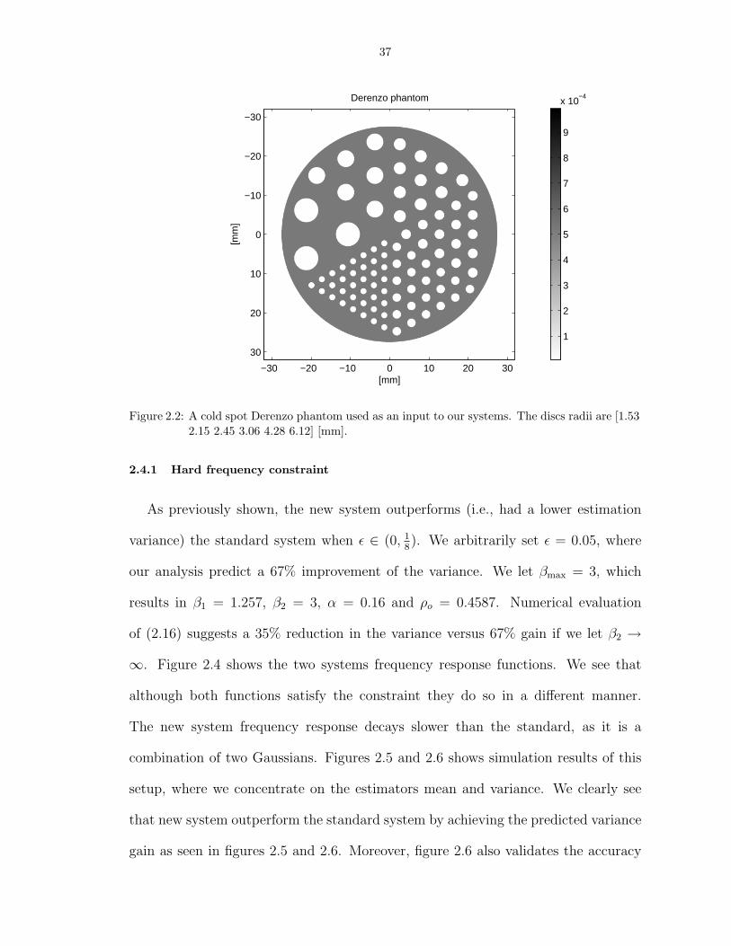
37

[mm]

[mm

]

Derenzo phantom

−30 −20 −10 0 10 20 30

−30

−20

−10

0

10

20

30

1

2

3

4

5

6

7

8

9

x 10−4

Figure 2.2: A cold spot Derenzo phantom used as an input to our systems. The discs radii are [1.532.15 2.45 3.06 4.28 6.12] [mm].

2.4.1 Hard frequency constraint

As previously shown, the new system outperforms (i.e., had a lower estimation

variance) the standard system when ε ∈ (0, 18). We arbitrarily set ε = 0.05, where

our analysis predict a 67% improvement of the variance. We let βmax = 3, which

results in β1 = 1.257, β2 = 3, α = 0.16 and ρo = 0.4587. Numerical evaluation

of (2.16) suggests a 35% reduction in the variance versus 67% gain if we let β2 →

∞. Figure 2.4 shows the two systems frequency response functions. We see that

although both functions satisfy the constraint they do so in a different manner.

The new system frequency response decays slower than the standard, as it is a

combination of two Gaussians. Figures 2.5 and 2.6 shows simulation results of this

setup, where we concentrate on the estimators mean and variance. We clearly see

that new system outperform the standard system by achieving the predicted variance

gain as seen in figures 2.5 and 2.6. Moreover, figure 2.6 also validates the accuracy

38

[mm]

[mm

]

jinc masked kernel

−20 0 20

−30

−20

−10

0

10

20

30

[mm]

[mm

]

Hard Frequency constraint

−20 0 20

−30

−20

−10

0

10

20

30

[mm]

[mm

]

Identical pihnoles

−20 0 20

−30

−20

−10

0

10

20

30

[mm]

[mm

]

BW−RMS constraint

−20 0 20

−30

−20

−10

0

10

20

30

2

4

6

8

x 10−4

2

4

6

8

x 10−4

2

4

6

8

x 10−4

2

4

6

8

x 10−4

Figure 2.3: We show samples of reconstructed images of all systems used in the mentioned sim-ulations. Top left, a standard system. Top right, a new system satisfying the hardfrequency constraint. Bottom left, a new system satisfying the BW-RMS constraint.Bottom right, a new system using a jinc masked reconstruction kernel satisfying hardfrequency constraint.

of our variance approximation, as the predicted variance curve agrees well with the

calculated variance of each system. The actual variance gain that we see is about

39%. As in any other equivalent estimation problem (see [26], [17]), we note the bias-

variance tradeoff effect. The new system, with a lower estimated image variance also

produce blurrier images (see the upper row in figure 2.5). Thus, despite the fact that

both system satisfy the same hard frequency constraint, it is not clear if the new

system visually “outperforms” the standard system application wise.

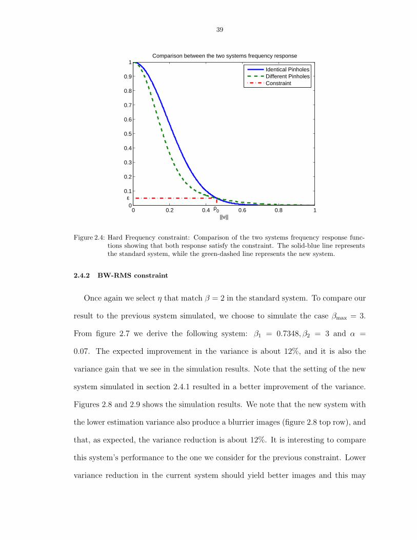
39

0 0.2 0.4 0.6 0.8 10

0.1

0.2

0.3

0.4

0.5

0.6

0.7

0.8

0.9

1

||ν||

Comparison between the two systems frequency response

ε

ρ0

Identical PinholesDifferent PinholesConstraint

Figure 2.4: Hard Frequency constraint: Comparison of the two systems frequency response func-tions showing that both response satisfy the constraint. The solid-blue line representsthe standard system, while the green-dashed line represents the new system.

2.4.2 BW-RMS constraint

Once again we select η that match β = 2 in the standard system. To compare our

result to the previous system simulated, we choose to simulate the case βmax = 3.

From figure 2.7 we derive the following system: β1 = 0.7348, β2 = 3 and α =

0.07. The expected improvement in the variance is about 12%, and it is also the

variance gain that we see in the simulation results. Note that the setting of the new

system simulated in section 2.4.1 resulted in a better improvement of the variance.

Figures 2.8 and 2.9 shows the simulation results. We note that the new system with

the lower estimation variance also produce a blurrier images (figure 2.8 top row), and

that, as expected, the variance reduction is about 12%. It is interesting to compare

this system’s performance to the one we consider for the previous constraint. Lower

variance reduction in the current system should yield better images and this may

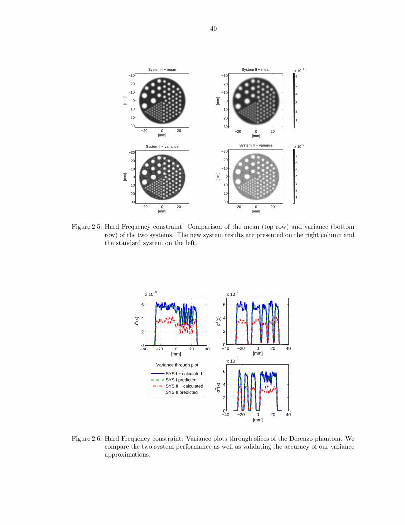
40

System I − mean

[mm]

[mm

]

−20 0 20

−30

−20

−10

0

10

20

30

[mm]

[mm

]

System II − mean

−20 0 20

−30

−20

−10

0

10

20

30

System I − variance

[mm]

[mm

]

−20 0 20

−30

−20

−10

0

10

20

30

[mm]

[mm

]

System II − variance

−20 0 20

−30

−20

−10

0

10

20

301

2

3

4

5

6

7

x 10−9

1

2

3

4

5

6

x 10−4

Figure 2.5: Hard Frequency constraint: Comparison of the mean (top row) and variance (bottomrow) of the two systems. The new system results are presented on the right column andthe standard system on the left.

−40 −20 0 20 400

2

4

6

x 10−9

[mm]

σ2 (x)

−40 −20 0 20 400

2

4

6

x 10−9

[mm]

σ2 (x)

−40 −20 0 20 400

2

4

6

x 10−9

[mm]

σ2 (x)

Variance through plot

SYS I − calculatedSYS I predictedSYS II − calculatedSYS II predicted

Figure 2.6: Hard Frequency constraint: Variance plots through slices of the Derenzo phantom. Wecompare the two system performance as well as validating the accuracy of our varianceapproximations.

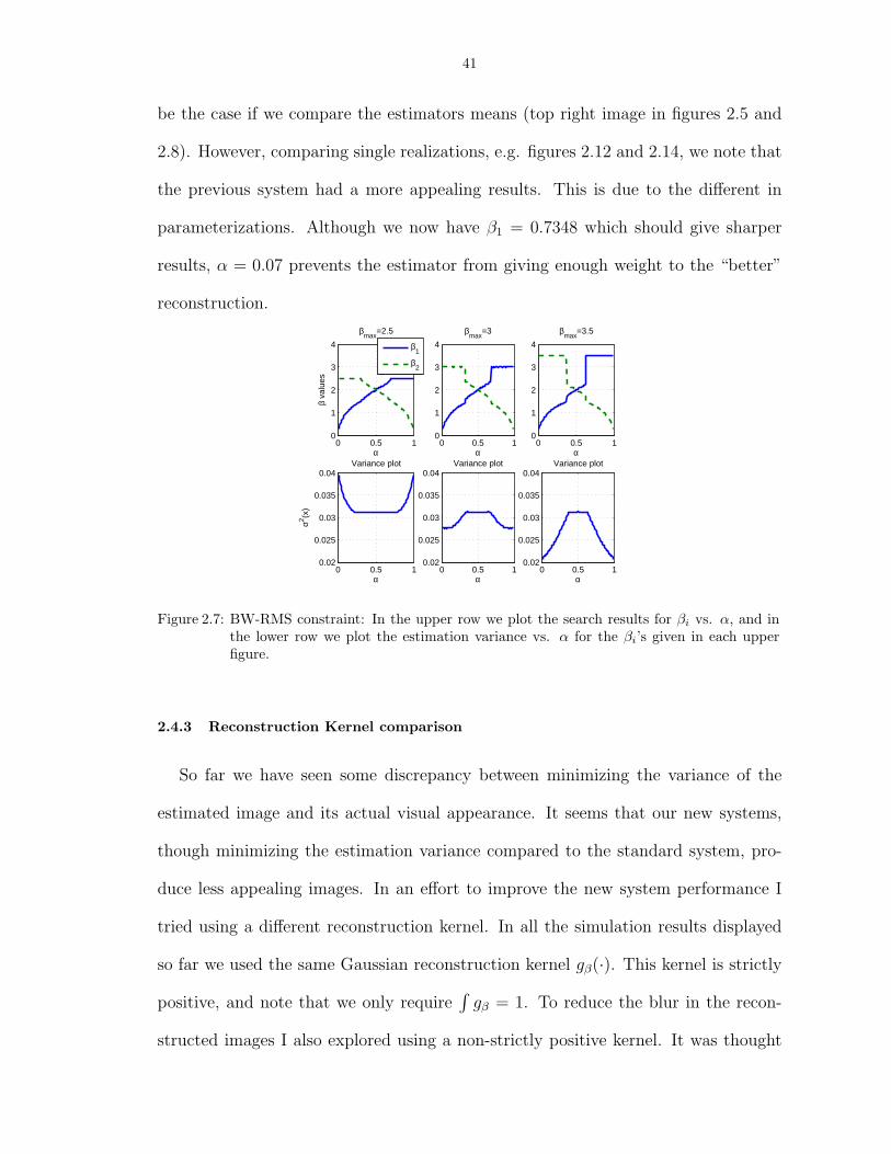
41

be the case if we compare the estimators means (top right image in figures 2.5 and

2.8). However, comparing single realizations, e.g. figures 2.12 and 2.14, we note that

the previous system had a more appealing results. This is due to the different in

parameterizations. Although we now have β1 = 0.7348 which should give sharper

results, α = 0.07 prevents the estimator from giving enough weight to the “better”

reconstruction.

0 0.5 10

1

2

3

4

βmax

=3

α

0 0.5 10.02

0.025

0.03

0.035

0.04Variance plot

α

0 0.5 10

1

2

3

4

βmax

=3.5

α

0 0.5 10.02

0.025

0.03

0.035

0.04Variance plot

α

0 0.5 10

1

2

3

4

α

β va

lues

βmax

=2.5

β1

β2

0 0.5 10.02

0.025

0.03

0.035

0.04Variance plot

σ2 (x)

α

Figure 2.7: BW-RMS constraint: In the upper row we plot the search results for βi vs. α, and inthe lower row we plot the estimation variance vs. α for the βi’s given in each upperfigure.

2.4.3 Reconstruction Kernel comparison

So far we have seen some discrepancy between minimizing the variance of the

estimated image and its actual visual appearance. It seems that our new systems,

though minimizing the estimation variance compared to the standard system, pro-

duce less appealing images. In an effort to improve the new system performance I

tried using a different reconstruction kernel. In all the simulation results displayed

so far we used the same Gaussian reconstruction kernel gβ(·). This kernel is strictly

positive, and note that we only require∫

gβ = 1. To reduce the blur in the recon-

structed images I also explored using a non-strictly positive kernel. It was thought

42

System I − mean

[mm]

[mm

]−20 0 20

−30

−20

−10

0

10

20

30

[mm]

[mm

]

System II − mean

−20 0 20

−30

−20

−10

0

10

20

30

System I − variance

[mm]

[mm

]

−20 0 20

−30

−20

−10

0

10

20

30

[mm]

[mm

]

System II − variance

−20 0 20

−30

−20

−10

0

10

20

301

2

3

4

5

6

7

x 10−9

1

2

3

4

5

6

x 10−4

Figure 2.8: BW-RMS constraint: Comparison of the mean (top row) and variance (bottom row) ofthe two systems. The new system results are presented on the right column and thestandard system on the left.

−40 −20 0 20 400

1

2

3

4

5

6

x 10−9

[mm]

σ2 (x)

−40 −20 0 20 400

1

2

3

4

5

6

x 10−9

[mm]

σ2 (x)

−40 −20 0 20 400

1

2

3

4

5

6

x 10−9

[mm]

σ2 (x)

Variance through plot

SYS I − calculated

SYS I predicted

SYS II − calculated

SYS II predicted

Figure 2.9: BW-RMS constraint: Variance plots through slices of the Derenzo phantom. We com-pare the two system performance as well as validating the accuracy of our varianceapproximations.

43

that a reconstruction kernel with negative (or partially negative) tail would reduce

the blur in the reconstructed image. We used the parameters of the hard frequency

constraint system, namely β1 = 1.257, β2 = 3 and α = 0.16, and compared two

other reconstruction kernels. The first one had a strictly negative tail, and the sec-

ond had a sinusoidal tail. Both kernels resulted in negligible differences both in the

estimation variance and the reconstructed image blur. As it turns out, the dominant

feature of a reconstruction kernel is its FWHM. Since our new kernels only differ

from the Gaussian kernel in their tail sections, the difference in the final result was

insignificant.

2.5 Single pinhole with a general reconstruction kernel

To complete our analysis we wish to explore the possibilities of other useful re-

construction kernels. Based on the general results in [20] (equation (17) in page

246), we note that the estimation variance is proportional to the integral of |Gβ(ν)|2.

Assuming that the Fourier transform of the reconstruction kernel is real, we pose the

following minimization problem in a Calculus of Variations format. Find f : R2 →

R+, f ∈ L2 that minimizes

(2.59) J(f) =

∫f 2(ν)dν,

subject to constraints (2.19) and (2.21), where the system frequency response is

(2.60) H(ν) = f(ν)H0(ν),

and H0(ν) is the fourier transform of h(v − x). Starting with condition (2.21), we

form the following Lagrangian

(2.61) J(f, φ) =

∫f 2(ν)dν + φ(

∫|f(ν)H0(ν)|2dν − γ),

44

where φ is a Lagrange multiplier. If we further assume that H0(ν) is real, e.g., a

Gaussian profile pinhole, then our problem becomes

(2.62) minf,φ

J(f, φ) =

1

2

[∫f 2(ν)(1 + φH2

0 (ν))dν − φγ

],

where the factor 12

was added as a matter of convenience. Taking derivative of J(f, φ)

w.r.t. f and equating it to zero, yields

(2.63)∂

∂fJ(f, φ) = J ′f (f, φ) =

∫f(ν)(1 + φH2

0 (ν))dν = 0.

First, we obviously ignore the trivial solution f = 0 almost everywhere (a.e.). Also,

since f ∈ L2, we may rule out any solution of the form of a Dirac delta function.

Another valid solution for (2.63) can be found if f ⊥ (1 + φH20 ) ⇒ < f,H2

0 >= c,

for some constant c ∈ R. However < f, H20 >= c, implies that we may decompose

f = f ′+c′, where c′ is a constant and < f ′, H20 >= 0. Since f is the Fourier transform

of the reconstruction kernel it is in general a function of non-compact support. Hence

it cannot contain an additive constant since a constant function defined on R2 is not

integrable. Finally, consider the following function

(2.64) f(ν) =

f0, ||ν|| < α

0, otherwise

.

For any such function, we have

(2.65) J ′f (f, φ) = f0

∫

||ν||<α

(1 + φH20 (ν))dν = 0,

as long as

(2.66) φ = − −πα2

∫||ν||<α

H20 (ν)dν

.

45

To satisfy the constraint we must have

(2.67)

∫

||ν||<α

|f(ν)H0(ν)|2dν = γ.

Hence,

(2.68) f0 =

√γ∫

||ν||<αH2

0 (ν)dν,

and, therefore α → 0 ⇒ f0 →∞. Since J(f, φ) is convex in f , (2.64) is a minimum,

and the corresponding minimal variance is

(2.69) J(f) =

∫f 2(ν)dν = f 2

0 πα2 =γπα2

∫||ν||<α

H20 (ν)dν

.

If we further assume that H0(0) = c 6= 0, we have

(2.70) limα→0

J(f) =γ

c2.

We note that (2.70) is a lower bound of the variance in this case, since H0(0) = 1

and H0 was assumed to be a non-increasing function. Hence, the lower bound of the

estimation variance is proportional to the constraint. This means that minimizing

the variance, subject to (2.21) yields a very low bandwidth for the reconstruction

kernel, which in turns implies poor resolution of the overall system.

Next we seek to minimize (2.59) subject to (2.19). Rearranging the constraint we

derive the following functional

(2.71) J(f, φ) =1

2

[∫f 2(ν)dν + φ

∫f 2(ν)H2

0 (ν)(||ν||2 − η)dν

].

Taking derivative w.r.t. f , we get

(2.72) J ′f (f, φ) =

∫f(ν)

[1 + φH2

0 (ν)(||ν||2 − η)]dν = 0.

46

Consider a solution of the form (2.64), then3

(2.73) φ =−πα2

∫||ν||<α

H20 (ν)(||ν||2 − η)dν

is enough to guaranty that (2.72) holds. However, using constraint (2.19) to derive

f0 we note that f0 cancels out

(2.74)f 2

0

∫||ν||<α

||ν||2H20 (ν)dν

f 20

∫||ν||<α

H20 (ν)dν

> η2,

and, thus we may set f0 = 1 and it remains to figure out α. Rearranging (2.74) we

get

(2.75)

∫

||ν||<α

(||ν||2 − η2)H20 (ν)dν > 0.

Therefore, we must have α > η. However the exact lower limit of α depends on the

specific H0. Minimizing (2.59) suggests the selection of the minimal α allowed and a

minimal f0 > 0. This yields the behavior that we had witnessed in the two pinhole

case, i.e., we may find a trajectory, in (α, f0) plane, that satisfy the constraint yet

yielding σ2(x) → 0. To conclude this section we note that the first constraint, which

was forcing the frequency response to exceed a certain value at a specific frequency

is not suitable for the Calculus of variations framework.

2.6 Conclusions and future work

We have shown examples where selecting different diameter pinholes results in a

lower estimation variance compared to a standard system with equal width pinholes.

Moreover, we showed limiting behavior of the considered systems. Under the hard3Since H0 6= 0 a.e. the denominator of (2.73) is not zero.

47

frequency constraint the system degenerates to a single pinhole of constant width

and constant weight α. For the BW-RMS constraint the system degenerates to a

composition of a very narrow pinhole with very little weighting coefficient and a very

wide pinhole that yield most of the estimated image. We had also shown roots for

that behavior in a single pinhole system. All of the above holds for an estimator

reconstructing the underlying images as a linear combination of the two independent

system measurements.

Notwithstanding the reduction in estimation variance, we had come to question

the validity of our cost function as a performance measure for an actual imaging

system. It is either that minimizing variance has little merit for capturing image

quality, considering the bias-variance tradeoff, or that we failed to choose proper

constraints for the minimization problem. As mentioned, quantifying resolution is

a daunting task. Thus, we leave for future work the task of finding a more suitable

cost function or constraints or both. A possible such constraint would be the FWHM

of the overall system, although we could not come up with a good way of utilizing

it. We believe that future work should consider multiplexing between the different

pinholes, as this is often the case for real systems.

There are obvious advantages for using a multi-resolution design for SPECT scan-

ners. The constant struggle over SNR and resolution encourage us to find a way,

perhaps non-linear, to combine a high-resolution noisy image with a low resolution

low noise background image. Such an estimator, although hard to analyze, may

produce better images for the actual tasks they are being used for by physicians.

Another viable future direction is to consider using a (two) multi-diameter pinhole

scanner in an adaptive manner. Such a system may start by producing a coarse

image, then refine the image by re-scanning parts of the object where details are

48

needed using a finer pinhole diameter.

2-A Appendix: Full size reconstructed images of the different systems

For comparison purposes we present the four images shown in figure 2.3 in full

size. Figure 2.11 was generated with the standard system while 2.12 and 2.13 were

generated by a system satisfying the hard frequency constraint where the latter used

the jinc masked reconstruction kernel. Finally, figure 2.14 was generated by a system

using the BW-RMS constraint. We can see that in figures 2.12-2.14 it is hard to see

the smallest radii discs due to the extra blur. Also, in figure 2.14 we see the nature

of the BW-RMS constraint driving the image to appear flat with some details (black

spots) contributed by the smaller pinhole. In addition, in figure 2.10 (which is the

same as figure 2.7) we show, for the BW-RMS constraint, the behavior of β1 β2

and the expected variance as a function of α plotted for different βmax. We observe

the following: (i) As expected the results are symmetric in β, i.e. for every triplet

(β1, β2, α) there is a matching triplet (β2, β1, 1 − α). (ii) The reference standard

system (β1 = β2 = 2) is a specific case of this grid search with α = 12. (iii) As

we increase βmax the optimal solution, in terms of minimal variance, converges to

β1 → 0 and σ20(x) → 0. We also note that the gain in the expected variance in the

new system is far less than the one expected by the new system satisfying the hard

frequency constraint, yet the reconstructed image look much worse.

49

0 0.5 10

1

2

3

4

βmax

=3

α

0 0.5 10.02

0.025

0.03

0.035

0.04Variance plot

α

0 0.5 10

1

2

3

4

βmax

=3.5

α

0 0.5 10.02

0.025

0.03

0.035

0.04Variance plot

α

0 0.5 10

1

2

3

4

α

β va

lues

βmax

=2.5

β1

β2

0 0.5 10.02

0.025

0.03

0.035

0.04Variance plot

σ2 (x)

α

Figure 2.10: BW-RMS constraint: In the upper row we plot the search results for βi vs. α, and inthe lower row we plot the estimation variance vs. α for the βi’s given in each upperfigure.

[mm]

[mm

]

System I: identical pinholes

−30 −20 −10 0 10 20 30

−30

−20

−10

0

10

20

30

1

2

3

4

5

6

x 10−4

Figure 2.11: Standard system, image reconstruction of the Derenzo phantom.

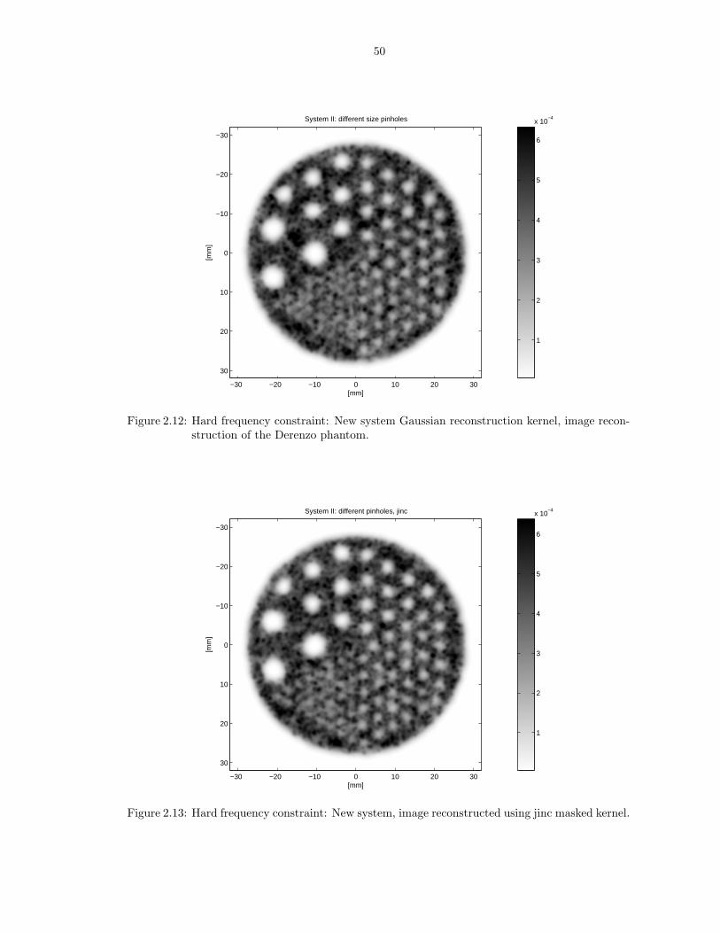
50

[mm]

[mm

]

System II: different size pinholes

−30 −20 −10 0 10 20 30

−30

−20

−10

0

10

20

30

1

2

3

4

5

6

x 10−4

Figure 2.12: Hard frequency constraint: New system Gaussian reconstruction kernel, image recon-struction of the Derenzo phantom.

[mm]

[mm

]

System II: different pinholes, jinc

−30 −20 −10 0 10 20 30

−30

−20

−10

0

10

20

30

1

2

3

4

5

6

x 10−4

Figure 2.13: Hard frequency constraint: New system, image reconstructed using jinc masked kernel.

51

[mm]

[mm

]

System II: different size pinholes

−30 −20 −10 0 10 20 30

−30

−20

−10

0

10

20

30

1

2

3

4

5

6

x 10−4

Figure 2.14: BW-RMS constraint: New system, image reconstruction of the Derenzo phantom.

CHAPTER III

Optimal Two-stage Search for Sparse Targets using Convex

Criteria

3.1 Introduction

This chapter considers the problem of estimating and detecting sparse signals

over a large area of an image or other medium. We introduce a novel cost function

that captures the tradeoff between allocating energy to signal regions, called regions

of interest (ROI), versus exploration of other regions. We show that minimizing

our cost guarantees reduction of both the error probability over the unknown ROI

and the mean square error (MSE) in estimating the ROI content. Two solutions to

the resource allocation problem, subject to a total resource constraint, are derived.

Asymptotic analysis shows that the estimated ROI converges to the true ROI. We

show that our adaptive sampling method outperforms exhaustive search and are

nearly optimal in terms of MSE performance. An illustrative example of our method

in SAR imaging is given.

This problem arises in many applications including: target detection and classifi-

cation, computer aided diagnosis, and screening. For example, in a radar reconnais-

sance mission, active radar may be used to image a given scene. A typical system is

designed to detect targets exceeding a minimal profile. This minimal target profile

52

53

dictates the scan parameters such as the energy level the radar transmits and the

scan time duration. Moreover, targets usually occupy a small section of the scanned

area, called the ROI. Most systems consider exhaustive search with equal energy

allocation, defined as a search policy where all cells are searched with equal effort

allocated to each cell, to spread sensitivity over all locations. As a result, a relatively

large portion of the energy is allocated outside the ROI. This excess energy could

be used to better illuminate the ROI. Furthermore in surveillance applications, by

deploying energy over an unknown area the searcher risks exposure. Reducing the

scan energy outside the ROI reduces exposure risks.

As another application, consider the task of early detection of tumors using med-

ical imaging, e.g., X-ray computed tomography (CT). Early detection is concerned

with detecting small tumors. In many cases, little a priori knowledge about the

tumor location exists. Consider the area containing the tumor as an unknown ROI.

Lifetime radiation exposure constraints limit the total energy that can be used in

a specific scan. There are two questions: a) where are tumors located? b) what

kind of tumors does the ROI contain? This combined detection/estimation suggests

using adaptive sampling over the image to improve both detection and estimation

performance.

The search problem considered in this chapter bears some similarity to Posner’s

work on minimizing expected search time for finding a satellite lost in the sky [46].

Posner suggests a two step procedure. First, briefly search the entire domain to

generate a likelihood function of possible satellite locations. Second, sequentially

search the domain again in order of decreasing likelihood of satellite position. Pos-

ner’s model assumes that the search is stopped as soon as the satellite has been

found and that detection probability is increasing with search time. Therefore, se-

54

quentially searching the cells with the highest likelihood reduces the overall expected

search time. By minimizing expected search time Posner imposes a ‘soft’ resource

constraint on the total time used to search each cell. In this chapter, we adopt

a Bayesian framework for sequential search for multiple objects obscured by noise.

Thus the posterior distribution of objects presence replaces the likelihood of object

presence used in [46]. The use of the posterior in place of the likelihood guarantees

minimization of an average cost and a stronger sense of optimality.

Although we search for multiple targets within a signal, we focus on applications

where the total support of the signal part containing targets is small compared to the

entire signal support. Such signals can be viewed as sparse and we define the sparsity

parameter p as the proportion of the signal support containing targets. Johnstone

and Silverman consider a Bayesian framework for estimating sparse signals from a

single measurements vector in [29]. They consider thresholding the vector entries

and setting the estimated signal equal zero for all measurements below the thresh-

old. Thus, significant gains in estimation mean square error (MSE) are achieved for

small p. They utilize a Bayesian framework to find an optimal threshold minimizing

the average squared error. We also use the Bayesian framework to find an opti-

mal threshold. However, we use this threshold to generate additional measurements

of all signal elements exceeding it. This adaptive sampling approach and added

measurements enables higher gains in reducing estimation MSE. Wipf and Rao use

sparse Bayesian learning in the problem of basis selection from overcomplete dic-

tionaries [60]. They use a parameterized prior on the basis weight coefficients to

encourage sparse solution to an otherwise l2-norm minimization problem. The pa-

rameters of the prior are estimated from the data along with the basis weights using

an expectation-maximization (EM) algorithm. However, the EM algorithm uses a

55

single measurement of the underlying signal. In this paper, the posterior distribu-

tion is used to partially remeasure the underlying signal. By spatially focusing the

measurement process onto the ROI we can better estimate the correct signal values.

Adaptive sampling or active learning for the purpose of estimating functions in

noise has been considered in [13]. Castro et al. show that for piecewise constant

functions, active learning methods can capitalize on the highly localized nature of the

boundary by focusing the sampling process in the estimated vicinity of the boundary.

Thus, estimation error converges at higher rates than with passive sampling. A two-

step approach is proposed where first a rough estimate of the underlying signal

is generated and second the signal is resampled in the vicinity of the estimated

boundaries. We use a similar two-stage approach where previous measurements are

used to determine where to sample next. However, our work differs in two aspects

as we do not limit the discussion to a class of spatially inhomogeneous signals and

we consider the additional aspect of resource allocation. While [13] assume identical

sampling procedure for all samples, e.g. similar measurement noise variance, we

consider different sampling procedures between stages and among different spatial

locations within a particular stage.

Resource allocation in the context of adaptive waveform amplitude design for

estimating parameters of an unknown medium under average energy constraints is

discussed in [49]. Rangarajan et al. derive an optimal amplitude allocation for the

second stage in a two-stage problem as a function of the first stage measurements.

In this work we consider the more general problem of waveform design under a total

energy constraint. Therefore, measurements at the first stage are used to select the

optimal waveform among all possible waveforms with some bounded total energy.

Thus we are able to focus the sampling process onto the ROI.

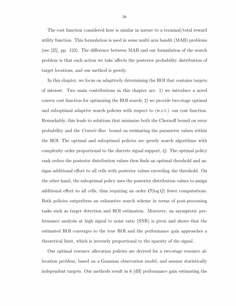
56

The cost function considered here is similar in nature to a terminal/total reward

utility function. This formulation is used in some multi arm bandit (MAB) problems

(see [25], pp. 123). The difference between MAB and our formulation of the search

problem is that each action we take affects the posterior probability distribution of

target locations, and our method is greedy.

In this chapter, we focus on adaptively determining the ROI that contains targets

of interest. Two main contributions in this chapter are: 1) we introduce a novel

convex cost function for optimizing the ROI search; 2) we provide two-stage optimal

and suboptimal adaptive search policies with respect to (w.r.t.) our cost function.

Remarkably, this leads to solutions that minimize both the Chernoff bound on error

probability and the Cramer-Rao bound on estimating the parameter values within

the ROI. The optimal and suboptimal policies are greedy search algorithms with

complexity order proportional to the discrete signal support, Q. The optimal policy

rank orders the posterior distribution values then finds an optimal threshold and as-

signs additional effort to all cells with posterior values exceeding the threshold. On

the other hand, the suboptimal policy uses the posterior distribution values to assign

additional effort to all cells, thus requiring an order O(log Q) fewer computations.

Both policies outperform an exhaustive search scheme in terms of post-processing

tasks such as target detection and ROI estimation. Moreover, an asymptotic per-

formance analysis at high signal to noise ratio (SNR) is given and shows that the

estimated ROI converges to the true ROI and the performance gain approaches a

theoretical limit, which is inversely proportional to the sparsity of the signal.

Our optimal resource allocation policies are derived for a two-stage resource al-

location problem, based on a Gaussian observation model, and assume statistically

independent targets. Our methods result in 6 [dB] performance gain estimating the

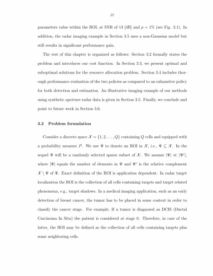
57

parameters value within the ROI, at SNR of 13 [dB] and p = 1% (see Fig. 3.1). In

addition, the radar imaging example in Section 3.5 uses a non-Gaussian model but

still results in significant performance gain.

The rest of this chapter is organized as follows: Section 3.2 formally states the

problem and introduces our cost function. In Section 3.3, we present optimal and

suboptimal solutions for the resource allocation problem. Section 3.4 includes thor-

ough performance evaluation of the two policies as compared to an exhaustive policy

for both detection and estimation. An illustrative imaging example of our methods

using synthetic aperture radar data is given in Section 3.5. Finally, we conclude and

point to future work in Section 3.6.

3.2 Problem formulation

Consider a discrete space X = 1, 2, . . . , Q containing Q cells and equipped with

a probability measure P . We use Ψ to denote an ROI in X , i.e., Ψ ⊆ X . In the

sequel Ψ will be a randomly selected sparse subset of X . We assume |Ψ| ¿ |Ψc|,

where |Ψ| equals the number of elements in Ψ and Ψc is the relative complement

X \ Ψ of Ψ. Exact definition of the ROI is application dependent. In radar target

localization the ROI is the collection of all cells containing targets and target related

phenomena, e.g., target shadows. In a medical imaging application, such as an early

detection of breast cancer, the tumor has to be placed in some context in order to

classify the cancer stage. For example, If a tumor is diagnosed as DCIS (Ductal

Carcinoma In Situ) the patient is considered at stage 0. Therefore, in case of the

latter, the ROI may be defined as the collection of all cells containing targets plus

some neighboring cells.

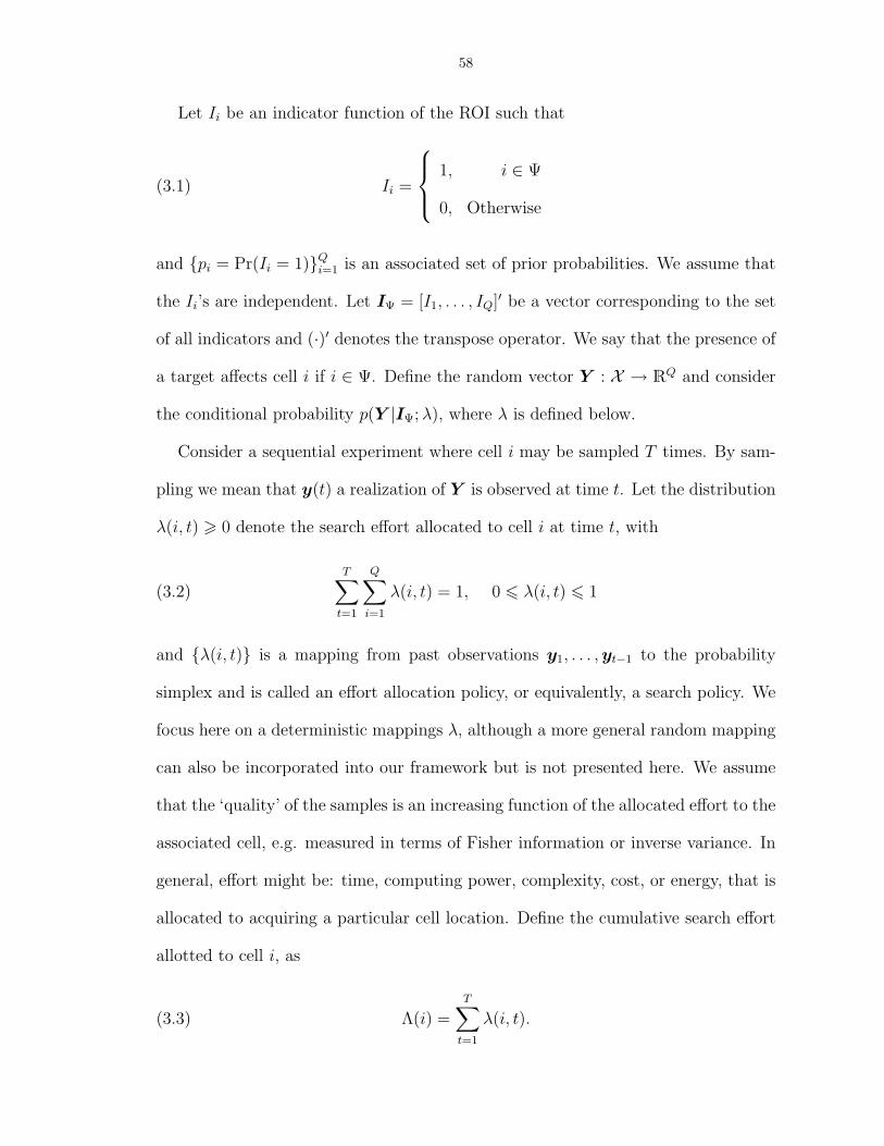
58

Let Ii be an indicator function of the ROI such that

(3.1) Ii =

1, i ∈ Ψ

0, Otherwise

and pi = Pr(Ii = 1)Qi=1 is an associated set of prior probabilities. We assume that

the Ii’s are independent. Let IΨ = [I1, . . . , IQ]′ be a vector corresponding to the set

of all indicators and (·)′ denotes the transpose operator. We say that the presence of

a target affects cell i if i ∈ Ψ. Define the random vector Y : X → RQ and consider

the conditional probability p(Y |IΨ; λ), where λ is defined below.

Consider a sequential experiment where cell i may be sampled T times. By sam-

pling we mean that y(t) a realization of Y is observed at time t. Let the distribution

λ(i, t) > 0 denote the search effort allocated to cell i at time t, with

(3.2)T∑

t=1

Q∑i=1

λ(i, t) = 1, 0 6 λ(i, t) 6 1

and λ(i, t) is a mapping from past observations y1, . . . , yt−1 to the probability

simplex and is called an effort allocation policy, or equivalently, a search policy. We

focus here on a deterministic mappings λ, although a more general random mapping

can also be incorporated into our framework but is not presented here. We assume

that the ‘quality’ of the samples is an increasing function of the allocated effort to the

associated cell, e.g. measured in terms of Fisher information or inverse variance. In

general, effort might be: time, computing power, complexity, cost, or energy, that is

allocated to acquiring a particular cell location. Define the cumulative search effort

allotted to cell i, as

(3.3) Λ(i) =T∑

t=1

λ(i, t).

59

Consider the following cost function

(3.4) J(Λ) =

Q∑i=1

IiA(Λ(i)) +

Q∑i=1

B(Λ(i)),

where A(·) and B(·) are decreasing functions that may depend on additional pa-

rameters. This restriction ensures that allocating more effort to cells reduces the

over-all cost. Note that our cost function (3.4) depends directly on the ROI via the

summand of the first sum on the right hand side (r.h.s.) of (3.4). Choosing B(·) = 0

emphasizes focusing efforts on the ROI. Selecting A(x) = 2ν−1x

and B(x) = 1−νx

, with

ν ∈ [12, 1], simplifies J(Λ) to

(3.5) J(Λ) =

Q∑i=1

νIi + (1− ν)(1− Ii)

Λ(i),

which has some intuitive and appealing properties. Minimizing this cost function

concentrates ν of the total effort over the ROI Ψ and (1 − ν) to its complement Ψc

with ν being the dividing factor. Setting ν = 1 focuses all the effort at the ROI, while

ν = 12

results in an exhaustive effort allocation policy, i.e., equal energy allocated

to all cells inside and outside the ROI. The choice ν = 1 has some very intuitive

and appealing properties. For example, in the context of estimating a deterministic

signal µ in additive Gaussian noise, minimizing (3.5) is equivalent to minimizing the

Cramer-Rao lower bound on E∑i Ii(µi− µi)2, see Appendix 3-A for details. In a

sense, ν controls the tradeoff between exploitation of signal in the ROI (ν = 1) and

exploration of the entire signal (ν = 12).

In addition, consider a binary Gaussian hypothesis testing problem. Define the

null hypothesis, H0(i), as µi = 0, and the alternative, H1(i), as µi > 0 with a prior

probability π = Pr(H1). Consider the task of deciding between the two hypothe-

60

sis, ∀i ∈ Ψ. The probability of error, i.e., making the wrong decision, defined as

Pe = Pr(decide H0|H1)π + Pr(decide H1|H0)(1 − π), can be broken into two parts:

misdetect probability Pm over Ψ, and false alarm probability Pfa over Ψc. With

ν = 1, we show in Appendix 3-B that minimizing (3.5) is equivalent to uniformly

minimizing the Chernoff bound on the probability of error Pm over the ROI. Setting

ν = 12, most of the energy is spread over Ψc due to the assumed sparsity |Ψ| ¿ |Ψc|.

This leads to a lower Chernoff bound on Pfa, or correspondingly, fewer false alarms.

If ν ∈ (12, 1) we trade the two cases, either relaxing the upper bound on Pm or on Pfa.

In Section 3.4 we corroborate this intuition with simulation results, where adaptive

measurement policies derived from minimization of (3.5) are used to generate data

that is used for both estimation and detection tasks.

Next, we provide an achievable lower bound on our cost function (3.5).

Lemma 3.1. The cost function (3.5) is lower bounded by

(3.6) J(Λ) >[√

ν|Ψ|+√1− ν(Q− |Ψ|)]2

.

This lower bound is achievable with a two-level effort allocation scheme Λo, equal

over the ROI and equal over its complement, defined as

(3.7) Λo(i) =

√ν√

ν|Ψ|+√1−ν(Q−|Ψ|) , i ∈ Ψ√

1−ν√ν|Ψ|+√1−ν(Q−|Ψ|) , i ∈ Ψc

.

Proof. For a nonnegative series ai, Cauchy-Schwarz inequality provides

(3.8)

(Q∑

i=1

ai

Λ(i)

)(Q∑

i=1

Λ(i)

)>

(Q∑

i=1

√ai

Λ(i)

√Λ(i)

)2

.

61

Since∑Q

i=1 Λ(i) = 1, (3.8) simplifies to

(3.9)

Q∑i=1

ai

Λ(i)>

(Q∑

i=1

√ai

)2

.

Substituting ai = νIi + (1− ν)(1− Ii), i.e., ∀i ∈ Ψ : ai = ν and ∀i ∈ Ψc : ai = 1− ν,

into the r.h.s. of (3.9) yields

(3.10)

(Q∑

i=1

√ai

)2

=[√

ν|Ψ|+√1− ν(Q− |Ψ|)]2

.

Noting that on the l.h.s. of (3.9) we have J(Λ) =∑Q

i=1ai

Λ(i)proves the validity of

(3.6). To prove the second part of the lemma note that

(3.11) J(Λo) =∑i∈Ψ

ν

Λo(i)+

∑i∈Ψc

1− ν

Λo(i),

and algebra yields

(3.12) J(Λo) =[√

ν|Ψ|+√1− ν(Q− |Ψ|)]2

,

which is exactly the r.h.s. of (3.6). This completes the proof. 2

Discussion

We would like to point out the potential performance gains using our cost function

(3.5). Let ΛU denote an exhaustive search policy with ΛU(i) = 1Q

. As previously

mentioned, ΛU is the optimal search policy for ν = 12

in (3.7). For a general ν, the

cost (3.5) associated with ΛU is

(3.13) J(ΛU) = Q [ν|Ψ|+ (1− ν)(Q− |Ψ|)] ,

62

with the two special cases of

(3.14) J(ΛU) =

Q2

2, ν = 0.5

Q|Ψ|, ν = 1

.

Since ΛU does not offer any adaptivity, any good adaptive effort allocation scheme

Λ should result in J(Λ) 6 J(ΛU). Therefore, we define the performance gain in [dB]

as

(3.15) G(Λ) = −10 logJ(Λ)

J(ΛU).

For ν = 1, J(Λo) = |Ψ|2 and thus the optimal gain is

(3.16) G(Λo) = −10 log|Ψ|Q

,

which is achieved by the omniscient energy allocation strategy that knows the ROI

and consequently concentrates all energy in the ROI. Define p∗ = |Ψ|Q

, then p∗ → 0

forces G(Λo) →∞. Consequently, a good sampling method should yield large gains

in a sparse setting, i.e., when p∗ is small the ROI is small. In the following, we will

develop a sampling method that exploits these gains. Taking the derivative of the

r.h.s. in (3.6) w.r.t. ν, it can be shown that J(·) > |Ψ|2 for all ν ∈ [12, 1] and |Ψ|

Q6 1

2

(see Appendix 3-C). In other words, if |Ψ|Q

6 12

the optimal gain is achieved by Λo

for ν = 1. Unfortunately, Λo represents the omniscient search policy and is not a

feasible policy since we do not know the location of the ROI in advance. Our goal

is to derive a feasible policy that comes close to achieving the performance of Λo for

unknown ROI.

63

In this chapter, we restrict our attention to minimizing the expected value of

(3.5). This probabilistic setting utilizes the conditional distribution p(Y |IΨ; λ) in

our model. Assuming we observe realizations of Y , our goal is to find a search policy

(3.17) λ(i, t) = arg minλ(i,t)

E

Q∑

i=1

νIi + (1− ν)(1− Ii)

Λ(i)

,

where Λ(i) is given by (3.3). Next, we introduce a total energy constraint.

3.2.1 Energy allocation with energy constraint

Consider a fixed-target radar measurements in the presence of noise. We assume

that a radar transmits energy in some known beam pattern to probe a collection of

cells. We further assume that the radar is subject to an energy constraint, and that

observations obey the following model

(3.18) yj(t) =

Q∑i=1

hij(t)√

λ(i, t)θi(t)Ii + nj(t), t = 1, 2, . . . , T,

where hij(t) are known weights corresponding to the beam pattern, λ(i, t) is the

energy allocated for measuring cell i, θi(t) is a random return from cell i, and nj(t) is

an additive observation noise, all at time t. Note that since the indicator of the ROI

Ii is independent of t, this model corresponds to a static target scenario. We assume

that the additive noise nj(t) is independent for different j and t. Also, assume that

the positive θi(t) follow a prior distribution pΘ(θ) and are independent for different

i but may be dependent for different t. The model in (3.18) can be written in vector

form

(3.19) y(t) = H(t)′diag√

λ(t)diagθ(t)IΨ + n(t),

64

where

y(t) = [y1(t), y2(t), . . . , yMt(t)]′,

λ(t) = [λ(1, t), λ(2, t), . . . , λ(Q, t)]′,

θ(t) = [θ1(t), θ2(t), . . . , θQ(t)]′,

IΨ = [I1, I2, . . . , IQ]′,

n(t) = [n1(t), n2(t), . . . , nMt(t)]′,

and [H(t)]ij = hij(t). The notation√

λ(t) denotes a Q × 1 vector with [√

λ(t)]i =

√λ(i, t), while the operator diagx corresponds to a Q×Q (square) diagonal matrix

with x(i) as its iith element. The objective is to specify a resource allocation policy

λ(i, t) that improves the ‘quality’ of the measurements over the ROI as measured by

(3.17). In addition we assume an energy constraint

(3.20)1

λT

Q∑i=1

T∑t=1

λ(i, t) = 1.

At time t, the energy allocated to cell i may depend on past observations, i.e.,

λ(i, t) is a function of y(1), y(2), . . . , y(t−1). For brevity, we use the notation λ(i, t)

to denote λ(i, t; y(1),y(2), . . . , y(t − 1)). Following (3.3), define Λ the cumulative

energy distributed to cell i as Λ(i) =∑T

t=1 λ(i, t). Our cost function is J(Λ), as

defined in (3.5), and our goal is to minimize the expected cost in the r.h.s. of (3.17)

over all possible energy allocations λ(i, t), subject to (3.20). Consider ν = 1 and let

p = Pr(Ii = 1) be a uniform prior distribution on the location of targets, where p

represents the sparsity of the vector IΨ, i.e. |Ψ| is a Binomial random variable (r.v.)

with E|Ψ| = pQ. Define p∗ = |Ψ|Q

then Ep∗ = p and var(p∗) = p(1−p)Q

. To find an

upper bound on possible performance gains we use J(Λo) 6 J(Λ) for any Λ and,

65

thus

(3.21) G(Λ) 6 G(Λo) = −10 log p∗.

In Appendix 3-D we use (3.21) and Bernstein’s inequality to prove, for δ > exp−Q 3p8(1−p)

,

that

(3.22) Pr(G(Λ) 6 −10 log p + ε(δ, p, Q)) > 1− δ.

In the SAR imaging example from Section 3.5 this yields

Pr(G(Λ) 6 20 + 0.333) > 0.999.

3.3 Search policy

In the following section we solve the optimization problem for T = 2. The idea is

to expend at t = 1 a portion of the total energy to learn about the data domain and

obtain a posterior distribution. Then use it at stage t = 2 to refine the posterior and

estimate the ROI. We will solve

(3.23) λ(i, t) = arg minλ(i,t)

E

Q∑

i=1

νIi + (1− ν)(1− Ii)∑2t=1 λ(i, t)

,

subject to the energy constraint 1λT

∑i

∑t λ(i, t) = 1. Initially, the prior distribution

on targets location is uniform, pi = p for all i. This could be modified if there were

prior knowledge on targets location. Let λ(t) be the total energy spent at search

step t with 1λT

∑t λ

(t) = 1, t = 1, 2. Our goal is to optimize the energy distribution

between the two steps and among cells in each step. See [5] for a discussion of the

case of T > 2.

66

3.3.1 Optimal two stage search policy

With T = 1 and a uniform prior, we show in Appendix 3-E.1 that the minimizer

of the cost (3.23) is an equal energy allocation

(3.24) λ(i, 1) =λ(1)

Q

4= λ1.

Let Γ be the set of all search policies with λ(i, 1) = λ1. For T = 2 we find the optimal

search policy λ ∈ Γ minimizing (3.23). Since, λT = Qλ1 + λ(2) optimizing the total

effort allocated for each step is equivalent to finding an optimal pair (Qλ1, λT−Qλ1),

which involves minimizing over a single variable. Hence the cost function (3.23)

simplifies to

(3.25) J(Λ) =

Q∑i=1

E

νIi + (1− ν)(1− Ii)

λ1 + λ(i, 2)

,

where expectation is taken w.r.t. y(1) and IΨ. Note that λ(i, 2) depends only

on y(1), thus y(2) does not affect the cost function and can be omitted from the

expectation. In addition, (3.25) is constant in θ and therefore we omit it from the

expectation as well. Rewriting (3.25) using iterated expectation yields

(3.26) J(Λ) =

Q∑i=1

E

E

νIi + (1− ν)(1− Ii)

λ1 + λ(i, 2)

∣∣∣∣ y(1)

.

Note that Ii is a binary r.v.. In addition, given y(1), λ(i, 2) is deterministic. Hence

(3.26) becomes

(3.27)

Q∑i=1

E

E νIi + (1− ν)(1− Ii)|y(1)

λ1 + λ(i, 2)

=

67

(3.28)

Q∑i=1

E

νPr (Ii = 1|y(1)) + (1− ν)(1− Pr (Ii = 1|y(1)))

λ1 + λ(i, 2)

.

Using Bayes rule we obtain

(3.29) Pr(Ii = 1|y(1)) =P (y(1)|Ii = 1)p

P (y(1)|Ii = 1)p + P (y(1)|Ii = 0)(1− p)

4= pIi|y(1),

where P (y|Ii) =∫

P (y|Ii, θi)pΘ(θ)dθ is the given conditional probability model de-

scribing the measurement dependency on the target. Finally, we rewrite our cost

function on the r.h.s. of (3.25) and solve

(3.30) λ(i, t) = arg minλ1,λ(i,2)

E

Q∑

i=1

νpIi|y(1) + (1− ν)(1− pIi|y(1))

λ1 + λ(i, 2)

.

Let λ1 be the energy allocated to each cell at the first step, with Qλ1 6 λT . Define

the r.v.

(3.31) Wj = νpIj |Y + (1− ν)(1− pIj |Y ), j = 1, 2, . . . , Q,

with vector of corresponding realizations w = [w1, w2, . . . , wQ]′. Let τ : X → X be

a permutation operator that corresponds to the rank ordering of the wi’s:

(3.32) τ(j) = arg mini=1,...,Q

wi : wi > wτ(j−1), j ∈ 1, 2, . . . , Q,

with wτ(0)4= 0. Whenever the r.h.s. of (3.32) is not unique we select an arbitrary i

satisfying wτ(1) 6 wτ(2) 6 . . . 6 wτ(Q). The solution λ1, λ(i, 2) of (3.30) will depend

on an integer threshold k0 that is equal to the number of cells that are not searched

at t = 2. Assuming1 wτ(1) > 0, define k0, the threshold parameter, as k0 = 0 if

(3.33)λT

λ1

>

∑Qi=1

√wτ(i)√

wτ(1)

,

1The special case of wτ(1) = 0 is treated in Appendix 3-E.2.

68

otherwise k0 ∈ 1, . . . , Q− 1 is the integer satisfying

(3.34)

∑Qi=k0+1

√wτ(i)√

wτ(k0+1)

<λT

λ1

− k0 6∑Q

i=k0+1

√wτ(i)√

wτ(k0)

.

An optimal solution for the second step λ(i, 2) is given in Appendix 3-E and the

special case where wτ(i) = 0, for all i, is treated there (Appendix 3-E.2). Its prop-

erties are summarized below: Given λ1 and k0, it is shown that the optimal energy

allocation λ(τ(i), 2) minimizing the cost (3.30) is of the form

(3.35) λ(τ(i), 2) =

(λT − k0λ1∑Qj=k0+1

√wτ(j)

√wτ(i) − λ1

)I(i > k0).

Substituting (3.35) into (3.30), the optimization problem is equivalent to finding λ∗1

minimizing

(3.36) λ∗1 = arg minλ1

E

Q∑i=1

Wτ(i)

λ1 +

(λT−k0λ1∑Q

j=k0+1

√Wτ(j)

√Wτ(i) − λ1

)I(i > k0)

(3.37) = arg minλ1

E

1

λ1

k0∑i=1

Wτ(i) +1

λT − k0λ1

Q∑

i=k0+1

Q∑

j=k0+1

√Wτ(i)Wτ(j)

,

where if k0 = 0 then the first summation in (3.37) equals zero. We can find λ∗1 via a

one dimensional search. In summary, the optimal policy minimizing (3.30) is

69

Algorithm 3.1. Two stage Adaptive Resource Allocation Policy (ARAP) λA

Step 1: Allocate λA(i, 1) = λ∗1 to each cell and measure y(1).

Step 2: Given y(1) compute posteriors PIi|yi(1) defined in (3.29), then sort the

Wi’s defined in (3.31).

Step 3: Use λ∗1 and the ordered statistic wτ(i) to find k0 using (3.33) and (3.34).

Step 4: Given k0, apply λ(i, 2) the energy allocation to cell i as

(3.38)

λA(τ(i), 2) = λ(τ(i), 2) =

(λT − k0λ

∗1∑Q

j=k0+1

√wτ(j)

√wτ(i) − λ∗1

)I(i > k0),

and measure y(2).

Note that ARAP is a water-filling algorithm. This is a direct consequences of the

facts that the cost function minimized in (3.30) is convex, λ(i, t) is positive, and our

constraint is linear of the form∑

i,t λ(i, t) = C (see [8] pp. 245).

3.3.2 Properties of the optimal energy allocation

Theorem 3.2. For some ν ∈ [12, 1] and λ∗1, let ΛA(i) be the search policy obtained

using ARAP. Then, for a uniform prior distribution, we have

(3.39) J(ΛA) 6 J(ΛU),

with equality achieved if PIi|y(1) = c, ∀i.

Proof. Note that an equal effort allocation policy can be broken into any arbitrarily

70

number T of consecutive search steps, as long as for all i

(3.40) ΛU(i) =1

λT

T∑t=1

λ(i, t) =1

Q.

Without loss of generality let T = 2 and let Γ denote the family of all effort allocation

policies with λ(i, 1) = λ1 (equal effort allocation) at the first stage

(3.41) Γ =

λ(i, t) :

Q∑i=1

2∑t=1

λ(i, t) = λT , λ(i, 1) = λ1 > 0, λ(i, 2) > 0

.

Since ARAP yields the optimal effort allocation for any set of posterior distribution

PIi|y(1)Qi=1, we have J(ΛA) 6 J(ΛU). If PIi|y(1) = c for all i, then wi = c′, ∀i, for

which ARAP yields k0 = 0. Thus, from (3.38) we obtain λA(i, 2) = λT

Q− λ1, or,

equivalently, ΛA(i) = λT

Q= ΛU(i). This completes the proof. 2

ARAP is optimal over all policies that allocate energy uniformly at the first step.

In [5] we give the optimal (ARAP) strategy for a general case of a non-uniform prior.

However, in this general case λ∗(i, 1) depends on the specific prior and is a function

of i. Therefore, the optimization problem involves searching a Q + 1 dimensional

space and is computationally exhaustive.

Asymptotic (high SNR) properties of ARAP

Next we prove some asymptotic properties of ARAP, when ν = 1. By asymptotic

conditions we mean high SNR. We define SNR as the signal to noise ratio per cell

for an equal energy allocation, i.e., SNR=λT /Qσ2 . For ARAP, we show:

(3.42) Ek0 → (1− p)Q,

71

(3.43) λ∗1 → 0,

(3.44) G(ΛA) → −10 log p∗.

These asymptotic properties are proved under the condition that

(3.45) pIi|y(1) → Ii,

in probability. In Appendix 3-F we prove the validity of (3.45) for the Gaussian case,

where yi(1) ∼ N (√

λ1θiIi, σ2), and we speculate that (3.45) holds for other cases as

well. Hence, for high SNR, the set pIi|yiQ

i=1 can be approximated as, i.i.d., Bernoulli

r.v.’s, with Pr(pIi|yi= 1) = p. In addition, ν = 1 provides wi = pIi|y(1) and therefore,

for any realization, ∃k such that the ordered posterior probabilities obey

(3.46) pIτ(i)|yτ(i)=

0, i 6 k

1, i > k

.

Evaluating inequalities (3.34) for k0 = k, yields

(3.47) Q <λT

λ1

6 ∞.

Hence, ∀λ1 > 0, the desired solution of (3.34) is k0 = k. Moreover, k = Q −∑

i I(pIi|yi= 1) equals the total number of zeros in the sequence, and is a Binomial

random variable distributed k ∼ B(Q, 1− p), thus

(3.48) Ek0 = (1− p)Q.

Let Ψ = i ∈ X : λ(i, 2) > 0 denote the second stage allocation set. Note that

together (3.45) and (3.42) suggests that Ψ converges to Ψ or |Ψ M Ψ| → 0, where

72

’M’ is the symmetric set difference operator. To see that, note

(3.49) i ∈ Ψ ⇒ pIi|y(1) → 1 ⇒ i ∈ Ψ,

thus Ψ ⊆ Ψ. At the same time

(3.50) i ∈ Ψ ⇒ pIi|y(1) = 1 ⇒ i ∈ Ψ,

and therefore Ψ ⊆ Ψ.

To prove (3.43), we substitute k for k0 and use the fact that wτ(i) = pIτ(i)|yτ(i)= 0

for τ(i) 6 k, thus (3.37) yields

(3.51) λ∗1 = arg minλ1

E

(Q− k)2

λT − kλ1

,

and since k ∈ 1, 2, . . . , Q− 1, (Q−k)2

λT−kλ1is monotonically increasing in λ1, regardless

of the expectation operator. Thus, the minimizer w.r.t. λ1 is achieved at the lowest

possible value for λ1. Since λ1 ∈ (0, λT

Q), the best one can do is to allocate the

minimum feasible positive energy value to all cells at the first step. Thus, most

resources are ‘saved’ for the second step, which is depict in (3.44) that claims that

ΛA converges to Λo and is asymptotically optimal.

For large Q we have p∗ → p in probability. This leads our optimal search policy

to approach the lower bound for the cost function. Recall from (3.7) that the best

possible search policy uniformly allocate the total among all cells in the ROI. Hence

the expected minimal cost is E |Ψ|2λT = p2Q2+p(1−p)Q

λT, letting λ1 → 0 in our cost

function yields

(3.52) limSNR→∞

E

(Q− k)2

λT − kλ1

∼= E(Q− k)2

λT

=p2Q2 + p(1− p)Q

λT

,

73

therefore, G(ΛA) → −10 log p. Hence, in this Q the asymptotic gain is proportional

to log 1p

and we conclude that higher gains are achieved for sparser signals.

3.3.3 Suboptimal two stage search policy

Note that ARAP requires sorting the wi’s and solving Q inequalities to find ko.

This requires an order O(log Q) computations. As a simple alternative to ARAP,

we consider a search policy where λ(i, 1) = λ1 and

λ(i, 2) =λT −Qλ1∑Q

j=1

√wj

√wi,

leading to a corresponding cumulative energy allocation Λ. Substituting Λ in (3.30)

yields a single variable optimization problem and we grid search λ1 to find λ∗1 mini-

mizing the expected cost. Finally we define λso(i, 1) = λ∗1 and

(3.53) λso(i, 2) =λT −Qλ∗1∑Q

j=1

√wj

√wi,

with its equivalent cumulative energy allocation Λso. The simple allocation policy

(3.53) is optimal, i.e. minimizing (3.30) when ν = 1, for two extreme cases: (i)

uniform posterior distribution, (ii) posterior distribution vector [pI1|y(1), . . . , pIQ|y(1)]

with L elements for which pIi|y(1) = 1 and (Q − L) elements for which pIi|y(1) = 0.

For (i) we get an equal energy allocation, while for (ii), (3.53) results in

(3.54) λ(i, 2) =

λT−Qλ1

L, pIi|y(1) = 1

0, Otherwise

,

both equivalent to the optimal mapping (3.38). Although (3.53) does not make the

analytical evaluation of the expectation in (3.25) tractable, it is less computationally

74

demanding than the optimal solution. In fact, since λ∗1 is a function of SNR and

the sparsity p it can be computed offline. Thus, λso is a direct mapping from the

observation space to the search space. In Section 3.4 we compare the two policies

and show that λso nearly optimizes (3.25).

3.4 Comparison of search algorithms

Assume either λA or λso were used to generate data vectors (y(1), y(2)). A natural

question is whether or not this data is better in some sense than the measurement

vector y obtained using the standard exhaustive search policy. In this section, we

compare performance of both the optimal and suboptimal effort allocation policies to

those achieved by exhaustive search. We start by showing performance gains in both

estimation and detection due to our adaptive measuring schemes. Next, we compare

the performance (3.25) achieved by λA and λso to show that λso is nearly optimal.

In the following section we assume θi(t) = θi > 0 are independent and identically

distributed (i.i.d.) truncated Gaussian random variables with mean µθ = 1 and

standard deviation σθ = 0.25, for all i.

3.4.1 Estimation post-processing

Consider the problem of estimating the true value of a target return θi from y(t)

given by

(3.55) yi(t) =√

λ(i, t)θiIi + ni(t),

where ni(t) ∼ N (0, σ2), t = 0 represent an exhaustive search with λ(i, 0) = λT

Q

4= λ0,

and t = 1, 2 are due to either the optimal or suboptimal measurement policies λA

or λso. For estimation the choice of ν = 1 seems natural. Recall that in Section 3.2

75

we claimed that minimizing our cost is entirely equivalent, in the Gaussian case,

to minimizing the estimation mean squared error (MSE). Assuming θi ∼ N (µθ, σ2θ)

we use a Bayesian framework for estimating θi based on its prior distribution. The

optimal estimator minimizing the MSE is the conditional mean estimator (CME).

We compare the performance of the CME Eθi|y(0) for an exhaustive search policy

to the CME Eθi|y(1), yi(2) for either ARAP or the suboptimal search policy. The

MSE of the CME for the exhaustive search policy is given by

(3.56) varθi|yi(0)) = σ2θ −

λ0σ4θ

σ2 + λ0σ2θ

=σ2

θ

1 + λ0σ2

θ

σ2

.

The competing estimator is a Naive Bayes estimator [62] of Eθ|y(1), yi(2), which

is derived under the assumption that (y(1), yi(2)) are independent. The Naive Bayes

estimator is

(3.57) θi = µθ +yi(1)

√λ1 + yi(2)

√λ(i, 2)− µθ(λ1 + λ(i, 2))

λ1 + λ(i, 2) + σ2/σ2θ

.

Monte-Carlo simulations were used to estimate the MSE of (3.57). In Figure 3.1, we

plot the MSE performance gain g(λ), defined as

(3.58) g(λ) = 10 logvar(θi|yi(0))

MSE(θi)

as a function of SNR, where Monte-Carlo simulations were used to estimate the MSE

of (3.57). We chose Q = 4096, p ∈ 110

, 1100, and each point on the figure represents

an average over θ based on 2000 realizations. Curves with crosses and circles repre-

sents the optimal policy (ARAP) λA and the suboptimal policy λso respectively. Note

that ARAP yield better estimation performance compared to the suboptimal policy.

The high gains in Figure 3.1 reinforce the connection between our cost function (3.5)

and estimation MSE.

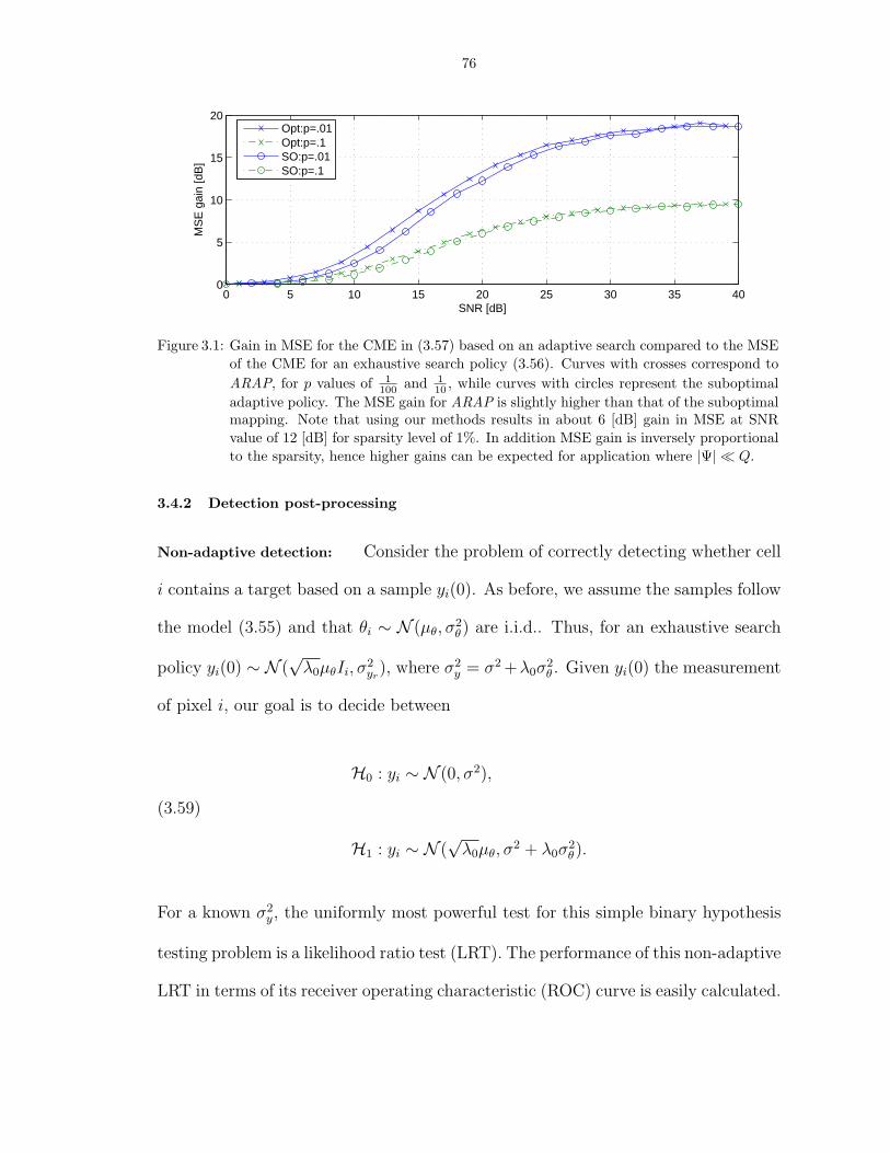
76

0 5 10 15 20 25 30 35 400

5

10

15

20

SNR [dB]

MS

E g

ain

[dB

]

Opt:p=.01Opt:p=.1SO:p=.01SO:p=.1

Figure 3.1: Gain in MSE for the CME in (3.57) based on an adaptive search compared to the MSEof the CME for an exhaustive search policy (3.56). Curves with crosses correspond toARAP, for p values of 1

100 and 110 , while curves with circles represent the suboptimal

adaptive policy. The MSE gain for ARAP is slightly higher than that of the suboptimalmapping. Note that using our methods results in about 6 [dB] gain in MSE at SNRvalue of 12 [dB] for sparsity level of 1%. In addition MSE gain is inversely proportionalto the sparsity, hence higher gains can be expected for application where |Ψ| ¿ Q.

3.4.2 Detection post-processing

Non-adaptive detection: Consider the problem of correctly detecting whether cell

i contains a target based on a sample yi(0). As before, we assume the samples follow

the model (3.55) and that θi ∼ N (µθ, σ2θ) are i.i.d.. Thus, for an exhaustive search

policy yi(0) ∼ N (√

λ0µθIi, σ2yr

), where σ2y = σ2 +λ0σ

2θ . Given yi(0) the measurement

of pixel i, our goal is to decide between

(3.59)

H0 : yi ∼ N (0, σ2),

H1 : yi ∼ N (√

λ0µθ, σ2 + λ0σ

2θ).

For a known σ2y, the uniformly most powerful test for this simple binary hypothesis

testing problem is a likelihood ratio test (LRT). The performance of this non-adaptive

LRT in terms of its receiver operating characteristic (ROC) curve is easily calculated.

77

The power β of this level α LRT is [32]

(3.60) β = 1− Φ

(Φ−1(1− α)−

√λ0µ2

θ

σ2

),

where Φ(·) is the normal cumulative distribution function.

Adaptive detection: First we derive the likelihood function f(y(2),y(1); IΨ).

Bayes rule provides

(3.61) f(y(2),y(1)) = f(y(2)|y(1))f(y(1)),

but, given y(1), the measurements at the second step are independent for different

cells and thus

(3.62) f(y(2),y(1)) =

Q∏i=1

f(yi(2)|y(1))f(yi(1)).

Therefore, the LRT statistic Tj is

(3.63) Tj =

∏Qi=1 f(yi(2)|y(1), Ij = 1)f(yi(1)|Ij = 1)∏Qi=1 f(yi(2)|y(1), Ij = 0)f(yi(1)|Ij = 0)

=

(3.64)f(yj(2)|y(1), Ij = 1)f(yj(1)|Ij = 1)

f(yj(2)|y(1), Ij = 0)f(yj(1)|Ij = 0).

For our model, we have yi(1) ∼ N (√

λ1µθIi, σ2 + λ1σ

2θIi) and, given y(1), the sec-

ond step measurements are also Gaussian yi(2) ∼ N (√

λ(i, 2)µθIi, σ2 + λ(i, 2)σ2

θIi).

Substituting these distributions into (3.64) provides the following LRT

(3.65)

Ti =σ2

√(σ2 + λ1σ2

θ)(σ2 + λ(i, 2)σ2

θ)

exp

−

(yi(2)−µθ

√λ(i,2)

)2

2(σ2+λ(i,2)σ2θ)

− (yi(1)−µθ

√λ1)

2

2(σ2+λ1σ2θ)

exp−y2

i (1)

2σ2 − y2i (2)

2σ2

≷ γ.

78

Note that for all cells where λ(i, 2) = 0 this test is a function of yi(1) alone.

Next, we compare the theoretical ROC curve (3.60) to the empirical ROC curve

calculated for the adaptive LRT (3.65) performed on the data pair (y(1),y(2)) using

the optimal λA and the suboptimal λso. We conducted multiple runs for varying SNR

levels and observed that with ν = 1 (3.65) provides higher detection probability than

the non-adaptive LRT having performance (3.60) for false alarm levels lower than

30%. At SNR values close to 0 [dB] the difference between the two tests is negligible,

but increases with SNR. Note that, for very low false alarm levels λA performs

better than λso in terms of detection probability. However, for higher test levels the

suboptimal search policy λso yield better detection performances.

Results are presented in Figure 3.2 (a) and (b) for SNR=10 [dB], Q = 1024, and

either p = 0.1 or p = 0.01. Monte-Carlo simulations were conducted with ν = 1

and each point on the figures represents an average over 2000 realizations. Detection

probability was averaged over the entire ensemble and over all pixels inside and

outside the ROI. At 10 [dB] the ROC curves are very sharp and are plotted on

a logarithmic scale. The solid curve represents (3.60) the non-adaptive LRT with

equal energy allocation. Curves with crosses represents λA, while curves with circles

represents λso. It is evident that the ROC curves of different tests have different

slopes for low false alarm values. Moreover, for high false alarm values no adaptive

policy outperforms the exhaustive search policy. Figure 3.2(b) zooms in to better

illustrate the differences for Pfa ∈ [0.005, 0.5]. One can see that the optimal search

policy has the best performances up to α = 3%, at which point the suboptimal policy

yields higher detection probability. The exhaustive search policy outperforms both

the adaptive methods for α > 30%.

Finally we compare detection probability values, for a fixed false alarm rate, and

79

10−4

10−3

10−2

10−1

100

0

0.5

1

Pfa

(a)

Pd

10−2

10−1

0.8

0.85

0.9

0.95

1

Pfa

(b)

Pd

UniformOpt:p=.01Opt:p=.1SO:p=.01SO:p=.1

UniformOpt:p=.01Opt:p=.1SO:p=.01SO:p=.1

Figure 3.2: ROC curves for the LRT tests based on an exhaustive search scheme and the twoadaptive policies measurements scheme, for p = 0.1 and p = 0.01 and SNR of 10 [dB].(a) shows the entire ROC curve while (b) zooms in on false alarm probability valuesless than 0.5. The simulation suggests that our adaptive search policies outperforms anexhaustive search policy in terms of detection probability for false alarm values lowerthan 30%.

estimation MSE gain g(·) in (3.58) as a function of ν. Results are shown in Fig-

ure 3.3. The curve with triangle markers represents estimation MSE gain and its

corresponding values are indexed on the right axis of the figure. The other curves

represent detection probability for a given test level, with the detection values in-

dexed at the left axis. All curves are a function of ν. For the selected operating

point it is clear that it is best to choose ν = 1, since it maximizes both detection

and estimation performance. In [5] we compare (3.65) to a test using a detection

optimized measurement and show that λA with ν < 1 is nearly optimal for detection.

80

0.5 0.55 0.6 0.65 0.7 0.75 0.8 0.85 0.9 0.95 10.5

0.6

0.7

0.8

0.9

1

Pd

0.5 0.55 0.6 0.65 0.7 0.75 0.8 0.85 0.9 0.95 10

0.8

1.6

2.4

3.2

4

MS

E g

ain

ν

Pfa

=0.001

Pfa

=0.005

Pfa

=0.01

Pfa

=0.05

Pfa

=0.1

MSE gain

Figure 3.3: Detection probability, for a fixed test level, and estimation MSE gain g(·) in (3.58) as afunction of ν when SNR is 10 [dB] and p = 0.01. Note that the MSE gain values (curvewith triangular markers) are given on the r.h.s. of the figure. Since MSE gain is definedover the true ROI it increases with ν.

3.4.3 Achievable cost

As a final comparison between our two policies, we compare the average perfor-

mance gain G(·), defined as the expected value of (3.15), achieved by the two search

policies for ν = 1. We chose Q = 8192 as the total number of cells and the sparsity

values of p ∈ 110

, 1100

, 11000

, i.e., a mean of roughly 800, 80, and 8 targets per realiza-

tion, respectively. Results are shown in Figures 3.4(a) and 3.4(b) where the curves

with crosses and circles describe the expected gain EG(ΛA) with optimal and with

suboptimal EG(Λso) allocation, respectively. Figure 3.4(a) shows the behavior of

the gain for the two policies for SNR values of 0 [dB] to 40 [dB]. Figure 3.4(b) zooms

in on SNR values of 0 [dB] to 13 [dB]. Each point on a graph represents 500 runs

in a Monte Carlo simulation. As can be seen from Figure 3.4(a), at extreme high

or low SNR values the performance gain of the two policies coincide. Figure 3.4(a)

indicates that the gain converges to its theoretical limit given by (3.44). The largest

gap in gain between the two algorithms is near the transition zone: SNR between

5-15 [dB], and the gap is less than 2 [dB]. Evidently, the simpler suboptimal mapping

rule does not significantly degrade performance gain.

81

0 5 10 15 20 25 30 35 400

10

20

30

SNR [dB] (a)

Per

form

ance

gai

n [d

B],

G(Λ

)

0 2 4 6 8 10 120

5

10

SNR [dB] (b)

Per

form

ance

gai

n [d

B],

G(Λ

)

Opt; p=0.001Opt; p=0.01Opt; p=0.01SO; p=0.001SO; p=0.01SO; p=0.1

Opt; p=0.001Opt; p=0.01Opt; p=0.01SO; p=0.001SO; p=0.01SO; p=0.1

Figure 3.4: The cost gain compared to an exhaustive search for both our optimal and suboptimalenergy allocation schemes. (a) shows that both algorithms converges to the asymptoticpredicted gain, at −10 log p. (b) enhances the difference between our two policies forSNR values in the range of 0− 13 [dB].

Figure 3.5 compares the percentage of effort λ1QλT

allocated in the first step for

both policies. While for SNR values greater than 25 [dB] the curves overlap, this is

not the case for low SNR values. As measurement quality decreases, ARAP invests

more energy at the first step. Considering the difference between the two policies,

this result makes sense: after the first step ARAP ignores all cells with posterior

probability values lower than some threshold. Decision errors at that stage can no

longer be compensated, i.e., the cumulative effort distribution ΛA(i) for those cells

will remain unchanged. Hence, more effort has to be allocated to the first step to

reduce decision errors, i.e., improve the agreement between Ψ and Ψ. On the other

hand, the suboptimal mapping invests energy in all Q cells at the second step. Thus,

82

it has a chance to compensate for poor estimated posterior probability values. As a

general remark we note that the incentive to use our methods increases with SNR

(e.g. Figure 3.1). Therefore, differences between the two policies in the low SNR

regime are of lesser importance.

0 5 10 15 20 25 30 35 400

20

40

60

80

SNR [dB]

% o

f tot

al e

nerg

y

Opt; p=0.001

Opt; p=0.01

Opt; p=0.01

SO; p=0.001

SO; p=0.01

SO; p=0.1

Figure 3.5: The proportion of energy invested at the first step for the two algorithms λA and λso.Curves correspond to prior probability values of 0.001, 0.01 and 0.1. As seen, the optimalsearch policy invest more energy at the first step. However, for SNR > 25 [dB] the twoare essentially equivalent.

3.5 Application - detecting and estimating a ROI in a SAR image

Consider the task of imaging a large area using a satellite equipped with a syn-

thetic aperture radar (SAR) system. Assume we have satellite access at two different

occasions for a limited time. In SAR imaging the measurement quality improves as

the dwell time increases. Therefore, with limited access to satellite time we face the

question of how to best utilize the resource available to us, i.e., where to dwell and for

how long to dwell in the SAR system. Problems concerning where to point a sensor

to are discussed in [31,33,34]. However, by allowing an additional continuous degree

of freedom for the varying dwell time we consider a different set of feasible policies.

Assume the satellite has enough time to acquire all cells of the image at each stage,

if so desired. Assuming our goal is to detect and identify targets spread out in a

83

large area we propose the following two stage search policy based on ARAP: The

first stage performs an exhaustive search with equal dwell time over all cells yielding

a preliminary image y(1) and an estimate Ψ of the ROI Ψ. In the second stage,

let ARAP allocate the dwell time in a non uniform manner to the different cells via

(3.38), i.e., focusing the search on Ψ. Finally, we combine both measurements to

form an image on which we detect the ROI and estimate its content. The competing

strategy performs an exhaustive search with equal dwell time at each cell twice, with

no adaptation between scans, than uses the arithmetic mean of the two independent

scans as the estimated image.

We used a SAR image, taken from the Sandia National Laboratories website2 as

an example of a “sparse” image. The image displays two columns of tanks in a field

and its sparsity ratio is p < 0.01. Let X denote the original image and let x be a

lexicographic ordering of X. We emulated the effect of the SAR varying dwell time

as modulated speckle noise variance in the post-processed SAR image. In particular,

the SAR image after the first stage (equal dwell time at all pixels) is modeled as:

(3.66) x1 = (1 + z1)x,

where z1 is a zero mean uniform random variable with var(z1) = 1λ1

noted as z1 ∼

U[−√

3λ1

,√

3λ1

] and λ1 = λ0. A tank template shown in Figure 3.6, was applied

as a matched filter to the noisy image X1 yielding X1. The input to the ARAP

algorithm y(1) = x1−x1√1Q

(x1−x1)′(x1−x1)was the variance normalized version of X1, where

x1 = 1Q

∑Qi=1 x1(i). ARAP was used to obtain a search policy for the second step

λ(i, 2) via (3.38). All indices i with λ(i, 2) < λ1 were set to zero and their cumulative

search effort was redistributed among the rest of the cells in a proportional manner.2http://www.sandia.gov/RADAR/images/rtv_tanks_9in.jpg

84

The SAR return x2 was modeled as

(3.67) x2 = (x + x¯ z2)¯ IΨ,

where z2(i) ∼ U[0,√

12λ(i,2)

] for all i ∈ Ψ and zero otherwise, and ¯ denotes an

element by element multiplication operator. This resulted in a non-uniform variance

for different cells in Ψ with var(z2(i)) = 1λ(i,2)

. Note that x2 = 0 for all i ∈ Ψc.

We considered several suboptimal linear estimators of x based on (x1,x2) that

performed comparably. The estimator presented here X was defined via x as

(3.68) x =

(x1 ¯ Ii ∈ Ψc√

1 + 1/λ1

+ x2 ¯ vec

1√

1 + 1/λ(i, 2)

)¯ s,

where vecri = [r1, r2, . . . , rQ]′ and s(i) =

(√1 + 1

λ1+

√1 + Ii∈Ψ

λ(i,2)

)−1

. The

pixels

pixe

ls

2 4 6 8 10 12

2

4

6

8

10

12

Figure 3.6: The above (13× 13) tank template was used as a matched filter to filter the noisy dataX1 and generate y(1).

estimator (3.68) is compared to an image reconstructed from two exhaustive searches

with equal effort allocation (xU1,xU2) given in (3.66), defined as xU = (xU1+xU2)/2.

SNR was defined as 10 log 2λ0.

85

Results are presented in Figures 3.7 and 3.8 for SNR values of 4 and 0 [dB], respec-

tively. Figure 3.7(a) show the original image, Figure 3.7(b) and (d) show a single

realization of images reconstructed using exhaustive search and ARAP via (3.68),

respectively. Figure 3.7(c) show the effort allocated by ARAP at the second stage

for that specific realization. Although all targets are identifiable in Figure 3.7(b),

they appear clearly in Figure 3.7(d). Figure 3.8 focuses on the ROI to demonstrate

the superiority of ARAP compared to the exhaustive search policy. Figures 3.8(a)

and (b) show a single realization of the two search methods exhaustive and ARAP

at 0 [dB] respectively, while Figs. 3.8(c) and (d) display a 1D profile, going through

the left columns of tanks, of 100 different realizations of each policy respectively. It

is evident that variations in profiles in images reconstructed using ARAP are much

smaller than those in images reconstructed from exhaustive search policy.

This illustrative example demonstrates the potential utility of our method in SAR

imaging. Note that energy allocation is equivalent to dwell time allocation in this

example.

3.6 Conclusions and future work

We introduced a novel convex cost function and showed that its minimization

relates to minimizing error probability or estimation MSE over an unknown ROI. A

closed form solution for the second stage in a two-stage optimal search policy was

provided, and numeric search for the first step was presented. A closed form low

complexity approximation for the two step minimization problem was also presented

and it was shown to perform comparably to the optimal solution. In a high SNR the

performance of the optimal and approximated algorithms was shown to converge to

the ideal omniscient limit. For the detection task, the two search policies introduced

86

pixels

pixe

ls

100 200 300 400 500

100

200

300

400

(a)

pixels

pixe

ls

100 200 300 400 500

100

200

300

400

(b)

pixels

pixe

ls

100 200 300 400 500

100

200

300

400

(c)

pixels

pixe

ls

100 200 300 400 500

100

200

300

400

(d)

Figure 3.7: SAR imaging example, SNR=4 [dB]. (a) Original image. (b) Image reconstructed usingtwo exhaustive searches. (c) Effort allocation using ARAP at the second stage. (d)Image resulted from (3.68) using ARAP.

outperformed the one step exhaustive measurement scheme when the false alarm

is less than 30%. For estimation, comparing the MSE of estimated values within

the ROI, our adaptive search policies dominate the exhaustive search policy. The

search policy is parameterized by ν which varies from 12

to 1 and controls the energy

allocated within the ROI. An offline lookup table can be generated for the optimal ν

in terms of the sparseness p and SNR of the target in the data. Finally, an illustrative

example of our method for SAR imaging was presented.

This approach is applicable to tumor detection where a cluster of calcification

may appear around the lesion. In this case multiscale hypothesis testing methods

presented in [21] may be relevant. Frakt et al. deals with anomaly detection once

87

pixels

pixe

ls

200 300 400

150

200

250

300

350

400

(a)

pixels

pixe

ls

200 300 400

150

200

250

300

350

400

(b)

0 50 100 1500

50

100

150

200

250

pixels

inte

nsity

(c)

50 100 1500

50

100

150

200

250

pixels

inte

nsity

(d)

Figure 3.8: SAR imaging example, SNR=0 [dB]. (a) Image reconstructed using two exhaustivesearches, targets are not easily identifiable. (b) Image resulted from (3.68) using ARAP.Figures (c) and (d) compare a 1D profile going through the targets on the lower leftcolumn for 100 different realizations. (c) Profiles of images reconstructed from anexhaustive search. (d) Profiles of images reconstructed using ARAP. The bold brightline on both figures represent the mean profile of the different realizations. Evidently,variations of profiles of images due to ARAP are much smaller compared to variationsof profiles of images resulted from an exhaustive scan.

measurements, at a fine resolution, have been acquired. Our goal is to generate fine

resolution measurements only where the are most informative. Another interesting

area of application is to compressive sensing. Work such as [56] and [55] consider

the problem of sampling a sparse medium via an arbitrary affine transformation.

In cases of sparse signals complete reconstruction of the underlying signal can be

accomplished with only a few samples. This exploitation of sparsity is analogous to

the methods proposed in this chapter.

88

3-A Appendix: Equivalency of minimizing our cost to minimizing theCramer-Rao bound

Consider the problem of estimating an unknown signal in the presence of a Gaus-

sian noise. Let ym×1 be a measurements vector given by

(3-A.1) y = diag√

λµ + n,

where n ∼ N (0, σ2I). Let Ψ be a collection of indices, namely the ROI, with

|Ψ| ¿ m. Assume that the effort to be distributed is the measurement energy λi

associated with measuring an element of y, with∑

i λi = 1. Define zi = yi√λi

, hence

(3-A.2) zi ∼ N(

µi,σ2

λi

).

Recall that the Cramer-Rao bound on the variance of any unbiased estimator µi(zi)

of µi is given as

(3-A.3) VAR(µi) > σ2

λi

,

which is also the measurement variance for this case. From (3.7) we know that the

minimizer of our cost (3.5) when ν = 1 is a uniform energy allocation within the

ROI. Hence the optimal solution minimizing our cost λi = 1|Ψ|I(i ∈ Ψ) also uniformly

minimizes the Cramer-Rao bound on all µi where i ∈ Ψ.

3-B Appendix: Chernoff bound on the probability of error and our costfunction

Let us consider simple binary, hypothesis testing problem of classifying an ob-

servation X as coming from one of two possible classes (hypotheses) H0,H1. Let

π0, π1 denote the a priori probabilities on the hypotheses, and let p0(x), p1(x) denote

89

the conditional probability density functions given the true hypothesis. Then, Bayes

decision rule minimizes the probability of error Pe by choosing the hypothesis with

the largest a posteriori probability. The Chernoff bound on Pe states that for any

α ∈ [0, 1]

(3-B.1) Pe 6 πα0 π1−α

1

∫

X

[p0(x)]α [p1(x)]1−α dx.

Further let X be a Gaussian r.v. with known variance σ2 and unknown mean with

the two hypothesis corresponds to H0 : µ0 = 0 and H1 : µ1 > 0. In this case

(3-B.1) yields

(3-B.2) Pe 6 πα0 π1−α

1 e−α(1−α)µ2

12σ2 ,

so the Chernoff bound on the probability of error Pe is a decreasing function of

the unknown mean µ and an increasing function of the variance σ2. Let wQ×1 ∼

N (µ, σ2I) and consider the problem of detecting between µi = 0 and µi > 0. Let

Ψ = i : µi > 0 and assume |Ψ| ¿ Q. Further assume that by allocating energy λ(i)

to the ith measurement we increase the detectability index µi

σ, e.g. as in (3.18). For

such a scenario, minimizing our cost function (3.5) with ν = 1 results in uniformly

allocating energy to all cells in Ψ. Utilizing (3-B.2) it implies uniformly minimizing

Pe over Ψ.

3-C Appendix: Showing a global lower bound on our cost

In Section 3.2 we claimed that the r.h.s. of (3.6) is lower bounded by |Ψ|2 for all

ν ∈ [12, 1] and |Ψ|

Q6 1

2. To prove this claim let f(ν) = [

√ν|Ψ| +√

1− ν(Q − |Ψ|)]2,

then we need to show

(3-C.1) f(ν) > |Ψ|2.

90

First note that

(3-C.2) f(1

2) =

Q2

2> |Ψ|2 = f(1),

since |Ψ|Q

6 12. Next we show that f(ν) 6 0 for all ν ∈ [1

2, 1], i.e., f(ν) is a decreasing

function over the interval of interest. When combined with (3-C.2) this proves the

claim. Note that

(3-C.3) f(ν) = 2[√

ν|Ψ|+√1− ν(Q− |Ψ|)]

[ |Ψ|√ν− Q− |Ψ|√

1− ν

],

hence it suffice to show

(3-C.4)

[ |Ψ|√ν− Q− |Ψ|√

1− ν

]6 0..

Rearranging (3-C.4) we need to show

(3-C.5)

√1− ν

ν6 Q− |Ψ|

|Ψ| =Q

|Ψ| − 1.

But ν ∈ [12, 1] provides 1−ν

ν6 1, while |Ψ|

Q6 1

2results in Q

|Ψ| − 1 > 1 and hence the

inequality in (3-C.5) holds. This completes the proof.

3-D Appendix: Showing an upper bound on the gain

Let Ii be a Bernoulli r.v. with Pr(Ii = 1) = p. Define |Ψ| =∑Q

i=1 Ii, then |Ψ|

is a Binomial r.v. and |Ψ| ∼ B(Q, p). Further let p∗ = |Ψ|Q

then Ep∗ = p and

var(p∗) = p(1−p)Q

.

Claim 1. For an arbitrary effort allocation policy Λ and δ > exp−Q 3p8(1−p)

we have

(3-D.1) Pr(G(Λ) 6 −10 log p + ε) > 1− δ,

91

where ε = −10 log ε′ and ε′ < 1 is the solution of

(3-D.2) (1− ε′)2 + (4− ε′)2

3

1− p

pQln δ = 0.

Proof. For all Λ

(3-D.3) J(Λo) 6 J(Λ),

and therefore

(3-D.4) G(Λ) 6 G(Λo) = −10 log p∗,

thus

(3-D.5) Pr(G(Λ) 6 −10 log p + ε) > Pr(−10 log p∗ 6 −10 log p + ε),

for some ε > 0. Next, we evaluate the expression on the r.h.s. of (3-D.5). Note that

Pr(−10 log p∗ 6 −10 log p + ε) =(3-D.6)

Pr(log p∗ > log p− ε

10

)=(3-D.7)

Pr(p∗ > p

10ε10

)= Pr(p∗ > ε′p) = 1− Pr(p∗ 6 ε′p),(3-D.8)

where ε′ = 1

10ε10

< 1. Note that

Pr(p∗ 6 ε′p) = Pr(p∗ − p 6 p(ε′ − 1)) =(3-D.9)

Pr(p− p∗ > p(1− ε′)).(3-D.10)

92

For a sequence of i.i.d. r.v.’s Xini=1 with EXi = 0, Bernstein’s inequality provides

(3-D.11) Pr

(n∑

i=1

Xi > t

)6 exp

− t2/2∑

i EX2i + M t

3

,

for t > 0, and where |Xi| 6 M with probability 1. Let Xi = p − Ii, then assuming

p 6 12

yield M = 1− p and

(3-D.12) Pr(p− p∗ > t) 6 exp

− Q t2

2

(1− p)(p + t

3

)

.

Utilizing (3-D.12) we obtain

Pr(p− p∗ > p(1− ε′)) 6 exp

−Q

3

2

p

1− p

(1− ε′)2

4− ε′

4= δ.(3-D.13)

When combined, (3-D.5)-(3-D.13) provide

(3-D.14) Pr(G(Λ) 6 −10 log p + ε) > 1− δ.

This completes the proof. 2

Discussion

Bernstein’s inequality requires t > 0 which hold provided that ε′ ∈ (0, 1). Unfor-

tuntaely, this means that we do not have δ → 0 since substituting ε′ = 0 in (3-D.13)

yields

δ > exp

−Q

3

8

p

1− p

,(3-D.15)

and Q and p are given. Nevertheless, δ may still be sufficiently small to make Claim

1 attractive. In Section 3.5 we provide a SAR imaging example of our methods. A

93

(450[pix] × 570[pix]) image containing 13 targets each roughly (13[pix] × 13[pix]) is

examined. This translates to p < 0.01 and Q = 256, 500. Therefore, setting δ = 10−3

yields ε = 0.333 or

Pr(G(Λ) 6 −10 log p + 0.333) > 1− 10−3,

i.e., the gain of any effort allocation policy Λ is smaller than 20.333[dB] with proba-

bility grater than 0.999.

3-E Appendix: Minimizing the cost function

Let Y (t) ∈ Y be a (Q × 1) random vector (r.v.) with a probability density

function (pdf) pY (t)(y) > 0, for all y ∈ Y and t ∈ 1, 2, . . . , T, representing random

observations. Let IΨ = [I1, I2, . . . , IQ]′ be a r.v. with Pr(Ii = 1) = pi. Let Y t1 =

Y (1),Y (2), . . . , Y (t) be a collection of all observation up to time t. Define x(i, t) :

Y t−11 → R+, then, for some ν ∈ (1

2, 1], our goal is to find x(i, t) with i = 1, . . . , Q

and t = 1, . . . , T , such that

x(i, t) = arg minx(i,t)

E

Q∑

i=1

νIi + (1− ν)(1− Ii)∑Tt=1 x(i, t)

,

where expectation is taken w.r.t. IΨ and Y T−11 , subject to

∑Qi=1

∑Tt=1 x(i, t) = X.

E.1 The case of T = 1

For T = 1, our cost function has the following form

x(i) = arg minx(i)

E

Q∑

i=1

νIi + (1− ν)(1− Ii)

x(i)

,

94

subject to∑Q

i=1 x(i) = X, with the expectation taken w.r.t. IΨ. Note that EIi =

pi, so xi can be derived using Lagrange multiplier, i.e., finding the minimizer of

L(x, λ) =

Q∑i=1

νpi + (1− ν)(1− pi)

x(i)+ λ

(Q∑

i=1

x(i)−X

).

Taking derivatives and setting them equal to zero, yields

x(i) =X

√νpi + (1− ν)(1− pi)∑Q

j=1

√νpj + (1− ν)(1− pj)

.

E.2 The case of T = 2

Consider the following problem, let x(i, 1) = x1 > 0 for all i, then∑Q

i=1 x(i, 1) =

Qx1. Our goal is minimize the cost, i.e., find

(3-E.1) x(i, 2) = arg minx(i,2)

E

Q∑

i=1

νIi + (1− ν)(1− Ii)

x1 + x(i, 2)

,

subject to

(3-E.2)

Q∑i=1

x(i, 2) = X −Qx1 > 0,

and x(i, 2) : Y (1) → R+. For brevity, let xi(Y ) = x(i, 2), and note that in (3-E.1)

expectation is taken w.r.t. IΨ and Y (1). Using iterated expectation, we obtain

(3-E.3)

E

Q∑

i=1

νIi + (1− ν)(1− Ii)

x1 + x(i, 2)

= E

Q∑

i=1

E

νIi + (1− ν)(1− Ii)

x1 + xi(Y )

∣∣∣∣ Y (1)

.

95

Given Y (1) the denominator is deterministic and expectation can be applied to the

numerator, therefore (3-E.3) becomes

E

Q∑

i=1

νPr(Ii = 1|Y (1)) + (1− ν)(1− Pr(Ii = 1|Y (1)))

x1 + xi(Y )

.

Define pIi|Y = Pr(Ii = 1|Y (1)) and Wi = νpIi|Y +(1−ν)(1−pIi|Y ), we use Lagrange

multiplier to minimize

E

Q∑

i=1

Wi

x1 + xi(Y )

+

∫

Yλ′(y)

(Q∑

i=1

xi(y)− (X −Qx1)

)dy =

(3-E.4)

Q∑i=1

∫

Y

[wi

x1 + xi(y)fY (y) + λ′(y) (xi(y)− (X −Qx1))

]dy.

where wi = Wi(y) is a realization of the r.v. Wi. Since fY (y) is strictly positive,

define λ(y) = λ′(y)fY (y)

, then, xi, the minimizer of (3-E.4) is also the minimizer of

Q∑i=1

∫

Y

[wi

x1 + xi(y)+ λ(y)xi(y)

]dy,

Note that our problem has translated to minimizing a separable sum of integrals of

a positive integrands. Hence, finding

xi(Y ) = arg minxi(Y )

wi

x1 + xi(Y )+ λ(Y )xi(Y ),

suffice. Solving for xi(y) given the Lagrange multiplier λ(Y ) yields

(3-E.5) xi(Y ) =

√wi

λ(Y )− x1,

√wi

λ(Y )> x1

0, Otherwise

,

96

which can be also written as xi(Y ) = (√

wi

λ(Y )− x1)I(λ(Y ) < wi

x21), where I(·) is an

indicator function. Utilizing the constraint∑

i xi(Y ) = X −Qc1, we obtain

(3-E.6)1√

λ(Y )

Q∑i=1

√wiI

(λ(Y ) <

wi

x21

)= X − x1

(Q−

Q∑i=1

I

(λ(Y ) <

wi

x21

)).

Note that

(3-E.7) Q =

Q∑i=1

I

(λ(Y ) <

wi

x21

)+

Q∑i=1

I

(λ(Y ) > wi

x21

),

substituting (3-E.7) into (3-E.6) and rearranging, yields

(3-E.8)√

λ(Y ) =

∑Qi=1

√wiI

(λ(Y ) < wi

x21

)

X − x1

∑Qi=1 I

(λ(Y ) > wi

x21

) .

Next, use τ : X → X defined in (3.32) such that wτ(1) 6 wτ(2) 6 . . . 6 wτ(Q).

Case λ(Y )x21 < wτ(1)

If λ(Y )x21 < wτ(1), for all Y , then λ(Y )x2

1 < wτ(i) for all i and√

λ(Y )x21 =

∑Qi=1

√wτ(i)

X. For which case, the cost minimizer is achieved at

xτ(i)(Y ) =X√

wτ(i)∑Qj=1

√wj

− x1,

and, for all i

(3-E.9)X

x1

>∑Q

j=1

√wj√

wτ(i)

.

97

Case λ(Y )x21 > wτ(Q)

For the other extreme, we have λ(Y )x21 > wτ(i) for all i, which in turn provides

λ(Y ) = 0, due to (3-E.8). This can only hold if both ν = 1 and pIi|Y = 0 for all i.

If this is the case, then for any choice of xi(Y ) the overall cost is zero.

Case wτ(k) 6 λ(Y )x21 < wτ(k+1), for some k ∈ 1, 2, . . . , Q− 1

The interesting case is when λ(Y ) has some intermittent value, i.e.,

(3-E.10)

√wτ(k)

x1

6∑Q

i=k+1

√wτ(i)

X − kx1

<

√wτ(k+1)

x1

.

Since all the terms in (3-E.10) are positive, we rewrite the inequality as

(3-E.11)

∑Qi=k+1

√wτ(i)√

wτ(k+1)

+ k <X

x1

6∑Q

i=k+1

√wτ(i)√

wτ(k)

+ k.

Define

(3-E.12)

LB(k) =∑Q

i=k+1√

wτ(i)√wτ(k+1)

+ k,

UB(k) =∑Q

i=k+1√

wτ(i)√wτ(k)

+ k.

To show that (3-E.11) makes sense, we need to show that for any X of interest there

exists a unique k = k0 ∈ 1, 2, . . . , Q − 1 such that Xx1∈ (LB(k0), UB(k0)]. To do

so we show that following: (i) LB(k) 6 UB(k), (ii) LB(k − 1) = UB(k), and (iii)

Xx1∈ (LB(Q− 1), UB(1)]. Start with (i)

(3-E.13)

∑Qi=k+1

√wτ(i)√

wτ(k+1)

+ k −(∑Q

i=k+1

√wτ(i)√

wτ(k)

+ k

)=

98

(√wτ(k) −√wτ(k+1)√

wτ(k)wτ(k+1)

)Q∑

i=k+1

√wτ(i) 6 0,

since wτ(k) 6 wτ(k+1). Note that wτ(k) = wτ(k+1) implies that the interval (LB(k), UB(k)]

is empty. To prove (ii) we substitute (k − 1) for k in the expression for LB(k) in

(3-E.12). This yields

(3-E.14) LB(k − 1)− UB(k) =

√wτ(k)√wτ(k)

− 1 = 0.

Combining (i) and (ii) provides LB(k) 6 UB(k) = LB(k−1), i.e., LB(k) is decreasing

in k. Finally, we need to show Xx1∈ (LB(Q − 1), UB(1)]. First, note from (3-E.9)

that Xx1

> UB(1) belongs to Case 1 for which a separate solution was provided.

Second, from (3-E.12) we obtain LB(Q − 1) = Q. If Qc1 = X then xi(Y ) = 0,

for all i, due to the constraint (3-E.2). Thus, for a two-step problem we must have

Xx1

> Q = LB(Q − 1). Hence, Xx1∈ (LB(Q − 1), UB(1)] as required. Together (i),

(ii), and (iii) proves existence and uniqueness of the solution, since

1. Xx1∈ (LB(Q− 1), UB(1)],

2.⋃Q

k=1(LB(k), UB(k)] = (LB(Q− 1), UB(1)],

3. (LB(i), UB(i)] ∩ (LB(j), UB(j)] = ∅, ∀i 6= j.

To conclude this section we note that xi(Y ) the minimizer of (3-E.1) is given by

(3.38) replacing x1 for λ∗1 and xτ(i)(Y ) for λ(τ(i), 2). A general solution for the case

of a non-uniform prior distribution is given in [5].

99

3-F Convergence of pIi|y(1),θ for the Gaussian case

For brevity, we prove the convergence given θ. This still holds for a random

target return, e.g. θi ∼ N (µθ, σ2θ), but the derivation is a little messier. Consider a

simplified version of the measurement model (3.18) given as

(3-F.1) yi(1) =√

λ1Iiθi(1) + ni(1),

where we substitute t = 1, λ(i, 1) = λ1, and hij(1) = δij with δij being the Kronecker

delta. We further assume that the r.v. θi > 0. For brevity we suppress the time

dependency from here on. In addition we assumed Pr(Ii = 1) = p for all i and the

noise samples are i.i.d. Gaussian with ni ∼ N (0, σ2). This setting results in i.i.d.

measurements distributed according to

(3-F.2) yi ∼ N (√

λ1Iiθi, σ2),

Therefore, the posterior probabilities pIi|y depends only on the ith sample, i.e., pIi|y =

pIi|yi. For the Gaussian case, pIi|yi

has an explicit form given as

(3-F.3) pIi|yi=

p exp− 12σ2 (yi − θi

√λ1)

2p exp− 1

2σ2 (yi − θi

√λ1)2+ (1− p) exp− 1

2σ2 y2i

,

which can be rearranged as

(3-F.4) pIi|yi=

1

1 + 1−pp

exp− θiλi

σ2

(yi√λ1− θi

2

) .

Let zi = yi√λ1

, then zi ∼ N (θiIi, η2) where η2 = σ2

λ1and at high SNR η2 → 0.

Substituting yi with zi in (3-F.4) provides

(3-F.5) pIi|yi= pIi|zi

=1

1 + 1−pp

exp− θi

η2

(zi − θi

2

) .

100

Claim 2. The conditional probability pIi|yidefined in (3-F.5) converges in probability

to Ii as η → 0 for any θi > 0, i.e., ∀ε > 0 and some δ > 0 there exists η0(ε), such

that ∀η 6 η0(ε)

(3-F.6) Pr(|pIi|yi(η)− Ii| > δ) 6 ε,

The intuition behind Claim 2 is derived from the following limit

(3-F.7) limη2→0

pIi|yi=

0, zi < θi

2

1, zi > θi

2

.

Proof. Using Chebyshev’s inequality we prove Claim 2 for the case of Ii = 0. A

symmetry argument suggests that the same line of proof can be applied for the case

of Ii = 1. Define A = zi : zi > θi

2 then

Pr(|pIi|yi− Ii| > δ) = Pr(A)Pr(|pIi|yi

− Ii| > δ|A)+

(3-F.8) Pr(Ac)Pr(|pIi|yi− Ii| > δ|Ac).

For Ii = 0 we have3

(3-F.9) Pr(pIi|yi> δ) 6 Pr(A) + Pr

(pIi|yi

> δ

∣∣∣∣zi 6 θi

2

).

We show that both elements on the r.h.s. (3-F.9) approach zero as η → 0. For some

α > 0, Chebyshev’s inequality provides

(3-F.10) Pr (|zi − θiIi| > α) 6 η2

α2.

3Since pIi|yi> 0 we can replace pIi|yi

= |pIi|yi|.

101

Note that

(3-F.11)

Pr(zi > θi

2) 6 Pr(|zi − θiIi| > θi

2), Ii = 0,

Pr(zi < θi

2) 6 Pr(|zi − θiIi| > θi

2), Ii = 1,

and therefore

(3-F.12) Pr(A) 6 Pr

(|zi| > θi

2

)6 4η2

θ2i

.

Next, we examine the term on r.h.s. of (3-F.9). Note that

Pr

(pIi|yi

> δ

∣∣∣∣zi 6 θi

2

)=(3-F.13)

Pr

1

1 + 1−pp

exp

θi

η2

(θi

2− zi

) > δ

∣∣∣∣∣∣zi 6 θi

2

=(3-F.14)

Pr

(θi

2− zi <

η2

θi

lnp

1− p

1− δ

δ

∣∣∣∣ zi 6 θi

2

).(3-F.15)

Let

(3-F.16) ε′ =η2

θi

lnp

1− p

1− δ

δ,

then (3-F.13) is equivalent to

(3-F.17) Pr

(zi ∈

[θi

2− ε′,

θi

2

])

102

First, note that δ > p results in ε′ < 0 and hence (3-F.17) equals zero. Second, since

fZ(z) 6 fZ(0) = 1√2πη2

we have the following simple bound for any ε′ > 0

(3-F.18) Pr

(zi ∈

[θi

2− ε′,

θi

2

])6 ε′

1√2πη2

= η1

θi

√2π

lnp

1− p

1− δ

δ,

thus

(3-F.19) Pr

(pIi|yi

> δ

∣∣∣∣zi 6 θi

2

)6 η

1

θi

√2π

lnp

1− p

1− δ

δ.

Finally, substituting (3-F.19) and (3-F.12) in (3-F.9) we obtain

(3-F.20) Pr(pIi|yi> δ) 6 4η2

θ2i

+ η1

θi

√2π

lnp

1− p

1− δ

δ.

Define η0(ε) as

(3-F.21) η0(ε) = supη>0

4η2

θ2i

+ η1

θi

√2π

lnp

1− p

1− δ

δ6 ε

, ∀δ > 0,

then using (3-F.20) we have

(3-F.22) pIi|yi→ 0

in probability when Ii = 0. In a similar manner, it can be shown that

(3-F.23) pIi|yi→ 1

in probability for Ii = 1. 2

CHAPTER IV

The multi-scale search problem

4.1 Introduction

This chapter considers the problem of estimating and detecting sparse signals

over a large area of an image or other medium from noisy observations. We further

assume that the nonzero signal elements, i.e., targets, tend to cluster together in areas

which we call regions of interest (ROI). In Chapter III we introduced a novel cost

function and solved a related minimization problem, which yielded an asymptotically

optimal adaptive resource allocation policy, namely ARAP. ARAP uses a two-stage

approach: first the entire domain is scanned, second a subset of it, suspected as part

of the ROI, is re-scanned. For signals in RQ, ARAP requires N > Q measurements

to complete. In this work we explore tradeoffs between the total number of expected

measurements and performance gain. We use the knowledge that targets tend to

cluster together and modify ARAP (M-ARAP) in a multi-scale fashion. In the first

stage M-ARAP takes M1 < Q measurements that cover the entire signal domain on

a coarse grid, then re-sample part of the signal domain on a fine grid at the second

stage. While we lose optimality, we show that the estimated ROI yielded by M-

ARAP still converges to the true ROI while the overall number of samples is greatly

reduced and significant estimation gains are maintained compared to an exhaustive

103

104

search policy. We show that for sparse signals with sufficient ROI to background

contrast we have 7 [dB] reduction in estimation error at signal to noise ratio of 5

[dB] with N < Q5

samples.

This scenario is common in radar target detection where large scattering objects

may occupy consecutive pixels on the Radar screen and appear as a cluster of targets.

Nevertheless, the overall area occupied by targets is small compared to the area a

scanning radar system covers. In early detection of cancer tumors such as in breast

cancer, the diameter of a typical tumor is a few millimeters to 1.5 centimeters. Hence,

on a fine grid a tumor may appear as a cluster of targets, yet, its overall volume is

very small compared to the volume of the entire breast.

The notion of saving measurements when sampling sparse signals has received sig-

nificant amount of attention in recent years. Work in the field of Compressed Sensing

(CS) challenges the traditional signal processing sampling requirements. Recent re-

sults show that a relatively small number of random projections of a signal can

contain most of its salient information. It follows that if a signal is compressible

in some orthonormal basis, it can be accurately recovered from random projections

even when they are contaminated with noise [9, 24]. Candes and Tao [9] introduce

the Dantzig selector (DS) algorithm which solves an l1-norm minimization problem

to reconstruct a sparse signal in RQ from a very limited set of N < Q noisy obser-

vations. Their algorithm converges to the true solution as long as the measurement

operator obeys the uniform uncertainty principle (UUP). They provide an upper

bound on the mean squared error (MSE) which, remarkably, is proportional up to

a C log Q factor of the noise level σ2. Haupt and Nowak present a similar result

but their measurement operator is randomized rather than following the UUP [24].

Although both methods work extremely well for (almost) truly sparse signals, they

105

do not focus efforts to specifically acquire the ROI. The measurement efforts are

uniformly spread at random locations in a single stage. While we share the goal

of reducing the overall number of measurements we chose an orthogonal approach.

Rather than randomly selecting the views used for the reconstruction, we learn from

past measurements and sequentially focus search efforts onto spatial locations of the

signal corresponding to an estimated ROI.

Abdel-Samad and Tewfik [2] study the problem of how to best allocate N mea-

surements to find a single target hidden in Q cells for radar target localization when

N < Q. They propose a hierarchical approach recursively grouping the Q cells into

q < Q groups in a tree like structure. They assume that the radar beam pattern

can be shaped accordingly and that signal to noise ratio (SNR) decreases as the

group size increases. Their multiple hypothesis testing approach is computationally

intense and does not account for large N and Q (Q = 64 is used in their example).

The solution complexity limits the number of measurements they can allocate at

each stage of the sequential search. In a similar manner we also note degradation in

performance as the scale increases. The main difference from our work is that they

account for a single target and the multi-hypothesis test cannot accept more than

one correct hypothesis at a single stage. Therefore, their method is not applicable

for large scale search problems of the type discussed here.

To the best of our knowledge, multiscale search approach was introduced in the

early 1940’s. Dorfman considered the problem of detecting defective members of

a large population in the context of weeding out all syphilitic men called up for

induction [16]. The test was so sensitive and accurate that Dorfman suggests the

following procedure: 1) draw blood from each candidate, 2) use half of each sample to

create a pool containing samples from n individual subjects, 3) test the pool. If a pool

106

was tested positive the other half sample of each pool member was individually tested

to detect the defective member. In the case of low disease prevalence rates a great

amount of time savings can be achieved. Dorfman type procedures use a binary model

(B-model) and do not account for false alarms or missed detections, which in our

setting is equivalent to an infinite SNR. Therefore they do not require the additional

degree of freedom of resource allocation and are only concerned with minimizing

the total number of samples required. An optimal group size n can be analytically

evaluated for each disease prevalence rate. Dorfman procedures enjoyed great success

due to their simplicity and effectiveness. Pfeifer modifies the binomial model (M-

model) and considers test values that were either zero (for negative) or greater than

zero (for the degree of contamination) [45]. This way, when a pool is tested positive,

each sample of a subgroup from the pool reveals information regarding the other pool

members, thus even greater savings are achieved. However, the modified model still

does not account for false alarms or missed detections. Although we use a structure

similar to the Dorfman procedure, the presence of noise creates a significant difference

between our work and the previous work done on blood pooling.

Finally, in Chapter III we examined utilities in a two-stage adaptive measuring

scheme for detection and estimation of sparse signals containing targets in noise.

We assumed independent and identical distribution (i.i.d.) of targets among pixels

and presented a two stage approach for resource allocation under a fixed energy con-

straint, namely ARAP. In this chapter we look at detecting and estimating clusters

of targets under additional sampling or time constraints. Since targets are assumed

to be clustered, a logical approach is to use a coarse measurement scale to reduce

the number of samples used at the first stage. A modified version of ARAP is intro-

duced to select locations and energy levels with which areas in the scanned domain

107

are re-sampled on a fine grid. The two measurements can be later combined to both

detect and estimate the region of interest (ROI) and its content. In Chapter III

we showed ARAP to be asymptotically optimal in terms of estimation gains being

inversely proportional to the signal sparsity. Here performance would depend on

sparsity, number of samples allowed, and the inherent contrast of the signal repre-

sented by the ‘detectability index’. We show that with sufficient contrast we improve

estimation accuracy by more than 7 [dB] while using less than 20% of the number of

measurements used by a traditional sampling scheme at SNR of 5 [dB] and sparsity

of 0.1%. Moreover, estimation gains increase with SNR leading to surprisingly large

gains.

The rest of this chapter is organized as follows. In Section 4.2 we formally intro-

duce the search problem and define a cost function. Section 4.3 discusses our search

methods and analyzes their properties. In Section 4.4 we compare the performance

of our adaptive multiscale approach to an exhaustive search. We conclude and point

out future work in Section 4.5.

4.2 Problem formulation

Consider a discrete space X = 1, 2, . . . , Q containing Q cells and equipped

with a probability measure P . We use Ψ to denote a region of interest (ROI) in

X , i.e., Ψ ⊆ X . In the sequel Ψ will be a randomly selected small subset of X .

Thus, we assume |Ψ| ¿ |Ψc|, where |Ψ| equals the number of elements in Ψ and Ψc

is the relative complement, X \ Ψ, of Ψ. Exact definition of the ROI is application

dependent. In radar target localization the ROI is the collection of all cells containing

targets and target related phenomena, e.g., target shadows. In a medical imaging

application, such as early detection of breast cancer, where tumor boundaries are

108

poorly defined, the ROI may be defined as the collection of all cells containing targets

(a tumor) plus some neighboring cells.

Let Ii be an indicator function of the ROI such that

(4.1) Ii =

1, i ∈ Ψ

0, Otherwise

and pi = Pr(Ii = 1)Qi=1 is an associated set of prior probabilities. In Chapter III

we considered the case where the Ii’s are i.i.d. and pi = p = E |Ψ|Q for all i.

In this chapter we consider the case where it is highly likely that targets tend to

cluster together and occupy neighboring pixels. In a one dimensional case we let the

random variable Ξ denote a cluster length and assume Ξ 6 ξ0 and p(Ξ) is known, e.g.

Pr(Ξ = i) = 1ξ0

for i = 1, 2, . . . , ξ0. Let IΨ = [I1, . . . , IQ]′ be a vector corresponding

to the set of all indicators and (·)′ denote the transpose operator. We say that the

presence of a target affects cell i if i ∈ Ψ. We define the random vector Y : X → RM

and consider the conditional probability p(Y |IΨ).

Consider a sequential experiment where in the first T −1 stages we observe Y (t) :

X → RMt with Mt < Q for t = 1, 2, . . . , T − 1 and in stage T we observe a selected

subset of Y (T ) : X → RQ, i.e., we observe yi(T ) for i ∈ Ψ ⊆ 1, 2, . . . , Q. This

formulation allows us to limit the total number of observations to N =∑T−1

t=1 Mt+|Ψ|.

Let the distribution λ(i, t) > 0 denote the search effort allocated to cell i at time t,

with

(4.2)T∑

t=1

Q∑i=1

λ(i, t) = 1, 0 6 λ(i, t) 6 1

and λ(i, t) is a mapping from past observations y1, . . . , yt−1 to the probability

109

simplex and is called an effort allocation policy. The set Ψ is formally defined as

(4.3) Ψ = i ∈ X : λ(i, T ) > 0.

The combination of λ(i, t), Mt, and Ψ is termed a search policy. We focus here

on a deterministic mappings λ, although a more general random mapping can also

be incorporated into our framework but is not presented here. We assume that a

sample’s ‘quality’ is an increasing function of the allocated effort to the associated

cell, e.g. measured in terms of information or inverse variance. In general, effort

might be: computing power, complexity, cost, or energy that is allocated to acquiring

a particular cell location. Define the cumulative search effort allotted to cell i as

(4.4) Λ(i) =T∑

t=1

λ(i, t).

In Chapter III we introduced the following cost function

(4.5) J(Λ) =

Q∑i=1

νIi + (1− ν)(1− Ii)

Λ(i),

with ν ∈ [12, 1]. Minimizing (4.5) subject to a total energy constraint λT yielded

ARAP, for the case of T = 2 and M1 = Q, which is summarized below.

110

Algorithm 4.1. Two stage Adaptive Resource Allocation Policy (ARAP) λA

Step 1: Allocate λA(i, 1) = λ∗1 to each cell and measure y(1).

Step 2: Given y(1) compute posterior probabilities, pIi|y(1)4= Pr(Ii = 1|y(1))

and wi = νpIi|y(1) + (1− ν)(1− pIi|y(1)), then rank order the wi’s.

Step 3: Use λ∗1 and the ordered statistic wτ(i) to find an optimal threshold k0.

Step 4: Given k0, apply λ(i, 2), the energy allocation, to cell i as

(4.6)

λA(τ(i), 2) = λ(τ(i), 2) =

(λT − k0λ

∗1∑Q

j=k0+1

√wτ(j)

√wτ(i) − λ∗1

)I(i > k0),

and measure y(2).

For ARAP the normalized number of observations, N∗ = Q+(Q−k0)Q

= 1+(1− k0

Q),

is a random variable that was shown to converge in probability to 1+p at high SNR,

where p = E |Ψ|Q. Our goal in this work is to add a sampling constraint on top of the

fixed energy constraint to limit the total search time or the number of measurements.

We use a modified version of ARAP to achieve that goal. We modify ARAP in two

ways: i) Keep M1 < Q and let N∗ be a random variable with bounded EN∗, ii)

Let M1 < Q and k0 be fixed, thus N∗ = M1

Q+ (1 − k0

Q) is also fixed. Note that we

do not intend to solve a new optimization problem but rather to modify an existing

optimal solution, namely ARAP, in a manner that suits the additional constraints.

111

4.3 Search policy for T = 2 under total effort and time constraints

Let Θ = [Θ1, . . . , ΘQ]′ be a random vector where Θi ∼ N (µθ, σ2θ) are i.i.d. random

variables (r.v.) corresponding to targets’ profiles. We assume known background

mean µb that is smaller than µθ and let (µθ − µb) represent the inherent contrast of

the search problem. Without loss of generality we further assume µb = 0. Let IΨ be

a vector of indicators marking whether or not cell i contains a target. Note that clus-

tering or spatial correlation between targets location would govern the distribution

of IΨ. Consider the following measurement model:

(4.7) y(t) = H(t)diag√

λ(t)diagθIΨ + n(t),

where H(t) is an (Mt ×Q) matrix describing the measurement operator (e.g. beam

forming), λ(t) is a vector describing resource allocation at time t, [√

x]i equals√

xi,

diagx is a square matrix with [diagx]ii = xi and [diagx]ij = 0 for i 6= j, and

n(t) ∼ N (0, σ2IMt) where IMt is an (Mt ×Mt) identity matrix. In our model (4.7),

both H(t) and λ(t) are design parameters subject to the mentioned constraints.

They are kept separate to ease the design procedure. We focus our attention here

on the following simple design: let h′j ∈ RQ, the rows of H(1), be a shifted version

of h′1 specified by its entries:

(4.8) H1j =

1L, j 6 L

0, j > L

and λi(1) = λ1 for all i. Let < x,y >= y′x denote the standard inner product in

R2 and assume < hi, hj >= 0 for all i 6= j, and that L∑Mt

i=1 h′i = 1′, where 1 ∈ RQ

is the vector of all ones. Hence, without overlapping between the rows of H(1), a

112

scalar version of the measurement model (4.7) is given by

(4.9) yj(1) =

√λ1

L

jL∑

i=(j−1)L+1

θiIi + nj(1), j = 1, 2, . . . ,Q

L,

where L > ξ0 is a factor of Q. Let Xj = (j − 1)L + 1, . . . , jL − 1, jL denote the

support being averaged by the sample yj(1) and |Xj| = L for all j. With small p,

large Q, and L ¿ Q the probability that Xj contains more than one cluster of targets

is negligible. Therefore, we assume that Xj contains at most one cluster of targets

of length ξj. Let H0 denote the event Eyj(1) = 0, i.e., the support Xj contains

no targets or Ii = 0 for all i ∈ Xj. Then yj(1)|H0 is a zero mean Gaussian r.v.

with variance σ2. Let H1 denote the complement event where Xj contains ξj targets.

The observation yj(1) given H1 is a Gaussian mixture and its mean depends on ξj,

L, and the position of the cluster within Xj. Further assume Pr(ξj = k) = 1ξ0

for

k = 1, . . . , ξ0 and zero otherwise, therefore we have

(4.10) Eyj(1)|H1 =µθ

ξ0

√λ1

L

ξ0∑

ξ=1

ξξ + L− 1

L + 3ξ − 3

4= µ1,

and

(4.11) varyj(1)|H1 =

ξ0∑i=1

qi

(Ey2

i − 2miµ1 + µ21

) 4= σ2

1,

where the probability of each Gaussian qi is given by

(4.12) qi =L + 4ξ0 + 1− 5i32ξ20 + (L− 3

2)ξ0

,

mi = i√

λ1

Lµθ, s2

i = σ2 + i λ1

L2 σ2θ , and Ey2

i = s2i + m2

i (see Appendix 4-A).

113

4.3.1 First search policy

We define the following Multiscale Adaptive Resource Allocation Policy (M-ARAP)

based on ARAP:

Algorithm 4.2. M-ARAP: Two stage Multiscale ARAP λM

Step 1: Allocate λM(j, 1) = λ∗1 to each support Xj and measure y(1) in (4.7).

Step 2: Define y(1) : RM1 → RQ as an interpolated version of y(1), then

compute posterior probabilities pIi|y(1)4= Pr(Ii = 1|y(1)) and wi =

νpIi|y(1) + (1− ν)(1− pIi|y(1)).

Step 3: Rank order the wi’s using (4.14), then use λ∗1 and the ordered statistic

wτ(i) to find a threshold k0 via (4.15) and (4.16).

Step 4: Given k0, apply λ(i, 2), the energy allocation, to cell i as

(4.13)

λM(τ(i), 2) = λ(τ(i), 2) =

λT − k0

λ∗1|Xj |∑Q

j=k0+1

√wτ(j)

√wτ(i) − λ∗1

|Xj|

I(i > k0),

and measure y(2) using H(2) = IQ and [λ(2)]i = λ(i, 2).

To complete the definition of M-ARAP, define the permutation operator τ : X →

X corresponding to the rank ordering of the wi’s as

(4.14) τ(j) = arg mini=1,...,Q

wi : wi > wτ(j−1), j ∈ 1, 2, . . . , Q,

with wτ(0)4= 0. Whenever the r.h.s. of (4.14) is not unique we select an arbitrary

i satisfying wτ(1) 6 wτ(2) 6 . . . 6 wτ(Q). Then, assuming wτ(1) > 0, define k0, the

114

threshold parameter, as k0 = 0 if

(4.15)λT

λ∗1/L>

∑Qi=1

√wτ(i)√

wτ(1)

,

otherwise k0 ∈ 1, . . . , Q− 1 is the integer satisfying

(4.16)

∑Qi=k0+1

√wτ(i)√

wτ(k0+1)

<λT

λ∗1/L− k0 6

∑Qi=k0+1

√wτ(i)√

wτ(k0)

.

A proof that there exists a unique solution for (4.16) and its properties are given in

Chapter III.

Note that if M1 = Q then M-ARAP is equivalent to ARAP, provided that λ∗1 is

correctly defined. To define λ∗1 accordingly let

(4.17) λ∗1 = arg minλ1∈

(0,

λTM1

) E

Q∑

i=1

νIi + (1− ν)(1− Ii)

Λ(i)

,

where Λ(i) = λ1

L+ λ(i, 2) and λ(i, 2) is defined in (4.13) substituting λ1 for λ∗1.

Note that ΛM(i) =∑2

t=1 λM(i, t) depends on pIi|y(1), which, in turns depends on the

statistical characteristics of Θ. To analyze expected performance of M-ARAP we

explore the properties of pIi|y(1).

4.3.2 Detectability index and asymptotic properties of pIi|Y (1) when ν = 1

Let |Xj| = L denote an observed support size for the first stage in M-ARAP.

Let the true expected sparsity of the observed signal be p = E|Ψ|Q

, and let Ξj be

a random variable corresponding to the total number of targets at support Xj. We

assume that the distribution p(Ξ), or at least EΞ, is known. In the current section

we analyze asymptotic properties of M-ARAP, where by asymptotic we mean high

SNR and large Q. We show:

115

1. Given that a target is present in support Xj, the posterior probabilities pIi|Y (1) →

1 in probability for all i ∈ Xj. For the complement case where Ii = 0 for all

i ∈ Xj we have pIi|Y (1) → 0.

2. The expected normalized number of samples N∗ is bounded, i.e.,

lim Pr(

1L

6 N∗ 6 1L

+ pL)

= 1.

3. The normalized symmetric set difference |ΨMΨ|Q

is bounded by p(L−EΞ) with

probability.

Recall that the detectability index, d, is defined as

(4.18) d =|Eyj|H1 − Eyj|H0|√

var(yj|H0),

and under H0 we have yj ∼ N (0, σ2). Substituting (4.10) into (4.18) yields

(4.19) d =µθ

ξ0L

√λ1

σ2

ξ0∑

ξ=1

ξξ + L− 1

L + 3ξ − 3,

which is proportional to µθ and to the square root of effective SNR λ1

σ2 , whereλ1 =λ∗1L

.

Therefore, we expect improved power for a likelihood ratio test (LRT) performed on

y(1) as either the inherent contrast µθ or effective SNR increase. Furthermore, the

posterior probabilities pIi|Y (1) are defined as

(4.20) pIi|y(1) =pif1(y(1))

pif1(y(1)) + (1− pi)f0(y(1)),

where fj(y(1)) denotes the probability density function (pdf) of a specific observation

conditioned on Hj for j = 0, 1. From (4.20) we have pIi|y(1) = 0 when pi = 0. If

pi > 0 we rearrange pIi|y(1) as

(4.21) pIi|y(1) =1

1 + 1−pi

pi

f0(y(1))f1(y(1))

.

116

Note that 1−pi

pi

f0(y(1))f1(y(1))

∝ 1LRT

, hence large d implies 1LRT

→ 0 with high probability

under H1, or, equivalently pIi|y(1) → 1. Moreover, using a Gaussian approximation

for f1(y(1)) we estimate 1−pi

pi

f0(y(1))f1(y(1))

as follows

(4.22)1− pi

pi

f0(y(1))

f1(y(1))∼= 1− pi

pi

σ1

σe

µ21

2σ21 exp

−y2

i (1)

2

σ21 − σ2

σ21σ

2− yi(1)

µ1

σ21

(4.23) = C1 exp

−y2

i (1)

2C2 − yi(1)

µ1

σ21

,

where C1 = 1−pi

pi

σ1

σe

µ21

2σ21 and C2 =

σ21−σ2

σ21σ2 > 0 since σ2

1 > σ2.

Claim 3. For every small pi we can bound C1 and use the Gaussian approximation

of f1(y(1)) to show that pIi|y(1) → 1 with probability under H1. Similarly, pIi|y(1) → 0

with probability under H0.

Proof. See Appendix 4-B for the proof. 2

Note that the Gaussian approximation is useful for low SNR, low contrast, or small

ξ0L

when the different modes of the Gaussian mixture are both centered relatively

close and/or have a high variance. At high SNR we can use a simpler bound to

show convergence. Assume that if a target exists it has length ξj = ξ0 = 1. Hence

yj(1)|H1 ∼ N (√

λ1

Lµθ, σ

2 + λ1σ2θ) and the posterior probability pIi|y(1)|H1 → 1 since

it follows the performance of an LRT for a simple binary hypothesis testing problem

with a Gaussian distribution. Recall that an LRT is the uniformly most powerful

test for distinguishing between two Gaussians with µ1 > µ0, where µr is the mean

conditioned on Hr and r = 0, 1.

In Chapter III we used the asymptotic consistency property of pIi|y(1) to show

that the threshold parameter k0 converges to the true sparsity of the scanned domain

117

(1− p)Q. For λM we can provide an asymptotic bound on k0 with probability. The

logic of the bound is that p can be used to bound K, the number of supports Xj’s

for which H1 is true, then k0 > Q−KL. Therefore, we have the following:

Claim 4. The normalized number of samples N∗ used by M-ARAP is upper bounded

by 1L

+ pL with probability for1 (µ1, σ21) ∈ R, where p is the true sparsity of the

underlying domain, i.e.,

(4.24) limSNR→∞

Pr

(1

L6 N∗ 6 1

L+ pL

)= 1,

for some large Q.

Proof. To prove (4.24) note first that

(4.25) N∗ =M1 + |Ψ|

Q=

1

L+|Ψ|Q

> 1

L,

hence the left side of the inequality is trivial and it suffices to show

(4.26) limSNR→∞

Pr

(|Ψ|Q

6 pL

)= 1.

In other words, we have to show that there exists Q0 and SNR0 such that for all

SNR > SNR0, Q > Q0, and for an arbitrary small ε > 0

(4.27) Pr

(|Ψ|Q

6 pL + ε

)= 1.

Note that |Ψ| ∼ B(Q, p0) is a binomial random variable with E|Ψ| = p0Q, where p0

is the expected proportion of supports Xj’s for which H1 is true. Since we assumed

1the convergence region of pIi|y(1)

118

a sparse domain with E |Ψ|Q = p ¿ 1, we have p0 6 pL, where pL < 1 represents a

worst case scenario when all targets are of length one and each resides in a different

support. Therefore: (i) from Appendix 4-B we have pIi|y(1)|Hr → r with probability,

for high SNR, where r = 0, 1. (ii) In Chapter III we showed that k0 converges in

probability to the transition value in the asymptotically Bernoulli sequence pIi|y(1).

(iii) Therefore |Ψ|Q→ p0 6 pL in the mean square sense, for large Q, since var( |Ψ|

Q) =

p0(1−p0)Q

. This completes the proof. 2

Claim 5. The expected proportion of the area that is scanned by M-ARAP at the

second stage but does not contain targets is bounded with probability, i.e.,

(4.28) Pr

(|Ψ M Ψ|

Q6 p(L− EΞ)

)= 1.

Proof. From Claim 3 we know that for high SNR and large Q the posterior prob-

abilities can be approximated as a Bernoulli sequence with Pr(pIi|y(1) = 1) = p0.

In Chapter III we showed that k0 → k, where k marks the transition point in the

ordered posterior probabilities sequence. Let H(j) ≡ Hr denote the fact that Hr is

true for support Xj and r = 0, 1. Hence, we have

(4.29) ∀i ∈ Xj , i ∈ Ψ ⇒ H(j) ≡ H1 ⇒ pIi|y(1) → 1,

which, in turn provides i ∈ Ψ, or Ψ ⊆ Ψ. Therefore,

(4.30) E

|Ψ M Ψ|

Q

=

E|Γ|Q

,

119

where Γ = Ψ \Ψ = i : i ∈ Ψ, i 6∈ Ψ. Note that,

(4.31) E|Γ| = E

Q/L∑j=1

I(H(j) ≡ H1)(L− ξj)

,

and ξj denotes the cluster length in support Xj. Since the indicator I(H(j) ≡ H1)

and the cluster length ξj are independent r.v., and Pr(I(H(j) ≡ H1)) = p0 we obtain

(4.32) E|Γ| = p0

L

Q

L−

Q/L∑j=1

Eξj .

We further assume that the ξj’s are i.i.d. and hence

(4.33) E|Γ| = p0Q

L(L− EΞ).

Let Z be a binomial r.v. with Z ∼ B(Q, p0), then, by construction |Γ|Q

= L−EΞLQ

Z

and hence

(4.34) var

( |Γ|Q

)=

(L− EΞ)2

L2Qp0(1− p0).

Therefore, |Γ|Q→ p0

L(L− EΞ) in the mean square sense for large Q. Since p0 < pL

we obtain the desired result. This completes the proof. 2

Corollary 4.1. Claim 5 provides a bound on the cardinality of the redundant support

which M-ARAP covers at the second stage. Not surprisingly, this bound is a function

of both L and Ξ. In a sense this is the penalty we pay for using large L compared

to the expected cluster length EΞ. This bound can be used to evaluate the tradeoff

between reducing the number of measurements and expected estimation gains. To do

120

so, we use our cost function (4.5) and assume that asymptotically we learn Ψ at

almost no cost. Thus, an optimal allocation policy is given by

(4.35) λMo(i, 2) =

λT

|Ψ| , i ∈ Ψ

0, otherwise

.

Hence, ΛMo(i) = λT

|Ψ|I(i ∈ Ψ) and with ν = 1 the expected cost is

(4.36) J(ΛMo) =∑i∈Ψ

1

λT /|Ψ|=|Ψ||Ψ|

λT

.

At the same time, the cost associated with an exhaustive search policy ΛU(i) = λT

Q

equals J(ΛU) = Q|Ψ|λT

. Define the gain function

(4.37) G(Λ) = 10 logJ(ΛU)

J(Λ),

then

(4.38) G(ΛMo) = 10 logQ

|Ψ|= 10 log

Q

|Ψ|+ |Ψ M Ψ|.

Using Claim 5 we obtain

(4.39) G(ΛMo) > 10 logQ

pQ(1 + L− EΞ) = 10 log1

p− 10 log(1 + L− EΞ),

where 10 log(1 + L− EΞ) is the gain penalty that we pay due to multiscaling.

4.3.3 Second search policy

Our second search policy is based on the sub-optimal search method λso given in

Chapter III. However, we keep k0 fixed and hence name this policy λMf. This means

121

that we start by rank ordering λMf(τ(i), 2) according to

(4.40) λMf(τ(i), 2) =

λT −Qλ∗1|Xj |∑Q

j=1

√wτ(j)

√wτ(i),

then set

(4.41) λMf(τ(i), 2) = 0, ∀i 6 k0.

To complete the definition of λMf, let

(4.42) λ∗1 = arg minλ1∈

(0,

λTM1

) E

Q∑

i=1

νIi + (1− ν)(1− Ii)

Λ(i)

,

where Λ(i) = λ1

L+ λ(i, 2) and λ(i, 2) is defined via (4.40) and (4.41) substituting λ1

for λ∗1 in the former.

4.4 Performance and comparison of search algorithms

4.4.1 Estimation

Assume that cell l belongs to the ROI or equivalently Il = 1. Our next goal is to

estimate θl using the measurement pair (y(1),y(2)). Let θl ∼ N (µθ, σ2θ), we use a

Bayesian framework to estimate θl based on its prior distribution. The optimal esti-

mator minimizing the MSE is the conditional mean estimator (CME). We compare

the performance of the CME for M-ARAP, Eθl|y(1), yl(2), to the CME Eθl|y(0)

for an exhaustive search policy, with

(4.43) yi(0) =√

λ0θiIi + ni(0), ni(0) ∼ N (0, σ2)

and λ0 = λT

Q. The MSE of the CME for an exhaustive search policy is given by

(4.44) varθl|yl(0) = σ2θ −

λ0σ4θ

σ2 + λ0σ2θ

=σ2

θ

1 + λ0σ2

θ

σ2

.

122

Let l ∈ Xj, then yl(1) is given as an interpolated version of yj(1). Consider a zero

order hold interpolation scheme, i.e., yi(1) = yj(1) for all i ∈ Xj, then

(4.45) yl(1) =

√λ1

L

jL∑

i=(j−1)L+1

θiIi + nl(1), (j − i)L < l 6 jL.

Furthermore, Il = 1 implies that H1 is true for Xj and hence yl(1) is a Gaussian

mixture with mean and variance defined in (4.10) and (4.11) respectively. We ap-

proximate the distribution of yl(1) using Gaussian distribution with

(4.46) yl(1) ∼ N (µ1, σ21).

The conditional distribution of yl(2) given y(1) is also Gaussian and defined as

(4.47) yl(2) ∼ N(√

λM(i, 2)µθ, σ2 + λM(i, 2)σ2

θ

).

The competing estimator is a Naive Bayes estimator [62] of Eθl|y(1), yl(2), which

is derived under the assumption that (y(1), yl(2)) defined in (4.46) and (4.47), re-

spectively, are independent. This is not optimal but serves as a good comparison

benchmark. Let vl = [yl(1) yl(2)]′, then the Naive Bayes estimator is given by

(4.48) θl4= Eθl|vl = µθ + cov(θl,vl)cov

−1(vl)(vl − Evl).

Note that

(4.49) cov(θl, vl) = σ2θ

[√λ1

L

√λM(l, 2)

],

(4.50) cov(vl) =

σ21

√λ1λM (l,2)

Lσ2

θ√λ1λM (l,2)

Lσ2

θ σ2 + λM(l, 2)σ2θ

,

123

and therefore

(4.51)

θl = µθ +σ2

√λ1

L(yl(1)− µ1) +

√λM(l, 2)

(σ2

1 − λ1σ2θ

L2

)(yl(2)−

√λM(l, 2)µθ

)

σ21(σ

2 + λM(l, 2)σ2θ)− λ1λM (l,2)

L2 σ4θ

σ2θ .

We conducted multiple simulations and representative results are seen in Figs.

4.1-4.3. In both figures 4.1 and 4.3 we plot the MSE performance gain g(λ), defined

as

(4.52) g(λ) = 10 logvar(θl|yl(0))

MSE(θl)

as a function of SNR (Fig. 4.1) and the detectability index given in (4.19) (Fig.

4.3). Monte-Carlo simulations were used to estimate the MSE of (4.51). We chose

Q = 12, 000, p = 11000

, and each point on the figure represents an average over θ

based on 500 realizations. We let signal to noise ratio, defined as 10 log λT /Qσ2 , vary

from 0 to 40 [dB], used contrast level µθ ∈ 0.5, 1, 2, 4, 8, and set σ2θ = 1

16. Different

lengths L were simulated for the first stage, but we present here the cases of L = 8

and L = 32 since it is enough to understand the general trends. Maximal cluster

length ξ0 = 6 was chosen and ξ ∼ U1, 2, 3, 4, 5, 6 was simulated. Curves with

different markers represent different contrast level µθ. Figure 4.2 show curves of the

normalized number of samples N∗ for the same settings.

Note that as opposed to ARAP we do not claim optimality of M-ARAP and indeed

the optimal gain of 30 [dB] is not realized. Moreover, asymptotic gains decreases as

L increases. This is natural since the posterior probabilities pIi|y(1) are identical

within each support. Hence, if the resource allocation scheme λM suspects that a

target exists in Xj, all cells within this support receive the same effort allocation for

124

the second stage. As the difference (L − EΞ) increases, this translates to wasted

resources according to Claim 5. Fig. 4.1 shows asymptotic gain of 25 [dB] for L = 8

and 20 [dB] for L = 32 both higher than (4.39) which yielded 22.6 and 15.3 [dB]

respectively. Therefore, we conclude that our bound (4.28) is not tight.

Similar phenomenon was observed by Posner in [46] when he considered a multi-

scale framework to minimize the expected search time. He concluded that there are

no benefits for multiscaling when the goal is to minimize search time. However, his

work had accounted for the case of a single target, a restriction that we have relaxed

here. Moreover, the normalized number of samples N∗ is lower bounded by 1L, hence

there is a tradeoff between possible estimation gain and reducing the overall number

of measurements as suggested in Corollary 4.1. We show here that if the contrast is

high enough (µθ > 2 in our case) we can both save measurements (according to claim

4) and enjoy significant estimation gain within the ROI. Figure 4.2 shows the ex-

pected saving in measurements or N∗ for the scenario depict in Fig. 4.1. Solid curves

represent L = 8 while dash-dot curves represent L = 32, with different contrast levels

identified using the same markers as in Fig. 4.1. Combining the information on both

figures shows measurement saving per estimation gain. For example for SNR of 15

[dB] and relatively low contrast level of µθ = 2, M-ARAP with L = 8 yields about 10

[dB] performance gain in estimation while using only 14% of the number of samples

used by an exhaustive search. Similar performance gain is achieved by M-ARAP for

L = 32 with µθ = 4 and about 22% of the samples. We used the fixed amount of

samples version of our adaptive method, λMf, given in (4.40) and (4.41) with values

of N∗ ∈ (0.15, 0.25) but did not see significant differences compared to the results of

λM displayed here.

In Fig. 4.3 we plot estimation gains vs. the detectability index since it incorpo-

125

0 5 10 15 20 25 30 35 40

−10

0

10

20

30L=8; Estimation gain

g(Λ

)

µθ=0.5 µθ=1 µθ=2 µθ=4 µθ=8

0 5 10 15 20 25 30 35 40

−10

0

10

20

30L=32; Estimation gain

SNR [dB]

g(Λ

)

Figure 4.1: We plot estimation gains as a function of SNR for different contrast levels. The upperplot show gains for L = 8 while the lower plot show gains for L = 32. Note that withoutsufficient contrast (µθ = 1

2 ), λM results in performance loss. However, for high contrastsignificant gains of 10 [dB] are achieved at SNR values less than 15 [dB]. At the sametime we only use about 15% of the samples compared to an exhaustive search. Notethat the asymptotic lower bound on the gain (4.39) yields 22.6 [dB] and 15.3 [dB] forL = 8 and L = 32 respectively. Since in both plots the gains exceed the bound weconclude that the bound is not tight.

rates both the contrast level and the SNR in a single parameter. One would expect

similar gains for similar detectability index values regardless of the actual contrast

or SNR. However, this is not necessarily the case here. Fig. 4.3 displays estimation

gains vs. detectability index for L = 8 and L = 32 in the upper and lower plots

respectively. While L = 32 results in the expected behavior, this is clearly not the

case for L = 8. The reason is that the detectability index was derived using a single

Gaussian approximation for the Gaussian mixture pdf of y(1). This approximation

is valid when the different modes of the mixture are relatively close by, which is the

case for L = 32. As conditions improves, i.e., either SNR or contrast increase or

126

0 2 4 6 8 10 12 14 16 18 200.1

0.2

0.3

0.4

0.5Normalized number of samples N*

SNR [dB]

N*

L=8;µθ=2

L=8;µθ=4

L=8;µθ=8

L=32;µθ=2

L=32;µθ=4

L=32;µθ=8

Figure 4.2: We plot the normalized number of samples N∗ as a function of SNR for L = 8, L =32, and different contrast levels µθ ∈ 2, 4, 8. These N∗ values are associated withestimation gains seen in Fig. 4.1 for SNR values ranging from 0 to 20 [dB] (the left halfof the SNR axis in Fig 4.1). For example for a relatively low contrast of µθ = 2, SNR of15 [dB], and L = 8, estimation performance gain of 10 [dB] is achieved with only 14%of the sampling used by exhaustive search.

L get closer to ξ0, the approximation does not hold anymore. What we see in the

upper plot is that performance is actually better than what the detectability index

predicts. Additional discussion regarding the statistical model used here is given in

Section 4.4.3.

4.4.2 Detection

Non-adaptive detection Consider the problem of correctly detecting whether cell l

contains a target based on a sample yl(0). As before, we assume the samples follow

the model (4.43) and that θl ∼ N (µθ, σ2θ) are i.i.d.. Thus, for an exhaustive search

policy yl(0) ∼ N (√

λ0µθIl, σ2yr

). Given yl(0), the measurement of pixel l, our goal is

to decide between

(4.53)H0 : yl(0) ∼ N (0, σ2),

H1 : yl(0) ∼ N (√

λ0µθ, σ2 + λ0σ

2θ).

For a known σ2yr

, the uniformly most powerful test for this binary hypothesis testing

problem is a likelihood ratio test (LRT). The performance of this non-adaptive LRT

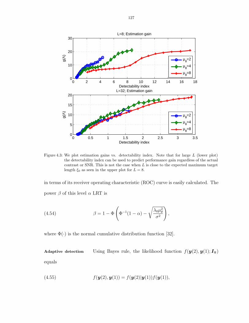
127

0 2 4 6 8 10 12 14 16 180

10

20

30L=8; Estimation gain

Detectability index

g(Λ

)

0 0.5 1 1.5 2 2.5 3 3.50

5

10

15

20L=32; Estimation gain

Detectability index

g(Λ

)

µθ=2

µθ=4

µθ=8

µθ=2

µθ=4

µθ=8

Figure 4.3: We plot estimation gains vs. detectability index. Note that for large L (lower plot)the detectability index can be used to predict performance gain regardless of the actualcontrast or SNR. This is not the case when L is close to the expected maximum targetlength ξ0 as seen in the upper plot for L = 8.

in terms of its receiver operating characteristic (ROC) curve is easily calculated. The

power β of this level α LRT is

(4.54) β = 1− Φ

(Φ−1(1− α)−

√λ0µ2

θ

σ2

),

where Φ(·) is the normal cumulative distribution function [32].

Adaptive detection Using Bayes rule, the likelihood function f(y(2),y(1); IΨ)

equals

(4.55) f(y(2),y(1)) = f(y(2)|y(1))f(y(1)),

128

but, given y(1), the measurements at the second step are independent for different

cells and thus

(4.56) f(y(2),y(1)) =

Q∏i=1

f(yi(2)|y(1))f(yi(1)).

Therefore, the LRT statistic, Tl, is

Tl =

∏Qi=1 f(yi(2)|y(1), Il = 1)f(yi(1)|Il = 1)∏Qi=1 f(yi(2)|y(1), Il = 0)f(yi(1)|Il = 0)

=

(4.57)f(yl(2)|y(1), Il = 1)f(yl(1)|Il = 1)

f(yl(2)|y(1), Il = 0)f(yl(1)|Il = 0).

Let l ∈ Xj and yl(1) is given in (4.45). Note that given Il = 1, yl(1) ∼ N (µ1, σ21)

and yl(2) ∼ N (µ2, σ22) are defined in (4.46) and (4.47), respectively. Under the null

hypothesis, Il = 0, we have yl(2) ∼ N (0, σ2) for the second measurement. However,

for the first measurement we have to account for two scenarios: (a) Xj does not

contain any targets. (b) Xj contains at most min(L − 1, ξ0) targets. Note that the

probability of (a) is

Pr

∏

i∈Xj

(1− Ii) = 1

= q0

∼= (1− p)L,

while the probability of (b) is (1 − q0). Since we are mainly interested in sparse

scenarios where p ¿ 1 we have q0 close to one and therefore approximate the pdf of

yl(1)|(Il = 0) as a Gaussian mixture with

(4.58) yl(1)|(Il = 0) ∼ q0N (0, σ2) + (1− q0)N (µb, σ2b ),

129

where (µb, σ2b ) represent case (b) and are evaluated using (4.10) and (4.11), respec-

tively, replacing ξ0 with min(L − 1, ξ0). Furthermore, we approximate the r.h.s. of

(4.58) as N (µ0, σ20), where

µ0 = (1− q0)µb,

σ20 = qσ2 + (1− q)σ2

b + q(1− q)µ2b .

Collecting all the previous results we obtain:

(4.59)

H0 :

yl(1) ∼ N (µ0, σ20)

yl(2)|y(1) ∼ N (0, σ2)

H1 :

yl(1) ∼ N (µ1, σ21)

yl(2)|y(1) ∼ N (µ2, σ22)

.

Substituting these distributions into (4.57) provides the following LRT

Tl =σσ0

σ1σ2

exp− (yl(2)−µ2)2

2σ22

− (yl(1)−µ1)2

2σ21

exp−yl(2)2

2σ2 − (yl(1)−µ0)2

2σ20

≷ γ,

which can also be expressed as

(4.60) Tl =y2

l (2)

2

(1

σ2− 1

σ22

)+ yl(2)

µ2

σ22

+y2

l (1)

2

(1

σ20

− 1

σ21

)+ yl(1)

(µ1

σ21

− µ0

σ20

)+

µ20

2σ20

− µ21

2σ21

− µ22

2σ22

+ logσσ0

σ1σ2

≷ γ′,

where γ′ = log γ. Note that λM(l, 2) = 0 yields µ2 = 0 and σ22 = σ2, hence, for

all cells in Ψc the test (4.60) is a function of yl(1) alone. Next, we compare the

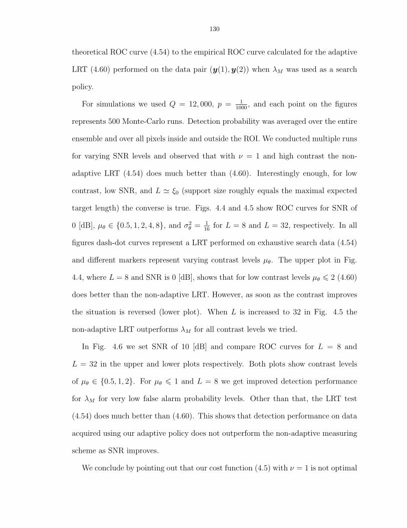
130

theoretical ROC curve (4.54) to the empirical ROC curve calculated for the adaptive

LRT (4.60) performed on the data pair (y(1),y(2)) when λM was used as a search

policy.

For simulations we used Q = 12, 000, p = 11000

, and each point on the figures

represents 500 Monte-Carlo runs. Detection probability was averaged over the entire

ensemble and over all pixels inside and outside the ROI. We conducted multiple runs

for varying SNR levels and observed that with ν = 1 and high contrast the non-

adaptive LRT (4.54) does much better than (4.60). Interestingly enough, for low

contrast, low SNR, and L ' ξ0 (support size roughly equals the maximal expected

target length) the converse is true. Figs. 4.4 and 4.5 show ROC curves for SNR of

0 [dB], µθ ∈ 0.5, 1, 2, 4, 8, and σ2θ = 1

16for L = 8 and L = 32, respectively. In all

figures dash-dot curves represent a LRT performed on exhaustive search data (4.54)

and different markers represent varying contrast levels µθ. The upper plot in Fig.

4.4, where L = 8 and SNR is 0 [dB], shows that for low contrast levels µθ 6 2 (4.60)

does better than the non-adaptive LRT. However, as soon as the contrast improves

the situation is reversed (lower plot). When L is increased to 32 in Fig. 4.5 the

non-adaptive LRT outperforms λM for all contrast levels we tried.

In Fig. 4.6 we set SNR of 10 [dB] and compare ROC curves for L = 8 and

L = 32 in the upper and lower plots respectively. Both plots show contrast levels

of µθ ∈ 0.5, 1, 2. For µθ 6 1 and L = 8 we get improved detection performance

for λM for very low false alarm probability levels. Other than that, the LRT test

(4.54) does much better than (4.60). This shows that detection performance on data

acquired using our adaptive policy does not outperform the non-adaptive measuring

scheme as SNR improves.

We conclude by pointing out that our cost function (4.5) with ν = 1 is not optimal

131

0 0.2 0.4 0.6 0.8 10

0.2

0.4

0.6

0.8

1ROC curve; SNR=0, L=8

Pd

Uniformµθ=.5

Uniformµθ=1

Uniformµθ=2

0 0.2 0.4 0.6 0.8 10.9

0.92

0.94

0.96

0.98

1

Pfa

Pd Uniform

µθ=4

Uniformµθ=8

Figure 4.4: Receiver operating characteristic (ROC) curves for SNR of 0 [dB] and L = 8 of dataacquired using M-ARAP vs. a non-adaptive exhaustive data acquisition. The upperplot shows low contrast levels of µθ 6 2, while the lower plot focuses on high contrastlevels. Dash-dot curves represent the ROC of the non-adaptive LRT and differentmarkers represent contrast. In the upper plot we see improved detection performanceof M-ARAP compared to the non-adaptive scheme. However, this is reversed for thelower plot.

for detection as was pointed out in Chapter III. It is possible to get improved

detection performances when optimizing over ν. However, we leave this experiment

to be done for a specific application.

4.4.3 Statistical models approximation

Most of the results in Section 4.3 rely on a Gaussian mixture (GM) statistical

model and a Gaussian approximation for the GM given in (4.10) and (4.11) and de-

veloped in Appendix 4-A. In the following section we provide a feel for the statistical

nature of the data and discuss the validity of the single Gaussian approximation of

the GM. As seen in Fig. 4.3 this approximation, which supported the detectability

132

0 0.2 0.4 0.6 0.8 10

0.2

0.4

0.6

0.8

1ROC curve; SNR=0, L=32

Pd

Uniformµθ=.5

Uniformµθ=1

Uniformµθ=2

10−4

10−3

10−2

10−1

100

0.6

0.7

0.8

0.9

1

Pfa

Pd Uniform

µθ=4

Uniformµθ=8

Figure 4.5: Receiver operating characteristic (ROC) curves for SNR of 0 [dB] and L = 32 of dataacquired using M-ARAP vs. a non-adaptive exhaustive data acquisition. The upperplot shows low contrast levels of µθ 6 2, while the lower plot focuses on high contrastlevels. Dash-dot curves represent the ROC of the non-adaptive LRT and differentmarkers represent contrast. The ROC curves due to the non-adaptive LRT dominatethe ROC curves resulting from M-ARAP.

index analysis, is only accurate for low values of d or low SNR, small ξ0L

, and low

contrast µθ. We examine the pdf of y(1)|H1 under different settings to better un-

derstand this phenomenon. To generate enough data under H1, we used simulations

with Q = 16, 384, p = 1100

and 500 Monte-Carlo runs.

We start by showing a scenario where the single Gaussian approximation is a

reasonable approximation to the Gaussian mixture. With either (L = 8, µθ = 2) or

(L = 32, µθ = 8) and SNR of 10 [dB] the detectability index (4.19) is roughly one.

Figs. 4.7 and 4.8 show the probability distribution functions (pdf) and cumulative

distribution functions (cdf) of y(1)|H1 for these scenarios, respectively. The upper

plot corresponds to (L = 8, µθ = 2) while the lower plot corresponds to (L = 32, µθ =

133

0 0.2 0.4 0.6 0.8 10.6

0.7

0.8

0.9

1ROC curve; SNR=10, L=8

Pd

Uniformµθ=.5

Uniformµθ=1

Uniformµθ=2

0 0.2 0.4 0.6 0.8 1

0.4

0.6

0.8

1ROC curve; SNR=10, L=32

Uniformµθ=.5

Uniformµθ=1

Uniformµθ=2

Figure 4.6: ROC curves for the two tests at SNR of 10 [dB] and low contrast levels of µθ 6 2. Inthe upper plot we set L = 8, while L = 32 was chosen for the lower plot. Note thatincreasing SNR improves test performance of the non-adaptive scheme far better thanfor M-ARAP. This is mainly attributed to the fact that with ν = 1, M-ARAP does notspend enough energy characterizing the alternative and focuses the sampling energyonto the ROI.

8) on both figures. While we are not interested in goodness-of-fit type results, it is

clearly seen that the single Gaussian approximation is not far from the actual GM

distribution.

On the other hand, Fig. 4.9 represents a case where the single Gaussian approx-

imation begins to breakdown. In both plots SNR is 20 [dB] and the contrast level

µθ = 4, while L = 8 and L = 32 for the upper and lower plots respectively. Both

plots shows distinctive modes for the true GM and it is clear that a single Gaussian

is no longer a reasonable representation of the true pdf. Nevertheless, this does not

suggest that the posterior probabilities pIi|y(1) will no longer converge to either one

or zero under the corresponding hypothesis Hr. As mentioned in Section 4.3.2 and

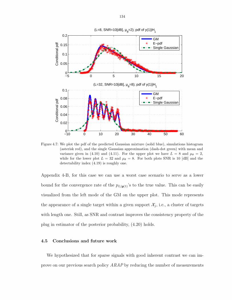
134

−10 0 10 20 30 40 50 600

0.02

0.04

0.06

0.08

0.1

(L=32, SNR=10[dB], µθ=8); pdf of y(1)|H1

Con

ditio

nal p

df

−5 0 5 10 15 200

0.05

0.1

0.15

0.2

Con

ditio

nal p

df

(L=8, SNR=10[dB], µθ=2); pdf of y(1)|H1

GME−pdfSingle Gaussian

GME−pdfSingle Gaussian

Figure 4.7: We plot the pdf of the predicted Gaussian mixture (solid blue), simulations histogram(asterisk red), and the single Gaussian approximation (dash-dot green) with mean andvariance given in (4.10) and (4.11). For the upper plot we have L = 8 and µθ = 2,while for the lower plot L = 32 and µθ = 8. For both plots SNR is 10 [dB] and thedetectability index (4.19) is roughly one.

Appendix 4-B, for this case we can use a worst case scenario to serve as a lower

bound for the convergence rate of the pIi|y(1)’s to the true value. This can be easily

visualized from the left mode of the GM on the upper plot. This mode represents

the appearance of a single target within a given support Xj, i.e., a cluster of targets

with length one. Still, as SNR and contrast improves the consistency property of the

plug in estimator of the posterior probability, (4.20) holds.

4.5 Conclusions and future work

We hypothesized that for sparse signals with good inherent contrast we can im-

prove on our previous search policy ARAP by reducing the number of measurements

135

−5 0 5 10 15 200

0.2

0.4

0.6

0.8

1

Con

ditio

nal c

df

(L=8, SNR=10[dB], µθ=2); cdf of y(1)|H1

−10 0 10 20 30 400

0.5

1

Con

ditio

nal c

df

(L=32, SNR=10[dB], µθ=8); pdf of y(1)|H1

GME−pdfSingle Gaussian

GME−pdfSingle Gaussian

Figure 4.8: We plot the cdf of the predicted Gaussian mixture (solid blue), simulations histogram(asterisk red), and the single Gaussian approximation (dash-dot green) with mean andvariance given in (4.10) and (4.11). For the upper plot we have L = 8 and µθ = 2,while for the lower plot L = 32 and µθ = 8. For both plots SNR is 10 [dB] and thedetectability index (4.19) is roughly one. As one can see, the Gaussian approximationis not far from the true GM distribution.

yet preserving estimation gains. M-ARAP was derived using the same cost func-

tion introduced in Chapter III under additional total number of measurements or

time constraints. We used multi-scaling where collections of cells were measured in

the first step to save measurements and decide where we need to focus the mea-

surement scheme and produce fine resolution at the second stage. We showed that

significant saving in measurements can be achieved while maintaining high estima-

tion gains. Specific examples showed 10-17 [dB] gain in estimation performance, for

different contrast levels, using less than 20% of the samples needed to perform an

exhaustive search, at SNR of 15 [dB]. Other methods capable of such saving in the

sampling process are active sampling (AS) and compressive sensing (CS). However,

136

0 10 20 30 40 50 60 700

0.05

0.1

(L=8, SNR=20[dB], µθ=4); pdf of y(1)|H1

0 10 20 30 40 50 60 700

0.05

0.1

(L=32, SNR=20[dB], µθ=4); pdf of y(1)|H1

GME−pdfSingle Gaussian

GME−pdfSingle Gaussian

Figure 4.9: We plot the pdf of the predicted Gaussian mixture (solid blue), simulations histogram(asterisk red), and the single Gaussian approximation (dash-dot green) with mean andvariance given in (4.10) and (4.11). For both plots SNR is 20 [dB] and µθ = 4, whileL = 8 in the upper plot and L = 32 for the lower plot. Note that while the singleGaussian approximation in the lower plot is still a somewhat reasonable approximationof the GM this is not the case for the upper plot. This explains the different behaviorexhibited by the curves in Fig. 4.3.

both methods lack the additional degree of freedom of ‘resource allocation’ that was

suggested here. Since AS and CS consider the problem of “where to sample” without

the “how to sample” part, there is limited, if any, estimation gain associated with

either method. Moreover, both AS and CS where suggested for sampling spatially

homogeneous signals. We do not impose such a constraint here and only require

reasonable contrast between the ROI and the signal background. Previous work

on blood pooling [16, 45, 53] considered detecting defective blood samples in a large

population. The main concern is to shorten the search time and there is an inherent

assumption of an infinite contrast [16]. In addition, as opposed to the clustering

137

scenario discussed here, blood pooling assumes that it is most likely that each pool

contains a single target [53]. By deciding “how to sample” and considering clusters

we improve estimation gains to all cells within the ROI.

Our methods displayed here have not been optimized for detection. Since we

allow many degrees of freedom, we leave this optimization for future work. This

optimization part may also be application dependent. We have yet to find a good

application for our methods and this is another part of our intended future work.

For some potential applications, like airport security screening or early detection of

breast cancer tumors, tools that can use a multi-scale measurement scheme have to

be developed. For other applications, like radar imaging or CT, sensor sensitivity or

resolution may still need to be improved to achieve the potential benefits our method

suggests.

4-A Appendix: Mean and variance of Yj(1) given H1

We derive the mean and variance of our measurement model (4.9) under the

assumption that Xj contains a cluster of targets of length ξj. We further assume

that ξj 6 ξ0 6 |Xj| = L and that Pr(ξj = k) = 1ξ0

for k = 1, 2, . . . , ξ0. In this case,

yj(1) is a Gaussian mixture with ξ0 components, each have a mean mi = µθ

√λ1

Li and

variance s2i = σ2 + i λ1

L2 σ2θ . To evaluate the conditional mean of Yj(1) we enumerate

all possible intersection of a targets with length ξ and supports of length L. Then,

using the total probability theorem we obtain

(4-A.1) Eyj(1)|H1 =

√λ1

LE

E

jL∑

i=(j−1)L+1

θiIi

∣∣∣∣∣∣ξj

138

(4-A.2) = µθ1

ξ0

√λ1

L

ξ0∑

ξ=1

1

L + ξ − 1

(4

ξ−1∑i=1

i + (L− ξ + 1)ξ

)

(4-A.3) =µθ

ξ0

√λ1

L

ξ0∑

ξ=1

ξξ + L− 1

L + 3ξ − 3= µyj(1)|H1

4= µ1.

Note that the probability of each Gaussian qi equals

(4-A.4) qi =L + 4ξ0 + 1− 5i32ξ20 + (L− 3

2)ξ0

.

Therefore, the conditional pdf is

(4-A.5) fY (1)|H1(y) =

ξ0∑i=1

qiN (mi, s2i ),

where N (mi, s2i ) is the i’th Gaussian pdf with mean mi and variance s2

i . The condi-

tional variance of yj(1) is given by

(4-A.6) varyj(1)|H1 =

ξ0∑i=1

qi

∫(y − µ1)

2 1√2πs2

i

exp

− 1

2s2i

(y −mi)2

dy

(4-A.7) =

ξ0∑i=1

qi

(Ey2

i − 2miµ1 + µ21

),

where Ey2i = s2

i + m2i .

4-B Appendix: Showing pIi|yi(1) → r under Hr

We show pIi|yi(1)|H1 → 1 and the complementary claim can be proved in a sym-

metric manner. Recall the definition of pIi|y(1)

(4-B.1) pIi|y =pif1(y)

pif1(y) + (1− pi)f0(y)=

1

1 + 1−pi

pi

f0(y)f1(y)

,

139

where for brevity the time dependency ‘(1)’ was omitted. From (4.9) we note that

the posterior probability depends on the specific yj for all i ∈ Xj yielding

(4-B.2) pIi|y =1

1 + 1−pi

pi

f0(yj)

f1(yj)

4= pIi|yj

.

Using the Gaussian approximation (4.22) we show that for an arbitrary small δ > 0

and ε′ > 0 there exists µ1 and σ12 such that for (µ1, σ

21) ∈ R

(4-B.3) Pr(pIi|yj> 1− ε′) > 1− δ,

where R = (x1, x2) ∈ R2 : x1 > µ1, x2 6 σ12. To prove (4-B.3) we note that

pIi|yj> 1− ε′ if and only if

(4-B.4)1− pi

pi

f0(yj)

f1(yj)< ε′′ =

1

1− ε′− 1.

Following (4.22) and (4.23) let

z = σ1eµ21

2σ21 exp

−y2

j (1)

2

σ21 − σ2

σ21σ

2− yj(1)

µ1

σ21

,

then it suffices to show that

(4-B.5) Pr(z < ε) > 1− δ,

and ε = σε′′ pi

1−pi. Using total probability we obtain

(4-B.6)

Pr(z < ε) = Pr(z < ε

∣∣∣yj >µ1

2

)Pr

(yj >

µ1

2

)+Pr

(z < ε

∣∣∣yj 6 µ1

2

)Pr

(yj 6 µ1

2

),

and claim that under H1 there exists µ1(ε) and σ21(ε) for which Pr(yj 6 µ1

2) < δ for

all µ1 > µ1(ε) and σ21 6 σ2

1(ε). Therefore, it is sufficient to assume yj > µ1

2and show

140

that ∃R 6= ∅ for which

(4-B.7) σ1eµ21

2σ21 exp

−y2

j

2

σ21 − σ2

σ21σ

2− yj

µ1

σ21

< ε, ∀(µ1, σ

21) ∈ R.

Note that (4-B.7) holds if and only if

(4-B.8) φ(yj) =σ2

1 − σ2

2σ21σ

2y2

j +µ1

σ21

yj + log ε− log σ1 − µ21

2σ21

> 0.

Since σ1 > σ, φ(yj) is a convex function, which is greater than zero for all yj >

max(roots[φ(yj)]) and roots[φ(·)] are the two solutions of φ(·) = 0. Note that for

yj = 0 it is easy to find an ε for which φ(0) < 0, hence the equation φ(yj) = 0 has

two solutions. The set R is defined by all pairs (µ1, σ21) satisfying

(4-B.9) φ(µ1

2

)=

σ21 − σ2

2σ21σ

2

µ21

4+ log ε− log σ1 > 0,

or, equivalently

(4-B.10) σ1 exp

−µ2

1

8

σ21 − σ2

σ21σ

2

6 ε.

Therefore, for (µ1, σ21) ∈ R we have

(4-B.11) Pr(z < ε) > 1− δ.

Substituting (4.11) and (4.10) for σ1 and µ1 in (4-B.10) respectively, we note that

the support R is a function of the inherent contrast µθ, the window length L, the

effort allocation at the first stage λ1, and the cluster statistics p(Ξ).

CHAPTER V

Conclusions and Future Work

5.1 Conclusions

We had started this journey believing that for sparse scenarios there has to be

a more efficient way to allocate resource compared to an exhaustive scheme. In

Chapter II we investigated design of nuclear imaging scanners. We established that

considerable gains in image reconstruction variance are possible using a non-uniform

system design. While this measure of performance may not be the best for evalua-

tion of system performance it indicates that further investigation is warranted. Our

later work on dynamic resource allocation schemes in Chapters III and IV shows

great promise. The main contribution of this dissertation is in forming a novel way

to think about dynamic resource allocation problems. We introduced a new cost

function capturing the tradeoffs between allocating efforts inside and outside the

region of interest. Then, we showed that minimizing this cost is equivalent to re-

ducing both error probability for detecting the ROI correctly and estimation MSE

in characterizing the ROI content.

We derived adaptive resource allocation policy, namely ARAP, and showed that it

is capable of concentrating resource onto the true unknown ROI. ARAP was shown

to converge to the oracle allocation policy that knows the location of the ROI in

141

142

advance and allocates resources only where it matters. We showed that using ARAP

as a pre-processing step, i.e., generating measurements, yields data of a better quality

compared to an exhaustive allocation policy. The data quality translates to improved

detection and estimation performance. Estimation gains converges to the optimal

gains achieved by the omniscient or oracle policy. For detection it is necessary

to allocate some efforts to characterize the ’alternative’ or the ROI complement.

Therefore, the tradeoff parameter ν has to be optimize to provide best combined

(detection and estimation) performance. This can be done generically, as seen in

Chapter III, but yield better results if done in an application specific context. The

price we pay for the significantly improved data yielded by ARAP is an increase in

the total number of measurements. We have devised M-ARAP specifically to address

this aspect.

Since in many of the application we had considered targets tend to cluster it seems

natural that we should try and take advantage of that knowledge. By clustering we

do not mean that independent targets appear in groups. In our understanding, a

cluster is a result of search steps smaller than targets size. Therefore, a single target

is highly likely to occupy several consecutive ‘pixels’ in the measurements grid. For

example, air traffic control (ATC) radar is designed to detect targets of minimal size

at a certain range. However, targets that are close by appear much larger than a

resolution cell on the radar screen. With that in mind, in Chapter IV we designed

M-ARAP to follow the principle of ARAP but use a multi-scale framework. In

essence, we believe that targets location can be resolved from a coarse ‘image’ where

spatial resolution is ’sacrificed’ to save measurements. The coarse image is then used

to decide which parts of the scanned domain should be re-scanned on a fine grid

and how much resource should we allocate to each point. For sparse scenarios with

143

sufficient ROI to background contrast, M-ARAP is capable of producing significant

gains while using less than 20% of the measurements required by an exhaustive

search. M-ARAP maintained most of the properties of ARAP such as convergence to

the true ROI yet with much fewer measurements. We explored the tradeoff between

estimation gains and measurement saving and conclude that it is best to keep the

coarse grid resolution at about 2-3 times of the expected cluster size.

5.2 Future work

For future work, we suggest to connect our work to work done in compressive

sampling (CS). For sparse scenarios one can use CS as a replacement for the coarse

grid used by M-ARAP. By reducing the number of measurement additional effort

can be allocated to each random projection collected by CS measuring operator.

This data can be processed to yield posterior probabilities which are then used to

define the second allocation step. Moreover, we deal with scenario that are not

necessarily sparse in the strict sense, i.e., the complement of the ROI is not limited

to be zero. However, we believe that there exist a transformation from the signal

space to another space where the signals we are looking at are truly sparse, i.e.,

the transformed signal values outside the ROI are almost or exactly zero. If such a

transformation exist, then compressive sampling methods can be directly applied to

the scenarios we consider. Furthermore, a most recent paper by Ji et al. introduces

Bayesian CS [28]. Among other things they suggest to adaptively optimize the CS

measurement operator in a non random manner using relevance vector machine. This

points out to another possible connection between ARAP and CS that needs to be

explored. A practical issue to address is how to realize CS measurement operator for

some of the applications mentioned here. It seems that applications such as radar,

144

CT, or screening are defined on some discrete grid and it is hard to visualize a radar

taking measurements as a random affine transformation of its entire search domain.

Nevertheless, the common assumption of sparseness make it worthwhile to further

explore such connections.

Another direction worth exploring is the connection to adaptive sampling (AS)

such as the work described in [12, 13, 58] and others. The literature on AS address

the question of where to sample next or how to focus the sampling process, which

was also addressed in this work. Using coarse to fine grid measurement scheme,

AS sequentially refines the sampling pattern around suspected edges in an acquired

image. The motivation to do so is justified by the assumption that the measured

signal has some continuity in a lower dimensional space. Also, since AS does not

consider the resource allocation part of the problem it is possible to extend the

number of measurement stages beyond two. We believe that techniques used in AS

can be combined with policy like M-ARAP to improve performance, but it is yet to

be determined how exactly the two should be connected.

Another interesting extension of our work is to extend the horizon beyond a

two-stage allocation policy. A straight forward extension suffers from the curse of

dimensionality since the optimization problem becomes combinatorically complex.

A possible solution is to use a rolling horizon approach. Using a rolling horizon one

may estimate potential advantages by going to T = 3, 4, . . .. However, at the end

of the first stage the posterior distribution (or prior distribution for the following

stages) on the location of targets is no longer uniform. While in [5] we introduce

a general version of ARAP that account for a non-uniform prior, the optimization

becomes dependent on the specific prior. More specifically, the optimal allocation

145

lies in a Q + 1 dimensional space1. Therefore, due to the fact that the cardinality of

the set of all possible priors is uncountably infinite, the optimization cannot be done

offline. Moreover, resource allocated to refine/improve the posterior distribution will

no longer be available to be distributed over the estimated ROI.

Finally, it would be interesting to do a sensitivity analysis for the performance

of the allocation policies suggested here. Checking how sensitive ARAP is for un-

certainties in the sparsity parameter p may yield new insights. In addition, it is

worthwhile to analyze what do one lose by assuming a uniform prior as oppose to

incorporating prior knowledge. While the general version of ARAP accounts for a

non-uniform prior, a uniform prior leads to a robust system design. If ARAP is not

very sensitive to such model mismatches it increases the motivation to use it in real

life applications.

1accounting for an optimal waveform in RQ plus its overall energy.

BIBLIOGRAPHY

146

147

BIBLIOGRAPHY

[1] A. A. Abdel-Samad and A. H. Tewfik. Search strategies for radar target localization. In Pro-ceeding 1999 International Conference on Image Processing, volume 3, pages 862–866, October1999.

[2] A. A. Abdel-Samad and A. H. Tewfik. Hierarchical radar target localization. In Proceeding2000 International Conference on Acoustics, Speech, and Signal Processing, volume 5, pages3033–3036, June 2000.

[3] A. A. Abdel-Samad and A. H. Tewfik. Sequential techniques in hierarchical radar targetlocalization. In Proceeding 2000 International Conference on Image Processing, volume 1,pages 697–700, September 2000.

[4] M. Aharon, M. Elad, and A. Bruckstein. k-svd: An algorithm for designing overcompletedictionaries for sparse representation. IEEE Transaction Signal Processing, 54(11):4311–4322,November 2006.

[5] E. Bashan, R. Raich, and A. O. Hero III. Adaptive sampling: Efficient search schemes underresource constraints. Technical Report 385, University of Michigan, Communications andSignal Processing Lab., October 2007.

[6] S. J. Benkoski, M. G. Monticino, and J. R. Weisinger. A survey of the search theory literature.Naval Research Logistics, 38(4):469–494, 1991.

[7] E. J. Bond, L. Xu, S. C. Hagness, and B. D. van Veen. Microwave imaging via space-timebeamforming for early detection of breast cancer. IEEE Transactions on Antennas and Prop-agation, 51(8):1690–1705, August 2003.

[8] S. Boyd and L. Vandenberghe. Convex Optimization. Cambridge University Press, March2004.

[9] E. Candes and T. Tao. The dantzig selector: statistical estimation when p is much larger thann. The Annals of Statistics, 35(6):2313–2351, 2007.

[10] D. A. Castanon. Optimal search strategies in dynamic hypothesis testing. IEEE Transactionon Systems, Man and Cybernetics, 25(7):1130–1138, July 1995.

[11] R. Castro, J. Haupt, and R. Nowak. Compressed sensing vs. active learning. In Proceedings2006 International Conference on Acoustics, Speech and Signal Processing, volume 3, pagesIII–III, May 2006.

[12] R. Castro, R. Willet, and R. Nowak. Coarse-to-fine manifold learning. In Proceedings 2004International Conference on Acoustics, Speech and Signal Processing, volume 3, pages iii–992–5, May 2004.

[13] R. Castro, R. Willett, and R. Nowak. Faster rates in regression via active learning. In Pro-ceedings of the Neural Information Processing Systems Conference (NIPS) 2005, Vancouver,Canada, December 2005.

148

[14] S. K. Davis, H. Tandradinata, S. C. Hagness, and B. D. van Veen. Ultrawideband microwavebreast cancer detection: a detection-theoretic approach using the generalized likelihood ratiotest. IEEE Transaction on Biomedical Engineering, 52(7):1237–1250, July 2005.

[15] A. den Dekker and A. van den Bos. Resolution: a survey. Journal Optical Society of America,14(3):547–557, March 1997.

[16] R. Dorfman. The detection of defective members of large populations. The Annals of Mathe-matical Statistics, 14(4):436–440, December 1943.

[17] Y. C. Eldar. Minimum variance in biased estimation: Bounds and asymptotically optimalestimators. IEEE Transactions on Signal Processing, 52(7):1915–1930, July 2004.

[18] O. D. Escoda, L. Granai, and P. Vandergheynst. On the use of a priori information for sparsesignal approximations. IEEE Transactions on Signal Processing, 54(9):3468–3482, September2006.

[19] E. C. Fear, P. M. Meaney, and M. A. Stuchly. Microwaves for breast cancer detection? IEEEPotentials, 22(1):12–18, Febuary-March 2003.

[20] J. A. Fessler. Spatial resolution and noise tradeoffs in pinhole imaging system design: a densityestimation approach. OPTICS EXPRESS, 2(6):237–253, March 1998.

[21] A. B. Frakt, W. C. Karl, and A. S. Willsky. A multiscale hypothesis testing approach toanomaly detection and localization from noisy tomographic data. IEEE Transactions on ImageProcessing, 7(6):825–837, June 1998.

[22] J. C. Gittins. Multi-Armed Bandit Allocation Indices. John Wiley and Sons, 1989.

[23] I.F. Gorodnitsky and B.D. Rao. Sparse signal reconstruction from limited data using focuss:a re-weighted minimum norm algorithm. IEEE Transactions on Signal Processing, 45(3):600–616, March 1997.

[24] J. Haupt and R. Nowak. Signal reconstruction from noisy random projections. InformationTheory, IEEE Transactions on, 52(9):4036–4048, September 2006.

[25] A. O. Hero III, D. A. Castanon, D. Cochran, and K. Kastella, editors. Foundations andApplications of Sensor Management. Springer, Boston, MA, 2007.

[26] A. O. Hero III, J. A. Fessler, and M. Usman. Exploring estimator bias-variance tradeoffs usingthe uniform cr bound. IEEE Transactions on Signal Processing, 44(8):2026–2041, August 1996.

[27] M. Ivanovic, D. A. Webber, and S. Loncaric. Multi-pinhole collimator optimization for highresolution spect imaging. In IEEE Nuclear Science Symposium, volume 2, pages 1097–1101,November 1997.

[28] S. Ji, Y. Xue, and L. Carin. Bayesian compressive sensing. Signal Processing, IEEE Transac-tions on, 56(6):2346–2356, June 2008.

[29] I. M. Johnstone and B. W. Silverman. Needles and straw in haystacks: Empirical Bayesestimates of possibly sparse sequences. Annals of Statistics, 32:1594–1649, 2004.

[30] J. B. Kadane. Optimal whereabouts search. Operations Research, 19:894–904, July-August1971.

[31] K. Kastella. Discrimination gain to optimize detection and classification. IEEE Transactionson Systems, Man and Cybernetics, Part A, 27(1):112–116, January 1997.

[32] S. M. Kay. Fundamentals of Statistical Signal Processing, Volume 2: Detection Theory.Prentice-Hall PTR, January 1998.

149

[33] C. Kreucher, K. Kastella, and A. O. Hero III. Multitarget tracking using the joint multitargetprobability density. IEEE Transactions on Aerospace and Electronic Systems, 41(4):1396–1414,October 2005.

[34] C. Kreucher, K. Kastella, and A. O. Hero III. Sensor management using an active sensingapproach. Signal Processing, 85(3):607–624, March 2005.

[35] V. Krishnamurthy. Algorithms for optimal scheduling and management of hidden markovmodel sensors. IEEE Transactions on Signal Processing, 50(6):1382–1397, June 2002.

[36] V. Krishnamurthy and R. J. Evans. Hidden markov model multiarm bandits: a methodol-ogy for beam scheduling in multitarget tracking. IEEE Transactions on Signal Processing,49(12):2893–2908, December 2001.

[37] D. Malioutov, M. Cetin, and A. S. Willsky. A sparse signal reconstruction perspective forsource localization with sensor arrays. IEEE Transactions on Signal Processing, 53(8):3010–3022, August 2005.

[38] S. G. Mallat and Z. Zhang. Matching pursuits with time-frequency dictionaries. IEEE Trans-actions on Signal Processing, 41(12):3397–3415, December 1995.

[39] L. J. Meng and N. H. Clinthorne. A modified uniform cramer-rao bound for multiple pinholeaperture design. IEEE Transactions on Medical Imaging, 23(7):896–902, July 2004.

[40] L. J. Meng, W. L. Rogers, N. H. Clinthorne, and J. A. Fessler. Feasibility study of comptonscattering enchanced multiple pinhole imager for nuclear medicine. IEEE Transactions onNuclear Science, 50(5):1609–1671, October 2003.

[41] M. Nafie, A. H. Tewfik, and M. Ali. Deterministic and iterative solutions to subset selectionproblems. IEEE Transactions on Signal Processing, 50(7):1591–1601, July 2002.

[42] R. Nowak, U. Mitra, and R. Willett. Estimating inhomogeneous fields using wireless sensornetworks. IEEE Journal on Selected Areas in Communication, 22(6):999–1006, August 2004.

[43] T. E. Peterson, D. W. Wilson, and H. H. Barrett. A small-animal imaging system based onsilicon strip detectors. In Proceedings 2002, IEEE International Symposium on BiommedicalImaging, pages 533–536, July 2002.

[44] T. E. Peterson, D. W. Wilson, and H. H. Barrett. Ultrahigh-resolution small-animal imagingusing a silicon detector. In Nuclear Science Symposium Conference Record, volume 3, pages1984–1987, October 2003.

[45] C. G. Pfeifer and P. Enis. Dorfman-type group testing for a modified binomial model. Journalof the American Statistical Association, 73(363):588–592, September 1978.

[46] E. Posner. Optimal search procedures. IEEE Transactions on Information Theory, 9(3):157–160, July 1963.

[47] R. Rangarajan, R. Raich, and A. O. Hero III. Optimal experimental design for an inversescattering problem. In Proceedings. IEEE International Conference on Acoustics, Speech, andSignal Processing, volume 4, pages 1117–1120, March 2005.

[48] R. Rangarajan, R. Raich, and A. O. Hero III. Sequential design of experiments for a rayleighinverse scattering problem. In 2005 IEEE/SP 13th Workshop on Statistical Signal Processing,pages 625–630, July 2005.

[49] R. Rangarajan, R. Raich, and A. O. Hero III. Optimal sequential energy allocation for inverseproblems. IEEE Journal on Selected Topics in Signal Processing, 1(1):67–78, June 2007.

150

[50] M. M. Rogulski, H. B. Barber, H. H. Barrett, R. L. Shoemaker, and J. M. Woolfenden. Ultra-high-resolution brain spect imaging: simulation results. IEEE Transactions on Nuclear Sci-ence, 40(4):1123–1129, August 1993.

[51] N. U. Schramm, G. Ebel, U. Engeland, T. Schurrat, M. Behe, and T. M. Behr. High-resolutionspect using multipinhole collimation. IEEE Transactions on Nuclear Science, 50(3):315–320,June 2003.

[52] Nah-Oak Song and D. Teneketzis. Discrete search with multiple sensors. Mathematical Methodsof Operations Research, 60(1):1–13, September 2004.

[53] A. Sterrett. On the detection of defective members of large populations. The Annals ofMathematical Statistics, 28(4):1033–1036, December 1957.

[54] J. A. Tropp. Just relax: convex programming methods for identifying sparse signals in noise.IEEE Transactions on Information Theory, 52(3):1030–1051, March 2006.

[55] M. B. Wakin and R. G. Baraniuk. Random projections of signal manifolds. In ProceedingsIEEE Conference on Acoustics, Speech and Signal Processing, volume 5, pages V–V, May 2006.

[56] M. B. Wakin, J. N. Laska, M. F. Duarte, D. Baron, S. Sarvotham, D. Takhar, K. F. Kelly, andR. G. Baraniuk. An architecture for compressive imaging. In IEEE International Conferenceon Image Processing, pages 1273–1276, October 2006.

[57] G. Wang and Y. Li. Axiomatic approach for quantification of image resolution. IEEE SignalProcessing Letters, 6(10):257–258, October 1999.

[58] R. Willett, A. Martin, and R. Nowak. Backcasting: adaptive sampling for sensor networks. InThird International Symposium on Information Processing in Sensor Networks, pages 124–133,April 2004.

[59] D. W. Wilson, H. H. Barrett, and L. R. Furenlid. A new design for a spect small-animal imager.In Nuclear Science Symposium Conference Record, volume 3, pages 1826–1829, November 2001.

[60] D. P. Wipf and B. D. Rao. Sparse Bayesian learning for basis selection. IEEE Transactionson Signal Processing, 52(8):2153–2164, August 2004.

[61] B. Wohlberg. Noise sensitivity of sparse signal representations: reconstruction error bounds forthe inverse problem. IEEE Transactions on Signal Processing, 51(12):3053–3060, December2003.

[62] B. Wray. Learning classification rules using Bayes. In Proceedings of the sixth internationalworkshop on Machine learning, pages 94–98, San Francisco, CA, USA, 1989. Morgan KaufmannPublishers Inc.

[63] L. Xu, E. J. Bond, B. D. van Veen, and S. C. Hagness. An overview of ultra-widebandmicrowave imaging via space-time beamforming for early-stage breast-cancer detection. IEEEAntennas and Propagation Magazine, 47(1):19–34, Febuary 2005.

[64] L. Xu, S. K. Davis, S. C. Hagness, D. W. van der Weide, and B. D. van Veen. Microwave imag-ing via space-time beamforming: experimental investigation of tumor detection in multilayerbreast phantoms. IEEE Transactions on Microwave Theory and Techniques, 52(8):1856–1865,August 2004.