earnings and human capital: evidence for finland … · earnings and human capital: evidence for...
TRANSCRIPT

1
EARNINGS AND HUMAN CAPITAL:
EVIDENCE FOR FINLAND
by
Rita Asplund
The Research Institute of the Finnish Economy ETLA
e-mail: [email protected]
(July 1999)
Literature review prepared for PURE.
2
1 INTRODUCTION
This paper reviews existing empirical evidence on the rewarding of individual human
capital in general and formal education in particular in the Finnish labour market. As
will become evident, the literature of this research field is still rather sparse in
Finland. Most of the available evidence has, in effect, been produced during the past
decade. Apart from a fairly limited number of studies, any generalisations of results
will also suffer from the fact that the comparability of reported results is impaired by
the use of different data sets, differing definitions of variables as well as crucial
differences in the estimated model specifications. Differences in the employed
estimation techniques seem to play a much smaller role, mainly because of the minor
impact of sample selection bias on the estimated coefficients.
The overall impression mediated by the reviewed research is that the average return
to education has declined substantially during the past decades. The decline was
particularly strong in the 1970s, and continued at a slower pace up to the mid-80s.
The average return to education has remained roughly unchanged since the latter half
of the 80s with the general trend still pointing downward rather than upward.
Moreover, the rewarding of human capital accumulated in working life turns out to be
very modest in Finland. This holds for general work experience and, especially, for
tenure as measured by the length of the current employment relationship.
2 PURPOSE AND DATA SETS USED
The influence of individual differences in human capital endowments on earnings
determination in the Finnish labour market has been examined using mainly three
extensive individual-level databases: Population Census Data constructed by
Statistics Finland, Labour Force Surveys conducted by Statistics Finland and Wage
Data Files gathered by the Confederation of Finnish Industry and Employers (TT).
The coverage and richness of these databases differ considerably. Moreover, they
have been utilised to a highly varying extent depending on the primary purpose of the

3
study. This diversification weakens profoundly the possibilities to draw general
conclusions concerning magnitudes and trends of private returns to human capital in
the Finnish labour market.1
2.1 Population Census Data
The Population Censuses cover the whole population and are available for every fifth
year starting in 1970.2 The most recent census is for 1995. Based on these
quinquennial censuses Statistics Finland has compiled the Finnish Longitudinal
Census Data File, which contains all individuals (some 6 million people) who lived
in Finland during at least one of the census years. The censuses are constructed
mainly by merging administrative registers; survey data have been used only
occasionally for complementary reasons. The earnings data come from the records of
the tax authorities and refer to all taxable wage and salary incomes including most
types of compensation such as fringe benefits, overtime and vacation pay, etc. Some
crucial disadvantages of the database are also worth mentioning: information on
working hours is not available for any of the census years, and the number of months
worked is missing for 1970; the income data for the 1970 census is actually from
1971 while all the other information refers to 1970; part-timers cannot be
distinguished from full-timers for 1970, 1990 or 1995; high income earners (the top
percentile) have persistently been top-coded and instead of their actual income, these
individuals have been given the average earnings above the top-code cut-offs.
Brunila (1990) uses two representative cross-sections from the 1975 and 1985
Population Censuses to investigate earnings differentials across genders. The one per
cent sample drawn from the employed population in respective year is for data-
1 Lilja and Vartia (1980) and Nygård (1989) have used Household Survey data to estimate the impactof the education of the head of the household on observed differences in household incomes.2 Recently Statistics Finland has made available a restricted sample covering the year 1950 (seeStatistics Finland, 1998). So far no estimations of the return to human capital have been reported basedon that data set.

4
related reasons restricted to full-year, full-time employees, exclusive of those
engaged in agriculture, forestry and mining. When further excluding employees
classified into agricultural or entrepreneurial occupations as well as those with annual
earnings below FIM 25 000, Brunila arrives at an estimating sample including some
11,000 full-year full-timers for both years investigated. The wage concept used is
gross annual earnings.
Helo and Uusitalo (1995) address the question whether it is worthwhile for Finnish
youths to invest in a university education. Apart from estimating Mincer-type
earnings equations, they also calculate and compare internal rates of return for
university degrees taken within different educational fields. Their analyses depart
from a 10 per cent sample drawn from the Longitudinal Census Data File covering
the years 1975, 1980, 1985 and 1990. They further restrict the estimating data to
individuals aged 19−64 having either completed a university degree at the MA- or
post-graduate level or merely taken the matriculation examination (i.e. completed the
Gymnasium). This procedure results in four cross-sections containing between 8,700
(in 1975) and 23,200 (in 1990) individuals. The wage concept is annual taxable
income including wage and salary income as well as entrepreneurial and capital
income.
Eriksson (1994) and Eriksson and Jäntti (1996,1997) analyse the distribution and
determination of earnings using a random sample containing some 10 per cent of the
population included in the Longitudinal Census Data File covering the years 1970,
1975, 1980, 1985 and 1990. Eriksson (1994) restricts the estimating data to wage and
salary earners between 16 and 65 years of age, giving a sample size that grows from
about 111,000 individuals for 1970 to over 202,000 for 1990. In Eriksson and Jäntti
(1996,1997) the sample is further restricted to those over 25 year old earning more
than 100 FIM in 1990 prices, which reduces the sample size to some 71,000
individuals for 1970 and about 180,000 for 1990. Two different wage concepts are

5
used: before-tax monthly and annual earnings.3 The analysis is restricted to all
employees in Eriksson (1994) and Eriksson and Jäntti (1996) but is separated also by
gender in Eriksson and Jäntti (1997).
Uusitalo (1999) explores the influence of ability bias and schooling choice on
estimated returns to education using two random samples of young men who
performed their military service in, respectively, 1970 and 1982. The first sample
departs from 2,000 recruits having performed the Finnish Defence Forces Basic
Ability Test in 1970. The Longitudinal Census Data File for 1970−90 is used to add
information on the sample individuals as well as on their parents. Due to missing data
some 1,500 men were retained in the final sample. Further reductions in sample size
were caused by restrictions to full-time employees and missing information on family
background. The wage concept used is gross annual earnings.
The second sample used by Uusitalo (1999) covers 37,000 young men who
performed their military service in 1982. Again labour market information on the
sample men and their parents was obtained from the Longitudinal Census Data File
for 1970−90. In addition, administrative labour market records were used to add
information for 1994 on earnings and completed formal education. When further
restricting the sample to men in full-time employment earning FIM 2 000 or more per
month (in 1994) and with information on family background available, the effective
sample dropped to 22,572 male employees. The wage concept used is gross monthly
earnings calculated from annual taxable income and an estimated number of months
worked.
2.2 The Labour Force Survey
The Labour Force Survey (LFS) is a biannual survey conducted by Statistics Finland.
It covers a random sample of some 9,000 individuals, representing the entire
3 The reported results are affected only marginally when excluding those who are younger than 25 andwhen using annual instead of monthly earnings (Eriksson and Jäntti, 1996).

6
population aged 15−64 years as stratified according to sex, age and region. Apart
from these three characteristics, only a few additional variables, such as the acquired
formal schooling, are taken from registers; most of the information provided in the
LFS is self-reported. The LFS has been conducted for several years, but only a
limited number of the surveys have been supplemented with income data from the tax
registers. So far Statistics Finland has made income-extended surveys available for
1987, 1989, 1991 and 1993, and recently also for 1995. Compared to the Population
Census Data the LFS has the advantage of comprising a rich set of background
characteristics concerning the individual and his/her job. A less satisfactory feature of
the data is that it lacks the panel property, i.e. the survey sample varies from year to
year.
Ingberg (1987) was the first to report empirical evidence on the effects of schooling
and experience on earnings in Finland. He used an ad hoc data set created by
Statistics Finland through merging the 1980 Labour Force Survey and income and
labour force status variables from the registers of the 1980 Housing and Population
Census. The data comprise some 10,000 individuals of which close to 6,200 are
recorded to be labour force participants. The wage concept refers to annual taxable
earnings, comprising wages and salaries, income from farming, and entrepreneurial
income (with capital income, pensions and other unearned income excluded).
Asplund (1993a) utilises the 1987 Labour Force Survey, i.e. the first LFS that was
supplemented with income data from the tax records, to explore the relationship
between individual earnings and human capital in the Finnish labour market.4 When
the sample was restricted to employed wage and salary earners aged 16−64 and sorted
out with respect to missing or incomplete information on crucial variables, the actual
estimating sample dropped to close to 4,000 individuals. The wage concept used is
the average (before-tax) hourly wage calculated as annual taxable earnings divided by
annual working hours estimated from the self-reported number of months worked and
4 Apart from extensively specified wage equations estimated for all employees and separately bygender, Asplund (1993a) also analyses occupational choice and earnings, sectoral choice and earnings,and inter-industry wage differentials with the emphasis on the human capital aspect.

7
normal weekly working hours. The same data set is used in several comprehensive
comparisons of wages and human capital in the Nordic countries (Albaek et al.,
1996a; Asplund et al., 1996a,b).
Asplund (1998a) extends the analysis of gender-specific wage formation in the
private and public sectors to the years 1989, 1991 and 1993. All four survey years
were also utilised in a recent study exploring the potential impact of computer skills
on the average return to schooling (Asplund, 1998b). The estimating data comprise
more than 4,000 individuals in 1989 and 1991, but only some 2,500 employees for
1993, which reflects the dramatically worsened employment situation in Finland
since 1991.
2.3 The TT Wage Data
The Confederation of Finnish Industry and Employers (TT) collects detailed
individual-level information from member firms once a year for non-manual workers
and four times a year for manual workers. The wage as well as all other information
provided is taken directly from the employers’ registers and should, accordingly, be
highly reliable. The member firms cover approximately 75 per cent of Finnish
manufacturing but only a minor share of the services sectors.
Asplund (1996, 1998c) and Asplund and Vuori (1996) utilise a representative sample
of full-time non-manual workers drawn from this broad TT database in such a way
that the estimating data has both cross-section and panel properties. The sample
covers the years 1980 to 1994 and comprises some 135,000 individual time
observations. Of these, part concerns non-manual workers observed during just one
year, whereas the rest concerns non-manual workers observed during at least two
consecutive years and at most during all 15 years investigated. Asplund (1996)
analyses all non-manual workers and three non-manual subcategories, i.e. upper-
level, technical and clerical non-manual workers. Asplund (1998c) extends the
analysis to a comparison of male and female non-manual workers. Asplund and

8
Vuori (1996), finally, divide the non-manual workers into two groups − those
engaged in high-tech and other growth industries and those in slowly growing
industries − and compare the labour market and wage performance of the two groups,
with a further distinction made between different-sized establishments. The wage
concept used in all three studies is the average (before-tax) hourly wage calculated as
gross monthly earnings divided by monthly working hours estimated from normal
weekly working hours.
Similar analyses have not been undertaken for manual workers because the TT
database does not comprise information on the manual workers’ formal schooling nor
on their working experience. The only human capital-related information concerns
the manual worker’s qualification category5 and age.
3 ESTIMATION METHODS
Most cross-section studies of the effect of human capital on wage determination in
the Finnish labour market have used ordinary least squares (OLS) techniques.6 In
other words, individual wages have been regressed on a varying number of personal
and job-related characteristics that are assumed to contribute to explaining the
observed variation in wage outcomes. This method overlooks at least two main
issues: the potential presence of a non-negligible sample selection bias and the fact
that one or more of the explanatory variables might be endogenously determined.
A sample selectivity bias problem may arise if the sample individuals recorded as
being employed are not randomly selected from the entire population. Asplund
(1993a) and Asplund et al. (1996b) adjust for this by estimating the earnings equation
5 The qualification categories, which rank workers according to their skills and tenure, differ acrossindustry branches and are settled in branch-level wage negotiations.6 OLS techniques have been used by Ingberg (1987), Brunila (1990), Eriksson (1994), Eriksson andJäntti (1996,1997), Asplund (1996, 1998b, 1998c), Asplund and Vuori (1996) and Asplund et al.(1996a). Helo and Uusitalo (1995) use a Tobit procedure in order to account for that fact that theirincome variable is censored in both ends.

9
in combination with a selection function of the probit type explaining the probability
of the ith sample individual being employed. The two equations are estimated first
using an ordinary Heckman two-stage procedure and are then re-estimated jointly
using the full-information maximum likelihood estimator (FIML), whereby the final
values from the Heckman two-stage procedure are used as starting values. Neither for
men nor for women did the estimation results (for 1987) point to a significant sample
selection bias affecting the estimation results for Finland. This finding indicates that
estimation of the earnings equation using OLS techniques produces consistent
parameter estimates. The finding of no serious sample selection bias may, however,
also be due − at least in part − to the usually high correlation between the exogenous
variables in the selection equation and the earnings equation making even the FIML
estimator very unrobust (see e.g. Puhani, 1997; Asplund, 1998b).
Several of the individual background variables commonly included in earnings
equations can be expected to be the outcome of a selection process rather than a
random drawing. These variables include not least education, occupational status and
sectoral affiliation (employment in the private or the public sector). Few attempts
have, however, been made in Finland to approach the obvious endogeneity of these
variables.
Uusitalo (1996,1999) addresses the question of endogeneity of education, i.e. the
possibility of non-negligible self-selectivity into different levels of education. This is
done by specifying and estimating various models of individual schooling choice and
by using more or less standard instruments, such as family background indicators (see
further Section 4.1.3 below).
Asplund (1993a) makes an attempt to explore whether the omission of any factors
influencing the individual’s choice or access to a given occupation might give rise to
problems of selectivity bias in the estimations. In order to correct for the potential
presence of selectivity bias arising from occupational choice, occupation-specific
earnings equations are estimated in combination with occupational attainment
equations using the multinomial logit-OLS two-stage estimator. More exactly, the

10
multinomial probability function capturing occupational choice is estimated by
maximum likelihood and the obtained information is used to compute occupation-
specific lambdas, i.e. the terms controlling for the potential effects of selectivity bias.
The occupation-specific earnings equations are then estimated using OLS techniques.
The results obtained from 1987 Labour Force Survey data provide evidence on some
degree of non-randomness in the allocation of employees across occupational
categories. Among female employees there seems to be a strong (negative) selectivity
into manual works outside manufacturing, which may be the outcome of relatively
low starting wages in typical female jobs in the distribution and services sectors.
This, in turn, points to some kind of crowding-in effect, implying that the category
comprises proportionally more jobs to which access is relatively easy especially for
less-skilled women. For male employees, in contrast, the results reveal a strong
(positive) selectivity into manufacturing jobs, which seems reasonable in view of the
fact that manufacturing comprises many export-led, male-dominated, relatively high-
paid sectors.
In analysing earnings determination in the private and public sectors in Finland,
attempts have been made to account for the fact that the individuals may exercise
some choice over their sectoral status (Asplund, 1993a, 1998a). In other words, the
observed allocation is thought to be the outcome of a non-random distribution of
individuals on sectors, reflecting different preferences over, inter alia, working
conditions. In addition to treating the individual’s sectoral status as endogenously
determined account is also taken for the potential presence of a sample selectivity
bias. This is done by estimating sector-specific earnings equations in combination
with a sequential selection model of the bivariate probit type explaining the
probability of the ith sample individual being employed and, moreover, in the given
sector. In other words, there are two criterion functions: the selection of being
employed, and the selection of private versus public status. More formally, the
applied estimation method allows the two decisions underlying employment in a
given sector to be correlated, and accounts for sample selection both in the bivariate
probit model and in the earnings model. The statistical significance of the estimated

11
correlation and correction terms varies strongly with the employee category
(men/women in private/public-sector employment) and the year investigated (1987,
1989, 1991, 1993). Although the variation in results seems to largely reflect the
different way in which the four employee categories were affected by the dramatic
changes in the activity level of the Finnish economy in these years, the sample
selectivity and endogeneity problems do not stand out as serious.
Because of the different occupational structure of the private and public sectors there
is, however, reason to expect some degree of selectivity also when it comes to the
occupational status of the employee. In a second step, therefore, Asplund (1993a)
treats both the private/public-sector status and the occupational social status of the
employee as endogenously determined through a selection process. This multiple
choice approach allows the employees to select across four labour markets: private-
and public-sector non-manual/manual jobs. The selection model is identical to the
one described above for the estimation of occupational earnings equations. The
results, which refer to 1987, point to no serious selectivity bias arising from labour
market choice influencing the estimation results. There is one notable exception,
though: a strong (negative) selection of women into private-sector manual jobs, a
result well in line with the strong (negative) selection of women into non-
manufacturing jobs obtained from estimating selectivity-corrected occupational
earnings equations (see above).
4 ESTIMATION RESULTS
Common to all the studies reviewed in the previous sections is that they estimate a
conventional Mincerian earnings equation with the natural logarithm of the sample
individuals’ wages regressed on their educational attainment (measured by years or
degrees), years of experience (actual, potential or proxied by age), gender and a
varying set of other key explanatory variables, including tenure. Apart from
estimations for all employees, some studies also run separate earnings regressions for
men and women and/or for the private and the public sector. Some analyses are

12
restricted to full-year, full-time employees while other comprise all employed. A few
studies, finally, focus on more restricted but nevertheless representative samples,
such as non-manual workers in manufacturing or particular male cohorts. Table A1 of
the Appendix provides a summary of the data, model specifications and estimation
methods used in the studies reviewed.
4.1 Returns to education
The regular education system in Finland is composed of the comprehensive school,
the senior secondary school, vocational and professional education institutions, and
universities. The comprehensive school provides basic education and is compulsory
for the whole age group 7 to 16. The post-comprehensive general education provided
by senior secondary schools is classified as an upper level of upper secondary
education. Vocational and professional education institutions provide education both
at the upper secondary level (vocational schools) and at the tertiary level (vocational
colleges, technical institutes). Based on the length of the vocational education
provided by vocational schools, upper secondary education is divided into lower-
level and upper-level education, whereby the former refers to less than three years of
vocational and professional training and the latter to about three years of training.
Tertiary-level or higher education comprises three (previously four) levels of
education.7 Vocational and professional schooling at the lowest level of tertiary
education is provided by vocational colleges and technical institutes and takes 4−6
years. The certificates issued at this level are not equivalent to university degrees.
A declining number of persons have completed an undergraduate, i.e. Bachelor-level,
university degree. This is partly the result of a degree system reform, whereby several
BA-level degrees were raised to Master’s level. Today, all first university degrees are
equivalent to a Master’s degree and take, on average, 6−8 years to complete. BA-
7 Degree reforms in higher education that have come into force in recent years, i.e. in years not coveredby the reviewed studies, are overlooked in this context.

13
level degrees are completed mainly in vocational and professional education
institutions. Post-graduate schooling, finally, includes degrees at the licentiate and
doctorate levels.
4.1.1 Returns to schooling years
Both the Labour Force Survey and the Population Census Data include register data,
compiled by Statistics Finland, on the formal schooling attained by each individual.
The registered degree, however, only shows the single highest level of education
completed by the individual. A total of eight levels of education are distinguished.
The educational classification available in the TT data up to 1994 is very similar,
albeit not identical, to that of Statistics Finland. From 1995 onwards also the TT data
is supplemented with official educational classification codes.
The registered levels of education can be turned into years of full-time schooling
using the Finnish Standard Classification of Education as follows: basic education = 9
years, lower level of upper secondary education = 10−11 years, upper level of upper
secondary education = 12 years, lowest level of higher education = 13−14 years, BA-
level = 15 years, MA-level = 16 years and postgraduate or equivalent education =
18+ years. Unless indicated otherwise, this is the stereotype key used when turning
educational degree levels into the years of schooling variable for which estimates are
reported in Table 1.
The existing evidence on average returns to schooling is rather limited. Obviously,
this is mainly due to the lack of information on actual years spent in schooling.
Instead information on schooling years has to be imputed from the available register
data on completed educational degrees. Moreover, the use of schooling years has
been noted to give a less satisfactory fit compared to adding educational degree
variables to the estimated wage model.

14
Table 1. Average returns to years of schooling, log-%
Year All Men Women
Ingberg (1987) a) 1980 9.1 9.3 −
Asplund et al. (1996a) b) 1987 7.0 7.4 6.4
Asplund (1993a) c) 1987 8.6 8.8 8.0
Asplund (unpublished) d) 1987 8.3 8.4 8.0
1989 8.2 8.4 7.8
1991 8.8 8.8 8.7
1993 8.2 7.8 8.3
Uusitalo (1999; recruits in 1970) 1975-90 e) 8.9
Ability-corrected return 7.4
Uusitalo (1999; recruits in 1982) 1994 9.1
Ability-corrected return 7.9
Private sector Public sector
Men Women Men Women
Asplund et al. (1996a) f) 1987 7.4 4.9 7.9 7.3
Asplund (unpublished) g) 1987 8.8 6.6 9.9 8.9
1989 10.5 5.7 8.7 10.0
1991 9.3 6.8 8.9 11.0
1993 7.6 7.4 8.2 9.3
Notes: All estimates are statistically significant at the 1 % level. (a) Only a schooling year variable isincluded. (b) Explanatory variables are: experience and experience squared, and a gender dummy inthe wage equation for all employees. A less detailed key than the stereotype one was used whentransforming educational degrees into years of schooling. (c) In addition to human capital variables,the wage equation is supplemented with a broad set of other personal and job-related characteristics.(d) Explanatory variables are: experience, experience squared, dummy for tenure less than one year,tenure and tenure squared, dummy for participation in employer-financed training, and a genderdummy in the wage equation for all employees. (e) The estimations are based on average values forthe period 1975−90. (f) Controls are added for experience, experience squared and tenure. (g)Account is made for differences in various personal and job-related characteristics, not occupationalor industrial status, though. See Table A1 of the Appendix for more detailed information.
The results obtained by Ingberg (1987) from the estimation of a simple schooling
model merely including a variable for the number of completed schooling years,

15
point to an average return on schooling of some 9.5 per cent8 when restricting the
analysis to individuals having been employed the whole year.9 The corresponding
estimate for all participants in the labour market amounts to some 12 per cent.
Table 1 further suggests that the average return to an additional year in schooling has
changed only marginally from 1987 to 1993, despite the turbulence in the Finnish
economy in these years.10 The gap between men and women in the average rewarding
of formal schooling stands out as small or negligible, but widens in favour of men
when more personal and job-related characteristics are added to the estimated wage
model (which, in the table, is illustrated for 1987). The difference in the reported
estimates for 1987 also reveals how sensitive the estimates are to even small changes
in the number of schooling years attached to each educational degree when turning
educational degrees into a continuous years of schooling variable.
The returns to schooling years are approximately halved when including controls for
the individual’s occupational status (e.g. Asplund, 1993a; Asplund et al., 1996a,b).
Moreover, this effect has been found to reflect the positive influence that education
has on the individual’s occupational chances rather than occupational attainment
having a tendency of weakening the earnings effects of the acquired formal education
(Asplund, 1993a). This is also to be expected for countries like Finland where formal
education contains a large amount of occupation-specific skills and the possession of
a given educational degree is even a prerequisite for certain occupations.
Simultaneously highly varying returns to human capital endowments among
8 The returns reported in the tables are the estimated coefficients for the variable in question,multiplied by 100. In the text, these log-returns are throughout turned into normal per cent by using theantilog formula [(ea – 1)*100], where a is the parameter estimate.9 Inclusion of the natural logarithm of the number of reported weeks worked during the year changesthe size of the estimated returns only marginally.10 It may also be noted in this context that the expansion of computer use has had no effect whatsoeveron the estimated returns to schooling in Finland. This result contrasts sharply with evidence reportedfor the US, where some 35−40 per cent of the increase in returns to schooling experienced over thepast decades in the US, are to be attributable to rapidly expanding use of computers at the job. (SeeAsplund, 1998b)

16
occupational categories indicate that occupation has a marked influence on the
sensitivity of the individual’s earnings to changes in crucial personal characteristics.11
Table 1 also shows that the public sector has persistently rewarded formal education
at least as good as the private sector. The estimates for 1993, however, point to a
clear narrowing in the average returns to additional years in schooling between both
sectors and genders.
A longer-term trend in the average returns to schooling years is obtained from the TT
wage data but for non-manual workers in manufacturing only. Figure 1 displays
estimated returns for all non-manual workers and separately by gender and non-
manual worker category. Figure 2 compares non-manual workers in high-tech and
other fast growing industries with those in slowly growing industries. For the former
category a further distinction is made between different-sized establishments. Too
few observations in some of the establishment-size categories prevented reasonable
estimates to be obtained for the slowly growing industry category and are, therefore,
not shown here.
The average effect of an additional year in schooling has remained approximately
unchanged over the investigated 15-year period when looking at all non-manual
workers. Separate analyses for men and women also point to roughly unchanged
average returns − around 6 per cent for men and about one percentage point less for
women, but only in the 1980s.12 In the early 1990s the average return to an additional
year in schooling dropped permanently to around 4 per cent per annum among female
non-manual workers, while it remained some 6 per cent for their male counterparts,
thus widening the gender gap in this respect to nearly two percentage points. Similar
11 Asplund (1993a) estimates the average return to years of schooling to be significantly higher fornon-manual workers than for manual workers in 1987: for men(women) in upper-level non-manualjobs the average return is estimated at 7.4(6.6) per cent, for those in lower-level non-manual jobs at6.5(4.6) per cent and for male manufacturing workers at 4.0 per cent. The corresponding estimate forwomen is insignificantly different from zero, as are the estimates for both men and women in non-manufacturing manual jobs.12 Asplund (1993a) also reports a significantly lower average return to additional years in schooling forwomen in private-sector non-manual jobs. In the public sector, in contrast, the difference ineducational returns is insignificant between men and women in non-manual jobs.

17
trends are discernible for the male-dominated categories of upper-level and technical
non-manual workers and the female-dominated category of clerical non-manual
workers.
Figure 1. Average returns to schooling years estimated for non-manual workers inmanufacturing, 1980−94, log-%
Source: Asplund (1996, 1998c)
Figure 2, in turn, reveals that the average returns to educational endowments have not
differed significantly between fast and slowly growing industries over the period
1980−94, not even in the deep recession years in the early 1990s. Substantial
variation in educational returns is rather found within industrial categories, not least
between different-sized establishments, but only in the early 1990s; the differences in
returns to education across different-sized establishments estimated for the 1980s are
statistically insignificant, implying that prior to the 1990s non-manual workers have,
1980 1981 1982 1983 1984 1985 1986 1987 1988 1989 1990 1991 1992 1993 19943
4
5
6
7
8
3
4
5
6
7
8
All non-manualemployees
Upper-levelnon-manuals
Clericalnon-manuals
Technicalnon-manuals
Women Men
% %

18
on average, been equally rewarded for their educational endowments irrespective of
the size of the establishment in which they are working.13
Figure 2. Average returns to schooling years estimated for non-manual workers inhigh-tech and other fast growing industries (also differentiated accordingto establishment size) and for non-manual workers in slowly growingindustries, 1980−94, log-%
Source: Asplund and Vuori (1996)
The average returns to extra years in schooling reported by Uusitalo (1999) for two
male cohorts having performed their military service in, respectively, 1970 and 1982,
are slightly higher than those obtained in other studies for the whole male population.
Most likely the (fairly minor) difference in estimated returns is a combination of
differences in the underlying population, the definition of variables and the model
13 This is in line with the finding of no significant differences in educational returns across different-sized plants reported in Albæk et al. (1996b).
1980 1981 1982 1983 1984 1985 1986 1987 1988 1989 1990 1991 1992 1993 19942
3
4
5
6
7
8
2
3
4
5
6
7
8
High-techindustries
Of which microplants (1-49)
Of which smallplants (50-99)
Of which mediumplants (100-499)
Of which largeplants (500+)
Slowly growingindustries
% %
19
specification used.14 More interestingly, when adding ability measures15 to the wage
equation, Uusitalo obtains significantly lower returns to education, the drop being 1.5
percentage points for the 1970 sample and slightly less (1.2 percentage points) for the
1982 sample. Hence, part of the estimated educational returns seems, indeed, to
capture individual differences in innate ability. This ability bias, however, turns out to
be relatively small, leaving the average return to additional schooling years at a
comparatively generous level.
4.1.2 Returns to educational degrees
The existing evidence on returns to educational degrees is fairly rich compared to that
on returns to schooling years. The set of schooling indicators that can be
distinguished based on the available register data, are: basic (compulsory) education,
lower level of upper secondary education, upper level of upper secondary education,
short non-university education, BA-level, MA-level and postgraduate degrees. The
number of schooling indicators actually accounted for in the estimations vary slightly
across studies but, nevertheless, allow cautious comparisons to be made. Comparison
of results across studies is, in fact, more impaired by differences in the set of other
personal and job-related characteristics added to the estimated wage model. Again the
inclusion of controls for the individuals’ occupational status affects the estimated
educational returns and thus the comparability of returns most strongly (see e.g.
Asplund, 1993a).
14 For instance, the rate of return estimate for the 1982 sample reported by Uusitalo (1999, Table 2, p.49)) drops from 0.091 to between 0.083 and 0.087 when using calculated work experience (timeelapsed since last degree) instead of potential experience, and depending on whether regional variables(describing the residential environment of the sample men in 1980) and the father’s and mother’sschooling and earnings (in 1980) are included.15 The ability measures are constructed from the Finnish Defence Force Basic Ability Test, which istaken by all new recruits at the beginning of their military service (for selection of the rookies that aregiven officer training). The test consists of three sub-tests measuring verbal ability, analyticalreasoning and mathematical reasoning (for more details, see Uusitalo, 1996). The estimations for the1970 sample are based on ‘raw’ ability measures while the estimations for the 1982 sample are basedon pre-test schooling adjusted ability measures.

20
Table A2 in the Appendix gives average returns to different educational degrees
estimated for all employees and separately by gender. The available evidence
indicates that the average return to educational investment declined at all degree
levels up to the mid-80s, albeit at a slower pace in the 1980−85 period than in the
1975−80 period.16 During the latter half of the 1980s, the decline stopped at the lower
end of the educational scale, and was even slightly reversed at the very top of the
educational scale.17 The deep recession in the early 1990s seems, however, to have
put an end to this stable or even increasing trend – the average returns estimated for
1993 point to a slight weakening in the rewarding of educational investment at
practically all educational levels. Moreover, much the same pattern is discernible
among both men and women. All in all, the average return to education was at all
degree levels significantly lower in the early 1990s than in the early 1970s.
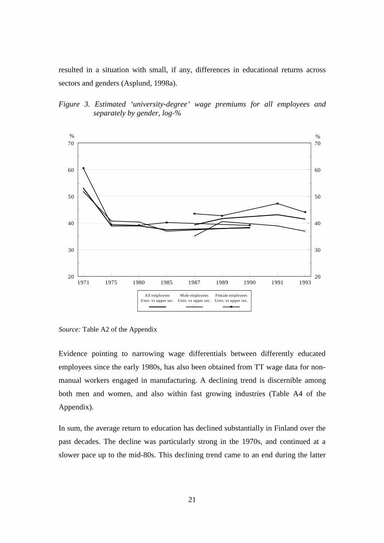
The overall trend in educational returns over the past decades is further highlighted in
Figure 3. The figure displays that the difference in returns between those with a
university degree and those with a degree at the upper level of upper secondary
education.
Separate analysis of the private and public sectors, however, points to certain
noteworthy sectoral differences in the development of returns to education between
1987 and 1993 (see Table A3 of the Appendix). In particular, while the educational-
induced wage differentials among men in private-sector employment declined
remarkably during the deep recession in the early 1990s, their female counterparts
experienced increasing returns especially to university degrees. In the public sector,
in contrast, both men and women have seen a continuous, albeit moderate, decline in
educational returns since the late 1980s. By 1993, these different time trends had
16 A declining trend between 1975 and 1985 is also reported by Brunila (1990), although the decline issmaller in absolute size since she also accounts for differences in occupational status.17 Roughly the same trend is reported for the private sector by Vainiomäki and Laaksonen (1995). Asimilar trend is also displayed by Helo and Uusitalo (1995) when relating the earnings of those with auniversity degree to the earnings of those having merely taken the matriculation examination. Theyalso show that the size of this university-degree wage premium varies considerably across educationalfields. This is evident also from their calculated internal rates of return to different university-leveleducational fields.
21
resulted in a situation with small, if any, differences in educational returns across
sectors and genders (Asplund, 1998a).
Figure 3. Estimated ‘university-degree’ wage premiums for all employees andseparately by gender, log-%
Source: Table A2 of the Appendix
Evidence pointing to narrowing wage differentials between differently educated
employees since the early 1980s, has also been obtained from TT wage data for non-
manual workers engaged in manufacturing. A declining trend is discernible among
both men and women, and also within fast growing industries (Table A4 of the
Appendix).
In sum, the average return to education has declined substantially in Finland over the
past decades. The decline was particularly strong in the 1970s, and continued at a
slower pace up to the mid-80s. This declining trend came to an end during the latter
1971 1975 1980 1985 1987 1989 1990 1991 199320
30
40
50
60
70
20
30
40
50
60
70
All employeesUniv. vs upper sec.
Male employeesUniv. vs upper sec.
Female employeesUniv. vs upper sec.
% %

22
half of the 1980s. Weak signs of increasing returns to university degrees have been
reported for the early 1990s, especially among women in private-sector employment.
4.1.3 Special issue: Endogeneity of schooling choice
There is, so far, only one study − that of Uusitalo (1999) − that attempts to adjust the
estimated return to education for the possibility of the observed distribution of
individuals across educational levels being the outcome of individual choice rather
than random selection into schooling of varying length. Uusitalo departs from a
random coefficient model of earnings determination which allows schooling choices
to vary across individuals because of differences in their returns to education and
because of their differing rates of substitution between schooling and future earnings.
While the first phenomenon may be due to differences in ability, the latter is related
to variation in access to funds and/or tastes for schooling. Broadly speaking, the
specified model is estimated using a control function approach, i.e. a two-step
selection correction combining the OLS regression of earnings on schooling with a
participation decision model. If the participation-in-schooling decision is assumed to
be linear (which turns out to be an acceptable approximation in the Finnish case), the
two-step selection correction is shown to be equivalent to the IV estimator and the
control function merely a less restrictive form of IV.
The instruments used by Uusitalo (1999) are standard. For the 1970 sample Uusitalo
experiments with father’s schooling and income as instruments. The 1982 sample
offers a slightly broader set of possible instruments: father’s and mother’s schooling
and earnings as well as residence in a university city, all information for 1980. These
instruments are grouped in four different ways, and returns to schooling are reported
for each of them with the earnings equation given four different specifications, each
of which is estimated using both the IV(2SLS) and the control function estimator.

23
This framework results in no less than 28 ability-adjusted18 return-to-schooling
estimates ranging from 0.052 to 0.112 (Uusitalo, 1999, Table 4, p. 54). The
corresponding ability-adjusted OLS estimates vary between 0.077 and 0.083
depending on whether work experience refers to potential or calculated years in
working life and whether or not the parents’ schooling is added to the earnings
equation. Thus, some of the IV estimates19 are clearly higher, some are clearly lower
than the OLS estimates.
There seem to be mainly two explanations for this outcome. First, the highest and
lowest IV estimates relate to specifications with parents’ schooling being used as an
instrument (alone or interacted with some other instrument) and/or included as an
exogenous variable in the earnings equation. Since the parents’ schooling turns out to
affect both the son’s schooling decision and his future earnings, it is not a valid
instrument.20 This is also the conclusion reached by Uusitalo (1999, p. 53). Second,
the university city stands out as a more credible instrument. Here, however,
significantly higher IV than OLS estimates are only to be expected as in this case, the
IV estimate obviously reflects to a larger extent the average return to a university year
than to a schooling year in general.
Faced with this mixed evidence on the variation of educational returns across
individuals, Uusitalo (1999) attempts to capture the potential effects of individual
selection into schooling of different length by interacting years of schooling with
ability and family background measures. In brief the results suggest that educational
returns do, on average, increase with ability (especially with math ability). The strong
18 The estimates are adjusted for ability bias by the inclusion of ability measures both in the earningsequation and in the schooling decision equation.19 The conclusions concerning IV estimates hold also for the control function estimates, since the twotechniques produce highly similar estimates.20 Uusitalo (1999, Table 5, p. 25) faces similar problems with his 1970 sample, where the father’sincome turns out to affect both the son’s schooling decision and his future earnings. The very highrates of return to schooling reported based on this sample (estimates ranging from 0.124 to 0.157compared to an OLS estimate of 0.081) are therefore to be interpreted not as an average return toschooling for the underlying population but as the marginal return that a son from a low income familywould have obtained from an additional schooling year, had he decided to continue in school.

24
effect of ability on the variation in returns to schooling and thus on schooling choice,
is noted to be the outcome of the combined effect of lower costs and higher returns
for individuals with higher ability (mainly to convert human capital absorbed in
school into marketable skills valued at the workplace). The substantial effect of
family background, on the other hand, is found to origin solely in its effect on the
discount rate. On the whole, though, observable heterogeneity turns out to leave a
significant part of the individual variation in returns to schooling unexplained.
Uusitalo (1999) goes deeper into the question of schooling choices and the impact on
these of various personal characteristics and family background by estimating a
discrete choice schooling model, which is given the specification of an ordered
generalised extreme value model. Earnings equations for different educational levels
are thereafter estimated using a simple selectivity correction model. In particular,
Uusitalo (1999) focuses on the selection point by which students are faced after
completed general upper secondary education (Gymnasium) giving them the
matriculation diploma.21
The returns to education are estimated in a setting where individuals have the
possibility to choose between several alternative educational levels. The schooling
investment decision is assumed to be driven by the different rewarding of skills
depending on the job performed. Consequently rational individuals can be expected
to choose the educational level that leads to the occupation where their skills are best
rewarded. Attempts are made to capture the effects on earnings of both cognitive and
non-cognitive skills measured from ability and personality tests administered by the
Finnish Army. The data used is the 1982 male sample, now restricted to those close
to 6,900 recruits with a recent high school diploma and no further education at the
time of entering military service.
In brief the results indicate that cognitive and non-cognitive test scores explain
relatively little of the within educational level variation in earnings. The effects of test
21 Of these about one-third are admitted to universities (the same year), while the rest continue theirstudies in vocational institutions or enter the labour market (for more details, see OECD, 1998).
25
scores are found to differ only marginally also between different educational levels,
which points to minor differences in skill prices across educational levels. The main
conclusion to be drawn concerning schooling choice is that neither the (non-
)cognitive skills nor family background provide a clear-cut pattern; only a few
characteristics stand out as statistically significant and most clearly for the choice of a
university education. Put differently, individual skills and family background do not
seem to cause clear self-selection into different educational levels.
4.2 Returns to work experience
4.2.1 Earnings effects of age
There is very limited evidence on the impact on earnings of the individual’s age. The
existing estimates are based on Population Census Data, which in contrast to the
Labour Force Survey and the TT wage data do not include information on actual
years spent in working life.
Brunila (1990) uses a single age variable and obtains a very modest average effect of
increasing age on annual earnings among full-year, full-time employees: 0.6 per cent
per annum for 1975 and 0.8 per cent per annum for 1985 among both men and
women. Uusitalo (1999) obtains insignificant wage effects for age from his sample of
males that performed their military service in 1970.
Eriksson and Jäntti (1997) distinguish between eight age groups in their estimations
of earnings equations for all employees and separately for male and female
employees for the years 1971, 1975, 1980, 1985 and 1990. Their estimates are
reproduced in Table 2 in the form of age premiums calculated as (unweighted)
percentage deviations from the overall mean earnings in the labour market.
Two main changes deserve attention. First, the increasing parts of the age-earnings
profiles have become steeper while the declining parts have become flatter, except in

26
the last year (1990) studied. Second, the age differentials have widened substantially
since the early 1970s. These results change only marginally when including
employees younger than 25 years (Eriksson, 1994) or when using monthly earnings
instead of annual earnings as in Table 2 (cf. Eriksson and Jäntti, 1996).
Table 2. Age premiums of different age groups for all employees and separately bygender, 1971−90, log-%
All employees
Age group 1971 1975 1980 1985 1990
25−29 2.3 −8.6 −13.6 −17.0 −15.9
30−34 7.2 2.0 −2.7 −7.4 −5.5
35−39 10.0 4.9 5.1 1.0 2.2
40−44 8.2 6.6 6.7 6.8 7.9
45−49 5.6 3.6 6.3 6.5 10.8
50−54 0.5 2.0 2.5 5.8 7.4
55−59 −9.2 −2.5 1.3 5.8 3.3
60−64 −24.4 −8.1 −5.5 −1.4 −10.0
Male employees
25−29 3.3 −7.5 −11.6 −14.1 −10.8
30−34 8.1 3.6 −2.0 −6.0 −1.4
35−39 10.7 4.8 4.6 1.6 2.3
40−44 7.8 5.9 6.2 5.8 6.6
45−49 5.6 3.0 4.6 4.7 8.4
50−54 0.5 1.7 1.8 4.4 4.0
55−59 −8.3 −2.0 1.0 4.7 0.8
60−64 −27.5 −9.5 −4.5 −1.0 −9.9
Female employees
25−29 1.3 −9.8 −16.0 −20.0 −21.0
30−34 5.8 0.1 −3.8 −8.8 −9.8
35−39 9.1 5.0 5.8 0.5 2.3
40−44 8.7 7.5 7.2 8.1 9.7
45−49 5.6 4.1 8.1 8.4 13.5
50−54 0.5 2.5 3.4 7.2 10.6
55−59 −10.1 −3.1 1.7 6.9 5.1
60−64 −20.7 −6.2 −6.6 −2.0 −10.1
Source: Eriksson and Jäntti (1997, Table 5) transformed into unweighted age premiums bythe author.

27
4.2.2 Earnings effects of work experience
The existing evidence on the influence of increasing work experience on individual
earnings is so far quite limited, as is evident from Table 3. The reported estimates
refer to the individuals’ total years actually (i.e. self-reportedly) spent in working
life.22
Table 3. Average wage effects of total (actual) work experience, log-%
Experience Experience squared
Year All Men Women All Men Women
Asplund et al. (1996a) a) 1987 1.8 2.6 0.9 −0.024 −0.039 −0.010i
Asplund et al. (1996a) a) 1987 1.6 2.5 0.8 −0.024 −0.039 −0.009i
Asplund (1993a) b) 1987 1.5 1.9 1.3 −0.020 −0.029 −0.017
Uusitalo (1999; recruitsin 1982)
1994 − 1.4 d) − − − −
PRIVATE SECTOR
Year Men Women Men Women
Asplund (1998a) c) 1987 2.1 1.4 −0.034 −0.021i
1989 2.4 1.2 −0.037 −0.016i
1991 2.5 1.2 −0.038 −0.012i
1993 2.5 2.9 −0.034 −0.053
PUBLIC SECTOR
Year Men Women Men Women
Asplund (1998a) c) 1987 2.2 1.1 −0.033 −0.006i
1989 1.3 1.6 −0.018i −0.021
1991 2.8 1.0 −0.048 −0.008i
1993 2.8 1.7 −0.045 −0.020i
Notes: i indicates insignificance at the 5 % level. (a) Explanatory variables are: first row, schooling
years, second row, four indicators for educational degree levels, and a gender dummy in the wageequation for all employees. (b) In addition to five indicators for educational degree levels, the wageequation is supplemented with a broad set of other personal and job-related characteristics. (c) Accountis made for differences in educational degree levels (five indicators) as well as for various otherpersonal and job-related characteristics, not occupational or industrial status, though. (d) Calculated asnumber of years after graduation. None of the wage equations control for tenure.
22 Asplund (1993a) shows that the use of potential instead of actual years in working life produces astrongly upward-biased estimate especially for female employees.

28
The experience acquired in working life turns out to be rather weakly reflected in the
wages of Finnish employees. Both the initial wage influence of work experience and
the experience-earnings profile are particularly modest for women. The only
exception is women employed in the private sector, who seem to be experiencing a
boom in the rewarding of their work experience. Among men, the wage advantage
arising from increasing work experience has persistently been approximately equally
strong irrespective of the sector of employment. Moreover, the experience-induced
effect on male wages seems to have strengthened slightly in the early 1990s.
The table also shows that the estimates of work experience are to some extent
sensitive to the definition of the schooling variable as well as to the inclusion of other
personal and job-related characteristics. As in the case for returns to schooling, the
decline in the estimated wage effect of work experience is non-negligible only when
supplementing the wage model with controls for the individuals’ occupational status
(see e.g. Asplund, 1993a; Asplund et al., 1996a).23
Experiments with work experience given the form of a linear spline (thereby
following Stewart, 1983) instead of the conventionally used concave shape display
quite an unexpected, but fairly similar overall pattern across genders and sectors.
Instead of rising steeply, the experience profiles tend to decline or remain
approximately unchanged for the first five years in working life. The rising trend
starts only during the next five years representing 5−9 years of work experience.
These years seem to be the most important ones especially for women in private-
sector employment and men in public-sector employment. The next ten years give a
further push up the wage scale, most strongly for men in private-sector employment.
After 20 years of work experience the experience-earnings profile stays flat towards
the end of working life. This lack of a declining trend with increasing work
23 It may also be noted in this context that Uusitalo (1999) attempts to treat (potential) work experienceas an endogenous variable by using age and age squared as instruments. This leads not only to adecline in the estimated coefficient for the experience variable; it turns insignificant altogether.

29
experience is repeated across genders and sectors and emerges irrespective of the
activity level of the economy.24
From the estimated coefficients of (actual) work experience obtained for non-manual
workers in manufacturing using TT wage data, it may be concluded that the
rewarding of work experience has weakened substantially over the 15-year period
1980−94 (Asplund, 1996). In other words, the wage position of the inexperienced
workers entering a manufacturing job has strengthened relative to their more
experienced colleagues. The overall trend has been much the same among upper-
level, technical and clerical non-manual workers (Asplund, 1993b). Comparison of
male and female non-manual workers, in turn, displays a huge gender gap in the wage
impact of work experience, a gap that has expanded further in the early 1990s
(Asplund, 1998c). The experience-earnings profiles look completely different also
when comparing non-manual workers employed in fast growing and slowly growing
industries. In particular, the former category has persistently faced a significantly
higher and also more steeply rising wage effect from increasing work experience
(Asplund and Vuori, 1996). Common to both categories, however, is that they have
seen a steady decline in the estimated wage effect, albeit of a highly different
magnitude. The experience-earnings gap between the two industry categories was, as
a consequence, notably larger in the early 1990s than in the early 1980s. This trend
was further strengthened by a weak recovering in experience-induced wage effects in
the fast growing industries in the mid-90s.25
Accounting for the individuals’ tenure not only adds to the drop in the estimated
wage effects of work experience but also changes the interpretation of the estimate of
the experience variable. Now the estimated wage effect of work experience reflects
the influence of the work experience acquired before entering the current job. The
difference between this experience-induced wage effect and the total wage effect
reported in Table 3 above thus illustrates the influence on wages of tenure, often
24 For more details, see Asplund (1998a).25 Asplund and Vuori (1996) also report corresponding results for different-sized establishments.

30
interpreted as capturing the firm-specific training acquired in working life. Table 4
reproduces some of the estimates from Table 3, now adjusted for the wage impact of
tenure. The general impression is that the change in the experience-earnings profiles
is minor, which is also to be expected from the small overall wage effect of work
experience and the minor overall role of tenure (see next subsection).
Table 4. Average wage effects of (actual) work experience when also controlling fortenure, log-%
Experience Experience squared
Year All Men Women All Men Women
Asplund et al. (1996a) a) 1987 1.4 2.3 0.5i −0.022 −0.038 −0.007i
Asplund (unpubl.) b) 1987 1.5 2.1 1.0 −0.026 −0.034 −0.020
1989 1.1 1.8 0.3i −0.018 −0.030 −0.004i
1991 1.8 2.3 1.5 −0.032 −0.040 −0.028
1993 1.7 2.3 1.1 −0.027 −0.036 −0.017i
PRIVATE SECTOR
Year Men Women Men Women
Asplund (1998a) c) 1987 1.8 0.9i −0.032 −0.016i
1989 2.0 0.6i −0.033 −0.008i
1991 1.9 0.8i −0.031 −0.012i
1993 1.8 3.0 −0.022 −0.062
PUBLIC SECTOR
Year Men Women Men Women
Asplund (1998a) c) 1987 1.8 0.6i −0.028i −0.006i
1989 0.5i 0.9i −0.005i −0.015i
1991 2.7 0.7i −0.047 −0.010i
1993 1.9 1.6 −0.030i −0.025i
Notes i indicates insignificance at the 5 % level. (a) Explanatory variables are: schooling years, tenure
and a gender dummy in the wage equation for all employees. (b) Explanatory variables are: fiveindicators for completed educational level, dummy for tenure less than one year, tenure and tenuresquared, dummy for participation in employer-financed training and a gender dummy in the wageequation for all employees. (c) Account is made for differences in educational degree levels (fiveindicators) and tenure (dummy for tenure less than one year, tenure and tenure squared) as well as forvarious other personal and job-related characteristics, not occupational or industrial status, though.

31
4.2.3 Earnings effects of tenure
The wage effects reported for work experience give a good hint of the size of the
wage growth induced by increasing tenure. The available evidence for the Finnish
labour market is reviewed in Table 5, with tenure referring to the length of the
individual’s employment relationship at the current employer. The overall impression
mediated by the table is, indeed, a minor wage influence of tenure. The very small
size of the tenure effect is also evident from the fact that the tenure-earnings profile is
throughout estimated to be flat or almost flat.
The results obtained for the boom years in the late 1980s indicate that the role of
longer tenure for wage growth was much more important among public-sector
employees, although the effect was quite strong also among women employed in the
private sector. The deep recession in the early 1990s seems, however, to have
fundamentally reversed this pattern. More precisely, by 1993 the tenure-induced
growth in female wages had disappeared in both sectors at the same time as the
rewarding of their general work experience boosted (cf. Table 4 above). Men in
private-sector employment, in contrast, faced the opposite change with the length of
the current employment relationship exerting an increasing influence on their wage
growth.
The tenure-induced wage effects estimated for non-manual workers in manufacturing
from TT wage data are equally moderate. Moreover, the wage advantage of a longer
employment relationship shows no time trend whatsoever and has varied quite
randomly − mostly between negligible and negative values. This overall pattern is
repeated for all non-manual categories as well as for all the subgroups investigated.26
26 See Asplund (1996) for results for all non-manual workers and separately for upper-level, clericaland technical non-manual workers, Asplund (1998c) for male and female non-manual workers, andAsplund and Vuori (1996) for non-manual workers employed in, respectively, fast and slowly growingindustries.

32
Table 5. Wage effects of tenure for all employees and separately by gender andsector, log-%
Tenure Tenure squared
Year All Men Women All Men Women
Asplund et al. (1996a) a) 1987 0.6 0.5 0.7 − − −
Asplund (1993) b) 1987 0.6 0.4i 0.7 −0.001i −0.001i 0.000 i
Tenure < 1 year Tenure Tenure squared
WHOLE ECONOMY Men Women Men Women Men Women
Asplund (unpubl.) c) 1987 1.2i 14.6 0.4i 1.3 −0.002i −0.021
1989 6.3 13.7 1.0 1.7 −0.012i −0.031
1991 4.6i 11.4 1.1 0.8 −0.017 −0.005i
1993 5.8i 14.2 1.1 0.1i −0.018i 0.014i
PRIVATE SECTOR
Asplund et al. (1996a) a) 1987 − − 0.5 0.4 − −Asplund (1998a) d) 1987 2.2i 9.0 0.3i 1.0 −0.003i −0.016i
1989 3.0i 10.8 0.7 1.6 −0.006i −0.030
1991 5.9i 17.2 1.2 1.0 −0.019 −0.009i
1993 6.8i 8.3i 1.7 0.3i −0.038 0.011i
PUBLIC SECTOR
Asplund et al. (1996a) a) 1987 − − 0.7 0.9 − −Asplund (1998a) d) 1987 12.6 20.0 1.2 1.9 −0.019i −0.026i
1989 31.1 19.3 1.8 2.0 −0.029i −0.032
1991 7.3i 10.6 0.6i 1.1 −0.010i −0.009I
1993 20.0 19.4 1.6 0.5i −0.026i 0.009i
Notes: i indicates insignificance at the 5 % level. (a) Explanatory variables are: schooling years,
experience, experience squared and a gender dummy in the wage equation for all employees. (b)Account is made for differences in educational degree levels (five indicators) and work experience aswell as for various other personal and job-related characteristics, not for occupational status, though.(c) Explanatory variables are: five indicators for completed educational level, experience, experiencesquared, dummy for participation in employer-financed training and a gender dummy in the wageequation for all employees. (d) Account is made for differences in educational degree levels (fiveindicators) and work experience as well as for various other personal and job-related characteristics,not for occupational status or industry affiliation, though.

33
4.2.4 Earnings effects of job training
The only individual-level database containing information about the individuals’
participation in employer-financed job training is the Labour Force Survey. The
sample individuals are asked whether they have participated in employer-financed
training courses outside the workplace and for how many days in total during the past
12 months. The available empirical evidence based on this information is displayed in
Table 6.
The estimates point to a substantially lower rewarding of participation in employer-
financed job training among women, which is primarily attributable to the negligible
wage advantage of women employed in the public sector of participating in this type
of training. It is also of interest to note that the deep recession seems to have
strengthened the importance not only of tenure but also of training in explaining
observed wage differentials among men employed in the private sector. Again an
opposite trend is observable for their female counterparts, i.e., a decline in the wage
influence of training as well as tenure.
The estimated differences in wage effects may, of course, be the result of crucial
differences both in the length and the content of the training received. Evidence for
1987 indicates, however, that the overall pattern is maintained when accounting for
differences in the total number of training days (Asplund, 1993a).

34
Table 7. Wage effects of participation in employer-financed job training outside theworkplace, log-%
Male employees Female employees
All Privatesector
Publicsector
All Privatesector
Publicsector
Asplund (1993a) a) 1987 10.1 13.0 8.2 3.1 8.9 −1.0i
Asplund b) 1987 10.8 11.7 7.2 3.0 9.5 −1.5i
1989 8.6 8.7 8.5 4.1 11.7 −2.8i
1991 8.5 9.6 4.1i 5.8 9.6 4.9
1993 9.9 12.4 6.7 3.8 8.3 1.8i
Notes: i indicates insignificance at the 5 % level. (a) Account is made for differences in educational
degree levels (five indicators), experience (and its square), tenure (and its square) as well as forvarious other personal and job-related characteristics, not for occupational status or industryaffiliation. (b) Account is made for differences in educational degree levels (five indicators),experience (and its square), tenure (tenure < 1 year –dummy, tenure and its square) in the ‘All’equations (unpublished), while the sectoral equations are, in addition, supplemented with a limitednumber of other personal and job-related characteristics, not occupational status or industryaffiliation, though (Asplund, 1998a).
5. CONCLUSIONS
Most existing evidence for Finland on the earnings effects of human capital
endowments refer to a rather short time period, viz. 1987 to 1993. Only occasionally
have results been reported for a longer sequence of years and then mostly for a very
limited set of human capital proxies or for a specific category of workers.
Moreover, the analysis of the interplay between the individuals’ earnings and their
human capital endowments has drawn heavily on the conventional Mincer-type
earnings model. Few attempts have been made to account for the fact that the human
capital acquired by the individual is not necessarily the outcome of a random process
but rather the result of individual choice. More research is needed on the impact of
innate ability and family background on returns to schooling and schooling choice.
Also totally unexplored areas should be penetrated. For instance, we are totally
lacking empirical evidence on the effects of screening/signalling and sheepskin
effects as well as on the link between educational returns and unemployment. In fact,

35
compared to many other European countries (see the other country-specific literature
reviews) Finland is without doubt lagging far behind when it comes to empirical
evidence on the rewarding in the labour market of investment in education and other
types of human capital.
Needless to say, the richness of the empirical evidence produced in a country largely
reflects the availability of proper data. This is certainly true when it comes to returns
to schooling. Enlarging our knowledge on returns to human capital in general and to
schooling in particular is thus a challenge not only for the research community but
also for the bodies creating and producing statistical databases.

36
REFERENCES
Albæk, K., M. Arai, R. Asplund, E. Barth and E. Strøjer Madsen (1996a), Inter-Industrywage Differentials in the Nordic Countries, in Westergård-Nielsen, N. (ed.),Wage Differentials in the Nordic Countries, in Wadensjö, E. (ed.), The NordicLabour Markets in the 1990s, Part 1. Amsterdam: North-Holland.
Albæk, K., M. Arai, R. Asplund, E. Barth and E. Strøjer Madsen (1996b), Employer Size-Wage Differentials in the Nordic Countries. Århus: Centre for Labour Marketand Social Research, Working Paper 96-03.
Asplund, R. (1993a), Essays on Human Capital and Earnings in Finland. Helsinki: TheResearch Institute of the Finnish Economy, Series A 18.
Asplund, R. (1993b), Teollisuuden toimihenkilöiden palkat ja inhimillinen pääoma. Helsinki:The Research Institute of the Finnish Economy, Series B 89.
Asplund, R. (1996), Är humankapital en lönsam investering?, in Lundholm, M. (ed.),Utmaningar för den offentliga sektorn. Uppsala: Nordiska EkonomiskaForskningsrådet, Rapport 6.
Asplund, R. (1998a), Private vs. Public Sector Returns to Human Capital in Finland, Journalof Human Resource Costing and Accounting, 3(1), pp. 11−44. Additional resultsreferred to in the text are given in Discussion papers No. 607 published by TheResearch Institute of the Finnish Economy ETLA, Helsinki.
Asplund, R. (1998b), Are Computer Skills Rewarded in the Labour Market? − Evidence forFinland. SNF Yearbook 1998, Bergen.
Asplund, R. (1998c), The Gender Wage Gap in Finnish Industry in 1980−94, in Persson, I.and C. Jonung (eds), Women’s Work and Wages. London: Routhledge.
Asplund, R. and S. Vuori (1996), Labour Force Response to Technological Change.Helsinki: The Research Institute of the Finnish Economy, Series B 118.
Asplund, R., E. Barth, C. le Grand, A. Mastekaasa and N. Westergård-Nielsen (1996a), WageDistribution Across Individuals, in Westergård-Nielsen, N. (ed.), WageDifferentials in the Nordic Countries, in Wadensjö, E. (ed.), The Nordic LabourMarkets in the 1990s, Part 1. Amsterdam: North-Holland.
Asplund, R., E. Barth, N. Smith and E. Wadensjö (1996b), The Male−Female Wage Gap inthe Nordic Countries, in Westergård-Nielsen, N. (ed.), Wage Differentials in theNordic Countries, in Wadensjö, E. (ed.), The Nordic Labour Markets in the1990s, Part 1. Amsterdam: North-Holland.
Eriksson, T. (1994), Unemployment and the Wage Structure – Some Finnish Evidence, inEriksson, T., S. Leppänen and P. Tossavainen (eds), Proceedings of theSymposium on Unemployment. Helsinki: Government Institute for EconomicResearch, VATT−Publications 14.
Eriksson, T. and M. Jäntti (1996), The distribution of earnings in Finland 1971−1990. Turku:Åbo Akademi University, Meddelanden från Ekonomisk−Statsvetenskapligafakulteten vid Åbo Akademi.
Eriksson, T. and M. Jäntti (1997), The distribution of earnings in Finland 1971−1990,European Economic Review 41(9), pp. 1763−1780.

37
Helo, T. and R. Uusitalo (1995), Kannattaako korkeakoulutus? Kustannus-hyöty –analyyttinen arvio korkeakoulutusinvestointien tuotoista Suomessa 1975-1990.Turku: Koulutussosiologian tutkimuskeskus, raportteja 24, Turun yliopisto.
Lilja, R. and Y. Vartia (1980), Koulutusaika kotitalouksien tuloerojen selitystekijänä.Helsinki: The Research Institute of the Finnish Economy, Series B 25.
Nygård, F. (1989), Relative Income Differences in Finland 1971−1981, in Hagfors, R. and P.Vartia (eds), Essays on Income Distribution, Economic Welfare and PersonalTaxation. Helsinki: The Research Institute of the Finnish Economy, Series A 13.
OECD (1998), Transition from initial education to working life. The Finnish country report.Mimeo. (forthcoming)
Puhani, P.A. (1997), Foul or Fair? The Heckman Correction for Sample Selection and ItsCritique. A Short Survey. ZEW, Discussion Paper No. 97−07 E.
Statistics Finland (1998), Vuoden 1950 väestölaskennan otosaineiston käsikirja. Helsinki.
Stewart, M. (1983), Relative Earnings and Individual Union Membership in the UnitedKingdom, Economica, Vol. 50, pp. 111−125.
Uusitalo, R. (1996), Return to Education in Finland. University of Helsinki, Department ofEconomics, Research reports Nro 71:1996.
Uusitalo, R. (1999), Essays in Economics of Education. University of Helsinki, Department ofEconomics, Research reports Nro 79:1999.
Vainiomäki, J. and S. Laaksonen (1995), Inter-industry wage differentials in Finland,Evidence from longitudinal census data for 1975−85, Labour Economics, Vol. 2,pp. 161−174.