earnings dynamics in europe - merit.unu.edumerit.unu.edu/publications/uploads/1301493462.pdf ·...
TRANSCRIPT

EARNINGS DYNAMICS IN EUROPE

© 2010 Denisa Maria Sologon
All rights reserved. No part of this publication may be reproduced, stored
in a retrieval system, or transmitted in any form, or by any means,
electronic, mechanical, photocopying, recording or otherwise, without the
prior permission in writing, from the author.
ISBN 978 90 8666 144 2
Cover picture by Denisa Maria Sologon
Published by Boekenplan, Maastricht
EARNINGS DYNAMICS IN EUROPE
DISSERTATION
PROEFSCHRIFT
To obtain the degree of Doctor at the Maastricht University,
on the authority of the Rector Magnificus Prof. Dr. G.P.M.F. Mols,
in accordance with the decision of the Board of Deans,
to be defended in public on 4 June 2010, at 10:00 hours
by
Denisa Maria Sologon

Promoter: Prof. Dr. Chris de Neubourg
Supervisors: Dr. Cathal O’Donoghue, Teagasc Rural Economy
Research Centre; NUI Galway; IZA and ULB
Dr. Raymond Wagener, Inspection Générale De La
Sécurité Sociale (IGSS), Luxembourg
Assessment Committee: Prof. Dr. Lex Borghans (Chairman)
Prof. Dr. Hans Heijke
Dr. Erik de Regt
Prof. Dr. Gary Solon, Michigan State University
(USA)
Dr. Philippe Van Kerm, CEPS/INSTEAD
(Luxembourg), Institute for Social and Economic
Research, University of Essex (UK), University of
Namur (Belgium)

In loving remembrance of my mother, Lia

i
Acknowledgements
This book is dedicated to my beloved parents and grandparents, whose love and
sustained support made this accomplishment possible. There are no words to
capture my love and my gratitude for all their sacrifices.
I thank Victor for his love and for being my pillar of strength through the hardest
moments of my life. We started our Master together and now we are finishing our
PhDs together: thank you for making these challenging years a beautiful, happy
and enriching experience.
My deepest gratitude goes towards my supervisors, Dr. Cathal O’Donoghue and
Dr. Raymond Wagener, whose kind and fruitful guidance led my steps towards
obtaining my PhD. I learned tremendously from working with you and I am so
grateful for the stimulating working environment you have created for me. Thank
you for being so supportive, for believing in me and for the amazing opportunities
you have opened to me. You hold a very special place in my heart.
I would like to thank the reading committee members, Prof. Dr. Lex Borghans,
Prof. Dr. Hans Heijke, Dr. Erik de Regt, Prof. Dr. Gary Solon and Dr. Philippe Van
Kerm for their useful comments in finalizing this manuscript.
My PhD developed within a unique place - Maastricht Graduate School of
Governance - created with a unique vision. I thank our promoter Chris de
Neubourg and his team - Annemarie Rima, Mindel van de Laar, Franziska
Gassmann, Mieke Drossaert, Celine Duijsens and Susan Roggen - for creating not
only an amazing educational environment, but also a real family. This School has
become home for many of us, extremely rewarding and motivating those far away
from their homes. My PhD years have been the best years of my life. And this was
due to the School and my dear colleagues, who became cherished lifetime friends.
We share so many memories…from the stressful moments and the amazing PhD
parties, to the great joy of the four marriages and four PhD babies – Paola, Farouk,
Izzy and Calvin. Yes, we have been very productive! Thank you, my dear friends
for the unforgettable moments we have shared!
Zina - we started this road together sharing the same office and we grew into more
than friends. I am so grateful to have met somebody as special as you. Thank you
for being there with your love, friendship and wisdom! You have enriched my life
in so many ways!

ii
Melissa – you won my heart with your delicious lactose-free brownies in the first
year! There are so many memories I cherish... Thank you for the memorable “ladies
nights”, the great parties, brunches, and diners you hosted... but for them, these
years wouldn’t have been as much fun. I thank you and Flo for visiting my family
in Romania and for the nice vacations we spent together.
Britta – one of the warmest and sincere hearts I have ever met! Thank you for being
there during tough times and for the wonderful moments we have shared!
Jessica – you are our “Superwoman”: three adorable, smart babies and a PhD. I
thank you, Alex and Paola for visiting my family in Romania and for the precious
memories.
Jinjing – there are so many memories that bond us and I cherish them all...Thank
you for being there both during tough and good times, and for visiting my family
in Romania.
Frieda – unique Frieda... our French “touch”. Liege has stolen you from Maastricht,
but not from my heart.
Metka – I will always remember our cosy girly movie evenings. Not to mention the
great parties, brunches, dinners at your house...great memories!
The Mexicans Paty and David– one of my regrets is missing your great wedding!
Thank you for always making me laugh and for the great parties, brunches and
chats we had!
Robert – thank you for your help during my first year in Maastricht...it helped me
make Maastricht my home. Lina – we share nice memories from the summer
school in Palma de Mallorca and our visits in Luxembourg.
Carlos, Eze, Irina, Ilire, Luciana, Jasmin, Nevena, Seda– thank you for the nice
parties, chats, brunches, lunches and dinners we had together.
These years were also a culinary delight. I thank Sonila and Florian for sharing
with us the great Albanian cuisine; Maha and Cheng for the amazing Asian diners;
Ana Maria for the delicious pizza moments; Carlos and Carolina for the exquisite
Columbian dishes; and Jinjing for opening the doors to the diverse Chinese cuisine.
I thank Bart, Keetie, Kristine, and Mindel for helping me with the Dutch
translation. It was not an easy job and I am very grateful.
Thank you to my other friends at the School, Bianca, Christiane, Geranda, Hao,
Judith, Julie, Keetie, Marina, Michal, Mirtha, Pascal, and Renée for their friendship
and the nice moments we shared.

iii
My PhD project developed within a larger project – The Coherence of Social
Transfer Policies and Microsimulation - REDIS - initiated by the Inspection
Générale de la Sécurité Sociale (Luxembourg) in cooperation with CEPS/ INSTEAD
(Luxembourg) and Cathal O’Donoghue (Teagasc Rural Economy Research Centre;
NUI Galway; IZA and ULB). I would like to thank all team members of the REDIS
project – Raymond Wagener, Isabelle Debourg, Tom Dominique, Thierry Mazoyer,
Frédéric Berger, Philippe Liegeois, Nizamul Islam - who created a pleasant and
stimulating working environment.
I thank the Harvard Kennedy School of Government, Harvard University, for
accepting me as a visiting research fellow. It was an amazing experience which
enriched both my personal and my professional development. I would like to
thank Gerardo for his useful comments and his friendship during our research
visit at Harvard University.
I thank the Marie Curie Fellowship and the Fonds National de la Recherche
(Luxembourg) who funded my PhD research fellow work contract at Maastricht
University, and without whom this PhD would not have been possible.
I thank Mihai Focsa, Adrian Postelnicu and Prof. Tutuianu Ion, who cultivated my
passion for Mathematics, which proved to be of invaluable help for my thesis.
I thank Gabi and Roger - my Luxembourgish family – for their love and
enthusiastic support.
Last but not least I thank the rest of my family and my oldest friends from
Romania – Corina, Cristi, Levi, Roxana, Silvia, Silviu and Stefan who always
believed in me.

iv
Table of Contents
Preface iv
1. Introduction 1
1.1. Objective and relevance 3
1.2. Structure of the study 7
2. Increased opportunity to move up the economic ladder? Earnings mobility in the EU:
1994-2001 10
2.1. Introduction 11
2.2. Literature review 12
2.3. Methodology 13
2.3.1. Transition matrix approach to mobility 14
2.3.2. Alternative approach to mobility (Dickens 2000a) 15
2.4. Data 16
2.5. Changes in the cross-section earnings distribution over time 17
2.6. Linking earnings inequality and mobility: individual movements within the
distribution over time 25
2.6.1. Mobility among labour market states 25
2.6.2. The transition matrix approach to mobility among income quintiles 27
2.6.3. Alternative approach to mobility (Dickens 2000a) 37
2.7. Linking mobility and inequality 47
2.7.1. Short-term mobility and yearly inequality 47
2.7.2. Long-term mobility and yearly inequality 49
2.8. Concluding remarks 50
2.9. Annex 55
3. Equalizing or disequalizing lifetime earnings differentials? Earnings mobility in the
EU: 1994-2001 76
3.1. Introduction 77
3.2. Literature review 79
3.3. Methodology 81
3.3.1. Shorrocks 81
3.3.2. Fields 83
3.4. Data 84
v
3.5. Changes in earnings inequality 85
3.5.1. Changes in the cross-section earnings distribution over time 85
3.5.2. Changes in the earnings distribution over the lifecycle: short versus long-term
income inequality 93
3.6. Mobility profile 99
3.6.1. Stability profile - Shorrocks 99
3.6.2. Mobility Profile – as equalizer on long-term earnings inequality 109
3.6.3. The evolution of mobility over time 122
3.7. Concluding remarks 125
3.8. Annex 129
4. Earnings dynamics and inequality in EU, 1994-2001 137
4.1. Introduction 138
4.2. Literature review 139
4.3. Theoretical model of the determinants of wage differentials 141
4.3.1. Determinants of earnings inequality 141
4.3.2. Alternative model specifications for the permanent and transitory components 142
4.3.3. Earnings mobility 147
4.4. Data 148
4.5 Econometric specification and estimation method of covariance structures 150
4.5.1. Econometric earnings specification 151
4.5.2. Specification of the covariance structure of earnings 153
4.5.3. Estimation of covariance structures 154
4.6. Strategy for model specification 157
4.7. The dynamic autocovariance structure of hourly earnings 158
4.8. Results of covariance structure estimation 163
4.8.1. Error component model estimation results 163
4.9. Inequality decomposition into permanent and transitory inequality 175
4.9.1. Absolute decomposition 175
4.9.2. Relative decomposition – structure of inequality 181
4.10. Concluding remarks 190
4.11. Annex 193
5. Policy, institutional factors and earnings mobility 203
5.1. Introduction 204
5.2. Theoretical model of the determinants of wage differentials 207
5.2.1. Literature review 207
5.2.2. Determinants of earnings inequality 207
5.2.3. Permanent and transitory components of earnings inequality 209
5.3. Data 225
5.4. Econometric specifications and estimation methods 228
5.4.1. Econometric specifications and estimation methods of covariance structures 228
vi
5.4.2. Estimation of the links between policy, institutions and outcomes 232
5.5. Results - descriptive 234
5.5.1. The dynamic autocovariance structure of hourly earnings 234
5.5.2. The evolution of the main labour market and institutional factors 236
5.6. Results of covariance structure estimation 239
5.6.1. Estimation results 239
5.6.2. Inequality decomposition into permanent and transitory inequality 243
5.7. Linking policy with outcomes 256
5.7.1. Explaining the changes and differences 257
5.7.2. Correlations 259
5.7.3. Estimation 262
5.8. Concluding remarks 278
5.9. Annex 281
6. Earnings dynamics and inequality among men in Luxembourg, 1988-2004: evidence
from administrative data 291
6.1. Introduction 292
6.2. Literature review 294
6.3. Theoretical model of the determinants of wage differentials 297
6.3.1. Determinants of earnings inequality 297
6.3.2. Earnings mobility 302
6.4. Data 304
6.5. Econometric specification and estimation method of covariance structures 310
6.5.1. Econometric earnings specification 310
6.5.2. Specification of the covariance structure of earnings 313
6.5.3. Estimation of covariance structures 314
6.5.4. Strategy for model specification 318
6.6. The dynamic autocovariance structure of hourly earnings 319
6.7. Results of Covariance Structure Estimation 324
6.7.1. Error component model estimation results 338
6.7.2. Inequality Decomposition into Permanent and Transitory Inequality 338
6.8. Concluding remarks 360
6.9. Annex 363
7. Conclusions and forward looking 365
Bibliography 378
Samenvatting 385
Curriculum Vitae 389
Maastricht Graduate School of Governance Dissertation Series 394
vii
Preface
This dissertation is a collection of five articles written as standalone papers
included as separate chapters. Given the strong link between the articles due to the
common theme and in some cases common methodology, this dissertation
includes a certain degree of duplication. I summarize below the overlapping parts
between the five papers, together with the working papers these chapters are
based on.
Chapter 2 - Increased opportunity to move up the economic ladder? Earnings
mobility in the EU: 1994-2001 - is based on Sologon and O'Donoghue (2009d).
Chapter 3 - Equalizing or disequalizing lifetime earnings differentials? Earnings
mobility in the EU: 1994-2001 - is based on Sologon and O'Donoghue (2009c). The
information in section 3.4 and 3.5.1 has already been discussed in section 2.4 and
2.5.
Chapter 4 - Earnings dynamics and inequality in EU, 1994-2001 - is based on
Sologon and O'Donoghue (2009a, 2009b). Part of the information in section 4.4 has
been discussed in section 2.4 and 3.4. This version benefitted from the valuable
comments received from Gary Solon, University of Michigan, Christopher Jencks,
Harvard University, and Peter Gottschalk, Boston College.
Chapter 5 - Policy, institutional factors and earnings mobility - is based on Sologon
and O'Donoghue (2009e). It builds on the results obtained by Sologon and
O'Donoghue (2009a, 2009b) discussed in Chapter 4: using the predicted
components from the error component models estimated in Chapter 4 and the
OECD data, we estimate the relationship between the three labour market
outcomes – permanent inequality, transitory inequality and earnings immobility –
and the labour market policy and institutional factors. Since this Chapter is written
as a standalone paper, the information in sections 5.2.3.1, 5.2.3.2, 5.4.1, 5.5.1, 5.6
summarises the core aspects of Chapter 4: the econometric specification and
estimation method of the covariance earnings structure, the dynamic
autocovariance structure of hourly earnings, and the results of the covariance
structure estimation for each country.
Chapter 6 - Earnings dynamics and inequality among men in Luxembourg, 1988-
2004: evidence from administrative data - is based on Sologon (2009). The
information in section 6.2, 6.3, 6.5.3, and 6.5.4 has been discussed in Chapter 4.
viii
List of Figures
Figure 2.1. Epanechinov Kernel Density Estimates for Selected Years - EU 15 ....................... 18
Figure 2.2. Percentage Change in Mean Hourly Earnings by Percentiles Over The Sample
Period .......................................................................................................................................... 20
Figure 2.3. Ratio between Mean Earnings at the 9th Decile and the 1st Decile ....................... 21
Figure 2.4. Relative Change in Inequality over Time – Gini, Theil, Atkinson(1), D9/D1 ........ 24
Figure 2.5. Immobility Ratio for One-Year Transitions between Earnings Quintiles over Time
..................................................................................................................................................... 29
Figure 2.6. Average Jump for One-Year Transitions between Earnings Quintiles over Time 30
Figure 2.7. Relative Change over Time in Short-Term Immobility Ratio (IR) and Average
Jump (AJ) .................................................................................................................................... 30
Figure 2.8. Relative Difference between Long and Short-term Immobility Ratio and Average
Jump ............................................................................................................................................ 33
Figure 2.9. Short and Long Term Immobility Ratio and Average Jump.................................. 35
Figure 2.10. One-Year Earnings Mobility over Time ................................................................ 38
Figure 2.11. One-Year and Seven-Year Period Earnings Mobility: 1994-1995; 1994-2001 ....... 39
Figure 2.12. Dickens Mobility Index for Different Time Horizons the Sample Period
(Index*100) .................................................................................................................................. 42
Figure 2.13. Dickens Short-Term Mobility over Time (Index*100)........................................... 43
Figure 2.14. Relative Change in Short-term Mobility Measured by the Dickens Index .......... 44
Figure 2.15. Relative Difference between Long and Short-term Mobility Measured by the
Dickens Index ............................................................................................................................. 45
Figure 2.16. Short (1994/1995) and Long Term (1994/2001) Mobility Measured by the Dickens
Index ........................................................................................................................................... 45
Figure 2.17. Relative Difference between Long-Term and Cross-sectional Earnings Inequality
(1st Wave) .................................................................................................................................... 46
Figure 2.18. Link between Short-Term Mobility and Cross-Sectional Inequality: .................. 48
Figure 2.19. Relative Change in Cross-Sectional Inequality and Short-Term Mobility Over
Time ............................................................................................................................................ 49
Figure 2.20. Long-Term Mobility and Cross-Sectional Inequality ........................................... 50
Figure 3.1 Percentage Change in Mean Hourly Earnings by Percentiles Over The Sample
Period .......................................................................................................................................... 88
Figure 3.2 Ratio between Mean Earnings at the 9th Decile and the 1st Decile ........................ 89
Figure 3.3.Relative Change in Inequality over Time – Gini, Theil, Atkinson(1), D9/D1 ......... 92
Figure 3.4. Short and Long Term Income Inequality and their Relative Difference ............... 94
ix
Figure 3.5. Stability Profiles for Male Earnings by Selected Countries (based on Theil) –
Balanced vs Unbalanced .......................................................................................................... 100
Figure 3.6. Stability Profiles for Male Earnings for Selected Countries (based on Theil) –
Balanced vs Unbalanced .......................................................................................................... 101
Figure 3.7. Long-Term Earnings Mobility based on the Shorrocks Index ............................. 108
Figure 3.8. Mobility Profile based on the Fields Index ........................................................... 112
Figure 3.9. Mobility Profile based on the Fields Index ........................................................... 113
Figure 3.10. Long-Term Earnings Mobility (Fields) ................................................................ 116
Figure 3.11. Scatter plot of 6-year and 7-year period mobility: Shorrocks vs. Fields ............ 118
Figure 3.12. Scatter plot of 8-year period mobility: Shorrocks vs. Fields ............................... 119
Figure 3.13. The Evolution of 2-Year Period Mobility ............................................................ 123
Figure 3.14. The Evolution of Long-Term Mobility Over Time ............................................. 125
Figure 3-A-1. Epanechinov Kernel Density Estimates for Selected Years - EU 15. ............... 136
Figure 4.1. Overall Autocovariance Structure of Hourly Earnings: Years 1994-2001 ........... 160
Figure 4.2. Permanent and Transitory Variance for Selected Cohorts in 2001 ...................... 178
Figure 4.3. Actual and Predicted Variance of Earnings with Permanent and Transitory
Predicted Components for Selected Cohorts: 1994-2001 ........................................................ 179
Figure 4.4. Predicted Permanent and Transitory Variance as % of Predicted Overall Variance
for Selected Cohorts: 1994-2001 ............................................................................................... 182
Figure 4.5. Ratio between Permanent Variance and Transitory Variance over Time for
Selected Cohorts ....................................................................................................................... 184
Figure 4.6. Permanent Inequality - % of the Overall Inequality and Earnings Immobility for
Selected Cohorts over Time ..................................................................................................... 185
Figure 4.7. Average Earnings Immobility – Ratio between Average Permanent Variance and
Average Transitory Variance over Time ................................................................................. 188
Figure 4.8. Average Earnings Inequality and Average Earnings Immobility Ratio in 2001 . 189
Figure 4-A-1. Autocovariance Structure of Hourly Earnings for Selected Cohorts: years 1994-
2001 ........................................................................................................................................... 200
Figure 4-A-2. Lifecycle Autocovariances for Selected Years: First and Last Wave, by Country
................................................................................................................................................... 202
Figure 5.1. Determinants of Permanent and Transitory Inequality and Earnings Mobility . 217
Figure 5.2. Labour Market Evolution: Union Density, EPL, PMR, Tax Wedge, , EPLT, EPLR,
Degree of Corporatism, Bargaining Coverage ........................................................................ 237
Figure 5.3.Actual and Predicted Variance of Earnings with Permanent and Transitory
Predicted Components for Selected Cohorts: 1994-2001 ........................................................ 245
Figure 5.4. Predicted Permanent and Transitory Variance as % of Predicted Overall Variance
for Selected Cohorts: 1994-2001 ............................................................................................... 247
x
Figure 5.5. Ratio Between Permanent Variance and Transitory Variance Over Time For
Selected Cohorts ....................................................................................................................... 249
Figure 5.6. Permanent Inequality - % of the Overall Inequality and Earnings Immobility for
Selected Cohorts over Time ..................................................................................................... 254
Figure 5-A-1. Overall Autocovariance Structure of Hourly Earnings: Years 1994-2001 ....... 289
Figure 5-A-2. Evolution of Macroeconomic Shocks ................................................................ 290
Figure 6.1. The variance and mean of log hourly earnings, 1988-2004 .................................. 306
Figure 6.2. The evolution of the labour market structure by occupational status in the sample
in 1988, 1996 and 2004. ............................................................................................................. 308
Figure 6.3. The evolution of the labour market structure by sector in the sample in 1988, 1996
and 2004. ................................................................................................................................... 308
Figure 6.4. The evolution of the age structure of the active population in the sample ......... 309
Figure 6.5. Autocovariance Structure of Earnings for Selected Cohorts: 1940 – 1975 ........... 321
Figure 6.6. Lifecycle Autocovariances for Selected Years : 1988, 1992, 1996, 2000, 2004 ....... 323
Figure 6.7. The pattern of the permanent component without time and cohort loading
factors ........................................................................................................................................ 325
Figure 6.8. Year-specific factor loadings on the persistent and transitory components ....... 325
Figure 6.9. Cohort-specific loading factors on the permanent and transitory components .. 326
Figure 6.10. Cohort-specific initial transitory variances ......................................................... 327
Figure 6.11. The age profile of the variance of the transitory innovation, base model ......... 328
Figure 6.12. Actual and Predicted Variance of Earnings with Permanent and Transitory
Predicted Components for Selected Cohorts: 1940-1975 ........................................................ 341
Figure 6.13. Predicted Permanent and Transitory Variance as % of Predicted Overall
Variance for Selected Cohorts: 1994-2001 ................................................................................ 345
Figure 6.14. Earnings immobility for men by cohort over time – base model ....................... 347
Figure 6.15. Cross-sectional age profile of the permanent and transitory variance for selected
years .......................................................................................................................................... 349
Figure 6.16. Cross-sectional age profile of the share of the permanent component from the
overall variance for selected years: 1988, 1993, 1998, 2004 ..................................................... 351
Figure 6.17. The cross-sectional age – immobility profile for selected years 1988, 1993, 1998,
2004 ........................................................................................................................................... 352
Figure 6.18. A decomposition of the variance of log hourly earnings for men, 40 years old:
base model ................................................................................................................................ 353
Figure 6.19. Earnings immobility for men of age 30, 40 and 50 – base model ....................... 355
Figure 6.20. Earnings immobility for men of age 20, 25, 30, 35, 40, 45, 50, 55 – base model . 356
Figure 6.21. A decomposition of the variance of log hourly earnings for men, 40 years old:
restricted model ........................................................................................................................ 359

xi
Figure 6-A-1. The evolution of the labour market structure by occupation status in
Luxembourg in 1988, 1996 and 2004 ........................................................................................ 362
Figure 6-A-2. The evolution of the labour market structure by sector of activity in
Luxembourg in 1988, 1996 and 2004 ....................................................................................... 363
Figure 6-A-3. The evolution of the age structure in Luxembourg in 1988, 1996 and 2004 ... 364
xii
List of Tables
Table 2.1. Sample Statistics of Hourly Earnings........................................................................ 19
Table 2.2. Earnings Inequality (Index*100) ............................................................................... 22
Table 2.3. Immobility Ratio (IR) and Average Jump (AJ) for 1-year and 7-year Transition
Rates of Earnings Quintiles (%) ................................................................................................. 36
Table 2.4. Mobility Index for different time horizons over time: year 1994-2001 (Index*100)
..................................................................................................................................................... 41
Table 2-A-1. Inflows and Outflows of Individuals in the Sample ............................................ 55
Table 2-A-2. Short-Term Transition Rates Among Labour Market States ............................... 62
Table 2-A-3. Long-Term Transition Rates Among Labour Market States ............................... 67
Table 2-A-4. Short-Term Transition Rates Among Income Quintiles ...................................... 70
Table 2-A-5. Long-Term Transition Rates Among Income Quintiles ...................................... 74
Table 3.1. Sample Statistics of Hourly Earnings........................................................................ 87
Table 3.2. Earnings Inequality (Index*100) ................................................................................ 90
Table 3.3. Earnings Inequality (Theil) for Different Time Horizons - Balanced sample over
sub-periods ................................................................................................................................. 95
Table 3.4. Earnings Inequality (Theil) for Different Time Horizons - Unbalanced sample over
sub-periods ................................................................................................................................. 96
Table 3.5. Shorrocks Mobility based on Theil for Different Time Horizons - Balanced sample
over sub-periods ....................................................................................................................... 106
Table 3.6. Shorrocks Mobility based on Theil for Different Time Horizons - Unbalanced
sample over sub-periods .......................................................................................................... 107
Table 3.7. Fields Mobility based on Theil for Different Time Horizons - Balanced sample
over sub-periods ....................................................................................................................... 110
Table 3.8. Fields Mobility based on Theil for Different Time Horizons - Unbalanced sample
over sub-periods ....................................................................................................................... 111
Table 3.9. Dominance relations in long term earnings mobility: Shorrocks and Fields Index
................................................................................................................................................... 121
Table 3-A-1. Inflows and Outflows of Individuals in the Sample .......................................... 129
Table 4.1. Mean hourly earnings (~Euro) and number of individuals with positive earnings
................................................................................................................................................... 150
xiii
Table 4.2. Error-Components Models for Log Real Hourly Earnings .................................... 164
Table 4.3. Alternative Model Specifications ............................................................................ 174
Table 4-A-1. Inflows and Outflows of Individuals in the Sample .......................................... 193
Table 5.1. Mean hourly earnings and number of individuals with positive earnings .......... 226
Table 5.2. Summary of the evolution of the actual inequality, permanent and transitory
inequality, the permanent inequality as % of predicted overall variance, and the immobility
ratio, by cohorts: 1994-2001 ...................................................................................................... 250
Table 5.3. Summary of the evolution of the average actual inequality, average permanent
and transitory inequality, and the average immobility ratio : 1994-2001 .............................. 251
Table 5.4. Pair wise Correlations Between the Labour Market Outcomes, Labour Market
Institutional Factors and Macroeconomic Shocks................................................................... 260
Table 5.5. Model 1 - Systemic Effects across Institutions ........................................................ 264
Table 5.6. Models with cross-interactions between institutions and macroeconomic shocks,
and between institutions .......................................................................................................... 273
Table 5.7. Summary results for permanent variance .............................................................. 275
Table 5.8. Summary results for transitory variance ................................................................ 276
Table 5.9. Summary results for wage immobility ................................................................... 277
Table 5-A-1. Description of the OECD variables .................................................................... 281
Table 5-A-2. Institutional Variables - Summary Statistics ...................................................... 282
Table 5-A-3. The Evolution of the labour market policy and institutional factors: 1994-2001
................................................................................................................................................... 283
Table 5-A-4. Share of employees by educational level, by sector, by type of contract, by
employment status, by occupation - for selected cohorts based on ECHP ............................ 284
Table 5-A-5. Error-Components Models for Log Real Hourly Earnings ............................... 285
Table 6.1. Cohorts Included in the Working Sample .............................................................. 305
Table 6.2. Wald tests of model restrictions in the base model ................................................ 329
Table 6.3. Error Component Model Estimates ........................................................................ 331
Table 6.4. Trend and cyclical variation of the persistent and transitory components, base and
restricted model ........................................................................................................................ 360

1
1. INTRODUCTION
2
Nearly half a century ago Milton Friedman (1962) called attention to the
importance of mobility in understanding inequality:
“A major problem in interpreting evidence on the distribution of income is
the need to distinguish two basically different kinds of inequality:
temporary, short-run differences in income, and differences in long-run
income status. Consider two societies that have the same distribution of
annual income. In one there is great mobility and change so that the
position of particular families in the income hierarchy varies widely from
year to year. In the other, there is great rigidity so that each family stays in
the same position year after year. Clearly, in any meaningful sense, the
second would be the more unequal society. The one kind of inequality is a
sign of dynamic change, social mobility, equality of opportunity; the other
of a status society.”
Interest in the extent of mobility in individual earnings over time has increased
greatly in recent years and was fuelled mainly by the rise in earnings inequality
experienced by many developed countries during the 1980s and 1990s, which
triggered a strong debate with respect to the driving factors and the implications of
this increase.
Some analysts argue that rising annual inequality does not necessarily have
negative implications. This statement relies on the “offsetting mobility” argument,
which states that if there has been a sufficiently large simultaneous increase in
mobility, the inequality of income measured over a longer period of time, such as
lifetime income or “permanent” income - can be lower despite the rise in annual
inequality, with a positive impact on social welfare. This statement, however, holds
only under the assumption that individuals are not averse to income variability,
future risk or multi-period inequality (Creedy and Wilhelm, 2002; Gottschalk and
Spolaore, 2002). Therefore, there is not a complete agreement in the literature on
the value judgement of income mobility (Atkinson, Bourguignon, and Morrisson,
1992).
Those that value income mobility positively perceive it in two ways: as a goal in its
own right or as an instrument to another end. The goal of having a mobile society
is linked to the goal of securing equality of opportunity in the labour market and of
having a more flexible and efficient economy (Friedman, 1962; Atkinson et al.,
1992). The instrumental justification for mobility takes place in the context of
3
achieving distributional equity: lifetime equity depends on the extent of movement
up and down the earnings distribution over the lifetime (Atkinson et al., 1992).
In this line of thought, Friedman (1962) underlined the role of social mobility in
reducing lifetime earnings differentials between individuals, by allowing them to
change their position in the income distribution over time. Thus earnings mobility
is perceived in the literature as a way out of poverty. In the absence of mobility the
same individuals remain stuck at the bottom of the earnings distribution, hence
annual earnings differentials are transformed into lifetime differentials.
Hence the scarcity of data on lifetime earnings motivated the study of economic
mobility, viewed as the link between short and long-term earnings differentials: a
cross-sectional snapshot of income distribution overstates lifetime inequality to a
degree that depends on the degree of earnings mobility (Lillard, 1977; Atkinson et
al., 1992; Creedy, 1998). If countries have different earnings mobility levels, then
single-year inequality country rankings may lead to a misleading picture of long-
term inequality ranking. To support this statement, Creedy (1998), conducted a
simulation study to examine the relationship between cross-sectional and lifetime
income distributions. His conclusion was that simple inferences about lifetime
income distributions cannot be made on the basis of cross-sectional distributions
alone, thus the need for information on earnings mobility.
In order to understand fully the evolution of economic inequality and opportunity,
it is crucial to combine the analysis of earnings inequality with the analysis of
earnings mobility.
1.1.Objective and relevance
This dissertation explores the dynamics of individual male earnings in order to
explain what is happening behind the changes in the distribution of labour market
income across 14 EU countries. In the study of earnings, the treatment of dynamics
has become increasingly sophisticated. The same strategy is applied here. The
objective of this dissertation is twofold.
1st Objective: Cross-national EU comparative studies on earnings dynamics
As a first objective, I conduct four cross-national comparative studies on earnings
dynamics at the EU level between 1994 and 2001, to answer the following research
questions aimed to cover complementary parts of the inequality-mobility story and
to fill part of the research gap on mobility at the EU level:
4
(1) Do EU citizens have an increased opportunity to improve their position in the distribution of earnings over time?
Earnings mobility is evaluated using rank measures which capture positional
movements in the distribution of earnings.
(2) Do EU citizens have an increased opportunity to improve their position in
the distribution of lifetime earnings? To what extent does earnings
mobility work to equalize/disequalize longer-term earnings relative to cross-sectional inequality and how does it differ across the EU?
Earnings mobility is evaluated using measures as equalizer of long-term
earnings differentials.
(3) To what extent do changes in cross-sectional earnings inequality reflect
transitory or permanent components of individual lifecycle earnings
variation?
This question is answered using the most complex models of earnings
dynamics: starting with the US and Canada, followed by the UK and Europe,
recent studies on earnings dynamics stressed the importance of decomposing
the growth in earnings inequality into permanent and transitory components,
due to their implications for long-run differentials.
Following the terminology introduced by Friedman and Kuznets (1954),
individual earnings are composed of a permanent and a transitory component,
assumed to be independent of each other. The permanent component of
earnings reflects personal characteristics, education, training and other
persistent elements. The transitory component captures the chance and other
factors influencing earnings in a particular period and is expected to average
out over time. Following the structure of individual earnings, overall
inequality at any point in time is composed from inequality in the transitory
component and inequality in the permanent component of earnings. An
increase in cross-sectional earnings inequality triggered by an increase in the
permanent component signals an increase in lifetime earnings differentials,
suggesting a worsening of the relative lifetime earnings position of the
chronically poor. An increase in cross-sectional earnings differentials triggered
by an increase in earnings instability signals an increase in earnings mobility,
implying an increased opportunity for the poor to improve their relative
income position in a lifetime perspective.

5
(4) What are the labour market policy and institutional driving factors behind
the evolution of the three labour market outcomes - permanent inequality,
transitory inequality and earnings mobility?
The answers to the first three questions bring complementary pieces of information
regarding the evolution of earnings mobility, the evolution of cross-sectional
earnings inequality, its permanent and transitory components, and their
implications for lifetime earnings inequality across the EU. So far, at the EU level,
no study attempted to analyse and to understand these issues in a comparative
manner.
The forth question puts forward an issue neglected so far by the empirical
literature on earnings dynamics: the role of labour market policy and institutional
factors in explaining cross-national differences in the evolution of permanent
inequality, transitory inequality and earnings mobility.
These questions are highly relevant in the context of the changes that took place in
the EU labour market policy framework after 1995 under the incidence of the 1994
OECD Jobs Strategy and the 2000 Lisbon Agenda, which recommended policies to
increase wage flexibility, lower non-wage labour costs and allow relative wages to
better reflect individual differences in productivity and local labour market
conditions. Before 1995, Europe could have been described as making labour more
expensive, accompanied by a decline in employment and an increase in
productivity. Starting at different dates for different policies, Europe began the
process of shifting toward making labour less expensive, accompanied by higher
employment per capita but lower average productivity per hour. Moreover, all
OECD countries moved towards greater decentralization, which could result in
greater inter-firm wage differentials. These trends appear to have worsened the
apparent trade-off between a strong employment performance and a more equal
distribution of earnings, consistent with relative labour demand having shifted
towards high-skilled workers (OECD, 2004; Dew-Becker and Gordon, 2008).
As pointed out by Dew-Becker and Gordon (2008) and OECD (2004), the most
notable change after 1995 in Europe has been increased country heterogeneity. I
investigate how this heterogeneity translates itself in the level and components of
the cross-sectional earnings inequality and earnings mobility.
Understanding wage dynamics and the driving factors behind these labour market
outcomes – permanent inequality, transitory inequality and earnings mobility - is
vitally important from a welfare perspective, particularly given the large variation
in the evolution of cross-sectional wage inequality across the EU. It is highly
relevant to understand what the source of this variation is. Did the increase in
6
cross-sectional wage inequality observed in some countries result from greater
transitory fluctuations in earnings and individuals facing a higher degree of
earnings mobility? Or is this rise reflecting increasing permanent differences
between individuals with mobility remaining constant or even falling? What about
countries that recorded a decrease in cross-sectional earnings inequalities, what
lessons can we learn from them? Can increased mobility be a factor behind
shrinking earnings differentials? In some countries, earnings distribution might not
change to a large extent over a period of one or two years, and the core question is
what happens in different parts of the distribution. Are the same people stuck at
the bottom of the earnings distribution or are low earnings largely transitory? How
mobile are people in the earnings distribution over different time horizons? Did
mobility patterns change over time? Is mobility equalizing or disequalizing
lifetime earnings inequality compared with annual inequality? Are there common
trends in earnings inequality and mobility across different countries? What lessons
can we learn from the different mobility approaches? What are the possible labour
market policy and institutional factors that can explain these trends in permanent
and transitory differentials, and earnings mobility?
These questions have a twofold importance. One the one hand, understanding the
contributions of the changes in permanent and transitory components of earnings
variation to the changes in cross-sectional earnings inequality, and the possible link
with earnings mobility is very useful in the evaluation of alternative hypotheses for
wage structure changes and for determining the potential welfare consequences of
rising inequality (Katz and Autor, 1999).
On the other hand, understanding the driving factors behind the changes in
permanent and transitory inequality and earnings mobility is very useful for the
design of policies and labour market institutions. Understanding the factors that
enhance earnings mobility, represents a step forward towards designing policies
and institutions that enable low-wage workers to escape low-wage trap and
improve their position in the distribution of lifetime earnings.
2nd Objective: Zooming in - earnings dynamics in Luxembourg
As a second objective, in the fifth study, I zoom in and explore earnings dynamics
in the EU country which underwent the most dramatic labour market structural
changes during the last decades – Luxembourg. Starting with the late 1970s and
intensifying after early 1990s, Luxembourg evolved from an industrial economy to
an economy dominated by the tertiary sector, which relies heavily on the cross-
border workforce. Moreover, Luxembourg recorded a large increase in the number
of active population, both residents and cross-borders, which more than doubled
7
in 2004 compared with 1988. The change in the structure of the labour market
reveals an increase in the share of white collars and civil servants in the detriment
of the share of blue collars, an increase in the share of the service sector in the
detriment of the share of the industry sector. The evolution of the labour market
age distribution reveals a clear shift in men’s labour market behaviour due to the
education system: the share of people present in the labour market until age 25 is
almost double in 1988 compared with 2004. Following these changes cross-
sectional earnings inequality increased.
(5) What are the implications of these changes for the structure of earnings
inequality and for earnings mobility? To what extent do changes in cross-
sectional earnings inequality in Luxembourg between 1988 and 2004 reflect changes in the transitory or permanent components of earnings?
Using 17 years of longitudinal earnings information drawn from the administrative
data on the professional career, I decompose Luxembourg’s growth in earnings
inequality into persistent and transitory components and conclude about their
evolution.
The contribution of this study to the literature on earnings dynamics and
inequality is twofold. First, it aims to expand the research regarding the possible
implications of the labour market structural changes on the structure of earnings
inequality and on earnings mobility. Second, I exploit my extraordinary dataset on
Luxembourg to achieve some methodological advances at the EU level. The limited
scale of most European panels has forced EU researchers to rely on simple country
models, which impose economically implausible restrictions. Due to my long
panel, I am able to estimate much richer models that nest the various specifications
used in the US, Canadian and European literature up to date.
1.2.Structure of the study
The dissertation is structured as a collection of five articles comprised in separate
chapters, which answer the research questions stated above. The next four chapters
explore the evolution of earnings mobility, permanent and transitory inequality in
the context of the EU labour market changes after 1995, and the role of the labour
market policy and institutional factors in explaining the evolution of the three
labour market outcomes across the 14 EU countries. These chapters use the
European Community Household Panel across 14 EU countries between 1994 and
2001. Following the tradition of previous studies I focus only on men to avoid the
problems of selection bias characterising female earnings.

8
Chapter 2. Increased opportunity to move up the economic ladder? Earnings
mobility in the EU: 1994-2001
Chapter 2 explores whether the EU citizens have an increased opportunity to
improve their position in the distribution of earnings over time. This question is
answered by exploring short and long-term wage mobility, evaluated using two
types of rank measures which capture positional movements in the distribution of
earnings. The first one is derived from the transition matrix approach between
income quintiles, and the second is based on individual ranks, as derived by
Dickens (2000a).
Chapter 3. Equalizing or disequalizing lifetime earnings differentials? Earnings
mobility in the EU: 1994-2001
Chapter 3 explores whether EU citizens have an increased opportunity to improve
their position in the distribution of lifetime earnings, and whether earnings
mobility works towards equalizing/disequalizing lifetime earnings relative to
cross-sectional inequalities. Our basic assumption is that mobility measured over a
horizon of 8 years is a good proxy for lifetime mobility. These questions are
answered by using the Shorrocks (1978) and the Fields (2008) indices. Moreover, I
explored the impact of differentials attrition on the study of earnings mobility as
equalizer of longer-term earnings.
Chapter 4. Earnings dynamics and inequality in EU, 1994-2001
Chapter 4 explores the dynamic structure of earnings and the extent to which
changes in cross-sectional earnings inequality across the 14 EU countries reflect
transitory or permanent components of individual lifecycle earnings variation.
Equally weighted minimum distance methods are used to estimate the covariance
structure of earnings, decompose earnings inequality into a permanent and a
transitory component, and estimate earnings immobility.
Chapter 5. Policy, institutional factors and earnings mobility
Chapter 5 builds on the estimation results from Chapter 4 and the OECD data for
the 14 EU countries to explore the role of the labour market factors in explaining
cross-national differences in the dynamic structure of earnings. The predicted
labour market outcomes from Chapter 4 – permanent inequality, transitory
inequality and earnings immobility - together with the institutional OECD data are
used in a non-linear least squares setting to estimate the relationship between the

9
three labour market outcomes, and the labour market policy and institutional
factors.
Chapter 6. Earnings dynamics and inequality among men in Luxembourg, 1988-
2004: evidence from administrative data
In Chapter 6, using an extraordinary longitudinal dataset drawn from
administrative records on professional career, I decompose Luxembourg’s growth
in earnings inequality into persistent and transitory components, and assess the
evolution of the inequality structure and earnings mobility following the dramatic
labour market structural changes characterising the transition from an industrial
economy to an economy dominated by the tertiary sector, which relies heavily on
the cross-border workforce.
Chapter 7 concludes and sets the next steps.

10
2. INCREASED OPPORTUNITY TO MOVE UP THE
ECONOMIC LADDER? EARNINGS MOBILITY IN THE
EU: 1994-2001
11
2.1.Introduction
Do EU citizens have an increased opportunity to improve their position in the
distribution of earnings over time? This question is relevant in the context of the
EU labour market policy changes that took place after 1995 under the incidence of
the 1994 OECD Jobs Strategy, which recommended policies to increase wage
flexibility, lower non-wage labour costs and allow relative wages to reflect better
individual differences in productivity and local labour market conditions (OECD,
2004). Following these reforms, the labour market performance improved in some
countries and deteriorated in others, with heterogeneous consequences for cross-
sectional earnings inequality and earnings mobility. Averaged across OECD,
however, gross earnings inequality increased after 1994 (OECD, 2006).
Some people argue that rising annual inequality does not necessarily have negative
implications. This statement relies on the “offsetting mobility” argument, which
states that if there has been a sufficiently large simultaneous increase in mobility,
the inequality of income measured over a longer period of time, such as lifetime
income or permanent income - can be lower despite the rise in annual inequality,
with a positive impact on social welfare. This statement, however, holds only
under the assumption that individuals are not averse to income variability, future
risk or multi-period inequality (Creedy and Wilhelm, 2002; Gottschalk and
Spolaore, 2002). Therefore, there is not a complete agreement in the literature on
the value judgement of income mobility (Atkinson et al., 1992).
Those that value income mobility positively perceive it in two ways: as a goal in its
own right or as an instrument to another end. The goal of having a mobile society
is linked to the goal of securing equality of opportunity in the labour market and of
having a more flexible and efficient economy (Friedman, 1962; Atkinson et al.,
1992). The instrumental justification for mobility takes place in the context of
achieving distributional equity: lifetime equity depends on the extent of movement
up and down the earnings distribution over the lifetime (Atkinson et al., 1992). In
this line of thought, Friedman (1962) underlined the role of social mobility in
reducing lifetime earnings differentials between individuals, by allowing them to
change their position in the income distribution over time. Thus earnings mobility
is perceived in the literature as a way out of poverty. In the absence of mobility the
same individuals remain stuck at the bottom of the earnings distribution, hence
annual earnings differentials are transformed into lifetime differentials.
This paper explores earnings mobility across 14 EU countries over the period 1994-
2001 using the European Community Household Panel (ECHP) to identify the
possible consequences of the labour market changes occurred across Europe after
12
1995. We are interested in mobility as the degree of opportunity to better ones
position in the earnings distribution over time. The second aspect of mobility
mentioned above – as equalizer of lifetime earnings differentials – is left for future
research. The comparative perspective aims to shed light on the link between the
evolution of earnings mobility and cross-sectional earnings inequality.
The question regarding the degree of wage mobility is vitally important from a
welfare perspective, particularly given the large variation in the evolution of cross-
sectional wage inequality across Europe over the period 1994-2001. It is highly
relevant to understand what the source of this variation is. Did the increase in
cross-sectional wage inequality observed in some countries result from greater
transitory fluctuations in earnings and individuals facing a higher degree of
earnings mobility? Or is this rise reflecting increasing permanent differences
between individuals with mobility remaining constant or even falling? What about
countries which recorded a decrease in cross-sectional earnings inequality? Can
increased mobility be a factor behind shrinking earnings differentials? In some
countries, earnings distribution might not change to a large extent over a period of
one or two years, and the core question is what happens in different parts of the
distribution. Are the same people stuck at the bottom of the earnings distribution
or are low earnings largely transitory? How mobile are people in earnings
distribution over different time horizons? Did mobility patterns change over time?
Are there common trends in earnings inequality and mobility across different
countries? What lessons can we learn from the different mobility approaches?
Mobility is measured using two approaches based on rank measures which
capture positional movements in the distribution of earnings. The first one is based
on estimating transition probabilities between earnings quintiles, and the second
one on the changes in the individual ranks in the earnings distribution between
different time periods.
2.2.Literature review
The number of comparative studies on earnings mobility is limited because of the
lack of sufficiently comparable panel cross-country data. Most of the existing
studies focus on the comparison between the US and a small number of European
countries.
Aaberge, Bjorklund, Jantti, Palme, Pedersen, Smith, and Wannemo (2002)
compared income (family income, disposable income and earnings) inequality and
mobility in the Scandinavian countries and the US during 1980-1990. They
measured mobility as the proportionate reduction of inequality when the
13
accounting period of income is extended and found low mobility levels for all
countries. Independent of the accounting period, they found that earnings
inequality is higher in the US than in the Scandinavian countries. Mobility is
higher for the US only for long accounting periods. They also found evidence of
greater dispersion of first differences of relative earnings and income in the United
States.
Brukhauser and Poupore (1997) and Brukhauser, Holtz-Eakin, and Rhody (1998)
found that, the US, in spite of having a higher earnings or disposable income
dispersion than Germany, its mobility is similar with Germany between 1983 and
1988.
Fritzell (1990) studied mobility in Sweden using mobility tables from 1973 and
1980 and compared them with Duncan and Morgan (1981) for the US for the
period 1971 and 1978, and found remarkable similarities between the two
countries.
OECD (1996, 1997) presented a variety of comparisons of earnings inequality and
mobility across OECD countries over the period 1986-1991. The results vary
depending on the definition and measure of mobility.
At the EU level, no study attempted to analyse and to understand in a comparative
manner earnings mobility and its link with earnings inequality over a more recent
period and covering a longer time frame than six years. By exploiting the eight
years of panel in ECHP, our paper aims to fill part of this gap and to make a
substantive contribution to the literature on cross-national comparisons of mobility
at the EU level.
2.3.Methodology
There are many approaches to measuring mobility.(Fields and Ok, 1999; Fields,
Leary, and Ok, 2003) We focus on two rank measures, which capture positional
movements in the distribution of earnings. The first one is derived from the
transition matrix approach between income quintiles and other labour market
states, and the second one is based on individual ranks, as derived by Dickens
(2000a).
We estimate two types of mobility measures:
• short-term mobility M(t, t+1) - defined as mobility between periods
one year apart, meaning between year t and year t+1. This is used to
14
assess the pattern of short-term mobility over time, between M(1994,
1995) and M(2000, 2001).
• longer period mobility M(t, t+7) - defined as mobility between periods
seven1 years apart, meaning between year t and year t+7. This will be
compared with short-term mobility to assess the extent to which
mobility increases with the time span.
Finally, we explore the link between short and long-term mobility and the
evolution of yearly inequality: first, the link between the relative change in short-
term mobility M(t, t+1)2 and in yearly inequality I(t+1)3 over the sample period;
second the link between the relative difference between mobility in the first and
last wave, M(t,t+7), and the relative change in inequality between the first and last
wave4.
2.3.1. Transition matrix approach to mobility
Mobility measures derived from transition probabilities between different earnings
ranges (e.g. quintiles) or between different labour market states are purely relative.
For example, in the case of earnings transition probabilities, in a country with a
low level of cross-sectional earnings inequality, a modest increase in earnings
could cause a large change in an individual’s relative position. The same quintile
transition in a second country, with high cross-sectional inequality, would require
a larger percentage increase in earnings. Thus, equal transition probabilities
indicate similar relative mobility, meaning that the frequency of changes in the
earnings rankings is the same in both countries, but earnings volatility is higher in
the second country. The extent of relative mobility has important implication for
long-period or lifetime inequality (OECD, 1996).
The information contained in the transition matrices can be summarized by several
immobility indices, which allows one to create mobility rankings. Two of them are
selected for summarizing the transitions between the earnings quintiles: the
immobility ratio and the average jump (Atkinson et al., 1992).
The immobility ratio measures the percentage of people staying in the same
quintile or entering the quintile immediately above/below. Because the immobility
ratio focuses on the near-diagonal entries, it is insensitive to the movement outside
the diagonal (Atkinson et al., 1992). One popular alternative which circumvents
1 6 for Luxembourg and Austria and 5 for Finland. 2 M(1994,1995) to M(2000,2001) 3 I(1995) to I(2001) 4 The link between M(1994,2001) and the relative difference between I(1994) and I(2001)
15
this problem is the average jump (AJ), which captures the degree of movement in a
transition matrix:
1 1
| |q q
ij
i j
i j p
AJq
= =
−
=
∑∑ i
(2.1)
where q is the number of quintiles, ijp is the transition rate located in row i and
column j. AJ represents the expected jumps in terms of quintiles. One drawback of
the AJ is that it is insensitive to purely exchange mobility.
In order to be interpretable, these measures of immobility need to be compared
with the degree of mobility achieved under “perfect mobility”, meaning where the
probability of occupying each rank is independent of the starting point (Atkinson
et al., 1992). For a transition matrix defined in terms of quintiles, perfect mobility
means that the probability of moving into a particular rank from one period to the
next is 0.2. The immobility ratio under the assumption of perfect mobility for a
transition matrix defined in terms of quintiles equals 0.525. The expected AJ under
the assumption of perfect mobility for a quintile transition matrix equals 1.6.
Therefore, the value of the immobility ratio should be compared with 52% (base
line for perfect mobility) and the value of the AJ should be compared with 1.6 (base
line for perfect mobility).
2.3.2. Alternative approach to mobility (Dickens 2000a)
The main limitation of the transition matrix approach to mobility is that it fails to
capture the movement within each earnings quintile or income group. An
alternative approach to the quintile transition matrices presented above is to
compute the ranking of the individuals in the wage distribution for each year and
examine the degree of movement in percentile ranking from one year to the next
(Dickens, 2000a). For each mobility comparison only individuals that have
earnings in both periods are considered.
One way to give an indication of the level of mobility is to plot the percentile
rankings for pairs of years. If there is no mobility, meaning that each individual
preserves his/her rank in the income distribution from one period to the next, then
the plot looks like a 45-degree line that starts at the origin. If there is no association
between earnings from different years, then one would expect a random scatter.
5 (2*0.2+3*0.2+3*0.2 +3*0.2+2*0.2)/5=0.52
16
Following Dickens (2000a), the percentile rankings can be used to construct a
measure of mobility based on the degree of change in ranking from one year to the
other. The measure of mobility between year t and year s is:
1
2 | ( ) ( ) |N
it is
i
F w F w
MN
=
−
=∑i
(2.2)
where ( )it
F w and ( )is
F w are the cumulative distribution function for earnings in
year t and year s and N is the number of individuals that record positive earnings
in both year t and year s. Based on this measure, the degree of mobility equals
twice the average absolute change in percentile ranking between year t and year s.
When there is no mobility and people hold their position in the income
distribution from year t to year s, the difference between ( )it
F w and ( )is
F w is
equal to 0 for all individuals, and therefore M is equal to 0. The index takes a
maximum value of 1 if earnings in the two years are perfectly negatively
correlated, meaning that in the second period there is a complete reversal of ranks,
and the value 2/3 if earnings in the two periods are independent. The robustness of
this measure of mobility was discussed in Dickens (2000a).
2.4.Data
The study is conducted using the European Community Household Panel (ECHP)6
over the period 1994-2001 for 14 EU countries. Not all countries are present for all
waves. Luxembourg and Austria are observed over a period of 7 waves (1995-2001)
and Finland over a period of 6 waves (1996-2001). Following the tradition of
previous studies, the analysis focuses only on men.
A special problem with panel data is that of attrition over time, as individuals are
lost at successive dates causing the panel to decline in size and raising the problem
of representativeness. Several papers analysed the extent and the determinants of
panel attrition in ECHP. A. Behr, E. Bellgardt, U. Rendtel (2005) found that the
extent and the determinants of panel attrition vary between countries and across
waves within one country, but these differences do not bias the analysis of income
or the ranking of the national results. L.Ayala, C. Navrro, M.Sastre (2006) assessed
the effects of panel attrition on income mobility comparisons for some EU
countries from ECHP. The results show that ECHP attrition is characterized by a
6 The European Community Household Panel provided by Eurostat via the Department of Applied
Economics at the Université Libre de Bruxelles.
17
certain degree of selectivity, but only affecting some variables and some countries.
Moreover, the income mobility indicators show certain sensitivity to the weighting
system.
In this paper, we use the weighting system recommended by Eurostat, namely
using the “base weights” of the last wave observed for each individual, bounded
between 0.25 and 10. The dataset is scaled up to a multiplicative constant7 of the
base weights of the last year observed for each individual.
For this study we use real net8 hourly wage adjusted for consumer price index
(CPI) of male workers aged 20 to 57, born between 1940 and 1981. Only
observations with hourly wage lower than 50 Euros and higher than 1 Euro were
considered in the analysis. The resulting sample for each country is an unbalanced
panel. Details on the number of observations, inflows and outflows of the sample
by cohort over time for each country are provided in Table 2-A-1 (Annex).
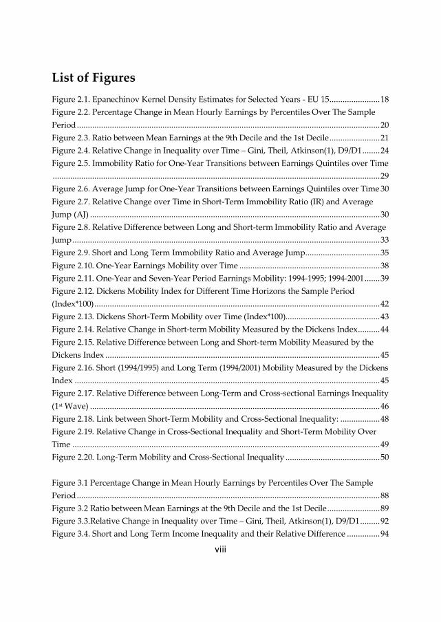
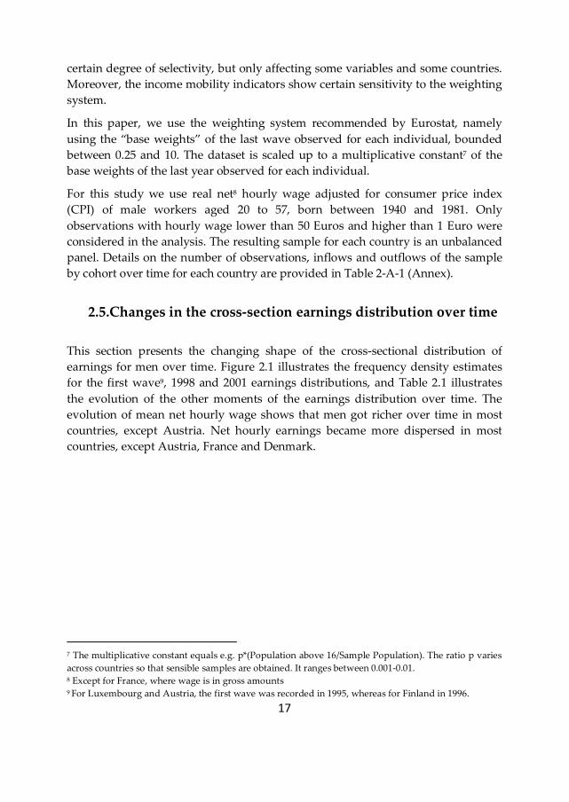
2.5.Changes in the cross-section earnings distribution over time
This section presents the changing shape of the cross-sectional distribution of
earnings for men over time. Figure 2.1 illustrates the frequency density estimates
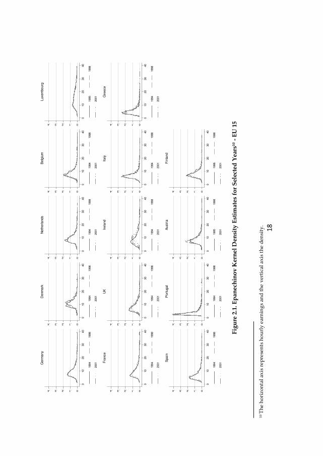
for the first wave9, 1998 and 2001 earnings distributions, and Table 2.1 illustrates
the evolution of the other moments of the earnings distribution over time. The
evolution of mean net hourly wage shows that men got richer over time in most
countries, except Austria. Net hourly earnings became more dispersed in most
countries, except Austria, France and Denmark.
7 The multiplicative constant equals e.g. p*(Population above 16/Sample Population). The ratio p varies
across countries so that sensible samples are obtained. It ranges between 0.001-0.01. 8 Except for France, where wage is in gross amounts 9 For Luxembourg and Austria, the first wave was recorded in 1995, whereas for Finland in 1996.
18
F
igu
re 2
.1. E
pan
ech
ino
v K
ern
el D
ensi
ty E
stim
ates
fo
r S
elec
ted
Yea
rs1
0 -
EU
15
1
0 T
he
ho
riz
on
tal
axis
re
pre
sen
ts h
ou
rly
ear
nin
gs
and
th
e v
erti
cal
ax
is t
he
den
sity
.
0.1.2.3.4
010
20
30
40
1994
1998
2001Ge
rma
ny
0.1.2.3.4
010
20
30
40
1994
1998
2001De
nm
ark
0.1.2.3.4
010
20
30
40
1994
1998
2001
Ne
the
rla
nds
0.1.2.3.4
010
20
30
40
1994
1998
2001B
elg
ium
0.1.2.3.4
010
20
30
40
1995
1998
2001
Luxe
mbo
urg
0.1.2.3.4
010
20
30
40
1994
1998
2001F
rance
0.1.2.3.4
010
20
30
40
1994
1998
2001
UK
0.1.2.3.4
010
20
30
40
1994
1998
2001Ir
ela
nd
0.1.2.3.4
010
20
30
40
1994
1998
2001
Ita
ly
0.1.2.3.4
010
20
30
40
1994
1998
2001G
ree
ce
0.1.2.3.4
010
20
30
40
1994
1998
2001
Spa
in
0.1.2.3.4
010
20
30
40
1994
1998
2001Po
rtuga
l
0.1.2.3.4
010
20
30
40
1995
1998
2001A
ustr
ia
0.1.2.3.4
010
20
30
40
1996
1998
2001F
inla
nd
19
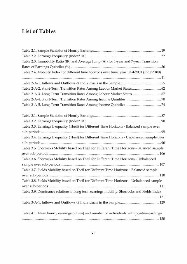
Table 2.1. Sample Statistics of Hourly Earnings
Year 1994 1995 1996 1997 1998 1999 2000 2001
Germany
Mean 9.43 9.49 9.61 9.52 9.57 9.48 9.60 9.72
Median 8.65 8.68 8.78 8.84 8.70 8.65 8.75 8.82
Standard Deviation 4.00 4.17 4.09 4.01 4.39 4.32 4.39 4.37
Denmark
Mean 10.89 11.40 11.58 11.61 11.86 11.85 12.02 12.08
Median 10.36 10.76 10.96 11.14 11.46 11.36 11.77 11.50
Standard Deviation 3.23 3.31 3.52 3.54 3.13 3.31 3.43 3.20
Netherlands
Mean 9.69 9.56 9.59 9.70 10.02 9.88 10.04 9.91
Median 9.11 9.07 9.01 9.10 9.27 9.18 9.32 9.23
Standard Deviation 3.39 3.37 3.55 3.56 3.64 3.40 3.48 3.95
Belgium
Mean 8.48 8.82 8.71 8.75 8.81 8.83 8.92 9.10
Median 7.86 8.17 7.99 8.09 8.08 8.34 8.25 8.30
Standard Deviation 3.17 3.08 3.02 3.09 2.97 2.94 3.00 3.21
Luxembourg
Mean 16.18 15.81 16.73 17.39 17.15 17.22 17.10
Median 14.90 14.52 15.31 15.72 15.60 15.65 15.29
Standard Deviation 7.50 7.19 7.77 8.21 8.38 8.37 8.22
France11
Mean 10.23 9.92 9.87 10.05 10.33 10.60 10.55 10.87
Median 8.56 8.57 8.53 8.53 8.84 9.04 9.06 9.48
Standard Deviation 5.82 5.33 5.17 5.65 5.62 5.78 5.51 5.72
UK
Mean 8.16 8.11 8.22 8.34 8.68 9.01 9.21 9.68
Median 7.30 7.29 7.51 7.52 7.67 8.00 8.22 8.68
Standard Deviation 3.99 3.95 3.80 3.79 4.01 4.13 4.24 4.49
Ireland
Mean 9.30 9.54 9.76 10.02 10.43 10.84 11.69 12.44
Median 8.06 8.44 8.84 8.86 9.33 9.73 10.25 11.36
Standard Deviation 5.14 4.99 4.85 4.98 5.17 5.02 5.24 5.15
Italy
Mean 7.16 6.91 6.96 7.05 7.29 7.37 7.28 7.32
Median 6.65 6.32 6.43 6.48 6.69 6.76 6.59 6.67
Standard Deviation 2.77 2.59 2.67 2.68 3.01 3.00 2.99 3.04
Greece
Mean 4.95 5.03 5.23 5.59 5.63 5.85 5.70 5.77
Median 4.49 4.41 4.53 4.90 4.91 4.99 4.89 4.99
Standard Deviation 2.33 2.42 2.43 2.91 2.87 3.14 3.07 3.21
Spain
Mean 6.83 6.95 7.09 6.89 7.18 7.37 7.45 7.42
Median 5.86 5.82 5.92 5.72 6.04 6.15 6.29 6.33
Standard Deviation 3.81 3.86 4.00 3.92 4.06 4.15 4.07 3.87
Portugal
Mean 3.70 3.74 3.84 3.92 3.99 4.08 4.31 4.46
Median 2.92 2.82 2.98 3.03 3.05 3.08 3.29 3.34
Standard Deviation 2.34 2.45 2.54 2.65 2.81 2.82 3.16 3.33
Austria
Mean 9.08 8.33 8.37 8.49 8.55 8.55 8.54
Median 8.51 7.64 7.63 7.84 7.82 7.86 7.93
Standard Deviation 3.52 3.00 3.07 2.95 2.89 2.84 2.82
Finland
Mean 7.89 8.01 8.41 8.45 8.66 8.86
Median 7.48 7.57 7.85 7.90 8.18 7.97
Standard Deviation 2.70 2.77 2.92 2.91 2.93 3.29
11 Gross Amounts

20
Plotting the percentage change in mean hourly earnings between the beginning of
the sample period and 2001 at each point of the distribution for each country
(Figure 2.2), revealed that, in most countries, the relationship between the
quantile12 rank and growth in real earnings is negative and nearly monotonic: the
higher the rank, the smaller the increase in earnings. This shows that in most
countries, over time, the situation of the low paid people improved to a larger
extent than for the better off ones. In Austria, people at the top of the distribution
experience a decrease in mean hourly wage over time, which might explain the
decrease in the overall mean.
Netherlands, Germany, Greece and Finland diverge in their pattern from the other
EU countries experiencing a higher relative increase in earnings the higher the
rank. Netherlands is the only country where men at the bottom of the income
distribution recorded a deterioration of their work pay. For these countries, the
increase in mean earnings might be the result of an increase in the earnings
position of the better off individuals, not the low paid.
Figure 2.2. Percentage Change in Mean Hourly Earnings by Percentiles Over The Sample
Period Note: Vertical axis – the percentage change in mean hourly earnings; Horizontal axis – percentiles.
12 100 Quantiles
-20
02
04
06
0
10 20 30 40 50 60 70 80 90
Germany Netherlands Belgium
Luxembourg
-20
02
04
06
0
10 20 30 40 50 60 70 80 90
France Austria UK
Ireland Finland Denmark
-20
02
04
06
0
10 20 30 40 50 60 70 80 90
Italy Spain Portugal
Greece
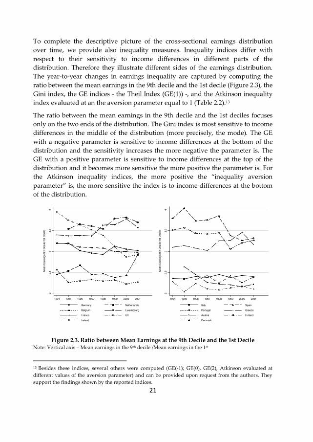
21
To complete the descriptive picture of the cross-sectional earnings distribution
over time, we provide also inequality measures. Inequality indices differ with
respect to their sensitivity to income differences in different parts of the
distribution. Therefore they illustrate different sides of the earnings distribution.
The year-to-year changes in earnings inequality are captured by computing the
ratio between the mean earnings in the 9th decile and the 1st decile (Figure 2.3), the
Gini index, the GE indices - the Theil Index (GE(1)) -, and the Atkinson inequality
index evaluated at an the aversion parameter equal to 1 (Table 2.2).13
The ratio between the mean earnings in the 9th decile and the 1st deciles focuses
only on the two ends of the distribution. The Gini index is most sensitive to income
differences in the middle of the distribution (more precisely, the mode). The GE
with a negative parameter is sensitive to income differences at the bottom of the
distribution and the sensitivity increases the more negative the parameter is. The
GE with a positive parameter is sensitive to income differences at the top of the
distribution and it becomes more sensitive the more positive the parameter is. For
the Atkinson inequality indices, the more positive the “inequality aversion
parameter” is, the more sensitive the index is to income differences at the bottom
of the distribution.
Figure 2.3. Ratio between Mean Earnings at the 9th Decile and the 1st Decile Note: Vertical axis – Mean earnings in the 9th decile /Mean earnings in the 1st
13 Besides these indices, several others were computed (GE(-1); GE(0), GE(2), Atkinson evaluated at
different values of the aversion parameter) and can be provided upon request from the authors. They
support the findings shown by the reported indices.
22.5
33.5
4
Mean E
arn
ings
9th
Deci
le/1
st D
eci
le
1994 1995 1996 1997 1998 1999 2000 2001
Germany Netherlands
Belgium Luxembourg
France UK
Ireland
22.5
33.5
4
Mean E
arn
ings
9th
Deci
le/1
st D
eci
le
1994 1995 1996 1997 1998 1999 2000 2001
Italy Spain
Portugal Greece
Austria Finland
Denmark
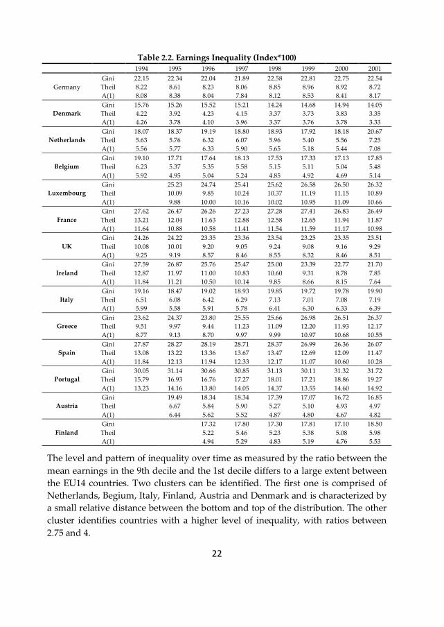
22
Table 2.2. Earnings Inequality (Index*100) 1994 1995 1996 1997 1998 1999 2000 2001
Germany
Gini 22.15 22.34 22.04 21.89 22.58 22.81 22.75 22.54
Theil 8.22 8.61 8.23 8.06 8.85 8.96 8.92 8.72
A(1) 8.08 8.38 8.04 7.84 8.12 8.53 8.41 8.17
Denmark
Gini 15.76 15.26 15.52 15.21 14.24 14.68 14.94 14.05
Theil 4.22 3.92 4.23 4.15 3.37 3.73 3.83 3.35
A(1) 4.26 3.78 4.10 3.96 3.37 3.76 3.78 3.33
Netherlands
Gini 18.07 18.37 19.19 18.80 18.93 17.92 18.18 20.67
Theil 5.63 5.76 6.32 6.07 5.96 5.40 5.56 7.25
A(1) 5.56 5.77 6.33 5.90 5.65 5.18 5.44 7.08
Belgium
Gini 19.10 17.71 17.64 18.13 17.53 17.33 17.13 17.85
Theil 6.23 5.37 5.35 5.58 5.15 5.11 5.04 5.48
A(1) 5.92 4.95 5.04 5.24 4.85 4.92 4.69 5.14
Luxembourg
Gini 25.23 24.74 25.41 25.62 26.58 26.50 26.32
Theil 10.09 9.85 10.24 10.37 11.19 11.15 10.89
A(1) 9.88 10.00 10.16 10.02 10.95 11.09 10.66
France
Gini 27.62 26.47 26.26 27.23 27.28 27.41 26.83 26.49
Theil 13.21 12.04 11.63 12.88 12.58 12.65 11.94 11.87
A(1) 11.64 10.88 10.58 11.41 11.54 11.59 11.17 10.98
UK
Gini 24.26 24.22 23.35 23.36 23.54 23.25 23.35 23.51
Theil 10.08 10.01 9.20 9.05 9.24 9.08 9.16 9.29
A(1) 9.25 9.19 8.57 8.46 8.55 8.32 8.46 8.51
Ireland
Gini 27.59 26.87 25.76 25.47 25.00 23.39 22.77 21.70
Theil 12.87 11.97 11.00 10.83 10.60 9.31 8.78 7.85
A(1) 11.84 11.21 10.50 10.14 9.85 8.66 8.15 7.64
Italy
Gini 19.16 18.47 19.02 18.93 19.85 19.72 19.78 19.90
Theil 6.51 6.08 6.42 6.29 7.13 7.01 7.08 7.19
A(1) 5.99 5.58 5.91 5.78 6.41 6.30 6.33 6.39
Greece
Gini 23.62 24.37 23.80 25.55 25.66 26.98 26.51 26.37
Theil 9.51 9.97 9.44 11.23 11.09 12.20 11.93 12.17
A(1) 8.77 9.13 8.70 9.97 9.99 10.97 10.68 10.55
Spain
Gini 27.87 28.27 28.19 28.71 28.37 26.99 26.36 26.07
Theil 13.08 13.22 13.36 13.67 13.47 12.69 12.09 11.47
A(1) 11.84 12.13 11.94 12.33 12.17 11.07 10.60 10.28
Portugal
Gini 30.05 31.14 30.66 30.85 31.13 30.11 31.32 31.72
Theil 15.79 16.93 16.76 17.27 18.01 17.21 18.86 19.27
A(1) 13.23 14.16 13.80 14.05 14.37 13.55 14.60 14.92
Austria
Gini 19.49 18.34 18.34 17.39 17.07 16.72 16.85
Theil 6.67 5.84 5.90 5.27 5.10 4.93 4.97
A(1) 6.44 5.62 5.52 4.87 4.80 4.67 4.82
Finland
Gini 17.32 17.80 17.30 17.81 17.10 18.50
Theil 5.22 5.46 5.23 5.38 5.08 5.98
A(1) 4.94 5.29 4.83 5.19 4.76 5.53
The level and pattern of inequality over time as measured by the ratio between the
mean earnings in the 9th decile and the 1st decile differs to a large extent between
the EU14 countries. Two clusters can be identified. The first one is comprised of
Netherlands, Begium, Italy, Finland, Austria and Denmark and is characterized by
a small relative distance between the bottom and top of the distribution. The other
cluster identifies countries with a higher level of inequality, with ratios between
2.75 and 4.

23
In 1994, based on the Gini index, Portugal is the most unequal, followed by Spain,
France, Ireland, UK, Greece, Germany, Italy, Belgium, Netherlands and Denmark.
In general, the other two indices confirm this ranking. However, using the Theil
index, France appears to be more unequal than Spain, whereas using the Atkinson
index, Ireland appears to be more unequal than France and as equal as Spain.
In 2001, based on the Gini index, Portugal is still the most unequal, followed by
France, Greece, Luxembourg, Spain, UK, Germany, Ireland, Netherlands, Italy,
Finland, Belgium, Austria and Denmark. In general, the other two indices confirm
this ranking. Based on Theil, however, Greece is more unequal than France, and
Spain than Luxembourg. Based on Atkinson, Luxembourg is more unequal than
Greece.
For most countries, all indices show a consistent story regarding the evolution of
inequality over the sample period, except for Germany, France and Portugal,
where the evolution of the Gini, Theil and Atkinson index is opposite to the one
observed for the D9/D1. Based on Gini, Theil and Atkinson, Netherlands, Greece,
Finland, Portugal, Luxembourg, Italy and Germany recorded an increase in yearly
inequality, and the rest a decrease.
The relative evolution over the sample period is captured in Figure 2.4, which
illustrates for each country, the change in inequality as measured by Gini, Theil,
Atkinson index and the D9/D1. Based on Gini, the highest increase in inequality
was recorded by Netherlands (around 15%), followed by Greece, Finland,
Portugal, Luxembourg, Italy and Germany. The highest decrease was recorded in
Ireland (around 20%), followed by Austria, Denmark, Belgium, Spain, France and
UK. Based on the Theil index, Portugal records a higher increase than Finland,
Italy a higher increase than Luxembourg and Spain a higher decrease than
Belgium. Based on Atkinson index, Portugal records a higher increase than Finland
and UK a higher decrease than France.
For Netherlands, Finland and Greece the increase in the distance between the top
and bottom of the distribution and in the overall level of inequality can be
explained by the improved earnings position of the better off individuals. Hence in
these countries, the economic growth benefitted the high income people and led to
an increase in earnings inequality.
Luxembourg and Italy recorded an increase in inequality based on all indices, but
the situation at the bottom improved to a larger extent than for the top. Thus the
increase in inequality might be the result of other forces affecting the distribution,
such as mobility in the bottom and top deciles.
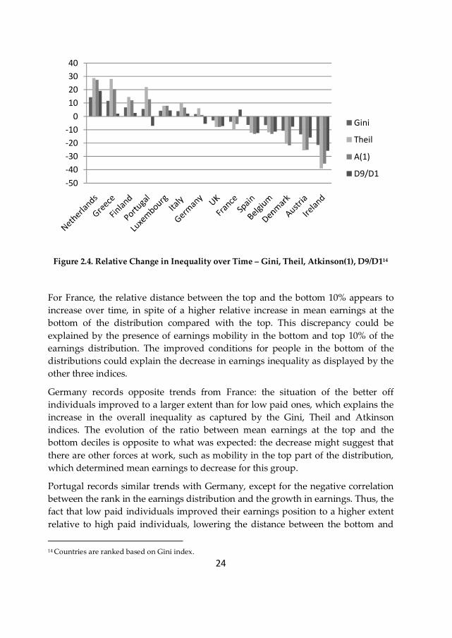
24
Figure 2.4. Relative Change in Inequality over Time – Gini, Theil, Atkinson(1), D9/D114
For France, the relative distance between the top and the bottom 10% appears to
increase over time, in spite of a higher relative increase in mean earnings at the
bottom of the distribution compared with the top. This discrepancy could be
explained by the presence of earnings mobility in the bottom and top 10% of the
earnings distribution. The improved conditions for people in the bottom of the
distributions could explain the decrease in earnings inequality as displayed by the
other three indices.
Germany records opposite trends from France: the situation of the better off
individuals improved to a larger extent than for low paid ones, which explains the
increase in the overall inequality as captured by the Gini, Theil and Atkinson
indices. The evolution of the ratio between mean earnings at the top and the
bottom deciles is opposite to what was expected: the decrease might suggest that
there are other forces at work, such as mobility in the top part of the distribution,
which determined mean earnings to decrease for this group.
Portugal records similar trends with Germany, except for the negative correlation
between the rank in the earnings distribution and the growth in earnings. Thus, the
fact that low paid individuals improved their earnings position to a higher extent
relative to high paid individuals, lowering the distance between the bottom and
14 Countries are ranked based on Gini index.
-50
-40
-30
-20
-10
0
10
20
30
40
Gini
Theil
A(1)
D9/D1

25
the top deciles of the earnings distribution did not have the expected effect of
lowering overall earnings inequality as measured by the Gini, Theil and Atkinson
indices. Mobility is expected to be the factor counteracting all these movements.
For the rest of the countries, the increase in the overall mean, coupled with the
higher relative increase in the earnings position of the low paid individuals
compared with high earnings individuals can be an explanation for their decrease
in inequality.
Besides the direction of evolution, also the magnitude of the change records
differences among inequality indices. In general, the magnitude of the change is
the highest for the index that is most sensitive to the income differences at the top
of the distribution, followed by bottom and middle sensitive one, sign that most of
the major changes happened at the top and the bottom of the distribution. There
are a few exceptions. In UK, Spain, Belgium and Denmark the magnitude of the
evolution is the highest for the bottom sensitive one, followed by the top and
middle ones.
2.6. Linking earnings inequality and mobility: individual
movements within the distribution over time
When analysing the change in the distribution of earnings, one has to pay attention
to two basic characteristics. First, how far apart are individuals in terms of their
wage and to what extent does the ranking of each individual change from one
period to the next. Section 2.5 offered a broad overview of the first characteristic.
This section focuses on the second one and analyses the intra-distributional
mobility of earnings over the period 1994 – 2001.
2.6.1. Mobility among labour market states
To understand mobility patterns over time, it is informative to inspect mobility
both within the wage distribution and into and out of the distribution to other
employment states. For this purpose, we compute the quintiles of the wage
distribution and present short-term and long-term transitions both between
quintiles and to other employment states. 15
Table 2-A-2 (Annex) presents one-year period transition matrices for men between
the first and second wave and between 2000 and 2001. For all countries, one-year
15 Short-term transitions are defined as transitions from one year to the next. Long-term transitions are
defined as transitions from the first to the last wave.
26
labour market transition matrices portray a picture of persistence, with little short-
term mobility. The diagonal elements of these matrices are much higher than the
off-diagonal elements, suggesting a low degree of mobility from one period to the
next, both in terms of quintiles of the earnings distribution and in states outside of
employment. The concentration around the diagonal decreases the further one
moves from the diagonal, indicating that those individuals that do change their
labour market position from one period to the next, do not move very far.
In most countries, individuals in the lowest two quintiles are more likely to enter
unemployment and inactivity compared with the rest of the distribution.
Netherlands is an exception, where the top and the bottom of the distribution have
similar high rates of entering unemployment and inactivity. Similarly, those
unemployed and inactive that manage to get a job in the next period are more
likely to enter the lower quintiles of the distribution. These findings are consistent
with previous findings, for example Dickens (2000a) for UK over the period 1975-
1994.
In the beginning of the sample period, the highest short-term persistence in
unemployment was recorded in Ireland, Luxembourg, Italy, Finland, Belgium and
Austria where between 62.45% and 50.63% kept their status from one year to the
next, followed by Spain and Netherlands with 46% and 42.92%, and Germany,
UK, Greece, Portugal, France and Denmark with rates between 39.42% and 34%.
The highest persistency in inactivity was recorded in France, Belgium, Ireland and
Portugal where more than half kept the same status in 1995. Over time, short-term
mobility out of unemployment increased in Luxembourg, Ireland, Italy, Spain,
Portugal, Austria and Finland, whereas short-term mobility out of inactivity
increased only in Belgium, France and UK.
Looking at the pattern of mobility over a longer time span (Table 2-A-3, Annex),
mobility measured over the whole sample period is higher than one-period
mobility: the concentration along the diagonal is much less than when measured
over one year. These trends are consistent with previous findings. (Atkinson et al.,
1992; OECD, 1996; Dickens, 2000a) The highest long-term persistency in
unemployment is found in Belgium, UK, Italy, Germany and Spain, where
between 23% and 12% maintained their status in 2001. The highest persistency in
inactivity is in France, Belgium, Portugal, Spain, Netherlands and Ireland with
rates between 29% and 23%.
27
2.6.2. The transition matrix approach to mobility among
income quintiles
Having introduced the general picture of mobility between different labour market
states, the next step is to explore short and long-term mobility between income
classes, as well as how short-term earnings mobility patterns changed over time.
Short-term earnings transition matrices (Table 2-A-4, Annex) portray a picture of
persistence, with little mobility over a one-year period: the diagonal elements of
these matrices are much higher than the off-diagonal elements. All rows display
high predictability and origin dependence (the transition probabilities are not
equal) meaning that the position in the earnings distribution in the next period
depends heavily on the initial state. The concentration around the diagonal
decreases the further one moves from the diagonal, indicating that those
individuals that do change their income position from one period to the next, do
not move very far. For all countries, short-term persistency appears to be the
highest for the top quintile, followed by the bottom and middle ones.
Of those in the lowest quintile in the first wave, the highest percentage of people
that are still in the lowest quintile one year later is recorded in Luxembourg
(76.59%), followed by Germany (71.28%), Italy, France, Finland, Netherlands and
Ireland, with values between 60% and 70%, and Portugal, Austria, UK, Denmark,
Spain, Belgium and Greece, with values between 50% and 60%.
For the middle quintile, in the first wave, the highest mobility is observed in
Austria, where 27.53% maintained their state from one year to the next, followed
by Denmark (32.22%), Greece, Finland, Spain, Italy, Belgium, Ireland and Germany
with a persistency between 40% and 50%, France, UK and Portugal with values
between 50% and 55%, and finally Luxembourg, where 68.15% of those in the
middle quintile in the first wave maintained their earnings position in the next
period.
For the top quintile, Portugal, followed by Germany, UK, Netherlands, Ireland,
Spain record the highest persistency in the first wave, with a probability of over
80% of remaining in the same state one year later. Next follow Luxembourg,
Belgium, Italy, France and Finland, with a probability between 80% and 70%,
Austria, Denmark and Greece, with a probability between 70% and 60%.
Over time, short-term income mobility for individuals belonging to the first
quintile decreased in all countries, with three exceptions: Luxembourg, Spain and
Finland. This decrease in short-term mobility over time suggests that in 2000-2001,
low paid individuals find more difficult to move up the income distribution
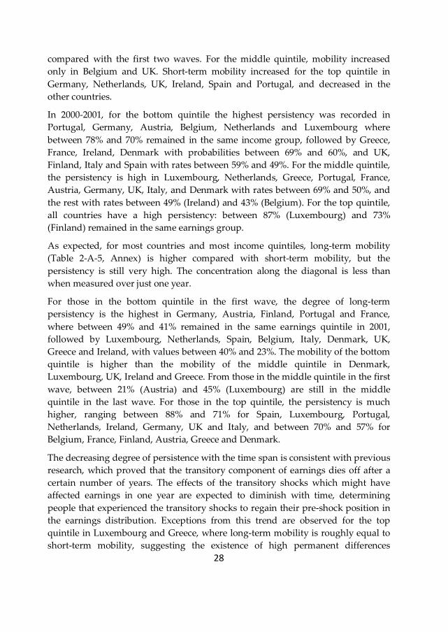
28
compared with the first two waves. For the middle quintile, mobility increased
only in Belgium and UK. Short-term mobility increased for the top quintile in
Germany, Netherlands, UK, Ireland, Spain and Portugal, and decreased in the
other countries.
In 2000-2001, for the bottom quintile the highest persistency was recorded in
Portugal, Germany, Austria, Belgium, Netherlands and Luxembourg where
between 78% and 70% remained in the same income group, followed by Greece,
France, Ireland, Denmark with probabilities between 69% and 60%, and UK,
Finland, Italy and Spain with rates between 59% and 49%. For the middle quintile,
the persistency is high in Luxembourg, Netherlands, Greece, Portugal, France,
Austria, Germany, UK, Italy, and Denmark with rates between 69% and 50%, and
the rest with rates between 49% (Ireland) and 43% (Belgium). For the top quintile,
all countries have a high persistency: between 87% (Luxembourg) and 73%
(Finland) remained in the same earnings group.
As expected, for most countries and most income quintiles, long-term mobility
(Table 2-A-5, Annex) is higher compared with short-term mobility, but the
persistency is still very high. The concentration along the diagonal is less than
when measured over just one year.
For those in the bottom quintile in the first wave, the degree of long-term
persistency is the highest in Germany, Austria, Finland, Portugal and France,
where between 49% and 41% remained in the same earnings quintile in 2001,
followed by Luxembourg, Netherlands, Spain, Belgium, Italy, Denmark, UK,
Greece and Ireland, with values between 40% and 23%. The mobility of the bottom
quintile is higher than the mobility of the middle quintile in Denmark,
Luxembourg, UK, Ireland and Greece. From those in the middle quintile in the first
wave, between 21% (Austria) and 45% (Luxembourg) are still in the middle
quintile in the last wave. For those in the top quintile, the persistency is much
higher, ranging between 88% and 71% for Spain, Luxembourg, Portugal,
Netherlands, Ireland, Germany, UK and Italy, and between 70% and 57% for
Belgium, France, Finland, Austria, Greece and Denmark.
The decreasing degree of persistence with the time span is consistent with previous
research, which proved that the transitory component of earnings dies off after a
certain number of years. The effects of the transitory shocks which might have
affected earnings in one year are expected to diminish with time, determining
people that experienced the transitory shocks to regain their pre-shock position in
the earnings distribution. Exceptions from this trend are observed for the top
quintile in Luxembourg and Greece, where long-term mobility is roughly equal to
short-term mobility, suggesting the existence of high permanent differences
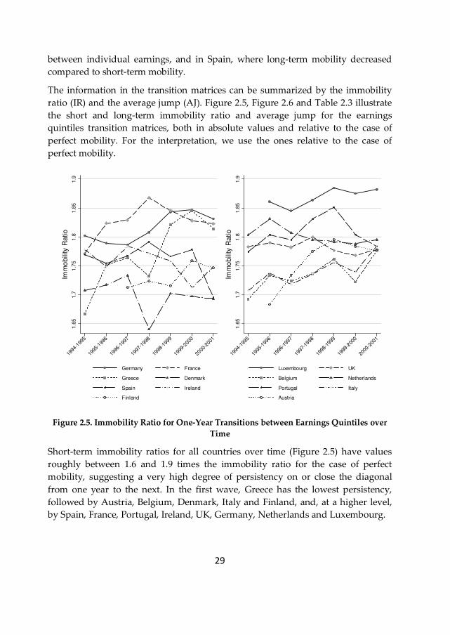
29
between individual earnings, and in Spain, where long-term mobility decreased
compared to short-term mobility.
The information in the transition matrices can be summarized by the immobility
ratio (IR) and the average jump (AJ). Figure 2.5, Figure 2.6 and Table 2.3 illustrate
the short and long-term immobility ratio and average jump for the earnings
quintiles transition matrices, both in absolute values and relative to the case of
perfect mobility. For the interpretation, we use the ones relative to the case of
perfect mobility.
Figure 2.5. Immobility Ratio for One-Year Transitions between Earnings Quintiles over
Time
Short-term immobility ratios for all countries over time (Figure 2.5) have values
roughly between 1.6 and 1.9 times the immobility ratio for the case of perfect
mobility, suggesting a very high degree of persistency on or close the diagonal
from one year to the next. In the first wave, Greece has the lowest persistency,
followed by Austria, Belgium, Denmark, Italy and Finland, and, at a higher level,
by Spain, France, Portugal, Ireland, UK, Germany, Netherlands and Luxembourg.
1.6
51.7
1.7
51
.81
.85
1.9
Imm
obili
ty R
atio
1994
-199
5
1995
-199
6
1996
-199
7
1997
-199
8
1998
-199
9
1999
-200
0
2000
-200
1
Germany France
Greece Denmark
Spain Ireland
Finland
1.6
51.7
1.7
51
.81
.85
1.9
Imm
obili
ty R
atio
1994
-199
5
1995
-199
6
1996
-199
7
1997
-1998
1998
-1999
1999
-200
0
2000
-200
1
Luxembourg UK
Belgium Netherlands
Portugal Italy
Austria
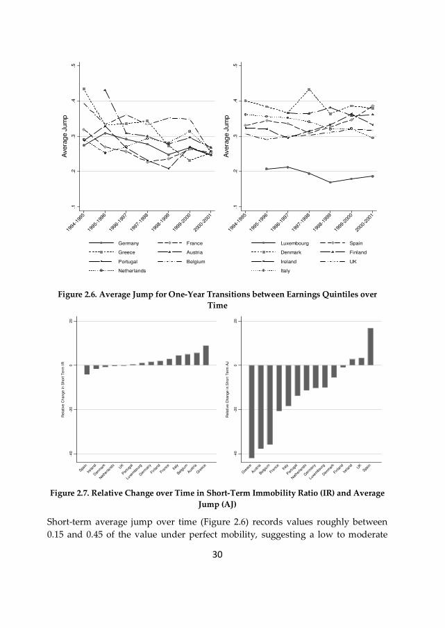
30
Figure 2.6. Average Jump for One-Year Transitions between Earnings Quintiles over
Time
Figure 2.7. Relative Change over Time in Short-Term Immobility Ratio (IR) and Average
Jump (AJ)
Short-term average jump over time (Figure 2.6) records values roughly between
0.15 and 0.45 of the value under perfect mobility, suggesting a low to moderate
.1.2
.3.4
.5
Avera
ge J
um
p
1994
-199
5
1995
-199
6
1996
-199
7
1997
-199
8
1998
-199
9
1999
-200
0
2000
-200
1
Germany France
Greece Austria
Portugal Belgium
Netherlands
.1.2
.3.4
.5
Avera
ge J
um
p19
94-1
995
1995
-199
6
1996
-199
7
1997
-199
8
1998
-199
9
1999
-200
0
2000
-200
1
Luxembourg Spain
Denmark Finland
Ireland UK
Italy
-40
-20
020
Rela
tive C
hange in S
hort
Term
IR
Spa
in
Ireland
Den
mar
k
Neth
erland
sUK
Por
tugal
Luxem
bour
g
Germ
any
Finland
Franc
eIta
ly
Belgium
Aus
tria
Gre
ece
-40
-20
020
Rela
tive C
hange in S
hort
Term
AJ
Gre
ece
Aust
ria
Belg
ium
Franc
eIta
ly
Por
tuga
l
Netherla
nds
Germ
any
Luxem
bourg
Denm
ark
Finland
Ireland
UK
Spa
in
31
degree of mobility outside the diagonal for all countries. In the first wave, the
lowest average jump is recorded in Luxembourg (above 0.2), followed by
Germany, Portugal and Netherlands (with values close to 0.3), UK, France, Ireland,
Spain, Italy, Finland, and Belgium (with values between 0.3 and 0.4), and
Denmark, Austria and Greece (with values greater than 0.4).( Figure 2.6 and Table
2.3)
As illustrated in Figure 2.5 and Figure 2.6, some countries recorded a decrease and
others an increase in short-term mobility over time. In general, over time, the
evolution of the immobility ratio is negatively associated with the evolution of the
average jump: the larger the decrease in the share of individuals staying in the
same quintile or entering the quintile immediately above/below (decrease in the
immobility ratio), the larger the increase in mobility away from the diagonal
(increase in average jump), and vice versa.
Greece, Austria, Belgium, France, Italy, Portugal, Germany, Luxembourg and
Finland recorded a decrease in the average jump and an increase in the immobility
ratio, suggesting that over time the degree of movement in the earnings
distribution decreased leading to a high concentration on and close to the main
diagonal. As captured in Figure 2.7, the magnitude of the evolution is the highest
in the first five countries, ranging between 9% and 3% for the immobility ratio, and
41% and 18% for the average jump.
The relative decrease in mobility as measured by the average jump is higher than
the relative decrease in mobility as measured by the immobility ratio, suggesting
that the degree of movement away from the initial earnings position decreased to a
higher extent than the increase in the share of individuals who maintained their
earnings status or moved in the position immediately above/below. Thus the off-
diagonal transition probabilities are shrinking towards the main diagonal at a
higher rate than captured by the immobility ratio, signalling an increase in the
share of individuals who maintained their status from one period to the next. An
exception is Finland, where the relative decrease in the average jump is low, and
slightly smaller than the relative increase in the immobility ratio, sign of a small
increase in the share of individuals which maintained their income class from one
period to the next between 1st wave – 2nd wave and 2000-2001.
Among the countries recording an increase in earnings mobility, Spain has the
largest decrease in the immobility ratio (4%) and the largest increase in average
jump (16.8%), sign of increased mobility throughout the earnings distribution. In
the same category we find Ireland and UK, but with a lower magnitude of the
evolution (around 0.3%-1% for the immobility ratio and 3%-4% for AJ). The
relative increase in the average jump is higher than the relative decrease in the
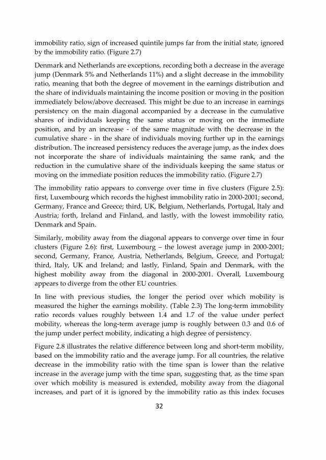
32
immobility ratio, sign of increased quintile jumps far from the initial state, ignored
by the immobility ratio. (Figure 2.7)
Denmark and Netherlands are exceptions, recording both a decrease in the average
jump (Denmark 5% and Netherlands 11%) and a slight decrease in the immobility
ratio, meaning that both the degree of movement in the earnings distribution and
the share of individuals maintaining the income position or moving in the position
immediately below/above decreased. This might be due to an increase in earnings
persistency on the main diagonal accompanied by a decrease in the cumulative
shares of individuals keeping the same status or moving on the immediate
position, and by an increase - of the same magnitude with the decrease in the
cumulative share - in the share of individuals moving further up in the earnings
distribution. The increased persistency reduces the average jump, as the index does
not incorporate the share of individuals maintaining the same rank, and the
reduction in the cumulative share of the individuals keeping the same status or
moving on the immediate position reduces the immobility ratio. (Figure 2.7)
The immobility ratio appears to converge over time in five clusters (Figure 2.5):
first, Luxembourg which records the highest immobility ratio in 2000-2001; second,
Germany, France and Greece; third, UK, Belgium, Netherlands, Portugal, Italy and
Austria; forth, Ireland and Finland, and lastly, with the lowest immobility ratio,
Denmark and Spain.
Similarly, mobility away from the diagonal appears to converge over time in four
clusters (Figure 2.6): first, Luxembourg – the lowest average jump in 2000-2001;
second, Germany, France, Austria, Netherlands, Belgium, Greece, and Portugal;
third, Italy, UK and Ireland; and lastly, Finland, Spain and Denmark, with the
highest mobility away from the diagonal in 2000-2001. Overall, Luxembourg
appears to diverge from the other EU countries.
In line with previous studies, the longer the period over which mobility is
measured the higher the earnings mobility. (Table 2.3) The long-term immobility
ratio records values roughly between 1.4 and 1.7 of the value under perfect
mobility, whereas the long-term average jump is roughly between 0.3 and 0.6 of
the jump under perfect mobility, indicating a high degree of persistency.
Figure 2.8 illustrates the relative difference between long and short-term mobility,
based on the immobility ratio and the average jump. For all countries, the relative
decrease in the immobility ratio with the time span is lower than the relative
increase in the average jump with the time span, suggesting that, as the time span
over which mobility is measured is extended, mobility away from the diagonal
increases, and part of it is ignored by the immobility ratio as this index focuses
33
only on the near-diagonal entries. Thus the longer the time period, the more likely
it is that people move away from their initial state, and the degree of movement
among the income quintiles increases to a larger extent than the relative reduction
in the share of individuals maintaining the same status or moving in the position
immediately below/above.
The ranking of the countries based on the relative difference between long and
short-term mobility reveals that the relative change in the average jump with the
time horizon is negatively associated with the relative change in the immobility
ratio with the time horizon.
Figure 2.8. Relative Difference between Long and Short-term Immobility Ratio and
Average Jump
The first six countries which record the highest drop in the immobility ratio with
the time horizon are among the first seven countries with the highest increase in
the average jump. It is the case of Denmark, Ireland, UK, Germany, Netherlands
and Portugal. Denmark appears to record the highest decrease in persistency close
to the main diagonal (approximately 17%), whereas the increase in mobility away
from the diagonal is of almost 55%. Ireland, which has a similar decrease in the
immobility ratio, has the highest increase in the average jump, almost 90%. UK,
Germany, Portugal and Netherlands record a relatively smaller reduction in the
immobility ratio (between 11% and 14%) than Denmark and Ireland, and a higher
increase in the average jump (over 60%) than Denmark, but lower than Ireland.
Thus this countries record the largest relative increases in the degree of movement
in the earnings distribution and the largest relative decreases in the degree of
persistency on and close to the diagonal as the horizon over which mobility is
measured is extended.
-20
-15
-10
-50
Re
lative
Diffe
ren
ce
Btw
Lo
ng
an
d S
ho
rt T
erm
IR
Den
mar
k
Irela
nd UK
Ger
man
y
Neth
erlands
Portugal
Italy
Spa
in
Finla
nd
Austri
a
Belgium
Gre
ece
Franc
e
Luxe
mbo
urg
02
04
06
08
01
00
Re
lative
Diffe
ren
ce
Btw
Lo
ng
an
d S
ho
rt T
erm
AJ
Austria
Gre
ece
Spa
in
Belgiu
m
Finland
France
Italy
Denm
ark
Net
herla
nds UK
Ger
man
y
Portu
gal
Luxe
mbou
rg
Irela
nd
34
These countries are followed by Italy, Spain, Finland, Belgium, Greece and France,
which record a smaller decrease in the immobility ratio (between 6% and 11%) and
a smaller increase of in the average jump (roughly between 40% and 50%). Thus
these countries exhibit a higher degree of earnings persistency compared with the
previous country cluster. Austria records the lowest increase in the average jump
(around 25%) and the 5th decrease in the immobility ratio (around 9%).
Luxembourg stands out, recording the lowest decrease (around 6%) in the long-
term immobility ratio relative to the short-term immobility ratio, and among the
highest increases (over 70%) in the long-term average jump relative to the short-
term average jump, suggesting that when the horizon is extended, the share of
individuals who “escape” their rank moving further away from it increases to a
much smaller extent compared with the relative increase in their degree of
movement. Thus, long-term, there are slightly more people that move further away
from their initial position, but their degree of movement in the earnings
distribution is relatively much higher compared with short-term.
In the long run (Figure 2.9), Luxembourg and France appear to be the least mobile,
and Denmark and Ireland the most mobile, confirmed by both indices. In between,
in ascending order based on the average jump we find Spain, Germany,
Netherlands, Portugal, UK, Finland, Austria, Italy, Belgium and Greece. The long-
term immobility ratios have similar values among countries, whereas for the
average jump more heterogeneity is observed. Overall, we observed less
heterogeneity with respect to long-term mobility rates compared with short-term
rates, suggesting that over the lifetime earnings mobility rates are expected to
converge to similar levels in most countries. The convergence is expected to be
more evident for the immobility ratio than for the average jump. (Figure 2.9)
35
Figure 2.9. Short and Long Term Immobility Ratio and Average Jump
Note: The value for Luxembourg and Austria illustrate mobility over a period of 6 years, and for
Finland over 5 years.
0.5
11
.52
Den
mar
k
Irela
nd
Austria
Italy
Gre
ece
Belgiu
m UK
Finla
nd
Portu
gal
Ger
man
y
Spain
Net
herla
nds
Franc
e
Luxem
bour
g
Short Term Immobility Ratio Long Term Immobility Ratio
0.2
.4.6
Luxe
mbou
rg
Franc
e
Spain
Germ
any
Neth
erlands
Portu
gal UK
Finla
nd
Austri
aIta
ly
Belgiu
m
Gre
ece
Ireland
Denm
ark
Short Term Average Jump Long Term Average Jump
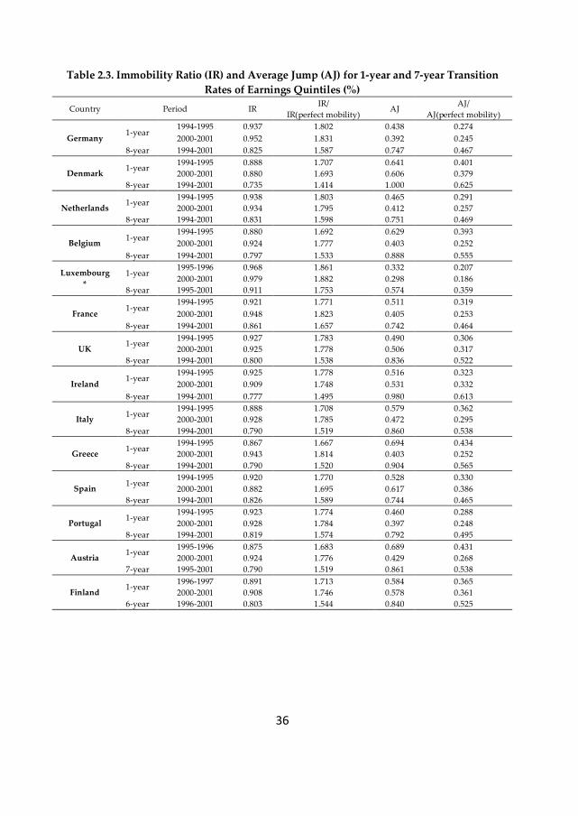
36
Table 2.3. Immobility Ratio (IR) and Average Jump (AJ) for 1-year and 7-year Transition
Rates of Earnings Quintiles (%)
Country Period IR IR/
IR(perfect mobility) AJ
AJ/
AJ(perfect mobility)
Germany 1-year
1994-1995 0.937 1.802 0.438 0.274
2000-2001 0.952 1.831 0.392 0.245
8-year 1994-2001 0.825 1.587 0.747 0.467
Denmark 1-year
1994-1995 0.888 1.707 0.641 0.401
2000-2001 0.880 1.693 0.606 0.379
8-year 1994-2001 0.735 1.414 1.000 0.625
Netherlands 1-year
1994-1995 0.938 1.803 0.465 0.291
2000-2001 0.934 1.795 0.412 0.257
8-year 1994-2001 0.831 1.598 0.751 0.469
Belgium 1-year
1994-1995 0.880 1.692 0.629 0.393
2000-2001 0.924 1.777 0.403 0.252
8-year 1994-2001 0.797 1.533 0.888 0.555
Luxembourg
*
1-year 1995-1996 0.968 1.861 0.332 0.207
2000-2001 0.979 1.882 0.298 0.186
8-year 1995-2001 0.911 1.753 0.574 0.359
France 1-year
1994-1995 0.921 1.771 0.511 0.319
2000-2001 0.948 1.823 0.405 0.253
8-year 1994-2001 0.861 1.657 0.742 0.464
UK 1-year
1994-1995 0.927 1.783 0.490 0.306
2000-2001 0.925 1.778 0.506 0.317
8-year 1994-2001 0.800 1.538 0.836 0.522
Ireland 1-year
1994-1995 0.925 1.778 0.516 0.323
2000-2001 0.909 1.748 0.531 0.332
8-year 1994-2001 0.777 1.495 0.980 0.613
Italy 1-year
1994-1995 0.888 1.708 0.579 0.362
2000-2001 0.928 1.785 0.472 0.295
8-year 1994-2001 0.790 1.519 0.860 0.538
Greece 1-year
1994-1995 0.867 1.667 0.694 0.434
2000-2001 0.943 1.814 0.403 0.252
8-year 1994-2001 0.790 1.520 0.904 0.565
Spain 1-year
1994-1995 0.920 1.770 0.528 0.330
2000-2001 0.882 1.695 0.617 0.386
8-year 1994-2001 0.826 1.589 0.744 0.465
Portugal 1-year
1994-1995 0.923 1.774 0.460 0.288
2000-2001 0.928 1.784 0.397 0.248
8-year 1994-2001 0.819 1.574 0.792 0.495
Austria 1-year
1995-1996 0.875 1.683 0.689 0.431
2000-2001 0.924 1.776 0.429 0.268
7-year 1995-2001 0.790 1.519 0.861 0.538
Finland 1-year
1996-1997 0.891 1.713 0.584 0.365
2000-2001 0.908 1.746 0.578 0.361
6-year 1996-2001 0.803 1.544 0.840 0.525
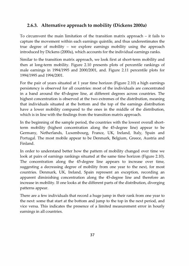
37
2.6.3. Alternative approach to mobility (Dickens 2000a)
To circumvent the main limitation of the transition matrix approach – it fails to
capture the movement within each earnings quintile, and thus underestimates the
true degree of mobility – we explore earnings mobility using the approach
introduced by Dickens (2000a), which accounts for the individual earnings ranks.
Similar to the transition matrix approach, we look first at short-term mobility and
then at long-term mobility. Figure 2.10 presents plots of percentile rankings of
male earnings in 1994/1995 and 2000/2001, and. Figure 2.11 percentile plots for
1994/1995 and 1994/2001.
For the pair of years situated at 1 year time horizon (Figure 2.10) a high earnings
persistency is observed for all countries: most of the individuals are concentrated
in a band around the 45-degree line, at different degrees across countries. The
highest concentration is observed at the two extremes of the distribution, meaning
that individuals situated at the bottom and the top of the earnings distribution
have a lower mobility compared to the ones in the middle of the distribution,
which is in line with the findings from the transition matrix approach.
In the beginning of the sample period, the countries with the lowest overall short-
term mobility (highest concentration along the 45-degree line) appear to be
Germany, Netherlands, Luxembourg, France, UK, Ireland, Italy, Spain and
Portugal. The most mobile appear to be Denmark, Belgium, Greece, Austria and
Finland.
In order to understand better how the pattern of mobility changed over time we
look at pairs of earnings rankings situated at the same time horizon (Figure 2.10).
The concentration along the 45-degree line appears to increase over time,
suggesting a decreasing degree of mobility from one year to the next, for most
countries. Denmark, UK, Ireland, Spain represent an exception, recording an
apparent diminishing concentration along the 45-degree line and therefore an
increase in mobility. If one looks at the different parts of the distribution, diverging
patterns appear.
There are a few individuals that record a huge jump in their rank from one year to
the next: some that start at the bottom and jump to the top in the next period, and
vice versa. This indicates the presence of a limited measurement error in hourly
earnings in all countries.
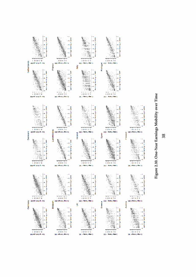
38
Fig
ure
2.1
0. O
ne-
Yea
r E
arn
ing
s M
ob
ilit
y o
ver
Tim
e
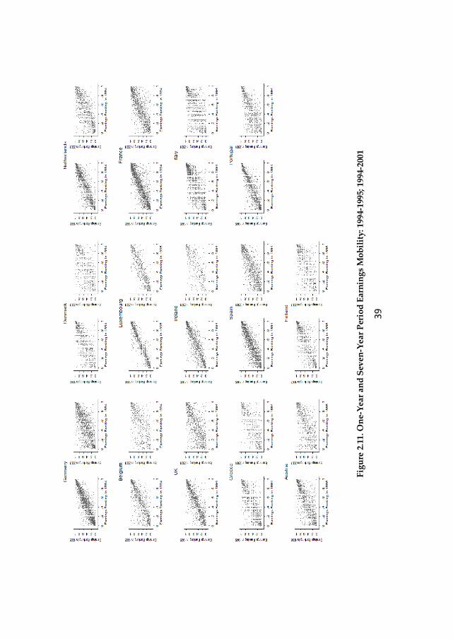
39
Fig
ure
2.1
1. O
ne-
Yea
r an
d S
even
-Yea
r P
erio
d E
arn
ing
s M
ob
ilit
y: 1
994-
1995
; 199
4-20
01
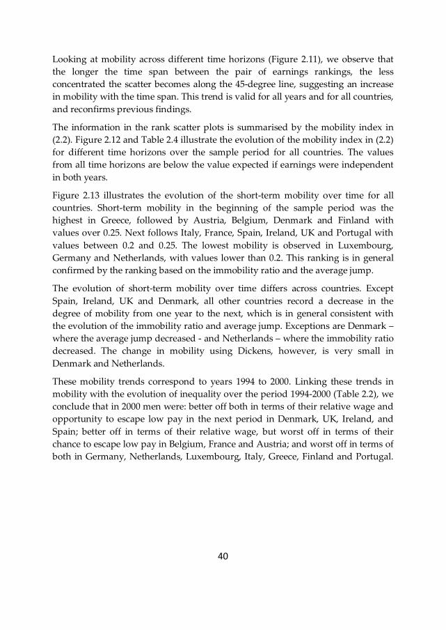
40
Looking at mobility across different time horizons (Figure 2.11), we observe that
the longer the time span between the pair of earnings rankings, the less
concentrated the scatter becomes along the 45-degree line, suggesting an increase
in mobility with the time span. This trend is valid for all years and for all countries,
and reconfirms previous findings.
The information in the rank scatter plots is summarised by the mobility index in
(2.2). Figure 2.12 and Table 2.4 illustrate the evolution of the mobility index in (2.2)
for different time horizons over the sample period for all countries. The values
from all time horizons are below the value expected if earnings were independent
in both years.
Figure 2.13 illustrates the evolution of the short-term mobility over time for all
countries. Short-term mobility in the beginning of the sample period was the
highest in Greece, followed by Austria, Belgium, Denmark and Finland with
values over 0.25. Next follows Italy, France, Spain, Ireland, UK and Portugal with
values between 0.2 and 0.25. The lowest mobility is observed in Luxembourg,
Germany and Netherlands, with values lower than 0.2. This ranking is in general
confirmed by the ranking based on the immobility ratio and the average jump.
The evolution of short-term mobility over time differs across countries. Except
Spain, Ireland, UK and Denmark, all other countries record a decrease in the
degree of mobility from one year to the next, which is in general consistent with
the evolution of the immobility ratio and average jump. Exceptions are Denmark –
where the average jump decreased - and Netherlands – where the immobility ratio
decreased. The change in mobility using Dickens, however, is very small in
Denmark and Netherlands.
These mobility trends correspond to years 1994 to 2000. Linking these trends in
mobility with the evolution of inequality over the period 1994-2000 (Table 2.2), we
conclude that in 2000 men were: better off both in terms of their relative wage and
opportunity to escape low pay in the next period in Denmark, UK, Ireland, and
Spain; better off in terms of their relative wage, but worst off in terms of their
chance to escape low pay in Belgium, France and Austria; and worst off in terms of
both in Germany, Netherlands, Luxembourg, Italy, Greece, Finland and Portugal.
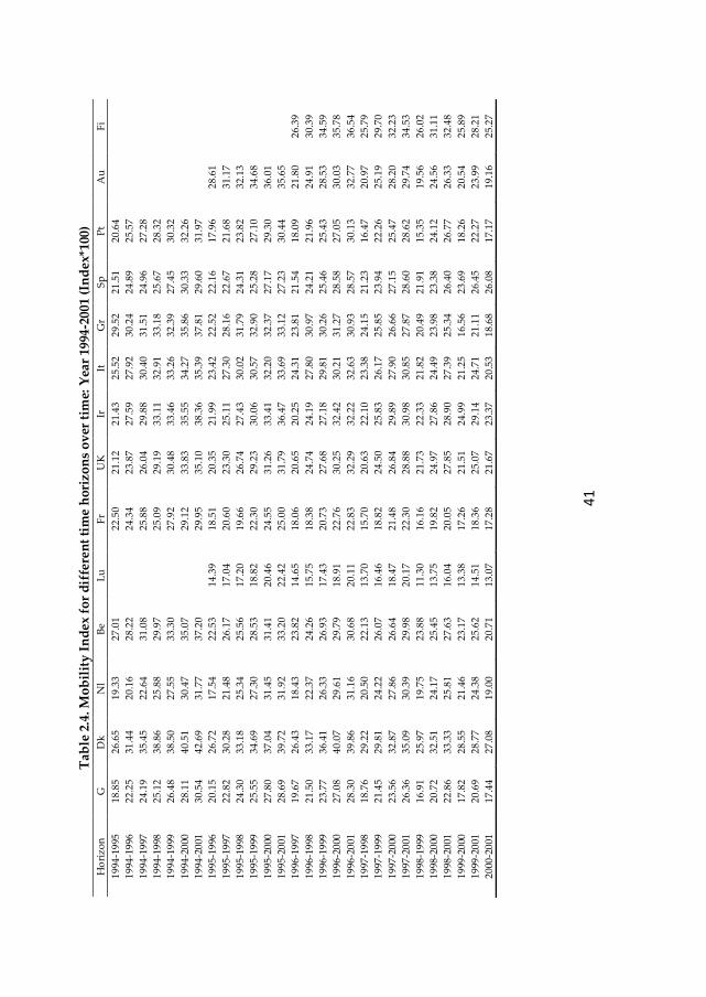
41
Tab
le 2
.4. M
ob
ilit
y I
nd
ex f
or
dif
fere
nt
tim
e h
ori
zon
s o
ver
tim
e: Y
ear
1994
-200
1 (I
nd
ex*1
00)
Ho
riz
on
G
D
k
Nl
Be
Lu
F
r U
K
Ir
It
Gr
Sp
P
t A
u
Fi
19
94-1
995
1
8.8
5 2
6.6
5 1
9.3
3 2
7.0
1
22
.50
21
.12
21
.43
25
.52
29
.52
21
.51
20
.64
1
994
-19
96
22
.25
31
.44
20
.16
28
.22
2
4.3
4 2
3.8
7 2
7.5
9 2
7.9
2 3
0.2
4 2
4.8
9 2
5.5
7
19
94-1
997
2
4.1
9 3
5.4
5 2
2.6
4 3
1.0
8
25
.88
26
.04
29
.88
30
.40
31
.51
24
.96
27
.28
1
994
-19
98
25
.12
38
.86
25
.88
29
.97
2
5.0
9 2
9.1
9 3
3.1
1 3
2.9
1 3
3.1
8 2
5.6
7 2
8.3
2
19
94-1
999
2
6.4
8 3
8.5
0 2
7.5
5 3
3.3
0
27
.92
30
.48
33
.46
33
.26
32
.39
27
.45
30
.32
1
994
-20
00
28
.11
40
.51
30
.47
35
.07
2
9.1
2 3
3.8
3 3
5.5
5 3
4.2
7 3
5.8
6 3
0.3
3 3
2.2
6
19
94-2
001
3
0.5
4 4
2.6
9 3
1.7
7 3
7.2
0
29
.95
35
.10
38
.36
35
.39
37
.81
29
.60
31
.97
1
995
-19
96
20
.15
26
.72
17
.54
22
.53
14
.39
18
.51
20
.35
21
.99
23
.42
22
.52
22
.16
17
.96
28
.61
1
995
-19
97
22
.82
30
.28
21
.48
26
.17
17
.04
20
.60
23
.30
25
.11
27
.30
28
.16
22
.67
21
.68
31
.17
1
995
-19
98
24
.30
33
.18
25
.34
25
.56
17
.20
19
.66
26
.74
27
.43
30
.02
31
.79
24
.31
23
.82
32
.13
1
995
-19
99
25
.55
34
.69
27
.30
28
.53
18
.82
22
.30
29
.23
30
.06
30
.57
32
.90
25
.28
27
.10
34
.68
1
995
-20
00
27
.80
37
.04
31
.45
31
.41
20
.46
24
.55
31
.26
33
.41
32
.20
32
.37
27
.17
29
.30
36
.01
1
995
-20
01
28
.69
39
.72
31
.92
33
.20
22
.42
25
.00
31
.79
36
.47
33
.69
33
.12
27
.23
30
.44
35
.65
1
996
-19
97
19
.67
26
.43
18
.43
23
.82
14
.65
18
.06
20
.65
20
.25
24
.31
23
.81
21
.54
18
.09
21
.80
26
.39
19
96-1
998
2
1.5
0 3
3.1
7 2
2.3
7 2
4.2
6 1
5.7
5 1
8.3
8 2
4.7
4 2
4.1
9 2
7.8
0 3
0.9
7 2
4.2
1 2
1.9
6 2
4.9
1 3
0.3
9
19
96-1
999
2
3.7
7 3
6.4
1 2
6.3
3 2
6.9
3 1
7.4
3 2
0.7
3 2
7.6
8 2
7.1
8 2
9.8
1 3
0.2
6 2
5.4
6 2
5.4
3 2
8.5
3 3
4.5
9
19
96-2
000
2
7.0
8 4
0.0
7 2
9.6
1 2
9.7
9 1
8.9
1 2
2.7
6 3
0.2
5 3
2.4
2 3
0.2
1 3
1.2
7 2
8.5
8 2
7.0
5 3
0.0
3 3
5.7
8
19
96-2
001
2
8.3
0 3
9.8
6 3
1.1
6 3
0.6
8 2
0.1
1 2
2.8
3 3
2.2
9 3
2.2
2 3
2.6
3 3
0.9
3 2
8.5
7 3
0.1
3 3
2.7
7 3
6.5
4
19
97-1
998
1
8.7
6 2
9.2
2 2
0.5
0 2
2.1
3 1
3.7
0 1
5.7
0 2
0.6
3 2
2.1
0 2
3.3
8 2
4.1
5 2
1.2
3 1
6.4
7 2
0.9
7 2
5.7
9
19
97-1
999
2
1.4
5 2
9.8
1 2
4.2
2 2
6.0
7 1
6.4
6 1
8.8
2 2
4.5
0 2
5.8
3 2
6.1
7 2
5.8
5 2
3.9
4 2
2.2
6 2
5.1
9 2
9.7
0
19
97-2
000
2
3.5
6 3
2.8
7 2
7.8
6 2
6.6
4 1
8.4
7 2
1.4
8 2
6.8
4 2
9.8
9 2
7.9
0 2
6.6
6 2
7.1
5 2
5.4
7 2
8.2
0 3
2.2
3
19
97-2
001
2
6.3
6 3
5.0
9 3
0.3
9 2
9.9
8 2
0.1
7 2
2.3
0 2
8.8
8 3
0.9
8 3
0.8
5 2
7.8
7 2
8.6
0 2
8.6
2 2
9.7
4 3
4.5
3
19
98-1
999
1
6.9
1 2
5.9
7 1
9.7
5 2
3.8
8 1
1.3
0 1
6.1
6 2
1.7
3 2
2.3
3 2
1.8
2 2
0.4
9 2
1.9
1 1
5.3
5 1
9.5
6 2
6.0
2
19
98-2
000
2
0.7
2 3
2.5
1 2
4.1
7 2
5.4
5 1
3.7
5 1
9.8
2 2
4.9
7 2
7.8
6 2
4.4
9 2
3.9
8 2
3.3
8 2
4.1
2 2
4.5
6 3
1.1
1
19
98-2
001
2
2.8
6 3
3.3
3 2
5.8
1 2
7.6
3 1
6.0
4 2
0.0
5 2
7.8
5 2
8.9
0 2
7.3
9 2
5.3
4 2
6.4
0 2
6.7
7 2
6.3
3 3
2.4
8
19
99-2
000
1
7.8
2 2
8.5
5 2
1.4
6 2
3.1
7 1
3.3
8 1
7.2
6 2
1.5
1 2
4.9
9 2
1.2
5 1
6.5
6 2
3.6
9 1
8.2
6 2
0.5
4 2
5.8
9
19
99-2
001
2
0.6
9 2
8.7
7 2
4.3
8 2
5.6
2 1
4.5
1 1
8.3
6 2
5.0
7 2
9.1
4 2
4.7
1 2
1.1
1 2
6.4
5 2
2.2
7 2
3.9
9 2
8.2
1
20
00-2
001
1
7.4
4 2
7.0
8 1
9.0
0 2
0.7
1 1
3.0
7 1
7.2
8 2
1.6
7 2
3.3
7 2
0.5
3 1
8.6
8 2
6.0
8 1
7.1
7 1
9.1
6 2
5.2
7
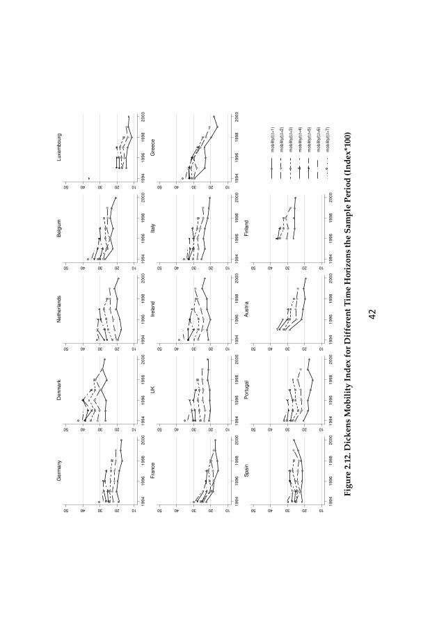
42
F
igu
re 2
.12.
Dic
ken
s M
ob
ilit
y I
nd
ex f
or
Dif
fere
nt
Tim
e H
ori
zon
s th
e S
amp
le P
erio
d (
Ind
ex*1
00)
1020304050
19
94
19
96
19
98
20
00
Ge
rma
ny
1020304050
19
94
19
96
19
98
20
00
De
nm
ark
1020304050
19
94
19
96
19
98
20
00
Ne
the
rla
nds
1020304050
19
94
19
96
19
98
20
00
Be
lgiu
m
1020304050
19
94
19
96
19
98
20
00
Luxe
mbo
urg
1020304050
19
94
19
96
19
98
20
00
Fra
nce
1020304050
19
94
19
96
19
98
20
00
UK
1020304050
19
94
19
96
19
98
20
00
Ire
land
1020304050
19
94
19
96
19
98
20
00
Ita
ly
1020304050
19
94
19
96
19
98
20
00
Gre
ece
1020304050
19
94
19
96
19
98
20
00
Spa
in
1020304050
19
94
19
96
19
98
20
00
Po
rtuga
l
1020304050
19
94
19
96
19
98
20
00
Austr
ia
1020304050
19
94
19
96
19
98
20
00
Fin
land
mo
bili
ty(t
,t+
1)
mo
bili
ty(t
,t+
2)
mo
bili
ty(t
,t+
3)
mo
bili
ty(t
,t+
4)
mo
bili
ty(t
,t+
5)
mo
bili
ty(t
,t+
6)
mo
bili
ty(t
,t+
7)
43
Figure 2.13. Dickens Short-Term Mobility over Time (Index*100)
In 2000-2001 a convergence in mobility rates is observed for four country clusters.
(Figure 2.13) Luxembourg, which records the lowest mobility, and Denmark,
which records the highest mobility, have a singular evolution. Spain and Finland
converge towards a lower mobility than Denmark, followed by Ireland, which also
has a singular evolution. The next cluster in terms of mobility is formed by UK,
Italy and Belgium. The last two clusters are Austria and Netherlands, and Greece,
Portugal, France and Germany. This ranking is in general confirmed by the
ranking based on the average jump and the immobility ratio.
Figure 2.14 summarizes the relative change in short-term mobility for all countries.
The largest decrease in mobility is recorded by Greece (almost 40%), followed by
Austria, with a reduction of more than 30%, Belgium and France over 20%, Italy
and Portugal between 15% and 20%, and Luxembourg, Germany, Finland and
Netherlands with a reduction lower than 10%. Spain records the highest increase in
short-term mobility with a rate of over 20%, followed by Ireland, UK and
Denmark, with a rate below 10%.
The ranking, the magnitude and the direction of the relative change in short-term
mobility based on Dickens index are, in general, similar with those based on the
average jump. (Figure 2.7 and Figure 2.14). A big discrepancy is observed in the
direction of evolution for Denmark: based on average jump mobility decreased
10
15
20
25
30
Mobili
ty D
ickens
1994
-199
5
1995
-199
6
1996
-199
7
1997
-199
8
1998
-199
9
1999
-200
0
2000
-200
1
Luxembourg Greece
Portugal France
Germany Austria
Netherlands
10
15
20
25
30
Mobili
ty D
ickens
1994
-199
5
1995
-199
6
1996
-199
7
1997
-199
8
1998
-199
9
1999
-200
0
2000
-200
1
UK Belgium
Italy Ireland
Denmark Spain
Finland
44
with almost 10%, whereas based on Dickens index it increases with almost 2%.
Differences in the magnitude of the evolution are observed for Netherlands,
Germany, Luxembourg and Finland, where the increase in mobility was higher as
measured by the average jump than by the Dickens index.
The difference in the ranking, magnitude and the direction of evolution of short-
term mobility might be explained by the limitations of using quintile transition
matrices to look at mobility, particularly when looking at changes in mobility over
time. If the earnings distribution has widened over time, then the size of the
quintiles has also increased, so it might be that the movement across quintiles
decreased. However, it might also be the case that mobility within quintiles has
increased, which cannot be captured by the transition matrix approach.
Figure 2.14. Relative Change in Short-term Mobility Measured by the Dickens Index
Consistent with the transition matrix approach and previous studies, long-term
mobility is higher than short-term mobility and the trend is valid across countries.
The relative increase in long term mobility relative to short-term mobility is
summarized in Figure 2.15. The highest relative increase in mobility with the time
span is recorded in Ireland with a value of almost 80%, followed by UK,
Netherlands, Germany, Denmark, Luxembourg and Portugal with values between
50% and 70%. The other countries record values between 20% and 40%.
-40
-20
02
0
Re
lative
Ch
an
ge
in
Sh
ort
Te
rm I
nco
me
Mo
bili
ty
Gre
ece
Austri
a
Belgi
um
Franc
eIta
ly
Portu
gal
Luxe
mbo
urg
Ger
man
y
Finla
nd
Net
herla
nds
Den
mar
kUK
Ireland
Spain
45
Figure 2.15. Relative Difference between Long and Short-term Mobility Measured by the
Dickens Index
This evolution triggered a re-ranking of the countries with respect to their long-
term mobility.(Figure 2.16) Luxembourg appears to have the lowest earnings
mobility also in the long run, followed by Spain, France and Germany which
record similar values, Netherlands, and Portugal, UK, Italy and Austria, Greece,
Finland, Belgium and Ireland, and the highest Denmark. This ranking coincides in
general with the one from the transition matrix approach.
Figure 2.16. Short (1994/1995) and Long Term (1994/2001) Mobility Measured by the
Dickens Index
02
04
06
08
0
Re
lative
Diffe
ren
ce
Btw
Lo
ng
an
d S
ho
rt T
erm
In
co
me
Mo
bility
Gre
ece
Aus
tria
Franc
e
Spain
Bel
gium
Finl
and
Italy
Por
tuga
l
Luxe
mbo
urg
Den
mar
k
Ger
man
y
Net
herla
nds
UK
Irela
nd
01
02
03
04
0
Sh
ort
an
d L
on
g T
erm
In
co
me
Mo
bili
ty
Luxe
mbo
urg
Spain
France
Germ
any
Nether
lands
Portuga
lUK
Italy
Austri
a
Gre
ece
Finla
nd
Belgiu
m
Ireland
Denm
ark
Short Term Mobility Long Term Mobility
46
Judging whether this mobility is high or low depends on the question being asked.
Long term mobility is certainly high enough to make the point that people are not
stuck at the bottom top of the earnings distribution. The degree of mobility,
however, is too low to wash out the effect of the yearly inequality. Even when
earnings are summed over the sample period, a substantial inequality remains,
signalling the presence of a substantial inequality in the “permanent” component
of earnings.
Figure 2.17 shows the reduction in long-term inequality - measured by the Theil
index for individual hourly earnings summed over the sample period – relative to
cross-sectional inequality in the first wave – measured by the Theil index. These
rates, however, overestimate the true values because cross-sectional inequality is
based on all positive earnings, whereas longer-term inequality is based on a
balanced panel. The rate of decrease ranges from 50%-35% for Denmark, Austria,
Ireland, UK, Belgium, France, Luxembourg and Finland, to 30%-10% for
Netherlands, Spain, Germany, Greece, Italy and Portugal, which provides a first
clue that the first cluster of countries has a higher chance in reducing lifetime
earnings differentials compared with the second one. This conclusion, however,
needs to be explored further by estimating appropriate indicators that measure
mobility as equalizer/disequalizer of longer term incomes, which represents a topic
for future research.
Figure 2.17. Relative Difference between Long-Term and Cross-sectional Earnings
Inequality (1st Wave)
-50
-40
-30
-20
-10
0
Rela
tive C
hange (%
)
Den
mark
Aus
tria
Ireland U
K
Belgium
Fran
ce
Luxe
mbo
urg
Finlan
d
Nethe
rland
s
Spa
in
Ger
man
y
Gre
ece
Italy
Por
tuga
l
47
2.7. Linking mobility and inequality
Next we aim to link the patterns in short and long-term mobility with yearly
inequality. This requires a backward looking approach. In interpreting the figures
one has to pay attention to the difference in samples in computing inequality and
mobility. The inequality measures are based on all individuals with positive
earnings. The mobility measures refer to balanced 2-year panels, meaning
individuals that recorded positive earnings in both years. We chose an unbalanced
panel for inequality to avoid underestimating the degree of dispersion. When
interpreting the results, however, we have to bear in mind that the degree of
inequality in period t depends also on the inflows and outflows of the sample in
period t, not only on the degree of mobility from one period.
2.7.1. Short-term mobility and yearly inequality
Inequality in time t depends on inequality in time t-1, mobility between t and t-1
and individuals entering and exiting the sample between period t-1 and t. Thus
inequality in the 2nd wave depends on inequality in the 1st wave, and the mobility
between the 1st wave and the 2nd wave. Similarly, inequality in 2001 depends on
inequality in 2000 and mobility between 2000 and 2001.
To shed some light on the potential link between short-term mobility and yearly
inequality we look comparatively at the evolution of short term mobility between
the 1st wave/2nd wave, and 2000/2001, and the evolution of yearly inequality
between the 2nd wave and 2001. Figure 2.18 – left panel - ranks the countries with
respect to their mobility between the 1st wave and the 2nd wave and the inequality
in the 2nd wave. The same is done in the right panel for inequality in 2001 and
mobility in 2000-2001
Overall, it appears that the higher the inequality in year t, the lower the mobility
between year t-1 and t. The ranking, however, has some exceptions. For example,
in 1995, Greece ranks among the countries with the highest mobility and the
highest inequality, suggesting that earnings mobility 1994-1995 might have had a
disequalizing impact on earnings inequality in 1995. Similarly for Spain, which in
2001 ranks among the countries with the highest mobility and the highest
inequality. These exceptions indicate that there are cases when earnings (part of)
mobility might have a disequalizing impact on cross-sectional earnings inequality.
48
Figure 2.18. Link between Short-Term Mobility and Cross-Sectional Inequality:
Mobility (1st Wave, 2nd Wave) -> Inequality (2nd Wave)
Mobility (2000, 2001) -> Inequality (2001)
Looking at the relative change in cross-sectional inequality and short-term mobility
over the sample period, the picture is not clear-cut. (Figure 2.19) Most countries
recording a decrease in short-term mobility, record also an increase in cross-
sectional inequality. Exceptions are Austria and France, where both decrease. One
possible explanation is that the decrease in mobility was due to a decrease in the
disequalizing part of mobility, which led to a decrease in inequality.
All countries recording an increase in short-term mobility over time – Denmark,
UK, Spain and Ireland - record a decrease in cross-sectional inequality between
1995 and 2001, signalling a reducing effect of short-term mobility on yearly
inequality. (Figure 2.19)
The ranking, however, is ambiguous. The countries with the smallest
(Netherlands) and the largest (Greece) reduction in short-term mobility have the
highest increase in cross-sectional inequality over time. Similarly, the countries
with the lowest (UK) and the largest (Spain) increase in mobility do not have the
largest reduction in inequality. These exceptions reinforce the argument that
mobility can have both equalizing and disequalizing impacts on inequality, and
010
20
30
Luxe
mbo
urg
Ger
man
y
Net
herla
nds
Por
tuga
lUK
Irela
nd
Spa
in
Franc
eIta
ly
Finlan
d
Den
mar
k
Belgium
Austri
a
Gre
ece
Cross-sectional Inequality (Theil) in the 2nd Wave
Mobility(1st Wave, 2nd Wave)
010
20
30
Luxe
mbo
urg
Franc
e
Ger
man
y
Gre
ece
Net
herla
nds
Austri
aIta
ly
Belgi
um UK
Ireland
Finland
Spa
in
Den
mar
k
Cross-sectional Inequality (Theil) in 2001
Mobility(2000, 2001)
49
the change in inequality depends on which facet of mobility changes with a
dominating effect.
In general, it appears that short-term mobility has a reducing effect on yearly
inequality, but the exceptions signal that mobility is not always beneficial.
Figure 2.19. Relative Change in Cross-Sectional Inequality and Short-Term Mobility Over
Time Note: Inequality – between the 2nd and the last wave; Mobility between 1st-2nd wave and 2000-2001
2.7.2. Long-term mobility and yearly inequality
Extending the time frame, inequality in time t depends on inequality in time t-s
and mobility between t and t-s. Figure 2.20 ranks the 14 countries in terms of their
long term mobility displaying at the same time the cross-sectional inequality in
2001 and the relative change in cross-sectional inequality between the 1st wave and
2001 for each country.
On average it appears that a higher long-term mobility is associated with a lower
cross-sectional inequality in 2001, but the ranking in the two measures is not
consistent. The highest long-term mobility is present in Denmark, which records
also the lowest inequality in 2001, but the highest inequality (Portugal) does not
-40
-20
020
40
Gre
ece
Austri
a
Belgium
Fran
ceIta
ly
Portu
gal
Luxe
mbo
urg
Ger
man
y
Finlan
d
Nethe
rland
s
Den
mar
kUK
Ireland
Spain
Relative Change in Cross_Sectional Inequality between 2nd Wave and 2001
Relative Change in Short-Term Mobility over Time
50
have the lowest mobility. Thus in Portugal, part of long-term earnings mobility is
disequalizing yearly inequality.
The link between long-term mobility and the relative change in inequality is
ambiguous. Mobility rates are similar, but the relative change in inequality is very
heterogeneous, with no visible pattern. A possible explanation for the ambiguity in
the mobility-inequality story relates to the nature of mobility: long-term mobility
might have an equalizing effect on cross-sectional inequality in Denmark, Ireland,
Belgium, Austria, UK, France, and Spain, and a disequalizing impact in the other
countries.
Figure 2.20. Long-Term Mobility and Cross-Sectional Inequality
2.8.Concluding remarks
In this paper we explored wage mobility for males across 14 EU countries between
1994 and 2001 using ECHP. We used two types of rank measures, which capture
positional movements in the distribution of earnings. The first one is derived from
the transition matrix approach between income quintiles and other labour market
states, and the second one is based on individual earnings ranks, as derived by
Dickens (2000a).
-40
-20
020
40
Luxe
mbo
urg
Spa
in
Franc
e
Ger
man
y
Net
herla
nds
Portu
gal
UK
Italy
Austri
a
Gre
ece
Finland
Belgium
Ireland
Den
mar
k
Cross-Sectional Inequality in 2001
Long-Term Mobility
-40
-20
020
40
Luxe
mbo
urg
Spa
in
Fran
ce
Ger
man
y
Net
herla
nds
Portu
gal
UK
Italy
Austri
a
Gre
ece
Finlan
d
Belgium
Irela
nd
Den
mar
k
Relative Change in Inequality over Time
Long-Term Mobility

51
Starting with the transition matrices among labour market states, we find
considerable levels of short-term immobility in all countries, with high shares of
individuals staying in the same earnings quintile from one period to the next.
Individuals situated in the bottom of the distribution are more likely to enter
unemployment and inactivity compared with the rest of the distribution.
Moreover, those that manage to get a job in the next period are more likely to enter
the bottom of the earnings distribution. Mobility over the sample period is higher
than one-period mobility, suggesting that the longer the period, the higher the
opportunity to escape the initial state. The highest persistency in unemployment is
found in Belgium, UK, Italy, Germany and Spain, and in inactivity in France,
Belgium, Spain, Netherlands and Ireland.
Looking at the transition matrices among the income quintiles, we find a high level
of persistency from one period to the next in all countries. Moreover, individuals
that change their income position from one period to the next do not move very
far. Individuals situated at the top of the distribution are less mobile than people at
the bottom, which in turn are less mobile than the middle of the distribution. Long-
term mobility is higher than short-term mobility, suggesting that the longer the
period, the higher the opportunity to escape the initial earnings state.
Over time, short-term income mobility for individuals belonging to the first
quintile decreased in all countries, except Luxembourg, Spain and Finland. In 2000-
2001 the highest persistency for low-earnings individuals is in Portugal, Germany,
Austria, Belgium, Netherlands and Luxembourg where between 78% and 70%
remained in the same income group, followed by Greece, France, Ireland, Denmark
with probabilities between 69% and 60%, and UK, Finland, Italy and Spain with
rates between 59% and 49%.
Long-term mobility is higher than short-term mobility, but the persistency is still
high: in Germany, Austria, Finland, Portugal and France, between 49% and 41%
remained in bottom quintile in 2001, followed by Luxembourg, Netherlands, Spain,
Belgium, Italy, Denmark, UK, Greece and Ireland, with values between 40% and
23%.
Most countries that recorded an increase in cross-sectional earnings inequality
between the 2nd wave and 2001, recorded also a decrease in short-term mobility
over time, supported both by the increase in the share of individuals maintaining
their state or moving to the closest state from one period to the next, and by the
decrease in the degree of movement far away from the initial state. Netherlands is
an exception, recording a decrease in the share of individuals maintaining their
state or moving in the immediate income group.

52
The decrease in cross-sectional earnings inequality between the 2nd wave and 2001
was accompanied by a decrease in short-term mobility – captured by an increase in
the share of individuals maintaining their state or moving in the income state
immediately below/above and by a decrease in the degree of movement - in France
and Austria, and by the opposite in UK, Spain, and Ireland. In Denmark, the
decrease in inequality was accompanied by a decrease in the share of individuals
who maintained their income state or moved in the one immediately below/above,
and by a decrease in the average quintile jump.
The short-term immobility ratio converges over time in five clusters: first,
Luxembourg which records the highest immobility ratio in 2000-2001; second,
Germany, France and Greece; third, UK, Belgium, Netherlands, Portugal, Italy and
Austria; forth, Ireland and Finland, and lastly, with the lowest immobility ratios,
Denmark and Spain. Similarly, short-term mobility away from the diagonal
converges over time in four clusters: first, Luxembourg – the lowest average jump
in 2000-2001; second, Germany, France, Austria, Netherlands, Belgium, Greece,
and Portugal; third, Italy, UK and Ireland; and lastly, Finland, Spain and Denmark,
with the highest mobility away from the diagonal in 2000-2001. Overall,
Luxembourg appears to diverge from the other EU countries.
In the long-run, Luxembourg and France appear to be the least mobile, and
Denmark and Ireland the most mobile, confirmed by both indices. In between, in
ascending order based on the average jump we find Spain, Germany, Netherlands,
Portugal, UK, Finland, Austria, Italy, Belgium and Greece. The long-term
immobility ratios have similar values among countries, whereas for the average
jump more heterogeneity is observed. Overall, we observe less heterogeneity with
respect to long-term mobility rates compared with short-term rates, suggesting
that, over the lifetime, earnings mobility rates are expected to converge to similar
levels in most countries. The convergence is expected to be more evident for the
immobility ratio than for the average jump.
To overcome the main drawbacks of the transition matrix approach, we looked at
the actual percentile rankings of workers within the wage distribution and
computed a measure of mobility following Dickens (2000a). This approach
reconfirmed most of the findings above.
Based on the proposed index, all countries recording an increase in cross-sectional
inequality between the 2nd wave and 2001 recorded also a decrease in short-term
mobility. Among the countries where inequality decreased, earnings mobility
increased in UK, Spain, Denmark and Ireland, and decreased in France and
Austria. The trend in the Dickens mobility index is consistent with the trend in the
53
average jump in all countries except Denmark, and with the trend in the
immobility ratio in all countries except Netherlands.
What are the welfare implications of these trends in short-term mobility? In
Netherlands, Greece, Finland, Portugal, Luxembourg, Italy, Germany, and
Belgium, individuals find it harder in 2000-2001 to better their position in the
earnings distribution short-term compared with the 1st-2nd wave, factor which
might have contributed to the increase in earnings differentials between the 2nd
wave and 2001. Moreover, the decrease in mobility rates might signal an increase
in permanent earning differentials.
In France and Austria, despite the decrease in cross-sectional earnings differentials
between the 2nd wave and 2001, individuals have a decreased opportunity in 2000-
2001 to better their position in the earnings distribution compared with the 1st-2nd
wave. In the UK, Spain, Denmark, and Ireland individuals have an increased
opportunity in 2000 to improve their earnings position short-term compared with
1994, which might have contributed to reduce cross-sectional differentials over
time.
Short-term mobility rates converge towards 2001 in four country clusters.
Luxembourg - the lowest mobility in 2001 - and Denmark - the highest mobility in
2001 - have a singular evolution. Spain and Finland converge towards a lower
mobility than Denmark, followed by Ireland, with a singular evolution. Next, UK,
Italy and Belgium converge towards a lower level than Ireland. The last two
clusters are Austria and Netherlands, and Greece, Portugal, France and Germany.
This ranking is in general confirmed by the ranking based on the immobility ratio
and the average jump.
The lowest opportunity of improving the earnings position in the long run is found
in Luxembourg followed by four clusters which record similar values: first, Spain,
France and Germany; second, Netherlands and Portugal; third, UK, Italy and
Austria; forth Greece, Finland, Belgium and Ireland. Finally, men in Denmark have
the highest opportunity of improving their income position in the long run.
We also tried to link the patterns in short and long-term mobility with yearly
inequality. Overall, it appears that the higher the inequality in the 2nd wave, the
lower the mobility between the 1st and 2nd wave. Similarly, a higher long-term
mobility (between the 1st wave and 2001) is associated with a lower cross-sectional
inequality in 2001.The rankings, however, has some exceptions, indicating that
there are cases when (part of earnings) mobility might have a disequalizing impact
on cross-sectional earnings inequality. These factors reinforce the belief that
mobility is not always beneficial.

54
A topic for further research is to explore the implications of the long-term mobility
rates for lifetime inequality.
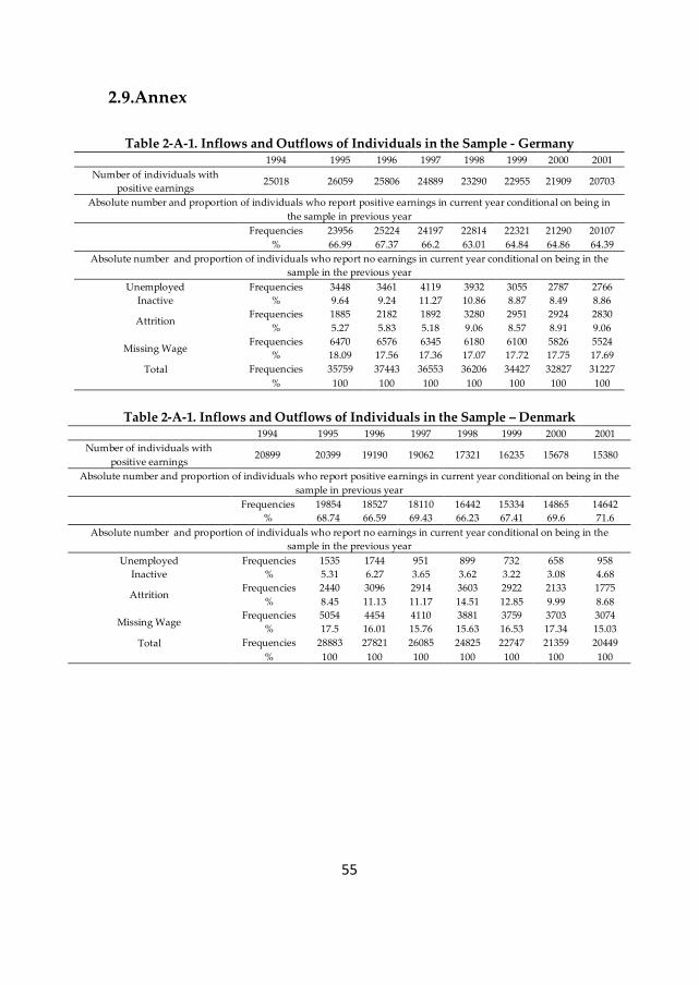
55
2.9.Annex
Table 2-A-1. Inflows and Outflows of Individuals in the Sample - Germany
1994 1995 1996 1997 1998 1999 2000 2001
Number of individuals with
positive earnings 25018 26059 25806 24889 23290 22955 21909 20703
Absolute number and proportion of individuals who report positive earnings in current year conditional on being in
the sample in previous year
Frequencies 23956 25224 24197 22814 22321 21290 20107
% 66.99 67.37 66.2 63.01 64.84 64.86 64.39
Absolute number and proportion of individuals who report no earnings in current year conditional on being in the
sample in the previous year
Unemployed
Inactive
Frequencies 3448 3461 4119 3932 3055 2787 2766
% 9.64 9.24 11.27 10.86 8.87 8.49 8.86
Attrition Frequencies 1885 2182 1892 3280 2951 2924 2830
% 5.27 5.83 5.18 9.06 8.57 8.91 9.06
Missing Wage Frequencies 6470 6576 6345 6180 6100 5826 5524
% 18.09 17.56 17.36 17.07 17.72 17.75 17.69
Total
Frequencies 35759 37443 36553 36206 34427 32827 31227
% 100 100 100 100 100 100 100
Table 2-A-1. Inflows and Outflows of Individuals in the Sample – Denmark
1994 1995 1996 1997 1998 1999 2000 2001
Number of individuals with
positive earnings 20899 20399 19190 19062 17321 16235 15678 15380
Absolute number and proportion of individuals who report positive earnings in current year conditional on being in the
sample in previous year
Frequencies 19854 18527 18110 16442 15334 14865 14642
% 68.74 66.59 69.43 66.23 67.41 69.6 71.6
Absolute number and proportion of individuals who report no earnings in current year conditional on being in the
sample in the previous year
Unemployed
Inactive
Frequencies 1535 1744 951 899 732 658 958
% 5.31 6.27 3.65 3.62 3.22 3.08 4.68
Attrition Frequencies 2440 3096 2914 3603 2922 2133 1775
% 8.45 11.13 11.17 14.51 12.85 9.99 8.68
Missing Wage Frequencies 5054 4454 4110 3881 3759 3703 3074
% 17.5 16.01 15.76 15.63 16.53 17.34 15.03
Total
Frequencies 28883 27821 26085 24825 22747 21359 20449
% 100 100 100 100 100 100 100
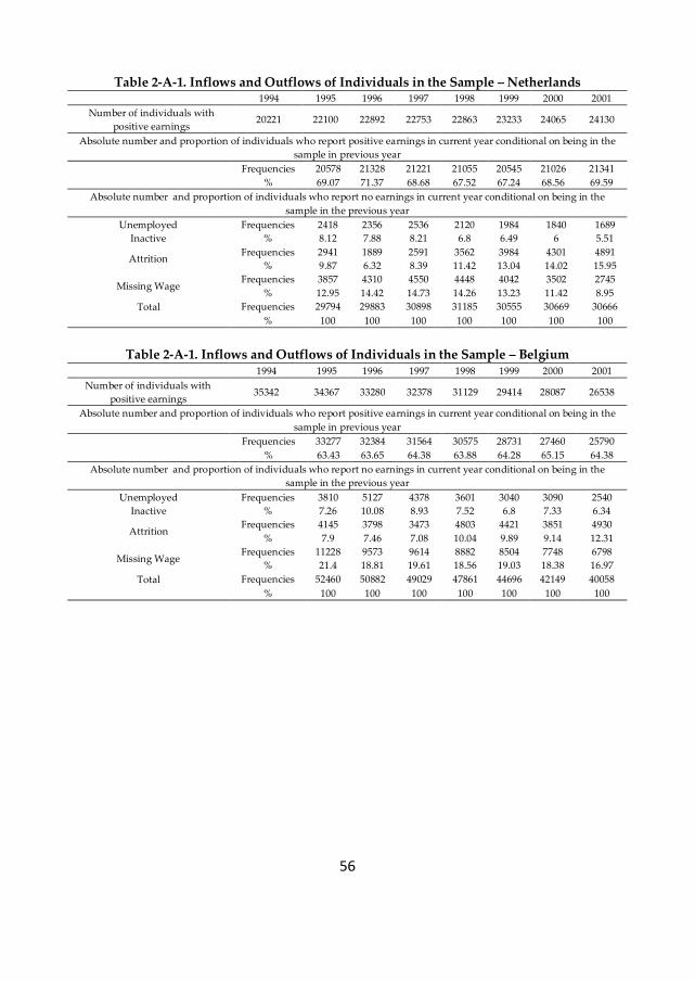
56
Table 2-A-1. Inflows and Outflows of Individuals in the Sample – Netherlands
1994 1995 1996 1997 1998 1999 2000 2001
Number of individuals with
positive earnings 20221 22100 22892 22753 22863 23233 24065 24130
Absolute number and proportion of individuals who report positive earnings in current year conditional on being in the
sample in previous year
Frequencies 20578 21328 21221 21055 20545 21026 21341
% 69.07 71.37 68.68 67.52 67.24 68.56 69.59
Absolute number and proportion of individuals who report no earnings in current year conditional on being in the
sample in the previous year
Unemployed
Inactive
Frequencies 2418 2356 2536 2120 1984 1840 1689
% 8.12 7.88 8.21 6.8 6.49 6 5.51
Attrition Frequencies 2941 1889 2591 3562 3984 4301 4891
% 9.87 6.32 8.39 11.42 13.04 14.02 15.95
Missing Wage Frequencies 3857 4310 4550 4448 4042 3502 2745
% 12.95 14.42 14.73 14.26 13.23 11.42 8.95
Total
Frequencies 29794 29883 30898 31185 30555 30669 30666
% 100 100 100 100 100 100 100
Table 2-A-1. Inflows and Outflows of Individuals in the Sample – Belgium
1994 1995 1996 1997 1998 1999 2000 2001
Number of individuals with
positive earnings 35342 34367 33280 32378 31129 29414 28087 26538
Absolute number and proportion of individuals who report positive earnings in current year conditional on being in the
sample in previous year
Frequencies 33277 32384 31564 30575 28731 27460 25790
% 63.43 63.65 64.38 63.88 64.28 65.15 64.38
Absolute number and proportion of individuals who report no earnings in current year conditional on being in the
sample in the previous year
Unemployed
Inactive
Frequencies 3810 5127 4378 3601 3040 3090 2540
% 7.26 10.08 8.93 7.52 6.8 7.33 6.34
Attrition Frequencies 4145 3798 3473 4803 4421 3851 4930
% 7.9 7.46 7.08 10.04 9.89 9.14 12.31
Missing Wage Frequencies 11228 9573 9614 8882 8504 7748 6798
% 21.4 18.81 19.61 18.56 19.03 18.38 16.97
Total
Frequencies 52460 50882 49029 47861 44696 42149 40058
% 100 100 100 100 100 100 100
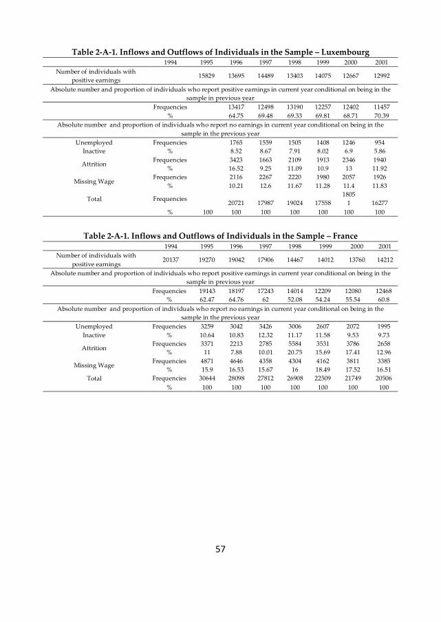
57
Table 2-A-1. Inflows and Outflows of Individuals in the Sample – Luxembourg
1994 1995 1996 1997 1998 1999 2000 2001
Number of individuals with
positive earnings 15829 13695 14489 13403 14075 12667 12992
Absolute number and proportion of individuals who report positive earnings in current year conditional on being in the
sample in previous year
Frequencies
13417 12498 13190 12257 12402 11457
%
64.75 69.48 69.33 69.81 68.71 70.39
Absolute number and proportion of individuals who report no earnings in current year conditional on being in the
sample in the previous year
Unemployed
Inactive
Frequencies
1765 1559 1505 1408 1246 954
%
8.52 8.67 7.91 8.02 6.9 5.86
Attrition Frequencies
3423 1663 2109 1913 2346 1940
%
16.52 9.25 11.09 10.9 13 11.92
Missing Wage Frequencies
2116 2267 2220 1980 2057 1926
%
10.21 12.6 11.67 11.28 11.4 11.83
Total
Frequencies 20721 17987 19024 17558
1805
1 16277
% 100 100 100 100 100 100 100
Table 2-A-1. Inflows and Outflows of Individuals in the Sample – France
1994 1995 1996 1997 1998 1999 2000 2001
Number of individuals with
positive earnings 20137 19270 19042 17906 14467 14012 13760 14212
Absolute number and proportion of individuals who report positive earnings in current year conditional on being in the
sample in previous year
Frequencies 19143 18197 17243 14014 12209 12080 12468
% 62.47 64.76 62 52.08 54.24 55.54 60.8
Absolute number and proportion of individuals who report no earnings in current year conditional on being in the
sample in the previous year
Unemployed
Inactive
Frequencies 3259 3042 3426 3006 2607 2072 1995
% 10.64 10.83 12.32 11.17 11.58 9.53 9.73
Attrition Frequencies 3371 2213 2785 5584 3531 3786 2658
% 11 7.88 10.01 20.75 15.69 17.41 12.96
Missing Wage Frequencies 4871 4646 4358 4304 4162 3811 3385
% 15.9 16.53 15.67 16 18.49 17.52 16.51
Total
Frequencies 30644 28098 27812 26908 22509 21749 20506
% 100 100 100 100 100 100 100
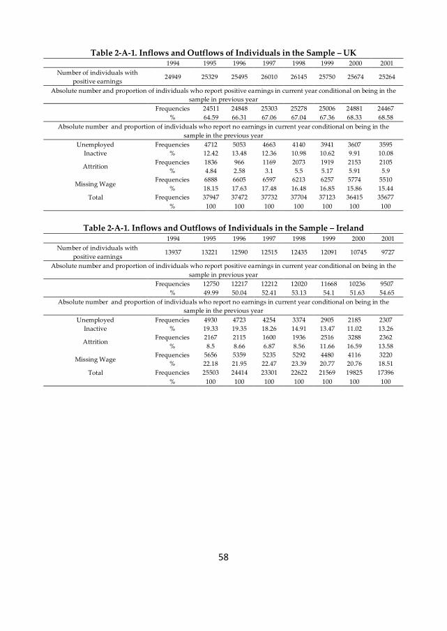
58
Table 2-A-1. Inflows and Outflows of Individuals in the Sample – UK
1994 1995 1996 1997 1998 1999 2000 2001
Number of individuals with
positive earnings 24949 25329 25495 26010 26145 25750 25674 25264
Absolute number and proportion of individuals who report positive earnings in current year conditional on being in the
sample in previous year
Frequencies 24511 24848 25303 25278 25006 24881 24467
% 64.59 66.31 67.06 67.04 67.36 68.33 68.58
Absolute number and proportion of individuals who report no earnings in current year conditional on being in the
sample in the previous year
Unemployed
Inactive
Frequencies 4712 5053 4663 4140 3941 3607 3595
% 12.42 13.48 12.36 10.98 10.62 9.91 10.08
Attrition Frequencies 1836 966 1169 2073 1919 2153 2105
% 4.84 2.58 3.1 5.5 5.17 5.91 5.9
Missing Wage Frequencies 6888 6605 6597 6213 6257 5774 5510
% 18.15 17.63 17.48 16.48 16.85 15.86 15.44
Total
Frequencies 37947 37472 37732 37704 37123 36415 35677
% 100 100 100 100 100 100 100
Table 2-A-1. Inflows and Outflows of Individuals in the Sample – Ireland
1994 1995 1996 1997 1998 1999 2000 2001
Number of individuals with
positive earnings 13937 13221 12590 12515 12435 12091 10745 9727
Absolute number and proportion of individuals who report positive earnings in current year conditional on being in the
sample in previous year
Frequencies 12750 12217 12212 12020 11668 10236 9507
% 49.99 50.04 52.41 53.13 54.1 51.63 54.65
Absolute number and proportion of individuals who report no earnings in current year conditional on being in the
sample in the previous year
Unemployed
Inactive
Frequencies 4930 4723 4254 3374 2905 2185 2307
% 19.33 19.35 18.26 14.91 13.47 11.02 13.26
Attrition Frequencies 2167 2115 1600 1936 2516 3288 2362
% 8.5 8.66 6.87 8.56 11.66 16.59 13.58
Missing Wage Frequencies 5656 5359 5235 5292 4480 4116 3220
% 22.18 21.95 22.47 23.39 20.77 20.76 18.51
Total
Frequencies 25503 24414 23301 22622 21569 19825 17396
% 100 100 100 100 100 100 100
59
Table 2-A-1. Inflows and Outflows of Individuals in the Sample – Italy
1994 1995 1996 1997 1998 1999 2000 2001
Number of individuals with
positive earnings 32633 32236 32111 29661 28865 26993 26912 25170
Absolute number and proportion of individuals who report positive earnings in current year conditional on being in the
sample in previous year
Frequencies 30946 31028 28717 27188 25717 25348 24139
% 51.58 51.19 47.18 47.34 46.87 48.73 48.86
Absolute number and proportion of individuals who report no earnings in current year conditional on being in the
sample in the previous year
Unemployed
Inactive
Frequencies 7900 7799 7670 6627 6890 5662 5027
% 13.17 12.87 12.6 11.54 12.56 10.88 10.18
Attrition Frequencies 3175 2947 5922 6030 5941 5399 5920
% 5.29 4.86 9.73 10.5 10.83 10.38 11.98
Missing Wage Frequencies 17978 18836 18559 17585 16325 15610 14315
% 29.96 31.08 30.49 30.62 29.75 30.01 28.98
Total
Frequencies 59999 60610 60868 57430 54873 52019 49401
% 100 100 100 100 100 100 100
Table 2-A-1. Inflows and Outflows of Individuals in the Sample – Greece
1994 1995 1996 1997 1998 1999 2000 2001
Number of individuals with
positive earnings 27974 27654 26150 24865 22675 22001 21335 21929
Absolute number and proportion of individuals who report positive earnings in current year conditional on being in the
sample in previous year
Frequencies 26868 25946 24385 21815 20357 20443 21342
% 45.83 45.69 44.98 42.09 43.52 46.06 49.72
Absolute number and proportion of individuals who report no earnings in current year conditional on being in the
sample in the previous year
Unemployed
Inactive
Frequencies 7537 6813 6419 4523 4489 4427 3858
% 12.86 12 11.84 8.73 9.6 9.97 8.99
Attrition Frequencies 4417 4392 4347 7892 6222 4159 2363
% 7.53 7.73 8.02 15.23 13.3 9.37 5.5
Missing Wage Frequencies 19802 19640 19068 17599 15707 15352 15365
% 33.78 34.58 35.17 33.96 33.58 34.59 35.79
Total
Frequencies 58624 56791 54219 51829 46775 44381 42928
% 100 100 100 100 100 100 100
60
Table 2-A-1. Inflows and Outflows of Individuals in the Sample – Spain
1994 1995 1996 1997 1998 1999 2000 2001
Number of individuals with
positive earnings 22559 21863 21296 20975 20371 20580 19898 20185
Absolute number and proportion of individuals who report positive earnings in current year conditional on being in the
sample in previous year
Frequencies 21460 20521 20329 19456 19679 19167 19352
% 47.6 48.29 48.49 48.63 52.13 52.12 56.06
Absolute number and proportion of individuals who report no earnings in current year conditional on being in the
sample in the previous year
Unemployed
Inactive
Frequencies 8419 8230 7353 5970 5083 4512 4761
% 18.67 19.37 17.54 14.92 13.46 12.27 13.79
Attrition Frequencies 4467 3000 4120 4327 3188 3922 3052
% 9.91 7.06 9.83 10.81 8.44 10.66 8.84
Missing Wage Frequencies 10741 10742 10121 10259 9802 9176 7357
% 23.82 25.28 24.14 25.64 25.96 24.95 21.31
Total
Frequencies 45087 42493 41923 40012
3775
2
3677
7 34522
% 100 100 100 100 100 100 100
Table 2-A-1. Inflows and Outflows of Individuals in the Sample – Portugal
1994 1995 1996 1997 1998 1999 2000 2001
Number of individuals with
positive earnings 14653 15450 15379 15087 14837 14569 14604 14550
Absolute number and proportion of individuals who report positive earnings in current year conditional on being in the
sample in previous year
Frequencies 13892 14538 14321 13977 13921 13952 13942
% 57.84 57.5 57.32 56.98 59.12 60.83 62.16
Absolute number and proportion of individuals who report no earnings in current year conditional on being in the
sample in the previous year
Unemployed
Inactive
Frequencies 2187 2264 2396 2019 2067 1843 1702
% 9.11 8.95 9.59 8.23 8.78 8.04 7.59
Attrition Frequencies 1701 1908 1918 2346 1956 1617 1575
% 7.08 7.55 7.68 9.56 8.31 7.05 7.02
Missing Wage Frequencies 6236 6573 6350 6189 5602 5525 5211
% 25.97 26 25.42 25.23 23.79 24.09 23.23
Total
Frequencies 24016 25283 24985 24531 23546 22937 22430
% 100 100 100 100 100 100 100
61
Table 2-A-1. Inflows and Outflows of Individuals in the Sample – Austria
1994 1995 1996 1997 1998 1999 2000 2001
Number of individuals with
positive earnings 17944 17789 17199 16209 15162 13816 13056
Absolute number and proportion of individuals who report positive earnings in current year conditional on being in the
sample in previous year
Frequencies 16472 16384 15634 14551 13403 12601
% 67.96 68.2 67.49 67.2 66.51 68.21
Absolute number and proportion of individuals who report no earnings in current year conditional on being in the
sample in the previous year
Unemployed
Inactive
Frequencies 1209 1231 906 790 803 843
% 4.99 5.12 3.91 3.65 3.98 4.56
Attrition Frequencies 2195 2080 2435 2470 2409 1794
% 9.06 8.66 10.51 11.41 11.95 9.71
Missing Wage Frequencies 4361 4330 4189 3842 3538 3235
% 17.99 18.02 18.08 17.74 17.56 17.51
Total
Frequencies 24237 24025 23164 21653 20153 18473
%
100 100 100 100 100 100
Table 2-A-1. Inflows and Outflows of Individuals in the Sample – Finland
1996 1997 1998 1999 2000 2001
Number of individuals with
positive earnings
15811 15845 15895 15546 13329 13057
Absolute number and proportion of individuals who report positive earnings in current year conditional on being in the
sample in previous year
Frequencies
15246 15345 14753 12756 12588
%
55.95 57.2 59.29 53.83 64.16
Absolute number and proportion of individuals who report no earnings in current year conditional on being in the
sample in the previous year
Unemployed
Inactive
Frequencies
3446 2327 1657 1326 1267
%
12.65 8.67 6.66 5.6 6.46
Attrition Frequencies
1933 3219 2658 5219 1708
%
7.09 12 10.68 22.02 8.71
Missing Wage Frequencies
6623 5937 5814 4398 4057
%
24.31 22.13 23.37 18.56 20.68
Total
Frequencies
27248 26828 24882 23699 19620
%
100 100 100 100 100
62
Table 2-A-2.Short-Term Transition Rates Among Labour Market States G
erm
an
y
State in 1995 1st Q 2nd Q 3rd Q 4th Q 5th Q Unempl. Inactiv. Missing* S
tate
in
19
94
1st Quintile 56.21 17.05 4.73 0.86 0 6.81 1.58 12.76
2nd Quintile 13.66 47.58 17.52 6.19 0.84 6.31 0.76 7.13
3rd Quintile 3.6 17 42.71 20.28 3.14 2.2 0.56 10.44
4th Quintile 0.43 4.48 18.92 51.67 17.33 1.55 1.44 4.17
5th Quintile 0 0.46 2.36 11.86 77.28 0.93 0.97 6.14
Unemployed 19.35 10.13 4.95 1.2 0.08 39.72 1.95 22.62
Inactive 3.5 4.56 2.12 0.53 2.01 20.25 27.47 39.55
Missing Wage* 6.29 3.93 2.78 1.58 1.89 5.55 4.32 73.67
State in 2001 1st Q 2nd Q 3rd Q 4th Q 5th Q Unempl. Inactiv. Missing*
Sta
te i
n 2
00
0
1st Quintile 54.96 12.34 2.99 0.52 0.16 9.31 1.98 17.73
2nd Quintile 14.92 48.06 17.06 3.65 0.34 3.97 0.64 11.36
3rd Quintile 3.3 20 47.65 18.01 1 1.55 0.89 7.91
4th Quintile 0.53 2.31 13.86 58.68 12.4 0.48 0.53 11.23
5th Quintile 0.53 2.31 2.63 13.49 71.68 0.5 0.57 8.27
Unemployed 14.83 2.71 5.93 1.1 0.08 46.44 2.37 26.53
Inactive 8.46 0 2.57 1.65 1.47 8.09 45.77 31.99
Missing 2.51 2.03 1.35 0.72 1.09 2.11 0.89 89.3
Den
ma
rk
State in 1995 1st Q 2nd Q 3rd Q 4th Q 5th Q Unempl. Inactiv. Missing*
Sta
te i
n 1
99
4
1st Quintile 41.28 19.41 9.96 1.7 1.98 4.61 0 21.06
2nd Quintile 21.45 40.87 14.52 7.36 1.07 3.69 0.79 10.26
3rd Quintile 6.28 30 28.78 17.72 6.16 2.02 0 8.66
4th Quintile 0.78 6.91 22.95 43.62 14.92 1.07 0 9.74
5th Quintile 2.25 1.06 1.69 25.86 61.83 0.48 0 6.83
Unemployed 12.86 15.85 6.16 3.25 2.87 34.02 0.25 24.75
Inactive 4.55 0 0 0 0 26.14 0 69.32
Missing Wage* 8.82 1.39 0.29 0.94 4.4 1.86 1.19 81.1
State in 2001 1st Q 2nd Q 3rd Q 4th Q 5th Q Unempl. Inactiv. Missing*
Sta
te i
n 2
00
0
1st Quintile 48.61 16.15 12.74 1.74 0.7 2.09 3.63 14.35
2nd Quintile 24.64 35.88 18.56 3 4.81 4.93 0 8.18
3rd Quintile 5.88 21 45.01 14.56 3.05 0.14 0 10.83
4th Quintile 4.39 8.29 21.01 39.61 17.96 2.43 0 6.31
5th Quintile 0.57 0.67 5.59 13.02 66.9 1.95 0.38 10.92
Unemployed 7.9 3.71 2.9 3.71 0 41.77 0 40
Inactive 41.46 0 0 0 0 7.32 51.22 0
Missing 3.11 1.81 2.24 1.09 0.76 0.9 0.05 90.03
Net
her
lan
ds
State in 1995 1st Q 2nd Q 3rd Q 4th Q 5th Q Unempl. Inactiv. Missing*
Sta
te i
n 1
99
4
1st Quintile 47.57 22.85 4.74 1.65 0.07 2.25 1.3 19.57
2nd Quintile 11.35 44.68 24.03 5.72 1.45 0.66 0.71 11.41
3rd Quintile 2.96 14 45.96 22.65 3.07 0.4 1.03 9.62
4th Quintile 0.51 2.67 13.11 52.7 18.97 2.21 0.78 9.04
5th Quintile 0.91 0.51 2.35 13.61 73.84 1.85 0.46 6.48
Unemployed 15.02 5.69 6.81 2.47 3 42.92 8.05 16.04
Inactive 8.1 1.49 2.79 3.45 1.12 22.44 47.49 13.13
Missing Wage* 13.79 6.97 4.49 5.99 4.77 2.85 0.8 60.34
State in 2001 1st Q 2nd Q 3rd Q 4th Q 5th Q Unempl. Inactiv. Missing*
Sta
te i
n 2
00
0
1st Quintile 53.88 15.15 3.56 2.7 0.45 0.29 0.31 23.66
2nd Quintile 7.82 49.78 18.96 6.14 1.31 0.57 0.17 15.25
3rd Quintile 4.74 7 52.65 16.22 4.42 0.89 0.32 13.42
4th Quintile 0.85 1.15 15.05 52.18 12.51 1.06 0.61 16.59
5th Quintile 0 0.71 1.19 15.11 65.95 0.27 0 16.78
Unemployed 7.2 1.83 0.54 0 2.47 46.13 18.6 23.23
Inactive 4.96 1.6 0.8 0 1.77 4.96 59.75 26.15
Missing 3.78 1.92 0.82 1.34 1.06 0.38 0.45 90.24
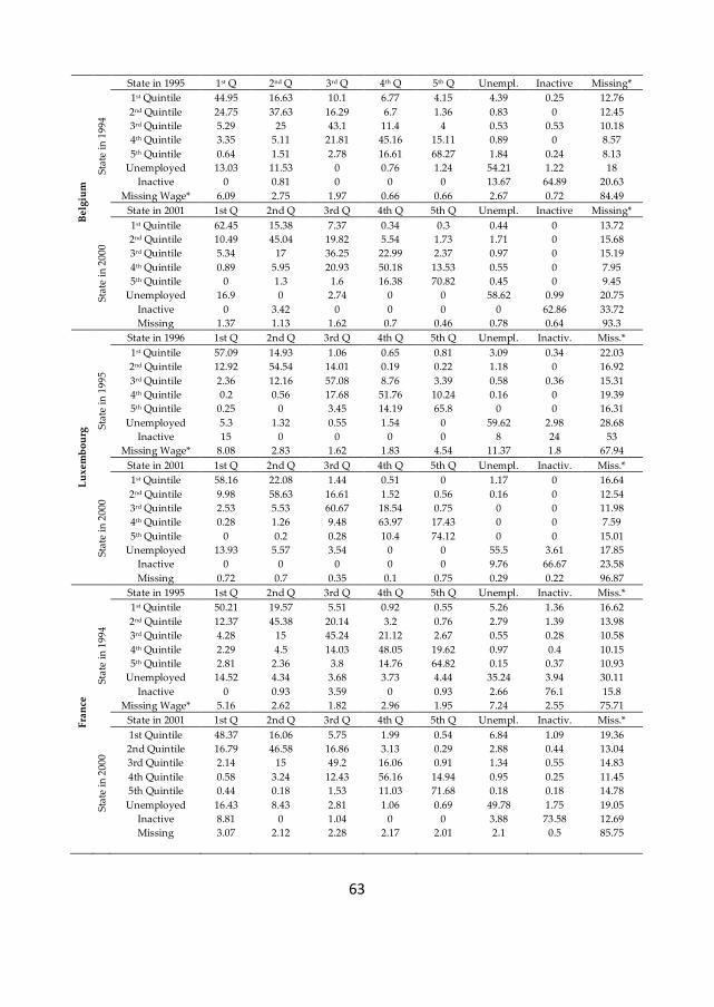
63
Be
lgiu
m
State in 1995 1st Q 2nd Q 3rd Q 4th Q 5th Q Unempl. Inactive Missing*
Sta
te i
n 1
99
4 1st Quintile 44.95 16.63 10.1 6.77 4.15 4.39 0.25 12.76
2nd Quintile 24.75 37.63 16.29 6.7 1.36 0.83 0 12.45
3rd Quintile 5.29 25 43.1 11.4 4 0.53 0.53 10.18
4th Quintile 3.35 5.11 21.81 45.16 15.11 0.89 0 8.57
5th Quintile 0.64 1.51 2.78 16.61 68.27 1.84 0.24 8.13
Unemployed 13.03 11.53 0 0.76 1.24 54.21 1.22 18
Inactive 0 0.81 0 0 0 13.67 64.89 20.63
Missing Wage* 6.09 2.75 1.97 0.66 0.66 2.67 0.72 84.49
State in 2001 1st Q 2nd Q 3rd Q 4th Q 5th Q Unempl. Inactive Missing*
Sta
te i
n 2
00
0
1st Quintile 62.45 15.38 7.37 0.34 0.3 0.44 0 13.72
2nd Quintile 10.49 45.04 19.82 5.54 1.73 1.71 0 15.68
3rd Quintile 5.34 17 36.25 22.99 2.37 0.97 0 15.19
4th Quintile 0.89 5.95 20.93 50.18 13.53 0.55 0 7.95
5th Quintile 0 1.3 1.6 16.38 70.82 0.45 0 9.45
Unemployed 16.9 0 2.74 0 0 58.62 0.99 20.75
Inactive 0 3.42 0 0 0 0 62.86 33.72
Missing 1.37 1.13 1.62 0.7 0.46 0.78 0.64 93.3
Lu
xe
mb
ou
rg
State in 1996 1st Q 2nd Q 3rd Q 4th Q 5th Q Unempl. Inactiv. Miss.*
Sta
te i
n 1
99
5
1st Quintile 57.09 14.93 1.06 0.65 0.81 3.09 0.34 22.03
2nd Quintile 12.92 54.54 14.01 0.19 0.22 1.18 0 16.92
3rd Quintile 2.36 12.16 57.08 8.76 3.39 0.58 0.36 15.31
4th Quintile 0.2 0.56 17.68 51.76 10.24 0.16 0 19.39
5th Quintile 0.25 0 3.45 14.19 65.8 0 0 16.31
Unemployed 5.3 1.32 0.55 1.54 0 59.62 2.98 28.68
Inactive 15 0 0 0 0 8 24 53
Missing Wage* 8.08 2.83 1.62 1.83 4.54 11.37 1.8 67.94
State in 2001 1st Q 2nd Q 3rd Q 4th Q 5th Q Unempl. Inactiv. Miss.*
Sta
te i
n 2
00
0
1st Quintile 58.16 22.08 1.44 0.51 0 1.17 0 16.64
2nd Quintile 9.98 58.63 16.61 1.52 0.56 0.16 0 12.54
3rd Quintile 2.53 5.53 60.67 18.54 0.75 0 0 11.98
4th Quintile 0.28 1.26 9.48 63.97 17.43 0 0 7.59
5th Quintile 0 0.2 0.28 10.4 74.12 0 0 15.01
Unemployed 13.93 5.57 3.54 0 0 55.5 3.61 17.85
Inactive 0 0 0 0 0 9.76 66.67 23.58
Missing 0.72 0.7 0.35 0.1 0.75 0.29 0.22 96.87
Fra
nce
State in 1995 1st Q 2nd Q 3rd Q 4th Q 5th Q Unempl. Inactiv. Miss.*
Sta
te i
n 1
99
4
1st Quintile 50.21 19.57 5.51 0.92 0.55 5.26 1.36 16.62
2nd Quintile 12.37 45.38 20.14 3.2 0.76 2.79 1.39 13.98
3rd Quintile 4.28 15 45.24 21.12 2.67 0.55 0.28 10.58
4th Quintile 2.29 4.5 14.03 48.05 19.62 0.97 0.4 10.15
5th Quintile 2.81 2.36 3.8 14.76 64.82 0.15 0.37 10.93
Unemployed 14.52 4.34 3.68 3.73 4.44 35.24 3.94 30.11
Inactive 0 0.93 3.59 0 0.93 2.66 76.1 15.8
Missing Wage* 5.16 2.62 1.82 2.96 1.95 7.24 2.55 75.71
State in 2001 1st Q 2nd Q 3rd Q 4th Q 5th Q Unempl. Inactiv. Miss.*
Sta
te i
n 2
00
0
1st Quintile 48.37 16.06 5.75 1.99 0.54 6.84 1.09 19.36
2nd Quintile 16.79 46.58 16.86 3.13 0.29 2.88 0.44 13.04
3rd Quintile 2.14 15 49.2 16.06 0.91 1.34 0.55 14.83
4th Quintile 0.58 3.24 12.43 56.16 14.94 0.95 0.25 11.45
5th Quintile 0.44 0.18 1.53 11.03 71.68 0.18 0.18 14.78
Unemployed 16.43 8.43 2.81 1.06 0.69 49.78 1.75 19.05
Inactive 8.81 0 1.04 0 0 3.88 73.58 12.69
Missing 3.07 2.12 2.28 2.17 2.01 2.1 0.5 85.75
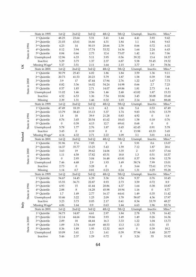
64
U
K
State in 1995 1st Q 2nd Q 3rd Q 4th Q 5th Q Unempl. Inactiv. Miss.*
Sta
te i
n 1
99
4
1st Quintile 48.25 23.64 5.51 3.41 1.44 4.41 3.93 9.42
2nd Quintile 21.03 43.61 16.66 4.31 1.84 1.1 1.84 9.63
3rd Quintile 4.23 14 50.15 20.66 2.78 0.66 0.72 6.32
4th Quintile 0.12 3.94 17.74 53.52 14.36 1.64 2.24 6.43
5th Quintile 0.84 0.66 2.73 12.4 73.07 1.42 1.81 7.06
Unemployed 12.96 6.33 5.11 3.95 0.56 39.32 13.4 18.37
Inactive 5.29 3.75 1.37 2.37 6.87 5.58 55.45 19.32
Missing Wage* 5.37 3.51 2.11 1.64 2.15 3.77 2.9 78.56
State in 2001 1st Q 2nd Q 3rd Q 4th Q 5th Q Unempl. Inactiv. Miss.*
Sta
te i
n 2
00
0
1st Quintile 50.79 25.43 6.02 1.86 1.84 3.59 1.36 9.11
2nd Quintile 20.73 41.53 20.23 5.79 1.87 1.58 0.39 7.88
3rd Quintile 3.9 17 47.44 17.94 2.76 1.22 1.67 7.73
4th Quintile 0.82 3.36 16.02 54.24 14.98 0.66 2.7 7.23
5th Quintile 0.57 1.85 2.71 14.07 69.86 1.81 2.73 6.4
Unemployed 11.02 1.46 2.56 1.46 2.48 63.82 1.87 15.33
Inactive 4.52 6.53 1.36 7.54 10.84 3.45 30.08 35.68
Missing 2.39 1.31 1.46 0.32 1.03 2.14 2.66 88.68
Ire
lan
d
State in 1995 1st Q 2nd Q 3rd Q 4th Q 5th Q Unempl. Inactiv. Miss.*
Sta
te i
n 1
99
4
1st Quintile 47.49 18.19 6.11 4.2 1.06 5.4 0.53 47.49
2nd Quintile 13.79 38.43 15.13 5.37 1.74 9.83 0.76 13.79
3rd Quintile 1.8 18 39.9 21.28 0.83 4.92 0 1.8
4th Quintile 0.76 3.45 20.54 41.62 18.63 1.58 0.18 0.76
5th Quintile 0 0.39 4.13 12.7 69.61 0.68 0 0
Unemployed 5.78 1.77 2.76 1.87 0.45 62.45 0.91 5.78
Inactive 3.45 0 0.19 0 0 13.98 65.33 3.45
Missing Wage* 4.14 4.32 2.71 2.22 1.09 3.1 3.01 4.14
State in 2001 1st Q 2nd Q 3rd Q 4th Q 5th Q Unempl. Inactiv. Miss.*
Sta
te i
n 2
00
0
1st Quintile 51.96 17.6 7.85 3 0 5.91 0.6 13.07
2nd Quintile 14.37 35.77 13.25 5.43 1.59 7.12 1.87 20.6
3rd Quintile 3.63 19 39.62 14.06 3.35 2 0.37 17.64
4th Quintile 1.11 4.58 17.82 45.51 18.8 1.3 0.51 10.37
5th Quintile 0 2.95 3.04 16.48 63.81 0.37 0.56 12.78
Unemployed 7.46 4.48 2.9 1.93 1.49 58.74 7.99 15.01
Inactive 2.73 0 3.28 0 0 3.64 72.61 17.74
Missing 1.14 0.7 0.81 0.23 0.24 1.31 0.29 95.28
Ita
ly
State in 1995 1st Q 2nd Q 3rd Q 4th Q 5th Q Unempl. Inactiv. Miss.*
Sta
te i
n 1
99
4
1st Quintile 54.67 14.45 6.39 3.36 0.54 9.37 0.76 10.45
2nd Quintile 15.55 36.71 22.87 8.93 2.73 3.59 0.72 8.9
3rd Quintile 4.93 15 41.44 20.86 4.37 1.64 0.38 10.87
4th Quintile 2.88 8 14.28 45.98 18.94 1.16 0 8.77
5th Quintile 1.7 1.49 2.77 16.17 64.61 1.49 0.35 11.42
Unemployed 10.46 3.22 1.25 2.09 1.78 58.87 4.36 17.97
Inactive 3.23 3.73 0.05 2.17 0.41 8.34 33.79 48.27
Missing Wage* 4.06 1.64 0.9 0.63 1.44 6.63 1.96 82.74
State in 2001 1st Q 2nd Q 3rd Q 4th Q 5th Q Unempl. Inactiv. Miss.*
Sta
te i
n 2
00
0
1st Quintile 54.73 14.87 4.61 2.97 1.84 2.78 1.78 16.42
2nd Quintile 12.14 44.66 19.66 3.93 1.49 1.49 0.26 16.36
3rd Quintile 2.09 18 44.44 16.3 3.33 1.22 1.04 13.73
4th Quintile 1.09 3.74 16.69 48.53 13.3 1.33 0.31 15
5th Quintile 0.36 1.89 1.95 12.32 64.9 0 0.39 18.2
Unemployed 10.09 3.41 2.3 1.61 0.39 57.96 3.48 20.77
Inactive 5.46 2.37 1.29 0.72 0 3.24 55 31.92
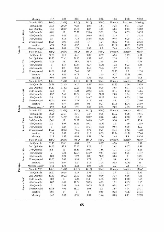
65
Missing 1.17 1.23 0.81 1.12 0.88 1.78 0.48 92.52 G
ree
ce
State in 1995 1st Q 2nd Q 3rd Q 4th Q 5th Q Unempl. Inactive Missing* S
tate
in
19
94
1st Quintile 39.99 20.39 9.28 2.09 1.84 7.28 0.91 18.23
2nd Quintile 16.5 28.77 25.81 4.87 4.05 6.05 0.13 13.82
3rd Quintile 4.81 17 35.22 19.86 5.99 1.56 0.39 14.95
4th Quintile 2.94 6.44 20.1 36.09 18.06 2.13 0 14.24
5th Quintile 0.7 3.13 7.73 18.06 56.56 0.46 0.25 13.11
Unemployed 15.29 6.95 5.53 1.4 1.74 36.37 9.35 23.38
Inactive 6.74 2.58 0.52 0 0.63 19.07 44.73 25.73
Missing Wage* 3.68 3.03 1.79 0.92 1.5 7.48 4.83 76.77
State in 2001 1st Q 2nd Q 3rd Q 4th Q 5th Q Unempl. Inactiv. Miss.*
Sta
te i
n 2
00
0
1st Quintile 57.69 19.5 4.41 1.08 0.37 6.24 1.19 9.51
2nd Quintile 10.75 52.41 20.83 6.52 0.82 2.18 0 6.49
3rd Quintile 4.26 14 55.8 13.9 2.45 1.59 0 7.76
4th Quintile 0 2.19 17.84 52.7 19.34 1.32 0.23 6.38
5th Quintile 0 0.5 2.58 10.8 76.59 1.57 0.95 7
Unemployed 16.89 8.83 7.46 5.7 0 39.23 9.5 12.39
Inactive 8.28 4.42 0.75 0 1.05 5.37 53.51 26.61
Missing 0.98 1.03 0.6 0.36 0.38 0.79 1.05 94.8
Sp
ain
State in 1995 1st Q 2nd Q 3rd Q 4th Q 5th Q Unempl. Inactiv. Miss.*
Sta
te i
n 1
99
4
1st Quintile 38.99 21.45 9.27 1.57 0.18 10.95 2.06 15.55
2nd Quintile 14.17 31.82 22.21 5.62 0.78 7.95 0.71 16.74
3rd Quintile 4.64 13 33.48 20.93 2.92 8.16 0.52 16.66
4th Quintile 0.37 2.65 11.34 49.61 21.04 2.03 1.64 11.32
5th Quintile 0.4 0.24 1.22 14.67 69.13 1.94 0.33 12.06
Unemployed 13.21 8.97 7.79 2.17 0.52 46 3.27 18.06
Inactive 6.08 3.77 2.03 0.6 0.21 19.96 40.77 26.59
Missing Wage* 3.92 3.63 1.91 0.55 0.95 7.02 4.85 77.18
State in 2001 1st Q 2nd Q 3rd Q 4th Q 5th Q Unempl. Inactiv. Miss.*
Sta
te i
n 2
00
0
1st Quintile 38.28 23.31 8.71 6.47 0.38 11.92 0.78 10.16
2nd Quintile 21.29 34.57 18.5 10.27 0.28 6.04 0.68 8.38
3rd Quintile 7.61 17 38.97 14.88 3.67 3.94 0.32 13.4
4th Quintile 3.5 4.99 18.15 40.77 16.36 2.5 1.19 12.53
5th Quintile 0 1.29 1.11 15.31 69.04 0.68 0.38 12.2
Unemployed 14.22 10.02 7.66 3.72 0.77 39.71 7.62 16.28
Inactive 2.14 0.35 0.25 0.15 0.35 10.74 68.39 17.64
Missing 2.15 1.57 0.99 1.51 1.56 1.48 1.4 89.34
Po
rtu
ga
l
State in 1995 1st Q 2nd Q 3rd Q 4th Q 5th Q Unempl. Inactiv. Miss.*
Sta
te i
n 1
99
4
1st Quintile 51.15 23.41 8.84 2.5 0.17 4.76 0.2 8.97
2nd Quintile 16.63 43.8 22.63 4.26 0 2.62 0.07 9.99
3rd Quintile 5.1 12 45.81 19.03 1.86 4.21 3.72 8.14
4th Quintile 2 6.32 12.94 53.79 9.81 3.23 0.75 11.17
5th Quintile 0.03 0.21 1.72 8.8 71.88 3.85 0 13.51
Unemployed 18.83 7.45 9.93 1.79 0 36 6.41 19.59
Inactive 4.84 2.67 0.2 4.15 1.28 5.53 50.35 31
Missing Wage* 4.42 2.31 2.22 2.08 2.95 2.2 2.4 81.41
State in 2001 1st Q 2nd Q 3rd Q 4th Q 5th Q Unempl. Inactiv. Miss.*
Sta
te i
n 2
00
0
1st Quintile 68.37 10.58 4.28 2.31 1.71 2.9 1.32 8.53
2nd Quintile 13.53 50.22 21.93 3.24 0.09 3.78 0.16 7.05
3rd Quintile 4.82 10 52.41 15.01 6.42 2.72 0.18 8.66
4th Quintile 0.07 6.08 17.34 58.25 6.85 1.91 0.85 8.65
5th Quintile 0 0.48 2.43 10.25 76.13 0.51 0.07 10.12
Unemployed 10.98 7.94 15.07 1.05 2.1 34.7 4.44 23.71
Inactive 4.05 0 0 0 0.85 0.28 73.47 21.35
Missing 1.42 0.53 0.96 1.31 1.46 0.83 0.71 92.78
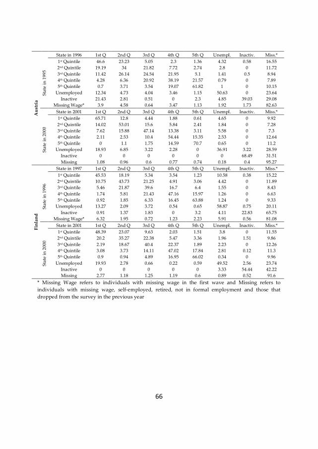
66
A
ust
ria
State in 1996 1st Q 2nd Q 3rd Q 4th Q 5th Q Unempl. Inactiv. Miss.*
Sta
te i
n 1
99
5
1st Quintile 46.6 23.23 5.05 2.3 1.36 4.32 0.58 16.55
2nd Quintile 19.19 34 21.82 7.72 2.74 2.8 0 11.72
3rd Quintile 11.42 26.14 24.54 21.95 5.1 1.41 0.5 8.94
4th Quintile 4.28 6.36 20.92 38.19 21.57 0.79 0 7.89
5th Quintile 0.7 3.71 3.54 19.07 61.82 1 0 10.15
Unemployed 12.34 4.73 4.04 3.46 1.15 50.63 0 23.64
Inactive 21.43 2.81 0.51 0 2.3 4.85 39.03 29.08
Missing Wage* 3.9 4.58 0.64 3.47 1.13 1.92 1.73 82.63
State in 2001 1st Q 2nd Q 3rd Q 4th Q 5th Q Unempl. Inactiv. Miss.*
Sta
te i
n 2
00
0
1st Quintile 65.71 12.8 4.44 1.88 0.61 4.65 0 9.92
2nd Quintile 14.02 53.01 15.6 5.84 2.41 1.84 0 7.28
3rd Quintile 7.62 15.88 47.14 13.38 3.11 5.58 0 7.3
4th Quintile 2.11 2.53 10.4 54.44 15.35 2.53 0 12.64
5th Quintile 0 1.1 1.75 14.59 70.7 0.65 0 11.2
Unemployed 18.93 6.85 3.22 2.28 0 36.91 3.22 28.59
Inactive 0 0 0 0 0 0 68.49 31.51
Missing 1.08 0.96 0.6 0.77 0.74 0.18 0.4 95.27
Fin
lan
d
State in 1997 1st Q 2nd Q 3rd Q 4th Q 5th Q Unempl. Inactiv. Miss.*
Sta
te i
n 1
99
6
1st Quintile 45.53 18.19 5.34 3.54 1.23 10.58 0.38 15.22
2nd Quintile 10.75 43.73 21.25 4.91 3.06 4.42 0 11.89
3rd Quintile 5.46 21.87 39.6 16.7 6.4 1.55 0 8.43
4th Quintile 1.74 5.81 21.43 47.16 15.97 1.26 0 6.63
5th Quintile 0.92 1.85 6.33 16.45 63.88 1.24 0 9.33
Unemployed 13.27 2.09 3.72 0.54 0.65 58.87 0.75 20.11
Inactive 0.91 1.37 1.83 0 3.2 4.11 22.83 65.75
Missing Wage* 6.32 1.95 0.72 1.23 2.23 5.91 0.56 81.08
State in 2001 1st Q 2nd Q 3rd Q 4th Q 5th Q Unempl. Inactiv. Miss.*
Sta
te i
n 2
00
0
1st Quintile 48.39 23.07 9.63 2.03 1.51 3.8 0 11.55
2nd Quintile 20.2 35.27 22.38 5.47 3.36 1.96 1.51 9.86
3rd Quintile 2.19 18.67 40.4 22.37 1.89 2.23 0 12.26
4th Quintile 3.08 3.73 14.11 47.02 17.84 2.81 0.12 11.3
5th Quintile 0.9 0.94 4.89 16.95 66.02 0.34 0 9.96
Unemployed 19.93 2.78 0.66 0.22 0.59 49.52 2.56 23.74
Inactive 0 0 0 0 0 3.33 54.44 42.22
Missing 2.77 1.18 1.25 1.19 0.6 0.89 0.52 91.6
* Missing Wage refers to individuals with missing wage in the first wave and Missing refers to
individuals with missing wage, self-employed, retired, not in formal employment and those that
dropped from the survey in the previous year
67
Table 2-A-3. Long-Term Transition Rates Among Labour Market States G
erm
an
y
State in 2001 1st Q 2nd Q 3rd Q 4th Q 5th Q Unemp. Inactiv. Miss.* S
tate
in
19
94
1st Quintile 24.7 13.38 8.87 2.4 0.88 10.62 1.84 37.32
2nd Quintile 10.35 21.27 13.02 12.84 2.98 4.69 0.14 34.7
3rd Quintile 5.97 11.48 17.89 17.2 4.6 4.95 1.17 36.74
4th Quintile 1.32 5.8 11.66 25.46 16.74 2.19 1.38 35.45
5th Quintile 0.52 0.91 2.6 10.65 44.21 0.48 0.4 40.22
Unemployed 16.84 6.38 5.36 6.53 3.34 14.37 1.84 45.35
Inactive 7.95 1.91 7.85 0.21 2.55 3.82 8.7 67.02
Missing Wage* 8.66 5.78 7.98 6.26 3.29 3.13 2.42 62.48
De
nm
ark
State in 2001 1st Q 2nd Q 3rd Q 4th Q 5th Q Unemp. Inactiv. Miss.*
Sta
te i
n1
99
4
1st Quintile 16.67 9.31 14.33 5.83 2.48 4.89 2.24 44.25
2nd Quintile 24.11 17.35 12.64 2.17 7.36 0.14 0 36.23
3rd Quintile 6.56 11.35 18.59 7.29 8.58 1.08 0.36 46.19
4th Quintile 2.85 12.07 12.07 16.37 12.66 1.45 0 42.53
5th Quintile 2.29 2.22 3.6 14.22 30.78 1.52 0 45.36
Unemployed 5.94 10.58 2.99 4.38 8.47 7.21 0.67 59.74
Inactive 21.59 0 0 0 0 0 0 78.41
Missing 6.21 4.56 8.31 5.05 3.82 3.19 0.16 68.7
Ne
the
rln
ad
s
State in 2001 1st Q 2nd Q 3rd Q 4th Q 5th Q Unemp. Inactiv. Miss.*
Sta
te i
n 1
99
4
1st Quintile 18.3 12.93 8.78 6.36 1.63 0.88 1.11 50.01
2nd Quintile 6.14 19.42 15.38 8.01 1.74 1.08 1.5 46.73
3rd Quintile 1.19 9.3 19.44 16.57 9.04 0.56 0.45 43.45
4th Quintile 0.24 2.48 9.98 23.29 12.55 0.81 1.19 49.46
5th Quintile 0.33 0.46 2.86 10.32 43.37 0.08 0.53 42.05
Unemployed 9.87 9.39 2.15 3.59 2.15 9.6 7.3 55.95
Inactive 3.54 0 1.4 0.84 5.49 9.31 26.82 52.61
Missing Wage* 9.07 7 8.73 9.56 4.76 0.55 1.08 59.24
Be
lgiu
m
State in 2001 1st Q 2nd Q 3rd Q 4th Q 5th Q Unemp. Inactiv. Miss.*
Sta
te i
n 1
99
4
1st Quintile 19.91 13.81 10.73 7.76 3.8 2.53 0.72 40.74
2nd Quintile 15.53 16.71 11.06 8.06 4.29 2.76 0.9 40.7
3rd Quintile 7.53 17.91 15.34 12.69 5.46 0.7 0.62 39.76
4th Quintile 2.14 2.8 13.85 23.12 13.15 0.68 0 44.26
5th Quintile 0.8 2.16 1.79 12.41 39.45 0.97 0.68 41.74
Unemployed 4.13 7.04 8.34 1.53 0.48 22.39 0.99 55.12
Inactive 0.81 0 2.9 0 0 0 28.78 67.51
Missing 6.79 4.18 6.34 5.72 1.94 1.93 1.53 71.56
Lu
xe
mb
ou
rg
State in 2001 1st Q 2nd Q 3rd Q 4th Q 5th Q Unemp. Inactiv. Miss.*
Sta
te i
n 1
99
5
1st Quintile 17.82 19.54 5.58 1 0.87 0.5 0.81 53.88
2nd Quintile 4.64 23.77 16.99 4.93 0 0 0 49.68
3rd Quintile 1.06 4.12 25.04 18.88 6.24 0 0 44.65
4th Quintile 0 0.92 6.29 28.65 18.6 0 0 45.54
5th Quintile 0 0.25 1.36 9.85 42.91 0 0 45.63
Unemployed 2.98 3.47 11.42 7 2.26 4.58 1.99 66.3
Inactive 0 20 0 0 0 0 9 71
Missing Wage* 5.9 4.26 1.71 0.53 3.51 2.14 2.49 79.47
Fra
nce
State in 2001 1st Q 2nd Q 3rd Q 4th Q 5th Q Unemp. Inactiv. Miss.*
Sta
te i
n 1
99
4
1st Quintile 19.2 18.63 6.8 1.61 0.57 4.07 1.71 47.41
2nd Quintile 8.33 14.69 16.79 5.79 1.32 4.55 1.05 47.48
3rd Quintile 1.59 6.45 18.62 20.01 4.89 1.79 0.68 45.97
4th Quintile 2.36 3.21 7.68 20.62 18.73 1.12 0.72 45.56
5th Quintile 0.99 1.32 4.22 10.29 38.46 0.75 0.42 43.55
Unemployed 10.84 6.27 3.55 3.66 2.67 8.96 3.12 60.93
Inactive 1.86 1.06 0 4.25 0.66 1.33 29.88 60.96
Missing 4.69 5.81 4.03 4.52 2.12 4.23 1.61 73
68
UK
State in 2001 1st Q 2nd Q 3rd Q 4th Q 5th Q Unempl. Inactive Missing*
Sta
te i
n 1
99
4 1st Quintile 20.32 19.25 15.53 6.11 2.99 5.31 3.11 27.39
2nd Quintile 13.82 22.88 15.82 10.43 3.37 0.48 1.4 31.8
3rd Quintile 6.95 11.35 24.86 17.05 10.17 1.35 0 28.27
4th Quintile 2.38 4.81 11.71 29.82 22.79 0.84 3.14 24.51
5th Quintile 1.63 0.42 2.15 12.96 45.2 1.87 2.29 33.49
Unemployed 11.92 7.52 7.67 6.3 3.18 16.2 5.32 41.9
Inactive 6.74 5.62 4.33 3.54 4.04 24.9 7.41 43.42
Missing
Wage* 5.64 5.65 7.37 5.61 4.2 3.26 3.81 64.45
Ire
lan
d
State in 2001 1st Q 2nd Q 3rd Q 4th Q 5th Q Unemp. Inactiv. Miss.*
Sta
te i
n1
99
4
1st Quintile 10.49 11.65 8.72 8.33 5.97 2.05 0 52.79
2nd Quintile 9 6.2 10.05 7.22 1.63 2.1 2.9 60.89
3rd Quintile 1.94 9.74 13.55 9.06 8.12 0 0.54 57.05
4th Quintile 0.76 0.76 8.42 11.8 18.09 1.15 0.32 58.71
5th Quintile 0.65 0.83 1.18 7 29.17 0.72 0 60.46
Unemployed 5.7 6.28 7 1.91 0.35 13.89 5.72 59.14
Inactive 6.52 0 1.12 0 0 9.04 23.86 59.46
Missing 2.57 2.71 1.89 4.85 0.85 0.76 3.89 82.48
Ita
ly
State in 2001 1st Q 2nd Q 3rd Q 4th Q 5th Q Unemp. Inactiv. Miss.*
Sta
te i
n 1
99
4
1st Quintile 17.46 16.67 9.27 5.29 2.29 3.9 0.61 44.5
2nd Quintile 4.97 14.49 16.73 10.58 3.66 2.23 0.49 46.85
3rd Quintile 3 7.93 16.19 14.2 7.53 1.29 1.67 48.19
4th Quintile 1.01 5.38 8.97 21.99 16.94 0.37 1.27 44.07
5th Quintile 0.17 1.79 3.23 9.01 34.99 0.29 0.58 49.93
Unemployed 13.24 7.71 4.45 3.44 2.09 16.22 2.84 50
Inactive 3.87 1.98 3.04 1.71 1.34 6.69 11.3 70.08
Missing
Wage* 4.15 2.61 3.03 3.17 2.16 3.93 1.67 79.29
Gre
ece
State in 2001 1st Q 2nd Q 3rd Q 4th Q 5th Q Unemp. Inactiv. Miss.*
Sta
te i
n 1
99
4
1st Quintile 15.45 13.37 11.53 5.46 3.26 2.21 0.7 48.02
2nd Quintile 7.72 10.31 15.43 10.12 2.98 1.41 0.26 51.79
3rd Quintile 1.42 4.84 17.51 18.75 4.45 0.23 0.66 52.13
4th Quintile 3.16 2.9 11.96 19.13 12.53 0.68 0 49.63
5th Quintile 0 2.7 3 12.27 34.75 0 0.57 46.71
Unemployed 8.11 12.07 6.86 3.69 1.57 8.09 3.16 56.44
Inactive 6.62 6.3 3.01 4.44 0.59 1.59 16.18 61.26
Missing 3.3 4.17 3.56 1.11 2.28 2.75 2.27 80.57
Sp
ain
State in 2001 1st Q 2nd Q 3rd Q 4th Q 5th Q Unemp. Inactiv. Miss.*
Sta
te i
n 1
99
4
1st Quintile 18.47 14.53 9.31 5.33 1.33 3.98 2.01 45.05
2nd Quintile 5.49 15.59 12.21 6.62 2.18 2.53 1.04 54.34
3rd Quintile 6.01 6.16 17.34 15.75 5.62 2.83 1.61 44.67
4th Quintile 1.51 1.39 5.89 23.28 19.72 2.33 3.33 42.56
5th Quintile 0 1.25 1.29 3.56 44.87 0.51 2.49 46.03
Unemployed 10.5 8.75 8.53 7.49 0.91 12.46 2.96 48.39
Inactive 3.85 4.55 4.91 2 0.78 6.91 24.74 52.26
Missing
Wage* 4.87 4.48 3.64 4.86 4.3 2.62 2.52 72.7
Po
rtu
ga
l
State in 2001 1st Q 2nd Q 3rd Q 4th Q 5th Q Unemp. Inactiv. Miss.*
Sta
te i
n 1
99
4
1st Quintile 25.3 18.35 9.01 7.83 0.67 3.1 0.64 35.09
2nd Quintile 11.42 16.67 18.81 9.58 1.36 1.47 1.74 38.96
3rd Quintile 6.27 13.65 16.61 15.99 6.34 2.79 2.38 35.95
4th Quintile 3.43 3.94 8.49 22.34 14.43 1.05 0.48 45.84
5th Quintile 0.07 0.07 3.85 7.18 40.43 1.31 0.14 46.96
Unemployed 9.66 14.07 8.34 3.1 3.45 4.69 9.66 47.03
Inactive 11.06 1.68 3.06 1.78 1.09 2.96 28.43 49.95
69
Missing 3.2 2.67 4.49 4.34 7.07 1.49 1.27 75.48 A
ust
ria
State in 2001 1st Q 2nd Q 3rd Q 4th Q 5th Q Unemp. Inactiv. Miss.* S
tate
in
19
95
1st Quintile 23.54 16.86 7.6 3.13 1.94 2.25 0.39 44.3
2nd Quintile 10.63 14.49 17.77 11.53 2.8 3.11 0 39.68
3rd Quintile 8.85 12.93 11.45 14.4 5.82 4.3 0.41 41.84
4th Quintile 0.62 5.86 7.46 24.87 13.32 1.24 0.59 46.04
5th Quintile 1.51 3.15 3.85 8.84 35.19 1.14 0 46.32
Unemployed 10.27 1.15 3.58 1.73 2.08 19.03 0 62.17
Inactive 14.29 0 2.81 6.63 2.3 0.51 9.18 64.29
Missing
Wage* 4.91 3.65 3.63 1.3 3.4 0.17 0.14 82.81
Fin
lan
d
State in 2001 1st Q 2nd Q 3rd Q 4th Q 5th Q Unemp. Inactiv. Miss.*
Sta
te i
n1
99
6
1st Quintile 20.59 11.87 7.01 6.76 2.68 2.12 0.6 48.37
2nd Quintile 7.29 19.15 19.27 10.53 1.95 0.56 0.28 40.98
3rd Quintile 5.07 10.82 21.71 14.7 8.04 2 0 37.66
4th Quintile 0.69 4.32 10.95 20.96 17.83 1.64 0 43.59
5th Quintile 1.72 0.95 3.88 10.79 35.23 0.67 0.29 46.47
Unemployed 14.51 9.58 5.16 3.49 1.45 12.88 0.83 52.1
Inactive 0 0 4.57 2.74 0 6.39 0 86.3
Missing 5.66 4.51 4.35 5.08 4.25 3.17 1.81 71.16
* Missing Wage refers to individuals with missing wage in the first wave and Missing refers to
individuals with missing wage, self-employed, retired, not in formal employment and those that
dropped from the survey in the previous year.
70
Table 2-A-4. Short-Term Transition Rates Among Income Quintiles G
erm
an
y
State in 1995
State in 1994 1st Quintile 2nd Quintile 3rd Quintile 4th Quintile 5th Quintile
1st Quintile 71.28 21.63 6 1.09 0
2nd Quintile 15.93 55.46 20.42 7.22 0.98
3rd Quintile 4.15 19.68 49.2 23.36 3.62
4th Quintile 0.47 4.82 20.38 55.66 18.67
5th Quintile 0 0.5 2.56 12.9 84.03
State in 2001
State in 2000 1st Quintile 2nd Quintile 3rd Quintile 4th Quintile 5th Quintile
1st Quintile 77.43 17.39 4.21 0.74 0.23
2nd Quintile 17.75 57.19 20.3 4.34 0.41
3rd Quintile 3.68 21.97 53.15 20.09 1.12
4th Quintile 0.6 2.63 15.79 66.86 14.13
5th Quintile 0.58 2.55 2.91 14.89 79.08
De
nm
ark
State in 1995
State in 1994 1st Quintile 2nd Quintile 3rd Quintile 4th Quintile 5th Quintile
1st Quintile 55.54 26.12 13.4 2.28 2.67
2nd Quintile 25.15 47.93 17.03 8.63 1.26
3rd Quintile 7.03 34.02 32.22 19.84 6.89
4th Quintile 0.88 7.75 25.73 48.91 16.73
5th Quintile 2.42 1.15 1.82 27.9 66.71
State in 2001
State in 2000 1st Quintile 2nd Quintile 3rd Quintile 4th Quintile 5th Quintile
1st Quintile 60.81 20.21 15.94 2.17 0.87
2nd Quintile 28.36 41.29 21.36 3.45 5.54
3rd Quintile 6.61 23.05 50.56 16.36 3.42
4th Quintile 4.81 9.09 23.02 43.4 19.68
5th Quintile 0.66 0.77 6.44 15.01 77.12
Ne
the
rlan
ds
State in 1995
State in 1994 1st Quintile 2nd Quintile 3rd Quintile 4th Quintile 5th Quintile
1st Quintile 61.88 29.72 6.16 2.14 0.09
2nd Quintile 13.02 51.22 27.54 6.55 1.66
3rd Quintile 3.33 16.08 51.68 25.46 3.45
4th Quintile 0.58 3.04 14.91 59.91 21.56
5th Quintile 1 0.55 2.58 14.92 80.94
State in 2001
State in 2000 1st Quintile 2nd Quintile 3rd Quintile 4th Quintile 5th Quintile
1st Quintile 71.13 20.01 4.7 3.56 0.6
2nd Quintile 9.31 59.25 22.57 7.3 1.56
3rd Quintile 5.55 8.59 61.68 19 5.18
4th Quintile 1.04 1.41 18.41 63.84 15.3
5th Quintile 0 0.85 1.43 18.22 79.5
Be
lgiu
m
State in 1995
State in 1994 1st Quintile 2nd Quintile 3rd Quintile 4th Quintile 5th Quintile
1st Quintile 54.42 20.13 12.22 8.2 5.03
2nd Quintile 28.54 43.39 18.78 7.72 1.57
3rd Quintile 5.96 28.14 48.55 12.84 4.51
4th Quintile 3.7 5.64 24.09 49.88 16.68
5th Quintile 0.71 1.68 3.09 18.49 76.02
State in 2001
State in 2000 1st Quintile 2nd Quintile 3rd Quintile 4th Quintile 5th Quintile
1st Quintile 72.75 17.92 8.59 0.39 0.35
2nd Quintile 12.7 54.52 23.99 6.7 2.09
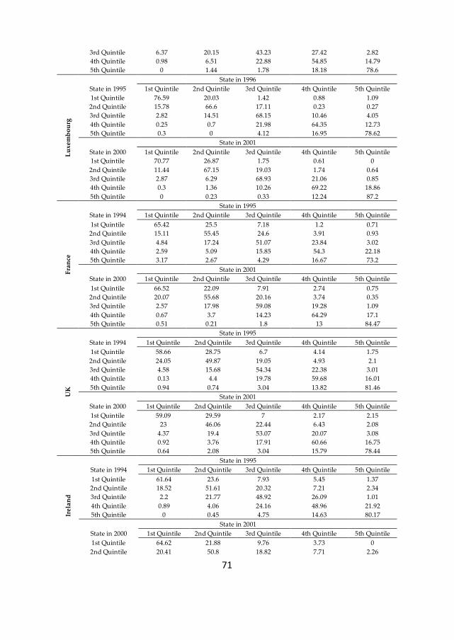
71
3rd Quintile 6.37 20.15 43.23 27.42 2.82
4th Quintile 0.98 6.51 22.88 54.85 14.79
5th Quintile 0 1.44 1.78 18.18 78.6 L
ux
em
bo
urg
State in 1996
State in 1995 1st Quintile 2nd Quintile 3rd Quintile 4th Quintile 5th Quintile
1st Quintile 76.59 20.03 1.42 0.88 1.09
2nd Quintile 15.78 66.6 17.11 0.23 0.27
3rd Quintile 2.82 14.51 68.15 10.46 4.05
4th Quintile 0.25 0.7 21.98 64.35 12.73
5th Quintile 0.3 0 4.12 16.95 78.62
State in 2001
State in 2000 1st Quintile 2nd Quintile 3rd Quintile 4th Quintile 5th Quintile
1st Quintile 70.77 26.87 1.75 0.61 0
2nd Quintile 11.44 67.15 19.03 1.74 0.64
3rd Quintile 2.87 6.29 68.93 21.06 0.85
4th Quintile 0.3 1.36 10.26 69.22 18.86
5th Quintile 0 0.23 0.33 12.24 87.2
Fra
nce
State in 1995
State in 1994 1st Quintile 2nd Quintile 3rd Quintile 4th Quintile 5th Quintile
1st Quintile 65.42 25.5 7.18 1.2 0.71
2nd Quintile 15.11 55.45 24.6 3.91 0.93
3rd Quintile 4.84 17.24 51.07 23.84 3.02
4th Quintile 2.59 5.09 15.85 54.3 22.18
5th Quintile 3.17 2.67 4.29 16.67 73.2
State in 2001
State in 2000 1st Quintile 2nd Quintile 3rd Quintile 4th Quintile 5th Quintile
1st Quintile 66.52 22.09 7.91 2.74 0.75
2nd Quintile 20.07 55.68 20.16 3.74 0.35
3rd Quintile 2.57 17.98 59.08 19.28 1.09
4th Quintile 0.67 3.7 14.23 64.29 17.1
5th Quintile 0.51 0.21 1.8 13 84.47
UK
State in 1995
State in 1994 1st Quintile 2nd Quintile 3rd Quintile 4th Quintile 5th Quintile
1st Quintile 58.66 28.75 6.7 4.14 1.75
2nd Quintile 24.05 49.87 19.05 4.93 2.1
3rd Quintile 4.58 15.68 54.34 22.38 3.01
4th Quintile 0.13 4.4 19.78 59.68 16.01
5th Quintile 0.94 0.74 3.04 13.82 81.46
State in 2001
State in 2000 1st Quintile 2nd Quintile 3rd Quintile 4th Quintile 5th Quintile
1st Quintile 59.09 29.59 7 2.17 2.15
2nd Quintile 23 46.06 22.44 6.43 2.08
3rd Quintile 4.37 19.4 53.07 20.07 3.08
4th Quintile 0.92 3.76 17.91 60.66 16.75
5th Quintile 0.64 2.08 3.04 15.79 78.44
Ire
lan
d
State in 1995
State in 1994 1st Quintile 2nd Quintile 3rd Quintile 4th Quintile 5th Quintile
1st Quintile 61.64 23.6 7.93 5.45 1.37
2nd Quintile 18.52 51.61 20.32 7.21 2.34
3rd Quintile 2.2 21.77 48.92 26.09 1.01
4th Quintile 0.89 4.06 24.16 48.96 21.92
5th Quintile 0 0.45 4.75 14.63 80.17
State in 2001
State in 2000 1st Quintile 2nd Quintile 3rd Quintile 4th Quintile 5th Quintile
1st Quintile 64.62 21.88 9.76 3.73 0
2nd Quintile 20.41 50.8 18.82 7.71 2.26
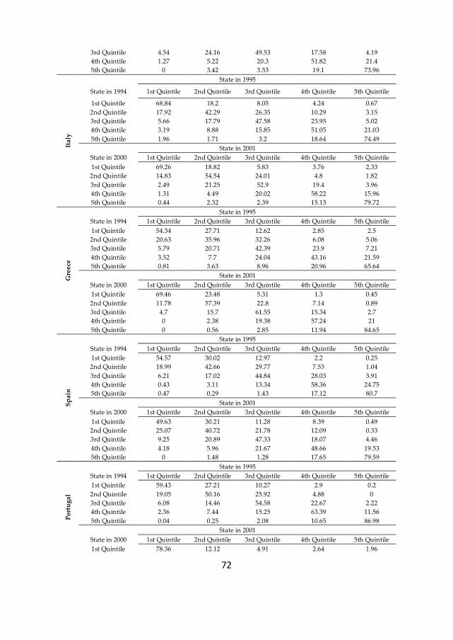
72
3rd Quintile 4.54 24.16 49.53 17.58 4.19
4th Quintile 1.27 5.22 20.3 51.82 21.4
5th Quintile 0 3.42 3.53 19.1 73.96 It
aly
State in 1995
State in 1994 1st Quintile 2nd Quintile 3rd Quintile 4th Quintile 5th Quintile
1st Quintile 68.84 18.2 8.05 4.24 0.67
2nd Quintile 17.92 42.29 26.35 10.29 3.15
3rd Quintile 5.66 17.79 47.58 23.95 5.02
4th Quintile 3.19 8.88 15.85 51.05 21.03
5th Quintile 1.96 1.71 3.2 18.64 74.49
State in 2001
State in 2000 1st Quintile 2nd Quintile 3rd Quintile 4th Quintile 5th Quintile
1st Quintile 69.26 18.82 5.83 3.76 2.33
2nd Quintile 14.83 54.54 24.01 4.8 1.82
3rd Quintile 2.49 21.25 52.9 19.4 3.96
4th Quintile 1.31 4.49 20.02 58.22 15.96
5th Quintile 0.44 2.32 2.39 15.13 79.72
Gre
ece
State in 1995
State in 1994 1st Quintile 2nd Quintile 3rd Quintile 4th Quintile 5th Quintile
1st Quintile 54.34 27.71 12.62 2.85 2.5
2nd Quintile 20.63 35.96 32.26 6.08 5.06
3rd Quintile 5.79 20.71 42.39 23.9 7.21
4th Quintile 3.52 7.7 24.04 43.16 21.59
5th Quintile 0.81 3.63 8.96 20.96 65.64
State in 2001
State in 2000 1st Quintile 2nd Quintile 3rd Quintile 4th Quintile 5th Quintile
1st Quintile 69.46 23.48 5.31 1.3 0.45
2nd Quintile 11.78 57.39 22.8 7.14 0.89
3rd Quintile 4.7 15.7 61.55 15.34 2.7
4th Quintile 0 2.38 19.38 57.24 21
5th Quintile 0 0.56 2.85 11.94 84.65
Sp
ain
State in 1995
State in 1994 1st Quintile 2nd Quintile 3rd Quintile 4th Quintile 5th Quintile
1st Quintile 54.57 30.02 12.97 2.2 0.25
2nd Quintile 18.99 42.66 29.77 7.53 1.04
3rd Quintile 6.21 17.02 44.84 28.03 3.91
4th Quintile 0.43 3.11 13.34 58.36 24.75
5th Quintile 0.47 0.29 1.43 17.12 80.7
State in 2001
State in 2000 1st Quintile 2nd Quintile 3rd Quintile 4th Quintile 5th Quintile
1st Quintile 49.63 30.21 11.28 8.39 0.49
2nd Quintile 25.07 40.72 21.78 12.09 0.33
3rd Quintile 9.25 20.89 47.33 18.07 4.46
4th Quintile 4.18 5.96 21.67 48.66 19.53
5th Quintile 0 1.48 1.28 17.65 79.59
Po
rtu
ga
l
State in 1995
State in 1994 1st Quintile 2nd Quintile 3rd Quintile 4th Quintile 5th Quintile
1st Quintile 59.43 27.21 10.27 2.9 0.2
2nd Quintile 19.05 50.16 25.92 4.88 0
3rd Quintile 6.08 14.46 54.58 22.67 2.22
4th Quintile 2.36 7.44 15.25 63.39 11.56
5th Quintile 0.04 0.25 2.08 10.65 86.98
State in 2001
State in 2000 1st Quintile 2nd Quintile 3rd Quintile 4th Quintile 5th Quintile
1st Quintile 78.36 12.12 4.91 2.64 1.96
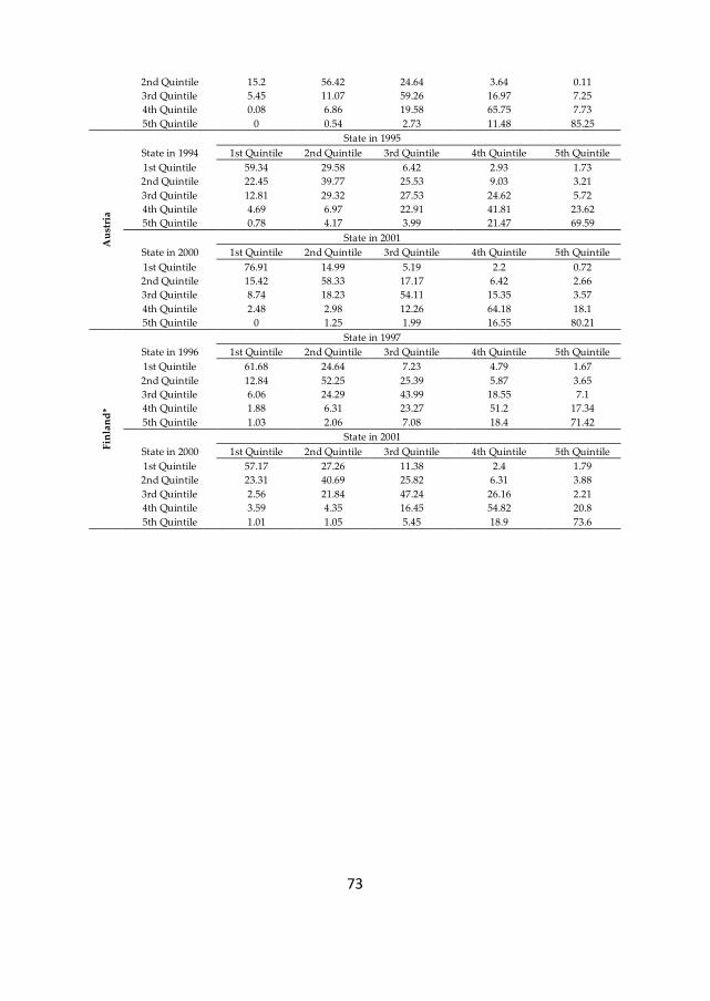
73
2nd Quintile 15.2 56.42 24.64 3.64 0.11
3rd Quintile 5.45 11.07 59.26 16.97 7.25
4th Quintile 0.08 6.86 19.58 65.75 7.73
5th Quintile 0 0.54 2.73 11.48 85.25
Au
stri
a
State in 1995
State in 1994 1st Quintile 2nd Quintile 3rd Quintile 4th Quintile 5th Quintile
1st Quintile 59.34 29.58 6.42 2.93 1.73
2nd Quintile 22.45 39.77 25.53 9.03 3.21
3rd Quintile 12.81 29.32 27.53 24.62 5.72
4th Quintile 4.69 6.97 22.91 41.81 23.62
5th Quintile 0.78 4.17 3.99 21.47 69.59
State in 2001
State in 2000 1st Quintile 2nd Quintile 3rd Quintile 4th Quintile 5th Quintile
1st Quintile 76.91 14.99 5.19 2.2 0.72
2nd Quintile 15.42 58.33 17.17 6.42 2.66
3rd Quintile 8.74 18.23 54.11 15.35 3.57
4th Quintile 2.48 2.98 12.26 64.18 18.1
5th Quintile 0 1.25 1.99 16.55 80.21
Fin
lan
d*
State in 1997
State in 1996 1st Quintile 2nd Quintile 3rd Quintile 4th Quintile 5th Quintile
1st Quintile 61.68 24.64 7.23 4.79 1.67
2nd Quintile 12.84 52.25 25.39 5.87 3.65
3rd Quintile 6.06 24.29 43.99 18.55 7.1
4th Quintile 1.88 6.31 23.27 51.2 17.34
5th Quintile 1.03 2.06 7.08 18.4 71.42
State in 2001
State in 2000 1st Quintile 2nd Quintile 3rd Quintile 4th Quintile 5th Quintile
1st Quintile 57.17 27.26 11.38 2.4 1.79
2nd Quintile 23.31 40.69 25.82 6.31 3.88
3rd Quintile 2.56 21.84 47.24 26.16 2.21
4th Quintile 3.59 4.35 16.45 54.82 20.8
5th Quintile 1.01 1.05 5.45 18.9 73.6
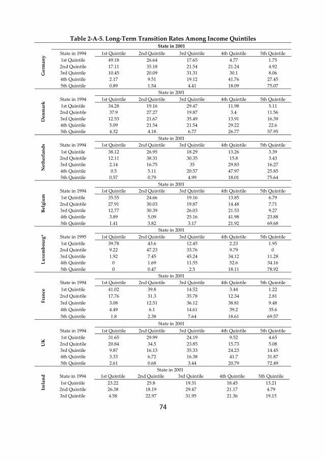
74
Table 2-A-5. Long-Term Transition Rates Among Income Quintiles G
erm
an
y
State in 2001
State in 1994 1st Quintile 2nd Quintile 3rd Quintile 4th Quintile 5th Quintile
1st Quintile 49.18 26.64 17.65 4.77 1.75
2nd Quintile 17.11 35.18 21.54 21.24 4.92
3rd Quintile 10.45 20.09 31.31 30.1 8.06
4th Quintile 2.17 9.51 19.12 41.76 27.45
5th Quintile 0.89 1.54 4.41 18.09 75.07
De
nm
ark
State in 2001
State in 1994 1st Quintile 2nd Quintile 3rd Quintile 4th Quintile 5th Quintile
1st Quintile 34.28 19.16 29.47 11.98 5.11
2nd Quintile 37.9 27.27 19.87 3.4 11.56
3rd Quintile 12.53 21.67 35.49 13.91 16.39
4th Quintile 5.09 21.54 21.54 29.22 22.6
5th Quintile 4.32 4.18 6.77 26.77 57.95
Ne
the
rlan
ds
State in 2001
State in 1994 1st Quintile 2nd Quintile 3rd Quintile 4th Quintile 5th Quintile
1st Quintile 38.12 26.95 18.29 13.26 3.39
2nd Quintile 12.11 38.31 30.35 15.8 3.43
3rd Quintile 2.14 16.75 35 29.83 16.27
4th Quintile 0.5 5.11 20.57 47.97 25.85
5th Quintile 0.57 0.79 4.99 18.01 75.64
Be
lgiu
m
State in 2001
State in 1994 1st Quintile 2nd Quintile 3rd Quintile 4th Quintile 5th Quintile
1st Quintile 35.55 24.66 19.16 13.85 6.79
2nd Quintile 27.91 30.03 19.87 14.48 7.71
3rd Quintile 12.77 30.39 26.03 21.53 9.27
4th Quintile 3.89 5.09 25.16 41.98 23.88
5th Quintile 1.41 3.82 3.17 21.92 69.68
Lu
xe
mb
ou
rg*
State in 2001
State in 1995 1st Quintile 2nd Quintile 3rd Quintile 4th Quintile 5th Quintile
1st Quintile 39.78 43.6 12.45 2.23 1.95
2nd Quintile 9.22 47.23 33.76 9.79 0
3rd Quintile 1.92 7.45 45.24 34.12 11.28
4th Quintile 0 1.69 11.55 52.6 34.16
5th Quintile 0 0.47 2.5 18.11 78.92
Fra
nce
State in 2001
State in 1994 1st Quintile 2nd Quintile 3rd Quintile 4th Quintile 5th Quintile
1st Quintile 41.02 39.8 14.52 3.44 1.22
2nd Quintile 17.76 31.3 35.78 12.34 2.81
3rd Quintile 3.08 12.51 36.12 38.81 9.48
4th Quintile 4.49 6.1 14.61 39.2 35.6
5th Quintile 1.8 2.38 7.64 18.61 69.57
UK
State in 2001
State in 1994 1st Quintile 2nd Quintile 3rd Quintile 4th Quintile 5th Quintile
1st Quintile 31.65 29.99 24.19 9.52 4.65
2nd Quintile 20.84 34.5 23.85 15.73 5.08
3rd Quintile 9.87 16.13 35.33 24.23 14.45
4th Quintile 3.33 6.72 16.38 41.7 31.87
5th Quintile 2.61 0.68 3.44 20.79 72.49
Ire
lan
d
State in 2001
State in 1994 1st Quintile 2nd Quintile 3rd Quintile 4th Quintile 5th Quintile
1st Quintile 23.22 25.8 19.31 18.45 13.21
2nd Quintile 26.38 18.19 29.47 21.17 4.79
3rd Quintile 4.58 22.97 31.95 21.36 19.15

75
4th Quintile 1.9 1.9 21.14 29.63 45.44
5th Quintile 1.66 2.13 3.05 18.02 75.14 It
aly
State in 2001
State in 1994 1st Quintile 2nd Quintile 3rd Quintile 4th Quintile 5th Quintile
1st Quintile 34.25 32.69 18.18 10.38 4.5
2nd Quintile 9.86 28.73 33.17 20.98 7.26
3rd Quintile 6.14 16.23 33.14 29.08 15.41
4th Quintile 1.85 9.92 16.51 40.51 31.21
5th Quintile 0.34 3.64 6.57 18.32 71.12
Gre
ece
State in 2001
State in 1994 1st Quintile 2nd Quintile 3rd Quintile 4th Quintile 5th Quintile
1st Quintile 31.48 27.25 23.5 11.12 6.65
2nd Quintile 16.57 22.14 33.15 21.74 6.4
3rd Quintile 3.02 10.31 37.28 39.92 9.47
4th Quintile 6.35 5.85 24.07 38.51 25.23
5th Quintile 0 5.12 5.7 23.27 65.91
Sp
ain
State in 2001
State in 1994 1st Quintile 2nd Quintile 3rd Quintile 4th Quintile 5th Quintile
1st Quintile 37.71 29.67 19.02 10.89 2.71
2nd Quintile 13.03 37.04 29.02 15.73 5.17
3rd Quintile 11.81 12.1 34.08 30.96 11.05
4th Quintile 2.91 2.69 11.37 44.95 38.08
5th Quintile 0 2.45 2.53 6.99 88.03
Po
rtu
ga
l
State in 2001
State in 1994 1st Quintile 2nd Quintile 3rd Quintile 4th Quintile 5th Quintile
1st Quintile 41.37 30.01 14.73 12.8 1.1
2nd Quintile 19.74 28.82 32.53 16.56 2.36
3rd Quintile 10.66 23.19 28.22 27.17 10.77
4th Quintile 6.52 7.48 16.13 42.45 27.42
5th Quintile 0.13 0.13 7.46 13.92 78.35
Au
stri
a
State in 2001
State in 1994 1st Quintile 2nd Quintile 3rd Quintile 4th Quintile 5th Quintile
1st Quintile 44.36 31.77 14.32 5.9 3.66
2nd Quintile 18.58 25.33 31.05 20.15 4.89
3rd Quintile 16.56 24.2 21.41 26.93 10.89
4th Quintile 1.19 11.24 14.32 47.7 25.55
5th Quintile 2.87 6 7.32 16.83 66.99
Fin
lan
d*
State in 2001
State in 1996 1st Quintile 2nd Quintile 3rd Quintile 4th Quintile 5th Quintile
1st Quintile 42.09 24.27 14.33 13.82 5.49
2nd Quintile 12.53 32.91 33.12 18.1 3.34
3rd Quintile 8.4 17.93 35.97 24.36 13.33
4th Quintile 1.27 7.9 20 38.27 32.56
5th Quintile 3.27 1.82 7.38 20.52 67.01

76
3. EQUALIZING OR DISEQUALIZING LIFETIME
EARNINGS DIFFERENTIALS? EARNINGS MOBILITY
IN THE EU: 1994-2001
77
3.1.Introduction
Do EU citizens have an increased opportunity to improve their position in the
distribution of lifetime earnings? To what extent does earnings mobility work to
equalize/disequalize longer-term earnings relative to cross-sectional inequality and
how does it differ across the EU?
These questions are relevant in the context of the EU labour market policy changes
that took place after 1995 under the incidence of the 1994 OECD Jobs Strategy,
which recommended policies to increase wage flexibility, lower non-wage labour
costs and allow relative wages to reflect better individual differences in
productivity and local labour market conditions (OECD, 2004). Following these
reforms, the labour market performance improved in some countries and
deteriorated in others, with heterogeneous consequences for cross-sectional
earnings inequality and earnings mobility. Averaged across the OECD, however,
gross earnings inequality increased after 1994 (OECD, 2006).
To explore the possible lifetime inequality consequences of these labour market
changes, one has to expand the typical cross-sectional view usually taken in cross-
national comparisons of earnings distribution because a simple cross-sectional
picture of earnings inequality is inadequate in capturing the true degree of
inequality faced by individuals during their lifetime. The welfare implications of
any labour market changes should to be analysed in a lifetime perspective because
lifetime earnings reflect to a larger extent the differences in the opportunities faced
by individuals.
The lifetime approach faces a huge impediment: the scarcity of data on lifetime
earnings. This motivated the study of economic mobility, viewed as the link
between short and long-term earnings differentials: a cross-sectional snapshot of
income distribution overstates lifetime inequality to a degree that depends on the
degree of earnings mobility (Lillard, 1977; Atkinson et al., 1992; Creedy, 1998). If
countries have different earnings mobility levels, then single-year inequality
country rankings may lead to a misleading picture of long-term inequality ranking.
To support this statement, Creedy (1998), conducted a simulation study to examine
the relationship between cross-sectional and lifetime income distributions. His
conclusion was that simple inferences about lifetime income distributions cannot
be made on the basis of cross-sectional distributions alone, dismissing the
conclusions drawn by the OECD (1996) report.
Some people argue that rising annual inequality does not necessarily have negative
implications. This statement relies on the “offsetting mobility” argument, which
78
states that if there has been a sufficiently large simultaneous increase in mobility,
the inequality of income measured over a longer period of time, such as lifetime
income or permanent income - can be lower despite the rise in annual inequality,
with a positive impact on social welfare. This statement, however, holds only
under the assumption that individuals are not averse to income variability, future
risk or multi-period inequality (Creedy and Wilhelm, 2002; Gottschalk and
Spolaore, 2002). Therefore, there is not a complete agreement in the literature on
the value judgement of income mobility (Atkinson et al., 1992).
Those that value income mobility positively perceive it in two ways: as a goal in its
own right or as an instrument to another end. The goal of having a mobile society
is linked to the goal of securing equality of opportunity in the labour market and of
having a more flexible and efficient economy (Friedman, 1962; Atkinson et al.,
1992). The instrumental justification for mobility takes place in the context of
achieving distributional equity: lifetime equity depends on the extent of movement
up and down the earnings distribution over the lifetime (Atkinson et al., 1992). In
this line of thought, Friedman (1962) underlined the role of social mobility in
reducing lifetime earnings differentials between individuals, by allowing them to
change their position in the income distribution over time.
Thus earnings mobility is perceived in the literature as a way out of poverty. In the
absence of mobility the same individuals remain stuck at the bottom of the
earnings distribution, hence annual earnings differentials are transformed into
lifetime differentials.
Using ECHP over the period 1994-2001, we explore earnings mobility across 14 EU
countries to identify whether mobility operates as an equalizer or disequalizer of
lifetime earnings differentials, a question much neglected at the EU level. Our
paper contributes to the existing literature in three ways. First, by exploring a
different facet of mobility – as an equalizer or disequalizer of lifetime earnings
differentials -, we complement Sologon and O'Donoghue (2009d) findings on the
evolution of earnings mobility over time across the EU, thus filling part of the gap
in the study of earnings mobility at the EU level. Second, we apply a new class of
measures of mobility as an equalizer of longer-term incomes - developed by Fields
(2008) – in comparison to the well-known measure developed by Shorrocks (1978).
Third, unlike previous studies that rely on a fully balanced sample to explore
mobility (only those individuals that record positive earnings independent of the
sub-period), we extend the analysis by including the results for the unbalanced
sample over different sub-periods. By doing so, we want to explore mobility as
equalizer of longer term incomes not only for the people that remain employed
over the entire sample period, but also for those that move into and out of
79
employment. Focusing only on the fully balanced sample might bias the estimation
of mobility due to the overestimation of earnings persistency. Moreover, besides
the employment status, there are other factors determining panel attrition. All in
all, this exercise provides is an interesting check of the impact of differential
attrition on the study of earnings mobility as equalizer of longer term differentials
using the Shorrock and the Fields index.
3.2.Literature review
The concept of mobility as an equalizer of longer term income is an old one,
complementing mobility-as-time-independence, positional movement, share
movement, non-directional income movement, and directional income movement.
(Fields, 2008) The number of comparative studies on earnings mobility as a source
of equalization of longer term income is limited because of the lack of sufficiently
long comparable panel cross-country data. To investigate the link between
longitudinal earnings mobility and the reduction in long-term earnings inequality
most studies used the Shorrocks index (Shorrocks, 1978). One of the main critiques
regarding this index is that it treats equalizing and disequalizing changes in
essentially identical fashion (Benabou and Ok, 2001; Fields, 2008).
Most of the existing studies focus on the comparison between the US and a small
number of European countries. OECD (1996, 1997) presented a variety of
comparisons of earnings inequality and mobility across the OECD countries over
the period 1986-1991. They included also the Shorrocks mobility index and
concluded that the results vary depending on the inequality index used for
computing the Shorrocks index. This sensitivity was investigated more in depth by
Jarvis and Jenkins (1998), which concluded that measures focusing on the tails of
the distribution (e.g. Theil) shows greater mobility compared with the situation
when more weight is given to the middle of the distribution (e.g. Gini).
Burkhauser and Poupore (1997), using GSOEP between 1983 and 1988, compared
long-term inequality in Germany and the US. To evaluate the extent to which
mobility reduces longer term differentials, they used the Shorrocks(1978) index
based on the Theil index. Their findings identified a higher mobility in Germany
than in the US for all time periods.
Aaberge, Bjorklund, Jantti, Palme, Pedersen, Smith, and Wannemo (2002)
compared income (family income, disposable income and earnings) inequality and
mobility in the Scandinavian countries and the United Stated during 1980-1990.
They used the Shorrocks (1978) index based on the Gini index and found low
mobility levels for all countries, with higher values for the US only for long
80
accounting periods. Despite the higher mobility, independent of the accounting
period, they found that earnings inequality is higher in the US than in the
Scandinavian countries.
Hofer and Weber (2002) looked at mobility in Austria between 1986-1991 using
among other indices also the Shorrocks index calculated using the Gini, the Theil
and Mean log deviation index. They compared their results with the OECD (1996,
1997). In Austria they found a weak equalization effect of long-term mobility over
the selected period compared with Denmark, France, Germany, Italy, the UK and
the US. Moreover they underlined that “except the Austrian case, country rankings
in this panel depends on the chosen inequality index and there emerges no clear
picture which countries are the most mobile or the most immobile”.
Gregg and Vittori (2008), starting from the approach proposed by Schluter and
Trede (2003) developed a continuous alternative measure of “Shorrocks” mobility
which first, allows to identify mobility over different parts of the earnings
distribution and second, to distinguish between mobility that tends to reduce or
increase the level of permanent or long-term inequality. They used the ECHP data
on annual earnings for four countries - Denmark, Germany, Spain and the UK.
Mobility was found to equalize long-term differentials. Denmark had the highest
mobility, steaming mainly from the middle and top parts of the distribution,
whereas the lowest was found in Germany.
Most recently, Fields (2008) developed a new index to explore mobility as an
equalizer of longer term income, which unlike Shorrocks index, is able to identify
whether longitudinal mobility is equalizing or disequalizing long-term earnings
differentials. The results for the United States and France showed that the new
index picks up different trends compared with the Shorrocks index. Income
mobility was found to equalize longer-term incomes among U.S. men in the 1970s
but not in the 1980s and 1990s. In France, income mobility has been equalizing
since the late 1960s, with a higher degree of equalization in more recent years.
At the EU level, no study explored in a comparative setting earnings mobility as an
equalizer of longer-term inequality using a panel longer than six years. Moreover,
except for the short exercise in Fields (2008), The Fields index, has not been applied
in any other European country or in a comparative setting at the EU level. We
argue that the Fields and the Shorrocks indices provide complementary pieces of
information regarding the link between longitudinal mobility and long-term
earnings differentials. By exploiting the 8 years of panel in ECHP, and coupling the
information provided by the two indices, our paper aims to fill part of that gap and
make a substantive contribution to the literature on cross-national comparisons of
longitudinal mobility at the EU level. Moreover, the balanced and unbalanced
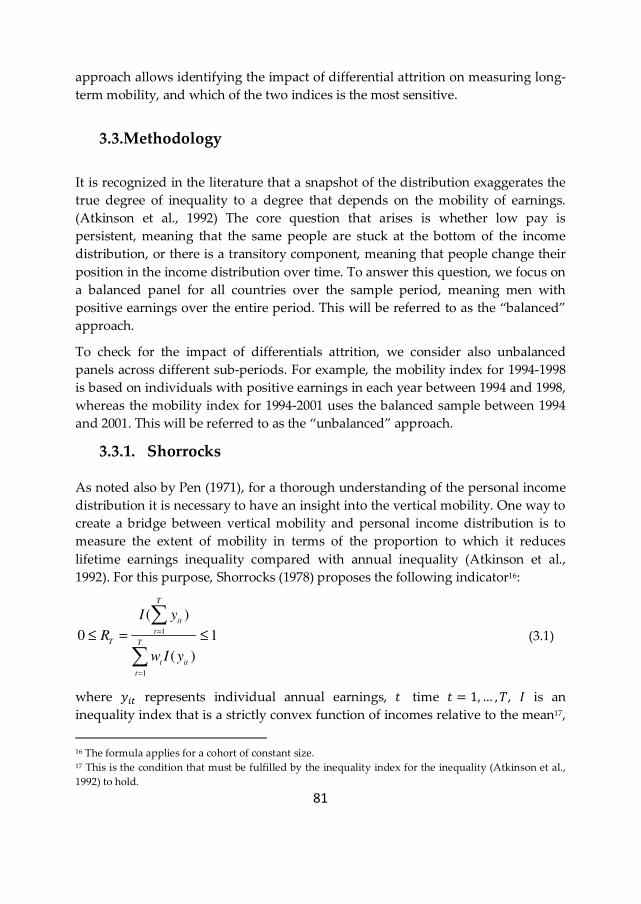
81
approach allows identifying the impact of differential attrition on measuring long-
term mobility, and which of the two indices is the most sensitive.
3.3.Methodology
It is recognized in the literature that a snapshot of the distribution exaggerates the
true degree of inequality to a degree that depends on the mobility of earnings.
(Atkinson et al., 1992) The core question that arises is whether low pay is
persistent, meaning that the same people are stuck at the bottom of the income
distribution, or there is a transitory component, meaning that people change their
position in the income distribution over time. To answer this question, we focus on
a balanced panel for all countries over the sample period, meaning men with
positive earnings over the entire period. This will be referred to as the “balanced”
approach.
To check for the impact of differentials attrition, we consider also unbalanced
panels across different sub-periods. For example, the mobility index for 1994-1998
is based on individuals with positive earnings in each year between 1994 and 1998,
whereas the mobility index for 1994-2001 uses the balanced sample between 1994
and 2001. This will be referred to as the “unbalanced” approach.
3.3.1. Shorrocks
As noted also by Pen (1971), for a thorough understanding of the personal income
distribution it is necessary to have an insight into the vertical mobility. One way to
create a bridge between vertical mobility and personal income distribution is to
measure the extent of mobility in terms of the proportion to which it reduces
lifetime earnings inequality compared with annual inequality (Atkinson et al.,
1992). For this purpose, Shorrocks (1978) proposes the following indicator16:
1
1
( )
0 1
( )
T
it
t
T T
t it
t
I y
R
w I y
=
=
≤ = ≤∑
∑ (3.1)
where ��� represents individual annual earnings, � time � = 1, … , , � is an
inequality index that is a strictly convex function of incomes relative to the mean17,
16 The formula applies for a cohort of constant size. 17 This is the condition that must be fulfilled by the inequality index for the inequality (Atkinson et al.,
1992) to hold.
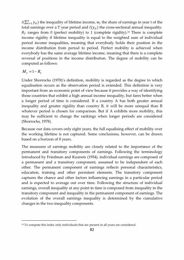
82
�(∑ ���)���� the inequality of lifetime income, �� the share of earnings in year t of the
total earnings over a T year period and �(���) the cross-sectional annual inequality.
�� ranges from 0 (perfect mobility) to 1 (complete rigidity).18 There is complete
income rigidity if lifetime inequality is equal to the weighted sum of individual
period income inequalities, meaning that everybody holds their position in the
income distribution from period to period. Perfect mobility is achieved when
everybody has the same average lifetime income, meaning that there is a complete
reversal of positions in the income distribution. The degree of mobility can be
computed as follows:
1T T
M R= −
Under Shorrocks (1978)’s definition, mobility is regarded as the degree to which
equalisation occurs as the observation period is extended. This definition is very
important from an economic point of view because it provides a way of identifying
those countries that exhibit a high annual income inequality, but fares better when
a longer period of time is considered. If a country A has both greater annual
inequality and greater rigidity than country B, it will be more unequal than B
whatever period is chosen for comparison. But if A exhibits more mobility, this
may be sufficient to change the rankings when longer periods are considered
(Shorrocks, 1978).
Because our data covers only eight years, the full equalising effect of mobility over
the working lifetime is not captured. Some conclusions, however, can be drawn
based on a horizon of 8 years.
The measures of earnings mobility are closely related to the importance of the
permanent and transitory components of earnings. Following the terminology
introduced by Friedman and Kuznets (1954), individual earnings are composed of
a permanent and a transitory component, assumed to be independent of each
other. The permanent component of earnings reflects personal characteristics,
education, training and other persistent elements. The transitory component
captures the chance and other factors influencing earnings in a particular period
and is expected to average out over time. Following the structure of individual
earnings, overall inequality at any point in time is composed from inequality in the
transitory component and inequality in the permanent component of earnings. The
evolution of the overall earnings inequality is determined by the cumulative
changes in the two inequality components.
18 To compute this index only individuals that are present in all years are considered.
83
An increase in the cross-sectional earnings inequality could reflect a rise in the
permanent and/or transitory component of earnings inequality. The rise in the
inequality in the permanent component of earnings may be consistent with
increasing returns to education, on-the-job training and other persistent abilities
that are among the main determinants of the permanent component of earnings
(Mincer, 1957, 1958, 1962, 1974; Hause, 1980). The increase in the inequality in the
transitory component of earnings may be attributed to the weakening of the labour
market institutions (e.g. unions, government wage regulation, internal labour
markets) which increases earnings exposion to shocks. Overall, the increase in the
return to persistent skills is expected to have a much larger impact on long-run
earnings inequality than an increase in the transitory component of earnings (Katz
and Autor, 1999).
In order to make inferences concerning the sources of mobility, meaning whether
income changes were determined by large variations in transitory earnings and
small variations in permanent earnings or vice-versa, we construct the stability
profile or the rigidity curve, which plots the rigidity measure TR against different
time horizons. A mobile earnings structure is represented by a stability profile that
declines with time away from the immobility horizontal line, where 1TR = . If
incomes changes are purely due to transitory effects, relative incomes will rapidly
approach their permanent values and there will then be no substantial further
equalisation. The stability profile will therefore tend to become horizontal after the
first few years. If income changes are due to more mobility in permanent incomes,
the stability profile will continue to decline as the aggregation period is extended
(Shorrocks, 1978).
3.3.2. Fields
To recall, Shorrocks (1978) conceptualized income mobility as the opposite of
income rigidity. As highlighted by Benabou and Ok (2001) and Fields (2008), the
main limitation of this measure was that it does not quantify the direction and the
extent of the difference between inequality of longer-term income and inequality of
base year income, meaning that it treats equalizing and disequalizing changes in
essentially identical fashion. Fields (2008) explained with the following example,
which uses Gini as the inequality index. The mobility index, TM , for a “Gates-
gains” mobility process (100, 200, 20000) → (100, 200, 30000) equals 4.99·10-5 , 5.91
10-5 for a “Gates-loses” mobility process and 0 for “no change”. The ranking in
mobility is “Gates-loses”, “Gates-gains” and “no change”, but neither the sign nor
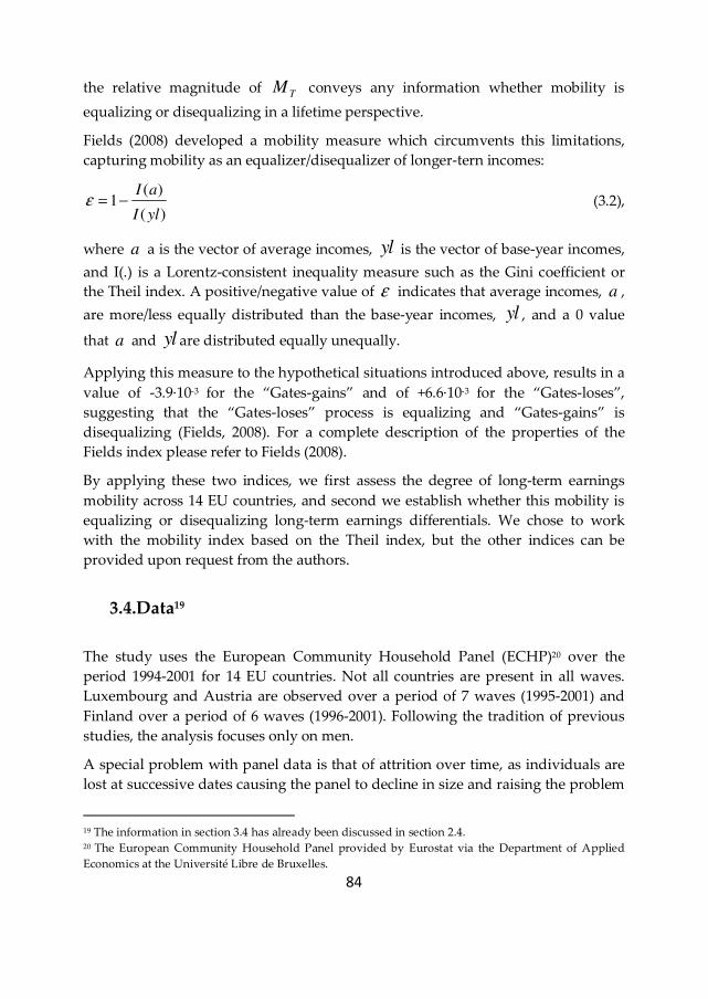
84
the relative magnitude of TM conveys any information whether mobility is
equalizing or disequalizing in a lifetime perspective.
Fields (2008) developed a mobility measure which circumvents this limitations,
capturing mobility as an equalizer/disequalizer of longer-tern incomes:
( )1
( )
I a
I ylε = − (3.2),
where a a is the vector of average incomes, yl is the vector of base-year incomes,
and I(.) is a Lorentz-consistent inequality measure such as the Gini coefficient or
the Theil index. A positive/negative value of ε indicates that average incomes, a ,
are more/less equally distributed than the base-year incomes, yl , and a 0 value
that a and yl are distributed equally unequally.
Applying this measure to the hypothetical situations introduced above, results in a
value of -3.9·10-3 for the “Gates-gains” and of +6.6·10-3 for the “Gates-loses”,
suggesting that the “Gates-loses” process is equalizing and “Gates-gains” is
disequalizing (Fields, 2008). For a complete description of the properties of the
Fields index please refer to Fields (2008).
By applying these two indices, we first assess the degree of long-term earnings
mobility across 14 EU countries, and second we establish whether this mobility is
equalizing or disequalizing long-term earnings differentials. We chose to work
with the mobility index based on the Theil index, but the other indices can be
provided upon request from the authors.
3.4.Data19
The study uses the European Community Household Panel (ECHP)20 over the
period 1994-2001 for 14 EU countries. Not all countries are present in all waves.
Luxembourg and Austria are observed over a period of 7 waves (1995-2001) and
Finland over a period of 6 waves (1996-2001). Following the tradition of previous
studies, the analysis focuses only on men.
A special problem with panel data is that of attrition over time, as individuals are
lost at successive dates causing the panel to decline in size and raising the problem
19 The information in section 3.4 has already been discussed in section 2.4. 20 The European Community Household Panel provided by Eurostat via the Department of Applied
Economics at the Université Libre de Bruxelles.
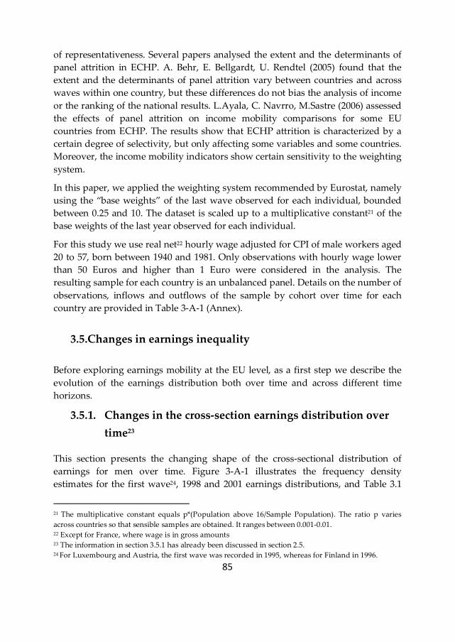
85
of representativeness. Several papers analysed the extent and the determinants of
panel attrition in ECHP. A. Behr, E. Bellgardt, U. Rendtel (2005) found that the
extent and the determinants of panel attrition vary between countries and across
waves within one country, but these differences do not bias the analysis of income
or the ranking of the national results. L.Ayala, C. Navrro, M.Sastre (2006) assessed
the effects of panel attrition on income mobility comparisons for some EU
countries from ECHP. The results show that ECHP attrition is characterized by a
certain degree of selectivity, but only affecting some variables and some countries.
Moreover, the income mobility indicators show certain sensitivity to the weighting
system.
In this paper, we applied the weighting system recommended by Eurostat, namely
using the “base weights” of the last wave observed for each individual, bounded
between 0.25 and 10. The dataset is scaled up to a multiplicative constant21 of the
base weights of the last year observed for each individual.
For this study we use real net22 hourly wage adjusted for CPI of male workers aged
20 to 57, born between 1940 and 1981. Only observations with hourly wage lower
than 50 Euros and higher than 1 Euro were considered in the analysis. The
resulting sample for each country is an unbalanced panel. Details on the number of
observations, inflows and outflows of the sample by cohort over time for each
country are provided in Table 3-A-1 (Annex).
3.5.Changes in earnings inequality
Before exploring earnings mobility at the EU level, as a first step we describe the
evolution of the earnings distribution both over time and across different time
horizons.
3.5.1. Changes in the cross-section earnings distribution over
time23
This section presents the changing shape of the cross-sectional distribution of
earnings for men over time. Figure 3-A-1 illustrates the frequency density
estimates for the first wave24, 1998 and 2001 earnings distributions, and Table 3.1
21 The multiplicative constant equals p*(Population above 16/Sample Population). The ratio p varies
across countries so that sensible samples are obtained. It ranges between 0.001-0.01. 22 Except for France, where wage is in gross amounts 23 The information in section 3.5.1 has already been discussed in section 2.5. 24 For Luxembourg and Austria, the first wave was recorded in 1995, whereas for Finland in 1996.

86
illustrates the evolution of the other moments of the earnings distribution over
time. The evolution of mean net hourly wage shows that men in most countries got
richer over time, except Austria. Net hourly earnings became more dispersed in
most countries, except Austria, France and Denmark.
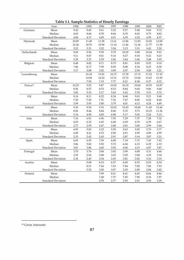
87
Table 3.1. Sample Statistics of Hourly Earnings Year 1994 1995 1996 1997 1998 1999 2000 2001
Germany Mean 9.43 9.49 9.61 9.52 9.57 9.48 9.60 9.72
Median 8.65 8.68 8.78 8.84 8.70 8.65 8.75 8.82
Standard Deviation 4.00 4.17 4.09 4.01 4.39 4.32 4.39 4.37
Denmark Mean 10.89 11.40 11.58 11.61 11.86 11.85 12.02 12.08
Median 10.36 10.76 10.96 11.14 11.46 11.36 11.77 11.50
Standard Deviation 3.23 3.31 3.52 3.54 3.13 3.31 3.43 3.20
Netherlands Mean 9.69 9.56 9.59 9.70 10.02 9.88 10.04 9.91
Median 9.11 9.07 9.01 9.10 9.27 9.18 9.32 9.23
Standard Deviation 3.39 3.37 3.55 3.56 3.64 3.40 3.48 3.95
Belgium Mean 8.48 8.82 8.71 8.75 8.81 8.83 8.92 9.10
Median 7.86 8.17 7.99 8.09 8.08 8.34 8.25 8.30
Standard Deviation 3.17 3.08 3.02 3.09 2.97 2.94 3.00 3.21
Luxembourg Mean 16.18 15.81 16.73 17.39 17.15 17.22 17.10
Median 14.90 14.52 15.31 15.72 15.60 15.65 15.29
Standard Deviation 7.50 7.19 7.77 8.21 8.38 8.37 8.22
France25 Mean 10.23 9.92 9.87 10.05 10.33 10.60 10.55 10.87
Median 8.56 8.57 8.53 8.53 8.84 9.04 9.06 9.48
Standard Deviation 5.82 5.33 5.17 5.65 5.62 5.78 5.51 5.72
UK Mean 8.16 8.11 8.22 8.34 8.68 9.01 9.21 9.68
Median 7.30 7.29 7.51 7.52 7.67 8.00 8.22 8.68
Standard Deviation 3.99 3.95 3.80 3.79 4.01 4.13 4.24 4.49
Ireland Mean 9.30 9.54 9.76 10.02 10.43 10.84 11.69 12.44
Median 8.06 8.44 8.84 8.86 9.33 9.73 10.25 11.36
Standard Deviation 5.14 4.99 4.85 4.98 5.17 5.02 5.24 5.15
Italy Mean 7.16 6.91 6.96 7.05 7.29 7.37 7.28 7.32
Median 6.65 6.32 6.43 6.48 6.69 6.76 6.59 6.67
Standard Deviation 2.77 2.59 2.67 2.68 3.01 3.00 2.99 3.04
Greece Mean 4.95 5.03 5.23 5.59 5.63 5.85 5.70 5.77
Median 4.49 4.41 4.53 4.90 4.91 4.99 4.89 4.99
Standard Deviation 2.33 2.42 2.43 2.91 2.87 3.14 3.07 3.21
Spain Mean 6.83 6.95 7.09 6.89 7.18 7.37 7.45 7.42
Median 5.86 5.82 5.92 5.72 6.04 6.15 6.29 6.33
Standard Deviation 3.81 3.86 4.00 3.92 4.06 4.15 4.07 3.87
Portugal Mean 3.70 3.74 3.84 3.92 3.99 4.08 4.31 4.46
Median 2.92 2.82 2.98 3.03 3.05 3.08 3.29 3.34
Standard Deviation 2.34 2.45 2.54 2.65 2.81 2.82 3.16 3.33
Austria Mean 9.08 8.33 8.37 8.49 8.55 8.55 8.54
Median 8.51 7.64 7.63 7.84 7.82 7.86 7.93
Standard Deviation 3.52 3.00 3.07 2.95 2.89 2.84 2.82
Finland Mean 7.89 8.01 8.41 8.45 8.66 8.86
Median 7.48 7.57 7.85 7.90 8.18 7.97
Standard Deviation 2.70 2.77 2.92 2.91 2.93 3.29
25 Gross Amounts
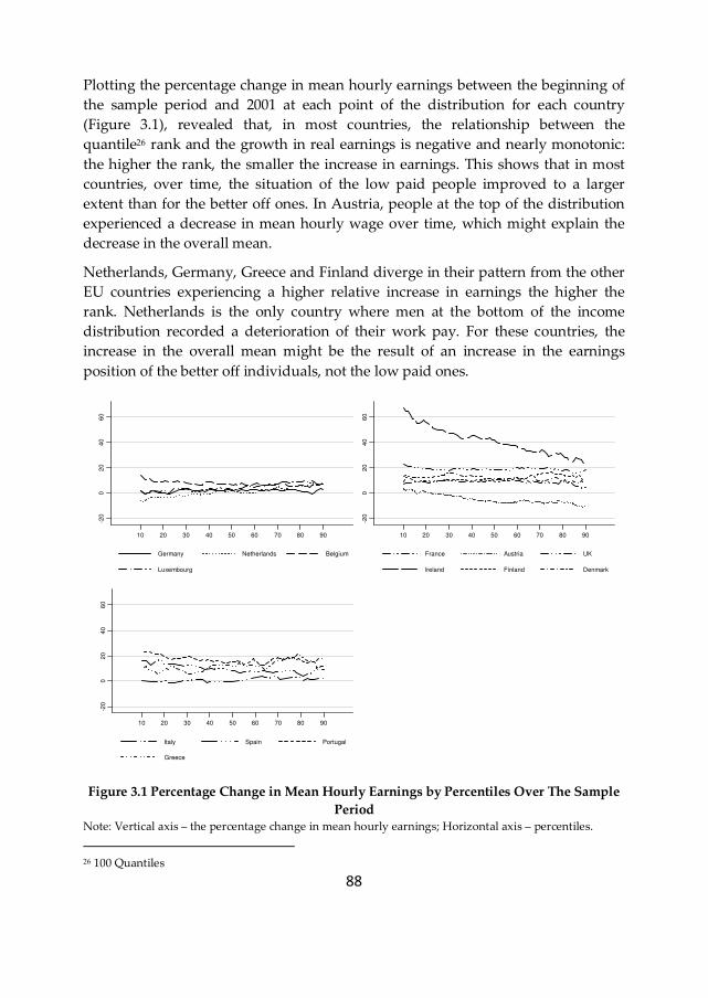
88
Plotting the percentage change in mean hourly earnings between the beginning of
the sample period and 2001 at each point of the distribution for each country
(Figure 3.1), revealed that, in most countries, the relationship between the
quantile26 rank and the growth in real earnings is negative and nearly monotonic:
the higher the rank, the smaller the increase in earnings. This shows that in most
countries, over time, the situation of the low paid people improved to a larger
extent than for the better off ones. In Austria, people at the top of the distribution
experienced a decrease in mean hourly wage over time, which might explain the
decrease in the overall mean.
Netherlands, Germany, Greece and Finland diverge in their pattern from the other
EU countries experiencing a higher relative increase in earnings the higher the
rank. Netherlands is the only country where men at the bottom of the income
distribution recorded a deterioration of their work pay. For these countries, the
increase in the overall mean might be the result of an increase in the earnings
position of the better off individuals, not the low paid ones.
Figure 3.1 Percentage Change in Mean Hourly Earnings by Percentiles Over The Sample
Period Note: Vertical axis – the percentage change in mean hourly earnings; Horizontal axis – percentiles.
26 100 Quantiles
-20
02
04
06
0
10 20 30 40 50 60 70 80 90
Germany Netherlands Belgium
Luxembourg
-20
02
04
06
0
10 20 30 40 50 60 70 80 90
France Austria UK
Ireland Finland Denmark
-20
02
04
06
0
10 20 30 40 50 60 70 80 90
Italy Spain Portugal
Greece
89
To complete the descriptive picture of the cross-sectional earnings distribution
over time, we provide also inequality measures. Inequality indices differ with
respect to their sensitivity to income differences in different parts of the
distribution. Therefore they illustrate different sides of the earnings distribution.
The year-to-year changes in earnings inequality are captured by computing the
ratio between mean earnings in the 9th decile and the 1st decile (Figure 3.2), the Gini
index, the GE indices - the Theil Index (GE(1)) -, and the Atkinson inequality index
evaluated at an the aversion parameter equal to 1 (Table 3.2).27
Figure 3.2 Ratio between Mean Earnings at the 9th Decile and the 1st Decile
The ratio between the mean earnings in the 9th decile and the 1st deciles focuses
only on the two ends of the distribution. The Gini index is most sensitive to income
differences in the middle of the distribution (more precisely, the mode). The GE
with a negative parameter is sensitive to income differences at the bottom of the
distribution and the sensitivity increases the more negative the parameter is. The
GE with a positive parameter is sensitive to income differences at the top of the
distribution and it becomes more sensitive the more positive the parameter is. For
the Atkinson inequality indices, the more positive the “inequality aversion
parameter” is, the more sensitive the index is to income differences at the bottom
of the distribution.
27 Besides these indices, several others were computed (GE(-1); GE(0), GE(2), Atkinson evaluated at
different values of the aversion parameter) and can be provided upon request from the authors. They
support the findings shown by the reported indices.
22
.53
3.5
4
Me
an
Ea
rnin
gs 9
th D
ecile
/1st D
ecile
1994 1995 1996 1997 1998 1999 2000 2001
Germany Netherlands
Belgium Luxembourg
France UK
Ireland
22
.53
3.5
4
Me
an
Ea
rnin
gs 9
th D
ecile
/1st D
ecile
1994 1995 1996 1997 1998 1999 2000 2001
Italy Spain
Portugal Greece
Austria Finland
Denmark
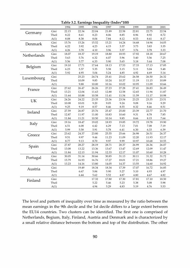
90
Table 3.2. Earnings Inequality (Index*100) 1994 1995 1996 1997 1998 1999 2000 2001
Germany Gini 22.15 22.34 22.04 21.89 22.58 22.81 22.75 22.54
Theil 8.22 8.61 8.23 8.06 8.85 8.96 8.92 8.72
A(1) 8.08 8.38 8.04 7.84 8.12 8.53 8.41 8.17
Denmark Gini 15.76 15.26 15.52 15.21 14.24 14.68 14.94 14.05
Theil 4.22 3.92 4.23 4.15 3.37 3.73 3.83 3.35
A(1) 4.26 3.78 4.10 3.96 3.37 3.76 3.78 3.33
Netherlands Gini 18.07 18.37 19.19 18.80 18.93 17.92 18.18 20.67
Theil 5.63 5.76 6.32 6.07 5.96 5.40 5.56 7.25
A(1) 5.56 5.77 6.33 5.90 5.65 5.18 5.44 7.08
Belgium Gini 19.10 17.71 17.64 18.13 17.53 17.33 17.13 17.85
Theil 6.23 5.37 5.35 5.58 5.15 5.11 5.04 5.48
A(1) 5.92 4.95 5.04 5.24 4.85 4.92 4.69 5.14
Luxembourg Gini 25.23 24.74 25.41 25.62 26.58 26.50 26.32
Theil 10.09 9.85 10.24 10.37 11.19 11.15 10.89
A(1) 9.88 10.00 10.16 10.02 10.95 11.09 10.66
France Gini 27.62 26.47 26.26 27.23 27.28 27.41 26.83 26.49
Theil 13.21 12.04 11.63 12.88 12.58 12.65 11.94 11.87
A(1) 11.64 10.88 10.58 11.41 11.54 11.59 11.17 10.98
UK Gini 24.26 24.22 23.35 23.36 23.54 23.25 23.35 23.51
Theil 10.08 10.01 9.20 9.05 9.24 9.08 9.16 9.29
A(1) 9.25 9.19 8.57 8.46 8.55 8.32 8.46 8.51
Ireland Gini 27.59 26.87 25.76 25.47 25.00 23.39 22.77 21.70
Theil 12.87 11.97 11.00 10.83 10.60 9.31 8.78 7.85
A(1) 11.84 11.21 10.50 10.14 9.85 8.66 8.15 7.64
Italy Gini 19.16 18.47 19.02 18.93 19.85 19.72 19.78 19.90
Theil 6.51 6.08 6.42 6.29 7.13 7.01 7.08 7.19
A(1) 5.99 5.58 5.91 5.78 6.41 6.30 6.33 6.39
Greece Gini 23.62 24.37 23.80 25.55 25.66 26.98 26.51 26.37
Theil 9.51 9.97 9.44 11.23 11.09 12.20 11.93 12.17
A(1) 8.77 9.13 8.70 9.97 9.99 10.97 10.68 10.55
Spain Gini 27.87 28.27 28.19 28.71 28.37 26.99 26.36 26.07
Theil 13.08 13.22 13.36 13.67 13.47 12.69 12.09 11.47
A(1) 11.84 12.13 11.94 12.33 12.17 11.07 10.60 10.28
Portugal Gini 30.05 31.14 30.66 30.85 31.13 30.11 31.32 31.72
Theil 15.79 16.93 16.76 17.27 18.01 17.21 18.86 19.27
A(1) 13.23 14.16 13.80 14.05 14.37 13.55 14.60 14.92
Austria Gini 19.49 18.34 18.34 17.39 17.07 16.72 16.85
Theil 6.67 5.84 5.90 5.27 5.10 4.93 4.97
A(1) 6.44 5.62 5.52 4.87 4.80 4.67 4.82
Finland Gini 17.32 17.80 17.30 17.81 17.10 18.50
Theil 5.22 5.46 5.23 5.38 5.08 5.98
A(1) 4.94 5.29 4.83 5.19 4.76 5.53
The level and pattern of inequality over time as measured by the ratio between the
mean earnings in the 9th decile and the 1st decile differs to a large extent between
the EU14 countries. Two clusters can be identified. The first one is comprised of
Netherlands, Begium, Italy, Finland, Austria and Denmark and is characterized by
a small relative distance between the bottom and top of the distribution. The other
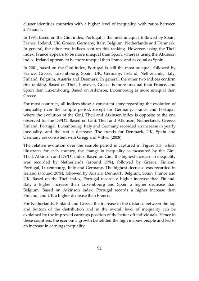
91
cluster identifies countries with a higher level of inequality, with ratios between
2.75 and 4.
In 1994, based on the Gini index, Portugal is the most unequal, followed by Spain,
France, Ireland, UK, Greece, Germany, Italy, Belgium, Netherlands and Denmark.
In general, the other two indices confirm this ranking. However, using the Theil
index, France appears to be more unequal than Spain, whereas using the Atkinson
index, Ireland appears to be more unequal than France and as equal as Spain.
In 2001, based on the Gini index, Portugal is still the most unequal, followed by
France, Greece, Luxembourg, Spain, UK, Germany, Ireland, Netherlands, Italy,
Finland, Belgium, Austria and Denmark. In general, the other two indices confirm
this ranking. Based on Theil, however, Greece is more unequal than France, and
Spain than Luxembourg. Based on Atkinson, Luxembourg is more unequal than
Greece.
For most countries, all indices show a consistent story regarding the evolution of
inequality over the sample period, except for Germany, France and Portugal,
where the evolution of the Gini, Theil and Atkinson index is opposite to the one
observed for the D9/D1. Based on Gini, Theil and Atkinson, Netherlands, Greece,
Finland, Portugal, Luxembourg, Italy and Germany recorded an increase in yearly
inequality, and the rest a decrease. The trends for Denmark, UK, Spain and
Germany are consistent with Gregg and Vittori (2008).
The relative evolution over the sample period is captured in Figure 3.3, which
illustrates for each country, the change in inequality as measured by the Gini,
Theil, Atkinson and D9/D1 index. Based on Gini, the highest increase in inequality
was recorded by Netherlands (around 15%), followed by Greece, Finland,
Portugal, Luxembourg, Italy and Germany. The highest decrease was recorded in
Ireland (around 20%), followed by Austria, Denmark, Belgium, Spain, France and
UK. Based on the Theil index, Portugal records a higher increase than Finland,
Italy a higher increase than Luxembourg and Spain a higher decrease than
Belgium. Based on Atkinson index, Portugal records a higher increase than
Finland, and UK a higher decrease than France.
For Netherlands, Finland and Greece the increase in the distance between the top
and bottom of the distribution and in the overall level of inequality can be
explained by the improved earnings position of the better off individuals. Hence in
these countries, the economic growth benefitted the high income people and led to
an increase in earnings inequality.
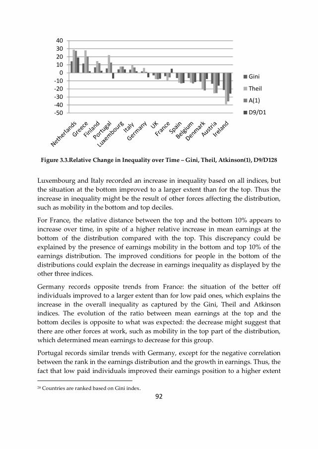
92
Figure 3.3.Relative Change in Inequality over Time – Gini, Theil, Atkinson(1), D9/D128
Luxembourg and Italy recorded an increase in inequality based on all indices, but
the situation at the bottom improved to a larger extent than for the top. Thus the
increase in inequality might be the result of other forces affecting the distribution,
such as mobility in the bottom and top deciles.
For France, the relative distance between the top and the bottom 10% appears to
increase over time, in spite of a higher relative increase in mean earnings at the
bottom of the distribution compared with the top. This discrepancy could be
explained by the presence of earnings mobility in the bottom and top 10% of the
earnings distribution. The improved conditions for people in the bottom of the
distributions could explain the decrease in earnings inequality as displayed by the
other three indices.
Germany records opposite trends from France: the situation of the better off
individuals improved to a larger extent than for low paid ones, which explains the
increase in the overall inequality as captured by the Gini, Theil and Atkinson
indices. The evolution of the ratio between mean earnings at the top and the
bottom deciles is opposite to what was expected: the decrease might suggest that
there are other forces at work, such as mobility in the top part of the distribution,
which determined mean earnings to decrease for this group.
Portugal records similar trends with Germany, except for the negative correlation
between the rank in the earnings distribution and the growth in earnings. Thus, the
fact that low paid individuals improved their earnings position to a higher extent
28 Countries are ranked based on Gini index.
-50
-40
-30
-20
-10
0
10
20
30
40
Gini
Theil
A(1)
D9/D1
93
relative to high paid individuals, lowering the distance between the bottom and
the top deciles of the earnings distribution did not have the expected effect of
lowering overall earnings inequality as measured by the Gini, Theil and Atkinson
indices. Mobility is expected to be the factor counteracting all these movements.
For the rest of the countries, the increase in the overall mean, coupled with the
higher relative increase in the earnings position of the low paid individuals
compared with high earnings individuals can be an explanation for their decrease
in inequality.
Besides the direction of evolution, also the magnitude of the change records
differences among inequality indices. In general, the magnitude of the change is
the highest for the index that is most sensitive to the income differences at the top
of the distribution, followed by bottom and middle sensitive one, sign that most of
the major changes happened at the top and the bottom of the distribution. There
are a few exceptions. In UK, Spain, Belgium and Denmark the magnitude of the
evolution is the highest for the bottom sensitive one, followed by the top and
middle ones.
3.5.2. Changes in the earnings distribution over the lifecycle:
short versus long-term income inequality
Finally we complete the earnings distribution picture with the evolution of
earnings inequality when we extend the horizon over which inequality is
measured. We consider both the balanced and the unbalanced approach. We report
only the results for the Theil index. The results on the other inequality indices can
be provided upon request from the authors.
Table 3.3 and Table 3.4 illustrate the evolution of inequality at different time
horizons for all EU14 countries using a balanced and an unbalanced sample.
Inequality measures based on the unbalanced approach are higher than those
based on the balanced approach. This is not surprising given that people working
over the entire sample are expected to have more stable jobs, and thus lower
earnings differentials as opposed to the case when we include also those with
instable jobs.
As expected, as time horizon increases, inequality reduces in all countries, except
Portugal under the balanced approach.29 The rate of change in inequality as the
time horizon increases differs across countries. As proof, Figure 3.4 (Panel A -
balanced approach and Panel B – unbalanced approach) shows the short and long-
29 This trend is confirmed by all four inequality indices, for all countries.
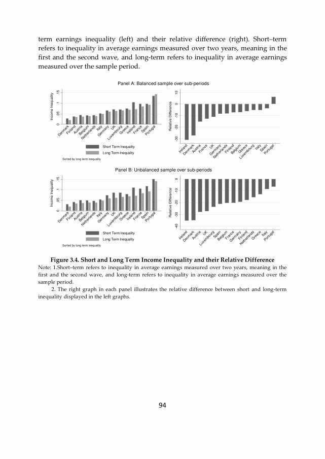
94
term earnings inequality (left) and their relative difference (right). Short–term
refers to inequality in average earnings measured over two years, meaning in the
first and the second wave, and long-term refers to inequality in average earnings
measured over the sample period.
Figure 3.4. Short and Long Term Income Inequality and their Relative Difference
Note: 1.Short–term refers to inequality in average earnings measured over two years, meaning in the
first and the second wave, and long-term refers to inequality in average earnings measured over the
sample period.
2. The right graph in each panel illustrates the relative difference between short and long-term
inequality displayed in the left graphs.
0.0
5.1
.15
Inco
me
In
eq
ua
lity
Den
mar
k
Finla
nd
Austri
a
Belgium
Neth
erlands
Italy
Germ
any UK
Luxe
mbo
urg
Gre
ece
Irela
nd
France
Spain
Portugal
Sorted by long term inequality
Short Term Inequality
Long Term Inequality
-30
-20
-10
01
0
Re
lative
Diffe
ren
ce
Irela
nd
Denm
ark
Austri
a
France U
K
Ger
many
Net
herla
nds
Finla
nd
Belgium
Gre
ece
Luxem
bourg
Italy
Spai
n
Portu
gal
Panel A: Balanced sample over sub-periods
0.0
5.1
.15
Inco
me
In
eq
ua
lity
Den
mar
k
Finla
nd
Austri
a
Belgium
Neth
erlands
Italy
Germ
any UK
Luxe
mbo
urg
Gre
ece
Irela
nd
France
Spain
Portugal
Sorted by long term inequality
Short Term Inequality
Long Term Inequality
-40
-30
-20
-10
0
Re
lative
Diffe
ren
ce
Irela
nd
Denm
ark
Austri
aUK
Luxem
bour
g
Spain
Belgium
Franc
e
Ger
man
y
Finland
Net
herla
nds
Gre
ece
Italy
Portu
gal
Panel B: Unbalanced sample over sub-periods
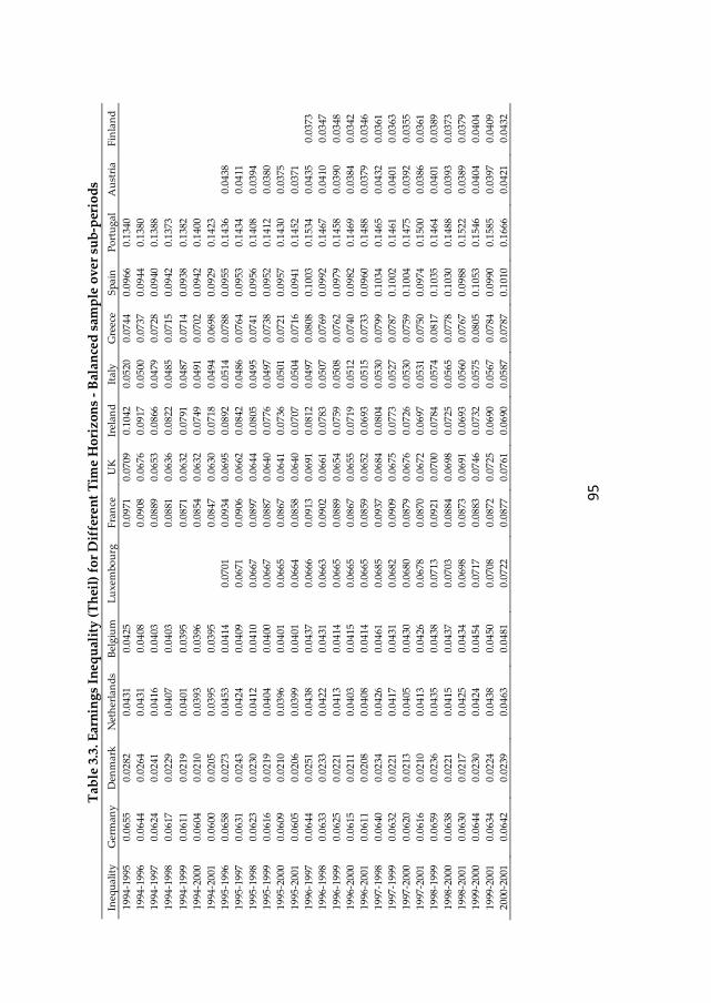
95
Tab
le 3
.3. E
arn
ing
s In
equ
alit
y (
Th
eil)
fo
r D
iffe
ren
t T
ime
Ho
rizo
ns
- B
alan
ced
sam
ple
ov
er s
ub
-per
iod
s
Ineq
ua
lity
G
erm
an
y
Den
ma
rk
Net
her
lan
ds
Bel
giu
m
Lu
xem
bo
urg
F
ran
ce
UK
Ir
ela
nd
It
aly
G
reec
e
Sp
ain
P
ort
ug
al
Au
stri
a
Fin
lan
d
19
94-1
995
0
.06
55
0.0
282
0
.04
31
0.0
425
0
.09
71
0.0
709
0
.10
42
0.0
520
0
.07
44
0.0
966
0
.13
40
19
94-1
996
0
.06
44
0.0
264
0
.04
31
0.0
408
0
.09
08
0.0
676
0
.09
17
0.0
500
0
.07
37
0.0
944
0
.13
80
19
94-1
997
0
.06
24
0.0
241
0
.04
16
0.0
403
0
.08
89
0.0
653
0
.08
66
0.0
479
0
.07
28
0.0
940
0
.13
88
19
94-1
998
0
.06
17
0.0
229
0
.04
07
0.0
403
0
.08
81
0.0
636
0
.08
22
0.0
485
0
.07
15
0.0
942
0
.13
73
19
94-1
999
0
.06
11
0.0
219
0
.04
01
0.0
395
0
.08
71
0.0
632
0
.07
91
0.0
487
0
.07
14
0.0
938
0
.13
82
19
94-2
000
0
.06
04
0.0
210
0
.03
93
0.0
396
0
.08
54
0.0
632
0
.07
49
0.0
491
0
.07
02
0.0
942
0
.14
00
19
94-2
001
0
.06
00
0.0
205
0
.03
95
0.0
395
0
.08
47
0.0
630
0
.07
18
0.0
494
0
.06
98
0.0
929
0
.14
23
19
95-1
996
0
.06
58
0.0
273
0
.04
53
0.0
414
0
.07
01
0.0
934
0
.06
95
0.0
892
0
.05
14
0.0
788
0
.09
55
0.1
436
0
.04
38
19
95-1
997
0
.06
31
0.0
243
0
.04
24
0.0
409
0
.06
71
0.0
906
0
.06
62
0.0
842
0
.04
86
0.0
764
0
.09
53
0.1
434
0
.04
11
19
95-1
998
0
.06
23
0.0
230
0
.04
12
0.0
410
0
.06
67
0.0
897
0
.06
44
0.0
805
0
.04
95
0.0
741
0
.09
56
0.1
408
0
.03
94
19
95-1
999
0
.06
16
0.0
219
0
.04
04
0.0
400
0
.06
67
0.0
887
0
.06
40
0.0
776
0
.04
97
0.0
738
0
.09
52
0.1
412
0
.03
80
19
95-2
000
0
.06
09
0.0
210
0
.03
96
0.0
401
0
.06
65
0.0
867
0
.06
41
0.0
736
0
.05
01
0.0
721
0
.09
57
0.1
430
0
.03
75
19
95-2
001
0
.06
05
0.0
206
0
.03
99
0.0
401
0
.06
64
0.0
858
0
.06
40
0.0
707
0
.05
04
0.0
716
0
.09
41
0.1
452
0
.03
71
19
96-1
997
0
.06
44
0.0
251
0
.04
38
0.0
437
0
.06
66
0.0
913
0
.06
91
0.0
812
0
.04
97
0.0
808
0
.10
03
0.1
534
0
.04
35
0.0
373
19
96-1
998
0
.06
33
0.0
233
0
.04
22
0.0
431
0
.06
63
0.0
902
0
.06
61
0.0
783
0
.05
07
0.0
769
0
.09
92
0.1
467
0
.04
10
0.0
347
19
96-1
999
0
.06
25
0.0
221
0
.04
13
0.0
414
0
.06
65
0.0
889
0
.06
54
0.0
759
0
.05
08
0.0
762
0
.09
79
0.1
458
0
.03
90
0.0
348
19
96-2
000
0
.06
15
0.0
211
0
.04
03
0.0
415
0
.06
65
0.0
867
0
.06
55
0.0
719
0
.05
12
0.0
740
0
.09
82
0.1
469
0
.03
84
0.0
342
19
96-2
001
0
.06
11
0.0
208
0
.04
08
0.0
414
0
.06
65
0.0
859
0
.06
52
0.0
693
0
.05
15
0.0
733
0
.09
60
0.1
488
0
.03
79
0.0
346
19
97-1
998
0
.06
40
0.0
234
0
.04
26
0.0
461
0
.06
85
0.0
937
0
.06
84
0.0
804
0
.05
30
0.0
799
0
.10
34
0.1
465
0
.04
32
0.0
361
19
97-1
999
0
.06
32
0.0
221
0
.04
17
0.0
431
0
.06
82
0.0
909
0
.06
75
0.0
773
0
.05
27
0.0
787
0
.10
02
0.1
461
0
.04
01
0.0
363
19
97-2
000
0
.06
20
0.0
213
0
.04
05
0.0
430
0
.06
80
0.0
879
0
.06
76
0.0
726
0
.05
30
0.0
759
0
.10
04
0.1
475
0
.03
92
0.0
355
19
97-2
001
0
.06
16
0.0
210
0
.04
13
0.0
426
0
.06
78
0.0
870
0
.06
72
0.0
697
0
.05
31
0.0
750
0
.09
74
0.1
500
0
.03
86
0.0
361
19
98-1
999
0
.06
59
0.0
236
0
.04
35
0.0
438
0
.07
13
0.0
921
0
.07
00
0.0
784
0
.05
74
0.0
817
0
.10
35
0.1
464
0
.04
01
0.0
389
19
98-2
000
0
.06
38
0.0
221
0
.04
15
0.0
437
0
.07
03
0.0
884
0
.06
98
0.0
725
0
.05
65
0.0
778
0
.10
30
0.1
488
0
.03
93
0.0
373
19
98-2
001
0
.06
30
0.0
217
0
.04
25
0.0
434
0
.06
98
0.0
873
0
.06
91
0.0
693
0
.05
60
0.0
767
0
.09
88
0.1
522
0
.03
89
0.0
379
19
99-2
000
0
.06
44
0.0
230
0
.04
24
0.0
454
0
.07
17
0.0
883
0
.07
46
0.0
732
0
.05
75
0.0
805
0
.10
53
0.1
546
0
.04
04
0.0
404
19
99-2
001
0
.06
34
0.0
224
0
.04
38
0.0
450
0
.07
08
0.0
872
0
.07
25
0.0
690
0
.05
67
0.0
784
0
.09
90
0.1
585
0
.03
97
0.0
409
20
00-2
001
0
.06
42
0.0
239
0
.04
63
0.0
481
0
.07
22
0.0
877
0
.07
61
0.0
690
0
.05
87
0.0
787
0
.10
10
0.1
666
0
.04
21
0.0
432
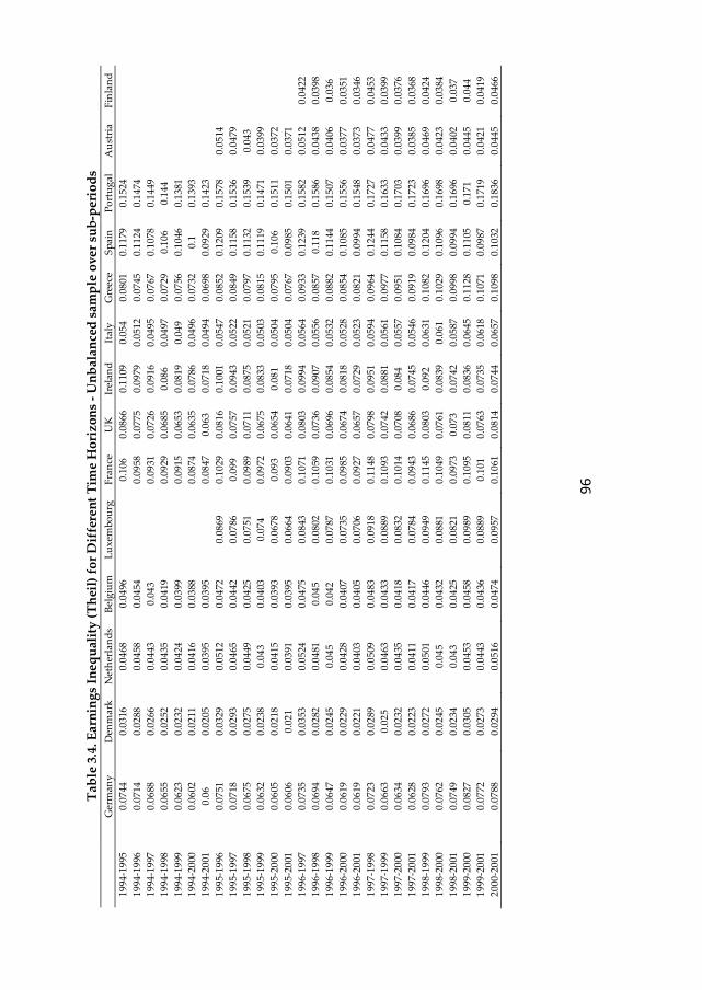
96
Tab
le 3
.4. E
arn
ing
s In
equ
alit
y (
Th
eil)
fo
r D
iffe
ren
t T
ime
Ho
rizo
ns
- U
nb
alan
ced
sam
ple
ov
er s
ub
-per
iod
s G
erm
an
y
Den
ma
rk
Net
her
lan
ds
Bel
giu
m
Lu
xem
bo
urg
F
ran
ce
UK
Ir
ela
nd
It
aly
G
reec
e
Sp
ain
P
ort
ug
al
Au
stri
a
Fin
lan
d
19
94-1
995
0
.07
44
0.0
316
0
.04
68
0.0
496
0
.10
6 0
.08
66
0.1
109
0
.05
4 0
.08
01
0.1
179
0
.15
24
19
94-1
996
0
.07
14
0.0
288
0
.04
58
0.0
454
0
.09
58
0.0
775
0
.09
79
0.0
512
0
.07
45
0.1
124
0
.14
74
19
94-1
997
0
.06
88
0.0
266
0
.04
43
0.0
43
0.0
931
0
.07
26
0.0
916
0
.04
95
0.0
767
0
.10
78
0.1
449
19
94-1
998
0
.06
55
0.0
252
0
.04
35
0.0
419
0
.09
29
0.0
685
0
.08
6 0
.04
97
0.0
729
0
.10
6 0
.14
4
19
94-1
999
0
.06
23
0.0
232
0
.04
24
0.0
399
0
.09
15
0.0
653
0
.08
19
0.0
49
0.0
756
0
.10
46
0.1
381
19
94-2
000
0
.06
02
0.0
211
0
.04
16
0.0
388
0
.08
74
0.0
635
0
.07
86
0.0
496
0
.07
32
0.1
0
.13
93
19
94-2
001
0
.06
0.0
205
0
.03
95
0.0
395
0
.08
47
0.0
63
0.0
718
0
.04
94
0.0
698
0
.09
29
0.1
423
19
95-1
996
0
.07
51
0.0
329
0
.05
12
0.0
472
0
.08
69
0.1
029
0
.08
16
0.1
001
0
.05
47
0.0
852
0
.12
09
0.1
578
0
.05
14
19
95-1
997
0
.07
18
0.0
293
0
.04
65
0.0
442
0
.07
86
0.0
99
0.0
757
0
.09
43
0.0
522
0
.08
49
0.1
158
0
.15
36
0.0
479
19
95-1
998
0
.06
75
0.0
275
0
.04
49
0.0
425
0
.07
51
0.0
989
0
.07
11
0.0
875
0
.05
21
0.0
797
0
.11
32
0.1
539
0
.04
3
19
95-1
999
0
.06
32
0.0
238
0
.04
3 0
.04
03
0.0
74
0.0
972
0
.06
75
0.0
833
0
.05
03
0.0
815
0
.11
19
0.1
471
0
.03
99
19
95-2
000
0
.06
05
0.0
218
0
.04
15
0.0
393
0
.06
78
0.0
93
0.0
654
0
.08
1 0
.05
04
0.0
795
0
.10
6 0
.15
11
0.0
372
19
95-2
001
0
.06
06
0.0
21
0.0
391
0
.03
95
0.0
664
0
.09
03
0.0
641
0
.07
18
0.0
504
0
.07
67
0.0
985
0
.15
01
0.0
371
19
96-1
997
0
.07
35
0.0
353
0
.05
24
0.0
475
0
.08
43
0.1
071
0
.08
03
0.0
994
0
.05
64
0.0
933
0
.12
39
0.1
582
0
.05
12
0.0
422
19
96-1
998
0
.06
94
0.0
282
0
.04
81
0.0
45
0.0
802
0
.10
59
0.0
736
0
.09
07
0.0
556
0
.08
57
0.1
18
0.1
586
0
.04
38
0.0
398
19
96-1
999
0
.06
47
0.0
245
0
.04
5 0
.04
2 0
.07
87
0.1
031
0
.06
96
0.0
854
0
.05
32
0.0
882
0
.11
44
0.1
507
0
.04
06
0.0
36
19
96-2
000
0
.06
19
0.0
229
0
.04
28
0.0
407
0
.07
35
0.0
985
0
.06
74
0.0
818
0
.05
28
0.0
854
0
.10
85
0.1
556
0
.03
77
0.0
351
19
96-2
001
0
.06
19
0.0
221
0
.04
03
0.0
405
0
.07
06
0.0
927
0
.06
57
0.0
729
0
.05
23
0.0
821
0
.09
94
0.1
548
0
.03
73
0.0
346
19
97-1
998
0
.07
23
0.0
289
0
.05
09
0.0
483
0
.09
18
0.1
148
0
.07
98
0.0
951
0
.05
94
0.0
964
0
.12
44
0.1
727
0
.04
77
0.0
453
19
97-1
999
0
.06
63
0.0
25
0.0
463
0
.04
33
0.0
889
0
.10
93
0.0
742
0
.08
81
0.0
561
0
.09
77
0.1
158
0
.16
33
0.0
433
0
.03
99
19
97-2
000
0
.06
34
0.0
232
0
.04
35
0.0
418
0
.08
32
0.1
014
0
.07
08
0.0
84
0.0
557
0
.09
51
0.1
084
0
.17
03
0.0
399
0
.03
76
19
97-2
001
0
.06
28
0.0
223
0
.04
11
0.0
417
0
.07
84
0.0
943
0
.06
86
0.0
745
0
.05
46
0.0
919
0
.09
84
0.1
723
0
.03
85
0.0
368
19
98-1
999
0
.07
93
0.0
272
0
.05
01
0.0
446
0
.09
49
0.1
145
0
.08
03
0.0
92
0.0
631
0
.10
82
0.1
204
0
.16
96
0.0
469
0
.04
24
19
98-2
000
0
.07
62
0.0
245
0
.04
5 0
.04
32
0.0
881
0
.10
49
0.0
761
0
.08
39
0.0
61
0.1
029
0
.10
96
0.1
698
0
.04
23
0.0
384
19
98-2
001
0
.07
49
0.0
234
0
.04
3 0
.04
25
0.0
821
0
.09
73
0.0
73
0.0
742
0
.05
87
0.0
998
0
.09
94
0.1
696
0
.04
02
0.0
37
19
99-2
000
0
.08
27
0.0
305
0
.04
53
0.0
458
0
.09
89
0.1
095
0
.08
11
0.0
836
0
.06
45
0.1
128
0
.11
05
0.1
71
0.0
445
0
.04
4
19
99-2
001
0
.07
72
0.0
273
0
.04
43
0.0
436
0
.08
89
0.1
01
0.0
763
0
.07
35
0.0
618
0
.10
71
0.0
987
0
.17
19
0.0
421
0
.04
19
20
00-2
001
0
.07
88
0.0
294
0
.05
16
0.0
474
0
.09
57
0.1
061
0
.08
14
0.0
744
0
.06
57
0.1
098
0
.10
32
0.1
836
0
.04
45
0.0
466
97
The ranking in inequality when the horizon is extended from one to two years is
roughly maintained and this is consistent across both approaches. Short-term
Denmark is the least unequal and Portugal the most unequal. A difference in short-
term ranking between the two approaches is observed for Greece, which is more
unequal than Denmark, Finland, Austria, Belgium, Netherland, Italy, Germany,
UK, and Luxembourg in the balanced approach and more unequal than the former
7 countries in the unbalanced approach. Similarly, Spain is less unequal than
Ireland and Portugal under the balanced approach, and less unequal than Portugal
under the unbalanced approach. Thus short-term differential attrition affects
Greece and Spain the most. More shuffling occurs as the horizon is extended to the
sample period.
The relative difference between short and long-term inequality displayed in Figure
3.4 (right) provide a first clue regarding the degree to which each country manages
to reduce long-term earnings differentials compared with short-term ones. If
inequality measured over the whole sample period can be considered as a proxy
for lifetime earnings inequality or inequality in the permanent component of
earnings, the rate of decrease with the time horizon can be interpreted as a
reduction in the transitory earnings inequality over the lifetime or the fading off of
the transitory component of earnings. Some countries manage to reduce inequality
over the lifetime at a higher extent than others.
Based on the balanced approach (Figure 3.4 – Panel A) Ireland and Denmark
display the highest reduction in long-term earnings inequality as the time horizon
increases (over 30%), followed by Austria (over 15%), France and UK (over 10%),
and the rest below 9%. Portugal is the only one recoding an increase in long-term
inequality relative to short-term (over 6%). Based on these trends, we expect
Ireland and Denmark to have the highest equalizing mobility over the lifecycle,
Italy and Spain the lowest, and Portugal to have a disequalizing mobility.
The relative difference between long-term and short-run inequality is lower in the
balanced (Figure 3.4 – Panel A) compared with the unbalanced approach (Figure
3.4 – Panel B), showing that differential attrition affects all countries. The
explanation is that looking only at people that work over the entire sample period
might overestimate the degree of earnings persistency and underestimate the
degree of earnings instability.
Comparing between the two approaches, the most drastic difference is observed
for Portugal, where also the direction of change differs, indicating an increase in
long-term differentials relative to short-term ones. Also the ranking in the relative
changes differs under the two approaches. Under the unbalanced approach,
Portugal still records the lowest rank, and Ireland, Denmark and Austria the
98
highest. For the rest the ranks are shuffled. UK, Luxembourg and Spain jump
towards higher positions, after Ireland, Denmark and Austria. The rest lower their
rank. Thus except for the extremes, differential attrition plays a significant role in
country ranking with respect to the degree to which earnings differentials are
reduced with the time horizon.
The countries with the highest reduction in long-term inequality relative to short-
term inequality (over 20%) in the unbalanced approach (Figure 3.4 – Panel B) are
observed to be also the ones which record a decrease in inequality30 over time,
except Luxembourg. Hence, on the one hand one might expect that the reduction
in the transitory earnings inequality is one of the factors determining the decrease
in the overall inequality over time. This might indicate the presence of a shock in
the beginning of the sample period that influenced the temporary component of
earnings and whose impact faded off over time. One the other hand, it might
indicate that people became more mobile, improved their income position in the
long run and reduced permanent income differentials. The outcome depends
mainly on the evolution of mobility over time.
Under the balanced approach, the situation is confirmed for the countries with
decreasing cross-sectional inequality, except for Spain and Belgium, which record
among the smallest decreases in long-term inequality relative to short-term
inequality. Thus among the countries with decreasing cross-sectional inequality,
based on the differences between the balanced and the unbalanced approach,
Spain and Belgium appear to be the most affected by differential attrition.
Based on the balanced approach, for countries that recorded an increase in the
overall inequality over the sample period, the small decrease in inequality with the
time horizon, signals the presence of strong permanent earnings differences
between individuals or the existence of some shocks with permanent effects,
whose inequality is accentuated by the inequality in the transitory component of
earnings. Moreover, the magnitude of the transitory component of earnings is
expected to be lower for these countries. Except for Luxembourg which records a
high decrease in inequality with the time horizon, the unbalanced approach reveals
a similar picture.
Under the unbalanced approach, in Luxembourg, the increase in the overall
inequality over the sample period coupled with the high decrease in inequality
with the time horizon signals the presence of some transitory shocks, which fade
away in the long run. The difference in the two approached indicate that the
30 as measured by the Gini, Theil and Atkinson index

99
attrition incidence is higher in Luxembourg compared with the other countries
where cross-sectional inequality increased.
To conclude, even based on average earnings over the whole sample period, a
substantial inequality in the permanent component of earnings is still present in all
countries under analysis. The lowest long-term inequality, meaning the lowest
inequality in permanent earnings, is recorded in Denmark, followed by Finland,
Austria, Belgium and Netherlands with similar values, then Italy, Germany, UK,
Luxembourg, Greece, Ireland, France and Spain. Portugal differentiates itself with
a particularly high long-term inequality compared with the other countries. (Figure
3.4)
3.6.Mobility profile
What are the possible implications in a lifetime perspective? To answer this
question we need to couple the information on the evolution of inequality with
earnings mobility. Is there any earnings mobility in a lifetime perspective, meaning
are the relative income positions observed on an annual basis shuffled long-term?
If yes, is mobility equalizing or disequalizing lifetime earnings differentials
compared with annual earnings differentials? We report the mobility indices based
on the Theil index. The ones based on the other inequality indices can be provided
upon request from the authors.
3.6.1. Stability profile - Shorrocks
To answer the first question we look at the stability profile, both under the
balanced and the unbalanced approach, illustrated in Figure 3.5 and Figure 3.6.
Both figures contain the same information, organized differently for the ease of the
interpretation.
10
0
F
igu
re 3
.5. S
tab
ilit
y P
rofi
les
for
Mal
e E
arn
ing
s b
y S
elec
ted
Co
un
trie
s (b
ased
on
Th
eil)
– B
alan
ced
vs
Un
bal
ance
d
No
te: T
he
sta
bil
ity
pro
file
plo
ts t
he
rig
idit
y i
nd
ex a
ga
inst
th
e h
ori
zon
ov
er
wh
ich
th
e in
de
x i
s m
easu
red
: 1
-ye
ar r
igid
ity
= 1
; 2-y
ear
rig
idit
y =
rig
idit
y i
nd
ex
ov
er a
ho
rizo
n o
f 2
ye
ars,
sp
an w
av
e(1
)-w
av
e(2
); 8
-yea
r ri
gid
ity
= r
igid
ity
in
de
x o
ver
a h
ori
zo
n o
f 8
yea
rs,
span
(wa
ve(
1)-
wa
ve(
8))
.7.8.91
12
34
56
78
Span(w
ave(1
) -
wave(t
))
Germ
any
.7.8.91
12
34
56
78
Span(w
ave(1
) -
wave(t
))
Denm
ark
.7.8.91
12
34
56
78
Span(w
ave(1
) -
wave(t
))
Neth
erlands
.7.8.91
12
34
56
78
Span(w
ave(1
) -
wave(t
))
Belg
ium
.7.8.91
12
34
56
78
Span(w
ave(1
) -
wave(t
))
Luxe
mbo
urg
.7.8.91
12
34
56
78
Span(w
ave(1
) -
wave(t
))
Fra
nce
.7.8.91
12
34
56
78
Span(w
ave(1
) -
wave(t
))
UK
.7.8.91
12
34
56
78
Span(w
ave(1
) -
wave(t
))
Irela
nd
.7.8.91
12
34
56
78
Span(w
ave(1
) -
wave(t
))
Italy
.7.8.91
12
34
56
78
Span(w
ave(1
) -
wave(t
))
Gre
ece
.7.8.91
12
34
56
78
Span(w
ave(1
) -
wave(t
))
Spain
.7.8.91
12
34
56
78
Span(w
ave(1
) -
wave(t
))
Po
rtugal
.7.8.91
12
34
56
78
Span(w
ave(1
) -
wave(t
))
Austr
ia
.7.8.91
12
34
56
78
Span(w
ave(1
) -
wave(t
))
Fin
land
Rig
idity -
bala
nced a
ppro
ach
Rig
idity -
unbala
nced a
ppro
ach
101
Figure 3.6. Stability Profiles for Male Earnings for Selected Countries (based on Theil) –
Balanced vs Unbalanced Note: The stability profile plots the rigidity index against the horizon over which the index is measured:
1-year rigidity = 1; 2-year rigidity = rigidity index over a horizon of 2 years, span wave(1)-wave(2); 8-
year rigidity = rigidity index over a horizon of 8 years, span(wave(1)-wave(8))
.7.8
.91
1 2 3 4 5 6 7 8
Span(wave(1) - wave(t))
Germany Luxembourg
France Italy
Spain Portugal
.7.8
.91
1 2 3 4 5 6 7 8
Span(wave(1) - wave(t))
Denmark Netherlands Belgium
UK Ireland Greece
Austria Finland
Panel A: Balanced sample over sub-periods.7
.8.9
1
1 2 3 4 5 6 7 8
Span(wave(1) - wave(t))
Germany Luxembourg
France Italy
Spain Portugal
.7.8
.91
1 2 3 4 5 6 7 8
Span(wave(1) - wave(t))
Denmark Netherlands Belgium
UK Ireland Greece
Austria Finland
Panel B: Unbalanced sample over sub-periods
102
To recall, the stability profile plots the Shorrocks rigidity index31 across different
time horizons. In Figure 3.5 and Figure 3.6 the time horizons are expressed in
reference to the 1st wave for each country. The stability profile allows the visual
identification of the presence of permanent and transitory earnings components.
All countries record similar trends: the rigidity declines monotonically as the time
horizon is extended (Figure 3.5 and Figure 3.6). Moreover, the longer the time-
horizon is, the more heterogeneous the stability profiles become. The story is
confirmed by both approaches. As illustrated in Figure 3.5, the profiles under the
two approaches evolve close to one another sign that the impact of attrition is
limited. Some countries are affected to a larger extent by attrition than others. A
larger impact is identified in Luxembourg, France, Ireland, Greece, Spain and
Austria, which have a higher differentiation between the two profiles. For
Luxembourg, Spain and Austria the rigidity index under the unbalanced approach
is higher than in the balanced approach for horizons 1 to 4, suggesting that
including also those individuals that move in and out of employment results in a
higher degree of earnings rigidity. The opposite is observed in Ireland, Greece and
France, suggesting that more income rigidity is observed among those that worked
for the whole sample than including also those that moved in and out of paid work
over the sample period.
Based on the stability profiles in Figure 3.5 and Figure 3.6, we make inferences
concerning the source of mobility in each country. Based on the overall pattern of
the profiles, we identify two country clusters, confirmed under both approaches,
illustrated in Figure 3.6. Overall, the stability profiles on the right side of Figure 3.6
are steeper than on the left side, suggesting that income changes in Denmark,
Finland, Austria, UK, Belgium, Greece, Ireland and Netherlands are due to
transitory effects to a larger extent than in the other countries. Hence we can expect
a higher lifetime mobility in the former.
Among the countries with less steep profiles, we identify countries where the
profile (both the balanced and the unbalanced one) drops sharply in the beginning
and then tends to become horizontal after a few years, suggesting that the income
changes are purely due to transitory effects which average out over time. (Figure
3.5) Thus relative incomes approach rapidly their permanent values and there is no
further equalization. It is the case of France. A similar trend (consistent across the
two approaches) is observed in Portugal, except the last drop in the 8-year period
31 R is based in the Theil index. R based on other inequality can be provided upon request from the
authors.
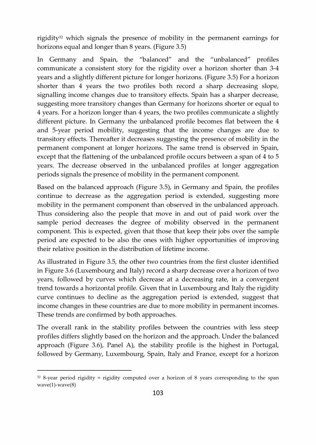
103
rigidity32 which signals the presence of mobility in the permanent earnings for
horizons equal and longer than 8 years. (Figure 3.5)
In Germany and Spain, the “balanced” and the “unbalanced” profiles
communicate a consistent story for the rigidity over a horizon shorter than 3-4
years and a slightly different picture for longer horizons. (Figure 3.5) For a horizon
shorter than 4 years the two profiles both record a sharp decreasing slope,
signalling income changes due to transitory effects. Spain has a sharper decrease,
suggesting more transitory changes than Germany for horizons shorter or equal to
4 years. For a horizon longer than 4 years, the two profiles communicate a slightly
different picture. In Germany the unbalanced profile becomes flat between the 4
and 5-year period mobility, suggesting that the income changes are due to
transitory effects. Thereafter it decreases suggesting the presence of mobility in the
permanent component at longer horizons. The same trend is observed in Spain,
except that the flattening of the unbalanced profile occurs between a span of 4 to 5
years. The decrease observed in the unbalanced profiles at longer aggregation
periods signals the presence of mobility in the permanent component.
Based on the balanced approach (Figure 3.5), in Germany and Spain, the profiles
continue to decrease as the aggregation period is extended, suggesting more
mobility in the permanent component than observed in the unbalanced approach.
Thus considering also the people that move in and out of paid work over the
sample period decreases the degree of mobility observed in the permanent
component. This is expected, given that those that keep their jobs over the sample
period are expected to be also the ones with higher opportunities of improving
their relative position in the distribution of lifetime income.
As illustrated in Figure 3.5, the other two countries from the first cluster identified
in Figure 3.6 (Luxembourg and Italy) record a sharp decrease over a horizon of two
years, followed by curves which decrease at a decreasing rate, in a convergent
trend towards a horizontal profile. Given that in Luxembourg and Italy the rigidity
curve continues to decline as the aggregation period is extended, suggest that
income changes in these countries are due to more mobility in permanent incomes.
These trends are confirmed by both approaches.
The overall rank in the stability profiles between the countries with less steep
profiles differs slightly based on the horizon and the approach. Under the balanced
approach (Figure 3.6), Panel A), the stability profile is the highest in Portugal,
followed by Germany, Luxembourg, Spain, Italy and France, except for a horizon
32 8-year period rigidity = rigidity computed over a horizon of 8 years corresponding to the span
wave(1)-wave(8)
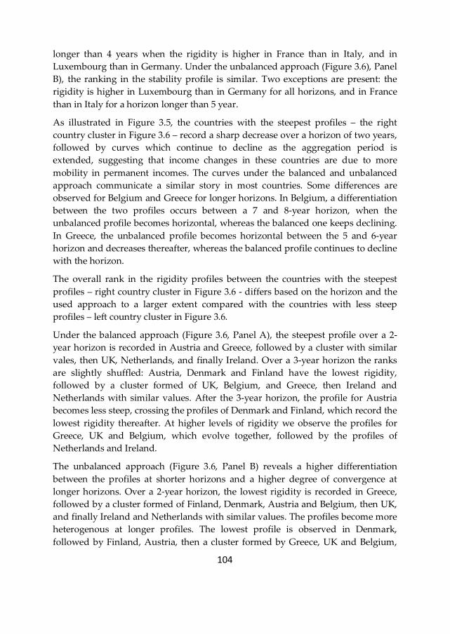
104
longer than 4 years when the rigidity is higher in France than in Italy, and in
Luxembourg than in Germany. Under the unbalanced approach (Figure 3.6), Panel
B), the ranking in the stability profile is similar. Two exceptions are present: the
rigidity is higher in Luxembourg than in Germany for all horizons, and in France
than in Italy for a horizon longer than 5 year.
As illustrated in Figure 3.5, the countries with the steepest profiles – the right
country cluster in Figure 3.6 – record a sharp decrease over a horizon of two years,
followed by curves which continue to decline as the aggregation period is
extended, suggesting that income changes in these countries are due to more
mobility in permanent incomes. The curves under the balanced and unbalanced
approach communicate a similar story in most countries. Some differences are
observed for Belgium and Greece for longer horizons. In Belgium, a differentiation
between the two profiles occurs between a 7 and 8-year horizon, when the
unbalanced profile becomes horizontal, whereas the balanced one keeps declining.
In Greece, the unbalanced profile becomes horizontal between the 5 and 6-year
horizon and decreases thereafter, whereas the balanced profile continues to decline
with the horizon.
The overall rank in the rigidity profiles between the countries with the steepest
profiles – right country cluster in Figure 3.6 - differs based on the horizon and the
used approach to a larger extent compared with the countries with less steep
profiles – left country cluster in Figure 3.6.
Under the balanced approach (Figure 3.6, Panel A), the steepest profile over a 2-
year horizon is recorded in Austria and Greece, followed by a cluster with similar
vales, then UK, Netherlands, and finally Ireland. Over a 3-year horizon the ranks
are slightly shuffled: Austria, Denmark and Finland have the lowest rigidity,
followed by a cluster formed of UK, Belgium, and Greece, then Ireland and
Netherlands with similar values. After the 3-year horizon, the profile for Austria
becomes less steep, crossing the profiles of Denmark and Finland, which record the
lowest rigidity thereafter. At higher levels of rigidity we observe the profiles for
Greece, UK and Belgium, which evolve together, followed by the profiles of
Netherlands and Ireland.
The unbalanced approach (Figure 3.6, Panel B) reveals a higher differentiation
between the profiles at shorter horizons and a higher degree of convergence at
longer horizons. Over a 2-year horizon, the lowest rigidity is recorded in Greece,
followed by a cluster formed of Finland, Denmark, Austria and Belgium, then UK,
and finally Ireland and Netherlands with similar values. The profiles become more
heterogenous at longer profiles. The lowest profile is observed in Denmark,
followed by Finland, Austria, then a cluster formed by Greece, UK and Belgium,
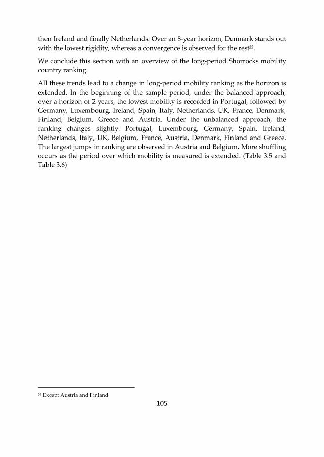
105
then Ireland and finally Netherlands. Over an 8-year horizon, Denmark stands out
with the lowest rigidity, whereas a convergence is observed for the rest33.
We conclude this section with an overview of the long-period Shorrocks mobility
country ranking.
All these trends lead to a change in long-period mobility ranking as the horizon is
extended. In the beginning of the sample period, under the balanced approach,
over a horizon of 2 years, the lowest mobility is recorded in Portugal, followed by
Germany, Luxembourg, Ireland, Spain, Italy, Netherlands, UK, France, Denmark,
Finland, Belgium, Greece and Austria. Under the unbalanced approach, the
ranking changes slightly: Portugal, Luxembourg, Germany, Spain, Ireland,
Netherlands, Italy, UK, Belgium, France, Austria, Denmark, Finland and Greece.
The largest jumps in ranking are observed in Austria and Belgium. More shuffling
occurs as the period over which mobility is measured is extended. (Table 3.5 and
Table 3.6)
33 Except Austria and Finland.
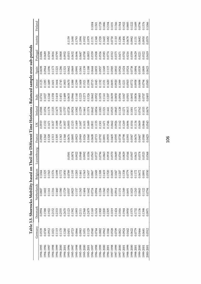
10
6
Tab
le 3
.5. S
ho
rro
cks
Mo
bil
ity
bas
ed o
n T
hei
l fo
r D
iffe
ren
t T
ime
Ho
rizo
ns
- B
alan
ced
sam
ple
ov
er s
ub
-per
iod
s
Ger
ma
ny
D
enm
ark
N
eth
erla
nd
s B
elg
ium
L
ux
emb
ou
rg
Fra
nce
U
K
Irel
an
d
Ita
ly
Gre
ece
S
pa
in
Po
rtu
ga
l A
ust
ria
F
inla
nd
19
94-1
995
0
.05
39
0.0
994
0
.08
07
0.1
044
0
.09
89
0.0
919
0
.05
88
0.0
741
0
.11
25
0.0
698
0
.04
96
19
94-1
996
0
.07
49
0.1
588
0
.10
02
0.1
325
0
.12
60
0.1
332
0
.10
54
0.1
027
0
.12
85
0.0
964
0
.06
89
19
94-1
997
0
.09
12
0.1
922
0
.11
61
0.1
543
0
.13
28
0.1
471
0
.11
78
0.1
240
0
.14
89
0.1
096
0
.07
69
19
94-1
998
0
.10
21
0.2
152
0
.13
16
0.1
576
0
.13
13
0.1
637
0
.13
35
0.1
358
0
.16
01
0.1
173
0
.08
16
19
94-1
999
0
.11
15
0.2
333
0
.14
60
0.1
698
0
.13
05
0.1
688
0
.14
75
0.1
418
0
.16
64
0.1
221
0
.07
95
19
94-2
000
0
.11
70
0.2
555
0
.15
80
0.1
772
0
.13
43
0.1
799
0
.16
55
0.1
451
0
.17
45
0.1
286
0
.08
00
19
94-2
001
0
.12
40
0.2
670
0
.17
29
0.1
850
0
.13
48
0.1
857
0
.17
57
0.1
489
0
.18
03
0.1
321
0
.09
32
19
95-1
996
0
.04
51
0.1
123
0
.05
57
0.0
789
0
.05
81
0.0
676
0
.09
55
0.0
728
0
.06
35
0.0
670
0
.06
62
0.0
515
0
.11
59
19
95-1
997
0
.07
23
0.1
592
0
.09
25
0.1
195
0
.08
74
0.0
895
0
.12
15
0.0
924
0
.09
66
0.1
088
0
.08
69
0.0
632
0
.16
90
19
95-1
998
0
.08
66
0.1
893
0
.11
57
0.1
283
0
.09
22
0.0
923
0
.14
09
0.1
082
0
.11
40
0.1
299
0
.09
91
0.0
696
0
.17
93
19
95-1
999
0
.09
83
0.2
111
0
.13
43
0.1
461
0
.09
48
0.0
949
0
.14
97
0.1
259
0
.12
25
0.1
408
0
.10
61
0.0
687
0
.18
94
19
95-2
000
0
.10
51
0.2
368
0
.14
84
0.1
563
0
.09
92
0.1
026
0
.16
31
0.1
461
0
.12
73
0.1
521
0
.11
39
0.0
700
0
.19
32
19
95-2
001
0
.11
29
0.2
479
0
.16
42
0.1
657
0
.10
36
0.1
060
0
.16
89
0.1
574
0
.13
26
0.1
598
0
.11
88
0.0
853
0
.19
79
19
96-1
997
0
.05
40
0.1
169
0
.07
24
0.0
867
0
.05
63
0.0
608
0
.08
11
0.0
642
0
.06
62
0.0
715
0
.06
44
0.0
339
0
.11
51
0.1
004
19
96-1
998
0
.07
44
0.1
634
0
.09
94
0.1
049
0
.07
27
0.0
715
0
.11
55
0.0
854
0
.09
52
0.1
045
0
.08
55
0.0
508
0
.13
48
0.1
501
19
96-1
999
0
.08
82
0.1
900
0
.12
06
0.1
308
0
.07
96
0.0
792
0
.13
01
0.1
083
0
.10
78
0.1
192
0
.09
57
0.0
536
0
.15
28
0.1
728
19
96-2
000
0
.09
62
0.2
200
0
.13
60
0.1
419
0
.08
63
0.0
891
0
.14
71
0.1
321
0
.11
41
0.1
331
0
.10
49
0.0
585
0
.16
02
0.1
886
19
96-2
001
0
.10
46
0.2
305
0
.15
26
0.1
520
0
.09
18
0.0
935
0
.15
46
0.1
441
0
.12
07
0.1
420
0
.11
15
0.0
774
0
.16
82
0.2
184
19
97-1
998
0
.05
28
0.1
019
0
.05
97
0.0
605
0
.05
70
0.0
405
0
.06
62
0.0
525
0
.06
59
0.0
695
0
.05
85
0.0
312
0
.07
30
0.1
031
19
97-1
999
0
.07
09
0.1
424
0
.09
14
0.1
047
0
.06
89
0.0
595
0
.09
26
0.0
845
0
.08
50
0.0
920
0
.08
10
0.0
375
0
.11
10
0.1
366
19
97-2
000
0
.08
21
0.1
816
0
.11
51
0.1
207
0
.07
66
0.0
738
0
.11
62
0.1
128
0
.09
56
0.1
099
0
.09
26
0.0
471
0
.12
86
0.1
564
19
97-2
001
0
.09
24
0.1
944
0
.13
49
0.1
338
0
.08
29
0.0
798
0
.12
69
0.1
271
0
.10
47
0.1
221
0
.10
24
0.0
702
0
.14
04
0.1
922
19
98-1
999
0
.04
42
0.0
950
0
.06
91
0.0
779
0
.03
44
0.0
393
0
.06
96
0.0
613
0
.05
01
0.0
503
0
.05
24
0.0
216
0
.06
78
0.0
885
19
98-2
000
0
.06
22
0.1
575
0
.10
25
0.1
030
0
.05
07
0.0
587
0
.10
14
0.1
001
0
.06
92
0.0
772
0
.07
38
0.0
359
0
.09
82
0.1
222
19
98-2
001
0
.07
79
0.1
732
0
.12
43
0.1
172
0
.06
21
0.0
676
0
.11
34
0.1
171
0
.08
36
0.0
958
0
.08
94
0.0
629
0
.11
31
0.1
689
19
99-2
000
0
.04
66
0.1
136
0
.08
43
0.0
672
0
.03
74
0.0
447
0
.06
09
0.0
762
0
.04
83
0.0
498
0
.05
39
0.0
221
0
.06
82
0.0
796
19
99-2
001
0
.06
81
0.1
398
0
.11
22
0.0
891
0
.05
25
0.0
580
0
.08
44
0.1
033
0
.07
07
0.0
794
0
.08
09
0.0
522
0
.09
50
0.1
376
20
00-2
001
0
.05
12
0.0
971
0
.07
94
0.0
550
0
.03
68
0.0
425
0
.05
43
0.0
679
0
.04
93
0.0
585
0
.06
23
0.0
419
0
.05
79
0.1
066
10
7
Tab
le 3
.6. S
ho
rro
cks
Mo
bil
ity
bas
ed o
n T
hei
l fo
r D
iffe
ren
t T
ime
Ho
rizo
ns
- U
nb
alan
ced
sam
ple
ov
er s
ub
-per
iod
s G
erm
an
y
Den
ma
rk
Net
her
lan
ds
Bel
giu
m
Lu
xem
bo
urg
F
ran
ce
UK
Ir
ela
nd
It
aly
G
reec
e
Sp
ain
P
ort
ug
al
Au
stri
a
Fin
lan
d
19
94-1
995
0
.05
25
0.1
081
0
.07
77
0.1
061
0
.10
72
0.0
884
0
.07
73
0.0
852
0
.12
98
0.0
652
0
.04
79
19
94-1
996
0
.08
63
0.1
557
0
.09
66
0.1
300
0
.13
04
0.1
277
0
.11
60
0.1
056
0
.14
52
0.0
926
0
.06
85
19
94-1
997
0
.09
34
0.1
859
0
.11
07
0.1
547
0
.14
09
0.1
488
0
.12
84
0.1
224
0
.15
61
0.1
017
0
.07
93
19
94-1
998
0
.09
21
0.2
174
0
.12
66
0.1
589
0
.14
04
0.1
651
0
.14
58
0.1
368
0
.16
79
0.1
073
0
.08
03
19
94-1
999
0
.10
76
0.2
345
0
.14
12
0.1
708
0
.14
10
0.1
717
0
.16
01
0.1
451
0
.16
86
0.1
085
0
.07
95
19
94-2
000
0
.11
50
0.2
603
0
.14
98
0.1
865
0
.13
66
0.1
797
0
.16
52
0.1
452
0
.17
53
0.1
199
0
.07
98
19
94-2
001
0
.12
40
0.2
670
0
.17
29
0.1
850
0
.13
48
0.1
857
0
.17
57
0.1
489
0
.18
03
0.1
321
0
.09
32
19
95-1
996
0
.07
52
0.1
051
0
.05
95
0.0
775
0
.05
08
0.0
774
0
.09
01
0.0
739
0
.06
82
0.0
727
0
.06
47
0.0
432
0
.10
77
19
95-1
997
0
.08
98
0.1
533
0
.09
60
0.1
217
0
.07
64
0.1
053
0
.11
87
0.0
949
0
.09
90
0.1
139
0
.08
11
0.0
640
0
.14
97
19
95-1
998
0
.08
28
0.1
905
0
.11
47
0.1
303
0
.08
32
0.1
051
0
.14
33
0.1
131
0
.11
74
0.1
397
0
.09
07
0.0
722
0
.16
73
19
95-1
999
0
.09
99
0.2
192
0
.13
36
0.1
484
0
.08
85
0.1
062
0
.15
64
0.1
294
0
.13
15
0.1
435
0
.09
60
0.0
747
0
.17
69
19
95-2
000
0
.10
86
0.2
409
0
.14
38
0.1
650
0
.09
98
0.1
063
0
.16
56
0.1
509
0
.13
21
0.1
484
0
.10
77
0.0
767
0
.19
31
19
95-2
001
0
.11
62
0.2
461
0
.16
77
0.1
669
0
.10
36
0.1
065
0
.17
62
0.1
644
0
.13
40
0.1
553
0
.11
94
0.0
927
0
.19
79
19
96-1
997
0
.05
76
0.0
997
0
.07
37
0.0
903
0
.05
47
0.0
710
0
.08
16
0.0
542
0
.07
48
0.0
805
0
.05
85
0.0
396
0
.09
13
0.1
109
19
96-1
998
0
.06
99
0.1
692
0
.09
82
0.1
033
0
.07
00
0.0
819
0
.11
83
0.0
870
0
.10
12
0.1
154
0
.07
87
0.0
522
0
.12
06
0.1
495
19
96-1
999
0
.08
96
0.1
996
0
.12
38
0.1
306
0
.07
91
0.0
920
0
.13
69
0.1
110
0
.11
85
0.1
204
0
.08
92
0.0
586
0
.14
42
0.1
734
19
96-2
000
0
.09
98
0.2
265
0
.13
67
0.1
491
0
.08
92
0.0
926
0
.15
38
0.1
394
0
.11
95
0.1
312
0
.10
12
0.0
621
0
.16
74
0.1
879
19
96-2
001
0
.10
75
0.2
357
0
.16
35
0.1
523
0
.09
35
0.0
954
0
.16
63
0.1
513
0
.12
38
0.1
377
0
.11
36
0.0
810
0
.17
55
0.2
184
19
97-1
998
0
.04
98
0.1
203
0
.07
06
0.0
780
0
.04
59
0.0
563
0
.07
38
0.0
652
0
.06
47
0.0
790
0
.05
56
0.0
309
0
.07
18
0.0
977
19
97-1
999
0
.07
47
0.1
670
0
.10
34
0.1
095
0
.06
03
0.0
726
0
.10
98
0.0
955
0
.09
37
0.0
986
0
.07
71
0.0
416
0
.10
72
0.1
464
19
97-2
000
0
.08
54
0.2
006
0
.12
18
0.1
305
0
.07
19
0.0
801
0
.12
49
0.1
231
0
.09
92
0.1
136
0
.09
38
0.0
515
0
.14
08
0.1
651
19
97-2
001
0
.09
66
0.2
118
0
.14
56
0.1
365
0
.07
88
0.0
864
0
.13
77
0.1
356
0
.10
80
0.1
229
0
.11
10
0.0
702
0
.15
32
0.1
953
19
98-1
999
0
.04
28
0.1
161
0
.06
99
0.0
811
0
.03
18
0.0
494
0
.07
84
0.0
679
0
.06
62
0.0
563
0
.05
54
0.0
253
0
.06
47
0.1
010
19
98-2
000
0
.05
83
0.1
759
0
.10
74
0.1
066
0
.04
87
0.0
674
0
.10
35
0.1
084
0
.08
14
0.0
813
0
.07
77
0.0
438
0
.10
87
0.1
354
19
98-2
001
0
.07
15
0.1
923
0
.13
52
0.1
190
0
.05
99
0.0
760
0
.12
21
0.1
317
0
.09
55
0.0
953
0
.10
07
0.0
654
0
.12
67
0.1
748
19
99-2
000
0
.04
37
0.1
136
0
.08
69
0.0
714
0
.04
08
0.0
476
0
.07
16
0.0
778
0
.05
62
0.0
469
0
.06
15
0.0
301
0
.07
73
0.1
052
19
99-2
001
0
.06
30
0.1
472
0
.12
39
0.0
938
0
.05
25
0.0
614
0
.10
05
0.1
142
0
.07
92
0.0
714
0
.09
66
0.0
552
0
.10
33
0.1
494
20
00-2
001
0
.04
55
0.1
079
0
.08
24
0.0
569
0
.04
20
0.0
554
0
.07
25
0.0
783
0
.06
04
0.0
582
0
.07
81
0.0
400
0
.06
20
0.1
141
108
Following these changes, the ranking in long-term earnings Shorrocks mobility is
revealed in Figure 3.7.
Figure 3.7. Long-Term Earnings Mobility based on the Shorrocks Index
Note: Ranked in an ascendant order based on the 8-year period mobility. Austria Finland and
Luxembourg are displayed the last because the 8-year period mobility is missing.
Based on the balanced approach, the highest mobility over a horizon of 6 years is
recorded in Denmark and Finland, followed by Austria, Belgium, UK, Greece,
Ireland, Netherlands, Italy, France, Spain, Germany, Luxembourg and Portugal.
Denmark and Finland record the lowest annual inequality, and Portugal the
highest annual inequality. Thus we can expect, among the selected countries,
Denmark and Finland to trigger the lowest lifetime inequality and Portugal the
highest. The country ranking is confirmed by the unbalanced approach, except
Netherlands which, under the unbalanced approach, has a lower mobility than
Italy.
Based on the balanced approach, over a horizon of 7 years the ranking is in general
preserved: Denmark and Austria record the highest mobility, and Portugal and
Luxembourg the lowest. One exception is UK which scores a higher rank than
0.1
.2.3
Incom
e M
obili
ty (
Shorr
ocks)
Portu
gal
Ger
man
y
Spain
Franc
eIta
ly
Net
herla
nds
Ireland
Gre
ece
Belgium U
K
Den
mar
k
Aus
tria
Finlan
d
Luxe
mbo
urg
Panel A: Balanced sample over sub-periods
6-Year Period Shorrocks Mobility
7-Year Period Shorrocks Mobility
8-Year Period Shorrocks Mobility
0.1
.2.3
Incom
e M
obili
ty (
Shorr
ocks)
Portu
gal
Ger
man
y
Spain
Franc
eIta
ly
Net
herla
nds
Ireland
Gre
ece
Belgium U
K
Den
mar
k
Aus
tria
Finlan
d
Luxe
mbo
urg
Panel B: Unbalanced sample over sub-periods
6-Year Period Shorrocks Mobility
7-Year Period Shorrocks Mobility
8-Year Period Shorrocks Mobility

109
Belgium. Austria has the 5th lowest annual inequality and Luxembourg the 9th.
Thus we expect Austria to reduce lifetime earnings differential compared with
annual differentials to a higher extent than Portugal and Luxembourg, and to a
lesser extent than Denmark. This result is consistent with Hofer and Weber (2002).
Similarly, we expect Luxembourg to reduce lifetime differentials to a higher extent
than Portugal and to a lesser extent than Denmark. The ranking is confirmed by
the unbalanced approach, except for the UK which ranks lower than Belgium.
Finally, over an eight-year horizon34, the ranking is in general preserved. The
highest mobility is recorded in Denmark, followed by UK, Belgium, Greece,
Ireland, Netherlands, Italy, France, Spain, Germany, and the lowest, Portugal.
Therefore Denmark provides the highest opportunity of reducing lifetime earnings
differentials and Portugal the lowest. The ranking between Denmark, UK, Spain
and Germany is consistent with the one found by Gregg and Vittori (2008) using
the Shorrocks index based on all indices considered, including Theil and Gini.
To sum up, all countries record an increase in earnings mobility when the horizon
over which mobility is measured is extended. This shows that men do have an
increasing mobility in the distribution of lifetime earnings as they advance in their
career. This result is confirmed both by the balanced and the unbalanced approach.
The differential attrition appears to have a limited impact on the stability profiles,
but a higher impact on the country ranking which decreases with the horizon over
which mobility is measured.
But is this mobility equalizing or disequalizing lifetime earnings differentials?
3.6.2. Mobility Profile – as equalizer on long-term earnings
inequality
Next we introduce the mobility profile based on the Fields index, which unlike
Shorrocks captures whether mobility is equalizing or disequalizing long-term
differentials. (Table 3.7, Table 3.8, Figure 3.8 and Figure 3.9)
34 The balanced and unbalanced approach are the same for the 8-year horizon because they use the same
sample.
11
0
Tab
le 3
.7. F
ield
s M
ob
ilit
y b
ased
on
Th
eil
for
Dif
fere
nt
Tim
e H
ori
zon
s -
Bal
ance
d s
amp
le o
ver
su
b-p
erio
ds
Fie
lds
G
erm
an
y
Den
ma
rk
Net
her
lan
ds
Bel
giu
m
Lu
xem
bo
urg
F
ran
ce
UK
Ir
ela
nd
It
aly
G
reec
e
Sp
ain
P
ort
ug
al
Au
stri
a
Fin
lan
d
19
94-1
995
0
.07
50
0.1
419
0
.10
12
0.1
772
0
.12
77
0.1
178
0
.10
42
0.0
913
0
.12
22
0.1
155
0
.05
24
19
94-1
996
0
.09
17
0.1
964
0
.10
02
0.2
087
0
.18
43
0.1
585
0
.21
16
0.1
276
0
.13
07
0.1
354
0
.02
36
19
94-1
997
0
.11
91
0.2
673
0
.13
26
0.2
192
0
.20
17
0.1
868
0
.25
57
0.1
634
0
.14
15
0.1
392
0
.01
80
19
94-1
998
0
.12
86
0.3
032
0
.15
13
0.2
185
0
.20
91
0.2
086
0
.29
30
0.1
534
0
.15
68
0.1
372
0
.02
86
19
94-1
999
0
.13
78
0.3
347
0
.16
42
0.2
345
0
.21
75
0.2
126
0
.32
00
0.1
504
0
.15
74
0.1
405
0
.02
25
19
94-2
000
0
.14
76
0.3
607
0
.18
01
0.2
331
0
.23
31
0.2
129
0
.35
60
0.1
432
0
.17
26
0.1
367
0
.00
93
19
94-2
001
0
.15
33
0.3
762
0
.17
51
0.2
349
0
.23
97
0.2
161
0
.38
23
0.1
379
0
.17
70
0.1
485
-0
.006
7
19
95-1
996
0
.02
81
0.0
862
0
.01
16
0.0
475
0
.12
09
0.1
036
0
.08
27
0.1
542
0
.06
76
0.0
500
0
.03
38
-0.0
219
0.1
255
19
95-1
997
0
.06
90
0.1
866
0
.07
38
0.0
596
0
.15
78
0.1
303
0
.12
58
0.2
019
0
.11
78
0.0
788
0
.03
57
-0.0
205
0.1
790
19
95-1
998
0
.07
96
0.2
302
0
.10
06
0.0
571
0
.16
29
0.1
383
0
.14
96
0.2
369
0
.10
29
0.1
064
0
.03
26
-0.0
018
0.2
120
19
95-1
999
0
.09
00
0.2
670
0
.11
68
0.0
795
0
.16
34
0.1
485
0
.15
49
0.2
641
0
.09
94
0.1
108
0
.03
73
-0.0
047
0.2
410
19
95-2
000
0
.10
15
0.2
961
0
.13
58
0.0
764
0
.16
53
0.1
679
0
.15
39
0.3
026
0
.09
10
0.1
311
0
.03
20
-0.0
175
0.2
508
19
95-2
001
0
.10
72
0.3
108
0
.12
79
0.0
777
0
.16
70
0.1
760
0
.15
61
0.3
300
0
.08
57
0.1
374
0
.04
76
-0.0
333
0.2
590
19
96-1
997
0
.08
15
0.2
055
0
.12
50
0.0
580
0
.03
51
0.0
504
0
.11
25
0.0
705
0
.09
08
0.0
593
0
.05
10
0.0
500
0
.11
16
0.1
168
19
96-1
998
0
.09
67
0.2
619
0
.15
72
0.0
710
0
.03
87
0.0
614
0
.15
09
0.1
037
0
.07
21
0.1
047
0
.06
09
0.0
917
0
.16
28
0.1
775
19
96-1
999
0
.10
92
0.3
017
0
.17
51
0.1
071
0
.03
62
0.0
752
0
.16
01
0.1
317
0
.07
06
0.1
129
0
.07
34
0.0
972
0
.20
31
0.1
754
19
96-2
000
0
.12
28
0.3
310
0
.19
54
0.1
058
0
.03
63
0.0
981
0
.15
96
0.1
774
0
.06
22
0.1
381
0
.07
07
0.0
903
0
.21
51
0.1
905
19
96-2
001
0
.12
87
0.3
432
0
.18
55
0.1
089
0
.03
64
0.1
062
0
.16
29
0.2
076
0
.05
75
0.1
458
0
.09
11
0.0
784
0
.22
51
0.1
797
19
97-1
998
0
.03
06
0.0
753
0
.04
15
0.0
661
0
.04
80
0.0
460
0
.05
79
0.0
683
-0
.022
1 0
.09
27
0.0
482
0
.06
22
0.1
247
0
.11
36
19
97-1
999
0
.04
36
0.1
248
0
.06
02
0.1
272
0
.05
29
0.0
745
0
.07
09
0.1
041
-0
.017
6 0
.10
62
0.0
776
0
.06
50
0.1
876
0
.10
79
19
97-2
000
0
.06
10
0.1
589
0
.08
80
0.1
293
0
.05
59
0.1
048
0
.06
92
0.1
583
-0
.022
5 0
.13
80
0.0
763
0
.05
57
0.2
057
0
.12
72
19
97-2
001
0
.06
72
0.1
699
0
.07
04
0.1
356
0
.05
81
0.1
145
0
.07
46
0.1
923
-0
.024
4 0
.14
83
0.1
037
0
.04
00
0.2
169
0
.11
30
19
98-1
999
0
.04
68
0.1
193
0
.05
76
0.1
018
0
.02
80
0.0
513
0
.05
35
0.0
601
0
.06
55
0.0
241
0
.06
69
-0.0
004
0.0
861
0
.02
22
19
98-2
000
0
.07
68
0.1
751
0
.10
05
0.1
042
0
.04
07
0.0
897
0
.05
56
0.1
317
0
.07
94
0.0
699
0
.07
18
-0.0
172
0.1
048
0
.06
15
19
98-2
001
0
.08
87
0.1
897
0
.07
86
0.1
090
0
.04
85
0.1
007
0
.06
50
0.1
701
0
.08
86
0.0
841
0
.10
99
-0.0
403
0.1
129
0
.04
77
19
99-2
000
0
.06
37
0.0
926
0
.10
34
0.0
184
0
.03
48
0.0
682
0
.02
38
0.1
254
0
.03
27
0.0
878
0
.02
13
-0.0
121
0.0
408
0
.11
28
19
99-2
001
0
.07
76
0.1
151
0
.07
34
0.0
277
0
.04
68
0.0
793
0
.05
13
0.1
748
0
.04
70
0.1
115
0
.08
05
-0.0
378
0.0
579
0
.10
15
20
00-2
001
0
.03
14
0.1
008
-0
.022
5 0
.05
82
0.0
333
0
.02
73
0.0
757
0
.08
12
0.0
443
0
.02
89
0.1
212
-0
.021
6 0
.05
54
-0.0
216
11
1
Tab
le 3
.8. F
ield
s M
ob
ilit
y b
ased
on
Th
eil
for
Dif
fere
nt
Tim
e H
ori
zon
s -
Un
bal
ance
d s
amp
le o
ver
su
b-p
erio
ds
Ger
ma
ny
D
enm
ark
N
eth
erla
nd
s B
elg
ium
L
ux
emb
ou
rg
Fra
nce
U
K
Irel
an
d
Ita
ly
Gre
ece
S
pa
in
Po
rtu
ga
l A
ust
ria
F
inla
nd
19
94-1
995
0
.06
66
0.1
678
0
.08
51
0.1
702
0
.15
32
0.1
159
0
.12
72
0.0
938
0
.13
14
0.0
913
0
.05
68
19
94-1
996
0
.11
46
0.1
994
0
.08
73
0.2
046
0
.19
39
0.1
766
0
.23
25
0.1
222
0
.15
02
0.1
2 0
.06
33
19
94-1
997
0
.12
89
0.2
599
0
.09
9 0
.20
14
0.2
223
0
.22
24
0.2
785
0
.14
06
0.1
496
0
.11
76
0.0
638
19
94-1
998
0
.10
52
0.2
722
0
.11
5 0
.21
76
0.2
244
0
.21
54
0.3
285
0
.12
21
0.1
231
0
.13
99
0.0
489
19
94-1
999
0
.12
08
0.3
089
0
.14
02
0.2
372
0
.23
84
0.2
244
0
.37
42
0.1
409
0
.13
04
0.1
403
0
.06
95
19
94-2
000
0
.14
13
0.3
558
0
.16
02
0.2
321
0
.23
12
0.2
228
0
.34
16
0.1
453
0
.16
7 0
.13
64
0.0
484
19
94-2
001
0
.15
33
0.3
762
0
.17
51
0.2
349
0
.23
97
0.2
161
0
.38
23
0.1
379
0
.17
7 0
.14
85
-0.0
067
19
95-1
996
0
.10
99
0.1
084
0
.05
26
0.0
867
0
.08
01
0.1
041
0
.10
21
0.1
22
0.0
691
0
.08
41
0.0
57
0.0
229
0
.13
04
19
95-1
997
0
.14
8 0
.17
81
0.0
793
0
.11
2 0
.11
85
0.1
187
0
.14
42
0.1
766
0
.10
73
0.0
771
0
.05
58
0.0
565
0
.18
96
19
95-1
998
0
.09
36
0.2
335
0
.11
59
0.1
108
0
.13
48
0.1
139
0
.18
41
0.2
22
0.0
979
0
.11
22
0.0
666
0
.04
86
0.2
505
19
95-1
999
0
.11
96
0.2
991
0
.14
26
0.1
399
0
.14
19
0.0
871
0
.19
21
0.2
488
0
.10
36
0.0
714
0
.06
9 0
.06
99
0.2
258
19
95-2
000
0
.13
11
0.3
198
0
.16
11
0.1
348
0
.16
05
0.1
223
0
.16
81
0.3
086
0
.11
37
0.0
854
0
.06
65
0.0
266
0
.23
89
19
95-2
001
0
.13
51
0.3
384
0
.14
88
0.1
268
0
.16
7 0
.15
37
0.1
767
0
.35
37
0.1
064
0
.11
06
0.0
786
-0
.009
3 0
.25
9
19
96-1
997
0
.06
75
0.1
172
0
.11
06
0.0
745
0
.07
74
0.0
257
0
.09
77
0.0
879
0
.08
66
0.0
224
0
.05
91
0.0
311
0
.10
05
0.1
035
19
96-1
998
0
.08
45
0.2
303
0
.15
46
0.0
864
0
.08
86
0.0
469
0
.15
19
0.1
278
0
.08
53
0.0
91
0.0
911
0
.05
08
0.1
729
0
.13
19
19
96-1
999
0
.11
3 0
.29
93
0.1
917
0
.13
55
0.0
766
0
.05
14
0.1
856
0
.17
92
0.0
822
0
.08
04
0.0
978
0
.08
89
0.2
138
0
.13
87
19
96-2
000
0
.12
73
0.3
295
0
.22
02
0.1
459
0
.09
54
0.0
838
0
.19
62
0.2
479
0
.08
25
0.0
81
0.1
127
0
.08
19
0.2
267
0
.17
18
19
96-2
001
0
.13
33
0.3
475
0
.23
0.1
603
0
.09
87
0.1
03
0.1
97
0.2
749
0
.08
91
0.1
03
0.1
308
0
.06
28
0.2
495
0
.17
97
19
97-1
998
0
.03
58
0.1
4 0
.07
0.1
123
0
.03
81
0.0
903
0
.08
98
0.0
694
0
.01
03
0.0
938
0
.07
88
0.0
141
0
.11
09
0.1
14
19
97-1
999
0
.04
79
0.1
927
0
.11
2 0
.14
88
0.0
59
0.1
142
0
.12
64
0.1
45
0.0
341
0
.10
41
0.1
098
0
.01
54
0.1
805
0
.14
33
19
97-2
000
0
.06
64
0.1
785
0
.15
25
0.1
67
0.0
664
0
.12
55
0.1
272
0
.22
11
0.0
298
0
.13
59
0.1
377
0
.00
02
0.2
255
0
.18
52
19
97-2
001
0
.08
45
0.1
686
0
.13
32
0.1
496
0
.08
72
0.1
389
0
.13
32
0.2
484
0
.04
93
0.0
865
0
.15
63
0.0
101
0
.25
68
0.1
846
19
98-1
999
0
.05
57
0.1
22
0.1
161
0
.10
55
0.0
328
0
.05
78
0.0
837
0
.11
94
0.0
699
0
.04
5 0
.07
05
0.0
198
0
.09
99
0.0
799
19
98-2
000
0
.07
99
0.1
547
0
.16
6 0
.12
75
0.0
586
0
.11
13
0.1
136
0
.20
05
0.0
948
0
.07
38
0.1
154
0
.02
62
0.1
48
0.1
362
19
98-2
001
0
.10
57
0.1
787
0
.15
69
0.1
262
0
.08
29
0.1
396
0
.13
14
0.2
562
0
.10
45
0.0
773
0
.15
6 0
.01
68
0.1
904
0
.13
25
19
99-2
000
0
.04
18
0.1
398
0
.10
05
0.0
615
0
.03
97
0.0
971
0
.05
92
0.1
234
0
.04
11
0.0
607
0
.07
42
-0.0
236
0.0
735
0
.12
16
19
99-2
001
0
.08
26
0.1
958
0
.08
49
0.0
672
0
.06
25
0.1
176
0
.09
31
0.1
839
0
.06
03
0.0
88
0.1
497
-0
.016
5 0
.13
47
0.1
419
20
00-2
001
0
.05
29
0.1
648
-0
.018
3 0
.05
0.0
724
0
.06
65
0.1
024
0
.12
78
0.0
511
0
.04
97
0.1
209
0
.02
84
0.0
556
0
.02
27
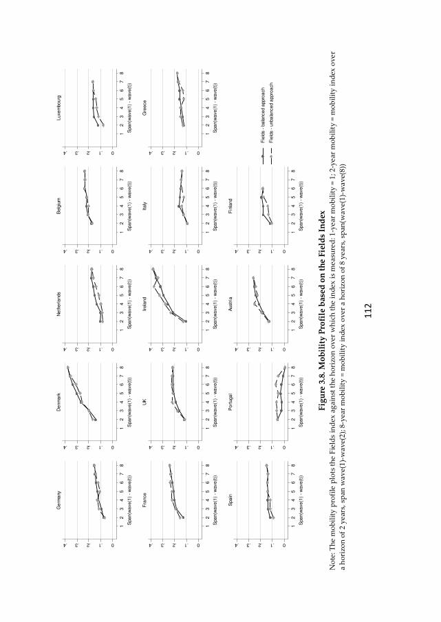
11
2
F
igu
re 3
.8. M
ob
ilit
y P
rofi
le b
ased
on
th
e F
ield
s In
dex
N
ote
: Th
e m
ob
ilit
y p
rofi
le p
lots
th
e F
ield
s in
dex
ag
ain
st t
he
ho
rizo
n o
ver
wh
ich
th
e in
dex
is
me
asu
red
: 1-y
ear
mo
bil
ity
= 1
; 2
-ye
ar m
ob
ilit
y =
mo
bil
ity
in
dex
ov
er
a h
ori
zon
of
2 y
ear
s, s
pan
wa
ve(
1)-
wa
ve(
2);
8-y
ear
mo
bil
ity
= m
ob
ilit
y i
nd
ex o
ver
a h
ori
zo
n o
f 8
ye
ars,
sp
an(w
av
e(1
)-w
av
e(8
))
0.1.2.3.4
12
34
56
78
Spa
n(w
ave
(1)
- w
ave
(t))
Ge
rma
ny
0.1.2.3.4
12
34
56
78
Spa
n(w
ave
(1)
- w
ave
(t))
De
nm
ark
0.1.2.3.4
12
34
56
78
Spa
n(w
ave
(1)
- w
ave
(t))
Ne
the
rla
nds
0.1.2.3.4
12
34
56
78
Spa
n(w
ave
(1)
- w
ave
(t))
Be
lgiu
m
0.1.2.3.4
12
34
56
78
Spa
n(w
ave
(1)
- w
ave
(t))
Luxe
mbo
urg
0.1.2.3.4
12
34
56
78
Spa
n(w
ave
(1)
- w
ave
(t))
Fra
nce
0.1.2.3.4
12
34
56
78
Spa
n(w
ave
(1)
- w
ave
(t))
UK
0.1.2.3.4
12
34
56
78
Spa
n(w
ave
(1)
- w
ave
(t))
Ire
land
0.1.2.3.4
12
34
56
78
Spa
n(w
ave
(1)
- w
ave
(t))
Ita
ly
0.1.2.3.4
12
34
56
78
Spa
n(w
ave
(1)
- w
ave
(t))
Gre
ece
0.1.2.3.4
12
34
56
78
Spa
n(w
ave
(1)
- w
ave
(t))
Spa
in
0.1.2.3.4
12
34
56
78
Spa
n(w
ave
(1)
- w
ave
(t))
Po
rtuga
l
0.1.2.3.4
12
34
56
78
Spa
n(w
ave
(1)
- w
ave
(t))
Austr
ia
0.1.2.3.4
12
34
56
78
Spa
n(w
ave
(1)
- w
ave
(t))
Fin
land
Fie
lds -
ba
lance
d a
ppro
ach
Fie
lds -
unba
lance
d a
ppro
ach
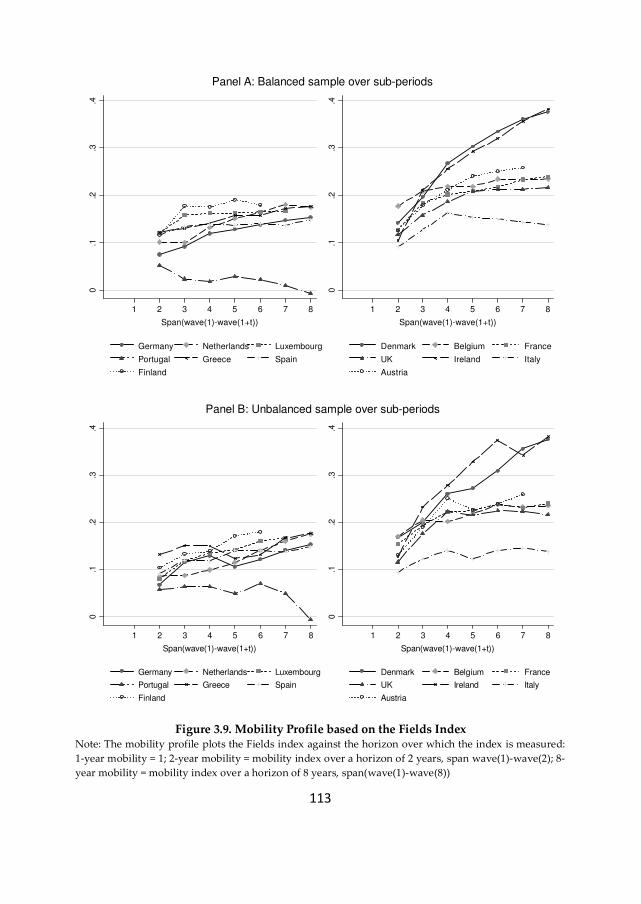
113
Figure 3.9. Mobility Profile based on the Fields Index
Note: The mobility profile plots the Fields index against the horizon over which the index is measured:
1-year mobility = 1; 2-year mobility = mobility index over a horizon of 2 years, span wave(1)-wave(2); 8-
year mobility = mobility index over a horizon of 8 years, span(wave(1)-wave(8))
0.1
.2.3
.4
1 2 3 4 5 6 7 8
Span(wave(1)-wave(1+t))
Germany Netherlands Luxembourg
Portugal Greece Spain
Finland
0.1
.2.3
.4
1 2 3 4 5 6 7 8
Span(wave(1)-wave(1+t))
Denmark Belgium France
UK Ireland Italy
Austria
Panel A: Balanced sample over sub-periods0
.1.2
.3.4
1 2 3 4 5 6 7 8
Span(wave(1)-wave(1+t))
Germany Netherlands Luxembourg
Portugal Greece Spain
Finland
0.1
.2.3
.4
1 2 3 4 5 6 7 8
Span(wave(1)-wave(1+t))
Denmark Belgium France
UK Ireland Italy
Austria
Panel B: Unbalanced sample over sub-periods
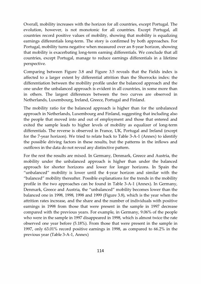
114
Overall, mobility increases with the horizon for all countries, except Portugal. The
evolution, however, is not monotonic for all countries. Except Portugal, all
countries record positive values of mobility, showing that mobility is equalizing
earnings differentials long-term. The story is confirmed by both approaches. For
Portugal, mobility turns negative when measured over an 8-year horizon, showing
that mobility is exacerbating long-term earning differentials. We conclude that all
countries, except Portugal, manage to reduce earnings differentials in a lifetime
perspective.
Comparing between Figure 3.8 and Figure 3.5 reveals that the Fields index is
affected to a larger extent by differential attrition than the Shorrocks index: the
differentiation between the mobility profile under the balanced approach and the
one under the unbalanced approach is evident in all countries, in some more than
in others. The largest differences between the two curves are observed in
Netherlands, Luxembourg, Ireland, Greece, Portugal and Finland.
The mobility ratio for the balanced approach is higher than for the unbalanced
approach in Netherlands, Luxembourg and Finland, suggesting that including also
the people that moved into and out of employment and those that entered and
exited the sample leads to higher levels of mobility as equalizer of long-term
differentials. The reverse is observed in France, UK, Portugal and Ireland (except
for the 7-year horizon). We tried to relate back to Table 3-A-1 (Annex) to identify
the possible driving factors in these results, but the patterns in the inflows and
outflows in the data do not reveal any distinctive pattern.
For the rest the results are mixed. In Germany, Denmark, Greece and Austria, the
mobility under the unbalanced approach is higher than under the balanced
approach for shorter horizons and lower for longer horizons. In Spain the
“unbalanced” mobility is lower until the 4-year horizon and similar with the
“balanced” mobility thereafter. Possible explanations for the trends in the mobility
profile in the two approaches can be found in Table 3-A-1 (Annex). In Germany,
Denmark, Greece and Austria, the “unbalanced” mobility becomes lower than the
balanced one in 1998, 1998, 1998 and 1999 (Figure 3.8), which is the year when the
attrition rates increase, and the share and the number of individuals with positive
earnings in 1998 from those that were present in the sample in 1997 decrease
compared with the previous years. For example, in Germany, 9.06% of the people
who were in the sample in 1997 disappeared in 1998, which is almost twice the rate
observed one year before (5.18%). From those that were present in the sample in
1997, only 63.01% record positive earnings in 1998, as compared to 66.2% in the
previous year (Table 3-A-1, Annex)

115
Four clusters are identified in the evolution of long-term mobility profiles,
confirmed both by the balanced and the unbalanced approach. (Figure 3.9)
Independent of the horizon, Portugal and Italy have the lowest profiles, indicating
that they have the lowest mobility as equalizer of long term differentials. The
ranking for the other countries changes to a large extent for horizons up to 4 years.
Looking after the 4th horizon, three clusters are observed. The first cluster, with
values higher than Portugal and Italy, is formed by Germany, Spain, Netherlands,
Greece, Luxembourg and Finland. This is followed by a cluster formed by UK,
Belgium, France and Austria. Finally, Denmark and Ireland stand out with respect
to the steepness of their profiles and to the high level of their long-term mobility.
Some convergence trends emerge as the horizon over which mobility is measured
increases. For a horizon of 7-8 years, mobility converges to similar values in
Denmark and Ireland, in Belgium and France, in Spain and Germany, and in
Luxembourg, Greece and Netherlands. (Figure 3.9)
We conclude this section with an overview of the country ranking in Fields
mobility. Similar with the trend observed for the Shorrocks index, the country
ranking changes with the horizon over which mobility is measured.
Based on the balanced approach, the 2-year mobility is the highest in Belgium,
followed by Denmark, France, Greece, Austria, Luxembourg, UK, Finland, Spain,
Ireland, Netherlands, Italy, Germany and Portugal. The unbalanced approach
reveals a slightly different picture than the balanced one, sign that the Fields index
is more sensitive to differential attrition compared with the Shorrocks index where
the rankings are similar between the two approaches. Belgium, Denmark, France,
Greece, Austria still have the highest mobility, and Germany and Portugal the
lowest. In between, in a descendent order we find Ireland, UK, Finland, Italy,
Spain, Netherlands and Luxembourg.
Figure 3.10 displays the ranking in long-term Fields mobility. Based on the
balanced approach (Panel A), over a horizon of 6 years, Denmark, Ireland and
Austria record the highest mobility, followed by Belgium, France, UK, Finland,
Luxembourg, Netherlands, Greece, Italy, Spain Germany and Portugal. Thus
except for Portugal, the mobility picture over the 6-year horizon looks different
from the one over the 2-year horizon. Based on the unbalanced approach (Panel B),
Ireland has the highest mobility, followed by Denmark, Austria, France, Belgium,
UK, Finland, Luxembourg, Italy, Spain, Netherlands, Greece, Germany and
Portugal.
Over a 7-year horizon, the balanced approach reveals the same ranking as over a 6-
year horizon for the first 6 countries and Portugal. In between, in a descending
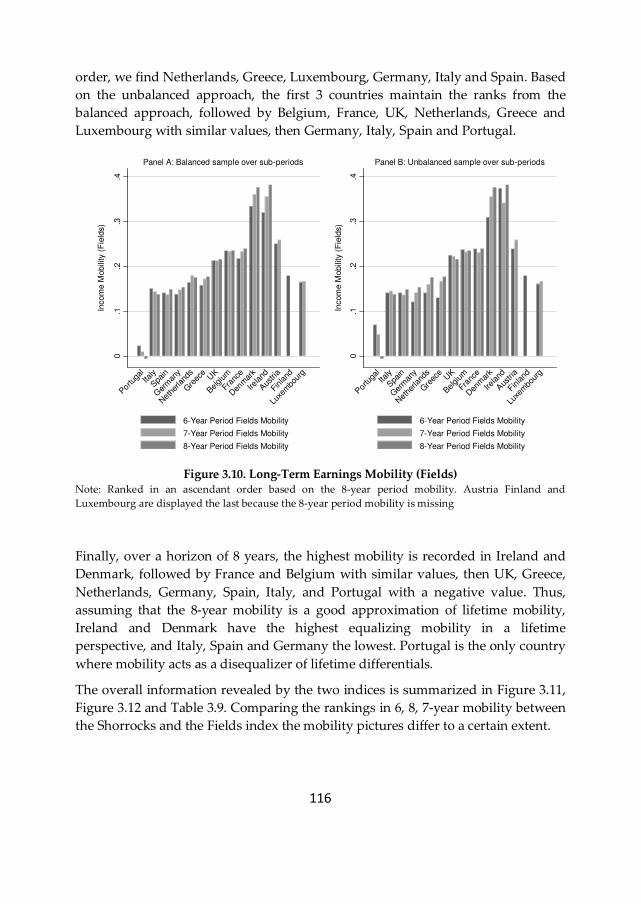
116
order, we find Netherlands, Greece, Luxembourg, Germany, Italy and Spain. Based
on the unbalanced approach, the first 3 countries maintain the ranks from the
balanced approach, followed by Belgium, France, UK, Netherlands, Greece and
Luxembourg with similar values, then Germany, Italy, Spain and Portugal.
Figure 3.10. Long-Term Earnings Mobility (Fields)
Note: Ranked in an ascendant order based on the 8-year period mobility. Austria Finland and
Luxembourg are displayed the last because the 8-year period mobility is missing
Finally, over a horizon of 8 years, the highest mobility is recorded in Ireland and
Denmark, followed by France and Belgium with similar values, then UK, Greece,
Netherlands, Germany, Spain, Italy, and Portugal with a negative value. Thus,
assuming that the 8-year mobility is a good approximation of lifetime mobility,
Ireland and Denmark have the highest equalizing mobility in a lifetime
perspective, and Italy, Spain and Germany the lowest. Portugal is the only country
where mobility acts as a disequalizer of lifetime differentials.
The overall information revealed by the two indices is summarized in Figure 3.11,
Figure 3.12 and Table 3.9. Comparing the rankings in 6, 8, 7-year mobility between
the Shorrocks and the Fields index the mobility pictures differ to a certain extent.
0.1
.2.3
.4
Incom
e M
obili
ty (
Fie
lds)
Portuga
lIta
ly
Spa
in
Ger
man
y
Neth
erland
s
Gre
ece
UK
Belgi
um
Franc
e
Den
mar
k
Ireland
Aus
tria
Finland
Luxe
mbo
urg
Panel A: Balanced sample over sub-periods
6-Year Period Fields Mobility
7-Year Period Fields Mobility
8-Year Period Fields Mobility
0.1
.2.3
.4
Incom
e M
obili
ty (
Fie
lds)
Portu
galIta
ly
Spa
in
Ger
man
y
Neth
erland
s
Gre
ece
UK
Belgi
um
Franc
e
Den
mar
k
Ireland
Aus
tria
Finland
Luxe
mbo
urg
Panel B: Unbalanced sample over sub-periods
6-Year Period Fields Mobility
7-Year Period Fields Mobility
8-Year Period Fields Mobility

117
Based on the 8-year mobility (Figure 3.12 and Table 3.9), Portugal records the
lowest values based on both indices. Lifetime mobility is present in Portugal, but is
disequalizing, thus it does not benefit low earnings individuals.
Among the countries with the highest 5 values in lifetime Shorrocks mobility –
Denmark, UK, Belgium, Greece, Ireland - only Denmark, Ireland, Belgium and UK
score among the 5 highest in the Fields lifetime equalizing mobility, suggesting
that these countries have the highest lifetime mobility with the highest equalizing
impact on lifetime earnings differentials. Denmark scores the highest in lifetime
mobility, but the second highest after Ireland in equalizing mobility, suggesting
that mobility in Ireland is slightly more equalizing in a lifetime perspective than in
Denmark. Compared with the other countries, Denmark has a higher lifetime
mobility with a higher lifetime equalizing impact.
UK has a lower lifetime mobility and a lower equalizing impact than Denmark.
Compared with Ireland, Belgium and France, UK has a higher lifetime mobility,
but with a lower equalizing impact. A possible explanation is that UK has a higher
share of lifetime mobility which is disequalizing than Ireland, Belgium and France.
Compared with the remaining countries, UK has a higher lifetime mobility with a
higher lifetime equalizing impact.
Belgium scores the third highest after Denmark and UK based on Shorrocks and
the 4th highest after Ireland, Denmark, and France based on Fields. Thus Belgium
has a lower lifetime mobility with a lower equalizing impact than Denmark, a
higher lifetime mobility and a lower equalizing mobility than Ireland and France,
and a lower lifetime mobility but with a higher equalizing impact than in UK.
Compared with the remaining countries Belgium has a higher lifetime mobility
with a higher lifetime equalizing impact.

118
Figure 3.11. Scatter plot of 6-year and 7-year period mobility: Shorrocks vs. Fields
PT
GE
SP
IT
GR
NL
LU
FI
UK
F
B
AT
IR
DK.0
5.1
.15
.2.2
5
Six
-Ye
ar
Pe
rio
d S
ho
rro
cks M
ob
ility -
Ba
lan
ce
d
0 .1 .2 .3 .4
Six-Year Period Fields Mobility - Balanced
Panel A: Balanced sample over sub-periods
PT
GE
GR
NL
SP
IT
LU
FI
UKB
F
AT
DK
IR
.05
.1.1
5.2
.25
Six
-Ye
ar
Pe
rio
d S
ho
rro
cks M
ob
ility
0 .1 .2 .3 .4
Six-Year Period Fields Mobility
Panel B: Unbalanced sample over sub-periods
PT
SP
IT
GE
LU
GR
NL
UKB
F
AT
IR
DK
.1.1
5.2
.25
Se
ve
n-Y
ea
r P
eri
od
Sh
orr
ocks M
ob
ility -
Ba
lan
ce
d
0 .1 .2 .3 .4
Seven-Year Period Fields Mobility - Balanced
Panel A: Balanced sample over sub-periods
PT
SPGE
ITNL
GR
LU
UK
F
B
AT
IR
DK
.1.1
5.2
.25
Se
ve
n-Y
ea
r P
eri
od
Sh
orr
ocks M
ob
ility
0 .1 .2 .3 .4
Seven-Year Period Fields Mobility
Panel B: Unbalanced sample over sub-periods

119
Figure 3.12. Scatter plot of 8-year period mobility: Shorrocks vs. Fields
Greece has a higher lifetime mobility with a higher equalizing impact than
Netherlands, Italy, Germany, Spain and Portugal. Compared with Denmark,
Belgium and UK, Greece has a lower lifetime mobility and a lower equalizing
mobility. Compared with Ireland and France, Greece has a higher lifetime mobility
and a lower equalizing impact, signalling that a lower part of the mobility in
Greece is equalizing lifetime earnings differentials compared with Ireland and
France.
Ireland has a higher lifetime mobility than Netherlands, Italy, France, Spain,
Germany and Portugal, and a lower lifetime mobility than the other countries. In
terms of equalizing impact, however, Ireland is the strongest.
Netherlands has a middle rank both in lifetime mobility and in lifetime equalizing
mobility. It has a higher lifetime mobility and a higher equalizing impact than
Germany, Spain, Italy and Portugal. Compared to France it has a higher lifetime
mobility, but a lower equalizing mobility, sign that a higher share of mobility is
disequalizing in the Netherlands.
Italy has a lower lifetime mobility with a lower equalizing impact compared with
most countries, except Portugal, for which the opposite holds, and Germany,
PT
IT
SPGE
NLGR
UK B
F
DK
IR
.1.1
5.2
.25
.3
Lo
ng
-Te
rm S
ho
rro
cks M
ob
ility
0 .1 .2 .3 .4
Long-Term Fields Mobility

120
Spain, and France, which have a lower lifetime mobility and a higher equalizing
mobility.
France has a higher lifetime mobility and a higher equalizing mobility than Spain,
Germany and Portugal, and a lower lifetime inequality coupled with a lower
equalizing mobility than Denmark and Ireland. Compared with the rest, France
has a lower lifetime inequality but with a higher equalizing impact.
Spain has a higher lifetime mobility with a higher equalizing impact than Portugal,
a higher lifetime mobility and a lower equalizing mobility than Germany and the
reverse compared with Italy. Compared with the remaining countries, Spain has a
lower lifetime mobility with a lower equalizing impact.
Germany has a higher lifetime mobility with a higher equalizing impact than
Portugal, a lower lifetime mobility and a higher equalizing mobility than Spain
and Italy. Compared with the remaining countries, Germany has a lower lifetime
mobility with a lower equalizing impact.
Based on the 7-year mobility (Figure 3.11 and Table 3.9), Austria has a higher
lifetime mobility with a higher equalizing impact than most countries, except
Denmark where the reverse holds, and Ireland which has a higher equalizing
mobility. This is confirmed under both approaches. Using the same horizon as
Austria, Luxembourg has a lower lifetime mobility with a lower equalizing impact
than most countries, except Portugal, where the reverse holds, and Germany, Spain
and Italy, which have a higher lifetime mobility but with a lower equalizing
impact.
Based on the 6-year mobility (Figure 3.11 and Table 3.9), Finland has a higher
lifetime mobility with a higher equalizing impact than Germany, Netherlands,
Luxembourg, Italy, Greece, Spain, and Portugal, a lower lifetime mobility with a
lower equalizing impact than Denmark, and a higher lifetime mobility but with a
lower equalizing mobility than Belgium, France, UK, Ireland and Austria.

12
1
Tab
le 3
.9. D
om
inan
ce r
elat
ion
s in
lo
ng
ter
m e
arn
ing
s m
ob
ilit
y: S
ho
rro
cks
and
Fie
lds
Ind
ex
D
enm
ark
N
eth
erla
nd
s B
elg
ium
L
ux
emb
ou
rg*
Fra
nce
U
K
Irel
an
d
Ita
ly
Gre
ece
S
pa
in
Po
rtu
ga
l A
ust
ria
* F
inla
nd
**
Ger
ma
ny
<
<
<
>
<
<
<
<
<
<
>
<
<
S
ho
rro
cks
<
<
<
<
<
<
<
>
<
>
>
<
<
Fie
lds
D
enm
ark
>
>
>
>
>
>
>
>
>
>
>
>
S
ho
rro
cks
>
>
>
>
>
<
>
>
>
>
>
>
F
ield
s
Net
her
lan
ds
<
>
>
<
<
>
<
>
>
<
<
Sh
orr
ock
s
<
>1
<
<
<
>
<
>
>
<
<
Fie
lds
B
elg
ium
>
>
<
>
>
>
>
>
<
<
S
ho
rro
cks
>
<
>
<
>
>
>
>
<
>
F
ield
s
Lu
xem
bo
urg
* <
<
<
<
<
<
>
<
<
S
ho
rro
cks
<
<
<
>
<2
>
>
<
<
Fie
lds
F
ran
ce
<
<
<
<
>
>
<
<
Sh
orr
ock
s
>
<
>
>
>
>
<
>
F
ield
s
UK
>
>
>
>
>
<
<
S
ho
rro
cks
<
>
>
>
>
<
>
Fie
lds
Ir
ela
nd
>
<
>
>
<
<
S
ho
rro
cks
>
>
>
>
>
>
F
ield
s
Ita
ly
<
>
>
<
<
Sh
orr
ock
s
<
<
>
<
<
Fie
lds
G
reec
e
>
>
<
<
Sh
orr
ock
s
>
>
<
<
F
ield
s
No
te: T
he
rea
din
g o
f th
e ta
ble
go
es
fro
m l
eft
to r
igh
t.
(*)
Th
e co
mp
aris
on
is
ba
sed
on
7-y
ear
per
iod
mo
bil
ity
(**)
Th
e co
mp
aris
on
is
ba
sed
on
7-y
ear
per
iod
mo
bil
ity
(1)
Ba
sed
on
th
e b
ala
nce
d a
pp
roa
ch.
Th
e re
ver
se h
old
s u
nd
er t
he
un
bal
ance
d a
pp
roac
h
(2)
Ba
sed
o
n
the
ba
lan
ced
a
pp
roa
ch.
Un
der
th
e u
nb
ala
nce
d
ap
pro
ach
, th
ey a
re e
qu
al
Sp
ain
>
<
<
S
ho
rro
cks
>
<
<
Fie
lds
P
ort
ug
al
<
<
Sh
orr
ock
s
<
<
F
ield
s
Au
stri
a*
<
Sh
orr
ock
s
>
Fie
lds
F
inla
nd
**
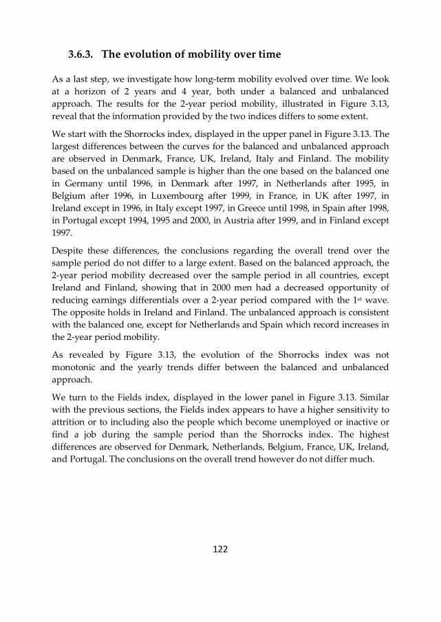
122
3.6.3. The evolution of mobility over time
As a last step, we investigate how long-term mobility evolved over time. We look
at a horizon of 2 years and 4 year, both under a balanced and unbalanced
approach. The results for the 2-year period mobility, illustrated in Figure 3.13,
reveal that the information provided by the two indices differs to some extent.
We start with the Shorrocks index, displayed in the upper panel in Figure 3.13. The
largest differences between the curves for the balanced and unbalanced approach
are observed in Denmark, France, UK, Ireland, Italy and Finland. The mobility
based on the unbalanced sample is higher than the one based on the balanced one
in Germany until 1996, in Denmark after 1997, in Netherlands after 1995, in
Belgium after 1996, in Luxembourg after 1999, in France, in UK after 1997, in
Ireland except in 1996, in Italy except 1997, in Greece until 1998, in Spain after 1998,
in Portugal except 1994, 1995 and 2000, in Austria after 1999, and in Finland except
1997.
Despite these differences, the conclusions regarding the overall trend over the
sample period do not differ to a large extent. Based on the balanced approach, the
2-year period mobility decreased over the sample period in all countries, except
Ireland and Finland, showing that in 2000 men had a decreased opportunity of
reducing earnings differentials over a 2-year period compared with the 1st wave.
The opposite holds in Ireland and Finland. The unbalanced approach is consistent
with the balanced one, except for Netherlands and Spain which record increases in
the 2-year period mobility.
As revealed by Figure 3.13, the evolution of the Shorrocks index was not
monotonic and the yearly trends differ between the balanced and unbalanced
approach.
We turn to the Fields index, displayed in the lower panel in Figure 3.13. Similar
with the previous sections, the Fields index appears to have a higher sensitivity to
attrition or to including also the people which become unemployed or inactive or
find a job during the sample period than the Shorrocks index. The highest
differences are observed for Denmark, Netherlands, Belgium, France, UK, Ireland,
and Portugal. The conclusions on the overall trend however do not differ much.
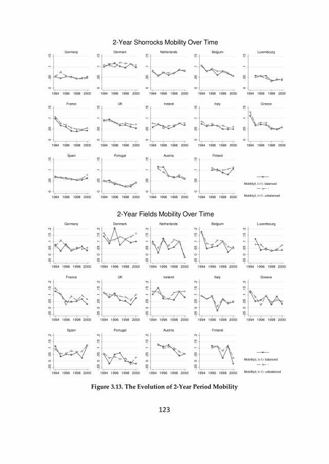
123
Figure 3.13. The Evolution of 2-Year Period Mobility
0.0
5.1
.15
1994 1996 1998 2000
Germany
0.0
5.1
.15
1994 1996 1998 2000
Denmark
0.0
5.1
.15
1994 1996 1998 2000
Netherlands
0.0
5.1
.15
1994 1996 1998 2000
Belgium
0.0
5.1
.15
1994 1996 1998 2000
Luxembourg0
.05
.1.1
5
1994 1996 1998 2000
France
0.0
5.1
.15
1994 1996 1998 2000
UK
0.0
5.1
.15
1994 1996 1998 2000
Ireland
0.0
5.1
.15
1994 1996 1998 2000
Italy
0.0
5.1
.15
1994 1996 1998 2000
Greece
0.0
5.1
.15
1994 1996 1998 2000
Spain
0.0
5.1
.15
1994 1996 1998 2000
Portugal
0.0
5.1
.15
1994 1996 1998 2000
Austria
0.0
5.1
.15
1994 1996 1998 2000
Finland
Mobility(t, t+1)- balanced
Mobility(t, t+1)- unbalanced
2-Year Shorrocks Mobility Over Time-.
05
0.0
5.1
.15
.2
1994 1996 1998 2000
Germany
-.0
50
.05
.1.1
5.2
1994 1996 1998 2000
Denmark
-.0
50
.05
.1.1
5.2
1994 1996 1998 2000
Netherlands
-.0
50
.05
.1.1
5.2
1994 1996 1998 2000
Belgium
-.0
50
.05
.1.1
5.2
1994 1996 1998 2000
Luxembourg
-.0
50
.05
.1.1
5.2
1994 1996 1998 2000
France
-.0
50
.05
.1.1
5.2
1994 1996 1998 2000
UK
-.0
50
.05
.1.1
5.2
1994 1996 1998 2000
Ireland
-.0
50
.05
.1.1
5.2
1994 1996 1998 2000
Italy
-.0
50
.05
.1.1
5.2
1994 1996 1998 2000
Greece
-.0
50
.05
.1.1
5.2
1994 1996 1998 2000
Spain
-.0
50
.05
.1.1
5.2
1994 1996 1998 2000
Portugal
-.0
50
.05
.1.1
5.2
1994 1996 1998 2000
Austria
-.0
50
.05
.1.1
5.2
1994 1996 1998 2000
Finland
Mobility(t, t+1)- balanced
Mobility(t, t+1)- unbalanced
2-Year Fields Mobility Over Time

124
Based on the balanced approach, the evolution of the 2-year Fields index reveals
that mobility became less equalizing in 2000-2001 compared with the first two
waves in most countries, except Spain where it became more equalizing, and
Netherlands, Portugal and Finland, where 2-year period mobility turned
disequalizing. Based on the unbalanced approach, 2-year period mobility became
more equalizing in Spain and Ireland, disequalizing in Netherlands and less
equalizing in the other countries.
Similar with the Shorrocks index, the evolution of the Fields index was not
monotonic and the yearly trends differ between the balanced and unbalanced
approach.
Figure 3.14 shows the evolution of the 4-year mobility using both the Fields and
the Shorrocks index. Based on the balanced approach (Panel A) using the
Shorrocks index, long-term mobility decreased over time in all countries. The same
is observed in the unbalanced approach (Panel B), except for Netherlands and
Denmark where long-period mobility increased.
The balanced approach (Panel A) using the Fields index reveals that the 4-year
period mobility became less equalizing over time in all countries, except Portugal,
where it became more equalizing, and Italy it became disequalizing. The
unbalanced approach (Panel B) reveals a slightly different picture for some
countries, highlighting again that the Fields index is more sensitive to differential
attrition. The 4-year period mobility became less equalizing in all countries, except
Spain and Netherlands. No country records a disequalizing mobility under the
unbalanced approach.
To sum up, under the balanced approach all countries record a decrease in long-
term mobility which also becomes less equalizing in most countries. Exceptions are
Italy where it becomes disequalizing, and Portugal, where it becomes more
equalizing. The divergent trend between the Shorrocks and the Fields index might
signal that Portugal records a decrease in the disequalizing part of mobility, which
in turn increases the Fields index.
Turning to the unbalanced approach, all countries except Netherlands and
Denmark, record a decrease in long-term mobility, which also becomes less
equalizing in all countries except Spain and Netherlands. The divergent trend
between the two indices in Spain and Denmark might signal that Spain records a
decrease in the disequalizing part of mobility, which in turn increases the Fields
index, whereas Denmark records an increase in the disequalizing part of mobility,
which in turn decreases the Fields index. In Netherlands long-term mobility
increases, becoming more equalizing.
125
Figure 3.14. The Evolution of Long-Term Mobility Over Time
Note: (*) For Luxembourg and Austria the figure displays the value for 1995-1998, and for Finland
for 1996-1999
(**) For Luxembourg and Austria the figure displays the value for 1998-2001
3.7.Concluding remarks
This paper explores the degree of lifetime earnings mobility for men in 14 EU
countries using ECHP between 1994 and 2001. We address two questions. First, do
EU citizens have an increased opportunity to improve their position in the
distribution of lifetime earnings? Second, to what extent does earnings mobility
work to equalize/disequalize longer-term earnings relative to cross-sectional
inequality and how does it differ across the EU? Moreover, we explored how the
findings differ, first if we consider only individuals which record positive earnings
in each year between 1994 and 2001 – “the balanced approach”, and second if we
consider also individuals which do not record positive earnings in each year
between 1994 and 2001, but only during the horizon over which mobility is
measured – “the unbalanced approach”. The basic assumption is that mobility
measured over a horizon of 8 years is a good proxy for lifetime mobility.
0.1
.2.3
Inco
me
Mo
bili
ty (
Sh
orr
ocks)
Portugal
Luxem
bour
g
Franc
e
Ger
man
y
Spain
Italy
Gre
ece
Irela
nd
Austri
a
Net
herla
nds UK
Belgi
um
Den
mar
k
Finla
nd
Shorrocks Mobility 1994-1997*
Shorrocks Mobility 1997-2000**
0.1
.2.3
Inco
me
Mo
bili
ty (
Fie
lds)
Italy
Luxe
mbo
urg
Portuga
l
Germ
any UK
Spain
Net
herla
nds
France
Austri
a
Belgiu
m
Gre
ece
Irela
nd
Denm
ark
Finla
nd
Fields Mobility 1994-1997*
Fields Mobility 1997-2000**
Panel A: Balanced sample over sub-periods
0.1
.2.3
Inco
me
Mo
bili
ty (
Sh
orr
ocks)
Portugal
Luxem
bour
g
France
Ger
many
Spain
Italy
Gre
ece
Net
herla
nds
Irela
nd UK
Austria
Belgium
Den
mark
Finla
nd
Shorrocks Mobility 1994-1997*
Shorrocks Mobility 1997-2000**
0.1
.2.3
Inco
me
Mo
bili
ty (
Fie
lds)
Portuga
lIta
ly
Germ
any
Luxe
mbo
urg
France U
K
Gre
ece
Spain
Net
herla
nds
Belgiu
m
Denm
ark
Austri
a
Irela
nd
Finla
nd
Fields Mobility 1994-1997*
Fields Mobility 1997-2000**
Panel B: Unbalanced sample over sub-periods

126
The first question is answered by applying the Shorrocks (1978) index. We find that
all countries record an increase in earnings mobility when the horizon over which
mobility is measured is extended. This shows that men do have an increasing
mobility in the distribution of lifetime earnings as they advance in their career,
result confirmed both by the “balanced” and the “unbalanced” approach.
Differential attrition appears to have a limited impact on the stability profiles, but a
higher impact on the country ranking in Shorrock mobility.
Using the mobility index computed over a horizon of 8 years, we conclude that the
highest lifetime mobility is recorded in Denmark, followed by the UK, Belgium,
Greece, Ireland, Netherlands, Italy, France, Spain, Germany, and the lowest,
Portugal. Therefore Denmark provides the highest opportunity of reducing
lifetime earnings differentials and Portugal the lowest. Based on the 6-year
mobility, Finland records the second highest lifetime mobility after Denmark.
Based on the 7-year mobility, Austria records the second highest lifetime mobility
after Denmark, and Luxembourg the second lowest after Portugal. Both
approaches confirm these rankings.
The main limitation of this approach is that it fails to answer our second question,
whether this mobility is equalizing or disequalizing lifetime earnings differentials.
To overcome this limitation we applied the newly developed Fields index. (Fields
2008) In general, mobility increases with the horizon in all countries, except
Portugal where mobility decreases with the horizon, turning negative when
measured over an 8-year horizon. This finding is confirmed both by the balanced
and the unbalanced approach. Thus only in Portugal mobility is exacerbating long-
term earning differentials, whereas the other countries manage to reduce earnings
differentials in a lifetime perspective.
The Fields index however is affected to a larger extent by differential attrition than
the Shorrocks index: the differentiation between the mobility profile under the
balanced approach and the one under the unbalanced approach is evident in all
countries, in some more than in others. The largest differences between the two
curves are observed in Netherlands, Luxembourg, Ireland, Greece, Portugal and
Finland.
Using the mobility index computed over a horizon of 8 years as proxy for lifetime
mobility, we conclude that in all countries, except Portugal, mobility acts as an
equalizer of lifetime differentials. The highest mobility as equalizer of longer term
inequality is recorded in Ireland and Denmark, followed by France and Belgium
with similar values, then UK, Greece, Netherlands, Germany, Spain and Italy.
Based on the 6-year mobility, Finland records the 7th highest equalizing mobility.
Based on the 7-year mobility, Austria records the third highest equalizing mobility

127
after Ireland and Denmark, and Luxembourg the fifth lowest according to the
balanced approach and the sixth lowest according to the unbalanced approach.
Regarding the evolution of long-term mobility over time, the two indices bring
complementary pieces of information. The longest time horizon to be followed
over time in our data is of 4 years. Due to the short horizon, the implications of the
trends in the 4-year period mobility for the evolution of lifetime mobility should be
regarded with caution. Some differences are present between the balanced and the
unbalanced approach.
Under the balanced approach all countries record a decrease in long-term mobility
which also becomes less equalizing in most countries. Exceptions are Italy where it
becomes disequalizing, and Portugal, where it becomes more equalizing. The
divergent trend between the Shorrocks and the Fields index might signal that
Portugal records a decrease in the disequalizing part of mobility, which in turn
increases the Fields index.
Turning to the unbalanced approach, all countries except Netherlands and
Denmark, record a decrease in long-term mobility, which also becomes less
equalizing in all countries except Spain and Netherlands. The divergent trend
between the two indices in Spain and Denmark might signal that Spain records a
decrease in the disequalizing part of mobility, which in turn increases the Fields
index, whereas Denmark records an increase in the disequalizing part of mobility,
which in turn decreases the Fields index. Netherlands records an increase in long-
term mobility, which also becomes more equalizing.
What are the possible implications for lifetime earnings inequality, assuming that
the 8-year period mobility is a good proxy for lifetime mobility? Among the
countries which recorded an increase in cross-sectional earnings inequality over
the sample period – Netherlands, Greece, Finland, Portugal, Luxembourg, Italy,
and Germany - only in Portugal lifetime mobility is expected to exacerbate annual
differentials in a lifetime perspective. For the rest, mobility acts as an equalizer of
lifetime differentials, thus counteracting the increase in annual inequality. For the
countries recording a decrease in annual inequality – Ireland, Austria, Denmark,
Belgium, Spain, France, and UK - lifetime mobility is expected to enhance the
reduction in lifetime earnings differentials.
Given these trends we expect Portugal to record the highest and Denmark the
lowest lifetime earnings inequality among the 14 EU countries. The outstanding
performance of the labour market in Denmark, which records the lowest cross-
sectional earnings inequality, coupled with the highest lifetime mobility and the
second highest equalizing lifetime mobility - might be due to the so called
128
“flexicurity approach” (OECD, 2004), which represents an interesting combination
of high labour market dynamism and a relatively high social protection. It is a mix
of flexibility (a high degree of job mobility thanks to low employment protection
legislation), social security (a generous system of unemployment benefits) and
active labour market programmes. The coupled effect of these factors assures a
small annual inequality and an earnings mobility which acts as an equalizer of
lifetime differentials, offering at the same time a high opportunity to low wage
individuals to improve their relative position in the distribution of lifetime
earnings.
Our paper has a threefold contribution to the existing literature. First, by exploring
a different facet of mobility – as an equalizer or disequalizer of lifetime earnings
differentials -, we fill part of the gap in the study of earnings mobility at the EU
level. Second, we apply a new class of measures of mobility as equalizer of long-
term differentials - developed by Fields (2008) –, which complement the
information provided by the well-known Shorrocks measure. Therefore we
highlight once again the limitations of the Shorrocks measure put forward by
Benabou and Ok (2001) and Fields (2008), and the need to provide additional
measures for capturing the real nature of lifetime earnings mobility. Third, by
comparing the findings between the “unbalanced” and the “balanced approach”,
meaning between including/and not the individuals that exited and (re)entered the
panel, we explored the impact of differentials attrition on the study of earnings
mobility as an equalizer of long-term differentials.
129
3.8.Annex
Table 3-A-1. Inflows and Outflows of Individuals in the Sample – Germany
1994 1995 1996 1997 1998 1999 2000 2001
Number of individuals with
positive earnings 25018 26059 25806 24889 23290 22955 21909 20703
Number of individuals with
positive earnings over the entire
sample
11057
Absolute number and proportion of individuals who report positive earnings in current year conditional on being in
the sample in previous year
Frequencies 23956 25224 24197 22814 22321 21290 20107
% 66.99 67.37 66.2 63.01 64.84 64.86 64.39
Absolute number and proportion of individuals who report no earnings in current year conditional on being in the
sample in the previous year
Unemployed
Inactive
Frequencies 3448 3461 4119 3932 3055 2787 2766
% 9.64 9.24 11.27 10.86 8.87 8.49 8.86
Attrition Frequencies 1885 2182 1892 3280 2951 2924 2830
% 5.27 5.83 5.18 9.06 8.57 8.91 9.06
Missing Wage Frequencies 6470 6576 6345 6180 6100 5826 5524
% 18.09 17.56 17.36 17.07 17.72 17.75 17.69
Total
Frequencies 35759 37443 36553 36206 34427 32827 31227
% 100 100 100 100 100 100 100
Table 3-A-1. Inflows and Outflows of Individuals in the Sample – Denmark
1994 1995 1996 1997 1998 1999 2000 2001
Number of individuals with
positive earnings 20899 20399 19190 19062 17321 16235 15678 15380
Number of individuals with
positive earnings over the entire
sample
8247
Absolute number and proportion of individuals who report positive earnings in current year conditional on being in the
sample in previous year
Frequencies 19854 18527 18110 16442 15334 14865 14642
% 68.74 66.59 69.43 66.23 67.41 69.6 71.6
Absolute number and proportion of individuals who report no earnings in current year conditional on being in the
sample in the previous year
Unemployed
Inactive
Frequencies 1535 1744 951 899 732 658 958
% 5.31 6.27 3.65 3.62 3.22 3.08 4.68
Attrition Frequencies 2440 3096 2914 3603 2922 2133 1775
% 8.45 11.13 11.17 14.51 12.85 9.99 8.68
Missing Wage Frequencies 5054 4454 4110 3881 3759 3703 3074
% 17.5 16.01 15.76 15.63 16.53 17.34 15.03
Total
Frequencies 28883 27821 26085 24825 22747 21359 20449
% 100 100 100 100 100 100 100
130
Table 3-A-1.Inflows and Outflows of Individuals in the Sample – Netherlands
1994 1995 1996 1997 1998 1999 2000 2001
Number of individuals with
positive earnings 20221 22100 22892 22753 22863 23233 24065 24130
Number of individuals with
positive earnings over the entire
sample
8173
Absolute number and proportion of individuals who report positive earnings in current year conditional on being in the
sample in previous year
Frequencies 20578 21328 21221 21055 20545 21026 21341
% 69.07 71.37 68.68 67.52 67.24 68.56 69.59
Absolute number and proportion of individuals who report no earnings in current year conditional on being in the
sample in the previous year
Unemployed
Inactive
Frequencies 2418 2356 2536 2120 1984 1840 1689
% 8.12 7.88 8.21 6.8 6.49 6 5.51
Attrition Frequencies 2941 1889 2591 3562 3984 4301 4891
% 9.87 6.32 8.39 11.42 13.04 14.02 15.95
Missing Wage Frequencies 3857 4310 4550 4448 4042 3502 2745
% 12.95 14.42 14.73 14.26 13.23 11.42 8.95
Total
Frequencies 29794 29883 30898 31185 30555 30669 30666
% 100 100 100 100 100 100 100
Table 3-A-1.Inflows and Outflows of Individuals in the Sample – Belgium
1994 1995 1996 1997 1998 1999 2000 2001
Number of individuals with
positive earnings 35342 34367 33280 32378 31129 29414 28087 26538
Number of individuals with
positive earnings over the entire
sample
16910
Absolute number and proportion of individuals who report positive earnings in current year conditional on being in the
sample in previous year
Frequencies 33277 32384 31564 30575 28731 27460 25790
% 63.43 63.65 64.38 63.88 64.28 65.15 64.38
Absolute number and proportion of individuals who report no earnings in current year conditional on being in the
sample in the previous year
Unemployed
Inactive
Frequencies 3810 5127 4378 3601 3040 3090 2540
% 7.26 10.08 8.93 7.52 6.8 7.33 6.34
Attrition Frequencies 4145 3798 3473 4803 4421 3851 4930
% 7.9 7.46 7.08 10.04 9.89 9.14 12.31
Missing Wage Frequencies 11228 9573 9614 8882 8504 7748 6798
% 21.4 18.81 19.61 18.56 19.03 18.38 16.97
Total
Frequencies 52460 50882 49029 47861 44696 42149 40058
% 100 100 100 100 100 100 100
131
Table 3-A-1.Inflows and Outflows of Individuals in the Sample – Luxembourg
1994 1995 1996 1997 1998 1999 2000 2001
Number of individuals with
positive earnings 15829 13695 14489 13403 14075 12667 12992
Number of individuals with
positive earnings over the entire
sample
7283
Absolute number and proportion of individuals who report positive earnings in current year conditional on being in the
sample in previous year
Frequencies
13417 12498 13190 12257 12402 11457
%
64.75 69.48 69.33 69.81 68.71 70.39
Absolute number and proportion of individuals who report no earnings in current year conditional on being in the
sample in the previous year
Unemployed
Inactive
Frequencies
1765 1559 1505 1408 1246 954
%
8.52 8.67 7.91 8.02 6.9 5.86
Attrition Frequencies
3423 1663 2109 1913 2346 1940
%
16.52 9.25 11.09 10.9 13 11.92
Missing Wage Frequencies
2116 2267 2220 1980 2057 1926
%
10.21 12.6 11.67 11.28 11.4 11.83
Total
Frequencies
20721 17987 19024 17558 18051 16277
% 100 100 100 100 100 100 100
Table 3-A-1.Inflows and Outflows of Individuals in the Sample – France
1994 1995 1996 1997 1998 1999 2000 2001
Number of individuals with
positive earnings 20137 19270 19042 17906 14467 14012 13760 14212
Number of individuals with
positive earnings over the entire
sample
5895
Absolute number and proportion of individuals who report positive earnings in current year conditional on being in the
sample in previous year
Frequencies 19143 18197 17243 14014 12209 12080 12468
% 62.47 64.76 62 52.08 54.24 55.54 60.8
Absolute number and proportion of individuals who report no earnings in current year conditional on being in the
sample in the previous year
Unemployed
Inactive
Frequencies 3259 3042 3426 3006 2607 2072 1995
% 10.64 10.83 12.32 11.17 11.58 9.53 9.73
Attrition Frequencies 3371 2213 2785 5584 3531 3786 2658
% 11 7.88 10.01 20.75 15.69 17.41 12.96
Missing Wage Frequencies 4871 4646 4358 4304 4162 3811 3385
% 15.9 16.53 15.67 16 18.49 17.52 16.51
Total
Frequencies 30644 28098 27812 26908 22509 21749 20506
% 100 100 100 100 100 100 100
132
Table 3-A-1. Inflows and Outflows of Individuals in the Sample – UK
1994 1995 1996 1997 1998 1999 2000 2001
Number of individuals with
positive earnings 24949 25329 25495 26010 26145 25750 25674 25264
Number of individuals with
positive earnings over the entire
sample
13977
Absolute number and proportion of individuals who report positive earnings in current year conditional on being in the
sample in previous year
Frequencies 24511 24848 25303 25278 25006 24881 24467
% 64.59 66.31 67.06 67.04 67.36 68.33 68.58
Absolute number and proportion of individuals who report no earnings in current year conditional on being in the
sample in the previous year
Unemployed
Inactive
Frequencies 4712 5053 4663 4140 3941 3607 3595
% 12.42 13.48 12.36 10.98 10.62 9.91 10.08
Attrition Frequencies 1836 966 1169 2073 1919 2153 2105
% 4.84 2.58 3.1 5.5 5.17 5.91 5.9
Missing Wage Frequencies 6888 6605 6597 6213 6257 5774 5510
% 18.15 17.63 17.48 16.48 16.85 15.86 15.44
Total
Frequencies 37947 37472 37732 37704 37123 36415 35677
% 100 100 100 100 100 100 100
Table 3-A-1. Inflows and Outflows of Individuals in the Sample – Ireland
1994 1995 1996 1997 1998 1999 2000 2001
Number of individuals with
positive earnings 13937 13221 12590 12515 12435 12091 10745 9727
Number of individuals with
positive earnings over the entire
sample
4453
Absolute number and proportion of individuals who report positive earnings in current year conditional on being in the
sample in previous year
Frequencies 12750 12217 12212 12020 11668 10236 9507
% 49.99 50.04 52.41 53.13 54.1 51.63 54.65
Absolute number and proportion of individuals who report no earnings in current year conditional on being in the
sample in the previous year
Unemployed
Inactive
Frequencies 4930 4723 4254 3374 2905 2185 2307
% 19.33 19.35 18.26 14.91 13.47 11.02 13.26
Attrition Frequencies 2167 2115 1600 1936 2516 3288 2362
% 8.5 8.66 6.87 8.56 11.66 16.59 13.58
Missing Wage Frequencies 5656 5359 5235 5292 4480 4116 3220
% 22.18 21.95 22.47 23.39 20.77 20.76 18.51
Total
Frequencies 25503 24414 23301 22622 21569 19825 17396
% 100 100 100 100 100 100 100
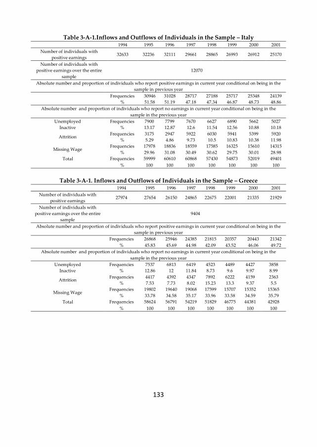
133
Table 3-A-1.Inflows and Outflows of Individuals in the Sample – Italy
1994 1995 1996 1997 1998 1999 2000 2001
Number of individuals with
positive earnings 32633 32236 32111 29661 28865 26993 26912 25170
Number of individuals with
positive earnings over the entire
sample
12070
Absolute number and proportion of individuals who report positive earnings in current year conditional on being in the
sample in previous year
Frequencies 30946 31028 28717 27188 25717 25348 24139
% 51.58 51.19 47.18 47.34 46.87 48.73 48.86
Absolute number and proportion of individuals who report no earnings in current year conditional on being in the
sample in the previous year
Unemployed
Inactive
Frequencies 7900 7799 7670 6627 6890 5662 5027
% 13.17 12.87 12.6 11.54 12.56 10.88 10.18
Attrition Frequencies 3175 2947 5922 6030 5941 5399 5920
% 5.29 4.86 9.73 10.5 10.83 10.38 11.98
Missing Wage Frequencies 17978 18836 18559 17585 16325 15610 14315
% 29.96 31.08 30.49 30.62 29.75 30.01 28.98
Total
Frequencies 59999 60610 60868 57430 54873 52019 49401
% 100 100 100 100 100 100 100
Table 3-A-1. Inflows and Outflows of Individuals in the Sample – Greece
1994 1995 1996 1997 1998 1999 2000 2001
Number of individuals with
positive earnings 27974 27654 26150 24865 22675 22001 21335 21929
Number of individuals with
positive earnings over the entire
sample
9404
Absolute number and proportion of individuals who report positive earnings in current year conditional on being in the
sample in previous year
Frequencies 26868 25946 24385 21815 20357 20443 21342
% 45.83 45.69 44.98 42.09 43.52 46.06 49.72
Absolute number and proportion of individuals who report no earnings in current year conditional on being in the
sample in the previous year
Unemployed
Inactive
Frequencies 7537 6813 6419 4523 4489 4427 3858
% 12.86 12 11.84 8.73 9.6 9.97 8.99
Attrition Frequencies 4417 4392 4347 7892 6222 4159 2363
% 7.53 7.73 8.02 15.23 13.3 9.37 5.5
Missing Wage Frequencies 19802 19640 19068 17599 15707 15352 15365
% 33.78 34.58 35.17 33.96 33.58 34.59 35.79
Total
Frequencies 58624 56791 54219 51829 46775 44381 42928
% 100 100 100 100 100 100 100
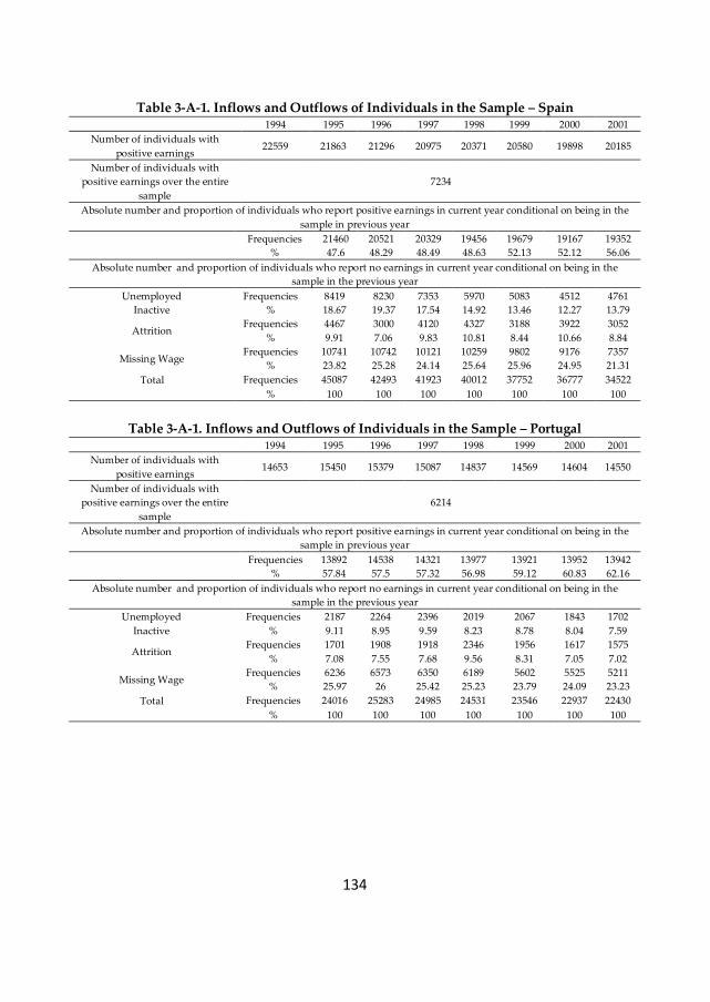
134
Table 3-A-1. Inflows and Outflows of Individuals in the Sample – Spain
1994 1995 1996 1997 1998 1999 2000 2001
Number of individuals with
positive earnings 22559 21863 21296 20975 20371 20580 19898 20185
Number of individuals with
positive earnings over the entire
sample
7234
Absolute number and proportion of individuals who report positive earnings in current year conditional on being in the
sample in previous year
Frequencies 21460 20521 20329 19456 19679 19167 19352
% 47.6 48.29 48.49 48.63 52.13 52.12 56.06
Absolute number and proportion of individuals who report no earnings in current year conditional on being in the
sample in the previous year
Unemployed
Inactive
Frequencies 8419 8230 7353 5970 5083 4512 4761
% 18.67 19.37 17.54 14.92 13.46 12.27 13.79
Attrition Frequencies 4467 3000 4120 4327 3188 3922 3052
% 9.91 7.06 9.83 10.81 8.44 10.66 8.84
Missing Wage Frequencies 10741 10742 10121 10259 9802 9176 7357
% 23.82 25.28 24.14 25.64 25.96 24.95 21.31
Total
Frequencies 45087 42493 41923 40012 37752 36777 34522
% 100 100 100 100 100 100 100
Table 3-A-1. Inflows and Outflows of Individuals in the Sample – Portugal
1994 1995 1996 1997 1998 1999 2000 2001
Number of individuals with
positive earnings 14653 15450 15379 15087 14837 14569 14604 14550
Number of individuals with
positive earnings over the entire
sample
6214
Absolute number and proportion of individuals who report positive earnings in current year conditional on being in the
sample in previous year
Frequencies 13892 14538 14321 13977 13921 13952 13942
% 57.84 57.5 57.32 56.98 59.12 60.83 62.16
Absolute number and proportion of individuals who report no earnings in current year conditional on being in the
sample in the previous year
Unemployed
Inactive
Frequencies 2187 2264 2396 2019 2067 1843 1702
% 9.11 8.95 9.59 8.23 8.78 8.04 7.59
Attrition Frequencies 1701 1908 1918 2346 1956 1617 1575
% 7.08 7.55 7.68 9.56 8.31 7.05 7.02
Missing Wage Frequencies 6236 6573 6350 6189 5602 5525 5211
% 25.97 26 25.42 25.23 23.79 24.09 23.23
Total
Frequencies 24016 25283 24985 24531 23546 22937 22430
% 100 100 100 100 100 100 100
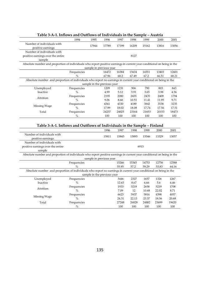
135
Table 3-A-1. Inflows and Outflows of Individuals in the Sample – Austria
1994 1995 1996 1997 1998 1999 2000 2001
Number of individuals with
positive earnings 17944 17789 17199 16209 15162 13816 13056
Number of individuals with
positive earnings over the entire
sample
8127
Absolute number and proportion of individuals who report positive earnings in current year conditional on being in the
sample in previous year
Frequencies 16472 16384 15634 14551 13403 12601
% 67.96 68.2 67.49 67.2 66.51 68.21
Absolute number and proportion of individuals who report no earnings in current year conditional on being in the
sample in the previous year
Unemployed
Inactive
Frequencies 1209 1231 906 790 803 843
% 4.99 5.12 3.91 3.65 3.98 4.56
Attrition Frequencies 2195 2080 2435 2470 2409 1794
% 9.06 8.66 10.51 11.41 11.95 9.71
Missing Wage Frequencies 4361 4330 4189 3842 3538 3235
% 17.99 18.02 18.08 17.74 17.56 17.51
Total
Frequencies 24237 24025 23164 21653 20153 18473
%
100 100 100 100 100 100
Table 3-A-1. Inflows and Outflows of Individuals in the Sample – Finland
1996 1997 1998 1999 2000 2001
Number of individuals with
positive earnings
15811 15845 15895 15546 13329 13057
Number of individuals with
positive earnings over the entire
sample
6913
Absolute number and proportion of individuals who report positive earnings in current year conditional on being in the
sample in previous year
Frequencies
15246 15345 14753 12756 12588
%
55.95 57.2 59.29 53.83 64.16
Absolute number and proportion of individuals who report no earnings in current year conditional on being in the
sample in the previous year
Unemployed
Inactive
Frequencies
3446 2327 1657 1326 1267
%
12.65 8.67 6.66 5.6 6.46
Attrition Frequencies
1933 3219 2658 5219 1708
%
7.09 12 10.68 22.02 8.71
Missing Wage Frequencies
6623 5937 5814 4398 4057
%
24.31 22.13 23.37 18.56 20.68
Total
Frequencies
27248 26828 24882 23699 19620
%
100 100 100 100 100
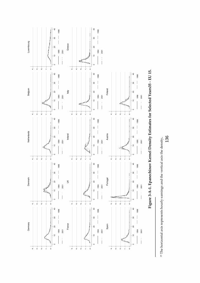
13
6
F
igu
re 3
-A-1
. Ep
anec
hin
ov
Ker
nel
Den
sity
Est
imat
es f
or
Sel
ecte
d Y
ears
35 -
EU
15.
35 T
he
ho
rizo
nta
l a
xis
re
pre
sen
ts h
ou
rly
ear
nin
gs
an
d t
he
ver
tica
l ax
is t
he
den
sity
.
0.1.2.3.4
01
02
03
04
0
19
94
19
98
20
01Germ
any
0.1.2.3.4
01
02
03
04
0
19
94
19
98
20
01Denm
ark
0.1.2.3.4
01
02
03
04
0
19
94
19
98
20
01
Neth
erlands
0.1.2.3.4
01
02
03
04
0
19
94
19
98
20
01B
elg
ium
0.1.2.3.4
01
02
03
04
0
19
95
19
98
20
01
Luxe
mbo
urg
0.1.2.3.4
01
02
03
04
0
19
94
19
98
20
01F
rance
0.1.2.3.4
01
02
03
04
0
19
94
19
98
20
01
UK
0.1.2.3.4
01
02
03
04
0
19
94
19
98
20
01Ir
ela
nd
0.1.2.3.4
01
02
03
04
0
19
94
19
98
20
01
Italy
0.1.2.3.4
01
02
03
04
0
19
94
19
98
20
01G
reece
0.1.2.3.4
01
02
03
04
0
19
94
19
98
20
01
Spain
0.1.2.3.4
01
02
03
04
0
19
94
19
98
20
01P
ort
ugal
0.1.2.3.4
01
02
03
04
0
19
95
19
98
20
01A
ustr
ia
0.1.2.3.4
01
02
03
04
0
19
96
19
98
20
01F
inla
nd

137
4. EARNINGS DYNAMICS AND INEQUALITY IN EU,
1994-2001
138
4.1.Introduction
Interest in the extent of individual earnings dynamics has increased greatly in
recent years and was fuelled mainly by the rise in earnings inequality experienced
by many developed countries during the 1980s and 1990s, which triggered a strong
debate with respect to the driving factors and the implications of this increase.
This paper analyses the dynamic structure of individual earnings in order to
explain what is happening behind the changes in the distribution of labour market
income across 14 EU countries over the period 1994-2001 using ECHP. More
precisely, the aim is to examine the extent to which changes in cross-sectional
earnings inequality reflect transitory or permanent components of individual
lifecycle earnings variation. So far, at the EU level, no study attempted to analyse
and to understand these issues in a comparative manner.
Understanding wage dynamics is vitally important from a welfare perspective,
particularly given the large variation in the evolution of cross-sectional wage
inequality across Europe over the period 1994-2001. It is highly relevant to
understand what the source of this variation is. Did the increase in cross-sectional
wage inequality observed in some countries result from greater transitory
fluctuations in earnings and individuals facing a higher degree of earnings
mobility? Or is this rise reflecting increasing permanent differences between
individuals with mobility remaining constant or even falling? What about
countries that recorded a decrease in cross-sectional earnings inequalities, what
lessons can we learn from them? Is this decrease the effect of an increase in
mobility which helped individuals improve their income position in the
distribution of permanent income? Are there common trends in earnings
inequality and mobility across different countries? Understanding the
contributions of the changes in permanent and transitory components of earnings
variation to increased cross-sectional earnings inequality is very useful in the
evaluation of alternative hypotheses for wage structure changes and for
determining the potential welfare consequences of rising inequality. (Katz and
Autor, 1999)
These questions are highly relevant in the context of the changes that took place in
the EU labour market policy framework after 1995 under the incidence of the 1994
OECD Jobs Strategy, which recommended policies to increase wage flexibility,
lower non-wage labour costs and allow relative wages to better reflect individual
differences in productivity and local labour market conditions (OECD 2004; Dew-
Becker and Gordon 2008). This appears to have worsened the apparent trade-off
139
between a strong employment performance and a more equal distribution of
earnings, consistent with relative labour demand having shifted towards high-
skilled workers OECD (2004).
As pointed out by OECD (2004) and Dew-Becker and Gordon (2008), the most
notable change after 1995 in Europe has been increased country heterogeneity. We
will investigate how this heterogeneity translates itself in the level and components
of the cross-sectional earnings inequality and earnings mobility. Equally weighted
minimum distance methods are used to estimate the covariance structure of
earnings, decompose earnings into a permanent and a transitory component and
conclude about their evolution.
The structure of this paper is as follows. Section two presents an overview of the
literature review. Section three introduces the theoretical background for wage
differentials. Section four provides a description of the data. Section five introduces
the econometric specification and estimation method. Section six describes the
dynamic structure of individual log earnings for 14 EU countries. Section seven fits
the error components models to the covariance structure for each country,
decomposing the change in inequality into that accounted for by the change in the
permanent and transitory components. Lastly, section eight offers some
conclusions.
4.2.Literature review
The existing literature on earnings dynamics is predominantly based on US data.
Atkinson, Bourguignon et al. (1992) provide a comprehensive survey of the
literature on earnings dynamics until 1992. Earlier work focused on fitting
statistical models to the earnings process. E.g. Lillard and Willis (1978), Lillard and
Weiss (1979), MaCurdy (1982), Abowd and Card (1989) fitted models to the
autocovariance structure of earnings and hours, but they did not account for the
changes in the autocovariance structure of earnings over time.
Later work, Moffitt and Gottschalk (1995, 1998, 2002) used PSID to estimate the
permanent and transitory components of male earnings and how it evolved over
time. In Moffitt and Gottschalk (1998), the earnings process was fit by a permanent
component, modelled as a random walk in age and a highly persistent serially
correlated transitory component, with weights on these components for each year.
They found that the increase in the cross-sectional inequality of individual
earnings and wage rates in the U.S. between 1969 and 1991 has been roughly
equally composed of increases in the variances of the permanent and transitory
components of earnings, with little change in earnings mobility rates. Since most of
140
the theoretical explanations for the increase in inequality have been aimed at
explaining increases in the variance of the permanent component of earnings (e.g.
increases in the price of skills), they found their result surprising and unexpected.
Therefore, in their most recent study, Moffitt and Gottschalk (2008) estimated the
trend in the transitory variance of male earnings using PSID from 1970 to 2004.
They found that the transitory variance increased substantially in the 1980’s and
remained at the same level until 2004, for both less and more educated workers.
Moreover, the transitory variance appears to have a strong cyclical component: its
increase accounts for between 30% and 65% of the rise in the overall inequality,
depending on the period.
Using the PSID, Baker (1997) compared two competing specifications for the
permanent component of earnings: the “profile heterogeneity or the random
growth model” and the “random walk model”. In spite of the increased popularity
of the latter, Baker (1997) proved that the profile heterogeneity model provides a
better representation of the data.
Baker and Solon (2003) decomposed the growth in earnings inequality into its
persistent and transitory components using longitudinal income tax records from
Canada. The earnings process was fit by a permanent component, modelled as a
mixed process composed of a random growth and a random walk in age and a
highly persistent serially correlated transitory component, with weights on these
components for each year. They found that growth in earnings inequality reflects
both an increase in the long-run inequality and an increase in earnings instability.
Up until recently, little work has been carried out in Europe on the dynamic nature
of individual earnings. Dickens (2000b) analysed the pattern of individual male
wages over time in UK using the New Earnings Survey (NES) panel data set for the
period 1975-1995. This study divided the data into year birth cohorts and analysed
the auto-covariance structure of hourly and weekly earnings for each cohort. In the
tradition of Moffitt and Gottschalk (1998), the earnings process was fit by a
permanent component, modelled as a random walk in age and a highly persistent
serially correlated transitory component, with weights on these components for
each year. The results showed that about half of the rise of the overall cross-
sectional inequality can be explained by the rise in the permanent variance and the
rest by the rise in the persistent transitory component.
Ramos (2003) analysed the dynamic structure of earnings in UK using the British
Household Panel Study for the period 1991-1999. The earnings specification
followed a similar specification with Baker and Solon (2003). Using information on
monthly earnings of male full-time employees, this study decomposed the
covariance structure of earnings into its permanent and transitory components and
141
concluded that the increase in inequality over the 1990’s was due to increased in
earnings volatility. Moreover, the relative earnings persistent was found to decline
over the lifecycle, which implies a lower mobility for younger cohorts. These
findings are at odds with previous literature on earnings dynamics both for UK
and the OECD. Unlike previous literature, this study considered also the effects of
observed characteristics and found that human capital and job related
characteristics account for nearly all persistent earnings differences and that the
transitory component is highly persistent.
Kalwij and Alessie (2003) examined the variance-covariance structure of log-wages
over time and over the lifecycle of British men from 1975 to 2001, controlling for
cohort effects. Their model follows closely the specification used by Abowd and
Card (1989), Dickens (2000b) and Baker and Solon (2003) accounting also for cohort
effects. They showed that the increase in the cross-sectional inequality was caused
mainly by the increase in the transitory component of earnings and to a lesser
extent by an increase in the permanent wage inequality. Thus the increase in cross-
sectional inequality was accompanied by an increase in earnings mobility.
Cappellari (2003) used the Italian National Social Security Institute for the period
1979-1995 and decomposed the male earnings autocovariance structure into its
long-term and transitory components using a model specification similar with
Moffitt and Gottschalk (1995) and Backer (1997). The model included a permanent
component, modelled as a random growth in age and a highly persistent serially
correlated transitory component, with weights on these components for each year
and cohort. The findings showed that growth was determined by the long-term
earnings component. Other evidence on the contribution of permanent and
transitory earnings components to cross-sectional inequality has become available
in recent year in Sweden (Gustavson, 2004).
4.3.Theoretical model of the determinants of wage differentials
4.3.1. Determinants of earnings inequality
As pointed out by Katz and Autor (1999), the existing literature contains many
explanations for the rise in earnings inequality experienced by many developed
countries during the 1980s and 1990s. One approach for explaining the changes in
wage differential is to decompose overall wage inequality into permanent
inequality and transitory inequality.

142
Following the terminology introduced by Friedman and Kuznets (1954), individual
earnings are composed of a permanent and a transitory component, assumed to be
independent of each other. The permanent component of earnings reflects personal
characteristics, education, training and other persistent elements. The transitory
component captures the chance and other factors influencing earnings in a
particular period and is expected to average out over time. Following the structure
of individual earnings, overall inequality at any point in time is composed from
inequality in the transitory component and inequality in the permanent component
of earnings. The evolution of the overall earnings inequality is determined by the
cumulative changes in the two inequality components.
A rise in permanent inequality is consistent with increasing returns to education,
on-the-job training and other persistent abilities that are among the main
determinants of the permanent component of earnings, meaning enhanced relative
earnings position of the highly skilled individuals (Mincer, 1957, 1958, 1962, 1974;
Hause, 1980).
An increase in transitory inequality can be attributed to the weakening of the
labour market institutions (e.g. unions, government wage regulation, and internal
labour markets), increased labour market instability, increased competitiveness, a
rise in the temporary workforce which increase earnings exposure to shocks. A
period of skill-biased technological change with the spread of new technologies
can, both, increase the demand for skills, and increase earnings instability (Katz
and Autor, 1999). Rodrik (1997) argued that also globalization and international
capital mobility can increase wage instability. Overall, the increase in the return to
persistent skills is expected to have a much larger impact on long-run earnings
inequality than an increase in the transitory component of earnings (Katz and
Autor, 1999; Moffitt and Gottschalk, 2002).
4.3.2. Alternative model specifications for the permanent and
transitory components
Next we introduce several models of earnings dynamics that have been
dominating the literature on permanent and transitory earnings inequality over the
past 30 years. To begin with, we introduce the simplest specification, which in spite
of its simplicity provides a very intuitive insight into the decomposition of
earnings into their permanent and transitory components. Based on this
specification earnings are being decomposed as follows:
2 2, ~ (0, ), ~ (0, ), 1, ..., , 1,...,it i it i it v i
Y v iid v iid t T i Nµµ µ σ σ= + = =
(4.1)
143
where i
µ represents the permanent time-invariant individual specific component
and it
v represents the transitory component, which is independent distributed
both over individuals and time. This model imposes very rigid restrictions on the
covariance structure of earnings:
2 2
2
,( , )
,
v
it is
t sCov Y Y
t s
µ
µ
σ σ
σ
+ ==
≠
Since i
µ is assumed to incorporate the effect of lifetime persistent individual
specific characteristics such as ability, the variance of the permanent component 2
µσ represents the persistent dispersion of earnings or permanent earnings
inequality. The transitory shocks are captured by the transitory variance 2
vσ and
are assumed to persist only one year.
This model facilitates the understanding of the inequality decomposition into its
permanent and transitory components. The variance of earnings at a certain point
in time (2
yσ ), as a measure of earnings dispersion, is composed both from a
permanent and transitory dispersion (2 2
vµσ σ+ ). The covariances are determined
solely by the permanent component (2
µσ ). Therefore, the assessment of the relative
importance of the two components in the overall earnings dispersion is
straightforward: the ratio 2 2
/ yµσ σ captures the relative importance of the
permanent component, whereas the ratio 2 2
/v yσ σ captures the relative importance
of the transitory component.
Notwithstanding its attractive features, the empirical evidence rejected the rigid
restrictions imposed by model (4.1). One of the main drawbacks of model (4.1) is
that it does not allow for changes in earnings inequality over time (Lillard and
Willis, 1978; Lillard and Weiss, 1979; MaCurdy, 1982; Abowd and Card, 1989).
Other studies (Katz, 1994; Moffitt and Gottschalk, 1995) took the model complexity
further by allowing the covariance structure of earnings to vary over time. To
account for these time effects, these models considered also time specific loading
factors or shifters on both components, which allow the parameters of the process
to change with calendar time.
1 2it t it t itY vλ µ λ= + (4.2)
144
, 1, 2kt
kλ = are time-varying factor loadings on the permanent and transitory
components of earnings. The variance of it
Y implied by this model takes the form:
2 2
1 2
2 2( )t tit v
Var Y µλ σ λ σ= +
(4.3)
An increase in either time loading factors generates an increase in the cross-
sectional earnings inequality. The nature of the change in inequality depends on
which of the loading factors changes. On the one hand, a persistent rise in 1t
λ
increases the permanent or long-run inequality (inequality in earnings measured
over a long period of time, such as lifetime earnings). As 1t
λ is interpreted as time-
varying return to skills or skill price, its increase suggests that the relative labour
market advantage of high-skilled workers is enhanced. In this situation, the
autocovariances grow in greater proportion than the variance, causing the
autocorrelation to increase. As a consequence, the increase in overall cross-
sectional inequality is accompanied by a decrease in mobility.
On the other hand, an increase in 2 t
λ without a change in 1t
λ increases cross-
sectional earnings inequality by increasing the transitory inequality, but without
any impact on long-run or permanent inequality. In this situation the rise in the
variances is not accompanied by a rise in the autocovariances, hence the
autocorrelations decrease and the increase in the overall inequality is accompanied
by an increase in mobility (Baker and Solon, 2003). As pointed out by Katz and
Autor (1999), 1t
λ maintains the rank of the individuals in the earnings distribution,
but causes a persistent increase in the spread of the distribution and an increase in
2 tλ changes the rank of the individual in the short-run. In other words an increase
in the time parameters associated with the permanent component of earnings
indicates a growing earnings inequality with no impact on the relative position of
individuals in the distribution of permanent earnings, whereas an increase in the
transitory time parameters indicates an increase in earnings instability.
Although model (4.2) incorporates changes over time in the permanent and
temporary components of earnings inequality, it disregards other important
features of earnings dynamics. Firstly, it disregards the cohort effects. As argued
by Katz and Autor (1999), the increased wage inequality may arise from greater
dispersion of unobserved labour quality within younger cohorts, resulting from
unequal school quality. Some studies rejected the hypothesis that the return to
education is the same across cohorts. These differences could be attributed either to
the cohort effects or to the larger impact of the labour market shocks on younger
than on older cohorts of workers. In the same line of thought, Freeman (1975) put

145
forward the “active labour market” hypothesis, which postulates that changes in
the labour market conditions, such as changes in the supply and demand for skills,
affect mainly new entrants in the labour market.
To account for these cohort effects, these models considered also cohort specific
loading factors or shifters on both components, which allow the parameters of the
process to change with cohort.
1 1 2 2it c t it c t itY vγ λ µ γ λ= + (4.4)
where , 1, 2jc jγ = are cohort specific loading factors.
Secondly, regarding the permanent component, some studies brought evidence in
favour of the “random growth rate model” or the “profile heterogeneity model”:
(Hause, 1977; Lillard and Weiss, 1979; MaCurdy, 1982; Baker, 1997; Cappellari,
2003)
2 2, ~ (0, ), ~ (0, ), ( , )it i i it i i i i
age iid iid Eµ ϕ µϕµ µ ϕ µ σ ϕ σ µ ϕ σ= + =
(4.5)
According to this model, which is consistent with labour market theories such as
human capital, and matching models, each individual has a unique age-earning
profile with an individual specific intercept (initial earnings i
µ ) and slope
(earnings growth i
ϕ ) that may be systematically related. The variances 2
µσ and
2
ϕσ capture individual heterogeneity with respect to time-invariant characteristics
and age-earnings profiles. The covariance between i
µ and i
ϕ , µϕσ , represents a
key element in the development of earnings differentials over the active life. A
positive covariance between i
µ and i
ϕ implies a rising inequality in the
permanent component of earnings over the life cycle. This is consistent with the
school-matching models where the more tenure one individual accumulates, the
more is revealed about his ability. Thus highly educated people are expected to
experience a faster growth in their earnings as the quality of the match is revealed
to their employers. A negative covariance implies that the two sources of
heterogeneity offset each other, which is consistent with the on-the-job training
hypothesis (Mincer, 1974; Hause, 1980). A negative covariance is expected to
generate mobility within the distribution of the permanent component of earnings
(Cappellari, 2003).
This structure is equivalent to a random coefficient model where the intercept and
the coefficient on age in model (4.5) are randomly distributed across individuals.
Therefore, because earnings evolve along an individual specific age profile, a good
146
prediction of future earnings requires additional information besides the current
earnings.
An alternative/additional specification for the permanent component of earnings is
the “random walk model” or the “unit root model”, which is used in the literature
to accommodate earnings shocks that might have permanent effects: (MaCurdy,
1982; Abowd and Card, 1989; Moffitt and Gottschalk, 1995; Dickens, 2000b)
2
, 1 , 1, ~ (0, ), ( , ) 0ia i a ia ia i a iau u iid E uππ π σ π− −= + =
(4.6)
Equation (4.6) specifies a random walk process in age, where the current value
depends on the one from the previous age and an innovation term ia
π , which
represent white-noise non-mean-reverting shocks to permanent earnings. In other
words, ia
π accommodates any permanent re-ranking of individuals in the earnings
distribution. As argued by Baker (1997), the intuition for this model is not obvious,
but the high persistency of the unit root model might result from low rates of
depreciation of human capital investments or labour market conditions through
implicit contracts. In this model, current earnings are a sufficient statistic for future
earnings.
Thirdly, previous research found that the transitory component of earnings is
serially correlated. Therefore, a more general autocorrelation structure is called for,
that relaxes the restriction on 'it
v s from the canonical model. For the construction
of such a structure, longitudinal studies on earnings dynamics turned to error
processes from the literature on time series analysis. Based on MaCurdy (1982), the
structure of the transitory component, it
v , is assumed to follow an ARMA(p,q)
process:
2 2
0 0,
0 0
, ~ (0, ), ~ (0, )p q
j it j j it j it i c
j j
v iid vερ θ ε ε σ σ− −= =
=∑ ∑ , (4.7)
itε is assumed to be white noise with mean 0 and variance 2
εσ . The variance 2
0,cσ
measures the volatility of shocks at the start of the sample period and 2
εσ the
volatility of shocks in subsequent years. jρ is the autoregressive parameter with
01ρ = , which measures the persistence of shocks.
jθ is the moving average
parameter with 0
1θ = , which accommodates sharp drops of the lag-j
autocovariance compared with the other autocovariances. In this model, the
autoregressive and moving average parameters are assumed to be constant over
time.
147
4.3.3. Earnings mobility
Another aspect relevant for the evolution of earnings differentials is earnings
mobility, defined by Katz and Autor (1999) as the rate at which individuals shift
positions in the earnings distribution. Earnings mobility is closely related to the
importance of the permanent and transitory components in earnings variation. A
large contribution of the permanent component implies that individual earnings
are highly correlated over time and individuals do not change their income
position to a large extent experiencing low rates of earnings mobility. Therefore,
the changes in earnings mobility are determined by the extent to which changes in
cross-sectional inequality are driven by changes in the permanent or transitory
variance.
Earnings mobility is a very complex phenomenon, and the ways of measuring it
are diverse. We look at the degree of immobility, measured by the ratio between
permanent and transitory inequality, following Kalwij and Alessie (2003). This
measure offers also a summary of the evolution in the structure of inequality: a(n)
decrease (increase) in the immobility ratio indicates an increase (decrease) in
earnings mobility, equivalent with a(n) decrease (increase) in the relative share of
permanent differentials in the overall inequality. This mobility index captures non-
directional earnings movements and can be interpreted as the opportunity to
improve one’s position in the distribution of lifetime earnings.
An increase in cross-sectional inequality accompanied by a decrease in earnings
mobility is expected to have negative implications for long-run or lifetime earnings
differentials, as it shows that over time low wage men get worse off both in terms
of their relative earnings position and in terms of their opportunity to escape low
wage trap. Thus it is reasonable to expect that cross-sectional earnings differentials
will be enhanced in a lifetime perspective.
An increase in cross-sectional inequality accompanied by an increase in earnings
mobility has uncertain implications for long-run or lifetime earnings differentials.
Over time low wage men get worse off in terms of their relative earnings position,
but better off in terms of the opportunity to escape low wage trap in a lifetime
perspective. Thus earnings mobility could either enhance or decrease lifetime
earnings differentials compared with the cross-sectional ones.
A decrease in cross-sectional inequality accompanied by an increase in earnings
mobility is expected to have positive implications for lifetime earnings
differentials, as over time low wage men better their relative earnings position and
their opportunity to escape low wage trap in a lifetime perspective. Thus, lifetime
148
earnings differentials are expected to be reduced compared with annual
differentials.
A decrease in cross-sectional inequality accompanied by a decrease in earnings
mobility has uncertain implications for lifetime earnings differentials, as over time
low wage men get better off in terms of their relative earnings position, but worse
off in terms of their opportunity to escape low wage trap in a lifetime perspective.
Thus, lifetime earnings differentials could be either reduced or enhanced compared
with annual differentials.
It becomes obvious that the question regarding the link between earnings mobility
and earnings inequality does not have a straight forward answer and mobility is
not always beneficial. It depends on the underlying factors: “changes in earnings
mobility could either work to offset or to increase changes in cross-sectional
dispersion”, with very different implications for permanent earnings inequality
(Dickens, 2000a). Nonetheless, no controversy surrounds the fact that mobility is
beneficial when it helps low paid individuals to improve their income position in
the long-term or lifetime income distribution.
4.4.Data36
The study is conducted using the European Community Household Panel
(ECHP)37 over the period 1994-2001 for 14 EU countries. Not all countries are
present for all waves. Luxembourg and Austria are observed between 1995 and
2001 and Finland between 1996 and 2001. Following the tradition of previous
studies, the analysis focuses only on men to avoid the selection bias associated
with women’s earnings.
A special problem with panel data is that of attrition over time, as individuals are
lost at successive dates causing the panel to decline in size and raising the problem
of representativeness. Several papers analysed the extent and the determinants of
panel attrition in ECHP. Behr, Bellgardt and Rendtel (2005) found that the extent
and the determinants of panel attrition vary between countries and across waves
within one country, but these differences do not bias the analysis of income or the
ranking of the national results. Ayala, Navrro and Sastre (2006) assessed the effects
of panel attrition on income mobility comparisons for some EU countries. The
results show that ECHP attrition is characterized by a certain degree of selectivity,
36 Part of the information in section 4.4 has been discussed in section 2.4 and 3.4. 37 The European Community Household Panel provided by Eurostat via the Department of Applied
Economics at the Université Libre de Bruxelles.

149
but only affecting some variables and some countries. Moreover, income mobility
indicators show certain sensitivity to the weighting system.
We apply the weighting system recommended by Eurostat, namely the “base
weights” of the last wave observed for each individual, bounded between 0.25 and
10. The dataset is scaled up to a multiplicative constant38 of the base weights of the
last year observed for each individual.
For the empirical analysis, individuals are categorized into four birth cohorts,
which are followed through time. Ideally, one should use birth cohorts formed
from people born in a particular year. The limited number of observations forces
us to group more birth years in one cohort. The first birth cohort contains people
born between 1940-1950, the second one people born between 1951-1960, the third
cohort people born between 1961-1970 and lastly people born between 1971-1981.
This grouping allows the analysis of the earnings covariance structure for
individuals of the same age, followed at different points in time.
Earnings are expressed in real log net hourly wage adjusted for CPI of male
workers aged 20 to 57, born between 1940 and 1981. Only observations with hourly
wage lower than 50 Euros and higher than 1 Euro were considered in the analysis.
The resulting sample for each country is an unbalanced panel. The choice of using
unbalanced panels for estimating the covariance structure of earnings is motivated
by the need to mitigate the potential overestimation of earnings persistence that
would arise from balanced panels where the estimation is based only on people
that have positive earnings for the entire sample period.
38 The multiplicative constant equals e.g. p*(Population above 16/Sample Population). The ratio p varies
across countries so that sensible samples are obtained. It ranges between 0.001-0.01.
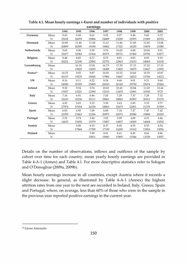
150
Table 4.1. Mean hourly earnings (~Euro) and number of individuals with positive
earnings
1994 1995 1996 1997 1998 1999 2000 2001
Germany Mean 9.43 9.49 9.61 9.52 9.57 9.48 9.60 9.72
N 25018 26059 25806 24889 23290 22955 21909 20703
Denmark Mean 10.89 11.40 11.58 11.61 11.86 11.85 12.02 12.08
N 20899 20399 19190 19062 17321 16235 15678 15380
Netherlands Mean 9.69 9.56 9.59 9.70 10.02 9.88 10.04 9.91
N 33277 32384 31564 30575 28731 27460 25790 33277
Belgium Mean 8.48 8.82 8.71 8.75 8.81 8.83 8.92 9.10
N 20221 22100 22892 22753 22863 23233 24065 24130
Luxembourg Mean 16.18 15.81 16.73 17.39 17.15 17.22 17.10
N 15829 13695 14489 13403 14075 12667 12992
France39 Mean 10.23 9.92 9.87 10.05 10.33 10.60 10.55 10.87
N 20137 19270 19042 17906 14467 14012 13760 14212
UK Mean 8.16 8.11 8.22 8.34 8.68 9.01 9.21 9.68
N 24949 25329 25495 26010 26145 25750 25674 25264
Ireland Mean 9.30 9.54 9.76 10.02 10.43 10.84 11.69 12.44
N 13937 13221 12590 12515 12435 12091 10745 9727
Italy Mean 7.16 6.91 6.96 7.05 7.29 7.37 7.28 7.32
N 32633 32236 32111 29661 28865 26993 26912 25170
Greece Mean 4.95 5.03 5.23 5.59 5.63 5.85 5.70 5.77
N 27974 27654 26150 24865 22675 22001 21335 21929
Spain Mean 6.83 6.95 7.09 6.89 7.18 7.37 7.45 7.42
N 22559 21863 21296 20975 20371 20580 19898 20185
Portugal Mean 3.70 3.74 3.84 3.92 3.99 4.08 4.31 4.46
N 14653 15450 15379 15087 14837 14569 14604 14550
Austria Mean 9.08 8.33 8.37 8.49 8.55 8.55 8.54
N 17944 17789 17199 16209 15162 13816 13056
Finland Mean 7.89 8.01 8.41 8.45 8.66 8.86
N 15811 15845 15895 15546 13329 13057
Details on the number of observations, inflows and outflows of the sample by
cohort over time for each country, mean yearly hourly earnings are provided in
Table 4-A-1 (Annex) and Table 4.1. For more descriptive statistics refer to Sologon
and O’Donoghue (2009a, 2009b).
Mean hourly earnings increase in all countries, except Austria where it records a
slight decrease. In general, as illustrated by Table 4-A-1 (Annex) the highest
attrition rates from one year to the next are recorded in Ireland, Italy, Greece, Spain
and Portugal, where, on average, less than 60% of those who were in the sample in
the previous year reported positive earnings in the current year.
39 Gross Amounts
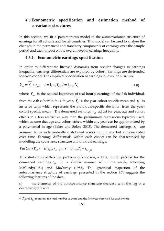
151
4.5.Econometric specification and estimation method of
covariance structures
In this section, we fit a parsimonious model to the autocovariance structure of
earnings for all cohorts and for all countries. This model can be used to analyse the
changes in the permanent and transitory components of earnings over the sample
period and their impact on the overall level of earnings inequality.
4.5.1. Econometric earnings specification
In order to differentiate lifecycle dynamics from secular changes in earnings
inequality, earnings differentials are explored by cohort. Earnings are de-trended
for each cohort. The empirical specification of earnings follows the structure:
, 1,..., , 1,...,ict ct ict i c
Y Y r t T i N= + = = (4.8)
where ict
Y is the natural logarithm of real hourly earnings of the i-th individual,
from the c-th cohort in the t-th year, ctY is the year-cohort specific mean and ict
r is
an error term which represents the individual-specific deviation from the year-
cohort specific mean. . The demeaned earnings ict
r adjust for year, age and cohort
effects in a less restrictive way than the preliminary regressions typically used,
which assume that age and cohort effects within any year can be approximated by
a polynomial in age (Baker and Solon, 2003). The demeaned earnings ict
r are
assumed to be independently distributed across individuals, but autocorrelated
over time. Earnings differentials within each cohort can be characterised by
modelling the covariance structure of individual earnings:
0( ) ( , ), 0,...,
ict ict ict s c cVarCov Y E r r s T t−= = −
.40
This study approaches the problem of choosing a longitudinal process for the
demeaned earnings,ict
r , in a similar manner with time series, following
MaCurdy(1981) and MaCurdy (1982). The graphical inspection of the
autocovariance structure of earnings, presented in the section 4.7, suggests the
following features of the data:
(i) the elements of the autocovariance structure decrease with the lag at a
decreasing rate and
40 c
T and 0c
t represent the total number of years and the first year observed for each cohort.
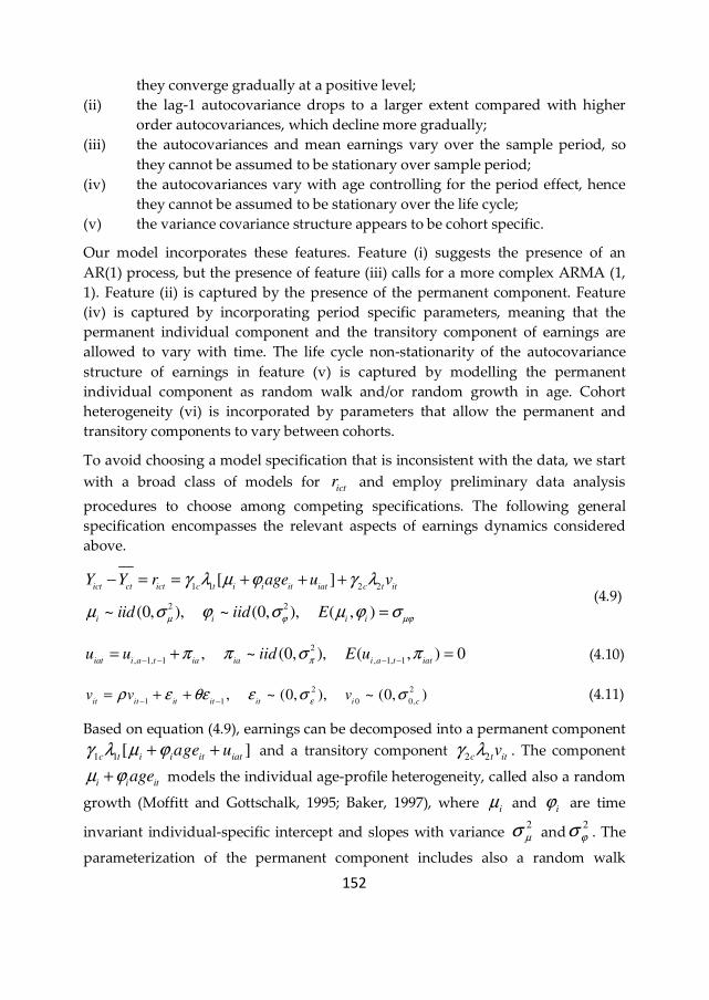
152
they converge gradually at a positive level;
(ii) the lag-1 autocovariance drops to a larger extent compared with higher
order autocovariances, which decline more gradually;
(iii) the autocovariances and mean earnings vary over the sample period, so
they cannot be assumed to be stationary over sample period;
(iv) the autocovariances vary with age controlling for the period effect, hence
they cannot be assumed to be stationary over the life cycle;
(v) the variance covariance structure appears to be cohort specific.
Our model incorporates these features. Feature (i) suggests the presence of an
AR(1) process, but the presence of feature (iii) calls for a more complex ARMA (1,
1). Feature (ii) is captured by the presence of the permanent component. Feature
(iv) is captured by incorporating period specific parameters, meaning that the
permanent individual component and the transitory component of earnings are
allowed to vary with time. The life cycle non-stationarity of the autocovariance
structure of earnings in feature (v) is captured by modelling the permanent
individual component as random walk and/or random growth in age. Cohort
heterogeneity (vi) is incorporated by parameters that allow the permanent and
transitory components to vary between cohorts.
To avoid choosing a model specification that is inconsistent with the data, we start
with a broad class of models for ict
r and employ preliminary data analysis
procedures to choose among competing specifications. The following general
specification encompasses the relevant aspects of earnings dynamics considered
above.
1 1 2 2
2 2
[ ]
~ (0, ), ~ (0, ), ( , )
ict ct ict c t i i it iat c t it
i i i i
Y Y r age u v
iid iid Eµ ϕ µϕ
γ λ µ ϕ γ λ
µ σ ϕ σ µ ϕ σ
− = = + + +
= (4.9)
2
, 1, 1 , 1, 1, ~ (0, ), ( , ) 0
iat i a t ia ia i a t iatu u iid E u
ππ π σ π
− − − −= + =
(4.10)
2 2
1 1 0 0,, ~ (0, ), ~ (0, )
it it it it it i cv v v
ερ ε θε ε σ σ
− −= + +
(4.11)
Based on equation (4.9), earnings can be decomposed into a permanent component
1 1[ ]
c t i i it iatage uγ λ µ ϕ+ + and a transitory component
2 2c t itvγ λ . The component
i i itageµ ϕ+ models the individual age-profile heterogeneity, called also a random
growth (Moffitt and Gottschalk, 1995; Baker, 1997), where i
µ and i
ϕ are time
invariant individual-specific intercept and slopes with variance 2
µσ and2
ϕσ . The
parameterization of the permanent component includes also a random walk
153
process in age (Equation (4.10)) (Moffit and Gottschalk 1995, Baker and Solon
2003). The variance of the first period shock (assumed to be at age 20, which is also
the lowest age observed in our dataset) is estimated together with the 2
µσ and is
considered part of the unobserved heterogeneity.
The transitory component follows an ARMA(1,1) process (equation (4.11)), where
the serial correlation ρ parameter captures the decreasing rate of decay of the
covariances with the lag, the moving-average parameter θ captures the sharp
drop of the lag-1 autocovariance compared with the other autocovariances, and it
ε
the white-noise mean-reverting transitory shocks. The variances 2
0,cσ measure the
volatility of shocks at the start of the sample period, 2
εσ the volatility of shocks in
subsequent years and ρ the persistence of shocks. Measurement error in this
model is captured by this transitory component.
The non-stationary pattern of earnings is captured by time specific loading factors,
both on the permanent and transitory component of earnings, , 1,2; 0,7kt k tλ = =
,
normalized to 1 in the first wave for identification41. Cohort heterogeneity is
accommodated by allowing both the permanent and the transitory component to
vary by cohort. , 1, 2jc jγ = are cohort loading factor, normalized to 1 for the
oldest cohort for identification.
4.5.2. Specification of the covariance structure of earnings
When working with ARMA(p,q) processes in the context of panel data, MaCurdy
(1981, 1982) and Anderson and Hsiao (1982) underlined the need for a treatment of
initial conditions42. As illustrated in equations (4.13) and (4.14), the autoregressive
process induces a recursive structure in the moments: the variance-covariance in
year t depends on the transitory variance-covariance in year t-1. If one tracks the
recursion back to the first sample year for each cohort, this raises the question of
what is the transitory variance for each cohort in that year. In the earlier stage of
the literature on earnings dynamics, it was common to restrict the initial transitory
variance to be the same for all cohorts. In line with the most recent literature on
earnings dynamics, our model acknowledges that earnings volatility varies across
cohorts because they illustrate different stages of the lifecycle and they have
experienced different period effects. Therefore such a strong assumption is
untenable.
411994 refers to t=0 42 See MaCurdy(1982, page 92/93)

154
Following MaCurdy (1981, 1982), the cohort initial transitory variances are treated
as 4 additional parameters to be estimated. The covariance structure for the first
sample period takes the form:
0
0 0
2 2 2 2 2
0 0 0 0
( )
( )
( ) 2cov( ) ( ) ( 20) ( ) 0
ic
ic ic
i i i i i
Var Y
E r r
E age E age a Var v if tµ ϕ π
σ σ µ ϕ σ
=
= =
= + + + − + =
(4.12),
where 0a is the central age of the cohort c in the first wave.
The covariance structure for subsequent years is expressed as follows:
2 2 2 2 2 2 2
1 1
2 2 2 2 2
2 2 1
( ) ( )
[ ( ) 2 cov( ) ( ) ( 20) ]
[ ( ) (1 2 )] 0
ict ict ict
c t it i i it t
c t it
Var Y E r r
E age E age a
Var v if t
µ ϕ π
ε
γ λ σ σ µ ϕ σ
γ λ ρ σ ρθ θ−
= =
= + + + − +
+ + + + >
(4.13)
2 2 2 2
1 1
2 2
2 2 2 1
( ) ( )
{ ( ) ( ) cov( )[ ( ) ( )]
( 20)( 20)} [ ( , )] 0 & 1
ict ict s ict ict s
c t it it s i i it it s
t t c t t s it it s
Cov Y Y E r r
E age E age E age E age
a a s Cov v v if t s
µ ϕ
π
γ λ σ σ µ ϕ
σ γ λ λ ρ
− −
− −
− − −
= =
= + + + +
+ − − − + > >
(4.14)
1 1
2 2 2 2
1 1 1 1
2 2 2
2 2 2 1 1
( ) ( )
{ ( ) ( ) cov( )[ ( ) ( )]
( 20)( 1 20)} { ( ) )} 0 & 1
ict ict ict ict
c t it it i i it it
t t c t t it
Cov Y Y E r r
E age E age E age E age
a a Var v if t s
µ ϕ
π ε
γ λ σ σ µ ϕ
σ γ λ λ ρ θσ
− −
− −
− −
= =
= + + + +
+ − − − + + > =
(4.15)
, where t
a is the central age of the cohort c in period t.
The degree of immobility is measured by the ratio between the permanent and
transitory variance.
4.5.3. Estimation of covariance structures
The parameters of the models are fit to the covariance structure for each cohort
using equally weighted minimum distance methods of estimation. The
methodology is similar with Cappellari (2003), Baker and Solon (2003), Ramos
(2003), Kalwij and Alessie (2003), Dickens (2000b), Baker (1997), Abowd and Card
(1989), Cervini and Ramos (2006) adapted to unbalanced panels.
For each cohort � and individual �, define a vector which identifies the presence for
each individual in the respective cohort and year:

155
1...
c
ict
ict
d
d
=
icd
where ict
d is an indicator variable that is equal to 1 if the individual from cohort c
is present in year t of the panel and c
t is the total length of the panel for each
cohort. Similarly, the vector containing the cohort earnings residuals can be
represented as follows:
1...
c
ict
ict
r
r
=
icR
where ict
r are the earnings residuals for individual i belonging to cohort c, in year t
in mean deviation form for each cohort and year. The elements of the ic
R
corresponding to missing years are set to 0. The variance-covariance matrix of the
earnings is computed separately for each cohort,c
C . The elements of the variance-
covariance matrix for cohort c, c
C , which is of dimension ( )c c
t t× are computed
as follows:
1
1
[ , ]
c
c
n
ick icli
c n
ick icli
r rm k l
d d
=
=
=∑∑
(4.16)
where c
n is the total number of individuals in cohort c, , {1,..., }c
k l t= .
Conformably with c
m , ci
m represent the distinct elements of the individual cross-
product matrix '
ic icR R . Then 1
1
[ , ][ , ]
c
c
n
cii
c n
ick icli
m k lm k l
d d
=
=
=∑∑
.
The matrix c
C is symmetric with ( 1)
( 1)2
c ct t +
× distinct elements. Let
cVech(C ) be a column vector of dimension
( 1)( 1)
2
c ct t +
× which stacks all the
156
elements of the variance covariance matrix c
C for cohort c. The aggregate vector
of moments for all cohorts is denoted by: T T T
1 4m = (Vech(C ) , ..., Vech(C ) ) ,
which is a column vector of dimension 4
1
( 1)( 1)
2
c c
c
t t
=
+×∑ . In this paper, each
cohort is observed between 1994 and 2001, therefore 8c
t = . Since the individuals
were grouped in four cohorts, m is a column vector of dimension (144 1)× .
To estimate the error components of the structural model illustrated by equations
(4.9), (4.10) and (4.11), the elements of m are fit to a parameter vector θ , so that
( )f=m θ , ( )f θ takes the form of equations (4.12), (4.13), (4.14), and (4.15).
Minimum distance estimation requires minimising the weighted sum of the
squared distance between the actual covariances (m ) and a function of the
parameter vector ( ( )f θ ) which encapsulates the covariance structure implied by
the error component model. Therefore, minimum distance estimation involves the
following quadratic form: ( ) [ ( )] [ ( )]'D f f= − −θ m θ W m θ , where W is a
positive definite weighting matrix. Minimum distance estimator chooses ɵθ to
minimise the distance function ɵ( )D θ .
Based on Chamberlain (1984), the asymptotic optimal choice of W is the inverse
of a matrix that consistently estimates the covariance matrix of m , which leads to
the optimum minimum distance estimator (OMD). However, Clark (1996) and
Altonji and Segal (1994) provided Monte Carlo evidence that OMD is biased in
small samples because of the correlation between the measurement error in the
second moments and forth moments. Instead, they proposed using the identity
matrix as a weighting matrix. This approach, often called “equally weighted
minimum distance estimation” (EWMD), involves using the standard nonlinear
least squares to fit ( )f θ tom . The same procedure is followed in this paper.
For estimating the asymptotic standard errors of the parameter estimates, we apply
the delta method. Following Chamberlain (1984), the asymptotic variance-
covariance matrix of the estimated parameters is obtained from the following
formula:
-1 -1AsyVar(θ) = (G'WG) G' 'WVWG(G WG) (4.17)
where G is the Jacobian of the transformation ( )f θ evaluated at ɵ=θ θ . G has
dimension ( )m
t p× and rank p, where m
t is the sum across cohorts of
157
( 1)( 1)
2
c ct t +
× and p is the number of parameters. W is the identity matrix and
V the matrix of fourth sample moments.
Chamberlain (1984) showed that under some fairly general regularity assumptions,
the independence of ic
R implies that the sample mean of ci
m has an asymptotic
normal distribution * *( , )c c cm N m V∼ , where *
cm is the expectation of ci
m ,
meaning the true covariance matrix of earnings, and *
cV is the variance-covariance
matrix, which can be estimated consistently by computing the sample moment
matrix of the c
Vech(C ) vector, c
V . The elements of the variance covariance c
V
can be written as follows:
1
1 1
( [ , ], [ , ]) ( [ , , , ] [ , ] [ , ])
c
c c
n
ick icl icp icqi
c c c c cn n
ick icl icp icqi i
d d d dCov m k l m p q m k l p q m k l m p q
d d d d
=
= =
= −∑
∑ ∑,
where 1
1
[ , , , ]
c
c
n
ick icl icp icqi
c n
ick icl icp icqi
r r r rm k l p q
d d d d
=
=
=∑∑
The variance-covariance matrix of m was denoted by V , where V is the block
diagonal matrix which is constructed from all the c
V matrices.
4.6. Strategy for model specification
The chi-squared goodness of fit statistic is computed following Newey(1985):
ɵ ɵ[ ( )] [ ( )]'f fχ = − −-1m θ R m θ
where χ follows a chi-squared distribution with degrees of freedom equal to
4
1
( 1)144
2
c c
c
t tp p
=
+− = −∑ , =-1 -1R (WVW') and
-1W = I - G(G AG)' G'A .
The majority of the existing studies estimating the covariance structure of earnings
used this general form of specification test to assess the goodness of fit of the
model. However, in most cases, all models have been rejected. Baker and Solon
(2003), Baker (1997), Leamer (1983) criticized these type of tests for several reasons.
158
First, Baker and Solon (2003) and Leamer (1983) underlined that “diagnostic tests
such as goodness-of-fit tests, without explicit alternative hypothesis, are useless,
since if the sample size is large enough, any maintained hypothesis will be rejected.
Such tests therefore degenerate into elaborate rituals for measuring the effective
sample size.” Second, as pointed by Baker and Solon (2003), an additional problem
is that these specification tests have inflated size in small samples and the inflation
is positively related with the number of overidentifying restrictions. For example,
Baker (1997) revealed through a Monte Carlo study, that for a test with fewer than
150 overidentifying restrictions, the critical values are 40%-50% greater than the
critical values based on the asymptotic theory. Therefore, we decided to report this
statistic as a reference, but not to use it to assess the goodness of fit of our model.
Instead we employed the SSR as a measure of fit.
To test between nested models, we could use Preposition 3’ in Chamberlain (1984)
or the LR test. Based on Preposition 3’ in Chamberlain (1984), assuming that the
general model has p parameters, to test between two nested models, one in which
1k parameters are restricted to 0 (
1p kχ −) and one in which
2k 43 parameters are
restricted to 0 (2p kχ −
), Chamberlain (1984) showed that the incremental chi square
statistic 1 2p k p kχ χ χ− −= − follows a chi-squared distribution with
1 2k k− degrees
of freedom. The LR test takes the following form: log R
U
SSELR N
SSE= . Under the
null hypothesis, LR follows a chi-square distribution with d.o.f equal to the
number of restrictions 1 2
k k− . To test between non-nested model, we use the BIC
criterion: the smaller the value of BIC, the better the fit.
144( 144 ) (144 )k
BIC SSE k= ⋅ −
4.7.The dynamic autocovariance structure of hourly earnings
To begin with, it is informative to have a description of the dynamic structure of
individual log hourly earnings for all 14 countries under analysis. The
autocovariance structure of earnings is computed for each cohort separately, as
well as overall, using formula (4.16) introduced in the previous section. The overall
autocovariance structure of earnings is displayed in Figure 4.1, whereas the
structure by cohort is included in Figure 4-A-1. The model used to fit the
43 k1>k2
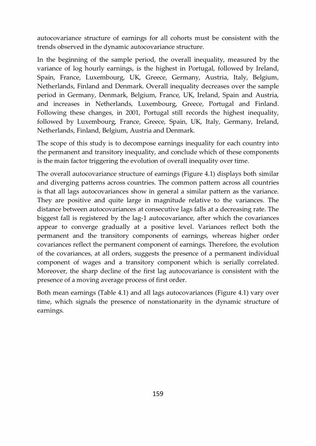
159
autocovariance structure of earnings for all cohorts must be consistent with the
trends observed in the dynamic autocovariance structure.
In the beginning of the sample period, the overall inequality, measured by the
variance of log hourly earnings, is the highest in Portugal, followed by Ireland,
Spain, France, Luxembourg, UK, Greece, Germany, Austria, Italy, Belgium,
Netherlands, Finland and Denmark. Overall inequality decreases over the sample
period in Germany, Denmark, Belgium, France, UK, Ireland, Spain and Austria,
and increases in Netherlands, Luxembourg, Greece, Portugal and Finland.
Following these changes, in 2001, Portugal still records the highest inequality,
followed by Luxembourg, France, Greece, Spain, UK, Italy, Germany, Ireland,
Netherlands, Finland, Belgium, Austria and Denmark.
The scope of this study is to decompose earnings inequality for each country into
the permanent and transitory inequality, and conclude which of these components
is the main factor triggering the evolution of overall inequality over time.
The overall autocovariance structure of earnings (Figure 4.1) displays both similar
and diverging patterns across countries. The common pattern across all countries
is that all lags autocovariances show in general a similar pattern as the variance.
They are positive and quite large in magnitude relative to the variances. The
distance between autocovariances at consecutive lags falls at a decreasing rate. The
biggest fall is registered by the lag-1 autocovariance, after which the covariances
appear to converge gradually at a positive level. Variances reflect both the
permanent and the transitory components of earnings, whereas higher order
covariances reflect the permanent component of earnings. Therefore, the evolution
of the covariances, at all orders, suggests the presence of a permanent individual
component of wages and a transitory component which is serially correlated.
Moreover, the sharp decline of the first lag autocovariance is consistent with the
presence of a moving average process of first order.
Both mean earnings (Table 4.1) and all lags autocovariances (Figure 4.1) vary over
time, which signals the presence of nonstationarity in the dynamic structure of
earnings.
160
Figure 4.1. Overall Autocovariance Structure of Hourly Earnings: Years 1994-2001
.05
.1.1
5.2
.25
1994 1996 1998 2000
Germany
.05
.1.1
5.2
.25
1994 1996 1998 2000
Denmark
.05
.1.1
5.2
.25
1994 1996 1998 2000
Netherlands.0
5.1
.15
.2.2
5
1994 1996 1998 2000
Belgium
.05
.1.1
5.2
.25
1994 1996 1998 2000
France
.05
.1.1
5.2
.25
1994 1996 1998 2000
Luxembourg
.05
.1.1
5.2
.25
1994 1996 1998 2000
UK
.05
.1.1
5.2
.25
1994 1996 1998 2000
Ireland
.05
.1.1
5.2
.25
1994 1996 1998 2000
Italy
.05
.1.1
5.2
.25
1994 1996 1998 2000
Greece
.05
.1.1
5.2
.25
1994 1996 1998 2000
Spain
.05
.1.1
5.2
.25
1994 1996 1998 2000
Portugal
.05
.1.1
5.2
.25
1994 1996 1998 2000
Austria
.05
.1.1
5.2
.25
1994 1996 1998 2000
FinlandVariance(t)
Covariance(t, t-1)Covariance(t, t-2)Covariance(t, t-3)Covariance(t, t-4)Covariance(t, t-5)Covariance(t, t-6)Covariance(t, t-7)
161
In all countries, the autocovariances display different patterns across cohorts
(Figure 4-A-1, Annex), supporting the hypothesis of cohort heterogeneity with
respect to individual earnings dynamics. In most countries, the variance of
earnings for all cohorts follows the evolution of the overall variance. Mixed trends
across cohorts are observed in Germany – where the variance increased for the
cohorts born in 1941-1950 and 1961-1970 -, in Belgium – where the variance
increased for the youngest cohort -, in France - where the variance increased for the
cohort born in 1961-1970 -, in UK – where the variance increased for the youngest
two cohorts -, in Spain - where the variance increased for the youngest and the
oldest cohorts, and in Finland - where the variance decreased for the youngest
cohort.
The evolution of the variance is not monotonic and the rate of change differs
among cohorts. In general, in countries that record a decrease in the variance, the
older the cohort, the steeper the decrease. For those that record an increase in the
variance over time, the older the cohort, the steeper the increase is. Moreover, the
younger the cohort is, the lower are the autocovariances. Hence, given that higher
order autocovariances capture the permanent component of earnings, it is
reasonable to expect that in all countries, for younger cohorts, the transitory
variance plays a larger role in the earnings formation than the permanent
component compared with older cohorts.
As illustrated in Figure 4-A-1 (Annex), for all cohorts, all lags autocovariances
show in general similar pattern as the variance, in line with the overall pattern. The
evolution of the covariances, at all orders, suggests the presence of a permanent
individual component of wages and a transitory component which is serially
correlated. Moreover, the sharp decline of the first lag autocovariance is consistent
with the presence of a moving average process of first order. Similar with the
overall trend, there is evidence of nonstationarity in the dynamic structure of
earnings by cohort.
To look at these lifecycle effects more clearly, it is necessary to remove the time
effect that is present in these within cohort autocovariances. Lifecycle
autocovariances are illustrated in Figure 4-A-2 (Annex). They are positive and
evolve at different rates over the life cycle. The smoothed lifecycle profiles
illustrate that, on average, all lags autocovariances increase with age at a
decreasing rate, which is consistent with the presence of a permanent component
of earnings that rises with age at a diminishing rate. (Dickens, 2000b)
To sum up, the description of the dynamic structure of individual earnings for men
suggests five main features of the data, which were incorporated in our model, as
mentioned previously:

162
• First, the covariance elements are not the same at all lags. They decrease with
the lag at a decreasing rate and converge gradually at a positive level,
suggesting the presence of a transitory element, which is serially correlated,
and of a permanent individual component of earnings. The most popular
specification for the serially correlated term is the AR(1) process. However, the
fact that the lag-1 autocovariance drops to a larger extent compared with the
other autocovariances and that the autocovariances at high orders decline very
slowly suggest that earnings cannot be modelled simply as a first-order
autoregressive process. Therefore a more complex ARMA (p, q) process might
be a better choice, where p represents the order of the autoregressive process
and q the order of the moving average process.
• Second, as the autocovariances and mean earnings vary over the sample
period, they cannot be assumed to be stationary over sample period. The
stationarity assumption was tested and rejected using the methodology
introduced by MaCurdy (1982). One way to capture this feature is to
incorporate period specific parameters, meaning that the permanent individual
component and the transitory component of earnings are allowed to vary with
time.
• Third, as autocovariances vary with age controlling for the period effect, they
cannot be assumed to be stationary over the life cycle. This non-stationarity
can be captured by modelling the permanent individual component as random
walk and/or random growth in age.
• Lastly, the variance covariance structure appears to be cohort specific, which
can be incorporated by parameters that allow the permanent and transitory
components to vary between cohorts.
163
4.8. Results of covariance structure estimation
4.8.1. Error component model estimation results
The general specification of the error component model outlined in section 4.5.2,
which encompasses all relevant aspects of earnings dynamics considered above, is
fit to the elements of the covariance matrix of each country, for all cohorts pooled
together44. For choosing the best model for each country we followed a general to
specific strategy, by imposing additional restrictions on the general model. The
estimation of the general model which incorporates both the random growth and
the random walk specifications in the permanent component had some
identification problems in all countries. The ARMA process was found only in
three countries and homogenous initial conditions only in four. In all countries, the
models incorporating both time and cohort shifters performed the best.
We present the parameter estimates only for the models that fit data the best for
each country. The estimation results are illustrated in Table 4.2. Similar to Dickens
(2000b), all variances are restricted to be positive by estimating the variance equal
to the exponent of the parameter. The reported estimates of the variances represent
the exponent of the parameter and the reported standard errors correspond to the
parameter estimates.45
44 i.e. 144 auto-covariances for countries observed over 8 waves, 122 for those with 7 waves and 84 for
those with 6 waves. 45 The SE column reports the standard error for the parameter estimate. Where I report the
exp(estimate), the SE corresponds to the log(exp(estimate)) = estimate
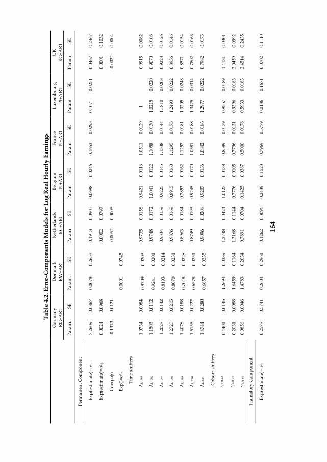
16
4
Tab
le 4
.2. E
rro
r-C
om
po
nen
ts M
od
els
for
Lo
g R
eal
Ho
url
y E
arn
ing
s
Ger
ma
ny
RG
+A
R1
Den
ma
rk
RW
+A
R1
Net
her
lan
ds
RG
+A
R1
Bel
giu
m
PI+
AR
1
Fra
nce
PI+
AR
1
Lu
xem
bo
urg
PI+
AR
1
UK
RG
+A
R1
P
ara
m.
SE
P
ara
m.
SE
P
ara
m
SE
P
ara
m
SE
P
ara
m
SE
P
ara
m
SE
P
ara
m
SE
Per
ma
nen
t C
om
po
nen
t
Ex
p(e
stim
ate
)=σ
2μ
7.2
609
0
.08
67
0.0
078
0
.26
53
0.1
913
0
.09
05
0.0
698
0
.02
46
0.1
653
0
.02
93
0.1
071
0
.02
51
0.0
467
0
.24
67
Ex
p(e
stim
ate
)=σ
2φ
0.0
024
0
.09
68
0.0
002
0
.07
97
0.0
001
0
.10
32
Co
v(μ
,φ)
-0.1
313
0.0
121
-0
.005
2 0
.00
05
-0.0
022
0.0
004
Ex
p()
=σ
2π
0.0
001
0
.07
45
Tim
e sh
ifte
rs
λ1
, 199
5 1
.07
34
0.0
084
0
.97
09
0.0
203
0
.97
35
0.0
158
0
.94
21
0.0
116
1
.05
11
0.0
129
1
0.9
915
0
.00
82
λ1
, 199
6 1
.15
03
0.0
112
0
.92
41
0.0
201
0
.97
48
0.0
172
1
.00
41
0.0
122
1
.10
58
0.0
130
1
.02
15
0.0
220
0
.90
70
0.0
103
λ1
, 199
7 1
.20
28
0.0
142
0
.81
93
0.0
214
0
.93
34
0.0
159
0
.92
25
0.0
145
1
.13
38
0.0
144
1
.18
10
0.0
208
0
.92
28
0.0
126
λ1
, 199
8 1
.27
20
0.0
215
0
.80
70
0.0
231
0
.98
76
0.0
169
0
.89
15
0.0
160
1
.12
95
0.0
173
1
.24
93
0.0
222
0
.89
36
0.0
146
λ1
, 199
9 1
.40
78
0.0
188
0
.70
48
0.0
228
0
.89
63
0.0
184
0
.78
53
0.0
162
1
.12
57
0.0
181
1
.32
05
0.0
248
0
.85
71
0.0
154
λ1
, 200
0 1
.51
55
0.0
222
0
.65
78
0.0
251
0
.87
49
0.0
193
0
.92
45
0.0
170
1
.05
81
0.0
188
1
.34
25
0.0
314
0
.78
02
0.0
163
λ1
, 200
1 1
.47
44
0.0
280
0
.66
57
0.0
235
0
.90
96
0.0
208
0
.92
07
0.0
156
1
.08
42
0.0
186
1
.29
77
0.0
222
0
.79
82
0.0
175
Co
ho
rt s
hif
ters
γ1
,51
-60
0.4
401
0
.01
45
1.2
694
0
.03
39
1.2
748
0
.04
24
1.0
127
0
.01
38
0.8
589
0
.01
39
0.9
557
0
.01
89
1.4
131
0
.03
01
γ1
,61
-70
0.2
031
0
.00
88
1.6
459
0
.11
64
1.3
168
0
.11
44
0.7
776
0
.01
05
0.7
796
0
.01
31
0.9
396
0
.01
83
2.0
459
0
.09
92
γ1
,71
-80
0.0
856
0
.00
46
1.4
783
0
.20
34
0.7
891
0
.07
04
0.1
425
0
.03
87
0.5
000
0
.01
78
0.5
933
0
.01
83
2.4
514
0
.24
35
Tra
nsi
tory
Co
mp
on
ent
Ex
p(e
stim
ate
)=σ
2ε
0.2
578
0
.57
41
0.2
604
0
.29
61
0.1
262
0
.30
96
0.2
439
0
.15
23
0.7
969
0
.57
79
0.0
186
0
.16
71
0.0
702
0
.11
10
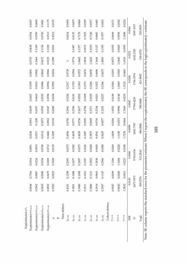
16
5
Ex
p(e
stim
ate
)=σ
20
Ex
p(e
stim
ate
)=σ
20
,40
-50
0.0
044
0
.73
16
0.0
314
0
.08
51
0.0
228
0
.09
13
0.0
639
0
.04
37
0.1
039
0
.04
91
0.0
753
0
.06
38
0.0
764
0
.04
37
Ex
p(e
stim
ate
)=σ
20
,51
-60
0.0
562
0
.08
87
0.0
224
0
.08
13
0.0
271
0
.12
08
0.0
357
0
.06
63
0.0
913
0
.09
02
0.1
064
0
.11
09
0.0
789
0
.06
05
Ex
p(e
stim
ate
)=σ
20
,61
-70
0.0
419
0
.09
40
0.0
334
0
.07
40
0.0
112
0
.20
73
0.0
392
0
.05
35
0.0
486
0
.08
43
0.0
672
0
.11
36
0.0
750
0
.06
81
Ex
p(e
stim
ate
)=σ
20
,71
-80
0.0
832
0
.06
79
0.0
269
0
.07
12
0.0
406
0
.09
62
0.0
347
0
.05
96
0.0
956
0
.09
66
0.0
225
0
.12
20
0.0
313
0
.11
79
ρ
0.3
583
0
.02
23
0.5
459
0
.01
35
0.3
289
0
.01
18
0.6
280
0
.01
04
0.3
993
0
.02
54
0.2
389
0
.01
61
0.4
512
0
.01
25
θ
Tim
e sh
ifte
rs
λ2
, 199
5 0
.45
31
0.1
298
0
.25
91
0.0
373
0
.49
36
0.0
756
0
.29
41
0.0
226
0
.25
17
0.0
739
1
0.8
214
0
.04
18
λ2
, 199
6 0
.38
01
0.1
088
0
.24
77
0.0
382
0
.48
39
0.0
771
0
.23
96
0.0
181
0
.17
03
0.0
504
1
.97
74
0.1
487
0
.81
35
0.0
475
λ2
, 199
7 0
.34
80
0.1
008
0
.24
97
0.0
375
0
.48
39
0.0
756
0
.26
77
0.0
202
0
.19
63
0.0
572
1
.44
02
0.1
377
0
.71
79
0.0
406
λ2
, 199
8 0
.35
11
0.1
013
0
.21
87
0.0
326
0
.32
87
0.0
505
0
.27
84
0.0
209
0
.23
73
0.0
676
1
.08
18
0.0
915
0
.70
25
0.0
359
λ2
, 199
9 0
.38
86
0.1
121
0
.29
23
0.0
428
0
.38
75
0.0
605
0
.33
71
0.0
255
0
.22
84
0.0
650
1
.24
22
0.1
019
0
.71
40
0.0
377
λ2
, 200
0 0
.29
18
0.0
841
0
.28
38
0.0
420
0
.45
41
0.0
710
0
.27
04
0.0
201
0
.24
32
0.0
696
1
.36
44
0.1
127
0
.84
82
0.0
482
λ2
, 200
1 0
.39
57
0.1
147
0
.25
66
0.0
380
0
.56
29
0.0
877
0
.32
55
0.0
257
0
.23
46
0.0
675
1
.40
03
0.1
195
0
.79
77
0.0
453
Co
ho
rt s
hif
ters
γ2
,51
-60
0.9
547
0
.02
99
1.1
306
0
.02
69
1.0
459
0
.02
94
1.0
555
0
.01
89
0.9
383
0
.02
93
0.8
573
0
.03
55
0.8
949
0
.01
71
γ2
,61
-70
0.9
643
0
.02
68
1.1
604
0
.02
28
1.1
180
0
.03
13
0.9
996
0
.01
40
1.0
469
0
.03
03
1.0
445
0
.04
29
0.9
938
0
.01
82
γ2
,71
-80
1.3
832
0
.04
11
1.8
221
0
.03
40
1.7
278
0
.04
64
1.3
569
0
.02
33
1.5
123
0
.04
65
1.4
318
0
.05
95
1.1
898
0
.02
24
SS
R
0.0
143
0
.00
68
0.0
099
0
.00
47
0.0
240
0
.02
22
0.0
061
Χ2
24
73.7
073
57
10.0
156
24
92.7
787
17
769
.42
20
17
56.3
574
16
32.2
320
25
97.3
157
Lo
gL
4
59
.25
76
51
3.2
610
4
86
.00
84
54
0.0
406
4
21
.96
93
31
8.4
753
5
20
.50
53
No
te:
SE
co
lum
n r
ep
ort
s th
e st
and
ard
err
or
for
the
par
amet
er e
stim
ate.
Wh
ere
I r
ep
ort
th
e e
xp
(est
imat
e), t
he
SE
co
rre
spo
nd
s to
th
e lo
g(e
xp
(est
imat
e))
= e
stim
ate
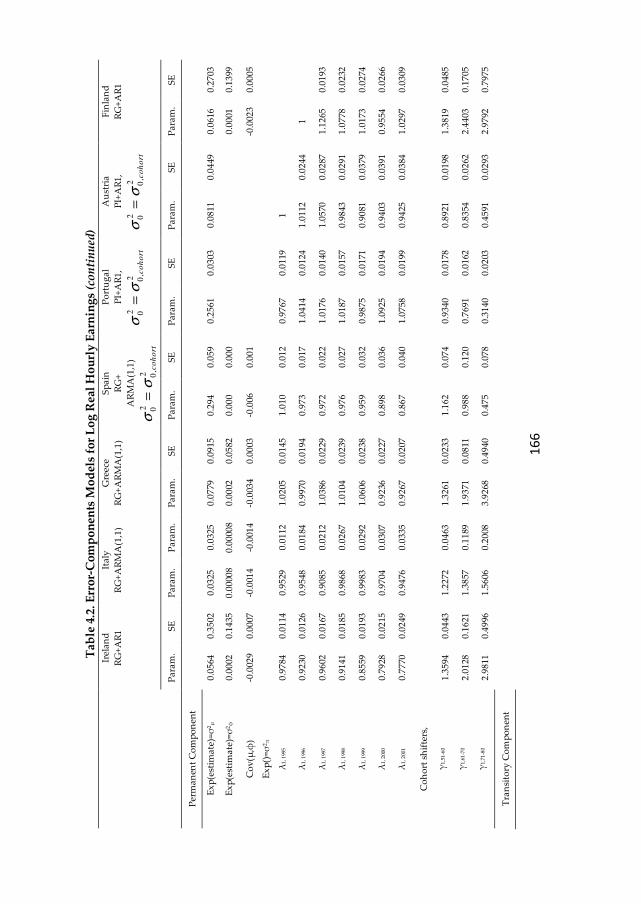
16
6
Tab
le 4
.2. E
rro
r-C
om
po
nen
ts M
od
els
for
Lo
g R
eal
Ho
url
y E
arn
ing
s (c
on
tin
ued
)
Irel
an
d
RG
+A
R1
Ita
ly
RG
+A
RM
A(1
,1)
Gre
ece
RG
+A
RM
A(1
,1)
Sp
ain
RG
+
AR
MA
(1,1
)
22
00
,co
ho
rtσ
σ=
Po
rtu
ga
l
PI+
AR
1,
22
00
,co
ho
rtσ
σ=
Au
stri
a
PI+
AR
1,
22
00
,co
ho
rtσ
σ=
Fin
lan
d
RG
+A
R1
P
ara
m.
SE
P
ara
m.
Pa
ram
. P
ara
m.
SE
P
ara
m.
SE
P
ara
m.
SE
P
ara
m.
SE
P
ara
m.
SE
Per
ma
nen
t C
om
po
nen
t
Ex
p(e
stim
ate
)=σ
2μ
0.0
564
0
.35
02
0.0
325
0
.03
25
0.0
779
0
.09
15
0.2
94
0.0
59
0.2
561
0
.03
03
0.0
811
0
.04
49
0.0
616
0
.27
03
Ex
p(e
stim
ate
)=σ
2φ
0.0
002
0
.14
35
0.0
000
8 0
.00
008
0.0
002
0
.05
82
0.0
00
0.0
00
0.0
001
0
.13
99
Co
v(μ
,φ)
-0.0
029
0.0
007
-0
.001
4 -0
.001
4 -0
.003
4 0
.00
03
-0.0
06
0.0
01
-0.0
023
0.0
005
Ex
p()
=σ
2π
λ1
, 199
5 0
.97
84
0.0
114
0
.95
29
0.0
112
1
.02
05
0.0
145
1
.01
0 0
.01
2 0
.97
67
0.0
119
1
λ1
, 199
6 0
.92
30
0.0
126
0
.95
48
0.0
184
0
.99
70
0.0
194
0
.97
3 0
.01
7 1
.04
14
0.0
124
1
.01
12
0.0
244
1
λ1
, 199
7 0
.96
02
0.0
167
0
.90
85
0.0
212
1
.03
86
0.0
229
0
.97
2 0
.02
2 1
.01
76
0.0
140
1
.05
70
0.0
287
1
.12
65
0.0
193
λ1
, 199
8 0
.91
41
0.0
185
0
.98
68
0.0
267
1
.01
04
0.0
239
0
.97
6 0
.02
7 1
.01
87
0.0
157
0
.98
43
0.0
291
1
.07
78
0.0
232
λ1
, 199
9 0
.85
59
0.0
193
0
.99
83
0.0
292
1
.06
06
0.0
238
0
.95
9 0
.03
2 0
.98
75
0.0
171
0
.90
81
0.0
379
1
.01
73
0.0
274
λ1
, 200
0 0
.79
28
0.0
215
0
.97
04
0.0
307
0
.92
36
0.0
227
0
.89
8 0
.03
6 1
.09
25
0.0
194
0
.94
03
0.0
391
0
.95
54
0.0
266
λ1
, 200
1 0
.77
70
0.0
249
0
.94
76
0.0
335
0
.92
67
0.0
207
0
.86
7 0
.04
0 1
.07
58
0.0
199
0
.94
25
0.0
384
1
.02
97
0.0
309
Co
ho
rt s
hif
ters
,
γ1
,51
-60
1.3
594
0
.04
43
1.2
272
0
.04
63
1.3
261
0
.02
33
1.1
62
0.0
74
0.9
340
0
.01
78
0.8
921
0
.01
98
1.3
819
0
.04
85
γ1
,61
-70
2.0
128
0
.16
21
1.3
857
0
.11
89
1.9
371
0
.08
11
0.9
88
0.1
20
0.7
691
0
.01
62
0.8
354
0
.02
62
2.4
403
0
.17
05
γ1
,71
-80
2.9
811
0
.49
96
1.5
606
0
.20
08
3.9
268
0
.49
40
0.4
75
0.0
78
0.3
140
0
.02
03
0.4
591
0
.02
93
2.9
792
0
.79
75
Tra
nsi
tory
Co
mp
on
ent
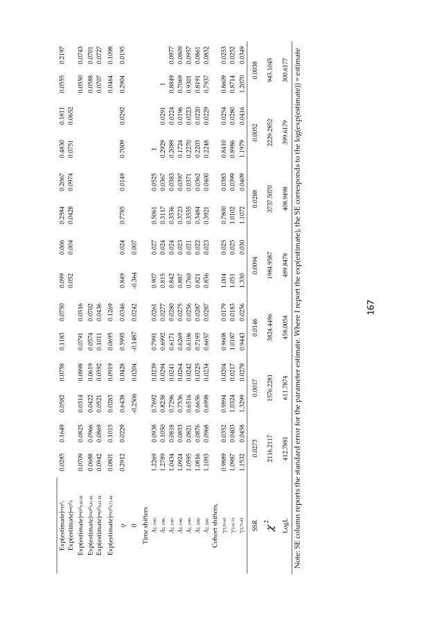
16
7
Ex
p(e
stim
ate
)=σ
2ε
0.0
285
0
.16
49
0.0
582
0
.07
58
0.1
183
0
.07
50
0.0
99
0.0
06
0.2
584
0
.20
67
0.4
830
0
.18
11
0.0
555
0
.21
97
Ex
p(e
stim
ate
)=σ
20
0.0
52
0.0
04
0.0
428
0
.09
74
0.0
751
0
.06
52
Ex
p(e
stim
ate
)=σ
20
,40
-50
0.0
709
0
.08
25
0.0
314
0
.08
98
0.0
791
0
.05
16
0.0
550
0
.07
43
Ex
p(e
stim
ate
)=σ
20
,51
-60
0.0
688
0
.09
66
0.0
422
0
.06
19
0.0
574
0
.07
02
0.0
588
0
.07
01
Ex
p(e
stim
ate
)=σ
20
,61
-70
0.0
942
0
.08
69
0.0
521
0
.05
92
0.1
011
0
.04
36
0.0
707
0
.07
27
Ex
p(e
stim
ate
)=σ
20
,71
-80
0.0
801
0
.10
15
0.0
283
0
.09
19
0.0
695
0
.12
69
0.0
464
0
.10
98
ρ
0.2
912
0
.02
29
0.6
438
0
.04
28
0.5
995
0
.03
46
0.8
49
0.0
24
0.7
785
0
.01
49
0.7
009
0
.02
92
0.2
904
0
.01
95
θ
-0.2
506
0.0
204
-0
.148
7 0
.02
42
-0.3
64
0.0
07
Tim
e sh
ifte
rs
λ2
, 199
5 1
.22
69
0.0
938
0
.76
92
0.0
239
0
.79
91
0.0
261
0
.90
7 0
.02
7 0
.50
61
0.0
525
1
λ2
, 199
6 1
.27
89
0.1
050
0
.82
38
0.0
294
0
.69
92
0.0
277
0
.81
5 0
.02
4 0
.31
17
0.0
367
0
.29
29
0.0
291
1
λ2
, 199
7 1
.04
34
0.0
818
0
.72
96
0.0
241
0
.61
71
0.0
280
0
.84
2 0
.02
4 0
.35
36
0.0
383
0
.20
89
0.0
224
0
.88
49
0.0
977
λ2
, 199
8 1
.09
24
0.0
853
0
.75
36
0.0
264
0
.62
69
0.0
275
0
.88
7 0
.02
3 0
.37
23
0.0
397
0
.17
24
0.0
196
0
.70
69
0.0
809
λ2
, 199
9 1
.05
95
0.0
821
0
.65
16
0.0
242
0
.61
06
0.0
256
0
.76
0 0
.02
1 0
.35
55
0.0
371
0
.22
70
0.0
223
0
.93
01
0.0
957
λ2
, 200
0 1
.08
16
0.0
876
0
.66
56
0.0
225
0
.71
95
0.0
287
0
.82
1 0
.02
2 0
.34
84
0.0
362
0
.22
03
0.0
220
0
.81
91
0.0
861
λ2
, 200
1 1
.10
93
0.0
968
0
.69
98
0.0
234
0
.66
57
0.0
287
0
.85
6 0
.02
3 0
.39
21
0.0
400
0
.22
48
0.0
229
0
.79
37
0.0
852
Co
ho
rt s
hif
ters
,
γ2
,51
-60
0.9
889
0
.03
52
0.9
894
0
.02
04
0.9
608
0
.01
79
1.0
04
0.0
25
0.7
800
0
.03
83
0.8
410
0
.02
54
0.8
609
0
.02
53
γ2
,61
-70
1.0
987
0
.04
03
1.0
324
0
.02
17
1.0
187
0
.01
83
1.0
51
0.0
25
1.0
102
0
.03
99
0.8
986
0
.02
80
0.8
714
0
.02
52
γ2
,71
-80
1.1
532
0
.04
58
1.3
299
0
.02
78
0.9
443
0
.02
56
1.3
30
0.0
30
1.1
072
0
.04
09
1.1
979
0
.04
16
1.2
070
0
.03
49
SS
R
0.0
273
0
.00
17
0.0
146
0
.00
94
0.0
288
0
.00
52
0.0
038
2χ
2
116
.211
7 1
576
.228
1 3
824
.449
6 1
984
.958
7 3
737
.507
0 2
229
.285
2 9
45
.10
45
Lo
gL
4
12
.78
81
61
1.7
874
4
58
.00
54
48
9.8
478
4
08
.94
98
39
9.6
179
3
00
.61
77
No
te:
SE
co
lum
n r
ep
ort
s th
e st
and
ard
err
or
for
the
par
amet
er e
stim
ate.
Wh
ere
I r
ep
ort
th
e e
xp
(est
imat
e), t
he
SE
co
rre
spo
nd
s to
th
e lo
g(e
xp
(est
imat
e))
= e
stim
ate
168
The formulation of the permanent and transitory components of earnings differs
between countries.
Permanent component
In Germany, Netherlands, UK, Ireland, Italy, Greece, Spain and Finland, the
permanent component follows a random growth model with time and cohort
specific loading factors. The estimated coefficients for the permanent component of
earnings show that time-invariant heterogeneity and age-earning profile
heterogeneity play a significant role in the formation of long-term earnings
differentials in all these countries. Individual specific heterogeneity plays the
highest role in Germany, followed by Spain, Netherlands, Greece, UK, Ireland and
Italy, which suggests that in Germany there is a higher dispersion in the time-
invariant individual specific attributes that determine wage differentials.
The estimated random slope variance implies that hourly earnings growth for an
individual located one standard deviation above the mean in the distribution of φ
is the largest in Germany, where it is with 4.89%46 faster than the cohort mean,
followed by Greece, Ireland, Spain, Netherlands, UK and Finland with rates
between 1% and 1.41% and Italy with 0.89%. All these countries have a negative
covariance between the time invariant individual specific effect and the individual
specific slope of the age-earning profile, which implies that the initial and lifecycle
heterogeneity are negatively associated. This negative association corresponds to
the trade-off between earnings early in the career and subsequent earnings growth
and is consistent with the on-the-job training hypothesis (Mincer, 1974). Therefore,
this suggests the presence of mobility within the distribution of permanent
earnings over the sample period. These findings reinforce the results from
previous studies.
Therefore, for these countries the evolution of the permanent component without
the time loading factors could be either increasing or decreasing. The time-specific
loading factors for the permanent component are highly significant with values
close to 1 in all countries. The trends of the returns to the permanent component
vary to a large extent across countries. One common feature is that they reflect the
trends in the high-order autocovariances in the data. These estimates show that
overall, controlling for age and cohort effects, the returns to skills decreased over
the sample period in Netherlands, UK, Ireland, Italy, Greece, Spain and increased
46 2
4.89 100ϕ
σ= ⋅

169
in Germany and Finland. The trends over time differ between countries, some
record a smooth evolution, others noisier. For example, Netherlands experienced
decreases in returns almost every second year. In UK the returns increased in 1997
and 2001, and decreased in the rest. Ireland recorded a decrease until 1996, a boost
in 1997 and a clear decline thereafter. In Italy, 1998 and 1999 appear to be years
with increases in the return to skills, in Greece every second year, in Spain 1995
and 1998. Germany experienced increasing returns to human capital until 2000,
and Finland in 1997 and 2001. Therefore, in these years, the relative position of the
highly skilled individuals was enhanced.
In Denmark the permanent component follows a random walk in age. The variance
of the innovation in the random walk is significantly larger than zero. As the
variance of a variable that follows a random walk is the sum of the variances of the
innovation term, this finding implies that permanent inequality increases over
lifetime. In Denmark, the variance at the age of 20 is lower than the variance at
subsequent ages, suggesting the presence of larger permanent shocks at older ages,
which is consistent with matching models, in which the information revealed
about a worker’s ability increases with time. The final trend in the permanent
variance depends on the period specific loading factors, which reveal that overall,
the relative position of the highly skilled individuals decreased over the sample
period in Denmark. The yearly evolution revealed a smooth decrease until 2000,
followed by a small increase in 2001.
In Belgium, France, Luxembourg, Portugal and Austria the persistent dispersion of
earnings follows the canonical model, where the permanent component is time-
invariant. The highest variance in the time invariant characteristics is recorded in
Portugal, followed by France, Luxembourg, Austria and Belgium. In this case, the
time-specific loading factors determine the final trend of the permanent
differentials: they decreased in Belgium and Austria, and increased in France,
Luxembourg and Portugal. Year by year, France records an increase in the returns
to skills until 1997 and again in 2001, Luxembourg until 2000, Belgium in 1996 and
2000, Austria during most of the period, except 1998-1999, and Portugal in 1996,
1998 and 2000.
The estimates of the cohort-specific shifters for the permanent earnings are highly
significant in all countries. The trends, however, differ between countries. A
monotonic increase over the lifecycle is observed in Germany, France,
Luxembourg, Portugal and Austria. In Denmark, Netherlands, Belgium and Spain
the permanent component of earnings has an inverted-U shape evolution over the
lifecycle. These trends confirm the expectation that permanent earnings
differentials play a much larger role in the formation of overall earnings
170
differentials of older cohorts compared with younger ones, which experience
higher earnings volatility due to temporary contracts. We expect the opposite to
hold in the case of cohort-specific shifters for transitory earnings.
The permanent component of earnings decreases over the life cycle in UK, Ireland,
Italy, Greece and Finland. This may be due to younger cohorts having more
heterogeneous skills or experiencing larger permanent shocks even without a
larger dispersion of skills. This could be the case if the labour market has become
tougher over time, as in the case of Italy, which is characterised by high rates of
youth unemployment.
Transitory component
The formulation of the temporary component of earnings differs between
countries. It follows an AR(1) process with time and cohorts loading factors in all
countries, except Italy, Greece and Spain, where it follows an ARMA(1,1). Except
for Spain, Portugal and Austria, the other countries are characterized by
heteroskedastic initial conditions. The estimated coefficients for the transitory
component of earnings are all significant, suggesting that the initial variance(s), the
AR(1) process, the ARMA(1,1) process, and the time and cohort loading factors
contribute significantly to earnings volatility in all countries.
The variance of initial conditions, which represents the accumulation of shocks up
to the starting year of the panel, is smaller than the variance of subsequent shocks
in all countries, except Luxembourg, Ireland, the oldest three cohorts in UK, and
the middle two cohorts in Finland. Overall, the variance of initial conditions
increases over the lifecycle in Denmark, Belgium, France, Luxembourg, UK, Italy,
Greece and Finland, suggesting that the initial variance plays a larger role in the
formation of earnings differentials for the oldest cohort compared with the
youngest. The opposite is observed in Germany, Netherlands and Ireland.
The pattern of the heteroskedstic initial conditions, however, is not monotonic
across cohorts. In Luxembourg, UK, Italy, and Finland it follows an inverted-U
shape: the variance of initial conditions increases over the lifecycle and decreases at
the end. The opposite holds for France, where the oldest and the youngest cohorts
have the highest initial variances.
In Germany and Netherlands the pattern of the heteroskedastic initial conditions
records a sharp drop for the second youngest cohort, an increase for the second
oldest and a small drop for the oldest cohort. In Denmark, Belgium, Ireland and
171
Greece, the variance of initial conditions records an increase for the second
youngest cohort, a drop for the second oldest and an increase for the oldest cohort.
The magnitude of the autoregressive parameter varies between countries. A large
autoregressive parameter, which suggests that shocks are persistent, is recorded in
Spain with 26.9% of a shock still present after 8 years, in Portugal with 13.5% and
in Austria with 5.8%. A moderate autoregressive parameter suggesting that shocks
die out rather quickly is recorded in Italy with 2.8% of a shock still present after 8
years, in Belgium with 2.4%, and in Greece with 1.4%. A small autoregressive
parameter is present in Luxembourg, Ireland, Finland, Netherlands, Germany,
France, UK and Denmark, where between 0.0008% and 0.8% of a shock is still
present after 8 years. The negative sign of the MA component implies that the
autocovariances decline sharply over the first period, confirming the trends
observed in the previous section for Italy, Greece and Spain.47
The time-specific loading factors for the transitory component are highly
significant and display a higher variation than for the permanent component in all
countries. The trends of the transitory inequality vary to a large extent across
countries. These estimates show that overall the transitory variance decreased over
the sample period in all countries, except Luxembourg and Ireland.
The estimates of the cohort-specific shifters for the transitory earnings are highly
significant in all countries. They indicate that earnings volatility is higher for
younger cohorts, thus confirming the pattern observed in the dynamic description
of the autocovariance structure of earnings, where autocovariances were found to
be lower for younger cohorts. This is expected, given that younger people
experience in general more frequent job changes, and consequently less stable
earnings.
Alternative model specifications
Table 4.3 introduces the alternative model specifications for each country to justify
the choice for the preferred models. Through these models, we tested whether the
restrictions imposed by previous studies hold for each country.
First compared with the simple canonical model, our country-models revealed a
significant improvement, both with respect to SSR and the Newey chi-squared
goodness of fit. Moreover, the overall Wald test showed that, for each country, the
47 For the other countries, the MA component was either rejected by the data or could not be identified
due to the low number of waves.
172
restrictions imposed by the canonical model do not hold in the data. In Germany,
assuming away the restrictions imposed by the canonical model decreased the2χ
with 46764.97 at a cost of 26 degrees of freedom. Similarly, in Denmark the
decrease in 2χ was of 23668.02, in Netherlands of 21880.65, in Belgium of 28937.06,
in France of 6602.395, in Luxembourg of 33598.94, in UK of 9651.35, in Ireland of
22338.56, in Italy of 10858.77, in Greece of 23150.67, in Spain of 9833.018, in
Portugal of 35182.5, in Austria of 12829.92 and in Finland of 5733.26. We then
tested these restrictions in turn.
If we assume away the random growth in the permanent component ( 2 0ϕσ = and
cov( , ) 0µ ϕ = ), the Wald test on this restrictions clearly rejects the null in Germany
(2
859.6255χ = , df=2), Netherlands (2
178.7331χ = , df=3), UK (2
185.2973χ = ,
df=2), Ireland (2
8.8093χ = , df=2), Italy (2
65.2755χ = , df=2), Spain (2
28.2711χ =
, df=2), Finland (2
99.2208χ = , df=2). In Greece, this assumption leads to an
unidentified model. Identification problems from incorporating a random growth
are found in Belgium, France, Luxembourg, Portugal and Austria.
Assuming away the random walk in the permanent component was rejected by the
Wald test in Denmark (2χ =115.65, df = 1). Incorporating a random walk in the
permanent component was rejected in Portugal, and led to identification problems
in Belgium, France, Luxembourg and Austria. Among the countries that favoured
the random growth, the random walk either triggered some identification
problems or a higher BIC than the model incorporating a random growth.
Based on Wald test, the restriction of homogenous initial conditions (2 2 2 2 2
0 0 ,40 50 0 ,51 60 0 ,61 70 0 ,71 80σ σ σ σ σ
− − − −= = = = ) was rejected in Germany (
2125.1595χ = , df=5), Denmark (
2436.3263χ = , df=3), Netherlands (
2207.3169χ = , df=3), Belgium (
21063.161χ = , df=3), France (
261.0812χ = ,
df=3), Luxembourg (2
268.491χ = , df=3), Ireland (2
8.8093χ = , df=2), Italy (
270.1507χ = , df=3) and Greece (
2172.1103χ = , df=3). Assuming heterogeneous
initial conditions worsened the fit of the model in Portugal and Austria, as
illustrated by the increase of 11613.2 and 152.77 in 2χ . A similar result was
obtained in Finland, however given that in our preferred model the SSR is smaller
and the parameter estimates are significant, we decided to keep the specification.
Assuming heterogenous initial conditions led to convergence or identification
problems in UK and Spain.
173
Introducing an MA(1) component besides the AR(1) improved significantly the fit
of the model in Italy (2
323.1314χ = , df=1), Greece (2
121.2267χ = , df=1) and
Spain (2
47.9717χ = , df=1). MA(1) component was rejected in Luxembourg and
Portugal, as suggested by the increase of 1.073, respectively 4015.76 in 2χ . In rest,
this specification failed to converge or suffered from identification problems.
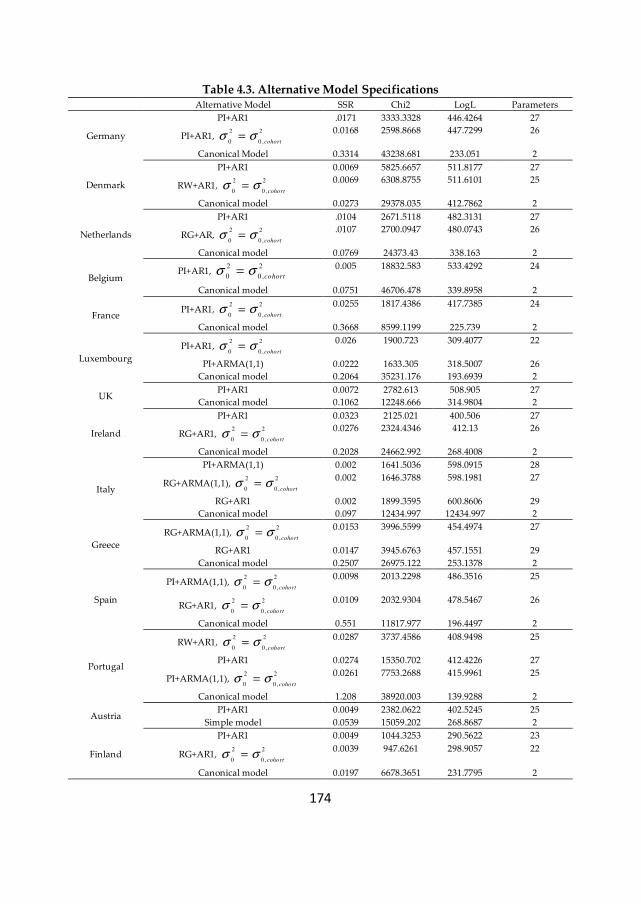
174
Table 4.3. Alternative Model Specifications Alternative Model SSR Chi2 LogL Parameters
Germany
PI+AR1 .0171 3333.3328 446.4264 27
PI+AR1, 2 2
0 0 ,cohortσ σ=
0.0168 2598.8668 447.7299 26
Canonical Model 0.3314 43238.681 233.051 2
Denmark
PI+AR1 0.0069 5825.6657 511.8177 27
RW+AR1, 2 2
0 0 ,cohortσ σ=
0.0069 6308.8755 511.6101 25
Canonical model 0.0273 29378.035 412.7862 2
Netherlands
PI+AR1 .0104 2671.5118 482.3131 27
RG+AR, 2 2
0 0 ,cohortσ σ=
.0107 2700.0947 480.0743 26
Canonical model 0.0769 24373.43 338.163 2
Belgium PI+AR1,
2 2
0 0 ,cohortσ σ=
0.005 18832.583 533.4292 24
Canonical model 0.0751 46706.478 339.8958 2
France PI+AR1,
2 2
0 0 ,cohortσ σ=
0.0255 1817.4386 417.7385 24
Canonical model 0.3668 8599.1199 225.739 2
Luxembourg
PI+AR1, 2 2
0 0 ,cohortσ σ=
0.026 1900.723 309.4077 22
PI+ARMA(1,1) 0.0222 1633.305 318.5007 26
Canonical model 0.2064 35231.176 193.6939 2
UK PI+AR1 0.0072 2782.613 508.905 27
Canonical model 0.1062 12248.666 314.9804 2
Ireland
PI+AR1 0.0323 2125.021 400.506 27
RG+AR1, 2 2
0 0 ,cohortσ σ=
0.0276 2324.4346 412.13 26
Canonical model 0.2028 24662.992 268.4008 2
Italy
PI+ARMA(1,1) 0.002 1641.5036 598.0915 28
RG+ARMA(1,1), 2 2
0 0 ,cohortσ σ=
0.002 1646.3788 598.1981 27
RG+AR1 0.002 1899.3595 600.8606 29
Canonical model 0.097 12434.997 12434.997 2
Greece
RG+ARMA(1,1), 2 2
0 0 ,cohortσ σ=
0.0153 3996.5599 454.4974 27
RG+AR1 0.0147 3945.6763 457.1551 29
Canonical model 0.2507 26975.122 253.1378 2
Spain
PI+ARMA(1,1), 2 2
0 0 ,cohortσ σ=
0.0098 2013.2298 486.3516 25
RG+AR1, 2 2
0 0 ,cohortσ σ=
0.0109 2032.9304 478.5467 26
Canonical model 0.551 11817.977 196.4497 2
Portugal
RW+AR1, 2 2
0 0 ,cohortσ σ=
0.0287 3737.4586 408.9498 25
PI+AR1 0.0274 15350.702 412.4226 27
PI+ARMA(1,1), 2 2
0 0 ,cohortσ σ=
0.0261 7753.2688 415.9961 25
Canonical model 1.208 38920.003 139.9288 2
Austria PI+AR1 0.0049 2382.0622 402.5245 25
Simple model 0.0539 15059.202 268.8687 2
Finland
PI+AR1 0.0049 1044.3253 290.5622 23
RG+AR1, 2 2
0 0 ,cohortσ σ=
0.0039 947.6261 298.9057 22
Canonical model 0.0197 6678.3651 231.7795 2
175
4.9. Inequality decomposition into permanent and transitory
inequality
Having estimated a suitable error component model for earnings in each country,
next we use these parameters estimates to decompose earnings inequality into its
permanent and transitory components, assess their absolute and relative
contribution to the evolution of overall inequality, and estimate earnings mobility
over the sample period, by cohort.
There is a fundamental conceptual underidentification of time, life-cycle, and
cohort effects due to the exact multicollinearity of time, age, and birth year. Our
decompositions control for cohort effects, but the age and period effects are
confounded. Since our scope is to decompose within-cohort inequality into the two
components, the lifecycle effect is considered part of the permanent component,
and thus its specific identification was disregarded.
4.9.1. Absolute decomposition
Figure 4.3 illustrates the absolute decomposition of the variance, together with the
actual and predicted variance of earnings by cohort. The decomposition by cohort
identifies how inequality and its components are affected by labour market
changes at different lifecycle stages. For all countries, the evolution of the predicted
variance follows closely the evolution of the actual variance, confirming the fit of
the country models, indicated by the low sum of square residuals.
Earnings inequality measured by the actual variance decreased overall in Germany
- except for the cohorts born in 1941-1950 and 1961-1970 where it increased -, in
Denmark, in Belgium - except for the youngest cohort where it increased -, in
France - except for the cohort born in 1961-1970 -, in UK - except for the youngest
two cohorts where it increased -, in Ireland, in Spain - except the youngest and the
oldest cohort -, and in Austria. Earnings inequality measured by the actual
variance increased overall for all cohorts in Netherlands, Luxembourg, Italy,
Greece, Portugal, and Finland - except for the youngest cohort. These are countries
where wages appear to be more responsive to market forces.
The pattern of the absolute decomposition of the overall variance varies between
countries and cohorts. Nevertheless, some common traits emerge. Permanent
variance is higher and transitory variance is lower, the older is the cohort, which is
consistent with the evidence of lifecycle earnings divergence showing that older
176
cohorts experience a lower earnings volatility compared with younger cohorts.
Similar results are found by Dickens (2000b) and Ramos (1999, 2003) for UK,
Cervini and Ramos (2006) for Spain, and Capellari (2003) for Italy.
The decrease in the overall cross-sectional inequality is the result of decreasing
permanent and transitory differentials in Denmark and Austria, of decreasing
permanent differentials with offsetting effect over the increasing transitory
differentials in Belgium and Spain, and of decreasing transitory differentials with
offsetting effects over the increasing permanent differentials in Germany, France,
UK and Ireland. In most countries, these trends are consistent across cohorts.
Mixed trends across cohorts are observed in: Denmark - where the transitory
variance increased for the second oldest cohort -, Belgium – where both component
decreased for the oldest cohort and the increase in the transitory variance
dominated for the youngest cohort -, Spain – where the increase in the transitory
variance dominated for the oldest and the youngest cohort -, Germany - where
both components increased for the 1941-1950 and 1961-1970 cohorts, and decreased
for the cohort 1951-1960 -; France – where both components increased for the
second youngest cohort -, Ireland - where both components decreased for the
oldest cohort -, and UK – where both components decreased for the oldest cohort,
and the increase in inequality for the youngest two cohorts was determined by an
increase in the permanent variance for the cohort 1961-1970 and by an increase in
the transitory variance for the cohort 1971-1980.
In Luxembourg, Italy, Greece and Finland, the exacerbation of permanent
differentials, meaning the increase in returns to skills was the dominant factor
behind the increase in overall inequality, offsetting the decrease in transitory
differentials, whereas in Portugal and Netherlands both components increased.
These trends are consistent across cohorts, except for the youngest cohort in
Luxembourg and Italy, and the second oldest cohort in Greece - where both
components increased -, the youngest two cohorts in Netherlands - where
permanent differentials decreased -, and Finland - where both components
decreased.
To summarize these trends we averaged permanent and transitory variance across
cohorts: the decrease in overall inequality was driven by a decrease in both
components in Denmark and Austria, by a decrease in permanent differentials in
Belgium and Spain, and by a decrease in transitory differentials in Germany,
France, UK and Ireland. The exacerbation of overall inequality was the result of
increasing permanent differentials in Luxembourg, Italy, Greece and Finland, and
of an increase in both components in Portugal and Netherlands.
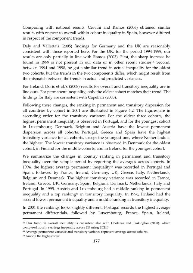
177
Comparing with national results, Cervini and Ramos (2006) obtained similar
results with respect to overall within-cohort inequality in Spain, however differed
in respect of the component trends.
Daly and Valletta’s (2005) findings for Germany and the UK are reasonably
consistent with those reported here. For the UK, for the period 1994-1999, our
results are only partially in line with Ramos (2003). First, the sharp increase he
found in 1999 is not present in our data or in other recent studies48. Second,
between 1994 and 1998, he got a similar trend in actual inequality for the oldest
two cohorts, but the trends in the two components differ, which might result from
the mismatch between the trends in actual and predicted variances.
For Ireland, Doris et al.’s (2008) results for overall and transitory inequality are in
line ours. For permanent inequality, only the oldest cohort matches their trend. The
findings for Italy are consistent with Capellari (2003).
Following these changes, the ranking in permanent and transitory dispersion for
all countries by cohort in 2001 are illustrated in Figure 4.2. The figures are in
ascending order for the transitory variance. For the oldest three cohorts, the
highest permanent inequality is observed in Portugal, and for the youngest cohort
in Luxembourg. Denmark, Belgium and Austria have the lowest permanent
dispersion across all cohorts. Portugal, Greece and Spain have the highest
transitory variance for all cohorts, except the youngest one, where Netherlands is
the highest. The lowest transitory variance is observed in Denmark for the oldest
cohort, in Finland for the middle cohorts, and in Ireland for the youngest cohort.
We summarize the changes in country ranking in permanent and transitory
inequality over the sample period by reporting the averages across cohorts. In
1994, the highest average permanent inequality49 was recorded in Portugal and
Spain, followed by France, Ireland, Germany, UK, Greece, Italy, Netherlands,
Belgium and Denmark. The highest transitory variance was recorded in France,
Ireland, Greece, UK, Germany, Spain, Belgium, Denmark, Netherlands, Italy and
Portugal. In 1995, Austria and Luxembourg had a middle ranking in permanent
inequality and a top ranking50 in transitory inequality. In 1996, Finland had the
second lowest permanent inequality and a middle ranking in transitory inequality.
In 2001 the rankings looks slightly different. Portugal records the highest average
permanent differentials, followed by Luxembourg, France, Spain, Ireland,
48 Our trend in overall inequality is consistent also with Cholezas and Tsakloglou (2008), which
compared hourly earnings inequality across EU using ECHP. 49 Average permanent variance and transitory variance represent average across cohorts. 50 Among the highest four.
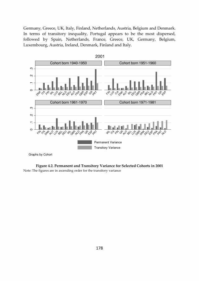
178
Germany, Greece, UK, Italy, Finland, Netherlands, Austria, Belgium and Denmark.
In terms of transitory inequality, Portugal appears to be the most dispersed,
followed by Spain, Netherlands, France, Greece, UK, Germany, Belgium,
Luxembourg, Austria, Ireland, Denmark, Finland and Italy.
Figure 4.2. Permanent and Transitory Variance for Selected Cohorts in 2001 Note: The figures are in ascending order for the transitory variance
0.1
.2.3
0.1
.2.3
DNK
ITA
FIN IRL
LUX
BEL
NLD
DEU
AUT
FRA
GBR
ESP
GR
PRT
FINLU
XIT
ADNK
AUT
IRL
DEU
GBR
FRA
BEL
NLD
PRT
GR
ESP
FIN ITA
DNK
AUT
LUX
BELDEU
IRLGBR
NLD
FRA
GR
ESPPR
TIR
LIT
AFIN G
RAU
TBEL
LUX
GBR
DNK
DEU
ESPFR
APR
TNLD
Cohort born 1940-1950 Cohort born 1951-1960
Cohort born 1961-1970 Cohort born 1971-1981
Permanent Variance
Transitory Variance
Graphs by Cohort
2001
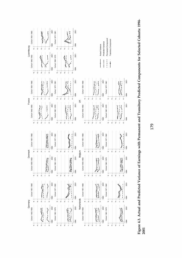
17
9
Fig
ure
4.3
. A
ctu
al a
nd
Pre
dic
ted
Var
ian
ce o
f E
arn
ing
s w
ith
Per
man
ent
and
Tra
nsi
tory
Pre
dic
ted
Co
mp
on
ents
fo
r S
elec
ted
Co
ho
rts:
199
4-
2001
0.1.2.3.4
1994
2001
Cohort
1940-1
950
0.1.2.3.4
1994
2001
Cohort
1951-1
960
0.1.2.3.4
1994
2001
Cohort
1961-1
970
0.1.2.3.4
1994
2001
Cohort
1971-1
981
Ge
rma
ny
0.1.2.3.4
1994
2001
Cohort
1940-1
950
0.1.2.3.4
1994
2001
Cohort
1951-1
960
0.1.2.3.4
1994
2001
Cohort
1961-1
970
0.1.2.3.4
1994
2001
Cohort
1971-1
981
De
nm
ark
0.1.2.3.4
1994
2001
Cohort
1940-1
950
0.1.2.3.4
1994
2001
Cohort
1951-1
960
0.1.2.3.4
1994
2001
Cohort
1961-1
970
0.1.2.3.4
1994
2001
Cohort
1971-1
981
Ne
the
rla
nds
0.1.2.3.4
1994
2001
Cohort
1940-1
950
0.1.2.3.4
1994
2001
Cohort
1951-1
960
0.1.2.3.4
1994
2001
Cohort
1961-1
970
0.1.2.3.4
1994
2001
Cohort
1971-1
981
Be
lgiu
m
0.1.2.3.4
1994
2001
Cohort
1940-1
950
0.1.2.3.4
1994
2001
Cohort
1951-1
960
0.1.2.3.4
1994
2001
Cohort
1961-1
970
0.1.2.3.4
1994
2001
Cohort
1971-1
981
Fra
nce
0.1.2.3.4
1994
2001
Cohort
1940-1
950
0.1.2.3.4
1994
2001
Cohort
1951-1
960
0.1.2.3.4
1994
2001
Cohort
1961-1
970
0.1.2.3.4
1994
2001
Cohort
1971-1
981
Luxe
mbo
urg
0.1.2.3.4
1994
2001
Cohort
1940-1
950
0.1.2.3.4
1994
2001
Cohort
1951-1
960
0.1.2.3.4
1994
2001
Cohort
1961-1
970
0.1.2.3.4
1994
2001
Cohort
1971-1
981
UK
Actu
al V
ariance
Pre
dic
ted
Variance
Pe
rmane
nt C
om
po
ne
nt
Tra
nsito
ry C
om
po
ne
nt
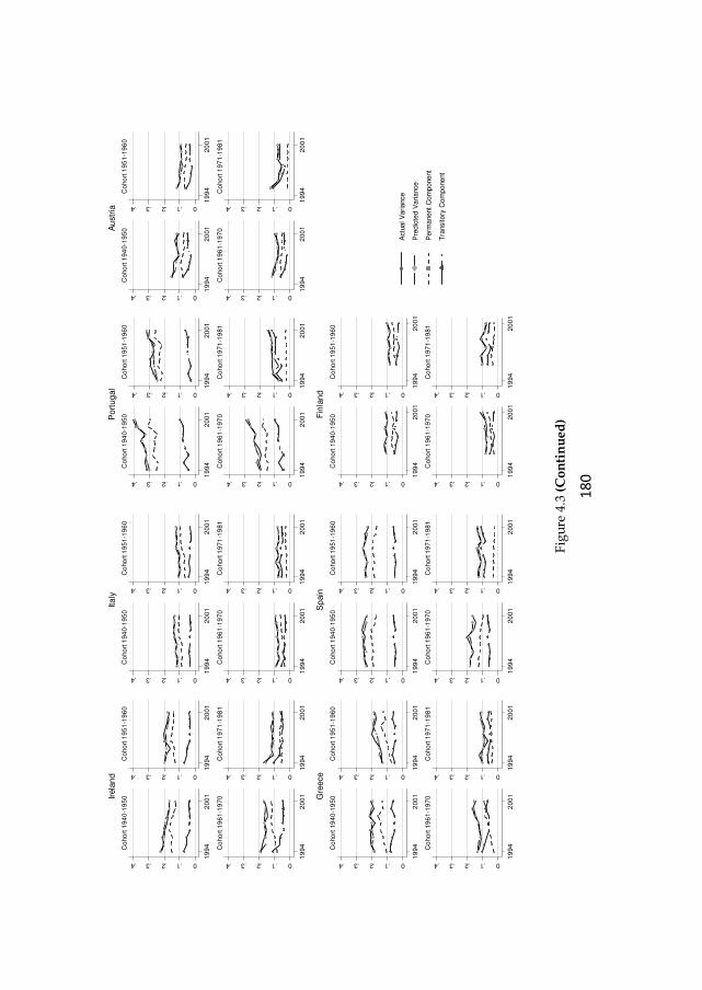
18
0
Fig
ure
4.3
(C
on
tin
ued
)
0.1.2.3.4
19
94
20
01
Co
ho
rt 1
94
0-1
95
0
0.1.2.3.41
99
42
00
1
Co
ho
rt 1
95
1-1
96
00.1.2.3.4
19
94
20
01
Co
ho
rt 1
96
1-1
97
00.1.2.3.4
19
94
20
01
Co
ho
rt 1
97
1-1
98
1
Irela
nd
0.1.2.3.4
19
94
20
01
Co
ho
rt 1
94
0-1
95
0
0.1.2.3.4
19
94
20
01
Co
ho
rt 1
95
1-1
96
0
0.1.2.3.41
99
42
00
1
Co
ho
rt 1
96
1-1
97
0
0.1.2.3.4
19
94
20
01
Co
ho
rt 1
97
1-1
98
1
Italy
0.1.2.3.4
19
94
20
01
Co
ho
rt 1
94
0-1
95
0
0.1.2.3.4
19
94
20
01
Co
ho
rt 1
95
1-1
96
0
0.1.2.3.4
19
94
20
01
Co
ho
rt 1
96
1-1
97
0
0.1.2.3.4
19
94
20
01
Co
ho
rt 1
97
1-1
98
1
Gre
ece
0.1.2.3.4
19
94
20
01
Co
ho
rt 1
94
0-1
95
0
0.1.2.3.4
19
94
20
01
Co
ho
rt 1
95
1-1
96
0
0.1.2.3.4
19
94
20
01
Co
ho
rt 1
96
1-1
97
0
0.1.2.3.4
19
94
20
01
Co
ho
rt 1
97
1-1
98
1
Sp
ain
0.1.2.3.4
19
94
20
01
Co
ho
rt 1
94
0-1
95
0
0.1.2.3.4
19
94
20
01
Co
ho
rt 1
95
1-1
96
0
0.1.2.3.4
19
94
20
01
Co
ho
rt 1
96
1-1
97
0
0.1.2.3.4
19
94
20
01
Co
ho
rt 1
97
1-1
98
1
Port
ug
al
0.1.2.3.4
19
94
20
01
Co
ho
rt 1
94
0-1
95
0
0.1.2.3.4
19
94
20
01
Co
ho
rt 1
95
1-1
96
0
0.1.2.3.4
19
94
20
01
Co
ho
rt 1
96
1-1
97
0
0.1.2.3.4
19
94
20
01
Co
ho
rt 1
97
1-1
98
1
Au
str
ia
0.1.2.3.4
19
94
20
01
Co
ho
rt 1
94
0-1
95
0
0.1.2.3.4
19
94
20
01
Co
ho
rt 1
95
1-1
96
0
0.1.2.3.41
99
42
00
1
Co
ho
rt 1
96
1-1
97
0
0.1.2.3.4
19
94
20
01
Co
ho
rt 1
97
1-1
98
1
Fin
lan
d
Actu
al V
ariance
Pre
dic
ted V
ariance
Perm
anent
Com
ponent
Tra
nsitory
Com
ponent
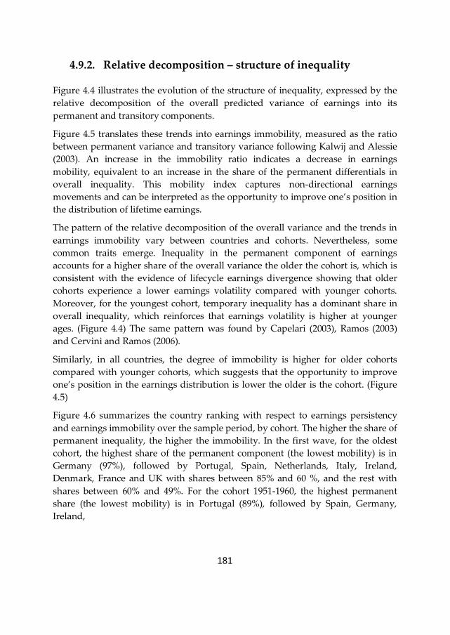
181
4.9.2. Relative decomposition – structure of inequality
Figure 4.4 illustrates the evolution of the structure of inequality, expressed by the
relative decomposition of the overall predicted variance of earnings into its
permanent and transitory components.
Figure 4.5 translates these trends into earnings immobility, measured as the ratio
between permanent variance and transitory variance following Kalwij and Alessie
(2003). An increase in the immobility ratio indicates a decrease in earnings
mobility, equivalent to an increase in the share of the permanent differentials in
overall inequality. This mobility index captures non-directional earnings
movements and can be interpreted as the opportunity to improve one’s position in
the distribution of lifetime earnings.
The pattern of the relative decomposition of the overall variance and the trends in
earnings immobility vary between countries and cohorts. Nevertheless, some
common traits emerge. Inequality in the permanent component of earnings
accounts for a higher share of the overall variance the older the cohort is, which is
consistent with the evidence of lifecycle earnings divergence showing that older
cohorts experience a lower earnings volatility compared with younger cohorts.
Moreover, for the youngest cohort, temporary inequality has a dominant share in
overall inequality, which reinforces that earnings volatility is higher at younger
ages. (Figure 4.4) The same pattern was found by Capelari (2003), Ramos (2003)
and Cervini and Ramos (2006).
Similarly, in all countries, the degree of immobility is higher for older cohorts
compared with younger cohorts, which suggests that the opportunity to improve
one’s position in the earnings distribution is lower the older is the cohort. (Figure
4.5)
Figure 4.6 summarizes the country ranking with respect to earnings persistency
and earnings immobility over the sample period, by cohort. The higher the share of
permanent inequality, the higher the immobility. In the first wave, for the oldest
cohort, the highest share of the permanent component (the lowest mobility) is in
Germany (97%), followed by Portugal, Spain, Netherlands, Italy, Ireland,
Denmark, France and UK with shares between 85% and 60 %, and the rest with
shares between 60% and 49%. For the cohort 1951-1960, the highest permanent
share (the lowest mobility) is in Portugal (89%), followed by Spain, Germany,
Ireland,
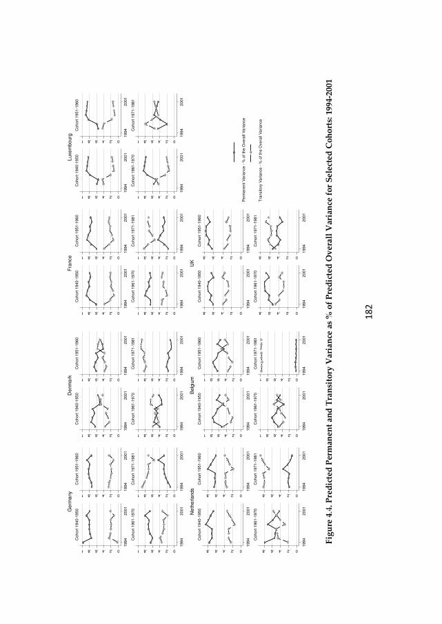
18
2
Fig
ure
4.4
. Pre
dic
ted
Per
man
ent
and
Tra
nsi
tory
Var
ian
ce a
s %
of
Pre
dic
ted
Ov
eral
l V
aria
nce
fo
r S
elec
ted
Co
ho
rts:
199
4-20
01
0.2.4.6.81
19
94
20
01
Co
ho
rt 1
94
0-1
95
0
0.2.4.6.811
99
42
00
1
Co
ho
rt 1
95
1-1
96
00.2.4.6.81
19
94
20
01
Co
ho
rt 1
96
1-1
97
0
0.2.4.6.81
19
94
20
01
Co
ho
rt 1
97
1-1
98
1
Ge
rma
ny
0.2.4.6.81
19
94
20
01
Co
ho
rt 1
94
0-1
95
0
0.2.4.6.81
19
94
20
01
Co
ho
rt 1
95
1-1
96
0
0.2.4.6.81
19
94
20
01
Co
ho
rt 1
96
1-1
97
0
0.2.4.6.81
19
94
20
01
Co
ho
rt 1
97
1-1
98
1
De
nm
ark
0.2.4.6.8
19
94
20
01
Co
ho
rt 1
94
0-1
95
0
0.2.4.6.8
19
94
20
01
Co
ho
rt 1
95
1-1
96
0
0.2.4.6.8
19
94
20
01
Co
ho
rt 1
96
1-1
97
0
0.2.4.6.8
19
94
20
01
Co
ho
rt 1
97
1-1
98
1
Ne
the
rla
nds
0.2.4.6.81
19
94
20
01
Co
ho
rt 1
94
0-1
95
0
0.2.4.6.811
99
42
00
1
Co
ho
rt 1
95
1-1
96
0
0.2.4.6.81
19
94
20
01
Co
ho
rt 1
96
1-1
97
0
0.2.4.6.81
19
94
20
01
Co
ho
rt 1
97
1-1
98
1
Be
lgiu
m
0.2.4.6.81
19
94
20
01
Co
ho
rt 1
94
0-1
95
0
0.2.4.6.81
19
94
20
01
Co
ho
rt 1
95
1-1
96
0
0.2.4.6.81
19
94
20
01
Co
ho
rt 1
96
1-1
97
0
0.2.4.6.81
19
94
20
01
Co
ho
rt 1
97
1-1
98
1
Fra
nce
0.2.4.6.81
19
94
20
01
Co
ho
rt 1
94
0-1
95
0
0.2.4.6.81
19
94
20
01
Co
ho
rt 1
95
1-1
96
0
0.2.4.6.81
19
94
20
01
Co
ho
rt 1
96
1-1
97
0
0.2.4.6.81
19
94
20
01
Co
ho
rt 1
97
1-1
98
1
Luxe
mbo
urg
0.2.4.6.8
19
94
20
01
Co
ho
rt 1
94
0-1
95
0
0.2.4.6.8
19
94
20
01
Co
ho
rt 1
95
1-1
96
0
0.2.4.6.8
19
94
20
01
Co
ho
rt 1
96
1-1
97
0
0.2.4.6.8
19
94
20
01
Co
ho
rt 1
97
1-1
98
1
UK
Pe
rma
ne
nt
Va
ria
nce
- %
of
the
Ove
rall
Va
ria
nce
Tra
nsito
ry V
ari
an
ce
- %
of
the
Ove
rall
Va
ria
nce
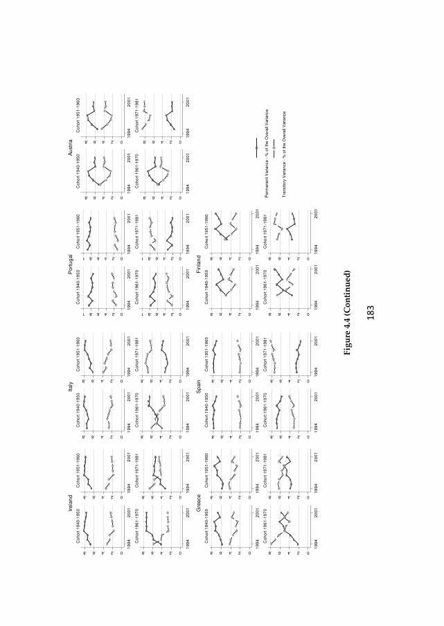
18
3
Fig
ure
4.4
(C
on
tin
ued
)
0.2.4.6.8
19
94
20
01
Co
ho
rt 1
94
0-1
95
0
0.2.4.6.81
99
42
00
1
Co
ho
rt 1
95
1-1
96
0
0.2.4.6.8
19
94
20
01
Co
ho
rt 1
96
1-1
97
0
0.2.4.6.8
19
94
20
01
Co
ho
rt 1
97
1-1
98
1
Irela
nd
0.2.4.6.8
19
94
20
01
Co
ho
rt 1
94
0-1
95
0
0.2.4.6.8
19
94
20
01
Co
ho
rt 1
95
1-1
96
0
0.2.4.6.81
99
42
00
1
Co
ho
rt 1
96
1-1
97
0
0.2.4.6.8
19
94
20
01
Co
ho
rt 1
97
1-1
98
1
Italy
0.2.4.6.8
19
94
20
01
Co
ho
rt 1
94
0-1
95
0
0.2.4.6.8
19
94
20
01
Co
ho
rt 1
95
1-1
96
0
0.2.4.6.8
19
94
20
01
Co
ho
rt 1
96
1-1
97
0
0.2.4.6.8
19
94
20
01
Co
ho
rt 1
97
1-1
98
1
Gre
ece
0.2.4.6.8
19
94
20
01
Co
ho
rt 1
94
0-1
95
0
0.2.4.6.8
19
94
20
01
Co
ho
rt 1
95
1-1
96
0
0.2.4.6.8
19
94
20
01
Co
ho
rt 1
96
1-1
97
0
0.2.4.6.8
19
94
20
01
Co
ho
rt 1
97
1-1
98
1
Sp
ain
0.2.4.6.81
19
94
20
01
Co
ho
rt 1
94
0-1
95
0
0.2.4.6.81
19
94
20
01
Co
ho
rt 1
95
1-1
96
0
0.2.4.6.81
19
94
20
01
Co
ho
rt 1
96
1-1
97
0
0.2.4.6.81
19
94
20
01
Co
ho
rt 1
97
1-1
98
1
Port
ug
al
0.2.4.6.8
19
94
20
01
Co
ho
rt 1
94
0-1
95
0
0.2.4.6.8
19
94
20
01
Co
ho
rt 1
95
1-1
96
0
0.2.4.6.8
19
94
20
01
Co
ho
rt 1
96
1-1
97
0
0.2.4.6.8
19
94
20
01
Co
ho
rt 1
97
1-1
98
1
Au
str
ia
0.2.4.6.8
19
94
20
01
Co
ho
rt 1
94
0-1
95
0
0.2.4.6.8
19
94
20
01
Co
ho
rt 1
95
1-1
96
0
0.2.4.6.81
99
42
00
1
Co
ho
rt 1
96
1-1
97
0
0.2.4.6.8
19
94
20
01
Co
ho
rt 1
97
1-1
98
1
Fin
lan
d
Pe
rmane
nt V
ariance
- %
of
the
Ove
rall
Variance
Tra
nsito
ry V
ariance
- %
of
the
Ove
rall
Variance
18
4
Fig
ure
4.5
. Rat
io b
etw
een
Per
man
ent
Var
ian
ce a
nd
Tra
nsi
tory
Var
ian
ce o
ver
Tim
e fo
r S
elec
ted
Co
ho
rts
0246810
19
94
19
95
19
96
19
97
19
98
19
99
20
00
20
01
Ge
rma
ny
0246810
19
94
19
95
19
96
19
97
19
98
19
99
20
00
20
01
De
nm
ark
0246810
19
94
19
95
19
96
19
97
19
98
19
99
20
00
20
01
Ne
the
rla
nd
s
0246810
19
94
19
95
19
96
19
97
19
98
19
99
20
00
20
01
Be
lgiu
m0246810
19
94
19
95
19
96
19
97
19
98
19
99
20
00
20
01
Fra
nce
02468101
99
41
99
51
99
61
99
71
99
81
99
92
00
02
00
1
Lu
xem
bo
urg
0246810
19
94
19
95
19
96
19
97
19
98
19
99
20
00
20
01
UK
0246810
19
94
19
95
19
96
19
97
19
98
19
99
20
00
20
01
Ire
lan
d
0246810
19
94
19
95
19
96
19
97
19
98
19
99
20
00
20
01
Ita
ly
0246810
19
94
19
95
19
96
19
97
19
98
19
99
20
00
20
01
Gre
ece
0246810
19
94
19
95
19
96
19
97
19
98
19
99
20
00
20
01
Sp
ain
0246810
19
94
19
95
19
96
19
97
19
98
19
99
20
00
20
01
Po
rtu
ga
l
0246810
19
94
19
95
19
96
19
97
19
98
19
99
20
00
20
01
Au
str
ia
0246810
19
94
19
95
19
96
19
97
19
98
19
99
20
00
20
01
Fin
lan
d
Wage Im
mo
bili
ty C
oho
rt 1
940-1
950
Wage Im
mo
bili
ty C
oho
rt 1
951-1
960
Wage Im
mo
bili
ty C
oho
rt 1
961-1
970
Wage Im
mo
bili
ty C
oho
rt 1
971-1
981
185
Netherlands, Belgium, UK, Italy, Denmark and France with shares between 78%
and 60%, and the rest with shares between 58% (Greece) and 47% (Finland).
For the 1961-1970 cohort, the highest permanent shares (the lowest mobility) are in
Netherlands and Portugal (77%), followed by Spain, France and Germany - with
shares between 68% and 64% -, Luxembourg, UK, Belgium, Austria and Ireland -
with shares between 56% and 42% -, and the rest with shares between 40%
(Denmark) and 21% (Greece). For the cohort 1971-1981, the highest permanent
share is recorded in UK (52%), followed by Luxembourg (45%), Greece, Finland,
Ireland, Portugal, Italy and Spain - with shares between 38% and 25% -, and the
rest with shares between 18% (Netherlands) and 2% (Belgium).
Figure 4.6. Permanent Inequality - % of the Overall Inequality and Earnings Immobility
for Selected Cohorts over Time
Turning to Figure 4.4 and Figure 4.5 we observe that among the countries with
decreasing inequality, in Denmark, Belgium and Spain the structure of inequality
and earnings mobility by cohort did not change much in 2001 compared with 1994.
02
04
06
08
01
00
02
04
06
08
01
00
FIN
AU
TB
EL
GR
LU
XG
BR
FR
AD
NK
IRL
ITA
NL
DE
SP
PR
TD
EU
FIN
AU
TL
UX
GR
FR
AD
NK
ITA
GB
RB
EL
NL
DIR
LD
EU
ES
PP
RT
GR
FIN
ITA
DN
KIR
LA
UT
BE
LG
BR
LU
XD
EU
FR
AE
SP
PR
TN
LD
BE
LD
EU
AU
TF
RA
DN
KN
LD
ES
PIT
AP
RT
IRL
FIN
GR
LU
XG
BR
Cohort born 1940-1950 Cohort born 1951-1960
Cohort born 1961-1970 Cohort born 1971-1981
Permanent Variance as % of Overall Variance
Earning Immobility (Immobility Index*10)
Graphs by Cohort
1st Wave
02
04
06
08
00
20
40
60
80
DN
KB
EL
AU
TG
BR
FIN
NL
DG
RE
SP
PR
TIR
LIT
AD
EU
FR
AL
UX
DN
KB
EL
NL
DA
UT
GR
FIN
GB
RE
SP
DE
UF
RA
ITA
IRL
PR
TL
UX
DN
KN
LD
BE
LA
UT
GR
ES
PP
RT
ITA
DE
UF
RA
GB
RF
INIR
LL
UX
BE
LD
NK
NL
DE
SP
AU
TP
RT
DE
UF
RA
FIN
ITA
GB
RL
UX
GR
IRL
Cohort born 1940-1950 Cohort born 1951-1960
Cohort born 1961-1970 Cohort born 1971-1981
Permanent Variance as % of Overall Variance
Earning Immobility (Immobility Index*10)
Graphs by Cohort
2001
186
The share of the permanent component decreased – the immobility ratio decreased,
thus mobility increased - for all cohorts in Spain, for all cohorts except the second
youngest in Denmark, and for the youngest three cohorts in Belgium. For the other
countries with decreasing inequality, the structure of inequality changed to a large
extent and led to an increase in the share of the permanent inequality – an increase
in the immobility ratio, thus a decrease in mobility- for all cohorts, except the
oldest in Germany and the youngest in UK.
Most countries with increasing inequality recorded an increasing share of
permanent inequality – an increasing immobility ratio, thus decreasing mobility –
for all cohorts. Netherlands, Portugal, and the youngest cohort in Luxembourg and
Finland, however, are exceptions.
The results for Germany over 1994-1999 and for UK over 1994-1998 are in line with
Daly and Valletta (2005), which found increasing shares of permanent differentials.
For UK, Ramos(2003) found decreasing shares between 1994-1999 for all cohorts.
For Spain, our results are at odds with Cervini and Ramos (2006), which found
increasing shares of permanent inequality for all cohorts. For Ireland, our results
are in line with Doris et al. (2008). For Italy, the results are in line with Capelari
(2003).
Following these changes, the structure of inequality and earnings immobility in
2001 is summarized in Figure 4.6. For the oldest cohort, the highest share of
permanent inequality implying the highest earning persistency (lowest mobility) is
found in Luxembourg, France, Germany, Italy, Ireland, Portugal and Spain, with
rates between 82% and 73%. Greece, Netherlands, Finland, UK and Austria are less
persistent with values between 70% and 60%. The least persistent – most mobile -
are Denmark and Belgium, where permanent variance accounts for 56-58% of the
overall variance.
For the 1951-1960 cohort, the highest persistency – lowest mobility - is recorded by
the same countries, including UK and Finland, with shares between 85% and 71%,
followed by Greece, Austria and Netherlands with shares between 68% and 61%,
and lastly Belgium (56%) and Denmark (49%). For the 1961-1970 cohort in
Luxembourg, Ireland and Finland permanent variance accounts for 79% to 70% of
the overall variance, followed by UK, France, Germany, Italy and Portugal with
shares between 66% and 63%, by Spain, Greece and Austria with shares between
58% and 56%, and by Belgium, Netherlands and Denmark with shares between
45% and 42%.
For the youngest cohort, the variance is dominantly transitory in all countries,
except Ireland where the transitory variance accounts for 46% of the overall
187
variance, suggesting that Irish youngsters have the lowest degree of earnings
mobility in Europe. The most volatile earnings are found in Belgium, where 98.5%
of the variance is transitory. Next follow Denmark and Netherlands where
transitory variance accounts for 89% of the overall variance; Spain, Austria and
Portugal, with transitory shares between 84% and 81%; Germany, France, Finland,
Italy and UK with transitory shares between 72% and 63%; Greece and
Luxembourg where transitory inequality accounts for 56% of the variance.
Based on Daly and Valetta (2007) the contribution of permanent variance to the
overall inequality is of 54% for the US, 58% for Germany and 52% for Great Britain
over the 1990’s. For UK, over 1994-1999, Ramos (2003) found a lower persistency
than us: the permanent component varied from about 60% to 30-40% for people
born after 1960, and from 50% to 30-40% for people born between 1941 and 1960.
For Spain, over 1994-2000, Cervini and Ramos (2006) found an increasing
contribution from 60% and 70% to 90% and 80% for people born in 1944-1953 and
1954-1963, and from 30% to 40% for people born after 1964. For Ireland, Doris et al.
(2008) reported an average permanent share of 71%.
The evolution of the two components, both in absolute and relative terms, and of
earnings immobility was not monotonic. Most countries experienced a turnaround
after 1996-1999. The labour market explanations for these changes are explored in
Sologon and O'Donoghue (2009e).
To sum up, the decrease in inequality was accompanied by an increase in mobility
(decrease in immobility ratio) only in Denmark, Belgium and Spain. In a few
countries some cohorts diverged from the general trend. The youngest cohort
recorded an increase in inequality accompanied by an increase in mobility
(decrease in immobility ratio) in Belgium, Spain, and UK. The second youngest
cohort recorded a decrease in inequality accompanied by a decrease in mobility
(increase in immobility ratio) in Denmark, and an increase in inequality
accompanied by a decrease in mobility (increase in immobility ratio) in Germany,
France and UK. The oldest cohort recorded an increase in inequality accompanied
by an increase in mobility (decrease in immobility ratio) in Germany and Spain,
and a decrease in inequality accompanied by a decrease in mobility (increase in
immobility ratio) in Belgium.
Except for Netherlands and Portugal, all countries recording an increase in
inequality experienced also a decrease in mobility (increase in immobility ratio).
This trend is valid across cohorts, which suggests that the changes in the labour
market affected all workers in a similar way. The youngest cohort in Luxembourg
and Finland are exceptions: the increase in inequality in Luxembourg and the
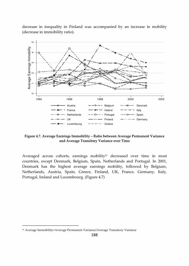
188
decrease in inequality in Finland was accompanied by an increase in mobility
(decrease in immobility ratio).
Figure 4.7. Average Earnings Immobility – Ratio between Average Permanent Variance
and Average Transitory Variance over Time
Averaged across cohorts, earnings mobility51 decreased over time in most
countries, except Denmark, Belgium, Spain, Netherlands and Portugal. In 2001,
Denmark has the highest average earnings mobility, followed by Belgium,
Netherlands, Austria, Spain, Greece, Finland, UK, France, Germany, Italy,
Portugal, Ireland and Luxembourg. (Figure 4.7)
51 Average Immobility=Average Permanent Variance/Average Transitory Variance
01
23
45
Ave
rag
e E
arn
ing
s I
mm
ob
ility
1994 1996 1998 2000 2002
Austria Belgium Denmark
France Ireland Italy
Netherlands Portugal Spain
UK Finland Germany
Luxembourg Greece
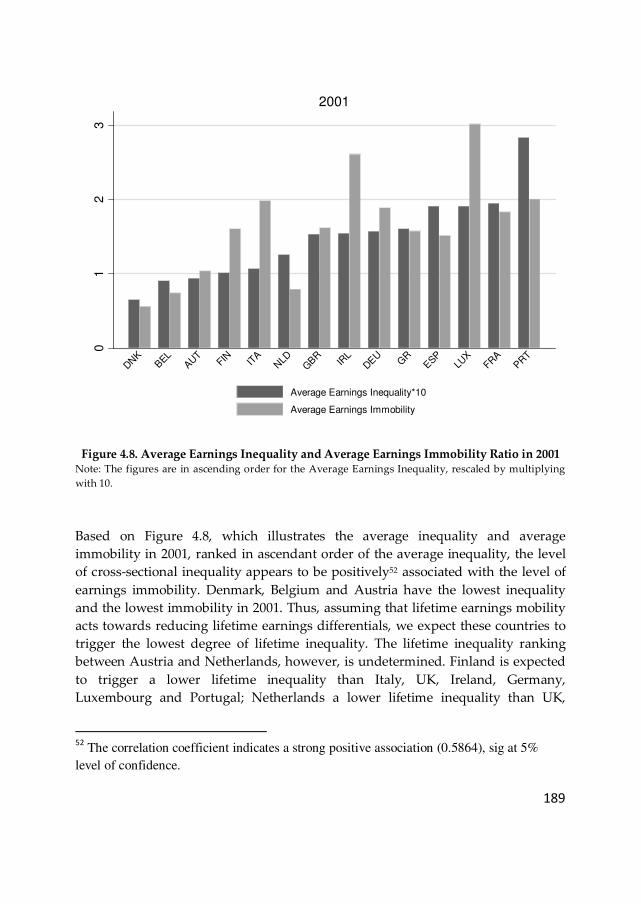
189
Figure 4.8. Average Earnings Inequality and Average Earnings Immobility Ratio in 2001 Note: The figures are in ascending order for the Average Earnings Inequality, rescaled by multiplying
with 10.
Based on Figure 4.8, which illustrates the average inequality and average
immobility in 2001, ranked in ascendant order of the average inequality, the level
of cross-sectional inequality appears to be positively52 associated with the level of
earnings immobility. Denmark, Belgium and Austria have the lowest inequality
and the lowest immobility in 2001. Thus, assuming that lifetime earnings mobility
acts towards reducing lifetime earnings differentials, we expect these countries to
trigger the lowest degree of lifetime inequality. The lifetime inequality ranking
between Austria and Netherlands, however, is undetermined. Finland is expected
to trigger a lower lifetime inequality than Italy, UK, Ireland, Germany,
Luxembourg and Portugal; Netherlands a lower lifetime inequality than UK,
52
The correlation coefficient indicates a strong positive association (0.5864), sig at 5%
level of confidence.
01
23
DNK
BEL
AUT
FIN ITA
NLD
GBR
IRL
DEU
GR
ESP
LUX
FRA
PRT
2001
Average Earnings Inequality*10
Average Earnings Immobility
190
Ireland, Denmark, Greece, Spain, Luxembourg, France and Portugal; UK a lower
lifetime inequality than Ireland Germany, Luxembourg, France and Portugal;
Ireland a lower lifetime inequality than Luxembourg; Germany a lower lifetime
inequality than Luxembourg and Portugal; Greece and Spain a lower lifetime
inequality than Luxembourg, France and Portugal; and France a lower lifetime
inequality than Portugal.
These expectations, however, are based on the strong assumption that lifetime
mobility acts towards reducing lifetime differentials.
4.10. Concluding remarks
We explored the extent to which the changes in cross-sectional earnings inequality
in 14 EU countries over the period 1994 and 2001 reflect changes in transitory
and/or permanent earnings inequality and the potential link with earnings
mobility. The analysis was broken down by cohorts to identify the potential
consequences of the labour market changes occurred after 1995 on earnings
persistency and mobility at different lifecycle stages.
Overall earnings inequality, measured by the variance in log hourly earnings,
decreased in Germany, Denmark, Belgium, France, UK, Ireland, Spain, Austria and
increased in Netherlands, Luxembourg, Italy, Greece, Portugal and Finland. For all
countries, both in relative and absolute terms, individual earnings inequality
contains a highly permanent component for the oldest three cohorts and a highly
transitory component for the youngest cohort. This is consistent with the evidence
of lifecycle earnings divergence showing that earnings volatility is higher at
younger ages. The degree of immobility is higher for older cohorts compared with
younger cohorts, which suggests that the older the cohort, the lower the
opportunity to improve one’s position in the distribution of lifetime earnings.
Overall, the decrease in inequality resulted from a decrease in transitory
differentials in Germany, France, UK and Ireland, in permanent differentials in
Belgium and Spain, and in both components in Denmark and Austria. The increase
in inequality reflects an increase in permanent differentials in Luxembourg, Italy,
Greece and Finland, and an increase in both components in Portugal and
Netherlands. The decrease in inequality was accompanied by an increase in
mobility only in Denmark, Belgium and Spain. Except for Netherlands and
Portugal, all countries recording an increase in inequality experienced also a
decrease in mobility.

191
More important are the welfare implications of these trends. We start with the
countries recording a decrease in overall inequality. In Denmark, Belgium and
Spain, mobility appears to be beneficial: in 2001, low wage individuals are better
off both in terms of their relative wage and in terms of the opportunities to escape
the low-wage trap in a lifetime perspective. Thus in a lifetime perspective,
Denmark, Belgium and Spain are expected to reduce lifetime earnings differentials
compared with annual differentials.
In Austria, Germany, France, UK and Ireland, in 2001, low-wage individuals are
worse off in terms of the opportunity to escape the low-wage trap, but their
relative position in the earnings distribution is improved compared with the 1st
wave. For these countries mobility is expected to play a decreasing role in reducing
lifetime inequality, therefore annual differentials have a high chance of being
preserved in a lifetime perspective.
The inequality and mobility behaviour across cohorts differ from the general trend
in a few countries. The youngest cohort recorded an increase in inequality
accompanied by an increase in mobility in Belgium, Spain, and UK, suggesting that
in 2001 young low wage workers are worst of in terms of their relative wage, but
better off in terms of their opportunity to improve their earnings position in a
lifetime perspective. Hence, the reforms might have increased employment and
wage flexibility among young workers. The second youngest cohort recorded a
decrease in inequality accompanied by a decrease in mobility in Denmark, and an
increase in inequality accompanied by a decrease in mobility in Germany, France
and UK. The oldest cohort recorded an increase in inequality accompanied by an
increase in mobility in Germany and Spain, suggesting that in 2001 older low wage
workers are worst off in terms of their relative wage, but better off in terms of their
opportunity to escape low-wage trap. This might result from increased
employment and wage flexibility among older workers. In Belgium, the oldest
cohort recorded a decrease in inequality accompanied by a decrease in mobility,
suggesting that in 2001, among older workers, low wage workers are better off in
terms of their relative wage, but worst off in terms of the opportunity to escape
low-wage trap in a lifetime perspective.
Among countries recording an increase in earnings inequality, in Luxembourg,
Italy, Greece, and Finland, besides the widening wages differentials, low wage
individuals find it harder to better their position in the wage distribution in 2001
compared with the first wave. Thus we can expect these countries to increase
lifetime earnings differentials compared with annual differentials. Netherlands and
Portugal record widening wages differentials accompanied by increased
opportunity of low wage individuals to improve their position in the distribution

192
of lifetime earnings. Thus, for Netherlands and Portugal, earnings mobility could
either decrease or exacerbate lifetime earnings differentials compared with annual
ones.
These trends are valid across cohorts, suggesting that the changes in the labour
market affected all workers in a similar way. Two exceptions are Finland, where
for the youngest cohort inequality decreased and was accompanied by an increase
in mobility, and Luxembourg, where for the youngest cohort inequality increased
and was accompanied by an increase in mobility.
The evolution of the inequality structure and earnings mobility was not monotonic.
Most countries experienced a sharp turnaround around 1996-1999, which could be
linked with the EU labour market changes after 1995. Hence, future research could
explore the role of labour market factors in explaining cross-national differences in
permanent and transitory inequality, and earnings mobility, a topic neglected by
the existing literature.

193
4.11. Annex
Table 4-A-1. Inflows Inflows and Outflows of Individuals in the Sample - Germany
1994 1995 1996 1997 1998 1999 2000 2001
Number of individuals with
positive earnings 25018 26059 25806 24889 23290 22955 21909 20703
Absolute number and proportion of individuals who report positive earnings in current year conditional on being in
the sample in previous year
Frequencies 23956 25224 24197 22814 22321 21290 20107
% 66.99 67.37 66.2 63.01 64.84 64.86 64.39
Absolute number and proportion of individuals who report no earnings in current year conditional on being in the
sample in the previous year
Unemployed
Inactive
Frequencies 3448 3461 4119 3932 3055 2787 2766
% 9.64 9.24 11.27 10.86 8.87 8.49 8.86
Attrition Frequencies 1885 2182 1892 3280 2951 2924 2830
% 5.27 5.83 5.18 9.06 8.57 8.91 9.06
Missing Wage Frequencies 6470 6576 6345 6180 6100 5826 5524
% 18.09 17.56 17.36 17.07 17.72 17.75 17.69
Total
Frequencies 35759 37443 36553 36206 34427 32827 31227
% 100 100 100 100 100 100 100
Table 4-A-1. Inflows and Outflows of Individuals in the Sample – Denmark
1994 1995 1996 1997 1998 1999 2000 2001
Number of individuals with
positive earnings 20899 20399 19190 19062 17321 16235 15678 15380
Absolute number and proportion of individuals who report positive earnings in current year conditional on being in the
sample in previous year
Frequencies 19854 18527 18110 16442 15334 14865 14642
% 68.74 66.59 69.43 66.23 67.41 69.6 71.6
Absolute number and proportion of individuals who report no earnings in current year conditional on being in the
sample in the previous year
Unemployed
Inactive
Frequencies 1535 1744 951 899 732 658 958
% 5.31 6.27 3.65 3.62 3.22 3.08 4.68
Attrition Frequencies 2440 3096 2914 3603 2922 2133 1775
% 8.45 11.13 11.17 14.51 12.85 9.99 8.68
Missing Wage Frequencies 5054 4454 4110 3881 3759 3703 3074
% 17.5 16.01 15.76 15.63 16.53 17.34 15.03
Total
Frequencies 28883 27821 26085 24825 22747 21359 20449
% 100 100 100 100 100 100 100
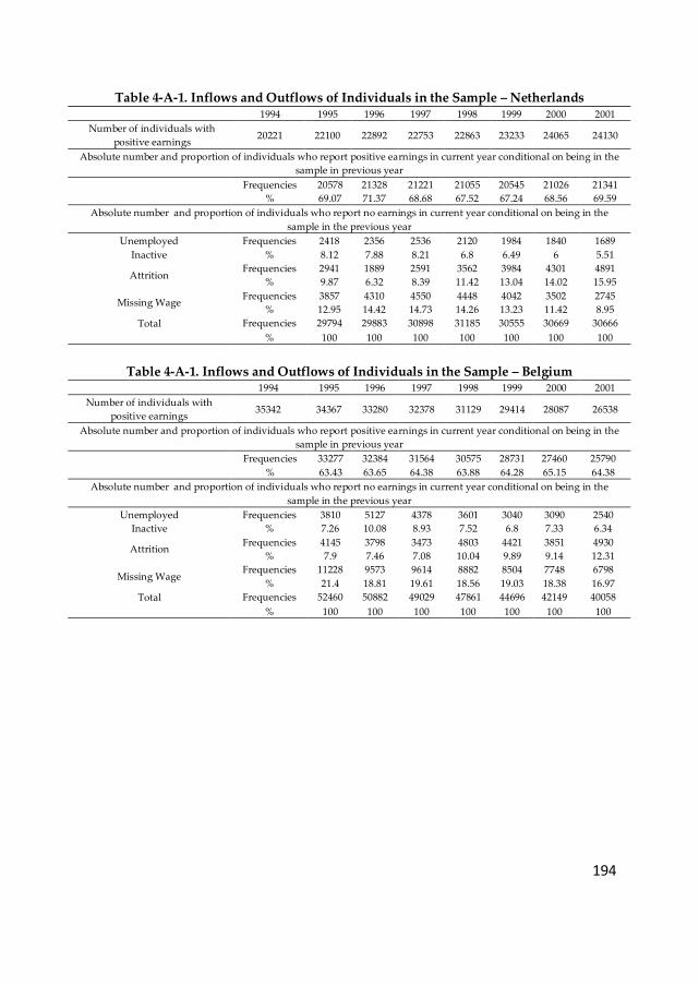
194
Table 4-A-1. Inflows and Outflows of Individuals in the Sample – Netherlands
1994 1995 1996 1997 1998 1999 2000 2001
Number of individuals with
positive earnings 20221 22100 22892 22753 22863 23233 24065 24130
Absolute number and proportion of individuals who report positive earnings in current year conditional on being in the
sample in previous year
Frequencies 20578 21328 21221 21055 20545 21026 21341
% 69.07 71.37 68.68 67.52 67.24 68.56 69.59
Absolute number and proportion of individuals who report no earnings in current year conditional on being in the
sample in the previous year
Unemployed
Inactive
Frequencies 2418 2356 2536 2120 1984 1840 1689
% 8.12 7.88 8.21 6.8 6.49 6 5.51
Attrition Frequencies 2941 1889 2591 3562 3984 4301 4891
% 9.87 6.32 8.39 11.42 13.04 14.02 15.95
Missing Wage Frequencies 3857 4310 4550 4448 4042 3502 2745
% 12.95 14.42 14.73 14.26 13.23 11.42 8.95
Total
Frequencies 29794 29883 30898 31185 30555 30669 30666
% 100 100 100 100 100 100 100
Table 4-A-1. Inflows and Outflows of Individuals in the Sample – Belgium
1994 1995 1996 1997 1998 1999 2000 2001
Number of individuals with
positive earnings 35342 34367 33280 32378 31129 29414 28087 26538
Absolute number and proportion of individuals who report positive earnings in current year conditional on being in the
sample in previous year
Frequencies 33277 32384 31564 30575 28731 27460 25790
% 63.43 63.65 64.38 63.88 64.28 65.15 64.38
Absolute number and proportion of individuals who report no earnings in current year conditional on being in the
sample in the previous year
Unemployed
Inactive
Frequencies 3810 5127 4378 3601 3040 3090 2540
% 7.26 10.08 8.93 7.52 6.8 7.33 6.34
Attrition Frequencies 4145 3798 3473 4803 4421 3851 4930
% 7.9 7.46 7.08 10.04 9.89 9.14 12.31
Missing Wage Frequencies 11228 9573 9614 8882 8504 7748 6798
% 21.4 18.81 19.61 18.56 19.03 18.38 16.97
Total
Frequencies 52460 50882 49029 47861 44696 42149 40058
% 100 100 100 100 100 100 100
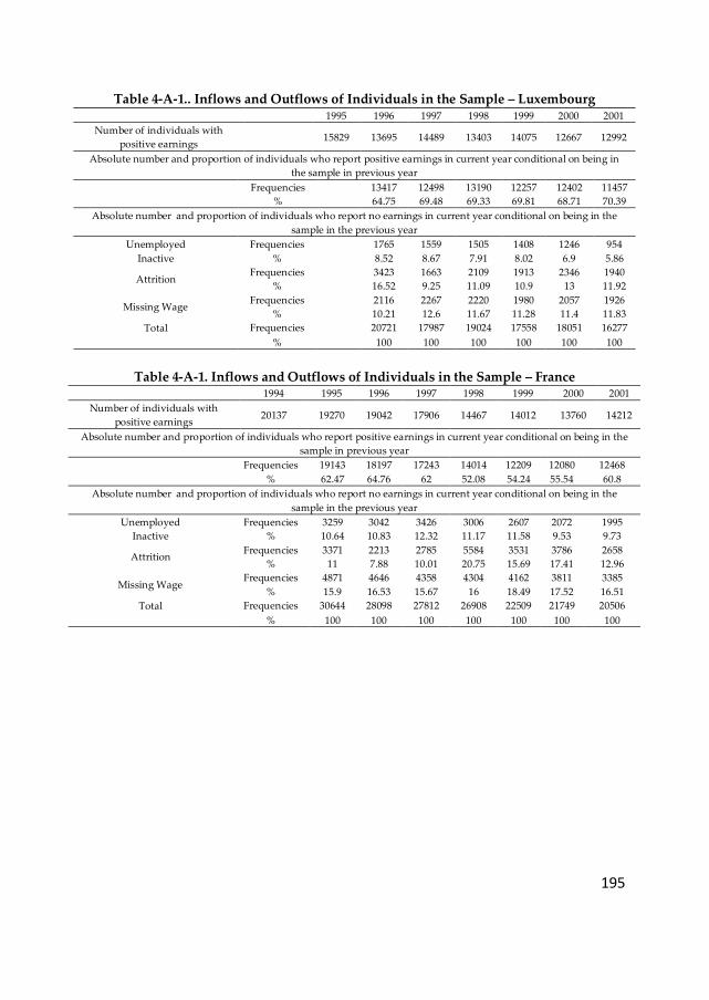
195
Table 4-A-1.. Inflows and Outflows of Individuals in the Sample – Luxembourg
1995 1996 1997 1998 1999 2000 2001
Number of individuals with
positive earnings 15829 13695 14489 13403 14075 12667 12992
Absolute number and proportion of individuals who report positive earnings in current year conditional on being in
the sample in previous year
Frequencies
13417 12498 13190 12257 12402 11457
%
64.75 69.48 69.33 69.81 68.71 70.39
Absolute number and proportion of individuals who report no earnings in current year conditional on being in the
sample in the previous year
Unemployed
Inactive
Frequencies
1765 1559 1505 1408 1246 954
%
8.52 8.67 7.91 8.02 6.9 5.86
Attrition Frequencies
3423 1663 2109 1913 2346 1940
%
16.52 9.25 11.09 10.9 13 11.92
Missing Wage Frequencies
2116 2267 2220 1980 2057 1926
%
10.21 12.6 11.67 11.28 11.4 11.83
Total
Frequencies
20721 17987 19024 17558 18051 16277
%
100 100 100 100 100 100
Table 4-A-1. Inflows and Outflows of Individuals in the Sample – France
1994 1995 1996 1997 1998 1999 2000 2001
Number of individuals with
positive earnings 20137 19270 19042 17906 14467 14012 13760 14212
Absolute number and proportion of individuals who report positive earnings in current year conditional on being in the
sample in previous year
Frequencies 19143 18197 17243 14014 12209 12080 12468
% 62.47 64.76 62 52.08 54.24 55.54 60.8
Absolute number and proportion of individuals who report no earnings in current year conditional on being in the
sample in the previous year
Unemployed
Inactive
Frequencies 3259 3042 3426 3006 2607 2072 1995
% 10.64 10.83 12.32 11.17 11.58 9.53 9.73
Attrition Frequencies 3371 2213 2785 5584 3531 3786 2658
% 11 7.88 10.01 20.75 15.69 17.41 12.96
Missing Wage Frequencies 4871 4646 4358 4304 4162 3811 3385
% 15.9 16.53 15.67 16 18.49 17.52 16.51
Total
Frequencies 30644 28098 27812 26908 22509 21749 20506
% 100 100 100 100 100 100 100
196
Table 4-A-1.1. Inflows and Outflows of Individuals in the Sample – UK
1994 1995 1996 1997 1998 1999 2000 2001
Number of individuals with
positive earnings 24949 25329 25495 26010 26145 25750 25674 25264
Absolute number and proportion of individuals who report positive earnings in current year conditional on being in the
sample in previous year
Frequencies 24511 24848 25303 25278 25006 24881 24467
% 64.59 66.31 67.06 67.04 67.36 68.33 68.58
Absolute number and proportion of individuals who report no earnings in current year conditional on being in the
sample in the previous year
Unemployed
Inactive
Frequencies 4712 5053 4663 4140 3941 3607 3595
% 12.42 13.48 12.36 10.98 10.62 9.91 10.08
Attrition Frequencies 1836 966 1169 2073 1919 2153 2105
% 4.84 2.58 3.1 5.5 5.17 5.91 5.9
Missing Wage Frequencies 6888 6605 6597 6213 6257 5774 5510
% 18.15 17.63 17.48 16.48 16.85 15.86 15.44
Total
Frequencies 37947 37472 37732 37704 37123 36415 35677
% 100 100 100 100 100 100 100
Table 4-A-1.. Inflows and Outflows of Individuals in the Sample – Ireland
1994 1995 1996 1997 1998 1999 2000 2001
Number of individuals with
positive earnings 13937 13221 12590 12515 12435 12091 10745 9727
Absolute number and proportion of individuals who report positive earnings in current year conditional on being in the
sample in previous year
Frequencies 12750 12217 12212 12020 11668 10236 9507
% 49.99 50.04 52.41 53.13 54.1 51.63 54.65
Absolute number and proportion of individuals who report no earnings in current year conditional on being in the
sample in the previous year
Unemployed
Inactive
Frequencies 4930 4723 4254 3374 2905 2185 2307
% 19.33 19.35 18.26 14.91 13.47 11.02 13.26
Attrition Frequencies 2167 2115 1600 1936 2516 3288 2362
% 8.5 8.66 6.87 8.56 11.66 16.59 13.58
Missing Wage Frequencies 5656 5359 5235 5292 4480 4116 3220
% 22.18 21.95 22.47 23.39 20.77 20.76 18.51
Total
Frequencies 25503 24414 23301 22622 21569 19825 17396
% 100 100 100 100 100 100 100
197
Table 4-A-1. Inflows and Outflows of Individuals in the Sample – Italy
1994 1995 1996 1997 1998 1999 2000 2001
Number of individuals with
positive earnings 32633 32236 32111 29661 28865 26993 26912 25170
Absolute number and proportion of individuals who report positive earnings in current year conditional on being in the
sample in previous year
Frequencies 30946 31028 28717 27188 25717 25348 24139
% 51.58 51.19 47.18 47.34 46.87 48.73 48.86
Absolute number and proportion of individuals who report no earnings in current year conditional on being in the
sample in the previous year
Unemployed
Inactive
Frequencies 7900 7799 7670 6627 6890 5662 5027
% 13.17 12.87 12.6 11.54 12.56 10.88 10.18
Attrition Frequencies 3175 2947 5922 6030 5941 5399 5920
% 5.29 4.86 9.73 10.5 10.83 10.38 11.98
Missing Wage Frequencies 17978 18836 18559 17585 16325 15610 14315
% 29.96 31.08 30.49 30.62 29.75 30.01 28.98
Total
Frequencies 59999 60610 60868 57430 54873 52019 49401
% 100 100 100 100 100 100 100
Table 4-A-1. Inflows and Outflows of Individuals in the Sample – Greece
1994 1995 1996 1997 1998 1999 2000 2001
Number of individuals with
positive earnings 27974 27654 26150 24865 22675 22001 21335 21929
Absolute number and proportion of individuals who report positive earnings in current year conditional on being in
the sample in previous year
Frequencies 26868 25946 24385 21815 20357 20443 21342
% 45.83 45.69 44.98 42.09 43.52 46.06 49.72
Absolute number and proportion of individuals who report no earnings in current year conditional on being in the
sample in the previous year
Unemployed
Inactive
Frequencies 7537 6813 6419 4523 4489 4427 3858
% 12.86 12 11.84 8.73 9.6 9.97 8.99
Attrition Frequencies 4417 4392 4347 7892 6222 4159 2363
% 7.53 7.73 8.02 15.23 13.3 9.37 5.5
Missing Wage Frequencies 19802 19640 19068 17599 15707 15352 15365
% 33.78 34.58 35.17 33.96 33.58 34.59 35.79
Total
Frequencies 58624 56791 54219 51829 46775 44381 42928
% 100 100 100 100 100 100 100
198
Table 4-A-1. Inflows and Outflows of Individuals in the Sample – Spain
1994 1995 1996 1997 1998 1999 2000 2001
Number of individuals with
positive earnings 22559 21863 21296 20975 20371 20580 19898 20185
Absolute number and proportion of individuals who report positive earnings in current year conditional on being in the
sample in previous year
Frequencies 21460 20521 20329 19456 19679 19167 19352
% 47.6 48.29 48.49 48.63 52.13 52.12 56.06
Absolute number and proportion of individuals who report no earnings in current year conditional on being in the
sample in the previous year
Unemployed
Inactive
Frequencies 8419 8230 7353 5970 5083 4512 4761
% 18.67 19.37 17.54 14.92 13.46 12.27 13.79
Attrition Frequencies 4467 3000 4120 4327 3188 3922 3052
% 9.91 7.06 9.83 10.81 8.44 10.66 8.84
Missing Wage Frequencies 10741 10742 10121 10259 9802 9176 7357
% 23.82 25.28 24.14 25.64 25.96 24.95 21.31
Total
Frequencies 45087 42493 41923 40012 37752 36777 34522
% 100 100 100 100 100 100 100
Table 4-A-1. Inflows and Outflows of Individuals in the Sample – Portugal
1994 1995 1996 1997 1998 1999 2000 2001
Number of individuals with
positive earnings 14653 15450 15379 15087 14837 14569 14604 14550
Absolute number and proportion of individuals who report positive earnings in current year conditional on being in the
sample in previous year
Frequencies 13892 14538 14321 13977 13921 13952 13942
% 57.84 57.5 57.32 56.98 59.12 60.83 62.16
Absolute number and proportion of individuals who report no earnings in current year conditional on being in the
sample in the previous year
Unemployed
Inactive
Frequencies 2187 2264 2396 2019 2067 1843 1702
% 9.11 8.95 9.59 8.23 8.78 8.04 7.59
Attrition Frequencies 1701 1908 1918 2346 1956 1617 1575
% 7.08 7.55 7.68 9.56 8.31 7.05 7.02
Missing Wage Frequencies 6236 6573 6350 6189 5602 5525 5211
% 25.97 26 25.42 25.23 23.79 24.09 23.23
Total
Frequencies 24016 25283 24985 24531 23546 22937 22430
% 100 100 100 100 100 100 100
199
Table 4-A-1. Inflows and Outflows of Individuals in the Sample – Austria
1994 1995 1996 1997 1998 1999 2000 2001
Number of individuals with
positive earnings 17944 17789 17199 16209 15162 13816 13056
Absolute number and proportion of individuals who report positive earnings in current year conditional on being in the
sample in previous year
Frequencies 16472 16384 15634 14551 13403 12601
% 67.96 68.2 67.49 67.2 66.51 68.21
Absolute number and proportion of individuals who report no earnings in current year conditional on being in the
sample in the previous year
Unemployed
Inactive
Frequencies 1209 1231 906 790 803 843
% 4.99 5.12 3.91 3.65 3.98 4.56
Attrition Frequencies 2195 2080 2435 2470 2409 1794
% 9.06 8.66 10.51 11.41 11.95 9.71
Missing Wage Frequencies 4361 4330 4189 3842 3538 3235
% 17.99 18.02 18.08 17.74 17.56 17.51
Total
Frequencies 24237 24025 23164 21653 20153 18473
%
100 100 100 100 100 100
Table 4-A-1.. Inflows and Outflows of Individuals in the Sample – Finland
1996 1997 1998 1999 2000 2001
Number of individuals with
positive earnings
15811 15845 15895 15546 13329 13057
Absolute number and proportion of individuals who report positive earnings in current year conditional on being in the
sample in previous year
Frequencies
15246 15345 14753 12756 12588
%
55.95 57.2 59.29 53.83 64.16
Absolute number and proportion of individuals who report no earnings in current year conditional on being in the
sample in the previous year
Unemployed
Inactive
Frequencies
3446 2327 1657 1326 1267
%
12.65 8.67 6.66 5.6 6.46
Attrition Frequencies
1933 3219 2658 5219 1708
%
7.09 12 10.68 22.02 8.71
Missing Wage Frequencies
6623 5937 5814 4398 4057
%
24.31 22.13 23.37 18.56 20.68
Total
Frequencies
27248 26828 24882 23699 19620
%
100 100 100 100 100
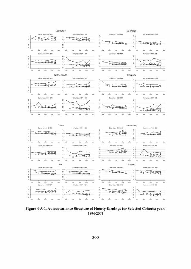
200
Figure 4-A-1. Autocovariance Structure of Hourly Earnings for Selected Cohorts: years
1994-2001
0.0
5.1
.15
.2
1994 1996 1998 2000 2002
Cohort born 1940-1950
0.0
5.1
.15
.2
1994 1996 1998 2000 2002
Cohort born 1951-1960
0.0
5.1
.15
.2
1994 1996 1998 2000 2002
Cohort born 1961-1970
0.0
5.1
.15
.2
1994 1996 1998 2000 2002
Cohort born 1971-1981
Germany
0.0
5.1
.15
1994 1996 1998 2000 2002
Cohort born 1940-1950
0.0
5.1
.15
1994 1996 1998 2000 2002
Cohort born 1951-1960
0.0
5.1
.15
1994 1996 1998 2000 2002
Cohort born 1961-1970
0.0
5.1
.15
1994 1996 1998 2000 2002
Cohort born 1971-1981
Denmark
0.0
5.1
.15
1994 1996 1998 2000 2002
Cohort born 1940-1950
0.0
5.1
.15
1994 1996 1998 2000 2002
Cohort born 1951-1960
0.0
5.1
.15
1994 1996 1998 2000 2002
Cohort born 1961-1970
0.0
5.1
.15
1994 1996 1998 2000 2002
Cohort born 1971-1981
Netherlands
0.0
5.1
.15
1994 1996 1998 2000 2002
Cohort born 1940-1950
0.0
5.1
.15
1994 1996 1998 2000 2002
Cohort born 1951-1960
0.0
5.1
.15
1994 1996 1998 2000 2002
Cohort born 1961-1970
0.0
5.1
.15
1994 1996 1998 2000 2002
Cohort born 1971-1981
Belgium
0.1
.2.3
1994 1996 1998 2000 2002
Cohort born 1940-1950
0.1
.2.3
1994 1996 1998 2000 2002
Cohort born 1951-1960
0.1
.2.3
1994 1996 1998 2000 2002
Cohort born 1961-1970
0.1
.2.3
1994 1996 1998 2000 2002
Cohort born 1971-1981
France
0.0
5.1
.15
.2.2
5
1994 1996 1998 2000 2002
Cohort born 1940-1950
0.0
5.1
.15
.2.2
5
1994 1996 1998 2000 2002
Cohort born 1951-1960
0.0
5.1
.15
.2.2
5
1994 1996 1998 2000 2002
Cohort born 1961-1970
0.0
5.1
.15
.2.2
5
1994 1996 1998 2000 2002
Cohort born 1971-1981
Luxembourg
0.0
5.1
.15
.2
1994 1996 1998 2000 2002
Cohort born 1940-1950
0.0
5.1
.15
.2
1994 1996 1998 2000 2002
Cohort born 1951-1960
0.0
5.1
.15
.2
1994 1996 1998 2000 2002
Cohort born 1961-1970
0.0
5.1
.15
.2
1994 1996 1998 2000 2002
Cohort born 1971-1981
UK
0.0
5.1
.15
.2
1994 1996 1998 2000 2002
Cohort born 1940-1950
0.0
5.1
.15
.2
1994 1996 1998 2000 2002
Cohort born 1951-1960
0.0
5.1
.15
.2
1994 1996 1998 2000 2002
Cohort born 1961-1970
0.0
5.1
.15
.2
1994 1996 1998 2000 2002
Cohort born 1971-1981
Ireland
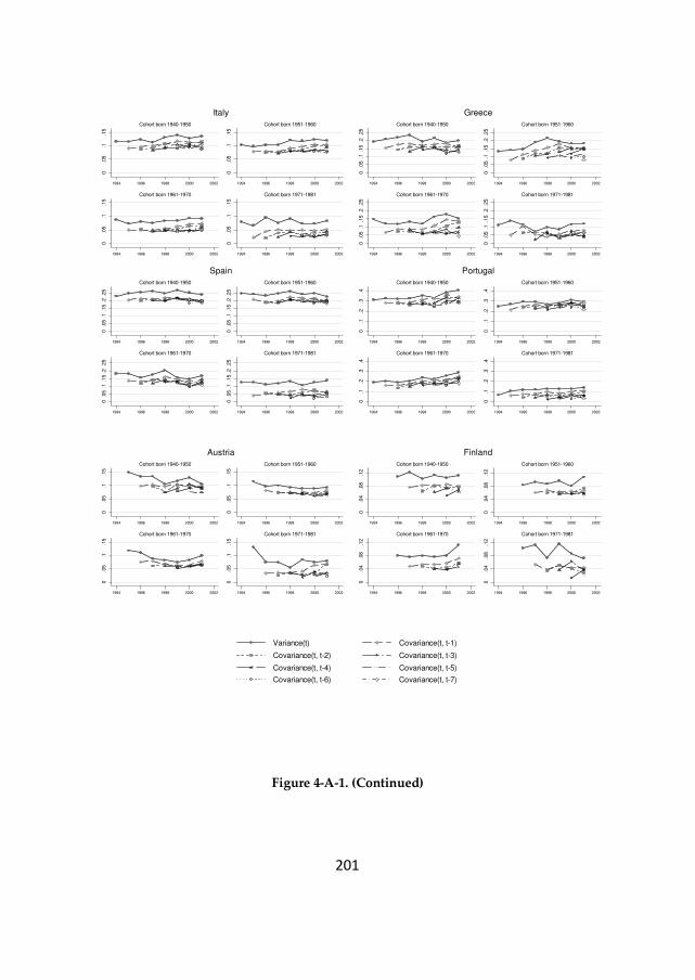
201
Figure 4-A-1. (Continued)
0.0
5.1
.15
1994 1996 1998 2000 2002
Cohort born 1940-1950
0.0
5.1
.15
1994 1996 1998 2000 2002
Cohort born 1951-1960
0.0
5.1
.15
1994 1996 1998 2000 2002
Cohort born 1961-1970
0.0
5.1
.15
1994 1996 1998 2000 2002
Cohort born 1971-1981
Italy
0.0
5.1
.15
.2.2
5
1994 1996 1998 2000 2002
Cohort born 1940-1950
0.0
5.1
.15
.2.2
5
1994 1996 1998 2000 2002
Cohort born 1951-1960
0.0
5.1
.15
.2.2
5
1994 1996 1998 2000 2002
Cohort born 1961-1970
0.0
5.1
.15
.2.2
5
1994 1996 1998 2000 2002
Cohort born 1971-1981
Greece
0.0
5.1
.15
.2.2
5
1994 1996 1998 2000 2002
Cohort born 1940-1950
0.0
5.1
.15
.2.2
5
1994 1996 1998 2000 2002
Cohort born 1951-1960
0.0
5.1
.15
.2.2
5
1994 1996 1998 2000 2002
Cohort born 1961-1970
0.0
5.1
.15
.2.2
5
1994 1996 1998 2000 2002
Cohort born 1971-1981
Spain
0.1
.2.3
.4
1994 1996 1998 2000 2002
Cohort born 1940-1950
0.1
.2.3
.4
1994 1996 1998 2000 2002
Cohort born 1951-1960
0.1
.2.3
.4
1994 1996 1998 2000 2002
Cohort born 1961-1970
0.1
.2.3
.4
1994 1996 1998 2000 2002
Cohort born 1971-1981
Portugal
0.0
5.1
.15
1994 1996 1998 2000 2002
Cohort born 1940-1950
0.0
5.1
.15
1994 1996 1998 2000 2002
Cohort born 1951-1960
0.0
5.1
.15
1994 1996 1998 2000 2002
Cohort born 1961-1970
0.0
5.1
.15
1994 1996 1998 2000 2002
Cohort born 1971-1981
Austria
0.0
4.0
8.1
2
1994 1996 1998 2000 2002
Cohort born 1940-1950
0.0
4.0
8.1
2
1994 1996 1998 2000 2002
Cohort born 1951-1960
0.0
4.0
8.1
2
1994 1996 1998 2000 2002
Cohort born 1961-1970
0.0
4.0
8.1
2
1994 1996 1998 2000 2002
Cohort born 1971-1981
Finland
Variance(t) Covariance(t, t-1)
Covariance(t, t-2) Covariance(t, t-3)
Covariance(t, t-4) Covariance(t, t-5)
Covariance(t, t-6) Covariance(t, t-7)
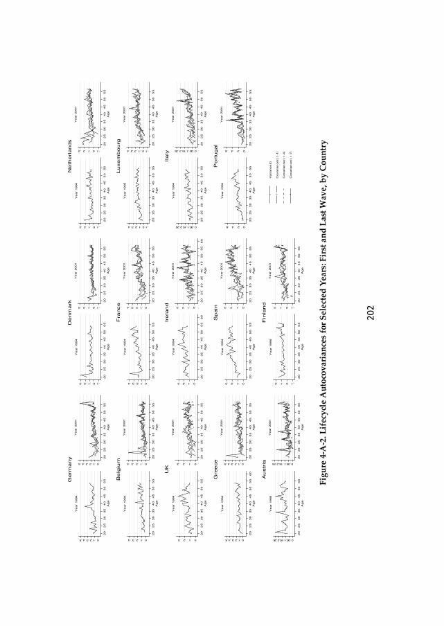
20
2
F
igu
re 4
-A-2
. Lif
ecy
cle
Au
toco
var
ian
ces
for
Sel
ecte
d Y
ears
: Fir
st a
nd
Las
t W
ave,
by
Co
un
try
0.1.2.3.4.5
20
25
30
35
40
45
50
55
Ag
e
Ye
ar
19
94
0.1.2.3.4.5
20
25
30
35
40
45
50
55
Ag
e
Ye
ar
20
01
Germ
any
-.10.1.2.3
20
25
30
35
40
45
50
55
Ag
e
Ye
ar 1
994
-.10.1.2.3
20
25
30
35
40
45
50
55
Ag
e
Ye
ar
20
01
De
nm
ark
-.10.1.2.3
20
25
30
35
40
45
50
55
Ag
e
Ye
ar 1
994
-.10.1.2.3
20
25
30
35
40
45
50
55
Ag
e
Ye
ar
20
01
Ne
the
rlan
ds
0.1.2.3.4
20
25
30
35
40
45
50
55
Ag
e
Ye
ar
19
94
0.1.2.3.4
20
25
30
35
40
45
50
55
Ag
e
Ye
ar
20
01
Be
lgiu
m
0.1.2.3.4
20
25
30
35
40
45
50
55
Ag
e
Ye
ar 1
994
0.1.2.3.4
20
25
30
35
40
45
50
55
Ag
e
Ye
ar
20
01
Fra
nce
-.10.1.2.3.4
20
25
30
35
40
45
50
55
Ag
e
Ye
ar 1
995
-.10.1.2.3.4
20
25
30
35
40
45
50
55
Ag
e
Ye
ar
20
01
Luxe
mbo
urg
0.1.2.3
20
25
30
35
40
45
50
55
Ag
e
Ye
ar
19
94
0.1.2.3
20
25
30
35
40
45
50
55
Ag
e
Ye
ar
20
01
UK
0.1.2.3
20
25
30
35
40
45
50
55
60
Ag
e
Ye
ar 1
994
0.1.2.3
20
25
30
35
40
45
50
55
60
Ag
e
Ye
ar
20
01
Ire
lan
d
0.05.1.15.2.25
20
25
30
35
40
45
50
55
Ag
e
Ye
ar 1
994
0.05.1.15.2.25
20
25
30
35
40
45
50
55
Ag
e
Ye
ar
20
01
Ita
ly
0.1.2.3.4.5
20
25
30
35
40
45
50
55
60
Ag
e
Ye
ar
19
94
0.1.2.3.4.5
20
25
30
35
40
45
50
55
Ag
e
Ye
ar
20
01
Gree
ce
0.1.2.3
20
25
30
35
40
45
50
55
Ag
e
Ye
ar 1
994
0.1.2.3
20
25
30
35
40
45
50
55
Ag
e
Ye
ar
20
01
Sp
ain
0.2.4.6
20
25
30
35
40
45
50
55
Ag
e
Ye
ar 1
994
0.2.4.6
20
25
30
35
40
45
50
55
Ag
e
Ye
ar
20
01
Po
rtug
al
0.05.1.15.2.25
20
25
30
35
40
45
50
55
Ag
e
Ye
ar
19
95
0.05.1.15.2.25
20
25
30
35
40
45
50
55
Ag
e
Ye
ar
20
01
Au
str
ia
-.10.1.2
20
25
30
35
40
45
50
55
Ag
e
Ye
ar 1
996
-.10.1.2
20
25
30
35
40
45
50
55
Ag
e
Ye
ar
20
01
Fin
lan
d
Vari
an
ce
(t)
Covari
an
ce
(t,
t-1
)
Covari
an
ce
(t,
t-4
)
Covari
an
ce
(t,
t-7
)

203
5. POLICY, INSTITUTIONAL FACTORS AND EARNINGS
MOBILITY
204
5.1.Introduction53
The rise in earnings inequality experienced by many developed countries during
the 1980s and 1990s triggered a strong debate with respect to the driving factors
behind individual earnings dynamics and the implications of this increase. The
empirical literature has covered extensively the driving factors behind the increase
in cross-sectional earnings inequality. Factors like economic growth (“Kuznetz
hypothesis”); “the shift in demand away from unskilled labour in favour of skilled
workers” (Atkinson 1996) under the impact of trade liberalization, skill-biased
technological change and organizational change; the role of changes in the labour
market institutions, such as unionization and centralized bargaining,
macroeconomic volatility, are among the main possible drivers of income
inequality as identified by the empirical literature (Freeman and Katz, 1994; 1995;
Fortin and Lemieux, 1997; Gottschalk and Smeeding, 1997; Katz and Autor, 1999;
Aghion and Williamson, 2001).
Notwithstanding this, the empirical literature has neglected so far the driving
factors behind the two components of earnings inequality: permanent and
transitory inequality. Even less attention was given to the driving factors behind
earnings mobility, which, as stated by Milton Friedman (1962), represents a very
important aspect for understanding inequality. All these labour market outcomes
are highly important given that the interplay between them determines the final
earnings inequality outcome, both in an annual and lifetime perspective.
In this line of thought, this paper explores the role of labour market policy and
institutional factors in explaining cross-national differences in the evolution of
permanent inequality, transitory inequality and earnings mobility across 14 EU
countries. So far, at the EU level, no study attempted to analyse and to understand
the driving factors behind the three labour market outcomes in a comparative
manner.
53 This Chapter builds on the results discussed in Chapter 4: using the predicted components from the
error component models estimated in Chapter 4 and the OECD data, we estimate the relationship
between the three labour market outcomes – permanent inequality, transitory inequality and earnings
immobility – and the labour market policy and institutional factors. Since this Chapter is written as a
standalone paper, the information in sections 5.2.3.1, 5.2.3.2, 5.4.1, 5.5.1, 5.6 summarises the core aspects
of Chapter 4: the econometric specification and estimation method of the covariance earnings structure,
the dynamic autocovariance structure of hourly earnings, and the results of the covariance structure
estimation for each country.

205
Understanding the driving forces behind these labour market outcomes is vitally
important from a welfare perspective, particularly given the large variation in the
evolution of cross-sectional wage inequality across Europe over the period 1994-
2001. Did the increase in cross-sectional wage inequality observed in some
countries result from greater transitory fluctuations in earnings and individuals
facing a higher degree of earnings mobility? Or is this rise reflecting increasing
permanent differences between individuals with mobility remaining constant or
even falling? What about countries that recorded a decrease in cross-sectional
earnings inequalities, what lessons can we learn from them? What are the possible
labour market policy and institutional factors that can explain these trends in
permanent and transitory differentials, and earnings mobility?
These questions have a twofold importance. On the one hand, understanding the
contributions of the changes in permanent and transitory components of earnings
variation to the changes in cross-sectional earnings inequality is very useful in the
evaluation of alternative hypotheses for wage structure changes and for
determining the potential welfare consequences of rising inequality (Katz and
Autor 1999).
On the other hand, understanding the driving factors behind the changes in
permanent and transitory inequality and earnings mobility is very useful for the
design of policies and labour market institutions. Earnings mobility is perceived in
the literature as a way out of poverty. In the absence of mobility the same
individuals remain stuck at the bottom of the distribution, hence annual earnings
differentials are transformed into lifetime earnings differentials. Understanding the
factors that enhance earnings mobility, represents a step forward towards
designing policies and institutions that enable low-wage workers to escape low-
wage jobs and improve their position in the distribution of lifetime earnings.
These questions are highly relevant in the context of the changes that took place in
the EU labour market policy framework under the incidence of the 1994 OECD
Jobs Strategy and the 2000 Lisbon Agenda, which recommended policies to
increase wage flexibility, lower non-wage labour costs and allow relative wages to
better reflect individual differences in productivity and local labour market
conditions. The turnaround in the institutional and policy framework occurred
more or less after 1995 (OECD, 2004; Dew-Becker and Gordon, 2008). Before 1995,
Europe could have been described as making labour more expensive, accompanied
by a decline in employment and an increase in productivity. Starting at different
dates for different policies, Europe began the process of shifting toward making
labour less expensive, accompanied by higher employment per capita but lower
average productivity per hour (Dew-Becker and Gordon 2008). Moreover, all

206
OECD countries moved towards greater decentralization, which could result in
greater inter-firm wage differentials. These trends appear to have worsened the
apparent trade-off between a strong employment performance and a more equal
distribution of earnings, consistent with relative labour demand having shifted
towards high-skilled workers OECD (2004).
As pointed out by Dew-Becker and Gordon (2008) and OECD (2004), the most
notable change after 1995 in Europe has been increased country heterogeneity. We
will investigate how the heterogeneity in main labour market policy and
institutional factors translates itself in the level and components of cross-sectional
earnings inequality and earnings mobility.
Using ECHP we apply equally weighted minimum distance methods to estimate
the covariance structure of earnings by four birth cohorts for each country,
decompose earnings into a permanent and a transitory component and compute
earnings mobility. The predicted components – permanent variance, transitory
variance and earnings mobility -, together with OECD data on institutional factors,
are used to estimate the relationship between these components and labour market
policy and institutional factors. The relationship between the labour market policy
and institutional factors and the three labour market outcomes is estimated using
non-linear least squares.
The structure of this paper is as follows. Section two introduces the literature
review, the theoretical background for wage differentials and the theoretical link
between labour market factors and the three labour market outcomes. Section three
provides a description of the ECHP and OECD data. Section four introduces the
econometric specifications and estimation methods for the covariance structure of
earnings and for the link between institutional and policy factors and labour
market outcomes. Section five describes the dynamic structure of individual log
earnings for 14 EU countries and the evolution of the labour market institutions
and policies. Section six fits the error components models to the covariance
structure for each country, decomposing the change in inequality into that
accounted for by the change in the permanent and transitory components. Section
seven presents the results on the link between policies and outcomes. Lastly,
section eight offers some conclusions.
207
5.2.Theoretical model of the determinants of wage differentials
5.2.1. Literature review
The existing literature on earnings dynamics is predominantly based on US data.
Atkinson, Bourguignon et al. (1992) provide a comprehensive survey of the
literature on earnings dynamics until 1992. The most representative contributions
using US or Canadian data were brought by Lillard and Willis (1978), Lillard and
Weiss (1979), MaCurdy (1982), Abowd and Card (1989)), Moffitt and Gottschalk
(1995, 1998, 2002, 2008), Baker (1997), Baker and Solon (2003). For Europe, the most
representative papers are Dickens (2000b), Ramos (2003), Kalwij and Alessie (2003),
Cappellari (2003), Gustavson (2004).
Finally, Sologon and O'Donoghue (2009a, 2009b) used ECHP for 14 EU countries to
explore the dynamic structure of individual earnings and the extent to which
changes in cross-sectional earnings inequality reflect transitory or permanent
components of individual lifecycle earnings variation. Their main findings are
used further in this paper.
The main limitation of the existing studies on earnings dynamics is that they do
not explain the main labour market policy and institutional driving factors behind
the evolution of the two inequality component and earnings mobility. Our paper
attempts to fill part of this gap.
5.2.2. Determinants of earnings inequality
As pointed out by Katz and Autor (1999), the existing literature contains many
explanations for the rise in earnings inequality experienced by many developed
countries during the 1980s and 1990s. The theory regarding the determinants of
wage differentials goes back to Adam Smith, who provided a comprehensive
discussion in his capital work, The Wealth of Nations. It was emphasized that
wage differentials are determined by competitive factors relating to the workplace
(e.g. cost of training), by innate abilities and by labour market institutional factors,
which regulated wages, restricted wages and labour mobility. The tension between
the demand and supply factors and the institutional factors affecting wage
structures that emerged from Adam Smith’s analysis has remained until today one
of the key themes of research on the wage structure. Following Freeman and Katz
(1994), this supply-demand-institutions (SDI) explanation for the changes in the
wage structure has three parts.

208
The first part assumes that different demographic and skill groups are imperfect
substitutes in production, which implies that shifts in the demand and supply for
labour skills can alter wage and employment outcomes. Potential important
sources of shifts in the relative demand among skill groups include skill-biased
technological change and a complementary increase in the prices of other inputs,
and forces of globalization (trade and outsourcing). Sources of relative supply
include cohort size variation, changes in access to education, immigration. Supply
and demand factors are expected to have their largest effect on young workers as
opposed to experienced workers with substantial work tenure (Freeman, 1976).
However, since most advanced countries operate in the same world markets, with
similar technology, industry and occupation mixes, demand and supply factors
cannot by themselves explain all the differing changes in inequality among these
countries. To fully understand the differences in labour market outcomes across
advanced countries something else is needed: the institutional framework
(Freeman and Katz 1994).
The second part states that the shock in the demand and supply may have different
effects on wages and employment, depending on different wage-setting
mechanisms and other labour market institutional factors. The stronger the wage-
setting mechanism is, meaning the higher trade union density, the higher the
union coverage and the higher the centralisation/co-ordination of wage bargaining,
the less impact these shocks have on wages. As argued by OECD (2004), there is a
strong evidence that unions reduce wage inequality and that this compression
effect is stronger in countries where union membership and bargaining coverage
are high, and bargaining is centralised and/or co-ordinated (Aidt and Tzannatos,
2002; Blau and Kahn, 1999, 2002; OECD, 1997a). National labour markets
characterized by decentralized wage bargaining experience also a higher skill
premia and a higher responsiveness of wages to local conditions, therefore a higher
wage inequality.
The third part states that institutional changes, such as changes in the degree of
unionization, the degree of centralization/co-ordination of collective bargaining, or
product market regulation have an impact on the wage structures.
Katz and Autor (1999) used the SDI model to look at cross-country differences in
wage structure changes. The shift in the demand for more skilled workers did not
result in a sharp increase in wage dispersion for all OECD countries. The
differences in the growth of skills supply appear to be an important factor in
explaining cross-country differences. The same holds for labour market
institutions. Countries, where unions, wage bargaining structure play a larger role

209
in the determination of wages recorded smaller increases in inequality. The key
issue in the interplay between demand, supply and institutions, however, is the
erroneous assumption that institutional change is exogenous. The reality is that
institutions are influenced by labour market forces. As argued by Freeman and
Gibbons (1995), shifts in supply and demand that raise relative wage differentials
are expected to reduce the strength of the centralized collective bargaining and
lower union influence on the wage setting mechanism.
5.2.3. Permanent and transitory components of earnings
inequality
Following the terminology introduced by Friedman and Kuznets (1954), individual
earnings are composed from a permanent and a transitory component. The
permanent component of earnings reflects personal characteristics, education,
training and other persistent elements. The transitory component captures both
individual random factors (e.g. illness and accident) and random changes in the
market conditions in a particular period and is expected to average out over time,
with no influence on permanent earnings. In general terms, these are factors which
are random to the individual perception. Hence, it is logical to require
independence between the permanent component and the transitory component
(Weizsäcker, 1993). Following the structure of individual earnings and the
independence assumption between the two components, overall inequality at any
point in time is composed from inequality in the permanent component of earnings
and inequality in the transitory component.
One approach for explaining changes in wage differential is to decompose overall
wage inequality into the two components. The evolution of the overall earnings
inequality is determined by the cumulative changes in the two inequality
components. As the factors from the SDI model influence overall inequality,
implicitly they influence its two components. The intriguing question that arises is
which factors influence which component and to what extent. Our focus in this
paper is mainly on labour market policy and institutional factors.
This section tries to establish a theoretical link between the changes in the two
inequality components and earnings mobility, and labour market policy and
institutional factors. First we introduce alternative specifications for decomposing
inequality. Second we introduce the concept of earnings mobility and its link with
permanent and transitory inequality. Finally we present the theoretical link
between institutions and the three labour marker outcomes – permanent
inequality, transitory inequality and earnings mobility.
210
5.2.3.1. Alternative model specifications for the permanent and
transitory components 54
Based on Sologon and O'Donoghue (2009a, 2009b), we summarize several models
of earnings dynamics that have been dominating the literature on permanent and
transitory earnings inequality over the past 30 years. For a full review, please refer
to Sologon and O'Donoghue (2009a, 2009b). We begin with the simplest
specification, which provides a very intuitive insight into the decomposition of
earnings into their permanent and transitory components. Based on this
specification earnings are being decomposed as follows:
2 2, ~ (0, ), ~ (0, ), 1,..., , 1,...,it i it i it v iY v iid v iid t T i Nµµ µ σ σ= + = =
(5.1)
where i
µ represents the permanent time-invariant individual specific component
and it
v represents the transitory component, which is independently distributed
both over individuals and time. This model imposes very rigid restrictions on the
covariance structure of earnings:
2 2
2
,( , )
,
v
it is
t sCov Y Y
t s
µ
µ
σ σ
σ
+ ==
≠
Becausei
µ is assumed to incorporate the effect of lifetime persistent individual
specific characteristics such as ability, the variance of the permanent component 2
µσ represents the persistent dispersion of earnings or the inequality in the
permanent component of earnings. The transitory shocks are captured by the
transitory variance 2
vσ and are assumed to persist only one year.
This model facilitates the understanding of the inequality decomposition into its
permanent and transitory components. The variance of earnings at a certain point
in time, as a measure of earnings dispersion, is composed both from a permanent
and a transitory dispersion (2 2
vµσ σ+ ). The covariances, on the other hand, are
determined solely by the permanent component (2
µσ ). Therefore, the assessment
of the relative importance of the two components in the overall earnings dispersion
is straightforward: the ratio 2 2
/ yµσ σ captures the relative importance of the
54 The information in this section has already been discussed in section 4.3.2.

211
permanent component, whereas the ratio 2 2
/v yσ σ captures the relative importance
of the transitory component.
Notwithstanding its attractive features, the empirical evidence rejected the rigid
restrictions imposed by model (5.1). One of the main drawbacks of model (5.1) is
that it does not allow for changes in earnings inequality over time. Other studies
(Katz, 1994; Moffitt and Gottschalk, 1995) took the model complexity further by
allowing the covariance structure of earnings to vary over time. To account for
these time effects, these models considered also time specific loading factors or
shifters on both components, which allow the parameters of the process to change
with calendar time.
1 2it t it t itY vλ µ λ= + (5.2)
, 1, 2kt
kλ = are time-varying factor loadings on the permanent and transitory
components of earnings. The variance of it
Y implied by this model takes the form:
2 2
1 2
2 2( )t tit v
Var Y µλ σ λ σ= + (5.3)
An increase in either time loading factors generates an increase in the cross-
sectional earnings inequality. The nature of the change in inequality depends on
which of the loading factors changes. On the one hand, a persistent rise in 1t
λ
increases the permanent or long-run inequality (inequality in earnings measured
over a long period of time, such as lifetime earnings). As 1t
λ can be interpreted as
time-varying return to skills or skill price, its increase suggests that the relative
labour market advantage of high skill workers is enhanced. In this situation, the
autocovariances grow in greater proportion than the variance, causing the
autocorrelation to increase. As a consequence, the increase in overall cross-
sectional inequality is accompanied by a decrease in mobility. On the other hand,
an increase in 2 t
λ without a change in 1t
λ increases cross-sectional earnings
inequality by increasing the transitory inequality, but without any impact on long-
run or permanent inequality. In this situation the rise in the variances is not
accompanied by a rise in the autocovariances, hence autocorrelations decrease and
the increase in the overall inequality is accompanied by an increase in mobility.
(Baker and Solon, 2003) As pointed out by Katz and Autor (1999), 1t
λ maintains
the rank of the individuals in the earnings distribution, but causes a persistent
increase in the spread of the distribution and an increase in 2 t
λ changes the rank
of the individual in the short-run. In other words an increase in the time
parameters associated with the permanent component of earnings indicates a
212
growing earnings inequality with no impact on the relative position of individuals
in the distribution of permanent earnings, whereas an increase in the transitory
time parameters indicates an increase in earnings mobility.
Although model (5.2) incorporates changes over time in the permanent and
temporary components of earnings inequality, it disregards other important
features of earnings dynamics. Firstly, it disregards the cohort effects. As argued
by Katz and Autor (1999), the increased wage inequality may arise from increased
dispersion of unobserved labour quality within recent entry cohorts, resulting from
unequal school quality. Some studies brought evidence against the hypothesis that
the return to education is the same for different cohorts. These changes could be
attributed either to the cohort effects or to the larger impact of the labour market
shocks on younger than on older cohorts of workers. In the same line of thought,
Freeman (1975) put forward the “active labour market” hypothesis, which
postulates that changes in the labour market conditions, such as changes in the
supply and demand for skills, affect mainly new entrants in the labour market. To
account for these cohort effects, these models considered also cohort specific
loading factors or shifters on both components, which allow the parameters of the
process to change with cohort.
1 1 2 2it c t it c t itY vγ λ µ γ λ= + (5.4)
where , 1, 2jc jγ = are cohort specific loading factors.
Secondly, regarding the permanent component, some studies brought evidence in
favour of the “random growth rate model”55 or the “profile heterogeneity model”:
(Hause, 1977; Lillard and Weiss, 1979; MaCurdy, 1982; Baker, 1997; Cappellari,
2003; Sologon and O'Donoghue, 2009a, 2009b). According to this model, which is
consistent with labour market theories such as human capital, and matching
models (Mincer, 1974; Hause, 1980), each individual has a unique age-earning
profile with an individual specific intercept (initial earnings) and slope (earnings
growth) that may be systematically related.
55 2 2
, (0, ), (0, ), ( , )it i i it i i i i
age iid iid Eµ ϕ µϕ
µ µ ϕ µ σ ϕ σ µ ϕ σ= + =∼ ∼ . The variances
2
µσ and
2
ϕσ capture individual heterogeneity with respect to time-invariant characteristics and age-
earnings profiles. A positive covariance between i
µ and i
ϕ implies a rising inequality in the
permanent component of earnings over the life cycle, which is consistent with the school-matching
models. A negative covariance implies that the two sources of heterogeneity offset each other, which is
consistent with the on-the-job training. A negative covariance is expected to generate mobility within
the distribution of the permanent component of earnings. Cappellari, L. (2003).
213
An alternative/additional specification for the permanent component of earnings is
the “random walk model”56 or the “unit root model”, which is used in the
literature to accommodate earnings shocks that might have permanent effects
(MaCurdy 1982; Abowd and Card 1989; Moffitt and Gottschalk 1995; Baker 1997;
Dickens 2000b; Sologon and O'Donoghue 2009a, 2009b).
Thirdly, regarding the transitory component of earnings, previous research has
brought evidence that transitory earnings are serially correlated. Therefore, a more
general autocorrelation structure is called for that relaxes the restriction on 'it
v s
from the canonical model. For the construction of such a structure, longitudinal
studies on earnings dynamics turned to error processes from the literature on time
series analysis. Based on MaCurdy (1982), the structure of the transitory
component, it
v , is assumed to follow an ARMA(p,q) process57.
5.2.3.2. Earnings Mobility58
Another aspect relevant for the evolution of earnings differentials is earnings
mobility, defined by Katz and Autor (1999) as the rate at which individuals shift
positions in the earnings distribution. Earnings mobility is closely related to the
importance of the permanent and transitory components in earnings variation. A
large contribution of the permanent component implies that individual earnings
are highly correlated over time and individuals do not change their income
position to a large extent experiencing low rates of earnings mobility. Therefore,
the changes in earnings mobility are determined by the extent to which changes in
cross-sectional inequality are driven by changes in the permanent or transitory
variance.
Earnings mobility is a very complex phenomenon, and the ways of measuring it
are diverse. We look at the degree of immobility, measured by the ratio between
permanent and transitory inequality, following Kalwij and Alessie (2003). This
56 2
, 1 , 1, (0, ), ( , ) 0
ia i a ia ia i a iau u iid E u
ππ π σ π
− −= + =∼
The current value depends on the one
from the previous age and an innovation term ia
π , which accommodates any permanent re-ranking of
individuals in the earnings distribution. The high persistency of the unit root model might result from
low rates of depreciation on human capital investments or labour market conditions through implicit
contacts. (Baker 1997)
57 2 2
0 0,
0 0
, (0, ), (0, )
p q
j it j j it j it i c
j j
v iid vε
ρ θ ε ε σ σ− −
= =
=∑ ∑ ∼ ∼
58 The information in this section has already been discussed in section 4.3.3.

214
measure offers also a summary of the evolution in the structure of inequality: a(n)
decrease (increase) in the immobility ratio indicates an increase (decrease) in
earnings mobility, equivalent with a(n) decrease (increase) in the relative share of
permanent differentials in the overall inequality. This mobility index captures non-
directional earnings movements and can be interpreted as the opportunity to
improve one’s position in the distribution of lifetime earnings.
An increase in cross-sectional inequality accompanied by a decrease in earnings
mobility is expected to have negative implications for long-run or lifetime earnings
differentials, as it shows that over time low wage men get worse off both in terms
of their relative earnings position and in terms of their opportunity to escape low
wage trap. Thus it is reasonable to expect that cross-sectional earnings differentials
will be enhanced in a lifetime perspective.
An increase in cross-sectional inequality accompanied by an increase in earnings
mobility has uncertain implications for long-run or lifetime earnings differentials.
Over time low wage men get worse off in terms of their relative earnings position,
but better off in terms of the opportunity to escape low wage trap in a lifetime
perspective. Thus earnings mobility could either enhance or decrease lifetime
earnings differentials compared with the cross-sectional ones.
A decrease in cross-sectional inequality accompanied by an increase in earnings
mobility is expected to have positive implications for lifetime earnings
differentials, as over time low wage men better their relative earnings position and
their opportunity to escape low wage trap in a lifetime perspective. Thus, lifetime
earnings differentials are expected to be reduced compared with annual
differentials.
A decrease in cross-sectional inequality accompanied by a decrease in earnings
mobility has uncertain implications for lifetime earnings differentials, as over time
low wage men get better off in terms of their relative earnings position, but worse
off in terms of their opportunity to escape low wage trap in a lifetime perspective.
Thus, lifetime earnings differentials could be either reduced or enhanced compared
with annual differentials.
It becomes obvious that the question regarding the link between earnings mobility
and earnings inequality does not have a straight forward answer and mobility is
not always beneficial. It depends on the underlying factors: “changes in earnings
mobility could either work to offset or to increase changes in cross-sectional
dispersion”, with very different implications for permanent earnings inequality
(Dickens, 2000a). Nonetheless, no controversy surrounds the fact that mobility is

215
beneficial when it helps low paid individuals to improve their income position in
the long-term or lifetime income distribution.
5.2.3.3. Linking labour market policies and institutions with
outcomes
To understand the differences in labour market outcomes – permanent inequality,
transitory inequality and earnings mobility – across the 14 EU countries we relate
to factors from the “SDI explanation of change” – the institutional setting. To our
knowledge no study before tried to determine the possible links between these
outcomes and the main labour market policy and institutional factors. Moreover,
there is no specific theory that can explain this link. Therefore, we build our
expectations based on existing labour market theories and empirical findings
regarding the impact of the SDI factors on overall earnings inequality.
The rise of inequality in the permanent component of earnings may be consistent
with increasing returns to education, on-the-job training and other persistent
abilities that are among the main determinants of the permanent component of
earnings, meaning enhanced relative earnings position of the highly skilled
individuals (Mincer, 1957, 1958, 1962, 1974; Hause, 1980). Thus the increase in
permanent differentials may be driven by an increase in the relative demand for
high-skilled labour which has outstripped the rise in supply.
Among the factors that determine shifts in relative demand are skill-biased
technological changes, which enhances the relative earnings position of the highly-
skilled workers, the increase in prices of the other products, which imply changes
in product demands, and forces of globalization, such as reduction in trade barriers
and outsourcing (Fortin and Lemieux, 1997; Topel, 1997). A possible solution to the
economic and social problem of rising permanent earnings differentials is to
enhance the supply of high skill labour through investment in human capital to
match the rise in the demand (Topel 1997). Shifts in the supply demand are
determined by cohort variation, changes in access to education and immigration.
Another factor is the change in the interest rate. Von Weizsäcker (1993) analysed its
influence on permanent inequality and concluded that an increase in the interest
rate leads to a decrease in permanent inequality within the younger cohort and to a
rise in permanent inequality in the older cohorts.
As underlined by Katz and Autor (1999), the rise of earnings instability appears to
be “a bit of a puzzle for hypotheses only emphasizing rising skills prices associated
with increased growth in the demand for skills relative to the supply of skills”.
216
However, some explanations could be formulated. The increase in the inequality of
the transitory component of earnings may be attributed to increased earnings
exposure to macroeconomic shocks and/or a rise in the temporary workforce
which increases earnings exposure to shocks, increased labour market instability,
increased competitiveness, globalization, increasing international capital mobility,
and to the weakening of the labour market institutions (e.g. unions, government
wage regulation, and internal labour markets) in filtering the impact of these
shocks on earnings (Rodrik, 1997; Katz and Autor, 1999).
Some of the factors influencing directly permanent inequality might impact also
transitory inequality. E.g. a period of skill-biased technological change with the
spread of new technologies can, on the one hand, increase the demand for skills,
and on the other hand increase earnings instability, as firms might face uncertainty
with respect to the abilities of the individual workers (Katz and Autor 1999).
Overall, the increase in the return to persistent skills is expected to have a much
larger impact on long-run earnings inequality than an increase in the transitory
component of earnings.. (Katz and Autor 1999; Moffitt and Gottschalk 2002).
Across age groups, as postulated by Freeman’s (1975) “active labour market
hypothesis”, similarly with overall income, supply and demand factors together
with the other macroeconomic shocks are expected to have the largest effect on the
youngest generations of workers. Moreover the limiting impact of these factors on
both inequality components is expected to be lower for younger workers, which
have a weaker attachment to the labour market compared with senior workers.
The discussion is summarized in Figure 5.1. Permanent earnings inequality within
birth cohorts is the result of the interactions between ability distributions, lifecycle
decisions, economic structures and labour market policy and institutions.
Transitory inequality within birth cohorts is expected to be driven mainly by
random macroeconomic and individual-specific shocks, but its final evolution
depends on the ability of the labour market policy and institutions to minimize its
increase.

217
Figure 5.1. Determinants of Permanent and Transitory Inequality and Earnings Mobility
Once we account for all these factors influencing each component, the complexity
of the mechanism determining earnings mobility is revealed. The evolution of
mobility, which reflects the evolution in the structure of inequality, depends on
which component is influenced the most: an increase in mobility is triggered when
transitory inequality becomes relatively more important than permanent
differentials in the composition of overall inequality and people manage to change
their position in the income distribution. An equal relative increase in both
components suggests an increase in earnings instability with no change in
mobility, which might point to an increase in persistent differentials which are
exacerbated by transitory differentials.
Policies and Institutions – permanent effects
Economic theory and previous empirical studies have identified a number of
possible policy and institutional determinants of inequality. These include inter
alia trade union bargaining power and the structure of collective bargaining,
employment protection legislation (EPL), anti-competitive product market
218
regulation (PMR), taxes, active labour market policies (ALMPs) and
unemployment benefits. We investigate to what extent the changes in permanent
earnings inequality, transitory earnings variability and earnings mobility are
related to changes in these policy and institutional variables.
(i) Trade unions and the structure of collective bargaining
Unionization and collective bargaining represent important institutional factors in
the determination of wages and implicitly earnings inequality. It is well recognized
that the stated purpose of unions is to reduce earnings disparities, and covered
workers earn significantly higher wages and have less volatile profiles than the
uncovered ones. Hence, unionization could be expected to lower transitory
differentials.
Unions affect wage dispersion indirectly, mainly through their impact on training
and minimum wage. By forcing employers to provide training to their employees,
they increase the employees’ human capital and adaptability to new technologies
(Aghion and Williamson 2001). Thus unionization stimulates earnings mobility
and increases employees’ opportunity to improve their position in the permanent
earnings distribution. Hence permanent earnings inequality can be reduced at any
given rate of technical change (Aghion and Williamson 2001). In conclusion,
unionization could be expected to lower both components and enhance earnings
mobility.
However, even if unions decrease within-group earnings disparities, they may still
increase both overall transitory and permanent inequality by increasing between-
group wage differentials, meaning between those unionized and non-unionized.
Thus, the impact of unionization depends also on the wage gap between unionized
and non-unionised workers.
Furthermore, strong trade unions have the ability to increase wages above market-
clearing levels at the cost of lower employment, which affects mainly workers with
more elastic labour supply, such as younger workers, women and older workers
(Bertola, Blau, and Kahn, 2002). Hence, by pushing these workers out of the labour
market, both components might be expected to decrease for those still in the labour
market. Similarly with overall inequality, because of these potentially offsetting
effects, the impact of unionization on permanent differentials, transitory
differentials and earnings mobility can only be resolved empirically (Fortin and
Lemieux 1997).

219
Existing studies brought evidence that a high union density is usually associated
with a low overall earnings inequality, which results from claims for high wages
and earnings stability for covered workers OECD (2004).
Nonetheless, it has long been argued that, in practice, union influence on wage
formation depends on the structure of collective bargaining. On the one hand, a
low degree of corporatism, meaning a decentralized wage bargaining at the firm
level is expected to prevent excessive wage claims since this would lead to a loss of
market shares to competitors with detrimental effects on employment. This implies
that wages are less uniformly distributed, meaning that there is a higher dispersion
in the returns to skills and in earnings variability (Bassanini and Duval 2006).
Therefore we can expect countries with low degrees of corporatism to display high
levels of permanent earnings inequality, a high variability and a high degree of
earnings mobility.
The impact of coupling a high union density with low corporatism can be argued
either way. On the one hand, a high or increasing union density could decrease the
level of the high permanent and transitory inequality associated with low
corporatism and might stimulate earnings mobility. On the other hand, even if
union density increases, in the absence of coordination, this might lead to even
higher permanent and transitory differentials. Moreover, as mentioned above, the
wage gap between those unionized and those non-unionized is expected to play a
significant role as well in determining the final outcome.
On the other hand, a very high degree of corporatism, meaning a very centralized
and coordinated bargaining system is associated with a compressed wage
structure across qualification levels because it is expected to exclude low skilled
workers from the labour market (Calmfors, 1993). Therefore we can expect
permanent and transitory earnings inequality and mobility to be lower the higher
is the degree of centralization/coordination and the effect to be stronger the
stronger the unionization. Again, the union-non-union wage gap might play a role.
Nonetheless, a very high degree of corporatism is more likely to lead to wage
modernization, because they induce unions to internalize the detrimental
macroeconomic effects of excessive wage pressure by restraining the wage
demands. In this situation the degree of permanent inequality under high
corporatism might be similar as under low corporatism. Thus the relationship
between the degree of corporatism and wages may not be monotonic, but follow a
“U-shaped” pattern, similar with employment.
For employment, an intermediate level of corporatism is expected to trigger the
worst labour market outcomes, as they do not benefit from either of the advantages
220
of low and high corporatism: when bargaining takes place at the firm level
(without coordination), the high elasticity of demand in the product market
implies that any price increase resulting from higher wages would result in severe
drops both in output and employment. By contrast, when the bargaining takes
place at the industry level, unions are able to secure higher wages because product
demand elasticity is generally lower, given the lower substitution possibilities
compared with the firm level (Bassanini and Duval, 2006b, 2006a; Calmfors and
Driffill, 1988). Thus it is reasonable to expect both higher transitory and permanent
differentials for intermediate levels of corporatism compared with low and high
levels. Given the high earnings volatility, we might expect also higher levels of
earnings mobility for intermediate corporatism compared with the other two.
(ii) Employment protection legislation (EPL)
EPL is one of the factors which affect the elasticity of labour demand to the
bargained wage. It is considered to be a key factor in generating labour market
rigidity by incurring costs to employers when dismissing workers. Two
consequences emerge. On the one hand, employers might offer lower wages in
order to compensate for the firing costs. On the other hand, employees might feel
better protected and push for higher wages, which in turn puts a pressure on
employers. Employers will reduce hiring rates, thus increase unemployment spells.
Consequently, the cost of unemployment becomes too high, which might create an
incentive for employees to accept lower wages to maintain their wage. Hence the
equilibrium is restored (Blanchard, 1999). Therefore, theory predicts that EPL
increases the cost of hiring and of layoffs, and consequently lowers labour
turnover, which might reduce transitory inequality and earnings mobility, and
wages, which might reduce permanent inequality. This is consistent with OECD
(2004) findings, which state that a strict EPL is usually associated with a low
overall inequality. Moreover, the low turnover is expected to affect mainly workers
with temporary contracts, because they have a weaker protection in the labour
market.
In conclusion, an increase in the strictness of the EPL can be expected to decrease
both permanent and transitory earnings inequality and earnings mobility.
However, the overall impact of the EPL depends on the difference in regulating
regular (EPLR) and temporary contracts (EPLT), which affects the labour market
structure with respect to the type of contract. A higher share of transitory contracts
is expected to bring along a higher transitory inequality, given the higher exposure
of these workers to the economic shocks.

221
If a strict EPLR coexists with a low EPLT, this represents a strong disincentive for
employers to train temporary workers, as the cost of their layoff is low.
Consequently, temporary workers are trapped in this type of contracts, without a
chance towards permanent contracts, meaning without a chance towards
increasing their human capital and, at the same time, facing more earnings
instability under the impact of macroeconomic shocks. However, this type of
earnings instability is not expected to increase mobility rates that could help these
individuals improve their relative position in the distribution of lifetime earnings.
At the same time, workers with a permanent contract might benefit from higher
bargaining power and might push towards higher wages. Thereby, permanent
differentials and earnings instability are expected to be enhanced, and earnings
mobility to be reduced by an increase in the relative difference between EPLR and
EPLT.
(iii) Tax wedge
An increase in the tax wedge, defined as the sum of the personal income tax and all
social security contributions as a percentage of total labour cost, results in
employers paying more and employees receiving less. The resulting impact on
permanent inequality is twofold. On the one hand, tax wedge influences
permanent inequality through its influence on human capital price. An increase in
the tax wedge lowers human capital price. Von Weizsäcker (1993) proved within
the context of an explicit comparative dynamic inequality analysis that a decrease
in human capital price results in a decrease in permanent inequality within age
groups.
On the other hand, an increase in the tax wedge suggests that the cost to employers
increases to a larger extent than the increase of the wage offered. This has
detrimental effects especially for employment, pushing minimum wage workers,
for which the rise in payroll taxes cannot be shifted onto, into unemployment
(Bassanini and Duval, 2006b, 2006a). Thus an increase in the tax wedge is expected
to push low wage workers into unemployment and to decrease permanent
earnings inequality for the working population. These effects might be exacerbated
by strong unions. Similarly with the findings for employment, its effects are
expected to depend also on the degree of corporatism. No direct effect is expected
on transitory income.
(iv) Product market regulation (PMR)
A good example of the impact of product market regulation on wage inequality is
the comparison between public and private sector: the public sector, which is
222
highly regulated, displays a more compressed earnings structure. Hence, we
expect highly regulated sectors to display reduced permanent and transitory
differentials.
Lower product market regulations (PMR) are expected to determine an increase in
competition in the previously regulated sectors, and consequently lower market
rents, which in turn determine lower wage claims, aimed to close the gap between
productivity and real wages that generates unemployment. Therefore a decrease in
product market regulation is expected to shift labour demand, increase its elasticity
to wages, increase the returns to skills, and consequently increase permanent
differentials in the previously regulated sectors. At the same time, increased
competition is expected to increase transitory inequality. In the same line of
thought, more competitive environments are expected to determine higher levels
of earnings mobility.
These effects might hold in the previously regulated sectors, but the impact on the
overall level of inequality, including also those which were not regulated, might be
different. The final effect depends on a large extent on the ex-ante wage gap
between regulated and non-regulated sectors. Moreover, interaction effects with
other institutions cannot be neglected. For example, previous findings showed that
the effect of deregulation on wage differentials depend on union density and the
degree of corporatism. For example, Fortin and Lemieux (1997) found that
deregulation increases overall inequality, but the effect is larger among unionized
male workers.
(v) Active labour market policies (ALMPs)
Active Labour Market Programs (ALMP), which typically consist of job placement
services and labour market programmes such as job-search, vocational training or
hiring subsidies can reduce permanent earnings differentials by improving the
efficiency of the job matching process and by enhancing the work experience and
skills of the unemployed. Thus by increasing human capital of low wage
individuals and decreasing permanent wage differentials, ALMP is expected to
increase their wage mobility, helping them improve their position in the
distribution of permanent earnings.
However, these reintegrated workers are the ones with least protection in the
labour market and they are expected to be the most affected by macroeconomic
shocks. Hence, in the face of macroeconomic shocks, their presence in the labour
market might exacerbate permanent and transitory differentials.
223
Another aspect to be considered are interactions with other factors: the effects of
the ALMP depend on the other labour market policies and institutions. For
example, a strict EPL is expected to dampen the effect of active labour market
policies aimed to reintegrate the unemployed into the labour market (Bassanini
and Duval, 2006b, 2006a). On the one hand, the increase in the ALMP increases
employability and on the other hand the low EPL facilitates their labour market
reintegration. Hence, an increase in ALMP coupled with a low or decreasing EPL
could be expected to reduce permanent differentials and increase earnings
mobility.
(vi) Unemployment benefits
The expected impacts of the unemployment benefits on labour market outcomes
are not so straightforward. On the one hand, generous unemployment benefits are
expected to weaken the job-search intensity and decrease the employability and
human capital for the unemployed, thus increase permanent differentials.
Moreover, generous unemployment benefits are expected to increase the economic
cost of employment, which in turn may put an upward pressure on worker’s wage
claims and exacerbate the increase in permanent earnings dispersion.
On the other hand, longer and more generous unemployment benefits represent
incentives not to accept low-paid jobs and improve the job-matching, thus
increasing the likelihood of a more stable employment and earnings patterns
(Bassanini and Duval, 2006b, 2006a). In this situation, both transitory and
permanent differentials are expected to be reduced. Moreover, if they are coupled
with active labour market programs they are expected to increase human capital
even further, thereby reducing permanent differentials.
Regarding the interactions between all these policy and institutional factors that
are expected to impact permanent inequality, transitory inequality and earnings
mobility, based on the standard wage-setting/price-setting (WS/PS) model (Layard,
Nickell, and Jackman, 1991), any factor that affects the slope of the wage-setting
curve - the elasticity of wage claims to employment (e.g. unemployment benefits,
unionization, degree of corporatism, PMR) and/or the slope of the price-setting
curve – elasticity of labour demand to bargaining wage (e.g EPL, PMR, tax wedge)
may be expected to interact with policies and institutions that affect the level of the
wage-setting - level of wage claims (e.g. unemployment benefits) and the level of
price-setting curve – level of labour demand (e.g. PMR) (Bassanini and Duval,
2006b, 2006a).

224
Similar with the conclusions reached by Bassanini and Duval (2006a, 2006b)
regarding the impact of the labour market institutional and policy factors, the
overall lessons that emerge are that, in theory, all possible interactions across
policies and institutions can affect permanent inequality, transitory inequality and
earnings mobility. And which policies complement each other should be
established empirically.
Interactions between policies, institutions and macroeconomic shocks – transitory
effects
From what has been presented so far, policies and institutions appear to play a
major role in shaping primarily permanent differentials and earnings mobility.
However, for transitory differentials and earnings mobility a big part of the story is
missing. Besides their permanent effects, policies and institutions may also have a
temporary impact via their interactions with a series of macroeconomic shocks
which have affected the OECD countries. We are going to consider the impact of
globalization, technological changes, interest rate, labour demand shocks,
aggregate supply and demand shocks. These macroeconomic shocks are expected
to explain to a larger extent the evolution of the transitory variance and earnings
mobility compared with permanent variance, which appears to be shaped at a
larger extent by institutional and policy factors.
The effects of these shocks on all three elements are expected to be “filtered” by the
labour market policies and institutions, which are put in place to protect earnings
against the exposure to the possible adverse effects of these shocks.
We expect that strong unionization, a high degree of corporatism, strict EPL, strict
PMR and high unemployment benefits will have a dampening effect on the
sensitivity of wages to general economic conditions, thus limiting the increase or
even reducing transitory variance, and thus reducing earnings mobility. The
effectiveness of these policies and institutions is expected to be lower for the
youngest cohort compared with more experienced workers, as younger workers
are expected to be affected the most by demand and supply shocks.
225
5.3.Data59
The estimation of the permanent variance, transitory variance and earnings
mobility is done using the European Community Household Panel (ECHP)60 over
the period 1994-2001 for 14 EU countries. Not all countries are present for all
waves. Luxembourg and Austria are observed between 1995 and 2001 and Finland
between 1996 and 2001. Following the tradition of previous studies, the analysis
focuses only on men.
A special problem with panel data is that of attrition over time, as individuals are
lost at successive dates causing the panel to decline in size and raising the problem
of representativeness. Several papers analysed the extent and the determinants of
panel attrition in ECHP. Behr, Bellgardt and Rendtel (2005) found that the extent
and the determinants of panel attrition vary between countries and across waves
within one country, but these differences do not bias the analysis of income or the
ranking of the national results. Ayala, Navrro and Sastre (2006) assessed the effects
of panel attrition on income mobility comparisons for some EU countries from
ECHP. The results show that ECHP attrition is characterized by a certain degree of
selectivity, but only affecting some variables and some countries. Moreover, the
income mobility indicators show certain sensitivity to the weighting system.
In this paper, the weighting system applied to correct for the attrition bias is the
one recommended by Eurostat, namely using the “base weights” of the last wave
observed for each individual, bounded between 0.25 and 10. The dataset is scaled
up to a multiplicative constant61 of the base weights of the last year observed for
each individual.
For the empirical analysis, individuals are categorized into four birth cohorts,
which are followed through time. Ideally, one should use birth cohorts formed
from people born in a particular year. The limited number of observations forces
us to group more birth years in one birth cohort. The first birth cohort are people
born between 1940-1950, the second one people born between 1951-1960, the third
cohort people born between 1961-1970 and lastly people born between 1971-1981.
59 The description of the ECHP has been covered in section 4.4. The readers, who already covered it,
should proceed with the description of the OECD data set. 60 The European Community Household Panel provided by Eurostat via the Department of Applied
Economics at the Université Libre de Bruxelles. 61 The multiplicative constant equals e.g. p*(Population above 16/Sample Population). The ratio p varies
across countries so that sensible samples are obtained. It ranges between 0.001-0.01.
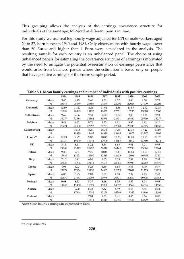
226
This grouping allows the analysis of the earnings covariance structure for
individuals of the same age, followed at different points in time.
For this study we use real log hourly wage adjusted for CPI of male workers aged
20 to 57, born between 1940 and 1981. Only observations with hourly wage lower
than 50 Euros and higher than 1 Euro were considered in the analysis. The
resulting sample for each country is an unbalanced panel. The choice of using
unbalanced panels for estimating the covariance structure of earnings is motivated
by the need to mitigate the potential overestimation of earnings persistence that
would arise from balanced panels where the estimation is based only on people
that have positive earnings for the entire sample period.
Table 5.1. Mean hourly earnings and number of individuals with positive earnings
1994 1995 1996 1997 1998 1999 2000 2001
Germany Mean 9.43 9.49 9.61 9.52 9.57 9.48 9.60 9.72
N 25018 26059 25806 24889 23290 22955 21909 20703
Denmark Mean 10.89 11.40 11.58 11.61 11.86 11.85 12.02 12.08
N 20899 20399 19190 19062 17321 16235 15678 15380
Netherlands Mean 9.69 9.56 9.59 9.70 10.02 9.88 10.04 9.91
N 33277 32384 31564 30575 28731 27460 25790 33277
Belgium Mean 8.48 8.82 8.71 8.75 8.81 8.83 8.92 9.10
N 20221 22100 22892 22753 22863 23233 24065 24130
Luxembourg Mean 16.18 15.81 16.73 17.39 17.15 17.22 17.10
N 15829 13695 14489 13403 14075 12667 12992
France62 Mean 10.23 9.92 9.87 10.05 10.33 10.60 10.55 10.87
N 20137 19270 19042 17906 14467 14012 13760 14212
UK Mean 8.16 8.11 8.22 8.34 8.68 9.01 9.21 9.68
N 24949 25329 25495 26010 26145 25750 25674 25264
Ireland Mean 9.30 9.54 9.76 10.02 10.43 10.84 11.69 12.44
N 13937 13221 12590 12515 12435 12091 10745 9727
Italy Mean 7.16 6.91 6.96 7.05 7.29 7.37 7.28 7.32
N 32633 32236 32111 29661 28865 26993 26912 25170
Greece Mean 4.95 5.03 5.23 5.59 5.63 5.85 5.70 5.77
N 27974 27654 26150 24865 22675 22001 21335 21929
Spain Mean 6.83 6.95 7.09 6.89 7.18 7.37 7.45 7.42
N 22559 21863 21296 20975 20371 20580 19898 20185
Portugal Mean 9.08 8.33 8.37 8.49 8.55 8.55 8.54 9.08
N 14653 15450 15379 15087 14837 14569 14604 14550
Austria Mean 9.08 8.33 8.37 8.49 8.55 8.55 8.54
N 17944 17789 17199 16209 15162 13816 13056
Finland Mean 7.89 8.01 8.41 8.45 8.66 8.86
N 15811 15845 15895 15546 13329 13057
Note: Mean hourly earnings are expressed in Euro.
62 Gross Amounts
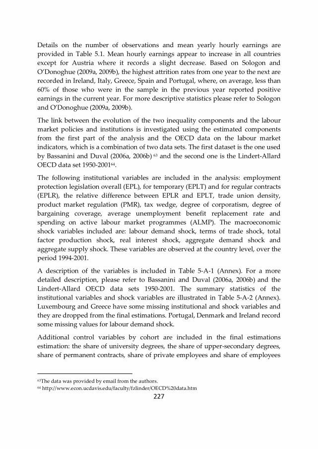
227
Details on the number of observations and mean yearly hourly earnings are
provided in Table 5.1. Mean hourly earnings appear to increase in all countries
except for Austria where it records a slight decrease. Based on Sologon and
O’Donoghue (2009a, 2009b), the highest attrition rates from one year to the next are
recorded in Ireland, Italy, Greece, Spain and Portugal, where, on average, less than
60% of those who were in the sample in the previous year reported positive
earnings in the current year. For more descriptive statistics please refer to Sologon
and O’Donoghue (2009a, 2009b).
The link between the evolution of the two inequality components and the labour
market policies and institutions is investigated using the estimated components
from the first part of the analysis and the OECD data on the labour market
indicators, which is a combination of two data sets. The first dataset is the one used
by Bassanini and Duval (2006a, 2006b) 63 and the second one is the Lindert-Allard
OECD data set 1950-200164.
The following institutional variables are included in the analysis: employment
protection legislation overall (EPL), for temporary (EPLT) and for regular contracts
(EPLR), the relative difference between EPLR and EPLT, trade union density,
product market regulation (PMR), tax wedge, degree of corporatism, degree of
bargaining coverage, average unemployment benefit replacement rate and
spending on active labour market programmes (ALMP). The macroeconomic
shock variables included are: labour demand shock, terms of trade shock, total
factor production shock, real interest shock, aggregate demand shock and
aggregate supply shock. These variables are observed at the country level, over the
period 1994-2001.
A description of the variables is included in Table 5-A-1 (Annex). For a more
detailed description, please refer to Bassanini and Duval (2006a, 2006b) and the
Lindert-Allard OECD data sets 1950-2001. The summary statistics of the
institutional variables and shock variables are illustrated in Table 5-A-2 (Annex).
Luxembourg and Greece have some missing institutional and shock variables and
they are dropped from the final estimations. Portugal, Denmark and Ireland record
some missing values for labour demand shock.
Additional control variables by cohort are included in the final estimations
estimation: the share of university degrees, the share of upper-secondary degrees,
share of permanent contracts, share of private employees and share of employees
63The data was provided by email from the authors. 64 http://www.econ.ucdavis.edu/faculty/fzlinder/OECD%20data.htm
228
by occupation. The summary statistics for the control variables are presented in
Table 5-A-4 (Annex).
5.4.Econometric specifications and estimation methods
The aim of this section is twofold: first, to fit a parsimonious model to the
autocovariance structure of earnings for all countries, decompose overall earnings
inequality into its permanent and transitory components and compute earnings
immobility; second to estimate the relationship between these estimated
components and the main labour market policy and institutional factors.
5.4.1. Econometric specifications and estimation methods of
covariance structures65
5.4.1.1. Econometric Earnings Specification
The methodology used to estimate earnings inequality, its permanent and
transitory component, and earnings mobility by cohorts and for each country
follows Sologon and O'Donoghue (2009a, 2009b). This paper represents a follow-
up of their analysis. We use the same data and the models identified by Sologon
and O'Donoghue (2009a, 2009b) as the best fit for each country to estimate the two
inequality components and earnings mobility. A summary of this methodology is
provided below.
The inspection of the covariance structure of earnings, included in section 5.5.1,
suggests the following features of the data, which must be incorporated in the
model:
(i) the elements of the autocovariance structure decrease with the lag at a
decreasing rate and
(ii) they converge gradually at a positive level;
(iii) the lag-1 autocovariance drops to a larger extent compared with higher
order autocovariances, which decline more gradually;
(iv) the autocovariances and mean earnings vary over the sample period, so
they cannot be assumed to be stationary over sample period;
(v) the autocovariances vary with age controlling for the period effect, hence
they cannot be assumed to be stationary over the life cycle;
65 The information in this section has been discussed in section 4.5 and 4.6.
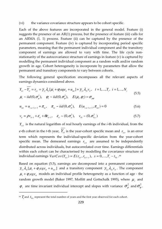
229
(vi) the variance covariance structure appears to be cohort specific.
Each of the above features are incorporated in the general model. Feature (i)
suggests the presence of an AR(1) process, but the presence of feature (iii) calls for
an ARMA (1, 1) process. Feature (ii) can be captured by the presence of the
permanent component. Feature (iv) is captured by incorporating period specific
parameters, meaning that the permanent individual component and the transitory
component of earnings are allowed to vary with time. The life cycle non-
stationarity of the autocovariance structure of earnings in feature (v) is captured by
modelling the permanent individual component as a random walk and/or random
growth in age. Cohort heterogeneity is incorporate by parameters that allow the
permanent and transitory components to vary between cohorts.
The following general specification encompasses all the relevant aspects of
earnings dynamics considered above.
1 1 2 2
2 2
[ ] , 1,..., , 1,...,
~ (0, ), ~ (0, ), ( , )
ict ct ict c t i i it iat c t it i c
i i i i
Y Y r age u v t T i N
iid iid Eµ ϕ µϕ
γ λ µ ϕ γ λ
µ σ ϕ σ µ ϕ σ
− = = + + + = =
= (5.5)
2
, 1, 1 , 1, 1, ~ (0, ), ( , ) 0
iat i a t ia ia i a t iatu u iid E u
ππ π σ π
− − − −= + =
(5.6)
2 2
1 1 0 0,, ~ (0, ), ~ (0, )
it it it it it i cv v v
ερ ε θε ε σ σ
− −= + +
(5.7)
ictY is the natural logarithm of real hourly earnings of the i-th individual, from the
c-th cohort in the t-th year, ctY is the year-cohort specific mean and ict
r is an error
term which represents the individual-specific deviation from the year-cohort
specific mean. The demeaned earnings ict
r are assumed to be independently
distributed across individuals, but autocorrelated over time. Earnings differentials
within each cohort can be characterised by modelling the covariance structure of
individual earnings 0( ) ( , ), 0,...,
ict ict ict s c cVarCov Y E r r s T t−= = − .66
Based on equation (5.5), earnings are decomposed into a permanent component
1 1 [ ]c t i i it iat
age uγ λ µ ϕ+ + and a transitory component 2 2c t it
vγ λ . The component
i i itageµ ϕ+ models an individual profile heterogeneity as a function of age - the
random growth model (Baker 1997, Moffitt and Gottschalk 1995), where i
µ and
iϕ are time invariant individual intercept and slopes with variance
2
µσ and2
ϕσ .
66
cT and
0 ct represent the total number of years and the first year observed for each cohort.
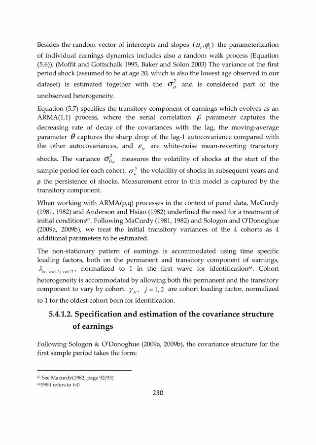
230
Besides the random vector of intercepts and slopes ( , )i i
µ ϕ the parameterization
of individual earnings dynamics includes also a random walk process (Equation
(5.6)). (Moffit and Gottschalk 1995, Baker and Solon 2003) The variance of the first
period shock (assumed to be at age 20, which is also the lowest age observed in our
dataset) is estimated together with the 2
µσ
and is considered part of the
unobserved heterogeneity.
Equation (5.7) specifies the transitory component of earnings which evolves as an
ARMA(1,1) process, where the serial correlation ρ parameter captures the
decreasing rate of decay of the covariances with the lag, the moving-average
parameter θ captures the sharp drop of the lag-1 autocovariance compared with
the other autocovariances, and it
ε are white-noise mean-reverting transitory
shocks. The variance 2
0,cσ measures the volatility of shocks at the start of the
sample period for each cohort, 2
εσ the volatility of shocks in subsequent years and
ρ the persistence of shocks. Measurement error in this model is captured by the
transitory component.
When working with ARMA(p,q) processes in the context of panel data, MaCurdy
(1981, 1982) and Anderson and Hsiao (1982) underlined the need for a treatment of
initial conditions67. Following MaCurdy (1981, 1982) and Sologon and O'Donoghue
(2009a, 2009b), we treat the initial transitory variances of the 4 cohorts as 4
additional parameters to be estimated.
The non-stationary pattern of earnings is accommodated using time specific
loading factors, both on the permanent and transitory component of earnings,
, 1,2; 0 ,7kt k tλ = =, normalized to 1 in the first wave for identification68. Cohort
heterogeneity is accommodated by allowing both the permanent and the transitory
component to vary by cohort. , 1, 2jc jγ = are cohort loading factor, normalized
to 1 for the oldest cohort born for identification.
5.4.1.2. Specification and estimation of the covariance structure
of earnings
Following Sologon & O’Donoghue (2009a, 2009b), the covariance structure for the
first sample period takes the form:
67 See Macurdy(1982, page 92/93) 681994 refers to t=0
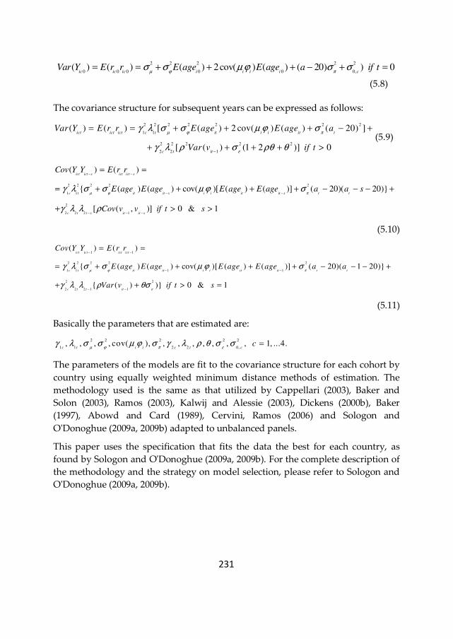
231
2 2 2 2 2
0 0 0 0 0 0,( ) ( ) ( ) 2cov( ) ( ) ( 20) ) 0
ic ic ic i i i i cVar Y E r r E age E age a if t
µ ϕ πσ σ µ ϕ σ σ= = + + + − + =
(5.8)
The covariance structure for subsequent years can be expressed as follows:
2 2 2 2 2 2 2
1 1
2 2 2 2 2
2 2 1
( ) ( ) [ ( ) 2 cov( ) ( ) ( 20) ]
[ ( ) (1 2 )] 0
ict ict ict c t it i i it t
c t it
Var Y E r r E age E age a
Var v if t
µ ϕ π
ε
γ λ σ σ µ ϕ σ
γ λ ρ σ ρθ θ−
= = + + + − +
+ + + + >(5.9)
2 2 2 2 2
1 1
2
2 2 2 1
( ) ( )
{ ( ) ( ) cov( )[ ( ) ( )] ( 20)( 20)}
[ ( , )] 0 & 1
ict ict s ict ict s
c t it it s i i it it s t t
c t t s it it s
Cov Y Y E r r
E age E age E age E age a a s
Cov v v if t s
µ ϕ πγ λ σ σ µ ϕ σ
γ λ λ ρ
− −
− −
− − −
= =
= + + + + − − − +
+ > >
(5.10)
1 1
2 2 2 2 2
1 1 1 1
2 2
2 2 2 1 1
( ) ( )
{ ( ) ( ) cov( )[ ( ) ( )] ( 20)( 1 20)}
{ ( ) )} 0 & 1
ict ict ict ict
c t it it i i it it t t
c t t it
Cov Y Y E r r
E age E age E age E age a a
Var v if t s
µ ϕ π
ε
γ λ σ σ µ ϕ σ
γ λ λ ρ θσ
− −
− −
− −
= =
= + + + + − − − +
+ + > =
(5.11)
Basically the parameters that are estimated are:
2 2 2 2 2
1 1 2 2 0 ,, , , , cov( ), , , , , , , , 1, ...4.
c t i i c t cc
µ ϕ π εγ λ σ σ µ ϕ σ γ λ ρ θ σ σ =
The parameters of the models are fit to the covariance structure for each cohort by
country using equally weighted minimum distance methods of estimation. The
methodology used is the same as that utilized by Cappellari (2003), Baker and
Solon (2003), Ramos (2003), Kalwij and Alessie (2003), Dickens (2000b), Baker
(1997), Abowd and Card (1989), Cervini, Ramos (2006) and Sologon and
O'Donoghue (2009a, 2009b) adapted to unbalanced panels.
This paper uses the specification that fits the data the best for each country, as
found by Sologon and O'Donoghue (2009a, 2009b). For the complete description of
the methodology and the strategy on model selection, please refer to Sologon and
O'Donoghue (2009a, 2009b).

232
5.4.2. Estimation of the links between policy, institutions and
outcomes
This section describes the methodology used to estimate the relationships between
labour market policy and institutional factors as independent variables and
permanent inequality, transitory inequality and earnings mobility, as dependent
variables. Each model is estimated independently, for all cohorts and countries
pooled together. The unit of analysis is the cohort. Hence we have four cohorts for
each country, observed between 1994-200169.
The analysis follows a general to specific strategy. First, we test whether policies
interact with the overall institutional framework, controlling for the cohorts effects
and for all the unobserved shocks. Second, we test whether there are any specific
interactions between different institutional factors, and between the institutional
factors and the observed aggregate shocks in shaping the pattern of the two
inequality components and earnings mobility.
5.4.2.1. Systemic interactions
In macroeconomic equations interactions between institutions are usually specified
in a multiplicative form between deviations of institutions from their sample mean,
which enables the interpretation of the marginal effects of each institution when
the others are kept constant at the sample mean. Before analysing the specific
cross-interactions between all institutions, we want to get a grasp of the systemic
interactions, meaning the interactions between each institution and the overall
institutional setting.
Systemic reform complementarity patterns are explored by estimating a separate
non-linear equation for each labour market outcome, pooling all cohorts, where
each institution is interacted with the overall institutional framework, defined as
the sum of the direct effects of institutions.
1 1 1
( ( )( ( ))K K K
it c t k kit k kit k k kit k i it
k k k
y X X X X X vδ τ υ ϕ υ µ= = =
= + − − + +∑ ∑ ∑
(5.12)
ity represents the labour market outcomes -permanent variance, temporary
variance and wage immobility of the cohort i in year t. The parameters kυ , jϕ , cδ
69 Exception are countries which are not observed for all eight waves, and consequently will have less
observations.
233
and tτ are estimated simultaneously. kυ denotes the direct effect of institution
kX on ity , for a country with an average mix of policies and institutions, while
kϕ indicates the strength of the interaction between kX and the overall
institutional framework, expressed as the sum of direct effect of policies and
institutions, expressed in deviation form in the interaction. kX is measured at the
country level. A negative and significant effect suggests that there is a systemic
reform complementarity between kX and the overall framework in reducing
permanent variance, temporary variance and earnings immobility, at the cohort
level. cδ and tτ represent cohort and respectively period shifters, which capture
cohorts heterogeneity and all the unobserved shocks that might affect permanent
variance, transitory variance and earnings immobility by altering the slopes of the
direct and indirect effects.
The estimation results are included in Table 5.5.
5.4.2.2. Specific 2-by-2 interactions between institutions, and
between institutions and shocks
This section attempts to open the black box of the systemic interactions
investigated in the previous section and explore the specific interactions between
institutions, and between institutions and shocks, which are expected to shape the
pattern of permanent inequality, transitory inequality and earnings mobility. We
start with a relatively simple model in which we explore the direct effect of
institutions, shocks and the interactions between shocks and institutions.
Moreover, we allow the effects to differ by cohorts to account for cohort
heterogeneity. The model is expressed as follows:
1 1 1
[ ( )(1 ( ( ))]K S K
it c k kit s sit s k kit k i it
k s k
y X Z Z X X vδ υ ψ γ µ= = =
= + − + − + +∑ ∑ ∑
(5.13),
where 1
( )S
s sit s
s
Z Zψ=
−∑ is a set of observed macroeconomic shocks expressed in
deviation from their mean, which are interacted with policy and institutional
factors. cδ , kυ , sψ and kγ are estimated simultaneously. As before cδ represent
the cohort shifters, normalized to 1 for the oldest cohort for identification, kυ
represents the direct effect of institution kX when the other intuitions and shocks
234
are at their sample means, sψ captures the direct effects of shocks and kγ capture
the interaction effects between institution kX and the aggregate effects of
macroeconomic shocks. The estimation results are presented in Model 2, Table 5.6.
The final model augments model (5.13) by adding also the 2-by-2 interaction effects
between institutions and policies. Moreover, additional controls are added, which
are aimed to control for educational structure (proportions of university and
upper-secondary graduates), for sector structure (proportion of private
employees), for the structure of the type of contract (proportion of employees with
a permanent contract), for the structure of employment status (proportion of
unemployed) and for occupational structure, by cohort. The estimation results are
presented in Model 3, Table 5.6.
One note needs to be made. iµ captures the unobserved unit-specific
heterogeneity, in our case cohort-specific heterogeneity. One might argue that our
model suffers from unobserved heterogeneity bias. We tested for unobserved
heterogeneity for each model, by cohort, using the Breusch and Pagan Lagrangian
multiplier test for random effects. The test rejected the presence of unit-specific
effects at 5% level of confidence.
Another problem is the endogeneity between institutions and overall inequality
that is expected to be transferred to the estimation of the two inequality
components. The lack of good instruments prevented us from correcting for this
problem. Hence, our estimates reflect the complex associations that exist within the
institutional framework, and between the institutional framework and the
macroeconomic shocks, and not causal relationships.
5.5.Results - descriptive
5.5.1. The dynamic autocovariance structure of hourly
earnings70
We begin with the description of the dynamic structure of individual log hourly
earnings for all 14 countries under analysis. This description is used to confirm that
the model used to fit the autocovariance structure of earnings for all cohorts is
consistent with the trends observed in the dynamic autocovariance structure. For a
70 The information in this section summarizes the discussion in section 4.7.
235
full description of the overall and cohort autocovariance structure of earnings
please refer to Sologon and O'Donoghue (2009a, 2009b). The overall autocovariance
structure of earnings is presented in Figure 5-A-1 (Annex). We summarize the
main findings as follows.
In the beginning of the sample period, the overall inequality, measured by the
variance of log hourly earnings, is the highest in Portugal, followed by Ireland,
Spain, France, Luxembourg, UK, Greece, Germany, Austria, Italy, Belgium,
Netherlands, Finland and Denmark. Overall inequality decreases over the sample
period in Germany, Denmark, Belgium, France, UK, Ireland, Spain and Austria,
and increases in Netherlands, Luxembourg, Greece, Portugal and Finland.
Following these changes, in 2001, Portugal still records the highest inequality,
followed by Luxembourg, France, Greece, Spain, UK, Italy, Germany, Ireland,
Netherlands, Finland, Belgium, Austria and Denmark.
In summary, the description of the dynamic structure of individual earnings for
men for each country suggests five main common features of the data, which are
incorporated in our model, as mentioned previously:
• First, the covariance elements are not the same at all lags. They decrease with
the lag at a decreasing rate and converge gradually at a positive level,
suggesting the presence of a transitory element which is serially correlated and
of a permanent individual component of earnings.
• Second, as the autocovariances and mean earnings vary over the sample
period, they cannot be assumed to be stationary over sample period. The
stationarity assumption was tested and rejected using the methodology
introduced by MaCurdy (1982).
• Third, as the autocovariances vary with age controlling for the period effect,
they cannot be assumed to be stationary over the life cycle.
• Lastly, the variance-covariance structure appears to be cohort specific. In most
countries, the variance of earnings for all cohorts follows the evolution of the
overall variance. Mixed trends across cohorts are observed in Germany –
where the variance increased for the cohorts born in 1941-1950 and 1961-1970 -,
in Belgium – where the variance increased for the youngest cohort -, in France -
where the variance increased for the cohort born in 1961-1970 -, in UK – where
the variance increased for the youngest two cohorts -, in Spain - where the
variance increased for the youngest and the oldest cohorts, and in Finland -
where the variance decreased for the youngest cohort.
236
5.5.2. The evolution of the main labour market and
institutional factors
This section presents the evolution of the main labour market policy and
institutional variables that will be used to explain the differences in labour market
outcomes – permanent inequality, transitory inequality and earnings mobility –
across the 14 EU countries. A summary is provided in Table 5-A-3 (Annex) and
Figure 5.2.
Over the period 1994-2001, the OECD index of employment protection legislation
decreased in most countries under analysis, except for Austria, France, Ireland and
Greece, where it was constant and UK, where it increased slightly. Employment
protection legislation (EPL) exhibited a sharp turnaround around 1995 in
Denmark, 1996 in Portugal, 1997 in Belgium, Germany and Spain, 1999 in
Netherlands, 2000 in Finland, which marked the year when EPL started
decreasing. For Italy the decrease continued through the rest of the period,
whereas for the others the evolution was roughly stable. An increase in EPL was
recorded in Spain in 2001 and in Ireland in 2000.
Employment protection legislation for regular contracts (EPLR) did not change
much, except for Spain and Finland, where it decreased in 1997, respectively in
2001, and France and UK, where it increased in 2000, respectively in 1999.
The greatest changes were recorded for employment protection legislation for
temporary contracts (EPLT). A decrease was recorded in Denmark, Portugal,
Germany, Belgium, Italy and Netherland, and an increase in Spain. The rest
remained constant. Denmark recorded a sharp drop in 1995, Belgium and
Germany in 1997, Italy in 1997-1998, Portugal in 1996, Netherlands in 1998.
As a result, over the sample period, an increasing or stagnant positive relative
difference between EPL for permanent contracts and for temporary contracts was
recorded in Austria, Ireland, Netherlands, Portugal, UK and Finland. Denmark,
Germany and Netherlands recorded a sharp increase in the relative difference
between EPL for permanent contracts and for temporary contracts, which turned
from a negative value in 1994 to a positive one in 2001. Belgium, France, Italy,
Spain and Greece exhibited a negative relative difference between EPL for
permanent contracts (EPLP) and for temporary contracts (EPLT), which, over the
sample period, decreased or remained constant in absolute value, except for Spain.
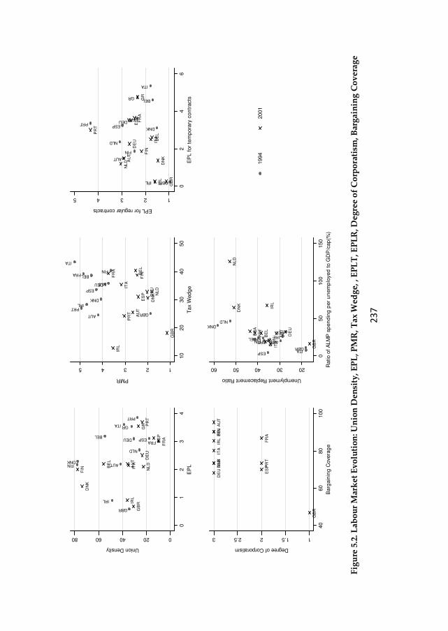
23
7
F
igu
re 5
.2. L
abo
ur
Mar
ket
Ev
olu
tio
n: U
nio
n D
ensi
ty,
EP
L, P
MR
, Tax
Wed
ge,
, E
PL
T, E
PL
R, D
egre
e o
f C
orp
ora
tism
, Bar
gai
nin
g C
ov
erag
e
GBR
IRL
FIN AUTDNK
NLD
FRADEU ESP
BEL
GRITA
PRT
GB
RIRL
DN
KF
IN NL
D
ITA
BE
L
AU
T
DE
U
FR
A
ES
P
GR P
RT
020406080
Union Density
01
23
4
EP
L
AUT GBR
PRTIRL
DNK
ESP
DEU NLD
BELFRAFIN
ITA
IRL
GB
R
PR
T
AU
T
DN
K
ES
P DE
U
NL
D
ITA
FINFR
A
BE
L
12345
PMR
10
20
30
40
50
Tax
Wed
ge
GBRIRL
AUT
FIN
NLD
DNKESP
PRTDEU
FRA
BELGR
ITA
IRL
GB
R
NL
D
DN
K
AU
T FIN
DE
U ITA
BE
LPR
T
ES
PF
RA
GR
12345
EPL for regular contracts
02
46
EP
L f
or
tem
pora
ry c
on
tracts
GB
R
DE
U
ES
PPR
T
NL
DD
NK
ITA
IRL
FR
AFIN
BE
LA
UT
11.522.53
Degree of Corporatism
40
60
80
100
Barg
ain
ing
Cove
rag
e
ESPITAGBR
PRT AUTFINFRABEL
IRLDEU
DNKNLD
GB
R
ITA
ES
PF
IN
AU
T
PR
T
BE
L
DE
U
FR
A
DN
K
IRL
NL
D
2030405060
Unemplyment Replacement Ratio
050
100
150
Ratio o
f A
LM
P s
pen
din
g p
er
un
em
plo
yed
to G
DP
/cap
(%)
1994
2001

238
A decrease in union density is reported in all countries, except Belgium. The
degree of corporatism was characterized by stable rates in all countries. The tax
wedge exhibited a high turnaround in 1995 for all countries, except the continental
ones. The largest decline was in the Anglo-Saxon countries, followed by Nordic
and Mediterranean countries. Exceptions are Austria, Belgium, Denmark and
France, where the tax wedge increased. The index of product market regulation
(PMR) declined through the entire period, but the rate of decrease intensified after
1998 for most countries. Unemployment benefits replacement rates rose in all
countries, except Denmark, Finland and UK. Sharp increases were recorded
around 1998-1999 in Italy and Portugal, and around 2000-2001 in France and
Ireland. Active labour market policies (ALMP) developed in all countries, except
Germany, where they decreased. The largest increases were recorded in
Netherlands, Denmark and Ireland.
The possible static effects of these policies are raising employment and reducing
productivity, whereas the possible dynamic effects are raising investment
following the raise in employment and raising incentives for adoption of new
technologies, which implies a shift in the demand for skills. (Dew-Becker and
Gordon 2008) Hence all these are expected to influence permanent earnings
inequality and volatility and earnings mobility.
Nevertheless, institutional factors do not exist in a vacuum. They are expected to
interact with external factors, such as macroeconomic shocks. The evolution of the
macroeconomic shocks is illustrated in Figure 5-A- 2 (Annex). Changes in demand
and supply factors, in technology, in terms of trade, in real interest do not differ
significantly among countries; hence they cannot by themselves explain all the
changes in the inequality components. These trends are not surprising, given that
all these countries operate in the same world markets, with similar technology,
industry and occupation mixes.
For example, all countries experience the same turning points in both demand and
supply shocks. The supply shocks had three turning points: a decrease until 1996,
followed by a decrease until 1998, an increase until 2000, and a drop thereafter. The
supply shocks converged in a decreasing trend for all countries towards 1999,
followed by an increase in 2000, and a slight decrease in 2001. The convergence in
the trends was maintained until 2001. Overall, the highest demand and supply
shocks are experienced by Ireland, followed by Belgium, Austria and Netherlands.
One country stands out with respect to its evolution in total production factors
shock: Ireland. It records a sharp increase until 1997, followed by stabilization
239
towards 2001. Similarly, the real interest shock drops towards 1998 and stabilizes
afterwards. These trends are most likely related to the Celtic Tiger.
The OECD data on education attainment by country reveals that the average level
of education has an increasing trend and evolves parallel for all countries. Three
clusters can be identified. A high average level is achieved in Germany, followed
by Finland, Denmark, then very closely Ireland, UK and Belgium. A medium level
is recorded in Greece, Austria, France, Spain and Italy. The lowest level is in
Portugal.
To sum up, labour market policy and institutional factors are expected to interact
significantly with each other and with the macroeconomic shocks in shaping the
patterns of permanent inequality, transitory inequality and earnings mobility.
5.6. Results of covariance structure estimation71
5.6.1. Estimation results
The general specification of the error component model outlined in section 4.5.2,
which encompasses all relevant aspects of earnings dynamics considered above, is
fit to the elements of the covariance matrix of each country, for all cohorts pooled
together 72. We present only the models that fit the data the best for each country,
as identified by Sologon and O'Donoghue (2009a, 2009b). The estimation results
are illustrated in Table 5-A-5 (Annex). Similar to Dickens (2000b), all variances are
restricted to be positive by estimating the variance equal to the exponent of the
parameter. The reported estimates of the variance in Table 5-A-5 (Annex) represent
the exponent of the parameter and the reported standard errors correspond to the
parameter estimates.73
We summarize the interpretation from Sologon and O'Donoghue (2009a, 2009b).
The formulation of the permanent and transitory components of earnings differs
between countries.
71 This section summarizes the estimation results in Chapter 4. 72 i.e. 144 auto-covariances for countries observed over 8 waves, 122 for those with 7 waves and 84 for
those with 6 waves. 73 The SE column reports the standard error for the parameter estimate. Where I report the
exp(estimate), the SE corresponds to the log(exp(estimate)) = estimate
240
Permanent component
In Germany, Netherlands, UK, Ireland, Italy, Greece, Spain and Finland, the
permanent component follows a random growth model with time and cohort
specific loading factors. The estimated coefficients for the permanent component of
earnings show that time-invariant heterogeneity and age-earning profile
heterogeneity play a significant role in the formation of long-term earnings
differentials in all these countries. Individual specific heterogeneity plays the
highest role in Germany, followed by Spain, Netherlands, Greece, UK, Ireland and
Italy, which suggests that in Germany there is a higher dispersion in the time-
invariant individual specific attributes that determine wage differentials.
The estimated random slope variance implies that hourly earnings growth for an
individual located one standard deviation above the mean in the distribution of φ
is the largest in Germany, where it is with 4.89%74 faster than the cohort mean,
followed by Greece, Ireland, Spain, Netherlands, UK and Finland with rates
between 1% and 1.41% and Italy with 0.89%. All these countries have a negative
covariance between the time invariant individual specific effect and the individual
specific slope of the age-earning profile, which implies that the initial and lifecycle
heterogeneity are negatively associated. This negative association corresponds to
the trade-off between earnings early in the career and subsequent earnings growth
and is consistent with the on-the-job training hypothesis (Mincer, 1974). Therefore,
this suggests the presence of mobility within the distribution of permanent
earnings over the sample period. These findings reinforce the results from
previous studies.
Therefore, for these countries the evolution of the permanent component without
the time loading factors could be either increasing or decreasing. The time-specific
loading factors for the permanent component are highly significant with values
close to 1 in all countries. The trends of the returns to the permanent component
vary to a large extent across countries. One common feature is that they reflect the
trends in the high-order autocovariances in the data. These estimates show that
overall, controlling for age and cohort effects, the returns to skills decreased over
the sample period in Netherlands, UK, Ireland, Italy, Greece, Spain and increased
in Germany and Finland. The trends over time differ between countries, some
record a smooth evolution, others noisier. For example, Netherlands experienced
decreases in returns almost every second year. In UK the returns increased in 1997
742
4.89 100ϕ
σ= ⋅
241
and 2001, and decreased in the rest. Ireland recorded a decrease until 1996, a boost
in 1997 and a clear decline thereafter. In Italy, 1998 and 1999 appear to be years
with increases in the return to skills, in Greece every second year, in Spain 1995
and 1998. Germany experienced increasing returns to human capital until 2000,
and Finland in 1997 and 2001. Therefore, in these years, the relative position of the
highly skilled individuals was enhanced.
In Denmark the permanent component follows a random walk in age. The variance
of the innovation in the random walk is significantly larger than zero. As the
variance of a variable that follows a random walk is the sum of the variances of the
innovation term, this finding implies that permanent inequality increases over
lifetime. In Denmark, the variance at the age of 20 is lower than the variance at
subsequent ages, suggesting the presence of larger permanent shocks at older ages,
which is consistent with matching models, in which the information revealed
about a worker’s ability increases with time. The final trend in the permanent
variance depends on the period specific loading factors, which reveal that overall,
the relative position of the highly skilled individuals decreased over the sample
period in Denmark. The yearly evolution revealed a smooth decrease until 2000,
followed by a small increase in 2001.
In Belgium, France, Luxembourg, Portugal and Austria the persistent dispersion of
earnings follows the canonical model, where the permanent component is time-
invariant. The highest variance in the time invariant characteristics is recorded in
Portugal, followed by France, Luxembourg, Austria and Belgium. In this case, the
time-specific loading factors determine the final trend of the permanent
differentials: they decreased in Belgium and Austria, and increased in France,
Luxembourg and Portugal. Year by year, France records an increase in the returns
to skills until 1997 and again in 2001, Luxembourg until 2000, Belgium in 1996 and
2000, Austria during most of the period, except 1998-1999, and Portugal in 1996,
1998 and 2000.
The estimates of the cohort-specific shifters for the permanent earnings are highly
significant in all countries. The trends, however, differ between countries. A
monotonic increase over the lifecycle is observed in Germany, France,
Luxembourg, Portugal and Austria. In Denmark, Netherlands, Belgium and Spain
the permanent component of earnings has an inverted-U shape evolution over the
lifecycle. These trends confirm the expectation that permanent earnings
differentials play a much larger role in the formation of overall earnings
differentials of older cohorts compared with younger ones, which experience
higher earnings volatility due to temporary contracts. We expect the opposite to
hold in the case of cohort-specific shifters for transitory earnings.

242
The permanent component of earnings decreases over the life cycle in UK, Ireland,
Italy, Greece and Finland. This may be due to younger cohorts having more
heterogeneous skills or experiencing larger permanent shocks even without a
larger dispersion of skills. This could be the case if the labour market has become
tougher over time, as in the case of Italy, which is characterised by high rates of
youth unemployment.
Transitory component
The formulation of the temporary component of earnings differs between
countries. It follows an AR(1) process with time and cohorts loading factors in all
countries, except Italy, Greece and Spain, where it follows an ARMA(1,1). Except
for Spain, Portugal and Austria, the other countries are characterized by
heteroskedastic initial conditions. The estimated coefficients for the transitory
component of earnings are all significant, suggesting that the initial variance(s), the
AR(1) process, the ARMA(1,1) process, and the time and cohort loading factors
contribute significantly to earnings volatility in all countries.
The variance of initial conditions, which represents the accumulation of shocks up
to the starting year of the panel, is smaller than the variance of subsequent shocks
in all countries, except Luxembourg, Ireland, the oldest three cohorts in UK, and
the middle two cohorts in Finland. Overall, the variance of initial conditions
increases over the lifecycle in Denmark, Belgium, France, Luxembourg, UK, Italy,
Greece and Finland, suggesting that the initial variance plays a larger role in the
formation of earnings differentials for the oldest cohort compared with the
youngest. The opposite is observed in Germany, Netherlands and Ireland.
The pattern of the heteroskedstic initial conditions, however, is not monotonic
across cohorts. In Luxembourg, UK, Italy, and Finland it follows an inverted-U
shape: the variance of initial conditions increases over the lifecycle and decreases at
the end. The opposite holds for France, where the oldest and the youngest cohorts
have the highest initial variances.
In Germany and Netherlands the pattern of the heteroskedstic initial conditions
records a sharp drop for the second youngest cohort, an increase for the second
oldest and a small drop for the oldest cohort. In Denmark, Belgium, Ireland and
Greece, the variance of initial conditions records an increase for the second
youngest cohort, a drop for the second oldest and an increase for the oldest cohort.
The magnitude of the autoregressive parameter varies between countries. A large
autoregressive parameter, which suggests that shocks are persistent, is recorded in
243
Spain with 26.9% of a shock still present after 8 years, in Portugal with 8.5% and in
Austria with 5.7%. A moderate autoregressive parameter suggesting that shocks
die out rather quickly is recorded in Italy with 2.8% of a shock still present after 8
years, in Belgium with 2.4%, and in Greece with 1.4%. A small autoregressive
parameter is present in Luxembourg, Ireland, Finland, Netherlands, Germany,
France, UK and Denmark, where between 0.0008% and 0.8% of a shock is still
present after 8 years. The negative sign of the MA component implies that the
autocovariances decline sharply over the first period, confirming the trends
observed in the previous section for Italy, Greece and Spain.75
The time-specific loading factors for the transitory component are highly
significant and display a higher variation than for the permanent component in all
countries. The trends of the transitory inequality vary to a large extent across
countries. These estimates show that overall the transitory variance decreased over
the sample period in all countries, except Luxembourg and Ireland.
The estimates of the cohort-specific shifters for the transitory earnings are highly
significant in all countries. They indicate that earnings volatility is higher for
younger cohorts, thus confirming the pattern observed in the dynamic description
of the autocovariance structure of earnings, where autocovariances were found to
be lower for younger cohorts. This is expected, given that younger people
experience in general more frequent job changes, and consequently less stable
earnings.
5.6.2. Inequality decomposition into permanent and transitory
inequality
Having estimated a suitable error component model for earnings in each country,
next we use these parameters estimates to decompose the variance-covariance
structure of earnings into its permanent and transitory components, assess their
relative importance, and estimate earnings immobility over the sample period, by
cohort.
Following Sologon and O'Donoghue (2009a, 2009b), Figure 5.3 illustrates the
absolute decomposition of the variance, together with the actual and predicted
variance of earnings by cohort. The decomposition by cohort identifies how
inequality and its components are affected by labour market changes at different
lifecycle stages. For all countries, the evolution of the predicted variance follows
75 For the other countries, the MA component was either rejected by the data or could not be identified
due to the low number of waves.

244
closely the evolution of the actual variance, confirming the fit of the country
models, indicated by the low sum of square residuals. Figure 5.4 illustrates the
evolution of the structure of inequality, expressed by the relative decomposition of
the overall predicted variance of earnings into its permanent and transitory
components. Figure 5.5 translates these trends into earnings immobility, measured
by the ratio between permanent and transitory differentials. An increase in the
immobility ratio indicates a decrease in mobility, equivalent to an increase in the
share of the permanent differentials in the overall inequality. This mobility index
captures non-directional earnings movements and can be interpreted as the
opportunity to improve one’s position in the distribution of lifetime earnings.
The trends by cohort illustrated in Figure 5.3, Figure 5.4 and Figure 5.5 for the
actual earnings inequality, permanent inequality, transitory inequality, the share of
the permanent inequality in the overall inequality, and the immobility ratio are
described in Table 5.2. The trends in average actual inequality, average
components and average immobility ratio76 across cohorts are described in Table
5.3. We underline only the key points. For a complete description, please refer to
Table 5.2, Table 5.3 and Sologon and O'Donoghue (2009a, 2009b).
For all countries, both in relative and absolute terms (Figure 5.3 and Figure 5.4),
individual earnings inequality contains a highly permanent component for the
oldest three cohorts and a highly transitory component for the youngest cohort.
This is consistent with the evidence of lifecycle earnings divergence showing that
earnings volatility is higher at younger ages. The degree of immobility (Figure 5.5)
is higher for older cohorts compared with younger cohorts, which suggests that the
older the cohort, the lower the opportunity to improve one’s position in the
distribution of lifetime earnings.
The overall trends are established by looking at averages across cohorts (Table 5.3).
Overall, the decrease in inequality resulted from a decrease in transitory
differentials in Germany, France, UK and Ireland, in permanent differentials in
Belgium and Spain, and in both components in Denmark and Austria. The increase
in inequality reflects an increase in permanent differentials in Luxembourg, Italy,
Greece and Finland, and an increase in both components in Portugal and
Netherlands.
The decrease in inequality was accompanied by an increase in mobility only in
Denmark, Belgium and Spain. Except for Netherlands and Portugal, all countries
recording an increase in inequality experienced also a decrease in mobility.
76 Average Immobility Ratio = Average Permanent Variance/Average Transitory Variance
24
5
Fig
ure
5.3
.Act
ual
an
d P
red
icte
d V
aria
nce
of
Ear
nin
gs
wit
h P
erm
anen
t an
d T
ran
sito
ry P
red
icte
d C
om
po
nen
ts f
or
Sel
ecte
d C
oh
ort
s: 1
994-
2001
0.1.2.3.4
19
94
20
01
Co
ho
rt 1
94
0-1
95
0
0.1.2.3.41
99
42
00
1
Co
ho
rt 1
95
1-1
96
00.1.2.3.4
19
94
20
01
Co
ho
rt 1
96
1-1
97
00.1.2.3.4
19
94
20
01
Co
ho
rt 1
97
1-1
98
1
Germ
an
y
0.1.2.3.4
19
94
20
01
Co
ho
rt 1
94
0-1
95
0
0.1.2.3.4
19
94
20
01
Co
ho
rt 1
95
1-1
96
0
0.1.2.3.4
19
94
20
01
Co
ho
rt 1
96
1-1
97
0
0.1.2.3.4
19
94
20
01
Co
ho
rt 1
97
1-1
98
1
Den
mark
0.1.2.3.4
19
94
20
01
Co
ho
rt 1
94
0-1
95
0
0.1.2.3.4
19
94
20
01
Co
ho
rt 1
95
1-1
96
0
0.1.2.3.4
19
94
20
01
Co
ho
rt 1
96
1-1
97
0
0.1.2.3.4
19
94
20
01
Co
ho
rt 1
97
1-1
98
1
Neth
erl
an
ds
0.1.2.3.4
19
94
20
01
Co
ho
rt 1
94
0-1
95
0
0.1.2.3.41
99
42
00
1
Co
ho
rt 1
95
1-1
96
0
0.1.2.3.4
19
94
20
01
Co
ho
rt 1
96
1-1
97
0
0.1.2.3.4
19
94
20
01
Co
ho
rt 1
97
1-1
98
1
Belg
ium
0.1.2.3.4
19
94
20
01
Co
ho
rt 1
94
0-1
95
0
0.1.2.3.4
19
94
20
01
Co
ho
rt 1
95
1-1
96
0
0.1.2.3.4
19
94
20
01
Co
ho
rt 1
96
1-1
97
0
0.1.2.3.4
19
94
20
01
Co
ho
rt 1
97
1-1
98
1
Fra
nce
0.1.2.3.4
19
94
20
01
Co
ho
rt 1
94
0-1
95
0
0.1.2.3.4
19
94
20
01
Co
ho
rt 1
95
1-1
96
0
0.1.2.3.4
19
94
20
01
Co
ho
rt 1
96
1-1
97
0
0.1.2.3.4
19
94
20
01
Co
ho
rt 1
97
1-1
98
1
Lu
xem
bou
rg
0.1.2.3.4
19
94
20
01
Co
ho
rt 1
94
0-1
95
0
0.1.2.3.4
19
94
20
01
Co
ho
rt 1
95
1-1
96
0
0.1.2.3.4
19
94
20
01
Co
ho
rt 1
96
1-1
97
0
0.1.2.3.4
19
94
20
01
Co
ho
rt 1
97
1-1
98
1
UK
Actu
al V
ariance
Pre
dic
ted V
ariance
Perm
anent
Com
ponent
Tra
nsitory
Com
ponent
24
6
F
igu
re 5
.3 (
Co
nti
nu
ed)
0.1.2.3.4
19
94
20
01
Co
ho
rt 1
94
0-1
95
0
0.1.2.3.4
19
94
20
01
Co
ho
rt 1
95
1-1
96
00.1.2.3.4
19
94
20
01
Co
ho
rt 1
96
1-1
97
00.1.2.3.4
19
94
20
01
Co
ho
rt 1
97
1-1
98
1
Ire
lan
d
0.1.2.3.4
19
94
20
01
Co
ho
rt 1
94
0-1
95
0
0.1.2.3.4
19
94
20
01
Co
ho
rt 1
95
1-1
96
0
0.1.2.3.4
19
94
20
01
Co
ho
rt 1
96
1-1
97
0
0.1.2.3.4
19
94
20
01
Co
ho
rt 1
97
1-1
98
1
Ita
ly
0.1.2.3.4
19
94
20
01
Co
ho
rt 1
94
0-1
95
0
0.1.2.3.4
19
94
20
01
Co
ho
rt 1
95
1-1
96
0
0.1.2.3.4
19
94
20
01
Co
ho
rt 1
96
1-1
97
0
0.1.2.3.4
19
94
20
01
Co
ho
rt 1
97
1-1
98
1
Gre
ece
0.1.2.3.4
19
94
20
01
Co
ho
rt 1
94
0-1
95
0
0.1.2.3.4
19
94
20
01
Co
ho
rt 1
95
1-1
96
0
0.1.2.3.4
19
94
20
01
Co
ho
rt 1
96
1-1
97
0
0.1.2.3.4
19
94
20
01
Co
ho
rt 1
97
1-1
98
1
Sp
ain
0.1.2.3.4
19
94
20
01
Co
ho
rt 1
94
0-1
95
0
0.1.2.3.4
19
94
20
01
Co
ho
rt 1
95
1-1
96
0
0.1.2.3.4
19
94
20
01
Co
ho
rt 1
96
1-1
97
0
0.1.2.3.4
19
94
20
01
Co
ho
rt 1
97
1-1
98
1
Po
rtu
ga
l
0.1.2.3.4
19
94
20
01
Co
ho
rt 1
94
0-1
95
0
0.1.2.3.4
19
94
20
01
Co
ho
rt 1
95
1-1
96
0
0.1.2.3.4
19
94
20
01
Co
ho
rt 1
96
1-1
97
0
0.1.2.3.4
19
94
20
01
Co
ho
rt 1
97
1-1
98
1
Au
str
ia
0.1.2.3.4
19
94
20
01
Co
ho
rt 1
94
0-1
95
0
0.1.2.3.4
19
94
20
01
Co
ho
rt 1
95
1-1
96
0
0.1.2.3.41
99
42
00
1
Co
ho
rt 1
96
1-1
97
0
0.1.2.3.4
19
94
20
01
Co
ho
rt 1
97
1-1
98
1
Fin
lan
d
Actu
al V
ariance
Pre
dic
ted V
ariance
Perm
anent
Com
ponent
Tra
nsitory
Com
ponent
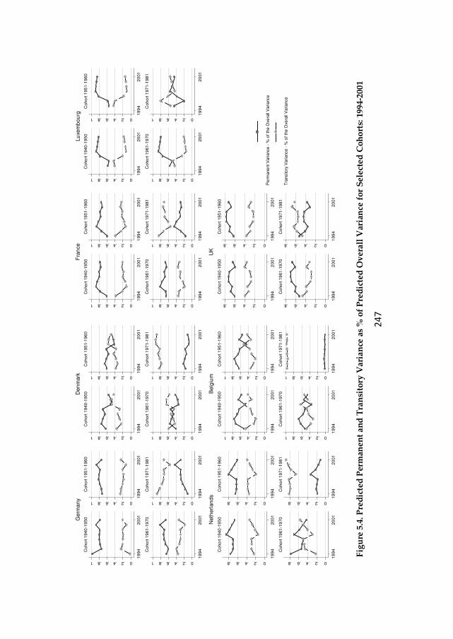
24
7
Fig
ure
5.4
. Pre
dic
ted
Per
man
ent
and
Tra
nsi
tory
Var
ian
ce a
s %
of
Pre
dic
ted
Ov
eral
l V
aria
nce
fo
r S
elec
ted
Co
ho
rts:
199
4-20
01
0.2.4.6.81
19
94
20
01
Co
ho
rt 1
94
0-1
95
0
0.2.4.6.811
99
42
00
1
Co
ho
rt 1
95
1-1
96
0
0.2.4.6.81
19
94
20
01
Co
ho
rt 1
96
1-1
97
0
0.2.4.6.81
19
94
20
01
Co
ho
rt 1
97
1-1
98
1
Germ
an
y
0.2.4.6.81
19
94
20
01
Co
ho
rt 1
94
0-1
95
0
0.2.4.6.81
19
94
20
01
Co
ho
rt 1
95
1-1
96
0
0.2.4.6.811
99
42
00
1
Co
ho
rt 1
96
1-1
97
0
0.2.4.6.81
19
94
20
01
Co
ho
rt 1
97
1-1
98
1
Den
mark
0.2.4.6.8
19
94
20
01
Co
ho
rt 1
94
0-1
95
0
0.2.4.6.8
19
94
20
01
Co
ho
rt 1
95
1-1
96
0
0.2.4.6.8
19
94
20
01
Co
ho
rt 1
96
1-1
97
0
0.2.4.6.8
19
94
20
01
Co
ho
rt 1
97
1-1
98
1
Neth
erl
an
ds
0.2.4.6.81
19
94
20
01
Co
ho
rt 1
94
0-1
95
0
0.2.4.6.81
19
94
20
01
Co
ho
rt 1
95
1-1
96
0
0.2.4.6.81
19
94
20
01
Co
ho
rt 1
96
1-1
97
0
0.2.4.6.81
19
94
20
01
Co
ho
rt 1
97
1-1
98
1
Belg
ium
0.2.4.6.81
19
94
20
01
Co
ho
rt 1
94
0-1
95
0
0.2.4.6.81
19
94
20
01
Co
ho
rt 1
95
1-1
96
0
0.2.4.6.81
19
94
20
01
Co
ho
rt 1
96
1-1
97
0
0.2.4.6.81
19
94
20
01
Co
ho
rt 1
97
1-1
98
1
Fra
nce
0.2.4.6.81
19
94
20
01
Co
ho
rt 1
94
0-1
95
0
0.2.4.6.81
19
94
20
01
Co
ho
rt 1
95
1-1
96
0
0.2.4.6.81
19
94
20
01
Co
ho
rt 1
96
1-1
97
0
0.2.4.6.81
19
94
20
01
Co
ho
rt 1
97
1-1
98
1
Lu
xem
bou
rg
0.2.4.6.8
19
94
20
01
Co
ho
rt 1
94
0-1
95
0
0.2.4.6.8
19
94
20
01
Co
ho
rt 1
95
1-1
96
0
0.2.4.6.81
99
42
00
1
Co
ho
rt 1
96
1-1
97
0
0.2.4.6.8
19
94
20
01
Co
ho
rt 1
97
1-1
98
1
UK
Pe
rmane
nt V
ariance
- %
of
the
Ove
rall
Variance
Tra
nsito
ry V
ariance
- %
of
the
Ove
rall
Variance
24
8
Fig
ure
5.4
. (C
on
tin
ued
)
0.2.4.6.8
19
94
20
01
Co
ho
rt 1
94
0-1
95
0
0.2.4.6.81
99
42
00
1
Co
ho
rt 1
95
1-1
96
0
0.2.4.6.8
19
94
20
01
Co
ho
rt 1
96
1-1
97
0
0.2.4.6.8
19
94
20
01
Co
ho
rt 1
97
1-1
98
1
Ire
lan
d
0.2.4.6.8
19
94
20
01
Co
ho
rt 1
94
0-1
95
0
0.2.4.6.8
19
94
20
01
Co
ho
rt 1
95
1-1
96
0
0.2.4.6.81
99
42
00
1
Co
ho
rt 1
96
1-1
97
0
0.2.4.6.8
19
94
20
01
Co
ho
rt 1
97
1-1
98
1
Ita
ly0.2.4.6.8
19
94
20
01
Co
ho
rt 1
94
0-1
95
0
0.2.4.6.8
19
94
20
01
Co
ho
rt 1
95
1-1
96
0
0.2.4.6.8
19
94
20
01
Co
ho
rt 1
96
1-1
97
0
0.2.4.6.8
19
94
20
01
Co
ho
rt 1
97
1-1
98
1
Gre
ece
0.2.4.6.8
19
94
20
01
Co
ho
rt 1
94
0-1
95
0
0.2.4.6.8
19
94
20
01
Co
ho
rt 1
95
1-1
96
0
0.2.4.6.8
19
94
20
01
Co
ho
rt 1
96
1-1
97
0
0.2.4.6.8
19
94
20
01
Co
ho
rt 1
97
1-1
98
1
Sp
ain
0.2.4.6.81
19
94
20
01
Co
ho
rt 1
94
0-1
95
0
0.2.4.6.81
19
94
20
01
Co
ho
rt 1
95
1-1
96
0
0.2.4.6.81
19
94
20
01
Co
ho
rt 1
96
1-1
97
0
0.2.4.6.81
19
94
20
01
Co
ho
rt 1
97
1-1
98
1
Po
rtu
ga
l
0.2.4.6.8
19
94
20
01
Co
ho
rt 1
94
0-1
95
0
0.2.4.6.8
19
94
20
01
Co
ho
rt 1
95
1-1
96
0
0.2.4.6.8
19
94
20
01
Co
ho
rt 1
96
1-1
97
0
0.2.4.6.8
19
94
20
01
Co
ho
rt 1
97
1-1
98
1
Au
str
ia
0.2.4.6.8
19
94
20
01
Co
ho
rt 1
94
0-1
95
0
0.2.4.6.8
19
94
20
01
Co
ho
rt 1
95
1-1
96
0
0.2.4.6.8
19
94
20
01
Co
ho
rt 1
96
1-1
97
0
0.2.4.6.8
19
94
20
01
Co
ho
rt 1
97
1-1
98
1
Fin
lan
d
Pe
rmane
nt V
ariance
- %
of
the
Ove
rall
Variance
Tra
nsito
ry V
ariance
- %
of
the
Ove
rall
Variance
24
9
Fig
ure
5.5
. Rat
io B
etw
een
Per
man
ent
Var
ian
ce a
nd
Tra
nsi
tory
Var
ian
ce O
ver
Tim
e F
or
Sel
ecte
d C
oh
ort
s
0246810
1994
1995
1996
1997
1998
1999
2000
2001
Germ
any
0246810
1994
1995
1996
1997
1998
1999
2000
2001
Denm
ark
0246810
1994
1995
1996
1997
1998
1999
2000
2001
Neth
erlands
0246810
1994
1995
1996
1997
1998
1999
2000
2001
Belg
ium
0246810
1994
1995
1996
1997
1998
1999
2000
2001
Fra
nce
02468101994
1995
1996
1997
1998
1999
2000
2001
Luxe
mbourg
0246810
1994
1995
1996
1997
1998
1999
2000
2001
UK
0246810
1994
1995
1996
1997
1998
1999
2000
2001
Irela
nd
0246810
1994
1995
1996
1997
1998
1999
2000
2001
Italy
0246810
1994
1995
1996
1997
1998
1999
2000
2001
Gre
ece
0246810
1994
1995
1996
1997
1998
1999
2000
2001
Spain
0246810
1994
1995
1996
1997
1998
1999
2000
2001
Port
ugal
0246810
1994
1995
1996
1997
1998
1999
2000
2001
Austr
ia
0246810
1994
1995
1996
1997
1998
1999
2000
2001
Fin
land
Wage Im
mo
bili
ty C
oho
rt 1
940-1
950
Wage Im
mo
bili
ty C
oho
rt 1
951-1
960
Wage Im
mo
bili
ty C
oho
rt 1
961-1
970
Wage Im
mo
bili
ty C
oho
rt 1
971-1
981

25
0
Tab
le 5
.2. S
um
mar
y o
f th
e ev
olu
tio
n o
f th
e ac
tual
in
equ
alit
y,
per
man
ent
and
tra
nsi
tory
in
equ
alit
y, t
he
per
man
ent
ineq
ual
ity
as
% o
f
pre
dic
ted
ov
eral
l v
aria
nce
, an
d t
he
imm
ob
ilit
y r
atio
, b
y c
oh
ort
s: 1
994-
2001
Act
ua
l
Ineq
ua
lity
↑
Net
her
lan
ds
Lu
xem
bo
urg
Gre
ece
Po
rtu
ga
l
Fin
lan
d (
2, 3
, 4)
Ita
ly
Ger
ma
ny
(4
, 2)
Fra
nce
(2)
Bel
giu
m (
1)
UK
(1, 2
)
Sp
ain
(4
, 1)
P
V
Per
ma
nen
t co
mp
on
ent
as
% o
f o
ve
rall
va
ria
nce
incr
ease
d
�
Imm
ob
ilit
y I
ncr
ease
d
Lu
xem
bo
urg
(2
, 3, 4
)
Gre
ece
Fin
lan
d (
2, 3
, 4)
Ita
ly
Ger
ma
ny
(2
)
Fra
nce
(2)
UK
(2)
↑
↓
TV
↑
Net
her
lan
ds
(3, 4
)
Lu
xem
bo
urg
(1
)
Gre
ece
(3)
Po
rtu
ga
l,
Ita
ly (
1)
Ger
ma
ny
(4
, 2)
Fra
nce
(2)
Net
her
lan
ds
(1, 2
)
Bel
giu
m (
1)
Sp
ain
(4
, 1)
UK
(1
)
Per
ma
nen
t co
mp
on
ent
as
% o
f o
ve
rall
va
ria
nce
dec
rea
sed
�
Imm
ob
ilit
y D
ecre
ase
d
Net
her
lan
ds,
Po
rtu
ga
l,
Lu
xem
bo
urg
(1
),
Ger
ma
ny
(4
),
Bel
giu
m (
1),
UK
(1),
Sp
ain
(4
, 1)
↓
Lu
xem
bo
urg
(2
, 3, 4
)
Ita
ly (
2, 3
, 4),
Gre
ece
(4, 1
, 2)
Fin
lan
d (
2, 3
, 4)
UK
(2
)
↓
Den
ma
rk
Ger
ma
ny
(3
, 1)
Fra
nce
(3
, 4, 1
)
Bel
giu
m (
2, 3
, 4)
UK
(3, 4
)
Irel
an
d
Au
stri
a
Sp
ain
(2
, 3)
Fin
lan
d (
1)
P
V
Per
ma
nen
t co
mp
on
ent
as
% o
f o
ve
rall
va
ria
nce
incr
ease
d
�
Imm
ob
ilit
y I
ncr
ease
d
Den
ma
rk (
2)
Ger
ma
ny
(3
, 1)
Fra
nce
(3
, 4, 1
)
Bel
giu
m (
4)
UK
(3, 4
)
Irel
an
d
Au
stri
a
↑
↓
TV
↑
Den
ma
rk (
3)
Bel
giu
m (
2, 3
)
Sp
ain
(2
, 3)
↓
Ger
ma
ny
(1
)
Fra
nce
(3
, 4, 1
)
UK
(3
)
Ire
lan
d (
1, 2
, 3)
Den
ma
rk (
4, 1
, 2)
Ger
ma
ny
(3
)
Bel
giu
m (
4)
UK
(4
)
Irel
an
d (
4)
Au
stri
a
Fin
lan
d (
1)
Per
ma
nen
t co
mp
on
ent
as
% o
f o
ve
rall
va
ria
nce
dec
rea
sed
�
Imm
ob
ilit
y D
ecre
ase
d
Den
ma
rk (
3, 4
, 1)
Bel
giu
m (
2, 3
)
Sp
ain
(2
, 3),
Fin
lan
d (
1)
No
te: 1
= c
oh
ort
19
71
-19
80; 2
= c
oh
ort
19
61
-197
0; 3
=co
ho
rt 1
95
1-1
960
; 4=
co
ho
rt 1
94
0-1
950

25
1
Tab
le 5
.3. S
um
mar
y o
f th
e ev
olu
tio
n o
f th
e av
erag
e ac
tual
in
equ
alit
y, a
ver
age
per
man
ent
and
tra
nsi
tory
in
equ
alit
y, a
nd
th
e av
erag
e
imm
ob
ilit
y r
atio
: 19
94-2
001
Av
era
ge
Act
ua
l
Ineq
ua
lity
Incr
ease
d
Net
her
lan
ds,
Lu
xem
bo
urg
,
Gre
ece,
Po
rtu
ga
l,
Fin
lan
d,
Ita
ly
A
ver
ag
e P
erm
an
ent
Ineq
ua
lity
Av
era
ge
Per
ma
nen
t
Ineq
ua
lity
as
% o
f A
ver
ag
e
Ineq
ua
lity
Incr
ease
d
�
Av
era
ge
Imm
ob
ilit
y
Incr
ease
d
Lu
xem
bo
urg
, Gre
ece,
Fin
lan
d,
Ita
ly
Incr
ease
d
Dec
rea
sed
Av
era
ge
Tra
nsi
tory
Ineq
ua
lity
Incr
ease
d
Net
her
lan
ds,
Po
rtu
ga
l
Dec
rea
sed
Lu
xem
bo
urg
,
Gre
ece,
Fin
lan
d,
Ita
ly
Dec
rea
sed
�
Av
era
ge
Imm
ob
ilit
y
Dec
rea
sed
Net
her
lan
ds,
Po
rtu
ga
l
Dec
rea
sed
:
Den
ma
rk,
Ger
ma
ny
,
Fra
nce
,
Bel
giu
m,
UK
,
Irel
an
d,
Au
stri
a,
Sp
ain
A
ver
ag
e P
erm
an
ent
Ineq
ua
lity
Av
era
ge
Per
ma
nen
t
Ineq
ua
lity
as
% o
f A
ver
ag
e
Ineq
ua
lity
Incr
ease
d
�
Av
era
ge
Imm
ob
ilit
y
Incr
ease
d
Ger
ma
ny
, Fra
nce
,
UK
,
Irel
an
d,
Au
stri
a
Incr
ease
d
Dec
rea
sed
Av
era
ge
Tra
nsi
tory
Ineq
ua
lity
Incr
ease
d
B
elg
ium
,
Sp
ain
Dec
rea
sed
�
Av
era
ge
Imm
ob
ilit
y
Dec
rea
sed
Den
ma
rk, B
elg
ium
, Sp
ain
,
D
ecre
ase
d
Ger
ma
ny
,
Fra
nce
, UK
,
Irel
an
d
Den
ma
rk,
Au
stri
a
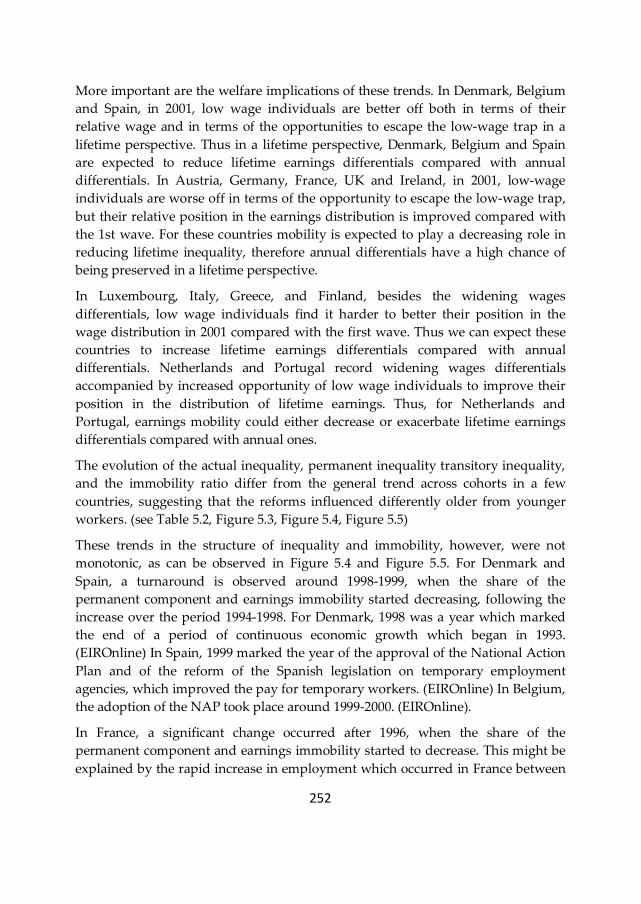
252
More important are the welfare implications of these trends. In Denmark, Belgium
and Spain, in 2001, low wage individuals are better off both in terms of their
relative wage and in terms of the opportunities to escape the low-wage trap in a
lifetime perspective. Thus in a lifetime perspective, Denmark, Belgium and Spain
are expected to reduce lifetime earnings differentials compared with annual
differentials. In Austria, Germany, France, UK and Ireland, in 2001, low-wage
individuals are worse off in terms of the opportunity to escape the low-wage trap,
but their relative position in the earnings distribution is improved compared with
the 1st wave. For these countries mobility is expected to play a decreasing role in
reducing lifetime inequality, therefore annual differentials have a high chance of
being preserved in a lifetime perspective.
In Luxembourg, Italy, Greece, and Finland, besides the widening wages
differentials, low wage individuals find it harder to better their position in the
wage distribution in 2001 compared with the first wave. Thus we can expect these
countries to increase lifetime earnings differentials compared with annual
differentials. Netherlands and Portugal record widening wages differentials
accompanied by increased opportunity of low wage individuals to improve their
position in the distribution of lifetime earnings. Thus, for Netherlands and
Portugal, earnings mobility could either decrease or exacerbate lifetime earnings
differentials compared with annual ones.
The evolution of the actual inequality, permanent inequality transitory inequality,
and the immobility ratio differ from the general trend across cohorts in a few
countries, suggesting that the reforms influenced differently older from younger
workers. (see Table 5.2, Figure 5.3, Figure 5.4, Figure 5.5)
These trends in the structure of inequality and immobility, however, were not
monotonic, as can be observed in Figure 5.4 and Figure 5.5. For Denmark and
Spain, a turnaround is observed around 1998-1999, when the share of the
permanent component and earnings immobility started decreasing, following the
increase over the period 1994-1998. For Denmark, 1998 was a year which marked
the end of a period of continuous economic growth which began in 1993.
(EIROnline) In Spain, 1999 marked the year of the approval of the National Action
Plan and of the reform of the Spanish legislation on temporary employment
agencies, which improved the pay for temporary workers. (EIROnline) In Belgium,
the adoption of the NAP took place around 1999-2000. (EIROnline).
In France, a significant change occurred after 1996, when the share of the
permanent component and earnings immobility started to decrease. This might be
explained by the rapid increase in employment which occurred in France between

253
1997 and 2002 as a result of the policies aimed to lower the cost of unskilled jobs
and stimulate job creation.
In Ireland, the significant turnaround in 1997 might be due to the slowing down of
the Celtic Tiger: the remarkable economic growth which started in 1994 was
accompanied by a rise in the share of permanent inequality and earnings
immobility, which contracted slightly after 1997. Hence, the economic growth was
a shock that accentuated the share of permanent differentials in the overall
inequality and increased earnings immobility between 1994 and 1997. After 1997,
the trends reversed.
A dramatic change occurred in Austria after 1998. Until 1998, wage immobility and
the share of permanent inequality increased sharply. In 1999, Austria experienced a
considerable rise in employment and a further decline in unemployment, which
was the effect of the labour market initiatives pursued by the Austrian
Government. This explains the increase in inequality after 1999: higher
employment is usually accompanied by higher inequality. These measures appear
to have decreased earnings immobility and the share of permanent inequality in
1999, which stabilized thereafter.
In Netherlands, a significant change occurred after 1998, when immobility and the
share of permanent inequality started decreasing, offsetting the increasing trend
which dominated the period before 1998. Among the important issues addressed
by the labour market legislation in 1998 were part-time employment, labour
market flexibility and active labour market policies. In 2001, the share of the
permanent components was the lowest among all countries which recorded an
increase in overall inequality.
For Luxembourg, Italy, Portugal, Greece and Finland, a turning point occurred
around 1998-1999. This period coincides with the approval of the National Action
plan for employment aimed, among others, to lower labour cost, promote active
labour market policies, training and increase labour market flexibility. This
appears to have affected the structure of wage differentials to a large extent.
Immediately after 1998-1999, the share of permanent inequality and wage
immobility started to decrease.
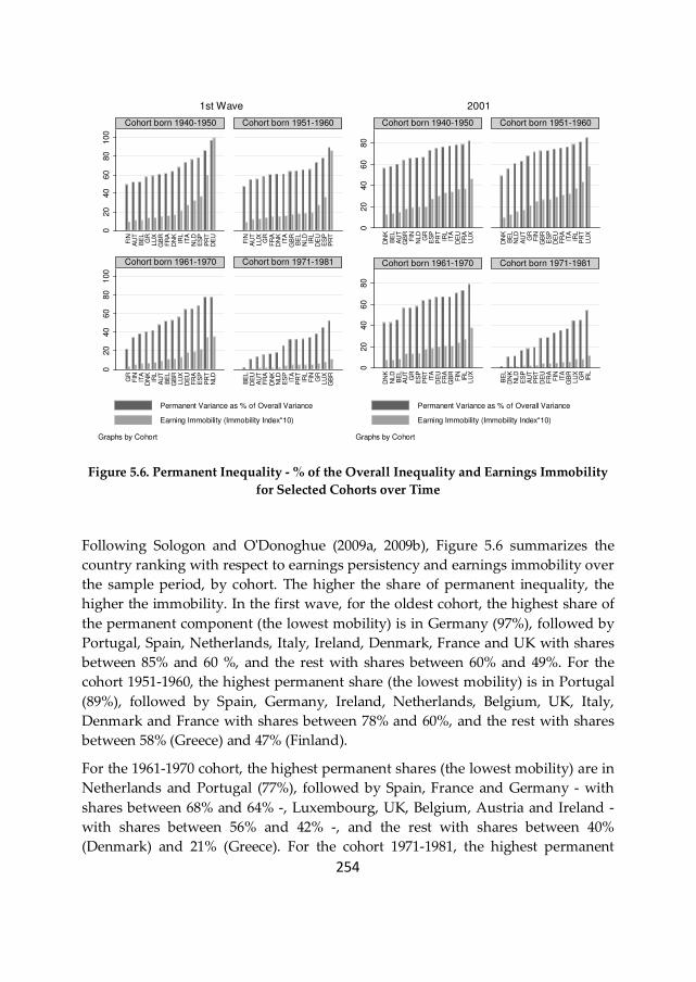
254
Figure 5.6. Permanent Inequality - % of the Overall Inequality and Earnings Immobility
for Selected Cohorts over Time
Following Sologon and O'Donoghue (2009a, 2009b), Figure 5.6 summarizes the
country ranking with respect to earnings persistency and earnings immobility over
the sample period, by cohort. The higher the share of permanent inequality, the
higher the immobility. In the first wave, for the oldest cohort, the highest share of
the permanent component (the lowest mobility) is in Germany (97%), followed by
Portugal, Spain, Netherlands, Italy, Ireland, Denmark, France and UK with shares
between 85% and 60 %, and the rest with shares between 60% and 49%. For the
cohort 1951-1960, the highest permanent share (the lowest mobility) is in Portugal
(89%), followed by Spain, Germany, Ireland, Netherlands, Belgium, UK, Italy,
Denmark and France with shares between 78% and 60%, and the rest with shares
between 58% (Greece) and 47% (Finland).
For the 1961-1970 cohort, the highest permanent shares (the lowest mobility) are in
Netherlands and Portugal (77%), followed by Spain, France and Germany - with
shares between 68% and 64% -, Luxembourg, UK, Belgium, Austria and Ireland -
with shares between 56% and 42% -, and the rest with shares between 40%
(Denmark) and 21% (Greece). For the cohort 1971-1981, the highest permanent
020
40
60
80
100
020
40
60
80
100
FIN
AU
TB
EL
GR
LU
XG
BR
FR
AD
NK
IRL
ITA
NLD
ES
PP
RT
DE
U
FIN
AU
TLU
XG
RF
RA
DN
KIT
AG
BR
BE
LN
LD
IRL
DE
UE
SP
PR
T
GR
FIN
ITA
DN
KIR
LA
UT
BE
LG
BR
LU
XD
EU
FR
AE
SP
PR
TN
LD
BE
LD
EU
AU
TF
RA
DN
KN
LD
ES
PIT
AP
RT
IRL
FIN
GR
LU
XG
BR
Cohort born 1940-1950 Cohort born 1951-1960
Cohort born 1961-1970 Cohort born 1971-1981
Permanent Variance as % of Overall Variance
Earning Immobility (Immobility Index*10)
Graphs by Cohort
1st Wave
020
40
60
80
020
40
60
80
DN
KB
EL
AU
TG
BR
FIN
NLD
GR
ES
PP
RT
IRL
ITA
DE
UF
RA
LU
X
DN
KB
EL
NLD
AU
TG
RF
ING
BR
ES
PD
EU
FR
AIT
AIR
LP
RT
LU
X
DN
KN
LD
BE
LA
UT
GR
ES
PP
RT
ITA
DE
UF
RA
GB
RF
INIR
LLU
X
BE
LD
NK
NLD
ES
PA
UT
PR
TD
EU
FR
AF
INIT
AG
BR
LU
XG
RIR
L
Cohort born 1940-1950 Cohort born 1951-1960
Cohort born 1961-1970 Cohort born 1971-1981
Permanent Variance as % of Overall Variance
Earning Immobility (Immobility Index*10)
Graphs by Cohort
2001
255
share is recorded in UK (52%), followed by Luxembourg (45%), Greece, Finland,
Ireland, Portugal, Italy and Spain - with shares between 38% and 25% -, and the
rest with shares between 18% (Netherlands) and 2% (Belgium).
Following these changes, the structure of inequality and earnings immobility in
2001, for the oldest cohort, the highest share of permanent inequality implying the
highest earning persistency (lowest mobility) is found in Luxembourg, France,
Germany, Italy, Ireland, Portugal and Spain, with rates between 82% and 73%.
Greece, Netherlands, Finland, UK and Austria are less persistent with values
between 70% and 60%. The least persistent – most mobile - are Denmark and
Belgium, where permanent variance accounts for 56-58% of the overall variance.
For the 1951-1960 cohort, the highest persistency – lowest mobility - is recorded by
the same countries, including UK and Finland, with shares between 85% and 71%,
followed by Greece, Austria and Netherlands with shares between 68% and 61%,
and lastly Belgium (56%) and Denmark (49%). For the 1961-1970 cohort in
Luxembourg, Ireland and Finland permanent variance accounts for 79% to 70% of
the overall variance, followed by UK, France, Germany, Italy and Portugal with
shares between 66% and 63%, by Spain, Greece and Austria with shares between
58% and 56%, and by Belgium, Netherlands and Denmark with shares between
45% and 42%.
For the youngest cohort, the variance is dominantly transitory in all countries,
except Ireland where the transitory variance accounts for 46% of the overall
variance, suggesting that Irish youngsters have the lowest degree of earnings
mobility in Europe. The most volatile earnings are found in Belgium, where 98.5%
of the variance is transitory. Next follow Denmark and Netherlands where
transitory variance accounts for 89% of the overall variance; Spain, Austria and
Portugal, with transitory shares between 84% and 81%; Germany, France, Finland,
Italy and UK with transitory shares between 72% and 63%; Greece and
Luxembourg where transitory inequality accounts for 56% of the variance.
Based on Sologon and O'Donoghue (2009a, 2009b), we summarize the changes in
country ranking in permanent inequality, transitory inequality, and earnings
immobility over the sample period by reporting the averages across cohorts. In
1994, the highest average permanent inequality77 was recorded in Portugal and
Spain, followed by France, Ireland, Germany, UK, Greece, Italy, Netherlands,
Belgium and Denmark. The highest transitory variance was recorded in France,
Ireland, Greece, UK, Germany, Spain, Belgium, Denmark, Netherlands, Italy and
77 Average permanent variance and transitory variance represent average across cohorts.
256
Portugal. Portugal has the lowest mobility, followed by Spain, Germany, UK, Italy,
Ireland, Netherlands, France, Belgium, Greece and Denmark. In 1995, Austria and
Luxembourg had a middle ranking in permanent inequality and a top ranking78 in
transitory inequality and mobility. In 1996, Finland had the second lowest
permanent inequality, a middle ranking in transitory inequality, and the highest
mobility.
In 2001 the rankings looks slightly different. Portugal records the highest average
permanent differentials, followed by Luxembourg, France, Spain, Ireland,
Germany, Greece, UK, Italy, Finland, Netherlands, Austria, Belgium and Denmark.
In terms of transitory inequality, Portugal appears to be the most dispersed,
followed by Spain, Netherlands, France, Greece, UK, Germany, Belgium,
Luxembourg, Austria, Ireland, Denmark, Finland and Italy. Denmark has the
highest average earnings mobility, followed by Belgium, Netherlands, Austria,
Spain, Greece, Finland, UK, France, Germany, Italy, Portugal, Ireland and
Luxembourg.
5.7.Linking policy with outcomes
What are the factors explaining country heterogeneity in the level and the
evolution of permanent differentials, transitory differentials and earnings
mobility? We try to explain the cross-country differences in these labour market
outcomes by relating to the differences in the wage setting mechanism and the
other labour marker institutions and policies - such as active labour market policies
and income maintenance institutions (e.g. unemployment benefits) -, and the
institutional and policy changes - such as employment protection legislation,
product market regulation, tax wedge, unionization.
First we describe with the naked eye the possible associations that can be formed
between the trends in the labour market outcomes identified in the previous
section and the changes in the labour market policy and institutional factors
identified in Section 5.5.2 and summarized in Figure 5.2. Second, by cohorts, we
estimate uncontrolled pairwise correlations to put some numbers on the observed
trends and see whether the relationships differ by cohorts. Finally, using non-
linear least squares, we estimate the complex relationship between the institutional
factors and permanent inequality, transitory inequality and earnings immobility.
78 Among the highest four.

257
5.7.1. Explaining the changes and differences
We start with the rankings in average permanent and transitory differentials and
average mobility observed in 1994 and 2001 (see Section 5.6.2). At a first glance, the
diverging characteristics of the labour markets (see Figure 5.2) recording the
highest and the lowest average permanent differentials – Portugal and Denmark -,
suggest that permanent variance appears to be positively associated with
employment protection legislation (EPL), employment protection legislation for
regular contracts (EPLR), employment protection legislation for temporary
contracts (EPLT), the relative difference between the EPLR and EPLT, and product
market regulation (PMR), and negatively associated with union density, the degree
of corporatism, the tax wedge, the generosity of the unemployment benefit and the
level of spending for active labour market policies (ALMPs).
Similarly, temporary variance appears to be positively associated with EPLT, the
unemployment benefit generosity, and negatively with union density, PMR and
the degree of corporatism.
Looking at the labour markets with the highest and lowest average immobility in
1994 and 2001 (Section 5.6.2), a positive association was found with the union
density, the tax wedge and the unemployment benefit replacement rate, and a
negative association with EPLR, the relative difference between EPLR and EPLT,
and PMR. For the other factors the trend is less clear-cut.
Next, we try to link the evolution of the three labour market outcomes with the
evolution of the institutional factors summarized in Figure 5.2.
The common factors that might explain the common trends in permanent
differentials and mobility in Denmark, Belgium and Spain are the decrease in EPL,
the increase in ALMP and the decrease in PMR. ALMP can reduce permanent and
transitory differentials by improving the efficiency of the job matching process and
by enhancing the skills of the unemployed. Moreover its effects are expected to be
enhanced when they are coupled with a low or decreasing EPL. Denmark
represents a proof of the efficiency of this mix in reducing both components.
The ALMP–EPL mix might also be one of the factors explaining the divergence in
the transitory variance trends between these countries: Denmark exhibits a high
ALMP coupled with a low EPL, whereas the other two exhibit a relatively low
ALMP coupled with a medium high EPL. This suggests that the impact of ALMP
on transitory inequality might decrease with the EPL. A second factor could be the
interaction between the decrease in PMR and the other factors. Lower PMRs are
expected to determine an increase in both components. However, these effects

258
appear to be completely offset in Denmark, whereas in Belgium and Spain they are
offset only for permanent differentials.
Third, the decrease in transitory variance in Denmark might signal the presence of
strong wage bargaining structures, finding supported by the high union density,
corporatism and bargaining coverage indicators. This is consistent with the OECD
(2004) results, which placed Denmark as having one of the highest collective
bargaining and trade union density among all 14 EU countries under analysis. In
Belgium and Spain, another potential factor explaining the increase in transitory
inequality might be immigration, which increased considerably with the expansion
of the European Union.
To sum up, the outstanding performance of the labour market in Denmark which
assured a decreasing cross-sectional inequality by reducing both components,
might be due to the so called “flexicurity approach” (OECD(2004)), which
represents an interesting combination of high labour market dynamism and
relatively high social protection. It is a mix of flexibility (a high degree of job
mobility thanks to low EPL), social security (a generous system of unemployment
benefits) and active labour market programmes, which allows individuals to
improve their position in the permanent income distribution by reducing
permanent income differentials, maintain at the same time a low degree of
earnings volatility.
The common factors that might explain the decrease in transitory differentials and
the decrease in mobility in Germany, France, UK, Ireland and Austria are the
decrease in union density and PMR, the increase in ALMP and the low EPL which
was roughly constant, except for Germany where the latter two factors decreased.
The decrease in union density and PMR are potential factors explaining the
increase in permanent differentials in Germany, France, UK and Ireland, which
appear to have offset the effect of the increase in ALMP present in the latter three
countries. UK, Ireland and Austria exhibit another factor with a potential
increasing effect on permanent differentials: the decrease in the tax wedge.
The decrease in transitory variance, which is common to all these countries,
reinforces the finding that developed increasing ALMP coupled with a relatively
low EPL can be expected to dampen earnings volatility. Hence, for transitory
differentials, the impact of the ALMP-EPL mix appears to have offset the potential
effects of the decrease in union density and PMR. Moreover, the dampening effect
of the ALMP-EPL mix on the transitory inequality appears to be accentuated when
it is coupled with an increase in the unemployment benefit generosity. It is the case
in France, Ireland and Austria.
259
In France, other factors which might contribute to the absolute increase in the
permanent component are the increase in EPLR, because of the potential reducing
effect on the incidence of permanent contracts. The decrease in transitory
inequality might also signal a labour market mechanism put in place to reduce
transitory inequality. This is consistent with OECD (2004): France ranks the lowest
on union density, but managed to increase coverage levels after the introduction of
the legislation promoting collective bargaining and is now among the countries
with the highest coverage rates of 90% and above, together with Austria, Belgium
and Finland. Moreover, based on OECD (2004), France was found to have a low
level of labour market dynamics, which might explain the reduction in transitory
inequality and mobility.
In UK, the positive increasing relative difference between EPLR and EPLT, coupled
with the low degree of corporatism could have accentuated the disincentive for
employers to train temporary workers, and thus could have contributed to increase
permanent differentials.
In Luxembourg, Italy, Greece, Finland, and Portugal the common institutional
trends that might explain the increase in permanent differentials are the decrease
or constant evolution of the EPL, the decrease in union density, PMR and the tax
wedge. Italy and Portugal exhibit also a decrease in EPLT relative to EPLR, which
might accentuate permanent differentials. The decrease in transitory differentials
and the increase in immobility in Luxembourg, Italy, Greece, and Finland might be
explained by the increase in the ALMPs, coupled with the increase in the
generosity of the unemployment benefit, except for Finland. The increase in
transitory differentials recorded by Portugal might be due to the level of
corporatism: an intermediate level appears to accentuate transitory differentials,
whereas a high level might help to reduce them.
5.7.2. Correlations
Given the clear distinction in the trends of the two components and earnings
immobility between the oldest three cohort and the youngest cohorts, we expect
also the underlying factors to differ to a certain extent. Thus, it is necessary to
account for cohort heterogeneity when analysing the link between the three labour
market outcomes and the institutional and policy factors. As a first step, we
estimate the simple uncontrolled correlations (Table 5.4) comparatively between
the oldest there cohorts, polled together, and the youngest one. Permanent
variance for the older cohorts is significantly79 positively associated with all the
79 At 1% and 5% level of confidence
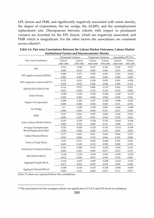
260
EPL factors and PMR, and significantly negatively associated with union density,
the degree of corporatism, the tax wedge, the ALMPs, and the unemployment
replacement rate. Discrepancies between cohorts with respect to permanent
variance are recorded for the EPL factors, which are negatively associated, and
PMR which is insignificant. For the other factors the associations are consistent
across cohorts80.
Table 5.4. Pair wise Correlations Between the Labour Market Outcomes, Labour Market
Institutional Factors and Macroeconomic Shocks
Pair wise Correlations
Permanent Variance Temporary Variance Immobility (PV/TV)
Cohort
1940-1969
Cohort
1970-1981
Cohort
1940-1969
Cohort
1970-1981
Cohort
1940-1969
Cohort
1970-1981
EPL 0.313 -0.245 0.207 0.166 0.140 -0.317
0.000 0.014 0.000 0.096 0.015 0.001
EPL regular contracts (EPLR) 0.488 -0.171 0.190 0.259 0.225 -0.263
0.000 0.087 0.001 0.009 0.000 0.008
EPL temporary contracts (EPLT) 0.122 -0.213 0.158 0.070 0.051 -0.254
0.034 0.032 0.006 0.488 0.380 0.010
[(EPLR-EPLT)/EPLT]*100 0.116 0.555 0.086 -0.147 0.024 0.593
0.041 0.000 0.135 0.142 0.674 0.000
Union Density -0.588 -0.333 -0.323 -0.340 -0.245 -0.110
0.000 0.000 0.000 0.000 0.000 0.256
Degree of Corporatism -0.498 -0.441 -0.477 -0.228 -0.086 -0.201
0.000 0.000 0.000 0.028 0.151 0.054
Tax Wedge -0.3 -0.385 -0.245 0.096 -0.066 -0.449
0.000 0.000 0.000 0.361 0.271 0.000
PMR 0.247 0.041 0.053 0.046 0.160 0.018
0.000 0.695 0.381 0.664 0.007 0.863
Active Labour Market Policies -0.267 -0.219 -0.240 0.150 -0.063 -0.184
0.000 0.035 0.000 0.151 0.294 0.077
Average Unemployment
Benefit Replacement Rate
-0.223 -0.450 -0.225 0.214 -0.114 -0.465
0.000 0.000 0.000 0.039 0.057 0.000
Labour Demand Shock 0.177 0.605 0.021 0.005 0.066 0.574
0.005 0.000 0.742 0.966 0.291 0.000
Terms of Trade Shock -0.03 0.151 -0.061 -0.068 0.105 0.102
0.623 0.149 0.314 0.520 0.080 0.330
Total Factor Production Shock -0.241 -0.082 -0.371 -0.259 -0.041 0.163
0.000 0.454 0.000 0.017 0.517 0.137
Real Interest Shock -0.148 -0.134 -0.010 -0.011 -0.056 -0.218
0.013 0.200 0.875 0.918 0.352 0.036
Aggregate Supply Shock -0.104 -0.075 -0.007 -0.008 -0.014 -0.103
0.071 0.456 0.903 0.934 0.805 0.308
Aggregate Demand Shock -0.208 -0.156 -0.237 -0.236 -0.092 -0.003
0.000 0.121 0.000 0.017 0.111 0.977
Note: P-values are reported below the correlations.
80 The associations for the youngest cohorts are significant at 1%,5% and 10% level of confidence.

261
Transitory variance for the older cohorts is significantly81 positively associated with
the EPL, EPLR and EPLT, and significantly negatively associated with the rest,
except the relative difference between EPLR and EPLT and PMR which are
insignificant. The youngest cohort records fewer significant associations: a positive
association82 is recorded with EPL, EPLR and the unemployment replacement rate,
and a negative association83 with union density and the degree of corporatism.
The immobility ratio for the oldest three cohorts exhibits a positive significant
association with EPL, EPLR and PMR, and a significant negative association with
union density84 and the unemployment benefit replacement rate85. For the
youngest cohort, the immobility ratio is significantly positively associated with the
relative difference between EPLR and EPLT, and significantly negatively86
associated with the other factors except the union density and PMR, which are
insignificant.
The trend differences in permanent inequality, transitory inequality and
immobility observed between cohorts (Figure 5.3, Figure 5.5, and Table 5.2) might
be related also with the different levels of responsiveness to the macroeconomic
shocks and their interactions with the other labour market policy and institutional
factors. Younger workers are expected to be affected to a larger extent by these
shocks, compared with experienced workers, which have a high attachment to the
labour market and a better protection from the institutional framework. This might
explain the much higher share of transitory inequality observed for younger
cohorts.
The correlations with the macroeconomic shocks (Table 5.4) reveal differences
between cohorts. For permanent variance, the youngest cohort records a much
stronger positive correlation with labour demand shocks compared with the oldest
cohorts, and insignificant correlations for the other shocks. For the oldest cohorts,
the other shocks exhibit significant negative correlations, except the terms of trade
shock. For transitory variance, only the total factor production and the aggregate
demand shocks exhibit a significant negative association. Across cohorts, the
negative association with the total factor production shock is stronger for the
oldest cohorts. More differences between cohorts emerge for earnings immobility.
81 At 1% evel of confidence 82 Significant at 5% and 10% level of confidence 83 Significant at 1% and 5% level of confidence 84 At 1% level of confidence 85 At 10% level of confidence 86 At 1%, 5% and 10% levels of confidence
262
For the oldest cohorts, a significant87 positive association is observed for the terms
of trade shock. For the youngest cohort, a significant88 positive association is
observed for the labour demand shock, and a significant negative association89
with the real interest rate shock
Nevertheless, these correlations are far from telling the true story given the
complexity of the interactions that take place between institutions on the one hand,
and between institutions and macroeconomic shocks on the other hand.
To conclude, the institutional factors are expected to shape the pattern and the
level of permanent inequality, transitory inequality and earnings immobility not
only directly, but also in interaction with macroeconomic shocks. The overall
institutional factors is expected to be a “filtering mechanism” for the adverse effect
that these shocks might have on the three labour market outcomes, provided that
their aim is to keep permanent and transitory inequality low, assuring at the same
time that low wage individuals are not trapped in low pay, but have the
opportunity to improve their position in the distribution of lifetime income
through earnings mobility.
Moreover, we expect institutional factors to play a much larger role in shaping
permanent differentials compared with transitory differentials and earnings
immobility, given that the latter two are exposed to a much larger extent to
random shocks, against which the institutional factors might have a delayed
response or any at all.
5.7.3. Estimation
This section aims to provide some empirical evidence with respect to the impact of
the main labour market policy and institutional factors and their complex
interactions in shaping permanent inequality, transitory inequality and earnings
immobility.
5.7.3.1. Systemic interactions: do policies and institutions
interact with the overall institutional framework?
The results regarding systemic interactions are included in Model 1 in Table 5.5. A
summary of the results is displayed in Model 1 in Table 5.7-Table 5.9. The models
with systemic interactions are estimated to explain 97.8% of the cross-country
87 At 10% level of confidence 88 At 1% level of confidence 89 At 5% level of confidence

263
variation in permanent inequality, 93.2% of the cross-country variation in
transitory inequality, and 71.6% of the cross-country variation in earnings
immobility, between 1994 and 2001.
The cohorts shifters are highly significant in all models, confirming the cohort-
heterogeneous trends identified previously by the error component model (Figure
5.3): the older the cohort, the higher the permanent variance and wage immobility,
and the lower the transitory inequality.
Similarly, the time effects are highly significant in all models. They indicate that,
overall, at the EU level, controlling for the effects of institutional and policy factors,
the unobserved shocks had a decreasing impact on permanent variance in 1995, an
increasing impact until 1997 and decreasing impact thereafter. The impact of the
unobserved shocks on transitory inequality decreased until 2000 and increased in
2001. For wage immobility more variation is observed: it decreased in 1995,
increased until 1997, decreased until 1999, increased again in 2000, followed by a
drop in 2001. Overall, it appears that the unobserved shocks had a decreasing
effect on both permanent and transitory dispersion, and an increasing effect on
wage mobility.
The direct effects, controlling for the systemic interactions, cohort and the period
effects, indicate that, except for product market regulation (PMR) and active labour
market policies (ALMPs), all other factors have a significant impact on permanent
dispersion. Factors that appear to reduce permanent inequality are the union
density and the average unemployment benefit replacement rate. The hump shape
profile of the impact of the degree of corporatism is confirmed: the intermediate
level of corporatism appears to trigger the highest permanent dispersion, followed
by a high and then a low corporatism.
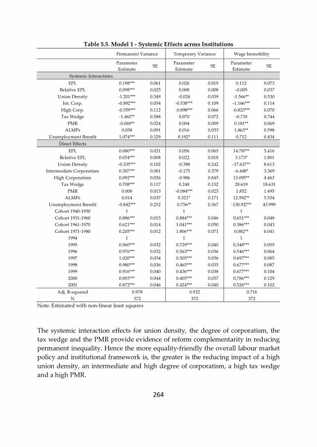
264
Table 5.5. Model 1 - Systemic Effects across Institutions
Permanent Variance Temporary Variance Wage Immobility
Parameter
Estimate SE
Parameter
Estimate SE
Parameter
Estimate SE
Systemic Interactions
EPL 0.198*** 0.061 0.026 0.019 0.112 0.073
Relative EPL 0.098*** 0.025 0.008 0.008 -0.005 0.037
Union Density -1.201*** 0.349 -0.024 0.039 -1.566** 0.530
Int. Corp. -0.892*** 0.054 -0.538*** 0.109 -1.166*** 0.114
High Corp. -0.559*** 0.112 -0.898*** 0.066 -0.823*** 0.070
Tax Wedge -1.462** 0.588 0.070 0.072 -0.718 0.744
PMR -0.069** 0.024 0.004 0.009 0.181** 0.069
ALMPs 0.058 0.091 0.016 0.033 1.863** 0.598
Unemployment Benefit 1.074*** 0.329 0.192* 0.111 0.712 0.434
Direct Effects
EPL 0.080*** 0.021 0.056 0.065 14.787** 5.416
Relative EPL 0.054*** 0.008 0.022 0.018 3.173* 1.801
Union Density -0.335*** 0.102 -0.388 0.242 -17.637** 8.613
Intermediate Corporatism 0.307*** 0.081 -0.175 0.379 -6.448* 3.369
High Corporatism 0.092*** 0.026 -0.986 0.845 13.095** 4.463
Tax Wedge 0.708*** 0.117 0.248 0.152 28.619 18.631
PMR 0.008 0.013 -0.084*** 0.025 1.852 1.495
ALMPs 0.014 0.037 0.321* 0.171 12.592** 5.534
Unemployment Benefit -0.842*** 0.252 0.756** 0.367 -130.927** 43.999
Cohort 1940-1950 1 1
1
Cohort 1951-1960 0.886*** 0.015 0.884*** 0.046 0.651*** 0.048
Cohort 1961-1970 0.621*** 0.014 1.041*** 0.050 0.386*** 0.043
Cohort 1971-1980 0.205*** 0.012 1.806*** 0.071 0.082** 0.041
1994 1 1
1
1995 0.960*** 0.032 0.729*** 0.040 0.348*** 0.055
1996 0.976*** 0.032 0.563*** 0.036 0.546*** 0.064
1997 1.020*** 0.034 0.505*** 0.036 0.697*** 0.085
1998 0.980*** 0.036 0.465*** 0.035 0.677*** 0.087
1999 0.916*** 0.040 0.436*** 0.038 0.677*** 0.104
2000 0.893*** 0.044 0.405*** 0.037 0.786*** 0.129
2001 0.872*** 0.046 0.424*** 0.040 0.526*** 0.102
Adj. R-squared 0.978 0.932 0.716
N 372 372 372
Note: Estimated with non-linear least squares
The systemic interaction effects for union density, the degree of corporatism, the
tax wedge and the PMR provide evidence of reform complementarity in reducing
permanent inequality. Hence the more equality-friendly the overall labour market
policy and institutional framework is, the greater is the reducing impact of a high
union density, an intermediate and high degree of corporatism, a high tax wedge
and a high PMR.
265
The model for transitory variance, despite having a similar level of explained
variation as the model for permanent inequality, exhibits fewer significant effects
for the institutional factors. The period effects and the cohort effects explain a large
share of the variation in transitory inequality: random exogenous shocks increase
earnings variability and the magnitude of their impact depends on the specific
lifecycle stage a respective cohort is in.
Only the PMR, the ALMPs and the unemployment benefit replacement rate have a
significant direct impact on transitory inequality. Ceteris paribus, an increase in the
spending for ALMPs and in the unemployment benefit replacement rate increases
transitory differentials, whereas an increase in the PMR reduces transitory
differentials. Moreover, albeit insignificant, the higher the union density and the
higher the degree of corporatism are, the larger is the reduction in transitory
variance.
The systemic interactions suggest that there is a complementarity with the overall
framework in reducing transitory inequality for the union density and the degree
of corporatism. Hence, the more inclined the overall framework is towards
reducing transitory differentials, the effect is larger the higher is the union density
and the larger is the degree of corporatism. The effect of union density, however, is
not significant at conventional levels. The other factors appear to counteract with
the overall system, but the effect is significant only for the unemployment benefit
replacement rate.
For earnings immobility, ceteris paribus, a significant positive direct effect is found
for employment protection legislation (EPL), the relative difference between
employment protection legislation for regular contracts (EPLR) and temporary
contracts (EPLT), a high degree of corporatism and ALMPs. Similarly for PMR, but
the effect is insignificant. A U-shaped profile is found for the degree of
corporatism: a high degree of corporatism is found to increase wage immobility
compared with low corporatism, whereas an intermediate corporatism appears to
decrease it. Besides an intermediate corporatism, other factors that contribute
directly to decrease earnings immobility are the union density and the
unemployment benefit replacement rate.
The systemic interactions suggest that there is a complementarity with the overall
framework in reducing wage immobility for the union density, and the degree of
corporatism – with an stronger negative effect for the intermediate level than for a
high level. The tax wedge also has a negative effect, but insignificant. PMR and
ALMPs counteract with the overall framework, in a tendency to increase wage
immobility.
266
5.7.3.2. Specific Interactions
This section explores the specific interactions between institutions, and between
institutions and observed macroeconomic shocks, expected to shape the pattern of
permanent inequality, transitory inequality and earnings immobility. First we look
at the direct effect of shocks and institutions, and the interactions between
institutions and the systemic shock (Model 2 in Table 5.6). Second, we enhance the
model by adding cross-interactions between institutions, and other controls (Model
3 in Table 5.6).
Model 2 in Table 5.6 illustrates the estimates for the direct effects of institutions,
observed macroeconomic shocks, and the interactions between institutions and the
systemic shock. A summary of the results is displayed in Model 2 in Table 5.7-
Table 5.9.
The models for the three labour market outcomes explain 97.9% of the variation in
permanent inequality, 92.9% of the variation in the transitory inequality and 68.9%
of the variation in wage immobility.
Compared with Model 1, including the effects of the observed macroeconomic
shocks and the interactions between institutions and the systemic shock (Model 2),
affects the direct effects of the institutions on all three labour market outcomes. For
transitory inequality and earnings immobility, however, the direct effects of the
institutions change to a larger extent than for permanent inequality.
For permanent inequality, most coefficient estimates maintain the direction of
influence and the significance level, except the union density which becomes
insignificant, a high corporatism and the PMR which become negative, the ALMPs
which become significant, and the unemployment benefit replacement rate which
becomes positive and insignificant. Among those that maintained the direction of
influence, the magnitude of the direct effects reduced in absolute value in Model 2
compared with Model 1, except for the ALMPs where it increased.
For transitory inequality, the EPL factors become significant, the degree of
corporatism becomes positive and significant, and ALMPs become negative and
insignificant. Among those that maintained the direction of influence and the
significance, the magnitude of the effects decreased in absolute value in Model 2
compared with Model 1.
For earnings immobility, the EPL, the union density, and the high degree of
corporatism become insignificant, the tax wedge becomes negative, the
intermediate degree of corporatism becomes positive and insignificant, the ALMPs
267
become negative and insignificant, and the unemployment benefit replacement
rate becomes positive. Among those that maintained the direction of influence and
the significance, the magnitude of the effects decreased in absolute value in Model
2 compared with Model 1. These results reinforce our expectation that the
institutional factors are a “filtering mechanism” for the effects of the macro shocks
on the three labour market outcomes.
We turn to the direct effects of the macroeconomic shocks. As expected, permanent
inequality appears to be affected directly by these shocks to a much lesser extent
compared with transitory inequality and wage immobility: only the aggregate
demand and the terms of trade shock are significant. For transitory inequality all
shocks show a highly significant effect, and for wage immobility all except the
aggregate labour supply shock.
For permanent inequality, a negative influence is observed for the terms of trade
shock and a positive one for the aggregate demand shock. Transitory inequality is
positively affected by the aggregate supply, the terms of trade and the total factor
production shocks, and negatively by the rest. Wage immobility is affected
negatively by the aggregate demand, the labour demand and the interest rate
shock, and positively by the rest.
The explanation for the lack of significance of the direct effects of shock in
explaining permanent inequality is found in the interaction effects between the
institutional factors and the aggregate shock. All interaction effects are significant,
except for ALMPs, suggesting that these policies and institution filter out the
effects of the macro shocks. EPL, the relative difference between EPLR and EPLT
and the tax wedge have a positive significant direct effect on permanent variance,
which is amplified under the aggregate impact of these shocks. The positive
significant effect of ALMPs is diminished under the impact of aggregate shocks,
but the interaction term is not significant at conventional levels.
If for the directs effects the hump-shaped pattern of the relationship between the
degree of corporatism and permanent inequality is confirmed, with the high level
triggering the lowest permanent inequality, followed by low and intermediate
corporatism, in interaction with aggregate shocks the degree of corporatism clearly
becomes a tool for reducing permanent differentials: the higher is the degree of
corporatism, the larger is the magnitude of the negative impact in reducing
permanent inequality. The union density, the PMR and the unemployment benefit
replacement rate have an insignificant direct effect, but in interaction with the
aggregate shock they appear to work significantly towards increasing permanent
differentials.
268
Compared with permanent inequality and wage immobility, fewer factors are
significant in filtering out the effects of the systemic shock on transitory inequality.
The direct effect for intermediate corporatism appears to trigger the highest
transitory inequality, followed by high and low corporatism. In interaction with
the aggregate shocks, however, the impact of an intermediate corporatism impact
becomes insignificant, whereas for high corporatism it becomes negative and
highly significant. Thus, similarly with permanent inequality, a high corporatism is
an efficient tool in reducing or limiting the increase of transitory inequality under
in the impact of macroeconomic shocks. A more generous unemployment benefit
appears to have a significant positive impact on transitory inequality that is
reduced in interaction with macroeconomic shocks.
The tax wedge does not have a significant direct effect on transitory inequality, but
in interaction with macroeconomic shocks, it appears to be an efficient tool in
reducing or limiting the increase of transitory inequality under the impact of
macroeconomic shocks. The opposite holds for PMR and ALMPs90: they have a
negative direct effect, but in interaction with the systemic shock, they appear to
have a positive impact on transitory inequality.
Wage immobility is explained to a lesser extent by the direct effects of institutions
than permanent and transitory inequality. Most of the direct and interaction effects
of shocks, however, are highly significant, suggesting that wage immobility is
influenced mainly by the macroeconomic shocks and their interaction with the
institutional setting. The relative difference between EPLR and EPLT and
unemployment benefit generosity have a positive effect on wage immobility,
which is diminished in interaction with the systemic shock. The effect of the
systemic macroeconomic shock on wage immobility appears to increase
significantly with the EPL, the union density, the PMR and the ALMPs, and to
decrease with the degree of corporatism, the tax wedge, and the unemployment
benefit replacement rate. An intermediate level of corporatism appears to be the
most effective in reducing the impact of shocks, followed by a high and a low level
of corporatism.
In order to grasp more in depth the nature of the relationship between institutions
and shocks, these models are augmented by including also 2-by-2 interactions
between the institutional factors, and other controls. The results are illustrated in
Model 3 in Table 5.6. A summary of the results is displayed in Model 3 in Table
5.7-Table 5.9.
90 Albeit insignificant
269
The new model specifications explain 98.9% of the variance in permanent
inequality, 94.2% for transitory inequality and 80.6% for wage immobility.
Including the institutional interaction effects and the other controls at the cohort
level (the shares of university and upper- secondary graduates, the sector
structure, the occupational structure, the share of unemployed, the share of
permanent contracts), several changes are observed.
First, for permanent inequality, the direct effects of institutions and most of their
cross interactions are highly significant, whereas all six macroeconomic shocks and
their interactions with the institutional factors become insignificant, except for high
corporatism. This suggests that the overall institutional structure manages to filter
out all direct and indirect effect of these shocks. Hence, in shaping permanent
inequality patterns, not the interactions between the systemic shock and the
institutions count, but how institutions interact with each other in dealing with the
effects of these shocks. One factor which interacts significantly with the aggregate
shock is high corporatism, which decreases the impact of the aggregate
macroeconomic shock on permanent inequality to a larger extent compared with
low and intermediate corporatism.
All direct effects that were insignificant in the previous specification of the
permanent inequality become significant once we control for cross-institutional
interactions. Among those that were significant in Model 2, a change in sign is
observed for the EPL, the relative difference between EPLR and EPLT, the tax
wedge, and a high degree of corporatism.
EPL has a negative direct effect on permanent inequality, enhanced by the relative
difference between EPLR and EPLT, and counteracted by the tax wedge. Union
density has a positive direct effect, which increases in interaction with the tax
wedge and decreases in interaction with PMR and ALPMs. The interaction with
the degree of corporatism confirms the hump-shaped pattern hypothesis: the
positive effect of the union density is enhanced in interaction with an intermediate
level of corporatism, and counteracted in interaction with a high level of
corporatism. The tax wedge has a negative direct effect on permanent inequality,
which is accentuated in interaction with the PMR and the generosity of the
unemployment benefit, and counteracted in interaction with the EPL, the union
density and the ALMPs.
PMR has a positive direct effect, counteracted in interaction with the union density,
the tax wedge and the ALMPs. ALMPs increases permanent inequality, effect
which is accentuated in interaction with the tax wedge, and reduced in interaction
with the PMR. Also union density and unemployment benefit lower the effect of
270
ALMP, but the effect is not significant. Unemployment benefit has a negative direct
effect on permanent inequality, which is reinforced by the tax wedge and the
AMPLs91, and counteracted by PMR.
Second, for transitory inequality, similarly with permanent inequality, controlling
for the interactions between institutions renders the direct and indirect effects of
shocks insignificant. This reconfirms that the key role in shaping transitory and
permanent inequality patterns is played by the interplay between labour market
policies and institutions in dealing with macroeconomic shocks.
The direct effects on transitory inequality modify to large extent when these
interactions are being introduced. Among those that remained significant, an
intensification of the effects is recorded by the EPL, and a change in sign is
recorded by the degree of corporatism, which exhibits a U-shaped relationship
with transitory inequality: the lowest transitory inequality is triggered by an
intermediate level, followed by a high level and a low level. The relative difference
between EPLR and EPLT becomes insignificant, the unemployment benefit
becomes negative and insignificant, the tax wedge negative and significant, and
the union density becomes positive but remains insignificant.
EPL increases transitory inequality, but the effect is counteracted by an
intermediate and a high corporatism, the tax wedge and the ALMPs. Union
density has an insignificant positive direct effect, which decreases in interaction
with an intermediate degree of corporatism, and increases in interaction with the
tax wedge and the PMR. The tax wedge reduces transitory inequality, effect
amplified by the EPL and the unemployment benefit replacement rate, and
counteracted by union density. PMR has a negative direct effect, counteracted by
the interaction effect with the union density. The ALMPs have a negative but
insignificant direct effect, which is amplified in interaction with EPL. Similarly, the
unemployment benefit replacement rate has an insignificant negative effect, which
is amplified in interaction with the tax wedge.
Third, for earnings immobility, the inclusion of the cross-institution interactions
renders all institutional factors highly significant, except the tax wedge and the
ALMPs. Among those that remain significant, a change in sign is observed for the
relative difference between the EPLR and EPLT, which turn negative. Among
those that turn significant in the last specification, a change in sign is recorded for
the union density, the degree of corporatism, and the PMR.
91 Albeit not significant
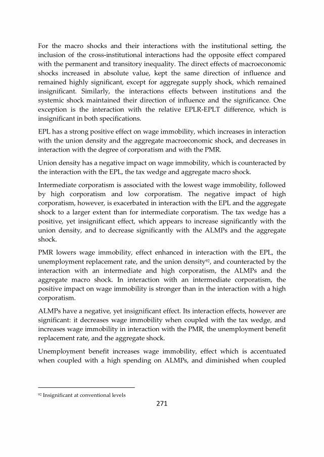
271
For the macro shocks and their interactions with the institutional setting, the
inclusion of the cross-institutional interactions had the opposite effect compared
with the permanent and transitory inequality. The direct effects of macroeconomic
shocks increased in absolute value, kept the same direction of influence and
remained highly significant, except for aggregate supply shock, which remained
insignificant. Similarly, the interactions effects between institutions and the
systemic shock maintained their direction of influence and the significance. One
exception is the interaction with the relative EPLR-EPLT difference, which is
insignificant in both specifications.
EPL has a strong positive effect on wage immobility, which increases in interaction
with the union density and the aggregate macroeconomic shock, and decreases in
interaction with the degree of corporatism and with the PMR.
Union density has a negative impact on wage immobility, which is counteracted by
the interaction with the EPL, the tax wedge and aggregate macro shock.
Intermediate corporatism is associated with the lowest wage immobility, followed
by high corporatism and low corporatism. The negative impact of high
corporatism, however, is exacerbated in interaction with the EPL and the aggregate
shock to a larger extent than for intermediate corporatism. The tax wedge has a
positive, yet insignificant effect, which appears to increase significantly with the
union density, and to decrease significantly with the ALMPs and the aggregate
shock.
PMR lowers wage immobility, effect enhanced in interaction with the EPL, the
unemployment replacement rate, and the union density92, and counteracted by the
interaction with an intermediate and high corporatism, the ALMPs and the
aggregate macro shock. In interaction with an intermediate corporatism, the
positive impact on wage immobility is stronger than in the interaction with a high
corporatism.
ALMPs have a negative, yet insignificant effect. Its interaction effects, however are
significant: it decreases wage immobility when coupled with the tax wedge, and
increases wage immobility in interaction with the PMR, the unemployment benefit
replacement rate, and the aggregate shock.
Unemployment benefit increases wage immobility, effect which is accentuated
when coupled with a high spending on ALMPs, and diminished when coupled
92 Insignificant at conventional levels

272
with a high PMR. Moreover, in interaction with the systemic shock, the positive
impact on wage immobility is being reduced.
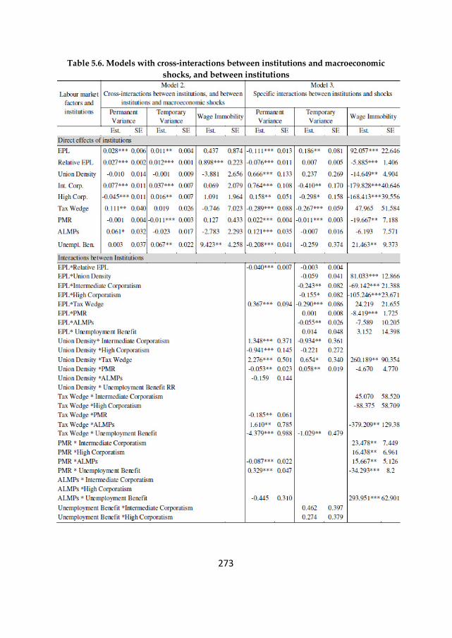
273
Table 5.6. Models with cross-interactions between institutions and macroeconomic
shocks, and between institutions
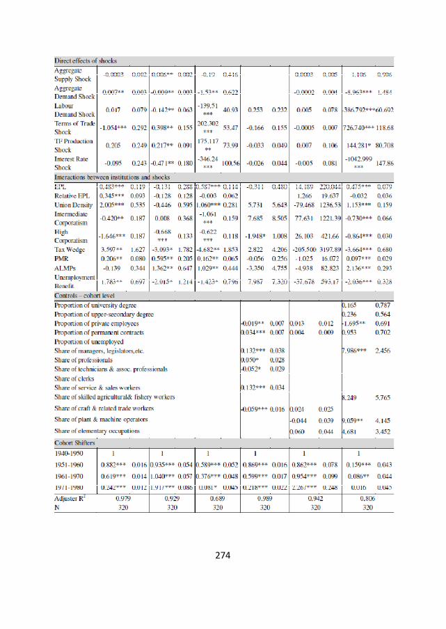
274

27
5
Tab
le 5
.7. S
um
mar
y r
esu
lts
for
per
man
ent
var
ian
ce
Per
ma
nen
t
Va
ria
nce
Mo
de
l 1
M
od
el
2
Mo
de
l 3
Dir
ect
Sy
st. X
D
irec
t
Sy
st.
Sh
ock
X
Dir
ect
Sy
st.
Sh
ock
X
Inte
ract
ion
s b
etw
een
in
stit
uti
on
s
EP
L
X
Re
l.
EP
L
X
UD
X
Int.
Co
rp
X
Hig
h
Co
rp
X
TW
X
PM
R
X
AL
MP
X
UB
X
EP
L
+
***
+
***
+
***
+
***
- ***
-
- ***
+
***
Re
lati
ve
EP
L
+
***
+
***
+
***
+
***
- ***
- **
*
Un
ion
Den
sity
- **
*
- ***
- +
***
+
***
+
+
***
- ***
+
***
- **
-
Inte
r. C
orp
+
***
>
- ***
<
+
***
- **
>
+
***
>
+
+
***
Hig
h C
orp
+
***
- ***
- ***
- ***
+
**
- *
- ***
Ta
x W
edg
e
+
***
- **
+
***
+
**
- ***
+
+
***
+
***
- **
+
**
- ***
PM
R
+
- **
- +
**
+
***
-
- **
- **
- **
*
+
***
AL
MP
s +
+
+
*
- +
***
-
-
+
**
- ***
-
Un
emp
loy
.
ben
efit
re
pl.
ra
te
- ***
+
***
+
+
**
- ***
+
- **
*
+
***
-
Sh
ock
s
2 s
ig.
N
ot
Sig
.
Co
ho
rt
Hig
her
th
e o
lder
th
e
coh
ort
***
Hig
her
th
e o
lder
th
e
coh
ort
***
Hig
her
th
e o
lder
th
e co
ho
rt**
*
Per
iod
D
ecre
asi
ng
***
Ad
j-R
2
N
0.9
78
37
2 0
.97
9 3
20
0.9
89
32
0
No
te: <
, >
ran
ks
the
eff
ects
of
the
inte
rme
dia
te c
orp
ora
tism
re
lati
ve
to t
he
hig
h c
orp
ora
tism
.
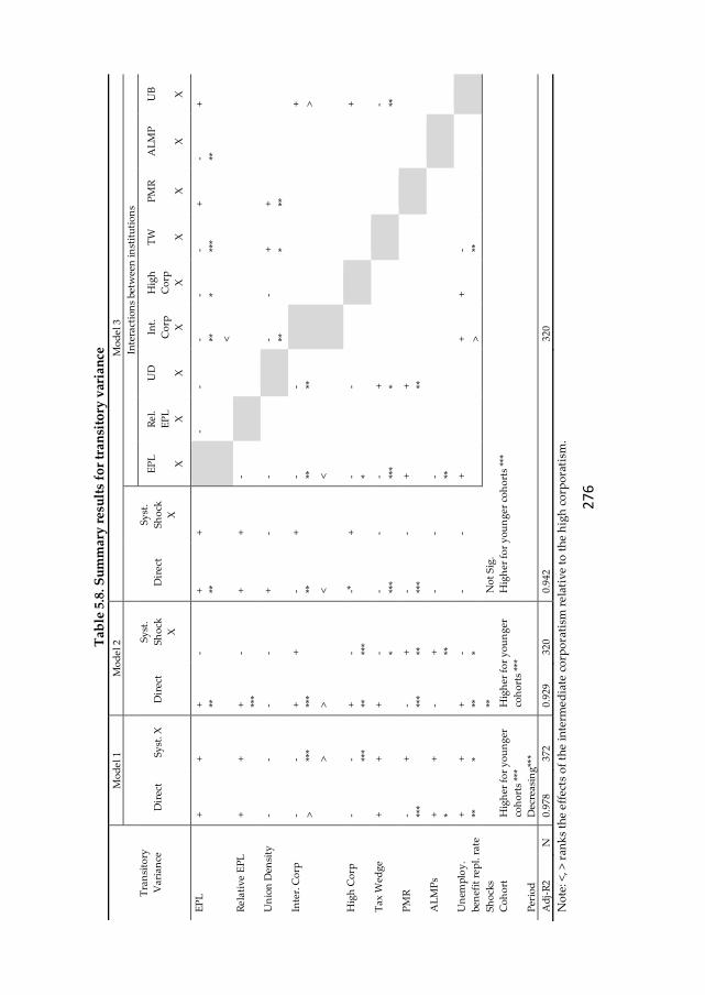
27
6
Tab
le 5
.8. S
um
mar
y r
esu
lts
for
tran
sito
ry v
aria
nce
Tra
nsi
tory
Va
ria
nce
Mo
de
l 1
M
od
el
2
Mo
de
l 3
Dir
ect
Sy
st. X
D
irec
t
Sy
st.
Sh
ock
X
Dir
ect
Sy
st.
Sh
ock
X
Inte
ract
ion
s b
etw
een
in
stit
uti
on
s
EP
L
X
Re
l.
EP
L
X
UD
X
Int.
Co
rp
X
Hig
h
Co
rp
X
TW
X
PM
R
X
AL
MP
X
UB
X
EP
L
+
+
+
**
- +
**
+
-
- - **
<
- *
- ***
+
- **
+
Re
lati
ve
EP
L
+
+
+
***
- +
+
-
Un
ion
Den
sity
-
- -
- +
-
-
- **
- +
*
+
**
Inte
r. C
orp
- >
- ***
>
+
***
>
+
- **
<
+
- **
<
- **
+
>
Hig
h C
orp
-
- ***
+
**
- ***
-*
+
- *
-
+
Ta
x W
edg
e
+
+
+
- *
- ***
- - **
*
+
*
- **
PM
R
- ***
+
- ***
+
**
- ***
- +
+
**
AL
MP
s +
*
+
- +
**
-
- - **
Un
emp
loy
.
ben
efit
re
pl.
ra
te
+
**
+
*
+
**
- *
- -
+
+
>
+
- **
Sh
ock
s
**
N
ot
Sig
.
Co
ho
rt
Hig
her
fo
r y
ou
ng
er
coh
ort
s **
*
Hig
her
fo
r y
ou
ng
er
coh
ort
s **
*
Hig
her
fo
r y
ou
ng
er c
oh
ort
s **
*
Per
iod
D
ecre
asi
ng
***
Ad
j-R
2
N
0.9
78
37
2 0
.92
9 3
20
0.9
42
32
0
No
te: <
, >
ran
ks
the
eff
ects
of
the
inte
rme
dia
te c
orp
ora
tism
re
lati
ve
to t
he
hig
h c
orp
ora
tism
.
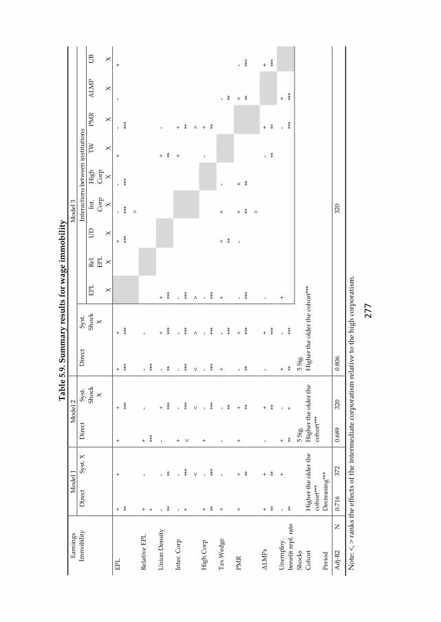
27
7
Tab
le 5
.9. S
um
mar
y r
esu
lts
for
wag
e im
mo
bil
ity
E
arn
ing
s
Imm
ob
ilit
y
Mo
de
l 1
M
od
el
2
Mo
de
l 3
Dir
ect
Sy
st. X
D
irec
t S
yst
.
Sh
ock
X
Dir
ect
Sy
st.
Sh
ock
X
Inte
ract
ion
s b
etw
een
in
stit
uti
on
s
EP
L
X
Re
l.
EP
L
X
UD
X
Int.
Co
rp
X
Hig
h
Co
rp
X
TW
X
PM
R
X
AL
MP
X
UB
X
EP
L
+
**
+
+
+
***
+
***
+
***
+
***
- ***
>
- ***
+
- ***
-
+
Re
lati
ve
EP
L
+
*
- +
***
- - **
*
-
Un
ion
Den
sity
- **
- **
- +
***
- **
+
***
+
***
+
**
-
Inte
r. C
orp
- *
- ***
<
+
<
- ***
<
- ***
<
- ***
>
- ***
>
+
+
**
>
Hig
h C
orp
+
**
- ***
+
- ***
- ***
- ***
- ***
- +
**
Ta
x W
edg
e
+
- -
- **
+
- ***
+
+
**
+
-
- **
PM
R
+
+
**
+
+
**
- **
+
***
- ***
-
+
**
>
+
**
+
**
- ***
AL
MP
s +
**
+
**
- +
**
- +
***
-
- **
+
**
+
***
Un
emp
loy
.
ben
efit
re
pl.
ra
te
- **
+
+
**
- *
+
**
- ***
+
- **
*
+
***
Sh
ock
s
5 S
ig.
5
Sig
.
Co
ho
rt
Hig
her
th
e o
lder
th
e
coh
ort
***
Hig
her
th
e o
lder
th
e
coh
ort
***
Hig
her
th
e o
lder
th
e co
ho
rt**
*
Per
iod
D
ecre
asi
ng
***
Ad
j-R
2
N
0.7
16
37
2 0
.68
9 3
20
0.8
06
32
0
No
te: <
, >
ran
ks
the
eff
ects
of
the
inte
rme
dia
te c
orp
ora
tism
re
lati
ve
to t
he
hig
h c
orp
ora
tism
.

278
5.8.Concluding remarks
Using the ECHP and OECD data, this paper explores the role of labour market
policy and institutional factors in explaining cross-national differences in the
evolution of permanent inequality, transitory inequality and earnings mobility
across 14 EU countries. So far, at the EU level, no study attempted to analyse and
to understand the driving factors behind the three labour market outcomes in a
comparative manner. In Europe, the most notable change after 1995, which is the
approximate year of the turnaround in the labour market institutional and policy
framework, represents the increased country heterogeneity, which translated itself
in the level and the evolution of the cross-sectional earnings inequality components
and earnings mobility.
Overall, the decrease in inequality resulted from a decrease in transitory
differentials in Germany, France, UK and Ireland, in permanent differentials in
Belgium and Spain, and in both components in Denmark and Austria. The increase
in inequality reflects an increase in permanent differentials in Luxembourg, Italy,
Greece and Finland, and an increase in both components in Portugal and
Netherlands. The decrease in inequality was accompanied by an increase in
mobility only in Denmark, Belgium and Spain. Except for Netherlands and
Portugal, all countries recording an increase in inequality experienced also a
decrease in mobility. Several common traits emerge across countries: the older the
cohort, the higher the impact of permanent variance and wage immobility, and the
lower the impact transitory inequality. Thus earnings volatility is higher at
younger ages.
To what extent do labour market policies and institutional factors shape the
pattern in permanent inequality, transitory inequality and earnings immobility?
The estimation results reveal a highly complex framework, where institutions
interact significantly not only with each other and with the overall institutional
setting, but also with the macroeconomic shocks in shaping the pattern of the three
labour market outcomes. A summary of the estimation results is provided in Table
5.7, Table 5.8 and Table 5.9.
Permanent inequality and transitory inequality are determined mainly by the
institutional setting, which wipe out both the direct and interaction effects of the
macro shocks. This suggests that the overall institutional structure manages to
filter out all direct and indirect effect of the macro shocks. Hence, in shaping
permanent and transitory inequality patterns, not the individual interactions

279
between shocks and each institution count, but how institutions interact with each
other in dealing with the effects of these shocks. We identified more significant
institutional direct and indirect effects for permanent inequality, sign that the
institutional factors play a larger role in shaping permanent than transitory
inequality. The only stand-alone factor which is effective in reducing or limiting
the increase of permanent inequality under in the impact of macroeconomic shocks
is the high degree of corporatism.
Earnings immobility is determined by the direct effects of institutions, macro
shocks and their interactions with the institutional setting. The institutional and
policy factors that amplify the positive impact of the systemic shock on wage
immobility are the EPL, the union density, the PMR, the ALMPs. The factors that
decrease the impact of the systemic shock on wage immobility are the degree of
corporatism, and the generosity of the unemployment benefit.
The direct effects of the institutions are mixed, depending on the interactions
included in the model. Controlling for cross-institutional interactions, macro
shocks and their interactions with the institutional setting, a positive direct effect
on permanent inequality is identified for the union density – which intensifies in
interaction with an intermediate corporatism, and the tax wedge, and decreases in
interaction with a high corporatism and the PMR -, for an intermediate
corporatism – which increases in interaction with the union density -, for a high
corporatism – which decreases with union density -, for the PMR – which increases
with the unemployment benefit replacement rate, and decreases in interaction with
the union density, the tax wedge, and the ALMPs -, and for the ALMPs – which
increases in interaction with the tax wedge, and decreases in interaction with the
PMR. A negative effect is identified for the EPL – which intensifies in interaction
with the relative EPL, and is counteracted in interaction with the tax wedge -, for
the tax wedge – which is amplified in interaction with the PMR and the
unemployment benefit replacement rate, and is counteracted in interaction with
the EPL, the union density, and the ALMPs -, and for the unemployment benefit
replacement rate – which intensifies with the tax wedge, and is counteracted in
interaction with the PMR.
For transitory inequality, a positive direct effect is identified for the EPL – which
decreases with an intermediate corporatism to a larger extent compared with a
high corporatism, with the tax wedge, and with the ALMPs. A negative effect is
identified for an intermediate corporatism – which intensifies with the EPL and the
union density -, for a high corporatism – which intensifies with the EPL -, for the
tax wedge – which intensifies with the EPL and the unemployment benefit
280
replacement rate, and is counteracted in interaction with union density -, for the
PMR – which is counteracted in interaction with union density.
For earnings immobility, a positive direct effect is recorded for the EPL – which
intensifies with the union density, and decreases with the degree of corporatism
and the PMR -, and for the unemployment benefit replacement rate – which
increases with the ALMPs and decreases with the PMR. A negative effect is
observed for the union density – which is counteracted in interaction with the EPL
and the tax wedge -, for the degree of corporatism – which intensifies in interaction
with EPL, and is counteracted in interaction with the PMR -, for the PMR – which
intensifies in interaction with the EPL and the unemployment benefit replacement
rate, and is counteracted in interaction with the degree of corporatism and the
ALMPs.
The systemic interactions reveal that the more equality/mobility-friendly the
overall labour market policy and institutional framework is, the greater is the
reducing impact: (i) of the union density, the degree of corporatism – a stronger
reducing effect for an intermediate level than for a high level -, the tax wedge and
the product market regulation on permanent inequality; (ii) of the union density
and the degree of corporatism on transitory inequality; and (iii) of the union
density and the degree of corporatism – a stronger reducing effect for an
intermediate level than for a high level - on earnings immobility.
To conclude, a highly complex institutional mechanism is at work in shaping the
pattern of the three labour market outcomes. This complexity is enhanced by the
endogeneity bias characterising this framework, which in the absence of reliable
instruments, prevents the establishment of causality.
281
5.9.Annex
Table 5-A-1. Description of OECD variables OECD Variables Description
Source: Bassanini and Duval (2006)
EPL = Employment
Protection Legislation
OECD summary indicator of the stringency of Employment Protection Legislation. EPL
ranges from 0 to 6.
EPLR = Employment
Protection Legislation for
regular contracts
OECD summary indicator of the stringency of Employment Protection Legislation for
regular contracts
EPLT= Employment
Protection Legislation for
temporary contracts
OECD summary indicator of the stringency of Employment Protection Legislation for
temporary contracts
Union Density Trade union density rate, i.e. the share of workers affiliated to a trade union, in %.
Union Coverage Collective bargaining coverage rate, i.e. the share of workers covered by a collective
agreement, in %.
Degree of Corporatism Indicator of the degree of centralisation/co-ordination of the wage bargaining processes,
which takes values 1 for decentralised and uncoordinated processes, and 2 and 3 for
intermediate and high
Tax Wedge The tax wedge expresses the sum of personal income tax and all social security
contributions as a percentage of total labour cost.
PMR
= Product Market
Regulation
OECD summary indicator of regulatory impediments to product market competition in
seven non-manufacturing industries. The data used in this paper cover regulations and
market conditions in seven energy and service industries. PMR ranges from 0 to 6.
ALMPs = Public
expenditures on active
labour market
policies
Public expenditures on active labour market programmes per unemployed worker as a
share of
GDP per capita, in %.
Average unemployment
benefit replacement rate
Average unemployment benefit replacement rate across two income situations (100% and
67% of APW earnings), three family situations (single, with dependent spouse, with
spouse in work)
Labour Demand Shock Logarithm of the labour share in business sector GDP purged from the short-run
influence of factor prices.
Terms of Trade Shock Logarithm of the relative price of imports weighted by the share of imports in GDP
Total Factor Productivity
Shock
Deviation of the logarithm of Total Factor Productivity (TFP) from its trend calculated by
means of a Hodrick-Prescott (HP) filter (smoothing parameter λ = 100)
Real Interest Shock Difference between the 10-year nominal government bond yield (in %) and the annual
change in the GDP deflator (in %).
Lindert-Allard OECD data sets 1950-2001
Aggregate Supply Shock At the OECD level, amplified by openness = (INFLOECD-UNCHOECD)*OPEN/100 ,
INFLOECD = inflation for the OECD as a whole, averaged over the 21 countries,
UNCHOECD= Three-year change in the unemployment rate for the OECD as a whole)
OPEN= (exports + imports) as a percentage of GDP, from Penn World Tables
Aggregate Demand
Shock
At the OECD level, amplified by openness= (INFLOECD+UNCHOECD)*OPEN/100
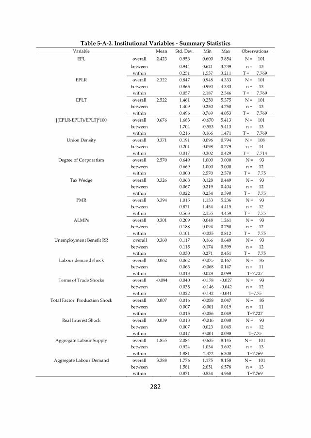
282
Table 5-A-2. Institutional Variables - Summary Statistics
Variable Mean Std. Dev. Min Max Observations
EPL overall 2.423 0.956 0.600 3.854 N = 101
between 0.944 0.621 3.739 n = 13
within 0.251 1.537 3.211 T = 7.769
EPLR overall 2.322 0.847 0.948 4.333 N = 101
between 0.865 0.990 4.333 n = 13
within 0.057 2.187 2.546 T = 7.769
EPLT overall 2.522 1.461 0.250 5.375 N = 101
between 1.409 0.250 4.750 n = 13
within 0.496 0.769 4.053 T = 7.769
[(EPLR-EPLT)/EPLT]*100 overall 0.676 1.683 -0.670 5.413 N = 101
between 1.704 -0.553 5.413 n = 13
within 0.216 0.166 1.471 T = 7.769
Union Density overall 0.371 0.191 0.096 0.794 N = 108
between 0.201 0.098 0.779 n = 14
within 0.017 0.302 0.429 T = 7.714
Degree of Corporatism overall 2.570 0.649 1.000 3.000 N = 93
between 0.669 1.000 3.000 n = 12
within 0.000 2.570 2.570 T = 7.75
Tax Wedge overall 0.326 0.068 0.128 0.449 N = 93
between 0.067 0.219 0.404 n = 12
within 0.022 0.234 0.390 T = 7.75
PMR overall 3.394 1.015 1.133 5.236 N = 93
between 0.871 1.454 4.415 n = 12
within 0.563 2.155 4.459 T = 7.75
ALMPs overall 0.301 0.209 0.048 1.261 N = 93
between 0.188 0.094 0.750 n = 12
within 0.101 -0.035 0.812 T = 7.75
Unemployment Benefit RR overall 0.360 0.117 0.166 0.649 N = 93
between 0.115 0.174 0.599 n = 12
within 0.030 0.271 0.451 T = 7.75
Labour demand shock overall 0.062 0.062 -0.075 0.167 N = 85
between 0.063 -0.068 0.147 n = 11
within 0.013 0.028 0.099 T=7.727
Terms of Trade Shocks overall -0.094 0.040 -0.178 -0.027 N = 93
between 0.035 -0.146 -0.042 n = 12
within 0.022 -0.142 -0.041 T=7.75
Total Factor Production Shock overall 0.007 0.016 -0.058 0.047 N = 85
between 0.007 -0.001 0.019 n = 11
within 0.015 -0.056 0.049 T=7.727
Real Interest Shock overall 0.039 0.018 -0.016 0.080 N = 93
between 0.007 0.023 0.045 n = 12
within 0.017 -0.001 0.088 T=7.75
Aggregate Labour Supply overall 1.855 2.084 -0.635 8.145 N = 101
between 0.924 1.054 3.692 n = 13
within 1.881 -2.472 6.308 T=7.769
Aggregate Labour Demand overall 3.388 1.776 1.175 8.158 N = 101
between 1.581 2.051 6.578 n = 13
within 0.871 0.534 4.968 T=7.769
28
3
Tab
le 5
-A-3
. T
he
evo
luti
on
of
the
lab
ou
r m
ark
et p
oli
cies
an
d i
nst
itu
tio
nal
fac
tors
199
4-20
01
Yea
r C
ou
ntr
y
EP
L
EP
LR
E
PL
T
Re
lati
ve
EP
L
Un
ion
Den
sity
PM
R
Ta
x W
edg
e
Co
rpo
rati
sm
Un
emp
l. B
enef
it R
R
AL
MP
s
19
94
AU
T
2.2
0 M
L
2.9
2 M
L
1.5
0 L
0
.94
41
.43
ML
4
.19
H
24
.60
ML
3
.00
H
29
.55
M
20
.34
ML
20
01
AU
T
2.2
0 M
L
2.9
2 M
L
1.5
0 L
0
.94
35
.68
ML
2
.66
ML
2
5.4
0 M
L
3.0
0 H
3
1.5
2 M
H
29
.91
ML
19
94
BE
L
3.2
0 M
H
1.6
8 L
4
.63
H
-0.6
4 5
4.6
9 M
H
4.4
9 H
3
8.6
0 H
3
.00
H
39
.56
MH
2
4.2
2 M
L
20
01
BE
L
2.2
0 M
H
1.7
3 L
2
.63
ML
-0
.34
55
.76
MH
2
.54
M
40
.30
H
3.0
0 H
3
8.4
9 M
H
30
.51
ML
19
94
DN
K
2.3
0 M
L
1.5
2 L
3
.13
MH
-0
.51
77
.51
H
4.0
7 H
3
0.3
0 M
H
3.0
0 H
5
8.1
1 V
H
40
.89
MH
20
01
DN
K
1.4
0 L
1
.47
L
1.3
8 L
0
.07
73
.83
H
1.9
9 L
3
0.7
0 M
H
3.0
0 H
5
0.8
9 H
6
4.4
9 H
19
94
FR
A
3.0
0 M
2
.34
ML
3
.63
MH
-0
.35
10
.02
L
4.8
5 H
3
9.3
0 H
2
.00
M
37
.56
MH
2
4.0
4 M
L
20
01
FR
A
3.0
0 M
2
.47
ML
3
.63
MH
-0
.32
9.6
4 L
3
.74
MH
3
9.4
0 H
2
.00
M
43
.53
H
33
.09
ML
19
94
IRL
0
.90
VL
1
.60
L
0.2
5 V
L
5.4
1 4
8.6
0 M
4
.70
H
28
.41
ML
3
.00
H
28
.54
M
26
.42
ML
20
01
IRL
0
.90
VL
1
.60
L
0.2
5 V
L
5.4
1 3
5.9
2 M
L
3.5
4 H
1
2.8
0 L
3
.00
H
35
.84
MH
6
7.3
3 H
19
94
ITA
3
.60
MH
1
.77
L
5.3
8 V
H
-0.6
7 3
8.7
3 M
L
5.2
4 H
4
3.5
0 H
3
.00
H
18
.00
L
7.9
7 V
L
20
01
ITA
2
.14
ML
1
.77
L
2.5
0 M
L
-0.2
9 3
4.8
5 M
L
3.1
8 M
H
35
.40
MH
3
.00
H
34
.14
MH
1
6.0
3 L
19
94
NL
D
2.7
0 M
L
3.0
8 M
H
2.3
8 M
L
0.3
0 2
5.6
3 L
3
.73
MH
3
5.9
0 M
H
3.0
0 H
5
2.5
2 H
4
6.8
3 M
H
20
01
NL
D
2.1
0 M
L
3.0
5 M
H
1.1
9 L
1
.57
22
.50
L
1.8
1 L
3
3.0
0 M
H
3.0
0 H
5
2.8
6 H
1
26
.10
VH
19
94
PR
T
3.8
5 M
H
4.3
3 H
3
.38
MH
0
.28
27
.31
L
4.9
4 H
2
7.0
5 M
L
2.0
0 M
3
5.3
9 M
H
20
.30
ML
20
01
PR
T
3.7
0 M
H
4.3
3 H
3
.00
M
0.4
4 2
3.4
3 L
3
.05
M
24
.09
ML
2
.00
M
41
.25
H
30
.36
ML
19
94
ES
P
3.1
1 M
H
2.9
7 M
L
3.2
5 M
H
-0.0
9 1
7.6
4 L
4
.27
H
33
.70
MH
2
.00
M
35
.35
MH
4
.81
VL
20
01
ES
P
3.1
0 M
H
2.6
1 M
L
3.5
0 M
H
-0.2
6 1
3.7
8 L
2
.43
ML
3
1.1
0 M
H
2.0
0 M
3
6.4
6 M
H
18
.34
L
19
94
GB
R
0.6
0 V
L
0.9
5 V
L
0.2
5 V
L
2.7
9 3
4.1
6 M
L
1.8
7 L
2
5.2
0 M
L
1.0
0 L
1
8.1
3 L
1
1.1
9 V
L
20
01
GB
R
0.6
8 V
L
1.1
2 L
0
.25
VL
3
.46
30
.73
ML
1
.13
L
18
.10
L
1.0
0 L
1
6.5
9 L
1
5.8
4 L
19
94
FIN
2
.17
ML
2
.47
ML
1
.88
L
0.3
2 7
8.0
2 H
3
.62
MH
4
0.4
7 H
3
.00
H
37
.09
MH
2
0.4
1 M
L
20
01
FIN
2
.00
L
2.1
7 M
L
1.8
8 L
0
.16
77
.82
H
2.4
7 M
L
38
.80
H
3.0
0 H
3
4.7
8 M
H
20
.62
ML
19
94
DE
U
3.0
9 M
H
2.6
8 M
L
3.5
0 M
H
-0.2
3 3
0.3
8 M
L
3.8
8 M
H
35
.70
MH
3
.00
H
27
.06
ML
3
2.5
2 M
L
20
01
DE
U
2.5
0 M
L
2.6
8 M
L
2.2
5 M
L
0.1
9 2
3.5
3 L
2
.03
L
32
.70
MH
3
.00
H
27
.69
ML
3
1.9
3 M
L
19
94
LU
X
4
2.6
0 M
L
20
01
LU
X
3
7.3
7 M
L
19
94
GR
3
.54
MH
2
.33
ML
4
.75
H
-0.5
1 3
2.3
7 M
L
20
01
GR
3
.54
MH
2
.33
ML
4
.75
H
-0.5
1 2
6.7
3 L
No
te: H
– h
igh
, M
H -
me
diu
m h
igh
, M
L –
me
diu
m l
ow
, L –
lo
w
284
Table 5-A-4. Share of employees by educational level, by sector, by type of contract, by
employment status, by occupational - for selected cohorts based on ECHP
Variable
Cohort
1940-1950
Cohort
1951-1960
Cohort
1961-1970
Cohort
1971-1981
Obs
Mea
n
Std.
Dev. Mean Std. Dev. Mean Std. Dev. Mean Std. Dev.
Share of University Degree 108 0.228 0.115 0.248 0.128 0.250 0.130 0.134 0.144
Share of Upper-Sec Degree 108 0.327 0.191 0.367 0.177 0.401 0.195 0.451 0.197
Share of permanent contracts 108 0.896 0.074 0.875 0.060 0.849 0.087 0.755 0.170
Share of private employees 108 0.657 0.096 0.678 0.082 0.789 0.052 0.860 0.055
Share of Unemployed 108 0.068 0.033 0.057 0.037 0.078 0.043 0.129 0.096
Occupation Structure (ECHP)
Share of managers, legislators,etc. 108 0.118 0.044 0.109 0.045 0.077 0.041 0.021 0.022
Share of professionals 108 0.112 0.049 0.116 0.047 0.103 0.044 0.042 0.032
Share of technicians & assoc. professionals 108 0.099 0.039 0.118 0.044 0.111 0.045 0.069 0.035
Share of clerks 108 0.057 0.028 0.069 0.040 0.072 0.026 0.056 0.026
Share of service & sales workers 108 0.046 0.021 0.057 0.024 0.065 0.023 0.074 0.029
Share of skilled agricultural & fishery
workers 108 0.052 0.042 0.042 0.025 0.037 0.025 0.024 0.017
Share of craft & related trade workers 108 0.160 0.046 0.185 0.054 0.197 0.062 0.165 0.071
Share of plant & machine operators 108 0.093 0.029 0.102 0.025 0.101 0.024 0.066 0.021
Share of elementary occupations 108 0.052 0.022 0.062 0.023 0.063 0.026 0.066 0.032
28
5
Tab
le 5
-A-5
. Err
or-
Co
mp
on
ents
Mo
del
s fo
r L
og
Rea
l H
ou
rly
Ear
nin
gs
Ger
ma
ny
RG
+A
R1
Den
ma
rk
RW
+A
R1
Net
her
lan
ds
RG
+A
R1
Bel
giu
m
PI+
AR
1
Fra
nce
PI+
AR
1
Lu
xem
bo
urg
PI+
AR
1
UK
RG
+A
R1
P
ara
m.
SE
P
ara
m.
SE
P
ara
m
SE
P
ara
m
SE
P
ara
m
SE
P
ara
m
SE
P
ara
m
SE
Per
ma
nen
t C
om
po
nen
t
Ex
p(e
stim
ate
)=σ
2μ
7.2
609
0
.08
67
0.0
078
0
.26
53
0.1
913
0
.09
05
0.0
698
0
.02
46
0.1
653
0
.02
93
0.1
071
0
.02
51
0.0
467
0
.24
67
Ex
p(e
stim
ate
)=σ
2φ
0.0
024
0
.09
68
0.0
002
0
.07
97
0.0
001
0
.10
32
Co
v(μ
,φ)
-0.1
313
0.0
121
-0
.005
2 0
.00
05
-0.0
022
0.0
004
Ex
p()
=σ
2π
0.0
001
0
.07
45
Tim
e sh
ifte
rs
λ1
, 199
5 1
.07
34
0.0
084
0
.97
09
0.0
203
0
.97
35
0.0
158
0
.94
21
0.0
116
1
.05
11
0.0
129
1
0.9
915
0
.00
82
λ1
, 199
6 1
.15
03
0.0
112
0
.92
41
0.0
201
0
.97
48
0.0
172
1
.00
41
0.0
122
1
.10
58
0.0
130
1
.02
15
0.0
220
0
.90
70
0.0
103
λ1
, 199
7 1
.20
28
0.0
142
0
.81
93
0.0
214
0
.93
34
0.0
159
0
.92
25
0.0
145
1
.13
38
0.0
144
1
.18
10
0.0
208
0
.92
28
0.0
126
λ1
, 199
8 1
.27
20
0.0
215
0
.80
70
0.0
231
0
.98
76
0.0
169
0
.89
15
0.0
160
1
.12
95
0.0
173
1
.24
93
0.0
222
0
.89
36
0.0
146
λ1
, 199
9 1
.40
78
0.0
188
0
.70
48
0.0
228
0
.89
63
0.0
184
0
.78
53
0.0
162
1
.12
57
0.0
181
1
.32
05
0.0
248
0
.85
71
0.0
154
λ1
, 200
0 1
.51
55
0.0
222
0
.65
78
0.0
251
0
.87
49
0.0
193
0
.92
45
0.0
170
1
.05
81
0.0
188
1
.34
25
0.0
314
0
.78
02
0.0
163
λ1
, 200
1 1
.47
44
0.0
280
0
.66
57
0.0
235
0
.90
96
0.0
208
0
.92
07
0.0
156
1
.08
42
0.0
186
1
.29
77
0.0
222
0
.79
82
0.0
175
Co
ho
rt s
hif
ters
γ1
,51
-60
0.4
401
0
.01
45
1.2
694
0
.03
39
1.2
748
0
.04
24
1.0
127
0
.01
38
0.8
589
0
.01
39
0.9
557
0
.01
89
1.4
131
0
.03
01
γ1
,61
-70
0.2
031
0
.00
88
1.6
459
0
.11
64
1.3
168
0
.11
44
0.7
776
0
.01
05
0.7
796
0
.01
31
0.9
396
0
.01
83
2.0
459
0
.09
92
γ1
,71
-80
0.0
856
0
.00
46
1.4
783
0
.20
34
0.7
891
0
.07
04
0.1
425
0
.03
87
0.5
000
0
.01
78
0.5
933
0
.01
83
2.4
514
0
.24
35
28
6
Tra
nsi
tory
Co
mp
on
ent
Ex
p(e
stim
ate
)=σ
2ε
0.2
578
0
.57
41
0.2
604
0
.29
61
0.1
262
0
.30
96
0.2
439
0
.15
23
0.7
969
0
.57
79
0.0
186
0
.16
71
0.0
702
0
.11
10
Ex
p(e
stim
ate
)=σ
20
Ex
p(e
stim
ate
)=σ
20
,40
-50
0.0
044
0
.73
16
0.0
314
0
.08
51
0.0
228
0
.09
13
0.0
639
0
.04
37
0.1
039
0
.04
91
0.0
753
0
.06
38
0.0
764
0
.04
37
Ex
p(e
stim
ate
)=σ
20
,51
-60
0.0
562
0
.08
87
0.0
224
0
.08
13
0.0
271
0
.12
08
0.0
357
0
.06
63
0.0
913
0
.09
02
0.1
064
0
.11
09
0.0
789
0
.06
05
Ex
p(e
stim
ate
)=σ
20
,61
-70
0.0
419
0
.09
40
0.0
334
0
.07
40
0.0
112
0
.20
73
0.0
392
0
.05
35
0.0
486
0
.08
43
0.0
672
0
.11
36
0.0
750
0
.06
81
Ex
p(e
stim
ate
)=σ
20
,71
-80
0.0
832
0
.06
79
0.0
269
0
.07
12
0.0
406
0
.09
62
0.0
347
0
.05
96
0.0
956
0
.09
66
0.0
225
0
.12
20
0.0
313
0
.11
79
ρ
0.3
583
0
.02
23
0.5
459
0
.01
35
0.3
289
0
.01
18
0.6
280
0
.01
04
0.3
993
0
.02
54
0.2
389
0
.01
61
0.4
512
0
.01
25
θ
Tim
e sh
ifte
rs
λ2
, 199
5 0
.45
31
0.1
298
0
.25
91
0.0
373
0
.49
36
0.0
756
0
.29
41
0.0
226
0
.25
17
0.0
739
1
0.8
214
0
.04
18
λ2
, 199
6 0
.38
01
0.1
088
0
.24
77
0.0
382
0
.48
39
0.0
771
0
.23
96
0.0
181
0
.17
03
0.0
504
1
.97
74
0.1
487
0
.81
35
0.0
475
λ2
, 199
7 0
.34
80
0.1
008
0
.24
97
0.0
375
0
.48
39
0.0
756
0
.26
77
0.0
202
0
.19
63
0.0
572
1
.44
02
0.1
377
0
.71
79
0.0
406
λ2
, 199
8 0
.35
11
0.1
013
0
.21
87
0.0
326
0
.32
87
0.0
505
0
.27
84
0.0
209
0
.23
73
0.0
676
1
.08
18
0.0
915
0
.70
25
0.0
359
λ2
, 199
9 0
.38
86
0.1
121
0
.29
23
0.0
428
0
.38
75
0.0
605
0
.33
71
0.0
255
0
.22
84
0.0
650
1
.24
22
0.1
019
0
.71
40
0.0
377
λ2
, 200
0 0
.29
18
0.0
841
0
.28
38
0.0
420
0
.45
41
0.0
710
0
.27
04
0.0
201
0
.24
32
0.0
696
1
.36
44
0.1
127
0
.84
82
0.0
482
λ2
, 200
1 0
.39
57
0.1
147
0
.25
66
0.0
380
0
.56
29
0.0
877
0
.32
55
0.0
257
0
.23
46
0.0
675
1
.40
03
0.1
195
0
.79
77
0.0
453
Co
ho
rt s
hif
ters
γ2
,51
-60
0.9
547
0
.02
99
1.1
306
0
.02
69
1.0
459
0
.02
94
1.0
555
0
.01
89
0.9
383
0
.02
93
0.8
573
0
.03
55
0.8
949
0
.01
71
γ2
,61
-70
0.9
643
0
.02
68
1.1
604
0
.02
28
1.1
180
0
.03
13
0.9
996
0
.01
40
1.0
469
0
.03
03
1.0
445
0
.04
29
0.9
938
0
.01
82
γ2
,71
-80
1.3
832
0
.04
11
1.8
221
0
.03
40
1.7
278
0
.04
64
1.3
569
0
.02
33
1.5
123
0
.04
65
1.4
318
0
.05
95
1.1
898
0
.02
24
SS
R
0.0
143
0
.00
68
0.0
099
0
.00
47
0.0
240
0
.02
22
0.0
061
Χ2
24
73.7
073
57
10.0
156
24
92.7
787
17
769
.42
20
17
56.3
574
16
32.2
320
25
97.3
157
Lo
gL
4
59
.25
76
51
3.2
610
4
86
.00
84
54
0.0
406
4
21
.96
93
31
8.4
753
5
20
.50
53
No
te:
SE
co
lum
n r
ep
ort
s th
e st
and
ard
err
or
for
the
par
amet
er e
stim
ate.
Wh
ere
I r
ep
ort
th
e e
xp
(est
imat
e), t
he
SE
co
rre
spo
nd
s to
th
e lo
g(e
xp
(est
imat
e))
= e
stim
ate
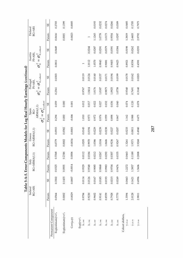
28
7
Tab
le 5
-A-5
. Err
or-
Co
mp
on
ents
Mo
del
s fo
r L
og
Rea
l H
ou
rly
Ear
nin
gs
(co
nti
nu
ed)
Ir
ela
nd
RG
+A
R1
Ita
ly
RG
+A
RM
A(1
,1)
Gre
ece
RG
+A
RM
A(1
,1)
Sp
ain
RG
+
AR
MA
(1,1
)
22
00
,co
ho
rtσ
σ=
Po
rtu
ga
l
PI+
AR
1,
22
00
,co
ho
rtσ
σ=
Au
stri
a
PI+
AR
1,
22
00
,co
ho
rtσ
σ=
Fin
lan
d
RG
+A
R1
P
ara
m.
SE
P
ara
m.
Pa
ram
. P
ara
m.
SE
P
ara
m.
SE
P
ara
m.
SE
P
ara
m.
SE
P
ara
m.
SE
Per
ma
nen
t C
om
po
nen
t
Ex
p(e
stim
ate
)=σ
2μ
0.0
564
0
.35
02
0.0
325
0
.55
68
0.0
779
0
.09
15
0.2
94
0.0
59
0.2
561
0
.03
03
0.0
811
0
.04
49
0.0
616
0
.27
03
Ex
p(e
stim
ate
)=σ
2φ
0.0
002
0
.14
35
0.0
001
0
.23
46
0.0
002
0
.05
82
0.0
00
0.0
00
0.0
001
0
.13
99
Co
v(μ
,φ)
-0.0
029
0.0
007
-0
.001
4 0
.00
06
-0.0
034
0.0
003
-0
.006
0
.00
1
-0
.002
3 0
.00
05
Ex
p()
=σ
2π
λ1
, 199
5 0
.97
84
0.0
114
0
.95
29
0.0
112
1
.02
05
0.0
145
1
.01
0 0
.01
2 0
.97
67
0.0
119
1
λ1
, 199
6 0
.92
30
0.0
126
0
.95
48
0.0
184
0
.99
70
0.0
194
0
.97
3 0
.01
7 1
.04
14
0.0
124
1
.01
12
0.0
244
1
λ1
, 199
7 0
.96
02
0.0
167
0
.90
85
0.0
212
1
.03
86
0.0
229
0
.97
2 0
.02
2 1
.01
76
0.0
140
1
.05
70
0.0
287
1
.12
65
0.0
193
λ1
, 199
8 0
.91
41
0.0
185
0
.98
68
0.0
267
1
.01
04
0.0
239
0
.97
6 0
.02
7 1
.01
87
0.0
157
0
.98
43
0.0
291
1
.07
78
0.0
232
λ1
, 199
9 0
.85
59
0.0
193
0
.99
83
0.0
292
1
.06
06
0.0
238
0
.95
9 0
.03
2 0
.98
75
0.0
171
0
.90
81
0.0
379
1
.01
73
0.0
274
λ1
, 200
0 0
.79
28
0.0
215
0
.97
04
0.0
307
0
.92
36
0.0
227
0
.89
8 0
.03
6 1
.09
25
0.0
194
0
.94
03
0.0
391
0
.95
54
0.0
266
λ1
, 200
1 0
.77
70
0.0
249
0
.94
76
0.0
335
0
.92
67
0.0
207
0
.86
7 0
.04
0 1
.07
58
0.0
199
0
.94
25
0.0
384
1
.02
97
0.0
309
Co
ho
rt s
hif
ters
,
γ1
,51
-60
1.3
594
0
.04
43
1.2
272
0
.04
63
1.3
261
0
.02
33
1.1
62
0.0
74
0.9
340
0
.01
78
0.8
921
0
.01
98
1.3
819
0
.04
85
γ1
,61
-70
2.0
128
0
.16
21
1.3
857
0
.11
89
1.9
371
0
.08
11
0.9
88
0.1
20
0.7
691
0
.01
62
0.8
354
0
.02
62
2.4
403
0
.17
05
γ1
,71
-80
2.9
811
0
.49
96
1.5
606
0
.20
08
3.9
268
0
.49
40
0.4
75
0.0
78
0.3
140
0
.02
03
0.4
591
0
.02
93
2.9
792
0
.79
75
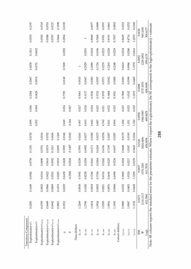
28
8
Tra
nsi
tory
Co
mp
on
ent
Ex
p(e
stim
ate
)=σ
2ε
0.0
285
0
.16
49
0.0
582
0
.07
58
0.1
183
0
.07
50
0.0
99
0.0
06
0.2
584
0
.20
67
0.4
830
0
.18
11
0.0
555
0
.21
97
Ex
p(e
stim
ate
)=σ
20
0.0
52
0.0
04
0.0
428
0
.09
74
0.0
751
0
.06
52
Ex
p(e
stim
ate
)=σ
20
,40
-50
0.0
709
0
.08
25
0.0
314
0
.08
98
0.0
791
0
.05
16
0.0
550
0
.07
43
Ex
p(e
stim
ate
)=σ
20
,51
-60
0.0
688
0
.09
66
0.0
422
0
.06
19
0.0
574
0
.07
02
0.0
588
0
.07
01
Ex
p(e
stim
ate
)=σ
20
,61
-70
0.0
942
0
.08
69
0.0
521
0
.05
92
0.1
011
0
.04
36
0.0
707
0
.07
27
Ex
p(e
stim
ate
)=σ
20
,71
-80
0.0
801
0
.10
15
0.0
283
0
.09
19
0.0
695
0
.12
69
0.0
464
0
.10
98
ρ
0.2
912
0
.02
29
0.6
438
0
.04
28
0.5
995
0
.03
46
0.8
49
0.0
24
0.7
785
0
.01
49
0.7
009
0
.02
92
0.2
904
0
.01
95
θ
-0.2
506
0.0
204
-0
.148
7 0
.02
42
-0.3
64
0.0
07
Tim
e sh
ifte
rs
λ2
, 199
5 1
.22
69
0.0
938
0
.76
92
0.0
239
0
.79
91
0.0
261
0
.90
7 0
.02
7 0
.50
61
0.0
525
1
λ2
, 199
6 1
.27
89
0.1
050
0
.82
38
0.0
294
0
.69
92
0.0
277
0
.81
5 0
.02
4 0
.31
17
0.0
367
0
.29
29
0.0
291
1
λ2
, 199
7 1
.04
34
0.0
818
0
.72
96
0.0
241
0
.61
71
0.0
280
0
.84
2 0
.02
4 0
.35
36
0.0
383
0
.20
89
0.0
224
0
.88
49
0.0
977
λ2
, 199
8 1
.09
24
0.0
853
0
.75
36
0.0
264
0
.62
69
0.0
275
0
.88
7 0
.02
3 0
.37
23
0.0
397
0
.17
24
0.0
196
0
.70
69
0.0
809
λ2
, 199
9 1
.05
95
0.0
821
0
.65
16
0.0
242
0
.61
06
0.0
256
0
.76
0 0
.02
1 0
.35
55
0.0
371
0
.22
70
0.0
223
0
.93
01
0.0
957
λ2
, 200
0 1
.08
16
0.0
876
0
.66
56
0.0
225
0
.71
95
0.0
287
0
.82
1 0
.02
2 0
.34
84
0.0
362
0
.22
03
0.0
220
0
.81
91
0.0
861
λ2
, 200
1 1
.10
93
0.0
968
0
.69
98
0.0
234
0
.66
57
0.0
287
0
.85
6 0
.02
3 0
.39
21
0.0
400
0
.22
48
0.0
229
0
.79
37
0.0
852
Co
ho
rt s
hif
ters
,
γ2
,51
-60
0.9
889
0
.03
52
0.9
894
0
.02
04
0.9
608
0
.01
79
1.0
04
0.0
25
0.7
800
0
.03
83
0.8
410
0
.02
54
0.8
609
0
.02
53
γ2
,61
-70
1.0
987
0
.04
03
1.0
324
0
.02
17
1.0
187
0
.01
83
1.0
51
0.0
25
1.0
102
0
.03
99
0.8
986
0
.02
80
0.8
714
0
.02
52
γ2
,71
-80
1.1
532
0
.04
58
1.3
299
0
.02
78
0.9
443
0
.02
56
1.3
30
0.0
30
1.1
072
0
.04
09
1.1
979
0
.04
16
1.2
070
0
.03
49
SS
R
0.0
273
0
.00
17
0.0
146
0
.00
94
0.0
288
0
.00
52
0.0
038
Χ2
21
16.2
117
15
76.2
281
38
24.4
496
19
84.9
587
37
37.5
070
22
29.2
852
94
5.1
045
Lo
gL
4
12
.78
81
61
1.7
874
4
58
.00
54
48
9.8
478
4
08
.94
98
39
9.6
179
3
00
.61
77
No
te:
SE
co
lum
n r
ep
ort
s th
e st
and
ard
err
or
for
the
par
amet
er e
stim
ate.
Wh
ere
I r
ep
ort
th
e e
xp
(est
imat
e), t
he
SE
co
rre
spo
nd
s to
th
e lo
g(e
xp
(est
imat
e))
= e
stim
ate

289
Figure 5-A-1. Overall Autocovariance Structure of Hourly Earnings: Years 1994-2001
.05
.1.1
5.2
.25
1994 1996 1998 2000
Germany
.05
.1.1
5.2
.25
1994 1996 1998 2000
Denmark
.05
.1.1
5.2
.25
1994 1996 1998 2000
Netherlands
.05
.1.1
5.2
.25
1994 1996 1998 2000
Belgium
.05
.1.1
5.2
.25
1994 1996 1998 2000
France
.05
.1.1
5.2
.25
1994 1996 1998 2000
Luxembourg
.05
.1.1
5.2
.25
1994 1996 1998 2000
UK
.05
.1.1
5.2
.25
1994 1996 1998 2000
Ireland
.05
.1.1
5.2
.25
1994 1996 1998 2000
Italy
.05
.1.1
5.2
.25
1994 1996 1998 2000
Greece
.05
.1.1
5.2
.25
1994 1996 1998 2000
Spain
.05
.1.1
5.2
.25
1994 1996 1998 2000
Portugal
.05
.1.1
5.2
.25
1994 1996 1998 2000
Austria
.05
.1.1
5.2
.25
1994 1996 1998 2000
FinlandVariance(t)Covariance(t, t-1)Covariance(t, t-2)Covariance(t, t-3)Covariance(t, t-4)Covariance(t, t-5)Covariance(t, t-6)
Covariance(t, t-7)
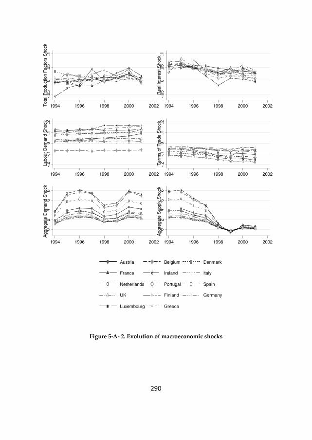
290
Figure 5-A- 2. Evolution of macroeconomic shocks
-.05
0.0
5.1
Tota
l P
roduction F
acto
rs S
hock
1994 1996 1998 2000 2002
-.05
0.0
5.1
Real In
tere
st S
hock
1994 1996 1998 2000 2002
-.2
-.1
0.1
.2Labour
Dem
and S
hock
1994 1996 1998 2000 2002
-.2
-.1
0.1
.2T
erm
s o
f T
rade S
hock
1994 1996 1998 2000 2002
02
46
8A
ggre
gate
Dem
and S
hock
1994 1996 1998 2000 2002
02
46
8A
ggre
gate
Supply
Shock
1994 1996 1998 2000 2002
Austria Belgium Denmark
France Ireland Italy
Netherlands Portugal Spain
UK Finland Germany
Luxembourg Greece

291
6. EARNINGS DYNAMICS AND INEQUALITY AMONG
MEN IN LUXEMBOURG, 1988-2004: EVIDENCE
FROM ADMINISTRATIVE DATA
292
6.1.Introduction
Understanding the source of the growth in earnings inequality has become a major
topic in economics over the past two decades, fuelled mainly by the rise in
earnings inequality experienced by many developed countries during the 1980s
and 1990s.
Starting with the US and Canada, followed by UK and Europe, recent studies on
earnings dynamics have stressed the importance of decomposing the growth in
earnings inequality into permanent and transitory components, due to their
implications for long-run differentials. An increase in cross-sectional earnings
inequality triggered by an increase in the permanent component signals an
increase in lifetime earnings differentials, suggesting a worsening of the relative
lifetime earnings position of the chronically poor. An increase in cross-sectional
earnings differentials triggered by an increase in earnings instability signals an
increase in earnings mobility, implying an increased opportunity for the poor to
improve their relative income position in a lifetime perspective.
In Europe, the advancement and the full potential of this research in
understanding the structural changes in inequality has been limited, due to
insufficiently long panels. My study aims to fill part of this gap.
The contribution of this study to the literature on earnings dynamics and
inequality is twofold. First, it aims to expand the research regarding the possible
implications of the labour market structural changes on the structure of earnings
inequality and earnings mobility. The specific context of the Luxembourgish
labour market, which underwent significant structural changes during the last
decades, makes Luxembourg a relevant case for studying the structural changes in
earnings inequality and the implications for lifetime earnings differentials. This
study is the first of its kind in Luxembourg. Following the tradition of previous
studies I focus on men to avoid the problem of selection bias characterising female
earnings.
Starting with the late 1970s and intensifying after early 1990s, Luxembourg
evolved from an industrial economy to an economy dominated by the tertiary
sector, which relies heavily on the cross-border workforce. Moreover, Luxembourg
recorded a large increase in the number of active population, both residents and
cross-borders, which more than doubled in 2004 compared with 1988. The change
in the structure of the labour market by occupation status (Figure 6-A- 1, Annex),
reveals an increase in the share of white collars and civil servants, and a decrease
in the share of blue collars. The change in the labour market structure by the sector
293
of activity (Figure 6-A-2, Annex) reveals a significant increase in the share of the
service sector and a decrease in the share of the industry sector. The evolution of
the labour market age distribution (Figure 6-A-3, upper panel, Annex) reveals a
clear shift in men’s labour market behaviour due to the education system: from a
high concentration of active men around ages 20-25 in 1988 to a high concentration
around ages 25-45 in 2004. The change in the labour market behaviour is confirmed
also by the cumulative age distribution (Figure 6-A-3, bottom panel, Annex), which
shifted towards higher ages: e.g. the share of people present in the labour market
until age 25 is almost double in 1988 than in 1996 or 2004. Following these changes
cross-sectional earnings inequality increased.
What are the implications of these changes for the structure of earnings inequality
and earnings mobility? Using 17 years of longitudinal earnings information drawn
from the administrative data on the professional career, I decompose
Luxembourg’s growth in earnings inequality into persistent and transitory
components. I explore the extent to which changes in cross-sectional earnings
inequality in Luxembourg between 1988 and 2004 reflect changes in the transitory
or permanent components of earnings.
On the one hand, did the increases in cross-sectional wage inequality result from
greater transitory fluctuations and a higher degree of earnings mobility? Or does it
reflect increasing permanent differences between individuals with mobility
remaining constant or even falling? On the other hand, did mobility influence falls
in cross-sectional inequality? Understanding the contributions of the changes in
permanent and transitory inequality to increased cross-sectional inequality is
useful therefore in evaluating alternative structural changes hypotheses and for
determining the potential welfare consequences of rising inequality. (Katz and
Autor, 1999)
Second, I exploit my extraordinary dataset to achieve some methodological
advances at the EU level. The limited scale of most European panels has forced EU
researchers to rely on simple country models, which impose economically
implausible restrictions. For example, the 7 ECHP waves available for Luxembourg
have forced Sologon and O'Donoghue (2009a, 2009b) to impose the assumption of
invariant permanent component with no permanent shocks (age specific or not), no
life-cycle variation in the variance of transitory earnings shocks and no MA process
in the transitory variance. Due to my long panel, I am able to estimate much richer
models that nest the various specifications used in the US, Canadian and European
literature up to date.
294
Unlike previous studies, I decompose my analysis by 36 birth cohorts composed of
people born in a certain year. This small age window allows the precise
identification of the two components at different lifecycle stages. Equally weighted
minimum distance methods are used to estimate the covariance structure of
earnings, decompose earnings inequality into a permanent and a transitory
component, estimate earnings mobility and conclude about their evolution.
6.2.Literature review 93
The existing literature on earnings dynamics is predominantly based on US data.
Atkinson, Bourguignon et al. (1992) provide a comprehensive survey of the
literature on earnings dynamics until 1992. Earlier work focused on fitting
statistical models to the earnings process. E.g. Lillard and Willis (1978), Lillard and
Weiss (1979), MaCurdy (1982), Abowd and Card (1989) fitted models to the
autocovariance structure of earnings and hours, but they did not account for the
changes in the autocovariance structure of earnings over time.
Later work, Moffitt and Gottschalk (1995, 1998, 2002) used PSID to estimate the
permanent and transitory components of male earnings and how it evolved over
time. In Moffitt and Gottschalk (1998), the earnings process was fit by a permanent
component, modelled as a random walk in age and a highly persistent serially
correlated transitory component, with weights on these components for each year.
They found that the increase in the cross-sectional inequality of individual
earnings and wage rates in the U.S. between 1969 and 1991 has been roughly
equally composed of increases in the variances of the permanent and transitory
components of earnings, with little change in earnings mobility rates. Since most of
the theoretical explanations for the increase in inequality have been aimed at
explaining increases in the variance of the permanent component of earnings (e.g.
increases in the price of skills), they found their result surprising and unexpected.
Therefore, in their most recent study, Moffitt and Gottschalk (2008) estimated the
trend in the transitory variance of male earnings using PSID from 1970 to 2004.
They found that the transitory variance increased substantially in the 1980’s and
remained at the same level until 2004, for both less and more educated workers.
Moreover, the transitory variance appears to have a strong cyclical component: its
increase accounts for between 30% and 65% of the rise in the overall inequality,
depending on the period.
93 Most of the information in this section has been covered in section 4.2.
295
Using the PSID, Baker (1997) compared two competing specifications for the
permanent component of earnings: the “profile heterogeneity or the random
growth model” and the “random walk model”. In spite of the increased popularity
of the latter, Baker (1997) proved that the profile heterogeneity model provides a
better representation of the data.
Baker and Solon (2003) decomposed the growth in earnings inequality into its
persistent and transitory components using longitudinal income tax records from
Canada. The earnings process was fit by a permanent component, modelled as a
mixed process composed of a random growth and a random walk in age and a
highly persistent serially correlated transitory component, with weights on these
components for each year. They found that growth in earnings inequality reflects
both an increase in the long-run inequality and an increase in earnings instability.
Up until recently, little work has been carried out in Europe on the dynamic nature
of individual earnings. Dickens (2000b) analysed the pattern of individual male
wages over time in UK using the New Earnings Survey (NES) panel data set for the
period 1975-1995. This study divided the data into year birth cohorts and analysed
the auto-covariance structure of hourly and weekly earnings for each cohort. In the
tradition of Moffitt and Gottschalk (1998), the earnings process was fit by a
permanent component, modelled as a random walk in age and a highly persistent
serially correlated transitory component, with weights on these components for
each year. The innovative element of their model was the extension of the random
walk to a specification that allows for age-specific innovation variances until age 40
and a random effects model thereafter. The results showed that about half of the
rise of the overall cross-sectional inequality can be explained by the rise in the
permanent variance and the rest by the rise in the persistent transitory component.
Ramos (2003) analysed the dynamic structure of earnings in UK using the British
Household Panel Study for the period 1991-1999. The earnings specification
followed a similar specification with Baker and Solon (2003). Using information on
monthly earnings of male full-time employees, this study decomposed the
covariance structure of earnings into its permanent and transitory components and
concluded that the increase in inequality over the 1990’s was due to increased in
earnings volatility. Moreover, the relative earnings persistency was found to
decline over the lifecycle, which implies a lower mobility for younger cohorts.
These findings are at odds with the previous literature on earnings dynamics both
for UK and the OECD. Unlike previous literature, this study considered also for
the effect of observed characteristics and found that human capital and job related
characteristics account for nearly all persistent earnings differences and that the
transitory component is highly persistent.
296
Kalwij and Alessie (2003) examined the variance-covariance structure of log-wages
over time and over the lifecycle of British men from 1975 to 2001, controlling for
cohort effects. Their model follows closely the specification used by Abowd and
Card (1989), Dickens (2000b) and Baker and Solon (2003) accounting also for cohort
effects. They showed that the increase in the cross-sectional inequality was caused
mainly by an increase in the transitory component of earnings and to a lesser
extent by an increase in the permanent wage inequality. Thus the increase in cross-
sectional inequality was accompanied by an increase in earnings mobility.
Cappellari (2003) used the Italian National Social Security Institute for the period
1979-1995 and decomposed the male earnings autocovariance structure into its
long-term and transitory components using a model specification similar with
Moffitt and Gottschalk (1995) and Backer (1997). The model included a permanent
component, modelled as a random growth in age and a highly persistent serially
correlated transitory component, with weights on these components for each year
and cohort. The findings showed that growth was determined by the long-term
earnings component. Other evidence on the contribution of permanent and
transitory earnings components to cross-sectional inequality has become available
in recent year in Sweden. Gustavson (2004a, 2009b) used a hybrid model between
Baker and Solon (2003) and Dickens (2000b) and concluded that the decrease in
earnings inequality was due to a decrease in the permanent component.
Most recently, Sologon and O'Donoghue (2009a, 2009b) used the 8 waves of ECHP
for 14 EU countries to explore the dynamic structure of individual earnings and the
extent to which changes in cross-sectional earnings inequality reflect transitory or
permanent components of individual lifecycle earnings variation. Overall, the
decrease in inequality resulted from a decrease in transitory differentials in
Germany, France, UK and Ireland, in permanent differentials in Belgium and Spain
and in both components in Denmark and Austria. The increase in inequality
reflects an increase in permanent differentials in Luxembourg, Italy, Greece and
Finland, and an increase in both components in Portugal and Netherlands. The
decrease in inequality was accompanied by an increase in mobility only in
Denmark, Belgium and Spain. Except for Netherlands and Portugal, all countries
recording an increase in inequality experienced also a decrease in mobility.
297
6.3.Theoretical model of the determinants of wage
differentials94
The theoretical and methodological specifications in this section follow closely
Sologon and O’Donoghue (2009a, 2009b).
6.3.1. Determinants of earnings inequality
As pointed out by Katz and Autor (1999), the existing literature contains many
explanations for the rise in earnings inequality experienced by many developed
countries during the 1980s and 1990s. One approach for explaining changes in
wage differential is to decompose overall wage inequality into permanent
inequality and transitory inequality.
Following the terminology introduced by Friedman and Kuznets (1954), individual
earnings are composed of a permanent and a transitory component, assumed to be
independent of each other. The permanent component of earnings reflects personal
characteristics, education, training and other systematic elements. The transitory
component captures the chance and other factors influencing earnings in a
particular period and is expected to average out over time. Following the structure
of individual earnings, overall inequality at any point in time is composed from
inequality in the transitory component and inequality in the permanent component
of earnings. The evolution of the overall earnings inequality is determined by the
cumulative changes in the two inequality components.
The rise in the inequality in the permanent component of earnings may be
consistent with increasing returns to education, on-the-job training and other
persistent abilities that are among the main determinants of the permanent
component of earnings, meaning enhanced relative earnings position of the highly
skilled individuals (Mincer, 1957, 1958, 1962, 1974; Hause, 1980).
The increase in the inequality of the transitory component of earnings may be
attributed to the weakening of the labour market institutions (e.g. unions,
government wage regulation, and internal labour markets), increased labour
market instability, increased competitiveness, a rise in the temporary workforce
which increase earnings exposure to shocks. A period of skill-biased technological
change with the spread of new technologies can on the one hand increase the
demand for skills, and on the other hand it can increase earnings instability (Katz
and Autor, 1999). Rodrik (1997) argued that also globalization and international
94 The information in this section has been covered in section 4.3.
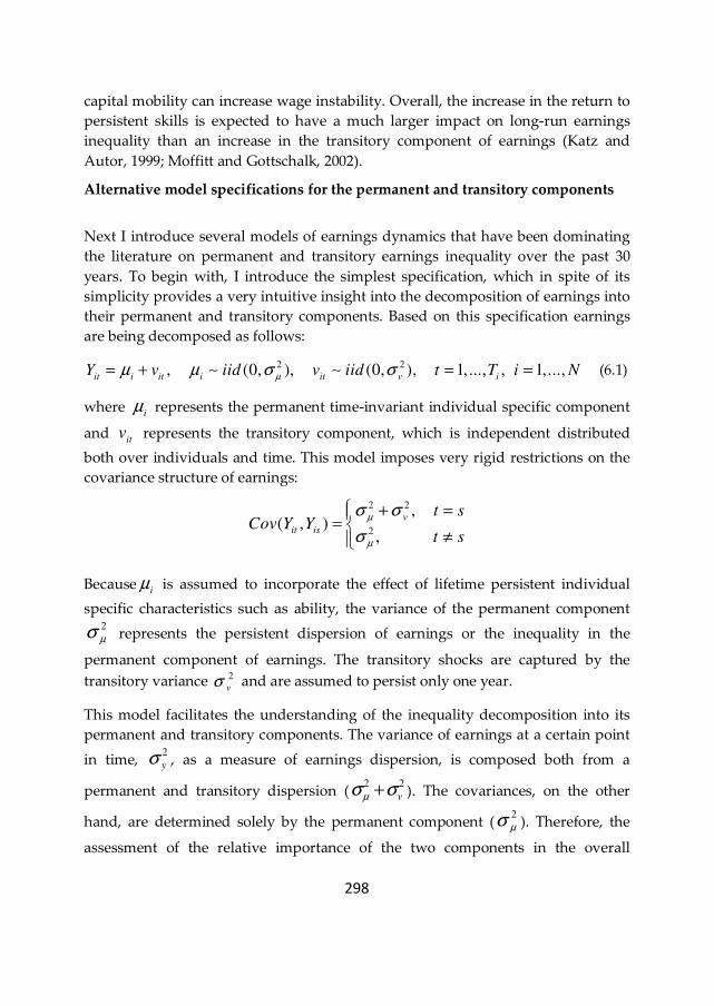
298
capital mobility can increase wage instability. Overall, the increase in the return to
persistent skills is expected to have a much larger impact on long-run earnings
inequality than an increase in the transitory component of earnings (Katz and
Autor, 1999; Moffitt and Gottschalk, 2002).
Alternative model specifications for the permanent and transitory components
Next I introduce several models of earnings dynamics that have been dominating
the literature on permanent and transitory earnings inequality over the past 30
years. To begin with, I introduce the simplest specification, which in spite of its
simplicity provides a very intuitive insight into the decomposition of earnings into
their permanent and transitory components. Based on this specification earnings
are being decomposed as follows:
2 2, (0, ), (0, ), 1, ..., , 1,...,it i it i it v i
Y v iid v iid t T i Nµµ µ σ σ= + = =∼ ∼
(6.1)
where i
µ represents the permanent time-invariant individual specific component
and it
v represents the transitory component, which is independent distributed
both over individuals and time. This model imposes very rigid restrictions on the
covariance structure of earnings:
2 2
2
,( , )
,
v
it is
t sCov Y Y
t s
µ
µ
σ σ
σ
+ ==
≠
Becausei
µ is assumed to incorporate the effect of lifetime persistent individual
specific characteristics such as ability, the variance of the permanent component 2
µσ represents the persistent dispersion of earnings or the inequality in the
permanent component of earnings. The transitory shocks are captured by the
transitory variance 2
vσ and are assumed to persist only one year.
This model facilitates the understanding of the inequality decomposition into its
permanent and transitory components. The variance of earnings at a certain point
in time, 2
yσ , as a measure of earnings dispersion, is composed both from a
permanent and transitory dispersion (2 2
vµσ σ+ ). The covariances, on the other
hand, are determined solely by the permanent component (2
µσ ). Therefore, the
assessment of the relative importance of the two components in the overall
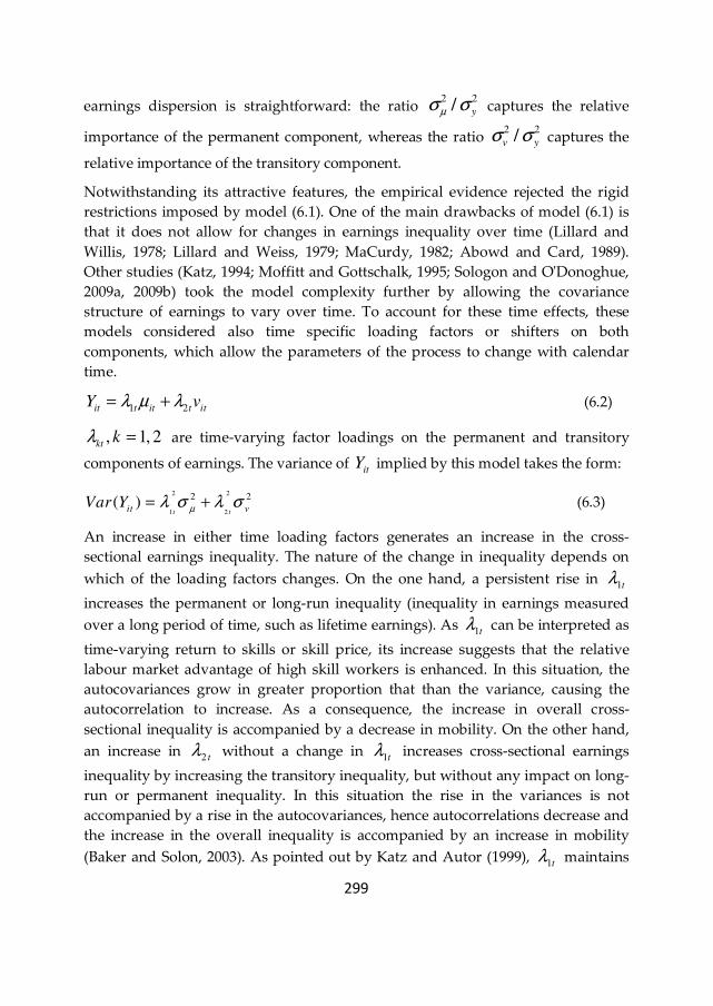
299
earnings dispersion is straightforward: the ratio 2 2
/ yµσ σ captures the relative
importance of the permanent component, whereas the ratio 2 2
/v yσ σ captures the
relative importance of the transitory component.
Notwithstanding its attractive features, the empirical evidence rejected the rigid
restrictions imposed by model (6.1). One of the main drawbacks of model (6.1) is
that it does not allow for changes in earnings inequality over time (Lillard and
Willis, 1978; Lillard and Weiss, 1979; MaCurdy, 1982; Abowd and Card, 1989).
Other studies (Katz, 1994; Moffitt and Gottschalk, 1995; Sologon and O'Donoghue,
2009a, 2009b) took the model complexity further by allowing the covariance
structure of earnings to vary over time. To account for these time effects, these
models considered also time specific loading factors or shifters on both
components, which allow the parameters of the process to change with calendar
time.
1 2it t it t itY vλ µ λ= +
(6.2)
, 1, 2kt
kλ = are time-varying factor loadings on the permanent and transitory
components of earnings. The variance of it
Y implied by this model takes the form:
2 2
1 2
2 2( )t tit v
Var Y µλ σ λ σ= + (6.3)
An increase in either time loading factors generates an increase in the cross-
sectional earnings inequality. The nature of the change in inequality depends on
which of the loading factors changes. On the one hand, a persistent rise in 1t
λ
increases the permanent or long-run inequality (inequality in earnings measured
over a long period of time, such as lifetime earnings). As 1t
λ can be interpreted as
time-varying return to skills or skill price, its increase suggests that the relative
labour market advantage of high skill workers is enhanced. In this situation, the
autocovariances grow in greater proportion that than the variance, causing the
autocorrelation to increase. As a consequence, the increase in overall cross-
sectional inequality is accompanied by a decrease in mobility. On the other hand,
an increase in 2 t
λ without a change in 1t
λ increases cross-sectional earnings
inequality by increasing the transitory inequality, but without any impact on long-
run or permanent inequality. In this situation the rise in the variances is not
accompanied by a rise in the autocovariances, hence autocorrelations decrease and
the increase in the overall inequality is accompanied by an increase in mobility
(Baker and Solon, 2003). As pointed out by Katz and Autor (1999), 1t
λ maintains
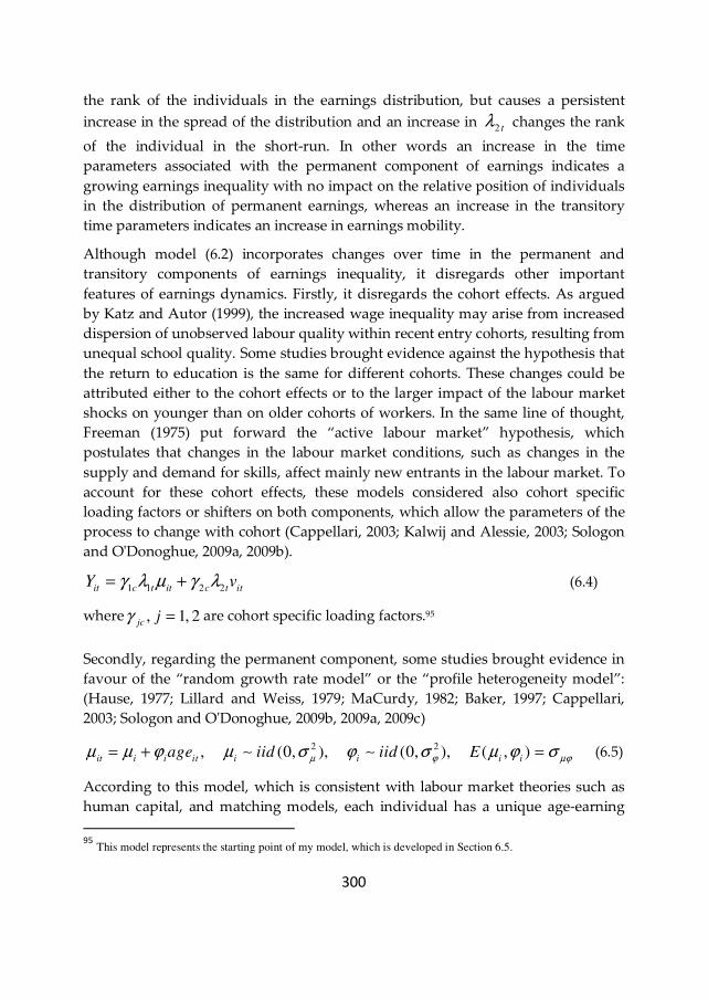
300
the rank of the individuals in the earnings distribution, but causes a persistent
increase in the spread of the distribution and an increase in 2 t
λ changes the rank
of the individual in the short-run. In other words an increase in the time
parameters associated with the permanent component of earnings indicates a
growing earnings inequality with no impact on the relative position of individuals
in the distribution of permanent earnings, whereas an increase in the transitory
time parameters indicates an increase in earnings mobility.
Although model (6.2) incorporates changes over time in the permanent and
transitory components of earnings inequality, it disregards other important
features of earnings dynamics. Firstly, it disregards the cohort effects. As argued
by Katz and Autor (1999), the increased wage inequality may arise from increased
dispersion of unobserved labour quality within recent entry cohorts, resulting from
unequal school quality. Some studies brought evidence against the hypothesis that
the return to education is the same for different cohorts. These changes could be
attributed either to the cohort effects or to the larger impact of the labour market
shocks on younger than on older cohorts of workers. In the same line of thought,
Freeman (1975) put forward the “active labour market” hypothesis, which
postulates that changes in the labour market conditions, such as changes in the
supply and demand for skills, affect mainly new entrants in the labour market. To
account for these cohort effects, these models considered also cohort specific
loading factors or shifters on both components, which allow the parameters of the
process to change with cohort (Cappellari, 2003; Kalwij and Alessie, 2003; Sologon
and O'Donoghue, 2009a, 2009b).
1 1 2 2it c t it c t itY vγ λ µ γ λ= +
(6.4)
where , 1, 2jc jγ = are cohort specific loading factors.95
Secondly, regarding the permanent component, some studies brought evidence in
favour of the “random growth rate model” or the “profile heterogeneity model”:
(Hause, 1977; Lillard and Weiss, 1979; MaCurdy, 1982; Baker, 1997; Cappellari,
2003; Sologon and O'Donoghue, 2009b, 2009a, 2009c)
2 2, (0, ), (0, ), ( , )it i i it i i i i
age iid iid Eµ ϕ µϕµ µ ϕ µ σ ϕ σ µ ϕ σ= + =∼ ∼
(6.5)
According to this model, which is consistent with labour market theories such as
human capital, and matching models, each individual has a unique age-earning
95
This model represents the starting point of my model, which is developed in Section 6.5.
301
profile with an individual specific intercept (initial earnings i
µ ) and slope
(earnings growth i
ϕ ) that may be systematically related. The variances 2
µσ and
2
ϕσ capture individual heterogeneity with respect to time-invariant characteristics
and age-earnings profiles. The covariance between i
µ and i
ϕ ,µϕσ , represents a
key element in the development of earnings differentials over the active life. A
positive covariance between i
µ and i
ϕ implies a rising inequality in the
permanent component of earnings over the life cycle. This is consistent with the
school-matching models where the more tenure one individual accumulates, the
more is revealed about his ability. Thus highly educated people are expected to
experience a faster growth in their earnings as the quality of the match is revealed
to their employers. A negative covariance implies that the two sources of
heterogeneity offset each other, which is consistent with the on-the-job training
hypothesis (Mincer, 1974; Hause, 1980). A negative covariance is expected to
generate mobility within the distribution of the permanent component of earnings
(Cappellari, 2003).
This structure is equivalent to a random coefficient model where the intercept and
the coefficient on age in model (6.5) are randomly distributed across individuals.
Therefore, because earnings evolve along an individual specific age profile, a good
prediction of future earnings requires additional information besides the current
earnings.
An alternative/additional specification for the permanent component of earnings is
the “random walk model” or the “unit root model”, which is used in the literature
to accommodate earnings shocks that might have permanent effects: (MaCurdy,
1982; Abowd and Card, 1989; Moffitt and Gottschalk, 1995; Dickens, 2000b;
Sologon and O'Donoghue, 2009a, 2009b)
2
, 1 , 1, (0, ), ( , ) 0ia i a ia ia i a iau u iid E uππ π σ π− −= + =∼
(6.6)
Equation (6.6) specifies the random walk process, where the current value depends
on the one from the previous age and an innovation term ia
π , which represent
white-noise non-mean-reverting shocks to permanent earnings. In other words, ia
π
accommodates any permanent re-ranking of individuals in the earnings
distribution. As argued by Baker (1997), the intuition for this model is not obvious,
but the high persistency of the unit root model might result from low rates of
depreciation of human capital investments or labour market conditions through
implicit contacts. In this model, current earnings are a sufficient statistic for future
302
earnings. Most studies forced the innovation variance to be lifecycle invariant,
except for Gustavsson (2004b) and Dickens (2000b).
Thirdly, regarding the transitory component of earnings, previous research has
brought evidence that transitory earnings might be serially correlated. Therefore, a
more general autocorrelation structure is called for, that relaxes the restriction on
'it
v s from the canonical model. For the construction of such a structure,
longitudinal studies on earnings dynamics turned to error processes from the
literature on time series analysis. Based on MaCurdy (1982), the structure of the
transitory component, it
v , is assumed to follow an ARMA(p,q) process:
2 2
0 0,
0 0
, (0, ), (0, )p q
j it j j it j it i c
j j
v iid vερ θ ε ε σ σ− −= =
=∑ ∑ ∼ ∼ , (6.7)
itε is assumed to be white noise with mean 0 and variance 2
εσ . The variance 2
0,cσ
measures the volatility of shocks at the start of the sample period and 2
εσ the
volatility of shocks in subsequent years. jρ is the autoregressive parameter with
01ρ = , which measures the persistence of shocks.
jθ is the moving average
parameter with 0
1θ = , which accommodates sharp drops of the lag-j
autocovariance compared with the other autocovariances. In this model, the
autoregressive and moving average parameters are assumed to be constant over
time. Additionally, some studies have found that the variance of the transitory
shocks, 2
εσ , varies over the lifecycle and incorporated a polynomial in age in the
transitory component (Backer and Solon, 2003; Gustavson, 2004b).
6.3.2. Earnings mobility
Another aspect relevant for the evolution of earnings differentials is earnings
mobility, defined by Katz and Autor (1999) as the rate at which individuals shift
positions in the earnings distribution. Earnings mobility is closely related to the
importance of the permanent and transitory components in earnings variation. A
large contribution of the permanent component implies that individual earnings
are highly correlated over time and individuals do not change their income
position to a large extent experiencing low rates of earnings mobility. Therefore,
the changes in earnings mobility are determined by the extent to which changes in
cross-sectional inequality are driven by changes in the permanent or transitory
variance.

303
Earnings mobility is a very complex phenomenon, and the ways of measuring it
are diverse. We look at the degree of immobility, measured by the ratio between
permanent and transitory inequality, following Kalwij and Alessie (2003). This
measure offers also a summary of the evolution in the structure of inequality: a(n)
decrease (increase) in the immobility ratio indicates an increase (decrease) in
earnings mobility, equivalent with a(n) decrease (increase) in the relative share of
permanent differentials in the overall inequality. This mobility index captures non-
directional earnings movements and can be interpreted as the opportunity to
improve one’s position in the distribution of lifetime earnings.
An increase in cross-sectional inequality accompanied by a decrease in earnings
mobility is expected to have negative implications for long-run or lifetime earnings
differentials, as it shows that over time low wage men get worse off both in terms
of their relative earnings position and in terms of their opportunity to escape low
wage trap. Thus it is reasonable to expect that cross-sectional earnings differentials
will be enhanced in a lifetime perspective.
An increase in cross-sectional inequality accompanied by an increase in earnings
mobility has uncertain implications for long-run or lifetime earnings differentials.
Over time low wage men get worse off in terms of their relative earnings position,
but better off in terms of the opportunity to escape low wage trap in a lifetime
perspective. Thus earnings mobility could either enhance or decrease lifetime
earnings differentials compared with the cross-sectional ones.
A decrease in cross-sectional inequality accompanied by an increase in earnings
mobility is expected to have positive implications for lifetime earnings
differentials, as over time low wage men better their relative earnings position and
their opportunity to escape low wage trap in a lifetime perspective. Thus, lifetime
earnings differentials are expected to be reduced compared with annual
differentials.
A decrease in cross-sectional inequality accompanied by a decrease in earnings
mobility has uncertain implications for lifetime earnings differentials, as over time
low wage men get better off in terms of their relative earnings position, but worse
off in terms of their opportunity to escape low wage trap in a lifetime perspective.
Thus, lifetime earnings differentials could be either reduced or enhanced compared
with annual differentials.
It becomes obvious that the question regarding the link between earnings mobility
and earnings inequality does not have a straight forward answer and mobility is
not always beneficial. It depends on the underlying factors: “changes in earnings
mobility could either work to offset or to increase changes in cross-sectional
304
dispersion”, with very different implications for permanent earnings inequality.
(Dickens, 2000a) Nonetheless, no controversy surrounds the fact that mobility is
beneficial when it helps low paid individuals to improve their income position in
the long-term or lifetime income distribution.
6.4.Data
The study is conducted using the administrative input data file on the professional
career coming from the Social Security Institutions in Luxembourg. In Luxembourg
each person with a gainful occupation must be affiliated to the social security
system in the beginning of his professional career. The file contains detailed
information on the professional career characteristics such as gross annual labour
income, months, days or hours worked per year, occupational status, over the
period 1950 and 2004. Important limitations of this file are that income from
property is not recorded, wage income is known up to 4 times the minimum wage
until 1991, and 5 times the minimum thereafter, and white collars’ hours or days
worked per year before 1988 are missing.
The chosen measure of earnings is real log gross hourly wage. Hourly wage is
computed by dividing the capped gross annual income96 by the total number of
hours worked. Given the missing information for white collars’ hours of work
prior to 1988, the study is restricted to 17 years of panel: 1988-2004. The monetary
values recorded in the data set are at the "nombre indice 100" (price index) and at
the wage level of 1984. In order to get these values at the price and wage level of
2004 they are multiplied by 6.2463 * 1.33797. Overtime hours and multiple jobs are
disregarded from the analysis, therefore the total number of hours worked is
capped at 12 multiplied by 173 for white collars and 176 for the rest. The values of
hourly wage below the minimum wage are set to the minimum wage98. Individuals
with gross hourly wage above 100 Euro at 2004 level or who worked less than 1
hour per year are excluded from the analysis.
To avoid biases several filters are applied. Following the tradition of previous
studies, the analysis focuses only on men to avoid the problem of selection bias
characterising women’s earnings. I choose individuals born between 1940 and
1975, with ages between 20 and 57, recorded working at least once during 1988 and
2004. Individuals that experienced at least five years of inactivity gaps because of
96 Capped annual income was computed based on the capped monthly wage. 97 n.i. 2004: 624.63, wage level +33,7% 98 The number of hours is recalculated accordingly.
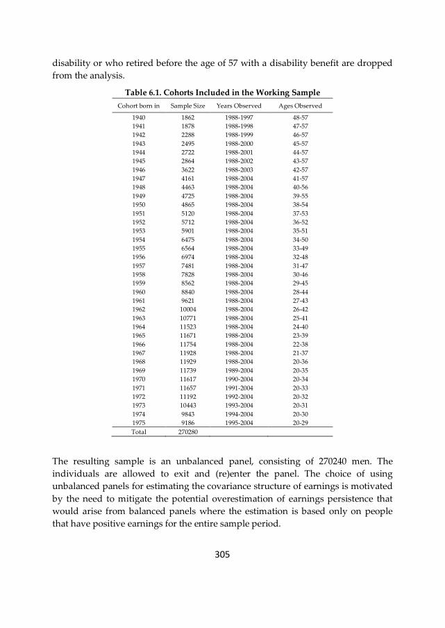
305
disability or who retired before the age of 57 with a disability benefit are dropped
from the analysis.
Table 6.1. Cohorts Included in the Working Sample
Cohort born in Sample Size Years Observed Ages Observed
1940 1862 1988-1997 48-57
1941 1878 1988-1998 47-57
1942 2288 1988-1999 46-57
1943 2495 1988-2000 45-57
1944 2722 1988-2001 44-57
1945 2864 1988-2002 43-57
1946 3622 1988-2003 42-57
1947 4161 1988-2004 41-57
1948 4463 1988-2004 40-56
1949 4725 1988-2004 39-55
1950 4865 1988-2004 38-54
1951 5120 1988-2004 37-53
1952 5712 1988-2004 36-52
1953 5901 1988-2004 35-51
1954 6475 1988-2004 34-50
1955 6564 1988-2004 33-49
1956 6974 1988-2004 32-48
1957 7481 1988-2004 31-47
1958 7828 1988-2004 30-46
1959 8562 1988-2004 29-45
1960 8840 1988-2004 28-44
1961 9621 1988-2004 27-43
1962 10004 1988-2004 26-42
1963 10771 1988-2004 25-41
1964 11523 1988-2004 24-40
1965 11671 1988-2004 23-39
1966 11754 1988-2004 22-38
1967 11928 1988-2004 21-37
1968 11929 1988-2004 20-36
1969 11739 1989-2004 20-35
1970 11617 1990-2004 20-34
1971 11657 1991-2004 20-33
1972 11192 1992-2004 20-32
1973 10443 1993-2004 20-31
1974 9843 1994-2004 20-30
1975 9186 1995-2004 20-29
Total 270280
The resulting sample is an unbalanced panel, consisting of 270240 men. The
individuals are allowed to exit and (re)enter the panel. The choice of using
unbalanced panels for estimating the covariance structure of earnings is motivated
by the need to mitigate the potential overestimation of earnings persistence that
would arise from balanced panels where the estimation is based only on people
that have positive earnings for the entire sample period.
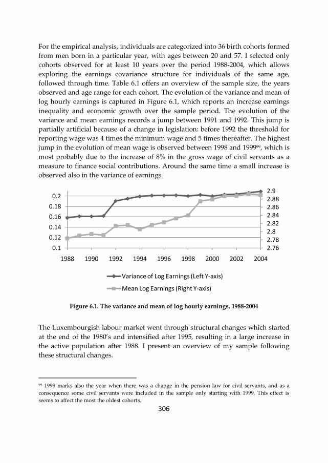
306
For the empirical analysis, individuals are categorized into 36 birth cohorts formed
from men born in a particular year, with ages between 20 and 57. I selected only
cohorts observed for at least 10 years over the period 1988-2004, which allows
exploring the earnings covariance structure for individuals of the same age,
followed through time. Table 6.1 offers an overview of the sample size, the years
observed and age range for each cohort. The evolution of the variance and mean of
log hourly earnings is captured in Figure 6.1, which reports an increase earnings
inequality and economic growth over the sample period. The evolution of the
variance and mean earnings records a jump between 1991 and 1992. This jump is
partially artificial because of a change in legislation: before 1992 the threshold for
reporting wage was 4 times the minimum wage and 5 times thereafter. The highest
jump in the evolution of mean wage is observed between 1998 and 199999, which is
most probably due to the increase of 8% in the gross wage of civil servants as a
measure to finance social contributions. Around the same time a small increase is
observed also in the variance of earnings.
Figure 6.1. The variance and mean of log hourly earnings, 1988-2004
The Luxembourgish labour market went through structural changes which started
at the end of the 1980’s and intensified after 1995, resulting in a large increase in
the active population after 1988. I present an overview of my sample following
these structural changes.
99 1999 marks also the year when there was a change in the pension law for civil servants, and as a
consequence some civil servants were included in the sample only starting with 1999. This effect is
seems to affect the most the oldest cohorts.
2.76
2.78
2.8
2.82
2.84
2.86
2.88
2.9
0.1
0.12
0.14
0.16
0.18
0.2
1988 1990 1992 1994 1996 1998 2000 2002 2004
Variance of Log Earnings (Left Y-axis)
Mean Log Earnings (Right Y-axis)

307
First, the number of active men more than doubled in 2004 compared with 1988,
reaching a value of 160,315 in 2004.
Second, the evolution of the composite of the sample by occupation status and
sector illustrated in Figure 6.2 and Figure 6.3 resemble the one for the whole
population illustrated in Figure 6-A- 1 and Figure 6-A-2: there is a clear shift in the
structure, with white collars and civil servants, and the tertiary sector recording a
significant increase in their share over time. Thirdly, as illustrated in Figure 6.4, the
evolution of the composite of the sample by age is affected slightly by the filters
applied, but maintains similar characteristics as the whole population (Figure 6-A-
3).
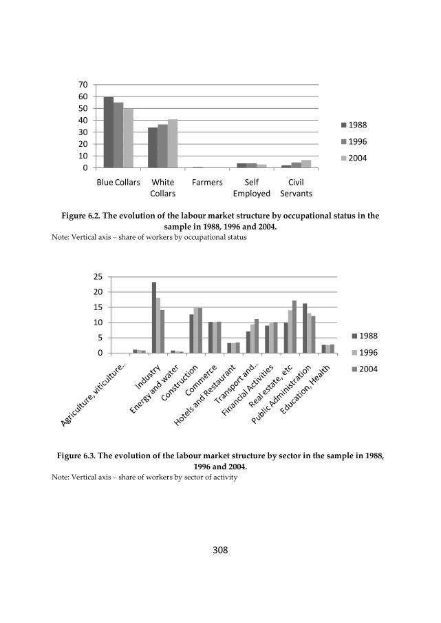
308
Figure 6.2. The evolution of the labour market structure by occupational status in the
sample in 1988, 1996 and 2004. Note: Vertical axis – share of workers by occupational status
Figure 6.3. The evolution of the labour market structure by sector in the sample in 1988,
1996 and 2004. Note: Vertical axis – share of workers by sector of activity
0
10
20
30
40
50
60
70
Blue Collars White
Collars
Farmers Self
Employed
Civil
Servants
1988
1996
2004
0
5
10
15
20
25
1988
1996
2004
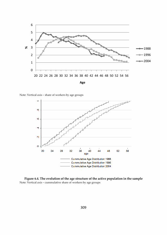
309
Note: Vertical axis – share of workers by age groups
Figure 6.4. The evolution of the age structure of the active population in the sample Note: Vertical axis – cummulative share of workers by age groups
0
1
2
3
4
5
6
20 22 24 26 28 30 32 34 36 38 40 42 44 46 48 50 52 54 56
%
Age
1988
1996
2004

310
6.5.Econometric specification and estimation method of
covariance structures
The aim of this section is to fit a parsimonious model to the autocovariance
structure of earnings for all cohorts. This model is use to explore the changes in the
permanent and transitory components of earnings over the sample period and
their impact on overall earnings inequality.
6.5.1. Econometric earnings specification
In order to differentiate lifecycle dynamics from secular changes in earnings
inequality, the earnings differentials are analysed within the 36 cohorts defined in
the previous section. The first step is to de-trend earnings for each cohort. The
empirical specification of earnings follows the structure:
, 1,..., , 1,...,ict ct ict i c
Y Y r t T i N= + = = (6.8)
where ict
Y is the natural logarithm of real hourly earnings of the i-th individual,
from the c-th cohort in the t-th year, ctY is the year-cohort specific mean and ict
r is
an error term which represents the individual-specific deviation from the year-
cohort specific mean. The demeaned earnings ict
r are assumed to be
independently distributed across individuals, but autocorrelated over time.
Earnings differentials within each cohort can be characterised by modelling the
covariance structure of individual earnings:
0( ) ( , ), 0,...,
ict ict ict s c cVarCov Y E r r s T t−= = − .100
This study approaches the problem of choosing a longitudinal process for the
demeaned earnings,ict
r following the methodology used by MaCurdy(1981) and
MaCurdy (1982), meaning in a similar manner with time series. The inspection of
the covariance structure of earnings, which is presented in section 6.6, suggests the
following features of the data:
(i) the elements of the autocovariance structure decrease with the lag at a
decreasing rate and
100 c
T and 0c
t represent the total number of years and the first year observed for each cohort.
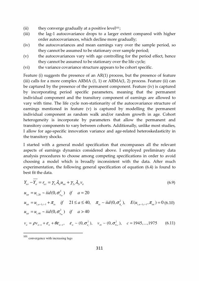
311
(ii) they converge gradually at a positive level101;
(iii) the lag-1 autocovariance drops to a larger extent compared with higher
order autocovariances, which decline more gradually;
(iv) the autocovariances and mean earnings vary over the sample period, so
they cannot be assumed to be stationary over sample period;
(v) the autocovariances vary with age controlling for the period effect, hence
they cannot be assumed to be stationary over the life cycle;
(vi) the variance covariance structure appears to be cohort specific.
Feature (i) suggests the presence of an AR(1) process, but the presence of feature
(iii) calls for a more complex ARMA (1, 1) or ARMA(1, 2) process. Feature (ii) can
be captured by the presence of the permanent component. Feature (iv) is captured
by incorporating period specific parameters, meaning that the permanent
individual component and the transitory component of earnings are allowed to
vary with time. The life cycle non-stationarity of the autocovariance structure of
earnings mentioned in feature (v) is captured by modelling the permanent
individual component as random walk and/or random growth in age. Cohort
heterogeneity is incorporate by parameters that allow the permanent and
transitory components to vary between cohorts. Additionally, unlike most studies,
I allow for age-specific innovation variance and age-related heteroskedasticity in
the transitory shocks.
I started with a general model specification that encompasses all the relevant
aspects of earnings dynamics considered above. I employed preliminary data
analysis procedures to choose among competing specifications in order to avoid
choosing a model which is broadly inconsistent with the data. After much
experimentation, the following general specification of equation (6.4) is found to
best fit the data.
1 1 2 2ict ct ict c t iat c t itY Y r u vγ λ γ λ− = = + (6.9)
20
40
2
,20
2
, 1, 1 , 1, 1
2
,40
~ (0, ) 20
21 40, (0, ), ( , ) 0
~ (0, ) 40
a
iat i u
iat i a t ia ia i a t iat
iat i u
u u iid if a
u u if a iid E u
u u iid if a
π
σ
π π σ π
σ
− − − −
= =
= + ≤ ≤ =
= >
∼ (6.10)
2 2
1 1 0 0,, (0, ), (0, ), 1945, ...,1975
tit it it it it i cv v v c
ερ ε θε ε σ σ
− −= + + =∼ ∼
(6.11)
101
convergence with increasing lags
312
2 2 3 4
0 1 2 3 3( 20) ( 20) ( 20) ( 20)
tt t t t
age age age ageεσ β β β β β= + − + − + − + −
(6.12)
I refer to the model in equation (6.9)-(6.12) as my “base model”. According to
equation (6.9), earnings can be decomposed into a permanent component 1 1c t iat
uγ λ
and a transitory component 2 2c t it
vγ λ . The permanent component iat
u (Equation
(6.10)) specifies a random walk in age in earnings growth after age 20 up to age 40,
where 2
~ (0, )a
iaiid ππ σ is the innovation at each age, and after that a random
effects model with the distribution of the effects fixed at that implied by the
random walk. Previous research forced the innovation variance 2
aπσ to be the same
over the lifecycle. My rich data allowed us to estimate age specific innovation
variances. The model with age-specific innovation variances until the age of 40 was
found to fit the data the best. This decision is backed up also by Figure 6.6. I also
estimate the variance of an initial permanent shock (assumed to be at age 20, which
is also the lowest age observed in my dataset), denoted 20
2
uσ . Thus the permanent
earnings variance within a cohort rises with age up until age 40, after which it
remains at its current level. Consistent with many matching and human capital
models, whereby human capital or ability is revealed for the first 20 years of labour
market experience after which the permanent differentials start shrinking, I expect
larger permanent shocks at younger age. (Jovanovic, 1979)
Equation (6.11) specifies the transitory component of earnings which evolves as an
ARMA(1,1) process, where the serial correlation ρ parameter captures the
decreasing rate of decay of the covariances with the lag, the moving-average
parameter θ captures the sharp drop of the lag-1 autocovariance compared with
the other autocovariances, and it
ε are white-noise mean-reverting transitory
shocks. The variance 2
0,cσ measures the volatility of shocks at the start of the
sample period, 2
tεσ the volatility of shocks in subsequent years and ρ the
persistence of shocks. Measurement error in this model is captured by this
transitory component. Additionally, equation (6.12) allows the variance of it
ε to
change over the lifecycle, as a polynomial of order 4 in age.
The non-stationary pattern of earnings is accommodated using time specific
loading factors, both on the permanent and transitory component of earnings,
, 1,2; 0,16kt k tλ = =, normalized to 1 in the first wave for identification102. Cohort
1021994 refers to t=0
313
heterogeneity is accommodated by allowing both the permanent and the transitory
component to vary with the cohort. , 1, 2jc jγ = are cohort loading factor,
normalized to 1 for the cohort born in 1945 for identification.
6.5.2. Specification of the covariance structure of earnings
When working with ARMA(p,q) processes in the context of panel data, MaCurdy
(1981), MaCurdy (1982) and Anderson and Hsiao (1982) underlined the need for a
treatment of initial conditions103. As illustrated in equations (6.14) and (6.15), the
autoregressive process induces a recursive structure in the moments: the variance-
covariance in year t depends on the transitory variance-covariance in year t-1. If
one tracks the recursion back to the first sample year for each cohort, this raises the
question of what is the transitory variance for each cohort in that year. In the
earlier stage of the literature on earnings dynamics, it was common to restrict the
initial transitory variance to be the same for all cohorts. In line with the most recent
literature on earnings dynamics, my model acknowledges that earnings volatility
varies across cohorts because they illustrate different stages of the lifecycle and
they have experienced different period effects. Therefore such a strong assumption
is untenable.
Following MaCurdy (1981), MaCurdy (1982), I treat the initial transitory variances
of the 36 cohorts as 36 additional parameters to be estimated. The covariance
structure for the first sample period takes the form:
0
20
20 40
40
0 0 0
2 2
0 0
21
2 2
0 0
402 2
0
21
( ) ( )
( ) 0 40,
( ) 0 40,
0,
a
a
ic ic ic
a
i
a
u i
u
a
Var Y E r r
Var v if t for a
Var v if t for a
where a age in period
µ π
µ
π
σ σ
σ σ
σ σ
=
=
= =
= + + = ≤
= + + = >
= =
∑
∑
(6.13)
The covariance structure for subsequent years can be expressed as follows:
103 See Macurdy(1982, page 92/93)

314
20
20 40
40
2 2 2 2 2 2 2 2 2
1 1 2 2 1
21
2 2 2 2 2 2 2 2 2
1 1 2 2 1
402 2
21
( ) ( )
[ ] [ ( ) (1 2 )] 0 40
[ ] [ ( ) (1 2 )] 0 40,
t
a t
t
a
ict ict ict
a
c t c t it t
a
c t u c t it t
u
a
Var Y E r r
Var v if t for a
Var v if t for a
where
µ π ε
µ ε
π
γ λ σ σ γ λ ρ σ ρθ θ
γ λ σ σ γ λ ρ σ ρθ θ
σ σ
−
=
−
=
= =
= + + + + + > ≤
= + + + + + > >
=
∑
∑
(6.14)
20
20 40
40
2 2 2 2 2
1 1 2 2 2 1
21
2 2 2 2 2
1 1 2 2 2 1
2 2
( ) ( )
[ ] [ ( , )] 0 & 1 40
[ ] [ ( , )] 0 & 1 40
t s
a
a
ict ict s ict ict s
a
c t c t t s it it s t s
a
c t c t t s it it s t s
a
Cov Y Y E r r
Cov v v if t s for a
Cov v v if t s for a
where
µ π
µ µ
µ π
γ λ σ σ γ λ λ ρ
γ λ σ σ γ λ λ ρ
σ σ
−
− −
− − − −
=
− − − −
= =
= + + > > ≤
= + + > > >
=
∑
21
t sa −
=
∑ (6.15)
1
20 1
20 40 1
40
1 1
2 2 2 2 2 2
1 1 2 2 2 1 1 1
21
2 2 2 2 2 2
1 1 2 2 2 1 1 1
2
( ) ( )
[ ] { ( ) )} 0 & 1 40
[ ] { ( ) )} 0 & 1 40
t
a t
t
ict ict ict ict
a
c t c t t it t
a
c t c t t it t
Cov Y Y E r r
Var v if t s for a
Var v if t s for a
where
µ π ε
µ µ ε
µ
γ λ σ σ γ λ λ ρ θσ
γ λ σ σ γ λ λ ρ θσ
σ
−
−
−
− −
− − −
=
− − −
= =
= + + + > = ≤
= + + + > = >
∑
1
2
21
t
a
a
a
πσ
−
=
=∑
(6.16)
6.5.3. Estimation of covariance structures104
Covariance structures are models that specify a structure for the covariance matrix
of the regression error. They can be used to model structures for error dynamics
and measurement error. The goal is to estimate the parameters of the covariance
structure of earnings for all cohorts. This can be used to analyse the changes in the
permanent and transitory components of earnings over the sample period.
104 The information in this section has been covered in section 4.5.3.

315
The parameters of the models are fit to the covariance structure for each cohort
using equally weighted minimum distance methods of estimation. The
methodology used is the same as that utilized by Cappellari (2003), Baker and
Solon (2003), Ramos (2003), Kalwij and Alessie (2003), Dickens (2000b), Baker
(1997), Abowd and Card (1989), Cervini and Ramos (2006), Sologon and
O’Donoghue (2009a, 2009b).
Following Sologon and O’Donoghue (2009a, 2009b), for each cohort c and
individual i, define a vector which identifies the presence for each individual in the
respective cohort and year:
1...
c
ict
ict
d
d
=
icd
where ict
d is an indicator variable that is equal to 1 if the individual from cohort c
is present in year t of the panel and c
t is the total length of the panel for each
cohort. Similarly, the vector containing the cohort earnings residuals can be
represented as follows:
1...
c
ict
ict
r
r
=
icR
where ict
r are the earnings residuals for individual i belonging to cohort c in year t
in mean deviation form for each cohort and year. The elements of the ic
R
corresponding to missing years are set to 0. The variance-covariance matrix of the
earnings is computed separately for each cohort,c
C . The elements of the variance-
covariance matrix for cohort c, c
C , which is of dimension ( )c c
t t× are computed
follows:
1
1
[ , ]
c
c
n
ick icli
c n
ick icli
r rm k l
d d
=
=
=∑∑
(6.17)
316
where c
n is the total number of individuals in cohort c, , {1,..., }c
k l t= .
Conformably with c
m , ci
m represent the distinct elements of the individual cross-
product matrix '
ic icR R . Then 1
1
[ , ][ , ]
c
c
n
cii
c n
ick icli
m k lm k l
d d
=
=
=∑∑
.
The matrix c
C is symmetric with ( 1)
( 1)2
c ct t +
× distinct elements. Let c
Vech(C )
be a column vector of dimension ( 1)
( 1)2
c ct t +
× which stacks all the elements of
the variance covariance matrix c
C for cohort c. The aggregate vector of moments
for all cohorts is denoted by: T T T
1 4m = (Vech(C ) , ..., Vech(C ) ) , which is a
column vector of dimension 36
1
( 1)( 1) ( 1)
2
c c
c
t tN
=
+× = ×∑ . In this paper, N=4668.
To estimate the error components of the structural model illustrated by equations
(6.9)-(6.12), the elements of m are fit to a parameter vector θ , so that ( )f=m θ ,
( )f θ takes the form of equations (6.13) - (6.16). Minimum distance estimation
requires minimising the weighted sum of the squared distance between the actual
covariances ( m ) and a function of the parameter vector ( ( )f θ ) which
encapsulates the covariance structure implied by the error component model.
Therefore, minimum distance estimation involves the following quadratic form:
( ) [ ( )] [ ( )]'D f f= − −θ m θ W m θ , where W is a positive definite weighting
matrix. Minimum distance estimator chooses ɵθ to minimise the distance function ɵ( )D θ .
Based on Chamberlain (1984), the asymptotic optimal choice of W is the inverse
of a matrix that consistently estimates the covariance matrix of m , which leads to
the optimum minimum distance estimator (OMD). However, Clark (1996) and
Altonji and Segal (1994) provided Monte Carlo evidence that OMD is biased in
small samples because of the correlation between the measurement error in the
second moments and forth moments. Instead, they proposed using the identity
matrix as a weighting matrix. This approach, often called “equally weighted
minimum distance estimation” (EWMD), involves using the standard nonlinear
least squares to fit ( )f θ tom . The same procedure is followed in this paper.
317
For estimating the asymptotic standard errors of the parameter estimates, I apply
the delta method. Following Chamberlain (1984), the asymptotic variance-
covariance matrix of the estimated parameters is obtained from the following
formula:
-1 -1AsyVar(θ) = (G'WG) G' 'WVWG(G WG) (6.18)
where G is the Jacobian of the transformation ( )f θ evaluated at ɵ=θ θ . G has
dimension ( )m
t p× and rank p, where m
t is the sum across cohorts of
( 1)( 1)
2
c ct t +
× and p is the number of parameters. W is the identity matrix and
V the matrix of fourth sample moments.
Chamberlain (1984) showed that under some fairly general regularity assumptions,
the independence of ic
R implies that the sample mean of ci
m has an asymptotic
normal distribution * *( , )c c cm N m V∼ , where *
cm is the expectation of ci
m ,
meaning the true covariance matrix of earnings, and *
cV is the variance-
covariance matrix, which can be estimated consistently by computing the sample
moment matrix of the c
Vech(C ) vector, c
V . The elements of the variance
covariance c
V can be written as follows:
1
1 1
( [ , ], [ , ]) ( [ , , , ] [ , ] [ , ])
c
c c
n
ick icl icp icqi
c c c c cn n
ick icl icp icqi i
d d d dCov m k l m p q m k l p q m k l m p q
d d d d
=
= =
= −∑
∑ ∑,
where 1
1
[ , , , ]
c
c
n
ick icl icp icqi
c n
ick icl icp icqi
r r r rm k l p q
d d d d
=
=
=∑∑
The variance-covariance matrix of m was denoted by V , where V is the block
diagonal matrix which is constructed from all the c
V matrices.
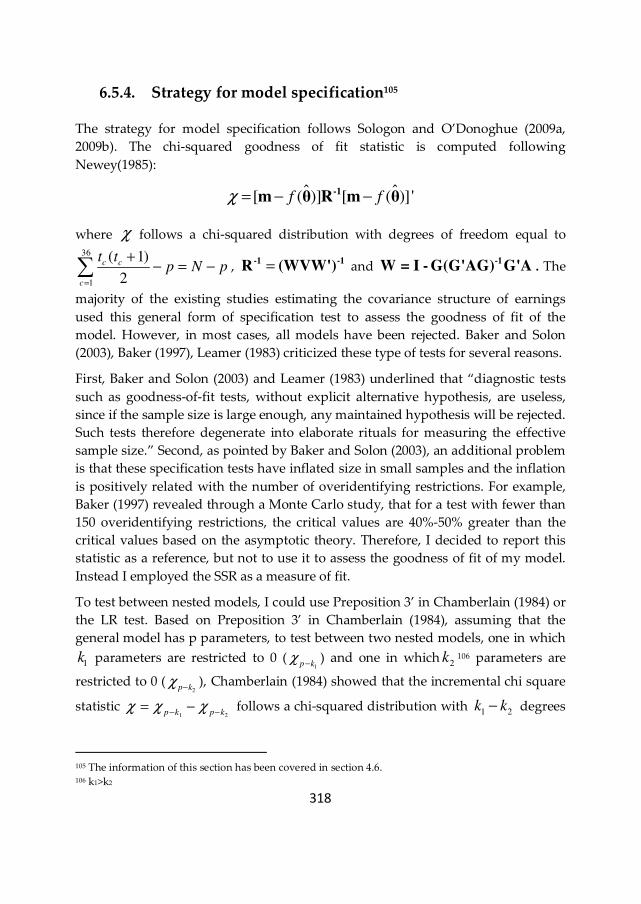
318
6.5.4. Strategy for model specification105
The strategy for model specification follows Sologon and O’Donoghue (2009a,
2009b). The chi-squared goodness of fit statistic is computed following
Newey(1985):
ɵ ɵ[ ( )] [ ( )]'f fχ = − −-1m θ R m θ
where χ follows a chi-squared distribution with degrees of freedom equal to 36
1
( 1)
2
c c
c
t tp N p
=
+− = −∑ , =-1 -1R (WVW') and
-1W = I - G(G AG)' G'A . The
majority of the existing studies estimating the covariance structure of earnings
used this general form of specification test to assess the goodness of fit of the
model. However, in most cases, all models have been rejected. Baker and Solon
(2003), Baker (1997), Leamer (1983) criticized these type of tests for several reasons.
First, Baker and Solon (2003) and Leamer (1983) underlined that “diagnostic tests
such as goodness-of-fit tests, without explicit alternative hypothesis, are useless,
since if the sample size is large enough, any maintained hypothesis will be rejected.
Such tests therefore degenerate into elaborate rituals for measuring the effective
sample size.” Second, as pointed by Baker and Solon (2003), an additional problem
is that these specification tests have inflated size in small samples and the inflation
is positively related with the number of overidentifying restrictions. For example,
Baker (1997) revealed through a Monte Carlo study, that for a test with fewer than
150 overidentifying restrictions, the critical values are 40%-50% greater than the
critical values based on the asymptotic theory. Therefore, I decided to report this
statistic as a reference, but not to use it to assess the goodness of fit of my model.
Instead I employed the SSR as a measure of fit.
To test between nested models, I could use Preposition 3’ in Chamberlain (1984) or
the LR test. Based on Preposition 3’ in Chamberlain (1984), assuming that the
general model has p parameters, to test between two nested models, one in which
1k parameters are restricted to 0 (
1p kχ −) and one in which
2k 106 parameters are
restricted to 0 (2p kχ −
), Chamberlain (1984) showed that the incremental chi square
statistic 1 2p k p kχ χ χ− −= − follows a chi-squared distribution with
1 2k k− degrees
105 The information of this section has been covered in section 4.6. 106 k1>k2
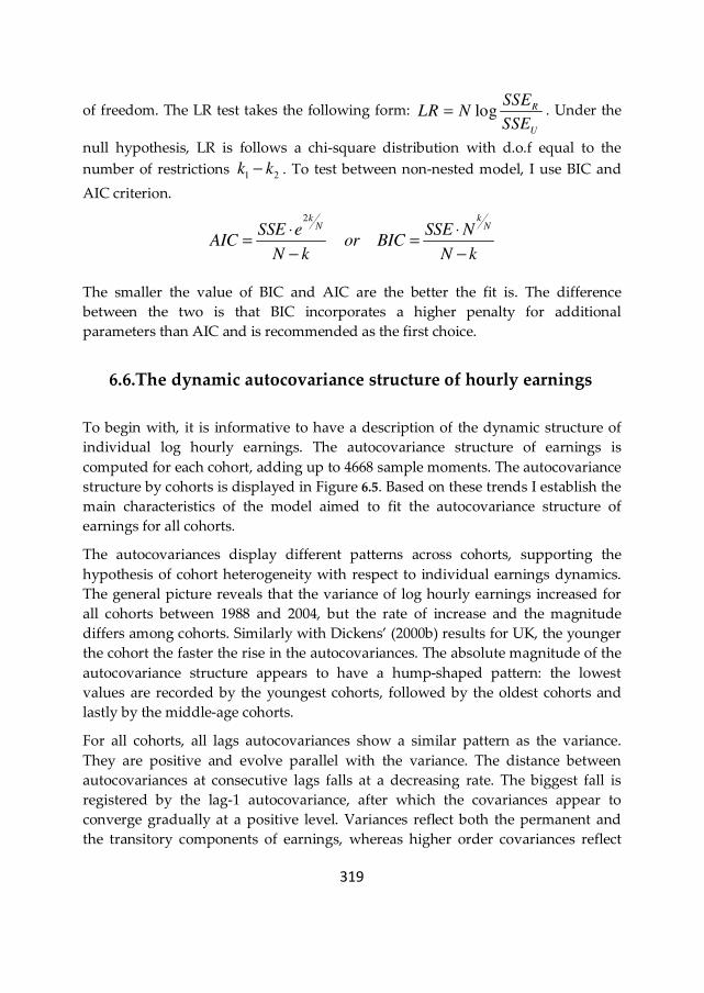
319
of freedom. The LR test takes the following form: log R
U
SSELR N
SSE= . Under the
null hypothesis, LR is follows a chi-square distribution with d.o.f equal to the
number of restrictions 1 2
k k− . To test between non-nested model, I use BIC and
AIC criterion.
2k kN NSSE e SSE N
AIC or BICN k N k
⋅ ⋅= =
− −
The smaller the value of BIC and AIC are the better the fit is. The difference
between the two is that BIC incorporates a higher penalty for additional
parameters than AIC and is recommended as the first choice.
6.6.The dynamic autocovariance structure of hourly earnings
To begin with, it is informative to have a description of the dynamic structure of
individual log hourly earnings. The autocovariance structure of earnings is
computed for each cohort, adding up to 4668 sample moments. The autocovariance
structure by cohorts is displayed in Figure 6.5. Based on these trends I establish the
main characteristics of the model aimed to fit the autocovariance structure of
earnings for all cohorts.
The autocovariances display different patterns across cohorts, supporting the
hypothesis of cohort heterogeneity with respect to individual earnings dynamics.
The general picture reveals that the variance of log hourly earnings increased for
all cohorts between 1988 and 2004, but the rate of increase and the magnitude
differs among cohorts. Similarly with Dickens’ (2000b) results for UK, the younger
the cohort the faster the rise in the autocovariances. The absolute magnitude of the
autocovariance structure appears to have a hump-shaped pattern: the lowest
values are recorded by the youngest cohorts, followed by the oldest cohorts and
lastly by the middle-age cohorts.
For all cohorts, all lags autocovariances show a similar pattern as the variance.
They are positive and evolve parallel with the variance. The distance between
autocovariances at consecutive lags falls at a decreasing rate. The biggest fall is
registered by the lag-1 autocovariance, after which the covariances appear to
converge gradually at a positive level. Variances reflect both the permanent and
the transitory components of earnings, whereas higher order covariances reflect

320
the permanent component of earnings. Therefore, for all cohorts, the evolution of
covariances, at all orders, suggests the presence of a permanent individual
component of wages and a transitory component which is serially correlated. In
addition, the magnitude of the longer lag covariances relative to the variances is
higher the older the cohort.
One possible explanation for these trends is given by the theory on matching
models, which sustains that the more experience an individual accumulates, the
more information is revealed on the individual’s ability. (Jovanovic, 1979)
Therefore, permanent wage dispersion and implicitly overall inequality within a
cohort is expected to rise as the cohort ages.
To look at the life cycle effects more clearly it is necessary to control for the period
effect which is present in the within-cohort covariances. Thus I keep year constant
and illustrate the life cycle autocovariances by age. Figure 6.6 presents the
variance-covariance structure by age for the selected years.
All lags autocovariances of log real gross hourly earnings show a similar pattern as
the variance. They are positive and evolve parallel with the variance, at different
rates over the life cycle. They rise sharply over the life cycle until the late 30s and
early 40s, after which they have a rather stable evolution up until late 50s. The
diminishing rate of increase of all lags autocovariances observed from the age of 20
until the late 50s is consistent with the presence of a permanent component of
earnings that rises with age at a diminishing rate (Dickens, 2000b).
Comparing across years, the life cycle profile of the auto-covariances of log gross
hourly earnings appears to become steeper over time. The slope of the life cycle
profile can be interpreted as the returns to the permanent complement of earnings.
Therefore, steeper slopes in later years imply increasing returns to the permanent
component of earnings over time.
32
1
Fig
ure
6.5
. Au
toco
var
ian
ce S
tru
ctu
re o
f E
arn
ing
s fo
r S
elec
ted
Co
ho
rts:
194
0 –
1975
N
ote
: In
th
e le
gen
d, t
sta
nd
s fo
r th
e e
ach
yea
r d
isp
lay
ed
on
th
e h
ori
zo
nta
l ax
is o
f ea
ch g
rap
h.
.1.15.2.25
19
88
19
92
19
96
20
00
20
04
Co
ho
rt b
orn
19
40
.1.15.2.25
19
88
19
92
19
96
20
00
20
04
Co
ho
rt b
orn
19
41
.1.15.2.25
19
88
19
92
19
96
20
00
20
04
Co
ho
rt b
orn
19
42
.1.15.2.25
19
88
19
92
19
96
20
00
20
04
Co
ho
rt b
orn
19
43
.1.15.2.25
19
88
19
92
19
96
20
00
20
04
Co
ho
rt b
orn
19
44
.1.15.2.25
19
88
19
92
19
96
20
00
20
04
Co
ho
rt b
orn
19
45
.1.15.2.25
19
88
19
92
19
96
20
00
20
04
Co
ho
rt b
orn
19
46
.1.15.2.25
19
88
19
92
19
96
20
00
20
04
Co
ho
rt b
orn
19
47
.1.15.2.25
19
88
19
92
19
96
20
00
20
04
Co
ho
rt b
orn
19
48
.1.15.2.25
19
88
19
92
19
96
20
00
20
04
Co
ho
rt b
orn
19
49
.1.15.2.25
19
88
19
92
19
96
20
00
20
04
Co
ho
rt b
orn
19
50
.1.15.2.25
19
88
19
92
19
96
20
00
20
04
Co
ho
rt b
orn
19
51
.1.15.2.25
19
88
19
92
19
96
20
00
20
04
Co
ho
rt b
orn
19
52
.1.15.2.25
19
88
19
92
19
96
20
00
20
04
Co
ho
rt b
orn
19
53
.1.15.2.25
19
88
19
92
19
96
20
00
20
04
Co
ho
rt b
orn
19
54
.1.15.2.25
19
88
19
92
19
96
20
00
20
04
Co
ho
rt b
orn
19
55
.1.15.2.25
19
88
19
92
19
96
20
00
20
04
Co
ho
rt b
orn
19
56
.1.15.2.25
19
88
19
92
19
96
20
00
20
04
Co
ho
rt b
orn
19
57
Variance
(t)
Co
variance
(t, t-
1)
Co
variance
(t, t-
2)
Co
variance
(t, t-
3)
Co
variance
(t, t-
4)
Co
variance
(t, t-
5)
Co
variance
(t, t-
6)
Co
variance
(t, t-
7)
Co
variance
(t, t-
8)
Co
variance
(t, t-
9)
Co
variance
(t, t-
10
)C
ovariance
(t, t-
11
)
Co
variance
(t, t-
12
)C
ovariance
(t, t-
13
)
Co
variance
(t, t-
14
)C
ovariance
(t, t-
15
)
Co
variance
(t, t-
16
)
32
2
Fig
ure
6.5
(C
on
tin
ued
)
0.05.1.15.2.25
1988
1992
1996
2000
2004
Cohort
born
1958
0.05.1.15.2.25
1988
1992
1996
2000
2004
Cohort
born
1959
0.05.1.15.2.25
1988
1992
1996
2000
2004
Cohort
born
1960
0.05.1.15.2.25
1988
1992
1996
2000
2004
Cohort
born
1961
0.05.1.15.2.25
1988
1992
1996
2000
2004
Cohort
born
1962
0.05.1.15.2.25
1988
1992
1996
2000
2004
Cohort
born
1963
0.05.1.15.2.25
1988
1992
1996
2000
2004
Cohort
born
1964
0.05.1.15.2.25
1988
1992
1996
2000
2004
Cohort
born
1965
0.05.1.15.2.25
1988
1992
1996
2000
2004
Cohort
born
1966
0.05.1.15.2.25
1988
1992
1996
2000
2004
Cohort
born
1967
0.05.1.15.2.25
1988
1992
1996
2000
2004
Cohort
born
1968
0.05.1.15.2.25
1988
1992
1996
2000
2004
Cohort
born
1969
0.05.1.15.2.25
1988
1992
1996
2000
2004
Cohort
born
1970
0.05.1.15.2.25
1988
1992
1996
2000
2004
Cohort
born
1971
0.05.1.15.2.25
1988
1992
1996
2000
2004
Cohort
born
1972
0.05.1.15.2.25
1988
1992
1996
2000
2004
Cohort
born
1973
0.05.1.15.2.25
1988
1992
1996
2000
2004
Cohort
born
1974
0.05.1.15.2.25
1988
1992
1996
2000
2004
Cohort
born
1975
Variance(t
)C
ovariance(t
, t-
1)
Covariance(t
, t-
2)
Covariance(t
, t-
3)
Covariance(t
, t-
4)
Covariance(t
, t-
5)
Covariance(t
, t-
6)
Covariance(t
, t-
7)
Covariance(t
, t-
8)
Covariance(t
, t-
9)
Covariance(t
, t-
10)
Covariance(t
, t-
11)
Covariance(t
, t-
12)
Covariance(t
, t-
13)
Covariance(t
, t-
14)
Covariance(t
, t-
15)
Covariance(t
, t-
16)
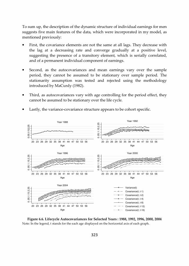
323
To sum up, the description of the dynamic structure of individual earnings for men
suggests five main features of the data, which were incorporated in my model, as
mentioned previously:
• First, the covariance elements are not the same at all lags. They decrease with
the lag at a decreasing rate and converge gradually at a positive level,
suggesting the presence of a transitory element, which is serially correlated,
and of a permanent individual component of earnings.
• Second, as the autocovariances and mean earnings vary over the sample
period, they cannot be assumed to be stationary over sample period. The
stationarity assumption was tested and rejected using the methodology
introduced by MaCurdy (1982).
• Third, as autocovariances vary with age controlling for the period effect, they
cannot be assumed to be stationary over the life cycle.
• Lastly, the variance-covariance structure appears to be cohort specific.
Figure 6.6. Lifecycle Autocovariances for Selected Years : 1988, 1992, 1996, 2000, 2004
Note: In the legend, t stands for the each age displayed on the horizontal axis of each graph.
0.0
5.1.
15.
2.2
5
20 23 26 29 32 35 38 41 44 47 50 53 56
Age
Year 1988
0.0
5.1
.15.2
.25
20 23 26 29 32 35 38 41 44 47 50 53 56
Age
Year 1992
0.0
5.1
.15.2
.25
20 23 26 29 32 35 38 41 44 47 50 53 56
Age
Year 1996
0.0
5.1
.15.2
.25
20 23 26 29 32 35 38 41 44 47 50 53 56
Age
Year 2000
0.0
5.1
.15
.2.2
5
20 23 26 29 32 35 38 41 44 47 50 53 56
Age
Year 2004Variance(t)
Covariance(t, t-1)
Covariance(t, t-2)
Covariance(t, t-4)
Covariance(t, t-8)
Covariance(t, t-12)
Covariance(t, t-16)
324
6.7.Results of Covariance Structure Estimation
6.7.1. Error component model estimation results
To investigate these patterns more formally, I proceed to the GMM estimation of
the earnings dynamics model described in Section 6.5. Table 6.3 shows the
resulting estimates. The first three columns show the parameter estimates and the
associated SE estimates for the base model outlined in equations (6.9)-(6.12). All the
parameter estimates are highly significant. Recall that this model incorporates a
persistent component, composed of terms capturing a random walk after age 20
until age 40, with age-specific innovation variances, and a random effects model
after age 40 with the distribution of the effects fixed at that implied by the random
walk, plus a transitory component following an ARMA(1,1) process with age-
based heteroskedastic innovations. Furthermore, the persistent and transitory
components are allowed to shift over time and over cohort by separate year-
specific and cohort-specific factor loadings.
The significant estimates of 20
2
uσ and 2
aπσ , show that the variance of the initial
permanent shock at age 20 and the random walk with age-specific innovation
variances until age 40 play a significant role in the formation of the persistent
component. As each cohort ages, the permanent component increases by the
innovation variance, 2
aπσ , which records the highest values at younger ages and
declines with age. The pattern of the permanent variance, holding time and cohort
shifters constant is captured in Figure 6.7.
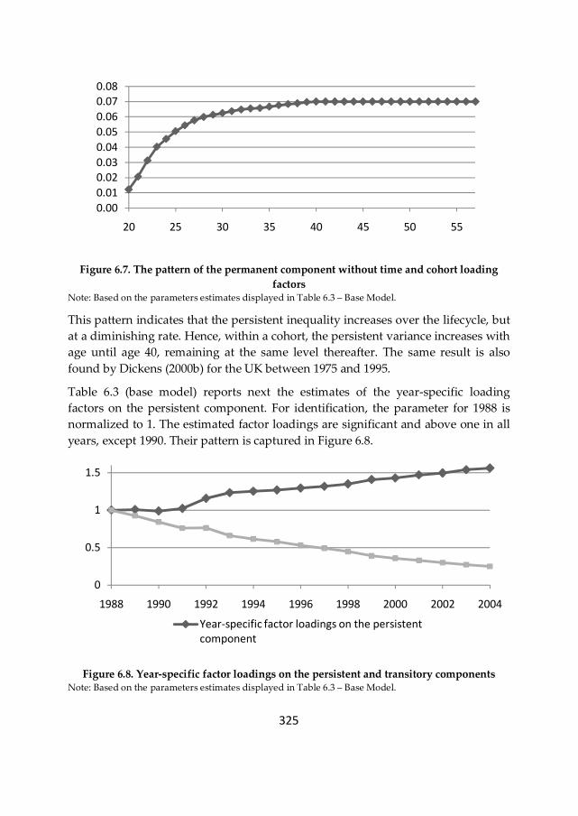
325
Figure 6.7. The pattern of the permanent component without time and cohort loading
factors Note: Based on the parameters estimates displayed in Table 6.3 – Base Model.
This pattern indicates that the persistent inequality increases over the lifecycle, but
at a diminishing rate. Hence, within a cohort, the persistent variance increases with
age until age 40, remaining at the same level thereafter. The same result is also
found by Dickens (2000b) for the UK between 1975 and 1995.
Table 6.3 (base model) reports next the estimates of the year-specific loading
factors on the persistent component. For identification, the parameter for 1988 is
normalized to 1. The estimated factor loadings are significant and above one in all
years, except 1990. Their pattern is captured in Figure 6.8.
Figure 6.8. Year-specific factor loadings on the persistent and transitory components Note: Based on the parameters estimates displayed in Table 6.3 – Base Model.
0.00
0.01
0.02
0.03
0.04
0.05
0.06
0.07
0.08
20 25 30 35 40 45 50 55
0
0.5
1
1.5
1988 1990 1992 1994 1996 1998 2000 2002 2004
Year-specific factor loadings on the persistent
component
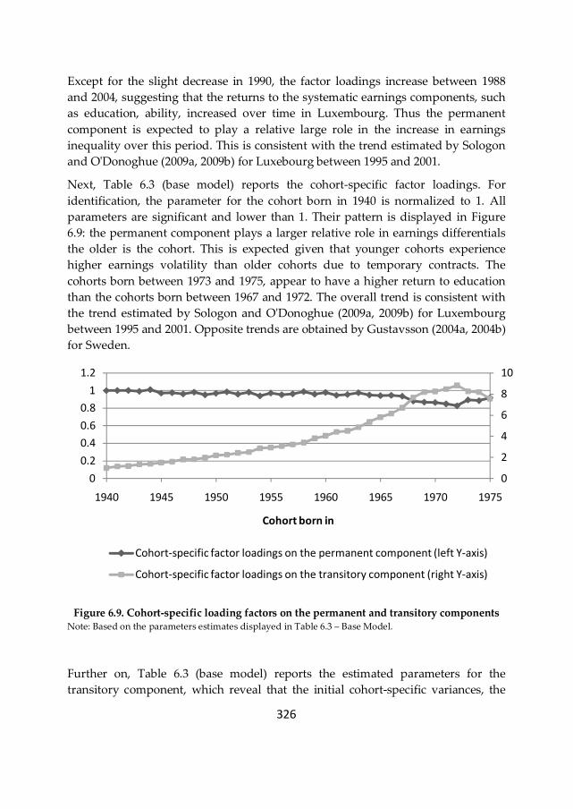
326
Except for the slight decrease in 1990, the factor loadings increase between 1988
and 2004, suggesting that the returns to the systematic earnings components, such
as education, ability, increased over time in Luxembourg. Thus the permanent
component is expected to play a relative large role in the increase in earnings
inequality over this period. This is consistent with the trend estimated by Sologon
and O'Donoghue (2009a, 2009b) for Luxebourg between 1995 and 2001.
Next, Table 6.3 (base model) reports the cohort-specific factor loadings. For
identification, the parameter for the cohort born in 1940 is normalized to 1. All
parameters are significant and lower than 1. Their pattern is displayed in Figure
6.9: the permanent component plays a larger relative role in earnings differentials
the older is the cohort. This is expected given that younger cohorts experience
higher earnings volatility than older cohorts due to temporary contracts. The
cohorts born between 1973 and 1975, appear to have a higher return to education
than the cohorts born between 1967 and 1972. The overall trend is consistent with
the trend estimated by Sologon and O'Donoghue (2009a, 2009b) for Luxembourg
between 1995 and 2001. Opposite trends are obtained by Gustavsson (2004a, 2004b)
for Sweden.
Figure 6.9. Cohort-specific loading factors on the permanent and transitory components Note: Based on the parameters estimates displayed in Table 6.3 – Base Model.
Further on, Table 6.3 (base model) reports the estimated parameters for the
transitory component, which reveal that the initial cohort-specific variances, the
0
2
4
6
8
10
0
0.2
0.4
0.6
0.8
1
1.2
1940 1945 1950 1955 1960 1965 1970 1975
Cohort born in
Cohort-specific factor loadings on the permanent component (left Y-axis)
Cohort-specific factor loadings on the transitory component (right Y-axis)
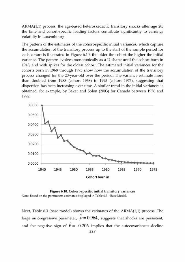
327
ARMA(1,1) process, the age-based heteroskedactic transitory shocks after age 20,
the time and cohort-specific loading factors contribute significantly to earnings
volatility in Luxembourg.
The pattern of the estimates of the cohort-specific initial variances, which capture
the accumulation of the transitory process up to the start of the sample period for
each cohort is illustrated in Figure 6.10: the older the cohort the higher the initial
variance. The pattern evolves monotonically as a U-shape until the cohort born in
1948, and with spikes for the oldest cohort. The estimated initial variances for the
cohorts born in 1968 through 1975 show how the accumulation of the transitory
process changed for the 20-year-old over the period. The variance estimate more
than doubled from 1988 (cohort 1968) to 1995 (cohort 1975), suggesting that
dispersion has been increasing over time. A similar trend in the initial variances is
obtained, for example, by Baker and Solon (2003) for Canada between 1976 and
1992.
Figure 6.10. Cohort-specific initial transitory variances Note: Based on the parameters estimates displayed in Table 6.3 – Base Model.
Next, Table 6.3 (base model) shows the estimates of the ARMA(1,1) process. The
large autoregressive parameter, � 0.964ρ = , suggests that shocks are persistent,
and the negative sign of ɵ 0.206θ = − implies that the autocovariances decline
0.0000
0.0100
0.0200
0.0300
0.0400
0.0500
0.0600
1940 1945 1950 1955 1960 1965 1970 1975
Cohort born in
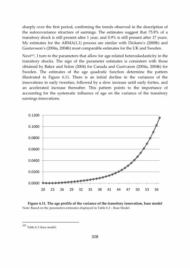
328
sharply over the first period, confirming the trends observed in the description of
the autocovariance structure of earnings. The estimates suggest that 75.8% of a
transitory shock is still present after 1 year, and 0.9% is still present after 17 years.
My estimates for the ARMA(1,1) process are similar with Dickens’s (2000b) and
Gustavsson’s (2004a, 2004b) most comparable estimates for the UK and Sweden.
Next107, I turn to the parameters that allow for age-related heteroskedasticity in the
transitory shocks. The sign of the parameter estimates is consistent with those
obtained by Baker and Solon (2004) for Canada and Gustvason (2004a, 2004b) for
Sweden. The estimates of the age quadratic function determine the pattern
illustrated in Figure 6.11. There is an initial decline in the variances of the
innovations in early twenties, followed by a slow increase until early forties, and
an accelerated increase thereafter. This pattern points to the importance of
accounting for the systematic influence of age on the variance of the transitory
earnings innovations.
Figure 6.11. The age profile of the variance of the transitory innovation, base model Note: Based on the parameters estimates displayed in Table 6.3 – Base Model.
107
Table 6.3 (base model)
0.0000
0.0200
0.0400
0.0600
0.0800
0.1000
0.1200
20 23 26 29 32 35 38 41 44 47 50 53 56
329
Finally, I report the estimates of the period and cohort-specific loading factors for
the transitory component. For identification, the factor loadings for 1988 and for
the cohort born in 1940 were normalized to unity. The pattern of the year-specific
loading factors is captured in Figure 6.8, which illustrate a monotonic decrease
over the period. Thus the relative share of the transitory component appears to
decrease over the sample period. The divergence observed in the trends of the time
factor loading of the two components (Figure 6.8), suggest that the structural
labour market changes favoured a rise in the returns to skills over time and a
decrease in earnings instability.
Figure 6.9 captures the pattern of the cohort-specific loading factors for the
transitory earnings, which reveals that earnings volatility is higher for younger
cohorts, confirming the pattern observed in the dynamic description of the
autocovariance structure of earnings, where autocovariances were found to be
lower for younger cohorts. This is expected, given the more frequent job changes
and less stable earnings of younger workers. A similar trend was obtained by
Sologon and O'Donoghue (2009a, 2009b) for Luxembourg.
Our base model nests and extends most of the specification used in the US,
Canadian, and European studies. The studies based on relatively small-scale panel
surveys imposed often economically implausible restrictions. I tested whether
some of these restrictions hold in my data. The Wald test and the p- values for
testing these restrictions are reported in Table 6.2.
Table 6.2. Wald tests of model restrictions in the base model
Restriction χ2 Degrees of
freedom P-value
(1) 21 22 40
2 2 2... 0π π πσ σ σ= = = =
(no random walk)
10326.6302 31 0.0001
(2) 21 22 40
2 2 2 2...π π π πσ σ σ σ= = = =
(no age-specific innovation variance)
2463.3344 21 0.0001
(3) 1 2 3 4
0, 0, 0, 0β β β β= = = =
(no age-related heteroskedastic transitory shocks)
2963.499 4 0.0001
Some studies assumed away the heterogeneity in earnings growth rates and/or the
existence of earnings shocks with permanent effects. Backer and Solon (2003) and
Ramos (2003) were able to incorporate both in the permanent component. My
model, however incorporates only the random walk process, as a specification with
330
both components leads to identification problems for two parameters of the
random growth model.
I extended the specification of the permanent component to follow a random walk
process with age-specific innovation variances until age 40, and a random effects
model with the distribution of the effects fixed at that implied by the random walk
thereafter. These features were incorporated only by Dickens (2000b) for the UK.
Another study which did a similar attempt is Gustavsson (2004b), but he
constrained the innovation variance to be the same for two adjacent ages between
28 and 53.
If I assume away the random walk until age 40 in the permanent component, the
Wald test on this restrictions clearly rejects the null (χ2 = 10326.6302, df = 31). If I
assume away the age-specific innovation variance until age 40, keeping all the
other specifications of the base model, the Wald test on this restrictions rejects the
null (χ2 = 2463.3344, df = 21) with a p-value equal to 0.0001.
Except Baker and Solon (2003) and Gustavsson (2004b), previous studies imposed
the restriction of invariant variance of the transitory shocks, which was rejected by
the Canadian and Swedish data. My study proves once again that assuming away
the presence of age-related heteroskedastic transitory shocks, meaning that
1 2 3 40, 0, 0, 0β β β β= = = = , is statistically indefensible: the p-value for the
Wald test is 0.0001, clearly rejecting the null hypothesis in the Luxembourgish
data.
In order to see the implications of imposing some of these restrictions on the
inequality decomposition, I estimated a restricted model, where the permanent
component follows a standard random walk in age with the variance of the first
period shock at age 20 fixed at 0, and the transitory component follows an
ARMA(1,1) process with cohort-specific initial variances, with time and cohort
loading factors on both components. The estimation results are displayed in Table
6.3, columns 4-6.
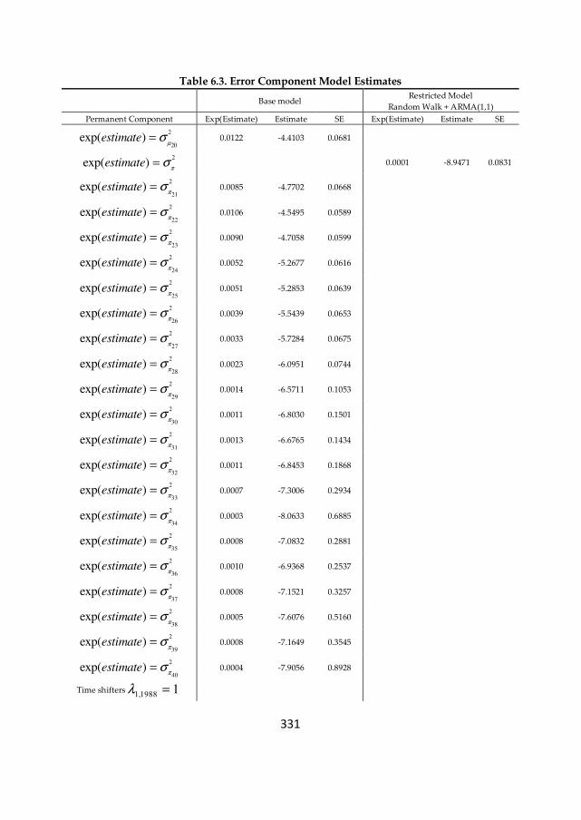
331
Table 6.3. Error Component Model Estimates
Base model Restricted Model
Random Walk + ARMA(1,1) Permanent Component Exp(Estimate) Estimate SE Exp(Estimate) Estimate SE
2
20exp( )estimate
µσ= 0.0122 -4.4103 0.0681
2exp( )estimate
πσ= 0.0001 -8.9471 0.0831
2
21exp( )estimate
πσ= 0.0085 -4.7702 0.0668
2
22exp( )estimate
πσ= 0.0106 -4.5495 0.0589
2
23exp( )estimate
πσ= 0.0090 -4.7058 0.0599
2
24exp( )estimate
πσ= 0.0052 -5.2677 0.0616
2
25exp( )estimate
πσ= 0.0051 -5.2853 0.0639
2
26exp( )estimate
πσ= 0.0039 -5.5439 0.0653
2
27exp( )estimate
πσ= 0.0033 -5.7284 0.0675
2
28exp( )estimate
πσ= 0.0023 -6.0951 0.0744
2
29exp( )estimate
πσ= 0.0014 -6.5711 0.1053
2
30exp( )estimate
πσ= 0.0011 -6.8030 0.1501
2
31exp( )estimate
πσ= 0.0013 -6.6765 0.1434
2
32exp( )estimate
πσ= 0.0011 -6.8453 0.1868
2
33exp( )estimate
πσ= 0.0007 -7.3006 0.2934
2
34exp( )estimate
πσ= 0.0003 -8.0633 0.6885
2
35exp( )estimate
πσ= 0.0008 -7.0832 0.2881
2
36exp( )estimate
πσ= 0.0010 -6.9368 0.2537
2
37exp( )estimate
πσ= 0.0008 -7.1521 0.3257
2
38exp( )estimate
πσ= 0.0005 -7.6076 0.5160
2
39exp( )estimate
πσ= 0.0008 -7.1649 0.3545
2
40exp( )estimate
πσ= 0.0004 -7.9056 0.8928
Time shifters1,1988 1λ =
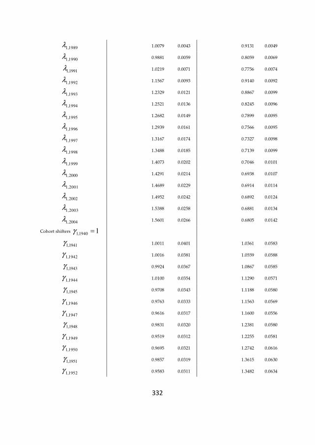
332
1,1989λ
1.0079 0.0043 0.9131 0.0049
1,1990λ
0.9881 0.0059 0.8059 0.0069
1,1991λ
1.0219 0.0071 0.7756 0.0074
1,1992λ
1.1567 0.0093 0.9140 0.0092
1,1993λ
1.2329 0.0121 0.8867 0.0099
1,1994λ
1.2521 0.0136 0.8245 0.0096
1,1995λ
1.2682 0.0149 0.7899 0.0095
1,1996λ
1.2939 0.0161 0.7566 0.0095
1,1997λ
1.3167 0.0174 0.7327 0.0098
1,1998λ
1.3488 0.0185 0.7139 0.0099
1,1999λ
1.4073 0.0202 0.7046 0.0101
1,2000λ
1.4291 0.0214 0.6938 0.0107
1,2001λ
1.4689 0.0229 0.6914 0.0114
1,2002λ
1.4952 0.0242 0.6892 0.0124
1,2003λ
1.5388 0.0258 0.6881 0.0134
1,2004λ
1.5601 0.0266 0.6805 0.0142
Cohort shifters 1,1940 1γ =
1,1941γ
1.0011 0.0401 1.0361 0.0583
1,1942γ
1.0016 0.0381 1.0559 0.0588
1,1943γ
0.9924 0.0367 1.0867 0.0585
1,1944γ
1.0100 0.0354 1.1290 0.0571
1,1945γ
0.9708 0.0343 1.1188 0.0580
1,1946γ
0.9763 0.0333 1.1563 0.0569
1,1947γ
0.9616 0.0317 1.1600 0.0556
1,1948γ
0.9831 0.0320 1.2381 0.0580
1,1949γ
0.9519 0.0312 1.2255 0.0581
1,1950γ
0.9695 0.0321 1.2742 0.0616
1,1951γ
0.9857 0.0319 1.3615 0.0630
1,1952γ
0.9583 0.0311 1.3482 0.0634
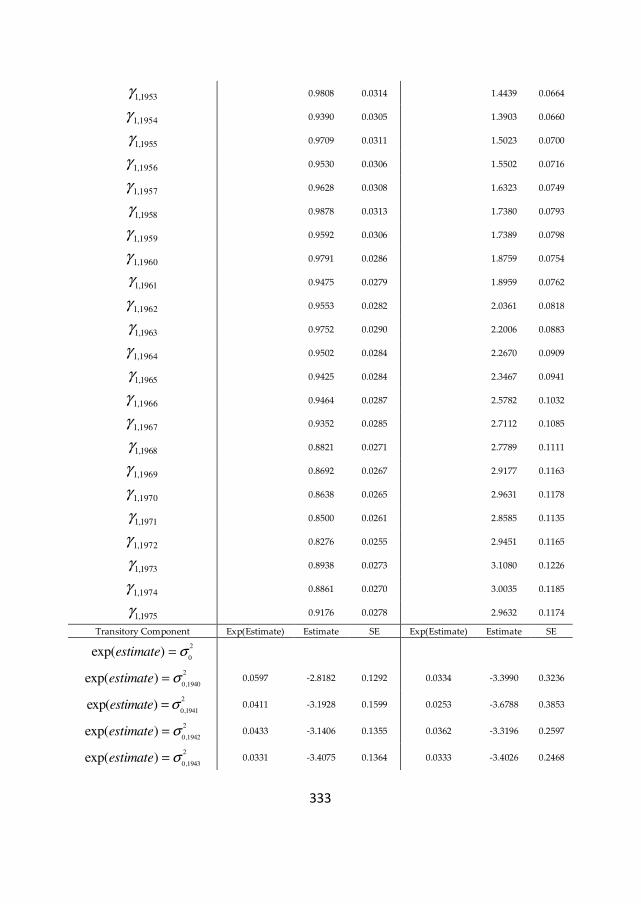
333
1,1953γ
0.9808 0.0314 1.4439 0.0664
1,1954γ
0.9390 0.0305 1.3903 0.0660
1,1955γ
0.9709 0.0311 1.5023 0.0700
1,1956γ
0.9530 0.0306 1.5502 0.0716
1,1957γ
0.9628 0.0308 1.6323 0.0749
1,1958γ
0.9878 0.0313 1.7380 0.0793
1,1959γ
0.9592 0.0306 1.7389 0.0798
1,1960γ
0.9791 0.0286 1.8759 0.0754
1,1961γ
0.9475 0.0279 1.8959 0.0762
1,1962γ
0.9553 0.0282 2.0361 0.0818
1,1963γ
0.9752 0.0290 2.2006 0.0883
1,1964γ
0.9502 0.0284 2.2670 0.0909
1,1965γ
0.9425 0.0284 2.3467 0.0941
1,1966γ
0.9464 0.0287 2.5782 0.1032
1,1967γ
0.9352 0.0285 2.7112 0.1085
1,1968γ
0.8821 0.0271 2.7789 0.1111
1,1969γ
0.8692 0.0267 2.9177 0.1163
1,1970γ
0.8638 0.0265 2.9631 0.1178
1,1971γ
0.8500 0.0261 2.8585 0.1135
1,1972γ
0.8276 0.0255 2.9451 0.1165
1,1973γ
0.8938 0.0273 3.1080 0.1226
1,1974γ
0.8861 0.0270 3.0035 0.1185
1,1975γ
0.9176 0.0278 2.9632 0.1174
Transitory Component Exp(Estimate) Estimate SE Exp(Estimate) Estimate SE
2
0exp( )estimate σ=
2
0,1940exp( )estimate σ= 0.0597 -2.8182 0.1292 0.0334 -3.3990 0.3236
2
0,1941exp( )estimate σ= 0.0411 -3.1928 0.1599 0.0253 -3.6788 0.3853
2
0,1942exp( )estimate σ= 0.0433 -3.1406 0.1355 0.0362 -3.3196 0.2597
2
0,1943exp( )estimate σ= 0.0331 -3.4075 0.1364 0.0333 -3.4026 0.2468
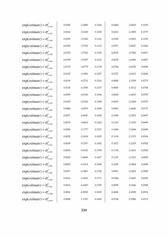
334
2
0,1944exp( )estimate σ= 0.0369 -3.3000 0.1244 0.0468 -3.0623 0.1692
2
0,1945exp( )estimate σ= 0.0264 -3.6340 0.1292 0.0412 -3.1905 0.1757
2
0,1946exp( )estimate σ= 0.0292 -3.5322 0.1141 0.0545 -2.9091 0.1235
2
0,1947exp( )estimate σ= 0.0229 -3.7765 0.1123 0.0571 -2.8627 0.1066
2
0,1948exp( )estimate σ= 0.0235 -3.7510 0.1106 0.0635 -2.7560 0.0971
2
0,1949exp( )estimate σ= 0.0199 -3.9187 0.1116 0.0678 -2.6906 0.0907
2
0,1950exp( )estimate σ= 0.0170 -4.0770 0.1158 0.0704 -2.6536 0.0838
2
0,1951exp( )estimate σ= 0.0152 -4.1881 0.1207 0.0727 -2.6212 0.0840
2
0,1952exp( )estimate σ= 0.0139 -4.2731 0.1216 0.0800 -2.5259 0.0775
2
0,1953exp( )estimate σ= 0.0130 -4.3393 0.1273 0.0845 -2.4712 0.0768
2
0,1954exp( )estimate σ= 0.0099 -4.6196 0.1296 0.0828 -2.4915 0.0705
2
0,1955exp( )estimate σ= 0.0105 -4.5522 0.1349 0.0976 -2.3269 0.0707
2
0,1956exp( )estimate σ= 0.0080 -4.8270 0.1429 0.0903 -2.4042 0.0717
2
0,1957exp( )estimate σ= 0.0077 -4.8647 0.1450 0.1005 -2.2976 0.0697
2
0,1958exp( )estimate σ= 0.0079 -4.8412 0.1482 0.1161 -2.1532 0.0699
2
0,1959exp( )estimate σ= 0.0056 -5.1777 0.1517 0.1060 -2.2448 0.0680
2
0,1960exp( )estimate σ= 0.0052 -5.2634 0.1429 0.1156 -2.1575 0.0504
2
0,1961exp( )estimate σ= 0.0038 -5.5767 0.1492 0.1072 -2.2329 0.0502
2
0,1962exp( )estimate σ= 0.0035 -5.6525 0.1550 0.1150 -2.1631 0.0500
2
0,1963exp( )estimate σ= 0.0028 -5.8699 0.1617 0.1147 -2.1651 0.0499
2
0,1964exp( )estimate σ= 0.0020 -6.2214 0.1690 0.1002 -2.3004 0.0498
2
0,1965exp( )estimate σ= 0.0017 -6.3801 0.1740 0.0961 -2.3429 0.0499
2
0,1966exp( )estimate σ= 0.0014 -6.5932 0.1771 0.0944 -2.3607 0.0502
2
0,1967exp( )estimate σ= 0.0014 -6.6023 0.1795 0.0959 -2.3446 0.0508
2
0,1968exp( )estimate σ= 0.0010 -6.9092 0.1859 0.0826 -2.4939 0.0514
2
0,1969exp( )estimate σ= 0.0008 -7.1767 0.1849 0.0744 -2.5986 0.0515
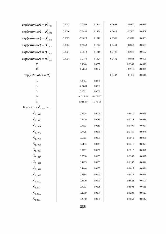
335
2
0,1970exp( )estimate σ= 0.0007 -7.2768 0.1844 0.0698 -2.6622 0.0513
2
0,1971exp( )estimate σ= 0.0006 -7.3486 0.1836 0.0614 -2.7902 0.0509
2
0,1972exp( )estimate σ= 0.0005 -7.6823 0.1819 0.0506 -2.9829 0.0506
2
0,1973exp( )estimate σ= 0.0004 -7.8563 0.1824 0.0451 -3.0991 0.0503
2
0,1974exp( )estimate σ= 0.0004 -7.9512 0.1816 0.0405 -3.2065 0.0502
2
0,1975exp( )estimate σ= 0.0004 -7.7175 0.1824 0.0452 -3.0968 0.0503
ρ 0.9640 0.0052 0.9508 0.0018
θ -0.2060 0.0037 -0.2700 0.0024
2exp( )estimate
εσ= 0.0442 -3.1180 0.0514
β0 0.0004 0.0001
β1 -0.0004 0.0000
β2 0.0001 0.0000
β3 -6.01E-06 6.47E-07
β4 1.54E-07 1.37E-08
Time shifters 2,1988
1λ =
2,1989λ
0.9258 0.0058 0.9911 0.0038
2,1990λ
0.8420 0.0089 0.9716 0.0056
2,1991λ
0.7603 0.0110 0.9400 0.0067
2,1992λ
0.7626 0.0135 0.9151 0.0078
2,1993λ
0.6603 0.0139 0.9010 0.0086
2,1994λ
0.6153 0.0145 0.9211 0.0090
2,1995λ
0.5781 0.0151 0.9217 0.0091
2,1996λ
0.5310 0.0153 0.9200 0.0092
2,1997λ
0.4925 0.0155 0.9152 0.0094
2,1998λ
0.4466 0.0152 0.9015 0.0096
2,1999λ
0.3898 0.0143 0.8815 0.0099
2,2000λ
0.3579 0.0140 0.8622 0.0107
2,2001λ
0.3293 0.0138 0.8504 0.0116
2,2002λ
0.2990 0.0134 0.8208 0.0127
2,2003λ
0.2710 0.0131 0.8060 0.0142
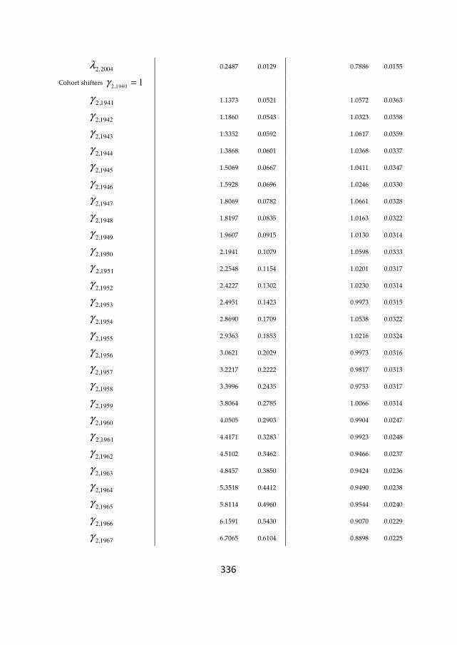
336
2,2004λ
0.2487 0.0129 0.7886 0.0155
Cohort shifters 2,1940
1γ =
2,1941γ
1.1373 0.0521 1.0572 0.0363
2,1942γ
1.1860 0.0543 1.0323 0.0358
2,1943γ
1.3352 0.0592 1.0617 0.0359
2,1944γ
1.3868 0.0601 1.0368 0.0337
2,1945γ
1.5069 0.0667 1.0411 0.0347
2,1946γ
1.5928 0.0696 1.0246 0.0330
2,1947γ
1.8069 0.0782 1.0661 0.0328
2,1948γ
1.8197 0.0835 1.0163 0.0322
2,1949γ
1.9607 0.0915 1.0130 0.0314
2,1950γ
2.1941 0.1079 1.0598 0.0333
2,1951γ
2.2548 0.1154 1.0201 0.0317
2,1952γ
2.4227 0.1302 1.0230 0.0314
2,1953γ
2.4951 0.1423 0.9973 0.0315
2,1954γ
2.8690 0.1709 1.0538 0.0322
2,1955γ
2.9363 0.1853 1.0216 0.0324
2,1956γ
3.0621 0.2029 0.9973 0.0316
2,1957γ
3.2217 0.2222 0.9817 0.0313
2,1958γ
3.3996 0.2435 0.9753 0.0317
2,1959γ
3.8064 0.2785 1.0066 0.0314
2,1960γ
4.0505 0.2903 0.9904 0.0247
2,1961γ
4.4171 0.3283 0.9923 0.0248
2,1962γ
4.5102 0.3462 0.9466 0.0237
2,1963γ
4.8457 0.3850 0.9424 0.0236
2,1964γ
5.3518 0.4412 0.9490 0.0238
2,1965γ
5.8114 0.4960 0.9544 0.0240
2,1966γ
6.1591 0.5430 0.9070 0.0229
2,1967γ
6.7065 0.6104 0.8898 0.0225
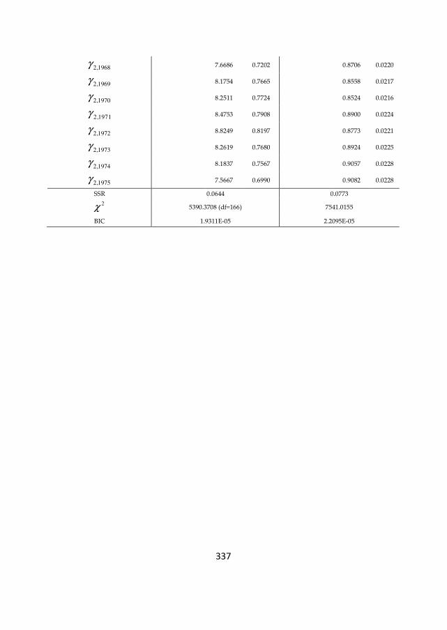
337
2,1968γ
7.6686 0.7202 0.8706 0.0220
2,1969γ
8.1754 0.7665 0.8558 0.0217
2,1970γ
8.2511 0.7724 0.8524 0.0216
2,1971γ
8.4753 0.7908 0.8900 0.0224
2,1972γ
8.8249 0.8197 0.8773 0.0221
2,1973γ
8.2619 0.7680 0.8924 0.0225
2,1974γ
8.1837 0.7567 0.9057 0.0228
2,1975γ
7.5667 0.6990 0.9082 0.0228
SSR 0.0644 0.0773
2χ 5390.3708 (df=166) 7541.0155
BIC 1.9311E-05 2.2095E-05
338
6.7.2. Inequality Decomposition into Permanent and
Transitory Inequality
I now use the parameters estimates from the error component models to
decompose earnings inequality into permanent and transitory inequality, assess
their absolute and relative contribution to the evolution of overall inequality and
estimate earnings mobility over the sample period. In interpreting the findings one
has to keep in mind that there is a fundamental conceptual underidentification of
time, life-cycle, and cohort effects due to the exact multicollinearity of time, age,
and birth year. Thus two effects will always be confounded. In order to provide a
more comprehensive picture, I perform first the inequality decomposition by
cohort over time, second the decomposition of the cross-sectional age-inequality
profile in four selected years, and third the inequality decomposition by selected
age groups over time.
6.7.2.1. Inequality decomposition by cohort over time
I start with the decompositions by cohort over time, which reveals how the
structure of inequality and earnings mobility evolved between 1988 and 2004 for
people born in each birth cohort considered. This decomposition enables to see
whether the labour market structural changes had a different impact depending on
the birth year. This decomposition controls for the cohort effect, but confounds age
and period effects.
Absolute decomposition
Figure 6.12 illustrates the absolute decomposition of the variance, together with the
actual and predicted variance of earnings by cohort for the base model. The
predicted variance follows closely the evolution of the actual variance, confirming
the fit of the base model.
In a longitudinal view, over the sample period, earnings differentials increased for
all cohorts. Overall, the increase in cross-sectional inequality is the result of
increasing permanent differentials, trend consistent across cohorts. This finding is
consistent with the results obtained by Sologon and O'Donoghue (2009a, 2009b) for
Luxembourg between 1995 and 2001. More heterogeneity is observed in the
evolution of the transitory variance, which increased for the oldest cohorts 1940-
1945 and for the youngest cohorts 1964-1975, and decreased for the rest. Thus the
cohorts 1940-1945 experienced an increase in their earnings instability between
ages 43 (for the youngest) and 48 (for the oldest) until age 57. Similarly, earnings
339
instability increased for cohorts 1964-1975 between early 20s until late 30s and 40s.
For the middle cohorts, earnings instability decreased between age 25 and 57.
The trends of the two components present some similarities across cohorts. For
most cohorts permanent variance was lower than transitory variance in the
beginning of the sample, and then surpassed it in 1993 for cohorts 1940-1963, in
1991 for cohorts 1964-1967, in 1992 for cohorts 1968-1970, in 1995 for cohort 1971-
1973, in 1996 for cohort 1974, and in 1997 for cohort 1975. Thus the structural
change appears to affect the cohorts born in 1940-1943 around their 50s, the cohorts
born between 1944-1953 around their 40s, the cohorts 1954-1962 around their 30s,
the cohorts 1963-1965 around their late 20s, and finally the cohorts 1966-1975
around their early 20s.
Given that for most cohorts the changes occur around mid 1990’s, suggest that the
trends observed are not age effects, but the result of the changes in the structure of
the labour market, which intensified beginning with early 1990’s. This explanation
is sustained by the evolution of the occupation structure for each cohort, which
reveals a common trend: they all record an increase in the share of the white collars
and civil servants, accompanied by a reduction in the share of blue collars.
Similarly, the share of the tertiary sector increases for all cohorts over time.
Moreover, these trends are more pronounced for younger compared with older
cohorts. 108
An explanation for the slightly delayed effect for the cohorts born 1971-1973, which
record an intensification of their permanent differentials in 1995, meaning around
age 22-23 could be the evolution in the education and in the occupation structure.
Younger cohorts tend to spend longer time in education and thus highly educated
men enter the labour market after the age of 22, exacerbating permanent
differentials. This effect coupled with the evolution towards a service economy
results in an increasing share of men entering the labour market as highly educated
white collars and civil servants. Similarly, for the youngest two cohorts, the
structural change kicks in two years after their entrance into the labour market,
meaning at 22, when also highly educated men join the labour market, probably as
white collars or civil servants. For example, looking at the cohort born in 1975, the
share of people working in the financial sector doubled in 1997, and quadrupled in
108
The tables can be provided upon request from the author.
340
2004 compared with 1995. Similarly, the share of white collars almost doubled in
1997 and more than tripled in 2004 compared with 1995. 109
Except for the youngest six cohorts, the persistent dispersion tends towards overall
inequality during the last years of the panel and diverges from the trend of the
transitory component, suggesting a general diffusion of earnings persistence for
mid-career (older than 35) and older workers.
Following these trends, the contribution of the two components to the growth in
overall inequality differs across periods and across cohorts. The inequality growth
until 1992 was determined by an increase in both components for the cohorts 1940
through 1965, and by an increase in the permanent component counteracted by a
decrease in the transitory component for the other cohorts. The increase between
1992 and 1997 was due to the increase in the permanent component counteracted
by the decrease in the transitory component for most cohorts, except the cohorts
born in 1963 through 1970. For the rest of the sample period, the growth in
inequality was due to an increase in earnings persistency accompanied by a
decrease in earnings instability for the cohorts born in 1940 through 1968, and by
an increase in both components for the cohorts born in 1969 through 1975.
1997 appears to be an important period in the evolution of both components,
marking the moment when the two components accentuated their fanning out
pattern. First, permanent dispersion intensified its increase for all cohorts. This is
what I expect given the increasing shares of white collars and civil servants, which
for the youngest cohorts is equivalent also to an increasing share of highly
educated people. Second, the intensification of the structural changes appears to
have decreased transitory dispersion for older workers and increased it for the
young. This might be linked with the increased ability of younger workers of
adapting to the new economy as opposed to older workers, first due to their higher
level of education and second due to their availability for flexible work contracts.
The reduction in the transitory component for older workers might signal their
reduced ability of adapting to the new economy.
109
The tables can be provided upon request from the author.
34
1
Fig
ure
6.1
2. A
ctu
al a
nd
Pre
dic
ted
Var
ian
ce o
f E
arn
ing
s w
ith
Per
man
ent
and
Tra
nsi
tory
Pre
dic
ted
Co
mp
on
ents
fo
r S
elec
ted
Co
ho
rts:
194
0-
1975
0.05.1.15.2.25
19
88
19
92
19
96
20
00
20
04
Co
ho
rt b
orn
19
40
0.05.1.15.2.25
19
88
19
92
19
96
20
00
20
04
Co
ho
rt b
orn
19
41
0.05.1.15.2.25
19
88
19
92
19
96
20
00
20
04
Co
ho
rt b
orn
19
42
0.05.1.15.2.25
19
88
19
92
19
96
20
00
20
04
Co
ho
rt b
orn
19
43
0.05.1.15.2.25
19
88
19
92
19
96
20
00
20
04
Co
ho
rt b
orn
19
44
0.05.1.15.2.25
19
88
19
92
19
96
20
00
20
04
Co
ho
rt b
orn
19
45
0.05.1.15.2.25
19
88
19
92
19
96
20
00
20
04
Co
ho
rt b
orn
19
46
0.05.1.15.2.25
19
88
19
92
19
96
20
00
20
04
Co
ho
rt b
orn
19
47
0.05.1.15.2.25
19
88
19
92
19
96
20
00
20
04
Co
ho
rt b
orn
19
48
0.05.1.15.2.25
19
88
19
92
19
96
20
00
20
04
Co
ho
rt b
orn
19
49
0.05.1.15.2.25
19
88
19
92
19
96
20
00
20
04
Co
ho
rt b
orn
19
50
0.05.1.15.2.25
19
88
19
92
19
96
20
00
20
04
Co
ho
rt b
orn
19
51
0.05.1.15.2.25
19
88
19
92
19
96
20
00
20
04
Co
ho
rt b
orn
19
52
0.05.1.15.2.25
19
88
19
92
19
96
20
00
20
04
Co
ho
rt b
orn
19
53
0.05.1.15.2.25
19
88
19
92
19
96
20
00
20
04
Co
ho
rt b
orn
19
54
0.05.1.15.2.25
19
88
19
92
19
96
20
00
20
04
Co
ho
rt b
orn
19
55
0.05.1.15.2.25
19
88
19
92
19
96
20
00
20
04
Co
ho
rt b
orn
19
56
0.05.1.15.2.25
19
88
19
92
19
96
20
00
20
04
Co
ho
rt b
orn
19
57
Actu
al V
ariance
Pre
dic
ted
Variance
Pe
rmane
nt C
om
po
ne
nt
Tra
nsito
ry C
om
po
ne
nt
34
2
F
igu
re 6
.12
(Co
nti
nu
ed)
0.05.1.15.2.25
19
88
19
92
19
96
20
00
20
04
Co
ho
rt b
orn
19
58
0.05.1.15.2.25
19
88
19
92
19
96
20
00
20
04
Co
ho
rt b
orn
19
59
0.05.1.15.2.25
19
88
19
92
19
96
20
00
20
04
Co
ho
rt b
orn
19
60
0.05.1.15.2.25
19
88
19
92
19
96
20
00
20
04
Co
ho
rt b
orn
19
61
0.05.1.15.2.25
19
88
19
92
19
96
20
00
20
04
Co
ho
rt b
orn
19
62
0.05.1.15.2.25
19
88
19
92
19
96
20
00
20
04
Co
ho
rt b
orn
19
63
0.05.1.15.2.25
19
88
19
92
19
96
20
00
20
04
Co
ho
rt b
orn
19
64
0.05.1.15.2.25
19
88
19
92
19
96
20
00
20
04
Co
ho
rt b
orn
19
65
0.05.1.15.2.25
19
88
19
92
19
96
20
00
20
04
Co
ho
rt b
orn
19
66
0.05.1.15.2.25
19
88
19
92
19
96
20
00
20
04
Co
ho
rt b
orn
19
67
0.05.1.15.2.25
19
88
19
92
19
96
20
00
20
04
Co
ho
rt b
orn
19
68
0.05.1.15.2.25
19
88
19
92
19
96
20
00
20
04
Co
ho
rt b
orn
19
69
0.05.1.15.2.25
19
88
19
92
19
96
20
00
20
04
Co
ho
rt b
orn
19
70
0.05.1.15.2.25
19
88
19
92
19
96
20
00
20
04
Co
ho
rt b
orn
19
71
0.05.1.15.2.25
19
88
19
92
19
96
20
00
20
04
Co
ho
rt b
orn
19
72
0.05.1.15.2.25
19
88
19
92
19
96
20
00
20
04
Co
ho
rt b
orn
19
73
0.05.1.15.2.25
19
88
19
92
19
96
20
00
20
04
Co
ho
rt b
orn
19
74
0.05.1.15.2.25
19
88
19
92
19
96
20
00
20
04
Co
ho
rt b
orn
19
75
Actu
al V
ari
ance
Pre
dic
ted V
ari
ance
Perm
anent
Com
ponent
Tra
nsitory
Com
ponent
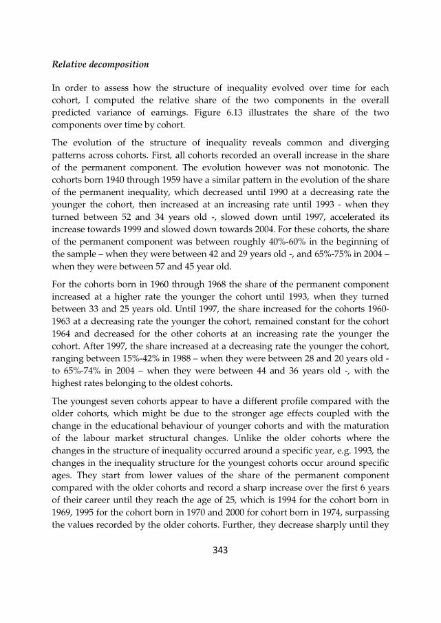
343
Relative decomposition
In order to assess how the structure of inequality evolved over time for each
cohort, I computed the relative share of the two components in the overall
predicted variance of earnings. Figure 6.13 illustrates the share of the two
components over time by cohort.
The evolution of the structure of inequality reveals common and diverging
patterns across cohorts. First, all cohorts recorded an overall increase in the share
of the permanent component. The evolution however was not monotonic. The
cohorts born 1940 through 1959 have a similar pattern in the evolution of the share
of the permanent inequality, which decreased until 1990 at a decreasing rate the
younger the cohort, then increased at an increasing rate until 1993 - when they
turned between 52 and 34 years old -, slowed down until 1997, accelerated its
increase towards 1999 and slowed down towards 2004. For these cohorts, the share
of the permanent component was between roughly 40%-60% in the beginning of
the sample – when they were between 42 and 29 years old -, and 65%-75% in 2004 –
when they were between 57 and 45 year old.
For the cohorts born in 1960 through 1968 the share of the permanent component
increased at a higher rate the younger the cohort until 1993, when they turned
between 33 and 25 years old. Until 1997, the share increased for the cohorts 1960-
1963 at a decreasing rate the younger the cohort, remained constant for the cohort
1964 and decreased for the other cohorts at an increasing rate the younger the
cohort. After 1997, the share increased at a decreasing rate the younger the cohort,
ranging between 15%-42% in 1988 – when they were between 28 and 20 years old -
to 65%-74% in 2004 – when they were between 44 and 36 years old -, with the
highest rates belonging to the oldest cohorts.
The youngest seven cohorts appear to have a different profile compared with the
older cohorts, which might be due to the stronger age effects coupled with the
change in the educational behaviour of younger cohorts and with the maturation
of the labour market structural changes. Unlike the older cohorts where the
changes in the structure of inequality occurred around a specific year, e.g. 1993, the
changes in the inequality structure for the youngest cohorts occur around specific
ages. They start from lower values of the share of the permanent component
compared with the older cohorts and record a sharp increase over the first 6 years
of their career until they reach the age of 25, which is 1994 for the cohort born in
1969, 1995 for the cohort born in 1970 and 2000 for cohort born in 1974, surpassing
the values recorded by the older cohorts. Further, they decrease sharply until they

344
reach the age of 30 and increase slightly thereafter, with lower shares of the
permanent component compared with the older cohorts.
Earnings mobility
What are the implications for earnings mobility for each cohort over time? The
answer is summarized in Figure 6.14, which plots the yearly evolution in earnings
immobility110 by cohort. The evolution of earnings immobility resembles the
evolution of the share of the persistent component. An increase in the profile
implies a decrease in earnings mobility, meaning a decrease in the opportunity for
low income men in a specific cohort to improve their position in the distribution of
lifetime earnings.
The overall picture is that for all cohorts mobility decreased over the sample
period, meaning that low wage men in all cohorts find it more difficult at the end
of the sample period to improve their income position in the distribution of
lifetime earnings compared with the beginning of the sample period.
The evolution was not monotonic. Similar with the structure of inequality, the
immobility profiles differ considerably between the cohorts 1940-1968 and 1969-
1975. The cohorts 1940 - 1968 recorded a sharp increase in earnings immobility
until 1993, followed by a positive trend for the cohorts 1940-1963 and a negative
trend for the cohorts 1964-1968 until 1997, and by an increase thereafter. Given that
the changes in mobility occur at the same time for all cohorts represents a strong
clue that the changes in the economy are the main triggers.
The youngest seven cohorts recorded an increase in earning immobility until age
25, followed by a sharp decrease until age 30 and a slight increase thereafter.
Unlike previous cohorts, the profiles of the youngest seven cohorts shift through
time, with the main changes occurring around the same age, which indicate a
strong age effect. Looking at the degree of immobility at age 25, the shift indicates
an increasing immobility over time. At the end of the sample earnings mobility
appears to be higher for younger cohorts compared with older cohorts.
110 Immobility = permanent variance/transitory variance
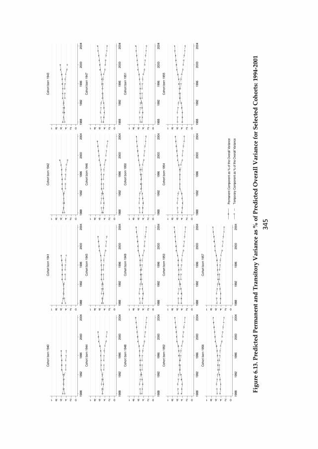
34
5
Fig
ure
6.1
3. P
red
icte
d P
erm
anen
t an
d T
ran
sito
ry V
aria
nce
as
% o
f P
red
icte
d O
ver
all
Var
ian
ce f
or
Sel
ecte
d C
oh
ort
s: 1
994-
2001
0.2.4.6.81
1988
1992
1996
2000
2004
Cohort
born
1940
0.2.4.6.81
1988
1992
1996
2000
2004
Cohort
born
1941
0.2.4.6.81
1988
1992
1996
2000
2004
Cohort
born
1942
0.2.4.6.81
1988
1992
1996
2000
2004
Cohort
born
1943
0.2.4.6.81
1988
1992
1996
2000
2004
Cohort
born
1944
0.2.4.6.81
1988
1992
1996
2000
2004
Cohort
born
1945
0.2.4.6.81
1988
1992
1996
2000
2004
Cohort
born
1946
0.2.4.6.81
1988
1992
1996
2000
2004
Cohort
born
1947
0.2.4.6.81
1988
1992
1996
2000
2004
Cohort
born
1948
0.2.4.6.81
1988
1992
1996
2000
2004
Cohort
born
1949
0.2.4.6.81
1988
1992
1996
2000
2004
Cohort
born
1950
0.2.4.6.81
1988
1992
1996
2000
2004
Cohort
born
1951
0.2.4.6.81
1988
1992
1996
2000
2004
Cohort
born
1952
0.2.4.6.81
1988
1992
1996
2000
2004
Cohort
born
1953
0.2.4.6.81
1988
1992
1996
2000
2004
Cohort
born
1954
0.2.4.6.81
1988
1992
1996
2000
2004
Cohort
born
1955
0.2.4.6.81
1988
1992
1996
2000
2004
Cohort
born
1956
0.2.4.6.81
1988
1992
1996
2000
2004
Cohort
born
1957
Perm
anent C
om
ponent as %
of th
e O
vera
ll V
ariance
Tem
pora
ry C
om
ponent as %
of th
e O
vera
ll V
ariance
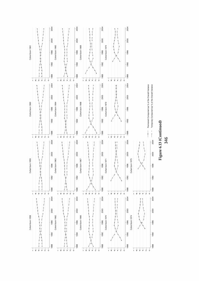
34
6
F
igu
re 6
.13
(Co
nti
nu
ed)
0.2.4.6.81
19
88
19
92
19
96
20
00
20
04
Co
ho
rt b
orn
19
58
0.2.4.6.81
19
88
19
92
19
96
20
00
20
04
Co
ho
rt b
orn
19
59
0.2.4.6.81
19
88
19
92
19
96
20
00
20
04
Co
ho
rt b
orn
19
60
0.2.4.6.81
19
88
19
92
19
96
20
00
20
04
Co
ho
rt b
orn
19
61
0.2.4.6.81
19
88
19
92
19
96
20
00
20
04
Co
ho
rt b
orn
19
62
0.2.4.6.81
19
88
19
92
19
96
20
00
20
04
Co
ho
rt b
orn
19
63
0.2.4.6.81
19
88
19
92
19
96
20
00
20
04
Co
ho
rt b
orn
19
64
0.2.4.6.81
19
88
19
92
19
96
20
00
20
04
Co
ho
rt b
orn
19
65
0.2.4.6.81
19
88
19
92
19
96
20
00
20
04
Co
ho
rt b
orn
19
66
0.2.4.6.81
19
88
19
92
19
96
20
00
20
04
Co
ho
rt b
orn
19
67
0.2.4.6.81
19
88
19
92
19
96
20
00
20
04
Co
ho
rt b
orn
19
68
0.2.4.6.81
19
88
19
92
19
96
20
00
20
04
Co
ho
rt b
orn
19
69
0.2.4.6.81
19
88
19
92
19
96
20
00
20
04
Co
ho
rt b
orn
19
70
0.2.4.6.81
19
88
19
92
19
96
20
00
20
04
Co
ho
rt b
orn
19
71
0.2.4.6.81
19
88
19
92
19
96
20
00
20
04
Co
ho
rt b
orn
19
72
0.2.4.6.81
19
88
19
92
19
96
20
00
20
04
Co
ho
rt b
orn
19
73
0.2.4.6.81
19
88
19
92
19
96
20
00
20
04
Co
ho
rt b
orn
19
74
0.2.4.6.81
19
88
19
92
19
96
20
00
20
04
Co
ho
rt b
orn
19
75
Pe
rmane
nt C
om
po
ne
nt as %
of
the
Ove
rall
Variance
Te
mp
ora
ry C
om
po
ne
nt as %
of
the
Ove
rall
Variance
34
7
Fig
ure
6.1
4. E
arn
ing
s im
mo
bil
ity
fo
r m
en b
y c
oh
ort
ov
er t
ime
– b
ase
mo
del
N
ote
: E
ach
lin
e p
lots
th
e ea
rnin
gs
imm
ob
ilit
y r
atio
by
co
ho
rt o
ver
tim
e
0123
1988
1992
1996
2000
2004
Cohort
1940
Cohort
1941
Cohort
1942
Cohort
1943
Cohort
1944
Cohort
1945
0123
1988
1992
1996
2000
2004
Cohort
1946
Cohort
1947
Cohort
1948
Cohort
1949
Cohort
1950
Cohort
1951
0123
1988
1992
1996
2000
2004
Cohort
1952
Cohort
1953
Cohort
1954
Cohort
1955
Cohort
1956
Cohort
1957
0123
1988
1992
1996
2000
2004
Cohort
1958
Cohort
1959
Cohort
1960
Cohort
1961
Cohort
1962
Cohort
1963
0123
1988
1992
1996
2000
2004
Cohort
1964
Cohort
1965
Cohort
1966
Cohort
1967
Cohort
1968
0123
1988
1992
1996
2000
2004
Cohort
1969
Cohort
1970
Cohort
1971
Cohort
1972
Cohort
1973
Cohort
1974
Cohort
1975
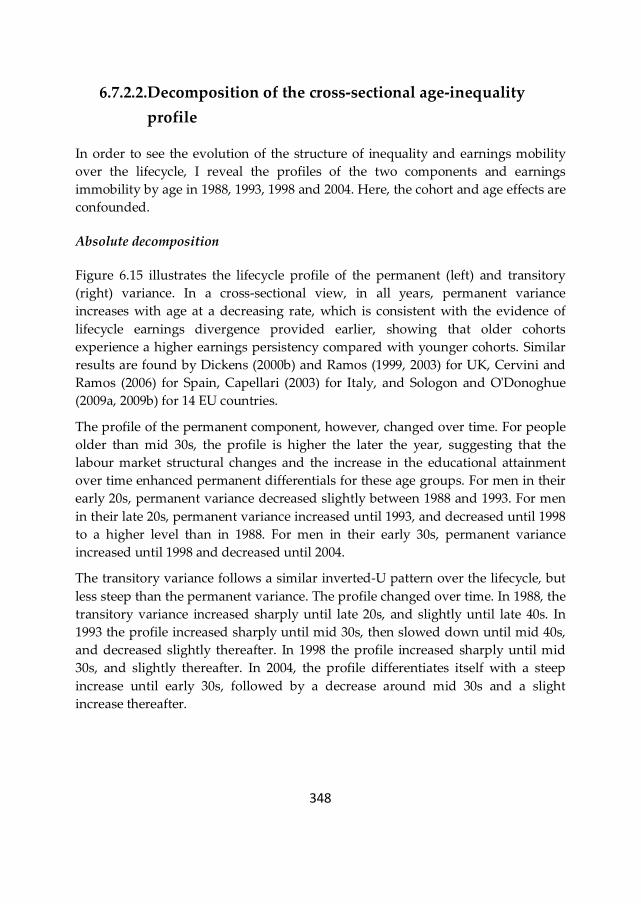
348
6.7.2.2.Decomposition of the cross-sectional age-inequality
profile
In order to see the evolution of the structure of inequality and earnings mobility
over the lifecycle, I reveal the profiles of the two components and earnings
immobility by age in 1988, 1993, 1998 and 2004. Here, the cohort and age effects are
confounded.
Absolute decomposition
Figure 6.15 illustrates the lifecycle profile of the permanent (left) and transitory
(right) variance. In a cross-sectional view, in all years, permanent variance
increases with age at a decreasing rate, which is consistent with the evidence of
lifecycle earnings divergence provided earlier, showing that older cohorts
experience a higher earnings persistency compared with younger cohorts. Similar
results are found by Dickens (2000b) and Ramos (1999, 2003) for UK, Cervini and
Ramos (2006) for Spain, Capellari (2003) for Italy, and Sologon and O'Donoghue
(2009a, 2009b) for 14 EU countries.
The profile of the permanent component, however, changed over time. For people
older than mid 30s, the profile is higher the later the year, suggesting that the
labour market structural changes and the increase in the educational attainment
over time enhanced permanent differentials for these age groups. For men in their
early 20s, permanent variance decreased slightly between 1988 and 1993. For men
in their late 20s, permanent variance increased until 1993, and decreased until 1998
to a higher level than in 1988. For men in their early 30s, permanent variance
increased until 1998 and decreased until 2004.
The transitory variance follows a similar inverted-U pattern over the lifecycle, but
less steep than the permanent variance. The profile changed over time. In 1988, the
transitory variance increased sharply until late 20s, and slightly until late 40s. In
1993 the profile increased sharply until mid 30s, then slowed down until mid 40s,
and decreased slightly thereafter. In 1998 the profile increased sharply until mid
30s, and slightly thereafter. In 2004, the profile differentiates itself with a steep
increase until early 30s, followed by a decrease around mid 30s and a slight
increase thereafter.
34
9
Fig
ure
6.1
5. C
ross
-sec
tio
nal
ag
e p
rofi
le o
f th
e p
erm
anen
t an
d t
ran
sito
ry v
aria
nce
fo
r se
lect
ed y
ears
N
ote
: v
erti
cal
axis
–
p
erm
ane
nt
var
ian
ce
of
log
e
arn
ing
s (l
eft
),
tran
sito
ry
var
ian
ce
of
log
ea
rnin
gs
(rig
ht)
; h
ori
zon
tal
axis
–
ag
e;
each
li
ne
plo
ts
the
per
ma
nen
t/tr
an
sito
ry v
aria
nce
fo
r ag
es
20
-57
in
se
lect
ed
yea
rs
0.05.1.15.2
20
24
28
32
36
40
44
48
52
56
1988
1993
1998
2004
Pe
rma
ne
nt
Va
ria
nce
0.05.1.15.2
20
24
28
32
36
40
44
48
52
56
1988
1993
1998
2004
Tra
nsito
ry V
ari
an
ce
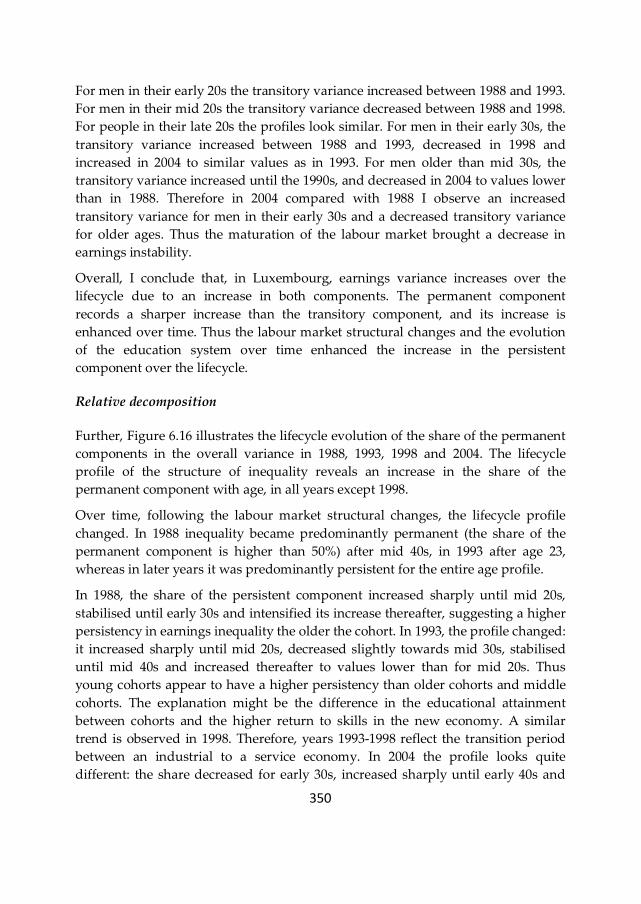
350
For men in their early 20s the transitory variance increased between 1988 and 1993.
For men in their mid 20s the transitory variance decreased between 1988 and 1998.
For people in their late 20s the profiles look similar. For men in their early 30s, the
transitory variance increased between 1988 and 1993, decreased in 1998 and
increased in 2004 to similar values as in 1993. For men older than mid 30s, the
transitory variance increased until the 1990s, and decreased in 2004 to values lower
than in 1988. Therefore in 2004 compared with 1988 I observe an increased
transitory variance for men in their early 30s and a decreased transitory variance
for older ages. Thus the maturation of the labour market brought a decrease in
earnings instability.
Overall, I conclude that, in Luxembourg, earnings variance increases over the
lifecycle due to an increase in both components. The permanent component
records a sharper increase than the transitory component, and its increase is
enhanced over time. Thus the labour market structural changes and the evolution
of the education system over time enhanced the increase in the persistent
component over the lifecycle.
Relative decomposition
Further, Figure 6.16 illustrates the lifecycle evolution of the share of the permanent
components in the overall variance in 1988, 1993, 1998 and 2004. The lifecycle
profile of the structure of inequality reveals an increase in the share of the
permanent component with age, in all years except 1998.
Over time, following the labour market structural changes, the lifecycle profile
changed. In 1988 inequality became predominantly permanent (the share of the
permanent component is higher than 50%) after mid 40s, in 1993 after age 23,
whereas in later years it was predominantly persistent for the entire age profile.
In 1988, the share of the persistent component increased sharply until mid 20s,
stabilised until early 30s and intensified its increase thereafter, suggesting a higher
persistency in earnings inequality the older the cohort. In 1993, the profile changed:
it increased sharply until mid 20s, decreased slightly towards mid 30s, stabilised
until mid 40s and increased thereafter to values lower than for mid 20s. Thus
young cohorts appear to have a higher persistency than older cohorts and middle
cohorts. The explanation might be the difference in the educational attainment
between cohorts and the higher return to skills in the new economy. A similar
trend is observed in 1998. Therefore, years 1993-1998 reflect the transition period
between an industrial to a service economy. In 2004 the profile looks quite
different: the share decreased for early 30s, increased sharply until early 40s and
351
decreased slightly thereafter. Thus in 2004, the middle and oldest cohort have the
highest persistency.
Looking across age groups over time, for men in their early-mid 20s, the share of
the permanent component increased over time. For those in their late 20s the share
increased between 1988 and 1993, and decreased in 1998 to values above the ones
in 1988. For men in their early 30s, the share increased until 1998 and decreased in
2004. For those older than 35, the share of the permanent component increased
over time.
Figure 6.16. Cross-sectional age profile of the share of the permanent component from the
overall variance for selected years: 1988, 1993, 1998, 2004 Note: vertical axis – share (%) of the permanent component from the overall variance , horizontal axis -
age
Earnings mobility
What are the implications for earnings mobility? The lifecycle immobility profiles
for years 1988, 1993, 1998 and 2004 are illustrated in Figure 6.17. Overall, earnings
immobility increases over the lifecycle in all years, except 1998. The trend in
immobility follows closely the trend in the share of the permanent component.
Thus, in 1988, earnings immobility was higher the older the age. In 1993 and 1998
0.2
.4.6
.8
20 24 28 32 36 40 44 48 52 56
1988 1993
1998 2004
Share of the Permanent Variance
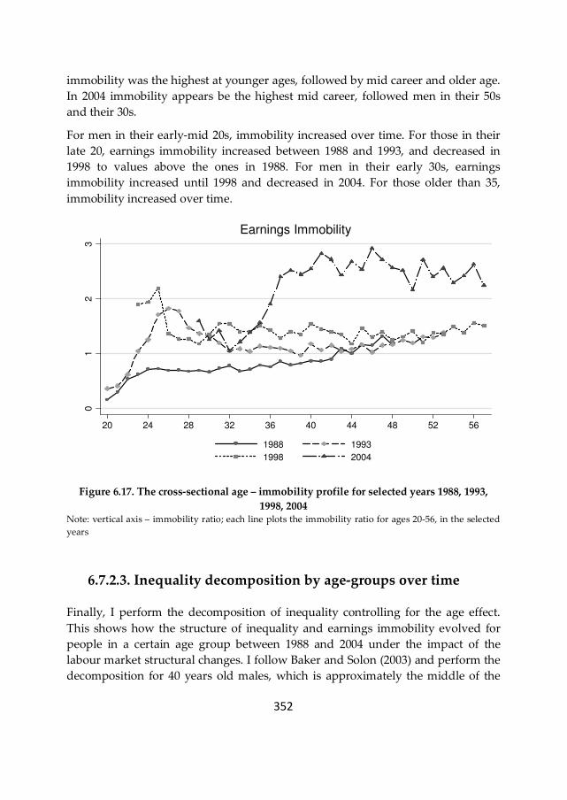
352
immobility was the highest at younger ages, followed by mid career and older age.
In 2004 immobility appears be the highest mid career, followed men in their 50s
and their 30s.
For men in their early-mid 20s, immobility increased over time. For those in their
late 20, earnings immobility increased between 1988 and 1993, and decreased in
1998 to values above the ones in 1988. For men in their early 30s, earnings
immobility increased until 1998 and decreased in 2004. For those older than 35,
immobility increased over time.
Figure 6.17. The cross-sectional age – immobility profile for selected years 1988, 1993,
1998, 2004 Note: vertical axis – immobility ratio; each line plots the immobility ratio for ages 20-56, in the selected
years
6.7.2.3. Inequality decomposition by age-groups over time
Finally, I perform the decomposition of inequality controlling for the age effect.
This shows how the structure of inequality and earnings immobility evolved for
people in a certain age group between 1988 and 2004 under the impact of the
labour market structural changes. I follow Baker and Solon (2003) and perform the
decomposition for 40 years old males, which is approximately the middle of the
01
23
20 24 28 32 36 40 44 48 52 56
1988 1993
1998 2004
Earnings Immobility
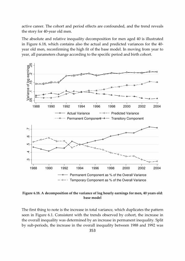
353
active career. The cohort and period effects are confounded, and the trend reveals
the story for 40-year old men.
The absolute and relative inequality decomposition for men aged 40 is illustrated
in Figure 6.18, which contains also the actual and predicted variances for the 40-
year old men, reconfirming the high fit of the base model. In moving from year to
year, all parameters change according to the specific period and birth cohort.
Figure 6.18. A decomposition of the variance of log hourly earnings for men, 40 years old:
base model
The first thing to note is the increase in total variance, which duplicates the pattern
seen in Figure 6.1. Consistent with the trends observed by cohort, the increase in
the overall inequality was determined by an increase in permanent inequality. Split
by sub-periods, the increase in the overall inequality between 1988 and 1992 was
.05
.1.1
5.2
.25
Variance o
f lo
g e
arn
ings
1988 1990 1992 1994 1996 1998 2000 2002 2004
Actual Variance Predicted Variance
Permanent Component Transitory Component
.3.4
.5.6
.7
1988 1990 1992 1994 1996 1998 2000 2002 2004
Permanent Component as % of the Overall Variance
Temporary Component as % of the Overall Variance
354
determined by an increase in both components, and by an increase in the
permanent variance counteracted by a decrease in the transitory variance
thereafter. Transitory inequality displays more variation compared with
permanent inequality, evolving opposite to it: three spikes are observed in 1990,
1992 and 1994, followed by a monotonic decrease thereafter.
In 1988, the persistent component accounted for 46.5% of the inequality in hourly
earnings. Its share decreased until 1990, increased until 1993 surpassing the
transitory variance, decreased in 1994 to roughly 50%, and increased thereafter
reaching a value of over 70% in 2004. Thus, after 1993, the permanent inequality
had a dominant share in the overall inequality of men aged 40.
I also performed the decomposition for ages 30 and 50.111 The general trends are
maintained, however some differences are noted. For age 50, the evolution of the
two components was similar with age 40, except that for age 50 the share of the
permanent component in the overall inequality was higher than for the transitory
inequality for most of the period. The share of the permanent component increased
from below 50% in 1990 to almost 70% in 2004.
For age 30, the trends display more noise compared with age 40 and 50: except for
1988-1992 and 2002, the persistent components dominated overall inequality. The
share of the permanent component increased from around 40% in 1988 to over 56%
2004. The maximum persistency for the 30-year old was reached in 1996-1997,
when the share of persistent inequality was of 60%. Overall, the incidence of the
transitory component is higher for men aged 30 than for those aged 40 and 50.
Following the labour market structural changes, the ranking between these age
groups in terms of earnings persistency changed, sign that the impact of these
changes differed by age groups. In the beginning of the sample period the highest
persistency was observed for men aged 50, followed by those aged 40 and 30. In
the middle of the sample period, the persistency became higher for men aged 30,
followed by those aged 50 and 40. In 2004, earnings persistency was higher for age
40, followed by age 50 and age 30.
What are the implications for earnings mobility for these age groups over time?
The answer is summarized in Figure 6.19, which plots the pattern in earnings
immobility112 for these age groups. Recall, an increase in the profile implies a
decrease in earnings mobility, meaning a decrease in the opportunity for low
income men to improve their position in the distribution of lifetime earnings.
111 Available on request 112 Immobility = permanent variance/transitory variance
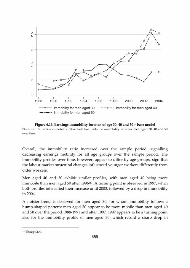
355
Figure 6.19. Earnings immobility for men of age 30, 40 and 50 – base model Note: vertical axis – immobility ratio; each line plots the immobility ratio for men aged 30, 40 and 50
over time
Overall, the immobility ratio increased over the sample period, signalling
decreasing earnings mobility for all age groups over the sample period. The
immobility profiles over time, however, appear to differ by age groups, sign that
the labour market structural changes influenced younger workers differently from
older workers.
Men aged 40 and 50 exhibit similar profiles, with men aged 40 being more
immobile than men aged 50 after 1996113. A turning point is observed in 1997, when
both profiles intensified their increase until 2003, followed by a drop in immobility
in 2004.
A noisier trend is observed for men aged 30, for whom immobility follows a
hump-shaped pattern: men aged 30 appear to be more mobile than men aged 40
and 50 over the period 1988-1991 and after 1997. 1997 appears to be a turning point
also for the immobility profile of men aged 30, which record a sharp drop in
113 Except 2001
.51
1.5
22
.5
1988 1990 1992 1994 1996 1998 2000 2002 2004
Immobility for men aged 30 Immobility for men aged 40
Immobility for men aged 50
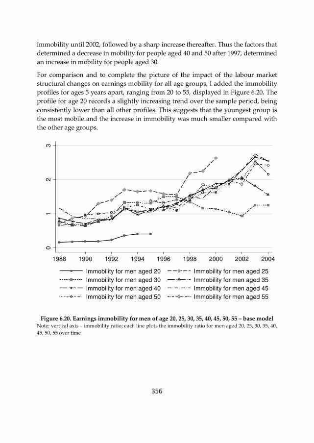
356
immobility until 2002, followed by a sharp increase thereafter. Thus the factors that
determined a decrease in mobility for people aged 40 and 50 after 1997, determined
an increase in mobility for people aged 30.
For comparison and to complete the picture of the impact of the labour market
structural changes on earnings mobility for all age groups, I added the immobility
profiles for ages 5 years apart, ranging from 20 to 55, displayed in Figure 6.20. The
profile for age 20 records a slightly increasing trend over the sample period, being
consistently lower than all other profiles. This suggests that the youngest group is
the most mobile and the increase in immobility was much smaller compared with
the other age groups.
Figure 6.20. Earnings immobility for men of age 20, 25, 30, 35, 40, 45, 50, 55 – base model Note: vertical axis – immobility ratio; each line plots the immobility ratio for men aged 20, 25, 30, 35, 40,
45, 50, 55 over time
01
23
1988 1990 1992 1994 1996 1998 2000 2002 2004
Immobility for men aged 20 Immobility for men aged 25
Immobility for men aged 30 Immobility for men aged 35
Immobility for men aged 40 Immobility for men aged 45
Immobility for men aged 50 Immobility for men aged 55

357
The profiles for ages 21 and 22, not shown in Figure 6.20114, evolve parallel with
age 20, showing a lower mobility the older the age.
The profile for age 25 is quite surprising. Starting from slightly higher values than
age 30 in 1988, it records the largest increase until 1993, then a slight decrease until
1997 followed by a sharp increase until 2000, surpassing the immobility ratios of all
other profiles over the period 1991-2000. Thus the labour market structural changes
increased earnings immobility for men aged 25 to a much larger extent compared
with other age groups.
The profiles for ages 23-24, not shown in Figure 6.20115, evolve similar with age 25,
but shifted backwards with 2 and 1 year. Thus immobility increased until 1996 for
age 24, and 1995 for age 23, at a lower rate compared with age 25, and intensified
their increase thereafter. Overall, for age range 20-25, earnings mobility is higher
the younger the age.
The profiles for ages 26-29, not shown in Figure 6.20116, illustrate transition
immobility profiles between age 25 and 30: they record a similar trend slightly
lower the older the age until 1993, followed by a decrease, steeper and lasting one
year longer the older the age, and finally a sharp increase parallel with the trend
observed for age 25. Basically the profiles for ages 26-29 look like the profile for age
25, lower the older the age, with a decrease after 1997 longer with one year the
further we move from age 25, followed by a similar parallel increase thereafter.
The profiles for ages 31-39 represent a transition from the profile for age 30 to the
profile for age 40: they evolve similar to age 30 recording lower values than the
profile for age 30 until 1997, and surpassing it thereafter, at an increasing rate the
younger the cohort. Similar with the profile for age 30, they start decreasing
towards the end of the sample one year later for each age group, at a decreasing
rate the older the age. Thus from age 30, the trends for each age group converges
towards the profile for age 40.
The profiles for ages 41-49 behave similar to the profile for age 40. The profiles for
ages 51-57 behave similar to the profile for age 50. Overall, the immobility around
40s is slightly higher than for 50s.
Thus these trends confirm the hump-shaped immobility profile observed in Figure
6.17.
114 Provided upon request from the author. 115 Provided upon request. 116 Provided upon request.
358
In order to see whether the estimated changes over the sample period are likely to
be due to real changes in the functioning of the labour market rather than to short
term fluctuations in the business cycle, I follow Baker and Solon (2003) and apply
least squares to estimate time-series regressions of the persistent and transitory
components and earnings immobility on a linear trend and a variable that captures
the business cycle – the growth rate in real GDP117. The results are reported in
Table 6.4.
The point estimates indicate a strongly significant positive trend for the permanent
component and earnings immobility, and a less strong significant negative trend
for the transitory component. Thus permanent variance contributes positively to
the upward trend in earnings inequality, whereas the transitory variance
counteracts with the increase in the permanent component. The insignificant
coefficient estimates of the GDP growth rate for the permanent component and the
immobility index indicate that the permanent variance and earnings mobility are
insensitive to the business cycle. Hence, the estimated changes in the persistent
components and earnings immobility between 1988 and 2004 are due to changes in
the functioning of the labour market. The estimated coefficient of the GDP growth
rate for the transitory component indicates a significant cyclical sensitivity in the
transitory variance.
To conclude, the changes that occurred in the labour market in this period
intensified permanent differentials and decreased transitory differentials among
men, thus decreasing their earnings mobility in a lifetime perspective.
As a last step I look at the implications of estimating the restricted model displayed
in Table 6.3. This model assumes away age-specific innovation variances and age-
related heteroskedasticity in the transitory shocks. The decomposition implied by
the restricted model for men aged 40 is revealed in Figure 6.21.
117 The real GDP is expressed in constant prices 2004. Source: STATEC, IGSS
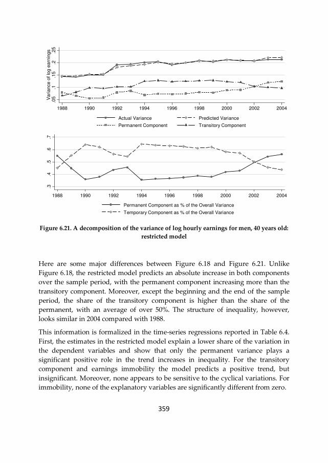
359
Figure 6.21. A decomposition of the variance of log hourly earnings for men, 40 years old:
restricted model
Here are some major differences between Figure 6.18 and Figure 6.21. Unlike
Figure 6.18, the restricted model predicts an absolute increase in both components
over the sample period, with the permanent component increasing more than the
transitory component. Moreover, except the beginning and the end of the sample
period, the share of the transitory component is higher than the share of the
permanent, with an average of over 50%. The structure of inequality, however,
looks similar in 2004 compared with 1988.
This information is formalized in the time-series regressions reported in Table 6.4.
First, the estimates in the restricted model explain a lower share of the variation in
the dependent variables and show that only the permanent variance plays a
significant positive role in the trend increases in inequality. For the transitory
component and earnings immobility the model predicts a positive trend, but
insignificant. Moreover, none appears to be sensitive to the cyclical variations. For
immobility, none of the explanatory variables are significantly different from zero.
.05
.1.1
5.2
.25
Variance o
f lo
g e
arn
ings
1988 1990 1992 1994 1996 1998 2000 2002 2004
Actual Variance Predicted Variance
Permanent Component Transitory Component
.3.4
.5.6
.7
1988 1990 1992 1994 1996 1998 2000 2002 2004
Permanent Component as % of the Overall Variance
Temporary Component as % of the Overall Variance
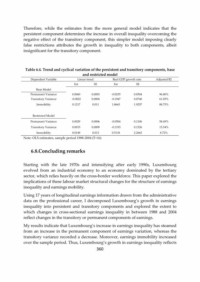
360
Therefore, while the estimates from the more general model indicates that the
persistent component determines the increase in overall inequality overcoming the
negative effect of the transitory component, this simpler model imposing clearly
false restrictions attributes the growth in inequality to both components, albeit
insignificant for the transitory component.
Table 6.4. Trend and cyclical variation of the persistent and transitory components, base
and restricted model Dependent Variable Linear trend Real GDP growth rate Adjusted R2
Est SE Est SE
Base Model
Permanent Variance 0.0060 0.0003 -0.0235 0.0504 96.80%
Transitory Variance -0.0022 0.0004 -0.1947 0.0740 61.05%
Immobility 0.1217 0.011 1.8663 1.9257 88.75%
Restricted Model
Permanent Variance 0.0029 0.0006 -0.0504 0.1106 58.49%
Transitory Variance 0.0015 0.0009 -0.1193 0.1526 15.54%
Immobility 0.0149 0.013 0.5118 2.2663 8.72%
Note: OLS estimates, sample period 1988-2004 (T=16)
6.8.Concluding remarks
Starting with the late 1970s and intensifying after early 1990s, Luxembourg
evolved from an industrial economy to an economy dominated by the tertiary
sector, which relies heavily on the cross-border workforce. This paper explored the
implications of these labour market structural changes for the structure of earnings
inequality and earnings mobility.
Using 17 years of longitudinal earnings information drawn from the administrative
data on the professional career, I decomposed Luxembourg’s growth in earnings
inequality into persistent and transitory components and explored the extent to
which changes in cross-sectional earnings inequality in between 1988 and 2004
reflect changes in the transitory or permanent components of earnings.
My results indicate that Luxembourg’s increase in earnings inequality has steamed
from an increase in the permanent component of earnings variation, whereas the
transitory variance recorded a decrease. Moreover, earnings immobility increased
over the sample period. Thus, Luxembourg’s growth in earnings inequality reflects

361
increasing long-run (permanent) differentials between individuals accompanied by
decreasing earnings mobility, meaning decreasing opportunity for low wage
individuals of improving their income position in a lifetime perspective.
While my focus has been to extend the research on earnings dynamics at the
European level and to understand the driving factors behind the increase in
earnings inequality in Luxembourg in the context of the labour market structural
changes that occurred starting with the late 1980s, I also tried to bring a
methodological advancement in modelling earnings dynamics. Thanks to the large
size of my panel, I was able to estimate a more general model that incorporates
most of the features identified by the previous research on earnings mobility from
the US, Canada and Europe.
First, unlike previous studies, I was able to account for cohort and age effects in a
more precise way by considering cohorts formed of individuals born in one year,
not several years pulled together. This is a quite unique feature in the literature
given the huge data requirements. To my knowledge, only one study had the
luxury of capturing the true cohort and age effect, Dickens (2000b) for the UK.
Moreover, the richness of my data allowed us to incorporate cohort loading factors
both on the permanent and transitory component, a feature which is not so
common. Most studies used the cohort shifters only on one component.
Second, for modelling the permanent component, I extended the random walk
specification to incorporate age-specific innovation variances after age 20 until age
40, and a random effects model after age 40 with the distribution of the effects
fixed at that implied by the random walk, a specification which was used
previously only by Dickens (2000b). This model is consistent with the expectations
steaming from many matching and human capital models, whereby human capital
is accumulated for the first 20 year of labour market experiences, after which
between-individual differences stop growing. I attempted to incorporate also the
random growth specification, as persistent differences between individuals with
respect to their human capital accumulation do exist. The specifications, however,
led to identification problems in my data.
Third, for modelling the transitory component, besides allowing for cohort specific
initials transitory variances to accommodate cohort heterogeneity with respect to
the accumulation of the transitory process until the start of the panel, I
incorporated also age-related heteroskedastic transitory innovations to
accommodate the lifecycle variation in the volatility of the transitory earnings
innovations.
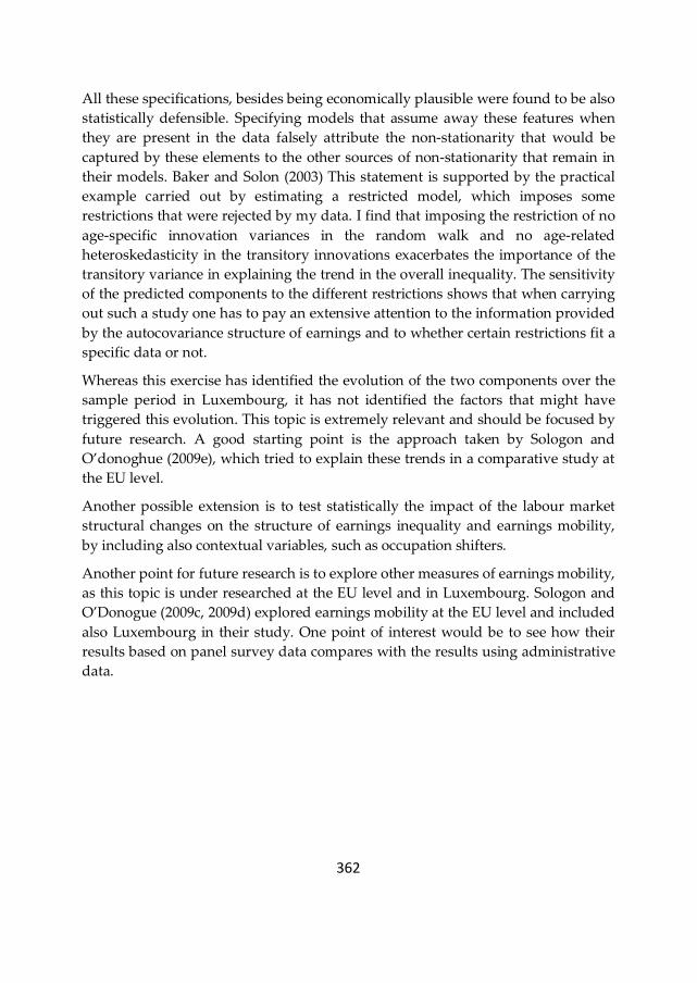
362
All these specifications, besides being economically plausible were found to be also
statistically defensible. Specifying models that assume away these features when
they are present in the data falsely attribute the non-stationarity that would be
captured by these elements to the other sources of non-stationarity that remain in
their models. Baker and Solon (2003) This statement is supported by the practical
example carried out by estimating a restricted model, which imposes some
restrictions that were rejected by my data. I find that imposing the restriction of no
age-specific innovation variances in the random walk and no age-related
heteroskedasticity in the transitory innovations exacerbates the importance of the
transitory variance in explaining the trend in the overall inequality. The sensitivity
of the predicted components to the different restrictions shows that when carrying
out such a study one has to pay an extensive attention to the information provided
by the autocovariance structure of earnings and to whether certain restrictions fit a
specific data or not.
Whereas this exercise has identified the evolution of the two components over the
sample period in Luxembourg, it has not identified the factors that might have
triggered this evolution. This topic is extremely relevant and should be focused by
future research. A good starting point is the approach taken by Sologon and
O’donoghue (2009e), which tried to explain these trends in a comparative study at
the EU level.
Another possible extension is to test statistically the impact of the labour market
structural changes on the structure of earnings inequality and earnings mobility,
by including also contextual variables, such as occupation shifters.
Another point for future research is to explore other measures of earnings mobility,
as this topic is under researched at the EU level and in Luxembourg. Sologon and
O’Donogue (2009c, 2009d) explored earnings mobility at the EU level and included
also Luxembourg in their study. One point of interest would be to see how their
results based on panel survey data compares with the results using administrative
data.
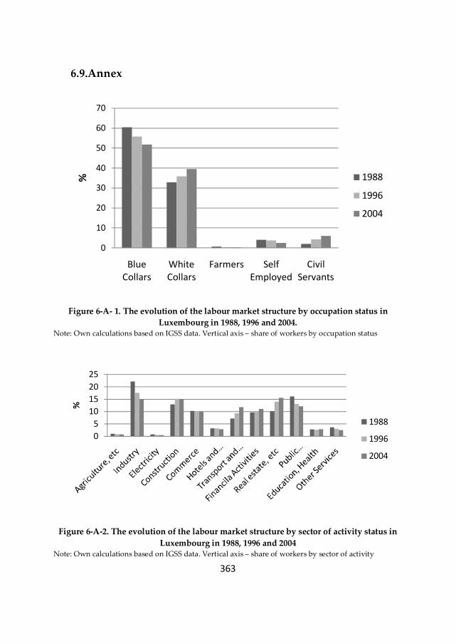
363
6.9.Annex
Figure 6-A- 1. The evolution of the labour market structure by occupation status in
Luxembourg in 1988, 1996 and 2004. Note: Own calculations based on IGSS data. Vertical axis – share of workers by occupation status
Figure 6-A-2. The evolution of the labour market structure by sector of activity status in
Luxembourg in 1988, 1996 and 2004 Note: Own calculations based on IGSS data. Vertical axis – share of workers by sector of activity
0
10
20
30
40
50
60
70
Blue
Collars
White
Collars
Farmers Self
Employed
Civil
Servants
% 1988
1996
2004
0
5
10
15
20
25
%
1988
1996
2004
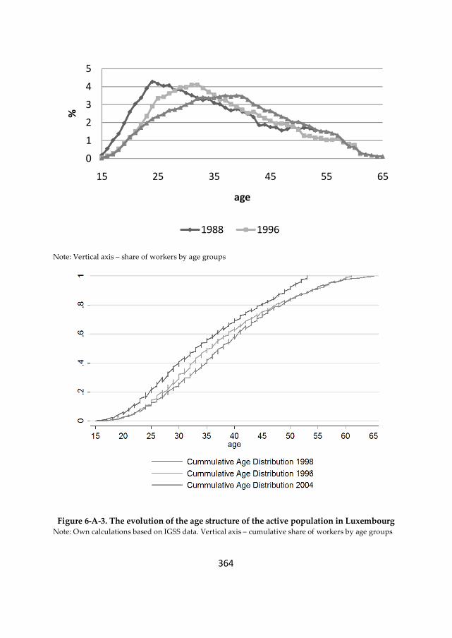
364
Note: Vertical axis – share of workers by age groups
Figure 6-A-3. The evolution of the age structure of the active population in Luxembourg Note: Own calculations based on IGSS data. Vertical axis – cumulative share of workers by age groups
0
1
2
3
4
5
15 25 35 45 55 65
%
age
1988 1996

365
7. CONCLUSIONS AND FORWARD LOOKING
366
This dissertation explores the dynamics of individual male earnings across 14 EU
countries to explain what is happening behind the changes in the distribution of
labour market income across 14 EU countries. We explore different facets of the
earnings inequality-mobility story, highly relevant in the context of the labour
market policy changes that occurred in Europe over the last decades. Several
lessons can be drawn.
Earnings Mobility and Cross-sectional Earnings Inequality
Based on the Dickens rank mobility measure, we bring evidence that across 12 EU
countries between 1994 and 2001, the evolution of cross-sectional inequality is
negatively associated with the evolution of short-term mobility.
What are the welfare implications of the cross-country trends in short-term
mobility? In Netherlands, Greece, Finland, Portugal, Luxembourg, Italy, Germany,
and Belgium, individuals find it harder in 2000-2001 to better their position in the
earnings distribution short-term compared with the 1st-2nd wave, factor which
might have contributed to the increase in earnings differentials between the 2nd
wave and 2001. Moreover, the decrease in mobility rates may signal an increase in
permanent earning differentials.
In France and Austria, despite the decrease in cross-sectional earnings differentials
between the 2nd wave and 2001, individuals have a decreased opportunity in 2000-
2001 to better their position in the earnings distribution compared with the 1st-2nd
wave. In the UK, Spain, Denmark, and Ireland individuals have an increased
opportunity in 2000-2001 to improve their earnings position short-term compared
with 1994-1995, which might have contributed to reduce cross-sectional
differentials over time.
In 2001, the highest short-term mobility is recorded in Denmark and the lowest in
Luxembourg. Thus men in Denmark observe the highest opportunity to move in
the earnings distribution between 2000 and 2001.
Consistent across countries, mobility is found to be higher when measured over a
longer time period, suggesting that the longer the period, the higher the
opportunity to escape the initial earnings state. The highest long-term (over the
sample period) mobility in terms of positional movements is found in Denmark
and Ireland, and the lowest in Luxembourg.
367
Overall, it appears that the higher the cross-sectional inequality in the 2nd wave, the
lower the mobility between the 1st and 2nd wave. Similarly, a higher long-term
mobility (between the 1st wave and 2001) is associated with a lower cross-sectional
inequality in 2001. The rankings, however, have some exceptions, indicating that
there are cases when (part of) earnings mobility might have a disequalizing impact
on cross-sectional earnings inequality. These findings reinforce the debate that
mobility is not always beneficial.
Earnings Mobility and Lifetime Earnings Inequality
If the establishment of the link between mobility and cross-sectional inequality
faces problems, the implications of earnings mobility for lifetime or permanent
inequality are even more cumbersome. Two approaches were used to shed some
light on the potential link between earnings mobility and lifetime earnings
inequality.
First, in Chapter 3 we looked at mobility as equalizer / disequalizer of longer-term
earnings relative with cross-sectional inequality. Using the Fields mobility index
computed over the longest observed horizon as a proxy for lifetime mobility, we
bring evidence that in all countries except Portugal, mobility acts as an equalizer of
lifetime/long-term differentials. The highest long-term equalizing mobility is found
in Ireland and Denmark, and the only disequalizing mobility in Portugal.
Second, in Chapter 4 we decomposed the evolution in earnings inequality into
permanent and transitory components to gauge their implications for long-run or
lifetime earnings differentials. Earnings mobility – defined by Katz and Autor (1999) as
the rate at which individuals shift positions in the earnings distribution - is closely related to the
importance of the permanent and transitory components in earnings variation. A
large contribution of the permanent component implies that individual earnings
are highly correlated over time and individuals do not change their income
position to a large extent experiencing low rates of earnings mobility. Therefore,
the changes in earnings mobility are determined by the extent to which changes in
cross-sectional inequality are driven by changes in the permanent or transitory
inequality: the higher the incidence of the persistent differentials in the overall
inequality, the lower the year-to-year mobility, thus the lower opportunity for the
poor to improve their relative income position in a lifetime perspective. Thus we
regard mobility as the opposite of persistency. We do not take the stand that that
mobility is necessarily good, but that the lack of it is bad, as it signals a lack of
opportunity to move.
368
An increase in cross-sectional earnings inequality triggered by an increase in the
permanent component signals an increase in lifetime earnings differentials,
suggesting a worsening of the relative lifetime earnings position of the chronically
poor. An increase in cross-sectional earnings differentials triggered by an increase
in earnings instability signals an increase in earnings mobility, implying an
increased opportunity for the poor to improve their relative income position in a
lifetime perspective.
Overall earnings inequality, measured by the variance in log hourly earnings,
decreased in Denmark, Belgium, France, Germany, UK, Ireland, Spain, Austria and
increased in Netherlands, Luxembourg, Italy, Greece, Portugal and Finland. For all
countries, both in relative and absolute terms, individual earnings inequality
contains a highly permanent component for the oldest cohorts and a highly
transitory component for the youngest cohort. The degree of immobility, measured
by the ratio between the permanent variance and the transitory variance, is higher
for older cohorts compared with younger cohorts, which suggests that the older
the cohort, the lower the opportunity to improve one’s position in the distribution
of lifetime earnings.
Overall, the decrease in inequality resulted from a decrease in transitory
differentials in Germany, France, UK and Ireland, in permanent differentials in
Belgium and Spain, and in both components in Denmark and Austria. The increase
in inequality reflects an increase in permanent differentials in Luxembourg, Italy,
Greece and Finland, and an increase in both components in Portugal and
Netherlands. The decrease in inequality was accompanied by an increase in
mobility only in Denmark, Belgium and Spain. Except Netherlands and Portugal,
all countries recording an increase in inequality experienced also a decrease in
mobility.
What are the potential welfare implications of these trends? In Denmark, Belgium
and Spain, mobility appears to be beneficial: in 2001, low wage individuals are
better off both in terms of their relative wage and in terms of the opportunities to
escape the low-wage trap in a lifetime perspective. Thus in a lifetime perspective,
Denmark, Belgium and Spain are expected to reduce lifetime earnings differentials
compared with annual differentials.
In Austria, Germany, France, UK and Ireland, in 2001, low-wage individuals are
worse off in terms of the opportunity to escape the low-wage trap, but their
relative position in the earnings distribution is improved compared with the 1st
wave. For these countries mobility is expected to play a decreasing role in reducing
369
lifetime inequality, therefore annual differentials have a high chance of being
preserved in a lifetime perspective.
Among countries recording an increase in earnings inequality, in Luxembourg,
Italy, Greece, and Finland, besides the widening wages differentials, low wage
individuals find it harder to better their position in the wage distribution in 2001
compared with the 1st wave. Thus we can expect these countries to increase lifetime
earnings differentials compared with annual differentials. Netherlands and
Portugal record widening wages differentials accompanied by increased
opportunity for low wage individuals to improve their position in the distribution
of lifetime earnings. Thus, for Netherlands and Portugal, earnings mobility could
either decrease or exacerbate lifetime earnings differentials compared with annual
ones.
Linking labour market policy and institutional factors with outcomes –
permanent inequality, transitory inequality and earnings mobility
What has caused the differential trends in long-run inequality, transitory
inequality and earnings mobility across the 14 EU countries is an important subject
for continuing research. We take the first steps in this direction in Chapter 5.
The changes in the three labour market outcomes – permanent inequality,
transitory inequality and wage immobility – occurred in the context of the labour
market institutional and policy framework changes that characterized the EU after
1995. Given that all countries face similar macroeconomic shocks, the difference in
institutions can potentially explain the differences in outcomes across countries.
Thus we explored the link between the three labour market outcomes and the
labour market institutional and policy factors.
The estimation results reveal a highly complex framework, where institutions
interact significantly not only with each other and with the overall institutional
setting, but also with the macroeconomic shocks in shaping the pattern of the three
labour market outcomes. This complexity is enhanced by the endogeneity bias
characterising this framework, which in the absence of reliable instruments,
prevents the establishment of causality. We see our results as preliminary.
The model specifications provide clearly more a description of the data than the
outcome of a tightly specified theory of interactions. But they capture the basic
hypothesis, that given similar shocks, countries with worse institutions will
experience worse outcomes.

370
The direct effects of the institutions are mixed, depending on the interactions
included in the model.
The systemic interactions reveal that the more equality/mobility-friendly the
overall labour market policy and institutional framework is, the greater is the
reducing impact: (i) of the union density, the degree of corporatism – a stronger
reducing effect for an intermediate level than for a high level -, the tax wedge and
the product market regulation on permanent inequality; (ii) of the union density
and the degree of corporatism on transitory inequality; and (iii) of the union
density and the degree of corporatism – a stronger reducing effect for an
intermediate level than for a high level - on earnings immobility.
The findings for the effect of union density validate our hypotheses: unionization
reduces persistent earnings disparities and earning instability, and enhances
earnings mobility. Thus we reinforce the existing evidence that a high union
density is usually associated with a low overall earnings inequality, which results
from claims for high wages and earnings stability for covered workers (Card,
Lemieux, Riddell, 2003; OECD, 2004).
Unions affect wage dispersion indirectly, mainly through their impact on training
and minimum wage. By forcing employers to provide training to their employees,
they increase the employees’ human capital and adaptability to new technologies
(Aghion and Williamson 2001). Thus unionization increases employees’
opportunity to improve their position in the permanent earnings distribution.
Hence permanent earnings inequality can be reduced at any given rate of technical
change (Aghion and Williamson 2001).
However, similarly with overall inequality (Fortin and Lemieux 1997), there are
potential offsetting effects. Even if unions decrease within-group earnings
disparities, they may still increase both overall transitory and permanent
inequality by increasing wage differentials between those unionized and non-
unionized. Thus, the impact of unionization depends also on the wage gap
between unionized and non-unionised workers. Our findings bring evidence that
when the overall institutional framework is equality/mobility-friendly, the
potential offsetting effects of unionization on wage differentials may be reduced /
cancelled.
For the degree of corporatism, the findings are only partially in line with our
theoretical expectations. We confirm that a high corporatism favours a lower
persistent and transitory inequality compared with low corporatism. A high
degree of corporatism, meaning a very centralized and coordinated bargaining
system is associated with a compressed wage structure across qualification levels
371
because it is expected to exclude low skilled workers from the labour market
(Calmfors, 1993). A low degree of corporatism, meaning a decentralized wage
bargaining at the firm level is expected to prevent excessive wage claims since this
would lead to a loss of market shares to competitors with detrimental effects on
employment. This implies that wages are less uniformly distributed, meaning that
there is a higher dispersion in the returns to skills and in earnings variability
(Bassanini and Duval 2006).
However, instead of the expected hump-shaped relationship between the degree of
corporatism and persistent and transitory inequality, we find a “U-shaped” pattern
with permanent inequality and a negative relationship with transitory inequality.
Consistent with our expectations, we find that an intermediate corporatism favours
the highest mobility. Contrary to our expectations we find that a high corporatism
favours a higher earnings mobility compared with low corporatism. The potential
explanation may be that under a high corporatism, expected to exclude low skill
workers from the labour market, the remaining workers have a higher opportunity
to improve their lifetime earnings position.
The validity of our hypothesis that the tax wedge reduces the human capital price,
and thus reduces persistent inequality is confirmed.
PMR is found to reduce persistent differentials, in line with our expecations. The
effect of PMR on persistent inequality, however, depends also on the wage gap
between regulated and non-regulated sectors. Our findings provide evidence that
the more equality-friendly the overall framework is, the potentially offsetting effect
of PMR due to the wage gap between regulated/non-regulated sectors is reduced.
Overall, our findings show that permanent inequality and transitory inequality are
determined mainly by the institutional setting, which wipe out both the direct and
interaction effects of the macro shocks. This suggests that the overall institutional
structure manages to filter out all direct and indirect effect of the macro shocks.
Hence, in shaping permanent and transitory inequality patterns, not the individual
interactions between shocks and each institution count, but how institutions
interact with each other in dealing with the effects of these shocks. We identified
more significant institutional direct and indirect effects for permanent inequality,
sign that the institutional factors play a larger role in shaping permanent than
transitory inequality. The only stand-alone factor which is effective in reducing or
limiting the increase of permanent inequality under in the impact of
macroeconomic shocks is the high degree of corporatism.
372
Earnings immobility is determined by the direct effects of institutions, macro
shocks and their interactions with the institutional setting. The institutional and
policy factors that amplify the positive impact of the systemic shock on wage
immobility are the employment protection legislation (EPL), the union density, the
product market regulation (PMR), the active labour market policies (ALMPs). The
factors that decrease the impact of the systemic shock on wage immobility are the
degree of corporatism, and the generosity of the unemployment benefit.
Overall, the current study appoints Denmark as the “champion country” in terms
of best labour market distributional outcomes. In 2001, Denmark records the
lowest average persistent inequality, one of the lowest average transitory
inequalities and the highest average degree of mobility. Moreover, as seen in
Chapter 2, both short (2000-2001) and long term (1994-2001), men in Denmark
observe the highest opportunity to move in the earnings distribution across all
countries. Additionally, as seen in Chapter 3, Denmark records among the highest
long-term equalizing mobility.
Among the worst outcomes are observed in Portugal, which records the highest
average persistent and transitory differentials, and one of the lowest mobility.
Moreover, as found in Chapter 3, the only disequalizing mobility long-term is
observed in Portugal. The potential explanation lies in the different institutional
setting.
The outstanding performance of the labour market in Denmark might be due to
the so-called “flexicurity approach” (OECD, 2004), which represents an interesting
combination of high labour market dynamism and a relatively high social
protection. It is a mix of flexibility (a high degree of job mobility thanks to low
employment protection legislation), social security (a generous system of
unemployment benefits) and active labour market programmes. Moreover,
Denmark exhibits a high union density and degree of corporatism, a low product
market regulation and a medium high tax wedge. The coupled effect of these
factors appears to assure a small annual inequality – small persistent inequality
and earnings volatility -, a high opportunity to low wage individuals to improve
their relative position in the distribution of lifetime earnings and an earnings
mobility with a strong equalizing effect on lifetime differentials.
At the opposite pole lies Portugal, with a high employment protection legislation,
less generous unemployment benefits, much less developed active labour market
programmes, a low union density and an intermediate corporatism, a more
regulated product market, and a lower tax wedge.

373
Thus we may conclude that potential complementary factors in keeping persistent
inequality and earnings instability low, assuring at the same time a high degree of
earnings mobility is a high union density, a high corporatism, a low EPL,
developed active labour market programmes, generous unemployment benefits,
deregulated product market and a relatively high tax wedge.
A high union density coupled with a high corporatism is expected to favour a
compressed wage structure and earnings stability for covered workers, assuring at
the same time increasing human capital and adaptability to new technologies for
the covered workers through training (Aghion and Williamson 2001). Thus these
coupled effects have the potential to increase the employees’ opportunity to
improve their position in the permanent earnings distribution.
Following Cazes and Nesporova (2003), the argument against the employment
protection legislation (EPL) is its key role in generating labour market rigidity as it
increases the cost of hiring and of layoffs, and consequently lowers labour
turnover. Hence it may reduce total employment. Moreover, the low turnover is
expected to affect mainly workers with temporary contracts, because they have a
weaker protection in the labour market. Thus, the potential cost of a stricter EPL is
the widening differentials between those covered by the EPL who enjoy regular
jobs and those non-covered who have irregular jobs, unemployed jobseekers: the
former benefit from tenure increases with age and thus decreasing likelihood of job
loss, whereas the latter experience the opposite. Moreover the cost of EPL is
augmented in periods of high economic volatility, when irregular jobs tend to
increase at the expense of regular jobs. Under this scenario, taking into account the
differentials between covered and non-covered workers, a strict EPL is expected to
increase permanent inequality, transitory inequality and wage immobility, in line
with our findings.
Active Labour Market Programs (ALMP), which typically consist of job placement
services and labour market programmes such as job-search, vocational training or
hiring subsidies may reduce permanent earnings differentials and earnings
volatility, increasing at the same time the opportunity of the vulnerable groups to
advance in the distribution of lifetime earnings, by improving the efficiency of the
job matching process and by enhancing the work experience and skills of the most
vulnerable groups. The effects of the ALMPs, however, depend on the other labour
market policies and institutions: e.g. a strict EPL is expected to dampen the effect
of active labour market policies aimed to reintegrate the unemployed into the
labour market (Bassanini and Duval, 2006b, 2006a). Generous ALMPs increase the
employability of the vulnerable groups and the low EPL facilitates their labour
market reintegration.
374
Hence, from a policy point of view, an increase in ALMP coupled with a low or
decreasing EPL which facilitates the labour market reintegration of the vulnerable
groups may be a promising path towards increasing their human capital, reducing
their earnings vulnerability, and reducing lifetime earnings differentials.
Moreover, as argued by Bassanini and Duval (2006b, 2006a), developed ALMPs are
expected to reduce the adverse effect of generous unemployment benefits on
employment and implicit wages, thus reducing persistent and transitory
differentials, assuring at the same time a high opportunity to move in the lifetime
earnings distribution. More generous unemployment benefits represent incentives
not to accept low-paid jobs. Thus they improve the job-matching and they increase
the likelihood of a more stable employment and earnings patterns.
Product market deregulation coupled with high unionization and a high
corporatism appears to favour a reduction in persistent and transitory inequality,
and an increase in earnings mobility. Thus we may conclude that a high
unionization and corporatism should complement the process of deregulation in
order to keep persistent inequality and earnings volatility low, and to assure at the
same time a high mobility.
Similarly, a high tax wedge appears to be an efficient tool in reducing persistent
differentials, thus for reducing lifetime earnings differentials.
Zooming in – potential consequences of dramatic labour market structural
changes for the structure of earnings inequality
As a last step, using 17 years of administrative data, I zoomed in and decomposed
the growth in earnings inequality into permanent and transitory components in the
EU country which underwent the most dramatic labour market structural changes
during the last decades – Luxembourg. The transition from an industrial economy
to one dominated by the tertiary sector which relies heavily on the cross-border
workers led to an increase in earnings inequality between 1988 and 2004, which
reflects increasing long-run (permanent) differentials between individuals
accompanied by decreasing earnings mobility, meaning decreasing opportunity for
low wage individuals of improving their income position in a lifetime perspective.
Thus, in Luxembourg, cross-sectional inequality may be exacerbated in a lifetime
perspective.
These results reconfirm the trends predicted in Chapter 4 for Luxembourg between
1995 and 2001, using ECHP. Besides the methodological advancements, the value
added of Chapter 6 compared with Chapter 4 resides in the predicted trends before
375
1995 and after 2001. 1993-1994- mark a turning point in the evolution of the
inequality structure in Luxembourg. Before this turning point, transitory inequality
is the dominant inequality component, recording an increasing trend, similar with
persistent inequality. After 1994, persistent inequality continued to increase
becoming dominant, whereas transitory inequality started to decrease. The
potential explanation for the turning point around this period is the intensification
of the transition from the steel sector to the financial sector.
Thus we may conclude that the transition from an industrial economy to one
dominated by the tertiary sector is one of the main driver behind the dominant
increase in persistent differentials, and consequently behind the increase in overall
inequality in Luxembourg.
Forward looking
This dissertation has set the first steps towards several future studies.
The cross-national comparative studies on earnings mobility undertaken in
Chapter 2 – 5 can be extended by exploring more mobility measures and the link
between the evolution of mobility and the labour market policy and institutional
factors. Moreover, what has caused the differential trends in long-run inequality,
transitory inequality and earnings mobility across the 14 EU countries remains an
important subject for continuing research.
The research undertaken in Chapter 4 can be continued by developing a single
European earnings dynamic model, with country-specific parameters. Moreover,
the model can be extended by including policy and institutional variables.
Whereas the exercise in Chapter 6 identified the evolution of the two components
over the sample period in Luxembourg, it has not identified the factors that might
have triggered this evolution. This topic is extremely relevant and should be
focused by future research. A good starting point is the approach taken in Chapter
5. Another possible extension is to test statistically the impact of the labour market
structural changes on the structure of earnings inequality and earnings mobility,
by including also contextual variables, such as occupation shifters.
Additionally, the inflow of foreign-born and cross-border workers led to quite an
important change in the composition of the labour force, expected to have
influenced the structure of earnings inequality and earnings mobility in
Luxembourg. Chapter 6 does not touch upon this issue. It would be interesting to
see to what extent the results in Chapter 6 can be linked and explained by this.
376
Another point for future research is to exploit the richness of the Luxembourgish
data by exploring other measures of earnings mobility, as this topic is under
researched at the EU level and in Luxembourg. Another point of interest is to see
how the results based on panel survey data compares with the results using the
administrative data.
Moreover, the richness of the administrative data in Luxembourg allows the study
of annual earnings mobility going back to 1950, an amazing opportunity given the
scarcity of longitudinal data.
For closure, I highlight the methodological implications of this dissertation. One
unexplored area in earnings dynamics relates to the potential implications of the
earnings dynamics models for improving the dynamics earnings microsimulation
models. The need of a sound dynamic earnings microsimulation model can be
understood in the larger context of evaluating the coherence of the national
systems of social transfers. For example, evaluating the distributional outcomes of
lifecycle programmes, such as the pension systems, requires data on lifetime
earnings. However, in most cases, these studies target the unretired population,
with incomplete lifetime earnings data. This is where the relevance of a dynamic
earnings microsimulation model kicks in.
Of core importance in evaluating lifecycle programmes is the development of a
dynamic earnings microsimulation model able to simulate longitudinal individual
earnings profiles. And the first step towards designing a dynamic earnings
microsimulation is to understand thoroughly the dynamics of earnings
characterising a particular labour market, aim accomplished by this dissertation.
Thus understanding earnings dynamics in a particular labour market, leads to
understanding how to model sophisticated error components structures. My next
step is to utilize the earnings dynamics methodology developed in this dissertation
to improve the methodology used for simulating earnings variability in a dynamic
microsimulation model both internationally and in Luxembourg. The existing
earnings models used for dynamic microsimulations are limited, in the sense that
they rely on simple econometric models that incorporate a low degree of
individual heterogeneity and neglect to a large extent the inherent dynamics in the
earnings structure (O’Donoghue ,2001; Baekgaard, 2002; Zaidi, 2004).
My aim is to advance a more complex methodology which, unlike existent studies
which exploit mainly the observed heterogeneity, allows incorporating also a high
degree of unobserved heterogeneity by decomposing the error structure of the
earnings function using various error components models.

377
By improving the dynamic microsimulation of individual earnings, this
methodology is particularly suitable for enhancing the performance of pension
microsimulation models, thus providing a better reference for policy making.
378
BIBLIOGRAPHY
Aaberge, Rolf, Bjorklund, Anders, Jantti, Markus, Palme, Marten, Pedersen, Peder
J., Smith, Nina, and Wannemo, Tom. 2002. Income inequlaity and income
mobility in the Scandinavian countries compared to the United States.
Review of Income and Wealth, 48(4).
Abowd, John M., and Card, David. 1989. On the covariance structure of earnings
and hours changes. Econometrica, 57(2), 411-445.
Aghion, Philippe, and Williamson, Jeffrey G. 2001. Growth, Inequality and
Globalization: Theory, History and Policy: Cambridge University Press.
Anderson, T. W., and Hsiao, Cheng. 1982. Formulation and estimation of dynamic
models using panel data. Journal of Econometrics.
Atkinson, Anthony, B., Bourguignon, Francois, and Morrisson, C. (Eds.). (1992).
Empirical studies of earnings mobility: Suisse : Harwood Academic
Publishers.
Baekgaard, Hans .2002. Modelling the Dynamics of the Distribution of Earned
Income, NATSEM.
Baker, Michael. 1997. Growth-rate heterogeneity and the covariance structure of
life-cycle earnings. Journal of Labor Economics, 15(2), 338-375.
Baker, Michael, and Solon, Gary. 2003. Earnings dynamics and inequality among
Canadian men, 1976-1992: evidence from longitudinal income tax records.
Journal of Labor Economics, 21(2), 289-321.
Bassanini, A., and Duval, R. 2006a. The Determinants Of Unemployment Across
OECD Countries: Reassessing The Role of Policies And Institutions. OECD
Economics Studies, 42.
Bassanini, A., and Duval, R. 2006b. Employment Patterns In OECD Countries:
Reassessing The Role Of Policies And Institutions. OECD Economics
Department Working Papers, 486.
Benabou, R, and Ok, E. A. 2001. Mobility and progressivity: ranking income
processes according to equality of opportunity. NBER Working Paper, 8431.
Bertola, G., Blau, F., and Kahn, L. 2002. Labor Market Institutions and
Demographic Employment Patterns. NBER Working Paper 9043.
379
Blanchard, O. 1999. European unemployed: the role of shocks and institutions Paper
presented at the Baffi Lecture.
Brukhauser, Richard V., Holtz-Eakin, Douglas, and Rhody, Stephen E. 1998.
Mobility and inequality in the 1980s: a cross-national comparison of the
Unite States and Germany. In Jenkins, Kapteyn andVan Praag (Eds.), The
distribution of welfare and household production (pp. 111-175). Cambridge:
Cambridge University Press.
Brukhauser, Richard V., and Poupore, John G. 1997. A cross-national comparison
of permanent inequality in the United States and Germany. Review of
Economics and Statistics, 79, 10-17.
Cappellari, Lorenzo. 2003. The dynamics and inequlaity of Italian men's earnings.
The Journal of Human Resources, XXXIX.
Card, David, Lemieux, Thomas and Riddell, W. Craig. 2003. Unionization and
Wage Inequality: A Comparative Study of The US, The UK and Canada.
NBER Working paper, 9473.
Cervini, Morilla, and Ramos, Xavier. 2006. Permanent and Transitory Earnings
Inequlaity in Spain, 1993-2000. Paper presented at the EALE 2006.
Cholezas, Ioannis , and Tsakloglou, Panos 2008. Earnings inequality in Europe:
structure and patterns of inter-temporal changes. IZA Discussion Papers,
No. 2636.
Clark, Todd E. 1996. Small sample properties of estimators of non-linear models of
covariance structure. Journal of Business and Economic Statistics, 14, 367-373.
Creedy, J. 1998. The Dynamics of Inequality and Poverty. Northampton: Edward Elgar
Publishing Limited.
Creedy, J., and Wilhelm, M. 2002. Income Mobility, Inequality and Social Welfare.
Australian Economic Papers, 41(2), 140-150.
Daly, Mary C, and Valletta, Robert G. 2005. Cross-national trends in earnings
instability and earnings inequality. Economic Letters, 99 (2), 215-219.
Dew-Becker, Ian, and Gordon, Robert J. 2008. The Role of Labour Market Changes
in the Slowdown of European Productivity Growth. CEPR Discussion
Papers.
Dickens, Richard. 2000a. Caught in a trap? Wage mobility in Great Britain: 1975-
1994. Economica(67), 477-497.
380
Dickens, Richard. 2000b. The evolution of individual male earnings in Great
Britain: 1975-95. The Economic Journal, 110(460), 27-49.
Doris, Aedín, O’Neill, Donal, and Sweetman, Olive. 2008. Does growth affect the
nature of inequality? Ireland 1994-2001. NUI Maynooth Seminar.
Duncan, Greg J., and Morgan, James N. 1981. Persistence an change in economic
status and the role of changing family composition. In Hill, Hill
andMorgan (Eds.), Five thousand American families: patterns of economic
progress (Vol. 9, pp. 1-44). Ann Arbor: Institute for Social Resarch,
University of Michigan.
EIROnline. http://www.eurofound.europa.eu/eiro/country_index.htm.
Fields, Gary S. 2008. Does income mobility equalize longer-term incomes? New
measures of an old concept. Available at:
http://works.bepress.com/gary_fields/23
Fields, Gary S., Leary, Jesse, and Ok, Efe. 2003. Stochastic dominance in mobility
analysis. Economic Letters, 75(3), 333-339.
Fields, Gary S., and Ok, Efe. 1999. The measurement of income mobility: an
introduction to the literature. In Silber (Ed.), Handbook of Income Inequality
Measurement. Boston: Kluwer Academic Publishing.
Fortin, Nicole M., and Lemieux, Thomas. 1997. Institutional Changes and Rising
Wage Inequality: Is there a Linkage? The Journal of Economic Perspectives,
11(2), 75-96.
Freeman, R., and Gibbons, R. 1995. Getting together and breaking appart: the
decline in centralized bargaining. In Freeman andKatz (Eds.), Differences
and changes in wage structures. Chicago: University of Chicago Press and
NBER.
Freeman, Richard B. 1975. Overinvestment in college training? Journal of human
resources, 10, 287-311.
Freeman, Richard B. 1976. The overeducated American. San Diego: Academic Press.
Freeman, Richard B., and Katz, Lawrence F. 1994. Rising wage inequality: the
United States vs. other advanced countries. In Freeman (Ed.), Working
under different rules (pp. 29-62). New York: Russel Sage Foundation.
Friedman, M. 1962. Capitalism and Freedom. Chicago: University of Chicago Press.
381
Friedman, Milton, and Kuznets, Simon. 1954. Income from independent
professional practice. New York, NBER
Fritzell, Johan. 1990. The dynamics of income distributions: economic mobility in
Sweden in comparizon with the United States. Social Science Research, 17-
46.
Gottschalk, Peter, and Smeeding, Timothy M. 1997. Cross-national comparisons of
earnings and income inequality. Journal of Economic Literature, 35(2), 633-
687.
Gottschalk, Peter, and Spolaore, Enrico. 2002. On the evaluation of economic
mobility. Review of Economic Studies, 68, 191-208.
Gregg, Paul , and Vittori, Claudia 2008. Exploring Shorrocks Mobility Indices
Using European Data. THE CENTRE FOR MARKET AND PUBLIC
ORGANISATION, 08(206).
Gustavsson, Magnus. 2004a. Changes in Permanent and Transitory Earnings
Inequality in Sweden: 1991:1999". In "Empirical Essays on Earnings
Inequality": Ph.D. Dissertation, Uppsala University.
Gustavsson, Magnus. 2004b. Trends in the transitory variance of earnings:
evidence from Sweden 1960-1990 and a comparison with the United States.
Uppsala University Working Papers, No. 11.
Hause, John C. 1977. The covariance structure of earnings and on-the-job training
hypothesis. Annals of Economic and Social Measurement, 335-366.
Hause, John C. 1980. The fine structure of earnings and the on-the-job training
hypothesis. Econometrica, 48(4), 1013-1029.
Hofer, H., and Weber, A. 2002. Wage mobility in Austria 1986-1996? Labour
Economics, 9, 563-577.
Jarvis, S., and Jenkins, S. 1998. How much income mobility is there in Britain?
Economic Journal, 108(447), 428-443.
Kalwij, Adriaan, and Alessie, Rob. 2003. Permanent and transitory wage inequality
of British men, 1975-2001: year, age and cohort effect. Journal of Applied
Econometrics, 22, 1063-1093.
Katz, Lawrence F. 1994. Comments and discussion. Brookings Papers on Economic
Activity(2), 255-261.
382
Katz, Lawrence F., and Autor, David H. 1999. Changes in the wage structure and
earnings inequality. In Handbook of Labor Economics (Vol. 3): Elsevier
Science B.V.
Layard, R., Nickell, S., and Jackman, R. 1991. Unemployment: macroeconomic
performance and the labour market. Oxford: Oxford University Press.
Leamer, Edward E. 1983. Let's take the con out of econometrics. American Economic
Review, 74(March), 31-43.
Lillard, Lee A. 1977. The distribution of earnings and human wealth in a life-cycle
context. In Cambridge (Ed.), The Distribution of Economic Well-Being: NBER.
Lillard, Lee A., and Weiss, Y. 1979. Components of variation in panel earnings
data: American scientists 1960-70. Econometrica, 47(2), 437-454.
Lillard, Lee A., and Willis, R. 1978. Dynamic aspects of earnings mobility.
Econometrica, 46(5), 985-1012.
MaCurdy, Thomas E. 1981. Time series models applied to panel data. Stanford
University.
MaCurdy, Thomas E. 1982. The use of time series processes to model the error
structure of earnings in a longitudinal data analysis. Journal of Econometrics,
18(1), 83-114.
Mincer, Jacob. 1957. A study of income distribution. Columbia University.
Mincer, Jacob. 1958. Investment in human capital and personal income
distribution. Joournal of Political Economy, 66(4), 281-302.
Mincer, Jacob. 1962. On-the-job training: costs, returns and some implications.
Journal of Political Economy, 70(5, Part 2), S50-S79.
Mincer, Jacob. 1974. Schooling, experience and earnings. New York: NY: NBER.
Moffitt, Robert, and Gottschalk, Peter. 1995. Trends in the covariance structure of
earnings in the United States: 1969-1987. Paper presented at the Working
Papers in Economics, No. 355.
Moffitt, Robert, and Gottschalk, Peter. 1998. Trends in the variances of permanent
and transitory earnings in the U.S. and their relation to earnings mobility.
Boston College Working Papers, No. 444.
Moffitt, Robert, and Gottschalk, Peter. 2002. Trends in the transitory variance of
earnings in the United States. The Economic Journal, 112(478), C68-C73.

383
Moffitt, Robert, and Gottschalk, Peter. 2008. Trends in the transitory variance of
male earnings in the U.S., 1970-2004. Boston College Working Papers, No. 697.
OECD. 1996. Earnings inequality, low paid employment and earnings mobility. In
Employment Outlook (pp. 59-99). Paris: OECD.
OECD. 1997. Earnings mobility: taking a longer view. In Employment Outlook. Paris:
OECD.
OECD. 2004. Chapter 2. Employment Protection Regulation and Labour Market
Performance. In Employment Outlook. Paris: OECD.
OECD. 2006. Labour Market Performance since 1994 and Future Challenges. In
Employment Outlook.
O’Donoghue, Cathal. 2001. Dynamic Microsimulation: A Survey, Brazilian
Electronic Journal of Economics.
Pen, J. (1971). Income Distribution. Harmondsworth Mx.: Penguin Books. Pelican
edition, 1974.
Ramos, Xavier. 1999. Anatomy of earnings mobility in Britain: evidence from
BHPS, 1991-1995. Working Papers of the ESRC Research Centre on Micro-social
Change(99-11).
Ramos, Xavier. 2003. The covariance structure of earnings in Great Britain, 1991-
1999. Economica, vol. 70(278), 353-374.
Rodrik, Dani. 1997. Has international integration gone too far? Washington, DC.
Shorrocks, A.F. 1978. Income inequality and income mobility. Journal of Economic
Theory(19), 376-393.
Sologon, Denisa M. 2009. Earnings dynamics and inequality among men in
Luxembourg, 1988-2004: Evidence from administrative data. MGSOG
Working Series(December).
Sologon, Denisa M., and O'Donoghue, Cathal. 2009a. Earnings dynamics and
inequality among men across 14 EU countries: evidence from ECHP. IZA
Discussion Papers, No. 4012(February).
Sologon, Denisa M., and O'Donoghue, Cathal. 2009b. Earnings dynamics and
inequality in EU, 1994-2001. Revised and resubmitted to Labour Economics.
/ SOEPpapers on Multidisciplinary Panel Data Research, No. 184. / MGSOG
Working Series(December).
384
Sologon, Denisa M., and O'Donoghue, Cathal. 2009c. Equalizing or disequalizing
lifetime earnings differentials? Earnings mobility in the EU: 1994-2001. IZA
Discussion Papers, 4642(December). / MGSOG Working Series(December). /
SOEPpapers on Multidisciplinary Panel Data Research, No. 251.
Sologon, Denisa M., and O'Donoghue, Cathal. 2009g,h,i. Increased Opportunity to
Move Up the Economic Ladder? Earnings Mobility in EU: 1994-2001. IZA
Discussion Papers, No. 4311(July). / MGSOG Working Series(December). /
SOEPpapers on Multidisciplinary Panel Data Research, No. 221.
Sologon, Denisa M., and O'Donoghue, Cathal. 2009j,k,l. Policy, Institutional Factors
and Earnings Mobility. IZA Discussion Papers, No. 4151(April) / SOEPpapers
on Multidisciplinary Panel Data Research, No. 183. / MGSOG Working
Series(December).
Topel, Robert H. 1997. Factor Proportions and Relative Wages: The Supply-Side
Determinants of Wage Inequality. The Journal of Economic Perspectives,
11(2), 55-74.
Van Kerm, Philippe. 2004. What lies behind income mobility? Reranking and
distributional change in Belgium, Western Germany and the USA.
Economica, 71, 223-239.
Weizsäcker, Robert K. Von. 1993. A theory of earnings distributions. New York:
Cambridge University Press.
Zaidi, Asghar .2004. Estimation of earnings in the SAGE dynamic microsimulation
model. SAGE Technical Note No.10.

385
SAMENVATTING
Dit proefschrift onderzoekt de dynamiek van de individuele inkomens van
mannen om de veranderingen in de distributie van arbeidsmarktinkomen in 14 EU
landen te verklaren. In inkomensstudies is de strategie om dynamiek te meten
steeds verfijnder geworden. Dit proefschrift hanteert dezelfde strategie. Dit
proefschrift heeft twee doelstellingen.
Ten eerste voer ik vier studies uit waarin ik de inkomensdynamiek tussen EU-
landen vergelijk tussen 1994 en 2001. De contributie van deze studies ligt op de
gebieden van ongelijkheid-mobiliteit en mobiliteit op EU niveau.
Deze studies onderzoeken de evolutie van inkomensmobiliteit, permanente en
voorbijgaande ongelijkheid, en de rol van arbeidsmarktbeleiden institutionele
factoren in de evolutie van deze drie arbeidsmarktresultaten in 14 EU landen. Deze
vragen zijn hoogst relevant in de context van de veranderingen binnen het
arbeidsmarktbeleidkader van de EU na 1995 die onder de weerslag van de OESO
werkgelegenheid strategie van 1994 en de Agenda van Lissabon van 2000
plaatsvonden. De veranderingen betreffen beleid om loonflexibiliteit te verhogen,
lagere niet bezoldigde loonkosten te verhogen en relatieve lonen toe te staan om
individuele verschillen in productiviteit en lokale arbeidsmarktvoorwaarden beter
weer te geven (OESO, 2004; Dauw-Becker en Gordon, 2008).
Voor deze studies maak ik gebruik van data uit het European Community
Household Panel, van 14 EU landen tussen 1994 en 2001. In navolging van vorige
studies focus ik op mannen, om problemen van selectie bias betreffende
vrouwelijke inkomens te vermijden.
De eerste studie onderzoekt of de burgers van de EU een verhoogde kans hebben
om hun positie in de distributie van inkomens over tijd te verbeteren. Deze vraag
wordt beantwoord door loonmobiliteit te onderzoeken op korte en lange termijn.
Loonmobiliteit wordt geëvalueerd door middel van twee maatstaven, die
positionele bewegingen in de distributie van inkomens meten. De eerste indicator
wordt afgeleid uit de overgangsmatrices aanpak tussen inkomenskwintalen, en de
tweede indicator is gebaseerd op de individuele rangorde, zoals afgeleid door
Dickens (2000a).
In Nederland, Griekenland, Finland, Portugal, Luxemburg, Italië, Duitsland en
België was het voor individuen in 2000-2001 lastiger om hun positie op de

386
inkomensverdeling te verbeteren in vergelijking met de eerste en tweede golf. 118
Dit zou kunnen hebben bijgedragen aan een toename in inkomensverschillen
tussen de tweede golf en 2001. Daarnaast zou een afname in mobiliteit kunnen
duiden op een toename in permanente inkomensverschillen.
Ondanks een afname in cross-sectie inkomensverschillen tussen de tweede golf en
2001, hebben individuen in Frankrijk en Oostenrijk in 2000-2001 minder kans om
hun positie op de inkomensverdeling te verbeteren in vergelijking met de eerste en
tweede golf. In het Verenigd Koninkrijk, Spanje, Denemarken, en Ierland hebben
individuen een grotere kans om in hun inkomenspositie op korte termijn te
verbeteren in vergelijking met 1994-1995. Dit zou kunnen hebben bijgedragen aan
een reductie in de verschillen tussen landen over tijd.
De tweede studie onderzoekt of de burgers van de EU een verhoogde kans hebben
om hun positie in de distributie van levensinkomens te verbeteren, en of de
inkomensmobiliteit tot meer gelijkheid in leveninkomens leidt relatief aan
ongelijkheid in de cross-sectie. Onze basisveronderstelling is dat mobiliteit,
gemeten over een tijdsperiode van 8 jaar, een goede maatstaf is voor mobiliteit
gedurende het arbeidsleven. Voor de beantwoording van de vragen gebruik ik
indices van Shorrocks (1978) en Fields (2008). Verder onderzocht ik het effect van
inkomensmobiliteit als determinant van inkomensongelijkheid op langere termijn.
Gebruik makende van de mobiliteitsindex van Fields (gemeten over de langst
geobserveerde periode als proxy voor mobiliteit gedurende het arbeidsleven),
vinden we bewijs dat mobiliteit in alle landen behalve Portugal tot minder
verschillen in inkomensongelijkheid over het leven leidt. In Ierland en
Denemarken bracht mobiliteit de meeste gelijkheid. Alleen in Portugal vonden we
bewijs dat mobiliteit meer ongelijkheid bracht.
De derde studie onderzoekt de dynamische structuur van inkomens en de mate
waarin veranderingen in inkomensongelijkheid in de cross-sectie op tijdelijke of
permanente componenten van de individuele variatie van levensinkomens wijzen.
Deze studie is wederom gebaseerd op data uit 14 EU landen. Ik maak gebruik van
Equally Weighted Minimum Distance methoden om de covariantiestructuur van
inkomens te schatten, om inkomensongelijkheid in een permanente en tijdelijke
component te verdelen, en om gebrek aan inkomensmobiliteit te schatten.
118
In de dataset zijn 12 landen geobserveerd tussen 1994-2001, 2 landen tussen 1995-2001 en 1 land
tussen 1996-2001. De eerste golf is het eerste jaar dat ik het land observeer.

387
De vermindering in ongelijkheid werd in Duitsland, Frankrijk, het Verenigd
Koninkrijk, en Ierland bewerkstelligd door een vermindering in tijdelijke
verschillen. In België en Spanje werd dit bewerkstelligd door permanente
verschillen, en in Denemarken en Oostenrijk door zowel tijdelijke als permanente
verschillen. De toegenomen ongelijkheid weerspiegelt een toename in permanente
verschillen in Luxemburg, Italië, Griekenland en Finland en een toename in beide
componenten in Portugal en Nederland. De afname in ongelijkheid ging alleen in
Denemarken, België en Spanje gepaard met een toename in mobiliteit. In alle
landen behalve Nederland en Portugal ging een toename in ongelijkheid gepaard
met een afname in mobiliteit.
De vierde studie bouwt op de schattingsresultaten van de derde studie en de
OECD-gegevens voor de 14 EU landen. In de vierde studie wordt de rol van
arbeidsmarktfactoren onderzocht om internationale verschillen in de dynamische
structuur van inkomenste verklaren. De institutionele OECD data en de
voorspelde arbeidsmarktuitkomsten uit de derde studie, te weten permanente
ongelijkheid, tijdelijke ongelijkheid en gebrek aan inkomensmobiliteit, worden
gebruikt in een niet-lineaire least squares analyse. Deze analyse schat het verband
tussen de drie arbeidsmarktresultaten, arbeidsmarktbeleid en institutionele
factoren.
De resultaten laten een zeer complex raamwerk zien, waarin instituties vaak met
elkaar en met overkoepelende institutionele settings samenwerken maar waarin
ook macroeconomische veranderingen die het patroon van de drie
arbeidsmarktuitkomsten beïnvloeden. De complexiteit wordt vergroot doordat
endogeniteit een rol speelt. Zonder betrouwbare instrumenten kan causaliteit niet
worden aangetoond. Onze resultaten zijn daarom preliminair.
Als tweede doelstelling van het proefschrift, bekijk en analyseer ik in de vijfde
studie de inkomensdynamiek in Luxemburg, het EU land dat de meest
dramatische structurele arbeidsmarktveranderingen tijdens de laatste decennia
onderging. Eind jaren '70 en nog intensiever begin jaren '90, veranderde
Luxemburg van een industriële economie in een service economie, die sterk
afhankelijk is van grote aantallen grensoverschrijdende arbeidskrachten. Voorts
groeide de actieve arbeidsmarktbevolking in Luxemburg sterk, voortkomend uit
groei in zowel nationale bevolking als groei in aantal grensarbeiders. In 2004 is dit
aantal meer dan verdubbeld in vergelijking met 1998. Door deze veranderingen
vergrootte de cross-sectionele inkomensongelijkheid.
Bouwend op een buitengewoon uitgebreide dataset gebaseerd opadministratieve
gegevens van professionele carrières, deel ik de groei van inkomensongelijkheid in

388
Luxemburg in permanente en tijdelijke componenten. Tevens bestudeer ik de
verandering van de inkomensongelijkheid en inkomensmobiliteit. De verandering
in de structuur van de arbeidsmarkt leidde tot een grotere inkomensongelijkheid
tussen 1988 en 2004. Dit weerspiegelt een groter wordende lange termijn
verschillen tussen individuen, hetgeen gepaard gaat met minder
inkomensmobiliteit. Dit houdt in dat individuen met lagere inkomens minder
kansen hebben om hun inkomenspositie over hun leven te verbeteren.

389
CURRICULUM VITAE Name: Denisa Maria Sologon
E-mail: [email protected]
Date and place of birth: 4 March 1981, Brasov, Romania
Gender: Female
Nationality: Romanian
Research Interests
Themes: welfare and labour economics, applied econometrics, dynamic
microsimulation
Particulars: income distribution dynamics, income mobility, estimation and
projection of age-earning profiles and lifetime labour supply using panel data
econometrics, lifetime intra-generational redistributive effects of public pension
systems, static and dynamic microsimulation techniques
Education
January 2010: Fifth Winter School on Inequality and Collective Welfare Theory
(IT5): "Inequality in a Dynamic Perspective", University of Verona, Italy
January 2009 – June 2009: Visiting Research Fellow, Harvard University, Harvard
Kennedy School of Government
May 2009: IZA Summer School, Germany
July –August 2008: Essex Summer School in Econometrics, The UK
July 2007: Essex Summer School in Econometrics, The UK
June 2007: Wageningen Summer School in Economatrics, The Netherlands
February 200: Training in microsimulation, UCL, the UK
September 2005 – : PhD in European Social Protection Policy, Maastricht
University, Maastricht Graduate School of Governance
September 2004 – August 2005: MSc International Master in Social Policy Analysis,
Katholieke Universiteit Leuven, Leuven, Belgium.
September 2003 – January 2004: Period Abroad, Lund University, Sweden
390
September 2000 – June 2004: BA in Economics, Transylvania University, Brasov,
Romania
Academic Awards
September 2008 – August 2010: AFR Scholarship, National Research Fund,
Luxembourg
September 2005-August 2008: Marie Curie Fellowship, Maastricht University,
Netherlands
September 2004 – August 2005: IMPALLA Scholarship, CEPS/INSTEAD
Luxembourg
Academic Affiliations
Research Affiliate, IZA, Bonn, 2010 –
Research Fellow, Maastricht Graduate School of Governance, Maastricht
University, 2005 –
Visiting Fellow, Harvard Kennedy School of Government, Harvard University
2009
Relevant Work Experience
Netherlands (2005-2010), Marie Curie Research Fellow, Universiteit Maastricht,
Maastricht, the Netherlands
Relevant Project Experience
The Netherlands and Luxembourg (2007–2010), team member and researcher in
the project - “Coherence of social transfer policies and microsimulation” within the
program “Living tomorrow in Luxembourg” organized by Inspection Généralé de
la Securité Sociale (IGSS Luxembourg), CEPS/ INSTEAD (Luxembourg), CREPP
Institute, Université de Liège, (Belgium) and Maastricht Graduate School of
Governance (MGSOG), Maastricht University.
Research Interest – the lifetime intra-generational redistribution of the General
Pension System in Luxembourg

391
The Netherlands (2006), researcher in the EC project organized by Maastricht
Graduate School of Governance in cooperation with Arcadis: “Assessment of the
labour market impact of the pension reform in the Russian Federation”.
Research interest: the Russian pension reform in an international perspective;
retirement age around the world.
The Netherlands (2006), Content tutor for UNICEF staff, “Learning Program on
Public Policy, Advocacy and Partnership for Children’s Rights”, Maastricht
Graduate School of Governance, Maastricht University
Relevant teaching experience
Course Lecturer and Tutor: “Public Economics and Empirical Analysis”, Master
Program in Public Policy, Maastricht Graduate School of Governance, Maastricht
University, The Netherlands (2009, 2008, 2007)
Course Lecturer and Tutor: “Introduction to Econometrics using STATA”, Master
Program in Public Policy, Maastricht Graduate School of Governance, Maastricht
University, The Netherlands (2009)
Course Lecturer and Tutor: “Introduction to STATA”, Master Program in Public
Policy, Maastricht Graduate School of Governance, Maastricht University, The
Netherlands (2009, 2008, 2007)
Course Lecturer: “Analysis of Policy Processes”, PhD Program in Governance and
Policy Analysis Dual Career , Maastricht Graduate School of Governance,
Maastricht University, The Netherlands (2008)
Course Lecturer: “Essentials of Policy Analysis”, PhD Program in Governance and
Policy Analysis, Maastricht University, The Netherlands (2008)
Lecturer: “Theory of Insurance”, Social Protection Financing Master Program,
Maastricht Graduate School of Governance, Maastricht University, The
Netherlands (2008, 2007, 2006)
Lecturer: “Pension reforms around the world” within the course “Comparative
Analysis of Social Protection Policy”, Social Protection Financing and Public Policy
Master Programs, Maastricht Graduate School of Governance, Maastricht
University, The Netherlands (2006)
Content tutor for UNICEF staff, “Learning Program on Public Policy, Advocacy
and Partnership for Children’s Rights”, Maastricht Graduate School of
Governance, Maastricht University, The Netherlands (2006)
392
Assisting Supervision of Social Protection Financing Master Theses, Maastricht
Graduate School of Governance, Maastricht University, The Netherlands (2006)
Thesis Supervision for students enrolled in the Master Program in Public Policy,
Maastricht Graduate School of Governance, Maastricht University, The
Netherlands (2008-2009)
Selected Publications
Sologon, Denisa M. 2010. Earnings dynamics in Europe, PhD thesis, Maastricht
University.
Sologon, Denisa M., and O'Donoghue, Cathal. 2009. Earnings dynamics and
inequality in EU, 1994-2001. (Revised and Resubmitted to Labour Economics); IZA
Working Series, No. 4012; MGSOG Working Series(December); SOEPpapers on
Multidisciplinary Panel Data Research, No. 184.
Sologon, Denisa M., and O'Donoghue, Cathal. 2009. Equalizing or disequalizing
lifetime earnings differentials? Earnings mobility in the EU: 1994-2001. IZA
Working Series, 4642(December), SOEPpapers on Multidisciplinary Panel Data
Research, No. 251, MGSOG Working Series(December).
Sologon, Denisa M., and O'Donoghue, Cathal. 2009. Increased Opportunity to
Move Up the Economic Ladder? Earnings Mobility in EU: 1994-2001. IZA Working
Series, No. 4311(July); SOEPpapers on Multidisciplinary Panel Data Research, No.
221; MGSOG Working Series(December).
Sologon, Denisa M., and O'Donoghue, Cathal. 2009. Policy, Institutional Factors
and Earnings Mobility. IZA Working Series, No. 4151(April); SOEPpapers on
Multidisciplinary Panel Data Research, No. 183.
Sologon, Denisa M. 2009. Earnings Dynamics and Inequality among Men in
Luxembourg, 1988-2004: Evidence From Administrative Data. MGSOG Working
Series (December).
Li, J., Sologon, D.M. Simulating Labour Supply: A Lifetime Modelling Approach
with Heterogeneity and Uncertainty Extension, MGSOG Working Paper,
November 2007
Neubourg, C. and Sologon, D.M. The Russian Pension Reform in an International
Perspective, mimeographed, Maastricht, September 2006
Neubourg, C. and Sologon, D.M. Retirement Age around the World,
mimeographed Maastricht, September 2006
393
Sologon D. M. The Governance of the General Pension Scheme in Grand-Duchy of
Luxembourg, MGSOG Working Paper, January 2005
Sologon, D.M. The Redistribution Effects of Public Pension Schemes – the case of
the Luxembourg General Pension Scheme, Master Thesis, KU Leuven, Belgium,
July 2005
Miscellaneous
Referee for The Berkeley Electronic Journal of Economic Analysis & Policy
Maastricht, April 15, 2010
394
MAASTRICHT GRADUATE SCHOOL OF GOVERNANCE
DISSERTATION SERIES
Geranda Notten
Measuring and Managing Poverty Risks
Maastricht Graduate School of Governance Dissertation Series, nr. 1 (2008)
Britta Augsburg
Microfinance - Greater Good or Lesser Evil?
Maastricht Graduate School of Governance Dissertation Series, nr. 2 (2009)
Christiane Arndt
Governance Indicators
Maastricht Graduate School of Governance Dissertation Series, nr. 3 (2009)
Mirtha R. Muniz Castillo
Human Development and Autonomy in Project Aid: Experiences from four
bilateral projects in Nicaragua and El Salvador
Maastricht Graduate School of Governance Dissertation Series, nr. 4 (2009)
Jessica S. Hagen-Zanker
Modest expectations: Causes and effects of migration on migrant households in
source countries
Maastricht Graduate School of Governance Dissertation Series, nr. 5 (2010)
Melissa Siegel
Money and Mobility: Migration and Remittances
Maastricht Graduate School of Governance Dissertation Series, nr. 6 (2010)
Denisa Maria Sologon
Earnings Dynamics in Europe
Maastricht Graduate School of Governance Dissertation Series, nr. 7 (2010)