earnings management to avoid losses: a cost of debt ... · pdf file1 earnings management to...
TRANSCRIPT

DP 2007– 04
Earnings Management to Avoid Losses:
a cost of debt explanat ion
José A. C. Moreira
Peter F. Pope
April 2007
CETE − Centro de Estudos de Economia Industrial, do Trabalho e da Empresa
Research Center on Industrial, Labour and Managerial Economics
Research Center supported by Fundação para a Ciência e a Tecnologia, Programa de Financiamento
Plurianual through the Programa Operacional Ciência, Tecnologia e Inovação (POCTI)/Programa
Operacional Ciência e Inovação 2010 (POCI) of the III Quadro Comunitário de Apoio, which is financed by
FEDER and Portuguese funds.
Faculdade de Economia, Universidade do Porto
http://www.fep.up.pt /investigacao/cete/papers/DP0704.pdf

1
Earnings Management to Avoid Losses:
a cost of debt explanat ion
José A. C. Moreira * CETE – Research Center in Industrial, Labour and Managerial Economics,
Faculty of Economics / University of Oporto (Portugal)
and
Peter F. Pope International Centre for Research in Accounting, Lancaster University Management School (UK)
(*) José gratefully acknowledges the generous financial support of Bolsa de Valores de Lisboa e Porto (currently Euronext Lisbon), Faculdade de Economia da Universidade do Porto, and CETE, a Research Center supported by FCT - Fundação para a Ciência e a Tecnologia. Corresponding author: José A. C. Moreira, Faculdade de Economia, Universidade do Porto, Rua Roberto Frias, 4200-464 Porto, Portugal. Tel: +351-22-5571272. Email: [email protected]. We are grateful to Prof. Ross Watts for his suggestions and valuable insights. We also thank the comments of participants at the XVI Annual Congress of the European Accounting Association (Seville 2003), I Grudis Seminar (Porto 2003) and Asia-Pacific Journal of Accounting and Economics Symposium (Guangzhou 2005).

2
Abstract
In this paper we analyze firms’ earnings management behavior to avoid losses conditional
on the (asymmetric) incentive underlying market (positive/negative) returns. Our intuition
is that firms with negative returns in the period (bad news, BN) face a higher incentive to
undertake earnings management, and that their ultimate intention is to hide from credit
markets a signal (loss) that could be translated into a negative impact on their cost of debt.
The empirical evidence supports this intuition. BN firms show higher earnings
management pervasiveness than their counterparts with good news (GN), and the set with
simultaneous BN and prior period positive earnings undertake more pervasive earnings
manipulation than BN firms in general. Within this restricted set of firms, and consistent
with a cost of debt explanation, we find that firms with larger needs of debt show a higher
incidence of earnings management to avoid losses.
The overall empirical evidence challenges the implicit assumption in Burgstahler and
Dichev (1997) that the incentive to manage earnings is homogeneous to all firms, and
suggests that the discontinuities around zero in the earnings distributions are driven, at
least partly, by firms’ earnings management behavior.
Keywords: earnings management, earnings thresholds, earnings discontinuities, cost of
debt.
Data availability: data are available from the commercial sources identified in the paper.
JEL: M41, C21, L29.

3
1. Introduction
In this paper we analyze firms’ earnings management behavior to avoid losses conditional
on the (asymmetric) incentive underlying market (positive/negative) returns.1 Our intuition
is that firms with negative returns in the period face a higher incentive to undertake
earnings management, and that their ultimate intention is to hide from credit markets a
signal (loss) that could negatively affect their cost of debt.
The transaction costs theory predicts that the costs of information treatment might lead
some stakeholders to determine the terms of the transactions with the firm based on
heuristic cutoffs at zero (change in) earnings. A loss (earnings decrease) may thus convey
a signal to outsiders evaluating the firm, in particular credit raters and stock analysts,
negatively affecting firms’ credit ratings and their cost of debt (e.g. Dechow et al., 2000).
However, such a signal may be differently weighed by outsiders, depending on the firms’
past signals.
Consider a firm with negative returns (BN) and pre-managed earnings slightly below zero.
It is likely that this firm had positive earnings in the previous year, so a signal is being sent
to credit markets. Managers might avoid the cost of a rating change if they manage
earnings upward. They have a strong incentive to do so.
Now consider a firm with positive returns (GN) and pre-managed earnings slightly below
zero. GN suggests that the firm’s previous earnings were also negative. The signal was
sent out the previous year and the cost incurred. As it is unlikely that credit markets use
zero earnings as a signal on the up side the manipulation is not worth the cost. As a result,
1 Schipper (1989) and Healy and Wahlen (1999), amongst others, define earnings management as the
outcome of managers’ use of judgment in financial reporting and in structuring transactions to alter financial
reports with the intent of obtaining a specific gain for themselves or for their firms.

4
less earnings management will be expected for this GN firm. Hence, firms might face an
asymmetric incentive to manipulate, depending on the sign of their market returns and on
how they approach the earnings target – from above or from below –, and a higher
incentive is expected to be translated into greater earnings management.2
This intuition seems to highlight the importance of the cost of debt as firms’ ultimate
incentive to undertake earnings management to avoid losses. Given that the sensitivity of a
firm to this cost depends on its exposure to credit markets, we expect such an incentive to
be higher for firms with larger needs of debt.
Burgstahler and Dichev (1997), hereafter referred to as BD (1997), DeGeorge et al. (1999)
and Gore et al. (2001), amongst others, analyze the distribution of net income departing
from the assumption that in the absence of earnings management, such a distribution will
be smooth. They find graphical and statistical evidence that there is an unusually high
frequency of firms in earnings intervals immediately to the right of zero and an unusually
low frequency in those to the left.3 Using earnings levels and earnings changes as their
variables, they take these unexpected frequencies as evidence that firms manage their
earnings to avoid earnings losses or earnings decreases, consistent with the transaction
costs theory. The implicit assumption in all these studies is that firms’ incentives to
undertake earnings management are homogeneous. The intuition discussed so far
challenges this assumption.
2 We thank Professor Ross Watts for this insight on firms’ incentives to undertake earnings management
around the zero target.
3 Throughout the paper “unusual frequencies” and “discontinuities around/at zero” are interchangeably used
with the same meaning.

5
To detect evidence of earnings management we depart from the same graphical
methodology as in BD (1997), but extend it to control for the effect of GN and BN, and
that of approaching the earnings target from above (below).4
The empirical evidence supports our expectations. Earnings management is
asymmetrically related to the type of news firms receive during the period. BN firms have
a higher degree of earnings management pervasiveness to avoid losses, consistent with a
higher incentive to manipulate earnings. Moreover, such an incentive is also affected by
the way firms approach the zero earnings target. BN firms approaching the target from
above, i.e. having prior period positive earnings, show higher pervasiveness than BN firms
approaching the target from below, consistent with a higher incentive. Finally, but of equal
importance, firms’ needs of debt appear as a significant determinant of earnings
management to avoid losses, consistent with the expectation that firms avoid sending
signals to credit markets that may negatively affect their cost of debt. The evidence we
gathered thus shows that the empirical global earnings distribution is the joint effect of
distributions of firms with distinct incentives to manipulate earnings. Such evidence
challenges the implicit assumption in BD (1997) that the incentives are homogeneous to
all firms in the distribution. The results are robust to graphical and statistical tests, and to
4 Because the distribution of earnings changes is a noisy version of the distribution of earnings levels (e.g.
Beaver et al., 2003) and because DeGeorge et al. (1999) present the avoidance of losses as firms’ main
earnings management threshold, we follow BD (1997) and restrict our analysis to the latter distribution.
More recently, Brown and Caylor (2005) find evidence suggesting that firms’ earnings management
thresholds evolved through time. For the period 1996-2001, their evidence shows that the main threshold is
the avoidance of negative earnings surprises. However, such evidence does not contradict, and even
supports, the fact that for the years of our sample DeGeorge et al.’s (1999) and BD’s (1997) rankings of the
thresholds are valid. Nevertheless, we also tested for change in earnings distribution and the conclusions,
although weaker, are not qualitatively different from those discussed in the paper.

6
tests of Probit models that control for some of the main variables that might affect
earnings and the shape of its distribution.
The paper proceeds as follows. In the next section we develop the hypotheses to be tested
and briefly discuss the literature. In Section 3 we introduce the research design and the
sample selection, and in Section 4 the empirical results are discussed. Finally, in Section
5, we draw a brief conclusion.
2. Earnings management to avoid losses: development of the testing hypotheses.
Managers’ earnings management behavior is all related to costs and benefits. The costs
are, for example, the time managers take in planning and implementing earnings
management actions and the effect on managers’ reputation if and when manipulation is
discovered. The benefits can be grouped by taking into account the direct beneficiary of
earnings management: managers or the firm. Amongst the incentives related to managers’
private benefit, the maximization of bonus compensation and hiding poor performance to
keep their jobs should be mentioned. Amongst those related to direct benefit for the firm,
the most important are the avoidance of (i) debt covenants violations; (ii) market
penalization for reporting losses, breaking a string of positive earnings or not meeting
analysts’ forecasts; (iii) increases in transaction costs with stakeholders, and (iv) a rating
change in credit markets. There is an incentive (motivation) to undertake earnings
management when the benefits outweigh the costs.
In their analysis BD (1997) assume that the benefits of earnings management are constant
to all firms and thus the incentives are related to the (ex ante) costs of manipulation.
However, this perspective does not explain why, for example, firms with longer strings of
positive (change in) earnings have a higher incentive to undertake earnings management.

7
In our paper we therefore adopt a contrasting perspective. We assume that the costs of
manipulation are (relatively) constant to all firms, making the incentive directly related to
the benefits firms may obtain. For example, firms that may avoid a change in their credit
ratings face a higher potential benefit, and incentive, than those that saw already their
ratings degraded. This seems to be a more realistic perspective, and is consistent with
long or short term strategies underlying earnings management.
DeFond and Park (1997) find evidence suggesting that firms tend to smooth (manage)
earnings in order to spread profits obtained in the current period over future periods (a
“save for the future” strategy), or to reflect in the current period benefits expected to be
gained in the future (a “borrow from the future” strategy). These strategies are consistent
with investors’ preference for stable earnings through time (e.g. Barth et al., 1999) and,
potentially, may be considered to be informative regarding firms’ persistent earnings.
However, firms may also manage earnings to achieve more immediate earnings targets,
such as avoiding current earnings decreases or losses. This behavior is not at all
informative and may be deemed as opportunistic, fitting with the earnings management
definitions of Schipper (1989) and Healy and Wahlen (1999).
The evidence in BD (1997), DeGeorge et al. (1999) and Beatty et al. (2002) for the USA,
and Gore et al. (2001) for the UK, amongst others, seems to support this behavior. They
find graphical and statistical evidence suggesting that firms manage their earnings to avoid
small earnings losses or decreases. BD (1997) suggest an explanation for firms’ earnings
management behavior based on the transaction costs theory. This theory predicts that: (i)
earnings information affects the terms of transactions between the firm and its
stakeholders, favoring firms with higher earnings. Firms that report earnings decreases or
losses tend to face higher costs in transactions; (ii) the costs of information treatment
might lead some stakeholders to determine the terms of the transactions with the firm

8
based on heuristic cutoffs at zero (change in) earnings. A loss (earnings decrease) may
thus convey a signal to outsiders evaluating the firm, in particular credit raters and stock
analysts, negatively affecting firms’ credit ratings and their cost of debt (e.g. Dechow et
al., 2000). Thus, both these predictions suggest that firms tend to avoid reporting earnings
decreases or losses, and face an incentive to manage earnings.
Accounting and finance literatures show that stock prices in efficient and unbiased capital
markets reflect investors’ expectations about firms’ future performance, built upon all
available information (e.g. Ball and Brown, 1968). The sign of market returns can thus be
a source of information about such expectations, implicitly about firms’ (pre-managed)
earnings, and reflect firms’ signals. These can be differently weighed by outsiders
depending on firms’ past signals.
Consider a firm with current negative returns (BN) and pre-managed earnings slightly
below zero. It is likely that this firm reported positive earnings in the previous year, so a
signal is being sent to credit markets. Managers might avoid the cost of a rating change if
they manage earnings upward. They have a strong incentive to do so.5 Now consider a
firm with current positive returns (GN) and pre-managed earnings slightly below zero. GN
suggests that firm’s previous reported earnings were also negative. The signal was sent out
the previous year and the cost incurred. As it is unlikely that credit markets use zero
earnings as a signal on the up side, the manipulation is not worth the cost. As a result less
earnings management is expected for this GN firm. Hence, a firm might face an
asymmetric incentive to undertake manipulation depending on the sign of its market
returns and on how it approaches the earnings target – from above or from below.
5 The literature shows evidence that the level of pre-managed earnings is a determinant of earnings
management (e.g. Gore et al., 2001).

9
Therefore, for firms with pre-managed negative earnings close to zero, it seems intuitive
that those with BN face a stronger incentive to manage earnings upwards.6 Amongst
them, firms that had prior period positive earnings, i.e. that approach the zero earnings
target from above, might have a stronger incentive to undertake earnings management
than otherwise. These intuitions are expressed in the following hypotheses:
H1: BN firms manage earnings to avoid losses in a more pervasive way than GN
firms.
H2: BN firms approaching the earnings target from above, i.e. with prior period
positive earnings, manage earnings to avoid losses in a more pervasive way
than firms with prior period negative earnings.
DeFond and Jiambalvo (1994) and Sweeney (1994) show empirical evidence that firms
manage earnings to avoid debt covenants violation and the related penalty in the cost of
debt. The intuition we discussed above suggests that debt may play another important role
in motivating firms’ earnings management beyond that of the debt covenant hypothesis.
For BN firms that had prior period positive earnings, the cost of debt seems to be the
ultimate incentive to avoid losses. Given that the sensitivity of a firm to this type of cost
depends on its exposure to credit markets, we expect that incentive to be higher for firms
with larger needs of debt.
This intuition is expressed in the following hypothesis:
6 The direction of the manipulation is considered for firms with pre-managed (change in) earnings close to
the target. Otherwise, firms may choose an income decreasing strategy of the “big-bath” type, creating
conditions to show better performance in the future.

10
H3: BN firms with prior period positive earnings and larger needs of debt manage
earnings to avoid losses in a more pervasive way than firms with fewer needs of
debt.
The next section discusses the research design and sample selection adopted to test these
hypotheses.
3. Research design and sample selection
3.1. Graphical analysis
The main feature of BD’s (1997) methodology is its simplicity.7 It is based on the
distribution of earnings and on the assumption that in the absence of earnings management
this distribution will be smooth. The empirical distribution is a histogram of the cross-
sectional frequency of firm-years by intervals of the deflated earnings variable.8 The
existence of earnings management to avoid losses is expected to take the form of
unusually low frequencies of small losses and unusually high frequencies of small profits.
BD (1997), using a sample of USA companies from the period 1976-1994, find such
discontinuities at zero and take them as evidence of firms’ earnings management.
To test the null hypothesis that the distribution is smooth or, stated the other way round,
that there are discontinuities around zero earnings, BD (1997) use a statistic based on the
difference between the actual number of observations (firm-years) in an interval and the
7 For a discussion of the limitations of this methodology to deal with managers’ incentives to undertake
earnings management and the earnings targets they pursue, see, amongst others, McNichols (2000).
8 The intervals are defined as a percentage of deflated earnings. As in BD (1997), we use 0.0025 and 0.005
width intervals with similar results. The tabulated evidence is based on a 0.0025 width.

11
expected number for that same interval, divided by the standard deviation of the
difference. The latter is defined as follows:
( ) ( )( )41
1 1111 +−+− −−++−= iiii
iippppN
pNpstd ,
where N is the total number of observations in the sample and pi is the probability that an
observation will fall into interval i. Under the null hypothesis of smoothness, this statistic
is distributed approximately normally with a mean of zero and standard deviation of one.
The expected number of observations for a given interval is defined as the average of the
number of observations in the two adjacent intervals.
This statistic has its shortcomings. For example, it does not work well for maxima or
minima of the distributions. Moreover, if the null hypothesis of smoothness does not hold
at zero, the standardized differences for the interval immediately left of zero and
immediately right of zero are not independent. However, the same insufficiencies apply to
other similar statistics available in the literature, such as that proposed by DeGeorge et al.
(1999).9 10
The specificity of our own research design is based on the classification of each firm-year
according to the sign of market returns (BN, bad news if negative) related to that
observation, and on the way firms approach the zero earnings target. The analysis is thus
performed for sub-samples of GN and BN firm-year observations, and sub-samples of
9 Using the same notation we used above to describe BD’s (1997) statistic, DeGeorge et al.’s (1999) statistic
is defined as the difference between 1−− ii pp and its expected value measured as mean 1−− jj pp , where j
includes all classes in the distribution excluding class i. This difference is standardized by the standard
deviation of 1−− jj pp .
10 Given the explicit nature of the graphical evidence we do not expect the conclusions to be sensitive to the
statistic adopted.

12
prior period positive and negative earnings. The differences between the distributions of
each sub-sample are then statistically tested.11
3.2. Probit analysis
BD (1997), DeGeorge et al. (1999) and Beatty et al. (2002), for the USA, and Gore et al.
(2001), for the UK, amongst others, relate earnings management to the use of
(discretionary) accruals, consistent with the evidence in the literature, and with accruals
flexibility and low management cost relative to cash flows (e.g. Healy, 1985; DeFond and
Jiambalvo, 1994; Bushee, 1998). However, Dechow et al. (2003) do not find evidence
supporting discretionary accruals as an explanation for the earnings distribution
discontinuities at zero. Their results do not come as a complete surprise if we take into
account, as the authors do, the evidence in the literature showing that the methodology
underlying the estimation of (aggregate) discretionary accruals is not completely reliable
(e.g. McNichols, 2000). Nevertheless, Beaver et al. (2003) argue that at least a part of the
discontinuities is driven by nondiscretionary earnings components, for instance the
asymmetric impact on profit and loss firms of taxes and special items, and Dechow et al.
(2003) and Durtschi and Easton (2005) relate these discontinuities to the deflator of the
earnings variable.
Beatty et al. (2002), for the bank industry, put forward additional evidence supporting the
notion that the discontinuities around zero are due to earnings management. As in their
11 The assumptions underlying this type of analysis, about the shape of the earnings distribution, may be
questionable due to their lack of theoretical support. However, Hayn (1995), using a different research
design, finds a similar kind of discontinuity at zero earnings. One may always argue that such discontinuities
may not be due to earnings management, but to firms’ achievement of “normal business targets” (e.g.
increase in sales, positive earnings). This is an old unresolved question. The literature is still in need of a
clear distinction between earnings management and the accomplishment of “normal business targets”.

13
research, we use Probit models. Our aim is to test whether our graphical results and the
differences in the discontinuities hold after controlling for some of the main effects that
may influence the sign of current earnings. It is thus a way of testing the robustness of the
results obtained from the graphical analysis. Moreover, we also use the model to test for
the intuition on the cost of debt hypothesis (H3).
The control variables included in the model, such as size, taxes and special items, find
support in the literature, namely in Beatty et al. (2002), BD (1997) and Beaver et al.
(2003).
We estimate a set of models based on the following global model:
ittkijitit
ititit
ititititit
eYEARINDTAXSPITEM
SIZEDEBTPRIORDDEBTPRIOR
DEBTPRIORDPRIORDINTERV
�� +++++
+++++++++=
__1_
_11
98
765
43210
ααααααα
ααααα
where the variables are:
INTERV = dummy variable that takes a value of one if net income is in the interval ] 0;
0.0025 ] and a value of zero if the firm has deflated net income in the interval ] -
0.0025; 0 ];
D1 = dummy variable that takes a value of one if the firm has negative market returns
(bad news) in the year, zero otherwise;
PRIOR = dummy variable that takes a value of one if prior period earnings (#172) is
positive, zero otherwise;
D1_ PRIOR = interactive variable defined as D1*PRIOR;
DEBT = dummy variable that takes a value of one if the percentage change in total debt
[�(#6-#216)t / (#6-#216)t-1] in the current period is positive, zero otherwise;
PRIOR_DEBT = interactive variable defined as PRIOR*DEBT;
D1_PRIOR_DEBT = interactive variable defined as D1*PRIOR*DEBT;
SIZE = dummy variable that takes a value of one if firm market value (#199*#25) is in
the upper third of the distribution, zero otherwise;
SPITEM = Special Items (#17), deflated by prior period total assets (#6);
TAX = Income Taxes (#16), deflated by prior period total assets (#6);
14
ΣIND = set of dummy variables that take a value one if the firm belongs to the
industry, zero otherwise;
ΣYEAR = set of dummy variables that take a value one if the firm-year corresponds to
the year, zero otherwise;
i,t = firm and year (1976-1994) indexes, respectively.12
D1 is a variable that controls for the sign of market returns. The evidence in Basu (1997)
shows an asymmetric relation between net income and current returns, with the former
variable being more sensitive to negative returns. Taking this relation, Garrod and
Valentincic (2001), for the UK, and Moreira (2002), for the USA, find that by controlling
an earnings sample for the sign of net income, the coefficient on a dummy variable with a
value of one for negative current returns (BN) tends not to be significant for positive
earnings. This means that in our model we should also expect the coefficient on D1 not to
be statistically significant. However, if our intuition about the impact of BN on firms’
incentive to undertake earnings management holds, then we will expect the coefficient on
D1 to be positive, i.e. BN firms are expected to report significantly more small positive
and fewer small negative earnings. We thus predict a positive coefficient on D1 ( 0 1 >α ).
PRIOR controls for prior period earnings sign. As discussed above and expressed in
hypothesis H2, the way firms approach the earnings target might affect the incentive they
have to undertake earnings management. BN firms with prior period positive earnings are
expected to undertake more pervasive earnings manipulation. However, PRIOR, in itself,
is not expected to be a determinant of the discontinuities. Thus, we predict that the
coefficient on this variable ( 2α ) will not be statistically significant, and that on
D1_PRIOR it will be positive ( 03 >α ).
12 The sign # stands for Compustat variable code.

15
DEBT is a proxy for firms’ needs of debt, reflecting the current pressure they may suffer
to avoid increases in their cost of debt. However, such a pressure is expected to exist only
in cases where there was no previous negative signal sent to credit markets. Therefore, we
expect the coefficient on this variable ( 4α ) and that on PRIOR_DEBT ( 5α ) not to be
statistically significant. The coefficient on D1_PRIOR_DEBT ( 6α ) is expected to be
positive, consistent with our third hypothesis.
SIZE, SPITEM and TAX are control variables. Given that there is no strong theory to
explain their potential impact on firms’ incentives to undertake earnings management, we
do not assign any prediction about the sign of their coefficients. The same applies to ΣIND
and ΣYEAR, two sets of variables that aim to control for industry and year effects.
3.3. Definition of the variables
a) The degree of earnings management pervasiveness (pp)
Considering ian as the number of actual firms in interval i (i = first interval to the left of
zero; first interval to the right of zero) and ien as the expected number of firms in that
same interval in the pre-managed earnings distribution, we define firms’ degree of earning
management pervasiveness (pp) as the absolute value of the following ratio (proportion):
ie
ia
ie
n
nnpp
−= .
This definition is similar to that used in BD (1997), and the same happens to the
expectation of the number of observations in a given interval. Such an expectation is
defined as the average of the actual number of observations in two adjacent intervals.13
13 We used other definitions for this expectation, namely the average of up to eight adjacent intervals, but the
results were very similar to those reported.

16
Thus, the degree of pervasiveness appears as a proportion of the predicted number of firms
undertaking earnings management in a given interval over the expected number of firms in
this interval in the pre-managed earnings distribution.14
b) Good and bad news
GN and BN are defined as positive and negative yearly market returns, respectively.15 16
c) Other variables
As in BD (1997), we use net income (#172) as the earnings variable. To dilute the
differences in the size of firms in the sample the observations are deflated. We use the
beginning-of-the-year total assets for year t (#6) to deflate earnings.17
14 The literature does not offer clear evidence to guarantee that this measure is completely uncorrelated with
the partition variable. If there were any correlation, there would be a measurement error (McNichols and
Wilson, 1988; Beaver et al., 2003). However, given that the research design adopted is based on the
comparison of such a measure for two sub-samples, measurement errors, if any, might offset each other, at
least partly. Moreover, since we use graphical and statistical approaches simultaneously, we do not expect
our conclusions to be affected by any potential measurement error.
15 As a robustness test, we re-performed the graphical analysis of the discontinuities around zero controlling
for small (positive and negative) returns. That is, we defined GN (BN) firms as those with RET > x% (< -
x%), where x is equal to 1%, 2%, 5% and 10%. In all these situations the results were qualitatively similar to
those discussed in the paper. We thank Professor David Otley for this suggestion.
16 The market returns used in this paper are estimated using Compustat fiscal year-end prices (#199) and
dividends per share (#26). We have taken missing dividends per share as no dividend payment. Although
this specification of buy-and-hold returns does not reflect the impact of the earnings announcement, it has
the advantage of isolating the impact of publicly available “news” received from other sources not related to
the previous year (e.g. Basu, 1997; Ball et al., 2000; Pope and Walker, 1999). Moreover, it tends not to
reflect the impact of earnings management performed at the fiscal year end, consistent with our
interpretation that GN and BN may reflect investors’ expectation of pre-managed earnings.

17
3.4. Sample selection and descriptive statistics
We follow the same procedure as in BD (1997) to replicate their sample of earnings levels.
The data is for the USA, and for the period 1976/1994.18 From the 2003 Compustat disks
we consider all non-financial companies, except utilities, available in Primary, Secondary
and Tertiary, Full Coverage and Research Annual Industrial Files. All missing
observations in earnings variables, deflators and returns are deleted. As in BD (1997), the
upper and lower 1% of deflated earnings for each year is considered as missing. The
sample we obtain after controlling for GN/BN news is slightly larger than the equivalent
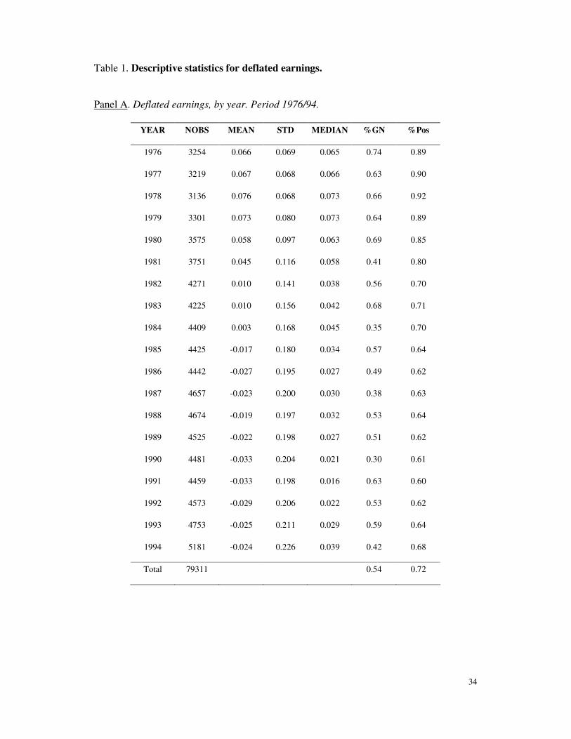
sample in BD (1997), i.e. 79 311 as opposed to 75 999 observations.19 In Table 1, Panel A,
we tabulate some descriptive statistics for the global sample. The number of observations
per year is in most cases higher than 4000 observations, increasing steadily until the last
year (1994) where it reaches 5181. The proportion of GN and BN per year does not follow
a steady evolution, but ranges between 40 percent and 60 percent, with a slight decrease of
GN in the second half of the period. The global proportion of GN is approximately 54
percent.
[TABLE 1]
17 We also tested for earnings before extraordinary items and discontinued operations available for common
stock (#237), and for (lagged) market value of common equity (#199*#25) as a deflator. The results are
qualitatively similar to those reported, and do not support the suggestion in Durtschi and Easton (2005) that
the discontinuities are (at least partly) driven by the use of lagged market value as the deflator.
18 The analysis was also performed using different data samples. The results are qualitatively similar to those
reported.
19 This difference arises because we use a different deflator (lagged total assets instead of lagged market
value), collect the data from more recent disks, and control the sample for market returns and for prior
period earnings.

18
Around 72 percent of the total firm-years have current positive earnings, but since 1985
this percentage is very close to 60 percent. The mean of deflated earnings is consistent
with this evolution and with previous literature showing an increased number of firms
reporting negative earnings over time (e.g. Givoly and Hayn, 2000). It becomes
increasingly negative after 1984, although the median stays positive and relatively stable,
consistent with more negative earnings and a higher dispersion.
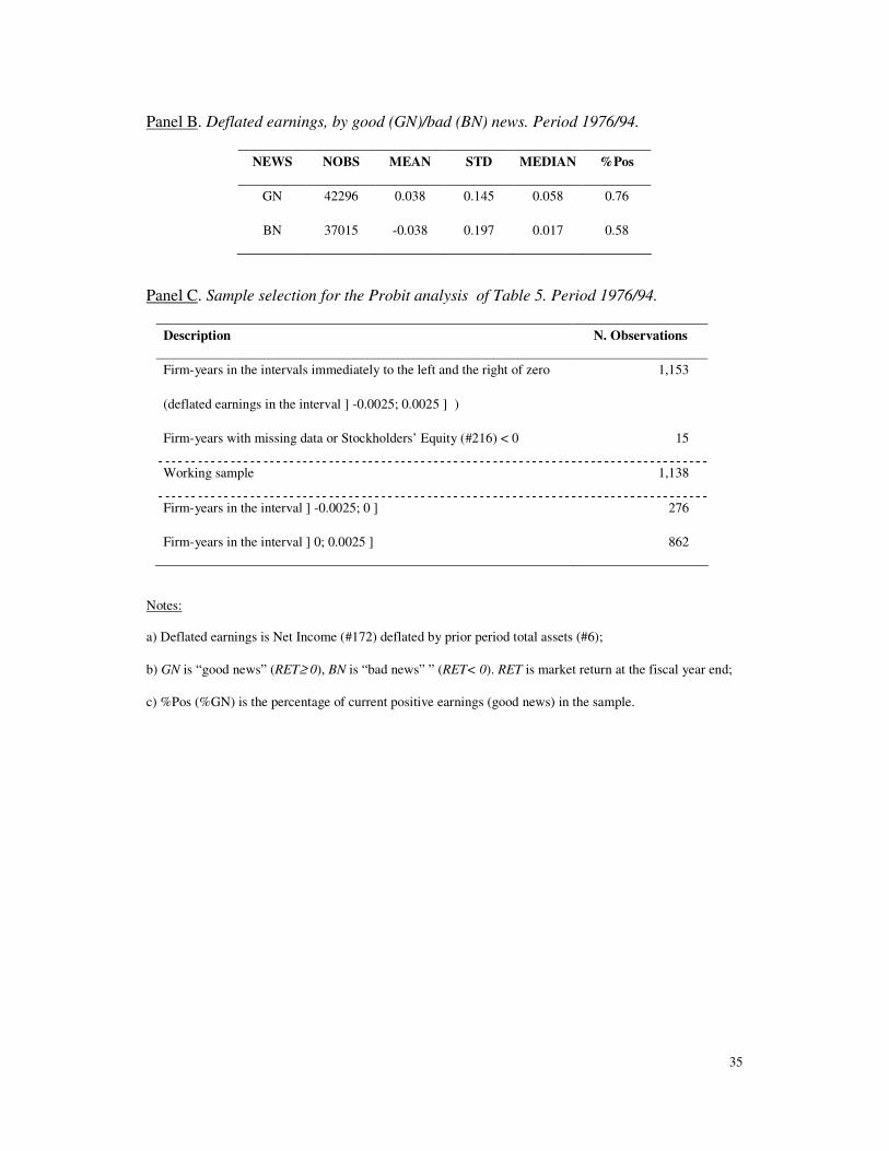
Panel B shows that BN firms on average have lower mean and median deflated earnings
than GN firms and a lower proportion of profits (around 58 percent), consistent with our
early expectation that bad news (negative returns) tend to reflect (pre-managed) earnings
decreases or losses.
The firm-years in the two central intervals of the earnings distribution are the basic sample
used to perform the Probit analysis. Panel C shows the selection of the working sample,
which has 1,138 observations (276 and 862, respectively to the left and to the right of
zero) after deleting those with missing data in any variable of the model and also negative
Stockholders’ Equity.20
For this sample, untabulated descriptive statistics show that the correlation coefficients of
the main variables used in the Probit analysis are very small or even insignificant. The
(obvious) exception is NI, deflated net income, which is highly correlated with the sign of
earnings. Moreover, it is apparent that firm-years in the interval to the right and left of
20 By deleting firm-years with negative Stockholder’s Equity we attempt to prevent any potential spurious
effect arising from firms that might have particular incentives, if any, to undertake earnings management.
However, re-performing the analysis with those observations does not change the results.

19
zero have no significant difference in mean and median TAX and SPITEM,21 and that the
right interval has proportionally more BN firms that its counterpart on the left, consistent
with our expectations.
[TABLE 2]
Table 2 displays descriptive statistics for DEBT, the change in total debt [�(#6-#216)t /
(#6-#216)t-1], by quadrants of market returns and prior period earnings (PRIOR), for both
the left and right intervals. We take this variable as a proxy for firms’ needs of debt.22 One
can see that the changes are statistically different across classes of PRIOR, with the
exception of GN firms for the left interval, consistent with the intuition that firms with
larger needs of debt tend to have a stronger incentive to report positive earnings. They are
statistically independent of the sign of market returns, i.e. GN and BN firms have similar
needs of debt. This applies for both the left and right intervals.23
21 The lack of statistical difference for variables TAX and SPITEM do not follow the evidence in Beaver et
al. (2003). Even the difference we obtain when considering the whole earnings sample rather than the
observations around zero suggests that the impact of those variables may not be a driving force of the
discontinuities in the earnings distribution.
22 We take the change in debt instead of total debt as a proxy for firms’ needs of debt because the cost of
debt is expected to be more related to the former than to the later.
23 We also defined firms’ needs of debt as the change in long term debt (#9), the change in debt in current
liabilities (#34) and the change in total debt defined as (#9+#34). The results are qualitatively similar to
those reported in Table 2.

20
4. Empirical results
4.1. Earnings management to avoid losses: graphical analysis
4.1.1. The discontinuities of the earnings distributions
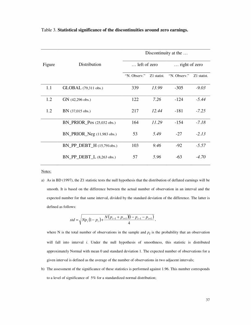
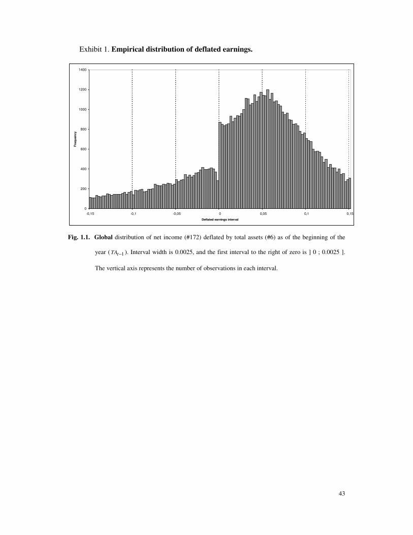
Exhibit 1, Fig. 1.1, reports the (truncated) distribution of deflated earnings levels.24 It
compares to Fig. 3 in BD (1997), and uses an interval width of 0.0025.25 As expected, the
frequency discontinuities at zero are visible and, as shown in Table 3, have highly
significant standardized differences (13.99 and -9.03, for the interval to the left and right
of zero, respectively).26
[EXHIBIT 1]
Fig. 1.2 comparatively reports the (truncated) distributions of GN and BN firms. It can be
seen that the distribution of GN firms (bars) is slightly skewed to the right, contrasting
with the distribution of BN firms (solid line). This is consistent with the descriptive
statistics in Table 1, Panel B, showing that GN firms tend to have higher mean and median
deflated earnings. The discontinuities at zero are visible in both distributions. The
standardized differences reported in Table 3 corroborate the visual assessment. For the
interval to the left (right) of zero, they are 7.26 (-5.44) for GN and 12.44 (-7.25) for BN
distributions. Moreover, the relative magnitude of these standardized differences together
24 Displaying truncated distributions, rather than complete ones, is intended to highlight the aim of the
analysis, that is to say, the discontinuities around zero.
25 The analysis was re-performed using an interval width of 0.005. The results are qualitatively similar.
26 The standardized differences are higher than the maximum values tabulated in a standardized normal
distribution for the usual level of confidence (5%). They are different from zero at less than 0.0001.
Throughout the paper the significance of these statistics is assessed against 1.96 (the 5% two-tail z-stat for a
standardized normal distribution).
21
with the visual graphical evidence suggest that the discontinuities around zero are of
different relative size, higher for BN firms, supporting our first hypothesis.
[TABLE 3]
Table 3 also reports the standardized differences for the discontinuities in the distributions
of BN firms with prior period positive (BN_PRIOR_Pos) and negative (BN_PRIOR_Neg)
earnings. For the interval to the left (right) of zero they are 11.29 (-7.18) for prior period
positive earnings and 5.49 (-2.13) for negative earnings. For the sake of parsimony we do
not display the graphs, but a visual assessment of the relative size of these differences
suggests that the discontinuities are higher for BN_PRIOR_Pos, consistent with our
second hypothesis.
Finally, this Table displays the standardized differences for the discontinuities in the
distributions of BN firms with prior period positive earnings and high (BN_PP_DEBT_H)
and low (BN_PP_DEBT_L) needs of debt.27 The discontinuities are all significant. For the
interval to the left (right) of zero they are 9.46 (-5.57) for high needs of debt and 5.96 (-
4.70) for low needs.28 The relative size of the computed statistics is consistent with our
third hypothesis, which states that BN firms with prior period positive earnings and high
needs of debt undertake more earnings management than firms with low needs of debt.
Thus, this graphical analysis seems to support all our hypotheses. However, as BD (1997)
point out, the statistics we use do not allow precise inferences about relative differences in
the discontinuities. Although their differences reflect the proportionate discontinuity, they
27 The 978 BN observations with missing DEBT have been deleted. This explains the difference, in Table 3,
between the sum of BN_PP_DEBT_H plus BN_PP_DEBT_L and the number of observations in
BN_PRIOR_Pos sub-sample.
28 Also in this case, and for the same reason as before, we do not display the graphs of the distribution.

22
also depend on the number of observations, which varies across earnings intervals and
distributions. Hence, those differences cannot be directly compared in order to assess the
relative earnings management pervasiveness.
Table 3 also shows an estimate of the number of firms that (supposedly) managed
earnings around zero. The expected number of observations minus the actual number of
observations in the interval is labeled as “N. Observ.”, the former being defined as the
average of the number of observations in the two adjacent intervals. Although the numbers
seem to support all our hypotheses, the same constraint of the different number of
observations in each sub-sample prevents us from drawing a grounded conclusion. Our
next step is thus to test statistically whether these estimates are different across
distributions.29
4.1.2. Statistical difference in the degree of earnings management pervasiveness
In sub-section 3.3) a) we defined the degree of earnings management pervasiveness (pp)
as the proportion of the (predicted) number of firms in a given interval that undertakes
earnings management over the expected number of firms in that interval. This definition
has two advantages over the measurement discussed in the previous sub-section. Firstly,
this new measurement takes into account the number of observations in each interval and
thus enables direct comparisons to be made across earnings distributions and intervals.
Secondly, it also allows the use of statistical methods to test the differences in
pervasiveness.
[TABLE 4]
29 These results are robust to different definitions of the variables, namely: i) definition of earnings (using
#237); ii) deflator (using market value, #199*#25); iii) interval width (0.005); iv) sample period.
23
Table 4, Panel A, reports estimates of the degree of pervasiveness to avoid losses for both
intervals around zero, and for GN and BN firms. The latter have, for both intervals, a
degree of pervasiveness slightly higher than 60 percent. That of GN firms is around 45
percent. Thus, there is a difference in that degree of around 17 (13) percentage points to
the left (right) interval. Using the statistical test for the difference between the proportions
of success in two independent samples (Sandy, 1990) we find that such an estimated
difference is significant at less than 0.0001 in both intervals. Hence, BN firms show a
higher degree of pervasiveness in avoiding earnings losses, consistent with the
hypothesized incentive they face to manage earnings. This evidence is fully supportive of
our first hypothesis and corroborates the conclusions of our previous visual assessment
based on the empirical distributions.
Table 4, Panel B, shows similar information for the sub-samples of BN firms with prior
period positive (BN_PRIOR_Pos) and negative (BN_PRIOR_Neg) earnings. The
difference in pervasiveness is 11 percentage points to the left interval and 45 to the right,
both of which are statistically significant. BN firms with prior period positive earnings, i.e.
approaching the earnings target from above, are expected to face a higher incentive to
manipulate earnings. A higher degree of pervasiveness suggests that such an incentive
exists. This evidence adds to that discussed in the previous sub-section and is supportive
of our second hypothesis.30 31
30 Untabulated results show that when we control for GN firms and prior period earnings sign there is no
statistical difference in the degree of pervasiveness in the left interval, and this difference in the right interval
is much smaller than that reported in Panel B and in favor of prior period negative earnings. Thus, the
opposite we hypothesized for BN firms.
31 We also tested for sub-samples of prior period positive and prior period negative earnings (untabulated
results). There is no significant difference in the degree of pervasiveness in the left and the right intervals.

24
Finally, Panel C displays information for the sub-samples of BN firms with prior period
positive earnings and low (DEBT Low) and high (DEBT High) needs of debt. The
evidence is mixed. In the left interval the difference in pervasiveness is 12 percentage
points and is statistically significant at the usual level of confidence. Firms with higher
needs of debt seem to undertake more earnings manipulation, consistent with our third
hypothesis. Conversely, and contrary to our expectations, in the right interval there is no
significant difference in the degree of pervasiveness across distributions. However, given
the technical characteristics of the methodology we use, the smaller number of
observations in each sub-sample might affect the precision of the assessment. The
statistics displayed in Table 2, on the number of observations, seem to give some support
to this potential explanation for such an unexpected result. The proportion of firms with
BN and prior period positive earnings is higher than that of GN firms in both intervals,
and this proportion is higher in the right interval.
In sum, the empirical evidence collected so far fully supports our first and second
hypotheses. It suggests that firms with BN in the current period and prior period positive
earnings face a higher incentive to avoid losses, and do have a higher degree of earnings
management pervasiveness. The occurrence of prior positive earnings does not by itself
explain differences in this degree. Moreover, the empirical evidence partly supports our
third hypothesis and the intuition that the needs of debt play a role in firms’ incentive to
undertake earnings management.
The importance of the overall evidence is threefold. Firstly, it adds to the literature that
supports the discontinuities in the earnings distribution as being driven (at least partly) by
earnings management. Secondly, it highlights the role of some of firms’ earnings
The sign of prior earnings is a determinant of the incentive to undertake earnings management only when
interacting with the sign of return.

25
management incentives. The theory we test, and the results we obtain, contribute to a
better understanding of these incentives and how they work. Thirdly, it challenges the
implicit assumption in BD (1997) that the incentives to undertake earnings management
are similar in all firms. Our research shows that the earnings distribution is the joint
impact of (at least) two groups of firms with differentiated incentives to manipulate
earnings.
Recent research (e.g. Dechow et al., 2003; Beaver et al., 2003; Durtschi and Easton, 2005)
argues that the discontinuities in the earnings distributions may not be due to earnings
management but to other reasons underlying those distributions. Despite the fact that the
evidence in such research conflicts with the empirical results of other recent studies that
support the earnings management explanation (e.g. Beatty et al., 2002), and with that
presented so far in this paper, we perform a Probit analysis to test whether the underlying
impact of market news on earnings, the way firms approach the zero earnings target and
their needs of debt, are (in fact) driving forces of firms’ earnings management when other
controls are in place.
Below, we discuss the results of this analysis.
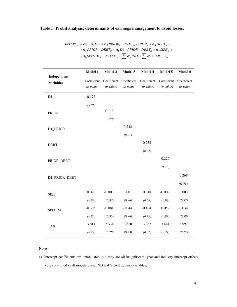
4.2. Probit analyses of differences in earnings management to avoid losses
Table 5 displays the results of Probit analyses for the differential likelihood of reporting
small profits versus small losses. As in the previous sub-section, we control for classes of
GN and BN firms (D1), for classes of BN firms with prior period positive (negative)
earnings (PRIOR) and, within those with prior positive earnings, for classes of high (low)
needs of debt (DEBT).
We perform six models with a similar structure. All of them control for some of the effects
referred to in the literature as potential determinants of the discontinuity at zero in the
26
earnings distribution. These effects are size (SIZE), special items (SPITEM) and taxes
(TAX). The analysis includes 1,138 firm-year observations with deflated earnings
between ] -0.0025; 0.0025 ], 54 percent of which are classified as BN firms.
[TABLE 5]
Model 1 tests whether BN firms do undertake earnings management to avoid losses in a
more pervasive way than GN firms. The coefficient on D1, the dummy variable reflecting
the dichotomy GN vs. BN firms, is significantly positive, consistent with our expectation
and the statistical evidence reported in Tables 3 and 4. This evidence supports our first
testing hypothesis and suggests that BN firms are more pervasive in undertaking earnings
management, reporting a significantly greater number of small profits and fewer small
losses than GN firms do.32
We hypothesized that prior period earnings sign (PRIOR), i.e. the way firms approach the
earnings target, is a determinant of the incentive to undertake manipulation. Models 2 and
3 test this effect. The former shows that the coefficient on PRIOR is statistically
insignificant, corroborating our previous intuition that this variable is not, by itself, a
driving force of the discontinuities in the earnings distributions.33 Model 3 tests, and
supports, the intuition underlying our second hypothesis. BN firms with prior period
positive earnings (D1_PRIOR) do undertake more pervasive earnings management,
32 The proportion of BN firm-years in the first interval in the right hand side of the distribution is consistent
with this result: approximately 57% against 46% in the first interval in the left and 47% for the whole
distribution.
33 Consistent with this outcome, graphical evidence not reproduced here shows that when we split the global
sample by the sign of prior period earnings there is no statistical difference in the degree of pervasiveness.

27
consistent with the statistical evidence in Tables 3 and 4 (Panel B).34 Thus, the way firms
approach the earnings target – from above or from below – is a determinant of their
incentive to manipulate earnings.
Our third hypothesis proposes a likely reason why BN firms with prior period positive
earnings (PRIOR) face an incentive to undertake earnings management: to avoid an
increase in their cost of debt. Thus, within this set of firms, those with larger needs of debt
are expected to face a higher incentive to manipulate. Models 4 to 6 test this intuition
using DEBT, a dummy variable that proxies for firms’ future needs of debt. Model 4
shows that the coefficient on this variable is statistically insignificant, consistent with our
intuition that firms’ needs of debt are not, by themselves, a driving force of the
discontinuities in the earnings distribution. However, testing for the interaction of this
variable with PRIOR (Model 5), the coefficient is statistically significant, suggesting that
firms approaching the earnings target from above (PRIOR) and with larger needs of debt
(DEBT) do face a higher incentive to manipulate earnings. This is an unexpected result,
and contradicts the expectation we formulated in sub-section 3.2. A potential reason for
the significance of this coefficient is that the variable PRIOR_DEBT might be acting as a
proxy for D1_PRIOR_DEBT. The fact that the coefficient on the latter (Model 6) and its
level of significance are higher than those on PRIOR_DEBT seems to be supportive of
this tentative explanation.35 The evidence in Model 6 is consistent with the graphical and
statistical evidence discussed in the previous sub-section, showing that BN firms
approaching the earnings target from above and with larger needs of debt do report a
significantly greater number of small profits and fewer small losses than other firms. This
34 If we test for BN firms with prior period negative earnings the coefficient is not significant.
35 As we move from Model 1 to Model 6 the coefficient on the main variable is increasing, consistent with
the intuition that the cost of debt is the ultimate incentive for firms’ earnings manipulation.

28
result is also consistent with the statistical evidence in Table 3 and complements the
evidence in Table 4 (Panel C). Altogether, the empirical evidence in Models 4 to 6 fully
support our third hypothesis.36
The coefficients on the control variables are systematically insignificant across models,
consistent with untabulated descriptive statistics discussed in sub-section 3.4. This
evidence suggests that firm size is not a driving force of firms’ location around zero
earnings, and that the tax and special items effects discussed in Beaver et al. (2003) do not
have, in the current study, a role in explaining the discontinuity at zero in the earnings
distribution. More than a denial of previous evidence about the determinants of the
discontinuities, our results suggest that at least a part of them is driven by discretionary
actions undertaken by managers.
In sum, the empirical evidence discussed in this sub-section highlights the importance of
the sign of market returns (GN and BN) as a proxy for managers’ incentive to undertake
earnings management to avoid losses, and the roles played by PRIOR and DEBT in
maximizing such an incentive. The results corroborate the empirical evidence collected
from the graphical and statistical analyses, and bring to light a new and intuitive
explanation for the discontinuities around zero in the earnings distribution. They are
indeed an important contribution to our understanding of the determinants of such
discontinuities.
36 The models in Table 5 are tested for the right interval at zero, i.e. for the likelihood of firms reporting a
greater number of small profits. However, testing for the left interval (likelihood of reporting fewer small
losses) does not qualitatively change the results. The same is true when we use other proxies for firms’ needs
of debt [the sign of the change in long term debt (#9) and in total debt (#9+#34), and ranks of high/low long
term debt (#9) and total debt (#9+#34)].

29
5. Conclusion
In this paper we analyze firms’ earnings management behavior to avoid losses conditional
on the (asymmetric) incentive underlying market returns and prior period earnings signs.
Our intuition is that firms with negative returns in the period face a higher incentive to
undertake earnings management, and that their ultimate intention is to hide from credit
markets a signal (loss) that could negatively affect their cost of debt.
Our graphical and statistical empirical evidence supports this intuition. BN firms show
higher earnings management pervasiveness than their counterparts with good news (GN),
reporting a greater number of small profits and fewer small losses. The set with
simultaneously BN and prior period positive earnings (PRIOR) undertakes more pervasive
earnings manipulation than BN firms in general. However, PRIOR is not in itself a
determinant of the location of firm-years around the zero earnings target.
Within this restricted set of firms with BN and PRIOR, and consistent with a cost of debt
explanation, we find that firms with larger needs of debt (DEBT) show higher
pervasiveness in undertaking earnings management to avoid losses. As for PRIOR, we
also tested for DEBT as the determinant of the discontinuity in the earnings distribution,
but the variable was not significant. The results are robust to the use of graphical and
statistical tests, including Probit models that control for some of the main variables that
might affect the shape of the earnings distribution.
This paper adds to a large and growing body of literature that discusses firms’ earnings
management behavior. Recently the discussion has focused on whether the graphical
evidence in BD (1997) is driven by firms’ intentional earnings manipulation or by a mere
statistical effect related to an asymmetric impact of some earnings components, or even to
the research design adopted in the studies (e.g. Dechow et al., 2003, Beaver et al., 2003,

30
Beatty et al., 2002 and Durtschi and Easton, 2005). The empirical evidence provided in
these studies is mixed.
The main contributions of our research to this literature are threefold. Firstly, it extends
the methodology introduced in BD (1997) and uses it to compare the earnings
management behavior across sets of firms with differentiated characteristics and/or
incentives. Secondly, it discusses the existence of asymmetric earnings management
incentives and relates them to the discontinuities around the earnings zero target. Thus, it
challenges the implicit assumption in the seminal paper of BD (1997) that this kind of
incentive is homogeneous to all firms in the distribution. Our research shows that the
earnings distribution is the joint impact of sets of firms with differentiated incentives to
manipulate earnings. Finally, based on a well-grounded theory, it also contributes to a
better understanding of the roles of earnings signals sent to credit markets and of firms’
debt as determinants of earnings management. At a time when firms’ earnings
management behavior is still a “black box” this is an important contribution indeed.
31
References
Ball, R. and Brown, P. 1968. “An Empirical Evaluation of Accounting Income Numbers”. Journal
of Accounting Research, n. 6, Autumn, pp. 159-178.
Ball, R. and S. Kothari, and A. Robin. 2000. “The effect of institutional factors on properties of
accounting earnings: international evidence”. Journal of Accounting and Economics, v.
29, pp. 1-51.
Barth, M., J. Elliot and M. Finn. 1999. “Market Rewards Associated with Patterns of Increasing
Earnings”. Journal of Accounting Research, n. 37, pp. 378-413.
Basu, S. 1997. “The conservatism principle and the asymmetric timeliness of earnings”. Journal of
Accounting and Economics, v. 24, pp. 3-37.
Beatty, A., B. Ke and K. Petroni. 2002. “Earnings Management to Avoid Earnings Declines across
Publicly and Privately Held Banks”. The Accounting Review, v.77, n.3, July, pp. 547-570.
Beaver, W., M. McNichols and K. Nelson. 2003. “An Alternative Interpretation of the Discontinuity
in Earnings Distributions”. Working Paper, www.ssrn.com, February.
Brown, L. and M. Caylor. 2005. “A Temporal Analysis of Quarterly Earnings Thresholds”. The
Accounting Review, v. 80, n. 2, pp. 423-440.
Burgstahler, D. and I. Dichev. 1997. “Earnings management to avoid earnings decreases and
losses”. Journal of Accounting and Economics, v.24, pp. 99-126.
Bushee, B. 1998. “The influence of institutional investors on myopic R&D investment behavior”.
The Accounting Review, v.73, n.3, July, pp. 305-333.
Dechow, P., S. Richardson and I. Tuna. 2000. "Are Benchmark Beaters Doing Anything Wrong?",
WP, April, http://ssrn.com/abstract=222552 .

32
________________________________. 2003. “Why are Earnings Kinky? An Examination of the
Earnings management Explanation”. Review of Accounting Studies, v. 8, pp. 355-384.
DeFond, M. and J. Jiambalvo. 1994. “Debt covenant violation and manipulation of accruals”.
Journal of Accounting and Economics, v. 17, pp. 145-176.
__________ and C. Park. 1997. “Smoothing income in anticipation of future earnings”. Journal of
Accounting and Economics, v. 23, pp. 115-139.
Degeorge, F., J. Patel, and R. Zeckhauser. 1999. “Earnings Management to Exceed Thresholds”.
Journal of Business, v. 72, n. 1, January, pp. 1-33.
Durtschi, C. and P. Easton. 2005. “Earnings Management? The Shapes of the Frequency
Distributions of Earnings Metrics Are Not Evidence Ipso Facto”. Journal of Accounting
Research, vol. 43, n. 4, September, pp. 557-592.
Garrod, N. and A. Valentincic. 2001. “Differential Ex-post Conservatism Effects for Loss Making Firms
in UK”. WP (tentative), University of Glasgow, September.
Givoly, D. and C. Hayn. 2000. “The changing time-series properties of earnings, cash flows and
accruals: Has financial reporting become more conservative?”. Journal of Accounting and
Economics, v. 29, pp. 287-320.
Gore, P., P. Pope, and A. Singh. 2001. “Discretionary Accruals and the Distribution of Earnings
Relative to Targets”. Working Paper, Lancaster University, January.
Hayn, C. 1995. “The information content of losses”. Journal of Accounting and Economics, v. 20,
pp. 125-153.
Healy, P. 1985. “The Effect of Bonus Schemes on Accounting Decisions”. Journal of Accounting
and Economics, v. 7, pp. 85-107.
_________ and J. Wahlen. 1999. “A review of the earnings management literature and its
implications for standard settings”. Accounting Horizons, vol. 13, n. 4, pp. 365-383.

33
McNichols, M. 2000. “Research design issues in earnings management studies”. Journal of
Accounting and Public Policy, v. 19, pp. 313-345.
_____________ and G. Wilson. 1988. “Evidence of earnings management from the provision for
bad debts”. Journal of Accounting Research, v. 26 (Supplement), pp. 1-31.
Moreira, J. 2002. Essays in Links Between Firm Value and Earnings Components Under
Conservative Accounting. PhD dissertation, Lancaster University, January.
Pope, P. and M. Walker. 1999. “International differences in the timeliness, conservatism, and
classification of earnings”. Journal of Accounting Research, v. 37, Supplement, pp. 53-87.
Sandy, R. 1990. Statistics for Business and Economics. Singapore: McGraw Hill.
Schipper, K. 1989. “Commentary on earnings management”. Accounting Horizons, v. 3, Dec., pp.
91-102.
Sweeney, A. 1994. Debt Covenant Violations and Managers’ Accounting Responses. Journal of
Accounting and Economics, vol. 17, pp.281-308.
34
Table 1. Descriptive statistics for deflated earnings.
Panel A. Deflated earnings, by year. Period 1976/94.
YEAR NOBS MEAN STD MEDIAN %GN %Pos
1976 3254 0.066 0.069 0.065 0.74 0.89
1977 3219 0.067 0.068 0.066 0.63 0.90
1978 3136 0.076 0.068 0.073 0.66 0.92
1979 3301 0.073 0.080 0.073 0.64 0.89
1980 3575 0.058 0.097 0.063 0.69 0.85
1981 3751 0.045 0.116 0.058 0.41 0.80
1982 4271 0.010 0.141 0.038 0.56 0.70
1983 4225 0.010 0.156 0.042 0.68 0.71
1984 4409 0.003 0.168 0.045 0.35 0.70
1985 4425 -0.017 0.180 0.034 0.57 0.64
1986 4442 -0.027 0.195 0.027 0.49 0.62
1987 4657 -0.023 0.200 0.030 0.38 0.63
1988 4674 -0.019 0.197 0.032 0.53 0.64
1989 4525 -0.022 0.198 0.027 0.51 0.62
1990 4481 -0.033 0.204 0.021 0.30 0.61
1991 4459 -0.033 0.198 0.016 0.63 0.60
1992 4573 -0.029 0.206 0.022 0.53 0.62
1993 4753 -0.025 0.211 0.029 0.59 0.64
1994 5181 -0.024 0.226 0.039 0.42 0.68
Total 79311 0.54 0.72
35
Panel B. Deflated earnings, by good (GN)/bad (BN) news. Period 1976/94.
NEWS NOBS MEAN STD MEDIAN %Pos
GN 42296 0.038 0.145 0.058 0.76
BN 37015 -0.038 0.197 0.017 0.58
Panel C. Sample selection for the Probit analysis of Table 5. Period 1976/94.
Description N. Observations
Firm-years in the intervals immediately to the left and the right of zero
(deflated earnings in the interval ] -0.0025; 0.0025 ] )
1,153
Firm-years with missing data or Stockholders’ Equity (#216) < 0 15
Working sample 1,138
Firm-years in the interval ] -0.0025; 0 ] 276
Firm-years in the interval ] 0; 0.0025 ] 862
Notes:
a) Deflated earnings is Net Income (#172) deflated by prior period total assets (#6);
b) GN is “good news” (RET≥ 0), BN is “bad news” ” (RET< 0). RET is market return at the fiscal year end;
c) %Pos (%GN) is the percentage of current positive earnings (good news) in the sample.

36
Table 2. Change in total debt around the zero earnings target.
Prior Period Earnings (PRIOR)
Negative Positive
[1]
DEBT Median
(N.Obs.)
[2]
DEBT Median
(N.Obs.)
Probability
[1=2]
%N.Obs.
[2/1]
LEFT INTERVAL
Positive (GN) -0.017
(63)
-0.037
(82)
0.815
1.30 Market
Returns
Negative (BN) -0.123
(44)
0.014
(87)
0.020
1.98
Probability [GN=BN] 0.057 0.572
RIGHT INTERVAL
Positive (GN) -0.021
(173)
0.034
(210)
0.003
1.21 Market
Returns
Negative (BN) -0.032
(121)
0.035
(358 )
<0.001
2.96
Probability [GN=BN] 0.300 0.929
Notes:
a) The values reported in the table are the medians of DEBT, the percentage change in total debt [�(#6-
#216)t / (#6-#216)t-1]), that we take as a proxy for firms’ needs of debt. For example, firms with prior
period negative earnings and GN have DEBT median equal to -0.017. In parenthesis we report the
number of observations in each quadrant. Taking the same example, the number of observations is 63.
b) The left interval is deflated net income ] -0.0025; 0 ] and the right interval is ] 0; 0.0025 ];
c) “Probability” is the p-value of a Wilcoxon test for the equality of medians across classes; “%N.Obs.” is
the proportion of prior period positive earnings observations in each market returns class.
37
Table 3. Statistical significance of the discontinuities around zero earnings.
Discontinuity at the …
Figure … left of zero … right of zero
Distribution
“N. Observ.” Z1 statist. “N. Observ.” Z1 statist.
1.1 GLOBAL (79,311 obs.) 339 13.99 -305 -9.03
1.2 GN (42,296 obs.) 122 7.26 -124 -5.44
1.2 BN (37,015 obs.) 217 12.44 -181 -7.25
BN_PRIOR_Pos (25,032 obs.) 164 11.29 -154 -7.18
BN_PRIOR_Neg (11,983 obs.) 53 5.49 -27 -2.13
BN_PP_DEBT_H (15,791obs.) 103 9.46 -92 -5.57
BN_PP_DEBT_L (8,263 obs.) 57 5.96 -63 -4.70
Notes: a) As in BD (1997), the Z1 statistic tests the null hypothesis that the distribution of deflated earnings will be
smooth. It is based on the difference between the actual number of observation in an interval and the
expected number for that same interval, divided by the standard deviation of the difference. The latter is
defined as follows:
( ) ( )( )41
1 1111 +−+− −−++−= iiii
iippppN
pNpstd ,
where N is the total number of observations in the sample and pi is the probability that an observation
will fall into interval i. Under the null hypothesis of smoothness, this statistic is distributed
approximately Normal with mean 0 and standard deviation 1. The expected number of observations for a
given interval is defined as the average of the number of observations in two adjacent intervals;
b) The assessment of the significance of these statistics is performed against 1.96. This number corresponds
to a level of significance of 5% for a standardized normal distribution;

38
c) “Global” stands for the whole earnings distribution; GN (BN) for good (bad) news sub-sample;
BN_PRIOR_Pos (BN_PRIOR_Neg) for sub-samples of BN firms with prior period positive (negative)
earnings; BN_PP_DEBT_H (BN_PP_DEBT_L) for sub-samples of BN firms with prior period positive
earnings and High (Low) needs of DEBT. DEBT is the percentage change in total debt [�(#6-#216)t /
(#6-#216)t-1];
d) Earnings (#172) is deflated by total assets (#6) as of the end of the prior period;
e) “N. Observ.” equals the expected minus the actual number of observations in the interval. To the left of
zero the interval width is ]-0.0025; 0 ], to the right it is ] 0 ; 0.0025 ].

39
Table 4. Differences in the degree of pervasiveness to avoid losses.
Discontinuity at the …
Description … left of zero … right of zero
Panel A: sub-samples of good and bad news firms
Good News Bad News Good News Bad News
1. Number of actual firms 149 133 390 481
2. Number of expected firms 271 350 266 300
3. Pervasiveness (2-1)/2 0.45 0.62 0.47 0.60
4. Difference in pervasiveness 0.17 0.13
5. Standard deviation 0.039 0.042
6. Z2 Statistic [4/5] 4.26 3.29
7. P-value < 0.0001 < 0.0001
Panel B: sub-samples of bad news firms with prior period positive / negative
earnings
PRIOR Neg PRIOR Pos PRIOR Neg PRIOR Pos
…
4. Difference in pervasiveness 0.11 0.45
5. Standard deviation 0.058 0.056
6. Z2 Statistic [4/5] 1.87 8.01
7. P-value 0.06 < 0.0001

40
Panel C: sub-samples of bad news firms with prior period positive earnings
and high/low needs of debt
DEBT Low DEBT High DEBT Low DEBT High
…
4. Difference in pervasiveness 0.12 -0.04
5. Standard deviation 0.062 0.060
6. Z2 Statistic [4/5] 1.94 -0.71
7. P-value 0.05 0.47
Notes:
a) The Z2 statistic is the probability density function of the difference between the proportions of success in
two independent samples (Sandy, 1990: chap. 10), and is distributed approximately Normal with mean 0
and variance 1. Under the null hypothesis of no difference in the proportions, this statistic is defined as
follows: std
ppZ
gb�� −
=2 , where the numerator is the difference between the proportions of “bad news”
(b) and “good news” firms (g) undertaking earnings management.
The standard deviation is estimated as: ( ) ( )
bg npp
npp
std−+−= 11
, where n is the number of expected
“good news” (g) and “bad news” firms (b) in the interval. p is the pooled proportion of both samples:
bg
bbgg
nn
pnpnp
+
+=
��
.
b) The p-value underlying the critical value of the Z2 statistic are two-tailed;
c) The expected number of observations for a given interval is defined as the average of the number of
observations in two adjacent intervals. To the left of zero the interval width is ]-0.0025; 0 ], to the right it
is ] 0 ; 0.0025 ].
d) PRIOR_Pos (PRIOR_Neg) are BN firms with prior period positive (negative) earnings; DEBT Low
(High) are BN firms with prior period positive earnings and Low (High) needs of debt.
41
Table 5. Probit analysis: determinants of earnings management to avoid losses.
ittkijitit
ititit
ititititit
eYEARINDTAXSPITEM
SIZEDEBTPRIORDDEBTPRIOR
DEBTPRIORDPRIORDINTERV
�� +++++
+++++++++=
__1_
_11
98
765
43210
αααα
αααααααα
Independent
variables
Model 1
Coefficient
(p-value)
Model 2
Coefficient
(p-value)
Model 3
Coefficient
(p-value)
Model 4
Coefficient
(p-value)
Model 5
Coefficient
(p-value)
Model 6
Coefficient
(p-value)
D1 0.177
(0.05)
PRIOR 0.119
(0.20)
D1_PRIOR 0.242
(0.01)
DEBT 0.252
(0.21)
PRIOR_DEBT 0.226
(0.02)
D1_PRIOR_DEBT 0.268
(0.01)
SIZE 0.020
(0.83)
-0.003
(0.97)
0.001
(0.98)
0.018
(0.88)
-0.009
(0.92)
0.003
(0.97)
SPITEM -0.305
(0.85)
-0.081
(0.96)
-0.044
(0.98)
-0.124
(0.95)
0.052
(0.97)
-0.034
(0.98)
TAX 3.811
(0.22)
3.331
(0.28)
3.810
(0.23)
3.967
(0.32)
3.441
(0.27)
3.597
(0.25)
Notes:
a) Intercept coefficients are untabulated, but they are all insignificant; year and industry intercept effects
were controlled in all models using IND and YEAR dummy variables;

42
b) Variable definitions: INTERV is a dummy variable that takes value one if net income is in the interval ]
0; 0.0025 ], and value zero if the firm has deflated net income in the interval ] -0.0025; 0 ]; D1 is a
dummy variable that takes value one if the firm has “bad news” in the year, zero otherwise; PRIOR is a
dummy variable that takes value one if prior period earnings (#172) is positive, zero otherwise;
D1_PRIOR is an interactive variable defined as D1*PRIOR; DEBT is a dummy variable that takes value
one if the change in total debt [�(#6-#216)] in the current period is positive, zero otherwise;
PRIOR_DEBT is an interactive variable defined as PRIOR*DEBT; D1_PRIOR_DEBT is an interactive
variable defined as D1*PRIOR*DEBT; SIZE is a dummy variable that takes value one if firm market
value (#199*#25) is in the upper third of the distribution, zero otherwise; SPITEM is Special Items (#17)
and TAX is Income Taxes (#16), both deflated by prior period total assets (#6); ΣIND is a set of dummy
variables, taking a value of one if the firm belongs to the industry, zero otherwise; ΣYEAR is a set of
dummy variables, taking a value of one if the firm-year corresponds to the year, zero otherwise; i,t are
firm and year (1976-1994) indexes, respectively.
c) The models have been regressed using 1,138 observations, and test for the likelihood of reporting a
greater number of small profits (right interval). INTERV has 276 and 862 observations for classes 0
(left) and 1 (right), respectively; BN firm-years (D1=1) are 54 percent of the total number of
observations, 78 percent of which are in class 1 (right); firm-years with positive change in total debt
(DEBT=1) are 51 percent of the total number of observations, 53 percent of which are in class 1 (right);
firm-years with prior period positive earnings (PRIOR=1) are 65 percent of the total number of
observations, 66 percent of which are in class 1 (right).
d) P-values are two-tailed.
43
Exhibit 1. Empirical distribution of deflated earnings.
0
200
400
600
800
1000
1200
1400
-0,15 -0,1 -0,05 0 0,05 0,1 0,15
Deflated earnings interval
Freq
uenc
y
Fig. 1.1. Global distribution of net income (#172) deflated by total assets (#6) as of the beginning of the
year ( 1−tTA ). Interval width is 0.0025, and the first interval to the right of zero is ] 0 ; 0.0025 ].
The vertical axis represents the number of observations in each interval.

44
0
100
200
300
400
500
600
700
800
-0,15 -0,1 -0,05 0 0,05 0,1 0,15
Deflated earnings intervals
Freq
uenc
y
Good News Bad News
Fig. 1.2. Comparative Good and Bad News distributions of net income (#172) deflated by total assets (#6)
as of the beginning of the year ( 1−tTA ). Interval width is 0.0025, and the first interval to the right
of zero is ] 0 ; 0.0025]. The vertical axis represents the number of observations in each interval.