Earnings Quality Metrics and What They Measure

Ralf Ewert

and

Alfred Wagenhofer

University of Graz

We thank Jeremy Bertomeu, Miles Gietzmann, Roland Koenigsgruber, Eva Labro, Iván Marinovic, Ulf Schiller, Joerg Werner, and workshop participants at the University of North Carolina and the University of Bremen for useful comments.

Corresponding author: Ralf Ewert University of Graz Universitaetsstrasse 15, A-8010 Graz, Austria Tel.: +43 (316) 380 7168 Email: ralf.ewert@uni-graz.at

December 2009

revised September 2010

1

Earnings Quality Metrics and What They Measure

This paper discusses and evaluates the usefulness and appropriateness of commonly used earnings metrics. In a rational expectations equilibrium model, we study the information content of earnings that can be biased by a manager who has market price, earnings, and smoothing incentives. We define earnings quality as the reduction of the market’s uncertainty about the firm’s terminal value due to the earnings report and compare this measure with value relevance, persistence, predictability, smoothness, and accrual quality. The evaluation is based on their ability to capture the effects of a variation of the manager’s incentives and information, and of accounting risk. We find that each metric captures different effects, but some of them, including value relevance and persistence, are closely related to our earnings quality measure. Discretionary accruals are problematic as their behavior depends on specific circumstances. These results provide insights into regulatory changes and guidance for selecting earnings quality metrics in empirical tests of earnings quality.

Keywords: Earnings quality; value relevance; earnings management; accrual quality.

2

1. Introduction

Earnings quality is one of the most important characteristics of financial reporting systems.

High quality is said to improve capital market efficiency, therefore investors and other users

should be interested in high-quality financial accounting information. For that reason, standard

setters strive to develop accounting standards that improve earnings quality, and many recent

changes in auditing, corporate governance, and enforcement have a similar objective.

Earnings quality is used in numerous empirical studies to show trends over time; to

evaluate changes in financial accounting standards and in other institutions, such as enforcement

and corporate governance; to compare financial reporting systems in different countries; and to

study the effect of earnings quality on the cost of capital.

Surprisingly, the concept of earnings quality is quite vague, despite several attempts to

make it more precise and to provide a theoretical foundation. For example, Schipper and Vincent

[2003] deduce earnings quality from the theory of economic income, and Dechow and Schrand

[2004] define earnings quality as a measure of how well earnings reflect the actual performance

of a firm. Standard setters such as the Financial Accounting Standards Board (FASB) and the

International Accounting Standards Board (IASB) formulate in their draft on the first part of a

common conceptual framework the need for high-quality financial reporting [IASB, 2008]. They

avoid defining quality, but list a number of qualitative characteristics that should achieve a high

quality, including relevance, faithful representation, comparability, verifiability, timeliness, and

understandability.

The empirical literature has developed several metrics to proxy for earnings quality (see the

surveys in, e.g., Schipper and Vincent [2003]; Dechow and Schrand [2004]; Francis, Olsson and

Schipper [2008]; and Dechow, Ge, and Schrand [2010]). The metrics are based on the qualitative

characteristics in the conceptual framework, but also on other concepts. Some of them are based

on accounting numbers only, while others include market prices, too. Despite their widespread

use, there is no agreement on several metrics whether a high value of the metric indicates high or

3

low earnings quality. For example, smoothness is used to proxy for earnings management

(indicating low earnings quality) or for additional information incorporated by the manager

(indicating high earnings quality). Therefore, some studies use the neutral term “earnings

attributes” rather than earnings quality metrics. Nevertheless, even if the different directions of

the interpretation are acknowledged,1 most studies a priori assume a particular interpretation in

their analyses.

The metrics capture only certain aspects that are considered important for earnings quality,

e.g., the time series of earnings or market price reactions on earnings. Therefore, many empirical

studies aggregate several metrics into an earnings quality score, often by adding up the ranks of

the metrics. Doing so, the researchers implicitly assume equal weights of the metrics, which

neglects perhaps different importance of certain effects, a potential overlap of metrics,

correlations among the metrics, and the potential information content in the cardinal

measurement.

The objective of this paper is to provide a theory of measures of earnings quality to

evaluate the usefulness and appropriateness of commonly used earnings quality metrics. We

develop a model with a firm whose terminal value (liquidating cash flow) is uncertain and the

uncertainty reduces over time. The firm’s manager makes a decision about the bias (accrual,

earnings management) in her earnings report, and rational investors in a capital market use the

earnings report to make inferences about the value of the firm. We incorporate typical incentives

of the manager, increasing the market price, increasing or smoothing reported earnings, and we

consider costs of earnings management. We do not model these incentives endogenously because

we want to vary them in the analysis of earnings quality metrics. The manager has private

information about the future cash flows and uses this information when deciding on the bias.

Thus, we consider both earnings management and information content of accruals together. We

1 See, e.g, the discussion in Barth, Landsman, and Lang [2008].

4

do not distinguish between quality of financial reporting and earnings quality because our

earnings capture all the information about the terminal value in the model.

After characterizing the unique linear rational expectations equilibrium we define earnings

quality in our framework as the reduction of the market’s assessment of the variance of the

terminal value due to the earnings report. This notion arises naturally from our model, and it is

consistent with the definition by Francis, Olsson, and Schipper [2008, p. 8], who define quality of

information as the precision (and lack of uncertainty) of a measure with respect to a valuation

relevant construct, which they assume is to support certain judgments and decisions in the capital

markets.

In addition to this benchmark measure, we study value relevance, persistence,

predictability, smoothness, and accrual quality, each of them suitably defined in our underlying

setting. We examine the behavior of each of these metrics on variations of fundamental

determining factors of earnings quality. In particular, we consider four sets of factors: (i)

managerial incentives, which affect the earnings report due to earnings management; (ii)

operating risk, which is the variation of the future cash flows and the terminal value; (iii) private

information of the manager about the operating risk; and (iv) accounting risk which determines

the precision of the accounting system.

The main results are as follows: There is no metric of those we study that perfectly traces

the behavior of our benchmark measure. Closest to the benchmark’s performance are value

relevance, followed by persistence. We show conditions when they behave similarly or not and

when their relation is monotonic or not. Predictability is generally an appropriate metric except if

one is interested in a change of the private information of the manager, where using predictability

can lead to false conclusions. Probably the most striking result is that metrics that depend directly

on the discretionary accruals are highly problematic metrics for earnings quality and conclusions

based on them should be interpreted with caution. Our correlation-based smoothness metric

generally does not pick up variations in the incentives and reacts to changes in information and

5

accounting risks in a way that is opposite to our benchmark. Similarly, our metrics for accrual

quality, the expected value of accruals or of squared accruals, capture an incentive effect that is

not existent for the earnings quality measure and react to variations of other determining factors

opposite to the benchmark or ambiguously, depending on specific realizations of other factors.

Thus, using these metrics is likely to lead to false conclusions from empirical tests.

An advantage of our model is that we are able to trace any differences that occur in the

behavior of the metrics to their economic causes. The model analysis explains why the metrics

react similarly or opposite to the behavior of our earnings quality measure, and under which

conditions they do so. For example, we show when the information content explanation for

smoothing and accrual quality is more consistent with the results than the earnings management

explanation. These results caution against using certain metrics as indicating higher or lower

earnings quality without controlling for such conditions.

Our results contribute to the empirical literature by providing a framework that guides the

formulation of hypotheses and the appropriate selection of earnings quality metrics for specific

research questions, such as the impact of tighter accounting standards, stronger enforcement,

more precise accounting information, stronger corporate governance, and management

compensation schemes, on earnings quality.

There are few theoretical papers that directly address earnings quality measures, although a

notion of earnings quality is embedded in many studies. Our linear rational expectations

equilibrium is based on Fischer and Verrecchia [2000], who focus on the manager’s market price

incentive in a one-period model, but do not consider smoothing incentives. Ewert and

Wagenhofer [2005] use a similar model to consider value relevance when the manager can

manage earnings or affect real cash flows of the firm. Sankar and Subrahmanyam [2001] study a

model with a risk averse manager with a time-additive utility function so that smoothing results

from the manager’s desire to smooth consumption. Similar to our model, they find that allowing

for earnings management improves the information in the capital market because the bias allows

6

the manager to incorporate private value relevant information early. However, they do not

consider earnings quality metrics. Dye and Sridhar [2004] study relevance and reliability of

accounting information and model the accountant as the gatekeeper to trade off these two

characteristics in a capital market equilibrium. Marinovic [2010] examines earnings management

and capital market reactions when it is uncertain if the manager can bias the earnings report. He

shows the existence of an equilibrium with a mixed earnings management strategy and a market

price reaction that is bounded from above for increasing earnings reports. He finds that price

volatility around earnings announcements and persistence are useful metrics, whereas

predictability and smoothness do not capture earnings quality appropriately because they are non-

monotonic measures.

Like our paper, these models exclusively focus on decision usefulness of accounting

earnings in a capital market equilibrium. They do not consider stewardship uses of accounting

information as do, for example, the optimal contracting models by Christensen, Feltham, and

Şabac [2005] and Christensen, Frimor, and Şabac [2009]. A recent paper that addresses both

stewardship and valuation purposes is by Drymiotes and Hemmer [2009]. They study a multi-

period agency model and explicitly consider empirical earnings quality metrics in that setting.

Similar in spirit to our results, they find that empirical metrics for earnings quality do not capture

many of the real economic effects. Individual results differ, however, due to the different

objectives of financial reporting and the model structures used in the two studies.

We do not claim that higher earnings quality in the sense that earnings reports provide more

precise information about firm value is necessarily a socially desirable objective. For example,

Kanodia, Singh, and Spero [2005] and Göx and Wagenhofer [2010] find situations in which

maximizing precision is not in the interest of the firm and investors, even if it is costless to do so.

Nagar and Yu [2009] test the prediction of models that “too” precise public information may

coordinate speculators’ behavior, which can lead to self-fulfilling beliefs and, ultimately, crisis.

7

In the next section we set up the model and explain main factors that influence earnings

quality. Section 3 establishes the rational expectations equilibrium and describes the properties of

the earnings reporting and market pricing strategies. In section 4, we define earnings quality

within the model structure and show its determinants. Section 5 includes a detailed analysis of the

behavior of the earnings quality metrics on variations of the main influencing factors. Section 6

draws together these results and discusses implications. Section 7 concludes.

2. The Model

We consider a firm that has a stochastic terminal value x% . To focus on the characteristics of

accounting information we assume that the firm’s operating activities are held constant and do

not affect the distribution of x% . Therefore, we essentially model a pure exchange economy with

one risky asset (the firm). The terminal value consists of the following components:

x μ ε δ ω= + + +%% %% . (1)

μ denotes the prior expected value of the terminal value and ε% , δ% , and ω% are normally

distributed random variables with zero means and variances 2 2,ε δσ σ and 2ωσ , respectively. The

random variables are mutually independent. They depend on the business model of the firm and

the environment in which the firm operates. The structure of the terminal value and μ are

common knowledge. The random variables realize sequentially over time, starting with ε% , then

δ% , and ω% at the liquidation date. The realizations are not observed before the respective date, but

there is some specific information about them as we describe below. We refer to the random

components in x% as operating risk.

For simplicity, we do not model realizations of cash flows in each period, but assume that

all cash flows obtain when the terminal value realizes. Adding observable period cash flows are

unlikely to add significant new insights.

8

Accounting system

The accounting system generates noisy signals of components of the operating risk. In the

first period, the manager privately receives a signal

1y nμ ε= + +%% % . (2)

This signal includes the expected value of x% and one random component, ε% , but also includes an

accounting noise term n% , which is normally distributed with zero mean and variance 2nσ . In the

second period, the manager privately receives another accounting signal

2y uμ ε δ= + + +%%% % . (3)

It captures the information content of 1y% with respect to x% plus another random component, δ% ,

and includes a noise term u% , which has zero mean and variance 2uσ . All random variables are

mutually independent.

Both accounting signals, 1y% and 2y% , are unbiased estimates of the terminal value x% . 1y%

provides information about the realized risk, ε% , and 2y% includes information about both ε% and

δ% . Ignoring the signal noise, signal 2y% is a more precise measure about x% because it includes

more of the “permanent” operating risk than 1y% . The noise terms n% and u% determine the

precision of the accounting system, and we refer to their variances 2nσ and 2

uσ as accounting risk,

which is the inverse of accounting precision.

In each period, the manager releases a mandatory earnings report based on her private

information about 1y% and 2y% . Each report is restricted to a single number (“earnings”), and we

assume the manager cannot make additional voluntary disclosures about her private information.2

However, we allow for earnings management so that the manager can report a biased earnings

number. Let b denote the bias (“accrual”) in the first period, then the earnings report is

2 This blocked communication assumption may be a result of the difficulty to verify information other than in

mandatory accounting reports. See Sankar and Subrahmanyam [2001] for a similar assumption.

9

1 1m y b= +% % . (4)

The value of b can be positive or negative. Consistent with most accounting standards, we

assume a clean surplus condition for the bias, so that the accrual reverses in subsequent periods.3

In our two-period model, we do not allow the manager to introduce another bias in the second

period, hence, the second period earnings report simply is

2 2m y b= −% % .

The manager decides on the bias after observing the realized accounting signal y1 and

additional information that is not included in 1y% . For simplicity and without significant loss of

generality, we assume the additional information is a perfect signal of the (future) realization of

the operating risk parameter δ% . We refer to δ% also as information risk to capture the amount of

private information of the manager. δ% is informative about the terminal value x% over and above

what is included in 1y% , and it can be embedded in the first-period earnings via the accrual chosen

by the manager. In some of the subsequent analyses, we consider a situation in which the

manager does not have additional information. We represent this situation by setting the variance

of δ% to zero, i.e., 2 0δσ = , which also implies δ% = 0. Note that 2y% is still informative about x%

given 1y% , because it depends on ε% .

Investors in the capital market are risk neutral and hold rational expectations. They interpret

the earnings reports accordingly and trade so that the market price P(⋅) of the firm captures the information in the earnings reports, that is, P(m1) = 1E x m⎡ ⎤⎣ ⎦% and P(m1, m2) = 1 2E ,x m m⎡ ⎤⎣ ⎦% .

Figure 1 summarizes the sequence of events and the basic notation of the model.

3 We assume that the accounting risk (defined in the sequel) is subject to clean surplus only in the terminal period, so

that it is outside our analysis. Assuming otherwise adds to complexity without affecting the main results, as

accounting risk is not strategic.

10

[Insert Figure 1 about here]

Management incentives

The choice of the bias b depends on the manager’s private information and on her

incentives. The literature on earnings management usually assumes that managers are interested

in maximizing the (short-term) market price of the firm and/or reported earnings, and they favor

smooth earnings over time.4 To cover a broad set of possible incentives, we assume the following

utility function of the manager:

( ) ( )2

21 1 2 1 1, 2

bU pP m gm s m m y rδ⎡ ⎤= + − Ε − −⎣ ⎦% % . (5)

The manager cares for up to four different components, market price, reported earnings,

smooth earnings, and the cost of biasing the earnings report. The weights attached to each of

these components are p, s, g% and r, respectively. They are exogenous given because we are

interested in the effects of variations of these weights on earnings quality metrics. Therefore, we

use four weights rather than three (which would be sufficient to capture the substitution effect

between the components) to be able to isolate the effect of individual components in equilibrium.

This approach is consistent with empirical studies that identify changes in institutional or

economic factors and predict their effects on earnings quality.

The structure of the manager’s utility function is common knowledge. All weights except

for g% are constants; only the manager knows the realization of g% , whereas investors only know

the distribution of g% . Assuming that the weights are exogenous, we can vary the incentives (or

the parameters of their distribution) in the subsequent analysis directly and study their effects on

earnings quality.

4 For example, Graham, Harvey, and Rajgopal [2005, pp. 24-26, 44-47] report that the overwhelming majority of the

managers they surveyed are interested in a high stock price and in smooth earnings.

11

The first component of the utility function captures the manager’s interest in the market

price P1 = 1( )P m , which depends on the earnings report m1. For example, the manager plans to

raise external capital after the earnings release and wants to boost the market price. For

simplicity, we do not include in the utility function the second-period market price P2 = P(m1,

m2). However, since the bias b reverses in the second period, the expected net effect of a bias

would depend on the weights attached to P1 and P2. In that sense, the weight p can be interpreted

as the weight on P1 relative to P2. For most of the analysis, we assume p ≥ 0 in explaining the

results, but the analysis is not restricted by p being positive.

The second component is the manager’s interest in the reported earnings m1 directly. This

interest may arise from earnings targets the manager wants to reach, from the compensation

scheme, from political cost considerations or debt covenants. The weight g is the realization of a random variable, g% , which is normally distributed with mean g and variance 2

gσ . The manager

knows g, but the market only knows the distribution. We allow for asymmetric information about

the weight to capture an important aspect of reality, in which the manager knows better about

some aspects of her incentives.5

The third component of the utility function captures the manager’s smoothing desire. A

smoothing incentive may arise even under risk neutrality to reduce earnings volatility (Trueman

and Titman [1988]), from earnings targets, and the like. We use the expected value of the squared

differences between (expected) second period earnings and first period earnings (which is known

by the manager in period 1), conditional on the set of available information (y1, δ). The weight

s ≥ 0 denotes the intensity of the smoothing incentive, and the higher s, the more emphasis the

manager puts on smooth earnings.

5 Arguably, the manager may have private information about each of the weights of the components in her utility

function. We include only one such component in our analysis, mainly for tractability reasons. Private information

about the weight on market price p is studied in Fischer and Verrecchia [2000].

12

The fourth component in the utility function denotes the cost that the manager has to bear

by reporting earnings that deviate from those provided by the accounting system. In line with

many other earnings management models, we assume that this cost increases in the accounting

bias b at an increasing rate. A higher weight r ≥ 0 on the cost captures the difficulty and

increasing effort to add bias to the underlying accounting signal. The cost of earnings

management can be a result of personal discomfort of earnings management and of institutional

factors, such as liability risk or tightness of accounting standards and corporate governance

provisions.6

To summarize, the model captures in a parsimonious way four fundamental sets of factors

that determine earnings quality:

(i) The operating risk of the firm. Operating risk is the “real” volatility of firm value, captured

by the three random variables ε% , δ% , and ω% , which realize sequentially over time, so that

each realization is a “permanent” (rather than transitory) value-generating factor.

(ii) The private information of the manager about the operating risk. Since we assume that the

manager privately obtains δ, we refer to δ% also as information risk because from an ex ante

point of view, the variance 2δσ also represents the volatility of the manager’s signal. A

higher variance 2δσ implies more private information of the manager.7 The private

information depends on the business model, the environment the firm operates in, the

6 The subsequent results reveal that earnings management has a positive effect in that it allows for communication of

the manager’s private information to the capital market. In that sense, earnings management can be useful.

Nevertheless, corporate governance and enforcement are not responsive to such effects, but penalize earnings

management.

7 In subsequent analyses we vary the information content of the manager’s private information, which also varies the

total operating risk of the firm. However, our results are not affected by that change in total operating risk in the

metrics we study.

13

expertise of the manager and the availability of a management accounting system that

include forward-looking information of different quality.

(iii) The precision of the accounting system. Accounting risk affects the information content of

the accounting system as captured by the variance of the noise terms n% and u% of the

accounting signals that provide information about the operating risk. Since we focus on the

first period, we refer to the variance of n% , 2nσ , as accounting risk. Higher risk is equivalent

to a lower precision of the accounting system. It is a result of financial accounting

standards, and as such it is a design variable for accounting standard setters and, perhaps,

firms as well.

(iii) Management incentives. Incentives are captured by the weights p, g% , s, and r attached to

the market price, reported earnings, the smoothing desire and the cost of earnings

management in the manager’s utility function, respectively. Incentives drive earnings

quality by providing direction on the manager’s earnings management choices. They can be

affected by the design of corporate governance (in particular, management compensation),

by accounting standards, and by institutions in which financial reporting is embedded,

including internal control systems, compliance, auditing, and regulatory scrutiny.

In the subsequent analysis, we vary these factors and examine their effects on a variety of

earnings quality metrics. We focus on the first period after such a change occurs, rather than on

some weighted average of the two periods of our model. This is in line with most of the empirical

studies that use critical events as a basis for their analysis.

3. Equilibrium

3.1. Characterization of the linear equilibrium

A rational expectations equilibrium consists of a reporting strategy by the manager

(defining the bias of the report) and a capital market reaction that correctly infers the information

14

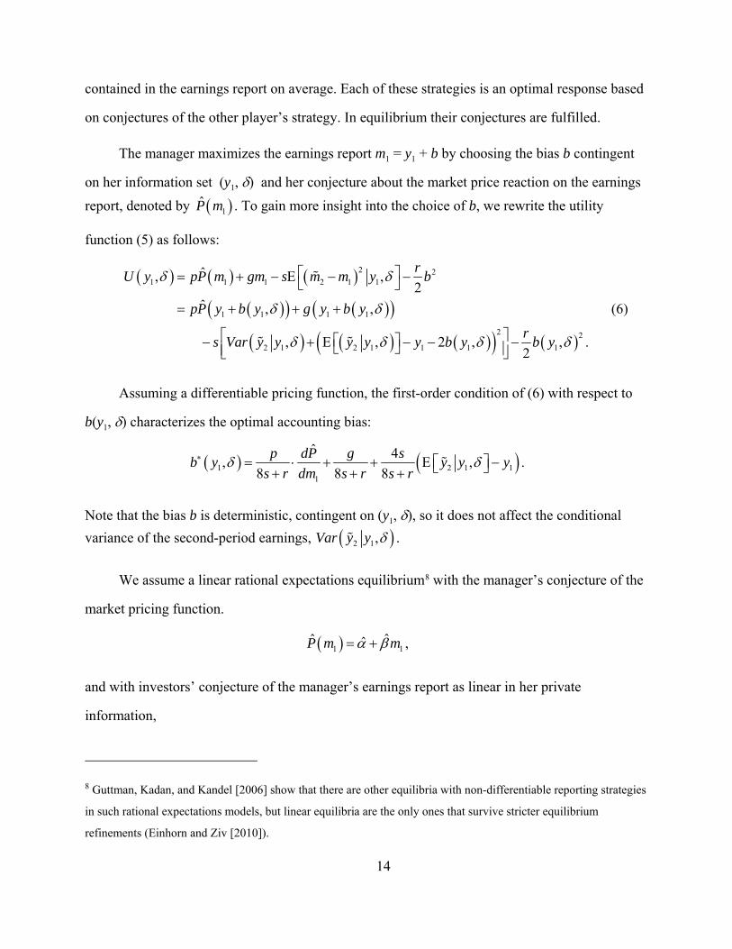
contained in the earnings report on average. Each of these strategies is an optimal response based

on conjectures of the other player’s strategy. In equilibrium their conjectures are fulfilled.

The manager maximizes the earnings report m1 = y1 + b by choosing the bias b contingent

on her information set (y1, δ) and her conjecture about the market price reaction on the earnings report, denoted by ( )1P m . To gain more insight into the choice of b, we rewrite the utility

function (5) as follows:

( ) ( ) ( )

( )( ) ( )( )

( ) ( ) ( )( ) ( )

2 21 1 1 2 1 1

1 1 1 1

2 22 1 2 1 1 1 1

ˆ, ,2

ˆ , ,

, , 2 , , .2

rU y pP m gm s m m y b

pP y b y g y b y

rs Var y y y y y b y b y

δ δ

δ δ

δ δ δ δ

⎡ ⎤= + − Ε − −⎣ ⎦

= + + +

⎡ ⎤⎡ ⎤− + Ε − − −⎣ ⎦⎢ ⎥⎣ ⎦

%

% %

(6)

Assuming a differentiable pricing function, the first-order condition of (6) with respect to

b(y1, δ) characterizes the optimal accounting bias:

( ) ( )1 2 1 11

ˆ 4, ,8 8 8

p dP g sb y y y ys r dm s r s r

δ δ∗ = ⋅ + + Ε ⎡ ⎤ −⎣ ⎦+ + +% .

Note that the bias b is deterministic, contingent on (y1, δ), so it does not affect the conditional variance of the second-period earnings, ( )2 1,Var y y δ% .

We assume a linear rational expectations equilibrium8 with the manager’s conjecture of the

market pricing function.

( )1 1ˆˆ ˆP m mα β= + ,

and with investors’ conjecture of the manager’s earnings report as linear in her private

information,

8 Guttman, Kadan, and Kandel [2006] show that there are other equilibria with non-differentiable reporting strategies

in such rational expectations models, but linear equilibria are the only ones that survive stricter equilibrium

refinements (Einhorn and Ziv [2010]).

15

1ˆ ˆ ˆ ˆˆb g yξ τ ϕ γδ= + + + .

The next result shows the existence of a unique linear equilibrium and characterizes the

optimal reporting strategy.

Proposition 1: There exists a unique linear equilibrium in which the manager reports earnings

( ) ( ) ( )*1 1 1 1 1, , 1 4m y y b y Q Qy sR pR gRδ δ μ δ β∗= + = − + + + + . (7)

The equilibrium market price is ( )1 1P m mα β= + where

( ) 21 pR gRα μ β β β≡ − − − (8)

and

( )

( )( )

2 21

2 2 2 2 2 2 21

,0

n g

Cov x mQ ZVar mQ Z R

ε δ

ε δ

σ σβσ σ σ σ

+≡ = >

+ + +

% %

%. (9)

The proof is in the appendix. R, Z, and Q are positive constants that be used throughout the

paper to save notation R and Z collect smoothing incentives and the cost of earnings

management,

18

Rs r

≡+

and 4 48

sZ sRs r

≡ =+

.

Since s and r are greater or equal to zero, Z ∈ [0, 1/2]. Q also includes variance terms and is

defined as

2

2 2

41 18

nn

n

sQ ZSs r ε

σσ σ

≡ − ⋅ = −+ +

,

where 2

2 2n

nn

Sε

σσ σ

≡+

. Since Sn ∈ (0, 1), the range of Q is (1/2, 1].

16

3.2. Properties of the equilibrium strategies

Proposition 1 shows that b* is a linear function of y1 and δ, and that the market price is a

linear function of m1, thus confirming the conjectures. We now discuss the properties of the

equilibrium strategies. The equilibrium bias is

( ) ( )1 1, n nb y S Zy Z S Z p R gRδ δ μ β∗ = − + + + + . (10)

A first observation is that the equilibrium generally entails a biased earnings report.9

The bias b* is negatively related to y1 so that b* smoothes the “shock” of y1 over the two

periods. It does so with a weight SnZ that lies between 0 and 1/2. To understand why, assume the

special case that earnings management is costless (r = 0). The manager wants to smooth the

reported earnings over the two periods (s > 0). Since y1 is the best estimate for 2y% (and for x% ),

she would want to include as much of the “permanent” component in y1, that is the operating risk

component ε, into the earnings report. If y1 measures ε without noise, i.e., 2 0nσ = , then Sn = 0 and

the equilibrium earnings *1m fully includes y1.10 Conversely, if y1 is a very noisy measure of ε,

then most of the variation in y1 is due to the realization of n% , which is transitory and does not

affect 2y% . If 2nσ →∞ then Sn → 1, and since Z = 1/2, the weight on y1 is SnZ = 1/2, which implies

an equal spread of the transitory component over the two periods. In more general situations, Sn

lies between 0 and 1 and its exact value depends on the relative precision of the permanent (ε% )

and the transitory ( n% ) components. The weight (1 – Sn) is the earnings response coefficient if y1

was unaffected by incentives and the private information δ of the manager. Finally, if earnings

management becomes increasingly costly (higher r), then Z decreases and a lower share of the

transitory component in y1 is shifted to the second-period earnings.

9 However, there exists a set of values (y1, δ) for which b* = 0.

10 The fixed effect μ that is carried in the signal y1 is adjusted with the same factor according to (10).

17

The earnings report *1m and the bias b* increase in the private information δ for a similar

reason, although there are two differences. First, the manager learns δ without noise, so no

correction (similar to Sn) applies. Second, y1 does not contain δ, whereas it is included in 2y% .

Therefore, smoothing requires anticipation of a share of δ in the first-period earnings, thus

increasing the bias. If earnings management is costless, then half of δ is shifted to period one, and

if it is costly, only a lower amount is shifted. The share is precisely Z, and therefore b* includes

Zδ.

The equilibrium bias strongly depends on the manager’s incentives. The market price

incentive is captured by the incentive parameter p on the first-period market price, P1. The

equilibrium bias is linear increasing in p at with a weight of pβR, which increases reported

earnings in the first period. The weight depends on the smoothing incentive s, the cost of earnings

management r, and on β, which is determined by the capital market reactions to a shift in

earnings in equilibrium. We discuss β below. The earnings incentive g has a similar, but more

direct effect on the equilibrium bias. The bias increases linearly in g with a weight of R. The

capital market corrects for the bias by deducting the market price incentive and the expected

earnings biases in the fixed term α.

A crucial effect on the bias stems from the manager’s smoothing incentive, s. For example,

assume s → 0, then Z → 0 and the bias only depends on the last terms,

( )1 0, sp gb y

r rβδ∗

→ = + .

For s → 0 β approaches 1 – Sn > 0, therefore, b* → p(1 – Sn)/r + g/r is a positive constant that

decreases in the cost of bias. Moreover, the bias becomes completely uninformative about the

private information of the manager.

The sole effect of the cost of earnings management r is to somewhat dampen the bias that is

induced by the other incentives. It is not itself a source for bias.

18

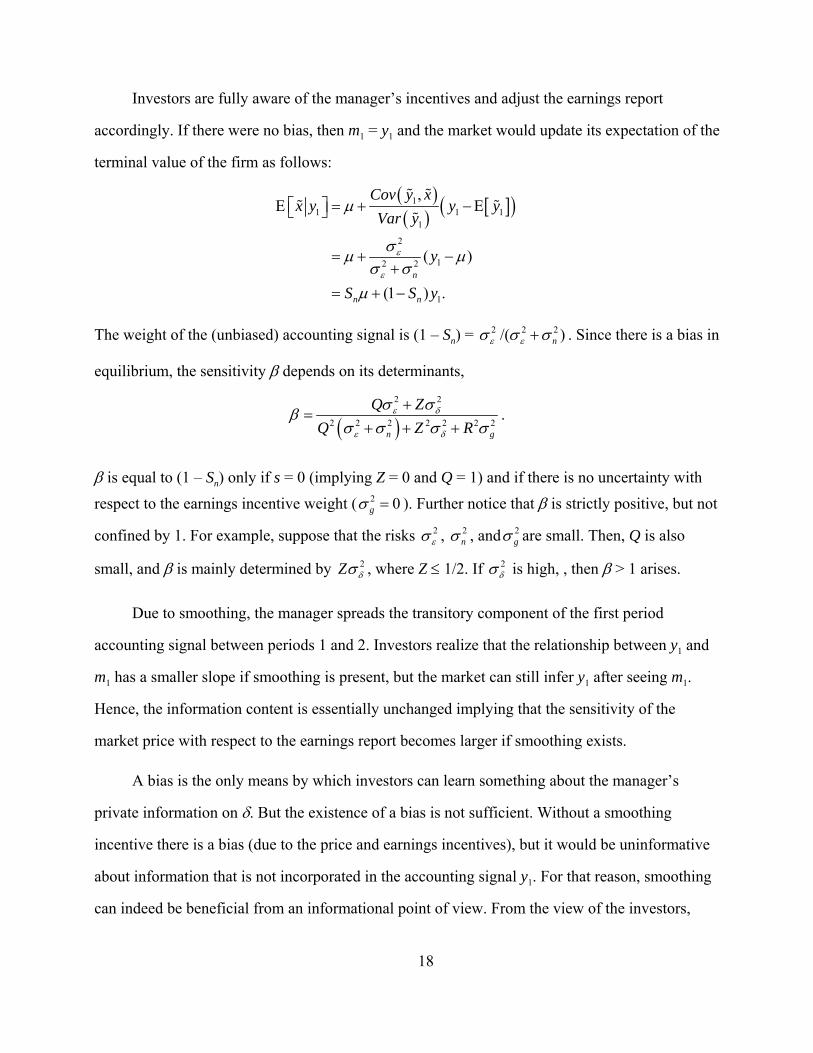
Investors are fully aware of the manager’s incentives and adjust the earnings report

accordingly. If there were no bias, then m1 = y1 and the market would update its expectation of the

terminal value of the firm as follows:

( )( ) [ ]( )1

1 1 11

2

12 2

1

,

( )

(1 ) .n

n n

Cov y xx y y y

Var y

y

S S y

ε

ε

μ

σμ μσ σ

μ

Ε ⎡ ⎤ = + −Ε⎣ ⎦

= + −+

= + −

% %% %

%

The weight of the (unbiased) accounting signal is (1 – Sn) = 2 2 2/( )nε εσ σ σ+ . Since there is a bias in

equilibrium, the sensitivity β depends on its determinants,

( )

2 2

2 2 2 2 2 2 2n g

Q ZQ Z R

ε δ

ε δ

σ σβσ σ σ σ

+=

+ + +.

β is equal to (1 – Sn) only if s = 0 (implying Z = 0 and Q = 1) and if there is no uncertainty with respect to the earnings incentive weight ( 2 0gσ = ). Further notice that β is strictly positive, but not

confined by 1. For example, suppose that the risks 2εσ , 2

nσ , and 2gσ are small. Then, Q is also

small, and β is mainly determined by 2Z δσ , where Z ≤ 1/2. If 2δσ is high, , then β > 1 arises.

Due to smoothing, the manager spreads the transitory component of the first period

accounting signal between periods 1 and 2. Investors realize that the relationship between y1 and

m1 has a smaller slope if smoothing is present, but the market can still infer y1 after seeing m1.

Hence, the information content is essentially unchanged implying that the sensitivity of the

market price with respect to the earnings report becomes larger if smoothing exists.

A bias is the only means by which investors can learn something about the manager’s

private information on δ. But the existence of a bias is not sufficient. Without a smoothing

incentive there is a bias (due to the price and earnings incentives), but it would be uninformative

about information that is not incorporated in the accounting signal y1. For that reason, smoothing

can indeed be beneficial from an informational point of view. From the view of the investors,

19

however, reported earnings are no longer a precise indicator of the underlying accounting signal

y1 as they are now mingled with the additional information δ and its interpretation is difficult because of the incentive risk 2

gσ . The combined effect determines the quality of earnings.

4. Earnings quality

In this paper, we adopt a pure decision-usefulness perspective of financial reports: Earnings

are of higher quality the more information they contain with respect to the terminal value x% of

the firm. The following definition of earnings quality arises naturally in this setting:11

Definition: Earnings quality EQ is the reduction of the market’s uncertainty about the terminal

value due to the earnings report in period 1, formally:

( ) ( )1 .EQ Var x Var x m≡ −% % (11)

A greater EQ implies higher earnings quality.12 Our definition is similar to that in Francis, Olsson

and Schipper [2008] and equivalent to that used in Marinovic [2010] as applied to our setting.

Since

( ) ( ) ( )( )

21

11

,Cov x mVar x m Var x

Var m= −

% %% %

%

EQ can equivalently be written as

( )( )

21

1

,.

Cov x mEQ

Var m=

% %

% (12)

11 In order to save notation, we use b and m1 for the equilibrium values and drop the (y1, δ) dependencies in the

analysis if there is no confusion.

12 An alternative would be to define EQ as the proportion of the reduction in the variance of the terminal value over

the prior variance. Since the denominator is independent from incentives and the accounting precision, an ordering

based on this measure would result in similar results.

20

Upon the release of the earnings report, investors revise their expectation of the terminal value to P1 = 1E x m⎡ ⎤⎣ ⎦% . EQ does not directly capture the level of the price reaction but considers

the distribution of the posterior market price relative to that of the previous price.

Although not obvious from the above definition, EQ is based on an equilibrium notion,

which takes appropriate account of the manager’s incentives for earnings management, rational

expectations by investors, and the information content of earnings. Thus, EQ is determined by

several exogenous and endogenous factors that interact in a complex way. The next proposition

records the properties of EQ with respect to variations in the determining factors.

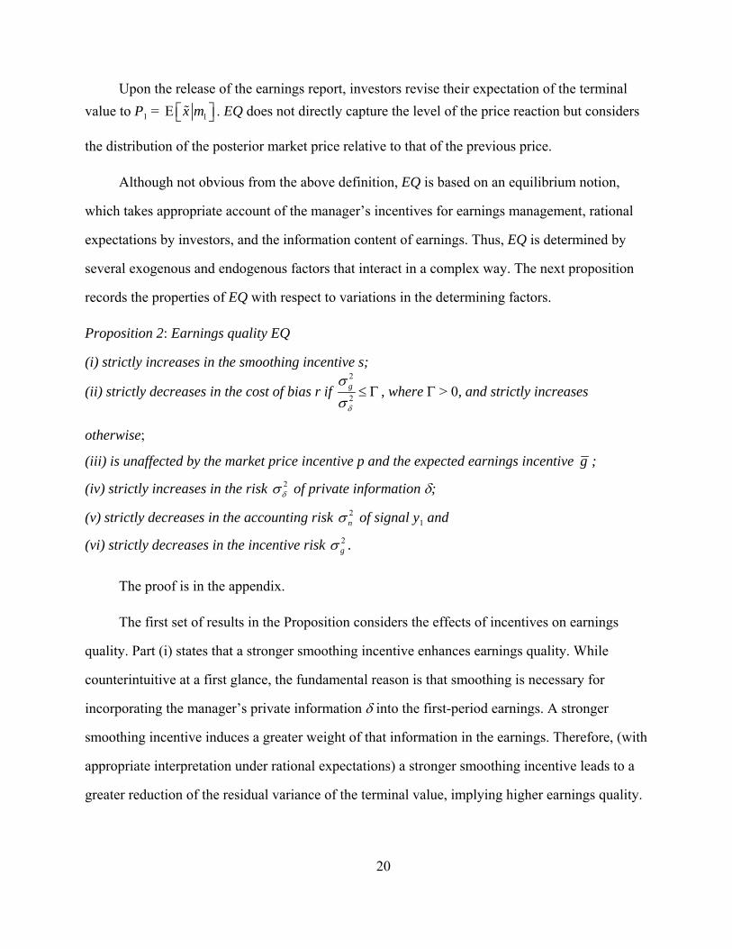
Proposition 2: Earnings quality EQ

(i) strictly increases in the smoothing incentive s;

(ii) strictly decreases in the cost of bias r if 2

2g

δ

σσ

≤ Γ , where Γ > 0, and strictly increases

otherwise;

(iii) is unaffected by the market price incentive p and the expected earnings incentive g ;

(iv) strictly increases in the risk 2δσ of private information δ;

(v) strictly decreases in the accounting risk 2nσ of signal y1 and

(vi) strictly decreases in the incentive risk 2gσ .

The proof is in the appendix.

The first set of results in the Proposition considers the effects of incentives on earnings

quality. Part (i) states that a stronger smoothing incentive enhances earnings quality. While

counterintuitive at a first glance, the fundamental reason is that smoothing is necessary for

incorporating the manager’s private information δ into the first-period earnings. A stronger

smoothing incentive induces a greater weight of that information in the earnings. Therefore, (with

appropriate interpretation under rational expectations) a stronger smoothing incentive leads to a

greater reduction of the residual variance of the terminal value, implying higher earnings quality.

21

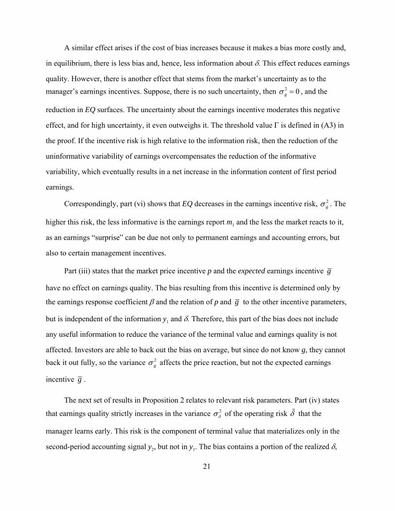
A similar effect arises if the cost of bias increases because it makes a bias more costly and,

in equilibrium, there is less bias and, hence, less information about δ. This effect reduces earnings

quality. However, there is another effect that stems from the market’s uncertainty as to the manager’s earnings incentives. Suppose, there is no such uncertainty, then 2 0gσ = , and the

reduction in EQ surfaces. The uncertainty about the earnings incentive moderates this negative

effect, and for high uncertainty, it even outweighs it. The threshold value Γ is defined in (A3) in

the proof. If the incentive risk is high relative to the information risk, then the reduction of the

uninformative variability of earnings overcompensates the reduction of the informative

variability, which eventually results in a net increase in the information content of first period

earnings.

Correspondingly, part (vi) shows that EQ decreases in the earnings incentive risk, 2gσ . The

higher this risk, the less informative is the earnings report m1 and the less the market reacts to it,

as an earnings “surprise” can be due not only to permanent earnings and accounting errors, but

also to certain management incentives.

Part (iii) states that the market price incentive p and the expected earnings incentive g

have no effect on earnings quality. The bias resulting from this incentive is determined only by

the earnings response coefficient β and the relation of p and g to the other incentive parameters,

but is independent of the information y1 and δ. Therefore, this part of the bias does not include

any useful information to reduce the variance of the terminal value and earnings quality is not

affected. Investors are able to back out the bias on average, but since do not know g, they cannot back it out fully, so the variance 2

gσ affects the price reaction, but not the expected earnings

incentive g .

The next set of results in Proposition 2 relates to relevant risk parameters. Part (iv) states

that earnings quality strictly increases in the variance 2δσ of the operating risk δ% that the

manager learns early. This risk is the component of terminal value that materializes only in the

second-period accounting signal y2, but not in y1. The bias contains a portion of the realized δ,

22

and the higher the variance of δ% , the lower the residual variance after information about the

realization is received.

Part (v) states that earnings quality strictly decreases in the noise 2nσ in the accounting

signal y1. The higher this noise, the less informative is the signal about the underlying operating

risk ε, which is the information in the earnings report that is of interest to investors when

updating their expectations. Therefore, a less precise accounting signal reduces earnings quality.

Proposition 2 and the subsequent results do not record results on a change in the operating risk ε%

because it has the reverse effect of the accounting noise n% .

A practical difficulty with EQ is that it cannot be empirically estimated directly because x%

is not observable. However, in our equilibrium structure, EQ can be expressed in terms of

observables13 because

( )( )

( )( ) ( ) ( )

221 1 2

1 11 1

, ,Cov x m Cov x mEQ Var m Var m

Var m Var mβ

⎛ ⎞≡ = =⎜ ⎟⎜ ⎟

⎝ ⎠

% % % %% %

% %,

where ( )( )

1

1

,Cov x mVar m

β ≡% %

% is the earnings response coefficient (and our value relevance metric that

we examine below). Since ( ) ( )( ) ( )1 1 1 1 1, ,Cov m P Cov m m Var mα β β= + =%% % % % in equilibrium, β can

be expressed as

( )( )

1 1

1

,.

Cov m P

Var mβ =

%%

%

Thus, in an empirical study the product of the square of the coefficient β (resulting from

regressing price on earnings) and the earnings variance captures the reduction of the market’s

uncertainty with respect to firm value.

13 We thank Jeremy Bertomeu for suggesting this point.

23

5. Analysis of earnings quality metrics

Our earnings quality measure EQ provides a benchmark for evaluating the behavior of

commonly used metrics for earnings quality (or earnings attributes). The closer the behavior of a

particular metric is in line with that of EQ upon a variation of a determining factor of earnings

quality, the more appropriate is its use in empirical studies.

In this section we study metrics that are commonly used as proxies for earnings quality in

the empirical accounting literature.14 We begin with value relevance, which is a metric that uses

accounting information and market prices, and continue with metrics that rely solely on

accounting information, namely, persistence, predictability, smoothness, and accrual quality. We

define each of these metrics within the confines of our model and examine their behavior for a

variation in the factors that determine earnings quality, incentives (s, p, g , and r), private

information ( 2δσ ), accounting risk ( 2

nσ ), and incentive risk ( 2gσ ), and then we compare this

behavior with that of EQ.

We do not examine metrics such as conservatism or distributional properties of earnings

because our model is not specified so as to capture such metrics. Conditional conservatism

introduces a non-linearity that does not fit our linear framework. For example, a metric that uses

the asymmetric timeliness for positive and negative market returns introduces a “kink” in the

market reaction function. Metrics that examine earnings distributions, such as loss avoidance, are

based on deviations from normal distributions that we assume throughout the analysis.

5.1. Value relevance

Value relevance captures the notion that earnings are of high quality if they are capable to

explain the firm’s market price and/or market returns. The literature employs several approaches,

14 For a survey see, e.g., Dechow, Ge, and Schrand [2010].

24

most of which can be classified according to Holthausen and Watts [2001] into two categories.15

One set are relative association studies, which focus on the R2 from a regression of the market

price and/or return on earnings (and potentially other accounting variables). Another set,

incremental association studies, concentrate on the ability of a specific accounting item (e.g.,

earnings, book value) to explain market value or return. This category uses the estimated

regression coefficient.

We begin with the incremental association and define value relevance as the slope

coefficient from a regression of the market price (or return) on reported earnings,

( )( ) ( )

2 21

2 2 2 2 2 2 21

,.

n g

Cov x m Q ZVar m Q Z R

ε δ

ε δ

σ σβσ σ σ σ

+= =

+ + +

% %

%

This metric is often referred to as earnings response coefficient. A greater β indicates higher

earnings quality.

The value relevance β is closely related to our earnings quality measure EQ because from

(12) we have

( )1,EQ Cov x mβ= % % .

The next proposition shows that the behavior of β and EQ on variations of the determining

factors is similar, but not fully aligned.

Proposition 3: Value relevance β (i) strictly increases in the smoothing incentive s if ( )2 2 2n nSδσ σ≤ − . Otherwise, if 2

δσ is

sufficiently large, then β is inversely u-shaped in s;

(ii) (1) strictly decreases in the cost of bias r if 2

2g

δ

σσ

≤ Γ and either 2 2nSδ εσ σ≤ or both

15 In their survey, Holthausen and Watts [2001] mention a third category of value relevance studies, which they refer

to as “marginal information content studies.”

25

( ) ( )( )2 2 2 2 2 2 22 and 16 2n n n g n nS S s Sε δ δσ σ σ σ σ σ≤ ≤ − ≤ − − − hold. (2) β strictly increases if 2

2g

δ

σσ

> Γ and 2 2nSδ εσ σ> . (3),If 2

δσ is sufficiently large, then β is inversely u-shaped in r;

(iii) is unaffected by the market price incentive p and the expected earnings incentive g ;

(iv) strictly increases in the risk 2δσ of private information δ;

(v) strictly decreases in the accounting risk 2nσ of signal y1; and

(vi) strictly decreases in the incentive risk 2gσ .

The proof is in the appendix. Parts (iii), (iv) and (v) state that the market price and expected

earnings incentives p and g , the operating risk 2δσ and the accounting risk 2

nσ induce the same

ordering of earnings quality as does EQ. The difference lies in the first two parts that consider

changes in the smoothing incentive s and in the cost of bias r. Proposition 3 provides a sufficient condition on the risk terms, ( )2 2 2n nSδσ σ≤ − , so that β and EQ move in the same direction.

However, it also states that for large 2δσ , value relevance β decreases for an increasingly strong

smoothing incentive while EQ always increases.

The sufficient condition

( )2 2 2n nSδσ σ≤ − , (13)

where (2 – Sn) > 1, is satisfied if the information content of δ% is not much higher than the noise

in the accounting system. A large variability of the private information δ% implies that the

covariance between the earnings report 1m% and the terminal value x% increases for a larger

smoothing incentive since the manager injects a higher proportion of the signal into the reported

earnings, so these earnings covary stronger with the terminal value. On the other hand, the

earnings variance initially decreases in s because of the lower impact of the accounting risk on

26

the earnings variability16 and the only moderately increasing effect of δ. However, the greater the

smoothing incentive, the more 2δσ determines the earnings variance; and if 2

δσ is large enough,

then the variability of earnings may increase for sufficiently high smoothing incentives. This

effect works against the market response to the earnings report, which can ultimately lead to a

reduced value relevance for high values of s. The same reasoning applies for the effect of an

increase in the cost of bias r.

The second deviation from the behavior of EQ is in the effect of varying the cost of bias r.

As discussed in Proposition 2, EQ strictly decreases in r if

2

2g

δ

σσ

≤ Γ , (14)

and strictly increases otherwise. Γ > 0 is defined in (A3) in the appendix. The behavior of value

relevance β is broadly similar, although additional conditions apply for conforming effects.

Proposition 3 states three sufficient conditions for a specific behavior of β on a change in r.

These conditions are determined by the relative values of the operating risks 2εσ and 2

δσ and

accounting risk 2nσ . They are also reminiscent of the condition that also appears in part (i) of the

Proposition, ( )2 2 2n nSδσ σ≤ − , for a similar reason. Therefore, the relationship of EQ and β

cannot be stated unambiguously.

It is instructive to consider the special case when the manager does not have private

information about δ% ( 2δσ = 0) and there is no market uncertainty about the earnings incentive

( 2gσ = 0). Value relevance β then becomes

( )

2

2 2 2

1 n

n

Q SQQ

ε

ε

σβσ σ

−= =

+.

16 Recall that, due to smoothing, the manager attempts to smooth the contemporaneous shock in the firm’s earnings

across the two periods, thus lowering the portion of variability in first-period reported earnings that results from the

noise inherent in the accounting system.

27

Since Q strictly decreases in s and strictly increases in r, β strictly increases in s and strictly

decreases in r. The reason is that the capital market adjusts for the bias that is induced by the

manager’s incentives. In contrast, EQ does not change with varying s or r in the case of 2δσ = 0

and 2 0gσ = . Note that

2 42

11 12 2 2

1

( , )( ) ( ) ( ) ( )( ) ( )n

QCov x mVar x m Var x Var x Var x yVar m Q

ε

ε

σσ σ

= − = − =+

% %% % % %

%.

Therefore, the information content of m1 (absent δ and 2gσ = 0) does not vary with incentives, and

so the earnings quality EQ does not vary either. As Proposition 3 states, this is a limiting case as

for small 2δσ > 0 the direction of the effects become aligned. However, caution should be taken in

interpreting the value relevance as a cardinal metric of earnings quality.

Relative association studies use the R2 as measure of value relevance. Our linear

equilibrium yields an R2 which always equals 1 because reported earnings are the sole

information source for the market and R2 is the correlation coefficient between the market price

and the reported earnings.17 However, there is a close connection of R2 with β. To see this, we

briefly consider a slight extension of the price formation. Suppose the market price includes a

stochastic term ν% , for example due to liquidity or noise trading,

1P x m ν= Ε ⎡ ⎤ +⎣ ⎦ %% %

where ν% is normally distributed with mean zero and independent from the other random

variables.

17 This is because R2 is the correlation coefficient between the market price and the reported earnings, ( )

( ) ( )( )

( ) ( )1 1

1 11

,1.

Cov P m Var mStd m Std mStd m Std P

ββ

= =% % %

% % %%See Lev [1989] for a linear model based on changes of variables (stock

price revisions and unexpected reported earnings). It also applies for the levels version since the a priori stock price

and expectations are given and irrelevant for the correlation coefficient.

28

Corollary: Let the market price be 1P x m ν= Ε ⎡ ⎤ +⎣ ⎦ %% % . Then the R2 from regressing market returns

on earnings is strictly increasing in EQ.

Proof: R2 is defined as

( )( ) ( )

( )( ) ( )

( )( ) ( )

( )( )

( )( )( )( )

1 1 1 12

1 1 1 11

211

2 21 1

2

, ,

.

Cov P m Cov m m Var mR

Std m Std m Std m Std mStd m Std P

Var mStd mStd m Var m

EQEQ

ν

ν

α β ν βα β ν α β ν

ββα β ν β σ

σ

+ += = =

+ + + +

= =+ + +

=+

% % %% % %

% % %% % % %%

%%

%% %

(q.e.d.)

This expression shows that R2 is monotone in EQ given the price volatility is caused by

noise trading. This result is even stronger than the results we report in Proposition 3 for the

earnings response coefficient β, which is closely aligned with EQ.

5.2. Persistence

Persistence measures the extent current earnings persist or recur in the future. High

persistence is regarded a desirable earnings attribute by investors, and of high earnings quality,

since it suggests a stable, sustainable and low-risk earnings process. Accounting standards may

support the persistence by separating recurring from non-recurring items; firms often disclose pro

forma earnings that do not include non-recurring or special items, and analysts often eliminate

certain items that they believe are not persistent.

Persistence is commonly estimated by the slope coefficient from a regression of current

earnings on lagged earnings (or, sometimes, components of lagged earnings, such as cash flows

and accruals). In our setting, we use the slope coefficient from regressing expected second-period

earnings 2m% on first-period earnings m1, which is tantamount to an “earnings relevance

29

coefficient” that shows how expected second-period earnings are affected by first-period

earnings.18 Since

[ ] ( )( ) [ ]( )1 2

2 1 2 1 11

,Cov m mm m m m m

Var mΕ ⎡ ⎤ = Ε + ⋅ −Ε⎣ ⎦

% %% % %

%,

we define persistence PS as

( )( )

1 2

1

,Cov m mPS

Var m≡

% %

%.

A greater persistence PS is supposed to indicate higher earnings quality. Rewriting PS yields (see

the proof of Proposition 4 in the appendix)

( )

( )

2 2

1

1.nQPS

Var mεσ σ

β+

≡ + −%

This shows that PS is a metric that augments the value relevance β by an additional term that results from the impact of smoothing on the time series of earnings. Note that if s = 0 and 2

gσ

= 0, then Q = 1 and 1 1( ) ( )Var m Var y=% % , so that the additional term vanishes and PS = β. The

additional term in the definition of PS can be either positive or negative. For example, if 2δσ

becomes sufficiently large, the second term in the PS equation is less than 1, thus implying

PS < β.

The term 2 21( ) / ( )nQ Var mεσ σ+ % adds some complexity to the behavior of PS with respect to

the determining factors. For example, whereas β increases in 2δσ , this term decreases; similarly, β

decreases in the accounting risk 2nσ , but the additional term increases.19 However, the next

proposition shows that for many cases, the effect resulting from β dominates the other effect, so

18 While this definition may appear as being a two-period metric, it is based strictly on information available in

period 1, because it uses the expectation of m2 conditional on m1.

19 This can be verified by differentiating the new term with respect to the accounting noise.

30

the net effect is often not very different from that of β (as stated in Proposition 3). Proposition 4

provides the results.

Proposition 4: Persistence PS (i) strictly increases in the smoothing incentive s if ( )2 2 2n nSδσ σ≤ − . Otherwise, if 2

δσ is

sufficiently large, then PS is inversely u-shaped in s; (ii) is inversely u-shaped in r if ( )1 2, 0Cov m m ≥% % and ( )( ){ }2 2 2 2max 0; 16 2g n ns Sδσ σ σ> − − − .

Otherwise, the effect is ambiguous and depends on the specific parameters;

(iii) is unaffected by the market price incentive p and the expected earnings incentive g ;

(iv) strictly increases in the risk 2δσ of private information δ; and

(v) strictly decreases in the accounting risk 2nσ of signal y1 for 2

gσ ≤ Λ , first strictly decreases

and then increases in 2nσ for 2

gσΛ < ≤ Λ , and strictly increases in 2nσ for 2

gσΛ < ; and

(vi) strictly decreases in the incentive risk 2gσ .

The proof is in the appendix. Persistence PS behaves similarly to value relevance β for

changes in the smoothing parameter, market price and earnings incentives, information risk, and

incentive risk.

Differences occur for changes in the cost of bias r and of the precision of the accounting

system (accounting risk 2nσ ). Note that persistence is the covariance of earnings in the two

periods over the variance of first-period earnings. As shown in detail in the proof,

1 2( , )Cov m m% % first increases and then decreases in r. The variance 1( )Var m% strictly increases in r,

but for large 2gσ it first decreases and then increases. The total effect of 1 2( , )Cov m m% % / 1( )Var m% is

ambiguous. The Proposition gives a sufficient condition for PS to be inversely u-shaped in r if ( )1 2, 0Cov m m ≥% % and ( )( ){ }2 2 2 2max 0; 16 2g n ns Sδσ σ σ> − − − . But it also implies that persistence

PS can be negative in equilibrium because the covariance ( )1 2, 0Cov m m <% % can become negative

for low r. In any case, the behavior is distinctly different from that of EQ.

Another difference occurs for changes in the accounting risk 2nσ . The effect depends on the

uncertainty of investors with respect to the manager’s earnings incentive 2gσ : For low uncertainty,

31

persistence strictly decreases; for intermediate uncertainty, it is u-shaped; and for high

uncertainty it strictly increases in 2nσ . The thresholds are defined in the proof of the Proposition.

Notice that EQ and β always strictly decrease in accounting risk. Persistence shows the same effect only for low incentive risk. Otherwise, persistence can increase, because for large 2

gσ , the

covariance is negative as m1 and m2 move in opposite directions if bias is added due to the

accounting incentive. Moreover, the resulting noise is completely unrelated to the operating risk

of the firm. Therefore, an increase in the accounting risk 2nσ raises the importance of the

accounting signal relative to the accounting incentive g, so that the (negative) covariance

increases.

5.3. Predictability

Predictability encompasses the notion that earnings are of high quality the more useful they

are to predict itself. Similar to persistence, predictability is generally viewed as a desirable

attribute of earnings because it reduces the variability of forecasts of earnings. There are several

ways to empirically estimate predictability. One is using the same regression of current earnings

on lagged earnings, as for estimating persistence, but taking R2 as the proxy for predictability.

Another way is taking the standard deviation of the residuals from the same regression.

We use the variance of second-period earnings 2m% conditional on the earnings report in the

first period m1, that is, ( )2 1Var m m% . A lower conditional variance implies that investors have

more precise information for forecasting second-period earnings. To retain the convention that a

higher value of the metric is indicative of higher earnings quality, we define predictability PD as

the negative value of the conditional variance of second-period earnings 2m% , that is,

( )2 1 .PD Var m m≡ − %

Rewriting PD (see the proof of Proposition 5) shows its close relationship to persistence PS:

32

( ) ( )

( )( ) ( ) ( ) ( )

21 2

21

221 2 1

,

2 1 .

Cov m mPD Var m

Var m

Var y Var y PS Var mεσ

− = −

= + + − +

% %%

%

% % %

(15)

This expression shows that the persistence PS is a main driver of predictability, as it

captures the bias in both earnings reports, which is driven by incentives and the additional

information δ% . However, accounting risk 2nσ and operating risk 2

δσ are also included in the

variance terms ( )1Var y% , ( )2Var y% , and ( )1Var m% . Therefore, the behavior of PD is not directly

apparent. The next proposition establishes the effects of a variation of the determining factors on

PD.

Proposition 5: Predictability PD

(i) strictly increases in the smoothing incentive s;

(ii) strictly decreases in the cost of bias r if ( )2 2 2 11 2 n nSZδ εσ σ σ ⎛ ⎞< + + −⎜ ⎟

⎝ ⎠. Otherwise, if the

incentive risk 2gσ is sufficiently large, then PD strictly increases in r;

(iii) is unaffected by the market price incentive p and the expected earnings incentive g ;

(iv) decreases in the risk 2δσ of private information δ;

(v) strictly decreases in the accounting risk 2nσ of signal y1; and

(vi) strictly decreases in the incentive risk 2gσ .

The proof is in the appendix. Comparing these results with those obtained for EQ in

Proposition 2, we find that predictability PD corresponds with EQ except for part (ii), where the

conditions for a decrease or increase differ, and for part (iv), which states a converse relationship

for the risk of private information δ% . But as shown in the proof, the effects that lead to this

correspondence differ somewhat in the details.

To explain the results in the proposition, note that a higher smoothing incentive s leads to a

greater incorporation of the manager’s private information into the bias and, hence, first-period

earnings. In the second period, the same information is included in the accounting signal m2,

33

although somewhat dampened by the reversal of the bias. Therefore, the precision with which the

second-period earnings can be predicted increases with higher smoothing incentives. Second, a

change in the market price incentive p and the earnings incentive g have no effect since in this

model the market can undo its effect on the bias. A higher magnitude of the accounting risk 2nσ

increases the conditional variance of second-period earnings 2m% since the variability of the bias

in the first period also increases with accounting risk, and the same variability increases the

variance of second-period earnings due to the clean surplus condition on the bias.

An increase in the cost of bias r decreases predictability due to its lower incorporation of

the manager’s private information δ as long as the private information is not large (low 2δσ ).

Otherwise, if the incentive risk 2gσ becomes large, this effect is inverted and predictability

increases in higher cost r because the high cost dampens the effect of the earnings incentive on

the earnings report.

Perhaps surprisingly, the behavior of PD for a variation of the risk 2δσ is opposite from that

of EQ. The reason is that 2δσ also appears as a direct component in PD because it is embedded in

the second-period accounting signal m2 and, hence, in the variance 2( )Var y% . This is due to the

fact that δ% stands for information risk, but also for operating risk that is resolved in the second

period. Whereas the earlier metrics do not pick up the operating risk effect, predictability does.

Hence, a larger operating risk increases the variance of 2m% , which is not outweighed by the

effects of the information transfer that influences the conditional variance of 2m% . Therefore,

using predictability PD would lead to a wrong conclusion on earnings quality for a variation of

private information held by the manager and embedded in the bias.

5.4. Smoothness

The smoothness of earnings can be considered either as a favorable or an unfavorable

earnings attribute. Consistent with persistence and predictability, a smoother earnings series is

less volatile and allows for better forecasting. For example, managers can use their private

34

information to smooth out nonrecurring effects. Smoothness is then the converse of volatility and,

therefore, smoother earnings are indicative of higher earnings quality. On the other hand,

smoothness can be considered as reducing the information content in earnings and mask the

firm’s “true” performance. Under this view, smoothness is a measure for earnings management,

and since earnings management is considered undesirable, smoother earnings are associated with

a lower earnings quality. An advantage of the equilibrium model is that we can identify which

interpretation is more appropriate in our setting.

Empirical studies use various metrics for smoothness. One metric is the ratio of the

standard deviation of earnings and the standard deviation of operating cash flows. Our model

does not include a periodic cash flow process and, therefore, we do not employ this metric.

Another metric uses the fact that smoothness implies a negative correlation between the change

in accounting accruals and the change in operating cash flows. A stronger (negative) correlation

indicates greater smoothness. A related metric is the correlation between the change in

discretionary accruals and the change in pre-discretionary income.20 We use the variables

themselves and not their changes, as we have no period 0 values and are interested only in

relative changes upon varying parameters. We define our metric for smoothness, SM, as the

negative correlation between discretionary accruals, which is the bias b, and pre-discretionary

earnings, which is our accounting signal 1y% , that is,

( ) ( )( ) ( )

11

1

,, .

Cov b ySM Corr b y

Std b Std y≡ − = −

% %% %

% %

A higher SM implies greater smoothness. The following results obtain.

Proposition 6: Smoothness SM

(i) strictly increases in the smoothing incentive s;

20 See, e.g., Tucker and Zarowin [2006].

35

(ii) is unaffected by the cost of bias r;

(iii) is unaffected by the market price incentive p and the expected earnings incentive g ;

(iv) strictly decreases in the risk 2δσ of private information δ;

(v) strictly increases in the accounting risk 2nσ of signal y1; and

(vi) strictly decreases in the incentive risk 2gσ .

The proof is in the appendix. It shows that SM can be expressed as

( )1

2

2

4 2 2 2 22

.1

16

n

n g n

SM

sδ ε

σ

σ σ σ σ σ

=⎛ ⎞⎛ ⎞+ + +⎜ ⎟⎜ ⎟⎝ ⎠⎝ ⎠

From this equation, it is immediate that SM is unaffected by the market price incentive p, the

expected earnings incentive g , and the cost of bias r. A greater smoothing incentive induces an

increase in SM because the variance of the equilibrium bias decreases in 2gσ as a result of the

manager’s private knowledge of the importance of the earnings incentive. If there is no incentive risk ( 2

gσ = 0), then SM is independent of any incentive effects, but depends on the operating and

accounting risks only.

Therefore, this metric generally does not capture most incentives as a determining factor for

earnings quality and earnings management. Intuitively, these results obtain since SM is a

correlation coefficient that measures the degree of linear dependence between discretionary

accruals and pre-discretionary income. As our model studies linear equilibria with linear pricing

and reporting strategies, there is always a perfect linear relationship between the interesting

variables, which does not depend on the magnitude of p, g , and r. It captures smoothing

incentives similar to EQ only because the variance of the bias decreases in s.

Smoothness strictly decreases in the variance 2δσ of private information δ; and strictly

increases in the variance 2nσ of the accounting signal y1. Both effects are generally in contrast to

other metrics. Consider the dependence on 2δσ first. According to SM, a higher variability 2

δσ of

36

the private information δ decreases SM, which implies a lower smoothness. Even more striking is

the fact that increasing accounting risk 2nσ implies that SM always strictly increases.

These results are surprising not only because of the diametrically opposed conclusions that

are drawn on smoothness with respect to changes in factors that are important for earnings

quality, but also because it is not obvious whether more smoothing is an indicator of higher or

lower earnings quality. We discuss this observation in more detail later.

5.5. Accrual quality

Most of the metrics focus on the information content of earnings about the terminal value,

that is, about the operating risk components inherent in the terminal value. Only the smoothness

metric SM separately considers two components of reported earnings, the accounting signal y1

and the bias b. The bias is the accounting accrual, which is determined by the manager’s

incentives (earnings management), but also carries additional information. The accrual quality

specifically seeks to capture the quality of the accounting system, rather than the quality of the

accounting and the operating environment. The idea is that high accrual quality also proxies for

high earnings quality, holding the operating environment constant.

To estimate the accrual quality, many empirical studies employ a metric suggested by

Dechow and Dichev [2002], which is based on the standard deviation of the residuals from a

regression of working capital accruals on lagging, contemporaneous and leading operating cash

flows. This metric focuses on measurement errors in specific accruals. Our model is not

sufficiently specified to study this metric.

Another metric separates earnings into “normal” and discretionary (or “abnormal”)

accruals, based on some model that predicts “normal” accruals from other variables, e.g., based

on the Jones [1991] model. Accrual quality is estimated based on the statistical properties of the

discretionary accruals. In our setting, we directly use the accounting signal y1 as “normal”

accruals and the bias b as discretionary accruals. In an empirical study the econometrician must

37

estimate these “normal” accruals from other observables, which introduces noise in the estimate

and decreases the “quality” of the accrual metric relative to our model.21

This separation between “normal” and discretionary accruals is in line with the common

interpretation that discretionary accruals are the result of earnings management because our bias

is a consequence of the manager’s incentives; were there no incentives (p, s, g and r equal to

zero), the bias would be zero. Therefore, most literature considers high discretionary accruals as

indicating low accrual quality and, ultimately, low earnings quality. However, we note that the

bias is the carrier for the private information of the manager, so it cannot be considered as

necessarily indicating low earnings quality. This latter effect is more prominent as much of the

earnings management is backed out by the rational investors.

We define two different, but related, metrics for discretionary accruals. The first metric is

the negative expected value of the bias,

1DA b⎡ ⎤≡ −Ε ⎣ ⎦% .

We use the negative value to interpret DA1 in conformance with the notion that a larger value of

the metric indicates higher accrual quality and higher earnings quality.

A potential problem with this metric is that positive and negative realizations of the bias

cancel out in expectation. In the extreme, DA1 can remain constant although the bias is

significantly affected by a change in a determining factor, which affects the variance, but not the

expected value. Therefore, some studies use the expected value of the absolute amount of bias.

Since taking absolutes introduces a deviation from our linear setting, we define the second metric

for discretionary accruals as the negative expected value of the squared bias,

21 One may argue that if an econometrician is able to estimate discretionary accruals from observable data, then

investors can do so, too. Such an assumption can be included in our model by assuming that the market receives a

noisy signal of b in addition to the firm’s earnings. We conjecture that our results would qualitatively carry over to

such an extended model.

38

22DA b⎡ ⎤≡ −Ε ⎣ ⎦

% .

Again, a higher value of DA2 is supposed to indicate higher accrual quality and higher earnings

quality.

To see the behavior of the first accrual quality metric, DA1, it is instructive to write DA1 in

the following form:

( ) ( )1 11 18

p gDA Q Q y Z pR Rgs r

βμ δ β +⎡ ⎤= −Ε − + − + + + = −⎣ ⎦ +%% . (16)

Proposition 7: Assuming p > 0 and 0g > , accrual quality DA1

(i) strictly increases in the smoothing incentive s if β decreases (which occurs for

( )2 2 2n nSδσ σ> − and large s). Otherwise, the effect depends on the parameter values;

(ii) strictly increases in the cost of bias r if β decreases (see Proposition 3 (ii)). Otherwise, the

effect depends on the parameter values;

(iii) strictly decreases in the market price incentive p and the expected earnings incentive g ;

(iv) strictly decreases in the risk 2δσ of private information δ;

(v) strictly increases in the accounting risk 2nσ of signal y1;and

(vi)strictly increases in the incentive risk 2gσ .

If p < 0 and 0g < , the direction of the effects reverse.

To explain these results, note first that DA1 is affected by both the market price incentive p

and the expected earnings incentive g , whereas p and g are irrelevant for earnings quality EQ

as the market can completely adjust for it. For example, if the manager is particularly interested

in a high market price in the first period (p > 0), DA1 strictly decreases in p because higher p

increases the bias, which reduces the accrual quality metric. A similar reasoning holds for a

change in g . The direction of the effect of the other factors depends on whether the sum (βp +

g ) is positive or negative. For the following discussion, we assume p > 0 and (βp + g ) > 0;

otherwise, the results reverse.

39

To see the other effects, note that the behavior of DA1 is essentially determined by the

behavior of β, moderated by a base term gR . A general observation is that a higher value

relevance β is generally seen as indicative for high earnings quality, although we establish in

Proposition 3 that there are situations where higher β is associated with lower EQ. Since DA1

varies negatively with β, the effects of changes in the determining factors are reversed.

The effects of varying the private information 2δσ and accounting risk 2

nσ of signal y1

follow immediately from (16) because the other terms are not affected by these factors.

Therefore, accrual quality DA1 strictly decreases in 2δσ and strictly increases in 2

nσ , just the

opposite of most of the other metrics. The reason is that an increase in 2δσ increases the

informative bias (thus leading to an increase in value relevance), whereas an increase in 2nσ

reduces it, as there is less information content about the operating risk ε in the accounting signal

(implying a decrease in value relevance).

The behavior of DA1 is less obvious for variations of the smoothing incentive s and the cost

parameter r because they affect not only β but also the denominator (8s + r). The term 1/(8s + r)

= R decreases in s and r. The proposition records cases in which β also decreases in s or r,

because then DA1 is unambiguously increasing and accrual quality strictly increases. Proposition

7 (i) and (ii) essentially repeat the conditions for a decrease in β (see Proposition 3). These

conditions also imply that DA1 and β are affected in opposite directions (as long as p > 0 and (p +

g ) > 0). In other cases the effect of varying s and r is indeterminate. It is easy to find parameter

values for which the effect on DA1 is positive or negative. We do not record more conditions as

they would involve a combination of conditions on most of the determining factors, and no

general patterns emerge.

One special case is of interest, though. It is the case if the manager does not have private

information about δ% and there is no earnings incentive, which is equivalent to setting 2δσ = 0,

2gσ = 0, 0g = , and 2

gσ = 0. Then DA1 is determined by

40

( ) ( )

2

1 2 2 .8 4 n

pDAs r s r

ε

ε

σσ σ

= −+ + +

In this case, DA1 strictly increases in both s and r. The increase for s obtains since a higher

smoothing incentive essentially curbs the manager’s desire to boost first-period earnings to

induce a higher market price. That would increase the difference between second and first-period

earnings, which is negatively valued by the manager. Thus, discretionary accruals decrease on

average, and DA1 increases as it is defined as the negative expected value of these accruals. The

increase in r follows from the fact that higher cost for earnings management directly lead to a reduction of earnings management. Recall that in the case of 2

δσ = 0 and 2gσ = 0, earnings quality

EQ is unaffected by the smoothing and cost parameter, and this again demonstrates that the use of

DA1 as a metric for earnings quality may be misleading.

The accrual quality metric DA2can be expressed as follows:

( ){

( )( )

1

22

2 2 2 22 22

1 .16 8

n n g

DA

p gDA Var b b Z S

s s rδ

βσ σ σ

−

⎛ ⎞ +⎛ ⎞⎜ ⎟⎡ ⎤= − − Ε = − + + −⎜ ⎟⎣ ⎦⎜ ⎟ ⎝ ⎠ +⎜ ⎟⎝ ⎠

% % (17)

Proposition 8: Assuming p > 0 and 0g > , accrual quality DA2

(i) is ambiguous in the smoothing incentive s;

(ii) strictly increases in the cost of bias r if β decreases (see Proposition 3 (ii)). Otherwise, the

effect depends on the parameter values;

(iii) strictly decreases in the absolute values of the market price incentive p and the expected

accounting incentive g ;

(iv) strictly decreases in the risk 2δσ of private information δ;

(v) is ambiguous in the accounting risk 2nσ of signal y1; and

(vi) is ambiguous in the incentive risk 2gσ .

The results follow from the fact that DA2 is determined by two terms, ( )Var b% and E[ ]b% , as

shown in equation (17). Equation (17) also shows a close relationship with the behavior of DA1.

41

Part (iii) is related to the behavior of E[ ]b% but differs in that p and g are included in

squared form. Therefore, the more pronounced the market price or the expected earnings

incentive in either direction, the lower is the metric DA2. This effect indicates a higher magnitude

of discretionary accruals, which is intuitive since a larger absolute market price incentive induces

more bias (in absolute terms) to either boost the firm’s reported earnings (if p > 0 and g > 0) or

to reduce them (if p < 0 and g < 0). However, this effect does not mirror the behavior of our

earnings quality measure EQ as investors are able to anticipate and back out the effect of the

market price incentive p and the expected earnings incentive g (see Proposition 3).

Part (iv) follows from the fact that a change in 2δσ moves the two terms in equation (17) in

the same direction. Both results are similar to the behavior of DA1, but again opposite to most

other metrics. To see part (v) note that the first term in the equation of DA2, ( )Var b% , increases in

the accounting risk 2nσ , and the second term, E[ ]b% , decreases. Therefore, the effect cannot be

signed unambiguously, but depends on the specific parameter values.

An increase in the cost of bias r reduces Z and, thus, ( )Var b% , and it reduces E[ ]b% under the

conditions stated in Proposition 7 (ii), so that the terms are affected in the same direction. This

means that DA2 increases in r. Similarly, an increase in the smoothing incentive s increases

( )Var b% , but the effect on E[ ]b% is ambiguous. This ambiguity and the interaction with the effect

on ( )Var b% prohibit a more general statement on the behavior of DA2.22 And finally, an increase in

the uncertainty about the manager’s earnings incentive 2gσ results in an ambiguous effect on DA2

because ( )Var b% increases in 2gσ , but β and, thus, the second term in (17) decrease in 2

gσ .

6. Discussion

In this section, we summarize the results of the propositions and discuss some implications

for the choice of earnings quality metrics. Table 1 shows the main results of the behavior of the

22 Even for the special case of no private information of the manager, the effect of varying s is ambiguous.

42

earnings quality metrics we study upon a variation of the factors that determine earnings quality.

Note that we derive results only on the direction of the effects and not on their amounts so that

quantitative comparisons cannot be made.

[Insert Table 1 about here]

Table 1 provides a number of insights into the appropriateness of earnings quality metrics

in empirical studies. A first and important insight is that there is no metric that perfectly traces

our measure EQ that we consider the most appropriate earnings quality metric in our model.23

While some metrics are closely aligned with EQ, other measures are non-monotonic in a change

of earnings quality factors.

Second, closest to the benchmark is value relevance, followed by persistence, which react

similarly because they are closely linked to EQ and to each other. This similarity obtains in the

model, which predicts the direct link between market price reactions and future expected

earnings. In practice, these two metrics are likely to perform somewhat differently, depending on

the efficiency of the market and the existence of effects such as noise trading, among others. This

result lends credibility to the use of value relevance as a metric for earnings quality.24 The only

difference in prediction between value relevance and EQ occurs for the smoothing incentive and

the cost of bias: An increase in the smoothing incentive has an unambiguous effect on EQ

whereas the direction of the effect on value relevance can depend on the different risk

23 Although we find that value relevance R2 is strongly monotonic in our earnings quality measure, we show this

result for a slight variation of the original setting.

24 Holthausen and Watts [2001] are very critical as to the inferences one can draw from value relevance studies.

However, our results do not directly speak to their arguments, because our model focuses on the information content

of earnings, while Holthausen and Watts largely consider contractual roles of accounting (e.g., stewardship).

43

parameters. For variations in the cost of bias, the effects of both EQ and value relevance depends

on the relation between private information and accounting risk, albeit the conditions are not the

same. Therefore, empirical studies that examine the effect of a variation of incentives and cost of

earnings management on earnings quality should make sure that the conditions under which these

metrics behave similarly are satisfied in the sample.

Third, the behavior of predictability deviates from that of earnings quality EQ is similar,

except for the effect of information risk on the metrics and the cost of bias (in some cases). The

information risk stands for the private information endowment of the manager when choosing the

bias. Since the behavior of predictability is strictly opposite to that of EQ for a variation of

information risk, when studying the effect of different levels of private information on earnings

quality, predictability would lead to false conclusions. On the other hand, if changes in the

incentives are the focus of a study, predictability is generally an appropriate metric.

Fourth, metrics that depend directly on the discretionary accruals (our bias b) are highly

problematic metrics for earnings quality. The smoothness metric SM, which is the negative

correlation between discretionary accruals and pre-discretionary income, does not react on

changes in the incentives except for smoothing, which are the driving force behind discretionary

accruals and much of the earnings management. The reason is that incentives cancel out in

equilibrium. If it reacts to a variation of information risk and accounting risk, it is in a direction

opposite of that of EQ.

Fifth, our two metrics for accrual quality also do not capture the actual effects of a variation

of factors. Again, the reason is that they use discretionary accruals as the basis for the metric.

They are the only two metrics we study that are affected by the market price and earnings

incentives because an increase in these incentives increases the level of bias, albeit there is no

such effect on EQ because the information content of earnings is not affected. The behavior of

both metrics is mostly ambiguous and does not allow gaining more general insights for a

variation of the smoothing incentive. Even worse, the majority of the effects that are systematic

44

are opposite to those of EQ and most of the other earnings quality metrics, if one assumes a

positive incentive increases the short-term market price of the firm. This result suggests that the

common interpretation of both measures in a way that large discretionary accruals reduce the

accrual quality and earnings quality is not appropriate. It is the discretionary accrual that

incorporates the manager’s private information in the reported earnings, thus, making them

decision-useful.25 Empirical results on earnings management that rely on discretionary accruals

metrics should be interpreted with caution.

The results summarized in Table 1 this paper contributes to the empirical literature in that

they provide a theory for selecting suitable earnings quality metrics for specific analyses. Some

metrics are more appropriate than others for studying certain economic effects and interpreting

the results.

The results also provide conditions under which the effect of varying determining factors of

earnings quality reverses. As Table 1 shows, these conditions require an assessment of underlying

private information of the manager and the precision of the accounting system, but also the

incentive structure (long-term versus short-term market price incentives). Controlling for these

conditions and their effects may help sharpen empirical tests.

The results also provide insights into interdependencies of earnings quality metrics. For

example, Francis et al. [2004] provide a table of correlations among earnings attributes. Their

definition of metrics differs somewhat from ours; for example, they use the R2 for value

relevance. However, persistence and predictability are defined similarly, and their data show a

significantly positive correlation between these two metrics.26 This is consistent with our results

except for the case of varying the information risk (and less so the cost of bias), but a direct

25 This view is also supported by empirical studies, such as Tucker and Zarowin [2006].

26 See Francis et al. [2004], p. 982.

45

comparison is difficult as our results are based on a variation of single determining factors,

whereas the correlation is calculated for their entire data set.

Many studies on earnings quality employ more than one metric acknowledging possible

deficiencies in each metric. Often, these studies aggregate these metrics by using the sum of their

ranks. Suppose a study employs discretionary accruals (DA1) and value relevance (β), then our

results predict that they generally react in opposite directions, so the aggregate metric based on

the sum of ranks would be unaffected by the regulatory change. Such effects can also explain

why studies can find insignificant results.

We do note that some of our results on the effect of determining factors on earnings quality

EQ and other metrics appear counterintuitive at first sight. However, considering the market

reactions in equilibrium, they become understandable. A particular example is the null effect of

the market price incentive p and on the expected earnings incentive g . The reason is that the

capital market is aware of these incentives and can back out the bias on average. Therefore, the

information content of earnings does not change, although the earnings level changes.

The results are also helpful to predict the effects of a regulatory change, for example, the

introduction of tighter accounting standards. This change can be captured (ceteris paribus) by an

increase in the cost of earnings management, which translates into an increase in the cost of bias

r. Our results suggest that the effect of tighter accounting standards is neither straightforward nor

generally robust. Consider again Proposition 2, which states that earnings quality EQ decreases

for tighter standards because it prohibits that the accruals carry private information. However, if

the uncertainty of the manager’s earnings incentives is high this relationship reverses, so that

tighter accounting standards increase earnings quality. Interestingly, a change in the corporate

governance to increase the transparency of management compensation reduces the uncertainty of

the manager’s incentives, which again implies that earnings quality is negatively affected by

tighter standards. Results like this indicate that earnings quality is determined by many

46

interacting factors, and a regulatory change in one factor may lead to unintended consequences, if

the change is not coordinated with other changes.

7. Conclusions

The aim of this paper is to provide a theory about the usefulness and appropriateness of

earnings metrics commonly used in empirical studies. The analysis is in the context of a rational

expectations equilibrium model in which we analyze the information content, or decision

usefulness, of earnings reported by a manager who has market price, reported earnings, and

smoothing incentives. Our benchmark measure of earnings quality captures the reduction of the

market’s assessment of the variance of the terminal value due to the earnings report. The earnings

quality metrics examined are value relevance, persistence, predictability, smoothness, and accrual

quality. While we define these metrics suitably within our model, we believe these definitions are

faithful to the statistical constructs used in empirical studies.

We describe the behavior of these earnings quality metrics upon a variation of private

information, accounting risk and management incentives. The results show that these parameters

jointly determine earnings quality and that the various metrics capture variations in the

underlying factors very differently. We find that value relevance is closely aligned with earnings

quality, followed by persistence, whereas other metrics react differently, often even non-

monotonic in earnings quality. The most striking result is that metrics that depend on

discretionary accruals are difficult to interpret as their behavior depends on the specific

circumstances, despite there is a clear effect of the variation of the factors that determine earnings

quality in equilibrium.

The model provides a rich setting for studying the interaction of reporting strategies and the

information content of earnings in a capital market setting. However, we stress that our model

uses several simplifying assumptions that are necessary to keep the analysis tractable, so that our

results may not be robust for changes in the set of assumptions. One assumption is a simple (pure

47

exchange) economic setting in which uncertainty is exogenous and there are no productive

activities of the manager. Of particular importance for our results are smoothing incentives,

which are the cause for the conveyance of the manager’s private information into earnings. We

also assume that only one of the incentives of the manager is not known by the market. Even so,

the market is able to back out on average the bias that results from the manager’s incentives. We

consider a two-period model in which the initial uncertainty about the liquidating firm value

resolves over time; and we concentrate on the effects of a change in the earnings quality factors

in the period of that change. This event window is often the basis for empirical studies, so our

results should provide predictions usable for empirical tests. Finally, we focus on decision

usefulness of reported earnings in capital markets and abstract from contracting uses of

accounting information.

The model could be extended along various dimensions. The manager may be able to affect

the cash flow distribution, have additional communication channels available, or can voluntarily

disclosure her private information outside the reported earnings. Another extension is to consider

a full-fledged multi-period or a steady-state model, where new information can arise or being

released at different times. Such extensions may affect our results, particularly for time-series

based metrics.

This paper is a first step to provide a theory to understand what commonly used earnings

metrics really measure, to offer explanations for the relationship between these metrics, to guide

the selection and form predictions on the behavior of earnings quality metrics in empirical

studies.

Appendix

Proof of Proposition 1

The optimal bias conditional on (y1, δ) and the conjecture about the market price

reaction P is

( ) ( )1 2 1 11

ˆ 4, ,8 8 8

p dP g sb y y y ys r dm s r s r

δ δ∗ = ⋅ + + Ε ⎡ ⎤ −⎣ ⎦+ + +% .

Due to normality,

( )( ) [ ]( ) ( )

( ) ( )

( ) ( )

21 22 1 1 1

1

2 2

12 2 2

,,,

0 .n

Cov yCov y yy y y y

Var y Var

yε δ

ε δ

δδ μ δ δ

δ

σ σμ μ δσ σ σ

⎡ ⎤Ε ⎡ ⎤ = + −Ε + −Ε⎣ ⎦ ⎣ ⎦

= + − + −+

% %% % %% %%%

Therefore,

( ) ( )2

11 1 2 2

ˆ

4,8 8 8

n

n

dPpdm g sb y y

s r s r s r ε

σδ μ δσ σ

∗ ⎛ ⎞= + + − +⎜ ⎟+ + + +⎝ ⎠

.

Let 18

Rs r

≡+

, 4Z sR≡ , 2

2 2n

nn

Sε

σσ σ

≡+

, and 1 nQ ZS≡ − . Given linear conjectures, 1

ˆ ˆdPdm

β= ,

and the optimal bias is

( ) ( ) ( )1 1ˆ, 1 1 .b y Q Q y Z p R gRδ μ δ β∗ = − − − + + +

It is easy to see that b* is linear in g, y1 and δ.

The equilibrium earnings report is

( ) ( ) ( )*1 1 1 1 1

ˆ, , 1

8pm y y b y Q Qy Z gRs rβδ δ μ δ∗= + = − + + + ++

.

In a rational expectations equilibrium, the market price equals the expected terminal

value conditional on the earnings report, The conditional expectation is

49

( ) ( )( ) [ ]( )

( ) ( )

11 1 1 1

1

2 2

12 2 2 2 2 2 2

,

ˆ .n g

Cov m xP m x m m m

Var m

Q Z m p R gRQ Z R

ε δ

ε δ

β

μ

σ σμ μ βσ σ σ σ

= Ε ⎡ ⎤ = + −Ε⎣ ⎦

+= + ⋅ − − −

+ + +

% %% %

%

1444442444443

Thus, the market price is linear in m1, ( )1 1P m mα β= + , where

( )

2 2

2 2 2 2 2 2 2n g

Q ZQ Z R

ε δ

ε δ

σ σβσ σ σ σ

+≡

+ + +

( ) ˆ1 pR gRα μ β ββ β≡ − − − .

In equilibrium ˆα α= and ˆβ β= . Inserting these conditions implies

( ) 21 pR gRα μ β β β≡ − − −

and β as defined above.

(q.e.d.)

The next two lemmas are useful for proving the subsequent results.

Lemma 1: ( )1,Cov m x% %

(i) strictly decreases in s if 2 2nSδ εσ σ< and strictly increases otherwise;

(ii) strictly increases in r if 2 2nSδ εσ σ< and strictly decreases otherwise;

(iii) strictly increases in 2δσ ;

(iv) strictly decreases in 2nσ ; and

(v) is unaffected by 2gσ .

Proof of Lemma 1

( ) ( ) ( )2 2

2 2 2 2 2 2 21 2 2, n

nn

Cov m x Q Z Z Z Sεε δ ε δ ε δ ε

ε

σ σσ σ σ σ σ σ σσ σ

⎛ ⎞⎜ ⎟= + = + − = + −⎜ ⎟+⎝ ⎠

% % .

s and r affect the covariance only via Z. Note that Z increases in s and decreases in r.

Therefore, the effect on the covariance depends on the sign of the term in parentheses. If 2 2

nSδ εσ σ> then ( )1,Cov m x% % increases in s and decreases in r; and vice versa. This proves (i)

50

and (ii). Parts (iii), (iv) and (v) are immediate from the above expression.

(q.e.d.)

Lemma 2: 1( )Var m%

(i) strictly decreases in s if ( )2 2 2n nSδσ σ≤ − . If ( )2 2 2n nSδσ σ> − , then 1( )Var m% achieves a

unique minimum at some ˆ 0s > and increases for ˆs s> ; (ii) strictly increases in r if ( )( ){ }2 2 2 2max 0; 16 2g n ns Sδσ σ σ≤ − − − .

If ( )( ){ }2 2 2 2max 0; 16 2g n ns Sδσ σ σ> − − − , then 1( )Var m% achieves a unique minimum at some

ˆ 0r > and increases for ˆr r> ;

(iii) strictly increases in 2δσ ;

(iv) strictly increases in 2nσ and

(v) strictly increases in 2gσ .

Proof of Lemma 2

The variance can be written as follows:

( ) ( ) ( ) ( )2 2 2 2 2 2 2 2 2 2 2 2 2 21 1 2n g n n n gVar m Q Z R Z Z S Rε δ ε δσ σ σ σ σ σ σ σ σ= + + + = + − + + +%

Since 1 – 2Z ≥ 0, parts (iii), (iv) and (v) follow immediately. To prove parts (i) and (ii), take

the partial derivative with respect to variable j (j = s or r):

( ) ( )1 2 2 2

0

2 1 2j n n j g

T

Var mZ ZS Z RR

j δσ σ σ<

≡

⎡ ⎤∂⎢ ⎥= − + +

∂ ⎢ ⎥⎣ ⎦

%

14243144424443

.

Part (i): j = s. T strictly increases in Z and achieves its maximum at the upper bound Z =1/2. Setting Z = 1/2 and solving for 2

δσ yields a threshold ( )2 2n nSσ − . If

( )2 2 2n nSδσ σ≤ − , then T is always non-positive, which implies that the variance always

strictly decreases with respect to s due to Zs > 0 and Rs < 0.

Next consider ( )2 2 2n nSδσ σ> − . Substituting sZ RZ r s= and 2sR RZ s= − in the first

derivative of the variance yields

( ) ( )1 212 2 g

Var mRZ rT R

s sσ

∂= −

∂

%

51

Since ( )2 2 2n nSδσ σ> − , there always exist (s, r) such that T is positive. Fix some r > 0,

then s must be large enough to result in T > 0, and if T > 0 for some s, then T > 0 for any s > s.

Furthermore, R strictly decreases in s and converges to zero if s approaches infinity. Thus, if

the combined expression in parentheses is positive for some s’, it is positive for all s > s’.

Therefore, the variance achieves a unique minimum at some positive s and then increases for

increasing s further. This completes the proof of part (i).

Part (ii): j = r. If ( )2 2 2n nSδσ σ≤ − then 0T ≤ , and due to Zr < 0 and Rr < 0, the sign of

( ){

1 2

0 0

2 2r r g

Var mZ T RR

rσ

> <

∂= +

∂

%

14243

depends on the magnitude of 2gσ .The variance increases (decreases) in r if 2

gσ is relatively

small (large). Suppose that the derivative is positive at r = 0, then it remains positive for all r > 0. If ( )1Var m% has a stationary point, then it must be a minimum since the second

derivative is positive:

( )

( )( )

21 2 2 2

2

2 2 2

1 2 2

2 2 2 2

2 2 2 2 2

2 2 2 ,

rr r r r g rr g

r g r r r r g

r r r g

Var mZ T Z T R RR

rR Z T RR Z T R

Var mR Z T R

r

σ σ

σ σ

σ

∂= + + +

∂= − + + +

∂= − + +

∂

%

%

where

( ) ( ) ( )3 2

8 2 4 288 8

rr rs sZ RZ

s rs r s r= = = −

++ + and

( ) ( ) ( )

24 3

2 2 1 2 .88 8

rr rRR R Rs rs r s r

= = = −++ +

At a stationary point, ( )1 0Var m r∂ ∂ =% , and since Zr < 0 and Tr < 0, the second

derivative is positive. Therefore, any stationary point of ( )1Var m% with respect to r is a

minimum. The threshold that 2gσ must not exceed to guarantee ( )1 0 0Var m r r∂ = ∂ >% can be

calculated by inserting r = 0 (and Z = 1/2) into the expression for ( )1Var m r∂ ∂% and solving

for 2gσ which eventually leads to

52

( ) ( )2 2 2 2 2 2 2 2

0

1 132 0 32 1 16 2 .2 2g n n n ns T r s S s Sδ δσ σ σ σ σ

<

⎡ ⎤⎛ ⎞ ⎡ ⎤< − = = − − + = − − −⎜ ⎟⎢ ⎥ ⎣ ⎦⎝ ⎠⎣ ⎦14243

Now assume that 2gσ exceeds this threshold but we still have ( )2 2 2n nSδσ σ≤ − . Then the

variance strictly decreases for small r, attains a minimum at some positive value r and then

increases in r. To see this observe that a positive sign of the derivative requires

( )1 2 20 .rr r g g

r

Var m Z TZ T RRr RR

σ σ∂

> ⇔ > − ⇔ >∂ −

%

Using rZ ZR= − , 2rR R= − and ( )2 2 216R Z s= , the inequality becomes

2 2 2 2116 .n n gs SZδσ σ σ⎛ ⎞⎛ ⎞− − − >⎜ ⎟⎜ ⎟⎝ ⎠⎝ ⎠

The left hand side of this inequality strictly increases in r and approaches infinity as r →∞ . Thus, for any 2

gσ , there exists a value ( )2gr σ such that ( )1Var m% strictly increases for

( )2gr r σ> . The same argument holds for the case ( )2 2 2n nSδσ σ> − , as the threshold

( )2 2 216 2 0n ns Sδσ σ⎡ ⎤− − − <⎣ ⎦ , thus, the derivative is negative for any 2 0gσ > and small r and

changes sign for large r. This completes the proof of part (ii). (q.e.d.)

Proof of Proposition 2

The partial derivative of EQ with respect to any parameter j in the proposition (j = s, r, p, g , 2

nσ , 2δσ and 2

gσ ) can be written as follows:

( ) ( )

( ) ( ) ( ) ( )

( )( ) ( )

11

1 11 1

112

1

,,

,, ,

,

Cov m xEQ Cov m xj j j

Cov m x Var mVar m Cov m x Cov m xj j Cov m x

jVar m

β β

β

∂∂ ∂= +

∂ ∂ ∂

∂ ∂⎛ ⎞−⎜ ⎟ ∂∂ ∂⎜ ⎟= +

⎜ ⎟ ∂⎜ ⎟⎝ ⎠

% %% %

% % %% % %

% %% %

%

( )

( ) ( ) ( ) ( )1 11 1

1

,2 ,

B

Cov m x Var mVar m Cov m x

Var m j jβ

≡

∂ ∂⎛ ⎞= −⎜ ⎟∂ ∂⎝ ⎠

% % %% % %

%144444444424444444443

. (A1)

It is sufficient to evaluate the sign of the term in parentheses, B, to to sign the derivative of

EQ.

53

Part (i) j = s: The two additive terms of B are

( ) ( ) ( ) ( )( )1 2 2 2 2 2 2 2 2 21

,2 2 s n n g

Cov m xVar m Z S Q Z R

s δ ε ε δσ σ σ σ σ σ∂

= − + + +∂

% %%

( ) ( ) ( ) ( )( )1 2 2 2 2 21, 2 2s n s g

Var mCov m x Q Z Z Z Q RR

s ε δ δσ σ σ σ σ∂

= + − +∂

%% % .

Taking the difference and rearranging yields (B1 and B2 collects all terms without and with the incentive risk 2

gσ , respectively):

1 2B B B= +

( )( ) ( )

( ) ( )

( ) ( )

2 2 2 2 2 2 2 2 2 2 2 2 21

2 2 2 2 2 2 22

2 2 2 2 2 2

2 2 2 2 2

2

2 2

12 2

12 2 2

s n n n

s n g s g

g n

g n

B Z Q QZ Q Z S ZQ

B Z S R Q Z RR

R ZRr S Z Q Zs

R ZRr Z Z Q S Rrs

δ ε δ ε δ δ ε δ

δ ε ε δ

δ ε ε δ

δ ε

σ σ σ σ σ σ σ σ σ σ

σ σ σ σ σ σ

σ σ σ σ σ

σ σ σ

= − + − +

= − − +

⎡ ⎤= − + +⎣ ⎦

⎡ ⎤= + + −⎣ ⎦

(A2)

B1 is positive since Q > Z and Zs > 0, and ( )2 2 2n n nS Sεσ σ< − , which holds because

( )2 2

2 2 22 2 2n

n n n nn

S Sεε

ε

σ σσ σ σσ σ

= < < −+

and Sn < 1.

B2 ist positive because

( )2

2 2

42 1 1 08

nn n n

n

s rQ S Rr Q Q S Rr Q S Z Rr Qs rε

σσ σ⎛ ⎞ +⎛ ⎞− = + − = + − + = + − >⎜ ⎟⎜ ⎟+ +⎝ ⎠⎝ ⎠

which proves part (i).

Part (ii): j = r: Note that 0r ssZ Zr

= − < . The sign of B1 is obtained by substituting this

expression for Zs in B1 in (A2), which shows that B1 < 0.

( ) ( )( ) ( )

( ) ( )

2 2 2 2 2 2 22

3 2 2 2 2 2

3 2 2 3 2 2

3 2 2

2 2

2

2 2 1

2 0.

r n g r g

g n

g n g n n

g

B Z S R Q Z RR

R Z S Q Z

R ZS Q R ZS ZS

R

δ ε ε δ

δ ε ε δ

ε ε

ε

σ σ σ σ σ σ

σ σ σ σ σ

σ σ σ σ

σ σ

= − − +

⎡ ⎤= − − + +⎣ ⎦= + = + −

= >

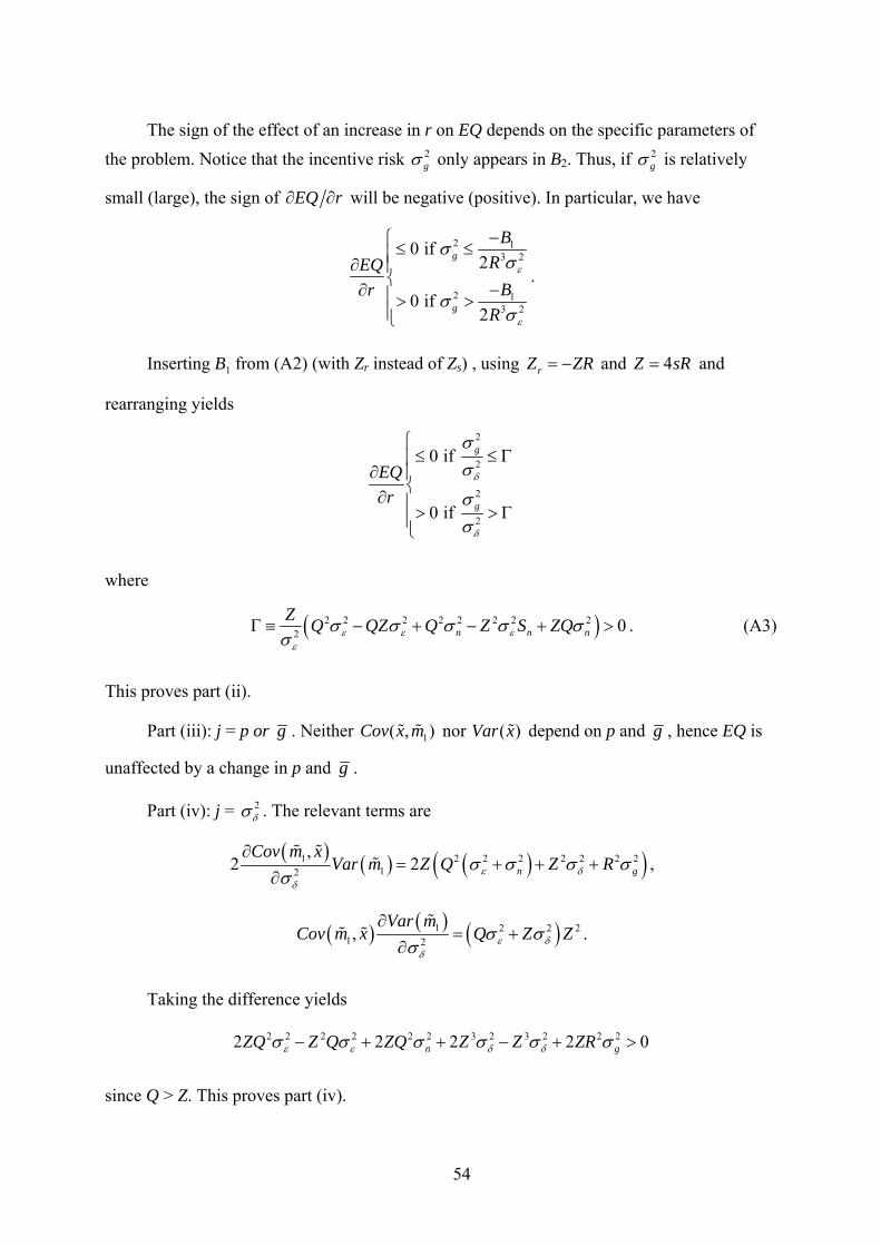
54

The sign of the effect of an increase in r on EQ depends on the specific parameters of the problem. Notice that the incentive risk 2

gσ only appears in B2. Thus, if 2gσ is relatively

small (large), the sign of EQ r∂ ∂ will be negative (positive). In particular, we have

2 13 2

2 13 2

0 if 2

0 if 2

g

g

BREQ

BrR

ε

ε

σσ

σσ

−⎧≤ ≤⎪∂ ⎪⎨ −∂ ⎪> >⎪⎩

.

Inserting B1 from (A2) (with Zr instead of Zs) , using rZ ZR= − and 4Z sR= and

rearranging yields

2

2

2

2

0 if

0 if

g

g

EQr

δ

δ

σσ

σσ

⎧≤ ≤ Γ⎪

∂ ⎪⎨∂ ⎪> > Γ⎪⎩

where

( )2 2 2 2 2 2 2 22 0n n n

Z Q QZ Q Z S ZQε ε εε

σ σ σ σ σσ

Γ ≡ − + − + > . (A3)

This proves part (ii).

Part (iii): j = p or g . Neither 1( , )Cov x m% % nor ( )Var x% depend on p and g , hence EQ is

unaffected by a change in p and g .

Part (iv): j = 2δσ . The relevant terms are

( ) ( ) ( )( )1 2 2 2 2 2 2 212

,2 2 n g

Cov m xVar m Z Q Z Rε δ

δ

σ σ σ σσ

∂= + + +

∂

% %% ,

( ) ( ) ( )1 2 2 21 2,

Var mCov m x Q Z Zε δ

δ

σ σσ

∂= +

∂

%% % .

Taking the difference yields

2 2 2 2 2 2 3 2 3 2 2 22 2 2 2 0n gZQ Z Q ZQ Z Z ZRε ε δ δσ σ σ σ σ σ− + + − + >

since Q > Z. This proves part (iv).

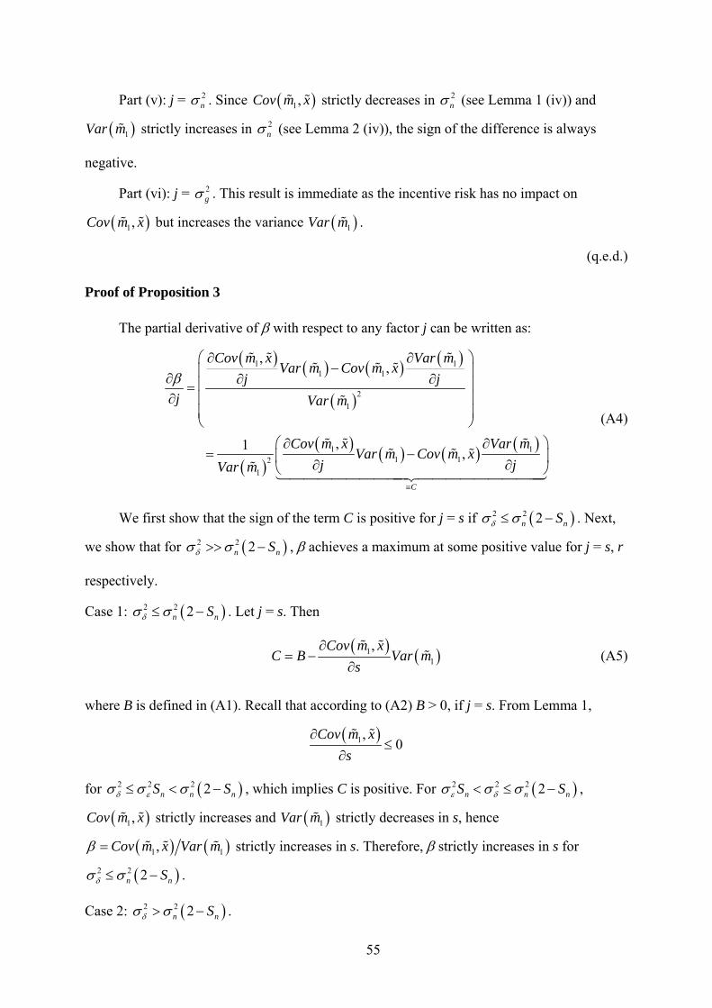
55

Part (v): j = 2nσ . Since ( )1,Cov m x% % strictly decreases in 2

nσ (see Lemma 1 (iv)) and

( )1Var m% strictly increases in 2nσ (see Lemma 2 (iv)), the sign of the difference is always

negative.

Part (vi): j = 2gσ . This result is immediate as the incentive risk has no impact on

( )1,Cov m x% % but increases the variance ( )1Var m% .

(q.e.d.)

Proof of Proposition 3

The partial derivative of β with respect to any factor j can be written as:

( ) ( ) ( ) ( )

( )

( )( ) ( ) ( ) ( )

1 11 1

21

1 11 12

1

,,

,1 ,

C

Cov m x Var mVar m Cov m x

j jj Var m

Cov m x Var mVar m Cov m x

j jVar m

β

≡

∂ ∂⎛ ⎞−⎜ ⎟∂ ∂ ∂⎜ ⎟=

⎜ ⎟∂⎜ ⎟⎝ ⎠

∂ ∂⎛ ⎞= −⎜ ⎟∂ ∂⎝ ⎠

% % %% % %

%

% % %% % %

%144444444424444444443

(A4)

We first show that the sign of the term C is positive for j = s if ( )2 2 2n nSδσ σ≤ − . Next,

we show that for ( )2 2 2n nSδσ σ>> − , β achieves a maximum at some positive value for j = s, r

respectively.

Case 1: ( )2 2 2n nSδσ σ≤ − . Let j = s. Then

( ) ( )11

,Cov m xC B Var m

s∂

= −∂

% %% (A5)

where B is defined in (A1). Recall that according to (A2) B > 0, if j = s. From Lemma 1,

( )1, 0Cov m x

s∂

≤∂

% %

for ( )2 2 2 2n n nS Sδ εσ σ σ≤ < − , which implies C is positive. For ( )2 2 2 2n n nS Sε δσ σ σ< ≤ − ,

( )1,Cov m x% % strictly increases and ( )1Var m% strictly decreases in s, hence

( ) ( )1 1,Cov m x Var mβ = % % % strictly increases in s. Therefore, β strictly increases in s for

( )2 2 2n nSδσ σ≤ − .

Case 2: ( )2 2 2n nSδσ σ> − .

56

First we show that for each combination s > 0 and r > 0, there exists a value of 2δσ such

that ( )( ) ( )2 2, , 1/ 2,Z s r Zδ δβ σ β σ> = , i.e., for that 2δσ , β under Z(s, r) exceeds its

corresponding value if Z is set to its maximum of 1/2. As 1/ 2Z → for s →∞ and/or 0r → ,

β must have at least one stationary point with respect to s and r, respectively. We then show

that if β has a stationary point, then it is a maximum.

β is defined as

( )

2 2

2 2 2 2 2 2 2n g

Q ZQ Z R

ε δ

ε δ

σ σβσ σ σ σ

+=

+ + + .

β strictly increases in 2δσ , and

2 2

1lim 2ZZ Zδσ

β→∞

= = > for Z < 1/2. Thus, for each combination

(s > 0, r > 0), 2δσ can be chosen large enough such that ( )( ) ( )2 2, , 1/ 2,Z s r Zδ δβ σ β σ> = . To

see that a stationary point of β is a maximum, consider the second partial derivatives of β:

( )

( ) ( ) ( ) ( )( )

( )2 221 1 1

1 12 32 2 21 1

,1 2,

D

Cov m x Var m Var mCVar m Cov m xj j j jVar m Var mβ

≡

⎛ ⎞∂ ∂ ∂∂= − −⎜ ⎟

∂ ∂ ∂ ∂⎝ ⎠

% % % %% % %

% %144444444424444444443

.

At a stationary point, C = 0, and it suffices to evaluate the sign of D. First let j = s and

collect the relevant terms as follows:

( ) ( ) ( ) ( )21 12 2 2 2

2

, ,16 16ss n s n

Cov m x Cov m xZ S RZ S R

s sδ ε δ εσ σ σ σ∂ ∂

= − = − − = −∂ ∂

% % % %

( ) ( ) ( ) ( )( ) ( )( ) ( )

21 2 2 2 2 2 2

2

2 2 2 2 2 2 2

1 2 2 2 2

0

2 2 2

16 2 2 2 2

16 2 2

ss n s s s n g s ss

s n g s s s s n g s

s s s n g s

Var mZ Z Q Z Z Q R RR

sR Z Z Q RR Z Z Q R

Var mR Z Z Q R

s

δ δ

δ δ

δ

σ σ σ σ σ

σ σ σ σ σ σ

σ σ σ>

∂= − + − + +

∂⎡ ⎤= − − + + − +⎣ ⎦∂

= − + − +∂

%

%

144424443

where ( ) ( ) ( ) ( ) ( )

23 2

1 16 8 16 1 8 168 8 88 8

ss sRR R Rs r s r s rs r s r

⋅= = = −

+ + ++ +.

The sign of ( )2 2s s s nZ Z Qδσ σ− is positive due to Zs > 0 and Qs = −ZsSn. Rewrite D as follows:

57

( ) ( ) ( ) ( )

( ) ( )( )( ) ( )( )

( ) ( )( )

1 11 1

2 2 2 21

2 2 2 21

2 2 2 21

,16 ,

, 2 2

16 , 2 2

, 2 2 0.

s s s n g s

s s s n g s

s s s n g s

Cov m x Var mD R Var m Cov m x

s s

Cov m x Z Z Q R

RC Cov m x Z Z Q R

Cov m x Z Z Q R

δ

δ

δ

σ σ σ

σ σ σ

σ σ σ

∂ ∂⎛ ⎞= − −⎜ ⎟∂ ∂⎝ ⎠

− − +

= − − − +

= − − + <

% % %% % %

% %

% %

% %

Thus, if β has a stationary point in s, it is a maximum. It follows that if 2δσ is large

enough, then β first strictly increases in s, reaches a maximum at some value s and then

decreases in s. This completes the proof of part (i).

Part (ii): j = r. If 2

2g

δ

σσ

≤ Γ , EQ decreases according to Proposition 2 (ii) and we have

0B ≤ . If 2 2nSδ εσ σ≤ also holds, then ( )1, 0Cov m x r∂ ∂ ≥% % (see Lemma 1 (ii)) implying that

C < 0 if at least one of the above inequalities is strict. If ( )2 2 2 2n n nS Sε δσ σ σ< ≤ − and

( )( ){ } ( )( )2 2 2 2 2 2 2max 0; 16 2 16 2g n n n ns S s Sδ δσ σ σ σ σ≤ − − − = − − − are satisfied, then

( )1, 0Cov m x r∂ ∂ <% % and ( )1, 0Var m x r∂ ∂ >% % (Lemma 2-(ii)), which implies C < 0. In this

case, EQ strictly decreases in r, hence 2

2g

δ

σσ

≤ Γ must additionally be satisfied. If 2

2g

δ

σσ

> Γ and

2 2nS ε δσ σ< , then B > 0 (Proposition 2 (ii)) and ( )1, 0Cov m x r∂ ∂ <% % (Lemma 1 (ii)), thus,

C > 0 and β strictly increases in r.

To prove the last statement of part (ii), note that

( ) ( ) ( )21 12 2

2

, ,2rr n

Cov m x Cov m xZ S R

r rδ εσ σ∂ ∂

= − = −∂ ∂

% % % %,

( ) ( ) ( ) ( )( ) ( )

21 2 2 2 2 2 2

2

1 2 2 2 2

0

2 2 2

2 2 2 .

rr n r r r n g r rr

r r r n g r

Var mZ Z Q Z Z Q R RR

rVar m

R Z Z Q Rr

δ δ

δ

σ σ σ σ σ

σ σ σ>

∂= − + − + +

∂∂

= − + − +∂

%

%

144424443

Hence,

58

( ) ( ) ( ) ( )

( ) ( )( )( ) ( )( )

( ) ( )( )

1 11 1

2 2 2 21

2 2 2 21

2 2 2 21

,2 ,

, 2 2

2 , 2 2

, 2 2 0.

r r r n g r

r r r n g r

r r r n g r

Cov m x Var mD R Var m Cov m x

r r

Cov m x Z Z Q R

RC Cov m x Z Z Q R

Cov m x Z Z Q R

δ

δ

δ

σ σ σ

σ σ σ

σ σ σ

∂ ∂⎛ ⎞= − −⎜ ⎟∂ ∂⎝ ⎠

− − −

= − − − −

= − − − <

% % %% % %

% %

% %

% %

Thus, if β has a stationary point in r, then it is a maximum. It follows that if 2δσ is large

enough, then β first strictly increases in r, reaches a maximum at some value r and then

decreases in r.

Part (iii) follows from the fact that all terms in β are independent from p and g . Part

(iv) obtains from evaluating the sign of the partial derivative of β with respect to 2δσ :

( )( ) ( )( )

( )( )

2 2 2 2 2 2 2 2 2 2

221

2 2 2 2 2 2 2

21

0.

n g

n g

Z Q Z R Q Z Z

Var m

ZQ R Z Q

Var m

ε δ ε δ

δ

ε ε

σ σ σ σ σ σβσ

σ σ σ σ

+ + + − +∂=

∂

+ + −= >

%

%

where the inequality follows due to Q > Z. Finally, parts (v) and (vi) follow from Lemmas 1

and 2.

(q.e.d.)

Proof of Proposition 4

First, we show that ( )

( )

2 2

1

1.nQPS

Var mεσ σ

β+

= + −%

( ) ( )( )( )( )

( ) ( ) ( )( )( )( )

( )( ) ( )( )

( )( )

1 2 1

2 2 2 2 2 2 2

1 1

2 2 2 2 2 2 2

2 2 2 2 2 2

2 2 2 2 2 2 2

2 2

1

, 1

, 1 1

1 1

1.

n g

n g

n g

n g

n

Cov Qy Z Rg y Q y Z RgPS

Q Z R

Cov Qy Z Rg u Q y Z Rg

Q Z R

Q Q Q Z Z R

Q Z R

QVar m

ε δ

ε δ

ε ε δ

ε δ

ε

δ δ

σ σ σ σ

δ ε δ

σ σ σ σ

σ σ σ σ σ

σ σ σ σ

σ σβ

+ + − − − −=

+ + +

+ + + + − + − −=

+ + +

+ − + + − −=

+ + +

+= + −

% %% % % % %

% %%% % % % %

%

59

To prove parts (i) and (ii), consider the first derivative of the last representation of PS

with respect to variable j = s, r.

( ) ( )

( )2 2 2 2 2

1 22 2 2 2 2 2 2

1

1( , )( )

n g

n g

Z Q Z Z RCov m mPSVar m Q Z R

ε δ

ε δ

σ σ σ σ

σ σ σ σ

+ + − −= =

+ + +% %

%

Differentiating the numerator yields:

( ) ( )( ) ( )

( )( ) ( )( ) ( )

( )( ) ( )

( )( )

2 2 21 2 2 2 2 2

2 22 2

2 2 2 2 2 22 2

2 2

42 2

2 2

2 2

,1 1 2 2

11 2 2

1 21 2 2

1 2 2

n nj n n j g

nn

n n n nj j g

n

nj j g

n

j n n

ZCov m mZ Z Z RR

j

Z ZZ Z RR

ZZ Z RR

Z Z S

εδ

εε

ε εδ

ε

δε

δ

σ σ σσ σ σ σσ σσ σ

σ σ σ σ σ σσ σ

σ σ

σσ σ

σ σ

σ σ

⎛ ⎞+∂ ⎛ ⎞⎜ ⎟= − + − + − −⎜ ⎟⎜ ⎟∂ ++ ⎝ ⎠⎝ ⎠⎛ ⎞+ − − +⎜ ⎟= + − −⎜ ⎟+⎝ ⎠⎛ ⎞−⎜ ⎟= + − −⎜ ⎟+⎝ ⎠

= − + −

% %

2.j gRR σ

Let j = s. Since Zs > 0, Rs < 0, and Z ∈ [0, 1/2], the covariance always increases in s.

Case 1: Assume ( )1 2, 0Cov m m ≥% % . Together with Lemma 2 this proves that PS is strictly

increasing in s if ( )2 2 2n nSδσ σ≤ − .

If ( )2 2 2n nSδσ σ> − , for each combination of s > 0 and r > 0, PS(Z(s, r)) > PS(Z = 1/2) if 2δσ is sufficiently large. The proof is similar to that in Proposition 3: Take the limit of PS as 2δσ →∞ :

( ) ( ) ( )2 22

1 1 1 0.5lim , 1 lim 1/ 20.5

Z Z ZPS s r PS ZZ Zδ δσ σ→∞ →∞

− − −= = > = = =

since Z ≤ 1/2. Uniqueness of the stationary point follows from the sign of the second

derivative of PS with respect to s at the stationary point where

( ) ( ) ( ) ( )

( )

1 2 11 1 2

21

,,

0

Cov m m Var mVar m Cov m mPS s s

s Var m

∂ ∂−∂ ∂ ∂= =

∂

% % %% % %

%.

Evaluated at the stationary point, the second derivative is

60

( ) ( ) ( ) ( )

( )

2 21 2 1

2 1 1 22 2

221

,,

Cov m m Var mVar m Cov m mPS s s

s Var m

∂ ∂−∂ ∂ ∂=

∂

% % %% % %

%.

( ) ( )( )( ) ( )( )( )( ) ( )( ) ( )

21 2 2 2 2 2 2 2 2 2

2

2 2 2 2 2 2 2 2

1 2 2 2 2 2 2

,1 2 2 2 2

16 1 2 2 2 2

,16 2 2

ss n n s n n s g ss g

s n n s g s n n s g

s n n s g

Cov m mZ Z S Z S R RR

sRZ Z S RR Z S R

Cov m mR Z S R

s

δ δ

δ δ

δ

σ σ σ σ σ σ

σ σ σ σ σ σ

σ σ σ

∂= − + − + − −

∂

= − − + − − + −

∂= − − + −

∂

% %

% %

( ) ( ) ( )2

1 1 2 2 2 22

0

16 2 2s s s n g s

Var m Var mR Z Z Q R

s s δσ σ σ>

∂ ∂= − + − +

∂ ∂

% %

144424443.

Taking together, the sign of the numerator of 2

2

PSs

∂∂

evaluated at a stationary point is

( ) ( ) ( ) ( )

( ) ( ) ( ) ( )( )

( ) ( ) ( ) ( )

2 21 2 1

1 1 22 2

1 2 2 2 2 2 21 1

1 2 2 2 21 2 1 2

0

1

,,

,16 2 2

16 , , 2 2

,16

s n n s g

s s s n g s

Cov m m Var mVar m Cov m m

s sCov m m

R Var m Var m Z S Rs

Var mR Cov m m Cov m m Z Z Q R

s

Cov m mR

δ

δ

σ σ σ

σ σ σ>

∂ ∂−

∂ ∂∂⎛ ⎞

= − − + +⎜ ⎟∂⎝ ⎠⎛ ⎞⎛ ⎞∂⎜ ⎟⎜ ⎟− − + − +⎜ ⎟⎜ ⎟∂

⎝ ⎠⎝ ⎠∂

= −

% % %% % %

% %% %

%% % % %

144424443

% %( ) ( ) ( ) ( )

( ) ( )( ) ( ) ( )

( ) ( )( ) ( )( )

2 11 1 2

0(stationary point)

2 2 2 2 2 2 2 2 21 1 2

0

2 2 2 2 21 1 2

,

2 2 , 2 2

, 2 2

2

s n n s g s s s n g s

s n n s g

Var mVar m Cov m m

s s

Var m Z S R Cov m m Z Z Q R

Var m Cov m m Z S R

Q

δ δ

δ

σ σ σ σ σ σ

σ σ σ

=

>

∂⎛ ⎞−⎜ ⎟∂ ∂⎝ ⎠

⎛ ⎞⎜ ⎟− + + − − +⎜ ⎟⎝ ⎠

= − + + +

= −

%% % %

144444444424444444443

% % %144424443

% % %

( )( ) ( )( )2 2 2 2 2 2 2 22 2 0.n s n n s gZ Z S Rε δ δσ σ σ σ σ σ+ + + + <

Thus, PS achieves a unique maximum in s if ( )2 2 2n nSδσ σ>> − . Notice that the proof of this

result is independent of the sign of ( )1 2,Cov m m% % .

Case 2: ( )1 2, 0Cov m m <% % and ( )2 2 2n nSδσ σ≤ − . ( )1Var m% strictly decreases in s (Lemma 2 (i)).

( )1 2,Cov m m% % strictly increases in s and approaches a positive value if s →∞ , thus

( )1 2, 0Cov m m <% % can only hold for a lower interval of s. Suppose that 0PSs

∂<

∂ for small s,

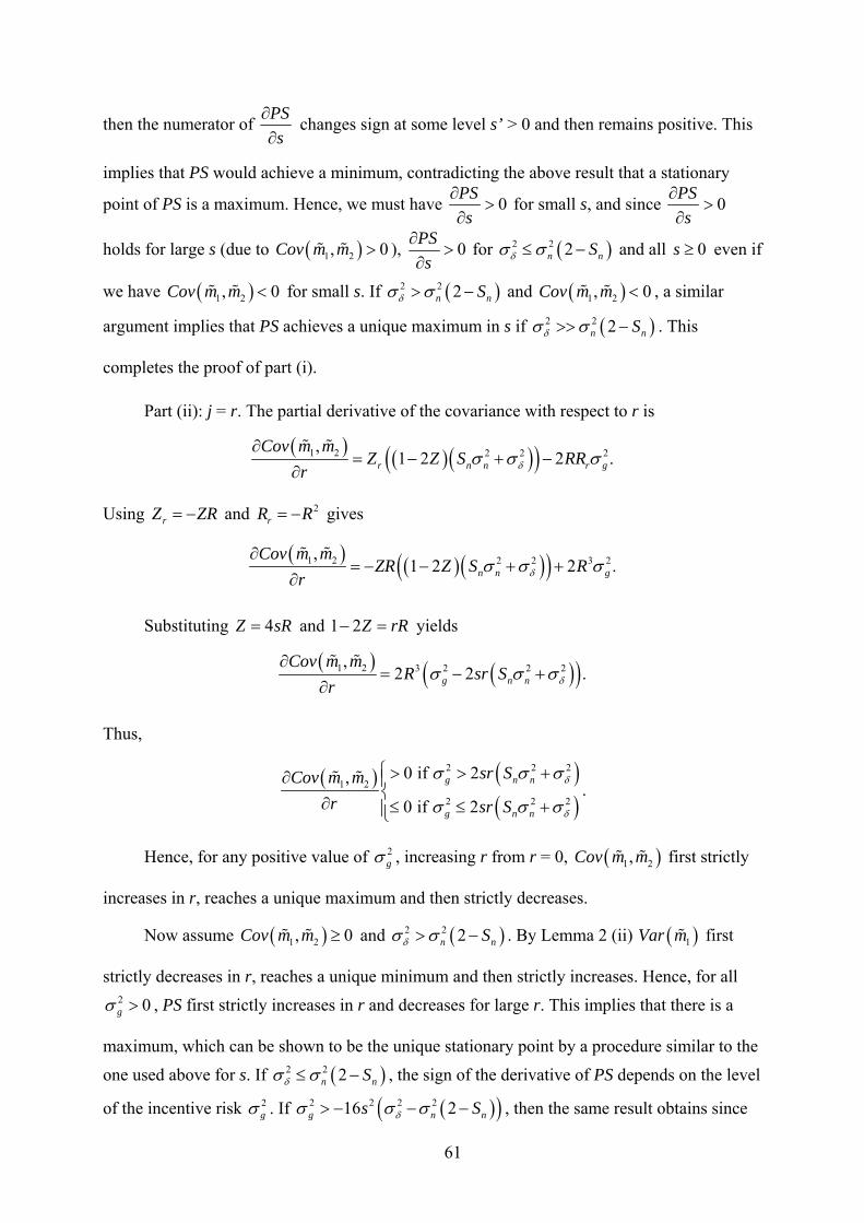
61

then the numerator of PSs

∂∂

changes sign at some level s’ > 0 and then remains positive. This

implies that PS would achieve a minimum, contradicting the above result that a stationary

point of PS is a maximum. Hence, we must have 0PSs

∂>

∂ for small s, and since 0PS

s∂

>∂

holds for large s (due to ( )1 2, 0Cov m m >% % ), 0PSs

∂>

∂ for ( )2 2 2n nSδσ σ≤ − and all 0s ≥ even if

we have ( )1 2, 0Cov m m <% % for small s. If ( )2 2 2n nSδσ σ> − and ( )1 2, 0Cov m m <% % , a similar

argument implies that PS achieves a unique maximum in s if ( )2 2 2n nSδσ σ>> − . This

completes the proof of part (i).

Part (ii): j = r. The partial derivative of the covariance with respect to r is

( ) ( )( )( )1 2 2 2 2,1 2 2 .r n n r g

Cov m mZ Z S RR

r δσ σ σ∂

= − + −∂

% %

Using rZ ZR= − and 2rR R= − gives

( ) ( )( )( )1 2 2 2 3 2,1 2 2 .n n g

Cov m mZR Z S R

r δσ σ σ∂

= − − + +∂

% %

Substituting 4Z sR= and 1 2Z rR− = yields

( ) ( )( )1 2 3 2 2 2,2 2 .g n n

Cov m mR sr S

r δσ σ σ∂

= − +∂

% %

Thus,

( ) ( )( )

2 2 2

1 2

2 2 2

0 if 2,

0 if 2

g n n

g n n

sr SCov m mr sr S

δ

δ

σ σ σ

σ σ σ

⎧> > +∂ ⎪⎨∂ ≤ ≤ +⎪⎩

% %.

Hence, for any positive value of 2gσ , increasing r from r = 0, ( )1 2,Cov m m% % first strictly

increases in r, reaches a unique maximum and then strictly decreases.

Now assume ( )1 2, 0Cov m m ≥% % and ( )2 2 2n nSδσ σ> − . By Lemma 2 (ii) ( )1Var m% first

strictly decreases in r, reaches a unique minimum and then strictly increases. Hence, for all 2 0gσ > , PS first strictly increases in r and decreases for large r. This implies that there is a

maximum, which can be shown to be the unique stationary point by a procedure similar to the

one used above for s. If ( )2 2 2n nSδσ σ≤ − , the sign of the derivative of PS depends on the level

of the incentive risk 2gσ . If ( )( )2 2 2 216 2g n ns Sδσ σ σ> − − − , then the same result obtains since

62

the behavior of ( )1Var m% is qualitatively similar according to Lemma 2 (ii). If

( )( )2 2 2 216 2g n ns Sδσ σ σ≤ − − − , then the variance always strictly increases in r. Here, the sign

of the change in PS depends on the specific parameters. If it turns out that PS first increases in

r, the behavior is similar to the two cases above. If PS decreases in r for r = 0, it always

decreases in r. Otherwise PS would have to reach a minimum at some positive r ,

contradicting the fact that any stationary point of PS is a maximum.

Now consider the combination ( )1 2, 0Cov m m <% % and ( )2 2 2n nSδσ σ> − . Similar to part

(i), the sign of PSr

∂∂

seems ambiguous for small r, and ( )1 2, 0Cov m m <% % can only hold for a

lower interval of r as ( ) 21 2,Cov m m εσ→% % if r →∞ and ( )1 2,Cov m m% % achieves a unique

maximum for some r < ∞ . It follows that at the point r′ for which ( )1 2, 0Cov m m =% % holds,

we must have ˆr r′ < and ( )1 2,Cov m m% % still strictly increases in r. Hence, we have

( )( ) ( )

( )

1 21

21

,

0

Cov m m rVar mPS r r

r Var m

′∂′∂ ∂= >

∂

% %%

%.

Thus, it cannot be the case that 0PSr

∂<

∂ for some r r′< as this would imply that PS

achieves a minimum in the interval ( )0;r′ contradicting the result that a stationary point of PS

is a maximum. Therefore, PS strictly increases in r for small r and then decreases.

Finally, consider ( )1 2, 0Cov m m <% % and ( )2 2 2n nSδσ σ≤ − . If

( )( )2 2 2 216 2g n ns Sδσ σ σ> − − − , PS first strictly increases and then decreases in r. If

( )( )2 2 2 216 2g n ns Sδσ σ σ≤ − − − , then ( )1Var m% always strictly increases in r. If

( )1 2, 0Cov m m <% % then

( ) ( ) ( ) ( )

( )

1 2 11 1 2

21

,,

0

Cov m m Var mVar m Cov m mPS r r

r Var m

∂ ∂−∂ ∂ ∂= >

∂

% % %% % %

%.

for 0 ≤ r ≤ r′ and 2gσ sufficiently small.

We conclude that for ( )1 2, 0Cov m m <% % , PS always first strictly increases and then

decreases in r, completing the proof of part (ii).

Part (iii) follows because all terms appearing in PS are independent from p and g .

63

Part (iv): The derivative of PS with respect to 2δσ is

( ) ( )( ) ( ) ( )( )( )

( ) ( ) ( )( )

2 2 2 2 2 2 2 2 2 2 2 2 2

221

2 2 2 2 2 2 2 2

21

1 1

1.

n g n g

n n g

Z Z Q Z R Z Q Z Z R ZPSVar m

Z Z Q Z QZ ZR

Var m

ε δ ε δ

δ

ε ε

σ σ σ σ σ σ σ σ

σ

σ σ σ σ σ

− + + + − + + − −∂=

∂

− + − + +=

%

%

Expanding the individual terms results in:

( ) ( ) ( ) ( ) ( )

( ) ( ) ( )

( ) ( ) ( ) ( ) ( )

22

2 2 2 2 22 2

42 2 2

2 2

42 2 3 4

2 2

1 1 1

1 1 2

1 1 1 2 .

nn n

n

nn

n

nn

n

Z Z Q Z Z Z

Z Z Z Z

Z Z Z Z Z Z Z

ε εε

εε

εε

σσ σ σ σσ σ

σσ σσ σ

σσ σσ σ

⎛ ⎞⎜ ⎟− + = − − +⎜ ⎟+⎝ ⎠⎛ ⎞⎜ ⎟= − + − +⎜ ⎟+⎝ ⎠

= − + − − + −+

( ) ( ) ( )( )( )

( ) ( )

( ) ( )

22 2 2 2 2 2

2 2

2 22 2 3 2 3 2

2 2

3 22 2 2 2 2 2

2 2

42 2 3 4

2 2

1

.

nn n

n

nn n

n

nn n

n

n

n

Z QZ Z Z Z

ZZ Z Z

ZZ Z

Z Z Z

ε εε

εε

ε

ε ε εε

εε

σσ σ σ σσ σ

σ σσ σ σ

σ σ

σσ σ σ σ σσ σ

σσσ σ

⎛ ⎞⎜ ⎟+ = + −⎜ ⎟+⎝ ⎠

+= + −

+

= + + − −+

= + −+

Taking the difference yields:

( ) ( ) ( ) ( ) ( )( )2 2 2 2 2 2 2 21 1 2 1 0n n nZ Z Q Z QZ Z Z Z Zε ε εσ σ σ σ σ σ− + − + = − + − ≥ ,

where the equality holds for s = 0 (then Z = 0) and/or r = 0 (then Z = 1/2). Hence, since 2 2 0gZR σ > for s > 0 and r > 0,

2 0.PS

δσ∂

>∂

Part (v): Write PS as

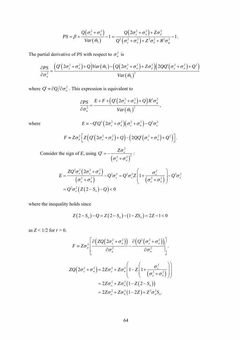
64

( )

( )( )

( )2 2 2 2 2

2 2 2 2 2 2 21

21 1n n

n g

Q Q ZPS

Var m Q Z Rε ε δ

ε δ

σ σ σ σ σβ

σ σ σ σ

+ + += + − = −

+ + +%.

The partial derivative of PS with respect to 2nσ is

( )( ) ( ) ( )( ) ( )( )

( )

2 2 2 2 2 2 2 21

221

2 2 2n n n

n

Q Q Var m Q Z QQ QPSVar m

ε ε δ εσ σ σ σ σ σ σ

σ

′ ′+ + − + + + +∂=

∂

%

%

where 2nQ Q σ′ ≡ ∂ ∂ . This expression is equivalent to

( )( )

( )

2 2 2 2

221

2 n g

n

E F Q Q RPSVar m

εσ σ σ

σ

′+ + + +∂=

∂ %,

where ( )( )2 2 2 2 2 3 22 n nE Q Q Qε ε εσ σ σ σ σ′≡ − + + −

( )( ) ( )( )2 2 2 2 2 22 2n nF Z Z Q Q QQ Qδ ε εσ σ σ σ σ⎡ ⎤′ ′≡ + + − + +⎣ ⎦ .

Consider the sign of E, using ( )

2

22 2n

ZQ ε

ε

σ

σ σ′ = −

+:

( )

( ) ( )( )( )

2 2 2 2 23 2 2 2 3 2

2 2 2 2

2 2

21

2 0

n

n n

n

ZQE Q Q Z Q

Q Z S Q

ε ε εε ε ε

ε ε

ε

σ σ σ σσ σ σσ σ σ σ

σ

⎛ ⎞+⎜ ⎟= − = + −⎜ ⎟+ +⎝ ⎠

= − − <

where the inequality holds since

( ) ( ) ( )2 2 1 2 1 0n n nZ S Q Z S ZS Z− − = − − − = − <

as Z < 1/2 for r > 0.

( )( ) ( )( )2 2 2 2 2

22 2

2 n n

n n

ZQ QF Z

ε εδ

σ σ σ σσ

σ σ

⎡ ⎤∂ + ∂ +⎢ ⎥≡ −

∂ ∂⎢ ⎥⎣ ⎦

.

( ) ( )( )( )

( )

22 2 2 2

2 2

2 2

2 2 2 2

2 2 1 1

2 1 2

2 1 2 .

n nn

n n

n n n

ZQ Z Z Z

Z Z Z S

Z Z Z Z S

εε ε

ε

ε

ε

σσ σ σ σσ σ

σ σ

σ σ σ

⎛ ⎞⎛ ⎞⎜ ⎟⎜ ⎟+ = + − +

⎜ ⎟⎜ ⎟+⎝ ⎠⎝ ⎠= + − −

= + − +

65

( )( )

( )( )

4

2 2 2 22

2 2

21 2

n

n n

n n

ZQZ Z Z

ε ε

σσ σ σ σ

σ σ

⎛ ⎞⎜ ⎟∂⎜ ⎟∂ + +⎝ ⎠= − +

∂ ∂

Similarly, substituting for Q in ( )2 2 2nQ εσ σ+ yields

( ) ( ) ( )4

2 2 2 2 2 22 2

1 2 nn n

n

Q Z Zε εε

σσ σ σ σσ σ

+ = + − ++

,

and the partial derivative with respect to 2nσ is:

( )( )

( )( )

4

2 2 2 2 22

2 21 2

n

n n

n n

QZ Z

ε ε

σσ σ σ σ

σ σ

⎛ ⎞⎜ ⎟∂⎜ ⎟∂ + +⎝ ⎠= − +

∂ ∂.

The term F becomes:

( )( ) ( )( )

( )( )2 2 2 2 2

2 22 2

21 2 1 0

n n

n n

ZQ QF Z Z Z Z

ε εδ δ

σ σ σ σσ σ

σ σ

⎡ ⎤∂ + ∂ +⎢ ⎥≡ − = − − <⎡ ⎤⎣ ⎦∂ ∂⎢ ⎥⎣ ⎦

as Z ∈ (0, 1/2) for s > 0 and r > 0. Since both E and F are negative,

( )

222

1

0 if 0gn

PS E FVar m

σσ∂ +

= < =∂ %

.

Further,

( )( )

( ) ( )

( ) ( ) ( )( )( )

2 22 2 2 2 2

2 2 22 2

4 2 2

2 2 2 2 22 2

2

2 1

1

1 1 1 1 2 0,

nn n

nn

n

n nn

n

Q Q Z Z

Z Z Z

Z S Z

εε ε ε

εε

ε ε

ε εε

σ σσ σ σ σ σσ σσ σ

σ σ σσ σ σ σσ σ

′ + + = − + + + −++

= − − + −+ ++

= − + − ≥ − ≥

due to 120 Z≤ ≤ and 0 1nS≤ < , and it follows that

( )2 2 2 2(2 ) 0n gQ Q Rεσ σ σ′ + + >

if 2nσ > 0 and Z < 1/2. This term strictly increases in 2

gσ so that for any combination of the

other parameters, 2gσ can be chosen sufficiently large that PS increases in 2

nσ . The threshold

is

66

( )( )2 2 2 22 0n gE F Q Q Rεσ σ σ′+ + + + ≥

or ( ) ( )( )

( )( )( )2 2 2

22 2

1 2 1.

1 1 1g

n

Z Q Z Z

Z S R

ε δσ σσ

− + −≥

− + −

Due to 2 0n nS σ∂ ∂ > and 1 nQ ZS= − , the threshold strictly decreases in 2nσ . Hence, if

2gσ exceeds the threshold for 2 0nσ = , it exceeds it for all values of 2

nσ . Inserting 2 0nσ = in

the threshold yields

( ) ( ) ( )

( )

( ) ( )( )( )

( )( )

2

2

2 2 22 2

0

222

0

2 2

2

1 2 1 1 2 11 2

1 1 1

1.

n

nn

Z Q Z Z Z Z ZZ R

Z S R

Z ZR

ε δσ ε δ

σ

ε δ

σ σ σ σ

σ σ

=

=

⎛ ⎞− + −⎜ ⎟ − + −⎝ ⎠ =−⎛ ⎞⎛ ⎞⎛ ⎞− + −⎜ ⎟⎜ ⎟⎜ ⎟⎜ ⎟⎝ ⎠⎝ ⎠⎝ ⎠

+ −= ≡ Λ

If 2gσ is smaller than the threshold for 2

nσ →∞ , then PS always decreases in 2nσ .

Taking the limit of the threshold for 2nσ →∞ gives

( ) ( ) ( )

( )

( ) ( ) ( )( )( )

( ) ( )( )

2

2

2 2 2 2 2 2

222

2 2

2

1 2 1 1 2 1 1

11 1 1

1 2 1.

n

nn

Z Q Z Z Z Z Z Z

Z RZ S R

Z Z ZR

ε δσ ε δ

σ

ε δ

σ σ σ σ

σ σ

→∞

→∞

⎛ ⎞− + −⎜ ⎟ − − + −⎝ ⎠ =−⎛ ⎞⎛ ⎞⎛ ⎞− + −⎜ ⎟⎜ ⎟⎜ ⎟⎜ ⎟⎝ ⎠⎝ ⎠⎝ ⎠

− − += = Λ

This completes the proof of part (v).

Part (vi): PS can be written as

( )( )

( )( )

2 2 2 2 2

1 1

21 1n nQ Q Z

PSVar m Var m

ε ε δσ σ σ σ σβ

+ + += + − = −

% %.

Only ( )1Var m% is affected by 2gσ and strictly increases in 2

gσ . Hence, PS strictly decreases in 2gσ .

(q.e.d.)

Proof of Proposition 5

67

Derivation of (15)

( ) ( ) ( ) ( ) ( )2 2 2 22 ,Var m Var y b Var y Var b Cov y b= − = + −% % %% % % % ,

where

( ) 2 2 22 uVar y ε δσ σ σ= + +%

( ) ( ) ( )( )( )

( ) ( ) ( )

2 2 2 2 2 2 2

2 2 2 2 2 2 2

2 21 1

1

2 1

2

n g

n g

n

Var b Q Z R

Q Q Z R

Var m Var y Q

ε δ

ε δ

ε

σ σ σ σ

σ σ σ σ

σ σ

= − + + +

= − + + + +

= + − +

%

% %

( ) ( ) ( )2 2 22 12 , 2 1 2 2 , 2Cov y b Q Z Cov m xε δ εσ σ σ= − + = −%% %

Inserting these terms yields

( ) ( ) ( ) ( ) ( ) ( )2 2 22 1 2 1 12 2 , 2 nVar m Var y Var y Var m Cov m x Qε εσ σ σ= + + + − − +% % % % % % .

As shown in the proof of Proposition 4

( ) ( )( ) ( )2 2 2 2 2 21 2, 1 1n gCov m m Q Q Q Z Z Rε ε δσ σ σ σ σ= + − + + − −% %

or ( ) ( ) ( )( ) ( )2 21 2 1 1, , nCov m m Cov m x Q Var mεσ σ= + + −% % % % % .

( )( )

( ) ( )( )( ) ( ) ( )( ) ( )

22 2211 2 2 2

1 11 1

,,2 ,

nn

Cov m x QCov m mCov m x Q Var m

Var m Var mε

ε

σ σσ σ

+ += − + + +

% %% %% % %

% %.

Inserting this expressions into the definition of PD yields

( ) ( )( ) ( )( )

( )

22 212

1 21

,2

nCov m x QPD Var y Var y

Var mε

ε

σ σσ

+ +− = + + −

% %% %

%.

Recall that PS can be written as

( ) ( )

( )

2 21

1

,1nCov m x Q

PSVar m

εσ σ+ += −

%

%.

Therefore,

( ) ( ) ( ) ( )( )22 2 2 21 11 , nPS Var m Cov m x Q εσ σ+ = + +% % .

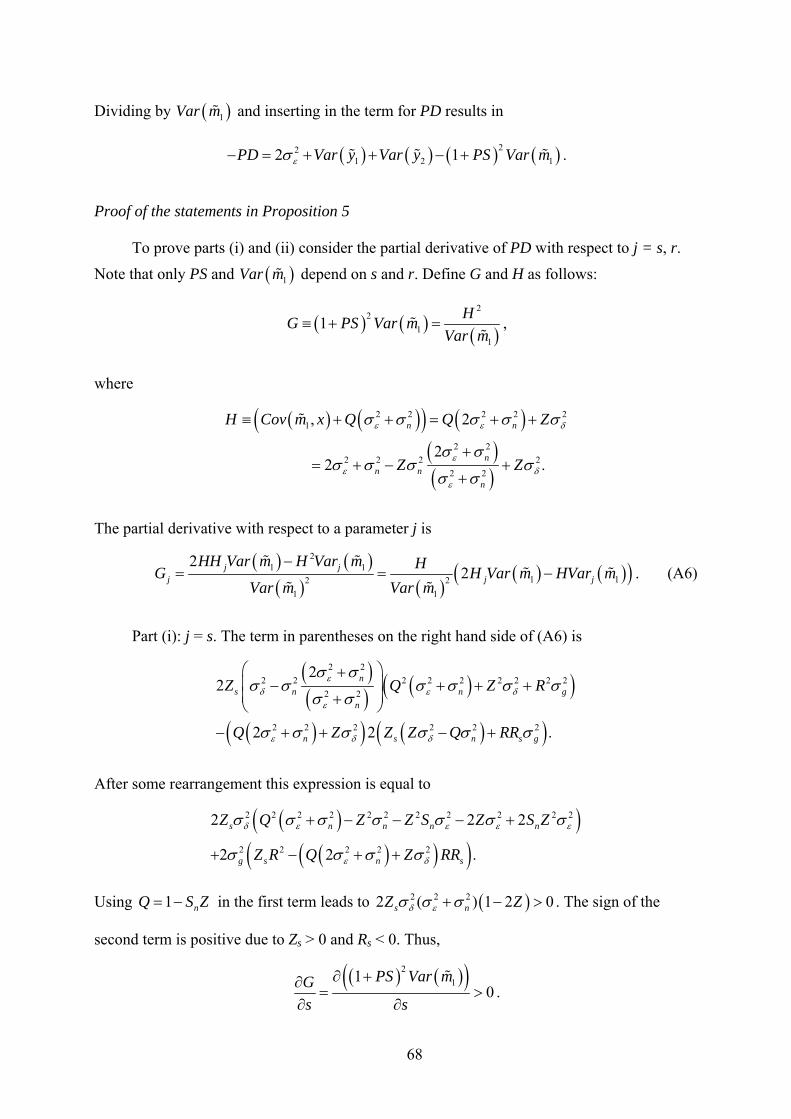
68

Dividing by ( )1Var m% and inserting in the term for PD results in

( ) ( ) ( ) ( )221 2 12 1PD Var y Var y PS Var mεσ− = + + − +% % % .

Proof of the statements in Proposition 5

To prove parts (i) and (ii) consider the partial derivative of PD with respect to j = s, r. Note that only PS and ( )1Var m% depend on s and r. Define G and H as follows:

( ) ( ) ( )2

21

1

1 HG PS Var mVar m

≡ + =%%

,

where

( ) ( )( ) ( )( )( )

2 2 2 2 21

2 22 2 2 2

2 2

, 2

22 .

n n

nn n

n

H Cov m x Q Q Z

Z Z

ε ε δ

εε δ

ε

σ σ σ σ σ

σ σσ σ σ σ

σ σ

≡ + + = + +

+= + − +

+

%

The partial derivative with respect to a parameter j is

( ) ( )

( ) ( )( ) ( )( )

21 1

1 12 21 1

22j j

j j j

HH Var m H Var m HG H Var m HVar mVar m Var m

−= = −

% %% %

% %. (A6)

Part (i): j = s. The term in parentheses on the right hand side of (A6) is

( )( ) ( )( )

( )( ) ( )( )

2 22 2 2 2 2 2 2 2 2

2 2

2 2 2 2 2 2

22

2 2 .

ns n n g

n

n s n s g

Z Q Z R

Q Z Z Z Q RR

εδ ε δ

ε

ε δ δ

σ σσ σ σ σ σ σ

σ σ

σ σ σ σ σ σ

⎛ ⎞+⎜ ⎟− + + +⎜ ⎟+⎝ ⎠

− + + − +

After some rearrangement this expression is equal to

( )( )

( )( )( )2 2 2 2 2 2 2 2 2 2 2

2 2 2 2 2

2 2 2

2 2 .

s n n n n

g s n s

Z Q Z Z S Z S Z

Z R Q Z RR

δ ε ε ε ε

ε δ

σ σ σ σ σ σ σ

σ σ σ σ

+ − − − +

+ − + +

Using 1 nQ S Z= − in the first term leads to ( )2 2 22 ( ) 1 2 0s nZ Zδ εσ σ σ+ − > . The sign of the

second term is positive due to Zs > 0 and Rs < 0. Thus,

( ) ( )( )2

110

PS Var mGs s

∂ +∂= >

∂ ∂

%.

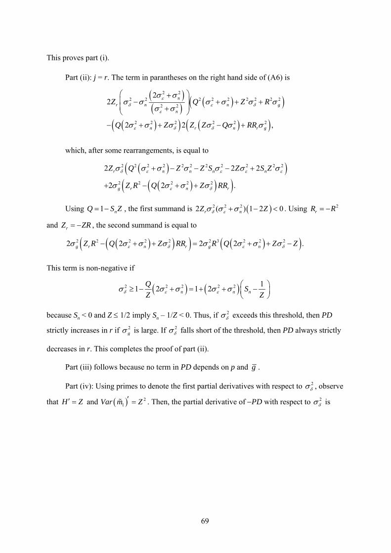
69

This proves part (i).

Part (ii): j = r. The term in parantheses on the right hand side of (A6) is

( )( ) ( )( )

( )( ) ( )( )

2 22 2 2 2 2 2 2 2 2

2 2

2 2 2 2 2 2

22

2 2 ,

nr n n g

n

n r n r g

Z Q Z R

Q Z Z Z Q RR

εδ ε δ

ε

ε δ δ

σ σσ σ σ σ σ σ

σ σ

σ σ σ σ σ σ

⎛ ⎞+⎜ ⎟− + + +⎜ ⎟+⎝ ⎠

− + + − +

which, after some rearrangements, is equal to

( )( )

( )( )( )2 2 2 2 2 2 2 2 2 2 2

2 2 2 2 2

2 2 2

2 2 .

r n n n n

g r n r

Z Q Z Z S Z S Z

Z R Q Z RR

δ ε ε ε ε

ε δ

σ σ σ σ σ σ σ

σ σ σ σ

+ − − − +

+ − + +

Using 1 nQ S Z= − , the first summand is ( )2 2 22 ( ) 1 2 0r nZ Zδ εσ σ σ+ − < . Using 2rR R= −

and rZ ZR= − , the second summand is equal to

( )( )( ) ( )( )2 2 2 2 2 2 3 2 2 22 2 2 2 .g r n r g nZ R Q Z RR R Q Z Zε δ ε δσ σ σ σ σ σ σ σ− + + = + + −

This term is non-negative if

( ) ( )2 2 2 2 2 11 2 1 2n n nQ SZ Zδ ε εσ σ σ σ σ ⎛ ⎞≥ − + = + + −⎜ ⎟

⎝ ⎠

because Sn < 0 and Z ≤ 1/2 imply Sn – 1/Z < 0. Thus, if 2δσ exceeds this threshold, then PD

strictly increases in r if 2gσ is large. If 2

δσ falls short of the threshold, then PD always strictly

decreases in r. This completes the proof of part (ii).

Part (iii) follows because no term in PD depends on p and g .

Part (iv): Using primes to denote the first partial derivatives with respect to 2δσ , observe

that H Z′ = and ( ) 21Var m Z′ =% . Then, the partial derivative of −PD with respect to 2

δσ is

70

( ) ( )

( )( )( )

( ) ( )

( ) ( )( )( )

22

212

1

22

211

2 2

2

1 2

1 2

1 1 2 1

1 1 0,

PDVar y G

H ZVar m HZVar m

H HZ ZVar mVar m

PS Z PS Z

PS Z

δσ∂ − ′ ′= −∂

= − −

= + −

= + + − +

= − + ≥

%

%%

%%

where the last inequality is strict except for special cases in which 1/Z = 1 + PS. Therefore,

PD decreases in 2δσ , which proves part (iv).

Part (v): Using primes to denote the first partial derivatives with respect to 2nσ , obtain

( )

4

22 21 1

n

H Z ε

ε

σ

σ σ

⎛ ⎞⎜ ⎟′ = − +⎜ ⎟+⎝ ⎠

and

( ) ( )( )

2 22 2

1 22 2

21 2 n

n

n

Var m Z Z ε

ε

σ σσ

σ σ

+′ = − ++

% .

Then

( )

( )( ) ( )( )

( )( )( ) ( ) ( )

( ) ( )( )

( )( )

12

1 121

2 2 422 2

2 2 22 2 2 211

2 2 42 2 2

22 2 2 2

( )

1 2

21 1 2 2 1 1

21 1 1 2 2 1 1 1

n

nn

n n

nn

n n

PD Var y G

H H Var m HVar mVar m

H HZ Z ZVar mVar m

PS Z Z PS Z

ε ε

ε ε

ε ε

ε ε

σ

σ σ σσσ σ σ σ

σ σ σσσ σ σ σ

∂ − ′ ′= −∂

′′= − −

⎛ ⎞⎛ ⎞ ⎛ ⎞+ ⎜ ⎟⎜ ⎟ ⎜ ⎟= + − + − − +⎜ ⎟⎜ ⎟ ⎜ ⎟+ +⎝ ⎠ ⎝ ⎠⎝ ⎠

⎛ ⎞+⎜ ⎟= + + − + − + − +⎜ ⎟+ +⎝ ⎠

%

% %%

%%

2 .⎛ ⎞⎛ ⎞⎜ ⎟⎜ ⎟⎜ ⎟⎜ ⎟

⎝ ⎠⎝ ⎠

This expression is positive for Z = 0 because

( )( ) ( )( ) ( )( )( ) ( )22 21 1 0 2 1 0 1 1 0 0 0PS Z PS Z PS Z PS Z+ + = − + = = − + = = = > .

The proof that it is positive for all feasible Z is by contradiction. Assume to the contrary

that there exists a Z for which the derivative is negative, then due to continuity it must change

71

signs somewhere in the interval [0, 1/2] and equal zero at some positive Z ≤ 1/2, implying that

there exists a Z ≤ 1/2 for which the equation

( ) ( ) ( )211 1 2 1 0PS Var m PS H′ ′+ + − + =%

holds. This equation is quadratic in (1 + PS) for any given values of ( )1Var m′ % and H ′ .

Therefore, holding ( )1Var m′ % and H ′ fixed, the solution contains two roots ρ1 and ρ2,

provided that a solution exists in the set of real numbers ℜ. Choose one of the roots, ρ, we

demonstrate that the resulting quadratic equation

( ) ( )21 2 1 0Var m Hρ ρ′ ′− + =%

has no solution in ℜ for 0 < Z ≤ 1/2. A necessary condition for the existence of real roots is

( ) ( ) ( ) ( )2 21 12 4 0H Var m H Var m′ ′ ′ ′≥ ⇔ − ≥% % .

( )( ) ( )

24 4

2 22 22 2 2 2

1 2 1 1n n

H Z Zε ε

ε ε

σ σ

σ σ σ σ

⎛ ⎞ ⎛ ⎞⎜ ⎟ ⎜ ⎟′ = − + + +⎜ ⎟ ⎜ ⎟+ +⎝ ⎠ ⎝ ⎠

( ) ( )

( ) ( ) ( )

( ) ( ) ( )

( )

21

24 4 2 2 4

2 22 2 22 2 2 2 2 2

24 4 2 2 4

22 2 22 2 2 2 2 2

24

222 2

21 2 1 1 1 2

22 1

2

n n

n n n

n n

n n n

n

n

H Var m

Z Z Z Z

Z Z

Z Z

ε ε ε

ε ε ε

ε ε ε

ε ε ε

εε

ε

σ σ σ σ σ

σ σ σ σ σ σ

σ σ σ σ σ

σ σ σ σ σ σ

σ σσ

σ σ

′ ′− =

⎛ ⎞ ⎛ ⎞ ⎛ ⎞+⎜ ⎟ ⎜ ⎟ ⎜ ⎟= − + + + − + −⎜ ⎟ ⎜ ⎟ ⎜ ⎟+ + +⎝ ⎠ ⎝ ⎠ ⎝ ⎠

⎛ ⎞⎛ ⎞ ⎛ ⎞+⎜ ⎟⎜ ⎟ ⎜ ⎟= − + + −⎜ ⎟⎜ ⎟ ⎜ ⎟+ + +⎜ ⎟⎝ ⎠ ⎝ ⎠⎝ ⎠

+= − +

+

%

( )( ) ( ) ( )( ) ( )

( )( )( ) ( )

( )( ) ( ) ( ) ( )

22 22 4 2 2 2 2 4

2 22 2 2 2

22 2 4 842

2 2 22 2 2 2 2 2

4 2 2 4 4 8 6 2 4 42

2 2 2 22 2 2 2 2 2 2 2

2

32

2 4 6 32

2

n n n

n n

n

n n n

n n n n

n n n n

Z Z

Z Z

ε ε ε

ε ε

ε ε εε

ε ε ε

ε ε ε ε ε ε

ε ε ε ε

ε

σ σ σ σ σ σ

σ σ σ σ

σ σ σ σσ

σ σ σ σ σ σ

σ σ σ σ σ σ σ σ σ σ

σ σ σ σ σ σ σ σ

σ

⎛ ⎞+ − + +⎜ ⎟⎜ ⎟

+ +⎜ ⎟⎝ ⎠⎛ ⎞+ +⎜ ⎟= − +⎜ ⎟+ + +⎝ ⎠

⎛ ⎞+ + + +⎜ ⎟= − +⎜ ⎟+ + + +⎝ ⎠

=( ) ( ) ( )

( ) ( )8 6 2 4 43 3

2 22 22 2 2 2

2 1 4 1 2 10n n

n n

Z Z Z Z Z Zε ε

ε ε

σ σ σ σ

σ σ σ σ

− + − + −<

+ +

72

The last inequality follows since 0 < Z ≤ 1/2. Thus, no real roots exist for the above quadratic

equation. We conclude that the derivative of PD with respect to 2nσ is negative, which

completes the proof of part (v).

Part (vi): To see the impact of a change of 2gσ on PD, observe that 2 0gG σ∂ ∂ < since

the variance ( )1Var m% increases in 2gσ and H remains unaffected. Hence PD decreases in the

incentive risk.

(q.e.d.)

Proof of Proposition 6

Using 4ZRs

= ,

( )( ) ( )

( )( )( )( )( ) ( )

( )( )( ) ( )( ) ( )

( ) ( )

( )

1 12 2

12

12

1

1

1 1

1 1

2 2

2 2 2 2 2 2 2 2 2

2

4 22 2 2 2 2 2

22 2

2

42 2

22 2

,

1 ,

1

1

1

16

116

n

n g n

n

ng n

n

n

ng

n

Cov b ySM

Std b Std y

Cov Q y Z Rg y

Std Q y Z Rg Std y

Q

Q Z R

Z

ZZ Zs

Z

Zs

ε

ε δ ε

δ εε

δε

δ

δ

σ σ

σ σ σ σ σ σ

σ

σ σ σ σ σσ σ

σ

σ σ σσ σ

≡ −

− + += −

− + +

− += −

− + + + +

=⎛ ⎞⎜ ⎟+ + +⎜ ⎟+⎝ ⎠

=⎛⎜ + +

+⎝

% %

% %

%% % %

%% % %

( )

( )

12

12

12

2 2

2

4 2 2 2 22

0.1

16

n

n

n g ns

ε

δ ε

σ σ

σ

σ σ σ σ σ

⎞⎟ +

⎜ ⎟⎠

= >⎛ ⎞⎛ ⎞+ + +⎜ ⎟⎜ ⎟⎝ ⎠⎝ ⎠

This term is independent of r and p, and parts (ii) and (iii) follow immediately. As the

denominator decreases in s, SM increases in s which proves part (i). Parts (iv), (v) and (vi)

follow by observing that 2 2 20, 0 and 0n g

SM SM SM

δσ σ σ∂ ∂ ∂

< > <∂ ∂ ∂

.

(q.e.d.)

73

References

BARTH, M.E., W.R. LANDSMAN, and M.H. LANG. ‘International Accounting Standards and Accounting Quality’. Journal of Accounting Research 46 (2008): 467-498.

CHRISTENSEN, P.O., G.A. FELTHAM, and F. ŞABAC. ‘A Contracting Perspective on Earnings Quality’. Journal of Accounting and Economics 39 (2005): 265-294.

CHRISTENSEN, P.O., H. FRIMOR, and F. ŞABAC. ‘Earnings Quality and Earnings Management’, Unpublished working paper, University of Aarhus et al., April 2009.

DECHOW, P.M., and I.D. DICHEV. ‘The Quality of Accruals and Earnings: The Role of Accrual Estimation Errors’. The Accounting Review 77 (2002): 35-59.

DECHOW, P.M., and K.M. SCHRAND. Earnings Quality, Charlotteville, VA, 2004.

DECHOW, P.M., W. GE, and K.M. SCHRAND. ‘Understanding Earnings Quality: A Review of the Proxies, Their Determinants and Their Consequences’, Unpublished working paper, University of California at Berkeley et al., August 2010.

DRYMIOTES, G., and T. HEMMER. ‘On the Stewardship and Valuation Implications of Accrual Accounting Systems’. Unpublished working paper, University of Houston et al., September 2009.

DYE, R.A., and S.S. SRIDHAR. ‘Reliability-relevance trade-offs and the efficiency of aggregation’. Journal of Accounting Research 42 (2004): 51-88.

EINHORN, E., and A. ZIV. ‚Biased Voluntary Disclosure’. Unpublished working paper, Tel Aviv University et al., 2010.

EWERT, R., and A. WAGENHOFER. ‘Economic Effects of Tightening Accounting Standards to Restrict Earnings Management’. The Accounting Review 80 (2005): 1101-1124.

FISCHER, P.E., and R.E. VERRECCHIA. ‘Reporting Bias’. The Accounting Review 75 (2000): 229-245.

FRANCIS, J., R. LAFOND, P. OLSSON, and K. SCHIPPER. ‘Costs of Equity and Earnings Attributes’. The Accounting Review 79 (2004): 967-1010.

FRANCIS, J., P. OLSSON, and K. SCHIPPER. ‘Earnings Quality’. Foundations and Trends in Accounting 1(4) (2008): 259-340.

GÖX, R.F., and A. WAGENHOFER. ‘Optimal Precision of Accounting Information in Debt Financing’. European Accounting Review 19 (2010): 579-602.

GRAHAM, J.R., C.R. HARVEY, and S. RAJGOPAL. ‘The Economic Implications of Corporate Financial Reporting’. Journal of Accounting and Economics 40 (2005): 3-73.

GUTTMAN, I., O. KADAN, and E. KANDEL. ‘A Rational Expectations Theory of Kinks in Financial Reporting’. The Accounting Review 81 (2006): 811-848.

HOLTHAUSEN, R.W., and R.L. WATTS. ‘The Relevance of the Value-relevance Literature for Financial Accounting Standard Setting’. Journal of Accounting and Economics 31 (2001): 3-75.

IASB: Exposure Draft of An Improved Conceptual Framework for Financial Reporting. Chapters 1 and 2, London, May 2008.

JONES, J. ‘Earnings Management during Import Relief Investigations’. Journal of Accounting Research 29 (1991): 193-228.

74

KANODIA, C., R. SINGH, and A.E. SPERO. ‘Imprecision in Accounting Measurement: Can It Be Value Enhancing?’. Journal of Accounting Research 43 (2005): 487-519.

LEUZ, C., D. NANDA, and P. WYSOCKI. ‚Earnings Management and Investor Protection: An International Comparison’. Journal of Financial Economics 69 (2003): 505-527.

LEV, B. ‘On the Usefulness of Earnings and Earnings Research: Lessons and Directions from Two Decades of Empirical Research’. Journal of Accounting Research 27 (Issue Current Studies on the Information Content of Accounting Earnings) (1989): 153-192.

MARINOVIC, I. ‘Internal Control System, Earnings Quality and Restatements’. Unpublished working paper, Northwestern University, September 2010.

NAGAR, V., and G. YU. ‘Accounting for Crises’. Unpublished working paper, University of Michigan, July 2009.

SANKAR, M.R., and K.R. SUBRAMANYAM. ‘Reporting Discretion and Private Information Communication through Earnings’. Journal of Accounting Research 39 (2001): 365-386.

SCHIPPER, K., and L. VINCENT. ‘Earnings Quality’. Accounting Horizons 17 (2003) Supplement: 97-110.

TRUEMAN, B., and S. TITMAN. ‘An Explanation for Income Smoothing’. Journal of Accounting Research 26 (1988) Supplement: 127-139.

TUCKER, J.W., and P.A. ZAROWIN. ‘Does Income Smoothing Improve Earnings Informativeness?’. The Accounting Review 81 (2006): 251-270.

75

Fig. 1: Sequence of events

Market price P0 = [ ]E x μ=%

Manager observes

accounting signal

1y nμ ε= + +%% % and private

information δ%

Market price adjusts to

P1 = 1[ ]E x m%

Manager observes

accounting signal

2y μ ε= + +%%

uδ+ +% %

Manager reports 2 2m y b= −

Manager selects accrual

b(y1,δ) and reports

earnings 1 1m y b= +

Market price adjusts to

P2 =

1 2[ , ]E x m m%

Tab. 1: Behavior of earnings quality metrics for an increase in incentives, information risk and accounting risk

Earnings quality metric Smoothing incentive s Cost of bias r

Price and earnings incent-

ives p and g Information risk

2δσ

Accounting risk 2nσ

Incentive risk 2gσ

Benchmark: Earnings quality EQ + – / + 1 no + – – Value relevance β + 2 – / + 3 no + – – Persistence PS + 2 + / – 4 no + – / +5 – Predictability PD + – or + 6 no – – – Smoothness SM + no no – + – Discretionary accruals DA1

7 ± + – – + + Discretionary accruals DA2

7 ± + – – ± ± 1 Decrease if 2 2

g δσ σ is low; and vice versa. 2 If ( )2 2 2n nSδσ σ≤ − ; otherwise increase and then decrease. 3 Decrease if 2 2

g δσ σ is low and other conditions are satisfied; otherwise sign depends on other variables. 4 Inverse u-shaped if certain conditions apply; ambiguous otherwise. 5 Increase, u-shaped, or decrease for low, intermediate, and high 2

gσ . 6 Decrease if 2

δσ is low; increase if 2gσ is very high.

7 If p > 0 and g > 0; otherwise, effects may reverse.

This table shows how each earnings quality metric is affected for an increase in incentives, information risk and accounting risk. “+” indicates an increase, “–“ a decrease and “±“ an ambiguous effect that depends on several other parameters. The earnings report consists of the sum of an (unbiased) accounting signal and on a bias (accrual) that is determined by the manager based on the incentives she has from her utility function. Incentives include smoothing (higher s implies a larger smoothing incentive), an incentive to influence the market price and reported earnings

77

(higher p implies a higher effect of the contemporaneous market price on the utility, higher g increases the expected importance of reported earnings), and the cost of the bias (larger r implies more costly accruals or earnings management). A higher information risk 2

δσ implies more private information of the manager. A higher accounting risk 2

nσ indicates a less precise accounting system producing the first-period accounting signal. A higher incentive risk 2

gσ increases the investors’ uncertainty with respect to the manager’s earnings incentive.

Definitions: Earnings quality is the reduction of the variance of the terminal value due to the earnings report. Value relevance is the slope coefficient from regressing market price on earnings. Persistence is the slope coefficient from regressing expected second-period earnings on first-period earnings. Predictability is the variance of second-period earnings conditional on first-period earnings. Smoothness SM is the negative correlation between discretionary accruals and pre-discretionary earnings. Discretionary accruals DA1 is the negative expected value of the bias (discretionary accruals). Discretionary accruals DA2 is the negative expected value of the squared bias (discretionary accruals).