Earth Magnetometer Project

Stuart Green

Figure 1below illustrates the effect on Earth’s magnetic field of a passing coronal mass ejection

(CME) as recorded on my magnetometer located in my garden at home in the UK. The recording

shows significant structure and detail and is in very close agreement with records produced by

professional magnetic observatories as can be found on the INTERMAGNET network, yet the

equipment used to detect and record these data was obtained at a fraction of the cost of

commercially available magnetometers and in its most basic form is very simple to set up and

operate.

This note describes the design and construction of my magnetometer and how to set up, operate,

log and present the results in graphical form. Construction is mostly about the power supply and

waterproof housing for the sensor. I have kept the functioning magnetometer as simple as possible

to avoid the need to build circuits beyond simple voltage regulation circuits.

The most basic form of the instrument comprises a magnetic sensor in a protective housing, an

ultrasonic emitter, a detector in the form of an ultrasonic to audio frequency converter (Bat

detector) and a computer to capture, record and display the data in graphical format, using free

spectrum analysis software, as illustrated as a schematic in Figure 2.

Figure 1

Magnetometer response to

geomagnetic storm created

by a passing CME

Figure 2

Schematic layout of magnetometer: Sensor to PC

The Magnetic Field Sensor

The magnetic field sensor used in this project is called a fluxgate magnetometer. The principles of

this type of sensor can be found on the Web, for example, at

http://www3.imperial.ac.uk/spat/research/areas/space_magnetometer_laboratory/spaceinstrumen

tationresearch/magnetometers/fluxgatemagnetometers/howafluxgateworks

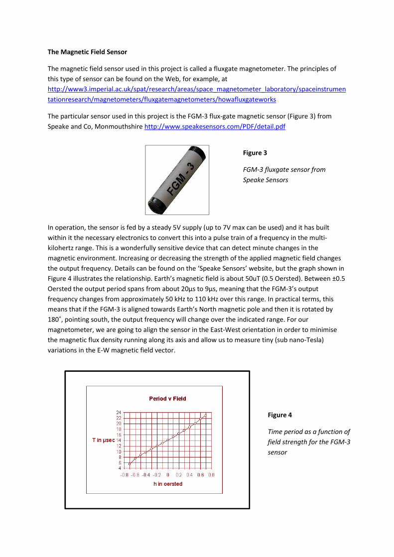
The particular sensor used in this project is the FGM-3 flux-gate magnetic sensor (Figure 3) from

Speake and Co, Monmouthshire http://www.speakesensors.com/PDF/detail.pdf

In operation, the sensor is fed by a steady 5V supply (up to 7V max can be used) and it has built

within it the necessary electronics to convert this into a pulse train of a frequency in the multi-

kilohertz range. This is a wonderfully sensitive device that can detect minute changes in the

magnetic environment. Increasing or decreasing the strength of the applied magnetic field changes

the output frequency. Details can be found on the ‘Speake Sensors’ website, but the graph shown in

Figure 4 illustrates the relationship. Earth’s magnetic field is about 50uT (0.5 Oersted). Between ±0.5

Oersted the output period spans from about 20µs to 9µs, meaning that the FGM-3’s output

frequency changes from approximately 50 kHz to 110 kHz over this range. In practical terms, this

means that if the FGM-3 is aligned towards Earth’s North magnetic pole and then it is rotated by

180˚, pointing south, the output frequency will change over the indicated range. For our

magnetometer, we are going to align the sensor in the East-West orientation in order to minimise

the magnetic flux density running along its axis and allow us to measure tiny (sub nano-Tesla)

variations in the E-W magnetic field vector.

Figure 3

FGM-3 fluxgate sensor from

Speake Sensors

Figure 4

Time period as a function of

field strength for the FGM-3

sensor

Ultrasonic (Emitter) transducer

The ultrasonic pulse train from the FGM-3 can be converted into ultrasonic sound using an ultrasonic

transducer as illustrated in Figure 5. I used a general purpose transducer with a centre frequency of

40kHz, driven by a max. 10V signal voltage. This covers the range of frequencies produced by the

FGM-3 very well and the drive voltage is within range of the output voltage from the sensor. These

transducers are common and easily can be obtained from electrical component stores.

Ultrasonic to Audio Converter

There are various circuits described on the internet for converting ultrasonic frequencies (>20kHz) to

audio frequencies (<20kHz) and these are of greater or lesser complexity depending on the

conversion method and quality of reproduced sound. There are also pulse counting circuits that

provide a direct conversion to frequency. The preferred method for this project is to use a

heterodyne circuit in which the input signal is mixed with a reference signal of a close frequency to

generate an audible output signal. The frequency of this audio signal will be equal to the frequency

difference between input and reference frequencies. For example, if the input frequency is 100kHz

and the reference frequency is 97kHz, then the difference between them (3kHz) is the output

frequency. So by this process, the ultrasonic input frequency from the FGM-3 sensor is converted to

an audio output frequency which can now be logged using a computer via the soundcard. Adjusting

the reference frequency up or down the scale proportionally changes the output frequency.

Conversely, if the input frequency varies (with a varying magnetic field as illustrated in Figure 1) then

with a steady reference frequency, the output audio frequency will also vary substantially in

proportion to the changing magnetic field.

For those so inclined and talented, such circuits off the web can certainly be built and deployed to

measure Earth’s magnetic field, but described here is an ultra-simple alternative for those who are

not inclined to build a circuit from scratch. Commercially available magnetometers are expensive.

However a digital heterodyne instrument can be relatively inexpensive and one suitable for this

application can be purchased for about £90 in the form of a bat detector.

A bat detector is nothing more than a device that converts ultrasonic sound emitted from the bat

into audio frequencies so that the operator can hear the calls from the animal. This is precisely what

is required for this application, except that the obliging bat is replaced with the FGM-3 and

ultrasonic transducer.

Figure 5

Ultrasonic transducer used to

couple the output from the

FGM-3 with the Magenta Bat 5

I use a crystal controlled heterodyne detector from Magenta (Magenta bat-5)

http://www.nhbs.com/magenta_bat_5_tefno_156155.html as this gives sufficiently precise

frequency control and excellent stability, which is what we need. The output is also of very high

quality as an audio signal. Input is via an electret microphone located on the right hand side of the

top edge of the instrument.

The Magenta bat-5 with ultrasonic transducer is illustrated in Figure 6.

Conveniently, the Magenta Bat-5 also comes with a 3.5mm jack output socket intended for

headphones, but which can also be used to pass the audio signal into the PC/laptop via the sound

card. The device also comes with a tuneable oscillator conveniently operating over the frequency

range of interest for this project and volume control.

Sensor Housing

The FGM-3 magnetometer is sensitive to changes in ambient temperature and its output frequency

will increase and decrease appreciably between daytime and night time and summer and winter

temperatures. This means that the sensor has to be located somewhere where the temperature

fluctuations are minimised. Also, the sensor clearly has to be set away from local magnetic

disturbances which will impact the instrument’s ability to discern solar storms from general

background clutter.

A good location for the sensor is underground and away from magnetic sources, as here the

temperature can be relatively stable, with the surrounding soil providing sufficient thermal

insulation to provide thermal ‘inertia’ against daily temperature swings. Being buried underground

means that the sensor has to be housed in a waterproof container to prevent the contacts shorting

out (all other components such as the bat detector and ultrasonic transducer remain above ground

several metres away in a dry environment).

A suitable container can be made using plumbing hardware as illustrated in Figure 7. Here I’ve used

40&43mm ABS tubes and end-stops with screw-on end fittings and saddle clamp. The central tube

was 2m long and had to be cut to length. The remaining hardware was purchased as shown. These

are sold as pipe joining sleeves and blanking plates.

Figure 6

Magenta Bat 5 ultrasonic to

audio frequency converter

All of the pieces were assembled using suitable solvent from the supplier, which was used in

accordance with the instructions provided, including health and safety for this volatile and

flammable substance.

The assembled housing is shown in Figure 8. Also added is a cable gland to allow the cable to enter

the housing via a watertight seal. This contains a rubber cuff that compresses onto the cable,

forming a seal. The saddle clamp is added as a means of attaching the housing to a solid base prior

to installing it underground. DO NOT apply solvent to the end cap fittings, as access to the tube will

be required and these caps will need to be removed.

Figure 7

a) Plumbing hardware layout ahead of assembly

b) Application of solvent to end fitting

(a) (b)

Figure 8

Assembled housing with

saddle clamp for fixation to

solid base

With the end caps removed install a length of copper pipe foam insulation sleeve. This again can be

purchased from a hardware store and conveniently for this project it has an outside diameter slightly

larger than the inside bore of the housing and a hollow core diameter slightly smaller than the

diameter of the FGM-3 sensor. This is going to hold the sensor centrally within the bore of the

housing which will be important during device set-up and operation. Cut the foam so that it extends

about halfway down the length of the housing, as this will provide space in the housing for some

basic voltage regulation electronics to be co-located with the sensor. Figures 9a and 9b show the

housing with foam core viewed from each end.

Wiring up the device

There are two schemes: the first (Type 1) is battery operated whilst the second (Type 2) is mains

supplied and voltage regulated. The first is the easiest to set up, but like all battery operated devices

it requires the batteries to be replaced periodically, whilst the second can be left to run permanently

without further attention to the power source. However, the second does require some basic circuit

board assembly skills, which the use of a bat detector was intended to avoid. Nevertheless, the

circuit is very simple and it is worth the effort in order to have a permanently running system.

Type 1

The wiring arrangement for this set-up is shown in Figure 10. There are two sets of batteries

required; one set (four AA batteries) runs the FGM-3 and the second set is located within the

Magenta Bat-5 (four AAA batteries). A minimum 3-core cable is required for +ve, ground and signal.

Depending on the degree of electrical noise in the local environment and the distance between the

sensor and ultrasonic transducer/detector, it may be necessary to provide local decoupling to

ground any unwanted noise on the supply line. This can be achieved using a 56nH induction coil and

33µF capacitor as shown. Leads can be soldered directly onto the pins of the FGM-3. It is advisable

to use heat-shrink tubing on all soldered terminals to minimise the risk of shorting. The cable should

preferably be one of the internally shielded types with wrapped foil, available from electrical stores.

Figure 9

a) Foam core with central open core to take the FGM-3

b) Opposite view with space in housing for voltage regulation

electronics

(a) (b)

Type 2

The wiring arrangement and circuit for the type 2 set-up with mains supply is shown in Figure 11. A

key factor in the successful operation of the FGM-3 sensor is a stable voltage supply, as without this

the output signal will carry an imprint of any fluctuation in the supply voltage, thereby degrading the

quality of the output from the device. Simple mains to +5V D.C. conversion using a standard power

supply is not adequate for this purpose and instead it is necessary to introduce an electrical circuit in

the feed. Details can be found on the ‘Speake Sensors’ web site and information will additionally be

provided by Bill Speake with the sensor upon delivery. The components required are reproduced in

Figure 11. Basically, the arrangement comprises two voltage regulators of the LM78xx series,

available from any electronic components supplier, to step the applied voltage from +12V D.C.

(provided by a low power mains transformer, such as might be used to power a laptop) to +9V D.C.

and then to +5V D.C. with a high degree of stability. These components should be located close to

the sensor. A 10µF capacitor may be added close to the sensor, as well, in order to provide further

stability to the feed voltage. The Magenta Bat-5 can also be powered from the same12V D.C. power

supply as for the sensor, using a single LM7805 (or equivalent) to provide a +5V supply and avoid

using batteries. This is below the regular +6V provided by the four AAA batteries normally used, but

is within the working voltage parameter for the device. Pin connections for LM78xx devices can be

found on the manufacturer’s web site. The feed from the LM7805 is simply soldered to the +ve and

ground battery terminals within the battery compartment WITHOUT the batteries being in place.

However, care must be taken not to overheat the connectors during soldering as the internal wiring

can come unattached. If internal disconnection does occur, then simply open the detector using the

Figure 10

Type 1 version: battery operated sensor and detector

four screws, removing the tuning dial by loosening a small grub screw on the edge and then locate

the red and black feed wires from the battery compartment and connect into these instead.

Loading the Sensor and Power Electronics in the Housing

With the cable pushed through the gland (loose), and through the housing, the voltage regulator

circuit board can be soldered to the FGM-3 sensor and the cable can be soldered to the board. With

the connections secured the board and FGM-3 can be pushed through the bore within the foam core

as illustrated in Figures 12a and b. Continue to push the sensor back into the core so that it is flush

with the end of the foam.

Figure 11

Type 2 version: mains supplied and voltage regulated sensor and

detector

Figures 12 a & b

Introducing the voltage regulator and FGM-3 sensor into the housing

using a foam core to locate the sensor centrally and hold it firm.

(a) (b)

It is worth checking that the device works at this point. This can be done by powering up the sensor

(either with batteries, or the 12V D.C. supply if voltage regulators are used) ensuring that the

ultrasonic transducer is first connected between the output wire and ground. The Magenta Bat-5

should produce a steady tone when tuned close to the output frequency of the sensor and the

audible frequency will decrease to zero and then increase as it is tuned ‘through’ the sensor’s output

frequency. The frequency will also change when the FGM-3 is moved around within Earth’s magnetic

field.

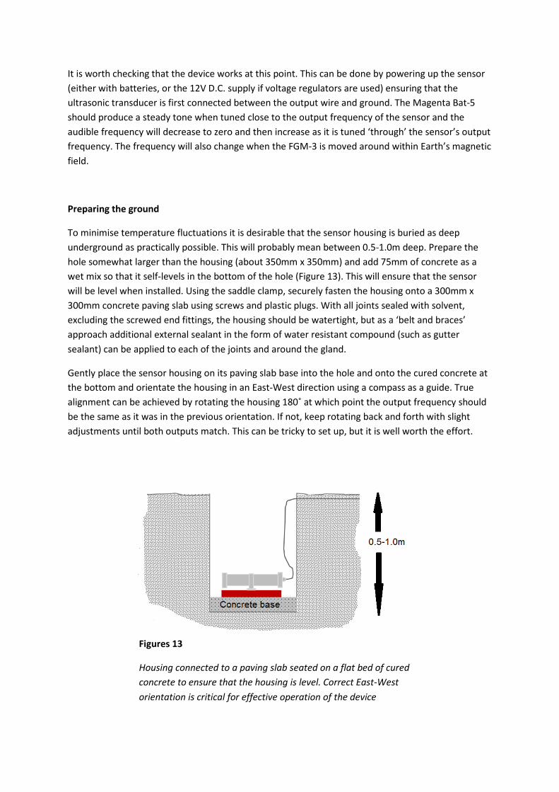
Preparing the ground

To minimise temperature fluctuations it is desirable that the sensor housing is buried as deep

underground as practically possible. This will probably mean between 0.5-1.0m deep. Prepare the

hole somewhat larger than the housing (about 350mm x 350mm) and add 75mm of concrete as a

wet mix so that it self-levels in the bottom of the hole (Figure 13). This will ensure that the sensor

will be level when installed. Using the saddle clamp, securely fasten the housing onto a 300mm x

300mm concrete paving slab using screws and plastic plugs. With all joints sealed with solvent,

excluding the screwed end fittings, the housing should be watertight, but as a ‘belt and braces’

approach additional external sealant in the form of water resistant compound (such as gutter

sealant) can be applied to each of the joints and around the gland.

Gently place the sensor housing on its paving slab base into the hole and onto the cured concrete at

the bottom and orientate the housing in an East-West direction using a compass as a guide. True

alignment can be achieved by rotating the housing 180˚ at which point the output frequency should

be the same as it was in the previous orientation. If not, keep rotating back and forth with slight

adjustments until both outputs match. This can be tricky to set up, but it is well worth the effort.

Figures 13

Housing connected to a paving slab seated on a flat bed of cured

concrete to ensure that the housing is level. Correct East-West

orientation is critical for effective operation of the device

Before refilling the hole it is prudent to check again that everything functions as required by

connecting the power supply and monitoring the output using the Magenta Bat-5. It should be

possible to tune the detector to produce a whistling tone. Once it has been established that the

sensor is functioning correctly, the hole may be refilled, ensuring that the housing does not move

during the refilling process.

Output Frequency

The frequency of the output will depend on the supply voltage, the temperature of the sensor, the

tuned frequency of the Magenta Bat-5 and the orientation of the FGM-3 sensor. For a

comprehensive summary of the performance of the FGM-3 sensor refer to

https://www.cv.nrao.edu/~demerson/cs/magnet.htm and in relation to temperature

https://www.cv.nrao.edu/~demerson/cs/magtherm.htm

Voltage

The frequency/voltage coefficient of the FGM-3 sensor is about 3.5% per volt at the nominal 5 volt

supply level according to Speake Sensors. With the type 1 version, the output will drift, therefore, as

the batteries run out of power and the voltage drops. However, useful results can still be obtained

when recording over relatively short periods of time (couple of days) to capture specific events such

as CMEs, the approach of which can be monitored by following space weather prediction websites

such as Spaceweather.com to give the observer time to set up and monitor the magnetic interaction.

For longer-term monitoring it is better to use the type 2 version with voltage regulation.

Temperature

The output frequency will change depending on the temperature of the sensor. When the sensor is

first installed it will not be at equilibrium temperature of its new surroundings, of course, so it will

take a little time to equilibrate. Also, when the sensor is operating, the small amount of current

running through the sensor (about 12mA) will produce a small amount of heat (about 60mW) which

will also affect the output frequency. Again, it will be necessary to allow the sensor to equilibrate

with its environment. The whole system may take a day or two to settle down. It should be noted

that the Magenta Bat-5 detector also is temperature sensitive and the output frequency will change

depending on the ambient conditions within which this is operating. This should also be housed

somewhere where the temperature fluctuations are minimised. I house my Magenta Bat-5 in a box

indoors and run the wire from it, to the buried sensor, through a hole in the wall.

Tuning the Magenta Bat-5 Detector

The detector can be tuned very easily using the dial. As the dial is rotated the audio output

frequency will be heard to decrease, pass through a minimum and then increase again as it passes

through the point at which it exactly matches the output frequency from the sensor. This is the ‘null’

frequency. This means that there are two possible positions on the dial at which the output audio

frequency is within the desirable 3-4kHz range. The first being 3-4kHz above the null frequency and

the second being 3-4kHz below the null frequency. The correct tuned frequency will depend on the

orientation of the sensor in relation to the East-West direction.

Orientation

Figure 14 illustrates the output frequency from the FGM-3 in kHz as a function of orientation (the

actual frequency will depend on the temperature and voltage as described above). This chart was

obtained by experimentation using 6V batteries to drive the sensor, setting the sensor at different

angles relative to north and tuning the detector to find the null point. As illustrated, the maximum

frequency occurred with the sensor pointing south and minimum occurred with the sensor pointing

north. Here the connection tabs to the sensor were selected to represent the ‘tail’ and the opposite

end the ‘head’ of the sensor.

As can be seen, the output frequency in the East-West direction is the same (give or take with some

experimental error) as the frequency in the West-East direction. However, the response to a

fluctuating magnetic field will be different in these two cases and in practice one will be the mirror

image of the other, rising in frequency whilst the other is falling under the same applied field. This

means that the sensor in the ground will respond differently to the field fluctuations if oriented in

one, or other direction. In other words, for a sensor that has its head pointing West, an increase in

the strength of the magnetic field from the East (for example, as a result of a passing CME) may

produce an increase in the detected output frequency, but for a sensor with its head pointing East,

the same change in applied field may produce a decrease in the output frequency. Why is this

important? It means that the output recorded on the data capture software (see later) could be the

inverse of what is presented by professional networks, such as INTERMAGNET when the charts are

compared, with upward trending data showing as downward trending data and vice versa. This

problem easily can be overcome by using the null frequency and tuning 3-4kHz above this null, OR 3-

4kHz below the null (depending on the orientation of the sensor East-West, or West-East), which will

reverse the response of the sensor and bring it in line with published professional results. This

means that the polarity of the buried sensor relative to east-west is not so important, as it can be

corrected using this method.

Figures 14

Sensor output frequency as a function of orientation relative to

magnetic north

Logging the output

The Magenta Bat-5 detector can be connected to a computer’s sound card via the line input socket

using a 3.5mm jack to 3.5mm jack lead via the headphone output socket located on the base of the

detector. When first connecting up, ensure that the detector volume is set to minimum and steadily

increase until the signal registers on screen using the logging software.

A useful piece of software for the purpose is ‘Spectrum Lab’

http://www.qsl.net/dl4yhf/spectra1.html by Wolfgang "Wolf" Buescher. This is superb software not

only because it is technically excellent, but also it is free. Like all unfamiliar software, it takes a little

time to get used to the layout and features, but it is well worth the effort. The application can be

configured to plot the audio frequency output from the detector as a function of time and sampling

can be defined from fractions of a second to minutes or hours. A convenient period is 150 seconds

(2.5 minutes) which gives sufficient resolution without generating too much data (576 data points

over a 24hr period). However, data can also be captured very rapidly, if required, by selecting the

appropriate sampling period in the configuration menu. The shortest period for practical purposes

may be once per second to capture magnetic fluctuations in high resolution, providing 86400 data

points over 24hrs.

The output from the detector can be captured as an image of the chart on the screen, which can be

automatically stored as a JPEG file by the software at any period that you select (such as once per

day). In addition, the software can be configured such that it stores every data point as a line of text

in a memo-text file along with the date and time of capture. This is very convenient for later analysis,

as the text can be copied and pasted into Excel, scaled and plotted as a chart.

Main screen

The main screen is shown in Figure 15. This has been configured to display frequency on the vertical

axis and time along the horizontal axis, with new data joining the screen from the right (so the chart

indexes left as each new data point is added). Initially, when first setting up the chart, it might show

a whole series of lines, indicating that the frequency from the FGM-3 is not one single frequency, but

may instead be composed of a mix of frequencies although there will be one dominant frequency,

which is the one of interest. Fortunately, all unwanted clutter can be excluded from the display by

adjusting the brightness and contrast bars highlighted on the display. Additionally, and conveniently,

Spectrum Lab allows full configuration of background colour, pen colour, text colour, font, size,

position and so on, so all of these parameters can be set according to taste to produce a clean image

with a single line of data.

Logging data to file

In addition to enabling the screen image to be captured automatically, Spectrum Lab can also be

configured to automatically log data to a predetermined file continuously at a chosen interval of

time. This is achieved by selecting ‘File’ and the submenu ‘Export calculated data (continuously)’.

This will open a panel ‘Spectrum Lab- File Export Format’ as illustrated in Figure 16.

Figures 15

Configured Spectrum Lab main screen with frequency on the vertical axis

Figure 16

Spectrum Lab- File Export

Format menu: File contents

tab for defining date/time

and peak frequency

Frequency bar

Signal

Time markers

Control Panel

Brightness &

Contrast

Under ‘File Contents’ the information to be saved can be defined (date, time and frequency) and

under the ‘Filename and Activation’ tab the file name, location of the file and write interval can be

defined, as shown in Figure 17.

It is important to define the frequency band width in the file contents definition in order to ensure

that only the frequency range of interest is logged. The defined contents are stored as a Comma

Separated Values (CSV) notepad text file (Figure 18), which is added to with new data at the selected

update period. Conveniently, the contents of this file (such as the data for a specific period in time)

can be directly copied and pasted into an Excel spread sheet.

Figure 17

Spectrum Lab- File Export

Format menu: Filename and

activation to define filename,

location and logging

frequency

Figure 18

Partial dataset in CSV format

saved as text file in Notepad

Analysis

It is convenient to transfer the data from Spectrum Lab to Excel. This is because of the flexibility in

data presentation that Excel brings. It also means that data can be manipulated in multiple ways to

zoom in on points of interest, run calculations, or compare data from different periods, add notes, or

incorporate images as a means of illustration and so on. It is also a good way to convert the

frequency output from the log to something close to nano-Tesla (nT). I say close to nT because at no

point has the sensor been calibrated in this project, nor at this stage has there been any attempt to

correct for temperature variation, or any frequency drift of the detector, or any other factors that

might affect the accuracy of the output (such as passing traffic in the street, parked cars which come

and go and so on). Remember, this is for the hobbyist and we are not intending to generate truly

accurate scientific data.

Figure 19 shows a few lines of the worksheet that I use. The defined contents of the CSV file are

copied from memo and pasted directly into the first column. Column B is the measured frequency

value which is automatically extracted from this CSV file. Column C (frequency delta) is the

difference between the measured frequency and the ‘offset frequency’ which itself is the difference

between the null frequency (the frequency of the output signal from the sensor) and the frequency

setting on the Magenta Bat-5 at the time the data are recorded. The ‘total frequency’ in column D is

the null frequency less the frequency delta (column C). The time period (E) is simply the reciprocal of

D with the necessary conversion factor to convert to µs. Finally, this allows the calculation of the

strength of the magnetic field vector in nT using the relationship shown in Figure 4.

When correctly set up the instrument is more than capable of detecting changes in the magnetic

environment as a result of geomagnetic storms and even in very quiet periods when geomagnetic

activity is very low, the correlation between this instrument and professional instruments is,

pleasingly, very good. An example of the degree of correlation is illustrated below in Figures 20a and

A B C D E F G H

East-West DataOffset Frequency 3.520 kHz Null Frequency 69.970 kHz

Start Date Set Frequency 66.450 kHz

Null time period 14.292 µS

Time

Measured Freq Frequency Delta Total Frequency Time Period µs µTeslar Time (hhmmss) (nT)

26/01/2014 00:01 3570.11 50.110 69919.890 14.3021 0.0854 00:01:35 18.97

26/01/2014 00:04 3570.11 50.110 69919.890 14.3021 0.0854 00:04:05 18.97

26/01/2014 00:06 3571.82 51.820 69918.180 14.3024 0.0883 00:06:35 19.62

26/01/2014 00:09 3575.78 55.780 69914.220 14.3032 0.0950 00:09:05 21.12

26/01/2014 00:11 3575.8 55.800 69914.200 14.3032 0.0951 00:11:35 21.12

26/01/2014 00:14 3581.95 61.950 69908.050 14.3045 0.1055 00:14:05 23.45

26/01/2014 00:16 3583.93 63.930 69906.070 14.3049 0.1089 00:16:35 24.20

26/01/2014 00:19 3586.42 66.420 69903.580 14.3054 0.1132 00:19:05 25.15

26/01/2014 00:21 3588.25 68.250 69901.750 14.3058 0.1163 00:21:35 25.84

26/01/2014 00:24 3587.41 67.410 69902.590 14.3056 0.1149 00:24:05 25.52

26/01/2014 00:26 3588.45 68.450 69901.550 14.3058 0.1166 00:26:35 25.92

26/01/2014 00:29 3585.05 65.050 69904.950 14.3051 0.1108 00:29:05 24.63

26/01/2014 00:31 3582.91 62.910 69907.090 14.3047 0.1072 00:31:35 23.82

Figures 19

Part of Excel spreadsheet used to convert measured output frequency to nT. There are

576 lines of data per 24hr period, captured at 2.5 minute intervals.

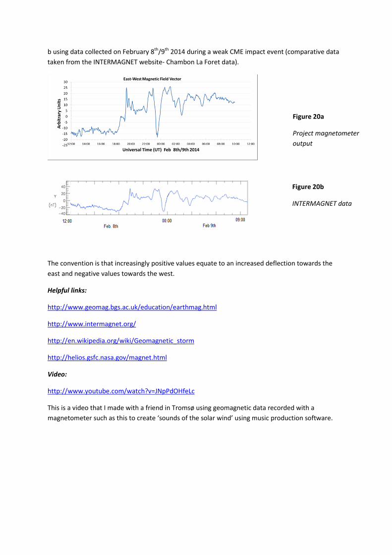
b using data collected on February 8th

/9th

2014 during a weak CME impact event (comparative data

taken from the INTERMAGNET website- Chambon La Foret data).

The convention is that increasingly positive values equate to an increased deflection towards the

east and negative values towards the west.

Helpful links:

http://www.geomag.bgs.ac.uk/education/earthmag.html

http://www.intermagnet.org/

http://en.wikipedia.org/wiki/Geomagnetic_storm

http://helios.gsfc.nasa.gov/magnet.html

Video:

http://www.youtube.com/watch?v=JNpPdOHfeLc

This is a video that I made with a friend in Tromsø using geomagnetic data recorded with a

magnetometer such as this to create ‘sounds of the solar wind’ using music production software.

Figure 20a

Project magnetometer

output

Figure 20b

INTERMAGNET data

Appendix

Here is my prototype magnetometer with two deconstructed Magenta-Bat 5 detectors coupled to

two FGM-3s configured to measure north-south and east-west magnetic field vectors. Here I

coupled the sensors directly, rather than acoustically, using a resistor ladder to lower the voltage

and a capacitor to eliminate any potential DC component. However, I have not seen any advantage

doing so and it is much simpler to just use an acoustic couple with the ultrasonic emitter and leave

the Magenta Bat-5s untouched, except for the power supply to convert them from battery power.

Disclaimer

It is intended that the information contained in this document is accurate and reliable. However,

errors may occasionally occur. Therefore, all information and materials are provided "AS IS". In no

event will the author be liable for any indirect, special, incidental, or consequential damages arising

out of the use of the information contained herein.