Earthquake distribution is not random: very narrow deforming zones(= plate boundaries) versus large areas with no earthquakes (= rigid

plate interiors)

Tectonic plates and their boundaries today -- continentsare embedded in the plates and move with them

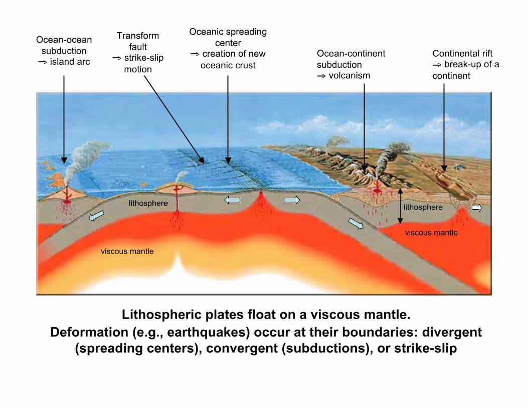
Ocean-oceansubduction⇒ island arc

Oceanic spreadingcenter

⇒ creation of newoceanic crust

Ocean-continentsubduction⇒ volcanism

Continental rift⇒ break-up of acontinent

Lithospheric plates float on a viscous mantle.Deformation (e.g., earthquakes) occur at their boundaries: divergent

(spreading centers), convergent (subductions), or strike-slip

Transformfault

⇒ strike-slipmotion

lithosphere

viscous mantle

viscous mantle

lithosphere

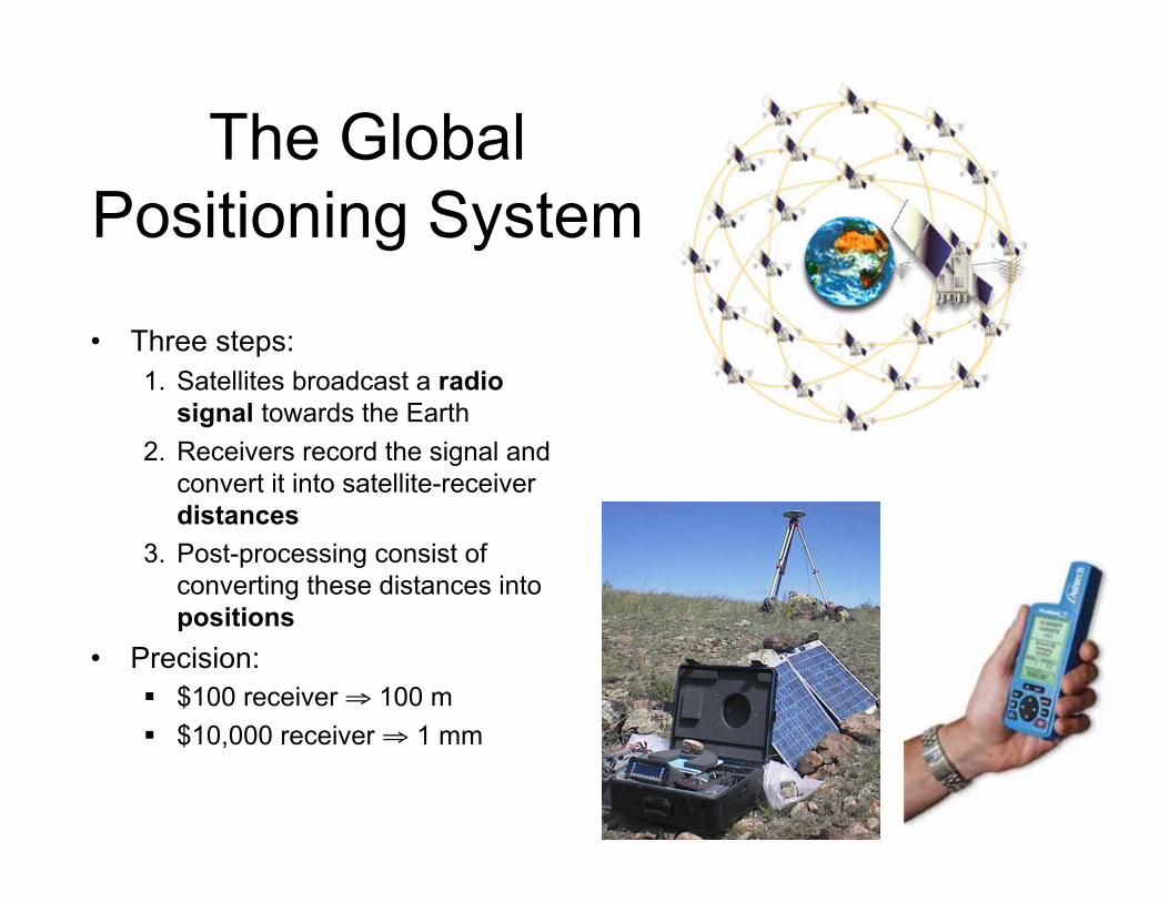
The GlobalPositioning System

• Three steps:1. Satellites broadcast a radio

signal towards the Earth2. Receivers record the signal and

convert it into satellite-receiverdistances

3. Post-processing consist ofconverting these distances intopositions

• Precision: $100 receiver ⇒ 100 m $10,000 receiver ⇒ 1 mm

Principle of GPS positioning

satellite 1

Earth

ρ1

satellite 3

ρ3

ρ2

You are here

x

ρ2

satellite 2

• Satellites broadcast signals on 1.2 GHzand 1.5 GHz frequencies:

– Satellite 1 sends a signal at time te1– Ground receiver receives it signal at time tr– The range measurement ρ1 to satellite 1 is:

ρ1 = (tr-te1) x speed of light– We are therefore located on a sphere

centered on satellite 1, with radius ρ1– 3 satellites => intersection of 3 spheres

• Or use the mathematical model:

• A! The receiver clocks are mediocre andnot synchronized with the satellite clocks

– Time difference between the satellite clocksand the receiver clock

– Additional unknown => we need 4observations = 4 satellites visible at thesame time

222 )()()(rsrsrs

s

rZZYYXX !+!+!="

Principle of GPS positioning• GPS data = satellite-receiver

range measurements (ρ)• Range can be measured in two

ways:1. Measuring the propagation time of

the GPS signal:• Easy, cheap• Limited post-processing required• As precise as the time

measurements ~1-10 m2. Counting the number of cycles of

the carrier frequency• More difficult• Requires significant post-processing• As precise as the phase detection ~1

mmEarth

x

te

tr

data = (tr-te) x c data = λ x n

λ ~ 20 cm

From codes: From carrier:

(unit = meters) (unit = cycles)

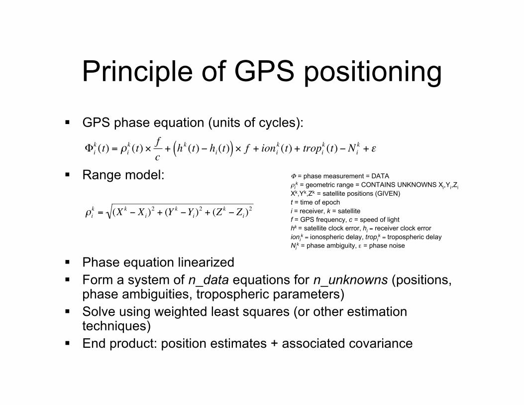
Principle of GPS positioning GPS phase equation (units of cycles):

Range model:

Phase equation linearized Form a system of n_data equations for n_unknowns (positions,

phase ambiguities, tropospheric parameters) Solve using weighted least squares (or other estimation

techniques) End product: position estimates + associated covariance

!

"i

k(t) = #i

k(t) $

f

c+ h

k(t) % hi(t)( ) $ f + ioni

k(t) + tropi

k(t) % Ni

k + &

!

"i

k= (X

k # Xi)2

+ (Yk #Y

i)2

+ (Zk # Z

i)2

Φ = phase measurement = DATAρi

k = geometric range = CONTAINS UNKNOWNS Xi,Yi,ZiXk,Yk,Zk = satellite positions (GIVEN)t = time of epochi = receiver, k = satellitef = GPS frequency, c = speed of lighthk = satellite clock error, hi = receiver clock errorioni

k = ionospheric delay, tropik = tropospheric delay

Nik = phase ambiguity, ε = phase noise

Principle of GPS positioning

⇒ Precise GPS positioning requires:• Dual-frequency equipment• Rigorous field procedures• Long (several days) observation sessions• Complex data post-processing

MagnitudeTreatmentError source

~ 1 cmUse correction tablesAntenna phase center

~ 0.5 mChoose good sites!Multipath

???Choose good operators!Site setup

centimetersPrecession, Nutation, UT, Polar motionGeodetic models

centimetersTides (polar and solid Earth), Ocean loadingGeophysical models

2 cm to 100 mGet precise (2-3 cm) orbitsSatellite orbits

1-50 mDual frequency measurementsIonospheric refraction

0.5-2 mExternal measurement or estimation of “troposphericparameters”

Tropospheric refraction

metersDouble difference or direct estimationReceiver clock errors

~1 mDouble difference or direct estimationSatellite clocks errors

< 1 mmNonePhase measurement noise

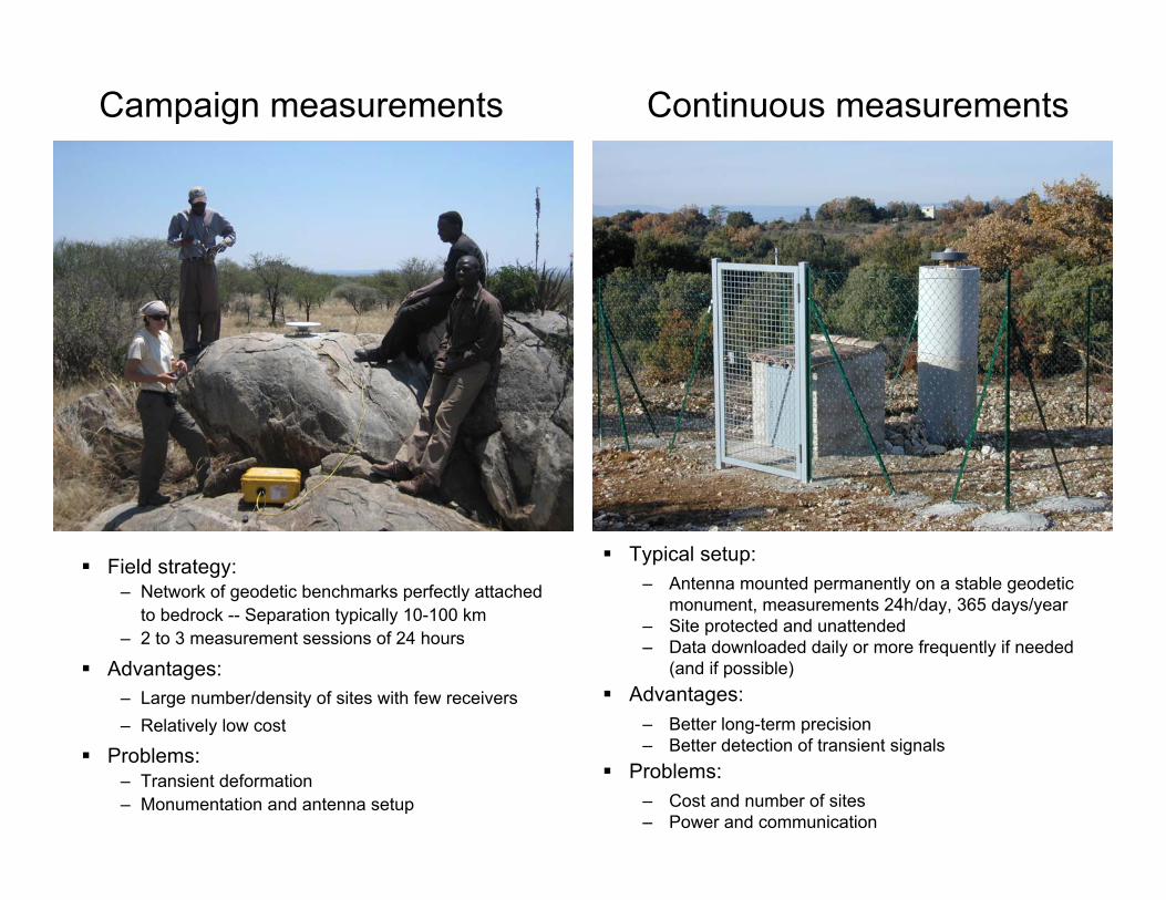
Campaign measurements Continuous measurements

Field strategy:– Network of geodetic benchmarks perfectly attached

to bedrock -- Separation typically 10-100 km– 2 to 3 measurement sessions of 24 hours

Advantages:– Large number/density of sites with few receivers– Relatively low cost

Problems:– Transient deformation– Monumentation and antenna setup

Typical setup:– Antenna mounted permanently on a stable geodetic

monument, measurements 24h/day, 365 days/year– Site protected and unattended– Data downloaded daily or more frequently if needed

(and if possible) Advantages:

– Better long-term precision– Better detection of transient signals

Problems:– Cost and number of sites– Power and communication

Continents show consistentpattern of displacement

They move at speeds ~fewcm/yr = the speed your

fingernails grow…

Repeated GPS measurements show that the longitude of Algonquin(Canada) is changing at a rate of 1.5 cm/yr

• Norabuena et al.(1999): decelerationback to at least 20My, initiation ofAndes growth

• Consequence ofconstruction of theAndes?

• Increased friction andviscous drag asleading edge of Sathickens?

Norabuena et al., Science, 1998

Hutton et al., GJI, 2001

Jalisco earthquake, October1995, Mw=8.0

Episodic Tremors and SlipDragert et al., Science 2001

http://www.pgc.nrcan.gc.ca/seismo/ETS/ETS.htm

• Juan de Fuca subduction• Typical interseismic strain accumulation• Episodes of aseismic slip every 13 to 16 months• Typically 10 day long, 5 mm surface displacement

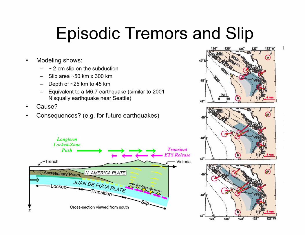
Episodic Tremors and Slip• Modeling shows:

– ~ 2 cm slip on the subduction– Slip area ~50 km x 300 km– Depth of ~25 km to 45 km– Equivalent to a M6.7 earthquake (similar to 2001

Nisqually earthquake near Seattle)• Cause?• Consequences? (e.g. for future earthquakes)

Vertical motions:post-glacial rebound, up to cm/yr

Sella et al., 2007

Time dependent vertical motions:hydrological loading

VanDam et al., 2001

Bevis et al., 2005

Comparison between GPS observations at Manaus(Amazonian basin, red dots) and the predicted flexure

of an elastic plate under water loading. A model of the peak-to-peak amplitude of vertical motionsdue to hydrological loading (=water + snow)