earthquake settlement

EARTHQUAKE-INDUCEDSETTLEMENT

The following notation is used in this chapter:

SYMBOL DEFINITION

amax, ap Maximum horizontal acceleration at ground surface (also known as peak ground accelera-tion)

CSR Cyclic stress ratio

Dr Relative density

Em

Hammer efficiency

F Lateral force reacting to earthquake-induced base shear

FS, FSL Factor of safety against liquefaction

g Acceleration of gravity

Geff Effective shear modulus at induced strain level

Gmax Shear modulus at a low strain level

H Initial thickness of soil layer

H1 Thickness of surface layer that does not liquefy

H2 Thickness of soil layer that will liquefy during earthquake

�H Change in height of soil layer

k0 Coefficient of earth pressure at rest

Ncorr Value added to (N1)60 to account for fines in soil

N Uncorrected SPT blow count (blows per foot)

N1 Japanese standard penetration test value for Fig. 7.1

(N1)60 N value corrected for field testing procedures and overburden pressure

OCR Overconsolidation ratio � �vm′ /�v 0′qc1 Cone resistance corrected for overburden pressure

rd Depth reduction factor

ue Excess pore water pressure

V Base shear induced by earthquake

� Earthquake-induced maximum differential settlement of foundation

εv Volumetric strain

�eff Effective shear strain

CHAPTER 7

7.1

�max Maximum shear strain

�t Total unit weight of soil

�max Earthquake-induced total settlement of foundation

�v0 Total vertical stress

�m′ Mean principal effective stress

�vm′ Maximum past pressure, also known as preconsolidation pressure

�v0′ Vertical effective stress

�1′ Major principal effective stress

�2′ Intermediate principal effective stress

�3′ Minor principal effective stress

��v Increase in foundation pressure due to earthquake

�cyc Uniform cyclic shear stress amplitude of earthquake

�eff Effective shear stress induced by earthquake

�max Maximum shear stress induced by earthquake

7.1 INTRODUCTION

As discussed in Sec. 4.2, those buildings founded on solid rock are least likely to experi-ence earthquake-induced differential settlement. However, buildings on soil could be sub-jected to many different types of earthquake-induced settlement. This chapter deals withonly settlement of soil for a level-ground surface condition. The types of earthquake-induced settlement discussed in this chapter are as follows:

● Settlement versus the factor of safety against liquefaction (Sec. 7.2): This section dis-cusses two methods that can be used to estimate the ground surface settlement for vari-ous values of the factor of safety against liquefaction (FS). If FS is less than or equal to1.0, then liquefaction will occur, and the settlement occurs as water flows from the soilin response to the earthquake-induced excess pore water pressures. Even for FS greaterthan 1.0, there could still be the generation of excess pore water pressures and hence set-tlement of the soil. However, the amount of settlement will be much greater for the liq-uefaction condition compared to the nonliquefied state.

● Liquefaction-induced ground damage (Sec. 7.3): There could also be liquefaction-induced ground damage that causes settlement of structures. For example, there could beliquefaction-induced ground loss below the structure, such as the loss of soil through thedevelopment of ground surface sand boils. The liquefied soil could also cause the devel-opment of ground surface fissures that cause settlement of structures.

● Volumetric compression (Sec. 7.4): Volumetric compression is also known as soil den-sification. This type of settlement is due to ground shaking that causes the soil to com-press together, such as dry and loose sands that densify during the earthquake.

● Settlement due to dynamic loads caused by rocking (Sec. 7.5): This type of settlementis due to dynamic structural loads that momentarily increase the foundation pressure act-ing on the soil. The soil will deform in response to the dynamic structural load, resultingin settlement of the building. This settlement due to dynamic loads is often a result of thestructure rocking back and forth.

7.2 CHAPTER SEVEN

The usual approach for settlement analyses is to first estimate the amount of earthquake-induced total settlement �max of the structure. Because of variable soil conditions and struc-tural loads, the earthquake-induced settlement is rarely uniform. A common assumption isthat the maximum differential settlement � of the foundation will be equal to 50 to 75 per-cent of �max (that is, 0.5�max � � � 0.75�max). If the anticipated total settlement �max and/orthe maximum differential settlement � is deemed to be unacceptable, then soil improve-ment or the construction of a deep foundation may be needed. Chapters 12 and 13 deal withmitigation measures such as soil improvement or the construction of deep foundations.

7.2 SETTLEMENT VERSUS FACTOR OF SAFETYAGAINST LIQUEFACTION

7.2.1 Introduction

This section discusses two methods that can be used to estimate the ground surface settle-ment for various values of the factor of safety against liquefaction. A liquefaction analysis(Chap. 6) is first performed to determine the factor of safety against liquefaction. If FS isless than or equal to 1.0, then liquefaction will occur, and the settlement occurs as waterflows from the soil in response to the earthquake-induced excess pore water pressures.Even for FS greater than 1.0, there could still be the generation of excess pore water pres-sures and hence settlement of the soil. However, the amount of settlement will be muchgreater for the liquefaction condition compared to the nonliquefied state.

This section is solely devoted to an estimation of ground surface settlement for variousvalues of the factor of safety. Other types of liquefaction-induced movement, such as bear-ing capacity failures, flow slides, and lateral spreading, are discussed in Chaps. 8 and 9.

7.2.2 Methods of Analysis

Method by Ishihara and Yoshimine (1992). Figure 7.1 shows a chart developed byIshihara and Yoshimine (1992) that can be used to estimate the ground surface settlementof saturated clean sands for a given factor of safety against liquefaction. The procedure forusing Fig. 7.1 is as follows:

1. Calculate the factor of safety against liquefaction FSL: The first step is to calculatethe factor of safety against liquefaction, using the procedure outlined in Chap. 6 [i.e., Eq.(6.8)].

2. Soil properties: The second step is to determine one of the following properties:relative density Dr of the in situ soil, maximum shear strain to be induced by the designearthquake �max, corrected cone penetration resistance qc1 kg/cm2, or Japanese standardpenetration test N1 value.

Kramer (1996) indicates that the Japanese standard penetration test typically transmitsabout 20 percent more energy to the SPT sampler, and the equation N1 � 0.83(N1)60 can beused to convert the (N1)60 value to the Japanese N1 value. However, R. B. Seed (1991) statesthat Japanese SPT results require corrections for blow frequency effects and hammerrelease, and that these corrections are equivalent to an overall effective energy ratio Em of0.55 (versus Em � 0.60 for U.S. safety hammer). Thus R. B. Seed (1991) states that the(N1)60 values should be increased by about 10 percent (that is, 0.6/0.55) when using Fig. 7.1to estimate volumetric compression, or N1 � 1.10(N1)60. As a practical matter, it can be

EARTHQUAKE-INDUCED SETTLEMENT 7.3

assumed that the Japanese N1 value is approximately equivalent to the (N1)60 value calcu-lated from Eq. (5.2) (Sec. 5.4.3).

3. Volumetric strain: In Fig. 7.1, enter the vertical axis with the factor of safety againstliquefaction, intersect the appropriate curve corresponding to the Japanese N1 value [assumeJapanese N1 � (N1)60 from Eq. (5.2)], and then determine the volumetric strain εv from thehorizontal axis. Note in Fig. 7.1 that each N1 curve can be extended straight downward toobtain the volumetric strain for very low values of the factor of safety against liquefaction.

4. Settlement: The settlement of the soil is calculated as the volumetric strain,expressed as a decimal, times the thickness of the liquefied soil layer.

7.4 CHAPTER SEVEN

FIGURE 7.1 Chart for estimating the ground surface settlement of clean sand as a functionof the factor of safety against liquefaction FSL. To use this figure, one of the following proper-ties must be determined: relative density Dr of the in situ soil, maximum shear strain to beinduced by the design earthquake �max, corrected cone penetration resistance qc1 (kg/cm2), orJapanese standard penetration test N1 value. For practical purposes, assume the Japanese stan-dard penetration test N1 value is equal to the (N1)60 value from Eq. (5.2). (Reproduced fromKramer 1996, originally developed by Ishihara and Yoshimine 1992.)

Note in Fig. 7.1 that the volumetric strain can also be calculated for clean sand that hasa factor of safety against liquefaction in excess of 1.0. For FSL greater than 1.0 but less than2.0, the contraction of the soil structure during the earthquake shaking results in excess porewater pressures that will dissipate and cause a smaller amount of settlement. At FSL equalto or greater than 2.0, Fig. 7.1 indicates that the volumetric strain will be essentially equalto zero. This is because for FSL higher than 2.0, only small values of excess pore water pres-sures ue will be generated during the earthquake shaking (i.e., see Fig. 5.15).

Method by Tokimatsu and Seed (1984, 1987). Figure 7.2 shows a chart developed byTokimatsu and Seed (1984, 1987) that can be used to estimate the ground surface settle-ment of saturated clean sands. The solid lines in Fig. 7.2 represent the volumetric strain forliquefied soil (i.e., factor of safety against liquefaction less than or equal to 1.0). Note thatthe solid line labeled 1 percent volumetric strain in Fig. 7.2 is similar to the dividing line inFig. 6.6 between liquefiable and nonliquefiable clean sand.

The dashed lines in Fig. 7.2 represent the volumetric strain for a condition where excesspore water pressures are generated during the earthquake, but the ground shaking is not suf-ficient to cause liquefaction (that is, FS 1.0). This is similar to the data in Fig. 7.1, in that


FIGURE 7.2 Chart for estimating the ground surface settlement of clean sand for fac-tor of safety against liquefaction less than or equal to 1.0 (solid lines) and greater than1.0 (dashed lines). To use this figure, the cyclic stress ratio from Eq. (6.6) and the (N1)60value from Eq. (5.2) must be determined. (Reproduced from Kramer 1996, originallydeveloped by Tokimatsu and Seed 1984.)

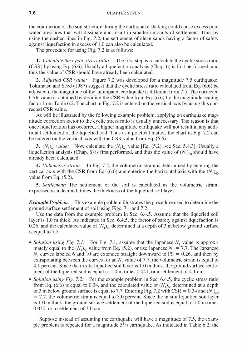
the contraction of the soil structure during the earthquake shaking could cause excess porewater pressures that will dissipate and result in smaller amounts of settlement. Thus byusing the dashed lines in Fig. 7.2, the settlement of clean sands having a factor of safetyagainst liquefaction in excess of 1.0 can also be calculated.

The procedure for using Fig. 7.2 is as follows:

1. Calculate the cyclic stress ratio: The first step is to calculate the cyclic stress ratio(CSR) by using Eq. (6.6). Usually a liquefaction analysis (Chap. 6) is first performed, andthus the value of CSR should have already been calculated.

2. Adjusted CSR value: Figure 7.2 was developed for a magnitude 7.5 earthquake.Tokimatsu and Seed (1987) suggest that the cyclic stress ratio calculated from Eq. (6.6) beadjusted if the magnitude of the anticipated earthquake is different from 7.5. The correctedCSR value is obtained by dividing the CSR value from Eq. (6.6) by the magnitude scalingfactor from Table 6.2. The chart in Fig. 7.2 is entered on the vertical axis by using this cor-rected CSR value.

As will be illustrated by the following example problem, applying an earthquake mag-nitude correction factor to the cyclic stress ratio is usually unnecessary. The reason is thatonce liquefication has occurred, a higher magnitude earthquake will not result in any addi-tional settlement of the liquefied soil. Thus as a practical matter, the chart in Fig. 7.2 canbe entered on the vertical axis with the CSR value from Eq. (6.6).

3. (N1)60 value: Now calculate the (N1)60 value [Eq. (5.2), see Sec. 5.4.3]. Usually aliquefaction analysis (Chap. 6) is first performed, and thus the value of (N1)60 should havealready been calculated.

4. Volumetric strain: In Fig. 7.2, the volumetric strain is determined by entering thevertical axis with the CSR from Eq. (6.6) and entering the horizontal axis with the (N1)60value from Eq. (5.2).

5. Settlement: The settlement of the soil is calculated as the volumetric strain,expressed as a decimal, times the thickness of the liquefied soil layer.

Example Problem. This example problem illustrates the procedure used to determine theground surface settlement of soil using Figs. 7.1 and 7.2.

Use the data from the example problem in Sec. 6.4.5. Assume that the liquefied soillayer is 1.0 m thick. As indicated in Sec. 6.4.5, the factor of safety against liquefaction is0.26, and the calculated value of (N1)60 determined at a depth of 3 m below ground surfaceis equal to 7.7.

● Solution using Fig. 7.1: For Fig. 7.1, assume that the Japanese N1 value is approxi-mately equal to the (N1)60 value from Eq. (5.2), or use Japanese N1 � 7.7. The JapaneseN1 curves labeled 6 and 10 are extended straight downward to FS � 0.26, and then byextrapolating between the curves for an N1 value of 7.7, the volumetric strain is equal to4.1 percent. Since the in situ liquefied soil layer is 1.0 m thick, the ground surface settle-ment of the liquefied soil is equal to 1.0 m times 0.041, or a settlement of 4.1 cm.

● Solution using Fig. 7.2: Per the example problem in Sec. 6.4.5, the cyclic stress ratiofrom Eq. (6.6) is equal to 0.34, and the calculated value of (N1)60 determined at a depthof 3 m below ground surface is equal to 7.7. Entering Fig. 7.2 with CSR � 0.34 and (N1)60� 7.7, the volumetric strain is equal to 3.0 percent. Since the in situ liquefied soil layeris 1.0 m thick, the ground surface settlement of the liquefied soil is equal to 1.0 m times0.030, or a settlement of 3.0 cm.

Suppose instead of assuming the earthquake will have a magnitude of 7.5, the exam-ple problem is repeated for a magnitude 514 earthquake. As indicated in Table 6.2, the

7.6 CHAPTER SEVEN

magnitude scaling factor � 1.5, and thus the corrected CSR is equal to 0.34 divided by1.5, or 0.23. Entering Fig. 7.2 with the modified CSR � 0.23 and (N1)60 � 7.7, the volu-metric strain is still equal to 3.0 percent. Thus, provided the sand liquefies for both themagnitude 51⁄4 and magnitude 7.5 earthquakes, the settlement of the liquefied soil is thesame.

● Summary of values: Based on the two methods, the ground surface settlement of the1.0-m-thick liquefied sand layer is expected to be on the order of 3 to 4 cm.

Silty Soils. Figures 7.1 and 7.2 were developed for clean sand deposits (fines � 5 per-cent). For silty soils, R. B. Seed (1991) suggests that the most appropriate adjustment is toincrease the (N1)60 values by adding the values of Ncorr indicated below:

Percent fines Ncorr

�5 010 125 250 475 5

7.2.3 Limitations

The methods presented in Figs. 7.1 and 7.2 can only be used for the following cases:

● Lightweight structures: Settlement of lightweight structures, such as wood-framebuildings bearing on shallow foundations

● Low net bearing stress: Settlement of any other type of structure that imparts a low netbearing pressure onto the soil

● Floating foundation: Settlement of floating foundations, provided the zone of lique-faction is below the bottom of the foundation and the floating foundation does not imparta significant net stress upon the soil

● Heavy structures with deep liquefaction: Settlement of heavy structures, such as mas-sive buildings founded on shallow foundations, provided the zone of liquefaction is deepenough that the stress increase caused by the structural load is relatively low

● Differential settlement: Differential movement between a structure and adjacent appur-tenances, where the structure contains a deep foundation that is supported by strata belowthe zone of liquefaction

The methods presented in Figs. 7.1 and 7.2 cannot be used for the following cases:

● Foundations bearing on liquefiable soil: Do not use Figs. 7.1 and 7.2 when the foun-dation is bearing on soil that will liquefy during the design earthquake. Even lightlyloaded foundations will sink into the liquefied soil.

● Heavy buildings with underlying liquefiable soil: Do not use Figs. 7.1 and 7.2 when theliquefied soil is close to the bottom of the foundation and the foundation applies a largenet load onto the soil. In this case, once the soil has liquefied, the foundation load willcause it to punch or sink into the liquefied soil. There could even be a bearing capacitytype of failure. Obviously these cases will lead to settlement well in excess of the valuesobtained from Figs. 7.1 and 7.2. It is usually very difficult to determine the settlement forthese conditions, and the best engineering solution is to provide a sufficiently high static


factor of safety so that there is ample resistance against a bearing capacity failure. This isdiscussed further in Chap. 8.

● Buoyancy effects: Consider possible buoyancy effects. Examples include buried stor-age tanks or large pipelines that are within the zone of liquefied soil. Instead of settling,the buried storage tanks and pipelines may actually float to the surface when the groundliquefies.

● Sloping ground condition: Do not use Figs. 7.1 and 7.2 when there is a sloping groundcondition. If the site is susceptible to liquefaction-induced flow slide or lateral spreading,the settlement of the building could be well in excess of the values obtained from Figs.7.1 and 7.2. This is discussed further in Chap. 9.

● Liquefaction-induced ground damage: The calculations using Figs. 7.1 and 7.2 do notinclude settlement that is related to the loss of soil through the development of groundsurface sand boils or the settlement of shallow foundations caused by the developmentof ground surface fissures. These types of settlement are discussed in the next section.

7.3 LIQUEFACTION-INDUCED GROUND DAMAGE

7.3.1 Types of Damage

As previously mentioned, there could also be liquefaction-induced ground damage thatcauses settlement of structures. This liquefaction-induced ground damage is illustrated inFig. 7.3. As shown, there are two main aspects to the ground surface damage:

1. Sand boils: There could be liquefaction-induced ground loss below the structure, suchas the loss of soil through the development of ground surface sand boils. Often a line ofsand boils, such as shown in Fig. 7.4, is observed at ground surface. A row of sand boilsoften develops at the location of cracks or fissures in the ground.

2. Surface fissures: The liquefied soil could also cause the development of ground sur-face fissures which break the overlying soil into blocks that open and close during theearthquake. Figure 7.5 shows the development of one such fissure. Note in Fig. 7.5 thatliquefied soil actually flowed out of the fissure.

The liquefaction-induced ground conditions illustrated in Fig. 7.3 can damage all typesof structures, such as buildings supported on shallow foundations, pavements, flatwork,and utilities. In terms of the main factor influencing the liquefaction-induced ground dam-

7.8 CHAPTER SEVEN

FIGURE 7.3 Ground damage caused by the liquefaction of an underlying soil layer. (Reproduced fromKramer 1996, originally developed by Youd 1984.)

age, Ishihara (1985) states:

One of the factors influencing the surface manifestation of liquefaction would be the thick-ness of a mantle of unliquefied soils overlying the deposit of sand which is prone to liquefac-tion. Should the mantle near the ground surface be thin, the pore water pressure from theunderlying liquefied sand deposit will be able to easily break through the surface soil layer,thereby bringing about the ground rupture such as sand boiling and fissuring. On the otherhand, if the mantle of the subsurface soil is sufficiently thick, the uplift force due to the excesswater pressure will not be strong enough to cause a breach in the surface layer, and hence, therewill be no surface manifestation of liquefaction even if it occurs deep in the deposit.

7.3.2 Method of Analysis

Based on numerous case studies, Ishihara (1985) developed a chart (Fig. 7.6a) that can beused to determine the thickness of the unliquefiable soil surface layer H1 in order to preventdamage due to sand boils and surface fissuring. Three different situations were used by


FIGURE 7.4 Line of sand boils caused by liquefaction during theNiigata (Japan) earthquake of June 16, 1964. (Photograph from theSteinbrugge Collection, EERC, University of California, Berkeley.)

Ishihara (1985) in the development of the chart, and they are shown in Fig. 7.6b.Since it is very difficult to determine the amount of settlement due to liquefaction-induced

ground damage (Fig. 7.3), one approach is to ensure that the site has an adequate surface layerof unliquefiable soil by using Fig. 7.6. If the site has an inadequate surface layer of unlique-fiable soil, then mitigation measures such as the placement of fill at ground surface, soilimprovement, or the construction of deep foundations may be needed (Chaps. 12 and 13).

To use Fig. 7.6, the thickness of layers H1 and H2 must be determined. Guidelines are asfollows:

1. Thickness of the unliquefiable soil layer H1: For two of the three situations in Fig.7.6b, the unliquefiable soil layer is defined as that thickness of soil located above thegroundwater table. As previously mentioned in Sec. 6.3, soil located above the groundwa-ter table will not liquefy.

One situation in Fig. 7.6b is for a portion of the unliquefiable soil below the groundwa-ter table. Based on the case studies, this soil was identified as unliquefiable cohesive soil(Ishihara 1985). As a practical matter, it would seem the “unliquefiable soil” below the

7.10 CHAPTER SEVEN

FIGURE 7.5 Surface fissure caused by the Izmit earthquake inTurkey on August 17, 1999. Note that liquefied soil flowed out ofthe fissure. (Photograph from the Izmit Collection, EERC,University of California, Berkeley.)

groundwater table that is used to define the layer thickness H1 would be applicable for anysoil that has a factor of safety against liquefaction in excess of 1.0. However, if the factorof safety against liquefaction is only slightly in excess of 1.0, it could still liquefy due tothe upward flow of water from layer H2. Considerable experience and judgment arerequired in determining the thickness H1 of the unliquefiable soil when a portion of thislayer is below the groundwater table.

2. Thickness of the liquefied soil layer H2: Note in Fig. 7.6b that for all three sit-uations, the liquefied sand layer H2 has an uncorrected N value that is less than orequal to 10. These N value data were applicable for the case studies evaluated byIshihara (1985). It would seem that irrespective of the N value, H2 could be the thick-ness of the soil layer which has a factor of safety against liquefaction that is less thanor equal to 1.0.

7.3.3 Example Problem

This example problem illustrates the use of Fig. 7.6. Use the data from Prob. 6.15, whichdeals with the subsurface conditions shown in Fig. 6.15 for the sewage disposal site. Basedon the standard penetration test data, the zone of liquefaction extends from a depth of 1.2to 6.7 m below ground surface. Assume the surface soil (upper 1.2 m) shown in Fig. 6.15consists of an unliquefiable soil. Using a peak ground acceleration amax of 0.20g, will therebe liquefaction-induced ground damage at this site?


FIGURE 7.6 (a) Chart that can be used to evaluate the possibility of liquefaction-induced ground damagebased on H1, H2, and the peak ground acceleration amax. (b) Three situations used for the development of thechart, where H1 � thickness of the surface layer that will not liquefy during the earthquake and H2 � thick-ness of the liquefiable soil layer. (Reproduced from Kramer 1996, originally developed by Ishihara 1985.)

Solution. Since the zone of liquefaction extends from a depth of 1.2 to 6.7 m, the thick-ness of the liquefiable sand layer H2 is equal to 5.5 m. By entering Fig. 7.6 with H2 � 5.5m and intersecting the amax � 0.2g curve, the minimum thickness of the surface layer H1needed to prevent surface damage is 3 m. Since the surface layer of unliquefiable soil isonly 1.2 m thick, there will be liquefaction-induced ground damage.

Some appropriate solutions would be as follows: (1) At ground surface, add a fill layerthat is at least 1.8 m thick, (2) densify the sand and hence improve the liquefaction resis-tance of the upper portion of the liquefiable layer, or (3) use a deep foundation supportedby soil below the zone of liquefaction.

7.4 VOLUMETRIC COMPRESSION

7.4.1 Main Factors Causing Volumetric Compression

Volumetric compression is also known as soil densification. This type of settlement is due toearthquake-induced ground shaking that causes the soil particles to compress together.Noncemented cohesionless soils, such as dry and loose sands or gravels, are susceptible to thistype of settlement. Volumetric compression can result in a large amount of ground surface set-tlement. For example, Grantz et al. (1964) describe an interesting case of ground vibrationsfrom the 1964 Alaskan earthquake that caused 0.8 m (2.6 ft) of alluvium settlement.

Silver and Seed (1971) state that the earthquake-induced settlement of dry cohesionlesssoil depends on three main factors:

1. Relative density Dr of the soil: The looser the soil, the more susceptible it is to volu-metric compression. Those cohesionless soils that have the lowest relative densities willbe most susceptible to soil densification. Often the standard penetration test is used toassess the density condition of the soil.

2. Maximum shear strain �max induced by the design earthquake: The larger the shearstrain induced by the earthquake, the greater the tendency for a loose cohesionless soilto compress. The amount of shear strain will depend on the peak ground accelerationamax. A higher value of amax will lead to a greater shear strain of the soil.

3. Number of shear strain cycles: The more cycles of shear strain, the greater the ten-dency for the loose soil structure to compress. For example, it is often observed that thelonger a loose sand is vibrated, the greater the settlement. The number of shear straincycles can be related to the earthquake magnitude. As indicated in Table 2.2, the higherthe earthquake magnitude, the longer the duration of ground shaking.

In summary, the three main factors that govern the settlement of loose and dry cohe-sionless soil are the relative density, amount of shear strain, and number of shear straincycles. These three factors can be accounted for by using the standard penetration test, peakground acceleration, and earthquake magnitude.

7.4.2 Simple Settlement Chart

Figure 7.7 presents a simple chart that can be used to estimate the settlement of dry sand(Krinitzsky et al. 1993). The figure uses the standard penetration test N value and the peakground acceleration ap to calculate the earthquake-induced volumetric strain (that is, �H/H,expressed as a percentage). Figure 7.7 accounts for two of the three main factors causing

7.12 CHAPTER SEVEN

volumetric compression: the looseness of the soil based on the standard penetration test andthe amount of shear strain based on the peak ground acceleration ap.

Note in Fig. 7.7 that the curves are labeled in terms of the uncorrected N values. As apractical matter, the curves should be in terms of the standard penetration test (N1)60 values[i.e., Eq. (5.2), Sec. 5.4.3]. This is because the (N1)60 value more accurately represents thedensity condition of the sand. For example, given two sand layers having the same uncor-rected N value, the near-surface sand layer will be in a much denser state than the sand layerlocated at a great depth.

To use Fig. 7.7, both the (N1)60 value of the sand and the peak ground acceleration apmust be known. Then by entering the chart with the ap/g value and intersecting the desired(N1)60 curve, the volumetric strain (�H/H, expressed as a percentage) can be determined.The volumetric compression (i.e., settlement) is then calculated by multiplying the volu-metric strain, expressed as a decimal, by the thickness of the soil layer H.

7.4.3 Method by Tokimatsu and Seed

A much more complicated method for estimating the settlement of dry sand has been pro-posed by Tokimatsu and Seed (1987), based on the prior work by Seed and Silver (1972)and Pyke et al. (1975). The steps in using this method are as follows:

1. Determine the earthquake-induced effective shear strain �eff. The first step is todetermine the shear stress induced by the earthquake and then to convert this shear stressto an effective shear strain �eff. Using Eq. (6.6) and deleting the vertical effective stress �v0′from both sides of the equation gives

�cyc � 0.65rd�v0 (amax/g) (7.1)


FIGURE 7.7 Simple chart that can be used to determine the settlement of dry sand. In this figure, use thepeak ground acceleration ap and assume that N refers to (N1)60 values from Eq. (5.2). (Reproduced fromKrinitzsky et al. 1993, with permission from John Wiley & Sons.)

where �cyc � uniform cyclic shear stress amplitude of the earthquakerd � depth reduction factor, also known as stress reduction coefficient (dimen-

sionless). Equation (6.7) or Fig. 6.5 can be used to obtain the value of rd.�v 0 � total vertical stress at a particular depth where the settlement analysis is being

performed, lb/ft2 or kPa. To calculate total vertical stress, total unit weight �tof soil layer (s) must be known.

amax � maximum horizontal acceleration at ground surface that is induced by theearthquake, ft/s2 or m/s2, which is also commonly referred to as the peakground acceleration (see Sec. 5.6)

g � acceleration of gravity (32.2 ft/s2 or 9.81 m/s2)

As discussed in Chap. 6, Eq. (7.1) was developed by converting the typical irregularearthquake record to an equivalent series of uniform stress cycles by assuming that �cyc �0.65�max, where �max is equal to the maximum earthquake-induced shear stress. Thus �cyc isthe amplitude of the uniform stress cycles and is considered to be the effective shear stressinduced by the earthquake (that is, �eff � �cyc). To determine the earthquake-induced effec-tive shear strain, the relationship between shear stress and shear strain can be utilized:

�cyc � �eff � �effGeff (7.2)

where �eff � effective shear stress induced by the earthquake, which is considered to beequal to the amplitude of uniform stress cycles used to model earthquakemotion (�cyc � �eff), lb/ft2 or kPa

�eff � effective shear strain that occurs in response to the effective shear stress(dimensionless)

Geff � effective shear modulus at induced strain level, lb/ft2 or kPa

Substituting Eq. (7.2) into (7.1) gives

�effGeff � 0.65rd�v0 (amax/g) (7.3)

And finally, dividing both sides of the equation by Gmax, which is defined as the shearmodulus at a low strain level, we get as the final result

�eff � � � 0.65rd � � � � (7.4)

Similar to the liquefaction analysis in Chap. 6, all the parameters on the right side of theequation can be determined except for Gmax. Based on the work by Ohta and Goto (1976)and Seed et al. (1984, 1986), Tokimatsu and Seed (1987) recommend that the followingequation be used to determine Gmax:

Gmax � 20,000 [(N1)60]0.333 (�m′ )0.50 (7.5)

where Gmax � shear modulus at a low strain level, lb/ft2

(N1)60 � standard penetration test N value corrected for field testing procedures andoverburden pressure [i.e., Eq. (5.2)]

�m′ � mean principal effective stress, defined as the average of the sum of the threeprincipal effective stresses, or (�1′ � �2′ � �3′)/3. For a geostatic condition anda sand deposit that has not been preloaded (i.e., OCR � 1.0), the coefficient

amax�g

�v0�Gmax

Geff�Gmax

7.14 CHAPTER SEVEN

of earth pressure at rest k0 � 0.5. Thus the value of �m′ � 0.67��v0′ . Note inEq. (7.5) that the value of �m′ must be in terms of pounds per square foot.

After the value of Gmax has been determined from Eq. (7.5), the value of �eff (Geff /Gmax)can be calculated by using Eq. (7.4). To determine the effective shear strain �eff of the soil,Fig. 7.8 is entered with the value of �eff(Geff/Gmax) and upon intersecting the appropriatevalue of mean principal effective stress (�m′ in ton/ft2), the effective shear strain �eff isobtained from the vertical axis.

2. Determine the volumetric strain εv. Figure 7.9 can be used to determine the volu-metric strain εv of the soil. This figure was developed for cases involving 15 equivalent uni-form strain cycles, which is representative of a magnitude 7.5 earthquake. In Fig. 7.9, thecyclic shear strain �cyc is equivalent to the effective shear strain �eff calculated from step 1,except that the cyclic shear strain �cyc is expressed as a percentage (%�cyc � 100 �eff). Todetermine the volumetric strain εv in percent, either the relative density Dr of the in situ soilor data from the standard penetration test must be known. For Fig. 7.9, assume the N1 in thefigure refers to (N1)60 values from Eq. (5.2).

To use Fig. 7.9, first convert �eff from step 1 to percent cyclic shear strain (%�cyc �100�eff ). Then enter the horizontal axis with percent �cyc, and upon intersecting the relative


FIGURE 7.8 Plot that is used to estimate the effective shear strain �efffor values of �eff(Geff /Gmax) from Eq. (7.4) and the mean principaleffective stress �m′ . (Reproduced from Tokimatsu and Seed 1987, withpermission from the American Society of Civil Engineers.)

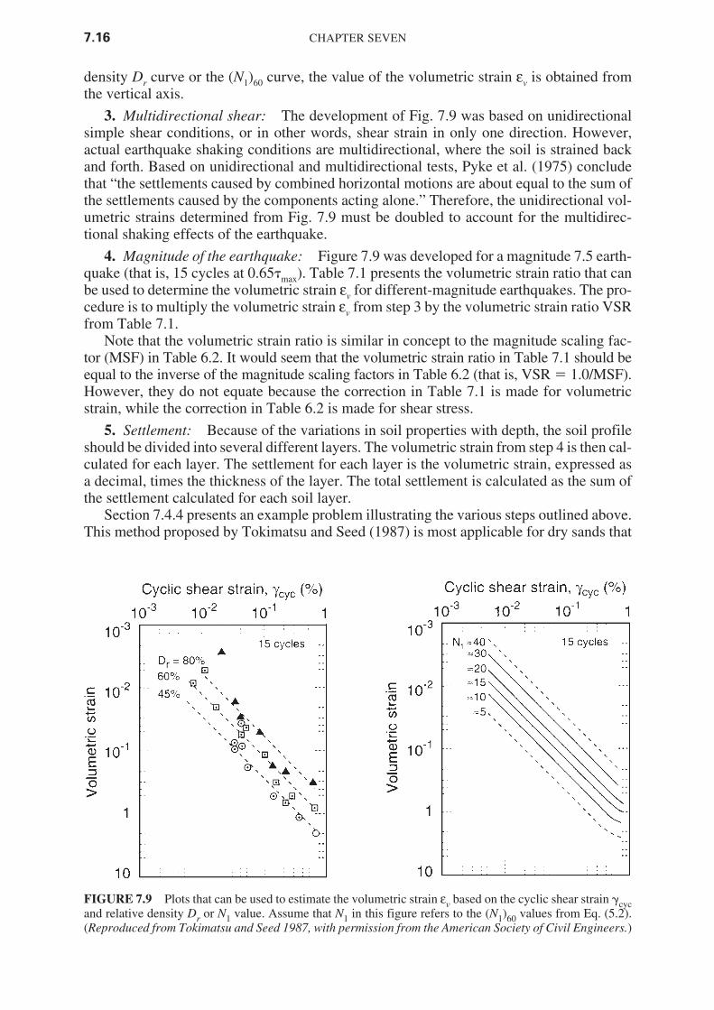
density Dr curve or the (N1)60 curve, the value of the volumetric strain εv is obtained fromthe vertical axis.

3. Multidirectional shear: The development of Fig. 7.9 was based on unidirectionalsimple shear conditions, or in other words, shear strain in only one direction. However,actual earthquake shaking conditions are multidirectional, where the soil is strained backand forth. Based on unidirectional and multidirectional tests, Pyke et al. (1975) concludethat “the settlements caused by combined horizontal motions are about equal to the sum ofthe settlements caused by the components acting alone.” Therefore, the unidirectional vol-umetric strains determined from Fig. 7.9 must be doubled to account for the multidirec-tional shaking effects of the earthquake.

4. Magnitude of the earthquake: Figure 7.9 was developed for a magnitude 7.5 earth-quake (that is, 15 cycles at 0.65�max). Table 7.1 presents the volumetric strain ratio that canbe used to determine the volumetric strain εv for different-magnitude earthquakes. The pro-cedure is to multiply the volumetric strain εv from step 3 by the volumetric strain ratio VSRfrom Table 7.1.

Note that the volumetric strain ratio is similar in concept to the magnitude scaling fac-tor (MSF) in Table 6.2. It would seem that the volumetric strain ratio in Table 7.1 should beequal to the inverse of the magnitude scaling factors in Table 6.2 (that is, VSR � 1.0/MSF).However, they do not equate because the correction in Table 7.1 is made for volumetricstrain, while the correction in Table 6.2 is made for shear stress.

5. Settlement: Because of the variations in soil properties with depth, the soil profileshould be divided into several different layers. The volumetric strain from step 4 is then cal-culated for each layer. The settlement for each layer is the volumetric strain, expressed asa decimal, times the thickness of the layer. The total settlement is calculated as the sum ofthe settlement calculated for each soil layer.

Section 7.4.4 presents an example problem illustrating the various steps outlined above.This method proposed by Tokimatsu and Seed (1987) is most applicable for dry sands that

7.16 CHAPTER SEVEN

FIGURE 7.9 Plots that can be used to estimate the volumetric strain εv based on the cyclic shear strain �cycand relative density Dr or N1 value. Assume that N1 in this figure refers to the (N1)60 values from Eq. (5.2).(Reproduced from Tokimatsu and Seed 1987, with permission from the American Society of Civil Engineers.)

have 5 percent or less fines. For dry sands (i.e., water content � 0 percent), capillary actiondoes not exist between the soil particles. As the water content of the sand increases, capil-lary action produces a surface tension that holds together the soil particles and increasestheir resistance to earthquake-induced volumetric settlement. As a practical matter, cleansands typically have low capillarity and thus the method by Tokimatsu and Seed (1987)could also be performed for damp and moist sands.

For silty soils, R. B. Seed (1991) suggests that the most appropriate adjustment is toincrease the (N1)60 values by adding the values of Ncorr indicated in Sec. 7.2.2.

7.4.4 Example Problem

Silver and Seed (1972) investigated a 50-ft- (15-m-) thick deposit of dry sand that experi-enced about 21⁄2 in (6 cm) of volumetric compression caused by the San Fernando earth-quake of 1971. They indicated that the magnitude 6.6 San Fernando earthquake subjectedthe site to a peak ground acceleration amax of 0.45g. The sand deposit has a total unit weight�t � 95 lb/ft3 (15 kN/m3) and an average (N1)60 � 9. Estimate the settlement of this 50-ft-(15-m-) thick sand deposit using the methods outlined in Secs. 7.4.2 and 7.4.3.

Solution Using Fig. 7.7. As shown in Fig. 7.7, the volumetric compression rapidlyincreases as the (N1)60 value decreases. Since the peak ground acceleration ap � 0.45g, thehorizontal axis is entered at 0.45. For an (N1)60 value of 9, the volumetric strain �H/H isabout equal to 0.35 percent. The ground surface settlement is obtained by multiplying thevolumetric strain, expressed as a decimal, by the thickness of the sand layer, or 0.0035 50 ft � 0.18 ft or 2.1 in (5.3 cm).

Solution Using the Tokimatsu and Seed (1987) Method. Table 7.2 presents the solutionusing the Tokimatsu and Seed (1987) method as outlined in Sec. 7.4.3. The steps are as fol-lows:

1. Layers: The soil was divided into six layers.

2. Thickness of the layers: The upper two layers are 5.0 ft (1.5 m) thick, and the lowerfour layers are 10 ft (3.0 m) thick.

3. Vertical effective stress: For dry sand, the pore water pressures are zero and the ver-tical effective stress �v0′ is equal to the vertical total stress �v. This stress was calcu-lated by multiplying the total unit weight (�t � 95 lb/ft3) by the depth to the center ofeach layer.


TABLE 7.1 Earthquake Magnitude versus Volumetric Strain Ratio for Dry Sands

Number of representative Earthquake magnitude cycles at 0.65�max Volumetric strain ratio

81⁄2 26 1.2571⁄2 15 1.0063⁄4 10 0.856 5 0.6051⁄4 2–3 0.40

Notes: To account for the earthquake magnitude, multiply the volumetric strain εv fromFig. 7.9 by the VSR. Data were obtained from Tokimatsu and Seed (1987).

7.18

TA

BLE

7.2

Settl

emen

t Cal

cula

tions

Usi

ng th

e T

okim

atsu

and

See

d (1

987)

Met

hod

Mul

ti-L

ayer

Gm

axdi

rect

iona

l L

ayer

thic

knes

s,�

v0′

��

v,[E

q. (7

.5)]

�ef

f(Gef

f/Gm

ax)

�ef

f%

�cy

c�

ε vsh

ear �

Mul

tiply

Settl

emen

t,nu

mbe

rft

lb/f

t2(N

1)60

kip/

ft2

[Eq.

(7.4

)](F

ig. 7

.8)

100�

eff

(Fig

. 7.9

)2ε

vby

VSR

in

(1)

(2)

(3)

(4)

(5)

(6)

(7)

(8)

(9)

(10)

(11)

(12)

15

238

951

71.

3

10�

45

10

�4

5

10�

20.

14

0.28

0.

220.

132

571

39

896

2.3

10

�4

1.0

10

�3

1.0

10

�1

0.29

0.

58

0.46

0.28

310

1425

912

703.

1

10�

41.

3

10�

31.

3

10�

10.

40

0.80

0.

640.

774

1023

759

1630

3.9

10

�4

1.4

10

�3

1.4

10

�1

0.43

0.

86

0.69

0.83

510

3325

919

304.

4

10�

41.

3

10�

31.

3

10�

10.

40

0.80

0.

640.

776

1042

759

2190

4.8

10

�4

1.3

10

�3

1.3

10

�1

0.40

0.

80

0.64

0.77

Tot

al �

3.5

in

4. (N1)60 values: As previously mentioned, the average (N1)60 value for the sand depositwas determined to be 9.

5. Gmax: Equation (7.5) was used to calculate the value of Gmax. It was assumed that themean principal effective stress �m′ was equal to 0.65�v 0′ . Note that Gmax is expressed interms of kips per square foot (ksf) in Table 7.2.

6. Equation (7.4): The value of �eff(Geff/Gmax) was calculated by using Eq. (7.4). A peakground acceleration amax of 0.45g and a value of rd from Eq. (6.7) were used in theanalysis.

7. Effective shear strain �eff: Based on the values of �eff(Geff/Gmax) and the mean princi-pal effective stress (�m′ in ton/ft2), Fig. 7.8 was used to obtain the effective shear strain.

8. Percent cyclic shear strain %�cyc: The percent cyclic shear strain was calculated as�eff times 100.

9. Volumetric strain εv: Entering Fig. 7.9 with the percent cyclic shear strain and using(N1)60 � 9, the percent volumetric strain εv was obtained from the vertical axis.

10. Multidirectional shear: The values of percent volumetric strain εv from step 9 weredoubled to account for the multidirectional shear.

11. Earthquake magnitude: The earthquake magnitude is equal to 6.6. Using Table 7.1,the volumetric strain ratio is approximately equal to 0.8. To account for the earthquakemagnitude, the percent volumetric strain εv from step 10 was multiplied by the VSR.

12. Settlement: The final step was to multiply the volumetric strain εv from step 11,expressed as a decimal, by the layer thickness. The total settlement was calculated asthe sum of the settlement from all six layers (i.e., total settlement � 3.5 in).

Summary of Values. Based on the two methods, the ground surface settlement of the 50-ft- (15-m-) thick sand layer is expected to be on the order of 2 to 31⁄2 in (5 to 9 cm). As pre-viously mentioned, the actual settlement as reported by Seed and Silver (1972) was about21⁄2 in (6 cm).

7.4.5 Limitations

The methods for the calculation of volumetric compression as presented in Sec. 7.4 canonly be used for the following cases:

● Lightweight structures: Settlement of lightweight structures, such as wood-framebuildings bearing on shallow foundations

● Low net bearing stress: Settlement of any other type of structure that imparts a low netbearing pressure onto the soil

● Floating foundation: Settlement of floating foundations, provided the floating founda-tion does not impart a significant net stress upon the soil

● Heavy structures with deep settlement: Settlement of heavy structures, such as massivebuildings founded on shallow foundations, provided the zone of settlement is deepenough that the stress increase caused by the structural load is relatively low

● Differential settlement: Differential movement between a structure and adjacent appur-tenances, where the structure contains a deep foundation that is supported by strata belowthe zone of volumetric compression


The methods for the calculation of volumetric compression as presented in Sec. 7.4 can-not be used for the following cases:

● Heavy buildings bearing on loose soil: Do not use the methods when the foundationapplies a large net load onto the loose soil. In this case, the heavy foundation will punchdownward into the loose soil during the earthquake. It is usually very difficult to deter-mine the settlement for these conditions, and the best engineering solution is to providea sufficiently high static factor of safety so that there is ample resistance against a bear-ing capacity failure. This is further discussed in Chap. 8.

● Sloping ground condition: These methods will underestimate the settlement for a slop-ing ground condition. The loose sand may deform laterally during the earthquake, and thesettlement of the building could be well in excess of the calculated values.

7.5 SETTLEMENT DUE TO DYNAMIC LOADSCAUSED BY ROCKING

Details on this type of settlement are as follows:

● Settlement mechanism: This type of settlement is caused by dynamic structural loadsthat momentarily increase the foundation pressure acting on the soil, such as illustratedin Fig. 7.10. The soil will deform in response to the dynamic structural load, resulting insettlement of the building. This settlement due to dynamic loads is often a result of thestructure rocking back and forth.

● Vulnerable soil types: Both cohesionless soil and cohesive soil are susceptible to rock-ing settlement. For cohesionless soils, loose sands and gravels are prone to rocking set-tlement. In addition, rocking settlement and volumetric compression (Sec. 7.4) oftenwork in combination to cause settlement of the structure.

Cohesive soils can also be susceptible to rocking settlement. The types of cohesivesoils most vulnerable are normally consolidated soils (OCR � 1.0), such as soft clays andorganic soils. There can be significant settlement of foundations on soft saturated claysand organic soils because of undrained plastic flow when the foundations are overloadedduring the seismic shaking. Large settlement can also occur if the existing vertical effec-tive stress �v 0′ plus the dynamic load ��v exceeds the maximum past pressure �vm′ of thecohesive soil, or �v 0′ � ��v �vm′ .

Another type of cohesive soil that can be especially vulnerable to rocking settlementis sensitive clays. These soils can lose a portion of their shear strength during the cyclicloading. The higher the sensitivity, the greater the loss of shear strength for a given shearstrain.

● Susceptible structures: Lightly loaded structures would be least susceptible to rockingsettlement. On the other hand, tall and heavy buildings that have shallow foundationsbearing on vulnerable soils would be most susceptible to this type of settlement.

● Example: Figure 7.11 presents an example of damage caused by rocking settlement.The rocking settlement occurred to a tall building located in Mexico City. The rockingsettlement was caused by the September 19, 1985, Michoacan earthquake, which isdescribed in Sec. 4.6.1.

In terms of the analysis for rocking settlement, R. B. Seed (1991) states:

7.20 CHAPTER SEVEN

Vertical accelerations during earthquake seldom produce sufficient vertical thrust to causesignificant foundation settlements. Horizontal accelerations, on the other hand, can cause“rocking” of a structure, and the resulting structural overturning moments can produce signif-icant cyclic vertical thrusts on the foundation elements. These can, in turn, result in cumulativesettlements, with or without soil liquefaction or other strength loss. This is generally a poten-tially serious concern only for massive, relatively tall structures. Structures on deep founda-tions are not necessarily immune to this hazard; structures founded on “friction piles” (asopposed to more solidly-based end-bearing piles) may undergo settlements of up to severalinches or more in some cases. It should be noted that the best engineering solution is generallysimply to provide a sufficiently high static factor of safety in bearing in order to allow for ampleresistance to potential transient seismic loading.

As indicated above, the best engineering solution is to provide a sufficiently high factorof safety against a bearing capacity failure, which is discussed in Chap. 8.

7.6 PROBLEMS

The problems have been divided into basic categories as indicated below:

Liquefaction-Induced Settlement

7.1 Use the data from the example problem in Sec. 7.2.2, but assume that amax/g � 0.1and the sand contains 15 percent nonplastic fines. Calculate the settlement, using Figs. 7.1and 7.2. Answer: See Table 7.3.


FIGURE 7.10 Diagram illustrating lateral forces F in response to the base shear V caused by the earth-quake. Note that the uniform static bearing pressure is altered by the earthquake such that the pressure isincreased along one side of the foundation. (Reproduced from Krinitzsky et al. 1993, with permission fromJohn Wiley & Sons.)

7.22 CHAPTER SEVEN

7.2 Use the data from the example problem in Sec. 7.2.2, but assume that amax/g � 0.2and the earthquake magnitude M � 51⁄4. Calculate the liquefaction-induced settlement,using Figs. 7.1 and 7.2. Answer: See Table 7.3.

7.3 Use the data from the example problem in Sec. 7.2.2, but assume at a depth of 3 mthat qc � 3.9 MPa. Calculate the liquefaction-induced settlement, using Figs. 7.1 and 7.2.Answer: See Table 7.3.

7.4 Use the data from the example problem in Sec. 7.2.2, but assume that the shearwave velocity Vs � 150 m/s. Calculate the liquefaction-induced settlement, using Figs. 7.1and 7.2. Answer: See Table 7.3.

7.5 Use the data from the example problem in Sec. 7.2.2, but assume that the soil typeis crushed limestone (i.e., soil type 1, see Fig. 6.12) and at a depth of 3 m, qc1 � 5.0 MPa.Calculate the liquefaction-induced settlement, using Figs. 7.1 and 7.2. Answer: See Table 7.3.

7.6 Use the data from the example problem in Sec. 7.2.2, but assume that the soil typeis silty gravel (i.e., soil type 2, see Fig. 6.12) and at a depth of 3 m, qc1 � 7.5 MPa. Calculatethe liquefaction-induced settlement, using Figs. 7.1 and 7.2. Answer: See Table 7.3.

FIGURE 7.11 Settlement caused by the building rocking backand forth during the Michoacan earthquake in Mexico on September19, 1985. (Photograph from the Steinbrugge Collection, EERC,University of California, Berkeley.)

7.23

TA

BLE

7.3

Sum

mar

y of

Ans

wer

s fo

r Pr

obs.

7.1

to 7

.9

(N1)

60bl

./ft

Cyc

lic

Settl

emen

t,Se

ttlem

ent,

Ear

thqu

ake

q c1, M

PaC

yclic

str

ess

resi

stan

ce

FS �

cm

cmPr

oble

m n

o.So

il ty

pea m

ax/g

mag

nitu

deV

s1, m

/s

ratio

(C

SR)

ratio

(C

RR

) C

RR

/ C

SR(F

ig. 7

.1)

(Fig

. 7.2

)

Sect

ion

7.2.

2C

lean

san

d0.

4071

27.

7 bl

ows/

ft0.

340.

090.

264.

13.

0Pr

oble

m 7

.1Sa

nd—

15%

fi

nes

0.10

71 2

7.7

blow

s/ft

0.08

40.

141.

670.

150.

15Pr

oble

m 7

.2C

lean

san

d0.

2051

47.

7 bl

ows/

ft0.

170.

140.

824.

12.

9Pr

oble

m 7

.3C

lean

san

d0.

4071

25.

8 M

Pa0.

340.

090.

263.

63.

0Pr

oble

m 7

.4C

lean

san

d0.

4071

218

5 m

/s0.

340.

160.

472.

82.

1Pr

oble

m 7

.5C

rush

ed

limes

tone

0.40

71 2

5.0

MPa

0.34

0.18

0.53

4.2

3.1

Prob

lem

7.6

Silty

gra

vel

0.40

71 2

7.5

MPa

0.34

0.27

0.79

3.0

2.2

Prob

lem

7.7

Gra

velly

sa

nd0.

4071

214

MPa

0.34

0.44

1.29

0.3

1.2

Prob

lem

7.8

Eol

ian

sand

0.40

71 2

7.7

blow

s/ft

0.34

0.09

0.26

4.1

3.0

Prob

lem

7.9

Loe

ss0.

4071

27.

7 bl

ows/

ft0.

340.

180.

533.

02.

3

Not

e:Se

e A

pp. E

for

sol

utio

ns.

7.7 Use the data from the example problem in Sec. 7.2.2, but assume that the soil typeis gravelly sand (i.e., soil type 3, see Fig. 6.12) and at a depth of 3 m, qc1 � 14 MPa.Calculate the settlement, using Figs. 7.1 and 7.2. Answer: See Table 7.3.

7.8 Use the data from the example problem in Sec. 7.2.2, but assume that the soil typeis eolian sand (i.e., soil type 4, see Fig. 6.12). Calculate the liquefaction-induced settlement,using Figs. 7.1 and 7.2. Answer: See Table 7.3.

7.9 Use the data from the example problem in Sec. 7.2.2, but assume that the soil typeis noncemented loess (i.e., soil type 7, see Fig. 6.12). Calculate the liquefaction-inducedsettlement, using Figs. 7.1 and 7.2. Answer: See Table 7.3.

7.10 Assume a site has clean sand and a groundwater table near ground surface. Thefollowing data are determined for the site:

Layer depth, m Cyclic stress ratio (N1)60

2–3 0.18 103–5 0.20 55–7 0.22 7

Using Figs. 7.1 and 7.2, calculate the total liquefaction-induced settlement of these layerscaused by a magnitude 7.5 earthquake. Answer: Per Fig. 7.1, 22 cm; per Fig. 7.2, 17 cm.

Liquefaction-Induced Settlement, Subsoil Profiles

7.11 Use the data from Prob. 6.12 and the subsoil profile shown in Fig. 6.13. Ignore anypossible settlement of the soil above the groundwater table (i.e., ignore settlement from groundsurface to a depth of 1.5 m). Also ignore any possible settlement of the soil located below adepth of 21 m. Using Figs. 7.1 and 7.2, calculate the earthquake-induced settlement of the sandlocated below the groundwater table. Answer: Per Fig. 7.1, 61 cm; per Fig. 7.2, 53 cm.

7.12 Use the data from Prob. 6.15 and the subsoil profile shown in Fig. 6.15. Ignoreany possible settlement of the surface soil (i.e., ignore settlement from ground surface to adepth of 1.2 m). Also ignore any possible settlement of soil located below a depth of 20 m.Using Figs. 7.1 and 7.2, calculate the earthquake-induced settlement of the sand locatedbelow the groundwater table. Answer: Per Fig. 7.1, 22 cm; per Fig. 7.2, 17 cm.

7.13 Figure 7.12 shows the subsoil profile at the Agano River site in Niigata. Assumea level-ground site with the groundwater table at a depth of 0.85 m below ground surface.The medium sand, medium to coarse sand, and coarse sand layers have less than 5 percentfines. The fine to medium sand layers have an average of 15 percent fines. The total unitweight �t of the soil above the groundwater table is 18.5 kN/m3, and the buoyant unit weight�b of the soil below the groundwater table is 9.8 kN/m3.

The standard penetration data shown in Fig. 7.12 are uncorrected N values. Assume ahammer efficiency Em of 0.6 and a boring diameter of 100 mm; and the length of drill rodsis equal to the depth of the SPT below ground surface. The design earthquake conditionsare a peak ground acceleration amax of 0.20g and magnitude of 7.5. Based on the standardpenetration test data and using Figs. 7.1 and 7.2, calculate the earthquake-induced settle-ment of the soil located at a depth of 0.85 to 15.5 m below ground surface. Answer: Per Fig. 7.1, 30 cm; per Fig. 7.2, 24 cm.

7.14 Figure 7.13 shows the subsoil profile at a road site in Niigata. Assume a level-ground site with the groundwater table at a depth of 2.5 m below ground surface. Alsoassume that all the soil types located below the groundwater table meet the criteria forpotentially liquefiable soil. The medium sand layers have less than 5 percent fines, the

7.24 CHAPTER SEVEN

sandy silt layer has 50 percent fines, and the silt layers have 75 percent fines. The total unitweight �t of the soil above the groundwater table is 18.5 kN/m3, and the buoyant unit weight�b of the soil below the groundwater table is 9.8 kN/m3.

The standard penetration data shown in Fig. 7.13 are uncorrected N values. Assume ahammer efficiency Em of 0.6 and a boring diameter of 100 mm; and the length of drill rodsis equal to the depth of the SPT below ground surface. The design earthquake conditionsare a peak ground acceleration amax of 0.20g and magnitude of 7.5. Based on the standardpenetration test data and using Figs. 7.1 and 7.2, calculate the earthquake-induced settle-ment of the soil located at a depth of 2.5 to 15 m below ground surface. Answer: Per Fig. 7.1, 34 cm; per Fig. 7.2, 27 cm.

7.15 Use the data from Prob. 6.18 and Fig. 6.11. Based on Figs. 7.1 and 7.2, calculatethe earthquake-induced settlement of the soil located at a depth of 0.5 to 16 m below groundsurface for the before-improvement and after-improvement conditions. Answers: Before


FIGURE 7.12 Subsoil profile, Agano River site, Niigata. (Reproduced from Ishihara, 1985.)

improvement: per Fig. 7.1, 45 cm; per Fig. 7.2, 35 cm. After improvement: per Fig. 7.1, 0.3cm; and per Fig. 7.2, 2.7 cm.

7.16 Use the data from Prob. 6.12 and Fig. 6.13. Assume that there has been soilimprovement from ground surface to a depth of 15 m, and for the zone of soil having soilimprovement (0 to 15-m depth), the factor of safety against liquefaction is greater than 2.0.A mat foundation for a heavy building will be constructed such that the bottom of the matis at a depth of 1.0 m. The mat foundation is 20 m long and 10 m wide, and according tothe structural engineer, the foundation will impose a net stress of 50 kPa onto the soil (the50 kPa includes earthquake-related seismic load). Calculate the earthquake-induced settle-ment of the heavy building, using Figs. 7.1 and 7.2. Answer: Per Fig. 7.1, 17 cm; per Fig. 7.2, 19 cm.

7.17 Use the data from Prob. 6.15 and Fig. 6.15. A sewage disposal tank will beinstalled at a depth of 2 to 4 m below ground surface. Assuming the tank is empty at the

7.26 CHAPTER SEVEN

FIGURE 7.13 Subsoil profile, road site, Niigata. (Reproduced from Ishihara, 1985.)

time of the design earthquake, calculate the liquefaction-induced settlement of the tank.Answer: Since the tank is in the middle of a liquefied soil layer, it is expected that the emptytank will not settle, but rather will float to the ground surface.

Liquefaction-Induced Ground Damage

7.18 A soil deposit has a 6-m-thick surface layer of unliquefiable soil underlain by a4-m-thick layer that is expected to liquefy during the design earthquake. The design earth-quake has a peak ground acceleration amax equal to 0.40g. Will there be liquefaction-induced ground damage for this site? Answer: Based on Fig. 7.6, liquefaction-inducedground damage is expected for this site.

7.19 Use the data from Prob. 6.12 and Fig. 6.13. Assume that the groundwater tableis unlikely to rise above its present level. Using a peak ground acceleration amax equal to0.20g and the standard penetration test data, will there be liquefaction-induced grounddamage for this site? Answer: Based on Fig. 7.6, liquefaction-induced ground damage isexpected for this site.

7.20 Use the data from Prob. 7.13 and Fig. 7.12. Assume that the groundwater tableis unlikely to rise above its present level. Using a peak ground acceleration amax equal to0.20g and the standard penetration test data, determine the minimum thickness of a filllayer that must be placed at the site in order to prevent liquefaction-induced ground dam-age for this site. Answer: Based on Fig. 7.6, minimum thickness of fill layer � 2.2 m.

7.21 Use the data from Prob. 7.14 and Fig. 7.13. Assume that the groundwater tableis unlikely to rise above its present level. Using a peak ground acceleration amax equal to0.20g and the standard penetration test data, will there be liquefaction-induced grounddamage for this site? Answer: The solution depends on the zone of assumed liquefaction(see App. E).

Volumetric Compression

7.22 Solve the example problem in Sec. 7.4.4, using the Tokimatsu and Seed (1987)method and assuming that the 50-ft-thick deposit of sand has (N1)60 � 5. Answer: 11 in (28 cm).

7.23 Solve the example problem in Sec. 7.4.4, using the Tokimatsu and Seed (1987)method and the chart shown in Fig. 7.7, assuming that the 50-ft-thick deposit of sand has(N1)60 � 15. Answer: Using the Tokimatsu and Seed (1987) method, settlement � 1.3 in(3.3 cm). Using the chart shown in Fig. 7.7, settlement � 0.9 in (2 cm).

7.24 Solve the example problem in Sec. 7.4.4, using the Tokimatsu and Seed (1987)method and the chart shown in Fig. 7.7, assuming that the 50-ft-thick deposit of sand willbe subjected to a peak ground acceleration of 0.20g and the earthquake magnitude � 7.5.Answer: Using the Tokimatsu and Seed (1987) method, settlement � 0.9 in (2.3 cm). Usingthe chart shown in Fig. 7.7, settlement � 0.6 in (1.5 cm).

7.25 Solve the example problem in Sec. 7.4.4, using the Tokimatsu and Seed (1987)method and assuming that the 50-ft-thick deposit of sand has (N1)60 � 5, a peak ground accel-eration of 0.20g, and the earthquake magnitude � 7.5. Answer: Settlement � 2 in (5 cm).


earthquake settlement

Documents

induced settlement

earthquake earthquake

ground surface settlement

effective shear stress

withonly settlement

settlement of structures

effective shear strainchapter

loss of soil