University of Rhode IslandDigitalCommons@URI

Physical Oceanography Technical Reports Physical Oceanography

2005

East China Sea Kuroshio 2002-2004 Data ReportMagdalena Andres

Chang-Su Hong

See next page for additional authors

Creative Commons License

This work is licensed under a Creative Commons Attribution-Noncommercial-Share Alike 3.0 License.

Follow this and additional works at: http://digitalcommons.uri.edu/physical_oceanography_techrpts

This Article is brought to you for free and open access by the Physical Oceanography at DigitalCommons@URI. It has been accepted for inclusion inPhysical Oceanography Technical Reports by an authorized administrator of DigitalCommons@URI. For more information, please contactdigitalcommons@etal.uri.edu.

Recommended CitationAndres, Magdalena; Hong, Chang-Su; Lee, Jae-Hak; Lim, Byung-Ho; Tracey, Karen L.; Wimbush, Mark; Chang, Kyung-Il; Ichikawa,Hiroshi; Lee, Dong-Kyu; Mitchell, Douglas A.; Teague, William; and Watts, D. Randolph, "East China Sea Kuroshio 2002-2004 DataReport" (2005). Physical Oceanography Technical Reports. Paper 12.http://digitalcommons.uri.edu/physical_oceanography_techrpts/12http://digitalcommons.uri.edu/physical_oceanography_techrpts/12

AuthorsMagdalena Andres, Chang-Su Hong, Jae-Hak Lee, Byung-Ho Lim, Karen L. Tracey, Mark Wimbush, Kyung-IlChang, Hiroshi Ichikawa, Dong-Kyu Lee, Douglas A. Mitchell, William Teague, and D. Randolph Watts

This article is available at DigitalCommons@URI: http://digitalcommons.uri.edu/physical_oceanography_techrpts/12

Graduate School of Oceanography University of Rhode Island

Narragansett, Rhode Island 02882-1197

East China Sea Kuroshio 2002-2004

Data Report

120oE 125oE 130oE 135oE 20oN

25oN

30oN

35oN

40oN

Ryuky

u Is.

Part I. The URI/JAMSTEC Measurements Part II. The SNU/KORDI Measurements

Magdalena Andres1†

Chang-Su Hong3*

Jae-Hak Lee3*

Byung-Ho Lim2*

Jae-Hun Park1†

Karen Tracey1†

Mark Wimbush1†

Kyung-Il Chang2*

Hiroshi Ichikawa4,5†

Dong-Kyu Lee6*

Douglas A. Mitchell7†

William Teague7†

D. Randolph Watts1†

1 Graduate School of Oceanography, University of Rhode Island, Narragansett, RI 02882-1197, U.S.A. 2 School of Earth and Environmental Sciences, Seoul National University, Silim-dong Gwanak-gu, Seoul 151-742, Korea. 3 Ocean Climate and Environment Research Division, Korea Ocean Research and Development Institute, Ansan, P.O. Box 29,

Seoul 425-600, Korea. 4 Institute of Observational Research for Global Change, Japan Agency for Marine-Earth Science and Technology , 2-15

Natsushima-cho, Yokosuka-city, Kanagawa, 237-0061, Japan. 5 Faculty of Fisheries, Kagoshima University, 4-50-20, Shimoarata, Kagoshima, 890-0056, Japan (left Sept. 2005). 6 Department of Ocean System Science, Pusan National University, Geumjeong-gu, Busan 609-735, Korea. 7 Naval Research Laboratory, Code 7332, Stennis Space Center, MS 39529-5004, U.S.A. † Contributed mainly to Part I. The onshore segment. * Contributed mainly to Part II. The offshore segment.

GSO Technical Report No. 2005-02

2

Table of Contents

Table of Contents................................................................................................................ 1 List of Figures..................................................................................................................... 2 List of Tables ...................................................................................................................... 3 Introduction ........................................................................................................................ 4

Part I. The URI/JAMSTEC Measurements

Introduction......................................................................................................................... 5 The ECS study .................................................................................................................... 5

Instrumentation ........................................................................................................... 5 Instrument locations.................................................................................................... 5 Data ............................................................................................................................. 6

Data Processing................................................................................................................... 7 Removing the “jumps”................................................................................................ 7 Pressure and temperature ............................................................................................ 8 Acoustic travel time .................................................................................................... 8 Current data............................................................................................................... 14

Deployment cruise data .................................................................................................... 15 XCTD data ................................................................................................................ 15 Near-surface current data.......................................................................................... 15

Recovery cruise data......................................................................................................... 18 Ship ADCP data........................................................................................................ 18

GEM.................................................................................................................................. 18

Part II. The SNU/KORDI Measurements

Introduction....................................................................................................................... 26 ADCP moorings................................................................................................................ 26

Instrumentation ......................................................................................................... 26 Instrument locations.................................................................................................. 27 Data ........................................................................................................................... 28

Data Processing................................................................................................................. 36 Pressure and temperature .......................................................................................... 36 Current data............................................................................................................... 36

CTD data........................................................................................................................... 41

Acknowledgements........................................................................................................... 45 References......................................................................................................................... 46

1

List of Figures

Part I. The URI/JAMSTEC Measurements Figure 1. Timing of measurements in CPIES and PIES instruments ................................. 6 Figure 2. Map of instrument locations................................................................................ 7 Figure 3. Pressure Gage Drifts.......................................................................................... 10 Figure 4. CPIES and PIES pressure time series............................................................... 11 Figure 5. CPIES and PIES temperature time series......................................................... 12 Figure 6. CPIES and PIES acoustic-travel-time time series ............................................. 13 Figure 7. Current time series............................................................................................. 14 Figure 8. Partial current record for C5.............................................................................. 14 Figure 9. Hydrographic sections across the CPIES and PIES lines................................. 16 Figure 10. Currents and SST during the deployment cruise............................................ 17 Figure 11. Currents and SST during the recovery cruise................................................. 18 Figure 12. Detailed map of the region around C6 ........................................................... 19 Figure 13. SLACTS seasonal signals............................................................................... 20 Figure 14. SLACTS acoustic-travel-time seasonal signal ............................................... 21 Figure 15. Main ECS GEM’s and error fields ................................................................. 22 Figure 16. Localized ECS GEM’s and error fields.......................................................... 23 Figure 17. τ700 plotted with τp ........................................................................................... 24

Part II. The SNU/KORDI Measurements Figure 18. Positions of ADCP moorings .......................................................................... 28 Figure 19. Two types of ADCP moorings ........................................................................ 29 Figure 20. Records of temperature, pressure, heading, pitch, and roll at mooring A1..... 30 Figure 21. Records of temperature, pressure, heading, pitch, and roll at mooring A2..... 31 Figure 22. Raw ADCP currents observed at mooring A1 ................................................ 32 Figure 23. Raw ADCP currents observed at mooring A2 ................................................ 33 Figure 24. Vector time series of low-pass filtered 12-hourly currents at mooring A1..... 38 Figure 25. Vector time series of low-pass filtered 12-hourly currents at mooring A2..... 39 Figure 26. Time series of along-shelf and cross-shelf currents and temperature at A1.... 40 Figure 27. Time series of along-shelf and cross-shelf currents and temperature at A2.... 40 Figure 28. Positions of CTD stations................................................................................ 43 Figure 29. Vertical distribution of temperature and salinity............................................. 44

2

List of Tables

Part I. The URI/JAMSTEC Measurements Table 1. IES instrument depths and locations..................................................................... 6 Table 2. Jump corrections .................................................................................................. 8 Table 3. Coefficients for the pressure sensor drift equation: AeBt + Ct + D....................... 9 Table 4. Basic Statistics for Ur and Vr at CPIES sites .................................................... 15 Table 5. Locations, depths and times of XCTD casts.................................................... 16 Table 6. Coefficients for the conversion: τ700 = ao + a1τp + a2τp

2 .................................... 25

Part II. The SNU/KORDI Measurements Table 7. Mooring locations and depths, and settings of ADCPs for each leg .................. 27 Table 8. ADCP mooring time coverage............................................................................ 27 Table 9. Basic statistics Ur and Vr at A1.......................................................................... 34 Table 10. Basic statistics Ur and Vr at A2........................................................................ 35 Table 11. Locations of CTD stations, water depths, and CTD lowering depths .............. 42

3

Introduction The University of Rhode Island (URI) together with the Japan Agency for Marine-Earth Science and Technology (JAMSTEC), Seoul National University (SNU) and the Korea Ocean Research & Development Institute (KORDI) undertook a joint effort to study the time variability of the Kuroshio in the East China Sea (ECS). The URI/JAMSTEC group measured the offshelf segment of the flow (between the 550 m isobath of the continental shelf and the Ryukyu Islands), principally using pressure-sensor equipped inverted echo sounders (PIES), current meter equipped PIES (CPIES), and ship-mounted acoustic Doppler current profilers (ADCP). The SNU/KORDI group principally measured the onshelf segment of the flow with moored ADCPs. The two groups made hydrographic measurements (with XCTDs and CTDs, respectively). The following Data Report is presented in two parts. Part I focuses on the data collected by the URI/JAMSTEC group and Part II focuses on the data collected by the SNU/KORDI group.

4

Part I. The URI/JAMSTEC Measurements

Introduction In order to study the time variability of Kuroshio transport and structure in the East China Sea (ECS), two lines of inverted echo sounders (IES) extending across the axis of the Kuroshio from the continental shelf to the Ryukyu Island chain were deployed for nearly two years. This part of the report describes the data recorded by these instruments and its preliminary processing. During the deployment cruise, XCTD casts were taken at each IES site; these data are also reported along with ship ADCP data taken during the IES deployment cruise. In addition, the technique used to generate GEM fields from historical hydrographic data in the ECS is explained. These GEM fields will be used to infer the dynamics of the region from the IES acoustic-travel-time (τ) records.

The ECS study

Instrumentation In December 2002, 11 IESs were deployed from the R/V Yokosuka of the Japan Agency for Marine-Earth Science and Technology (JAMSTEC). In November 2004, all were recovered aboard the T/V Kagoshima-maru of the Faculty of Fisheries, Kagoshima University. Two types of IES instruments were deployed: six “CPIES” instruments (manufactured by and belonging to the University of Rhode Island) and five “PIES” instruments (manufactured by WHISL and belonging to the Naval Research Laboratory). All these instruments measured round-trip acoustic travel time (τ) from the bottom to the surface, together with near-bottom pressure and temperature. In addition, the CPIESs were equipped with Aanderaa current sensors which measured current velocity and temperature 51 m above the sea floor. The IESs all emitted 24 acoustic pings per hour, from which a single hourly acoustic travel time value was calculated (see the Data Processing section below), but the timing and frequency of these pings were different in the two instrument types (see Figure 1). The CPIESs emitted sets of 4 12-kHz pings every 10 minutes over an entire hour. The PIESs sent 24 10-kHz pings at 10-second intervals at the beginning of each hour. Both the CPIES and PIES instruments were equipped with Paroscientific pressure sensors which measured hourly near-bottom pressure and temperature values. In the CPIESs, both the pressure and temperature were measured over a 16 s interval following the first burst of 4 pings. In the PIESs, pressure was averaged over the entire hour and temperature was averaged over the last minute of the hour. Each CPIES was connected through a 50 m cable to an Aanderaa Model 3820R Doppler Current Sensor, which recorded current speed and direction as well as temperature.

Instrument locations The Kuroshio flows through the strait east of Taiwan into the ECS and along the edge of the continental shelf before exiting the ECS through the Tokara Strait. Our IES array,

5

north of Okinawa, was situated in the Okinawa Trough between the shelf and the Ryukyu Island chain. Instrument locations are listed in Table 1 and shown in Figure 2. The 6 CPIESs were deployed across the axis of the Kuroshio from the ECS continental shelf slope southeast across the Okinawa Trough to the Ryukyu Islands, with spacing between instruments ranging from ~20 to ~40 km (instruments were spaced closest beneath the Kuroshio). The CPIESs were placed near the PN line, along which hydrographic data are regularly collected four times per year by the Nagasaki Marine Observatory, Japan Meteorological Agency. The 5 PIESs were deployed across the Kuroshio axis ~40 km downstream of the PN line (towards the northeast). The PIES spacing was also between ~20 and ~40 km.

taupress.temp.

Aanderaa current & temp.

CPIES

0 10 20 30 40 50 60

tau

press.

temp.

time (minutes)

PIES

Figure 1. Timing of measurements in CPIES and PIES instruments.

Table 1. IES instrument depths and locations. Spacing is separation in x-direction along 128°T.

Instrument C = CPIES P = PIES

IES Serial No.

Current Sensor Serial

No.

Latitude (°N)

Longitude(°E)

Spacing (km)

Pressure level

(dbar) C1 36 164 28.3425 127.0058 553.5 C2 43 165 28.2622 127.1822 1005.7 C3 45 166 28.1234 127.2968 1131.4 C4 53 168 27.9706 127.5711 1338.9 C5 63 169 27.7712 127.8644 1115.5 C6 68 170 27.5369 128.1973

19.43 19.07 31.81 36.35 41.85 891.2

P1 117 n/a 28.6370 127.2637 1033.1 P2 118 n/a 28.5273 127.4124 1121.3 P3 106 n/a 28.3533 127.6808 856.3 P4 111 n/a 28.1743 127.9462 1079.9 P5 116 n/a 27.9614 128.2481

18.95 20.25 32.71 37.90 749.9

Data With the following exceptions, acoustic-travel-time, pressure, temperature and current data records are all of excellent quality and complete. (1) Current data from the

6

Aanderaa sensor on instrument C6 are intermittent from April 2004 until the end of the record. It is not clear what caused this failure. (2) After about one week, the current sensor on C5 failed. Also about 1/3 is missing of the Paroscientific pressure and temperature records from this instrument (though the acoustic-travel-time record is complete). These problems on C5 appear to have been caused by a faulty o-ring seal on the current-sensor connector.

87654

Depth (km) 123oE 125oE 127oE 129oE

24oN

25oN

26oN

27oN

28oN

29oN

30oN

31oN

p1p2

p3p4

p5

A1A2 c1

c2c3

c4c5

c6

Figure 2. Map of instrument locations. CPIES sites are designated C; PIES sites are designated P; bottom-

mounted ADCP sites (see Part II of this report) are designated A.

Data Processing

Removing the “jumps” The pressure records of the two shallowest instruments show several pressure “jumps,” probably because the instruments were dragged by bottom-fishing gear. The westernmost CPIES (C1 at about 550 m depth) was moved twice, leaving the instrument about 1 m deeper after the first incident and another 5 m deeper after the second. The easternmost PIES (P5 at 760 m depth) was moved once about 1 m deeper. Before processing the data from these two instruments, their pressure and acoustic-travel-time records were modified to remove the effects of these changes in instrument depth. Each jump was corrected by adding to the entire record prior to the jump an amount equal to the size of the jump. A preliminary detiding of the data records containing jumps was first performed using the response method (Munk and Cartwright, 1966). The time of the pressure jumps was identified from this preliminary detided record. The magnitude of each jump was

7

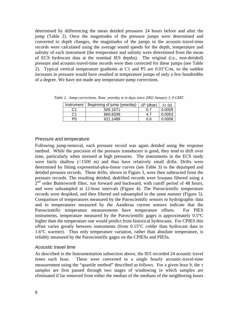
determined by differencing the mean detided pressures 24 hours before and after the jump (Table 2). Once the magnitudes of the pressure jumps were determined and converted to depth changes, the magnitudes of the jumps in the acoustic-travel-time records were calculated using the average sound speeds for the depth, temperature and salinity of each instrument (the temperature and salinity were determined from the mean of ECS hydrocast data at the nominal IES depths). The original (i.e., non-detided) pressure and acoustic-travel-time records were then corrected for these jumps (see Table 2). Typical vertical temperature gradients at C1 and P5 are 0.01°C/m, so the sudden increases in pressure would have resulted in temperature jumps of only a few hundredths of a degree. We have not made any temperature-jump corrections.

Table 2. Jump corrections. Note: yearday is in days since 2002 January 1, 0 GMT.

Instrument Beginning of jump (yearday) ΔP (dbar) Δτ (s) C1 505.1671 0.7 0.0009 C1 860.8338 4.7 0.0063 P5 621.1489 0.6 0.0008

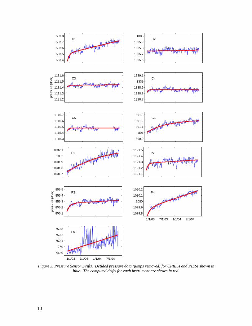
Pressure and temperature Following jump-removal, each pressure record was again detided using the response method. While the precision of the pressure transducers is good, they tend to drift over time, particularly when stressed at high pressures. The instruments in the ECS study were fairly shallow (<1500 m) and thus have relatively small drifts. Drifts were determined by fitting exponential-plus-linear curves (see Table 3) to the dejumped and detided pressure records. These drifts, shown in Figure 3, were then subtracted from the pressure records. The resulting detided, dedrifted records were lowpass filtered using a 2nd order Butterworth filter, run forward and backward, with cutoff period of 48 hours, and were subsampled at 12-hour intervals (Figure 4). The Paroscientific temperature records were despiked, and then filtered and subsampled in the same manner (Figure 5). Comparison of temperatures measured by the Paroscientific sensors to hydrographic data and to temperatures measured by the Aanderaa current sensors indicate that the Paroscientific temperature measurements have temperature offsets. For PIES instruments, temperature measured by the Paroscientific gages is approximately 0.5°C higher than the temperature one would predict from historical hydrocasts. For CPIES this offset varies greatly between instruments (from 0.15°C colder than hydrocast data to 1.6°C warmer). Thus only temperature variation, rather than absolute temperature, is reliably measured by the Paroscientific gages on the CPIESs and PIESs.

Acoustic travel time As described in the Instrumentation subsection above, the IES recorded 24 acoustic travel times each hour. These were converted to a single hourly acoustic-travel-time measurement using the “quartile method” described as follows. For a given hour h, the τ samples are first passed through two stages of windowing in which samples are eliminated if far removed from either the median of the medians of the neighboring hours

8

or from the first-quartile point of the hour-h samples. From the remaining acceptable n≤24 samples, the τ value assigned to hour-h is taken to be the average of the n/6 samples beginning with the last sample of the first quartile. For instance, for hour h, if n=24 (i.e., all samples in the hour are acceptable), the average of the 6th, 7th, 8th, and 9th smallest τ samples is assigned as the hour-h τ value. The resulting records were despiked, then lowpass filtered using a 2nd order Butterworth filter, run forward and backward, with cutoff period of 48 hours, and finally subsampled at 12 hour samples. These processed acoustic-travel-time series are plotted in Figure 6.

Table 3. Coefficients for the pressure sensor drift equation: drift (dbar) = AeBt + Ct + D, t is time in days since the beginning of the record. Note yearday is in days since 2002 January 1, 0 GMT.

IES

t = 0 time (yearday)

A B C D

C1 339.3754 -0.13132 -0.04085 0.00030 553.51 C2 339.3341 0 0 0.00002 1005.75 C3 339.5430 -0.02373 -0.04945 0.00002 1131.43 C4 339.6258 -0.04468 -0.07860 0.00000 1338.86 C5 339.7090 -0.05135 -0.06790 0.00000 1115.48 C6 339.9173 -0.17442 -0.00427 0.00004 891.18 P1 339.9792 -1.36200 -0.00089 -0.00045 1033.10 P2 340.0208 -0.11676 -0.04382 0.00008 1121.28 P3 340.1042 -0.14191 -0.02474 0.00007 856.27 P4 340.1875 -0.16524 -0.02220 0.00041 1079.89 P5 340.3125 0 0 0.00039 749.93

9

553.4

553.5

553.6

553.7

553.8C1

1005.6

1005.7

1005.8

1005.9

1006C2

1131.2

1131.3

1131.4

1131.5

1131.6C3

pres

sure

(db

ar)

1338.7

1338.8

1338.9

1339

1339.1C4

1115.3

1115.4

1115.5

1115.6

1115.7C5

890.9

891

891.1

891.2

891.3C6

1031.7

1031.8

1031.9

1032

1032.1P1

1121.1

1121.2

1121.3

1121.4

1121.5P2

856.1

856.2

856.3

856.4

856.5P3

pres

sure

(db

ar)

1079.8

1079.9

1080

1080.1

1080.2P4

1/1/03 7/1/03 1/1/04 7/1/04

749.9

750

750.1

750.2

750.3P5

1/1/03 7/1/03 1/1/04 7/1/04 Figure 3. Pressure Sensor Drifts. Detided pressure data (jumps removed) for CPIESs and PIESs shown in

blue. The computed drifts for each instrument are shown in red.

10

−1.2

−1

−0.8

−0.6

−0.4

−0.2

0CPIES

pres

sure

(db

)C1

C2

C3

C4

C5

C6

1/1/03 4/1/03 7/1/03 10/1/03 1/1/04 4/1/04 7/1/04 10/1/04

−1.2

−1

−0.8

−0.6

−0.4

−0.2

0PIES

pres

sure

(db

)

P1

P2

P3

P4

P5

1/1/03 4/1/03 7/1/03 10/1/03 1/1/04 4/1/04 7/1/04 10/1/04 Figure 4. CPIES and PIES pressure time series (jumps removed). Records have been detided, dedrifted and lowpass filtered. Means have been removed and series have been displaced for clarity by 0.2 dbar

(except P5 which has been displaced by 0.4 dbar).

11

−7

−6

−5

−4

−3

−2

−1

0CPIES

tem

pera

ture

(C

)C1

C2

C3

C4

C5

C6

1/1/03 4/1/03 7/1/03 10/1/03 1/1/04 4/1/04 7/1/04 10/1/04

−7

−6

−5

−4

−3

−2

−1

0PIES

P1

P2

P3

P4

P5

tem

pera

ture

(C

)

1/1/03 4/1/03 7/1/03 10/1/03 1/1/04 4/1/04 7/1/04 10/1/04 Figure 5. CPIES and PIES temperature time series (blue lines). Aanderaa Current Sensor temperature

time series (red lines). Records have been despiked and lowpass filtered. Means have been removed and successive series displaced for clarity by 1ºC.

12

−0.035

−0.03

−0.025

−0.02

−0.015

−0.01

−0.005

0CPIES

tau

(s)

C1

C2

C3

C4

C5

C6

1/1/03 4/1/03 7/1/03 10/1/03 1/1/04 4/1/04 7/1/04 10/1/04

−0.03

−0.025

−0.02

−0.015

−0.01

−0.005

0

PIES

P1

P2

P3

P4

P5

tau

(s)

1/1/03 4/1/03 7/1/03 10/1/03 1/1/04 4/1/04 7/1/04 10/1/04 Figure 6. CPIES and PIES acoustic-travel-time time series (jumps removed). Records have been despiked

and lowpass filtered. Means have been removed and successive series displaced for clarity by 5 ms.

13

Current data Current sensor records were corrected for the local magnetic declination at each site (data from http://www.ngdc.noaa.gov/seg/geomag/declination.shtml; roughly 5°W), so U is eastward and V is northward. The velocities were then lowpass filtered using a 2nd order Butterworth filter, run forward and backward, with cutoff period of 48 hours The resulting records were subsampled at 12-hour intervals and are shown as stick-plots in Figure 7. The partial record from the current sensor on C5, which failed after 6 days, is shown in Figure 8. Table 4 gives the basic statistics for the components of the current vectors ahown in Figures 8 and 9 in the directions along the array (128°T) and across the array (38°T). The temperatures recorded by the Aanderaa Current Sensors are shown in Figure 5 together with the respective CPIES temperature records, except for site C5, where the Aanderaa Current Sensor failed.

−20

0

20 C1

−20

0

20 C2

−20

0

20 C3

curr

ent v

eloc

ity (

cm/s

)

−20

0

20 C4

−20

0

20

1/1/03 4/1/03 7/1/03 10/1/03 1/1/04 4/1/04 7/1/04 10/1/04

C6

Figure 7. Current time series. Vertical axis is toward True north.

−5

0

5

12/0

7/02

12/0

8/02

12/0

9/02

12/1

0/02

12/1

1/02

12/1

2/02

C5

curr

ent v

eloc

ity (

cm/s

)

Figure 8. Partial current record for C5. Vertical axis is towards True North.

14

Table 4. Basic Statistics for CPIES measurement of currents 51 m above bottom for Ur (towards 128°) and Vr (towards 38°) components (48-hour lowpass filtered). Max and Min denote maximum and minimum values of current components. The direction of vector current is measured clockwise from True North.

Vector Mean

CPIES Depth (m) Vel. Mean

(cm/s) STD

(cm/s) Max.

(cm/s) Min.

(cm/s) Dir. (°)

Speed (cm/s)

Data Returned

(%)

Ur 1.42 3.51 18.09 -10.49 C1 498 Vr -1.39 7.83 26.07 -34.00 172.4 1.99 100

Ur 0.46 3.14 12.82 -9.57 C2 946 Vr -2.88 5.56 16.13 -21.18 208.9 2.92 100

Ur -4.33 3.44 7.50 -20.55 C3 1070 Vr 11.06 6.80 29.06 -8.15 16.6 11.88 100

Ur 1.29 2.71 21.12 -7.06 C4 1275 Vr -0.43 2.84 15.28 -9.01 146.3 1.36 98.6

Ur -1.26 0.47 -0.81 -2.25 C5 1054 Vr -2.95 0.45 -2.21 -3.74 241.1 3.21 1.0

Ur -1.41 3.16 10.67 -20.65 C6 832 Vr -4.28 2.92 5.67 -19.37 236.2 4.51 85.6

Deployment cruise data

XCTD data XCTD casts were taken after each instrument deployment during the December 2002 cruise aboard the R/V Yokosuka. Figure 9 shows the temperature and salinity sections for each of the two lines of instruments. Table 5 lists the locations and depths of these casts.

Near-surface current data Ship speed relative to sea water measured by electromagnetic log and ship heading measured by gyro-compass were collected every 5 seconds during the deployment cruise aboard the R/V Yokosuka together with water temperature at the ship’s hull bottom (6 m depth) and ship’s DGPS position. The 30-minute-mean near-surface current vectors calculated from these data are plotted in Figure 10 together with the near-surface temperature. Due to characteristics of the above-mentioned conventional measurement system, the calculated current vectors may have large errors during times when the ship was not running at high speed.

15

Longitude (oE)

Pre

ssur

e (d

bar)

Temperature

CPIES(oC)

127 127.5 128 128.5

0

200

400

600

800

1000

1200

1400 5

10

15

20

Longitude (oE)

Salinity

(psu)

127 127.5 128 128.5

0

200

400

600

800

1000

1200

1400

34.3

34.4

34.5

34.6

34.7

34.8

Longitude (oE)

Pre

ssur

e (d

bar)

Temperature

(oC)

PIES

127 127.5 128 128.5

0

200

400

600

800

1000

1200

1400 5

10

15

20

Longitude (oE)

Salinity

(psu)

127 127.5 128 128.5

0

200

400

600

800

1000

1200

1400

34.3

34.4

34.5

34.6

34.7

34.8

Figure 9. Hydrographic sections across the CPIES and PIES lines. Open circles show the longitude and

depth of nearby IES instruments

.Table 5. Locations, depths and times of XCTD casts during 2002 deployment cruise.

Nearest IES

Longitude (°E)

Latitude (°N)

Cast depth (m)

Cast time mo/day hr GMT

C1 127.0065 28.3473 518 12/5 21 C2 127.1794 28.2599 990 12/5 23 C3 127.2989 28.1217 741 12/6 0 C4 127.5752 27.9699 1001 12/6 2 C5 127.8661 27.7712 1001 12/6 4 C6 128.1997 27.5361 886 12/6 6 P1 127.2619 28.6367 1001 12/6 21 P2 127.4120 28.5255 1001 12/6 23 P3 127.6785 28.3526 858 12/7 1 P4 127.9439 28.1740 1001 12/7 3 P5 128.2464 27.9610 719 12/7 5

16

126.5 127 127.5 128 128.5 129 129.5 130

26.5

27.0

27.5

28.0

28.5

29.0

29.5

Longitude (E)

Latitude (N)

SST and SFC on Dec.5−7, 2002

500

500

500

500

500

500

500

500

500

500

500

500

500

500

500

500

500

500

500

1000

1000

1000

1000

1000

1000

1000

1000

1000

1000

1000

1000

1000

1000

1000

1000

1000

1000

1000

1000

1000

10001000

1000

100 cm/s

23.0

23.5

24.0

24.5

25.0

25.5

Figure 10. Near-surface currents and sea surface temperatures (SST) during the deployment cruise.

17

Recovery cruise data

Ship ADCP data The current velocities at 50 depths beginning at 26 m with 16 m intervals were collected every second by the 75 kHz Ocean Surveyor Vessel-Mounted ADCP (RDI) during the recovery cruise aboard the T/V Kagoshima-maru, together with water temperature at the ship’s hull bottom (5 m depth) and ship’s DGPS position. The misalignment angle of the ADCP system was determined to be 0.8996 degree anti-clockwise from the available bottom tracked data during the cruise. From the short term (1 minute) average (STA) of ADCP data and navigation data, the 10-minute mean current vectors at 26 m depth were calculated and are plotted in Figure 11 together with water temperature at 5 m depth.

126.5 127 127.5 128 128.5 129 129.5 130

26.5

27.0

27.5

28.0

28.5

29.0

29.5

Longitude (E)

Latitude (N)

SST and SFC on Nov.18−20, 2004

26 m Vel. (10 min mean) Ref: nav

500

500

500

500

500

500

500

500

500

500

500

500

500

500

500

500

500

500

500

1000

1000

1000

1000

1000

1000

1000

1000

1000

1000

1000

1000

1000

1000

1000

1000

1000

1000

1000

1000

1000

1000

1000 100 cm/s

25.5

26.0

26.5

27.0

27.5

28.0

28.5

Figure 11. Near-surface currents and sea surface temperatures (SST) during the recovery cruise.

GEM The vertical structures of the current and temperature fields are related to vertically integrated quantities such as acoustic travel time (e.g., a deeper thermocline is associated with a shorter acoustic travel time). For a given region, this relationship (if it exists) between vertical temperature profile (or specific-volume-anomaly profile) and acoustic travel time can be determined from historical hydrographic data. That part of the vertical structure captured by this relationship is the Gravest Empirical Mode (GEM).

18

To compute GEMs for the region we used 1833 historic ECS hydrographic profiles obtained from North Pacific Hydrobase (Macdonald et al., 2001) and the Nagasaki Marine Observatory (NMO), Japan Meteorological Agency. All of these profiles extended to at least 700 dbar. Data were extracted at 10 dbar intervals. The data were quality controlled by removing those hydrocasts having density inversions. For this purpose, if the density at any pressure level was 0.04 kg/m3 lower than the density in the overlying layer (i.e., 10 dbar shallower), it was identified as a density inversion. In many applications, a single GEM field for a particular parameter, such as temperature, is used as a lookup table for a given region. In the ECS, however, it was necessary to construct two separate fields: a localized GEM for a small region around C6 and a main GEM for the rest of the IES sites. Detailed bathymetry data (Choi et al., 2002) show that C6 (885 m depth) was isolated from the rest of the ECS because it was situated within a small Y-shaped basin with a sill depth of ~800 m and a maximum bottom depth of ~1200 m (Figure 12). Being just off the west coast of the island Okinoerabushima in the Ryukyu Island chain, we call this the Okinoerabushima Basin. A comparison of temperature profiles from the 1833 hydrographic stations shows that water within this basin is warmer than water at the same depths elsewhere in the ECS, typically about 1.5°C warmer at 850 dbar. The basin appears to be completely filled with Pacific Intermediate Water. Only the 1720 ECS profiles from outside the basin are used to compute the ECS main GEM, while the localized GEM is calculated exclusively from the 113 “warm” hydrocasts taken in the basin.

21.510.50Depth (km)

127oE 128oE

27oN

28oN

29oN

C6

Figure 12. Detailed map of the region around C6. Blue contour indicates the 800 m isobath. Dots show

IES positions. Bathymetry data from Choi et al., 2002.

19

To compute the main and localized GEMs the hydrographic data for each of the two regions were first de-seasoned using the SLACTS∗ method of Book (1998), with the year split into 5 bins and the center of the bins shifted 8 times. Figure 13 shows the SLACTS curves for temperature and specific-volume-anomaly signals at different depths. Vertical round-trip acoustic travel time from 700 dbar to the surface, τ700, was calculated from the historical hydrographic data using a constant value for gravitational acceleration, g = 9.8 m/s2 (rather than the local g). This was then deseasoned using the SLACTS method; in this case (since only casts beyond 700 dbar could be used) the year was split into 4 bins with the center of the bins shifted 10 times. The τ700 SLACTS curve is shown in Figure 14. A spline fit was used to quantify the relationship between the deseasoned hydrographic temperature data and deseasoned hydrographic τ700 at each pressure level from the surface to 2000 dbar in 10 dbar increments. From this, we generated a lookup table of temperature as a function of pressure (in 10 dbar intervals) and τ700 (in 0.1 ms intervals). The temperature and specific-volume-anomaly GEMs computed from these deseasoned data are shown for the main and localized region in Figure 15 and Figure 16, respectively.

0 100 200 300−4

−2

0

2

4

T (

o C)

yearday

’cold’ castsSeasonal Signals

0 100 200 300−1.5

−1

−0.5

0

0.5

1

1.5x 10

−6

spec

. vol

. ano

m.(

m3 /k

g)

yearday

0 100 200 300−4

−2

0

2

4

T (

o C)

yearday

’warm’ casts

0 100 200 300−1.5

−1

−0.5

0

0.5

1

1.5x 10

−6

spec

. vol

. ano

m.(

m3 /k

g)

yearday Figure 13. SLACTS Temperature (top) and Specific-Volume-Anomaly (bottom) seasonal signals, from the surface (largest amplitude) to 130 dbar in 10 dbar increments for the ‘cold’ casts (left) and ‘warm’ casts

(right).

∗ “SLACTS” stands for “Surface Layer Annual Correction for Temperature and Salinity”.

20

0 100 200 300−0.5

0

0.5

τ se

ason

al s

igna

l (m

s)

yearday

’cold’ casts

0 100 200 300−0.5

0

0.5’warm’ casts

yearday Figure 14. SLACTS acoustic-travel-time seasonal signal for ‘cold’ casts (left) and ’warm’ casts (right).

In order to evaluate how well the GEM represents the vertical structure of the water column, the GEM-predicted temperature and specific-volume-anomaly profiles are compared to the actual temperature and specific-volume-anomaly profiles of the historical hydrographic data. For each hydrocast, τ700 is calculated from the data. Then this is used to look up the GEM-predicted temperature and specific-volume-anomaly profiles. The rms error between the GEM-predicted and hydrocast values is calculated. Then the average rms error in 0.5 ms by 10 dbar bins is calculated and contoured as a function of pressure and τ700.

21

Pre

ssur

e (d

bar)

Temperature GEM (oC)

0.918 0.92 0.922 0.924 0.926 0.928 0.93

0

200

400

600

800

1000

12005

10

15

20

25

Pre

ssur

e (d

bar)

RMS error (oC)

0.918 0.92 0.922 0.924 0.926 0.928 0.93

0

200

400

600

800

1000

1200

0.5

1

1.5

2

2.5

Pre

ssur

e (d

bar)

Spec. Vol. Anom. GEM (m3/kg)

0.918 0.92 0.922 0.924 0.926 0.928 0.93

0

200

400

600

800

1000

1200

1

2

3

4

5x 10

−6

τ700

Pre

ssur

e (d

bar)

RMS error (m3/kg)

0.918 0.92 0.922 0.924 0.926 0.928 0.93

0

200

400

600

800

1000

12001

2

3

4

5

6

7

x 10−7

Figure 15. Main ECS GEMs and error fields. Upper panels are for temperature, lower panels are for

specific volume anomaly.

22

Pre

ssur

e (d

bar)

Localized Temp. GEM (oC)0

200

400

600

800 5

10

15

20

25

Pre

ssur

e (d

bar)

RMS error (oC)

0.9175 0.918 0.9185 0.919 0.9195 0.92 0.9205 0.921 0.9215

0

200

400

600

8000.5

1

1.5

2

2.5

Pre

ssur

e (d

bar)

Localized Spec. Vol. Anom. GEM (m3/kg)0

200

400

600

800 1.5

2

2.5

3

3.5

4

4.5

x 10−6

τ700

Pre

ssur

e (d

bar)

RMS error (m3/kg)

0.9175 0.918 0.9185 0.919 0.9195 0.92 0.9205 0.921 0.9215

0

200

400

600

8001

2

3

4

5

6

7

x 10−7

Figure 16. Localized ECS GEMs and error fields. Upper panels are for temperature, lower panels are for

specific volume anomaly.

23

In order to use the GEM lookup table which is based on acoustic travel times referenced to 700 dbar, the travel time data from each IES instrument must be converted from travel time referenced to the instrument’s pressure level, τp, to travel time referenced to 700 dbar, τ700. First the pressure level of each instrument is determined from the mean of its dedrifted pressure record minus atmospheric pressure (10.1325 dbar = 1 atm). Then hydrographic data are used to calculate τ700 and τp for each historic ECS hydrographic profile extending to this pressure level. These are plotted one against the other in Figure 17. Also shown in this figure are least-squares fitted straight lines, except for C1 where a second degree polynomial is fitted since it provides a significantly better fit. Table 6 gives the coefficients for all these fitted functions. Only the 113 hydrocasts taken in the Okinoerabushima Basin were used to determine the conversion factor for C6. The 1720 other ECS hydrocasts were used to determine the conversion relationships for all the other instrument sites.

710 715 720915

920

925

930

τ543

C1

1312 1314 1316 1318 1320

τ996

C2

1480 1482 1484 1486 1488

τ1121

C3

1756 1758 1760 1762915

920

925

930

τ1329

C4

τ 700 (

ms) 1458 1460 1462 1464 1466

τ1105

C5

1158 1160 1162915

920

925

930

τ881

C6

1346 1348 1350 1352 1354915

920

925

930

τ1022

P1

1466 1468 1470 1472 1474

τ1111

P2

1112 1116 1120 1124

τ846

P3

1410 1412 1414 1416 1418915

920

925

930

τ1070

P4

972 974 976 978 980 982

τ740

P5

τp (ms)

Figure 17. τ700 plotted with τp for each of the IES sites. Each of the best-fit lines (red) is a linear fit, except for C1 which is fitted with a second-degree polynomial (Table 5).

24

Table 6. Coefficients for the conversion: τ700 = ao + a1τp + a2τp 2 (τ in ms), representing the red lines in

Figure 17.

IES a0 a1 a2 rms error (ms) C1 -12648.00 36.78 -0.024897 0.30 C2 -274.40 0.91 0 0.19 C3 -415.67 0.90 0 0.23 C4 -638.96 0.89 0 0.24 C5 -396.85 0.90 0 0.22 C6 -163.97 0.93 0 0.14 P1 -300.81 0.91 0 0.20 P2 -405.32 0.90 0 0.22 P3 -125.92 0.94 0 0.12 P4 -353.30 0.90 0 0.21 P5 -27.82 0.97 0 0.05

25

Part II. The SNU/KORDI Measurements

Introduction Two bottom-mounted Acoustic Doppler Current Profiler (ADCP) moorings were deployed in the East China Sea (ECS) for 13 months to observe the part of the Kuroshio flowing over the outer continental shelf of the ECS. The main objectives of this study are to quantify the entire Kuroshio transport and to investigate the dynamics of its temporal variability using the ADCP data together with CPIES (current-and-pressure-sensor-equipped inverted echo sounder) data simultaneously obtained in the Okinawa Trough. This report describes the data recorded by the ADCPs and the preliminary processing. During the 4 ADCP mooring cruises, CTD casts were conducted along the CPIES-ADCP mooring line and these data are also reported.

ADCP moorings

Instrumentation The ADCPs were bottom moored at two sites located on the outer continental shelf of the ECS (Figure 18, Table 7). The ADCP moored at the shallower site (station A1) was housed in a barnacle-shaped trawl-resistant bottom mount shown in Figure 19a (Barny TRBM; Perkins et al., 2000). The TRBM has proven to be effective for measuring current profiles in active fishing areas for relatively long times, e.g., up to 6 months in the Korea/Tsushima Strait (Teague et al., 2002). Currently, the TRBM-ADCP package can only be used in areas shallower than 150 m due to the limited length of the recovery line. Thus, the ADCP mooring at the deeper site (station A2) was made using a subsurface foam buoy as shown in Figure 19b. The field work consisted of four cruises to improve the likelihood of sufficient data return, despite the risk of instrument loss in this intensively fished region: initial deployment, two turnarounds, and final recovery (Table 8). In October 2003, two ADCP moorings were initially deployed (Leg I) from the R/V Onnuri of the Korea Ocean Research and Development Institute. Turnarounds of the moorings (beginnings of Leg II and III, respectively) were made in November 2003 from T/V Kagoshima-maru of the Faculty of Fisheries, Kagoshima University, and in May 2004 from R/V Tamyang of Pukyung National University. The ADCP moorings were finally recovered aboard R/V Tamyang in November 2004. The ADCPs used are RDI Model WHS300, utilizing “Janus” beam geometry (four beams) with 300 kHz frequency. The location, mooring depth, and setting of the ADCPs for each leg are given in Table 7. The ADCPs recorded current speed and direction at elevations from 5-10 m to about 120 m above the sea floor at 4 or 8 m intervals. The ADCPs also recorded pressure and temperature at their mooring depths. The ADCP mooring depths in Table 7, 152m at A1 and 285 m at A2, were estimated using the measured pressure data from Legs III and II, respectively. The ADCPs at stations A1 and A2 were respectively placed at about 0.5m and 5 m above the sea floor. Hence the total

26

water depths at stations A1 and A2 are about 152.5 m and 290 m, respectively. As the measurement range of the WH300 ADCP is only about 120 m, vertical profiles of currents are measured in only the deeper parts of the water column, about 80% and 40% of total water depths at stations A1 and A2, respectively. An attempt was made to measure the upper currents near station A2 by deploying an additional mooring equipped with an ADCP at 140 m and an RCM-11 current meter at 165 m during Leg III, but this mooring was lost. Correlation and error velocity were set to their recommended default values, 64 and 2 m/s, respectively, for all ADCPs. When an ADCP is collecting data, the correlation of each beam is handled independently for the purpose of data quality analysis. Correlation is essentially a measure of how much the particle distribution has changed between phase measurements. The less the distribution has changed, the higher the correlation, and the more precise the velocity measurement. The ADCPs used here record the velocity as bad if the individual correlation from at least 2 beams is below a pre-determined threshold (64). If the error velocity reported is greater than the error velocity threshold (2 m/s), then the data is also marked as bad. The low correlation and large error-velocity setting are to avoid data loss. Table 7. Mooring locations and depths, and settings of ADCPs for each leg.

Table 8. ADCP mooring time coverage.

Instrument locations To observe the part of the Kuroshio over the outer continental shelf of the ECS, the ADCPs were bottom moored at depths shallower than 300m. The ADCP moorings were placed northwest of a CPIES array near the PN line, along which hydrographic data are regularly collected by the Nagasaki Marine Observatory, Japan Meteorological Agency.

27

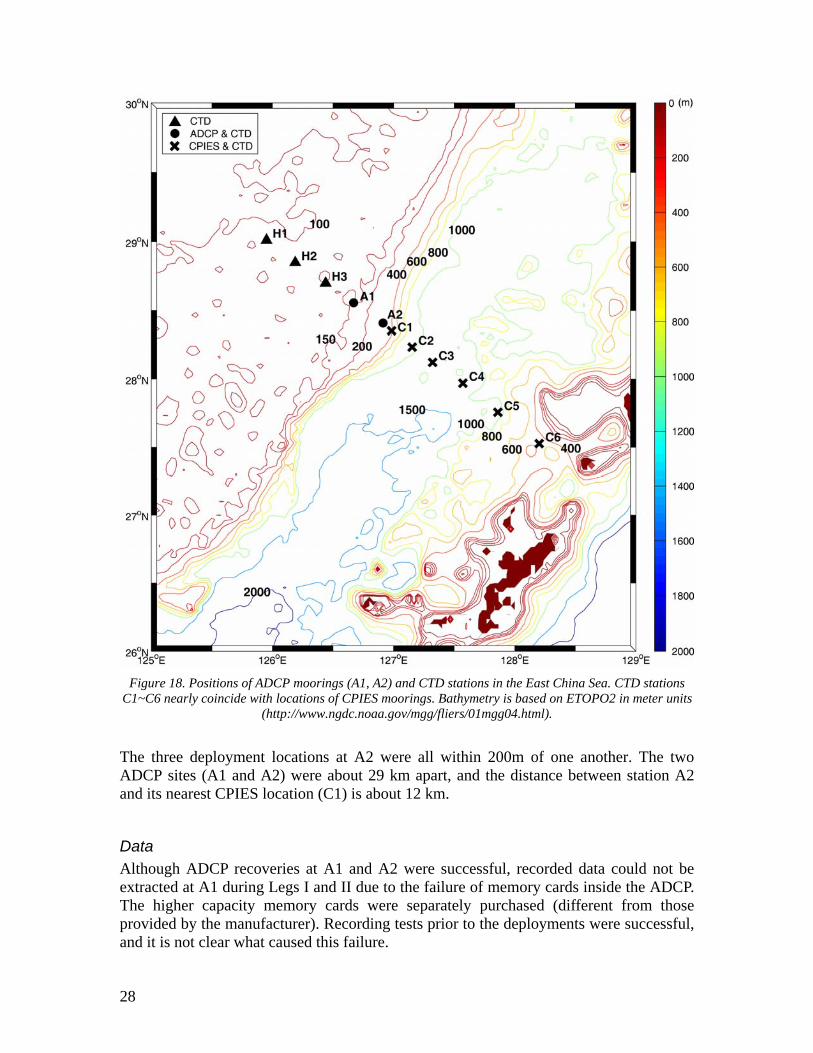
Figure 18. Positions of ADCP moorings (A1, A2) and CTD stations in the East China Sea. CTD stations

C1~C6 nearly coincide with locations of CPIES moorings. Bathymetry is based on ETOPO2 in meter units (http://www.ngdc.noaa.gov/mgg/fliers/01mgg04.html).

The three deployment locations at A2 were all within 200m of one another. The two ADCP sites (A1 and A2) were about 29 km apart, and the distance between station A2 and its nearest CPIES location (C1) is about 12 km.

Data Although ADCP recoveries at A1 and A2 were successful, recorded data could not be extracted at A1 during Legs I and II due to the failure of memory cards inside the ADCP. The higher capacity memory cards were separately purchased (different from those provided by the manufacturer). Recording tests prior to the deployments were successful, and it is not clear what caused this failure.

28

Figures 20 and 21 show raw records of temperature, pressure, heading, pitch and roll at moorings A1 and A2. Despite the proximity of A2 positions for all Legs (within 200 m of one another), the mean recorded pressure difference between Legs I, III and Leg II is about 45 dbar. Moreover, a tidal signal superimposed on a linear trend was obvious during Leg II, while tidal signals were indistinct during Legs I and III. The tidal signal was also seen in the pressure record at A1 for Leg III. The pressure records were thought to be erroneous at A2 during Legs I and III, presumably due to the pressure sensor being deployed about 90 m beyond its limit. The ADCP (Serial No. 2937) used at A2 during Legs I and III has a 200 m-rated housing. This was upgraded to a 500 m-rated housing for the deployment at a depth greater than 200 m. The original pressure sensor, however, was rated for 200 m, and was not upgraded. Apart from these problems, pressure, temperature, and current data records are complete. The pitch and roll of ADCP transducers changed little at both locations during the mooring periods. The heading remained almost unchanged for the TRBM-ADCP package at A1. On the other hand, heading variation was large at mooring A2, especially during Leg III. During Leg II, the heading changed abruptly from about 250° to 90° in December 2003 and then gradually increased to about 160°. (Due to the limited vertical range of WHS300, current data return was reduced below 50% at depths shallower than the 30th bin (30m) at A1 and the 14th bin (171m) at A2 (Tables 9 and 10). Figures 22 and 23 show the raw current data from A1 and A2, respectively. The first bin depth at each mooring, determined by the pressure records, is 10.1 m and 6.0 m above the ADCP mooring depth for 8 m and 4 m bin lengths, respectively. The first bin depth at each mooring and on each leg is listed in Table 7.

Figure 19. Two types of ADCP moorings: (a) TRBM-ADCP package at A1, (b) I-type subsurface mooring

line at A2.

29

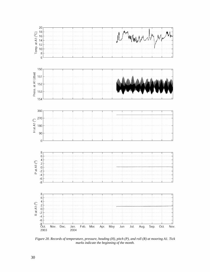
Figure 20. Records of temperature, pressure, heading (H), pitch (P), and roll (R) at mooring A1. Tick marks indicate the beginning of the month.

30

Figure 21. Records of temperature, pressure, heading (H), pitch (P), and roll (R) at mooring A2. Tick marks indicate the beginning of the month.

31

Figure 22. Raw ADCP currents observed at mooring A1. Vertical axis is towards True North. Tick marks

indicate the beginning of the month.

32

Figure 23. Raw ADCP currents observed at mooring A2. Vertical axis is towards True North. Tick marks indicate the beginning of the month.

33

Table 9. Mooring A1. Basic statistics for cross-shelf (Ur, toward 128°) and along-shelf (Vr, toward 38°) components of despiked, unfiltered currents, and data return in %. Max. and Min. denote recorded maximum and minimum values of current components. The direction of vector currents is measured clockwise from True North.

34

Table 10. Mooring A2. Basic statistics for cross-shelf (Ur, toward 128°) and along-shelf (Vr, toward 38°) components of despiked, unfiltered currents, and data return in %. Max. and Min. denote recorded maximum and minimum values of current components. The direction of vector currents is measured clockwise from True North.

35

Data Processing

Pressure and temperature

The accuracy and precision of the RDI temperature sensor are ±0.4°C and the resolution is 0.01°C. The accuracy and precision of the RDI pressure sensor are 0.25% of the rated sensor range and the resolution is 0.01% of the range (200 m for the sensors on ADCP Serial No. 2937 and 2279, and 500 m for sensor on ADCP Serial No. 3569). No information is available on the stability of the sensors. Tidal signals are obvious in pressure records from both sites (except Legs I and III at A2), and there exists a pressure drift during Leg II at A2 while the drift is indistinct at A1 (Figures 20 and 21). The drift at A2, determined by fitting a linear curve, was 0.0028 dbar/day. The record-length mean pressures at A1 and A2 are 152.4 dbar and 286.3 dbar, respectively. Each ADCP record was used to determine the depth of the pressure transducer by converting the pressure record to depth using a pre-set salinity value of 34.0 and the following equation provided by the manufacturer:

depth (in dm) = recorded pressure (in kPa) × (1.02 - [0.00069 × S]), where S is salinity. The resulting mean depth of each mooring is 151.7 m and 285.0 m at A1 and A2, respectively. Since the three deployment locations at A2 are all within 200 m of one another, representative depths of ADCP moorings for the entire observation periods are taken to be 152 m at A1 and 285 m at A2, based on the pressure records during Leg III at A1 and Leg II at A2. The procedures for despiking and low-pass filtering of temperature records are the same as those for the current data.

Current data Data from A2 are combined for each leg and for each 8 m bin to make a 13-month velocity time series at each bin depth. Gaps in the time series at mooring A2 occur for two reasons. First, shorter gaps exist because of the time between mooring recovery and re-deployment, 25.5 hours between Legs I and II, and 3.5 hours between Legs II and III. Second, longer gaps in the upper bin depths are due to the limited vertical range of the WHS300 ADCP. In processing the current data, the depth bins where the data return is less than 50% of the complete record are excluded. The resulting current records are from 146 m to 34 m depth at 4 m intervals for A1, and from 275 m to 179 m depth at 8 m intervals for A2. The longest gap is 77 hours at A1, and 38 hours at A2. After the correction for local magnetic variation of 5°W (http://www.ngdc.noaa.gov/ seg/geomag/jsp/IGRFGrid.jsp), data spikes in U (eastward) and V (northward) components are removed first by calculating the mean and standard deviation for the

36

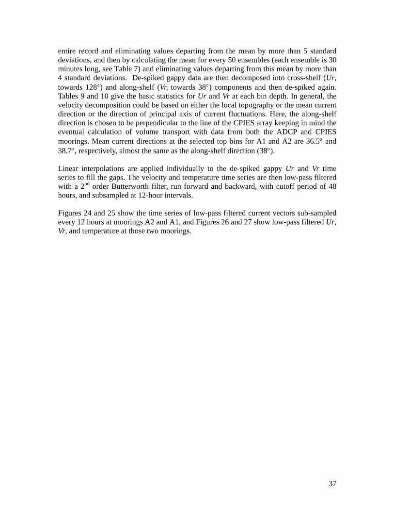
entire record and eliminating values departing from the mean by more than 5 standard deviations, and then by calculating the mean for every 50 ensembles (each ensemble is 30 minutes long, see Table 7) and eliminating values departing from this mean by more than 4 standard deviations. De-spiked gappy data are then decomposed into cross-shelf (Ur, towards 128°) and along-shelf (Vr, towards 38°) components and then de-spiked again. Tables 9 and 10 give the basic statistics for Ur and Vr at each bin depth. In general, the velocity decomposition could be based on either the local topography or the mean current direction or the direction of principal axis of current fluctuations. Here, the along-shelf direction is chosen to be perpendicular to the line of the CPIES array keeping in mind the eventual calculation of volume transport with data from both the ADCP and CPIES moorings. Mean current directions at the selected top bins for A1 and A2 are 36.5° and 38.7°, respectively, almost the same as the along-shelf direction (38°). Linear interpolations are applied individually to the de-spiked gappy Ur and Vr time series to fill the gaps. The velocity and temperature time series are then low-pass filtered with a 2nd order Butterworth filter, run forward and backward, with cutoff period of 48 hours, and subsampled at 12-hour intervals. Figures 24 and 25 show the time series of low-pass filtered current vectors sub-sampled every 12 hours at moorings A2 and A1, and Figures 26 and 27 show low-pass filtered Ur, Vr, and temperature at those two moorings.

37

Figure 24. Vector time series of low-pass filtered 12-hourly currents at mooring A1. Vertical axis is

towards True North. Tick marks indicate the beginning of the month.

38

Figure 25. Vector time series of low-pass filtered 12-hourly currents at mooring A2. Vertical axis is

towards True North. Tick marks indicate the beginning of the month.

39

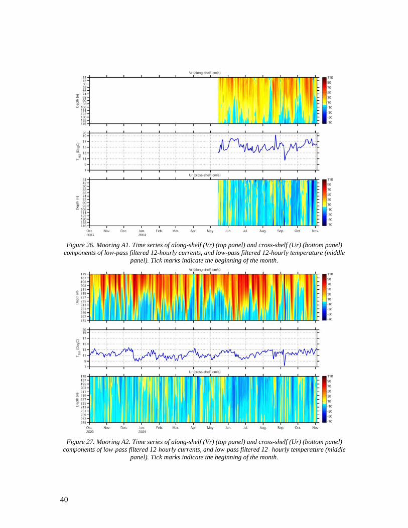
Figure 26. Mooring A1. Time series of along-shelf (Vr) (top panel) and cross-shelf (Ur) (bottom panel)

components of low-pass filtered 12-hourly currents, and low-pass filtered 12-hourly temperature (middle panel). Tick marks indicate the beginning of the month.

Figure 27. Mooring A2. Time series of along-shelf (Vr) (top panel) and cross-shelf (Ur) (bottom panel)

components of low-pass filtered 12-hourly currents, and low-pass filtered 12- hourly temperature (middle panel). Tick marks indicate the beginning of the month.

40

CTD data CTD data were collected along the section shown in Figure 18 during each of four cruises using a SeaBird SBE 911 Plus CTD system. Table 11 lists the locations and depths of the CTD casts. The CTD casts were taken at 4 stations in October 2003 (during the initial deployment cruise) and at 11 stations in May and November 2004. The locations of CTD stations A1 and A2 and C1 through C6 shown in Figure 18 almost coincide with the locations of the ADCP and CPIES moorings. CTD data were taken at 9 stations along the PN-line in November 2003 on board T/V Kagoshima-maru (Figure 28), and the stations are listed in Table 11. Downcast CTD data were processed, binned into 1m depth bins, with parameters derived using the Seabird SEASOFT software package. The CTD data taken in November 2003 were processed at Kagoshima University. Figure 29 shows the resulting vertical sections of temperature and salinity with Figure 29b being taken from a cruise report prepared by Dr. Hiroshi Ichikawa during the November 2003 cruise.

41

Table 11. Locations of CTD stations, water depths, and CTD lowering depths. The listed time, position and water depths are the averages between the cast start and end values.

42

Figure 28. Positions of CTD stations (solid circles) occupied in November, 2003. ADCP mooring positions (A1, A2) are also shown (solid squares). Bathymetry is based on ETOPO2 in meter units.

43

Figure 29. Temperature (left panels) and salinity (right panels) along CTD sections measured four times in

October, November 2003, and May, November 2004 (from top to bottom).

44

Acknowledgements The support and assistance of Capt. Sadao Ishida and his crew aboard the R/V Yokosuka of JAMSTEC and Capt. Sunao Masumitsu and his crew aboard the T/V Kagoshima-maru of Kagoshima University are gratefully acknowledged. Michael Mulroney and Gerard Chaplin provided invaluable help with CPIES and PIES preparation, deployment and recovery. The CTD data used in the GEM calculations were kindly provided by the Nagasaki Marine Observatory, Japan Meteorological Agency. The University of Rhode Island group was supported by ONR Grant number N000140210271. The Naval Research Laboratory group was supported by ONR Grant number N0001402WX20881. We would also like to acknowledge the help of Xiao-Hua Zhu, Takahiro Miura and Kazuhiro Obama of the Institute of Observational Research for Global Change, JAMSTEC, and Fujio Kobayashi and his group members of Marine Works Japan Co. during the 2002 ADCP deployment cruise and Hirohiko Nakamura, Ayako Nishina and their students at the Faculty of Fisheries, Kagoshima University, during the 2004 ADCP recovery cruise. The support and assistance of Capt. Bong-Won Lee and his crew aboard the R/V Onnuri of KORDI, Capt. Masumitsu Sunao and his crew aboard the T/V Kagoshima-maru of Kagoshima University, and Capt. Jeoung Chang Kim of Pukyong National University and his crew aboard the R/V Tamyang are gratefully acknowledged. We would like to acknowledge the help of Mr. Sang-Chul Hwang and Young-Suk Jang from KORDI with the instrumentation and, especially, their dedication and support during the mooring operations on all these cruises. We would also like to acknowledge the help of Professors Jae-Chul Lee and Mi-Ok Park, and their students at Pukyong National University during the 2004 cruises. The T/V Kagoshima-maru cruise in 2003 was conducted as one of the activities under the joint study of the circulation in the ECS between KORDI and the Faculty of Fisheries, Kagoshima University. This work was supported by grants from the United States Office of Naval Research NICOP “Kuroshio Variability on the Shelf of the East China Sea” (KORDI code PI41900), Korea Science and Engineering Foundation (R01-2003-000-10842-0), and KORDI’s in-house projects (PE89000, PE87000).

45

References Book, J., 1998. Kuroshio variations off southwest Japan. M.S. thesis, Graduate School of Oceanography, University of Rhode Island. Choi, B.H., K.O. Kim, and H.M. Eum, 2002. Digital bathymetric and topographic data for neighboring seas of Korea. J. Korean Soc. Coastal and Ocean Engrs, 14, 1, 41-50 (in Korean). Macdonald, A.M., T. Suga and R.G. Curry, 2001. An isopycnally averaged north Pacific climatology. J. Atmos. Oceanic Technol., 18, 394-420. Munk, W.H. and D.E. Cartwright, 1966. Tidal spectroscopy and prediction. Phil. Trans. R. Soc. London, A, 259, 533-581. Perkins, H., F. de Strobel, and L. Gualdesi, 2000. The Barny sentinel trawl-resistant ADCP bottom mount: Design, testing, and application. IEEE J. Oceanic Eng., 25, 430-436. Teague, W.J., G.A. Jacobs, H.T. Perkins, J.W. Book, K.-I. Chang, and M.-S. Suk, 2002. Low-frequency current observations in the Korea/Tsushima Strait. J. Phys. Oceanogr., 32, 1621-1641.

46