eastern washington biomass accessibility
TRANSCRIPT
Report to the Washington State Legislature and Washington
Department of Natural Resources
Eastern Washington Biomass Accessibility
October 2009
Elaine Oneil Bruce Lippke
Rural Technology Initiative School of Forest Resources College of the Environment University of Washington
Box 352100 Seattle, WA. 98195-2100
www.ruraltech.org


i
Acknowledgements
This report represents a synthesis of data, information, and analysis provided from many sources. The
work of the research team included field surveys and data analysis, literature review, and discussions with individuals, companies, and other organizations. Members of the research team included Elaine Oneil,
Research Scientist for The Rural Technology Initiative (RTI) and Bruce Lippke, Economics Professor at
the University of Washington, College of Forest Resources and Director of RTI. The report also
benefited from concurrent studies on barriers to the development of biofuel processing reported in "Wood to Energy in Washington; Imperatives, Opportunities, and Obstacles to Progress" (Mason et al 2009) and
research on life cycle analysis for Inland West Forest Resources by the Consortium for Research on
Renewable Industrial
Craig Partridge and Karen Ripley at Washington Department of Natural Resources in Olympia helped
frame the research questions and project focus for maximum operational impact. Data collection for this
project was made possible with input from many sources. Input from agency staff came from Robert McKellar, Phil Anderson, Dan Griggs, Mike Johnson, at the Washington Department of Natural
Resources, Northeast Region and Rick Brazell and Edward Maffei at the Colville National Forest.
Additional data and information was provided by Brian Vrablick at Northwest Management, Maurice Williamson and staff at Williamson Consulting, Bob Playfair, Patti Playfair, and Brian Cullen at Rafter
Seven Ranch, Robert Broden and Skyler Johnson at Forest Capital Partners, Bill Burdett at ABCO Wood
Recycling, Ron Gray at Avista Power Corporation, Lloyd McGee at Vaagen Brothers Lumber and Bill Berrigan at Berrigan Forestry. The information and professional insights on biomass availability
provided by these people has made an invaluable contribution to this report.
This work was made possible by support provided through the Future of Washington Forests Project funded by the Washington State Legislature and administered by the Washington Department of Natural
Resources.
Any opinions, findings, conclusions, or recommendations expressed in this publication are those of the
authors and do not necessarily reflect the views of the funding agencies or project cooperators.
ii
Executive Summary
Forest residuals represent the largest unexploited source of biomass feedstock for energy in Washington. Prior studies of potential forest residual availability were based on 30 year old logging residue surveys
which did not take into account the substantial change in forest management in the ensuing years. This
study developed new estimators for post-harvest forest residues across a range of ownerships and forest
types in eastern Washington. A cross section of owners, management objectives, forest types, harvest methods, and silvicultural regimes were assessed to derive estimators that are consistent with current
harvest and management operations including forest health and restoration thinning activities. Our
samples included (1) sites where forest health improvement and fire risk reduction were the focus, and (2) sites where timber values alone support the harvest.
Field surveys were conducted after harvest activity on federal, state and private lands, across six major
forest types grouped into three categories (dry, moist, or wet), a range of silvicultural systems and objectives, four harvest methods, and two market conditions (high or low pulp utilization at the time of
harvest). These surveys measured residual biomass in piles (hereafter called slash piles) as well as
dispersed slash summarized by diameter class. Generalized linear modeling found no significant differences between owner groups, harvest types, market conditions, and only weakly significant
differences between broad forest type groupings. The best overall predictor of total and available residual
biomass was harvested biomass tonnage. Pre-harvest inventory was not a good predictor of total potential logging residue because there were so many different configurations of cut and leave volumes present
within the sample.
A subset of slash piles were removed from select harvest units and processed through a grinder to determine the actual volume and energy equivalent relative to measured volume estimates. This study
component revealed that current measurement protocols for piled slash only predict about ½ as much
material as is actually there when the material is ground and weigh scaled. This means that there is twice as much material available for bioenergy feedstock as current measurement protocols predict. It also
highlights the fact that burning slash piles generates twice as many emissions as is being projected for air
quality guidelines.
Sample data were used to generate a model of the relationship between harvest volume and logging
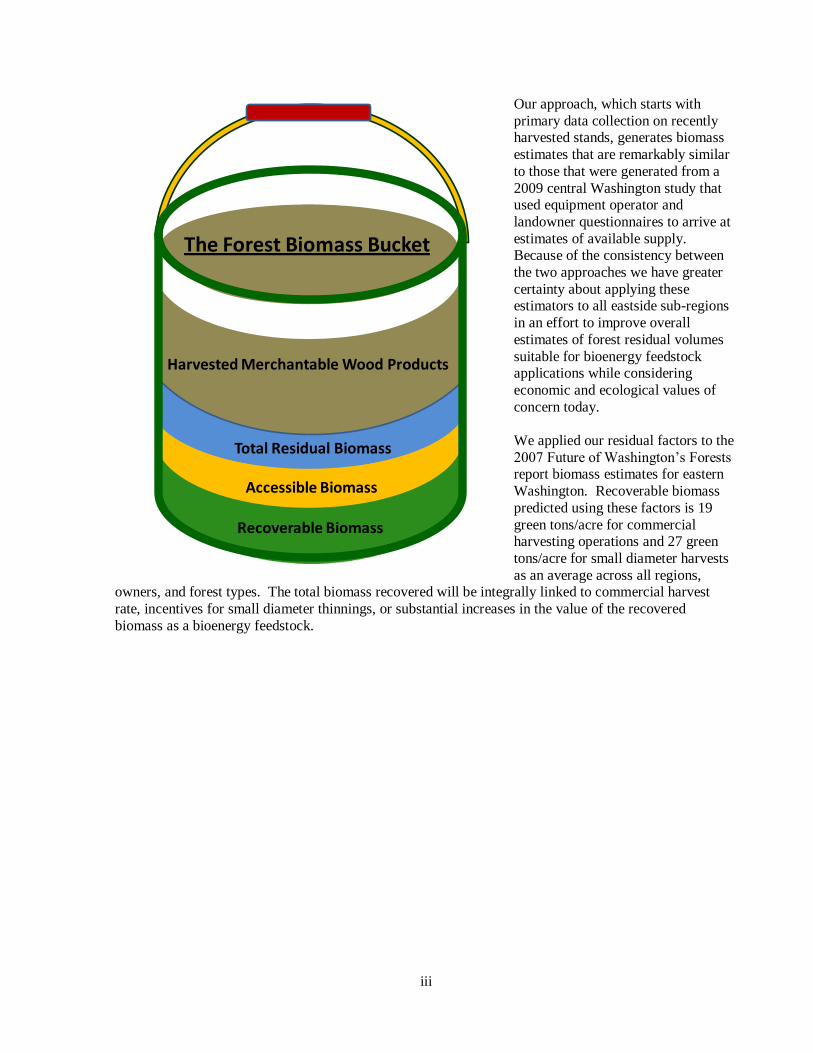
residue identified as total residual biomass. The forest biomass bucket (shown below) highlights the
relative proportion of harvested biomass that is found in each category. For simplicity, standing residual biomass is not included in the bucket analogy. In the bucket, merchantable log volume that is currently
sent to wood processing facilities is approximately 50% of the total harvested biomass with the other 50%
identified as total residual biomass. Net-down factors to sustain ecological function reduce the total residuals by approximately 30% resulting in 35% of the total harvested biomass defined as accessible
biomass. Not all the accessible biomass is economically recoverable, so a net-down of a further 30% to
account for economic viability generates the estimate of recoverable biomass.
In effect, 20% of the total harvested biomass is recoverable as feedstock for biofuel production which is
equivalent to 40% of the volume currently harvested for wood processing. Since mill surveys show only
about 12% of harvest volume being used as biofuel for processing energy, the recoverable forest residual biomass provides roughly a 400% increase in biofuel feedstock. This is sufficient to make existing mills
more than energy self sufficient or support stand alone bioprocessing facilities.
iii
Our approach, which starts with
primary data collection on recently harvested stands, generates biomass
estimates that are remarkably similar
to those that were generated from a
2009 central Washington study that used equipment operator and
landowner questionnaires to arrive at
estimates of available supply. Because of the consistency between
the two approaches we have greater
certainty about applying these estimators to all eastside sub-regions
in an effort to improve overall
estimates of forest residual volumes
suitable for bioenergy feedstock applications while considering
economic and ecological values of
concern today.
We applied our residual factors to the
2007 Future of Washington’s Forests report biomass estimates for eastern
Washington. Recoverable biomass
predicted using these factors is 19
green tons/acre for commercial harvesting operations and 27 green
tons/acre for small diameter harvests
as an average across all regions, owners, and forest types. The total biomass recovered will be integrally linked to commercial harvest
rate, incentives for small diameter thinnings, or substantial increases in the value of the recovered
biomass as a bioenergy feedstock.
Total Residual Biomass
Accessible Biomass
Recoverable Biomass
Harvested Merchantable Wood Products
The Forest Biomass Bucket
iv
Table of Contents Page
Acknowledgements ................................................................................................................................. i
Executive Summary............................................................................................................................... ii
Background ........................................................................................................................................... 1
Methods ........................................................................................................................................... 3
Identification and Stratification of Measurement Sites.......................................................................... 3
Field surveys ....................................................................................................................................... 3
Sampling Piled Slash ....................................................................................................................... 3
Sampling Dispersed Slash 5
Sampling Chipped Biomass .............................................................................................................. 5
Analysis of Field Data ......................................................................................................................... 6
Simulation methods ............................................................................................................................. 7
Results ........................................................................................................................................... 9
Calibration of sampled biomass and recoverable biomass................................................................... 10
Results by owner group and forest type .............................................................................................. 11
Discussion ......................................................................................................................................... 17
Biomass for retaining ecological functions ......................................................................................... 17
Comparisons to Past Woody Biomass Estimates ................................................................................ 21
Howard (1981) .............................................................................................................................. 21
Frear et al. (2005) ......................................................................................................................... 22
TSS (2009) ..................................................................................................................................... 22
The Future of Washington’s Forests (2007) ................................................................................... 23
Operational Constraints ..................................................................................................................... 26
Slash Handling and Densification .................................................................................................. 26
Transportation Costs as Operational Barriers ............................................................................... 29
Conclusions ......................................................................................................................................... 31
References ......................................................................................................................................... 33
Appendix ......................................................................................................................................... 35
Data Summaries by forest type and owner group. ............................................................................... 35
v
List of Figures Page
Figure 1. Washington State Biomass availability by sector (Frear et al. 2005) ......................................... 1
Figure 2. Sampling piled logging slash on forest landings in NE Washington .......................................... 4
Figure 3. Multiple small logging slash piles in NE Washington ............................................................... 4
Figure 4. Dispersed logging slash in NE Washington .............................................................................. 5
Figure 5. Ground logging slash ready for transport to the bioenergy generation facility
in NE Washington .............................................................................................................. 6
Figure 6. Relationships between pile measurement and scaled tonnage reported at Avista Power .......... 11
Figure 7. Relative percentage of harvested biomass by forest type......................................................... 12
Figure 8. Tons/acre of harvested biomass by forest type. ....................................................................... 12
Figure 9. Relative percentage of harvested biomass by owner group. .................................................... 13
Figure 10. Percentage of harvested biomass by forest type and owner group. ........................................ 13
Figure 11. Tons of dispersed slash by diameter class ............................................................................. 17
Figure 12. Accessible biomass as a function of total residual biomass ................................................... 18
Figure 13. Recoverable biomass as a function of total residual biomass................................................. 19
Figure 14. Retained and accessible biomass relative to total biomass .................................................... 20
Figure 15. Retained and recoverable biomass relative to total biomass .................................................. 20
Figure 16. A comparison of harvested to residual biomass by size class and accessibility ...................... 22
Figure 17. A load of low density harvest residue ready for transport to the main processing location ..... 27
Figure 18. Long in-woods haul distances substantially increase the cost of removal .............................. 28
Figure 19. Processing equipment waiting for the trucks to return ........................................................... 28
Figure 20. Slash ground and waiting for transportation to the biomass facility ....................................... 28
Figure 21. In-woods transportation costs as a function of distance to the landing ................................... 29
Figure 22. Trucking cost to remove biomass to closest bio-energy facility for DNR Timber sales.......... 30
Figure A.1. Comparison of residual biomass to harvested biomass for dry forest types .......................... 35
Figure A.2. Comparison of residual biomass to harvested biomass for moist forest types ...................... 36
Figure A.3. Comparison of residual biomass to harvested biomass for wet forest types ......................... 37
Figure A.4. Allocation of Harvested Biomass on Federal Lands by forest type ...................................... 38
Figure A.5. Allocation of harvested biomass on private lands by forest type ......................................... 38
Figure A.6. Allocation of biomass on DNR lands by forest type ............................................................ 39
vi
List of Tables Page
Table 1. Allocation of forest biomass by location and residue type based on Frear et al (2005) data ................ 2
Table 2. Number of biomass residue samples by owner group and forest type .................................................. 9
Table 3. Number of transects and piles measured by owner group and forest type .......................................... 10
Table 4. Total residual biomass by owner group and forest type group. ........................................................... 14
Table 5. Residual biomass in piles and larger diameter dispersed material. ..................................................... 14
Table 6. Potentially recoverable residual biomass ............................................................................................ 14
Table 7. Sub-regional estimates of potentially recoverable residual biomass on a per acre basis..................... 23
Table 8. Sub-regional estimates of potentially recoverable residual biomass for private and tribal lands ........ 24
Table 9. Sub-regional estimates of potentially recoverable residual biomass for state trust lands.................... 25
Table 10. Sub-regional estimates of potentially recoverable residual biomass for federal lands ...................... 25
Table A1. Average biomass with upper and lower bound by owner group, forest type,
and biomass category. ................................................................................................................. 40
1
Background
A synopsis of what became the 2007 Future of Washington’s Forests and Forest Industries report to the
Washington State legislature was presented to forestry stakeholders at the Northwest Environmental Forum in November 2006. From that meeting, stakeholders determined that more research was needed
on biomass availability and accessibility from woody feedstocks and the state legislature provided
funding for a University of Washington study to expand on what was currently known about woody
biomass availability so that more accurate estimates of supply could be determined.
Preliminary analysis identified two recent broad scale estimates of biomass availability -Frear et al 2005
and Kersetter and Lyons 2001. While the Frear study provided an exhaustive inventory of all biomass sources, Kersetter and Lyons focused only on private inventory within hauling distance to existing pulp
milling facilities. It was therefore not surprising that each study gave a different estimate of available
biomass supply because different parameters were used in the analyses. More problematic from an
operational standpoint was that both of these studies used a single year’s harvest data to estimate residual inventories, and both were based on the Howard (1981) forest residue study estimates that reflected forest
inventories and logging practices of the late 1970’s.
Biomass and Bioenergy by Category
0
1,000
2,000
3,000
4,000
5,000
6,000
7,000
8,000
9,000
Field Residue Animal Waste Forestry Food Packing/Processing Municipal Solid Waste
Valu
e
Biomass (1,000 Dry Tons) Energy (M kWh)
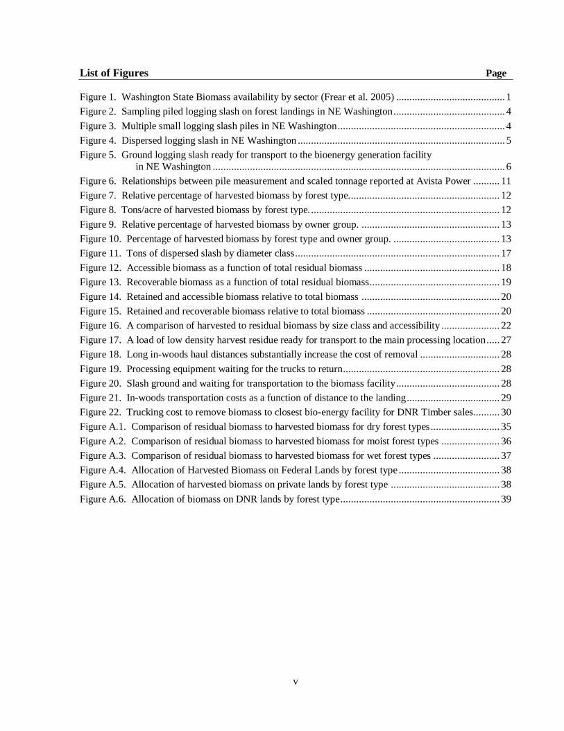
Figure 1. Washington State Biomass availability by sector (Frear et al. 2005)
Frear et al (2005) did however identify forestry biomass as the largest source of biomass feedstock for
energy in Washington (Figure 1) which suggested that clearly quantifying the availability of this material
would be of significant value for a developing renewable energy industry in the state. Based on his residue assumptions, Frear found that most of the forestry related biomass was mill processing residues.
These residues are already at milling facilities (Table 1) where they are almost all utilized for co-products
or energy generation (Milota et al. 2005). As such, milling residues might not be available for additional
renewable energy initiatives unless they are bid away from current uses. Of the forest biomass that is not currently utilized, most was estimated to be available from logging residues and thinning slash, making
up 29.7% of the biomass statewide and 53.5% of the forest biomass available in Eastern Washington (E
WA) (Table 1). Because the percentage figures from the Frear estimate were based on 30 year old forest residue data and a single harvest year they do not necessarily account for current logging practices, the
need to retain downed wood for ecological function or economic recovery constraints.

2
Table 1. Allocation of forest biomass by location and residue type based on Frear et al (2005) data
Forest residue type State wide volume
(dry tons) % by type
E WA volume
(dry tons) % of total in E WA % by type
Logging 1,901,072 23.5% 805,214 42.4% 35.2%
Thinning 505,666 6.2% 419,970 83.1% 18.3%
Land Clearing 418,595 5.2% 14,633 3.5% 0.6%
Milling 5,278,353 65.1% 1,050,041 19.9% 45.9%
Total 8,103,686 100.0% 2,289,858 28.3% 100.0%
At this time, most of these post-harvest forest residuals and thinning slash are piled and burned, or left to decay in-situ resulting in lost opportunity to generate clean energy, reduce fossil fuel reliance, and avoid
green house gas emissions. Given what was already known from these prior studies, this study was
designed to quantify the most likely sources of under-utilized biomass material (logging slash and
thinning slash), and identify issues related to obtaining this material as a renewable feedstock. Because logging systems, utilization standards, sawing specifications, and the forest types that we now harvest
have changed substantially since 1979 when the Howard (1981) data were gathered, the first step was to
update estimators for post-harvest forest biomass across a range of ownerships and forest types.
These field measurements to update the prior logging residue studies are the most critical element of this
study for numerous reasons. First, they inform both coarse resolution biomass estimates and provide specific information needed to model biomass availability at the sub-regional scale. In particular, these
estimates of forest residues can be linked with modeled projections of current and future harvest activities
to quantify forest biomass feedstock availability now and into the future providing short-, mid-, and long-
term estimates. Estimators of forest residuals can be formatted into modeling modules for use with publicly-available forest growth models such as the Forest Vegetation Simulator (Wyckoff 1981) so that,
with minimal effort, region specific volume estimates can be developed. And finally, estimates of slash
availability can be periodically updated to real time when used in conjunction with annual Washington State Department of Natural Resources (DNR) state harvest reports.
3
Methods
Identification and Stratification of Measurement Sites
The design goal for measurements was to maximize the sampling of a range of forest types, harvest types, utilization standards, and owners. It was anticipated that obtaining data for a large sample of very recent
harvests would be difficult and costly. It was not possible to sample the entire state with available funding
so we chose Northeastern Washington as an important study location with multiple ownership categories. For this region there is a large cross section of owners that are actively harvesting in a multitude of forest
types and the milling infrastructure is still sufficiently diverse so that we could maximize data collection
for the largest number of strata possible. Strata were defined by a combination of forest type (grouped into dry, moist, and cold categories), harvest type (even and uneven aged), market condition (high or low
pulp utilization at the time of harvest) and ownership. No owner group had active harvest units in all
strata, but all available strata were included in the sample.
The DNR and the Colville National Forest (CNF) identified all sites where harvest had occurred and site
preparation had not been completed during the field survey windows. Harvest and inventory data on
these sites were collected and sampling plans were developed to measure residual on-site slash loadings, both at the landing and as dispersed slash across the unit. Seven (7) DNR timber sales and four (4) USFS
timber sales with a total of 48 distinct sample units were assessed. For private landowner samples we
endeavored to stratify the sample using the DNR forest practices application reporting system (FPARS) to
identify potential harvest site data sources for Northeastern Washington. However, this reporting system does not identify which applications are already harvested, which have not had slash disposal, and which
units of the cutting permit might still be available for sampling. Thus we chose an alternative method to
identify potential survey sites on private lands. In order to maximize the likelihood of permission to sample private forests, we chose to work through local consulting firms that had ongoing relationships
with private landowners. The consultants were able to contact landowners in the region to determine
which of their sites might be in the appropriate condition for sampling to occur and to gain permission to survey on private lands. Permission was granted in all cases. Using this method we were able to sample
eleven (11) private sites and the Turnbull Wildlife refuge which had been recently harvested, but had not
had site preparation conducted at the time of survey.
Field surveys
Sampling Piled Slash
All available sites in the survey were assessed for both piled and dispersed slash. The cross section of
samples we obtained had sites with only dispersed slash, sites with only piled slash and sites with a
combination of the two potential sources of woody biomass. The piled slash was measured as a 100%
sample (i.e. all piles were measured on a unit whether they were on the landing or in the woods). Pile volume was calculated from measurements of length, width, height, and classification of pile shape
according to the volume and tonnage equations in Appendix 3 of the DNR Smoke Management Plan
(revision date 1998). The estimated species composition of the piles was used to convert the volume measures to tonnage figures based on density values provided in the Smoke Management Plan. On a few
units, there were more than 100 small piles and on one unit there were more than 1200 piles. For these
cases a total count of piles combined with representative measurements of the average pile(s) were used
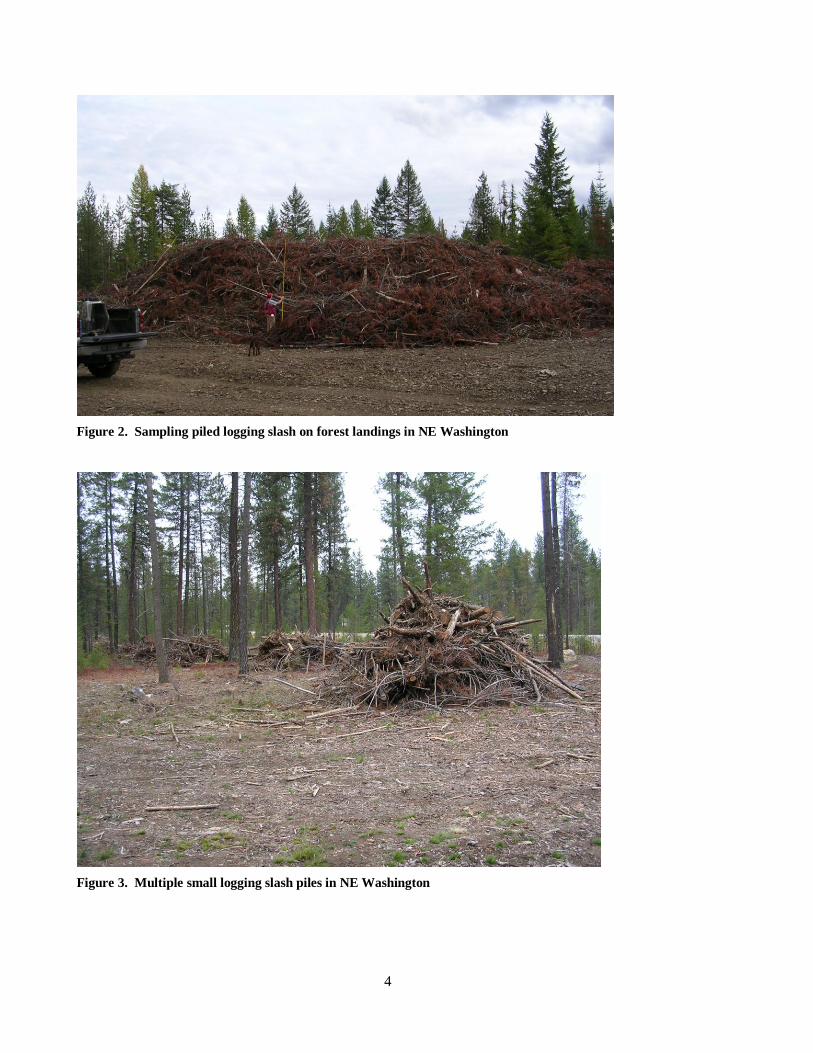
to arrive at woody biomass estimates for the unit. Figure 2 is an example of a large landing biomass pile on one of the units with a calculated volume of 119 CCF (hundred cubic feet) and 140 green tons. Figure
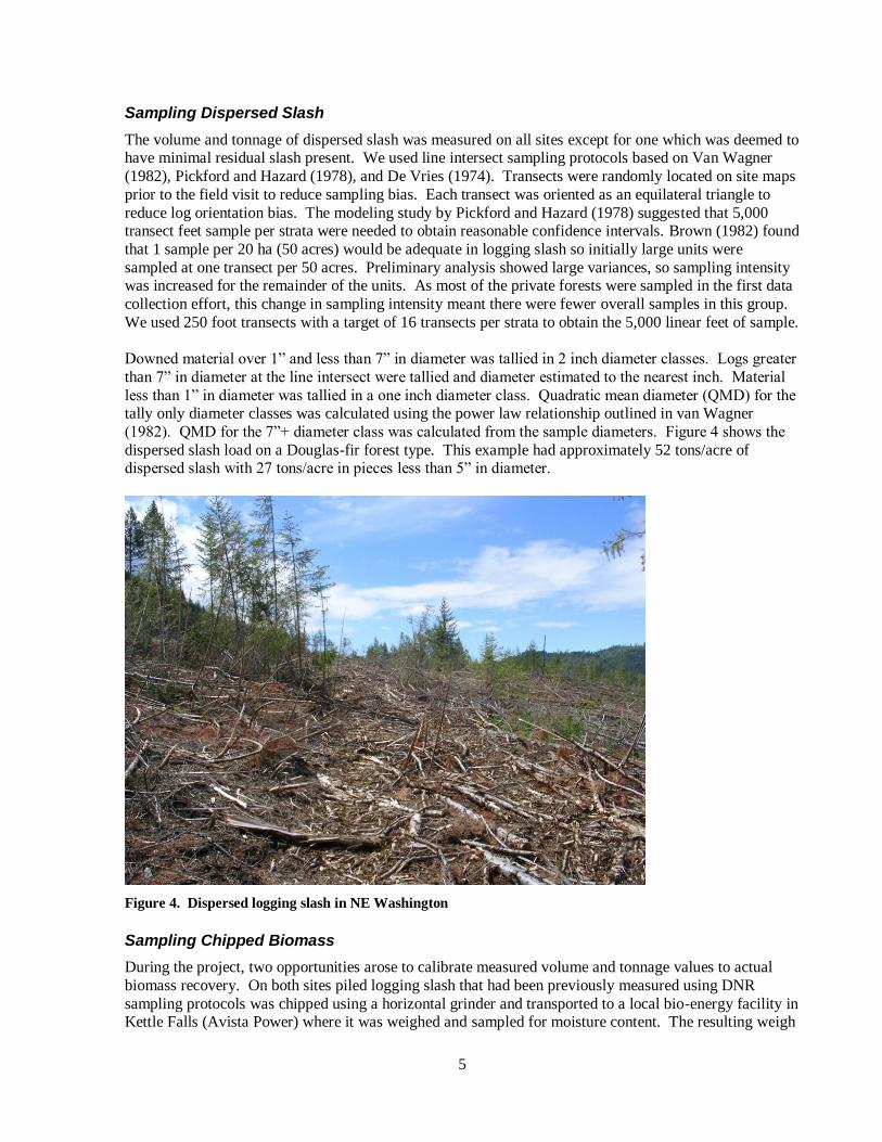
3 shows a row of small piles that were dispersed throughout the woods on another unit. These small piles
were calculated to have 2-15 CCF and 0.5-3.5 green tons per pile depending on dimensions and size.
4
Figure 2. Sampling piled logging slash on forest landings in NE Washington
Figure 3. Multiple small logging slash piles in NE Washington
5
Sampling Dispersed Slash
The volume and tonnage of dispersed slash was measured on all sites except for one which was deemed to have minimal residual slash present. We used line intersect sampling protocols based on Van Wagner
(1982), Pickford and Hazard (1978), and De Vries (1974). Transects were randomly located on site maps
prior to the field visit to reduce sampling bias. Each transect was oriented as an equilateral triangle to
reduce log orientation bias. The modeling study by Pickford and Hazard (1978) suggested that 5,000 transect feet sample per strata were needed to obtain reasonable confidence intervals. Brown (1982) found
that 1 sample per 20 ha (50 acres) would be adequate in logging slash so initially large units were
sampled at one transect per 50 acres. Preliminary analysis showed large variances, so sampling intensity was increased for the remainder of the units. As most of the private forests were sampled in the first data
collection effort, this change in sampling intensity meant there were fewer overall samples in this group.
We used 250 foot transects with a target of 16 transects per strata to obtain the 5,000 linear feet of sample.
Downed material over 1” and less than 7” in diameter was tallied in 2 inch diameter classes. Logs greater
than 7” in diameter at the line intersect were tallied and diameter estimated to the nearest inch. Material
less than 1” in diameter was tallied in a one inch diameter class. Quadratic mean diameter (QMD) for the tally only diameter classes was calculated using the power law relationship outlined in van Wagner
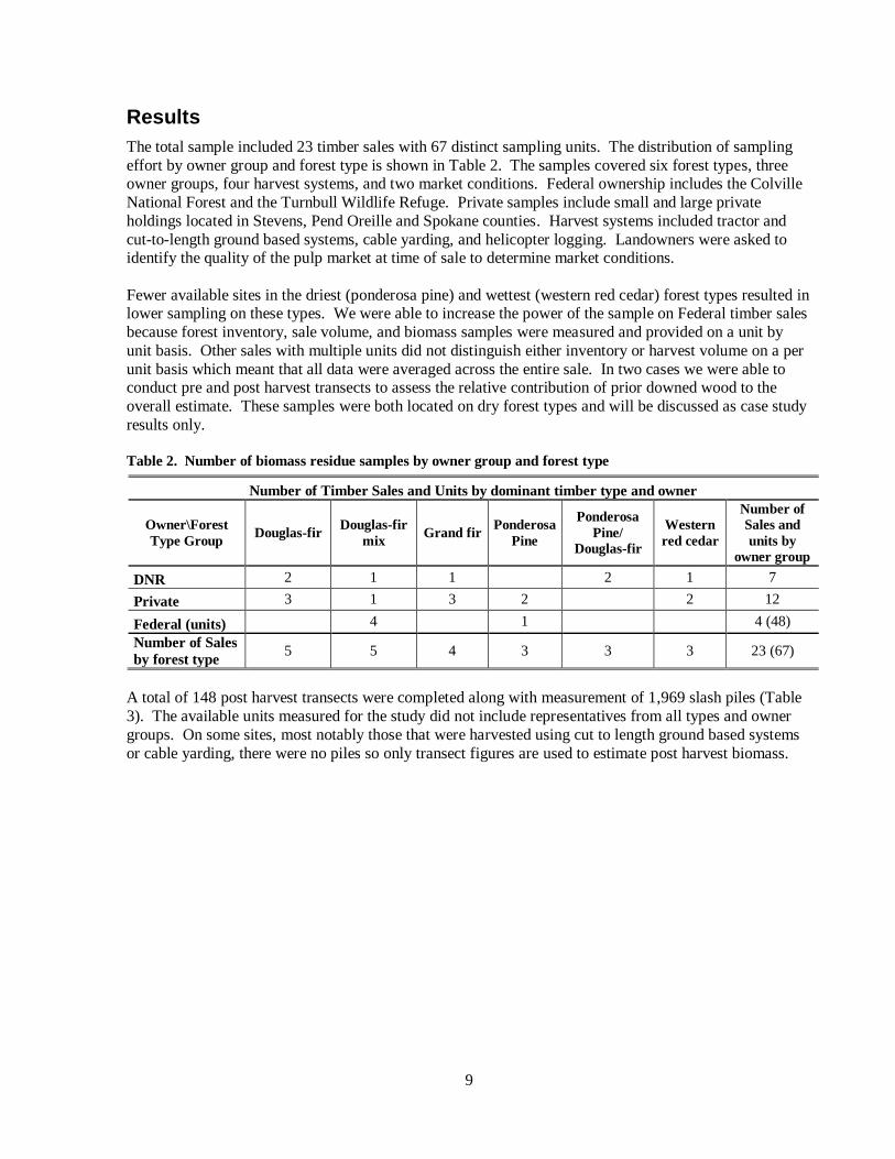
(1982). QMD for the 7”+ diameter class was calculated from the sample diameters. Figure 4 shows the
dispersed slash load on a Douglas-fir forest type. This example had approximately 52 tons/acre of dispersed slash with 27 tons/acre in pieces less than 5” in diameter.
Figure 4. Dispersed logging slash in NE Washington
Sampling Chipped Biomass
During the project, two opportunities arose to calibrate measured volume and tonnage values to actual
biomass recovery. On both sites piled logging slash that had been previously measured using DNR
sampling protocols was chipped using a horizontal grinder and transported to a local bio-energy facility in Kettle Falls (Avista Power) where it was weighed and sampled for moisture content. The resulting weigh

6
scale values for green ton and bone dry ton (BDT) were used to calibrate the actual slash volume for all
piled slash as reported in the results. Figure 5 shows the chipped material ready for transport to the biomass energy facility.
Figure 5. Ground logging slash ready for transport to the bioenergy generation facility in NE Washington
Analysis of Field Data
Volume and tonnage of piled and dispersed slash were calculated and combined to arrive at overall
biomass volume and tonnage per acre. For USFS sites where inventory and harvest volume data were
available by unit, the biomass data were summarized by unit. All other data were summarized by timber
sale in order to allow comparison to the harvest and inventory data. The number of transects per unit varied from 1 to 8 depending on the size of the unit with an average of 2.2 transects/unit. The number of
piles per sample unit varied from 1 to over 1200 with a median value of 1 as the average was skewed
tremendously by the sample with over 1200 piles.
Because of the way the dispersed slash was measured it was possible to summarize it in a number of
different ways. For a number of reasons we chose to summarize it in two size classes: > 5” in diameter and <5” in diameter. As most timber cruise and sale volume is based on a top diameter ranging from 4-
5.5”, a diameter limit of 4” would divide the sample between potentially merchantable and non-
merchantable wood. In calculating the quadratic mean diameter for the diameter classes, we found that
only 2% of the transects had a QMD >4” for the 3-5” size class, meaning that on average most of the volume in the 3-5” class is below current utilization specifications. The distinction between potential
recovery by conventional machinery and that which would require specialized baling machinery to
remove is likely to be in the vicinity of merchantability limits.
Residue volumes were compared to pre-harvest inventory and sale volume to estimate logging residues
per unit of volume harvested and per unit of standing timber. The inventory data varied substantially in
quality. The majority of the data were from pre-harvest cruises, but in some cases older, low density

7
sample data were used to estimate the volume for the strata in a timber sale. This source of uncertainty is
not explicitly measurable and therefore is not part of the results. It does however inform the discussion and interpretation of the results.
Simulation methods
Because not all strata were sampled for lack of suitable sites, and because the residue to harvest volume
ratios do not differ substantially between owner groups, the results are grouped by forest type group to
maximize our ability to simulate future supplies using large scale inventory databases such as the Forest Inventory and Analysis (FIA) data provided by the USFS. The relationships derived from the field survey
were used to revisit the simulation estimates generated for the Future of Washington’s Forests study to
develop estimates at a regional level.

9
Results
The total sample included 23 timber sales with 67 distinct sampling units. The distribution of sampling
effort by owner group and forest type is shown in Table 2. The samples covered six forest types, three owner groups, four harvest systems, and two market conditions. Federal ownership includes the Colville
National Forest and the Turnbull Wildlife Refuge. Private samples include small and large private
holdings located in Stevens, Pend Oreille and Spokane counties. Harvest systems included tractor and
cut-to-length ground based systems, cable yarding, and helicopter logging. Landowners were asked to identify the quality of the pulp market at time of sale to determine market conditions.
Fewer available sites in the driest (ponderosa pine) and wettest (western red cedar) forest types resulted in lower sampling on these types. We were able to increase the power of the sample on Federal timber sales
because forest inventory, sale volume, and biomass samples were measured and provided on a unit by
unit basis. Other sales with multiple units did not distinguish either inventory or harvest volume on a per
unit basis which meant that all data were averaged across the entire sale. In two cases we were able to conduct pre and post harvest transects to assess the relative contribution of prior downed wood to the
overall estimate. These samples were both located on dry forest types and will be discussed as case study
results only. Table 2. Number of biomass residue samples by owner group and forest type
Number of Timber Sales and Units by dominant timber type and owner
Owner\Forest
Type Group Douglas-fir
Douglas-fir
mix Grand fir
Ponderosa
Pine
Ponderosa
Pine/
Douglas-fir
Western
red cedar
Number of
Sales and
units by
owner group
DNR 2 1 1 2 1 7
Private 3 1 3 2 2 12
Federal (units) 4 1 4 (48)
Number of Sales
by forest type 5 5 4 3 3 3 23 (67)
A total of 148 post harvest transects were completed along with measurement of 1,969 slash piles (Table
3). The available units measured for the study did not include representatives from all types and owner
groups. On some sites, most notably those that were harvested using cut to length ground based systems
or cable yarding, there were no piles so only transect figures are used to estimate post harvest biomass.
10
Table 3. Number of transects and piles measured by owner group and forest type
Number of Transects by forest type and owner
Forest Type Group\Owner DNR Federal Private Total by forest type
Douglas-fir 15 17 32
Douglas-fir mix 8 52 2 62
Grand fir 6 13 19
Ponderosa Pine 5 4 9
Ponderosa Pine/Douglas-fir 14 14
Western red cedar 8 4 12
Total by owner group 51 57 40 148
Number of sample piles by forest type and owner
Forest Type Group\Owner DNR Federal Private Total by forest type
Douglas-fir 101 34 135
Douglas-fir mix 66 206 272
Grand fir 46 29 75
Ponderosa Pine 1 45 46
Ponderosa Pine/Douglas-fir 1333 1333
Western red cedar 108 108
Total by owner group 1654 207 108 1969
Calibration of sampled biomass and recoverable biomass
The relationship between scaled and measured tons of biomass (Figure 6) shows that field measurements
substantially under-estimate tonnage for piled slash for the two sites where we have available data. The under-estimate may be a function of the kind of residual material and the utilization standard for these
particular timber sales. An excellent pulp market for one sale meant that much of the material greater
than 2” in diameter was removed from the site, leaving predominantly small limbs, needles, and broken material only. This kind of residual material will pack more tightly than is assumed for a conventional
harvest where air space makes up a large component of the pile volume. Under such conditions,
calculations for solid wood volume in the piles would have to be altered to reflect the true volume
remaining on site. The second sample site was part of a forest health improvement treatment which targeted removal of small diameter timber in a wildland urban interface. Again, because of the nature of
the residues, the piles would have been packed more tightly than one would assume for a normal harvest
project.
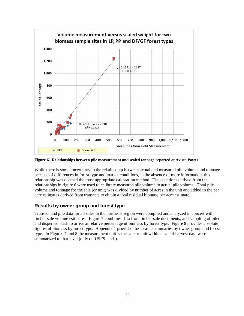
11
Figure 6. Relationships between pile measurement and scaled tonnage reported at Avista Power
While there is some uncertainty in the relationship between actual and measured pile volume and tonnage
because of differences in forest type and market conditions, in the absence of more information, this relationship was deemed the most appropriate calibration method. The equations derived from the
relationships in figure 6 were used to calibrate measured pile volume to actual pile volume. Total pile
volume and tonnage for the sale (or unit) was divided by number of acres in the unit and added to the per acre estimates derived from transects to obtain a total residual biomass per acre estimate.
Results by owner group and forest type
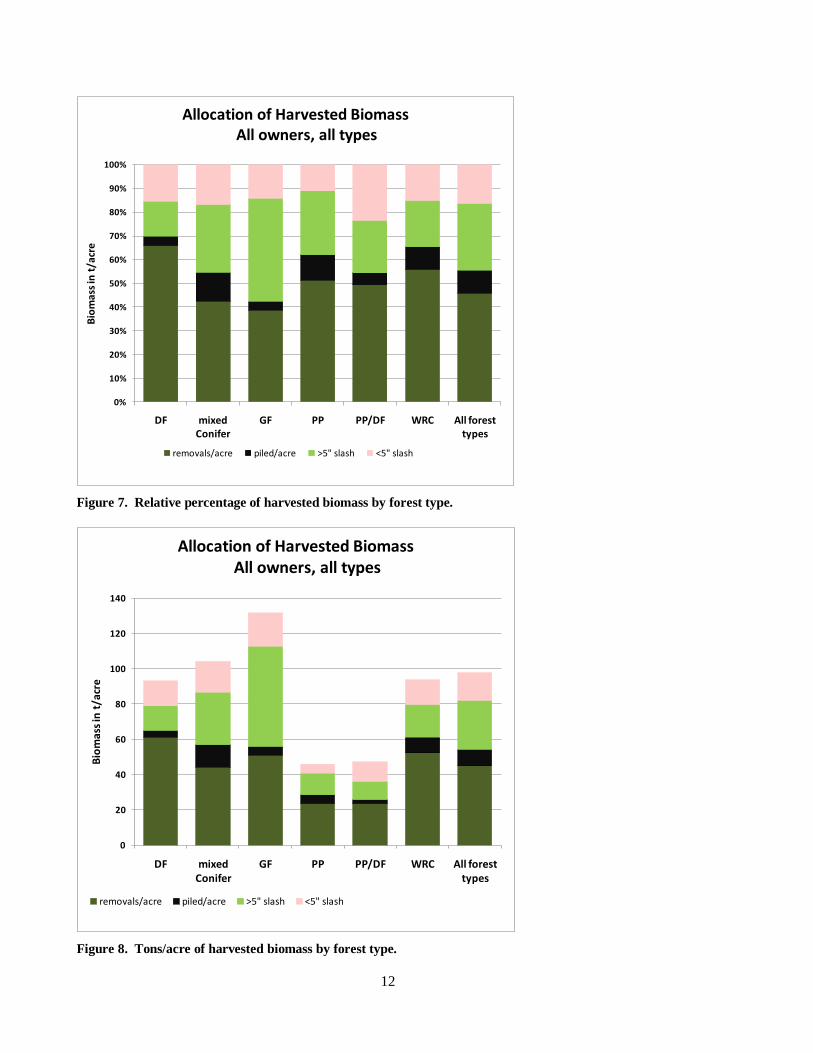
Transect and pile data for all sales in the northeast region were compiled and analyzed in concert with
timber sale volume estimates. Figure 7 combines data from timber sale documents, and sampling of piled and dispersed slash to arrive at relative percentage of biomass by forest type. Figure 8 provides absolute
figures of biomass by forest type. Appendix 1 provides these same summaries by owner group and forest
type. In Figures 7 and 8 the measurement unit is the sale or unit within a sale if harvest data were
summarized to that level (only on USFS lands).
12
0%
10%
20%
30%
40%
50%
60%
70%
80%
90%
100%
DF mixed Conifer
GF PP PP/DF WRC All forest types
Bio
mas
s in
t/a
cre
Allocation of Harvested Biomass All owners, all types
removals/acre piled/acre >5" slash <5" slash
Figure 7. Relative percentage of harvested biomass by forest type.
0
20
40
60
80
100
120
140
DF mixed Conifer
GF PP PP/DF WRC All forest types
Bio
ma
ss in
t/a
cre
Allocation of Harvested Biomass All owners, all types
removals/acre piled/acre >5" slash <5" slash
Figure 8. Tons/acre of harvested biomass by forest type.

13
Figure 9 summarizes the removal and residual data by owner group and Figure 10 summarizes the data by both forest type and owner group. Comparing Figures 7-10 shows that summarizing results by owner
group and/or forest type generates slightly different average values for removals and residuals.
Merchantable volume is approximately 50% of total harvested biomass with a range of 33-62% remaining
post harvest across all owner groups and forest types (Figure 10), whereas summarizing by just owner group or forest type generates an estimate of 46-48% of the total harvest biomass is merchantable volume.
0%
10%
20%
30%
40%
50%
60%
70%
80%
90%
100%
DNR Federal Private All Owners
Biomass Allocation by Owner Group
removals/acre Piled t/ac Total Average of >5" slash Total Average of <5" slash
Figure 9. Relative percentage of harvested biomass by owner group.
0%
10%
20%
30%
40%
50%
60%
70%
dry moist wet all forest types
Percent of harvested biomass remaining post-harvest
DNR
Federal
Private
All Owners
Figure 10. Percentage of harvested biomass by forest type and owner group.
14
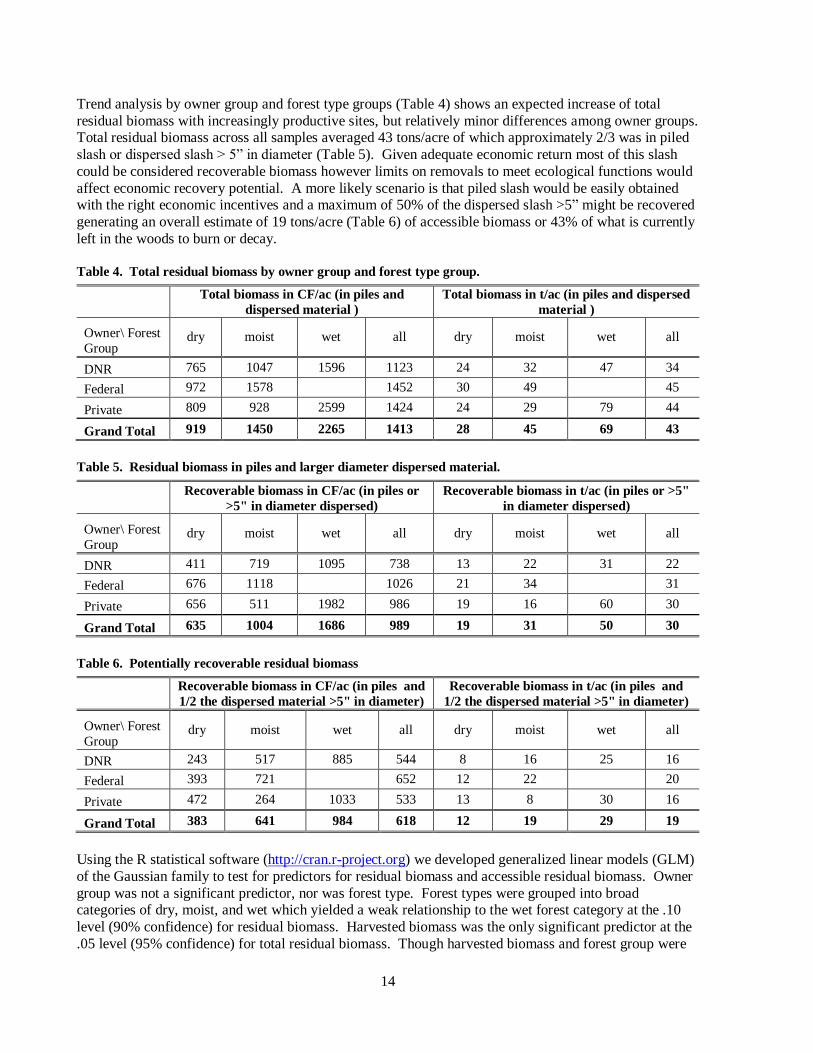
Trend analysis by owner group and forest type groups (Table 4) shows an expected increase of total
residual biomass with increasingly productive sites, but relatively minor differences among owner groups. Total residual biomass across all samples averaged 43 tons/acre of which approximately 2/3 was in piled
slash or dispersed slash > 5” in diameter (Table 5). Given adequate economic return most of this slash
could be considered recoverable biomass however limits on removals to meet ecological functions would
affect economic recovery potential. A more likely scenario is that piled slash would be easily obtained with the right economic incentives and a maximum of 50% of the dispersed slash >5” might be recovered
generating an overall estimate of 19 tons/acre (Table 6) of accessible biomass or 43% of what is currently
left in the woods to burn or decay. Table 4. Total residual biomass by owner group and forest type group.
Total biomass in CF/ac (in piles and
dispersed material )
Total biomass in t/ac (in piles and dispersed
material )
Owner\ Forest
Group dry moist wet all dry moist wet all
DNR 765 1047 1596 1123 24 32 47 34
Federal 972 1578 1452 30 49 45
Private 809 928 2599 1424 24 29 79 44
Grand Total 919 1450 2265 1413 28 45 69 43
Table 5. Residual biomass in piles and larger diameter dispersed material.
Recoverable biomass in CF/ac (in piles or
>5" in diameter dispersed)
Recoverable biomass in t/ac (in piles or >5"
in diameter dispersed)
Owner\ Forest
Group dry moist wet all dry moist wet all
DNR 411 719 1095 738 13 22 31 22
Federal 676 1118 1026 21 34 31
Private 656 511 1982 986 19 16 60 30
Grand Total 635 1004 1686 989 19 31 50 30
Table 6. Potentially recoverable residual biomass
Recoverable biomass in CF/ac (in piles and
1/2 the dispersed material >5" in diameter)
Recoverable biomass in t/ac (in piles and
1/2 the dispersed material >5" in diameter)
Owner\ Forest
Group dry moist wet all dry moist wet all
DNR 243 517 885 544 8 16 25 16
Federal 393 721 652 12 22 20
Private 472 264 1033 533 13 8 30 16
Grand Total 383 641 984 618 12 19 29 19
Using the R statistical software (http://cran.r-project.org) we developed generalized linear models (GLM)
of the Gaussian family to test for predictors for residual biomass and accessible residual biomass. Owner
group was not a significant predictor, nor was forest type. Forest types were grouped into broad categories of dry, moist, and wet which yielded a weak relationship to the wet forest category at the .10
level (90% confidence) for residual biomass. Harvested biomass was the only significant predictor at the
.05 level (95% confidence) for total residual biomass. Though harvested biomass and forest group were

15
significant predictors using the GLM, the resulting model explained only 14% PDE (Percent Deviance
Explained). These results highlight how difficult it is to arrive at reliable estimates of available biomass across a broad region without many hundreds of units to sample and many dozens of samples within each
unit.

17
Discussion
Biomass for retaining ecological functions
There is a tension between the value of woody debris as a key ecosystem component that provides habitats, water retention, and nutrient storage within the forest system and the use of wood for bioenergy
feedstocks. In order to determine potentially available supply, quantifying ecological need and current
post harvest biomass and reconciling the appropriate removal rates by forest type, ecological condition, or risk parameters is needed. While specific studies of northeastern Washington have not been conducted,
there is a substantial body of literature for Idaho and Montana that recommends the kinds and amounts of
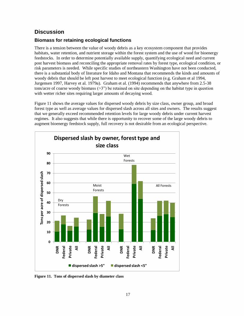
woody debris that should be left post harvest to meet ecological function (e.g. Graham et al 1994, Jurgensen 1997, Harvey et al. 1979a). Graham et al. (1994) recommends that anywhere from 2.5-38
tons/acre of coarse woody biomass (>3”) be retained on site depending on the habitat type in question
with wetter richer sites requiring larger amounts of decaying wood.
Figure 11 shows the average values for dispersed woody debris by size class, owner group, and broad
forest type as well as average values for dispersed slash across all sites and owners. The results suggest
that we generally exceed recommended retention levels for large woody debris under current harvest regimes. It also suggests that while there is opportunity to recover some of the large woody debris to
augment bioenergy feedstock supply, full recovery is not desirable from an ecological perspective.
0
10
20
30
40
50
60
70
80
90
DN
R
Fed
era
l
Pri
va
te All
DN
R
Fed
era
l
Pri
va
te All
DN
R
Fed
era
l
Pri
va
te All
DN
R
Fed
era
l
Pri
va
te All
Ton
s p
er
acre
of
dis
pe
rse
d s
lash
Dispersed slash by owner, forest type and size class
dispersed slash >5" dispersed slash <5"
Dry
Forests
Wet
Forests
Moist
ForestsAll Forests
Figure 11. Tons of dispersed slash by diameter class

18
We can conduct sensitivity tests on recovery rates and use those tests to inform the discussion about how
much biomass should be removed and remain on site after harvest. For these tests accessible biomass is defined as piled slash and the dispersed slash >5” in diameter whereas recoverable biomass is defined as
piled slash and 50% of the dispersed slash >5” in diameter. For these analyses we assume that dispersed
material <5” in diameter is left on site. As one would expect, accessible biomass and recoverable biomass
are highly correlated to total residual biomass (94% PDE and 85% PDE respectively). These correlations were used to model accessibility and potential recovery of materials as a percentage of the total residual
slash load in Figures 12-13 and as absolute green ton recovery values in Figures 14-15. Figure 12
suggests that beyond 25 t/ac of total residual biomass, accessibility is constrained to 67-70% of the total residual biomass and that below that level there is a rapidly diminishing potential for recovery. This
means that even with maximum investment in equipment, no slope constraints, and sufficient economic
incentives to conduct operations we would still not remove more than 70% of the downed biomass under this scenario. The more likely recovery scenario in Figure 13 indicates that we can expect to recover
approximately 43% of the downed material on most sites, and perhaps a greater percentage on sites with
low slash loads, whole tree yarding, and little breakage during harvest and skidding operations.
0%
10%
20%
30%
40%
50%
60%
70%
80%
90%
0 20 40 60 80 100
Total Tons of Residual Biomass
Thresholds of Biomass Accessibility
Percent Accessible
Percent retained
Figure 12. Accessible biomass as a function of total residual biomass
19
0%
10%
20%
30%
40%
50%
60%
70%
80%
0 20 40 60 80 100
Total Tons of Residual Biomass
Thresholds of Biomass Recoverability
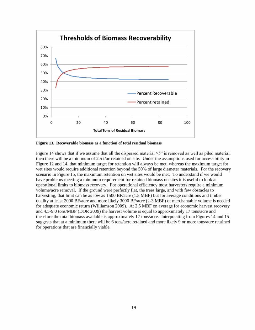
Percent Recoverable
Percent retained
Figure 13. Recoverable biomass as a function of total residual biomass
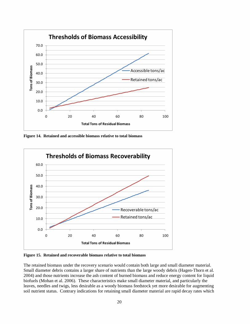
Figure 14 shows that if we assume that all the dispersed material >5” is removed as well as piled material,
then there will be a minimum of 2.5 t/ac retained on site. Under the assumptions used for accessibility in
Figure 12 and 14, that minimum target for retention will always be met, whereas the maximum target for wet sites would require additional retention beyond the 50% of large diameter materials. For the recovery
scenario in Figure 15, the maximum retention on wet sites would be met. To understand if we would
have problems meeting a minimum requirement for retained biomass on sites it is useful to look at operational limits to biomass recovery. For operational efficiency most harvesters require a minimum
volume/acre removal. If the ground were perfectly flat, the trees large, and with few obstacles to
harvesting, that limit can be as low as 1500 BF/acre (1.5 MBF) but for average conditions and timber
quality at least 2000 BF/acre and more likely 3000 BF/acre (2-3 MBF) of merchantable volume is needed for adequate economic return (Williamson 2009). At 2.5 MBF on average for economic harvest recovery
and 4.5-9.0 tons/MBF (DOR 2009) the harvest volume is equal to approximately 17 tons/acre and
therefore the total biomass available is approximately 17 tons/acre. Interpolating from Figures 14 and 15 suggests that at a minimum there will be 6 tons/acre retained and more likely 9 or more tons/acre retained
for operations that are financially viable.
20
0.0
10.0
20.0
30.0
40.0
50.0
60.0
70.0
0 20 40 60 80 100
Ton
s o
f B
iom
ass
Total Tons of Residual Biomass
Thresholds of Biomass Accessibility
Accessible tons/ac
Retained tons/ac
Figure 14. Retained and accessible biomass relative to total biomass
0.0
10.0
20.0
30.0
40.0
50.0
60.0
0 20 40 60 80 100
Ton
s o
f B
iom
ass
Total Tons of Residual Biomass
Thresholds of Biomass Recoverability
Recoverable tons/ac
Retained tons/ac
Figure 15. Retained and recoverable biomass relative to total biomass
The retained biomass under the recovery scenario would contain both large and small diameter material. Small diameter debris contains a larger share of nutrients than the large woody debris (Hagen-Thorn et al.
2004) and those nutrients increase the ash content of burned biomass and reduce energy content for liquid
biofuels (Mohan et al. 2006). These characteristics make small diameter material, and particularly the leaves, needles and twigs, less desirable as a woody biomass feedstock yet more desirable for augmenting
soil nutrient status. Contrary indications for retaining small diameter material are rapid decay rates which

21
result in accelerated soil carbon emissions and the potential for wildfire from these activity fuels. A focus
on dispersing small diameter material so as to reduce fire risk while maintaining nutrients on site is one approach to addressing these multiple management challenges.
Comparisons to Past Woody Biomass Estimates
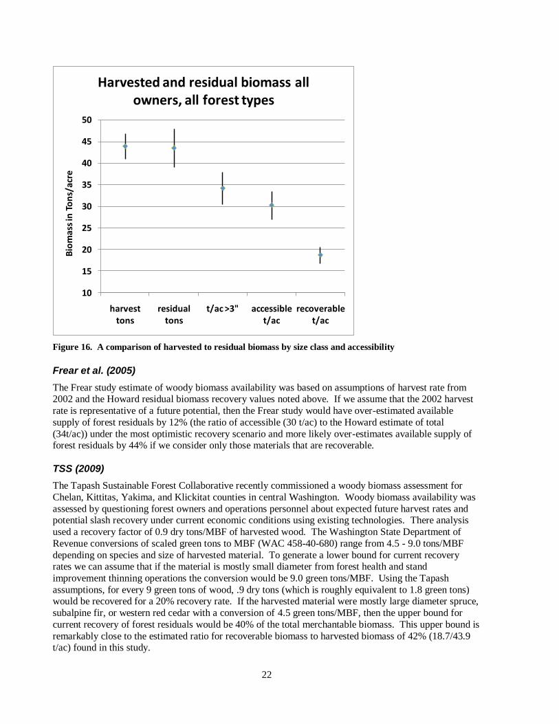
Howard (1981)
The Howard (1981) (hereafter Howard) study was used for multiple reports on woody biomass
availability in Washington State in recent years (e.g. Kersetter and Lyons 2001, Frear et al. 2005). One of our goals was to update the Howard study to represent current harvest protocols and regimes so that more
accurate estimates could be generated into the future. Howard’s estimate of potentially available biomass
was based on dispersed materials >3” in diameter with no measurement of the materials that were piled at
roadside. Our sample measured material <3” in diameter as well as piled slash. Our sampling protocol increased the per acre estimates by 4-24 additional tons/ac (average of 9.3 t/ac) over what would have
been sampled with the Howard protocols. In addition, the current estimate of materials >3” averages
144% of the Howard estimate over all types and all owners.
There is however substantial variation between owner groups with DNR sales averaging 74% of the
Howard estimate for dispersed slash > 3”, federal sales at 139% of the Howard estimate, and private sales at 243% of the Howard estimate. These large differentials are likely a result of the harvest systems that
were used on the sample sites we were able to measure. The DNR samples had only skidder harvest to
roadside which results in more residuals at the roadside and less dispersed large wood. There were 6.6-
23.9 t/ac in piled and small diameter dispersed slash on DNR samples. The federal and private samples included a mix of cable yarding, helicopter harvest, cut-to-length ground based systems, and slash
dispersal to retain nutrients on site so there was comparatively more large dispersed wood relative to the
Howard estimate. Piled and small diameter dispersed slash added another 4-13.9 t/ac beyond what would have been measured under the Howard protocols on private and federal sales.
Using the Howard protocols our estimate of dispersed biomass would have been 34 t/ac, whereas total biomass is estimated at 43.5 t/ac including piled material and dispersed biomass <3” in diameter (Figure
16). Because not all dispersed material would or should be recoverable, the accessible biomass is in the
range of 30 t/ac. How much can be economically recovered will be driven by the price of energy, the
market for residual biomass, equipment improvements, slope considerations and changes to the current operating environment. That operating environment includes average per acre harvest volumes, logging
systems, management and silvicultural regimes, cut and leave tree requirements, levels of stand mortality
and existing loads of downed wood. If we assume that at best we can recover the piled material and ½ the material >5” in diameter then the recoverable biomass is approximately 19 t/ac (Figure 16 recoverable
biomass/acre).
22
10
15
20
25
30
35
40
45
50
harvest tons
residual tons
t/ac >3" accessible t/ac
recoverable t/ac
Bio
mas
s in
To
ns/
acre
Harvested and residual biomass all owners, all forest types
Figure 16. A comparison of harvested to residual biomass by size class and accessibility
Frear et al. (2005)
The Frear study estimate of woody biomass availability was based on assumptions of harvest rate from 2002 and the Howard residual biomass recovery values noted above. If we assume that the 2002 harvest
rate is representative of a future potential, then the Frear study would have over-estimated available
supply of forest residuals by 12% (the ratio of accessible (30 t/ac) to the Howard estimate of total
(34t/ac)) under the most optimistic recovery scenario and more likely over-estimates available supply of forest residuals by 44% if we consider only those materials that are recoverable.
TSS (2009)
The Tapash Sustainable Forest Collaborative recently commissioned a woody biomass assessment for
Chelan, Kittitas, Yakima, and Klickitat counties in central Washington. Woody biomass availability was
assessed by questioning forest owners and operations personnel about expected future harvest rates and potential slash recovery under current economic conditions using existing technologies. There analysis
used a recovery factor of 0.9 dry tons/MBF of harvested wood. The Washington State Department of
Revenue conversions of scaled green tons to MBF (WAC 458-40-680) range from 4.5 - 9.0 tons/MBF
depending on species and size of harvested material. To generate a lower bound for current recovery rates we can assume that if the material is mostly small diameter from forest health and stand
improvement thinning operations the conversion would be 9.0 green tons/MBF. Using the Tapash
assumptions, for every 9 green tons of wood, .9 dry tons (which is roughly equivalent to 1.8 green tons) would be recovered for a 20% recovery rate. If the harvested material were mostly large diameter spruce,
subalpine fir, or western red cedar with a conversion of 4.5 green tons/MBF, then the upper bound for
current recovery of forest residuals would be 40% of the total merchantable biomass. This upper bound is
remarkably close to the estimated ratio for recoverable biomass to harvested biomass of 42% (18.7/43.9 t/ac) found in this study.

23
The extrapolation of biomass estimates from one region to another has high uncertainty associated with it because of differences in milling infrastructure, forest type, landowner objectives, and forest structure and
how the interplay of these factors influences utilization and harvest options. Given the differences in
analytical techniques and sites it is encouraging that the estimates of recoverable biomass are so close
across neighboring regions. Based on these similarities, we re-analyzed the biomass availability reported in the 2007 Future of Washington’s Forests report using the relationships derived in this study. The
analysis reports on estimates of total and recoverable biomass to arrive at an estimate of sub-regional
biomass availability for the entire eastern Washington region.
The Future of Washington’s Forests (2007)
The Future of Washington’s Forests report in 2007 provided an estimate of available biomass supply based on FIA inventory and simulations of harvest volume consistent with historic harvest rates for
eastern Washington (Oneil and Mason 2007). That report estimated that 1.45 million dry tons of biomass
were available in eastern Washington with 1.28 million of those dry tons from the tree tops from current
harvest with the remainder from waste and breakage of material that is of merchantable size. Those estimates are based on maintaining an aggressive harvest rate coupled with forest land management
intensities sufficient to ensure that timber supply remains available. The estimate relies on known
merchantability factors coupled with growth model estimates of biomass allocation between tree components.
The simulation data was reconciled to incorporate the ratios of harvest volume removed and remaining on site from this study. This resulted in lowering the estimates of merchantable material by 33% and
increasing the estimate of residual crown biomass by 48% to account for the additional losses to waste
and breakage over and above merchantability net down factors used in the original assessment. Applying
volume and biomass correction factors based on this study produces the overall estimates of total residual biomass, accessible biomass and recoverable biomass in Table 7.
Table 7. Sub-regional estimates of potentially recoverable residual biomass on a per acre basis
Region Okanogan Southeast Tonasket Wenatchee Yakima Northeast All Regions
Merchantability
& volume
assumptions
Merchantable
BF
harvest/acre
5249 3265 8459 9422 7055 6806 6956
average
eastside
merchantability
Total
residuals
(GT/acre)
34 21 55 61 46 44 45
Accessible
residuals
(GT/acre)
24 15 38 43 32 31 31
Recoverable
residuals (GT/acre)
15 9 24 26 20 19 19
small diameter
harvests
Total
residuals
(GT/acre)
47 29 76 85 63 61 63
Accessible
residuals
(GT/acre)
33 20 53 59 44 43 44
Recoverable
residuals
(GT/acre)
20 13 33 36 27 26 27

24
Total residual values in Table 7 were calculated as equal to the total biomass of the merchantable volume in keeping with the ratios reported in Figure 16. Accessible biomass excludes the dispersed small
diameter slash that is difficult to retrieve and provides valuable inputs for soil fertility. It is
approximately 70% (69.6%) of the total residual biomass based on our samples. Of the accessible
biomass not all large diameter material is retrievable and a portion should be left for habitat values. The recoverable biomass estimate derived from our sample assumes only ½ the large diameter (>5”) dispersed
slash and all the piles are obtainable as woody feedstock inputs. The average recoverable biomass is 43%
of the total residuals. There are several assumptions about harvest volume/acre and merchantability that influence the estimated volume/acre in Table 7. Harvested wood of average merchantability is
approximately 6.5 tons/MBF whereas small diameter wood is similar to pulp logs at 9 tons/MBF. These
differentials in tons of material per unit volume account for the differences in recoverable residuals in Table 7. The newly estimated average harvest volume/acre for the northeast region is approximately 2/3
of the simulated per acre volume from the 2007 timber supply study. This ratio was used to reduce
estimated harvest volume/acre for the remaining sub-regions.
The 2007 timber supply estimate for eastern Washington private and tribal forests was 744,633 MBF/year
over the 1st 3 decades. With average merchantability this volume would be equivalent to 4,840,000 green
tons of merchantable wood, (6.5 tons/MBF x 744,633 MBF) and the equivalent amount of total residual biomass. By applying the ratios from Figure 16 and Table 7, we can estimate that there would be 2.1
million green tons of recoverable biomass or 1.0 million dry tons of woody biomass feedstocks at those
harvest rates allocated across the sub-regions according to anticipated harvest levels (Table 8). Woody biomass obtainable from state trust lands is in the range of 227,000 green tons/year at historic harvest
rates (Table 9). If harvest volumes from USFS lands remain consistent with the 1994-2003 harvest rate
then an additional 200,000 green tons of material would be available off these lands under similar
merchantability assumptions (Table 10). If USFS wood were all small diameter, then the total available woody biomass feedstock from this source would be closer to 276,000 green tons/year. In addition an
aggressive thinning program to reduce fire risks could increase the supply by 400% or more.
Table 8. Sub-regional estimates of potentially recoverable residual biomass for private and tribal lands
Average harvest and forest residual volume: 2001-2030
Region Total
MBF/year Total green tons of
residuals Accessible green tons of residuals
Recoverable green tons of
residuals
Recoverable dry tons of residuals
Okanogan 56,733 368,767 256,662 158,570 79,285
Wenatchee 121,600 790,400 550,118 339,872 169,936
Yakima 228,733 1,486,767 1,034,790 639,310 319,655
Timbershed 6 407,067 2,645,933 1,841,570 1,137,751 568,876
Northeast 246,500 1,602,250 1,115,166 688,968 344,484
Tonasket 73,867 480,133 334,173 206,457 103,229
Southeast 17,200 111,800 77,813 48,074 24,037
Timbershed 7 337,567 2,194,183 1,527,152 943,499 471,749

25
Table 9. Sub-regional estimates of potentially recoverable residual biomass for state trust lands
State Trust Lands Base Case
FVS variant Total
MBF/year
Total green tons
of residuals
Accessible green
tons of residuals
Recoverable green
tons of residuals
Recoverable dry
tons of residuals
Blue Mountains 1,363 8,857 6,164 3,808 1,904
East Cascades 53,217 345,914 240,756 148,743 74,371
North Idaho/Inland
Empire 26,927 175,025 121,818 75,261 37,630
Total 81,342 528,720 367,989 227,349 113,675
Table 10. Sub-regional estimates of potentially recoverable residual biomass for federal lands
FVS variant
Total MBF/year
base case
Total green tons
of residuals
Accessible green
tons of residuals
Recoverable
green tons of
residuals
Recoverable dry
tons of residuals
Blue Mountains 7,170 46,605 32,437 20,040 10,020
East Cascades 43,254 281,151 195,681 120,895 60,447
North Idaho/Inland
Empire 27,511 178,822 124,460 76,893 38,447
Total 71,326 463,619 322,679 199,356 99,678
Total MBF/year
firewise
alternative
Total green tons
of residuals
Accessible green
tons of residuals
Recoverable
green tons of
residuals
Recoverable dry
tons of residuals
Blue Mountains 28,680 186,420 129,748 80,161 40,080
East Cascades 173,016 1,124,604 782,724 483,580 241,790
North Idaho/Inland Empire
110,044 715,286 497,839 307,573 153,786
Total 285,304 1,854,476 1,290,715 797,425 398,712
The revised estimates of recoverable biomass are 1.25 million dry tons/year for all eastern Washington
sub-regions and owner groups as compared to the initial estimates of 1.45 million dry tons in the Future
of Washington’s Forests study. These recoverable biomass estimates are based on historic harvest rates:
changes to those harvest rates such as what we have experienced in the past 2 years would alter them substantially.
The analysis identifies the core parameter for determining total residual biomass and recoverable biomass as the harvest rate. The natural variation across stands is large making other attributes insignificant. Since
the pre-harvest inventory data was not a reliable predictor of harvest rate or recoverable biomass,
improvements in growth modeling and more current inventory data may be necessary to improve on predictions for residual biomass. Other operational constraints and the potential for improvements as well
as end use technologies will also play a role in determining recoverable supply.
The recoverable biomass is 20% of the total harvested biomass which is equivalent to 40% of the volume currently harvested for wood processing. Since mill surveys show only about 12% of harvest volume
being used as biofuel for processing energy (Milota et al. 2005), the recoverable forest residual biomass
provides roughly a 400% increase in biofuel feedstock sufficient to make existing mills more than energy
26
self sufficient if the material were economically retrievable. It could also support stand alone
bioprocessing facilities but the scale of these facilities will have to be carefully considered.
An efficient scale biorefinery of 50 million gallons per year requires 625,000 dry tons of biomass as a
base volume, and substantially more for investors to have confidence that adequate feedstocks will be
available (Mason et al 2009). The Northeast sub-region could provide 425,000 dry tons from residuals and the Yakima/Wenatchee region could provide 588,000 dry tons of forest residuals at historic harvest
levels. If a Fire-Wise approach to forest management that actively sought to reduce fuels on high risk
national forest lands were instituted in the East Cascades approximately 805,000 dry tons per year would be available in that region. These numbers illustrate that without increased investment in fuel removals
on national forest lands, there is no opportunity to develop a new scale efficient liquid fuel biorefinery
capacity in eastern Washington. While alternative strategies that use woody biomass for electricity are possible, they do not address the most critical carbon emission source in Washington which is from
transportation emissions (Mason et al. 2009). Fragmentation of the resource such as for electrical co-
generation facilities to meet renewable energy standards will further compromise the opportunity for even
below scale efficient biofuel production facilities on the eastside. Much of the region will be limited to less than efficient scale operations which will require incentives for start-up and production unless carbon
and biomass stock prices increase substantially. Consistent with the Mason et al. (2009) report, the
location of available supply highlights the importance of haul distance, the need for other mixed wastes and more efficient operating technologies in order to attract adequate supply from other sources and
outside the region for a margin of safety.
Operational Constraints
A good case study example of operational constraints was demonstrated for one sample site that appears
to be an outlier with respect to the amount of volume remaining on site post harvest. This site had two significant limitations to merchantable recovery: first, it was cable harvested during an average to low
pulp year and second, it had experienced a severe insect infestation resulting in significant mortality in the
grand-fir during the decade prior to harvest. There was a substantial amount of large wood left on site because of defect caused by rapid decay after mortality. Given that the pulp markets were low, and the
cost of recovery using cable systems is high, that particular stand had inordinately high residual volumes
relative to the harvest volume (3.25:1 ratio rather than the average of 1:1 ratio.) This site, while an outlier
in the current sample, reflects the broader impact of mortality events on the potential for biomass recovery for both existing product markets and the biomass to bioenergy market. The current bark beetle
outbreaks and ongoing spruce budworm infestations infect huge swaths of timber annually in Washington
State. During these outbreaks, trees are killed or weakened sufficiently that they succumb to other mortality agents. This results in forests with high proportions of dead trees which may not be sound
enough for solid wood products but would be ideal for bioenergy purposes if they could be economically
removed. At this time the major limits to recovery include finding efficient ways to handle slash and
small diameter material, ways to densify the material once it has been brought to the landing, and ways to haul it at the most cost effective payload possible. Each of these challenges carries with it an opportunity
for technological improvements.
Slash Handling and Densification
Discussions with logging and facility personnel identified several operational constraints that will have to
be overcome if we are to be successful at obtaining forest residuals as bioenergy feedstocks. Key among them is a way to efficiently collect and densify the slash so that it can be transported efficiently. A
biomass recovery demonstration project on the DNR Chattawood sale is a good case study to highlight
these particular issues. The Chattawood Timber Sale provided a unique opportunity to test systems and
identify key operational parameters for economic recovery of slash for use as a bio-energy feedstock. Chattawood is located approximately 10 miles north of Deer Park, Washington on State Route 395. The
27
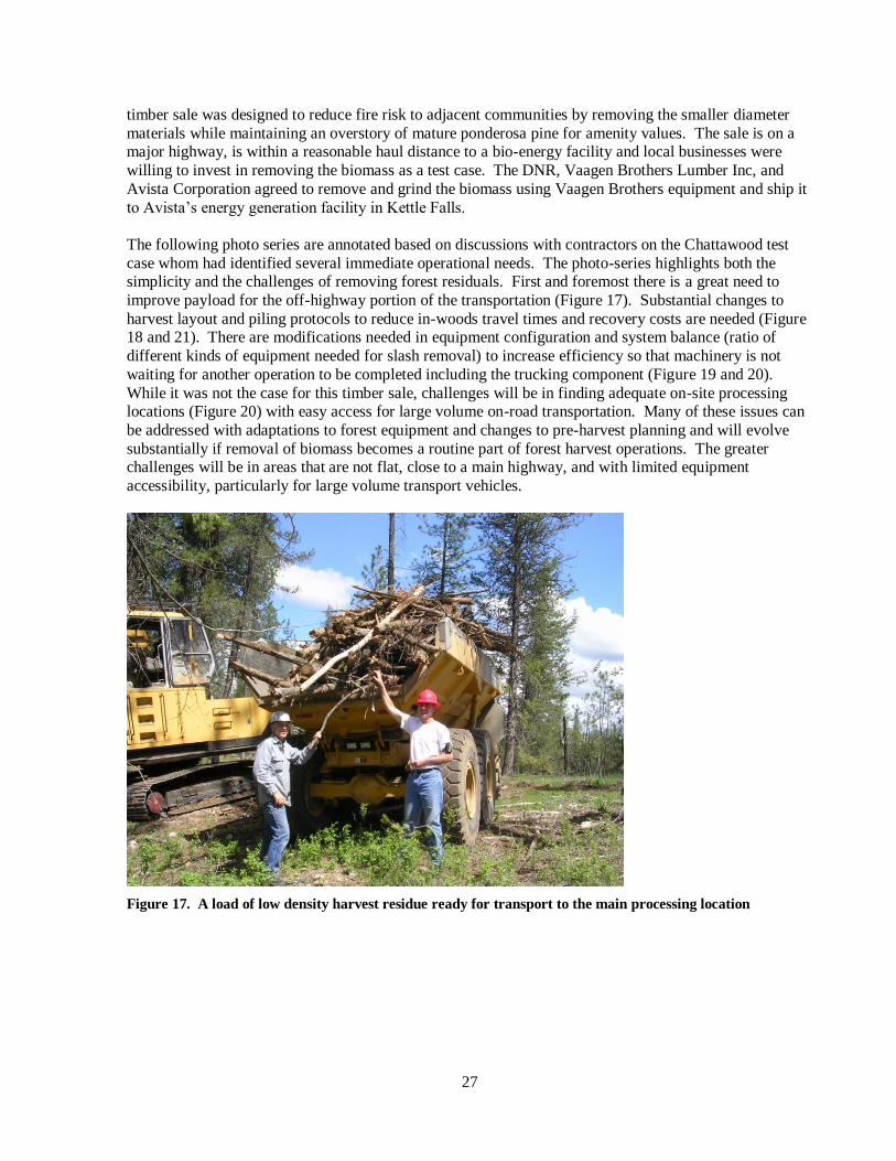
timber sale was designed to reduce fire risk to adjacent communities by removing the smaller diameter
materials while maintaining an overstory of mature ponderosa pine for amenity values. The sale is on a major highway, is within a reasonable haul distance to a bio-energy facility and local businesses were
willing to invest in removing the biomass as a test case. The DNR, Vaagen Brothers Lumber Inc, and
Avista Corporation agreed to remove and grind the biomass using Vaagen Brothers equipment and ship it
to Avista’s energy generation facility in Kettle Falls.
The following photo series are annotated based on discussions with contractors on the Chattawood test
case whom had identified several immediate operational needs. The photo-series highlights both the simplicity and the challenges of removing forest residuals. First and foremost there is a great need to
improve payload for the off-highway portion of the transportation (Figure 17). Substantial changes to
harvest layout and piling protocols to reduce in-woods travel times and recovery costs are needed (Figure 18 and 21). There are modifications needed in equipment configuration and system balance (ratio of
different kinds of equipment needed for slash removal) to increase efficiency so that machinery is not
waiting for another operation to be completed including the trucking component (Figure 19 and 20).
While it was not the case for this timber sale, challenges will be in finding adequate on-site processing locations (Figure 20) with easy access for large volume on-road transportation. Many of these issues can
be addressed with adaptations to forest equipment and changes to pre-harvest planning and will evolve
substantially if removal of biomass becomes a routine part of forest harvest operations. The greater challenges will be in areas that are not flat, close to a main highway, and with limited equipment
accessibility, particularly for large volume transport vehicles.
Figure 17. A load of low density harvest residue ready for transport to the main processing location

28
Figure 18. Long in-woods haul distances substantially increase the cost of removal
Figure 19. Processing equipment waiting for the trucks to return
Figure 20. Slash ground and waiting for transportation to the biomass facility
29
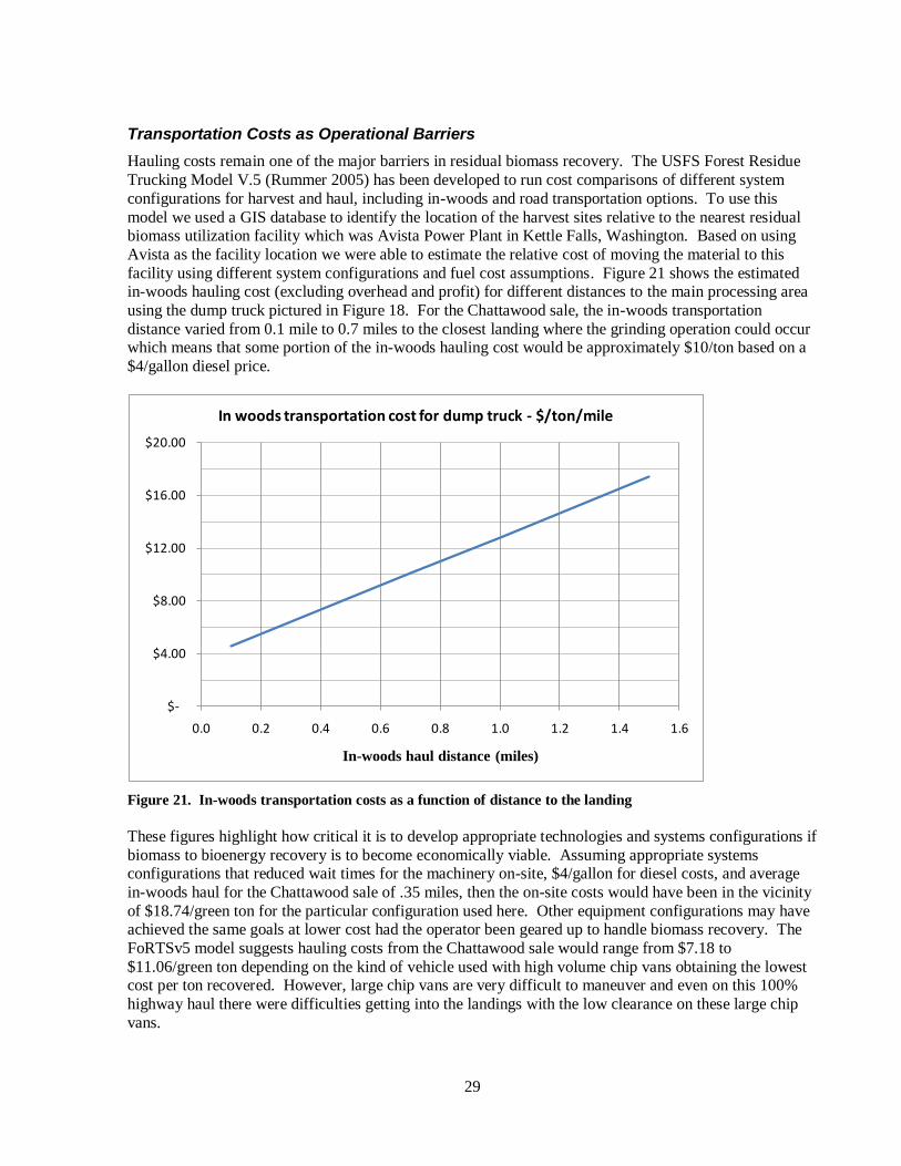
Transportation Costs as Operational Barriers
Hauling costs remain one of the major barriers in residual biomass recovery. The USFS Forest Residue
Trucking Model V.5 (Rummer 2005) has been developed to run cost comparisons of different system
configurations for harvest and haul, including in-woods and road transportation options. To use this
model we used a GIS database to identify the location of the harvest sites relative to the nearest residual biomass utilization facility which was Avista Power Plant in Kettle Falls, Washington. Based on using
Avista as the facility location we were able to estimate the relative cost of moving the material to this
facility using different system configurations and fuel cost assumptions. Figure 21 shows the estimated in-woods hauling cost (excluding overhead and profit) for different distances to the main processing area
using the dump truck pictured in Figure 18. For the Chattawood sale, the in-woods transportation
distance varied from 0.1 mile to 0.7 miles to the closest landing where the grinding operation could occur which means that some portion of the in-woods hauling cost would be approximately $10/ton based on a
$4/gallon diesel price.
$-
$4.00
$8.00
$12.00
$16.00
$20.00
0.0 0.2 0.4 0.6 0.8 1.0 1.2 1.4 1.6
In-woods haul distance (miles)
In woods transportation cost for dump truck - $/ton/mile
Figure 21. In-woods transportation costs as a function of distance to the landing
These figures highlight how critical it is to develop appropriate technologies and systems configurations if
biomass to bioenergy recovery is to become economically viable. Assuming appropriate systems configurations that reduced wait times for the machinery on-site, $4/gallon for diesel costs, and average
in-woods haul for the Chattawood sale of .35 miles, then the on-site costs would have been in the vicinity
of $18.74/green ton for the particular configuration used here. Other equipment configurations may have achieved the same goals at lower cost had the operator been geared up to handle biomass recovery. The
FoRTSv5 model suggests hauling costs from the Chattawood sale would range from $7.18 to
$11.06/green ton depending on the kind of vehicle used with high volume chip vans obtaining the lowest cost per ton recovered. However, large chip vans are very difficult to maneuver and even on this 100%
highway haul there were difficulties getting into the landings with the low clearance on these large chip
vans.
30
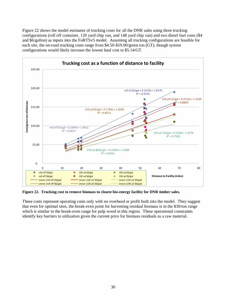
Figure 22 shows the model estimates of trucking costs for all the DNR sales using three trucking
configurations (roll off container, 120 yard chip van, and 148 yard chip van) and two diesel fuel costs ($4 and $6/gallon) as inputs into the FoRTSv5 model. Assuming all trucking configurations are feasible for
each site, the on-road trucking costs range from $4.50-$19.00/green ton (GT), though system
configurations would likely increase the lowest haul cost to $5.14/GT.
roll off $4/gal = 0.2099x + 1.9812R² = 0.9657
120 yd $4/gal = 0.1764x + 1.2038R² = 0.8531
150 yd $4/gal = 0.1324x + 1.5979R² = 0.7919
roll of $6/gal = 0.2559x + 1.9576R² = 0.9765
120 yd $ 6/gal = 0.2152x + 1.1329R² = 0.8809
150 yd @$6/gal = 0.1636x + 1.5009R² = 0.8261
$-
$5.00
$10.00
$15.00
$20.00
$25.00
0 10 20 30 40 50 60 70 80
Co
st/g
ree
n t
on
of b
iom
ass
Distance to Facility (miles)
Trucking cost as a function of distance to facility
roll off $4/gal 120 yd $4/gal 150 yd $4/gal
roll off $6/gal 120 yd $6/gal 150 yd $6/gal
Linear (roll off $4/gal) Linear (120 yd $4/gal) Linear (150 yd $4/gal)
Linear (roll off $6/gal) Linear (120 yd $6/gal) Linear (150 yd $6/gal)
Figure 22. Trucking cost to remove biomass to closest bio-energy facility for DNR timber sales.
These costs represent operating costs only with no overhead or profit built into the model. They suggest
that even for optimal sites, the break-even point for harvesting residual biomass is in the $30/ton range
which is similar to the break-even range for pulp wood in this region. These operational constraints identify key barriers to utilization given the current price for biomass residuals as a raw material.
31
Conclusions
Field measurements to update the prior logging residue studies are the most significant element of this
study as they inform both coarse resolution biomass estimates and provide specific information needed to model biomass availability at the sub-regional scale. Post-harvest forest residual estimators developed by
this project will provide entrepreneurs, policy-makers, and scientists with the ability to more accurately
predict volumes of forest biomass available following silvicultural activities. Estimates of available
biomass can be linked with modeled projections of current and future forest harvest activities to quantify forest biomass feedstock availability now and into the future providing short-, mid-, and long-term
estimates. Estimators of forest residuals can be formatted into modeling modules for use with publicly-
available forest growth models such as the Forest Vegetation Simulator (USDA Forest Service). Estimates of slash availability can be periodically updated to real time when used in conjunction with
annual DNR state harvest reports. And finally, these results demonstrate the use of publicly available
tools (FoRTSv5) for optimizing equipment configurations for economic recovery of residual biomass.
For the sample NE Washington region, on average 20% of the total harvested biomass is recoverable as a
feedstock for biofuel production which is equivalent to 40% of the volume currently harvested for wood
processing. Since mill surveys show only about 12% of harvest volume being used as biofuel for processing energy, the recoverable forest residual biomass provides roughly a 400% increase in biofuel
feedstock sufficient to make existing mills more than energy self sufficient or support stand alone
bioprocessing facilities. The limited supply of recoverable biomass residuals in each sub region will inhibit investments in new efficient scale liquid fuel bioprocessing facilities requiring increased attention
to smaller scale processing, operating equipment improvements and effective incentives for effective
utilization.

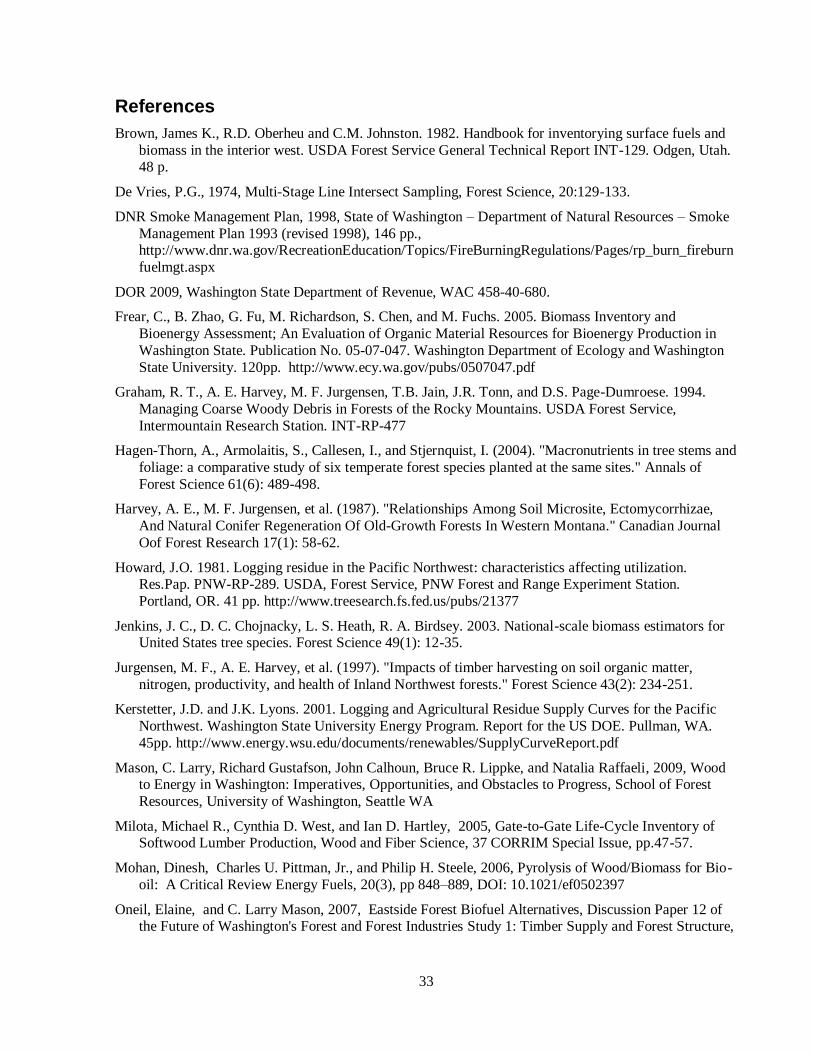
33
References
Brown, James K., R.D. Oberheu and C.M. Johnston. 1982. Handbook for inventorying surface fuels and
biomass in the interior west. USDA Forest Service General Technical Report INT-129. Odgen, Utah. 48 p.
De Vries, P.G., 1974, Multi-Stage Line Intersect Sampling, Forest Science, 20:129-133.
DNR Smoke Management Plan, 1998, State of Washington – Department of Natural Resources – Smoke
Management Plan 1993 (revised 1998), 146 pp., http://www.dnr.wa.gov/RecreationEducation/Topics/FireBurningRegulations/Pages/rp_burn_fireburn
fuelmgt.aspx
DOR 2009, Washington State Department of Revenue, WAC 458-40-680.
Frear, C., B. Zhao, G. Fu, M. Richardson, S. Chen, and M. Fuchs. 2005. Biomass Inventory and
Bioenergy Assessment; An Evaluation of Organic Material Resources for Bioenergy Production in
Washington State. Publication No. 05-07-047. Washington Department of Ecology and Washington
State University. 120pp. http://www.ecy.wa.gov/pubs/0507047.pdf
Graham, R. T., A. E. Harvey, M. F. Jurgensen, T.B. Jain, J.R. Tonn, and D.S. Page-Dumroese. 1994.
Managing Coarse Woody Debris in Forests of the Rocky Mountains. USDA Forest Service,
Intermountain Research Station. INT-RP-477
Hagen-Thorn, A., Armolaitis, S., Callesen, I., and Stjernquist, I. (2004). "Macronutrients in tree stems and
foliage: a comparative study of six temperate forest species planted at the same sites." Annals of
Forest Science 61(6): 489-498.
Harvey, A. E., M. F. Jurgensen, et al. (1987). "Relationships Among Soil Microsite, Ectomycorrhizae,
And Natural Conifer Regeneration Of Old-Growth Forests In Western Montana." Canadian Journal
Oof Forest Research 17(1): 58-62.
Howard, J.O. 1981. Logging residue in the Pacific Northwest: characteristics affecting utilization. Res.Pap. PNW-RP-289. USDA, Forest Service, PNW Forest and Range Experiment Station.
Portland, OR. 41 pp. http://www.treesearch.fs.fed.us/pubs/21377
Jenkins, J. C., D. C. Chojnacky, L. S. Heath, R. A. Birdsey. 2003. National-scale biomass estimators for United States tree species. Forest Science 49(1): 12-35.
Jurgensen, M. F., A. E. Harvey, et al. (1997). "Impacts of timber harvesting on soil organic matter,
nitrogen, productivity, and health of Inland Northwest forests." Forest Science 43(2): 234-251.
Kerstetter, J.D. and J.K. Lyons. 2001. Logging and Agricultural Residue Supply Curves for the Pacific
Northwest. Washington State University Energy Program. Report for the US DOE. Pullman, WA.
45pp. http://www.energy.wsu.edu/documents/renewables/SupplyCurveReport.pdf
Mason, C. Larry, Richard Gustafson, John Calhoun, Bruce R. Lippke, and Natalia Raffaeli, 2009, Wood to Energy in Washington: Imperatives, Opportunities, and Obstacles to Progress, School of Forest
Resources, University of Washington, Seattle WA
Milota, Michael R., Cynthia D. West, and Ian D. Hartley, 2005, Gate-to-Gate Life-Cycle Inventory of Softwood Lumber Production, Wood and Fiber Science, 37 CORRIM Special Issue, pp.47-57.
Mohan, Dinesh, Charles U. Pittman, Jr., and Philip H. Steele, 2006, Pyrolysis of Wood/Biomass for Bio-
oil: A Critical Review Energy Fuels, 20(3), pp 848–889, DOI: 10.1021/ef0502397
Oneil, Elaine, and C. Larry Mason, 2007, Eastside Forest Biofuel Alternatives, Discussion Paper 12 of the Future of Washington's Forest and Forest Industries Study 1: Timber Supply and Forest Structure,

34
School of Forest Resources, University of Washington,
http://www.ruraltech.org/projects/fwaf/final_report/pdfs/18_Discussion_Paper_12.pdf
ORNL, 1999, Oak Ridge National Laboratory, Biomass Feedstock Availability in the US – 1999 State
Level Analysis, lead scientist Marie Walsh, http://bioenergy.ornl.gov/resourcedata/
Pickford, Stewart G. and J.W. Hazard. 1978. Simulation studies on line intersect sampling of forest
residue. Forest Science 24(4):469-483.
Rummer, Robert, 2005, USFS Forest Residue Trucking Model spreadsheet calculator,
www.srs.fs.usda.gov/forestops/downloads/FoRTSv5.xls, downloaded April 2008.
Rummer, B., et al. 2005. A Strategic Assessment of Forest Biomass and Fuel Reduction Treatments in Western States. Gen. Tech. Rep. RMS-GTR-149. USDA Forest Service, Rocky Mountain Research
Station. 17pp. http://www.fs.fed.us/rm/pubs/rmrs_gtr149.pdf
TSS 2009: TSS Consultants, 2009, Wood Supply Assessment for Commercial-Scale Biomass Power Cogeneration and Biomass Utilization Projects in Central Washington, report prepared for The
Tapash Sustainable Forest Collaborative and South Central Washington Resource Conservation and
Development Council, 93 pp., http://scwrcd.org/docs/biomass_assessment_report_20090422.pdf ,
accessed Aug 31, 2009.
Van Wagner, C.E., 1982, Practical Aspects of the Line Intersect Method, Petawawa National Forestry
Institute, Canadian Forestry Service, Chalk River, Ontario, Canada, Information Report PI-X-12, 18
pp.
Williamson, Maurice, 2009, (personnel communication), Eastern Washington Forestry Consultant
Wykoff, William R., Nicholas L. Crookston and Albert Stage, 1982, User’s Guide to the Stand Prognosis
Model, USDA Forest Service, Intermountain Forest and Range Experiment Station, Ogden UT, Gen Tech Report, INT-GTR-133, 113 pp.

35
Appendix
Data Summaries by forest type and owner group.
5
10
15
20
25
30
35
40
45
50
harvest tons
residual tons
t/ac >3" accessible t/ac
recoverable t/ac
Bio
mas
s in
To
ns/
acre
Harvested and residual biomass all owners, dry forest types
Figure A.1. Comparison of residual biomass to harvested biomass for dry forest types
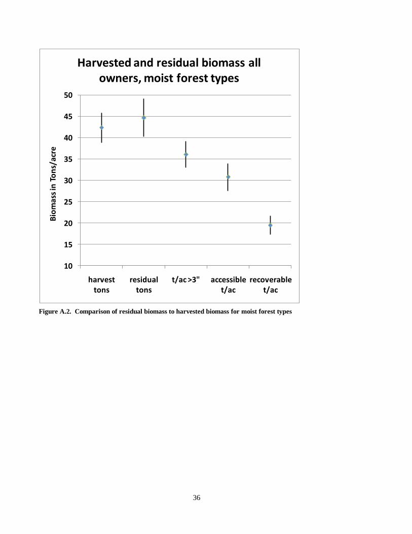
36
10
15
20
25
30
35
40
45
50
harvest tons
residual tons
t/ac >3" accessible t/ac
recoverable t/ac
Bio
ma
ss in
To
ns/
acr
e
Harvested and residual biomass all owners, moist forest types
Figure A.2. Comparison of residual biomass to harvested biomass for moist forest types
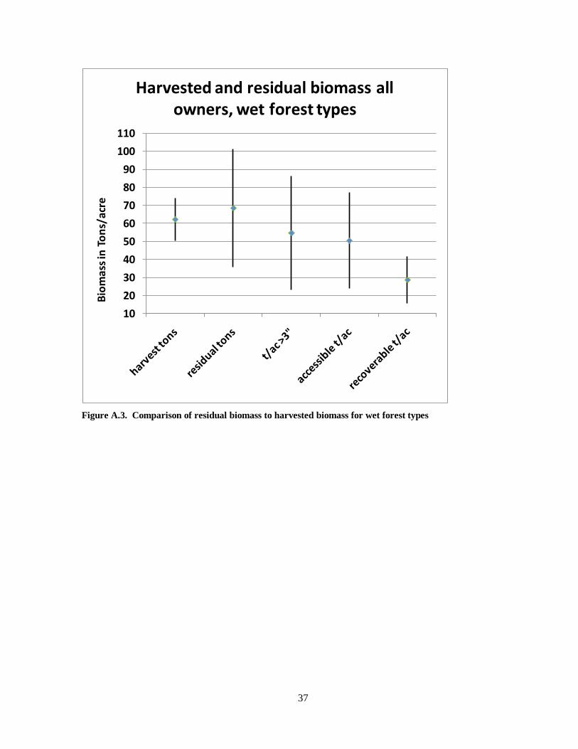
37
10
20
30
40
50
60
70
80
90
100
110
Bio
ma
ss in
To
ns/
acr
eHarvested and residual biomass all
owners, wet forest types
Figure A.3. Comparison of residual biomass to harvested biomass for wet forest types

38
0
20
40
60
80
100
120
DF mixed Conifer
GF PP PP/DF WRC All forest types
Bio
mas
s in
t/a
cre
Allocation of Harvested Biomass Federal, All forest types
removals/acre piled/acre >5" slash <5" slash
Figure A.4. Allocation of Harvested Biomass on Federal Lands by forest type
0
20
40
60
80
100
120
140
160
DF mixed Conifer
GF PP PP/DF WRC All forest types
Bio
mas
s in
t/a
cre
Allocation of Harvested Biomass Private, All forest types
removals/acre piled/acre >5" slash <5" slash
Figure A.5. Allocation of harvested biomass on private lands by forest type
39
0
20
40
60
80
100
120
140
160
DF mixed Conifer
GF PP PP/DF WRC All forest types
Bio
mas
s in
t/a
cre
Allocation of Harvested Biomass DNR, All forest types
removals/acre piled/acre >5" slash <5" slash
Figure A.6. Allocation of biomass on DNR lands by forest type

40
Table A1. Average biomass with upper and lower bound by owner group, forest type, and biomass category.
Forest
Group biomass bin
Lower Bound Average Upper Bound
DNR Federal Private All
Owners DNR Federal Private
All
Owners DNR Federal Private
All
Owners
All
harvest tons/ac 50.6 40.9 26.5 40.9 60.7 44.1 33.9 43.9 70.8 47.3 41.3 46.8
residual tons/ac 27.5 40.3 27.9 39.1 34.1 44.8 43.7 43.5 40.8 49.2 59.4 47.8
t/ac >3" 15.2 32.5 22.5 30.4 18.9 35.7 37.3 34.1 22.7 38.9 52.0 37.8
accessible t/ac 16.9 28.3 17.2 26.9 22.1 31.5 30.0 30.2 27.3 34.6 42.8 33.5
recoverable t/ac 11.9 17.7 9.5 16.7 16.1 19.8 15.8 18.7 20.3 22.0 22.2 20.6
dry
harvest tons/ac 16.8 41.4 11.0 35.5 27.1 47.7 21.4 41.0 37.4 54.0 31.8 46.5
residual tons/ac 23.1 26.2 5.8 24.9 23.9 30.1 23.7 28.3 24.8 34.1 41.7 31.8
t/ac >3" 16.5 16.6 0.0 16.0 17.4 21.0 14.0 19.5 18.2 25.3 28.0 22.9
accessible t/ac 11.7 17.9 5.8 16.8 12.9 20.9 18.9 19.5 14.1 24.0 32.1 22.2
recoverable t/ac 6.8 10.5 5.8 10.2 7.7 12.1 13.2 11.6 8.5 13.6 20.6 13.0
moist
harvest tons/ac 62.4 39.4 17.7 38.9 65.7 43.2 28.4 42.4 69.0 46.9 39.2 45.9
residual tons/ac 25.3 43.2 24.2 40.3 32.5 48.6 29.0 44.7 39.6 54.0 33.7 49.2
t/ac >3" 13.5 36.6 20.8 33.0 17.3 40.3 24.9 36.1 21.0 44.0 29.1 39.2
accessible t/ac 16.8 30.4 13.7 27.6 22.2 34.2 15.9 30.8 27.7 38.1 18.2 34.0
recoverable t/ac 11.5 19.3 7.0 17.3 15.9 21.8 8.2 19.5 20.4 24.4 9.4 21.7
wet
harvest tons/ac 74.5 37.1 50.5 86.9 49.8 62.2 99.3 62.6 73.9
residual tons/ac 24.3 29.6 35.8 46.8 79.4 68.5 69.3 129.2 101.3
t/ac >3" 7.8 23.7 23.1 22.9 70.5 54.6 38.1 117.2 86.1
accessible t/ac 13.7 19.6 23.8 31.2 60.1 50.5 48.6 100.6 77.2
recoverable t/ac 11.8 10.4 15.3 24.6 30.5 28.5 37.5 50.6 41.8