easy java simulations the manual
TRANSCRIPT

Easy Java Simulations
The Manual
Version 3.4 - September 2005
Francisco Esquembre


Contents
1 A first contact 1
1.1 About Easy Java Simulations . . . . . . . . . . . . . . . . . . . . . . 1
1.2 Installing and running Ejs . . . . . . . . . . . . . . . . . . . . . . . . 2
1.3 Working with a simulation . . . . . . . . . . . . . . . . . . . . . . . . 10
1.4 Inspecting the simulation . . . . . . . . . . . . . . . . . . . . . . . . 15
1.5 Modifying the simulation . . . . . . . . . . . . . . . . . . . . . . . . 23
1.6 A global vision . . . . . . . . . . . . . . . . . . . . . . . . . . . . . . 35
2 Creating models 39
2.1 Definition of a model . . . . . . . . . . . . . . . . . . . . . . . . . . . 39
2.2 Interface for the model in Easy Java Simulations . . . . . . . . . . . 43
2.3 Declaration of variables . . . . . . . . . . . . . . . . . . . . . . . . . 45
2.4 Initializing the model . . . . . . . . . . . . . . . . . . . . . . . . . . . 51
2.5 Evolution equations . . . . . . . . . . . . . . . . . . . . . . . . . . . 53
2.6 Constraint equations . . . . . . . . . . . . . . . . . . . . . . . . . . . 65
2.7 Custom methods and additional libraries . . . . . . . . . . . . . . . . 65
iii

iv chapter
3 Building a view 77
3.1 Graphical interfaces . . . . . . . . . . . . . . . . . . . . . . . . . . . 78
3.2 Association between variables and properties . . . . . . . . . . . . . 81
3.3 How a simulation runs . . . . . . . . . . . . . . . . . . . . . . . . . . 82
3.4 Interface of Easy Java Simulations for the view . . . . . . . . . . . . 83
3.5 Editing properties . . . . . . . . . . . . . . . . . . . . . . . . . . . . 89
3.6 Learning more about view elements . . . . . . . . . . . . . . . . . . . 94
4 Using the simulation 103
4.1 Using your simulations . . . . . . . . . . . . . . . . . . . . . . . . . . 103
4.2 Files generated for a simulation . . . . . . . . . . . . . . . . . . . . . 105
4.3 Ejs configuration options . . . . . . . . . . . . . . . . . . . . . . . . 107
4.4 Running the simulation as an applet . . . . . . . . . . . . . . . . . . 109
4.5 Running the simulation as an application . . . . . . . . . . . . . . . 115
4.6 Distribution of simulations . . . . . . . . . . . . . . . . . . . . . . . . 117

CHAPTER 1
A first contact
c©2005 by Francisco Esquembre, September 2005
We describe in this chapter how to create an interactive simulation in Java usingEasy Java Simulations (Ejs for short). In order to get a general perspective of thecomplete process, we will inspect, run and finally modify, slightly but meaningfully,an already existing simulation. This will help us identify the parts that make asimulation, as well as become acquainted with our authoring tool. 1
1.1 About Easy Java Simulations
Every technical work requires the right tool. Easy Java Simulations is an authoringtool that has been specifically designed for the creation of interactive simulationsin Java. Though it is important not to confuse the final product with the toolused to create it, and, in principle, the simulations we will create with Ejs can alsobe built with the help of any modern computer programming language, this tooloriginates from the specific expertise accumulated along several years of experiencein the creation of computer simulations, and will therefore be very useful to simplifyour task, both from the technical and from the conceptual point of view.
From the technical point of view because Ejs greatly simplifies the creation of theview of a simulation, that is, the graphical part of it, a process that usually requires
1Readers of the OSP Guide (see http://www.opensourcephysics.org) may skip this chapter. Theinformation contained in it has been already covered in the chapter about Ejs of the guide.
1

2 CHAPTER 1. A FIRST CONTACT
an advanced level of technical know-how on programming computer graphics. Fromthe conceptual point of view, because Ejs provides a simplified structure for thecreation of the model of the simulation, that is, the scientific description of thephenomenon under study.
Obviously, part of the task still depends on us. Ours is the responsibility for thedesign of the view and for providing the variables and algorithms that describe themodel of the simulation. We will soon learn how to use Ejs to build a view. For themodel, we will learn to declare the variables that describe its state and to write theJava code needed to specify the algorithms of the model. Stated in different words,we will learn to program the computer to solve our model.
If you have never programmed a computer, let me tell you that it is a fascinatingexperience. And, actually, it is not difficult in itself. All that is needed is to followa set of basic rules determined by the syntax of the programming language, Java inour case, and, obviously, to have a clear idea of what we want to program. It canbe compared to writing in a given human language. No need to say that one canattempt to write simple essays or complete literary creations.
With this software tool, we can create models of different complexity, from thevery simple to the far-from-trivial. Once more, Easy Java Simulations has somebuilt-in features that will make our task easier, also when writing our algorithms.For instance, Ejs will allow us to solve numerically complex systems of ordinarydifferential equations in a very comfortable way, as well as it will automatically takecare of a number of internal issues of technical nature (such as multitasking, to nameone) which, if manually done, would require the help of an expert programmer.
But let us proceed little by little.
1.2 Installing and running Ejs
Easy Java Simulations can be run under any operating system that supports aJava Virtual Machine, and it works exactly the same in all cases. Only what thissection describes can be different depending on the operating system you use in yourcomputer.
Though we will illustrate the process assuming you are using the Microsoft Win-dows operating system, the explanations should be clear enough for users of differentsoftware platforms, with obvious changes.
Nevertheless, you will find detailed installation and start-up instructions for themost popular operating systems in the Web pages for Ejs, http://fem.um.es/Ejs.

1.2. INSTALLING AND RUNNING EJS 3
1.2.1 Installation
Let’s start our work! First of all, we must install the software we need in ourcomputer. The steps needed for this are the following:
1. Copy the files for Ejs to you hard disk.
2. Install the Java 2 Standard Edition Development Kit (JDK) in your computer.
3. Inform Ejs where to find the JDK.
All the software required to run Ejs is completely free and can be found in the Webserver of Ejs.
The installation of Ejs consists in uncompressing a single ZIP file that you willmost likely have downloaded from the Web server. It is recommended that neitherthis directory, nor any of its parents, contains white spaces in its name. We willassume that you uncompressed this file in the root directory of your hard disk, thuscreating a new directory called, say, C:\Ejs. But any other directory will serve aswell. 2
The installation of the JDK follows a standard process established by Sun Mi-crosystems (the company that created Java) which, under Windows, consists inrunning a simple installation program. The version recommended at the time ofthis writing is 1.5.0 04, although any release later than 1.4.2 should work just fine.The only important decision you need to take during the installation is to choose thedirectory where Java files will be copied to. We recommend that you just accept thedirectory suggested by the installation program. In the case of version 1.5.0 04, thisdefaults (in English-based computers) to C:\Program files\Java\jdk1.5.0 04.
Easy Java Simulations requires the Java Development Kit to run. Please, do notconfuse this with the Java Runtime Environment (JRE), sometimes called the Javaplug-in. The JRE is a simpler set of Java utilities that allows your browser to run Javaapplets (a Java applet is an application that runs inside an HTML page) and certainapplications, but does not include, for instance, the Java compiler. Thus, although youmight be able to run Ejs’ interface, you won’t be able to generate simulations. Hence,please make sure that you download the (larger) JDK.
It is possible that your computer has already a copy of the JDK installed in it. Forinstance, if you use an operating system that ships with a Java Virtual Machine, suchas Mac OS X or some distributions of Linux. In this case, we still recommend that youcheck the version of Java you got. If it is too old, you should consider updating to amore recent version.
2In Unix-like systems, the directory may be uncompressed as read-only. In this case, pleaseenable write permissions for the whole Ejs directory.
4 CHAPTER 1. A FIRST CONTACT
The last step you need to complete is to let Ejs know in which directory youinstalled the JDK. 3 The way to do this depends on which method you will use tolaunch Ejs.
The recommended method to run Easy Java Simulations is to use Ejs’ console.In this case, once you run the console (usually by double-clicking on the EjsCon-sole.jar file), you will just need to write the installation directory you used forthe JDK in the console’s “Java (JDK)” text field. We describe this in detail inSubsection 1.2.3 below.
Alternatively, for operating system purists, Ejs’ installation includes three scriptfiles (one for each major operating system: Windows, Mac OS X, and Linux) thatwill help you run Ejs from the command line. If you choose this method, youwill need to edit the script file for your operating system and modify the variableJAVAROOT defined in the first few lines of this script to point to the installationdirectory of the JDK.
Thus, for instance, if you are using Windows and have used the suggested in-stallation directory, then you may not even need to do anything at all. If, on thecontrary, you installed the JDK in the directory, say, C:\jdk1.5.0 04, then youmust edit the file called Ejs.bat that you will find in the directory where you in-stalled Ejs, and modify the line in this file that reads:
set JAVAROOT=C:\Program files\Java\jdk1.5.0_04
so that it reads as follows:
set JAVAROOT=C:\jdk1.5.0_04
Virtually all the reported installation problems have their origin in Ejs not findingthe JDK because this environment variable is not properly set.
There are some options that you may want to configure before running Ejs. The mostinteresting one is, perhaps, the language for the interface. Ejs offers an interface inseveral different languages from which you need to choose before running it. You canchoose that of the operating system installation itself, English, Spanish, and TraditionalChinese from the console. If you can’t obtain Ejs’ interface in the language you want,try editing the script file for your operating system and modifying the self-explanatorycommands in there.
All in all, if you followed the installation instructions provided and cannot getEjs to run as described in Subsection 1.2.3, please e-mail us at [email protected]. Send asimple description of the problem, including any error message you may have gottenin the process. We’ll try to help.
3This step is not necessary in Mac OS X.

1.2. INSTALLING AND RUNNING EJS 5
1.2.2 Directory structure
We need to say some words about the organizational structure of the files in the Ejsdirectory. Once you have created this directory in your hard disk, please inspect itwith the file browser of your operating system.
You will find in it a set of three files, all with the same name, Ejs, if onlythey have different suffixes (extensions is the technical word). These files, Ejs.bat,Ejs.macosx, and Ejs.linux are those used to run Ejs under the different majoroperating systems. You will also find the JAR file for Ejs’ console, EjsConsole.jar.These four files are covered in the next subsection. Finally, there are also twofiles called LaunchBuilder.bat and LaunchBuilder.sh in this directory. Theyare used to run a utility program called LaunchBuilder, which we will cover inSubsection 4.5.1.
Besides those files, you will also find two directories called data and Simula-tions. The first directory contains the program files for Ejs, and you should nottouch it. The second directory will be your working directory and you can modifyits contents at your will, with one important exception: do not touch the directorycalled library that you will find in it.
This directory contains the library of files required for the simulations that wewill create. Because of its importance and also so that it does not interfere withthe files and directories that you may create in the directory Simulations, we havegiven this library a directory name that starts with the character “ ”. It is thereforeforbidden (if this sounds too strict, let’s say it is very dangerous) to use this characteras the first letter of the name of any simulation file that you may create in the future.
You will also find other subdirectories of Simulations that begin with the char-acter “ ”. We have included, for instance, a directory called examples with manysample simulations (and auxiliary files for them) that may be useful for you to in-spect and run. Depending on the distribution you got, there might be additionalsample directories.
The usual operation with Easy Java Simulations takes place in the directorySimulations. We will save our simulation files in it and Ejs will also generate therethe files needed for the simulations to run. As you work with Ejs, this directory willcontain more and more files (it may even become crowded!). You can do whateveryou think appropriate with your files, but recall not to delete, move, nor rename thelibrary directory (or, even better, do not touch any directory or file whose name
starts with the character “ ”).

6 CHAPTER 1. A FIRST CONTACT
1.2.3 Running Easy Java Simulations
Please return now to the Ejs directory. As we already mentioned, there are twoways of running Easy Java Simulations.
Using the console (recommended)
To run Ejs from the console, we need to run the console file EjsConsole.jar first.This is a self-executable JAR file. Thus, if your system is properly configured (usu-ally Windows and Mac OS X systems are, once you have installed the JDK on them),you just need to double-click this file. If you cannot make it run this way, open asystem prompt, change the current directory to Ejs, and type the following: 4
java -jar EjsConsole.jar
You should get a window like that of Figure 1.1.
Figure 1.1. Easy Java Simulations’ start-up console under Windows.
Notice that the console includes a text field labeled “Java (JDK)”, near the top.This field can be left empty in Mac OS X computers, but in Windows and Linux,
4You may need to fully qualify the java command if it is not in your system PATH for binaries.

1.2. INSTALLING AND RUNNING EJS 7
you must write there the location of your JDK. The figure shows the default valuefor Windows systems.
If the “Java (JDK)” text field doesn’t point to the directory where you installedthe JDK, either type the correct installation directory in this field, or use the buttonto its right to bring-in a file browser, and use it to select the JDK installationdirectory.
Then, click on the “Launch Easy Java Simulations” button and Ejs’ windowshould appear.
Again, there are some options that you may want to configure before running Ejs. Theconsole offers you an easy way to select them. Also, the console includes a button thatruns LaunchBuilder. This utility program is described in Subsection 4.5.1.
Notice that the console includes a text area in which Ejs will print whatevermessages it produces.
Using the script file
Among the files called Ejs, select the one that corresponds to your operating systemand run it.
• Under Windows, use the file called Ejs.bat and double-click on it to run it.
• The start-up file for Ejs under Mac OS X has the name Ejs.macosx. To run it,you’ll need to open a terminal (also know as shell) window, change the currentdirectory to Ejs and type “./Ejs.macosx”. Before this, however, make surethat this file has execution permission. For this, write in the terminal windowthe command “chmod +x Ejs.macosx”.
• The file called Ejs.linux corresponds to Linux operating systems. The stepsto run this file are the same as for Mac OS X.
If everything went well, in a few seconds you will find two windows in your screen.
The first of these is the operating system window from which Ejs is run andcontains just a few (rather strange) sentences. See Figure 1.2. This window will notbe of interest for us, except for the fact that it will display any message that Ejsproduces. You can minimize it (but do not close it!) or just place it where it won’tdisturb and ignore it (except for messages).
The second window is Ejs user interface itself..

8 CHAPTER 1. A FIRST CONTACT
Figure 1.2. Terminal window that launches Easy Java Simulations under Windows.
The interface of Easy Java Simulations
Figure 1.3 shows the interface of Easy Java Simulations, to which we have addedsome notes. From now on, we will just concentrate on it, and minimize (or justignore) either the console or the terminal window we used to launch Ejs.
You will notice that Ejs interface is rather basic. This was a design decision. Itoften happens (at least it happens to us) that the first look at a software programwith an enormous amount of icons in its taskbar, causes fear rather than ease. Recallthat Easy Java Simulations has the adjective Easy in its name and we want thisto be appreciated (specially when used by students) from the very first moment.However, despite its austere aspect, Ejs has all it needs to have. The program willbe displaying its capabilities as we need them.
We’ll start exploring the interface by looking at the set of icons to the right,what is called in the figure the taskbar. You may be surprised by the place chosento locate this taskbar. Usually, this bar (that provides tasks such as loading andsaving our files, for instance) appears at the top of most program windows.
Well, it is an option. We first decided to place it on the right-hand side becauseit seemed to us that this was the place where it would leave more free space for thereal work. Actually, once we got used to it, we think it is a very comfortable placeto have it.
The taskbar shows the following icons:
“New”. Clicking this icon clears the current simulation (if there is one)and returns Ejs to its original initial state.
“Open”. This icon lets you load an existing simulation file.

1.2. INSTALLING AND RUNNING EJS 9
Figure 1.3. Easy Java Simulations user interface (with annotations).
“Save”. This is used to save the current simulation on disk in the samefile from which it was loaded.
“Save as”. This icon also lets you save the current simulation on disk,but in a file different from the one currently in use.
“Run”. When this icon is clicked, Ejs generates and runs the simulationcurrently loaded. It then changes its color to red (returning to green when youexit the simulation).
“Font”. This icon lets you change the type and size of the font used inthe text areas of Ejs.
“Options”. This allows you to modify some options that change theappearance and behavior of Ejs. See Subsection 4.3.
“Information”. This icon shows information about Easy Java Simula-tions.

10 CHAPTER 1. A FIRST CONTACT
We will show how to use these icons as we need them for our work, though theirmeaning and use should be rather natural.
Coming back to Figure 1.3, please notice that there is a blank area at the lowerpart of the window with a header that reads “You will receive output messageshere”. This means exactly what it promises. This is a message area that Ejs willuse to display information about the results of the actions we ask it to take.
Let us turn now our attention to the most important part of the interface, theworkpanel, the central area of the interface, and the three radio buttons on topon it, labeled “Introduction”, “Model” and “View”. When you select one of thesebuttons, the central area of Ejs displays the panel associated to the edition of thecorresponding part of the simulation. Obviously, these parts are the introduction,the model and the view.
1.3 Working with a simulation
Now that we are familiar with the interface, we will use it to work with an existingsimulation. Click with the mouse on the “Open” icon and a dialog window, similarto the one shown in Figure 1.4, will appear. This window will show you the filescontained in your Simulations directory.
Figure 1.4. Contents of the Simulations directory.
Open the directory examples/Manual/FirstContact. You will find therethe simulation file Spring.xml. Select it and click the “Open” button in this dialogwindow; Ejs will then load this simulation. Notice that the message area of Ejs willdisplay a confirmation message (“File successfully read. . . ”) and that the title ofEjs window will change to include the name of the file just loaded.

1.3. WORKING WITH A SIMULATION 11
1.3.1 The introduction
Figure 1.5 shows the aspect of the workpanel of Ejs with the short introduction thatwe prepared for this simulation.
Figure 1.5. Introduction pages for the simulation of a spring.
You can read the second introduction page by clicking on the corresponding tab.As user of an existing simulation, this panel allows you to read the narrative thatthe author included as prelude or as instructions of use for the simulation. Later inthis chapter we will learn how to modify these pages.
1.3.2 The view
Besides the changes to the interface of Ejs itself, you will notice that two new win-dows have appeared on the screen. These windows, which are displayed in Figure 1.6,correspond to the interface of the simulation we loaded and make what we call itsview.
We can investigate how this view has been built. If we select the panel for theview in Ejs (clicking the corresponding radio button), we will see in the central areatwo frames which display several icons, see Figure 1.7. The frame on the right-handside shows the set of graphical elements of Ejs that can be used to build a view,grouped by functionality. The frame on the left displays the actual constructionchosen for this particular simulation.
In a first approach, we can consider this panel as an advanced drawing toolspecialized in the visualization of scientific phenomena and its data. Obviously, if

12 CHAPTER 1. A FIRST CONTACT
Figure 1.6. Visualization of the phenomenon (left) and panel for plots (right) forthe simulation of a spring.
we want to create nice drawings, we’ll need to learn all the drawing tools at hand,and an important part of the task of learning how to use Easy Java Simulationsconsists in learning which elements exist and what they can do for us.
1.3.3 The model
To proceed in this first inspection of the simulation, please click now the radiobutton for the model. The central panel will now show a set of five subpanels, eachcontaining a part of the model (see Figure 1.8). You can explore these subpanelson your own, you will probably guess what each of them does. We’ll be doing thissoon, but we are now interested in running the simulation.
1.3.4 Running the simulation
A warning: do not try to run the simulation clicking on the buttons of the windowsthat appeared when we loaded the simulation! These windows are actually staticand only serve us to get an idea of how the final simulation will look like. (Moreprecisely, they are there to help the author build the view, during the creation ofthe simulation). You can distinguish these static windows from others that will soonappear because the static ones have a note between parentheses in their title thatreads “Ejs window”.
To run the simulation correctly, you need to click on the Run icon in Ejs taskbar.Then, after a few seconds (the fewer, the faster your computer is) Ejs will displaysome reassuring messages in its message area and two new windows, very similar tothe previous ones, will appear, if only this time their title won’t tell they are “Ejswindows”.
Now, you can interact with the simulation. Click the “Play” button and the

1.3. WORKING WITH A SIMULATION 13
Figure 1.7. Tree of elements for the simulation (left) and set of graphical elementsof Ejs (right).
spring will start oscillating, since it starts from a non-equilibrium position. Thedialog window on the right will plot the graph of the displacement of the ball atthe end of the spring with respect to the equilibrium (the graph in black) and of itsvelocity in the X axis (the graph in red), as Figure 1.9 shows.
You can now work with the simulation to show some of the characteristics ofsimple harmonic motion. In particular, you can illustrate the dependence (or in-dependence) of the period with respect to the parameters of the system and to itsinitial conditions. You can also modify the values of the mass and the elasticityconstant of the spring using the input fields provided by the interface. You canplace the spring in different initial positions just by clicking the ball at its end anddragging it to the position you want. You can measure the period by clicking themouse on the plotting panel so that a yellow box appears displaying the coordinatesof the point you clicked upon.
You now have a small laboratory to work with your students on the motion of aspring.
1.3.5 Publishing the simulation on a Web server
If this simulation is of interest for you, you will probably like to be able to publishit on the Internet so that other people (your students, for instance) can run it in aremote way.
Now, this is one of the greatest benefits from the fact that Easy Java Simulationsis based on Java: you already have all you need! Indeed, if you inspect the directory

14 CHAPTER 1. A FIRST CONTACT
Figure 1.8. Subpanels of the model. The panel for the definition of variables iscurrently shown.
Figure 1.9. The simulation as it runs.
Simulations, you will see in it a set of files, of different type, whose names all startwith the word “Spring” (well, one of them starts with the word “spring”). Open theone called Spring.html with your favorite Web browser and you will get somethingsimilar to what Figure 1.10 displays.
Explore the links offered by this Web page and you will see that Ejs has usedthe introduction pages of the simulation to create the corresponding HTML pages,and that it has added to them a new page that includes the simulation itself in formof a Java applet, see Figure 1.11. It is important to remember that the simulationwill only appear correctly if your browser is capable of displaying applets of Javaversion 1.4.2 or later. (If the simulation doesn’t appear in your browser as shown inFigure 1.11, you’ll need to install the necessary Java plug-in or JRE. You’ll find theinstructions for this on the Web pages for Ejs, at http://fem.um.es/Ejs.)
1.4. INSPECTING THE SIMULATION 15
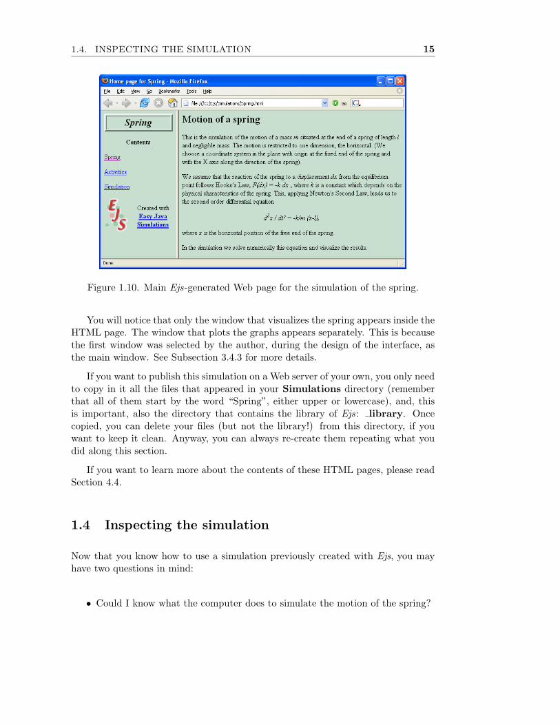
Figure 1.10. Main Ejs-generated Web page for the simulation of the spring.
You will notice that only the window that visualizes the spring appears inside theHTML page. The window that plots the graphs appears separately. This is becausethe first window was selected by the author, during the design of the interface, asthe main window. See Subsection 3.4.3 for more details.
If you want to publish this simulation on a Web server of your own, you only needto copy in it all the files that appeared in your Simulations directory (rememberthat all of them start by the word “Spring”, either upper or lowercase), and, thisis important, also the directory that contains the library of Ejs: library. Oncecopied, you can delete your files (but not the library!) from this directory, if youwant to keep it clean. Anyway, you can always re-create them repeating what youdid along this section.
If you want to learn more about the contents of these HTML pages, please readSection 4.4.
1.4 Inspecting the simulation
Now that you know how to use a simulation previously created with Ejs, you mayhave two questions in mind:
• Could I know what the computer does to simulate the motion of the spring?

16 CHAPTER 1. A FIRST CONTACT
Figure 1.11. The simulation of the spring in applet form.
• Even more interesting, could I modify this simulation to include other typesof motions, or to plot different graphs?
These are the two questions that, because their answers are positive, make ofEasy Java Simulations a very special tool. You can surely find on the Internet manyapplets that simulate scientific processes. However, very few of them will allow youto see their “secrets”, that is, how they have been done. And those that allowyou this, will surely do it by providing the full Java code of the applet, somethingwhich is only useful for expert Java programmers (which can also understand thephenomenon).
Ejs on the contrary, because it was designed to be used by people that don’t needto be Java programmers, allows you to understand and customize the simulation ina much simpler and efficient way. We’ll show this in the present and next sectionby inspecting and modifying our example in a substantial way.
1.4.1 Inspecting the model
Let’s go back to the model by clicking the corresponding radio button. We alreadysaw, in Figure 1.8, that this panel contains five subpanels.

1.4. INSPECTING THE SIMULATION 17
Declaration of variables
The first of these, labeled “Variables” and visible in Figure 1.8, displays the table ofvariables needed for our model. When programming, we use the term variables eitherfor the parameters, the state variables or the inputs and outputs of the model. Everynumerical value (or of any other type, such as boolean or text) is called a variable,even if its value remains constant all along the simulation.
For the model of our example, these variables are the following:
m, the mass of the ball at the end of the spring,
k, the elastic constant of the spring,
l, the length of the spring in equilibrium,
x, the horizontal coordinate of the end of the spring,
y, the vertical coordinate (which must remain constant),
vx, the velocity of the horizontal motion,
t, the variable that represents the time of the simulation,
dt, the increment of time for each step of the simulation.
As we can see, some variables correspond to parameters of the system (m, k and l),others describe the state of it (x, y and vx), and others are variables needed for thesimulation itself (t and dt).
Initialization of the model
Variables need to be initialized. The table of Figure 1.8 provides an initial valuefor each of our variables, thus specifying the precise initial state of the system.In occasions, however, we will need a more complex initialization (for instance, ifsome preliminary computation is required). For these cases, we can use the secondsubpanel of the model. This is not necessary for our model, though, and we willleave this panel empty (we don’t display it either).
Evolution of the model
Next panel, labeled “Evolution”, is of special importance. It is used to indicate thesimulation what to do when the evolution runs. The panel can contain two typesof pages: a first type in which the author must directly write the Java code thatimplements the desired algorithm, and a second one, the type that this example is

18 CHAPTER 1. A FIRST CONTACT
using, specially indicated for models that can be described using systems of ordinarydifferential equations.
In our model, the differential equation that rules the motion is obtained from ap-plying Newton’s Second Law, F = m a, and the basic assumption that the responseof the spring to a displacement dx obeys Hooke’s Law, F = −k dx. We thereforeobtain the second order differential equation:
x = − k
m(x− l), (1.1)
where x is the horizontal coordinate of the end of the spring. (We are choosing acoordinate system with its origin placed at the fixed end of the spring and the Xaxis along it).
To enter this second order equation in the editor for differential equations ofEjs we need to rewrite it as a system of first order differential equations, which weachieve by using the variable vx = x. All this results in the formulation displayedin Figure 1.12. 5
Figure 1.12. Evolution panel with the differential equations for our spring.
Actually, this form of writing the previous second order differential equationmay be easier to understand for students not familiar with the concept of differentialequations. Note in the figure that we have selected t as the independent variable andthat we are asking the editor to provide a solution for the equation for an incrementof time given by dt.
With this information, when the simulation is created, the editor will generateall the code needed for the numerical computation of the solution of the equation,
5Note that the products require the character “*”.

1.4. INSPECTING THE SIMULATION 19
using for this the numerical method indicated in the field right below the equations.For this relatively simple problem, we have chosen the so-called Euler–Richardsonmethod, a method of order two that provides a reasonable ratio speed/precision (forthis problem).
The field called “Tolerance”, that appears here empty, is only required when themethod of numerical solution is of the type called adaptive, see Subsection 2.5.3. Thefield “Events” tells us that there are no events defined for this differential equation.We’ll discuss events in Subsection 2.5.4.
Solving differential equations numerically is a sophisticated task, although it canbe automated in an effective way. This is precisely what Easy Java Simulationsoffers: you write the equations in this editor and Ejs automatically generates thecorresponding code.
Before proceeding, we need to turn our attention to the left frame of this sub-panel. In it we instruct Ejs to play 20 steps of the simulation per second (or, indifferent words, to display 20 frames per second). This, together with the value of0.05 that we used for the variable dt will result in a simulation that runs approx-imately in real time (although this is not absolutely necessary). Notice also thatthere is a checkbox called “Autoplay”, that is now unchecked. This box must bechecked if we want the simulation to start automatically playing the evolution whenit is run.
Constraints among variables
The subpanel labeled “Constraints” is used to write the Java code needed to estab-lish fixed relationships among variables of the system. We call these relationshipsconstraints. In our model, the panel (not shown here) is empty since there are noconstraints among variables.
Custom methods
The last subpanel of the model is labeled “Custom”. This panel can be used bythe author of the simulation to define his/her own Java methods 6 Differently tothe rest of panels of the model, that play a well-defined role in the structure of thesimulation, methods created in this panel must be explicitly used by the author inany of the other parts of the simulation. Again, in our example, this panel is emptyand is not displayed.
6“Method” is the name that Java gives to what other programming languages call functions orsubroutines. The object-oriented nature of Java turns these methods into something even morepowerful than that. However, given the simplified use of Java that we chose for Ejs, this definitionwill be sufficient for us.

20 CHAPTER 1. A FIRST CONTACT
The model as a whole
We can now describe the integral behavior of all subpanels of the model. To startthe simulation, Ejs declares the variables and initializes them, using for this boththe initial value as specified in the table of variables, and whatever code the usermay have written in the initialization panel. At this moment (ignoring for oncethe left-to-right order), Ejs also executes whatever code the user may have writtenin the constraint pages. The reason for this is that the constraints contain equa-tions that can modify the initial value of certain variables, as will be explained inSubsection 1.5.1 and, in more detail, in Chapter 2.
Next, when the simulation plays, Ejs executes the code provided by the evolutionpanel and, immediately after, also the possible constraints. Once this is done, thesystem will be ready for a new step of the evolution, which it will repeat at theprescribed speed (number of images per second).
Notice that, as we mentioned already, methods in the panel “Custom” are notautomatically included in this process.
1.4.2 Inspecting the view
Specifying the view of the simulation takes two steps. In the first place, we needto build the tree of elements displayed in the left frame of Figure 1.7. This treeis graphically descriptive of the components of the view because each element ap-pears next to an icon representative of its function. Usually, the author also giveseach element an illustrative name (at least, we do so), which also facilitates thecomprehension.
The second step, less evident but also easy to accomplish, consists in editing theso-called properties of each element. Properties are internal values of the elementthat determine how the element looks and behaves on the screen. We may beinterested in editing the properties of an element either to change any of its staticgraphical peculiarities (such as the color or font, for instance), or to instruct it touse the variables of the model to modify its dynamic aspect (position or size) on thescreen. This second possibility is what turns the simulation into a really dynamic,interactive visualization of the phenomenon under study. Let us see how we used itin this particular example.
Select the panel for the view and, in the tree of elements of our simulation, clickon the element called Ball to select it. The graphical aspect of this element isprecisely that of a filled ellipse, and corresponds to the ball that you can see at theend of the spring. Once selected (you will see a colored frame around its name),click again on it, but this time with the right button of the mouse. The menu ofFigure 1.13 will appear.

1.4. INSPECTING THE SIMULATION 21
Figure 1.13. Popup menu for the element Ball of the view.
Select the option “Properties” (the one highlighted in the figure) and the windowdisplayed in Figure 1.14 will appear. (Double-clicking directly on the Ball elementis a short cut for this option.)
Figure 1.14. Table of properties for the element Ball of the view.
This window displays the table of properties of the element. In our case, thestatic values indicate that the ball will be displayed filled with the color cyan (a sortof light blue), in the form of an ellipse of size (0.2,0.2) (which finally results in acircle being drawn), and that the element is enabled, that is, that it will respond touser interaction if (s)he clicks on it with the mouse.
You can also notice, and this is the most interesting thing, that other propertiesof the element are associated to variables of the model, or use expressions that usethem. For instance, the position of the element is associated to the point (x,y),where x and y are the corresponding variables of the model. This association is atwo-way link. In one direction it means that, every time the value of these variableschanges during the execution of the model, the element will be informed and thecorresponding properties updated to the new values, causing the ball to move atthe simulation’s pace. In the other direction, if the user interacts with the ball tomodify its position, then, in an automatic way, the value of the variables of the

22 CHAPTER 1. A FIRST CONTACT
model associated to these properties will also be modified. In this simple manner,associating variables of the model to properties of the view elements, we can easilybuild complete dynamic, interactive simulations.
Finally, the way the element Ball must react when it is interacted by the userhas been established associating to the (so called) action properties of the elementexpressions that use variables of the model, or methods of it. We can see in Fig-ure 1.14 that the action produced “On Press”ing the element is associated to thepredefined method pause(). (This method just pauses the simulation). The actionproduced “On Drag”ing the element evaluates the sentence y = 0.0;, which keepsthe spring in a horizontal position. Finally, the action produced “On Release” ofthe element evaluates the code: 7
vx = 0.0;_resetView();
We can use for this code any valid Java expression that involves the variables ofthe model and even any Java method that we may have defined in the “Custom”subpanel of the model.
According to the code written in these three action properties, the sequence ofthe interaction with the element Ball is the following:
1. When the ball is first clicked, the simulation is paused (if it was playing). Thisis necessary because it is rather uncomfortable to try to reposition a ball whileit is moving because of the effect of the evolution of the system.
2. When moving the ball, we force the y coordinate to keep the value 0. This way,even if the user inadvertently tries to move the ball in the vertical direction,the spring remains horizontal.
3. When the ball is finally released, the system will freeze the ball (vx = 0),clean the graphs ( resetView()) and leave the system ready to start a newsimulation run with the new initial conditions.
You can also inspect the properties of the other elements to become familiar withsome of the different types of elements that Ejs offers and their properties. Ofparticular interest are the elements called Displacement and Velocity.
7Code in action properties can span more than one line. When this happens, the field adopts adifferent background color. If the code is not clearly visible, click on the first button to its right,
, and an editor window will display it more clearly.

1.5. MODIFYING THE SIMULATION 23
1.5 Modifying the simulation
We have already used one of the big peculiarities of Easy Java Simulations, the factthat it lets us see how the simulation works. In this section we will use the otherimportant characteristic of it, the possibility of modifying the simulation to adaptit to our preferences or to include new possibilities.
Very often, when we explore a program created by another person, right afterlearning the possibilities that the program offers, we come to the universal question:“What if. . . ?” (or a variant of this one: “Is it possible to. . . ?”). Unless the authorhas taken into account all different possibilities (which is unlikely), the answer maycause us a small disappointment.
This doesn’t need to be the case with Easy Java Simulations. The tool not onlylets us see the interiors of the author’s creation, but also allows us to contribute toit adapting or enriching the model and the view according to our needs. We willillustrate this process by extending our simulation in the following way:
1. We will modify the model so that it includes both friction and an externalforce, turning our originally free spring into a forced, damped oscillator. Theresulting second order differential equation is:
x = − k
m(x− l)− b
mx +
1m
fe(t) (1.2)
where b is the so-called coefficient of dynamic friction and fe(t) is an externalforce applied to the system. We’ll use in particular an oscillatory force of theform fe(t) = A sin(ω t), that allows us to explore interesting phenomena suchas resonance.
2. We will modify the view so that it also displays a diagram of the phase space;that is, of velocity versus displacement.
3. We will compute and plot the potential and kinetic energies of the system andtheir sum.
1.5.1 Modifying the model
We begin by modifying the model according to our new needs. Please select again,in Ejs’ interface, the panel for the model and, inside it, the subpanel for variables.We are going to add some new variables to our model.
Even though we could simply add the new variables to the existing table, it issometimes preferable, for clarity, to keep several separated tables of variables. Thishas only organizational purposes; actually, all variables can be used in exactly thesame way, independently of the page in which they have been defined.

24 CHAPTER 1. A FIRST CONTACT
Adding new variables
Click with the right button on the upper tab of the page (where the label “Simplespring” is) and a popup menu will appear, as Figure 1.15 shows.
Figure 1.15. Popup menu for the page of variables.
In this menu, select the “Add a new page” option (the one highlighted in thefigure) and the program will add a new page with an empty table for variables. (Ejswill first prompt you for a name for the new page, you can choose, for instance,“Advanced spring”.)
In this new table, initially empty, click on the first (and only) cell of the column“Name” and type b. In the next column, “Value”, type 0.1. This will be ourcoefficient of dynamic friction. You can write a comment about it in the text fieldsituated at the lower part of the table. The table will look as in Figure 1.16.
In a similar way, please create new variables called amplitude and frequency,with values 0.2 and 2.0, respectively. Finally, create three new variables calledpotentialEnergy, kineticEnergy and totalEnergy, for the potential and kineticenergy and their sum, respectively. Do not assign to these variables any initial value(we’ll soon see why this is not necessary).
You can comment all these variables, if you want to do so. The final result canbe seen in Figure 1.17. 8
8Do not worry about the extra blank row at the end of the table, Ejs ignores it. But it youwant, you can delete this empty row by right-clicking on it and selecting the option “Remove thisvariable” from the popup menu that appears.

1.5. MODIFYING THE SIMULATION 25
Figure 1.16. Adding the coefficient of dynamic friction b to our model.
Modifying the equations of the evolution
Let’s go now to the evolution page and edit the right-hand side of the second differ-ential equation so that it reads now:
-k/m*(x-l) - b*vx/m + externalForce(t)/m
The result is shown in Figure 1.18. Notice that we are using in this expressionthe method externalForce(), that is not yet defined. We’ll need to create it as acustom method, when we get to this panel.
Adding the computation of the energy
But, before this, select the subpanel for the constraints. Click on the message “Clickto create a new page” and give the new page the name “Energies”. In the editorthat appears, write the following code:
potentialEnergy = 0.5*k*(x-l)*(x-l);kineticEnergy = 0.5*m*vx*vx;totalEnergy = potentialEnergy + kineticEnergy;
Please, play special attention and copy this code exactly as it appears above! (Themultiplication character “*” and the semicolon “;” are particularly easy to forget.)Compilers of computer languages are inflexible concerning syntax errors. Any smallmistake when typing the code can result in the compiler issuing a (sometimes very

26 CHAPTER 1. A FIRST CONTACT
Figure 1.17. The complete table for the new variables.
long) sequence of error messages. The appendices (which are distributed separatelyfrom this manual, visit http://fem.um.es/Ejs) include some instructions to un-derstand these messages but, for the moment, we will assume that you copied thiscode correctly. The result (once we add a short comment to this page) is shown inFigure 1.19.
This is the first time that we use constraints. You may remember that we definedthe constraints as “fixed relationships among variables”. In our model, the potentialand kinetic energy respond to the expressions Ep = 1
2kx2 and Ek = 12mvx
2. Thecode we wrote above is the translation of these equations to Java code.
Now comes a subtle point. One of the questions most frequently asked by newusers of Ejs is: “why don’t we write these equations into a page of the evolution,instead of one of constraints?” The reason is that this relationship among variablesmust always hold, even if the evolution is not running. It could very well happenthat the simulation is paused and the user interacts with the simulation to repositionthe ball. If we write the code to compute the energy in the evolution, the valuesfor the energy will not be properly updated, since the evolution is not evaluated(because the simulation is not playing). To prevent this situation we need to writethese equations in a constraint page.
Constraint pages are always automatically executed after the initialization (atthe beginning of the simulation), after every step of the evolution (when the simu-lation is playing) and each time the user interacts with the simulation. Therefore,any relationship among variables that we code in here, will always be verified.

1.5. MODIFYING THE SIMULATION 27
Figure 1.18. The new differential equations of the model.
Coding the external force
Recall finally that, to complete our model, we still need to specify the expressionfor the external force. 9 To this end, go to the “Custom” subpanel and click on itto create a new page called “External force”.
The new page will be created with the code necessary to create a standardmethod. Edit this code to read as follows (see also Figure 1.20):
public double externalForce (double time) {return amplitude * Math.sin(frequency*time);
}
This code illustrates the syntax for a method that returns a (double precision)numeric value. (The expression Math.sin corresponds to a call to the sine functionof the mathematical library of Java.) Notice that this method accepts a parameter,time, that can be used as another variable inside the body of the method (time isthen called a local variable), and that it uses the (global) variables amplitude andfrequency. The use of the parameter time is important; it would be a mistake todefine the method as follows:
public double externalForce () {return amplitude * Math.sin(frequency*t);
}9Even when we could have written the expression for this force directly in the corresponding cell
of the differential equation, it will be simpler for our students or users to interpret the model if wewrite it separately.

28 CHAPTER 1. A FIRST CONTACT
Figure 1.19. Constraint equations for the computation of the energy.
which uses directly the global variable t. This is incorrect because t is a variable thatchanges during the process of solution of the differential equation (while amplitudeand frequency do not), and this affects the precision of the numerical algorithm forthe solution. Thus, as a general rule, we must state that:
If a global variable can change during the resolution of a differential equation, thisvariable must be included as one of the parameters sent to any method called from thecells of the equation editor.
This is exactly what we did. Our new model is ready.
You will notice in Figure 1.20 that the “Custom” panel of the model includes someextra controls at its bottom. Although Ejs tries to provide all the programming toolsthat a typical user may need, experienced Java programmers may always want to go astep further and, for example, reuse any previous Java code or libraries that they mayhave created previously. These controls allow just this, as will be explained in detail inSection 2.7.
1.5.2 Modifying the view
Lets us now enrich the visualization of our phenomenon with the graph of the phasespace, velocity versus displacement. For this, select the panel for the view and, in theright-hand frame, from the upper set of elements called “Containers”, click on theicon for “PlottingPanel”, . 10 When you click on it, the icon will be highlighted
10If you doubt about which icon is the right one, place the cursor over it and wait a second untila tip appears revealing the type of the element selected and displaying a brief description of it.

1.5. MODIFYING THE SIMULATION 29
Figure 1.20. Custom method with the expression for the external force.
with a colored background and the cursor will change to a magic wand, . Withthis wand, go to the tree of elements and click on the element called Dialog. Youare then asking Ejs to create an element of type “PlottingPanel” inside the windowDialog. This window is prepared to accept this type of “children”.
When you do this (give the new element the name PhaseSpacePanel), a newpanel with axes will appear inside the window with the plots, sharing the availablespace with the previous plotting panel. Get rid of the magic wand by clicking with iton any blank space of the tree of elements’ frame. Then, since both plotting panels(the old and the new one) look too small, double-click on the tree element calledDialog to bring-in its property editor and modify the one called “Size”, changingit from the current value of 400,200 to the value 400,400 (it may also appearas ‘‘400,400’’), thus doubling its height. The table of properties for this dialogwindow will look as in Figure 1.21.
Figure 1.21. Properties for the dialog window.
Edit now the properties of the new element PhaseSpacePanel so that they ap-pear as in Figure 1.22.

30 CHAPTER 1. A FIRST CONTACT
Figure 1.22. Properties for the element PhaseSpacePanel.
Notice that, when you type on the text field of a property to modify it, thebackground color of the field turns yellow. This is Ejs’ way of telling you that thevalue won’t be accepted until you hit the “return” key. In this very moment, thebackground will turn white again. For this reason, never leave any field with theyellow background!
An exception to this rule are the fields of action properties. These fields are special:any edition on them is automatically accepted, and they only change color (to a sort oflight green) to warn you that they span more than one line. These editors can obviouslybe left colored.
The window with the plots will finally look as in Figure 1.23.
Adding the graph of velocity versus displacement
The plotting panel we added is only the container for the graph we want to add.
The graph is visualized using an element of the type called “Trace”, with icon ,which you can find on the subpanel of drawing elements (or “Drawables”) called“Basic”.
Click on this icon to select it and to get the magic wand again, and use it tocreate an element of this type, named PhaseSpace, inside PhaseSpacePanel. Onceyou do this, edit the properties of the new element and give to its properties “X” and“Y” the values x-l (recall l is the length of the spring at rest) and vx, respectively.

1.5. MODIFYING THE SIMULATION 31
Figure 1.23. Dialog window with two plotting panels.
This is all we need to do to display the phase space graph.
As this example shows, the value of a property can also be specified using an expressionin which one or more variables of the model appear. In this case, however, the bi-directionality of the connection between model variables and view properties is lost, itonly works in the obvious direction.
Plotting the energy
The process we carried out for the phase space graph is very similar to what we needto do to display a graph of the three energies we computed in the model. Createanother plotting panel, called EnergyPanel, in the Dialog window and increaseagain the vertical size of this window (changing the “Size” property to 400,600).Edit the new panel and change the property “Title” to Evolution of the energy,and the properties “Title X” and “Title Y” to Time and Energy, respectively. Leavethe other properties as they appear originally.
Use the magic wand to create three elements of type “Trace” called Potential,Kinetic and Total, inside EnergyPanel. Edit the properties of these three tracesassociating the property “X” to the variable t in all three cases, and the property “Y”to the variables potentialEnergy, kineticEnergy and totalEnergy, respectively.
Additionally, for all three traces, type the fixed value 300 in the field for theproperty called “Points” (this value indicates that the traces should only displaythe last 300 points of data they have received) and choose a different value for the

32 CHAPTER 1. A FIRST CONTACT
property called “Line Color” of each of the traces, so that you can distinguish thegraphs. To obtain a panel with the available colors, click on the icon immediatelyto the right of the text field for this property. We chose (for no particular reason) thecolor red for the potential energy, green for the kinetic energy and blue for the totalenergy. As an example, Figure 1.24 shows the panel of properties for the elementPotential.
Figure 1.24. Properties of the trace Potential.
Displaying the new parameters
Finally, we will add new elements of the type “NumberField” so that the user canvisualize and edit the values of the variables b, amplitude and frequency. Theywill be located below those already existing for the mass and the elastic constant ofthe spring.
You can find this type of element, with icon , in the “Display” tab of the“Basic” central panel of the right frame. Select this icon and, with the magic wand,click on the element of the tree called LowerPanel to create three new elementswith names identical to the variables we want to display, that is, b, amplitudeand frequency. This coincidence on names doesn’t cause any problem. Names ofvariables in the model must be unique, but they do not conflict with similar namesfor the elements of the view.
We must finally edit the properties of these elements so that they fulfill theirwork. We’ll show you how to do this for the first of them. Bring the panel ofproperties for the new element b into view and edit the properties as in Figure 1.25.
The association of the property “Variable” with the variable of the model b tells

1.5. MODIFYING THE SIMULATION 33
Figure 1.25. Properties for the number field for b.
the element that the value displayed or edited in this field is that of b. The propertycalled “Format”, to which we assigned the value b = 0.00, has a special meaning. Itdoesn’t indicate that b should take the value of 0, but is interpreted by the elementas an instruction to display the value of b with the prefix “b = ” and with twodecimal digits (hence the value 0.00).
That’s all, do the same for the other two number fields, associating the sameproperties to amplitude and amp = 0.00, and to frequency and freq = 0.00,respectively. To facilitate the association of properties with variables of the model,you can use the icon that appears to the right of the text field for the correspondingproperty. If you click on this icon, a list of all the variables of the model that can beassociated to this property will be offered to you. You can then comfortably selectthe one you want with the mouse.
1.5.3 An improved laboratory
Our simulation is now ready! This is a perfect moment to save our changes. 11
Because we don’t want to overwrite the original simulation (we may be interested inpreserving it), we will save this new one in a different file. Click then on the “Saveas” icon of Ejs’ taskbar. A dialog window will appear as shown in Figure 1.26, thatwill allow you to chose the name of the file for the new simulation.
Type the name MySpringAdvanced.xml in the field called “File Name” andclick the “Save” button of this dialog window. Ejs will then save the new file andwill notify you in the message area.
We can now run the simulation. Click the “Run” icon and you will obtain resultssimilar to those of Figure 1.27.
We have thus created a complete laboratory to explore the behavior of simpleharmonic motion plus damping and external forces. You can use this laboratory with
11Actually, we should have done this earlier. If you are used to work with computers, you’ll knowthat they have the bad habit of stopping (hanging is the slang word for this) with no apparentreason and with no previous warning. We therefore recommend you to learn to save your work fromtime to time.

34 CHAPTER 1. A FIRST CONTACT
Figure 1.26. Saving our simulation.
your students to explore interesting phenomena such as resonance (try a value for thefrequency close to
√k/m). Besides the file MySpringAdvanced.xml that you just
created, you will find this simulation in the examples/Manual/FirstContactdirectory, with the name AdvancedSpring.xml.
Modifying the introduction
You might want to modify now the introduction for the simulation. Select the panelfor the “Introduction” and add a new page or edit the existing ones. Use for this thepopup menu for each page and select the option “Edit/View this page”. A simplevisual editor for HTML pages will then appear to help you edit the HTML code.See Figure 1.28.
HTML pages are text pages that include special instructions, or tags, that allowWeb browsers to give a nice format to the text as well as to include several typesof multimedia elements. The editor allows you to work in a WYSIWYG (what yousee is what you get) mode. However, if you know HTML already and want to workdirectly on the code (which, sometimes, is preferable), select the option that appearshighlighted in Figure 1.28.
You can write as many introduction pages as you want. As we saw earlier, eachof the pages will turn into a link in the main HTML page that Ejs generates forthe simulation. A second possibility is to delay until the last moment the editionof the introduction and, once the HTML pages have been generated by Ejs, copythe simulation and their pages to a different directory (for instance, that of theWeb server from which they will be published) and modify them using your favoriteHTML editor. If this is the option of your choice, we insist that you do this workin a directory other that Simulations. Otherwise, if you ever run your simulation

1.6. A GLOBAL VISION 35
Figure 1.27. The improved simulation in action.
again from within Ejs, you will loose whatever edition you have made, because Ejswill overwrite the edited pages!
1.6 A global vision
We end this chapter taking an overview of what we did in it. We first learnedto install and run Easy Java Simulations. Next, we loaded one of the examplesincluded in the examples directory and run it. We checked that, besides runningthe simulation as an independent Java application, Ejs also generates a complete setof Web pages, ready to be published, that contain the simulation in form of a Javaapplet. We then learned to distinguish and to explore the different parts that makea simulation, and, finally, we even modified these parts to improve the simulation,adding new functionality.
The three parts of a simulation are the introduction, the model and the view.Each of these parts has its function and its own panel in Ejs’ interface with aparticular look and feel.

36 CHAPTER 1. A FIRST CONTACT
Figure 1.28. Improving the introduction.
The introduction contains an editor for HTML code needed to create the multi-media narrative that wraps the simulation. We can create the pages we need withthis editor, either working in WYSIWYG mode or writing directly the HTML code.
The model contains a series of subpanels needed for the specification of thedifferent parts of it: definition of variables, initialization, evolution of the system,constraints or relationships among variables, and custom methods. Each panel pro-vides edition tools that facilitate the job of creation.
Finally, the view contains a set of predefined elements that can be used as in-dividual building blocks to construct a structure in form of a tree for the interfaceof our simulation. These elements, that are added through a procedure of click andcreate (our magic wand), have in turn a set of properties that indicate how each ele-ment looks and behaves, and that, when associated to variables from the model (orexpressions that use them), turn the simulation into a true dynamic and interactivevisualization of the phenomenon under study.
Well, and this is all! Though the chapter is a bit long because we accompanied thedescription with many details and instructions, the process can be summarized in thefew paragraphs above. Obviously, learning to manipulate with fluency the interfaceof Easy Java Simulations requires a bit of practice, as well as the familiarizationwith all the possibilities that exist. In particular, with respect to the creation of theview, you’ll need to learn the many several types of elements offered and what eachof them can do for you.
The rest of this manual will give more information about all these possibilities.Also, the examples provided with Ejs are a great source of information. If youare anxious to start exploring our simulations and create your own ones, and if you

1.6. A GLOBAL VISION 37
think you got a sufficiently general overview of the way Ejs works (this was preciselythe goal of this chapter), you can go directly to explore some examples, returninglater to the other chapters of this manual when you need to improve your knowledgeabout Ejs.
Exercises
Exercise 1.1. Modify the example of the spring to remove the restriction that themotion is only horizontal. Introduce also a second external force along the Y axis ofthe form A2 cos(ω2t+φ) (φ is the phase difference between both external oscillatoryforces) and explore the different resulting motions.
Exercise 1.2. Include new elements of the type “NumberField” for the values ofthe velocities in X and Y for the simulation of the previous exercise. Modify thecode for the “On Release” action of the ball to allow initial conditions that do notstart from rest.
You’ll find this exercise solved in the examples/Manual/FirstContact directorywith the name Spring2D.xml.


CHAPTER 2
Creating models
c©2005 by Francisco Esquembre, September 2005
In this chapter we cover in detail the different parts that make the model ofa simulation and explain the support that Easy Java Simulations offers for theirimplementation. This chapter can be considered as a complete reference for the useof the panel of Ejs for the description of the model.
2.1 Definition of a model
Let’s start with a bit of theory. We create the model of a phenomenon when wedefine its relevant magnitudes, set their values at a given initial instant of time, andestablish the rules that govern how these magnitudes change.
We use the term “magnitude” here to refer either to state variables (the variablesthat describe the state of the phenomenon), or to parameters, or to any other inputor output quantities of the model. When we work with our simulation, we’ll alwaysrefer to these magnitudes as variables.
Actually, a variable can hold a value that changes along the execution of thesimulation or one that doesn’t. In other words, it can represent a constant orvariable magnitude, but this won’t prevent us from using this terminology. 1
1It is possible that a magnitude considered constant at one initial implementation, changes later,either because we change the model and the role that this variable plays in it, or because we allow
39

40 CHAPTER 2. CREATING MODELS
This way, the state of a model is completely determined by the value of itsvariables at a given instant of time. This state can change because of two reasons:
• The internal dynamics of the simulation, which we will call evolution.
• The influence of external agents. In our case (since we are using simulationsthat do not read data from the real world, for instance), because of the inter-action of the user with the simulation, to changes the value of one or more ofthe variables of the model.
Changes directly caused by any of these reasons may cause other changes in anindirect way. This is actually the case when there exist variables in the model whosevalues explicitly depend on the values of those who where modified. In this situation,we say that there exist constraints among the variables affected.
All these changes are ruled by equations that describe the laws under whichthe evolution takes place, or that state the interdependence of the variables. Theseequations must be made explicit by using mathematical formulas or logical computeralgorithms.
So, finally, in order to specify the model of a simulation, we need to establish:
• the variables of the model,
• their initial state,
• the evolution equations, and
• the constraint equations.
2.1.1 Variables and the initial state of a model
First of all, we need to declare the variables of our model. This is a crucialprocess from which a good or a bad simulation can result: we need to choose theright reference system, the magnitudes that allow us to write simpler formulas,. . .
In order to illustrate what follows, we will assume that the variables of ourmodel are called x1, x2, . . . , xn. Obviously, if we want our model to be more easilyunderstood, it is customary to give meaningful names to the variables, such asposition, velocity, number of individuals of a species, concentration of a chemicalelement, etc., which are in turn simplified using easy to identify shorter acronyms.However, since our exposition is general, we will assume this naming mechanismwith subscripts.
the user to interact with the simulation to modify the magnitude. Thus, the term variable turnsout finally to be appropriate.

2.1. DEFINITION OF A MODEL 41
In the second place, we need to set the initial state by giving the right value toeach of the variables. This can be done, in the majority of cases, by simply typingthe desired value. In occasions, however, the initial value of some variables can onlybe obtained by making some previous computations. We call this process (by eitherof both methods) initializing the model.
2.1.2 Evolution equations
Continuing with the terminology introduced above, the system can evolve in anautonomous way from the current state, x1, x2, . . . , xn, to a new state x∗1, x
∗2, . . . , x
∗n,
thus simulating the passing of time (which, by the way, can or cannot be one of ourvariables—although it frequently is). We call the equations that rule this transitionevolution equations, which can be written using one or more expressions of the form
x∗i = fi(x1, x2, . . . , xn) (2.1)
Sometimes, these laws have a direct mathematical formulation, as in the case of theso-called discrete systems. In other situations, they derive from the discretizationof continuous models which are described by differential equations. In many cases,however, the formulation (2.1) (so typically mathematical) requires of a combina-tion of numerical techniques and of logical algorithms that conforms an elaboratedcomputer algorithm.
But, as a conclusion, we will state that simulating the evolution in time of themodel consists in computing, from the current state x1, x2, . . . , xn, the new valuesx∗1, x
∗2, . . . , x
∗n, take these as the new state of the model, and iterate this process
indefinitely while the simulation runs.
Thus, the third step that we need consists in writing the evolution equations.
2.1.3 Constraint equations
The last step consists in writing the constraint equations. As we mentionedabove, changes in the variables directly caused by evolution equations can haveindirect effects on other variables. This indirect changes are determined by whatwe will call constraint equations, which can be made explicit by one or more ofexpressions of the form
xi = gi(x1, x2, . . . , xi−1, xi+1, . . . , xn) (2.2)
where, as you can see, a variable should only appear at one side of the equation.
These expressions indicate that, if one or several of the variables on the right-hand side change, then equation (2.2) must be evaluated so that the variable on

42 CHAPTER 2. CREATING MODELS
the left is consequently modified. Similarly to evolution equations, this theoreticalformulation can require in practice the need to write a sophisticated algorithm,partially logical, partially numerical.
It is a common temptation to consider constraint equations as part of the evo-lution. That is, if the changes are caused primarily by the evolution,. . . why notinclude these relationships as part of it?
That would be, however, a bad practice. The reason is that there is a secondsource for changes, namely the direct interaction of the user with the simulation.Indeed, if constraints interrelationships among variables must always be valid, thenthey should also hold when the user changes any of these variables, even if thesimulation is paused (that is, if the evolution is not taking place). For this, it isconvenient to identify clearly and to write separately both types of equations. Thiswill allow the computer to know which equations it must evaluate in each case (seeSubsection 2.1.4 below).
A useful (though perhaps not always valid) criterion to distinguish both types ofequations is to examine the expression we use to compute the value of a variable ata given instant of time and, if this value depends on the current value of the samevariable, then this is most likely an evolution equation. If, on the contrary, the valueof the variable can be computed exclusively from the value of other variables, thenit is a constraint.
2.1.4 Running the model
Once we complete the four steps described above, the model is precisely defined. Ifwe now run the simulation, the following events will take place: 2
1. The variables are created and their values set according to what the initializa-tion states.
2. The constraint equations are evaluated, since the initial value of some variablesmay depend on the initial values of others.
In this moment, the model is found to be in its initial state, and the simulationwaits until an evolution step takes place or the user interacts with it.
3. In the first case, the evolution equations are evaluated and, immediately after,the constraints. A new state of the model at a new instant of time is thenreached.
4. In the second case, when the user changes a variable, constraint equations areevaluated and we obtain a new state of the model at the same instant of time.
2See, however, the more complete description, which includes the view, in Section 3.3.

2.2. INTERFACE FOR THE MODEL IN EASY JAVA SIMULATIONS 43
A coherent model should take care that there exist no contradictions among theirdifferent parts. In particular, the values given to a variable during the initializationor the evolution should not be different to what it results from any constraint that af-fects this variable. However, if this actually happens, Ejs will solve the contradictionby giving always priority to (that is, evaluating in the last place) the constraint.
Because of the multitasking form in which simulations are run in Ejs, it is possible thatthe user interacts with the simulation right when it is in the middle of one evolutionstep. Although this doesn’t necessarily need to be bad in itself, it can occasionallyproduce undesired effects, such as the change of the value of a parameter in the middleof an algorithm. In these situations, it is preferable to ask the user to pause thesimulation (using a control that allows him/her to do this) before interacting with it.
This is the scheme, simple but effective, that Ejs uses for the creation of the modelof our simulations.
2.2 Interface for the model in Easy Java Simulations
Let us now describe the structure that Ejs provides for this task. The panel in Ejsdedicated to the creation of the model displays five radio buttons (see Figure 2.1),one for each of the four steps described in the previous section, plus an extra one,labeled “Custom”, whose use will be explained in Section 2.7.
Figure 2.1. Panel of Easy Java Simulations for the model.
Each radio button allows us to visualize the corresponding subpanel in the centralworking area of Ejs. The aspect of these subpanels is, in principle, rather similar,displaying a message that invites us to create a new page. If you click on this

44 CHAPTER 2. CREATING MODELS
message, the system will effectively create a new page, asking first for a name forit, as Figure 2.2 shows. Although Ejs always proposes a generic name for the newpages, we recommend that you use descriptive names for them. You can type anyname you want, with no restrictions. The only recommendation is that these namesare different and not too long.
Figure 2.2. Asking for the name of a new page.
Once you type the new name and click “Ok”, a new page will appear. The aspectof this page depends on the subpanel you are working on. Figure 2.3 shows a partialview of a new page for variables.
Figure 2.3. Partial view of a new page for variables.
Notice that the new page has a header tab with its name on it. This system oftabs is very convenient to organize the pages when there are more than one in a panel.The reason to create several pages in the same panel is just to group variables oralgorithms with similar purposes or meaning in separated pages, thus helping clarifythe model. Ejs actually uses all these pages in the same way, processing them fromleft to right.
Each page offers an option popup menu that appears right-clicking the mouseon its header tab. See Figure 2.4.
You can use the options in this menu to create a new empty page for this panel,to copy, rename or remove the current one, or to change the order of the pages.There are finally two other options that require a small explanation.
The option to enable and disable the page can be used when we want Ejs not touse a page that we have created, but without removing it. This can be useful whenwe are testing different algorithms for the same model and we want to compare themby enabling and disabling them in turns.
On the other hand, the option to show and hide a page is used (very rarely,that’s the truth) for pedagogical reasons, when the author wants to hide pages with

2.3. DECLARATION OF VARIABLES 45
Figure 2.4. Popup menu for a page.
difficult to understand algorithms that (s)he doesn’t want to expose the students to,at least in a first approach. The “Options” icon (see also Subsection 4.3) in Ejs’staskbar offers the possibility of making completely invisible the pages defined ashidden. Later on, when the students are ready to understand the pages, the authorcan ask them to use this option to make them visible again.
When any of these two options is used, the name on the header tab will appenda letter between parentheses indicating the status of the page, (D) for disabled, (H)for hidden. Disabled pages are ignored by Ejs when it generates the simulation.Hidden pages, on the contrary, are perfectly valid.
This way of working is common to all subpanels, the rest of the chapter describeseach of these subpanels in more detail.
2.3 Declaration of variables
Let’s start with the first step of the creation of a model: the declaration of variables.Variables are easy to define, we just need to give them a valid name, specify thetype of each of them and, for the case of arrays (vectors or matrices), also specifytheir dimension. Optionally, we can also give an initial value to each variable. Letus describe each of these points in detail.
2.3.1 Types of variables
Even when in mathematical formulas we frequently use the so-called real numbers(integers, rationals and irrationals) 3 without distinguishing among them, when wewrite a computer program we do make distinctions among different types of variables,
3In some problems we may use complex numbers. However, Java doesn’t support them natively,hence any computation with complex numbers must be done accessing explicitly the correspondingreal and imaginary parts of the numbers.

46 CHAPTER 2. CREATING MODELS
depending on the use we plan to do of them and on the computer memory requiredto hold their possible values.
Thus, for instance, variables that will only hold integer values require consider-ably less memory and the computations that involve only integer numbers performfaster because modern computers implement optimized routines for integer arith-metic.
Java language implements the following basic types of variables:
• boolean, for variables of boolean type, that is, those which can hold only twovalues: true or false.
• byte, short, int, and long, for integer values.
• float and double, for the so-called floating-point numbers (what we wouldcall real numbers).
• char and String, for characters and texts, respectively.
As an object-oriented programming language, Java introduces also a new type calledObject as the basis of a whole new world of advanced constructions called classes.
Nevertheless, except in the occasions in which it is absolutely essential to dothe computations using the minimal possible type of variable so that to optimizememory usage, we can choose to work only with the standard type for each category.This will be our case, and Ejs will only make use of variables of types boolean, int,double, String, and (to open the world of object-orientation) Object.
Although Ejs was not designed as a tool for professional programmers, it leaves a dooropen for them to use directly object-oriented constructions by accepting also variablesof type Object. These can also be used for simple, still useful, things, such as tocreate colors (objects of the class java.awt.Color) that change along with the stateof the model.
2.3.2 Creation of variables
Each new page of the panel labeled “Variables” contains a copy of the editor forvariables, that takes the form of a table. See Figure 2.5.
To add a variable, we write its name in the first column of the edition row andselect its type using the selector of the third column. If we want to give the variablean initial value, we only need to type it in the corresponding column. On the lowerpart of the editor there exists also a comment field in which we can type a shortdescription of the role the variable plays in the model. This can be useful to facilitatethe comprehension of the model.

2.3. DECLARATION OF VARIABLES 47
Figure 2.5. Table for the edition of variables (with annotations).
If the variable is an array, 4 we must indicate its dimension as well. Ejs can workboth with simple and multidimensional variables. If the field of the “Dimension”column is left empty, then a simple variable will be created, that is, just one variableof the given type. If, on the contrary, we type in this field one or more integernumbers (it’s important that these numbers are integer!) between square brackets,then Ejs will create a set of variables of the given type, where each of the numbersamong square brackets indicates a dimension.
Hence, for instance, if we type [50] in this field, Ejs will create a unidimensionalarray (or vector) with 50 coordinates, reserving memory space for 50 individual vari-ables of the type indicated. If we write [10][100], it will create a two-dimensionalmatrix of 10 rows, each of them with 100 elements. The integer number used toindicate a dimension can be either a constant or a variable of type int that has beenpreviously defined.
It is important to notice that, if a dimension of an array is indicated using an integervariable, the array will be created using (for the corresponding dimension) the valuethat the variable holds at the moment of the initialization of the array. Any later changein the value of the variable will not directly affect the dimension of the matrix.
Each time you create a new variable, a new edition row will automatically appearto accept more variables. But we can also insert a variable between two existingones using the popup menu for each row (different from the popup menu for thepage) that appears when you right-click on the corresponding row. The options ofthis menu can be seen in Figure 2.6.
4We use the term array to refer both to vectors and to matrices of any number of dimensions.
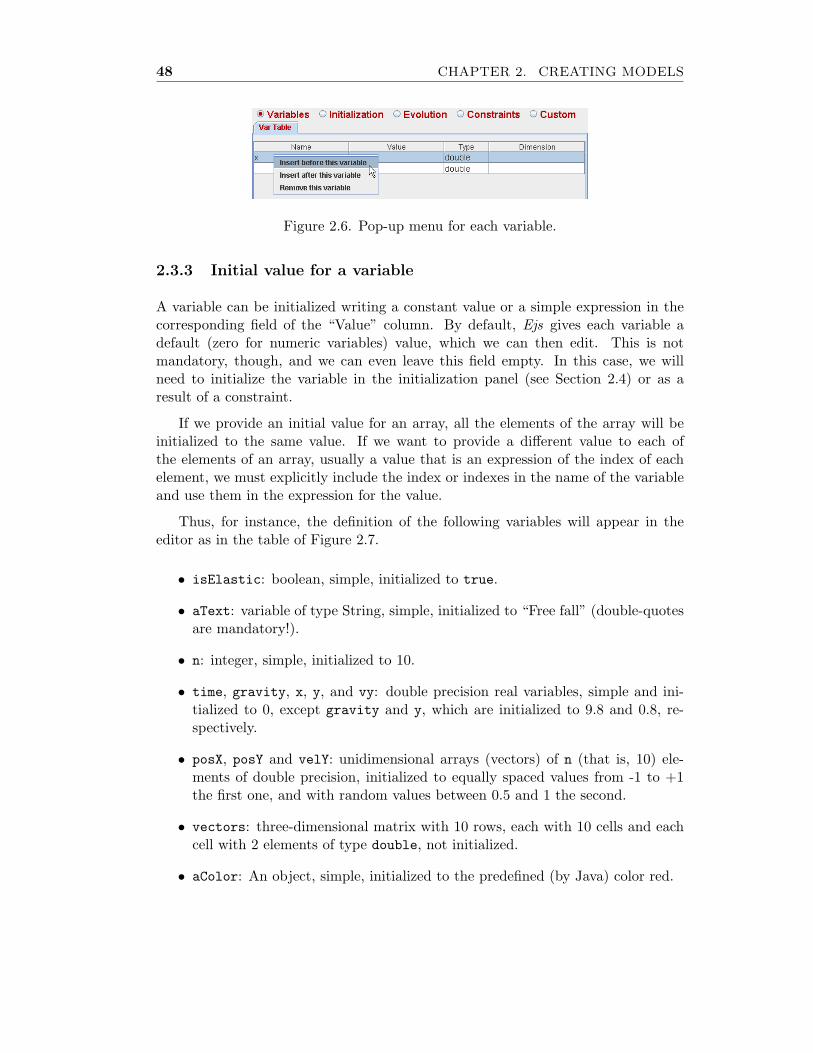
48 CHAPTER 2. CREATING MODELS
Figure 2.6. Pop-up menu for each variable.
2.3.3 Initial value for a variable
A variable can be initialized writing a constant value or a simple expression in thecorresponding field of the “Value” column. By default, Ejs gives each variable adefault (zero for numeric variables) value, which we can then edit. This is notmandatory, though, and we can even leave this field empty. In this case, we willneed to initialize the variable in the initialization panel (see Section 2.4) or as aresult of a constraint.
If we provide an initial value for an array, all the elements of the array will beinitialized to the same value. If we want to provide a different value to each ofthe elements of an array, usually a value that is an expression of the index of eachelement, we must explicitly include the index or indexes in the name of the variableand use them in the expression for the value.
Thus, for instance, the definition of the following variables will appear in theeditor as in the table of Figure 2.7.
• isElastic: boolean, simple, initialized to true.
• aText: variable of type String, simple, initialized to “Free fall” (double-quotesare mandatory!).
• n: integer, simple, initialized to 10.
• time, gravity, x, y, and vy: double precision real variables, simple and ini-tialized to 0, except gravity and y, which are initialized to 9.8 and 0.8, re-spectively.
• posX, posY and velY: unidimensional arrays (vectors) of n (that is, 10) ele-ments of double precision, initialized to equally spaced values from -1 to +1the first one, and with random values between 0.5 and 1 the second.
• vectors: three-dimensional matrix with 10 rows, each with 10 cells and eachcell with 2 elements of type double, not initialized.
• aColor: An object, simple, initialized to the predefined (by Java) color red.

2.3. DECLARATION OF VARIABLES 49
Figure 2.7. Sample declaration of variables.
Notice in particular the expression that uses the function random() from Javamathematical library (see Section 2.7) and the form in which the elements of thearray posX are initialized with equally spaced values from -1 to 1, using the ad-hocvariable i.
In the expression of the right-hand field for posX, we are using that the first elementof an array in Java has the index 0, and the last one, the size of the array minus one.Also, it was necessary for us to write the expression (2.0*i) between parentheses tomake sure that Java doesn’t use integer arithmetic to evaluate this expression, which itdoes when it has the opportunity to, and that would result in values different to whatwe expect. Recall these two principles and you will save yourself some troubles!
With respect to the initial value of aColor, this example illustrates the use wecan do of the (literally) hundreds of classes in Java. This manual doesn’t try to teachyou Java in all its extension, but this is actually one of the few classes that can bereally useful for us, for instance, to make our objects change color dynamically. Oncewe have declared the variable this way, we can give aColor the value of the color wewant using a sentence such as :
aColor = new java.awt.Color(255,0,0);
where the parameters of this invocation to the class java.awt.Color must be threeinteger numbers between 0 and 255 that indicate the levels of red, green and blue,respectively, for the color we want. In the case shown, the color created is, again,red. If you want to get semi-transparent colors (which is rarely really necessary andcauses the computer to run slower), you can include a fourth parameter indicatingthe level of transparency.

50 CHAPTER 2. CREATING MODELS
2.3.4 Using the variables
When, later on, we want to use a simple variable in a Java expression, we only needto write its name. If we want to use an element of an array, we need to indicatewhich element we refer to. 5 For this, if the array is unidimensional, we write thename of the array and, between square brackets, an integer number that indicatesthe position of the element in the array. If the array has more than one dimension,we must specify as many integers between square brackets as needed.
Once more, recall that the first element of an array has the index 0, and the lastone, the size of the array minus one. Forgetting this (for many, a bit strange) way ofnumbering, is a frequent source of severe errors during the execution of a simulation.Thus, in the case shown above, trying to use the element posX[10] will cause whatis known as an exception, that is, a long complaint of the Java virtual machine. Thiserrors, unfortunately, are not detected during the compilation, which makes them evenmore of a nuisance.
Correct examples of use of the variables defined above are the following:
isElastic = false; time = 3.5; posY[0] = 1.0; posY[n-1] = 4.2;vectors[9][9][1]=5.0;
while next ones are incorrect:
n = 1.5; x[0] = 0.1; posX[10] = 1.0; posY[0][0] = 1.0;vectors[9][9] = 5.0;
2.3.5 Naming conventions
Along the process of creating the simulation, we will need to provide a name forseveral different elements of it: pages for the different panels, variables, custommethods (see Section 2.7) and elements of the view (Chapter 3).
Names for pages you create have no restrictions, since they are only used fororganizational purposes. You can even use (if there is a good reason for it) the samename for different pages. But the names for the other elements do need to followsome rules in order to avoid conflicts among them (and to help keep clarity, as well).Thus, we will respect the following conventions:
1. The name of each variable or custom method must be unique in the model.The name of view elements must be unique in the view (even when it cancoincide with a name used in the model).
5Java doesn’t natively support matrix algebra.

2.4. INITIALIZING THE MODEL 51
2. Names are constructed by a combination of alphanumerical characters (from“a” to “z”, from “A” to “Z”, and from “0” to “9”) with no limit of length.The first character must be alphabetical.
3. Although not strictly compulsory, the first character of the names of variablesand of custom methods of the model will be lowercase. For view elements, onthe contrary, the first character will be uppercase.
4. It is recommended to use descriptive names. If we need to write more than oneword, there must be no blank spaces among them; words can be joined, forinstance, by using uppercase for the first letter of the second and consecutivewords. Thus, instead of cm, we will write centerOfMasses.
5. It is forbidden to use names that start with the character “ ”, since Ejs canuse some such names for internal tasks.
Finally, the following words cannot be used because they are reserved words eitherby Java or by Ejs: 6
Palabras reservadas: boolean, break, byte, case, catch, char, continue, default, do,double, else, float, for, getSimulation, getView, if, import, initialize, instanceof, int,long, Object, package, private, public, reset, return, short, static, step, String, switch,synchronized, throws, try, update, void, while.
2.4 Initializing the model
As we have seen in the previous section, we can initialize the variables of the modelwith constant values or with simple expressions, using the field in the column “Value”of the table of variables. However, we sometimes require initializations which are abit more complex. For instance, if we want to give elaborated values to the elementsof an array, or if we want to do some previous computations. In these situations, wecan use the second of the subpanels of the model, “Initialization”.
We can create in this panel one or more pages of an editor where we can writethe Java code that does these computations. This code will be executed once, whenthe simulation starts. For instance, we can give values to the elements of the arrayvectors in the example above using the code shown in Figure 2.8. 7
Although the algorithm we write in these pages can be as sophisticated as theproblem requires, the process is rather simple in itself: just add as many pages asyou wish and write in them the Java code you need. This code only needs to contain
6This list may grow as new releases of Java introduce new features.7This code is not actually very interesting in itself. It is included only for illustrative purposes.

52 CHAPTER 2. CREATING MODELS
Figure 2.8. Sample initialization code.
the Java expressions and sentences that your algorithm requires, thus avoiding othertechnicalities of Java (such as method declaration). Recall that, if there are morethan one initialization pages, Ejs will process them always from left to right. If youwant to change the order in which a given page appears, use the popup menu for it.
The editor for the code (the white edition area) has its own popup menu, dis-played in Figure 2.9. This menu offers the typical edition options, but also a simplecode assistant that will help you introduce standard Java constructions, such asloops and conditional statements. It also offers an option that displays some of thepredefined methods of Ejs (see Subsection 2.7.3).
Figure 2.9. Popup menu (left) and code assistant (right).
You will finally observe that the lower part of the editor includes a text field inwhich you can write a short comment about the code of the page. Documentingthe code, either with comments inside the code,8 or using this text field, is an effortthat will be very much appreciated both by your users and by yourself when, aftersome time, you need to re-read your own code.
8Lines which start with a double slash, //, are considered comments.

2.5. EVOLUTION EQUATIONS 53
2.5 Evolution equations
The interface for this subpanel, that we see in Figure 2.10, is a bit more elaborated.
Figure 2.10. Panel for the evolution of the model.
2.5.1 Setting the parameters for the evolution
To the left of the panel we see a slider that lets us modify a value called “Framesper second” (“FPS” for short) that is also shown in the field immediately below it.This parameter tells Ejs how many times per second it should execute the evolutionequations.
The value we can see in the image corresponds to the symbolic value “MAX”(for maximum), which tells Ejs that it should run the evolution as fast as it can.However, even when this may seem to you in principle the most desirable thing, inmany situations it is not so. Modern computers can be so fast that this may preventus from appreciating properly the evolution of the phenomenon under study. Inthese cases, you can use this slider to set a smaller FPS number.
The change from the value “MAX” to the one immediately below it (24) is actuallyqualitatively important. A value of 10 FPS can be enough for simple processes. Ifaccompanied by a value of 0.1 seconds for your time step (if you have such a variable),it will approximately display a simulation running in real time. Finally, the setDelay()predefined method (see Subsection 2.7.3) allows you a finer control of the speed ofexecution of a simulation.

54 CHAPTER 2. CREATING MODELS
Below these controls, and still on the left of the panel, you will see a checkboxlabeled “Autoplay”, which appears activated in the image. This tells Ejs that theevolution should start automatically when the simulation is run. You can leave thecheckbox selected if this is what you want. In many situations, however, you mayprefer that the evolution doesn’t start automatically; for instance, if you prefer thatyour users can first manipulate the interface of the simulation to select appropriateinitial conditions for your model. In these cases, you must click on the “Auto-play” box to deactivate it and, obviously, provide an alternative way of starting theevolution.
The easiest way for this is to include a button in your simulation’s view that, whenclicked, will invoke the predefined method play() (see Subection 2.7.3 and Chap-ter 3).
2.5.2 Editors for the evolution
Differently to the rest of subpanels in the model, the central area of the evolutionsubpanel is divided into two parts. The upper one invites us to create a page (forJava code), while the lower one allows us to create a page with an editor for ODEs,that is, ordinary differential equations. 9 This corresponds to the fact that theevolution of a model can be described in two, complementary ways.
In principle, the implementation of the evolution equations will simply consistin the transcription of expressions (2.1) to Java code. That would certainly be thecase for the so-called discrete models, in which variables change in time steps ofpreviously defined duration. However, many of the processes that we will studyare based in continuous models, in which time is considered as a continuous magni-tude. In these cases, since the computer is essentially a discrete machine, evolutionequations may derive, at least in part, from the numerical resolution (which impliesthe discretization) of systems of ordinary differential equations, a task that implieswriting rather sophisticated code.
Even when it is possible that you prefer to write this type of code by yourself (forinstance, if your interest is precisely the teaching of this type of numerical methods),Ejs includes the possibility of typing these equations in a specialized editor that willautomatically generate, when the simulation is created, the Java code required toimplement some of the most popular methods for numerical solution of ordinarydifferential equations.
Hence, when you come to work on the evolution, you need to start choosingwhich of the two editors you want to use, the one for plain Java code or the one
9These differential equations are called ordinary to distinguish them from partial differentialequations.

2.5. EVOLUTION EQUATIONS 55
specialized in ODE. Obviously, since your model may require using both types ofeditors, the popup menu for these pages allows you to create as many additionalpages of both types as you may need.
2.5.3 Editing ordinary differential equations
The editor for plain Java code is identical to the one described in Section 2.4, so wedon’t need to talk about it here. Figure 2.11 shows the editor for ordinary differentialequations.
Figure 2.11. Editor for ordinary differential equations.
This editor allows us to introduce systems of explicit, first-order ordinary dif-ferential equations. That is, these in which the first derivative of a variable of themodel is expressed as an explicit function of itself and the other variables. Thisapparent limitation still allows us to solve a great deal of differential problems withthis editor, in particular because the variables that are differentiated can be eithersimple variables or vectors, i.e. unidimensional arrays. In both cases, for obviousreasons, the variables need to be of double type.
The fact that the differential equations need to be of first order is no restrictionin itself, since any system of equations of higher order can be rewritten as anothersystem of first order, introducing some auxiliary variables. The fact that expressionsneed to be explicit may require, we admit it, to elaborate a bit our equations, orcarefully choosing our variables.
We will illustrate the process using an example that involves both simple anddimensioned variables. We will be using the variables we declared in Section 2.3.Thus, suppose, to begin with, that we want to solve the second-order differential

56 CHAPTER 2. CREATING MODELS
equation:y(t) = −g, (2.3)
which corresponds to a body in free-fall, where variable y represents the positionin height of the body and g = 9.8 m/s2 is the acceleration due to gravity on theEarth’s surface. 10 Using vy as an auxiliary variable, the equation can be rewrittenas the system:
y(t) = vy(t)vy(t) = −g
(2.4)
Similarly, suppose that the vector variable posY represents the position in heightof a set of bodies that fall freely, so we are faced with the vector system of ODEs(using velY as auxiliary variable):
˙posY(t) = velY(t)˙velY(t) = −g
(2.5)
where g denotes a vector with all its components equal to g.
Declaring an ODE
Before typing these equations in Ejs’ editor, we must first select the independentvariable for our system. Usually (and also in this example) this variable is the time.Even when we have written time in the equations above as t, in our set of samplevariables, the name we chose for it was time. This will be therefore the value thatwe must type in the field of the editor devoted for the independent variable. Wecan either directly type this value in the field, or use the icon that appears to theright of it, , that (since the independent variable must always be a simple, doublevariable) will show the list of all simple variables of type double.
In the second place, we must indicate the integration step that we want oureditor to use to solve the differential equation. This value can either be a constantor a variable of type double, and indicates the increment that the independentvariable must experiment, in each step of the evolution, at the end of the processof numerical resolution of the differential equation. Thus, for instance, if we typein this field the value, say, 0.01, in each step of the evolution, Ejs will solve theequation advancing from the current state of the system at time t, to a later stateat time t + 0.01. Notice that, as part of the solution of the system, the independentvariable time will be augmented by the given increment. For this reason, all thedifferential equations that use the same independent variable need to be written inthe same page.
10Obviously, this differential equation can be easily solved analytically, but we will ignore this.

2.5. EVOLUTION EQUATIONS 57
Once we have introduced these data, the editor looks as in Figure 2.12. Noticehow the variable time appears automatically in the denominator of the differentialexpression of the first row of the table.
Figure 2.12. Introduction of the independent variable and its increment.
We now need to edit one row of the table for each of the differential equations ofour system. The process for simple (non-dimensioned) variables consists in double-clicking on the left cell of each row and typing in there the variable that we want todifferentiate, and then double-clicking on the right cell of the same row and typingthe expression for the corresponding derivative. The editor takes care of displayingthe differential expression in a familiar way. Thus, for instance, for equations (2.4),the result must look like in Figure 2.13.
Figure 2.13. Differential equations for simple variables.
To facilitate the editing process, we can alternatively use the popup menu forthis table. If we right-click on a cell, a popup menu will appear that will allow usto select the variables that we want to type, as well as other standard options fortable maintenance.
The mechanism to introduce the derivative of vectors is very similar, but withone small difference. Since the editor can only really differentiate (for technicalreasons) simple variables, we must include the index of the array in the differentialexpression, both on the left and the right-hand side. We can choose for the index anyname that doesn’t conflict with a global variable. The typical name is i, variablethat we can consider as local. 11 If we use the popup menu for the cell to choose thevariable to differentiate and the one selected is a vector, then Ejs will automaticallyadd this index. The result of the edition of equation (2.5) (together with those
11A local variable is one that is defined and used only inside a given block of code.

58 CHAPTER 2. CREATING MODELS
already edited for (2.4)) are displayed in Figure 2.14. This concludes the definitionof the differential equations for our example.
Figure 2.14. Differential equations for simple variables and for vectors.
Using custom methods in an ODE
In this example, the expressions on the right-hand side of the equations were rathersimple. However, it could very well happen that these expression are longer to writeor that they require a more complex algorithm. In these cases, it is more appropri-ated to define a custom Java method (see Section 2.7) that makes the computationsseparately and invoke this method from the right-hand side cell of our equation.
When we choose to do this, it is very important that the methods that appearin these expressions are self-contained. With this we mean that, if the expressiondepends on one or more of the variables that are being differentiated, or on theindependent variable, then all of them must appear as parameters of the invokedmethod. The reason for this is that (almost all) the algorithms of numerical inte-gration used to solve the equations compute intermediate states of the system, inorder to improve their precision. Including all the variables involved as parametersallows them to do these computations correctly.
For instance, if we wanted to do this for our equation (2.4), the editor should lookas in Figure 2.15, where we should previously declare, in the “Custom” subpanel,the following methods: 12
double f1 (double t, double pos, double vel) { return vel; }double f2 (double t, double pos, double vel) { return -gravity; }
12The simplicity of these equations would allow us to declare f1 and f2 with less parameters.However, it is a good practice to get used to include as parameters all the variables that couldpossibly appear in the expressions, in case we change later the dynamics of the problem.

2.5. EVOLUTION EQUATIONS 59
Figure 2.15. Differential equations using custom methods.
Although we will see in detail the generic syntax of custom methods in Section 2.7,it is important to underline here the following peculiarities:
• It is a good programming practice to use for the parameters names differ-ent to those of the global variables, thus stressing that their values (at theintermediate states computed by the solver) can be different.
• The method can still use for its algorithms any other global variable, as long asthis variable doesn’t appear differentiated in this system of differential equa-tions.
• These methods don’t need to be declared public (see Section 2.7), unless theywill also be used by the view (which is actually rather unusual).
For the case of dimensioned variables it is very usual that the index is also includedas a parameter of the method invoked. This is the case when the expression in theright cell depends on the element of the matrix that is being differentiated.
Choosing the numerical algorithm
Immediately below the table that defines the differential equations, we can see aselector that allows us to choose the numerical algorithm that we want to use tosolve our equations. The algorithms offered are currently: 13
Euler This is a method of order 1, and therefore of very low precision. This methodis included only for pedagogical reasons, since it is easy to understand bystudents.
Euler–Richardson This is a method or order 2 with a ratio speed/precision ap-propriated for simple problems. We typically recommend to start always withthis method and, if you observe that the results lack precision, use a morepowerful method (that also requires more computing time).
13We may add new algorithms in the future.
60 CHAPTER 2. CREATING MODELS
Runge–Kutta This is the clasical Runge-Kutta method of order 4. A very popularmethod with more than reasonable precision.
Runge–Kutta–Fehlberg This is a method with adaptive step size. It consists ina sophistication of the previous one that automatically adjusts the integrationstep to obtain an error smaller than a predefined value called tolerance. If youselect this method, you’ll need to indicate the tolerance in the field that willbe enabled for this purpose.
To the right of the tolerance field you will see the elements of the interface that helpus include events for our differential equations. Events are discussed in the nextsubsection.
Commenting the page
Notice, finally, that each page of equations offers a text field where you can write ashort comment for it.
2.5.4 Events of a differential equation
Sometimes, when we are implementing the evolution of our simulation through thesolution of a system of differential equations, we want the computer to detect thata given condition which depends on the variables of the system has taken place,allowing us then to make some corrections to adjust the simulation.
For instance, suppose that the falling body that we are simulating using equa-tions (2.4) is an elastic ball that we have thrown against the floor. The numericalsolution of these equations doesn’t take into account, by itself, the fact that thecomputed solution will eventually take the ball to a position below ground, thatis, y(t) < 0. As the method for numerical solution advances at constants step oftime, it is very likely that the exact moment of the collision of the ball with thefloor doesn’t coincide with any of the solution steps of the algorithm, taking the ballto a, let’s put it this way, ‘illegal state’. Instead of this, we would have preferredthat the computer had detected the problem and had momentaneously stopped atthe precise instant of the collision, applying then the code necessary to simulate therebounding of the ball against the floor, and continuing the simulation from thesenew initial conditions. This is the archetypical example of what we call an event.
More precisely, we define an event as the change of sign of a real-valued functionof the state variables (the variables that we differentiate) and of the independentvariable of an ODE. (Events caused only by the independent variable are tradition-ally called time events, while those caused by the other variables are called state

2.5. EVOLUTION EQUATIONS 61
events). To simplify the discussion that follows and, since actually all variables de-pend on the independent variable, we will denote by h(t) the function that changessign in the event.
Operational definition of event
Finding the instant of time at which the event takes places consists therefore infinding the solution of the equation h(t) = 0. We will assume that the usual stateof the system implies h(t) ≥ 0 and that the event takes place when h(t + δt) < 0 (δtis the increment we set for the independent variable of this ODE). Notice that wetake as valid a state of the system that verifies h(t) = 0. 14 It is only when at thenext instant of time the system becomes illegal that we consider that the event hastaken place.
This is, however, the theoretical approach. In practice, the numerical resolutionof differential equations can only be done in an approximate way. Even more, smallround-off errors during the computations can produce states where h(t) < 0, withh(t) extremely small, even when the system is actually legal.
For these reasons, we must slightly modify our definition so that it becomesmore operational. The definition of event that we will use is established through thefollowing procedure:
1. Each valid state of the system at instant t has associated to it a non-negativenumber h(t). Because of possible round-off errors in the computation of thisnumber, a state will still be considered valid if h(t) > −ε, where ε is a smallpositive tolerance.
2. If the evolution step takes the system to a state such that h(t+ δt) ≤ −ε, thenthe method of numerical solution will consider that an event has taken placein the interval [t, t + δt]. Then,
(a) The method will search for a point t′ in this interval that verifies |h(t′)| <ε. In this search, the first point to check will be t itself (this is done toimprove the treatment of simultaneous events).
(b) When it finds this point, the method of resolution will invoke a user-defined action. The result of this action must bring the system back to astate such that either h(t+ δt) > −ε immediately (evolving from the newconditions set by the action) or, at least, this will become true in a finitenumber of iterations of this same process (starting again from point 1).
14In our example, the ball can be lying on the ground without the need to rebound.

62 CHAPTER 2. CREATING MODELS
Thus, with this definition, an event is specified by providing: (a) the function hwhich depends on the state, (b) the desired tolerance, and (c) the action to invokeat the event instant.
Although the function h doesn’t need to be continuous (this allows for greater flexibilitywhen specifying events), it must be defined so that the procedure indicated above canwork. That is, if h(t) is a legal state and h(t+ δt) ≤ −ε, then there must exist a pointt′ in [t, t + δt] such that |h(t′)| < ε.
Creating events for an ODE
Notice that the editor for differential equations includes a button labeled “Events”and a field that indicates that, by default, there are no events defined for thisequation. Clicking the button “Events” will bring in an independent window withan editor with a behavior similar to that found in other parts of the model, andwhich we can use to create as many pages of events for our differential equation aswe want.
There exist, however, some differences. Observe in Figure 2.16 that a page forthe edition of events appears divided into two sections (besides the text field forcomments).
Figure 2.16. A page for an event of our differential equation.
In the upper section of this page we need to indicate how to detect the event. Forthis, we need to write the code that computes the function h(t) from the values of

2.5. EVOLUTION EQUATIONS 63
the state and the independent variable of our ODE. This code must end, necessarily,returning a value of type double. To help us remember this, the editor writes bydefault the next code (which, by the way, causes no event at all):
return 1.0;
In the “Tolerance” field on the upper right corner of this section we need to indicatethe value for the tolerance that we want for this event (this is the ε in the discussionabove).
The lower section is used to tell the computer what to do when it detects (andthen precisely locates) an event. Recall that this action must solve, or at leastsimplify, the situation that triggered the event. In the upper-right corner of thissecond section we find a checkbox labeled “Stop at event”, currently activated, thattells the computer whether it should return from the solution of the ODE at theinstant of the event or not. Notice that, if checked, this causes the real incrementof the independent variable to be smaller that the one originally desired. But still,checking this option may be useful if you want to appreciate the exact moment ofthe event.
A technical tip: the code for the action doesn’t need to return any value explicitly usinga return statement, the checkbox “Stop at event” takes care of this. However, if thecode for the action has any return statement in its body, for instance to interrupt theexecution of the code at any given point (never as the last sentence of the code), thevalue returned must be a boolean. This boolean will indicate, if true, that the eventmust interrupt the computation of the solution at the moment of the event.
We can use our example of the falling ball to construct a sample event. For this,edit the code of the upper section of the page so that it reads:
return y;
This indicates that the event will take place when the ball reaches the level of theground, y = 0. The default value for the tolerance is adequate. As action for theevent, write the code:
vy = -vy;
which simulates a totally elastic rebounding at the instant the event takes place.Leave the box “Stop at event” checked, so that the system visualizes the instant ofthe rebounding.

64 CHAPTER 2. CREATING MODELS
Final considerations about events
The creation of the function for the “Zero condition” and of the “Action” are totallyunder the responsibility of the user. He or she must consider carefully the processthat they will cause according to the procedure described above.
Notice that the event editor allows us to define more than one events for thesame differential equation. When there are more than one events defined, the editorwill look for those that take place in the same interval [t, t + δt], and, among these,which one takes place first, executing the action associated to this one. If two eventstake place simultaneously, the editor can invoke the corresponding actions in anyorder. The user should bear this possibility in mind and try to avoid infinite loops,in which one event causes a second event, which in turn reproduces the first one,and so indefinitely. This would cause the computer to hang.
A second problem arises from the so-called Zeno-type problems. 15 This takesplace when the system reaches a state in which a big number of events take placewith increasingly smaller gaps of time between two consecutive ones. This causesthe computer to spend all its time solving events instead of simulating the process,which slows down the simulation so that it even seems that it has stopped.
Zeno-type problems can appear in apparently innocent problems. Try an inelasticrebounding of the ball and you will get one! Just be warned. See an example of howwe solved this one in the examples/Events/BouncingBall.xml sample file.
Finally, since the method for the solution of events checks the state of the systemin several different instants of time when looking for the precise (well, actuallyapproximate) moment of the event, it is difficult to predict how many times thesystem will execute the code for the function h and with which states of the system.
However, in order to facilitate the creation of elaborated events, the systemmakes the following compromise with you. If,
(a) the function h(t) of a given event returns a value less than or equal to thetolerance, and
(b) this event is the one that finally triggers its action (when there are more thanone events defined, this could not be the case, even if the first condition holds),
then the action of the event will be called immediately after the evaluation of thecorresponding function h. That is, the function of this same event will not be calledwith a different state of the system before invoking the action.
15Do you remember Zeno, the one of the paradox of Aquiles and the turtle?: “Aquiles will nevercatch the turtle because when Aquiles covers the distance that separates him from the turtle, it hasalready moved a little bit. And when Aquiles covers this new distance, again the turtle has movedfurther. And so, infinitely many times. . . ”

2.6. CONSTRAINT EQUATIONS 65
We can benefit from this compromise, for instance, to set the value of certainglobal variables, during the evaluation of the function h, which will be used in thecorresponding action for the event. In the examples/Events/BallsInBox.xmlexample file, you can see how we used this compromise to build an event that handlesa situation with collisions among many balls.
2.6 Constraint equations
The panel for the creation of constraint equations behaves exactly the same wayas the panel for the initialization does (although, obviously, the role of these pagesis different). The only thing we need to do is to write the code that transcribeconstraints equations (2.2) into sentences of Java language.
2.7 Custom methods and additional libraries
The last radio button of the model is labeled “Custom”. The main purpose ofthe corresponding subpanel is to allow us to create our own methods (what otherprogramming languages call functions or subroutines) that we may need in otherparts of the simulation. A second use of this subpanel is to let advanced users accesstheir own libraries of Java classes packed in JAR or ZIP archives. We will refer tothem as additional libraries (additional to Ejs itself).
Accordingly, the interface for this panel is divided in two parts, as Figure 2.17shows. The bigger upper part lets us create our custom methods. The lower part isused to add additional Java libraries.
Figure 2.17. Subpanel for custom methods and additional libraries.

66 CHAPTER 2. CREATING MODELS
We cover first custom methods and leave for Subsection 2.7.2 the description ofhow to access your own Java libraries.
2.7.1 Custom methods
Custom methods are frequently used to group portions of code with the intention ofmaking other parts of the model (or the view) simpler, either because the resultingmodel is easier to read and hence to understand, or because it reuses code thatappears in several parts of the model. A second utility of custom methods is thatof preparing actions that can be invoked as response of user interaction with theinterface of the simulation (by using them in action properties of view elements, seeChapter 3).
The look and feel and the way of working of the panel for custom methods isvery similar to those for the initialization and constraints. There exist, however, twoimportant differences.
The first one lies in the use that Ejs makes of what we write in these pages. Tobe more precise, Ejs makes no explicit use of it. Differently to the code that wemay have written in any of the other editors, that played a defined role in the lifeof the simulation, methods defined here will not be used unless we explicitly invokethem from another part of the simulation.
The second difference is that we have an even greater degree of freedom (if this ispossible) to write Java code in this panel. The only requisite in that what we writeconforms valid Java methods. You can create methods as complex as you want, thattake several parameters and have return values of any type.
Creating custom methods
When we create a new page in this panel called, say, “My Method”, Ejs helps usincluding in the page the initial skeleton for the method. See Figure 2.18.
Figure 2.18. Initial page for a custom method.
Creating a Java method requires, besides writing the necessary code, providinga name for it, indicating the type of the returned value (if any), and specifyingthe method’s accessibility. We also need to indicate whether the method acceptsparameters or not, and their type.

2.7. CUSTOM METHODS AND ADDITIONAL LIBRARIES 67
With respect to the method’s name, we can choose whichever we want, respectingthe conventions that we established in Subsection 2.3.5.
The term ‘accessibility’ refers to which other parts of the simulation can use themethod. If the method is declared as ‘public’ (this is the purpose of the publickeyword which we see in Figure 2.18) then the method is universally visible. It canbe used anywhere in the model and in the view. It also results visible from outsidethe simulation by using JavaScript. (This will be explained in detail in Chapter 4.)If the method is not declared as public (either using the keyword private or justnothing) then the method can only be used inside the model. There is actuallyno powerful reason that prevents us from declaring all our custom methods public,except perhaps reducing the offer to final users which don’t know what every methoddoes and for whom it could even be confusing to see so many methods available.
The return value of the method makes reference to whether the method returns avalue (thus acting as a function) or not (a subroutine). If it doesn’t return any value,then we must indicate the special type void. If it does, we must indicate the typeof value returned, which can be any valid Java type, either simple or dimensioned.If this is the case, the execution of the method must always end with a returnsentence that indicates the value effectively returned. The code that accompaniedFigure 2.15, for instance, illustrates this.
Finally, parameters are indicated by a comma-separated list of pairs type namewhich declare local variables that can be used in the method’s body. This list mustbe written between the parentheses that follow the method’s name. If a methodaccepts parameters, then it must be always invoked using the exact same numberand type of variables. If a method requires no parameters, then we can leave thelist of parameters empty.
You can change any aspect of the basic declaration provided by Ejs when itcreates the new page: the accessibility, the type of the return value, the list ofparameters (initially empty) and even the method’s name (which will then be usedonly to decorate the page header tab). You can also declare more than one methodsin the same page.
For example, the following methods compute the exponential of the cosine ofa double value, and the conjugate of a complex number (specified by a double[2]array), respectively:
double expCos (double x) { return Math.exp (Math.cos(x)); }
double[] conjugate (double[] complex) {return new double[]{complex[0],-complex[1]};
}

68 CHAPTER 2. CREATING MODELS
2.7.2 Using your own Java libraries
Advanced users may have legacy code that they want to reuse. These code is usuallyalready compiled and has been packed in compressed Java archives, also known asJAR files.
Using Java classes in packed in JAR files is straightforward. There are only threesteps required for this:
1. Place a copy of the JAR file in an accessible place. A good place is anywhereunder the Simulations directory.
2. Use the “Additional libraries” control to add this JAR file to the libraries Ejswill use to run your simulation.
3. Use your classes normally in the code. Classes you use need to be fully quali-fied. Alternatively, you can use the “Import statements” control to ask Ejs toadd import statements to the generated Java code.
We illustrate these three steps with a simple example.
Suppose you have created a Java class which provides a static method thatcomputes the norm of a vector (given as a double array). The code of this class maylooks as follows:
package mylibrary.math;
public class VectorMath {static public double norm (double[] vector) {double norm2 = 0;for (int i=0; i<vector.length; i++) norm2 += vector[i]*vector[i];return Math.sqrt(norm2);
}}
Suppose, also, that this class file has been compiled and included in a JAR file calledmyLibrary.jar.
To use this class from within Ejs, you would typically do the following:
1. Copy myLibrary.jar to the Simulations directory.
2. Go to the “Custom” subpanel of the model and, on the “Additional libraries”control, click on the “Add” button. In the file dialog that will appear, selectthe file myLibrary.jar and click “Ok”. The “Additional libraries” controlwill change to reflect that this library has been added. See Figure 2.19.

2.7. CUSTOM METHODS AND ADDITIONAL LIBRARIES 69
Figure 2.19. Adding a new additional libraries.
3. Now, you can just type, in any of the code editors of Ejs, the following code:
_println ("Norm = " +mylibrary.math.VectorMath.norm (new double[]{1,1,1}));
If you run the simulation, the console will read “Norm = 1.7320508075688772”.
As you see, we fully qualified (mylibrary.math.VectorMath) the VectorMathclass in our code. Obviously, if we only need to use the methods from this classonce, this is just fine.
However, if we need to make frequent use of methods in this class, we can avoidhaving to fully qualify them every time by adding a, so called, import statement.For this, click on the “Add” button of the “Import statements” control and typemylibrary.math.VectorMath in the input dialog that appears. The control willreflect the change (see Figure 2.20).
Figure 2.20. Adding an import statement.
Now the code above can be written simply as:
_println ("Norm = "+VectorMath.norm (new double[]{1,1,1}) );
2.7.3 Predefined methods
A special type of methods are those that control the execution of the simulationitself. For instance, to pause or play the evolution, to modify the speed at which itplays, to play it step by step, or to return the simulation to its initial state, amongothers. Maybe, the most sophisticated of them are those that allow you to save thestate of the simulation in a disk file and read it later across the Internet.
Because implementing these methods requires specific knowledge of the way Ejsworks internally, they are provided by the system for your perusal. These methods

70 CHAPTER 2. CREATING MODELS
can be used as any other method, either by themselves or in the body of othermethods. The tables that follow list these methods, grouped by category, and theeffect that each of them causes.
Methods that control the execution of the simulation
void _play()
Starts the evolution of the simulation.
void _pause()
Stops the evolution of the simulation.
void _step()
Executes one step of the evolution of the simulation.
void _setFPS(int fps)
Sets the number of frames per second for the simulation (which will modify thesettings of the slider of the evolution panel) to the integer value fps.
void _setDelay(int delay)
This method is, so to say, the reciprocal of the previous one. It allows to control thenumber of milliseconds that Ejs must wait when it finishes one step of the evolution,before executing the next one. Obviously, this affects the number of frames per secondof the simulation.
void _reset()
This initializes all model variables to the values set in the tables of variables, it alsoexecutes the pages of initialization code (followed by those of constraints) and clears theview. This brings back the simulation to its exact initial state.
void _initialize()
This method can be considered as a soft reset. It executes the initialization pages(plus constraints), but doesn’t use the initialization values of the tables of variables.This can be useful when we want to initialize the simulation while respecting the valuesof some variables that the user has modified using the interface of the simulation.
boolean _isPlaying()
This method returns a true boolean if the evolution is playing and a false one if it isnot. This method is typically used to enable and disable some view elements dependingon whether the simulation is playing or not.
boolean _isPaused()
This method returns a true boolean if the evolution is paused and a false one if itis not. It is the opposite of the previous one and its use is similar to that one.
Methods specific for the view
void _resetView()
It resets all the view elements to their original state. The precise meaning of thisdepends on each type of element. For instance, the result of this method on an elementof type “Trace” will clear all the points drawn so far, including the memory (if it hasmemory).
void _clearView()
Clears all the elements of the view. Again, the precise meaning of this depends oneach type of elements. In general, this method can be considered as a softer version ofthe previous one. For instance, the result of this method on an element of type “Trace”will clear the points drawn so far in the current trace, but will respect the traces inmemory (if it has memory).

2.7. CUSTOM METHODS AND ADDITIONAL LIBRARIES 71
void _print(String text)
Prints the provided text in the view of the simulation if this contains an elementof the type “TextArea”. If this is not the case, the message will appear on the consolefrom which the program was launched or on the Java console of the Web browser thatis running the applet.
void _println(String text)
Prints the indicated text, followed by a (so-called) carriage return and a new line, sothat the next message will appear at the beginning of a new line. The text will appearas with the method _print.
void _println()
Prints a blank line, followed by a carriage return and a new line. Works similarlyto the method _print.
void _clearMessages()
Clears the text area of the view. If the view has no such element, the method hasno effect at all.
String _format(double value, String format)
Returns a String with the provided numerical value written according to the formatindicated. The possible values for the format are the same as those for the “Format”properties that several view elements exhibit. See for instance the HTML reference pagefor the element of type “NumberField”.
void _alert(String element, String title, String message)
Displays a dialog, with the given title, that shows the given message. The element
parameter must be the name of an element of the view on top of which the dia-log will appear. If null the dialog will appear on top of the element set using thesetParentComponent() method or, if this is not set, at the center of the computerscreen. The view can’t be accessed until the message is acknowledged.
void _setParentComponent(String element)
Sets the element of the view on top of which subsequent alert dialogs will appear.
org.opensourcephysics.ejs.control.ControlElement
_view.getElement(String element)
Gets the ControlElement object for the given element of the view. Consult theJavaDoc documentation for ControlElement for more information.
java.awt.Component _view.getVisual(String element)
Gets the java.awt.Component wrapped by a given element of the view. See_view.getComponent() for an explanation.
java.awt.Component _view.getComponent(String element)
Gets the java.awt.Component wrapped by a given element of the view. Usually,the component and the visual of an element are the same. There are occasions in whichthey are different. For example, for a TextArea, the visual is the JTextArea and thecomponent a ScrollPane. It is wise to check the class before using it.
java.awt.Container _view.getContainer(String element)
Gets the java.awt.Container wrapped by a given container element of the view.Usually, the container and the component of a container element are the same. Thereare occasions in which they are different. For example, for a Frame, the component isthe JFrame and the container is its content pane. It is wise to check the class beforeusing the object returned.
Object _view.getObject(String element, String objectName)
Some view elements define particular objects in its interior (the function of a Con-trolFunction is a good example). This method gets the object with the given namedefined inside the given element of the view. Elements should document which objectsthey contain.

72 CHAPTER 2. CREATING MODELS
org.opensourcephysics.ejs.Function
_view.getFunction(String element, String functionName)
Some view elements define org.opensourcephysics.ejs.Function objects in itsinterior (the function of a ControlFunction is a good example). This method gets theobject with the given name defined inside the given element of the view. Elementsshould document which functions they define.
Methods for input and output
boolean _isApplet()
Whether the simulation is running as an applet.
String _getParameter(String name)
When the simulation runs as an applet, this method can be used to retrieve thevalue of a given <param> tag of the applet. The name of the parameter is given by name.If the parameter of the applet is not set, this method returns null.
If the simulation runs as an application, this method looks for a pair of arguments(of the Java start-up command for the application) of the form "-name value" (wherename is the argument of this method). If found, the method return returns the value ofvalue.
This method can therefore be used to read parameters from either the <applet>
HTML tag or the start-up command, using exactly the same program logic for both,applet and application form.
String[] _getArguments(String name)
When the simulation runs as an application, this method returns the array of ar-guments that was specified at the Java start-up command. If the simulation runs as anapplet, this method returns null.
boolean _saveText(String filename, String text)
Saves the given text to the specified file. The method returns true if everythingwent well, and false if there was any problem (then you might also get an error messagein the console from which you run Ejs).
If the filename starts with the prefix “ejs:”, then the text is written to a temporarymemory location. This means that data can be later read as if they had been storedin a file (using the readText method), but only during the same working session of thesimulation, since data will be lost when the simulation ends. This possibility of savingtemporarily to memory is useful when the application is running as an applet, since(for security reasons) an (unsigned) applet can not save to the hard disk. However, thispossibility of saving to memory can be used without problems.
If any other case, the text is written to a file on the hard disk. Security restrictionsapply. This means that, again, if the simulation is running as an applet, then the appletneeds to be signed or the method will trigger a security exception. You’ll need to consulta specialized book to learn how to sign Java applets (Ejs can’t -for security reasons- dothis for you, sorry.)
boolean _saveText(String filename, StringBuffer textBuffer)
A variant of the previous method that uses a StringBuffer. (StringBuffer is aJava class that works faster when you need to handle many small texts.)

2.7. CUSTOM METHODS AND ADDITIONAL LIBRARIES 73
String _readText(String filename)
It reads text from the file filename. Returns null if it was not successful.If the name of the file starts with the prefix “url:”, then the method will inter-
pret the rest of the name as a location on the Internet relative to the location of thesimulation itself and will try to connect to this location and read the data from the cor-responding Web server. If, moreover, the rest of the name starts with the prefix “http:”,then the Internet location will be considered as an absolute URL. These options arespecially interesting when we call this method from an HTML page using JavaScript(see Subsection 4.4.1).
Finally, if the name starts with the prefix “ejs:”, Ejs will try to read the data fromthe specified memory location (see _saveText()).
boolean _saveImage(String filename, String element)
Saves the image of a given element of the view to the specified file. The methodreturns true if everything went well, and false if there was any problem (then youmight also get an error message in Ejs’ console).
The filename parameter is used as in _saveText() above. Moreover, if the filenamehas an extension, this extension is used as the format in which to save the image file,and the system tries to do so. Different systems may support different graphic formats.Currently, only PNG and JPEG formats are guarantied to be supported by all JavaVirtual Machines (JPEG is used by default). We have added support for GIF format,but it only works well with images with less than 256 different colors on it.
boolean _saveState(String filename)
Saves the state of all model variables in the specified file. If successful, it returns atrue boolean; if it encounters any problem, it returns false. The parameter filename in-dicates the name of the file where to store the data, and is used as in _saveText() above.The file is created as a binary file. To create text files, use the method _saveText()
described above.
boolean _readState(String filename)
It reads the value of all model variables from the file filename. This file musthave been created using a previous call to the _saveState() method from the samesimulation, that is, with exactly the same variables, declared in the same exact order.Returns a true boolean if successful and a false if it is not.
The filename parameter is used as in _readText() above.
boolean _saveVariables(String filename, String variablesList)
Similar to _saveState(), but only saves the variables specified in the given list.This must be a String with the names of the variables you want to save, separated byeither spaces, commas, or semicolons. The parameter filename indicates the name ofthe file where to store the data, and is used as in _saveText() above. The file is createdas a binary file. To create text files, use the method _saveText() described above.
boolean _saveVariables(String filename, java.util.ArrayList variablesList)
Similar to _saveState(), but only saves the variables specified in the given list.The parameter filename indicates the name of the file where to store the data, and isused as in _saveText() above. The file is created as a binary file. To create text files,use the method _saveText() described above.
boolean _readVariables(String filename, String variablesList)
Similar to _readState(), but only reads the variables specified in the given list. Thedata file must have been created with a matching call to _saveVariables(). The list ofvariables must be a String with the names of the variables you want to read, separatedby either spaces, commas, or semicolons. The parameter filename indicates the nameof the file where to read the data from, and is used as in _readText() above.

74 CHAPTER 2. CREATING MODELS
boolean _readVariables(String filename, java.util.ArrayList variablesList)
Similar to _readState(), but only saves the variables specified in the given list.The data file must have been created with a matching call to _saveVariables(). Theparameter filename indicates the name of the file where to read the data from, and isused as in _saveText() above.
Methods to access variables using JavaScript
boolean _setVariables(String command)
This method is used to set the value of one or more variables of the model.The parameter command must consist on a semicolon-separated list of instructions ofthe type variable=value. As in, for example, _setVariables("x = 1.0; y = 0.0").If the variable is a unidimensional array (a vector), it is still possible to use thismethod, separating the values of the different array elements by commas, as in_setVariables("posX = -0.5,0.0,0.5").
This method is not designed to be used from within Ejs, but from HTML pagesusing JavaScript. See Subsection 4.4.2.
boolean _setVariables(String command, String sep, String arraySep)
This is a variant of the previous methods in which it is possible to specify thecharacters that separate variables and array elements. This may be necessary when youwant to assign a value to variables of type String which contain commas or semicolons..
String _getVariable(String variable)
This method is the counterpart of _setVariables. Given the name of a variable, itreturns a String with its value. The user must extract the value of the variable (usingthe right type) from this String.
2.7.4 Methods from Java mathematical library
Even when these methods are not properly from Ejs, but belong to Java mathe-matical library, we find it useful to end this section providing a list of them, sincethey are of frequent use when writing code. These method must be invoked addingto their names the prefix “Math.”. Thus, for instance, to compute the sine of 0.5(radians) we must write:
Math.sin(0.5).
Methods of the mathematical library of Java
double abs(double x)
Returns the absolute value of x.
double acos(double x)
Returns the inverse function of the cosine, cos−1(x), from 0 to π.
double asin(double x)
Returns the inverse function of the sine, sin−1(x), from −π/2 to π/2.
double atan(double x)
Returns the inverse function of the tangent, tan−1(x), from −π/2 to π/2.
double ceil(double x)
Returns the smallest integer greater than or equal to x.
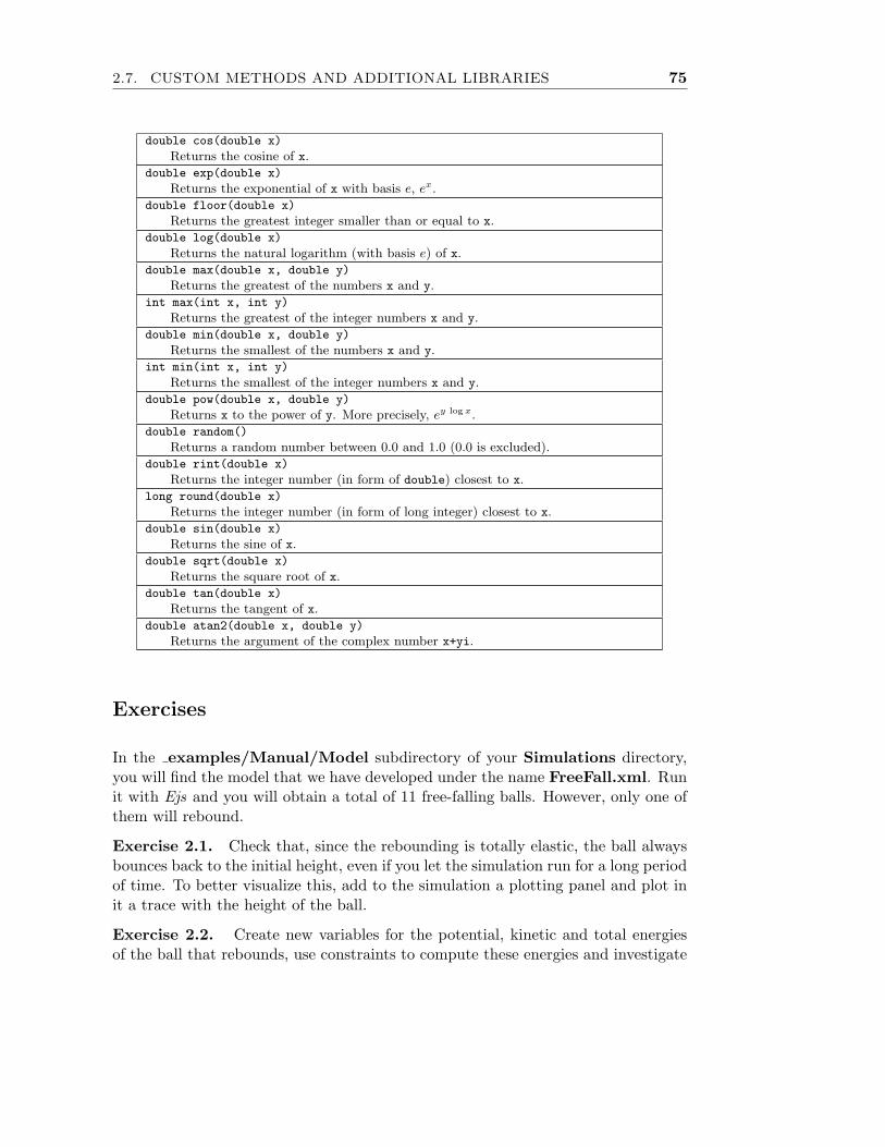
2.7. CUSTOM METHODS AND ADDITIONAL LIBRARIES 75
double cos(double x)
Returns the cosine of x.
double exp(double x)
Returns the exponential of x with basis e, ex.
double floor(double x)
Returns the greatest integer smaller than or equal to x.
double log(double x)
Returns the natural logarithm (with basis e) of x.
double max(double x, double y)
Returns the greatest of the numbers x and y.
int max(int x, int y)
Returns the greatest of the integer numbers x and y.
double min(double x, double y)
Returns the smallest of the numbers x and y.
int min(int x, int y)
Returns the smallest of the integer numbers x and y.
double pow(double x, double y)
Returns x to the power of y. More precisely, ey log x.
double random()
Returns a random number between 0.0 and 1.0 (0.0 is excluded).
double rint(double x)
Returns the integer number (in form of double) closest to x.
long round(double x)
Returns the integer number (in form of long integer) closest to x.
double sin(double x)
Returns the sine of x.
double sqrt(double x)
Returns the square root of x.
double tan(double x)
Returns the tangent of x.
double atan2(double x, double y)
Returns the argument of the complex number x+yi.
Exercises
In the examples/Manual/Model subdirectory of your Simulations directory,you will find the model that we have developed under the name FreeFall.xml. Runit with Ejs and you will obtain a total of 11 free-falling balls. However, only one ofthem will rebound.
Exercise 2.1. Check that, since the rebounding is totally elastic, the ball alwaysbounces back to the initial height, even if you let the simulation run for a long periodof time. To better visualize this, add to the simulation a plotting panel and plot init a trace with the height of the ball.
Exercise 2.2. Create new variables for the potential, kinetic and total energiesof the ball that rebounds, use constraints to compute these energies and investigate

76 CHAPTER 2. CREATING MODELS
how well is the energy preserved.
Exercise 2.3. Try to create an event so that all balls rebound when they reachthe ground, and check again if the energy for the whole set is still preserved.
You will find the solution to these exercises in the cited subdirectory.

CHAPTER 3
Building a view
c©2005 by Francisco Esquembre, September 2005
There is no doubt. The creation of the graphical user interface, or view, isthe part of the simulation that requires a deeper knowledge of advanced program-ming techniques. Usually, the graphical tools provided by a high-level programminglanguage have general applicability and, because of this, no specialization for anyparticular task. Hence, an important technical effort is required to apply these toolsfor a use as specific as the one we want.
However, the current degree of development of computer graphics makes it im-possible to conceive a simulation without an advanced graphic visualization. More-over, if the simulation is to be used for pedagogical purposes, we also need to provideit with a high level of interactivity.
For all these reasons, Easy Java Simulations uses its own powerful library. Alibrary that is specialized in the visualization of scientific processes and data, andwhose use has been simplified as much as possible. This library is based on thestandard Java library called Swing and on the Open Source Physics tools created byWolfgang Christian at Davidson College, 1 but it also adds its own developments.All these sets of Java classes are supported by Java 2 and its plug-ins (version 1.4.2or later), so they can visualized by most modern Web browsers.
1Davidson College is a reputed institution of higher education located in North Carolina, in theUSA. For more information, visit the Web site http://www.opensourcephysics.org.
77

78 CHAPTER 3. BUILDING A VIEW
We will introduce these elements in a simplified, though effective, way that issufficient for our purposes.
3.1 Graphical interfaces
We will create a graphical user interface for our simulation through the constructionof a tree-like structure of selected graphical elements. The process can be comparedto playing with one of these block-construction games.
We call graphical element, or simply element, each of these building blocks, apiece of the interface that occupies an area of the computer screen and that performsa specific task on which this element is specialized on. There are elements of severaltypes: panels, labels, buttons, particles, arrows,. . . and an important part of thegame consists in learning which elements exist and how to use all their possibilities.
The graphical aspect of each element is very much determined by its type. How-ever, each element has a set of inner characteristics, called properties, that we canmodify so that the element looks and behaves according to our needs. These proper-ties are usually set using constant values, but they can also be changed dynamically,thus creating the animations we want. Moreover, some elements have a special typeof properties, called actions, that allow us to define the response of the interface tothe user interaction with these elements (for instance when clicking the mouse ortyping on the keyboard). This provides the required interactivity.
In this chapter we will show the common principles of use of these elements tobuild sophisticated user interfaces, without getting into details about any particulartype of element. The names of the element types are rather descriptive of theirnatural use. However, the best way to learn how to use them is through exam-ples, and consulting the reference pages that you will find in the web server of Ejs,http://fem.um.es/Ejs.
In order to continue with our general description, we need to mention now onlya big classification of the elements in three groups: containers, basic elements anddrawing elements (or drawables).
3.1.1 Containers
A container is a graphical element that can host other elements in its area of thescreen. When this happens, we call the container element the parent, and the elementcontained the child. Since a container can be both parent and child, we can form acomplete hierarchical structure of graphical elements with the form of a tree, whoseroot (which is not really an element) we will refer to as the Simulation View.

3.1. GRAPHICAL INTERFACES 79
As the first child of this root, we will usually create what we call the mainwindow, which is the window that first appears on the computer screen when we runthe simulation as an application, or the one that appears embedded in the HTMLpage, when we run the simulation as an applet.
The elements that need to interact with the rest of windows of the operating systemare containers of a special group generically called windows. There exist two concretetypes of these: frames and dialogs. See the corresponding entry in the reference pages.
There are, in turn, two main families of containers: containers that can hostbasic elements and other containers, and containers for drawing elements.
The first group is used, together with basic elements, to configure the skeletonof the simulation’s view, providing the user with elements to control the simulationand to modify the value of the variables of the model. In this group of containerswe list windows, toolbars, standard panels, split panels, and tabbed panels.
The second group is used, together with drawing elements, to create animationsor to visualize graphs of the simulated phenomenon. The group comprises two-dimensional drawing panels, plotting panels (2D panels with coordinate axes), andthree-dimensional drawing panels.
The Layout property
Maybe the most important property of a container of the first group mentionedabove is the layout. When an element is added to a container, the parent assigns tothe child appropriated position and size according to the available space, the childrequirements, and of, so to call it, the container’s own policy of space distribution orlayout. Some layouts allow the child to choose its relative position inside the parent,but in most of them position is a consequence of the “order of birth” of the child.
Containers of the second group mentioned above define their own system of coordinatesthat allows their children (which must be drawing elements) to specify their positionusing user coordinates. For this reasons these containers have no layout property.
We need to admit that the first time a new user is faced with layouts, they alwaysseem an unnecessary nuisance: “Why can’t I just place a child exactly here with afixed, prescribed size?”. The answer appears naturally when the user resizes or addsnew elements to a view (which happens rather frequently). Then, the original sizesand positions are almost always inadequate. Using layout policies in the containersof our view instructs them how to proceed in these situations to distribute the newavailable space in a form that is congruent with the previous one. After a bit ofpractice, the use of layout policies becomes not only simple, but it even appears asthe natural way of designing the interface.

80 CHAPTER 3. BUILDING A VIEW
Even when Java provides a great deal of layout policies (and allows the program-mer to create new ones), we will only use the following layouts:
Flow It distributes the children in one row, from left to right, in a way muchsimilar to how words appear in a paragraph. Children can be left, right, orcenter justified.
Border Maybe the most frequently used layout, distributes its children in one offive possible locations: up, down, left, right and center, from which each childmust choose a different one.
Grid The second most popular, places its children in a rectangular table with asmany equally sized rows as columns as indicated.
Horizontal box This distribution works similarly to a grid with only one row, ifonly it doesn’t force all its children to have the same size.
Vertical box This works as a single-columned grid, with children of possible dif-ferent height.
For all these layouts it is possible to provide two additional parameters that indicatehow much it should separate children among them, both horizontal and vertically.
3.1.2 Basic elements
The group of basic elements is made of a set of interface elements that can be usedto decorate the view, to visualize and edit variables of the model, and also to invokecontrol actions (that is, methods that manipulate the model).
You will find the elements in this group rather familiar, since they appear inpractically all computer programs that you may use. The group includes labels,buttons, sliders, text fields, etc. These basic elements can be added to any of thecontainers of the first group of Subsection 3.1.1, but can not host other elements.That is, they are not containers themselves.
There are two exceptions to this assertion. The tab of basic elements labeled “Menu”contains all the elements you need to create menus for your view. In this tab, you willalso find the “MenuBar” and “Menu” types, which are, in purity, containers.
3.1.3 Drawing elements
The set of drawing elements is one of the main contributions to Ejs of the OpenSource Physics project. It consists of a set of view elements that can be included

3.2. ASSOCIATION BETWEEN VARIABLES AND PROPERTIES 81
in dedicated containers (these of the second group of Subsection 3.1.1) to createanimated graphics that visualize the different states of the model.
These animated graphics can range from the simple to the sophisticated, and bedrawn in two or three dimensions, including particles, arrows, springs, GIF images,polygons, vector fields, contour maps, three-dimensional bodies, and even more.
3.1.4 Creation of the view
Thus, finally, the creation of the view consists in generating a structure, or tree, ofelements that serves our purposes. This tree must include elements that visualizethe state of the model, elements for the interaction of the user with the simulation,and containers that host all other elements.
3.2 Association between variables and properties
As we mentioned above, graphical elements have certain internal values, which wecall properties, that can be customized to make the element behave in a particularway.
Since we are mainly interested in the dynamical visualization of the state ofour models and in providing the required interactivity to our simulations, whatwe really want is to use our model variables as value for some of the propertiesand as arguments for the actions of the view elements. This process, which we callassociating or linking objects of the model with properties of the view, is what turnsour simulation into a really dynamic, interactive application.
In traditional programming, these links are created using calls to predefinedmethods of the graphic components. The main problem is that, since the standardgraphical library was created, as we said before, to support any general use, themethods we are talking about are of rather low level, which demands high technicalskills from the user.
Easy Java Simulations dramatically simplifies this situation, in the first place,by adapting the graphical elements it offers to the use we expect of them, but alsoallowing us to establish the required links through a simple process of edition ofthe properties of each element. In this process, the only thing we need to do isto indicate in the so-called panel of properties of the element, which object of themodel must be associated to which property. In most occasions this can simply bedone by choosing from a list of possible values the one we want for the link. Withthis information, Ejs will generate the code required to ensure that, later, when thesimulation runs, all the necessary calls to the low-level routines are done correctlyfor this connection between model and view to work properly.
82 CHAPTER 3. BUILDING A VIEW
Linking is a two-way, dynamic process. With this we mean that at any timeduring the execution of the simulation, the element property will hold the value ofthe model variable to which it has been associated. Thus, if the evolution of themodel changes this value, the element will automatically reflect the change. Butalso, in a reciprocal way, if a property changes as result of the interaction of theuser with the view (by introducing a value, moving a slider,. . . ), the variable of themodel will immediately receive the new input value.
The configuration of the so-called action properties of the elements with codeexpressions that modify model variables or that use model methods, allows in turnthe control of the simulation by the user, who will be able to execute the codeinteractively (by clicking a button for instance).
This mechanism turns out to be, as we will see, both simple and effective tocreate advanced user interfaces for our simulations.
3.3 How a simulation runs
Once we have established the associations between model and view that we need, thesimulation will be ready to be run. With this information, Ejs generates the codenecessary for the correct behavior of the future simulation. We can now completethe description of the execution of a simulation generated by Ejs that we started inSubsection 2.1.4.
When a simulation runs, this is exactly what takes place behind the scenes:
1. The variables are created and their values set according to what the initializa-tion states.
2. The constraint equations are evaluated, since the initial value of some variablesmay depend on the initial values of others.
3. The view of the simulation is created and it appears on the computer screen.All the associations that we may have created are used to instruct the viewelements how to correctly visualize the state of the model, and how to properlyrespond to user interaction.
At this moment, the model is found to be in its initial state, the view reflectsthis state, and the simulation waits until an evolution step takes place or theuser interacts with it.
4. In the first case, the evolution equations are evaluated and, immediately after,the constraints. A new state of the model at a new instant of time is thenreached. The view is then updated through the links with the model.

3.4. INTERFACE OF EASY JAVA SIMULATIONS FOR THE VIEW 83
5. In the second case, if the user changes a variable associated to a model variable,this is consequently modified, or, if the user invokes a control action, thecorresponding code is executed. In any of both cases, constraint equations areevaluated immediately after. We then obtain a new state of the model at thesame instant of time and the view is updated using the links with the model.
3.4 Interface of Easy Java Simulations for the view
The interface of Ejs for this panel is shown in Figure 3.1.
Figure 3.1. Ejs interface for the view.
The left-hand side of the working area of Ejs is now occupied by a panel thatdisplays the (initially empty) tree of elements that forms the view. The node calledSimulation View shown corresponds to the root of this tree. When we add newelements to our view, this panel will be displaying them reflecting the correspondingtree-form structure.
The right-hand side of the working area displays a panel with three sections invertical. Each section contains a set of icons, grouped according to the classificationthat we did in Section 3.1. Each icon represents one of the types of elements thatwe can use to create the view. Whenever the number of icons is high, the sectiongroups them in subpanels with identification tabs.
Figure 3.2. Detail of the infor-mation for the type “Button”.
You can explore the icons by placing the mouseon top of each of them and waiting, without clicking,for a second, until a small tip appears indicatingthe name of the type and a short description of itsfunction. See Figure 3.2.

84 CHAPTER 3. BUILDING A VIEW
3.4.1 Types of elements
We make in this paragraph a short introduction of the main types of elements offeredby Ejs. Please notice that we don’t cover all the types, but leave the complete listfor the reference you will find on the Web pages for Ejs.
Containers
Frame The main characteristic of frames is that they know how to deal withthe windows environment of your operating system. In particular they can beminimized and maximized in the usual way. Each view must have at least afirst element of this type in which to place other elements, we will call thisfirst frame the main window.
Dialog Window dialogs, or simply dialogs, are also independent windows, but,differently to frames, they can not be minimized (though they can be hidden).Besides this, they have the ability to always display on top of the frame thatprecedes them in the tree of elements, which can be useful in simulations withmore than one windows.
Panel Panels are the most basic type of container, and hence the first candi-dates to use when we just want to group other elements.
SplitPanel This is a container that has two clearly separated resizable areas.
TabbedPanel This is a container that displays only one of its several childrenat a time, organizing them using tabs.
DrawingPanel This is a basic container for two-dimensional drawings.
PlottingPanel Similar to the previous one, it adds a system of cartesian orpolar axes.
DrawingPanel3D This is a three-dimensional version of DrawingPanel.
Basic elements
Button Element in form of a button, used to invoke actions.
CheckBox A button that allows to select one of two possible boolean states,true or false.

3.4. INTERFACE OF EASY JAVA SIMULATIONS FOR THE VIEW 85
RadioButton Similar to the previous one, it has the particularity that it worksin group with all other radio buttons in the same container. Then, selectingany of the buttons, automatically unselects all the others.
ComboBox An element in form of a list that allows selecting one of severaloptions.
Slider Allows to visualize and modify a numerical value, within a given range,in a graphical way .
NumberField Allows to visualize and modify a numerical value using thekeyboard.
TextField Allows to visualize and modify a value of type String using thekeyboard.
Label Used to write labels for decorative or informational purposes.
Drawables
Particle Draws an interactive ellipse or rectangle in a given position and witha given size.
Arrow Draws an interactive arrow or segment.
Spring Draws an interactive spring.
Image Draws an interactive GIF image or animated image.
Text Draws an interactive text.
Trace Draws a polygonal line created by accumulation of successive points,thus forming the trace of a motion.
Sets Draw sets with several of the corresponding elements.
Polygon Draws a polygonal line from the coordinates of its vertex.
Surface Draws a parametric surface from the coordinates of the points of aregular grid on the surface. There exist particular elements for some surfacessuch as spheres, cylinders and other bodies.
ContourPlot Draws a contour map of a scalar field.

86 CHAPTER 3. BUILDING A VIEW
GridPlot Alternative (simpler) visualization of a scalar field.
VectorField Visualizes a vector field.
SurfacePlot Draws in 3D the graph of a scalar field.
3.4.2 Adding elements to the view
The creation of new view elements follows the next four steps.
Choosing the type of element to create
For this, just click on the icon for the type you want to create. When you do this,the background of the icon will change color, indicating that it has been selected.Moreover, the cursor will change to a hand when you are on top of an icon, and toa magic wand when the icon is selected. See Figure 3.3.
Figure 3.3. Choosing the icon for an element of type “Frame”.
Choosing the parent for the new element
That is, the container that will host the new element. For this, click with the magicwand on a container element (that you created previously) in the tree of elements.If the new element is a frame or a dialog, which require no parent, you need to clickdirectly on the root node, the one called “Simulation View”. This is precisely thecase that Figure 3.4 illustrates.
Choosing a name for the new element
Each element needs a name for it. Ejs will propose one based on the type of elementthat you are creating (see Figure 3.5), you can either accept it or choose a morerepresentative name according to the role of the element in the interface. Recall,however, the naming conventions that we established in Subsection 2.3.5.
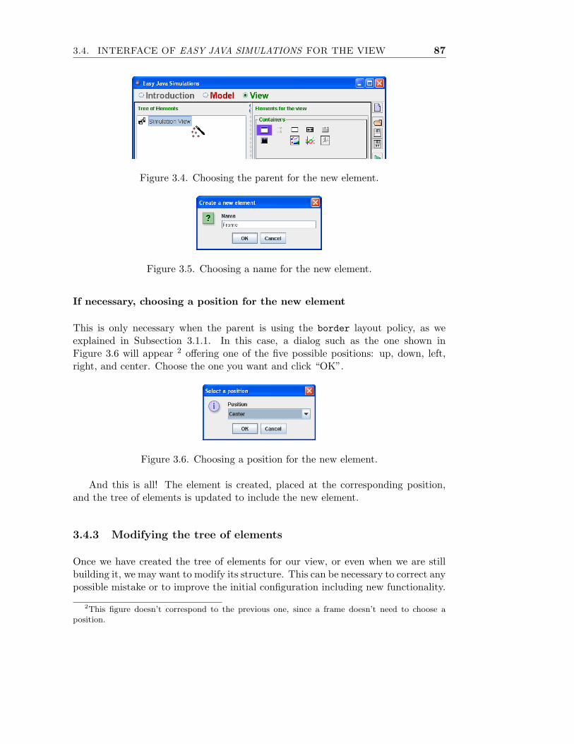
3.4. INTERFACE OF EASY JAVA SIMULATIONS FOR THE VIEW 87
Figure 3.4. Choosing the parent for the new element.
Figure 3.5. Choosing a name for the new element.
If necessary, choosing a position for the new element
This is only necessary when the parent is using the border layout policy, as weexplained in Subsection 3.1.1. In this case, a dialog such as the one shown inFigure 3.6 will appear 2 offering one of the five possible positions: up, down, left,right, and center. Choose the one you want and click “OK”.
Figure 3.6. Choosing a position for the new element.
And this is all! The element is created, placed at the corresponding position,and the tree of elements is updated to include the new element.
3.4.3 Modifying the tree of elements
Once we have created the tree of elements for our view, or even when we are stillbuilding it, we may want to modify its structure. This can be necessary to correct anypossible mistake or to improve the initial configuration including new functionality.
2This figure doesn’t correspond to the previous one, since a frame doesn’t need to choose aposition.

88 CHAPTER 3. BUILDING A VIEW
For this, each element in the tree has a popup menu that can be invoked byright-clicking with the mouse on the element. Figure 3.7 shows the view of theexample of Section 3.6 with the popup menu for one of its elements. This menu canvary a little bit depending on the precise element that we choose, but the imageshows a typical case. 3
Figure 3.7. Popup menu for a new element.
The first entry in the menu is the one most frequently used. (Actually, it is sofrequently used, that Ejs provides a shortcut for it. If you double-click on an elementon the tree, this option is selected –even when the popup menu is not shown.) Thisoption allows us to modify the properties of the element and will be described indetail in the next section.
The second option allows us to change the name of the element, and the thirdone, its parent. In both cases, a dialog window will appear to allow us to choose adifferent name or parent, respectively.
In a second group, there appear the options that allow us to change the positionof the element inside its parent. A label tells us the current position of the element.This position may have been chosen by ourselves (if the layout policy of the parentis border) or be “imposed” by the parent according to the order of creation of itschildren. In the first case, to change the position we will need to use the optioncalled “Change position”. In the second case, this option will be disabled and wewill need to use the other two options to change the relative order of the elementwith respect to its “brothers”. The tree of elements will always reflect the actualorder.
There exist a final group of options, cautiously separated from the others, that
3Because of its special nature, the popup menu for the root of the tree contains only the “Paste”option.

3.5. EDITING PROPERTIES 89
is used to cut, copy, paste, and remove the element. Be careful, Ejs will not ask forconfirmation if you choose any of these options! (And there is no “Undo”, either.)
A special option, only for frames
A special option, that only appears in menus for elements of type “Frame”, is theone called “Main Window”. Perhaps you noticed that, although the icon for the“Frame” class is , the icon that appears associated to the first of the frames of atree looks slightly different, . This has a special meaning.
Figure 3.8. Detail of the“Main Window” option.
When the simulation is run in form of an applet,that is, inside an HTML page (see Chapter 4), oneof the windows of the view appears inside this page,while all others will appear separately. We call thiswindow the main window. A second property ofthis window is that, when the simulation runs as anindependent application, closing the main windowwill end the simulation.
The icon identifies this window and the option“Main Window” of the menu for a frame element(see Figure 3.8) will allow you to choose which ofthe frames (if there are more than one) will be themain window.
3.5 Editing properties
When we create new elements, they appear with default values for their properties.As we said already, properties are internal values that determine how the elementslook and behave. We can modify these properties using the panel for the edition ofproperties of each element. For this, we need to select the first of the options of thepopup menu for the element, “Properties”, or double-click on the element’s node inthe tree of elements. Figure 3.9 shows the panel of properties for an element of theclass “Button”.
3.5.1 Choosing constant values
The way to modify a property is, in principle, straightforward: you just need to clickon the corresponding entry field and type the desired value for the property.
However, it is sometimes difficult to remember the correct format for some ofthese values, specially if the property is one of the technical ones (such as color,
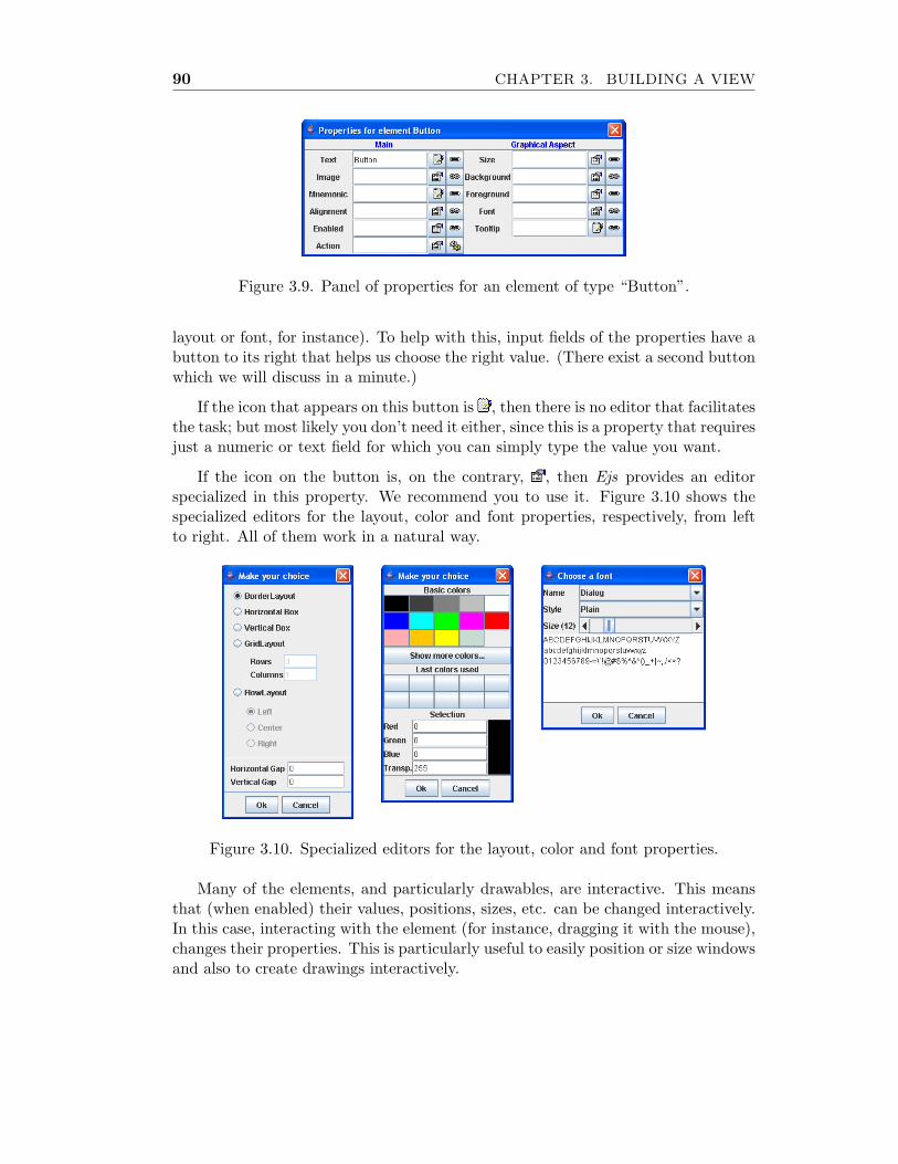
90 CHAPTER 3. BUILDING A VIEW
Figure 3.9. Panel of properties for an element of type “Button”.
layout or font, for instance). To help with this, input fields of the properties have abutton to its right that helps us choose the right value. (There exist a second buttonwhich we will discuss in a minute.)
If the icon that appears on this button is , then there is no editor that facilitatesthe task; but most likely you don’t need it either, since this is a property that requiresjust a numeric or text field for which you can simply type the value you want.
If the icon on the button is, on the contrary, , then Ejs provides an editorspecialized in this property. We recommend you to use it. Figure 3.10 shows thespecialized editors for the layout, color and font properties, respectively, from leftto right. All of them work in a natural way.
Figure 3.10. Specialized editors for the layout, color and font properties.
Many of the elements, and particularly drawables, are interactive. This meansthat (when enabled) their values, positions, sizes, etc. can be changed interactively.In this case, interacting with the element (for instance, dragging it with the mouse),changes their properties. This is particularly useful to easily position or size windowsand also to create drawings interactively.

3.5. EDITING PROPERTIES 91
3.5.2 Association with variables and use of methods of the model
As we said in Section 3.2, properties can also be set through their association withvariables of the model, with Java expressions that use them, or, in the case of actionproperties, using Java sentences that involve variables and methods from the model.These associations are the essence of the interactivity of the simulation.
This process is also easy to accomplish. You just need to type the variable orthe Java expression in the corresponding property field.
To facilitate this task, though, there exists a second column of buttons, one foreach property, in the table of properties. These buttons display one of the two icons:
or .
If you click on a button with the icon , a dialog window will appear, listingall the variables of the model that can be associated to the property that you areediting. It is possible that not all variables of the model are listed, since, for instance,a property of numeric type can not be associated to a variable of type String.Choose among the offered variables the one you want and click “Ok”.
Figure 3.11. List of all possibleboolean variables.
Thus, for instance, if we click on this secondbutton for the property “Enabled” of the panel inFigure 3.9, whose value needs a boolean, we willobtain a list of all boolean variables of the model.If our model only defines the boolean isVisible,we will obtain the list of Figure 3.11.
Observe that, as this example shows, this listcan also include, besides the variables that ourmodel define, some variables and methods prede-fined by Ejs. These are displayed in a differentcolor. (In this concrete example, isPlaying is a boolean variable that is true if theevolution of the simulation is playing and false if it is not. The variable isPausedis the negation of isPlaying. Finally, isApplet() is a method that returns a trueboolean if the simulation runs as an applet, and false if it runs as an application.)
Any connection between a model variable and an element’s property works right fromthe start. With this we mean that the connection will of course work when the simula-tion runs, but also under Ejs. You can appreciate that properties associated to modelvariables use the values of the variables specified in the corresponding “Value” cells ofthe table of variables. If you change any of these values, the view will readily reflectthis change.
But the connection also works the other way round. If you interact with a view elementand change one of its connected properties, the value in the “Value” cell will be updatedtoo. This can be useful to set initial conditions of your simulation in an interactive

92 CHAPTER 3. BUILDING A VIEW
way.
There is only one exception for this rule. If the “Value” column for the variable affectedby this interaction contains an expression (instead of a constant value), Ejs will askyou for confirmation before replacing the expression with the constant value obtainedfrom the interaction.
Finally, if the button on the second column exhibits the icon , this tells us thatthe property is one of the so-called action properties. That is, that it can be usedto define an action that will be invoked when the user interacts with the element ina given way (which depends on the type of element and on the property chosen).
If we click on a button with this icon, a dialog will display all custom methodsdefined by the model (see Subsection 2.7.1), together with some of the predefinedmethods defined by Ejs (Subsection 2.7.3) in different color, to help us choose oneof them. Thus, if the model defines the methods action1() and action2(), andwe click on the second button of the property “Action” of Figure 3.9, the result willbe like in Figure 3.12.
Figure 3.12. List of model methods for an action.
The action can consist in a simple call to any of the model or predefined methodsor can include directly Java sentences that perform the action. It can even consistof a combination of both. Clicking on the first icon to the right of the input field ofan action property brings in a simple editor specialized on edition of Java code thatwill help us write our code more comfortably.
3.5.3 The color codes of the property fields
Property fields, that is, the text fields where you type in the values for the properties,implement a simple color code.

3.5. EDITING PROPERTIES 93
Fields for properties that are not action properties are always displayed in whitebackground. When you edit them, however, their background turns yellow, so towarn you that you are modifying them, but that the value has not yet been appliedto the property. Only when you hit return, thus accepting the value, gets thebackground white again. For this reason, don’t leave yellow backgrounds behind!
Actions properties are different. Since their values are only really used whenthe simulation is generated, whatever you type in the corresponding field is imme-diately valid. For this reason, their background never turns yellow. However, since(differently to all other properties) the code you write for an action property canspan more than one line, whenever this happens, the background of the field changescolor to a sort of dim green, to warn you that there are possibly more lines thanthose you can see in the field. You can therefore leave green backgrounds behind.And we recommend that you always use the editor provided to view and modify thecorresponding code.
3.5.4 Special case: properties of type String
When we assign manually the value of a property, it is possible that there exist asmall ambiguity in the case of properties that require text values. Indeed, supposethat we edit the “Title” property for a frame and write in it the value “graph”,and suppose that we have defined a variable of String type in our model which iscalled precisely graph. In this situation, what should Ejs do? Should it use the text“graph” for the title of the frame, or should it use the value of the variable graphfor it?
Even if you think that the example is a bit forced, it sometimes happens. Inprinciple, Ejs will almost always do what we expect it to do, but if this is not thecase, we need to solve the problem either changing the name of the variable of themodel or using the following additional rules:
• If we write the text between quotes (simple or double), we force the elementto use the text literally. In our example, we should write either ‘graph’ or“graph”.
• If we write the text between per cent characters, %, we will force the elementto consider the text as the name of a variable. In our example, we would needto write %graph%.
The use of these rules helps Ejs to completely solve the ambiguity. The specializededitors make automatic use of these rules.

94 CHAPTER 3. BUILDING A VIEW
3.6 Learning more about view elements
Well, this is actually all you need to know, in general, about building views with EasyJava Simulations! Of course, you will need to learn more about the different typesof elements that exist and how they can be used, together with the possible valuesof their properties, to achieve several visualizations and interactive capabilities. Butthis is learned in a more effective and nicer way through examples.
For this reason, we end here the general description and refer to the examplesdistributed with Ejs to see practical cases of use. Recall also that on the Web serverof Ejs you will find a set of HTML pages describing all the elements that Ejs offers.Do not hesitate to explore these pages on your own to learn more about a given typeof element.
We end this chapter with a concrete example of use that also has interest initself. Although, usually, the model of the simulation contains the greatest part ofits dynamic information, the view we build with Ejs can have its own life by itself.The degree of utility of it will depend on the capabilities of the graphical elementsthat we use to build it.
We will illustrate this life of the view by constructing a simple function plotterusing an element called “AnalyticCurve” as the main component of the view. Thisplotter will visualize the graph of a function f(x) which depends on three parameters.To reinforce all that we explained in this chapter, we will guide you through all theprocess.
Main window
Let’s start with an empty simulation. For this, click the “New” icon, , in Ejstaskbar; this will delete any previous simulation.
Now, choose the panel for the “View” and create an element of type “Frame”.For this, click on the first icon of the subpanel for containers, , and click with themagic wand the root node of the tree of elements, the one called Simulation View.Accept for the new element the proposed name Frame. The result will look as inFigure 3.13.
Now edit the properties of the frame to change its title to Function plotter.The panel of properties will look as in Figure 3.14.
Notice that, as we said in Subsection 3.5.3, when you modify a field, it takes a yellowbackground (except for action properties). Don’t forget to hit the return key of yourkeyboard to accept the value, so that the background looks white again. Only thenwill the change really affect the element’s property.

3.6. LEARNING MORE ABOUT VIEW ELEMENTS 95
Figure 3.13. Initial tree of elements and the non-edited frame.
For the figures of this chapter, though, we have left the fields we edited with the yellowbackground, so that you can easily distinguish which fields have been modified.
Figure 3.14. Panel of properties for the main window.
In this new frame, which has by default a border layout, we will create twochildren. The one at the center will be a plotting panel and the one in the Downposition will hold the controls for the parameters of the function.
Plotting panel
Select the icon for the type “PlottingPanel”, , and click with the magic wand onour frame. Accept the proposed name and place the new panel on its parent’s center.A big panel with axes will be created and will occupy the interior of the frame. Editthe properties of the panel to change its “Title” to Graph of the function, its“Title X” to x, and its “Title Y” to f(x).

96 CHAPTER 3. BUILDING A VIEW
Now, from the subpanel of drawable elements, select the tab header labeled as“Bodies”. From the icons in the corresponding subpanel, select the one for the type“AnalyticCurve”, and create an element of this type as child of the plotting panelwe created above. The name suggested by Ejs is acceptable.
The element “AnalyticCurve” creates the graph of a curve in space (that is a set ofpoints (x,y,z)) from the analytic formula provided to compute these points. In thissense, it is one of the elements offered by Ejs that incorporates more computationalpower independently of the model. For more information about the element “Analyt-icCurve” consult its reference page.
Edit the properties of this new element as shown in Figure 3.15. With this weare asking the element to display a blue colored graph made of 50 points withcoordinates (x,%Fx%), where these expressions for the X and Y coordinates areinterpreted as functions of the “Variable” x which varies in the interval from 0 to2*π. This finally results in the graph of the function of variable x, given by theexpression contained in the text variable Fx.
Figure 3.15. Panel of properties for the analytic curve.
The tree of elements for our simulation will reflect the changes and will nowlook as Figure 3.16 shows. You will notice that the plotting panel now displays ahorizontal blue line. This is the graph of the function we are plotting. The reasonthat it is just a horizontal line is that we haven’t yet defined the text variable Fx.
Control panel
In order to define this variable, as well as other parameters that may help definingthe function, we will create a panel that will hold several controls. In the first place,select the “Panel” icon, , in the panel of containers, and click with the magicwand on Frame to create an element of type “Panel” as second child of it. The name

3.6. LEARNING MORE ABOUT VIEW ELEMENTS 97
Figure 3.16. Tree of elements (under construction) and panel displaying the graph.
suggested by Ejs, Panel, is acceptable. Place the panel in the “Down” position ofthe frame. We won’t need to edit the properties of this element.
Notice that, although the panel appears in the tree of elements, it is not visiblein the frame itself. This is because the panel is still empty, and it therefore doesn’tclaim any screen space from its parent. As soon as we add children that do claimfor space, the situation will change.
Figure 3.17. Tree of elementsunder construction.
The two children that we will add to the panelwill be again elements of type “Panel”. Since thisicon is probably still selected, create two new ele-ments of this type as children of Panel with namesPanelFx and PanelParameters. Place them in thepositions “Up” and “Center”, respectively.
Even when the frame still looks the same, thetree of elements should look like in Figure 3.17.
We will only need to modify the layout propertyof the element PanelParameters so that it takesthe form of a grid with 0 rows and 1 column (that is, a column as long as needed).For this type grid:0,1 in the “Layout” text field of the panel of properties forPanelParameters, or use the specialized editor for layouts by clicking the auxiliaryedition button, , for this property.
Now, create a label, , on the left side of the panel PanelFx (the proposed namewill do) and edit its “Text” property typing f(x)= in the corresponding field. In thecenter of this panel, create a text field, , called FieldFx and edit its properties asin Figure 3.18. With this we are instructing the text field to associate whatever we

98 CHAPTER 3. BUILDING A VIEW
write on it with the variable Fx. We also give an initial value to this variable usingthe property called “Value”, typing in it the function we want to visualize, usingthe correct Java syntax: a*Math.sin(b*x+c).
Figure 3.18. Properties for FieldFx.
Observe that the function we are suggesting (of course, you can use any other one)contains three variables a, b and c, that have not been defined (x in the expressionrefers to the independent variable with respect to which the graph is built). We willneed to give non-zero values to these parameters so that the curve is interesting.
We will do this using the PanelParameters panel. Choose now the element oftype “Slider”, , and create three such sliders in this panel with names SliderA,SliderB and SliderC. Since the layout of the parent places the elements in formof a column, you will not be prompted to choose the position for the new elements.This takes us to the final structure of the tree of elements for our view, which youcan see in the left image of Figure 3.19.
We will still need to customize the sliders, but since the creation of new elementsis limiting the available space for the original plot (and the customization we foreseefor the sliders will make these even bigger), we will resize the main window. Forthis, edit again the properties for Frame and change its size to 300,500. The finalresult should look as in the right-hand side image of Figure 3.19.
To finish the example, edit first the properties of SliderA as in Figure 3.20.The most important fact of this customization is that the slider will allow us tomodify the variable a in a range from 0.0 to 5.0, giving to a an initial value of1.0. (The value a=0.00 for the property “Format” doesn’t assign to a any value, itjust indicates how the value of a should be displayed; in this case, with two decimalfigures.)
Finally, edit the properties of SliderB exactly as those above but changing a byb, and those of SliderC as shown in Figure 3.21.
Using the plotter
The example is now complete. (Don’t forget to save it to disk!). Now, if you run it,the graph displayed in the upper panel will correspond to the sine function. Play

3.6. LEARNING MORE ABOUT VIEW ELEMENTS 99
Figure 3.19. Final tree of elements (left) and frame still under construction.
with the sliders for a, b, and c to see the effect of each of the parameters on thegraph of the curve. You can also introduce different expressions in the text field forthe function to plot (respecting the correct Java syntax) which can or can not usethe parameters. See Figure 3.22.
We would like to emphasize that this example shows how the view can have alife on its own, independently of the model. In our example, in fact, we createdno model at all, and all the variables have been autonomously created by the view.However, if you now create the variables a, b, and c in the table of variables ofthe model and modify them in the body of it, the variables of the view will always
Figure 3.20. Properties for SliderA.

100 CHAPTER 3. BUILDING A VIEW
Figure 3.21. Properties for SliderC.
use the corresponding values, thus automatically establishing a connection betweenthem thanks to their common name.
A corollary of this is that we can create simulations in which the view definesand uses variables that don’t need to have been declared by the model. However,these variables are usually of auxiliary nature; any really interesting behavior willundoubtedly be based in the definition and modification of variables in the model.
Exercises
The subdirectory examples/Manual/View of your Simulations directory con-tains the complete example of this chapter under the name FunctionPlotter.xml.
Exercise 3.1. Create a simple model for the example of Section 3.6 that definesthe variables a, b, and c, and such that it gives them an interesting use. For instance,one in which the evolution consists in increasing 20 times per second the variable cin, say, 0.1 units. The result must be a traveling wave that moves to the left.
Exercise 3.2. If you look again, in Figure 3.15, at the table of properties ofthe element AnalyticCurve, you will observe that you can provide an analyticexpression for the three coordinates X, Y, and Z. This means that you can easilycreate a plotter for parametric curves. That is, for curves in the plane of the form(x(t), y(t)) (or of the form (x(t), y(t), z(t)) for curves in space).
Create a plotter for planar (or spatial, if you prefer) parametric curves startingfrom the example in Section 3.6.
Exercise 3.3. If you feel inclined to work in three dimensions, create a plotter for
functions of two variables f(x, y) using the element “AnalyticSurface”, . (You willneed to use “DrawingPanel3D” instead of the two-dimensional “PlottingPanel”.)
Exercise 3.4. If you still feel inclined to it, create a plotter for parametric surfaces(x(u, v), y(u, v), z(u, v)) in general, and use it to display different surfaces such as a

3.6. LEARNING MORE ABOUT VIEW ELEMENTS 101
Figure 3.22. Graphs of two functions using our plotter.
sphere, a cylinder, a hyperbolic paraboloid, a Mobius band, etc.
Exercise 3.5. Create a model for the simulations of the two previous exercisesthat allows you to animate the resulting graphs to simulate waves in two and threedimensions, or dynamic changes in the surfaces.
You will find the solution to some of these exercises in the directory cited above.


CHAPTER 4
Using the simulation
c©2005 by Francisco Esquembre, September 2005
As soon as you create your own simulations, you will most likely be interestedin using them in your lectures or sharing them with your colleagues. You may evenwant to publish them on the Internet! This chapter will teach you how to do this.
4.1 Using your simulations
Simulations created with Easy Java Simulations can be run in three different forms.The first form is using Ejs itself, in a way similar to what we did in Chapter 1.The second form consists in executing the simulation as an applet, using a Webbrowser. The third form consists in running the simulation as an independent Javaapplication.
The first option has an important pedagogical advantage: the user can see howthe simulation was created, learning from the knowledge that you used when buildingthe simulation. This offers, in our opinion, a great added value. But we must admitthat it also has a small inconvenience: the user must have Ejs installed in hercomputer and need to know how to use it, at least in a basic way.
Even when we may agree that Ejs is a wonderful tool1 which, furthermore, is freefor distribution, you, most likely, don’t want that all your users need to install it and
1We, proud authors, do think so! ¨
103

104 CHAPTER 4. USING THE SIMULATION
learn its use just to be able to run a simulation. Fortunately, simulations created withEjs are, once generated, independent from it. Thus, when this situation appears,we recommend to run the simulation in form of Java applet.
A Java applet is a special type of application that has been designed to be runinside a Web browser. The browser loads an HTML file (HTML stands for HyperText Markup Language) which indicates the browser that it must run the requiredapplet inside its own window. This HTML file and the corresponding applet can belocated on your hard disk or in an Internet location and be served to you throughthe network by a so-called Web server, a computer that runs this special service.
A second reason for this recommendation is that the HTML pages that Ejscreates for the applet can be modified so that to complete the narrative that youincluded in the introduction for the simulation. This allows you to create a completeset of pedagogical units that can be used for your teaching duties. Finally, it isalso possible to include in this narrative controls of a simple script language calledJavaScript that integrate the text with the control of the simulation in a very naturalway. 2
The third form of execution of simulations, as independent Java applications,is also possible without installing Ejs. The user only needs to have a Java VirtualMachine (such as that provided by the Java Runtime Environment) installed in hercomputer. Simulations running as applications can be installed on the hard disk,or can also be served through the network by a Web server using Java Web Starttechnology. We describe this technology further below.
An important reason to use this third form is when you want to run (independently ofEjs) a simulation that saves data to the hard disk. As we explained in Subsection 2.7.3,simulations created with Ejs can, if the author decided to offer this possibility, readdata from the hard disk or from the Web, independently of the form in which they run.
However, to first create this data, it is necessary to be able to write on disk, which, forsecurity reasons included in Web browsers, is only possible when you run the simulationfrom within Ejs or as an independent application. (In this second case, the applicationsmust be installed in your hard disk. Java Web Start includes a security system similarto that of applets.)
Distribution of a simulation within Ejs
Distributing a simulation created with Ejs for other people to use it with Ejs isimmediate: you just need to provide your user with the simulation file (the one with
2Although it is out of the scope of this manual the complete description of the format of HTMLfiles and of JavaScript, we will provide a basic introduction which is enough to illustrate their usewith Ejs. You can surely find appropriated books on these topics in your usual technical bookstore.
4.2. FILES GENERATED FOR A SIMULATION 105
extension .xml) together with any auxiliary files, such as images or data, that thesimulation may need.
Hence, for instance, for the simulation of Chapter 1 (which uses no additionaldata file), you’ll only need to provide the file called Spring.xml. Your user willneed to know how to start Ejs, load this file, and work with it, similarly to whatyou did in that chapter.
The rest of this chapter is devoted to explain how to run the simulations inany of the other two forms, as well as to teach you how to correctly distribute thesimulations created with Ejs independently from it.
Copyright and disclaimer
This is a good moment to remind you of the copyright restrictions about Easy JavaSimulations and the simulations created with it. Good news! There are very minorrestrictions. Here is a copy of the conditions of use of Ejs.
Easy Java Simulations is the exclusive copyright of its author, Francisco Esquembre,who distributes it under a GNU GPL license. Examples of simulations included withEjs are copyright of their authors.
Easy Java Simulations and its JAR library files can be copied and distributed withoutlimit and without previous permission, provided this is done for non-commercial reasons.In any case, the reference to the author that appears in the program must always bepreserved.
Authors can distribute any simulation that they create using Easy Java Simulations,provided a reference to this fact is included, together with a link to the official Web pagefor Easy Java Simulations, http://fem.um.es/Ejs. It is not necessary to include thisin all pages with a simulation on it of an educational unit; including a reference for thewhole set in a clearly visible place will suffice.
Any publication that results from the use of Easy Java Simulations must refer to theofficial Web server for Ejs, http://fem.um.es/Ejs.
Finally, a short disclaimer. Although Ejs has gone through a long sequence of tests,Easy Java Simulations is provided ’as is’. That is, we refuse any responsibility forany problem or damage caused by the use of the software.
4.2 Files generated for a simulation
We need to describe briefly what files are created when we run a simulation withEjs, right before the simulation actually appears on the computer screen. We willillustrate the process using the example of Chapter 1.

106 CHAPTER 4. USING THE SIMULATION
Recall that the name of that example was Spring.xml. After running theexample you will find the following files in your Simulations directory:
Spring.java and SpringApplet.java These are the files that contain the Javacode for the simulation and its applet. Recall that Ejs is, after all, a codegenerator: it collects all the information that you provide to it in its differentpanels and generates the necessary Java code.
There is a long way from the information you provide to the final result, but Ejstakes care of everything automatically. The Java code contained in these filesunveils some of our secrets and you can inspect it if you want. However, onlya Java programmer with particular needs would be interested in modifyingthe code directly. You can therefore, after all, safely instruct Ejs to deleteautomatically these files after using them.
Actually, it is very likely that you don’t find these files in your Simulations directory, tobegin with. This is because Ejs is configured by default to delete them after generatingthe simulation. We mention them here because they are important to understand howEjs works. See Subsection 4.3 to learn how to configure Ejs to not to delete them.
spring.jar This is the final file produced by the Java compiler when it processesthe previous files. Well. . . , not quite. Compilation can produce a lot of smallfiles that Ejs groups on a single file that it then compresses to facilitate thedistribution. This file is, for our example, precisely spring.jar.
This file is a (Java) self-executable file. Thus, if your system has the JavaRuntime Environment installed, you can, most likely, run the simulation bydouble-clicking on the JAR file. (Read however, the distribution notes ofSection 4.6.)
Spring.html This is the main HTML file generated by Ejs in order to run thesimulation in form of a Java applet. 3 We say that this is the main HTML filebecause, depending on the configuration options of Ejs (see Subsection 4.3)and on the number of pages of introduction that we wrote for the simulation,Ejs generates a set of more or less HTML pages that all start with the nameSpring. We will describe in more detail the contents of this main HTML filein Section 4.4.
Spring.bat This is, finally, an auxiliary file that can be used to run the simulationas an application, if double-clicking the JAR file fails. It will be discussed indetail in Section 4.5.
3It is possible that Ejs is configured not to generate HTML files. Although it is not by default.See Subsection 4.3.
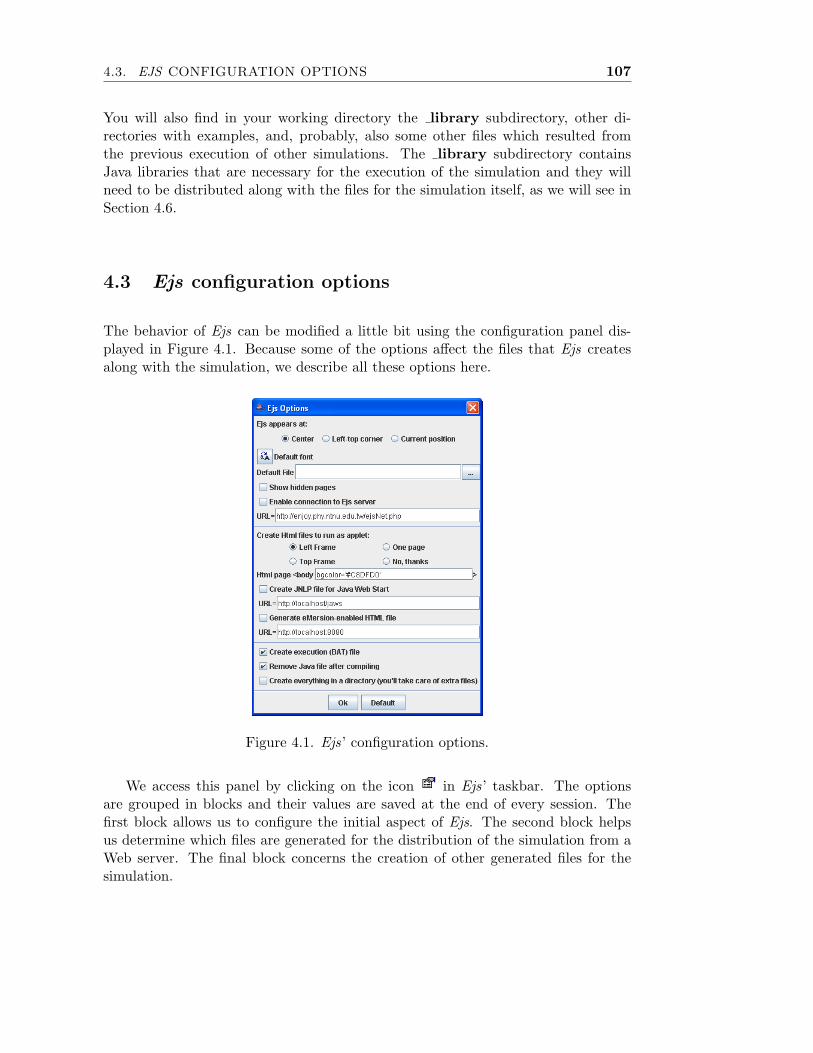
4.3. EJS CONFIGURATION OPTIONS 107
You will also find in your working directory the library subdirectory, other di-rectories with examples, and, probably, also some other files which resulted fromthe previous execution of other simulations. The library subdirectory containsJava libraries that are necessary for the execution of the simulation and they willneed to be distributed along with the files for the simulation itself, as we will see inSection 4.6.
4.3 Ejs configuration options
The behavior of Ejs can be modified a little bit using the configuration panel dis-played in Figure 4.1. Because some of the options affect the files that Ejs createsalong with the simulation, we describe all these options here.
Figure 4.1. Ejs’ configuration options.
We access this panel by clicking on the icon in Ejs’ taskbar. The optionsare grouped in blocks and their values are saved at the end of every session. Thefirst block allows us to configure the initial aspect of Ejs. The second block helpsus determine which files are generated for the distribution of the simulation from aWeb server. The final block concerns the creation of other generated files for thesimulation.

108 CHAPTER 4. USING THE SIMULATION
Options which affect the appearance of Ejs
The first option in the first block lets us to choose the location in which Ejs appearsat the beginning of a session. The options are the center of the screen, the upper-leftcorner of it, or the current position. This last option allows us to select any locationon the screen.
The second option lets us choose the default font for the code editors in Ejs.
The third option allows us to select a predefined file as basis for future sim-ulations. This can be useful if, for instance, all your simulations happen to havea similar basic structure for the view. In this case, you can create this structurebeforehand, save it to a file, and indicate the name of this file in this configurationfield. This way, every time you click on the “New” icon of Ejs’s taskbar, Ejs willremove the current simulation and will automatically load this file. This feature canbe of special interest to facilitate your students the creation of standard views.
A fourth option in the first block tells Ejs whether it should show or hide theso-called hidden pages of the model. See Section 2.2 for more details about whatthis means.
The final option in this first block enables Ejs to connect to a special type ofnetwork server that can be used to exchange simulation files among users. Thisis still an experimental development. But, typically, this will enable a new iconin Ejs’ taskbar that you can click to connect to the server specified in the corre-sponding “URL” field. We will provide more details about this in Ejs’ home page,http://fem.um.es/Ejs, when it is ready for general use.
Options for files for Web-based distribution of simulations
As mentioned already, Ejs creates a set of HTML pages, all starting with the nameof the simulation, with the purpose of including in them all the information providedby you in the “Introduction” panel, together with an extra page that embeds thesimulation itself in form of a Java applet. It also creates, finally, a master page thatorganizes the structure of all other pages and serves as entry point for the set.
The first option in this block allows you to choose the appearance of this masterHTML page: either using frames with the table of contents on the left, similarly butwith the table of contents located at the top, everything in one single page (whichwe only recommend if the introduction is really small), or even not to create HTMLpages at all. This last possibility can help you keep your Simulations directoryclean if you plan to use your simulations always from within Ejs, or run them asapplications.
The option labeled “HTML page <body” refers to the possibility of adding aparameter of your choice to the <body> tag of all HTML pages generated by Ejs.

4.4. RUNNING THE SIMULATION AS AN APPLET 109
This can be useful, for instance, to let you choose your favorite background color forthe pages, or to include a background image in them.
A third option in this same block lets you choose whether you want Ejs togenerate a JNLP file for distribution using Java Web Start. In this case, you’ll needto provide the URL from which you will be serving the JNLP file. See Section 4.6for more details.
Finally, there is an option in this block that allows you to create a separateHTML file for use with eMersion. eMersion (see http://eMersion.epfl.ch) isa collaborative tool created at the EPFL in Lausanne, Switzerland. Although thisis still an experimental development, Ejs generates eMersion-enabled simulations.The use of Ejs with eMersion will be described in a separate document, once it isready for general use.
Options for the creation of other generated files
Finally, we find a block with three options. The first option asks us whether or notwe want Ejs to generate an execution BAT file for running the simulation from asystem prompt. Typically, you will uncheck this option if running under Windowsand Mac OSX operating systems, and will leave this checked for Linux (which areusually not configured by default to run JAR files by double-clicking on them).
The second option in this block allows you to instruct Ejs to automatically deletethe Java files that it creates when generating the simulation, after processing them.This can help you keep your Simulations directory clean.
The final option lets you tell Ejs to generate all the files for a simulation in asubdirectory of the Simulations directory. This option can help you keep yourSimulations directory organized and clean, but has a small inconvenience. Ejscan’t guarantee that all the data files that your simulation needs are copied to thissubdirectory. For this reason, if you check this option, you’ll need to make sure byyourself that all data (specially image) files are present in this subdirectory, copyingthem by yourself if necessary.
4.4 Running the simulation as an applet
As we said above, one of the possible ways to run a simulation created with Ejs,independently of it, is through the corresponding HTML page. When a simulationis successfully generated, Ejs creates (except if configured otherwise) a set of HTMLpages for it. One of these pages, the one we called master HTML page, will benamed exactly as the simulation, if only it will have the extension .html.
110 CHAPTER 4. USING THE SIMULATION
You can run the simulation by simply loading this master HTML page in yourfavorite Web browser. We need to make an important remark, though. Both Ejsand the simulations it generates use Java components that require version 1.4 orlater of Java. (Current release, at the time of this writing, is 1.5.0 04.) For thisreason, your Web browser will need to support this version in order to successfullyrun the simulations.
Unfortunately, even when Java is a well established standard, different com-mercial interests of the software companies involved, caused that, nowadays, somebrowsers only support, by default, versions of Java that we could call prehistorical.The good news is that updating your browser to more recent versions is not onlyeasy, but also free.
All you need to do is to download an updated version of the so-called Javaplug-in and install it. If you followed the installation instructions of Section 1.2,then your browser has most likely already been updated. If, on the contrary, yourbrowser doesn’t visualize properly the simulations generated by Ejs, please referto the installation instructions for Ejs, which you will find in the Web server forEjs. (If you got Easy Java Simulations from a CD ROM, please look there for thisinformation, too.) You can also find the necessary software in the Web server of SunMicrosystems, http://java.sun.com. The recommended Java version is 1.5.0 04or later.
4.4.1 The content of the HTML files
Ejs generates an HTML file for each of the pages of the introduction, which containbasically what you wrote in them. Ejs creates also a master page that organizesall other pages by using frames, one of which displays a table of contents. Finally,Ejs generates an HTML page that includes the simulation in form of Java applet.The name of this page is that of the simulation followed by the word Simulationand by the extension .html. Thus, for instance, the file created for the example ofChapter 1 is called SpringSimulation.html. We now describe the contents of thispage. 4
The file SpringSimulation.xml has three different parts, that we list sepa-rately. The result of loading this file on a Web browser is shown in Figure 4.2.
The first part of the file consists of a simple header, necessary in all HTML pages:
<html><head><title> Home page for Spring</title>
4In case you configured Ejs to generate a single HTML page, the content of this file will appearinside that page.

4.4. RUNNING THE SIMULATION AS AN APPLET 111
Figure 4.2. HTML page with the simulation.
</head><body bgcolor=’#C8DFD0’>
This header declares the file as an HTML page, gives it a title, and opens the section<body> of the page, where the real content is. You will recognize in this header thename of the simulation in the <title> tag, and the value of the <body> tag indicatedin Ejs’ configuration panel.
The second is the most important part of the page, since, after a short introduc-tory message (which you can remove, if you wish):
The simulation’s view should appear right under this line.<br>
we find the <applet> tag, used to embed the simulation in the HTML page:
<applet code="spring.SpringApplet.class"codebase="." archive="_library/ejsBasic.jar,spring.jar"name="Spring" id="Spring"width="315" height="248">
</applet>

112 CHAPTER 4. USING THE SIMULATION
This instruction tells the browser to load the applet called SpringApplet, which Ejsgenerated for our simulation. The tag also tells the browser to display the simulationwith the size it had in our view. In this case, 315 pixels wide and 248 pixels high.
Please pay attention to the second line of the <applet> tag above. The parametercalled archive lists the files that the applet will need to run correctly. In thiscase, these are the JAR files generated for the simulation, spring.jar and the basiclibrary of Ejs, ejsBasic.jar. Their location is indicated relatively starting from thedirectory indicated by the parameter codebase which, in this case, is “.”, that is,the same directory where the HTML page is.
For this reason, the library directory must always be present in the Simulationsdirectory. However, you can easily modify, if you want, any of these parameters,codebase or archive, in order to place your JAR files in any other location.
Pay attention too, finally, to the third line of the <applet> tag. This line providesa name for the simulation inside the HTML page through the use of the parametersname and id, 5 which we will use in the next paragraph.
4.4.2 Control of the simulation using JavaScript
The third part of the content of the page is made of the following lines:
<!--- Finally the JavaScript buttons ---><br><hr width="100%" size="2"><br><p>You can control it using JavaScript. For example, using buttons:</p><p><input type="BUTTON" value="Play" onclick="document.Spring._play();";><input type="BUTTON" value="Pause" onclick="document.Spring._pause();";><input type="BUTTON" value="Reset" onclick="document.Spring._reset();";><input type="BUTTON" value="Step" onclick="document.Spring._step();";></p><p><input type="BUTTON" value="Slow" onclick="document.Spring._setFPS(1);";><input type="BUTTON" value="Fast" onclick="document.Spring._setFPS(10);";><input type="BUTTON" value="Faster"
onclick="document.Spring._setFPS(1000);";></p></body>
</html>
in which you will observe that the name of the simulation appears several times,exactly as indicated by the parameters name and id above.
5We need both parameters for compatibility reasons with the two main browsers.

4.4. RUNNING THE SIMULATION AS AN APPLET 113
The lines with the </body> and </html> tags simply close the page. The mostinteresting lines are those with the <input> tag, that show how we can defineJavaScript buttons that interact with the simulation.
JavaScript is a simple script language supported by most Web browsers thatallows a basic level of programming inside an HTML page. Even when we do notdescribe JavaScript in detail here, we will show how to use it to control the simulationin an additional way to the use of its user interface.
JavaScript can access the simulations created with Ejs to:
• Invoke any of the predefined methods of Ejs.
• Invoke any of the custom public methods that we may have defined in themodel.
• Set or read the value of any of the variables of the model.
JavaScript control using buttons
The procedure is always similar to the one shown above. We first need to includean entry button using the <input> tag:
<input type="BUTTON" value="Play"onclick="document.Spring._play();";>
where the value of the parameter value indicates the text that will be displayed bythe button in the page (in our case, Play), and the value of the parameter onclick,the method that must be invoked . In this case, the method is the predefined methodplay(). The prefix document.Spring must be included exactly as shown, since itidentifies the object (Spring) in this page (document) that defines the method. Theresult is that clicking the button labeled Play of Figure 4.2 will play the simulation.
Thus, for instance, if we had a public method called myMethod(), defined in thepanel of custom methods of Ejs for the model of this simulation, we could includea JavaScript button that will invoke it, using the following <input> tag (notice theinclusion of the word _model):
<input type="BUTTON" value="Invoke my method"onclick="document.Spring._model.myMethod();";>
JavaScript control using hyperlinks
An alternative way of using JavaScript is through the HTML tag for hyperlinks,<a>. The same example as above would now read as follows:

114 CHAPTER 4. USING THE SIMULATION
To invoke my method,<a href="JavaScript:document.Spring._model.myMethod();">
click here</a>
Methods with parameters
If the method that you want to invoke accepts parameters (such as setDelay(intdelay) or readState(String filename), for instance) simply include these pa-rameters between the parentheses of the method’s invocation. In the particular casethat the parameter is a text, you will need to delimit it using simple quotes, as in:
<input type="BUTTON" value="Read State"onclick="document.Spring._readState(‘url:data.dat’);";>
This example requires that we previously create the file data.dat (invoking themethod saveState("data.dat")) which must be located in the same directory ofthe hard disk or Web server from which the HTML file for the simulation has beenloaded.
Warning: The example may not work with some configurations when reading thesimulation from the hard disk, depending on how strict the security policy of your Webbrowser is. Reading data from a Web server should cause no problems, though.
A particularly interesting method is setVariables(String command), that canbe used to set the value of one or more variables of the simulation. Thus, to set theinitial conditions x = 0.5 and vx = 0 for the spring, we would use the instruction:
<input type="BUTTON" value="Initial conditions"onclick="document.Spring._setVariables(’x=0.5; vx=0;’);";>
Of course, the model must define the corresponding variables. Notice how the indi-viduals instructions are separated by semicolons.
4.4.3 Passing parameters to the applet
Every applet has a built-in way of reading parameters from the <applet> tag. Forthis, you need to give the parameter a name and a value and include a <param> linebetween the lines which contain the <applet> and </applet> keyword.
For instance, suppose we want to pass our simulation the parameter calledMyParameter with the value 10. The corresponding applet tag for the Springsimulation would be:
4.5. RUNNING THE SIMULATION AS AN APPLICATION 115
<applet code="spring.SpringApplet.class"codebase="." archive="_library/ejsBasic.jar,spring.jar"name="Spring" id="Spring"width="315" height="248">
<param name="MyParameter" value="10"></applet>
Note the inverted commas that surround the parameter’s name and value.
To get the value of this parameter in the simulation, you’ll need to invoke, in anysuitable part of it, the predefined method String _getParameter(String name)(see Subsection 2.7.3). It is important to notice that this method returns a String.You should take care of properly extracting the information, if this is a numericvalue, from the returned string. Notice also that, if the parameter is not defined,the _getParameter() method returns a null string.
For the example above, a correct (and safe) way of processing a parameter wouldbe as follows:
double value = 0.0; // default value for the variableString parameter = _getParameter ("MyParameter");if (parameter!=null) value = Double.valueOf (parameter);
Finally, note that you can define as many parameters and include as many<param> lines in the <applet> tag as you need.
4.4.4 Writing your own HTML code
Once we have seen the basic content that your HTML needs in order to include thesimulation as an applet, and the format of the possible JavaScript commands tocontrol it, you can modify your HTML page in any way you find convenient.
In particular, if you know how to write HTML code or you have an specializededitor, you can enrich your Web pages for the simulation with new narrative or withdetailed instructions of use of the simulation.
4.5 Running the simulation as an application
The third of the forms in which you can run a simulation is, as we said in the in-troduction for this chapter, as an independent Java application. For this, however,your computer must have a Java Virtual Machine installed. If you followed theinstallation instructions of Chapter 1, then there is one already installed in your

116 CHAPTER 4. USING THE SIMULATION
computer. If you didn’t, please read the installation instructions for Ejs (see Sec-tion 1.2) or get a Java Virtual Machine from the Web server of Sun Microsystems,http://java.sun.com. The recommended version is, again, 1.5.0 04 or later.
The file you need to run the simulation as an application is Spring.bat. If weinspect its contents, 6 we find the following lines:
"C:\Program files\Java\jdk1.5.0_04\jre\bin\java" -jar itt.jar
This single line calls the run-time engine of Java (which in our system is in thedirectory C:\Program files\Java\jdk1.5.0 04\jre\bin) telling it to run the sim-ulation contained in the self-executable JAR file spring.jar.
Recall that the file is self-executable, but that it requires the library subdirectory tobe present in the same directory as spring.jar. This dependence is specified in theso-called manifest file inside the spring.jar file. Advanced programmers can edit thismanifest to change the location of the library directory.
If you execute the file Spring.bat in the standard way for your operating system,a window will appear displaying the view of the simulation.
4.5.1 Running the simulation using Launcher
Launcher and LaunchBuilder are two tools, created by Doug Brown and includedin the Open Source Physics library distributed with Ejs, that can be used to organizea set of self-executable JAR files, and to provide an end-user with a single windowfrom where to run them.
We don’t describe any of these tools in detail here (interested readers can read theOSP Guide –consult http://www.opensourcephysics.org) since, actually, they arevery easy to use. But we need to mention that Easy Java Simulations includes bothtools to help you organize the simulations you create with it. This is specially usefulif you want to distribute a number of simulations in a single directory. These toolscan help you provide a single, documented, and easy to use, entry point to all ofthem.
For this, once you have generated the simulation, or simulations, you want, startLaunchBuilder using the button provided by Ejs’ console or running one of thescript files LaunchBuilder.bat (for Windows) or LaunchBuilder.sh (for Mac OSX and Linux). This creates automatically in your Simulations directory two filescalled Launcher .bat and Launcher .osp which can be used to organize yoursimulation JAR files.
6We illustrate here only the file which corresponds to Windows operating system. The files forother operating systems are equally simple.

4.6. DISTRIBUTION OF SIMULATIONS 117
Actually, after creating the files, LaunchBuilder appears on the screen to helpyou customize this organization. (Again, the use of LaunchBuilder is rather nat-ural, but you can refer to the OSP Guide for more information.) See Figure 4.3.
Figure 4.3. LaunchBuilder interface for the simulations of Chapter 1.
Once the edition is finished, you can run your simulations from Launcher bydouble clicking the Launcher .jar file that has been now created in the Simula-tions directory. The interface for Launcher is displayed in Figure 4.4.
Figure 4.4. The final Launcher interface for the same simulations.
The Launcher .jar and the Launcher .osp files can be distributed togetherwith the simulations (see below) to help your end users run the simulations.
4.6 Distribution of simulations
As we have said several times, simulations created with Ejs are independent of it, ifonly they need some libraries that include the graphic elements and other required

118 CHAPTER 4. USING THE SIMULATION
Java classes. These libraries are not part of the standard Java distribution, becausethey have been specially created for Ejs to simplify the construction of simulationsand to help add specific functionality without much user effort.
Because of this, when you distribute your simulations, you need to remember toinclude these libraries in the distribution package. This, fortunately, is very easyto do. To distribute any simulation created with Ejs, you just need to provide thefiles generated by Ejs for the simulation, as we saw in Section 4.2, together with thelibrary directory (with all its contents). Also, if you designed your simulation to
use additional files (such as GIF images, sound, or other data files), you’ll need toprovide these too.
Simulations created with Ejs can be distributed using any of the following ways:
From a Web server You’ll need to copy the JAR, HTML, and auxiliary files forthe simulation in a directory of your server. Copy also the library directoryinto the same directory as your simulation on the Web server.
In a CD-ROM This procedure is similar to the previous one. Just copy the JAR,HTML, and auxiliary files, and the library directory to the CD.
As mentioned above, you can also include properly configured copies of theLauncher .jar and Launcher .osp files, so that your users can use them
to run the simulations as applications.
Using Java Web Start This is a technology created by Sun to help deliver Javaapplications from a Web server. The programs are downloaded from a serverat a single mouse click, and they install automatically and run as independentapplications.
Easy Java Simulations is prepared to help you deliver your simulations usingthis technology. More precisely, Ejs can automatically generate a Java WebStart JNLP file for your simulation. For this, in Ejs’ configuration options(see Subsection 4.3) click on the “Create JNLP file for Java Web Start” checkbox and type in the file below it the URL of the directory (only the directory!)from which you will be serving this JNLP file. Now, when you generate thesimulation, a new file with the name of the simulation, but with the extensionjnlp, will be created. Copy this file along with the other files generated forthe simulation to the directory of the Web server you specified.
Finally, your server will need to report, for any file with the extension jnlp, aMIME type of application/x-java-jnlp-file. Not all servers are config-ured to do this by default. The way to do this depends on your browser, but,for instance, on the Apache server you just need to stop the server, edit theconf/mime.types file to add a line like the following:
application/x-java-jnlp-file JNLP
4.6. DISTRIBUTION OF SIMULATIONS 119
and re-start the server again.
If you distribute more than one simulation on a CD or from the same Web server, youcan install a single copy of the library directory, as long as all the execution files foryour simulations correctly point to that directory. This can be achieved by editing the<applet> tags (for applets) or the manifest files of the JAR files (for applications) ina convenient way. However, we recommend you to take the easy way out and just copyall the simulations in the same directory.
Finally, don’t forget to tell your users to install a Java Virtual Machine, or thenecessary Java plug-in for the Web browser. The recommended version is 1.5.0 04or later.
Exercises
Exercise 4.1. If you have access to a Web server, place one of the simulations wecreated on the previous chapters in it. Check that the simulation can be executedusing a Web browser (with the corresponding plug-in).
Exercise 4.2. Modify the HTML for the simulation you published in this Webserver, introducing in it some JavaScript controls, using both buttons and hyperlinks.
Exercise 4.3. Create a complete didactic unit on resonances from the improvedsimulation of the spring that we created in Chapter 1. Distribute the resultingdidactic unit on a CD or from a Web server.