ec150 co and h o open-path gas analyzer
TRANSCRIPT

INST
RU
CT
ION
MA
NU
AL
EC150 CO2/H2O Open-Path Gas Analyzer
Revision: 11/17
C o p y r i g h t © 2 0 1 0 - 2 0 1 7 C a m p b e l l S c i e n t i f i c , I n c .


Assistance
Products may not be returned without prior authorization. The following
contact information is for Canadian and international clients residing in
countries served by Campbell Scientific (Canada) Corp. directly. Affiliate
companies handle repairs for clients within their territories. Please visit
www.campbellsci.ca to determine which Campbell Scientific company serves
your country.
To obtain a Returned Materials Authorization (RMA), contact CAMPBELL
SCIENTIFIC (CANADA) CORP., phone (780) 454-2505. After a
measurement consultant determines the nature of the problem, an RMA
number will be issued. Please write this number clearly on the outside of the
shipping container. Campbell Scientific’s shipping address is:
CAMPBELL SCIENTIFIC (CANADA) CORP. RMA#_____
14532 131 Avenue NW
Edmonton, Alberta T5L 4X4
Canada
For all returns, the client must fill out a “Statement of Product Cleanliness and
Decontamination” form and comply with the requirements specified in it. The
form is available from our web site at www.campbellsci.ca/repair. A
completed form must be either emailed to [email protected] or faxed to
(780) 454-2655. Campbell Scientific (Canada) Corp. is unable to process any
returns until we receive this form. If the form is not received within three days
of product receipt or is incomplete, the product will be returned to the client at
the client’s expense. Campbell Scientific (Canada) Corp.f reserves the right to
refuse service on products that were exposed to contaminants that may cause
health or safety concerns for our employees.

Precautions DANGER — MANY HAZARDS ARE ASSOCIATED WITH INSTALLING, USING, MAINTAINING, AND WORKING ON OR AROUND
TRIPODS, TOWERS, AND ANY ATTACHMENTS TO TRIPODS AND TOWERS SUCH AS SENSORS, CROSSARMS, ENCLOSURES,
ANTENNAS, ETC. FAILURE TO PROPERLY AND COMPLETELY ASSEMBLE, INSTALL, OPERATE, USE, AND MAINTAIN TRIPODS,
TOWERS, AND ATTACHMENTS, AND FAILURE TO HEED WARNINGS, INCREASES THE RISK OF DEATH, ACCIDENT, SERIOUS
INJURY, PROPERTY DAMAGE, AND PRODUCT FAILURE. TAKE ALL REASONABLE PRECAUTIONS TO AVOID THESE HAZARDS.
CHECK WITH YOUR ORGANIZATION'S SAFETY COORDINATOR (OR POLICY) FOR PROCEDURES AND REQUIRED PROTECTIVE EQUIPMENT PRIOR TO PERFORMING ANY WORK.
Use tripods, towers, and attachments to tripods and towers only for purposes for which they are designed. Do not exceed design
limits. Be familiar and comply with all instructions provided in product manuals. Manuals are available at www.campbellsci.ca or by
telephoning (780) 454-2505 (Canada). You are responsible for conformance with governing codes and regulations, including safety
regulations, and the integrity and location of structures or land to which towers, tripods, and any attachments are attached. Installation
sites should be evaluated and approved by a qualified personnel (e.g. engineer). If questions or concerns arise regarding installation,
use, or maintenance of tripods, towers, attachments, or electrical connections, consult with a licensed and qualified engineer or
electrician.
General
Prior to performing site or installation work, obtain required approvals and permits.
Use only qualified personnel for installation, use, and maintenance of tripods and towers, and
any attachments to tripods and towers. The use of licensed and qualified contractors is
highly recommended.
Read all applicable instructions carefully and understand procedures thoroughly before
beginning work.
Wear a hardhat and eye protection, and take other appropriate safety precautions while
working on or around tripods and towers.
Do not climb tripods or towers at any time, and prohibit climbing by other persons. Take
reasonable precautions to secure tripod and tower sites from trespassers.
Use only manufacturer recommended parts, materials, and tools.
Utility and Electrical
You can be killed or sustain serious bodily injury if the tripod, tower, or attachments you are
installing, constructing, using, or maintaining, or a tool, stake, or anchor, come in contact
with overhead or underground utility lines.
Maintain a distance of at least one-and-one-half times structure height, 6 meters (20 feet), or
the distance required by applicable law, whichever is greater, between overhead utility lines
and the structure (tripod, tower, attachments, or tools).
Prior to performing site or installation work, inform all utility companies and have all
underground utilities marked.
Comply with all electrical codes. Electrical equipment and related grounding devices should
be installed by a licensed and qualified electrician.
Elevated Work and Weather
Exercise extreme caution when performing elevated work.
Use appropriate equipment and safety practices.
During installation and maintenance, keep tower and tripod sites clear of un-trained or non-
essential personnel. Take precautions to prevent elevated tools and objects from dropping.
Do not perform any work in inclement weather, including wind, rain, snow, lightning, etc.
Maintenance
Periodically (at least yearly) check for wear and damage, including corrosion, stress cracks,
frayed cables, loose cable clamps, cable tightness, etc. and take necessary corrective actions.
Periodically (at least yearly) check electrical ground connections.
WHILE EVERY ATTEMPT IS MADE TO EMBODY THE HIGHEST DEGREE OF SAFETY IN ALL CAMPBELL SCIENTIFIC PRODUCTS,
THE CLIENT ASSUMES ALL RISK FROM ANY INJURY RESULTING FROM IMPROPER INSTALLATION, USE, OR MAINTENANCE OF
TRIPODS, TOWERS, OR ATTACHMENTS TO TRIPODS AND TOWERS SUCH AS SENSORS, CROSSARMS, ENCLOSURES, ANTENNAS,
ETC.

PLEASE READ FIRST About this manual Please note that this manual was originally produced by Campbell Scientific Inc. (CSI) primarily for the US market. Some spellings, weights and measures may reflect this origin. Some useful conversion factors:
Area: 1 in2 (square inch) = 645 mm2
Length: 1 in. (inch) = 25.4 mm 1 ft (foot) = 304.8 mm 1 yard = 0.914 m 1 mile = 1.609 km Mass: 1 oz. (ounce) = 28.35 g 1 lb (pound weight) = 0.454 kg Pressure: 1 psi (lb/in2) = 68.95 mb Volume: 1 US gallon = 3.785 litres
In addition, part ordering numbers may vary. For example, the CABLE5CBL is a CSI part number and known as a FIN5COND at Campbell Scientific Canada (CSC). CSC Technical Support will be pleased to assist with any questions.
About sensor wiring Please note that certain sensor configurations may require a user supplied jumper wire. It is recommended to review the sensor configuration requirements for your application and supply the jumper wire is necessary.


i
Table of Contents PDF viewers: These page numbers refer to the printed version of this document. Use the PDF reader bookmarks tab for links to specific sections.
1. Introduction ................................................................ 1
2. Precautions ................................................................ 1
3. Initial Inspection ......................................................... 2
4. Overview ..................................................................... 2
4.1 General ................................................................................................. 2 4.2 Features ................................................................................................ 2 4.3 Gas Head Memory ............................................................................... 3 4.4 Self-diagnostics and Data Integrity ...................................................... 3 4.5 Field Zero/Span Capabilities ................................................................ 4 4.6 EC100 Electronics Module .................................................................. 4
4.6.1 EC100 Communications and Control ........................................... 4 4.6.2 EC100 Outputs .............................................................................. 5
4.6.2.1 SDM Output ....................................................................... 5 4.7 Automatic Heater Control .................................................................... 5 4.8 Theory of Operation ............................................................................. 6
5. Specifications ............................................................. 7
5.1 Measurements ...................................................................................... 7 5.2 Output Signals ...................................................................................... 9 5.3 Physical Description ............................................................................ 9 5.4 Power Requirements .......................................................................... 10
6. Installation ................................................................ 10
6.1 Orientation ......................................................................................... 10 6.2 Mounting Analyzer to Support Hardware .......................................... 11
6.2.1 Preparing the Mounting Structure ............................................... 16 6.2.2 Mounting EC150 with Optional CSAT3A .................................. 16 6.2.3 Mounting EC150 without CSAT3A ........................................... 19 6.2.4 Attaching EC100 Electronics Enclosure to Mounting
Structure .................................................................................. 20 6.2.5 Install the EC150 Temperature Probe ......................................... 21
6.3 Wiring and Connections ..................................................................... 22 6.3.1 Connecting the EC150 Gas Analyzer Head ................................ 23 6.3.2 Connect the CSAT3A Sonic Head .............................................. 23 6.3.3 Connect the EC150 Temperature Probe ...................................... 24 6.3.4 Ground the EC100 Electronics ................................................... 24 6.3.5 Connect SDM Communications to the EC100 ........................... 24 6.3.6 Wire Power and Ground the EC100 ........................................... 25
6.4 Data Collection and Data Processing ................................................. 25 6.4.1 Data Collection and Processing with EasyFlux DL .................... 26 6.4.2 Datalogger Programming with CRBasic ..................................... 26

Table of Contents
ii
7. Zero and Span .......................................................... 26
7.1 Introduction ....................................................................................... 26 7.2 Zero-and-Span Procedure .................................................................. 27
8. Maintenance and Troubleshooting ......................... 31
8.1 Routine Site Maintenance ................................................................. 31 8.2 Gas Analyzer Wicks .......................................................................... 32 8.3 Cleaning Analyzer Windows ............................................................. 33 8.4 Zero and Span.................................................................................... 33 8.5 Replacing CO2 Scrubber Bottles ....................................................... 33 8.6 Factory Recalibration ........................................................................ 35 8.7 Troubleshooting ................................................................................ 35
8.7.1 Data Loss During Precipitation Events ...................................... 35 8.7.2 EC100 Diagnostics for Gas Analyzer Troubleshooting ............. 35 8.7.3 LED Status Lights ...................................................................... 35 8.7.4 Diagnostic Flags ......................................................................... 37
Appendices
A. EC150 Settings ....................................................... A-1
A.1 Factory Defaults .............................................................................. A-1 A.2 Details ............................................................................................. A-1
A.2.1 SDM Address ........................................................................... A-2 A.2.2 Bandwidth ................................................................................ A-2 A.2.3 Unprompted Output ................................................................. A-2 A.2.4 Unprompted Output Rate ......................................................... A-2 A.2.5 RS-485 Baud Rate .................................................................... A-3 A.2.6 Analog Output .......................................................................... A-3 A.2.7 ECMon Update Rate ................................................................ A-3 A.2.8 Temperature Sensor ................................................................. A-3 A.2.9 Fixed Temperature Value ......................................................... A-3 A.2.10 Pressure Sensor ........................................................................ A-4
A.2.10.1 Pressure Gain ................................................................. A-6 A.2.10.2 Pressure Offset ............................................................... A-6 A.2.10.3 Fixed Pressure Value ..................................................... A-6
A.2.11 Pressure Differential Enable ..................................................... A-6 A.2.12 Heater Control .......................................................................... A-7 A.2.13 Head Power Off........................................................................ A-7
A.3 ECMon ............................................................................................ A-7 A.4 Device Configuration Utility ........................................................... A-9 A.5 EC100Configure() Instruction ......................................................... A-9
A.5.1 ConfigCmd 11 Zero-and-Span Control .................................. A-12 A.6 Example CRBasic Program ........................................................... A-12
B. Filter Bandwidth and Time Delay .......................... B-1
C. Alternate EC100 Outputs ....................................... C-1
C.1 USB or RS-485 Output.................................................................... C-1 C.1.1 Specifications ........................................................................... C-1 C.1.2 Detailed Information ................................................................ C-1
C.2 Analog Output ................................................................................. C-3

Table of Contents
iii
C.2.1 Specifications ............................................................................ C-3 C.2.2 Detailed Information ................................................................. C-3
D. Useful Equations .................................................... D-1
E. Safety Data Sheets (SDS) ...................................... E-1
E.1 Molecular Sieve, Type 13X ............................................................. E-1 E.1 Magnesium Perchlorate .................................................................... E-5 E.2 Decarbite ........................................................................................ E-12
F. Packing Information ............................................... F-1
F.1 EC150-GH Packing Information ...................................................... F-1 F.2 EC150-SH Packing Information ...................................................... F-2
Figures 4-1. EC100 electronics module ................................................................... 4 5-1. Optical path and envelope dimensions of EC150 analyzer head........ 10 6-1. Three mounting bracket options for the EC150: pn 26785 is for
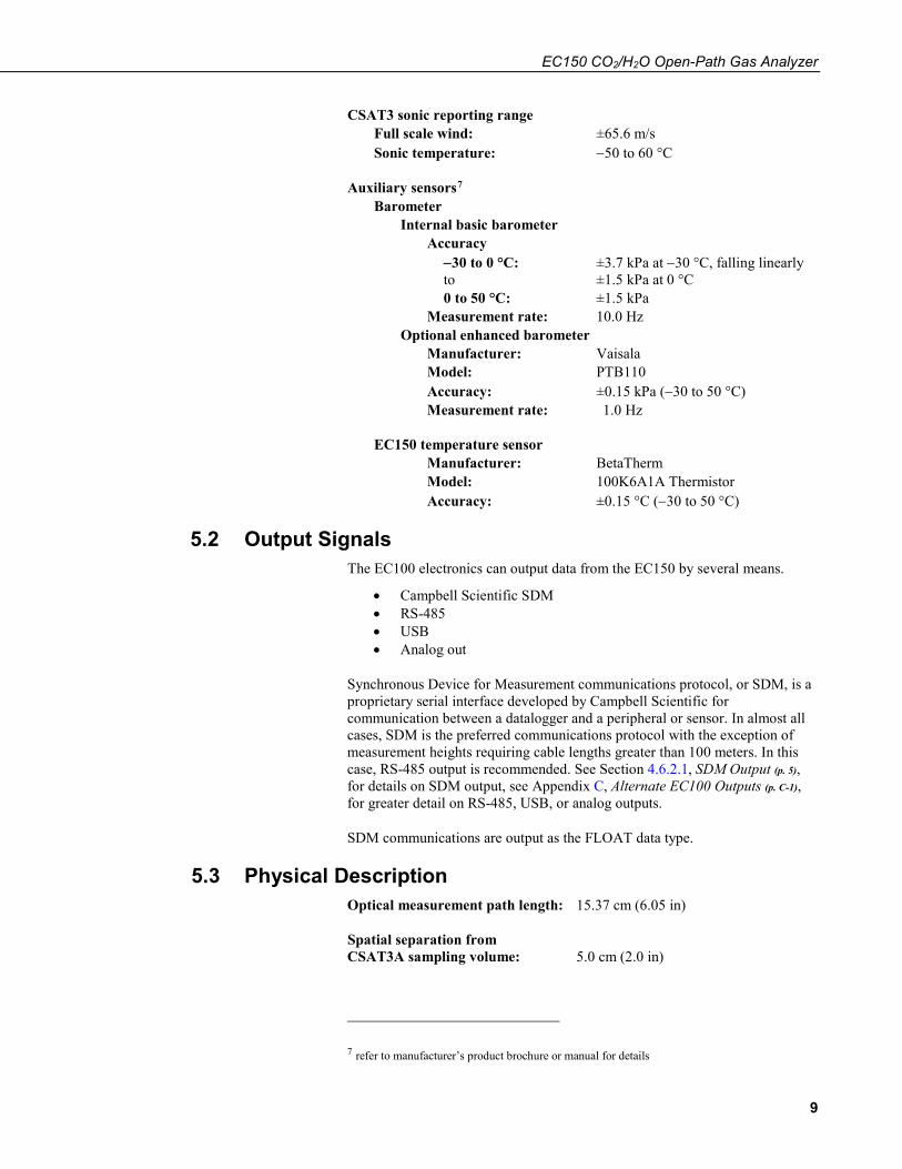
the EC150 head only, pn 26786 is for the EC150 head with CSAT3A of serial numbers less than 2000, and pn 32065 is for the EC150 head with CSAT3A serial numbers 2000 and greater. .. 12
6-2. Changes in flux attenuation ratio relative to sensor height at the most fore and aft positions .............................................................. 13
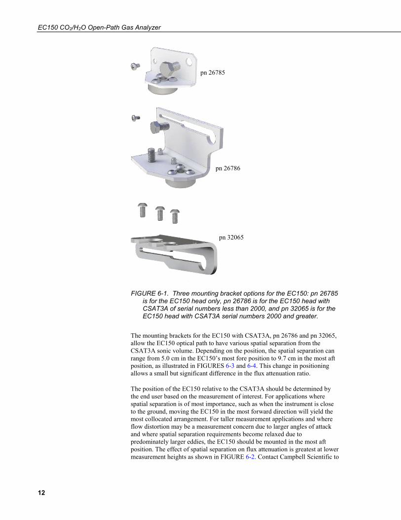
6-3. The most forward mounting position of the EC150 relative to the CSAT3A, resulting in a 4.9 cm sensor separation. The top images show the mounting with the current CSAT3A (CSAT3A serial numbers greater than 2000), while the bottom images show the mounting with the original version CSAT3A (serial numbers less than 2000). ............................................................................... 14
6-4. The most aft (back) mounting position of the EC150 relative to the CSAT3A, resulting in a spatial separation of 9.7 cm. The top images show the mounting with the current CSAT3A (CSAT3A serial numbers greater than 2000), while the bottom images show the mounting with the original version CSAT3A (serial numbers less than 2000). ............................................................................... 15
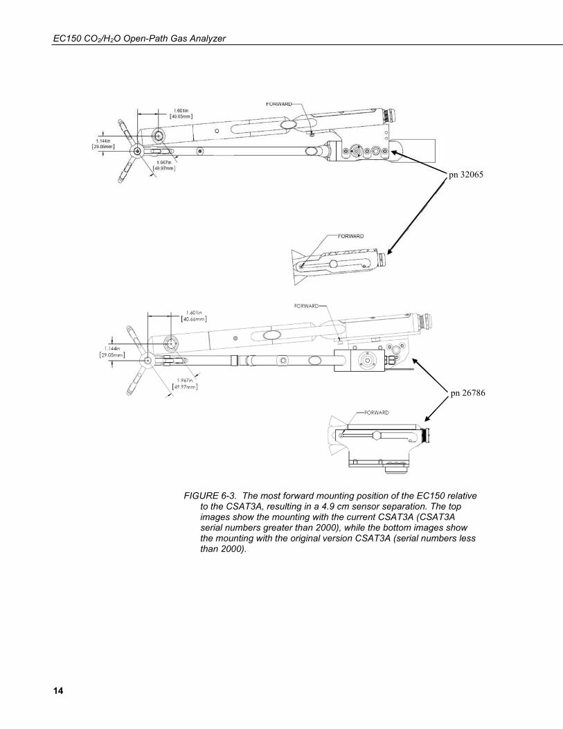
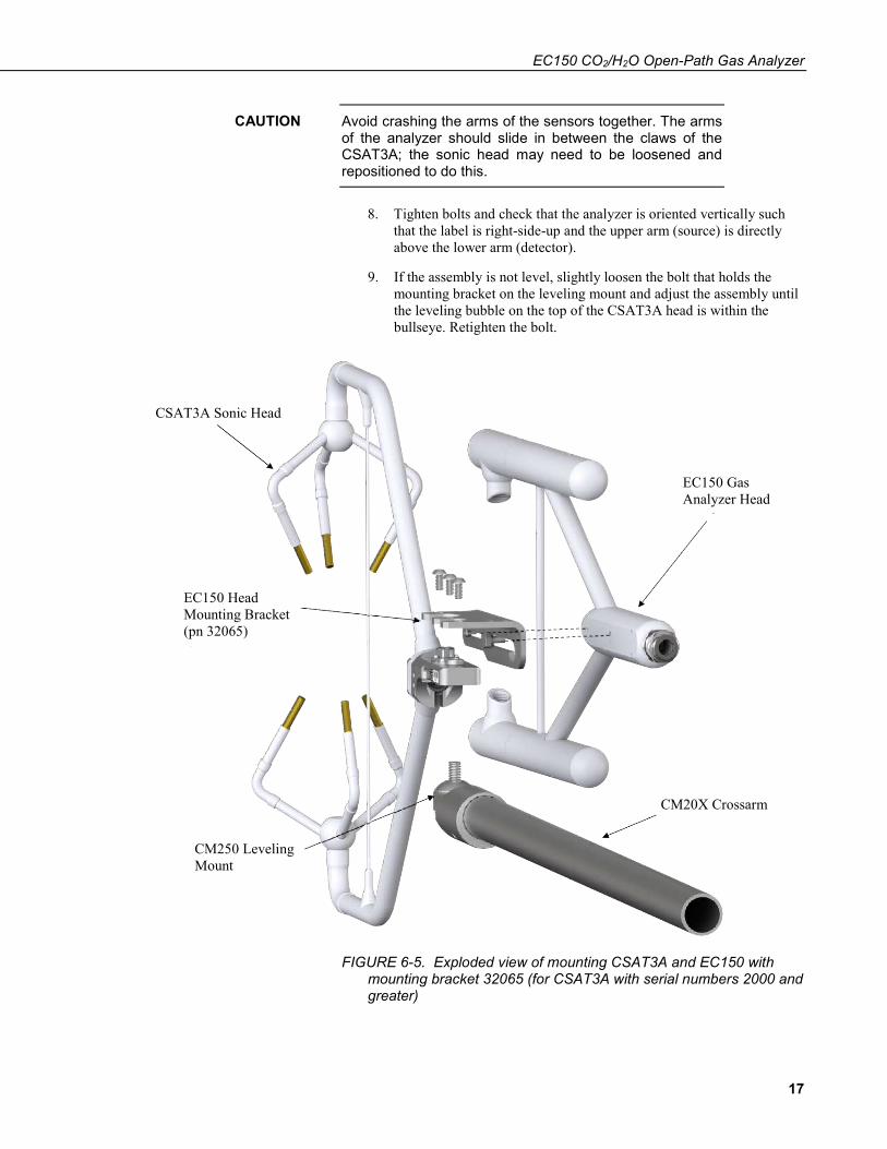
6-5. Exploded view of mounting CSAT3A and EC150 with mounting bracket 32065 (for CSAT3A with serial numbers 2000 and greater) ............................................................................................ 17
6-6. Exploded view of mounting CSAT3A and EC150 with mounting bracket 26786 (for CSAT3A with serial numbers less than 2000) ............................................................................................... 18
6-7. Exploded view of mounting the EC150 without the CSAT3A using mounting bracket pn 26785 ................................................... 19
6-8. EC100 enclosure mounting bracket mounted on a vertical mast (left) and a tripod leg (right) ........................................................... 20
6-9. Exploded view of mounting the EC100 enclosure ............................. 21 6-10. EC150 temperature probe .................................................................. 22 6-11. Solar radiation shield with EC150 temperature probe ....................... 22 6-12. EC100 electronics front panel showing EC100 as shipped (left)
and after completed wiring and connections (right) ....................... 22 6-13. Bottom of EC100 enclosure ............................................................... 23 7-1. Zero-and-span shroud mounted on the zero-and-span stand .............. 28 7-2. ECMon zero-and-span window .......................................................... 29
Table of Contents
iv
8-1. Proper location of the gas analyzer top wick (left) and bottom wick (right) .................................................................................... 33
8-2. Replacing the desiccant and CO2 scrubber bottles (replacement bottles purchased in or after July 2017 may appear different than in the figure) ........................................................................... 34
8-3. LED status during normal operation ................................................. 36 A-1. Location of EC100 basic barometer ................................................ A-4 A-2. Location of EC100 enhanced barometer ......................................... A-5 A-3. Comparison of error in basic versus enhanced barometer over
operational temperatures .............................................................. A-5 A-4. Main screen of ECMon.................................................................... A-8 A-5. Setup screen in ECMon ................................................................... A-8 B-1. Amplitude response of EC100 filter at various bandwidths ............ B-1 B-2. Frequency response comparison of EC100 10-Hz bandwidth and
a 50-msec moving average ........................................................... B-2 C-1. USB data output in terminal mode .................................................. C-2
Tables 6-1. EC100 SDM Output .......................................................................... 25 8-1. Rain Wick Replacement Parts ........................................................... 32 8-2. Diagnostic Flags of Sonic Status LED .............................................. 36 8-3. Diagnostic Flags and Suggested Actions........................................... 38 A-1. Factory Default Settings .................................................................. A-1 A-2. ConfigCmd Values for Setting and Retrieving Settings ................ A-10 B-1. Filter Time Delays for Various Bandwidths .................................... B-3 C-1. USB and RS-485 Output Elements ................................................. C-1 C-2. Multipliers and Offsets for Analog Outputs .................................... C-4 D-1. Variables and Constants .................................................................. D-1

1
EC150 CO2/H2O Open-Path Gas Analyzer 1. Introduction
The EC150 is an in situ, open-path, mid-infrared absorption gas analyzer that measures the absolute densities of carbon dioxide and water vapor. The EC150 was designed for open-path eddy covariance flux measurements as part of an open-path eddy covariance measurement system. It is most often used in conjunction with the CSAT3A sonic anemometer and thermometer, which measures orthogonal wind components along with sonically determined air temperature.
Before attempting to assemble, install or use the EC150, please study: • Section 2, Precautions (p. 1) • Section 3, Initial Inspection (p. 2) • Section 6, Installation (p. 10)
Greater detail is available in the remaining sections.
Other manuals that may be helpful include:
• CR3000 Micrologger Operator’s Manual • CFM100 CompactFlash Module Instruction Manual • NL115 Ethernet and CompactFlash Module Instruction Manual • Application Note 3SM-F, PC/CF Card Information • LoggerNet Instruction Manual, Version 4.1 • CSAT3 Three Dimensional Sonic Anemometer Manual • ENC10/12, ENC12/14, ENC14/16, ENC16/18 Instruction Manual • CM106 Tripod Instruction Manual • Tripod Installation Manual Models CM110, CM115, CM120
2. Precautions • DANGER:
o The scrubber bottles in EC150 instruments shipped prior to July 2017 contain sodium hydroxide (NaOH) and anhydrous magnesium perchlorate (Mg(ClO4)2). If you are handling or exchanging the scrubber bottles (see Section 8.5, Replacing CO2 Scrubber Bottles (p. 33)), use the following precautions. Beginning in July 2017, EC150 instruments ship with a 13X molecular sieve instead.
− Avoid direct contact with the chemicals. − Ensure your work area is well ventilated and free of
reactive compounds and combustible materials. − Store used chemical bottles in a sealed container until
disposal. − Dispose of chemicals and bottles properly. − Safety Data Sheets (SDS) are provided in Appendix E,
Safety Data Sheets (SDS) (p. E-1). SDS are updated periodically by chemical manufacturers. Obtain current SDS at www.campbellsci.com.

EC150 CO2/H2O Open-Path Gas Analyzer
2
• WARNING: o Do not carry the EC150 by the arms or the strut between the
arms. Always hold it by the mounting base where the upper and lower arms connect.
o Handle the EC150 carefully. The optical source may be damaged by rough handling, especially while the analyzer is powered.
o Overtightening bolts will damage or deform the mounting hardware.
• CAUTION: o Grounding the EC100 measurement electronics is critical. Proper
grounding to Earth will ensure maximum electrostatic discharge (ESD) and lightning protection and improve measurement accuracy.
o Do not connect or disconnect the gas analyzer or sonic anemometer connectors while the EC100 is powered.
o Resting the analyzer on its side during the zero-and-span procedure may result in measurement inaccuracy.
3. Initial Inspection Upon receipt of your equipment, inspect the packaging and contents for damage. File damage claims with the shipping company.
Model numbers are found on each component. On cables, the model number is located both on the sensor head and on the connection end of the cable. Check this information against the enclosed shipping document to verify the expected products and that the correct accessories are included.
4. Overview 4.1 General
The EC150 measures absolute densities of carbon dioxide and water vapor. The EC150 analyzer was designed specifically for open-path, eddy covariance flux measurement systems. The EC150 gas analyzer head connects directly to Campbell Scientific’s EC100 electronics. The EC150 is commonly used with a CSAT3A sonic anemometer head. When the CSAT3A is used in conjunction with the EC150, the EC100 can make gas and wind measurements simultaneously. Similarly, the EC100 can simultaneously record measurements from temperature sensors and a pressure transducer.
The EC150 analyzer has a rugged, aerodynamic design with low power requirements, making it suitable for field applications including those with remote access.
4.2 Features The EC150 has been designed specifically to address issues of aerodynamics, power consumption, spatial displacement, temporal synchronicity, and to minimize sensitivity to environmental factors.
The analyzer windows are scratch resistant and treated with a durable hydrophobic coating that facilitates shedding of raindrops from critical surfaces. The coating also impedes the accumulation of dust and deposits, and keeps the surfaces cleaner over longer periods of time. To minimize data loss

EC150 CO2/H2O Open-Path Gas Analyzer
3
due to humid environments, the EC150 is provided with window wicks that draw moisture away from the measurement path and are easily replaceable during routine maintenance.
• Unique design contains little obstruction surrounding the sample volume
• 5 W total power consumption • Synchronously samples data from the EC150 and CSAT3A • Automatically configured via a Campbell Scientific datalogger • Minimal spatial displacement between sample volume and CSAT3A • Slim housings located away from the measurement volume to
minimize body heating effects due to solar radiation • Symmetrical design for improved flux measurements without a bias
for updrafts and downdrafts • Slanted windows to prevent water from pooling and blocking the
optical path • Scratch-resistant windows for easy cleaning • Hydrophobic coating on windows to repel water, dust and pollen and
to prolong time between window cleaning • Equipped with internal window heaters to keep the windows surfaces
free from condensation and frost – especially beneficial in humid environments or conditions with frequent frost formation
• Optical layout that is not affected by solar interference • Mercury cadmium telluride (MCT) detector for low-noise
measurements and long-term stability of factory calibration • Chopper housing without thermal control results in significantly
reduced power consumption • Any CSAT3A with serial numbers of 2000 or greater have an updated
design with more rigid geometry for improved sonic-temperature accuracy and stability, and with a more stream-lined, aerodynamic mounting block
4.3 Gas Head Memory The EC100 electronics (see Section 4.6, EC100 Electronics Module (p. 4)) are universal for the entire Campbell Scientific family of gas analyzer heads. In addition to the EC150 gas analyzer head, the IRGASON or EC155 gas analyzer head can be connected to the EC100 electronics (one gas analyzer head per EC100). All sensor heads have dedicated, non-volatile memory, which stores all calibration, configuration, and setting information. The EC100 electronics can be mated with any of these gas analyzers or an optional CSAT3A sonic anemometer head.
4.4 Self-diagnostics and Data Integrity EC100 electronics provide an extensive set of diagnostic tools which include warning flags, status LEDs, and signal strength outputs to identify instrument malfunctions and warn the user of compromised data. These flags are further described in Section 8.7.4, Diagnostic Flags (p. 37). The flags also prompt the user when the instrument needs servicing and can facilitate troubleshooting in the field. The EC150 outputs the optical strength of signals, which can be used to filter data when the path of the instrument is obstructed due to precipitation or dirty windows.
EC150 CO2/H2O Open-Path Gas Analyzer
4
4.5 Field Zero/Span Capabilities A zero/span for CO2 and H2O can be accomplished in the field with an optional shroud. The shroud allows the flow of a gas with known composition in the measurement path of the analyzer to account for instrument drift and changing environmental conditions.
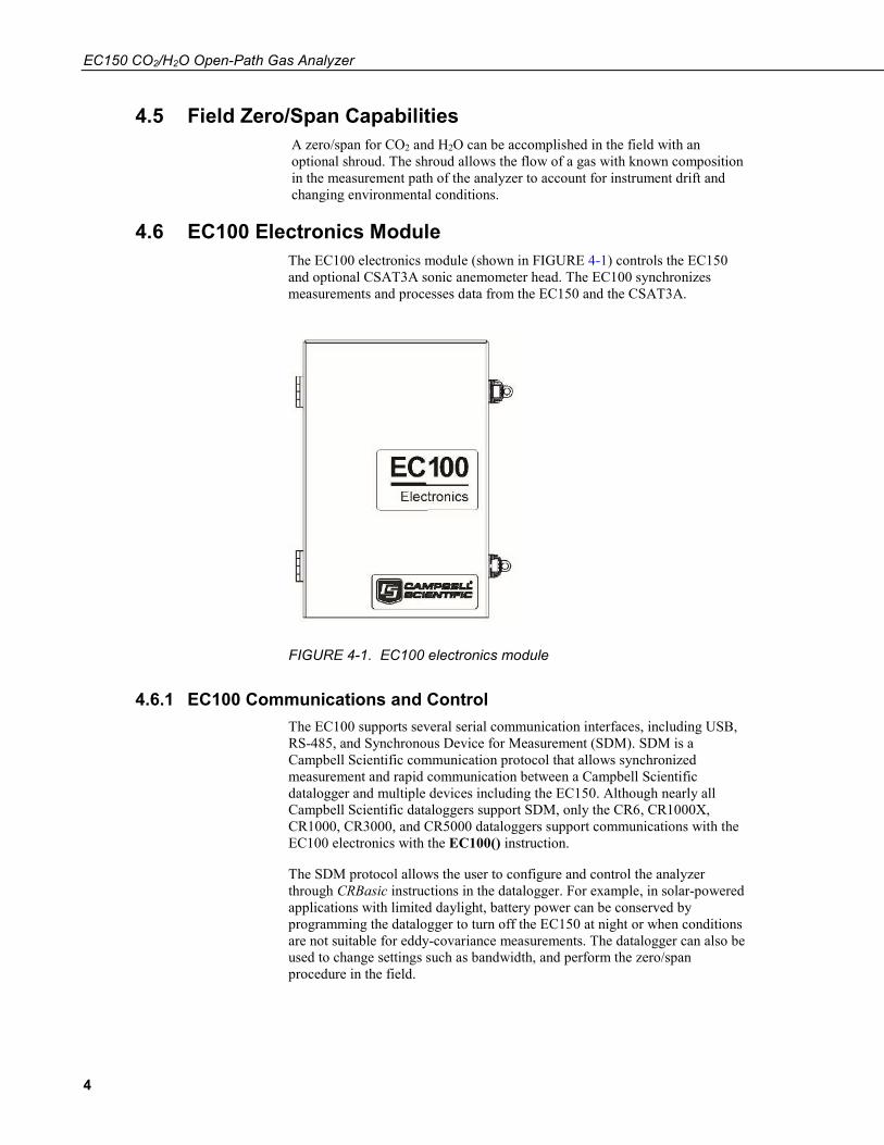
4.6 EC100 Electronics Module The EC100 electronics module (shown in FIGURE 4-1) controls the EC150 and optional CSAT3A sonic anemometer head. The EC100 synchronizes measurements and processes data from the EC150 and the CSAT3A.
FIGURE 4-1. EC100 electronics module
4.6.1 EC100 Communications and Control The EC100 supports several serial communication interfaces, including USB, RS-485, and Synchronous Device for Measurement (SDM). SDM is a Campbell Scientific communication protocol that allows synchronized measurement and rapid communication between a Campbell Scientific datalogger and multiple devices including the EC150. Although nearly all Campbell Scientific dataloggers support SDM, only the CR6, CR1000X, CR1000, CR3000, and CR5000 dataloggers support communications with the EC100 electronics with the EC100() instruction.
The SDM protocol allows the user to configure and control the analyzer through CRBasic instructions in the datalogger. For example, in solar-powered applications with limited daylight, battery power can be conserved by programming the datalogger to turn off the EC150 at night or when conditions are not suitable for eddy-covariance measurements. The datalogger can also be used to change settings such as bandwidth, and perform the zero/span procedure in the field.

EC150 CO2/H2O Open-Path Gas Analyzer
5
4.6.2 EC100 Outputs The EC100 outputs data in one of four types: SDM, USB, RS-485, or analog. In general, Campbell Scientific recommends that SDM be used if a Campbell Scientific datalogger is collecting data. However, RS-485 output is recommended over SDM if cable lengths exceed 100 meters. If a PC is being used as the data collection platform, USB and RS-485 are suitable outputs.
Information for SDM, the preferred output, is detailed below. See Appendix C, Alternate EC100 Outputs (p. C-1), for USB, RS-485, and analog outputs.
4.6.2.1 SDM Output
To use SDM data output, connect an SDM communications cable from the EC100 (see Section 6.3, Wiring and Connections (p. 22)) to an SDM port on a CR6, CR1000X, CR1000, CR3000, or CR5000 datalogger. On CR1000 dataloggers, the SDM port is made of terminals C1 – C3. The default SDM port for CR6 and CR1000X dataloggers is made of terminals C1 – C3, though it can be changed with the SDMBeginPort() instruction. On CR3000 and CR5000 dataloggers, the SDM protocol uses SDM-dedicated ports SDM-C1, SDM-C2, and SDM-C3.
Each SDM device on the SDM bus must have a unique address. The EC150 has a factory default SDM address of 1, but may be changed to any integer value between 0 and 14 (see Appendix A.2.1, SDM Address (p. A-2)).
The sample rate for SDM output is determined by the datalogger program. Data are output from the EC100 when a request is received from the datalogger (for example, a prompted output mode). The number of data values sent from the EC100 to the datalogger is also set by the user in the datalogger program. CRBasic, the programming language used by Campbell Scientific dataloggers, uses the EC100() instruction to get data from an EC150. This instruction is explained in greater detail under Appendix A, EC150 Settings (p. A-1), and in Appendix A.5, EC100 Configure() Instruction (p. A-9).
4.7 Automatic Heater Control An advantage of the EC150’s low power consumption (5W) is that the instrument remains at a temperature very close to ambient air temperature, which is an important feature for eddy-covariance measurements. Under some environmental conditions, however, the analyzer can become colder than ambient air temperature which may increase the likelihood of frost or condensation building on the optical windows. This will affect signal strength. The EC150 design includes internal heaters located at the optical windows, which aid in minimizing data loss during these specific environmental conditions.
An automatic heater control algorithm can be activated from either Device Configuration Utility or ECMon by putting in a value of −2, or deactivated by putting in a value of −1.1 The algorithm uses the internal heaters to maintain a temperature that is a couple of degrees above the ambient dewpoint (or frost point) to prevent condensation and icing from forming on the surface of the optical windows.
1 Automatic heater control is available in EC100 OS version 4.07 or greater and is turned on by default starting with the OPEC program version 3.2.
EC150 CO2/H2O Open-Path Gas Analyzer
6
The heater control will be disabled under any of the following conditions:
• Temperature of the detector housing is outside the −35 to 55 °C range • Temperature of the source housing exceeds 40 °C • Ambient temperature is outside the −35 to 55 °C range • The supply voltage is below 10 V
The algorithm uses the following environmental parameters to control the heater:
• Analyzer body temperature, measured inside the source housing (heater control does not allow the body temperature to drop below ambient air temperature)
• Ambient relative humidity (in humidity greater than 80% heaters will try to maintain internal temperature 2 degrees warmer than ambient)
• CO2 signal level (1 min average CO2 signal level; below 0.7 will cause the heater to turn on maximum power until the signals recover)
• Average slope of the CO2 signal level over 1 min • Standard deviation of the CO2 signal over 1 min
4.8 Theory of Operation The EC150 is a non-dispersive mid-infrared absorption analyzer. Infrared radiation is generated in the upper arm of the analyzer head before propagating along a 15.0 cm (5.9 in) optical path as shown in FIGURE 5-1. Chemical species located within the optical beam will absorb radiation at characteristic frequencies. A mercury cadmium telluride (MCT) detector in the lower arm of the gas analyzer measures the decrease in radiation intensity due to absorption, which can then be related to analyte concentration using the Beer-Lambert Law:
cloePP ε−=
where: P = irradiance after passing through the optical path Po = initial irradiance, ε is molar absorptivity, c is analyte
concentration, and l = path length.
In the EC150, radiation is generated by applying constant power to a tungsten lamp which acts as a 2200 K broadband radiation source. Specific wavelengths are then selected using interference filters located on a spinning chopper wheel. For CO2 measurements, light with a wavelength of 4.3 µm is selected as that corresponds to the asymmetric stretching vibrational band of the CO2 molecule. For H2O, the symmetric stretching vibration band is 2.7 µm.
The EC150 is a dual wavelength, single-beam analyzer. This design eliminates the need for a separate reference cell and detector. Instead, the initial intensity of the radiation is calculated by measuring the intensity of nearby, non-absorbing wavelengths (4.0 µm for CO2 and 2.3 µm for H2O). These measurements mitigate measurement inaccuracy that may arise from source or detector aging, as well as for low-level window contamination. For window contamination that reduces the signal strength below 0.8, windows should be cleaned as described in Section 8.3, Cleaning Analyzer Windows (p. 33).

EC150 CO2/H2O Open-Path Gas Analyzer
7
The chopper wheel spins at a rate of 60 revolutions per second and the detector is measured 1024 times per revolution, resulting in a detector sampling rate of 51.2 kHz. The detector is maintained at −40 °C using a three-stage thermoelectric cooler and is coupled to a low noise pre-amp module.
The EC100 electronics module digitizes and process the detector data (along with ancillary data such as ambient air temperature and barometric pressure) to give the CO2 and H2O density for each chopper wheel revolution (50 Hz). This high measurement rate is beneficial when there is a need to synchronize the gas measurements with additional sensors measured by the datalogger. To prevent aliasing, measurements are filtered to a bandwidth that is specified by the user.
5. Specifications 5.1 Measurements
To compute carbon dioxide and water vapor fluxes using the eddy-covariance method, the EC150 and a sonic anemometer measure:
• Absolute carbon dioxide density (mg·m–3) • Water vapor density (g·m–3) • Three-dimensional wind speed (m·s–1; requires the CSAT3A) • Sonic air temperature (°C; requires the CSAT3A) • Air temperature (°C; requires an auxiliary temperature probe) • Barometric pressure (kPa; requires an auxiliary barometer)
These measurements are required to compute carbon dioxide and water vapor fluxes using the:
• Standard outputs: o CO2 density, H2O density o Gas analyzer diagnostic flags o Air temperature o Air pressure o CO2 signal strength o H2O signal strength
• Additional outputs from auxiliary instruments: o ux, uy, and uz orthogonal wind components (requires the
CSAT3A) o Sonic temperature (requires the CSAT3A, and is based on the
measurement of c, the speed of sound) o Sonic diagnostic flags (from the CSAT3A)
Datalogger Compatibility: CR6 CR1000X CR1000 CR3000 CR5000
Measurement Rate: 60 Hz Output bandwidth2: 5, 10, 12.5, 20, or 25 Hz Output rate2: 10, 25 or 50 Hz
2 user selectable
EC150 CO2/H2O Open-Path Gas Analyzer
8
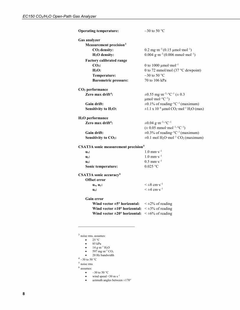
Operating temperature: −30 to 50 °C
Gas analyzer Measurement precision3
CO2 density: 0.2 mg·m–3 (0.15 µmol·mol–1) H2O density: 0.004 g·m–3 (0.006 mmol·mol–1)
Factory calibrated range CO2: 0 to 1000 µmol·mol–1 H2O: 0 to 72 mmol/mol (37 °C dewpoint) Temperature: −30 to 50 °C Barometric pressure: 70 to 106 kPa
CO2 performance Zero max drift4: ±0.55 mg·m–3·°C–1 (± 0.3
μmol·mol·°C–1) Gain drift: ±0.1% of reading·°C–1 (maximum) Sensitivity to H2O: ±1.1 x 10⁻⁴ µmol CO2·mol–1 H2O (max)
H2O performance Zero max drift4: ±0.04 g·m–3·°C–1 (± 0.05 mmol·mol–1·°C–1) Gain drift: ±0.3% of reading·°C–1 (maximum) Sensitivity to CO2: ±0.1 mol H2O·mol–1 CO2 (maximum)
CSAT3A sonic measurement precision5 ux: 1.0 mm·s–1 uy: 1.0 mm·s–1 uz: 0.5 mm·s–1 Sonic temperature: 0.025 °C
CSAT3A sonic accuracy6 Offset error
ux, uy: < ±8 cm·s–1 uz: < ±4 cm·s–1
Gain error Wind vector ±5° horizontal: < ±2% of reading Wind vector ±10° horizontal: < ±3% of reading Wind vector ±20° horizontal: < ±6% of reading
3 noise rms, assumes: • 25 °C • 85 kPa • 14 g·m–3 H2O • 597 mg·m–3 CO2 • 20 Hz bandwidth
4 −30 to 50 °C 5 noise rms 6 assumes:
• −30 to 50 °C • wind speed <30 m·s–1 • azimuth angles between ±170°
EC150 CO2/H2O Open-Path Gas Analyzer
9
CSAT3 sonic reporting range Full scale wind: ±65.6 m/s Sonic temperature: −50 to 60 °C
Auxiliary sensors7 Barometer
Internal basic barometer Accuracy
−30 to 0 °C: ±3.7 kPa at −30 °C, falling linearly to ±1.5 kPa at 0 °C 0 to 50 °C: ±1.5 kPa
Measurement rate: 10.0 Hz Optional enhanced barometer
Manufacturer: Vaisala Model: PTB110 Accuracy: ±0.15 kPa (−30 to 50 °C) Measurement rate: 1.0 Hz
EC150 temperature sensor Manufacturer: BetaTherm Model: 100K6A1A Thermistor Accuracy: ±0.15 °C (−30 to 50 °C)
5.2 Output Signals The EC100 electronics can output data from the EC150 by several means.
• Campbell Scientific SDM • RS-485 • USB • Analog out
Synchronous Device for Measurement communications protocol, or SDM, is a proprietary serial interface developed by Campbell Scientific for communication between a datalogger and a peripheral or sensor. In almost all cases, SDM is the preferred communications protocol with the exception of measurement heights requiring cable lengths greater than 100 meters. In this case, RS-485 output is recommended. See Section 4.6.2.1, SDM Output (p. 5), for details on SDM output, see Appendix C, Alternate EC100 Outputs (p. C-1), for greater detail on RS-485, USB, or analog outputs.
SDM communications are output as the FLOAT data type.
5.3 Physical Description Optical measurement path length: 15.37 cm (6.05 in)
Spatial separation from CSAT3A sampling volume: 5.0 cm (2.0 in)
7 refer to manufacturer’s product brochure or manual for details

EC150 CO2/H2O Open-Path Gas Analyzer
10
Dimensions Head housing diameter: 3.2 cm (1.3 in) Head length: 29.7 cm (11.7 in) EC100 enclosure: 24.1 cm x 35.6 cm x 14 cm (9.5 in x 14.0 in x 5.5 in)
Weight Analyzer and cable: 2 kg (4.4 lbs) EC100 electronics and EC100 enclosure: 3.2 kg (7.0 lbs)
FIGURE 5-1. Optical path and envelope dimensions of EC150 analyzer head
5.4 Power Requirements Voltage supply: 10 to 16 Vdc Power at 25 °C excluding CSAT3A: 4.1 W Power at 25 °C including CSAT3A: 5.0 W Power at 25 °C in power-down mode
(CSAT3A fully powered and EC150 off): 3.0 W
6. Installation 6.1 Orientation
During operation, the EC150 should be positioned vertically (±15°) so that the product label reads right side up and the upper arm (source) is directly above the lower arm (detector). If the sensor is being used with a sonic anemometer, the anemometer should be leveled and pointed into the prevailing wind to minimize flow distortion from the analyzer’s arms and other supporting structures.
For applications using the EC150 with the CSAT3A sonic anemometer, certain environmental conditions should be considered when choosing an appropriate

EC150 CO2/H2O Open-Path Gas Analyzer
11
installation configuration. If the EC155 is coupled with a CSAT3A sonic anemometer and is to be used in a marine environment, or in an environment where it is exposed to corrosive chemicals (for example, the sulfur-containing compounds in viticulture), attempt to mount the EC155 with CSAT3A in a way that reduces the exposure of the sonic transducers of the CSAT3A to saltwater or corrosive chemicals. In marine or viticulture environments, the sonic transducers are expected to age more quickly and require replacement sooner than a unit deployed in an inland, chemical-free environment.
6.2 Mounting Analyzer to Support Hardware The EC150 is supplied with mounting hardware to attach it to the end of a horizontal pipe of 3.33 cm (1.31 in) outer diameter, such as the CM202 (pn 17903), CM204 (pn 17904), or CM206 crossarm (pn 17905).
There are three different mounting brackets for the EC150. A head only mounting bracket (pn 26785), the EC150/CSAT3A mounting bracket (pn 26786) that was shipped with any CSAT3A with a serial number of less than 2000, and a new EC150/CSAT3A mounting bracket (pn 32065) that ships with any CSAT3A with a serial number of 2000 or greater. The three mounting brackets are shown in FIGURE 6-1.
The CSAT3A sonic anemometer head is an option when ordering the EC150 and the appropriate mounting bracket is included with the EC150 depending on if the CSAT3A is ordered. If the user is already in possession of a CSAT3A and intends to use it with the EC150, the proper mounting bracket should be specified at time of order.
The screws and bolts for either mounting bracket are easily lost in the field. Replacements are available through Campbell Scientific or can be sourced elsewhere. To use bracket 26785, use pn 15807 (screw #8-32 x 0.250 socket head) and pn 26712 (screw 3/8-16 x 0.625 hex cap). To use bracket 26786, use pn 26711 (screw #8-32 x 0.250 shoulder cap) and pn 26712 (screw 3/8-16 x 0.625 hex cap). To use bracket 32065, use pn 10393 (screw 1/4-20 X 0.375 cap socket) and pn 26712 (screw 3/8-16 x 0.625 hex cap).
NOTE
EC150 CO2/H2O Open-Path Gas Analyzer
12
FIGURE 6-1. Three mounting bracket options for the EC150: pn 26785 is for the EC150 head only, pn 26786 is for the EC150 head with CSAT3A of serial numbers less than 2000, and pn 32065 is for the EC150 head with CSAT3A serial numbers 2000 and greater.
The mounting brackets for the EC150 with CSAT3A, pn 26786 and pn 32065, allow the EC150 optical path to have various spatial separation from the CSAT3A sonic volume. Depending on the position, the spatial separation can range from 5.0 cm in the EC150’s most fore position to 9.7 cm in the most aft position, as illustrated in FIGURES 6-3 and 6-4. This change in positioning allows a small but significant difference in the flux attenuation ratio.
The position of the EC150 relative to the CSAT3A should be determined by the end user based on the measurement of interest. For applications where spatial separation is of most importance, such as when the instrument is close to the ground, moving the EC150 in the most forward direction will yield the most collocated arrangement. For taller measurement applications and where flow distortion may be a measurement concern due to larger angles of attack and where spatial separation requirements become relaxed due to predominately larger eddies, the EC150 should be mounted in the most aft position. The effect of spatial separation on flux attenuation is greatest at lower measurement heights as shown in FIGURE 6-2. Contact Campbell Scientific to
pn 26785
pn 26786
pn 32065

EC150 CO2/H2O Open-Path Gas Analyzer
13
help determine the best positioning of the EC150 relative to the CSAT3A in scenarios where the measurement height is below 10 meters.
FIGURE 6-2. Changes in flux attenuation ratio relative to sensor height at the most fore and aft positions
EC150 CO2/H2O Open-Path Gas Analyzer
14
FIGURE 6-3. The most forward mounting position of the EC150 relative to the CSAT3A, resulting in a 4.9 cm sensor separation. The top images show the mounting with the current CSAT3A (CSAT3A serial numbers greater than 2000), while the bottom images show the mounting with the original version CSAT3A (serial numbers less than 2000).
pn 32065
pn 26786

EC150 CO2/H2O Open-Path Gas Analyzer
15
FIGURE 6-4. The most aft (back) mounting position of the EC150 relative to the CSAT3A, resulting in a spatial separation of 9.7 cm. The top images show the mounting with the current CSAT3A (CSAT3A serial numbers greater than 2000), while the bottom images show the mounting with the original version CSAT3A (serial numbers less than 2000).
The following steps describe the normal mounting procedure. Refer to FIGURE 6-6 and 6-7 throughout this section.
pn 32065
pn 26786

EC150 CO2/H2O Open-Path Gas Analyzer
16
6.2.1 Preparing the Mounting Structure 1. Secure a CM20X crossarm to a tripod or other vertical structure using a
CM210 crossarm-to-pole bracket (pn 17767).
2. Point the horizontal arm into the direction of the prevailing wind.
3. Tighten all fitting set screws.
Do not carry the EC150 by the arms or the strut between the arms. Always hold the sensor by the block where the upper and lower arms connect.
6.2.2 Mounting EC150 with Optional CSAT3A The guideline below gives general instructions for mounting an EC150 and optional CSAT3A to a mounting structure. The order of assembly will somewhat be determined by the user’s application; primarily the height of the tower. Steps 6, 7, and 8 should be performed in sequential order.
Please refer to all steps and the referenced figure of this section before deciding on an assembly strategy. In general, Campbell Scientific suggests that if the equipment is to be mounted at heights above what can be reached while standing, to preassemble as much as possible and then hoist that assembly into a position to be mounted on the appropriate crossarm.
1. Attach CSAT3A to the proper mounting bracket according to the CSAT3A serial number.
• If using a CSAT3A with current design (serial numbers 2000 and greater), attach the EC150/CSAT3A mounting bracket (pn 32065; see FIGURE 6-1) to the CSAT3A using the three included screws and then bolt the CM250 leveling mount (pn 26559) to the threaded hole of the CSAT3A sensor block.
• If using a CSAT3A with original design (serial numbers less than 2000), align and tighten the bolt on the pn 26786 mounting bracket to the bottom of the threaded hole on the CSAT3A sensor block. Then bolt the CM250 leveling mount (pn 26559) to the threaded hole on the bottom of the pn 26786 mounting bracket.
2. Install the assembly to the end of the crossarm by fitting the CM250 leveling mount over the end of the crossarm.
3. Tighten the set screws on the leveling mount.
4. Install the EC150 gas analyzer head to the EC150/CSAT3A mounting bracket by tightening the mounting screw and loosely thread the mounting bolt into the analyzer head.
5. Align the analyzer parallel with the vertical plate of the mounting bracket and insert the mounting screw and bolt into the slot of the mounting bracket.
6. Carefully slide the analyzer forward to the desired position. For a more detailed discussion of positioning the EC150 relative to the CSAT3A, see Section 6.2, Mounting Analyzer to Support Hardware (p. 11).
WARNING
EC150 CO2/H2O Open-Path Gas Analyzer
17
Avoid crashing the arms of the sensors together. The arms of the analyzer should slide in between the claws of the CSAT3A; the sonic head may need to be loosened and repositioned to do this.
8. Tighten bolts and check that the analyzer is oriented vertically such that the label is right-side-up and the upper arm (source) is directly above the lower arm (detector).
9. If the assembly is not level, slightly loosen the bolt that holds the mounting bracket on the leveling mount and adjust the assembly until the leveling bubble on the top of the CSAT3A head is within the bullseye. Retighten the bolt.
FIGURE 6-5. Exploded view of mounting CSAT3A and EC150 with mounting bracket 32065 (for CSAT3A with serial numbers 2000 and greater)
CAUTION
CSAT3A Sonic Head
EC150 Head Mounting Bracket (pn 32065)
CM250 Leveling Mount
EC150 Gas Analyzer Head
CM20X Crossarm

EC150 CO2/H2O Open-Path Gas Analyzer
18
FIGURE 6-6. Exploded view of mounting CSAT3A and EC150 with mounting bracket 26786 (for CSAT3A with serial numbers less than 2000)
CSAT3A Sonic Head
EC150/CSAT3A Mounting Bracket (pn 26786)
EC150 Gas Analyzer Head
CM20X Crossarm CM250 Leveling Mount

EC150 CO2/H2O Open-Path Gas Analyzer
19
FIGURE 6-7. Exploded view of mounting the EC150 without the CSAT3A using mounting bracket pn 26785
Overtightening bolts will damage or deform mounting hardware.
6.2.3 Mounting EC150 without CSAT3A The instructions for mounting the EC150 without the CSAT3A should generally follow those in Section 6.2.2, Mounting EC150 with Optional CSAT3A (p. 16), but requires the use of a different mounting bracket as described below and in Section 6.2, Mounting Analyzer to Support Hardware (p. 11).
1. Bolt the EC150 head-only mounting bracket (pn 26785; see FIGURE 6-1) to the CM250 leveling mount (pn 26559).
2. Mount the EC150 gas analyzer head to the EC150 head-only mounting bracket using the bolt and set screw included with the bracket.
3. Mount this assembly to the end of the crossarm by fitting the leveling mount over the end of the crossarm.
4. Tighten the set screws on the leveling mount.
5. If the assembly is not level, slightly loosen the bolt that holds the mounting bracket on the leveling mount and adjust the assembly. Retighten the bolt.
CAUTION
EC150 Head-Only Mounting Bracket (pn 26785)
CM250 Leveling Mount
EC150 Gas Analyzer Head

EC150 CO2/H2O Open-Path Gas Analyzer
20
Use caution when handling the EC150 gas analyzer head. The optical source may be damaged by rough handling, especially while the EC150 is powered.
The CSAT3A sonic anemometer is an updated version of the CSAT3, designed to work with the EC100 electronics. An existing CSAT3 may be upgraded to a CSAT3A. Contact Campbell Scientific for details.
6.2.4 Attaching EC100 Electronics Enclosure to Mounting Structure The EC100 electronics enclosure can be mounted to the mast, tripod leg, or other part of the mounting structure but must be mounted within 3.0 m (10.0 ft) of the sensors due to restrictions imposed by the cable length.
1. Attach the EC100 enclosure mounting bracket (pn 26604) to the pipe of the mounting structure by loosely tightening the u-bolts around the pipe. The u-bolts are found in the mesh pocket inside the EC100 enclosure.
2. For configurations in which the pipe is not vertical (such as a tripod leg as in FIGURE 6-8) rotate the bracket to the side of the pipe so that when the enclosure is attached it will hang vertically upright. Make any necessary angle adjustments by loosening the four nuts and rotating the bracket plates relative to one another. If the necessary angle cannot be reached in the given orientation, remove the four nuts completely and index the top plate by 90° to allow the bracket to travel in the other direction (see FIGURE 6-8).
FIGURE 6-8. EC100 enclosure mounting bracket mounted on a vertical mast (left) and a tripod leg (right)
3. Tighten all nuts after final adjustments have been made.
4. Attach the EC100 enclosure to the bracket by loosening the bolts on the back of the enclosure, hanging the enclosure on the mounting
CAUTION
NOTE
EC150 CO2/H2O Open-Path Gas Analyzer
21
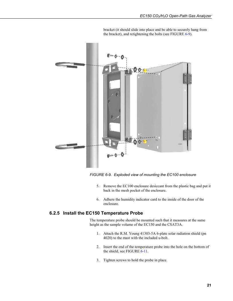
bracket (it should slide into place and be able to securely hang from the bracket), and retightening the bolts (see FIGURE 6-9).
FIGURE 6-9. Exploded view of mounting the EC100 enclosure
5. Remove the EC100 enclosure desiccant from the plastic bag and put it back in the mesh pocket of the enclosure.
6. Adhere the humidity indicator card to the inside of the door of the enclosure.
6.2.5 Install the EC150 Temperature Probe The temperature probe should be mounted such that it measures at the same height as the sample volume of the EC150 and the CSAT3A.
1. Attach the R.M. Young 41303-5A 6-plate solar radiation shield (pn 4020) to the mast with the included u-bolt.
2. Insert the end of the temperature probe into the hole on the bottom of the shield, see FIGURE 6-11.
3. Tighten screws to hold the probe in place.

EC150 CO2/H2O Open-Path Gas Analyzer
22
FIGURE 6-10. EC150 temperature probe
FIGURE 6-11. Solar radiation shield with EC150 temperature probe
6.3 Wiring and Connections FIGURES 6-12 and 6-13 show EC100 electronics panel and the bottom of the EC100 enclosure, respectively. Refer to these figures during the wiring and connecting of the various auxiliary sensors.
FIGURE 6-12. EC100 electronics front panel showing EC100 as shipped (left) and after completed wiring and connections (right)

EC150 CO2/H2O Open-Path Gas Analyzer
23
FIGURE 6-13. Bottom of EC100 enclosure
6.3.1 Connecting the EC150 Gas Analyzer Head 1. Remove the black rubber cable entry plug (pn 26224) that is located on the
bottom right of the EC100 enclosure labeled Cable 3. (This plug can be stored in the mesh pocket of the enclosure.)
2. Insert the cable entry plug that is attached to the large cable of the EC150 gas analyzer head into the vacant slot.
3. Push the connector at the end of the cable onto its mating connector (labeled Gas Analyzer) and tighten the thumbscrews (see FIGURE 6-13). The EC150 gas analyzer cable is approximately 3.0 m (10.0 ft) in length.
6.3.2 Connect the CSAT3A Sonic Head Skip the following two steps if not using a CSAT3A.
1. Similar to connecting the gas analyzer head, remove the black rubber cable entry plug found on the bottom left of the EC100 enclosure.
2. Insert the cable entry plug on the CSAT3A cable into the slot and connect the male end to the female connector labeled Sonic Anemometer on the EC100 electronics (see FIGURE 6-13).
Unlike previous models of the CSAT3 3D sonic anemometer, the CSAT3A sonic head and the EC150 gas analyzer head have embedded calibration information. This means that any CSAT3A and any EC150 may be used with any EC100.
NOTE

EC150 CO2/H2O Open-Path Gas Analyzer
24
6.3.3 Connect the EC150 Temperature Probe 1. Unscrew the temperature connector cover which is found on the bottom of
the EC100 enclosure labeled Temperature Probe (see FIGURE 6-13).
2. Insert the three-prong temperature probe connector into the female connector on the enclosure and screw it firmly in place. The EC150 temperature probe cable is approximately 3.0 m (10.0 ft) in length.
6.3.4 Ground the EC100 Electronics 1. Attach a user-supplied heavy gauge wire (12 AWG would be appropriate)
to the grounding lug found on the bottom of the EC100 enclosure.
2. Earth (chassis) ground the other end of the wire using a grounding rod. For more details on grounding, see the CR3000 datalogger manual grounding section.
Grounding the EC100 is critical. Proper grounding to earth (chassis) will ensure maximum electrostatic discharge (ESD) protection and improve measurement accuracy.
Do not connect or disconnect the EC150 gas analyzer head or CSAT3 sonic head once the EC100 is powered.
6.3.5 Connect SDM Communications to the EC100 The EC150 supports SDM communications with datalogger. SDM is the preferred communications to the EC100. RS-485 may be necessary in some situations. The USB is used mainly for diagnostic and trouble shooting. Connection instructions for these modes can be found in Appendix C, Alternate EC100 Outputs (p. C-1).
CABLE4CBL-L (pn 21972) is used for connecting SDM communications to the EC100. The “L” designation denotes the length of the cable which is user-specified.
1. Loosen the nut on one of the cable entry seals (Cable 1) on the bottom of the EC100 enclosure (refer to FIGURE 6-13).
2. Remove plastic plug and store in mesh pocket of enclosure.
3. Insert the cable while referring to TABLE 6-1 for details on which color of wire in the cable should be connected to each terminal found on the SDM connector of the EC100 panel.
4. Once the wires of the cable are fully connected, retighten the nut on the appropriate cable entry.
CAUTION
CAUTION

EC150 CO2/H2O Open-Path Gas Analyzer
25
TABLE 6-1. EC100 SDM Output
EC100 Channel Description Color
SDM-C1 SDM Data Green
SDM-C2 SDM Clock White
SDM-C3 SDM Enable Red (or Brown)
G Digital Ground Black
G Shield Clear
6.3.6 Wire Power and Ground the EC100 1. Feed cable CABLEPCBL-L (pn 21969-L) through Cable 2 at the bottom
of the EC100 enclosure (see FIGURE 6-13) and attach the ends into the green EC100 power connector (pn 3768).
2. Plug the connector into the female power connector on the EC100 panel. Ensure that the power and ground ends are going to the appropriate terminals labeled 12V and ground, respectively.
3. Connect the power cable to a power source. The power and ground ends may be wired to the 12V and G ports, respectively, of a Campbell Scientific datalogger or to another 12 Vdc source.
Once power is applied to the EC100, three LED status lights on the EC100 panel will illuminate. The power LED will be green if the power supply voltage is between 10 to 16 Vdc. The gas LEDs will be orange until the gas head has warmed up. The sonic LED will be red while the sonic acquires the ultrasonic signals. The sonic and gas LEDs will turn green if there are no diagnostic warning flags. Three green LEDs indicate that the instrument is ready to make measurements.
The EC150 power-up sequence takes under two minutes to complete. During power up the gas LED will be orange. If after two minutes the gas LED turns green, power-up sequence has been completed successfully. If the gas LED turns red, a diagnostic flag has been detected. Check the individual diagnostic bits to determine the specific fault.
Diagnostics may be monitored using the Status window of ECMon (see Appendix A.3, ECMon (p. A-7)), the user interface software included with the EC150 (see Appendix A, EC150 Settings (p. A-1)), or with a datalogger. The diagnostics may reveal that the unit needs to be serviced (for example, cleaning the optical windows on the EC150, cleaning the CSAT3A transducers of ice or debris, etc. See Section 8, Maintenance and Troubleshooting (p. 31)).
6.4 Data Collection and Data Processing Data from the EC150 is collected through the EC100 and then archived onto a datalogger. A common instrument configuration is to program a datalogger to retrieve and collect raw data from the EC150, to be used for post processing, for which various programs have been developed.

EC150 CO2/H2O Open-Path Gas Analyzer
26
More recently, programs have been developed that efficiently record and correctly process data from instruments such as the EC150, as well as compile them with data from other, complementary instruments. Campbell Scientific has developed a program, EasyFlux™ DL, that both records and processes raw data from the EC150 to provide useful measurements immediately. An overview of both approaches is given in the sections below.
6.4.1 Data Collection and Processing with EasyFlux DL EasyFlux DL is an open source CRBasic program that allows a CR6 or CR3000 datalogger to collect fully corrected measurements from an EC150 instrument. The program is compatible with other GPS and energy balance sensors which, in combination, can report corrected fluxes for CO2, latent heat (H2O), sensible heat, ground surface heat flux, and momentum. The program processes the EC data using commonly used corrections in the scientific literature. For detailed information about downloading, installing, and configuring the free program, refer to the EasyFlux DL manual located at www.campbellsci.com/easyflux-dl.
6.4.2 Datalogger Programming with CRBasic The datalogger of the EC150 is programmed in the CRBasic language, which features two instructions for communication with the EC100 via SDM. The first instruction is EC100(), which reads measurement data from the EC100. The second is the EC100Configure(), which receives and sends configuration settings.
With programs such as EasyFlux DL, there is little need for the user to become well versed in the CRBasic language and the instructions required for communicating with the EC100. In those cases in which it is needed or desired, the Campbell Scientific website has several tutorials and guidance for learning the CRBasic language. They can be accessed by entering CRBasic in the search field at www.campbellsci.com.
7. Zero and Span 7.1 Introduction
Calibration of optical instrumentation like the EC150 may drift slightly from the calibration that was performed in the factory with time and exposure to natural elements. A zero-and-span procedure should be performed after installation of the instrument to give appropriate baseline readings as a reference. A zero-and-span procedure should also be performed occasionally to assess drifts from factory calibration. In many cases, a zero and span can help resolve problems that are being experienced by the user during operating the EC150. For example, a zero-and-span procedure should always be performed on the analyzer after changing the internal chemicals. Before performing a zero-and-span procedure, clean the windows of the EC150 as described in Section 8.3, Cleaning Analyzer Windows (p. 33).
After the first several zero-and-span procedures, the rate of drift in gain and offset (explained later in this section) should be analyzed to better determine how frequently the zero-and-span procedure should be performed once the instrument has been put into service.

EC150 CO2/H2O Open-Path Gas Analyzer
27
The first part of the procedure listed below simply measures the CO2 and H2O span and zero without making any adjustments. This allows the CO2 and H2O gain factors to be calculated. These gain factors quantify the state of the analyzer before the zero-and-span procedure and, in theory, could be used to correct recent measurements for drift. The last part of the zero-and-span procedure adjusts internal processing parameters to correct subsequent measurements.
If the zero-and-span procedure is being performed off site (for example, in a laboratory), be sure to mount the EC150 on the zero-and-span stand (refer to FIGURE 7-1). This will ensure the analyzer is in the correct upright orientation and has the correct optical alignment.
The zero-and-span procedure must be performed correctly and not rushed. Allocate at least one hour (preferably more) for the procedure. Ensure that the readings are stable and all sensors are properly connected and functioning.
It is conceivable that there are circumstances in which both a zero and a span cannot be performed by the user. In these instances, it is recommended that the user attempt to perform a zero of the instrument even if spanning is not possible or inconvenient. The information gained through zeroing the instrument can help troubleshoot problems that may be encountered during field operations.
The water vapor measurement is used in the CO2 concentration calculations to correct instrument and pressure broadening effects. To achieve good CO2 calibration, it is imperative to maintain a reasonable water vapor calibration.
Resting the analyzer on its side during the zero-and-span procedure may result in measurement inaccuracy.
7.2 Zero-and-Span Procedure This section gives instructions for performing a zero-and-span procedure, and should be referred to any time a zero-and-span procedure is undertaken.
Check and then set the EC150 zero and span according to the following steps:
1. Remove power from the EC100/EC150. Unplugging the power cable from the EC100 is the easiest way to accomplish this.
2. Remove wicks from the snouts of the analyzer.
3. Clean windows and snouts with isopropyl alcohol and a lint-free, non-abrasive tissue or cloth as described in Section 8.3, Cleaning Analyzer Windows (p. 33).
Make sure any residual alcohol and water completely evaporate from the analyzer before proceeding with the zero-and-span procedure.
NOTE
CAUTION
CAUTION
EC150 CO2/H2O Open-Path Gas Analyzer
28
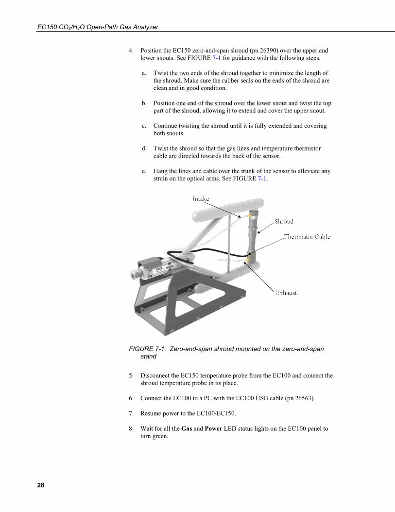
4. Position the EC150 zero-and-span shroud (pn 26390) over the upper and lower snouts. See FIGURE 7-1 for guidance with the following steps.
a. Twist the two ends of the shroud together to minimize the length of the shroud. Make sure the rubber seals on the ends of the shroud are clean and in good condition.
b. Position one end of the shroud over the lower snout and twist the top part of the shroud, allowing it to extend and cover the upper snout.
c. Continue twisting the shroud until it is fully extended and covering both snouts.
d. Twist the shroud so that the gas lines and temperature thermistor cable are directed towards the back of the sensor.
e. Hang the lines and cable over the trunk of the sensor to alleviate any strain on the optical arms. See FIGURE 7-1.
FIGURE 7-1. Zero-and-span shroud mounted on the zero-and-span stand
5. Disconnect the EC150 temperature probe from the EC100 and connect the shroud temperature probe in its place.
6. Connect the EC100 to a PC with the EC100 USB cable (pn 26563).
7. Resume power to the EC100/EC150.
8. Wait for all the Gas and Power LED status lights on the EC100 panel to turn green.

EC150 CO2/H2O Open-Path Gas Analyzer
29
9. Launch ECMon, select the appropriate USB port, and click Connect. The main screen should now be reporting real-time CO2 and H2O concentrations.
10. Click Zero/Span. A graph will appear in the lower half of the zero-and-span window showing measured CO2 and H2O concentrations (see FIGURE 7-2).
11. Connect a gas cylinder of known CO2 concentration to a pressure regulator, then to a flow controller, and finally to the intake of the shroud. Optimally, the concentration of span CO2 should be near the concentration of CO2 being measured in the field.
12. Beginning with both the pressure regulator and flow controller turned off, use the pressure regulator to slowly increase pressure to the recommended setting for the flow controller.
13. Set the flow between 0.2 and 0.4 LPM.
14. Monitor the ECMon zero-and-span graph and wait for the CO2 measurement readings to stabilize (5 to 10 minutes). Once stable, record the reported CO2 concentration.
Use a mixture of CO2 in air (not nitrogen) for the CO2 span gas. The use of pure nitrogen as the carrier gas will lead to errors because the pressure-broadening of the CO2 absorption lines is different for oxygen and nitrogen.
FIGURE 7-2. ECMon zero-and-span window
NOTE

EC150 CO2/H2O Open-Path Gas Analyzer
30
15. Remove the CO2 span gas from the inlet of the shroud and replace it with H2O span gas from a dew-point generator or another standard reference. As water molecules can adsorb to inside of the tubing and the shroud, it may take 30 minutes or more for the H2O concentration to stabilize. The user may increase the flow rate for the first several minutes to more quickly stabilize the system before returning it to between 0.2 and 0.4 LPM to make the H2O measurement. Record the reported H2O concentration. If a stable reading is not achieved within 45 to 60 minutes, troubleshooting steps should be undertaken.
16. Remove the H2O span gas, and connect a zero air source (no CO2 or H2O) to the inlet tube of the shroud. As described in step 11, use a pressure regulator and flow controller so that zero air flows through the shroud between 0.2 and 0.4 LPM. Wait for the measurement readings to stabilize and record the reported values for CO2 and H2O concentrations. If the readings remain erratic, ensure that flow of the zero air is sufficient and the shroud is correctly seated on the snouts.
If the quality of a zero gas is unknown or suspect, a desiccant and CO2 scrubber should be added between the zero gas tank and the shroud to confirm that the gas being sampled during the zero procedure is actually a zero air source.
17. Along with recording the CO2 and H2O zero and span values, also record the date and time, and temperature. With this information the user can examine zero/span drift with time and temperature.
Compute the drift in instrument gain using the following equation:
measmeas
actual
zerospanspangain
−=
where,
• spanactual = known concentration of the span gas • spanmeas = measured concentration of the span gas • zeromeas = measured concentration in zero gas
Note that in the zero-and-span window of ECMon, spanactual is reported to the right of the box where the user enters the span dewpoint temperature. The software calculates spanactual by taking into account the dewpoint temperature and current ambient temperature and pressure. The equations used for this calculation may be found in Appendix D, Useful Equations (p. D-1). If drift (offset or gain) for CO2 or H2O is excessive, it may be time to replace the desiccant and CO2 scrubber bottles (see Section 8.5, Replacing CO2 Scrubber Bottles (p. 33)).
18. With zero air still flowing and measurements stabilized, click on the Zero CO2 and H2O button in the ECMon zero-and-span window.
NOTE
EC150 CO2/H2O Open-Path Gas Analyzer
31
Air flow into the shroud should be close to the recommended rate. If the flow is too low, the shroud will not be properly flushed. If it is too high, the air pressure within the shroud will be too high, and the analyzer will not be zeroed and spanned properly.
19. Remove the zero air source and replace it with the CO2 span gas.
20. Allow the gas to flow through the shroud, maintaining a flow between 0.2 and 0.4 LPM. Wait for readings to stabilize.
21. In the zero-and-span window, enter the known concentration of CO2 (in ppm) in the box labeled Span Concentration (dry) and press Span.
22. Replace the CO2 span gas with an H2O span gas of known dewpoint. Allow the gas to flow through the shroud. Higher flows may be desired for a couple of minutes to more quickly establish equilibrium before resuming a flow between 0.2 and 0.4 LPM. Wait for the readings to stabilize.
23. Enter the known dewpoint (in °C) in the box labeled Span Dewpoint and press Span.
24. The zero-and-span procedure is now complete. Remove the shroud, reconnect the EC150 temperature probe, and prepare the site for normal operation. Verify that readings from the instrument are reasonable. Record the zero and span coefficients for future reference and to keep track of the rate of the analyzer drift. Make sure that the coefficients are between 0.9 and 1.1. Negative or numbers larger than 1.1 are usually an indication of improper calibration.
8. Maintenance and Troubleshooting EC150 operation requires six maintenance tasks:
• Routine site maintenance • Wick maintenance • Analyzer window cleaning • Zero and span • Replacing the analyzer desiccant/scrubber bottles • Factory recalibration
8.1 Routine Site Maintenance The following items should be examined periodically:
• Check the humidity indicator card in the EC100 enclosure. If the highest dot has turned pink, replace the desiccant bags. Replacement desiccant bags may be purchased as pn 6714.
• Make sure the Power and Gas LED status lights on the EC100 panel are green. If not, check the individual diagnostic bits for the specific fault. See TABLE 8-2, Diagnostic Flags of Sonic Status LED (p. 36), and Section 8.7.3, LED Status Lights (p. 35), for more information.
NOTE
EC150 CO2/H2O Open-Path Gas Analyzer
32
8.2 Gas Analyzer Wicks The windows of the EC150 gas analyzer are polished and slanted at an angle to prevent water from collecting on their surfaces. However, due to increased surface tension at the interface with the snout, water can pool at the edges and partially block the optical path and attenuate the signal. To minimize the occurrence of such events and the resulting data loss, consider using the wicks listed in TABLE 8-1. The weave of the wicking fabric promotes capillary action that wicks the water away from the edge of the windows. The seam and the straight edge of the wicks are permeated with a rubberized compound to prevent them from shifting during operation.
Proper installation of the wicks is critical. They should not block or encroach on the optical path. Before installation, record signal strengths for both H2O and CO2. Following installation, repeat testing of signal strength and check that these values are unchanged.
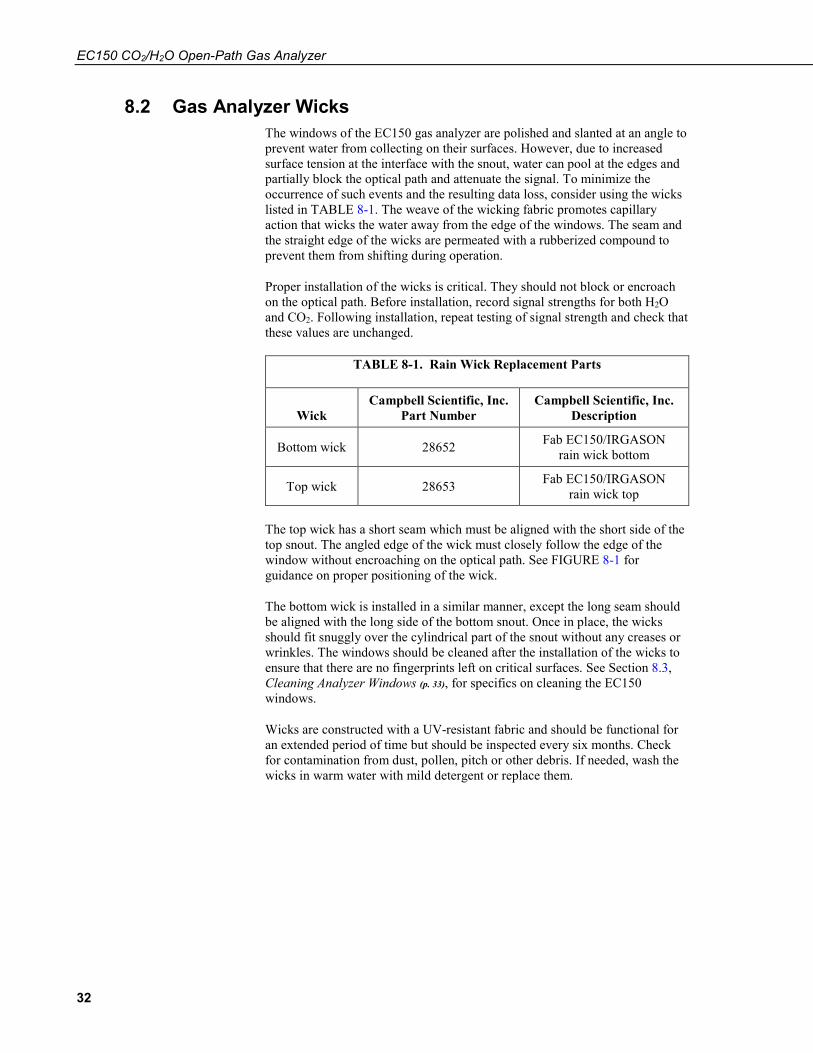
TABLE 8-1. Rain Wick Replacement Parts
Wick Campbell Scientific, Inc.
Part Number Campbell Scientific, Inc.
Description
Bottom wick 28652 Fab EC150/IRGASON rain wick bottom
Top wick 28653 Fab EC150/IRGASON rain wick top
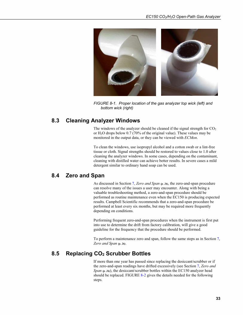
The top wick has a short seam which must be aligned with the short side of the top snout. The angled edge of the wick must closely follow the edge of the window without encroaching on the optical path. See FIGURE 8-1 for guidance on proper positioning of the wick.
The bottom wick is installed in a similar manner, except the long seam should be aligned with the long side of the bottom snout. Once in place, the wicks should fit snuggly over the cylindrical part of the snout without any creases or wrinkles. The windows should be cleaned after the installation of the wicks to ensure that there are no fingerprints left on critical surfaces. See Section 8.3, Cleaning Analyzer Windows (p. 33), for specifics on cleaning the EC150 windows.
Wicks are constructed with a UV-resistant fabric and should be functional for an extended period of time but should be inspected every six months. Check for contamination from dust, pollen, pitch or other debris. If needed, wash the wicks in warm water with mild detergent or replace them.
EC150 CO2/H2O Open-Path Gas Analyzer
33
FIGURE 8-1. Proper location of the gas analyzer top wick (left) and bottom wick (right)
8.3 Cleaning Analyzer Windows The windows of the analyzer should be cleaned if the signal strength for CO2 or H2O drops below 0.7 (70% of the original value). These values may be monitored in the output data, or they can be viewed with ECMon.
To clean the windows, use isopropyl alcohol and a cotton swab or a lint-free tissue or cloth. Signal strengths should be restored to values close to 1.0 after cleaning the analyzer windows. In some cases, depending on the contaminant, cleaning with distilled water can achieve better results. In severe cases a mild detergent similar to ordinary hand soap can be used.
8.4 Zero and Span As discussed in Section 7, Zero and Span (p. 26), the zero-and-span procedure can resolve many of the issues a user may encounter. Along with being a valuable troubleshooting method, a zero-and-span procedure should be performed as routine maintenance even when the EC150 is producing expected results. Campbell Scientific recommends that a zero-and-span procedure be performed at least every six months, but may be required more frequently depending on conditions.
Performing frequent zero-and-span procedures when the instrument is first put into use to determine the drift from factory calibration, will give a good guideline for the frequency that the procedure should be performed.
To perform a maintenance zero and span, follow the same steps as in Section 7, Zero and Span (p. 26).
8.5 Replacing CO2 Scrubber Bottles If more than one year has passed since replacing the desiccant/scrubber or if the zero-and-span readings have drifted excessively (see Section 7, Zero and Span (p. 26)), the desiccant/scrubber bottles within the EC150 analyzer head should be replaced. FIGURE 8-2 gives the details needed for the following steps.

EC150 CO2/H2O Open-Path Gas Analyzer
34
EC150 instruments sold prior to July 2017 were sold with scrubber bottles that contained strong oxidizing agents. Avoid direct contact with the chemicals inside the bottles. Also ensure your work area is well ventilated and free of any reactive compounds, including liquid water. Store used chemical bottles in a sealed container until disposal.
Replacing Scrubber Bottles
1. Twist the scrubber bottle covers of the upper and lower arms counter clockwise until they detach (they should loosen by hand).
2. Remove the EC150 chemical bottles from inside the covers, and replace them with new bottles (pn 32897) with the lid of the bottle pointing toward the snouts of the analyzer (see FIGURE 8-2).
Before opening the covers, have the chemical bottles ready so that the time the internal volume of the analyzer is exposed to the environment is minimized.
3. Screw the covers back on the arms. Do not overtighten.
4. Allow the sensor to equilibrate for at least 24 hours (longer if in high humidity).
5. After 24 hours, perform a zero-and-span procedure. If readings continue to be suspect, the sensor may need to be recalibrated at the factory (see Section 8.6, Factory Recalibration (p. 35), below).
The chemical bottles should be disposed of according to local and federal regulations. For more information, Safety Data Sheet (SDS) forms for the chemicals are included in Appendix E, Safety Data Sheets (SDS) (p. E-1).
FIGURE 8-2. Replacing the desiccant and CO2 scrubber bottles (replacement bottles purchased in or after July 2017 may appear different than in the figure)
DANGER
NOTE
EC150 CO2/H2O Open-Path Gas Analyzer
35
8.6 Factory Recalibration When the EC150 is manufactured, it goes through an extensive calibration process, covering a wide range of temperatures, pressures, and gas concentrations. All CO2 calibration gases used in this process are mixtures of CO2 in ambient air that are traceable to the WMO Mole Fraction Scale maintained by the Central Carbon Dioxide Laboratory and the Carbon Cycle Greenhouse Gases Group of the Global Monitoring Division/National Oceanographic and Atmospheric Administration in Boulder, CO, USA.
The long-term calibration stability of the EC150 is achieved by the use of high quality optical and electrical components, a long lasting IR source, and a stable MCT detector. The subtle, long-term aging effects are usually compensated by the user with the field zero-and-span adjustments which bring the performance of the analyzer within the original specifications. Proper handling and regular maintenance of the instrument should make factory recalibration unnecessary in most applications. If zero and span accessories and calibration standards are not available, Campbell Scientific can provide two-point calibration upon request (pn 27312).
However, if a user finds that signal strength outputs of greater than 0.75 cannot be achieved after both cleaning the windows and a subsequent zero-and-span procedure, contact Campbell Scientific. Contact Campbell Scientific to help determine if the instrument should be returned to Campbell Scientific for a factory recalibration.
For the CSAT3A, refer to the CSAT3 instruction manual for information on recalibration.
8.7 Troubleshooting 8.7.1 Data Loss During Precipitation Events
In extremely humid environments or after a precipitation event, data loss can occur. Wicks on the analyzer windows help mitigate some of these data loss events but cannot control for all conditions. In addition to wicking, heaters in the snouts can aid in the prevention of data loss during precipitation and condensation events. The heaters are automatically controlled by the EC100 electronics. The automatic heater control is activated using the Device Configuration Utility or ECMon software. A value of −1 turns the automatic heater control off and a value of −2 turns it on.
8.7.2 EC100 Diagnostics for Gas Analyzer Troubleshooting Before troubleshooting and servicing the analyzer, become familiar with Section 2, Precautions (p. 1).
The EC100 is also programmed to recognize problems with an associated gas analyzer and reports those with LED status lights and diagnostic flags. The two types of warnings are described in the sections that follow.
8.7.3 LED Status Lights The EC100 has three LED status lights located in the upper left corner of the front panel which provide immediate visual feedback and warn the user of
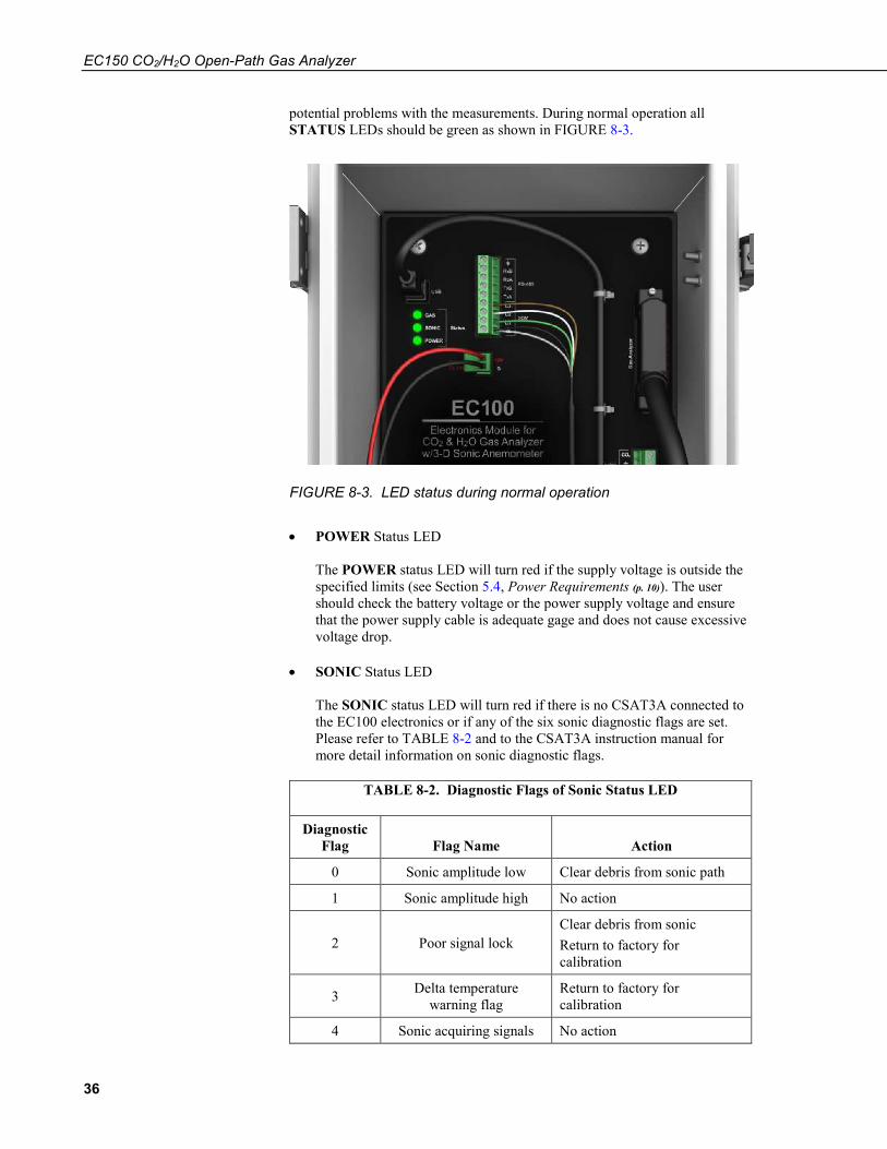
EC150 CO2/H2O Open-Path Gas Analyzer
36
potential problems with the measurements. During normal operation all STATUS LEDs should be green as shown in FIGURE 8-3.
FIGURE 8-3. LED status during normal operation
• POWER Status LED The POWER status LED will turn red if the supply voltage is outside the specified limits (see Section 5.4, Power Requirements (p. 10)). The user should check the battery voltage or the power supply voltage and ensure that the power supply cable is adequate gage and does not cause excessive voltage drop.
• SONIC Status LED The SONIC status LED will turn red if there is no CSAT3A connected to the EC100 electronics or if any of the six sonic diagnostic flags are set. Please refer to TABLE 8-2 and to the CSAT3A instruction manual for more detail information on sonic diagnostic flags.
TABLE 8-2. Diagnostic Flags of Sonic Status LED
Diagnostic Flag Flag Name Action
0 Sonic amplitude low Clear debris from sonic path
1 Sonic amplitude high No action
2 Poor signal lock Clear debris from sonic Return to factory for calibration
3 Delta temperature warning flag
Return to factory for calibration
4 Sonic acquiring signals No action

EC150 CO2/H2O Open-Path Gas Analyzer
37
TABLE 8-2. Diagnostic Flags of Sonic Status LED
Diagnostic Flag Flag Name Action
5 Signature error in reading
CSAT3A sonic head calibration
Check sonic umbilical cable connection Cycle power Contact Campbell Scientific for a new calibration file and upload procedure
• GAS Status LED
The GAS status LED will turn red in the following situations: o The EC150 gas head is not connected o Any of the gas diagnostic flags are set
The GAS status LED will turn orange during the initial power up sequence, usually 1-2 min and will turn to green when the sequence is completed and if no diagnostic flags have been set high.
8.7.4 Diagnostic Flags The EC100 operating system has extensive self-diagnostic capabilities. TABLE 8-3 lists 23 (numbered 0 through 22) diagnostic flags that allow the user to identify problems associated with the operation and the performance of the EC100 electronics and the gas analyzer. There is one master flag (BAD_DATA, or flag 0) that is set when measurements are compromised.
If any of the remaining 22 flags are set, the master flag (BAD_DATA) is set as well, so that the user can filter data based on this flag only. When this flag is set, more detailed information about the nature of the problem can be obtained from the 22 slave flags.
When a flag is set due to improper configuration of the analyzer, inadequate power supply voltage or grounding, extreme environmental conditions, and unreliable or missing connections, the user should try to correct the problem by checking the instrument setup, verifying that all components are properly connected and configured, and that operating conditions are within operational specifications. Other flags are associated with the proper function of the internal components of the analyzer. If any of these flags are set, consult with Campbell Scientific for assistance in diagnosing the problem and, if necessary, arrange to send the instrument for repair.
If connected to a datalogger, the EC100 could be automatically configured under CRBasic program control. The user should verify the proper configuration in the datalogger program.
NOTE

EC150 CO2/H2O Open-Path Gas Analyzer
38
TABLE 8-3. Diagnostic Flags and Suggested Actions
Flag Number Flag Name Comments
0 Bad Data
Set when any of flags 1 through 22 is set. Discard all data with this flag is set. If the flag persists, identify which of flags 1 through 22 is set. When this flag is set, the GAS status LED on the EC100 electronics panel is illuminated red.
1 General Fault Reserved for future use.
2 Startup
Set during the initial power up of the analyzer. It stays set only until all control loops have settled. The infrared detector temperature and the motor speed usually stabilize in 1 to 2 minutes. If the flag persists, verify that the operating conditions (temperature, pressure, supply voltage and current) are within specified limits and that all connections with the gas head and peripheral sensors are made properly. When this flag is set the GAS status LED turns orange. WARNING: Power off the EC100 electronics before disconnecting the gas analyzer.
3 Motor Speed
Set when the motor speed is outside the prescribed limits. It may occasionally be set for short periods of time (10 to 15 seconds), but if it persists, the user should consult with Campbell Scientific.
4 TEC Temperature
Set when the infrared detector temperature is outside the prescribed limits. It may occasionally be set for short periods of time (10 to 15 seconds), but if it persists the user should consult the factory. Verify that ambient temperature and power supply voltage are within the specifications.
5 Source Power
Set every time the infrared source power is outside the prescribed limits. It may occasionally be set for short periods of time (10 to 15 seconds), but if it persists, the user should consult with Campbell Scientific. Verify that ambient temperature and power supply voltage are within specifications.

EC150 CO2/H2O Open-Path Gas Analyzer
39
TABLE 8-3. Diagnostic Flags and Suggested Actions
Flag Number Flag Name Comments
6 Source Temperature
Set when the internal temperature is outside the specified safe operation limits (−35 to 55 °C). If this flag is set the sensor head will be turned off until the internal temperature is within the range −30 to 50 °C. If the flag is set and ambient temperature is within the specified range, consult with Campbell Scientific.
7 Source Current
Set when the infrared source current is outside the prescribed limits. It may occasionally be set for short periods of time, but if it persists the user should consult with Campbell Scientific.
8 Off
Set when the analyzer head is powered off by the user, the datalogger program, or the EC100 operating system when the LIGHT_TEMP flag is set.
9 Synchronization
Set when sampling errors are detected. Sampling errors are most often caused by strong electromagnetic interference. If the flag persists, consult with Campbell Scientific.
10 Ambient Temperature
Set when the ambient temperature is below −30 °C or above 55 °C or when the air temperature sensor is not connected. If the user enters a fixed temperature, this temperature must be within the range −30 to 55 °C.
11 Ambient Pressure
Set when the ambient pressure is outside the specified limits (55 to 120 kPa) or the external pressure sensor is configured but not connected.
12 CO2 I
Set if CO2 measurement signal is outside prescribed limits. It can be turned on when the measurement path is obstructed by insects, dust, precipitation, condensation etc. If it persists, consult with Campbell Scientific.
13 CO2 Io
Set if CO2 reference signal is outside prescribed limits. It can be turned on when the measurement path is obstructed by insects, dust, precipitation, condensation etc. If it persists, consult with Campbell Scientific.

EC150 CO2/H2O Open-Path Gas Analyzer
40
TABLE 8-3. Diagnostic Flags and Suggested Actions
Flag Number Flag Name Comments
14 H2O I
Set if H2O measurement signal is outside prescribed limits. It can be turned on when the measurement path is obstructed by insects, dust, precipitation, condensation etc. If it persists, consult with Campbell Scientific.
15 H2O Io
Set if H2O measurement signal is outside prescribed limits. It can be turned on when the measurement path is obstructed by insects, dust, precipitation, condensation etc. If it persists, consult with Campbell Scientific.
16 H2O Io Variation Set if fast changes in the CO2 reference signal are detected. If it persists, consult with Campbell Scientific.
17 CO2 O IoH2OIo Variation
Set if fast changes in the H2O reference signal are detected. If it persists, consult with Campbell Scientific.
18 CO2 Signal Strength
Set if the ratio of the CO2 measurement and the CO2 reference signals are outside prescribed limits. It can be turned on when the measurement path is obstructed by insects, dust, precipitation, condensation etc. If it persists, consult with Campbell Scientific.
19 H2O Signal Strength
Set if the ratio of the H2O measurement and the H2O reference signals is outside prescribed limits. It can be turned on when the measurement path is obstructed by insects, dust, precipitation, condensation etc. If it persists, consult with Campbell Scientific.
20 Calibration Error
Set if there is a problem reading or writing into the analyzer’s head memory. Power off the EC100 and reconnect the head. If the flag persists, consult with Campbell Scientific. For more information on the head memory refer to Section 4.3, Gas Head Memory (p. 3).
21 Heater Ctrl Off
22 Not Used

A-1
Appendix A. EC150 Settings Operation of the EC150 can be customized by changing the values of the settings. Factory defaults will work well for most applications, but the user may adjust the settings with a PC using either the ECMon software (see Appendix A.3, ECMon (p. A-7)) or the Device Configuration Utility (see Appendix A.4, Device Configuration Utility (p. A-9)), or with a datalogger using the EC100Configure() CR Basic instruction (see Appendix A.5, EC100Configure() Instruction (p. A-9)).
When the EC150 is connected to a datalogger, the settings of the analyzer can be configured automatically by the CR Basic program.
A.1 Factory Defaults TABLE A-1 shows the default value for each of the settings.
TABLE A-1. Factory Default Settings
Setting Default
SDM Address 1
Bandwidth 20 Hz
Unprompted Output disabled
RS-485 Baud Rate 115200 bp
Unprompted Output Rate 10 Hz
Analog Output disabled
ECMon Update Rate 10 Hz
Temperature Sensor Auto-select (EC150 Temperature Probe)
Pressure Sensor EC100 Basic or EC100 Enhanced (depends on initial order configuration)
Pressure Differential Enable
Auto-Select (Disabled for EC150)
Heater Control Disabled
A.2 Details This section gives an explanation for each setting. The value of each setting is stored either in the non-volatile memory of the EC100 electronics or the EC150 gas head. The section also explains the details of where settings are stored. For convenience all settings and calibration information associated with the operation of the gas head are stored in non-volatile memory located in the head.
Another group of settings pertinent to the operation of the EC100 electronics are stored in non-volatile memory. These settings are the first seven in TABLE A-1. For more details refer to the following sections.
Appendix A. EC150 Settings
A-2
A.2.1 SDM Address This parameter must be set to use SDM output from the EC100. See Section 4.6.2.1, SDM Output (p. 5), for details on using SDM output.
Each SDM device on the SDM bus must have a unique address. The EC150 has a factory default SDM address of 1, but may be changed to any integer value between 0 and 14. The value 15 is reserved as an SDM group trigger.
The SDM address is stored in non-volatile memory of the EC100 electronics.
A.2.2 Bandwidth The EC100 has a user-selectable, low-pass filter to select the bandwidth (5, 10, 12.5, 20, or 25 Hz). Setting the bandwidth to a lower value will reduce noise. However, it must be set high enough to retain the high-frequency fluctuations in CO2 and H2O, or the high frequency contributions to the flux will be lost. The factory default bandwidth is set to 20 Hz which is sufficient for most flux applications. Lower bandwidth settings may be used for higher measurement heights which inherently have lower frequency content. Refer to Appendix B, Filter Bandwidth and Time Delay (p. B-1), for more information on the digital filter options.
If a spectral analysis is performed to evaluate the experimental setup, the bandwidth should be set to the Nyquist frequency, which is half the datalogger sample rate (for SDM output) or half the unprompted output rate (for USB and RS-485 output). This ensures that the data will not be under-sampled and that higher frequency variations will not be aliased to lower frequencies.
If too small a bandwidth is selected, high frequency fluxes will be filtered.
The Bandwidth setting is stored in non-volatile memory of the EC100 electronics.
A.2.3 Unprompted Output If the EC100 is to output data in one of the unprompted modes (USB or RS-485, see Appendix C.1, USB or RS-485 Output (p. C-1)), this setting must be set accordingly. The factory default is to disable the unprompted output, assuming data will be logged via SDM (see Section 4.6.2.1, SDM Output (p. 5)).
Only one unprompted output type (for example, USB or RS-485) may be selected at a given time. The rate at which the EC100 outputs these data is determined by the Unprompted Output Rate setting.
The Unprompted Output Rate setting is stored in non-volatile memory of the EC100 electronics.
A.2.4 Unprompted Output Rate When the Unprompted output is enabled, this setting determines the output rate for unprompted output (USB or RS-485, see Appendix C.1, USB or RS-485 Output (p. C-1)). If the unprompted output is disabled, this parameter is not used. The factory default output rate is 10 Hz, but it may be set to 10, 25, or 50 Hz.
NOTE

Appendix A. EC150 Settings
A-3
The Unprompted Output setting is stored in non-volatile memory of the EC100 electronics.
A.2.5 RS-485 Baud Rate If the unprompted output mode is set to RS-485, the RS-485 Baud Rate parameter determines the baud rate. Otherwise this setting is not used. The RS-485 baud rate defaults to 115200 bps, although the user may enter another value.
The RS-485 Baud Rate setting is stored in non-volatile memory of the EC100 electronics.
A.2.6 Analog Output The EC100 has two analog outputs for CO2 and H2O densities (see Appendix C.2, Analog Outputs (p. C-3)). These outputs may be enabled or disabled with this setting. The default is for analog output to be disabled.
The Analog Output setting is stored in non-volatile memory of the EC100 electronics.
A.2.7 ECMon Update Rate The ECMon Update Rate setting determines the rate at which data are sent over the USB connection to the PC while running ECMon. The default setting of 10 Hz should be adequate in most situations.
The ECMon Update Rate setting is stored in non-volatile memory of the EC100 electronics.
A.2.8 Temperature Sensor The Temperature Sensor setting configures the EC100 electronics to work with either an EC150 open-path gas analyzer or an EC155 closed-path gas analyzer. The EC150 measures ambient air temperature using a thermistor probe mounted in the solar radiation shield (see Section 6.3.3, Connect the EC150 Temperature Probe (p. 24)).
With the Auto-Select default setting, the EC100 will automatically detect that an EC150 is connected to the electronics and will report ambient air temperature measurements from the thermistor probe.
The EC150 temperature sensor is measured at 1Hz, and is not synchronized to the CO2/H2O measurements.
To diagnose problems with the temperature measurement, a fixed temperature value may be used, or the temperature sensor may be selected manually.
The Temperature Sensor setting is stored in the non-volatile memory of the EC150 head.
A.2.9 Fixed Temperature Value If the Temperature Sensor setting is None, the EC150 will use the value of the Fixed Temperature Value setting for the sample temperature. This mode is intended for troubleshooting only. In normal operation, the Temperature Sensor is set to Auto-Select, and this setting is not used.

Appendix A. EC150 Settings
A-4
The Fixed Temperature Value setting is stored in non-volatile memory of the EC100 electronics.
A.2.10 Pressure Sensor There are three options for measuring barometric pressure for the EC150 that have different corresponding Pressure Sensor settings.
1. The EC100 has an on-board barometer that Campbell Scientific refers to as the EC100 basic barometer. This barometer is mounted on the EC100 electronics board as shown in FIGURE A-1. EC100 Basic Barometer: The EC100 always includes the EC100 basic barometer as a factory default and the default settings is EC100 Basic.
FIGURE A-1. Location of EC100 basic barometer
2. An enhanced-performance barometer can be specified when ordering an EC100 for any of Campbell’s gas analyzers, and is referred to as the enhanced barometer. The enhanced barometer is installed in the factory when specified at the time of order. It will come mounted on the top wall of the EC100 environmental enclosure towards the left, as shown in FIGURE A-2. The enhanced barometer can provide greater accuracy in certain environmental conditions that cannot be achieved with the standard barometer. FIGURE A-3 compares the expected error relative to environmental conditions for the two barometers. Errors related to the altitude of the study site may also warrant the choice of one barometer over the other. Given the various parameters that drive the decision, the most prudent route is to provide a Campbell Scientific sufficient detail about the expected monitoring site at the time of order. EC100 Enhanced Barometer: If the EC100 is ordered with the enhanced barometer, the factory default setting is EC100 Enhanced.

Appendix A. EC150 Settings
A-5
FIGURE A-2. Location of EC100 enhanced barometer
FIGURE A-3. Comparison of error in basic versus enhanced barometer over operational temperatures

Appendix A. EC150 Settings
A-6
3. The option of a third barometer choice is also available but is rarely used. A user-supplied barometer option can also be programmed in the EC100 electronics. This setting determines which pressure sensor will be used to measure the barometric pressure. User-supplied Barometer: When a user supplies a barometer, the setting should be changed to User Supplied and the appropriate values for gain and offset must be entered.
Sampling Frequency: The enhanced barometer is sampled at 1 Hz. If the user supplies an external pressure sensor, it is sampled at 1 Hz. The on-board pressure sensor is measured at 10 Hz. In all cases, the pressure sensor measurement is not synchronized to the CO2 and H2O measurements.
The pressure sensor also allows the setting None for the Pressure Sensor. This mode is intended for troubleshooting only. The EC100 will use a fixed value for pressure.
The Pressure Sensor setting is stored in non-volatile memory in the EC150 head.
A.2.10.1 Pressure Gain This setting is not used unless the Pressure Sensor is set to User Supplied. Then this setting gives the gain factor (kPa/V) used to convert measured voltage to pressure. If the Pressure Sensor is set to EC100 Basic or EC100 Enhanced, this setting is not used.
The Pressure Gain setting is stored in non-volatile memory of the EC100.
A.2.10.2 Pressure Offset This setting is not used unless the Pressure Sensor is set to User Supplied. Then this setting gives the offset (kPa) used to convert measured voltage to pressure. If the Pressure Sensor is set to EC100 Basic or EC100 Enhanced, this setting is not used.
The Pressure Offset setting is stored in the EC100 electronics.
A.2.10.3 Fixed Pressure Value If the Pressure Sensor setting is None, the EC150 will use the value of this setting for the barometric pressure. This mode is intended for troubleshooting only. In normal operation this setting is not used.
The Fixed Pressure Value setting is stored in the EC100 electronics.
A.2.11 Pressure Differential Enable This setting should remain disabled. It is used only for closed-path analyzers.
The Pressure Differential Enable setting is stored in non-volatile memory in the EC150 head.

Appendix A. EC150 Settings
A-7
A.2.12 Heater Control When set to automatic, this setting applies a voltage between 0 and 4600 mV to heaters near the optical windows of the analyzer. Heated windows inhibit the formation of condensation, such as dew and frost, and help the analyzer recover more quickly when precipitation has blocked the optical path.
The Heater Control setting is stored in non-volatile memory in the EC150 head.
A.2.13 Head Power Off When enabled, the EC150 gas head is turned off. The head may be turn on/off under datalogger control to conserve power or under EC100 control if the gas head temperature is outside the operating range. The EC100Configure() Instructions in the CRBasic program is used to turn the gas head on/off under datalogger control.
The Head Power Off setting is stored in non-volatile memory of the EC100.
A.3 ECMon Settings for the EC150 are easily verified and/or changed by using the Windows PC support software ECMon (short for Eddy Covariance Monitor), which is found at www.campbellsci.com/downloads.
Before connecting the EC100 to the computer, install the USB driver through Device Configuration Utility (available at www.campbellsci.com/downloads). Select the EC100 device type, and click Install USB Driver.
Once the driver is installed, download and run the ECMon.exe install file. Launch ECMon and connect the EC100 electronics to the PC with the included EC100 USB cable (pn 26563). The USB connection for the EC100 electronics is found on the bottom of the enclosure (see FIGURE 6-13). Once connected, select the appropriate communications port in the ECMon Main Page and click Connect (see FIGURE A-4). Next click on the Setup button. All of the above settings are now available for the user to change (see FIGURE A-5).
Besides changing settings, ECMon is also a useful tool for other common tasks such as:
• Monitoring real-time data from the EC150 using the Main window • Performing a manual zero and span of the instrument (see Section 7,
Zero and Span (p. 26)) • Troubleshooting and monitoring diagnostics using the Status window

Appendix A. EC150 Settings
A-8
FIGURE A-4. Main screen of ECMon
FIGURE A-5. Setup screen in ECMon

Appendix A. EC150 Settings
A-9
A.4 Device Configuration Utility The Device Configuration Utility software may also be used to change settings, although ECMon is generally preferred as the user interface is more intuitive.
Device Configuration Utility may be downloaded at www.campbellsci.com/downloads.
After launching the Device Configuration Utility, select EC100 from the list of device types. If this is the first time connecting it to the computer, click Install USB Driver before connecting with the USB cable. Then, with the EC100 connected to the computer, select the correct USB communication port, and click Connect. Once connected, the Settings tab displays all current settings. Click Apply to save any changes.
Device Configuration Utility is also used to send an updated operating system to the EC100 electronics. The Send OS tab gives directions on this procedure, or you can watch the video tutorial Updating the EC100 Operating System.
A.5 EC100Configure() Instruction EC100Configure() is an alternate way to retrieve and modify setting. While ECMon and Device Configuration Utility software are user-interactive, the EC100Configure() instruction allows automated control under CRBasic datalogger programming.
EC100Configure() is a processing task instruction. When running in pipeline mode, the datalogger will execute the instruction from the processing task. This functionality allows the instruction to be placed in conditional statements. Execution from processing also introduces ramifications when attempting to execute the EC100Configure() instruction while other SDM instructions are executing in pipeline mode. This instruction locks the SDM port during the duration of its execution. If the pipelined SDM task sequencer needs to run while the SDM is locked, it will be held off until the instruction completes. This locking will likely result in skipped scans when reconfiguring an EC150.
For the EC150 to save settings, it must go through a lengthy write-read-verify process. To avoid saving the settings after each set command, the resulting code can be used to determine if any settings were modified from their original value. When a change is detected, the save settings command (command code 99) can then be sent to the EC150. The DestSource parameter variable should be set to 2718 to save the settings. The reception of this command is acknowledged but since it takes up to a second to complete, a successful return code does not mean that all of the data was successfully written to the appropriate non-volatile memory.
The instruction syntax is:
EC100Configure(Result,SDMAddress,ConfigCmd,DestSource)
Result is a variable that contains a value indicating the success or failure of the command. A result code of 0 means that the command was successfully
NOTE

Appendix A. EC150 Settings
A-10
executed. If reading a setting, 0 in the result code means that the value in the DestSource variable is the value the desired setting has in the EC150. When writing a setting, if the result code is 0, the value and setting were compatible, but the value was not changed because it contained the same value that was sent. A return code of 1 from the set operation means that the value was valid, different, set and acknowledged. This allows CRBasic code to control whether or not to save the settings. NAN (not a number) indicates that the setting was not changed or acknowledged or a signature failure occurred.
SDMAddress defines the address of the EC150 to configure. Valid SDM addresses are 0 through 14. Address 15 is reserved for the SDMTrigger() instruction.
ConfigCmd is a variable that indicates whether to get or set a setting. The options are listed in TABLE A-2.
DestSource is a variable that will contain the value to read when getting a setting, or that will contain the value to send when writing a setting to the EC150.
TABLE A-2. ConfigCmd Values for Setting and Retrieving Settings
ConfigCmd Variable Setting Description (some settings list possible values for the DestSource variable) Set Retrieve
0 100
Bandwidth: • 5 = 5 Hz • 10 = 10 Hz • 12 = 12.5 Hz • 20 = 20 Hz • 25 = 25 Hz
1 101
Unprompted Output: • 10 = 10 Hz • 25 = 25 Hz • 50 = 50 Hz
2 102
Pressure Sensor: • 0 = EC100 Basic • 1 = User-supplied • 2 = EC100 Enhanced • 3 = None (use fixed value)
3 103 Differential Pressure:
• 0 = Disable • 1 = Enable
4 104 Fixed Pressure Value
5 105 Pressure Offset
6 106 Pressure Gain
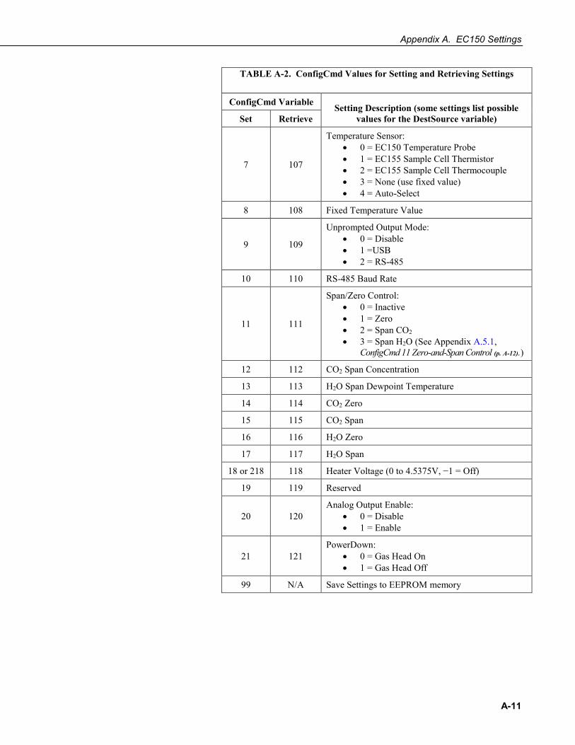
Appendix A. EC150 Settings
A-11
TABLE A-2. ConfigCmd Values for Setting and Retrieving Settings
ConfigCmd Variable Setting Description (some settings list possible values for the DestSource variable) Set Retrieve
7 107
Temperature Sensor: • 0 = EC150 Temperature Probe • 1 = EC155 Sample Cell Thermistor • 2 = EC155 Sample Cell Thermocouple • 3 = None (use fixed value) • 4 = Auto-Select
8 108 Fixed Temperature Value
9 109
Unprompted Output Mode: • 0 = Disable • 1 =USB • 2 = RS-485
10 110 RS-485 Baud Rate
11 111
Span/Zero Control: • 0 = Inactive • 1 = Zero • 2 = Span CO2 • 3 = Span H2O (See Appendix A.5.1,
ConfigCmd 11 Zero-and-Span Control (p. A-12).)
12 112 CO2 Span Concentration
13 113 H2O Span Dewpoint Temperature
14 114 CO2 Zero
15 115 CO2 Span
16 116 H2O Zero
17 117 H2O Span
18 or 218 118 Heater Voltage (0 to 4.5375V, −1 = Off)
19 119 Reserved
20 120 Analog Output Enable:
• 0 = Disable • 1 = Enable
21 121 PowerDown:
• 0 = Gas Head On • 1 = Gas Head Off
99 N/A Save Settings to EEPROM memory

Appendix A. EC150 Settings
A-12
A.5.1 ConfigCmd 11 Zero-and-Span Control To perform zeroing of CO2 and H2O, ConfigCmd 11 is set to 1. After the EC150 completes the zero, it will write the value to –1. The datalogger can poll this value or simply wait for a period of time to allow the zeroing to complete. To perform CO2 span, the CO2 Span Concentration setting (ConfigCmd 12) must be written to the proper value in ppm CO2 prior to setting the Span/Zero Control setting (ConfigCmd 11) to 2. After the CO2 span is completed, the value of the Span/Zero Control setting will change to –2. H2O span is similar to CO2. First the H2O Dew Point value (ConfigCmd 13) must be written to the desired value. Then the Span/Zero Control setting is set to 3. After the EC150 completes the span, the span control setting is written as –3. ConfigCmds 14 through 17 automatically store the results of the zero-and-span procedure. Each result is a coefficient used in the gas analyzer’s algorithms for calculating gas concentrations.
A.6 Example CRBasic Program 'CR3000 Series Datalogger Public sonic_irga(12) Alias sonic_irga(1) = Ux Alias sonic_irga(2) = Uy Alias sonic_irga(3) = Uz Alias sonic_irga(4) = Ts Alias sonic_irga(5) = diag_sonic Alias sonic_irga(6) = CO2 Alias sonic_irga(7) = H2O Alias sonic_irga(8) = diag_irga Alias sonic_irga(9) = cell_tmpr Alias sonic_irga(10) = cell_press Alias sonic_irga(11) = CO2_sig_strgth Alias sonic_irga(12) = H2O_sig_strgth Units Ux = m/s Units Uy = m/s Units Uz = m/s Units Ts = C Units diag_sonic = arb Units CO2 = mg/m^3 Units H2O = g/m^3 Units diag_irga = arb Units cell_tmpr = C Units cell_press = kPa Units CO2_sig_strgth = arb Units H2O_sig_strgth = arb DataTable (ts_data,TRUE,-1) DataInterval (0,0,mSec,10) Sample (12,Ux,IEEE4) EndTable BeginProg Scan (100,mSec,0,0) EC100 (Ux,1,1) CallTable ts_data NextScan EndProg
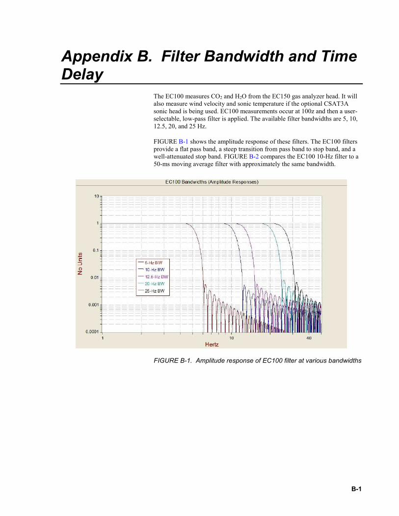
B-1
Appendix B. Filter Bandwidth and Time Delay
The EC100 measures CO2 and H2O from the EC150 gas analyzer head. It will also measure wind velocity and sonic temperature if the optional CSAT3A sonic head is being used. EC100 measurements occur at 100z and then a user-selectable, low-pass filter is applied. The available filter bandwidths are 5, 10, 12.5, 20, and 25 Hz.
FIGURE B-1 shows the amplitude response of these filters. The EC100 filters provide a flat pass band, a steep transition from pass band to stop band, and a well-attenuated stop band. FIGURE B-2 compares the EC100 10-Hz filter to a 50-ms moving average filter with approximately the same bandwidth.
FIGURE B-1. Amplitude response of EC100 filter at various bandwidths

Appendix B. Filter Bandwidth and Time Delay
B-2
FIGURE B-2. Frequency response comparison of EC100 10-Hz bandwidth and a 50-msec moving average
The ideal eddy-covariance filter is one that is wide enough to preserve the low-frequency signal variations that transport flux, yet narrow enough to attenuate high-frequency noise. In addition, to minimize aliasing (defined as the misinterpretation of high-frequency variation as lower-frequency variation), the measurement bandwidth must be less than half of the sample rate or the datalogger scan rate.
Two factors complicate choosing the ideal eddy-covariance bandwidth. First, the flux signal bandwidth varies from one installation to another, and the flux signal bandwidth varies with mean wind speed at a given installation. Second, the fast sample rate required to anti-alias a desired signal bandwidth may result in large, unwieldy data sets.
Fortunately, the covariance calculation itself relaxes the need for the ideal bandwidth. The time-averaged (typically thirty minutes) covariance calculations inherently reduce noise, and second, aliasing does not degrade the accuracy of covariance calculations. The factory default for the EC100 bandwidth (20 Hz) is rather wide to preserve the signal variations that transport flux. The default bandwidth is suitable for most flux applications. Additional bandwidths are available for users desiring to match the EC100 filter bandwidth to their data acquisition sample rate to avoid aliasing. In this case, the selected bandwidth should be one-half of the sample rate. However, users should be careful to avoid attenuation of flux-carrying signals.
The EC100 electronics synchronously sample the EC150 analyzer and the CSAT3A sonic head. However, users wishing to synchronize their EC100 data with other measurements (for example, a fine-wire thermocouple) in the data acquisition system must account for the time delay of the EC100 filter. TABLE B-1 shows the delay for each of the filter bandwidths. The EC100 provides a constant time delay for all spectral components within each filter’s pass band.

Appendix B. Filter Bandwidth and Time Delay
B-3
TABLE B-1. Filter Time Delays for Various Bandwidths
Bandwidth (Hz) Time Delay (ms)
5 800
10 400
12.5 320
20 200
25 160 The following examples show how to use TABLE B-1. To synchronize EC100 data to other datalogger measurements when the datalogger scan rate is 25 Hz and the EC100 bandwidth is set to 20 Hz (a 200-msec time delay from TABLE B-1), delay the non-EC100 data by five datalogger scans. Similarly, for a 10-Hz datalogger scan rate and the same 20-Hz EC100 bandwidth, delay the non-EC100 data by two datalogger scans to match the EC100 data. For the best synchronicity, choose a datalogger scan interval that is an integer multiple of the EC100 filter delay.
The EC100 measures the gas and wind data at 150 Hz, and the 150-Hz data are down-sampled to the datalogger’s scan rate through SDM communications (see Section 4.6.2, EC100 Outputs (p. 5)). This process synchronizes the EC100 gas and wind data with other signals measured by the datalogger to within ±3.33 ms (plus or minus one-half of the inverse of 150 Hz).
Alternately, when sending data to a data acquisition system that is not manufactured by Campbell Scientific, the EC100 down-samples its USB and RS-485 outputs to a user-selectable rate of 10, 25, or 50 Hz. Although the gas and wind data from the EC100 remain synchronized with one another, the user must consider the down-sampled output interval when synchronizing the EC100 data with other measurements in their system. These slower output intervals will increase the asynchronicity of EC100 data with other system measurements.

Appendix B. Filter Bandwidth and Time Delay
B-4
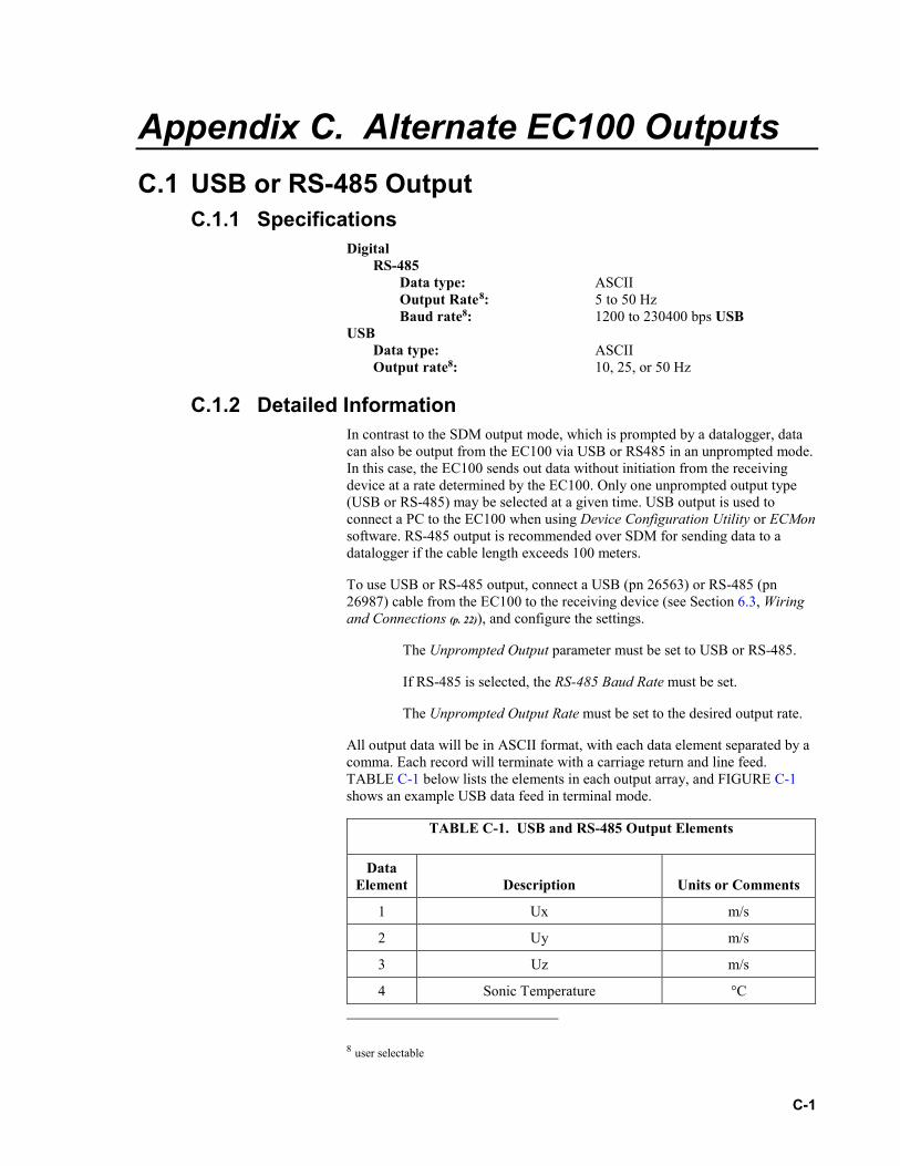
C-1
Appendix C. Alternate EC100 Outputs C.1 USB or RS-485 Output
C.1.1 Specifications Digital
RS-485 Data type: ASCII Output Rate8: 5 to 50 Hz Baud rate8: 1200 to 230400 bps USB
USB Data type: ASCII Output rate8: 10, 25, or 50 Hz
C.1.2 Detailed Information In contrast to the SDM output mode, which is prompted by a datalogger, data can also be output from the EC100 via USB or RS485 in an unprompted mode. In this case, the EC100 sends out data without initiation from the receiving device at a rate determined by the EC100. Only one unprompted output type (USB or RS-485) may be selected at a given time. USB output is used to connect a PC to the EC100 when using Device Configuration Utility or ECMon software. RS-485 output is recommended over SDM for sending data to a datalogger if the cable length exceeds 100 meters.
To use USB or RS-485 output, connect a USB (pn 26563) or RS-485 (pn 26987) cable from the EC100 to the receiving device (see Section 6.3, Wiring and Connections (p. 22)), and configure the settings.
The Unprompted Output parameter must be set to USB or RS-485.
If RS-485 is selected, the RS-485 Baud Rate must be set.
The Unprompted Output Rate must be set to the desired output rate.
All output data will be in ASCII format, with each data element separated by a comma. Each record will terminate with a carriage return and line feed. TABLE C-1 below lists the elements in each output array, and FIGURE C-1 shows an example USB data feed in terminal mode.
TABLE C-1. USB and RS-485 Output Elements
Data Element
Description
Units or Comments
1 Ux m/s
2 Uy m/s
3 Uz m/s
4 Sonic Temperature °C
8 user selectable

Appendix C. Alternate EC100 Outputs
C-2
TABLE C-1. USB and RS-485 Output Elements
Data Element
Description
Units or Comments
5 Sonic Diagnostic Flag
6 CO2 Density mg·m–3
7 H2O Density g·m–3
8 Gas Diagnostic Flag
9 Air Temperature °C
10 Air Pressure kPa
11 CO2 Signal Strength Nominally 0.0 to 1.0
12 H2O Signal Strength Nominally 0.0 to 1.0
13 Pressure Differential (used for EC155 only, disregard for IRGASON) kPa
14 Source Housing Temperature °C
15 Detector Housing Temperature °C
16 Counter Arbitrary
17 Signature Arbitrary in hexadecimal
FIGURE C-1. USB data output in terminal mode
The final data element in each row or output array is the signature which can be used to identify transmission errors similar to a Cyclic-Redundancy-Check (CRC). The signature is a four character hexadecimal value that is a function of the specific sequence and number of bytes in the output array. To check for transmission errors, the recording device (such as a PC or datalogger) calculates its own signature using each transmitted byte until encountering the transmitted signature. The computed signature and the transmitted signature are compared. If they match, the data were received correctly
If signatures do not match, the data should be disregarded.
The block of code below is an example implementation of Campbell Scientific’s signature algorithm in the programming language C. To generate the signature of an output array of bytes, the seed needs to be initialized to 0xaaaa and a pointer passed to the first byte of the output array. The number of

Appendix C. Alternate EC100 Outputs
C-3
bytes in the output array should be entered in as the swath. The returned value is the computed signature.
//signature(), signature algorithm. // Standard signature is initialized with a seed of 0xaaaa. // Returns signature. unsigned short signature( unsigned char* buf, int swath, unsigned short seed ) { unsigned char msb, lsb; unsigned char b; int i; msb = seed >> 8; lsb = seed; for( i = 0; i < swath; i++ ) { b = (lsb << 1) + msb + *buf++; if( lsb & 0x80 ) b++; msb = lsb; lsb = b; } return (unsigned short)((msb << 8) + lsb); }
C.2 Analog Output C.2.1 Specifications
Analog (two outputs for CO2 and H2O densities) Voltage range: 0 mV to 5000 mV Resolution: 76 µV (16 bit) Update rate: 60 Hz Accuracy (at 25 °C): ± 3 mV CO2 density equation: mg·m–3 = 0.38632· (mVout) − 102.59 Full scale range: −103 to 1829 mg·m–3 H2O density equation: g·m–3 = 0.00865· (mVout) − 2.26 Full scale range: −2 to 41 g·m–3
C.2.2 Detailed Information Although digital outputs are generally preferred, analog outputs are available on the EC100 for compatibility with simple recording devices that cannot use the digital outputs. Analog outputs are subject to additional noise and digitization errors. Digital outputs include additional diagnostic data to assist with data quality assessment and troubleshooting. If analog output is enabled, the EC100 will output two analog signals that correspond to CO2 density and H2O density. These signals range from 0 to +5 V. TABLE C-2 gives the multipliers and offsets for the analog outputs.
Analog output may also be used, however only CO2 density and H2O density will be output. For analog output, use cable CABLE2TP-L (pn 26986-L), the length of which is specified by the user when ordering. The connector labeled Analog Outputs on the EC100 panel indicates where each wire should be connected (CO2 voltage signal, H2O voltage signal, and two ground connections).

Appendix C. Alternate EC100 Outputs
C-4
TABLE C-2. Multipliers and Offsets for Analog Outputs
Density (mg·m–3) Voltage Output Multiplier
(mg·m–3 V–1) Offset (mg·m–3)
CO2 386.32 −102.59
H2O 8.65 −2.26

D-1
Appendix D. Useful Equations The following table lists all the variables and constants used in the equations below:
TABLE D-1. Variables and Constants
Variable or Constant Description Units
cρ CO2 mass density mg·m–3
vρ H2O mass density g·m–3
dρ Mass density of dry air g·m–3
cX CO2 molar mixing ratio
(concentration relative to dry air) µmol·mol–1
vX H2O molar mixing ratio
(concentration relative to dry air) mmol·mol–1
cM Molecular weight of CO2 44 mg·mmol–1
dM Molecular weight of dry air 0.029 g·mmol–1
vM Molecular weight of H2O 0.018 g·mmol–1
P Ambient pressure kPa
R Universal gas constant 8.3143×10⁻⁶ kPa·m3·K–1·mmol–1
T Ambient temperature °C
e Vapor pressure kPa
f Enhancement factor Arbitrary
dT Dewpoint temperature °C
tmpdT _ Temporary variable for dewpoint calculation Arbitrary
Mass Density from Molar Mixing Ratios
( )
−
+=
v
vccc MTR
PMX ρρ15.273106
(D-1)
( )( )v
vvv XTR
PMX++
=100015.273
ρ (D-2)
( )( )15.273+
−=
TRMeP d
dρ (D-3)

Appendix D. Useful Equations
D-2
( )15.2731000+
+
−=
TR
MX
PXP dv
v
dρ (D-4)
( )
+
−
+
=v
vdd X
XTR
PM1000
115.273
ρ (D-5)
Dew Point from Molar Mixing Ratio
tmpd
tmpdd T
TT
_
_
502.17 97.240−
= (D-6)
( )
+⋅
=v
vtmpd Xf
PXlnT100061121.0_ (D-7)
( ) ( ) 295 109.5102.300072.1 PTPf −− ×+×+= (D-8)
Water Vapor Molar Mixing Ratio from Dew Point
1000eP
eX v −= (D-9)
+
⋅⋅=d
d
TTEXPfe
97.240502.1761121.0 (D-10)
Water Vapor Mass Density from Dew Point
( )( )( )
++
=d
dv T
TEXPTR
f97.240502.17
15.27361121.0018.0ρ (D-11)
Vapor Pressure from Molar Mixing Ratio and Water Vapor Density
v
v
XPXe+
=1000
(D-12)
( )v
v
MTRe 15.273+
=ρ
(D-13)

Appendix D. Useful Equations
D-3
Equations (D-1) and (D-2) were derived from:
Leuning, R.: 2005, “Measurements of Trace Gas Fluxes in the Atmosphere Using Eddy Covariance: WPL Corrections Revisited”, Handbook of Micrometeorology, 29, 119-132.
Equations (D-3), (D-4), (D-5), (D-7), (D-9), and (D-13) were derived from:
Bolton, D.: 1980, “The Computation of Equivalent Potential Temperature”, Monthly Weather Review, 108, 1046-1053.
Equations (D-6), (D-8), (D-10) and (D-11) were derived from:
Buck, A. L.: 1981; “New Equations for Computing Vapor Pressure and Enhancement Factor”, Journal of Applied Meteorology, 20, 1528-1532.

Appendix D. Useful Equations
D-4
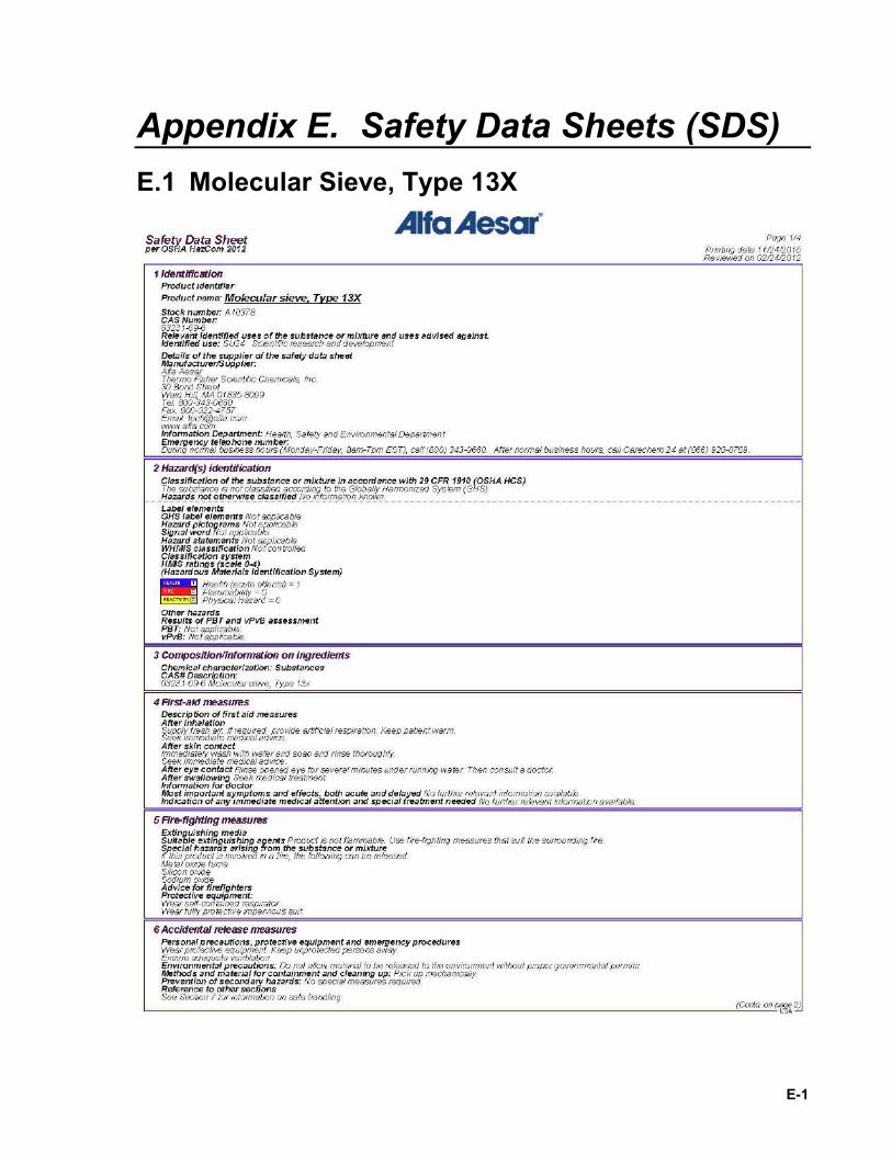
E-1
Appendix E. Safety Data Sheets (SDS) E.1 Molecular Sieve, Type 13X

Appendix E. Safety Data Sheets (SDS)
E-2

Appendix E. Safety Data Sheets (SDS)
E-3

Appendix E. Safety Data Sheets (SDS)
E-4

Appendix E. Safety Data Sheets (SDS)
E-5
E.1 Magnesium Perchlorate

Appendix E. Safety Data Sheets (SDS)
E-6
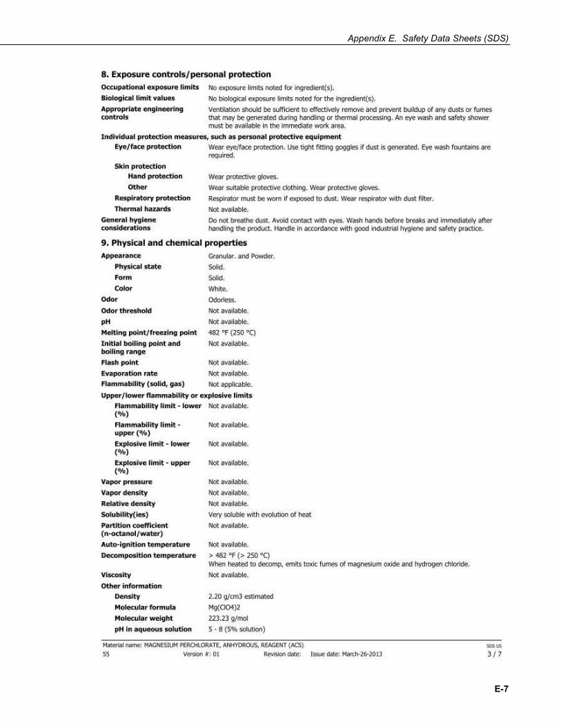
Appendix E. Safety Data Sheets (SDS)
E-7

Appendix E. Safety Data Sheets (SDS)
E-8

Appendix E. Safety Data Sheets (SDS)
E-9
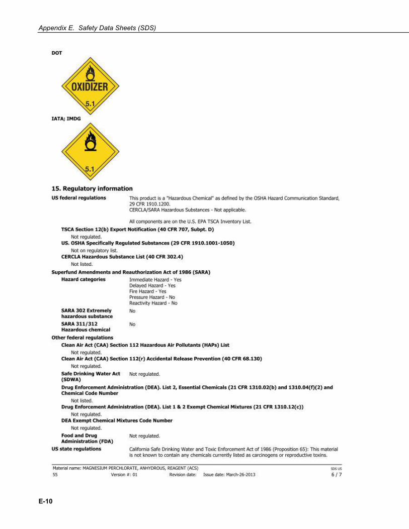
Appendix E. Safety Data Sheets (SDS)
E-10

Appendix E. Safety Data Sheets (SDS)
E-11

Appendix E. Safety Data Sheets (SDS)
E-12
E.2 Decarbite

Appendix E. Safety Data Sheets (SDS)
E-13
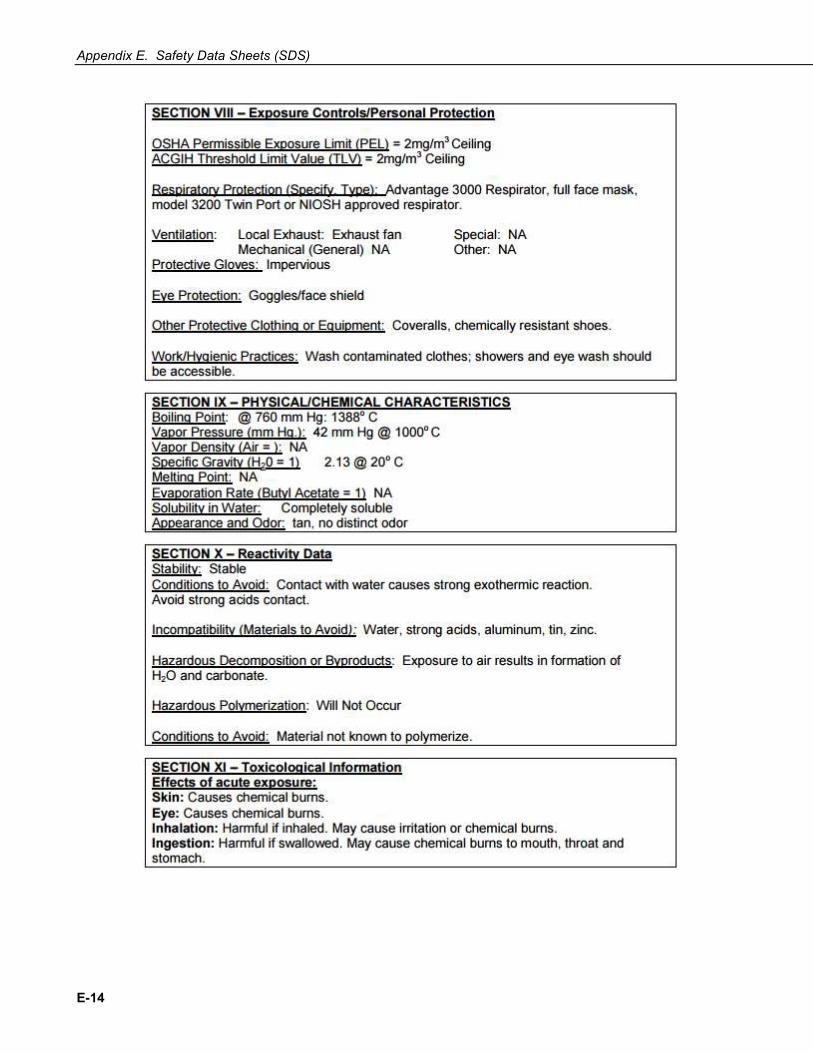
Appendix E. Safety Data Sheets (SDS)
E-14

Appendix E. Safety Data Sheets (SDS)
E-15

Appendix E. Safety Data Sheets (SDS)
E-16

F-1
Appendix F. Packing Information F.1 EC150-GH Packing Information
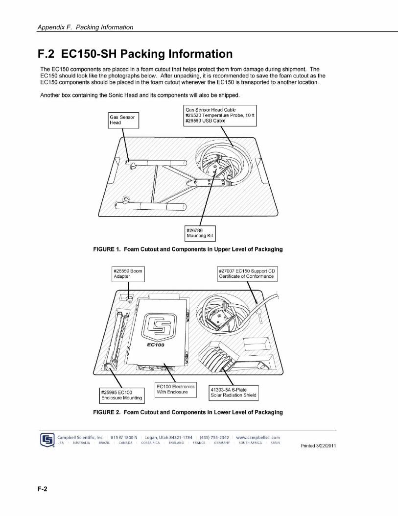
Appendix F. Packing Information
F-2
F.2 EC150-SH Packing Information


Campbell Scientific Companies
Campbell Scientific, Inc. 815 West 1800 North Logan, Utah 84321 UNITED STATES
www.campbellsci.com • [email protected]
Campbell Scientific Africa Pty. Ltd. PO Box 2450
Somerset West 7129 SOUTH AFRICA
www.campbellsci.co.za • [email protected]
Campbell Scientific Southeast Asia Co., Ltd. 877/22 Nirvana@Work, Rama 9 Road
Suan Luang Subdistrict, Suan Luang District Bangkok 10250
THAILAND www.campbellsci.asia • [email protected]
Campbell Scientific Australia Pty. Ltd. PO Box 8108
Garbutt Post Shop QLD 4814 AUSTRALIA
www.campbellsci.com.au • [email protected]
Campbell Scientific (Beijing) Co., Ltd. 8B16, Floor 8 Tower B, Hanwei Plaza
7 Guanghua Road Chaoyang, Beijing 100004
P.R. CHINA www.campbellsci.com • [email protected]
Campbell Scientific do Brasil Ltda. Rua Apinagés, nbr. 2018 ─ Perdizes CEP: 01258-00 ─ São Paulo ─ SP
BRASIL www.campbellsci.com.br • [email protected]
Campbell Scientific Canada Corp. 14532 – 131 Avenue NW Edmonton AB T5L 4X4
CANADA www.campbellsci.ca • [email protected]
Campbell Scientific Centro Caribe S.A. 300 N Cementerio, Edificio Breller
Santo Domingo, Heredia 40305 COSTA RICA
www.campbellsci.cc • [email protected]
Campbell Scientific Ltd. Campbell Park
80 Hathern Road Shepshed, Loughborough LE12 9GX
UNITED KINGDOM www.campbellsci.co.uk • [email protected]
Campbell Scientific Ltd. 3 Avenue de la Division Leclerc
92160 ANTONY FRANCE
www.campbellsci.fr • [email protected]
Campbell Scientific Ltd. Fahrenheitstraße 13
28359 Bremen GERMANY
www.campbellsci.de • [email protected]
Campbell Scientific Spain, S. L. Avda. Pompeu Fabra 7-9, local 1
08024 Barcelona SPAIN
www.campbellsci.es • [email protected]
Please visit www.campbellsci.com to obtain contact information for your local US or international representative.