EC339: Lecture 6Chapter 5: Interpreting OLS Regression

Regression as Double Compression DoubleCompression.xls EastNorthCentralFTWorkers.xls [DoubleCompression]SATData Math and Verbal scores

Note simple statistics summary and correlation Conditional Mean E[Y|X]

Start with Scatterplot

First Compression Examine values of Y, over various small

ranges of X Recognize the ‘variance’ of Y in these strips

Create a conditional mean function Average values of Y, given X (VerticalStrips) Slide bar along X-axis

Move to Accordian Examine 0, 2, 4, and Many intervals

First Compression Before Compressing: What is best guess at Math

SAT unconditional on X? After Compressing: What is best guess at Math SAT

conditional on X? Individual variation is hidden in “Graph of

Averages” Graphical equivalent of PivotTable (See

AccordianPivot) 500+ observations summarized with 35

Second Compression Linearizing graph of averages ‘Regression line w/ observations & averages

Smooth linear version of plot of averages Predicted Math SAT = 318.9 + 0.539 Verbal SAT This equation, gives SIMILAR results to the

previous compression Now summarized with two numbers

Interpret as predicted Y given X

Only an interpretation not a method “Double Compression” of the data is an

interpretation of regression, not how it is done

Method is either analytical or numerical (or using an algorithm)

In [EastNorthCentralFTWorkers]Regression Given education, estimate annual earnings

PivotTable: E[earn|edu=12] = 27,933 Regression: E[earn|edu=12] = 28,399

Average of WSAL_VAL EDUREC Total

8 17662.081639 24043.86

10 20385.8571411 19975.91026

11.5 20850.8947412 27933.9781913 33887.5469114 35687.1900516 48907.3524618 76187.29108

Grand Total 37796.10902

Eduy 631047325ˆ

What else might be going on here???

Regression and SD Line [DoubleCompression]SATData Examine two lines

SD Line: y = 94.6 + 0.978x Reg Line: y = 318.94 + 0.539x

Notice slope of Regression line is shallower Remember equation for slope in SIMPLE regression Notice poor prediction with SD line Calculate residuals

Another Example (SD vs. OLS) Go back to Reg.xls, and calculate SSR from

both lines. (SDx = 4.18, SDy = 50.56, xbar = 7.5, ybar = 145.6

OLS Line: y = 88.956 + 7.558x Calculate SD Line Compare SSR from SD and OLS lines What does point of averages mean here?

b 1O LS i 1

n xi x y i y i 1n xi x2 w h ic h is th e sa m e a s

ta k in g th e n u m e ra to r h e re a n d p e rfo rm in g a c o u p le o f o p e ra t io n s.1 . M u lt ip ly th e to p a n d b o t to m b y 1

n 1 le a vin g

th e e q u a t io n u n c h a n ge d .1

n 1 i 1n xi xyi y

1n 1 i 1

n xi x 2 1

n 1 i 1n xi x

sxyi y

s y

sx2

2 . N o w m u lt ip ly th e n u m e ra to r b y s y

s y 1 , s x

s x 1

Y o u c a n m o ve th e s x and s y inside the equation since they are constants.

1n 1 sx s y i 1

n xi xsx

yi ys y

sx

2 sx s y 1

n 1 i 1n xi x

sxyi y

s y

sx2

N otice the numerator conta ins the equation for corre la tion, and the squared te rm in the denominator cancels. sxs y rx , y

sx2 r x, y

s y

sx, giving b 1

O LS r x, ys y

sx

(N o te : T h is e q u a tio n o n ly w o rk s fo r O L S , b u t m a k e s a s ign if ic a n t p o in t)

OLS Regression vs. SD Simple Linear Regression (SLR)

Slope is SD line slope * correlation Must have slope less than SD line

Two Regression Lines Open TwoRegressionLines.xls

In PivotTables what do you notice? What happens in table TwoLines?

Do equations change when you switch axes? Compare with SDLine

How do you phrase the different regression lines? Do these lines have different meanings? Can you just solve one regression line to find the other?

“Someone who is 89 points above the mean in Verbal (1 sd) is predicted to be 0.55 x 87 (r x SDmath) or 48 points above the mean Math score” (thus regress!)

Two Regression Lines Given a verbal score what is the best guess of a

person’s math score? Predicted Math SAT = 318 + 0.54 Verbal SAT If Verbal = 600, Predicted Math SAT = 642

Given a math score, what is the best guess of a person’s verbal score Solve for verbal? From above

Predicted Verbal SAT = -589 + 1.85 Math SAT NO!!! This is not correct!

Must regress verbal on math (verbal is predicted) Predicted Verbal SAT = 176.1 + 0.564 Math SAT If Math SAT = 642, you would predict Verbal SAT = 538

Properties of Sample Average and Regression Line Examine OLSFormula.xls, SampleAveIsOLS

Sample average is a weighted sum Sample average is also the least squares estimator of

central tendency Here, weights sum to 1

Examine Excel’s “Auditing Tool”

Average SSR is never greater than Median SSR Sample average is least squares estimate of measure

of central tendency

Mean minimizes SSR (or OLS estimate) Run Solver, minimize SSR by changing

“Solver Estimate” starting at 100 Note the sum of the residuals (F16) Try with “Draw another dataset” in Live sheet What happens to sum of residuals? Try using the median

[OLSFormula.xls]Example Recall “weighted sum” calculation of slope

coefficient Regression goes through point of averages Slope is weighted sum of Y’s Weights bigger in absolute value the farther the

x-value is from the average value of x Weights sum to zero Change in Y value has a predictable effect on

OLS slope and intercept

Residuals and Root Mean Squared Error (RMSE) (ResidualPlot.xls) Residual Plots are “diagnostic tools”

There should be no discernable pattern in the plot Residual plots can be done in Excel and SPSS

Try using LINEST method here to calculate the residuals. First, find the equation, then calculate predicted values, and then calculate residuals

Remember (Residual = Actual Y – Predicted Y) Now, square the residuals, and find the average, and take

the square root… Root (of the) Mean (of the) Squared Errors Measures your average mistake Examine a scatterplot and histogram of the residuals

-300

-200

-100

0

100

200

300

250 350 450 550 650 750

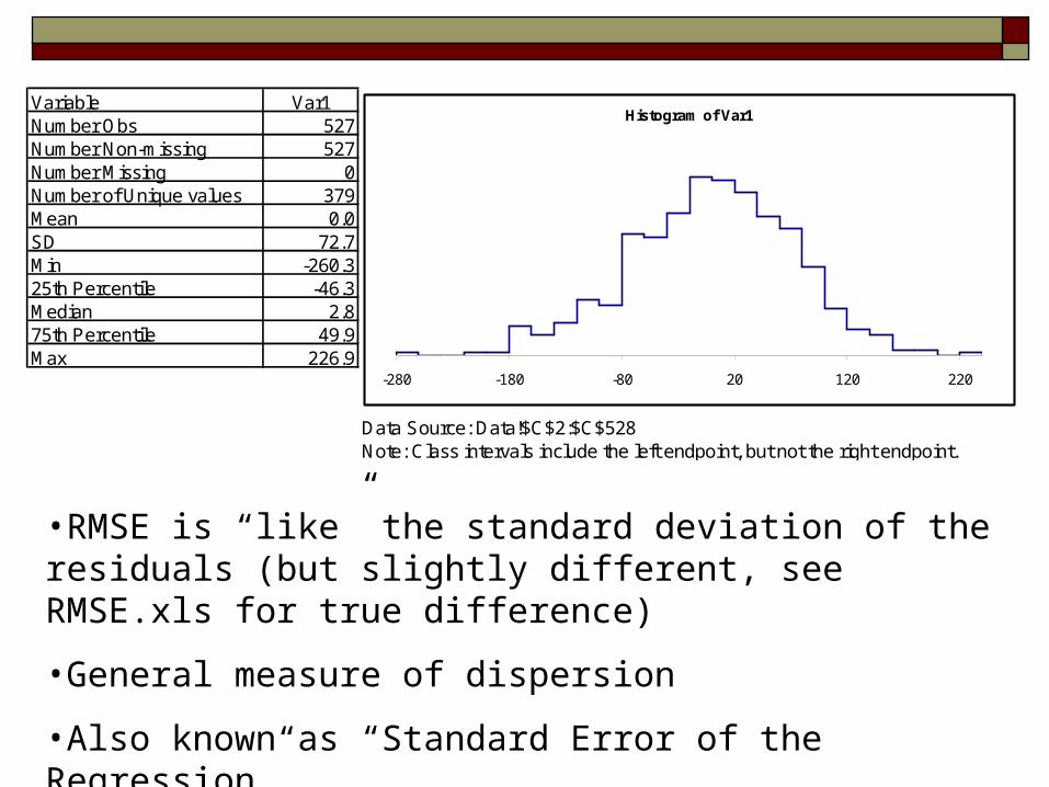
Variable Var1 26 26Number Obs 527Number Non-missing 527Number Missing 0Number of Unique values 379Mean 0.0SD 72.7Min -260.325th Percentile -46.3Median 2.875th Percentile 49.9Max 226.9

Data Source: Data!$C$2:$C$528Note: Class intervals include the left endpoint, but not the right endpoint.

Histogram of Var1

-280 -180 -80 20 120 220

•RMSE is “like” the standard deviation of the residuals (but slightly different, see RMSE.xls for true difference)

•General measure of dispersion

•Also known as “Standard Error of the Regression”

RMSE.xls For many data sets, 68% of the observations fall

within +/- 1 RMSE and 95% fall within +/- 2 RMSEs. When the RMSE is working as advertised, it should reflect these facts

Try changing spread in Computation Examine Histograms in SATData and Accordian to

understand that RMSE is the spread of the residuals Pictures sheet shows residual plots and regressions

n"" population using where,1

)ˆ(1 2

1

2y

n

ii kn

yynkn

n

RSquared.xls Play the game to convey the idea of the improvement in

prediction. R2 measures the percentage improvement in prediction over

just guessing average Y. R2 ranges from 0 to 1. R2 is a dangerous statistic because it is sometimes confused

as measuring the quality of a regression. Notice that Excel’s Trendline offers R2 (and only this statistic) as an option. There is no single statistic that can be used to decide if a particular regression equation is good or bad.

TSSSSRTSS

SSRR ;12 21 rRMSE y

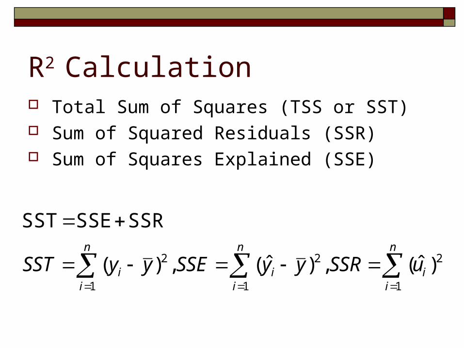
R2 Calculation Total Sum of Squares (TSS or SST) Sum of Squared Residuals (SSR) Sum of Squares Explained (SSE)

2

1

2

1

2

1

)ˆ(,)ˆ(,)(

SSRSSESST

n

ii

n

ii

n

ii uSSRyySSEyySST

Ordinary Least Squares-Fit

2

1

2

1

2

1

2

12

2

ii

2

)(

)ˆ(1

)(

)ˆ(

1

SSRSSESST

y andbetween x n correlatio down to boils this,t variableindependen one

on dependsonly prediction When .y and ybetween n correlatio the

of valuesquared the toequal is R same. eexactly th istion Interpreta

ncorrelatio squaresimply cannot you ,regression multipleIn

DGENERALIZE SQUARED-R

n

ii

n

ii

n

ii

n

ii

yy

u

yy

yyR

SST

SSR

SST

SSER Note: This is the RATIO of

what variation in y is EXPLAINED by the regression!

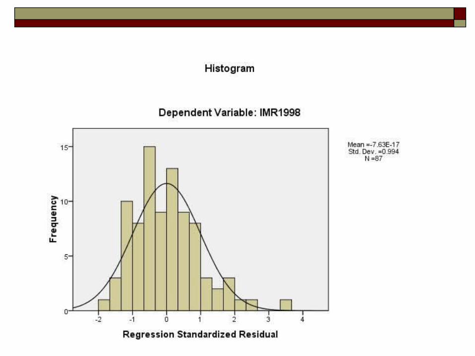
Infant Mortality IMRGDPReg.xls Start by moving data into SPSS Plot data: What is relationship? Save the residuals and plot against the

independent variable What and does this plot tell us?

SameRegLineDifferentData.xlsQ&A for SameRegLineDifferentData1) Click the Restore SAT Data button to make sure you have the original, actual SAT data.The two vertical strips shown are from 395 to 415 and 545 to 565.Compute the SDs for the residuals in these two vertical strips.HINTS: The predicted Math score is provided in column C, so you can easily compute the residual for each observation in column D.Since the data are sorted by Verbal, computing the SD for each strip should be a snap.

2) How does the regression RMSE compare to the two SDs you calculated in question 1?

3) Compute the SDs of the Math scores in each vertical strip. You should find that the SDs of the Math scores in each vertical strip are almost the same as SDs of the residuals in the same strip. Is this a coincidence? Explain.

4) Set the data to exhibit a linear heteroskedastic pattern and report the SDs of the two vertical strips.

5) Once again, how does the regression RMSE compare to the SDs from the two strips?

Real Data: HourlyEarnings.xls Residuals: Why are data shown in “strips”? Regress & Save residuals

Regression Interpretation: Summary Simplified Conditional Mean (more on this) Intercept and Slope coefficient Need theory to guide causation

BH call this “Two Regression Lines” OLS is weighted average RMSE and R2 are helpful