ecc report 263 - cept.org
TRANSCRIPT
Adjacent band compatibility studies between IMT operating in the frequency band 1492-1518 MHz and the MSS operating in the frequency band 1518-1525 MHz
Approved 03 March 2017
ECC Report 263

ECC REPORT 263 - Page 2
0 EXECUTIVE SUMMARY
The report has established the technical characteristics of the IMT and the MSS systems and determined the relevant scenarios to assess potential interference from IMT systems to MSS systems at 1518 MHz.
Three different frequency separations between IMT and MSS are examined: 1 MHz, 3 MHz and 6 MHz. The report has, from the characteristics and parameters, developed an MCL analysis with the resulting required separation distances for the 3 different frequency separations. Interference due to out-of-band emissions from IMT base stations into the first MES channel above the frequency separation and due to blocking of the MES is considered separately.
Furthermore, the report contains results from a number of 'Monte Carlo' simulations of the impact on a user of a MES terminal in an area with IMT coverage for the 3 different frequency separations.
The results of the simulations show that there will be some interference irrespective of the selected frequency separation.
With the assumed values for IMT e.i.r.p. and OOBE and current values of MES receiver blocking, the interference at 1 MHz frequency separation is high from both IMT OOBE and MES receiver blocking. However, at frequency separations of 3 MHz and 6 MHz the interference from IMT OOBE is reduced but the interference due to receiver blocking remains high for current MESs.
The report also examines the impact of a number of methods for mitigation of interference including a reduction in the IMT OOBE (these values have been used in the report for the analysis) and a future expectation for the MES receiver blocking characteristics. When the future expectations for MES receiver blocking is also taking into consideration, the interference is reduced to similar levels as for IMT OOBE interference (for frequency separations of 3 MHz and 6 MHz).
There may be a need to provide protection for MES at seaports and airports, and hence there may be a need to apply other mitigation techniques to IMT BSs in the vicinity of seaports and airports for the frequencies at the top end of the 1492-1518 MHz frequency band to avoid harmful interference to MESs.
Based on the final results of its compatibility studies, it is concluded that: The minimum in-band blocking characteristic for land mobile earth stations receivers from a 5 MHz
broadband signal interferer (LTE) operating below 1518 MHz shall be −30dBm above 1520 MHz1; The base station unwanted emission limits e.i.r.p. for a broadband signal interferer (LTE) operating
below 1518 MHz shall be −30dBm/MHz above 1520 MHz. This figure is 10 dB more stringent than ECC Decision (13)03 due to a different service in the adjacent band.
It is noted that the IMT block ends at 1517 MHz.
1 when the MES operates above 1520 MHz

ECC REPORT 263 - Page 3
TABLE OF CONTENTS
0 Executive summary ................................................................................................................................. 2
1 Introduction .............................................................................................................................................. 7
2 Background .............................................................................................................................................. 8
3 Technical characteristics ........................................................................................................................ 9 3.1 Mobile service system parameters .................................................................................................. 9
3.1.1 IMT Base station (BS) ......................................................................................................... 9 3.2 Mobile satellite service system parameters ................................................................................... 13
3.2.1 Mobile Earth station (MES) ............................................................................................... 13
4 Protection criteria .................................................................................................................................. 15 4.1 Protection criteria for interference from IMT to MSS ..................................................................... 15
5 Compatibility scenarios ........................................................................................................................ 16 5.1 Scenarios ....................................................................................................................................... 16 5.2 Propagation models and environments ......................................................................................... 16
5.2.1 Land .................................................................................................................................. 16 5.2.2 Sea (maritime) .................................................................................................................. 17 5.2.3 Air (aeronautical) ............................................................................................................... 17
5.3 Methodology .................................................................................................................................. 17 5.3.1 Minimum Coupling Loss (MCL) ........................................................................................ 17 5.3.2 Statistical analysis ............................................................................................................. 19
5.3.2.1 With random MES location and fixed frequency ............................................... 20 5.3.2.2 With random MES location and random frequency ........................................... 20
6 Compatibility analysis results .............................................................................................................. 22 6.1 Minimum Coupling Loss method analysis ..................................................................................... 22 6.2 Statistical analysis ......................................................................................................................... 22
6.2.1 With random MES location and fixed frequency ............................................................... 22 6.2.2 With random MES location and random frequency .......................................................... 22
7 Possible mitigation techniques ............................................................................................................ 24
8 Conclusions ............................................................................................................................................ 28
ANNEX 1: IMT antenna patterns ................................................................................................................... 30
ANNEX 2: Potential for MES receiver improved blocking resilience ....................................................... 32
ANNEX 3: MES example antenna patterns.................................................................................................. 37
ANNEX 4: Additional information regarding propagation model for land scenario ............................... 38
ANNEX 5: MCL results .................................................................................................................................. 39
ANNEX 6: MCL results for AES on aircraft in flight ................................................................................... 42
ANNEX 7: Study #1 ........................................................................................................................................ 47

ECC REPORT 263 - Page 4
ANNEX 8: Study #2 ........................................................................................................................................ 59
ANNEX 9: Study #3 ........................................................................................................................................ 64
ANNEX 10: List of Reference ........................................................................................................................ 69

ECC REPORT 263 - Page 5
LIST OF ABBREVIATIONS
Abbreviation Explanation
3GPP 3rd Generation Partnership Project
ACS Adjacent Channel Selectivity
AES Aircraft Earth Station
ALD Assistive Listening Devices
AMSS Aeronautical Mobile Satellite Services
BEM Block Edge Mask
BGAN Broadband Global Area Network
BS Base Station
BW Bandwidth
3GPP 3rd Generation Partnership Project
CL Coupling Loss
CW Continuous Wave
dB Decibel
dBc Decibel relative to the Carrier
dBi Decibel relative to an Isotropic antenna
dBm Decibel relative to 1 mW
dBW Decibel relative to 1 W
Δf Frequency offset
EC European Commission
ECC Electronic Communications Committee
EDT Electric Down Tilt
e.i.r.p. equivalent isotropic radiated power
ETSI European Telecommunications Standards Institute
FCC Federal Communications Commission
GMR Geostationary Earth Orbit Mobile Radio
GSPS Global Satellite Phone Service
I/N Interference to Noise ratio
IF Intermediate Frequency
IMT International Mobile Telephony

ECC REPORT 263 - Page 6
Abbreviation Explanation
ISD Inter-Site Distance
ITU International Telecommunication Union
K Kelvin
kHz Kilohertz (1000 oscillations per second)
LNA Low Noise Amplifier
LTE Long Term Evolution
MCL Minimum Coupling Loss
MES Mobile Earth Station
MHz Megahertz (1000000 oscillations per second)
MSS Mobile Satellite Service
NGSS Next Generation Satellite Service
OOB Out of Band/Out of Block
OOBE Out of Band Emissions/Out of Block Emissions
RF Radio Frequency
RTCA Radio Technical Commission for Aeronautics
SAW Surface Acoustic Wave
SDL Supplementary Downlink
SDO Standards Development Organisation
SNR Signal to Noise Ratio
TS Technical Standard
WRC World Radiocommunication Conference

ECC REPORT 263 - Page 7
1 INTRODUCTION
This report has been established because of the decision to identify the frequency band 1492-1518 MHz for IMT and therefore is investigating the adjacent band compatibility between IMT below 1518 MHz and MSS (MES) in the band above.
This band was identified for IMT at WRC-15 and is being considered within CEPT as a harmonised band for mobile and fixed communications networks. The adjacent frequency band 1452-1492 MHz is harmonised for supplementary downlink (SDL) through ECC/DEC/(13)03 [1]. CEPT supports that the frequency band 1427-1518 MHz for IMT is for a one direction down-link service, used in connection with another IMT band that provides the up-linking capabilities. It is anticipated that MFCN systems in the frequency band 1492-1518 MHz would use LTE technology and so the characteristics are based on those applicable to "IMT-Advanced" base stations.
The operation of IMT systems in the frequency band 1492-1518 MHz may cause interference to receiving mobile earth stations operating in the frequency band 1518-1559 MHz due to blocking and out-of-band (OOB) emissions. This report examines the impact of interference on currently operating MESs and also examines the impact on anticipated future deployed MESs, expected to have improved blocking performance.
The study has been performed for minimum coupling loss (MCL) and statistical analysis for rural/suburban/urban environment.

ECC REPORT 263 - Page 8
2 BACKGROUND
The frequency band 1518-1525 MHz was allocated to the mobile satellite-service (MSS) at WRC-03. The band is an extension to the frequency band 1525-1559 MHz, providing additional spectrum to the geostationary satellite networks which operate in this band. The frequency band 1518-1559 MHz is used by the "Alphasat" satellite which provides coverage of Europe, Africa and the Middle East. Additional L-band satellites that will operate in the frequency band 1518-1525 MHz are under development, expected to be launched around 2019.
There are a variety of MSS terminal types which operate in the frequency band 1518-1525 MHz, including land, maritime and aeronautical applications and each of these types is considered in this Report.
The frequency band 1518-1525 MHz is designated for systems in the MSS (space-to-Earth) through ECC Decision ECC/DEC/(04)09 [2].
The frequency band 1492-1518 MHz is allocated to the fixed and mobile service. In CEPT, according the ERC Report 25 [3], the major applications in this band are "fixed", "land military systems", "maritime military systems" and "radio microphones and ALD". The use of this band by the mobile service is limited to tactical radio relay applications (ECA36 applies).
The initial utilisation of frequency band 1492-1518 MHz for IMT is thought to be to provide more capacity which by nature will be focussing on urban areas but not limited to this.

ECC REPORT 263 - Page 9
3 TECHNICAL CHARACTERISTICS
3.1 MOBILE SERVICE SYSTEM PARAMETERS
3.1.1 IMT Base station (BS)
Characteristics of IMT-Advanced macro base stations are in accordance to Report ITU-R M.2292 [4] and are contained in Table 1. IMT BS OOB emission levels are in line with 3GPP TS 36.104 [5] spectrum emission mask (Table 6.6.3.2.2-1 (Category B, Option 2)) and EC Decision 2015/750 [6] Block Edge Mask (BEM) limits (Table 3 of the Annex 2). The antenna pattern used for the IMT base station is shown in Annex 1, according to Recommendation ITU-R F.1336-4 [7] (recommends 3.1).
Table 1: IMT base station characteristics
Parameter Unit Value
Downlink frequency MHz 1492-1518
Bandwidth MHz 5, 10
Deployment - Macro (urban, suburban, rural)
Maximum transmitter power2 dBm 43 for BW = 5 MHz 46 for BW = 10 MHz
Maximum antenna gain dBi 18 (rural), 16 (suburban, urban)
Antenna height m 30 (rural, suburban), 25 (urban)
Feeder loss dB 3
Sectorization sectors 3
Downtilt degrees 3 (rural), 6 (suburban), 10 (urban)
Polarization3 dB Linear
Antenna pattern4 -
Recommendation ITU-R F.1336-4 [7] (recommends 3.1) ka = 0.7 kp = 0.7 kh = 0.7 kv = 0.3
Spurious emissions limits (applicable for frequencies more than 10 MHz from the edge of the IMT operation band)
dBm/MHz –30 (Category B) (3GPP 36.104 v11.2.0 [5], Table 6.6.4.1.2.1-1)
Macro cell radius 5 km (rural), 1 km (suburban), 0.5 km (urban)
2 For frequency separation 1 MHz and 3 MHz channel bandwidth of 5 MHz has been assumed and for 6 MHz frequency separation
10 MHz channel bandwidth is assumed. 3 The transmitted signal from a BS antenna would normally consist of two orthogonal linear polarised components, each fed with half of
the BS transmitted power. The total transmitted e.i.r.p. is the sum of the two polarised components. 4 See Annex 1 for the detailed implementation for the antennas used in the study.
ECC REPORT 263 - Page 10
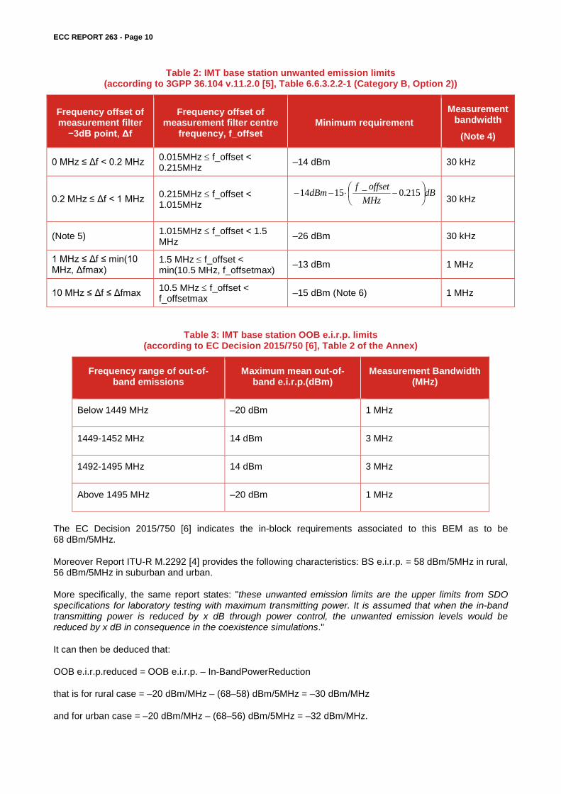
Table 2: IMT base station unwanted emission limits (according to 3GPP 36.104 v.11.2.0 [5], Table 6.6.3.2.2-1 (Category B, Option 2))
Frequency offset of measurement filter
−3dB point, Δf
Frequency offset of measurement filter centre
frequency, f_offset Minimum requirement
Measurement bandwidth
(Note 4)
0 MHz ≤ Δf < 0.2 MHz 0.015MHz ≤ f_offset < 0.215MHz –14 dBm 30 kHz
0.2 MHz ≤ Δf < 1 MHz 0.215MHz ≤ f_offset < 1.015MHz
dBMHz
offsetfdBm
−⋅−− 215.0_1514
30 kHz
(Note 5) 1.015MHz ≤ f_offset < 1.5 MHz –26 dBm 30 kHz
1 MHz ≤ Δf ≤ min(10 MHz, Δfmax)
1.5 MHz ≤ f_offset < min(10.5 MHz, f_offsetmax) –13 dBm 1 MHz
10 MHz ≤ Δf ≤ Δfmax 10.5 MHz ≤ f_offset < f_offsetmax –15 dBm (Note 6) 1 MHz
Table 3: IMT base station OOB e.i.r.p. limits
(according to EC Decision 2015/750 [6], Table 2 of the Annex)
Frequency range of out-of-band emissions
Maximum mean out-of-band e.i.r.p.(dBm)
Measurement Bandwidth (MHz)
Below 1449 MHz –20 dBm 1 MHz
1449-1452 MHz 14 dBm 3 MHz
1492-1495 MHz 14 dBm 3 MHz
Above 1495 MHz –20 dBm 1 MHz
The EC Decision 2015/750 [6] indicates the in-block requirements associated to this BEM as to be 68 dBm/5MHz.
Moreover Report ITU-R M.2292 [4] provides the following characteristics: BS e.i.r.p. = 58 dBm/5MHz in rural, 56 dBm/5MHz in suburban and urban.
More specifically, the same report states: "these unwanted emission limits are the upper limits from SDO specifications for laboratory testing with maximum transmitting power. It is assumed that when the in-band transmitting power is reduced by x dB through power control, the unwanted emission levels would be reduced by x dB in consequence in the coexistence simulations."
It can then be deduced that:
OOB e.i.r.p.reduced = OOB e.i.r.p. – In-BandPowerReduction
that is for rural case = –20 dBm/MHz – (68–58) dBm/5MHz = –30 dBm/MHz
and for urban case = –20 dBm/MHz – (68–56) dBm/5MHz = –32 dBm/MHz.

ECC REPORT 263 - Page 11
Table 4 depicts the EC Decision BEM with a reduction factor applied to the BS in-band power (10 dB for the rural case, 12 dB for the urban case).
Table 4: Adjusted IMT base station OOB e.i.r.p. values
Frequency separation from channel edge 0-1 MHz 1-3 MHz >3 MHz
Rural –0.8 dBm/MHz5 –0.8 dBm/MHz –30 dBm/MHz
Suburban/Urban –2.8 dBm/MHz6 –2.8 dBm/MHz –32 dBm/MHz
Table 5: IMT base station OOB e.i.r.p. values used in the studies
Frequency separation from channel edge Rural Suburban/Urban
1 MHz –0.8 dBm/MHz –2.8 dBm/MHz
3 MHz –30 dBm/MHz –32 dBm/MHz
6 MHz –33 dBm/MHz –35 dBm/MHz
13 MHz –40 dBm/MHz –42 dBm/MHz
43 MHz –60 dBm/MHz –62 dBm/MHz
70 MHz –78 dBm/MHz –80 dBm/MHz
73 MHz –80 dBm/MHz –80 dBm/MHz
80 MHz –80 dBm/MHz –80 dBm/MHz
The above roll-off slope for frequency separations greater than 3 MHz are calculated from the measurements performed in ECC Report 174 [8] (Annex 4 section 4.1).
5 OOB e.i.r.p.Preduced=OOB e.i.r.p.–Reduction Factor Rural=14dBm/3MHz–10dB=9.2dBm/MHz–10dB=–0.8dBm/MHz 6 OOB e.i.r.p.Preduced=OOB e.i.r.p.–Reduction Factor Suburban/Urban=14dBm/3MHz–12dB=9.2dBm/MHz–12dB=–2.8dBm/MHz

ECC REPORT 263 - Page 12
Figure 1: OOB e.i.r.p. values used in the studies
-90-80-70-60-50-40-30-20-10
0102030405060
0 10 20 30 40 50 60 70 80 90
Max
imum
mea
n ou
t-of
-ban
d e.
i.r.p
., dBm
/MH
z
Frequency offset, MHz
suburban/urban
rural

ECC REPORT 263 - Page 13
3.2 MOBILE SATELLITE SERVICE SYSTEM PARAMETERS
3.2.1 Mobile Earth station (MES)
Table 6: MES terminal characteristics
Parameter Unit Value
Receiver tuning range MHz 1518-1559 MHz
Reference bandwidth kHz 200
Receiver noise temperature K 316
Receiver thermal noise level dBW –150.6
Receiver thermal noise level for 200 kHz ref. BW dBm/200 kHz –120.6
Receiver thermal noise level for 1 MHz ref. BW dBm/MHz –113.6
ACS (1st adjacent channel) dBc 30
ACS (2nd adjacent channel and up to 2 MHz) dBc 37
ACS above 2 MHz dBc 87
Maximum antenna gain dBi (see Table 7)
Polarisation - circular
Receiver Blocking7 dBm –60 dBm (<2 MHz separation) –52 dBm (>2 MHz and < 5 MHz separation) –40 dBm (>5 MHz separation)
Land MES antenna height a.g.l. m 2
Sea (maritime) MES antenna height a.s.l. m 10
Air (aeronautical) MES antenna height a.g.l. m 0-10000
ETSI standard TS 101 377-5-5 [9] applies to the "GSPS" (Global Satellite Phone Service). This defines the requirements for GMR-2 Mobile Earth Station-to-satellite terminal uplink/downlink operating in the 1500/1600 MHz bands in section 7.1 “Mobile Earth Station Blocking characteristics”. In this standard the blocking requirements are defined as –43 dBm for frequency separation between carrier frequencies greater than 1.6 MHz and –53 dBm for frequency separation between carrier frequencies between 0.8 MHz and 1.6 MHz. These requirements are based on CW blocking requirements. Laboratory tests have been conducted to examine the difference between a CW blocking signal and an LTE signal. The results in Annex 2 show that 7 Aircraft Earth Stations used for safety-related communications are subject to the standards published by the RTCA
(http://www.rtca.org/). The two standards relevant to AES are: 1) DO-210 D: “Minimum Operational Performance Standards For Geosynchronous Orbit Aeronautical Mobile Satellite Services
(AMSS) Avionics” [10] operating in the frequency band 1530-1559 MHz; 2) DO-262 B: “Minimum Operational Performance Standards For Avionics Supporting Next Generation Satellite Systems (NGSS)” [11]
operating in the frequency band 1518-1559 MHz. Currently, both standards include minimum requirements related to the susceptibility of AES receivers to interference received on
frequencies below the band 1530 MHz (DO-210) and 1518 MHz (DO-262B). The requirements in the RTCA standards are for receivers to operate with interference levels around –65 dBm to –55 dBm when interference occurs on a frequency just below 1518 MHz, whereas the value assumed in this study is –40 dBm, a value found by measurements performed by the FCC a number of years ago on land and maritime terminals. Terminals compliant with the baseline value would therefore be more resistant to interference. It’s assumed that new or updated RTCA standards will take into account the evolutions of the regulation framework, especially the IMT identification just below 1518 MHz.

ECC REPORT 263 - Page 14
LTE signal interference power about 10 dB lower than the CW signal causes the same degradation of the MES receiver. The equivalent values for LTE blocking signals are therefore –63 dBm with 1 MHz frequency separation and –53 dBm with 3 MHz separation.
For each of the three scenarios, one “omni” or low gain antenna and one “high gain” directive antenna has been considered. These are presented in Table 7. For the high gain MES antenna, the elevation is set to 30 degrees. All antenna patterns are average sidelobe levels. Handheld terminals ("omni" antenna) would be pointing vertically.
Table 7: MES maximum antenna gain for the different scenarios
Scenario Type Value Antenna gain Inmarsat service Antenna pattern
Land Low gain dBi 3 GSPS Annex 3: Figure 13
High gain dBi 17.5 BGAN class 1 Annex 3: Figure 12
Sea (maritime) Low gain dBi 3 Inmarsat-C Annex 3: Figure 13
High gain dBi 21 Fleet-77 Annex 3: Figure 11
Air (aeronautical) Low gain dBi 3 Aero-L Annex 3: Figure 13
High gain dBi 17.5 Aero-H Annex 3: Figure 12

ECC REPORT 263 - Page 15
4 PROTECTION CRITERIA
4.1 PROTECTION CRITERIA FOR INTERFERENCE FROM IMT TO MSS
Interference criteria for this scenario are not defined in ITU-R Recommendations. Several proposals for OOB emission interference criteria have been presented, ranging from –20 dB to 0.9 dB I/N for long term criteria. To proceed with the studies with a reduced range, protection criteria of I/N of –6 dB and –10 dB should be studied, noting that these OOB emission criteria are typical criteria, respectively for mobile terminals and mobile base stations.
Interference analysis was also carried out against the receiver blocking criteria in accordance with Table 6.

ECC REPORT 263 - Page 16
5 COMPATIBILITY SCENARIOS
5.1 SCENARIOS
Interference into MSS terminals may occur for the following reasons: Unwanted emission from the IMT base station occurring in the frequency range above 1518 MHz. This
type of interference can only be mitigated at the IMT base station by adding extra transmitter filters; MSS terminal receiving frequencies below 1518 MHz, this is split into the following interference
mechanisms (common for these are that they can only be mitigated at the MSS receiver); Blocking of the MSS receiver which is a result of the wanted emission of the IMT base station. This
type of interference is caused by insufficient RF filtering and the design of the MSS receiver front-end;
Adjacent channel/band reception which is a result of the wanted emission of the IMT base station. This type of interference is caused by insufficient RF front-end plus IF filtering in the MSS receiver.
The following scenarios need to be investigated:
1 Impact of IMT base station unwanted emission on MES receiver in land, sea and air environment;
2 Blocking of MSS receivers from the wanted emission of the IMT base station in land, sea and air environment;
3 Adjacent channel/band selectivity of MSS receivers from the wanted emission of the IMT base station in land, sea and air environment.
Based on the MES characteristics contained in Table 6, it can be seen that the ACS for frequencies greater than 2 MHz from the MES carrier is very large (around 87 dB). As a consequence, the third of these interference mechanisms may not be considered under the following conditions: 1) that the frequency separation between the band used by IMT band and the band used by the MSS is at least 2 MHz, and 2) that the IMT OOB emission mask is quite flat for frequencies within 2 MHz from the MES channel.
The interference mechanisms mentioned above applies to MESs used for Land, Air and Sea scenarios. The aeronautical scenario where an aircraft is on the ground in an airport is considered covered by the land scenario and is always a 'special case' where the Administration in corporation with the appropriate authorities would have to approve any IMT coverage in an airport to avoid harmful interference to the airport or any aircraft operating within the airport . The perimeter fencing around an airport will also provide a rather large separation distance and it is not normally allowed to erect 30 m towers anywhere in close vicinity of an airport without the prior approval of the airport or aviation authorities. Similarly, the protection of maritime MESs on vessels may also be treated as a 'special case' in that deployment restrictions in the vicinity of harbours can be envisaged to ensure that the MESs on vessels do not suffer from harmful interference from IMT base stations.
The case of potential interference to MESs used on aircraft in flight is considered separately, using an MCL approach. The results for this scenario are in Annex 6.
5.2 PROPAGATION MODELS AND ENVIRONMENTS
5.2.1 Land Rural case - Recommendation ITU-R P.1546-5 [12], and Recommendation ITU-R P.1812-4 [13] for lower
clutter height than 10 m; Suburban case - Recommendation ITU-R P.1546-5 with 10 m clutter height; Urban case - Recommendation ITU-R P.1546-5 with 20 m clutter height.

ECC REPORT 263 - Page 17
All of these scenarios are carried out with 50% location variability and 50% time percentage.
Annex 4 contains a short description of the considerations that has gone into the selection of propagation models and the associated clutter height.
5.2.2 Sea (maritime)
Recommendation ITU-R P.452-16 [14] with 50% time. For the sea case, interference from a rural IMT base station only is considered.
5.2.3 Air (aeronautical)
Recommendation ITU-R P.525-2 [15]. (i.e. free space loss) is used to consider cases of interference to an AES in flight.
To consider potential interference to an AES located on an aircraft at an airport, analysis of interference to an AES located 10 m a.g.l. is also made in the land-rural environment.
5.3 METHODOLOGY
5.3.1 Minimum Coupling Loss (MCL)
The Minimum Coupling Loss is calculated with the antenna in boresight to each other and taking into account frequency separation. The corresponding separation distance at which each interference criterion is just met is then calculated taking into account the discrimination of both antennas and the frequency separation.
The interference from IMT unwanted emissions is evaluated using the following formula:
𝐼𝐼1 = 𝑃𝑃𝑇𝑇,𝑂𝑂𝑂𝑂𝑂𝑂 + 𝐺𝐺𝑇𝑇 + 𝐺𝐺𝑇𝑇,𝑅𝑅𝑅𝑅𝑅𝑅 − 𝐿𝐿𝐹𝐹 + 𝐺𝐺𝑅𝑅 + 𝐺𝐺𝑅𝑅,𝑅𝑅𝑅𝑅𝑅𝑅 − 𝐿𝐿𝑝𝑝𝑝𝑝𝑝𝑝𝑝𝑝 − 𝐿𝐿𝑝𝑝𝑝𝑝𝑝𝑝 = 𝑃𝑃𝑇𝑇,𝑂𝑂𝑂𝑂𝑂𝑂 + 𝐺𝐺𝑇𝑇 − 𝐿𝐿𝐹𝐹 + 𝐺𝐺𝑅𝑅 − 𝐿𝐿𝑝𝑝𝑝𝑝𝑝𝑝 − 𝐶𝐶𝐿𝐿 (1)
where
𝐼𝐼1 is the IMT unwanted emissions interferer power at the MES receiver;
𝑃𝑃𝑇𝑇,𝑂𝑂𝑂𝑂𝑂𝑂 is the maximum transmitted power by the interferer falling within the channel bandwidth of the MES receiver;
𝐿𝐿𝐹𝐹 is the IMT base station feeder loss;
𝐺𝐺𝑇𝑇 is the peak gain of the transmitter antenna (the interferer);
𝐺𝐺𝑇𝑇,𝑅𝑅𝑅𝑅𝑅𝑅 is the gain of the transmitter antenna in the direction of the MES, relative to the peak value.
𝐺𝐺𝑅𝑅 is the peak gain of the receiver antenna (the victim);
𝐺𝐺𝑅𝑅,𝑅𝑅𝑅𝑅𝑅𝑅 is the gain of the receiver antenna in the direction of the IMT BS, relative to the peak value.
𝐿𝐿𝑝𝑝𝑝𝑝𝑝𝑝𝑝𝑝 is the loss due to the propagation;
𝐿𝐿𝑝𝑝𝑝𝑝𝑝𝑝 is the polarisation loss.
𝐶𝐶𝐿𝐿 are the coupling losses and are given by the following formula:
𝐶𝐶𝐿𝐿 = 𝐿𝐿𝑝𝑝𝑝𝑝𝑝𝑝𝑝𝑝 − 𝐺𝐺𝑅𝑅,𝑅𝑅𝑅𝑅𝑅𝑅 − 𝐺𝐺𝑇𝑇,𝑅𝑅𝑅𝑅𝑅𝑅 (2)

ECC REPORT 263 - Page 18
The maximum allowed interference power at the MES receiver is given by:
𝐼𝐼1,𝑀𝑀𝑀𝑀𝑀𝑀 = 𝑁𝑁 + 𝐼𝐼/𝑁𝑁𝑡𝑡ℎ (3)
where
𝐼𝐼1,𝑀𝑀𝑀𝑀𝑀𝑀 is the maximum acceptable IMT unwanted emissions interferer power at the MES receiver;
𝑁𝑁 is the receiver thermal noise power;
𝐼𝐼/𝑁𝑁𝑡𝑡ℎ is the interference criterion
The minimum coupling loss (MCL) to meet the criterion can be therefore calculated as:
𝑀𝑀𝐶𝐶𝐿𝐿 = 𝑃𝑃𝑇𝑇,𝑂𝑂𝑂𝑂𝑂𝑂 + 𝐺𝐺𝑇𝑇 + 𝐺𝐺𝑅𝑅 − 𝐿𝐿𝑝𝑝𝑝𝑝𝑝𝑝 − 𝐿𝐿𝐹𝐹 − 𝐼𝐼1,𝑀𝑀𝑀𝑀𝑀𝑀 (4)
In this study, the coupling losses are determined as a function of the separation distance between the IMT base station and the MES.
The interference due to receiver overdrive is evaluated considering the overload criterion in Table 6. The interferer power from the IMT system into the MES receiver has been calculated using the following formula:
𝐼𝐼2 = 𝑃𝑃𝑇𝑇,𝐼𝐼𝑂𝑂 − 𝐿𝐿𝐹𝐹 + 𝐺𝐺𝑇𝑇 + 𝐺𝐺𝑇𝑇,𝑅𝑅𝑅𝑅𝑅𝑅 + 𝐺𝐺𝑅𝑅 + 𝐺𝐺𝑅𝑅,𝑅𝑅𝑅𝑅𝑅𝑅 − 𝐿𝐿𝑝𝑝𝑝𝑝𝑝𝑝𝑝𝑝 − 𝐿𝐿𝑝𝑝𝑝𝑝𝑝𝑝 = 𝑃𝑃𝑇𝑇,𝐼𝐼𝑂𝑂 + 𝐺𝐺𝑇𝑇 − 𝐿𝐿𝐹𝐹 + 𝐺𝐺𝑅𝑅 − 𝐿𝐿𝑝𝑝𝑝𝑝𝑝𝑝 − 𝐶𝐶𝐿𝐿 (5)
where
𝐼𝐼2 is the IMT interferer power at the MES receiver;
𝑃𝑃𝑇𝑇,𝐼𝐼𝑂𝑂 is the in-band transmitted power by the interferer;
𝐿𝐿𝐹𝐹 is the IMT base station feeder loss
𝐺𝐺𝑇𝑇 is the peak gain of the transmitter antenna;
𝐺𝐺𝑇𝑇,𝑅𝑅𝑅𝑅𝑅𝑅 is the gain of the transmitter antenna in the direction of the MES, relative to the peak value.
𝐺𝐺𝑅𝑅 is the peak gain of the receiver antenna;
𝐺𝐺𝑅𝑅,𝑅𝑅𝑅𝑅𝑅𝑅 is the gain of the receiver antenna in the direction of the IMT BS, relative to the peak value.
𝐿𝐿𝑝𝑝𝑝𝑝𝑝𝑝𝑝𝑝 is the loss due to the propagation;
𝐿𝐿𝑝𝑝𝑝𝑝𝑝𝑝 is the polarisation loss;
𝐶𝐶𝐿𝐿 are the coupling losses and are given by the following formula:
𝐶𝐶𝐿𝐿 = 𝐿𝐿𝑝𝑝𝑝𝑝𝑝𝑝𝑝𝑝 − 𝐺𝐺𝑅𝑅,𝑅𝑅𝑅𝑅𝑅𝑅 − 𝐺𝐺𝑇𝑇,𝑅𝑅𝑅𝑅𝑅𝑅 (6)
The maximum allowed interference power at the MES receiver is 𝐼𝐼2,𝑀𝑀𝑀𝑀𝑀𝑀 and values for the different cases are listed in Table 6.

ECC REPORT 263 - Page 19
The minimum coupling loss (MCL) to meet the criterion can be therefore calculated as:
𝑀𝑀𝐶𝐶𝐿𝐿 = 𝑃𝑃𝑇𝑇,𝐼𝐼𝑂𝑂 + 𝐺𝐺𝑇𝑇 + 𝐺𝐺𝑅𝑅 − 𝐿𝐿𝑝𝑝𝑝𝑝𝑝𝑝 − 𝐿𝐿𝐹𝐹 − 𝐼𝐼2,𝑀𝑀𝑀𝑀𝑀𝑀 (7)
The calculations for isolation and separation distance are provided in Annex 5.
5.3.2 Statistical analysis
Monte Carlo simulations have been developed to supplement the information available from the Minimum Coupling Loss calculations and to provide information about what the risk of interference is to a user when both the interferer and the victim system are operating under as close to normal conditions as possible.
In the performed Monte Carlo analysis, it is assumed that the MES may be located at any location within the IMT coverage area. By randomising the location of the MESs and determining the interference at each location, the probability of interference can be assessed.
This addresses the interference probability for a mobile (MES) user and is also taking into account that the MSS system will allocate a channel from within the MSS band to that user.
The deployment of the IMT network is based on the information in Report ITU-R M.2292 [4]. The typical macro cell coverage is formed of three hexagons, as illustrated in Figure 2.
Figure 2: Macro cell geometry (A is the cell radius and B is the inter-site distance)
For the maritime environment the scenarios of interest are where there is cover of a sea area that emanates from rural IMT base stations located inland or a coastal IMT base station which in this location would normally only have two sectors. IMT (SDL) do not generally cover water areas deliberately, it is not cost effective to do so as there is far too little traffic to justify SDL coverage. Rural IMT base stations are considered because base stations covering suburban and urban areas have too much down-tilt to reach very far.
The two scenarios of interest are:
1 A rural IMT base station located on the coast line with only two sectors pointing towards land;
2 A rural land based IMT base station that is covering the area up to the coast line.
B
A

ECC REPORT 263 - Page 20
Below is where the IMT base station positioned on the coastline with only two sectors both pointing towards land.
Figure 3: IMT BS on coastline with 2 sectors pointing towards land
Below is where IMT base station positioned 5 km (A) inland with 1 sector pointing towards the coast.
Figure 4: IMT BS 5 km inland with 1 sector pointing towards the coast
5.3.2.1 With random MES location and fixed frequency
This addresses the situation when the MES is allocated in the first channel above the frequency separation but randomly located in the area of IMT coverage. In addition some other fixed channels allocated to MES were investigated.
5.3.2.2 With random MES location and random frequency This addresses Monte Carlo simulations trying to establish how much a random user is affected by interference at a random location being allocated a random channel from within the MSS frequency band.

ECC REPORT 263 - Page 21
Network loading and simulation power Mobile networks will for the vast majority of time over a day loaded less than 50 %8 and more likely to be in the range of 10-50 %9. This is because they have to be able to cope with occasional peak traffic.
This means that the Monte Carlo simulations in rural, suburban, urban areas should be performed at average power – a value that is already conservative for these areas. In practice IMT base stations would be subject to different output power levels, but in order to simplify this study the simulation assumed average power, even if this is understood as not reflecting the real situation.
8 See ITU-R Report M.2241 [16] 9 3GPP TR 36.814 V9.0.0 (2010-03) [17]

ECC REPORT 263 - Page 22
6 COMPATIBILITY ANALYSIS RESULTS
6.1 MINIMUM COUPLING LOSS METHOD ANALYSIS
MCL calculations and the corresponding separation distances between IMT BS and the MES are shown in detail in Annex 5. Results are shown for the 3 different MES types (land, sea and air, where the aircraft is considered to be on the ground) and 3 different frequency separations (1 MHz, 3 MHz and 6 MHz). In the land MES case, 3 different environments are considered: rural, suburban and urban.
With 1 MHz frequency separation, the required separation distances range from 435-6100 m for land MESs; from 8800-13600 m for sea MESs; and from 7700-16500 m for aircraft MESs.
With 3 MHz frequency separation, the required separation distances range from 10-1550 m for land MESs; from 400-3400 m for sea MESs; and from 400-4585 m for aircraft MESs.
With 6 MHz frequency separation, the required separation distances range from 10-1100 m for land MESs; from 300-1300 m for sea MESs; and from 300-2000 m for aircraft MESs.
The size of the distances has prompted the use of a statistical analysis, to evaluate the probability of interference occurring to MESs and investigation into the use of mitigation techniques (see section 7). These distances also give an indication of the area around airports and harbours which could be necessary to protect aircraft MES and ships MESs at those locations.
MCL calculations for aircraft MESs for when the aircraft is in flight are shown in Annex 6. Due to the high antenna discrimination for both IMT BS and aircraft MES, the results show that for the frequency separation of 1 MHz the coupling loss meets the required MCL for all cases where the aircraft exceeds an altitude of 600 m, when no loss due to fuselage is considered.
6.2 STATISTICAL ANALYSIS
Two different studies were performed, both with random locations of MES within the IMT coverage area - one with the MES operating frequency is allocated adjacent to the frequency separation of the scenario, and the other with the MES operating frequencies randomly selected in the MES frequency range.
6.2.1 With random MES location and fixed frequency
From the results of the study into the impact on the interference experienced in the adjacent channel it can be seen that OOBE will provide a high level of interference in suburban and urban areas at 1 MHz frequency separation and that the interference from OOBE at this frequency separation is roughly the same as the interference experienced by MES receiver overload. This balance changes at a frequency of 3 MHz because of the reduction in OOBE due to the impact of additional filter and a much lower increase in the MES's susceptibility to overload. The interference due to MES receiver overload is persistently high for both 3 MHz and 6 MHz frequency separation. It should be remembered though that comparing two interference mechanisms (overload and unwanted emissions) in a single channel will not provide a comprehensive picture when one mechanism is a varying steep roll-off and the other a constant wide band interference mechanism.
6.2.2 With random MES location and random frequency
The MCL provides the theoretical maximum distance interference can occur and we see from the MCL calculations that large distances are apparently required to avoid interference, in particular for rural areas. In this report this is because of the impact of antenna discrimination and geographical area that makes the low probability of the conditions for the MCL to occur. This can be observed when a Monte Carlo scenario is set up with the varying location and the variability of the frequency allocated to the MES by the MSS system, the

ECC REPORT 263 - Page 23
rural, suburban and urban areas prove to be a minor problem when considering OOBE only (3 MHz and 6 MHz frequency separation).
With the frequency separation of 1 MHz interference due to IMT OOBE is low in rural case but high in urban and suburban cases. The interference due to current MES blocking however remains high for all frequency separations.
From the Monte Carlo scenarios, it can be seen that the interference due to OOBE from IMT is highly frequency dependent and rolls off very quickly while the MES's susceptibility to receiver blocking is independent of the MES frequency within the band 1518-1559 MHz.

ECC REPORT 263 - Page 24
7 POSSIBLE MITIGATION TECHNIQUES
Based on the findings of this report, the following mitigation techniques could further improve the compatibility between IMT and MSS around 1518 MHz: The interference due to IMT OOB emissions can be reduced by improved filtering on the IMT base
station. The interference due to blocking can be reduced by improving the MES resilience to LTE blocking
signals in the adjacent band. Either adding location based frequency allocation to MSS to avoid the use the lower couple of MHz
and/or, implementing interference avoidance which would in addition allow for a better frequency utilisation of the lower part of the 1518-1559 MHz frequency band for MSS. The feasibility and impact of these techniques have not been assessed.
Based on manufacturer information, it is estimated that MES receiver design changes could be implemented that would allow the MES to tolerate the signal from IMT transmitters in the adjacent band. There is a range of values as different terminal types have different constraints regarding their ability to implement more resilient receivers. For example, small battery powered MSS terminals are more restricted due to the limitations on the size, cost and power consumption of solutions to improve resilience. See Table 2 for further details.
The following values have been used to examine the impact of enhanced MES receiver performance.
Table 8: Assumed blocking level for enhanced MES receivers
Frequency separation between channel edges
Interference level (at output of receiving antenna)
1 MHz –55 to –45 dBm
3 MHz –35 to –30 dBm
6 MHz –30 to –25 dBm
When considering the results for enhanced MES receiver blocking characteristics it can be noted that the probability of interference due to IMT OOBE is similar to the probability of the interference due to MES receiver blocking in the same area. This can be seen from the comparison tables below which are an extract from the most critical Urban IMT OOBE and MES blocking.

ECC REPORT 263 - Page 25
Table 9: Comparison of IMT OOBE and MES Blocking in an urban area for enhanced blocking MES performance, normal environment, P.1546 propagation with 20 m clutter
Frequency separation Δf
(MHz) MES antenna
gain (dBi) I/N (dB) OOBE
interference probability
(%)
Blocking level (dBm)
Blocking interference probability
(%)
1
3 -6 2.62 -45 13.47
-10 3.88 -55 32.71
17.5 -6 1.82 -45 8.45
-10 2.44 -55 22.4
3
3 -6 0.09 -30 1.11
-10 0.34 -35 3.62
17.5 -6 0.19 -30 1.04
-10 0.37 -35 2.16
6 (10 MHz IMT channel BW)
3 -6 0.02 -25 0.62
-10 0.11 -30 1.74
17.5 -6 0.1 -25 0.81
-10 0.26 -30 1.57
Above is a comparison of interference from IMT OOBE and MES Blocking under 'normal' operating conditions for the area with most interference detected. The comparison is taken from Annex 7, where the suburban area is also compared. For completeness, the comparison of interference in the first adjacent channel is shown below for information.

ECC REPORT 263 - Page 26
Table 10: Comparison of IMT OOBE and MES Blocking in an urban area (first adjacent MES channel) for enhanced blocking MES performance, normal environment, P.1546 propagation with 20 m clutter
Frequency separation Δf
(MHz) MES antenna
gain (dBi) I/N (dB) OOBE
interference probability
(%)
Blocking level (dBm)
Blocking interference probability
(%)
1
3 -6 53.98 -45 13.47
-10 72.34 -55 32.71
17.5 -6 35.04 -45 8.45
-10 47.28 -55 22.4
3
3 -6 1.37 -30 1.11
-10 4.21 -35 3.62
17.5 -6 1.31 -30 1.04
-10 2.35 -35 2.16
6 (10 MHz IMT channel BW)
3 -6 0.77 -25 0.62
-10 1.63 -30 1.74
17.5 -6 0.85 -25 0.81
-10 1.49 -30 1.57
Using the Monte Carlo method that considers interference to a single MES channel and using the SEAMCAT model (version 5.0.1 rev3543, antenna plugin 'F.1336-4 for PT1') for the IMT base station antenna, the impact of reducing the IMT OOB emission level has been considered to determine the level at which the probability of interference to MESs in the urban/suburban area is 1% and 0.1%. The simulations have modelled the average level of OOB emissions. The results are shown in Table 11.
Table 11: OOB emission level to meet 1% and 0.1% probability of interference
Probability of interference MES Type
OOB emission level (dBm/MHz)
for Imax/N = -6 dB
OOB emission level (dBm/MHz)
for Imax/N = -10 dB
1% Omni (3 dBi) -37 -41
Directional (17.5 dBi) -34 -38
0.1% Omni (3 dBi) -43 -47
Directional (17.5 dBi) -42 -46 The results are based on peak sidelobe antenna pattern, the simulation radius used is higher than inter-site distance (according to
macro cell parameter indicated in Section 3.1.1) and circular interference area is used (though deployment of the IMT network is based according to Report ITU-R M.2292 [4])

ECC REPORT 263 - Page 27
Also using the same Monte Carlo method, the impact of enhanced MES receiver blocking on the probability of interference has been considered. Results for the urban and suburban areas are shown below.
Table 12: Probability of interference (%) for enhanced MES receivers
MES Type MES
blocking Level (dBm)
Scenario
Urban Suburban
Omni (3 dBi) -30
2.02 0.20
Directional (17.5 dBi) 1.24 0.12
Omni (3 dBi) -25
0.63 0.01
Directional (17.5 dBi) 0.50 0.00

ECC REPORT 263 - Page 28
8 CONCLUSIONS
The report has established the technical characteristics of the IMT and the MSS system and determined the relevant scenarios. It has also determined the appropriate propagation models for these scenarios according to the environment where the equipment is used and further the protection criteria has been established.
The report has, from these characteristics and parameters, developed an MCL analysis with the resulting required separation distances for the 3 different frequency separations (1 MHz, 3 MHz and 6 MHz frequency separations).
The frequency separation allocation is not addressed by this report.
Further the report makes use of the MCL to establish interference arising in the first MES channel above the 3 different frequency separations investigated for an area with IMT coverage.
Furthermore, the report contains a 'Monte Carlo' simulation of the impact on a user of a MES terminal in an area with IMT coverage for the 3 different frequency separations.
The results of the simulations show that there will be some interference irrespective of the selected frequency separation.
With the assumed IMT e.i.r.p. and OOBE values and current values of MES receiver blocking, the interference at 1 MHz frequency separation is high from both IMT OOBE and MES receiver blocking. However, at frequency separations of 3 MHz and 6 MHz the interference from IMT OOBE is reduced but the interference due to MES receiver overload to currently operating MESs remains high. It may be noted that currently operating MESs include those with the tuning range 1525-1559 MHz.
MES terminals currently on the market which have characteristics similar to those selected for this study, may experience interference problems because of the susceptibility of the MES receiver to the wanted signals from the IMT systems. As there are currently no available technical characteristics which outline at what frequency this effect starts to occur, blocking may also be experienced from IMT transmitters more than 6 MHz away into the IMT band below 1518 MHz.
Based on the findings of this report, the following mitigation techniques could further improve the compatibility between IMT and MSS around 1518 MHz: The interference due to IMT OOB emissions can be reduced by improved filtering on the IMT base
station; The interference due to blocking can be reduced by improving the MES resilience to IMT signals in the
adjacent band; Either adding location based frequency allocation to MSS to avoid the use of the lower couple of MHz
and/or, implementing interference avoidance which would in addition allow for a better frequency utilisation of the lower part of the 1518-1559 MHz frequency band for MSS. The feasibility and impact of these techniques have not been assessed.
The report also sets out proposals for mitigation of the IMT system OOBE and a future expectation for the MES receiver blocking characteristics.
From the calculations and simulations performed in this report it is clear that there is a need to reduce the IMT OOBE to a level derived from EC Decision 2015/750 [6]. As a baseline assumption OOBE values 10 dB and 12 dB lower (because of 10 dB and 12 dB lower in-band e.i.r.p. levels) compared to the EC Decision levels have been considered above 1518 MHz and the impact of lower values has been analysed.
The results show that the greatest impact is to MESs deployed in suburban and urban areas, frequency separation of 3 MHz and 6 MHz improves but does not completely solve the situation for the lowest MES channels.
ECC REPORT 263 - Page 29
It is expected that the majority use of IMT will be in urban areas but will of course not be limited to this. Also, it is anticipated that there may not be a huge demand for MSS in urban areas.
In rural areas, in general, probability of interference is low or zero in case of 3 MHz and 6 MHz frequency separation from either IMT OOBE (<1%) or considering current MES susceptibility to receiver blocking (<2.2%). However the MCL calculations show that the required separation distances between base stations and MES may be several kilometres with 1 MHz separation, reducing to around 1 km with 3 MHz separation and several hundreds of metres for 6 MHz separation.
In all cases (except for 1 MHz frequency separation where the MES is adjacent to the frequency separation) any OOBE interference will be much lower than interference resulting from MES receiver susceptibility to blocking from the adjacent band. As mentioned earlier there is currently no available information on how far the susceptibility problem stretches into the IMT band.
For MESs which are currently deployed and in operation and which conform to the current baseline assumptions, there is no apparent means to improve their resilience and so those MESs would be vulnerable to blocking interference from IMT base stations in certain conditions and environments.
There may be a need to provide protection for seaports and airports, and hence the national administration may need to apply limitations on IMT BSs to avoid harmful interference for MESs located at seaports and airports for the frequencies at the top end of the 1492-1518 MHz frequency range.
It is clear that MES in future will be required to withstand much higher levels of wanted signals from the adjacent band to avoid being blocked if used on land (see Section 7). The possibility for MESs to be designed to tolerate such interference is currently under review (see Annex 2), but it is apparent that the scope for improved resilience depends in part on the frequency separation.
Taking these future expectations for MES receiver blocking into consideration (see Section 7 and Annex 7), the interference produces similar interference levels for both IMT OOBE and MES receiver blocking, for frequency separations of 3 MHz and 6 MHz.
For the special cases where administrations allow a higher e.i.r.p. for IMT BSs than used in this report, they should ensure that this does not cover an area where they want to protect MSS.
Based on the final results of its compatibility studies, it is concluded that: the minimum in-band blocking characteristic for land mobile earth stations receivers from a 5 MHz
broadband signal interferer (LTE) operating below 1518 MHz shall be −30dBm above 1520 MHz10, the base station unwanted emission limits EIRP for a broadband signal interferer (LTE) operating
below 1518 MHz shall be −30dBm/MHz above 1520 MHz. This figure is 10 dB more stringent than ECC Decision (13)03 due to a different service in the adjacent band.
It is noted that the IMT block ends at 1517 MHz.
10 when the MES operates above 1520 MHz

ECC REPORT 263 - Page 30
ANNEX 1: IMT ANTENNA PATTERNS
Figure 5: IMT base station antenna pattern (Rural, 3 degrees down-tilted and normalised)
Figure 6: F. 1336-4 IMT antenna for a rural macro base station [7]; 18 dBi, 65° azimuth BW, 7.6° elevation BW, -3° EDT, peak values, figure showing ±30° elevation and ±90° azimuth
ECC REPORT 263 - Page 31
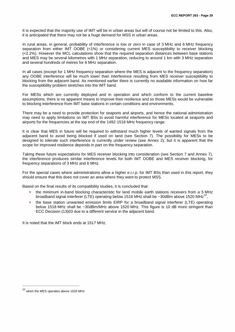
Figure 7: F. 1336-4 IMT antenna for a suburban macro base station; 16 dBi, 65° azimuth BW, 12° elevation BW, -6° EDT, peak values, figure showing ±30° elevation and ±90° azimuth
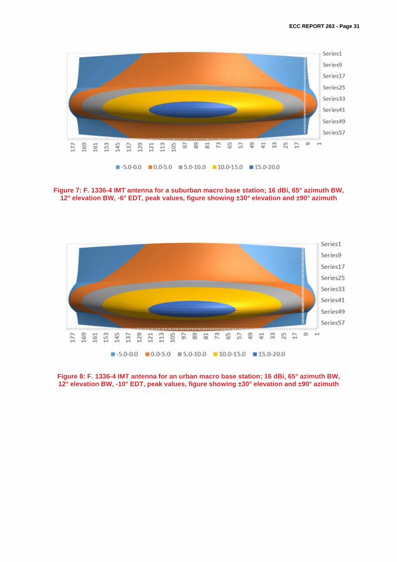
Figure 8: F. 1336-4 IMT antenna for an urban macro base station; 16 dBi, 65° azimuth BW, 12° elevation BW, -10° EDT, peak values, figure showing ±30° elevation and ±90° azimuth

ECC REPORT 263 - Page 32
ANNEX 2: POTENTIAL FOR MES RECEIVER IMPROVED BLOCKING RESILIENCE
A2.1 INTRODUCTION
While there is likely a need for improvements to MSS receiver performance, it is necessary to note and take into account the technical challenges that the possible new interference environment imposes on the design considerations and choices available for resilient MSS receiver design. It is also critically important to take into account the difference between LTE and CW based blocker levels on the performance degradation of the MSS receiver when determining the interference criterion based on a CW based blocker level.
A2.2 TECHNICAL CHALLENGES AND THE LIMITATION ON THE IMPROVEMENT OF RECEIVER PERFORMANCE
There would likely be a need to improve the MSS receiver resilience in order for MSS above 1518 MHz and IMT below 1518 MHz to coexist. However, in establishing technical measures to ensure compatibility, it is important to take into account the inherent technical challenges that are encountered in improving MSS receiver design; and the limitations that these challenges impose on the degree of improvements that can be reasonably achieved.
Satellite terminals, which receive satellite downlink signals are by necessity designed to be extremely sensitive devices. They are designed to receive a low-power signal emitted by small transmitters located in orbit 36,000 km above the equator.
Therefore for satellite terminals, the receiver sensitivity parameter is one of the main design drivers. Sensitivity is defined as minimum signal level at which the receiver is able to detect and decode the desired signal. This parameter determines the overall performance of MSS communication system and translates directly into service coverage and reliability.
The achievable sensitivity performance depends on the noise generated inside the receiver components (receiver noise figure), and therefore typically MSS receiver active components such LNA are chosen for the lowest possible noise figure, with the objective of the MSS receiver to have as low a noise floor as possible. This is because for an MSS receiver, the received power of the wanted signal at the terminal can be as low as -140dBm; and degrading the sensitivity could mean that the low power satellite broadcast and signalling carrier cannot be detected.
This sensitivity level may be compared with the level of interference from LTE emissions that could be expected in the band immediately below 1518 MHz. In the worst case (based on MCL analysis) the received interference from an LTE base station could exceed the criterion of –40 dBm by up to 29 dB, i.e. up to the level of –11 dBm. Hence the MES could be required to successfully receive the wanted signal while a few MHz away there is an interfering signal approximately 130 dB higher.
A2.2.1 LTE to MSS interference Mechanisms
Broadly there are two mechanisms by which IMT/LTE below 1518 MHz can interfere with an MSS receiver. LTE OOB emission into the MSS receiver: It should be noted that there is nothing that can be done on
the MSS receiver side to decrease the effect of this out of band interference and therefore it is necessary to note that the LTE OOB emission into the MSS band above 1518 MHz will increase the MSS receiver noise floor thereby degrading the receivers sensitivity;
Overload/blocking: This effect is due to the LTE high power signal below 1518 MHz causing overload/blocking conditions inside the MSS receiver. There are two ways to reduce the impact of overload/blocking in MSS receiver design; Improving preselector/front-end filtering of high power out-of-band LTE interferers to reduce the
power level reaching the receiver chain; Increasing the linearity (high power handling capability) of the receiver components in the receiver
chain.

ECC REPORT 263 - Page 33
A2.2.2 Filtering
To achieve a reasonable level of filtering performance for good portable MSS receiver design, the filter would be required to reduce the high level interfering signal at the receiver input by a considerable amount, but this is not easy to achieve for an LTE signal with an edge only few MHz away using a low-cost SAW filter.
Although SAW filters typically have quite a sharp roll-off, the turnover frequencies are highly temperature dependent which results in the filter manufacturers setting the specification masks to be quite wide.
An example of a filter currently in use is shown below in Figure 9. Note that although the typical curve appears to provide some attenuation in the 1500-1510 MHz region, the mask (straight lines) actually guarantees no attenuation at all above 1490 MHz.
Ceramic filters can provide somewhat better characteristics but are larger and more expensive.
Excellent performance can be provided by cavity filters but these are very large and extremely expensive, and impractical for use in mobile terminals.
Figure 9: Typical satellite receiver front-end SAW filter response
A2.2.3 MSS Receiver Linearity
Linearity of the receiver is an important parameter which determines the maximum power level that the receiver can handle at its input before its receiver chain is driven to its non-linear operation giving rise to the generation of distortions inside the receiver, resulting in the degradation of the receiver performance.
Therefore, the LNA and other active components of the receiver must be chosen with high linearity characteristics. However, it is always the case that the design criteria that prioritises the receiver linearity performance as a key design requirement is generally in conflict with its sensitivity performance, as the two parameters are conflicting requirements and have to be traded-off. The higher the linearity of a receiver, the higher the interference level it can handle and less susceptible to overload, however, as the receiver linearity improves, the receiver noise figure degrades, resulting in receiver sensitivity reduction.
Therefore the sensitivity and linearity parameters of an MSS receiver are two of the most important parameters for MSS operation in an environment where there is proliferation of high power systems operating in the adjacent band.

ECC REPORT 263 - Page 34
These two receiver parameter elements, receiver sensitivity and linearity, are two fundamental parameters that need to be taken into account when considering potential improvements to the resilience of terminals to interference from LTE in the adjacent band.
Blocking/overload performance improvement alone will give a misleading perception of compatibility of coexistence if the overall system level performance is degraded as the result of the reduced sensitivity, and consequently reduced reliability and service coverage.
Hence the challenge is to design an MSS receiver that can operate reliably as intended and at the same time be able to handle high power out of band LTE type of interferer. While the sensitivity of the receiver sets the lower limit, the upper limit is determined by its linearity performance.
As was stated above, the level of the received signal that the MSS receiver is required to detect for its operation is as low as –140 dBm while as the same time the power of a terrestrial transmission experienced by the same terminal (with a 0 dBi antenna) close to a cell tower radiating an in-band LTE signal can be as high as –11 dBm at the same measurement point.
The requirement on the receiver then is to receive its weak signal from the satellite in the presence of another signal which may be ~130 dB higher in power, and the edge of which may be only few MHz away. This is very challenging.
In summary, protection against large signals from close by LTE base stations is limited by: Practicalities of filtering: Both in the MSS receiver; and in LTE base stations;
MSS receiver overload performance is limited by extremely high dynamic range requirement in MSS systems.
A2.2.4 LTE and CW blocking comparisons
Historically it was common to test the receiver blocker performance using a CW where most systems were narrow-band with a constant-envelope (0 dB peak-to-average-power-ratio) modulation schemes. CW is unmodulated single-tone signal with constant-envelope and is a good approximation for a narrow-band interfering signal.
On the other hand, today’s systems are generally based on broadband signals like LTE with very high peak-to-average-power-ratio modulation schemes; hence CW as a blocker is not a good approximation for LTE.
In order to appreciate the difference between the impact of CW and LTE blocking on the MSS receiver, it is important to highlight the following points: Receiver overload occurs when a signal at the input of a receiver’s LNA reaches an amplitude sufficient
to cause the amplifier to attempt to exceed its maximum possible output level, consequently distorting the output signal waveform. If a strong signal from a nearby LTE base station overloads the LNA in an MSS terminal receiver, the amplifier will distort the waveforms of both the LTE signal and at the same time the received MSS wanted satellite signal;
When a receiver's LNA is operated in its linear range, the gain of the LNA is constant as the input signal level is varied, i.e. the output signal level is always G dB higher than the input signal level, where G is the gain of the LNA in dB. As the input signal level is increased beyond the linear range of the LNA, the 1 dB compression point of the LNA is the input signal power level at which the gain of the LNA becomes G-1 dB, the result of this is to reduce the gain available for the weak wanted signal and consequently degrading the SNR;
Both CW and LTE signals cause gain compression to the MSS receiver when their level is such that the LNA is driven to its 1 dB compression point. However, it should be noted that the LTE signal results in 1 dB compression point at lower average power levels than the CW signal. This is due to the higher peak-to-average power ratio of the LTE signal as compared to the CW signal, which is a constant-envelope signal;

ECC REPORT 263 - Page 35
Intermodulation products occur when two or more signals at different frequencies combine in a receiver to create signals at frequencies that are the sums and differences of integer multiples of the original signals. Intermodulation product frequencies are calculated by: f IM=n*f1 ± m*f2, where fIM is the frequency of the intermodulation product, f1 and f2 are the interfering signal frequencies, and n and m are integers greater than zero. For broadband signals like LTE, the individual spectral components within the bandwidth of the signal create an intermodulation product on a frequency being used by an MSS receiver, harmful interference to the MSS receiver may occur, depending on the levels of the LTE base station signals at the input to the MSS receiver. The strongest intermodulation products occur when m + n = 3, i.e. when m = 1 and n = 2, or m = 2 and n = 1. These are known as “third-order” intermodulation products and give rise to what is commonly known as spectral regrowth as depicted in Figure 10. Spectral regrowth effectively increases the noise floor of the MSS receive thereby degrading its sensitivity.
In summary while CW causes only gain compression in the MSS receiver, an LTE signal causes gain compression followed by intermodulation products resulting in spectral re-growth which degrades the noise floor of the receiver.
Therefore an LTE blocking signal results in a given MSS receiver degradation at lower average power level than a CW signal level causing the same level of MSS receiver degradation, this is due to both the higher peak-to-average-power-ratio of LTE and the spectral regrowth that it may cause at higher levels of compression.
In order to mitigate against the impact of spectral regrowth, it is necessary have sufficient guard band between the LTE blocker and the MSS receiver.
Figure 10: Spectral re-growth of LTE signal
Figure 10 shows spectral re-growth for a 20 MHz block, 3rd and 5th order re-growth effects extend further into the MSS band.

ECC REPORT 263 - Page 36
Table 13 and Table 14 show the test results of a CW and LTE blocking signals. The results clearly show an LTE blocking signal causing a 1 dB MSS receiver degradation at much lower average power level than a CW signal level causing the same level of MSS receiver degradation.
Table 13: CW and LTE Interferer levels causing 1 dB degradation in C/N0, with MES @ 1518.1 MHz
Test against MES carrier @ 1518.1 MHz, MES#1
Interferer Interferer levels (@ antenna connector) that cause 1 dB degradation in C/N0
1 MHz offset 3 MHz offset 5 MHz offset
CW -44.4 dBm -35.9 dBm -33.4 dBm
5 MHz LTE -51.4 dBm/5MHz -47.9 dBm/5MHz -39.9 dBm/5MHz
Table 14: CW and LTE Interferer levels causing 1 dB degradation in C/No,
with MES @ 1518.1 MHz
Test against MES carrier @ 1518.1 MHz, MES#2
Interferer Interferer levels (@ antenna connector) that cause 1 dB degradation in C/N0
1 MHz offset 3 MHz offset 5 MHz offset
CW -58.6 dBm -49.0 dBm -43.0 dBm
5 MHz LTE -67.8 dBm/5MHz -57.0 dBm/5MHz -49.8 dBm/5MHz
These results for current MESs illustrate the importance of the offset (or guard band) between the LTE signals and the MSS signal. For MES#1 there is a difference in susceptibility of 11.5 dB between the 1 MHz and 5 MHz cases. For MES#2 there is a difference in susceptibility of 18 dB between the 1 MHz and 5 MHz cases.
From these results, we can see that the overload level for an LTE modulated signals is approximately 10 dB lower than for CW interfering signals.
A2.2.5 Frequency separation
While it is likely that MSS receiver performance would need to improve to ensure compatibility with LTE operations in the band below 1518 MHz, there are practical limitations to what can be achieved by linearity alone. Regarding potential improvements to MSS receiver blocking/overload performance, the frequency separation between IMT and MSS is a key parameter, as it relates to both the potential to use filtering to improve performance and also reduce the impact of increase in noise due to spectral re-growth.

ECC REPORT 263 - Page 37
ANNEX 3: MES EXAMPLE ANTENNA PATTERNS
The following are antenna patterns representative of average sidelobe performance of typical MES antennas.
Figure 11: Inmarsat-B/F-77, Fleet broadband antenna (peak gain = 21 dBi)
Figure 12: BGAN Class 1 (peak gain = 17.5 dBi)
Figure 13: Inmarsat-C/GSPS (peak gain = 3 dBi)
200− 100− 0 100 20010−
0
10
20
30
off axis angle (degrees)
gain
(dB
i)
.
.
200− 100− 0 100 20010−
0
10
20
off axis angle (degrees)
gain
(dB
i)
100− 50− 0 50 1002−
1−
0
1
2
3
off-axis angle (degrees)
gain
(dB
i)
ECC REPORT 263 - Page 38
ANNEX 4: ADDITIONAL INFORMATION REGARDING PROPAGATION MODEL FOR LAND SCENARIO
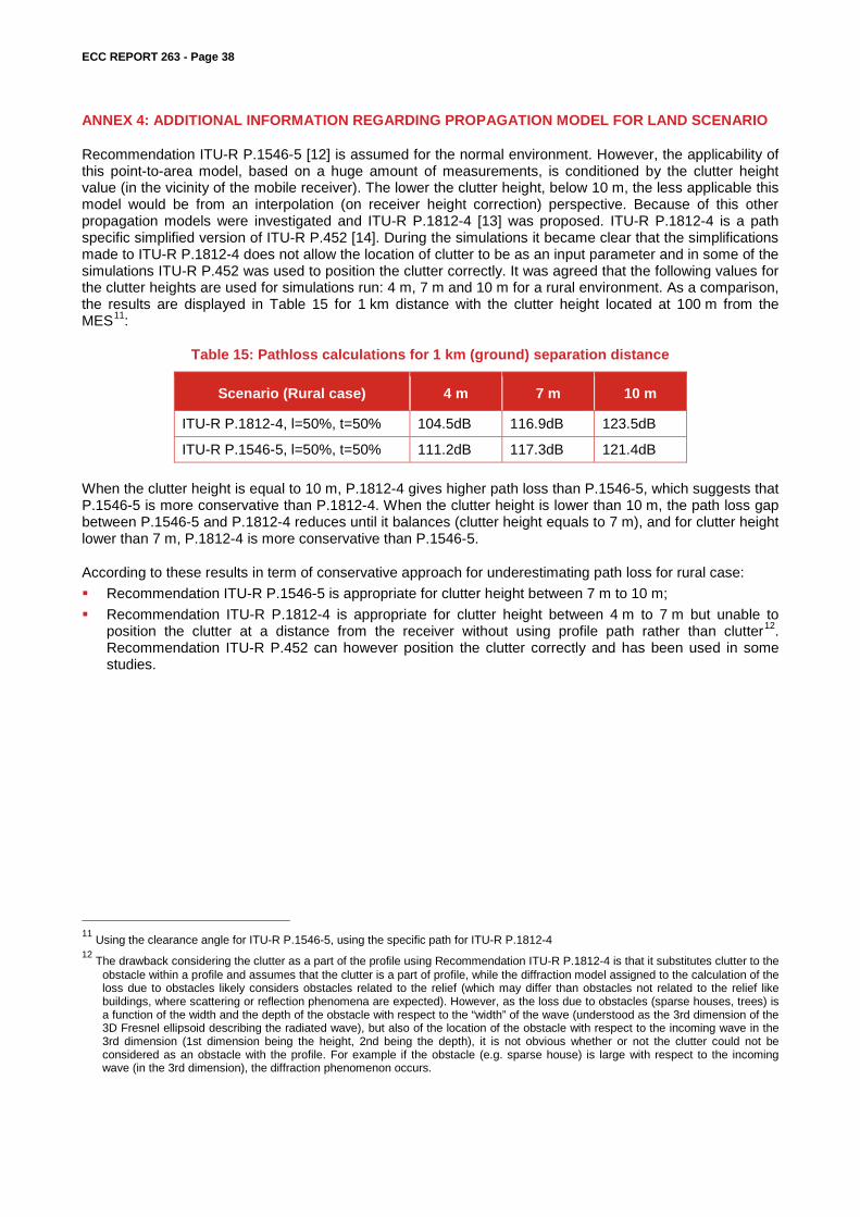
Recommendation ITU-R P.1546-5 [12] is assumed for the normal environment. However, the applicability of this point-to-area model, based on a huge amount of measurements, is conditioned by the clutter height value (in the vicinity of the mobile receiver). The lower the clutter height, below 10 m, the less applicable this model would be from an interpolation (on receiver height correction) perspective. Because of this other propagation models were investigated and ITU-R P.1812-4 [13] was proposed. ITU-R P.1812-4 is a path specific simplified version of ITU-R P.452 [14]. During the simulations it became clear that the simplifications made to ITU-R P.1812-4 does not allow the location of clutter to be as an input parameter and in some of the simulations ITU-R P.452 was used to position the clutter correctly. It was agreed that the following values for the clutter heights are used for simulations run: 4 m, 7 m and 10 m for a rural environment. As a comparison, the results are displayed in Table 15 for 1 km distance with the clutter height located at 100 m from the MES11:
Table 15: Pathloss calculations for 1 km (ground) separation distance
Scenario (Rural case) 4 m 7 m 10 m
ITU-R P.1812-4, l=50%, t=50% 104.5dB 116.9dB 123.5dB
ITU-R P.1546-5, l=50%, t=50% 111.2dB 117.3dB 121.4dB
When the clutter height is equal to 10 m, P.1812-4 gives higher path loss than P.1546-5, which suggests that P.1546-5 is more conservative than P.1812-4. When the clutter height is lower than 10 m, the path loss gap between P.1546-5 and P.1812-4 reduces until it balances (clutter height equals to 7 m), and for clutter height lower than 7 m, P.1812-4 is more conservative than P.1546-5.
According to these results in term of conservative approach for underestimating path loss for rural case: Recommendation ITU-R P.1546-5 is appropriate for clutter height between 7 m to 10 m; Recommendation ITU-R P.1812-4 is appropriate for clutter height between 4 m to 7 m but unable to
position the clutter at a distance from the receiver without using profile path rather than clutter12. Recommendation ITU-R P.452 can however position the clutter correctly and has been used in some studies.
11 Using the clearance angle for ITU-R P.1546-5, using the specific path for ITU-R P.1812-4 12 The drawback considering the clutter as a part of the profile using Recommendation ITU-R P.1812-4 is that it substitutes clutter to the
obstacle within a profile and assumes that the clutter is a part of profile, while the diffraction model assigned to the calculation of the loss due to obstacles likely considers obstacles related to the relief (which may differ than obstacles not related to the relief like buildings, where scattering or reflection phenomena are expected). However, as the loss due to obstacles (sparse houses, trees) is a function of the width and the depth of the obstacle with respect to the “width” of the wave (understood as the 3rd dimension of the 3D Fresnel ellipsoid describing the radiated wave), but also of the location of the obstacle with respect to the incoming wave in the 3rd dimension (1st dimension being the height, 2nd being the depth), it is not obvious whether or not the clutter could not be considered as an obstacle with the profile. For example if the obstacle (e.g. sparse house) is large with respect to the incoming wave (in the 3rd dimension), the diffraction phenomenon occurs.
ECC REPORT 263 - Page 39
ANNEX 5: MCL RESULTS
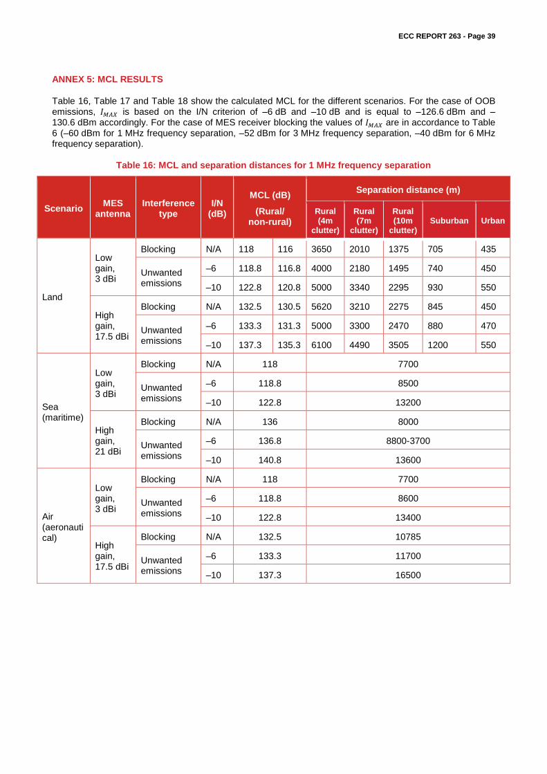
Table 16, Table 17 and Table 18 show the calculated MCL for the different scenarios. For the case of OOB emissions, 𝐼𝐼𝑀𝑀𝑀𝑀𝑀𝑀 is based on the I/N criterion of –6 dB and –10 dB and is equal to –126.6 dBm and –130.6 dBm accordingly. For the case of MES receiver blocking the values of 𝐼𝐼𝑀𝑀𝑀𝑀𝑀𝑀 are in accordance to Table 6 (–60 dBm for 1 MHz frequency separation, –52 dBm for 3 MHz frequency separation, –40 dBm for 6 MHz frequency separation).
Table 16: MCL and separation distances for 1 MHz frequency separation
Scenario MES antenna
Interference type
I/N (dB)
MCL (dB)
(Rural/ non-rural)
Separation distance (m)
Rural (4m
clutter)
Rural (7m
clutter)
Rural (10m
clutter) Suburban Urban
Land
Low gain, 3 dBi
Blocking N/A 118 116 3650 2010 1375 705 435
Unwanted emissions
–6 118.8 116.8 4000 2180 1495 740 450
–10 122.8 120.8 5000 3340 2295 930 550
High gain, 17.5 dBi
Blocking N/A 132.5 130.5 5620 3210 2275 845 450
Unwanted emissions
–6 133.3 131.3 5000 3300 2470 880 470
–10 137.3 135.3 6100 4490 3505 1200 550
Sea (maritime)
Low gain, 3 dBi
Blocking N/A 118 7700
Unwanted emissions
–6 118.8 8500
–10 122.8 13200
High gain, 21 dBi
Blocking N/A 136 8000
Unwanted emissions
–6 136.8 8800-3700
–10 140.8 13600
Air (aeronautical)
Low gain, 3 dBi
Blocking N/A 118 7700
Unwanted emissions
–6 118.8 8600
–10 122.8 13400
High gain, 17.5 dBi
Blocking N/A 132.5 10785
Unwanted emissions
–6 133.3 11700
–10 137.3 16500

ECC REPORT 263 - Page 40
Table 17: MCL and separation distances for 3 MHz frequency separation
Scenario MES antenna
Interference type
I/N (dB)
MCL (dB)
(Rural/ non-rural)
Separation distance (m)
Rural (4m
clutter)
Rural (7m
clutter)
Rural (10m
clutter) Suburban Urban
Land
Low gain, 3 dBi
Blocking N/A 110 108 1550 865 610 450 280
Unwanted emissions
–6 89.6 87.6 30 10 25 60 60
–10 93.6 91.6 60 20 60 80 70
High gain, 17.5 dBi
Blocking N/A 124.5 122.5 2560 1605 1150 570 335
Unwanted emissions
–6 104.1 102.1 500 100 70 220 170
–10 108.1 106.1 600 330 105 270 190
Sea (maritime)
Low gain, 3 dBi
Blocking N/A 110 3200
Unwanted emissions
–6 89.6 400
–10 93.6 600
High gain, 21 dBi
Blocking N/A 128 3400
Unwanted emissions
–6 107.6 500
–10 111.6 700
Air (aeronautical)
Low gain, 3 dBi
Blocking N/A 110 3175
Unwanted emissions
–6 89.6 400
–10 93.6 600
High gain, 17.5 dBi
Blocking N/A 124.5 4585
Unwanted emissions
–6 104.1 800
–10 108.1 1100
ECC REPORT 263 - Page 41
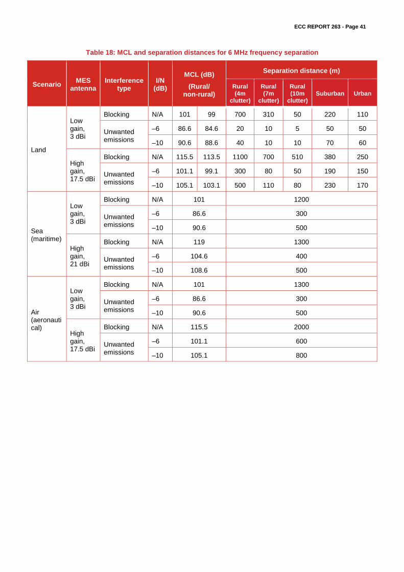
Table 18: MCL and separation distances for 6 MHz frequency separation
Scenario MES antenna
Interference type
I/N (dB)
MCL (dB)
(Rural/ non-rural)
Separation distance (m)
Rural (4m
clutter)
Rural (7m
clutter)
Rural (10m
clutter) Suburban Urban
Land
Low gain, 3 dBi
Blocking N/A 101 99 700 310 50 220 110
Unwanted emissions
–6 86.6 84.6 20 10 5 50 50
–10 90.6 88.6 40 10 10 70 60
High gain, 17.5 dBi
Blocking N/A 115.5 113.5 1100 700 510 380 250
Unwanted emissions
–6 101.1 99.1 300 80 50 190 150
–10 105.1 103.1 500 110 80 230 170
Sea (maritime)
Low gain, 3 dBi
Blocking N/A 101 1200
Unwanted emissions
–6 86.6 300
–10 90.6 500
High gain, 21 dBi
Blocking N/A 119 1300
Unwanted emissions
–6 104.6 400
–10 108.6 500
Air (aeronautical)
Low gain, 3 dBi
Blocking N/A 101 1300
Unwanted emissions
–6 86.6 300
–10 90.6 500
High gain, 17.5 dBi
Blocking N/A 115.5 2000
Unwanted emissions
–6 101.1 600
–10 105.1 800

ECC REPORT 263 - Page 42
ANNEX 6: MCL RESULTS FOR AES ON AIRCRAFT IN FLIGHT
This section shows the potential interference from IMT base stations to AESs operated on aircraft in flight. Interference from a rural base station only is considered, with the AES at example altitudes of 1000 m, 3000 m and 10000 m above ground level (a.g.l.).
A summary of MCL requirements for each of three cases: 1 MHz, 3 MHz and 6 MHz frequency separation, is shown in the tables below.
Table 19: MCL requirements for 1 MHz frequency separation
AES antenna Blocking/Unwanted emissions Criterion MCL (dB)
Low gain, 3 dBi
Blocking I < -60 dBm 121.0
Unwanted emissions I/N < -6 dB 118.8
I/N < -10 dB 122.8
High gain, 17.5 dBi
Blocking I < -60 dBm 135.5
Unwanted emissions I/N < -6 dB 133.3
I/N < -10 dB 137.3
Table 20: MCL requirements for 3 MHz frequency separation
AES antenna Blocking/Unwanted emissions Criterion MCL (dB)
Low gain, 3 dBi
Blocking I < -52 dBm 113.0
Unwanted emissions I/N < -6 dB 89.6
I/N < -10 dB 93.6
High gain, 17.5 dBi
Blocking I < -52 dBm 127.5
Unwanted emissions I/N < -6 dB 104.1
I/N < -10 dB 108.1
Table 21: MCL requirements for 6 MHz frequency separation
AES antenna Blocking/Unwanted emissions Criterion MCL (dB)
Low gain, 3 dBi
Blocking I < -40 dBm 101.0
Unwanted emissions I/N < -6 dB 86.6
I/N < -10 dB 90.6
High gain, 17.5 dBi
Blocking I < -40 dBm 115.5
Unwanted emissions I/N < -6 dB 101.1
I/N < -10 dB 105.1

ECC REPORT 263 - Page 43
Figure 14 shows the coupling loss and the minimum coupling loss for an AES with the high gain antenna. Figure 15 shows the coupling loss and minimum coupling loss for an AES with the low gain antenna. The MCL values shown are applicable for the case of 1 MHz frequency separation to represent the worst case frequency separation.
Figure 14: CL and MCL for interference from a rural IMT base station to a high gain AES at various altitudes
Figure 15: CL and MCL for interference from a rural IMT base station to a low gain AES at various altitudes
130.0
135.0
140.0
145.0
150.0
155.0
160.0
165.0
170.0
0 10 20 30 40 50 60 70 80 90 100
Coup
ling
loss
(dB)
Ground distance (km)
High gain AES, 10 km a.g.l.
High gain AES, 3 km a.g.l.
High gain AES, 1 km a.g.l.
MCL UW (-10 dB I/N)
MCL Blocking (-60 dBm)
MCL UW (-6 dB I/N)
110.0
120.0
130.0
140.0
150.0
160.0
0 10 20 30 40 50 60 70 80 90 100
Coup
ling
loss
(dB)
Ground distance (km)
High gain AES, 10 km a.g.l.
High gain AES, 3 km a.g.l.
High gain AES, 1 km a.g.l.
MCL UW (-10 dB I/N)
MCL Blocking (-60 dBm)
MCL UW (-6 dB I/N)

ECC REPORT 263 - Page 44
In all cases examined, the coupling loss exceeds the minimum coupling loss and hence interference would be below the criterion. Since the coupling loss exceeds the MCL values in the case of 1 MHz frequency separation, the coupling loss would also exceed the MCL values for 3 MHz and 6 MHz frequency separation.
Among these different scenarios, the MCL worst case corresponds to the High Gain AES antenna for I/N=–10 dB. It is therefore proposed to study it in this section.
Figure 16: Variation of current and required isolation loss with distance and altitude
The left side figure exhibits the required isolation loss as well as the current isolation loss for varying altitude and distance (including antenna gain discriminations for aeronautical MES receiver and ground IMT BS interferer) for the worst case I/N=–10 dB high gain MES antenna. As expected, the current isolation increases with altitude and distance. In addition, the shape of the curves shows that for 1 MHz frequency separation that required isolation loss is lower than current isolation loss (MES, BS) for altitude ≥ 0.8 km if I/N=–10 dB and for the sake of comparison for altitude ≥ 0.2 km if I/N=–10 dB for the low gain MES antenna13, resulting in no constraint in that case (since the required isolation loss is met). Note that this altitude=0.8km, called hmin is derived for the scenario where IMT BS interferer and Aeronautical Earth Station antennas are facing each other. For the general case where these systems have a discrimination angle in horizontal (azimuthal) plane denoted Δφ (depicted in figure below), the value of hmin is lower.
13 The rationale for comparing the low and high gain MES antenna in the results of the study is based on the fact that the discrimination
due to the antenna gain may facilitate the sharing for a high gain MES antenna depending on the location of the IMT BS with respect to the flying aircraft.

ECC REPORT 263 - Page 45
Figure 17: Orientation of aeronautical MES in relation to IMT BS
For example:
Figure 18: Variation of current and required isolation loss with distance and altitude, (left) Δφ =40°then hmin=0.7km, (right) Δφ =90° then hmin=0.5km
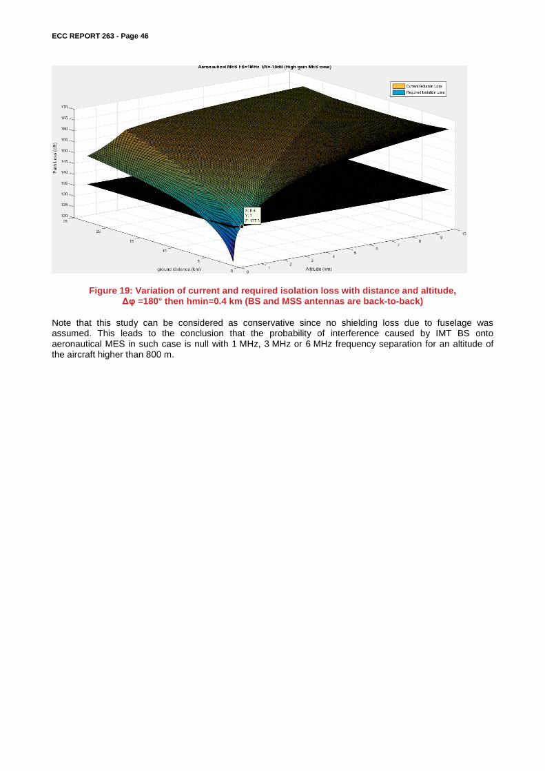
ECC REPORT 263 - Page 46
Figure 19: Variation of current and required isolation loss with distance and altitude, Δφ =180° then hmin=0.4 km (BS and MSS antennas are back-to-back)
Note that this study can be considered as conservative since no shielding loss due to fuselage was assumed. This leads to the conclusion that the probability of interference caused by IMT BS onto aeronautical MES in such case is null with 1 MHz, 3 MHz or 6 MHz frequency separation for an altitude of the aircraft higher than 800 m.

ECC REPORT 263 - Page 47
ANNEX 7: STUDY #1
A7.1 STATISTICAL ANALYSIS
In the following analysis, probabilistic simulations over a general area of IMT coverage are performed from a limited simulation area covered by a three sector IMT Base Station site, which has been simulated for cell radius of 0.5 km, 1 km and 5 km respectively for the different environments. For the land based simulation the IMT base station transmits in all three sectors and the three service hexagons have been populated with MESs that are monitored for interference. The MESs are strictly limited to move within the assigned hexagon such that the model is equivalent to a full network.
The simulations investigate scenarios where IMT is deployed in urban areas and also for the less likely case where it may be deployed in suburban or even rural areas. Normal clutter is used for the three environments. Frequency separations of 1 MHz, 3 MHz and 6 MHz are included. A sensitivity analysis is included to additionally show the impact of I/N = -10 dB for the MES. Further, an extreme situation where the clutter in a rural area is consistently below the standard 10 m is included, for this, clutter heights of 7 m and 4 m are used.
Simulations are also performed for the maritime environment with the IMT base stations located on land, the two relevant scenarios are as described in Section 5.3.
A7.2 AREA IMPACT ON MES INTERFERENCE
The study results below contain an extension to the MCL, it covers an artificial situation where the MES is always allocated the 1st adjacent channel above the frequency separations (1 MHz, 3 MHz or 6 MHz), but moves randomly around in the area of IMT coverage.
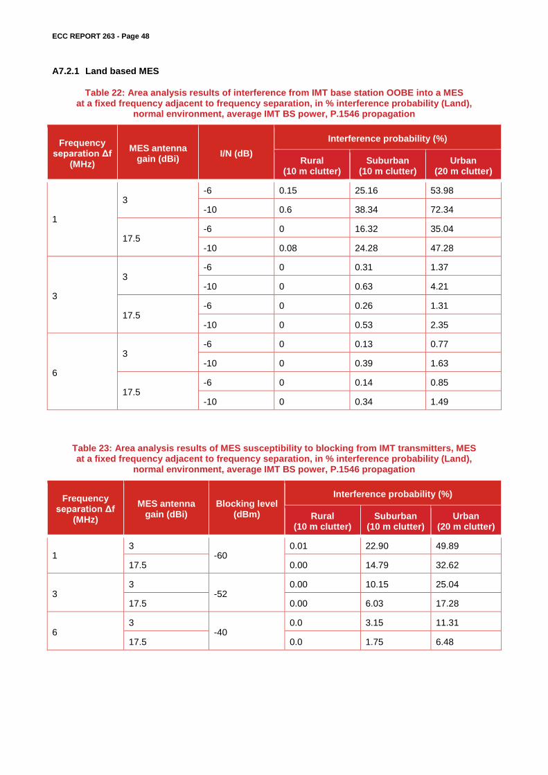
ECC REPORT 263 - Page 48
A7.2.1 Land based MES
Table 22: Area analysis results of interference from IMT base station OOBE into a MES at a fixed frequency adjacent to frequency separation, in % interference probability (Land),
normal environment, average IMT BS power, P.1546 propagation
Frequency separation Δf
(MHz) MES antenna
gain (dBi) I/N (dB) Interference probability (%)
Rural (10 m clutter)
Suburban (10 m clutter)
Urban (20 m clutter)
1
3 -6 0.15 25.16 53.98
-10 0.6 38.34 72.34
17.5 -6 0 16.32 35.04
-10 0.08 24.28 47.28
3
3 -6 0 0.31 1.37
-10 0 0.63 4.21
17.5 -6 0 0.26 1.31
-10 0 0.53 2.35
6
3 -6 0 0.13 0.77
-10 0 0.39 1.63
17.5 -6 0 0.14 0.85
-10 0 0.34 1.49
Table 23: Area analysis results of MES susceptibility to blocking from IMT transmitters, MES at a fixed frequency adjacent to frequency separation, in % interference probability (Land),
normal environment, average IMT BS power, P.1546 propagation
Frequency separation Δf
(MHz) MES antenna
gain (dBi) Blocking level
(dBm)
Interference probability (%)
Rural (10 m clutter)
Suburban (10 m clutter)
Urban (20 m clutter)
1 3
-60 0.01 22.90 49.89
17.5 0.00 14.79 32.62
3 3
-52 0.00 10.15 25.04
17.5 0.00 6.03 17.28
6 3
-40 0.0 3.15 11.31
17.5 0.0 1.75 6.48

ECC REPORT 263 - Page 49
Table 24: Sensitivity analysis of a more extreme rural scenario using lower clutter height and different propagation models for OOBE into MES in % probability (Land)
Frequency separation Δf (MHz)
MES antenna gain (dBi) I/N (dB)
Interference probability (%)
Rural (P.1812,
4 m clutter)
Rural (P.452,
4 m clutter)
Rural (P.1812,
7 m clutter)
Rural (P.452,
7 m clutter)
1
3 -6 22.37 3.69 6 1.14
-10 38.16 10.57 16.3 4.8
17.5 -6 9.13 0.82 1.53 0.16
-10 19.3 3.32 5.78 1.16
3
3 -6 0 0 0 0
-10 0 0 0 0
17.5 -6 0 0 0 0
-10 0 0 0 0
6
3 -6 0 0 0 0
-10 0 0 0 0
17.5 -6 0 0 0 0
-10 0 0 0 0 For more information on applicability of the Recommendation ITU-R P.1812-4 [13] see Annex 4.
Table 25: Sensitivity analysis of a more extreme rural scenario using lower clutter height and different propagation models for MES susceptibility to blocking from IMT transmitters,
in % interference probability (Land)
Frequency separation Δf
(MHz)
MES antenna
gain (dBi)
Blocking level
(dBm)
Interference probability (%)
Rural (P.1812,
4 m clutter)
Rural (P.452,
4 m clutter)
Rural (P.1812,
7 m clutter)
Rural (P.452,
7 m clutter)
1 3
-60 19.55 2.85 4.65 1.11
17.5 7.10 0.56 1.00 0.10
3 3
-52 2.20 0.08 0.15 0.00
17.5 0.31 0.00 0.00 0.00
6 3
-40 0.00 0.00 0.00 0.00
17.5 0.00 0.00 0.00 0.00 For more information on applicability of the Recommendation ITU-R P.1812-4 [13] see Annex 4

ECC REPORT 263 - Page 50
A7.2.2 Sea based MES
Table 26: Area analysis results of interference from the IMT base station OOBE into a MES at a fixed frequency adjacent to frequency separation in % probability (Sea)
Frequency separation Δf
(MHz) MES antenna
gain (dBi) I/N (dB)
Interference probability (%)
2 sector rural IMT located on the
coastline, 100% sea
1 sector rural IMT pointing to sea 5 km
from the coast
1
3 -6 1.67 0
-10 11.44 55.1
21 -6 1.75 0
-10 6.61 9.19
3
3 -6 0 0
-10 0 0
21 -6 0 0
-10 0 0
6
3 -6 0 0
-10 0 0
21 -6 0 0
-10 0 0
Table 27: Area analysis results of MSS susceptibility to blocking from transmitters, MES at a fixed frequency adjacent to frequency separation, in % interference probability (Sea)
Frequency separation Δf
(MHz)
MES antenna
gain (dBi) Blocking
level (dBm)
Interference probability (%)
2 sector rural IMT located on the
coastline, 100% sea
1 sector rural IMT pointing to sea 5 km
from the coast
1 3
-60 0.84 0.00
21 0.91 0.00
3 3
-52 0.00 0.00
21 0.00 0.00
6 3
-40 0.00 0.00
21 0.00 0.00

ECC REPORT 263 - Page 51
A7.3 AREA AND FREQUENCY IMPACT ON MES INTERFERENCE
In addition to the area analysis above simulations have also been performed to include the effect of the MES using the full frequency band.
In the study results below the impact on the user of MES is investigated, the parameters from above are used and the susceptibility of the MES is established by simulations over the entire IMT service area and over the full frequency range (1518-1559 MHz) available to MSS for downlink
Whilst the results for MES Blocking in the following are of course the same as for the 1st adjacent channel above the results are provided for an easier comparison MES Blocking and OOBE interference under the same conditions.
A7.3.1 Land based MES
Table 28: Area and frequency analysis results of interference from the IMT base station OOBE into MSS in % probability (Land), normal environment, P.1546 propagation
Frequency separation Δf
(MHz) MES antenna
gain (dBi) I/N (dB) Interference probability (%)
Rural (10 m clutter)
Suburban (10 m clutter)
Urban (20 m clutter)
1
3 -6 0.01 1.19 2.62
-10 0.02 1.87 3.88
17.5 -6 0 0.76 1.82
-10 0 1.19 2.44
3
3 -6 0 0.01 0.09
-10 0 0.05 0.34
17.5 -6 0 0.04 0.19
-10 0 0.05 0.37
6
3 -6 0 0.01 0.02
-10 0 0.02 0.11
17.5 -6 0 0.03 0.1
-10 0 0.04 0.26

ECC REPORT 263 - Page 52
Table 29: Area and frequency analysis results of MES susceptibility to blocking from IMT transmitters, in % interference probability (Land), normal environment, P.1546 propagation
Frequency separation Δf
(MHz) MES antenna
gain (dBi) Blocking level
(dBm)
Interference probability (%)
Rural (10 m clutter)
Suburban (10 m clutter)
Urban (20 m clutter)
1 3
-60 0.01 22.90 49.89
17.5 0.00 14.79 32.62
3 3
-52 0.00 10.15 25.04
17.5 0.00 6.03 17.28
6 3
-40 0.00 3.15 11.31
17.5 0.00 1.75 6.48
Table 30: Sensitivity analysis of a more extreme rural scenario using lower clutter height and different propagation models for OOBE into MSS in % probability (Land)
Frequency separation Δf (MHz)
MES antenna gain (dBi) I/N (dB)
Interference probability (%)
Rural (P.1812,
4 m clutter)
Rural (P.452,
4 m clutter)
Rural (P.1812,
7 m clutter)
Rural (P.452,
7 m clutter)
1
3 -6 1.04 0.12 0.23 0.06
-10 1.77 0.45 0.75 0.04
17.5 -6 0.44 0.04 0.07 0.01
-10 0.89 0.15 0.25 0.1
3
3 -6 0 0 0 0
-10 0 0 0 0
17.5 -6 0 0 0 0
-10 0 0 0 0
6
3 -6 0 0 0 0
-10 0 0 0 0
17.5 -6 0 0 0 0
-10 0 0 0 0 For more information on applicability of the Recommendation ITU-R P.1812-4 [13] see Annex 4

ECC REPORT 263 - Page 53
Table 31: Sensitivity analysis of a more extreme rural scenario using lower clutter height and different propagation models for MES susceptibility to blocking from IMT transmitters,
in % interference probability (Land)
Frequency separation Δf (MHz)
MES antenna
gain (dBi)
Blocking level
(dBm)
Interference probability (%)
Rural (P.1812,
4 m clutter)
Rural (P.452,
4 m clutter)
Rural (P.1812,
7 m clutter)
Rural (P.452,
7 m clutter)
1 3
-60 19.55 2.85 4.65 1.11
17.5 7.10 0.56 1.00 0.10
3 3
-52 2.20 0.08 0.15 0.00
17.5 0.31 0.00 0.00 0.00
6 3
-40 0.00 0.00 0.00 0.00
17.5 0.00 0.00 0.00 0.00 For more information on applicability of the Recommendation ITU-R P.1812-4 [13] see Annex 4
A7.3.2 Sea based MES
Table 32: Area and frequency analysis results of interference from the IMT base station OOBE into MES, in % probability (Sea)
Frequency separation Δf
(MHz) MES antenna
gain (dBi) I/N (dB)
Interference probability (%)
2 sector rural IMT located on the
coastline, 100% sea
1 sector rural IMT pointing to sea 5 km
from the coast
1
3 -6 0.09 0
-10 0.58 2.57
21 -6 0.06 0
-10 0.21 0.42
3
3 -6 0 0
-10 0 0
21 -6 0 0
-10 0 0
6
3 -6 0 0
-10 0 0
21 -6 0 0
-10 0 0

ECC REPORT 263 - Page 54
Table 33: Area and frequency analysis results of MSS susceptibility to blocking from IMT transmitters in % probability (Sea)
Frequency separation Δf
(MHz)
MES antenna
gain (dBi) Blocking
level (dBm)
Interference probability (%)
2 sector rural IMT located on the
coastline, 100% sea
1 sector rural IMT pointing to sea 5 km
from the coast
1 3
-60 0.84 0.00
21 0.91 0.00
3 3
-52 0.00 0.00
21 0.00 0.00
6 3
-40 0.00 0.00
21 0.00 0.00
A7.4 AREA IMPACT ON MES INTERFERENCE FOR THE MES WITH ENHANCED BLOCKING PERFORMANCE
Below are the results for the expected enhancement of the MES receiver blocking performance, performed under exactly the same conditions as in the simulations above.
Table 34: Area analysis results of MES susceptibility to blocking from IMT transmitters, in % interference probability (Land), normal environment, P.1546 propagation
Frequency separation Δf
(MHz) MES antenna
gain (dBi) Blocking level
(dBm)
Interference probability (%)
Rural (10 m clutter)
Suburban (10 m clutter)
Urban (20 m clutter)
1
3 -55 0 13.66 32.71
-45 0 4.35 13.47
17.5 -55 0 8.75 22.4
-45 0 2.28 8.45
3
3 -35 0 0.58 3.62
-30 0 0.24 1.11
17.5 -35 0 0.5 2.16
-30 0 0.2 1.04
6
3 -30 0 0.41 1.74
-25 0 0 0.62
17.5 -30 0 0.36 1.57
-25 0 0.13 0.81

ECC REPORT 263 - Page 55
Table 35: Sensitivity analysis of a more extreme rural scenario using lower clutter height and different propagation models
Frequency separation Δf (MHz)
MES antenna gain (dBi)
Blocking level
(dBm)
Interference probability (%)
Rural (P.1812,
4 m clutter)
Rural (P.452,
4 m clutter)
Rural (P.1812,
7 m clutter)
Rural (P.452,
7 m clutter)
1
3 -55 5.49 0.49 0.86 0.07
-45 0.01 0 0 0
17.5 -55 1.32 0 0.04 0
-45 0 0 0 0
3
3 -35 0 0 0 0
-30 0 0 0 0
17.5 -35 0 0 0 0
-30 0 0 0 0
6
3 -30 0 0 0 0
-25 0 0 0 0
17.5 -30 0 0 0 0
-25 0 0 0 0 For more information on applicability of the Recommendation ITU-R P.1812-4 see Annex 4

ECC REPORT 263 - Page 56
Table 36: Area analysis results of MSS susceptibility to blocking from IMT transmitters in % probability (Sea)
Frequency separation Δf (MHz)
MES antenna gain (dBi)
Blocking level
(dBm) I/N (dB)
Interference probability (%)
2 sector rural IMT located on the
coastline, 100% sea
1 sector rural IMT pointing to sea 5 km
from the coast
1
3 -55 -6 0 0
-45 -10 0 0
21 -55 -6 0 0
-45 -10 0 0
3
3 -35 -6 0 0
-30 -10 0 0
21 -35 -6 0 0
-30 -10 0 0
6
3 -30 -6 0 0
-25 -10 0 0
21 -30 -6 0 0
-25 -10 0 0
A7.5 COMPARISON BETWEEN IMT OOBE AND MES BLOCKING (ENHANCED BLOCKING PERFORMANCE)
A7.5.1 Land based MES
In the following are the simulations of the interference probability for future expected MES receiver overload characteristics compared to with the assumed IMT OOBE characteristics in order to see if these are of similar levels. The comparison simulations have been performed for the urban and suburban areas where the interference impact was greatest and is covering both the situation where the MES has use of the full frequency range and for completeness also the impact in the first adjacent channel to the frequency separation.
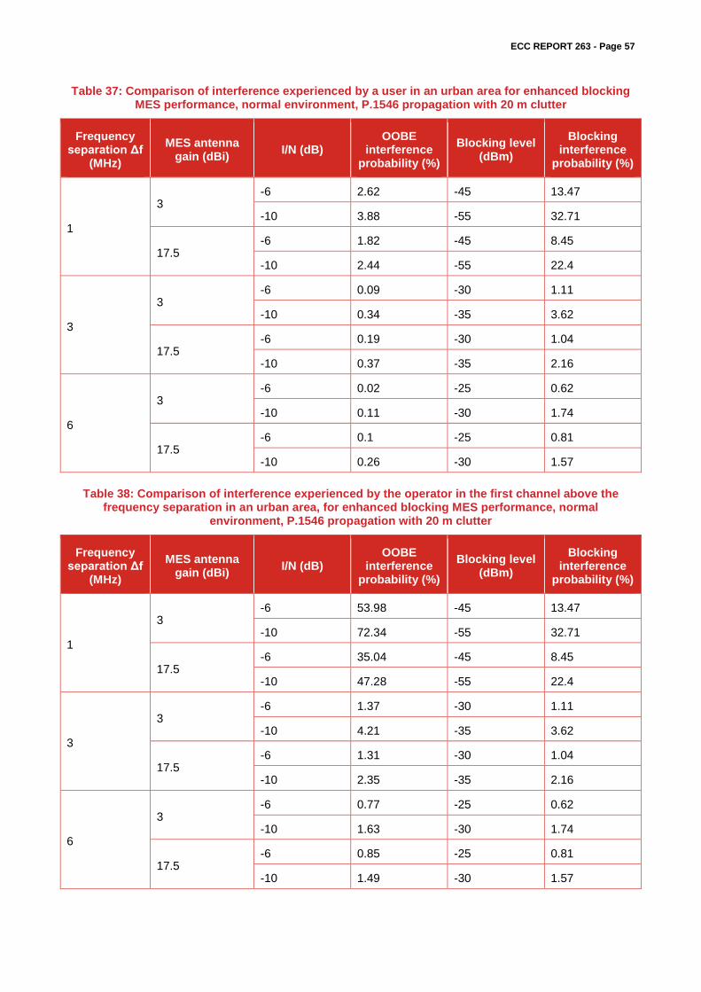
ECC REPORT 263 - Page 57
Table 37: Comparison of interference experienced by a user in an urban area for enhanced blocking MES performance, normal environment, P.1546 propagation with 20 m clutter
Frequency separation Δf
(MHz) MES antenna
gain (dBi) I/N (dB) OOBE
interference probability (%)
Blocking level (dBm)
Blocking interference
probability (%)
1
3 -6 2.62 -45 13.47
-10 3.88 -55 32.71
17.5 -6 1.82 -45 8.45
-10 2.44 -55 22.4
3
3 -6 0.09 -30 1.11
-10 0.34 -35 3.62
17.5 -6 0.19 -30 1.04
-10 0.37 -35 2.16
6
3 -6 0.02 -25 0.62
-10 0.11 -30 1.74
17.5 -6 0.1 -25 0.81
-10 0.26 -30 1.57
Table 38: Comparison of interference experienced by the operator in the first channel above the frequency separation in an urban area, for enhanced blocking MES performance, normal
environment, P.1546 propagation with 20 m clutter
Frequency separation Δf
(MHz) MES antenna
gain (dBi) I/N (dB) OOBE
interference probability (%)
Blocking level (dBm)
Blocking interference
probability (%)
1
3 -6 53.98 -45 13.47
-10 72.34 -55 32.71
17.5 -6 35.04 -45 8.45
-10 47.28 -55 22.4
3
3 -6 1.37 -30 1.11
-10 4.21 -35 3.62
17.5 -6 1.31 -30 1.04
-10 2.35 -35 2.16
6
3 -6 0.77 -25 0.62
-10 1.63 -30 1.74
17.5 -6 0.85 -25 0.81
-10 1.49 -30 1.57

ECC REPORT 263 - Page 58
Table 39: Comparison of interference experienced by a user in a suburban area for enhanced blocking MES performance, normal environment, P.1546 propagation with 10 m clutter
Frequency separation Δf
(MHz) MES antenna
gain (dBi) I/N (dB) OOBE
interference probability (%)
Blocking level (dBm)
Blocking interference
probability (%)
1
3 -6 1.19 -45 4.35
-10 1.87 -55 13.66
17.5 -6 0.76 -45 2.28
-10 1.19 -55 8.75
3
3 -6 0.01 -30 0.24
-10 0.05 -35 0.58
17.5 -6 0.04 -30 0.2
-10 0.05 -35 0.5
6
3 -6 0.01 -25 0
-10 0.02 -30 0.41
17.5 -6 0.03 -25 0.13
-10 0.04 -30 0.36
Table 40: Comparison of interference experienced by the operator in the first channel above the frequency separation in a suburban environment
Frequency separation Δf
(MHz) MES antenna
gain (dBi) I/N (dB) OOBE
interference probability (%)
Blocking level (dBm)
Blocking interference
probability (%)
1
3 -6 25.16 -45 4.35
-10 38.34 -55 13.66
17.5 -6 16.32 -45 2.28
-10 24.28 -55 8.75
3
3 -6 0.31 -30 0.24
-10 0.63 -35 0.58
17.5 -6 0.26 -30 0.2
-10 0.53 -35 0.5
6
3 -6 0.13 -25 0
-10 0.39 -30 0.41
17.5 -6 0.14 -25 0.13
-10 0.34 -30 0.36

ECC REPORT 263 - Page 59
ANNEX 8: STUDY #2
A8.1 MONTE CARLO ANALYSIS RESULTS
In this section, the adjacent band compatibility between MSS above 1518 MHz and IMT below 1518 MHz has been investigated using Monte Carlo simulation to determine the probability of harmful interference from IMT base station into MSS MES.
Two interference mechanisms are considered, the interference from IMT base station OOBE into an MSS MES and the blocking of MES caused by high transmit power from IMT base station for the following cases: Scenarios: Rural, Suburban and Urban; MES types: Omni (3 dBi) and directional (17.5 dBi); Interference Criteria (only for IMT OOBE) I/N: -6 dB and -10 dB; Frequency separation between IMT and MSS: 1 MHz, 3 MHz and 6 MHz; Polarisation discrimination was taken into account in all cases.
A8.2 IMT BASE STATION OOBE INTERFERENCE INTO MES SIMULATIONS
In order to investigate the probability of interference from IMT base station OOBE into MSS MES, simulations have been carried out with the following IMT base station OOBE levels at different frequency separation as shown in Table 41 below.
Table 41: IMT base station OOBE e.i.r.p. limits
Frequency Separation 1 MHz 3 MHz 6 MHz
Rural –0.8 dBm/MHz –30 dBm/MHz –33 dBm/MHz
Suburban/Urban –2.8 dBm/MHz –32 dBm/MHz –35 dBm/MHz
For all the OOBE interference simulations, the IMT base station was set to operate at frequencies below 1518 MHz while the MSS MES was operating at 1518.1 MHz.
The IMT OOBE interference into MSS simulation has been performed for rural (with clutter height of 4 m and 7 m), suburban and urban IMT base station deployments for two MSS MES types with an Omni antenna gain of 3 dBi and directional antenna of 17.5 dBi, with the interference criteria set to I/N of -6 dB and -10 dB.
A8.2.1 Propagation models
The simulations were carried out using the following propagation models: Rural scenarios: ITU-R P.1812 [13] with both 4 m and 7 m clutter heights14; Suburban and Urban scenarios: ITU-R P.1546-5 [12].
All the Monte Carlo simulations were run using SEAMCAT. SEAMCAT does not implement Recommendation ITU-R P.1812 propagation model and only implements Recommendation ITU-R P.1546-4.
Therefore, it was necessary to develop and implement an appropriate and valid propagation models based on Recommendation ITU-R P.1812 and ITU-R P.1546-5 for use in the Monte Carlo simulations for the three scenarios.
14 For more information on applicability of the Recommendation ITU-R P.1812-4 see Annex 4

ECC REPORT 263 - Page 60
In SEAMCAT the propagation models are implemented as plugins, and therefore it is possible to include a new propagation model and to add it to the list of existing pre-defined models. SEAMCAT propagation plugins of ITU-R P.1812 for the rural scenario and ITU-R P.1546-5 for suburban and urban scenarios were developed and implemented as a lookup table of distance gains propagation loss. The data for the lookup table were generated from ITU-R P.1812 and ITU-R P.1546-5 propagation models using the Visualyse simulation tool.
A8.2.2 Simulation configuration
The following study uses SEAMCAT (version 5.0.1 rev3543) where the F.1336-4 [7] antenna used is not fully in accordance with Section 3.1.1 due to its implementation in this software. The peak sidelobe antenna pattern is used for IMT base station. The simulation configuration was set up with seven IMT 3-sector base stations for each of the three deployment scenarios of rural, suburban and urban. The average IMT base station power was used. In each case, a simulation radius was determined and the MES was randomly placed around in the coverage area corresponding to the simulation radius. Simulation radius is set higher than inter-site distance (ISD) in accordance to macro cell parameters in Section 3.1.1 and circular interference area is used (though deployment of the IMT network is based according to Report ITU-R M.2292 [4]). All these would lead to the increased interference probability compared to the assumptions in the report.
A8.2.3 SEAMCAT results of IMT Base station OOBE interference
The SEAMCAT simulation results of the probability of interference from IMT base station into MES at frequency separation of 1 MHz, 3 MHz and 6 MHz are shown in Table 42, Table 43 and Table 44 respectively.
Table 42: Probability of interference (%) – Frequency Separation: 1 MHz
MES Type I/N Scenario
Urban Suburban Rural (4m clutter)
Rural (7m clutter)
Omni (3 dBi) -10 dB 100 100 100 100
-6 dB 100 100 100 50
Directional (17.5 dBi) -10 dB 99 95 100 49.9
-6 dB 74 52 81 21.4
Table 43: Probability of interference (%) – Frequency Separation: 3 MHz
MES Type I/N Scenario
Urban Suburban Rural (4m clutter)
Rural (7m clutter)
Omni (3 dBi) -10 dB 10.4 4.9 0.3 0
-6 dB 6 1.2 0.01 0
Directional (17.5 dBi) -10 dB 5.7 1.7 0.11 0
-6 dB 2.4 0.15 0 0

ECC REPORT 263 - Page 61
Table 44: Probability of interference (%) – Frequency Separation: 6 MHz
MES Type I/N Scenario
Urban Suburban Rural (4m clutter)
Rural (7m clutter)
Omni (3 dBi) -10 dB 7.2 2.9 0.01 0
-6 dB 3.6 0.5 0 0
Directional (17.5 dBi) -10 dB 3.2 0.32 0 0
-6 dB 0.4 0 0 0
Table 45 shows the impact on MES channels with a greater offset from the edge of the band when the IMT operates for the example case where the IMT upper band edge is 1515 MHz. The MES receiver frequency is increased by 1 MHz and 2 MHz (i.e. carrier frequency at 1519.1 MHz and 1520.1 MHz. Only the urban and suburban cases are examined.
Table 45: Probability of interference (%) – IMT upper band edge 1515 MHz, MSS channel 1519.1 MHz and 1520.1 MHz
MES Type I/N [email protected] MHz [email protected] MHz
Urban Suburban Urban Suburban
Omni (3 dBi) -10 dB 3.9 1.3 3.2 1.02
-6 dB 2.3 0.4 1.9 0.2
Directional (17.5 dBi) -10 dB 2.3 0.84 2.0 0.7
-6 dB 1.3 0.21 1.2 0.2
A8.3 MES BLOCKING
In order to investigate the probability of MES blocking caused by high transmit power from IMT base stations in the adjacent band, simulations have been carried out with the following baseline MES blocking performances at different frequency separations as shown in Table 46 below.
Table 46: Baseline MES blocking performance
Frequency Separation 1 MHz 3 MHz 6 MHz
MES Receiver blocking –60 dBm –52 dBm –40 dBm
For all the blocking simulations, the IMT base station was set to operate at frequencies below 1518 MHz while the MSS MES was operating at 1518.1 MHz.
The MES blocking simulation has been performed for rural (with clutter height of 4 m and 7 m), suburban and urban IMT base station deployments for two MSS MES types with an Omni antenna gain of 3 dBi and directional antenna of 17.5 dBi.
A8.3.1 SEAMCAT simulation results of MES blocking
The SEAMCAT simulation results of the probability of MES blocking from high power IMT base stations into MES at frequency separation of 1 MHz, 3 MHz and 6 MHz are shown in Table 47, Table 48 and Table 49

ECC REPORT 263 - Page 62
respectively. The IMT base station power was set to average power and not maximum transmit power. For frequency separations of 1 MHz and 3 MHz, in Table 47 and Table 48 respectively, the IMT base station carrier bandwidth was 5 MHz while for frequency separations of 6 MHz, the IMT base station carrier was 10 MHz.
Table 47: Probability of interference (%) – IMT upper band edge at 1517 MHz
MES Type MES blocking Level (dBm)
Scenario
Urban Suburban Rural (4m clutter)
Rural (7m clutter)
Omni (3 dBi) -60
76.3 63.1 89.6 29.3
Directional (17.5 dBi) 56.3 39.3 43.1 15.3
Table 48: Probability of interference (%) – IMT upper band edge at 1515 MHz
MES Type MES blocking Level (dBm)
Scenario
Urban Suburban Rural (4m clutter)
Rural (7m clutter)
Omni (3 dBi) -52
46 25.8 16.3 5.3
Directional (17.5 dBi) 32.3 17.1 9.1 3
Table 49: Probability of interference (%) – IMT upper band edge at 1512 MHz
MES Type MES blocking Level (dBm)
Scenario
Urban Suburban Rural (4m clutter)
Rural (7m clutter)
Omni (3 dBi) -40
21.2 9.5 3 0.5
Directional (17.5 dBi) 15.5 6.1 1.4 0.3
Table 50 below shows the SEAMCAT simulation results of the probability of interference from IMT base station into an improved MES receiver at frequency separation of 6 MHz.

ECC REPORT 263 - Page 63
Table 50: Probability of blocking interference (%) against improved MSS blocking levels
ES Type MES blocking Level (dBm)
Scenario
Urban Suburban Rural (4m clutter)
Rural (7m clutter)
Omni (3 dBi) -30
8 3 0.1 0
Directional (17.5 dBi) 4 1.2 0.1 0
Omni (3 dBi) -25
3.4 0.4 0 0
Directional (17.5 dBi) 2.2 0.7 0 0
ECC REPORT 263 - Page 64
ANNEX 9: STUDY #3
A9.1 LAND MOBILE SATELLITE SCENARIOS
A9.1.1 Considerations on assumptions for the analysis
Parameters required to derive the results of the current study are provided in Section 3 of this report. Regarding: The propagation model for the rural case: the agreed assumption for the rural case was to perform
Recommendation ITU-R P.1812-4 [13] with 50% percentage of time and location with 7 m clutter height at 100 m from the receiver. However, one could notice that the implementation of the clutter losses does not account the location of the clutter within the path making a conflict with the specific path that has been defined (no clutter except at 100 m from Rx). Other solutions are investigated, as discussed in Annex 4;
The derivation of the probability of interference: the following analysis derives this metric by calculating the surface of the area (within an IMT cell with 3 hexagonal sectors) on which the protection criterion for the MSS (that can be I/N or blocking threshold) is not met over the IMT cell. Since the separation distance of a MES with respect of the IMT BS is dependent of the location of the MSS Receivers (discrimination angle of Rx/Tx with respect of the Tx/Rx position), a fine sampling of the location of the MES (1° azimuth, 5 m distance (MES Rx, IMT BS)) is performed to estimate the surface of the exclusion zone. In that sense, the probability of interference is obtained by generating random positions of MES within the IMT cell.
A9.1.2 Statistical analysis with random MES location and fixed frequency
This section provides results of compatibility between MSS and IMT for MES at a fixed frequency adjacent to frequency separation, in terms of probability of interference (Land) for different scenarios (i.e. high/low gain antenna MES, blocking threshold and/or I/N, frequency separation, rural/urban).

ECC REPORT 263 - Page 65
Table 51: Rural case (P.1812-4 with 7 m path profile)
Frequency separation Δf
(MHz) MES antenna
gain (dBi) I/N (dB) OOBE
interference probability (%)
Blocking level (dBm)
Blocking interference
probability (%)
1
3 -6 4.50% -63 5.40%
-10 5.90% -60 4.10%
17.5 -6 3.10% -63 3.50%
-10 3.90% -60 3.00%
3
3 -6 0.30% -53 2.40%
-10 0.80% -52 2.20%
17.5 -6 0.20% -53 1.90%
-10 0.30% -52 1.80%
6
3 -6 0.00% -53 2.40%
-10 0.40% -40 1.40%
17.5 -6 0.10% -53 1.90%
-10 0.20% -40 1.00% For more information on applicability of the Recommendation ITU-R P.1812-4 see Annex 4
Table 52: Rural case (P.452-16 with 7 m clutter losses)
Frequency separation Δf
(MHz) MES antenna
gain (dBi) I/N (dB) OOBE
interference probability (%)
Blocking level (dBm)
Blocking interference
probability (%)
1
3 -6 7.10% -63 11%
-10 15.90% -60 6.10%
17.5 -6 4.60% -63 6.90%
-10 9.60% -60 3.90%
3
3 -6 0.30% -53 1.70%
-10 0.30% -52 1.40%
17.5 -6 0.10% -53 1.00%
-10 0.20% -52 0.90%
6
3 -6 0.20% -53 1.70%
-10 0.30% -40 0.30%
17.5 -6 0.10% -53 0.40%
-10 0.10% -40 0.40%

ECC REPORT 263 - Page 66
Table 53: Urban case (P.1546-5 with clutter height=20 m)
Frequency separation Δf
(MHz) MES antenna
gain (dBi) I/N (dB) OOBE
interference probability (%)
Blocking level (dBm)
Blocking interference
probability (%)
1
3 -6 68.50% -63 82.10%
-10 95.60% -60 63.90%
17.5 -6 49.60% -63 59.00%
-10 67.20% -60 46.20%
3
3 -6 1.60% -53 35.70%
-10 4.60% -52 32.80%
17.5 -6 2.20% -53 26.00%
-10 3.40% -52 23.80%
6
3 -6 1.00% -53 35.70%
-10 1.60% -40 15.00%
17.5 -6 1.50% -53 26.00%
-10 2.40% -40 7.70%
A9.1.3 Statistical analysis with random MES location and random frequency
This section provides results of compatibility between MSS and IMT for MES at a frequency within the full frequency band available to MES (1518-1559 MHz), in terms of probability of interference (Land) for different scenarios (i.e. high/low gain antenna MES, blocking threshold and/or I/N, frequency separation, rural/urban). The rationale not to only address the extension MSS frequency band 1518-1525 MHz (which is the one considered for the compatibility study with potential IMT systems operating in frequency band 1492-1518 MHz) is based on the fact that any satellite that enables MSS operation within the frequency band 1518-1525 MHz will also operate over frequency band 1525-1559 MHz, as with any current MSS satellites in orbit over this range.

ECC REPORT 263 - Page 67
Table 54: Rural case (P.1812-4 with 7 m path profile)
Frequency separation Δf
(MHz) MES antenna
gain (dBi) I/N (dB) OOBE
interference probability (%)
Blocking level (dBm)
Blocking interference
probability (%)
1
3 -6 0.20% -63 2.50%
-10 0.40% -60 4.10%
17.5 -6 0.20% -63 2.00%
-10 0.30% -60 3.00%
3
3 -6 0.00% -53 2.30%
-10 0.10% -52 2.20%
17.5 -6 0.00% -53 1.80%
-10 0.10% -52 1.80%
6
3 -6 0.00% -53 2.10%
-10 0.10% -40 1.40%
17.5 -6 0.00% -53 1.70%
-10 0.10% -40 1.00% For more information on applicability of the Recommendation ITU-R P.1812-4 [13] see Annex 4
Table 55: Rural case (P.452-16 with 7 m clutter losses)
Frequency separation Δf
(MHz) MES antenna
gain (dBi) I/N (dB) OOBE
interference probability (%)
Blocking level (dBm)
Blocking interference
probability (%)
1
3 -6 0.40% -63 2.20%
-10 0.90% -60 6.10%
17.5 -6 0.20% -63 1.30%
-10 0.50% -60 3.90%
3
3 -6 0.10% -53 1.60%
-10 0.10% -52 1.40%
17.5 -6 0.00% -53 1.00%
-10 0.00% -52 0.90%
6
3 -6 0.00% -53 1.50%
-10 0.10% -40 0.30%
17.5 -6 0.00% -53 0.90%
-10 0.00% -40 0.40%

ECC REPORT 263 - Page 68
Table 56: Urban case (P.1546-5 with clutter height=20 m)
Frequency separation Δf
(MHz) MES antenna
gain (dBi) I/N (dB) OOBE
interference probability (%)
Blocking level (dBm)
Blocking interference
probability (%)
1
3 -6 3.70% -63 38.00%
-10 5.50% -60 63.90%
17.5 -6 2.80% -63 27.60%
-10 4.00% -60 46.20%
3
3 -6 0.40% -53 34.00%
-10 0.80% -52 32.80%
17.5 -6 0.30% -53 24.70%
-10 0.70% -52 23.80%
6
3 -6 0.30% -53 31.30%
-10 0.50% -40 15.00%
17.5 -6 0.20% -53 22.80%
-10 0.40% -40 7.70%

ECC REPORT 263 - Page 69
ANNEX 10: LIST OF REFERENCE [1] ECC Decision (13)03 'The harmonised use of the frequency band 1452-1492 MHz for Mobile/Fixed
Communications Networks Supplemental Downlink (MFCN SDL)' [2] ECC Decision (04)09 'The designation of the bands 1518-1525 MHz and 1670-1675 MHz for systems in
the Mobile-Satellite Service ' [3] ERC Report 25 ' The European table of frequency allocations and applications in the frequency range
8.3 kHz to 3000 GHz', June 2016 [4] Report ITU-R M.2292 'Characteristics of terrestrial IMT-Advanced systems for frequency
sharing/interference analyses' [5] 3GPP TS 36.104 V11.2.0 'Evolved Universal Terrestrial Radio Access (E-UTRA); Base Station (BS)
radio transmission and reception' [6] EC Decision 2015/750 'On the harmonisation of the 1452-1492 MHz frequency band for terrestrial
systems capable of providing electronic communications services in the Union' [7] Recommendation ITU-R F.1336 'Reference radiation patterns of omnidirectional, sectoral and other
antennas for the fixed and mobile service for use in sharing studies in the frequency range from 400 MHz to about 70 GHz'
[8] ECC Report 174 'Co-existence study considering UWB applications inside aircraft and existing radio services in the frequency bands from 3.1 GHz to 4.8 GHz and from 6.0 GHz to 8.5 GHz', March 2012
[9] ETSI TS 101 377-5-5 'GEO-Mobile Radio Interface Specifications; Part 5: Radio interface physical layer specifications; Sub-part 5: Radio Transmission and Reception; GMR-2 05.005'
[10] RTCA DO-210 D: 'Minimum Operational Performance Standards For Geosynchronous Orbit Aeronautical Mobile Satellite Services (AMSS) Avionics'
[11] RTCA DO-262 B: 'Minimum Operational Performance Standards For Avionics Supporting Next Generation Satellite Systems (NGSS)'
[12] Recommendation ITU-R P.1546 'Method for point-to-area predictions for terrestrial services in the frequency range 30 MHz to 3 000 MHz'
[13] Recommendation ITU-R P.1812 'A path-specific propagation prediction method for point-to-area terrestrial services in the VHF and UHF bands'
[14] Recommendation ITU-R P.452 'Prediction procedure for the evaluation of interference between stations on the surface of the Earth at frequencies above about 0.1 GHz'
[15] Recommendation ITU-R P.525 'Calculation of free-space attenuation’ [16] ITU-R Report M.2241 ‘Compatibility studies in relation to Resolution 224 in the bands 698-806 MHz and
790-862 MHz’ [17] 3GPP TR 36.814 V9.0.0 ‘Evolved Universal Terrestrial Radio Access (E-UTRA); Further advancements
for E-UTRA physical layer aspects’