ece 472/572 - digital image processing lecture 3 - image enhancement - point processing 08/30/11
TRANSCRIPT

ECE 472/572 - Digital Image Processing
Lecture 3 - Image Enhancement - Point Processing08/30/11

2
Roadmap
Introduction– Image format (vector vs. bitmap)– IP vs. CV vs. CG– HLIP vs. LLIP– Image acquisition
Perception– Structure of human eye
• rods vs. cones (Scotopic vision vs. photopic vision)
• Fovea and blind spot• Flexible lens (near-sighted vs. far-sighted)
– Brightness adaptation and Discrimination
• Weber ratio• Dynamic range
– Image resolution• Sampling vs. quantization
Image enhancement– Enhancement vs. restoration
– Spatial domain methods• Point-based methods
– Negative
– Log transformation
– Power-law
– Contrast stretching
– Gray-level slicing
– Bit plane slicing
– Histogram equalization
– Averaging
• Mask-based (neighborhood-based) methods - spatial filter
– Frequency domain methods

3
Questions
Point-based vs. Mask-based (or neighbor-based) Spatial domain vs. Frequency domain Log transformation vs. Power-law
– Gamma correction– Dynamic range compression
Contrast stretching vs. Histogram equalization– Histogram– Uniform histogram– HE derivation (572)
Gray-level vs. Bit-plane slicing– MSB
What’s the philosophy behind Image averaging?– Derivation (572)

4
Intuitively
5
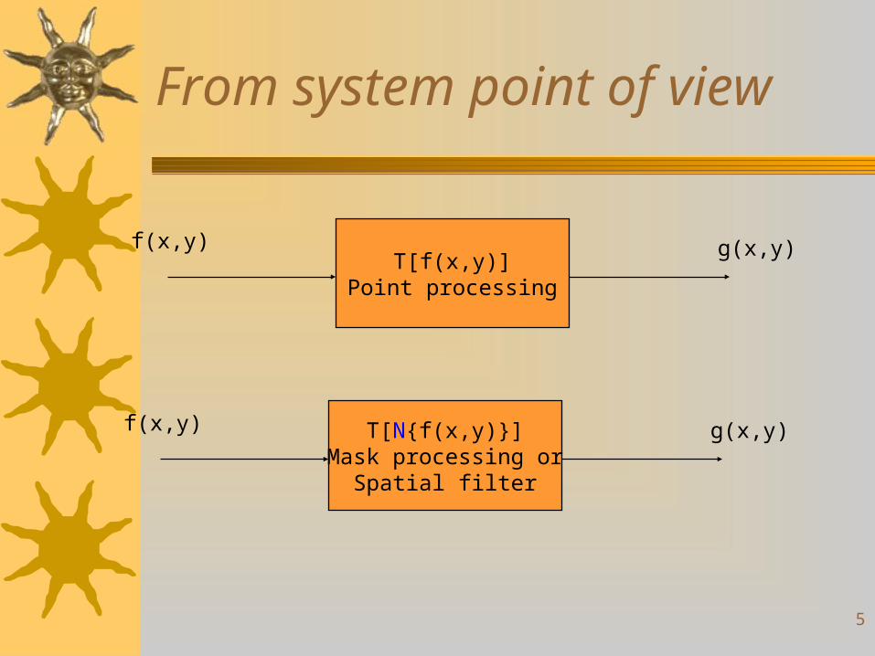
From system point of view
T[f(x,y)]Point processing
f(x,y) g(x,y)
T[N{f(x,y)}]Mask processing or
Spatial filter
f(x,y) g(x,y)

6
Different approaches
Spatial domain– Point-based processing
– Mask-based processing (neighbor-based processing) (spatial filters)
Frequency domain– Frequency domain filters

7
Point processing
Simple gray level transformations– Image negatives– Log transformations– Power-law transformations– Contrast stretching– Gray-level slicing– Bit-plane slicing
Histogram processing– Histogram equalization– Histogram matching (specification)
Arithmetic/logic operations– Image averaging

8
Some transformations
s = T(r) = L – 1 – r
s = cr

9
Image negatives
s = T(r) = L – 1 – r

10
Log transformation (Dynamic range compression)

11
Power-Law transformation
s = cr

12
Gamma correction

13
Contrast stretching
14
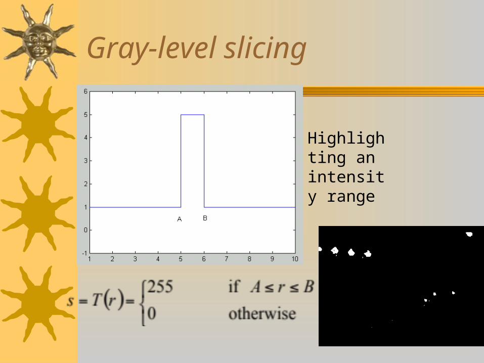
Gray-level slicing
Highlighting an intensity range

15
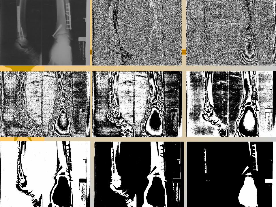
Bit-plane slicing
Highlighting the contribution made by a specific bit.
For pgm images, each pixel is represented by 8 bits.
Each bit-plane is a binary image
16

17
Point processing
Simple gray level transformations– Image negatives– Log transformations– Power-law transformations– Contrast stretching– Gray-level slicing– Bit-plane slicing
Histogram processing– Histogram equalization– Histogram matching (specification)
Arithmetic/logic operations– Image averaging
18
Histogram
Gray-level histogram is a function showing, for each gray level, the number of pixels in the image that have that gray level.
Normalized histogram (probability):

19
Histogram - Examples

20
Usage of histogram
Find threshold
Reveal the intensity distribution

21
Example

22
Question
What does the histogram of a low-contrast image look like?
How about high-contrast?

23
Histogram equalization
Why and when do we want to use HE?

24
HE – Example 2

25
HE – Derivation (572)
T(r) is single-valued and monotonically increasing within range of rT(r) has the same range as r [0, 1]

26
Histogram equalization
Transformation function
pr(w) is the probability density function (pdf)The transformation function is the cumulative
distribution function (CDF)To make the pdf of the transformed image
uniform, i.e. to make the histogram of the transformed image uniform

27
HE – Discrete case
0
1
2
3
10
80
95
100
r s
0
1
2
3
10
70
15
5
r hist(r)10
80
95
100
10
70
15
5
s hist(s)

28

29
HE - Discussion
Can contrast stretching achieve similar result as histogram equalization?
If it can, why histogram equalization then?Why isn’t the transformed histogram
uniform?

30

31
Problems with HE
???
Solutions– ???

32
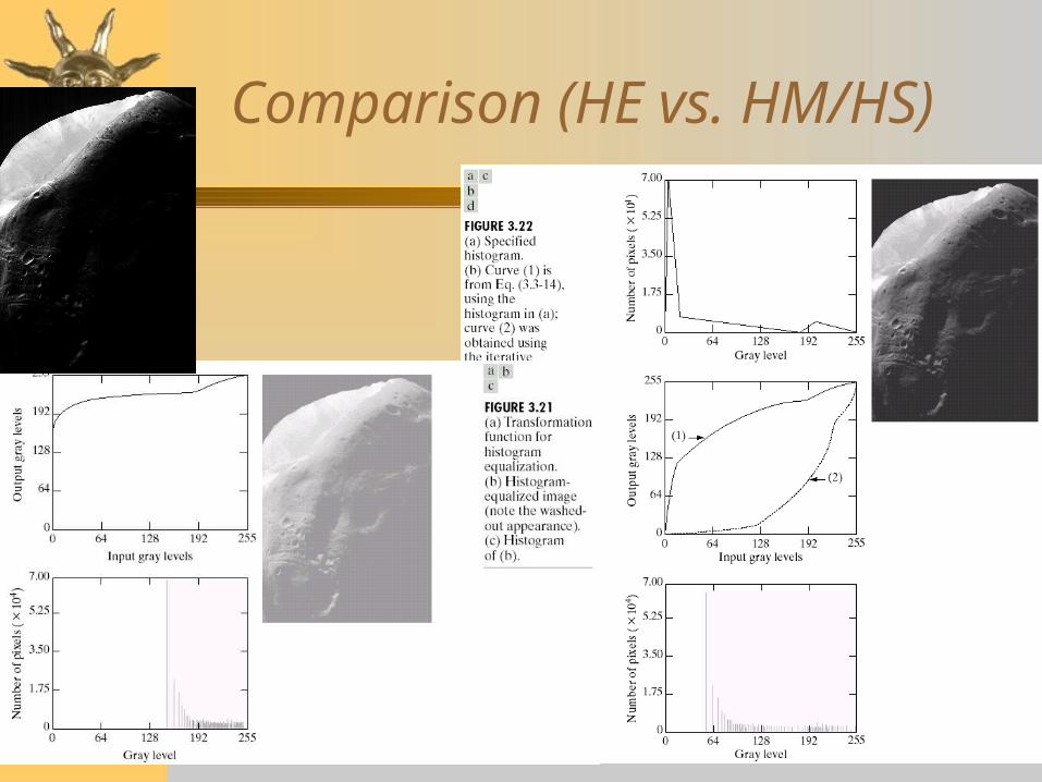
*Histogram specification
Step1: Equalize the levels of the original image
Step2: Specify the desired pdf and obtain the transformation function
Step3: Apply the inverse transformation function to the levels obtained in step 1

33
HS - Example
0
1
2
3
10
80
95
100
r s
0
1
2
3
10
70
15
5
r hist(r)
10
15
30
60
10
20
50
15
z hist(z)10
15
30
60
10
30
80
95
z G(z)
Specifiedhistogram
0
1
2
3
10
30
60
65
r z
34
Comparison (HE vs. HM/HS)
35
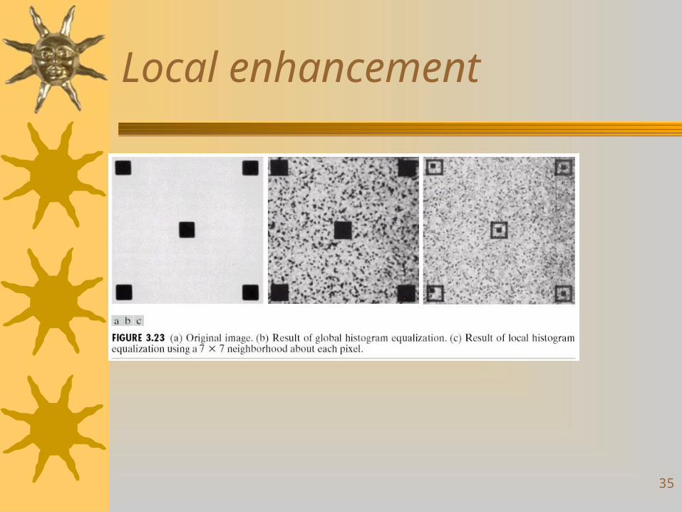
Local enhancement

36
Point processing
Simple gray level transformations– Image negatives– Log transformations– Power-law transformations– Contrast stretching– Gray-level slicing– Bit-plane slicing
Histogram processing– Histogram equalization– Histogram matching (specification)
Arithmetic/logic operations– Image averaging

37
Image averaging
original image f(x, y) +
noise (x, y)
noisy image g(x, y)

38
Image average (cont’)
If the noise is uncorrelated and has zero expectation, then

39
Image averaging – How to generate Gaussian noise? (572)
//This function creates a gaussian random number between -3 and 3double gaussrand() { static double V1, V2, S; static int phase = 0; double X;
if (phase == 0) { do { double U1 = (double)rand() / RAND_MAX; double U2 = (double)rand() / RAND_MAX; V1 = 2 * U1 - 1; V2 = 2 * U2 - 1; S = V1 * V1 + V2 * V2; } while(S >= 1 || S == 0); X = V1 * sqrt(-2 * log(S) / S); } else X = V2 * sqrt(-2 * log(S) / S); phase = 1 - phase; return X; }

40
Summary - Point processing
Simple gray level transformations– Image negatives – Log transformations– Power-law transformations– Contrast stretching – Gray-level slicing– Bit-plane slicing
Histogram processing– Histogram equalization
• Derivation (572 only)– Histogram matching (specification) (572 only)
Arithmetic/logic operations– Image averaging
• Generation of Gaussian noise (572 only)