ece 480: senior design laboratory - michigan …€¦ · · 2007-08-23ece 480: senior design...

1Copyright © 2007 by Gregory M. Wierzba. All rights reserved.

ECE 480: SENIOR DESIGN LABORATORY

DEPARTMENT OF ELECTRICAL AND COMPUTER ENGINEERING

MICHIGAN STATE UNIVERSITY

I. TITLE: Lab I - Introduction to the Oscilloscope, Function Generator,Digital Multimeter and Power Supply

II. PURPOSE: The oscilloscope, function generator and digital multimeterare the basic tools in the measurement and testing of circuits. This labintroduces the first time operation of these instruments along with theuse of a compensated probe.

The concepts covered are: 1. equivalent circuits of the oscilloscope inputs, function generator

output and digital multimeter inputs; 2. the use of a balanced bridge to compensate for the stray

capacitance of a measuring cable and the equivalent impedanceof the oscilloscope;

3. accuracy of components and instruments.

The laboratory techniques covered are: 1. voltage amplitude and time measurement with an oscilloscope; 2. a procedure for compensating an oscilloscope probe; 3. procedures for setting up multiple DC supplies.

III. BACKGROUND MATERIAL:

A) The Oscilloscope

The oscilloscope used in this course is a two channel digitalstorage oscilloscope that allows the observation of low frequencyrepetitive signals and transients over a wide range of frequencies. In thislab and the following labs we will be covering most of the availablefeatures.

The oscilloscope, or scope for short, is divided into five blocks: theDisplay Block, the Vertical Amplifier Block, the Sweep Block, the TriggerBlock and the Storage Block. The Display Block consists of the cathode-ray tube (CRT) and associated controls. The CRT is a device whichprovides a visual display of a voltage. This voltage is applied to the scopeat the Vertical Amplifier Block. The scope creates a CRT display bycapturing and overlaying successive windows of time. These windows


Figure 1. DC position

Figure 2. AC position

begin at the same trigger point on the voltage being examined and endat a specific increment of time. The trigger point is controlled by theTrigger Block and the time increment is controlled by the Sweep Block.The Storage Block allows us to save the wave form for future referenceor hard-copy.

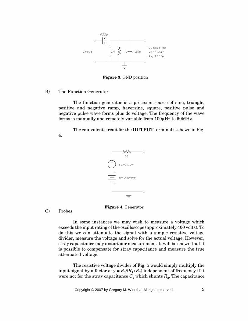
In measuring any circuit we will need to connect the measuringinstrument to our circuit. This changes the original circuit by connectingthe equivalent circuit of the instrument into the circuit. We will alwaysneed to know what the equivalent circuit of the instrument is, so that wecan either neglect loading effects or include loading effects in thecalculations of the circuit's response. The equivalent circuit for the A andB input terminals are shown in Figs. 1-3 for the three settings of theAC/DC and GND buttons. This is the load seen by our circuits.

In the DC position the measured signal is Directly Coupled to thevertical amplifier and we see displayed the actual wave form. In the ACposition, a blocking capacitor is inserted in series with the measuredsignal. This blocks any dc signal in steady-state and we see displayedonly the time varying component of our measured signal. This is usefulfor measuring transistor amplifier circuits where the time varying signalis very small compared to the dc level. In these cases displaying theactual wave form makes it difficult to see the characteristics of the timevarying signal. In the GND position the load seen by our circuit is anopen circuit but the vertical amplifier, internal to the scope, sees a shortand displays 0 volts. This feature is useful for setting a reference line.


Figure 3. GND position

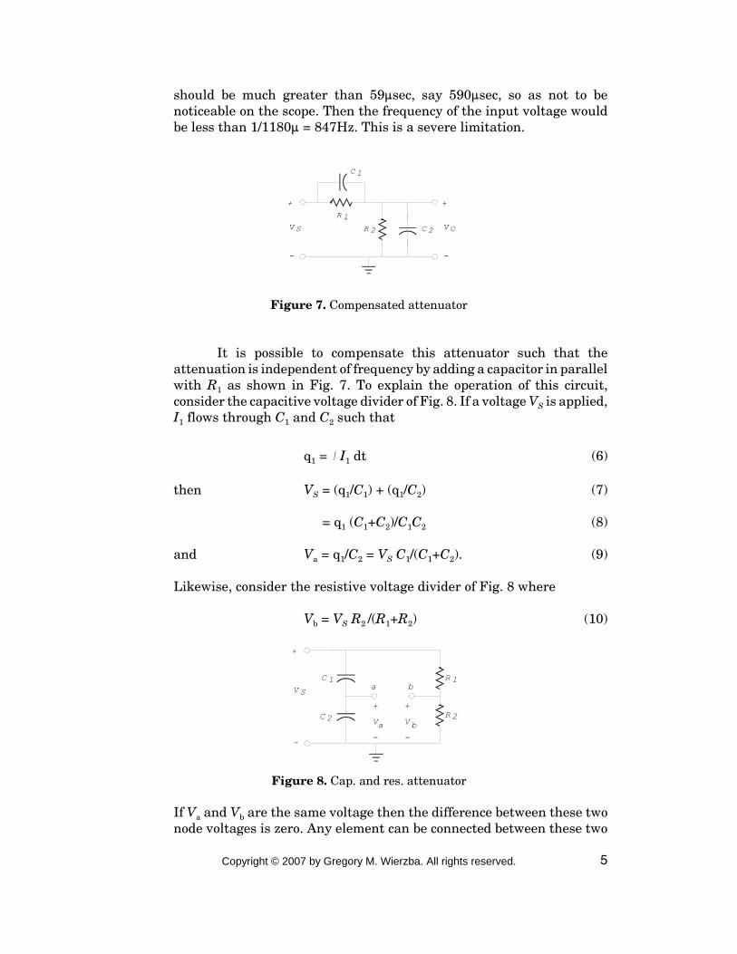
Figure 4. Generator

B) The Function Generator

The function generator is a precision source of sine, triangle,positive and negative ramp, haversine, square, positive pulse andnegative pulse wave forms plus dc voltage. The frequency of the waveforms is manually and remotely variable from 100:Hz to 50MHz.

The equivalent circuit for the OUTPUT terminal is shown in Fig.4.

C) Probes

In some instances we may wish to measure a voltage whichexceeds the input rating of the oscilloscope (approximately 400 volts). Todo this we can attenuate the signal with a simple resistive voltagedivider, measure the voltage and solve for the actual voltage. However,stray capacitance may distort our measurement. It will be shown that itis possible to compensate for stray capacitance and measure the trueattenuated voltage.

The resistive voltage divider of Fig. 5 would simply multiply theinput signal by a factor of y = R2/(R1+R2) independent of frequency if itwere not for the stray capacitance C2 which shunts R2. The capacitance


Figure 5. Divider with stray cap.

Figure 6. Thevenin equivalent circuit

C2 represents the parallel combination of the input capacitance of theoscilloscope and the stray capacitance of the probe's cable.

Using Thevenin's theorem, the circuit of Fig. 5 is replaced by itsequivalent in Fig. 6 where RTH = R15R2. For a step input of VP volts forVTH we have that,

VO = VP [1 - e-t/RTHC2] (1)

Solving for t, we find that

t = RTH C2 ln [VP /(VP - VO)] (2)

The rise time of a signal (tr) is the time required for the signal to go from10% (at time t1) to 90% (at time t2) of its final value, that is, tr = t2 - t1.Therefore,

t2 = RTH C2 ln [VP /(VP - 0.9VP)] (3)

t1 = RTH C2 ln [VP /(VP - 0.1VP)] (4)

Solving for the rise time, we find that

tr = 2.197 RTH C2 (5)

If R1 = 9MS, R2 = 1MS and C2 = 30pF then the rise time for a stepinput is 59:seconds. If the input is a square wave then half the period


Figure 7. Compensated attenuator

Figure 8. Cap. and res. attenuator

should be much greater than 59:sec, say 590:sec, so as not to benoticeable on the scope. Then the frequency of the input voltage wouldbe less than 1/1180: = 847Hz. This is a severe limitation.

It is possible to compensate this attenuator such that theattenuation is independent of frequency by adding a capacitor in parallelwith R1 as shown in Fig. 7. To explain the operation of this circuit,consider the capacitive voltage divider of Fig. 8. If a voltage VS is applied,I1 flows through C1 and C2 such that

q1 = * I1 dt (6)

then VS = (q1/C1) + (q1/C2) (7)

= q1 (C1+C2)/C1C2 (8)

and Va = q1/C2 = VS C1/(C1+C2). (9)

Likewise, consider the resistive voltage divider of Fig. 8 where

Vb = VS R2 /(R1+R2) (10)

If Va and Vb are the same voltage then the difference between these twonode voltages is zero. Any element can be connected between these two


Figure 9. Over-compensated

Figure 10. Under-compensated

points without affecting the voltage because no current will flow. This isthe concept of a balanced bridge. In Fig. 7, the element between pointsa and b is a short circuit. Setting Eqns. 9 and 10 equal, we find thecondition needed for compensation is

R1 C1 = R2 C2. (11)

If R1 = 9MS, R2 = 1MS and C2 = 30pF then C1 = 3.33pF and VO = VS /10.

What happens if Eqn. 11 is not satisfied? For a step input, thevoltage across the capacitors must change rapidly. This will require avery large current of short duration. So we can neglect the currents in R1

and R2 at t = 0+ and VO is basically determined by the capacitive voltagedivider. In steady-state the capacitors are open circuits and VO isdetermined by the resistive voltage divider. If

x = C1 /(C1+C2) > R2 /(R1+R2) = y (12)

then there will be an overshoot on the response at 0+. Solving Eqn. 12 wefind that R1 C1 > R2 C2. This is called over-compensation and is illustratedin Fig. 9. Likewise for R1 C1 < R2 C2 we find an undershoot on VO at t = 0+

and this is called under-compensation. This is shown in Fig. 10.

The probe used in lab is shown in Fig. 11. R1 = 9MS, C1 = 14pF,and C3 is effectively the parallel combination of the capacitance of thecoax cable (.10pF/foot of cable) and a variable capacitor. The probe also


Figure 11. Probe schematic

has a switch for connecting a resistance of 470S to ground. This makesa voltage divider that is very small and effectively applies zero volts tothe scope input. This allows the user to display the zero volt referencewhile holding the probe.

Although we started out with trying to measure large voltages byusing a voltage divider, it is desirable to use this compensated divider inany application where the loading effects of the cable and the oscilloscopeare significant. The only limit would be the smallest voltage scale of theoscilloscope. For the PM3365 this is 2mV/div. For at least a 1 divisiondisplay with an attenuation of 10, the measured voltage would need tobe greater than 10 x 2mV = 20mV.

It is important to note that the PM3365 senses whether the X10probe is connected and correctly displays the proper volts per division.Most other scopes do not do this and the user must make this correction.

BECAUSE THERE IS A 9MS RESISTOR INSIDE THE SCOPE PROBEYOU SHOULD NEVER USE THE SCOPE PROBE ON THE FUNCTIONGENERATOR. THIS WILL FORM A VERY LARGE VOLTAGEDIVIDER.

D) Accuracy

The scope has a horizontal and vertical accuracy of ±3 % for both theanalog and digital readings. The digital multimeter’s accuracy isdifferent on each scale. But if the maximum number of digits aredisplayed, it is better than ±0.02%.

IV. EQUIPMENT REQUIRED:

1 Philips PM3365 Digital Storage Oscilloscope1 Philips PM5193 Programmable Synthesizer/Function Generator1 HP 34401 A or Fluke 8840A Digital Multimeter1 HP E3630 A Triple Output Power Supply1 Philips PM8926/59 10:1 Passive Probes


CAUTION: If the cathode ray tube (CRT) is left with an extremely brightdot or trace for a very long time, the fluorescent screen may be permanentlydamaged. If a measurement requires high brightness, be certain to turndown the INTEN control immediately afterward.

V. PARTS REQUIRED:

1 BNC-BNC cable1 BNC-to-Banana cable1 Small screwdriver

VI. LABORATORY PROCEDURE:

A) First Time Operation of the PM3365 Oscilloscope

1. Before actually turning on the oscilloscope, there are a few controls youcan preset to facilitate the startup procedure. On the right side there aretwo columns of 4 round knobs. The outermost column are labeled Y POS,Y POS, X POS and TRIG LEVEL. These knobs should be pointingstraight up. The other column of knobs are labeled VAR, VAR, VAR andHOLD OFF. These knobs should be turned fully clockwise and pointingto CAL, CAL, CAL and MIN, respectively.

2. Press in the POWER switch found in the upper left corner. If the tracethat appears is extremely bright, turn the INTENS control counter-clockwise.

3. Turn the INTENS control to adjust the brightness to the desired level.

4. Turn the FOCUS control for a sharp trace.

B) The PM5193 Programmable Synthesizer/Function Generator

1. The laboratory function generator is a precision source of sine, triangle,positive and negative ramp, haversine, square, positive pulse andnegative pulse wave forms plus dc voltage.

2. Press the POWER switch found in the lower left corner to the onposition. Sometimes an ERR3 display comes up during power up. Thisindicates a low back up battery. We won’t be saving our settings so thisisn’t critical to our work. Just press any button and it should clear itself.

C) Wave form Measurement

1. Coaxial cable is the most common method of connecting an oscilloscope


to signal sources and equipment having output connectors. The outerconductor of the cable shields the central signal conductor from hum andnoise pickup. These cables are usually fitted with a BNC on each end.

Connect a BNC-to-BNC cable from the OUTPUT of the functiongenerator found on the lower right side to the A input terminal of thescope found in the lower center. Our first task will be to generate avoltage equal to 4 + 5 sin (2B 1000 t).

2. Press the button with the sinewave. This is the upper left button in theset of nine buttons under WAVE FORM. A red light should be on. Thisindicates that we have selected this particular wave form.

3. We next need to set the frequency of the wave form. This is done with theSTART button. This is the upper left button in the set of six buttonsunder FREQUENCY. Again a red light will indicate your selection. Thevalue is entered with the number key pad on the right side. Press 1 0 00. This value will appear on the left most display. Press ENTER whichis found on the lower right side. The frequency is now selected to be 1000Hz.

4. The parameters of our wave form are set with the LEVEL buttons. Pushthe button labeled Vpp. This is the peak-to-peak value of the wave formselected. Enter a value of 10. (This is done by selecting the number withthe key pad followed by enter.) You now have generated a voltage withthe expression 5 sin (2B 1000 t).

5. To add a dc offset onto our wave form, we need to select LEVEL buttonVdc. Enter a value of 4. We now have a voltage of 4 + 5 sin (2B 1000 t).

6. If you make a mistake or want to change any of the above settings, justrepeat the specific step.

7. A wave form should appear on your scope screen. If not ask your labinstructor for help.

8. The wave form on the screen may appear small or crowded. This isbecause of the setting selected by the scope during power-up. We willlearn shortly how to change this. However we can quickly re-set thescope so that it will try to make our wave form easier to view by pressingthe green AUTO SET button on the scope. Do this.

9. The scope has two different modes of operation. These are called analogand digital. In the analog mode the wave form is very smooth andcontinuous. In the digital mode the wave form is being sampled anddisplayed and may appear jagged on the screen.


Many digitizing scopes have phantom results displayed due to thecapture process. Although digitizing scopes are pretty good, there is nosubstitute for seeing the actual waveform to truly verify themeasurement wave shape is correct. However, digitizing scopes are greatfor wave form calculations and storage. The Philips PM3365 is one of therare (and very expensive) scopes that allows you to see both with thesame instrument.

Many employers expect engineers to be able to use analog scopes foradvanced measurement. This is why we are using an analog /digitalscope in ECE 480.

Press the white DIGITAL MEMORY button on the scope. You will seethese two modes. Place the display back in the analog mode.

10. The top number found in the menu window is the value for each of thevertical divisions. These are the large squares of the screen grid.Counting the number of these divisions from the highest to lowest pointof your sine wave and multiplying this times the setting displayed in themenu window is the peak-to-peak value of your sine wave. This may bedifficult depending on where your wave form is on the screen.

11. We can set and/or place the zero volt reference of the input. This is doneby first pressing the GND button. There are two such buttons. The topone is for the A input and the second one two rows down is for the Binput. Press the A input GND. This is zero voltage reference for thischannel. Rotate the Y POS for this channel and place this line in thecenter of the screen. Now press the A input GND button again.

Calculate the measured peak-to-peak value of your sine wave using thesetting of the scope, that is, the voltage per division times the number ofdivisions. Record this, and all data that follows, as indicated in the LabReport. If your calculated peak-to-peak voltage is not what was set inpart 4, ask your instructor for help.

12. Press the A input AC/DC button. Now you should be in the DC mode.Your wave form still has a zero reference at the center line of the screen.Calculate the dc level of your wave form. If this is not what was set inpart 5, ask your instructor for help.

What is the purpose of the AC/DC button? (Answer this and allquestions in a complete sentence in the Lab Report.)

13. The other number in the menu window is value of the horizontaldivisions. Count the number of divisions per cycle and calculate theperiod of your sine wave. The frequency of your sine wave is the


reciprocal of the period. Calculate the frequency. If this is not the sameas set in part 3, ask your instructor for help.

14. What function does the AC OFF perform on the function generator?What advantage do you see in this feature?

Restore the wave form to that in part 13.

15. The PM 3365 can also perform wave form measurement. Place the scopein the digital mode. Press the right most white button on the screen bezelso that the words: CURSORS SETTINGS SHIFT and TEXT-OFFappear.

Press the CURSORS button, then the CONTROL button. CURSORCONTROL should appear. The measurement cursors are the smallcursors. They float as necessary but are bounded on the left and right bythe large cursors. By moving the large cursors you can force an automaticmeasurement on a wave form. To have the greatest degree of freedom weneed to move the cursors to the extreme right and left position. Play withthis feature and leave the large cursors at the extreme right and leftposition. Press RETURN twice.

Press the CURSORS button. A new menu appears on the bottom of thescreen. Press the CALC button. A new menu appears. We can select themeasurement of amplitude or time. Select TIME. Again a new menuappears. Select FREQ. The frequency of your sine wave should nowappear in the upper portion of the screen. Record the value displayed inthe Lab Report. If the measurement is constantly changing, this may bedue to noise in the lab. There is a LOCK located in the center column ofbuttons and one row from the bottom. If you press it don’t forget to pressit again to take new measurements.

Now press RETURN and this time select AMPL. Record the peak-to-peak in the Lab Report. Also measure the MEAN (average) and RMSvalues.

16. At the time of manufacturing, the scope supported two printers. Theseare no longer available. We will use a digital camera in the future torecord wave forms.

17. Do not turn off or change the settings of the function generator.

D) Digital Multimeter

1. If your lab bench has Fluke 8840A Digital Multimeter proceed to SectionE).


If your lab bench has an HP 34401A Digital Multimeter proceed with thefollowing steps.

Turn On the multimeter by pressing the button on the lower left corner.The display should show mVDC. If not, press the DC V button.

Disconnect the function generator from the scope without changing thesetting on the function generator. Obtain a BNC-to-Banana cable andconnect the function generator to the HP 34401A Digital Multimeterwith the red banana connector inserted into the right most HI input andthe black (ground) banana connector into the right most LO input.

2. If the DC value is way off from the expected value, toggle the AC OFFbutton on the function generator. Sometimes powering up the multimetercharges up the blocking capacitor and this will help clear it. Turning themultimeter on and off should have the same effect. This is common indigitizing equipment and that is why having a true reading with theanalog scope can help resolve these phantom results.

Record the value of the DC voltage displayed on the multimeter in theLab Report.

This may be off by several hundred millivolts from what was set on thefunction generator. This is due to the fact that the DC offset tolerance isseveral hundred millivolts. If this is critical to an application we an nullthis by adjusting the dc level on the function generator.

3. Press the AC V button. Record the RMS value of the mutimeter in theLab Report.

The values measured in steps 2 and 3 are much more accurate thanreadings we can get off of the scope and this is why we have the meter.

4. Calculate the RMS value by dividing the value set peak-to-peak on thefunction generator by 2 times the square root of 2 which equals 2.828.How does this compare to the measured value in part 3?

5. Proceed to Section F).

E) Fluke 8840A Multimeter

1. If your lab bench has a Fluke 8840A Digital Multimeter proceed with thefollowing steps.

Turn On the multimeter by pressing the button on the lower rightcorner. The display should show mVDC. If not, press the V DC button.


Disconnect the function generator from the scope without changing thesetting on the function generator. Obtain a BNC-to-Banana cable andconnect the function generator to the Fluke Digital Multimeter with thered banana connector inserted into the left most HI input and the black(ground) banana connector into the left most LO input.

2. Record the value of the DC voltage displayed on the multimeter in theLab Report.

This may be off by several hundred millivolts from what was set on thefunction generator. This is due to the fact that the DC offset tolerance isseveral hundred millivolts. If this is critical to an application we an nullthis by adjusting the dc level on the function generator.

3. Press the V AC button. Record the RMS value of the multimeter in theLab Report.

The values measured in steps 2 and 3 are much more accurate thanreadings we can get off of the scope and this is why we have the meter.

4. Calculate the RMS value by dividing the value set peak-to-peak on thefunction generator by 2 times the square root of 2 which equals 2.828.How does this compare to the measured value in part 3?

Proceed to Section F).

F) Probe Compensation and Use

1. Locate a scope probe. Hold the base such that the set screw of theadjustment capacitance trimmer is face up. Connect the probe to the Ainput connector such that the set screw is still face up. Pull back on theprobe flange to expose the hook on the tip of the probe and attach to theCAL 1.2V connector.

2. Press the AUTO SET button. Measuring the peak-to-peak value of thiswave form would be easier if we could enlarge the picture on the screen.The setting of the vertical voltages per division can be changed by theuser with the rocker switch marked A. Push on one end and then theother and watch what happens on the screen. Set the value to 0.2 Volts(per division).

Now measure the peak-to-peak value of this by counting divisions on thescreen and record this value. How does this compare with the valuestamped on the scope?


CAUTION: Excessive turning of the adjustment trimmer screw willpermanently damage the probe. The replacement cost of one probe isapproximately $100.

3.

With a small screwdriver, adjust the set screw of the capacitancecorrection trimmer of the probe no more than a 1/8 turn in eitherdirection to display an under-compensated wave form (rounded edges).Make a rough sketch of this wave form in the Lab Report indicatingmaximums, minimums and levels.

4. Adjust the probe to display an over-compensated wave form (edges withpeaks). Make a rough sketch of this wave form in the Lab Reportindicating maximums, minimums and levels.

5. Adjust the probe so that the wave form is a correctly compensated squarewave.

6. Determine the DC (average) value and period by counting divisions.Record and determine the frequency of this calibration signal.

7. Measure the average (mean) value and frequency using the digital modeof the scope.

8. Because there is a 9MS resistor inside the scope probe you should neveruse the scope probe on the function generator. This will form a very largevoltage divider.

9. Disconnect the probe from the scope.

G) HP-E3630A Triple Output Lab Bench DC Power Supply

1. Got to a lab bench with an HP-E3630A power supply.

In using integrated circuits, it is often necessary to supply positive andnegative voltages to operate the chip. Suppose we need to supply +15VDC and !15 VDC. We will use the Lab Bench Power Supply to do this.This power supply has 3 adjustable DC voltages as indicated in Fig. 12.

With no external connections to the HP-E3630A Triple Output LabBench DC Power Supply, turn it On by pressing the button in the lowerleft corner and press the +20V button in the set labeled METER. Thedisplay should be lit and indicate the voltage and current of the 0 to +20V supply. Check that the Tracking Ratio knob in the upper right


corner is pointing to Fixed. Adjust the ±20 V knob in the upper rightside such that the displayed voltage is about 15. The current should bereading 0.00 since we have nothing connected to the +20V terminals.

Figure 12. Lab Bench Power Supply equivalent circuit

2. The power supply has a built in current limiter to protect its internalelectronics and our circuits from damage. This is the maximum currentwe can get from this voltage source. For this power supply it is NOTadjustable. So great care must be taken when building circuits. Check youwiring before you turn on the power supply.

Obtain a red banana wire from the racks on the wall. Connect the wirefrom the +20V terminal to the COM terminal. The voltage displayed isthe voltage at the terminals which should be around zero. The currentcoming out of our power supply and through our wire is displayed underAMPS. When we try to exceed the maximum allowed current anOVERLOAD light comes on for that supply. (If this happens when webuild and test any circuit, something is seriously wrong.)

Record the value of AMPS displayed in the Lab Report. 3. REMOVE THE RED BANANA WIRE from the terminal of the power

supply.

Press the -20V button in the set labeled METER. The display indicatesthe voltage and current of the -20 V to 0 supply. The meter should readabout -15 because we have the Tracking Ratio invoked. By this we meanthat the ratio of these two voltages is one in magnitude.

To illustrate this, adjust the ±20 V knob in the upper right side such thatthe displayed voltage is about -12. Press the +20V button in the set


labeled METER. The displayed voltage is now about 12.

Measure the short circuit current and record in the Lab Report. Removethe short circuit from the -20V supply.

4. Set the +6 V supply to 5 V. Measure the short circuit current for the + 6volt supply and record in the Lab Report. Remove the short circuit.

5. Adjust the ±20 V knob in the upper right side such that the displayedvoltage is again about 15. We now have a +5 V, +15 V and !15 V batteryavailable. Record in the Lab Report the actual values displayed for the+5 V, +15 V and !15 V settings.

6. Using the digital voltmeter, measure the +5 V, +15 V and !15 Vterminals. Record in the Lab Report. Again note that the digital voltmeter is more accurate than the settings on the supply.

It is good practice to build your circuit without power applied. If thevalue of the supply voltage is critical you may want to use the lab digitalvoltmeter.

H) Clean up

Please return all wires to the racks from which they were taken. Turn offall equipment. Assemble your lab report, staple it and hand it in to yourinstructor. Please read and sign the Code of Ethics Declaration on thecover.


Lab Report

Lab I - Introduction to the Oscilloscope, Function Generator, Digital Multimeter and Power Supply

Name: . . . . . . . . . . . . . . . . . . . . . . . . . . . . . . . . . . . . . . . . . . . . . . . . . . . . . . . . . . .

Partner: . . . . . . . . . . . . . . . . . . . . . . . . . . . . . . . . . . . . . . . . . . . . . . . . . . . . . . . . .

Date: . . . . . . . . . . . . . . . . . . . . . . . . . . . . . . . . . . . . . . . . . . . . . . . . . . . . . . . . . . .

Lab Section Number . . . . . . . . . . . . . . . . . . . . . . . . . . . . . . . . . . . . . . . . . . . . . .

Lab Station Number . . . . . . . . . . . . . . . . . . . . . . . . . . . . . . . . . . . . . . . . . . . . . .

Code of Ethics Declaration

All of the attached work was performed by our lab group as listed above. We didnot obtain any information or data from any other group in this lab.

Signature . . . . . . . . . . . . . . . . . . . . . . . . . . . . . . . . . . . . . . . . . . . . . . . . . . . . . . .


VI-C11

Voltage per division =

Number of divisions =

Measured Voltage Peak-to-Peak =

VI-C-12


Measured DC (average) Voltage =

. . . . . . . . . . . . . . . . . . . . . . . . . . . . . . . . . . . . . . . . . . . . . . . . . . . . . . . . . .

. . . . . . . . . . . . . . . . . . . . . . . . . . . . . . . . . . . . . . . . . . . . . . . . . . . . . . . . . .

. . . . . . . . . . . . . . . . . . . . . . . . . . . . . . . . . . . . . . . . . . . . . . . . . . . . . . . . . .

. . . . . . . . . . . . . . . . . . . . . . . . . . . . . . . . . . . . . . . . . . . . . . . . . . . . . . . . . .

VI-C-13

Seconds per division =


Measured Period =

Measured Frequency =

VI-C-14

. . . . . . . . . . . . . . . . . . . . . . . . . . . . . . . . . . . . . . . . . . . . . . . . . . . . . . . . . .

. . . . . . . . . . . . . . . . . . . . . . . . . . . . . . . . . . . . . . . . . . . . . . . . . . . . . . . . . .

. . . . . . . . . . . . . . . . . . . . . . . . . . . . . . . . . . . . . . . . . . . . . . . . . . . . . . . . . .

. . . . . . . . . . . . . . . . . . . . . . . . . . . . . . . . . . . . . . . . . . . . . . . . . . . . . . . . . .


VI-C-15

FREQ =

VPP =

VMEAN =

VRMS =

VI-D/E-2

VDC = VMEAN =

VI-D/E-3

VRMS =

VI-D/E-4

VRMS (calculated) =

. . . . . . . . . . . . . . . . . . . . . . . . . . . . . . . . . . . . . . . . . . . . . . . . . . . . . . . . . .

. . . . . . . . . . . . . . . . . . . . . . . . . . . . . . . . . . . . . . . . . . . . . . . . . . . . . . . . . .

VI-F-2



Measured Voltage Peak-to-Peak =

Value stamped on Scope =

. . . . . . . . . . . . . . . . . . . . . . . . . . . . . . . . . . . . . . . . . . . . . . . . . . . . . . . . . .

. . . . . . . . . . . . . . . . . . . . . . . . . . . . . . . . . . . . . . . . . . . . . . . . . . . . . . . . . .

. . . . . . . . . . . . . . . . . . . . . . . . . . . . . . . . . . . . . . . . . . . . . . . . . . . . . . . . . .


VI-F-3

Sketch of undercompensated probe below

VI-F-4

Sketch of overcompensated probe below

VI-F-6



Measured dc Voltage =

Seconds per division =

Number of divisions for one period =

Measured Period =

Calculated Frequency = _________


VI-F-7

Measured Mean (DC) Voltage =

Measured Frequency =

VI-G-2

Maximum current of the + 20 V supply = AMPS

VI-G-3

Maximum current of the - 20 V supply = AMPS

VI-G-4

Maximum current of the + 6 V supply = AMPS

VI-G-5

Voltage displayed on the + 6 V supply =

Voltage displayed on the + 20 V supply =

Voltage displayed on the - 20 V supply =

VI-G-6

Measured Voltage of the + 6 V supply =

Measured Voltage of the + 20 V supply =

Measured Voltage of the - 20 V supply =

ece 480: senior design laboratory - michigan …€¦ · · 2007-08-23ece 480: senior design...

Documents