ECO 445/545: International Trade

Jack RossbachSpring 2016

Trade Costs and Tariffs

So far in our models, international trade has been frictionless

• Instantly teleport goods from one country to another at no cost

• Obviously not true in the real world

Focus on two primary trade costs

• Iceberg Trade Costs

• Tariffs

Iceberg Trade Costs

Iceberg Trade Costs are costs associated with transporting goods across countries

• Fuel to ship the goods

• Loss of product due to spoilage

• Additional workers needed to fill out paper work and follow international regulations

Iceberg trade costs means to deliver 1 unit of exports, necessary to ship 𝜏𝜏 > 1 units

• For simplicity, we set domestic iceberg trade costs as 𝜏𝜏 = 1

Tariffs

Tariffs are a tax imposed on imports

• Tariffs are redistributed to consumers in the country imposing the tariff

Income = �𝑤𝑤𝑤𝑤

LaborIncome

+ ⏞𝑇𝑇

TariffIncome

• Unlike iceberg costs, nothing is physically lost

• Like iceberg costs, the presence of Tariffs distorts the equilibrium vs a frictionless world

• Tariffs are typically ad-valorem (applied proportionally to value). Model as

price with tariff = tariff × price without tariff

𝑝𝑝import = 𝜏𝜏𝑝𝑝world

Multi-Good Ricardian Model of Trade

Comparative advantage: countries differ in technology and therefore opportunity costs.

• 2x2 Ricardian Model is simple. Tariffs too high ⇒ stop trading.

• Tairffs more interesting with multiple goods (adds middleground between Trade and Autarky)

Dornbusch, Fischer and Samuelson (1979)

• Ricardian model with 2 countries and a continuum of goods

Model Setup

Two countries, 𝑖𝑖, 𝑗𝑗 = 1,2

Continuum of goods indexed by 𝑧𝑧 ∈ 0,1

Labor 𝑤𝑤𝑖𝑖 is only factor of production, supplied inelastically

Countries differ in labor productivities for each good 𝑎𝑎𝑖𝑖 𝑧𝑧 : 𝑦𝑦𝑖𝑖 = 𝑙𝑙𝑖𝑖 𝑧𝑧 /𝑎𝑎𝑖𝑖 𝑧𝑧

• Order the goods by relative comparative advantage 𝑎𝑎2 𝑧𝑧𝑎𝑎1 𝑧𝑧

(highest at 0, lowest at 1)

• Country 1 can make goods relatively cheaper near zero, and country 2 can make goods relatively cheaper near one.

Equilibrium Definition

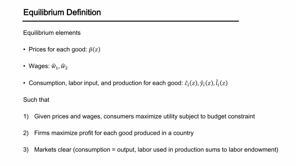
Equilibrium elements

• Prices for each good: �̂�𝑝 𝑧𝑧

• Wages: �𝑤𝑤1, �𝑤𝑤2

• Consumption, labor input, and production for each good: �̂�𝑐𝑖𝑖 𝑧𝑧 , �𝑦𝑦𝑖𝑖 𝑧𝑧 , 𝑙𝑙𝑖𝑖 𝑧𝑧

Such that

1) Given prices and wages, consumers maximize utility subject to budget constraint

2) Firms maximize profit for each good produced in a country

3) Markets clear (consumption = output, labor used in production sums to labor endowment)

1. Consumers problem

Given �̂�𝑝 𝑧𝑧 , �𝑤𝑤𝑖𝑖 consumer in country 𝑖𝑖 to solve

max�0

1𝑈𝑈 𝑐𝑐𝑖𝑖 𝑧𝑧 𝑑𝑑𝑧𝑧

subject to budget constraint

�0

1�̂�𝑝 𝑧𝑧 𝑐𝑐𝑖𝑖 𝑧𝑧 = �𝑤𝑤𝑖𝑖𝑤𝑤𝑖𝑖

𝑐𝑐𝑖𝑖 𝑧𝑧 ≥ 0,∀𝑧𝑧

2. Firms Problem

Given �̂�𝑝 𝑧𝑧 , �𝑤𝑤𝑖𝑖 firms in country 𝑖𝑖 maximize profits for each good 𝑧𝑧

max �̂�𝑝 𝑧𝑧 𝑦𝑦𝑖𝑖 𝑧𝑧 − �𝑤𝑤𝑙𝑙𝑖𝑖 𝑧𝑧

subject to production technology:

𝑦𝑦𝑖𝑖 𝑧𝑧 = 𝑙𝑙𝑖𝑖 𝑧𝑧 /𝑎𝑎𝑖𝑖 𝑧𝑧

Where 𝑎𝑎𝑖𝑖 𝑧𝑧 is unit labor costs for good 𝑧𝑧 in country 𝑖𝑖

Firm Optimization Yields: �̂�𝑝 𝑧𝑧 = �𝑤𝑤𝑖𝑖𝑎𝑎𝑖𝑖 𝑧𝑧 if �𝑦𝑦𝑖𝑖 𝑧𝑧 > 0

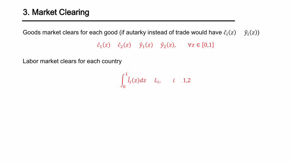
3. Market Clearing

Goods market clears for each good (if autarky instead of trade would have �̂�𝑐𝑖𝑖 𝑧𝑧 = �𝑦𝑦𝑖𝑖 𝑧𝑧 )

�̂�𝑐1 𝑧𝑧 + �̂�𝑐2 𝑧𝑧 = �𝑦𝑦1 𝑧𝑧 + �𝑦𝑦2 𝑧𝑧 , ∀𝑧𝑧 ∈ 0,1

Labor market clears for each country

�0

1𝑙𝑙𝑖𝑖 𝑧𝑧 𝑑𝑑𝑧𝑧 = 𝑤𝑤𝑖𝑖 , 𝑖𝑖 = 1,2

Equilibrium Solution: Cutoff

Cutoff ̅𝑧𝑧 such that country 1 produces and exports goods in 0, ̅𝑧𝑧

Country 2 produces and exports goods in ̅𝑧𝑧, 1

Equilibrium Solution: Cutoff

Cutoff ̅𝑧𝑧 such that country 1 produces and exports goods in 0, ̅𝑧𝑧

Country 2 produces and exports goods in ̅𝑧𝑧, 1

Analytic Simplifications:

Cobb Douglas Preferences: 𝑈𝑈 𝑐𝑐𝑖𝑖 𝑧𝑧 = log ci z

Symmetry: 𝑤𝑤1 = 𝑤𝑤2 = 𝑤𝑤

Production technologies:

𝑎𝑎1 𝑧𝑧 = 𝑒𝑒𝑎𝑎𝑧𝑧

𝑎𝑎2 𝑧𝑧 = 𝑒𝑒𝑎𝑎 1−𝑧𝑧

Production Technologies

𝑒𝑒𝑎𝑎𝑧𝑧𝑒𝑒𝑎𝑎 1−𝑧𝑧

𝑧𝑧

Uni

t Lab

or C

osts

Symmetry

Will have equilibrium with �𝑤𝑤1 = �𝑤𝑤2 (relative wages �w1�w2

= 1)

Will have cutoff ̅𝑧𝑧 = 1/2

• Country 1 produces and exports goods in Z1 = 0, 12

• Country 2 produces and exports goods in Z2 = 12

, 1

Symmetric Equilibrium

𝑒𝑒𝑎𝑎𝑧𝑧𝑒𝑒𝑎𝑎 1−𝑧𝑧

Uni

t Lab

or C

osts

𝑧𝑧

Symmetric Equilibrium

• Prices

�̂�𝑝 𝑧𝑧 = �𝑒𝑒𝑎𝑎𝑧𝑧 , , , , ,, 𝑧𝑧 ∈ 0, ̅𝑧𝑧𝑒𝑒𝑎𝑎 1−𝑧𝑧 , 𝑧𝑧 ∈ ̅𝑧𝑧, 1

• Wages: �𝑤𝑤1, �𝑤𝑤2 = 1 (normalize wages to 1)

• Consumption, labor input, and production:

�̂�𝑐𝑖𝑖 𝑧𝑧 =𝑤𝑤

�̂�𝑝 𝑧𝑧∀𝑧𝑧 ∈ 0,1

�𝑦𝑦𝑖𝑖 𝑧𝑧 =2𝑤𝑤�̂�𝑝 𝑧𝑧

𝑖𝑖𝑖𝑖 𝑧𝑧 ∈ 𝑍𝑍𝑖𝑖 , �𝑦𝑦𝑖𝑖 𝑧𝑧 = 0 𝑖𝑖𝑖𝑖 𝑧𝑧 ∉ 𝑍𝑍𝑖𝑖

𝑙𝑙𝑖𝑖 𝑧𝑧 = 2𝑤𝑤 𝑖𝑖𝑖𝑖 𝑧𝑧 ∈ 𝑍𝑍𝑖𝑖 , 𝑙𝑙𝑖𝑖 𝑧𝑧 = 0 𝑖𝑖𝑖𝑖 𝑧𝑧 ∉ 𝑍𝑍𝑖𝑖

Trade Costs and Trade Policy

Have a working model, can use it to think about the effects of trade costs and trade policy

Iceberg Trade Costs:

Suppose each country faces an iceberg transportation cost of 𝜏𝜏 > 1 when exporting:

𝑦𝑦𝑖𝑖𝑗𝑗 𝑧𝑧 =

𝑙𝑙𝑖𝑖 𝑧𝑧𝜏𝜏𝑎𝑎𝑖𝑖 𝑧𝑧

, 𝑖𝑖𝑖𝑖 𝑖𝑖 ≠ 𝑗𝑗

Still costless to produce for domestic market: 𝑦𝑦𝑖𝑖𝑖𝑖 𝑧𝑧 = 𝑙𝑙𝑖𝑖 𝑧𝑧 /𝑎𝑎𝑖𝑖 𝑧𝑧

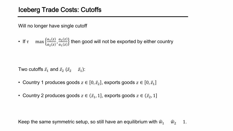
Iceberg Trade Costs: Cutoffs

Will no longer have single cutoff

• If 𝜏𝜏 > max 𝑎𝑎1 𝑧𝑧𝑎𝑎2 𝑧𝑧

, 𝑎𝑎2 𝑧𝑧𝑎𝑎1 𝑧𝑧

then good will not be exported by either country

Two cutoffs ̅𝑧𝑧1 and ̅𝑧𝑧2 ( ̅𝑧𝑧2 > ̅𝑧𝑧1):

• Country 1 produces goods 𝑧𝑧 ∈ 0, ̅𝑧𝑧2 , exports goods 𝑧𝑧 ∈ 0, ̅𝑧𝑧1

• Country 2 produces goods 𝑧𝑧 ∈ ̅𝑧𝑧1, 1 , exports goods 𝑧𝑧 ∈ ̅𝑧𝑧2, 1

Keep the same symmetric setup, so still have an equilibrium with �𝑤𝑤1 = �𝑤𝑤2 = 1.

Symmetric Equilibrium: Iceberg Trade Costs

𝜏𝜏𝑒𝑒𝑎𝑎 1−𝑧𝑧

𝑧𝑧

𝑒𝑒𝑎𝑎 1−𝑧𝑧

𝜏𝜏𝑒𝑒𝑎𝑎𝑧𝑧

𝑒𝑒𝑎𝑎𝑧𝑧U

nit L

abor

Cos

ts

1

Tariff Trade Costs

Now suppose 𝜏𝜏 is an ad valorem tariff instead of an iceberg trade cost.

• Tariffs go on prices rather than in production function

• Let 𝑝𝑝𝑖𝑖 𝑧𝑧 be the price firms in 𝑖𝑖 charge domestically if they produce the good

• Let 𝑝𝑝𝑖𝑖𝑗𝑗 𝑧𝑧 be the price of good z, produced in country 𝑖𝑖, and consumed in country 𝑗𝑗, then

𝑝𝑝𝑖𝑖𝑗𝑗 𝑧𝑧 = �𝜏𝜏𝑝𝑝𝑖𝑖 𝑧𝑧 , 𝑖𝑖𝑖𝑖 𝑖𝑖 ≠ 𝑗𝑗

𝑝𝑝𝑖𝑖 𝑧𝑧 , 𝑖𝑖𝑖𝑖 𝑖𝑖 = 𝑗𝑗

Tariff Trade Costs

For both iceberg trade costs and tariffs, will have

�̂�𝑝𝑖𝑖𝑗𝑗 𝑧𝑧 𝑦𝑦𝑖𝑖

𝑗𝑗 𝑧𝑧 = ��𝑤𝑤𝑖𝑖𝑙𝑙𝑖𝑖 𝑧𝑧𝜏𝜏

, 𝑖𝑖𝑖𝑖 𝑖𝑖 ≠ 𝑗𝑗

�𝑤𝑤𝑖𝑖𝑙𝑙𝑖𝑖 𝑧𝑧 , 𝑖𝑖𝑖𝑖 𝑖𝑖 = 𝑗𝑗

This means it doesn’t matter if we put 𝜏𝜏 on prices or output. Solution to problem is same.

Difference is that tariffs are rebated back to consumers. Consumer budget constraint:

�0

1�̂�𝑝𝑖𝑖 𝑧𝑧 𝑐𝑐𝑖𝑖 𝑧𝑧 𝑑𝑑𝑧𝑧 = �𝑤𝑤𝑖𝑖𝑤𝑤𝑖𝑖 + ⏞𝑇𝑇𝑖𝑖

TariffRevenue

𝑇𝑇𝑖𝑖 = �𝑧𝑧𝜏𝜏 − 1 �̂�𝑝𝑗𝑗 𝑧𝑧 𝑦𝑦𝑗𝑗𝑖𝑖 𝑧𝑧 𝑑𝑑𝑧𝑧

Cutoffs and Symmetric Equilibrium: Tariff Trade Costs

Same as with iceberg trade costs.

Two cutoffs ̅𝑧𝑧1 and ̅𝑧𝑧2 ( ̅𝑧𝑧2 > ̅𝑧𝑧1):

• Country 1 produces goods 𝑧𝑧 ∈ 0, ̅𝑧𝑧2 , exports goods 𝑧𝑧 ∈ 0, ̅𝑧𝑧1

• Country 2 produces goods 𝑧𝑧 ∈ ̅𝑧𝑧1, 1 , exports goods 𝑧𝑧 ∈ ̅𝑧𝑧2, 1

Consumption Differences: Iceberg Costs vs Tariffs

Under iceberg transportation costs:

𝑐𝑐1 𝑧𝑧 =

𝑤𝑤𝑒𝑒𝑎𝑎𝑧𝑧

, 𝑧𝑧 ∈ 0, ̅𝑧𝑧2𝑤𝑤

𝜏𝜏𝑒𝑒𝑎𝑎 1−𝑧𝑧 , 𝑧𝑧 ∈ ̅𝑧𝑧2, 1; 𝑐𝑐2 𝑧𝑧 =

𝑤𝑤𝜏𝜏𝑒𝑒𝑎𝑎𝑧𝑧

, 𝑧𝑧 ∈ 0, ̅𝑧𝑧1𝑤𝑤

𝑒𝑒𝑎𝑎 1−𝑧𝑧 , 𝑧𝑧 ∈ ̅𝑧𝑧1, 0

Under tariffs

𝑐𝑐1 𝑧𝑧 =

𝑤𝑤 + 𝑇𝑇1𝑒𝑒𝑎𝑎𝑧𝑧

, 𝑧𝑧 ∈ 0, ̅𝑧𝑧2𝑤𝑤 + 𝑇𝑇1𝜏𝜏𝑒𝑒𝑎𝑎 1−𝑧𝑧 , 𝑧𝑧 ∈ ̅𝑧𝑧2, 1

; 𝑐𝑐2 𝑧𝑧 =

𝑤𝑤 + 𝑇𝑇2𝜏𝜏𝑒𝑒𝑎𝑎𝑧𝑧

, 𝑧𝑧 ∈ 0, ̅𝑧𝑧1𝑤𝑤 + 𝑇𝑇2𝑒𝑒𝑎𝑎 1−𝑧𝑧 , 𝑧𝑧 ∈ ̅𝑧𝑧1, 1

Where 𝑇𝑇𝑖𝑖 =𝐿𝐿 𝜏𝜏−1

𝜏𝜏 �̅�𝑧1

1− 𝜏𝜏−1𝜏𝜏 �̅�𝑧1

Increased Consumption from Tariff Revenue (vs Iceberg Costs)

% C

hang

e in

Con

sum

ptio

n

𝜏𝜏

𝑎𝑎 = 1

𝑎𝑎 = 0.5

𝑎𝑎 = 1.5

GDP and Tariffs

Country 1’s Gross Domestic Product/Real Consumption (same in symmetric model)

𝐺𝐺𝐺𝐺𝑃𝑃1 = �0

�̅�𝑧2𝑝𝑝1 𝑧𝑧 𝑐𝑐1 𝑧𝑧 𝑑𝑑𝑧𝑧 + �

0

�̅�𝑧1𝑝𝑝12 𝑧𝑧 𝑐𝑐2 𝑧𝑧 𝑑𝑑𝑧𝑧 =

𝑤𝑤

1 − 𝜏𝜏 − 1𝜏𝜏 ̅𝑧𝑧1

• Can see how GDP and real GDP change as tariffs change

• Increasing in productivity level 𝑎𝑎 and country size 𝑤𝑤 , decreasing in tariffs 𝜏𝜏

Real GDP and Tariffs: Base Prices

Real GDP is value of production evaluated at base period prices

• Let the base period be at 𝜏𝜏 = 0, then base prices are

�𝑝𝑝 𝑧𝑧 =𝑒𝑒𝑎𝑎𝑧𝑧, 𝑧𝑧 ∈ 0,

12

𝑒𝑒𝑎𝑎 1−𝑧𝑧 , 𝑧𝑧 ∈12

, 1

Real GDP and Tariffs

Country 1’s Real Gross Domestic Product (constant price GDP)

𝑅𝑅𝐺𝐺𝐺𝐺𝑃𝑃1 = �0

�̅�𝑧2�𝑝𝑝 𝑧𝑧 𝑐𝑐1 𝑧𝑧 𝑑𝑑𝑧𝑧 + �

0

�̅�𝑧1�𝑝𝑝 𝑧𝑧 𝑐𝑐2 𝑧𝑧 𝑑𝑑𝑧𝑧

= 𝐺𝐺𝐺𝐺𝑃𝑃1𝑎𝑎 + 𝜏𝜏 − 1 + 𝑎𝑎𝜏𝜏 − log 𝜏𝜏

2𝑎𝑎𝜏𝜏

Note that 𝑅𝑅𝐺𝐺𝐺𝐺𝑃𝑃1 = 𝐺𝐺𝐺𝐺𝑃𝑃1 if 𝜏𝜏 = 1, otherwise 𝑅𝑅𝐺𝐺𝐺𝐺𝑃𝑃1 ≤ 𝐺𝐺𝐺𝐺𝑃𝑃1

Tariffs: Current vs Constant Price GDP

RGDP

/GDP

𝜏𝜏

𝑎𝑎 = 1

𝑎𝑎 = 0.5

𝑎𝑎 = 1.5

Overview of DFS

Dornbusch, Fischer, and Samuelson (1979):

• Ricardian model: 2 countries, 1 factor of production, continuum of goods

Strengths:

• Simple and intuitive. Can be used to think about effects of trade policy and trade costs.

Weaknesses:

• No explanation for why countries differ in productivity for producing goods

• Not straightforward to extend model to multiple countries

Application of DFS: Tariff Wars

Opp (2010):

• Similar model setup: 2 countries, continuum of goods, labor only factor of production

• Constant Elasticity of Substitution (CES) preferences

𝑈𝑈 = �0

1𝜃𝜃 𝑧𝑧

1𝜎𝜎 𝑐𝑐 𝑧𝑧

𝜎𝜎−1𝜎𝜎 𝑑𝑑𝑧𝑧

𝜎𝜎𝜎𝜎−1

Note: 𝜎𝜎 = 1 ⇒ Cobb-Douglas

Question: What is the optimal tariff rate schedule?

Tariff Wars and the Prisoner’s Dilemma

Holding fixed partner‘s tariff: optimal tariff is non-zero

• Partner may retaliate and charge non-zero tariffs in return

• Global welfare always maximized by free trade

Two subquestions:

1. Without committment to free trade, what is the Nash equilibrium for tariff rates?

2. When, if ever, will one of the countries prefer the above to free trade?

Optimal Tariffs: Propositions

1. Optimal tariffs schedule is uniform across goods

2. Lerner (1936) Symmetry: Import tariff is equivalent to export tax

3. Unique interior NE in tariff rates that dominates any no-trade NE

4. NE tariff rates are increasing in degree of comparative advantage and decreasing in transportation costs

Optimal Tariffs: Main Result and Intuition

If a country is sufficiently large (productivity adjusted labor), it will prefer NE tariffs to free trade

Tradeoffs of having tariffs:

+Intensive Margin: Gain from terms-of-trade effects (relative price of exports to imports)

-Extensive margin: Lose from having to produce goods that could have been imported

If country is large enough, terms-of-trade effects dominate

• Implications for self-regulating free trade agreements