ECON 208

Introduction to Microeconomics

Lecture Notes

Second Edition

HANY FAHMY, Ph.D. E. info@hftutoring.com

w. www.hftutoring.com T. 514 979 4232

This material is copyrighted and the author retains all rights. No part of this material may be reproduced or transmitted in any forms or by any means, or sorted in a data base or retrieval system without the prior written permission of HF Consulting.

C O U R S E P A C K A G E I N F O R M A T I O N

This is a free copy of the first part of ECON 208 course package. If you are interested to know more about this course package or any other course

you are currently taking, please take a minute and check our website w w w. h f t u t o r i n g . c o m

or call us on

514 963 3707 or 514 979 4232

You can also benefit from our WALK IN promotions on all our services:

Weekly Tutorials

Crash Courses

Private Tutoring

Free Advising with our instructors

Just visit our office located on 2015 Drummond (with Maisonneuve),

8th floor, Suite 822 to learn more about these promotions. Looking forward to hearing from you and wishing you a great semester!

The Administration

HF Tutoring

Microeconomics

Contents

Part 1. Lecture Notes on the Price Theory 2

Part 2. Lecture Notes on the Consumer Choice Theory 23

Part 3. Lecture Notes on the Theory of the Firm 37

Part 4. Lecture on the Market Structure and Game Theory 51

Part 5. Lecture Notes on International Trade 68

1

ECON 208, Fall 2010 Hany Fahmy1

Lecture Notes on The Price Theory: Demand, Supply, Market Equilibrium, Elasticity, and Applications

This lectme note discusses the price theory and its applications The theory is introduced after a brief review of some basic concepts The demand and supply of a normal good are defined and explained in detail Practice problems and examples are used for illustration The concept of market equilibrium is introduced and the efficiency conditions are explained The government interventions, through the implementation of price ceilings, floors, taxes, quotas, and subsidies, and the effects of these policies on the market equilibrium are dis­cussed The notion of elasticity is explored and finally, externalities and the other causes of market failure are explained by means of examples

1 E hany fahmy@hf-consnltingco com

2

I. Introduction and Basic Concepts

A. The Economic Concept

Economics is defined as a social science that aims to study how the society allocates its scarce resources to satisfy the society's unlimited needs and wants in the most efficient way Since resources are limited (scarce) and the needs and wants are unlimited, therefore, we can say that economics is the study of how people make choices

Definition 1 Resources (factors of productzon) are thmgs that are used to produce other thmgs to satrsfy people's wants

Definition 2 Productwn 1s defined as any actwity that leads to convertmg resources mto products for consumptwn The resowces used m productwn arc called the factors of produc­tron {FOP) The FOP can be class(fied mto land labo1 capital and entrepreneurship

Definition 3 Land zs the natural {non human) resource that 1s avarlable from natur·e Land as a resource {factor of productwn) incl·udes location, mmerals, cl1mate, water, and vegeta­t!on

Definition 4 Labor rs the human resovrce, whzch mcludes all contrzbutions by mdividuals who work

Definition 5 Capztal can be dwzded into physrcal cap1tal and human capital Physical capital r~fers to all manufactured resources which mcludes burldings, equipment, and machines Human capital r~fers to the accumulated trmnmg and education of workers {investzng m people)

Definition 6 Entrepreneurshrp {actually a subdiuision of labor) mvolves human r·esources that perform the functions of organizmg .. managrnq assembling the other factors of produc­tron, and making basrc dec1swn to zmpmvc the bns1ness

Definition 7 Wants reflers to all what people would buy (consume)

B. The Economic Problem

The economic problem, also known as 'scarcity problem', refers to the gap between the limited resources and the unlimited needs and wants of the society 2

Economrc Problem ==} Chmce ==} Oppmtunity Cost implies implies

2Even if we managed to increase our resources) om needs and wants will also increase and therefOre, the gap will always remain

3

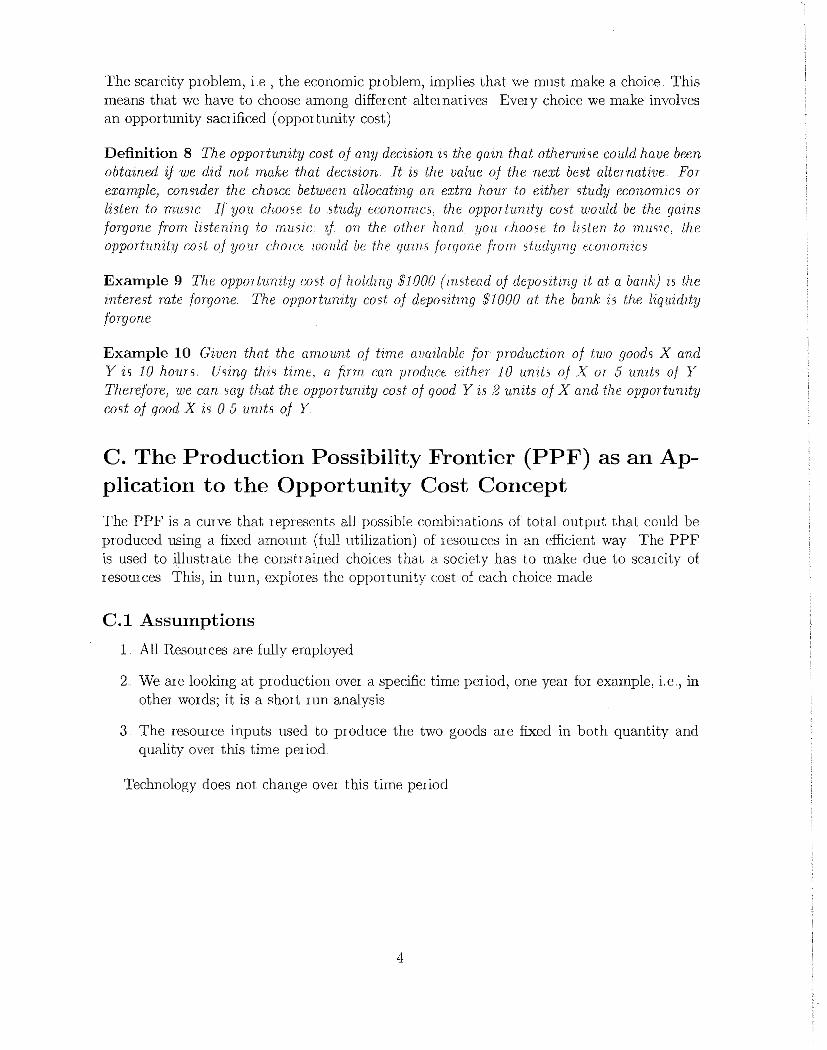
The scarcity problem, i e , the economic problem, implies that we must make a choice This means that we have to choose among different alternatives Every choice we make involves an opportunity sacrificed (opportunity cost)

Definition 8 The opportumty cost of any decision zs the gain that otherw"e could have been obtained if we dzd not make that deciswn. It is the value of the next best alternative. For example, conszder the choice between allocatmg an extra hour to either study econom1cs or l1sten to muszc If you choose to study econormcs, the opporf1mdy cost would be the gams for·gone from ll5teninq to mus1c zf on the other hand you choose to listen to muszc, the opportumty cost of yow chou:e would be the qams forgone from studymg ewnomzcs

Example 9 The opportumty cost of holdmg $1000 (rnstead of deposztmg zt at a bank) zs the mterest rate forgone The opportumty cost of deposztmg $1000 at the bank IS the liquzdzty forgone

Example 10 Given that the amount of tnne avmlable fol productwn of two goods X and Y zs 10 hours Usmg thzs time, a firm can produce edher 10 units of X or 5 units ~f Y Ther·efore, we can say that the opporflmdy cost of good Y zs 2 units of X and the opportumty cost ~f good X is 0 5 umts ~f Y

C. The Production Possibility Frontier (PPF) as an Ap­plication to the Opportunity Cost Concept

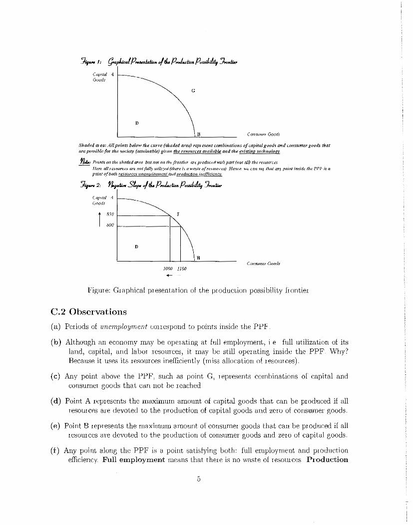
The PPF is a curve that represents all possible combinations of total output that could be produced using a fixed amount (full utilization) of resomces in an efficient way The PPF is used to illustrate the c:onstwined choices that a society has to make due to scarcity of resources This, in turn, explores the opportunity cost of each choice made

C.l Assumptions

1 All Resources are fully employed

2. We are looking at production over a specific time period, one year for example, i e, in other words; it is a short run analysis

3 The resomce inputs used to produce the two goods are fixed in both quantity and quality over this time period

Technology does not drange over this time period

4

Capital .. .j_

Goods

D

G

B Consumet Goods

Shaded m·ea: All points below the CUI'Ve (shaded area) represent combinations of capital goods and consumer goods that are pM:;ible for the vodety (attainable) given the resources available and the existing tecluwlogr

n~: Points on th~ shaded area but not on tilt frontier ar~ produadwith part (not all) rlw re.wurces Here all nsounc.s are not ful(l utili:ed (thert i~ a wmr~ o(re.10urce.\) Hena w~ wn mJ that am poinJ inside the PPF is a point ofbo!h resources unemplovmeni and producnon ine@cicncr.

Capaai ·t Goods

r 850

800 r-------+----1\

D

1000 1100

B Consumu Goods

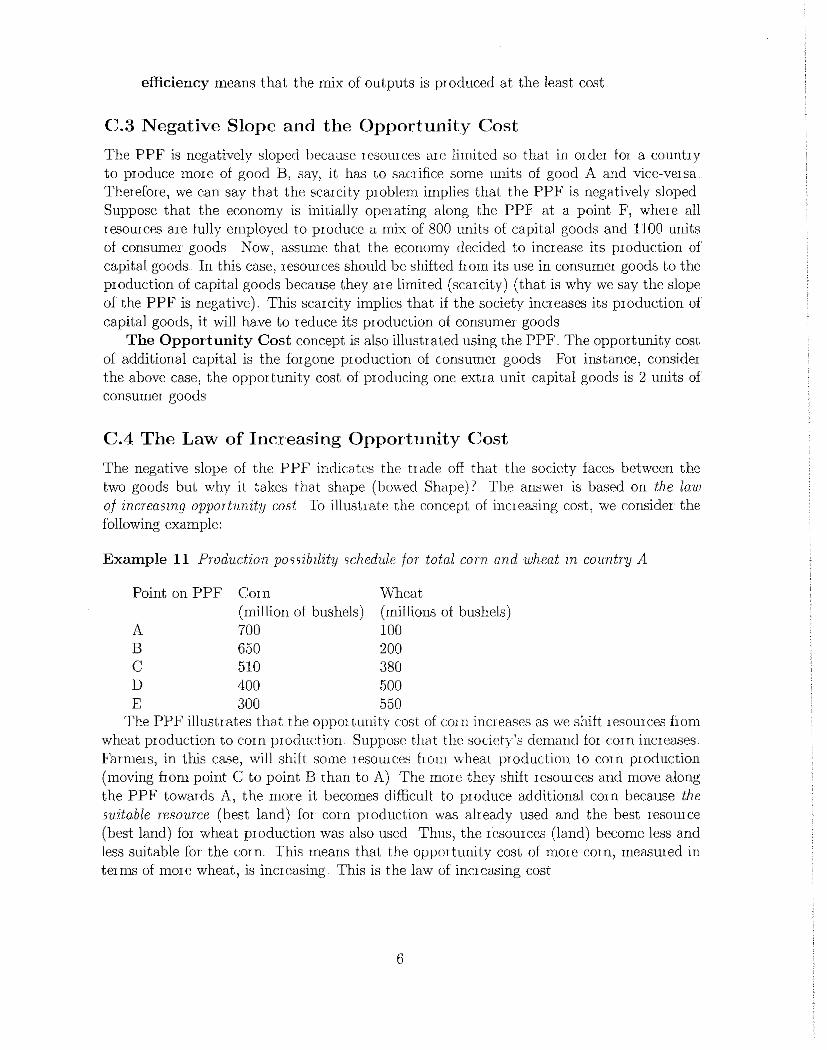
Figure: Graphical presentation of the production possibility frontier

C.2 Observations

(a) Periods of unemployment conespond to points inside the PPF

(b) Although an economy may be operating at full employment, i e full utilization of its land, capital, and labor resources, it may be still operating inside the PPF vVhy? Because it uses its resources inefficiently (miss allocation of resources)

(c) Any point above the PPF, such as point G, represents combinations of capital and consumer goods that can not be reached

(d) Point A represents the maximum amount of capital goods that can be produced if all resources are devoted to the production of capital goods and zero of consumer goods.

(e) Point B represents the maximum amount of consumer goods that can be pwduced if all resources are devoted to the production of consumer goods and zero of capital goods

(f) Any point along the PPF is a point satisfying both: full employment and production efficiency Full employment means that there is no waste of resources Production

5

efficiency means that the mix of outputs is produced at the least cost

C.3 Negative Slope and the Opportunity Cost

The PPF is negatively sloped because resomces me limited so that in order for a country to produce more of good B, say, it has to sacrifice some units of good A and vice-versa Therefore, we can say that the scarcity problem implies that the PPF is negatively sloped Suppose that the economy is initially operating along the PPF at a point F, where all resources are fully employed to produce a mix of 800 units of capital goods and 1100 units of consumer goods Now, assume that the economy decided to increase its production of capital goods .. In this case, resources should be shifted horn its use in consumer goods to the production of capital goods because they are limited (scarcity) (that is why we say the slope of the PPF is negative). This scarcity implies that if the society increases its production of capital goods, it will have to reduce its production of consumer goods

The Opportunity Cost concept is also illustrated using the PPF .. The opportunity cost of additional capital is the forgone production of consumer goods For instance, consider the above case, the opportunity cost of producing one extra unit capital goods is 2 units of consumer goods

C.4 The Law of Increasing Opportunity Cost

The negative slope of the PPF indicates the trade off that the society faces between the two goods but why it takes that shape (bowed Shape) 7 The answer is based on the law of increasmg opportunity cost To illustrate the concept of increasing cost, we consider the following example:

Example 11 Productwn possrbdity schedule for total com and wheat m country A

Point on PPF Corn Wheat (million of bushels) (millions of bushels)

A 700 100 B 650 200 c 510 380 D 400 500 E 300 550

The PPF illustrates that the oppor tuuitv cost of corn increases as we shift resources from wheat production to corn production Suppose that the society's demand for corn increases Farmers, in this case, will shift some resomces from "heat production to corn production (moving from point C to point B than to A) The more they shift resources and move along the PPF towards A, the more it becomes difficult to produce additional corn because the surtable resource (best land) for com production was already used and the best resource (best land) for wheat production was also used Thus, the resources (land) become less and less suitable for the corn This means that the opportunity cost of more corn, measured in terms of more wheat, is increasing This is the law of increasing cost

6

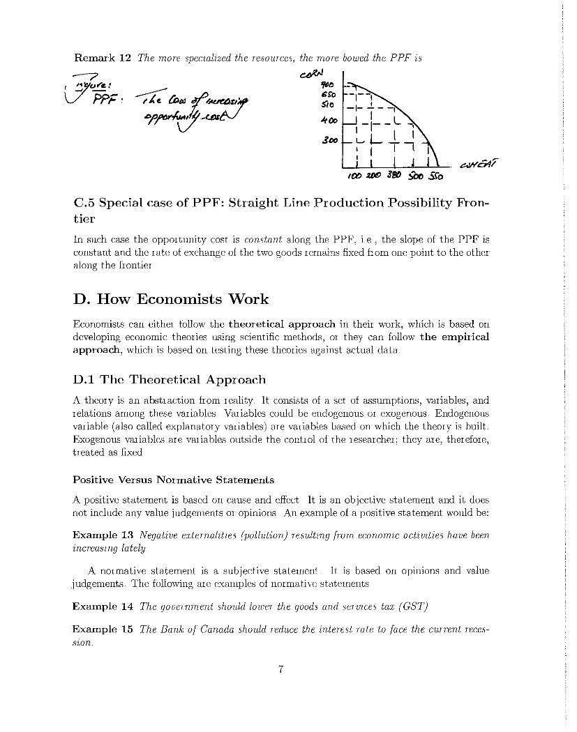
Remark 12 The morB specialzzed the resources, the more bowed the PPF zs

-------? ., ...... 1 -PPF·

C.5 Special case of PPF: Straight Line Production Possibility Fron­tier

In such case the opportunity cost is constant along the PPF, i e , the slope of the PPF is constant and the rate of exchange of the two goods remains fixed from one point to the other along the frontier

D. How Economists Work

Economists can either follow the theoretical approach in their work, which is based on developing economic theories using scientific methods, or they can follow the empirical approach, which is based on testing these theories against actual data.

D.l The Theoretical Approach

A theory is an abstraction from reality It consists of a set of assumptions, variables, and relations among these variables Variables could be endogenous or exogenous Endogenous variable (also called explanatory variables) are variables based on which the theory is built. Exogenous variables are variables outside the control of the researcher; they are, therefore, treated as fixed

Positive Versus Normative Statements

A positive statement is based on cause and effect It is an objective statement and it does not include any value judgements or opinions An example of a positive statement would be:

Example 13 Negatzve externalztws (pollution.) resultmg from economzc actzvzties have been inaeasmg lately

A normative statement is a subjective statement It is based on opinions and value judgements The following are examples of normative statements

Example 14 The government should lower the goods and servrces tax (GST)

Example 15 The Bank of Canada should reduce the interest rate to face the current reces­sion

7

Causality Versus Correlation

Two variables are said to be correlated if they tend to move together but not necessarily influence each other On the other hand, causality involves an influence of one variable (independent) on the other (dependent). Correlation does not imply causality

D.2 The Empirical Approach (the Data)

An empirical approach is based on testing the existing theories against actual data Data types can be classified as follows:

D 2 1 Time Series Data

Time series data are observations on one individual or variable over time.

D.2.2 Cross Section Data

Cross-section data are observations on different indi' iduals or variables at the same point in time So, for example, if a researcher wants to study the Canadian consumption in 2006, he or she will gather cross-section data in 2006

E. Economic Systems

Societies are organized through different economic systems that can be summarized in the following three systems:

E.l Market Economies (laissez faire)

A market economy is one in which individuals and private firms decide what to produce and what to consume There is no government intervention in the market to determine what, how and for whom to produce Those decisions, are r8lhcr determined by the intemction of market forces (demand and supply)

E.2 Comrnand Econ01nies

A command economy is one in which the government makes all important decisions about production and distribution; that is, the government owns all the means of production (land and capital) An example of command economy is the Soviet Union

Note that the above two economic systems are the extremes In reality, we can find neither a pUie laissez faire economy nor a pure command one, rather all societies are mixed economies that combine both the fiee market approach and the command approach

8

II. The Price Theory: Demand, Supply, and Market Equilibrium

A market is a place where individuals (consumers) and firms (producers) can meet to buy or sell goods and services The interaction between the demand side and the supply side of the market determine the equilibrium price of the good or service and the equilibrium quantity produced and pur chased

A. The Demand Curve

Definition 16 the demand for a good 01 a sermce 11 the amount of that good or service that the consumers are w'lllmg and able to buy at a certam pnce m a gwen perwd of tane The market demand (aggregate demand) shows the total demand of all consumers in the market m a gwen perwd of tune

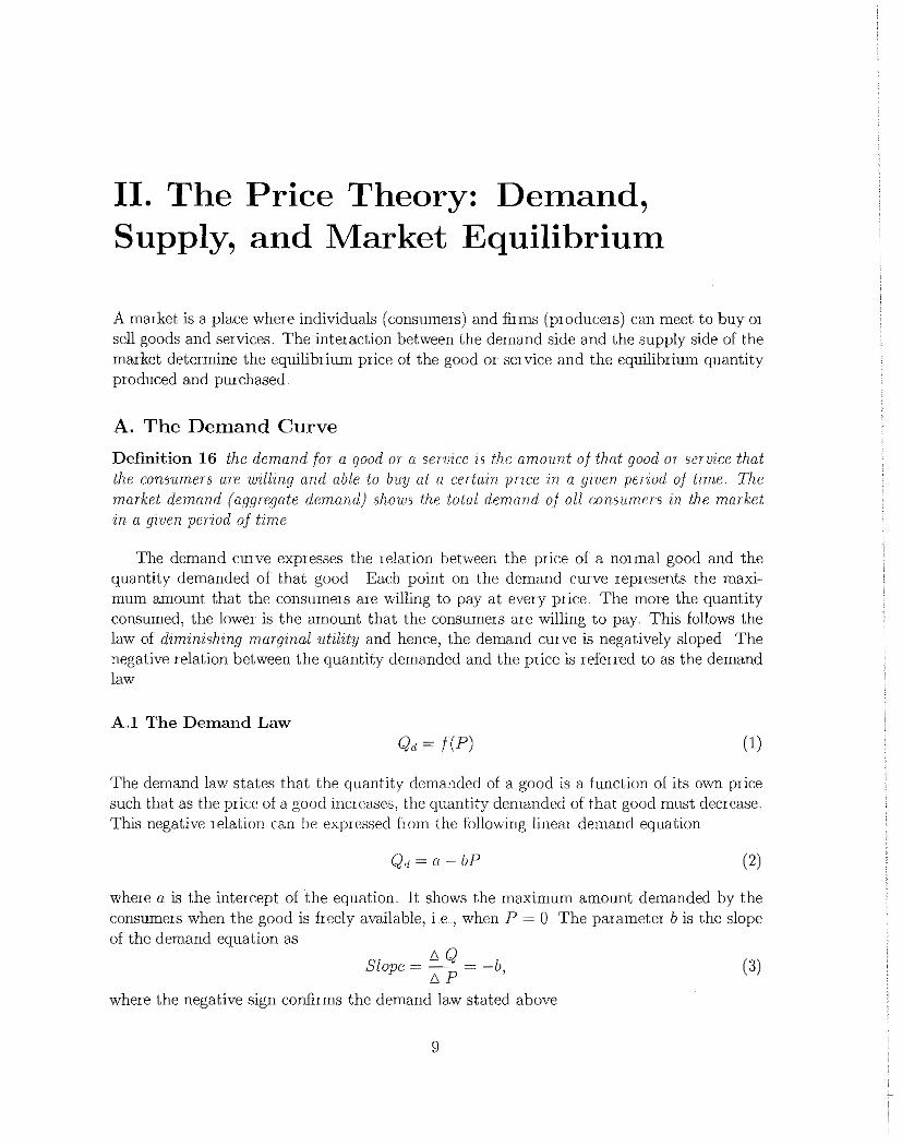
The demand curve expresses the relation between the price of a normal good and the quantity demanded of that good Each point on the demand curve represents the maxi­mum amount that the consumers are willing to pay at every price The more the quantity consumed, the lower is the amount that the consumers are willing to pay. This follows the law of drmini.shzng marginal utility and hence, the demand curve is negatively sloped The negative relation between the quantity demanded and the price is referred to as the demand law

A.l The Demand Law Qd = f(P) (1)

The demand law states that the quantity demanded of a good is a function of its own price such that as the price of a good incteases, the quantity demanded of that good must decrease This negative relation can be expressed from the following linear demand equation

(2)

where a is the intercept of the equation. It shows the maximum amount demanded by the consumers when the good is freely available, i e , when P = 0 The parameter b is the slope of the demand equation as

Slope= 6

Q = -b 6P '

(3)

where the negative sign confirms the demand law stated above

9

A,2 The Determinants of Demand

Q~ = f( ,Ps,Pc, Y,Pe,Taste,1V, T), +ve -ve +ve +ve +ve +ve -ve

(haug;e in qtumtity d(~waudcd Changrc iu Demand=: shift iu tlw dt~mnnd kf ovement shift the demand curve up or down

( 4)

where Ps is the price of substitutes, Pc is the price of complementary goods, Y is the consumers' income, P' is the expected price, N is the number of consumers, and T denotes taxes The expected signs are shown beneath the variables

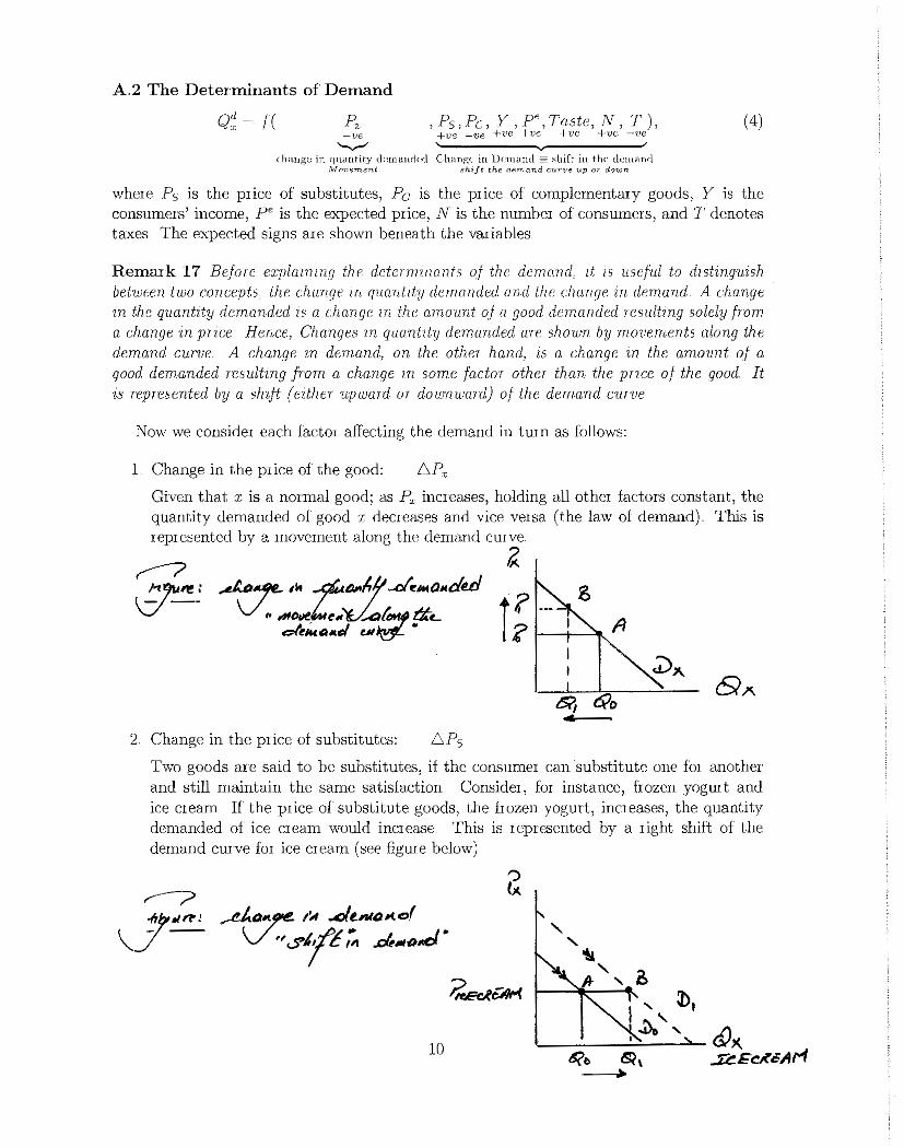
Remark 17 Before e2:plammg the deterrmnants of the demand, It " useful to dlStingmsh between two concepts the change tn quantzty demanded and the change m demand A change m the quantzty demanded ts o change w the amount of a good demanded resulting solely from a change m pnce Hence, Changes m quant1ty demanded are shown by movements along the demand curve A change m demand, on the other hand, rs a change m the amount of a good demanded resulting from a change m some factor other than the pnce of the good It is represented by a shzft (ezther upward or downward) of the demand curve

Now we consider each factor affecting the demand in turn as follows:

1 Change in the price of the good: 6Px

Given that x is a normal good; as Px increases, holding all other factors constant, the quantity demanded of good x decreases and vice versa (the law of demand) This is represented by a movement along the demand curve

r-? ;;. 'if~: ·tt 11! ~~/,f'...ofe~«OI<du:f

'' AIDut.iu~,~fmtpz'ifL 1? d~IU.~ .. d Ul~ • ? 1---t-----'"-

2 Change in the price of substitutes: 6P5

Two goods are said to be substitutes, if the consumer can substitute one for another and still maintain the same satisfaction Consider, for instance, frozen yogurt and ice cream If the price of substitute goods, the frozen yogurt, increases, the quantity demanded of ice cream would increase This is represented by a right shift of the demand curve for ice cream (see figure below)

__.e/..o~ t'A ..clt.ntOH.cf

V "<ft(L ;".. _&.,o...cf •

~~

10

3 Change in the price of complemcnto: l::,Pc

Two goods are said to be complements, if they are consumed together sugar and tea is a typical example Consider a fall in the price of sugar, holding all other factors constant, the quantity demanded of the tea, the complementary good, inCieases This is represented by a right shift of the demand curve f(JI tea

4 Change in income: !::, Y

For normal goods, an increase in income, holding other factors constant, leads to an increase in demand for that good This is represented by a rightward shift of the demand curve

5 Change in consumers' price expectations: t::,pe

Holding other factors constant, if the consumers, for instance, anticipate that there will be a futme price increase (inflation), then demand for the cunent p10ducts, with low prices, will increase This is represented by a rightward shift of the demand cmve

6 Change in fashion and tastes

Changes in fashion and taste, e g food, clothing and entertainments, affect also the demand for a given good and causes the demand cmve to shift either to the right or to the left depending on the consumers' preference

7 Change in the number of buyers served by the market: l::,N

An increase in the number of buyers, holding other factors constant, will shift the demand em ve to the right and vice versa

8 Change in govemment taxation policy: l::,T

Whether the govemment increases or decreases the income tax, this would definitely affect the people's disposable income and consequently their demand The higher the taxation, the lower the disposable income and the lower the demand in general

B. The Market Supply Curve

Definition 18 It refers to the quantity of a good or a servzce that mpplzers are able and willing to offer for sale to the market at varwus market przces durmg a specified period of tzme The market S'Upply (aggregate supply) shows the total quantdy of goods supplzed m an economy

Rl The Supply Law Q, = f(P) (5)

The law of supply states that an increase in the price of a good motivates the producer to increase production and thus the quantity supplied of that good must increase The supply cmve illustrates the maximum quantity of a good sellers are willing and able to produce at each and every price, all else equal. It is a cmve that slopes upward and to the right showing that as the price increases the quantity supplied increases because the good becomes more

11

profitable and vice versa This positive relation can be expressed from the following linear supply equation

Q,=c+dP (6)

where c is the intercept of the equation and the patameter d is the slope of the supply equation as

6 Q, Slope=-~= d

6P ' where the positive sign confirms the supply law stated above

B.2 The Determinants of Supply

Q~=f( Px C,L,z,0) +ve -ve -ve -ve +ve -chauge in Qs Shift in tlw Supply cmvc

lvfovement shift the demand CuTve up OT down

(7)

(8)

where C is the cost of raw materials, L is cost of labor, i is the interest charges, and 0 denotes technology The expected signs are shown beneath the variables The analysis of the determinants of supply is the same as the one for the determinants of demand explained above

C. The Market Equilibrium

The intersection between demand and supply yields the equilibrium quantity and equilibrium market price Observe the following:

• If the actual price in the market is above the equilibrium price, then the supply exceeds the demand in the market which yields a market surplus

• If the actual price in the market is below the equilibrium price, exceeds the supply in the market which yields a market shortage

then the demand

f;,u_

P" P<P* _

.SI.Jiff>i.,t/S

lf"~f¥1' ---

--L----'ll( E ~ -odcef /"/tJmi.J"" I

~I

We need to distinguish between the above two cases and their automatic adjustments as follows:

12

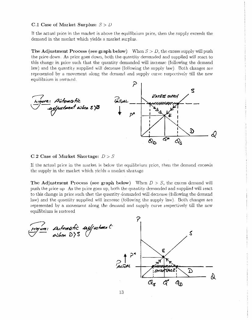
G.l Case of Market Surplus: S > D

If the actual price in the market is above the equilibrium price, then the supply exceeds the demand in the market which yields a market smplus.

The Adjustment Process (see graph below) When S > D, the excess supply will push the price down. As price goes down, both the quantity demanded and supplied will react to this change in price such that the quantity demanded will increase (following the demand law) and the quantity supplied will decrease (following the supply law) Both changes are represented by a movement along the. demand and supply curve respectively till the new equilibrium is restored

?

/')/<

G2 Case of Market Shortage: D > S

If the actual price in the market is below the equilibtium price, then the demand exceeds the supply in the market which yields a market shortage

The Adjustment Process (see graph below) When D > S, the excess demand will push the price up As the ptice goes up, both the quantity demanded and supplied will react to this change in price such that the quantity demanded will decrease (following the demand law) and the quantity supplied will increase (following the supply law) Both changes are represented by a movement along the demand and supply cmve respectively till the new equilibriUI!l is restored

?

13

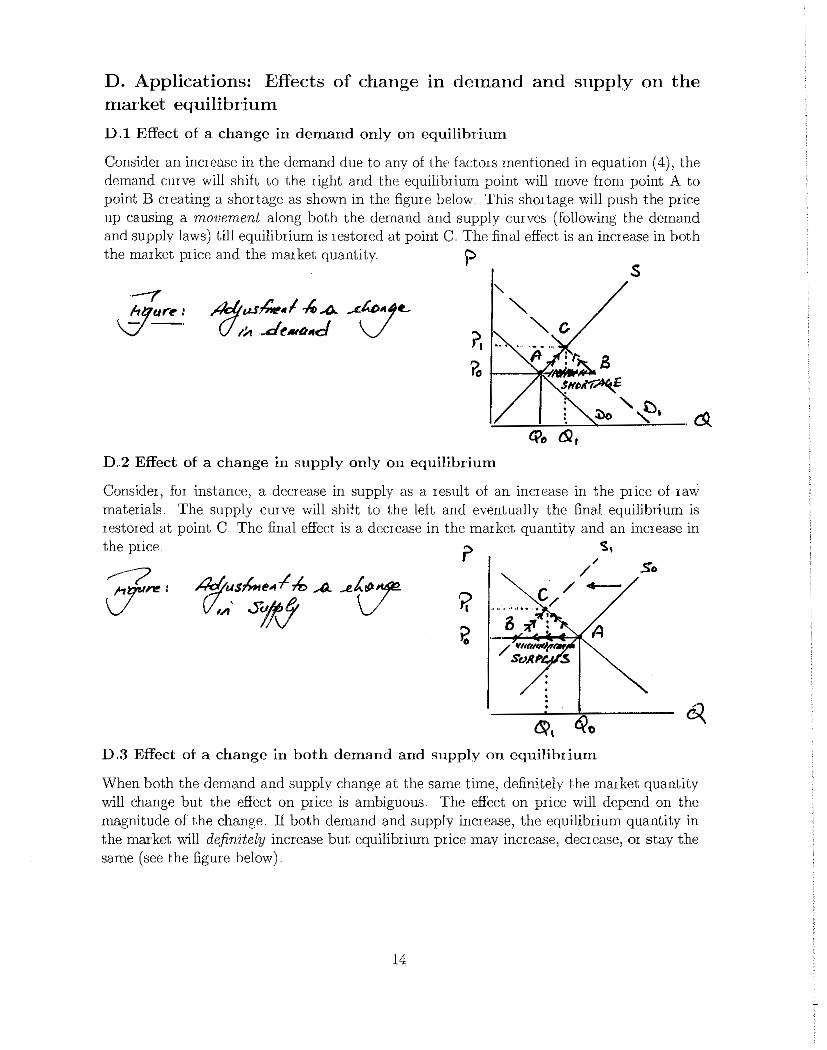
D. Applications: Effects of change in demand and supply on the market equilibrium

D.l Effect of a change in demand only on equilibrium

Consider an increase in the demand due to any of the factors mentioned in equation ( 4), the demand cmve will shift to the right and the equilibrium point will move from point A to point B creating a shortage as shown in the figme below. This shortage will push the price up causing a movement along both the demand and supply cmves (following the demand and supply laws) till equilibrium is restored at point C The final effect is an increase in both the market price and the market quantity )->

s

D..2 Effect of a change in supply only on equilibrium

Consider, for instance, a decrease in supply as a result of an increase in the price of raw materials The supply cmve will shift to the left and eventually the final equilibrium is restored at point C. The final effect is a decrease in the market quantity and an increase in the price f' /$,

/ So

c /-...... /

B ;if ;

D.3 Effect of a change in both demand and supply on equilibrium

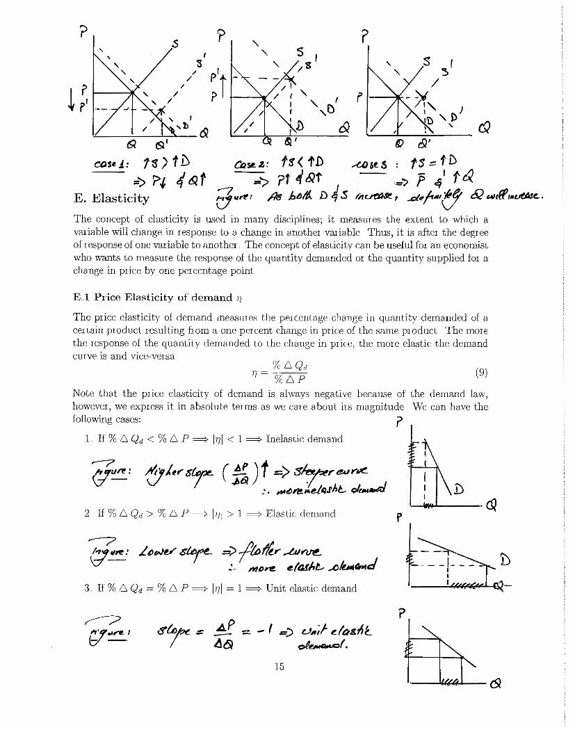
When both the demand and supply change at the same time, definitely the market quantity will change but the effect on price is ambiguous The effect on price will depend on the magnitude of the change. If both demand and supply increase, the equilibrium quantity in the market will d~fimtely increase but equilibrium price may increase, decrease, 01 stay the same (see the figure below)

14

?

t;r

s '

' ' ' ' /

' ·--· ~

61 tSl 1

CDs• .:t.: ts >tv

'? ,

s / p'

)

&

s , /s:

/I --"rl / I '-

1 ' r r ,D 'n &

?

' f' -

s ~' ' /

_':)I /1, }

I 'S) 'D '

I

& , ~ e9'

eose..z: f! < 1' .D ..-£O&t. s t s .::: t D

Q

=> ?.t 4 &t E. Elasticity

=-'/ ?f ~ &t =) f q I t cQ_ g "~' /78 htJ/t.. D 4 S tA~~ 7 ..c/#! f*' (f & wtfft•t.HISt.. •

The concept of elasticity is used in many disciplines; it measures the extent to which a variable will change in response to a change in another variable Thus, it is after the degree of response of one variable to another The concept of elasticity can be useful for an economist who wants to measure the response of the quantity demanded or the quantity supplied for a change in price by one percentage point

E .. l Price Elasticity of demand 'I

The price elasticity of demand rneasureo the pe1ccntage change in quantity demanded of a certain product resulting from a one percent change in price of the same product The more the response of the quantity demanded to the change in price, the more elastic the demand curve is and vice-versa

%60d 1/ = % /'., p (9)

Note that the price elasticity of demand is always negative because of the demand law, however, we express it in absolute terms as we care about its magnitude 'vVe can have the following cases: ?

1 If% 6 Od < % 6 P ==? 1'71 < 1 ==;. Inelastic demand

2 If% 6 0d > % 6 P ==;. 1'71 > 1 ==;. Elastic demand

3. If%/'., Od = %6 P ==;. 1'71 = 1 ==;. Unit elastic demand

_ , =) v";f ~to.s:M __ c~~r.

15

p

?

4 If% 6 Qd = 0 = I'll = 0 = Perfectly inelastic demand (vertical curve)

5. If% 6 P = 0 = l11l = oo = Perfectly elastic demand (horizontal curve) p

E 2 Calculations

There are two methods to calculate the elasticity; namely (1) Arc Elasticity and (2) Point Elasticity. We shall consider both methods in what follows

Arc Elasticity Arc elasticity calculates the elasticity of demand between two points The elasticity along the arc is calculated using the following formula

(Q2-Ql) (Q,+Ql)/2

I) = (P,-Pl)

(P,+Pl)/2

(10)

Point Elasticity Point Elasticity is calculated by knowing the slope of the demand curve equation and any given point on the demand The formula used to calculate the point elasticity can be derived from the definition of the demand elasticity as follows

%6Qd 6~2 6Q p

% 6 p = 6P = Q X 6P p

I) =

6Q p -x-6P Q'

where ~~ is slope of the demand curve

Example 19 Consider the followzng demand function

Q~ = 60- 2Px

Calculate the elasticzty of demand at a pnce o/10

(ll)

Solution 20 The quantity demanded at P = 10 zs obtamed by substitutmg P into the de­mand equabon This y1elds Q~ = 40 The pnce elasticity of demand 15 then

6Q p 10 -I)= -- X - = -2 X - = -0 0

6P Q 40

or 11)1=05<1

and th·us, we conclude that the demand 1s melashc at P = 10

16

D

j)

K3 Factors Determining the Elasticity of Demand'

Two main factors determine the elasticity of demand: (i) availability of substitutes and (ii) time period

(i) Availability of Substitutes The demand on the products that tend to have close substitutes is elastic, while the demand on the products with no close substitutes (such as gasoline) is inelastic

(ii) Short Run and Long Run The SR demand is less elastic than the LR demand curve; that is, in the SR, the quantity demanded do not respond much to the change in prices because people can not change their consumption pattems in the short-run In the LR, however, people can switch to other goods and thus, the LR demand curve for these goods is more elastic in the LR

• For durable goods (e.g , W'ashing machines, refiigerators, etc), the SR demand is more elastic than the LR demand This is because these types of goods are not purchased often and thus, in the SR, the consumer can postponed the~ purchase till the price decreases

• For non-durable goods (e.g .. , gasoline, coffee), the SR demand is less elastic than the LR demand curve; that is, in the SR, the quantity demanded do not respond much to the change in prices because people can not change their consumption patterns in the short-run. In the LR, however, people can switch to other goods and thus, the LR demand curve for these goods is more elastic in the LR

EA Elasticity and the total expenditures

Although the slope of the lmear demand curve is constant, the elasticity of demand is changing from one point to the other; moving down to the right along the demand curve, the price elasticity of demand will increase from 0 when Q = 0 to oo when P = 0 (see the figm e below)

Note that the change in total expcnditme on a product in ICspouse to a change in price depends on the elasticity of demand Along the elastic range of the demand curve (see figure below), the total expenditure increases <lB price falls; Along the inelastic range, the total expenditme decreases as price falls; and when the elasticity of demand is unity, the total expenditures is maximized.

Claim 21 [17[ = 1 = TE =max

Proof. This can be shown as follows •

JThis part is Ieproduced from: Ragan 1 C T 1 and Lipsey R G (2010), Microeconomics, 13th Canadian Edition, Pearson: Tmonto, pp 217

17

c 11/r.~ / e(~s~ve..

B /i(::: f

I

I 11/:r 0 I R

--•11-!/--'tl--'fl(--_,._·- c&::!fo~u:~

F. Price Elasticity of Supply

The price elasticity of supply measures the percentage change in the quantity supplied of a certain product resulting from a one percent change in price of the same product The more the response of the quantity supplied to the change in price, the more elastic. the supply curve is and vice-versa

%/.'o,Qs 1), = % /.', p ( 12)

Same as we did with the price elasticity of demand, we can calculate the price elasticity of supply using the arc: method of the point method as

or

(Q,-QJ) (Q,+Q,)/2

(P,-P,) (P,+Pt )/2

!.'o,Q, p 1), = f.'o,p X Q'

where ~c;; is slope of the supply cmve

18

(13)

(14)

Factors Determining the Elasticity of Supply'

(i) Substitution and Production Costs The more easily the producer can substitute one product for another, the more elastic the supply is For instance, if the resources can be shifted from the production of one crop to another easily, then the supply of each crop will be more elastic .. Also the supply elasticity will depend on how costs behave as output is varied. If the cost of production increases rapidly as output increases, supply is then inelastic

(ii) Short Run and Long Run Same as the demand, the SR supply curve is less elastic than the LR supply curve as in the long-run the suppliers will have enough time to adjust their productive capacity

F. Income Elasticity of Demand

The income elasticity of demand rneasmes the response of the quantity demanded to any change in the income level by one percentage point

%6Qd 'lr = % /'1, I (15)

Luxmy goods have positive income elasticity of demand; that is, if income increases, the demand on those goods will mcrease Inferior goods, on the other hand, have negative income elasticity of demand

G. Cross Elasticity of Demand

The cross elasticity of demand measures the percentage change in the quantity demanded for one good in response to a given percentage change in rnic:e of another good, i.e: it rneasures the responsiveness of the demand of our own product for a change in the price of another product (could be a complement 01 a substitute)

%6Q~ %6Py 6Qx Px --x-6Py Q"

'7x,y is negative if x and y are perfect substitutes and positive is they are complements

( 16)

H. Application: Elasticity and the burden of taxes (see separate handout)

I 1This part is reproduced from: Ragan. C I and Lipsey R G (2010), \licroeconomics_ 13th Canadian

Edition, Pemson: Tbronto pp 217

19

IV. Government Policies

A. Price Ceilings and Price Floors

The government can intervene in the market and sets a maximum or a minimum price The term price ceiling is used when the government sets a price in the market that is below the equilibrium price Price ceilings create situations of excess demand (a shortage at the government-regulated price) On the other hand, when the govemment sets a price that is above the equilibrium price, it is called a price floor Price floors create excess supply (a surplus at the government-regulated price). Although price ceiling or price floor prevents the market from being in equilibrium, they are policies implemented by the government to achieve other social goals Subsidies, taxes, and quotas are diflerent forms of government interventions Before explaining these policies, we need to consider the welfare implications of implementing such policies In other words, we need to assess the eflect on consumer swplus, producer swplus, and on the government due to such policies To this ends, we define the following

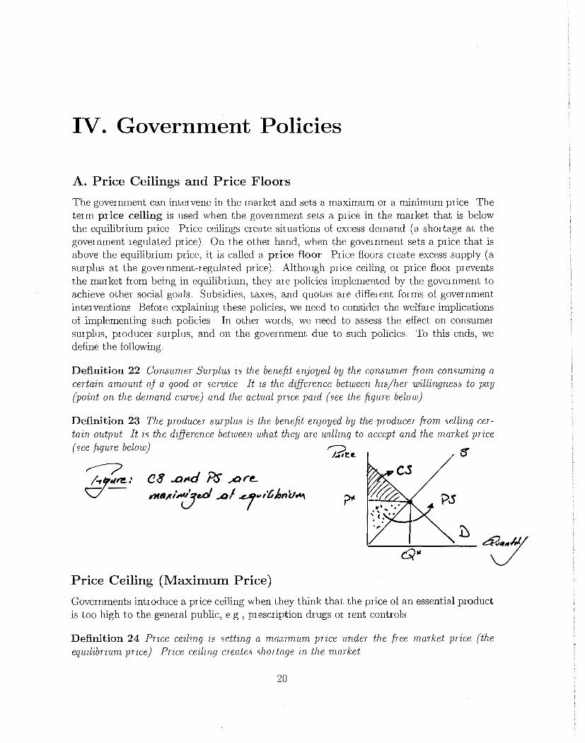
Definition 22 Consumer Surplus :s the benefit enJoyed by the consumer from consuming a certain amount ~~ a good or ser·uice It 1s the difference between h1sjher willingness to pay (point on the demand curve) and the actual price pazd (see the figure below)

Definition 23 The producer surplus zs the benefit enJoyed by the producer from selling cer­tam output It zs the d!jjerence between what they are wzllmg to accept and the market pnce (see figure below)

C8 ..O#fd Ps ,ar~ YMI!I~ti1Je.d Al/"'''ttJmu.,...

Price Ceiling (Maximum Price)

Governments introduce a price ceiling when they think that the price of an essential product is too high to the general public, e g , prescription drugs or rent controls

Definition 24 Pnce cedzng 1s settzng a maxnnum prtce vnder the free market przce (the equilibrwm pnce) Price cezlzng creates shortage m the market

20

Remark 25 Bindmg pnce cezlmqs can create a black market because a thzrd party can make profit by buymg at the controlled przce and selling the prod11ct at the black market price

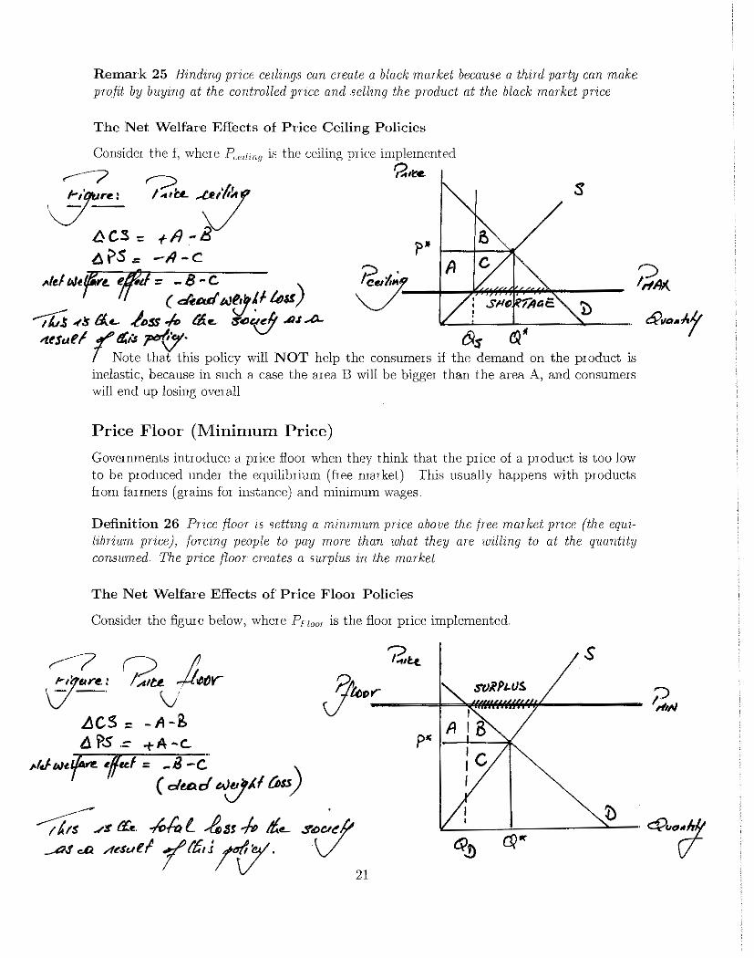
The Net We!f1ue Effects of Price Ceiling Policies

Consider the f, where PU'ilinu is the ceiling p1 ice implemented

~lte. s

,.(ef w~ifn ilfjg. ~ - 8 - c . fc>e~t~ fl _ IT ( d'uu/ t.Jfj~ f ltJ~) ~ ·--1--,.i!i ~.S.~'fl'f'io~1/l""'a~€~-'j)--

'/Ll -fS /:J..L lt>SS ~ I"& e. ~~~A./ A)... ! .. ~1JD11.Jrf ;tt!Jutf "!"" t!ls ~{7· 6/s et

T Note that this policy will NOT help the consumers if the demand on the product is inelastic, because in such a case the area B will be bigger than the area A, and consurneis will end up losing overall

Price Floor (Minimum Price)

Govermnents introduce a price floor when they think that the price of a product is too low to be produced under the equilibrium (hee market) This usually happens with products from farmers (grains for instance) and minimum wages

Definition 26 Price floor ;s settmg a minmwm pnce above the free maz ket price (the eqw­libnum pdce), forcmg people to pay more than what they are unllmg to at the quantzty consumed The pnce floor cr·eates a surplus m the market

The Net Welfare Effects of Price Floor Policies

Consider the figUie below, where Pnom is the floor price implemented

s