Econ 424/CFRM 462

Portfolio Risk Budgeting

Eric Zivot

August 14, 2014

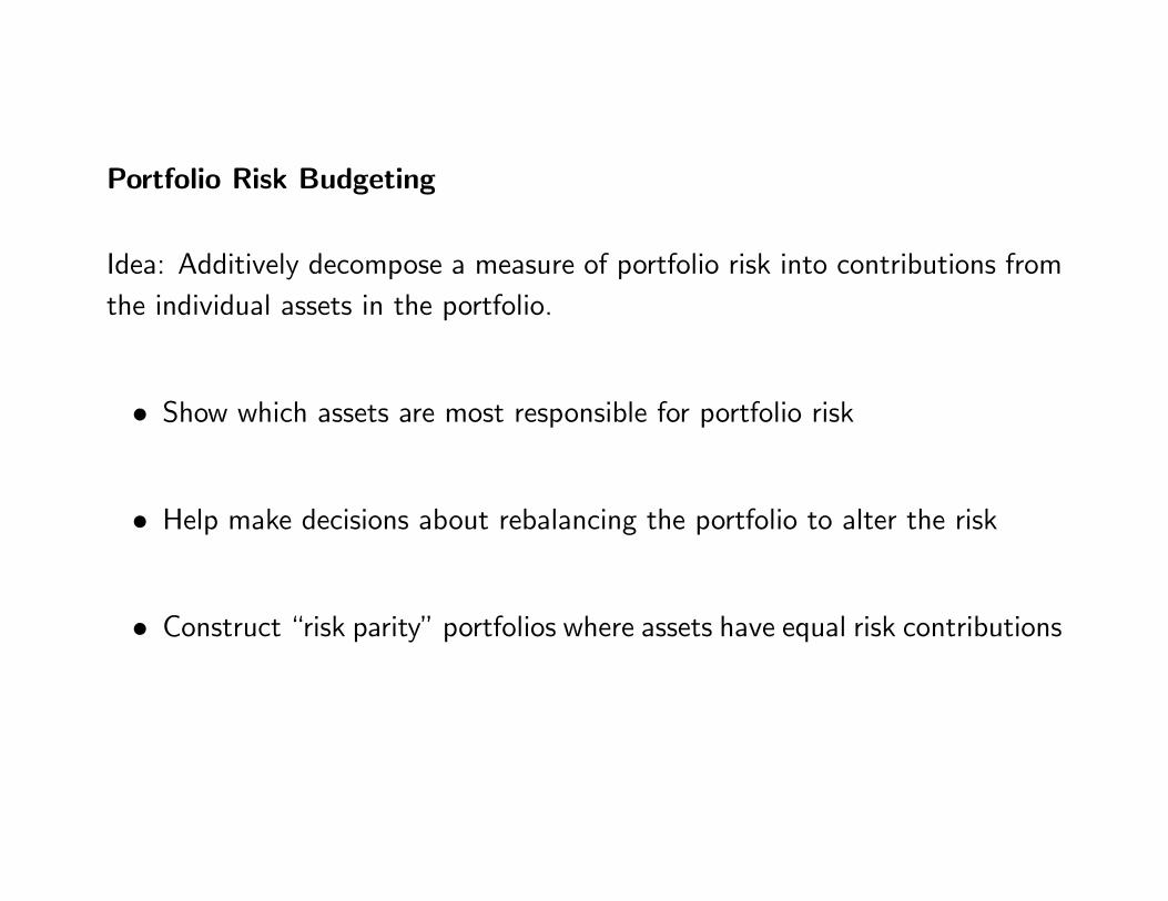
Portfolio Risk Budgeting

Idea: Additively decompose a measure of portfolio risk into contributions fromthe individual assets in the portfolio.

• Show which assets are most responsible for portfolio risk

• Help make decisions about rebalancing the portfolio to alter the risk

• Construct “risk parity” portfolios where assets have equal risk contributions

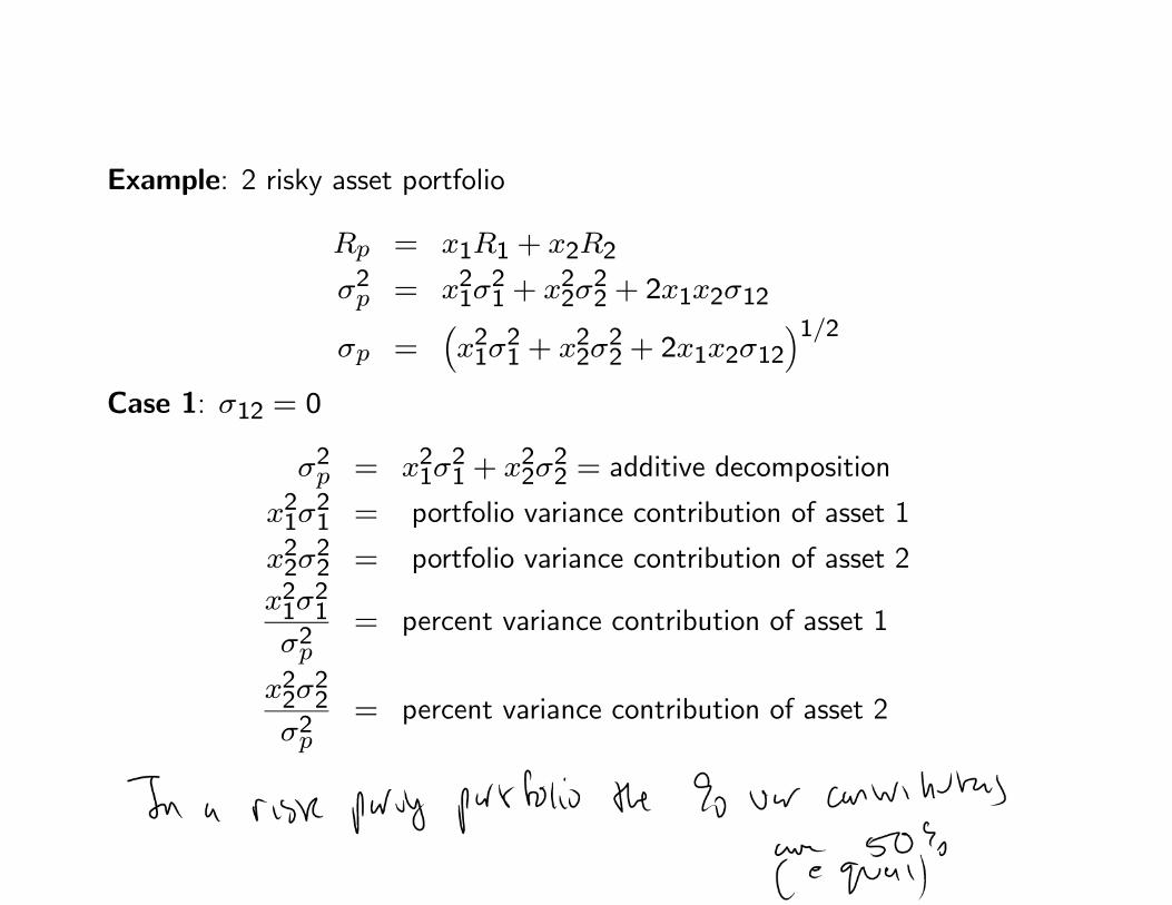
Example: 2 risky asset portfolio

= 11 + 22

2 = 2121 + 22

22 + 21212

=³21

21 + 22

22 + 21212

´12Case 1: 12 = 0

2 = 2121 + 22

22 = additive decomposition

2121 = portfolio variance contribution of asset 1

2222 = portfolio variance contribution of asset 2

2121

2= percent variance contribution of asset 1

2222

2= percent variance contribution of asset 2

Note

=q21

21 + 22

22 6= 11 + 22

To get an additive decomposition we use

2121

+22

22

=

2

=

2121

= portfolio sd contribution of asset 1

2222

= portfolio sd contribution of asset 2

Notice that percent sd contributions are the same as percent variance contri-butions.

Case 2: 12 6= 0

2 = 2121 + 22

22 + 21212

=³21

21 + 1212

´+³22

22 + 1212

´

Here we can split the covariance contribution 21212 to portfolio varianceevenly between the two assets and define

2121 + 1212 = variance contribution of asset 1

2222 + 1212 = variance contribution of asset 2

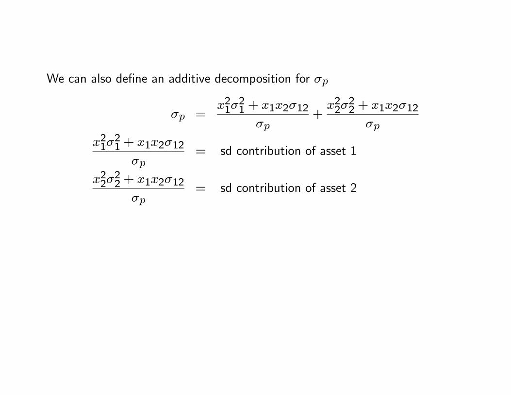
We can also define an additive decomposition for

=21

21 + 1212

+22

22 + 1212

2121 + 1212

= sd contribution of asset 1

2222 + 1212

= sd contribution of asset 2

Euler’s Theorem and Risk Decompositions

• When we used 2 or to measure portfolio risk, we were able to easilyderive sensible risk decompositions.

• If we measure portfolio risk by value-at-risk or some other risk measure itis not so obvious how to define individual asset risk contributions.

• For portfolio risk measures that are homogenous functions of degree onein the portfolio weights, Euler’s theorem provides a general method foradditively decomposing risk into asset specific contributions.

Homogenous functions and Euler’s theorem

First we define a homogenous function of degree one.

Definition 1 homogenous function of degree one

Let (1 ) be a continuous and differentiable function of the vari-ables 1 is homogeneous of degree one if for any constant ( · 1 · ) = · (1 )

Note: In matrix notation we have (1 ) = (x) where

x = (1 )0 Then is homogeneous of degree one if ( ·x) = ·(x)

Examples

Let (1 2) = 1 + 2 Then

( · 1 · 2) = · 1 + · 2 = · (1 + 2) = · (1 2)

Let (1 2) = 21 + 22 Then

( · 1 · 2) = 221 + 222 = 2(21 + 22) 6= · (1 2)

Let (1 2) =q21 + 22 Then

( · 1 · 2) =q221 + 222 =

q(21 + 22) = · (1 2)

Repeat examples using matrix notation

Define x = (1 2)0 and 1 = (1 1)0

Let (1 2) = 1 + 2 = x01 = f(x) Then

( · x) = ( · x)0 1 = · (x01) = · (x)

Let (1 2) = 21 + 22 = x0x = (x) Then

( · x) = ( · x)0( · x) = 2 · x0x 6= · (x)

Let (1 2) =q21 + 22 = (x

0x)12 = (x) Then

( · x) =³( · x)0( · x)

´12= ·

³x0x

´12= · (x)

Consider a portfolio of assets x = (1 )0

R = (1 )0

x = (1 )0

[R] = μ cov(R) = Σ

Define

= (x) = x0R

= (x) = x0μ

2 = 2(x) = x0Σx = (x) = (x

0Σx)12

Result: Portfolio return (x), expected return (x) and standard deviation(x) are homogenous functions of degree one in the portfolio weight vectorx

The key result is for volatility (x) = (x0Σx)12 :

( · x) = (( · x)0Σ( · x))12

= · (x0Σx)12

= · (x)

Theorem 2 Euler’s theorem

Let (1 ) = (x) be a continuous, differentiable and homogenous ofdegree one function of the variables x = (1 )0 Then

(x) = 1 ·(x)

1+ 2 ·

(x)

2+ · · ·+ ·

(x)

= x0(x)

x

where

(x)

x(×1)

=

⎛⎜⎜⎜⎝(x)1...(x)

⎞⎟⎟⎟⎠

Verifying Euler’s theorem

The function (1 2) = 1 + 2 = (x) = x01 is homogenous of degreeone, and

(x)

1=

(x)

2= 1

(x)

x=

⎛⎜⎝ (x)1(x)2

⎞⎟⎠ = Ã11

!= 1

By Euler’s theorem,

() = 1 · 1 + 2 · 1 = 1 + 2

= x01

The function (1 2) = (21+22)12 = (x) = (x0x)12 is homogenous of

degree one, and

(x)

1=

1

2

³21 + 22

´−1221 = 1

³21 + 22

´−12

(x)

2=

1

2

³21 + 22

´−1222 = 2

³21 + 22

´−12

By Euler’s theorem

() = 1 · 1³21 + 21

´−12+ 2 · 2

³21 + 22

´−12=

³21 + 22

´ ³21 + 22

´−12=

³21 + 22

´12

Using matrix algebra we have

(x)

x=

(x0x)12

x=1

2(x0x)−12

x0xx

=1

2(x0x)−122x = (x0x)−12 · x

so by Euler’s theorem

(x) = x0(x)

x= x0(x0x)−12 · x = (x0x)−12x0x = (x0x)12

Risk decomposition using Euler’s theorem

Let RM(x) denote a portfolio risk measure that is a homogenous function ofdegree one in the portfolio weight vector x For example,

RM(x) = (x) = (x0Σx)12

Euler’s theorem gives the additive risk decomposition

RM(x) = 1RM(x)

1+ 2

RM(x)

2+ · · ·+

RM(x)

=X=1

RM(x)

= x0RM(x)

x

Here, RM(x)

are called marginal contributions to risk (MCRs):

MCR =RM(x)

= marginal contribution to risk of asset i,

The contributions to risk (CRs) are defined as the weighted marginal contribu-tions:

CR = ·MCR = contribution to risk of asset i,

Then

RM(x) = 1 ·MCR1 + 2 ·MCR2 + · · ·+ ·MCR= CR1 + CR2 + · · ·+ CR

If we divide the contributions to risk by RM(x) we get the percent contribu-tions to risk (PCRs)

1 =CR1RM(x)

+ · · ·+ CRRM(x)

= PCR1 + · · ·+ PCR

where

PCR =CRRM(x)

= percent contribution of asset i

Risk Decomposition for Portfolio SD

RM(x) = (x) = (x0Σx)12

Because (x) is homogenous of degree 1 in x by Euler’s theorem

(x) = 1(x)

1+ 2

(x)

2+ · · ·+

(x)

= x0

(x)

x

Now

(x)

x=

(x0Σx)12

x=1

2(x0Σx)−122Σx

=Σx

(x0Σx)12=

Σx

(x)

⇒ (x)

= MCR = ith row of

Σx

(x)

Remark: In R, the PerformanceAnalytics function StdDev() performs thisdecomposition

Example: 2 asset portfolio

(x) = (x0Σx)12 =³21

21 + 22

22 + 21212

´12Σx =

Ã21 1212 22

!Ã12

!=

Ã1

21 + 212

222 + 112

!Σx

(x)=

⎛⎝ ³1

21 + 212

´(x)³

222 + 112

´(x)

⎞⎠so that

MCR1 =³1

21 + 212

´(x)

MCR2 =³2

22 + 112

´(x)

Then

MCR1 =³1

21 + 212

´(x)

MCR2 =³2

22 + 112

´(x)

CR1 = 1 ׳1

21 + 212

´(x) =

³21

21 + 1212

´(x)

CR2 = 2 ׳2

22 + 22

´(x) =

³22

22 + 1212

´(x)

and

PCR1 = CR1(x) =³21

21 + 1212

´2(x)

PCR2 = CR2(x) =³22

22 + 1212

´2(x)

Note: This is the decomposition we derived at the beginning of lecture.

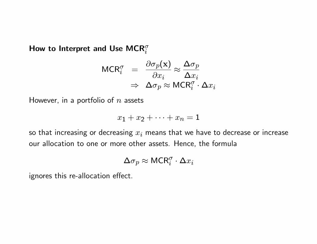
How to Interpret and Use MCR

MCR =(x)

≈ ∆

∆⇒ ∆ ≈ MCR ·∆

However, in a portfolio of assets

1 + 2 + · · ·+ = 1

so that increasing or decreasing means that we have to decrease or increaseour allocation to one or more other assets. Hence, the formula

∆ ≈ MCR ·∆

ignores this re-allocation effect.

If the increase in allocation to asset is offset by a decrease in allocation toasset then

∆ = −∆

and the change in portfolio volatility is approximately

∆ ≈ MCR ·∆ +MCR ·∆

= MCR ·∆ −MCR ·∆

=³MCR −MCR

´·∆

1 2 21 22 1 2 12 120.175 0.055 0.067 0.013 0.258 0.115 -0.004875 -0.164

Table 1: Example data for two asset portfolio.

Consider two portfolios:

• equal weighted portfolio 1 = 2 = 05

• long-short portfolio 1 = 15 and 2 = −05

MCR CR PCR = 01323

Asset 1 0.258 0.5 0.23310 0.11655 0.8807Asset 2 0.115 0.5 0.03158 0.01579 0.1193

= 04005Asset 1 0.258 1.5 0.25540 0.38310 0.95663Asset 2 0.115 -0.5 -0.03474 0.01737 0.04337

Table 2: Risk decomposition using portfolio standard deviation.

Interpretation: For equally weighted portfolio, increasing 1 from 05 to 06decreases 2 from 0.5 to 0.4. Then

∆ ≈ (MCR1 −MCR2) ·∆

= (023310− 003158)(01)= 002015

So increases from 13% to 15%

For the long-short portfolio, increasing 1 from 15 to 16 decreases 2 from-0.5 to -0.6. Then

∆ ≈ (MCR1 −MCR2) ·∆

= [025540− (−003474)] (01)= 002901

So increases from 40% to 43%

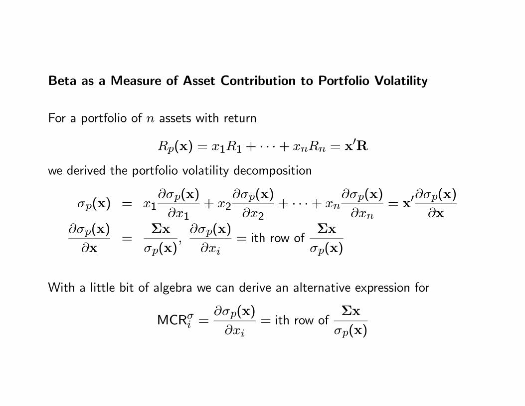
Beta as a Measure of Asset Contribution to Portfolio Volatility

For a portfolio of assets with return

(x) = 11 + · · ·+ = x0R

we derived the portfolio volatility decomposition

(x) = 1(x)

1+ 2

(x)

2+ · · ·+

(x)

= x0

(x)

x(x)

x=

Σx

(x)(x)

= ith row of

Σx

(x)

With a little bit of algebra we can derive an alternative expression for

MCR =(x)

= ith row of

Σx

(x)

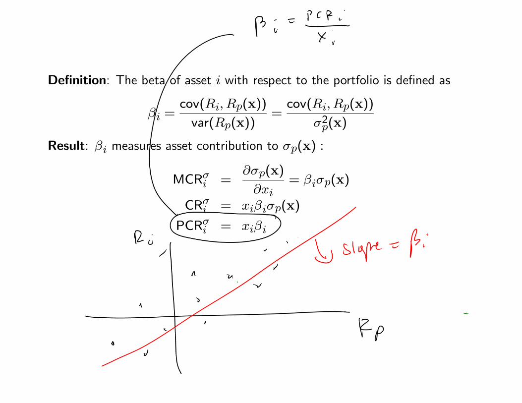
Definition: The beta of asset with respect to the portfolio is defined as

=cov((x))

var((x))=cov((x))

2(x)

Result: measures asset contribution to (x) :

MCR =(x)

= (x)

CR = (x)

PCR =

Remarks

• By construction, the beta of the portfolio is 1

=cov((x) (x))

var((x))=var((x))

var((x))= 1

• When = 1

MCR = (x)

CR = (x)

PCR =

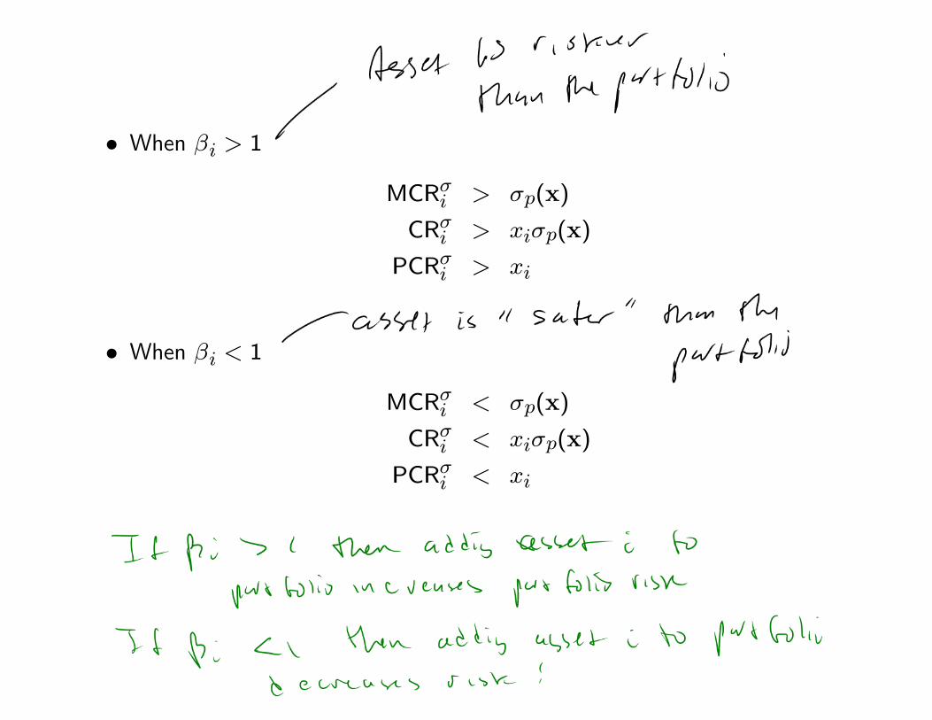
• When 1

MCR (x)

CR (x)

PCR

• When 1

MCR (x)

CR (x)

PCR

MCR CR PCR =PCR

= 01323Asset 1 0.258 0.5 0.23310 0.11655 0.8807 1.761Asset 2 0.115 0.5 0.03158 0.01579 0.1193 0.239

Table 3: Risk decomposition using portfolio standard deviation.

Example

• Asset 1 has 1 = 1761⇒ Asset 1’s percent contribution to risk (PCR )is much greater than its allocation weight ()

• Asset 2 has 2 = 0239⇒ Asset 1’s percent contribution to risk (PCR )is much less than its allocation weight ()

Derivation of Result:

Recall,

(x)

x=

Σx

(x)

Now,

Σx =

⎛⎜⎜⎜⎜⎝21 12 · · · 112 22 · · · 2... ... . . . ...

1 2 · · · 2

⎞⎟⎟⎟⎟⎠⎛⎜⎜⎜⎝

12...

⎞⎟⎟⎟⎠

The first row of Σx is

121 + 212 + · · ·+ 1

Now consider

cov(1 ) = cov(1 11 + · · ·+ )

= cov(1 11) + · · ·+ cov(1 )

= 121 + 212 + · · ·+ 1

Next, note that

1 =cov(1 )

2(x)⇒ cov(1 ) = 1

2(x)

Hence, the first row of Σx is

121 + 212 + · · ·+ 1 = 1

2(x)

and so

MCR1 =(x)

1= first row of

Σx

(x)

=1

2(x)

(x)= 1(x)

In a similar fashion, we have

MCR =(x)

= i’th row of

Σx

(x)

=

2(x)

(x)= (x)

− − Decomposition of Portfolio Volatility

Recall,

MCR =(x)

= ith row of

Σx

(x)=cov((x))

(x)

Using

= corr((x)) =cov((x))

(x)⇒ cov((x)) = (x)

gives

MCR =(x)

(x)=

Then

CR = ×MCR = × ×

= allocation× standalone risk× correlation with portfolio

Remarks:

• × = standalone contribution to risk (ignores correlation effects withother assets)

• CR = × only when = 1

• If 6= 1 then CR ×

MCR CR PCR = 01323

Asset 1 0.258 0.5 0.90 0.23310 0.11655 0.8807Asset 2 0.115 0.5 0.27 0.03158 0.01579 0.1193

= 04005Asset 1 0.258 1.5 0.99 0.25540 0.38310 0.95663Asset 2 0.115 -0.5 -0.30 -0.03474 0.01737 0.04337

Table 4: Risk decomposition using portfolio standard deviation.

Remarks:

• For the equally weighted portfolio, both assets are positively correlatedwith the portfolio

• For the long-short portfolio, Asset 2 is negatively correlated with the port-folio

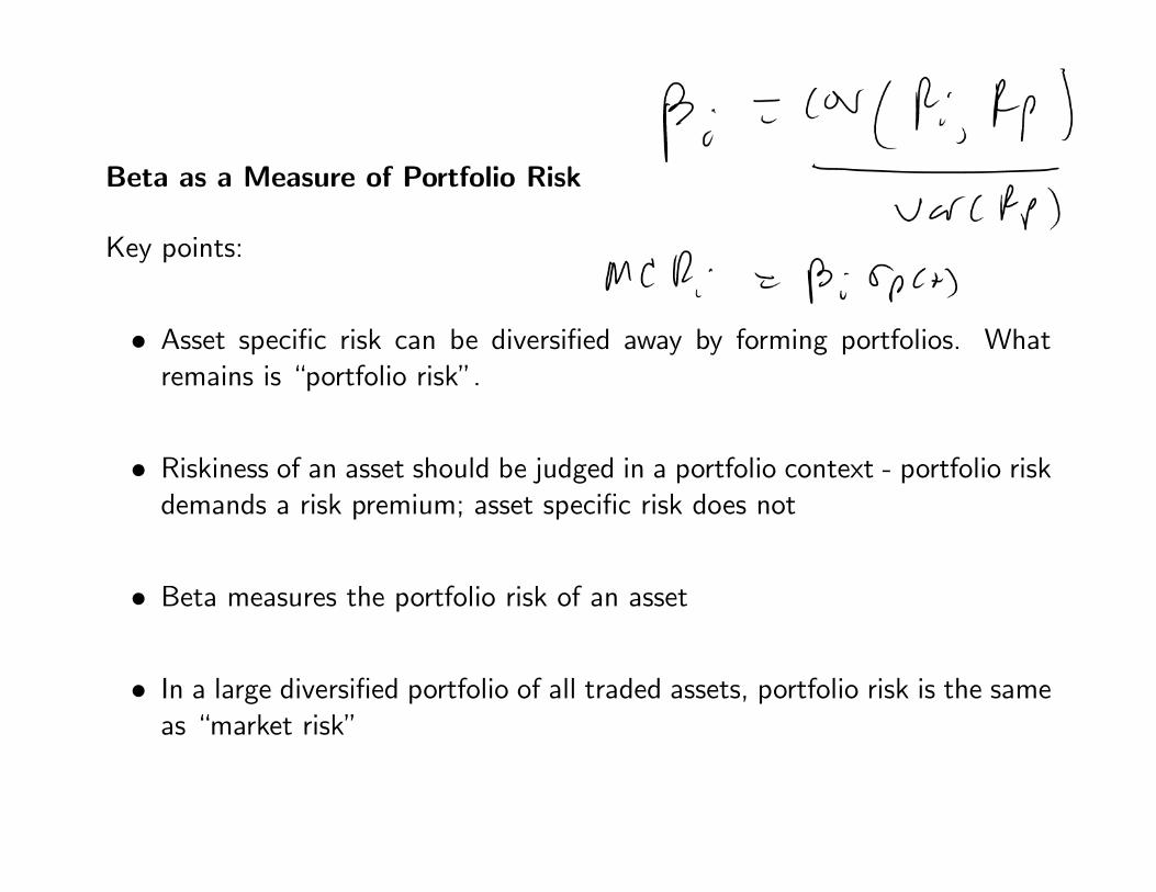
Beta as a Measure of Portfolio Risk

Key points:

• Asset specific risk can be diversified away by forming portfolios. Whatremains is “portfolio risk”.

• Riskiness of an asset should be judged in a portfolio context - portfolio riskdemands a risk premium; asset specific risk does not

• Beta measures the portfolio risk of an asset

• In a large diversified portfolio of all traded assets, portfolio risk is the sameas “market risk”

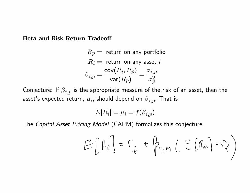
Beta and Risk Return Tradeoff

= return on any portfolio

= return on any asset

=cov()

var()=

2

Conjecture: If is the appropriate measure of the risk of an asset, then theasset’s expected return, should depend on That is

[] = = ()

The Capital Asset Pricing Model (CAPM) formalizes this conjecture.