econ 851 - financial economics - san francisco state...
TRANSCRIPT

ECON 851 - Financial Economics
Michael Bar1
November 12, 2018
1San Francisco State University, department of economics.

ii

Contents
1 Decision Theory under Uncertainty 1
1.1 Introduction . . . . . . . . . . . . . . . . . . . . . . . . . . . . . . . . . . . . 1
1.2 Expected Utility Theory . . . . . . . . . . . . . . . . . . . . . . . . . . . . . 4
1.2.1 Axiomatic foundations of Expected Utility Theory . . . . . . . . . . . 5
1.2.2 Risk Aversion . . . . . . . . . . . . . . . . . . . . . . . . . . . . . . . 13
1.2.3 Measuring risk aversion and applications . . . . . . . . . . . . . . . . 15
1.3 Mean-Variance Theory . . . . . . . . . . . . . . . . . . . . . . . . . . . . . . 26
1.3.1 Critique of the mean-variance theory . . . . . . . . . . . . . . . . . . 28
1.3.2 Validity of the mean-variance theory . . . . . . . . . . . . . . . . . . 31
1.4 Prospect Theory . . . . . . . . . . . . . . . . . . . . . . . . . . . . . . . . . 38
1.4.1 Motivation . . . . . . . . . . . . . . . . . . . . . . . . . . . . . . . . . 38
1.4.2 PT v.s. CPT . . . . . . . . . . . . . . . . . . . . . . . . . . . . . . . 41
2 Two-Period Model: Mean-Variance Approach 45
2.1 Mean-Variance Portfolio Analysis . . . . . . . . . . . . . . . . . . . . . . . . 45
2.1.1 Portfolios with two risky assets . . . . . . . . . . . . . . . . . . . . . 47
2.1.2 Portfolios with n risky assets . . . . . . . . . . . . . . . . . . . . . . . 55
2.1.3 Adding a risk-free asset . . . . . . . . . . . . . . . . . . . . . . . . . . 60
2.2 Capital Asset Pricing Model (CAPM) . . . . . . . . . . . . . . . . . . . . . . 69
2.2.1 Deriving the CAPM . . . . . . . . . . . . . . . . . . . . . . . . . . . 70
2.2.2 CAPM in practice . . . . . . . . . . . . . . . . . . . . . . . . . . . . 77
3 General Principles of Asset Pricing 89
3.1 Assets and Portfolios in a Two-Period Model . . . . . . . . . . . . . . . . . . 89
3.1.1 Financial markets . . . . . . . . . . . . . . . . . . . . . . . . . . . . . 89
3.1.2 Redundant assets . . . . . . . . . . . . . . . . . . . . . . . . . . . . . 96
3.1.3 Complete markets . . . . . . . . . . . . . . . . . . . . . . . . . . . . . 98
3.1.4 Law of One Price . . . . . . . . . . . . . . . . . . . . . . . . . . . . . 101
iii

iv CONTENTS
3.1.5 State prices . . . . . . . . . . . . . . . . . . . . . . . . . . . . . . . . 104
3.1.6 Arbitrage . . . . . . . . . . . . . . . . . . . . . . . . . . . . . . . . . 114
3.2 Fundamental Theorem of Asset Pricing . . . . . . . . . . . . . . . . . . . . . 117
3.2.1 State prices and utility maximization . . . . . . . . . . . . . . . . . . 121
3.2.2 Pricing using risk-neutral probabilities . . . . . . . . . . . . . . . . . 125
3.3 Option Pricing . . . . . . . . . . . . . . . . . . . . . . . . . . . . . . . . . . 128
3.3.1 Options terminology . . . . . . . . . . . . . . . . . . . . . . . . . . . 128
3.3.2 Binomial model (2-states) . . . . . . . . . . . . . . . . . . . . . . . . 131
3.3.3 Black-Scholes formula (in�nitely many states) . . . . . . . . . . . . . 136

Chapter 1
Decision Theory under Uncertainty
1.1 Introduction
Almost every decision we ever make in our lives, involves uncertainty, i.e. the outcome of
our choices cannot be predicted with absolute certainty. These decisions include not only
�nancial investment choices, but career choices, marriage, and college major. Decision theory
under uncertainty makes the foundations of all �nance and portfolio theories, therefore it
must be the starting point of this course.
We assume that decision maker faces a choice among a number of risky alternatives. Each
risky alternative may result in one of a number of possible outcomes, but which outcome
will actually occur is uncertain at the time of decision making. We represent these risky
alternatives by lotteries.
De�nition 1 A lottery is a probability distribution de�ned on a set of payo¤s. A lotterycan be discrete, in which case it is described by the list of payo¤s x1; x2; :::; xN and the
probabilities of these payo¤s p1; p2; :::; pN . The number of outcomes in a discrete lottery
can be �nite N < 1, or in�nite. A lottery can also be continuous, in which case the set
of payo¤s is usually a subset of real numbers (x � R) and the distribution is describedwith a probability density function (pdf) f (x) or the cumulative distribution function (cdf)
F (x) =R x�1 f (t) dt. Lotteries can also be a mix of discrete and continuous, but we will
not deal with such lotteries in this course. We use the notation L to denote the space of allpossible lotteries.
Just like in the case of any probability distribution of a random variable, we require that
1
2 CHAPTER 1. DECISION THEORY UNDER UNCERTAINTY
probabilities (or densities) will be non-negative, and add (or integrate) to 1:
[Discrete] : pi � 0 8i,Xi
pi = 1
[Continuos] : f (x) � 0 8x,Z 1
�1f (x) dx = 1
Just like with any random variables, we might want to compute the mean and variance of a
lottery, and also the covariance between any two lotteries.
In general, lotteries can have any kind of abstract outcomes, not only monetary payo¤s.
For example, when you play basketball, you can win, loose, end with an overtime or have
an injury. These outcomes are not stated in monetary terms. For simplicity of analysis, we
assume that these outcomes can be represented in terms of money, so a win is for example
equivalent to +$500, and a loss is equivalent to -$400. Moreover, money lotteries are all
we need for the study of �nancial decisions, where outcomes are naturally represented with
monetary returns. Also note that sure outcomes can also be viewed as lotteries, that have
one outcome occurring with probability 1.
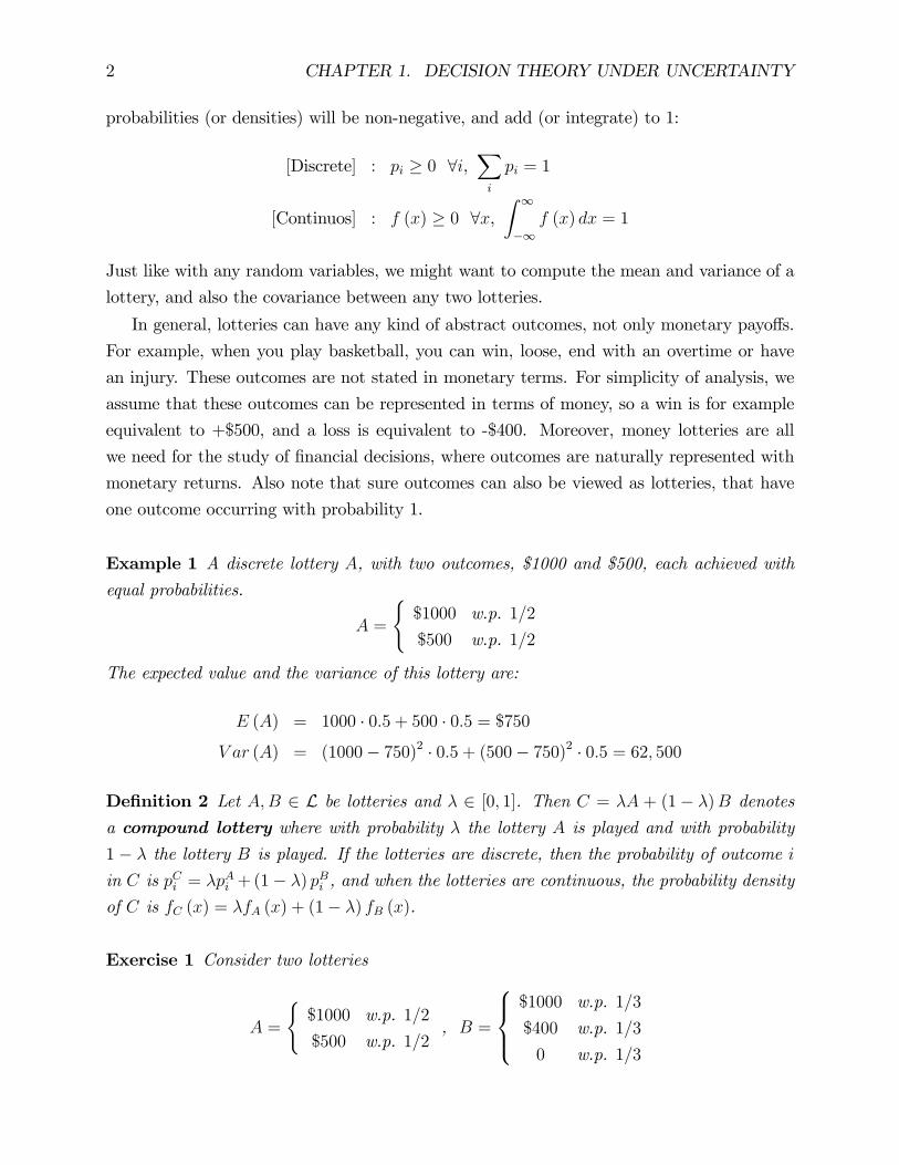
Example 1 A discrete lottery A, with two outcomes, $1000 and $500, each achieved withequal probabilities.
A =
($1000 w.p. 1=2
$500 w.p. 1=2
The expected value and the variance of this lottery are:
E (A) = 1000 � 0:5 + 500 � 0:5 = $750V ar (A) = (1000� 750)2 � 0:5 + (500� 750)2 � 0:5 = 62; 500
De�nition 2 Let A;B 2 L be lotteries and � 2 [0; 1]. Then C = �A + (1� �)B denotes
a compound lottery where with probability � the lottery A is played and with probability
1 � � the lottery B is played. If the lotteries are discrete, then the probability of outcome i
in C is pCi = �pAi +(1� �) pBi , and when the lotteries are continuous, the probability densityof C is fC (x) = �fA (x) + (1� �) fB (x).
Exercise 1 Consider two lotteries
A =
($1000 w.p. 1=2
$500 w.p. 1=2, B =
8><>:$1000 w.p. 1=3
$400 w.p. 1=3
0 w.p. 1=3

1.1. INTRODUCTION 3
Describe the payo¤s and the associated probabilities of the compound lottery C = 0:5A+0:5B.
Solution 1 The compound lottery C = 0:5A+ 0:5B is
C =
8>>>><>>>>:$1000 w.p. 1
2� 12+ 1
2� 13= 5
12
$500 w.p. 12� 12= 3
12
$400 w.p. 12� 13= 2
12
0 w.p. 12� 13= 2
12
For example, the payo¤ of $1000 is achieved if lottery A is played (which occurs with probabil-
ity 0:5) and the outcome of $1000 is realized (which occurs with probability 1=2), or if lottery
B is played (which occurs with probability 1=2) and then $1000 is realized (with probability
1=3), i.e. Pr (1000) = Pr (A) Pr (1000jA) + Pr (B) Pr (1000jB).
The main challenge of decision theory is to de�ne preference over lotteries that will allow
comparison of di¤erent lotteries. For example, consider a lottery D, which pays $750 with
probability 1. Which lottery is better, A or D? This question is equivalent to asking "would
you be willing to pay $750 for lottery A? More generally, how much are you willing to pay
for lottery A? This is the fundamental question of asset pricing. Most people will say that
they would pay less than $750 for lottery A. In general, most people are not willing to pay
the mean of a lottery to buy that lottery. This suggests that things other than the mean of a
lottery are also important. Nevertheless, until recently (mid 20th century), the only theory
of preferences over risky alternatives was the mean theory - i.e. the value of a lottery is given
by its mean payo¤. The next example illustrates the �rst challange to the mean theory. It
it is knows as the "St. Petersburg Paradox", analyzed by the Swiss mathematician Daniel
Bernoulli in 1738.
Example 2 (St. Petersburg Paradox). Consider the lottery A, based on the following gam-ble. A fair coin is tossed repeatedly, until "tails" �rst appears. This ends the game. Let the
number of times the coin is tossed until "tails" appears be k. The lottery pays $2k�1. Thus,
if you toss the coin once, and "tails" appear, then you are paid 21�1 = $1. If it takes 5 tosses
until the coin shows "tails", then you are paid 25�1 = 24 = $16. Thus, the possible payo¤s
of this lottery are 2k�1, k = 1; 2; :::, and the probabilities are�12
�k, k = 1; 2; :::. The expected
value of this lottery is:
E (A) =
1Xk=1
2k�1�1
2
�k=1
2
1Xk=0
2k�1
2
�k=1
2
1Xk=0
1 =1
2� 1 =1

4 CHAPTER 1. DECISION THEORY UNDER UNCERTAINTY
Once again, the question is, how much are you willing to pay for this lottery? Despite the
fact that the expected payo¤ of this lottery is1, there is not a single person who would pay$1 to play this lottery. In fact, most people are willing to pay no more than a few dollars
to play this lottery. Indeed, this game can give you a high payo¤ of more than a million
dollars, if you toss the coin 21 times before "tails" �rst appears (your payo¤ in this case is
220 = $1; 048; 576). But this happens with very low probability:�12
�21= 0:000000476837, or
once in more than 2 million plays.
Example 2 (St. Petersburg Paradox) demonstrates once again that, in general, the value
of a lottery is not equal to the expected value of its payo¤. Nevertheless, until middle of the
20th century, the expected value was the well-accepted theory of decisions under risk. In the
next 3 sections we develop alternative theories for choices under risk: (i) Expected Utility
Theory, (ii) Mean-Variance Theory, and (iii) Prospect Theory. We start with the main-
stream theory in economics - the Expected Utility Theory (EUT). The advantage of EUT
is that it is derived from reasonable axioms about rational behavior in risky environment.
The EUT is therefore prescriptive, in that it tells us how rational agents should behave.
Next we proceed to a simpler Mean-Variance Theory, which is popular exactly because of its
simplicity. Under MVT, all lotteries (and in particular all �nancial assets and all portfolios
of assets) can be represented with two numbers: mean and variance (�; �2). The MVT
violates some of the axioms of rational behavior, but nevertheless serves as the foundation of
modern portfolio theory. MVT is therefore the most practical theory in �nance, exactly due
to its simplicity. Finally, the prospect theory (PT) and its variants, are a result of recent
developments in behavioral and experimental economics, and it attempts to understand
actual behavior. PT is therefore a descriptive theory, and it tries to describe how people
actually behave. PT is by far the most complicated theory of the three, because it was
developed as a generalization to EUT with the goal to "�x" some problems with it. While
PT is successful in resolving some paradoxes which the EUT fails to explain, due to its
complexity the PT is di¢ cult to apply to real world �nancial problems of choosing portfolios
and pricing �nancial assets.
1.2 Expected Utility Theory
The motivation for the development of EUT is Example 2 (St. Petersburg Paradox).
Bernoulli realized that twice the money is not always "twice as good". If a person has
only a small amount of money, say $1000, then doubling it increases his utility by more,
than say doubling the wealth of someone who has 10 million dollars. Put in another way, the
marginal utility from money is diminishing - the more money you have, the smaller is the

1.2. EXPECTED UTILITY THEORY 5
gain from additional $1. This idea of diminishing marginal utility from money is equivalent
to risk aversion in EUT, and will be formalized later. For now, Bernoulli�s intuition is that
instead of computing the expected payo¤ of a lottery, we need to compute the expected
utility of a lottery. The strength of EUT is that it is not only intuitively appealing, but can
be derived from more fundamental axioms about preferences.
1.2.1 Axiomatic foundations of Expected Utility Theory
The starting point for any decision theory under risk is lotteries, and the assumption that
people have some preferences over the space of all lotteries.
De�nition 3 Let the space of all lotteries be L. We assume that there exists a weak pref-erence relation % on L, such that for two lotteries A;B 2 L, the notation A % B means
that "lottery A is at least as good as lottery B". From the weak preference relation, we
can derive the strict preference relation and the indi¤erence relation as follows. The strictpreference relation � on L means that A � B if A % B but not B % A. We read A � B
as "lottery A is strictly better than lottery B". The indi¤erence relation � on L meansA � B if A % B and B % A. We read A � B as "lottery A is as good as (or equivalent to)
lottery B".
Next, we make some assumptions (axioms) about the preference relation %, that willallow representing it with a utility functional and enable practical usage.
De�nition 4 A preference relation % on L is called rational if it satis�es the following twoaxioms:
A1. Completeness. A preference relation % on L is complete if for any two lotteriesA;B 2 L, either A % B or B % A or both. Completeness means that the decision maker is
able to choose among risky alternatives.
A2. Transitivity. A preference relation % on L is transitive if for any three lotteriesA;B;C 2 L, we have
A % B and B % C =) A % C
The transitivity assumption is a natural consistency of preferences. We can show that if
transitivity is violated for some individual, i.e his preferences are A % B and B % C and
C � A, then we can easily extract all his wealth by o¤ering him to trade B for C, A for
B, C for A, and repeat many times, and each time he gets C for A he pays some amount
(because C is strictly better than A).

6 CHAPTER 1. DECISION THEORY UNDER UNCERTAINTY
The next assumption is technical, and is needed in order to ensure representation of
preferences with utility.
De�nition 5 A3. Continuity. The weak preference relation % on L is continuous if forany lotteries A;B;C 2 L with A % B % C, there exists a probability p 2 [0; 1] such that
B � pA+ (1� p)C
The right hand side is the compound lottery, where with probability p lottery A is played and
with probability 1� p lottery C is played.
Continuity means that any lottery "in between" two other lotteries (here B is in between
A and C) is equivalent to some mixture of the two lotteries. What it also means is that there
are no "jumps" in preferences due to small changes in probabilities. For example, suppose
that A is "basketball game with friends", and B is "staying at home", and C is a "knee
injury", and I prefer playing basketball over staying at home: A � B. Then, when I add
a small enough probability of a knee injury to the basketball game, I would not suddenly
change my mind and decide to stay at home. That is, B does not become better than
pA + (1� p)C for small enough (1� p). This axiom is reasonable because most people do
go out to work, shopping, movies, despite the small risk of getting into accident.
The next theorem states that preferences which satisfy completeness, transitivity and
continuity assumptions, can be represented with a continuous utility functional.
Theorem 1 (Utility Representation). Let % on L be a weak preference relation on the spaceof lotteries. If % satis�es the axioms A1, A2 and A3, then there exists a continuos utility
functional U : L ! R such that U (A) � U (B) if and only if A % B for any lotteries
A;B 2 L. This also implies that, for any lotteries, U (A) > U (B) if and only if A � B and
U (A) = U (B) if and only if A � B.
Proof. Omitted.The concept of functional is needed here to emphasize that U maps lotteries (probability
distributions) into real numbers, while a regular function maps real numbers (or vectors)
into real numbers. Also note that theorem 1 does not state that U must have any speci�c
form; only that U is continuous. In particular, theorem 1 does not state that U must have
expected utility form.
De�nition 6 We say that a utility functional U : L ! R has expected utility form if
there exists a utility function u : R! R, such that for every lottery L 2 L,
U (L) = E [u (x)]

1.2. EXPECTED UTILITY THEORY 7
In words, the utility of a lottery is equal to the expected utility of its payo¤s. Speci�cally, for
discrete lottery
U (L) = E [u (x)] =Xi
u (xi) pi
and for continuous lottery (with pdf f (x))
U (L) = E [u (x)] =
Z 1
�1u (x) f (x) dx
Once again, the utility function u maps sure payo¤s (real numbers) into real numbers,
while the utility functional U maps lotteries (probability distributions) into real numbers.1
The utility function u is sometimes called "von Neumann-Morgenstern" (vNM) utility func-
tion, after the mathematician John von Neumann (1903 �1957) and the economist Oskar
Morgenstern (1902 �1977) who provided the axiomatic foundations for the EUT. These two
are also the founders of Game Theory.
Observe that a key advantage of the EUT is that in order to know the preferences over
risky alternatives, all we need to know is the preferences over sure outcomes, given by the
vNM utility function u : R! R. In all applications, we make the standard assumption thatu is increasing, which means that more money is better (formally monotonicity assumption).
An important property of expected utility form is linearity.
Proposition 1 (Linearity of Expected Utility Functional). Suppose that U : L ! R has theexpected utility form. Then U is linear, i.e. for any (�1; �2; :::; �K) > 0,
Pk �k = 1, and
lotteries L1; L2; :::; LK 2 L,
U
KXk=1
�kLk
!=
KXk=1
�kU (Lk)
In words, the utility of a compound lottery is the weighted average of utilities of individual
lotteries.
Observe that in a two-lottery case, A;B 2 L, linearity means:
U (�A+ (1� �)B) = �U (A) + (1� �)U (B)
It is recommended that you �rst prove the proposition for the two-lottery case, before proving
the K-lottery case.1Usually in math, the concept of functional is used to describe a map from a space of functions into
real numbers, and it is appropriate here because lotteries are probability distributions, which are functionsthemselves.

8 CHAPTER 1. DECISION THEORY UNDER UNCERTAINTY
Proof. Suppose that the lotteries are discrete, and all the possible payo¤s are indexed byi = 1; 2; :::; N . Then the probability of payo¤ xi, in the compound lottery, is
Pr (xi) = �1pi;1 + �2pi;2 + :::+ �Kpi;K =KXk=1
�kpi;k;
where pi;k is the probability of payo¤ i in lottery k. Then
U
KXk=1
�kLk
!=
NXi=1
u (xi)
"KXk=1
�kpi;k
#
=
KXk=1
�k
"NXi=1
u (xi) pi;k
#
=KXk=1
�kU (Lk)
The proof for continuous case is similar, with probabilities replaced with pdfs, and sums
with integrals.
Our last axiom will allow us to represent preferences over lotteries not just with any U ,
but with U that has expected utility form.
De�nition 7 A4. Independence of irrelevant alternatives. Let A;B 2 L two lotterieswith A � B, and let � 2 (0; 1]. Then for any lottery C 2 L, it must be
�A+ (1� �)C � �B + (1� �)C
The independence axiom means that the ranking of two lotteries does not change if you
mix each of them with a third lottery. Preferences that satisfy the independence axiom,
in addition to completeness, transitivity and continuity, can be represented with expected
utility form.
Theorem 2 (Expected Utility Theorem). Let % on L be a weak preference relation on thespace of lotteries.
(i) If % satis�es the axioms A1, A2, A3 and A4, then % can be represented with expectedutility form. That is, there exists a (continuous) von Neumann-Morgenstern utility function
u : R! R, such that for every lottery L 2 L, U (L) = E [u (x)].
(ii) Any expected utility functional satis�es axioms A1, A2, A3, and A4.
Proof. Part (i) is very technical and is omitted. We will only prove part (ii). Thus, weassume that U (L) = E [u (x)] represents % on L, and prove that U (�) satis�es the axioms.

1.2. EXPECTED UTILITY THEORY 9
A1, Completeness. Since by de�nition U : L ! R, which means that any lottery isassigned a real number, then for any two lotteries A;B 2 L, the expected utility U (A),U (B) are two numbers. Thus, just like for any two real numbers, we must have either
U (A) � U (B) or U (B) � U (A) or both. In other words, the completeness of % on Lfollows from the completeness of "�" on R.A2, Transitivity. For any three lotteries A;B;C 2 L with U (A) � U (B) and U (B) �
U (C), we must have U (A) � U (C) because U (A), U (B) and U (C) are just three real
numbers. In other words, the transitivity of % on L follows from the transitivity of "�" onR.A3, Continuity. Let A;B;C 2 L with U (A) � U (B) � U (C). We need to show that
there exists a probability p 2 [0; 1] such that
U (B) = U (pA+ (1� p)C)
Using the linearity of expected utility functional (proposition 1),
U (pA+ (1� p)C) = pU (A) + (1� p)U (C)
If U (A) = U (C) = U (B), then any p 2 R satis�es U (B) = pU (A) + (1� p)U (C). IfU (A) > U (C), then we can solve for p directly:
U (B) = pU (A) + (1� p)U (C)
=) p =U (B)� U (C)U (A)� U (C) 2 [0; 1]
A4, Independence. Let A;B 2 L two lotteries with U (A) > U (B), and let � 2(0; 1]. We need to show that for any lottery C 2 L, we must have U (�A+ (1� �)C) >U (�B + (1� �)C). Using the linearity of expected utility functional (proposition 1),
U (�A+ (1� �)C) = �U (A) + (1� �)U (C)> �U (B) + (1� �)U (C)= U (�B + (1� �)C)
The next exercise demonstrates how the Expected Utility Theory resolves the St. Pe-
tersburg Paradox, and explains why people are willing to pay very little for the gamble in
example 2, despite in�nite expected payo¤.

10 CHAPTER 1. DECISION THEORY UNDER UNCERTAINTY
Exercise 2 Suppose that your preferences over lotteries can be represented with expectedutility, and that your vNM utility function on sure payo¤s is u (x) = ln (x). How much are
you willing to pay for the gamble in St. Petersburg Paradox in example 2?
Solution 2 The expected utility from the gamble is:
E [u (x)] =
1Xk=1
u (xk) pk =
1Xk=1
ln�2k�1
��12
�k= ln (2)
1Xk=1
(k � 1)�1
2
�k= ln (2)
" 1Xk=1
k
�1
2
�k�
1Xk=1
�1
2
�k#= ln (2)
The second term in the brackets is
1Xk=1
�1
2
�k=
1=2
1� 1=2 = 1
To compute the �rst term in the brackets, we use the ruleP1
k=1 kak = a= (1� a)2:
1Xk=1
k
�1
2
�k=
1=2
(1� 1=2)2= 2
Therefore, I will pay at most $2 for this gamble, since u (2) = ln (2), which means that the
utility from $2 is the same as the utility from this gamble. We therefore say that $2 is the
certainty equivalent of this lottery.
De�nition 8 The certainty equivalent of a lottery L is the non-random payo¤ CE whichis equivalent to playing the lottery: CE � L. If preferences can be represented by expected
utility, then certainty equivalent is de�ned by u (CE) = E [u (x)].
Thus, in the last example, with vNM utility function u (x) = ln (x), we say that the
certainty equivalent to the St. Petersburg gamble is CE = 2, since ln (2) = E [ln (x)], i.e.
utility from the sure payo¤ of $2 is equal to the expected utility from the gamble. This
exercise is our �rst example of asset pricing. St. Petersburg gamble is a risky asset that has
a payo¤ 2k�1 with probability�12
�k. We found that the value of this risky asset, according
to EUT, to an investor with vNM utility function u (x) = ln (x) is $2.
Exercise 3 Suppose that your preferences over lotteries can be represented with expectedutility, and that your vNM utility function on sure payo¤s is u (x) =
px. How much are you
willing to pay for the gamble in St. Petersburg Paradox in example 2?

1.2. EXPECTED UTILITY THEORY 11
Solution 3 Do it yourself. You should get CE = 2:9142, which means that according to
EUT, an investor with vNM utility function u (x) =px is willing to pay about $2:91 for the
St. Petersburg gamble (risky asset).
The above examples illustrate that the value of any lottery depends on investor�s vNM
utility function. Investors with u (x) =px are willing to pay $2:91, while investors with
u (x) = ln (x) are willing to pay only $2. It would be nice if there was a way to estimate the
vNM utility function. We end this section by pointing out that the vNM utility function u
is not unique, and any increasing linear transformation of u represents the same preferences
as u. This property helps us estimate the vNM of individual investors.
Proposition 2 (Invariance of Expected Utility). Let a 2 R and b > 0. Suppose that the
preference relation % on L has expected utility representation with vNM utility function u.
Then, v (x) = a + bu (x) is another vNM utility function representing the same preferences
as u.
Proof. We need to show that for any two lotteries A;B 2 L,
EA [u (x)] � EB [u (x)] () EA [v (x)] � EB [v (x)]
where the subscripts A and B indicate that we are computing the expected values using the
probability distributions A and B. Note that we can write:
EA [v (x)] = EA [a+ bu (x)] = a+ bEA [u (x)]
EB [v (x)] = EB [a+ bu (x)] = a+ bEB [u (x)]
Subtracting the second from the �rst:
EA [v (x)]� EB [v (x)] = b fEA [u (x)]� EB [u (x)]g
All expectations are numbers, and since b > 0 we have:
EA [v (x)]� EB [v (x)] � 0 () EA [u (x)]� EB [u (x)] � 0
Example 3 The above result implies that if u (x) =px is vNM utility function correspond-
ing to preference relation % on L, then v (x) = 5+17px or v (x) = �3+0:8px also represent

12 CHAPTER 1. DECISION THEORY UNDER UNCERTAINTY
the same preferences as u. This means that for any lotteries A;B 2 L,
A % B () EA [u (x)] � EB [u (x)] () EA [v (x)] � EB [v (x)]
Exercise 4 Suppose some vNM utility function u has the following values at two points:
u (0) = 10 and u (1000) = 15. Show that there exists another utility function v, such that
v (0) = 0, and v (1000) = 1, that represents the same preferences as u.
Solution 4 By proposition 2, we know that v represents the same preferences as u if we can�nd two numbers, a 2 R and b > 0 such that v (x) = a + bu (x). Since the values of the
utility functions are given at two points, we have two equations that can be solved for a and
b, v (0) = a+ bu (0), and v (1000) = a+ bu (1000), i.e.
0 = a+ b � 101 = a+ b � 15
The solution is a = �2, and b = 0:2. Thus, v (x) = �2 + 0:2u (x) represents the samepreferences as u, and also v (0) = 0, v (1000) = 1 as required.
From the previous exercise we learned that we can assign any arbitrary to a vNM utility
function at any two points x1 and x2. This property allows us to estimate the preferences of
a decision maker by estimating one of her equivalent vNM utility functions. Suppose that
Steve has vNM utility function u, which is known at two points: u (0) = 0 and u (1000) = 1.
We o¤er him a lottery with payo¤s at these two points, and ask him what is the most he is
willing to pay it:
L1 =
($1000 w.p. 1=2
0 w.p. 1=2
Suppose Steve tells us that his certainty equivalent for this lottery is CE1 = 450. We can
�nd Steve�s utility from 450, using the de�nition of certainty equivalent:
u (CE1) = E [u (x)]
u (450) = 0:5u (0) + 0:5u (1000) = 0:5
Now, can obtain another point on the his utility function by o¤ering him a lottery:
L2 =
($1000 w.p. 1=2
$450 w.p. 1=2

1.2. EXPECTED UTILITY THEORY 13
Suppose tells us that his certainty equivalent for this lottery is CE2 = 700. We can �nd
Steve�s utility from 700, using the de�nition of certainty equivalent:
u (CE2) = E [u (x)]
u (700) = 0:5u (450) + 0:5u (1000) = 0:75
Notice that we started from two points u (0) = 0 and u (1000) = 1, and found two more
points u (450) = 0:5 and u (700) = 0:75. We can �nd more popints on Steve�s vNM utility
function, by o¤ering him lotteries based on any two points previously found, and asking him
for the certainty equivalent of these lotteries.
1.2.2 Risk Aversion
We have seen in example 1 a lottery that pays $1000 or $500 with equal probabilities,
A =
($1000 w.p. 1=2
$500 w.p. 1=2
The expected value of this lottery was found to be E (A) = $750, and we mentioned that
most people would not pay $750 for this lottery. In general, most people prefer the mean of
a lottery for sure, over the lottery itself. This behavior is called risk aversion.
De�nition 9 We call a person risk-averse if he prefers the expected value of every lotteryL 2 L over the lottery itself, i.e. E (L) � L. If preferences over lotteries can be represented
with expected utility form, then risk aversion means u [E (x)] > E [u (x)]. A person is risk-seeking if he prefers every lottery over its expected value, L � E (L). A person is risk-neutral if he is indi¤erent between lotteries and their expected return, L � E (L). Once
again, if preferences over lotteries can be represented with expected utility form, then risk-
seeking means E [u (x)] > u [E (x)], and risk-neutral means u [E (x)] = E [u (x)].
The concept of risk aversion in EUT is closely related to the shape of the vNM utility
function, as the next theorem states.
Theorem 3 (Risk aversion and concavity - Jensen�s inequality). A person described by EUTis
(i) risk-averse if and only if his vNM utility function u is strictly concave,
(ii) risk-seeking if and only if his vNM utility function u is strictly convex,
(iii) risk-neutral if and only if his vNM utility function u is linear.

14 CHAPTER 1. DECISION THEORY UNDER UNCERTAINTY
Proof. We only prove that if the vNM utility function u is strictly concave, then the
person described by EUT is risk averse. This result is known as Jensen�s inequality. We
also assume that u is once di¤erentiable. Suppose that vNM utility function u : R! R isstrictly concave. We need to prove that u [E (x)] > E [u (x)] for any lottery. Any tangent
line to the graph of a strictly concave function, lies above the graph of the function. Figure
1.1 illustrates this graphically. In particular, the �gure shows a tangent line g (x) at the
Figure 1.1: Strictly concave u and a tangent line at (�; u (�)).
point (�; u (�)), where � � E (x) is the mean of a lottery. The equation of the tangent line
is g (x) = u (�) + u0 (�) (x� �), and since it lies above u (x) for all x with the exception ofx = �, we have 8x 6= �
g (x) > u (x)
u (�) + u0 (�) (x� �) > u (x)

1.2. EXPECTED UTILITY THEORY 15
Taking expectations:
u (�) + u0 (�) [E (x)� �] > E [u (x)]
u (�) + u0 (�) [�� �] > E [u (x)]
u [E (x)] > E [u (x)]
The proof of the converse, u [E (x)] > E [u (x)] for any lottery =) u is strictly concave,
is omitted. One can prove this by contradiction, i.e. assuming that for any lottery u [E (x)] >
E [u (x)], but u is not strictly concave and has a convex area. Then construct a lottery for that
convex area, so that the lottery is better than its mean, which will lead to the contradiction
of u [E (x)] > E [u (x)]. Part (ii) about risk seeking is proved in a similar way, but now the
tangent line will be below the graph of u. Part (iii) is the simplest, and is left as an exercise.
Theorem 3 established the equivalence between risk aversion and concavity of the vNM
utility function. Intuitively, risk aversion is a result of the diminishing marginal utility of
concave functions, where a gain of a certain amount increases utility by less than the drop
in utility resulting from losing that same amount. Consider again example 1, where lottery
A pays $1000 or $500 with equal probabilities. This lottery can be seen as initial wealth of
$750 together with an equal chances of winning or losing $250. Looking at �gure 1.1 with
� = $750, we can see that the increase in utility from additional $250 is smaller than the loss
in utility from -$250. As a numerical example, consider the vNM utility function u (x) =px,
which is strictly concave. With this utility function, starting from $750, the gain in utility
from winning additional $250 isp1000�
p750 = 4:237, and the loss in utility from -$250 isp
750�p500 = 5:025. Thus, this risk averse individual prefers $750 with certainty over the
risk of winning or losing $250 with equal probabilities.
Exercise 5 Let A and B be two lotteries, with the same mean payo¤. Suppose that lottery Bhas higher variance than lottery A. Prove that any risk neutral individual will be indi¤erent
between these two lotteries.
Solution 5 Do it yourself.
1.2.3 Measuring risk aversion and applications
We have established that risk averse individuals, whose preferences can be represented with
expected utility functional, must have concave vNM utility function u. The question is,
which utility functions are suitable? Di¤erent individuals might have di¤erent degree of

16 CHAPTER 1. DECISION THEORY UNDER UNCERTAINTY
risk aversion, so how do we capture these di¤erences with the utility function? The next
de�nition introduces two ways of measuring the degree of risk aversion.
De�nition 10 Given a twice di¤erentiable vNM utility function u : R! R, the Arrow-Prattcoe¢ cient of absolute risk aversion at x is de�ned
ARA (x) = �u00 (x)
u0 (x)
De�nition 11 Given a twice di¤erentiable vNM utility function u : R! R, the Arrow-Prattcoe¢ cient of relative risk aversion at x is de�ned
RRA (x) = �u00 (x)
u0 (x)x
Intuitively, the "more concave" the utility function is, the greater should be the degree
of risk aversion. Therefore, both measures have the second derivative, which is supposed to
capture the degree of concavity. The minus in front makes both measures positive numbers
(since the second derivative is negative for strictly concave functions). Recall from proposi-
tion 2 that multiplying u by a positive constant, will not change the preferences it represents,
and therefore the degree of risk aversion should not change as well. This is the reason why
both have u0 (x) in the denominator - to eliminate the e¤ect of multiplication by a positive
constant.
The absolute risk aversion is relevant for choices involving absolute gains and losses from
current wealth, while the relative risk aversion is relevant for choices involving percentage
(or fractional) gains or losses of current wealth.
The Arrow-Pratt measures of degree of risk aversion allow us to establish whether one
individual is more risk-averse than another individual. That is, individual 2 is more risk
averse than individual 1 if for every x we have ARA2 (x) > ARA1 (x) or RRA2 (x) >
RRA1 (x) for x > 0. There are several other, equivalent ways, of making the same comparison
across individuals.
Recall from de�nition 8 that the Certainty Equivalent (CE) of a lottery is the non-random
payo¤ that gives the same utility as playing the lottery,
CE � L
When preferences are represented by expected utility, the certainty equivalent is de�ned by
the following equation:
u (CE) = E [u (x)]

1.2. EXPECTED UTILITY THEORY 17
We can think of certainty equivalent of a lottery as the maximal amount that an individual is
willing to pay for that lottery. We de�ned a risk averse individual as someone who prefers the
expected payo¤ of a lottery over the lottery itself: u [E (x)] > E [u (x)]. Since u is increasing
function, this implies that for risk averse individuals, the certainty equivalent of any lottery
is smaller than the mean of the lottery: CE < E (x). We can now say that individual 2 is
more risk averse than individual 1 if CE2 < CE1 for any lottery. Intuitively, a more risk
averse individual is willing to pay less for the same lottery.
A closely related concept to certainty equivalent is risk premium.
De�nition 12 A risk premium RP for a given lottery is the amount that an individual
is willing to pay out of the expected payo¤ in order to avoid playing the lottery, and instead
receive its mean with certainty:
u [E (x)�RP ] = E [u (x)]
Notice that on the left side we have utility from certainty equivalent. That is, the risk
premium is just the di¤erence between the mean of a lottery and its certainty equivalent,
i.e. RP = E (x) � CE. Therefore, an individual is more risk-averse if the risk premium he
is willing to pay for avoiding any lottery is higher.
Yet another equivalent way to compare individuals according to their degree of risk
aversion, is by letting the more risk averse vNM utility function be "more concave". In other
words, the vNM utility function u2 is more risk averse than u1 if u2 is obtained through an
increasing and concave transformation of u1. In other words, u2 (x) = (u1 (x)) for some
increasing and concave function (�).It turns out that all the above ways of de�ning more risk aversion are equivalent, as the
next theorem states.
Theorem 4 (More Risk Aversion Equivalence Theorem). The following de�nitions of "morerisk aversion" are equivalent. An individual with vNM utility function u2 is more risk averse
than individual with vNM utility function u1, if
(i) ARA2 (x) > ARA1 (x) or RRA2 (x) > RRA1 (x) for every x > 0,
(ii) There exists an increasing and concave function (�) such that u2 (x) = (u1 (x)),
(iii) CE2 < CE1 for any lottery,
(iv) RP2 > RP1 for any lottery.
Proof. First, we will prove that (i) and (ii) are equivalent. For any increasing utility
functions u1 and u2, we can always �nd some increasing function (�) such that
u2 (x) = (u1 (x))

18 CHAPTER 1. DECISION THEORY UNDER UNCERTAINTY
In particular, we can de�ne (u) = u2�u�11 (u)
�, since an inverse of increasing function
always exists.2 The �rst and second derivatives of u2 are:
u02 (x) = 0 (u1 (x))u01 (x)
u002 (x) = 00 (u1 (x)) (u01 (x))
2+ 0 (u1 (x))u
001 (x)
Dividing both sides by u02 (x) > 0 (remember that all vNM utility functions are assumed
increasing), and then multiplying by �1:
u002 (x)
u02 (x)=
00 (u1 (x)) (u01 (x))
2 + 0 (u1 (x))u001 (x)
0 (u1 (x))u01 (x)
�u002 (x)
u02 (x)= �
00 (u1 (x))
0 (u1 (x))u01 (x)�
u001 (x)
u01 (x)
ARA2 (x) = � 00 (u1 (x))
0 (u1 (x))u01 (x) + ARA1 (x)
Notice that the �rst expression on the right is positive whenever (�) is concave function.Thus, ARA2 (x) > ARA1 (x) if and only if (�) is concave.
Next we prove that (ii) and (iii) are equivalent. Suppose that u2 (x) = (u1 (x)) for some
increasing and concave function (�), and we prove that CE2 < CE1. Then
E [u2 (x)] = E [ (u1 (x))] < [E (u1 (x))]
The inequality above is the familiar Jensen�s inequality (see theorem 3), which applies be-
cause is concave. Next, using the de�nition of certainty equivalents u2 (CE2) = E [u2 (x)]
and u1 (CE1) = E [u1 (x)] in the above inequality, gives
u2 (CE2) < [u1 (CE1)] = u2 (CE1)
Since u2 is increasing, we must have CE2 < CE1.
To prove the converse, suppose that CE2 < CE1, and we will prove that (�) must beconcave. Since u2 (�) is increasing, we have
u2 (CE2) < u2 (CE1)
2For example, suppose that u = u1 (x) =px. Then x = u�11 (u) = u2.

1.2. EXPECTED UTILITY THEORY 19
By de�nition of certainty equivalent, the above inequality is
E [u2 (x)] < u2 (CE1)
As before let u2 (x) = (u1 (x)), for some increasing function (�). Substituting in theabove inequality, gives
E [ (u1 (x))] < (u1 (CE1))
Again, by de�nition of CE1, we have u1 (CE1) = E [u1 (x)]. Plug this in the last inequality
E [ (u1 (x))] < [E (u1 (x))]
Thus, by Jensen�s inequality (theorem 3), the function (�) must be concave.Finally, one can see immediately that (iii) and (iv) are equivalent
CE2 = E (x)�RP2CE1 = E (x)�RP1
Subtracting the above
CE2 � CE1 = � (RP2 �RP1)
which implies that
CE2 < CE1 () RP2 > RP1
Exercise 6 Based on the above theorem, show that individual with vNM utility function
u2 (x) = ln (x) is more risk averse than individual with u1 (x) =px. You should be able to
answer this question in more than one way.
Solution 6 Do it yourself.
Exercise 7 Find the certainty equivalents and risk premia of the lottery,
L =
($1000 w.p. 1=2
$500 w.p. 1=2
for the following vNM utility functions:
(i) u1 (x) =px,
(ii) u2 (x) = ln (x).

20 CHAPTER 1. DECISION THEORY UNDER UNCERTAINTY
Solution 7 Do it yourself.
The di¤erent de�nitions of risk aversion and of more risk aversion help us prove some
testable predictions about the behavior of risk averse individuals. For example, even risk
averse individuals will invest some of their wealth in risky assets, provided that the return
of the risky assets is high enough. However, the amount invested in risky assets is smaller
for more risk averse individuals.
Investment in risky asset
Suppose that an individual, with preferences represented by expected utility, has wealth w
and can invest an amount x 2 [0; w] in a risky asset with random net return r (return in
addition to risk-free return). Then, after one period, the wealth of the investor is w � x +x (1 + r) = w + rx. The optimal investment problem is:
max0�x�w
E [u (w + rx)]
The �rst order condition for interior optimum, x�, is
E [u0 (w + rx�) r] = 0
Second order condition for interior optimum
E�u00 (w + rx�) r2
�< 0
The second order condition is satis�ed if u00 (�) < 0, i.e. if the investor is risk averse. This
condition guarantees a unique global maximum of the objective function (expected utility).
Proposition 3 Any risk-averse investor will invest positive amount in the risky asset, if theexpected return on the asset is positive.
Proof. Figure 1.2 illustrates the optimal investment in risky asset, for a risk-averse investor.We know that the investor is risk averse because the shape of the objective function (expected
utility) is strictly concave. In the �gure, the optimal investment is positive. The optimal
investment is strictly positive if and only if the objective function at x = 0 is increasing,
which is like saying that the �rst derivative is positive at x = 0:
E [u0 (w + rx) r]jx=0 > 0
E [u0 (w) r] > 0
u0 (w)E (r) > 0

1.2. EXPECTED UTILITY THEORY 21
Figure 1.2: Investment in risky asset.
Since the vNM utility function is increasing, we must have u0 (w) > 0, and therefore the
expected return must be positive.
Example 4 We can modify the above example, by adding a risk-free asset with sure returnof rf , and then we will see that a risk-averse investor will invest positive amount in the risky
asset if its expected return is higher than the return on the risk-free asset. The wealth of the
investor after one period is
(w � x) (1 + rf ) + x (1 + r) = w (1 + rf ) + x (r � rf )
Here we assumed that any amount not invested in the risky asset is invested in the risk-free
asset. The optimal investment problem is:
max0�x�w
E [u (w (1 + rf ) + x (r � rf ))]
The �rst order condition for interior optimum, x�, is
E [u0 (w (1 + rf ) + x� (r � rf )) (r � rf )] = 0

22 CHAPTER 1. DECISION THEORY UNDER UNCERTAINTY
And the condition of positive investment in risky asset, x� > 0, becomes:
E [u0 (w (1 + rf )) (r � rf )] > 0
u0 (w (1 + rf ))E (r � rf ) > 0
Which holds if and only if
E (r) > rf
In other words, any risk averse investor will invest some positive amount in the risky asset,
as long as the expected return is greater than the return on the risk-free asset.
In the examples above, we established that even risk-averse investor will invest some
positive amount in a risky asset, provided that the expected return on the risky asset is
su¢ ciently high. We now show that investors who are more risk averse, will invest less in
the risky asset.
Proposition 4 Optimal investment in risky asset is decreasing with the degree of risk aver-sion. In particular, suppose individual with vNM utility function u2 is more risk averse than
individual with u1. Suppose that the individuals are identical in other respects, i.e. they both
have the same initial wealth and consider investment in the same risky asset. We will show
that their optimal investments are x�2 < x�1, i.e. the more risk averse person, will invest less
in a risky asset (ceteris paribus). Without loss of generality, the analysis below is for the
case rf = 0.
Proof. Let f (r) be the pdf or the risky return r. We write the �rst order conditions forinterior optimum for both individuals explicitly, as integrals:
E [u01 (w + rx�1) r] =
Zu01 (w + rx�1) rf (r) dr = 0 (1.1)
E [u02 (w + rx�2) r] =
Zu02 (w + rx�2) rf (r) dr = 0
Since u2 is more risk averse than u1, theorem 4 established that there exists an increasing
and concave function (�) such that u2 (x) = (u1 (x)). Now we evaluate the slope of the

1.2. EXPECTED UTILITY THEORY 23
objective function of individual 2, if he invested x�1, and we claim that this slope is negative:
E [u02 (w + rx�1) r]
=
Z 0 (u1 (w + rx�1))u
01 (w + rx�1) rf (r) dr
=
Z 0
�1 0 (u1 (w + rx�1))u
01 (w + rx�1) rf (r) dr
+
Z 1
0
0 (u1 (w + rx�1))u01 (w + rx�1) rf (r) dr < 0
The last step breaks the integral into two parts, where the �rst integrates over negative
returns r < 0, and the second integrates over the positive returns.3 The integrand in the
last inequality is the same as in (1.1), except that it is multiplied by 0 (u1 (w + rx�1)). Since
(�) is concave, 0 (�) is a decreasing function, so the term 0 (u1 (w + rx�1)) is larger when
r < 0 then when r > 0. Since the integral in (1.1) is equal to zero, it must now be negative
when we weigh the negative terms more than the positive ones.
Demand for insurance
Suppose that an individual, with preferences represented by expected utility, has wealth w
and faces a risk that with probability � his wealth will sustain damage d 2 [0; w], and withprobability 1�� his wealth remains intact. The individual can buy insurance with premiump per unit of wealth insured, and he needs to choose the amount of coverage q to purchase,
where 0 � q � d. Assuming that the utility over certain outcomes is represented by u (�),which is strictly increasing and strictly concave, the individual�s expected utility is
E [u] = �u (w � d� pq + q) + (1� �)u (w � pq)
Notice that in the case of damage occurring, he still needs to pay the premium, but he
receives a compensation at the amount of his coverage q. His problem is therefore
max0�q�d
�u (w � d� pq + q) + (1� �)u (w � pq)
The �rst order condition for interior solution is:
�u0 (w � d+ q� (1� p)) (1� p)� (1� �)u0 (w � pq�) p = 0
3There must be some chance of negative returns here because otherwise both individuals would invest alltheir wealth in the risky asset. To see this, note that if r > rf , the objective function is always increasing inx, i.e. x� = w (corner solution).

24 CHAPTER 1. DECISION THEORY UNDER UNCERTAINTY
The second order condition is
�u00 (w � d+ q� (1� p)) (1� p)2 + (1� �)u00 (w � pq�) p2 < 0
Thus, since the individual is risk averse (utility is strictly concave i.e. u00 < 0), the second
order condition is satis�ed. For interior solution, we must have
�u0 (w � d+ q� (1� p)) (1� p) = (1� �)u0 (w � pq�) pu0 (w � d+ q� (1� p))
u0 (w � pq�) =(1� �)�
p
(1� p)
An important general result is that if insurance is actuarially fair, then a risk averse person
will buy full coverage, i.e. q� = d. An actuarially fair insurance requires that p = �, in which
case the insurance company makes zero expected pro�t: E (�) = pq � �q = 0. Thus
u0 (w � d+ q� (1� p))u0 (w � pq�) = 1
w � d+ q� (1� p) = w � pq�
q� = d
If p > �, the insurance company makes positive pro�t and risk averse individuals will not
buy full coverage, and possibly will not buy any insurance at all if the premium is too high4.
In order to �nd exactly how much insurance is purchased, we need to know the function
u (�).
Proposition 5 Prove that only risk averse individuals will ever buy insurance.
Proof. We consider only the cheapest possible insurance - actuarially fair (i.e. p = �).5
Individuals who won�t buy actuarially fair insurance, will de�nitely not buy a more expensive
one. With coverage q 2 [0; d], and with p = �, the wealth is equal to the following lottery:
L =
(w � d� �q + q w.p. �
w � �q w.p. 1� �
We will show that the objective function (expected utility) is decreasing in q for risk seeking
individuals, as illustrated in �gure 1.3.
4This might explain why many Americans do not purchase health insurance.5Cheaper than actuarially fair insurance leads to negative pro�t of insurance companies, and therefore is
not sustainable.

1.2. EXPECTED UTILITY THEORY 25
Figure 1.3: Demand for insurance: Risk Seeking Individual.
The slope of the objective function (expected utility) is
�u0 (w � d� �q + q) (1� �)� (1� �)u0 (w � �q)�= � (1� �) [u0 (w � d� �q + q)� u0 (w � �q)]
For risk-seeking individuals, the vNM utility function is convex, and thus the marginal utility
is increasing: u0 (x1) < u0 (x2) () x1 < x2. Thus,
u0 (w � d� �q + q)� u0 (w � �q) < 0 ()w � d� �q + q < w � �q
q < d
At q = d (full coverage), the expected utility attains its global minimum, as shown in �gure
1.3. Thus, the optimal coverage for any risk-seeking individual is q� = 0, i.e. no insurance.
For risk-neutral individuals, the vNM utility function is linear, i.e. u (x) = a + bx, for
a 2 R, and some b > 0. The expected utility is then:
E [u] = � (a+ b (w � d� pq + q)) + (1� �) (a+ b (w � pq))= a+ bw � �bd+ b (� � p) q

26 CHAPTER 1. DECISION THEORY UNDER UNCERTAINTY
Notice that with actuarially fair insurance, p = �, the expected utility does not depend on
coverage: E [u] = a + bw � �bd, and risk-neutral individual is indi¤erent between all levelsof coverage q = [0; d]. With realistic insurance, with p > �, notice that expected utility is
decreasing in q, and therefore the optimal coverage of a risk-neutral individual is q� = 0, i.e.
no insurance.
Exercise 8 Consider two lotteries:
X � U [0; 2] and Y =
(1:2475 w.p. 0:8
0:01 w.p. 0:2
This means that X has a continuous uniform distribution on the interval [0; 2].
(i) Calculate the mean and variance of both lotteries.
(ii) Which lottery is preferred by an individual whose vNM utility function is u (x) =
ln (x)?
(iii) Based on your answers to (i) and (ii), is it true that any risk averse individual,
when comparing two lotteries with the same mean, would always prefer the one with the
lower variance?
Solution 8 Do it yourself.
1.3 Mean-Variance Theory
Expected utility theory has several advantages. First, it is derived from precise axioms about
human behavior, so users of the theory know exactly what assumptions about preferences
make the EUT valid. Second, the expected utility theory helped us understand why people
are usually unwilling to pay for a lottery the expected value of its payo¤s - a behavior known
as risk aversion. EUT explains why people buy insurance, while at the same time invest
in risky assets. We have seen applications of EUT to optimal investment and demand for
insurance. Notice however that in choosing optimal investment in risky asset, we assumed
that the entire distribution of returns is known. In a more realistic setting, of choosing
optimal portfolio with many risky assets, we would need to know (or estimate) the joint
distribution of all asset returns - a monumental task. This is why in 1952 Harry Markowitz
introduced a theory of portfolio selection based on the simplifying assumption that all risky
alternatives can be summarized by two numbers - mean � and variance �2 - the Mean-
Variance Theory (MVT). In the next chapter we will learn the details of Markowitz portfolio
selection theory, but in this section we discuss the assumptions behind the mean-variance

1.3. MEAN-VARIANCE THEORY 27
analysis. In particular, how good is the key assumption of the MVT, that in evaluating
risky alternatives people only care about the mean and variance of the returns? We also ask,
under what assumptions the MVT is as valid as the EUT.
De�nition 13 We say that a utility functional U : L ! R has mean-variance form if
there exists a utility function u : R� R+ ! R, such that for every lottery L 2 L
U (L) = u��; �2
�where � = E (L) and �2 = V ar (L), and such u is called the mean-variance utility function.
Equivalently, the mean-variance utility function can be written as u (�; �), i.e. as a function
of mean and standard deviation, instead of variance.
In other words, the utility derived from any lottery depends only on the mean and variance
of that lottery. Notice the notation u : R � R+ ! R, which means that the mean-varianceutility function umaps elements from the two dimensional Euclidian space into real numbers.
The second dimension is restricted to non-negative real numbers because variance cannot be
negative. Thus, the mean-variance utility function maps vectors (�; �2) into numbers. The
mean-variance utility function is therefore very di¤erent from the vNM utility function that
maps single numbers (quantities of money or payo¤s) into real numbers.
But there are some similarities between the mean-variance utility functions and the vNM
utility functions. Similar to monotonicity (more is better) of the vNM utility function u,
which requires that it is an increasing function, the mean-variance utility is assumed to be
increasing in the mean �.
De�nition 14 A mean-variance utility function u : R � R+ ! R is called monotone ifu (�1; �) � u (�2; �) for all � and all �1 > �2. It is called strictly monotone if �1 >�2 =) u (�1; �) > u (�2; �).
In other words, lotteries with higher mean are better, ceteris paribus (for the same
variance). We will always assume that u is strictly monotone.
Using mean-variance utility, one can de�ne risk aversion in the standard way, just like
in EUT, where risk averse individual is one who prefers the mean of any lottery over the
lottery itself.
De�nition 15 A mean-variance utility function u : R � R+ ! R is called risk-averseif u (�; 0) > u (�; �) for all � and all � > 0. Similarly, an individual is risk-seeking if� > 0 =) u (�; 0) < u (�; �), while risk-neutrality means that u (�; 0) = u (�; �) 8�.

28 CHAPTER 1. DECISION THEORY UNDER UNCERTAINTY
The next de�nition is a bit stronger assumption than risk aversion.
De�nition 16 A mean-variance utility function u : R�R+ ! R is called variance-averseif u (�; �1) � u (�; �2) for all � and all �1 < �2. It is strictly variance-averse if �1 <�2 =) u (�; �1) > u (�; �2).
Notice that risk aversion is a special case of variance aversion, when �1 = 0.
Example 5 An example of a typical mean variance utility function is
u (�; �) = ��
2�2, > 0
The parameter represents the degree of variance aversion. Notice that in this example
u (�; �) is strictly variance averse. We can de�ne indi¤erence curves as the set of all � and� that give the same utility:
��
2�2 = u, � = u+
2�2
Figure 1.4 illustrates indi¤erence curves in the (�; �) space. Higher indi¤erence curve rep-
resents higher utility level. Also notice that indi¤erence curves are increasing because higher
variance (a negative feature) needs to be compensated with a higher mean (a positive feature).
The applications of the mean-variance theory are vast, especially to the portfolio analysis.
We now turn to the critique of the mean-variance theory.
1.3.1 Critique of the mean-variance theory
One problem that is very obvious is that the mean-variance theory cannot always be applied
to all lotteries. For example, recall the St. Petersburg Paradox example 2. The lottery
in that example has in�nite mean and in�nite variance, and there is absolutely no mean-
variance utility function which can evaluate such lottery. The axioms in theorem 2 guarantee
that for any preferences that satisfy completeness, transitivity, continuity and independence,
there exists a vNM utility function that can represent these preferences. Mean-variance
representation is not grounded in such axioms, and it is not immediately clear what kind of
preferences can be represented with mean-variance utility.
The main problem with mean-variance theory is that it does not satisfy First Order
Stochastic Dominance.

1.3. MEAN-VARIANCE THEORY 29
Figure 1.4: Mean-variance indi¤erence curves.
De�nition 17 (First Order Stochastic Dominance). Let F (�) and G (�) be two cumulativedistribution functions describing the distribution of monetary payo¤s. Distribution F (�)�rst-order stochastically dominates distribution G (�) if
F (x) � G (x) for all x
Recall that cdf gives the probability that a lottery (or random variable) yields a payo¤no
greater than x, that is F (x) = Pr (payo¤ � x). This can be written as 1�F (x) � 1�G (x),i.e. under F the probability of gettig pay¤s higher than x is greater than under G, for any
possible payo¤ x. Intuitively, every decision maker, regardless of how we represent their
preferences, should prefer lottery with F (�) over the lottery with G (�).
Example 6 Consider two lotteries:
F =
($1000 w.p. 1=2
$500 w.p. 1=2; G =
8><>:$1000 w.p. 1=3
$400 w.p. 1=3
0 w.p. 1=3

30 CHAPTER 1. DECISION THEORY UNDER UNCERTAINTY
Lottery F �rst-order stochastically dominates lottery G. To see this, one needs to check that
for any payo¤ x, the probability of getting a higher payo¤ under F is no smaller than under
G.
x F (x) comparison G (x)
x � 1000 1 = 1
500 � x < 1000 1=2 < 2=3
400 � x < 500 0 < 2=3
0 � x < 400 0 < 1=3
x < 0 0 = 0
or
1� F (x) comparison 1�G (x)0 = 0
1=2 > 1=3
1 > 1=3
1 > 2=3
1 = 1
Thus, F (x) � G (x) 8x or 1� F (x) � 1�G (x) 8x, i.e. F FOSD G.
Our intuition tells us that any decision maker, regardless of his attitude towards risk,
should prefer a �rst-order stochastically dominant lottery, over the dominated one. Mean-
variance utility however often violates �rst-order stochastic dominance.
Example 7 Consider the two lotteries:
F =
($2 w.p. 0:1
0 w.p. 0:9, G =
n0 w.p. 1
Notice that F (�) �rst-order stochastically dominates G (�). The lottery G pays $0 with cer-
tainty, while in lottery F there is a positive chance of getting $2. Any decision maker should
prefer F over G. Consider a very typical mean-variance utility function u (�; �) = � � �2.This utility function prefers G over F . The utility from G is u (0; 0) = 0. The mean of F is
0:1 � 2 = 0:2, and the variance of F is 0:1 (2� 0:2)2 +0:9 (0� 0:2)2 = 0:36. Thus, the utilityfrom F is u (�; �) = 0:2� 0:36 = �0:16. Therefore, G is preferred to F .
The above example is not out of the ordinary. In fact, for any mean variance utility
function one can construct lotteries such that lottery F �rst-order stochastically dominates
lottery G, but the mean-variance utility chooses G over F . The expected utility theory on
the other hand, always satis�es �rst-order stochastic dominance.
Theorem 5 (Expected Utility Theory satis�es FOSD). For any two lotteries F and G, suchthat F �rst-order stochastically dominates G, i.e. F (x) � G (x) 8x, and for any increasingvNM utility function u (whether concave or convex), we haveZ 1
�1u (x) dF (x) �
Z 1
�1u (x) dG (x)

1.3. MEAN-VARIANCE THEORY 31
Proof. Integrating by parts (recallR bau (x) dv (x) = [u (x) v (x)]ba �
R bav (x) du (x) ):Z 1
�1u (x) dF (x) = [u (x)F (x)]1�1 �
Z 1
�1u0 (x)F (x) dxZ 1
�1u (x) dG (x) = [u (x)G (x)]1�1 �
Z 1
�1u0 (x)G (x) dx
Subtracting the aboveZ 1
�1u (x) dF (x)�
Z 1
�1u (x) dG (x) = [u (x) (F (x)�G (x))]1�1+
Z 1
�1u0 (x) [G (x)� F (x)] dx
Assuming that limx!1 u (x) (F (x)�G (x)) = 0 (since limx!1 F (x) = limx!1G (x) = 1,
this requires that u (x) does not increase "too fast"), the above reduces toZ 1
�1u (x) dF (x)�
Z 1
�1u (x) dG (x) =
Z 1
�1u0 (x) [G (x)� F (x)] dx
Since F (�) FOSD G (�), G (x)� F (x) � 0 8x, and since utility is increasing, u0 (x) > 0 8x.Thus, the right hand side is positive, which means that the left hand side is positive as well.
Corollary 1 Suppose a random variable X with cdf F (�) �rst order stochastically dominatesa random variable Y with cdf G (�). Then, E (X) � E (Y ). This is a special case of the above
theorem, with u (x) = x.
Thus, we have shown that the mean-variance theory violates �rst-order stochastic dom-
inance, while the expected utility theory always satis�es FOSD. As a result, one can show
that every strictly monotone and risk-averse Mean-Variance utility function also violates the
Independence Axiom. This result however is not very important, because to begin with, we
did not have much trust in the Independence Axiom, and experimental work showed that
it is violated on many occasions. The violation of the FOSD is a much bigger problem.
However, there are some cases, and additional assumptions, under which the MVT arises
naturally and is just as valid as the EUT. We discuss these cases in the next section.
1.3.2 Validity of the mean-variance theory
We discuss three cases when the mean-variance theory arises as a special case of the expected
utility theory:
1. The vNM utility function u is quadratic, i.e. u (x) = x� bx2, b > 0,

32 CHAPTER 1. DECISION THEORY UNDER UNCERTAINTY
2. The payo¤s are normally distributed, i.e. x � N (�; �2),
3. The risks are small, so the vNM utility function can be locally approximated by a
quadratic function.
Quadratic vNM utility function
Theorem 6 Let % be a preference relation on L which can be described by expected utilitywith vNM utility function u. If u is quadratic, then there exists a mean-variance utility
function v (�; �) which also describes %.
Proof. Suppose u (x) = x� bx2, b > 0. Then expected utility from any lottery is given by
E [u (x)] = E�x� bx2
�= E (x)� bE
�x2�= �� b
��2 + �2
�� v (�; �)
Here we used the fact that V ar (x) = E (x2)� E (x)2.
Exercise 9 Prove that the above mean-variance utility function, v (�; �) = � � b [�2 + �2],
is
(i) Not monotone, i.e. it is not always increasing in �,
(ii) Decreasing in �, i.e. variance-averse.
Solution 9 (i)@
@�v (�; �) = 1� 2b�
This is positive when � < 12b, and negative when � > 1
2b. Monotonicity requires that v (�; �)
is always increasing in �.
(ii)@
@�v (�; �) = �2b� < 0
There are drawbacks to assuming that vNM utility function is quadratic. For starters,
it is not monotone, and becomes decreasing for payo¤s that exceed certain amount. As we
have seen, this results in a non-monotone mean-variance utility function as well. Moreover,
experimental work �nds very little support for quadratic vNM utility function.
Exercise 10 Let the vNM utility function be quadratic u (x) = x�bx2. Show that it exhibitsincreasing absolute and relative risk aversion.

1.3. MEAN-VARIANCE THEORY 33
Solution 10 The �rst and second derivatives
u0 (x) = 1� 2bxu00 (x) = �2b
Thus,
ARA (x) = �u00 (x)
u0 (x)= � �2b
1� 2bx =2b
1� 2bx
RRA (x) =2bx
1� 2bx =2b
1=x� 2b
We see that ARA (x) is increasing since x is in the denominator with negative sign. Similarly,
after rewriting RRA (x) we can also see right away that x is decreasing the denominator,
and so RRA (x) is increasing in x.
The last exercise gives us another argument against quadratic vNM utility, because evi-
dence shows that risk aversion, at least the absolute, is decreasing with wealth.
Normally distributed payo¤s
Theorem 7 Let % be a preference relation on L which can be described by expected util-ity with vNM utility function u. Suppose that payo¤s are normally distributed, i.e. x �N (�; �2), with pdf
f (x) =1
�p2�exp
"�12
�x� ��
�2#, �1 < x <1
Then, there exists a mean-variance utility function v (�; �2) which describes % for all normallotteries.
Proof. The expected utility from any lottery with normal distribution is
E [u (x)] =
Z 1
�1u (x) f (x) dx
=
Z 1
�1u (x)
1
�p2�exp
"�12
�x� ��
�2#dx � v (�; �)
which is a function of � and � only.
The above result extends to distributions that are "relatives" of normal distribution, for
example, the LogNormal distribution, or any distribution that is completely determined by

34 CHAPTER 1. DECISION THEORY UNDER UNCERTAINTY
its mean and variance.6
Exercise 11 Prove that if payo¤s are normally distributed and if vNM utility function u
is strictly increasing and strictly concave, then the mean-variance utility function, v (�; �),
derived from expected utility is
(i) Increasing in �, i.e. monotone,(ii) Decreasing in �, i.e. variance-averse.
Solution 11 We can change the variable x to standardized variable
z =x� ��� N (0; 1)
The inverse transform is then x = �+�z. Then, the mean-variance utility function becomes
v (�; �) =
Z 1
�1u (�+ �z)
1p2�exp
��z
2
2
�dz
The integral is computed with respect to the standard normal distribution. Now,
@
@�v (�; �) =
Z 1
�1u0 (�+ �z)
1p2�exp
��z
2
2
�dz > 0
The sign is positive because u0 (x) > 0 for all x, since u is strictly increasing. Next,
@
@�v (�; �) =
Z 1
�1u0 (�+ �z) z
1p2�exp
��z
2
2
�dz
Now the sign is not obvious because �1 < z < 1, so half of the values of z are negative.Note that if we replace u0 (�+ �z) by a constant c > 0, then the integral is zero:
c
Z 1
�1z1p2�exp
��z
2
2
�dz = 0
This is because the mean of N (0; 1) is zero. The function u0 (�+ �z) puts more weight on
�1 < z < 0 than on 0 < z < 1 because u0 (�) is decreasing function since it is given thatu (�) is strictly concave. Thus, u0 (�+ �z) is larger for �1 < z < 0 than for 0 < z < 1,and the integral has to be negative.
While sometimes the assumption of normal returns is valid, there are many important
cases in �nance in which the returns are clearly not normally distributed. The most common6We say that Y has LogNormal distribution, Y � LN
��; �2
�, if ln (Y ) � N
��; �2
�. In other words, a
LogNormal random variable is obtained through exponentiation of a normal random variable: Y = exp (X),where X � N
��; �2
�.

1.3. MEAN-VARIANCE THEORY 35
case is options.
Small risks
Suppose that you have initial wealth w, to which we add a small risk z, with E (z) = 0 and
V ar (z) = �2, so the total wealth is random: w + z. We can always make the assumption
that �z = 0, because if the risk was y with �y 6= 0, we could write the resulting wealth
as w + �y + y � �y, and then rede�ne the initial wealth as w + �y and the mean-zero risk
z = y � �y. Therefore, the mean and variance of the �nal wealth are:
E (w + z) = w + E (z) = w = �
V ar (w + z) = V ar(z) = �2
Suppose that preferences are represented with expected utility, and with vNM utility function
u (�). We show that the expected utility when z is small, can be closely approximated withmean variance utility function v (�; �).
The vNM utility function u (w + z) can be closely approximated with second-order Taylor
approximation around w, when z is small:
u (w + z) � u (w) + zu0 (w) +z2
2u00 (w)
Taking expectations:
E [u (w + z)] � u (w) + E (z)u0 (w) +E (z2)
2u00 (w)
Since E (z) = 0, we have E (z2) = V ar (z) = �2. Thus, the above becomes
E [u (w + z)] � u (w) +�2
2u00 (w) = u (�) +
�2
2u00 (�) � v (�; �)
Thus, the expected utility functionalE [u (w + z)] can be approximated with a mean-variance
utility function, provided that the risk is small (so that w + z is not too-far from w).
Exercise 12 Prove that if vNM utility function u is strictly increasing and strictly concave,
then the mean-variance utility function, v (�; �), derived from approximating the expected
utility functional is variance-averse. Is it also monotone?
Solution 12 It is straightforward to verify that v (�; �) is variance-averse:
@
@�v (�; �) = �u00 (�) < 0

36 CHAPTER 1. DECISION THEORY UNDER UNCERTAINTY
Here we use the given that u (�) is strictly concave, u00 (x) < 0 8x.It is less clear that v (�; �) is monotone, i.e. increasing in �:
@
@�v (�; �) = u0 (�) +
�2
2u000 (�)
?> 0
We always assume that u (�) is strictly increasing, u0 (x) > 0 8x, but the sign of the derivativeof v (�; �) with respect to � depends on the third derivative of u. If we assume that u000 (x) � 0,which is the case for most vNM utility functions encountered in practice, then indeed v (�; �)
is monotone.
Exercise 13 Suppose that preferences have EUT form, with vNM uitlity function u (x). A
small risk z with E (z) = 0 is added to wealth w, so the wealth with the risk is w + z.
Here the risk leads to gains and losses of absolute amounts. Show that the risk premium is
approximately
RP =�2
2ARA (w)
Solution 13 u (CE) = u (w �RP ) = E [u (w + z)] by de�nition of certainty equivalent and
risk premium. First order Taylor expansion of u (w �RP ) around RP = 0, gives
u (w �RP ) � u (w)�RPu0 (w)
We have shown above that
u (w + z) � u (w) + zu0 (w) +z2
2u00 (w)
Plugging these approximations into the de�nition of certainty equivalent, gives:
u (w �RP ) = E [u (w + z)]
u (w)�RPu0 (w) = u (w) +�2
2u00 (w)
�RPu0 (w) =�2
2u00 (w)
RP = ��2
2
u00 (w)
u0 (w)=�2
2ARA (w)
Exercise 14 Suppose that preferences have EUT form, with vNM uitlity function u (x). A
small risk z with E (z) = 0 is multiplicative, i.e. the wealth with the risk is given byw (1 + z). In this example the risk leads to gains and losses that are a fraction z of wealth.
Show that the relative risk premium, rp (which is a fraction of w the individual is willing to

1.3. MEAN-VARIANCE THEORY 37
pay to avoid the risk z) is approximately
rp =�2
2RRA (x)
Solution 14 u (CE) = u (w � rp � w) = E [u (w (1 + z))] by de�nition of certainty equiva-
lent. First order Taylor expansion of u (w � rp � w) around rp = 0, gives
u (w � rp � w) � u (w)� rp � wu0 (w)
The vNM utility function u (w (1 + z)) can be closely approximated with second-order Taylor
approximation around w (when z is small):
u (w (1 + z)) � u (w) + zwu0 (w) +z2w2
2u00 (w)
Taking expectations:
E [u (w (1 + z))] � u (w) + E (z)wu0 (w) +E (z2)
2w2u00 (w)
Since E (z) = 0, we have E (z2) = V ar (z) = �2. Thus, the above becomes
E [u (w + z)] � u (w) +�2
2w2u00 (w)
Plugging the approximations into the de�nition of certainty equivalent, gives:
u (w � rp � w) = E [u (w (1 + z))]
u (w)� rp � wu0 (w) = u (w) +�2
2w2u00 (w)
rp = ��2
2
u00 (w)
u0 (w)w =
�2
2RRA (w)
To summarize, in this section we introduced the widely used in practice Mean-Variance
Theory. Its main advantage is simplicity, and the main drawback is that it violates the First
Order Stochastic Dominance. However, we have shown that under certain special cases, the
MVT is equivalent to the EUT: (i) when vNM is quadratic, (ii) when payo¤s have normal
distribution or any distribution completely determined by mean and variance, (iii) when
risks are small.

38 CHAPTER 1. DECISION THEORY UNDER UNCERTAINTY
1.4 Prospect Theory
Recall that Expected Utility Theory is grounded in axioms of what is considered rational
behavior. In that sense, the EUT is prescriptive - it prescribes how people should (or supposed
to) behave when choosing among risky alternatives. But does the EUT do a good job
describing how people actually behave? In many situations the EUT does describe actual
behavior pretty well. Nevertheless, there are plenty of experimental and real world examples
where the EUT fails. The development of Prospect Theory (Daniel Kahneman and Amos
Tversky 1979), and the Cumulative Prospect Theory (Daniel Kahneman and Amos Tversky
1992) is an attempt to improve on the EUT in order to explain actual behavior with risky
alternatives.7 Thus, Prospect Theory is descriptive attempts to describe actual behavior.
1.4.1 Motivation
The key ingredients of the di¤erent version of Prospect Theory are: (i) framing, and (ii) prob-
ability weighting. Framing refers to the way the particular choices are formulated (framed),
and the reference for gains and losses. Probability weighting is the observed tendency of
people to consistently in�ate low probabilities, and de�ate high probabilities. The next ex-
ample illustrates that people�s choices among risky alternatives may depend on the framing
of the choices.
Example 8 (Framing). Imagine that your country is preparing for the outbreak of a deadlyvirus, which is expected to kill 600 if no cure is found. You need to choose between two
programs: A,B. With program A, 200 people will be saved. With program B there is a 1/3
probability of saving all 600 people, and 2/3 probability of not saving anyone. Thus, when
the choice is framed in terms of numbers of people saved, the two alternatives are:
A =n+200 w.p. 1 , B =
(+600 w.p. 1=3
0 w.p. 2=3
The majority (72%) of doctors who participated in this experiment chose A over B. This is
indeed what the EUT predicts that a risk-averse individuals should choose. The mean of B is
200, so risk-averse individuals should prefer the mean of this lottery (i.e. program A) over
the lottery itself.
In a di¤erent experiment, with another group of doctors, the participants had to choose
between programs C and D. If program C is adopted, 400 people will die with certainty, and
7The word prospect has many meanings, but one of them is "probability of success", and in the work ofKahneman and Tversky a prospect has the same meaning as a lottery, or a risky alternative.

1.4. PROSPECT THEORY 39
if program D is adopted, there is 1/3 probability that nobody will die, and 2/3 probability that
600 will die. Thus, framed in terms of people dead, the two alternatives are:
C =n�400 w.p. 1 , D =
(0 w.p. 1=3
�600 w.p. 2=3
The majority of doctors who participated in this experiment (78%) chose D over C. Here
the EUT predicts that risk-averse individuals should again choose the mean of a lottery over
the lottery. The mean of D is �400, so the EUT predicts that risk-averse individuals willchoose C over D, which is the opposite from what the majority of participants chose. Thus,
it seemed like the participants in this experiment were risk-seeking.
Notice that A is the same as C, while B is exactly the same program as D. The di¤erence
is in the way these programs are framed - A and B are framed in terms of lives saved (gains)
and C and D are framed in terms of numbers of dead (losses). Thus, Kahneman and Tversky
modi�ed the original vNM utility function so that it is consistent with risk-averse behavior
for gains (concave), and risk-seeking behavior for losses (convex). Figure 1.5 describes such
utility function, which we call value function, and denote by v : R! R. As in EUT, we willalways assume that the value function v is monotone increasing.
Figure 1.5: Prospect theory value function.
Notice that the vNM utility function u : R ! R in EUT, was not restricted to be
concave or convex, and it potentially could have the shape of the Prospect Theory value
function in �gure 1.5. However, the EUT is usually applied to �nal wealth, which is usually
positive. For example, recall the investment in risky asset, example 1.2.3, with initial wealth
w, uncertain return r and amount invested is x. The expected utility theory was applied

40 CHAPTER 1. DECISION THEORY UNDER UNCERTAINTY
to the �nal wealth, and thus, we maximized E [u (w + rx)]. The prospect theory however
abstracts from wealth, and focuses on gains and losses. But nevertheless, the above value
function seems more like a re�nement of the EUT, rather than an altogether new theory.
In addition, Kahneman and Tversky estimated the shape of the value function in lab
experiments, and obtained a shape like this:
v (x) =
(x� x � 0
�� (�x)� x < 0
with �; �; � > 0. Their estimates are � = � = 0:88, and � = 2:25.
Despite the experimental evidence that supports risk-averse behavior for gains and risk-
seeking behavior for losses, there is plenty of real world data that suggests exactly the
opposite behavior! For example, millions of people buy state lottery tickets, like "Mega
Millions" California lottery, despite the fact that the price of the lottery is much greater
than the expected return. A risk-averse individual will never invest in an asset with negative
net return (see again the example 1.2.3). Kahneman and Tversky�s explanation for this is
that people can be risk-seeking with gains, when the probability of a gain is very small (like
Mega Millions lottery). People tend to "in�ate" the tiny probability of winning the lottery,
and behave as if it was much larger than it actually is.
Another real life example, that seems at odds with the shape of the prospect theory value
function in �gure 1.5 is insurance. Real world people spend large fractions of their incomes on
health insurance, life insurance, old-age insurance (pensions and retirement plans), property
insurance, and other types of insurance. Insurance is related to losses, and we showed
that only risk-averse individuals will buy any insurance. Therefore, the enormous demand
for insurance suggests that people are risk averse when it comes to losses, which again
contradicts the shape of the prospect theory value function in �gure 1.5. Kahneman and
Tversky�s explanation for this is again that people tend to overweight small probabilities, and
insurance is usually purchased against small probability events. Thus, if people overweight
small probabilities, they can still buy insurance against a small probability event, despite
being risk-seeking for losses.
In general, Kahneman and Tversky proposed a weighting function w (p) which over-
weights small probabilities and underweights large probabilities. Figure 1.6 illustrates a
typical shape of the weighting function. In their experimental work from 1992, Kahneman
and Tversky estimated the following weighting functions:
w+ (p) =p
[p + (1� p) ]1= , w� (p) =
p�hp� + (1� p)�
i1=�

1.4. PROSPECT THEORY 41
Figure 1.6: Weighting function: = 0:7
where w+ (p) and w� (p) are weighting functions for gains and for losses. The weighting
functions are always assumed to be monotone increasing. Kahneman and Tversky allowed
the probability weighting functions to be di¤erent from gains and losses. Their estimates are
= 0:61, and � = 0:69. Since these two estimates are similar, we will assume for simplicity
that there is only one weighting function, the same for gains and for losses.
1.4.2 PT v.s. CPT
There are many versions of Prospect Theory today, but they all share the properties of (i)
framing, and (ii) probability weighting.
De�nition 18 (Original Prospect Theory 1979). For any lottery A 2 L, with outcomesx1 < x2 < ::: < xn and probabilities p1; p2; :::; pn, and given the individual�s value function
v : R! R and his weighting function w : [0; 1]! [0; 1], the Prospect Theory utility from the
lottery A is given by
PT (A) �nXi=1
w (pi) v (xi)
This looks similar to EUT, except that the vNM utility function u is replaced by the
prospect theory value function v, and instead of the actual probabilities of outcomes pi, the
individual uses the weights w (pi).

42 CHAPTER 1. DECISION THEORY UNDER UNCERTAINTY
It turns out that the original Prospect Theory can violate First Order Stochastic Dom-
inance, which is the main drawback of the Mean-Variance Theory. Recall that if lottery A
FOSD lottery B, then for any payo¤x, the probability of getting at least x under A is greater
or equal than under B, and we feel that any decision theory should choose dominant lotteries
over the dominated. Therefore, the original prospect theory was modi�ed, and in 1992 Kah-
neman and Tversky developed the so called Cumulative Prospect Theory (CPT). The new
theory assumes that instead of weighting the actual probabilities of payo¤s, the weighting
function applies to the cumulative distribution function Fi = Pr (payo¤ � xi) =Pi
j=1 pj,
when the payo¤s are ordered in increasing order: x1 < x2 < ::: < xn.
De�nition 19 (Cumulative Prospect Theory 1992). For any lottery A 2 L, with outcomesx1 < x2 < ::: < xn and probabilities p1; p2; :::; pn, and given the individual value function
v : R ! R and his weighting function w : [0; 1] ! [0; 1], the Cumulative Prospect Theory
utility from the lottery A is given by
CPT (A) �nXi=1
[w (Fi)� w (Fi�1)] v (xi)
where F is the cumulative distribution function of the lottery A, and F0 � 0.
This seems like a very similar de�nition to the original Prospect Theory, and indeed in
many cases the resulting utility from a lottery is very similar (PT (A) is similar to CPT (A)).
However, the main advantage of the CPT is that it satis�es FOSD.
Proposition 6 CPT satis�es First Order Stochastic Dominance, i.e. for any non-identicallotteries A;B 2 L, with A FOSD B, we must have
CPT (A) > CPT (B)
Proof. Let FA and FB denote the cumulative distribution functions of lotteries A and B.Both lotteries are assumed discrete, with payo¤s ordered in increasing order: x1 < x2 < ::: <

1.4. PROSPECT THEORY 43
xn.
CPT (A) =
nXi=1
�w�FAi�� w
�FAi�1
��v (xi)
=nXi=1
w�FAi�v (xi)�
n�1Xi=0
w�FAi�v (xi+1)
= w�FAn�v (xn) +
n�1Xi=1
w�FAi�v (xi)�
n�1Xi=1
w�FAi�v (xi+1)� w
�FA0�v (x1)
=n�1Xi=1
[v (xi)� v (xi+1)]w�FAi�+ w (1) v (xn)� w (0) v (x1)
The last step follows from the general property of cumulative distribution functions, i.e.
FA (xn) = FB (xn) = 1, and the de�nition FA (x0) = FB (x0) = 0. Due to the monotonicity
of the value function v, we have xi+1 > xi =) v (xi+1) > v (xi), so all the terms in the
squared brackets are negative. Thus,
CPT (A) =n�1Xi=1
[v (xi)� v (xi+1)]w�FAi�+ w (1) v (xn)� w (0) v (x1)
>n�1Xi=1
[v (xi)� v (xi+1)]w�FBi�+ w (1) v (xn)� w (0) v (x1)
= CPT (B)
The inequality arises from the stochastic dominance of A over B: FBi � FAi for all i, and
monotonicity of the weighting function w (�), which implies that w�FBi�� w
�FAi�8i. Since
the lotteries being compared are not identical, at least one the the inequalities must be strict.
To summarize, the prospect theory (PT or CPT) is more general than the EUT, and seem
to be able to resolve some inconsistencies of EUT with empirical and experimental evidence.
The disadvantage of the CPT is its complexity, which makes it di¢ cult to apply in practice.
Of the three theories we presented in this chapter, the CPT is by far the most complicated,
while the MVT is the simplest. The next chapter presents the modern portfolio theory,
which is based on the assumption that people choose among risky alternative according to
the MVT, i.e. all we need to compare lotteries or �nancial assets is the mean and variance
of their returns.

44 CHAPTER 1. DECISION THEORY UNDER UNCERTAINTY

Chapter 2
Two-Period Model: Mean-VarianceApproach
We begin our analysis of �nancial markets with simplifying assumptions: (i) there are only
two periods, and (ii) preferences over risky returns are represented with Mean-Variance
Theory (MVT). That is, we assume that the mean-variance utility function is v (�; �), where
� is the mean return and �2 is the variance of the return. Throughout this chapter we assume
that the mean-variance utility function is monotone (increasing in �) and variance-averse
(decreasing in �). For example, a typical mean-variance utility function is v (�; �) = �� 2�2,
which is monotone and variance-averse. We allow investors to have di¤erent mean variance
utility functions. We shall see that the main results regarding optimal portfolio of risky
assets do not depend on the spici�c utility functions of investors. In later chapters we relax
these assumptions, and extend our analysis to many periods and more general preferences.
2.1 Mean-Variance Portfolio Analysis
Suppose that there are n assets indexed by i = 1; 2; :::; n. The price of an asset i in the �rst
period is qi and in the second period the asset pays dividend D0i and has the price q
0i. Thus,
the total value of the asset in the second period is A0i = D0i + q0i. The gross return on the
asset is Ri = A0i=qi, and the net return is ri = Ri � 1. In our analysis we focus primarily onthe net returns, since most of the examples we will encounter present data on net returns.
Mathematically however, the analysis of gross and net returns is identical. From the point
of view of the investor, who makes portfolio decisions in the �rst period, the return on a
45

46 CHAPTER 2. TWO-PERIOD MODEL: MEAN-VARIANCE APPROACH
given asset, ri, is a random variable, with mean (expected value) and variance:
[mean] : �i = E (ri)
[variance] : �2i = V ar (ri)
[standard deviation] : �i =pV ar (ri)
The standard deviation (or variance) tells us how volatile the asset returns are. An asset
that guarantees a particular return rf with certainty, is called a risk-free asset, and we have
E (rf ) = rf , and V ar (rf ) = 0. For any two assets, i and j, we will also be interested in
the degree of comovement of their returns (ri and rj), which is measured with covariance or
correlation:
[covariance] : �ij = Cov(ri; rj)
[correlation] : �ij =Cov(ri; rj)
�i�j
We will see that the correlation between assets is key determinant of the degree of risk
reduction due to diversi�cation (i.e. combining several assets in one portfolio). Speci�cally,
we will see that the variance of the portfolio depends crucially on the correlations of the asset
returns. Since preferences are assumed to be MVT, the mean and variance (or standard
deviation) are the only two features of any asset (or portfolio of assets) that investors care
about. Thus, any asset can be represented as a point in the mean-variance space, as �gure
2.1 illustrates. The �gure shows 3 assets: a risk-free asset with mean return of 2% and
Figure 2.1: Mean-variance space.

2.1. MEAN-VARIANCE PORTFOLIO ANALYSIS 47
variance of zero, a risky asset with mean return of 3% and standard deviation of 5%, and
another risky asset with mean return of 7% and standard deviation of 7%. The mean returns,
variances and covariances are usually estimated based on historical data. Although �gure
2.1 is called the mean-variance space, we prefer to use � (standard deviation) on the x-axis
instead of �2 (variance), because standard deviations have the same units as the data, while
the units of variance are the original units suqared. For example, if returns are measured as
percentages, the units of standard deviation are percentage points. That is, if the standard
deviation of asset return is 3%, then it means that the returns are on average distanced 3%
away from the mean. As another example, if the data represents prices of cars in dollars,
then a standard deviation of $10,000 means that on average, the prices of cars are $10,000
away (above or below) from the mean price of a car.
2.1.1 Portfolios with two risky assets
Suppose an investor divides some amount of his wealth, w, between two assets i and j, such
that a fraction � 2 [0; 1] is invested in i and the rest 1� � is invested in j. The net returnon a portfolio is (you should prove this):
r� = �ri + (1� �) rj
Since the returns ri and rj are random variables, the return on the portfolio r� is also a
random variable. Thus, any portfolio composed of risky assets can be viewed as just another
risky asset, with random return r�, and with mean and variance as follows:
�� = E [�ri + (1� �) rj] = ��i + (1� �)�j�2� = V ar [�ri + (1� �) rj] = �2�2i + (1� �)
2 �2j + 2� (1� �)Cov (ri; rj)= �2�2i + (1� �)
2 �2j + 2� (1� �) �ij�i�j
�� =qV ar [�ri + (1� �) rj]
Notice that the mean return on the portfolio depends on the mean returns of the com-
posing assets (�i and �j) as well as the asset shares � and 1� �. Thus, the mean return isa weighted average of the mean returns on individual assets. For example, if �i = 3% and
�j = 7%, the mean return on any portfolio consisting of these two assets, is between these
two returns (�i � r� � �j). By combining several assets in a portfolio, the mean return can
never exceed the highest mean return of the assets in the portfolio, and also it cannot fall
below the minimal mean return of the assets in the portfolio.

48 CHAPTER 2. TWO-PERIOD MODEL: MEAN-VARIANCE APPROACH
The variance of the portfolio return depends on the variances of returns of the composing
assets (�2i and �2j), on the asset shares � and 1 � �, and on the covariance (or correlation)
of the asset returns. Therefore, even an investor who cares only about mean and variance of
his portfolio (MVT investor), will still need information about the correlations of assets in
his portfolio.
We assume that asset returns are exogenous to investors, and investors can only choose
the portfolio share (or portfolio weight) of each asset, � 2 [0; 1] (and 1� �) in this case. Byvarying � 2 [0; 1], the investors can create in�nitely many portfolios, even if there are onlytwo assets available. The set of all possible portfolios can be presented graphically, in the
mean-variance space, as the mean-variance opportunity set.
De�nition 20 For any two assets with returns ri and rj, themean-variance opportunityset, is the set of all mean and standard deviations of returns on portfolios created frominvesting a share � 2 [0; 1] in asset i and share 1 � � in asset j. Mathematically, the
mean-variance opportunity set is de�ned as follows:
OSij =
�(��; ��) 2 R� R+j� 2 [0; 1] ; �� = ��i + (1� �)�j; �� =
qV ar (�ri + (1� �) rj)
�Figure 2.2 describes the mean-variance opportunity set for two assets with:
Table 2.1: Two assetsAsset i Asset j
� 3% 7%� 5% 7%�ij 0
Each point on the graph represents a portfolio created with a particular �. For example,
the point (3%, 5%) is created from � = 1, which means that the portfolio consists entirely of
asset i. Similarly, the point (7%, 7%) is the portfolio corresponding to � = 0, which means
that the entire investment is in asset j. All the other points on the graph represent portfolios
with 0 < � < 1, i.e. portfolios containing positive shares of both assets.
Notice the very interesting feature of the mean-variance opportunity set. The standard
deviation ("risk") of asset i is 5%, and when combined with a more risky asset j, with stan-
dard deviation of 7%, we are able to create a portfolio with around 4% standard deviation!
This is a stunning feature, which is called the diversi�cation e¤ect.

2.1. MEAN-VARIANCE PORTFOLIO ANALYSIS 49
Figure 2.2: Mean-variance opportinity set for two assets.
De�nition 21 The diversi�cation e¤ect is the reduction in portfolio risk (variance) thatresults from combining assets with certain statistical (probabilistic) features.
Exercise 15 Consider two assets i and j, with mean, standard deviation and correlationof returns from table 2.1. Compute the mean return and standard deviation of return on a
portfolio with � = 0:66.
Solution 15 The mean return on the portfolio is:
�� = ��i + (1� �)�j= 0:66 � 3% + (1� 0:66) � 7% = 4:36%
The standard deviation of the portfolio is:
�� =q�2�2i + (1� �)
2 �2j + 2� (1� �) �ij�i�j
=
q0:6620:052 + (1� 0:66)2 0:072 = 4:07%
Notice once again that we mixed a lower risk asset i with a higher risk asset j, and the
resulting portfolio has even lower risk than asset i. This diversi�cation e¤ect was achieved
despite the fact that the assets are not correlated. Many texts in �nance motivate the
diversi�cation e¤ect by the following example:

50 CHAPTER 2. TWO-PERIOD MODEL: MEAN-VARIANCE APPROACH
"You are invested equally in a company that produces suntan lotion and a com-
pany that produces umbrellas. If the summer turns out to be sunny, the �rst
company does well and the second poorly. In contrast, if the summer turns out to
be rainy, the �rst company does poorly and the second does well. In other words,
their returns are negatively correlated. By investing in both of them, instead of
only one of them, obviously you reduce your portfolio risk a lot."
This popular example, although intuitive, is very misleading, because it makes students
think that negative correlation of asset returns in necessary for risk reduction of portfolios.
In the example of assets in table 2.1, the returns on two assets are uncorrelated, �ij = 0.
If we change this example to positive, but not too large correlation, say �ij � 0:6, we canstill obtain some diversi�cation e¤ect. Although, if the correlation between the two asset
returns is positive and large, the diversi�cation e¤ect disappears. Figure 2.3 plots the mean-
variance opportunity sets, based on two assets in table 2.1, for di¤erent values of correlation
of returns: �ij = �0:7, 0, 0:7. Notice that indeed, as the correlation between the two assets
Figure 2.3: Correlation and mean-variance opportunity set.
gets smaller, the diversi�cation e¤ect increases. This means that we can reduce the variance
of a portfolio more if we combine assets with more negatively correlated returns.
So far, we did not discuss at all about which portfolios an investor might want to choose.
We merely described the opportunity set of portfolios that are available to investors. At this
point however it is instructive to think about which portfolio would you choose if you had

2.1. MEAN-VARIANCE PORTFOLIO ANALYSIS 51
a mean-variance opportunity set like the one in �gure 2.2, or opportunity sets like the ones
in �gure 2.3. While it is premature to decide on the optimal portfolio, it should be obvious
that some of the portfolios are clearly inferior - the ones located on a decreasing section
of the opportunity set. Assuming that higher return and lower risk are desirable, for any
portfolio on a decreasing section of the mean-variance opportunity set, there are portfolios
to the left of it which have higher mean return and lower variance. So any mean-variance
investor, with monotone and variance-averse preferences, will never choose a portfolio on a
decreasing part of the opportunity set.
Diversi�cation e¤ect - a closer look
Let us take a closer look at diversi�cation e¤ect in portfolios with two assets. The mean and
variance of portfolio returns were found to be:
�� = ��i + (1� �)�j (2.1)
�2� = �2�2i + (1� �)2 �2j + 2� (1� �) �ij�i�j (2.2)
We discuss three cases of possible correlation between asset returns: (i) perfect positive
correlation, (ii) perfect negative correlation, and (iii) imperfect correlation.
Case 1: �ij = 1 Suppose that assets are perfectly positively correlated. In this case, the
portfolio variance in equation (2.2) becomes
�2� = �2�2i + (1� �)2 �2j + 2� (1� �)�i�j
Recognize the quadratic form a2 + b2 + 2ab = (a+ b)2, where a = ��i and b = (1� �)�j.Thus, the variance and standard deviation of the portfolio can be written as:
�2� = [��i + (1� �)�j]2
�� = ��i + (1� �)�j
Thus, the standard deviation of portfolio return is a weighted average of the standard devi-
ation of assets i and j, just like the mean return on the portfolio. In this case �� cannot be
smaller than min f�i; �jg when short sells are prohibited (i.e. when � 2 [0; 1]).The mean-variance opportunity set in this case is a straight line connecting the two
assets in the mean-variance space (see �gure 2.4, the line labeled � = 1). To prove this

52 CHAPTER 2. TWO-PERIOD MODEL: MEAN-VARIANCE APPROACH
Figure 2.4: Range of diverci�cation with two assets.
claim, observe that
@��@��
=@��@�
@�
@��=@��@�
=@��@�
=�i � �j�i � �j
This is a constant slope, which is positive whenever asset with higher return also entails
greater risk (�i > �j =) �i > �j 8i; j).
Case 2: �ij = �1 Now suppose that the two assets are perfectly negatively correlated. In
this case, the portfolio variance in equation (2.2) becomes
�2� = �2�2i + (1� �)2 �2j � 2� (1� �)�i�j
Recognize the quadratic form a2 + b2 � 2ab = (a� b)2 = (b� a)2. Thus, the variance is[��i � (1� �)�j]2 = [(1� �)�j � ��i]2. But the standard deviation must always be non-negative, so depending on �, the standard deviation is the term in the squared brackets,

2.1. MEAN-VARIANCE PORTFOLIO ANALYSIS 53
which turns out to be non-negative. The �rst term is non-negative if
��i � (1� �)�j � 0
��i � �j + ��j � 0
� � �j�i + �j
Thus, the standard deviation of the portfolio has two sections:
�� =
(��i � (1� �)�j if �j
�i+�j< � � 1
� [��i � (1� �)�j] if 0 � � <�j
�i+�j
These two pieces of �� give rise to the portfolio opportunity set labeled � = �1 in �gure 2.4,which is a broken line.
Notice that with � = �j�i+�j
, the portfolio variance is 0. Thus, with two risky assets, that
have perfectly negative correlation, we can always �nd a portfolio of the two assets, which
has zero variance. In the real world, there are of course no such assets that have perfectly
negative correlation.
Exercise 16 Consider portfolios of two risky assets, with random returns ri and rj, with
crenellation �ij = �1.(i) Suppose that �i = 3%, �i = 5%, �j = 7% and �j = 7%. Calculate the portfolio share
�� invested in asset i, which eliminates the portfolio risk altogether (i.e., the portfolio has
zero variance: �� = 0).
(ii) Find the slopes of the two linear segments of the portfolio opportunity set.
Solution 16 (i)
�� =�j
�i + �j=
7
5 + 7=7
12
(ii)
@��@��
=
(�i��j�i+�j
= 3�55+7
= �16
if �j�i+�j
� � � 1�i��j�[�i+�j ] =
3�5�[5+7] =
16if 0 � � � �j
�i+�j
Case 3: �1 < �ij < 1 Finally, consider a more realistic case, where the assets are not
perfectly correlated. We can �nd the global minimum-variance portfolio mathematically as
follows:@�2�@�
= 2��2i � 2 (1� �)�2j + 2 (1� 2�) �ij�i�j = 0

54 CHAPTER 2. TWO-PERIOD MODEL: MEAN-VARIANCE APPROACH
This gives the portfolio weight on asset i that minimizes the variance of the portfolio.
�� =�2j � �i�j�ij
�2i + �2j � 2�i�j�ij
One also needs to check the second order condition, @2�2�@�2
> 0, which guarantees that we
indeed have found the minimal variance. In general, this portfolio share does not result in
zero variance, i.e. it is in general impossible to eliminate the risk of any portfolio. In �gure
2.4, the curve labeled � = 0, illustrates the portfolio opportunity set for two uncorrelated
assets. The global minimum variance portfolio in this case is the leftmost point on the
portfolio opportunity set, and it has a standard deviation of about 4%. In general, the
portfolio opportunity set for non-perfectly correlated assets, will be in between the two
curves labeled � = 1 and � = �1.Now that we have investigated the portfolio opportunity sets, it is useful to pause and
think what portfolios would an investor choose. Visit �gure 2.2, and think about what
portfolio would you choose from the set of all possible portfolios. Notice that the increasing
section of the opportunity set represents a tradeo¤ between mean and variance. On the
increasing section, you can increase the mean return only at the cost of higher variance.
The decreasing section of the opportunity set, on the other hand, depicts portfolios where
it is possible to increase the mean return and decrease the risk of the portfolio at the same
time - no tradeo¤. These are dominated portfolios, because if investors want a higher return
and lower risk, than for each portfolio on the decreasing section of the opportunity set,
there is another portfolio that achieves exactly that. So no mean-variance investor, with
monotone and variance averse preferences, will ever choose a portfolio on the decreasing part
of the opportunity set. You should think of the opportunity set as conceptually equivalent
to the budget constraint from consumer�s choice theory in microeconomics. Consumers
with monotone preferences would never choose a consumption bundle under the budget
line, because there are other bundles on the budget line (frontier), which contain higher
quantities of both goods, and "more-is-better". Bundles underneath the budget line are
therefore dominated by bundles on the budget line.
Exercise 17 Suppose an investor has mean-variance utility function v (�; �) = �� 2�2. She
can invest in any portfolio consisting of two risky assets, with random returns ri and rj.
(i) Write the asset allocation problem of this investor.
(ii) Derive the optimal portfolio for the investor. Make sure that you also check that the
second order conditions are satis�ed.

2.1. MEAN-VARIANCE PORTFOLIO ANALYSIS 55
Solution 17 (i)
max0���1
u (��; ��) = �� �
2�2�
s:t:
�� = ��i + (1� �)�j�2� = �2�2i + (1� �)
2 �2j + 2� (1� �) �ij�i�j
Substituting the constraints into the objective function, gives
max0���1
u (��; ��) = ��i + (1� �)�j �
2
��2�2i + (1� �)
2 �2j + 2� (1� �) �ij�i�j�
(ii) Do it yourself. Notice that the objective function is quadratic in the choice variable �.
This means that the �rst order condition is a linear function of �, and can be easily dolved.
Exercise 18 Suppose an investor has vNM utility function u (�). She has initial wealth ofw, and she can invest in any portfolio consisting of two risky assets, with random returns riand rj. The joint distribution of the returns is described by the pdf f (x; y).
(i) Write the asset allocation problem of this investor.
(ii) Discuss the di¢ culties with actually solving such problem.
Solution 18 Do it yourself.
2.1.2 Portfolios with n risky assets
Suppose there are n > 2 risky assets with random returns r1; r2; :::; rn. Let �1; �2; :::; �n be
the portfolio shares (weights) of some fund allocated to these assets. The shares must add
up to 1, which is like a "budget constraint":
nXi=1
�i = 1
The return on a portfolio with given shares is �1; �2; :::; �n
r� = �1r1 + �2r2 + :::+ �nrn =
nXi=1
�iri

56 CHAPTER 2. TWO-PERIOD MODEL: MEAN-VARIANCE APPROACH
As before, the return on a portfolio is random, and has mean and variance
�� = �1�1 + �2�2 + :::+ �n�n =
nXi=1
�i�i
�2� =
nXi=1
nXj=1
�i�jCov (ri; rj)
Recall that variance of a random variable can be de�ned as the covariance of that random
variable with itself. Therefore, the double summation terms for i = j captures the individual
variance terms of every return ri, multiplied by �2i .
The notation becomes much easier if we express the above in matrix form. Moreover,
matrix notation makes programming with Matlab straightforward. The means of all asset
returns can be expressed with the n-by-1 vector �:
� =
266664�1
�2...
�n
377775n�1
The covariance matrix of all individual assets is n-by-n matrix �:
� =
266664�21 �12 � � � �1n
�21 �22 � � � �2n...
.... . .
...
�n1 �n2 � � � �2n
377775n�n
Thus, the ijth element is �ij = Cov (ri; rj), and the elements on the diagonal are the
individual variances.
We introduce two more notations: the vector of portfolio weights, and a vector of 1-s:
� =
266664�1
�2...
�n
377775n�1
, 1n =
2666641
1...
1
377775n�1
With these notations, we can write the budget constraint as:
[BC] : �01n = 1 (2.3)

2.1. MEAN-VARIANCE PORTFOLIO ANALYSIS 57
The portfolio mean is:
�� = �0� (2.4)
and the portfolio variance as:
�2� = �0�� (2.5)
With more than 2 assets, the mean-variance opportunity set is not a curve, but rather an
elliptic shape as in �gure 2.5. We have seen that combining two assets in a portfolio, creates
Efficient frontier
Figure 2.5: Mean-variance opportunity set, n > 2 assets.
an opportunity set which is a curve. Even with 3 assets, one can create portfolios with pairs
of assets, and that will give three curves. But in addition to pairs, any portfolio consisting
of two assets can be considered as another asset, which can be combined with individual
assets in yet new portfolios. This is why the opportunity set is connected, i.e. does not have
"holes".
Imagine that you choose portfolios that give you minimum variance of return for any
level of mean return. These portfolios would be on the left boundary of the opportunity
set, and are called the minimum-variance frontier. However, only the increasing part of the
minimum-variance frontier constitutes the e¢ cient frontier, because any portfolio below the

58 CHAPTER 2. TWO-PERIOD MODEL: MEAN-VARIANCE APPROACH
e¢ cient frontier is dominated by some portfolio on the e¢ cient frontier. In other words, for
any portfolio under the e¢ cient frontier, there is another portfolio on the e¢ cient frontier
which has higher return and lower variance. Thus, with the opportunity set as in �gure 2.5,
any investor should choose portfolios on the e¢ cient frontier only.
The minimum-variance frontier is found by minimizing the variance of portfolio return
for any given level of portfolio mean, say �� = c. Using the matrix notation, the minimum-
variance, for any required level of returns, is found by solving the following problem:
min��2� = �0��
s:t:
[BC] : �01n = 1
[portfolio mean] : �0� = c
The solution to this problem is �c, and it gives the portfolio weights that minimize variance
for the required mean �� = c. By varying c, we obtain additional portfolios on the minimum-
variance frontier. Notice that mini f�ig � c < maxi f�ig. To �nd the global minimum-variance portfolio, we solve the above problem without the second constraint (i.e. minimizing
the variance with only the budget constraint). This is the portfolio located at the tip on the
left bound of the opportunity set. If there are short-sale restrictions, additional constraints
might be added to the above problem. For example, if short sales are not allowed (you cannot
sell a stock that you don�t hold), then � � 0 is another constraint added. Also notice thatthe minimum variance problem does not require any speci�c mean-variance utility function
u (�; �).
There are e¢ cient algorithms developed for solving such optimization problems, which
are called quadratic programming (optimizing a quadratic objective, subject to linear con-
straints). Matlab�s function quadprog.m (in Optimization toolbox), is perfect for most
portfolio problems. With nonlinear constraints, one needs to use fmincon.m, which solves
more general optimization problems. Even Excel�s solver can be used for optimal portfolio
problems, if there are not too many assets (it is limited to 150 unknowns).
Diversi�cation e¤ect with n assets
Although general results regarding diversi�cation e¤ect with n assets are hard to obtain,
our intuition says that with more assets available, there are more possibilities to reduce
the portfolio risk, than with only two assets. The next exercise illustrates that even with
uncorrelated assets, it is possible to eliminate the portfolio risk (variance) entirely, if we have
many assets (precisely, n ! 1). The second part of the exercise demonstrates that with

2.1. MEAN-VARIANCE PORTFOLIO ANALYSIS 59
positively correlated assets, the portfolio risk cannot be eliminated completely, even if we
have access to in�nitely many assets.
Exercise 19 Consider a portfolio with n assets, with equal shares of each asset (�i = 1=n8i).(i) Suppose the assets�returns are uncorrelated (�ij = 0 8 i 6= j) and all assets have the
same variance of return �2i = �2 8i. Find the portfolio variance �2�, and show that it goes tozero as the number of assets increases to in�nity. That is, prove that limn!1 �
2� = 0. That
is, all the risk can be eliminated if we have many assets.
(ii) Still under the assumption that all assets have the same variance of return �2i = �2
8i, suppose that asset returns are correlated, and all pairs of assets have the same positivecorrelation, �ij = � > 0 8 i 6= j. Find the portfolio variance, and show that limn!1 �
2� =
��2 > 0. Thus, no matter how many assets we have in our portfolio, there is no way to
eliminate the risk entirely.
Solution 19 (i) The portfolio variance is
�2� = V ar
�1
nr1 +
1
nr2 + :::+
1
nrn
�=
1
n2V ar (r1 + r2 + :::+ rn)
=1
n2n�2 =
�2
n
The last step used the property that for uncorrelated random variables, the variance of a sum
is sum of the variances. As n gets large, we have
limn!1
�2� = limn!1
�2
n= 0
(ii) The portfolio variance is
�2� =nXi=1
nXj=1
Cov
�1
nri;1
nrj
�=1
n2
nXi=1
nXj=1
Cov (ri; rj)
=1
n2
"nXi=1
V ar (ri) +nXi=1
nXj 6=i
Cov (ri; rj)
#=1
n2
"nXi=1
�2 +nXi=1
nXj 6=i
��2
#
=1
n2�n�2 + n (n� 1) ��2
�=�2
n+
�n� 1n
���2

60 CHAPTER 2. TWO-PERIOD MODEL: MEAN-VARIANCE APPROACH
As n gets large, we have
limn!1
�2� = limn!1
�2
n+ limn!1
�n� 1n
���2 = ��2 > 0
Thus, with positive correlations, diversi�cation cannot eliminate all the risk, no matter how
many assets we include in the portfolio. However, diversi�cation can signi�cantly reduce the
risk. For example, suppose that � = 0:5, and we have a symmetric portfolio of n = 100
assets. Then, using our result from above, the variance of such portfolio is
�2� =�2
n+
�n� 1n
���2 =
�2
100+
�100� 1100
�0:5�2 = 0:505�2
Thus, the variance of the portfolio is about half of the variance of individual assets, even
when we assume positive correlation of � = 0:5, and even though we used symmetric weights
instead of optimal weights!
To summarize, in this section we illustrated the shape of the mean-variance opportunity
set, and concluded that any MVT investor, with monotone and variance averse utility func-
tion, will choose a portfolio on the e¢ cient frontier only. However, we will show in the next
section, that investors can in general do much better than the e¢ cient frontier, if there exists
a risk-free asset. In reality, there are such assets, for example government bonds or treasury
bills, that have a guaranteed return over one period.
2.1.3 Adding a risk-free asset
Suppose that in addition to the n risky assets with random returns r1; r2; :::; rn, we also have
a risk-free asset with guaranteed return rf . Let the portfolio share in the risk-free asset
be �0, and the shares in other risky assets be as before � = [�1; �2; :::; �n]0. The "budget
constraint" on the weights is
�0 +
nXi=1
�i = 1
Notice that the sum of weights on risky assets isPn
i=1 �i = 1��0. For example, the portfolio�0 = 0:4, � = [0:1; 0:2; 0:3]
0 consists of 40% investment in risk-free asset, and 10%, 20% and
30% investment in risky assets 1, 2 and 3. Thus, 60% of the portfolio is invested in risky
assets. If we refer to the portfolio of the risky assets as a separate portfolio, then the weights
have to add up to 100%, and this is achieved by dividing � by the sum of its weights:
�Pni=1 �i
=�
1� �0=
�0:1
0:6;0:2
0:6;0:3
0:6
�0

2.1. MEAN-VARIANCE PORTFOLIO ANALYSIS 61
Consider a portfolio which combines a fraction �0 invested in the risk-free asset with
1� �0 invested in some portfolio p consisting of the other n risky assets only. Notice that if�0 < 0, the investor borrows money at the risk-free return. The return on this new portfolio
is:
r = �0rf + (1� �0) rp
with mean and variance:
�r = �0rf + (1� �0)�p�2r = (1� �0)2 �2p, �r = (1� �0)�p
Thus, combinations of the risk-free asset with any other portfolio of risky assets are located
on the line that connects the risk free asset and this other portfolio p (you should prove it).
In �gure 2.6 we see that the best investment opportunities are created when we combine
the risk-free asset with the tangent portfolio on the e¢ ciency frontier (portfolio T). The line
T
CML
Figure 2.6: Capital Market Line (CML)
that connects the risk-free portfolio with the tangent portfolio is called the Capital Market

62 CHAPTER 2. TWO-PERIOD MODEL: MEAN-VARIANCE APPROACH
Line (CML). The slope of the capital market line is called the Sharpe ratio, and is equal to1
SR =�T � rf�T
(2.6)
The Sharpe ratio gives the tradeo¤ between risk and return, i.e. the excess return that
investors can get over the risk-free asset, for every additional unit of risk (the standard
deviation).
Example 9 Suppose that �T = 7%, rf = 2%, �T = 10%. Then, the Sharpe ratio is
SR =�T � rf�T
=7� 210
= 0:5
This means that an increase in risk of a portfolio (standard deviation) by 1% is compensated
with a 0.5% higher expected return.
Notice that with the risk-free asset, investors have better set of portfolios to choose
from (CML) than the e¢ cient frontier, because the CML lies above the e¢ cient frontier,
and coincides with the e¢ cient frontier only at the tangent portfolio. All investors will
therefore choose some portfolios on the CML. Those who desire less risk, will invest a greater
proportion of their wealth in the risk-free asset (�0 is greater). These conservative investors
will choose portfolios on the CML that are close to rf . Others, more aggressive investors
will choose smaller �0 or even �0 < 0 (i.e. borrow at the risk-free rate, if they can). These,
more aggressive portfolios, are located higher on CML, and if �0 < 0, will be above the
tangent portfolio. However, regardless of investors�preferences, all of them will invest in
the same portfolio of risky assets - the tangent portfolio. This result is called the Two-Fund
Separation Theorem.
Theorem 8 (Two-Fund Separation). If investors�preferences are Mean-Variance, andif a risk-free asset exists, then all optimal investments combine some fractions of two funds
only: (i) the risk-free asset, and (ii) a single optimal portfolio of risky assets - the tangent
portfolio.
In other words, the theorem says that all investors should choose portfolios on the Capital
Market Line. The theorem also implies that all investors will hold the same portfolio of risky
assets - the tangent portfolio. In order to make optimal investment choices, we now need to
�nd the tangent portfolio (which is the same as �nding the Capital Market Line).
1Harry M. Markowitz, Merton H. Miller, William F. Sharpe were awarded Nobel Memorial prize ineconomics in 1990, "for their pioneering work in the theory of �nancial economics". For more information,visit: http://www.nobelprize.org/nobel_prizes/economic-sciences/laureates/1990/

2.1. MEAN-VARIANCE PORTFOLIO ANALYSIS 63
The easiest way of �nding the tangent portfolio is solving any utility maximization prob-
lem, for example, maximizing u (��; ��) = ��� 2�2�. It doesn�t matter which utility function
we pick, because according to the Two-Fund Separation Theorem, all mean-variance in-
vestors will buy the same portfolio of risky assets - the tangent portfolio T. Thus, the mean
and variance of return of an investor who allocates �0 of his wealth to risk-free asset (and
the rest � = [�1; �2; :::; �n]0 are invested in the risky assets of the tangent portfolio) are:
�� = �0rf + �0�
�2� = �0��
Notice that the risk-free asset does not contribute to the portfolio variance. The utility
maximization problem is therefore:
max�0;�
u (��; ��) = �0rf + �0��
2�0��
s:t:
�0 + �01n = 1
We can plug the budget constraint into the objective function, to get:
max�[1� �01n] rf + �0��
2�0��
max�
rf � �01nrf + �0��
2�0��
max�
rf + �0 (�� 1nrf )�
2�0��
The constant rf does not a¤ect the maximization, so it can be dropped from the objective
function. Also, since �0 (�� 1nrf ) = (�� rf1n)0 � (true for any two n� 1 vectors), we writethe above problem as:
max�(�� rf1n)0 ��
2�0�� (2.7)
The above problem has almost the same format as required by the Matlab function quadprog.
In particular, quadprog solves problems of the form:

64 CHAPTER 2. TWO-PERIOD MODEL: MEAN-VARIANCE APPROACH
minx0.5*x�*H*x + f�*x
subject to:
A*x <= b
Aeq*x = beq
lb <= x <= ub
(2.8)
Notice that quadprog solves minimization problems, while the problem we want to solve
in (2.7) is maximization. However, maximizing any function f(x) is equivalent to minimizing
�f (x) - the optimal x� is always the same. So we can write the problem in (2.7) as
min�
2�0��� (�� rf1n)0 �
Then, by letting x = �, H = �, and f = � (�� rf1n), we get exactly the same problem asin (2.8)
min�
1
2�0H�+ f 0�
Without any constraints, the solution to a quadratic problem (such as Ordinary Least
Squares) is a system of linear equations, and is usually expressed in matrix form. One
still needs to solve the linear system of n equations in order to obtain the portfolio shares
� = [�1; �2; :::; �n]0.
The other optional constraints in (2.8) allow accommodating various practical constraints
on traders in �nancial markets. For example, if a traders are not allowed to short-sale assets,
then setting lb = 0 (lower bound on shares), will accommodate this restriction. If there is an
upper bound restriction of certain assets, say no more that 15% in asset 7, then setting ub(7)
= 0.15 will accommodate this restriction. Borrowing constraint at the risk-free rate can be
accommodated by setting utilizing the constraint A*x <= b in (2.8). For example, suppose
that investors cannot borrow more than 40% of the funds at the risk-free rate, which means
the cannot incest more that 140% of their own wealth in risky assets (i.e. cannot leverage
more than 1.4). Thus, the �0 � �0:4 =) 1��0 =Pn
i=1 �i � 1:4. This can be programmedby setting A = [1; 1; :::; 1] and b = 1:4. Matlab�s quadprog can easily solve the problem in
(2.8) numerically, and almost any conceivable practical constraint can be imposed.
After the problem in (2.7) of in (2.8) is solved, let the solution be �opt. Notice however
that the sum of all the shares in �opt adds up to 1� �0, not to 1, and therefore �opt are notthe weights of the tangent portfolio T. We solved an arbitrary utility maximization problem,
and we know that the solution is on the CML, but not necessarily at the tangent portfolio.

2.1. MEAN-VARIANCE PORTFOLIO ANALYSIS 65
The tangent portfolio T consists of only risky assets and therefore the weights of all the
risky assets must add up to 1. Therefore, the weights of the tangent portfolio are obtained
by normalizing the weights as follows:
�Ti =�optiPnj=1 �
optj
=�opti1� �0
(2.9)
Also observe that �opt depends on the parameter , which describes the degree of variance
aversion of this particular investor. However, when we normalize by the sum of �opt, the
parameter must cancel out. Thus, the tangent portfolio, should not depend on any prefer-
ence parameter of particular investors, which is the main point of the Two-Fund Separation
Theorem.
Exercise 20 Consider asset market with risk-free return rf = 2% and two risky assets with
returns r1; r2, and mean returns and covariance matrix as follows:
� =
"�1
�2
#=
"5%
7:5%
#, � =
"�21 �12
�21 �22
#=
"2% �1%�1% 4%
#
Let the share invested in the risk free asset be �0 and shares � = [�1; �2]0 invested in the
risky assets.
(i) Calculate the mean and variance of the portfolio with shares �0; �.
(ii) Calculate the Global Minimum-Variance portfolio of risky assets.
(iii) Calculate the Tangent Portfolio.
(iv) Find the Capital Market Line (CML).
Solution 20 (i) The return on a portfolio with shares �0; � is:
r� = �0rf + �1r1 + �2r2
The mean and variance of the portfolio:
�� = �0rf + �1�1 + �2�2 = �0 � 2% + �1 � 5% + �2 � 7:5%�2� = �21�
21 + �22�
22 + 2�1�2Cov (r1; r2) = �21 � 2% + �22 � 4% + 2�1�2 � (�1%)
(ii) You are asked to �nd the global minimum variance portfolio of risky assets since
the risk-free asset has variance of zero, so the portfolio �0 = 1, �1 = �2 = 0 is the global
minimum-variance portfolio if risky-free asset is included. The global minimum-variance

66 CHAPTER 2. TWO-PERIOD MODEL: MEAN-VARIANCE APPROACH
portfolio of risky assets is found by solving:
min�1;�2
�21�21 + �22�
22 + 2�1�2Cov (r1; r2)
s:t:
�1 + �2 = 1
Notice that the budget constraint requires that all investment is in the two risky assets.
Substituting the budget constraint, gives
min�1
�21�21 + (1� �1)2�22 + 2�1 (1� �1)�12
The �rst order condition
2�1�21 � 2(1� �1)�22 + 2 (1� 2�1)�12 = 0
Solving for �1:
�1�21 � �22 + �1�
22 + �12 � 2�1�12 = 0
�1��21 + �22 � 2�12
�= �22 � �12
��1 =�22 � �12
�21 + �22 � 2�12
Plugging the numbers:
��1 =4� (�1)
2 + 4� 2 (�1) =5
8
��2 =3
8
The mean return, variance and standard deviation of this portfolio can be calculated.
�� = ��1�1 + ��2�2 =5
8� 5% + 3
8� 7:5% = 5:9375%
��2 = ��21 �21 + ��22 �
22 + 2�
�1��2Cov (r1; r2)
=
�5
8
�2� 2% +
�3
8
�2� 4% + 2
�5
8
��3
8
�(�1%) = 0:875
�� =p��2 =
p0:875 = 0:935 41
Notice that the variance of this portfolio is smaller than the smallest variance of individual

2.1. MEAN-VARIANCE PORTFOLIO ANALYSIS 67
assets in this portfolio - diversi�cation e¤ect.
(iii) The easiest way to �nd the tangent portfolio is to solve a utility maximization of
some MVT investor, say with mean-variance utility function u (�; �) = �� 2�2, by choosing
optimal portfolio weights �0; �1; �2. The budget constraint now is �0 + �1 + �2 = 1, and
plugging in the mean return, gives
�� = (1� �1 � �2) rf + �1�1 + �2�2
= rf + �1 (�1 � rf ) + �2 (�2 � rf )
Thus, to maximize utility, we need to solve:
max�1;�2
�1 (�1 � rf ) + �2 (�2 � rf )�
2
��21�
21 + �22�
22 + 2�1�2�12
�The �rst order conditions are:
[�1] : �1 � rf � ��1�
21 + �2�12
�= 0
[�2] : �2 � rf � ��2�
22 + �1�12
�= 0
Solving the second condition for �2:
�2 � rf � �2�22 � �1�12 = 0
�2 =�2 � rf � �1�12
�22
�2 =�2 � rf �22
� �1�12�22
Plugging into the �rst order condition for �1:
�1 � rf � �1�21 � �12��2 � rf �22
� �1�12�22
�= 0
�1 � rf � �1 �21 � �12�2 � rf�22
+ �1 �212�22
= 0
Solving for optimal �1:
�opt1 =1
��1 � rf � (�12=�22) (�2 � rf )
�21 � �212=�22
�

68 CHAPTER 2. TWO-PERIOD MODEL: MEAN-VARIANCE APPROACH
Similar steps yield the optimal �2:
�opt2 =1
��2 � rf � (�12=�21) (�1 � rf )
�22 � �212=�21
�Plugging the numerical values of means and covariances, gives:
�opt1 =1
"5� 2�
��14
�(7:5� 2)
2� (�1)2=4
#=2:5
�opt2 =1
"7:5� 2�
��12
�(5� 2)
4� (�1)2=2
#=2
Solving for �0:
�opt0 = 1� �opt1 � �opt2 = 1� 2:5
� 2 = 1� 4:5
Notice that the greater is , the more variance-averse the investor is, and the greater is the
share in the risk-free asset �0.
The tangent portfolio is the same for all investors, so the shares of each risky asset out of
the total fraction invested in risky assets 1��0, must be the same for all investors. In otherwords, �opt1 = �T1 (1� �0), and �
opt2 = �T2 (1� �0). Therefore, to �nd the tangent portfolio
weights, we use the normalization in equation (2.9):
�T1 =�opt11� �0
=
2:5
4:5
=2:5
4:5=5
9
�T2 =�opt21� �0
=
2
4:5
=2
4:5=4
9
Notice that the shares in the market portfolio do not depend on the variance aversion para-
meter . This is a consequence of the Two-Fund Separation Theorem: all investors hold the
same portfolio of risky assets - the tangent portfolio. Thus, under the assumption which led
to this theorem, the tangent portfolio is the same for every investor.
(iv) To �nd the Capital Market Line (CML), we need to calculate its slope, i.e. the Sharpe
ratio:
SR =�T � rf�T

2.2. CAPITAL ASSET PRICING MODEL (CAPM) 69
This requires calculating the mean and standard deviation of return on the tangent portfolio:
�T = �T1 �1 + �T2 �2 =5
9� 5 + 4
9� 7:5 = 55
9= 6:111%
�2T =��T1�2�21 +
��T2�2�22 + 2�
T1 �
T2 �12
=
�5
9
�2� 2 +
�4
9
�2� 4 + 2 � 5
9� 49(�1) = 0:91358%
�T =q�2T =
p0:0091358 = 9:5581%
The Sharpe ratio is then:
SR =�T � rf�T
=6:111� 29:5581
= 0:43
The Capital Market Line is:
� = rf + SR � � = 2 + 0:43 � �
This means that along the CML, an increase in risk of a portfolio (standard deviation) by
1% is compensated with a 0.43% higher expected return.
As you can see, �nding the optimal portfolios analytically (the CML) is a tedious task,
even with only two risky assets. With more that 3 risky assets, it is a mission impossible, and
requires the use of computer optimization software. All the calculations in the last example
can be performed with the Matlab script CML.m. Use this Matlab program to verify the
answers in the above exercise.
2.2 Capital Asset Pricing Model (CAPM)
In the previous section we derived optimal portfolios for investors whose preferences are
described by Mean-Variance Theory (MVT). Without a risk-free asset, we showed that
investors will choose portfolios from the e¢ cient frontier of the opportunity set. Under
the assumption that there is a risk-free asset, and that investors can borrow and lend at the
risk-free rate rf , we showed that all MVT investors will choose portfolios from the Capital
Market Line (CML), �gure 2.6, which is the highest slope line connecting the risk-free asset
with the mean-variance opportunity set. Thus, the CML is the set of optimal portfolios
such that any investor with MVT preferences will choose from. The implication is that all
investors hold the same portfolio of risky assets, called the tangent portfolio T, and the only

70 CHAPTER 2. TWO-PERIOD MODEL: MEAN-VARIANCE APPROACH
di¤erence between investors is the fraction �0 invested in risk-free asset versus the fraction
invested in the tangent portfolio T.
Since all investors hold the same portfolio of risky assets, shares of risky assets �1; �2; :::; �nin the tangent portfolio are common to all investors. For example, if IBM stock represents
0.1% of investor A portfolio of risky assets, it also represents 0.1% of investor B portfolio
of risky assets. Suppose there are I investors. The market share of asset i, out of the total
market value of all risky assets is:PIj=1 �iwjPI
j=1
Pni=1 �iwj
=�iPI
j=1wjPIj=1wj
nXi=1
�i
!| {z }
1
=�iW
W= �i
where wj is investor j wealth (money) invested in the market for risky assets (say the stock
market), andPI
j=1wj = W is the total value of all the risky-assets. Therefore, since all
the investors hold all the risky assets, the individual share of asset i in the tangent portfolio
is also the market share of asset i, and the tangent portfolio T in equilibrium is also the
Market portfolio M. Thus, in this section we will refer to the tangent portfolio as the market
portfolio.
Notice that this discussion implies that the market portfolio contains all assets from all
markets. If �i = 0 for some asset i for some investor j, then by the Two-Fund Separation
Theorem all investors don�t hold asset i, and therefore asset i will not exist in the market. The
Capital Asset Pricing Model, developed by Jack Treynor, William Sharpe, John Lintner and
Jan Mossin in the early 60s, builds on the Mean-Variance portfolio analysis in the last section
(by Markowitz), and shows its implications for individual assets returns. The key assumption
is that the tangent portfolio is the same as the market portfolio, and therefore must contain
all assets from all markets. With this assumption, we will show that the expected return on
any asset (here also called security) i (or portfolio of assets) is a linear function of that asset�s
market risk, �i, and the market portfolio risk premium. Obviously, not all investors in reality
hold exactly the same portfolio of risky asset, for a number of reasons to be discussed later.
However, one should see this model as a benchmark, similar to the perfectly competitive
equilibrium, which is the starting point of principles of microeconomics.
2.2.1 Deriving the CAPM
The starting point is the result that all investors hold the same market portfolio M of risky
assets (which is the same as the tangent portfolio T). Moreover, the market portfolio contains

2.2. CAPITAL ASSET PRICING MODEL (CAPM) 71
positive shares of all existing assets. Next we examine the e¤ect of slightly changing the share
of some security i. Consider mixing a small fraction ! of some security i with 1� ! of themarket portfolio. Such portfolios are similar to the market portfolio M , with the share
of security i is changed slightly. The combinations of asset i with the market portfolio, for
di¤erent !, are depicted on the mean-variance space in �gure 2.7 as the curve labeled i. When
M
CML
i
Figure 2.7: Market portfolio mixed with asset i.
! = 0, the i-curve coincides with the market portfolio. For 0 < ! � 1, the combination isbetween M and i. Values of ! < 0 mean that we are selling some of the existing holdings of
asset i in the market portfolio (it is a good exercise to plot such a curve in Matlab). Notice
that the i-curve cannot go outside the e¢ cient frontier since then there would be points on
this curve that dominate the e¢ cient frontier, which is impossible. Thus, the slope of the
i-curve and the capital market line must coincide at point M.
The return on portfolios that combine ! of asset i and 1� ! of the market portfolio is:
rp = !ri + (1� !) rM

72 CHAPTER 2. TWO-PERIOD MODEL: MEAN-VARIANCE APPROACH
With mean and variance:
�p = !�i + (1� !)�M�2p = !2�2i + (1� !)
2 �M + 2! (1� !)Cov (ri; rM)
�p =�!2�2i + (1� !)
2 �2M + 2! (1� !)Cov (ri; rM)�1=2
The slope of the i-curve in the �� � space, is:
@�p@�p
=@�p=@!
@�p=@!
@�p@!
= �i � �M@�p@!
=1
2
�!2�2i + (1� !)
2 �2M + 2! (1� !)�iM��1=2
��2!�2i � 2 (1� !)�2M + 2 (1� 2!)�iM
�As ! ! 0, portfolio p approaches the market portfolio M, we get:
@�p@!
����!=0
=1
2
��2M��1=2 � ��2�2M + 2�iM� = �iM � �2M
�M
Thus, the slope of the i-curve at point M is
@�p@�p
����!=0
=�i � �M
(�iM � �2M) =�M
This slope must be equal to the slope of the CML (Sharpe Ratio, equation (2.6)):
�i � �M(�iM � �2M) =�M
=�M � rf�M

2.2. CAPITAL ASSET PRICING MODEL (CAPM) 73
We can now solve for �i, the expected return on asset i:
�i � �M(�iM � �2M) =�M
=�M � rf�M
�i � �M =�iM � �2M
�2M(�M � rf )
�i � �M =
��iM�2M� 1�(�M � rf )
�i � �M = ��M + rf +�iM�2M
(�M � rf )
�i = rf +�iM�2M
(�M � rf )
The above equation is known as the Capital Asset Pricing Model (CAPM), or the Security
Market Line (SML):
�i = rf + �i (�M � rf ) (2.10)
where
�i =Cov (ri; rM)
�2M= �iM
�i�M
(2.11)
Figure 2.8 plots the Security Market Line (SML) from equation (2.10). Equation (2.10) must
hold (according to the model) for all securities (or portfolios of securities) in the market. It
says that the expected return on any security i (or portfolio of securities) must be the sum
of the risk-free rate rf and a risk premium �i (�M � rf ). The term �M � rf is known as themarket risk premium, i.e. the return on the market portfolio in excess of the risk-free return.
The term �i is called the Beta risk of security i.2 If �i > 0, then security i moves with the
market portfolio (its return is positively correlated with the market return), and therefore it
adds to the market risk. In this case, investors should be compensated with higher expected
return (�i > rf). If �i < 0, then security i is negatively correlated with the market portfolio,
and therefore reduces the market risk. The expected return on such security will be smaller
than the risk-free rate. Finally, if �i = 0, the expected return on asset i is �i = rf . Thus,
according to the model, expected returns on securities di¤er because they have di¤erent �,
i.e. according to their contribution to the risk of the market portfolio. Only assets with
positive � should have a positive excess return over the risk-free return rf .
Also observe that �i = �iM�i�M
increases in the standard deviation of asset i relative to
the standard deviation of the market portfolio. Thus, more risky assets are supposed to have
higher risk premium, according to this theory.
2Notice that the slope of the SML is the market risk premium �m� rf . Thus, in times of �nancial crisis,when market excess return is negative, people estimate a downward slopping SML curve.

74 CHAPTER 2. TWO-PERIOD MODEL: MEAN-VARIANCE APPROACH
Figure 2.8: Security Market Line.
Example 10 Suppose the market portfolio has an expected excess return of 8% (which hap-
pens to be close to the value for the US market return since WWII). An asset with a Beta
of � = 0:8 should then have an expected excess return of 6:4%, and an asset with a Beta of
� = 1:2 should have an expected excess return of 9:6%.
The Security Market Line (SML) should not be confused with the Capital Market Line
(CML), despite the vertical axes measuring the mean return in both graphs. While the CML
plots all the optimal portfolios that investors with MVT preferences might choose, the SML
on the other hand plots all assets and all portfolios (e¢ cient or not). Any portfolio p can
be viewed as a security, and therefore it has it own �p.
Exercise 21 We mentioned that according to the CAPM theory, all assets and all portfoliosare points on the SML, and every asset and every portfolio has some �. Consider a portfolio
p consisting of �0 share in risk-free asset and a share 1 � �0 in the market portfolio (notethat such portfolio is located on CML). Find this portfolio�s �p, and show its location on the
SML.

2.2. CAPITAL ASSET PRICING MODEL (CAPM) 75
Solution 21 The return on portfolio p is:
rp = �0rf + (1� �0) rM
The Beta of this portfolio, using the de�nition of Beta in equation (2.11), is:
�p =Cov (rp; rM)
V ar (rM)=Cov (�0rf + (1� �0) rM ; rM)
V ar (rM)
=�0
0z }| {Cov (rf ; rM) + (1� �0)Cov (rM ; rM)
V ar (rM)= 1� �0
Thus, the Beta of any portfolio on the Capital Market Line is equal to the share invested
in the market portfolio, 1 � �0. For example, if the investor borrows at risk-free rate, i.e.�0 < 0, then �p > 1, and the expected excess return on such portfolio will be greater than
the market excess return. From the SML, equation (2.10), we have:
�p � rf = �p|{z}>1
(�M � rf )
Exercise 22 Consider asset market with risk-free return rf = 2% and two risky assets with
returns r1; r2, and mean returns and covariance matrix as follows:
� =
"�1
�2
#=
"5%
7:5%
#, � =
"�21 �12
�21 �22
#=
"2% �1%�1% 4%
#
We found in exercise 20 that the market portfolio is �M1 = 59and �M2 = 4
9. Calculate the
Betas of the two risky assets, �1; �2, and the Beta of the risk-free asset �f .
Solution 22 There are two ways of calculating the Betas. One way uses the de�nition ofBeta in equation (2.11), we have:
�1 =Cov (r1; rM)
V ar (rM)=Cov
�r1; �
M1 r1 + �M2 r2
�V ar
��M1 r1 + �M2 r2
�=
�M1 �21 + �M2 �12�
�M1�2�21 +
��M2�2�22 + 2�
M1 �
M2 �12
=59� 2 + 4
9� (�1)�
59
�22 +
�49
�24 + 2 � 5
9� 49(�1)
=27
37= 0:7297
Recall that we already calculated the variance of the tangent (market) portfolio in exercise
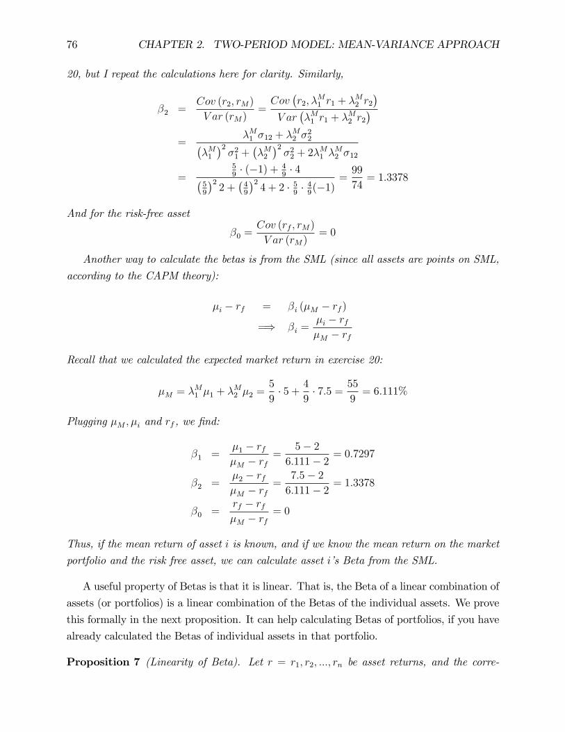
76 CHAPTER 2. TWO-PERIOD MODEL: MEAN-VARIANCE APPROACH
20, but I repeat the calculations here for clarity. Similarly,
�2 =Cov (r2; rM)
V ar (rM)=Cov
�r2; �
M1 r1 + �M2 r2
�V ar
��M1 r1 + �M2 r2
�=
�M1 �12 + �M2 �22�
�M1�2�21 +
��M2�2�22 + 2�
M1 �
M2 �12
=59� (�1) + 4
9� 4�
59
�22 +
�49
�24 + 2 � 5
9� 49(�1)
=99
74= 1:3378
And for the risk-free asset
�0 =Cov (rf ; rM)
V ar (rM)= 0
Another way to calculate the betas is from the SML (since all assets are points on SML,
according to the CAPM theory):
�i � rf = �i (�M � rf )
=) �i =�i � rf�M � rf
Recall that we calculated the expected market return in exercise 20:
�M = �M1 �1 + �M2 �2 =5
9� 5 + 4
9� 7:5 = 55
9= 6:111%
Plugging �M ; �i and rf , we �nd:
�1 =�1 � rf�M � rf
=5� 2
6:111� 2 = 0:7297
�2 =�2 � rf�M � rf
=7:5� 26:111� 2 = 1:3378
�0 =rf � rf�M � rf
= 0
Thus, if the mean return of asset i is known, and if we know the mean return on the market
portfolio and the risk free asset, we can calculate asset i�s Beta from the SML.
A useful property of Betas is that it is linear. That is, the Beta of a linear combination of
assets (or portfolios) is a linear combination of the Betas of the individual assets. We prove
this formally in the next proposition. It can help calculating Betas of portfolios, if you have
already calculated the Betas of individual assets in that portfolio.
Proposition 7 (Linearity of Beta). Let r = r1; r2; :::; rn be asset returns, and the corre-

2.2. CAPITAL ASSET PRICING MODEL (CAPM) 77
sponding Betas are �1; �2; :::; �n. Consider a protfolio with wieghts � = [�1; �2; :::; �n]0, and
return r� = �1r1 + �2r2 + :::+ �nrn. Let �� be the Beta risk of this portfolio. Then,
�� = �1�1 + �2�2 + :::+ �n�n
Proof. Applying the de�nition of Beta on the portfolio:
�� =Cov (r�; rM)
�2M=Cov (�1r1 + �2r2 + :::+ �nrn; rM)
�2M
=�1Cov (r1; rM) + �2Cov (r2; rM) + :::+ �nCov (rn; rM)
�2M
= �1Cov (r1; rM)
�2M+ �2
Cov (r2; rM)
�2M+ :::+ �n
Cov (rn; rM)
�2M= �1�1 + �2�2 + :::+ �n�n
The above result can be used to calculate Betas of portfolios, when the individual Betas
are known, as illustrated in the next example.
Example 11 Suppose the betas on three assets are �1 = 0:5, �2 = 0:8, and �3 = 1:4.
Calculate the beta on a portfolio, which combines these assets with weights �1 = 0:3, �2 = 0:2,
�3 = 0:5. Then, the Beta of the portfolio is
�� = �1�1 + �2�2 + �3�3
= 0:3 � 0:5 + 0:2 � 0:8 + 0:5 � 1:4= 0:15 + 0:32 + 0:7 = 1:17
2.2.2 CAPM in practice
In this chapter we studied optimal portfolio selection under the assumption that all investors
care about is the mean and variance of the return to their investment. In other words, we
assumed that preferences are described by the Mean-Variance Theory (MVT). This is not
the same as assuming that there is only one investor, or that all investors are identical. In
our examples we assumed that the mean-variance utility of individual i is
ui (�; �) = �� i2�2
Thus, there could be unlimited number of investors, which di¤er by their variance-aversion
(or risk aversion) parameter i.

78 CHAPTER 2. TWO-PERIOD MODEL: MEAN-VARIANCE APPROACH
Despite the di¤erences in preferences among individual investors, we arrived at a striking
conclusion - the Two-Fund Separation Theorem, which implies that all investors will invest in
two funds only: (i) the risk-free asset and (ii) market portfolio. In other words, all investors
will hold the same portfolio of risky assets, which we called the tangent portfolio T, and in
equilibrium is also the market portfolio M. All optimal portfolios then are located on the
Capital Market Line (CML), which connects the risk-free asset with the market portfolio.
The only di¤erence between investors� portfolios is the fraction of their �nancial wealth
invested in the risk-free asset, �0. We have seen in exercise 20 that �0 is increasing in the
investor�s risk-aversion parameter , i.e. more variance-averse investors will hold a larger
portion of their �nancial wealth in the risk-free asset. But nevertheless, all investors will hold
the same market portfolio of risky assets - M. Moreover, we showed that all assets (and all
portfolios for that matter), must lie on the same Security Market Line (SML, or the CAPM
equation), given in equation (2.10):
�i � rf = �i (�M � rf )
The expected excess return on asset i (or any portfolio) is proportional to its Beta
�i =Cov (ri; rM)
V ar (rM)= �iM
�i�M
In reality, investors di¤er substantially in the composition of their risky-assets portfolio.
Thus in reality, the Two-Fund Separation Theorem does not hold. In addition, some investors
(e.g. some hedge funds3) report returns that are above (or below) the expected returns
predicted by the SML. These deviations of actual returns from those predicted by the SML
are called the asset�s Alpha:
�i = �i � rf � �i (�M � rf ) (2.12)
The term �i � rf is the expected excess return on asset i, and �i (�M � rf ) is the predictedexcess return by the CAMP (SML). Figure 2.9 shows two such assets (or portfolios), which
deviate from the SML. Asset i has mean return higher than the one predicted by the SML
(positive Alpha), while asset j has mean return lower than the predicted by SML (negative
3A hedge fund is an investment fund that can undertake a wider range of investment and trading activitiesthan other funds, but which is only open for investment from particular types of investors speci�ed byregulators. These investors are typically institutions, such as pension funds, university endowments andfoundations, or high net worth individuals. As a class, hedge funds invest in a diverse range of assets, butthey most commonly trade liquid securities on public markets. They also employ a wide variety of investmentstrategies, and make use of techniques such as short selling and leverage. http://en.wikipedia.org/wiki/Hedge_fund

2.2. CAPITAL ASSET PRICING MODEL (CAPM) 79
Alpha).
M
SML
1
Figure 2.9: The Alpha of an asset (or portfolio).
Our �rst instinct tells us that positive Alpha of an asset (or portfolio) is an indicator that
the asset outperformed the market, and had average return above what the theory (CAPM)
predicts. Similarly, a negative Alpha indicates that an asset (or portfolio) underperforming,
and delivering returns below the levels required by its Beta risk. A very appealing (butdangerous!) investment strategy of buying assets with positive Alpha and short sellingassets with negative Alpha. In fact, many hedge funds emerged (and sunk), promising to
generate Alpha - i.e. higher returns and lower risks than the market. Goldman Sachs used
to have �Global Alpha�, which closed in 2011 after large losses. Before adopting a strategy
based on the "quest for Alpha", we need to understand the reasons behind observing non-zero
Alphas.
One explanation for observing non-zero Alphas is that di¤erent investors tend to specialize
in di¤erent subsets of assets. If a hedge fund specializes in particular industries, its tangent
portfolio will consist of that industry�s securities. The derivation of the CAPM shows that
if the tangent portfolio consists of a group of assets, then all the assets that make up the
tangent portfolio, or any combination of these assets, must have Alpha of zero. However,

80 CHAPTER 2. TWO-PERIOD MODEL: MEAN-VARIANCE APPROACH
when we introduce a new asset, that was not considered by the hedge fund, that asset is
likely to have a non-zero Alpha with respect to the previous tangent portfolio. The next
exercise illustrates this point.
Exercise 23 Consider asset market with risk-free return rf = 2% and two risky assets with
returns r1; r2, and mean returns and covariance matrix as follows:
� =
"�1
�2
#=
"5%
7:5%
#, � =
"�21 �12
�21 �22
#=
"2% �1%�1% 4%
#
We found in exercise 20 that the market (tangent) portfolio is �M1 = 59and �M2 = 4
9. Now,
suppose that a new asset, that we were not aware of before, appears, and the three risky assets
are now:
� =
264 �1
�2
�3
375 =264 5%
7:5%
10%
375 , � =
264 �21 �12 �13
�21 �22 �23
�31 �32 �23
375 =264 2% �1% �2%�1% 4% 6%
�2% 6% 10%
375Show that the new asset has positive Alpha with respect to the tangent portfolio that we found
based on the �rst two risky assets only.
Solution 23 We need to predict the return on the new asset using CAPM. The mean returnon the tangent portfolio based on the �rst two assets is (we already found it in exercise 20):
�T = �T1 �1 + �T2 �2 =5
9� 5 + 4
9� 7:5 = 55
9= 6:111%
The new asset�s Beta is:
�3 =Cov (r3; rM)
V ar (rM)=Cov
�r3; �
M1 r1 + �M2 r2
�V ar
��M1 r1 + �M2 r2
�=
�M1 �31 + �M2 �32��M1�2�21 +
��M2�2�22 + 2�
M1 �
M2 �12
=59� (�2) + 4
9� 6�
59
�22 +
�49
�24 + 2 � 5
9� 49(�1)
=63
37= 1:703
The predicted return on the new asset is:
�3 = rf + �3 (�M � rf )= 2 + 1:703 � (6:111� 2) = 9%

2.2. CAPITAL ASSET PRICING MODEL (CAPM) 81
The actual mean return on asset 3 is given to be 10%, therefore �3 = 10%� 9% = 1%.
The last exercise shows that an asset that was neglected by investors, might appear
to have positive Alpha, but this Alpha is measured with respect to the previous tangentportfolio. Once the new asset is available, it will change the opportunity set (increase it),
and a new market portfolio will emerge. The new asset then will have a zero Alpha with
respect to the new market portfolio. Obviously, the utility of all investors must improve
since the new CML will be higher than the old one. Verify this with Matlab. Using Matlab
code CML:m, �nd the tangent (market) portfolio based on all three assets, and verify that all
three assets have Alpha of zero with respect to the new market portfolio.
Another explanation for observing non-zero Alphas, is that di¤erent investors have dif-
ferent beliefs about the mean (and possibly the covariance) of returns on assets. This leads
to the Heterogeneous Beliefs CAPM. Of course if all investors estimate the means and co-
variances based on the same sample of historical data, then we do not expect to see any
di¤erences in beliefs among them. However, if investors also analyze �nancial statements,
and use economic forecasting to predict future returns, then it is possible that beliefs are dif-
ferent. For example of two risky assets, suppose that investor 1 believes that �1 = [2%; 4%]0,
while investor 2 believes �2 = [3%; 5%]0. These investors, when actively managing their
portfolios, will �nd di¤erent tangent portfolios: �ji is the share of risky asset i in the risky
assets portfolio of individual j. Suppose there are I investors, and n risky assets. Investor j
has �nancial wealth wj invested in risky assets (this is 1� �j0 of his total �nancial wealth).Then the market portfolio weight of asset i is given by
�Mi =
PIj=1 �
jiwjPn
i=1
PIj=1 �
jiwj
=
PIj=1 �
jiwjPI
j=1wj
nXi=1
�ji| {z }=1
=
PIj=1 �
jiwj
W=
IXj=1
�ji
�wjW
�(2.13)
where wj=W is the relative size of risky assets portfolio of investor j, as a fraction of total
�nancial wealth W invested in risky assets by all investors (W can be seen as the market
value of all stocks in say the New York Stock Exchange). The market portfolio shares of
assets in equilibrium, are weighted averages of individual investors, where the weights are
the relative "sizes" of investors�portfolios.
Example 12 Suppose that the market consists of two investors A and B. Their portfolio
shares in asset i are �Ai = 0:3 and �Bi = 0:4, and their wealth in risky assets is w
A = $200

82 CHAPTER 2. TWO-PERIOD MODEL: MEAN-VARIANCE APPROACH
and wB = $300. The market portfolio weight on asset i is therefore:
�Mi = �AiwA
wA + wB+ �Bi
wB
wA + wB= 0:3 � 200
500+ 0:4 � 300
500= 0:36
We know from CAPM, that when each investor evaluates assets or portfolios relative to
his tangent portfolio j, then all assets must lie on his SML, he should not see any Alpha forany asset. Investor j SML is given by:
�ji = �i � rf � �i��Tj � rf
�= 0
where Tj is the tangent portfolio of investor j. However, when investor j evaluates his
portfolio relative to the market portfolio (using his own beliefs), then the investor might �nd
non-zero alpha for his portfolio:
�ji = �i � rf � �i (�M � rf ) 6= 0
. Under some assumptions, it can be shown that on average, investors cannot all have
positive Alphas all the time, and the sum of all Alphas for any given asset must be zero. In
this sense, the CAPM equilibrium is a Zero Sum Game.
The practical implication of this is that all investors need to choose whether to actively
manage their portfolio (be active investors) or be passive. Active investors will choose their
own tangent portfolio, while passive investors will simply invest in some mutual fund (index
fund), for example in NYSE index, and thereby adopt the market portfolio. There has been
research about which investors should be passive and which should be active. One needs to
remember that � and � are not given, and active investors must estimate the mean returns
and covariances based on historical data, and sometimes make predictions based on �rm-
speci�c factors, industry-speci�c factors and macroeconomic forecasts. Thus, being active
investor entails a cost, and it can be shown theoretically that only the most e¢ cient and
informed investors will be active in equilibrium.
Exercise 24 (Heterogeneous beliefs CAPM). Let the risk-free return be rf = 1%, and sup-pose there are two risky assets with true mean returns and covariance matrix:
� =
"2%
2%
#; � =
"2% 0
0% 2%
#
The market consists of 4 groups of investors, who di¤er according to their beliefs of the mean

2.2. CAPITAL ASSET PRICING MODEL (CAPM) 83
returns:
�1 =
"6%
1%
#, �2 =
"3%
2%
#, �3 =
"2%
3%
#, �4 =
"1%
5%
#All investors have the same mean-variance utility u (�; �) = ��
2�2, and the same variance
aversion parameter = 2. In addition, all groups of investors have the same �nancial wealth
w = 10 invested in the risky assets.
(i) Find the optimal portfolio and the tangent portfolio of all investors, assuming that
they are active.
(ii) Find the market portfolio, and calculate the true mean and variance of its return.
(iii) Calculate the SML based on the market portfolio and the assets true mean returns.
(iv) Show that given his own (incorrect) beliefs about expected returns, investor 4 will
report that his chosen portfolio has positive Alpha.
Solution 24 (i) In exercise 20, we found analytically the optimal portfolios for investorswho have only two risky assets:
�opt1 =1
"�1 � rf � �12
�22(�2 � rf )
�21 � �212=�22
#
�opt2 =1
"�2 � rf � �12
�21(�1 � rf )
�22 � �212=�21
#�opt0 = 1� �opt1 � �
opt2
And the tangent portfolios are found after normalization:
�T1 =�opt11� �0
, �T2 =�opt21� �0
Notice that the numbers in this exercise were chosen such that you can �nd the tangent
portfolios without a calculator. For example the fact that asset returns are uncorrelated,
helps a lot. Plugging the given numbers, we obtain the tangent portfolios for all investors:
Investors
1 2 3 4
�opt1 1:25 0:5 0:25 0
�opt2 0 0:25 0:5 1
�opt0 �0:25 0:25 0:25 0
�T1 1 23
13
0
�T2 0 13
23
1

84 CHAPTER 2. TWO-PERIOD MODEL: MEAN-VARIANCE APPROACH
(ii) Using (2.13), we �nd the market portfolio weights, where !j = wj=W = 1=4 is the
relative �nancial wealth invested in risky assets by investor j, as a fraction of total �nancial
wealth W of all investors:
�M1 =
IXj=1
�ji!j =1
4
�1 +
2
3+1
3+ 0
�=1
2
�M2 =IXj=1
�ji!j =1
4
�0 +
1
3+2
3+ 1
�=1
2
This means that the market portfolio has equal shares of both risky assets. In terms of
�nancial wealth, the total wealth of 40 is equally divided among the two assets.
The true mean return on the market portfolio is:
�M = �M1 �1 + �M2 �2 = 0:5 � 2 + 0:5 � 2 = 2%
The true variance of the market portfolio is:
�2M = V ar��M1 r1 + �M2 r2
�=
��M1�2�21 +
��M2�2�22 + 2�
M1 �
M2 Cov (r1; r2)
=
�1
2
�22 +
�1
2
�22 = 1%
Notice that all investors see this true variance of the market portfolio, because they all have
correct beliefs about the variances and covariances of assets.
(iii) The SML (based on true mean returns) is given by:
�i = rf + �i (�M � rf )
Plugging the true values for �M and rf , gives the following SML:
�i = 1 + �i (2� 1)�i = 1 + �i
Notice that since investors have di¤erent beliefs about the mean returns, they will have dif-
ferent perceived SML. You should verify that investors 2 and 3 will have the same perceivedSML, which di¤ers from the SML perceived by investor 1 and also from that of investor 4.
No investor will perceive the correct SML.
(iv) Given investor 4 beliefs, he will think that his portfolio has an Alpha of 2%. His

2.2. CAPITAL ASSET PRICING MODEL (CAPM) 85
portfolio consists of 100% invested in risky asset 2. Thus, the beta of his portfolio is
�2 =Cov
�r2; �
M1 r1 + �M2 r2
��2M
=�M2 V ar (r2)
�2M
=0:5 � 21
= 1
Note that because all investors observe the market shares and all agree on the covariance
matrix, then all investors will �nd the same betas. Investor 4 believes that his portfolio mean
is �T4 = 5%, and his perceived mean of return on the market portfolio is
�4M = 0:5 � 1 + 0:5 � 5 = 3%
Thus, he will report that his own portfolio has the following Alpha:
�4 = �4 � rf � �2��4M � rf
�= 5� 1� 1 � (3� 1) = 2%
However, if we examine the portfolio of investor 4, equipped with correct beliefs about meanreturns, we would see that his portfolio and the market portfolio both have expected returns
of 2%, and his Alpha is zero. Moreover, notice that this investor is taking twice the risk of
the market portfolio, since he is not diversifying and investing 100% in risky asset 2 (his
portfolio variance is 2%, while market portfolio variance is only 1%, while the true mean
return on the market portfolio is the same as the mean return on this investor�s portfolio:
2%). Thus, often those hedge funds that report positive Alpha, are simply misguided about
the true expected returns on assets.
It is far from obvious which strategy is better for a given investor - being active or passive
when investors have heterogeneous beliefs. An active investor chooses his tangent portfolio
based on his beliefs about returns. If instead an investor chooses to be passive, and adopts
the market portfolio, then he still needs to solve the allocation problem between risk-free
asset and the market portfolio. A passive investor�s portfolio has return
r = �0rf + (1� �0) rM
with mean and variance
� = �0rf + (1� �0)�M�2 = (1� �0)2 �2M

86 CHAPTER 2. TWO-PERIOD MODEL: MEAN-VARIANCE APPROACH
Thus, a passive investor solves:
max�0
�0rf + (1� �0)�M �
2(1� �0)2 �2M
The �rst order condition is:
rf � �M + (1� �0)�2M = 0
1� �0 =�M � rf �2M
Notice that the fraction invested in the market portfolio, 1 � �0, depends positively on theexcess return of the market portfolio, and negatively on its variance and the variance-aversion
parameter.
With heterogeneous beliefs however (i.e. in the real world), the mean return on the
market portfolio, �M , is not given, and investors need to form some beliefs about it. There
are several alternative assumptions that we can make about how such passive individual
investors would form beliefs about the mean return on the market portfolio. It makes sense
to assume that the same beliefs that investors have for individual assets, also apply to the
market portfolio. An alternative assumption about aggregating beliefs is the so-called average
beliefs of investors. Thus, if the weights of the market portfolio are �M =��M1 ; �
M2 ; :::; �
Mn
�0,
and the beliefs about individual assets returns of investor j are �j =��M1 ; �
M2 ; :::; �
Mn
�0, then
that individual beliefs about the mean return on the market portfolio is
�jM =��M�0�j
Thus, given these beliefs about the market portfolio, a passive investor j will choose
1� �j0 =�jM � rf �2M
If this investor is active, he chooses his own tangent portfolio T j.
In order to determine whether particular investor is better o¤ being active or passive, we
need to compare their utility when active and passive. There are several ways of doing that
as well. Since utility depends on the mean and variance of the optimal portfolio, once again
we have several alternatives of computing such utility. For example we can compute the ex-
ante (before investing) utility, using the investor�s beliefs about mean returns. Alternatively,
we can compute the ex-post (after investing) utility, using the true returns on assets. We
might get di¤erent answers to the question of who should be active and who should be

2.2. CAPITAL ASSET PRICING MODEL (CAPM) 87
passive investor, depending on the assumptions we make about how investors form beliefs
about individual assets and the market portfolio, and depending on which notion of utility
we use. In addition, a model that investigates the decision between passive and active, must
incorporate the costs of being active versus passive. There is an ongoing research on this
topic, and if you are interested see the references in the textbook and the authors�web pages.

88 CHAPTER 2. TWO-PERIOD MODEL: MEAN-VARIANCE APPROACH

Chapter 3
General Principles of Asset Pricing
In the previous chapter we assumed that investors care only about mean and variance of
the return to their portfolio, and under this very restrictive assumption, we developed a
theory of optimal portfolio selection. In addition, the mean-variance assumption allowed us
to derive a theoretical prediction about individual asset returns - the CAPM (or the SML).
In this chapter we would like to relax the assumption of mean-variance utility, and ask what
can we say about asset prices in general, even if we have no knowledge about individuals�
preferences and their beliefs. Introducing the economic concepts of Law of One Price and
Arbitrage, will allow us to impose restrictions on asset prices, even without knowledge of
individual preferences. One would expect that regardless of investors�attitude towards risk,
any individual would like to get a "free lunch", i.e. get something for nothing. These
free lunches are called arbitrage opportunities, and we expect that well functioning markets
should not have such opportunities. The no-arbitrage principle will help us price certain
(redundant) assets in terms of other (fundamental) assets. The no-arbitrage principle is
especially useful for pricing derivatives, such as options. We then extend the analytical
framework to a general equilibrium asset pricing model, which embodies other �nancial
models (CAPM, and Arbitrage Pricing Theory) as special cases.
3.1 Assets and Portfolios in a Two-Period Model
In this section we introduce the general framework for analyzing �nancial markets.
3.1.1 Financial markets
We continue assuming, as in the previous chapter, that there are only two periods in the
economy, the �rst period (denoted 0) and the second period (denoted 1). There is no
89

90 CHAPTER 3. GENERAL PRINCIPLES OF ASSET PRICING
uncertainty in the current period, but uncertainty in the next period is captured by some
abstract S possible states of the world (or states of nature), s = 1; 2; :::; S. Figure 3.1
illustrates this uncertainty about the future in an event tree. The state of the world in the
Figure 3.1: Event tree.
�rst period, t = 0, is s = 0. In the second period there are S possible states of the world. For
example, suppose that there are three states of the world that describe the macroeconomic
performance: s = 1 if the economy is doing good, s = 2 if the economy is normal, and
s = 3 if the economy is bad (say recession). In general, the number of possible states can
be �nite or in�nite, with some probability distribution. Notice that this representation of
uncertainty is much more general than in the mean-variance analysis, where the uncertainty
was captured by two numbers - mean and variance.
Suppose there are K �nancial assets, indexed by k = 1; :::; K. Investors trade in assets
in the �rst period, and receive payo¤ in the second period. Assets payo¤s can depend on
the states of the world. Let Aks denote the payo¤ that a holder of 1 unit of asset k receives
in state s. The payo¤s of all assets in di¤erent states are described by the state-asset payo¤

3.1. ASSETS AND PORTFOLIOS IN A TWO-PERIOD MODEL 91
matrix :
A =
266664A11 A21 � � � AK1
A12 A22 � � � AK2...
......
A1S A2S � � � AKS
377775S�K
Notice that the rows of A represent the states of the world in the second period (t = 1),
while the columns of A represent the assets. The units of payo¤s could be monetary (e.g.
dollars), or units of output. Monetary payo¤s are called nominal payo¤s, while payo¤s in
units of output are called real payo¤s.
Example 13 The following is a payo¤ matrix for a �nancial market with 3 assets, and 4states of the world. The payo¤s in this example are nominal, in dollars.
A =
266664$2 $1 $4
$2 $2 $1
$2 $4 $1
$2 �$1 $0
3777754�3
The �rst asset, k = 1, has a payo¤ of $2 in all the states. Therefore, asset 1 is the risk-free
asset. The second asset pays $1 in state 1, $2 in state 2, $4 in state 3 and �$1 in state 4.Similarly, the 3rd asset pays 4; 1; 1; 0 in states 1; 2; 3; 4. Notice that assets 2 and 3 are risky
because in period t = 0, we don�t know which state of the world will realize in the next period
(t = 1).
Example 14 The following is a payo¤ matrix for a �nancial market that has 3 assets andthere are also 3 states of the world. The payo¤s are:
A =
264 $1 0 0
0 $1 0
0 0 $1
3753�3
Here each asset pays $1 in one state only, and zero in all other states. Asset 1 pays $1 in
state 1 only, asset 2 pays $1 in state 2 only, etc. An asset that pays 1 unit of payo¤ in one
state only, and zero in all other states, is called the state claim or Arrow security, afterthe economist Kenneth Arrow.

92 CHAPTER 3. GENERAL PRINCIPLES OF ASSET PRICING
The prices of all assets can be represented by a vector:
q =
266664q1
q2
...
qK
377775K�1
where qk is the price of asset k.
De�nition 22 A �nancial market (or asset market) consists of a payo¤ matrix A anda price vector q. We therefore denote a �nancial market by the pair (A; q).
Notice that the above de�nition omits investors (consumers), and their preferences, beliefs
and incomes. Eventually, our goal is to describe a general equilibrium model of an economy,
with �nancial markets and markets for other goods. In such an economy, investors trade
goods and �nancial assets, and the prices of �nancial assets, q, are determined in equilibrium.
However, as stated in the introduction, there are several important results about asset prices
that we can obtain without any discussion of investors�preferences. Therefore, it is useful
for now to focus on a �nancial markets consisting of asset payo¤s and prices only, (A; q).
From payo¤matrix A and asset prices, we can obtain the asset returns, which we studied
in the previous chapter. Given the payo¤s and asset prices, the gross rate of return on asset
k in state s is:
Rks =Aksqk
The net return on asset k in state s is therefore:
rks = Rks � 1
Our goal in this chapter is to develop a theory for determination of asset prices q, but it is
equivalent to having a theory of rates of returns.
Example 15 Suppose the payo¤ matrix and asset prices are given as follows:
A =
264 1 1
1 2
1 2
3753�2
, q =
"0:8
1:25
#2�1
Thus, in this �nancial market there are two assets, with the �rst one being risk-free. The

3.1. ASSETS AND PORTFOLIOS IN A TWO-PERIOD MODEL 93
gross returns on the assets are:
R =
26410:8
11:25
10:8
21:25
10:8
21:25
375 =264 1:25 0:8
1:25 1:6
1:25 1:6
375The net returns on the assets are:
r = R� 1 =
264 0:25 �0:20:25 0:6
0:25 0:6
375The net return on the risk-free asset is therefore 25% in all states, and the net return on the
risky asset is �20% in state 1 and 60% in states 2 and 3.
In this chapter, portfolios will be represented by the actual units of assets, and not in
terms of the fractions of �nancial wealth they represent. Let �k be the number of units of
asset k in a given investor�s portfolio. The entire portfolio is then:
� =
266664�1
�2
...
�K
377775K�1
Example 16 The following is the portfolio of some investor:
� =
266664�73
5
0
3777754�1
This investor has a short position of �7 units of asset 1 (an obligation to pay back 7 unitsof asset 1), and long positions of 3 and 5 units in assets 2 and 3 respectively. The investor
does not hold any units of asset 4.
Given the payo¤matrix A and portfolio �, we can obtain the investor�s payo¤s from the

94 CHAPTER 3. GENERAL PRINCIPLES OF ASSET PRICING
portfolio in all states by:
P = A� =
266664A11 A21 � � � AK1
A22 A22 � � � AK2...
......
A1S A2S � � � AKS
377775S�K
266664�1
�2
...
�K
377775K�1
=
266664A1�
A2�...
AS�
377775S�1
Here As is the s row of A, and it contains the payo¤s of all assets in state s. Since A is
S � K and � is K � 1, the product A� is S � 1, and each element is the payo¤ from the
portfolio in state s. In particular, investor�s payo¤ from portfolio � in state s is:
Ps =
KXk=1
Aks�k
Exercise 25 Suppose the payo¤ matrix on assets and investor�s portfolio are given by
A =
266664$2 $1 $4
$2 $2 $1
$2 $4 $1
$2 �$1 $0
3777754�3
, � =
264 �132
3753�1
Notice that this investor has a short position of �1 units in asset 1, and long positions of3 and 2 units in assets 2 and 3 respectively. Calculate the payo¤ this investor receives from
his portfolio in all 2nd period states of the world.
Solution 25 Notice that in this economy there are 3 �nancial assets and 4 states of theworld. The investor�s payo¤s are:
P = A� =
2666642 1 4
2 2 1
2 4 1
2 �1 0
3777754�3
264 �132
3753�1
=
2666642 � (�1) + 1 � 3 + 4 � 22 � (�1) + 2 � 3 + 1 � 22 � (�1) + 4 � 3 + 1 � 2
2 � (�1) + (�1) � 3 + 0 � 2
3777754�1
=
2666649
6
12
�5
3777754�1
in state 1
in state 2
in state 3
in state 4
Thus, the portfolio delivers payo¤s of 9; 6; 12;�5 is states of the world 1; 2; 3; 4 respectively.

3.1. ASSETS AND PORTFOLIOS IN A TWO-PERIOD MODEL 95
Notice that if individual asset prices are given by q, then the price of a portfolio � is q0�
or �0q. Since q01�K and �K�1, the product is a scalar (number).
Example 17 Suppose the price vector and two portfolios, �1 and �2, are given:
q =
2666645
2
1
7
377775 , �1 =
266664�23
10
0
377775 , �2 =
266664�32
0
1
377775The price of portfolio �1:
q0�1 =h5 2 1 7
i266664�23
10
0
377775= 5 � (�2) + 2 � 3 + 1 � 10 + 7 � 0 = 6
The price of portfolio �2:
q0�2 =h5 2 1 7
i266664�32
0
1
377775= 5 � (�3) + 2 � 2 + 1 � 0 + 7 � 1 = �4
Notice that the price of the second portfolio is negative due to short sells of the �rst asset.
In the previous chapter we used �k to denote the fraction of the �nancial wealth invested
in asset k, while in this chapter we introduced the notation �k to be the number of units of
asset k in the portfolio. These two notations can be related as follows:
�k =�kqkPKi=1 �
iqi=�kqk
�0q
The numerator is the monetary value invested in asset k, which is the number of units held
�k times the unit price qk. The denominator is the total value of all assets in the investor�s
portfolio. Therefore, the above gives the fraction of the portfolio invested in asset k.

96 CHAPTER 3. GENERAL PRINCIPLES OF ASSET PRICING
Example 18 The price vector q and portfolio � are given:
q =
2666642
4
3
1
377775 , � =
2666644
1
2
3
377775The total value of assets in the portfolio is
q0� =h2 4 3 1
i2666644
1
2
3
377775 = 21
Thus, the portfolio shares are:
� =1
21
2666642 � 44 � 13 � 21 � 3
377775 =266664
821421621321
3777753.1.2 Redundant assets
A portfolio is uniquely determined by the portfolio quantities: � =��1; �2; :::; �K
�0, while
the portfolio payo¤s in all S states are uniquely determined by the product A�, which is
S � 1 vector. However, it is possible that the same payo¤s can be achieved with di¤erentportfolios.
De�nition 23 A portfolio � is replicable if there is another portfolio, with di¤erent assetholdings �, such that their payo¤s are equal:
A� = A�, � 6= �
The de�nition of replicable portfolio also applies to portfolios consisting of one asset only.
In this case, we say that an asset is redundant if its payo¤can be replicated by some portfolio
of other assets.
De�nition 24 An asset k is called redundant asset if its payo¤ can be replicated by aportfolio of other assets.

3.1. ASSETS AND PORTFOLIOS IN A TWO-PERIOD MODEL 97
Example 19 Suppose the �nancial market has the following payo¤ matrix:
A =
"1 0 3
0 1 7
#2�3
This �nancial market consists of 3 assets and 2 states of the world in the second period. The
third asset (third column of A) is redundant because its payo¤ can be replicated with portfolio
of the �rst two assets: � = [3; 7; 0]0. The payo¤ of this portfolio is
A� =
"1 0 3
0 1 7
#2�3
264 370
3753�1
=
=
"1 � 3 + 0 � 7 + 3 � 00 � 3 + 1 � 7 + 7 � 0
#2�1
=
"3
7
#2�1
Thus, the payo¤ of portfolio � = [3; 7; 0]0 is the same as (replicates) the payo¤ of asset 3.
Therefore, asset 3 is redundant asset. We call assets that are non-redundant - primitiveassets.
Mathematically, the presence of redundant assets means that the columns of the payo¤
matrix are linearly dependent. Think of each column of A as a vector vk, and all the columns
are v1; v2; :::; vK .
De�nition 25 We say that vectors v1; v2; :::; vn are linearly dependent if there exist nnumbers, a1; a2; :::; an, not all zero, such that
a1v1 + a2v2 + :::+ anvn = 0
In the last example, letting the three columns of the payo¤ matrix be vectors v1; v2 and
v3, we have v3 = 3v1 + 7v2, or:
3v1 + 7v2 � v3 = 0
Thus, the columns of the payo¤ matrix are linearly dependent.
For completeness of our discussion, we also de�ne linearly independent vectors.
De�nition 26 We say that vectors v1; v2; :::; vn are linearly independent if
a1v1 + a2v2 + :::+ anvn = 0

98 CHAPTER 3. GENERAL PRINCIPLES OF ASSET PRICING
only for a1 = a2 = ::: = an = 0. That is, the only way that a linear combination of the
vectors can be equal the zero vector, is multiplying each vector by zero.
We should not think of redundant assets as unimportant. In fact, as we will see later,
options (or �nancial derivatives) are redundant assets since their payo¤s can be replicated
with portfolio of a bond and an underlying asset (e.g. stock in the case of a stock option).
The fact that some assets are redundant, and their payo¤s can be replicated with portfolios
of other assets, simply allows us to price these assets in terms of the replicating assets.
3.1.3 Complete markets
We discuss the notion of complete markets in an economy with K risky assets and S states.
In general, a �nancial market is complete if all second period consumption plans can be
achieved with some trade in assets.
De�nition 27 A consumption plan for second period is a vector c 2 RS,
c =
266664c1
c2...
cS
377775S�1
such that cs is the consumption in state s.
De�nition 28 An asset market with payo¤ matrix AS�K is complete if for any consump-tion plan c 2 RS, there exists a portfolio � 2 RK such that A� = c.
First, market completeness does not mean that all investors can a¤ord any consumption
they want. The portfolios � in the de�nition of complete markets are not free, so investors
will be able to buy only those portfolios that satisfy their budget constraint. Second, market
completeness is an idealized and not realistic assumption, but it allows us to obtain unique
asset pricing.
Example 20 Suppose the �nancial market has the following payo¤ matrix:
A =
264 1 0 0
0 1 0
0 0 1
3753�3

3.1. ASSETS AND PORTFOLIOS IN A TWO-PERIOD MODEL 99
Is this �nancial market complete? The answer to this question depends on whether any
consumption plan c = [c1; c2; c3]0 can be achieved with some portfolio � =
��1; �2; �3
�0. In
other words, A is complete if the next system has a solution for all c 2 RS:
A� = c264 1 0 0
0 1 0
0 0 1
375264 �1
�2
�3
375 =
264 c1
c2
c3
375The solution is �1 = c1, �
2 = c2, �3 = c3. Thus, A is complete.
Example 21 Suppose the �nancial market has the following payo¤ matrix:
A =
264 1 0
0 1
0 0
3753�2
Is this �nancial market complete? Can we �nd a portfolio � =��1; �2
�0of the 2 assets
such that any second period consumption c = [c1; c2; c3]0 can be achieved? We see right
away that both assets pay 0 in state 3 of the world. Therefore, it is impossible to achieve
consumption plans c 2 RS with c3 6= 0. For instance, no portfolio of the two assets can
achieve consumption plans with c3 = 23. Thus, A is incomplete.
Notice that in the above example, we had fewer assets than states of the world, i.e.
K < S and that both assets have zero payo¤ in state 3. The next example shows that even
if the two assets in the last example delivered non-zero payo¤s in the third state, the market
would still be incomplete.
Example 22 Suppose the �nancial market has the following payo¤ matrix:
A =
264 1 0
0 1
1 1
3753�2
Is this �nancial market complete? The payo¤s generated from some portfolio � are:
A� =
264 1 0
0 1
1 1
375" �1
�2
#=
264 �1
�2
�1 + �2
375 =264 c1
c2
c3
375

100 CHAPTER 3. GENERAL PRINCIPLES OF ASSET PRICING
Thus, only consumption plans with c3 = c1 + c2 can be achieved with asset trades in this
market. This is because the payo¤ in state 3 is always the sum of payo¤s in states 1 and 2,
no matter what portfolio is purchased. For example, c = [5; 6; 11]0 can be achieved, but not
c = [5; 6; 4]0. Thus, A is incomplete.
The next example illustrates that even if the number of assets is greater than the number
of states, and even if there are payo¤s in all states, the market can still be incomplete.
Example 23 Suppose the �nancial market has the following payo¤ matrix:
A =
264 1 0 1 4
0 1 1 �31 1 2 1
3753�4
Is this �nancial market complete? Can we �nd a portfolio � =��1; �2; �3; �4
�0of the 4
assets such that any second period consumption c = [c1; c2; c3]0 can be achieved? The payo¤s
generated from some portfolio � are:
A� =
264 1 0 1 4
0 1 1 �31 1 2 1
375266664�1
�2
�3
�4
377775 =264 �1 + �3 + 4�4
�2 + �3 � 3�4
�1 + �2 + 2�3 + �4
375 =264 c1
c2
c3
375
It is less obvious that A is incomplete, but a careful observation reveals that only consumption
plans with c3 = c1+ c2 can be achieved. This is because the the payo¤ in state 3 is always the
sum of payo¤s in states 1 and 2, regardless of what portfolio is held by the investor. Thus,
consumption plan such as c = [3; 7; 10]0 can be achieved, but not c = [3; 7; 5]0.
In the last example the �nancial market was incomplete despite the fact that there were
more assets than states of the world, K > S. Notice however that assets 3 and 4 are redun-
dant, and can be replicated with a portfolio of the �rst 2 assets. In particular, a portfolio
� = [1; 1; 0; 0]0 replicates the payo¤s of asset 3, while portfolio � = [4;�3; 0; 0]0 replicates thepayo¤s of asset 4. Redundant assets do not enlarge the set of possible consumption plans
that can be achieved in the economy. This set is called asset-span.
De�nition 29 An asset span of a payo¤ matrix AS�K, is the set of all possible consump-tion plans c 2 RS that can be achieved through trade in securities �. Formally, an asset spanis
M (A) =�c 2 RSjc = A� for some � 2 RK

3.1. ASSETS AND PORTFOLIOS IN A TWO-PERIOD MODEL 101
Based on the above de�nition, we can say that a market with payo¤ matrix AS�K is
complete ifM (A) = RS. In other words, the market can span (achieve) any consumptionplan c 2 RS, which is the de�nition of market completeness. Intuitively, based on the aboveexamples, we can say that in order to be able to achieve any consumption plan c 2 RS, wemust have at least S non-redundant assets. In the last example, we had 4 assets, but 2 of
them were redundant, and redundant assets do not enlarge the asset span. Therefore, the
necessary and su¢ cient condition for market completeness is that the payo¤ matrix have
at least as many non-redundant (primitive) assets as the states of the world. Formally,
the number of non-redundant assets is the number of independent columns (or rows) of the
matrix A, is called the rank of A.
Theorem 9 (Market Completeness Theorem). The asset market with payo¤ matrix AS�Kis complete if and only if
rank (A) = S
Notice that the above does not state that rank (A) � S because it is impossible for the
rank of a matrix to be greater than the number of rows or columns. For any matrix AS�K ,
we must have rank (A) � min fS;Kg. The rank of a 3� 7 matrix is therefore no more than3. This is a result of the fundamental theorem of linear algebra. Thus, market with K < S
cannot be complete, because rank (A) � K < S.
3.1.4 Law of One Price
Even though we did not make any assumptions about investors� preferences, one would
expect that investors should not care about the particular portfolios they hold, and only
care about the payo¤s generated by these portfolios in various states. Therefore, we expect
that if two portfolios have the same payo¤, they should also have the same price, i.e. the
law of one price.
De�nition 30 (LOP). We say that the law of one price holds in a �nancial market (A; q),if for any two portfolios � and �,
A� = A� =) q0� = q0�
The next example illustrates an asset market in which the law of one price is violated.

102 CHAPTER 3. GENERAL PRINCIPLES OF ASSET PRICING
Example 24 Suppose the �nancial market has the following payo¤ matrix:
A =
264 1 0 1 4
0 1 1 �31 1 2 1
3753�4
Notce that asset 3 is redundant, and is obtained as a sum of assets 1 and 2. Therefore, the
next two portfolios have the same payo¤s:
� =
2666641
1
0
0
377775 , � =
2666640
0
1
0
377775The payo¤ from both portfolios is
A� = A� =
264 112
375Now suppose that the prices of assets are:
q =
2666640:8
0:7
1:6
1:1
377775This is a violation of LOP because portfolio � costs 1:5 and portfolio �, which has the same
payo¤s, costs 1:6.
Exercise 26 (i) Show that asset 4 in the last example is redundant, i.e. demonstrate howits payo¤ can be replicated with portfolio of assets 1 and 2.
(ii) Veirfy that the price of asset 4 does not violate the LOP.
Solution 26 (i) A replicating portfolio � = [4;�3; 0; 0]0 has the same payo¤ as the asset 4.(ii) The price of the replicating portfolio is q0� = 0:8 � 4 + 0:7 � (�3) = 1:1, which is the
price of asset 4.
Exercise 27 Prove that if there are no redundant assets, then the LOP must holds trivially.

3.1. ASSETS AND PORTFOLIOS IN A TWO-PERIOD MODEL 103
Solution 27 We will show that without redundant, there is only one portfolio that can gener-ate any given payo¤ vector, so LOP must trivially hold. Let � and � be two distinct portfolios
that generate the same payo¤, A� = A� or A (� � �) = 0. Let ak � �k � �k. Notice thatthe left hand side of the equation A (� � �) = 0 can be written as linear combination of thecolumns of A:
a1
266664A11
A22...
A1S
377775+ a2
266664A21
A22...
A2S
377775+ :::+ aK
266664AK1
AK2...
AKS
377775 = 0Since there are no redundant assets, we must have K linearly independent assets, i.e. all the
columns of A must be linearly independent. This implies, by de�nition of linearly independent
vectors, that the above equation can hold only for a1 = a2 = ::: = aK = 0, which means that
� is the same exact portfolio as �.
A simple necessary and su¢ cient condition for the LOP to hold is that every portfolio
with payo¤ zero (in all states), must have a price of zero. This is formally stated in the next
proposition.
Proposition 8 LOP () [A� = 0 =) q0� = 0].
Proof. We �rst prove that LOP =) [A� = 0 =) q0� = 0]. Suppose A� = 0 but q0� 6= 0for some portfolio �. We need to prove that LOP is violated. Consider portfolio �+�, which
has a payo¤ of A (� + �) = A� + A� = 0 + A�. Thus, the payo¤s of the portfolios � and
�+� are the same. However, the price of �+� is q0 (� + �) = q0�+q0�, which is not the same
as q0�. Thus, the LOP is violated, because � and � + � have the same payo¤, but di¤erent
price.
Next, we prove that [A� = 0 =) q0� = 0] =) LOP. Suppose that LOP is violated, so
two portfolios with identical payo¤ have di¤erent price: A� = A� but q0� 6= q0�. Then the
portfolio � � � has zero payo¤, A (� � �) = 0, but non-zero price: q (� � �) 6= 0.If the law of one price does not hold, then the price of any asset or of any portfolio, can
be anything. To see this, �rst note that the zero payo¤, c = 0, can be purchased at any
price because if portfolio � has zero payo¤ and non-zero price (q0� = x 6= 0), then portfolio��, � 2 R, also has zero payo¤ and price q0 (��) = �x 2 R. Next, consider portfolios thatgenerate non-zero payo¤s. For example, suppose A� = c 6= 0. Then adding to � any portfolio� with zero payo¤, still gives the same payo¤ c, but the price of �+ � can be arbitrary, since
the price of � can be arbitrary. Thus, without assuming that the LOP holds in asset markets,
it is impossible to impose any discipline on asset prices. This is the reason why LOP is the

104 CHAPTER 3. GENERAL PRINCIPLES OF ASSET PRICING
minimal assumption that any theory of asset pricing must make. With the LOP assumption
however, we are able to price redundant assets in terms of other primitive (or fundamental)
assets, and with no further assumptions about investors�preferences.
3.1.5 State prices
An asset with payo¤ of 1 unit in state s and 0 in all other states, is called a state claim or
Arrow security. We have encountered these securities in previous examples of payo¤ matrix
A, where Arrow security was a column with payo¤ 1 in one state only, and zeros in all other
states.
Example 25 In the following payo¤ matrix, the �rst 3 assets are state claims of states1; 2; 3.
A =
264 1 0 0 2 �10 1 0 �1 3
0 0 1 7 0
3753�5
In asset pricing, the concept of state prices is fundamental, because all assets and portfo-
lios can be replicated with state claims, provided that we have state claims for all states of the
world. In the last example, the 4th asset can be replicated with a portfolio � = [2;�1; 7; 0; 0]0
of the �rst 3 state claims, and the 5th asset can be replicated with � = [�1; 3; 0; 0; 0]0. Wecan think of state claims as fundamental assets, which can replicate all other assets, provided
that there are enough state claims. In analogy to real numbers, state claims are like the
prime numbers, since all other real numbers can be constructed from the prime numbers.
This also means that the prices of all other assets (or potfolios) can be expressed in terms
of the state prices.
De�nition 31 We call �s the state price of state s, which is the price of the state claimof state s. The vector of all state prices is:
� =
266664�1
�2...
�S
377775S�1
The state prices are known as the Arrow-Debreu prices, after Kenneth Arrow and Gérard
Debreu. If state prices exist, then we can express any price of any security k as the weighted

3.1. ASSETS AND PORTFOLIOS IN A TWO-PERIOD MODEL 105
average of state prices:
qk = �1Ak1 + �2A
k2 + :::+ �SA
kS =
SXs=1
Aks�s
This says that the price of any security k is equal to the sum of its payo¤s in all the states,
times the price per unit of payo¤ in that state (the state price). The vector of all prices of
securities, expressed in terms of state prices, is:
q = A0�
Example 26 Suppose that the payo¤ matrix of some �nancial market is:
A =
264 1 2 �1 1 6 1 0
1 1 3 1 0 2 1
1 3 4 0 1 4 1
3753�7
Notice that none of the assets are state claims (Arrow securities). Nevertheless, suppose that
state prices are given:
� =
264 1
2
0:5
3753�1
Using these state prices we can obtain the prices of all the 7 assets that exist in this �nancial
market.
q = A0� =
2666666666664
1 1 1
2 1 3
�1 3 4
1 1 0
6 0 1
1 2 4
0 1 1
37777777777757�3
264 1
2
0:5
3753�1
=
2666666666664
3:5
5:5
7:0
3
6:5
7:0
2:5
37777777777757�1
In the above example, state prices � were given, and we illustrated how the prices of all
existing assets q could be obtained from the state prices. We did not say anything yet about
where these state prices could come from. All we know at this point is that all the prices of
existing assets, and even assets that could emerge in the future, can be obtained from the
state prices, if such prices existed and were known. Moreover, the payo¤s of any asset can
be replicated by portfolio consisting of state claims. Therefore, it makes intuitive sense that

106 CHAPTER 3. GENERAL PRINCIPLES OF ASSET PRICING
the prices of all assets should emerge from some state prices. Existence of state prices, is
therefore not only convenient device for asset pricing, but also impose discipline on prices of
all other assets. At this point, we need state precisely what we mean by existence of state
prices.
De�nition 32 Let (A; q) be a �nancial market. We say that state prices exist in thismarket if there exists a S � 1 vector � such that
A0� = q
In other words, the existing price vecotor q can be generated from some vector � of state
prices.
Mathematically, existence of state prices is equivalent to existence of a solution � to the
above system of K linear equations and S unknowns. Recall from linear algebra that any
linear system can have either one solution, or in�nitely many solutions, or no solution at all.
Below, we will establish conditions for existence and uniqueness of state prices. But �rst,
lets look at an example of a �nancial market, in which no such state prices exist.
Example 27 Consider the �nancial market (A; q):
A =
"1 0 2
0 1 1
#2�3
, q =
264 112
3753�1
There are no state prices � = [�1; �2] that could have generated the given asset prices q. To
see this, write the de�nition 32 A0� = q:
�1
264 102
375+ �2
264 011
375 =264 112
375This system of 3 linear equations and 3 unknowns can be written as
�1 = 1
�2 = 1
2�1 + �2 = 2
Plugging the �rst two equations into the third gives 3 = 2, which is a contradiction. This

3.1. ASSETS AND PORTFOLIOS IN A TWO-PERIOD MODEL 107
means that the above linear system does not have any solutions, and there are no state prices
that could have generated the observed asset prices.
The above example illustrates that in some �nancial markets (A; q), the price vector
cannot emerge from any state prices. Since the payo¤s of any asset can be expressed as a
portfolio of state claims, the fact that a price vector q in the last example cannot be derived
from any state prices, suggests that something is wrong with this price vector. Indeed, notice
that the law of one price is violated in the last example. The 3rd asset has the same payo¤
as portfolio consisting of 2 units of asset 1 and one unit of asset 2, but the price of the
third asset is 2 while the price of the portfolio with the same payo¤ is 3. Thus, the LOP is
violated in the above �nancial market. As it turns out, the law of one price is a necessary
and su¢ cient condition for existence of state prices, as the next proposition states.
Proposition 9 (Existence of State Prices). State price vector � exists in a �nancial market(A; q) if and only if the Law of One Price holds. That is,
9� () LOP
Proof. First, to prove " =) ", we assume that state price vector � exists, and need to prove
that LOP holds. Let � and � be two portfolios, with the same payo¤s: A� = A�. Since state
price vector � exists, the prices of these portfolios are:
q0� = (A0�)0� = �0A�
q0� = (A0�)0� = �0A�
Since A� = A�, we see from the above that the prices of these portfolios must be the same,
i.e. q0� = q0�.
To prove "(= " we assume that the law of one price holds, and need to prove that stateprice vector � exists. By proposition 8, LOP implies that any portfolio � with zero payo¤,
must have a price of zero:
A� = 0 =) q0� = 0 8�
A� = 0 means that � is orthogonal to the rows of A, while q0� = 0 means that q is orthogonal
to �. Thus, q is orthogonal to any vector � which is orthogonal to the rows of A, and therefore
q must be a linear combination of the rows of A. The coe¢ cients of such linear combination
can serve as the desired state prices � = [�1; �2; :::; �S]0.
The second part of the last proof relies on several major results from linear algebra, and
for those interested, I will brie�y mention them here. First, notice that the desired state

108 CHAPTER 3. GENERAL PRINCIPLES OF ASSET PRICING
prices �, are a solution to the system A0� = q, which can be written as
�1A1 + �2A2 + :::+ �SAS = q
where As is row s of the payo¤ matrix A. Thus, existence of state prices is equivalent
to representing q with some linear combination of the rows of A. The set of all linear
combinations of the rows of AS�K matrix, is called the row space of A, and denoted Row (A),
and it is a subspace of RK (because each row ofA hasK elements). Next, the set of all � 2 RK
such that A� = 0 is called the null space of A, and denoted by Null (A). Moreover, the
set of all vectors orthogonal to some subset W of RK , is called the orthogonal complementof W , and denoted by W?. Thus, the statement A� = 0 =) q0� = 0 reads that for
each � 2 Null (A), the vector q must also be orthogonal to �, so q must be orthogonal
to Null (A) or q 2 Null (A)?. An important theorem of linear algebra establishes that
Row (A)? = Null (A), and therefore Row (A) = Null (A)?. In words, the null space of
any matrix is equal to the orthogonal complement of its row space, and therefore the row
space is the orthogonal complement of the null space (A? = B () B? = A). Thus,
q 2 Row (A), which means that q can be expressed as a linear combination of the rows of A.Such combination may not be unique, but the theorem only establishes existence of such a
linear combination.
Ideally, we would also like the state prices to be unique. We can see that given the
state price vector �, we always obtain a unique asset price vector q. Di¤erent � will lead to
di¤erent q, but if state prices are unique, then each security has a unique price. In example
26, we expressed asset (security) prices in terms of state prices q = A0�. Our intuition tells
us that we should be able to solve this equation for � (if such solution exists) as follows:
(A0)�1q = (A0)
�1A0� = �
The problem is that A0 is K � S, so the inverse is not de�ned (the inverse of a matrix isonly de�ned for square matrices). However, for non-square matrices Am�n, a generalization
of inverse was developed, and one such generalization is the Moore�Penrose pseudoinverse.1
De�nition 33 (Moore�Penrose pseudoinverse). Let Am�n be a matrix. We say that A+ isMoore�Penrose pseudoinverse of A if it satis�es the following four criteria:
1. AA+A = A
2. A+AA+ = A+
1See https://en.wikipedia.org/wiki/Moore-Penrose_pseudoinverse

3.1. ASSETS AND PORTFOLIOS IN A TWO-PERIOD MODEL 109
3. (AA+)0 = AA+
4. (A+A)0 = A+A
A theorem in linear algebra establishes that Moore�Penrose pseudoinverse A+ exists for
any matrix A, and it is unique. This generalized inverse allows establishing existence and
uniqueness of solutions to any linear system with m equations and n unknowns.
Theorem 10 (Existence and uniqueness of solutions to linear systems). Let Ax = b be a
linear system with m equations and n unknowns (that is A is m � n, x is n � 1, and b ism� 1).(i) If Ax = b has at least one solution, then all solutions are given by:
x = A+b+�IS�S � A+A
�y;
where y 2 RS is arbitrary vector and IS�S is identity matrix (elements on diagonal are 1and all other elements are zeros).
(ii) There exists at least one solution to Ax = b if and only if
AA+b = b
(iii) If a solution exists, then it is unique if and only if rank (A) = n (number of un-
knowns). In such case, A+ = (A0A)�1A0, and the unique solution is
x = (A0A)�1A0b+
�IS�S � (A0A)�1A0A
�y = (A0A)
�1A0b
Notice that since rank (A) = rank (A0A), the inverse (A0A)�1 exists, and the second term
on the right vanishes. The above theorem is quite advanced, and is beyond the scope of these
notes, but the application of part (iii) of the theorem to establish uniqueness of state prices
is straightforward.
Proposition 10 (Uniqueness of State Prices). There exists a unique state price vector ifand only if the following two conditions are satis�ed: (i) Law of One Price holds, and (ii)
the �nancial market is complete. Moreover, such price vector is given by
� = (AA0)�1Aq
Proof. The LOP implies that there exists at least one solution to A0� = q, by proposition
9. Theorem 10 establishes that the solution is unique if and only if rank (A) = S, which is

110 CHAPTER 3. GENERAL PRINCIPLES OF ASSET PRICING
the market completeness condition. Moreover, from theorem 10, the unique solution is given
by:
� = (AA0)�1Aq
Observe that in a special case of S = K (i.e., A is a square matrix), and still assuming
full rank, rank(A) = S = K, the state prices become:
� = (AA0)�1Aq = A0�1A�1Aq = A0�1q
To summarize, when LOP holds, and the market is complete, there exists a unique state
price vector, which enables us to uniquely price all existing and any possible future assets.
However, when LOP holds, but the market is incomplete, then there are in�nitely many price
vectors that satisfy A0� = q, so q is also not unique. The object � = (AA0)�1Aq cannot be
calculated since AA0 is not invertible. Finally, if LOP is violated, then even if the market
is complete, and we can compute the object � = (AA0)�1Aq, this is not the solution to the
system A0� = q, since no solution exists according to proposition 9. We will illustrate these
cases with examples.
The next example illustrates an asset market where LOP holds and the market is com-
plete, so according to proposition 9, there is a unique state price vector, computed as
� = (AA0)�1Aq.
Example 28 Suppose that �nancial market (A; q), is:
A =
264 1 2 �1 1 6 1 0
1 1 3 1 0 2 1
1 3 4 0 1 4 1
3753�7
, q =
2666666666664
3:5
5:5
7:0
3
6:5
7:0
2:5
3777777777775Moreover, suppose that the LOP in this �nancial market holds, and the market is complete.
We �nd state prices as follows:
� = (AA0)�1Aq =
264 1
2
0:5
3753�1

3.1. ASSETS AND PORTFOLIOS IN A TWO-PERIOD MODEL 111
The above calculation can be done in Matlab: pai = inv(A*A�)*A*q
In the above example we relied on LOP and market completeness as given. We can use
Matlab to verify that LOP holds and that market is complete. From linear algebra we know
that a linear system Ax = b has at least one solution if and only if rank (A) = rank ([A b]),
where [A b] is the augmented matrix with b added as additional column to the coe¢ cient
matrix A. However, if rank (A) 6= rank ([A b]) (i.e. the rank of augmented matrix is higher
than the rank of the coe¢ cient matrix) then no solution exists. Thus, to check that at least
one solution to A0� = q exists, one needs check if rank (A0) = rank ([A0 q]). If so, then at
least one solution exists, which also implies that LOP holds. If in addition rank (A0) = S,
we know that the market is complete, and by proposition 10 the state prices must be unique.
The next example illustrates an asset market in which LOP holds, but the market is
incomplete. Therefore, state prices exist, but there are in�nitely many state price vectors
that solve A0� = q.
Example 29 Consider the �nancial market (A; q):
A =
"1 2
0 0
#2�2
, q =
"1
2
#2�1
In this market the LOP holds: rank (A0) = rank ([A0 q]) = 1. You can also verify directly
that any portfolio with zero payo¤ must have zero price. Such portfolios solve:
A� = 0
�1
"1
0
#+ �2
"2
0
#= 0
�1 + 2�2 = 0
�1 = �2�2
The price of such portfolios is
q0� = �2�2 + 2�2 = 0
Thus, by proposition 8, the LOP must hold, because we showed that any portfolio that has
zero payo¤, must have zero price. The LOP guarantees existence of state prices.
The market is incomplete because rank (A) 6= 2, i.e. we have only one independent asset.Thus, state prices are not unique, which means that A0� = q has in�nitely many solutions.

112 CHAPTER 3. GENERAL PRINCIPLES OF ASSET PRICING
Lets �nd these solutions.
A0� = q"1 0
2 0
#"�1
�2
#=
"1
2
#1 � �1 + 0 � �2 = 1
2 � �1 + 0 � �2 = 2
This gives �1 = 1, and �2 can be anything. Notice that these solutions cannot be found using
� = (AA0)�1Aq, because the inverse does not exist. Just like in the standard system of linear
equations, Ax = b, and An�n, we can �nd a unique x = A�1b if and only if A is invertible
(i.e. has full rank: rank (A) = n).
The next example illustrates an asset market in which LOP is violated, but the market
is complete. According to proposition 9, without LOP, state prices do not exist.
Example 30 Consider the �nancial market (A; q) from example 27:
A =
"1 0 2
0 1 1
#2�3
, q =
264 112
3753�1
The augmented matrix is
[A0 q] =
264 1 0 1
0 1 1
2 1 2
375We already proved that no state prices exist in this market, that could give rise to the given
asset prices. Using Matlab, we �nd that rank (A) = 2 and rank ([A0 q]) = 3. Thus, the
system A0� = q has no solution. Since state prices do not exist, we can also conclude that
LOP in this �nancial market is violated. Notice that this market is complete (rank (A) =
S = 2), but that is of no use in �nding state prices, because they don�t exist. Only if state
prices existed, then market completeness would establish that they are unique.
The fact that this market is complete, allows calculating the candidate solution to state
prices:
� = (AA0)�1Aq =
0B@" 1 0 2
0 1 1
#264 1 0
0 1
2 1
3751CA�1 "
1 0 2
0 1 1
#264 112
375 = " 2356
#

3.1. ASSETS AND PORTFOLIOS IN A TWO-PERIOD MODEL 113
The inverse in the above calculation can be computed because of market completeness. But
this candidate solution does not give us state prices that could have generated the existing
state price vector. Plugging the candidate solution into A0� = q gives:
A0� =
264 1 0
0 1
2 1
375" 2356
#=
2642356136
375 6=264 112
375Thus, although we were able to compute the object (AA0)�1Aq, it cannot be the solution to
A0� = q, since no such solution esits.
Exercise 28 In example 28, it was given that the LOP in the �nancial market holds, andthe market is complete. Verify these features using Matlab.
Solution 28 Using Matlab, we �nd that rank(A�)=3 and rank([A� q])=3. Since both ranksare the same, we conclude that a solution to the system A0� = q exists, i.e. state prices exist,
and therefore LOP must hold. Since rank (A0) = S, we conclude that the market is complete.
Exercise 29 Consider the �nancial market (A; q):
A =
264 1 1 0 0 2 �11 0 1 0 �1 3
1 0 0 1 7 0
3753�7
, q =
26666666664
3:5
1
2
0:5
3:5
5
37777777775(i) Is this market complete? Verify the rank condition in Matlab.
(ii) Use Matlab to verify that state prices exist, and solve for the state price vector � 2 RS.
Solution 29 (i) Once we see that the payo¤ matrix has a full set of state claims, one for eachstate, then we can immediately conclude that the market is complete. Indeed, assets 2,3,4 are
state claims of states 1,2,3, and these state claims can span any vector in RS. Since rank(A)gives the answer of 3, which is the required condition for market completeness, rank(A) = S.
(ii) Using Matlab, we �nd that rank(A�)=3 and rank([A� q])=3. Since both ranks are
the same, we conclude that a solution to the system A0� = q exists, i.e. state prices exist
(which also implies that LOP must hold). We calculate the state prices using Matlab as
follows: pai = inv(A*A�)*A*q, and get � = [1; 2; 0:5]0, as expected, because in this market
state claims are explicitly traded and their prices are contained in q.

114 CHAPTER 3. GENERAL PRINCIPLES OF ASSET PRICING
The next table summarizes the results about existence and uniquness of state prices.
LOP Complete mkt. � exists � unique
Yes Yes Yes Yes, � = (AA0)�1Aq:
Yes No Yes No.
No Yes No -
No No No -
3.1.6 Arbitrage
In general, an arbitrage opportunity is a trading strategy (portfolio) that either (i) requires
no investment today, but generates nonnegative payo¤s in the future, and positive payo¤ in
at least one state, or (ii) earns money today (has negative cost), but has no future obligations.
De�nition 34 (Arbitrage). An arbitrage is a portfolio � such that
q0� � 0 and A� � 0
with at least one strict inequality. We say that a �nancial market (A; q) has no arbitrageor is arbitrage-free if there is no such � that satis�es these conditions.
The price of any portfolio, q0�, is a scalar (number), but the payo¤s, A�, is S � 1 vector.Recall that for a vector y = [y1; y2; :::; yn]
0, y � 0 means that yi � 0 for all i = 1; 2; :::; n,
y > 0 means that yi � 0 for all i = 1; 2; :::; n and yi > 0 for at least one i, and y � 0 means
that yi > 0 for all i = 1; 2; :::; n.
Example 31 Consider the following �nancial market.
A =
"1 2
2 4:1
#, q =
"1
2
#
The portfolio � = [�2; 1]0 is an arbitrage portfolio. Notice that the cost of this portfolio is
q0� =h1 2
i " �21
#= 1 � (�2) + 2 � 1 = 0
The payo¤ from this portfolio is
A� =
"1 2
2 4:1
#"�21
#=
"1 � (�2) + 2 � 12 � (�2) + 4:1 � 1
#=
"0
0:1
#

3.1. ASSETS AND PORTFOLIOS IN A TWO-PERIOD MODEL 115
Thus, we have q0� � 0 and A� > 0, which satis�es de�nition 34, and � is an arbitrage
portfolio.
Example 32 Consider the following �nancial market.
A =
"1 2
�1 �2
#, q =
"1
1:9
#
The portfolio � = [�2; 1]0 is an arbitrage portfolio. The cost of this portfolio is
q0� =h1 1:9
i " �21
#= 1 � (�2) + 1:9 � 1 = �0:1
The payo¤ from this portfolio is
A� =
"1 2
�1 �2
#"�21
#=
"1 � (�2) + 2 � 1
(�1) � (�2) + (�2) � 1
#=
"0
0
#
Thus, we have q0� < 0 and A� � 0, and � is an arbitrage portfolio.
At this point you maybe suspecting that there must be a relationship between law of one
price and no-arbitrage. In particular, are these two concepts the same? Indeed, there is a
relationship between the LOP and NOARB, but these concepts are not identical. The next
proposition makes this precise.
Proposition 11 (NOARB =) LOP ). If there is no arbitrage in a �nancial market, then
the law of one price must hold in that market. The converse is not true, i.e. it is possible
that the law of one price holds in some �nancial market, yet there is an arbitrage opportunity
in that market. Mathematically,
NOARB =) LOP
but LOP ; NOARB
Figure 3.2 describes the relationship between LOP and NOARB in some abstract space
of �nancial markets.
Proof. First we prove that NOARB =) LOP , i.e. that LOP is a necessary condition for
NOARB. We will prove that if LOP is violated, then there must be an arbitrage opportunity,
i.e. :LOP =) ARB. Then there are two portfolios, �; �, with same payo¤s, A� = A�,
but di¤erent price, q0� 6= q0�. Without loss of generality, suppose that q0� < q0�. Then the

116 CHAPTER 3. GENERAL PRINCIPLES OF ASSET PRICING
Set of all financial markets (A,q)
No arbitrage
Law of One Price
Figure 3.2: Law of One Price vs. No Arbitrage.
portfolio �� � has negative price, q0 (� � �) < 0, but zero payo¤, A (� � �) = A��A� = 0,which is an arbitrage opportunity. Thus, whenever LOP does not hold, there exists arbitrage
opportunity.
To prove that LOP ; NOARB, it is enough to show one example where LOP holds,
but NOARB does not hold, i.e. there is arbitrage despite LOP. Such example is the following
�nancial market:
A =
"1 1
1 2
#; q =
"1
1
#The LOP holds in this market simply because there are no two portfolios that give the
same payo¤. In other words, for any payo¤ vector PS�1, there is a unique portfolio that
generates this payo¤, so LOP is trivially satis�ed (recall that the de�nition of LOP requires
that any two distinct portfolios that generate the same payo¤, must have the same price).Nevertheless, there is an arbitrage in this market: � = [�1; 1]0 is an arbitrage portfolio (withprice q0� = 0 but payo¤A� = [0; 1]0 > 0). Thus, we showed an example of a �nancial market
in which the LOP holds, but arbitrage opportunities still exists.
The last example is easy to generate if we realize that any payo¤ matrix that has no
redundant assets, must satisfy the LOP trivially, because only one portfolio can generate
any given payo¤. Mathematically, no redundant assets is equivalent to rank (A) = K.2 Any
2Mathematically, let PS�1 be the payo¤ vector. To �nd the portfolio(s) that generate this payo¤ vector,you need to solve A� = P for the unknown �K�1, i.e. S equations with K unknowns. If rank (A) = K, thenthis system has exactly K independent equations, and the unique solution is � = (A0A)�1A0P .

3.2. FUNDAMENTAL THEOREM OF ASSET PRICING 117
payo¤ matrix without redundant assets, guarantees that LOP holds, and you don�t even
need to know the price vector q to make that statement. Then we can choose the prices q
in a way that a superior asset (such as asset 2 in the last example) has the same price as
inferior asset (such as asset 1 in the last example), and this will lead to arbitrage opportunity
(buying superior asset and shorting inferior asset).
Thus, our discussion about the relationship between no-arbitrage and law of one price,
leads to the conclusion that no-arbitrage is a stronger condition than LOP, and whenever
we have no-arbitrage opportunities, the LOP must hold as well. The LOP however is a
statement about portfolios with the same payo¤s, and it does not preclude the possibility of
making something out of nothing (arbitrage) using portfolios with di¤erent payo¤s.
We can think of arbitrage as the mechanism that is responsible for the LOP to hold. Any
cases in which LOP does not hold will be eventually eliminated by arbitrage, if there is a
free trade which permits arbitrage. For example, not from �nance, haircuts in the U.S. are
more expensive (and from my experience, lower quality) than in China. However, we do not
expect the LOP for haircuts to hold in this case because one cannot perform arbitrage by
buying haircuts in China and selling in the U.S. However, in �nancial markets, whenever a
stock of a company is traded in NYSE (New York Stock Exchange) and LSE (London Stock
Exchange) at di¤erent prices, then arbitrage will quickly eliminate any such price di¤erences.
3.2 Fundamental Theorem of Asset Pricing
In any discipline only a few, most important theorems, include the word fundamental in
the title. For example, the Fundamental Theorem of Calculus, the Fundamental Theorem
of Linear Algebra and the First Fundamental Theorem of Welfare Economics, just to name
a few. The Fundamental Theorem of Asset Pricing (FTAP) connects the concepts of state
prices, arbitrage and investor�s utility maximization problem. Sometimes this theorem is
called the Fundamental Theorem of Finance, and as the title suggests, this is one of the
most important results in all of �nance.
The statement of FTAP refers to investors with the following characteristics. The in-
vestor�s budget constraints for periods t = 0, t = 1, written in matrix form:
[t = 0] : c0 + q0� = w0
[t = 1] : c = A� + w1
c0; c � 0
where w0 is some initial income, which could come from initial asset holdings or non-asset

118 CHAPTER 3. GENERAL PRINCIPLES OF ASSET PRICING
income (for example, labor income), while w1 is second period income, earned not from
trading �nancial assets. However, we allow w1 to be state-dependent, just like asset payo¤3.
Prices of assets and all payo¤s are real, i.e. in units of consumption. Note that q0� is the
price of portfolio �, which gives payo¤ A� in the next period. Notice that c = [c1; c2; :::; cS]0
is a vector describing the consumption plan for each state. Thus, for period t = 1 we have
a vector of budget constraints, of size S. If you wish to see the budget constraint in regular
(not matrix) notation:
[t = 0] : c0 +
KXk=1
qk�k = w0
[t = 1] : cs =KXk=1
Aks�k + w1s, s = 1; 2; :::; S:
c0; c � 0
We assume that investors derive utility from consumption in the �rst period and con-
sumption in all the state of the second period. Investor�s utility function is given by:
U (c0; c1; c2; :::; cS)
where c0 is consumption in period t = 0, and c1; c2; :::; cS is consumption plan for the next
period, t = 1, and all the states s = 1; 2; :::; S. The utility maximization problem of an
investor is then:
maxc0;c;�
U (c0; c1; c2; :::; cS)
s:t:
[t = 0] : c0 + q0� = w0
[t = 1] : c = A� + w1
c0; c � 0
We will not assume for now that U has expected utility form, and will de�nitely not
assume that it is quadratic (which will lead to mean-variance utility). For now, we will only
assume that U is (i) continuous and (ii) monotone.
De�nition 35 U (�) is (strictly)monotone, which means that U (c0; c1; c2; :::; cS) is increas-ing in all its arguments. This is sometimes called "more-is-better" assumption, so increasing
3Imagine unemployment as being one of the states. Surely, future income can be a¤ected by di¤erentstates of nature.

3.2. FUNDAMENTAL THEOREM OF ASSET PRICING 119
consumption in any of the states, increases utility. If U is di¤erentiable, then monotonicity
means@U (c0; c1; c2; :::; cS)
@ci> 0 8i = 0; 1; :::; S
The �rst assumption guarantees that investor�s utility maximization problem can be
solved, while the second guarantees that all states are "important", and therefore state
prices will be positive.
Theorem 11 (Fundamental Theorem of Asset Pricing, FTAP). The following 3 statementsare equivalent (if one of them holds, it implies that the others must also hold):
(i) There is no arbitrage.(ii) There exist a strictly positive state price vector � � 0 (meaning that �s > 0
for all s = 1; 2; :::; S), such that
q = A0�
(iii) There exists an investor with monotone preferences whose utility is max-imized.
Proof. To prove that the above statements are equivalent, one can either prove that anytwo pairs of statements are equivalent, e.g. (i) () (ii) and (ii) () (iii). Alternatively,
one can create a closed cycle of implications: (i) =) (ii) =) (iii) =) (i). The second
approach is often easier, and we choose it here.
First, we prove that (i) =) (ii), i.e. NOARB =) 9� � 0. Proposition 11
NOARB =) LOP , while proposition 9 states that � exists if and only if LOP holds. Thus,
these two propositions establish NOARB =) LOP () 9�, that is state price vectorexists. Next, we need to prove existence of strictly positive price vector � � 0. We only
prove the simple case of complete markets. When a market is complete, any payo¤ can be
replicated with existing assets, including the payo¤s of state claims: es = [0; :::; 0; 1; 0; :::; 0]0
that pays 1 unit in state s only, and nothing in all other states. The price of state s claim
is �s, and it must be strictly positive to avoid arbitrage. Indeed, if �s � 0 for some state s,then arbitrage is possible: buy state s claim for free (or for negative price), and receive 1 unit
payo¤ in state s. Thus, with complete markets, there is a unique �, and all the prices must
be strictly positive. When markets are incomplete, � is not unique, and there are in�nitely
many state price vectors that generate the existing asset price vector q.4 We need to prove
that among those in�nitely many �, there exists at least one � � 0. This part of the proof
is a bit more challenging, and is omitted.
4Recall that any linear system of equations can either have a unique solution, no solution, or in�nitelymany solutions. Thus, if � exists, and it is not unique, there must be in�nitely many � that solve A0� = q.

120 CHAPTER 3. GENERAL PRINCIPLES OF ASSET PRICING
Next, we prove that (ii) =) (iii), i.e. positive state prices 9� � 0 implies that investor�s
utility is maximized. From optimization theory, we know that a solution to constrained
optimization problem exists if the objective function (utility) is continuous and the constraint
set is compact. Compact set means closed and bounded in Euclidian spaces. Since state
prices are positive, and investor�s income is limited, the budget constraint will be closed
and bounded. In a non-formal language, positive prices guarantee that the investor cannot
a¤ord unlimited levels of consumption in any state, which would have been the case, if some
state prices were zero or negative. In section 3.2.1 we demonstrate that investor�s problem
with trading general assets is equivalent to trading Arrow securities only. Therefore, strictly
positive prices together with �nite income, guarantee that investors cannot buy unlimited
consumption (payo¤) in any state.
Finally, we prove that (iii) =) (i), i.e. if some investor, with monotone preferences,
maximizes his utility, there cannot be arbitrage opportunities in the �nancial markets. By
contradiction, suppose there is arbitrage opportunity, which means that an investor can
increase consumption in some states, without giving up consumption in the �rst period.
Since preferences are monotone, that would increase utility, contradicting (iii).
The fundamental theorem provides the basis of "no-arbitrage" pricing. Notice that the
theorem does not assume that all investors maximize utility. Indeed, we do not need to as-
sume that all investors are rational, and that all investors exploit all arbitrage opportunities;
it is enough to have at least one such investor to eliminate arbitrage. In practice, if we have
a few smart and well informed investors, that is enough to eliminate arbitrage.
The existence of state prices is very convenient, because we can price all assets in terms
of state prices. Notice however that the FTAP does not say that state prices are unique,
only that they exist. So it is possible, for example, under the assumptions of the FTAP, that
the price of state s will be any value �s 2 [0:9; 1]. Recall from proposition 10, that in order
to guarantee uniqueness of state prices, we also need to assume that markets are complete.
Exercise 30 Prove that if strictly positive state prices exist in some market, then there areno arbitrage opportunities in that market. That is, prove that 9� � 0 =) NOARB.
Solution 30 Suppose 9� � 0. Then the price of any portfolio � with non-negative payo¤
A� � 0 is also non-negative:q0� = (A0�)
0� = �0A� � 0
(or explicitly, the price of �k units of asset k is:
qk�k =SXs=1
�sAks�k

3.2. FUNDAMENTAL THEOREM OF ASSET PRICING 121
and notice that each term in the summation is � 0 because A� � 0). This means that
arbitrage is impossible, because the de�nition of arbitrage is a portfolio that has positive
payo¤s but negative price.
3.2.1 State prices and utility maximization
The FTAP says that with no-arbitrage or with monotone utility maximization, positive state
prices exist. This allows pricing all assets in terms of state prices:
q = A0�
or speci�cally, the price of asset k is
qk =SXs=1
Aks�s, 8k = 1; 2; :::; K
The question remains, how do we get these state prices? In this section we demonstrate how
state prices are determined in equilibrium, under the conditions of FTAP.
Shortcut to derivation of state prices
Pretend that instead of trading general assets, investors trade contingent claims to future
consumption in all states of the world (Arrow securities), at prices � = [�1; �2; :::; �s]0. Since
all investors care about is consumption (utility depends only on consumption in all states), it
makes sense that all investors need to trade are claims to consumption. Suppose an investor
purchases one extra state claim to state s consumption at the price of �s. His current period
"pain" is �Uc0�s. In the next period, the state claim pays 1 unit of consumption in state s,
and the "gain" is Ucs � 1. At the optimum, the gain is equal to the pain (at the margin):
�Uc0�s + Ucs = 0
Thus,
�s =UcsUc0
That is, the price of state s Arrow security is equal to the marginal rate of substitution
between future consumption in that state, cs, and current consumption c0.
Notice that we do not need to consider the probability of state s or discount factor,
because our utility function is general U (c0; c1; c2; :::; cS), and not necessarily EUT. The
state prices � are determined in equilibrium, and capture the beliefs of investors and their

122 CHAPTER 3. GENERAL PRINCIPLES OF ASSET PRICING
attitude towards risk.
Detailed derivation of state prices 1: investors trade general assets
Now we formally derive the state prices from utility maximization of investors that can trade
all existing assets. Consider �rst the investor�s problem who chooses consumption in the �rst
period, c0, consumption in the second period in all states of the world, c = [c1; c2; :::; cS]0,
and portfolio of assets � =��1; �2; :::; �K
�0. The investor�s problem is:
maxc0;c;�
U (c0; c1; c2; :::; cS)
s:t:
[t = 0] : c0 +KXk=1
qk�k = w0
[t = 1] : cs =KXk=1
Aks�k + w1s, s = 1; 2; :::; S:
c0; c � 0
Lagrange
L = U (c0; c1; c2; :::; cS)� 0
"c0 +
KXk=1
qk�k � w0
#�
SXs=1
s
"cs �
KXk=1
Aks�k � w1s
#
FOCs
[c0] : Uc0 � 0 = 0[cs] : Ucs � s = 0, s = 1; 2; :::; S��k�: � 0qk +
SXs=1
sAks = 0, k = 1; 2; :::; K
Thus,
�qk +SXs=1
UcsUc0
Aks = 0, k = 1; 2; :::; K

3.2. FUNDAMENTAL THEOREM OF ASSET PRICING 123
Since qk =PS
s=1Aks�s, we have
SXs=1
Aks�s �SXs=1
UcsUc0
Aks = 0, k = 1; 2; :::; K
SXs=1
��s �
UcsUc0
�Aks = 0, k = 1; 2; :::; K
Thus, a solution to the above equations is:
�s =UcsUc0
Note that if Aks = 0 8k, this means no existing asset has non-zero payo¤ in state s, i.e. themarket is incomplete. In shuch case, �s = Ucs=Uc0 is one of in�nitely many possible state
prices for state s.
Detailed derivation of state prices 2: investors trade state claims
Any asset or portfolio payo¤ can be expressed in terms of state claims (Arrow securities).
For example, if your portfolio pays 7 units in state s, this is equivalent to having a portfolio
with 7 state claims on state s. Therefore, in this section we demonstrate that investor�s
problem in section 3.2.1, in which investors choose portfolios of general assets, is equivalent
to a problem in which investors trade state claims only. Substituting state prices, q = A0�,
qk =PS
s=1Aks�s in the investor�s problem:
maxc0;c;�
U (c0; c1; c2; :::; cS)
s:t:
[t = 0] : c0 + �0A� = w0
[t = 1] : c = A� + w1s
c0; c � 0

124 CHAPTER 3. GENERAL PRINCIPLES OF ASSET PRICING
Letting the payo¤ vector be P = A�, and substituting above:
maxc0;c;P
U (c0; c1; c2; :::; cS)
s:t:
[t = 0] : c0 + �0P = w0
[t = 1] : c = P + w1
c0; c � 0
Note that investors now choose the payo¤s in each state, and P = [P1; P2; :::; PS]0 is investor�s
payo¤ vector, where Ps is the payo¤ in state s:
Ps =KXk=1
Aks�k
As mentioned in the beginning of this section, you can view Ps as the number of state claims
on state s in investor�s portfolio. The investor�s utility maximization problem explicitly:
maxc0;c;P
U (c0; c1; c2; :::; cS)
s:t:
[t = 0] : c0 +SXs=1
�sPs = w0
[t = 1] : cs = Ps + w1s, s = 1; 2; :::; S
c0; c � 0
The Lagrange:
L = U (c0; c1; c2; :::; cS)� 0
"c0 +
SXs=1
�sPs � w0
#�
SXs=1
s [c� Ps � w1s]
FOCs
[c0] : Uc0 � 0 = 0[cs] : Ucs � s = 0[Ps] : � 0�s + s = 0
Thus
�s =UcsUc0

3.2. FUNDAMENTAL THEOREM OF ASSET PRICING 125
Once again, the price of state s Arrow security is equal to the marginal rate of substitution
between future consumption in that state, cs, and current consumption c0.
3.2.2 Pricing using risk-neutral probabilities
Under the assumptions of the Fundamental Theorem of Asset Pricing (FTAP), all existing
asset prices are given in terms of state prices:
q = A0�
or speci�cally, the price of asset k is
qk =SXs=1
Aks�s, 8k = 1; 2; :::; K (3.1)
Lets apply this formula to the risk-free asset that pays Arfs = Arf 8s, i.e. the same payo¤ inall states. Thus, applying (3.1) to the risk-free asset, gives
qrf =SXs=1
Arf�s = ArfSXs=1
�s
The (gross) rate of return on such asset Rf = 1 + rf is given by 1 + rf = Arf=qrf , so the
above can be written as:
1 = (1 + rf )SXs=1
�s or 1 + rf =1PSs=1 �s
The last formula gives the relationship between the risk-free rate of return and state prices,
i.e. the risk-free return is the reciprocal of the sum of state prices. Dividing (3.1) by the
above equation, gives the so called risk-neutral pricing formula:
qk
1=
PSs=1A
ks�s
(1 + rf )PS
s=1 �s
qk =1
1 + rf
SXs=1
Aks��s =
1
1 + rfE��
�Ak�
(3.2)
where
��s =�sPSs=1 �s
, s = 1; 2; :::; S

126 CHAPTER 3. GENERAL PRINCIPLES OF ASSET PRICING
The terms ��s is called the risk-neutral probability, but the name is misleading, and an
alternative name can be risk-adjusted probabilities. The term ��s is the normalized state price
of state s, divided by the sum of all state prices. From FTAP, these state prices are positive,
and the normalization makes them add up to 1, so in a sense ��s can be viewed as probability -
non-negative, and add up to 1. As we have seen before, the state prices in equilibrium depend
on beliefs and preferences of investors, and they already take into account the investors risk-
aversion. This is the reason why we can can call the ��s risk-adjusted probabilities, and not
risk-neutral.
The pricing formula (3.2) gives the price of any asset k in the form of present expected
value of its payo¤s. It looks like a pricing formula derived from a risk-neutral investor,
because such investor cares only about the (present value) of mean returns. A risk-neutral
investor is indi¤erent between the risk-free return 1 + rf and the risky return that gives
the same expected payo¤�PS
s=1Aks�
�s
�=qk. Equating the two returns gives the pricing
formula (3.2) But as we mentioned before, the normalized state prices ��s are not the actual
probabilities of states, and they already take into account the risk aversion of investors,
because these prices are determined from utility maximization.
Thus, in conclusion, we have two asset pricing formulas, based on state prices:
Pricing formulas
1. Regular pricingqk =
PSs=1A
ks�s Individual assets k = 1; :::; K
q = A0� Matrix notation
2. Risk-neutral pricing
qk = 11+rf
PSs=1A
ks�
�s Individual assets k = 1; :::; K
q = 11+rf
A0�� Matrix notation
where ��s = �s=PS
s=1 �s
The two formulas are mathematically identical (we derived the second from the �rst),
and must give the same price qk. The �rst formula gives the price of an asset k as a weighted
sum of its payo¤s in all states Aks , where the weights are the state prices �s. The second
formula gives the price of an asset as the "expected" present value of the payo¤s, where the
"expected value" is computed using risk-neutral probabilities, and not actual probabilities.
The advantage of the second formula is its convenience, because it enables us to price assets
as if (i) all investors are risk-neutral, and (ii) the expected return on all risky assets is the
risk-free rate.

3.2. FUNDAMENTAL THEOREM OF ASSET PRICING 127
Exercise 31 Suppose state prices are known: � = [0:25; 0:3; 0:4]0, and the payo¤ matrix is
A =
264 10 20 30
10 10 10
10 5 5
375(i) Using the given state prices, �nd the price vector q of all the assets in A.
(ii) What is the net rate of return on the risk-free asset, rf?
(iii) Calculate the risk neutral probabilities, and use them together with the risk-free return
to �nd the asset price vector q.
Solution 31 (i) Notice the �rst asset is risk-free. The prices of all assets are:
q = A0� =
264 10 10 10
20 10 5
30 10 5
375264 0:250:30:4
375 =264 9:5
10
12:5
375(ii) The risk-free return is:
1 + rf =A1
q1=10
9:5= 1:052 6
=) rf = 5:26%
Alternatively, the risk-free return is the reciprocal of the sum of state prices:
1 + rf =1PSs=1 �s
=1
0:25 + 0:3 + 0:4= 1:052 6
=) rf = 5:26%
(iii) The sum of state prices is
SXs=1
�s = 0:25 + 0:3 + 0:4 = 0:95
Thus, the risk neutral probabilities are:
�� =
�0:25
0:95;0:3
0:95;0:4
0:95
�0=
�5
19;6
19;8
19
�0

128 CHAPTER 3. GENERAL PRINCIPLES OF ASSET PRICING
The asset prices then can be calculated with qk = 11+rf
PSs=1A
ks�
�s, and 1 + rf = 1:052 6:
q1 =1
1 + rf
�10 � 5
19+ 10 � 6
19+ 10 � 8
19
�= 9:5
q2 =1
1 + rf
�20 � 5
19+ 10 � 6
19+ 5 � 8
19
�= 10
q3 =1
1 + rf
�30 � 5
19+ 10 � 6
19+ 5 � 8
19
�= 12:5
3.3 Option Pricing
The previous section introduced the principle of no-arbitrage and the Fundamental Theorem
of Asset Pricing that justi�es the no-arbitrage assumption. In this section we will apply the
no-arbitrage principle to pricing of options. In all of the examples in this section, we will
assume that there is NO arbitrage.
3.3.1 Options terminology
An option is a contract that gives the person holding it the right, but not the obligation,
to buy or sell a particular asset (the underlying asset), on or before the option�s expiration
date (or maturity date), at an agreed price. The agreed price is called the strike price or
exercise price. A call option is the right to buy the underlying asset, and a put option is
the right to sell it. The act of buying or selling the underlying asset by using the option is
called exercising the option. An American option can be exercised any time prior to, or on
the expiration date. A European option can be exercised only on the expiration date. Thus,
there are four main types of options: an American call, an American put, a European call,
and European put. There are also options which are hybrids of these four types, that allow
exercising on some dates, but not all dates prior to expiration date. At any time t from today
to expiration date, an option holder can take one of three actions: (1) continue holding the
option, (2) exercise the option (if the terms permit it, e.g. if it is American option), and (3)
sell it.
In our discussion, we will talk about options on stocks, i.e. the underlying asset is a
stock. This is done for convenience, and the discussion generalizes to any underlying assets
(index of stocks like S&P 500, commodity like crude oil or gold, or any other underlying
asset). We use the following notation:
� T - expiration date of an option (or the option�s maturity date).
� X - strike price of an option.

3.3. OPTION PRICING 129
� St - the price of the underlying asset at time t (here, the price of the stock).
� Ct - the value of a call option at time t.
� Pt - the value of a put option at time t.
� qc - the price at which the call option was purchased (the cost of the option).
� qp - the price at which the put option was purchased (the cost of the option).
Suppose a holder of an option decides to hold it until expiration date. The value of a call
option, on the expiration date T , is:
CT = max fST �X; 0g
Suppose the strike price is X = 100, and stock price on the expiration date is ST = 150,
then the holder of the call option will exercise it, i.e. buys the stock at 100 and sells it at
150, so the call is worth 150� 100 = 50 to the holder. If the stock price at expiration dateis less than the strike price, say ST = 76, then the value of the option is CT = 0, and the
holder will not exercise it. The net pro�t to the holder of the call option, on the expiration
date, is:
�C = CT � qc
Since time passes from the date of purchase until the expiration, the cost of the option and
the value at expiration must be adjusted appropriately, say both are in present value or both
are in future value. We will ignore this issue here for simplicity.
Similarly, the value of a put option at expiration is
PT = max fX � ST ; 0g
and the net pro�t to its holder is
�P = PT � qp
Suppose that the stock price at expiration 76, and the strike price is X = 100. The holder
of the put option will exercise it, i.e. will sell the stock at 100 and will buy it at the market
price of 76, so the put is worth 100� 76 = 24 to the holder. If the stock price on expirationdate is 150, then the put is worth nothing because the holder of the put option will not
exercise it.
Figure 3.3 displays the pro�t from call option, with cost of 5, and strike of 100, as a
function of the stock price. Notice that if the stock price is below the strike price, the call

130 CHAPTER 3. GENERAL PRINCIPLES OF ASSET PRICING
Figure 3.3: Pro�t from call option.
option is not exercised, and the holder looses the price for which he purchased the option,
i.e. its cost of 5. If the stock increases above the strike price, the holder will exercise it. If
the stock price is above 105, the holder of the option will make positive pro�t.
Figure 3.4 shows the pro�t of a put option holder, who bought it at the price of 5 and
that has a strike price of 100. Notice that the holder of the put option will exercise it only
Figure 3.4: Pro�t from put option.
if the price of the stock at expiration date is below the strike price. If the stock price falls
below the strike price by more than the cost of the option, then the holder of the put option
will make positive pro�t.

3.3. OPTION PRICING 131
3.3.2 Binomial model (2-states)
In this section, we apply the no-arbitrage principle to price a call option, under simplifying
assumptions: (1) there are two periods5, and (2) there are only two states of the world in
the second period ("up" or "down"). Suppose the stock price in the �rst period is 50, and
its price in the second period depends on which state of the world is realized:
ST =
(60 up
40 down
Consider a call option to buy the stock in the second period at the strike price of X = 55.
If the risk-free return (interest rate on bonds) is 1%, what should be the call price today?
Notice that the payo¤ of the call option is 5 in the "up" state and 0 in the "down" state.
Recall that the value of a call option at expiration is CT = max fST �X; 0g. Thus,
CT =
(max f60� 55; 0g = 5 if up
max f40� 55; 0g = 0 if down
The payo¤ matrix for this market is as follows.
A =
"1 60 5
1 40 0
#
The �rst asset is bonds, i.e. the risk-free asset. Bonds usually are sold at a discount, so a
bond that pays interest rate of rf , is sold at the price of qrf = 1= (1 + rf ), and at maturity,
the holder gets 1. The second asset is the stock, that has a payo¤ of 60 in the "up" state
and 40 in the "down" state. The third asset is the call option. Thus, we know the payo¤s
of all 3 assets in this market, and we know the prices of only two assets, the bond and the
stock:
q =
2641
1+0:01
50
qc =?
375 � bond price � stock price � call price
We will demonstrate two ways of �nding the price of the call option: (i) pricing the replicating
portfolio, and (ii) using risk-neutral probabilities.
5Because of the two periods, there is no di¤erence between American and European options, since theoption must be held until expiration date.

132 CHAPTER 3. GENERAL PRINCIPLES OF ASSET PRICING
Replicating portfolio
One way to �nd the price of this option is to observe that its payo¤ can be replicated with
a portfolio of the stock and bond. In other words, the option is a redundant asset. To �nd
the replicating portfolio, we need to solve:"1 60
1 40
#"�1
�2
#=
"5
0
#
or
�1 + 60�2 = 5
�1 + 40�2 = 0
Subtracting the second equation from the �rst
20�2 = 5
�2 = 0:25
And from the second equation, �1 = �40�2 = �10. Thus, the portfolio � = [�10; 0:25]0 hasthe same payo¤ as the call option, and therefore, if there is no arbitrage, the option must
have the same price as this portfolio. The price of the replicating portfolio, and the price of
the option, is:
qc = �10 � 1
1:01+ 0:25 � 50 = 2:599
Risk-neutral pricing
Alternatively, we can use risk-neutral pricing formula in equation (3.2):
qk =1
1 + rf
SXs=1
Aks��s
The risk-neutral probabilities, ��s, are not given, but the formula tells us that the "expected
return" on all risky assets should be the same as the risk-free return, when we use risk-
neutral probabilities. Applying this formula to the stock, allows us to �nd the risk-neutral
probabilities:
S =1
(1 + rf )[Su � ��1 + Sd � ��2]
��1 + ��2 = 1

3.3. OPTION PRICING 133
Plugging the numbers,
50 (1:01) = 60 � ��1 + 40 � (1� ��1)50:5 = 60 � ��1 + 40� 40 � ��1��1 =
10:5
20= 0:525, ��2 = 0:475
The price of the call option is then given by the same formula (3.2), but now we use the
risk-neutral probabilities we just found:
qc =1
1 + rf(Cu�
�1 + Cd�
�2)
qc =1
1:01(5 � 0:525 + 0 � 0:475) = 2:599
Here Cu and Cd are the option�s payo¤s in states "up" and "down". Notice that this must
give the same price as the price we obtained using replicating portfolio.
There are sevaral advantages of risk-neutral pricing over the replicating portfolio ap-
proach. First, the calculations are simpler. Second, once we found the risk-neutral proba-
bilities, we can use them to price any other asset, including other call or put options, while
we would need to calculate a new replicating portfolio for every new asset.
Analytical solution
We now show a general analytical solution to the binomial model pricing. Consider the
�nancial market with two-states (binomial) risk-free asset, a stock and two options. The
payo¤ matrix is:
A =
"F Su Cu Pu
F Sd Cd Pd
#The �rst column is the risk-free payo¤, the second column is the stock, and the last two
columns are call and put options. The relationship between risk-free return and price, is:
1 + rf =F
qrfor qrf =
F
1 + rf
The replicating portfolio for the call option satis�es:"F Su
F Sd
#"�1
�2
#=
"Cu
Cd
#

134 CHAPTER 3. GENERAL PRINCIPLES OF ASSET PRICING
Solving for replicating portfolio:"�1
�2
#=
"F Su
F Sd
#�1 "Cu
Cd
#
=1
F � Sd � F � Su
"Sd �Su�F F
#"Cu
Cd
#
=1
F � Sd � F � Su
"CuSd � CdSuFCd � FCu
#
Thus, the replicating portfolio of the call option is:
�1 =CdSu � CuSdF (Su � Sd)
�2 =Cu � CdSu � Sd
The replicating portfolio for the put will be the same, with Pu; Pd replacing Cu; Cd:
�1 =PdSu � PuSdF (Su � Sd)
�2 =Pu � PdSu � Sd
The price of the options has to be the same as the price of the replicating portfolio:
qc =1
1 + rf
�CdSu � CuSdSu � Sd
�+ S
�Cu � CdSu � Sd
�qp =
1
1 + rf
�PdSu � PuSdSu � Sd
�+ S
�Pu � PdSu � Sd
�
Next, we derive the risk-neutral probabilities. The risk-neutral asset pricing formula is:
qk =1
1 + rf
SXs=1
Aks��s
Applying the risk-neutral asset pricing formula to the stock, and using the fact that risk-
neutral probabilities add up to 1 (��1 + ��2 = 1), gives:
S =1
1 + rf[Su�
�1 + Sd(1� ��1)]

3.3. OPTION PRICING 135
Solving for ��1:
S (1 + rf ) = Su��1 + Sd � Sd��1
��1 =S (1 + rf )� Sd
Su � Sd��2 =
Su � S (1 + rf )Su � Sd
Now, the price of the options:
qc =1
1 + rf[Cu�
�1 + Cd�
�2]
qp =F
1 + rf[Pu�
�1 + Pd�
�2]
One can verify that the replicating portfolio and the risk-neutral calculations, both lead to
the same option prices. Substituting the risk-neutral probabilities, and rearranging, gives:
qc =1
1 + rf
�CuS (1 + rf )� Sd
Su � Sd+ Cd
Su � S (1 + rf )Su � Sd
�=
1
1 + rf
�CdSu � CuSd + CuS (1 + rf )� CdS (1 + rf )
Su � Sd
�=
1
1 + rf
�CdSu � CuSdSu � Sd
+CuS (1 + rf )� CdS (1 + rf )
Su � Sd
�=
1
1 + rf
�CdSu � CuSdSu � Sd
�+ S
�Cu � CdSu � Sd
�This is exactly the same price of the call option that we found using the replicating portfolio
approach
Exercise 32 Suppose a put option on the stock in this section is also traded. The strikeprice on the put option is the same as the strike of the call option.
(i) Find the price of the put option by pricing a replicating portfolio.
(ii) Find the price of the put option using the risk-neutral probabilities.
Solution 32 Do it yourself.
Exercise 33 Calculate the prices of call and put options in the last exercise using stateprices. Hint: notice that the market consisting of the risk-free asset and the stock satis�es
the LOP, and is complete, so based on these two assets you should be able to �nd the state
prices � = [�1; �2]0.
Solution 33 Do it yourself.

136 CHAPTER 3. GENERAL PRINCIPLES OF ASSET PRICING
3.3.3 Black-Scholes formula (in�nitely many states)
In this section we derive the Black-Scholes formula for a European Call option. In the
binomial model we derived the price of a call option under the assumption that there is only
one period between purchase and expiration date, and the underlying asset can assume only
two possible values. In reality, if the stock price today is S0, then after T periods, the stock
price ST can assume many possible values. We therefore need to make assumptions about
the distribution of the stock prices. Suppose that the law of motion of the stock price is:
St+1 = Ste�+"t+1, "t+1 � N
�0; �2
�The "t+1 is a random shock, which is assumed to be normally distributed and the distribution
is identical and independent across time periods. If there is no random shock, then the
growth rate in the stock price is approximately ln (St+1=St) = �. By recursive substitution,
we obtain the stock price at time T :
S1 = S0e�+"1
S2 = S0e�+"1e�+"2 = S0e
2�+"1+"2
S3 = S0e3�+"1+"2+"3
...
ST = S0 exp
�T +
TXt=1
"t
!
The sum of normal random variables is also normal random variable. Thus, the sum of
"t has normal distribution with mean and variance:
E
TXt=1
"t
!=
TXt=1
E ("t) = 0
V ar
TXt=1
"t
!=
TXt=1
V ar ("t) =TXt=1
�2 = T�2
Notice that we used the fact that variance of the sum is the sum of the variances, when the
random variables are independent. Thus, letting xT =PT
t=1 "t, we have
xT � N�0; T�2
�The above can be expressed as xT = �
pT � z, where z � N (0; 1). The stock price at time

3.3. OPTION PRICING 137
of option expiration date is therefore
ST = S0 exp��T + �
pT � z
�� LN
�ln (S0) + �T; T�2
�Thus, ST has a LogNormal distribution, since ln (ST ) has normal distribution:
ln (ST ) = ln (S0) + �T + �pT � z � N
�ln (S0) + �T; T�2
�
In the binomial model, the price of a call option was computed using the risk-neutral
probabilities:
qc =1
1 + rf(Cu�
�1 + Cd�
�2)
This is the discounted "expected" value of the call option, where the expectation uses the
risk-neutral probabilities. With these probabilities, the "expected return" on all risky assets
should be the same as the risk-free return. We apply the same logic here:
qc = e�rfTE�� (CT )
The term e�rfT is the discount factor in continuous time, and is approximately equal to
1= (1 + rf )T . The term E�� (CT ) is the expected value of the option based on the risk-
neutral distribution. To �nd the risk-neutral distribution, we equate the expected return on
the stock with the risk-free return. The return on the stock is:
St+1St
= e�+"t+1 � LN��; �2
�The mean of eX , when X � N (�; �2) is e�+�
2=2. Thus,
E
�St+1St
�= e�+�
2=2 = erf
�+ �2=2 = rf
� = rf � �2=2
The risk-neutral distribution of the stock prices is LN (ln (S0) + �T; T�2), but we need to
substitute � = rf � �2=2.
The value of the call option at expiration is:
CT = max (ST �X; 0)

138 CHAPTER 3. GENERAL PRINCIPLES OF ASSET PRICING
The expected value, using risk-neutral distribution, can be written as:
E (CT ) = E�� (ST �XjST � X) Pr (ST � X) + E�� (0jST < X) Pr (ST < X)
= E�� (ST �XjST � X) Pr (ST � X)
= [E�� (ST jST � X)�X] Pr (ST � X)
To complete the formula, we need to calculate the probability Pr (ST � X), and the condi-
tional expectation E�� (ST jST � X). The random variable ST jST � X is truncated LogNor-
mal. These are computed as follows.
(To be completed).