econometric modelling of markov-switching vector ...fm modelling of markov-switching vector...

Econometric Modelling of

Markov-Switching Vector Autoregressions

using MSVAR for Ox

BY HANS-MARTIN KROLZIG �

Institute of Economics and Statistics and Nuffield College, Oxford.

December 15, 1998

Contents

1 Introduction . . . . . . . . . . . . . . . . . . . . . . . . . . . . . . . . . . . . . . . . . . . 12 Disclaimer . . . . . . . . . . . . . . . . . . . . . . . . . . . . . . . . . . . . . . . . . . . 23 Ox version . . . . . . . . . . . . . . . . . . . . . . . . . . . . . . . . . . . . . . . . . . . 24 Installation . . . . . . . . . . . . . . . . . . . . . . . . . . . . . . . . . . . . . . . . . . . 25 Main files . . . . . . . . . . . . . . . . . . . . . . . . . . . . . . . . . . . . . . . . . . . . 26 Data organization . . . . . . . . . . . . . . . . . . . . . . . . . . . . . . . . . . . . . . . . 27 Markov-switching vector autoregressions . . . . . . . . . . . . . . . . . . . . . . . . . . . 3

7.1 Types of regime-switching models . . . . . . . . . . . . . . . . . . . . . . . . . . 37.2 Markov-switching vector autoregressive processes . . . . . . . . . . . . . . . . . . 4

8 Model formulation . . . . . . . . . . . . . . . . . . . . . . . . . . . . . . . . . . . . . . . 99 Examples . . . . . . . . . . . . . . . . . . . . . . . . . . . . . . . . . . . . . . . . . . . . 9

9.1 Hamilton’s model of the US business cycle . . . . . . . . . . . . . . . . . . . . . 99.2 An MS-VAR model of international business cycles . . . . . . . . . . . . . . . . . 129.3 A Markov-switching vector equilibrium correction model . . . . . . . . . . . . . . 14

10 Notes and remarks . . . . . . . . . . . . . . . . . . . . . . . . . . . . . . . . . . . . . . . 19References . . . . . . . . . . . . . . . . . . . . . . . . . . . . . . . . . . . . . . . . . . . . . . . 19A Glossary of MSVAR functions . . . . . . . . . . . . . . . . . . . . . . . . . . . . . . . . . 21

1 Introduction

MSVAR (Markov-Switching Vector Autoregressions) is a package designed for the econometric modelling of uni-variate and multiple time series subject to shifts in regime. It provides the statistical tools for the maximum likeli-hood estimation (EM algorithm) and model evaluation of Markov-Switching Vector Autoregressions as discussedin Krolzig (1997b). A variety of model specifications regarding the number of regimes, regime-dependence versusinvariance of parameters etc. provides the necessary flexibility for empirical research and will be of use to econo-metricians intending to construct and use models of dynamic, non-linear, non-stationary or cointegrated systems.

MSVAR is a class written in Ox (see Doornik, 1998), and is used by writing small Ox programs which createand use an object of the MSVAR class. Some knowledge of Ox will be required to use MSVAR.

Ox is an object-oriented matrix language with a comprehensive mathematical and statistical function library.Matrices can be used directly in expressions, for example to multiply two matrices, or to invert a matrix. Use of theobject oriented features is optional, but facilitates code re-use. The syntax of Ox is similar to the C, C++ and Java

�I benefited greatly from comments of Mike Clements, Jurgen Doornik, Juan Toro and Carolina Sierimo .

1

MSVAR PACKAGE 2

languages. This similarity is most clear in syntax items such as loops, functions, arrays and classes. The MSVARclass derives from the Database class to allow the easy use and exchange with other classes such as PcFiml.

An additional simulation class (in development) allows Monte Carlo experimentation of the facilities in theestimation class.

2 Disclaimer

This package is functional enough to be useful, but by no means finished yet (see the short to do list at the end ofthis paper). This package is provided as is, and you may use it at your own risk. Please report any problems orsuggestions for improvement to the author (email: [email protected]).

This package must be cited whenever it is used.

3 Ox version

MSVAR requires Ox version 2.00 or later. To run the program in x9.3 under Windows 95/NT:oxl kroto

You can also use OxRun to run the program in x9.3 under Windows 3.1/95/NT. In that case the output willappear in GiveWin, instead of on the MS-DOS console. MSVAR is written as 100% pure Ox code, and will alsowork on Unix platforms.

4 Installation

Create a msvar subdirectory in the oxnpackages directory and put msvar.zip in that directory and unzipmsvar.zip1 into that directory.

This allows for running files from that directory. MSVAR uses the #import statement (introduced with Ox2.00) to allow convenient running of the package from any directory. Add#import<packages/msvar/msvar>at the top of your files to achieve this. You also might want to add the msvar subdirectory to your OXPATHstatement.

5 Main files

� msvar.h – the header file for the MSVAR class;� msvar.oxo – the compiled source code.� hmk.h – the header file for some general functions used by the MSVAR class;� hmk.oxo – the compiled source code.� msvar.pdf – this document.

The remaining files are sample programs and data.

6 Data organization

The following data files can be read directly into an MSVAR object: GiveWin (.in7/.bn7), spreadsheet (Excel,Lotus), ASCII and Gauss (.dht/.dat). This is explained in the Ox manual.

1Available for downloading through www.economics.ox.ac.uk/hendry/krolzig

MSVAR PACKAGE 3

7 Markov-switching vector autoregressions

7.1 Types of regime-switching models

Reduced form vector autoregressive (VAR) models have been become the dominant research strategy in empiricalmacroeconomics since Sims (1980) and implemented in programs as PcFiml (see Doornik and Hendry (1997)).The MSVAR class provides tools to estimate VAR models with changes in regime.

When the system is subject to regime shifts, the parameters � of the VAR process become time-varying. Butthe process might be time-invariant conditional on an unobservable regime variable st which indicates the regimeprevailing at time t. Let M denote the number of feasible regimes, so that st 2 f1; : : : ;Mg. Then the conditionalprobability density of the observed time series vector yt is given by

p(ytjYt�1; st) =

8><>:

f(ytjYt�1; �1) if st = 1...

f(ytjYt�1; �M ) if st =M;

(1)

where �m is the VAR parameter vector in regime m = 1; : : : ;M and Yt�1 are the observations fyt�jg1j=1.Thus, for a given regime st, the time series vector yt is generated by a vector autoregressive process of order

p (VAR(p) model) such that

E[ytjYt�1; st] = �(st) +

pXj=1

Aj(st)yt�j ;

where ut = yt � E[ytjYt�1; st] is an innovation process with a variance-covariance matrix �(st), assumed to beGaussian:

ut � NID(0 ;�(st)):

If the VAR process is defined conditionally upon an unobservable regime as in equation (1), the descriptionof the data generating mechanism has to be completed by assumptions regarding the regime generating process.In Markov-switching vector autoregressive (MS-VAR) models – the subject of this study – it is assumed that theregime st is generated by a discrete-state homogeneous Markov chain:2

Pr(stjfst�jg1

j=1; fyt�jg1

j=1) = Pr(stjst�1; �);

where � denotes the vector of parameters of the regime generating process.The MS-VAR model belongs to a more general class of models that characterize a non-linear data generating

process as piecewise linear by restricting the process to be linear in each regime, where the regime is conditionedis unobservable, and only a discrete number of regimes are feasible. These models differ in their assumptionsconcerning the stochastic process generating the regime:

(i.) The mixture of normal distributions model is characterized by serially independently distributed regimes:

Pr(stjfst�jg1

j=1; fyt�jg1

j=1) = Pr(st; �):

In contrast to MS-VAR models, the transition probabilities are independent of the history of the regime. Thusthe conditional probability distribution of yt is independent of st�1,

Pr(ytjYt�1; st�1) = Pr(ytjYt�1);

and the conditional mean E[ytjYt�1; st�1] is given by E[ytjYt�1]. Even so, this model can be considered as arestricted MS-VAR model where the transition matrix has rank one. Moreover, if only the intercept term willbe regime-dependent, MS(M )-VAR(p) processes with Gaussian errors and i:i:d: switching regimes are ob-servationally equivalent to time-invariant VAR(p) processes with non-normal errors. Hence, the modellingwith this kind of model is very limited.

2The notation Pr(�) refers to a discrete probability measure, while p(�) denotes a probability density function.

MSVAR PACKAGE 4

(ii.) In the self-exciting threshold autoregressive SETAR(p; d; r) model, the regime-generating process is not as-sumed to be exogenous but directly linked to the lagged endogenous variable yt�d.3 For a given but unknownthreshold r, the ‘probability’ of the unobservable regime st = 1 is given by

Pr(st = 1jfst�jg1

j=1; fyt�jg1

j=1) = I(yt�d � r) =

�1 if yt�d � r

0 if yt�d > r;

While the presumptions of the SETAR and the MS-AR model seem to be quite different, the relation betweenboth model alternatives is rather close. This is also illustrated in the appendix which gives an example show-ing that SETAR and MS-VAR models can be observationally equivalent.

(iii.) In the smooth transition autoregressive (STAR) model popularized by Granger and Terasvirta (1993), exo-genous variables are mostly employed to model the weights of the regimes, but the regime switching rulecan also be dependent on the history of the observed variables, i.e. yt�d:

Pr(st = 1jfst�jg1

j=1; fyt�jg1

j=1; ) = F (y0t�d� � r);

where F (y0t�d� � r) is a continuous function determining the weight of regime 1. For example, Terasvirtaand Anderson (1992) use the logistic distribution function in their analysis of the U.S. business cycle.

(iv.) All the previously mentioned models are special cases of an endogenous selection Markov-switching vectorautoregressive model. In an EMS(M;d)-VAR(p) model the transition probabilities pij(�) are functions ofthe observed time series vector yt�d:

Pr(st = mjst�1 = i; yt�d) = pim(y0t�d�):

Thus the observed variables contain additional information on the conditional probability distribution of thestates:

Pr(stjfst�jg1

j=1)a:e:

6= Pr(stjfst�jg1

j=1; fyt�jg1

j=1):

Thus the regime generating process is no longer Markovian. In contrast to the SETAR and the STAR model,EMS-VAR models include the possibility that the threshold depends on the last regime, e.g. that the thresholdfor staying in regime 2 is different from the threshold for switching from regime 1 to regime 2 .

The vector autoregressive model with Markov-switching regimes is founded on at least three traditions. Thefirst is the linear time-invariant vector autoregressive model, which is the framework for the analysis of the relationof the variables of the system, the dynamic propagation of innovations to the system, and the effects of changesin regime. Secondly, while the basic statistical techniques have been introduced by Baum and Petrie (1966) andBaum, Petrie, Soules and Weiss (1970) for probabilistic functions of Markov chains, the MS-VAR model also en-compasses older concepts as the mixture of normal distributions model attributed to Pearson (1894) and the hid-den Markov-chain model traced back to Blackwell and Koopmans (1975) and Heller (1965). Thirdly, in econo-metrics, the first attempt to create Markov-switching regression models were undertaken by Goldfeld and Quandt(1973) which, however, remained rather rudimentary. The first comprehensive approach to the statistical analysisof Markov-switching regression models has been proposed by Lindgren (1978) which is based on the ideas ofBaum et al. (1970). In time series analysis, the introduction of the Markov-switching model is due to Hamilton(1988), Hamilton (1989) which inspired most recent contributions. Finally, MS-VAR models as a Gaussian vec-tor autoregressive process conditioned on an exogenous regime generating process is closely related to state spacemodels as well as the concept of doubly stochastic processes introduced by Tjøstheim (1986).

7.2 Markov-switching vector autoregressive processes

Markov-switching vector autoregressions can be considered as generalizations of the basic finite order VAR modelof order p. Consider the p-th order autoregression for the K-dimensional time series vector yt = (y1t; : : : ; yKt)

0,t = 1; : : : ; T ,

yt = � +A1yt�1 + : : :+Apyt�p + ut; (2)

3In threshold autoregressive (TAR) processes, the indicator function is defined in a switching variable zt�d; d � 0. In addition, indicatorvariables can be introduced and treated with error-in-variables techniques. Refer for example to Cosslett and Lee (1985) and Kaminsky (1993).

MSVAR PACKAGE 5

where ut � IID(0 ;�) and y0; : : : ; y1�p are fixed. Denoting A(L) = IK � A1L � : : : � ApLp as the (K �K)

dimensional lag polynomial, we assume that there are no roots on or inside the unit circle jA(z)j 6= 0 for jzj � 1

where L is the lag operator, so that yt�j = Ljyt . If a normal distribution of the error is assumed, ut � NID(0 ;�),

equation (2) is known as the intercept form of a stable Gaussian VAR(p) model. This can be reparametrized asthe mean adjusted form of a VAR model:

yt � � = A1(yt�1 � �) + : : :+Ap(yt�p � �) + ut; (3)

where � = (IK �Pp

j=1 Aj)�1� is the (K � 1) dimensional mean of yt.

If the time series are subject to shifts in regime, the stable VAR model with its time invariant parameters mightbe inappropriate. Then, the MS–VAR model might be considered as a general regime-switching framework. Thegeneral idea behind this class of models is that the parameters of the underlying data generating process of theobserved time series vector yt depend upon the unobservable regime variable st, which represents the probabilityof being in a different state of the world.

The description of the data-generating process is not completed by the observational equations (6) or (8). Amodel for the regime generating process has to be formulated which then allows to infer the evolution of regimesfrom the data. The special characteristic of the Markov-switching model is the assumption that the unobservablerealization of the regime st 2 f1; : : : ;Mg is governed by a discrete time, discrete state Markov stochastic process,which is defined by the transition probabilities

pij = Pr(st+1 = jjst = i);

MXj=1

pij = 1 8i; j 2 f1; : : : ;Mg: (4)

More precisely, it is assumed that st follows an irreducible ergodic M state Markov process with the transitionmatrix

P =

26664

p11 p12 � � � p1M

p21 p22 � � � p2M...

.... . .

...p11 p12 � � � p1M

37775 ; (5)

where piM = 1� pi1 � : : :� pi;M�1 for i = 1; : : : ;M .The assumptions of ergodicity and irreducibility are essential for the theoretical properties of MS-VAR models.

A comprehensive discussion of the theory of Markov chains with application to Markov-switching models is givenby Hamilton (1994b, ch. 22.2). The estimation procedures discussed in Krolzig (1997b, ch.6) and Krolzig (1997b,ch.8) are flexible enough to capture even these degenerated cases, e.g. when there is a single jump (“structuralbreak”) into the absorbing state that prevails until the end of the observation period.

In generalization of the mean-adjusted VAR(p) model in equation (3) we would like to consider Markov-switching vector autoregressions of order p and M regimes:

yt � �(st) = A1(st) (yt�1 � �(st�1)) + : : :+Ap(st) (yt�p � �(st�p)) + ut; (6)

where ut � NID(0 ;�(st)) and �(st); A1(st); : : : ; Ap(st);�(st) are parameter shift functions describing thedependence of the parameters4 �;A1; : : : ; Ap;� on the realized regime st, e.g.

�(st) =

8><>:

�1 if st = 1;...�M if st = M:

(7)

In the model (6) there is after a change in the regime an immediate one–time jump in the process mean. Oc-casionally, it may be more plausible to assume that the mean smoothly approaches a new level after the transitionfrom one state to another. In such a situation the following model with a regime-dependent intercept term �(st)

may be used:

yt = �(st) +A1(st)yt�1 + : : :+Ap(st)yt�p + ut: (8)

4In the notation of state-space models, the varying parameters �; �; A1; : : : ; Ap;� become functions of the model’s hyper-parameters.

MSVAR PACKAGE 6

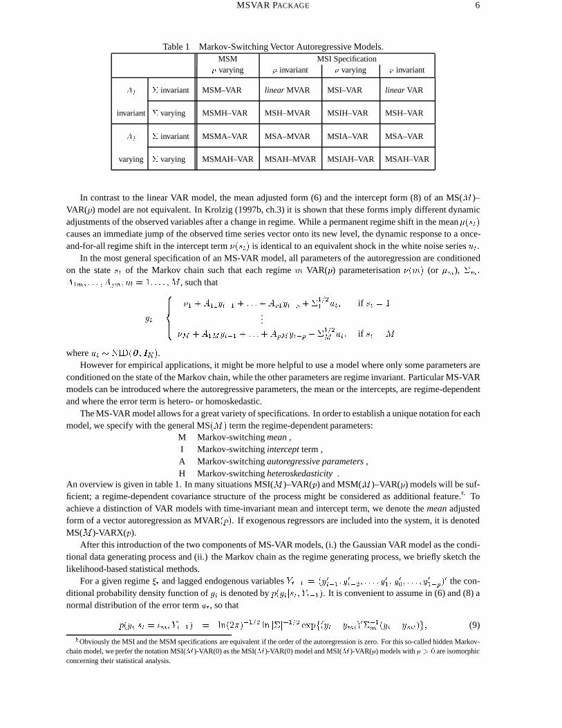
Table 1 Markov-Switching Vector Autoregressive Models.MSM MSI Specification

� varying � invariant � varying � invariant

Aj � invariant MSM–VAR linear MVAR MSI–VAR linear VAR

invariant � varying MSMH–VAR MSH–MVAR MSIH–VAR MSH–VAR

Aj � invariant MSMA–VAR MSA–MVAR MSIA–VAR MSA–VAR

varying � varying MSMAH–VAR MSAH–MVAR MSIAH–VAR MSAH–VAR

In contrast to the linear VAR model, the mean adjusted form (6) and the intercept form (8) of an MS(M )–VAR(p) model are not equivalent. In Krolzig (1997b, ch.3) it is shown that these forms imply different dynamicadjustments of the observed variables after a change in regime. While a permanent regime shift in the mean�(st)causes an immediate jump of the observed time series vector onto its new level, the dynamic response to a once-and-for-all regime shift in the intercept term �(st) is identical to an equivalent shock in the white noise series ut.

In the most general specification of an MS-VAR model, all parameters of the autoregression are conditionedon the state st of the Markov chain such that each regime m VAR(p) parameterisation �(m) (or �m), �m;

A1m; : : : ; Ajm;m = 1; : : : ;M , such that

yt =

8>><>>:

�1 +A11yt�1 + : : :+Ap1yt�p +�1=21 ut; if st = 1

...

�M +A1Myt�1 + : : :+ApMyt�p +�1=2M ut; if st =M

where ut � NID(0 ; IK).However for empirical applications, it might be more helpful to use a model where only some parameters are

conditioned on the state of the Markov chain, while the other parameters are regime invariant. Particular MS-VARmodels can be introduced where the autoregressive parameters, the mean or the intercepts, are regime-dependentand where the error term is hetero- or homoskedastic.

The MS-VAR model allows for a great variety of specifications. In order to establish a unique notation for eachmodel, we specify with the general MS(M) term the regime-dependent parameters:

M Markov-switching mean ,I Markov-switching intercept term ,A Markov-switching autoregressive parameters ,H Markov-switching heteroskedasticity .

An overview is given in table 1. In many situations MSI(M )–VAR(p) and MSM(M )–VAR(p) models will be suf-ficient; a regime-dependent covariance structure of the process might be considered as additional feature.5 Toachieve a distinction of VAR models with time-invariant mean and intercept term, we denote the mean adjustedform of a vector autoregression as MVAR(p). If exogenous regressors are included into the system, it is denotedMS(M )-VARX(p).

After this introduction of the two components of MS-VAR models, (i.) the Gaussian VAR model as the condi-tional data generating process and (ii.) the Markov chain as the regime generating process, we briefly sketch thelikelihood-based statistical methods.

For a given regime �t and lagged endogenous variables Yt�1 = (y0t�1; y0

t�2; : : : ; y0

1; y0

0; : : : ; y0

1�p)0 the con-

ditional probability density function of yt is denoted by p(ytjst; Yt�1). It is convenient to assume in (6) and (8) anormal distribution of the error term ut, so that

p(ytjst = �m; Yt�1) = ln(2�)�1=2 ln j�j�1=2 expf(yt � �ymt)0��1

m (yt � �ymt)g; (9)

5Obviously the MSI and the MSM specifications are equivalent if the order of the autoregression is zero. For this so-called hidden Markov-chain model, we prefer the notation MSI(M )-VAR(0) as the MSI(M )-VAR(0) model and MSI(M )-VAR(p) models with p > 0 are isomorphicconcerning their statistical analysis.

MSVAR PACKAGE 7

where �ymt = E[ytjst; Yt�1] is the conditional expectation of yt in regime m. Thus the conditional density of ytfor a given regime st is normal as in the VAR model defined in equation (2). Thus:

yt jst = m;Yt�1 � NID (�ymt;�m) ; (10)

where the conditional means �ymt are summarized in the vector �yt which is e.g. in MSI specifications of the form

�yt =

264

�y1t...

�yMt

375 =

264

�1 +Pp

j=1A1jyt�j...

�M +Pp

j=1AMjyt�j

375 :

Assuming that the information set available at time t � 1 consists only of the sample observations and the pre-sample values collected in Yt�1 and the states of the Markov chain up to st�1, the conditional density of yt is amixture of normals6:

p(ytjst�1 = i; Yt�1)

=

MXm=1

p(ytjst�1; Yt�1) Pr(st = mjst�1 = i)

=

MXm=1

MXi=1

pim

�ln(2�)�

1

2 ln j�mj�

1

2 expf(yt � �ymt)0��1

m (yt � �ymt)g�

(11)

The information about the realization of the Markov chain is collected to the vector �t,

�t =

264

I(st = 1)...

I(st = M)

375 ;

consisting of binary variables where the indicator function I(st = m) is defined as:

I(st = m) =

�1 if st = m

0 otherwise,

such that �(st) =PM

m=1 �mI(st = m) = M �t, where M = [�1; : : : ; �M ]. Thus, �t denotes the unobservedstate of the system. Analogously the densities of yt conditional on st and Yt�1 can be collected to the vector �t:

�t =

264

p(ytj�t = 1; Yt�1)...

p(ytj�t =M;Yt�1)

375 ; (12)

equation (11) can be written asp(ytj�t�1; Yt�1) = �0tP

0�t�1: (13)

Since the regime is assumed to be unobservable, the relevant information set available at time t � 1 consistsonly of the observed time series until time t and the unobserved regime vector �t has to be replaced by the inferencePr(�tjY� ). These probabilities of being in regime m given an information set Y� are denoted �mtj� and collectedin the vector �tj� as

�tj� ==

264

Pr(st = 1jY� )...

Pr(st =M jY� );

375

which allows two different interpretations. First, �tj� denotes the discrete conditional probability distribution of�t given Y� . Secondly, �tj� is equivalent to the conditional mean of �t given Y� . This is due to the binarity of theelements of �t, which implies that E[�mt] = Pr(�mt = 1) = Pr(st = m).

6The reader is referred to Hamilton (1994a) for an excellent introduction into the major concepts of Markov chains and to Titterington,Smith and Makov (1985) for the statistical properties of mixtures of normals.

MSVAR PACKAGE 8

Thus, the conditional probability density of yt based upon Yt�1 is given by

p(ytjYt�1) =

Zp(yt; �t�1jYt�1)d�t�1

=

Zp(ytj�t�1; Yt�1) Pr(�t�1jYt�1)d�t�1 (14)

= �0tP0�t�1jt�1;

whereRf(x; �t)d�t :=

PMm=1 f(x; �t = �m) denotes summation over all possible values of �t.

As with the conditional probability density of a single observation yt in (14) the conditional probability densityof the sample can be derived analogously. The techniques of setting-up the likelihood function in practice areintroduced in Krolzig (1997b, ch.6). Here we only sketch the basic approach.

For given presample values Y0, the density of the sample Y � YT conditional on the states � is determined by

p(Y j�) =

TYt=1

p(ytj�t; Yt�1): (15)

Hence, the joint probability distribution of observations and states can be calculated as

p(Y; �) = p(Y j�) Pr(�) =

TYt=1

p(ytj�t; Yt�1)

TYt=2

Pr(�tj�t�1) Pr(�1):

Thus, the unconditional density of Y is given by the marginal density

p(Y ) =

Zp(Y; �) d�: (16)

The maximization of the likelihood function of an MS-VAR model entails an iterative estimation technique toobtain estimates of the parameters of the autoregression and the transition probabilities governing the Markov chainof the unobserved states. Denote this parameter vector by � = (�; �), so � is chosen to maximize the likelihoodfor given observations YT = (y0T ; : : : ; y

0

1�p)0.

Maximum likelihood (ML) estimation of the model is based on an implementation of the Expectation Maxim-ization (EM) algorithm proposed by Hamilton (1990) for this class of model – an overview on alternative numericaltechniques for the maximum likelihood estimation of VAR(M )-MS(p) models is given in Krolzig (1997b). TheEM algorithm introduced by Dempster, Laird and Rubin (1977) is designed for a general class of models wherethe observed time series depends on some unobservable stochastic variables - for MS-AR models these are the re-gime variable st. Each iteration of the EM algorithm consists of two steps. The expectation step involves a passthrough the filtering and smoothing algorithms, using the estimated parameter vector �(j�1) of the last maximiz-ation step in place of the unknown true parameter vector. This delivers an estimate of the smoothed probabilitiesPr(�jY; �(j�1)) of the unobserved states �t (where � records the history of the Markov chain). In the maximiza-tion step, an estimate of the parameter vector � is derived as a solution e� of the first-order conditions associatedwith the likelihood function, where the conditional regime probabilitiesPr(�jY; �) are replaced with the smoothedprobabilities Pr(�jY; �(j�1)) derived in the last expectation step. Equipped with the new parameter vector � thefiltered and smoothed probabilities are updated in the next expectation step, and so on, guaranteeing an increasein the value of the likelihood function at each step.

Regimes constructed in this way are an important instrument for interpreting MS-VAR models. They constitutean optimal inference on the latent state of the economic process, whereby probabilities are assigned to the unob-served regimes conditional on the available information set. It follows by the definition of the conditional densitythat the conditional distribution of the total regime vector � is given by

Pr(�jY ) =p(Y; �)

p(Y ):

Thus, the desired conditional regime probabilities Pr(�tjY ) can be derived by marginalization of Pr(�jY ). Thesecumbrous calculations can be simplified by recursive filtering and smoothing algorithms discussed in Krolzig(1997b, ch.5). These statistical tools provide inference for �t given a specified observation set Y� ; � � T whichreconstruct the time path of the regime, f�tgTt=1, under alternative information sets:

MSVAR PACKAGE 9

�tj� ; � < t predicted regime probabilities.�tj� ; � = t filtered regime probabilities,�tj� ; t < � � T smoothed regime probabilities.

In practice, mainly the filtered regime probabilities, �tjt, the one-step predicted regime probabilities �tjt�1, and thefull-sample smoothed regime probabilities, �tjT , are considered.

The MS-VAR model provides a very flexible framework which allows for heteroskedasticity, occasional shifts,reversing trends, and forecasts performed in a non-linear manner. The implications of particular MS-VAR modelsfor their estimation are discussed in Krolzig (1997b, ch.9).

8 Model formulation

Model formulation is based on the names of variables. The following steps are involved in model formulation:

� Create a MSVAR object.� Load your data into the MSVAR database using the facilities of the Database class.� Transform the data.� Use Select to formulate the model. A constant will be included by default.� Use SetSample to specify the sample.� Use SetModel for a different specification of the model, for example:

– time-invariant intercept;– regime-dependent intercept;– regime-dependent mean.

� For reports of the progress of the EM algorithm, use SetPrint.� For changes of convergence threshold and the maximum number of iteration, use SetEmOptions.� By default, a graphic presentation of the results is shown, standard errors are calculated, and gwg files of all

givewin graphics saved. Use SetOptions to change this.� Finally, use Estimate for estimation.

9 Examples

9.1 Hamilton’s model of the US business cycle

MSVAR can be used to compute ML estimates of univariate and multivariate MS-VAR models. The first examplereplicates Hamilton (1989) and is provided in the file hamilton.ox.

/--------------------------------- hamilton.ox -----------------------------------/#include <oxstd.h>#import<maximize>#import<database>#import<hmk>#import<msvar>

main(){

decl msvar = new MSVAR();msvar->LoadIn7("gnp82.in7");msvar->Select(Y_VAR, { "DUSGNP", 0, 4});msvar->SetSample(1900,1,1999,4);msvar->SetModel(MSM, 2);msvar->Estimate();

}/--------------------------------- hamilton.ox -----------------------------------/

The Hamilton (1989) model of the US business cycle fostered a great deal of interest in the MS–AR model asan empirical vehicle for characterizing macroeconomic fluctuations, and there have been a number of subsequent

MSVAR PACKAGE 10

1955 1960 1965 1970 1975 1980 1985

0

2.5

MSM(2)-AR(4), 1952 (2) - 1984 (4)DUSGNP Mean(DUSGNP)

1955 1960 1965 1970 1975 1980 1985

.5

1Probabilities of Regime 1 Smoothed prob. filtered prob. predicted prob.

1955 1960 1965 1970 1975 1980 1985

.5

1Probabilities of Regime 2 Smoothed prob. filtered prob. predicted prob.

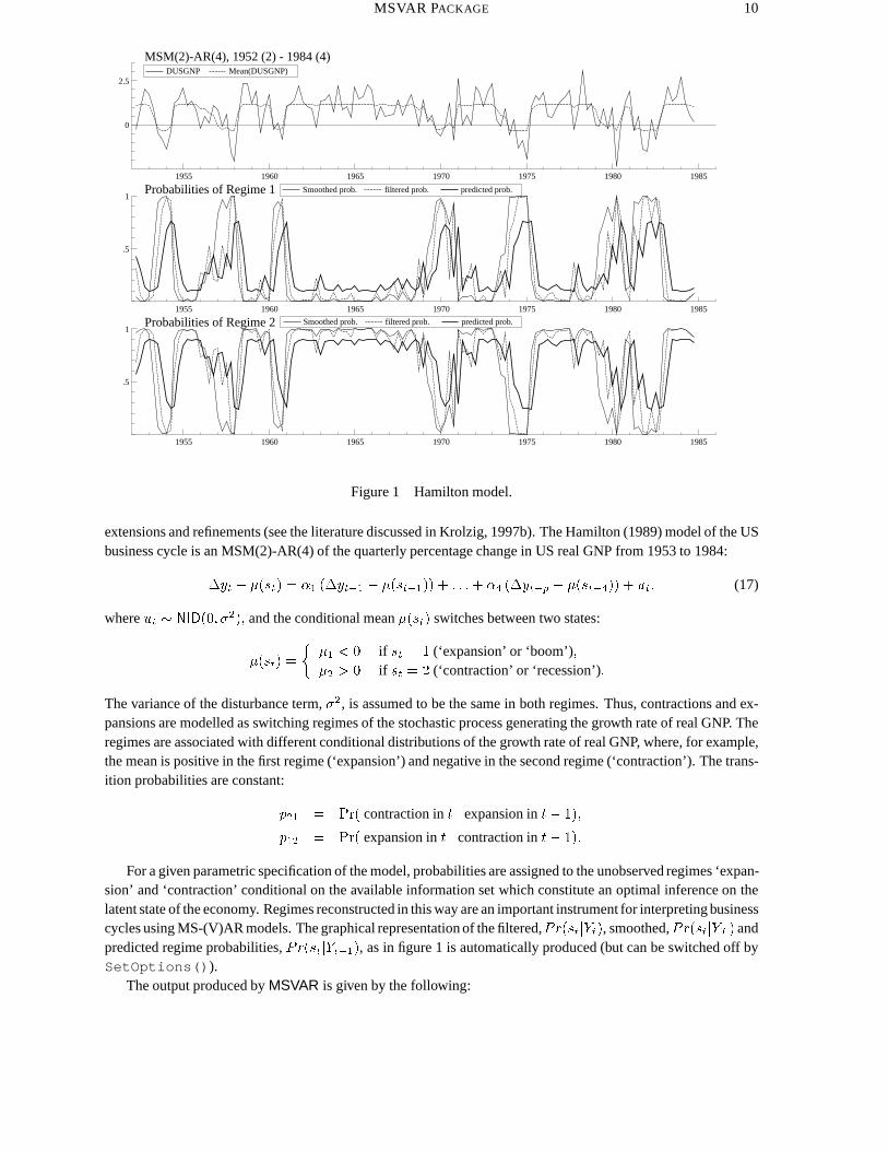
Figure 1 Hamilton model.

extensions and refinements (see the literature discussed in Krolzig, 1997b). The Hamilton (1989) model of the USbusiness cycle is an MSM(2)-AR(4) of the quarterly percentage change in US real GNP from 1953 to 1984:

�yt � �(st) = �1 (�yt�1 � �(st�1)) + : : :+ �4 (�yt�p � �(st�4)) + ut; (17)

where ut � NID(0; �2); and the conditional mean �(st) switches between two states:

�(st) =

��1 < 0 if st = 1 (‘expansion’ or ‘boom’);�2 > 0 if st = 2 (‘contraction’ or ‘recession’):

The variance of the disturbance term, �2, is assumed to be the same in both regimes. Thus, contractions and ex-pansions are modelled as switching regimes of the stochastic process generating the growth rate of real GNP. Theregimes are associated with different conditional distributions of the growth rate of real GNP, where, for example,the mean is positive in the first regime (‘expansion’) and negative in the second regime (‘contraction’). The trans-ition probabilities are constant:

p21 = Pr( contraction in t j expansion in t� 1);

p12 = Pr( expansion in t j contraction in t� 1):

For a given parametric specification of the model, probabilities are assigned to the unobserved regimes ‘expan-sion’ and ‘contraction’ conditional on the available information set which constitute an optimal inference on thelatent state of the economy. Regimes reconstructed in this way are an important instrument for interpreting businesscycles using MS-(V)AR models. The graphical representation of the filtered,Pr(stjYt), smoothed,Pr(stjYT ) andpredicted regime probabilities, Pr(stjYt�1), as in figure 1 is automatically produced (but can be switched off bySetOptions()).

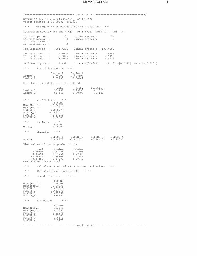
The output produced by MSVAR is given by the following:

MSVAR PACKAGE 11

/-------------------------------- hamilton.out --------------------------------/

MSVAR0.98 (c) Hans-Martin Krolzig, 06-12-1998Object created 11-12-1998, 4:33:34

**** EM algorithm converged after 43 iterations ****

Estimation Results for the MSM(2)-AR(4) Model, 1952 (2) - 1984 (4)

no. obs. per eq. : 131 in the system : 131no. parameters : 9 linear system : 6no. restrictions : 1no. nuisance p. : 2

log-likelihood : -181.4236 linear system : -183.6692

AIC criterion : 2.9072 linear system : 2.8957HQ criterion : 2.9875 linear system : 2.9492SC criterion : 3.1048 linear system : 3.0274

LR linearity test: 4.4911 Chi(1) =[0.0341] * Chi(3) =[0.2131] DAVIES=[0.2131]

**** transition matrix ****

Regime 1 Regime 2Regime 1 0.76202 0.098594Regime 2 0.23798 0.90141

Note that p[i][j]=Pr{s(t)=i|s(t-1)=j}

nObs Prob. DurationRegime 1 38.451 0.29293 4.2020Regime 2 92.549 0.70707 10.143

**** coefficients ****DUSGNP

Mean(Reg.1) -0.34027Mean(Reg.2) 1.1727DUSGNP_1 0.010772DUSGNP_2 -0.062674DUSGNP_3 -0.24615DUSGNP_4 -0.20087

**** variance ****DUSGNP

Variance 0.59270

**** dynamics ****

DUSGNP_1 DUSGNP_2 DUSGNP_3 DUSGNP_4DUSGNP 0.010772 -0.062674 -0.24615 -0.20087

Eigenvalues of the companion matrix

real complex modulus0.46991 0.61766 0.776090.46991 -0.61766 0.77609

-0.46452 0.34309 0.57749-0.46452 -0.34309 0.57749

Cannot show draw window!

**** Calculate numerical second-order derivatives ****

**** Calculate covariance matrix ****

**** standard errors *****

DUSGNPMean(Reg.1) 0.24409Mean(Reg.2) 0.14233DUSGNP_1 0.089525DUSGNP_2 0.081071DUSGNP_3 0.085861DUSGNP_4 0.086692

**** t - values *****

DUSGNPMean(Reg.1) 1.3940Mean(Reg.2) 8.2395DUSGNP_1 0.12033DUSGNP_2 0.77308DUSGNP_3 2.8669DUSGNP_4 2.3170

/-------------------------------- hamilton.out --------------------------------/

MSVAR PACKAGE 12

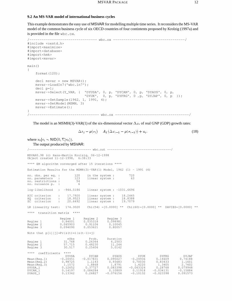
9.2 An MS-VAR model of international business cycles

This example demonstrates the easy use of MSVAR for modelling multiple time series. It reconsiders the MS-VARmodel of the common business cycle of six OECD countries of four contintents proposed by Krolzig (1997a) andis provided in the file wbc.ox.

/--------------------------------- wbc.ox -----------------------------------/#include <oxstd.h>#import<maximize>#import<database>#import<hmk>#import<msvar>

main(){

format(120);

decl msvar = new MSVAR();msvar->LoadIn7("wbc.in7");decl p=1;msvar->Select(Y_VAR, { "DYUSA", 0, p, "DYCAN", 0, p, "DYAUS", 0, p,

"DYUK", 0, p, "DYFRG", 0 ,p, "DYJAP", 0, p });msvar->SetSample(1962, 1, 1991, 4);msvar->SetModel(MSMH, 3)msvar->Estimate();

}/---------------------------------- wbc.ox ------------------------------------/

The model is an MSMH(3)-VAR(1) of the six-dimensional vector �xt of real GNP (GDP) growth rates:

�xt � �(st) = A1 (�xt�1 � �(st�1)) + ut: (18)

where utjst � NID(0;�)st)).The output produced by MSVAR:

/---------------------------------- wbc.out -----------------------------------/

MSVAR0.98 (c) Hans-Martin Krolzig, 06-12-1998Object created 11-12-1998, 6:38:33


Estimation Results for the MSMH(3)-VAR(1) Model, 1962 (1) - 1991 (4)




LR linearity test: 174.3020 Chi(54) =[0.0000] ** Chi(60)=[0.0000] ** DAVIES=[0.0000] **


Regime 1 Regime 2 Regime 3Regime 1 0.84001 0.035318 0.098981Regime 2 0.065903 0.91106 0.10045Regime 3 0.094090 0.053621 0.80057


nObs Prob. DurationRegime 1 31.768 0.26364 6.2503Regime 2 57.715 0.48230 11.244Regime 3 30.517 0.25406 5.0142

**** coefficients ****DYUSA DYCAN DYAUS DYUK DYFRG DYJAP

Mean(Reg.1) -0.20451 -0.017831 0.095027 -0.24936 0.14609 0.74188Mean(Reg.2) 0.98725 1.1143 0.93683 0.70030 0.83433 1.1601Mean(Reg.3) 1.1572 1.8868 1.8791 1.4220 1.3405 2.7402DYUSA_1 0.12652 0.37727 0.083398 -0.063324 0.28768 0.079948DYCAN_1 0.14197 0.084284 0.10809 0.11918 -0.034131 -0.15884DYAUS_1 0.13342 0.26827 -0.076156 -0.10132 -0.023398 0.091573

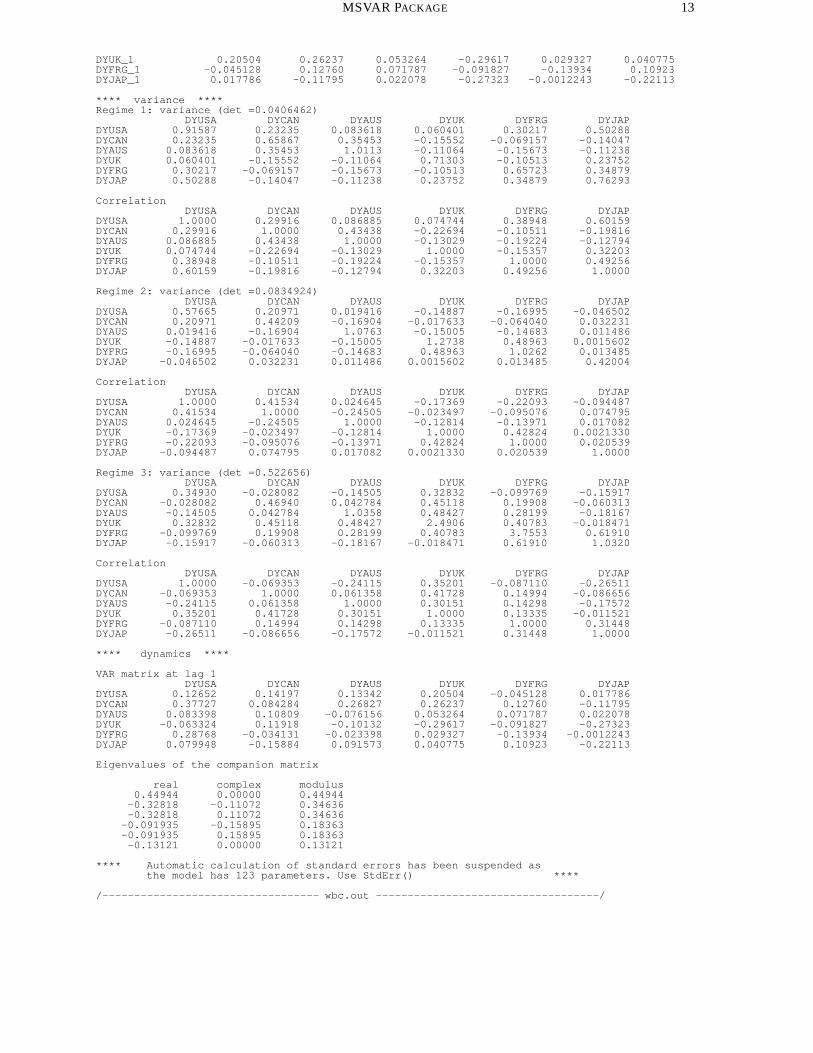
MSVAR PACKAGE 13

DYUK_1 0.20504 0.26237 0.053264 -0.29617 0.029327 0.040775DYFRG_1 -0.045128 0.12760 0.071787 -0.091827 -0.13934 0.10923DYJAP_1 0.017786 -0.11795 0.022078 -0.27323 -0.0012243 -0.22113

**** variance ****Regime 1: variance (det =0.0406462)

DYUSA DYCAN DYAUS DYUK DYFRG DYJAPDYUSA 0.91587 0.23235 0.083618 0.060401 0.30217 0.50288DYCAN 0.23235 0.65867 0.35453 -0.15552 -0.069157 -0.14047DYAUS 0.083618 0.35453 1.0113 -0.11064 -0.15673 -0.11238DYUK 0.060401 -0.15552 -0.11064 0.71303 -0.10513 0.23752DYFRG 0.30217 -0.069157 -0.15673 -0.10513 0.65723 0.34879DYJAP 0.50288 -0.14047 -0.11238 0.23752 0.34879 0.76293

CorrelationDYUSA DYCAN DYAUS DYUK DYFRG DYJAP

DYUSA 1.0000 0.29916 0.086885 0.074744 0.38948 0.60159DYCAN 0.29916 1.0000 0.43438 -0.22694 -0.10511 -0.19816DYAUS 0.086885 0.43438 1.0000 -0.13029 -0.19224 -0.12794DYUK 0.074744 -0.22694 -0.13029 1.0000 -0.15357 0.32203DYFRG 0.38948 -0.10511 -0.19224 -0.15357 1.0000 0.49256DYJAP 0.60159 -0.19816 -0.12794 0.32203 0.49256 1.0000

Regime 2: variance (det =0.0834924)DYUSA DYCAN DYAUS DYUK DYFRG DYJAP

DYUSA 0.57665 0.20971 0.019416 -0.14887 -0.16995 -0.046502DYCAN 0.20971 0.44209 -0.16904 -0.017633 -0.064040 0.032231DYAUS 0.019416 -0.16904 1.0763 -0.15005 -0.14683 0.011486DYUK -0.14887 -0.017633 -0.15005 1.2738 0.48963 0.0015602DYFRG -0.16995 -0.064040 -0.14683 0.48963 1.0262 0.013485DYJAP -0.046502 0.032231 0.011486 0.0015602 0.013485 0.42004


DYUSA 1.0000 0.41534 0.024645 -0.17369 -0.22093 -0.094487DYCAN 0.41534 1.0000 -0.24505 -0.023497 -0.095076 0.074795DYAUS 0.024645 -0.24505 1.0000 -0.12814 -0.13971 0.017082DYUK -0.17369 -0.023497 -0.12814 1.0000 0.42824 0.0021330DYFRG -0.22093 -0.095076 -0.13971 0.42824 1.0000 0.020539DYJAP -0.094487 0.074795 0.017082 0.0021330 0.020539 1.0000

Regime 3: variance (det =0.522656)DYUSA DYCAN DYAUS DYUK DYFRG DYJAP

DYUSA 0.34930 -0.028082 -0.14505 0.32832 -0.099769 -0.15917DYCAN -0.028082 0.46940 0.042784 0.45118 0.19908 -0.060313DYAUS -0.14505 0.042784 1.0358 0.48427 0.28199 -0.18167DYUK 0.32832 0.45118 0.48427 2.4906 0.40783 -0.018471DYFRG -0.099769 0.19908 0.28199 0.40783 3.7553 0.61910DYJAP -0.15917 -0.060313 -0.18167 -0.018471 0.61910 1.0320


DYUSA 1.0000 -0.069353 -0.24115 0.35201 -0.087110 -0.26511DYCAN -0.069353 1.0000 0.061358 0.41728 0.14994 -0.086656DYAUS -0.24115 0.061358 1.0000 0.30151 0.14298 -0.17572DYUK 0.35201 0.41728 0.30151 1.0000 0.13335 -0.011521DYFRG -0.087110 0.14994 0.14298 0.13335 1.0000 0.31448DYJAP -0.26511 -0.086656 -0.17572 -0.011521 0.31448 1.0000

**** dynamics ****

VAR matrix at lag 1DYUSA DYCAN DYAUS DYUK DYFRG DYJAP

DYUSA 0.12652 0.14197 0.13342 0.20504 -0.045128 0.017786DYCAN 0.37727 0.084284 0.26827 0.26237 0.12760 -0.11795DYAUS 0.083398 0.10809 -0.076156 0.053264 0.071787 0.022078DYUK -0.063324 0.11918 -0.10132 -0.29617 -0.091827 -0.27323DYFRG 0.28768 -0.034131 -0.023398 0.029327 -0.13934 -0.0012243DYJAP 0.079948 -0.15884 0.091573 0.040775 0.10923 -0.22113


real complex modulus0.44944 0.00000 0.44944

-0.32818 -0.11072 0.34636-0.32818 0.11072 0.34636

-0.091935 -0.15895 0.18363-0.091935 0.15895 0.18363-0.13121 0.00000 0.13121

**** Automatic calculation of standard errors has been suspended asthe model has 123 parameters. Use StdErr() ****

/---------------------------------- wbc.out -----------------------------------/

MSVAR PACKAGE 14

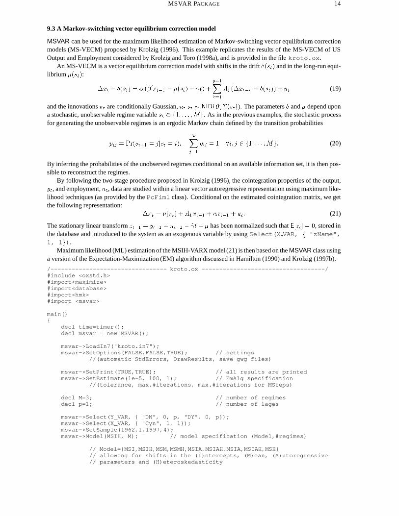
9.3 A Markov-switching vector equilibrium correction model

MSVAR can be used for the maximum likelihood estimation of Markov-switching vector equilibrium correctionmodels (MS-VECM) proposed by Krolzig (1996). This example replicates the results of the MS-VECM of USOutput and Employment considered by Krolzig and Toro (1998a), and is provided in the file kroto.ox.

An MS-VECM is a vector equilibrium correction model with shifts in the drift �(st) and in the long-run equi-librium �(st):

�xt � �(st) = � (�0xt�1 � �(st)� t) +

p�1Xk=1

Ai (�xt�k � �(st)) + ut (19)

and the innovations ut are conditionally Gaussian, utjst � NID(0 ;�(st)). The parameters � and � depend upona stochastic, unobservable regime variable st 2 f1; : : : ;Mg. As in the previous examples, the stochastic processfor generating the unobservable regimes is an ergodic Markov chain defined by the transition probabilities

pij = Pr(st+1 = jjst = i);

MXj=1

pij = 1 8i; j 2 f1; : : : ;Mg: (20)

By inferring the probabilities of the unobserved regimes conditional on an available information set, it is then pos-sible to reconstruct the regimes.

By following the two-stage procedure proposed in Krolzig (1996), the cointegration properties of the output,yt, and employment,nt, data are studied within a linear vector autoregressive representation using maximum like-lihood techniques (as provided by the PcFiml class). Conditional on the estimated cointegration matrix, we getthe following representation:

�xt = �(st) +A1xt�1 + �zt�1 + ut: (21)

The stationary linear transform zt�1 = yt�1 � nt�1 � ~ t� �� has been normalized such that E[zt] = 0, stored inthe database and introduced to the system as an exogenous variable by using Select(X VAR, f "zName",1, 1g).

Maximum likelihood (ML) estimation of the MSIH-VARX model (21) is then based on the MSVAR class usinga version of the Expectation-Maximization (EM) algorithm discussed in Hamilton (1990) and Krolzig (1997b).

/--------------------------------- kroto.ox -----------------------------------/#include <oxstd.h>#import<maximize>#import<database>#import<hmk>#import <msvar>

main(){

decl time=timer();decl msvar = new MSVAR();

msvar->LoadIn7("kroto.in7");msvar->SetOptions(FALSE,FALSE,TRUE); // settings

//(automatic StdErrors, DrawResults, save gwg files)

msvar->SetPrint(TRUE,TRUE); // all results are printedmsvar->SetEstimate(1e-5, 100, 1); // EmAlg specification

//(tolerance, max.#iterations, max.#iterations for MSteps)

decl M=3; // number of regimesdecl p=1; // number of lages

msvar->Select(Y_VAR, { "DN", 0, p, "DY", 0, p});msvar->Select(X_VAR, { "Cyn", 1, 1});msvar->SetSample(1962,1,1997,4);msvar->Model(MSIH, M); // model specification (Model,#regimes)

// Model={MSI,MSIH,MSM,MSMH,MSIA,MSIAH,MSIA,MSIAH,MSH}// allowing for shifts in the (I)ntercepts, (M)ean, (A)utoregressive// parameters and (H)eteroskedasticity

MSVAR PACKAGE 15

msvar->Estimate(); // estimatesmsvar->DrawResults(); // shows graphicsmsvar->DrawErrors(); // shows graphicsmsvar->DrawFit(); // shows graphicsmsvar->StdErr(); // calculates standard errors

delete msvar;print("\n\n****\ttime passed: ", timespan(time), "\t****\n");

/--------------------------------- kroto.ox -----------------------------------/

kroto.ox shows how the estimation can be implemented in MSVAR. The figures and tables produced by theprogram follow./--------------------------------- kroto.out -----------------------------------/

MSVAR.OX (c) Hans-Martin Krolzig, 06-08-1998Object created 4-12-1998, 1:57:04

**** Calculate starting values ****

It. 0 LogLik = -129.2101 Pct.Change =100.0000It. 1 LogLik = -119.1349 Pct.Change = 7.7975It. 2 LogLik = -115.3296 Pct.Change = 3.1941It. 3 LogLik = -114.1886 Pct.Change = 0.9894It. 4 LogLik = -113.9093 Pct.Change = 0.2446It. 5 LogLik = -113.8320 Pct.Change = 0.0679

.................................................

It. 39 LogLik = -112.2400 Pct.Change = 0.0032It. 40 LogLik = -112.2385 Pct.Change = 0.0013It. 41 LogLik = -112.2379 Pct.Change = 0.0005


Estimation Results for the MSIH(3)-VARX(1) Model, 1962 (3) - 1997 (1)




LR linearity test: 66.3990 Chi(10) =[0.0000] **Chi(16) =[0.0000] ** DAVIES =[0.0000] **


Regime 1 Regime 2 Regime 3Regime 1 0.83038 0.051274 0.030876Regime 2 0.035658 0.94834 0.068966Regime 3 0.13396 0.00038374 0.90016


nObs Prob. DurationRegime 1 28.561 0.20637 5.8955Regime 2 64.463 0.51476 19.358Regime 3 45.975 0.27887 10.016

**** coefficients ****DN DY

Const(Reg.1) -0.037737 -0.22234Const(Reg.2) 0.23522 0.61034Const(Reg.3) 0.43127 1.1774DN_1 0.53512 0.13230DY_1 0.022430 0.00027807Cyn_1 0.073950 -0.013330

**** variance ****Regime 1: variance (det =0.0623182)

DN DYDN 0.20525 0.40077DY 0.40077 1.0862

CorrelationDN DY

DN 1.0000 0.84880DY 0.84880 1.0000

MSVAR PACKAGE 16

Regime 2: variance (det =0.00289041)DN DY

DN 0.018729 0.022949DY 0.022949 0.18245

CorrelationDN DY

DN 1.0000 0.39259DY 0.39259 1.0000

Regime 3: variance (det =0.0285466)DN DY

DN 0.083341 0.15188DY 0.15188 0.61930

CorrelationDN DY

DN 1.0000 0.66851DY 0.66851 1.0000

**** dynamics ****

VAR matrix at lag 1DN DY

DN 0.53512 0.022430DY 0.13230 0.00027807


real0.54061

-0.0052139

**** Calculate numerical second-order derivatives ****

**** Calculate covariance matrix ****

**** standard errors *****

DN DYConst(Reg.1) 0.11021 0.27604Const(Reg.2) 0.042897 0.11384Const(Reg.3) 0.084215 0.21030DN_1 0.059509 0.16819DY_1 0.036103 0.097148Cyn_1 0.022969 0.067082

**** t - values *****

DN DYConst(Reg.1) 0.34241 0.80549Const(Reg.2) 5.4834 5.3616Const(Reg.3) 5.1211 5.5987DN_1 8.9921 0.78662DY_1 0.62129 0.0028624Cyn_1 3.2195 0.19871

/--------------------------------- kroto.out -----------------------------------/

MSVAR PACKAGE 17

1970 1980 1990

-2

0

2

MSIH(3)-VARX(1)1962 (3) - 1997 (1)

DNDYMean(DN)Mean(DY)

1970 1980 1990

.25

.5

.75

1Probabilities of Regime 1

Smoothed prob.filtered prob.predicted prob.

1970 1980 1990

.25

.5

.75



1970 1980 1990

.25

.5

.75



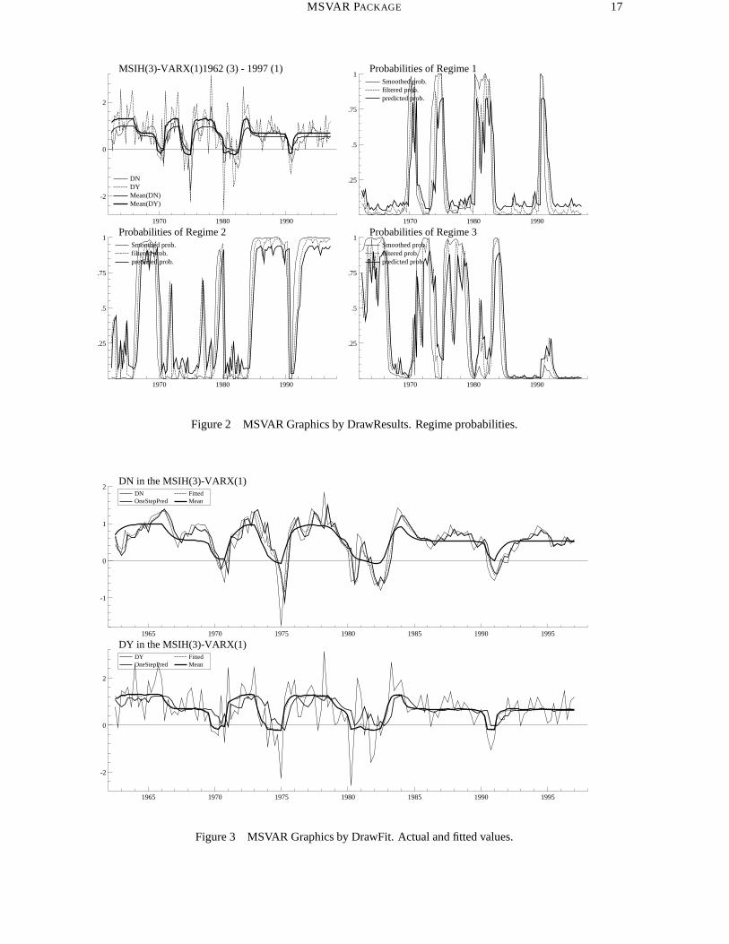
Figure 2 MSVAR Graphics by DrawResults. Regime probabilities.

1965 1970 1975 1980 1985 1990 1995

-1

0

1

2DN in the MSIH(3)-VARX(1)

DN FittedOneStepPred Mean

1965 1970 1975 1980 1985 1990 1995

-2

0

2

DY in the MSIH(3)-VARX(1)DY FittedOneStepPred Mean

Figure 3 MSVAR Graphics by DrawFit. Actual and fitted values.

MSVAR PACKAGE 18

0 5 10

0

1Correlogram

StdResids DN

0 .5 1

.1

.2Spectral density

StdResids DN

-2.5 0 2.5

.2

.4

DensityStdResids DNN(s=0.99)

-2 0 2

-2

0

2

QQ plotStdResids DN x normal

0 5 10

0

1Correlogram

PredErr DN

0 .5 1

.1

.2

Spectral densityPredErr DN

-2 -1 0 1 2

1

2

DensityPredErr DNN(s=0.314)

-2 0 2

0

QQ plotPredErr DN x normal

0 5 10

0

1Correlogram

StdResids DY

0 .5 1

.1

.2

Spectral densityStdResids DY

-2.5 0 2.5

.2

.4

DensityStdResids DYN(s=0.955)

-2 0 2

-2

0

2

QQ plotStdResids DY x normal

0 5 10

0

1Correlogram

PredErr DY

0 .5 1

.1

.2

Spectral densityPredErr DY

-5 0

.25

.5

.75Density

PredErr DYN(s=0.836)

-2 0 2

-2.5

0

2.5

QQ plotPredErr DY x normal

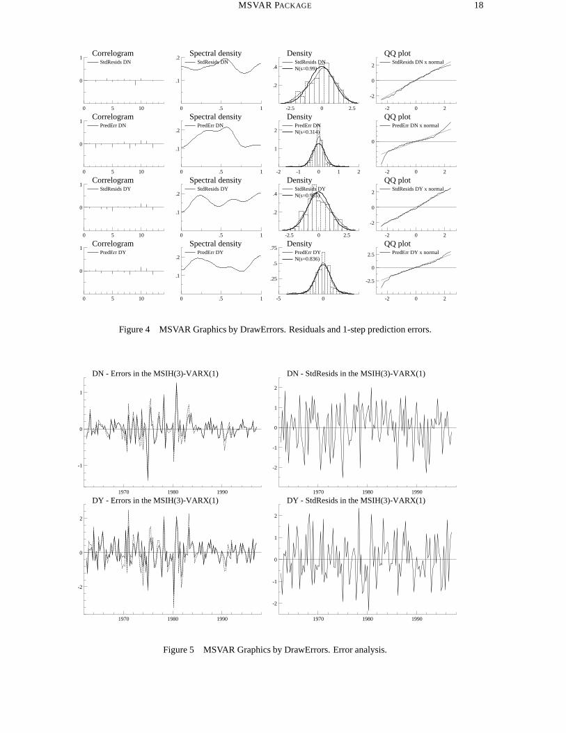
Figure 4 MSVAR Graphics by DrawErrors. Residuals and 1-step prediction errors.

1970 1980 1990

-1

0

1

DN - Errors in the MSIH(3)-VARX(1)

1970 1980 1990

-2

-1

0

1

2

DN - StdResids in the MSIH(3)-VARX(1)

1970 1980 1990

-2

0

2

DY - Errors in the MSIH(3)-VARX(1)

1970 1980 1990

-2

-1

0

1

2

DY - StdResids in the MSIH(3)-VARX(1)

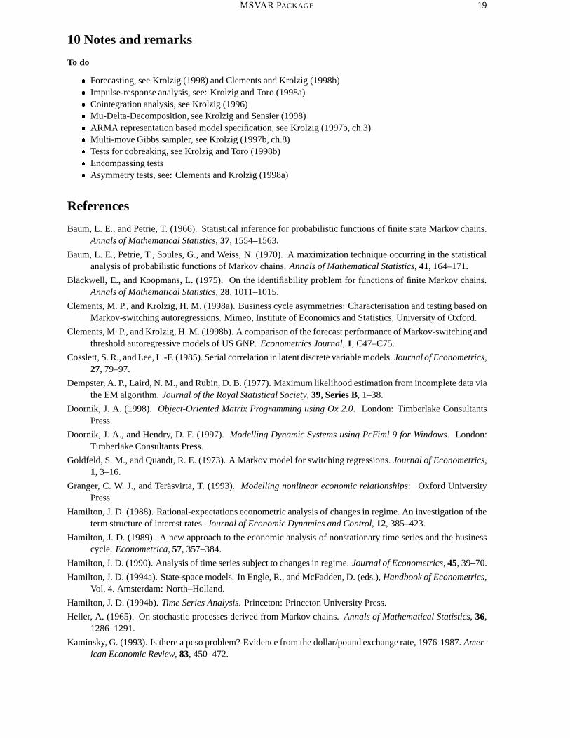
Figure 5 MSVAR Graphics by DrawErrors. Error analysis.

MSVAR PACKAGE 19

10 Notes and remarks

To do

� Forecasting, see Krolzig (1998) and Clements and Krolzig (1998b)� Impulse-response analysis, see: Krolzig and Toro (1998a)� Cointegration analysis, see Krolzig (1996)� Mu-Delta-Decomposition, see Krolzig and Sensier (1998)� ARMA representation based model specification, see Krolzig (1997b, ch.3)� Multi-move Gibbs sampler, see Krolzig (1997b, ch.8)� Tests for cobreaking, see Krolzig and Toro (1998b)� Encompassing tests� Asymmetry tests, see: Clements and Krolzig (1998a)

References

Baum, L. E., and Petrie, T. (1966). Statistical inference for probabilistic functions of finite state Markov chains.Annals of Mathematical Statistics, 37, 1554–1563.

Baum, L. E., Petrie, T., Soules, G., and Weiss, N. (1970). A maximization technique occurring in the statisticalanalysis of probabilistic functions of Markov chains. Annals of Mathematical Statistics, 41, 164–171.

Blackwell, E., and Koopmans, L. (1975). On the identifiability problem for functions of finite Markov chains.Annals of Mathematical Statistics, 28, 1011–1015.

Clements, M. P., and Krolzig, H. M. (1998a). Business cycle asymmetries: Characterisation and testing based onMarkov-switching autoregressions. Mimeo, Institute of Economics and Statistics, University of Oxford.

Clements, M. P., and Krolzig, H. M. (1998b). A comparison of the forecast performance of Markov-switching andthreshold autoregressive models of US GNP. Econometrics Journal, 1, C47–C75.

Cosslett, S. R., and Lee, L.-F. (1985). Serial correlation in latent discrete variable models. Journal of Econometrics,27, 79–97.

Dempster, A. P., Laird, N. M., and Rubin, D. B. (1977). Maximum likelihood estimation from incomplete data viathe EM algorithm. Journal of the Royal Statistical Society, 39, Series B, 1–38.

Doornik, J. A. (1998). Object-Oriented Matrix Programming using Ox 2.0. London: Timberlake ConsultantsPress.

Doornik, J. A., and Hendry, D. F. (1997). Modelling Dynamic Systems using PcFiml 9 for Windows. London:Timberlake Consultants Press.

Goldfeld, S. M., and Quandt, R. E. (1973). A Markov model for switching regressions. Journal of Econometrics,1, 3–16.

Granger, C. W. J., and Terasvirta, T. (1993). Modelling nonlinear economic relationships: Oxford UniversityPress.

Hamilton, J. D. (1988). Rational-expectations econometric analysis of changes in regime. An investigation of theterm structure of interest rates. Journal of Economic Dynamics and Control, 12, 385–423.

Hamilton, J. D. (1989). A new approach to the economic analysis of nonstationary time series and the businesscycle. Econometrica, 57, 357–384.

Hamilton, J. D. (1990). Analysis of time series subject to changes in regime. Journal of Econometrics, 45, 39–70.

Hamilton, J. D. (1994a). State-space models. In Engle, R., and McFadden, D. (eds.), Handbook of Econometrics,Vol. 4. Amsterdam: North–Holland.

Hamilton, J. D. (1994b). Time Series Analysis. Princeton: Princeton University Press.

Heller, A. (1965). On stochastic processes derived from Markov chains. Annals of Mathematical Statistics, 36,1286–1291.

Kaminsky, G. (1993). Is there a peso problem? Evidence from the dollar/pound exchange rate, 1976-1987. Amer-ican Economic Review, 83, 450–472.

MSVAR PACKAGE 20

Krolzig, H.-M. (1996). Statistical analysis of cointegrated VAR processes with Markovian regime shifts. SFB 373Discussion Paper 25/1996, Humboldt Universitat zu Berlin.

Krolzig, H.-M. (1997a). International business cycles: Regime shifts in the stochastic process of economic growth.Applied Economics Discussion Paper 194, University of Oxford.

Krolzig, H.-M. (1997b). Markov Switching Vector Autoregressions. Modelling, Statistical Inference and Applica-tion to Business Cycle Analysis. Berlin: Springer.

Krolzig, H.-M. (1998). Predicting Markov-switching vector autoregressive processes. Mimeo, Institute of Eco-nomics and Statistics, University of Oxford.

Krolzig, H.-M., and Sensier, M. (1998). A disaggregated markov-switching model of the business cycle in ukmanufacturing. Discussion paper 9812, School of Economic Studies, University of Manchester.

Krolzig, H.-M., and Toro, J. (1998a). A new approach to the analysis of shocks and the cycle in a model of outputand employment. Discussion Paper, Institute of Economics and Statistics, University of Oxford.

Krolzig, H.-M., and Toro, J. (1998b). Testing for cobreaking and superexogeneity in the presence of deterministicshifts. Discussion Paper, Institute of Economics and Statistics, University of Oxford.

Lindgren, G. (1978). Markov regime models for mixed distributions and switching regressions. ScandinavianJournal of Statistics, 5, 81–91.

Pearson, K. (1894). Contributions to the mathematical theory of evolution. Philosophical Transactions of theRoyal Society, 185, 71–110.

Sims, C. A. (1980). Macroeconomics and reality. Econometrica, 48, 1–48.

Terasvirta, T., and Anderson, H. (1992). Modelling nonlinearities in business cycles using smooth transition autore-gressive models. Journal of Applied Econometrics, 7, S119–S136.

Titterington, D. M., Smith, A. F. M., and Makov, U. E. (1985). Statistical Analysis of Finite Mixture Distributions:New York: Wiley.

Tjøstheim, D. (1986). Some doubly stochastic time series models. Journal of Time Series Analysis, 7, 51–72.

MSVAR PACKAGE 21

A Glossary of MSVAR functions

The documentation only includes the exported member functions of MSVAR. The non-exportedmember functionsare not documented here as they are only called from other MSVAR function members. Some functions are quitecomplex, and should be approached with care.

Notation:K number of endogenous variables,M number of regimes,N dimension of the state vector (MSIxx: M , MSMxx: Mp+1)p order of the VAR,R number of regressors (excluding constant),T number of observations.

MSVAR::DeSelect

DeSelect();

No return value.

DescriptionClears the model formulation, i.e. clears previous calls to Select() and SetSample().

MSVAR::Estimate

Estimate(const mMu, const mB, const m_mSigma, const Trans);Estimate(const mProbSt);Estimate(const );

mMu in: K �M matrix of means or intercepts (MSAx: K � 1)mB in: K �R matrix of coefficients (MSxAx: K �MR)mSigma in: K �M variance matrix (MSxxH: K �MK)mTrans in: M � M transition matrix (transposed matrix of transition

probabilities)mProbSt in: M � T matrix of initial regime probabilities

No return value.

DescriptionEstimates the model and prints the results, unless this is switched off by SetPrint(). UseSelect,Set-Sample and SetModel prior to Estimate to formulate the model.When initial parameter values or regime probabilities are not given, Estimate() will calculate them.

MSVAR::DrawErrors

DrawErrors(const fAcf);

fAcf in: integer, TRUE: draw error analysis

No return value.

DescriptionCalculates and draws the one-step prediction errors yt�E[ytjYt�1] and standardized residuals of each equa-tion. If fAcf is TRUE a graphic analysis of one-step prediction errors and standardized residuals is under-taken. The error analysis includes the estimated ACF, spectral density, histogram and a QQ plot.

MSVAR::DrawFit

DrawFit();

No return value.

DescriptionDraws actual and fitted values for all series.

MSVAR PACKAGE 22

MSVAR::DrawResults

DrawResults();

DescriptionDraws the series, the Markov chain component as well as the smoothed, filtered and predicted probabilitiesfor all regimes m = 1; : : : ;M .

MSVAR::GetA, MSVAR::GetB

MSVAR::GetMu, MSVAR::GetSigma

MSVAR::GetTrans, MSVAR::GetProbErg

MSVAR::GetProbInit, MSVAR::GetProbLast

MSVAR::GetProbS, MSVAR::GetProbSt

MSVAR::GetProbF, MSVAR::GetProbFt

MSVAR::GetProbP, MSVAR::GetProbPt

MSVAR::GetT, MSVAR::GetU

MSVAR::GetEmOptions, MSVAR::GetModel

MSVAR::GetAIC, MSVAR::GetHQ

MSVAR::GetLogLik, MSVAR::GetSC

Return valueGetA() gets VAR matricesGetAIC() returns Akaike Information CriterionGetB() returns K �R matrix of coefficients (MSxAx: K �MR)GetEmOptions() returns an array with the EM algorithm options as set using SetEmOptionsGetHQ() returns Hannan Quinn Information CriterionGetLogLik() returns log-likelihoodGetModel() returns an array with the model options as set using SetModelGetMu() returns K �M matrix of means or intercepts (MSAx: K � 1)GetProbInit() gets M � 1 vector of initial regime probabilities (MSMx: Mp � 1)GetProbErg() gets M � 1 vector of ergodic regime probabilitiesGetProbLast() gets N � 1 vector of smoothed regime probabilities at time TGetProbF() gets N � T matrix of filtered regime probabilitiesGetProbFt() gets M � T matrix of filtered regime probabilitiesGetProbP() gets N � T matrix of predicted regime probabilitiesGetProbPt() gets M � T matrix of predicted regime probabilitiesGetProbS() gets N � T matrix of smoothed regime probabilitiesGetProbSt() gets M � T matrix of smoothed regime probabilitiesGetSC() returns Schwarz Information CriterionGetSigma() returns K �K variance matrix (MSxxH: K �MK)GetT() gets number of observations TGetTrans() returns M �M transition matrix (transposed matrix of transition probabilities)GetU() gets K �NT matrix of residuals

DescriptionMost of these functions can be only called after the data has been loaded for estimation, or after successfulestimation.

MSVAR PACKAGE 23

MSVAR::MSVAR

MSVAR();

No return value.

DescriptionConstructor function.

MSVAR::LoadIn7

MSVAR::LoadDht, MSVAR::LoadFmtVar

MSVAR::LoadObs, MSVAR::LoadVar

MSVAR::LoadWks, MSVAR::LoadXls

LoadIn7(const sFilename);LoadDht(const sFilename, const iYear1, const iPeriod1, const iFreq);LoadFmtVar(const sFilename);LoadObs(const sFilename, const cVar,const cObs, const iYear1,

const iPeriod1, const iFreq, const fOffendMis);LoadVar(const sFilename, const cVar,const cObs, const iYear1,

const iPeriod1, const iFreq, const fOffendMis);LoadWks(const sFilename);LoadXls(const sFilename);

sFilename in: string, filenamecVar in: int, number of variablescObs in: int, number of observationsiYear1 in: int, start yeariPeriod1 in: int, start periodiFreq in: int, frequencyfOffendMis in: int, TRUE: offending text treated as missing

value FALSE: offending text skippedNo return value.

DescriptionIdentical to the functions of the underlying database class:LoadDht creates the database and loads the specified Gauss data file from disk.LoadIn7 creates the database and loads the specified GiveWin file (PcGive 7 data file) from disk.LoadFmtVar creates the database and loads the ASCII file with formatting information from disk. InGiveWin this is called ‘Data with load info’. Such a file is human-readable, with the data ordered by variable,and each variable preceded by a line of the type:

> name year1 period1 year2 period2 frequency

LoadObs and LoadVar create the database and load the specified human-readable data file from disk. Thedata is ordered by observation (LoadObs), or by variable. Since there is no information on the sample orthe variable names in these files, the sample must be provided as function arguments. The variable namesare set to Var1, Var2, etc., use Rename to rename the variables.LoadWks and LoadXLS create the database and load the specified spreadsheet file from disk. A .wks or.wk1 file is a Lotus file, an .xls file is an Excel worksheet.

MSVAR::IsConverged

IsConverged();

Return valueReturns 1 if the EM algorithm converged, 0 otherwise.

MSVAR PACKAGE 24

MSVAR::LogLik

LogLik(const vP, const adFunc, const avScore, const amHess);vP in: 1� 1 matrix, with current �adFunc in: address of variable

out: loglikelihood at �avScore in: should be 0amHess in: should be 0

Return valueReturns 1 if the likelihood can be evaluated, 0 otherwise.

DescriptionUses the BHLK filter to evaluate the likelihood.

MSVAR::Select

Select(const iGroup, const aSel);iGroup in: int, group indicator: Y VAR, X VAR, I VAR or IL VARaSel in: array, specifying database name, start lag, end lag

No return value.

DescriptionSelects variables by name and with specified lags, and assigns theiGroup status to the selection. The aSelargument is an array consisting of sequences of three values: name, start lag, end lag. For examples, see x9.3.The following types of variables are supported:Y VAR dependent and lagged dependent variableX VAR exogenous regressors

Each Select() adds to the current selection. Use DeSelect() to start afresh. Note: SetSample()checks for data availability; in case of missing observations it uses the largest available sample within theselection.

MSVAR::SetB, MSVAR::SetMu

MSVAR::SetSigma, MSVAR::SetTrans

SetB(const mB);SetMu(const mMu);SetSigma(const mSigma);SetTrans(const mTrans);

mMu in: K �M matrix of means or intercepts (MSAx: K � 1)mB in: K �R matrix of coefficients (MSxAx: K �MR)mSigma in: K �K variance matrix (MSxxH: K �MK)mTrans in: M � M transition matrix (transposed matrix of transition

probabilities)No return value.

DescriptionSet parameter matrices of the MS-VAR model.

MSVAR PACKAGE 25

MSVAR::SetEmOptions

SetEmOptions(const dTol, const iIt);SetEmOptions(const dTol, const iIt, const iItMsm);

dTol in: double, tolerance level for convergence of the Em algorithmas percentage change of the log-likelihood (1e-6 by default).

cItMsm in: integer, maximum number of iterations of the EM algorithm(100 by default).

cItMsm in: integer, number of internal iterations at each M-step (2 bydefault).

No return value.

DescriptionSpecifies options of the EM algorithm. Note that the third option only effects MSMx-VAR models.

MSVAR::SetModel

SetModel(const fModel, const M);fModel in: integer, specification of the MS-VAR, see below.M in: integer

No return value.

DescriptionSet the specification of the MS-VAR and the number of regimes to be used in the model. Use Select()prior to SetModel() to formulate the model.

The following model specifications are supported:MSH regime-dependent heteroscedasticityMSI regime-dependent interceptMSIH regime-dependent intercept and heteroscedasticityMSM regime-dependent meanMSHH regime-dependent mean and heteroscedasticityMSIA regime-dependent interceptMSIAH regime-dependent intercept and heteroscedasticityMSIA regime-dependent interceptMSIAH regime-dependent intercept and heteroscedasticity

Note: The computational burden associated with MSMx-VAR models can be quite high (compared to anMSIx-VAR the factor is Mp where p is the order of the VAR). In general it is not advised to work with anumber of regimes M � 4 due to local maxima and parameter inflation.

MSVAR::SetOptions

SetOptions(const fStdErr, const fShowDrawResults, const fSaveDrawWindow);fStdErr in: integer, TRUE: calculate automatically standard

errorsfShowDrawResults in: integer, TRUE: calls automatically DrawResultsfSaveDrawWindow in: integer, TRUE: saves gwg files of all MSVAR

graphicsNo return value.

DescriptionSets general options for the MSVAR class.

MSVAR PACKAGE 26

MSVAR::SetPrint

SetPrint(const fPrintResults, const fPrintSteps);fPrintResults in: int, TRUE or FALSEfPrintSteps in: int, TRUE or FALSE

No return value.

DescriptionSwitches printing on (TRUE) or off (FALSE). By default printing is on. If fPrintSteps is TRUE theprogress of the EM algorithm is printed after each iteration.

MSVAR::SetSample

SetSample(const iYear1, const iPeriod1, const iYear2, const iPeriod2);iYear1 in: integer, start year.iPeriod1 in: integer, start period.iYear2 in: integer, end year.iPeriod2 in: integer, end period.

No return value.

DescriptionThis function selects a subsample in the time dimension. Observations before the specified start sample pointand after the end are omitted from estimation. Note: SetSample() checks for data availability; in caseof missing observations it uses the largest available sample within the selection.

MSVAR::StdErr

StdErr();

No return value.

DescriptionPrints standard errors based on numerical calculations of the Hessian. If the Hessian is singular the general-ized inverse is calculated. As the transition probabilities pij are restricted to the [0; 1] interval, the parameters

are transformed logits �ij = log�

pij1�pij

�which avoids problems if one or more of the pij is close to the

border. If one of the transition parameters is estimated to lie on the border, pij 2 f0; 1g; then the parameteris taken as being fixed and eliminated from the parameter vector (under construction).Note: The computational burden is proportional to the squared number of parameters. For systems withmore than 100 parameters it is suggested to turn the automatical calculation off.

econometric modelling of markov-switching vector ...fm modelling of markov-switching vector...

Documents