economic analysis of social common capital
DESCRIPTION
economic journalTRANSCRIPT


P1: ICD0521847885agg.xml CB829B/Uzawa 0 521 84788 5 August 27, 1956 9:9
This page intentionally left blank

P1: ICD0521847885agg.xml CB829B/Uzawa 0 521 84788 5 August 27, 1956 9:9
Economic Analysis of Social Common Capital
Social common capital provides members of society with those servicesand institutional arrangements that are crucial in maintaining human andcultural life. The term social common capital comprises three categories:natural capital, social infrastructure, and institutional capital. Naturalcapital consists of all the natural environment and natural resources,including the earth’s atmosphere. Social infrastructure consists of roads,bridges, public transportation systems, electricity, and other public utilities.Institutional capital includes hospitals, educational institutions, judicialand police systems, public administrative services, financial and monetaryinstitutions, and cultural capital. This book attempts to modify and extendthe theoretical premises of orthodox economic theory to make thembroad enough to analyze the economic implications of social commoncapital. It further aims to find the institutional arrangements and policymeasures that will bring about the optimal state of affairs in which thenatural and institutional components are blended together harmoniouslyto realize the sustainable state suggested by John Stuart Mill.
Hirofumi Uzawa is Director of the Research Center of Social CommonCapital at Doshisha University and Emeritus Professor of Economics atthe University of Tokyo. He is a Fellow and former President of the Econo-metric Society and a former President of the Japan Association for Eco-nomics and Econometrics. He is a Member of the American Academy ofArts and Sciences, a Foreign Associate of the U.S. National Academy ofSciences, a Foreign Honorary Member of the American Economic Asso-ciation, and a Member of the Japan Academy.
Professor Uzawa has also served for more than thirty years asSenior Advisor in the Research Institute of Capital Formation at theDevelopment Bank of Japan.
Professor Uzawa has been one of the leading economic theorists forthe past four decades. In recent decades, he has become particularly wellknown for applied research in the areas of the economics of pollution, en-vironmental disruption, and global warming, the economics of educationand medical care, and the theory of social common capital.
Professor Uzawa is the author of more than twenty books, including Eco-nomic Theory and Global Warming (Cambridge University Press, 2003).He is the recipient of the Matsunaga Prize (1969), the Yoshino Prize (1970),and the Mainichi Prize (1974). The government of Japan designated hima Person of Cultural Merit in 1983, and the Emperor of Japan conferredthe Order of Culture upon him in 1997.
i

P1: ICD0521847885agg.xml CB829B/Uzawa 0 521 84788 5 August 27, 1956 9:9
ii

P1: ICD0521847885agg.xml CB829B/Uzawa 0 521 84788 5 August 27, 1956 9:9
Economic Analysis ofSocial Common Capital
HIROFUMI UZAWA
iii

cambridge university pressCambridge, New York, Melbourne, Madrid, Cape Town, Singapore, São Paulo
Cambridge University PressThe Edinburgh Building, Cambridge cb2 2ru, UK
First published in print format
isbn-13 978-0-521-80781-4
isbn-13 978-0-521-00291-2
isbn-13 978-0-511-12882-0
© Cambridge University Press 2005
2005
Information on this title: www.cambridge.org/9780521807814
This publication is in copyright. Subject to statutory exception and to the provision ofrelevant collective licensing agreements, no reproduction of any part may take placewithout the written permission of Cambridge University Press.
isbn-10 0-511-12882-7
isbn-10 0-521-80781-6
isbn-10 0-521-00291-5
Cambridge University Press has no responsibility for the persistence or accuracy of urlsfor external or third-party internet websites referred to in this publication, and does notguarantee that any content on such websites is, or will remain, accurate or appropriate.
Published in the United States of America by Cambridge University Press, New York
www.cambridge.org
hardback
paperback
paperback
eBook (EBL)
eBook (EBL)
hardback

P1: ICD0521847885agg.xml CB829B/Uzawa 0 521 84788 5 August 27, 1956 9:9
Contents
List of Figures page vi
Preface vii
Introduction Social Common Capital 1
1 Fisheries, Forestry, and Agriculture in the Theoryof the Commons 15
2 The Prototype Model of Social Common Capital 76
3 Sustainability and Social Common Capital 122
4 A Commons Model of Social Common Capital 156
5 Energy and Recycling of Residual Wastes 189
6 Agriculture and Social Common Capital 219
7 Global Warming and Sustainable Development 257
8 Education as Social Common Capital 292
9 Medical Care as Social Common Capital 322
Main Results Recapitulated 359
References 383
Index 393
v

P1: ICD0521847885agg.xml CB829B/Uzawa 0 521 84788 5 August 27, 1956 9:9
Figures
1.1 The change-in-population curves for the commons page 23
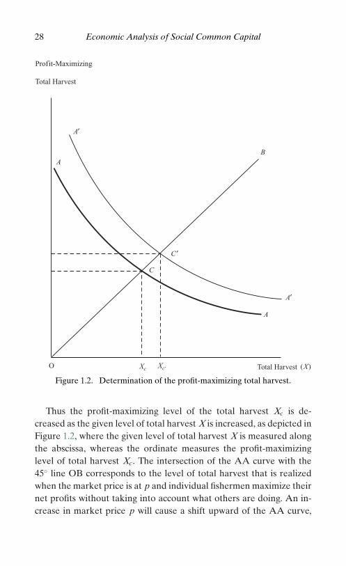
1.2 Determination of the profit-maximizing total harvest 28
1.3 Phase diagram for the commons 39
1.4 The change-in-population curves for the commons:a special case 41
1.5 Average and marginal rates of change in the stock 42
1.6 Construction of the phase diagram for the commons 45
vi

P1: ICD0521847885agg.xml CB829B/Uzawa 0 521 84788 5 August 27, 1956 9:9
Preface
Social common capital provides members of a society with thoseservices and institutional arrangements that are crucial in maintaininghuman and cultural life. It is generally classified in three categories:natural capital, social infrastructure, and institutional capital. Thesecategories are neither exhaustive nor exclusive; they merely illustratethe nature of functions performed by social common capital and thesocial perspectives associated with them.
Natural capital consists of the natural environment and natural re-sources such as forests, rivers, lakes, wetlands, coastal seas, oceans,water, soil, and, above all, the earth’s atmosphere. They all share thecommon feature of being regenerative, subject to intricate and subtleforces of the ecological and biological mechanisms. They provide allliving organisms, particularly human beings, with the environment tosustain their lives and to regenerate themselves.
Social infrastructure is another important component of social com-mon capital. It consists of roads, bridges, public transportation systems,water, electricity, other public utilities, and communication and postalservices, among others. Social common capital also includes institu-tional capital such as hospitals and medical institutions, educationalinstitutions, judicial and police systems, public administrative services,financial and monetary institutions, cultural capital, and others. Theyall provide members of a society with services that are crucial inmaintaining human and cultural life, without being unduly influencedby the vicissitudes of life.
Social common capital in principle is not appropriated to individ-ual members of the society but rather is held as common property
vii

P1: ICD0521847885agg.xml CB829B/Uzawa 0 521 84788 5 August 27, 1956 9:9
viii Preface
resources to be managed by the commons in question, without, how-ever, precluding private ownership arrangements. Nor is it to be con-trolled bureaucratically by the state. Thus, a problem of crucial impor-tance in the theory of social common capital is to devise the institutionalarrangements that result in the management of social common capitalthat is optimum from the social point of view. In this book, we introducean analytical framework in which economic implications of social com-mon capital are fully examined and we explore the conditions underwhich the intertemporal allocation of scarce resources, including bothsocial common capital and private capital, is dynamically optimum orsustainable from the social point of view.
The dynamic models of social common capital introduced in thisbook may be regarded as the general equilibrium versions of thoseformulated in Uzawa (1974a,b,c; 1975; 1982; 1992b), in which, how-ever, the phenomenon of externalities was not explicitly discussed. Inthe general model of social common capital introduced in this book,the phenomenon of externalities, both static and dynamic, is explic-itly incorporated in the construct of the model and their implicationsfor the processes of resource allocation, including both social commoncapital and privately managed scarce resources, are fully explored. Thedynamically optimum or sustainable allocation of scarce resources oc-curs when the imputed prices associated with the accumulation and useof social common capital are used as signals in the allocative processes.Privately owned scarce resources and goods and services produced byprivate economic units are allocated through the mechanism of marketinstitutions.
The present study, in conjunction with Economic Theory and GlobalWarming, recently published by Cambridge University Press, is an off-shoot of my attempt to modify and extend the theoretical premisesof orthodox economic theory to make them broad enough to analyzethe economic implications of social common capital, and to find theinstitutional arrangements and policy measures that will bring aboutthe optimal state of affairs in which the natural and institutional com-ponents are blended together harmoniously to realize the sustainablestate in the sense introduced by John Stuart Mill in his classic Principlesof Political Economy (1848), particularly in the chapter entitled “OnStationary States.”

P1: ICD0521847885agg.xml CB829B/Uzawa 0 521 84788 5 August 27, 1956 9:9
Preface ix
In this book and Economic Theory and Global Warming, I have en-deavored to construct a theoretical framework that enables us to ex-amine in detail the institutional and policy arrangements under whichthe utopian stationary state envisioned by John Stuart Mill may be real-ized. However, the problems posited here have turned out to be muchmore difficult than I originally anticipated. This book, therefore,presents the results of my endeavor, albeit in a very preliminary stage,in a form that may be accessible to colleagues and students interested inthe economics of social common capital as well as in economic theoryin general. Each chapter is presented in such a manner, occasionallyat the risk of repetition, that it may be read without prior knowledgeof other chapters. I wish that young economists with competent ana-lytical skills and a deep concern for the welfare of future generationswill follow the lead suggested and develop a comprehensive theory ofsocial common capital.
I would like to acknowledge with gratitude the valuable commentsand suggestions my colleagues have given me while I have been en-gaged in the study and research for this book. I particularly thankKenneth J. Arrow, Kazumi Asako, Partha Dasgupta, Yuko Hosoda,Dale W. Jorgenson, Karl-Goran Maler, Robert M. Solow, KeisukeTakegahara, David Throsby, and Katsuhisa Uchiyama. I would also liketo thank the readers of the original manuscript, who made thoughtfuland detailed comments and suggestions.
Generous support, financial or otherwise, from the Japanese Min-istry of Education and Science, the Keiyu Medical Foundation, theResearch Center of Social Common Capital at Doshisha University,the Development Bank of Japan, and the Beijer International Instituteof Ecological Economics in the Royal Swedish Academy of Sciencesis greatly appreciated.
Last, but not least, I would like to acknowledge with gratitude thepatience and encouragement that my wife, Hiroko, and other membersof my family have extended to me while I have been engaged in thestudy and research of economic theory in general and social commoncapital in particular during the past 40-some years.

P1: ICD0521847885agg.xml CB829B/Uzawa 0 521 84788 5 August 27, 1956 9:9
x

P1: ICD/NDN P2: IWV0521847885int.xml CB829B/Uzawa 0 521 84788 5 August 27, 1956 22:48
IntroductionSocial Common Capital
RERUM NOVARUM inverted: the abuses of socialismand the illusions of capitalism
In his historic 1891 encyclical Rerum Novarum, Pope Leo XIII identi-fied the most pressing problems of the times as “the abuses of capitalismand the illusions of socialism” (Leo XIII 1891). He called the atten-tion of the world on “the misery and wretchedness pressing so unjustlyon the majority of the working class” and condemned the abuses ofliberal capitalism, particularly the greed of the capitalist class. At thesame time, he vigorously criticized the illusions of socialism, primarilyon the ground that private property is a natural right indispensablefor the pursuit of individual freedom. Exactly 100 years after RerumNovarum, the New Rerum Novarum was issued by Pope John Paul IIon May 15, 1991, identifying the problems that plague the world todayas “the abuses of socialism and the illusions of capitalism” (John Paul II1991 and Uzawa 1991a, 1992c).
Contrary to the classic Marxist scenario of the transition of capital-ism to socialism, the world is now faced with an entirely different prob-lem of how to transform a socialist economy to a capitalist economysmoothly. For such a transformation to result in a stable, well-balancedsociety, however, we must be explicitly aware of the shortcomings ofthe decentralized market system as well as the deficiencies of the cen-tralized planned economy.
The centralized planned economy has been plagued by the enor-mous power that has been exclusively possessed by the state and hasbeen arbitrarily exercised. The degree of freedom bestowed upon the
1

P1: ICD/NDN P2: IWV0521847885int.xml CB829B/Uzawa 0 521 84788 5 August 27, 1956 22:48
2 Economic Analysis of Social Common Capital
average citizen has been held at the minimum, whereas human dig-nity and professional ethics have not been properly respected. Theexperiences of socialist countries during the last several decades haveclearly shown that the economic plans, both centralized and decen-tralized, that have been conceived of by the government bureaucracy,have been inevitably found untenable either because of technical de-ficiencies or in terms of incentive incompatibility. The living standardof the average person has fallen far short of the expectations, and thedreams and aspirations of the majority of the people have been leftunfulfilled.
On the other hand, the decentralized market economy has sufferedfrom the perpetual tendency toward an unequal income distribution,unless significant remedial measures are taken, and from the volatilefluctuations in price and demand conditions, under which productiveethics have been found extremely difficult to sustain. Profit motivesoften outrun moral, social, and natural constraints, whereas specula-tive motives tend to dominate productive ethics, even when properregulatory measures are administered.
We must now search for an economic system in which stable, har-monious processes of economic development may be realized with themaximum degree of individual freedom and with due respect to hu-man dignity and professional ethics, as eloquently prophesied by JohnStuart Mill in his classic Principles of Political Economy in a chapterentitled “On Stationary States” (Mill 1848). The stationary state, asenvisioned by Mill, is interpreted as the state of the economy in whichall macroeconomic variables, such as gross domestic product, nationalincome, consumption, investments, prices of all goods and services,wages, and real rates of interest, all remain stationary, whereas, withinthe society, individuals are actively engaged in economic, social, andcultural activities, new scientific discoveries are incessantly made, andnew products are continuously introduced still with the natural envi-ronment being preserved at the sustainable state. [Regarding Mill’sstationarity state, one may be referred to an excellent discussion byDaly (1977, 1999).]
We may term such an economic system as institutionalism, if weadopt the concept originally introduced by Thorstein Veblen in hisclassic The Theory of Leisure Class, (Veblen 1899) or The Theory ofBusiness Enterprise (Veblen 1904). It has been recently reactivated as

P1: ICD/NDN P2: IWV0521847885int.xml CB829B/Uzawa 0 521 84788 5 August 27, 1956 22:48
Social Common Capital 3
a theory of institutions by Williamson (1985) and others, in which in-stitutions are defined by the rules of games that specify the incentivesand mechanisms faced by the members of the society engaged in socialactivities. We would like to emphasize that it is not defined in termsof a certain unified principle, but rather the structural characteristicsof an institutionalist economy, as symbolized by the network of variouscomponents of social common capital, are determined by the interplayof moral, social, cultural, and natural conditions inherent in the soci-ety, and they change as the processes of economic development evolveand social consciousness transforms itself correspondingly. Institution-alism explicitly denies the Marxist doctrine that the social relations ofproduction and labor determine the basic tenure of moral, social, andcultural conditions of the society in concern. Adam Smith emphasizedseveral times in his Wealth of Nations (Smith 1776) that the design ofan economic system conceived of purely in terms of logical consistencyinevitably contradicts the diverse, basic nature of human beings, andinstead he chose to advocate the merits of a liberal economic systemevolved through the democratic processes of social and political devel-opment. It is in this Smithian sense that we would like to address theproblems of the economic and social implications of social commoncapital, as well as the analysis of institutional arrangements and policymeasures that ensure the processes of consumption and accumulationof both social common capital and private capital that are either dy-namically optimum or sustainable in terms of a certain well-defined,socially acceptable sense.
social common capital
Social common capital constitutes a vital element of any society inwhich we live. It is generally classified into three categories: naturalcapital, social infrastructure, and institutional capital. These categoriesare neither exhaustive nor exclusive, but they merely illustrate thenature of functions performed by social common capital and the socialperspectives associated with them.
Natural capital consists of the natural environment and natural re-sources such as forests, rivers, lakes, wetlands, coastal seas, oceans,water, soil, and the earth’s atmosphere. They all share the commonfeature of being regenerative, subject to intricate and subtle forces of

P1: ICD/NDN P2: IWV0521847885int.xml CB829B/Uzawa 0 521 84788 5 August 27, 1956 22:48
4 Economic Analysis of Social Common Capital
the ecological and biological mechanisms. They provide all living or-ganisms, particularly human beings, with the environment to sustaintheir lives and to regenerate themselves. However, the rapid processesof economic development and population growth in the past severaldecades, with the accompanying vast changes in social and natural con-ditions, have altered the delicate ecological balance of natural capitalto such a significant extent that their effectiveness has been lost inmany parts of the world.
The sustainable management of natural capital may be made pos-sible when the institutional arrangements of the commons are intro-duced, as indicated by the historical and traditional experiences of thecommons, with a particular reference to the fisheries and forestry com-mons, as discussed in detail by McCay and Acheson (1987) and Berkes(1989).
However, processes of industrialization themselves, together withthe ensuing changes in cultural, social, and political conditions, havemade the survival of the commons extremely difficult. Only a hand-ful of the commons now remain as viable social institutions in whicheconomic activities are effectively conducted with natural capitalprudently sustained.
Social infrastructure is another important component of social com-mon capital. It consists of roads; bridges; public mass transportationsystems; water, electricity, and other public utilities; communicationand postal services; and sewage, among others. Social common capitalalso includes institutional capital such as hospitals and medicalinstitutions, educational institutions, judicial and police systems, publicadministrative services, financial and monetary institutions, and so on.
Cultural capital may also be regarded as an important componentof social common capital, as extensively examined in particular byThrosby (2001). Cultural capital comprises those capital assets in soci-ety that yield goods and services of cultural value, including artworks,historic buildings, and so on, together with intangible assets such aslanguage, traditions, and others.
A word of caution may be necessary regarding the concept of socialcapital, originally introduced by James Coleman, Robert Putnam, andothers. The standard reference is Putnam (2000), and an extensivediscussion is reported in Dasgupta and Serageldin (2000). Social capitalrefers to intangible social networks and relationships of trust that exist

P1: ICD/NDN P2: IWV0521847885int.xml CB829B/Uzawa 0 521 84788 5 August 27, 1956 22:48
Social Common Capital 5
in communities. It means the connectivity of the social network eachindividual is embedded in, and facilitates the exchange of informationand encourages reciprocal altruism. It is an interesting and fascinatingconcept, molded in the traditional framework of sociology and politicalscience, though in good contrast with that of social common capital asenvisioned in this book. [See also Arrow (2000) and Solow (2000).]
Social common capital is held by the society as common propertyresources to be managed by social institutions of various kinds thatare entrusted on a fiduciary basis to maintain social common capitalin good order and to distribute the services derived from it equitably.Social common capital is in principle not appropriated to individualmembers of the society, without, however, precluding the private own-ership arrangements. Nor is it to be controlled bureaucratically by thestate. Thus, a problem of crucial importance in the theory of socialcommon capital is how to devise the institutional arrangements thatresult in the management of social common capital that is optimumfrom the social point of view.
dynamic optimality and sustainability
The problem of dynamic optimality was originally discussed by Ramsey(1928) and Hotelling (1931). It was revived as the theory of optimumeconomic growth in the 1960s, particularly by Koopmans (1965), Cass(1965), and others, and mathematical techniques of Pontryagin’s max-imum method have been effectively applied, as summarily describedin Uzawa (2003, Chapter 5) and again in Chapter 3 of this book.
The concept of sustainability is formally defined as the efficient pat-tern of intertemporal allocation of private capital and social commoncapital for which the imputed price of social common capital is assumedto remain at a stationary level. As the imputed price of social commoncapital expresses the subjective value of social common capital eachgeneration inherits from the past, the concept of sustainabililty thus de-fined may be regarded as expressing in formal terms the concept of thestationary state as envisioned by John Stuart Mill. It is closely linked tothe concept introduced by Pezzey (1992), in which the utility remainsconstant over time. On the other hand, it is not apparent to see the linkwith Page’s concept of sustainability, which emphasizes maintaininglife opportunity from generation to generation (Page 1997).

P1: ICD/NDN P2: IWV0521847885int.xml CB829B/Uzawa 0 521 84788 5 August 27, 1956 22:48
6 Economic Analysis of Social Common Capital
In reference to the context of environmental economics, Maler(1974) and Dasgupta and Heal (1974) formulated the intertemporalgeneral equilibrium model in which economic implications of the en-vironment could be fully explored, and then developed a detailed anal-ysis of the pattern of intertemporal allocations of scarce resources, in-cluding the accumulation and depletion of the environment, that aredynamically optimum from the social point of view. Since then, a largenumber of contributions have been made to the optimum theory ofeconomic growth and environmental quality. The dynamic analysis ofsocial common capital introduced in this book is largely within theframework of the optimum theory of environmental quality as intro-duced by Maler, Dasgupta, Heal, and others.
externalities
One of the intricate problems inherent in social common capital con-cerns the phenomenon of externalities. Since the classic treatment ofPigou (1925) and Samuelson (1954), economists were always puzzledby the phenomenon of externalities, but it was put aside as periph-eral and not worthy of serious consideration. Concern with environ-mental issues, however, has changed this habit of economic thinking,and a large number of contributions have appeared in which the is-sue of externalities occupies a central place from both theoretical andempirical points of view. The analytical treatment of externalities tobe formulated in this book is adopted from that introduced in Uzawa(1974a,b,c; 1975; 1982; 1992a), in which two kinds of externalities, staticon the one hand and dynamic on the other, are recognized with respectto the services derived from social common capital. Static externalitiesoccur when the levels of marginal products or utilities of individualeconomic units are affected by the aggregate amount of services ofsocial common capital used by all members of the society, assumingthat the stock of social common capital is kept at a constant level.Dynamic externalities, on the other hand, are observed when the con-ditions of production and consumption for each individual economicunit change over time owing to the changes in the stock of social com-mon capital, either accumulation or depreciation, that occur today.The analysis of dynamic optimality developed in Uzawa (1974a), how-ever, was confined to a restrictive type of social common capital, and

P1: ICD/NDN P2: IWV0521847885int.xml CB829B/Uzawa 0 521 84788 5 August 27, 1956 22:48
Social Common Capital 7
due attention was not paid to those categories of social common cap-ital, such as natural capital, whose regenerative capability has beendamaged to a significant extent largely because of the rapid processesof industrialization. In the formulation of a general dynamic modelof social common capital recently developed in Uzawa (1998), anattempt was made to incorporate some of the more salient aspectsof the disruption of natural capital and to elucidate their implicationsfor the economic welfare of the society in concern. The introduction ofthe general models of social common capital in this book is precededby the simple analysis of a specific type of social common capital – thenatural environment.
The natural environment, or rather natural capital, has been sub-ject to an extensive examination in the literature, particularly withrespect to the fisheries and forestry commons. The analysis of the fish-eries commons was initiated by Gordon (1954) and Scott (1955), andwas later extended to the general treatment within the framework ofmodern capital theory by Schaefer (1957), Crutchfield and Zellner(1962), Clark and Munro (1975), and Tahvonen (1991), among others.The simple dynamic model of the natural environment introduced inChapter 1 that has the case of the fisheries commons primarily in mindbelongs to the lineage of their approach. It is an extension of the anal-ysis developed by Uzawa (1992b), in which it is used to examine criti-cally the theory of the tragedy of the commons, as advanced by Hardin(1968).
The model of the natural environment developed in Uzawa (1992b)may be applicable to the dynamics of the forestry commons as well.As with the fisheries commons, the dynamics of the forestry commonshas been extensively analyzed in the literature. Indeed, it was made acentral issue in economic theory by Wicksell (1901), who developedthe core of modern capital theory with the analysis of forests as theprototype. The most recent contribution to forestry economics wasmade by Johansson and Lofgren (1985), and the basic premises of thedynamic model of natural capital introduced in this book may also beregarded as an application and extension of these contributions.
In this book, we address ourselves to formulating in analytical mod-els some of the empirical findings concerning the economic, technologi-cal, and ecological structure of the commons, and then to formulating interms of the theory of social common capital some of the more critical

P1: ICD/NDN P2: IWV0521847885int.xml CB829B/Uzawa 0 521 84788 5 August 27, 1956 22:48
8 Economic Analysis of Social Common Capital
problems concerning the dilemma between economic developmentand environmental degradation.
The theory of social common capital provides us with the theo-retical framework within which the role of institutional arrangementsconcerning social, cultural, and natural environments in the processesof resource allocation and income distribution may be effectively ana-lyzed. Social common capital is generally composed of those scarce re-sources that are in principle neither privately appropriated nor subjectto market transactions. Social common capital or the services derivedfrom it play a crucial and indispensable role for each member of thesociety in concern to conduct at least the minimum level of humanand dignified life. The management of social common capital thus isentrusted on a fiduciary basis to autonomous social institutions, to pro-vide the environmental framework within which all human activitiesare conducted and the allocative mechanism through which marketinstitutions work. The analysis of social common capital, as previouslyintroduced by Uzawa (1974a, 1989, 1991a, b) and recently developed inUzawa (1998), may be applied to discuss some of the difficulties aris-ing out of the tragedy-of-the-commons phenomenon. Particularly, theinstitutional arrangements whereby the dynamically optimum or sus-tainable use of resources in the commons may ensue are examined interms of the concept of imputed price of social common capital.
The society generally allocates a significant portion of scarce re-sources for the construction and maintenance of social common capi-tal, particularly social infrastructure, and one of the central issues in thedynamic theory of social common capital is to find the criteria by whichscarce resources are allocated between investment in social commoncapital on the one hand and production of goods and services that aretransacted on the market on the other.
In this book, we formulate an analytical framework in which eco-nomic implications of social common capital of various kinds are ex-amined and we explore the conditions under which the intertemporalallocation of social common capital and privately owned scarce re-sources is either dynamically optimum or sustainable from the socialpoint of view. The dynamic models introduced in this book may beregarded as the general equilibrium versions of those formulated inUzawa (1992b), in which the phenomenon of externalities is not ex-plicitly discussed. In the dynamic models of social common capital

P1: ICD/NDN P2: IWV0521847885int.xml CB829B/Uzawa 0 521 84788 5 August 27, 1956 22:48
Social Common Capital 9
introduced in this book, the phenomenon of externalities, both staticand dynamic, is incorporated in the construct of the model, and itsimplications for the processes of resource allocation, including bothsocial common capital and privately managed scarce resources, arefully explored. The dynamically optimum or sustainable allocation ofscarce resources occurs when the imputed prices associated with theaccumulation and use of social common capital are used as signals inthe allocative processes. Privately owned scarce resources and goodsand services produced by private economic units are allocated throughthe mechanism of market institutions.
In the dynamic analysis concerning the accumulation of social infras-tructure, referred to above, the technological conditions are assumedto remain largely constant, independent of the accumulation of thestock of social infrastructure. Technological progress induced by theavailability of social infrastructure and the accompanying increase ininvestment activities in the stock of privately owned scarce resourcesmay be regarded as the central issue in the theory of social infrastruc-ture, particularly within the context of developing nations, as exam-ined in detail by Hirschman (1958) in terms of the concept of socialoverhead capital. Social overhead capital as defined by Hirschmancomprises those basic services without which primary, secondary, andtertiary productive activities cannot function. In its wider sense, socialoverhead capital includes all public services, including law and order,education, public health, transportation, communications, and powerand water supplies, as well as agricultural overhead capital such as irri-gation and drainage systems. Thus the concept of social common cap-ital as introduced in this book may be regarded as an extension of theconcept of social overhead capital, in which natural resources are in-cluded in addition to social infrastructure and institutional and culturalcapital.
The theory of social common capital as developed in this book mayalso be regarded as an extension of the two-sector models of capitalaccumulation originally introduced by Uzawa (1962, 1963, 1964). Sim-ilarly, the problems of designing an institutional framework in whichthe optimum allocation of both social common capital and privatelyowned scarce resources may be realized are crucial in any attemptto practically implement the theory of social common capital to bedeveloped in this book.

P1: ICD/NDN P2: IWV0521847885int.xml CB829B/Uzawa 0 521 84788 5 August 27, 1956 22:48
10 Economic Analysis of Social Common Capital
When we include all components of social common capital in a par-ticular nation, the social institutions entrusted on a fiduciary basis withtheir management constitute the public sector in the broadest senseof the word. The aggregate expenditures incurred by all these socialinstitutions are nothing but the governmental expenditures, either onthe current account or on the capital account. Thus, the problem weaddress may be interpreted as that of devising an institutional frame-work in which the ensuing governmental activities are dynamicallyoptimum or sustainable from the social point of view.
summary of the contents
In Chapter 1, dynamic models are constructed to analyze the interre-lationships between the natural environment and economic develop-ment, with explicit reference to the phenomenon of externalities, bothstatic and dynamic. The institutional arrangements and behavioral cri-teria under which the processes of dynamically optimum economicdevelopment necessarily ensue are characterized.
Analysis of the static and dynamic implications of the externalities iscarried out with reference to three specific types of natural resources –fisheries, forestry, and agriculture – in which the modern theory ofoptimum economic growth and the theory of social common capitalmay be effectively utilized.
In Chapter 2, the prototype model of social common capital is intro-duced with a particular type of social common capital – social infras-tructure, such as highways, ports, and public transportation systems –in mind. We consider the general circumstances under which factors ofproduction that are necessary for the professional provision of servicesof social common capital are either privately owned or are managed asif privately owned. Services of social common capital are subject to thephenomenon of congestion, resulting in the divergence between pri-vate and social costs. Therefore, to obtain efficient and equitable allo-cation of scarce resources, it becomes necessary to levy social commoncapital taxes on the use of services of social common capital. The pricescharged for the use of services of social common capital exceed, by thetax rates, the prices paid for the provision of services of social com-mon capital to social institutions in charge of social common capital.One of the crucial problems in the prototype model of social common

P1: ICD/NDN P2: IWV0521847885int.xml CB829B/Uzawa 0 521 84788 5 August 27, 1956 22:48
Social Common Capital 11
capital introduced in Chapter 2 is to examine how the optimum taxrates for the services of various components of social common capi-tal are determined. In describing the behavior of social institutions incharge of social common capital, we assume that the levels of servicesof social common capital provided by these institutions are optimumand the use of factors of production by them are efficient. When weuse the term profit maximization, it is used in the sense that the effi-cient and optimum pattern of resource allocation in the provision ofservices of social common capital is sought strictly in accordance withprofessional disciplines and ethics.
In Chapter 3, we examine the problems of social common capitalprimarily from the viewpoint of the intergenerational distribution ofutility. Our analysis is based on the concept of sustainability introducedin Uzawa (1991b, 2003), and we examine the conditions under whichprocesses of the accumulation of social common capital over time aresustainable. The conceptual framework of the economic analysis ofsocial common capital developed in Chapter 2 is extended to deal withthe problems of the irreversibility of processes of the accumulation ofsocial common capital owing to the Penrose effect.
In Chapter 4, we introduce a commons model of social commoncapital in which the interplay of several commons is examined in detailand the institutional framework whereby the sustainable pattern of re-source allocation over time may be realized. The sustainable time-pathof consumption and investment is characterized by the stationarity ofthe imputed prices associated with the given intertemporal preferenceordering, whereas the efficiency of resource allocation in the short runis preserved at each time. When the natural environment is regardedas social common capital, there are two crucial properties that haveto be explicitly incorporated in any dynamic model. The first propertyconcerns the externalities, both static and dynamic, with respect to theuse of the natural environment as a factor of production. The secondproperty is related to the role of the natural environment as an impor-tant component of the living environment, significantly affecting thequality of human life.
In Chapter 5, we formulate a model of social common capital inwhich the energy use and recycling of residual waste are explicitlytaken into consideration and the optimum arrangements concerningthe pricing of energy and recycling of residual wastes are examined

P1: ICD/NDN P2: IWV0521847885int.xml CB829B/Uzawa 0 521 84788 5 August 27, 1956 22:48
12 Economic Analysis of Social Common Capital
within the framework of the prototype model of social common cap-ital introduced in Chapter 2. We consider a particular type of socialinstitution that specializes in reprocessing the disposed residual wastesand converting them to raw materials to be used as inputs for the pro-duction processes of energy-producing firms.
Services of social common capital are subject to the phenomenonof congestion, resulting in the divergence between private and socialcosts. To obtain efficient allocation of scarce resources, it becomes nec-essary to levy taxes on the disposal of residual wastes and to pay subsidypayments for the reprocessing of disposed residual wastes. Subsidy pay-ments are made to the social institutions specialized in the recycling ofdisposed residual wastes based on the imputed price of the disposedresidual wastes, whereas members of the society are charged taxes forthe disposal of residual wastes at exactly the same rate as the subsidypayments made to social institutions in charge of the recycling of resid-ual wastes. One of the crucial problems is to see how the optimum taxand subsidy rates are determined for the recycling model of residualwastes, as is the case with the various components of social commoncapital discussed in other chapters of this book.
Agriculture concerns not only economic, industrial aspects, but alsovirtually every aspect of human life – cultural, social, and natural. Itprovides us with food and the raw materials such as wood, cotton,silk, and others that are indispensable to sustain our existence. It alsohas sustained, with few exceptions, the natural environment such asforests, lakes, wetlands, soil, subterranean water, and the atmosphere.In Chapter 6, we formulate an agrarian model of social common cap-ital that captures some of the more salient aspects of the SanrizukaAgricultural Commons and we examine the conditions for the sustain-able development of social common capital and privately owned scarceresources. The Sanrizuka Agricultural Commons is a symbolic modelof the agricultural commons that has been devised as the prototypeof the “stationary state” advanced by John Stuart Mill in his Princi-ples of Political Economy (Mill 1848) to solve the difficulties facingJapanese agriculture today.
In Chapter 7, we are primarily concerned with the economic analy-sis of global warming within the theoretical framework, as introducedin Uzawa (1991b, 2003). We are particularly concerned with the policyarrangements of a proportional carbon tax scheme under which the

P1: ICD/NDN P2: IWV0521847885int.xml CB829B/Uzawa 0 521 84788 5 August 27, 1956 22:48
Social Common Capital 13
tax rate is made proportional either to the level of the per capita na-tional income of the countries where greenhouse gases are emitted orto the sum of the national incomes of all countries in the world. In thefirst part of Chapter 7, we consider the case in which the oceans are theonly reservoir of CO2 on the earth; whereas, in the second part, the roleof the terrestrial forests is explicitly taken into consideration in mod-erating processes of global warming by absorbing the atmospheric ac-cumulation of CO2 on the one hand and in affecting the level of thewelfare of people in the society by providing a decent and culturedenvironment on the other.
Education and medical care probably are the two most importantcomponents of social common capital and, as such, require institutionalarrangements substantially different from those for the standard eco-nomic activities that are generally pursued from the viewpoint of profitmaximization and are subject to transactions on the market. Educationis provided to help young people develop their human abilities, bothinnate and acquired, as fully as possible, whereas medical care is pro-vided for those who are not able to perform ordinary human functionsbecause of impaired health or injuries. Both activities play a crucial rolein enabling every member of the society in concern to maintain his orher human dignity and to enjoy basic human rights as fully as possible.If either education or medical care is subject to market transactionsbased merely on profit motives or under the bureaucratic control bystate authorities, their effectiveness may be seriously impaired and theresulting distribution of real income may tend to become unfair andunequal. Thus, education and medical care may be regarded as the twomost basic components of social common capital and the economicsof education and medical care may be better treated within the theo-retical framework of social common capital developed in this book. InChapters 8 and 9, we examine, respectively, the role of education andmedical care as social common capital within the analytical frameworkintroduced in Chapter 2.
As in other chapters, social institutions in charge of education ormedical care are characterized by the properties that all factors ofproduction necessary for the professional provision of education ormedical care are either privately owned or managed as if privatelyowned. However, as the social institutions in charge of social commoncapital, educational and medical institutions are managed strictly in

P1: ICD/NDN P2: IWV0521847885int.xml CB829B/Uzawa 0 521 84788 5 August 27, 1956 22:48
14 Economic Analysis of Social Common Capital
accordance with professional discipline and expertise concerning ed-ucation and medical care. In describing the behavior of educationaland medical institutions, we assume that the levels of education andmedical care provided by these social institutions are optimum and theuse of factors of productions by these institutions are efficient. Whenwe talk about the maximization of net value, the term is used in thesense that the optimum and efficient pattern of resource allocationin the provision of education and medical care is sought, strictly inaccordance with professional disciplines and ethics.
The main conclusion of both chapters is that to attain sustainablepatterns of resource allocation, including both privately owned scarcemeans of production and social common capital concerned with theprovision of education or medical care, subsidy payments, at rates equalto the marginal social benefits of the services of social common capital,are made to social institutions in charge of social common capital, asis the case with the various types of social common capital discussedin other chapters.

P1: ICD/NDN P2: IWV0521847885c01.xml CB829B/Uzawa 0 521 84788 5 August 27, 1956 13:38
1
Fisheries, Forestry, and Agriculture in theTheory of the Commons
1. introduction
In the past three decades, we have observed a significant change inthe nature of environmental problems and the economic, social, andcultural implications that the degradation of the natural environmenthas brought about. During the 1960s and early 1970s, our primary en-vironmental concern was with the disruption of the environment andthe ensuing hazard to human health caused by the rapid processes ofindustrialization and urbanization, both of which were taking place atan unprecedented, rapid pace in many parts of the world. The envi-ronmental damages were mainly caused by the emission of chemicalsubstances such as sulfur and nitrogen oxides that themselves are toxicand hazardous to human health. In recent years, however, we havebecome increasingly aware of the extensive degradation of the globalenvironment, as exemplified by such phenomena as global warming,the extensive depletion of tropical rain forests with the accompanyingloss of biodiversity, and pollution of the oceans. Global environmen-tal problems are primarily caused either by the imprudent use andexcess depletion of natural resources or by the emission of chemicalagents, such as carbon dioxide in the case of global warming, that bythemselves are neither harmful to human health nor hazardous to thenatural environment but on a global scale, contribute to atmosphericinstability and global disturbances.
As for the industrial pollution and similar environmental problemsthat were rampant and widespread in the 1960s, the causal relationshipswere fairly easy to recognize, from both a social and scientific point of
15

P1: ICD/NDN P2: IWV0521847885c01.xml CB829B/Uzawa 0 521 84788 5 August 27, 1956 13:38
16 Economic Analysis of Social Common Capital
view, and the remedial measures were not too difficult to take, fromboth an economic and a political point of view. However, one has to beaware of a significant number of major environmental problems in the1960s, such as the case of Minamata disease, that left a state of extremesocial injustice for the victims.
On the other hand, global environmental problems concern thedegradation and destabilization of the natural environment coveringan extensive area, with a large number of people involved. They notonly affect the current generation living in developing as well as devel-oped countries but also irreversibly involve all future generations, asexemplified by the phenomena of global warming, loss of biodiversity,and pollution of the oceans.
Global environmental problems are also noted for the intricate andsubtle interrelationships that exist between human activities, both eco-nomic and cultural, and the ecological and biological processes in thenatural environment. Traditional economic theory has not paid suffi-cient attention to the damages and threats to the natural environment,particularly with respect to the stability and resilience of regenerativeprocesses, that are exerted by industrial, urban, and other human activ-ities. Instead, it has treated the natural environment simply as the stockof natural capital, from which various natural resources are extractedto be used as factors of production for the productive processes in theeconomy.
However, in the economic analysis of fisheries, forestry, and otheragricultural activities, a large number of studies have explicitly rec-ognized the implications of economic activities for the stability andresilience of the natural environment, either in the fisheries or inforestry commons, and have analyzed the patterns of resource al-location that are dynamically optimum in terms of the intertempo-ral preference ordering prevailing within the society, as describedin detail, for example, by Johansson and Lofgren (1985) and Clark(1990).
When we examine the interaction of economic activities with thenatural environment, one of the more crucial issues concerns the or-ganizational characteristics of the social institutions that manage thenatural environment as well as their behavioral and financial crite-ria, which realize those patterns of the repletion and depletion ofthe natural environment and the levels of economic activities that are

P1: ICD/NDN P2: IWV0521847885c01.xml CB829B/Uzawa 0 521 84788 5 August 27, 1956 13:38
The Theory of the Commons 17
dynamically optimum from the social point of view. The dynamicallyoptimum time-paths generally converge to the long-run stationarystate at which the processes of economic activities are sustained atlevels that are at the optimum balance vis-a-vis the natural environ-ment, and the problem we face now concerns the organizational andinstitutional arrangements for sustainable economic development.
Such an organizational framework may be provided by the institu-tional arrangements of the commons, as has been shown in terms ofa large number of historical, traditional, and contemporary commonsdocumented, for example, in McCay and Acheson (1987) and Berkes(1989). The commons discussed by McCay and Acheson (1987) andBerkes (1989) refer to a variety of natural resources from fisheries,forests, and grazing grounds to irrigation and subterranean water sys-tems. The processes of industrialization, however, together with theaccompanying changes in economic, social, and cultural conditionsprevailing in modern society, have made these commons untenablefrom both an economic and a social point of view, and the survivalof the majority of the traditional commons has become extremelydifficult.
In this chapter, we focus our attention on examining the role ofthe commons in the intertemporal processes of resource allocation,with respect to both the natural environment and privately ownedproperty resources, and on analyzing the dynamic implications of theinstitutional arrangements of the commons for the sustainability ofeconomic development.
In our analysis, we are primarily concerned with the phenomenonof externalities, both static and dynamic, that is generally observedwith respect to the allocative processes in the commons. Static exter-nalities occur when, with the stock of the natural environment keptconstant, the schedules of marginal products for individual membersof the commons, of both private means of production and natural re-sources extracted from the environment, are affected by the levels ofeconomic activities carried out by other members of the commons. Onthe other hand, dynamic externalities concern the effect on the futureschedules of the marginal products for individual members of the com-mons due to the repletion or depletion of the stock of the commonscaused by economic activities carried out by members of the commonstoday.

P1: ICD/NDN P2: IWV0521847885c01.xml CB829B/Uzawa 0 521 84788 5 August 27, 1956 13:38
18 Economic Analysis of Social Common Capital
We are interested in analyzing those institutional arrangements re-garding the use of the natural resources extracted from the stock ofthe commons that may result in the intertemporal allocation of scarceresources in the commons as a whole that is dynamically optimumin terms of the intertemporal criterion prevailing in the society. Theanalysis is carried out with respect to three kinds of commons, whichrepresent most familiar cases of historical and traditional commons andare relatively easily examined in terms of the analytical apparatusesdeveloped in the recent literature described in Clark (1990) and elab-orated by Uzawa (1992b, 1998, 2003). They are the fisheries, forestry,and agricultural commons, and in this chapter, each case is discussedin such a manner, occasionally at the risk of repetition, that it does notnecessarily presuppose the analysis of other types of the commons.
2. the tragedy of the commons
In recent years, we have become increasingly aware of the extensivedegradation of the global environment, as signalized by phenomenasuch as global warming, acid rain, and ocean pollution. In industrial-ized nations, the rapid processes of industrialization during the pastfour decades have been accompanied by the emission into the at-mosphere of enormous quantities of radiative forcing agents, suchas carbon dioxide and chlorofluorocarbons, resulting in the destabi-lization of atmospheric equilibrium on a global scale. On the otherhand, developing nations have witnessed high population increasesand rapid processes of urbanization, bringing about an extensive de-pletion of terrestrial forests, particularly tropical rain forests, togetherwith extensive soil erosion, desertification, and loss of biodiversity. Alarge number of the reports issued by the Intergovernmental Panel onClimate Change (IPCC 1991a,b; 1992; 1996a,b; 2000; 2001a,b; 2002),for example, warn us that if the degradation of the global environ-ment were to continue at the current pace, the changes we wouldexperience in the next thirty to fifty years are most likely muchmore extensive than the climatic changes that took place during the10,000 years from the end of the last Ice Age to the time of the IndustrialRevolution.
The impact of the climatic changes due to the degradation of theglobal environment will be most painfully felt by developing nations,

P1: ICD/NDN P2: IWV0521847885c01.xml CB829B/Uzawa 0 521 84788 5 August 27, 1956 13:38
The Theory of the Commons 19
because it is the agriculture and related sectors of the economy thatare most sensitively affected by changes in the climatic and ecologicalenvironments.
Environmental issues such as outlined above may be regarded as theoutcomes of imprudent management of natural and environmentalresources, of which basic tenure was categorized by Hardin (1968)as the tragedy of the commons. Hardin advanced the theory that allcommon property resources, that is, natural or biological resourcesthat are communally owned and managed, tend to be overexploited,necessarily bringing about their complete depletion and thus “ruinsto all those involved.” Citing a tract written by an obscure politicaleconomist, William Lloyd (1833), Hardin’s argument was presentedin terms of the medieval English commons. A pasture is used as thecommons by a group of herdsmen, each of whom has an open accessto the pasture. It is then rational for each herdsman to put as manyof his animals as possible on the pasture because his marginal gainof putting an additional animal on the pasture is always greater thanhis marginal costs of overgrazing that are shared by all herdsmen inthe group. Hence, there is a tendency for the total number of animalsput on the pasture to increase without limit, even when it is evidentthat additional stocking will definitely worsen the conditions of thepasture. Hardin tried to derive a lesson that, when common propertyresources are involved, the rational behavior of each individual impliesthe irrationality for the whole group.
According to Godwin and Shepard (1979), Hardin’s theory of thetragedy of the commons presents us with “the dominant frameworkwithin which social scientists portray environmental and resource is-sues,” whereas to some others, such as Smith (1984), it fits the defini-tion of comedy rather than that of tragedy. Whichever the case maybe, however, it has reminded us of the enormous costs, both social andecological, of the processes of postwar economic development and theaccompanying degradation of the natural environment, and a largenumber of contributions since have been devoted to the theme of thetragedy of the commons, reflecting upon the dilemma between indi-vidual freedom and social control.
The tragedy-of-the-commons dispute was elaborated by numer-ous contributions to the search for the institutional arrangementswhereby the tragedy of the commons might effectively be avoided.

P1: ICD/NDN P2: IWV0521847885c01.xml CB829B/Uzawa 0 521 84788 5 August 27, 1956 13:38
20 Economic Analysis of Social Common Capital
Among them, there are two influential papers, each of an entirelyopposite view: Scott Gordon’s study of the commons in the marinefishing industry (Gordon 1954) and Ronald Coase’s classic paper(Coase 1960).
One school of thought, as forcefully brought forth by Demsetz(1967) and Furubotn and Pejovich (1972), argues that the tragedy of thecommons is necessarily caused by the absence of the private-propertyarrangements for the ownership and use of the commons and that thedilemma can be resolved only by privatization that internalizes costsand benefits, reduces uncertainty, eliminates free-riders, and results inthe prudent management of the natural environment and a rational useof its resources. It is the modern version of Lloyd’s original argumentfor privatization. The commons, in which property arrangements arecommunalized, prevent the market mechanism from working properlyand efficiently. Adam Smith’s “individual hand” can only work whenthe commons are privatized. This school of thought had captured themind of many economists and political scientists in the seventies andearly eighties, when the conservative “new neoclassical economic the-ory” was the Zeitgeist. It fails, however, to recognize a critical distinc-tion between open access and common property. As pointed out byBromley (1995), open-access resources are those that may be used byanyone who wishes to do so, whereas common-property resources aredefined with reference to the institutional arrangements specifying thepersons who may use them and the rules concerning the way they maybe used and how the costs incurred in the maintenance may be shared.The concept of property rights is deeply intertwined with the social,cultural, and historical contexts of the society involved, and it variesto a significant extent that the premises leading to the tragedy of thecommons have to be critically examined in view of the experiences ofthe numerous historical, traditional, and contemporary commons thathave functioned well, from both economic and cultural points of view.A large number of such cases have been documented, particularly inMcCay and Acheson (1987) and Berkes (1989).
Contrary to the arguments presented by Demsetz and others, morereasonable and sane views were forcefully put forward by Sen (1973),Dasgupta (1982b, 1993), Cornes and Sandler (1983), Bromley (1991),Ostrom (1992), Uzawa (1992b), Ostrom, Gardner, and Walker (1994),and Barrett (1994), among others.

P1: ICD/NDN P2: IWV0521847885c01.xml CB829B/Uzawa 0 521 84788 5 August 27, 1956 13:38
The Theory of the Commons 21
3. the fisheries commons
The dynamic analysis of the commons discussed in the previous sectionmay be illustrated by extensive studies made for the fisheries commons,such as Gordon (1954), Scott (1955), Schaefer (1957), Crutchfield andZellner (1962), Clark (1973, 1990), Clark and Munro (1975), Tahvonen(1991), and Tahvonen and Kuuluvainen (1993), among others. One ofthe focuses of these studies concerns casting the dynamic analysis ofthe fisheries commons in the mold of capital theory, in which the ana-lytic techniques of the calculus of variations are effectively applied, asdescribed in detail in Clark (1990). In this section, we develop the dy-namic analysis of the fisheries commons along the lines introduced bySchaefer, Crutchfield and Zellner, Clark and Munro, and others in theliterature cited above. Particular attention is paid to the implications ofthe communal property rights arrangements on the pattern of resourceallocation in the fisheries commons that is dynamically optimum.
A Simple Dynamic Model of the Fisheries Commons
We consider a fisheries commons with a well-demarcated fisheriesground in rivers, lakes, marine coastal areas, or open seas. The rightsto engage in fisheries activities in the fisheries ground are exclusivelyassigned to the group of fishermen in the fisheries commons as com-mon property resources. The fishermen in the commons are engagedin fisheries activities subject to certain rules and regulations concern-ing the way they may fish, whereas those outside the commons are, inprinciple, prohibited from fishing in the fisheries ground.
To begin with, we assume that only one kind of fish exists in thefisheries ground and the stock of fish at each time is simply measuredin terms of the number of fish in the fisheries ground, eliminating thecomplications that would arise from considering the various kinds andthe age distribution of fish.
We denote by Vt the number of fish at time t in the fisheries ground.
The change in the stock of fish Vt , to be denoted by Vt = dVt
dt, is de-
termined depending on various ecological and biological factors. It isprimarily determined by the ability of fish to breed; the availability ofalgae, plankton, and prey fish; and the ecological and climatic condi-tions around the fisheries ground. It also depends on the number of

P1: ICD/NDN P2: IWV0521847885c01.xml CB829B/Uzawa 0 521 84788 5 August 27, 1956 13:38
22 Economic Analysis of Social Common Capital
fish caught by the fishermen in the commons. The change in the stockof fish at time t , Vt , may be expressed in the following manner:
Vt = γ (Xt , Vt ),
where Xt is the number of fish caught by the fishermen in the commonsduring the unit time period at t .
We assume that the regenerating function γ (X, V ) is a decreasingfunction of total harvest X and the stock of fish population V:
γX(X, V ) < 0, γV(X, V ) < 0 for all X, V > 0.
We also assume that there exists a critical value X such that associ-ated with each level of total harvest X less than X, two critical levelsof the fish population, V0(X ) and V 0(X ), exist such that
γ (X, V0(X )) = γ (X, V 0(X )) = 0, V0(X ) < V 0(X )
γ (X, V ) > 0 for all V such that V0(X ) < V < V 0(X ).
The change in the stock of fish is depicted in Figure 1.1, where theabscissa measures the stock of fish V and the ordinate measures thechange in the stock of fish V. The curve A0 A0 corresponds to the casein which no fish are caught by the fishermen in the commons, whereasthe general case is depicted by the curve AA.
The change in the stock of fish when no fish are caught, γ (0, V ),represents the regenerative ability of the fish population in its naturalhabitat, reflecting the ecological and biological conditions prevailingin the fisheries ground of the commons. It is significantly influenced bythe climatic conditions as well as by the toxic substances discharged byindustrial and urban activities in the surrounding areas of the fisheriesground. If the fish population is smaller than the lower critical levelV0(0), then fish are unable to regenerate sufficiently to sustain the cur-rent population, resulting in a decrease in the stock of fish, V < 0,eventually becoming extinct. On the other hand, when the fish popula-tion is larger than the upper critical level, V 0(0), the fisheries ground istoo small to sustain the fish population, resulting in a steady decreasein the number of fish until the upper critical level V 0(0) is reached.
As the total number of fish caught X is increased, the change-in-population curve AA shifts downward, as indicated by the curves inFigure 1.1. The standard case discussed in the literature referred to

P1: ICD/NDN P2: IWV0521847885c01.xml CB829B/Uzawa 0 521 84788 5 August 27, 1956 13:38
The Theory of the Commons 23
A
(V )Stock
Change in Population (V )
A
Vo(0) Vo(X) V o(X) V o(0)
AoAo
˙
Figure 1.1. The change-in-population curves for the commons.
above specifies that
γ (X, V ) = γ (0, V ) − X. (1)
It may be generally the case, however, that an increase in the num-ber of the fish caught tends to affect the regenerating ability of the fishpopulation more than proportionally to the decrease in the fish popula-tion directly caused by harvesting. In the following analysis, we assume

P1: ICD/NDN P2: IWV0521847885c01.xml CB829B/Uzawa 0 521 84788 5 August 27, 1956 13:38
24 Economic Analysis of Social Common Capital
that the change-in-population function γ (X, V ) is strictly concave withrespect to (X, V ). That is, it will be assumed that
(i) γXX, γVV < 0, γXX γVV − γ 2XV > 0 for all (X, V ) > 0.
The following condition also will be assumed:
(ii) γXV < 0 for all (X, V ) > 0.
That is, the larger the stock of the fisheries ground V, the higher is themarginal decrease in the number of fish in the fisheries ground due tothe marginal increase in fish harvesting γX.
It may be noted that the change-in-population function γ (X, V )with the standard form (1) does not satisfy conditions (i) and (ii).
In what follows, we are interested in examining to what extent theconclusions for the standard case obtained in the literature referredto above may be generalized. We are particularly concerned with ex-tending the basic proposition that the dynamically optimum pattern ofresource allocation with respect to the fisheries commons asymptoti-cally approaches the maximum sustainable level of the fish population.The latter concept, however, must be defined relative to the level ofthe total harvest being contemplated.
Of the two critical levels of the stock of the fisheries ground, V0(0)and V 0(0), the more important role is played by the upper criticallevel V 0(0) that is stable and corresponds to the maximum sustainablelevel of the fish population when no fish are caught. The concept of themaximum sustainable level of the fish population may be extended tothe general situation in which a certain number of fish are caught by thefishermen in the commons. For each number of fish caught X, the uppercritical level of the fish population V 0(X ) represents the maximumlevel of the stock of the fisheries commons that is sustainable when fishare caught by the number X in the unit time interval, provided that Xdoes not exceed a certain critical level X.
We have, by definition,
γ (X, V 0(X )) = 0,
which, by taking a differential, yields
dV 0(X )dX
= −γX
γV< 0

P1: ICD/NDN P2: IWV0521847885c01.xml CB829B/Uzawa 0 521 84788 5 August 27, 1956 13:38
The Theory of the Commons 25
because we have assumed that γX, γV < 0. That is, the maximum sus-tainable level of the stock of the fisheries commons V 0(X ) is decreasedas the total harvest of fish X is increased.
We denote by X = X 0(V ) the maximum level of total harvest thatis sustainable when the stock of the fisheries commons is kept at V;that is,
γ (X 0(V ), V ) = 0.
Then, X = X 0(V ) is the inverse of the function V 0(X ) and
dX 0(V )dV
= −γV
γX< 0.
Static Externalities in the Fisheries Commons
The fisheries activities are noted for the extent to which they are sub-ject to the phenomenon of externalities. Whereas the specificationsconcerning the regenerative processes of the fish population in thefisheries commons are related to what may be termed the dynamicexternalities, those concerned with cost structure may be regarded asexternalities of the static nature.
To examine the structure of static externalities with respect to fish-eries activities conducted in a given fisheries commons, let us first lookinto technological conditions prevailing in the fisheries ground of thecommons.
We postulate that the schedule of marginal products of labor foreach individual fisherman is related to the number of fish caught byall other fishermen in the commons. Let individual fishermen in thecommons be generically denoted by ν, and let the production functionfor each fisherman ν be expressed as
xν = f ν(�ν, X, V ),
where xν is the number of fish caught by fisherman ν, �ν the hours spentby fisherman ν for fisheries activities, X the total number of fish caughtby all fishermen in the commons (all during the unit time period), andV the stock of fish in the fisheries ground. The total number of fishcaught, X, is given by
X =∑
ν
xν . (2)

P1: ICD/NDN P2: IWV0521847885c01.xml CB829B/Uzawa 0 521 84788 5 August 27, 1956 13:38
26 Economic Analysis of Social Common Capital
We assume that the production function f ν(�ν, X, V ) for each fish-erman ν in the commons satisfies the following neoclassical conditions:
(i) f ν(�ν, X, V ) > 0, f ν�ν (�ν, X, V ) � 0, f ν
�ν�ν (�ν, X, V ) � 0for all (�ν, X, V ) > 0.
(ii) Marginal rates of substitution between the number of fishcaught xν , the hours spent for fisheries activities �ν , the to-tal number of fish caught X, and the stock of fish V in the fish-eries ground are smooth and diminishing; that is, the productionfunction f ν(�ν, X, V ) is concave with respect to (�ν, X, V ).
(iii) An increase in the total number of fish caught X adverselyaffects fisheries activities in the commons in the sense that
f νX(�ν, X, V ) < 0, f ν
�ν X(�ν, X, V ) < 0.
(iv) An increase in the stock of fish V in the fisheries ground hasfavorable effects upon fisheries activities in the sense that
f νV(�ν, X, V ) > 0, f ν
�ν V(�ν, X, V ) > 0.
Perfectly Competitive Markets
We first consider the case in which the market for the fish from thecommons is perfectly competitive and individual fishermen are en-gaged in fisheries activities without taking into account the number offish caught by other fishermen in the commons. Then each fishermanν decides the hours he or she works in fisheries, �ν , in such a mannerthat his or her net profit
πν = pxν − wν�ν
is maximized, where p is the market price of fish (measured in certainreal terms) and wν is the maximum wage rate fisherman ν can earnwhile not working in the fisheries ground.
The maximum profit for each fisherman ν is obtained when themarginal product of his or her labor is equated to the marginal cost;that is,
f ν�ν (�ν, X, V ) = wν, (3)
for the given level of X. (The stock of fish in the fishing ground of thecommons, V, is kept constant in the static analysis.)

P1: ICD/NDN P2: IWV0521847885c01.xml CB829B/Uzawa 0 521 84788 5 August 27, 1956 13:38
The Theory of the Commons 27
The following analysis may be more easily carried out if we substi-tute the production function by the cost function. We solve (3) withrespect to �ν for given xν to obtain the cost function
cν = cν(xν, X, V ) = wν�ν(xν, X, V ),
for which the following conditions are satisfied:
(i)′ cν(xν, X, V ) > 0 for all (xν, X, V ) > 0.
(ii)′ cν(xν, X, V ) is convex with respect to (xν, X, V ).(iii)′ cν
X (xν, X, V ) > 0, cνxν X (xν, X, V ) > 0.
(iv)′ cνV(xν, X, V ) < 0, cν
xν V(xν, X, V ) < 0.
The marginality conditions (3) are now written as
p = cνxν (xν, X, V ). (4)
By taking a differential of both sides of (4) and rearranging, we obtain
dxν = − cνX
cνxν
dX − cνV
cνxν
dV + 1cν
xν
dp.
Hence,
∂xν
∂ X< 0,
∂xν
∂V> 0,
∂xν
∂p> 0.
That is, the larger the total harvests of fish in the commons X, thesmaller the optimum level of fish harvests xν for each fisherman ν;whereas the larger the total stock of the fisheries ground in the com-mons V, the larger the optimum level of fish harvests xν for each fish-erman ν. The higher the price of fish p, the higher the optimum levelof fish harvests xν for each fisherman ν.
To discuss the short-run determination of the individual levels offisheries activities for perfectively competitive markets, let us assumethat the stock of the fisheries commons V is kept at a constant level.Then, for the given level of market price p, the aggregate of fish harvestsby individual fishermen at their profit-maximizing levels is given by
Xc =∑
ν
xνc ,
where, for each fisherman ν, the level of harvest xνc is determined by
the cost minimization condition, (3) or (4), so that his or her net profitπν is maximized.
P1: ICD/NDN P2: IWV0521847885c01.xml CB829B/Uzawa 0 521 84788 5 August 27, 1956 13:38
28 Economic Analysis of Social Common Capital
Profit-Maximizing
Total Harvest
′ A
A
′ A
A
B
C
′ C
Xc X ′ c O Total Harvest (X)
Figure 1.2. Determination of the profit-maximizing total harvest.
Thus the profit-maximizing level of the total harvest Xc is de-creased as the given level of total harvest X is increased, as depicted inFigure 1.2, where the given level of total harvest X is measured alongthe abscissa, whereas the ordinate measures the profit-maximizinglevel of total harvest Xc. The intersection of the AA curve with the45◦ line OB corresponds to the level of total harvest that is realizedwhen the market price is at p and individual fishermen maximize theirnet profits without taking into account what others are doing. An in-crease in market price p will cause a shift upward of the AA curve,

P1: ICD/NDN P2: IWV0521847885c01.xml CB829B/Uzawa 0 521 84788 5 August 27, 1956 13:38
The Theory of the Commons 29
thus resulting in a larger level of total harvest X, whereas an increasein the stock of the commons V also shifts the AA curve upward, thusresulting again in a larger amount of total harvest, as is apparent fromFigure 1.2.
It is apparent that, in view of the externalities postulated by (iii),the harvest plan under the competitive assumption thus obtained isnot optimum from the point of view of the commons as a whole and itwould be possible to find an alternative harvest plan that would resultin a larger total profit
� =∑
ν
πν =∑
ν
[pxν − cν(xν, X, V )]. (5)
To see this, let us suppose that the commons decides to levy “taxes”on the fishermen according to the number of fish they catch. We denoteby θ the “tax” rate levied on individual fishermen by the number offish they catch. The net profit of each fisherman ν is
πν = pxν − cν(xν, X, V ) − θxν . (6)
The modified net profit (6) is maximized when the followingmarginality conditions are satisfied:
p = cνxν (xν, X, V ) + θ. (7)
The levels of individual harvests by fishermen satisfying themarginality conditions (7) are denoted by xν(θ ) to emphasize theirdependency upon the “tax” rate θ . We also denote by X(θ ) total har-vests of fish; that is,
∑ν
xν(θ) = X(θ). (8)
By differentiating both sides of (7) and (8) with respect to θ , we obtain
cνxν xν
dxν(θ)dθ
+ cνxν X
dX(θ)dθ
+ 1 = 0 (9)
∑ν
dxν(θ)dθ
= dX(θ)dθ
. (10)

P1: ICD/NDN P2: IWV0521847885c01.xml CB829B/Uzawa 0 521 84788 5 August 27, 1956 13:38
30 Economic Analysis of Social Common Capital
By substituting (9) into (10), we obtain the following formula:
dX(θ)dθ
= −∑ν
1cν
xν xν
1 + ∑ν
cνxν X
cνxν xν
< 0. (11)
Now let us denote by �(θ) the total profit corresponding to “tax”rate θ ; that is,
�(θ) =∑
ν
[pxν(θ) − cν(xν(θ), X(θ), V )]. (12)
Differentiate (12) with respect to θ , and substitute (7) to obtain
d�(θ)dθ
= (MSC − θ)[−dX(θ)
dθ
], (13)
where
MSC =∑
ν
cνX(xν, X, V ). (14)
The MSC defined by (14) expresses the extent to which the marginalincrease in total harvest X increases the marginal costs of all fishermenin the commons; it may be referred to as the marginal social costs ofharvesting.
Because of relation (11), equation (13) implies
d�(θ)dθ
�< 0, according to MSC�
< θ.
Hence, the total profits accrued to the fisheries commons �(θ) attainsthe maximum when the “tax” rate θ is equated to the marginal socialcosts of harvesting:
θ = MSC. (15)
Optimum Harvesting
Thus, we have shown that the “tax” rate evaluated at the marginal so-cial costs brings the maximum profit to the commons. However, thisis the maximum when a pricing scheme is used to regulate fisheriesactivities of fishermen in the commons, and it may be conceivably pos-sible to come out with a larger total profit if some other means of

P1: ICD/NDN P2: IWV0521847885c01.xml CB829B/Uzawa 0 521 84788 5 August 27, 1956 13:38
The Theory of the Commons 31
allocating the fisheries resources among fishermen of the commons isadopted.
The maximum profits for the fisheries commons may be obtainedby solving the following maximization problem:
Find the optimum harvest plan (xν) that maximizes the total profits(5) subject to the constraint (2).
This maximization problem is easily solved in terms of theLagrangian form:
L =∑
ν
[pxν − cν(xν, X, V )] + θ
[X −
∑ν
xν
], (16)
where the Lagrangian multiplier θ is associated with the constraint (2).By differentiating the Lagrangian form (16) with respect to xν and
X, we obtain, respectively, relations (7) and (15). Hence, the harvestplan obtained under the “tax” scheme based upon the marginal socialcost pricing is identical with the optimum solution to the maximizationproblem above.
The properties concerning the cost functions cν(xν, X, V ) as ob-tained above, (iii)′ and (iv)′, enable us to derive the following condi-tions for the marginal social costs, MSC:
∂ MSC∂ X
> 0,∂ MSC
∂V< 0.
That is, the larger the total harvests of fish in the commons X, thelarger the marginal social costs MSC, whereas the larger the stock ofthe fisheries ground in the commons V, the smaller the marginal socialcosts MSC.
Monopolistic Markets
A similar analysis may be carried out for the case in which the fisheriescommons in question is a monopolist in the market. If we denote byp(X ) the demand price for total harvest X, then the total net profit isgiven by
� =∑
ν
[p(X )xν − cν(xν, X, V )], (17)
where ∑ν
xν = X. (18)

P1: ICD/NDN P2: IWV0521847885c01.xml CB829B/Uzawa 0 521 84788 5 August 27, 1956 13:38
32 Economic Analysis of Social Common Capital
The optimum harvest schedule is obtained by maximizing total netprofit (17) subject to constraint (18). Such a harvest plan (xν) may beobtained in terms of Lagrangian form:
L =∑
ν
[p(X )xν − cν(xν, X, V )] + θ
[X −
∑ν
xν
], (19)
where the Lagrangian multiplier θ is associated with the constraint(18). (It may be noted that the Lagrangian multiplier θ for the mo-nopolistic case takes a value different from that for the competitivecase.)
By differentiating Lagrangian form (19) with respect to xν and X,and equating them to 0, we obtain
p(X ) = cνxν (xν, X, V ) + θ (20)
θ =∑
ν
cνX(xν, X, V ) + [−p′(X )X ]. (21)
The first term on the right-hand side of relation (21) is nothing butthe marginal social costs for the competitive case, as defined previously.The second term, [−p′(X )X ], expresses the marginal loss in the totalnet profits of the commons due to the marginal decrease in the demandprice caused by the marginal increase in total harvests X. The sum ofthese two terms may be regarded as the marginal social costs, MSC,for the monopolistic case:
MSC =∑
ν
cνX(xν, X, V ) + [−p′(X )X ].
The maximum total profit for the commons as a whole is obtainedwhen the marginal social costs MSC thus defined are taken into accountin the determination of the level of harvesting for each fisherman inthe commons, so that, for each fisherman ν, the marginal private costsare equal to the market price p minus the MSC:
cνxν (xν, X, V ) = p(X ) − θ,
θ = MSC = ∑ν
cνX(xν, X, V ) + [−p′(X )X ].
In view of the principle of marginal social cost pricing, it is now pos-sible to internalize the externalities associated with the use of fisheries

P1: ICD/NDN P2: IWV0521847885c01.xml CB829B/Uzawa 0 521 84788 5 August 27, 1956 13:38
The Theory of the Commons 33
resources in the commons ground. The analysis will be simplified if weintroduce the concept of consolidated cost function.
The Consolidated Cost Function
Suppose the stock of the commons V and the total harvest X are given.We consider the harvest plan (xν) for the fishermen of the commonsthat minimizes the total cost
C =∑
ν
cν(xν, X, V )
subject to ∑ν
xν � X. (22)
Such a harvest plan (xν) is obtained in terms of the Lagrangian form:
L =∑
ν
cν(xν, X, V ) + θ
[X −
∑ν
xν
], (23)
where the Lagrangian multiplier θ is associated with the constraint(22). (It may be noted again that the Lagrangian multiplier θ for thepresent case takes a value different from that for the competitive ormonopolistic case.)
By differentiating Lagrangian form (23) with respect to xν andequating it to 0, we obtain
θ = cνxν (xν, X, V ).
The minimized cost C becomes a function of (X, V ), to be referred toas the consolidated cost function:
C = C(X, V ).
The consolidated cost function C(X, V ) thus obtained is a convexfunction of (X, V ). The marginal cost with respect to total cost X interms of the consolidated cost function C(X, V ) is calculated as follows:
dC =∑
ν
cνxν dxν +
∑ν
cνXdX
= (θ + MSC)dX,
where MSC is the marginal social costs given by (14).
P1: ICD/NDN P2: IWV0521847885c01.xml CB829B/Uzawa 0 521 84788 5 August 27, 1956 13:38
34 Economic Analysis of Social Common Capital
Hence, we have
CX(X, V ) = θ + MSC,
where θ is the marginal private costs.The consolidated cost function C(X, V ) satisfies the following stan-
dard neoclassical conditions:
(i)′′ C(X, V ) > 0 for all (X, V ) > 0.
(ii)′′ C(X, V ) is a convex function of (X, V ); that is,CXX > 0, CVV > 0, CXXCVV − C2
XV � 0.
(iii)′′ CX(X, V ) > 0, CXV(X, V ) < 0.
(iv)′′ CV(X, V ) < 0, CVV(X, V ) < 0.
In terms of the consolidated cost function C(X, V ) introducedabove, the optimality conditions for the commons when the marketis perfectly competitive are simply expressed as
p = CX (X, V ),
where CX (X, V ) are the marginal costs in terms of the consolidatedcost function C(X, V ).
When the market is monopolistic, the optimality conditions for thecommons may be expressed by
p(X ) = CX (X, V ),
where p(X ) is the marginal revenue function defined by
p(X ) = p(X ) + p′ (X )X.
We may assume that the marginal revenue function p(X ) satisfiesthe following conditions:
p(X ) > 0, p ′(X ) < 0
0 < p(X ) < p(X ) for all X > 0.
Dynamically Optimum Harvest Plans
The gains accrued to the fishermen in the fisheries commons as ex-pressed by total profits (5) are of the short-run nature. The fisheriesground provides the fishermen in the commons the pecuniary gainsthat may be obtained for the entire future as long as the stock of the

P1: ICD/NDN P2: IWV0521847885c01.xml CB829B/Uzawa 0 521 84788 5 August 27, 1956 13:38
The Theory of the Commons 35
fisheries ground remains sustainable; hence, the fishermen in the com-mons as a whole may be concerned with the harvest plan over timethat gives them the maximum long-run profits.
We postulate that the fisheries commons seeks for the time-path ofharvesting (xν
t ) such that the discounted present value of future totalnet profits ∫ ∞
0�t e−δt dt
is maximized, where total profits at each time t are given by
�t = p(Xt )Xt − C(Xt , Vt ), (24)
C(X, V ) is the consolidated cost function
C(Xt , Vt ) =∑
ν
cν(xνt , Xt , Vt ),
xνt is the number of fish caught by fisherman ν, Xt is the total harvest,
Vt is the stock of the fisheries commons at time t ,
Xt =∑
ν
xνt , (25)
and
Vt = γ (Xt , Vt ) (26)
with the given initial stock V0.Thus the problem of finding dynamically optimum time-paths of har-
vesting becomes a calculus-of-variations problem, and the techniquesof the theory of optimum economic growth, as typically utilized byRamsey (1928), Koopmans (1965), Cass (1965), and others, may beapplied. In the context of fisheries commons, Clark and Munro (1975),Clark (1990), and Tahvonen (1991) in particular have developed theanalysis of dynamically optimum time-paths of harvesting for dynamicmodels of fisheries commons. The dynamic model posited here is anextension of their analysis to the circumstances where the externalitiesconcerning fisheries activities of individual fishermen in the commonsare explicitly brought out and their implications for dynamically opti-mum harvest plans are effectively examined.
Our dynamic optimum problem may be solved in terms of the im-puted price assigned to the stock of the fisheries commons at each

P1: ICD/NDN P2: IWV0521847885c01.xml CB829B/Uzawa 0 521 84788 5 August 27, 1956 13:38
36 Economic Analysis of Social Common Capital
time t , to be denoted byψt . It expresses the extent to which the marginalincrease in the stock of the commons at time t contributes to the long-run gain of the commons, which is defined as the discounted presentvalue of all future marginal increases in total net profits due to themarginal increase in the stock of the commons Vt at time t .
The imputed real income at time t is defined by
Ht = [p(Xt )Xt − C(Xt , Vt )] + ψtγ (Xt , Vt ),
where Xt is the total harvest at time t .For the given time-path of harvest plan (Xt , Vt ) to be dynamically
optimum, the imputed real income Ht at each time t must be maxi-mized. Hence,
p(Xt ) = CX(Xt , Vt ) + ψt [−γX(Xt , Vt )], (27)
where p(Xt ) is the marginal revenue at time t .The second term on the right-hand side of equation (27),
ψt [−γX(X, V )], is the value of the marginal loss in the stock of thefisheries commons, [−γX(X, V )], evaluated at imputed price ψt , ex-pressing the marginal environmental costs, MEC:
MEC = ψt [−γX(Xt , Vt )]. (28)
Equation (27) means that the amount equal to the marginal environ-mental costs, MEC, is levied on each individual fisherman so that thelevel of harvesting for each fisherman is determined in such a mannerthat the marginal private costs are equal to the market price subtractedby the marginal environmental costs, pt − MECt .
We next pay our attention to the mechanism by which the time-pathof imputed price, (ψt ), is determined.
The imputed price ψt at time t may be expressed in analytical termsin the following manner:
ψt =∫ ∞
t[−CV(Xτ , Vτ ) + ψτγV(Xτ , Vτ )]e−δ(τ−t)dτ, (29)
where [−CV(Xτ , Vτ )] represents the marginal increase in net profits atfuture time τ due to the marginal increase in the stock of the commonsat time t , whereas ψτγV(Xτ , Vτ ) expresses the marginal increase in theimputed value of the stock of the commons at future time τ due to themarginal increase in the stock at time t .

P1: ICD/NDN P2: IWV0521847885c01.xml CB829B/Uzawa 0 521 84788 5 August 27, 1956 13:38
The Theory of the Commons 37
By differentiating both sides of equation (29), we obtain
ψt = δψt − [−CV(Xt , Vt ) + ψtγV(Xt , Vt )]. (30)
Because of the convexity assumptions concerning the relevant func-tions in the dynamic optimum problem, a time-path of harvesting(Xt , Vt ) is optimum if, and only if, one finds a continuous, nonnega-tive time-path of imputed prices (ψt ) such that equations (26) and (30)are satisfied together with the transversality conditions:
limt→∞ ψt Vt e−δt = 0.
Perfectly Competitive Markets with Constant Prices
We first consider the case in which the market is perfectly competitiveand the market price remains constant:
pt = p for all t.
For the sake of expository brevity, the relevant equations are repro-duced with time suffix t being omitted:
V = γ (X, V ), (31)
with the given initial condition V0,
ψ
ψ= δ −
[−CV(X, V )ψ
+ γV(X, V )]
, (32)
where
p = CX(X, V ) + ψ[−γX(X, V )]. (33)
The structure of solution paths to the pair of differential equations,(31) and (32), may be examined in terms of the phase diagram. Letus first consider the combinations of (V, ψ) for which the stock of thecommons V remains stationary, V = 0; that is,
γ (X, V ) = 0. (34)
Taking differentials of both sides of equations (33) and (34), weobtain
(CXX − ψγXX)dX + (CXV − ψγXV)dV − γXdψ = 0 (35)
γXdX + γVdV = 0. (36)

P1: ICD/NDN P2: IWV0521847885c01.xml CB829B/Uzawa 0 521 84788 5 August 27, 1956 13:38
38 Economic Analysis of Social Common Capital
By eliminating dX from the pair of equations (35) and (36), we obtain[dVdψ
]V=0
= γ 2X
−γV(CXX − ψγXX) + γX(CXV − ψγXV).
We have assumed that regenerating function γ (X, V ) and consoli-dated cost function C(X, V ) satisfy, respectively, conditions (i) and (ii),and (i)′′–(iv)′′. We may also assume that the stock of the commons Vand total harvest X are in such a relation that the following conditionis always satisfied:
γV(X, V ) < 0.
Hence, we have [dVdψ
]V=0
> 0. (37)
The combinations of (V, ψ) for which imputed price ψ remainsstationary, ψ = 0, may be similarly examined. By taking differentialsof both sides of the stationarity equation,
−CV(X, V )ψ
+ γV(X, V ) = δ,
we obtain
(−CVX + ψγVX)dX − (CVV − ψγVV)dV + CVdψ
ψ= 0,
which, together with equation (35), yields the following relation:[dVdψ
]ψ=0
= CV(CXX − ψγXX) − ψγX(CVV − ψγVV)(CXX − ψγXX)(CVV − ψγVV) − (CXV − ψγXV)2
. (38)
Because C(X, V ) is convex and γ (X, V ) is concave, both withrespect to (X, V ), and imputed price ψ is nonnegative, C(X, V ) −ψγ (X, V ) is a convex function of (X, V ); hence, we have
(CXX − ψγXX)(CVV − ψγVV) − (CXV − ψγXV)2 � 0.
Hence, in view of conditions (i), (ii), and (i)′′–(iv)′′, relation (38) impliesthat [
dVdψ
]ψ=0
< 0. (39)
The inequalities (37) and (39) enable us to draw the phase dia-gram for the pair of differential equations, (31) and (32), as depicted in

P1: ICD/NDN P2: IWV0521847885c01.xml CB829B/Uzawa 0 521 84788 5 August 27, 1956 13:38
The Theory of the Commons 39
B
′ C
E
AO
A
B
Stock (V)
Imputed Price (ψ)
C
V o
ψ o
Figure 1.3. Phase diagram for the commons.
Figure 1.3. In Figure 1.3, the stock of the commons V is measured alongthe abscissa and the imputed price ψ along the ordinate. The combi-nations of (V, ψ) for which V remains stationary, V = 0, is depicted bythe upward sloping curve, AA, whereas those for which imputed priceψ remains stationary, ψ = 0, are depicted by the downward slopingcurve, BB.
It is apparent that solution paths (V, ψ) to the pair of differen-tial equations, (31) and (32), are generically indicated by the arrowedcurves. Hence, there always exists a pair of solution paths, CE andC′E, both of which converge to the stationary state E – the uniqueintersection of the AA and BB curves.
P1: ICD/NDN P2: IWV0521847885c01.xml CB829B/Uzawa 0 521 84788 5 August 27, 1956 13:38
40 Economic Analysis of Social Common Capital
Let the stationary state E be expressed by (Vo, ψo). Then, for anygiven initial stock of the commons V0, we determine the initial level ofimputed price ψ0 such that
ψ0 = ψo(V0),
where ψ0(V ) represents the functional relationship associated with thestable solution paths, CE and C′E. The dynamically optimum time-pathof harvesting may be obtained by choosing the imputed price ψt at eachtime t such that
ψt = ψ0(Vt ).
Structure of the Long-Run Stationary State: A Special Case
We have seen how the dynamically optimum time-path of harvestingmay be obtained in terms of the imputed price of the stock of thecommons. We now look more closely into the relationships betweenthe stock of the fisheries commons, the total harvest, and the totalnet profits at the long-run stationary state to which the dynamicallyoptimum time-path always converges. First, we consider a simple casein which the change-of-population function γ (X, V ) is of the followingform:
γ (X, V ) = γ (V ) − X,
where V is the stock of fish in the fisheries ground of the com-mons and X is the total harvest at each time t . The γ (V ) func-tion is the regenerating function, specifying the growth in the fishpopulation when no fish are caught by the fishermen in the village.The regenerating function γ (V ) is assumed to satisfy the followingconditions:
γ ′′(V ) < 0 for all V > 0
γ (V ) = γ (V ) = 0 for critical V, V(V < V ).
The regenerating function γ (V ) has a shape as illustrated in Fig-ure 1.4, where the stock of the commons V is measured along the ab-scissa and the ordinate measures the change in the stock V, V. Thereare two levels of the stock of the commons, Vm and Va . The level of thestock Vm corresponds to the point M at which the γ (V ) curve attains

P1: ICD/NDN P2: IWV0521847885c01.xml CB829B/Uzawa 0 521 84788 5 August 27, 1956 13:38
The Theory of the Commons 41
OV V m
V
(V )
γ (V )
Change in the Stock (V )
V o
˙
A
M
Figure 1.4. The change-in-population curves for the commons: a special case.
its maximum, whereas Va corresponds to the point A at which the lineOA is tangent to the γ (V ) curve. It is apparent that
γ ′(V ) �< 0, according to V �
> Vm
a′(V )�< 0, according to V �
> Va,
where a(V ) = γ (V )V
.
Thus, the marginal rate of change function γ ′(V ) and the averagerate of change function a(V ) are shaped as typically illustrated inFigure 1.5, where the stock of the commons V is measured along the

P1: ICD/NDN P2: IWV0521847885c01.xml CB829B/Uzawa 0 521 84788 5 August 27, 1956 13:38
42 Economic Analysis of Social Common Capital
a(V ) =γ (V )
V
A
V V δ V a V
δ
Rate of Changein the Stock (V /V )
Stock (V )
′ γ (V )
O
˙
Figure 1.5. Average and marginal rates of change in the stock.
abscissa, but the ordinate now measures the relative rate of change in
the stock,VV
.
The Linear Homogeneous Case
We now assume that the consolidated cost function C(X, V ) is subjectto constant returns to scale, so that we may write
C(X, V ) = c(x)V, x = XV
,

P1: ICD/NDN P2: IWV0521847885c01.xml CB829B/Uzawa 0 521 84788 5 August 27, 1956 13:38
The Theory of the Commons 43
where the cost-per-stock function c(x) is assumed to satisfy the follow-ing conditions:
c(0) = 0; c′(x) > 0, c′′(x) > 0 for all x > 0.
The basic differential equations, (31) and (32), that characterize thedynamically optimum time-path may be now expressed as follows:
VV
= a(V ) − x (40)
ψ
ψ= δ − γ ′ (V ) − c(x)
ψ, (41)
where
x = XV
, a(V ) = γ (V )V
, c(x) = c ′(x)x − c(x).
The long-run stationary state is characterized by the values of Vo,xo, and ψo that satisfy the following equations:
a(V ) − x = 0 (42)
c(x) − [δ − γ ′ (V )]ψ = 0 (43)
c′ (x) + ψ = p. (44)
By taking differentials of both sides of equations (42)–(44), weobtain
−1 a′ 0c′ γ ′′ψ −(δ − γ ′)c′′ 0 1
dx
dVdψ
=
0 0
0 ψ
1 0
(dpdδ
). (45)
The system of equations (45) may be solved to obtain dx
dVdψ
= 1
�
−a′(δ − γ ′)
−(δ − γ ′)−a′c′ − γ ′′ψ
−a′ψ−ψ
ψ a′c′′
(dpdδ
),
where
� = −γ ′′ψ − a′[c′ + (δ − γ ′)c′′] > 0.
We assume that the following conditions are satisfied at the long-runstationary state:
a′ = a′(x) < 0, γ ′(V ) < δ.

P1: ICD/NDN P2: IWV0521847885c01.xml CB829B/Uzawa 0 521 84788 5 August 27, 1956 13:38
44 Economic Analysis of Social Common Capital
Then dx
dVdψ
= 1
�
+
−+
+−−
(dpdδ
).
A higher market price (dp > 0) entails a higher imputed price(dψ > 0) and a lower long-run level of the stock of capital (dV < 0),together with a higher harvest/stock ratio (dx > 0).
Because of the relation
dX = γ ′(V )dV, γ ′(V ) < 0,
an increase in market price p implies an increase in the long-run levelof the total harvest Xo. On the other hand, a higher rate of discount(dδ > 0) entails a lower imputed price (dψ < 0) and a lower long-runlevel of the stock of the commons (dV < 0) but a higher long-run levelof the harvest/stock ratio (dx > 0).
The structure of the dynamically optimum time-path of the stockof the commons V may be more closely analyzed in terms of the basicdifferential equations (40) and (41), together with the short-run opti-mality condition (33), which, in the linear homogeneous case, may bewritten as
p = c′ (x) + ψ. (46)
To see how solution paths (Vt , ψt ) to the basic differential equa-tions (40) and (41) behave themselves, we express them in terms ofthe variables (Vt , xt ) rather than in terms of (Vt , ψt ). Let us first takedifferentials of both sides of the short-run optimality condition (46) toobtain
dψ = −c′′(x)dx,
which may be substituted in (41) to obtain a differential equation withrespect to x:
x = p − c′(x)c′′(x)
{c(x)
p − c′(x)− [δ − γ ′(V )]
}. (47)
The construction of the phase diagram for (Vt , xt ) is illustrated inFigure 1.6. The AA curve in the first quadrant depicts the average rate
of change in the stock of the commons a(V ) = γ (V )V
that represents

P1: ICD/NDN P2: IWV0521847885c01.xml CB829B/Uzawa 0 521 84788 5 August 27, 1956 13:38
The Theory of the Commons 45
(x)
(x)
D
C
B
F
C
C
F
B
G
E
AA
O
x p
x p V VVcV cVδ V o
xo
xo (V )
′ G
Figure 1.6. Construction of the phase diagram for the commons.
the combinations of (V, x) at which the stock of the commons V re-mains stationary V = 0. When (V, x) lies above the AA curve, thenthe stock of the commons V tends to decrease: V < 0; whereas, whenit lies below the AA curve, V tends to increase: V > 0.
On the other hand, the combinations of (V, x) at which the har-vest/stock ratio x remains stationary may be characterized in terms ofthe CO and FF curves in Figure 1.6. In the third quadrant, the CO curve

P1: ICD/NDN P2: IWV0521847885c01.xml CB829B/Uzawa 0 521 84788 5 August 27, 1956 13:38
46 Economic Analysis of Social Common Capital
depicts the curve: (x,
c(x)p − c′(x)
),
where x p is the harvest/stock ratio at which c′ (x p) = p.The FF curve in the fourth quadrant depicts the curve represented by
(V, δ − γ ′(V )). By transposing the value of x via the 45◦ line OD in thesecond quadrant, we can draw the BB curve in the first quadrant thatcorresponds to the combinations of (V, x) at which the harvest/stockratio x remains stationary: x = 0. When (V, x) lies above the BB curve,x tends to increase: x > 0; when it lies below the BB curve, x tends todecrease: x < 0. Hence, solution paths (V, x) to the system of differ-ential equations, (40) and (47), behave like the arrowed curves in thefirst quadrant in Figure 1.6.
It is apparent that there exist a pair of solution paths, GE and G′E,both of which converge to the stationary state E = (V 0, x0). Let thecurves, GE and G′E, be expressed in functional form:
x = xo(V ).
Then, for each given level of the stock of the commons at time t , Vt ,the optimum harvest/stock ratio xo
t is given by
xot = xo(Vt ),
and the optimum total harvest Xot may be accordingly obtained:
Xot = xo
t Vt .
The imputed price ψ0t is obtained by
ψ0t = p − c′ (x0
t
).
The effects of changes in the market price p and the rate of discountδ may be examined in terms of the diagram in the first quadrant in Fig-ure 1.6. An increase in the market price p (dp > 0) implies a shift in theCO curve upward, resulting in an upward shift in the BB curve. Hence,a higher market price p entails a lower long-run stationary level of thestock of the commons (dV < 0) and a higher long-run harvest/stockratio (dx > 0), with a higher long-run total harvest (dX > 0). Similarly,an increase in the rate of discount results in a shift downward of the FFcurve in the fourth quadrant in Figure 1.6, resulting in an upward shift

P1: ICD/NDN P2: IWV0521847885c01.xml CB829B/Uzawa 0 521 84788 5 August 27, 1956 13:38
The Theory of the Commons 47
of the BB curve in the first quadrant. Hence, a higher rate of discount(dδ > 0) entails a lower long-run level of the stock of the commons(dV < 0) and a higher long-run harvest/stock ratio (dx > 0), with ahigher long-run total harvest (dX > 0).
Along the optimum trajectory, we have(dxdV
)opt.
∼ c(x) − [p − c′(x)][δ − γ ′(V )]γ (V ) − x
, (48)
where symbol ∼ indicates that both sides of the equation are propor-tional, with the coefficient of proportionality independent of the valuesof p and δ.
When the market price p or the rate of discount δ is increased, theright-hand side of equation (48) is decreased. Hence, an increase inthe market price p or the rate of discount δ results in a shift upwardof the optimum trajectory GE as is apparent from Figure 1.6. Thus anincrease in the market price p or in the rate of discount δ implies anincrease in the harvest/stock ratio, x0
t , and an increase in the optimumtotal harvest, X0
t , at each time t . Accordingly, as is shown above, thelong-run level of the stock of the commons, V 0, is decreased.
Optimum versus Market Allocations of the Fisheries Resources
The analysis of dynamically optimum time-path of harvesting in thefisheries commons for the simple case may be applied to examinethe intertemporal allocations of the fisheries resources under variousinstitutional arrangements.
We first consider a case in which the market for fish is perfectlycompetitive, so that the number of fish caught by each individual fish-erman is determined independently of the number of fish caught byother fishermen. Then, for the simple case discussed above, the har-vest/stock ratio xt at each time t is determined at the level x p at whichthe marginal private cost is equal to market price p; that is,
p = c′(x p), xt = Xt
Vt= x p.
The long-run level of the stock of the commons then is specifiedby the condition that the average rate of change in the stock of thecommons is equal to the competitive harvest/stock ratio, x p. As illus-trated in Figure 1.6, the long-run level of the stock of the commons

P1: ICD/NDN P2: IWV0521847885c01.xml CB829B/Uzawa 0 521 84788 5 August 27, 1956 13:38
48 Economic Analysis of Social Common Capital
is determined by the intersection of the AA curve in the first quad-rant, depicting the schedule of the average rate of change a(V ), withthe horizontal line at the height of x p. In Figure 1.6, the case in whichthere exist two levels, Vc and Vc, at which the average of change isequal to x p is depicted; that is,
a(Vc) = a(Vc) = x p, Vc < Vc.
It is apparent that the higher level of the long-run stationary stateVc is stable, whereas the lower level Vc is unstable. When the initialstock of the commons V0 is less than the lower long-run stationarylevel Vc, then Vt tends to decrease, eventually converging to the stateof extinction. On the other hand, when the initial stock V0 is larger thanthe upper long-run stationary level Vc, then Vt again tends to steadilydecrease, converging to Vc as time t goes to infinity. When the initiallevel V0 is between the two long-run stationary levels (Vc < V0 < Vc),then Vt tends to increase steadily to approach Vc.
There naturally exists the possibility that the AA curve does notintersect with the x p line, implying that the stock of the commonsVt always is steadily decreasing to approach the state of extinction.Indeed, this is the situation referred to as the tragedy of the commonsby Hardin (1968).
It is apparent from Figure 1.1 that the harvest/stock ratio xt is alwayslarger than the optimum ratio xo
t , implying that the stable long-run levelof the stock of the commons under the competitive market hypothesisVc is always less than the optimum long-run level V o.
A similar analysis may be carried out for the situation in which themarket for the harvest from the fisheries commons is monopolistic.One only has to substitute for the x p line the harvest/stock ratio xm
t
obtained under the monopolistic market hypothesis; that is,
c′ (xmt ) = p (Xm
t ) , Xmt = xm
t Vt ,
where p(X ) is the marginal revenue function. Then we have
dxmt
dVt= p′ (Xm
t ) xmt
c′′ (xmt ) xm
t − p′(Xmt )Vt
< 0.
Hence, we can show that the harvest/stock ratio under the monopolis-tic market hypothesis, xm
t , may be expressed by a downward slopingcurve of the stock Vt , and, when Vt is less than the long-run optimum

P1: ICD/NDN P2: IWV0521847885c01.xml CB829B/Uzawa 0 521 84788 5 August 27, 1956 13:38
The Theory of the Commons 49
level V o, it always lies above the optimum trajectory GE. Accord-ingly, the long-run stationary level of the stock of the commons underthe monopolistic market hypothesis is less than the long-run optimumlevel V o.
In the analysis of the fisheries commons we have introduced above,two types of externalities are explicitly recognized. The first type of ex-ternalities concerns the effects upon each individual fisherman’s costschedule of the fisheries activities carried out by other fishermen in thevillage. The second type of externalities concerns the effects upon theschedules of marginal costs for fisheries activities carried out in the fu-ture owing to the decrease in the stock of the commons today.
Both types of externalities, static and dynamic, are internalized interms of the imputed prices associated with fisheries activities to re-sult in the time-path of harvesting in the fisheries commons that isdynamically optimum in the sense that the discounted present valueof future total profits of the commons is maximized among all feasibletime-paths.
4. the forestry commons
Dynamic Analysis of the Forestry Commons
The analysis of the fisheries commons we have developed in the pre-vious section may be readily applied to other types of the commonswhere natural resources are communally managed by a group of indi-viduals. In this section, we take up the case of the forestry commonsand see to what extent our analysis may be modified to examine thedynamic optimality of natural resources extracted from the forestrycommons.
We consider a well-defined forestry area to which the property rightsare held by a certain village community. The forestry may be usedfor slash-and-burn agriculture, fuels, the construction of residentialbuildings, or commercial purposes. As with the fisheries commons, theforestry area is open to any farmer belonging to the village community,but strictly prohibited to those outside the community. The commu-nity defines the rules, customs, and obligations concerning the use andmanagement of the forestry resources.
As with the fisheries commons, the stock of the forestry commonsis measured by the number of the trees in the forestry area, assuming

P1: ICD/NDN P2: IWV0521847885c01.xml CB829B/Uzawa 0 521 84788 5 August 27, 1956 13:38
50 Economic Analysis of Social Common Capital
that all trees are homogeneous. We thus avoid the complications thatwould arise if we were to consider the existence of various kinds of treesand differential age distribution of trees in the forest. This simplifica-tion imposes certain qualifications concerning the validity of institu-tional and empirical implications of our analysis, particularly regardingthe problems related to global warming and biodiversity.
We denote by Vt the stock of the forestry commons at time t , mea-sured in terms of the number of trees in the forest. There exist twotypes of factors in determining the rate at which the stock of the forestcommons changes over time. The first factor concerns the ecologicaland biological processes by which trees in the forest grow, mature, anddecay. The second factor concerns the economic, social, and culturalactivities by which trees are cut down or reforested.
The ecological and biological processes by which the stock of theforest changes over time are expressed by the regenerating functionγ (V ) that relates the change V in the stock of the forest to the stock Vitself. The γ (V ) function is assumed to possess the shape, as typicallyillustrated by the change-of-population curve in Figure 1.4. That is, thefunction γ (V ) is a strictly concave function of the stock V, and thereexist two critical levels of V, V and V, at which the regenerative rateof growth in the stock of the forestry commons is 0:
γ ′′(V ) < 0 for all V > 0
γ (V ) = γ (V ) = 0, V < V.
The upper critical level of the stock of the forest V is the long-runlevel of the stock that is stable; that is, if the forest is left at the naturalstate, then the stock of the forest Vt at time t tends to approach theupper critical level V, provided Vt is not less than the lower level ofthe stock of the forest V. If the stock of the forest Vt is less than thelower critical level V, then the ecological environment of the forest issuch that it is impossible for the forest to regenerate itself, resulting ina steady decrease in the stock of the forest Vt , converging eventuallyto the state of extinction.
The upper critical level V of the stock of the forest represents theecologically sustainable maximum number of trees that are sustain-able within the given forestry area, provided that no anthropogenicactivities are carried out.

P1: ICD/NDN P2: IWV0521847885c01.xml CB829B/Uzawa 0 521 84788 5 August 27, 1956 13:38
The Theory of the Commons 51
Unlike the case of the fisheries commons, the processes of extractingnatural resources from the forestry commons are seldom subject tothe phenomenon of static externalities. Let us focus our attention onlyon those activities involved with felling trees in the forest and sellingthem on the market. The number of trees each woodsman in the villagecommunity fells depends upon the hours he or she spends, assumingthat the tools and equipments used by him or her remain constantthroughout the following discussion; that is,
xν = f ν(�ν, V ),
where ν refers generically to individual woodsmen in the village and�ν is the hours a woodsman ν works in the forest, whereas V stands forthe stock of the forest.
We assume that the production function f ν(�ν, V ) is a concave func-tion of (�ν, V ), satisfying the following conditions:
f ν(�ν, V ) > 0, f ν�ν (�ν, V ) > 0, f ν
V(�ν, V ) > 0
f ν�ν�ν , f ν
VV < 0, f ν�ν�ν f ν
VV − f ν 2�ν V � 0 for all (�ν, V ) > 0.
The following analysis becomes simplified if we introduce the con-cept of consolidated cost function, as is the case with the fisheriescommons. Let us denote by wν the wage rate woodsman ν would bepaid if he or she would be engaged in other economic activities, thenthe net profit for woodsman ν is given by
�ν = pxν − wν�ν, (49)
where �ν is the hours he or she works in the forest and p is the marketprice of the wood, to be measured in real terms as the wage rate wν .The maximum net profit for woodsman ν is obtained if the hours �ν heor she works in the forest are determined so that the marginal productof his or her labor is equal to the real wage rate:
pf ν�ν (�ν, V ) = wν. (50)
The marginal productivity condition (50) may be solved with respectto �ν to yield the following cost function:
cν = wν�ν = cν(xν, V ). (51)
P1: ICD/NDN P2: IWV0521847885c01.xml CB829B/Uzawa 0 521 84788 5 August 27, 1956 13:38
52 Economic Analysis of Social Common Capital
The cost function (51) for each woodman ν satisfies the followingconditions:
cν(xν, V ) > 0, cνxν (xν, V ) > 0, cν
V(xν, V ) < 0
cνxν xν , cν
VV > 0, cνxν xν cν
VV − cνxν V
2 � 0 for all (xν, V ) > 0.
The consolidated cost function C = C(X, V ) now is obtained byfinding the harvest plan (xν) that minimizes the total cost
C =∑
ν
cν =∑
ν
wν�ν
subject to the constraint that
X =∑
ν
xν, xν = f ν(�ν, V ).
It is apparent that the consolidated cost function C(X, V ) satisfiesthe following conditions:
C(X, V ) > 0, CX(X, V ) > 0, CV(X, V ) < 0
CXV < 0, CXX, CVV > 0, CXXCVV − CXV2 � 0 for all(X, V ) > 0.
Because we postulate the absence of static externalities for the caseof the forestry commons, there is no divergence between private andsocial costs, and, under the competitive market hypothesis, the harvestplan (xν) that is optimum from individual woodsman’s point of view isalso optimum from the viewpoint of the commons as a whole.
Reforestation Activities in the Forestry Commons
A substantial amount of labor is used in reforestation activities in theforestry commons. If we denote by Y the increase in the stock of theforest of the commons due to reforestation activities, then the changein the stock of the forest V is given by
V = γ (V ) + Y − X,
where X is the number of trees in the forest felled by deforestationactivities.
The costs of reforestation activities of increasing the number of treesin the forest by Y may be expressed by the cost function of the form
B = B(Y, V ),

P1: ICD/NDN P2: IWV0521847885c01.xml CB829B/Uzawa 0 521 84788 5 August 27, 1956 13:38
The Theory of the Commons 53
where the dependency of the effect of reforestation on the stock V ofthe forest is explicitly brought out.
The cost function for reforestation, B(Y, V ), is assumed to satisfythe following conditions:
B(Y, V ) > 0, BY(Y, V ) > 0, BV(Y, V ) < 0
BYY, BVV > 0, BYY BVV − BYV2 � 0 for all (Y, V ) > 0.
Reforestation activities are purely external in the sense that theoutput is shared by all members of the forestry commons, not onlythe current generation but also all future generations. Hence, if thingswere done on an individually rational basis, no reforestation wouldtake place. On the other hand, reforestation activities play a crucialrole in maintaining the forest in the state that is optimum from bothan ecological and an economic point of view. We first examine howmuch scarce resources must be devoted to reforestation activities toattain the time-path of harvesting and the stock of the forest that isdynamically optimum in terms of the pecuniary gains accrued to theforestry commons as a whole.
Let us denote, as previously, by Vt , Xt , and Yt , respectively, the stockof the forest, the number of trees felled, and the number of trees re-forested, all at time t . Then, the change in the stock of the forest, Vt ,is determined by
Vt = γ (Vt ) + Yt − Xt , V0 = V 0, (52)
where γ (V ) is the regenerating function, as previously introduced, andV 0 is the initial stock of the forest.
A time-path (Vot , Xo
t , Yot ) is dynamically optimum if it maximizes
the discounted present value of future net profits accruing to thecommons:
� =∫ ∞
0�t e−δt dt,
where δ is the rate of discount and
�t = pXt − C(Xt , Vt ) − B(Yt , Vt )
among all feasible time-paths (Vt , Xt , Yt ) satisfying the basic dynamicequation (52).
The problem of the dynamic optimum thus formulated may againbe solved in terms of the imputed price ψt of the stock of the forestry
P1: ICD/NDN P2: IWV0521847885c01.xml CB829B/Uzawa 0 521 84788 5 August 27, 1956 13:38
54 Economic Analysis of Social Common Capital
commons at each time t . The imputed net profit of the commons attime t is given by
Ht = [pXt − C(Xt , Vt ) − B(Yt , Vt )] + ψt [γ (Vt ) − Xt + Yt ].
The optimum levels of the depletion and reforestation of the forestat each time t , X ν
t and Y νt , are so determined as to maximize imputed
profits Ht . Hence, we have
p = CX(Xt , Vt ) + ψt (53)
BY(Yt , Vt ) = ψt . (54)
On the other hand, the imputed price ψt satisfies the followingHamiltonian equation:
ψ t − δψt = ddt
[∂ Ht
∂Vt
],
which may be worked out to yield
ψ t = [δ − γ ′ (Vt )]ψt + [CV(Xt , Vt ) + BV(Yt , Vt )]. (55)
The dynamically optimum time-path (Vt , Xt , Yt ) now is obtainedif we find a continuous, positive time-path of imputed prices ψt suchthat the pair of differential equations, (52) and (55), together withconditions (53), (54), and the transversality condition
limt→∞ ψt Vt e−δt = 0
are satisfied.To examine the structure of the dynamically optimum time-path
(Vt , Xt , Yt ) let us first look at the way the short-run optimization isdetermined. We take differentials of both sides of equations (53) and(54) to obtain
dX = −[
CXV
CXX
]dV + 1
CXXdp − 1
CXXdψ (56)
dY = −[
BYV
BYY
]dV + 1
BYYdψ, (57)
where time suffix t is omitted.

P1: ICD/NDN P2: IWV0521847885c01.xml CB829B/Uzawa 0 521 84788 5 August 27, 1956 13:38
The Theory of the Commons 55
Because of the assumptions concerning cost functions C(X, V ) andB(Y, V ), equations (56) and (57) imply
∂ X∂V
> 0,∂ X∂p
> 0,∂ X∂ψ
< 0,∂Y∂V
< 0,∂Y∂ψ
> 0.
We next see how the long-run stationary state (V o, X o, Y o) is de-termined. The stationary conditions are
γ (Vo) − X o + Yo = 0 (58)
[δ − γ ′(Vo)][ψo + [CV(Xo, Vo) + BV(Yo, Vo)] = 0. (59)
By taking differentials of both sides of two equations, (58) and (59),and by substituting (56) and (57), we obtain
(β11 β12
β21 β22
) (dVo
dψo
)=
1CXX
0
−CXV
CXX−ψo
(dpdδ
), (60)
where
β11 = CXV
CXX− BYV
BYY+ γ ′ < 0
β12 = 1CXX
+ 1BYY
> 0
β21 = CXXCVV − CXV2
CXX+ BYY BVV − BYV
BYY
2
− γ ′′ > 0
β22 = −CXV
CXX− BYV
BYY+ (δ − γ ′) > 0.
The determinant � of the system of linear equations (60) is negative:
� = β11β22 − β12β21 < 0,
and the long-run stationary state (Vo, ψo) is uniquely determined �ν .The effects of changes in market price p and rate of discount δ on
the long-run optimum level of the stock of the commons Vo may becalculated from the system of linear equations (60):
∂Vo
∂p= 1
�
{−CXV
CVV− BYV
BYY+ (δ − γ ′)
}< 0,
∂Vo
∂δ= β12ψ
�< 0.

P1: ICD/NDN P2: IWV0521847885c01.xml CB829B/Uzawa 0 521 84788 5 August 27, 1956 13:38
56 Economic Analysis of Social Common Capital
An increase in market price p generally tends to decrease the long-runoptimum level of the stock of the forest, so does an increase in the rateof discount δ.
The calculation we have made proving the uniqueness of the long-run optimum levels of the stock of the forest and imputed price, Vo
and ψo, is also used to examine the phase diagram of the system ofdynamic equations (52) and (55).
First let us consider the combinations (V, ψ) at which the stock ofthe forest V remains stationary. It is apparent that(
dψ
dV
)V=0
= −β11
β12> 0.
Hence, the V = 0 curve may be expressed by the upward-sloping curveAA in Figure 1.3, where the stock of forestry commons V is measuredalong the abscissa, whereas the ordinate measures the imputed priceof the forestry resources ψ . When (V, ψ) lies on the right-hand sideof the AA curve, V < 0; when it lies on the left-hand side of the AAcurve, V > 0.
Next, we consider the combinations of (V, ψ) at which the imputedprice ψ remains stationary. We have(
dψ
dV
)ψ=0
= −β22
β21< 0.
Hence, the ψ = 0 curve may be depicted by the downward slopingcurve BB in Figure 1.3. When (V, ψ) lies above the BB curve, ψ > 0;when it lies below the BB curve, ψ < 0. Thus, the solution paths (Vt , ψt )to the system of dynamic equations (52) and (55) behave as indicatedby the arrowed curves in Figure 1.3.
Therefore, there exists a uniquely determined pair of solutionpaths, CE and C′E, both of which converge to the stationary state,E = (Vo, ψo). They are the only solution paths to the system of basicdynamic equations, (52) and (55), for which the transversality condi-tion is satisfied. The solution paths, CEC′, gives the optimal trajec-tory for the dynamic optimization problem of the forestry commons.Let us denote by ψ = ψ0(V ) the function corresponding to the curve,CEC′. Then, if the imputed price of the forestry resources, ψ0
t , is deter-mined by
ψ0t = ψ0(Vt ),

P1: ICD/NDN P2: IWV0521847885c01.xml CB829B/Uzawa 0 521 84788 5 August 27, 1956 13:38
The Theory of the Commons 57
the associated time-path (Vt , X0t , Y0
t ) is the uniquely determined dy-namically optimum time-path for the forestry commons in concern.
As indicated in Figure 1.3, the optimum imputed price ψ = ψo(V )is a decreasing function of the stock of the forest V. The larger thestock of the forest V, the lower the optimum imputed price ψo.
The analysis we have carried out above may be applied to show thata higher market price (dp > 0) implies a shift upward in the AA curveaccompanied by a slight upward shift in the BB curve, hence resultingin a decrease in the long-run optimum level Vo of the stock of thecommons (dVo < 0) and a higher long-run optimum level ψo of theimputed price of forestry resources (dψo > 0).
A higher rate of discount (dδ > 0) implies only a shift downwardin the BB curve, resulting both in decreases in the long-run optimumlevel Vo of the stock of the commons (dVo < 0) and in the long-runoptimum ψo of the imputed price (dψo < 0).
5. the agricultural commons
Sustainability and the Agricultural Commons
Agriculture today in many parts of the world is not in a desirable statefrom either an economic or an environmental point of view. Agricul-ture has long ceased to provide honorable and gainful opportunities forthose who have innate propensities for cultivation and the magnanim-ity to conform with the natural environment. Agriculture has ceasedto be the core of human activities that effectively sustain the natu-ral, ecological, and biological equilibrium in the forests, lakes, rivers,and woodlands. Instead, for agriculture to survive in a fiercely com-petitive economic world, particularly vis-a-vis the highly productiveindustry, occasionally it has become necessary for agriculture to adoptproduction technologies and processes that are highly destructive tothe natural environment and hazardous to human health.
The decline of agriculture has accelerated during the more thanfifty years since the end of the Second World War, primarily becauseof the prevalent political philosophy of neoclassical economic theory,which lies behind many international agreements and treaties con-cluded after the war. Neoclassical economic theory postulates that theallocative mechanism through market institutions is the only effectivemeans by which socially desirable processes of economic development

P1: ICD/NDN P2: IWV0521847885c01.xml CB829B/Uzawa 0 521 84788 5 August 27, 1956 13:38
58 Economic Analysis of Social Common Capital
are realized. It is one of the more basic propositions in neoclassicaleconomic theory that any obstacle to free trade or any governmentalintervention to perfectly competitive market arrangements necessarilyresults in allocations of scarce resources that are neither efficient norsocially desirable. It implies, as a corollary, that only market forces maydetermine what will be the optimum pattern of industrial compositionfor each country and that there should not be any attempt to seek anotion of optimum allocations of scarce resources that contradicts themarket allocation.
The political philosophy predominant in the postwar period hasparticularly harmful implications for agriculture, partly because of thesignificant difference in the overall productivity between industry andagriculture, in addition to the legal and institutional constraints im-posed upon agricultural activities that still exist in many countries. Inthe manufacturing industry, productive activities are carried out by theorganizational arrangements that best suit technological and marketconditions. In agriculture, it is often the case that rather stringent con-straints are imposed, legally or otherwise, particularly on the propertyrights regarding farmlands, and in many countries, it is virtually im-possible to adopt the organizational framework needed to carry outproductive activities in agriculture efficiently.
The best example may be that of Japanese agriculture, in which lawsand regulations explicitly prohibit any organization other than farmhouseholds to have tenure on farmlands or to engage in agriculture.Japanese agriculture is subject to further constraints with respect tothe sale of produce, the procurement of factors of production, theprovision of daily necessities, and the availability of finances. Theselegal and administrative constraints have been imposed on the pretextof safeguarding farmers from the speculative and predatory activitiesof commercial interests, but they have in practice helped agriculturedecline to the miserable situation it is in today.
This section concerns the problem of how to find the organizationalframework that is best suited to the technological and market condi-tions of agriculture and to examine those time-paths of agriculturalactivities that are sustainable with respect to both the natural environ-ment in which agricultural activities are carried out and the marketeconomy in which the products of agricultural activities are sold andfactors of production are procured.

P1: ICD/NDN P2: IWV0521847885c01.xml CB829B/Uzawa 0 521 84788 5 August 27, 1956 13:38
The Theory of the Commons 59
The analytical framework is similar to those concerning the dynamicanalysis of fisheries and forestry commons as described by Clark (1990),Tahvonen (1991), and others, as summarily stated in the previous sec-tions. In the dynamic model of the agricultural commons, we explicitlyrecognize two types of static externalities. The first type of static exter-nalities concerns the effects of social common capital of the commons,such as irrigation canals, drainage systems, and other common facilities,on the schedule of marginal products of various private factors of pro-duction for individual farmers. The second type of static externalitiesconcerns the economies of scale observed in relation to the diversityof the crop, uncertainties due to climatic changes, damages by blightand insects, and the work schedule of rice planting, rice mowing, andso forth. The latter also may be observed in relation to the process-ing and sales activities of agricultural produce and the use of forestryresources.
Agricultural activities necessarily tend to depreciate the stock ofthe agricultural commons, thus resulting in the decrease in the stockof the commons in the future. The dynamic externalities due to thedepreciation of the agricultural commons play a crucial role in thedetermination of the long-run stationary state at which the optimumbalance between the levels of agricultural activities and the stock ofthe agricultural commons may be sustained.
A time-path of agricultural activities together with the stock of thecommons is dynamically optimum when the resulting time-path of to-tal net profits of the commons as a whole has the maximum discountedpresent value among all feasible time-paths of total net profits. It isgenerally shown that the dynamically optimum time-path always con-verges, as time goes to infinity, to the long-run stationary state at whichthe highest total net profits for the commons as a whole are obtainedamong all levels of agricultural activities that are sustainable with re-spect to the stock of the commons.
The relationships between dynamic optimality and sustainability asdescribed above for the agricultural commons may be extended to thegeneral case of social common capital, in which dynamic optimality isdefined in terms of the intertemporal preference ordering prevailingwithin the society in question, whereas sustainability is defined in ref-erence to the stock of social common capital, as will be discussed indetail in later chapters.

P1: ICD/NDN P2: IWV0521847885c01.xml CB829B/Uzawa 0 521 84788 5 August 27, 1956 13:38
60 Economic Analysis of Social Common Capital
A Model of the Agricultural Commons
An agricultural commons consists of a village community of farmersand a well-defined acreage of land on which the village community as awhole possesses exclusive property rights, without, however, preclud-ing the private ownership arrangements of land. The commons’ land isprimarily composed of arable land and forests, but it also includes landfor irrigation and related infrastructure as well as land for residentialand other purposes. The farmers in the village may possess private land,either arable or residential, of their own. However, in the analysis de-veloped below, we focus our attention exclusively on the managementand use of the land controlled by the agricultural commons. Our anal-ysis, with slight modifications, will be applied to the general situationin which individual farmers in the village possess substantial privateland holdings.
In the simple model of the agricultural commons discussed in thissection, we assume that the outcome of agricultural activities is simplyrepresented by the amount of a particular crop (produced annuallyor during the unit time period). We also postulate that labor is theonly factor of production that is relevant for agricultural activities,assuming all other factors of production remain unchanged throughoutthe course of our discussion.
Let us denote generically by ν the farmers in the village commons;the amount of the crop produced by farmer ν, xν , is determined by thehours he works on the land �ν :
xν = f ν(�ν),
where the production function f ν(�ν) is assumed to satisfy the standardneoclassical conditions:
f ν(�ν) > 0, f ν ′ (�ν) > 0, f ν′′ (�ν) < 0 for all �ν > 0.
However, the productivity of agricultural activities crucially de-pends upon the expanse and quality of the land under the control ofthe commons, together with the irrigation system and other commonfacilities installed on the commons land. We postulate that the capacityof the commons land together with the infrastructure facilities, in theprocesses of agricultural production, is expressed by an index V. Then

P1: ICD/NDN P2: IWV0521847885c01.xml CB829B/Uzawa 0 521 84788 5 August 27, 1956 13:38
The Theory of the Commons 61
the production function for each farmer ν is of the form
xν = f ν(�ν, X, V ),
where xν is the quantity of crop produced by farmer ν, �ν is the numberof hours spent on agricultural activities by farmer ν, X is the totalquantity of crop produced in the commons:
X =∑
ν
xν,
and V is the stock of the commons.The production function f ν(�ν, X, V ) for each farmer ν in the agri-
cultural commons satisfies the following conditions:
(i) For any given (X, V ) > 0, f ν(�ν, X, V ) satisfies the standardneoclassical conditions:
f ν(�ν, X, V ) > 0, f ν�ν (�ν, X, V ) > 0,
f ν�ν�ν (�ν, X, V ) < 0 for all �ν > 0.
(ii) An increase in the total quantity of crop X favorably affectsagricultural activities in the commons; that is,
f νX(�ν, X, V ) > 0, f ν
�ν X(�ν, X, V ) > 0.
(iii) An increase in the stock of the commons V has favorable effectsupon agricultural activities; that is,
f νV(�ν, X, V ) > 0, f ν
�ν V(�ν, X, V ) > 0.
(iv) Marginal rates of substitution between the quantity xν of cropproduced by farmer ν, the hours spent for agricultural activities�ν , the total quantity X of crop produced, and the stock of thecommons V are smooth and diminishing; that is, the productionfunction f ν(�ν, X, V ) is concave with respect to (�ν, X, V ); inparticular,
f ν�ν�ν (�ν, X, V ) < 0, f ν
XX(�ν, X, V ) < 0, f ν�ν X(�ν, X, V ) < 0.
(v) Total quantity X of crop produced and the stock of the com-mons V are substitutes; that is,
f νXV(�ν, X, V ) < 0.

P1: ICD/NDN P2: IWV0521847885c01.xml CB829B/Uzawa 0 521 84788 5 August 27, 1956 13:38
62 Economic Analysis of Social Common Capital
The capacity of the commons is assumed to be depreciated by agri-cultural activities, with an increasing marginal effect with respect tothe aggregate amount of the crop. Let us denote by µ(X, V ) the rateof depreciation of the capacity of the commons V when the aggregateamount of the crop is X. We assume the following conditions:
(i)′ µ(X, V ) > 0, µX(X, V ) > 0, µV(X, V ) > 0.
(ii)′ µ(X, V ) is a convex function of (X, V ); that is,
µXX > 0, µVV > 0, µXXµVV − µ 2XV � 0.
(iii)′ For a fixed amount of total crop X, the marginal rate of de-preciation of the stock of the commons V is decreasing as thestock of the commons V is increased:
µXV(X, V ) < 0.
The stock of the commons V may be increased by investing laborand other factors of production in the irrigation system and other in-frastructure. To simplify the analysis, we postulate that the investmentexpenditures B associated with increasing the stock of the commonsby the quantity Y is given by a well-defined functional form:
B = B(Y, V ).
The investment expenditures B are measured in terms of the wage-units, assuming that the wage rate for standard labor is well defined andfixed. It may be assumed that investment activities concerning the stockof the common are subject to the Penrose effect, as was introduced inUzawa (1968, 1969) and described in detail in Uzawa (2003); that is,
(i)′′ B(Y, V ) > 0, BY(Y, V ) > 0, BV(Y, V ) > 0.
(ii)′′ B(Y, V ) is a convex function of (Y, V ):
BYY > 0, BVV > 0, BYY BVV − B2YV � 0.
The change in the stock of the commons Vt is described by thefollowing dynamic equation:
Vt = Yt − µ(Xt , Vt ), (61)

P1: ICD/NDN P2: IWV0521847885c01.xml CB829B/Uzawa 0 521 84788 5 August 27, 1956 13:38
The Theory of the Commons 63
with the given initial stock of the commons V0 and the total crop attime t , Xt , given by
Xt =∑
ν
xνt , xν
t = f ν(�νt , Xt , Vt ).
Total net profits accrued to the commons at each time t , �t , aregiven by
�t = pXt − Lt − Bt ,
where p is the market price of the crop measured in wage-units, whichfor the simple model of the agricultural commons, is assumed to remainconstant throughout the course of our discussion; Lt is the total laborinput at time t ,
Lt =∑
ν
�νt ;
and Bt is the investment expenditure at time t .The agricultural commons, being a perpetual institution, is con-
cerned with obtaining the maximum long-run net profits, the lattercondition being expressed as follows:
The agricultural commons is interested in finding the time-path(xν
t , Xt , Bt , Vt ) that maximizes the discounted present value of allfuture net profits,
� =∫ ∞
0�t e−δt dt,
among all feasible time-paths starting with the given initial stock of thecommons V0. The rate of discount δ is defined by the nominal rate ofinterest minus the expected rate of increase in the standard wage rate,and it is assumed to remain constant.
The problem thus defined is one of the calculus-of-variations prob-lems and the standard techniques in terms of the concept of imputedprice of the stock of the commons, as developed in relation to theanalysis of fisheries and forestry commons in the previous sections.Because we have postulated that agricultural activities are subject toexternal economies, as formulated by conditions (iii) and (iv), we de-scribe, at the risk of repetition, basic concepts required for our analysisand derivations of basic formulas and conclusions.

P1: ICD/NDN P2: IWV0521847885c01.xml CB829B/Uzawa 0 521 84788 5 August 27, 1956 13:38
64 Economic Analysis of Social Common Capital
We first discuss the short-run allocation of agricultural resources ofthe commons and then proceed with the discussion of an intertemporalpattern of resource allocation that is dynamically optimum.
The Consolidated Cost Function
The dynamic analysis of the agricultural commons is simplified if we in-troduce the consolidated cost function, as with the fisheries commons.Let us consider an individual farmer ν and see how the individualcost schedule is derived under the conditions of the competitive mar-ket for the crop of the commons. The net profit for each farmer ν isgiven by
πν = pxν − �ν, xν = f ν(�ν, X, V ),
where X is the total crop of the commons:
X =∑
ν
xν .
For each farmer ν, the maximum profit is obtained if he or shechooses the amount of the crop xν so that the marginal product of hisor her labor is equal to the wage/price ratio:
pf ν�ν (�ν, X, V ) = 1.
For given values of X and V, this marginality condition may besolved to obtain the cost function for each farmer ν:
�ν = cν(xν, X, V ),
where market price p is parametrically changed. We may assume thatthe cost function thus derived, cν(xν, X, V ), is a convex function of(xν, X, V ).
The consolidated cost function C = C(X, V ) is now given by
C(X, V ) = min
{∑ν
cν(xν, X, V ):∑
ν
xν � X
}.
Because each individual farmer’s cost function cν(xν, X, V ) is convexwith respect to (xν, X, V ), the consolidated cost function C(X, V ) thusdefined also is convex with respect to (X, V ).

P1: ICD/NDN P2: IWV0521847885c01.xml CB829B/Uzawa 0 521 84788 5 August 27, 1956 13:38
The Theory of the Commons 65
The assumptions made for individual production functions, par-ticularly (i)–(iv), imply the following conditions for individual costfunctions cν(xν, X, V ):
cν(xν, X, V ) > 0 for all (xν, X, V ) > 0,
and cν(xν, X, V ) is convex with respect to (xν, X, V ); in particular,
cνxν xν > 0, cν
XX > 0, cνVV > 0
cνxν > 0, cν
X < 0, cνV < 0
cνxν X < 0, cν
xν V < 0, cνXV < 0.
Then, similar conditions are satisfied for the consolidated cost func-tion C(X, V ):
(i)′′′ C(X, V ) > 0 for all (X, V ) > 0.
(ii)′′′ Consolidated cost function C(X, V ) is convex with respect to(X, V ); that is,
CXX > 0, CVV > 0, CXXCVV − CXV2 � 0.
(iii)′′′ CX > 0, CV < 0.
(iv)′′′ CXV = CVX < 0.
The consolidated cost function C(X, V ) is normally obtained interms of the Lagrangian method for constrained minimization prob-lems. We consider the Lagrangian form:
L[(xν), λ] =∑
ν
cν(xν, X, V ) + λ
[X −
∑ν
xν
],
where λ is the Lagrangian multiplier associated with the constraint:∑ν
xν � X.
Then the optimum levels of agricultural activities (xνo) are obtained if
there exists a nonnegative Lagrangian multiplier λo such that [(xνo), λo]
is a saddlepoint of the Lagrangian form
L[(xν), λo] � L[(xνo) , λo] � L[(xν
o) , λ] for all (xν), λ � 0.
Hence, we have the following marginality conditions:
cνxν (xν
o, Xo, V) � λo, (62)

P1: ICD/NDN P2: IWV0521847885c01.xml CB829B/Uzawa 0 521 84788 5 August 27, 1956 13:38
66 Economic Analysis of Social Common Capital
with equality whenever xνo > 0;∑
ν
xνo � Xo, (63)
with equality whenever λo > 0.We would like to see how the marginal cost for each farmer is related
to the marginal cost in terms of the consolidated cost function C(X, V ).Let us take a differential of the consolidated cost function
C =∑
ν
cν(xν, X, V ),
to obtain
dC =∑
ν
[cνxν dxν + cν
XdX + cνVdV]. (64)
On the other hand, by taking a differential of both sides of (63), weobtain ∑
ν
dxν = dX. (65)
By substituting (65) into (64) and noting the marginality conditions(62), we obtain
dC =[λo +
∑ν
cνX
]dX +
[∑ν
cνV
]dV.
Hence, we have
∂ C∂ X
= λo − MSB, (66)
where
MSB =∑
ν
[−cνX] (67)
corresponds to the notion of the marginal social benefit associated withagricultural activities in the commons.
The external economies are observed with respect to agriculturalactivities in the commons, as expressed by conditions (iii) and (iv),and [−cν
V] denotes the extent of the marginal benefit accruing to eachfarmer ν owing to the marginal increase in the aggregate level of agri-cultural activities. Thus, the MSB given by (67) expresses the total
P1: ICD/NDN P2: IWV0521847885c01.xml CB829B/Uzawa 0 521 84788 5 August 27, 1956 13:38
The Theory of the Commons 67
benefits all the farmers in the commons may obtain owing to themarginal increase in the aggregate level of agricultural activities.
Formula (66) expresses that the marginal cost in terms of the con-solidated cost function diverges from the private marginal cost λO bythe marginal social benefit, MSB. It implies that to obtain the levelsof agricultural activities of the farmers in the village commons thatare optimum in the short run, it is necessary to make arrangementswhereby each farmer in the commons receives a subsidy payment cor-responding to the marginal social benefit, MSB, per unit of the cropbeing produced. This proposition will be examined in more detail.
We consider the static situation in which the stock of the commons,V, is given and fixed, and we determine the levels of agricultural ac-tivities in the village commons at which the total net profit for thecommons as a whole is maximized. The problem for the commons isas follows:
Find the levels of agricultural activities, (xν), that maximize the totalnet profit
� =∑
ν
[ pxν − cν(xν, X, V )]
subject to the constraint
X =∑
ν
xν, (68)
where p is the market price (assuming a perfectly competitive marketfor the crop of the commons).
The maximization problem for the commons differs from the costminimization problem we discussed above in relation to the definitionof the consolidated cost function C(X, V ), where the aggregate levelX of the crop of the commons is assumed to be given, together with thestock of the common V, whereas the aggregate level X now is a vari-able to be determined, together with individual levels of agriculturalactivities (xν).
Let us denote by λ the Lagrangian multiplier associated with con-straint (68) and construct the Lagrangian form:
L((xν), X; λ) =∑
ν
{[ pxν − cν(xν, X, V )] + λ
[∑ν
xν − X
]}.

P1: ICD/NDN P2: IWV0521847885c01.xml CB829B/Uzawa 0 521 84788 5 August 27, 1956 13:38
68 Economic Analysis of Social Common Capital
Then the optimum levels of agricultural activities (xνo) and the total
output of the crop Xo are obtained as the solution to the followingmarginality conditions:
cνxν (xν
o, Xo, V) = p + λ (69)∑ν
xνo = Xo (70)
λ =∑
ν
[−cνxν (xν
o, Xo, V)] = MSB. (71)
Marginality conditions (69)–(71) mean that the optimum level ofthe crop for each individual farmer is obtained if a subsidy payment inthe amount equal to the marginal social benefit, MSB, is made per unitof the crop, so that the effective price for each farmer is the marketprice plus MSB.
In terms of the consolidated cost function C(X, V ), the optimumtotal crop in the short run is simply obtained by the condition:
CX(Xo, V ) = p.
Imputed Price and Dynamic Optimality
We now come back to the problem of the intertemporal allocation ofagricultural resources in the commons that would result in the time-path of resource allocation in which the discounted present value of allfuture total net profits of the commons is maximized among all feasibletime-paths of resource allocation in the commons.
Because our model of the agricultural commons is formulated interms of the concepts and premises that are not readily found in thestandard treatment of price theory, we put together some of the morerelevant variables and conditions that we have introduced in the pre-vious sections.
The stock of the commons V is assumed to serve as the capacityindex, and the change of the stock over time is described by the basicdynamic equation:
Vt = Yt − µ(Xt , Vt ), V0 = V 0, (72)
where Yt is the increase in the stock of the commons Vt due to in-vestment activities and µ(Xt , Vt ) is the rate at which the stock of the

P1: ICD/NDN P2: IWV0521847885c01.xml CB829B/Uzawa 0 521 84788 5 August 27, 1956 13:38
The Theory of the Commons 69
common is depreciated owing to agricultural activities, to be summa-rized by the total output of the crop at time t , Xt .
The expenditures related to the investment activities to increase thestock of the common by the quantity Yt is a function of Yt and the stockof the common at time t , Vt :
Bt = B(Yt , Vt ),
where the expenditure function B(Y, V ) satisfies conditions (i)′′ and(ii)′′.
On the other hand, the deprecation function µ(Y, V ) is assumed tosatisfy conditions (i)′–(iii)′. The current expenditures related to agricul-tural activities are specified by the consolidated cost function C(X, V ),satisfying conditions (i)′′′–(iv)′′′.
The total net profit at time t , �t , is given by
�t = pXt − B(Yt , Vt ) − C(Xt , Vt ),
where market price p is assumed to remain constant.A time-path of resource allocation (Xt , Yt , Vt ) is termed dynamically
optimum if it maximizes the discounted present value of all future totalnet profits for the commons,
� =∫ ∞
0�t e−δt dt,
with a constant positive rate of discount δ, among all feasible time pathsof resource allocation in the commons.
The dynamic optimum problem thus formulated may be solved interms of the concept of imputed price, in a manner largely identical tothat of the fisheries and forestry commons, described in detail in theprevious sections. Because we are primarily interested in the institu-tional and behavioral implications of the various concepts and rela-tionships that are introduced to solve the dynamic optimum problemfor the agricultural commons, we describe the analysis of the optimumproblem in detail, again at the risk of repetition.
We denote by ψt the imputed price of the stock of the commonsat time t and define the imputed real income of the commons attime t by
Ht = {pXt − B(Yt , Vt ) − C(Xt , Vt )} + ψt {Yt − µ(Xt , Vt )}. (73)

P1: ICD/NDN P2: IWV0521847885c01.xml CB829B/Uzawa 0 521 84788 5 August 27, 1956 13:38
70 Economic Analysis of Social Common Capital
The optimum levels of total crop Xt and investment in the stock ofthe common Yt at each time t are determined in such a manner that theimputed real income Ht is maximized for a given stock of the commonsVt and imputed price ψt . Therefore, by differentiating (73) with respectto Yt and Xt respectively, we obtain
BY = ψ (74)
CX + ψµX = p, (75)
where, for the sake of brevity, time suffix t is omitted.Relation (74) simply means that the optimum level Yt of investment
in the stock of the commons is determined at the level at which themarginal cost of investment BY is equal to the imputed price ψt of thestock of the commons at time t .
On the other hand, a marginal increase in the total crop Xt entailsnot only the marginal increase in the current cost, in the magnitudeof CX, but also the marginal increase in the rate of depreciation ofthe stock of the commons, to be evaluated at ψtµX. The left-handside of relation (75) expresses the marginal social cost associated withagricultural activities in the commons, which, at the optimum in theshort run, is equated with the market price p.
We may express the optimum condition (75) in terms of individ-ual cost functions cν(xν, X, V ). By substituting (69)–(71) into (75), weobtain
cνxν = p + MSB − ψµX. (76)
Relation (76) means that for individual farmers’ agricultural activ-ities to result in the optimum allocation of resources in the commonsin the short run, individual farmers must be given a subsidy paymentin the amount of the marginal social benefit, MSB, to be levied as themarginal environmental tax in the amount of ψtµX, both per unit ofoutput.
We now look into the way the imputed price of the stock of thecommons is determined. To do this, let us go back to the definition ofthe imputed price of the stock of the commons. The imputed price ofthe stock of the commons at time t , ψt , expresses the extent to which thecommons as a whole enjoys the benefit due to the marginal increase in

P1: ICD/NDN P2: IWV0521847885c01.xml CB829B/Uzawa 0 521 84788 5 August 27, 1956 13:38
The Theory of the Commons 71
the stock of the commons at time t . It is represented by the discountedpresent value of all future marginal increases in the net profits of thecommons. The marginal increase in the stock of the commons at timet first entails the marginal decreases in the consolidated costs, in theamount of [−CX ], at all future times. Secondly, it entails the marginalincrease in the investment expenditures, in the amount of BV , at allfuture times. It may be recalled that it is assumed that CX < 0 andBY > 0.
Because the marginal increase in the rate of depreciation is givenby µV , the discounted present value of the marginal increases in futurenet profits due to the marginal increase in the stock of the commonsat time t may be expressed as follows:
ψt =∫ ∞
t{−BV(τ ) − CV(τ )}e− ∫ τ
t (δ+µV(ν))dνdτ . (77)
By differentiating both sides of (77), we obtain
ψ t = (δ + µV )ψt + (BV + CV ), (78)
where µV , BV , CV are measured at time t . The dynamically opti-mum time-path (Yo
t , Xot , V o
t ) will be obtained if we find a positive,continuous function ψt that, together with (Yo
t , Xot , V o
t ), satisfies thesystem of basic differential equations, (72) and (78), together with thetransversality condition:
limt→∞ ψt V o
t e−δt = 0.
To see how the solutions to the system of differential equations, (72)and (78), behave, we examine how the optimum levels of investmentand agricultural activities, Yt and Xt , are related to changes in the stockof commons Vt and the imputed price ψt .
We take a differential of both sides of (74) and (75) and solve withrespect to dY and dX to obtain
dY = − BYV
BYYdV + 1
BYYdψ
dX = −CXV + ψµXV
CXX + ψµXXdV − µX
CXX + ψµXXdψ.

P1: ICD/NDN P2: IWV0521847885c01.xml CB829B/Uzawa 0 521 84788 5 August 27, 1956 13:38
72 Economic Analysis of Social Common Capital
We recall that we have made the following assumptions:
B > 0, BY > 0, BV > 0, BYY > 0, BYV > 0, BVV > 0
C > 0, CX > 0, CVV < 0, CXX > 0, CXV < 0, CVV > 0
µ > 0, µX > 0, µV < 0, µXX > 0, µXV < 0, µVV > 0.
Hence,
YV = ∂Y∂V
< 0, Yψ = ∂Y∂ψ
> 0
XV = ∂ X∂V
> 0, Xψ = ∂ X∂ψ
< 0
Yψ = − 1BYV
YV, Xψ = µX
CXV + ψµXVXV. (79)
We are now interested in the stationary state (Y o, ψo) for the systemof basic differential equations, (72) and (78), which is reproduced herewithout time suffix:{
V = Y − µ(X, V )ψ = (δ + µV ) + (BV + CV ).
(80)
The stationary state (Y0, ψ0) is characterized by the following systemof equations: {
Y − µ(X, V ) = 0(δ + µV ) + (BV + CV ) = 0.
(81)
We take differentials of both sides of the system of equations (81)to obtain (
β11 β12
β21 β22
) (dVdψ
)=
(00
),
where
β11 = YV − µXXV − µV < 0
β12 = Yψ − µXXψ > 0
β21 = BYVYV + (CXV + ψµXV)XV + (BVV + CVV + ψµVV)
β22 = δ + µV + BYVYψ + (CXV + ψµXV)Xψ.
P1: ICD/NDN P2: IWV0521847885c01.xml CB829B/Uzawa 0 521 84788 5 August 27, 1956 13:38
The Theory of the Commons 73
In view of relations (79), we have
β11 + β22 = δ > 0
� = β11β22 − β12β21 = β11δ − β12(BVV + CVV + ψµVV)
+ 1X
{µX + CXV + ψµXV
BYV
}2
Yψ Xψ −µV(µV − 2YV + µXXV )< 0.
Therefore, the stationary state (Vo, ψo) is uniquely determined, andthe characteristic roots of the system of differential equations (80)are both real, one negative and another positive, with the negativeroot having a larger absolute value than the positive root. Thus, thephase diagram for the system of differential equations (80) may have astructure as illustrated in Figure 1.3, where the abscissa now measuresthe stock of the common and the imputed price is measured along theordinate.
The combinations of (V, ψ) for which the stock of the commonV remains stationary is depicted by an upward-sloping curve, AA. If(V, ψ) lies on the right-hand side of the AA curve, V tends to decrease(V < 0); if it lies on the left-hand side of the AA curve, V tends toincrease (V > 0).
On the other hand, the combinations of (V, ψ) for which the im-puted price ψ remains stationary are depicted by the BB curve, whichintersects with the AA curve as illustrated in Figure 1.3. If (V, ψ) liesabove the BB curve, ψ tends to increase (ψ > 0); if it lies below the BBcurve, ψ tends to decrease (ψ < 0). Thus the solution paths to the sys-tem of differential equations (80) behave as indicated by the arrowedcurves in Figure 1.3, and there always exists a pair of solution paths, CEand C′E, both of which converge to the stationary point, E = (Vo, ψo).It is easily seen that the transversality condition is satisfied along thesestationary solution paths.
The dynamically optimum allocation of resources in our agriculturalcommons is obtained if, at each time t , the imputed price ψo
t is assignedat the level
ψot = g(Vt ),
where g(V ) is the functional form corresponding to the stationarysolution paths, CE and C′E.

P1: ICD/NDN P2: IWV0521847885c01.xml CB829B/Uzawa 0 521 84788 5 August 27, 1956 13:38
74 Economic Analysis of Social Common Capital
As the stock of the common V is increased, the imputed price asso-ciated with the dynamically optimum time-path tends to be decreased,as shown in Figure 1.3.
The effects of changes in the market price p and in the rate ofdiscount δ are also easily examined in terms of the phase diagram inFigure 1.3.
6. concluding remarks
This chapter examines the phenomenon of static and dynamic exter-nalities in terms of dynamic models concerning fisheries, forestry, andagricultural commons. The structure of the intertemporal processes ofresource allocation that are dynamically optimum with respect to thegiven intertemporal preference ordering is analyzed within the frame-work of the Ramsey-Koopmans-Cass theory of optimum economicgrowth. Particular attention is paid to the role of the imputed price ofthe environment in the process of resource allocation, including thenatural resources drawn from the given environment.
A number of propositions are established in which the implicationsof the static externalities are clarified for the patterns of intertemporalallocation of scarce resources that are dynamically optimum, and forthe institutional arrangements whereby dynamically optimum patternsof intertemporal resource allocation necessarily ensue. However, wehave not paid sufficient attention to the problems of actually designingfeasible and efficient systems for the management of common propertyresources.
Particularly relevant to the problems of the optimum managementof common property resources are the rules concerning individualmembers of the communities that have exclusive rights to the con-trol of common property resources or to the use of natural resourcesto be derived from such common property resources.
We have also not paid enough attention to the role of the infrastruc-ture, such as irrigation canals, drainage systems, and extension services,that is indispensable in carrying out agricultural activities. Infrastruc-ture, or social common capital in general, plays a pivotal role in theprocesses of economic development. The structure of social commoncapital influences whether the resulting pattern of economic develop-ment is sustainable.

P1: ICD/NDN P2: IWV0521847885c01.xml CB829B/Uzawa 0 521 84788 5 August 27, 1956 13:38
The Theory of the Commons 75
Finally, we have postulated throughout this chapter that the in-tertemporal preference ordering remains fixed regardless of changesin economic and other conditions, which is expressed by a Ramsey-Koopmans-Cass utility integral with a constant rate of utility discount.A detailed analysis of the implications of endogenous intertemporalpreference orderings for either dynamically optimum economic growthor sustainable economic development awaits future study.

P1: IBE/IWV0521847885c02.xml CB829B/Uzawa 0 521 84788 5 August 27, 1956 17:7
2
The Prototype Model of Social Common Capital
1. introduction
In the prototype model of social common capital introduced in thischapter, we consider a particular type of social common capital –social infrastructure, such as highways, ports, and public transporta-tion systems. We consider the general circumstances under which fac-tors of production that are necessary for the professional provisionof services of social common capital are either privately owned ormanaged as if private owned. Services of social common capital aresubject to the phenomenon of congestion, resulting in the divergencebetween private and social costs. Therefore, to obtain efficient and eq-uitable allocation of scarce resources, it becomes necessary to levytaxes on the use of services of social common capital. The pricescharged for the use of services of social common capital exceed, bythe tax rates, the prices paid to social institutions in charge of so-cial common capital for the provision of services of social commoncapital. One of crucial problems in the economic analysis of socialcommon capital is to examine how the optimum tax rates for the ser-vices of various components of social common capital are determined.The nature of services of social common capital varies to such a sig-nificant degree that it is extremely difficult to formulate a unifyingtheory concerning the determination of the optimum taxes on ser-vices of social common capital. In later chapters, we discuss the prob-lem of the optimum taxation for a number of specific types of socialcommon capital and examine the institutional and policy implicationson the pattern of resource allocation. The prototype model of social
76

P1: IBE/IWV0521847885c02.xml CB829B/Uzawa 0 521 84788 5 August 27, 1956 17:7
The Prototype Model of Social Common Capital 77
common capital introduced in this chapter incorporates some of themore salient features of social common capital, and the analytical ap-paratuses and institutional and policy implications regarding the pro-totype model of social common capital may serve as guidelines for theanalysis of the specific types of social common capital discussed in laterchapters.
In the first part of this chapter, we examine the conditions for thesocial common capital taxes to ensue market equilibrium that is socialoptimum, or Pareto optimum if we use the more traditional terminol-ogy in neoclassical welfare economics. Under certain qualifying con-straints concerning preference relations of individuals and productionpossibility sets of both private firms and social institutions in charge ofsocial common capital, the ensuing market equilibrium is a social op-timum if, and only if, social common capital taxes are levied with ratesthat are proportional to the prices of services of the various compo-nents of social common capital, with the coefficients of proportionalityat certain specific values.
The concept of social optimality is primarily concerned with the ef-ficiency aspect of resource allocation. Concerning the equity aspect ofresource allocation and income distribution, the concept of Lindahlequilibrium that was introduced by Lindahl (1919) to examine the eq-uity problems in the theory of public goods plays a crucial role in theanalysis of social common capital as well. In the second part of thischapter, we examine the conditions for market equilibrium of the pro-totype model of social common capital to be a Lindahl equilibrium.We particularly show that the market equilibrium under the socialcommon capital taxes with rates proportional to the prices of servicesof the various components of social common capital, with the coeffi-cients of proportionality at certain specific values, is always a Lindahlequilibrium.
The analysis of social common capital introduced in this chapter isstatic in the sense that all fixed factors of production endowed withinprivate firms and social institutions in charge of social common capitalare kept at constant levels. In Chapter 3, a dynamic analysis of socialcommon capital is developed whereby the sustainable processes ofaccumulation of factors of production endowed in both private firmsand social institutions in charge of social common capital are analyzedand welfare implications for future generations are examined.

P1: IBE/IWV0521847885c02.xml CB829B/Uzawa 0 521 84788 5 August 27, 1956 17:7
78 Economic Analysis of Social Common Capital
2. basic premises of the prototype modelof social common capital
We consider a society, either a nation or a specific region. The societyconsists of a finite number of individuals and two types of institutions –private firms specialized in producing goods that are transacted on themarket, on the one hand, and social institutions that are concernedwith the provision of services of social common capital, on the other.In constructing the prototype model of social common capital, we havein mind particularly the case of social infrastructure such as highways,ports, and public transportation systems.
Basic Premises of the Model
The type of social common capital discussed in this chapter is character-ized by the properties that all factors of production that are necessaryfor the professional provision of services of social common capital areeither owned by private individuals, or if not, are managed as if pri-vately owned. They are managed by social institutions in accordancewith professional discipline and expertise.
Social common capital taxes are levied on the use of services ofsocial common capital, with the tax rates to be administratively deter-mined by the government and announced prior to the opening of themarket. The prices charged for the use of services of social commoncapital exceed, by the tax rates, the prices paid to social institutionsin charge of social common capital for the provision of services of so-cial common capital. These two prices of services of social commoncapital are so determined that total amounts of services provided byall social institutions in charge of social common capital in the soci-ety are precisely equal to the total amounts of services required by allmembers of the society. One of the crucial roles of the governmentis to determine the tax rates on the use of services of social commoncapital in such a manner that the ensuing patterns of resource alloca-tion and income distribution are optimum in a certain well-defined,socially acceptable sense. In the theory of social common capital, weare primarily concerned with defining the concept of optimality in anoperational form and examining institutional and policy implicationsof the social common capital tax scheme that is optimum in the sensethus defined.

P1: IBE/IWV0521847885c02.xml CB829B/Uzawa 0 521 84788 5 August 27, 1956 17:7
The Prototype Model of Social Common Capital 79
Individuals are generically denoted by ν = 1, . . . , n, and privatefirms by µ = 1, . . . , m, whereas social institutions in charge of socialcommon capital are denoted by σ = 1, . . . , s. Goods produced by pri-vate firms are generically denoted by j = 1, . . . , J . We consider thesituation in which there are several kinds of social common capital, tobe generically denoted by i = 1, . . . , I. However, in the description ofthe model, we occasionally make statements as if there is only one kindof social common capital. There are two types of factors of production:variable and fixed. Variable factors of production are generically de-noted by η = 1, . . . , H, and fixed factors of production by f = 1, . . . , F .
Typical variable factors of production are various kinds of labor,so we often refer to them as labor. Fixed factors of production aretypically factories, machinery, tools, equipment, and others. They donot precisely coincide with the traditional concept of capital as the stockof material means by which industry is carried on, industrial equipment,raw materials, and means of subsistence. Fixed factors of productionin the present context are those means of production that are madeas fixed, specific components of private firms or social institutions incharge of social common capital, including intangible assets as well.In the following discussion, we occasionally refer to fixed factors ofproduction as capital goods.
Static analysis of private firms or social institutions in charge of so-cial common capital presupposes that the endowments of fixed factorsof production are given as the result of past activities of capital invest-ments carried out by the institutions in question. Dynamic analysis, onthe other hand, concerns processes of the accumulation of fixed factorsof production in private firms or social institutions in charge of socialcommon capital and the ensuing implications for productive capacityin the future.
Production of Goods by Private Firms
Quantities of fixed factors of production accumulated in each privatefirm µ are expressed by a vector K µ = (K µ
f ), where K µ
f is the quantityof factor of production f accumulated in firm µ. Quantities of goodsproduced by firm µ are denoted by a vector xµ = (x µ
j ), where x µ
j isthe quantity of goods j produced by firm µ, net of the quantities ofgoods used by firm µ itself. Amounts of labor employed by firm µ tocarry out production activities are expressed by a vector �µ = (�µ
η ),

P1: IBE/IWV0521847885c02.xml CB829B/Uzawa 0 521 84788 5 August 27, 1956 17:7
80 Economic Analysis of Social Common Capital
where �µη is the amount of labor of type η employed by firm µ. To carry
out production activities, private firms use services of social commoncapital. The amounts of services of social common capital used by firmµare denoted by a vector a µ = (a µ
i ), where a µ
i is the amount of servicesof type i used by firm µ.
Social Institutions in Charge of Social Common Capital
The manner in which social institutions in charge of social commoncapital provide their services with members of the society is similarlypostulated.
Quantities of fixed factors of production accumulated in social insti-tution σ are expressed by a vector Kσ = (Kσ
f ), where Kσf is the quantity
of fixed factor of production f accumulated in social institution σ . Itis assumed that Kσ ≥ 0. Amounts of services of social common capitalprovided by social institutions are expressed by a vector aσ = (aσ
i ),where aσ
i is the amount of services of type i provided by social insti-tution σ , net of the amounts of services of social common capital usedby social institution σ itself. Labor of various types employed by socialinstitution σ for the provision of services of social common capital areexpressed by a vector �σ = (�σ
η ), where �ση is the amount of labor of
type η employed by social institution σ . We also denote by xσ = (xσj )
the vector of quantities of produced goods used by social institution σ
for the provision of the services of social common capital.
Principal Agency of the Society
The principal agency of the society in question is the individuals whoconsume goods produced by private firms and use services provided bysocial institutions in charge of social common capital. The quantitiesof goods consumed by individual ν are denoted by a vector cν = (cν
j ),where cν
j is the quantity of good j consumed, whereas the amounts ofservices of social common capital used by individual ν are expressedby a vector aν = (aν
i ).All variable factors of production, including various kinds of labor,
are owned by the individuals. The amounts of labor of various typesof each individual ν are denoted by a vector �ν = (�ν
η), where �νη is
the amount of labor of type η of individual ν. It is generally the casethat for each individual ν, �ν
η are zero except for one type of labor η.

P1: IBE/IWV0521847885c02.xml CB829B/Uzawa 0 521 84788 5 August 27, 1956 17:7
The Prototype Model of Social Common Capital 81
It is assumed that all variable factors of production are inelasticallysupplied to the market.
We also assume that both private firms and social institutions incharge of social common capital are owned by individuals. We denoteby sνµ and sνσ , respectively, the shares of private firm µ and socialinstitution σ owned by individual ν, where
sνµ � 0,∑
ν
sνµ = 1; sνσ � 0,∑
ν
sνσ = 1.
3. specifications of the prototype modelof social common capital
The economic welfare of each individual ν is expressed by a preferenceordering that is represented by the utility function
uν = uν(cν, aν),
where cν = (cνj ) is the vector of goods consumed and av = (aν
i ) is thevector of amounts of services of social common capital used, both byindividual ν.
Neoclassical Conditions for Utility Functions
We assume that, for each individual ν, the utility function uν(cν, aν)satisfies the following neoclassical conditions:
(U1) uν(cν, aν) is defined, positive, continuous, and continuouslytwice-differentiable with respect to (cν, aν) for all (cν, aν) � 0.
(U2) Marginal utilities are positive both for the consumption ofprivate goods cν and the use of services of social commoncapital aν ; that is,
uνcν (cν, aν) > 0, uν
aν (cν, aν) > 0 for all (cν, aν) � 0.
(U3) Marginal rates of substitution between any pair of consump-tion goods and services of social common capital are dimin-ishing, or more specifically, uν(cν, aν) is strictly quasi-concavewith respect to (cν, aν); that is, for any (cν
0, aν0 ) and (cν
1, aν1 ),
such that uν(cν0, aν
0 ) = uν(cν1, aν
1 ) and (cν0, aν
0 ) �= (cν1, aν
1 ),
uν((1 − t)cν
0 + t cν1, (1 − t)aν
0 + t aν1
)< (1 − t)uν
(cν
0, aν0
)+ t uν
(cν
1, aν1
)for all 0 < t < 1.

P1: IBE/IWV0521847885c02.xml CB829B/Uzawa 0 521 84788 5 August 27, 1956 17:7
82 Economic Analysis of Social Common Capital
(U4) uν(cν, aν) is homogeneous of order 1 with respect to (cν, aν);that is,
uν(tcν, taν) = tuν(cν, aν) for all t � 0, (cν, aν) � 0.
The linear homogeneity hypothesis (U4) implies the following Euleridentity:
uν(cν, aν) = uνcν (cν, aν) cν + uν
aν (cν, aν) aν for all (cν, aν) � 0.
We will frequently make use of the Euler identity in the followingdiscussion.
Effects of Congestion on Individuals
Services derived from social common capital exhibit the phenomenonof congestion in the sense that the effectiveness of services of socialcommon capital for each member of the society depends upon the ex-tent to which other members of the society are using the same services.The phenomenon of congestion may be expressed by the postulate thatthe effectiveness of services of social common capital for each mem-ber of the society is a decreasing function of the aggregate amount ofservices of social common capital used by all members of the society;that is, the utility function of each individual ν may be expressed asfollows:
uν = uν(cν, aν, a),
where a is the total amount of services of social common capital usedby all members of the society; that is,
a =∑
ν
aν +∑
µ
aµ,
where aν and aµ are the amounts of services of social common capitalused, respectively, by individual ν and private firm µ.
We assume that the technological change induced by the phe-nomenon of congestion with respect to the use of social common capitalis Harrod-neutral in the sense originally introduced in Uzawa (1961).That is, a function ϕν(a) exists such that the utility function of individualν may be expressed in the following manner:
uν = uν(cν, ϕν(a)aν).

P1: IBE/IWV0521847885c02.xml CB829B/Uzawa 0 521 84788 5 August 27, 1956 17:7
The Prototype Model of Social Common Capital 83
The function ϕν(a) expresses the extent to which the utility of indi-vidual ν is affected by the phenomenon of congestion with respect tothe use of services of social common capital. It may be referred to asthe impact index of social common capital, similar to the case of theeconomic analysis of global warming, as introduced in Uzawa (1991b,1992a, 1993, 2003).
The phenomenon of congestion may be expressed by the condi-tions that, as the total use of services of social common capital a isincreased, the effect of congestion is intensified, although with dimin-ishing marginal effects. In terms of the impact index of social commoncapital ϕν(a) for each individual ν, these conditions may be stated asfollows:
ϕν(a) > 0, ϕνa (a) < 0, ϕν
aa(a) < 0 for all a > 0.
[As ϕνaa(a) is a matrix, ϕν
aa(a) < 0 means that matrix ϕνaa(a) is negative-
definite.]
Impact Coefficients of Social Common Capital
The relative rates of the marginal change in the impact index due tothe marginal increase in the use of social common capital are given by
τ ν(a) = − ϕνa (a)
ϕν (a),
which will play a crucial role in our analysis of social common capital.They may be referred to as the impact coefficients of social commoncapital.
As we consider the general circumstances under which there areseveral kinds of services of social common capital, the impact coeffi-cients of social common capital τ ν(a) are expressed as a vector ratherthan a scalar, contrary to the case of global warming, as discussed inUzawa (1991b, 1992a, 2003). That is,
τ ν(a) = (τ ν
i (a)), a = (ai ),
where
τ νi (a) = −ϕν
ai(a)
ϕν (a)(i = 1, . . . , I).

P1: IBE/IWV0521847885c02.xml CB829B/Uzawa 0 521 84788 5 August 27, 1956 17:7
84 Economic Analysis of Social Common Capital
It is apparent that impact coefficients τ ν(a) satisfy the following con-ditions:
τ ν(a) > 0, τ νa (a) = ϕν
a (a)ϕνa (a) − ϕν
aa(a)ϕν (a)
> 0.
[Note that ϕνa (a)ϕν
a (a) is a matrix of which (i,i′) elements areϕν
ai(a) ϕν
ai ′ (a).]In the following discussion, we assume that the impact coeffi-
cients τ ν(a) of social common capital are identical for all individuals;that is,
τ ν(a) = τ (a) for all ν.
The impact coefficient function τ (a) satisfies the following conditions:
τ (a) > 0, τa(a) > 0 for all a > 0.
As in the case of global warming, the impact index function ϕ (a) ofthe following form is often postulated, originally introduced in Uzawa(1991b) and extensively utilized in Uzawa (2003):
ϕ (a) = (�a − a)β, 0 < a <�a,
where �a is the critical level of services of social common capital and β
is the sensitivity parameter, 0 < β < 1.With respect to this impact index function ϕ (a), the impact coeffi-
cient τ (a) is given by
τ (a) = β�a − a
.
The Consumer Optimum
We assume that markets for produced goods are perfectly competitive;prices of goods are denoted by vector p = (pj ). Considering the pos-sibility of zero prices for some goods, we assume that price vectors pare nonzero, nonnegative: p ≥ 0; that is, pj � 0 for all j , and pj > 0for at least one j . We denote by θ = (θi ) the vector of prices chargedfor the use of services of social common capital, where θ � 0, that is,θi � 0 for all i .
Each individual ν chooses the combination (cν, aν) of the vectorof consumption of goods cν and the use of services of social commoncapital aν that maximizes individual ν’s utility function
uν = uν(cν, ϕν(a)aν)

P1: IBE/IWV0521847885c02.xml CB829B/Uzawa 0 521 84788 5 August 27, 1956 17:7
The Prototype Model of Social Common Capital 85
subject to the budget constraints
pcν + θ aν = yν, cν, aν � 0, (1)
where yν is individualν’s income. (In what follows, all relevant variablesare generally nonnegative, so the reference to the nonnegativity isoften omitted.)
The optimum combination (cν, aν) of vector of consumption cν anduse of services of social common capital aν is characterized by thefollowing marginality conditions:
uνcν (cν, ϕν(a)aν) � λν p (mod. cν)
uνaν (cν, ϕν(a)aν)ϕν(a) � λνθ (mod. aν),
where λν > 0 is the Lagrange unknown associated with the budgetaryconstraint (1). Lagrange unknown λν is nothing but the marginal util-ity of income yν of individual ν. [The notation (mod. cν) means thateach component of the vector on the left-hand side of the referredinequality is less than or equal to the corresponding component of thevector on the right-hand side, and is actually equal to the latter whencν
j > 0.]To express the marginality relations in units of market prices, we
divide both sides of these relations by λν to obtain the following rela-tions:
ανuνcν (cν, ϕν(a) aν) � p (mod. cν) (2)
αν uνaν (cν, ϕν(a) aν)ϕν(a) � θ (mod. aν), (3)
where αν = 1λν
> 0 is the inverse of the marginal utility of individual
ν’s income.Relation (2) expresses the familiar principle that the marginal utility
of each good is exactly equal to the market price when the utility ismeasured in units of market prices. Relation (3) expresses the similarprinciple that the marginal utility of services of social common capitalis equal to the price charged to the use of services of social commoncapital.
We derive a relation that will play a central role in our analysis of so-cial common capital. By multiplying both sides of relations (2) and (3),

P1: IBE/IWV0521847885c02.xml CB829B/Uzawa 0 521 84788 5 August 27, 1956 17:7
86 Economic Analysis of Social Common Capital
respectively, by cν and aν , and adding them, we obtain
αν[uν
cν (cν, ϕν(a)aν)cν + uνaν (cν, ϕν(a)aν)ϕν(a)aν
] = pcν + θaν .
In view of the Euler identity for utility function uν(cν, aν) and bud-getary constraint (1), we have
αν uν(cν, ϕν(a)aν) = pcν + θ aν = yν . (4)
Relation (4) means that, at the consumer optimum, the level ofutility of individual ν, when expressed in units of market prices, isprecisely equal to income yν of individual ν.
Production Possibility Sets of Private Firms
The conditions concerning the production of goods for each privatefirm µ are specified by the production possibility set Tµ that summa-rizes the technological possibilities and organizational arrangementsfor firm µ with the endowments of fixed factors of production availablein firm µ given by a vector Kµ = (Kµ
f ), where Kµ ≥ 0.In each private firm µ, the minimum quantities of factors of pro-
duction that are required to produce goods by xµ = (xµ
j ) with the em-ployment of labor by �µ = (�µ
η ) and the use of services of social com-mon capital at the levels aµ = (aµ
i ) are specified by an F-dimensionalvector-valued function:
f µ(xµ, �µ, aµ) = (f µ
f (xµ, �µ, aµ)).
We assume that marginal rates of substitution between any pairof the production of goods, the employment of labor, and the use ofservices of social common capital are smooth and diminishing, thatthere are always trade-offs among them, and that the conditions ofconstant returns to scale prevail. That is, we assume
(Tµ1) f µ(xµ, �µ, aµ) are defined, positive, continuous, and continu-ously twice-differentiable with respect to (xµ, �µ, aµ).
(Tµ2) f µxµ(xµ, �µ, aµ) > 0, f µ
�µ(xµ, �µ, aµ) � 0, f µaµ(xµ, �µ, aµ) � 0.
(Tµ3) f µ(xµ, �µ, aµ) are strictly quasi-convex with respect to(xµ, �µ, aµ).

P1: IBE/IWV0521847885c02.xml CB829B/Uzawa 0 521 84788 5 August 27, 1956 17:7
The Prototype Model of Social Common Capital 87
(Tµ4) f µ(xµ, �µ, aµ) are homogeneous of order 1 with respect to(xµ, �µ, aµ); that is,
f µ(t xµ, t�µ, taµ) = t f µ(xµ, �µ, aµ) for all t � 0.
From the constant returns to scale conditions (Tµ4), we have theEuler identity:
f µ(xµ, �µ, aµ) = f µxµ(xµ, �µ, aµ) xµ + f µ
�µ(xµ, �µ, aµ)�µ
+ f µaµ(xµ, �µ, aµ)aµ.
The production possibility set of each private firm µ, Tµ, is com-posed of all combinations (xµ, �µ, aµ) of vectors of production xµ, em-ployment of labor �µ, and use of services of social common capital aµ
that are possible with the organizational arrangements, technologicalconditions, and given endowments of factors of production Kµ in firmµ. Hence, it may be expressed as
Tµ = {(xµ, �µ, aµ): (xµ, �µ, aµ) � 0, f µ(xµ, �µ, aµ) � Kµ}.Postulates (Tµ1−Tµ3) imply that the production possibility set Tµ
is a closed, convex set of J + H + I-dimensional vectors (xµ, �µ, aµ).
Effects of Congestion for Private Firms
Processes of production of private firms are also affected by the phe-nomenon of congestion regarding the use of services derived fromsocial common capital. We assume that in each private firm µ, theminimum quantities of factors of production that are required to pro-duce goods by xµ with the employment of labor and services of socialcommon capital, respectively, at the levels �µ and aµ are specified bythe following F-dimensional vector-valued function:
f µ(xµ, �µ, aµ, a) = (f µ
f (xµ, �µ, aµ, a)).
As with the case of the utility functions for individuals, we alsoassume that the technological change induced by the phenomenon ofcongestion with respect to the use of social common capital is Harrod-neutral. That is, the factor-requirement function of private firm µ maybe expressed in the following manner:
f µ(xµ, �µ, ϕµ(a)aµ) = (f µ
f (xµ, �µ, ϕµ(a)aµ)),

P1: IBE/IWV0521847885c02.xml CB829B/Uzawa 0 521 84788 5 August 27, 1956 17:7
88 Economic Analysis of Social Common Capital
where ϕµ(a) is the impact index with regard to the extent to whichthe effectiveness of services of social common capital in processes ofproduction in private firm µ is impaired by congestion.
We assume that the impact index functions of social common cap-ital ϕµ(a) for private firms µ possess properties similar to those forconsumers. For each private firm µ, the impact index ϕµ(a) is positive,the marginal effect of congestion on the effectiveness of services ofsocial common capital is negative, and the law of diminishing marginalrates of substitution always prevails; that is, ϕµ(a) satisfies the followingconditions:
ϕµ(a) > 0, ϕµa (a) < 0, ϕµ
aa(a) < 0 for all a > 0.
The impact coefficients of social common capital for private firmsare similarly defined; that is,
τµ(a) = − ϕµa (a)
ϕµ (a).
We also assume that the impact coefficients τµ(a) for private firmsare identical to those for individuals; that is,
τµ(a) = τ (a) for all µ.
The impact coefficient function τ (a) is assumed to satisfy the followingconditions:
τ (a) > 0, τa(a) > 0.
The production possibility set of each private firm µ, Tµ, may nowbe expressed as follows:
Tµ = {(xµ, �µ, aµ): (xµ, �µ, aµ) � 0, f µ(xµ, �µ, ϕµ(a) aµ) � Kµ}.
The Producer Optimum for Private Firms
As in the case of the consumer optimum, prices of goods on a perfectlycompetitive market are denoted by a price vector p = (pj ), and pricescharged for the use of services of social common capital are denotedby a vector θ = (θi ). Wage rates are denoted by a vector w = (wη).
Each private firm µ chooses the combination (xµ, �µ, aµ) of vectorof production xµ, employment of labor �µ, and use of services of social

P1: IBE/IWV0521847885c02.xml CB829B/Uzawa 0 521 84788 5 August 27, 1956 17:7
The Prototype Model of Social Common Capital 89
common capital aµ that maximizes net profit
pxµ − w�µ − θ aµ
over (xµ, �µ, aµ) ∈ Tµ.Conditions (Tµ1−Tµ3) postulated above ensure that for any combi-
nation of prices p, wage rates w, and user charges for services of socialcommon capital θ , the optimum combination (xµ, �µ, aµ) of vectors ofproduction xµ, employment of labor �µ, and use of services of socialcommon capital aµ always exists and is uniquely determined.
To see how the optimum levels of production, the employment oflabor, and the use of services of social common capital are determined,let us denote the vector of imputed rental prices of fixed factors ofproduction by rµ = (rµ
f ) [ rµ
f � 0 ]. Then the optimum conditions are
p � rµ f µxµ(xµ, �µ, ϕµ(a) aµ) (mod. xµ) (5)
w � rµ[ − f µ
�µ(xµ, �µ, ϕµ(a) aµ)]
(mod. �µ) (6)
θ � rµ[− f µ
aµ(xµ, �µ, ϕµ(a) aµ)ϕµ(a)]
(mod. aµ) (7)
f µ(xµ, �µ, ϕµ(a)aµ) � Kµ (mod. rµ). (8)The first condition (5) means that
pj �∑
f
rµ
f f µ
j xµ
f(xµ, �µ, ϕµ(a) aµ) (with equality when xµ
j > 0),
which expresses the familiar principle that the choice of productiontechnologies and the levels of production are adjusted so as to equatemarginal factor costs with output prices.
The second condition (6) means that the employment of labor iscontrolled so that the marginal gains due to the marginal increase inthe employment of labor of type η are equal to the wage rate wη when�η > 0 and are not larger than wη when �η = 0.
The third condition (7) similarly means that the use of services ofsocial common capital is controlled so that the marginal gains due tothe marginal increase in the use of services of social common capitalare equal to user charges θi when aµ
i > 0 and are not larger than θi
when aµ
i = 0.The fourth condition (8) means that the employment of factors of
production does not exceed the endowments and the conditions of fullemployment are satisfied whenever imputed rental price rµ
f is positive.

P1: IBE/IWV0521847885c02.xml CB829B/Uzawa 0 521 84788 5 August 27, 1956 17:7
90 Economic Analysis of Social Common Capital
In what follows, for the sake of expository brevity, marginality con-ditions are occasionally assumed to be satisfied by equality.
The technologies are subject to constant returns to scale (Tµ4), andthus, in view of the Euler identity, conditions (5)–(8) imply that
pxµ − w�µ − θ aµ = rµ[
f µxµ(xµ, �µ, ϕµ(a)aµ) xµ
+ f µ
�µ(xµ, �µ, ϕµ(a)aµ)�µ
+ f µ
�µ(xµ, �µ, ϕµ(a)aµ) ϕµ(a)aµ]
= rµ f µ(xµ, �µ, ϕµ(a)aµ).
Hence,
pxµ − w�µ − θ aµ = rµKµ. (9)
That is, for each private firm µ, the net evaluation of output is equalto the sum of the imputed rental payments to all fixed factors of pro-duction of private firm µ. The meaning of relation (9) may be betterbrought out if we rewrite it as
pxµ = w�µ + θaµ + rµKµ.
That is, the value of output measured in market prices pxµ is equalto the sum of wages w�µ, user charges for services of social commoncapital θ aµ, and payments, in terms of imputed rental prices, made tofixed factors of production rµKµ. Thus, the validity of the Menger-Wieser principle of imputation is assured with respect to the processesof production of private firms.
Production Possibility Sets for Social Institutions
As in the case of private firms, the conditions concerning the provi-sion of services of social common capital by each social institution σ
are specified by the production possibility set Tσ that summarizes thetechnological possibilities and organizational arrangements for socialinstitution σ ; the endowments of factors of production in social institu-tion σ are given. The quantities of factors of production accumulatedin social institution σ are expressed by a vector Kσ = (Kσ
f ), where itis assumed Kσ ≥ 0.
In each social institution σ , the minimum quantities of factors ofproduction required to provide services of social common capital by

P1: IBE/IWV0521847885c02.xml CB829B/Uzawa 0 521 84788 5 August 27, 1956 17:7
The Prototype Model of Social Common Capital 91
aσ with the employment of labor and the use of produced goods,respectively, by �σ and xσ , are specified by an F-dimensional vector-valued function:
f σ (aσ , �σ , xσ ) = (f σ
f (aσ , �σ , xσ )).
We assume that, for each social institution σ , marginal rates of sub-stitution between any pair of the provision of services of social commoncapital, the employment of labor, and the use of produced goods aresmooth and diminishing, that there are always trade-offs between anypair of them, and that the conditions of constant returns to scale prevail.Thus we assume
(Tσ 1) f σ (aσ , �σ , xσ ) are defined, positive, continuous, and contin-uously twice-differentiable with respect to (aσ , �σ , xσ ) for all(aσ , �σ , xσ ) � 0.
(Tσ 2) f σaσ (aσ , �σ , xσ ) > 0, f σ
�σ (aσ , �σ , xσ ) < 0, f σxσ (aσ , �σ , xσ ) < 0
for all (aσ , �σ , xσ ) � 0.(Tσ 3) f σ (aσ , �σ , xσ ) are strictly quasi-convex with respect to
(aσ , �σ , xσ ) for all (aσ , �σ , xσ ) � 0.(Tσ 4) f σ (aσ , �σ , xσ ) are homogeneous of order 1 with respect to
(aσ , �σ , xσ ); that is,
f σ (t aσ , t �σ , t xσ ) = t f σ (aσ , �σ , xσ )
for all t � 0, (aσ , �σ , xσ ) � 0.
From the constant returns to scale conditions (T σ 4), we have theEuler identity:
f σ (aσ , �σ , xσ ) = f σaσ (aσ , �σ , xσ )aσ + f σ
�σ (aσ , �σ , xσ )�σ
+ f σxσ (aσ , �σ , xσ )xσ .
For each social institution σ , the production possibility set T σ iscomposed of all combinations (aσ , �σ , xσ ) of provision of services ofsocial common capital aσ , employment of labor �σ , and use of producedgoods xσ that are possibly produced with the organizational arrange-ments, technological conditions, and given endowments of factors ofproduction Kσ of social institution σ . Hence, it may be expressed as
Tσ = {(aσ , �σ , xσ ): (aσ , �σ , xσ ) � 0, f σ (aσ , �σ , xσ ) � Kσ }.

P1: IBE/IWV0521847885c02.xml CB829B/Uzawa 0 521 84788 5 August 27, 1956 17:7
92 Economic Analysis of Social Common Capital
Postulates (Tσ 1–Tσ 3) imply that the production possibility set Tσ ofsocial institution σ is a closed, convex set of I + H + J -dimensionalvectors (aσ , �σ , xσ ).
The Producer Optimum for Social Institutions
As in the case of private firms, conditions of the producer optimum forsocial institutions in charge of social common capital may be obtained.We denote by π = (πi ) the vector of prices paid for the provision ofservices of social common capital.
In describing the behavior of social institutions in charge of socialcommon capital, we assume that the levels of services of social com-mon capital provided by these institutions are optimum and the useof factors of production by them are efficient; that is, net profit, orrather net value, is maximized. When we use the term profit maximiza-tion, it is used in the sense that the efficient and optimum pattern ofresource allocation in the provision of services of social common cap-ital is sought, strictly in accordance with professional discipline andethics.
We assume that each social institution σ chooses the optimumcombination (aσ , �σ , wσ ) of provision of services of social commoncapital aσ , employment of labor �σ , and use of produced goods xσ ;that is, net value
πaσ − w�σ − pxσ
is maximized over (aσ , �σ , xσ ) ∈ Tσ .Conditions (Tσ 1–Tσ 3) postulated for social institutionσ ensure that,
for any combination of prices paid for the provision of services of so-cial common capital π , wage rates w, and prices of produced goodsp that maximize net value, the optimum combination (aσ , �σ , wσ ) ofprovision of services of social common capital bσ, employment of la-bor �σ, and use of produced goods xσ always exists and is uniquelydetermined.
The optimum combination (aσ, �σ, wσ) of provision of services of so-cial common capital aσ, employment of labor �σ, and use of producedgoods xσ may be characterized by the marginality conditions in ex-actly the same manner as for the case of private firms. We denote byrσ = (rσ
f ) [rσf � 0] the vector of imputed rental prices of fixed factors

P1: IBE/IWV0521847885c02.xml CB829B/Uzawa 0 521 84788 5 August 27, 1956 17:7
The Prototype Model of Social Common Capital 93
of production of social institution σ . Then the optimum conditionsare
π � rσ f σaσ (aσ , �σ , xσ ) (mod. aσ ) (10)
w � rσ [− f σ�σ (aσ , �σ , xσ )] (mod. �σ ) (11)
p � rσ [− f σxσ (aσ , �σ , xσ )] (mod. xσ ) (12)
f σ (aσ , �σ , xσ ) � Kσ (mod. rσ ). (13)
Condition (10) expresses the principle that the choice of productiontechnologies and levels of production are adjusted so as to equatemarginal factor costs with output prices.
Condition (11) means that employment of labor �σ is adjusted sothat the marginal gains due to the marginal increase in the employmentof labor of type η are equal to wage rate wη when �σ
η > 0 and are notlarger than wη when �σ
η = 0.Condition (12) means that the use of produced goods is adjusted
so that the marginal gains due to the marginal increase in the use ofgoods j are equal to price pj when xσ
j > 0 and are not larger than pj
when xσj = 0.
Condition (13) means that the employments of fixed factors of pro-duction do not exceed the endowments and the conditions of full em-ployment are satisfied whenever imputed rental price rσ
f is positive.We have assumed that the technologies are subject to constant re-
turns to scale, (Tσ 4), and thus, in view of the Euler identity, conditions(10)–(13) imply that
π aσ − w�σ − pxσ = rσ[
f σaσ (aσ , �σ , xσ )aσ + f σ
�σ (aσ , �σ , xσ )�σ
+ f σxσ (aσ , �σ , xσ )xσ
] = rσ f σ (aσ , �σ , xσ ).
Hence,
π aσ − w�σ − pxσ = rσ Kσ . (14)
That is, for each social institution σ , the net evaluation of services ofsocial common capital provided by social institution σ is equal to thesum of the imputed rental payments to all fixed factors of productionin social institution σ . As in the case for private firms, the meaning of
P1: IBE/IWV0521847885c02.xml CB829B/Uzawa 0 521 84788 5 August 27, 1956 17:7
94 Economic Analysis of Social Common Capital
relation (14) may be better brought out if we rewrite it as
π aσ = w�σ + pxσ + rσ Kσ .
The value of services of social common capital provided by social in-stitution σ , π aσ , is equal to the sum of wages w�σ , the payments forthe use of produced goods pxσ , and the payments in terms of the im-puted rental prices made to the fixed factors of production rσ Kσ . Thevalidity of the Menger-Wieser principle of imputation is also assuredfor the case of the provision of services of social common capital bysocial institutions.
4. activity analysis of production processes
Activity Analysis for Private Firms
The specifications of technological possibility sets as introduced in theprevious sections contain certain ambiguities when more than onefactor of production is involved. For each private firm µ, the quan-tities of factors of production required to produce goods by the vec-tor xµ = (xµ
j ) with the employment of labor at �µ = (�µη ) and the use
of services of social common capital at aµ = (aµ
i ) are determined bythe choice of technologies and levels of productive activities; thus, thequantities of factors of production required for (xµ, �µ, aµ) are mutu-ally dependent and the minimum quantity required for each type offactor of production may generally not be uniquely defined indepen-dently of the employment of other factors of production.
To explicitly examine the relationships between the choice of tech-nologies and the employment of various factors of production, we maycarry out the discussion better within the framework of the theory ofactivity analysis. For each private firm µ, let us denote the vector ofactivity levels by ξ µ = (ξ µ
s ), ξ µs � 0, where ξ
µs stands for the level of ac-
tivity s. We assume that activities {s} comprise all possible productionactivities carried out by the producers in the economy.
The vector of produced quantities of goods, the employment oflabor, the use of services of social common capital, and the quantitiesof factors of production required when production activities are carriedout at ξ µ are, respectively, represented by the functional form
xµ(ξ µ), �µ(ξ µ), aµ(ξ µ), Kµ(ξ µ).

P1: IBE/IWV0521847885c02.xml CB829B/Uzawa 0 521 84788 5 August 27, 1956 17:7
The Prototype Model of Social Common Capital 95
We assume that functions xµ(ξ µ), �µ(ξ µ), aµ(ξ µ), Kµ(ξ µ) satisfythe following conditions:
(Tµ1′) Substitution between any pair of outputs and various fac-tors of production are smooth; that is, xµ(ξ µ), �µ(ξ µ),aµ(ξ µ), Kµ(ξ µ) are defined, continuous, and continuouslytwice-differentiable for all ξ µ � 0.
(Tµ2′) Marginal rates of substitution are diminishing; that is, xµ(ξ µ)is strictly quasi-concave with respect to ξ µ � 0, whereas�µ(ξ µ), aµ(ξ µ), and Kµ(ξ µ) are strictly quasi-convex withrespect to ξ µ � 0.
(Tµ3′) Constant returns to scale prevail; that is, xµ(ξ µ), �µ(ξ µ),aµ(ξ µ), Kµ(ξ µ) are homogeneous of order 1 with respectto ξ µ � 0.
The production possibility set Tµ of firm µ may now be defined by
Tµ = {(xµ, �µ, aµ): 0 � xµ � xµ(ξµ), �µ � �µ(ξµ), aµ � aµ(ξµ),
Kµ(ξµ)� Kµ, ξµ � 0.}.The production possibility set Tµ of private firm µ thus defined is anonempty set of (xµ, �µ, aµ) that describes the technologically possiblecombinations of vectors xµ, �µ, and aµ, respectively, specifying theproduced quantities of goods, the employment of labor, and the useof services of social common capital by firm µ. Postulates (Tµ1′–Tµ3′)imply that the production possibility set Tµ is a closed, convex set inthe space of J + H + I-dimensional vectors (xµ, �µ, aµ).
The Producer Optimum for Private Firms
Suppose prices in a perfectly competitive market are given by pricevector p, wage rates are given by w, and the use of services of socialcommon capital are charged at θ . Then each private firm µ choosesthe vectors of activity levels ξµ and the combination (xµ, �µ, aµ) of theproduced quantities of goods, the employment of labor, and the use ofservices of social common capital that maximizes net profit
pxµ − w�µ − θaµ
over (xµ, �µ, aµ) ∈ Tµ.

P1: IBE/IWV0521847885c02.xml CB829B/Uzawa 0 521 84788 5 August 27, 1956 17:7
96 Economic Analysis of Social Common Capital
Postulates (Tµ1′–Tµ3′) guarantee that, for any given prices of pro-duced goods p, wage rates w, and user charges for the services of socialcommon capital θ , the vector of the optimum activity levels ξµ alwaysexists and is uniquely determined. The vector of the optimum activitylevels ξµ may be characterized by the following marginality conditions,where rµ = (rµ
f ) denotes the vector of the imputed rental prices of fac-tors of production:
(i) For each activity s, marginal net profit
pxµ
ξµs
(ξµ) − w�µ
ξµs
(ξµ) − θaµ
ξµs
(ξµ)
is less than or equal to marginal factor costs rµKµξµ(ξµ),
pxµ
ξµs
(ξµ) − w�µ
ξµs
(ξµ) − θaµ
ξµs
(ξµ) � rµKµξµ(ξµ),
with equality when activity s is operated at a positive levelξ
µs > 0.
(ii) For each fixed factor of production f , the required employmentKµ
f (ξµ) does not exceed the endowments Kµ
f ,
Kµ
f (ξµ) � Kµ
f ,
with equality when the imputed rental price rµ
f of factor of pro-duction f is positive: rµ
f > 0.
From the optimum conditions together with the constant returns toscale hypothesis, we obtain
pxµ − w�µ − θaµ = rµKµ.
That is, the net evaluation of output is equal to the total sum of therental payments to fixed factors of production.
For any given combination (xµ, �µ, aµ) of production vector xµ,use of variable factors of production �µ, and use of services of socialcommon capital aµ, let us define the set of quantities of factors ofproduction Tµ(xµ, �µ, aµ) by
Tµ(xµ, �µ, aµ) = {Rµ : Rµ � Kµ(ξµ), xµ(ξµ) � xµ, �µ(ξµ) � �µ,
aµ(ξµ) � aµ, for some ξ ν � 0}.
The set Tµ(xµ, �µ, aµ) thus defined is a closed convex set in the

P1: IBE/IWV0521847885c02.xml CB829B/Uzawa 0 521 84788 5 August 27, 1956 17:7
The Prototype Model of Social Common Capital 97
F-dimensional vector space of the vectors of the quantities of fixed fac-tors of production. When the number of factors of production is morethan one (F > 1), the functions f µ(xµ, �µ, aµ) specifying the minimumquantities of factors of production that are required to produce goodsby xµ with the employment of labor by �µ and the use of services ofsocial common capital at aµ as introduced above are generally not welldefined.
However, all the analyses developed in this book remain valid forthe general case formulated in terms of activity analysis. For the sakeof expository simplicity and intuitive reasoning, our discussion will becarried out in terms of the functional approach.
The Case of Simple Linear Technologies
In the simplest case, the vector of activity levels ξµ = (ξµs ) may be iden-
tified with the vector of produced quantities of goods xµ = (xµ
j ) andall technological coefficients are assumed to be constant. Then the em-ployment of labor �µ(xµ), the use of services of social common capitalaµ(xµ), and the quantities of factors of production Kµ(xµ) required toproduce xµ are, respectively, expressed by
aµ(xµ) = αµxµ, �µ(xµ) = γ µxµ, Kµ(xµ) = Aµxµ,
where αµ = (aµ
j ) and γ µ = (γ µ
j ) are, respectively, the vectors of tech-nological coefficients specifying the employment of labor and the use ofservices of social common capital required for the production of goodsand Aµ = (αµ
�j ) is the matrix of technological coefficients specifyingthe quantities of fixed factors of production required in the productionof goods. Then the production possibility set Tµ of private firm µ maybe given by
Tµ = { (xµ, �µ, aµ): xµ � 0, Aµxµ � Kµ, �µ � γ µxµ, aµ � αµxµ}.
In this simple linear case, the marginality conditions for the produceroptimum are given by
pj � wγµ
j + θαµ
j +∑
f
rµ
f αµ
f j

P1: IBE/IWV0521847885c02.xml CB829B/Uzawa 0 521 84788 5 August 27, 1956 17:7
98 Economic Analysis of Social Common Capital
with equality when xµ
j > 0, and∑j
αµ
f j xµ
j � Kµ
f
with equality when rµ
f > 0.
Activity Analysis for Social Institutions
In exactly the same manner as for private firms, the activity analysis ap-proach for social institutions in charge of social common capital may beformulated. For each social institution σ , the quantities of fixed factorsof production required to provide services of social common capital bythe amounts aσ with the employment of labor and the use of producedgoods at the levels �σ and xσ are determined by the choice of technolo-gies and levels of production activities so that the quantities of fixedfactors of production required for (aσ , �σ , xσ ) are mutually dependentand the minimum quantity required for each type of fixed factor ofproduction may generally not be uniquely defined, independently ofthe employment of other factors of production.
For each social institution σ , let us denote the vector of activity lev-els by ξσ = (ξσ
s ), ξ σs � 0, where ξ σ
s stands for the level of activity s.The vector of provision of services of social common capital, the em-ployment of labor, the use of produced goods, and the quantities offixed factors of production required when productive activities arecarried out at ξ σ are, respectively, represented by the functional form
aσ (ξ σ ), �σ (ξ σ ), xσ (ξ σ ), Kσ (ξ σ ).
We assume that functions aσ (ξ σ ), �σ (ξ σ ), xσ (ξ σ ), and Kσ (ξ σ ) sat-isfy the following conditions:
(Tσ 1′) Substitution between the provision and the use of services ofvarious components of social common capital are smooth;that is, aσ (ξ σ ), �σ (ξ σ ), xσ (ξ σ ), and Kσ (ξ σ ) are defined, con-tinuous, and continuously twice-differentiable, for all ξσ � 0.
(Tσ 2′) Marginal rates of substitution are diminishing; that is, bσ (ξ σ )is strictly quasi-concave with respect to ξ σ � 0, whereas�σ (ξ σ ), xσ (ξ σ ), and Kσ (ξ σ ) are strictly quasi-convex withrespect to ξ σ � 0.

P1: IBE/IWV0521847885c02.xml CB829B/Uzawa 0 521 84788 5 August 27, 1956 17:7
The Prototype Model of Social Common Capital 99
(Tσ 3′) Constant returns to scale prevail; that is, aσ (ξ σ ), �σ (ξ σ ),xσ (ξ σ ), and Kσ (ξ σ ) are homogeneous of order 1 with re-spect to ξ σ � 0.
The production possibility set Tσ of social institution σ may now bedefined by
Tσ = { (aσ , �σ , xσ ): 0 � aσ � aσ (ξσ ), �σ � �σ (ξσ ), xσ � xσ (ξσ ),
Kσ (ξσ ) � Kσ , ξσ � 0}.
The production possibility set T σ of social institution σ thus defined is anonempty set of (aσ , �σ , xσ ) that describes the technologically possiblecombinations of aσ , �σ , and xσ specifying, respectively, the provisionof services of social common capital, the employment of labor, and theuse of produced goods by social institution σ .
Postulates (Tσ 1′–Tσ 3′) imply that the production possibility set T σ
is a closed, convex set in the space of I + H + J -dimensional vectors(aσ , �σ , xσ ).
The Producer Optimum for Social Institutions
As with private firms, conditions for the producer optimum for so-cial institutions in charge of social common capital may be similarlyobtained.
Each social institution σ chooses the combination (aσ , �σ , xσ ) ofprovision of services of social common capital aσ , employment oflabor �σ , and use of produced goods xσ that maximizes net value
π aσ − w�σ − pxσ
over (aσ , �σ , xσ ) ∈ Tσ , where π denotes the vector of prices paid forservices of social common capital.
Postulates (Tσ 1′–Tσ 3′) ensure that, for any given prices for the pro-vision of services of social common capital π , wage rates w, and pricesof produced goods p, the vector of the optimum activity levels ξµ al-ways exists and is uniquely determined. The vector of the optimumactivity levels ξµ may be characterized by the following marginalityconditions, where rσ = (rσ
f ) denotes the vector of the imputed rental

P1: IBE/IWV0521847885c02.xml CB829B/Uzawa 0 521 84788 5 August 27, 1956 17:7
100 Economic Analysis of Social Common Capital
prices of fixed factors of production of social institution σ :
(i)′ For each activity s, marginal net value
π aσξσ
s(ξ σ ) − w�σ
ξσs
(ξ σ ) − p xσξσ
s(ξ σ )
is less than or equal to marginal factor costs rσ Kσξσ
s(ξ σ ):
π aσξσ
s(ξ σ ) − w�σ
ξσs
(ξ σ ) − p xσξσ
s(ξ σ ) � rσ Kσ
ξσs
(ξ σ ),
with equality when activity s is operated at a positivelevel ξ σ
s > 0.(ii)′ For each fixed factor of production f , the required employment
Kσf (ξσ ) does not exceed the endowments Kσ
f :
Kσf (ξσ ) � Kσ
f ,
with equality when the rental price rσf of fixed factor of produc-
tion f is positive: rσf > 0.
As with private firms, the optimum conditions and the constant re-turns to scale hypothesis imply
π aσ − w�σ − pxσ = rσ Kσ .
That is, the net evaluation of output is equal to the sum of the imputedrental payments to the fixed factors of production.
The Case of Simple Linear Technologies
In the simplest case for social institutions in charge of social commoncapital, the vector of activity levels ξ σ = (ξ σ
s ) may be identified with thevector of the provision of services of social common capital aσ = (aσ
i )and all technological coefficients are assumed to be constant. Then theemployment of labor �σ (aσ ), the quantities of produced goods xσ (aσ ),and the quantities of fixed factors of production Kσ (aσ ) required toprovide services of social common capital by aσ are, respectively, rep-resented by
�σ (aσ ) = γ σ aσ , xσ (aσ ) = χσ aσ , Kσ (aσ ) = Aσ aσ ,
where γ σ = (γ σj ) and χσ = (χσ
i ) are, respectively, the vectors of tech-nological coefficients specifying the employment of labor and pro-duced goods required for the provision of services of social common

P1: IBE/IWV0521847885c02.xml CB829B/Uzawa 0 521 84788 5 August 27, 1956 17:7
The Prototype Model of Social Common Capital 101
capital and Aσ = (ασf j ) is the matrix of technological coefficients spec-
ifying the quantities of fixed factors of production required in the pro-vision of services of social common capital. Then the production pos-sibility set Tσ for social institution σ may be given by
T σ = {(aσ , �σ , xσ ): aσ � 0, Aσ aσ � Kσ , �σ � γ σ aσ , xσ � χσ aσ }.In this simple linear case, the marginality conditions for the producer
optimum for social institution σ are given by
πi � wγ σi + pχσ
i +∑
f
rσf α
σf i
with equality when aσi > 0, and∑
i
ασf i a
σi � Kσ
f
with equality when rσf > 0.
5. social common capital and market equilibrium
We first recapitulate the basic premises of the prototype model of socialcommon capital as introduced in the previous sections.
The Basic Premises of the Model Recapitulated
The preference ordering of each individual ν is expressed by the utilityfunction
uν = uν(cν, ϕν(a) aν),
where cν is the vector of goods consumed by individual ν, av is thevector of the amounts of services of social common capital used byindividual ν, ϕν(a) is the impact index function indicating the effecton individual ν of congestion concerning the use of services of socialcommon capital, and a is the total amount of services of social commoncapital used by all members of the society:
a =∑
ν
aν +∑
µ
aµ.
Each individual ν chooses the combination (cν, aν) of the vector ofconsumption of goods and the use of services of social common capital

P1: IBE/IWV0521847885c02.xml CB829B/Uzawa 0 521 84788 5 August 27, 1956 17:7
102 Economic Analysis of Social Common Capital
in such a manner that the utility
uν = uν(cν, ϕν(a)aν)
is maximized subject to the budget constraint
pcν + θaν = yν, (15)
where yν is income of individual ν.The consumer optimum is characterized by the following marginal-
ity conditions:
ανuνcν (cν, ϕν(a) aν) � p (mod. cν) (16)
αν uνaν (cν, ϕν(a) aν)ϕν(a) � θ (mod. aν). (17)
The following basic identity holds:
αν uν(cν, ϕν(a)aν) = pcν + θaν = yν . (18)
The conditions concerning the production of goods in each privatefirm µ are specified by the production possibility set Tµ:
Tµ = {(xµ, �µ, aµ): (xµ, �µ, aµ) � 0, f µ(xµ, �µ, ϕµ(a) aµ) � Kµ},where f µ(xµ, �µ, ϕµ(a) aµ) is the F-dimensional vector-valued func-tion specifying the minimum quantities of factors of production thatare required to produce goods by xµ with the employment of labor by�σ and the use of services of social common capital at the levels aµ,ϕµ(a) is the impact index function expressing the effect of congestionconcerning the use of services of social common capital, and Kµ is thevector of the endowments of fixed factors of production accumulatedin private firm µ.
Each private firm µ chooses the combination (xµ, �µ, aµ) of vectorof production xµ, employment of labor �µ, and use of services of socialcommon capital aµ that maximizes net profit
pxµ − w�µ − θaµ
over (xµ, �µ, aµ) ∈ Tµ.The producer optimum for private firm µ is characterized by the
following marginality conditions:
p � rµ f µxµ(xµ, �µ, ϕµ(a) aµ) (mod. xµ) (19)
w � rµ[− f µ
�µ(xµ, �µ, ϕµ(a) aµ)]
(mod. �µ) (20)
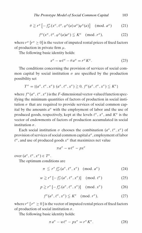
P1: IBE/IWV0521847885c02.xml CB829B/Uzawa 0 521 84788 5 August 27, 1956 17:7
The Prototype Model of Social Common Capital 103
θ � rµ[− f µ
aµ(xµ, �µ, ϕµ(a) aµ)ϕµ(a)]
(mod. aµ) (21)
f µ(xµ, �µ, ϕµ(a)aµ) � Kµ (mod. rµ), (22)
where rµ [rµ ≥ 0] is the vector of imputed rental prices of fixed factorsof production in private firm µ.
The following basic identity holds:
xµ − w�µ − θ aµ = rµKµ. (23)
The conditions concerning the provision of services of social com-mon capital by social institution σ are specified by the productionpossibility set
T σ = {(aσ , �σ , xσ ): (aσ , �σ , xσ ) � 0, f σ (aσ , �σ , xσ ) � Kσ }where f σ (aσ , �σ , xσ ) is the F-dimensional vector-valued function spec-ifying the minimum quantities of factors of production in social insti-tution σ that are required to provide services of social common cap-ital by the amounts aσ with the employment of labor and the use ofproduced goods, respectively, kept at the levels �σ , xσ , and Kσ is thevector of endowments of factors of production accumulated in socialinstitution σ .
Each social institution σ chooses the combination (aσ , �σ , xσ ) ofprovision of services of social common capital aσ , employment of labor�σ , and use of produced goods xσ that maximizes net value
πaσ − w�σ − pxσ
over (aσ , �σ , xσ ) ∈ Tσ .The optimum conditions are
π � rσ f σaσ (aσ , �σ , xσ ) (mod. aσ ) (24)
w � rσ [− f σ�σ (aσ , �σ , xσ )] (mod. �σ ) (25)
p � rσ [− f σxσ (aσ , �σ , xσ )] (mod. xσ ) (26)
f σ (aσ , �σ , xσ ) � Kσ (mod. rσ ), (27)
where rσ [ rσ ≥ 0 ] is the vector of imputed rental prices of fixed factorsof production of social institution σ .
The following basic identity holds:
π aσ − w�σ − pxσ = rσ Kσ . (28)

P1: IBE/IWV0521847885c02.xml CB829B/Uzawa 0 521 84788 5 August 27, 1956 17:7
104 Economic Analysis of Social Common Capital
Market Equilibrium for the Prototype Model of SocialCommon Capital
Suppose social common capital taxes with the rate τ are levied uponthe use of services of social common capital. Market equilibrium willbe obtained if we find prices of produced goods p; wage rates w; pricescharged for the use of services of social common capital θ ; and pricespaid for the provision of services of social common capital π , at whichdemand and supply are equal for all goods and labor services, and thetotal provision of services of social common capital is equal to the totaluse of services of social common capital. The prices charged for theuse of services of social common capital θ are higher, by the tax rate τ ,than the prices paid for the provision of services of social commoncapital π ; that is,
θ = π + τ θ. (29)
[To simplify the notational system, we are using the same symbol τ forsocial common capital tax rate τ and impact coefficient τ (a). To avoidconfusion, the impact coefficient is always expressed by the functionalform τ (a).]
The social common capital tax rates are administratively determinedby the government and announced prior to the opening of the mar-ket. Prices of produced goods p and wage rates w are determined inperfectly competitive markets, so are the prices charged for the use ofservices of social common capital and paid for the provision of servicesof social common capital, respectively, denoted by θ and π , where
p ≥ 0, w ≥ 0, π > 0, θ > 0.
Market Equilibrium and Social Common Capital
Market equilibrium under the presence of social institutions in chargeof social common capital is obtained if the following equilibrium con-ditions are satisfied:
(i) Each individual ν chooses the combination (cν, aν) of the vectorof consumption cν and the use of services of social commoncapital aν in such a manner that the utility of individual ν
uν = uν(cν, ϕν(a) aν)

P1: IBE/IWV0521847885c02.xml CB829B/Uzawa 0 521 84788 5 August 27, 1956 17:7
The Prototype Model of Social Common Capital 105
is maximized subject to the budget constraint
pcν + θaν = yν,
where yν is the income of individual ν in units of market pricesand a is the total amount of services of social common capitalused by all members of the society that is assumed to be givenwhen individual ν chooses (cν, aν).
(ii) Each private firm µ chooses the combination (xµ, �µ, aµ) ofvectors of production xµ, employment of labor �µ, and use ofservices of social common capital aµ that maximizes net profit
pxµ − w�µ − θaµ
over (xµ, �µ, aµ) ∈ Tµ.(iii) Each social institution σ chooses the combination (aσ , �σ , xσ )
of provision of services of social common capital aσ , employ-ment of labor �σ , and use of produced goods xσ that maximizesnet value
πaσ − w�σ − pxσ
over (aσ , �σ , xσ ) ∈ T σ .(iv) Total amounts of services of social common capital used by all
members of the society are equal to total amounts of servicesof social common capital provided by social institutions σ incharge of social common capital; that is,
a =∑
ν
aν +∑
µ
aµ (30)
a =∑
σ
aσ . (31)
(v) At wage rates w, total demand for employment of labor is equalto total supply: ∑
ν
�ν =∑
µ
�µ +∑
σ
�σ . (32)
(vi) At prices of produced goods p, total demand for goods is equalto total supply: ∑
µ
xµ =∑
ν
cν +∑
σ
xσ . (33)

P1: IBE/IWV0521847885c02.xml CB829B/Uzawa 0 521 84788 5 August 27, 1956 17:7
106 Economic Analysis of Social Common Capital
In the following discussion, we suppose that for any given level ofsocial common capital tax rate τ (τ ≥ 0), the state of the economy
E = (cν, aν, xµ, �µ, aµ, aσ , �σ , xσ , a, p, w, π, θ)
that satisfies all conditions for market equilibrium generally exists andis uniquely determined.
Concerning National Income Accounting
Income yν of each individual ν is given as the sum of wages, dividendpayments of private firms and social institutions, and subsidy pay-ments tν :
yν = w�ν +∑
µ
sνµrµKµ +∑
σ
sνσ rσ Kσ + tν,
where
sνµ � 0,∑
ν
sνµ = 1, sνσ � 0,∑
ν
sνσ = 1.
Subsidy payments {tν} for individuals are so arranged that the sumof subsidy payments to all individuals are equal to the sum of socialcommon capital tax payments τθa:∑
ν
tν = τ θa,
where
τθ = θ − π.
National income y is the sum of incomes of all individuals:
y =∑
ν
yν .
By taking note of the equilibrium conditions∑µ
xµ =∑
ν
cν +∑
σ
xσ ,∑
ν
�ν =∑
µ
�µ +∑
σ
�σ
a =∑
ν
aν +∑
µ
aµ, a =∑
σ
aσ ,
we have
y =∑
ν
w�ν +∑
µ
rµKµ +∑
σ
rσ Kσ + τθa

P1: IBE/IWV0521847885c02.xml CB829B/Uzawa 0 521 84788 5 August 27, 1956 17:7
The Prototype Model of Social Common Capital 107
=∑
ν
w�ν +∑
µ
(pxµ − w�µ − θaµ)
+∑
σ
( πaσ − w�σ − pxσ ) + τθa
=∑
ν
(pcν + θ aν) − (θ − π)a + τθa
=∑
ν
(pcν + θ aν).
Thus we have established the familiar identity of two definitions ofnational income.
6. market equilibrium and social optimum
To explore welfare implications of market equilibrium correspondingto the given levels of social common capital tax rates τ , we considerthe social utility U defined by
U =∑
ν
ανuν =∑
ν
ανuν(cν, ϕν(a)aν),
where utility weight αν is the inverse of marginal utility of income yν
of individual ν at market equilibrium.We consider the following maximum problem:
Maximum Problem for Social Optimum. Find the pattern of consump-tion and production of goods, employment of labor, use and provisionof services of social common capital, and total use of services of socialcommon capital, (cν, aν, xµ, �µ, aµ, aσ , �σ , xσ , a), that maximizes thesocial utility
U =∑
ν
ανuν =∑
ν
ανuν(cν, ϕν(a)aν) (34)
among all feasible patterns of allocation∑ν
cν +∑
σ
xσ �∑
µ
xµ (35)
∑µ
�µ +∑
σ
�σ �∑
ν
�ν (36)
∑ν
aν +∑
µ
aµ � a (37)
a �∑
σ
aσ (38)

P1: IBE/IWV0521847885c02.xml CB829B/Uzawa 0 521 84788 5 August 27, 1956 17:7
108 Economic Analysis of Social Common Capital
f µ(xµ, �µ, ϕµ(a) aµ) � Kµ (39)
f σ (aσ , �σ , xσ ) � Kσ , (40)
where utility weights αν are evaluated at the market equilibrium cor-responding to the given level of social common capital tax rate τ .
The maximum problem for social optimum may be solved in termsof the Lagrange method. Let us define the Lagrangian form:
L(cν, aν, xµ, �µ, aµ, aσ , �σ , xσ , a; p, w, θ, π, rµ, rσ )
=∑
ν
αν uν(cν, ϕν(a)aν) + p
( ∑µ
xµ −∑
ν
cν −∑
σ
xσ
)
+ w
( ∑ν
�ν −∑
µ
�µ −∑
σ
�σ
)
+ θ
(a −
∑ν
aν −∑
µ
aµ
)+ π
(∑σ
aσ − a
)
+∑
µ
rµ[Kµ − f µ(xµ, �µ, ϕµ(a) aµ)]
+∑
σ
rσ [Kσ − f σ (aσ , �σ , xσ )], (41)
where the Lagrange unknowns p, w, θ, π, rµ, and rσ are, respectively,associated with constraints (35), (36), (37), (38), (39), and (40).
The optimum solution may be obtained by partially differenti-ating the Lagrangian form (41) with respect to unknown variablescν, aν, xµ, �µ, aµ, aσ , �σ , xσ , a, and putting them equal to 0, where fea-sibility conditions (35)–(40) are satisfied:
ανuνcν (cν, ϕν(a) aν) � p (mod. cν) (42)
αν uνaν (cν, ϕν(a) aν)ϕν(a) � θ (mod. aν) (43)
p � rµ f µxµ(xµ, �µ, ϕµ(a) aµ) (mod. xµ) (44)
w � rµ[− f µ
�µ(xµ, �µ, ϕµ(a) aµ)]
(mod. �µ) (45)
θ � rµ[− f µ
aµ(xµ, �µ, ϕµ(a) aµ)ϕµ(a)]
(mod. aµ) (46)
f µ(xµ, �µ, ϕµ(a)aµ) � Kµ (mod. rµ) (47)
π � rσ f σaσ (aσ , �σ , xσ ) (mod. aσ ) (48)

P1: IBE/IWV0521847885c02.xml CB829B/Uzawa 0 521 84788 5 August 27, 1956 17:7
The Prototype Model of Social Common Capital 109
w � rσ[ − f σ
�σ (aσ , �σ , xσ )]
(mod. �σ ) (49)
p � rσ[ − f σ
xσ (aσ , �σ , xσ )]
(mod. xσ ) (50)
f σ (aσ , �σ , xσ ) � Kσ (mod. rσ ) (51)
θ = π + τ (a) aθ, (52)
where τ (a) is the vector of the impact coefficients of social commoncapital.
Only equation (52) may need clarification. Partially differentiatethe Lagrangian form (41) with respect to a, to obtain
∂ L∂ a
=∑
ν
αν uνaν (cν, ϕν(a) aν) [−τ (a)] ϕν(a) aν
+∑
µ
rµ[
f µaµ(xµ, �µ, ϕµ(a) aµ) τ (a)ϕµ(a) aµ
] + θ − π
= −τ (a)
[∑ν
θaν +∑
µ
θaµ
]+ θ − π = −τ (a)θa + θ − π.
Hence,∂ L∂ a
= 0 implies equation (52):
Equation (52) may be written as
θ − π = τθ, τ = τ (a)a, (53)
where τ is the social common capital tax rate that is administrativelydetermined prior to the opening of the market.
Applying the classic Kuhn-Tucker theorem on concave program-ming, Euler-Lagrange equations (42)–(52), together with feasibilityconditions (35)–(40), are necessary and sufficient conditions for theoptimum solution of the maximum problem for social optimum. [See,for example, Arrow, Hurwicz, and Uzawa (1958). In the mathematicalnotes at the end of Chapter 1 of Uzawa (2003), a brief description ofthe Kuhn-Tucker theorem on concave programming is presented.]
It is apparent that Euler-Lagrange equations (42)–(52), togetherwith feasibility conditions (35)–(40), coincide precisely with the equi-librium conditions for market equilibrium with the social common cap-ital tax rate given by (53).
As noted previously, marginality conditions (42) and (43) and thelinear homogeneity hypothesis for utility functions uν(cν, aν) imply
αν uν(cν, ϕν(a)aν) = pcν + θ aν = yν,

P1: IBE/IWV0521847885c02.xml CB829B/Uzawa 0 521 84788 5 August 27, 1956 17:7
110 Economic Analysis of Social Common Capital
which, by summing over ν, yield
U =∑
ν
yν = y.
We have thus established the following proposition.
Proposition 1. Consider the social common capital tax scheme with thetax rate τ for the use of services of social common capital given by
τ = τ (a)a,
where τ (a) is the vector of impact coefficients of social common capital.Then market equilibrium obtained under such a social common cap-
ital tax scheme is a social optimum in the sense that a set of positiveweights for the utilities of individuals (α1, . . . , αn)[αν > 0] exists suchthat the social utility
U =∑
ν
ανuν =∑
ν
ανuν(cν, ϕν(a)aν)
is maximized among all feasible patterns of allocation (cν, aν, xµ, �µ, aµ,
aσ , �σ , xσ , a).The optimum level of social utility U is equal to national income y:
U = y.
Social optimum is defined with respect to any social utility
U =∑
ν
ανuν =∑
ν
ανuν(cν, ϕν(a)aν),
where (α1, . . . , αn) is an arbitrarily given set of positive weights for theutilities of individuals. A pattern of allocation (cν, aν, xµ, �µ, aµ, aσ , �σ ,
xσ , a) is a social optimum if the given social utility U is maximizedamong all feasible patterns of allocation.
Social optimum necessarily implies the existence of the social com-mon capital tax scheme, where the tax rate τ is given by τ = τ (a)a.However, the budgetary constraints for individuals
pcν + θaν = yν
are not necessarily satisfied. It is apparent that the following proposi-tion holds.

P1: IBE/IWV0521847885c02.xml CB829B/Uzawa 0 521 84788 5 August 27, 1956 17:7
The Prototype Model of Social Common Capital 111
Proposition 2. Suppose a pattern of allocation (cν, aν, xµ, �µ, aµ, aσ ,
�σ , xσ , a) is a social optimum; that is, a set of positive weights forthe utilities of individuals (α1, . . . , αn) exists such that the given pat-tern of allocation (cν, aν, xµ, �µ, aµ, aσ , �σ , xσ , a) maximizes the socialutility
U =∑
ν
ανuν =∑
ν
ανuν(cν, ϕν(a)aν)
among all feasible patterns of allocation.Then, a system {tν} of income transfer among individuals of the so-
ciety exists such that ∑ν
tν = 0,
and the given pattern of allocation (cν, aν, xµ, �µ, aµ, aσ , �σ , xσ , a) cor-responds precisely to the market equilibrium under the social commoncapital tax scheme with the rate τ given by
τ = τ (a)a,
where τ (a) is the vector of impact coefficients of social common capital.
7. social common capital and lindahl equilibrium
The concept of Lindahl equilibrium was originally introduced byLindahl (1919) to examine the structure of a tax system that is justand equitable, rather than merely efficient. Since then, a large num-ber of contributions were made to clarify welfare implications ofLindahl equilibrium within the theory of public goods, in particular byJohansen (1963), Foley (1967, 1970), Fabre-Sender (1969), Malinvaud(1971), Milleron (1972), Roberts (1974), Kaneko (1977), Mas-Colell(1980), and Maler and Uzawa (1994), among others.
With respect to global warming, the existence of Lindahl equilib-rium and the implications for the welfare effect of global warmingwere examined in detail by Uzawa (2003). Within the context of globalwarming, Lindahl equilibrium is obtained when, in each country, theactual level of total CO2 emissions is exactly equal to the level thatwould be chosen by each country if it were free to choose the level oftotal CO2 emissions most desirable in terms of its preference ordering,assuming that the price it would be paid is equal to its own marginal

P1: IBE/IWV0521847885c02.xml CB829B/Uzawa 0 521 84788 5 August 27, 1956 17:7
112 Economic Analysis of Social Common Capital
disutility. With regard to social common capital, the concept of Lindahlequilibrium is similarly defined.
Lindahl Conditions
Let us recall the postulates for the behavior of individuals at marketequilibrium. At market equilibrium, conditions for the consumer opti-mum are obtained if each individual ν chooses the combination (cν, aν)of vector of consumption cν and use of services of social common cap-ital aν in such a manner that the utility of individual ν
uν = uν(cν, ϕν(a) aν)
is maximized subject to the budget constraint
pcν + θaν = yν .
Let us first rewrite the budget constraint as follows:
pcν + θaν − τ θaν = �y ν,
where�y ν = yν − τ θaν .
Lindahl conditions are satisfied if a system of individual tax rates{τ ν} exists such that∑
ν
τ ν = τ, τ ν � 0 for all ν,
and for each individual ν, (cν, aν, a) is the optimum solution to thefollowing virtual maximum problem:
Find (cν, aν, a(ν)) that maximizes
uν = ϕν(a(ν)) uν(cν, ϕν(a(ν)) aν)
subject to the virtual budget constraint
p cν + θ aν − τ ν θ a(ν) = yν .
Because (cν, aν, a) is the optimum solution to the virtual maximumproblem for individual ν, the optimum conditions imply
τ νθ = αν uνaν (cν, ϕν(a) aν) [τ (a) ϕν(a) aν],
where αν is the inverse of marginal utility of income yν of individual ν.

P1: IBE/IWV0521847885c02.xml CB829B/Uzawa 0 521 84788 5 August 27, 1956 17:7
The Prototype Model of Social Common Capital 113
Hence,
τ νθ = τ (a) aνθ,
which implies
τ νθ a = τ (a)aνθ a = τθ aν .
Thus, Lindahl conditions are always satisfied at market equilibrium.
Lindahl Equilibrium
A pattern of consumption, production, and use and provision of ser-vices of social common capital (cν, aν, xµ, �µ, aµ, aσ , �σ , xσ , a) is aLindahl equilibrium if there exist prices of produced goods p; wagerates and user charges for services of social common capital, respec-tively, denoted by w and θ ; and prices paid for the provision of ser-vices of social common capital π such that the following conditions aresatisfied:
(i) Each individual ν chooses the combination (cν, aν) of vector ofconsumption cν and use of services of social common capital aν
in such a manner that the utility of individual ν
uν = uν(cν, ϕν(a) aν)
is maximized subject to the budget constraint
pcν + θaν = yν,
where yν is the income of individual ν in units of market pricesand a is the total amount of services of social common capitalused by all members of the society:
a =∑
ν
aν +∑
µ
aµ.
(ii) Each private firm µ chooses the combination (xµ, �µ, aµ) ofvectors of production xµ, employment of labor �µ, and use ofservices of social common capital aµ that maximizes net profit
pxµ − w�µ − θaµ
over (xµ, �µ, aµ) ∈ Tµ.

P1: IBE/IWV0521847885c02.xml CB829B/Uzawa 0 521 84788 5 August 27, 1956 17:7
114 Economic Analysis of Social Common Capital
(iii) Each social institution σ chooses the combination (aσ , �σ , xσ )of provision of services of social common capital aσ , employ-ment of labor �σ , and use of produced goods xσ that maximizesnet value
πaσ − w�σ − pxσ
over (aσ , �σ , xσ ) ∈ Tσ .(iv) Total amounts of services of social common capital used by all
members of the society are equal to total amounts of servicesof social common capital provided by social institutions σ incharge of social common capital; that is,
a =∑
ν
aν +∑
µ
aµ
a =∑
σ
aσ .
(v) At the vector of wage rates w, total demand for the employmentof labor is equal to total supply:∑
ν
�ν =∑
µ
�µ +∑
σ
�σ .
(vi) At the vector of prices for produced goods p, total demand forgoods is equal to total supply:∑
µ
xµ =∑
ν
cν +∑
σ
xσ .
(vii) Lindahl conditions for individuals are satisfied; that is, for eachindividual ν, (cν, aν, a) is the optimum solution to the followingvirtual maximum problem:
Find (cν, aν, a(ν)) that maximizes
uν = ϕν(a(ν)) uν(cν, ϕν(a(ν)) aν)
subject to the virtual budget constraint
p cν + θ aν − τ ν a(ν) = yν,
where
yν = yν − τ θ aν .
It is apparent that the following proposition holds.

P1: IBE/IWV0521847885c02.xml CB829B/Uzawa 0 521 84788 5 August 27, 1956 17:7
The Prototype Model of Social Common Capital 115
Proposition 3. Consider the social common capital tax scheme with thetax rate τ for the use of services of social common capital given by
τ = τ (a)a,
where τ (a) is the vector of impact coefficients of social common capital.Then market equilibrium obtained under such a social common cap-
ital tax scheme is always a Lindahl equilibrium.
8. adjustment processes of social common capital
In the previous sections, we examined two patterns of resource alloca-tion involving social common capital: market allocation, on one hand,and social optimum, on the other. Market allocation is obtained ascompetitive equilibrium with social common capital taxes levied onthe use of services of social common capital with the tax rate
τ = τ (a)a,
where τ (a) is the vector of impact coefficients of social common capital.Social optimum is defined with respect to the social utility
U =∑
ν
ανuν =∑
ν
ανuν(cν, ϕν(a)aν),
where (α1, . . . , αn) [αν > 0] is an arbitrarily given set of positive weightsfor the utilities of individuals. A pattern of allocation is social optimumif the social utility U is maximized among all feasible patterns of allo-cation.
Market equilibrium with social common capital tax rate τ = τ (a)acoincides with the social optimum with respect to the social utility
U =∑
ν
ανuν =∑
ν
ανuν(cν, ϕν(a)aν),
where, for each individual ν, utility weight αν is the inverse of marginalutility of income yν at market equilibrium.
We have also shown that market equilibrium with social commoncapital tax rate τ = τ (a)a is always a Lindahl equilibrium.
The tax rate τ = τ (a)a is administratively determined and an-nounced prior to the opening of the market, when the total amount ofservices of social common capital a used by all members of the societyis not known. We may need to devise adjustment processes concerning

P1: IBE/IWV0521847885c02.xml CB829B/Uzawa 0 521 84788 5 August 27, 1956 17:7
116 Economic Analysis of Social Common Capital
the social common capital tax rate that are stable. We first consider analternative adjustment process concerning the total amount of servicesof social common capital a. In the following discussion, we work withthe prototype model of social common capital in which only one kindof social common capital exists.
We would first like to examine the relationships between the totalamount of services of social common capital and the ensuing level ofthe social utility.
Let us assume that the total amount of services of social commoncapital a is announced at the beginning of the adjustment process andconsider the pattern of resource allocation at the market equilibriumwith the total amount of services of social common capital at the givenlevel a.
Market equilibrium under the presence of social institutions incharge of social common capital is obtained if the following equilibriumconditions are satisfied:
(i) Each individual ν chooses the combination (cν, aν) of the vectorof consumption cν and the use of services of social commoncapital aν in such a manner that the utility of individual ν,
uν = uν(cν, ϕν(a) aν),
is maximized subject to the budget constraint
pcν + θaν = yν,
where yν is the income of individual ν in units of market pricesand a is the total amount of services of social common capitalused by all members of the society that is assumed to be givenwhen individual ν chooses (cν, aν):
a =∑
ν
aν +∑
µ
aµ.
(ii) Each private firm µ chooses the combination (xµ, �µ, aµ) ofvectors of production xµ, use of variable factors of production�µ, and use of services of social common capital aµ that maxi-mizes net profit
pxµ − w�µ − θaµ
over (xµ, �µ, aµ) ∈ Tµ.

P1: IBE/IWV0521847885c02.xml CB829B/Uzawa 0 521 84788 5 August 27, 1956 17:7
The Prototype Model of Social Common Capital 117
(iii) Each social institution σ chooses the combination (aσ , �σ , xσ )of provision of services of social common capital aσ , employ-ment of labor �σ , and use of produced goods xσ that maximizesnet value
πaσ − w�σ − pxσ
over (aσ , �σ , xσ ) ∈ Tσ .(iv) Total amounts of services of social common capital used by all
members of the society are equal to total amounts of servicesof social common capital provided by social institutions σ incharge of social common capital; that is,
a =∑
ν
aν +∑
µ
aµ
a =∑
σ
aσ .
(v) At the vector of wage rates w, total demand for the employmentof labor is equal to total supply:∑
ν
�ν =∑
µ
�µ +∑
σ
�σ .
(vi) At the vector of prices for produced goods p, total demand forgoods is equal to total supply:∑
µ
xµ =∑
ν
cν +∑
σ
xσ .
It may be noted that the total amount of services of social commoncapital is given at an arbitrarily given level a and announced prior tothe opening of the market, whereas social common capital tax rate τ
is given at the level satisfying
τθ = θ − π, (54)
where θ and π are, respectively, the prices charged for the use of socialcommon capital and paid for the provision of services of social commoncapital determined on the market.
Market equilibrium thus obtained corresponds to the social opti-mum with respect to the social utility
U =∑
ν
ανuν =∑
ν
ανuν(cν, ϕν(a)aν),

P1: IBE/IWV0521847885c02.xml CB829B/Uzawa 0 521 84788 5 August 27, 1956 17:7
118 Economic Analysis of Social Common Capital
where, for each individual ν, utility weight αν is the inverse of marginalutility of income of individual ν at the market equilibrium and thetotal amount of services of social common capital at the predeterminedlevel a.
We examine the effect of the marginal change in the total amountof services of social common capital a on the level of the social utilityU. The level of the social utility U at market equilibrium is given asthe value of the Lagrangian form, as defined by (41):
L = L(cν, aν, xµ, aµ, bσ , wσ ; p, π, θ, rµ, ρσ )
=∑
ν
αν uν (cν, ϕν(a)aν) + p
( ∑µ
xµ −∑
ν
cν −∑
σ
xσ
)
+ w
( ∑ν
�ν −∑
µ
�µ −∑
σ
�σ
)
+ θ
(a −
∑ν
aν −∑
µ
aµ
)+ π
(∑σ
aσ − a
)
+∑
µ
rµ[Kµ − f µ(xµ, �µ, ϕµ(a) aµ)]
+∑
σ
rσ [Kσ − f σ (aσ , �σ , xσ )],
where a is not a variable, but rather is regarded as a parameter.By taking total differentials of both sides of the Lagrangian form L
and by noting equilibrium conditions
∂L∂cν
= 0,∂L∂aν
= 0, . . . ,∂L∂aσ
= 0,∂L∂�σ
= 0,∂L∂xσ
= 0, . . . ,
we obtain
dU = [θ − π − τ (a)a θ ]da.
Hence,
dUda
= θ − π − τ (a)a θ. (55)
The Lagrangian unknown θ may be interpreted as the imputed pricefor the use of services of social common capital, and it is decreased asthe total amount of services of social common capital a is increased.Similarly, the Lagrangian unknown π may be interpreted as the im-puted price for the provision of services of social common capital, and

P1: IBE/IWV0521847885c02.xml CB829B/Uzawa 0 521 84788 5 August 27, 1956 17:7
The Prototype Model of Social Common Capital 119
it is increased as the total amount of services of social common capital ais increased. Hence, the right-hand side of equation (55) is a decreasingfunction of a when the following condition is satisfied:
τ (a)a < 1.
The tax rate τ at the market equilibrium with the total amount ofservices of social common capital a is also uniquely determined:
τθ = θ − π.
We have now established the following proposition.
Proposition 4. Consider the adjustment process defined by the followingdifferential equation:
(A) a = k [θ − π − τ (a)aθ ],
where the speed of adjustment k is a positive constant and all variablesrefer to the state of the economy at the market equilibrium under thesocial common capital tax scheme with the tax rate τ :
τθ = θ − π.
Then differential equation (A) is globally stable; that is, for any initialcondition a0, the solution path to differential equation (A) converges tothe stationary state a, where
θ − π = τ (a)aθ, τ (a)a < 1.
Adjustment Processes of Social Common Capital Tax Rate
At the market equilibrium with social common capital tax rate τ (a)a,individual social common capital tax payments are then given byτ (a)aθ aν (ν ∈ N).
We would like to introduce an adjustment process with respect tothe social common capital tax rate τ that is globally stable.
For an arbitrarily given social common capital tax rate τ , let usconsider the market equilibrium in which income yν of each individualν is given by
yν = w�ν +[∑
µ
sνµrµKµ +∑
σ
sνσ rσ Kσ
]+ tν,
sνµ � 0,∑
ν
sνµ = 1, sνσ � 0,∑
ν
sνσ = 1,

P1: IBE/IWV0521847885c02.xml CB829B/Uzawa 0 521 84788 5 August 27, 1956 17:7
120 Economic Analysis of Social Common Capital
where rµ and rσ are, respectively, the imputed rental prices of factorsof production of private firm µ and social institution σ , tν is the subsidypayments to individual ν, and∑
ν
tν = τθa, τθ = θ − π.
Such a market equilibrium is characterized by the following condi-tions, where p, θ , and π are, respectively, the prices of produced goods,the price charged for the use of services of social common capital θ , andthe price paid for the provision of services of social common capital:
(i) Each individual ν chooses the combination (cν, aν) of the vectorof consumption cν and the use of services of social commoncapital aν in such a manner that the utility of individual ν
uν = uν(cν, ϕν(a) aν)
is maximized subject to the budget constraint
pcν + θaν = yν,
where yν is the income of individual ν in units of market pricesand a is the total amount of services of social common capitalused by all members of the society that is assumed to be givenwhen individual ν chooses (cν, aν).
(ii) Each private firm µ chooses the combination (xµ, �µ, aµ) ofvectors of production xµ, employment of labor �µ, and use ofservices of social common capital aµ that maximizes net profit
pxµ − w�µ − θaµ
over (xµ, �µ, aµ) ∈ Tµ.(iii) Each social institution σ chooses the combination (aσ , �σ , xσ )
of provision of services of social common capital aσ , employ-ment of labor �σ , and use of produced goods xσ that maximizesnet value
πaσ − w�σ − pxσ
over (aσ , �σ , xσ ) ∈ Tσ .(iv) Total amounts of services of social common capital used by all
members of the society are equal to total amounts of services

P1: IBE/IWV0521847885c02.xml CB829B/Uzawa 0 521 84788 5 August 27, 1956 17:7
The Prototype Model of Social Common Capital 121
of social common capital provided by social institutions σ incharge of social common capital; that is,
a =∑
ν
aν +∑
µ
aµ
a =∑
σ
aσ .
(v) At the vector of prices of variable factors of production w, totaldemand for the use of variable factors of production is equalto total supply: ∑
ν
�ν =∑
µ
�µ +∑
σ
�σ .
(vi) At the vector of prices for produced goods p, total demand forgoods is equal to total supply:∑
µ
xµ =∑
ν
cν +∑
σ
xσ .
(vii) The price charged for the use of services of social commoncapital θ exceeds, by the tax rate τ θ , the price paid for theprovision of services of social common capital π :
θ − π = τ θ.
We then consider the adjustment process with respect to the so-cial common capital tax rate τ defined by the following differentialequation:
(B) τ = k[τ (a)a − τ ],
with initial condition τθ , where k is an arbitrarily given positive number.It is apparent that the following proposition holds.
Proposition 5. The adjustment process defined by differential equation(B) is globally stable; that is, for any initial condition τ0, the solution pathτ to differential equation (B) converges to the optimum social commoncapital tax rate τ (a)a.

P1: IBE/IWV/KAC P2: IWV0521847885c03.xml CB829B/Uzawa 0 521 84788 5 August 27, 1956 17:25
3
Sustainability and Social Common Capital
1. introduction
Social common capital involves intergenerational equity and justice.Although the construction and maintenance of social common capitalrequire the use of substantial portions of scarce resources, both humanand nonhuman, putting a significant burden on the current generation,future generations will benefit greatly if the construction of social com-mon capital carried out by the current generation is properly arranged.
In this chapter, we examine the problems of the accumulation ofsocial common capital primarily from the viewpoint of the intergener-ational distribution of utilities. Our analysis is based on the concept ofsustainability introduced in Uzawa (1991b, 2003), and we examine theconditions under which processes of the accumulation of social com-mon capital over time are sustainable. The conceptual framework ofthe economic analysis of social common capital developed in Chap-ter 2 are extended to deal with the problems of the irreversibility ofprocesses of the accumulation of social common capital owing to thePenrose effect. The concept of the Penrose effect was originally intro-duced in Uzawa (1968, 1969) in the context of macroeconomic analysis,and was extensively utilized in the dynamic analysis of global warm-ing as described in Uzawa (2003, Chapter 5 ). The presentation of thetheory of sustainable processes of capital accumulation in this chapterlargely reproduces the one introduced there.
The analysis focuses on the examination of the system of imputedprices associated with the time-path of consumption that is dynami-cally optimum with respect to the intertemporal preference relation,
122

P1: IBE/IWV/KAC P2: IWV0521847885c03.xml CB829B/Uzawa 0 521 84788 5 August 27, 1956 17:25
Sustainability and Social Common Capital 123
in which the presence of the Penrose effect implies the diminishingmarginal rates of investment in private capital and social commoncapital upon the rates at which private capital and social common cap-ital are accumulated. The sustainable time-path of consumption andinvestment is characterized by the stationarity of the imputed pricesassociated with the given intertemporal preference ordering, whereasthe efficiency of resource allocation from the short-run point of viewis preserved at each time.
Similar concepts may be applied to the general case of accumulationof both private and social common capital. A time-path of consump-tion and capital accumulation is sustainable when the imputed priceof each kind of social common capital remains identical over time. Inother words, a time-path of consumption and investment is sustainableif all future generations will face the same imputed prices of variouskinds of social common capital as those faced by the current genera-tion. The existence of the sustainable time-path of consumption andcapital accumulation starting with an arbitrarily given stock of capitalis ensured when the processes of accumulation of various kinds of capi-tal are subject to the Penrose effect that exhibits the law of diminishingmarginal rates of investment.
In what follows, we present a way of formulating the concept of sus-tainability within the theoretical framework of the economic analysis ofsocial common capital and derive propositions that may be consultedin devising institutional arrangements and policy measures likely tobe effective in realizing a sustainable state such as that introduced byJohn Stuart Mill in his classic Principles of Political Economy (Mill1848), particularly in the chapter entitled “On Stationary States.” Thestationary state, as envisioned by Mill, is interpreted as the state ofthe economy in which all macroeconomic variables, such as gross do-mestic product, national income, consumption, investments, prices ofall goods and services, wages, and real rates of interest, all remain sta-tionary, whereas, within the society, individuals are actively engaged ineconomic, social, and cultural activities, new scientific discoveries areincessantly made, and new products are continuously introduced whilethe natural environment is being preserved at the sustainable state.
The concept of sustainability also involves intergenerational equityand justice. The problems of intergenerational equity and justice havebeen studied by several economists and philosophers. Our formulation

P1: IBE/IWV/KAC P2: IWV0521847885c03.xml CB829B/Uzawa 0 521 84788 5 August 27, 1956 17:25
124 Economic Analysis of Social Common Capital
of the concept of sustainability is largely based on contributions byRawls (1971), Solow (1974a,b), Sen (1982), Norton (1989), Norgaard(1990a,b), Howarth and Norgaard (1990, 1992, 1995), Page (1991,1997), Uzawa (1991b, 1992a, 1998), Howarth and Monahan (1992),and Pezzey (1992).
2. review of the theory of dynamic optimality
We begin our discussion with a review of the theory of optimum capitalaccumulation that was originally introduced by Ramsey (1928) andelaborated by Arrow (1962a,b; 1965, 1968), Uzawa (1964), Srinivasan(1965), Koopmans (1965), Cass (1965), and Arrow and Kurz (1970).The Ramsey theory of dynamic optimality was further elaborated byEpstein and Haynes (1983), Lucas and Stokey (1984), Roemer (1986),Epstein (1987), and Rebelo (1993). It was later applied by Uzawa (1993,1996, 1998, 2003) to the problems of capital accumulation involvingsocial common capital such as the atmosphere and the commons.
In examining the processes of sustainability involving the accumu-lation of social common capital, we take specific note of the contribu-tions made by a large number of economists concerning the problemsof optimum economic growth and environmental quality. We cite onlya few among these contributions having implications pertinent to theanalysis developed in this chapter: d’Arge (1971a,b), Keeler, Spence,and Zeckhauser (1971), Forster (1973), Dasgupta and Heal (1974,1979), Maler (1974), Solow (1974b), Krautkraemer (1985), Musu (1990,1994), Grossman and Helpman (1991), Howarth (1991a,b), Aghionand Howitt (1992), Gradus and Smulders (1993), Huan and Cai (1994),Bovenberg and Smulders (1995), Smulders (1995), and Smulders andGradus (1996).
The Ramsey–Koopmans–Cass Theory of OptimumCapital Accumulation
The basic premises of the analysis of dynamic optimality are that theintertemporal preference ordering prevailing in the society in questionis independent of the technological conditions and processes of capitalaccumulation, as typically illustrated by the Ramsey–Koopmans–Cassutility integral, and the Pontryagin maximum method in the calculusof variations is effectively utilized.

P1: IBE/IWV/KAC P2: IWV0521847885c03.xml CB829B/Uzawa 0 521 84788 5 August 27, 1956 17:25
Sustainability and Social Common Capital 125
We consider an aggregative model of capital accumulation whosebehavioral characteristics are described by those of the representativeconsumer and producer. We first consider the simple case in whichonly one kind of goods serves both for consumption and investment.Those goods that are invested as capital may also be used either forconsumption or investment. The utility of the representative consumeris assumed to be cardinal.
The instantaneous level of the utility ut at each time t is representedby a utility function
ut = u(ct ),
where ct is the quantity of goods consumed by the representative con-sumer at time t.
We assume that the utility function u = u(c) remains identical overtime, is defined for all nonnegative c � 0, is continuous and continu-ously twice-differentiable, and satisfies the following conditions:
u(c) > 0, u ′(c) > 0, u′′ (c) < 0 for all c > 0.
We assume that the intertemporal preference ordering over the setof conceivable time-paths of consumption (ct: t � 0) may be expressedby the Ramsey–Koopmans–Cass utility integral
U(c) =∫ ∞
0u(ct )e−δ t dt, c = (ct ), (1)
where ut = u(ct ) is the utility function expressing the instantaneouslevel of utility at time t and δ is the utility rate of discount that isassumed to be a positive constant (δ > 0).
The utility rate of discount δ is assumed to be independent of thetime-path of consumption and capital accumulation, and to be con-stant and positive. The conceptual basis of the discount rate has beenintensively examined in the literature by Koopmans (1965), Arrow andKurz (1970), Bradford (1975), Dasgupta (1982a), Lind (1982a,b), Sen(1982), Stiglitz (1982), Stockfish (1982), Cropper and Portney (1992),Wallace (1993), and Weitzman (1993).
We denote by Kt the stock of capital at time t , and by ct , zt , respec-tively, consumption and investment at time t . Then, we have
ct + zt = f (Kt ), (2)

P1: IBE/IWV/KAC P2: IWV0521847885c03.xml CB829B/Uzawa 0 521 84788 5 August 27, 1956 17:25
126 Economic Analysis of Social Common Capital
where f (K) is the production function that is assumed to be indepen-dent of time t .
The production function f (K) expresses the net national productproduced from the given stock of capital K. We assume that produc-tion function f (K) is defined, continuous, and continuously twice-differentiable for all K>0, that marginal products of capital are al-ways positive, and that production processes are subject to the law ofdiminishing marginal returns:
f ′(K) > 0, f ′′(K) < 0 for all K > 0.
The rate of capital accumulation at time t , Kt , is given by the dynamicequation
Kt = α(zt , Kt ), K0 = K0, (3)
where K0 is the initial stock of capital and α(zt , Kt ) is the Penrosefunction relating the rate of capital accumulation Kt to investment zt
and the stock of capital Kt at time t .The Penrose function α(z, K) expresses the net rate of capital
accumulation; thus we may assume that the partial derivative of α(z, K)with respect to z is always positive, whereas with respect to K, it isalways negative:
αz = αz(z, K) > 0, αK = αK(z, K) < 0.
The Penrose Effect
The Penrose effect is expressed by the conditions that the Penrosefunction α(z, K) is concave and strictly quasi-concave with respect to(z, K):
αzz < 0, αKK < 0, αzzαKK − αzK2 � 0.
The following condition is usually assumed for the Penrose functionα(z, K):
αzK(z, K) = αKz(z, K) < 0.
Note that all variables are assumed to be nonnegative:
Kt , ct , zt � 0 for all t � 0.

P1: IBE/IWV/KAC P2: IWV0521847885c03.xml CB829B/Uzawa 0 521 84788 5 August 27, 1956 17:25
Sustainability and Social Common Capital 127
The concept of the Penrose effect was originally introduced byPenrose (1959) to describe the growth processes of an individual firm.It was later formalized by Uzawa (1968, 1969) in the context of aKeynesian analysis of macroeconomic processes of dynamic equilib-rium to elucidate the effect of investment activities on the processes ofcapital accumulation.
Marginal Efficiency of Investment
A particularly important concept associated with the Penrose functionα(z, K) is marginal efficiency of investment, which plays a crucial rolein the analysis of dynamic processes of capital accumulation and eco-nomic growth. Marginal efficiency of investment expresses the extentto which the marginal increase in investment z induces the marginalincrease in net national product f (K) in the future. The marginalefficiency of investment is composed of two components.
The first component is the marginal increase in net national productf (K) directly induced by the marginal increase αz(z, K) in the stockof capital due to the marginal increase in investment z; that is,
r(K)αz(z, K),
where r(K) = f ′(K) is the marginal product of capital.The second component measures the extent of the marginal effect on
future processes of capital accumulation due to the marginal increasein the stock of capital today K; that is,
αK(z, K).
Thus, the marginal efficiency of investment m = m(z, K) may beexpressed as
m = m(z, K) = r(K) αz(z, K) + αK(z, K).
The marginal efficiency of investment m = m(z, K) is a decreasingfunction of both investment z and the stock of capital K:
mz(z, K) = ∂m∂z
= rαzz + αKz < 0
mK(z, K) = ∂m∂K
= r ′αz + (αzK + αKK) < 0,
where r ′ = r ′(K) = f ′′(K) < 0.

P1: IBE/IWV/KAC P2: IWV0521847885c03.xml CB829B/Uzawa 0 521 84788 5 August 27, 1956 17:25
128 Economic Analysis of Social Common Capital
In the standard neoclassical theory of investment, the Penrose effectis not recognized; that is,
α(z, K) = z for all z � 0, K � 0.
Then,
m (z, K) = r
mz(z, K) = 0, mK(z, K) = r ′(K) < 0 for all z � 0, K � 0.
Dynamic Optimality and Imputed Price of Capital
A time-path of consumption and capital accumulation, (c, K) =(ct , Kt ), is dynamically optimum if it maximizes the Ramsey–Koopmans–Cass utility integral
U(c) =∫ ∞
0u(ct )e−δt dt, c = (ct ) (4)
subject to the constraints that
ct + zt = f (Kt ) (5)
Kt = α(zt , Kt ), K0 = K0, (6)
where the initial stock of capital K0 is given and positive (K0 > 0).The problem of the dynamic optimum may be solved in terms of
the concept of imputed price of capital. The imputed price of capital attime t , πt , is the discounted present value of the marginal increases inoutputs in the future measured in units of the utility due to the marginalincrease in investment at time t . The marginal increase in outputs atfuture time τ measured in units of the utility is given by
πτ mτ ,
where πt is the imputed price of capital at future time τ and mτ is themarginal efficiency of investment at future time τ :
mτ = m(zτ , Kτ ) = rτ αz(zτ , Kτ ) + αK(zτ , Kτ ), rτ = f ′(Kτ ).
Thus the imputed price of capital at time t , πt , is given by
πt =∫ ∞
tπτ mτ e−δ(τ−t)dτ . (7)

P1: IBE/IWV/KAC P2: IWV0521847885c03.xml CB829B/Uzawa 0 521 84788 5 August 27, 1956 17:25
Sustainability and Social Common Capital 129
By differentiating both sides of (7) with respect to time t , we obtainthe following differential equation:
πt = δπt − mtπt . (8)
Differential equation (8) is the Euler–Lagrange differential equa-tion in the calculus of variations. In the context of the theory of op-timum capital accumulation, it is often referred to as the Ramsey–Keynes equation. The economic meaning of the Ramsey–Keynesequation (8) may be brought out better if we rewrite it as
πt + mtπt = δπt . (9)
We suppose that capital is transacted as an asset on a virtual capitalmarket that is perfectly competitive and the imputed price πt is iden-tified with the market price at time t . Consider the situation in whichthe unit of such an asset is held for the short time period [t, t + �t](�t > 0). The gains obtained by holding such an asset are composedof capital gains �πt = πt+�t − πt and “earnings” mtπt�t ; that is,
�πt + mtπt�t.
On the other hand, the cost of holding such an asset for the time pe-riod [t, t + �t] consists of “interest” payment δπt�t , where the utilityrate of discount δ is identified with the “rate of interest.” Hence, on avirtual capital market, these two amounts become equal; that is,
�πt + mtπt�t = δπt�t.
Dividing both sides of this equation by �t and taking the limit as�t → 0, we obtain relation (9).
By dividing both sides of relation (8) by πt , we obtain the followingequation:
πt
πt= δ − mt . (10)
The imputed real national income at time t , Ht , is given by
Ht = u(xt ) + πtα(zt , Kt ). (11)
The optimum levels of consumption and investment at each timet , (ct , zt ), are obtained if imputed real national income Ht at time t

P1: IBE/IWV/KAC P2: IWV0521847885c03.xml CB829B/Uzawa 0 521 84788 5 August 27, 1956 17:25
130 Economic Analysis of Social Common Capital
is maximized subject to feasibility constraint (5). Let the Lagrangianform be given by
Lt = u(ct ) + πtα(zt , Kt ) + pt [ f (Kt ) − ct − zt ],
where pt is the Lagrangian unknown associated with constraint (5).The optimum conditions are
u′(ct ) = pt (12)
πtαz(zt , Kt ) = pt , (13)
where the value of pt is chosen so that feasibility condition (5) is satis-fied.
Lagrange unknown pt may be interpreted as the imputed price ofthe output at time t . Equation (12) means that the optimum level ofconsumption ct at time t is obtained when marginal utility u′(ct ) isequated with imputed price pt at time t . Equation (13) means that theoptimum level of investment zt at time t is obtained when the value ofthe marginal product of investment zt evaluated at the imputed priceπt of capital is equated with the imputed price pt of the output attime t .
The dynamically optimum time-path of consumption and capitalaccumulation, (c, K) = ((ct , Kt )), is obtained if the time-path of theimputed price of capital (πt ) thus obtained satisfies the transversalityconditions:
limt→+∞ πt Kt e−δt = 0.
Under the neoclassical conditions imposed on the utility func-tion, the production function, and the Penrose function, the dynam-ically optimum time-path of consumption and capital accumulation,(co, Ko) = ((co
t , Kot )), with an arbitrarily given initial stock of capi-
tal K0 [K0 > 0] generally exists and is uniquely determined, providedthat only one kind of capital goods is involved. For the general caseinvolving several kinds of capital goods, however, the dynamically op-timum time-path of consumption and capital accumulation, (co, Ko) =((co
t , Kot )), has been shown to exist only for exceptionally rare
circumstances.

P1: IBE/IWV/KAC P2: IWV0521847885c03.xml CB829B/Uzawa 0 521 84788 5 August 27, 1956 17:25
Sustainability and Social Common Capital 131
3. dynamic optimality for the economy with severalkinds of produced and capital goods
The optimum theory of capital accumulation, as briefly reviewed inthe previous section, may be applied to an economy involving severalkinds of produced goods as well as capital goods.
We consider an economy consisting of n individuals and m privatefirms. Individuals are generically denoted by ν = 1, . . , n, and privatefirms by µ = 1, . . , m. Goods produced by private firms are genericallydenoted by j = 1, . . , J .
We assume the utility of each individual ν is cardinal and is expressedby the utility function
uν = uν(cν),
where cν = (cνj ) is the vector of goods consumed by individual ν.
We assume that, for each individual ν, the utility function uν(cν) iscontinuous, continuously twice-differentiable, concave, strictly quasi-concave, and homogeneous of order 1 with respect to cν .
There are several kinds of variable factors of production, to be de-noted by η = 1, . . . , H. All variable factor of production are ownedby private individuals. The amounts of various kinds of variable fac-tors of production owned by each individual ν are expressed by anH-dimensional vector �ν = (�ν
η), where �νη denotes the amount of vari-
able factor of production η owned by individual ν. Each individual ν
owns at least one type of variable factor of production; that is, �ν ≥ 0.Typical variable factors of production are various kinds of labor, so thatvariable factors of production are often referred to simply as labor.
Capital goods that are needed by private firms to produce goodsare generically denoted by f = 1, . . . , F . Quantities of capital goodsaccumulated in each firm µ are expressed by an F-dimensional vectorKµ = (Kµ
f ), where Kµ
f denotes the quantity of capital goods f accu-mulated in firm µ. Each private firm µ owns at least one type of capitalgoods; that is, Kµ ≥ 0. The employment of labor by firm µ is expressedby an H-dimensional vector �µ = (�µ
η ), where �νη denotes the amount
of labor of type η employed by firm µ. Quantities of goods producedby firm µ are denoted by an J -dimensional vector xµ = (xµ
j ).The production possibility set Tµ of private firm µ is given by
Tµ = {(xµ, �µ) : (xµ, �µ) � 0, f µ(xµ, �µ) � Kµ},

P1: IBE/IWV/KAC P2: IWV0521847885c03.xml CB829B/Uzawa 0 521 84788 5 August 27, 1956 17:25
132 Economic Analysis of Social Common Capital
where the F-dimensional vector-valued function f µ(xµ, �µ) specifiesthe minimum quantities of capital goods required to produce goods byxµ with the employment of labor kept at the levels �µ.
The function f µ(xµ, �µ) is assumed to be continuous, continu-ously twice-differentiable, concave, strictly quasi-concave, and homo-geneous of order 1 with respect to (xµ, �µ), and
f µ(xµ, �µ) � 0, f µxµ(xµ, �µ) � 0, f µ
�µ(xµ, �µ) � 0
for all (xµ, �µ) � 0.
If we take into consideration investment activities carried out by firmµ, the production possibility set Tµ of firm µ is modified as follows:
Tµ = {(xµ, zµ, �µ, cµ) : (xµ, zµ, �µ, cµ) � 0, �µ = �µ
p + �µ
i ,
f µ(xµ, �µ
p
) + gµ(zµ, �µ
i , cµ) � Kµ},
where the function f µ(xµ, �µ) specifies the minimum quantities of cap-ital goods required to produce goods by xµ with the employment oflabor kept at the levels �µ, whereas the function gµ(zµ, �µ, cµ) specifiesthe minimum quantities of capital goods required for firm µ to increasethe stock of capital goods by zµ with the employment of labor and theuse of produced goods, respectively, kept at the levels �µ and cµ.
We assume that the function gµ(zµ, �µ, cµ) is defined, continuous,and continuously twice-differentiable, concave, strictly quasi-convex,and homogeneous of order 1 with respect to (zµ, �µ, cµ), and thefollowing conditions are satisfied:
gµ(zµ, �µ, cµ) � 0, gµzµ(zµ, �µ, cµ) � 0, gµ
�µ(zµ, �µ, cµ) � 0,
gµcµ(zµ, �µ, cµ) � 0 for all (zµ, �µ, cµ) � 0.
The rate of accumulation of the stock of capital goods in firm µ isgiven by the following system of differential equations:
Kµ
t = zµt − γ Kµ
t , Kµ
0 = Kµo ,
where γ is the rate of depreciation of the stock of capital goods. Weassume that the rate of depreciation γ is a positive constant.

P1: IBE/IWV/KAC P2: IWV0521847885c03.xml CB829B/Uzawa 0 521 84788 5 August 27, 1956 17:25
Sustainability and Social Common Capital 133
The Problem of the Dynamic Optimum
The problem of the dynamic optimum for the economy with severalkinds of produced goods and capital goods as specified above may beformulated as follows:
Find the pattern of consumption and production of goods, and in-vestment in capital goods at all times t , (cν
t , xµt , zµ
t ), such that the en-suing time-path of consumption and capital accumulation, (cν, Kµ) =((cν
t , Kµt )), maximizes the Ramsey–Koopmans–Cass utility integral
U =∫ ∞
0Ut e−δt dt, Ut =
∑ν
uν (cνt ) (14)
subject to the feasibility constraints
Kµ
t = zµt − γ Kµ
t , Kµ
0 = Kµo (µ = 1, . . . , m) (15)
∑ν
cνt +
∑µ
cµt �
∑µ
xµt (16)
∑µ
�µt �
∑ν
�ν (17)
f µ(xµ
t , �µpt
) + gµ(zµ
t , �µ
i t , cµt
)� Kµ
t , �µt = �
µpt + �
µ
i t (µ = 1, . . . , m).(18)
The problem of the dynamic optimum, as posited here, may besolved in terms of the Lagrange method. Let us define the Lagrangianform:
L =∫ ∞
0Lt e−δt dt,
where
Lt =∑
ν
uν (cνt ) +
∑µ
πµt
(zµ
t − γ Kµt
) + pt
[∑µ
xµt −
∑ν
cνt −
∑µ
cµt
]
+ wt
[∑ν
�ν −∑
µ
�µt
]+
∑µ
rµt
[Kµ
t − f µ(xµ
t , �µpt
)−gµ(zµ
t , �µ
i t , cµt
)],
(19)
and πµt , pt , wt , and rµ
t are the Lagrange unknowns associated, respec-tively, with constraints (15), (16), (17), and (18). In terms of the standardusage of terminology in economic analysis, πµ
t is the vector of imputedprices of capital goods in firm µ, pt is the vector of prices, wt is the

P1: IBE/IWV/KAC P2: IWV0521847885c03.xml CB829B/Uzawa 0 521 84788 5 August 27, 1956 17:25
134 Economic Analysis of Social Common Capital
vector of imputed wages, and rµt is the vector of imputed rental prices
of capital goods of firm µ, all at time t .The optimum solution at time t may be obtained by differentiating
the Lagrangian form (19) partially with respect to unknown variablescν
t , xµt , zµ
t , �µpt , �
µ
i t , and putting them equal to 0, where feasibility con-ditions (16)–(18) are satisfied (for the sake of expository brevity, thetime suffix t is often omitted):
uνcν (cν) � p (mod. cµ) (20)
p � rµ f µxµ
(xµ, �µ
p
)(mod. xµ) (21)
w � rµ[−f µ
�µp
(xµ, �µ
p
)](mod. �µ
p) (22)
πµ � rµgµzµ
(zµ, �
µ
i , cµ)
(mod. zµ) (23)
w � rµ[−gµ
�µi
(zµ, �
µ
i , cµ)]
(mod. �µ
i ) (24)
p � rµ[−gµ
cµ
(zµ, �
µ
i , cµ)]
(mod. cµ). (25)
Applying the classic Kuhn-Tucker theorem on concave program-ming, the Euler-Lagrange equations (20)–(25), together with feasibil-ity conditions (15)–(18), are necessary and sufficient conditions forthe short-run optimum of the problem of the dynamic optimum attime t .
The constant-returns-to-scale hypothesis implies the followingrelations:
uν(cν) = pcν (26)
pxµ = w�µp + rµKµ
p (27)
πµzµ = w�µ
i + pcµ + rµKµ
i , (28)
where Kµp and Kµ
i are the amounts of capital goods in firm µ that areused, respectively, for production and investment activities, and
Kµp + Kµ
i = Kµ.
The imputed prices of the stock of capital goods in firm µ at timet , π
µt , are the discounted present values of the marginal increases in
the outputs in the future, measured in units of the utility, due to the

P1: IBE/IWV/KAC P2: IWV0521847885c03.xml CB829B/Uzawa 0 521 84788 5 August 27, 1956 17:25
Sustainability and Social Common Capital 135
marginal increase in the stock of capital goods in firm µ at time t ;that is,
πµt =
∫ ∞
trµτ e−(δ + γ )(τ−t)dτ . (29)
Equation (29) is obtained if we note that the marginal increases inthe outputs at future time τ , measured in units of the utility, are givenby the vector of the imputed rental prices rµ
τ of capital goods at timeτ , and the depreciation rate of capital goods is γ .
By differentiating both sides of (29) with respect to time t , we obtainthe following system of differential equations:
πµt = (δ + µ)πµ
t − rµt (µ = 1, . . , m). (30)
The dynamically optimum time-path of consumption and capital ac-cumulation, (cµ, Kµ) = ((cν
t , Kµt )), is obtained when the control vari-
ables cνt , xµ
t , zµt , w
µt (ν = 1, . . , n; µ = 1, . . , m) at all times t are so cho-
sen that the marginality conditions (20)–(25), together with feasibilityconditions (15)–(18), are all satisfied and the imputed prices of capitalgoods π
µt (µ = 1, . . , m) satisfy the system of differential equations (30)
together with the transversality conditions
limt→+∞ π
µt Kµ
t e−(δ + γ )t = 0 (µ = 1, . . , m). (31)
Thus, we have derived the conditions for the dynamic optimality forthe economy involving several kinds of produced and capital goods.However, the existence of the dynamically optimum time-paths satis-fying these optimality conditions is generally not guaranteed. Indeed,the problems of finding dynamic optima are extremely difficult whenmore than one state variable is involved. Besides the mathematicalproblems concerning the existence of dynamic optima for the problemsof the dynamic optimum as posited here, we may need to be genuinelyconcerned with the more fundamental issues of perfect foresight andknowledge. The definition of imputed prices of capital goods (29), asis evident in the transversality conditions (31), presupposes that pricesof goods, wage rates, the imputed prices of capital goods, and all otherrelevant variables at all future times are known for certain, a presuppo-sition that is hardly accepted under any circumstances, and any analysisunder the hypothesis of perfect foresight would be only of an academic

P1: IBE/IWV/KAC P2: IWV0521847885c03.xml CB829B/Uzawa 0 521 84788 5 August 27, 1956 17:25
136 Economic Analysis of Social Common Capital
interest, without significant merit from social and policy pointsof view.
Dynamic Optimality and Perfect Foresight
The optimum conditions for the dynamic optimum are similar to thosefor market equilibrium with perfect foresight concerning the scheduleof marginal efficiency of investment in capital goods of individual firms,together with a certain income redistribution scheme.
Market equilibrium for such an economy is obtained when the fol-lowing conditions are satisfied:
(i) Each individual ν chooses the vector of consumption cν in sucha manner that the utility of individual ν
uν = uν(cν)
is maximized subject to the budget constraint
pcν = yν, (32)
where yν is the income of individual ν in units of market prices.Income yν of individual ν is given as the sum of dividend pay-ments of private firms subtracted by investment
yν =∑
µ
sνµ(rµKµ − πµzµ), (33)
where
sνµ � 0,∑
ν
sνµ = 1.
(ii) Each firm µ chooses the combination (xµ, zµ, �µ, cµ) of pro-duction xµ, investment zµ, labor employment �µ, and use ofproduced goods cµ in such a manner that net profit
pxµ + πµzµ − w�µ − pcµ
is maximized over (xµ, zµ, �µ, cµ) ∈ Tµ.(iii) At the vector of prices p, total demand for goods is equal to
total supply: ∑ν
cν +∑
µ
cµ =∑
µ
xµ. (34)
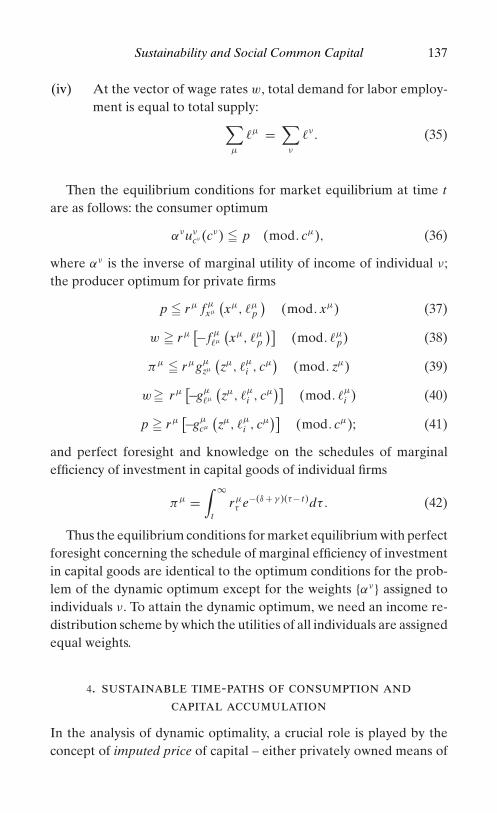
P1: IBE/IWV/KAC P2: IWV0521847885c03.xml CB829B/Uzawa 0 521 84788 5 August 27, 1956 17:25
Sustainability and Social Common Capital 137
(iv) At the vector of wage rates w, total demand for labor employ-ment is equal to total supply:∑
µ
�µ =∑
ν
�ν. (35)
Then the equilibrium conditions for market equilibrium at time tare as follows: the consumer optimum
ανuνcν (cν) � p (mod. cµ), (36)
where αν is the inverse of marginal utility of income of individual ν;the producer optimum for private firms
p � rµ f µxµ
(xµ, �µ
p
)(mod. xµ) (37)
w � rµ[−f µ
�µ
(xµ, �µ
p
)](mod. �µ
p) (38)
πµ � rµgµzµ
(zµ, �
µ
i , cµ)
(mod. zµ) (39)
w� rµ[−gµ
�µ
(zµ, �
µ
i , cµ)]
(mod. �µ
i ) (40)
p � rµ[−gµ
cµ
(zµ, �
µ
i , cµ)]
(mod. cµ); (41)
and perfect foresight and knowledge on the schedules of marginalefficiency of investment in capital goods of individual firms
πµ =∫ ∞
trµτ e−(δ + γ )(τ− t)dτ . (42)
Thus the equilibrium conditions for market equilibrium with perfectforesight concerning the schedule of marginal efficiency of investmentin capital goods are identical to the optimum conditions for the prob-lem of the dynamic optimum except for the weights {αν} assigned toindividuals ν. To attain the dynamic optimum, we need an income re-distribution scheme by which the utilities of all individuals are assignedequal weights.
4. sustainable time-paths of consumption andcapital accumulation
In the analysis of dynamic optimality, a crucial role is played by theconcept of imputed price of capital – either privately owned means of

P1: IBE/IWV/KAC P2: IWV0521847885c03.xml CB829B/Uzawa 0 521 84788 5 August 27, 1956 17:25
138 Economic Analysis of Social Common Capital
production or social common capital such as forests, oceans, the at-mosphere, and social infrastructure. The imputed price of a particularkind of capital expresses the extent to which the marginal increaseof the stock of the capital today contributes to the marginal increaseof the welfare of the future generations of the society. The concept ofsustainability introduced in this chapter is defined in terms of imputedprice. Dynamic processes involving the accumulation of private andsocial common capital are sustainable when, at each time, intertempo-ral allocation of scarce resources is so arranged that the imputed pricesof the various kinds of private capital and social common capital areto remain stationary at all future times.
Dynamic optimality may be obtained as market equilibrium with aperfectly competitive market under the hypothesis of perfect foresightwith respect to the schedule of marginal efficiency of investment invarious kinds of private capital. Sustainability, on the other hand, maybe identified as market equilibrium with stationary expectations withrespect to the schedules of marginal efficiency of investment in bothprivate and social common capital.
When we try to introduce the concept of sustainability with refer-ence to the imputed price of social common capital such as the naturalenvironment, we must be aware of the intrinsic difficulties involved inmaking calculations of its magnitude, as argued by Lind and Arrow(1970), Lind (1982b), and others. Nevertheless, in the analysis of thedynamic optimum for global warming, as developed in Uzawa (1991b,1992a, 1996, 2003), it is possible to find ways by which the processes ofeconomic activities, capital accumulation, and the abatement of green-house gas emissions are so harmonized within the market institutionsthat the ensuing time-paths of consumption and the atmospheric con-centrations of greenhouse gases are sustainable. We would like to see ifthe analytical apparatuses developed for the problem of global warm-ing may be extended to the general circumstances in which severalkinds of private capital as well as social common capital are involved.
Sustainability in the Simple Case
To begin, we introduce the concept of sustainability for the simplecase in which the same kind of goods serves for both consumptionand investment. As in previous sections, the instantaneous level of the

P1: IBE/IWV/KAC P2: IWV0521847885c03.xml CB829B/Uzawa 0 521 84788 5 August 27, 1956 17:25
Sustainability and Social Common Capital 139
utility ut at each time t is represented by the utility function
ut = u(ct ),
where ct is the quantity of goods consumed by the representative con-sumer at time t .
The utility function u = u(c) is defined for all nonnegative c � 0,is continuous and continuously twice-differentiable, and satisfies thefollowing conditions:
u(c) > 0, u′(c) > 0, u′′(c) < 0 for all c > 0.
It is assumed that the utility function u = u(c) remains identical overtime.
We first consider the case in which only one kind of private capitalexists. We denote by Kt the stock of capital at time t and by ct , zt ,respectively, consumption and investment at time t . Then, we have
ct + zt = f (Kt ),
where f (K) is the production function, which is assumed to be givenindependently of time t .
Production function f (K) is defined, continuous, and continuouslytwice-differentiable for all K � 0 and satisfies the following conditions:
f ′(K) > 0, f ′′(K) < 0 for all K > 0.
The rate of capital accumulation at time t , Kt , is given by
Kt = α(zt , Kt ), K0 = K0,
where K0 is the initial stock of capital, and α(z, K) is the Penrosefunction relating the rate of capital accumulation Kt with investmentzt and the stock of capital Kt , at time t .
The imputed price of capital at time t , πt , is defined as the dis-counted present value of the marginal increases in the outputs in thefuture, measured in units of the utility, due to the marginal increase ininvestment at time t , that is,
πt =∫ ∞
tπτ mτ e−δ(τ − t)dτ ,
where mτ is the marginal efficiency of investment at future time τ :
mτ = m(zτ , Kτ ) = rτ αz(zτ , Kτ ) + αK(zτ , Kτ ), rτ = f ′(Kτ ).

P1: IBE/IWV/KAC P2: IWV0521847885c03.xml CB829B/Uzawa 0 521 84788 5 August 27, 1956 17:25
140 Economic Analysis of Social Common Capital
A feasible time-path of consumption and capital accumulation,(c, K) = ((ct , Kt )), is sustainable when the imputed price of capitalπt remains stationary at a certain level π ; that is,
πt = π for all t � 0.
Under conditions of sustainability, we have, from the definition ofimputed price, that
m(zt , Kt ) = rtαz(zt , Kt ) + αK(zt , Kt ) = δ for all t.
Thus, if a time-path of consumption is sustainable, then all futuregenerations face the same imputed price of capital as the current gen-eration does. Because the imputed price of capital at each time t ex-presses the discounted present value of the marginal increases of allfuture utilities due to the marginal increase in the stock of capital timet , the concept of sustainability thus defined may capture certain aspectsof intergenerational equity. However, the more important issue of dis-tributional equity remains to be analyzed. In the following sections,keeping this deficiency of our approach in mind, we see how the levelof the imputed price π for sustainable time-paths is determined. Theanalysis to be introduced in the next few sections reproduces some ofthe basic results described in Uzawa (2003, Chapter 5).
Sustainable Levels of Consumption and Investment:One-Good Economy
First, we would like to see if the levels of consumption and investmentat the sustainable time-path (c, z) = ((ct , zt )) are uniquely determined.To see this, the conditions for sustainability are put together as follows:
K = α(z, K) (43)
c + z = f (K) (44)
m = rαz + αK = δ, (45)
where the time suffix t is omitted.By taking a differential of both sides of relations (44) and (45), we
obtain (1 10 mz
) (dcdz
)=
(r 0
−mK 1
) (dKdδ
),

P1: IBE/IWV/KAC P2: IWV0521847885c03.xml CB829B/Uzawa 0 521 84788 5 August 27, 1956 17:25
Sustainability and Social Common Capital 141
where
mz = rαzz + αKz < 0, mK = r ′αz + (rαzK + αKK) < 0
[r ′ = f ′′(K) < 0].
Hence, (dcdz
)=
(1 10 mz
)−1 (r 0
−mK 1
) (dKdδ
)
= 1mz
(rmz + mK −1
−mK 1
) (dKdδ
)
∂c∂K
= r + mK
mz> 0,
∂z∂K
= −mK
mz< 0,
∂c∂δ
= − 1mz
> 0,∂z∂δ
= 1mz
< 0.
Thus, the levels of consumption and investment (c, z) at the sustain-able time-path are uniquely determined. In addition, we have
∂α
∂K
∣∣∣∣K = 0
= αzdzdK
+ αK = −αzmK
mz+ αK < 0 [αz > 0, αK < 0].
Hence, the differential equation (43) has a uniquely determinedstationary state, and it is globally stable.
Thus, we have established the following proposition.
Proposition 1. For an economy with only one kind of capital, the levels(c,z) of consumption and investment at the sustainable time-path areuniquely determined for any given stock of capital K > 0.
The larger the stock of private capital K, the higher the level of con-sumption c along the sustainable time-path and the lower the level ofinvestment z. The higher the rate of discount δ, the higher the level ofconsumption c along the sustainable time-path and the lower the levelof investment z.
At the sustainable time-path, the levels (ct , zt ) of consumption andinvestment approach the long-run stationary state as time t goes toinfinity.
For the standard case of the neoclassical world, we have
α(z, K) = z for all z, K � 0
m(z, K) = f ′(K) for all z, K � 0.

P1: IBE/IWV/KAC P2: IWV0521847885c03.xml CB829B/Uzawa 0 521 84788 5 August 27, 1956 17:25
142 Economic Analysis of Social Common Capital
Hence, a z that satisfies sustainability conditions does not generallyexist.
Sustainable Levels of Consumption and Investment:A General Case with Several Produced and Capital Goods
We denote by K = (Kf ) the vector of stock of capital of various kinds,where f ( f = 1, . . . , F) generically refers to the type of private capital.The production function is represented by f (K), where all the neoclas-sical conditions postulated in Chapter 2 are satisfied. That is, f (K) isgiven independent of time t , is defined for all nonnegative K � 0, iscontinuous and continuously twice-differentiable, and is concave andstrictly quasi-concave with respect to K, and marginal products arealways positive.
The vector of stock of capital Kt at time t is then determined by thefollowing system of differentiable equations:
K f = α f (zf , Kf ) ( f = 1, . . . , F)
with initial condition K0 = Ko, where Ko ≥ 0 is the vector of the initialstock of private capital, and α f (zf , Kf ) is the Penrose function withregard to capital of type f , relating to the increase in the stock of capitalof type f with investment in capital of type f , zf , and the existing stockof capital of type f , Kf .
The Penrose effect is expressed by the conditions that, for capitalof type f , α f (zf , Kf ) is a concave and strictly quasi-concave functionof (zf , Kf ), and
∂α f
∂zf> 0,
∂α f
∂Kf< 0 ( f = 1, . . . , F).
Marginal products of investment in various kinds of private capitalare given by
mf = ∂ f∂Kf
∂α f
∂zf+ ∂α f
∂Kf> 0 ( f = 1, . . . , F).
Exactly as in the simple case, the imputed price of the capital oftype f at time t , πf t , is defined as the discounted present value of themarginal increases in the output in the future, measured in units ofthe utility, due to the marginal increase in investment in the capital of

P1: IBE/IWV/KAC P2: IWV0521847885c03.xml CB829B/Uzawa 0 521 84788 5 August 27, 1956 17:25
Sustainability and Social Common Capital 143
type f at time t ; that is,
π f t =∫ ∞
tπ f τ mf τ e−δ(τ− t)dτ ,
where mf τ is the marginal efficiency of investment at future time τ :
mf τ = m(zf τ , Kf τ ) = r f τ αzf (zf τ , Kf τ ) + αKf (zf τ , Kf τ ) = δ.
A feasible time-path of consumption and capital accumulation(c, K) = ((ct , Kt )) is sustainable when, for each type f of capital, theimputed price of capital π f t at time t remains constant at a certain levelπ f ; that is,
π f t = π f for all t � 0.
Hence, a feasible time-path of consumption and capital accumu-lation (ct , Kt ) is sustainable if a system of imputed prices of privatecapital (π f ) exists such that the following conditions are satisfied:
K f t = α f (zf t , Kf t )
ct +∑
�
z�t = f (Kt )
mf t = m(zf t , Kf t ) = r f tαzf (zf t , Kf t ) + αKf (zf t , Kf t ) = δ,
r�t = fK�(Kt ).
Proposition 2. For an economy with several kinds of private capital,the levels of consumption and stock of capital goods (ct , Kt ) with thevector of investment zt = (zf t ) at the sustainable time-path are uniquelydetermined for any vector of given stock of private capital, Ko ≥ 0.
The sustainable time-path of consumption and capital accumulation(ct , Kt ) approaches the long-run stationary state as t goes to infinity.
5. social common capital and sustainability
The concept of sustainability as introduced in the previous sections mayeasily be extended to the economy involving social common capital aswell as private capital. The following presentation largely reproducesthose discussed in Uzawa (2003, Chapter 5).

P1: IBE/IWV/KAC P2: IWV0521847885c03.xml CB829B/Uzawa 0 521 84788 5 August 27, 1956 17:25
144 Economic Analysis of Social Common Capital
We denote by Vt the stock of social common capital existing in thesociety at time t , and the stock of private capital is denoted by Kt . Out-put f (Kt ) at each time t is divided among consumption ct , investmentin private capital zt , and investment in social common capital wt :
ct + zt + wt = f (Kt ),
where the production function f (K) satisfies all the neoclassical con-ditions postulated in the previous sections.
The rate of increase in the stock of private capital, Kt , is determinedin terms of the Penrose function α(z, K):
Kt = α(zt , Kt ). (46)
The Penrose function α(z, K) concerning the accumulation of pri-vate capital is assumed to satisfy the following conditions.
The function α(z, K) is defined for all (z, K) � 0 and is continuous,continuously twice-differentiable, concave, and strictly quasi-concavewith respect to (z, K); that is,
αzz < 0, αKK < 0, αzzαKK − αzK2 � 0.
It is assumed that
αz(z, K) > 0, αK(z, K) < 0.
We also assume that the effect of investment in social common cap-ital is subject to the Penrose effect, and thus the rate of increase inthe stock of social common capital, Vt , is determined, in terms of thePenrose function β(w, V), as
Vt = β(wt , Vt ). (47)
The Penrose function β(w, V) concerning the accumulation of socialcommon capital is also assumed to satisfy the concavity conditions.
The function β(w, V) is defined for all (w, V) � 0 and is continuous,continuously twice-differentiable, concave, and strictly quasi-concavewith respect to (w, V); that is,
βww < 0, βVV < 0, βwwβVV − βwV2 � 0.
It is assumed that
βw(w, V) > 0, βV(w, V) < 0.

P1: IBE/IWV/KAC P2: IWV0521847885c03.xml CB829B/Uzawa 0 521 84788 5 August 27, 1956 17:25
Sustainability and Social Common Capital 145
Note that for the case of global warming as discussed in Uzawa(1991b, 2003), the stock V represents the difference between the criticallevel and the current level of the accumulation of atmospheric carbondioxide.
We assume that the utility ut at each time t is a function of the vectorof consumption ct and the stock of environmental capital Vt ,
ut = u(ct , Vt ),
where utility function u(c, V) is assumed to be defined for all (c, V) � 0,positive valued with positive marginal utilities, continuously twice-differentiable, concave, and strictly quasi-concave with respect to(c, V):
u(c, V) > 0, uc(c, V), uV(c, V) > 0
ucc, uVV > 0, uccuVV − ucV2 � 0 for all (c, V) � 0.
The sustainable time-path of consumption and capital accumulationis obtained in terms of the imputed prices of private capital and socialcommon capital, to be denoted, respectively, by πt and ψt . As with thecase of private capital, the imputed price ψt of social common capitalat time t is the discounted present value of the marginal increases inthe outputs in the future due to the marginal increase in the level ofinvestment in social common capital at time t ; that is,
ψt =∫ ∞
tψτ nτ e−δ(τ− t)dτ ,
where nt = n(ct , wt , Vt ) is the marginal efficiency of investment in so-cial common capital at time t .
The marginal efficiency of investment in social common capitaln = n(c, w, V) is defined by
n = n(c, w, V) = sβw(w, V) + βV(w, V),
where βw(w, V) is the marginal product of investment in social com-mon capital, whereas s = s(c, V) is the marginal rate of substitutionbetween consumption and social common capital:
s = s(c, V) = uV(c, V)uc(c, V)
.

P1: IBE/IWV/KAC P2: IWV0521847885c03.xml CB829B/Uzawa 0 521 84788 5 August 27, 1956 17:25
146 Economic Analysis of Social Common Capital
We now obtain the following Euler–Lagrange differential equationsfor the imputed prices of private capital and social common capital,πt , ψt :
πt
πt= δ − mt , mt = m(zt , Kt )
ψt
ψt= δ − nt , nt = n(ct , wt , Vt ).
The time-path (ct , zt , wt , Kt , Vt ) is sustainable when the imputedprices of private capital and social common capital, πt and ψt , aredetermined so that the following conditions are satisfied:
m(zt , Kt ) = n(ct , wt , Vt ) = δ.
The imputed real national income at time t is given by
Ht = u(ct , Vt ) + πtα(zt , Kt ) + ψtβ(wt , Vt ).
The optimum levels of consumption and investment in private cap-ital and social common capital at each time t , ct , zt , wt , are obtained sothat the imputed real national income Ht is maximized subject to theconstraints
ct + zt + wt = f (Kt ).
Let us denote by pt the imputed price of output at time t . Then weobtain the following marginality conditions:
uc(ct , Vt ) = pt
πtαz(zt , Kt ) = pt
ψtβw(wt , Vt ) = pt .
For any given stock of private capital and social common capital,K, V [K, V > 0], the levels of consumption and investment in pri-vate capital and social common capital at the sustainable time-path,(c, z, w), are uniquely determined.
To see this, note the following equations:
c + z + w = f (K)
m(z, K) = δ
n(c, w, V) = δ.

P1: IBE/IWV/KAC P2: IWV0521847885c03.xml CB829B/Uzawa 0 521 84788 5 August 27, 1956 17:25
Sustainability and Social Common Capital 147
By taking a differential of both sides of these equations, we obtain 1 1 1
0 mz 0nc 0 nw
dc
dzdw
=
r 0 0
−mK 0 10 −nV 1
dK
dVdδ
dc
dzdw
=
1 1 1
0 mz 0nc 0 nw
−1 r 0 0
−mK 0 10 −nV 1
dK
dVdδ
= 1�
1 − 1mz
− 1nw
01
mz
(1 − nc
nw
)0
− nc
nw
1mz
nc
nw
1nw
r 0 0
−mK 0 10 −nV 1
dk
dVdδ
= 1�
r + mK
mz
nV
nw
− 1mz
− 1nw
−mK
mz
(1 − nc
nV
)0
1mz
(1 − nc
nV
)
−(
r + mK
mz
)nc
nV−nV
nw
1mz
nV
nw
+ 1nw
dK
dVdδ
,
where
� = 1 − nc
nw
> 0, mz, mK < 0, nw, nV < 0, nc > 0.
Hence, dc
dzdw
=
+ + +
− 0 −+ − −
dK
dVdδ
.
On the other hand,(dKdV
)=
(dα
dβ
)
=
αK − αz
�
mK
mz
(1 − nc
nV
)0
−βw
�
(r + mK
mz
)nc
nVβV − βw
�
(1
mz
nV
nw
+ 1nw
)
(dkdV
),

P1: IBE/IWV/KAC P2: IWV0521847885c03.xml CB829B/Uzawa 0 521 84788 5 August 27, 1956 17:25
148 Economic Analysis of Social Common Capital
where
αK − αz
�
mK
mz
(1 − nc
nV
)< 0, βV − βw
�
(1
mz
nV
nw
+ 1nw
)< 0.
Hence, the system of differential equations, (46) and (47), is globallystable. We have thus established the following proposition.
Proposition 3. Suppose that there are several kinds of private capitaland social common capital. For any given stock of private capital andsocial common capital, K, V, (K, V > 0), the levels of consumption andinvestment in private capital and social common capital at the sustain-able time-path, (c, z, w), are always uniquely determined.
The larger the stock of private capital K, the higher the consumptionand investment in social common capital along the sustainable time-path, but the lower the investment in private capital. On the other hand,the larger the stock of social common capital V, the higher the consump-tion and investment in private capital along the sustainable time-path,but the lower is the investment in social common capital. The lower therate of discount δ, the lower the consumption along the sustainable time-path, whereas investments in private capital and social common capitalboth increase.
The sustainable time-path of consumption and investment in privatecapital and social common capital, (c, z, w), approaches the long-runstationary state as t goes to infinity.
6. sustainability for the prototype model of socialcommon capital
The analysis of sustainable processes of consumption and capital accu-mulation we have introduced in the previous sections may be readilyapplied to the prototype model of social common capital as introducedin Chapter 2.
As sustainability is defined in terms of the stationarity of the im-puted prices of various kinds of capital goods, the conditions for sus-tainability are identical with those for dynamic optimality except forthe optimality conditions in the short run.
We resume the discussion carried out in Chapter 2. Although thebasic premises of the model remain identical to those for the prototypemodel of social common capital introduced in Chapter 2, we mustexplicitly take care of investment activities in both private firms and

P1: IBE/IWV/KAC P2: IWV0521847885c03.xml CB829B/Uzawa 0 521 84788 5 August 27, 1956 17:25
Sustainability and Social Common Capital 149
social institutions in charge of social common capital. For the sake ofexpository brevity, we assume that only fixed factors of production arelimitational in the production processes of both private firms and socialinstitutions in charge of social common capital, thus abstracting fromthe role of labor entirely.
Basic Premises of the Prototype Model of SocialCommon Capital
We consider an economy consisting of n individuals, m private firms,and s social institutions in charge of social common capital. Individualsare generically denoted by ν = 1, . . , n, private firms by µ = 1, . . , m,and social institutions by σ = 1, . . , s. Goods produced by privatefirms are generically denoted by j = 1, . . . , J , whereas there is onlyone kind of social common capital.
The Principal Agency
The utility of each individual ν is cardinal and is expressed by the utilityfunction
uν = uν(cν, ϕν(a)aν),
where cν is the vector of goods consumed and aν is the amount ofservices of social common capital used, both by individual ν, whereasa is the total amount of services of social common capital used by allmembers of the society:
a =∑
ν
aν +∑
µ
aµ,
where aµ is the amount of services of social common capital used byprivate firm µ. The impact index function ϕν(a) expresses the extentto which the utility of individual ν is affected by the phenomenon ofcongestion with respect to the use of services of social common capital.The impact coefficients τ ν(a) of social common capital defined by
τ (a) = −ϕν′(a)ϕν(a)
are assumed to be identical for all individuals and satisfy the followingconditions:
τ (a) > 0, τ ′(a) > 0.
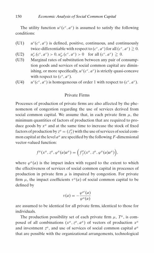
P1: IBE/IWV/KAC P2: IWV0521847885c03.xml CB829B/Uzawa 0 521 84788 5 August 27, 1956 17:25
150 Economic Analysis of Social Common Capital
The utility function uν(cν, aν) is assumed to satisfy the followingconditions:
(U1) uν(cν, aν) is defined, positive, continuous, and continuouslytwice-differentiable with respect to (cν, aν) for all (cν, aν) � 0.
(U2) uνcν (cν, aν) > 0, uν
aν (cν, aν) > 0 for all (cν, aν) � 0.
(U3) Marginal rates of substitution between any pair of consump-tion goods and services of social common capital are dimin-ishing, or more specifically, uν(cν, aν) is strictly quasi-concavewith respect to (cν, aν).
(U4) uν(cν, aν) is homogeneous of order 1 with respect to (cν, aν).
Private Firms
Processes of production of private firms are also affected by the phe-nomenon of congestion regarding the use of services derived fromsocial common capital. We assume that, in each private firm µ, theminimum quantities of factors of production that are required to pro-duce goods by xµ and at the same time to increase the stock of fixedfactors of production by zµ = (zµ
f ) with the use of services of social com-mon capital at the level aµ are specified by the following F-dimensionalvector-valued function:
f µ(xµ, zµ, ϕµ(a)aµ) =(
f µ
f (xµ, zµ, ϕµ(a)aµ)),
where ϕµ(a) is the impact index with regard to the extent to whichthe effectiveness of services of social common capital in processes ofproduction in private firm µ is impaired by congestion. For privatefirm µ, the impact coefficients τµ(a) of social common capital to bedefined by
τ (a) = −ϕµ′(a)ϕµ(a)
are assumed to be identical for all private firms, identical to those forindividuals.
The production possibility set of each private firm µ, Tµ, is com-posed of all combinations (xµ, zµ, aµ) of vectors of production xµ
and investment zµ, and use of services of social common capital aµ
that are possible with the organizational arrangements, technological

P1: IBE/IWV/KAC P2: IWV0521847885c03.xml CB829B/Uzawa 0 521 84788 5 August 27, 1956 17:25
Sustainability and Social Common Capital 151
conditions, and given endowments of factors of production Kµ in firmµ. It may be expressed as
Tµ = {(xµ, zµ, aµ): (xµ, zµ, aµ) � 0, f µ(xµ, zµ, ϕµ(a) aµ) � Kµ},where the total amount of services of social common capital used byall members of the society, a, is assumed to be a given parameter.
The following neoclassical conditions are assumed:
(Tµ1) f µ(xµ, zµ, aµ) are defined, positive, continuous, and continu-ously twice-differentiable with respect to (xµ, zµ, aµ).
(Tµ2) f µxµ(xµ, zµ, aµ) > 0, f µ
�µ(xµ, zµ, aµ) � 0, f µaµ(xµ, zµ, aµ) � 0.
(Tµ3) f µ(xµ, zµ, aµ) are strictly quasi-convex with respect to(xµ, zµ, aµ).
(Tµ4) f µ(xµ, zµ, aµ) are homogeneous of order 1 with respect to(xµ, zµ, aµ).
Social Institutions in Charge of Social Common Capital
Similarly, in each social institution σ , the minimum quantities of factorsof production required to provide services of social common capital byaσ and at the same time to engage in investment activities to accumulatethe stock of fixed factors of production by zσ = (zσ
f ) with the use ofproduced goods by xσ = (xσ
j ) are specified by an F-dimensional vector-valued function:
f σ (aσ , zσ , xσ ) = (f σ
f (aσ , zσ , xσ )).
For each social institution σ , the production possibility set Tσ iscomposed of all combinations (aσ , zσ , xσ ) of provision of services ofsocial common capital aσ , investment zσ , and use of produced goods xσ
that are possible with the organizational arrangements, technologicalconditions, and the given endowments of factors of production Kσ ofsocial institution σ . That is, it may be expressed as
Tσ = {(aσ , zσ , xσ ) : (aσ , zσ , xσ ) � 0, f σ (aσ , zσ , xσ ) � Kσ }.The following neoclassical conditions are assumed:
(Tσ 1) f σ (aσ , zσ , xσ ) are defined, positive, continuous, and continu-ously twice-differentiable with respect to (aσ , zσ , xσ ) for all(aσ , zσ , xσ ) � 0.

P1: IBE/IWV/KAC P2: IWV0521847885c03.xml CB829B/Uzawa 0 521 84788 5 August 27, 1956 17:25
152 Economic Analysis of Social Common Capital
(Tσ 2) f σaσ (aσ , zσ , xσ ) > 0, f σ
�σ (aσ , zσ , xσ ) < 0, f σxσ (aσ , zσ , xσ ) < 0
for all (aσ , zσ , xσ ) � 0.
(Tσ 3) f σ (aσ , zσ , xσ ) are strictly quasi-convex with respect to(aσ , zσ , xσ ) for all (aσ , zσ , xσ ) � 0.
(Tσ 4) f σ (aσ , zσ , xσ ) are homogeneous of order 1 with respect to(aσ , zσ , xσ ).
Dynamically Optimum Paths for the Prototype Modelof Social Common Capital
The accumulation of the stock of capital goods in firm µ is given by thefollowing differential equation:
Kµ
t = zµt − γ Kµ
t , Kµ
0 = Kµo , (48)
where zµt is the vector specifying the levels of investment in capital
goods in firm µ at time t and γ = (γ f ) is the vector of the rates ofdepreciation of capital goods.
Similarly, the accumulation of the stock of capital goods in socialinstitution σ is given by the following differential equation
Kσ
t = zσt − γ Kσ
t , Kσ0 = Kσ
o , (49)
where zσt is the vector specifying the levels of investment in capital
goods in social institution σ at time t and γ = (γ f ) is the vector of therates of depreciation of capital goods, assumed to be identical to thosefor private firms.
The dynamically optimum path of consumption and investmentfor the prototype model of social common capital may be obtainedas the optimum solution to the following problem of the dynamicoptimum.
The Problem of the Dynamic Optimum. Find the pattern of consump-tion and investment in private capital and social common capital atall times t , (cν
t , zµt , zσ
t ), that maximizes the Ramsey–Koopmans–Cassutility integral
U =∫ ∞
0Ut e−δt dt, Ut =
∑ν
uν (cνt , aν
t )

P1: IBE/IWV/KAC P2: IWV0521847885c03.xml CB829B/Uzawa 0 521 84788 5 August 27, 1956 17:25
Sustainability and Social Common Capital 153
subject to the feasibility constraints (48), (49), and∑ν
cνt +
∑σ
xσt �
∑µ
xµt (50)
at �∑
σ
aσt (51)
∑ν
aνt +
∑µ
aµt � at (52)
f µ(xµ
t , zµt , ϕµ(at ) aµ
t
)� Kµ
t (53)
f σ (aσi , zσ
i , xσi ) � Kσ
i , (54)
where aνt , aµ
t , aσt are, respectively, the amounts of services of social
common capital concerning individuals ν, private firms µ, and socialinstitutions σ , and at is the total amount of services of social commoncapital, all at time t .
We introduce the Lagrangian form
L =∫ ∞
0Lt e−δt dt,
where
Lt =∑
ν
uν (cνt , ϕ
ν(at )aνt ) +
∑µ
ψµt
(zµ
t − γ Kµt
) +∑
σ
ψσt (zσ
t − γ Kσt )
+ pt
[∑µ
xµt −
∑ν
cνt −
∑σ
xσt
]+ πt
[∑σ
aσt − at
]
+ θt
[at −
∑ν
aνt −
∑µ
aµt
]+
∑µ
rµt
[Kµ
t − f µ(xµ
t , zµt , ϕµ(at ) aµ
t
)]+
∑σ
rσt [Kσ
t − f σ (aσi , zσ
i , xσi )] ,
ψµt and ψσ
t are, respectively, the imputed prices of capital goods inprivate firm µ and social institution σ ; πt and θt are, respectively, theimputed prices of the provision and use of services of social commoncapital; and rµ
t and rσi are, respectively, the imputed rents of capital
goods in private firm µ and social institution σ , all at time t .The dynamically optimum time-path consumption and capital ac-
cumulation, (cνt , Kµ
t , Kσi ), are characterized by the following optimum
conditions, where the time suffix t is omitted, in addition to feasibility

P1: IBE/IWV/KAC P2: IWV0521847885c03.xml CB829B/Uzawa 0 521 84788 5 August 27, 1956 17:25
154 Economic Analysis of Social Common Capital
conditions (48)–(54):
uνcν (cν, ϕν(a)aν) � p (mod. cν)
uνaν (cν, ϕν(a)aν)ϕν(a) � θ (mod. aν)
p � rµ f µxµ(xµ, zµ, ϕµ(a) aµ) (mod. xµ)
ψµ � rµ f µzµ(xµ, zµ, ϕµ(a) aµ) (mod. zµ)
f µ(xµ, zµ, ϕµ(a) aµ) � Kµ (mod. rµ)
θ � rµ[− f µ
aµ(xµ, zµ, ϕµ(a) aµ)ϕµ(a)]
(mod. aµ)
π � rσ f σaσ (aσ , zσ , xσ ) (mod. aσ )
ψσ � rσ f σzσ (aσ , zσ , xσ ) (mod. zσ )
p � rσ [− f σxσ (aσ , zσ , xσ )] (mod. xσ )
f σ (aσ , zσ , xσ ) � Kσ (mod. rσ )
θ − π = τθ, τ = τ (a)a.
The dynamic equations for the imputed prices of private capital andsocial common capital are given by
ψµ = (δ + γ )ψµ − rµ (55)
ψσ = (δ + γ )ψσ − rσ , (56)
together with the transversality conditions:
limt→+∞ ψ
µt Kµ
t e−(δ+γ )t = 0, limt→+∞ ψσ
t Kσt e−(δ+γ )t = 0.
These optimum conditions coincide with those for market equilib-rium with perfect foresight concerning the schedules of marginal effi-ciency of investment in both private capital and social common capital.Thus, it is apparent that the following proposition holds.

P1: IBE/IWV/KAC P2: IWV0521847885c03.xml CB829B/Uzawa 0 521 84788 5 August 27, 1956 17:25
Sustainability and Social Common Capital 155
Proposition 4. In the prototype model of social common capital, theoptimum conditions for the dynamically optimum time-path of con-sumption and accumulation of private capital and social common cap-ital coincide precisely with those for market equilibrium with the socialcommon capital tax at the rate τ (a) y:
θ − π = τθ, τ = τ (a)a,
where τ (a) is the impact coefficient of social common capital, with per-fect foresight concerning the schedules of marginal efficiency of invest-ment in both private capital and social common capital.
Sustainable time-paths for the prototype model of social commoncapital may be similarly obtained. One only has to replace the dynamicequations for the imputed prices (55), (56), and the transversality con-ditions by the following conditions:
ψµ = rµ
δ + γ, ψσ = rσ
δ + γ.
It is apparent that the following proposition holds.
Proposition 5. In the prototype model of social common capital, theconditions for the sustainable time-path of consumption and accumula-tion of both private capital and social common capital coincide preciselywith the optimum conditions for market equilibrium with the social com-mon capital tax at the rate τ = τ (a)a:
θ − π = τθ, τ = τ (a)a,
with stationary expectations concerning the schedules of marginal effi-ciency of investment in both private capital and social common capital.

P1: KsF0521847885c04.xml CB829B/Uzawa 0 521 84788 5 August 27, 1956 18:17
4
A Commons Model of Social Common Capital
1. introduction
The natural environment comprises an important component of socialcommon capital. It is generally held as common property resourcesand is managed as the commons either by local communities or thestate authorities. The atmospheric environment, for example, as thelargest commons, is to be managed by all nations in the world. The nat-ural environment is in principle not privately appropriated to individ-ual members of the society or transacted through market institutions.In Chapter 1, we formulated simple dynamic models of the fisheries,forestry, and agricultural commons to examine critically the theme ofthe tragedy of the commons, originally put forward by Hardin (1968).However, the analysis was primarily confined to the cases in whichthe commons are evaluated in terms of the pecuniary gains accruedto the members of the communities that communally own or controlthe commons, where the role of the commons as social common cap-ital has been only tangentially noted. When the natural environmentis regarded as social common capital, there are two crucial propertiesthat must be explicitly incorporated in any dynamic model. The firstproperty concerns the externalities, both static and dynamic, with re-spect to the use of the natural environment as a factor of production.The second property concerns the role of the natural environment as animportant component of the living environment, significantly affectingthe quality of human life.
The institutions of the commons have historically been set up tosolve the problems of the optimum use of resources from the natural
156

P1: KsF0521847885c04.xml CB829B/Uzawa 0 521 84788 5 August 27, 1956 18:17
A Commons Model of Social Common Capital 157
environment. Some of the more successful historical and traditionalcommons have been studied in detail in the literature, as recorded inMcCay and Acheson (1987) and Berkes (1989).
In this chapter, we introduce a commons model of social commoncapital in which the interplay of a number of the commons is analyzedin detail and the institutional framework is examined whereby thesustainable pattern of resource allocation may be realized.
2. a commons model of social common capital
The analysis of the commons model of social common capital in thischapter is carried out within the framework of the prototype model ofsocial common capital introduced in Chapter 2, focusing the analysison the role of the commons. Virtually all the variables and relationsintroduced in Chapter 2 are retained.
The commons model of social common capital discussed in this chap-ter consists of a finite number of commons. Each commons consists ofindividuals and two types of institutions – private firms that are special-ized in producing goods that are transacted on the market and socialinstitutions that are concerned with the provision of services of so-cial common capital. For the sake of expository brevity, the followingdiscussion is carried out in terms of the representative individual, theprivate firm, and the social institution of each commons. Commonsare denoted by ν (ν = 1, . . . , n), and goods produced by private firmsare generically denoted by j = 1, . . . , J . We consider the situation inwhich there is only one kind of social common capital.
Utility Functions of the Commons
For each commons ν, the economic welfare is represented by the utilityfunction
uν = uν(cν, ϕν(a)aν
c
),
where a is the total amount of services of social common capital usedby all members of the economy:
a =∑
ν
aν, aν = aνc + aν
p (ν ∈ N),
where, for each commons ν, aν is the amount of services of social com-mon capital used by commons ν, whereas aν
c and aνp are the amounts

P1: KsF0521847885c04.xml CB829B/Uzawa 0 521 84788 5 August 27, 1956 18:17
158 Economic Analysis of Social Common Capital
of services of social common capital, respectively, used by the repre-sentative individual and the private firm of commons ν, and ϕν(a) isthe impact index function of social common capital for commons ν,where
ϕν(a) > 0, ϕν′(a) < 0, ϕν ′′(a) < 0.
The impact index of social common capital
τ (a) = −ϕν′(a)ϕν(a)
,
is assumed to be identical for all commons ν. The following conditionsare satisfied:
τ (a) > 0, τ ′(a) > 0.
The following neoclassical conditions are assumed:
(U1) Utility function uν(cν, ϕν(a)aνc ) is defined, positive, continu-
ous, and continuously twice-differentiable for all (cν, aνc , a) �
0.(U2) Marginal utilities are positive both for the consumption of
produced goods cν and the use of services of social commoncapital aν
c :
uνcν
(cν, ϕν(a)aν
c
)> 0, uν
aνc
(cν, ϕν(a)aν
c
)> 0
for all(cν, aν
c , a)
� 0.
(U3) Utility function uν(cν, ϕν(a)aνc ) is strictly quasi-concave with
respect to (cν, aνc , a) for all (cν, aν
c ) for any given a � 0.(U4) Utility function uν(cν, ϕν(a)aν
c ) is homogeneous of order 1with respect to (cν, aν
c ) for any given a � 0; that is,
uν(tcν, tϕν(a)aνc ) = tuν(cν, ϕν(a)aν
c )
for all t � 0, (cν, aνc , a) � 0.
The Euler identity holds:
uν(cν, ϕν(a)aν
c
) = uνcν
(cν, ϕν(a)aν
c
)cν + uν
aνc
(cν, ϕν(a)aν
c
)ϕν(a)aν
c .
Production Possibility Sets for Private Firms of the Commons
For each commons ν, the production possibility set Tν of the privatefirm of commons ν is composed of all combinations (xν, aν
p) of vectorsof production xν and use of services of social common capital aν
p that

P1: KsF0521847885c04.xml CB829B/Uzawa 0 521 84788 5 August 27, 1956 18:17
A Commons Model of Social Common Capital 159
are possibly produced with the organizational arrangements and tech-nological conditions of the representative firm of commons ν and thegiven endowments of factors of production of private firm ν, Kν . It isexpressed as
Tν = {(xν, aν
p
):(xν, aν
p
)� 0, f ν
(xν, ϕν(a) aν
p
)� Kν
}.
(T1) f ν(xν, ϕν(a) aνp) is defined, positive, continuous, and contin-
uously twice-differentiable with respect to (cν, aνc , a) for all
(xν, aνp, a) � 0.
(T2) f νxν (xν, ϕν(a) aν
p) > 0, f νaν
p(xν, ϕν(a) aν
p) � 0 for all (xν, aνp, a)
� 0.(T3) f ν(xν, ϕν(a) aν
p) is strictly quasi-convex with respect to(cν, aν
c , a) for all (xν, aνp, a) � 0.
(T4) f ν(xν, ϕν(a) aνp) is homogeneous of order 1 with respect to
(xν, aνp) for any given a � 0; that is,
f ν(t xν, tϕν(a) aν
p
) = t f ν(xν, ϕν(a) aν
p
)for all t � 0, (cν, aν
c , a) � 0.
The Euler identity holds:
f ν(xν, ϕν(a) aν
p
) = f νxν
(xν, ϕν(a) aν
p
)xν + f ν
aνp
(xν, ϕν(a) aν
p
)ϕν(a) aν
p.
Postulates (T1–T3) imply that the production possibility set Tν isa closed, convex set of J + 1-dimensional vectors (xν, aν
p). Note, how-ever, that the production possibility set Tν of the private firm of eachcommons ν depends on the total use of services of social commoncapital a.
Production Possibility Sets for Social Institutionsof the Commons
For each commons ν, the production possibility set of the social in-stitution in charge of social common capital, Sν , is composed of allcombinations (bν, wν) of the provision of services of social commoncapital bν and the use of produced goods wν that are possible with theorganizational arrangements and technological conditions, with givenendowments of factors of production of the social institution of thecommons ν, Vν . It is expressed as
Sν = {(bν, wν) : (bν, wν) � 0, gν(bν, wν) � Vν}.

P1: KsF0521847885c04.xml CB829B/Uzawa 0 521 84788 5 August 27, 1956 18:17
160 Economic Analysis of Social Common Capital
(S1) gν(bν, wν) is defined, positive, continuous, and continuouslytwice-differentiable for all (bν, wν) � 0.
(S2) gνbν (bν, wν) > 0, gν
wν (bν, wν) � 0 for all (bν, wν) � 0.(S3) gν(bν, wν) are strictly quasi-convex with respect to (bν, wν) for
all (bν, wν) � 0.(S4) gν(bν, wν) are homogeneous of order 1 with respect to (bν, wν)
for all (bν, wν) � 0; that is,
gν(tbν, twν) = tgν(bν, wν) for all t � 0, (bν, wν) � 0.
The Euler identity holds:
gν(bν, wν) = gνbν (bν, wν) bν + gν
wν (bν, wν) wν.
Postulates (S1–S3) imply that the production possibility set Sν is aclosed, convex set of 1 + J -dimensional vectors (bν, wν).
3. market equilibrium for the commons modelof social common capital
Suppose social common capital taxes with the rate τ are levied onthe use of services of social common capital. Market equilibrium isobtained if we find the vector of prices of produced goods p, the pricecharged for the use of services of social common capital θ , and the pricepaid for the provision of services of social common capital π such thatdemand and supply are equal for all goods and the total provision ofservices of social common capital is equal to the total use of servicesof social common capital. The price charged for the use of services ofsocial common capital θ is higher, by the tax rate τθ , than the pricepaid for the provision of services of social common capital π ; that is,
θ = π + τθ.
Market equilibrium for the commons model of social common cap-ital is obtained if the following conditions are satisfied:
(i) The representative individual of each commons ν chooses thecombination (cν, aν
c ) of the vector of consumption cν and theuse of services of social common capital aν
c in such a mannerthat the utility of commons ν
uν = uν(cν, ϕν(a) aν
c
)

P1: KsF0521847885c04.xml CB829B/Uzawa 0 521 84788 5 August 27, 1956 18:17
A Commons Model of Social Common Capital 161
is maximized subject to the budget constraint
pcν + θaνc = yν,
where yν is the income of commons ν in units of market pricesand a is the total amount of services of social common capitalused by all members of the society that is assumed to be givenwhen individual ν chooses (cν, aν
c ):
a =∑
ν
aν, aν = aνc + aν
p (ν ∈ N),
where aνp is the amount of services of social common capital
used by the private firm of commons ν.(ii) The private firm of each commons ν chooses the combi-
nation (xν, aνp) of production vector xν and the use of ser-
vices of social common capital aνp in such a manner that net
profit
pxν − θaνp
is maximized over (xν, aνp) ∈ Tν .
(iii) The social institution in charge of social common capital in eachcommons ν chooses the combination (bν, wν) of the provisionof services of social common capital bν and the use of producedgoods wν in such a manner that net value
πbν − pwν
is maximized over (bν, wν) ∈ Sν .(iv) The total amount of services of social common capital provided
by all social institutions in charge of social common capital isequal to the total use of services of social common capital byall commons of the economy; that is,∑
ν
bν = a.
(v) At the price vector p, total demand for goods is equal to totalsupply: ∑
ν
xν =∑
ν
cν +∑
ν
wν.

P1: KsF0521847885c04.xml CB829B/Uzawa 0 521 84788 5 August 27, 1956 18:17
162 Economic Analysis of Social Common Capital
(vi) For each commons ν, the balance-of-payments condition issatisfied; that is,
pxν − pcν − pwν + π(bν − aν) = 0.
Optimum Conditions for Market Equilibrium
Optimum and equilibrium conditions for market equilibrium forthe commons model of social common capital, [cν, aν
c , xν, aνp, bν, wν
(ν ∈ N); a, p, π, θ], are listed.The Consumer Optimum
pcν + θaνc = yν (1)
ανuνcν
(cν, ϕν(a) aν
c
)� p (mod. cν) (2)
ανuνaν
c
(cν, ϕν(a) aν
c
)ϕν(a) � θ
(mod. aν
c
)(3)
ανuν(cν, ϕν(a) aν
c
) = yν . (4)
The Producer Optimum for Private Firms
p � r ν f νxν
(xν, ϕν(a) aν
p
)(mod. xν) (5)
θ � r ν[− f ν
aνp
(xν, ϕν(a) aν
p
)ϕν(a)
] (mod. aν
p
)(6)
f ν(xν, ϕν(a) aν
p
)� Kν (mod. r ν) (7)
pxν − θaνp = r ν Kν . (8)
The Producer Optimum for Social Institutions in Charge of SocialCommon Capital
π � ρνgνbν (bν, wν) (mod. bν) (9)
p � ρν[−gν
wν (bν, wν)]
(mod. wν) (10)
gν(bν, wν) � Vν (mod. ρν) (11)
πbν − pwν = ρνVν . (12)

P1: KsF0521847885c04.xml CB829B/Uzawa 0 521 84788 5 August 27, 1956 18:17
A Commons Model of Social Common Capital 163
Equilibrium Conditions
a =∑
ν
aν, aν = aνc + aν
p (νεN) (13)
a =∑
ν
bν (14)
∑ν
xν =∑
ν
cν +∑
ν
wν (15)
θ = π + τθ. (16)
In the following discussion, we suppose that for any given level ofsocial common capital tax rate τ (τ > 0), the state of the economy
E = [cν, aν
c , xν, aνp, bν, wν (ν ∈ N); a, p, π, θ
]that satisfies all optimum and equilibrium conditions for market equi-librium generally exists and is uniquely determined.
National Income Accounting
Income yν of each commons ν is the sum of factor income r ν Kν + ρνVν
and social common capital tax payments τθaν :
yν = (r ν Kν + ρνVν) + τθaν,
where
τθ = θ − π.
National income y is the sum of incomes of all commons:
y =∑
ν
yν =∑
ν
r ν Kν +∑
ν
ρνVν + τθa.
Another definition of national income y is
y =∑
ν
pxν +∑
ν
πbν .
That is, national income y is the aggregate of the values in units of priceof produced goods and services of social common capital.
Because the conditions of constant returns to scale prevail, we haverelations (8) and (12):
pxν − θaνp = r ν Kν, πbν − pwν = ρνVν .

P1: KsF0521847885c04.xml CB829B/Uzawa 0 521 84788 5 August 27, 1956 18:17
164 Economic Analysis of Social Common Capital
Hence,∑ν
pxν −∑
ν
θaνp +
∑ν
πbν −∑
ν
pwν =∑
ν
r ν Kν +∑
ν
ρνVν
∑ν
(pcν + θaν
c
) =(∑
ν
r ν Kν +∑
ν
ρνVν
)+
∑ν
θaν −∑
ν
πbν
=(∑
ν
r ν Kν +∑
ν
ρνVν
)+ τθa.
That is, the following familiar identity in national income accountingholds:
y =∑
ν
pxν +∑
ν
πbν =(∑
ν
r ν Kν +∑
ν
ρνVν
)+ τθa.
4. market equilibrium and social optimum
To explore welfare implications of market equilibrium for the com-mons model of social common capital under the given level of socialcommon capital tax rate τ , we consider the social utility U given by
U =∑ν∈N
ανuν =∑ν∈N
ανuν(cν, ϕν(a) aν
c
),
where, for each commons ν, the utility weight αν is the inverse of themarginal utility of income yν of commons ν at market equilibrium.
We consider the following maximum problem:
Maximum Problem for Social Optimum. Find the pattern of consump-tion and production of goods, use and provision of services of socialcommon capital, and total use of services of social common capital[cν, aν
c , xν, aνp, bν, wν(ν ∈ N); a] that maximizes the social utility
U =∑ν∈N
ανuν =∑ν∈N
ανuν(cν, ϕν(a) aν
c
)(17)
among all feasible patterns of allocation:∑ν∈N
cν +∑ν∈N
wν �∑ν∈N
xν (18)
a =∑ν∈N
aν, aν = aνc + aν
p (ν ∈ N) (19)

P1: KsF0521847885c04.xml CB829B/Uzawa 0 521 84788 5 August 27, 1956 18:17
A Commons Model of Social Common Capital 165
a =∑ν∈N
bν (20)
f ν(xν, ϕν(a) aν
p
)� Kν (ν ∈ N) (21)
gν(bν, wν) � Vν (ν ∈ N). (22)
The maximum problem for social optimum may be solved in termsof the Lagrange method. Let us define the Lagrangian form:
L(
cν, aνc , xν, aν
p, bν, wν, a, p, π, θ, r ν, ρν(ν ∈ N))
=∑ν∈N
ανuν(cν, ϕν(a) aν
c
) + p
[∑ν∈N
xν −∑ν∈N
cν −∑ν∈N
wν
]
+ θ
[a −
∑ν∈N
aν
]+ π
[∑ν∈N
bν − a
]
+∑ν∈N
r ν[Kν − f ν
(xν, ϕν(a) aν
p
)]+
∑ν∈N
ρν[Vν − gν(bν, wν)]. (23)
The Lagrange unknowns p, θ, π, r ν , ρν are associated, respectively,with constraints (18), (19), (20), (21), and (22). The optimum solutionmay be obtained by partially differentiating the Lagrangian form (23)with respect to unknown variables cν, aν
c , xν, aνp, bν , wν , a and putting
them equal to 0, where feasibility conditions (18)–(22) are satisfied.That is, for each commons ν (ν ∈ N),
ανuνcν
(cν, ϕν(a) aν
c
)� p (mod. cν) (24)
ανuνaν
c(cν, ϕν(a) aν
c ) ϕν(a) � θ (mod. aνc ) (25)
p � r ν f νxν
(xν, ϕν(a) aν
p
)(mod. xν) (26)
θ � r ν[− f ν
aνp
(xν, ϕν(a) aν
p
)ϕν(a)
](mod. aν
p) (27)
f ν(xν, ϕν(a) aν
p
)� Kν (mod. r ν) (28)
π � ρνgνbν (bν, wν) (mod. bν) (29)
p � ρν[−gν
wν (bν, wν)]
(mod. wν) (30)

P1: KsF0521847885c04.xml CB829B/Uzawa 0 521 84788 5 August 27, 1956 18:17
166 Economic Analysis of Social Common Capital
gν(bν, wν) � Vν (mod. ρν) (31)
θ − π = τ (a)aθ, (32)
where τ (a) is the impact coefficient of social common capital.Only relation (32) may need clarification. Partially differentiate the
Lagrangian form (23) with respect to a, to obtain
∂L∂a
=∑ν∈N
ανuνaν
(cν, ϕν(a) aν
c
)[−τ (a)]ϕν(a) aν
c
+∑ν∈N
r ν[
f νaν
p
(xν, ϕν(a) aν
p
)τ (a)ϕν(a) aν
p
] + θ − π
= −τ (a)
[∑ν∈N
θaνc +
∑ν∈N
θaνp
]+ θ − π = −τ (a) aθ + θ − π.
Hence,∂L∂a
= 0 implies relation (32); relation (32) may be written as
θ − π = τθ, τ = τ (a)a, (33)
where τ is the social common capital rate administratively determinedprior to the opening of the market.
Exactly as in the case of the prototype model of social common capi-tal discussed in Chapter 2, the classic Kuhn-Tucker theorem on concaveprogramming may be enlisted to obtain the proposition that the Euler-Lagrange equations (24)–(32) and feasibility conditions (18)–(22) arenecessary and sufficient conditions for the optimum solution of themaximum problem for social optimum.
It is apparent that the Euler-Lagrange equations (24)–(32) and fea-sibility conditions (18)–(22) coincide precisely with the equilibriumconditions for market equilibrium with the social common capital taxrate τ = τ (a)a.
Marginality conditions, (24), (25), and the linear homogeneity hy-pothesis for utility functions uν(cν, aν) imply
ανuν(cν, ϕν(a) aν
c
) = pcν + θaνc = yν,
which, by summing over ν, yield
U =∑ν∈N
yν = y.

P1: KsF0521847885c04.xml CB829B/Uzawa 0 521 84788 5 August 27, 1956 18:17
A Commons Model of Social Common Capital 167
We have thus established the following proposition.
Proposition 1. In the commons model of social common capital, weconsider the social common capital tax scheme with the tax rate τ forthe use of services of social common capital given by
τ = τ (a)a,
where τ (a) is the impact coefficient of social common capital.Then market equilibrium obtained under such a social common cap-
ital tax scheme is a social optimum in the sense that a set of positiveweights for the utilities of the commons (α1, . . . , αn) [αν > 0] exists suchthat the social utility
U =∑ν∈N
ανuν =∑ν∈N
ανuν(cν, ϕν(a) aν
c
)is maximized among all feasible patterns of allocation [cν, aν
c , xν, aνp, bν,
wν(ν ∈ N); a].The optimum level of social utility U is equal to national income y:
U = y.
Social optimum is defined with respect to any social utility
U =∑ν∈N
ανuν =∑ν∈N
ανuν(cν, ϕν(a) aν
c
)where (α1, . . . , αn) is an arbitrarily given set of positive weights for theutilities of commons. A pattern of allocation (cν, aν
c , xν, aνp, bν, wν, a)
is a social optimum if the social utility U thus defined is maximizedamong all feasible patterns of allocation.
Social optimum necessarily implies the existence of the social com-mon capital tax scheme, where the tax rate τ is given by τ = τ (a)a.However, the budgetary constraints for the commons
pcν + θaνc = yν
are not necessarily satisfied. However, exactly the same proof as thatintroduced in Uzawa (2003, Chapter 1) may be enlisted to see thevalidity of the following proposition.
Proposition 2. In the commons model of social common capital, sup-pose a pattern of allocation [cν, aν
c , xν, aνp, bν, wν(ν ∈ N); a] is a so-
cial optimum; that is, a set of positive weights for the utilities of

P1: KsF0521847885c04.xml CB829B/Uzawa 0 521 84788 5 August 27, 1956 18:17
168 Economic Analysis of Social Common Capital
commons (α1, . . . , αn) [αν > 0] exists such that the given pattern of al-location [cν, aν
c , xν, aνp, bν, wν(ν ∈ N); a] maximizes the social utility
U =∑ν∈N
ανuν =∑ν∈N
ανuν(cν, ϕν(a) aν
c
)among all feasible patterns of allocation.
Then, a system of income transfer among the commons of the econ-omy, {tν}, exists such that ∑
ν∈N
tν = 0,
and the given pattern of allocation [cν, aνc , xν, aν
p, bν, wν(ν ∈ N); a] cor-responds precisely to the market equilibrium under the social commoncapital tax scheme with the rate τ given by
τ = τ (a)a,
where τ (a) is the impact coefficient of social common capital.
5. social common capital and lindahl equilibrium
In the commons model of social common capital introduced in theprevious sections, we would like to see if the market equilibrium underthe social common capital tax scheme with the tax rate τ = τ (a)a is aLindahl equilibrium.
Lindahl Conditions
Let us recall the postulates for the behavior of each commons at mar-ket equilibrium for the commons model of social common capital.At market equilibrium, conditions for the consumer optimum are ob-tained if the representative individual of each commons ν chooses thecombination (cν, aν
c ) of the vector of consumption cν and the use of ser-vices of social common capital aν
c in such a manner that the utility ofcommons ν
uν = uν(cν, ϕν(a) aν
c
)is maximized subject to the budget constraint
pcν + θaνc = yν,

P1: KsF0521847885c04.xml CB829B/Uzawa 0 521 84788 5 August 27, 1956 18:17
A Commons Model of Social Common Capital 169
where income yν of each commons ν is given by
yν = r ν Kν + ρνVν + τθaν,
where r ν and ρν are, respectively, the imputed rental prices of factorsof production of the private firm and the social institution of commonsν, and
τθ = θ − π.
Lindahl conditions are satisfied if a system of individual tax ratesfor the commons, {τ ν}, exists such that∑
ν
τ ν = τ, τ ν � 0 for all ν,
and, for the representative individual of each commons ν, (cν, aνc , a) is
the optimum solution to the following virtual maximum problem:Find (cν, aν
c , a(ν)) that maximizes the utility of commons ν:
uν = uν(
cν, ϕν(
a(ν))
aνc
)subject to the virtual budget constraint
pcν + θaνc − τ νθa(ν) = yν,
where
yν = yν − τθaν .
Because (cν, aν, a) is the optimum solution to the virtual maximumproblem for commons ν, the optimum conditions imply
τ νθ = ανuνaν
c
(cν, ϕν(a) aν
c
)[τ (a)ϕν(a) aν
c ] ,
where αν is the inverse of the marginal utility of income of com-mons ν.
Hence,
τ νθ = τ (a)aνθ,
which implies
τ νθa = τ (a)aνθa = τθaν .
Thus, Lindahl conditions are always satisfied at market equilibriumwith the tax rate τ for the use of services of social common capitalgiven by τ = τ (a)a.
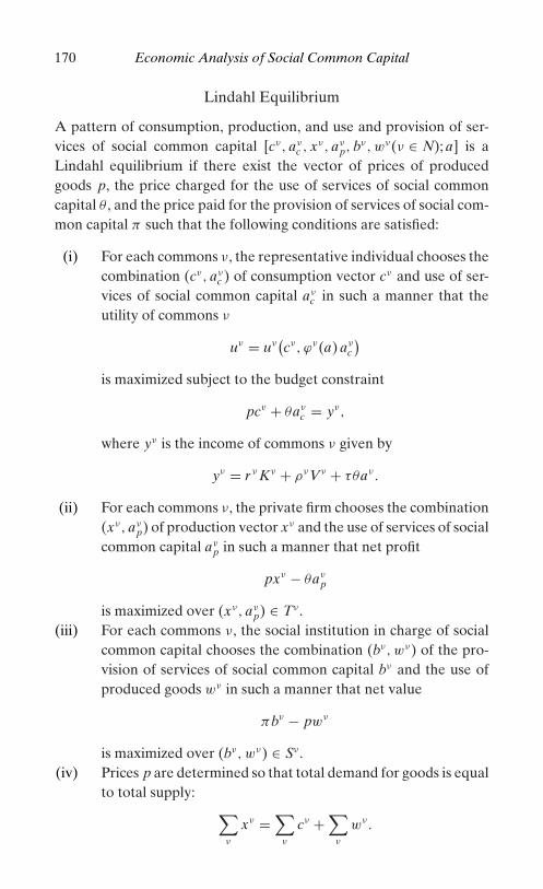
P1: KsF0521847885c04.xml CB829B/Uzawa 0 521 84788 5 August 27, 1956 18:17
170 Economic Analysis of Social Common Capital
Lindahl Equilibrium
A pattern of consumption, production, and use and provision of ser-vices of social common capital [cν, aν
c , xν, aνp, bν, wν(ν ∈ N); a] is a
Lindahl equilibrium if there exist the vector of prices of producedgoods p, the price charged for the use of services of social commoncapital θ , and the price paid for the provision of services of social com-mon capital π such that the following conditions are satisfied:
(i) For each commons ν, the representative individual chooses thecombination (cν, aν
c ) of consumption vector cν and use of ser-vices of social common capital aν
c in such a manner that theutility of commons ν
uν = uν(cν, ϕν(a) aν
c
)is maximized subject to the budget constraint
pcν + θaνc = yν,
where yν is the income of commons ν given by
yν = r ν Kν + ρνVν + τθaν .
(ii) For each commons ν, the private firm chooses the combination(xν, aν
p) of production vector xν and the use of services of socialcommon capital aν
p in such a manner that net profit
pxν − θaνp
is maximized over (xν, aνp) ∈ Tν .
(iii) For each commons ν, the social institution in charge of socialcommon capital chooses the combination (bν, wν) of the pro-vision of services of social common capital bν and the use ofproduced goods wν in such a manner that net value
πbν − pwν
is maximized over (bν, wν) ∈ Sν .(iv) Prices p are determined so that total demand for goods is equal
to total supply: ∑ν
xν =∑
ν
cν +∑
ν
wν.

P1: KsF0521847885c04.xml CB829B/Uzawa 0 521 84788 5 August 27, 1956 18:17
A Commons Model of Social Common Capital 171
(v) The total amount of services of social common capital is equal tothe total use of services of social common capital by all membersof the society; that is,
a =∑
ν
aν, aν = aνc + aν
p (ν ∈ N).
(vi) The total amount of services of social common capital providedby all social institutions in charge of social common capital isequal to the total use of services of social common capital byall members of the society; that is,∑
ν
bν = a.
(vii) Lindahl conditions for individual commons are satisfied; thatis, for each commons ν, (cν, aν
c , a) is the optimum solution tothe following virtual maximum problem:
Find (cν, aνc , a(ν)) that maximizes the utility of commons ν:
uν = uν(
cν, ϕν(
a(ν))
aνc
)subject to the virtual budget constraint
pcν + θaνc − τ νθa(ν) = yν,
where
yν = yν − τθaν .
Proposition 3. In the commons model of social common capital, weconsider the social common capital tax scheme with the tax rate τ for theuse of services of social common capital given by
τ = τ (a) a,
where τ (a) is the impact coefficient of social common capital.Then market equilibrium obtained under such a social common cap-
ital tax scheme is always a Lindahl equilibrium.
6. the cooperative game associated withthe commons model
We regard the commons model of social common capital introduced inthe previous sections as a cooperative game and examine the conditionsunder which the core of the cooperative game is nonempty.

P1: KsF0521847885c04.xml CB829B/Uzawa 0 521 84788 5 August 27, 1956 18:17
172 Economic Analysis of Social Common Capital
The players of the cooperative game for the commons model of so-cial common capital are the commons in the society. Each commonsmay choose as a strategy a combination of the vector of goods con-sumed and the amount of services of social common capital used bythe commons, and the payoff for each commons is simply the utilityof the representative individual of the commons. The unit of measure-ment for the utilities of the commons may be determined prior to thebeginning of the game, is decided by the consensus of all the commonsinvolved, and is assumed to remain fixed throughout the game.
A coalition for the social common capital game is any group of thecommons, and the value of each coalition is the maximum of the sumof the utilities of the commons in the coalition on the assumption thatthose commons not belonging to the coalition form their own coalitionand try to maximize the sum of their utilities.
The standard definition of the core in game theory is adopted. Thecore of the cooperative game for the commons model of social commoncapital consists of those allotments of the value of the game amongthe commons that no coalition can block. On the assumption that thestandard neoclassical conditions for utility functions and productionpossibility sets are satisfied, we would like to examine the conditionsunder which the core of the social common capital game is nonempty.
As in the case of the cooperative game associated with global warm-ing discussed in Uzawa (1997, 1999, 2003), the concept of the core ofthe social common capital game adopted in this chapter differs fromthat of Foley (1970) and those of virtually all game-theoretic contribu-tions, as described in the classic review article by Kurz (1994) on thegame-theoretic approach to the problems of public goods, where allthe articles referred to are formulated exactly in terms of Foley’s spec-ifications. In our formulation of the cooperative game associated withthe commons model of social common capital, the sum of the utilitiesof the commons in coalition S is defined as∑
ν∈S
uν =∑ν∈S
uν(cν, ϕν(a) aν
c
),
where a is the total amount of services of social common capital usedby all commons of the economy,
a =∑ν∈N
aν, aν = aνc + aν
p (ν ∈ N);

P1: KsF0521847885c04.xml CB829B/Uzawa 0 521 84788 5 August 27, 1956 18:17
A Commons Model of Social Common Capital 173
aνc and aν
p are, respectively, the amounts of services of social commoncapital used by the representative individual and the private firm ofcommons ν; and ϕν(a) is the impact index function of social commoncapital for commons ν.
On the other hand, in Foley’s model, the sum of the utilities of thecommons in coalition S is given by
∑ν∈S
uν =∑ν∈S
uν(cν, ϕν(aS) aν
c
),
where aS is the total amount of services of social common capital usedby the commons in coalition S:
aS =∑ν∈S
aν, aν = aνc + aν
p (ν ∈ S).
One of the difficulties involved in the analysis of the cooperative gameassociated with the commons model of social common capital is thatthe value of each coalition S is influenced by the choice made by theplayers in the complementary coalition N − S.
Value of Coalition
The value of a coalition S (N ⊂ S) is defined as the sum of the utilitiesof the commons in S when coalition S and the complementary coalitionN − S are in equilibrium. The core of the social common capital gameconsists of those allotments of the value of the game among commonsthat no coalition can block.
A coalition S is simply any subset of N = {1, . . . , n}. A pattern ofallocation [cν, aν
c , xν, aνp, bν, wν(ν ∈ S); aS] is feasible with respect to
coalition S if
∑ν∈S
cν +∑ν∈S
wν �∑ν∈S
xν
∑ν∈S
aν � aS, aν = aνc + aν
p (ν ∈ S)
aS �∑ν∈S
bν
f ν(xν, ϕν(a) aν
p
)� Kν (ν ∈ S)
gν(bν, wν) � Vν (ν ∈ S).

P1: KsF0521847885c04.xml CB829B/Uzawa 0 521 84788 5 August 27, 1956 18:17
174 Economic Analysis of Social Common Capital
A pattern of allocation [cν, aνc , xν, aν
p, bν, wν(ν ∈ S); aS] is optimumwith respect to coalition S if the utility of coalition S
US =∑ν∈S
uν =∑ν∈S
uν(cν, ϕν(a) aν
c
)
is maximized among all patterns that are feasible with respect to coali-tion S, where
a = aS + aN−S,
with the total use of services of social common capital by the commonsin the complementary coalition N − S given at the level aN−S.
The assumptions on utility functions and production possibilitysets for the commons model of social common capital postulated inthe previous sections ensure that, for any coalition S, the patternof allocation [cν, aν
c , xν, aνp, bν, wν(ν ∈ S); aS] that is optimum with re-
spect to coalition S always exists and is uniquely determined for anygiven aN−S.
The given amount aN−S represents the total amount of services ofsocial common capital used by all the commons that do not belong tocoalition S:
aN−S =∑
ν∈N−S
aν .
We suppose that the commons that do not belong to the given coali-tion S form their own coalition N − S and try to maximize the sum oftheir utilities
UN−S =∑
ν∈N−S
uν =∑
ν∈N−S
uν(cν, ϕν(a) aν
c
),
among all patterns that are feasible with respect to coalition N − S.A pattern of allocation [cν, aν
c , xν, aνp, bν, wν(ν ∈ N − S); aN−S] is op-
timum with respect to coalition N − S if the utility of coalition N − S,UN−S, is maximized among all patterns that are feasible with respectto coalition N − S: ∑
ν∈N−S
cν +∑
ν∈N−S
wν �∑
ν∈N−S
xν
∑ν∈N−S
aν � aN−S

P1: KsF0521847885c04.xml CB829B/Uzawa 0 521 84788 5 August 27, 1956 18:17
A Commons Model of Social Common Capital 175
aN−S �∑
ν∈N−S
bν
f ν(xν, ϕν(a) aνp) � Kν (ν ∈ N − S)
gν (bν, wν) � Vν (ν ∈ N − S),
where
a = aN−S + aS,
with total use of services of social common capital by the commons inthe complementary coalition S given at the level aS.
Equilibrium of Coalitions
Two coalitions, S and N − S, are in equilibrium if the total amount aN−S
of services of social common capital used by the commons belongingto the complementary coalition N − S that the commons belongingto coalition S take as given is exactly equal to the total amount aN−S
of services of social common capital actually used by the commonsbelonging to coalition N − S, and vice versa.
In exactly the same manner as in Uzawa (2003, Chapter 7), thepattern of consumption and production of goods for individual com-mons, the use of services of social common capital by individual com-mons, and the total use of services of social common capital by allcommons, [cν, aν
c , xν, aνp, bν, wν (ν ∈ N); a], that satisfy equilibrium con-
ditions for two coalitions, S and N − S, are uniquely determined. Thusour cooperative game may be regarded as a legitimate cooperativegame in game theory.
We denote the relevant values at the equilibrium for two coalitionsS and N − S as follows:
cν(S), aνc (S), xν(S), aν
p(S), bν(S), wν(S), aν(S), a(S) for ν ∈ S
cν(N − S), aνc (N − S), xν(N − S), aν
p(N − S), bν(N − S), wν(N − S),
aν(N − S), a(N − S) for ν ∈ N − S,
where
a(S) = a(N − S) =∑ν∈S
aν(S) +∑
ν∈N−S
aν(N − S).

P1: KsF0521847885c04.xml CB829B/Uzawa 0 521 84788 5 August 27, 1956 18:17
176 Economic Analysis of Social Common Capital
Then the values of two coalitions S and N − S are given, respectively,by
υ(S) =∑ν∈S
ανuν[cν(S), ϕν(a(S)) aν
c (S)]
υ(N − S) =∑
ν∈N−S
ανuν[cν(N − S), ϕν(a(N − S)) aν
c (N − S)].
The maximum problem for the equilibrium of two coalitions S andN − S may be solved in terms of the Lagrange method. Let us definethe Lagrangian form:
L[
(cν) , (aνc ) , (xν) ,
(aν
p
), (bν) , (wν) , a; pS, pN−S, πS, πN−S,
θ, θS, θN−S, (r ν) , (ρν)]
=∑ν∈N
ανuν(cν, ϕν(a) aν
c
) + pS
(∑ν∈S
xν −∑ν∈S
cν −∑ν∈S
wν
)
+ pN−S
( ∑ν∈N−S
xν −∑
ν∈N−S
cν −∑
ν∈N−S
wν
)+ θ(a − aS − aN−S)
+ θS
(aS −
∑ν∈S
aν
)+ θN−S
(aN−S −
∑ν∈N−S
aν
)+ πS
(∑ν∈S
bν − aS
)
+ πN−S
( ∑ν∈N−S
bν − aN−S
)+
∑ν∈N
r ν[Kν − f ν
(xν, ϕν(a) aν
p
)]+
∑ν∈N
ρν [Vν − gν(bν, wν)].
The equilibrium of coalitions S and N − S is uniquely obtained bydifferentiating the Lagrangian form with respect to the relevant vari-ables and equating them to 0.
The Whole Coalition N
A coalition of particular importance is the whole coalition consistingof all commons of the economy, N = {1, . . . , n}. A pattern of allocation[cν, aν
c , xν, aνp, bν, wν(ν ∈ N); a] is feasible if∑
ν∈N
cν +∑ν∈N
wν �∑ν∈N
xν
a =∑ν∈N
aν, aν = aνc + aν
p (ν ∈ N)

P1: KsF0521847885c04.xml CB829B/Uzawa 0 521 84788 5 August 27, 1956 18:17
A Commons Model of Social Common Capital 177
a =∑ν∈N
bν
f ν(xν, ϕν(a) aν
p
)� Kν (ν ∈ N)
gν(bν, wν) � Vν (ν ∈ N).
A feasible pattern [cν, aνc , xν, aν
p, bν, wν(ν ∈ N); a] is optimum if itmaximizes the aggregate utility
U =∑ν∈N
uν =∑ν∈N
uν(cν, ϕν(a) aν
c
)among all feasible patterns.
The relevant variables for the pattern of allocation [cν, aνc , xν, aν
p,
bν, wν(ν ∈ N); a] that is optimum with respect to coalition N and theassociated variables may be denoted as follows:
cν(N), aνc (N), xν(N), aν
p(N), bν(N), wν(N), aν(N), a(N),
where
a(N) =∑ν∈N
aν(N), aν(N) = aνc (N) + aν
p(N) (ν ∈ N).
The value of the whole coalition N is the maximum value of the sumof the utilities of the countries in coalition N; it is denoted by
υ(N) =∑ν∈N
uν(cν(N), ϕν(a(N)aν
c (N)).
Optimum Conditions for the Whole Coalition N
The optimum pattern of allocation [cν(N), aνc (N), xν(N), aν
p(N),bν(N), wν(N); a(N)] and the associated imputed prices p(N), π(N),θ(N), r ν(N), ρν(N) for the coalition N satisfy the following conditions.∑
ν∈N
xν(N) =∑ν∈N
cν(N) +∑ν∈N
wν(N)
a(N) =∑ν∈N
aν(N), aν(N) = aνc (N) + aν
p(N) (ν ∈ N)
a(N) =∑ν∈N
bν(N)
f ν(xν(N), ϕν(a(N)) aνp(N)) = Kν (ν ∈ N)
gν(bν(N), wν(N)) = Vν (ν ∈ N)
uνcν
(cν(N), ϕν(a(N)) aν
c (N)) = p(N) (ν ∈ N)
uνaν
c(cν(N), ϕν
(a(N)) aν
c (N))ϕν(a(N)) = θ(N) (ν ∈ N)

P1: KsF0521847885c04.xml CB829B/Uzawa 0 521 84788 5 August 27, 1956 18:17
178 Economic Analysis of Social Common Capital
p(N) = r ν(N) f νxν
(xν(N), ϕν(a(N)) aν
p(N))
(ν ∈ N)
θ(N) = r ν(N)[− f ν
aν (xν(N), ϕν(a(N)) aνp(N))ϕν(a(N)) (ν ∈ N)
π(N) = ρν(N)gνbν (bν(N), wν(N)) (ν ∈ N)
p(N) = r ν(N) [−gνwν (bν(N), wν(N))] (ν ∈ N)
θ(N) − π(N) = τ (a(N)) a(N)θ(N),
where, for the sake of expository brevity, all marginality conditions areassumed to be satisfied with equality.
7. the core of the cooperative gamefor the commons model
An allotment of the total value υ(N) of a cooperative game G =(N, υ(S)) with transferable utility is said to be in the core if no coalitionof players can block that allotment. Formally, we have the followingdefinition.
An allotment of the value υ(N) of the cooperative game (N, υ(S))is a vector ω = (ων) that satisfies the efficiency conditions∑
ν∈N
ων = υ(N).
An allotment ω = (ων) is in the core if the following conditions aresatisfied: ∑
ν∈S
ων � υ(S) for all coalitions S ⊂ N.
Bondareva-Shapley’s Theorem and the Nonemptinessof the Core
The nonemptiness of the core for any cooperative game is addressedin a classic theorem attributed to Bondareva and Shapley.
Bondareva-Shapley’s Theorem. Let G = (N, υ(S)) be a cooperativegame with characteristic function υ(S) (S ⊂ N). The core of thegame G = (N, υ(S)) is nonempty if, and only if, for any balancingweights (λS), the following Bondareva-Shapley inequality holds:∑
S
λSυ(S) � υ(N),
where∑S
means the summation over all possible coalitions S ⊂ N.
P1: KsF0521847885c04.xml CB829B/Uzawa 0 521 84788 5 August 27, 1956 18:17
A Commons Model of Social Common Capital 179
Note that a set of weights for all possible coalitions (λS) is said tobe balancing if the following conditions are satisfied:
λS � 0 for all S ⊂ N, and∑S�ν
λS = 1 for all ν ∈ N.
Bondareva-Shapley’s theorem was originally proved by Bondareva(1962, 1963) and Shapley (1967). Further development of Bondareva-Shapley’s theorem was provided by Aumann (1989), Kannai (1992),and others. Bondareva-Shapley’s theorem was effectively applied toprove the nonemptiness of the core for the cooperative game asso-ciated with global warming, as discussed in detail in Uzawa (2003,Chapter 7).
Proof of Bondareva-Shapley’s Theorem
If an allotment ω = (ων) is in the core, then the following conditionsare satisfied:
(i)∑ν∈N
ων = υ(N).
(ii)∑ν∈S
ων � υ(S) for all coalitions S.
For any balancing weights (λS), we multiply both sides of (ii) by λS
and sum over all S to obtain∑S
λSυ(S) �∑
S
λS
∑ν∈S
ων =∑ν∈N
∑S−ν
λSων =
∑ν∈N
ων = υ(N),
thus proving the necessity part of Bodareva-Shapley’s theorem.To prove the sufficiency part of Bondareva-Shapley’s theorem, let us
make the following observation. The relationships between the conceptof balancing weights and the definition of the core are easily seen ifwe consider the following linear programming problem (A) and itsdual (B).
(A) Find ω = (ων) that minimizes∑ν∈N
ων
subject to the constraints∑ν∈N
δνSω
ν � υ(S) for all S ⊂ N,
where δνS = 1, if ν ∈ S, and δν
S = 0, if ν /∈ S.
P1: KsF0521847885c04.xml CB829B/Uzawa 0 521 84788 5 August 27, 1956 18:17
180 Economic Analysis of Social Common Capital
(B) Find y = (yS) that maximizes∑S
υ(S)yS
subject to the constraints∑S
δνS yS = 1 for all ν ∈ N
yS � 0 for all S ⊂ N.
The duality theorem of linear programming ensures that the twolinear programming problems (A) and (B) have the same value.
As (λS) is a set of balancing weights, we know that the value of linearprogramming problem (B) is equal to υ(N). Hence, linear program-ming problem (A) also has the value υ(N), which implies the existenceof ω = (ων) such that the system of inequalities in linear programmingproblem (A) is satisfied, and∑
ν∈N
ων = υ(N).
Such an ω = (ων) clearly belongs to the core of the game G =(N, υ(S)). Thus the Bondareva-Shapley theorem has been proved.
Q. E. D.
Nonemptiness of the Core of the Cooperative Gamefor the Commons
Bondareva-Shapley’s theorem is now applied to examine the condi-tions for the nonemptiness of the core of the cooperative game for thecommons model of social common capital.
We first note the following fundamental inequalities concern-ing the optimum variables of the cooperative game for the com-mons model of social common capital. For the sake of expositorybrevity, the values of the relevant variables at the optimum of thewhole coalition N, cν(N), aν
c (N), xν(N), aνp(N), bν(N), wν(N), a(N),
p(N), π(N), θ(N), r ν(N), and ρν(N), are, respectively, denoted bycν
o, aνco, xν
o, aνpo, bν
o, wνo, ao, po, πo, θo, r ν
o , and ρνo. The value υ(N) of the
whole coalition N then is given by
υ(N) =∑ν∈N
ανuν(cνo, ϕ
ν(ao) aνco).

P1: KsF0521847885c04.xml CB829B/Uzawa 0 521 84788 5 August 27, 1956 18:17
A Commons Model of Social Common Capital 181
The following relations are satisfied:∑ν∈N
cνo +
∑ν∈N
wνo =
∑ν∈N
xνo∑
ν∈N
aνco +
∑ν∈N
aνpo = ao
ao =∑ν∈N
aνo
ao =∑ν∈N
bνo
uνcν (cν
o, ϕν(ao) aν
co) = po (ν ∈ N)
uνaν
c(cν
o, ϕν(ao) aν
co)ϕν(ao) = θo (ν ∈ N)
po = r νo f ν
xν (xνo, ϕν(ao) aν
po) (ν ∈ N)
θo = r νo
[− f νaν
p(xν
o, ϕν(ao) aνpo)ϕν(ao)
](ν ∈ N)
f ν(xνo, ϕν(ao) aν
po) = Kν (ν ∈ N)
πo = ρνo gν
bν (bνo, w
νo) (ν ∈ N)
po = −ρνo gν
wν (bνo, w
νo) (ν ∈ N)
gν(bνo, w
νo) = Vν (ν ∈ N)
θo = πo + τ (ao) aoθo.
Similar relationships hold for the optimum values of the relevantvariables for coalition S:
υ(S) =∑ν∈S
uν(cν(S), ϕν(a(S)) aνc (S)),
where the values of the relevant variables at the equilibrium are writtenas cν(S), aν
c (S), xν(S), aνp(S), aν(S), aS(S), and a(S). The Lagrange
unknowns p, π, θ, r ν, ρν are associated, respectively, with constraints(18), (19), (20), (21), and (22), where N is replaced by S. The optimumsolution may be obtained by partially differentiating the Lagrangianform (23) with respect to unknown variables cν, aν
c , xν, aνp, bν, wν , aS,
and putting them equal to 0, where feasibility conditions (18)–(22) aresatisfied:
f ν(xν(S), ϕν(a(S)) aν∗(S)) = Kν (ν ∈ S)
gν(bν(S), wν(S)) = Vν (ν ∈ S)
uνcν (cν(S), ϕν(a(S)) aν
c (S)) = p(S) (ν ∈ S)
uνaν (cν(S), ϕν(a(S)) aν
c (S))ϕν(a(S)) = θ(S)
p(S) = r ν(S) f νxν (xν(S), ϕν(a(S)) aν(S)) (ν ∈ S)

P1: KsF0521847885c04.xml CB829B/Uzawa 0 521 84788 5 August 27, 1956 18:17
182 Economic Analysis of Social Common Capital
θ(S) = r ν(S) [− f νaν (xν(S), ϕν(a(S)) aν(S))ϕν(a(S))] (ν ∈ S)
π(S) = ρν(S)gνbν (bν(S), wν(S)) (ν ∈ S)
p(S) = r ν(S) [−gνwν (bν(S), wν(S))] (ν ∈ S)
θ(S) = π(S) + τ (a(S)) a(S)θ(S),
where the imputed prices p(S), π(S), θ(S), r ν(S), ρν(S) are the valuesof the Lagrange unknowns p, π, θ, r ν, ρν at the optimum for coalitionS. Similar relations hold at the optimum for coalition N − S.
We may assume that by taking a suitable utility indicator,uν(cν, ϕν(a) aν
c ) is concave with respect to (cν, aνc , a). Such a utility
indicator may be chosen by a procedure similar to those of the utilityindicator in CO2 standards introduced in Uzawa (2003, Chapter 1).Then, we have the following inequality:
uν(cνo, ϕ
ν(ao)aνco) − uν(cν(S), ϕν(a(S)) aν
c (S))
� uνcν (cν
o, ϕν(ao)aν
co) [cνo − cν(S)]
+ uνaν (cν
o, ϕν(ao)aν
co) ϕν(ao) [aνco − aν
c (S)]
− uνaν (cν
o, ϕν(ao)aν
o) τ (ao)ϕν(ao)aνco [ao − a(S)]
= po[cνo − cν(S)] + θo[aν
co − aνc (S)] − τ (ao)θoaν
co[ao − a(S)] (ν ∈ S).
Thus, for commons ν in coalition S, we have
uν(cνo, ϕ
ν(ao)aνco) − uν(cν(S), ϕν(a(S)) aν
c (S))
� po[cνo − cν(S)] + θo[aν
co − aνc (S)] − τ (ao)θoaν
co[ao − a(S)]. (34)
As a(N − S) = a(S), inequality (34) also holds for the commons ν
in the complementary coalition N − S.Similarly, as f ν(xν, ϕν(a)aν
p) is assumed to be convex with respectto (xν, aν
p, a), we have the following inequality:
r νo
[Kν − f ν
(xν
o, ϕν(ao)aνpo
)] − r νo
[Kν − f ν(xν(S), ϕν(S)aν
p(S))]
� − r νo f ν
xν
(xν
o, ϕν(ao)aνpo
)[xν
o − xν(S)]
− r νo f ν
aν (xνo), ϕν(ao)aν
po
)ϕν(ao)
[aν
po − aνp(S)
]+ r ν
o f νaν
(xν
o, ϕν(ao)aνpo
)τ (ao)ϕν(ao)aν
po[ao − a(S)]
= −po[xν − xν(S)] + θo
[aν
po − aνp(S)
] − τ (ao)θoaνpo[ao − a(S)].
(35)

P1: KsF0521847885c04.xml CB829B/Uzawa 0 521 84788 5 August 27, 1956 18:17
A Commons Model of Social Common Capital 183
We also have from the convexity of gν(bν, wν) with respect to (bν, wν)that
ρνo [Vν − gν (bν
o, wνo)] − ρν
o[Vν − gν(bν(S), wν(S))]
� −πo [bνo − bν(S)] + po [wν
o − wν(S)] . (36)
Adding both sides of the inequalities (34)–(36) and noting
r νo
[Kν − f ν
(xν
o, ϕν(ao)aνpo
)] = 0
r νo
[Kν − f ν
(xν(S), ϕν(S)aν
p(S))]
� 0
ρνo [Vν − gν (bν
o, wνo)] = 0
ρνo [Vν − gν(bν(S), wν(S)] � 0,
we obtain
ανuν (cνo, ϕ
ν(ao)aνco) − ανuν (cν(S), ϕν(a(S)) aν
c (S))
� po [cνo − cν(S)] + θo [aν
co − aνc (S)] − τ (ao)θoaν
co[ao − a(S)]
− po[xν − xν(S)] + θo
[aν
po − aνp(S)
] − τ (ao)θoaνpo[ao − a(S)]
− πo [bνo − bν(S)] + po [wν
o − wν(S)] .
Hence,
uν(cνo, ϕ
ν(ao)aνco) − uν(cν(S), ϕν(a(S)) aν
c (S))
� po
{[cν
o + wνo − xν
o] − [cν(S) + wν(S) − xν(S)]}
+ [θoaν
o − πobνo − τ (ao)aoθoaν
o
]− [
θoaν(S) − πobν(S) − τ (ao)θoaνoa(S)
](ν ∈ N). (37)
Let {λS} be any set of balancing weights; that is,
λS � 0 for all S ⊂ N, and∑S�ν
λS = 1 (ν ∈ N).
We define the new variables as follows:
cν =∑S�ν
λScν(S), xν =∑S�ν
λSxν(S), wν =∑S�ν
λSwν(S),
aνc =
∑S�ν
λSaνc (S), aν
p =∑S�ν
λSaνp(S), aν =
∑S�ν
λSaν(S),
bν =∑S�ν
λSbν(S).

P1: KsF0521847885c04.xml CB829B/Uzawa 0 521 84788 5 August 27, 1956 18:17
184 Economic Analysis of Social Common Capital
Then, we have
a =∑ν∈N
aν, a = aνc + aν
p (ν ∈ N)
∑ν∈N
bν =∑
S
λS
∑ν∈S
bν(S) =∑
S
λS
∑ν∈S
aν(S) =∑ν∈N
aν
∑ν∈N
(cν + wν − xν) =∑
S
λS
∑ν∈S
[cν(S) + wν(S) − xν(S)] = 0
θo − πo − τ (ao)aoθo = 0.
Both sides of inequality (37) may be multiplied by λS, summed over∑ν∈N
∑S�ν=
∑S
∑ν∈S to obtain∑
ν∈N
uν(cνo, ϕ
ν(ao)aνo) −
∑S
λS
∑ν∈S
uν(cν(S), ϕν(a(S))aν(S))
� −(θo − πo)a + τ (ao)θo
∑S
λS
∑ν∈S
aνoa(S)
= τ (ao)θo
{∑S
λS
∑ν∈S
[aS(N)a(S) − a(N)aS(S)]
}
= τ (ao)θo
{∑S
λS
∑ν∈S
a(N)a(S)[
aS(N)a(N)
− aS(S)a(S)
]}.
Hence,
υ(N) −∑
S
λSυ(S)
� τ (ao)θo
{∑S
λS
∑ν∈S
a(N)a(S)[
aS(N)a(N)
− aS(S)a(S)
]}.
Suppose the following condition is satisfied:
(∗)aS(S)a(S)
= aS(N)a(N)
for all S ⊂ N.
Then condition (∗) implies the Bondareva-Shapley inequality
υ(N) �∑
S
λSυ(S), for all balancing weights {λS}.
Thus, we have established the following proposition.
Proposition 4. Let G = (N, υ(S)) be the cooperative game associatedwith the commons model of social common capital game. Then the
P1: KsF0521847885c04.xml CB829B/Uzawa 0 521 84788 5 August 27, 1956 18:17
A Commons Model of Social Common Capital 185
core of cooperative game G = (N, υ(S)) is nonempty if condition ( ∗)is satisfied.
(∗)aS(S)a(S)
= aS(N)a(N)
for all S ⊂ N.
Condition (∗) for the nonemptiness of the core of the cooperativegame associated with the commons model of social common capital,as is the case with the global warming game, is so stringent that it maybe satisfied only for an extremely limited class of the commons modelof social common capital.
8. an alternative definition of the core of thecooperative game for the commons model
The discussion of the value of coalition for the cooperative game associ-ated with the commons model of social common capital, as developedin the previous sections, assumes the strictly game-theoretic circum-stances concerning the outcome of the choice of the strategy for eachcoalition S and its complementary N − S. That is, the commons be-longing to coalition S presuppose that the total amount a of servicesof social common capital being used by all commons in the economyreflects the amount a of services of social common capital being usedby the commons of coalition S, on the assumption that the amountaN−S of the complementary coalition N − S remains as it is now.
Two coalitions S and N − S are in equilibrium if their respectiveamounts of services of social common capital, aS and aN−S, satisfy theequilibrium conditions
a = aS + aN−S.
Proposition 4 above states that for any coalitions S and N − S, theequilibrium always exists and is uniquely determined. Thus, the coop-erative game associated with the commons model of social commoncapital is defined, with the value of coalition S being the sum of theutilities of the commons of coalition S at the equilibrium.
In this section, we examine the implications of an alternative def-inition of the value of coalition for the cooperative game associatedwith the commons model of social common capital. Let us denote byuS and uN−S the sums of the utilities of the commons in coalitions S

P1: KsF0521847885c04.xml CB829B/Uzawa 0 521 84788 5 August 27, 1956 18:17
186 Economic Analysis of Social Common Capital
and N − S, respectively, by
uS =∑ν∈S
uν, uN−S =∑
ν∈N−S
uν .
A pair of the utilities (uS, uN−S) is admissible if there is no pair(uS
′, uN−S′) associated with allocations that are feasible with respect
to coalitions S and N − S such that
uS � uS′, uN−S � uN−S
′
with strict inequality for either S or N − S.The cooperative game associated with the commons model of social
common capital may alternatively be conceived if the values of eachcoalition S and its complementary N − S are defined by
υ(S) =∑ν∈S
ανuν(cν, ϕν(a) aνc ), υ(N − S) =
∑ν∈N−S
ανuν(cν, ϕν(a) aνc )
for any allocations {cν, aνc (ν ∈ S); aS} and {cν, aν
c (ν ∈ N − S); aN−S}that are admissible with respect to coalitions S and N − S.
If an allotment is in the core of the cooperative game associated withthe commons model under the alternative definition, it is a fortiori inthe core of the cooperative game under the original definition. Thealternative definition of the value of coalition, however, does not sat-isfy the standard condition required for cooperative games with trans-ferable utility, for admissible pairs (uS, uN−S) are not uniquely defined.
In terms of assumptions (U1–U3) and (T1–T3), a pair of feasi-ble allocations, {cν, aν
c , xν, aνp, bν, wν(ν ∈ S); aS} and {cν, aν
c , xν, aνp, bν,
wν(ν ∈ N − S); aN−S}, is admissible if, and only if, a pair of positiveweights β = (βS, βN−S), (βS, βN−S > 0), exists such that the weightedsum of utilities of two coalitions
U = βSUS + βN−SUN−S
= βS
∑ν∈S
uν(cν, ϕν(a) aνc ) + βN−S
∑ν∈S
uν(cν, ϕν(a) aνc )
is maximized subject to the constraints:∑ν∈S
cν +∑ν∈S
wν �∑ν∈S
xν
a =∑ν∈S
aν + aN−S, aν = aνc + aν
p (ν ∈ S)

P1: KsF0521847885c04.xml CB829B/Uzawa 0 521 84788 5 August 27, 1956 18:17
A Commons Model of Social Common Capital 187
f ν(xν, ϕν(a) aν∗) � Kν (ν ∈ S)
gν(bν, wν) � Vν (ν ∈ S),
where aN−S, bN−S are the relevant amounts for the complementarycoalition N − S. The similar constraints are for the complementarycoalition N − S.
The values of the relevant variables at the optimum for the max-imum problem above are uniquely determined and they may be de-noted by
cν(S, β), xν(S, β), aν(S, β), aS(S, β), a(S, β), and so on.
The values of the sums of the utilities for coalitions S and N − S at theoptimum may be denoted, respectively, by υ(S, β) and υ(N − S, β).
Then, for any pair β = (βS, βN−S) of positive weights βS, βN−S, thevalues thus defined, υ(S, β) and υ(N − S, β), are considered, respec-tively, to be the values of coalitions S and N − S for the alternativecooperative game associated with the commons model of social com-mon capital.
Balancedness of Coalitions for the Cooperative GameAssociated with the Commons Model
A coalition S and its complementary N − S are defined as being bal-anced if a pair of positive weights β = (βS, βN−S) exists such that
aS(S, β) = tSa(S, β), aN−S(S, β) = tN−Sa(S, β),
where
tS = aS(N)a(N)
, tN−S = aN−S(N)a(N)
, tS, tN−S > 0, tS + tN−S = 1.
The cooperative game associated with the cooperative game for thecommons model introduced in this section is balanced if the value υ(S)of each coalition S is given by
υ(S) =∑ν∈S
uν(cν(S, β), ϕν(a(S, β)) aνc (S, β)) ,
where β = (βS, βN−S) is the pair of positive weights with respect towhich coalition S and N − S are balanced.

P1: KsF0521847885c04.xml CB829B/Uzawa 0 521 84788 5 August 27, 1956 18:17
188 Economic Analysis of Social Common Capital
We now have the following proposition, which may be proved ina manner exactly the same as the one described in Uzawa (2003,Chapter 7).
Proposition 5. Let G(N, υ(S)) be the cooperative game with trans-ferable utility associated with the commons model of social commoncapital, where conditions (U1–U3) and (T1–T3) are assumed. Then,for any coalition S, (S ⊂ N), there exists a pair of positive weights,β = (βS, βN−S), βS, βN−S > 0, with respect to which coalition S and itscomplementary N − S are balanced, and the value υ(S) of the coop-erative game associated with G(N, υ(S)) is defined as the sum of theutilities of the commons belonging to coalition S when coalition S andits complementary N − S are balanced.
The core of the cooperative game associated with the commons modelof social common capital G(N, υ(S)) is always nonempty.

P1: IWV0521847885c05.xml CB829B/Uzawa 0 521 84788 5 August 27, 1956 18:58
5
Energy and Recycling of Residual Wastes
1. introduction
In this chapter, we formulate a model of social common capital inwhich the energy use and recycling of residual waste are explicitlytaken into consideration and the optimal arrangements concerningthe pricing of energy and recycling of residual wastes are examinedwithin the framework of the prototype model of social common capitalintroduced in Chapter 2.
The disposal of residual wastes – industrial, urban, and otherwise –has become one of the more menacing problems faced by any contem-porary society. In this chapter, we explore the possibility of convertingthe disposed stock of residual wastes to an “urban mine” from whichprecious metals and other materials are extracted to be used as rawmaterials for the industrial processes of production, particularly forthe production of energy.
In the model of social common capital introduced in this chapter,we consider a particular type of social institution that is specializedin reprocessing disposed residual wastes and converting them to rawmaterials to be used as inputs for the production processes of energy-producing firms.
As in the case of the models of social common capital introducedin the previous chapters, all factors of production that are necessaryfor the professional provision of services of social common capital areeither privately owned or are managed as though they are privatelyowned. As was discussed in detail in the Introduction, services of socialcommon capital are subject to the phenomenon of congestion, resulting
189
P1: IWV0521847885c05.xml CB829B/Uzawa 0 521 84788 5 August 27, 1956 18:58
190 Economic Analysis of Social Common Capital
in the divergence between private and social costs. Therefore, to obtainefficient allocation of scarce resources, it becomes necessary to levytaxes on the disposal of residual wastes and to pay subsidies for thereprocessing of disposed residual wastes. Subsidy payments are madeto the social institutions specialized in the recycling of disposed residualwastes based on the imputed price of the disposed residual wastes,whereas members of the society are levied taxes for the disposal ofresidual wastes at exactly the same rate as the subsidy payments madeto social institutions in charge of the recycling of residual wastes. Oneof the crucial problems is to see how the optimum tax and subsidy ratesare determined for the recycling model of residual wastes, as was thecase with the various components of social common capital discussedin the previous chapters.
2. specifications of the recycling modelof social common capital
The society in question consists of a finite number of individuals, pri-vate firms, and social institutions in charge of social common capital.There are two types of private firms: those specialized in producinggoods that are transacted on the market, on the one hand, and thosethat are engaged in the production of energy, on the other. The resid-ual wastes that are disposed of in the processes of consumption andproduction activities by members of the society are partly recycled bysocial institutions in charge of social common capital and convertedinto the raw materials to be used for energy production. Social in-stitutions in charge of social common capital are primarily concernedwith the management of residual wastes from a social point of view, butthe ownership arrangements of the institutions are private in the sensethat all the shares issued by social institutions are owned by privateindividuals.
Social common capital taxes are charged for the disposal of resid-ual wastes, with the rates to be administratively determined by thegovernment and announced prior to the opening of the market. So-cial institutions in charge of social common capital recycle the residualwastes disposed of by members of the society and convert them tothe raw materials used in the processes of energy production. Subsidypayments are made to social institutions for the recycling of residual

P1: IWV0521847885c05.xml CB829B/Uzawa 0 521 84788 5 August 27, 1956 18:58
Energy and Recycling of Residual Wastes 191
wastes, at the rates exactly equal to the tax rates charged on the disposalof residual wastes. The raw materials produced by social institutionsin charge of the recycling of residual wastes are sold, on a competitivemarket, to private firms engaged in the production of energy.
As in Chapter 2, one of the crucial roles of the government is todetermine the tax rates on the disposal of residual wastes in such amanner that the ensuing pattern of resource allocation is optimum ina certain well-defined, socially acceptable sense.
Individuals are generically denoted by ν = 1, . . . , n, and privatefirms that are specialized in producing goods and energy are, respec-tively, denoted by µ = 1, . . . , m and ε = 1, . . . , e. Social institutions incharge of waste management are denoted by σ = 1, . . . , s. Goods pro-duced by private firms are generically denoted by j = 1, . . . , J . Thereare two types of factors of production, variable and fixed. Variable fac-tors of production are generically denoted by η = 1, . . . , H and fixedfactors of production by f = 1, . . . , F . We often refer to variable fac-tors of production as labor, whereas fixed factors of production arereferred to as capital goods.
Quantities of capital goods accumulated in each private firm µ areexpressed by Kµ = (Kµ
f ), where Kµ
f denotes the quantity of capitalgoods f accumulated in firm µ. Quantities of goods produced by firm µ
are denoted by xµ = (xµ
j ), where xµ
j denotes the quantity of goods jproduced by firm µ, net of the quantities of goods used by firm µ
itself. The amounts of various types of labor employed by firm µ areexpressed by �µ = (�µ
η ), where �µη denotes the amount of labor of type η
employed by firm µ. To carry out productive activities, private firmsuse energy; the amount of energy used by firm µ is denoted by bµ. Theamount of residual wastes disposed of by firm µ is denoted by aµ.
Quantities of capital goods accumulated in energy-producing firmε are expressed by Kε = (Kε
f ). The amount of energy produced byfirm ε is denoted by bε, net of the amount of energy used by firmε itself. To carry out productive activities, energy-producing firms useraw materials. The amount of raw materials used by firm ε is denoted byqε, whereas the employment of labor and the use of produced goodsby firm ε are, respectively, denoted by �µ = (�µ
η ) and xε = (xεj ). The
amount of residual wastes disposed of by firm ε is denoted by aε.The manner in which social institutions in charge of waste man-
agement convert residual wastes to raw materials used in energy

P1: IWV0521847885c05.xml CB829B/Uzawa 0 521 84788 5 August 27, 1956 18:58
192 Economic Analysis of Social Common Capital
production is similarly postulated. Quantities of capital goods accumu-lated in social institution σ are expressed by Kσ = (Kσ
f ). We denoteby qσ the amount of raw materials for energy production used by so-cial institution σ . The employment of labor and the use of producedgoods by social institution σ are denoted, respectively, by �σ = (�σ
η ) andxσ = (xσ
j ). The amount of residual wastes recycled by social institutionσ is denoted by aσ .
Principal Agency of the Society
The principal agency of the society is each individual who consumesgoods produced by private firms, uses energy provided by energy-producing firms, and disposes of the residual wastes in relation to con-sumption activities. The vector of goods consumed by each individualν is denoted by cν = (cν
j ) and the amount of energy used by individualν is denoted by bν , whereas the amount of residual wastes disposed ofby individual ν is denoted by aν .
We assume that both private firms and social institutions in chargeof waste management are owned by individuals. We denote by sνµ,sνε, and sνσ , respectively, the shares of private firms µ, ε, and socialinstitution σ owned by individual ν, where
sνµ � 0,∑
ν
sνµ = 1; sνε � 0,∑
ν
sνε = 1; sνσ � 0,∑
ν
sνσ = 1.
The economic welfare of each individual ν is expressed by a prefer-ence ordering represented by the utility function
uν = uν(cν, bν, aν),
where cν is the vector of goods consumed, bν is the amount of energyused, and aν denotes the amount of residual wastes disposed of byindividual ν.
Neoclassical Conditions for Utility Functions
For each individual ν, the utility function uν = uν(cν, bν, aν) satisfiesthe following neoclassical conditions:
(U1) uν(cν, bν, aν) is defined, positive, continuous, and continuouslytwice-differentiable with respect to (cν, bν, aν).
(U2) Marginal utilities are always positive for the consumption ofproduced goods cν , the amount of energy used bν , and the

P1: IWV0521847885c05.xml CB829B/Uzawa 0 521 84788 5 August 27, 1956 18:58
Energy and Recycling of Residual Wastes 193
amount of residual wastes disposed aν ; that is,
uνcν (cν, bν, aν) > 0, uν
bν (cν, bν, aν) > 0, uνaν (cν, bν, aν) > 0.
(U3) Marginal rates of substitution between any pair of the con-sumption of produced goods cν , the use of energy bν , and thedisposal of residual wastes aν are always diminishing, or morespecifically, uν(cν, bν, aν) is strictly quasi-concave with respectto (cν, bν, aν).
(U4) uν(cν, bν, aν) is homogeneous of order 1 with respect to(cν, bν, aν); that is,
uν(t cν, tbν, taν) = tuν(cν, bν, aν) for all t � 0.
The linear homogeneity hypothesis (U4) implies the Euler identity:
uν(cν, bν, aν) = uνcν (cν, bν, aν) cν + uν
bν (cν, bν, aν) bν
+ uνaν (cν, bν, aν) aν .
Effects of Accumulated Residual Wastes
The quality of the environment, both natural and urban, is diminishedby the accumulation of residual wastes. The extent to which the qual-ity of the environment is diminished by the accumulation of residualwastes may be expressed by the postulate that utility level uν of eachindividual ν is a decreasing function of the accumulation of residualwastes W:
uν = φν(W)uν(cν, bν, aν).
The function φν(W) expresses the extent to which the utility of indi-vidual ν is negatively affected by the accumulation of residual wastes.It is referred to as the impact index of the accumulation of residualwastes. The impact index φν(W) for each individual ν is assumed tosatisfy the following conditions:
φν(W) > 0, φν′(W) < 0, φν′′(W) < 0 for all W � 0.
The relative rate of the marginal change in the impact index due tothe marginal increase in the accumulation of residual wastes is definedby
τ ν(W) = −φν′(W)φν(W)
.

P1: IWV0521847885c05.xml CB829B/Uzawa 0 521 84788 5 August 27, 1956 18:58
194 Economic Analysis of Social Common Capital
It is referred to as the impact coefficient of the disposal of residualwastes.
As in the case of the prototype model of social common capital,we assume that the impact coefficients τ ν(W) are identical for allindividuals:
τ ν(W) = τ (W) for all ν.
The impact coefficient function τ (W) satisfies the following conditions:
τ (W) > 0, τ ′(W) > 0.
The impact index function φ(W) of the following form is often postu-lated, originally introduced in Uzawa (1991b) and extensively utilizedin Uzawa (2003):
φ (W) = (�
W − W)β, W <�
W,
where�
W is the critical level of the accumulation of residual wastes andβ is the sensitivity parameter, 0 < β < 1.
With respect to this impact index function φ(W), the impact coeffi-cient τ (W) is given by
τ (W) = β�
W − W.
The Consumer Optimum
We assume markets for produced goods are perfectly competitive;prices of goods are denoted by an J -dimensional vector p = (pj )(p ≥ 0). The price of energy is denoted by π (π > 0), and the tax ratecharged to the disposal of residual wastes by θ (θ � 0).
Each individual ν chooses the combination (cν, bν, aν) of consump-tion of goods cν , use of energy bν , and disposal of residual wastes aν
that maximizes individual ν’s utility function
uν = φν(W)uν(cν, bν, aν)
subject to the budget constraint
pcν + π bν + θ aν = yν, (1)
where yν is individual ν’s income.

P1: IWV0521847885c05.xml CB829B/Uzawa 0 521 84788 5 August 27, 1956 18:58
Energy and Recycling of Residual Wastes 195
The optimum combination (cν, bν, aν) of consumption of goods cν ,use of energy bν , and disposal of residual wastes aν is characterized bythe following marginality conditions:
ανφν(W)uνcν (cν, bν, aν) � p (mod. cν) (2)
ανφν(W)uνbν (cν, bν, aν) � π (mod. bν) (3)
ανφν(W)uνaν (cν, bν, aν) � θ (mod. aν), (4)
where αν (αν > 0) is the inverse of the marginal utility of individual ν’sincome yν .
Relation (2) expresses the principle that the marginal utility of eachgood is exactly equal to the market price when the utility is measuredin units of market price. Relation (3) means that the marginal utilityof energy is equal to the price of energy, whereas relation (4) meansthat the marginal utility of the disposal of residual wastes is equal tothe tax rate charged for the disposal of residual wastes.
By multiplying both sides of relations (2), (3), and (4), respectively,by cν , bν , aν and adding them, we obtain
ανφν(W)[uν
cν (cν, bν, aν) cν + uνbν (cν, bν, aν) bν + uν
aν (cν, bν, aν) aν]
= pcν + π bν + θ aν .
On the other hand, in view of the Euler identity for utility functionuν(cν, bν, aν) and budgetary constraint (1), we have
ανφν(W)uν(cν, bν, aν) = yν . (5)
Relation (5) means that, at the consumer optimum, the level ofutility of individual ν, when expressed in units of market price, is exactlyequal to income yν of individual ν.
Production Possibility Sets of Firms Producing Goods
As in the case of the prototype model of social common capital, theconditions concerning the production of goods by firm µ are specifiedby the production possibility set Tµ that summarizes the technologicalpossibilities and organizational arrangements of firm µ; the endow-ments of capital goods of firm µ are given as Kµ.

P1: IWV0521847885c05.xml CB829B/Uzawa 0 521 84788 5 August 27, 1956 18:58
196 Economic Analysis of Social Common Capital
In firm µ, the minimum quantities of capital goods required to pro-duce goods by the vector xµ with the employment of labor, the use ofenergy, and the disposal of residual wastes, respectively, at �µ, bµ, andaµ are specified by an F-dimensional vector-valued function,
f µ(xµ, �µ, bµ, aµ) = (f µ
f (xµ, �µ, bµ, aµ)).
We assume that marginal rates of substitution between any pair ofthe production of goods, the employment of labor, the use of energy,and the disposal of residual wastes are smooth and diminishing, thatthere are always trade-offs among them, and that the conditions ofconstant returns to scale prevail. That is, we assume
(Tµ1) f µ(xµ, �µ, bµ, aµ) are defined, positive, continuous, and con-tinuously twice-differentiable with respect to (xµ, �µ, bµ, aµ).
(Tµ2) f µxµ(xµ, �µ, bµ, aµ) > 0, f µ
�µ(xµ, �µ, bµ, aµ) < 0,f µ
bµ(xµ, �µ, bµ, aµ) < 0, f µaµ(xµ, �µ, bµ, aµ) < 0.
(Tµ3) f µ(xµ, �µ, bµ, aµ) are strictly quasi-convex with respect to(xµ, �µ, bµ, aµ).
(Tµ4) f µ(xµ, �µ, bµ, aµ) are homogeneous of order 1 with respectto (xµ, �µ, bµ, aµ).
From the constant-returns-to-scale condition (Tµ4), we have theEuler identity:
f µ(xµ, �µ, bµ, aµ) = f µxµ(xµ, �µ, bµ, aµ)xµ + f µ
�µ(xµ, �µ, bµ, aµ)�µ
+ f µ
bµ(xµ, �µ, bµ, aµ)bµ + f µaµ(xµ, �µ, bµ, aµ)aµ.
The production possibility set of firm µ, Tµ, is composed of all com-binations (xµ, �µ, bµ, aµ) of vector of production xµ, employment oflabor �µ, use of energy bµ, and disposal of residual wastes aµ that arepossible with the organizational arrangements, technological condi-tions, and given endowments of capital goods Kµ in firm µ. Thus, itmay be expressed as
Tµ = {(xµ, �µ, bµ, aµ): (xµ, �µ, bµ, aµ) � 0, f µ(xµ, �µ, bµ, aµ) � Kµ}.
Postulates (Tµ1–Tµ3) imply that the production possibility setTµ is a closed, convex set of J + H + 1 + 1-dimensional vectors(xµ, �µ, bµ, aµ).

P1: IWV0521847885c05.xml CB829B/Uzawa 0 521 84788 5 August 27, 1956 18:58
Energy and Recycling of Residual Wastes 197
The Producer Optimum for Firms Producing Goods
Prices of goods on a perfectly competitive market are denoted by aprice vector p, wage rates by w, the price of energy by π , and the taxrate charged for the disposal of residual wastes by θ .
Each firm µ chooses the combination (xµ, �µ, bµ, aµ) of vector ofproduction xµ, employment of labor �µ, use of energy bµ, and disposalof residual wastes aµ that maximizes net profit
pxµ − w�µ − πbµ − θaµ
over (xµ, �µ, bµ, aµ) ∈ Tµ.Conditions (Tµ1–Tµ3) postulated above ensure that, for any com-
bination of price vector p, wage rates w, price of energy π , and tax ratecharged for the disposal of residual wastes θ , the optimum combina-tion (xµ, �µ, bµ, aµ) of vector of production xµ, employment of labor�µ, use of energy bµ, and disposal of residual wastes aµ always existsand is uniquely determined.
To examine how the optimum combination of vector of produc-tion xµ, employment of labor �µ, use of energy bµ, and disposal ofresidual wastes aµ is determined, let us denote the vector of imputedrental prices of capital goods by rµ = (rµ
f ) [rµ
f � 0]. Then the optimumconditions are
p � rµ f µxµ(xµ, �µ, bµ, aµ) (mod. xµ) (6)
w � rµ[− f µ
�µ(xµ, �µ, bµ, aµ)]
(mod. �µ) (7)
π � rµ[− f µ
bµ(xµ, �µ, bµ, aµ)]
(mod. bµ) (8)
θ � rµ[− f µ
aµ(xµ, �µ, bµ, aµ) (mod. aµ) (9)
f µ(xµ, �µ, bµ, aµ) � Kµ (mod. rµ). (10)
Condition (6) means that the choice of production technologies andthe levels of production are adjusted so as to equate marginal factorcosts with output prices.
Condition (7) means that the employment of labor is adjusted so thatthe marginal gains due to the marginal increase in the employment ofvarious types of labor are equal to the wage rates w.
Condition (8) means that the use of energy is adjusted so that themarginal gains due to the marginal increase in the use of energy areequal to the price of energy π .

P1: IWV0521847885c05.xml CB829B/Uzawa 0 521 84788 5 August 27, 1956 18:58
198 Economic Analysis of Social Common Capital
Condition (9) means that the disposal of residual wastes is controlledso that the marginal gains due to the marginal decrease in the disposalof residual wastes are equal to the tax rate charged for the disposal ofresidual wastes θ .
Condition (10) means that the use of factor of production f doesnot exceed the endowments Kµ
f , and the conditions of full employmentare satisfied whenever imputed rental price rµ
f is positive.We have assumed that the technologies are subject to constant re-
turns to scale (Tµ4), and thus, in view of the Euler identity, conditions(6)–(9) imply that
pxµ − w�µ − πbµ − θaµ = rµ[
f µxµ(xµ, �µ, bµ, aµ) xµ
+ f µ
�µ(xµ, �µ, bµ, aµ)�µ
+ f µ
bµ(xµ, �µ, bµ, aµ)bµ
+ f µaµ(xµ, �µ, bµ, aµ)aµ
]= rµ f µ(xµ, �µ, bµ, aµ) = rµKµ. (11)
That is, for each firm µ, the net evaluation of output is equal to the sumof the imputed rental payments to all factors of production of firm µ.The meaning of relation (11) may be better brought out if we rewriteit as
pxµ = w�µ + πbµ + θaµ + rµKµ.
That is, the value of output measured in market prices pxµ is equalto the sum of wages w�µ, payments for the use of energy πbµ, taxpayments for the disposal of residual wastes θaµ, and payments interms of the imputed rental prices made for the use of fixed factorsof production endowed within firm µ, rµKµ. Thus, the validity of theMenger-Wieser principle of imputation is assured.
Production Possibility Sets of Firms Producing Energy
Firms specialized in the production of energy are generically denotedby ε. The conditions concerning the production of energy by firm ε
are specified by the production possibility set Tε that summarizes thetechnological possibilities and organizational arrangements of firm ε,with the endowments of capital goods accumulated in firm ε givenas Kε.

P1: IWV0521847885c05.xml CB829B/Uzawa 0 521 84788 5 August 27, 1956 18:58
Energy and Recycling of Residual Wastes 199
In firm ε, the minimum quantities of factors of production that arerequired to produce energy by the amount bε with the employmentof labor, the use of raw materials, and the disposal of residual wastes,respectively, at �µ, qε, and aε are specified by an F-dimensional vector-valued function
f ε(bε, �ε, qε, aε) = (f ε
f (bε, �ε, qε, aε)).
For the sake of expository brevity, we assume that no producedgoods are used in the processes of energy production. The followingdiscussion will be easily extended to the general case in which producedgoods are used in the processes of energy production.
We assume that marginal rates of substitution between any pair ofthe production of energy, the employment of labor, the use of raw ma-terials, and the disposal of residual wastes are smooth and diminishing,that there are always trade-offs among them, and that the conditionsof constant returns to scale prevail. That is, we assume
(Tε1) f ε(bε, �ε, qε, aε) are defined, positive, continuous, and contin-uously twice-differentiable with respect to (bε, �ε, qε, aε).
(Tε2) f εbε (bε, �ε, qε, aε) > 0, f ε
�ε (bε, �ε, qε, aε) < 0,f εqε (bε, �ε, qε, aε) < 0, f ε
aε (bε, �ε, qε, aε) < 0.(Tε3) f ε(bε, �ε, qε, aε) are strictly quasi-convex with respect to
(bε, �ε, qε, aε).(Tε4) f ε(bε, �ε, qε, aε) are homogeneous of order 1 with respect to
(bε, �ε, qε, aε).
From the constant returns to scale conditions (Tε4), we have theEuler identity:
f ε(bε, �ε, qε, aε) = f εbε (bε, �ε, qε, aε)bε + f ε
�ε (bε, �ε, qε, aε)�ε
+ f εqε (bε, �ε, qε, aε)qε + f ε
aε (bε, �ε, qε, aε)aε.
The production possibility set of firm ε, Tε, is composed of all com-binations (bε, �ε, qε, aε) of production of energy bε, employment oflabor �ε, use of raw materials qε, and disposal of residual wastes aε thatare possible with the organizational arrangements and technologicalconditions in firm ε and the given endowments of factors of productionKε of firm ε. It may be expressed as
Tε = {(bε, �ε, qε, aε): (bε, �ε, qε, aε) � 0, f ε(bε, �ε, qε, aε) � Kε}.

P1: IWV0521847885c05.xml CB829B/Uzawa 0 521 84788 5 August 27, 1956 18:58
200 Economic Analysis of Social Common Capital
Postulates (Tε1–Tε3) imply that the production possibility set Tε is aclosed, convex set of 1 + H + 1 + 1-dimensional vectors (bε, �ε, qε, aε).
The Producer Optimum for Firms Producing Energy
The price of energy is denoted by π , the wage rates by w, the price ofraw materials for energy production by λ, and the tax rate charged forthe disposal of residual wastes by θ .
Firm ε chooses the combination (bε, �ε, qε, aε) of energy produc-tion bε, labor employment �ε, use of raw materials qε, and disposal ofresidual wastes aε that maximizes net profit
πbε − w�ε − λ qε − θ aε
over (bε, �ε, qε, aε) ∈ Tε.Conditions (Tε1–Tε3) postulated above ensure that, for any combi-
nation of energy price π , wage rates w, price of raw materials λ, and taxrate charged for the disposal of residual wastes θ , the optimum com-bination (bε, �ε, qε, aε) of energy production bε, labor employment �ε,use of raw materials qε, and disposal of residual wastes aε always existsand is uniquely determined.
To see how the optimum combination of energy production bε,labor employment �ε, use of raw materials qε, and disposal of residualwastes aε, (bε
o, �εo, qε
o, aεo), is determined, let us denote the vector of
imputed rental prices of factors of production by r ε = (r ε� ) [ r ε
� � 0 ].Then the optimum conditions are
π � r ε f εbε (bε, �ε, qε, aε) (mod. bε) (12)
w � r ε[− f ε
�ε (bε, �ε, qε, aε)]
(mod. �ε) (13)
λ � r ε[− f ε
qε (bε, �ε, qε, aε)]
(mod. qε) (14)
θ � r ε[− f ε
aε (bε, �ε, qε, aε)]
(mod. aε) (15)
f ε(bε, �ε, qε, aε) � Kε (mod. r ε). (16)
Condition (12) means that the choice of production technologiesand the levels of production are adjusted so as to equate marginalfactor costs with the price of energy π .
Condition (13) means that the employment of labor is adjusted sothat the marginal gain due to the marginal increase in the employmentof labor of type η is equal to wage rate wη.

P1: IWV0521847885c05.xml CB829B/Uzawa 0 521 84788 5 August 27, 1956 18:58
Energy and Recycling of Residual Wastes 201
Condition (14) means that the use of raw materials is adjusted sothat the marginal gain due to the marginal increase in the use of rawmaterials is equal to the price of raw materials λ.
Condition (15) means that the disposal of residual wastes is con-trolled so that the marginal gain due to the marginal increase in thedisposal of residual wastes is equal to the tax rate charged for thedisposal of residual wastes θ .
Condition (16) means that the use of factor of production f doesnot exceed the endowments Kε
f and the conditions of full employmentare satisfied whenever imputed rental price r ε
f is positive.We have assumed that the technologies are subject to constant re-
turns to scale (Tε4), and thus, in view of the Euler identity, conditions(12)–(16) imply that
πbε−w�ε− λ qε− θ aε = r ε[
f εbε (bε, �ε, qε, aε)bε + f ε
�ε (bε, �ε, qε, aε)�ε
+ f εqε (bε, �ε, qε, aε)qε + f ε
aε (bε, �ε, qε, aε)aε]
= r ε f ε(bε, �ε, qε, aε) = r ε Kε. (17)
That is, for each firm ε, the net evaluation of output is equal to thesum of the imputed rental payments to all fixed factors of productionof firm ε. The meaning of relation (17) may be better brought out if werewrite it as
π bε = w�ε + λ qε + θ aε + r ε Kε.
That is, the value of energy output measured in market prices π bε isequal to the sum of wages w�ε, payments for the use of raw mate-rials λ qε, tax payments for the disposal of residual wastes θaε, andpayments in terms of the imputed rental prices for the use of fixedfactors of production accumulated in firm ε, r ε Kε. Thus, the validityof the Menger-Wieser principle of imputation is assured for energy-producing firms, too.
Production Possibility Sets for Social Institutions in Chargeof Recycling of Residual Wastes
As in the case of firms producing goods and energy, the conditionsconcerning the processes of recycling of residual wastes for each so-cial institution σ are specified by the production possibility set Tσ
that summarizes the technological possibilities and organizational

P1: IWV0521847885c05.xml CB829B/Uzawa 0 521 84788 5 August 27, 1956 18:58
202 Economic Analysis of Social Common Capital
arrangements for social institution σ ; the endowments of factors ofproduction in social institution σ are given. The quantities of fixedfactors of production accumulated in social institution σ are givenas Kσ .
In social institution σ , the minimum quantities of factors of pro-duction required to produce raw materials for energy production byquantity qσ through the recycling processes of residual wastes by theamount aσ with the employment of labor �σ and the use of energy bσ
are specified by an F-dimensional vector-valued function:
f σ (qσ , aσ , �σ , bσ ) = (f σ
f (qσ , aσ , �σ , bσ )).
We assume that for each social institution σ , marginal rates of substi-tution between any pair of the production of raw materials for energyproduction, the recycling of residual wastes, the employment of labor,the use of energy, and the use of produced goods are smooth and di-minishing, that there are always trade-offs among them, and that theconditions of constant returns to scale prevail. That is, we assume
(Tσ 1) f σ (qσ , aσ , �σ , bσ ) are defined, positive, continuous, and con-tinuously twice-differentiable with respect to (qσ , aσ , �σ , bσ ).
(Tσ 2) f σqσ (qσ , aσ , �σ , bσ ) > 0, f σ
aσ (qσ , aσ , �σ , bσ ) > 0,
f σ�σ (qσ , aσ , �σ , bσ ) < 0, f σ
bσ (qσ , aσ , �σ , bσ ) < 0.(Tσ 3) f σ (qσ , aσ , �σ , bσ ) are strictly quasi-convex with respect to
(qσ , aσ , �σ , bσ ).(Tσ 4) f σ (qσ , aσ , �σ , bσ ) are homogeneous of order 1 with respect to
(qσ , aσ , �σ , bσ ).
From the constant-returns-to-scale conditions (Tσ 4), we have theEuler identity:
f σ (qσ , aσ , �σ , bσ ) = f σqσ (qσ , aσ , �σ , bσ )qσ + f σ
aσ (qσ , aσ , �σ , bσ )aσ
+ f σ�σ (qσ , aσ , �σ , bσ )�σ + f σ
bσ (qσ , aσ , �σ , bσ )bσ .
For each social institution σ in charge of recycling of residual wastes,the production possibility set Tσ is composed of all combinations(qσ , aσ , �σ , bσ ) of production of raw materials qσ , recycling of residualwastes aσ , labor employment �σ , and energy input bσ that are possi-ble with the organizational arrangements, technological conditions of

P1: IWV0521847885c05.xml CB829B/Uzawa 0 521 84788 5 August 27, 1956 18:58
Energy and Recycling of Residual Wastes 203
social institution σ , and given endowments of fixed factors of produc-tion Kσ :
Tσ = {(qσ , aσ , �σ , bσ ): (qσ , aσ , �σ , bσ ) � 0, f σ (qσ , aσ , �σ , bσ ) � Kσ }.Postulates (Tσ 1–Tσ 3) imply that the production possibility set Tσ of
social institution σ is a closed, convex set of 1 + 1 + H + 1-dimensionalvectors (qσ , aσ , �σ , bσ ).
The Producer Optimum for Social Institutions in Chargeof Recycling of Residual Wastes
Each social institution σ chooses the combination (qσ , aσ , �σ , bσ )of production of raw materials qσ , use of residual wastes aσ , laboremployment �σ , and energy input bσ that maximizes net profit
λqσ + θaσ − w�σ − πqσ
over (bε, �ε, qε, aε) ∈ Tε.Conditions (Tσ 1–Tσ 3) postulated for social institution σ ensure that
for any combination of price of produced raw materials λ, rate of sub-sidy payments for the use of residual wastes θ , wage rates w, and en-ergy price π , the optimum combination (qσ , aσ , �σ , bσ ) of productionof raw materials qσ , use of residual wastes aσ , labor employment �σ ,and energy input bσ always exists and is uniquely determined.
The optimum combination (qσ , aσ , �σ , bσ ) of production of raw ma-terials qσ , recycling of residual wastes aσ , labor employment �σ , andenergy input bσ may be characterized by the following marginalityconditions:
λ � rσ f σqσ (qσ , aσ , �σ , bσ ) (mod. qσ ) (18)
θ � rσ f σaσ (qσ , aσ , �σ , bσ ) (mod. aσ ) (19)
w � rσ[− f σ
�σ (qσ , aσ , �σ , bσ )]
(mod. �σ ) (20)
π = rσ[− f σ
bσ (qσ , aσ , �σ , bσ )]
(mod. bσ ) (21)
f σ (qσ , aσ , �σ , bσ ) � Kσ (mod. rσ ), (22)
where rσ is the vector of imputed rental prices of fixed factors ofproduction of social institution σ .

P1: IWV0521847885c05.xml CB829B/Uzawa 0 521 84788 5 August 27, 1956 18:58
204 Economic Analysis of Social Common Capital
Condition (18) means that the choice of production technologiesand the output of raw materials are adjusted so as to equate marginalfactor costs with the price of raw materials λ.
Condition (19) means that the recycling of residual wastes is ad-justed so that the marginal gains due to the marginal increase in thedisposal of residual wastes are equal to the tax rate charged for thedisposal of residual wastes θ .
Condition (20) means that the employment of labor is adjusted sothat the marginal gain due to the marginal increase in the employmentof labor of type η is equal to wage rate wη.
Condition (21) means that the use of energy is adjusted so that themarginal gain due to the marginal increase in the use of energy is equalto the price of energy π .
Condition (22) means that the use of factor of production f doesnot exceed the endowments Kσ
f and the conditions of full employmentare satisfied whenever imputed rental price rσ
f is positive.We have assumed that the technologies are subject to constant re-
turns to scale (Tσ 4), and thus, in view of the Euler identity, conditions(18)–(22) imply that
λqσ + θaσ − w�σ − πqσ = rσ[
f σqσ (qσ , aσ , �σ , bσ )qσ
+ f σaσ (qσ , aσ , �σ , bσ )aσ
+ f σ�σ (qσ , aσ , �σ , bσ )�σ
+ f σbσ (qσ , aσ , �σ , bσ )bσ
]= rσ f σ (qσ , aσ , �σ , bσ ) = rσ Kσ .
Thus,
λqσ + θaσ − w�σ − πqσ = rσ Kσ . (23)
The meaning of relation (23) may be better brought out if we rewriteit as
λqσ + θaσ = w�σ + πqσ + rσ Kσ .
That is, the sum of the value of output of raw materials measured inmarket prices λqσ and the subsidy payments for the use of residualwastes θaσ is equal to the sum of wage bills w�σ , payments for the useof energy πqσ , and payments in terms of imputed rental prices madeto the fixed factors of production accumulated in social institution

P1: IWV0521847885c05.xml CB829B/Uzawa 0 521 84788 5 August 27, 1956 18:58
Energy and Recycling of Residual Wastes 205
σ , r ε Kε. Thus, the validity of the Menger-Wieser principle of impu-tation is assured for social institution σ , too.
3. market equilibrium for the energy-recycling modelof social common capital
We first recapitulate the basic premises of the energy-recycling modelof social common capital introduced in the previous sections.
The Consumer Optimum
The preference ordering of each individual ν is expressed by the utilityfunction
uν = φν(W)uν(cν, bν, aν),
where cν is the vector of goods consumed by individual ν, bν is theamount of energy used by individual ν, and aν is the amount of resid-ual wastes disposed of by individual ν. The impact index φν(W) in-dicates the extent of the damage to the environment caused by theaccumulation of residual wastes. The impact coefficient of the disposalof residual wastes
τ (W) = −φν′(W)φν(W)
is assumed to be identical for all individuals.Each individual ν chooses the combination (cν, bν, aν) of the vector
of consumption of goods cν , the use of energy bν , and the disposal ofresidual wastes aν in such a manner that individual ν’s utility
φν(W)uν(cν, bν, aν)
is maximized subject to the budget constraint
pcν + π bν + θaν = yν, (24)
where p is the price vector of goods, π is the price of energy, θ is thetax rate charged to the disposal of residual wastes, and yν is the incomeof individual ν.
The optimum combination (cν, bν, aν) of consumption of goods cν ,use of energy bν , and disposal of residual wastes aν is characterized by

P1: IWV0521847885c05.xml CB829B/Uzawa 0 521 84788 5 August 27, 1956 18:58
206 Economic Analysis of Social Common Capital
the following marginality conditions:
ανφν(W)uνcν (cν, bν, aν) � p (mod. cν) (25)
ανφν(W)uνbν (cν, bν, aν) � π (mod. bν) (26)
ανφν(W)uνaν (cν, bν, aν) � θ (mod. aν), (27)
where αν(αν > 0) is the inverse of the marginal utility of individual ν’sincome yν .
The following basic identity holds:
ανφν(W)uν(cν, bν, aν) = pcν + πbν + θaν = yν . (28)
The Producer Optimum for Private Firms Producing Goods
The conditions concerning the production of goods in each privatefirm µ are specified by the production possibility set Tµ:
Tµ = {(xµ, �µ, bµ, aµ): (xµ, �µ, bµ, aµ) � 0, f µ(xµ, �µ, bµ, aµ) � Kµ},
where f µ(xµ, �µ, bµ, aµ) is the function specifying the minimum quan-tities of capital goods required to produce goods by xµ with the employ-ment of labor, the use of energy, and the disposal of residual wastes,respectively, at �µ, bµ and aµ.
Each firm µ chooses the combination (xµ, �µ, bµ, aµ) of vectors ofproduction xµ, employment of labor �µ, use of energy bµ, and disposalof residual wastes aµ that maximizes net profit
pxµ − w�µ − πbµ − θaµ (xµ, �µ, bµ, aµ) ∈ Tµ,
where p is the price vector, w is the vector of wage rates, π is theprice of energy, and θ is the tax rate charged to the disposal of residualwastes.
The producer optimum for private firm µ is characterized by thefollowing marginality conditions:
p � rµ f µxµ(xµ, �µ, bµ, aµ) (mod. xµ) (29)
w � rµ[ − f µ
�µ(xµ, �µ, bµ, aµ)]
(mod. �µ) (30)
π � rµ[ − f µ
bµ(xµ, �µ, bµ, aµ)]
(mod. bµ) (31)

P1: IWV0521847885c05.xml CB829B/Uzawa 0 521 84788 5 August 27, 1956 18:58
Energy and Recycling of Residual Wastes 207
θ � rµ[ − f µ
aµ(xµ, �µ, bµ, aµ)]
(mod. aµ) (32)
f µ(xµ, �µ, bµ, aµ) � Kµ (mod. rµ), (33)
where rµ is the vector of imputed rental prices of capital goods.
pxµ − w�µ − πbµ − θaµ = rµKµ. (34)
The Producer Optimum for Firms Producing Energy
The production possibility set of energy-producing firm ε, Tε, is com-posed of all combinations (bε, �ε, qε, aε) of energy production bε, la-bor employment �ε, use of raw materials qε, and disposal of residualwastes aε that are possible with the organizational arrangements andtechnological conditions in firm ε and the given endowments of factorsof production Kε of firm ε:
Tε = {(bε, �ε, qε, aε): (bε, �ε, qε, aε) � 0, f ε(bε, �ε, qε, aε) � Kε}.Firm ε chooses the combination (bε, �ε, qε, aε) of energy produc-
tion bε, labor employment �ε, use of raw materials qε, and disposal ofresidual wastes aε that maximizes net profit
πbε − w�ε − λqε − θaε
over (bε, �ε, qε, aε) ∈ Tε, where π is the price of energy, w is the vectorof wage rates, λ is the price of raw materials for energy production,and θ is the tax rate charged for the disposal of residual wastes. Theoptimum conditions are
π � r ε f εbε (bε, �ε, qε, aε) (mod. bε) (35)
w � r ε[− f ε
�ε (bε, �ε, qε, aε)]
(mod. �ε) (36)
λ � r ε[− f ε
qε (bε, �ε, qε, aε)]
(mod. qε) (37)
θ � r ε[− f ε
aε (bε, �ε, qε, aε)]
(mod. aε) (38)
f ε(bε, �ε, qε, aε) � Kε (mod. r ε), (39)
where r ε is the vector of imputed rental prices of factors of productionof energy-producing firm ε
πbε − w�ε − λqε − θaε = r ε Kε. (40)

P1: IWV0521847885c05.xml CB829B/Uzawa 0 521 84788 5 August 27, 1956 18:58
208 Economic Analysis of Social Common Capital
The Producer Optimum for Social Institutions in Chargeof Recycling of Residual Wastes
For each social institution σ in charge of recycling of residual wastes,the production possibility set Tσ is composed of all combinations(qσ , aσ , �σ , bσ ) of production of raw materials qσ , use of residual wastesaσ , labor employment �σ , and energy input bσ that are possible withthe organizational arrangements, technological conditions of social in-stitution σ , and given endowments of fixed factors of production Kσ :
Tσ = {(qσ , aσ , �σ , bσ ): (qσ , aσ , �σ , bσ ) � 0, f σ (qσ , aσ , �σ , bσ ) � Kσ },where the function f σ (qσ , aσ , �σ , bσ ) specifies the minimum quantitiesof factors of production required to produce raw materials for energyproduction by the quantity qσ through the recycling processes of resid-ual wastes by the amount aσ with employment of labor �σ and use ofenergy bσ
Each social institution σ chooses the combination (qσ , aσ , �σ , bσ )of production of raw materials qσ , use of residual wastes aσ , laboremployment �σ , and energy input bσ that maximizes net profit
λqσ + θaσ − w�σ − πqσ
over (bε, �ε, qε, aε) ∈ Tε. The optimum conditions are
λ � rσ f σqσ (qσ , aσ , �σ , bσ ) (mod. qσ ) (41)
θ � rσ f σaσ (qσ , aσ , �σ , bσ ) (mod. aσ ) (42)
w � rσ[− f σ
�σ (qσ , aσ , �σ , bσ )]
(mod. �σ ) (43)
π � rσ[− f σ
bσ (qσ , aσ , �σ , bσ )]
(mod. bσ ) (44)
f σ (qσ , aσ , �σ , bσ ) � Kσ (mod. rσ ), (45)
where rσ is the vector of imputed rental prices of fixed factors of pro-duction of social institution σ
πbε − w�ε − λqε − θaε = rσ Kσ . (46)
Market Equilibrium of the Energy-Recycling Modelof Social Common Capital
Suppose social common capital taxes with the rate θ are levied onthe disposal of residual wastes and announced prior to the opening of

P1: IWV0521847885c05.xml CB829B/Uzawa 0 521 84788 5 August 27, 1956 18:58
Energy and Recycling of Residual Wastes 209
the market. Social institutions in charge of waste management receivethe subsidy payments for the recycling of residual wastes at the rate θ .Market equilibrium will be obtained if we find prices of produced goodsp and prices of energy and raw materials, π and λ, at which demandand supply are equal for all goods, energy, and raw materials.
Equilibrium conditions are
Markets for Produced Goods∑µ
xµ =∑
ν
cν (47)
Market for Labor Employment∑ν
�ν =∑
µ
�µ +∑
ε
�ε +∑
σ
�σ (48)
Markets for Energy∑ε
bε =∑
ν
bν +∑
µ
bµ +∑
σ
bσ (49)
Markets for Raw Materials for Energy Production∑σ
qσ =∑
ε
qε. (50)
Net accumulation of residual wastes a is given by
a =∑
ν
aν +∑
µ
aµ +∑
ε
aε −∑
σ
aσ . (51)
Hence, the accumulation of residual wastes W is given by
W = a. (52)
In the following discussion, we suppose that for any given level ofsocial common capital tax rate θ , the state of the economy that satisfiesall conditions for market equilibrium generally exists and is uniquelydetermined.
Concerning National Income Accounting
Income yν of each individual ν is given as the sum of wage payments forthe supply of labor w�ν and tax payments for the disposal of residual

P1: IWV0521847885c05.xml CB829B/Uzawa 0 521 84788 5 August 27, 1956 18:58
210 Economic Analysis of Social Common Capital
wastes θaν , and the dividends for the shares of private firms and socialinstitutions:
yν = w�ν +∑
µ
sνµrµKµ +∑
ε
sνεr ε Kε +∑
σ
sνσ rσ Kσ ,
where
sνµ � 0,∑
ν
sνµ = 1, sνε � 0,∑
ν
sνε = 1, sνσ � 0,∑
ν
sνσ = 1.
National income y is the sum of incomes of all individuals and socialcommon capital tax payments:
y =∑
ν
yν + θa.
Hence,
y =∑
ν
w�ν +∑
µ
rµKµ +∑
ε
r ε Kε +∑
σ
rσ Kσ + θa
=∑
ν
w�ν +∑
µ
(pxµ − w�µ − πbµ − θaµ)
+∑
ε
(πbε − w�ε − λqε − θaε)
+∑
σ
(λqσ + θaσ − w�σ − πqσ ) + θa
=∑
ν
(pcν + π bν + θ aν).
Thus the fundamental identity in national accounting has been estab-lished.
4. market equilibrium and social optimum
To explore the welfare implications of market equilibrium correspond-ing to the given level of social common capital tax rate θ , we considerthe social utility U given by
U =∑
ν
ανuν =∑
ν
ανφν(W)uν(cν, bν, aν),
where utility weight αν is the inverse of marginal utility of income of in-dividual ν at market equilibrium. We consider the following maximumproblem:
Maximum Problem for Social Optimum. Find the pattern of theconsumption and production of goods, energy, and raw materialsfor energy production, and the disposal and use of residual wastes

P1: IWV0521847885c05.xml CB829B/Uzawa 0 521 84788 5 August 27, 1956 18:58
Energy and Recycling of Residual Wastes 211
(cν, bν, aν, xµ, �µ, bµ, aµ, bε, �ε, qε, aε, qσ , aσ , �σ , bσ , a) that maxi-mizes the social utility
U =∑
ν
ανuν =∑
ν
ανφν(W)uν(cν, bν, aν) (53)
subject to the constraints ∑ν
cν �∑
µ
xµ (54)
∑µ
�µ +∑
ε
�ε +∑
σ
�σ �∑
ν
�ν (55)
∑ν
bν +∑
µ
bµ +∑
σ
bσ �∑
ε
bε (56)
∑ε
qε �∑
σ
qσ (57)
a =∑
ν
aν +∑
µ
aµ +∑
ε
aε −∑
σ
aσ (58)
f µ(xµ, �µ, bµ, aµ) � Kµ (59)
f ε(bε, �ε, qε, aε) � Kε (60)
f σ (qσ , aσ , �σ , bσ ) � Kσ , (61)
where utility weights αν are evaluated at the market equilibrium cor-responding to the given level of social common capital tax rate θ and,similarly, a is the net level of the total disposal of residual wastes at themarket equilibrium.
The maximum problem for social optimum may be solved in termsof the Lagrange method. Let us define the Lagrangian form
L = L(cν, bν, aν, xµ, �µ, bµ, aµ, bε, �ε, qε, aε, qσ , aσ , �σ , bσ ,
p, w, π, λ, θ, rµ, r ε, rσ )
=∑
ν
ανφν(W)uν(cν, bν, aν) + p
[ ∑µ
xµ −∑
ν
cν
]
+ w
[∑ν
�ν −∑
µ
�µ −∑
ε
�ε −∑
σ
�σ
]+ λ
[∑ε
qε −∑
σ
qσ
]
+ θ
[a −
∑ν
aν −∑
µ
aµ −∑
ε
aε +∑
σ
aσ
]

P1: IWV0521847885c05.xml CB829B/Uzawa 0 521 84788 5 August 27, 1956 18:58
212 Economic Analysis of Social Common Capital
+∑
µ
rµ[Kµ− f µ(xµ, �µ, bµ, aµ)] +∑
ε
r ε[Kε− f ε(bε, �ε, qε, aε)]
+∑
σ
rσ [Kσ − f σ (qσ , aσ , �σ , bσ )], (62)
where the Lagrange unknowns p, w, π, λ, θ, rµ, r ε, and rσ are associ-ated, respectively, with constraints (54), (55), (56), (57), (58), (59), (60),and (61). At the risk of confusion, the same symbol θ is used for boththe Lagrangian unknown and the given level of social common capitaltax rate with respect to which the market equilibrium is obtained.
The optimum solution is obtained by partially differentiating theLagrangian form (62) with respect to the variables cν, bν, aν, xµ,
�µ, bµ, aµ, bε, �ε, qε, aε, qσ , aσ , �σ , bσ and putting them equal to 0,where feasibility conditions (54)–(61) are satisfied:
ανφν(W)uνcν (cν, bν, aν) � p (mod. cν) (63)
ανφν(W)uνbν (cν, bν, aν) � π (mod. bν) (64)
ανφν(W)uνaν (cν, bν, aν) � θ (mod. aν) (65)
p � rµ f µxµ(xµ, �µ, bµ, aµ) (mod. xµ) (66)
w � rµ[− f µ
�µ(xµ, �µ, bµ, aµ)]
(mod. �µ) (67)
π � rµ[− f µ
bµ(xµ, �µ, bµ, aµ)]
(mod. bµ) (68)
θ � rµ[− f µ
aµ(xµ, �µ, bµ, aµ)]
(mod. aµ) (69)
f µ(xµ, �µ, bµ, aµ) � Kµ (mod. rµ) (70)
π � r ε f εbε (bε, �ε, qε, aε) (mod. bε) (71)
w � r ε[ − f ε
�ε (bε, �ε, qε, aε)]
(mod. �ε) (72)
λ � r ε[− f ε
qε (bε, �ε, qε, aε)]
(mod. qε) (73)
θ � r ε[− f ε
aε (bε, �ε, qε, aε)]
(mod. aε) (74)
λ � rσ f σqσ (qσ , aσ , �σ , bσ ) (mod. qσ ) (75)
θ � rσ f σaσ (qσ , aσ , �σ , bσ ) (mod. aσ ) (76)
w � rσ[− f σ
�σ (qσ , aσ , �σ , bσ )]
(mod. �σ ) (77)

P1: IWV0521847885c05.xml CB829B/Uzawa 0 521 84788 5 August 27, 1956 18:58
Energy and Recycling of Residual Wastes 213
π � rσ[− f σ
bσ (qσ , aσ , �σ , bσ )]
(mod. bσ ) (78)
f σ (qσ , aσ , �σ , bσ ) � Kσ (mod. rσ ). (79)
As with the case of the prototype model of social common capitaldiscussed in Chapter 2, the classic Kuhn-Tucker theorem on concaveprogramming ensures that Euler-Lagrange equations (63)–(79) arenecessary and sufficient conditions for the optimum solution of themaximum problem for social optimum.
It is straightforward to see that Euler-Lagrange equations (63)–(79)coincide precisely with the equilibrium conditions for market equilib-rium with the social common capital tax rate θ .
As noted previously, marginality conditions (63)–(79), and the linearhomogeneity hypothesis for utility functions uν(cν, bν, aν) imply
ανφν(W)uν(cν, bν, aν) = yν,
which, by summing over ν, yield
U =∑
ν
yν = y.
We have thus established the following proposition.
Proposition 1. Consider the social common capital tax scheme with therate θ for the disposal of residual wastes in the energy-recycling modelof social common capital.
Then market equilibrium obtained under such a social common capi-tal tax scheme is a social optimum with respect to the given net level of thetotal disposal of residual wastes a in the sense that a set of positive weightsfor the utilities of individuals (α1, . . . , αn) exists such that the pattern ofconsumption and production of goods, energy, and raw materials forenergy production, and disposal and use of residual wastes at the mar-ket equilibrium (cν, bν, aν, xµ, �µ, bµ, aµ, bε, �ε, qε, aε, qσ , aσ , �σ , bσ )maximizes the social utility
U =∑
ν
ανuν =∑
ν
ανφν(W)uν(cν, bν, aν)
among all feasible patterns of allocation, where utility weight αν is theinverse of marginal utility of income of individual ν at the market equi-librium and a is the given net level of the total disposal of residual wastesat the market equilibrium.

P1: IWV0521847885c05.xml CB829B/Uzawa 0 521 84788 5 August 27, 1956 18:58
214 Economic Analysis of Social Common Capital
The optimum level of social utility U is equal to national income y:
U = y.
Optimum Taxation for the Disposal of Residual Wastes
To examine the adverse effect of the accumulation of residual wastes onthe welfare of the society, we calculate the imputed price of the disposalof residual wastes. The imputed price of the disposal of residual wastesψ is defined as the discounted present value of the marginal decreasein the social utility of the economy due to the marginal increase inthe accumulation of residual wastes. At each time t , the accumulatedamount of residual wastes is denoted by W, and the social utility isdefined by
U =∑
ν
ανuν =∑
ν
ανφν(W)uν(cν, bν, aν),
where utility weight αν is the inverse of marginal utility of income ofindividual ν at the market equilibrium and the net level of the totaldisposal of residual wastes is the level a at the market equilibrium.
The marginal increase in the accumulation of residual wastes in-duces the marginal increase in the stock of accumulated residual wastes,and the corresponding marginal decrease in social utility U is given by
− ∂ U∂ W
=∑
ν
αν[−ϕν′(W)]uν(cν, bν, aν)
= τ (W)∑
ν
ανϕν(W)uν(cν, bν, aν),
where τ (W) is the impact coefficient of the disposal of residual wastesand y is the national income at the market equilibrium. Hence, in viewof Proposition 1, we have
− ∂ U∂ W
= τ (W)y.
Assuming that the social rate of discount is a positive constantδ (δ > 0), we have the following formula for the imputed price ofthe disposal of residual wastes ψ :
ψ = τ (W)yδ
.

P1: IWV0521847885c05.xml CB829B/Uzawa 0 521 84788 5 August 27, 1956 18:58
Energy and Recycling of Residual Wastes 215
Now we would like to calculate the effect of the marginal increasein the net level of total disposal of residual wastes a on the level ofsocial utility
U =∑
ν
ανuν =∑
ν
ανφν(W)uν(cν, bν, aν),
where the resulting marginal increase in the accumulation of residualwastes W is explicitly taken into account.
By taking total differentials of both sides of (62) and noting optimumconditions
∂L∂cν
= 0,∂L∂bν
= 0,∂L∂aν
= 0, . . . ,∂L∂qσ
= 0,∂L∂aσ
= 0,∂L∂�σ
= 0,∂L∂bσ
= 0,
we obtain
dU = ∂L∂a
da − ψdW =[
θ − τ (W)yδ
]da.
Hence,
dUda
= θ − τ (W)yδ
.
Thus, the optimum net level of the total disposal of residual wastes ais obtained when
θ = τ (W)yδ
.
We have thus established the following proposition.
Proposition 2. In the energy-recycling model of social common capital,consider the social common capital tax scheme with the rate θ for thedisposal of residual wastes:
θ = τ (W)yδ
,
where τ (W) is the impact coefficient of the disposal of residual wastes, yis the national income at the market equilibrium, and δ is the social rateof discount.
Then market equilibrium obtained under such a social commoncapital tax scheme is a social optimum in the sense that a set of pos-itive weights for the utilities of individuals (α1, . . . , αn) exists suchthat the pattern of consumption and production of goods, energy, andraw materials for energy production, and disposal and use of residual

P1: IWV0521847885c05.xml CB829B/Uzawa 0 521 84788 5 August 27, 1956 18:58
216 Economic Analysis of Social Common Capital
wastes at the market equilibrium (cν, bν, aν, xµ, �µ, bµ, aµ, bε, �ε, qε, aε,
qσ , aσ , �σ , bσ , a) maximizes the social utility
U =∑
ν
ανuν =∑
ν
ανφν(W)uν(cν, bν, aν)
among all feasible patterns of allocation, where utility weight αν is theinverse of the marginal utility of income of individual ν at the marketequilibrium.
The optimum level of the social utility U is equal to national income y:
U = y.
Social Optimum and Market Equilibrium
Social optimum is defined with respect to any social utility
U =∑
ν
ανuν =∑
ν
ανϕν(W)uν(cν, bν, aν)
where (α1, . . . , αn) is an arbitrarily given set of positive weightsfor the utilities of individuals. A pattern of consumption and pro-duction of goods, energy, and raw materials for energy production,and disposal and use of residual wastes at the market equilibrium(cν, bν, aν, xµ, �µ, bµ, aµ, bε, �ε, qε, aε, qσ , aσ , �σ , bσ , a) is a social opti-mum if the social utility U thus defined is maximized among all feasiblepatterns of allocation.
Social optimum necessarily implies the existence of the social com-
mon capital tax scheme, where the tax rate θ is given by θ = τ (W)yδ
.However, the budgetary constraints for individuals
pcν + π bν + θaν = yν
are not necessarily satisfied. It is straightforward to see the validity ofthe following proposition.
Proposition 3. Suppose an allocation (cν, bν, aν, xµ, �µ, bµ, aµ, bε, �ε,
qε, aε, qσ , aσ , �σ , bσ , a) is a social optimum; that is, a set of positiveweights for the utilities of individuals (α1, . . . , αn) exists such that thegiven pattern of allocation maximizes the aggregate utility
U =∑
ν
ανuν =∑
ν
ανϕν(W)uν(cν, bν, aν)
among all feasible patterns of allocation.

P1: IWV0521847885c05.xml CB829B/Uzawa 0 521 84788 5 August 27, 1956 18:58
Energy and Recycling of Residual Wastes 217
Then, a system of income transfer among individuals of the society,{tν}, exists such that ∑
ν
tν = 0,
and the given pattern of allocation corresponds precisely to the marketequilibrium under the social common capital tax scheme with the taxrate θ given by
θ = τ (W)yδ
,
where τ (W) is the impact coefficient of the disposal of residual wastes, yis the national income at the market equilibrium, and δ is the social rateof discount.
Adjustment Processes of Social Common Capital Tax Rates
In the previous sections, we examined two patterns of resource al-location involving social common capital: market allocation, on onehand, and social optimum, on the other. Market allocation (cν, bν,
aν, xµ, �µ, bµ, aµ, bε, �ε, qε, aε, qσ , aσ , �σ , bσ , a) is obtained as com-petitive equilibrium with social common capital taxes levied on thedisposal of residual wastes with the tax rate θ given by
θ = τ (W)yδ
,
where τ (W) is the impact coefficient of the disposal of residual wastes,y is the national income at the market equilibrium, and δ is the socialrate of discount.
Social optimum (cν, bν, aν, xµ, �µ, bµ, aµ, bε, �ε, qε, aε, qσ , aσ , �σ ,
bσ , a) is defined with respect to the social utility
U =∑
ν
ανuν =∑
ν
ανφν(W)uν(cν, bν, aν),
where (α1, . . . , αn) is an arbitrarily given set of positive weights forthe utilities of individuals. A pattern of allocation is social optimum ifsocial utility U is maximized among all feasible patterns of allocation.
Market equilibrium with social common capital tax rate θ = τ (W)yδ
coincides with the social optimum with respect to the social utility
U =∑
ν
ανuν =∑
ν
ανϕν(W)uν(cν, bν, aν),

P1: IWV0521847885c05.xml CB829B/Uzawa 0 521 84788 5 August 27, 1956 18:58
218 Economic Analysis of Social Common Capital
where, for each individual ν, utility weight αν is the inverse of marginalutility of individual ν’s income yν at the market equilibrium.
The tax rate θ = τ (W)yδ
is administratively determined and an-nounced prior to the opening of the market when the level of nationalincome y is not known.
We consider the adjustment process with respect to the social com-mon capital tax rate θ defined by the following differential equation:
(A) θ = k[τ (W)y
δ− θ
],
with initial condition θo, where k is an arbitrarily given positive speedof adjustment.
An increase in the social common capital tax rate θ results in adecrease in the level of national income y. Hence, the right-hand sideof differential equation (A) is a decreasing function of θ . Thus, thefollowing proposition is easily established.
Proposition 4. The adjustment process defined by differential equation(A) is globally stable; that is, for any initial condition θo, the solutionpath θ to differential equation (A) converges to the optimum tax rateτ (w)y
δ.

P1: KsF0521847885c06.xml CB829B/Uzawa 0 521 84788 5 August 27, 1956 19:24
6
Agriculture and Social Common Capital
1. introduction
Agriculture concerns not only economic and industrial aspects but alsovirtually every aspect of human life – cultural, social, and natural. Itprovides us with food and the raw materials such as wood, cotton, silk,and others that are indispensable in sustaining our existence. It alsohas sustained, with few exceptions, the natural environment such asforests, lakes, wetlands, soil, subterranean water, and the atmosphere.
Agriculture has made possible a harmonious and sustainable in-teraction between nature and humankind through the social institu-tion of the rural community in many East Asian countries, particularlyJapan. This does not, however, necessarily imply that the traditional,conventional social institutions prevailing in most of the agriculturalcommunities are justifiable or desirable.
Land ownership is probably the single most serious and complexproblem in Japan. Japan is noted for a high population density anda long history of agricultural development. Land had been cultivatedliterally to the top of the mountains, and forestry had been subjectto a myriad of property rights arrangements. The modern Civil Law,enacted in 1898, adopted an extremely narrow definition of land owner-ship, voiding traditional forms of property ownership for villages as thecommons to manage and control the natural resources to be directly orindirectly obtained from land, forests, and other natural environments.The conflict between the modern Civil Law and traditional institutionsof the commons occupied the majority of the legal suits brought be-fore the Grand Court before the Second World War. The land reform
219

P1: KsF0521847885c06.xml CB829B/Uzawa 0 521 84788 5 August 27, 1956 19:24
220 Economic Analysis of Social Common Capital
measures implemented during the occupation by the Allied powersdid not help resolve the dilemma either. Postwar Japan has seen alarge number of conflicts, occasionally serious, between the state andits citizens, mostly farmers, in the processes of land expropriation forbuilding the infrastructure.
Since the end of the Second World War, the Narita airport projectis probably one of the thorniest problems Japan has faced regardinginfrastructure construction, bringing far more extensive damage to thesociety than the scope and magnitude of the infrastructure facilities asoriginally planned would have brought. It began on July 4, 1966, whenthe Cabinet decided to construct the New Tokyo International Air-port at Sanrizuka in Narita, without first consulting the inhabitants ofthe community or the local authorities. Thirty years of conflict claimedclose to 10,000 casualties on both sides, leading to a large number ofhuman tragedies, unprecedented in peacetime Japan. The conflict waspeacefully brought to an end on May 24, 1993, when the minister oftransportation and the representatives of the Airport Opposition Al-liance jointly declared that neither side would resort to any forcefulmeasures but instead would cooperate in devising a comprehensiveregional development plan, including the completion of the airport,that would be acceptable to all those involved. As part of the peacefulresolution of the Narita conflict, a commission was appointed to drawa blueprint for the Sanrizuka Agricultural Commons that would servenot only as the core organization for the comprehensive regional devel-opment plan, but also the prototype of the organizational renovationto revitalize Japanese agriculture.
In this chapter, we formulate the basic premises of the SanrizukaAgricultural Commons as a model for agriculture as social commoncapital and examine the conditions for the sustainable development ofsocial common capital and privately owned scarce resources.
2. an agrarian model of social common capital
We consider a society that consists of two sectors: the agricultural sec-tor and the industrial sector. The agricultural sector consists of a finitenumber of villages, each located around a forest and composed of afinite number of farmers engaged in the maintenance of the forestand agricultural activities. The forest of each village is regarded as so-cial common capital and managed as common property resources. The
P1: KsF0521847885c06.xml CB829B/Uzawa 0 521 84788 5 August 27, 1956 19:24
Agriculture and Social Common Capital 221
resources of the forest are used by farmers in the village for agriculturalactivities, primarily for the production of food and other necessities.The forests of the agricultural sector also play an important role in themaintenance of a decent cultural environment.
The industrial sector consists of a finite number of private firms,each engaged in the production of industrial goods that are eitherconsumed by individuals of the society or used by the agriculturaland industrial sectors in the processes of production activities. All thefactors of production that are necessary for the activities carried on byprivate firms and in the villages are either owned by private individualsor managed as if they were privately owned.
Subsidy payments are made by the central government to the vil-lages for the maintenance and preservation of the forests of the villages.At the same time, social common capital taxes are levied by each villageto be paid by the farmers in the village for the use of natural resourcesfrom the forest of the village. Social common capital subsidy and taxrates are administratively determined by either the central governmentor the villages and are announced prior to the opening of the market.
Industrial and agricultural goods are transacted on perfectly com-petitive markets. Labor is assumed to be variable and inelastically sup-plied to a perfectly competitive labor market.
As in other models of social common capital discussed in this book,the primary functions of the central government and the villages are,respectively, to determine the subsidy rate for the maintenance andpreservation of the forests of the villages and to determine the tax ratesfor the use of resources of natural capital in the forests of the villagesin such a manner that the ensuing patterns of resource allocation andincome distribution are optimum in a certain well-defined, sociallyacceptable sense.
Basic Premises of the Agrarian Model of Social Common Capital
Individuals are generically denoted by ν = 1, . . . , n, and villages inthe agricultural sector by σ = 1, . . . , s, whereas private firms in theindustrial sector are denoted by µ = 1, . . . , m.
Products of the agricultural sector are generically denoted by i =1, . . . , I, and produced goods of the industrial sector by j = 1, . . . , J .The stock of natural capital in each forest is expressed in certain

P1: KsF0521847885c06.xml CB829B/Uzawa 0 521 84788 5 August 27, 1956 19:24
222 Economic Analysis of Social Common Capital
well-defined units, such as the acreage of the forest or the numberof trees in the forest.
There are two types of factors of production: variable and fixed.Typical variable factors of production are various kinds of labor, so werefer to them as labor. In this chapter, we assume that there is only onekind of labor.
Fixed factors of production in the present context are those meansof production that are made as fixed, specific components of villages orprivate firms. In the following discussion, we occasionally refer to fixedfactors of production as capital goods. Fixed factors of production aregenerically denoted by f = 1, . . . , F .
Principal Agency of the Society
The principal agency of the society in question is each individual whoconsumes goods produced by private firms in the industrial sector andproducts of the agricultural sector. Goods consumed by individual ν
are denoted by a combination (cν, bν) of two vectors cν = (cνj ) and
bν = (bνi ), where cν
j and bνi are, respectively, the quantities of good j
produced in the industrial sector and good i produced in the agricul-tural sector.
The amount of labor of each individual ν is denoted by �ν , which isassumed to be inelastically supplied to the market.
We also assume that both private firms in the industrial sector andfarms in the agricultural sector are owned by individuals. We denoteby sνµ and sνσ , respectively, the shares of private firm µ and the forestof village σ owned by individual ν, where
sνµ � 0,∑
ν
sνµ = 1; sνσ � 0,∑
ν
sνσ = 1.
It is generally the case that sνσ = 0 for those individuals ν not residingin village σ .
Private Firms in the Industrial Sector
Quantities of fixed factors of production accumulated in each firm µ
in the industrial sector are expressed by a vector Kµ = (Kµ
f ), whereKµ
f denotes the quantity of factor of production f accumulated infirm µ. Quantities of goods produced by each firm µ are denoted by avector xµ = (xµ
j ), where xµ
j denotes the quantity of goods j producedby firm µ, net of the quantities of goods used by firm µ itself. The

P1: KsF0521847885c06.xml CB829B/Uzawa 0 521 84788 5 August 27, 1956 19:24
Agriculture and Social Common Capital 223
amount of labor employed by firm µ to carry out production activitiesis denoted by �µ. To carry out productive activities, private firms in theindustrial sector use products of the agricultural sector. The amountsof products of the agricultural sector used by firm µ are denoted by avector aµ = (aµ
i ), where aµ
i denotes the amount of product of type iused by firm µ.
Villages in the Agricultural Sector
The manner in which farmers in the villages are engaged in agricul-tural activities by using resources extracted from the forests as naturalcapital is similarly postulated. Farmers in the villages are also engagedin the activities related to the maintenance and reforestation of theforests of the villages.
Farmers in village σ are generically denoted by σν (ν = 1, . . . , nσ ).Amounts of agricultural products produced by each farmer σν areexpressed by a vector bσν = (bσν
i ), where bσν
i denotes the amount ofagricultural product i produced by farmer σν , net of the amounts ofagricultural products used by farmer σν himself or herself. The amountof labor employed by farmer σν for agricultural activities is denotedby �σν
p , whereas the amount of natural capital in the forest of villageσ that is depleted in the processes of agricultural activities carried outby farmer σν is denoted by aσν . The increase in the stock of naturalcapital in the forest of village σ that is enhanced by the reforestationactivities carried out by farmer σν is denoted by zσν . The amount oflabor employed by farmer σν for reforestation activities is denoted by�
σν
i , whereas the vector xσν specifies the amounts of industrial goodsused by farmer σν for reforestation activities.
Quantities of fixed factors of production accumulated in village σ
are expressed by a vector Kσ = (Kσf ), where Kσ
f denotes the quantityof fixed factor of production f accumulated in village σ . It is assumedthat Kσ ≥ 0. The stock of natural capital in the forests of village σ isdenoted by Vσ .
3. specifications of the agrarian modelof social common capital
We assume that markets for produced goods of the industrial andagricultural sectors are perfectly competitive; prices of industrial

P1: KsF0521847885c06.xml CB829B/Uzawa 0 521 84788 5 August 27, 1956 19:24
224 Economic Analysis of Social Common Capital
and agricultural goods are, respectively, denoted by vectors p = (pj )and π = (πi ), where p ≥ 0, π ≥ 0. The market for labor is also assumedto be perfectly competitive, and wage rate is denoted by w (w > 0).
Utility Functions and the Natural Environment
The economic welfare of each individual ν is expressed by a preferenceordering that is represented by the utility function:
uν = uν(cν, bν),
where cν = (cνj ) and bv = (bν
i ) are, respectively, the vectors of industrialand agricultural goods consumed by individual ν.
We assume that, for each individual ν, the utility function uν(cν, bν)satisfies the following neoclassical conditions:
(U1) Utility function uν(cν, bν) is defined, positive, continuous, andcontinuously twice-differentiable for all (cν, bν) � 0.
(U2) Marginal utilities are positive for the consumption of bothindustrial and agricultural goods cν and bv ; that is,
uνcν (cν, bν) > 0, uν
bν (cν, bν) > 0 for all (cν, bν) � 0.
(U3) Marginal rates of substitution between any pair of the con-sumption of industrial and agricultural goods are diminishing,or more specifically, uν(cν, bν) is strictly quasi-concave withrespect to (cν, bν).
(U4) Utility function uν(cν, bν) is homogenous of order 1 withrespect to (cν, bν).
The linear homogeneity hypothesis (U4) implies the following Euleridentity:
uν(cν, bν) = uνcν (cν, bν) cν + uν
bν (cν, bν) bν for all (cν, bν) � 0.
The level of utility of each individual is affected by the presenceof the natural environment. We assume that the utility function ofindividual ν may be expressed as
uν = φν(V)uν(cν, bν),
where the function φν(V) specifies the extent to which the presence ofthe natural environment affects the level of utility of individual ν, V

P1: KsF0521847885c06.xml CB829B/Uzawa 0 521 84788 5 August 27, 1956 19:24
Agriculture and Social Common Capital 225
is the aggregate sum of the stock of natural capital in all forests in thevillages
V =∑
σ
Vσ ,
where Vσ is the stock of natural capital in the forest of village σ .The function φν(V) is referred to as the impact index of natural
capital for individual ν. It may be assumed that the impact index φν(V)is increased as the total stock of natural capital V is increased, althoughwith diminishing marginal effects. These conditions may be stated asfollows:
φν(V) > 0, φν′(V) > 0, φν′′(V) < 0 for all V > 0.
The impact coefficient of natural capital for individual ν, τ ν(V), isthe relative rate of the marginal change in the impact index due to themarginal increase in the total stock of natural capital V; that is
τ ν(V) = φν′ (V)φν (V)
.
In the following discussion, we assume that the impact coefficientsτ ν(V) of natural capital are identical for all individuals ν; that is,
τ ν(V) = τ (V) for all ν.
The impact coefficients τ (V) satisfy the following relations:
τ (V) > 0, τ ′(V) < 0 for all V > 0.
The Consumer Optimum
Each individual ν chooses the combination of consumption of indus-trial and agricultural goods, (cν, bν), that maximizes the utility functionof individual ν
uν = φν(V)uν(cν, bν)
subject to the budget constraint
pcν + π bν = yν, (1)
where yν is income of individual ν.

P1: KsF0521847885c06.xml CB829B/Uzawa 0 521 84788 5 August 27, 1956 19:24
226 Economic Analysis of Social Common Capital
The optimum combination (cν, bν) of consumption of industrialand agricultural goods is characterized by the following marginalityconditions:
φν(V)uνcν (cν, bν) � λν p (mod. cν)
φν(V)uνbν (cν, bν) � λνπ (mod. bν),
where λν > 0 is the Lagrange unknown associated with budgetary con-straint (1). Lagrange unknown λν is nothing but the marginal utility ofincome yν of individual ν.
To express the marginality relations above in units of market price,we divide both sides of these relations by λν to obtain the followingrelations:
ανφν(V)uνcν (cν, bν) � p (mod. cν) (2)
ανφν(V)uνbν (cν, bν) � π (mod. bν), (3)
where αν = 1λν
> 0.
Relations (2) and (3) express the familiar principle that the marginalutility of each good is exactly equal to the market price when the utilityis measured in units of market price.
We derive a relation that will play a central role in our analysisof natural capital. By multiplying both sides of relations (2) and (3),respectively, by cν and bν and adding them, we obtain
ανφν(V) [uνcν (cν, bν)cν + uν
bν (cν, bν)bν] = pcν + πbν .
On the other hand, in view of the Euler identity for utility functionuν(cν, aν) and budgetary constraint (1), we have
ανφν(V)uν(cν, bν) = yν . (4)
Relation (4) means that, at the consumer optimum, the level of util-ity of individual ν, when expressed in units of market price, is preciselyequal to income yν of individual ν.
Production Possibility Sets of Private Firmsin the Industrial Sector
The conditions concerning the production of goods for each pri-vate firm µ in the industrial sector are specified by the production

P1: KsF0521847885c06.xml CB829B/Uzawa 0 521 84788 5 August 27, 1956 19:24
Agriculture and Social Common Capital 227
possibility set Tµ that summarizes the technological possibilities andorganizational arrangements for firm µ with the endowments of fixedfactors of production available in firm µ given. The quantities of fixedfactors of production accumulated in private firm µ are expressed bya vector Kµ = (Kµ
f ). It is assumed that Kµ ≥ 0.In each firm µ, the minimum quantities of factors of production that
are required to produce goods by xµ = (xµ
j ) with the employment oflabor by �µ and the use of agricultural goods bµ = (bµ
i ) are specifiedby an F-dimensional vector-valued function:
f µ(xµ, �µ, bµ) =(
f µ
f (xµ, �µ, bµ))
.
We assume that marginal rates of substitution between any pairof the production of industrial goods, the employment of labor, andthe use of agricultural goods are smooth and diminishing, that thereare always trade-offs among them, and that the conditions of constantreturns to scale prevail. That is, we assume
(Tµ1) f µ(xµ, �µ, bµ) are defined, positive, continuous, and contin-uously twice-differentiable with respect to (xµ, �µ, bµ).
(Tµ2) f µxµ(xµ, �µ, bµ) > 0, f µ
�µ(xµ, �µ, bµ) � 0, f µ
bµ(xµ, �µ, bµ) � 0.
(Tµ3) f µ(xµ, �µ, bµ) are strictly quasi-convex with respect to(xµ, �µ, bµ).
(Tµ4) f µ(xµ, �µ, bµ) are homogeneous of order 1 with respect to(xµ, �µ, bµ).
From constant-return-to-scale condition (Tµ4), we have the Euleridentity:
f µ(xµ, �µ, bµ) = f µxµ(xµ, �µ, bµ) xµ + f µ
�µ(xµ, �µ, bµ)�µ
+ f µ
bµ(xµ, �µ, bµ)bµ.
The production possibility set of each firm µ in the industrial sec-tor, Tµ, is composed of all combinations (xµ, �µ, bµ) of production ofindustrial goods xµ, employment of labor �µ, and use of agriculturalgoods bµ that are possible with the organizational arrangements, tech-nological conditions, and given endowments of factors of productionKµ in firm µ. Hence, it may be expressed as
Tµ = {(xµ, �µ, bµ) : (xµ, �µ, bµ) � 0, f µ(xµ, �µ, bµ) � Kµ}.

P1: KsF0521847885c06.xml CB829B/Uzawa 0 521 84788 5 August 27, 1956 19:24
228 Economic Analysis of Social Common Capital
Postulates (Tµ1–Tµ3) imply that the production possibility set Tµ
of each firm µ is a closed, convex set of J + 1 + I-dimensional vectors(xµ, �µ, bµ).
The Producer Optimum for Industrial Firms
Each industrial firm µ chooses the combination (xµ, �µ, bµ) of produc-tion of industrial goods, employment of labor, and use of agriculturalgoods that maximizes net profit
pxµ − w�µ − πbµ
over (xµ, �µ, bµ) ∈ Tµ.Conditions (Tµ1–Tµ3) postulated above ensure that for any com-
bination of prices p, π , and wage rate w, the optimum combination(xµ, �µ, bµ) of production of industrial goods xµ, employment of la-bor �µ, and use of agricultural goods bµ always exists and is uniquelydetermined.
To see how the optimum levels of production, employment of labor,and use of agricultural goods are determined, let us denote the vectorof imputed rental prices of fixed factors of production by rµ = (rµ
f )[ rµ
f � 0 ]. Then the optimum conditions are
p � rµ f µxµ(xµ, �µ, bµ) (mod. xµ) (5)
w � rµ[− f µ
�µ(xµ, �µ, bµ)]
(mod. �µ) (6)
π � rµ[− f µ
bµ(xµ, �µ, bµ)]
(mod. bµ) (7)
f µ(xµ, �µ, bµ) � Kµ (mod. rµ). (8)
Condition (5) means that the choice of production technologies andlevels of production is adjusted so as to equate marginal factor costswith output prices.
Condition (6) means that the employment of labor is adjusted so thatthe marginal gains due to the marginal increase in the employment oflabor are equal to wage rate w when �µ > 0, and are not larger than w
when �µ = 0.Condition (7) similarly means that the use of agricultural goods is
controlled so that the marginal gains due to the marginal increase in

P1: KsF0521847885c06.xml CB829B/Uzawa 0 521 84788 5 August 27, 1956 19:24
Agriculture and Social Common Capital 229
the use of agricultural goods are equal to price πi when bµ
i > 0, andare not larger than πi when bµ
i = 0.Condition (8) means that the employment of factors of production
does not exceed the endowments and the conditions of full employ-ment are satisfied whenever imputed rental price rµ
f is positive.The technologies are subject to constant returns to scale (Tµ4), and
thus, in view of the Euler identity, conditions (5)–(8) imply that
pxµ − w�µ − πbµ = rµ[
f µxµ(xµ, �µ, bµ) xµ + f µ
�µ(xµ, �µ, bµ)�µ
+ f µ
bµ(xµ, �µ, bµ) bµ]
= rµ f µ(xµ, �µ, bµ) = rµKµ. (9)
That is, for each private firm µ, the net evaluation of output is equalto the sum of the imputed rental payments to all fixed factors of pro-duction of private firm µ. The meaning of relation (9) may be broughtout better if we rewrite it as
pxµ = w�µ + πbµ + rµKµ.
That is, the value of output measured in market prices pxµ is equal tothe sum of wages w�µ, the payments for the use of agricultural goodsπ bµ, and the payments, in terms of imputed rental prices, made for theemployment of fixed factors of production rµKµ. Thus, the validity ofthe Menger-Wieser principle of imputation is assured with respect toprocesses of production of private firms in the industrial sector.
Production Possibility Sets of Villages in the Agricultural Sector
The conditions concerning the production of agricultural goods and thereforestation of the forest of village σ that are carried out by the farm-ers in village σ are specified by the production possibility set Tσ thatsummarizes the technological possibilities and organizational arrange-ments of village σ ; the stock of natural capital in the forest of villageσ and endowments of factors of production in village σ are given andare denoted, respectively, by Vσ and Kσ = (Kσ
f ). It is assumed Vσ > 0and Kσ ≥ 0.
Farmers in village σ are generically denoted by σν (ν = 1, . . . , nσ ).Amounts of agricultural products produced by each farmer σν are

P1: KsF0521847885c06.xml CB829B/Uzawa 0 521 84788 5 August 27, 1956 19:24
230 Economic Analysis of Social Common Capital
denoted by a vector bσν = (bσν
i ), where bσν
i denotes the amount ofagricultural product i produced by farmer σν , net of the amounts ofagricultural products used by farmer σν himself or herself. The amountof labor employed by farmer σν for agricultural activities is denotedby �σν
p , whereas the amount of natural capital in the forest of villageσ that is depleted in the processes of agricultural activities carried outby farmer σν is denoted by aσν . The increase in the stock of naturalcapital in the forest of village σ that is enhanced by the reforestationactivities carried out by farmer σν is denoted by zσν . The amount oflabor employed by farmer σν for reforestation activities is denoted by�
σν
i , whereas the vector xσν specifies the amounts of industrial goodsused by farmer σν for reforestation activities.
Conditions for the Production of Agricultural Goods
The minimum quantities of factors of production required for farmer σν
to produce agricultural products by bσν with the employment of laborfor agricultural activities by �σν
p and the depletion of natural capitalof village σ at the level aσν are specified by an F-dimensional vector-valued function:
f σν(bσν , �σν
p , aσν) =
(f σν
f
(bσν , �σν
p , aσν))
.
We assume that, for each farmer σν in village σ , marginal rates ofsubstitution between any pair of the production of agricultural prod-ucts, the employment of labor, and the depletion of natural capital aresmooth and diminishing, that there are always trade-offs among them,and that the conditions of constant returns to scale prevail. That is, weassume
(Tσp1) f σν (bσν , �σν
p , aσν ) are defined, positive, continuous, and con-tinuously twice-differentiable with respect to (bσν , �σν
p , aσν ).(Tσ
p2) f σν
bσν (bσν , �σνp , aσν ) > 0, f σν
�σνp
(bσν , �σνp , aσν ) < 0,
f σν
aσν (bσν , �σνp , aσν ) < 0.
(Tσp3) f σν (bσν , �σν
p , aσν ) are strictly quasi-convex with respect to(bσν , �σν
p , aσν ).(Tσ
p4) f σν (bσν , �σνp , aσν ) are homogeneous of order 1 with respect to
(bσν , �σνp , aσν ).

P1: KsF0521847885c06.xml CB829B/Uzawa 0 521 84788 5 August 27, 1956 19:24
Agriculture and Social Common Capital 231
Effects of Congestion on Agricultural Activities in the Villages
Agricultural activities in the villages are affected by the phenomenon ofcongestion concerning the use of resources extracted from the forestsof the villages. We assume that, for each farmer σν in village σ , theminimum quantities of factors of production required for farmer σν toproduce agricultural products by bσν with the employment of labor foragricultural activities by �σν
p and the depletion of natural capital in theforest of village σ at the level aσν are specified by the F-dimensionalvector-valued function
f σν
(bσν , �σν
p , ϕσν
(aσ
Vσ
)aσν
)=
(f σν
f
(bσν , �σν
p , ϕσν
(aσ
Vσ
)aσν
)),
where ϕσν
(aσ
Vσ
)is the impact index expressing the extent to which the
effectiveness of services of natural capital in the processes of produc-tion of agricultural goods by farmer σν in village σ is impaired by thephenomenon of congestion,
aσ
Vσexpresses the degree of congestion,
where Vσ is the stock of natural capital in village σ ; and aσ is the de-pletion of the stock of natural capital in the forest of village σ resultingfrom the agricultural activities carried out by all farmers in village σ ;that is,
aσ =∑
ν
aσν .
It is assumed that the following conditions are satisfied:
ϕσν
(aσ
Vσ
)> 0, ϕσν ′
(aσ
Vσ
)< 0, ϕσν ′′
(aσ
Vσ
)< 0.
The impact coefficient of natural capital for farmer σν , τσν
(aσ
Vσ
), is
defined as the relative rate of the marginal change in the impact index
ϕσν
(aσ
Vσ
)due to the marginal increase in the total stock of natural
capital V; that is
τσν
(aσ
Vσ
)= −
ϕσν ′(
aσ
Vσ
)
ϕσν
(aσ
Vσ
) .
We assume that the impact coefficients τσν
(aσ
Vσ
)of natural capital
in village σ are identical for all farmers in village σ ; that is,
τσν
(aσ
Vσ
)= τσ
(aσ
Vσ
)for all σν and
aσ
Vσ> 0.

P1: KsF0521847885c06.xml CB829B/Uzawa 0 521 84788 5 August 27, 1956 19:24
232 Economic Analysis of Social Common Capital
It is assumed that the following conditions are satisfied:
τσ
(aσ
Vσ
)> 0, τ σ ′
(aσ
Vσ
)> 0 for all
aσ
Vσ> 0.
Hence, we may assume, without loss of generality, that the impact
index functions ϕσν
(aσ
Vσ
)are identical for all farmers σν in village σ ;
that is,
ϕσν
(aσ
Vσ
)= ϕσ
(aσ
Vσ
)for all
aσ
Vσ> 0.
Conditions for the Reforestation of the Forests in the Villages
The minimum quantities of factors of production required for farmerσν in village σ to reforest the forest of village σ at the level zσν with theemployment of labor for reforestation activities by �
σν
I and the use ofindustrial goods by xσν are specified by an F-dimensional vector-valuedfunction:
gσν (zσν , �σν
i , xσν ) =(
gσν
f (zσν , �σν
i , xσν ))
.
We assume that, for each farmer σν in village σ , marginal rates ofsubstitution between any pair of the level of reforestation, the em-ployment of labor for reforestation activities, and the use of industrialgoods are smooth and diminishing, that there are always trade-offsamong them, and that the conditions of constant returns to scale pre-vail. That is, we assume:
(Tσi 1) gσν (zσν , �
σν
i , xσν ) are defined, positive, continuous, and con-tinuously twice-differentiable with respect to (zσν , �
σν
i , xσν ).(Tσ
i 2) gσν
zσν (zσν , �σν
i , aσν ) > 0, gσν
�σνi
(zσν , �σν
i , aσν ) < 0,
gσν
aσν (zσν , �σν
i , aσν ) < 0.
(Tσi 3) gσν (zσν , �
σν
i , xσν ) are strictly quasi-convex with respect to(zσν , �
σν
i , xσν ).(Tσ
i 4) gσν (zσν , �σν
i , xσν ) are homogeneous of order 1 with respect to(zσν , �
σν
i , xσν ).
Production Possibility Sets of the Villages
For each village σ , we denote the amount of agricultural products, thelevel of reforestation, the employment of labor, the use of producedgoods, and the depletion of natural capital in the forest of village σ ,

P1: KsF0521847885c06.xml CB829B/Uzawa 0 521 84788 5 August 27, 1956 19:24
Agriculture and Social Common Capital 233
respectively, by bσ , zσ , �σ , xσ , and aσ . For each village σ , the productionpossibility set Tσ consists of all combinations of (bσ , zσ , �σ , xσ , aσ ) suchthat
bσ =∑
ν
bσν , zσ =∑
ν
zσν , �σ =∑
ν
�σν(�σν = �σν
p + �σν
i
),
xσ =∑
ν
xσν , aσ =∑
ν
aσν
∑ν
f σν
(bσν , �σν
p , ϕσ
(aσ
Vσ
)aσν
)+
∑ν
gσν (zσν , �σν
i , xσν ) � Kσ .
Postulates (Tσp 1–Tσ
p 3) and (Tσi 1–Tσ
i 3) imply that the productionpossibility set Tσ for the production of agricultural goods in villageσ is a closed, convex set of J + 1 + 1 + I + 1-dimensional vectors(bσ , zσ , �σ , xσ , aσ ).
The Producer Optimum for the Productionof Agricultural Goods
As in the case of industrial firms, conditions of the producer optimumfor the production of agricultural goods and the reforestation of theforest in the villages may be obtained. We denote by θσ the imputedprice of resources in the forest of village σ .
Each village σ chooses the combination (bσ , zσ , �σ , xσ , aσ ) of pro-duction of agricultural goods bσ , level of reforestation zσ , employmentof labor �σ , and depletion of natural capital aσ that maximizes netprofit
πbσ + ψσ zσ − w�σ − pxσ − θσ aσ ,
over (bσ , zσ , �σ , xσ , aσ ) ∈ Tσ , where ψσ and θσ are, respectively, theimputed prices of the stock of natural capital and resources in the forestof village σ .
Postulates (Tσp1–Tσ
p3) and (Tσi 1–Tσ
i 3) for the agricultural and re-forestation activities in village σ ensure that for any combination ofprices of agricultural goods π , imputed price of stock of natural capitalψσ , wage rate w, and imputed price of resources in the forest θσ , theoptimum combination (bσ , zσ , �σ , xσ , aσ ) always exists and is uniquelydetermined.
The optimum combination (bσ , zσ , �σ , xσ , aσ ) may be characterizedby the marginality conditions, in exactly the same manner as in thecase of private firms in the industrial sector. If we denote by rσ = (rσ
f )

P1: KsF0521847885c06.xml CB829B/Uzawa 0 521 84788 5 August 27, 1956 19:24
234 Economic Analysis of Social Common Capital
[rσf � 0] the vector of imputed rental prices of fixed factors of produc-
tion in village σ , the optimum conditions are
π � rσ f σν
bσν
(bσν , �σν
p , ϕσ
(aσ
Vσ
)aσν
)(mod. bσν ) (10)
w � rσ
[− f σν
�σν
(bσν , �σν
p , ϕσ
(aσ
Vσ
)aσν
)](mod. �σν
p ) (11)
θσ � rσ
[− f σν
aσν
(bσν , �σν
p , ϕσ
(aσ
Vσ
)aσν
)ϕσ
(aσ
Vσ
)](mod. aσν ) (12)
ψσ � rσ gσν
zσν (zσν , �σν
i , xσν ) (mod. zσν ) (13)
w � rσ[−gσν
�σνI
(zσν , �σν
i , xσν )]
(mod. �σν
i ) (14)
θσ � rσ[ − gσν
xσν (zσν , �σν
i , xσν )]
(mod. xσν ) (15)
∑ν
f σν
(bσν , �σν
p , ϕσ
(aσ
Vσ
)aσν
)+
∑ν
gσν (zσν , �σν
i , xσν )
� Kσ (mod. rσ ), (16)
where
bσ =∑
ν
bσν , zσ =∑
ν
zσν , �σ =∑
ν
�σν(�σν = �σν
p + �σν
i
),
xσ =∑
ν
xσν , aσ =∑
ν
aσν .
Condition (10) expresses the principle that the choice of productiontechnologies and levels of agricultural production by farmer σν in vil-lage σ are adjusted so as to equate marginal factor costs with the pricesof agricultural goods.
Condition (11) means that employment of labor for agriculturalactivities is adjusted so that the marginal gains due to the marginalincrease in the employment are equal to wage rate w when �σν
p > 0 andare not larger than w when �σν
p = 0.Condition (12) means that the use of resources in the forest of village
σ by farmer σν in village σ is adjusted so that the marginal gains dueto the marginal increase in the use of resources in the forest of villageσ are equal to imputed price θσ when aσν > 0 and are not larger thanθσ when aσν = 0.
Condition (13) expresses the principle that the choice of productiontechnologies and the levels of reforestation by farmer σν in village σ

P1: KsF0521847885c06.xml CB829B/Uzawa 0 521 84788 5 August 27, 1956 19:24
Agriculture and Social Common Capital 235
are adjusted so as to equate marginal factor costs with the imputedprice of the stock of capital.
Condition (14) means that employment of labor for reforestationactivities is adjusted so that the marginal gains due to the marginalincrease in the employment are equal to wage rate w when �
σν
P > 0 andare not larger than w when �
σν
P = 0.Condition (15) means that the use of industrial goods by farmer σν
in village σ is adjusted so that the marginal gains due to the marginalincrease in the use of industrial goods are equal to price pj when xν
j > 0and are not larger than pj when xν
j = 0.Condition (16) means that the employments of fixed factors of pro-
duction do not exceed the endowments, and the conditions of full em-ployment are satisfied for factor of production f whenever imputedrental price rσ
f is positive.We have assumed that the technologies are subject to constant re-
turns to scale (Tσp4) and (Tσ
i 4), and thus, in view of the Euler identity,conditions (10)–(13) imply that
πbσ + ψσ zσ − w�σ − pxσ − θσ aσ
= π∑
ν
bσν + ψσ∑
ν
zσν − w
[∑ν
�σν
p +∑
ν
�σν
i
]
− p∑
ν
xσν − θσ∑
ν
aσν
=∑
ν
[πbσν − w�σν
p − θσ aσν] +
∑ν
[ψσ zσν − w�σν
i − pxσν ]
=∑
ν
rσ
[f σν
bσν
(bσν , �σν
p , ϕσ
(aσ
Vσ
)aσν
)bσν
+ f σν
�σν
(bσν , �σν
p , ϕσ
(aσ
Vσ
)aσν
)�σν
p
+ f σν
aσν
(bσν , �σν
p , ϕσ
(aσ
Vσ
)aσν
)ϕσ
(aσ
Vσ
)aσν
]
+∑
ν
rσ[gσν
zσν (zσν , �σν
i , xσν )zσν
+ gσν
�σνi
(zσν , �σν
i , xσν ) �σν
i + gσν
xσν (zσν , �σν
i , xσν ) xσν
]
= rσ
[∑ν
f σν
(bσν , �σν
p , ϕσ
(aσ
Vσ
)aσν
)+
∑ν
gσν (zσν , �σν
i , xσν )
]
= rσ Kσ . (17)

P1: KsF0521847885c06.xml CB829B/Uzawa 0 521 84788 5 August 27, 1956 19:24
236 Economic Analysis of Social Common Capital
That is, for each village σ , the net evaluation of agricultural activitiescarried out by farmers in the village is equal to the sum of the imputedrental payments to fixed factors of production in village σ . As in thecase for industrial firms, the meaning of relation (17) may be betterbrought out, if we rewrite it as
πbσ + ψσ zσ = w�σ + pxσ + θσ aσ + rσ Kσ .
For each village σ , the sum of the values of agricultural output π bσ
and reforestation ψσ zσ is equal to the sum of wages w�σ , payments forindustrial goods pxσ , payments for the use of resources in the forestθσ aσ , and payments in terms of the imputed rental prices made tofixed factors of production rσ Kσ . The validity of the Menger-Wieserprinciple of imputation is assured for the case of the production ofagricultural goods and the reforestation of the forest.
4. market equilibrium for the agrarian modelof social common capital
We first recapitulate the basic premises of the model of agriculture associal common capital introduced in the previous sections.
The Consumer Optimum
Each individual ν chooses the combination of consumption of indus-trial and agricultural goods, (cν, bν), that maximizes the utility of indi-vidual ν
uν = φν(V)uν(cν, bν)
subject to the budget constraint
pcν + πbν = yν, (18)
where yν is the income of individual ν, φν(V) is the impact index ofnatural capital for individual ν, V is the aggregate sum of the stock ofnatural capital in all forests in the society,
V =∑
σ
Vσ ,
and Vσ is the stock of natural capital in the forest of village σ .

P1: KsF0521847885c06.xml CB829B/Uzawa 0 521 84788 5 August 27, 1956 19:24
Agriculture and Social Common Capital 237
The optimum combination of consumption of industrial and agri-cultural goods, (cν, bν), is characterized by the following marginalityconditions:
ανφν(V)uνcν (cν, bν) � p (mod. cν) (19)
ανφν(V)uνbν (cν, bν) � π (mod. bν). (20)
The following basic identity holds:
αν uν(cν, ϕν(a)aν) = pcν + θaν = yν . (21)
The Producer Optimum for Private Firms in the Industrial Sector
Each private firm µ in the industrial sector chooses the combination(xµ, �µ, bµ) of production of industrial goods xµ, employment of labor�µ, and use of agricultural goods bµ that maximizes net profit
pxµ − w�µ − πbµ
over (xµ, �µ, bµ) ∈ Tµ, where Tµ is the production possibility set offirm µ:
Tµ = {(xµ, �µ, bµ): (xµ, �µ, bµ) � 0, f µ(xµ, �µ, bµ) � Kµ}.The optimum conditions are
p � rµ f µxµ(xµ, �µ, bµ) (mod. x µ) (22)
w � rµ[− f µ
�µ(xµ, �µ, bµ)]
(mod. � µ) (23)
π � rµ[− f µ
bµ(xµ, �µ, bµ)]
(mod. bµ) (24)
f µ(xµ, �µ, bµ) � Kµ (mod. rµ), (25)
where rµ is the vector of imputed rental prices of fixed factors of pro-duction of firm µ.
The following basic identity holds:
pxµ − w�µ − πbµ = rµKµ. (26)
The Producer Optimum for the Villages
Each village σ choose the combination (bσ , zσ , �σ , xσ , aσ ) of produc-tion of agricultural goods bσ , level of reforestation zσ , employment

P1: KsF0521847885c06.xml CB829B/Uzawa 0 521 84788 5 August 27, 1956 19:24
238 Economic Analysis of Social Common Capital
of labor �σ , and depletion of natural capital aσ that maximizes netprofit
πbσ + ψσ zσ − w�σ − pxσ − θσ aσ
over (bσ , zσ , �σ , xσ , aσ ) ∈ Tσ , where ψσ and θσ are, respectively, theimputed price of stock of natural capital and that of resources in theforest of village σ .
The optimum conditions are
π � rσ f σν
bσν
(bσν , �σν
p , ϕσ
(aσ
Vσ
)aσν
)(mod. bσν ) (27)
w � rσ
[− f σν
�σνp
(bσν , �σν
p , ϕσ
(aσ
Vσ
)aσν
)](mod. �σν
p ) (28)
θσ � rσ
[− f σν
aσν
(bσν , �σν
p , ϕσ
(aσ
Vσ
)aσν
)ϕσ
(aσ
Vσ
)](mod. aσν ) (29)
ψσ � rσ gσν
zσν (zσν , �σν
i , xσν ) (mod. zσν ) (30)
w � rσ[−gσν
�σνI
(zσν , �σν
i , xσν )]
(mod. �σν
i ) (31)
θσ � rσ[ − gσν
xσν (zσν , �σν
i , xσν )]
(mod. xσν ) (32)
∑ν
f σν
(bσν , �σν
p , ϕσ
(aσ
Vσ
)aσν
)+
∑ν
gσν (zσν , �σν
i , xσν )� Kσ (mod. rσ ),
(33)
where rσ is the vector of imputed rental prices of natural capital invillage σ , and
bσ =∑
ν
bσν , zσ =∑
ν
zσν , �σ =∑
ν
�σν(�σν = �σν
p + �σν
i
),
aσ =∑
ν
aσν , xσ =∑
ν
xσν .
The following basic identity holds:
πbσ + ψσ zσ − w�σ − pxσ − θσ aσ = rσ Kσ . (34)

P1: KsF0521847885c06.xml CB829B/Uzawa 0 521 84788 5 August 27, 1956 19:24
Agriculture and Social Common Capital 239
Market Equilibrium for the Agrarian Modelof Social Common Capital
We consider the institutional arrangements whereby subsidy paymentsare made by the government to the villages for the maintenance andreforestation of the forests of the villages. Subsidy payments are madeat the rate τ for the reforestation of the forest of village σ , and taxes atthe same rate are levied upon the depletion of resources of the forestof village σ . Thus, the subsidy payments to each village σ are given by
τ (zσ − aσ ),
where zσ is the level of reforestation in the forest of village σ and aσ isthe stock of natural capital in the forest of village σ that are depletedby the agricultural activities carried on by the farmers in village σ .
On the other hand, village σ makes arrangements whereby farmersin village σ are required to pay social common taxes at the rate θσ forthe use of natural resources in the forest of village σ . Total payments ofsocial common taxes made by the farmers in village σ for the depletionof resources in the forest of village is given by θσ aσ .
Prices of industrial and agricultural goods, p, π , and wage rate w
are determined on perfectly competitive markets. The social commoncapital subsidy rate τ is administratively determined by the centralgovernment, whereas the social common capital tax rates {θσ} aredetermined by the villages, both announced prior to the opening ofthe market.
Market equilibrium will be obtained if we find prices of industrialand agricultural goods p and π and wage rate w at which demand andsupply are equal for all goods and labor.
At market equilibrium, the following equilibrium conditions mustbe satisfied in addition to optimality conditions (18)–(20), (22)–(25),and (27)–(33):
(i) At prices of industrial and agricultural goods p and π , totaldemand for goods are equal to total supply:
∑µ
xµ =∑
ν
cν +∑
σ
xσ
(xσ =
∑ν
xσν
)(35)
∑σ
bσ =∑
ν
bν +∑
µ
bµ
(bσ =
∑ν
bσν
). (36)

P1: KsF0521847885c06.xml CB829B/Uzawa 0 521 84788 5 August 27, 1956 19:24
240 Economic Analysis of Social Common Capital
(ii) At wage rate w, total demand for employment of labor is equalto total supply:
∑ν
�ν =∑
µ
�µ +∑
σ
�σ
(�σ =
∑ν
�σν , �σν = �σν
p + �σν
i
).
(37)
(iii) In each village σ , the stock of natural capital in the forest ofvillage σ that is depleted, aσ , is equal to the sum of resourcesin the forest of village σ used by the farmers in village σ foragricultural activities:
aσ =∑
ν
aσν . (38)
Subsidy payments made by the central government to the villagesare given by
τ∑
σ
(zσ − aσ ),
and the net income of each village σ is given by
τ (zσ − aσ ) + θσ aσ − ψσ zσ ,
where ψσ is the imputed price of the forest of village σ .In the following discussion, we suppose that for any given levels
of social common capital subsidy rate τ that is paid by the centralgovernment to the villages and social common capital tax rates θσ
that are levied by the villages upon the farmers in the villages for thedepletion of resources in the forests of the villages, the state of theeconomy that satisfies all conditions for market equilibrium generallyexists and is uniquely determined.
The change of the stock of natural capital Vσ in the forest of eachvillage σ , Vσ , is given by
Vσ = γ σ (Vσ ) + zσ − aσ , (39)
where γ σ (Vσ ) is the ecological rate of increase in the stock of naturalcapital, zσ is the increase in the stock of natural capital, and aσ is thestock of natural capital depleted by the agricultural activities of thefarmers in village σ . The function γ σ (Vσ ) specifies the rate of changein the stock of natural capital in the forest of village σ that is determined

P1: KsF0521847885c06.xml CB829B/Uzawa 0 521 84788 5 August 27, 1956 19:24
Agriculture and Social Common Capital 241
by the ecological and climatic conditions. It is assumed that for eachvillage σ , γ σ (Vσ ) is a concave function of the stock of natural capitalin the forest of village σ ; that is,
γ σ ′′(Vσ ) < 0 for all Vσ > 0.
Concerning National Income Accounting
Income yν of each individual ν is given as the sum of wages and dividendpayments of private firms and social institutions, subtracted by the taxpayments tν :
yν = w�ν +∑
µ
sνµrµKµ
+∑
σ
sνσ [rσ Kσ − ψσ zσ + θσ aσ + τ (zσ − aσ )] − tν, (40)
where
sνµ � 0,∑
ν
sνµ = 1, sνσ � 0,∑
ν
sνσ = 1.
Tax payments {tν} for individuals are arranged so that the sum of taxpayments of all individuals is equal to the sum of social common capitalsubsidy payments made by the central government to the villages:∑
ν
tν =∑
σ
τ (zσ − aσ ).
A word of explanation may be necessary for the definition of incomeyν of each individual ν given by (40), particularly regarding the waythe net income of the villages are calculated; that is,
rσ Kσ − ψσ zσ + θσ aσ + τ (zσ − aσ ).
The first item, rσ Kσ , is the net income each village σ receives fromthe agricultural activities and the management of the forest of the vil-lage, whereas the investment expenditures for the reforestation, ψσ zσ ,is subtracted from the net income. The third item, θσ aσ , is the pay-ments made by the farmers in village σ to the village authorities forthe depletion of the stock of natural capital in the forest of the village,whereas the fourth item, τ (zσ − aσ ), is the subsidy payments made bythe central government to village σ for the accumulation of the stock,net of depletion, of natural capital in the forest of village σ .

P1: KsF0521847885c06.xml CB829B/Uzawa 0 521 84788 5 August 27, 1956 19:24
242 Economic Analysis of Social Common Capital
National income y is the sum of incomes of all individuals:
y =∑
ν
yν =∑
ν
{w�ν +
∑µ
sνµrµKµ
+∑
σ
sνσ [rσ Kσ − ψσ zσ + θσ aσ + τ (zσ − aσ )] − tν
}.
By taking note of the equilibrium conditions∑µ
xµ =∑
ν
cν +∑
σ
xσ ,∑
σ
bσ =∑
ν
bν +∑
µ
bµ, a =∑
σ
aσ ,
∑ν
�ν =∑
µ
�µ +∑
σ
�σ ,
we have
y =∑
ν
w�ν +∑
µ
rµKµ +∑
σ
rσ Kσ −∑
σ
ψσ zσ
+∑
σ
θσ aσ +∑
σ
τ (zσ − aσ ) −∑
ν
tν
=∑
ν
w�ν +∑
µ
(pxµ − w�µ − πbµ)
+∑
σ
( π bσ + ψσ zσ − w�σ − pxσ − θσ aσ )
−∑
σ
ψσ zσ +∑
σ
θσ aσ =∑
ν
(pcν + π bν).
Thus we have established the familiar identity of two definitions ofnational income.
Imputed Prices of the Stock of Natural Capital and theResources in the Forests of the Villages
Market equilibrium is obtained under the institutional arrangementswhereby subsidy payments, at the administratively determined rate τ ,are made by the central government to the villages for the maintenanceand reforestation of the forests of the villages. The subsidy paymentsto each village σ are given by
τ (zσ − aσ ),
where zσ is the level of reforestation in the forest of village σ and aσ
is the stock of natural capital in the forest of village σ that is depletedby the agricultural activities carried on by the farmers in village σ .

P1: KsF0521847885c06.xml CB829B/Uzawa 0 521 84788 5 August 27, 1956 19:24
Agriculture and Social Common Capital 243
When each village σ determines the imputed price ψσ of the stockof natural capital in the forest of village σ , the effect on the net incomeof village σ is taken into account and is expressed by marginal socialbenefit of the stock of natural capital in the forest of village σ , tobe denoted by MSBσ . It concerns the marginal increase in the levelof social utility U enhanced by the marginal decrease in the degree of
congestion ϕσ
(aσ
Vσ
)with respect to the use of resources in the forest
of village σ resulting from the marginal increase in the stock of naturalcapital Vσ in the forest of village σ . MSBσ is given by
MSBσ = − ∂
∂Vσ
∑ν
rσ f σν
(bσν , �σν
p , ϕσ
(aσ
Vσ
)aσν
)
= −∑
ν
rσ f σν
aσν
(bσν , �σν
p , ϕσ
(aσ
Vσ
)aσν
)τσ
(aσ
Vσ
)ϕσ
(aσ
Vσ
)aσ
Vσ
aσν
Vσ
=∑
ν
θσ τ σ
(aσ
Vσ
)aσ
Vσ
aσν
Vσ= θσ τ σ
(aσ
Vσ
) (aσ
Vσ
)2
.
Thus, the imputed price of the stock of natural capital in the forest ofvillage σ , ψσ , is given by
ψσ = 1δ
[τ + ψσγ σ ′(Vσ ) + θσ τ σ
(aσ
Vσ
) (aσ
Vσ
)2]
, (41)
where γ σ ′(Vσ ) is the marginal rate of change in the stock of naturalcapital in the forest of village σ and δ is the social rate of discount thatis assumed to be a given positive constant.
When each village σ determines the level of social common tax rateθσ that the farmers in village σ must pay for the depletion of naturalcapital in the forest of village σ , the effect on the net income of villageσ is taken into account and is expressed by marginal social costs ofthe use of resources in the forest of village σ , to be denoted by MSCσ .MSCσ consists of two components. The first component is the decreasein the level of social utility due to the marginal decrease in the stockof natural capital in the forest of village σ that is represented by theimputed price ψσ of the stock of natural capital in the forest of village σ .
The second component is the marginal decrease in the net incomeof village σ that is induced by the marginal increase in the use ofresources in the forest of village σ . It is given as the marginal decrease

P1: KsF0521847885c06.xml CB829B/Uzawa 0 521 84788 5 August 27, 1956 19:24
244 Economic Analysis of Social Common Capital
in the value, measured in imputed rental prices rσ , of the minimumquantities of factors of production of village σ ; that is,
∂
∂aσ
∑ν
rσ
[f σν
(bσν , �σν
p , ϕσ
(aσ
Vσ
)aσν
)]
=∑
ν
rσ
[− f σν
aσν
(bσν , �σν
p , ϕσ
(aσ
Vσ
)aσν
)τσ
(aσ
Vσ
)ϕσ
(aσ
Vσ
)aσν
Vσ
]
=∑
ν
θσ τ σ
(aσ
Vσ
)aσν
Vσ= θσ τ σ
(aσ
Vσ
)aσ
Vσ.
Hence, MSCσ is given by
MSCσ = ψσ + θσ τ σ
(aσ
Vσ
)aσ
Vσ.
Thus, for the optimum level of social common tax rate θσ for villageσ , the following relation is satisfied:
θσ = ψσ + θσ τ σ
(aσ
Vσ
)aσ
Vσ. (42)
5. market equilibrium and social optimum
To explore the welfare implications of market equilibrium correspond-ing to the given level of social common capital subsidy rate τ and theprices θσ charged for the use of resources in the forests of villages σ ,we consider the social utility U∗ given by
U∗ =∑
ν
ανφν(V)uν(cν, bν) + ψσ [γ σ (Vσ ) + zσ − aσ ],
where αν is the inverse of marginal utility of income of individual ν,cν and bν are, respectively, the quantities of industrial and agriculturalgoods consumed by individual ν, φν(V) is the impact index of naturalcapital for individual ν, V is the aggregate sum of the stock of naturalcapital in all forests in the society:
V =∑
σ
Vσ ,
where Vσ is the stock of natural capital in the forest of village σ , ψσ isthe imputed price of the stock of natural capital in the forest of eachvillage σ , zσ and aσ are, respectively, the levels of reforestation anddepletion of resources in the forest of village σ .

P1: KsF0521847885c06.xml CB829B/Uzawa 0 521 84788 5 August 27, 1956 19:24
Agriculture and Social Common Capital 245
We consider the following maximum problem:
Maximum Problem for Social Optimum. Find the pattern of consump-tion and production of industrial and agricultural goods, employmentof labor, depletion of natural capital and reforestation in the forests ofthe villages, (cν, bν, xµ, �µ, bµ, bσν , zσν , �σν
p .�σν
i , xσν , aσν , aσ ), that maxi-mizes the social utility
U∗ =∑
ν
ανφν(V)uν(cν, bν) + ψσ [γ σ (Vσ ) + zσ − aσ ]
among all feasible patterns of allocation∑ν
cν +∑
σ
xσ �∑
µ
xµ (43)
∑ν
bν +∑
µ
bµ �∑
σ
bσ (44)
∑µ
�µ +∑
σ
�σ �∑
ν
�ν (45)
aσ �∑
ν
aσν (46)
f µ(xµ, �µ, bµ) � Kµ (47)
∑ν
f σν
(bσν , �σν
p , ϕσ
(aσ
Vσ
)aσν
)+
∑ν
gσν (zσν , �σν
i , xσν ) � Kσ ,
(48)where
bσ = ∑ν
bσν , zσ = ∑ν
zσν , �σ = ∑ν
�σν(�σν = �σν
p + �σν
i
),
xσ = ∑ν
xσν .
The maximum problem for social optimum may be solved in termsof the Lagrange method. Let us define the Lagrangian form:
L(cν, bν, xµ, �µ, bµ, bσν , zσν , �σν
p . �σν
i , xσν , aσν , aσ ; p, π, w, θσ , rµ, rσ)
=∑
ν
ανφν(V)uν(cν, bν) +∑
σ
ψσ [γ σ (Vσ ) + zσ − aσ ]
+ p
(∑µ
xµ −∑
ν
cν −∑
σ
xσ
)+ π
(∑σ
bσ −∑
ν
bν −∑
µ
bµ
)

P1: KsF0521847885c06.xml CB829B/Uzawa 0 521 84788 5 August 27, 1956 19:24
246 Economic Analysis of Social Common Capital
+ w
(∑ν
�ν −∑
µ
�µ −∑
σ
�σ
)+
∑σ
θσ
(aσ −
∑ν
aσν
)
+∑
µ
rµ[Kµ − f µ(xµ, �µ, bµ)] +∑
σ
rσ
×[
Kσ −∑
ν
f σν
(bσν , �σν
p , ϕσ
(aσ
Vσ
)aσν
)−
∑ν
gσν (zσν , �σν
i , xσν )
],
(49)
where
bσ = ∑ν
bσν , zσ = ∑ν
zσν , �σ = ∑ν
�σν(�σν = �σν
p + �σν
i
),
xσ = ∑ν
xσν .
The Lagrange unknowns p, π, w, θσ , rµ, and rσ are, respectively,associated with constraints (43), (44), (45), (46), (47), and (48).
The optimum solution may be obtained by differentiating theLagrangian form (49) partially with respect to unknown variablescν, bν, xµ, �µ, bµ, bσν , zσν , �σν
p , �σν
i , xσν , aσν , aσ , and putting them equalto 0, where feasibility conditions (43)–(48) are satisfied:
ανφν(V)uνcν (cν, bν) � p (mod. cν) (50)
ανφν(V)uνbν (cν, bν) � π (mod. bν) (51)
p � rµ f µxµ(xµ, �µ, bµ) (mod. xµ) (52)
w � rµ[− f µ
�µ(xµ, �µ, bµ)]
(mod. �µ) (53)
π � rµ[− f µ
aµ(xµ, �µ, bµ)]
(mod. bµ) (54)
f µ(xµ, �µ, bµ) � Kµ (mod. rµ) (55)
π � rσ f σν
bσν
[bσν , �σν
p , ϕσ
(aσ
Vσ
)aσν
](mod. bσν ) (56)
w � rσ
[− f σν
�σνp
(bσν , �σν
p , ϕσ
(aσ
Vσ
)aσν
)](mod. �σν
p ) (57)
θσ � rσ
[− f σν
aσν
(bσν , �σν
p , ϕσ
(aσ
Vσ
)aσν
)ϕσ
(aσ
Vσ
)](mod. aσν )
(58)

P1: KsF0521847885c06.xml CB829B/Uzawa 0 521 84788 5 August 27, 1956 19:24
Agriculture and Social Common Capital 247
ψσ � rσ gσν
zσν (zσν , �σν
i , xσν ) (mod. zσν ) (59)
w � rσ[−gσν
�σνi
(zσν , �σν
i , xσν )]
(mod. �σν
i ) (60)
θσ � rσ[ − gσν
aσν (zσν , �σν
i , xσν )]
(mod. aσν ) (61)
∑ν
f σν
[bσν , �σν
p , ϕσ
(aσ
Vσ
)aσν
]+
∑ν
gσν (zσν , �σν
i , xσν ) � Kσ (mod. rσ )
(62)
θσ = ψσ + θσ τ σ
(aσ
Vσ
)aσ
Vσ, (63)
where τσ
(aσ
Vσ
)is the impact coefficient of resources of natural capital
in the forest of village σ .Only equation (63) may need clarification. Partially differentiate
Lagrangian form (49) with respect to aσ , to obtain
∂L∂aσ
= −ψσ + θσ − ∂
∂aσ
∑ν
rσ f σν
[bσν , �σν
p , ϕσ
(aσ
Vσ
)aσν
]
= −ψσ + θσ −∑
ν
rσ
[− f σν
aσν
(bσν , �σν
p , ϕσ
(aσ
Vσ
)aσν
)
× τσ
(aσ
Vσ
)ϕσ
(aσ
Vσ
)aσν
Vσ
]
= −ψσ + θσ −∑
ν
θσ τ σ
(aσ
Vσ
)aσν
Vσ
= −ψσ + θσ − θσ τ σ
(aσ
Vσ
)aσ
Vσ= 0.
Thus, equation (63) is obtained.Equation (63) means that the Lagrangian unknown θσ is nothing
more than the imputed price of resources in the forest of village σ , asgiven by (42).
Applying the classic Kuhn-Tucker theorem on concave program-ming, the Euler-Lagrange equations (50)–(63), together with feasibil-ity conditions (43)–(48), are necessary and sufficient conditions for theoptimum solution of the maximum problem for social optimum.
It is apparent that the Euler-Lagrange equations (50)–(63), to-gether with feasibility conditions (43)–(48), coincide precisely with

P1: KsF0521847885c06.xml CB829B/Uzawa 0 521 84788 5 August 27, 1956 19:24
248 Economic Analysis of Social Common Capital
the equilibrium conditions for market equilibrium where the price θσ
charged for the use of resources in the forest of each village σ is equalto the imputed price of resources of natural capital in the forest of eachvillage σ as given by (42):
θσ = ψσ + θσ τ σ
(aσ
Vσ
)aσ
Vσ.
As noted previously, marginality conditions (50) and (51) and thelinear homogeneity hypothesis for utility functions uν(cν, aν) imply
αν uν(cν, ϕν(a)aν) = pcν + θ aν = yν,
which, by summing over ν, yields
U =∑
ν
yν = y.
We have thus established the following proposition.
Proposition 1. Consider an agrarian model of social common capital,where subsidy payments at the rate τ are made by the central governmentto the villages for the reforestation of the forests, whereas, in each villageσ , social common taxes at the rate θσ are charged to the depletion ofresources in the forest of village σ , where θσ is equal to the imputedprice of resources in the forest of village σ , as given by
θσ = ψσ + θσ τ σ
(aσ
Vσ
)aσ
Vσ,
and ψσ is the imputed price of the stock of natural capital in the forestof village σ , as given by
ψσ = 1δ
[τ + ψσγ σ ′(Vσ ) + θσ τ σ
(aσ
Vσ
) (aσ
Vσ
)2]
.
Then market equilibrium obtained under such a social common cap-ital tax scheme is a social optimum in the sense that a set of positiveweights for the utilities of individuals (α1, . . . , αn) [αν > 0] exists suchthat the imputed social utility U∗ given by
U∗ =∑
ν
ανφν(V)uν(cν, bν) + ψσ [γ σ (Vσ ) + zσ − aσ ]

P1: KsF0521847885c06.xml CB829B/Uzawa 0 521 84788 5 August 27, 1956 19:24
Agriculture and Social Common Capital 249
is maximized among all feasible patterns of allocation (cν, bν, xµ, �µ, bµ,
bσ , zσ , �σ , xσ , aσ ).
The level of social utility U at the social optimum is equal to nationalincome y:
U =∑
ν
ανφν(V)uν(cν, bν) = y.
Social optimum is defined with respect to the imputed social utility
U∗ =∑
ν
ανφν(V)uν(cν, bν) + ψσ [γ σ (Vσ ) + zσ − aσ ],
where (α1, . . . , αn) is an arbitrarily given set of positive weights for theutilities of individuals. A pattern of allocation (cν, bν, xµ, �µ, bµ, bσ , zσ ,
�σ , xσ , aσ ) is social optimum if the social utility U thus defined is max-imized among all feasible patterns of allocation.
Social optimum necessarily implies the existence of the social com-mon capital tax scheme, where the tax rate τ is given by τ = τ (a)a.However, the budgetary constraints for individuals
pcν + θaν = yν
are not necessarily satisfied.
The Imputed Price of Natural Capital in the Forestsof the Villages
The imputed price of the stock of natural capital in the forest of eachvillage σ , ψσ , measures the extent to which the marginal increase in thestock of natural capital Vσ in village σ enhances the marginal increasein the level of social utility U, as expressed by
U =∑
ν
ανφν(V)uν(cν, bν),
where αν is the inverse of marginal utility of income of individual ν,φν(V) is the impact index of natural capital for individual ν, V is theaggregate sum of the stock of natural capital in all forests in the society,
V =∑
σ
Vσ ,
and Vσ is the stock of natural capital in the forest of village σ .The effect of the marginal increase in the stock of natural capital
Vσ in village σ on the level of social utility U is twofold. The first

P1: KsF0521847885c06.xml CB829B/Uzawa 0 521 84788 5 August 27, 1956 19:24
250 Economic Analysis of Social Common Capital
effect is the marginal increase in the level of social utility U resultingdirectly from the marginal increase in the total stock of natural capitalV. As the marginal increase in the stock of natural capital Vσ in villageσ induces the corresponding marginal increase in the total stock ofnatural capital V, the first effect is given by
∂U∂V
= τ (V)∑
ν
ανφν(V)uν(cν, bν) = τ (V)y,
where y is national income
y =∑
ν
yν .
The second effect concerns the marginal increase in the level ofsocial utility U enhanced by the marginal decrease in the degree of
congestion ϕσ
(aσ
Vσ
)with respect to the use of resources of the forest
in village σ resulting from the marginal increase in the stock of naturalcapital Vσ in village σ . As calculated above, the second effect is givenby
− ∂
∂Vσ
∑ν
rσ f σν
(bσν , �σν , ϕσ
(aσ
Vσ
)aσν
)= θσ τ σ
(aσ
Vσ
) (aσ
Vσ
)2
.
Thus, the imputed price of the stock of natural capital in the forest ofeach village σ , ψσ , is given by
ψσ = 1δ
[τ + ψσγ σ ′(Vσ ) + θσ τ σ
(aσ
Vσ
) (aσ
Vσ
)2]
. (64)
The market equilibrium under the subsidy scheme at the rate τ
corresponds to the sustainable allocation of scarce resources if, andonly if, the imputed price ψσ of the stock of natural capital under thesubsidy scheme at the rate τ is equal to the imputed price ψσ of naturalcapital in the forest of the village σ as given by (64); that is,
τ = τ (V)y.
We have thus established the following propositions.
Proposition 2. Consider an agrarian model of social common capital inwhich subsidy payments at the rate τ are made by the central governmentto the villages for the reforestation of the forests, whereas, in each village

P1: KsF0521847885c06.xml CB829B/Uzawa 0 521 84788 5 August 27, 1956 19:24
Agriculture and Social Common Capital 251
σ , social common taxes at the rate θσ are charged to the farmers of thevillage σ for the depletion of resources in the forest of the village σ , asgiven by
θσ = ψσ + θσ τ σ
(aσ
Vσ
)aσ
Vσ,
where ψσ is the imputed price of natural capital in the forest of the villageσ , as given by
ψσ = 1δ
[τ + ψσγ σ ′(Vσ ) + θσ τ σ
(aσ
Vσ
) (aσ
Vσ
)2]
.
The rate of change in the stock of natural capital in the forest of eachvillage σ , Vσ , is given by
Vσ = γ σ (Vσ ) + zσ − aσ ,
where γ σ (Vσ ) is the ecological rate of increase in the stock of naturalcapital, zσ is the investment in the stock of natural capital, and aσ isthe stock of natural capital depleted by the agricultural activities of thefarmers in village σ .
Then market equilibrium obtained under such a social common cap-ital subsidy and tax scheme induces a sustainable time-path of patternsof resource allocation if, and only if,
τ = τ (V)y,
where τ (V) is the impact coefficient of the welfare effect of forests andV is the total stock of natural capital in the forests of the villages.
Proposition 3. Suppose a pattern of allocation (cν, bν, xµ, �µ,bµ, bσ , zσ ,
�σ , xσ , aσ ) is a social optimum; that is, a set of positive weights for theutilities of individuals (α1, . . . , αn) exists such that the given pattern ofallocation (cν, bν, xµ, �µ, bµ, bσ , zσ , �σ , xσ , aσ ) maximizes the imputedsocial utility
U∗ =∑
ν
ανφν(V)uν(cν, bν) + ψσ [γ σ (Vσ ) + zσ − aσ ]
among all feasible patterns of allocation.

P1: KsF0521847885c06.xml CB829B/Uzawa 0 521 84788 5 August 27, 1956 19:24
252 Economic Analysis of Social Common Capital
Then, a system {tν} of income transfer among individuals of the so-ciety exists such that ∑
ν
tν = 0,
and the given pattern of allocation (cν, bν, xµ, �µ, bµ, bσ , zσ , �σ , xσ , aσ )corresponds precisely to the market equilibrium under the social com-mon capital tax scheme with the rate τ given by
τ = τ (V)y,
where τ (V) is the impact coefficient of the welfare effect of forests andV is the total stock of natural capital in the forests of the villages.
6. natural capital and lindahl equilibrium
Lindahl Conditions
Let us recall the postulates for the behavior of individuals at marketequilibrium in the agrarian model of social common capital. At mar-ket equilibrium, conditions for the consumer optimum are obtainedif each individual ν chooses the combination (cν, bν) of the vectors ofconsumption of industrial and agricultural goods, cν and bν , in such amanner that the utility of individual ν
uν = φν(V)uν(cν, bν)
is maximized subject to the budget constraint
pcν + πbν = yν .
Let us first rewrite the budget constraint as follows:
pcν + πbν − τ Vν = yν,
where
yν = yν − τ Vν, τ = τ (V)y,
and, for each individual ν, Vν expresses the virtual ownership of theforests of villages:
Vν =∑
σ
sνσ Vσ
(sνσ � 0,
∑ν
sνσ = 1
).

P1: KsF0521847885c06.xml CB829B/Uzawa 0 521 84788 5 August 27, 1956 19:24
Agriculture and Social Common Capital 253
Lindahl conditions are satisfied if a system of individual tax rates{τ ν} exists such that∑
ν
τ ν = τ (τ ν � 0 for all ν),
and for each individual ν, (cν, bν, Vν) is the optimum solution to thefollowing virtual maximum problem:
Find (cν, bν, V
(ν)) that maximizes
uν = φν(V(ν)
)uν(cν, bν)
subject to the virtual budget constraint
pcν + θbν − τ νV
(ν) = yν .
Because (cν, bν, Vν) is the optimum solution of the virtual maximumproblem for individual ν, the optimum conditions imply
τ ν = αντ (V)φν(V)uν(cν, bν) = τ (V)yν,
where αν is the inverse of marginal utility of income yν of individual ν.Hence,
τ (V)yVν = τ (V)yνV.
Thus, Lindahl conditions are satisfied if, and only if,
τ (V)yVν = τ (V)yνV ⇔ yν
y= Vν
V.
Thus we have established the following proposition.
Proposition 4. Consider an agrarian model of social common capitalin which subsidy payments at the rate τ = τ (V)y are made by the centralgovernment to the villages for the reforestation of the forests, where τ (V)is the impact coefficient of the welfare effect of forests and V is the totalstock of natural capital in the forests of the villages.
Then market equilibrium obtained under such a social common cap-ital tax scheme is a Lindahl equilibrium if, and only if, income of in-dividual ν, yν , is proportional to the virtual ownership of the forests ofvillages:
yν
y= Vν
V,

P1: KsF0521847885c06.xml CB829B/Uzawa 0 521 84788 5 August 27, 1956 19:24
254 Economic Analysis of Social Common Capital
where, for each individual ν, Vν is the virtual ownership of the forestsof the villages in the agricultural sector of the society
Vν =∑
σ
sνσ Vσ ,
where {sνσ } is the shares of forests in the villages owned by individual ν:
sνσ � 0,∑
ν
sνσ = 1.
7. adjustment processes of social common capitaltax rates
In the previous sections, we have examined two patterns of resource al-location involving natural capital for the model of agriculture as socialcommon capital: market allocation, on one hand, and social optimum,on the other.
Market allocation for the model of agriculture as social commoncapital is obtained as competitive equilibrium when subsidy paymentsat the rate τ = τ (V)y are made by the central government to the vil-lages for the reforestation of the forests, where τ (V) is the impactcoefficient of the welfare effect of forests and V is the total stock ofnatural capital in the forests of the villages.
Social optimum is defined with respect to the imputed social utility
U∗ =∑
ν
ανφν(V)uν(cν, bν) + ψσ [γ σ (Vσ ) + zσ − aσ ],
where (α1, . . . , αn) [αν > 0] is an arbitrarily given set of positive weightsfor the utilities of individuals, where αν is the inverse of marginal utilityof income of individual ν, φν(V) is the impact index of natural capitalfor individual ν, V is the aggregate sum of the stock of natural capitalin all forests in the society,
V =∑
σ
Vσ ,
and Vσ is the stock of natural capital in the forest of village σ , and forvillage σ , ψσ is the imputed price of the stock of natural capital in theforest of village σ , γ σ (Vσ ) is the ecological rate of increase in the stockof natural capital, zσ is the increase in the stock of natural capital, andaσ is the stock of natural capital depleted by the agricultural activitiesof the farmers in the forest of village σ . A pattern of allocation is

P1: KsF0521847885c06.xml CB829B/Uzawa 0 521 84788 5 August 27, 1956 19:24
Agriculture and Social Common Capital 255
social optimum if the social utility U∗ is maximized among all feasiblepatterns of allocation.
Market equilibrium with subsidy payments at the rate τ coincideswith the social optimum with respect to the social utility U∗ if, and onlyif, the subsidy rate τ is equal to the optimum rate τ (V)y; that is,
τ = τ (V)y.
As the social common capital subsidy rate τ is to be announcedprior to the opening of the market, we must devise adjustment pro-cesses with respect to the social common capital subsidy rate τ that arestable.
Let us consider the adjustment process with respect to the socialcommon capital subsidy rate τ by the following differential equation:
τ = k[τ (V)y − τ ],(A)
where the speed of adjustment k is a positive constant and all variablesrefer to the state of the economy at the market equilibrium with thesocial common capital subsidy rate τ .
Regarding the market equilibrium with the social common capitalsubsidy rate τ , the imputed price ψσ of the stock of natural capital inthe forest of each village σ is given by
ψσ = 1δ
[τ + ψσγ σ ′(Vσ ) + θσ τ σ
(aσ
Vσ
) (aσ
Vσ
)2]
.
As the social utility U∗ may be written as
U∗ = y +∑
σ
ψσ [γ σ (Vσ ) + zσ − aσ ],
an increase in the subsidy rate τ implies an increase in the imputed priceψσ , resulting in a decrease in national income y. Hence, the right-handside of differential equation (A) is a decreasing function of the subsidyrate τ . Hence, we have established the following proposition.
Proposition 5. Consider the adjustment process with respect to the socialcommon capital subsidy rate τ defined by the differential equation
τ = k[τ (V)y − τ ],(A)

P1: KsF0521847885c06.xml CB829B/Uzawa 0 521 84788 5 August 27, 1956 19:24
256 Economic Analysis of Social Common Capital
where the speed of adjustment k is a positive constant and all variablesrefer to the state of the economy at the market equilibrium with the socialcommon capital subsidy rate τ .
Then differential equation (A) is globally stable; that is, for any initialcondition τ0, the solution path to differential equation (A) converges tothe stationary state, where
τ = τ (V)y.

P1: ICD/KAC P2: IWV0521847885c07.xml CB829B/Uzawa 0 521 84788 5 August 27, 1956 19:57
7
Global Warming and Sustainable Development
1. introduction
The atmospheric concentration of greenhouse gases, particularly car-bon dioxide, has been increasing since the Industrial Revolution, withan accelerated rate in the past three decades. According to the IPCCreports (1991a, 1992, 1996a, 2001a, 2002), it is estimated that if theemission of CO2 and other greenhouse gases and the disruption oftropical rain forests were to continue at the present pace, global aver-age air surface temperature toward the end of the twenty-first centurywould be 3–6◦C higher than the level prevailing before the IndustrialRevolution, resulting in drastic changes in climatic conditions and thedisruption of the biological and ecological environments.
The problems of global warming are genuinely dynamic. From pasthuman activities we have inherited an excess concentration of atmo-spheric CO2, and the choices we make today concerning the use offossil fuels and related activities significantly affect all future genera-tions through the phenomenon of global warming that is brought aboutby the atmospheric concentrations of CO2 due to the combustion offossil fuels today. Thus, we explicitly have to take into account thechanges in the welfare levels of all future generations caused by theincreases in the atmospheric accumulations of CO2.
In this chapter, we are primarily concerned with the economic anal-ysis of global warming within the theoretical framework of dynamicanalysis of global warming, as introduced in Uzawa (1991b, 2003). Weare particularly concerned with the policy arrangements of a propor-tional carbon tax scheme under which the tax rate is made proportional
257

P1: ICD/KAC P2: IWV0521847885c07.xml CB829B/Uzawa 0 521 84788 5 August 27, 1956 19:57
258 Economic Analysis of Social Common Capital
either to the level of the per capita national income of the countrieswhere greenhouse gases are emitted or to the sum of the national in-comes of all countries in the world. In the first part of this chapter, weconsider the case in which the oceans are the earth’s only reservoirof CO2, whereas in the second part, we explicitly take into considera-tion the role of the terrestrial forests in moderating processes of globalwarming by absorbing the atmospheric accumulation of CO2, on theone hand, and in affecting the level of the welfare of people in thesociety by providing a decent and cultural environment, on the other.
2. carbon dioxide accumulated in the atmosphere
We denote by Vt the amount of CO2 that has accumulated in the at-mosphere at time t . The quantity Vt is measured in actual tons (inweights of carbon content) or in terms of the density of CO2 in theatmosphere. We also adopt as the origin of the measurement the sta-ble pre–Industrial Revolution level of 600 GtC (gigatons[109 tons] ofcarbon), approximately corresponding to the density of 280 ppm (partsper million). The current level of 750 GtC (approximately 360 ppm) isexpressed as Vt = 150 GtC.
The premises of the dynamic model introduced in this chapter areprimarily based on the scientific findings on global warming and relatedsubjects reported by Keeling (1968, 1983), Dyson and Marland (1979),Takahashi et al. (1980), Marland (1988), Myers (1988), Ramanathanet al. (1985), and IPCC (1991a,b, 1996a,b, 2000, 2001a,b, 2002), amongothers, and a detailed description of the model was presented in Uzawa(1991b, 2003).
Changes of CO2 Accumulations Owing to Natural Causes
The atmospheric accumulations of CO2 change over time as the resultof natural and anthropogenic factors. A certain portion of atmosphericconcentrations of CO2 is absorbed by the oceans (roughly estimatedat 50%) and to a lesser extent by living terrestrial plants. In the simpledynamic model postulated in this section, the exchange of CO2 be-tween the atmosphere and the terrestrial biosphere is not taken intoconsideration.
Approximately 75–90 GtC of carbon are annually exchanged be-tween the atmosphere and the surface oceans. The mechanisms by

P1: ICD/KAC P2: IWV0521847885c07.xml CB829B/Uzawa 0 521 84788 5 August 27, 1956 19:57
Global Warming and Sustainable Development 259
which atmospheric CO2 is absorbed into the surface oceans are com-plicated. They partly depend on the extent to which the surface watersof the oceans are saturated with CO2, on the one hand, and on theextent to which CO2 has accumulated in the atmosphere in excess ofthe equilibrium level, on the other. Studies made by several mete-orologists and oceanologists – in particular, Keeling (1968, 1983) andTakahashi et al. (1980) – suggest that the rate of ocean uptake is closelyrelated to the atmospheric accumulations of CO2 in excess of the stable,pre–Industrial Revolution level of 280 ppm.
In the simple dynamic model introduced in this chapter, we assumethat the amount of atmospheric CO2 annually absorbed by the oceansis given by µVt , whereVt is the atmospheric concentrations of CO2 mea-sured in actual tons of CO2, with the pre–Industrial Revolution levelof 600 GtC as the origin of measurement, and the rate of absorptionµ is a certain constant that is rather difficult to estimate. The studiesmade by Takahashi et al. (1980) and others indicate that the rate ofabsorption µ would have a magnitude of 2–4 percent. In what follows,we assume that µ = 0.04.
In the simple dynamic model, we assume that the anthropogenicchange in atmospheric CO2 is exclusively caused by the combustionof fossil fuels in connection with industrial, agricultural, and urbanactivities.
The change in the atmospheric level of CO2 is given by
Vt = at − µVt ,
where at is the annual rate of increase in the atmospheric level of CO2
due to anthropogenic activities and µVt is the amount of atmosphericCO2 annually absorbed by the oceans.
The rate of anthropogenic change in the atmospheric level of CO2,at , is determined by the combustion of fossil fuels and is closely re-lated to the levels of production and consumption activities conductedduring the year observed.
3. the simple dynamic model of global warming
We postulate that each greenhouse gas is measured so as to equate thegreenhouse effect with that of CO2. We postulate that the welfare effect

P1: ICD/KAC P2: IWV0521847885c07.xml CB829B/Uzawa 0 521 84788 5 August 27, 1956 19:57
260 Economic Analysis of Social Common Capital
of global warming is measured in relation to the stock of greenhousegases that have accumulated in the atmosphere.
There are a finite number of individual countries in the world econ-omy that share the earth’s atmosphere as a common environment.Each country is generically denoted by ν = 1, . . . , n.
The behavioral characteristics of individual countries are expressedin the aggregate by two representative economic agents – the con-sumers, who are concerned with the choice of economic activities re-lated to consumption, on the one hand, and the producers, who are incharge of the choice of technologies and levels of productive activities,on the other.
Specifications of the Utility Functions
We assume that the utility function for each country ν is expressed inthe following manner:
uν = uν (cν, aνc , V) ,
where cν = (cνj ) is the vector of goods consumed in country ν, aν
c is theamount of CO2 emissions released during the processes of consump-tion, and V is the atmospheric concentration of CO2 measured in tonsof carbon in CO2.
We assume that for each country ν, utility function uν(cν, aνc , V)
satisfies the following neoclassical conditions:
(U1) Utility function uν(cν, aνc , V) is defined, continuous, and con-
tinuously twice-differentiable for all (cν, aνc , V) � 0.
(U2) Marginal utilities are positive for the consumption of privategoods cν , but the atmospheric concentrations of carbon diox-ide have a negative marginal utility; that is,
uνcν (cν, aν
c , V) > 0, uνaν
c(cν, aν
c , V) > 0, uνV (cν, aν
c , V) < 0.
(U3) Marginal rates of substitution between any pair of consump-tion goods and CO2 emissions are diminishing; or more specif-ically, uν(cν, aν
c , V) is strictly quasi-concave with respect to(cν, aν
c ) for any given V > 0.
For each country ν, we also assume that utility function uν(cν, aνc , V)
is strongly separable with respect to (cν, aνc ) and V in the sense

P1: ICD/KAC P2: IWV0521847885c07.xml CB829B/Uzawa 0 521 84788 5 August 27, 1956 19:57
Global Warming and Sustainable Development 261
originally introduced by Goldman and Uzawa (1964), as discussed indetail in Uzawa (1991b, 2003); that is,
uν = ϕν(V) uν (cν, aνc ) .
As in the case of the models of social common capital introduced inthe previous chapters, the function φν(V) expresses the extent to whichpeople in country ν are adversely affected by global warming, whichis referred to as the impact index of global warming. We assume thatthe impact index function φν(V) of global warming for each country ν
satisfies the following conditions:
φν(V) > 0, φν ′(V) < 0, φν ′′(V) < 0 for all V > 0.
The impact coefficient of global warming for country ν is the relativerate of the marginal change in the impact index due to the marginalincrease in the atmospheric accumulation of CO2; that is,
τ ν(V) = −φν′(V)φν(V)
.
We assume that the impact coefficients of global warming τ ν(V) areidentical for all countries ν:
τ ν(V) = τ (V) for all V > 0 and ν.
The impact coefficient function τ (V) satisfies the following conditions:
τ (V) > 0, τ ′(V) > 0 for all V > 0.
As in Uzawa (1991b, 2003), the impact index function φ(V) of thefollowing form is often postulated:
φ(V) = (V − V)β, 0 < V < V,
where V is the critical level of the atmospheric accumulation of CO2
and β is the sensitivity parameter (0 < β < 1). The critical level V ofthe atmospheric accumulation of CO2 is usually assumed to be twicethe level prevailing before the Industrial Revolution; that is, V = 600GtC. The impact coefficient τ (V) is given by
τ (V) = β
V − V.

P1: ICD/KAC P2: IWV0521847885c07.xml CB829B/Uzawa 0 521 84788 5 August 27, 1956 19:57
262 Economic Analysis of Social Common Capital
Utility functions uν(cν, aνc ) satisfy the following neoclassical
conditions:
(U′1) Utility function uν(cν, aνc ) is defined, positive, continuous, and
continuously twice-differentiable for all (cν, aνc ) � 0.
(U′2) Marginal utilities are positive for both the consumption ofgoods cν and CO2 emissions aν
c :
uνcν (cν, aν
c ) � 0, uνaν
c(cν, aν
c ) � 0 for all (cν, aνc ) � 0.
(U′3) Utility function uν(cν, aνc ) is strictly quasi-concave with re-
spect to (cν, aνc ) � 0.
(U′4) Utility function uν(cν, aνc ) is homogeneous of order 1 with
respect to cν :
uν (t cν, taνc ) = t uν (cν, aν
c ) for all (cν, aνc ) � 0.
The Euler identity holds:
uν (cν, aνc ) = uν
cν (cν, aνc ) cν + uν
aνc
(cν, aνc ) aν
c for all (cν, aνc ) � 0.
The Consumer Optimum
The world markets for produced goods are assumed to be perfectlycompetitive and prices of goods are denoted by a nonzero, nonnegativevector p (p ≥ 0). Suppose carbon taxes at the rate θ ν are levied uponthe emission of CO2 in each country ν. Carbon tax rate θ ν is assumedto be nonnegative: θν � 0.
Suppose national income of country ν in units of world prices is givenby yν . Then, the consumers in country ν chooses consumption vector cν
and CO2 emissions aνc that maximize country ν’s utility function
uν(cν, V) = φν(V) uν (cν, aνc )
subject to the budget constraints
pcν + θνaνc = yν, (cν, aν
c ) � 0.
The optimum combination of consumption vector cν and CO2 emis-sions aν
c is characterized by the following marginality conditions:
ανφν(V) uνcν (cν, aν
c ) � p (mod. cν) (1)
ανφν(V) uνaν
c(cν, aν
c ) � θν (mod. aνc ), (2)

P1: ICD/KAC P2: IWV0521847885c07.xml CB829B/Uzawa 0 521 84788 5 August 27, 1956 19:57
Global Warming and Sustainable Development 263
where αν is the inverse of the marginal utility of income yν ofcountry ν.
If we note the Euler identity for the utility function uν(cν, aνc ) of
each country ν, we have the following basic relation:
ανφν(V)uν (cν, aνc ) = pcν + θνaν
c = yν . (3)
Specifications for Production Possibility Sets
The conditions concerning the production of goods in each country ν
are specified by the production possibility set Tν that summarizes thetechnological possibilities and organizational arrangements for coun-try ν; the endowments of factors of production available in country ν
are given.We assume that there is a finite number of factors of production that
are essentially needed in the production of goods. They are genericallydenoted by f ( f = 1, . . . , F). Without loss of generality, we may as-sume that the factors of production needed in productive activities arethe same for all countries involved.
The endowments of factors of production available in each countryν are expressed by an F-dimensional vector Kν = (Kν
f ), where Kν ≥ 0.In each country ν, the minimum quantities of factors of production
required to produce goods by the vector of production xν = (xνj ) with
CO2 emissions at the level aνp are specified by an F-dimensional vector-
valued function:
f ν(xν, aν
p
) = (f ν
f
(xν, aν
p
)).
We assume that marginal rates of substitution between any pair ofthe production of goods and the emission of CO2 are smooth and di-minishing, there are always trade-offs among them, and the conditionsof constant returns to scale prevail. That is, we assume
(T1) f ν(xν, aνp) are defined, positive, continuous, and continuously
twice-differentiable for all (xν, aνp) � 0.
(T2) f νxν (xν, aν
p) > 0, f νaν
p(xν, aν
p) � 0 for all (xν, aνp) � 0.
(T3) f ν(xν, aνp) are strictly quasi-convex with respect to (xν, aν
p) forall (xν, aν
p) � 0;(T4) f ν(xν, aν
p) are homogeneous of order 1 with respect to (xν, aνp)
for all (xν, aνp) � 0.

P1: ICD/KAC P2: IWV0521847885c07.xml CB829B/Uzawa 0 521 84788 5 August 27, 1956 19:57
264 Economic Analysis of Social Common Capital
Hence, the following Euler identity holds:
f ν(xν, aν
p
) = f νxν
(xν, aν
p
)xν + f ν
aνp
(xν, aν
p
)aν
p for all(xν, aν
p
)� 0.
The production possibility set of each country ν, Tν , is composedof all combinations (xν, aν
p) of vectors of production xν and CO2 emis-sions aν
p that are possibly produced with the organizational arrange-ments and technological conditions in country ν and the given en-dowments of factors of production Kν of country ν. Hence, it may beexpressed as
Tν = {(xν, aν
p
):(xν, aν
p
)� 0, f ν
(xν, aν
p
)� Kν
}.
Postulates (T1–T3) imply that the production possibility set Tν is aclosed, convex set of J + 1-dimensional vectors (xν, aν
p).
The Producer Optimum
The producers in country ν choose the combination (xν, aνp) of vector
of production xν and CO2 emissions aν that maximizes net profit
pxν − θνaνp
over (xν, aνp) ∈ Tν .
Conditions (T1–T3) postulated above ensure that for any combina-tion of price vector p and carbon tax rate θ ν , the optimum combination(xν, aν
p) of vector of production xν and CO2 emissions aνp always exists
and is uniquely determined.To see how the optimum levels of production and CO2 emissions are
determined, let us denote the vector of imputed rental prices of factorsof production by r ν = (r ν
f ), [ r νf � 0]. Then the optimum conditions are
p � r ν f νxν
(xν, aν
p
)(mod. xν) (4)
θν � r ν[− f ν
aνp
(xν, aν
p
)](mod. aν
p) (5)
f ν(xν, aν
p
)� Kν (mod. r ν). (6)
Condition (4) means the familiar principle that the choice of pro-duction technologies and the levels of production are adjusted so as toequate marginal factor costs with output prices.
Condition (5) similarly means that CO2 emissions are controlled sothat the marginal loss due to the marginal increase in CO2 emissions

P1: ICD/KAC P2: IWV0521847885c07.xml CB829B/Uzawa 0 521 84788 5 August 27, 1956 19:57
Global Warming and Sustainable Development 265
is equal to carbon tax rate θ ν when aνp > 0 and is not larger than θ ν
when aνp = 0.
Condition (5) means that the utilization of factors of productiondoes not exceed the endowments and the conditions of full employ-ment are satisfied whenever rental price r ν
f is positive.We have assumed that the technologies are subject to constant re-
turns to scale (T4), and thus, in view of the Euler identity, conditions(2)–(4) imply that
pxν − θνaνp = r ν
[f νxν
(xν, aν
p
)xν + f ν
aνp
(xν, aν
p
)aν
p
]= r ν f ν
(xν, aν
p
) = r ν Kν .
That is, the net evaluation of output is equal to the sum of the rentalpayments to all factors of production.
Suppose all factors of production are owned by individual membersof the country ν. Then, national income yν of country ν is equal tothe sum of the rental payments r ν Kν and the tax payments θνaν (aν =aν
c + aνp) made for the emission of CO2 in country ν; that is,
yν = r ν Kν + θνaν = (pxν − θνaν
p
) + θνaν
= pcν + θνaνc .
Hence, national income yν of country ν is equal to the aggregatesum of the expenditures, thus conforming with the standard practicein national income accounting.
Market Equilibrium and Global Warming
We consider the situation in which carbon taxes at the rate of θν arelevied on the emission of CO2 in each country ν.
Market equilibrium for the world economy is obtained if wefind the prices of goods p at which total demand is equal to totalsupply: ∑
ν
cν =∑
ν
xν .
Total CO2 emissions a are given by
a =∑
ν
aν, aν = aνc + aν
p.
P1: ICD/KAC P2: IWV0521847885c07.xml CB829B/Uzawa 0 521 84788 5 August 27, 1956 19:57
266 Economic Analysis of Social Common Capital
(i) Demand conditions in each country ν are obtained by maxi-mizing utility function
uν = φν(V) uν (cν, aνc )
subject to budget constraints
pcν + θνaνc = yν,
where yν is the national income of country ν.(ii) Supply conditions in each country ν are obtained by maximizing
net profits
pxν − θνaνp
over (xν, aνp) ∈ Tν .
(iii) Total CO2 emissions in the world, a, are given as the sum ofCO2 emissions in all countries; that is,
a =∑
ν
aν, aν = aνc + aν
p.
Deferential Equilibrium for Global Warming
Deferential equilibrium is obtained if, when each country chooses thelevels of consumption production activities today, it takes into accountthe negative impact on the future levels of its own utilities broughtabout by the CO2 emissions of that country today.
We suppose a virtual world in which the atmospheric accumulationof CO2, V, is divided into {Vν} such that
V =∑
ν
Vν, (7)
where Vν is the atmospheric accumulation of CO2 emitted by countryν since the time of the Industrial Revolution.
The rate of change in the atmospheric level of CO2 emitted by eachcountry ν, V
ν , is given by
Vν = aν − µVν, (8)
where aν is the annual rate of increase in the atmospheric level of CO2
due to anthropogenic activities in country ν, and µ is the amount ofatmospheric carbon dioxide annually absorbed by the oceans.

P1: ICD/KAC P2: IWV0521847885c07.xml CB829B/Uzawa 0 521 84788 5 August 27, 1956 19:57
Global Warming and Sustainable Development 267
Consider the situation in which a combination (xν, aν) of productionvector and CO2 emissions is chosen in country ν. Suppose CO2 emis-sions in country ν are increased by a marginal amount. This wouldinduce a marginal increase in the aggregate amount of CO2 emis-sions in the world, effecting a marginal increase in the atmosphericlevel of CO2. The resulting marginal increase in the degree of futureglobal warming would cause a marginal decrease in country ν’s util-ity. Deferential equilibrium is obtained if this marginal decrease incountry ν’s future utility due to the marginal increase in CO2 emis-sions today in country ν is taken into consideration in determiningthe levels of consumption, production, and CO2 emissions today incountry ν.
The marginal decrease in country ν’s utility due to the marginalincrease in CO2 emissions in country ν today is given by the partialderivative, with minus sign, of the level of country ν’s utility, measuredin units of world prices
ανuν = ανφν(V) uν (cν, aνc ) ,
where αν is the inverse of the marginal utility of income yν of countryν, with respect to atmospheric accumulations of CO2 in country ν, Vν ;that is,
−∂ (ανuν)∂ V
= −ανφν ′(V) uν (cν, aνc ) = τ (V)ανφν(V) uν (cν, aν
c )
= τ (V)yν,
where τ (V) is the impact coefficient of global warming.We assume that future utilities of country ν are discounted at a rate
δ that is exogenously given. We also assume that the rate of utilitydiscount δ is a positive constant and is identical for all countries inthe world. As atmospheric carbon dioxide is annually absorbed by therate µ, the imputed price ψν of the atmospheric accumulations of CO2
of each country ν is given by the discounted present value, with thediscount rate δ + µ, of the marginal decrease in country ν’s utility dueto the marginal increase in CO2 emissions in country ν; that is,
ψν = 1δ + µ
τ (V)yν . (9)

P1: ICD/KAC P2: IWV0521847885c07.xml CB829B/Uzawa 0 521 84788 5 August 27, 1956 19:57
268 Economic Analysis of Social Common Capital
The choice of the levels of consumption, production, and CO2 emis-sions for each country ν under the deferential behavioristic postulatesthen may be viewed as the optimum solution to the following maximumproblem:
Find the combination (cν, xν, aνc , aν
p, aν) of consumption vector, pro-duction vector, and CO2 emissions that maximizes the imputed utilityof country ν
uν∗ = ανφν(V) uν (cν, aν
c ) − ψνaν
subject to the constraints that
pcν = pxν (10)
f ν(xν, aν
p
)� Kν (11)
aν = aνc + aν
p, (12)
where V and ψν are given.The maximum problem is solved in terms of the Lagrangian form
Lν(cν, xν, aν
c , aνp, aν ; λν, λνr ν
)= [ανφν(V) uν (cν, aν
c ) − ψνaν] + λν (pxν − pcν)
+ λνr ν[Kν − f ν
(xν, aν
p
) ] + λνθν(aν − aν
c − aνp
),
where the variables λν, λνr ν , λνθν are the Lagrangian unknowns asso-ciated with constraints (10), (11), and (12), respectively.
The optimum conditions are
ανφν(V) uνcν (cν, aν
c ) � p (mod. cν) (13)
ανφν(V) uνaν
c(cν, aν
c ) � θν (mod. aνc ) (14)
p � r ν f νxν
(xν, aν
p
)(mod. xν) (15)
θν � r ν[− f ν
aνp
(xν, aν
p
) ](mod. aν
p) (16)
f ν(xν, aν
p
)� Kν (mod. r ν), (17)
where it may be assumed that with an appropriate change in notation,λν = 1 and
θν = ψν = 1δ + µ
τ (V)yν . (18)

P1: ICD/KAC P2: IWV0521847885c07.xml CB829B/Uzawa 0 521 84788 5 August 27, 1956 19:57
Global Warming and Sustainable Development 269
Marginality conditions (16) and (17) imply that net profits
pxν − θνaνp
are maximized over the technological possibility set (xν, aνp) ∈ Tν .
Hence, the conditions for deferential equilibrium in the dynamiccontext are identical to those for a standard market equilibrium whencarbon taxes with rate θν given by (18) are levied; that is,
(i) For each country ν, the combination (cν, aνc ) of consumption
vector cν and CO2 emissions aνp maximizes country ν’s utility
function
uν = φν(V) uν (cν, aνc )
subject to the budgetary constraints
pcν + θνaνc = yν,
where yν is the national income of country ν and the aggregatelevel of atmospheric CO2 accumulations, V, is assumed to begiven.
(ii) For each country ν, the combination (xν, aνp) of production vec-
tor xν and CO2 emissions aνp that maximizes net profits
pxν − θνaνp
over the technological possibility set (xν, aνp) ∈ Tν , where tax
rate θν in each country ν is given by
θν = 1δ + µ
τ (V)yν .
Differential equilibrium for the world economy then is obtained ifwe find the prices of goods p at which total demand is equal to totalsupply: ∑
ν
cν =∑
ν
xν
and total CO2 emissions, a, are given by
a =∑
ν
aν .

P1: ICD/KAC P2: IWV0521847885c07.xml CB829B/Uzawa 0 521 84788 5 August 27, 1956 19:57
270 Economic Analysis of Social Common Capital
The preceding discussion may be summarized as the followingproposition.
Proposition 1. Deferential equilibrium corresponds precisely to thestandard market equilibrium under the system of carbon taxes, where,in each country ν, carbon taxes are levied with the rate θν that is propor-tional to the national income yν of each country ν with the discounted
present valueτ (V)δ + µ
of the impact coefficient of global warming τ (V)
as the coefficient of proportion; that is,
θν = τ (V)δ + µ
yν ,
where τ (V) is the impact coefficient of global warming,
τ (V) = −φν ′(V)φν(V)
,
δ is the rate of utility discount, and µ is the rate at which atmosphericcarbon dioxide is annually absorbed by the oceans.
In terms of the concept of sustainability introduced in Chapter 3, thesustainable time-path of development with respect to global warmingis obtained if, and only if, deferential equilibrium is obtained at eachmoment in time.
4. uniform carbon taxes and social optimum
In the previous section, we saw that deferential equilibrium may beobtained as the standard market equilibrium provided the carbon taxrate θν in each country ν is equal to
θν = τ (V)δ + µ
yν,
where yν is the national income of country ν and τ (V) is the impactcoefficient of global warming. We now examine the implications ofmarket equilibrium when the uniform carbon taxes with the rate θ
given by
θ = τ (V)δ + µ
y, y =∑
ν
yν (19)
are levied.

P1: ICD/KAC P2: IWV0521847885c07.xml CB829B/Uzawa 0 521 84788 5 August 27, 1956 19:57
Global Warming and Sustainable Development 271
The conditions for market equilibrium under the uniform carbontax scheme are:
(i) For each country ν, the combination (cν, aνc ) of consumption
vector cν and CO2 emissions aνp maximizes country ν’s utility
function
uν = φν(V) uν (cν, aνc )
subject to the budgetary constraint
pcν + θaνc = yν,
where yν is the national income of country ν and the aggregatelevel of atmospheric CO2 accumulations, V, is assumed to begiven.
(ii) For each country ν, the combination (xν, aνp) of production vec-
tor xν and CO2 emissions aνp maximizes net profits
pxν − θaνp
over the technological possibility set (xν, aνp) ∈ Tν ; that is,
f ν(xν, aν
p
)� Kν . (20)
(iii) Prices of goods p are determined so that total demand is equalto total supply: ∑
ν
cν =∑
ν
xν . (21)
(iv) Total CO2 emissions a are given by
a =∑
ν
aν, aν = aνc + aν
p (ν ∈ N). (22)
The optimum conditions are
ανφν(V) uνcν
(cν, aν
c
)� p (mod. cν) (23)
ανφν(V) uνaν
c(cν, aν
c ) � θ (mod. aνc ) (24)
p � r ν f νxν
(xν, aν
p
)(mod. xν) (25)
θ � r ν[− f ν
aνp
(xν, aν
p
) ](mod. aν
p) (26)
f ν(xν, aνp) � Kν (mod. r ν). (27)

P1: ICD/KAC P2: IWV0521847885c07.xml CB829B/Uzawa 0 521 84788 5 August 27, 1956 19:57
272 Economic Analysis of Social Common Capital
The following relation holds for each country ν:
ανφν(V)uν (cν, aνc ) = pcν + θaν
c = yν . (28)
We now define the world utility U by
U =∑
ν
ανφν(V) uν (cν, aνc ),
which, in view of (28), may be written as
U =∑
ν
yν = y.
The imputed price ψ of the atmospheric concentrations of CO2 withrespect to the world utility U is given by
ψ = 1δ + µ
[−∂ U
∂ V
]= 1
δ + µ
∑ν
αντ (V) φν(V) uν (cν, aνc ),
which, in view of relation (28), may be written
ψ = τ (V)δ + µ
y.
That is, the imputed price ψ of the atmospheric concentrations of CO2
with respect to the world utility U is equal to the uniform carbon taxrate θ given by (19):
ψ = θ.
If we take into account the loss in the level of world utility U dueto total CO2 emissions a to be evaluated at the imputed price ψ of theatmospheric concentrations of CO2, the imputed world utility may begiven by
U∗ =∑
ν
ανφν(V) uν (cν, aνc ) − ψa.
The Problem of the Social Optimum. Find the pattern of consump-tion and production of goods for individual countries, the pattern ofCO2 emissions by individual countries, and the total CO2 emissions ofthe world, (cν, xν, aν
c,, aνp, aν (ν ∈ N); a), that maximizes the imputed

P1: ICD/KAC P2: IWV0521847885c07.xml CB829B/Uzawa 0 521 84788 5 August 27, 1956 19:57
Global Warming and Sustainable Development 273
world utility U∗:
U∗ =∑
ν
ανφν(V) uν (cν, aνc ) − ψa
among all feasible patterns of allocation (cν, xν, aνc,, aν
p, aν (ν ∈ N), a):∑ν
cν =∑
ν
xν, a =∑
ν
aν, aν = aνc + aν
p,(xν, aν
p
) ∈ Tν,
where V and ψ are, respectively, the atmospheric concentrations ofCO2 and the imputed price of the atmospheric concentrations of CO2
with respect to world utility U.The problem of the social optimum may be solved in terms of the
Lagrangian form
L(cν, xν, aν
c,, aνp, aν, a; p, θ, r ν (ν ∈ N)
)=
[∑ν
ανφν(V) uν (cν, aνc ) − ψa
]+
[∑ν
xν −∑
ν
cν
]
+ θ
[a −
∑ν
aν
]+
∑ν
r ν[Kν − f ν
(xν, aν
p
)],
where p, θ , and r ν are the Lagrangian unknowns associated with con-straints (21), (22), and (20), respectively.
It is apparent that marginal conditions (23)–(27) are the Euler–Lagrange conditions for the problem of the social optimum. Thus, wehave established the following propositions.
Proposition 2. Consider the uniform carbon tax scheme, where the rateθ is proportional to the aggregate income of the world y with the dis-
counted present valueτ (V)δ + µ
of the impact coefficient of global warming
τ (V) as the coefficient of proportion:
θ = τ (V)δ + µ
y,
where τ (V) is the impact coefficient of global warming and y is the worldnational income:
τ (V) = −φν′(V)φν(V)
, y =∑
ν
yν .
Then the market equilibrium obtained under such a uniform carbontax scheme is a social optimum in the sense that a set of positive weights

P1: ICD/KAC P2: IWV0521847885c07.xml CB829B/Uzawa 0 521 84788 5 August 27, 1956 19:57
274 Economic Analysis of Social Common Capital
exists for the utilities of individual countries (α1, . . . , αn), [αν > 0] suchthat the imputed world utility
U∗ =∑
ν
ανφν(V) uν (cν, aνc ) − ψa
is maximized among all feasible patterns of allocation (cν, xν, aνc,, aν
p, aν
(ν ∈ N), a):∑ν
cν =∑
ν
xν, a =∑
ν
aν, aν = aνc + aν
p
(xν, aν
p
) ∈ Tν ,
where V and ψ are, respectively, the atmospheric concentrations of CO2
and the imputed price of the atmospheric concentrations of CO2 withrespect to world utility U.
Then the world utility U is equal to the aggregate national income ofthe world y:
U =∑
ν
ανφν(V) uν(cν, aν
c,
) = y,
and the imputed price ψ of the atmospheric concentrations of CO2 isequal to the uniform carbon tax rate θ :
ψ = θ.
Proposition 3. There always exists a set of positive weights for the util-ities of individual countries (α1, . . . , αn), [αν > 0] such that the socialoptimum in the dynamic sense with respect to the imputed world utility,
U∗ =∑
ν
ανφν(V) uν(cν, aνc ) − ψa,
where ψ is the imputed price of the atmospheric concentrations of CO2
with respect to world utility U:
U =∑
ν
ανφν(V) uν(cν, aν
c,
),
satisfies the balance-of-payments requirements
pcν = pxν
and, accordingly, the corresponding pattern of allocation (cν, xν, aνc,,
aνp, aν(ν ∈ N), a), in conjunction with prices of goods p and the car-
bon tax scheme with the uniform rate θ = τ (V)δ + µ
y, constitutes a marketequilibrium for the world.

P1: ICD/KAC P2: IWV0521847885c07.xml CB829B/Uzawa 0 521 84788 5 August 27, 1956 19:57
Global Warming and Sustainable Development 275
The dynamical stability of the process of the atmospheric accumu-lation of CO2 under the uniform carbon tax scheme is established bythe following proposition, the proof of which may be given in exactlythe same manner as in Uzawa (2003).
Proposition 4. The process of the atmospheric accumulation of CO2
with the uniform carbon tax rate θ = τ (V)δ + µ
y is dynamically stable.
That is, solution paths for the dynamic equation
V = a − µV,
where a is the level of total emissions of CO2 at time t and µ is the rateat which atmospheric concentrations of CO2 are annually absorbed bythe oceans, always converge to the stationary level V∗ to be given by thestationarity condition
a∗ = µV∗ ,
where a∗ is the total CO2 emissions at the market equilibrium under theuniform carbon tax scheme with the atmospheric concentrations of CO2
at the level V∗.
5. global warming and forests
The economic analysis of global warming developed in the previoussections may be extended to examine the role of terrestrial forestsin moderating processes of global warming, on the one hand, and inaffecting the level of the welfare of people in the society by providinga decent and cultural environment, on the other.
A Simple Dynamic Model of Global Warming and Forests
In the simple, dynamic analysis of global warming introduced in theprevious sections, we have assumed that the combustion of fossil fuelsis the only cause for atmospheric instability and that the surface oceanis the only reservoir of carbon on the earth’s surface that exchangescarbon with the atmosphere. In this section, we consider the role ofterrestrial forests, particularly tropical rain forests, in stabilizing theprocesses of atmospheric equilibrium.
Terrestrial forests are regarded as social common capital and man-aged by social institutions with an organizational structure similar to

P1: ICD/KAC P2: IWV0521847885c07.xml CB829B/Uzawa 0 521 84788 5 August 27, 1956 19:57
276 Economic Analysis of Social Common Capital
that of private enterprise except for the manner in which prices of theforests themselves and products from the forests are determined. Weassume that the amount of atmospheric CO2 absorbed by the terrestrialforest per hectare in each country ν (ν = 1, . . . , n) is a certain constanton the average to be denoted by γ ν > 0. Then the basic dynamic equa-tion concerning the change in the atmospheric concentrations of CO2
V may be modified to take into account the amount of atmosphericCO2 absorbed by terrestrial forests. We have
V = a − µV −∑
ν
γ ν Rν, (29)
where a is the total CO2 emissions in the world,
a =∑
ν
aν,
µ is the rate at which atmospheric CO2 is absorbed by the oceans, andRν is the acreage of terrestrial forests of country ν (ν = 1, . . . , n).
According to Dyson and Marland (1979), the carbon sequesterrate for temperate forests is estimated at around 7.5 tC/ha/yr. Fortropical rain forests, it is estimated at 9.6–10.0 tC/ha/yr according toMarland (1988) and Myers (1988). See also IPCC (1991a,b, 1996a,b,2000, 2001a,b), World Resources Institute (1991, 1996), and Uzawa(1991b, 1992a, 1993, 2003).
The change in the acreages of the terrestrial forests Rν in each coun-try ν is determined first by the levels of reforestation activities and sec-ond by various economic activities carried out in country ν during theyear in question – particularly by agricultural and lumber industriesand by processes of urbanization. We denote by zν the acreages of ter-restrial forests annually reforested and by bν the acreages of terrestrialforests in country ν lost annually lost as a result of economic activities.Then the acreages of terrestrial forests Rν in each country ν are subjectto the following dynamic equations:
Rν = zν − bν (ν = 1, . . . , n). (30)
Specifications for Utility Functions
We assume that the utility level uν of each country ν is influenced bythe acreages of terrestrial forests Rν in country ν, in addition to the

P1: ICD/KAC P2: IWV0521847885c07.xml CB829B/Uzawa 0 521 84788 5 August 27, 1956 19:57
Global Warming and Sustainable Development 277
atmospheric concentrations of CO2, V. That is, the utility function foreach country ν is expressed in the following manner:
uν = uν(cν, aν
c , Rν, V),
where cν = (cνj ) is the vector of goods consumed in country ν, aν
c isthe amount of CO2 emitted by the consumers in country ν, Rν is theacreage of terrestrial forests in country ν, and V is the atmosphericconcentration of CO2 that has accumulated in the atmosphere, all attime t .
For each country ν, we assume that utility function uν(cν, aνc , Rν, V)
is strongly separable with respect to (cν, aνc ), Rν , and V in the sense
originally introduced by Goldman and Uzawa (1964), as postulated inUzawa (1991b, 2003); that is,
uν(cν, aνc , Rν, V) = φν(V)ϕν(Rν) uν(cν, aν
c ) .
As in the case discussed in the previous sections, the function φν(V)expresses the extent to which people in country ν are adversely af-fected by global warming, which is referred to as the impact index ofglobal warming. Similarly, the function φν(V) expresses the extent towhich people in country ν are positively affected by the presence ofthe terrestrial forests in country ν, which is referred to as the impactindex of forests. We assume that the impact indices, φν(V) and ϕν(Rν),satisfy the following conditions:
φν(V) > 0, φν ′(V) < 0, φν ′′(V) < 0,
ϕν(Rν) > 0, ϕν ′(Rν) > 0, ϕν ′′(Rν) < 0.
The impact coefficients of global warming and forests are, respec-tively, defined by
τ ν(V) = −φν′(V)φν(V)
, τ ν(Rν) = ϕν′(Rν)ϕν(Rν)
.
(At the risk of confusion, the symbol τ ν is used for both the impactcoefficients of global warming and forests.)
We assume that the impact coefficients of global warming τ ν(V) areidentical for all countries ν:
τ ν(V) = τ (V) for all ν and V.

P1: ICD/KAC P2: IWV0521847885c07.xml CB829B/Uzawa 0 521 84788 5 August 27, 1956 19:57
278 Economic Analysis of Social Common Capital
The impact coefficient functions, τ (V) and τ ν(Rν), satisfy the followingconditions:
τ (V) > 0, τ ′(V) > 0; τ ν(Rν) > 0, τ ν ′(Rν) < 0.
We assume that for each country ν, the utility function uν(cν, aνc )
satisfies the conditions (U′1)–(U′4), as introduced in Section 3.
The Consumer Optimum
The consumers in country ν choose the vector of consumption cν andCO2 emissions aν
c that maximizes country ν’s utility function
uν(cν, aνc , Rν, V) = φν(V)ϕν(Rν) uν(cν, aν
c )
subject to the budget constraint
pcν + θνaνc = yν,
where yν is the national income of country ν in units of world prices.The optimum combination of consumption cν and CO2 emissions
aνc is characterized by the following marginality conditions:
ανφν(V)ϕν(Rν) uνcν (cν, aν
c ) � p (mod. cν) (31)
ανφν(V)ϕν(Rν) uνaν
c(cν, aν
c ) � θν (mod. aνc ), (32)
where αν is the inverse of the marginal utility of income yν of country ν.The linear homogeneity hypothesis for the utility function uν(cν, aν
c )implies that
ανφν(V)ϕν(Rν)uν(cν, aνc ) = pcν + θνaν
c = yν .
Specifications for Production Possibility Sets
The conditions concerning the production of goods in each country ν
are specified by the production possibility set Tν in exactly the samemanner as in the previous sections.
In each country ν, the minimum quantities of factors of productionneeded to produce goods by the vector of production xν = (xν
j ) withthe use of the natural resources of the forests by the amount bν andthe CO2 emission at the level aν
p are specified by an F-dimensionalvector-valued function,
f ν(xν, bν, aν
p
) = (f ν
f
(xν, bν, aν
p
)).

P1: ICD/KAC P2: IWV0521847885c07.xml CB829B/Uzawa 0 521 84788 5 August 27, 1956 19:57
Global Warming and Sustainable Development 279
Similarly, the minimum quantities of factors of production neededto engage in reforestation activities at the level zν are specified by anF-dimensional vector-valued function,
gν(zν) = (gν
f (zν)).
In exactly the same manner as in the previous sections, we assumethat marginal rates of substitution between any pair of the productionof goods, the use of the natural resources of forests, reforestation activ-ities, and the emission of CO2 are smooth and diminishing, trade-offsalways exist among them, and the conditions of constant returns toscale prevail. That is, we assume that
(T′1) f ν(xν, bν, aνp), gν(zν) are defined, positive valued, continuous,
and continuously twice-differentiable for all (xν, bν, aνp) � 0
and zν � 0, respectively.(T′2) f ν
xν (xν, bν, aνp) � 0, f ν
bν (xνbν, aνp) < 0, f ν
aνp(xνbν, aν
p) < 0for all (xνbν, aν
p) � 0; and gνzν (zν) � 0 for all zν � 0.
(T′3) f ν(xν, bν, aνp) and gν(zν) are strictly quasi-convex with respect
to (xν, bν, aνp) and zν , respectively.
(T′4) f ν(xν, bν, aνp) and gν(zν) are homogeneous of order 1 with
respect to (xν, bν, aνp) and zν , respectively.
The production possibility set Tν is given by
Tν = {(xν, zν, bν, aν
p
):(xν, zν, bν, aν
p
)� 0,
f ν(xν, bν, aν
p
) + gν(zν) � Kν},
where Kν is the vector of endowments of fixed factors of productionin country ν.
Postulates (T′1–T′3), as specified above, imply that the productionpossibility set Tν is a closed convex set of J + 1 + 1 + 1-dimensionalvectors (xν, zν, bν, aν
p).
The Producer Optimum
Suppose that prices of goods are given by p = (pj ) and the imputedprice of forests in each country ν by πν , whereas carbon taxes at therate θν are levied upon the emission of CO2 in country ν.
Forests are generally regarded as social common capital, and thereare no markets on which either the ownership of forests or the

P1: ICD/KAC P2: IWV0521847885c07.xml CB829B/Uzawa 0 521 84788 5 August 27, 1956 19:57
280 Economic Analysis of Social Common Capital
entitlements for the products from forests are transacted. Hence, pricesof forests are generally not market prices but imputed prices. The im-puted price of the ownership of a particular forest is the discountedpresent value of the stream of the marginal utilities of the forest andthe expected value of the entitlements for the natural resources in theforest in the future.
The producers in country ν choose the combination (xν, zν, bν, aνp)
of vectors of production xν , levels of reforestation zν , use of resourcesof forests bν , and CO2 emissions aν
p that maximizes net profit
pxν + πν(zν − bν) − θν aν
over (xν, zν, bν, aνp) ∈ Tν ; that is, subject to the constraints,
f ν(xν, bν, aν
p
) + gν(zν) � Kν .
Marginality conditions for the producer optimum are
p � r ν f νxν
(xν, bν, aν
p
)(mod. xν) (33)
πν � r ν[− f ν
bν
(xν, bν, aν
p
)](mod. bν) (34)
θν � r ν[− f ν
aνp
(xν, bν, aν
p
)](mod. aν
p) (35)
πν � r νgνzν (zν) (mod. zν) (36)
f ν(xν, bν, aν
p
) + gν(zν) � Kν (mod. r ν), (37)
where r ν = (r νf ) [ r ν
f � 0] denotes the vector of imputed rental pricesof factors of production.
The meaning of these conditions is simple. Condition (33) meansthat the choice of production technologies and the levels of productionare adjusted so as to equate marginal factor costs with output prices.
Condition (34) means that the use of resources of forests is deter-mined so that the marginal gain due to the marginal increase in the useof resources of forests is equal to the imputed price of forests πν whenbν > 0 and is not larger than πν when bν = 0.
Condition (35) means that CO2 emissions are controlled so thatthe marginal gain due to the marginal increase in CO2 emissions isequal to carbon tax rate θ ν when aν
p > 0 and is not larger than θ ν whenaν
p = 0.Condition (36) means that the level of reforestation activities is
determined so that the marginal gain due to the marginal increase in

P1: ICD/KAC P2: IWV0521847885c07.xml CB829B/Uzawa 0 521 84788 5 August 27, 1956 19:57
Global Warming and Sustainable Development 281
the use of resources of forests is equal to the imputed price of forestsπν when zν > 0 and is not larger than πν when zν = 0.
Condition (37) means that the employment of factors of produc-tion does not exceed the endowment and that the conditions of fullemployment are satisfied whenever the rental price is positive.
We have assumed that the technologies are subject to constant re-turns to scale, and thus, in view of the Euler identity, conditions (33)–(37) imply that
pxν + πν(zν − bν) − θνaνp
= r ν[
f νxν
(xν, bν, aν
p
)xν + f ν
bν
(xν, bν, aν
p
)bν
+ f νaν
p
(xν, bν, aν
p
)aν
p + gνzν (zν)zν
]= r ν
[f νxν
(xν, bν, aν
p
)xν + gν
zν (zν)zν
− f νbν
(xν, bν, aν
p
)bν− f ν
aνp
(xν, bν, aν
p
)aν
p
]= r ν
[f ν
(xν, bν, aν
p
)xν + gν(zν)
] = r ν Kν .
That is, the net evaluation of output is equal to the sum of the rentalpayments to all factors of production.
6. forests and deferential equilibrium
Exactly as in Section 3 of this chapter, deferential equilibrium is ob-tained if, when the individuals and producers in each country choosethe levels of consumption, production, and reforestation activities, theytake into account the impact on the future levels of the country’s util-ities brought about by CO2 emissions of that country as well as thereforestation activities carried out today.
Imputed Prices of Atmospheric Concentrationsof CO2 and Forests
Consider the situation in which a combination (cν, aνc , xν, zν, bν, aν
p)of vectors of consumption and production, cν, xν , level of reforesta-tion activities zν, CO2 emissions aν
c , and aνp (aν = aν
c + aνp) is chosen in
country ν. Imputed prices of atmospheric concentrations of CO2 andforests are defined as follows.
Suppose CO2 emissions in country ν, aν , are increased by themarginal amount. This would induce the marginal increase in the ag-gregate amount of CO2 emissions in the world, causing the marginal

P1: ICD/KAC P2: IWV0521847885c07.xml CB829B/Uzawa 0 521 84788 5 August 27, 1956 19:57
282 Economic Analysis of Social Common Capital
increase in the atmospheric level of CO2. The resulting marginal in-crease in the degree of future global warming would cause the marginaldecrease in country ν’s utility.
The marginal decrease in country ν’s utility due to the marginalincrease in CO2 emissions in country ν today is given by the partialderivative, with minus sign, of the utility of country ν,
uν = ανφν(V)ϕν(Rν) uν(cν, aν
c
),
with respect to atmospheric accumulations of CO2, V; that is,
−∂uν
∂V= τ (V)φν(V)ϕν(Rν) uν
(cν, aν
c
),
where τ (V) is the impact coefficient of global warming.We assume that future utilities of country ν are discounted at a
certain constant rate δ that is exogenously given. We also assume thatthe rate of utility discount δ is positive and identical for all countries inthe world. We have assumed that the rate at which atmospheric CO2 isannually absorbed by the oceans is a certain constant µ. Hence, for eachcountry ν, the imputed price ψν of the atmospheric accumulations ofCO2, in units of utility of country ν, is given by the discounted presentvalue of the marginal decrease in utility of country ν due to the marginalincrease in CO2 emissions in country ν today; that is,
ψν = τ (V)δ + µ
φν(V)ϕν(Rν) uν(cν, aν
c
).
Hence, the imputed price θν of the atmospheric accumulations of CO2
for country ν, in units of world prices, is given by
θν = ανψν = τ (V)δ + µ
yν, (38)
where αν is the inverse of the marginal utility of national income yν ofcountry ν.
Similarly, the imputed prices of forests, in units of world price, aredefined as follows. Suppose the acreages of forests of country ν, Rν , areincreased by the marginal amount. On one hand, this would induce amarginal increase in the level of the utility of country ν and, on theother hand, the marginal increase in the utility of country ν in thefuture due to the marginal decrease in the atmospheric level of CO2
induced by the absorbing capacity of forests in country ν.

P1: ICD/KAC P2: IWV0521847885c07.xml CB829B/Uzawa 0 521 84788 5 August 27, 1956 19:57
Global Warming and Sustainable Development 283
The first component is the marginal utility with respect to theacreage of forests of country ν, Rν , in units of world prices. It is givenby
∂uν
∂ Rν= τ ν(Rν)ανφν(V)ϕν(Rν)uν
(cν, aν
c
) = τ ν(Rν)yν .
The second component is the marginal increase in country ν’s utilityin the future due to the marginal decrease in the atmospheric level ofCO2 induced by the absorbing capacity of forests in country ν. It isgiven by
γ νθν = γ ν τ (V)δ + µ
yν .
Hence, the imputed price πν of forests of country ν, in units of worldprices, is given by the discounted present value of the sum of these twocomponents:
πν = 1δ
[τ ν(Rν) + γ ν τ (V)
δ + µ
]yν . (39)
Forests and Deferential Equilibrium
Conditions for deferential equilibrium for each country ν are obtainedin the same manner as those derived in Section 3 of this chapter, exceptfor the introduction of the vector of acreage of forests in each countryν as a new variable.
We assume as given the atmospheric concentrations of CO2, V, andthe acreage of forests in each country ν, Rν , both at time t . Deferen-tial behavioristic postulates for each country ν may be viewed as theoptimum solution to the following maximum problem.
Find the combination (cν, aνc , xν, zν, bν, aν
p) of vectors of consump-tion and production c, xν , level of reforestation activities zν , and CO2
emissions aνc , aν
p, aν that maximizes the imputed utility of country ν,
uν∗ = φν(V)ϕν(Rν)uν
(cν, aν
c
) + ξν(zν − bν) − ψν(aν − γ ν Rν),
subject to the constraints
pcν = pxν (40)
f ν(xν, bν, aν
p
) + gν(zν) � Kν (41)
aν = aνc + aν
p, (42)

P1: ICD/KAC P2: IWV0521847885c07.xml CB829B/Uzawa 0 521 84788 5 August 27, 1956 19:57
284 Economic Analysis of Social Common Capital
where ψν and ξν are, respectively, the imputed prices of atmosphericconcentrations of CO2 and forests for country ν, measured in units ofutility of country ν.
The maximum problem for deferential equilibrium for country ν
may be solved in terms of the Lagrangian form
Lν(cν, aν
c , xν, zν, bν, aνp, aν ; λν, λνr ν, λνθν
)= φν(V)ϕν(Rν)uν
(cν, aν
c
) + ξν(zν − bν) − ψν(aν − γ ν Rν)
+ λν(pxν − pcν) + λνr ν[Kν − f ν
(xν, bν, aν
p
) − gν(zν)]
+ λνθν(aν − aν
c − aνp
), (43)
where the variables λν, λνr ν, λνθν are the Lagrangian unknowns, re-spectively, associated with constraints (40), (41), and (42).
When expressed in units of market price, the marginality conditionsat the optimum are
ανφν(V)ϕν(Rν) uνcν
(cν, aν
c
)� p (mod. cν) (44)
ανφν(V)ϕν(Rν) uνaν
c
(cν, aν
c
)� θν (mod. aν
c ) (45)
p � r ν f νxν
(xν, bν, aν
p
)(mod. xν) (46)
πν � r ν[− f ν
xν
(xν, bν, aν
p
)](mod. bν) (47)
θν � r ν[− f ν
aνp
(xν, bν, aν
p
)](mod. aν
p) (48)
πν � r νgνzν (zν) (mod. zν), (49)
where αν = 1λν
is the inverse of the marginal utility of country ν’s
income, and θν, πν are, respectively, the imputed prices of atmosphericconcentrations of CO2 and forests, both measured in units of marketprice:
θν = ανψν = τ (V)δ + µ
yν
πν = ανξν = 1δ
[τ ν(Rν) + γ ν τ (V)
δ + µ
]yν,
where
yν = pcν + θνaνc .

P1: ICD/KAC P2: IWV0521847885c07.xml CB829B/Uzawa 0 521 84788 5 August 27, 1956 19:57
Global Warming and Sustainable Development 285
Conditions (46)–(49) taken together mean that the combination(xν, zν, bν, aν
p) of vector of production xν , level of reforestation activi-ties zν , depletion of natural resources of forests bν , and CO2 emissionsaν
p maximizes net profit
pxν + πν(zν − bν) − θνaνp
over (xν, zν, bν, aνp) ∈ Tν .
Deferential equilibrium for the world economy, then, is obtained ifwe find the prices of goods p at which total demand is equal to totalsupply: ∑
ν
cν =∑
ν
xν .
Total CO2 emissions, a, are given by
a =∑
ν
aν, aν = aνc + aν
p (ν = 1, . . . , n).
The discussion above may be summarized in the following proposi-tion.
Proposition 5. Deferential equilibrium corresponds precisely to thestandard market equilibrium under the following system of proportionalcarbon taxes for the emission of CO2 and tax subsidy measures for thereforestation and depletion of resources of forests:(i) In each country ν, the carbon taxes are levied with the tax rate θν thatis proportional to the national income yν :
θν = τ (V)δ + µ
yν ,
where τ (V) is the impact coefficient of global warming, δ is the rate ofutility discount, and µ is the rate at which atmospheric CO2 is annuallyabsorbed by the oceans.(ii) In each country ν, tax subsidy arrangements are made for the re-forestation and depletion of resources of forests with the rate πν that isproportional to the national income yν , to be given by
πν = 1δ
[τ ν(Rν) + γ ν τ (V)
δ + µ
]yν ,
where τ ν(Rν) is the impact coefficient of forests of country ν.

P1: ICD/KAC P2: IWV0521847885c07.xml CB829B/Uzawa 0 521 84788 5 August 27, 1956 19:57
286 Economic Analysis of Social Common Capital
7. forests and social optimum
In the previous section, we saw that deferential equilibrium may beobtained as the standard market equilibrium provided a system ofproportional carbon taxes for the emission of CO2 and tax subsidymeasures for the reforestation and depletion of resources of forestsare adopted. The proportional carbon tax rate θν in each country ν isequal to
θν = τ (V)δ + µ
yν,
where yν is the national income of country ν.We next examine the implications of market equilibrium when the
uniform carbon taxes, with the rate θ , are levied:
θ = τ (V)δ + µ
y,
where y is the sum of national incomes yν of all countries in the world,given by
y =∑
ν
yν .
In each country ν, tax subsidy arrangements are made for the refor-estation and depletion of resources of the forests with the rate πν thatis proportional to the national income yν , to be given by
πν = 1δ
[τ ν(Rν) + γ ν τ (V)
δ + µ
]yν,
where τ ν(Rν) is the impact coefficient of forests of country ν.
Forests and Uniform Carbon Taxes
The conditions for market equilibrium under the uniform carbon taxscheme involving forests are obtained in exactly the same manner asdiscussed in Section 3 of this chapter.
The representative consumers and producers in each country ν mustsolve the following maximization problems:
(i) Find the combination of vector of consumption cν and CO2
emissions aνc that maximizes country ν’s utility
uν(cν, aν
c , Rν, V) = φν(V)ϕν(Rν) uν
(cν, aν
c
)

P1: ICD/KAC P2: IWV0521847885c07.xml CB829B/Uzawa 0 521 84788 5 August 27, 1956 19:57
Global Warming and Sustainable Development 287
subject to the budget constraints
pcν + θνaνc = yν,
where yν is the national income of country ν in units of worldprices.
(ii) Find the combination (xν, zν, bν, aνp) of vector of production xν ,
level of reforestation zν , use of resources of forests bν , and CO2
emissions aνp that maximizes net profit
pxν + πν(zν − bν) − θνaνp
over (xν, zν, bν, aνp) ∈ Tν ; that is, subject to the constraints
f ν(xν, bν, aνp) + gν(zν) � Kν,
where πν is the imputed price of the forests in country ν, in unitsof market price, to be given by (39).
Market equilibrium for the world economy, then, is obtained if wefind the prices of goods p at which total demand is equal to total supply:∑
ν
cν =∑
ν
xν .
Total CO2 emissions a are given by
a =∑
ν
aν .
When expressed in units of market price, the optimum marginalityconditions are
ανφν(V)ϕν(Rν) uνcν
(cν, aν
c
)� p (mod. cν) (50)
ανφν(V)ϕν(Rν) uνaν
c
(cν, aν
c
)� θ (mod. aν
c ) (51)
p � r ν f νxν
(xν, bν, aν
p
)(mod. xν) (52)
πν � r ν[− f ν
bν
(xν, bν, aν
p
)](mod. bν) (53)
θ � r ν[− f ν
aνp
(xν, bν, aν
p
)](mod. aν
p) (54)
πν � r νgνzν (zν), (mod. zν), (55)

P1: ICD/KAC P2: IWV0521847885c07.xml CB829B/Uzawa 0 521 84788 5 August 27, 1956 19:57
288 Economic Analysis of Social Common Capital
where αν is the inverse of the marginal utility of national income ofcountry ν,
θ = τ (V)δ + µ
y, y =∑
ν
yν
πν = 1δ
[τ ν(Rν) + γ ν τ (V)
δ + µ
]yν
yν = pcν + θνaνc .
By multiplying both sides of relations (50) and (51), respectively, bycν and aν
c , and by noting the Euler identity for utility function uν(cν, aνc ),
we obtain
ανφν(V)ϕν(Rν)uν(cν, aν
c
) = pcν + θaνc .
Hence,
ανφν(V)ϕν(Rν)uν(cν, aν
c
) = yν . (56)
We now define the world utility U by
U =∑
ν
ανφν(V)ϕν(Rν)uν(cν, aν
c
),
which, in view of (56), implies
U =∑
ν
yν = y .
By taking partial derivatives of U with respect to V, we obtain
∂U∂V
= −τ (V)∑
ν
ανφν(V)ϕν(Rν)uν(cν, aν
c
).
By noting relation (56), we obtain
∂U∂V
= −τ (V)∑
ν
yν = −τ (V)y.
The imputed price ψ of the atmospheric concentrations of CO2 withrespect to the world utility U is defined by
ψ = 1δ + µ
[−∂U
∂V
]= τ (V)
δ + µy.
Hence,
ψ = θ.

P1: ICD/KAC P2: IWV0521847885c07.xml CB829B/Uzawa 0 521 84788 5 August 27, 1956 19:57
Global Warming and Sustainable Development 289
The imputed price ψ of the atmospheric concentrations of CO2 withrespect to the world utility U is equal to the uniform carbon tax rate θ
that is initially given.If we take into account the loss in the level of world utility U due
to total CO2 emissions a to be evaluated at the imputed price ψ of theatmospheric concentrations of CO2 in addition to the gains due to thenet increase in the acreage of forests in each country ν, the imputedworld utility U∗ may be defined by
U∗ =∑
ν
ανφν(V)ϕν(Rν)uν(cν, aν
c
) +∑
ν
πν(zν − bν) − ψa,
where πν is the imputed price of forests in country ν and ψ is theimputed price of the atmospheric concentrations of CO2, respectively,given by
πν = 1δ
[τ ν(Rν) + γ ν τ (V)
δ + µ
]yν
θ = τ (V)δ + µ
y, y =∑
ν
yν .
Social Optimum in the Dynamic Context. Find the pattern of al-location [cν, aν
c , xν, zν, bν, aνp, aν(ν ∈ N)] that maximizes the imputed
world utility
U∗ =∑
ν
ανφν(V)ϕν(Rν)uν(cν, aν
c
) +∑
ν
πν(zν − bν) − ψa,
among all feasible patterns of allocation [cν, aνc , xν, zν, bν, aν
p, aν
(ν ∈ N)] such that∑ν
cν =∑
ν
xν, a =∑
ν
aν,(xν, zν, bν, aν
p
) ∈ Tν .
The social optimum may be obtained in terms of the Lagrangianform
L(cν, aν
c , xν, zν, bν, aνp, aν, a; p, r ν, θ
)=
∑ν
ανφν(V)ϕν(Rν)uν(cν, aν
c
) +∑
ν
πν(zν − bν) − ψa
+ p
[∑ν
xν −∑
ν
cν
]+
∑ν
r ν[Kν − f ν
(xν, bν, aν
p
) − gν(zν)]
+ θ
[a −
∑ν
aν
], aν = aν
c + aνp (ν ∈ N),

P1: ICD/KAC P2: IWV0521847885c07.xml CB829B/Uzawa 0 521 84788 5 August 27, 1956 19:57
290 Economic Analysis of Social Common Capital
where variables p, r ν, θ are the Lagrangian unknowns.It is apparent that
θ = ψ,
and the Euler-Lagrange equations for this Lagrangian form are iden-tical to (50)–(55).
Thus, we have established the following proposition.
Proposition 6. Consider the uniform carbon tax scheme with the samerate θ everywhere in the world, where the rate θ is proportional to the sumy of the national incomes of all countries in the world with the discounted
present valueτ (V)δ + µ
of the impact coefficient of global warming τ (V)
as the coefficient of proportion:
θ = τ (V)δ + µ
y, y =∑
ν
yν .
Then the market equilibrium obtained under such a uniform car-bon tax scheme is a social optimum in the sense that there exists a setof positive weights for the utilities of individual countries (α1, . . . , αn)[αν > 0] such that the net level of world utility defined by
U∗ =∑
ν
ανφν(V)ϕν(Rν)uν(cν, aν
c
) +∑
ν
πν(zν − bν) − ψa
is maximized among all feasible patterns of allocation [cν, aνc , xν, zν, bν,
aνp, aν(ν ∈ N)]:∑
ν
cν =∑
ν
xν, a =∑
ν
aν,(xν, zν, bν, aν
p
) ∈ Tν (ν ∈ N),
where πν is the imputed price of the forests in country ν and ψ is theimputed price of the atmospheric concentrations of CO2, respectively,to be given by
ψ = τ (V)δ + µ
y
πν = 1δ
[τ ν(Rν) + γ ν τ (V)
δ + µ
]yν (ν ∈ N).
Then the imputed price ψ of the atmospheric concentrations of CO2
is equal to carbon tax rate θ :
ψ = θ.

P1: ICD/KAC P2: IWV0521847885c07.xml CB829B/Uzawa 0 521 84788 5 August 27, 1956 19:57
Global Warming and Sustainable Development 291
Social optimum in the dynamic context may be defined for anyarbitrarily given set of positive weights for the utilities of individualcountries, (α1, . . . , αn) [αν > 0]. An allocation [cν, aν
c , xν, zν, bν, aνp, aν
(ν ∈ N)] is a social optimum if the imputed world utility U∗ is maxi-mized among all feasible patterns of allocation.
A social optimum in the dynamic context necessarily implies theexistence of the uniform carbon tax scheme with the same rate
θ = τ (V)δ + µ
y. However, the balance-of-payments requirements
pcν = pxν
are generally not satisfied.It is apparent that if a social optimum satisfies the balance-of-
payments requirements, then it corresponds to the market equilib-rium under the uniform carbon tax scheme. The existence of such asocial optimum is guaranteed by Proposition 7 below, which may beproved in exactly the same manner as Proposition 3 in Uzawa (2003,Chapter 1).
Proposition 7. There always exists a set of positive weights for theutilities of individual countries (α1, . . . , αn) [αν > 0] such that the socialoptimum with respect to the imputed world utility
U∗ =∑
ν
ανφν(V)ϕν(Rν)uν(cν, aν
c
) +∑
ν
πν(zν − bν) − ψa
satisfies the balance-of-payments requirements, that is,
pcν = pxν .
Hence, the corresponding pattern of allocation [cν, aνc , xν, zν, bν,
aνp, aν(ν ∈ N)], in conjunction with prices of goods p and the carbon
tax scheme with the uniform rate θ = τ (V)δ + µ
y, constitutes a marketequilibrium.

P1: KsF0521847885c08.xml CB829B/Uzawa 0 521 84788 5 August 27, 1956 21:13
8
Education as Social Common Capital
1. introduction
Education, along with medical care, constitutes one of the most impor-tant components of social common capital and, as such, may requireinstitutional arrangements substantially different from those for thestandard economic activities that are generally pursued from the view-point of profit maximization and are subject to transactions on themarket. Whereas medical care is provided for those who are not ableto perform ordinary human functions because of impaired health or in-juries, education is provided to help young people develop their humanabilities, both innate and acquired, as fully as possible. Both activitiesplay a crucial role in enabling every member of the society in ques-tion to maintain his or her human dignity and to enjoy basic humanrights as fully as possible. If either medical care or education is subjectto market transactions based merely on profit motives or falls underthe bureaucratic control of state authorities, its effectiveness may beseriously impaired and the resulting distribution of real income maytend to become extremely unfair and unequal. Thus the economics ofeducation and medical care may be better carefully analyzed withinthe theoretical framework of social common capital. In this chapter,we examine the role of education as social common capital within theanalytical framework introduced in Chapter 2.
2. education as social common capital
We consider a society that consists of a finite number of individualsand two types of institutions: private firms that specialize in producing
292

P1: KsF0521847885c08.xml CB829B/Uzawa 0 521 84788 5 August 27, 1956 21:13
Education as Social Common Capital 293
goods that are transacted on the market, on the one hand, and socialinstitutions concerned with the provision of education as services ofsocial common capital, on the other.
All social institutions discussed in this chapter are characterized bythe property that all factors of production needed for the professionalprovision of education are either privately owned or managed as ifprivately owned. However, the social institutions in charge of educa-tion are managed strictly in accordance with professional disciplineand expertise.
Subsidy payments are made for the provision of education, withthe rate to be administratively determined by the government and an-nounced prior to the opening of the market. The fees paid to socialinstitutions for the provision of education exceed, by the subsidy rate,those charged for the attainment of education. Given the subsidy ratefor the provision of education, the two levels of fees are determinedso that the general level of education provided by all educational insti-tutions in the society is precisely equal to the total level of educationattained by all individuals of the society. One of the crucial roles of thegovernment is to determine the subsidy rate for education in such amanner that the ensuing pattern of resource allocation and income dis-tribution is optimum in a certain well-defined, socially acceptable sense.
Production of Goods by Private Firms
Individuals are generically denoted by ν = 1, . . , n, and private firms byµ = 1, . . , m, whereas social institutions in charge of education are de-noted by σ = 1, . . , s. Goods produced by private firms are genericallydenoted by j = 1, . . . , J . We consider the situation in which servicesprovided by educational institutions are measured in a certain well-defined unit. There are two types of factors of production: labor andcapital. Labor is assumed to be homogeneous and measured in termsof a certain well-defined unit. As a factor of production, labor is as-sumed to be variable; that is, labor may be transferred from one typeof job to another, without incurring any significant cost or time. Thereare several kinds of capital goods; they are generically denoted byf = 1, . . . , F . Capital goods are all assumed to be fixed factors of pro-duction so that they are specific and fixed components of the particularinstitutions to which they belong. Once capital goods are installed in a

P1: KsF0521847885c08.xml CB829B/Uzawa 0 521 84788 5 August 27, 1956 21:13
294 Economic Analysis of Social Common Capital
particular institution, they are not shifted to another; only through theprocess of investment activities may the endowments of capital goodsin a particular institution be increased.
Static analysis of private firms or social institutions in charge of edu-cation presupposes that the endowments of fixed factors of productionare given, as the result of the investment activities carried out by theinstitutions in the past. Dynamic analysis, on the other hand, concernsprocesses of the accumulation of fixed factors of production in pri-vate firms or social institutions in charge of education and the ensuingimplications for the productive capacity in the future.
Quantities of fixed factors of production accumulated in each firm µ
are expressed by a vector Kµ = (Kµ
f ), where Kµ
f denotes the quantityof factor of production f accumulated in firm µ. Quantities of goodsproduced by firm µ are represented by a vector xµ = (xµ
j ), where xµ
j
denotes the quantity of goods j produced by firm µ, net of the quanti-ties of goods used by firm µ itself. The employment of labor employedby firm µ to carry out production activities is denoted by �µ.
Social Institutions in Charge of Education
The structure of social institutions in charge of education is similarlypostulated. Quantities of capital goods accumulated in social institu-tion σ are expressed by a vector Kσ = (Kσ
f ), where Kσf denotes the
quantity of fixed factor of production f accumulated in social insti-tution σ . It is assumed that Kσ ≥ 0. The level of education providedby educational institution σ is expressed by aσ . Labor employed byeducational institution σ for the provision of education is denoted by�σ . We also denote by xσ = (xσ
j ) the vector of quantities of producedgoods used by educational institution σ for the provision of education.
Principal Agency of the Society
The principal agency of the society in question is each individual whoconsumes goods produced by private firms and receives education pro-vided by educational institutions. The vector of goods consumed byindividual ν is denoted by cν = (cν
j ), where cνj is the quantity of good j
consumed by individual ν, whereas the level of education attained byindividual ν is denoted by aν . The amount of labor of each individual ν
is given by �ν . We assume that the labor of all individuals is inelasticallysupplied to the market.

P1: KsF0521847885c08.xml CB829B/Uzawa 0 521 84788 5 August 27, 1956 21:13
Education as Social Common Capital 295
We assume that both private firms and educational institutions areowned by individuals of the society. We denote by sνµ and sνσ , respec-tively, the shares of private firm µ and educational institution σ ownedby individual ν, where the following conditions are satisfied:
sνµ � 0,∑
ν
sνµ = 1; sνσ � 0,∑
ν
sνσ = 1.
3. specifications of the model of education associal common capital
Neoclassical Conditions for Utility Functions
As in previous chapters, we assume that the economic welfare of eachindividual ν is expressed by a preference ordering that is representedby the utility function
uν = uν(cν),
where cν is the vector of goods consumed by individual ν.We assume that for each individual ν, utility function uν(cν) satisfies
the following neoclassical conditions:
(U1) uν(cν) is defined, positive, continuous, and continuously twice-differentiable for all cν � 0.
(U2) Marginal utilities of consumption are positive; that is,
uνcν (cν) > 0 for all cν � 0.
(U3) Marginal rates of substitution between any pair of consump-tion goods are diminishing, or more specifically, uν(cν) isstrictly quasi-concave with respect to cν .
(U4) uν(cν) is homogeneous of order 1 with respect to cν .
The linear homogeneity hypothesis (U4) implies the following Euleridentity:
uν(cν) = uνcν (cν)cν for all cν � 0.
Effects of Education
The effect of education is twofold: private and social. First, regardingthe private effect of education, the ability of the labor of each individual

P1: KsF0521847885c08.xml CB829B/Uzawa 0 521 84788 5 August 27, 1956 21:13
296 Economic Analysis of Social Common Capital
as a factor of production is increased by the level of education he orshe attains. Second, regarding the social effect of education, an increasein the general level of education enhances an increase in the level ofsocial welfare, whatever the measure taken.
The private effect of education may be expressed by the hypothesisthat the ability of labor of each individual ν as a factor of productionis given by
ϕν(aν)�ν,
where �ν is the amount of labor provided by individual ν and ϕν(aν)expresses the extent to which the ability of labor of individual ν as afactor of production is affected by the level of education aν he or sheattains.
The function ϕν(aν) specifies the extent of the private effect ofeducation, depending upon the specific level of education aν each in-dividual ν attains and taking a functional relationship specific to in-dividual ν. It may be referred to as the impact index of education forindividual ν.
We may assume that for each individual ν, as the level of educationaν he or she attains becomes higher, the impact index of educationϕν(aν) is accordingly increased, but with diminishing marginal effects.These assumptions may be stated as follows:
ϕν(aν) > 0, ϕν′(aν) > 0, ϕν′′(aν) < 0 for all aν � 0.
In the analysis of education as social common capital, an importantrole is played by the impact coefficient of education. The impact coeffi-cient of education τ ν(aν) for each individual ν is defined as the relativerate of the marginal increase in the impact index of education due tothe marginal increase in the level of education; that is,
τ ν(aν) = ϕν ′(aν)ϕν (aν)
.
For each individual ν, the impact coefficient of education τ ν(aν) isdecreased as the level of education aν of individual ν is increased:
τ ν ′(aν) = ϕν′′(aν)ϕν (aν)
− [τ ν(aν)]2 < 0.
The social effect of education may be expressed by the hypothesisthat an increase in the general level of education induces an increase

P1: KsF0521847885c08.xml CB829B/Uzawa 0 521 84788 5 August 27, 1956 21:13
Education as Social Common Capital 297
in the utility of every individual in the society; that is, the utility of eachindividual ν is given by
φν(a)uν(cν),
where φν(a) is the function specifying the extent to which the utilityof each individual ν is increased as the general level of education ais increased. In the analysis developed in this chapter, we take as thegeneral level of education a the aggregate sum of the levels of educationof all individuals in the society; that is,
a =∑
ν
aν .
The function φν(a) specifies the extent of the social effect of edu-cation, depending upon the general level of education a of the societybut taking a functional relationship specific to each individual ν. It maybe referred to as the impact index of the general level of education forindividual ν.
We may assume that for each individual ν, as the general level of ed-ucation a of the society becomes higher, the impact index of the generallevel of education φν(a) is accordingly increased, but with diminishingmarginal effects. These assumptions may be stated as follows:
φν(a) > 0, φν ′ (a) > 0, φν′′(a) < 0 for all a > 0.
The impact coefficient of the general level of education for each indi-vidual ν, τ ν(a), is defined as the relative rate of the marginal increasein the impact index of general education φν(a) due to the marginalincrease in the level of general education a; that is,
τ ν(a) = φν ′(a)φν(a)
.
For each individual ν, the impact coefficient of the general levelof education τ ν(a) is decreased as the general level of education a isincreased:
τ ν ′(a) = φν′′(a)φν (a)
− [τ ν(a)]2 < 0.
We assume that the impact coefficient of the general level of edu-cation τ ν(a) is identical for all individuals:
τ ν(a) = τ (a) for all individuals ν.

P1: KsF0521847885c08.xml CB829B/Uzawa 0 521 84788 5 August 27, 1956 21:13
298 Economic Analysis of Social Common Capital
The Consumer Optimum
Markets for produced goods are perfectly competitive; prices of goodsare denoted by p = (pj ) (p ≥ 0), and the price charged for the use ofeducational services is denoted by θ (θ � 0).
Each individual ν chooses the combination (cν, aν) of consumptioncν and level of education aν that maximizes the utility of individual ν
uν = φν(a)uν(cν)
subject to the budget constraint
pcν + θaν = yν = wϕν(aν)�ν + �y ν, (1)
where wϕν(aν)�ν are wages of individual ν, �y ν is the portion of incomeyν of individual ν other than wages, φν(a) and φν(aν) are, respectively,the impact indices of social and private effects of education, �ν is theamount of labor of individual ν, and w is the wage rate.
The optimum combination (cν, aν) of consumption cν and level ofeducation aν is characterized by the following marginality conditions:
ανφν(a)uνcν (cν) � p (mod. cν) (2)
wτν(aν)ϕν(aν)�ν = θ, (3)
where αν > 0 is the inverse of marginal utility of income of individualν and τ ν(aν) is the impact coefficient of the private effect of educationfor individual ν.
Relation (2) expresses the familiar principle that the marginal utilityof each good, when measured in units of market price, is exactly equalto the market price. Relation (3) means that the marginal private gainsat the level of education aν are equal to the educational fee θ .
We derive a relation that will play a central role in our analysisof education as social common capital. By multiplying both sides ofrelation (2) by cν , we obtain
ανφν(a)uνcν (cν)cν = pcν .
On the other hand, in view of the Euler identity for utility functionuν(cν) and budgetary constraint (1), we have
ανφν(a)uν(cν) = pcν . (4)

P1: KsF0521847885c08.xml CB829B/Uzawa 0 521 84788 5 August 27, 1956 21:13
Education as Social Common Capital 299
Relation (4) means that at the consumer optimum, the level of utilityof individual ν, when expressed in units of market price, is preciselyequal to the consumption expenditures of individual ν.
Production Possibility Sets of Private Firms
The conditions concerning the production of goods for each privatefirm µ are expressed by the production possibility set Tµ that summa-rizes the technological possibilities and organizational arrangementsfor firm µ with the endowments of fixed factors of production of firmµ given at Kµ = (Kµ
f ). It is assumed that Kµ ≥ 0.In view of the hypothesis concerning the heterogeneity of the ability
of labor as a factor of production, we need to be careful about the roleof labor in production processes of firm µ when the employment oflabor by firm µ consists of labor of several individuals. Let us supposethat the employment of labor of firm µ consists of �νµ (ν = 1, . . . , n),where �νµ denotes the amount of labor of individual ν employed byfirm µ. As the amount of labor of individual ν is given by �ν , we havethe following relation:
�ν =∑
µ
�νµ +∑
σ
�νσ (ν = 1, . . . , n), (5)
where �νσ is the amount of labor of individual ν employed by socialinstitution σ engaged in education.
The amounts of labor of individual ν employed by private firms andsocial institutions, �νµ and �νσ , are in ordinary circumstances either �ν
or 0. However, to make the exposition as simple as possible, we expressthem as if they may take any amount not larger than �ν .
To define the total employment of labor of firm µ, we must takeinto account the private effect of education for the ability of labor asa factor of production. The employment of labor of individual ν bythe amount �νµ may be regarded as the employment of simple laborby the amount ϕν(aν)�νµ, where ϕν(aν) is the impact index of edu-cation for individual ν that specifies the extent of the private effectof education depending on the level of education aν attained by eachindividual ν.
Hence, the total labor employment of firm µ, consisting of the em-ployment of labor of individuals by �µν (ν = 1, . . . n), may be converted

P1: KsF0521847885c08.xml CB829B/Uzawa 0 521 84788 5 August 27, 1956 21:13
300 Economic Analysis of Social Common Capital
to the employment of simple labor of the following amount:
�µ =∑
ν
ϕν(aν)�νµ (µ = 1, . . . , m). (6)
In each private firm µ, the minimum quantities of factors of produc-tion required to produce goods by xµ with the employment of labor atthe level �µ are specified by an F-dimensional vector-valued function:
f µ(xµ, �µ) = (f µ
f (xµ, �µ)).
We assume that marginal rates of substitution between productionof goods and employment of labor are smooth and diminishing, thereare always trade-offs between them, and the conditions of constantreturns to scale prevail. That is, we assume
(Tµ 1) f µ(xµ, �µ) are defined, positive, continuous, and continu-ously twice-differentiable for all (xµ, �µ) � 0.
(Tµ 2) f µxµ(xµ, �µ) > 0, f µ
�µ(xµ, �µ) � 0 for all (xµ, �µ) � 0.(Tµ 3) f µ(xµ, �µ) are strictly quasi-convex with respect to (xµ, �µ).(Tµ 4) f µ(xµ, �µ) are homogeneous of order 1 with respect to
(xµ, �µ).
From the constant-returns-to-scale conditions (Tµ4), we have theEuler identity:
f µ(xµ, �µ) = f µxµ(xµ, �µ) xµ + f µ
�µ(xµ, �µ)�µ for all (xµ, �µ) � 0.
The production possibility set of each private firm µ, Tµ, is com-posed of all combinations (xµ, �µ) of vectors of production xµ andemployment of labor �µ that are possible with the organizational ar-rangements, technological conditions, and given endowments of factorsof production Kµ in firm µ. Hence, it may be expressed as
Tµ = {(xµ, �µ) : (xµ, �µ) � 0, f µ(xµ, �µ) � Kµ
}.
Postulates (Tµ1–Tµ3) imply that the production possibility set Tµ isa closed, convex set of J + 1-dimensional vectors (xµ, �µ).
The Producer Optimum for Private Firms
As in the case of the consumer optimum, prices of goods and wagerates in perfectly competitive markets are, respectively, denoted byp = (pj ) and w.

P1: KsF0521847885c08.xml CB829B/Uzawa 0 521 84788 5 August 27, 1956 21:13
Education as Social Common Capital 301
Each private firm µ chooses the combination (xµ, �µ) of vector ofproduction xµ and employment of labor �µ that maximizes net profit
pxµ − w�µ
over (xµ, �µ) ∈ Tµ.Conditions (Tµ1–Tµ3) postulated above ensure that for any combi-
nation of prices p and wage rate w, the optimum combination (xµ, �µ)of vector of production xµ and employment of labor �µ always existsand is uniquely determined.
To see how the optimum levels of production and labor employmentare determined, let us denote the vector of imputed rental prices ofcapital goods by rµ = (rµ
f ) [rµ
f � 0]. Then the optimum conditions are
p � rµ f µxµ(xµ, �µ) (mod. xµ) (7)
w � rµ[− f µ
�µ(xµ, �µ)]
(mod. �µ) (8)
f µ(xµ, �µ) � Kµ (mod. rµ). (9)
Condition (7) means that the choice of production technologies andthe levels of production are adjusted so as to equate marginal factorcosts with output prices.
Condition (8) means that the employment of labor is controlled sothat the marginal gains due to the marginal increase in the employmentof labor are equal to the wage rate w when �µ > 0, and no larger thanw when �µ = 0.
Condition (9) means that the employment of fixed factors of pro-duction does not exceed the endowments and the conditions of fullemployment are satisfied whenever imputed rental price rµ
f is positive.In what follows, for the sake of expository brevity, marginality con-
ditions are often assumed to be satisfied by equality.The technologies are subject to constant returns to scale, (Tµ4), and
thus, in view of the Euler identity, conditions (7)–(9) imply that
pxµ − w�µ = rµ[
f µxµ(xµ, �µ)xµ + f µ
�µ(xµ, �µ)�µ]
= rµ f µ (xµ, �µ) = rµKµ. (10)
That is, for each private firm µ, the net evaluation of output is equalto the sum of the imputed rental payments to all fixed factors of

P1: KsF0521847885c08.xml CB829B/Uzawa 0 521 84788 5 August 27, 1956 21:13
302 Economic Analysis of Social Common Capital
production of private firm µ. The meaning of relation (10) may bebetter brought out if we rewrite it as
pxµ = w�µ + rµKµ.
That is, the value of output measured in market prices, pxµ, is equalto the sum of wages for the employment of labor, w�µ, and the pay-ments, in terms of imputed rental prices, made to the fixed factors ofproduction, rµKµ. Thus, the validity of the Menger-Wieser principle ofimputation is assured with respect to processes of production of privatefirms.
Production Possibility Sets of Educational Institutions
As with private firms, the conditions concerning the level of educa-tion provided by each educational institution σ are specified by theproduction possibility set Tσ that summarizes the technological possi-bilities and organizational arrangements of educational institution σ ;the endowments of factors of production in educational institution σ
are given at
Kσ = (Kσ
f
)[Kσ ≥ 0].
In each educational institution σ , the minimum quantities of factorsof production required to provide education at the level aσ with theemployment of labor by the amount �σ and the use of produced goodsby the amounts xσ = (xσ
j ) are specified by an F-dimensional vector-valued function:
f σ (aσ , �σ , xσ ) = (f σ
f (aσ , �σ , xσ )).
Exactly as in the case of private firms, we must be careful about therole of labor in the provision of education by educational institution σ
when the employment of educational institution σ consists of labor ofseveral individuals. Let us suppose that the employment of labor of ed-ucational institution σ consists of �νσ (ν = 1, . . . , n), where �νσ denotesthe employment of labor of individual ν by educational institution σ .
To define the total employment of labor by educational institutionσ , we must take into account the private effect of education for theability of labor as a factor of production. The employment of labor ofindividual ν by the amount �νσ may be regarded as the employment

P1: KsF0521847885c08.xml CB829B/Uzawa 0 521 84788 5 August 27, 1956 21:13
Education as Social Common Capital 303
of simple labor by the amount ϕν(aν)�νσ . Hence, the total labor em-ployment of social institution σ may be regarded as the employmentof simple labor of the amount
�σ =∑
ν
ϕν(aν)�νσ . (11)
We assume that, for each educational institution σ , marginal ratesof substitution between any pair of the provision of education, theemployment of labor, and the use of produced goods are smooth anddiminishing, there are always trade-offs among them, and the condi-tions of constant returns to scale prevail. Thus we assume
(Tσ 1) f σ (aσ , �σ , xσ ) are defined, positive, continuous, and contin-uously twice-differentiable with respect to (aσ , �σ , xσ ) for all(aσ , �σ , xσ ) � 0.
(Tσ 2) f σaσ (aσ , �σ , xσ ) > 0, f σ
�σ (aσ , �σ , xσ ) < 0, f σxσ (aσ , �σ , xσ ) < 0
for all (aσ , �σ , xσ ) � 0.(Tσ 3) f σ (aσ , �σ , xσ ) are strictly quasi-convex with respect to
(aσ , �σ , xσ ).(Tσ 4) f σ (aσ , �σ , xσ ) are homogeneous of order 1 with respect to
(aσ , �σ , xσ ).
From the constant-returns-to-scale conditions (Tσ 4), we have theEuler identity
f σ (aσ , �σ , xσ ) = f σaσ (aσ , �σ , xσ )aσ + f σ
�σ (aσ , �σ , xσ )�σ
+ f σxσ (aσ , �σ , xσ )xσ for all (aσ , �σ , xσ ) � 0.
For each educational institution σ , the production possibility set Tσ
is composed of all combinations (aσ , �σ , xσ ) of provision of educationaσ , employment of labor �σ , and use of produced goods xσ that arepossibly produced with the organizational arrangements, technologi-cal conditions, and given endowments of factors of production Kσ ofeducational institution σ . Hence, it may be expressed as
Tσ = {(aσ , �σ , xσ ): (aσ , �σ , xσ ) � 0, f σ (aσ , �σ , xσ ) � Kσ }.
Postulates (Tσ 1–Tσ 3) imply that the production possibility set Tσ
of educational institution σ is a closed, convex set of 1 + 1 + J -dimensional vectors (aσ , �σ , xσ ).

P1: KsF0521847885c08.xml CB829B/Uzawa 0 521 84788 5 August 27, 1956 21:13
304 Economic Analysis of Social Common Capital
The Producer Optimum for Educational Institutions
As with private firms, the conditions of the producer optimum for socialinstitutions in charge of education may be obtained. We denote by π
the rate of fees paid for the provision of education.Each educational institution σ chooses the combination (aσ , �σ , xσ )
of provision of education aσ , employment of labor �σ , and use of pro-duced goods wσ that maximizes net value
πaσ − w�σ − pxσ , (aσ , �σ , xσ ) ∈ Tσ .
Conditions (Tσ 1–Tσ 3) postulated for educational institution σ en-sure that for any combination of fees paid for the provision of edu-cation π , wage rate w, and prices of produced goods p, the optimumcombination (aσ , �σ , xσ ) of provision of education aσ , employment oflabor �σ , and use of produced goods xσ always exists and is uniquelydetermined.
The optimum combination (aσ , �σ , xσ ) of provision of education aσ ,employment of labor �σ , and use of produced goods xσ may be charac-terized by the marginality conditions, in exactly the same manner as forthe case of private firms. We denote by rσ = (rσ
f ) [rσf � 0] the vector
of imputed rental prices of fixed factors of production of educationalinstitution σ . Then the optimum conditions are
π � rσ f σaσ (aσ , �σ , xσ ) (mod. aσ ) (12)
w � rσ [− f σ�σ (aσ , �σ , xσ )] (mod. �σ ) (13)
p � rσ [− f σxσ (aσ , �σ , xσ )] (mod. xσ ) (14)
f σ (aσ , �σ , xσ ) � Kσ (mod. rσ ). (15)
Condition (12) expresses the principle that the levels of educationalservices are adjusted so as to equate marginal factor costs with the feesfor education π .
Condition (13) means that employment of labor �σ is adjusted sothat the marginal gains due to the marginal increase in the employmentof labor are equal to the price w when �σ > 0 and are not larger thanthe price w when �σ = 0.
Condition (14) means that the use of produced goods is adjustedso that the marginal gains due to the marginal increase in the use ofproduced goods are equal to price pj when xσ
j > 0 and are not largerthan pj when xσ
j = 0.

P1: KsF0521847885c08.xml CB829B/Uzawa 0 521 84788 5 August 27, 1956 21:13
Education as Social Common Capital 305
Condition (15) means that the employments of fixed factors of pro-duction do not exceed the endowments and the conditions of full em-ployment are satisfied whenever imputed rental price rσ
f is positive.We have assumed that the technologies are subject to constant re-
turns to scale (Tσ 4), and thus, in view of the Euler identity, conditions(12)–(15) imply that
π aσ − w�σ − pxσ = rσ[
f σaσ (aσ , �σ , xσ )aσ + f σ
�σ (aσ , �σ , xσ )�σ
+ f σxσ (aσ , �σ , xσ )xσ
]= rσ Kσ . (16)
That is, for each educational institution σ , the net evaluation of provi-sion of education is equal to the sum of the imputed rental paymentsto all fixed factors of production in social institution σ . As in the casefor private firms, the meaning of relation (16) may be better broughtout if we rewrite it as
π aσ = w�σ + pxσ + rσ Kσ .
The value of education provided by educational institution σ, π aσ , isequal to the sum of wages w�σ , payments for the use of producedgoods pxσ , and payments, in terms of the imputed rental prices, madeto fixed factors of production rσ Kσ . The validity of the Menger-Wieserprinciple of imputation is also assured for the case of the provision ofeducation by educational institutions.
4. education as social common capitaland market mechanism
We first recapitulate the basic premises of the model of education associal common capital introduced in the previous sections. Markets forproduced goods are perfectly competitive; prices of goods are denotedby vector p, the fees charged for educational services and paid for theprovision of educational services are, respectively, denoted by θ andπ , and the wage rate is denoted by w.
Neoclassical Conditions for Utility Functions
The economic welfare of each individual ν is expressed by a preferenceordering that is represented by the utility function
uν = φν(a)uν(cν),

P1: KsF0521847885c08.xml CB829B/Uzawa 0 521 84788 5 August 27, 1956 21:13
306 Economic Analysis of Social Common Capital
where cν is the vector of goods consumed by individual ν and φν(a) isthe impact index of general education for individual ν, specifying theextent of the social effect of education, depending upon the generallevel of education a of the society:
a =∑
ν
aν,
where aν denotes the level of education of individual ν.The impact coefficient of general education for individual ν, as
defined by
τ (a) = φν ′(a)φν(a)
,
is assumed to be identical for all individuals ν, where
τ ′(a) < 0.
The private effect of education may be expressed by the hypothesisthat the ability of labor of each individual ν as a factor of productionis given by
ϕν(aν)�ν,
where ϕν(aν) is the impact index of education for individual ν.The impact coefficient of education τ ν(aν) for individual ν is
given by
τ ν(aν) = ϕν ′(aν)ϕν (aν)
,
where
τ ν ′(aν) < 0.
The Consumer Optimum
The consumer optimum is characterized by the following conditions:
pcν + θaν = yν = wϕν(aν)�ν + �y ν (17)
ανφν(a)uνcν (cν) � p (mod. cν) (18)
wτν(aν)ϕν(aν)�ν = θ (19)
ανφν(a)uν(cν) = pcν, (20)
P1: KsF0521847885c08.xml CB829B/Uzawa 0 521 84788 5 August 27, 1956 21:13
Education as Social Common Capital 307
where wϕν(aν)�ν denotes the wages of individual ν, �y ν is the portionof income yν of individual ν other than wages, αν > 0 is the inverseof marginal utility of income of individual ν, φν(a) and ϕν(aν) are, re-spectively, the impact indices of social and private effects of education,τ ν(aν) is the impact coefficient of the private effect of education forindividual ν, and �ν is the amount of labor of individual ν.
We denote by �νµ and �νσ the amounts of labor of individual ν,respectively, employed by private firm µ and educational institution σ
(µ = 1, . . . m; σ = 1, . . . s), so that
�ν =∑
µ
�νµ +∑
σ
�νσ (ν = 1, . . . , n), (21)
where �ν is the total labor of individual ν.
Production Possibility Sets of Private Firms
The production possibility set of each private firm µ, Tµ, is given by
Tµ = {(xµ, �µ): (xµ, �µ) � 0, f µ(xµ, �µ) � Kµ},
where f µ(xµ, �µ) specifies the minimum quantities of factors of pro-duction that are required to produce goods by xµ with the employmentof labor at �µ.
The employment of labor at firm µ, �µ, when converted to simplelabor, is given by
�µ =∑
ν
ϕν(aν)�νµ, (22)
where �νµ denotes the employment of labor of individual ν by firm µ
(ν = 1, . . . n).
The Producer Optimum for Private Firms
Each private firm µ chooses the combination (xµ, �µ) of vectors ofproduction xµ and labor employment �µ that maximizes net profit
pxµ − w�µ
over (xµ, �µ) ∈ Tµ.

P1: KsF0521847885c08.xml CB829B/Uzawa 0 521 84788 5 August 27, 1956 21:13
308 Economic Analysis of Social Common Capital
The producer optimum is characterized by the following marginalityconditions:
p � rµ f µxµ(xµ, �µ) (mod. xµ) (23)
w � rµ[− f µ
�µ(xµ, �µ)]
(mod. �µ) (24)
f µ(xµ, �µ) � Kµ (mod. rµ). (25)
The constant-returns-to-scale hypothesis implies the followingidentity:
pxµ − w�µ = rµKµ. (26)
Production Possibility Sets for Educational Institutions
For each educational institution σ , the production possibility set Tσ isgiven by
Tσ = {(aσ , �σ , xσ ): (aσ , �σ , xσ ) � 0, f σ (aσ , �σ , xσ ) � Kσ },where the F-dimensional vector-valued function f σ (aσ , �σ , xσ ) speci-fies the minimum quantities of factors of production required to pro-vide education by the level aσ with the employment of labor by �σ andthe use of produced goods by xσ , and Kσ denotes the endowments offixed factors of production of social institution σ .
Total employment of labor of social institution σ , �σ , is given by
�σ =∑
ν
ϕν(aν)�νσ . (27)
The Producer Optimum for Educational Institutions
Each educational institution σ chooses the combination (aσ , �σ , xσ ) ofprovision of educational services aσ , employment of labor �σ , and useof produced goods that maximizes net value
πaσ − w�σ − pxσ
over (aσ , �σ , xσ ) ∈ Tσ .The optimum conditions are
π � rσ f σaσ (aσ , �σ , xσ ) (mod. aσ ) (28)
w � rσ [− f σ�σ (aσ , �σ , xσ )] (mod. �σ ) (29)
P1: KsF0521847885c08.xml CB829B/Uzawa 0 521 84788 5 August 27, 1956 21:13
Education as Social Common Capital 309
p � rσ [− f σxσ (aσ , �σ , xσ )] (mod. xσ ) (30)
f σ (aσ , �σ , xσ ) � Kσ (mod. rσ ). (31)
The constant-returns-to-scale hypothesis implies the followingidentity:
π aσ − w�σ − pxσ = rσ Kσ . (32)
Market Equilibrium for the Model of Educationas Social Common Capital
Market equilibrium for the model of education as social common cap-ital is obtained if the following equilibrium conditions are satisfied:
(i) Each individual ν chooses the combination (cν, aν) of consump-tion cν and level of education aν that maximizes the utility ofindividual ν
uν = φν(a)uν(cν)
subject to the budget constraint
pcν + θaν = yν = wϕν(aν)�ν + �y ν,
where wϕν(aν)�ν denotes the wages of individual ν, �y ν is theportion of income yν of individual ν other than wages, and a isthe general level of education of the society:
a =∑
ν
aν . (33)
The optimum level of education attained by individual ν, aν ,is determined at the level at which
τ ν(aν)wϕν(aν)�ν = θ.
(ii) Each private firm µ chooses the combination (xµ, �µ) of vectorof production xµ and labor employment �µ that maximizes netprofits
pxµ − w�µ, (xµ, �µ) ∈ Tµ,

P1: KsF0521847885c08.xml CB829B/Uzawa 0 521 84788 5 August 27, 1956 21:13
310 Economic Analysis of Social Common Capital
where
�µ =∑
ν
ϕν(aν)�νµ.
(iii) Each educational institution σ chooses the combination(aσ , �σ , xσ ) of provision of education aσ , employment of labor�σ , and use of produced goods that maximizes net value
πaσ − w�σ − pxσ , (aσ , �σ , xσ ) ∈ Tσ ,
where
�σ =∑
σ
ϕν(aν)�νσ .
(iv) The general level a of education of the society is equal to thesum of the levels of education provided by all educational in-stitutions σ ; that is,
a =∑
σ
aσ . (34)
(v) At the wage rate w, total demand for the employment of laboris equal to total supply:∑
µ
�µ +∑
σ
�σ =∑
ν
ϕν(aν)�ν. (35)
(vi) At the vector of prices for produced goods p, total demand forgoods is equal to total supply:∑
ν
cν +∑
σ
xσ =∑
µ
xµ. (36)
(vii) Subsidy payments, at the rate τ (τ � 0), are made to socialinstitutions in charge of education, so that
π − θ = τ. (37)
In the following discussion, we suppose that for any given rate τ ofsubsidy payments to educational institutions, the state of the economythat satisfies all conditions for market equilibrium generally exists andis uniquely determined.

P1: KsF0521847885c08.xml CB829B/Uzawa 0 521 84788 5 August 27, 1956 21:13
Education as Social Common Capital 311
Concerning National Income Accounting
Income yν of each individual ν is given as the sum of wages and dividendpayments of private firms and social institutions, subtracted by taxpayments tν :
yν = wϕν(aν)�ν +∑
µ
sνµrµKµ +∑
σ
sνσ rσ Kσ − tν, (38)
where
sνµ � 0,∑
ν
sνµ = 1, sνσ � 0,∑
ν
sνσ = 1.
Tax payments of individuals {tν} are arranged so that the sum oftax payments made by all individuals is equal to the sum of subsidypayments to all social institutions in charge of education, τa:∑
ν
tν = τa, τ = π − θ. (39)
National income y is the sum of incomes of all individuals:
y =∑
ν
yν .
Hence,
y =∑
ν
wϕν(aν)�ν +∑
µ
rµKµ +∑
σ
ρσ Vσ −∑
ν
tνa
=∑
ν
wϕν(aν)�ν +∑
µ
(pxµ − w�µ) +∑
σ
(πaσ − w�σ − pxσ ) − τa
=∑
ν
(pcν + θ aν) + (π − θ)a − τa
=∑
ν
(pcν + θ aν).
Thus we have established the familiar identity of two definitions ofnational income.
5. market equilibrium and social optimum
To explore welfare implications of market equilibrium under the sub-sidy payment scheme to the social institutions in charge of educationwith the rate τ , we would like to consider the social utility U given by
U =∑
ν
ανuν =∑
ν
ανφν(a)uν(cν),

P1: KsF0521847885c08.xml CB829B/Uzawa 0 521 84788 5 August 27, 1956 21:13
312 Economic Analysis of Social Common Capital
where utility weight αν is the inverse of marginal utility of income yν
of individual ν at the market equilibrium.We consider the following maximum problem:
Maximum Problem for Social Optimum. Find the pattern of consump-tion and production of goods, employment of labor, and provision ofeducation cν, aν, xµ, �µ, aσ , �σ , xσ , a that maximizes the social utility
U =∑
ν
ανuν =∑
ν
ανφν(a)uν(cν)
among all feasible patterns of allocation∑ν
cν +∑
σ
xσ �∑
µ
xµ (40)
∑µ
�νµ +∑
σ
�νσ � �ν (41)
�µ =∑
ν
ϕν(aν)�νµ (42)
�σ =∑
ν
ϕν(aν)�σν (43)
∑ν
aν � a (44)
a �∑
σ
aσ (45)
f µ(xµ, �µ) � Kµ (46)
f σ (aσ , �σ , xσ ) � Kσ , (47)
where utility weights αν are evaluated at the market equilibrium cor-responding to the given subsidy rate τ .
The maximum problem for social optimum may be solved in termsof the Lagrange method. Let us define the Lagrangian form:
L(cν, aν, xµ, �µ, �νµ, aσ , �σ , �νσ , xσ , a; p, wν, wµ, wσ , θ, π, rµ, rσ )
=∑
ν
ανφν(a)uν(cν) + p
(∑µ
xµ −∑
ν
cν −∑
σ
xσ
)
+∑
ν
wν
[�ν −
∑µ
�νµ −∑
σ
�νσ
]+
∑µ
wµ
[∑ν
ϕν(aν)�νµ − �µ
]

P1: KsF0521847885c08.xml CB829B/Uzawa 0 521 84788 5 August 27, 1956 21:13
Education as Social Common Capital 313
+∑
σ
wσ
[∑ν
ϕν(aν)�νσ − �σ
]+ θ
(a −
∑ν
aν
)+ π
(∑σ
aσ − a
)
+∑
µ
rµ [Kµ − f µ(xµ, �µ)] +∑
σ
rσ [Kσ − f σ (aσ , �σ , xσ )] . (48)
The Lagrange unknowns p, wν, wµ, wσ , θ, π, rµ, and rσ are, respec-tively, associated with constraints (40), (41), (42), (43), (44), (45), (46),and (47).
The optimum solution may be obtained by differentiating theLagrangian form (47) partially with respect to unknown variablescν, aν, xµ, �µ, �νµ, aσ , �σ , �νσ , xσ , a, and putting them equal to 0:
ανφν(a)uνcν (cν) � p (mod. cν) (49)
wτν(aν)ϕν(aν)�ν = θ (50)
p � rµ f µxµ(xµ, �µ) (mod. xµ) (51)
w � rµ[ − f µ
�µ(xµ, �µ)]
(mod. �µ) (52)
π � rσ f σaσ (aσ , �σ , xσ ) (mod. aσ ) (53)
w � rσ [− f σ�σ (aσ , �σ , xσ )] (mod. �σ ) (54)
p � rσ [− f σxσ (aσ , �σ , xσ )] (mod. xσ ) (55)
f µ(xµ, �µ) � Kµ (mod. rµ) (56)
f σ (aσ , �σ , xσ ) � Kσ (mod. rσ ) (57)
π − θ = τ (a)pc, c =∑
ν
cν, (58)
where
wν = ϕν(aν)w, wµ = wσ = w
and τ (a) is the impact coefficient of the general level of education.

P1: KsF0521847885c08.xml CB829B/Uzawa 0 521 84788 5 August 27, 1956 21:13
314 Economic Analysis of Social Common Capital
Only equation (58) may need clarification. Partially differentiatethe Lagrangian form (48) with respect to a to obtain
∂L∂a
= τ (a)∑
ν
ανφν(a)ϕν(aν)uν(cν) + θ − π,
where it may be noted that marginality condition (49) and the linearhomogeneity hypothesis for utility functions uν(cν) imply∑
ν
ανφν(a)ϕν(aν)uν(cν) =∑
ν
pcν .
Hence,∂L∂a
= 0 implies equation (56).
Applying the classic Kuhn-Tucker theorem on concave program-ming, the Euler-Lagrange equations (49)–(58) are necessary and suf-ficient conditions for the optimum solution of the maximum problemfor social optimum.
It is apparent that the Euler-Lagrange equations (49)–(58) coincideprecisely with the equilibrium conditions for market equilibrium withthe subsidy payment to social institutions in charge of education at therate τ given by
τ = τ (a)pc.
We have thus established the following proposition.
Proposition 1. Consider the subsidy scheme to social institutions incharge of education at the rate τ given by
τ = τ (a)pc, c =∑
ν
cν,
where τ (a) is the impact coefficient of general education and c is aggre-gate consumption.
Tax payments of individuals {tν} are arranged so that the balance-of-budget conditions are satisfied:∑
ν
tν = τa.
Then market equilibrium obtained under such a subsidy scheme is asocial optimum in the sense that a set of positive weights for the utilitiesof individuals (α1, . . . , αn) [αν > 0] exists such that the social utility
U =∑
ν
ανuν =∑
ν
ανφν(a)uν(cν)

P1: KsF0521847885c08.xml CB829B/Uzawa 0 521 84788 5 August 27, 1956 21:13
Education as Social Common Capital 315
is maximized among all feasible patterns of allocation (cν, aν, xµ, �µ,
aσ , �σ , xσ , a).The optimum level of social utility U is equal to consumption expen-
ditures pc:
U = pc.
Social optimum may be defined with respect to social utility
U =∑
ν
ανuν =∑
ν
ανφν(a)uν(cν),
where (α1, . . . , αn) is an arbitrarily given set of positive weights forthe utilities of individuals. A pattern of allocation (cν, aν, xµ, �µ, aσ ,
�σ , xσ , a) is social optimum if the social utility U thus defined is maxi-mized among all feasible patterns of allocation.
Social optimum necessarily implies the existence of the subsidyscheme to social institutions in charge of education at the rate τ givenby
τ = τ (a)pc.
However, the budgetary constraints for individuals
pcν + θaν = yν
are not necessarily satisfied. It is apparent that the following proposi-tion holds.
Proposition 2. Suppose a pattern of allocation (cν, aν, xµ, �µ, aσ ,
�σ , xσ , a) is a social optimum; that is, a set of positive weights for theutilities of individuals (α1, . . . , αn) exists such that the given pattern ofallocation (cν, aν, xµ, �µ, aσ , �σ , xσ , a) maximizes the social utility
U =∑
ν
ανuν =∑
ν
ανφν(a)uν(cν)
among all feasible patterns of allocation.Then, a system of individual taxes {tν} satisfying the balance-of-
budget conditions ∑ν
tν = τa, τ = τ (a)pc
exists such that the given pattern of allocation (cν, aν, xµ, �µ, aσ , �σ ,
xσ , a) corresponds precisely to the market equilibrium under the subsidy

P1: KsF0521847885c08.xml CB829B/Uzawa 0 521 84788 5 August 27, 1956 21:13
316 Economic Analysis of Social Common Capital
scheme to social institutions in charge of education at the rate τ given byτ = τ (a)pc.
6. market equilibrium and lindahl equilibrium
Lindahl Conditions
Let us recall the postulates for the behavior of individuals at marketequilibrium. At market equilibrium, conditions for the consumer opti-mum are obtained if each individual ν chooses the combination (cν, aν)of consumption cν and level of education aν that maximizes the utilityof individual ν
uν = φν(a)uν(cν)
subject to the budget constraint
pcν + θaν = yν,
where
yν = wϕν(aν)�ν +∑
µ
sνµrµKµ +∑
σ
sνσ rσ Kσ − tν
and the following conditions are satisfied:∑ν
tν = τa, τ = τ (a)y.
Let us first rewrite the budget constraint as follows:
pcν − τaν = yν,
where
yν = yν − τaν, τ = τ (a)pc.
Lindahl conditions are satisfied if a system of individual subsidyrates {τ ν} exists such that∑
ν
τ ν = τ, τ = τ (a)pc
and for each individual ν, (cν, a) is the optimum solution to the follow-ing virtual maximum problem:
Find (cν, a(ν)) that maximizes
uν = ϕν(a(ν))uν(cν)

P1: KsF0521847885c08.xml CB829B/Uzawa 0 521 84788 5 August 27, 1956 21:13
Education as Social Common Capital 317
subject to the virtual budget constraint
pcν − τ νa(ν) = yν .
Because (cν, a) is the optimum solution to the virtual maximumproblem for individual ν, the optimum conditions imply
τ ν = αντ (a)φν(a)uν(cν) = τ (a)pcν,
where αν is the inverse of marginal utility of income of individual ν.Hence, Lindahl conditions are satisfied if, and only if,
τ νa = τaν,
which implies
[τ (a)pcν]a = [τ (a)pc]aν ⇔ aν
a= pcν
pc.
Thus, we have established the following proposition.
Proposition 3. Consider the subsidy scheme to social institutions incharge of education at the rate τ given by
τ = τ (a)pc, c =∑
ν
cν,
where τ (a) is the impact coefficient of the general level of education andc is aggregate consumption.
Then market equilibrium under such a subsidy scheme is Lindahlequilibrium if, and only if, the following conditions are satisfied:
aν
a= pcν
pc,
where aν is the level of education attained by individual ν and a is thegeneral level of education.
7. adjustment processes of subsidy ratesfor educational institutions
Market equilibrium under the subsidy scheme to social institutions incharge of education at the rate τ given by
τ = τ (a)pc

P1: KsF0521847885c08.xml CB829B/Uzawa 0 521 84788 5 August 27, 1956 21:13
318 Economic Analysis of Social Common Capital
coincides with the social optimum with respect to the social utility
U =∑
ν
ανuν =∑
ν
ανφν(a)uν(cν),
where for each individual ν, utility weight αν is the inverse of marginalutility of income yν at market equilibrium.
The subsidy rate τ = τ (a)pc is administratively determined and an-nounced prior to the opening of the market when the level of generaleducation a is not known. We would like to introduce adjustment pro-cesses concerning the subsidy rate τ that are stable. We first consideran alternative adjustment process concerning the general level of ed-ucation a.
First we examine the relationships between the general level of ed-ucation a and the ensuing level of the social utility U. Let us assumethat the general level of education a is announced at the beginning ofthe adjustment process and consider the pattern of resource alloca-tion at market equilibrium with the general level of education at theannounced level a.
Market equilibrium under the subsidy scheme to social institutionsin charge of education at the rate τ = τ (a)y is obtained if the followingequilibrium conditions are satisfied:
(i) Each individual ν chooses the combination (cν, aν) of consump-tion cν and level of education aν that maximizes the utility ofindividual ν
uν = φν(a)uν(cν)
subject to the budget constraint
pcν + θaν = yν,
where yν is the income of individual ν in units of market price.(ii) Each private firm µ chooses the combination (xµ, �µ) of vector
of production xµ and employment of labor �µ that maximizesnet profit
pxµ − w�µ, (xµ, �µ) ∈ Tµ,
where
�µ =∑
ν
ϕν(aν)�νµ

P1: KsF0521847885c08.xml CB829B/Uzawa 0 521 84788 5 August 27, 1956 21:13
Education as Social Common Capital 319
and �νµ is the amount of labor of individual ν employed byprivate firm µ.
(iii) Each educational institution σ chooses the combination(aσ , �σ , xσ ) of provision of education aσ , employment of labor�σ , and use of produced goods xσ that maximizes net value
πaσ − w�σ − pxσ , (aσ , �σ , xσ ) ∈ Tσ ,
where
�σ =∑
ν
ϕν(aν)�νσ
and �νσ is the amount of labor of individual ν employed byeducational institution σ .
(iv) At the prices for produced goods p, total demand for goods isequal to total supply:∑
ν
cν +∑
σ
xσ =∑
µ
xµ.
(v) At the wage rate w, total demand for the employment of laboris equal to total supply:∑
µ
�µ +∑
σ
�σ =∑
ν
ϕν(aν)�ν.
(vi) The general level of education a is equal to the sum of the levelsof education provided by all educational institutions σ ; that is,
a =∑
σ
aσ .
(vii) The general level of education a is equal to the sum of the levelsof education attained by all individuals of the society; that is,
a =∑
ν
aν .
It may be noted that the general level of education is given arbitrarilyat level a and announced prior to the opening of the market, whereasthe subsidy rate for educational institutions, τ , is simply given at thelevel given by
π − θ = τ,

P1: KsF0521847885c08.xml CB829B/Uzawa 0 521 84788 5 August 27, 1956 21:13
320 Economic Analysis of Social Common Capital
where π and θ are, respectively, the fees for the provision and attain-ment of education that are determined on the market.
Market equilibrium thus obtained corresponds to the social opti-mum with respect to the social utility
U =∑
ν
ανuν =∑
ν
ανφν(a)uν(cν),
where αν is the inverse of marginal utility of income of individual ν
at the market equilibrium, with the general level of education at thepredetermined level a.
We would like to examine the effect of the marginal change in thegeneral level of education a on the level of the social utility U. Thelevel of the social utility U at market equilibrium is given as the valueof the Lagrangian form L, as defined by (48), where a is not a variablebut rather is regarded as a parameter.
By taking total differentials of the Lagrangian form Land by notingequilibrium conditions
∂L∂cν
= 0,∂L∂aν
= 0,∂L∂xµ
= 0,∂L∂�µ
= 0,
∂L∂aµ
= 0,∂L∂aσ
= 0,∂L∂�σ
= 0,∂L∂xσ
= 0, etc.,
we obtain
dU = ∂L∂a
da = [τ (a)pc + θ − π ]da.
Hence,
dUda
= τ (a)pc + θ − π. (59)
The Lagrangian unknown θ may be interpreted as the imputed pricefor the use of educational services and it is decreased as the generallevel of education a is increased. Similarly, the Lagrangian unknown π
may be interpreted as the imputed price for the provision of education,and it is increased as the general level of education a is increased.Hence, the right-hand side of equation (59) is a decreasing functionof a.
Hence, the adjustment process with respect to the general level ofeducation a defined by the differential equation
a = k[τ (a)pc − τ ],

P1: KsF0521847885c08.xml CB829B/Uzawa 0 521 84788 5 August 27, 1956 21:13
Education as Social Common Capital 321
with a positive speed of adjustment k, is globally stable.The subsidy rate τ at the market equilibrium with the general level
of education a is also uniquely determined:
π − θ = τ.
An increase in the subsidy rate τ is always associated with anincrease in the general level of education a. It is apparent that thefollowing proposition holds.
Proposition 4. Consider the adjustment process defined by the followingdifferential equation:
(A) τ = k[τ (a)pc − τ ],
with a positive speed of adjustment k, where all variables refer to the stateof the economy at the market equilibrium under the subsidy scheme withthe rate τ :
π − θ = τ.
Then differential equation (A) is globally stable; that is, for any initialcondition a0, the solution path to differential equation (A) converges tothe stationary level a, where
τ = τ (a)pc.

P1: ICD0521847885c09.xml CB829B/Uzawa 0 521 84788 5 August 27, 1956 21:26
9
Medical Care as Social Common Capital
1. introduction
When medical care is regarded as social common capital, every mem-ber of the society is entitled, as basic human rights, to receive the bestavailable medical care that the society can provide, regardless of theeconomic, social, and regional circumstances, even though this doesnot necessarily imply that medical care is provided free of charge. Thegovernment is required to compose the overall plan that would resultin the management of the medical care component of social commoncapital that is socially optimum. This plan consists of the regional dis-tribution of various types of medical institutions and the schooling sys-tem to train physicians, nurses, technical experts, and other co-medicalstaff to meet the demand for medical care. The government is then re-quired to devise institutional and financial arrangements under whichthe construction and maintenance of the necessary medical institu-tions are realized and the required number of medical professionalsare trained without social or bureaucratic coercion. It should be em-phasized that all medical institutions and schools basically are privateand the management is supervised by qualified medical professionals.
The fees for medical care then are determined based on the principleof marginal social cost pricing, not through mere market mechanisms.It may be noted that the smaller the capacity of the medical componentof social common capital, the higher the fees charged to various typesof medical care services. Hence, in composing the overall plan for themedical care component of social common capital, we must explicitlytake into account the relationships between the capacity of the medical
322

P1: ICD0521847885c09.xml CB829B/Uzawa 0 521 84788 5 August 27, 1956 21:26
Medical Care as Social Common Capital 323
care component of social common capital and the imputed prices ofmedical care services. The socially optimum plan for the medical carecomponent of social common capital, then, is one in which the resultingsystem of imputed prices of various types of medical care servicesleads to the allocation of scarce resources, privately appropriated orotherwise, and the accompanying distribution of real income that aresocially optimum, in a way that is discussed in detail in this chapter.
When, however, physicians provide medical care services to thosewhose health is impaired because of diseases or injuries, the very natureof medical care necessarily implies that the processes of diagnosis andcurative treatment may occasionally involve the impairment, physicalor mental, of patients, whereas the curative effects are not necessarilyabsolutely guaranteed. If an ordinary person were to perform his orher job this way, he or she would certainly be criminally prosecuted.Only qualified physicians and co-medical staff are immune from suchprosecution, because in addition to being licensed to practice medicalcare and being trusted on a fiduciary basis with the management ofthe medical care component of social common capital, they must obeyprofessional codes of conduct truthfully and take care of patients usingthe best scientific knowledge and the highest technical proficiency ofthe medical sciences available today. For such presuppositions to befulfilled, it is not only necessary for arrangements to be institutionalizedso the provision of medical care and the conduct of each physician areproperly monitored in terms of peer review or some other means, but itis also necessary for an overall system of incentive mechanisms, in termsof social esteem and a compensatory scheme, to be established wherebyit becomes in physicians’ own self-interest to obey professional codesof conduct truthfully and to seek the best scientific knowledge and thehighest technical proficiency available in medicine.
Under such utopian presuppositions, total expenditures for the con-struction and maintenance of the socially optimum medical care com-ponent of social common capital exceed, generally by a large amount,the total fees paid by the patients under the principle of marginal socialcost pricing. The resulting pattern of resource allocation and real in-come distribution, however, is optimum from the social point of view.The magnitude of the deficits with respect to the management of thesocially optimum medical care component of social common capital
P1: ICD0521847885c09.xml CB829B/Uzawa 0 521 84788 5 August 27, 1956 21:26
324 Economic Analysis of Social Common Capital
then may appropriately be regarded as an indicator to measure therelative importance of medical care from the social point of view.
2. medical care as social common capital
The model of medical care as social common capital will be formu-lated within the analytical framework of the prototype model of socialcommon capital introduced in Chapters 2 and 3, along the lines of themodel of education as social common capital introduced in Chapter 8.
We consider a society that consists of a finite number of individualsand two types of institutions: private firms that specialize in producinggoods that are transacted on the market, on the one hand, and socialinstitutions concerned with the provision of medical care, on the other.
As in the previous chapters, social institutions in charge of medicalcare are characterized by the property that all factors of productionthat are necessary for the professional provision of medical care areeither privately owned or managed as if privately owned. The medicalinstitutions, however, are managed strictly in accordance with profes-sional discipline and expertise concerning medical care, as exemplifiedby the Hippocratic oath. In describing the behavior of medical institu-tions, we occasionally use the term profits strictly in accordance withaccounting sense. Similarly, when we use the term profit maximization,it is used in the sense that the optimum and efficient pattern of resourceallocations in the provision of medical care is sought strictly in accor-dance with professional disciplines and ethics.
Subsidy payments are made for the provision of medical care, withthe rate to be administratively determined by the government andannounced prior to the opening of the market. The fees paid to medicalinstitutions for the provision of medical care exceed, by the subsidyrate, those charged for medical care. Given the subsidy rate for theprovision of medical care, the two levels of fees are determined so thatthe total level of medical care provided by all medical institutions isprecisely equal to the general level of medical care for all individuals ofthe society. As in the case of the model of education as social commoncapital, one of the crucial roles of the government is to determine thesubsidy rate for the provision of medical care in such a manner thatthe ensuing pattern of resource allocation and income distribution isoptimum in a certain well-defined, socially acceptable sense.

P1: ICD0521847885c09.xml CB829B/Uzawa 0 521 84788 5 August 27, 1956 21:26
Medical Care as Social Common Capital 325
Basic Premises of the Model
Individuals are generically denoted by ν = 1, . . . , n, and private firmsby µ = 1, . . . , m, whereas medical institutions are denoted by σ =1, . . . , s. Goods produced by private firms are generically denoted byj = 1, . . . , J . We consider the situation in which medical care is mea-sured in a certain well-defined unit. There are two types of factors ofproduction: variable and fixed. Variable factors of production in ourmodel are various types of labor, each of which is assumed to be ho-mogeneous and measured in terms of a certain well-defined unit. Asa factor of production, labor is assumed to be variable; that is, labormay be transferred from one type of job to another without incurringany significant cost or time. There are several kinds of fixed factors ofproduction; they are generically denoted by f = 1, . . . , F . Physiciansand co-medical staff are either part of fixed factors of production orprofessional labor. Fixed factors of production are specific and fixedcomponents of the particular institutions to which they belong. Oncefixed factors of production are installed in a particular institution, theyare not shifted to another; only through the process of investment ac-tivities may the endowments of capital goods in a particular institutionbe increased.
Static analysis of private firms or social institutions in charge ofmedical care presupposes that the endowments of fixed factors of pro-duction are given, as the result of the investment activities carried outby the institutions in the past. Dynamic analysis, on the other hand,concerns processes of the accumulation of fixed factors of productionin private firms or social institutions in charge of medical care and theensuing implications for the productive capacity in the future. In thischapter, we primarily are concerned with the static analysis of medicalcare as social common capital.
Quantities of fixed factors of production accumulated in each firm µ
are expressed by a vector Kµ = (Kµ
f ), where Kµ
f denotes the quantityof factor of production f accumulated in firm µ. Quantities of goodsproduced by firm µ are denoted by a vector xµ = (xµ
j ), where xµ
j de-notes the quantity of goods j produced by firm µ, net of the quantitiesof goods used by firm µ itself. The amount of labor employed by firmµ to carry out production activities is denoted by �µ.
The structure of social institutions in charge of medical care is sim-ilarly postulated. Quantities of capital goods accumulated in medical

P1: ICD0521847885c09.xml CB829B/Uzawa 0 521 84788 5 August 27, 1956 21:26
326 Economic Analysis of Social Common Capital
institution σ are expressed by a vector Kσ = (Kσf ), where Kσ
f denotesthe quantity of fixed factor of production f accumulated in medicalinstitution σ . It is assumed that Kσ ≥ 0. The level of medical careprovided by medical institution σ is expressed by aσ . We assume thatprofessional labor employed in medical institutions requires specificknowledge, skill, and expertise, to be licensed as medical practitioners.Labor employed by medical institution σ for the provision of medicalcare is denoted by �σ . We also denote by xσ = (xσ
j ) the vector of quan-tities of produced goods used by social institution σ for the provisionof medical care.
The principal agency of the society in question is each individualwho consumes goods produced by private firms and receives medicalcare provided by medical institutions. The vector of goods consumedby individual ν is denoted by cν = (cν
j ), where cνj is the quantity of good
j consumed by individual ν, whereas the level of medical care receivedby individual ν is denoted by aν . Labor of each individual ν is given by�ν , which consists of two components, �ν
p and �νs :
�ν = �νp + �ν
s .
The �νp refers to the amount of labor of the standard quality, whereas the
�νs refers to those licensed as medical practitioners. It is generally the
case that, for each individual ν, either �νp = 0 or �ν
s = 0. The labor ofeach individual ν is inelastically supplied to the market.
We assume that both private firms and medical institutions areowned by individuals of the society. We denote by sνµ and sνσ , respec-tively, the shares of private firm µ and medical institution σ owned byindividual ν, where the following conditions are assumed:
sνµ � 0,∑
ν
sνµ = 1; sνσ � 0,∑
ν
sνσ = 1.
3. specifications of the medical care model of socialcommon capital
Uncertainty and Medical Care as Social Common Capital
We assume that the economic welfare of each individual ν is expressedby a preference ordering that is represented by the utility function
uν = uν(cν, ων),

P1: ICD0521847885c09.xml CB829B/Uzawa 0 521 84788 5 August 27, 1956 21:26
Medical Care as Social Common Capital 327
where cν is the vector of goods consumed by individual ν and ων is thestate of well-being of individual ν.
The state of well-being of individual ν, ων , is a complete list thatcharacterizes all health and medical symptoms concerning individualν. The set of all conceivable states of well-being of individual ν isdenoted by �ν , which is assumed to be identical for all individuals inthe society. For each individual ν, the state of well-being is subject toprobability distribution. The probability density function of states ofwell-being of individual ν is denoted by pν(ω), where
pν(ων) � 0 (ων ∈ �ν),∫�ν
pν(ων)dων = 1.
We assume that for each state of well-being ων(ων ∈ �ν), the utilityfunction uν(cν, ων) satisfies the following neoclassical conditions:
(U� 1) uν(cν, ων) is defined, positive, continuous, and continuouslytwice-differentiable for all cν � 0, ων ∈ �ν .
(U� 2) Marginal utilities of consumption are positive; that is,uν
cν (cν, ων) > 0 for all cν � 0, ων ∈ �ν .(U� 3) Marginal rates of substitution between any pair of consump-
tion goods are diminishing, or more specifically, uν(cν, ων)is strictly quasi-concave with respect to cν for givenων ∈ �ν .
(U� 4) uν(cν, ων) is homogeneous of order 1 with respect to cν ;that is,
uν(tcν, tων) = tuν(cν, ων) for all t � 0, cν � 0, ων ∈ �ν.The linear homogeneity hypothesis (U� 4) implies the following
Euler identity:
uν(cν, ων) = uνcν (cν, ων)cν for all cν � 0 for given ων ∈ �ν.
Effects of Medical Care
The effect of medical care is twofold: private and social. First, regardingthe private effect of medical care, the ability of labor of each individualas a factor of production is increased by the level of medical carehe or she receives. At the same time, the level of medical care eachindividual receives has a decisive impact on the level of well-being of

P1: ICD0521847885c09.xml CB829B/Uzawa 0 521 84788 5 August 27, 1956 21:26
328 Economic Analysis of Social Common Capital
each individual. Second, regarding the social effect of medical care, anincrease in the general level of medical care enhances an increase inthe level of welfare of each individual in society.
The private effect of medical care may be expressed by the hypothe-sis that the ability of labor of each individual ν as a factor of productionis given by
ϕν(aν, ων)�ν,
where �ν is the amount of labor provided by individual ν and ϕν(aν, ων)expresses the extent to which the ability of labor of individual ν as afactor of production is affected by the level of medical care aν he orshe receives, depending on the state of well-being ων .
The function ϕν(aν, ων) specifies the extent of the private effect ofmedical care, depending on the specific level of medical care aν eachindividual ν receives, and takes a functional relationship specific toeach individual ν. It may be referred to as the impact index of medicalcare on individual ν’s labor as a factor of production.
We may assume that for each individual ν, as the level of medicalcare aν he or she receives becomes higher, the impact index of medicalcare on the labor of individual ν as a factor of production, ϕν(aν, ων),is accordingly increased, but with diminishing marginal effects. Theseassumptions may be stated as follows:
ϕν(aν, ων) > 0, ϕν′(aν, ων) > 0, ϕν′′(aν, ων) < 0
for all aν � 0 and ων ∈ �ν .In the analysis of medical care as social common capital, an impor-
tant role is played by the impact coefficient of medical care on the laborof individual ν as a factor of production, τ ν(aν, ων). It is defined as therelative rate of the marginal increase in the impact index of medicalcare on the labor of individual ν as a factor of production due to themarginal increase in the level of medical care, ϕν(aν, ων); that is,
τ ν(aν, ων) = ϕν′(aν, ων)ϕν(aν, ων)
.
In the following discussion, we assume that the impact coefficientτ ν(aν, ων) is independent of the state of well-being ων ; that is,
τ ν(aν, ων) = τ ν(aν) for all aν � 0 and ων ∈ �ν.

P1: ICD0521847885c09.xml CB829B/Uzawa 0 521 84788 5 August 27, 1956 21:26
Medical Care as Social Common Capital 329
For each individual ν, the impact coefficient of medical care τ ν(aν)is decreased as the level of education aν of individual ν is increased:
τ ν′(aν) = ϕν′′(aν)ϕν(aν)
− [τ ν(aν)]2 < 0.
As for the private effect of medical care, we must take into accountanother, decisively more important effect. That effect is concernedwith the increase in the general level of well-being of each individualν, as expressed by the hypothesis that the level of utility of individualν is expressed in the following form:
uν(ων) = ϕν(aν, ων)uν(cν, ων),
where the function ϕν(aν, ων) expresses the extent to which the utilityof individual ν is affected by the level of medical care aν he or shereceives when the state of well-being is ων . It may be referred to as theimpact index of medical care on the state of well-being of individual ν.
We may assume that for each individual ν, as the level of medicalcare aν he or she receives becomes higher, the impact index of medicalcare on individual ν’s well-being, φν(a, ων), is accordingly increased,but with diminishing marginal effects. These assumptions may be statedas follows:
φν(a, ων) > 0, φν′(a, ων) > 0, φν′′(a, ων) < 0
for all aν � 0 and ων ∈ �ν.
The impact coefficient of medical care on individual ν’s well-being,τ ν(aνων), is defined as the relative rate of the marginal increase in theimpact index of medical care on individual ν’s well-being due to themarginal increase in the level of medical care, ϕν(aν, ων); that is,
τ ν(aν, ων) = ϕν′(aν, ων)ϕν(aν, ων)
.
We assume that the impact coefficient τ ν(aν, ων) is independent ofthe state of well-being ων ; that is,
τ ν(aν, ων) = τ ν(aν) for all aν � 0 and ων ∈ �ν.
We also assume that, for each individual ν, the two impact coeffi-cients of medical care, τ ν(aν) and τ ν(aν), are identical:
τ ν(aν) = τ ν(aν) for all aν � 0.

P1: ICD0521847885c09.xml CB829B/Uzawa 0 521 84788 5 August 27, 1956 21:26
330 Economic Analysis of Social Common Capital
Hence, we may, without loss of generality, assume that two indicesof the private effect of medical care ϕν(aν, ων) and ϕν(aν, ων) areidentical:
ϕν(aν, ων) = ϕν(aν, ων) for all aν � 0 and ων ∈ �.
The social effect of medical care may be expressed by the hypothesisthat an increase in the general level of medical care induces an increasein the utility of every individual in the society; that is, the utility of eachindividual ν, uν(ων), is given by
uν(ω) = φν(a, ω)ϕν(aν, ων)uν(cν, ων),
where φν(a, ω) is the function specifying the extent to which the utilityof each individual ν is increased as the general level of medical care ais increased. In the analysis developed in this chapter, we take as anapproximation of the first order the aggregate sum of the levels of med-ical care received by all individuals in the society as the general levelof medical care a(ω)[ω = (ω1, . . . , ωn) ∈ � = �1 × · · · × �n]; that is,
a(ω) =∑
ν
aν(ων).
The function φν(a, ω) specifies the extent of the social effect of med-ical care, depending on the general level of medical care a of the societywhen the state of well-being of individual ν is ω, taking a functionalrelationship specific to each individual ν. It may be referred to as theimpact index of the general level of medical care for individual ν.
We may assume that, for each individual ν, as the general level ofmedical care a of the society becomes higher, the impact index of thegeneral level of medical care φν(a, ω) is accordingly increased, butwith diminishing marginal effects. These assumptions may be stated asfollows:
φν(a, ω) > 0, φν′(a, ω) > 0, φν′′(a, ω) < 0 for all a > 0 and ω ∈ �.
The impact coefficient of the general level of medical care for eachindividual ν, τ ν(a, ω), is defined as the relative rate of the marginalincrease in the impact index of the general level of medical careφν(a, ω)due to the marginal increase in the general level of medical care a;that is,
τ ν(a, ω) = φν′(a, ω)φν(a, ω)
.

P1: ICD0521847885c09.xml CB829B/Uzawa 0 521 84788 5 August 27, 1956 21:26
Medical Care as Social Common Capital 331
We assume that the impact coefficient of medical care τ ν(a, ων) isindependent of the state of well-being ων ; that is,
τ ν(a, ω) = τ ν(a) (ω ∈ �).
For each individual ν, the impact coefficient of the general level ofmedical care τ ν(a) is decreased as the general level of medical care ais increased:
τ ν′(a) = φν′′(a)φν(a)
− [τ ν(a)]2 < 0.
We assume that the impact coefficient of the general level of medicalcare τ ν(a) is identical for all individuals:
τ ν(a) = τ (a) for all individuals ν.
The Optimum Levels of Medical Care for Individuals
We assume that markets for produced goods are perfectly competitive;prices of goods are denoted by p = (pj ) (p ≥ 0) and the fees chargedfor medical care are denoted by θ (θ > 0).
Each individual ν would choose the combination (cν, aν) of con-sumption cν and level of medical care aν that maximizes the mathe-matical expectations of individual ν’s utility uν(ω):
E[uν(ω)] =∫�
uν(ω)pν(ων)dω,
where the utility of each individual ν, uν(ων), is a stochastic variablegiven by
uν(ων) = φν(a, ω)ϕν(aν, ων)uν(cν, ων),
subject to the budget constraint
pcν + θE[uν(ων)] = E[yν(ων)],
where yν is the income of individual ν,
yν(ων) = wν(ων) + �yν ;
wν(ων) denotes the imputed wages of individual ν, to be given by
wν(ων) = ϕν(aν, ων)(wp�
νp + ws�
νs
);

P1: ICD0521847885c09.xml CB829B/Uzawa 0 521 84788 5 August 27, 1956 21:26
332 Economic Analysis of Social Common Capital
wp and ws are, respectively, the wage rates of standard labor and pro-fessional labor; φν(a, ω) and ϕν(aν, ων) are, respectively, the impactindices of social and private effects of medical care for individual ν;and �yν is the portion of income of individual ν other than wages.
It may be noted that the budget constraint above presupposes theexistence of a fair medical insurance scheme.
The optimum combination (cν, aν) of consumption cν and levelof medical care aν is characterized by the following marginalityconditions:
ανE[uν
cν (ων)]
� p (mod. cν)
τ ν(aν)E[uν(ω) + wν(ων)] = θ,
where αν > 0 is the inverse of marginal utility of income of individualν and τ ν(aν) is the impact coefficient of the private effect of medicalcare for individual ν.
Hence, the analysis of the consumer optimum concerning the choiceof the level of medical care may be carried out under the presuppositionthat there is only one state of well-being for each individual ν, so thatthe reference to the state of well-being may be dispensed with entirelyin our discussion of the model of medical care as social common capital.At the risk of repetition, the basic premises of the model are spelledout in detail.
The Consumer Optimum in the Certainty EquivalenceModel of Medical Care
We assume that for each individual ν, the utility function uν(cν) satisfiesthe following neoclassical conditions:
(U1) uν(cν) is defined, positive, continuous, and continuously twice-differentiable for all cν � 0.
(U2) Marginal utilities of consumption are positive; that is,
uνcν (cν) > 0 for all cν � 0.
(U3) Marginal rates of substitution between any pair of consump-tion goods are diminishing, or more specifically, uν(cν) isstrictly quasi-concave with respect to cν .
(U4) uν(cν) is homogeneous of order 1 with respect to cν ; that is,
uν(tcν) = tuν(cν) for all t � 0, cν � 0.

P1: ICD0521847885c09.xml CB829B/Uzawa 0 521 84788 5 August 27, 1956 21:26
Medical Care as Social Common Capital 333
The linear homogeneity hypothesis (U4) implies the following Euleridentity:
uν(cν) = uνcν (cν)cν for all cν � 0.
Effects of Medical Care
The effect of medical care is twofold: private and social. First, regardingthe private effect of medical care, the ability of labor of each individualas a factor of production is increased by the level of medical carehe or she receives. At the same time, the level of medical care eachindividual receives has a decisive impact on the level of well-being ofeach individual. Second, regarding the social effect of medical services,an increase in the general level of medical services enhances an increasein the level of the social welfare, whatever measure is taken.
The private effect of medical care may be expressed by the hypothe-sis that the ability of labor of each individual ν as a factor of productionis given by
ϕν(aν)�ν,
where �ν is the amount of labor provided by individual ν and ϕν(aν) isthe impact index of medical care on the labor of individual ν as a factorof production. The impact index function ϕν(aν) satisfies the followingassumptions:
ϕν(aν) > 0, ϕν′(aν) > 0, ϕν′′ (aν) < 0 for all aν � 0.
The impact coefficient of medical care on the labor of individual ν
as a factor of production τ ν(aν) is defined by
τ ν(aν) = ϕν′(aν)ϕν(aν)
,
where
τ ν′(aν) = ϕν′′(aν)ϕν(aν)
− [τ ν(aν)]2 < 0.
As for the second private effect of medical care, the increase in thegeneral level of well-being of each individual ν is expressed by thehypothesis that the level of utility of individual ν is expressed inthe following form:
uν = ϕν(aν)uν(cν),
P1: ICD0521847885c09.xml CB829B/Uzawa 0 521 84788 5 August 27, 1956 21:26
334 Economic Analysis of Social Common Capital
where the function ϕν(aν) is the impact index of medical care on thestate of well-being of individual ν. The function ϕν(aν) satisfies thefollowing assumptions:
ϕν(aν) > 0, ϕν′(aν) > 0, ϕν′′(aν) < 0 for all aν � 0.
The impact coefficient of medical care on individual ν’s well-being,τ ν(aν), is defined by
τ ν(aν) = ϕν′(aν)ϕν(aν)
.
We assume that for each individual ν, the two impact coefficients ofmedical services, τ ν(aν) and τ ν(aν), are identical:
τ ν(aν) = τ ν(aν) for all aν � 0.
Hence, we may also assume that two indices of the private effect ofmedical care ϕν(aν) and ϕν(aν) are identical:
ϕν(aν) = ϕν(aν) for all aν � 0.
The social effect of medical services may be expressed by the hy-pothesis that an increase in the general level of medical care inducesan increase in the utility of every individual in the society; that is, theutility of each individual ν is given by
uν = φν(a)ϕν(aν)uν(cν),
where φν(a) is the impact index of the general level of medical care forindividual ν and a = ∑
ν aν .The function φν(a) specifies the extent of the social effect of medical
care, depending upon the general level of medical care of the society a,but by taking a functional relationship specific to each individual ν. Itmay be referred to as the impact index of the general level of medicalcare for individual ν. It is assumed that
φν(a) > 0, φν′(a) > 0, φν′′(a) < 0 for all a > 0.
The impact coefficient of the general level of medical care for eachindividual ν, τ ν(a), is defined by
τ ν(a) = φν′(a)φν(a)
.

P1: ICD0521847885c09.xml CB829B/Uzawa 0 521 84788 5 August 27, 1956 21:26
Medical Care as Social Common Capital 335
We assume that the impact coefficient of the general level of medicalcare τ ν(a) is identical for all individuals; that is,
τ ν(a) = τ (a) for all ν.
The Consumer Optimum
We assume that markets for produced goods are perfectly competitive;prices of goods are denoted by p = (pj ) (p ≥ 0), and the fees chargedfor medical care are denoted by θ (θ > 0).
Each individual ν chooses the combination (cν, aν) of consumptioncν and level of medical care aν that maximizes the utility of individual ν
uν = φν(a)ϕν(aν)uν(cν)
subject to the budget constraint
pcν + θaν = yν, (1)
where yν is the income of individual ν,
yν = wν + �yν ;
wν is the imputed wages of individual ν, to be given by
wν = wpϕν(aν)�ν
p + wsϕν(aν)�ν
s ;
wp and ws are, respectively, the wage rates for standard labor and pro-fessional labor; φν(a) and ϕν(aν) are, respectively, the impact indicesof social and private effects of medical care for individual ν; and �yν isthe portion of income of individual ν other than wages.
The optimum combination (cν, aν) of consumption cν and levelof medical care aν is characterized by the following marginalityconditions:
ανφν(a)ϕν(aν)uνcν (cν) � p (mod. cν) (2)
τ ν(aν)[ανφν(a)ϕν(aν)uν(cν) + wν] = θ, (3)
where αν > 0 is the inverse of marginal utility of income of individualν and τ ν(aν) is the impact coefficient of the private effect of medicalcare for individual ν.
Condition (2) expresses the familiar principle that the marginal util-ity of each good, when measured in units of market price, is exactlyequal to the market price.

P1: ICD0521847885c09.xml CB829B/Uzawa 0 521 84788 5 August 27, 1956 21:26
336 Economic Analysis of Social Common Capital
Condition (3) means that the level of medical care individual ν
wishes to receive is determined so that the medical fee θ is equal to thesum of the marginal increase in individual ν’s utility enhanced by themarginal increase in the level of medical care individual ν receives plusthe marginal increase in the wages enhanced by the marginal increasein the level of medical care individual ν receives.
In view of the linear homogeneity condition for utility functionuν(cν), condition (3) implies
ανφν(a)ϕν(aν)uν(cν) = pcν, (4)
which may be substituted into (3), noting budget constraint (4), toobtain the following relations:
τ ν(aν)[pcν + wν] = θ. (5)
Let us denote the employment of labor of individual ν at privatefirms µ and medical institutions σ , respectively, by �νµ and �νσ . Thenwe have the following relations:
�νp =
∑µ
�νµ, �νs =
∑σ
�νσ (ν = 1, . . . , n). (6)
The employment of labor of individual ν at private firms �νµ arein ordinary circumstances either �ν
p or 0. However, for the sake ofexpository brevity, we express them as if they may take any amount nolarger than �ν
p. The same applies to employment at medical institutions.
Production Possibility Sets of Private Firms
The conditions concerning the production of goods for each privatefirm µ are expressed by the production possibility set Tµ that summa-rizes the technological possibilities and organizational arrangementsfor firm µ with the endowments of fixed factors of production availablein firm µ given at Kµ = (Kµ
f ).In view of the hypothesis concerning the heterogeneity of the abil-
ity of standard labor as a factor of production, we must pay specialattention to the composition of labor in production processes of firm µ
in which the employment of labor by firm µ consists of standard laborof several individuals. Let us suppose that the employment of labor offirm µ consists of �νµ (ν = 1, . . . , n), where �νµ denotes the amount ofstandard labor of individual ν employed by firm µ.

P1: ICD0521847885c09.xml CB829B/Uzawa 0 521 84788 5 August 27, 1956 21:26
Medical Care as Social Common Capital 337
To define total employment of labor of firm µ, we must take intoaccount the private effect of medical care on the ability of labor as afactor of production. The employment of labor of individual ν by theamount �νµ may be regarded as the employment of standard labor bythe amount ϕν(aν)�νµ, where ϕν(aν) is the impact index of the privateeffect of medical care for individual ν that specifies the extent of theprivate effect of medical care, depending upon the level of medicalcare aν received by each individual ν.
Hence, labor employment of firm µ, consisting of the employmentof labor of individuals by �νµ (ν = 1, . . . n), may be converted to theemployment of simple labor of the following amount:
�µ =∑
ν
ϕν(aν)�νµ (µ = 1, . . . , m). (7)
In each private firm µ, the minimum quantities of factors of produc-tion that are required to produce goods by xµ with the employment oflabor at the level �µ are specified by an F-dimensional vector-valuedfunction:
f µ(xµ, �µ) = (f µ
f (xµ, �µ)).
We assume that marginal rates of substitution between any pair ofthe production of goods and the employment of labor are smooth anddiminishing, there are always trade-offs among them, and the condi-tions of constant returns to scale prevail. That is, we assume:
(Tµ1) f µ(xµ, �µ) are defined, positive, continuous, and continu-ously twice-differentiable for all (xµ, �µ) � 0.
(Tµ2) f µxµ(xµ, �µ) > 0, f µ
�µ(xµ, �µ) � 0 for all (xµ, �µ) � 0.(Tµ3) f µ(xµ, �µ) are strictly quasi-convex with respect to (xµ, �µ)
for all (xµ, �µ) � 0.(Tµ4) f µ(xµ, �µ) are homogeneous of order 1 with respect to
(xµ, �µ).
From the constant returns to scale conditions (Tµ4), we have theEuler identity
f µ(xµ, �µ) = f µxµ(xµ, �µ)xµ + f µ
�µ(xµ, �µ)�µ for all (xµ, �µ) � 0.

P1: ICD0521847885c09.xml CB829B/Uzawa 0 521 84788 5 August 27, 1956 21:26
338 Economic Analysis of Social Common Capital
The production possibility set of each private firm µ, Tµ, is com-posed of all combinations (xµ, �µ) of production xµ and employmentof labor �µ that are possible with the organizational arrangements, tech-nological conditions, and given endowments of factors of productionKµ in firm µ. Hence, it may be expressed as
Tµ = {(xµ, �µ): (xµ, �µ) � 0, f µ(xµ, �µ) � Kµ}.Postulates (Tµ1–Tµ3) imply that the production possibility set Tµ is
a closed, convex set of J + 1-dimensional vectors (xµ, �µ).
The Producer Optimum for Private Firms
As in the case of the consumer optimum, prices of goods and the wagerate of standard labor in perfectly competitive markets are, respec-tively, denoted by p = (pj ) and wp.
Each private firm µ chooses the combination (xµ, �µ) of vectors ofproduction xµ and employment of labor �µ that maximizes net profit
pxµ − wp�µ
over (xµ, �µ) ∈ Tµ.Conditions (Tµ1–Tµ3) postulated above ensure that for any combi-
nation of prices p and wage rate wp, the optimum combination (xµ, �µ)of vector of production xµ and employment of labor �µ always existsand is uniquely determined.
To see how the optimum levels of production and labor employmentare determined, let us denote the vector of imputed rental prices ofcapital goods by rµ = (rµ
f ) [rµ
f � 0]. Then the optimum conditions are
p � rµ f µxµ(xµ, �µ) (mod. xµ) (8)
wp � rµ[ − f µ
�µ(xµ, �µ)]
(mod. �µ) (9)
f µ(xµ, �µ) � Kµ (mod. rµ). (10)
Condition (8) expresses the familiar principle that the choice ofproduction technologies and the levels of production are adjusted soas to equate marginal factor costs with output prices.
Condition (9) means that the employment of labor is controlled sothat the marginal gains due to the marginal increase in the employment

P1: ICD0521847885c09.xml CB829B/Uzawa 0 521 84788 5 August 27, 1956 21:26
Medical Care as Social Common Capital 339
of labor are equal to the wage rate wp when �µ > 0, and are no largerthan wp when �µ = 0.
Condition (10) means that the employment of fixed factors of pro-duction does not exceed the endowments and the conditions of fullemployment are satisfied whenever imputed rental price rµ
f is positive.The technologies are subject to constant returns to scale, (Tµ4), and
thus, in view of the Euler identity, conditions (8)–(10) imply that
pxµ − wp�µ = rµ
[f µxµ(xµ, �µ)xµ + f µ
�µ(xµ, �µ)�µ]
= rµ f µ(xµ, �µ) = rµKµ. (11)
That is, for each private firm µ, the net evaluation of output is equalto the sum of the imputed rental payments to all fixed factors of pro-duction of private firm µ. The meaning of relation (11) may be betterbrought out if we rewrite it as
pxµ = wp�µ + rµKµ.
The value of output measured in market prices, pxµ, is equal to thesum of wages for the employment of labor, wp�
µ, and the payments, interms of imputed rental prices, made to the fixed factors of production,rµKµ. Thus, the validity of the Menger-Wieser principle of imputationis assured with respect to processes of production of private firms.
Production Possibility Sets for Medical Institutions
As with private firms, the conditions concerning the level of medicalcare provided by each medical institution σ are specified by the produc-tion possibility set Tσ that summarizes the technological possibilitiesand organizational arrangements of medical institution σ; the endow-ments of factors of production in medical institution σ are given asKσ = (Kσ
f ).In each medical institution σ , the minimum quantities of factors
of production required to provide medical care at the level aσ withthe employment of professional labor by the amount �σ and the useof produced goods by the amounts xσ = (xσ
j ) are specified by anF-dimensional vector-valued function:
f σ (aσ , �σ , xσ ) = (f σ
f (aσ , �σ , xσ )).
Exactly as in the case of private firms, we must be careful about therole of labor in the provision of medical care by medical institution

P1: ICD0521847885c09.xml CB829B/Uzawa 0 521 84788 5 August 27, 1956 21:26
340 Economic Analysis of Social Common Capital
σ when the labor employment of medical institution σ consists of theprofessional labor of several individuals. Let us suppose that the em-ployment of professional labor by medical institution σconsists of �νσ
(ν = 1, . . . , n), where �νσ denotes the employment of professional la-bor of individual ν by medical institution σ .
To define the total employment of professional labor by medicalinstitution σ , we must take into account the private effect of medicalcare on the ability of professional labor as a factor of production. Theemployment of professional labor of individual ν by the amount �νσ
may be regarded as the employment of standard labor by the amountϕν(aν)�νσ . Hence, the total labor employment of medical institutionσ may be regarded as the employment of professional labor by thefollowing amount:
�σ =∑
ν
ϕν(aν)�νσ . (12)
We assume that for each medical institution σ , marginal rates ofsubstitution among the provision of medical care, the employment ofprofessional labor, and the use of produced goods are smooth and di-minishing, there are always trade-offs among them, and the conditionsof constant returns to scale prevail. Thus we assume:
(Tσ 1) f σ (aσ , �σ , xσ ) are defined, positive, continuous, and continu-ously twice-differentiable with respect to (aσ , �σ , xσ ).
(Tσ 2) f σaσ (aσ , �σ , xσ ) > 0, f σ
�σ (aσ , �σ , xσ ) < 0, f σxσ (aσ , �σ , xσ ) < 0.
(Tσ 3) f σ (aσ , �σ , xσ ) are strictly quasi-convex with respect to(aσ , �σ , xσ ).
(Tσ 4) f σ (aσ , �σ , xσ ) are homogeneous of order 1 with respect to(aσ , �σ , xσ ).
From the constant-returns-to-scale conditions (Tσ 4), we have theEuler identity:
f σ (aσ , �σ , xσ ) = f σaσ (aσ , �σ , xσ )aσ + f σ
�σ (aσ , �σ , xσ )�σ
+ f σxσ (aσ , �σ , xσ )xσ for all (aσ , �σ , xσ ) � 0.
For each medical institution σ , the production possibility set Tσ iscomposed of all combinations (aσ , �σ , xσ ) of provision of medical careaσ , employment of professional labor �σ , and use of produced goods xσ

P1: ICD0521847885c09.xml CB829B/Uzawa 0 521 84788 5 August 27, 1956 21:26
Medical Care as Social Common Capital 341
that are possibly produced with the organizational arrangements, tech-nological conditions, and given endowments of factors of productionKσ of medical institution σ . Hence, it may be expressed as
Tσ = {(aσ , �σ , xσ ): (aσ , �σ , xσ ) � 0, f σ (aσ , �σ , xσ ) � Kσ }.Postulates (Tσ 1–Tσ 3) imply that the production possibility set Tσ of
social institution σ is a closed, convex set of I + 1 + J -dimensional vec-tors (aσ , �σ , xσ ).
The Producer Optimum for Medical Institutions
As with private firms, conditions of the producer optimum for medicalinstitutions may be obtained. We denote by π = (πi ) the vector of feespaid for the provision of medical care.
Each social institution σ chooses the optimum and efficient com-bination (aσ , �σ , xσ ) of provision of medical care aσ , employment ofprofessional staff �σ , and use of produced goods xσ ; that is, the netvalue
πaσ − ws�σ − pxσ
is maximized over (aσ , �σ , xσ ) ∈ Tσ .Conditions (Tσ 1–Tσ 3) postulated for medical institution σensure
that for any combination of fees paid for medical care π , wage rateof professional staff ws , and prices of produced goods p, the optimumcombination (aσ , �σ , xσ ) of provision of medical care aσ , employmentof professional labor �σ , and use of produced goods xσ always existsand is uniquely determined.
The optimum combination (aσ , �σ , xσ ) of provision of medical careaσ , employment of professional labor �σ , and use of produced goodsxσ may be characterized by the marginality conditions, in exactly thesame manner as in the case of private firms. We denote by rσ = (rσ
f )[rσ
f � 0] the vector of imputed rental prices of fixed factors of produc-tion of medical institution σ . Then the optimum conditions are
π � rσ f σaσ (aσ , �σ , xσ ) (mod. aσ ) (13)
ws � rσ[− f σ
�σ (aσ , �σ , xσ )]
(mod. �σ ) (14)
p � rσ[− f σ
xσ (aσ , �σ , xσ )]
(mod. xσ ) (15)
f σ (aσ , �σ , xσ ) � Kσ (mod. rσ ). (16)

P1: ICD0521847885c09.xml CB829B/Uzawa 0 521 84788 5 August 27, 1956 21:26
342 Economic Analysis of Social Common Capital
Condition (13) expresses the principle that the choice of technolo-gies and the levels of medical care are adjusted so as to equate marginalfactor costs with the fees for medical care, π .
Condition (14) means that employment of professional staff �σ isadjusted so that the marginal gains due to the marginal increase in theemployment of professional staff are equal to wage rate w when �σ > 0and are no larger than w when �σ = 0.
Condition (15) means that the use of produced goods is adjustedso that the marginal gains due to the marginal increase in the use ofproduced goods are equal to price pj when xσ
j > 0 and are not largerthan pj when xσ
j = 0.Condition (16) means that the employments of fixed factors of pro-
duction do not exceed the endowments and the conditions of full em-ployment are satisfied whenever imputed rental price rσ
f is positive.We have assumed that the technologies are subject to constant re-
turns to scale (Tσ 4), and thus, in view of the Euler identity, conditions(13)–(16) imply that
πaσ − ws�σ − pxσ = rσ
[f σaσ (aσ , �σ , xσ )aσ + f σ
�σ (aσ , �σ , xσ )�σ
+ f σxσ (aσ , �σ , xσ )xσ
]= rσ Kσ .
Hence,
πaσ − ws�σ − pxσ = rσ Kσ . (17)
That is, for each medical institution σ , the net evaluation of provi-sion of medical care is equal to the sum of the imputed rental pay-ments to all fixed factors of production in medical institution σ . As inthe case of private firms, the meaning of relation (17) may be betterexpressed as
πaσ = ws�σ + pxσ + rσ Kσ .
The value of medical care provided by medical institution σ , πaσ , isequal to the sum of wages of professional labor ws�
σ , payments forthe use of produced goods pxσ , and payments, in terms of the imputedrental prices, made to fixed factors of production rσ Kσ . The validity ofthe Menger-Wieser principle of imputation is also assured for the caseof the provision of medicine by medical institutions.

P1: ICD0521847885c09.xml CB829B/Uzawa 0 521 84788 5 August 27, 1956 21:26
Medical Care as Social Common Capital 343
4. medical care as social common capital and marketequilibrium
The basic premises of the model of medical care as social commoncapital introduced in the previous sections may be recapitulated. Mar-kets for produced goods are perfectly competitive; prices of goods aredenoted by vector p, the fees charged for medical care and paid forthe provision of medical services are, respectively, denoted by θ and π ,and wage rates for standard labor and professional labor are denoted,respectively, by wp and ws .
The Consumer Optimum
The welfare of each individual ν is expressed by a preference orderingthat is represented by the utility function
uν = φν(a)ϕν(aν)uν(cν),
where φν(a) and ϕν(aν) are, respectively, the impact indices of socialand private effects of medical services and aν , a are, respectively, pri-vate and general levels of medical care are:
a =∑
ν
aν .
Each individual ν chooses the combination (cν, aν) of consumptioncν and level of medical care aν that maximizes the utility of individual ν
uν = φν(a)ϕν(aν)uν(cν)
subject to the budget constraint
pcν + θaν = yν, (18)
where yν is the income of individual ν,
yν = wν + �yν ;
wν is the imputed wages of individual ν, to be given by
wν = wpϕν(aν)�ν
p + wsϕν(aν)�ν
s ;
wp and ws are, respectively, the wage rates for standard labor and pro-fessional labor; φν(a) and ϕν(aν) are, respectively, the impact indicesof social and private effects of medical care for individual ν; and �yν isthe portion of income of individual ν other than wages.

P1: ICD0521847885c09.xml CB829B/Uzawa 0 521 84788 5 August 27, 1956 21:26
344 Economic Analysis of Social Common Capital
The optimum combination (cν, aν) of consumption cν and levelof medical care aν is characterized by the following marginalityconditions:
ανφν(a)ϕν(aν)uνcν (cν) � p (mod. cν) (19)
τ ν(aν)[pcν + wν] = θ (20)
ανφν(a)ϕν(aν)uν(cν) = pcν (21)
�νp =
∑µ
�νµ, �νs =
∑σ
�νσ (ν = 1, . . . , n). (22)
The Producer Optimum for Private Firms
The production possibility set of each private firm µ, Tµ, is given by
Tµ = {(xµ, �µ) : (xµ, �µ) � 0, f µ(xµ, �µ) � Kµ},
where f µ(xµ, �µ) specifies the minimum quantities of factors of pro-duction that are required to produce goods by xµ with the employmentof labor at �µ.
The employment of labor at firm µ, �µ, when converted to standardlabor, is given by
�µ =∑
ν
ϕν(aν)�νµ, (23)
where �νµ denotes the employment of labor of individual ν by firm µ
(ν = 1, . . . n).Each private firm µ chooses the combination (xµ, �µ) of vectors of
production xµ and labor employment �µ that maximizes net profit
pxµ − wp�µ
over (xµ, �µ) ∈ Tµ.The producer optimum is characterized by the following marginality
conditions:
p � rµ f µxµ(xµ, �µ) (mod. xµ) (24)
wp � rµ[− f µ
�µ(xµ, �µ)]
(mod. �µ) (25)
f µ(xµ, �µ) � Kµ (mod. rµ) (26)
pxµ − w�µ = rµKµ. (27)

P1: ICD0521847885c09.xml CB829B/Uzawa 0 521 84788 5 August 27, 1956 21:26
Medical Care as Social Common Capital 345
The Producer Optimum for Medical Institutions
For each medical institution σ , the production possibility set Tσ is givenby
Tσ = {(aσ , �σ , xσ ): (aσ , �σ , xσ ) � 0, f σ (aσ , �σ , xσ ) � Kσ },
where the function f σ (aσ , �σ , xσ ) specifies the minimum quantitiesof factors of production required to provide education by the levelaσ with the employment of professional labor by �σ and the use ofproduced goods by xσ , and Kσ denotes the endowments of fixed factorsof production of medical institution σ .
Total employment of professional staff at social institution σ , �σ , isgiven by
�σ =∑
ν
ϕν(aν)�νσ . (28)
Each social institution σ chooses the most efficient combination(aσ , �σ , xσ ) of provision of medical care aσ , employment of profes-sional labor �σ , and use of produced goods xσ ; that is, the net value
πaσ − w�σ − pxσ
is maximized over (aσ , �σ , xσ ) ∈ Tσ .
The optimum conditions are
π � rσ f σaσ (aσ , �σ , xσ ) (mod. aσ ) (29)
ws � rσ[− f σ
�σ (aσ , �σ , xσ )]
(mod. �σ ) (30)
p � rσ[− f σ
xσ (aσ , �σ , xσ )]
(mod. xσ ) (31)
f σ (aσ , �σ , xσ ) � Kσ (mod. rσ ) (32)
πaσ − ws�σ − pxσ = rσ Kσ . (33)
Market Equilibrium for the Medical Care Modelof Social Common Capital
Market equilibrium for the model of medical care as social com-mon capital is obtained if the following equilibrium conditions

P1: ICD0521847885c09.xml CB829B/Uzawa 0 521 84788 5 August 27, 1956 21:26
346 Economic Analysis of Social Common Capital
are satisfied:
(i) Each individual ν chooses the combination (cν, aν) of con-sumption cν and level of medical care aν in such a mannerthat the utility of individual ν
uν = φν(a)ϕν(aν)uν(cν)
is maximized subject to the budget constraint
pcν + θaν = yν = wϕν(aν)�ν + �yν,
where wϕν(aν)�ν denotes the wages of individual ν, �yν is theportion of income of individual ν other than wages, φν(a) andϕν(aν) are, respectively, the impact indices of social and pri-vate effects of medical care for individual ν, and aν and a are,respectively, private and general levels of medical care.
(ii) The general level a of medical care of the society is equal tothe sum of the levels of medical care provided by all medicalinstitutions; that is,
a =∑
σ
aσ .
(iii) Each private firm µ chooses the combination (xµ, �µ) of vectorof production xµ and labor employment �µ that maximize netprofits
pxµ − wp�µ, (xµ, �µ) ∈ Tµ,
where
�µ =∑
ν
ϕν(aν)�νµ.
(iv) Each medical institution σ chooses the optimum and efficientcombination (aσ , �σ , xσ ) of provision of medical care aσ , em-ployment of professional labor �σ , and use of produced goodsxσ ; that is, the net value
πaσ − ws�σ − pxσ , (aσ , �σ , xσ ) ∈ Tσ
is maximized, where
�σ =∑
σ
ϕν(aν)�νσ .

P1: ICD0521847885c09.xml CB829B/Uzawa 0 521 84788 5 August 27, 1956 21:26
Medical Care as Social Common Capital 347
(v) At the wage rate of the standard labor wp, total demand forthe employment of standard labor is equal to total supply:∑
ν
�νp =
∑µ
�νµ.
(vi) At the wage rate of professional staff ws , total demand for theemployment of professional labor is equal to total supply:∑
ν
�νs =
∑σ
�νσ .
(vii) At the vector of prices for produced goods p, total demandfor goods is equal to total supply:∑
ν
cν +∑
σ
xσ =∑
µ
xµ.
(viii) Subsidiary payments, at the rate τ (τ � 0), are made to socialinstitutions in charge of medical care so that
π − θ = τ.
In the following discussion, we suppose that for any given rate τ ofsubsidy payments to medical institutions, the state of the economy thatsatisfies all conditions for market equilibrium generally exists and isuniquely determined.
Concerning National Income Accounting
Income yν of each individual ν is given as the sum of wages and dividendpayments of private firms and medical institutions, subtracted by taxpayments tν :
yν = wϕν(aν)�ν +∑
µ
sνµrµKµ +∑
σ
sνσ rσ Kσ − tν,
where
sνµ � 0,∑
ν
sνµ = 1, sνσ � 0,∑
ν
sνσ = 1.
Tax payments of individuals {tν} are arranged so that the sum oftax payments made by all individuals are equal to the sum of subsidypayments to all social institutions in charge of medical care, τa:∑
ν
tν = τa, τ = π − θ
y =∑
ν
yν .

P1: ICD0521847885c09.xml CB829B/Uzawa 0 521 84788 5 August 27, 1956 21:26
348 Economic Analysis of Social Common Capital
Hence,
y =∑
ν
wϕν(aν)�ν +∑
µ
rµKµ +∑
σ
ρσ Vσ −∑
ν
tν
=∑
ν
wϕν(aν)�ν +∑
µ
(pxµ − wp�µ − θaµ)
+∑
σ
(πaσ − wp�σ − pxσ ) − τa
=∑
ν
(pcν + θaν) + (π − θ)a − τa
=∑
ν
(pcν + θaν).
Thus we have established the familiar identity of two definitions ofnational income.
5. market equilibrium and social optimum
To explore the welfare implications of market equilibrium under thesubsidy payment scheme to the social institutions in charge of medicalcare with the rate τ , we consider the social utility U given by
U =∑
ν
ανuν =∑
ν
ανφν(a)ϕν(aν)uν(cν),
where utility weight αν is the inverse of marginal utility of income yν
of individual ν at the market equilibrium.We consider the following maximum problem:
Maximum Problem for Social Optimum. Find the pattern of consump-tion and production of goods, employment of labor, and provision anduse of medical care cν, aν, xµ, �µ, aσ , �σ , xσ , a that maximizes the socialutility
U =∑
ν
ανuν =∑
ν
ανφν(a)ϕν(aν)uν(cν)
among all feasible patterns of allocation∑ν
cν +∑
σ
xσ �∑
µ
xµ (34)
∑µ
�νµ � �νp (35)

P1: ICD0521847885c09.xml CB829B/Uzawa 0 521 84788 5 August 27, 1956 21:26
Medical Care as Social Common Capital 349
∑σ
�νσ � �νs (36)
�µ =∑
ν
ϕν(aν)�νµ (37)
�σ =∑
ν
ϕν(aν)�νσ (38)
∑ν
aν � a (39)
a �∑
σ
aσ (40)
f µ(xµ, �µ) � Kµ (41)
f σ (aσ , �σ , xσ ) � Kσ , (42)
where utility weights αν are evaluated at the market equilibrium cor-responding to the given subsidy rate τ .
The maximum problem for social optimum may be solved in termsof the Lagrange method. Let us define the Lagrangian form
L(cν, aν, xµ, �µ, �νµ, aσ , �σ , �νσ , xσ , a; p, wνp, w
νs , w
µ, wσ , θ, π, rµ, rσ )
=∑
ν
ανφν(a)ϕν(aν)uν(cν) + p
(∑µ
xµ −∑
ν
cν −∑
σ
xσ
)
+∑
ν
wνp
[�ν
p −∑
µ
�νµ
]+
∑ν
wνs
[�ν
s −∑
σ
�νσ
]
+∑
µ
wµ
[∑ν
ϕν(aν)�νµ − �µ
]+
∑σ
wσ
[∑ν
ϕν(aν)�νσ − �σ
]
+ θ
(a −
∑ν
aν
)+ π
(∑σ
aσ − a
)+
∑µ
rµ[Kµ − f µ(xµ, �µ)]
+∑
σ
rσ [Kσ − f σ (aσ , �σ , xσ )]. (43)
The Lagrange unknowns p, wνp, w
νs , w
µ, wσ , θ, π, rµ, and rσ are asso-ciated, respectively, with constraints (34), (35), (36), (37), (38), (39),(40), (41), and (42).

P1: ICD0521847885c09.xml CB829B/Uzawa 0 521 84788 5 August 27, 1956 21:26
350 Economic Analysis of Social Common Capital
The optimum solution may be obtained by partially differenti-ating the Lagrangian form (43) with respect to unknown variablescν, aν, xµ, �µ, �νµ, aσ , �σ , �νσ , xσ , a, p, wν
p, wνs , w
µ, wσ , θ, π, rµ, rσ andputting them equal to 0:
ανφν(a)ϕν(aν)uνcν (cν) � p (mod. cν) (44)
τ ν(aν)[pcν + wν] = θ (45)
p � rµ f µxµ(xµ, �µ) (mod. xµ) (46)
wp � rµ[− f µ
�µ(xµ, �µ)]
(mod. �µ) (47)
f µ(xµ, �µ) � Kµ (mod. rµ) (48)
π � rσ f σaσ (aσ , �σ , xσ ) (mod. aσ ) (49)
ws � rσ[− f σ
�σ (aσ , �σ , xσ )]
(mod. �σ ) (50)
p � rσ[− f σ
xσ (aσ , �σ , xσ )]
(mod. xσ ) (51)
f σ (aσ , �σ , xσ ) � Kσ (mod. rσ ) (52)
π − θ = τ (a)pc, (53)
where
wνp = ϕν(aν)wp, wν
p = wp
wνs = ϕν(aν)ws, wν
s = ws,
wν denotes the wages of individual ν
wν = wpϕν(aν)�ν
p + wsϕν(aν)�ν
s ,
c is aggregate consumption
c =∑
ν
cν,
and τ (a) is the impact coefficient of the general level of medical care.

P1: ICD0521847885c09.xml CB829B/Uzawa 0 521 84788 5 August 27, 1956 21:26
Medical Care as Social Common Capital 351
Only equation (53) may need clarification. Partially differentiatethe Lagrangian form (43) with respect to a to obtain
∂L∂a
= τ (a)∑
ν
ανφν(a)ϕν(aν)uν(cν) + θ − π.
Note that marginality condition (44) and the linear homogeneityhypothesis for utility functions uν(cν) imply∑
ν
ανφν(a)ϕν(aν)uν(cν) =∑
ν
pcν .
Hence,∂L∂a
= 0 implies equation (53).
Applying the classic Kuhn-Tucker theorem on concave program-ming, the Euler-Lagrange equations (44)–(53) are necessary and suf-ficient conditions for the optimum solution of the maximum problemfor social optimum.
It is apparent that the Euler-Lagrange equations coincide preciselywith the equilibrium conditions for market equilibrium with the sub-sidy payment to social institutions in charge of medical care at the rateτ given by
τ = τ (a)pc.
We have thus established the following proposition.
Proposition 1. Consider the subsidy scheme to social institutions incharge of medical care at the rate τ given by
τ = τ (a)pc,
where τ (a) is the impact coefficient of the general level of medical careand c is aggregate consumption [c = ∑
ν cν]. Tax payments for indi-viduals {tν} are arranged so that the balance-of-budget conditions aresatisfied: ∑
ν
tν = τa.
Then market equilibrium obtained under such a subsidy scheme is asocial optimum in the sense that a set of positive weights for the utilitiesof individuals (α1, . . . , αn) exists such that the social utility
U =∑
ν
ανuν =∑
ν
ανφν(a)ϕν(aν)uν(cν)
is maximized among all feasible allocation (cν, aν, xµ, �µ, aσ , �σ , xσ , a).

P1: ICD0521847885c09.xml CB829B/Uzawa 0 521 84788 5 August 27, 1956 21:26
352 Economic Analysis of Social Common Capital
The optimum level of social utility U is equal to the value of aggregateconsumption:
U = pc.
Social optimum is defined with respect to social utility
U =∑
ν
ανuν =∑
ν
ανφν(a)ϕν(aν)uν(cν),
where (α1, . . . , αn) is an arbitrarily given set of positive weightsfor the utilities of individuals. A pattern of allocation (cν, aν, xµ,
�µ, aσ , �σ , xσ , a) is a social optimum if the social utility U thus definedis maximized among all feasible patterns of allocation.
Social optimum necessarily implies the existence of the subsidyscheme to medical institutions at the rate τ given by
τ = τ (a)pc.
However, the budgetary constraints for individuals
pcν + θaν = yν
are not necessarily satisfied. It is apparent that the following proposi-tion holds.
Proposition 2. Suppose a pattern of allocation (cν, aν, xµ, �µ, aσ , �σ ,
xσ , a) is a social optimum; that is, a set of positive weights for the utilitiesof individuals (α1, . . . , αn) exists such that the given pattern of allocation(cν, aν, xµ, �µ, aσ , �σ , xσ , a) maximizes the social utility
U =∑
ν
ανuν =∑
ν
ανφν(a)ϕν(aν)uν(cν)
among all feasible patterns of allocation.Then, a system of individual taxes {tν} satisfying the balance-of-
budget conditions: ∑ν
tν = τa, τ = τ (a)pc,
exists such that the given pattern of allocation (cν, aν, xµ, �µ, aσ ,
�σ , xσ , a) corresponds precisely to the market equilibrium under thesubsidy scheme to social institutions in charge of medical care at the rateτ given by τ = τ (a)pc.

P1: ICD0521847885c09.xml CB829B/Uzawa 0 521 84788 5 August 27, 1956 21:26
Medical Care as Social Common Capital 353
6. market equilibrium and lindahl equilibrium
Lindahl Conditions
Let us recall the postulates for the behavior of individuals at marketequilibrium. At market equilibrium, conditions for the consumer opti-mum are obtained if each individual ν chooses the combination (cν, aν)of consumption cν and medical care aν in such a manner that the utilityof individual ν
uν = φν(a)ϕν(aν)uν(cν)
is maximized subject to the budget constraint
pcν + θaν = yν,
where income yν of each individual ν is given as the sum of wages anddividend payments of private firms and social institutions, subtractedby tax payments tν :
yν = wpϕν(aν)�ν
p + wsϕν(aν)�ν
s +∑
µ
sνµrµKµ +∑
σ
sνσ rσ Kσ − tν,
where the following conditions are satisfied:∑ν
tν = τa,
where it is assumed that only one kind of medical care exists.Let us first rewrite the budget constraint as follows:
pcν + θaν − τaν = yν,
where
yν = yν − τaν, τ = τ (a)pc.
Lindahl conditions are satisfied if a system of individual subsidyrates {τ ν} exists such that∑
ν
τ ν = τ, τ = τ (a)pc,
and for each individual ν, (cν, aν, a) is the optimum solution to thefollowing virtual maximum problem:
Find (cν, aν, a(ν)) that maximizes
uν = φν(a(ν))ϕν(aν)uν(cν)

P1: ICD0521847885c09.xml CB829B/Uzawa 0 521 84788 5 August 27, 1956 21:26
354 Economic Analysis of Social Common Capital
subject to the virtual budget constraint
pcν + θaν − τ νa(ν) = yν .
Because (cν, aν, a) is the optimum solution of the virtual maximumproblem for individual ν, the optimum conditions imply
τ ν = αντ (a)φν(a)ϕν(aν)uν(cν) = τ (a)pcν,
where αν is the inverse of marginal utility of income of individual ν.Hence, Lindahl conditions are satisfied if, and only if,
τ νa = τaν,
which implies
[τ (a)pcν]a = [τ (a)pc]aν ⇔ aν
a= pcν
pc.
Thus, we have established the following proposition.
Proposition 3. Consider the case in which only one kind of medical careexists and the subsidy scheme to social institutions in charge of medicalservices at the rate τ is given by
τ = τ (a)pc, c =∑
ν
cν ,
where τ (a) is the impact coefficient of the general level of medical care.Then market equilibrium under such a subsidy scheme is Lindahl
equilibrium if, and only if, the following conditions are satisfied:
aν
a= pcν
pc,
where aν is the level of medical services received by individual ν and ais the general level of medical services.
7. adjustment processes of subsidy rates formedical institutions
Market equilibrium under the subsidy scheme to social institutions incharge of medical care at the rate τ = τ (a)pc coincides with the socialoptimum with respect to the social utility
U =∑
ν
ανuν =∑
ν
ανφν(a)ϕν(aν)uν(cν),

P1: ICD0521847885c09.xml CB829B/Uzawa 0 521 84788 5 August 27, 1956 21:26
Medical Care as Social Common Capital 355
where, for each individual ν, utility weight αν is the inverse of marginalutility of income yν at market equilibrium.
The subsidy rate τ = τ (a)pc is administratively determined and an-nounced prior to the opening of the market when the general levelof medical care a is not known. We introduce adjustment processesconcerning the subsidy rate τ that are stable. We first consider an alter-native adjustment process with respect to the general level of medicalcare a.
We examine the relationships between the general level of medicalcare a and the ensuing level of the social utility U.
Let us assume that the general level of medical care a is announcedat the beginning of the adjustment process and consider the patternof resource allocation at market equilibrium with the general level ofmedical care at the announced level a.
Market equilibrium with the subsidy scheme to medical institutionsat the rate τ is obtained if the following equilibrium conditions aresatisfied:
(i) Each individual ν chooses the combination (cν, aν) of consump-tion cν and level of medical care aν in such a manner that theutility of individual ν
uν = φν(a)ϕν(aν)uν(cν)
is maximized subject to the budget constraint
pcν + θaν = yν,
where yν is the income of each individual ν in units of marketprice.
(ii) Each private firm µ chooses the combination (xµ, �µ) of vectorof production xµ and the employment of labor �µ that maxi-mizes net profits
pxµ − wp�µ, (xµ, �µ) ∈ Tµ,
where
�µ =∑
ν
ϕν(aν)�νµ
and �νµ is the amount of standard labor of individual ν em-ployed by private firm µ.

P1: ICD0521847885c09.xml CB829B/Uzawa 0 521 84788 5 August 27, 1956 21:26
356 Economic Analysis of Social Common Capital
(iii) Each social institution σ chooses the combination (aσ , �σ , xσ )of provision of medical care aσ , employment of professionalstaff �σ , and use of produced goods xσ that maximizes net value
πaσ − ws�σ − pxσ , (aσ , �σ , xσ ) ∈ Tσ ,
where
�σ =∑
ν
ϕν(aν)�νσ
and �νσ is the amount of medical labor of individual ν employedby social institution σ .
(iv) At the prices for produced goods p, total demand for goods isequal to total supply:∑
ν
cν +∑
σ
xσ =∑
µ
xµ.
(v) At the wage rates wp and ws , total demand for the employmentof labor of two types is equal to total supply:
�µ =∑
ν
ϕν(aν)�νµ, �σ =∑
ν
ϕν(aν)�νσ .
(vi) The general level of medical care a is equal to the sum of thelevels of medical services provided by all medical institutionsσ ; that is,
a =∑
σ
aσ .
(vii) The general level of medical care a is equal to the sum of thelevels of medical care received by all individuals of the society;that is,
a =∑
ν
aν .
It may be noted that the general level of medical care is given atan arbitrarily given level a and announced prior to the opening of themarket, whereas the subsidy rate for medical institutions, τ , is simplygiven at the level:
τ = π − θ,
where π and θ are, respectively, the fees for the provision and use ofmedical care that are determined on the market.

P1: ICD0521847885c09.xml CB829B/Uzawa 0 521 84788 5 August 27, 1956 21:26
Medical Care as Social Common Capital 357
Market equilibrium thus obtained corresponds to the social opti-mum with respect to the social utility
U =∑
ν
ανuν =∑
ν
ανφν(a)ϕν(aν)uν(cν),
where for each individual ν, utility weight αν is the inverse of marginalutility of income of individual ν at the market equilibrium and thegeneral level of medical care at the predetermined level a.
We next examine the effect of the marginal change in the generallevel of medical care a on the level of the social utility U. The level ofthe social utility U at market equilibrium is given as the value of theLagrangian form (43), where a is not a variable but rather is regardedas a parameter.
By taking total differentials of both sides of the Lagrangian form Land by noting Euler-Lagrange conditions
∂L∂cν
= 0,∂L∂aν
= 0,∂L∂xµ
= 0,∂L∂�µ
= 0,
∂L∂aµ
= 0,∂L∂aσ
= 0,∂L∂�σ
= 0,∂L∂xσ
= 0,
we obtain
dU1 = [τ (a)pc + θ − π ]dθ.
Hence, we have
dUda
= τ (a)pc − (π − θ). (54)
The Lagrangian unknown θ may be interpreted as the imputed priceof medical care, and it is decreased as the general level of medicalcare a becomes higher. Similarly, the Lagrangian unknown π may beinterpreted as the imputed price for the provision of medical care,and it is increased as the general level of medical care a becomeshigher. Hence, the right-hand side of equation (54) is a decreasing func-tion of a.
Hence, the adjustment process with respect to the general level ofmedical care a defined by the differential equation
a = k[τ (a)pc − τ ],
with a positive constant k as the speed of adjustment, is globally stable.

P1: ICD0521847885c09.xml CB829B/Uzawa 0 521 84788 5 August 27, 1956 21:26
358 Economic Analysis of Social Common Capital
The subsidy rate τ at the market equilibrium with the general levelof medical care a is also uniquely determined:
π − θ = τ.
An increase in the subsidy rate τ is always associated with an in-crease in the general level of medical care a. The following propositionmay be established.
Proposition 4. Consider the adjustment process defined by the followingdifferential equation:
τ = k[τ (a)pc − τ ],(A)
where the speed of adjustment k is a positive constant and all variablesrefer to the state of the economy at the market equilibrium under thesubsidy scheme with the rate τ :
π − θ = τ.
Then differential equation (A) is globally stable; that is, for any initialsubsidy rate τo, the solution path to differential equation (A) convergesto the stationary state, where
τ = τ (a)pc.

P1: ICD0521847885res.xml CB829B/Uzawa 0 521 84788 5 August 27, 1956 21:41
Main Results Recapitulated
1. fisheries, forestry, and agriculture in the theoryof the commons
When we examine the interaction of economic activities with the nat-ural environment, one of the more crucial issues concerns the organi-zational characteristics of the social institutions that manage the nat-ural environment, in conjunction with their behavioral and financialcriteria, which would realize the patterns of repletion and depletionof the natural environment and the levels of economic activities thatare dynamically optimum from the social point of view. The dynami-cally optimum time-paths generally converge to the long-run stationarystate at which the processes of economic activities are sustained at lev-els that are at the optimum balance vis-a-vis the natural environment.The problem we face now concerns the organizational and institutionalarrangements for sustainable economic development.
Such an organizational framework may be provided by the insti-tutional arrangements of the commons, as has been demonstratedin terms of a large number of historical, traditional, and contempo-rary commons in McCay and Acheson (1987) and Berkes (1989), forexample. The commons discussed in these references refer to a vari-ety of natural resources extending from fisheries, forestry, and grazinggrounds, to irrigation and subterranean water systems. The processes ofindustrialization, however, together with the accompanying changes ineconomic, social, and cultural conditions prevailing in modern society,have made these commons untenable from both economic and social
359

P1: ICD0521847885res.xml CB829B/Uzawa 0 521 84788 5 August 27, 1956 21:41
360 Economic Analysis of Social Common Capital
points of view, and the survival of the majority of the traditional com-mons has become extremely difficult.
In Chapter 1, we focus our attention on examining the role of thecommons in the intertemporal processes of resource allocation, withrespect to both the natural environment and privately owned propertyresources, and on analyzing the dynamic implications of the institu-tional arrangements of the commons for the sustainability of economicdevelopment.
We are primarily concerned with the phenomenon of externalities,both static and dynamic, that is generally observed with respect to theallocative processes in the commons. Static externalities occur when,with the stock of the natural environment kept constant, the schedulesof marginal products of both private means of production and naturalresources extracted from the environment for individual members ofthe commons are affected by the levels of economic activities carriedout by other members of the commons. On the other hand, dynamicexternalities concern the effect on the future schedules of the marginalproducts for individual members of the commons due to the repletionor depletion of the stock of the commons as the result of economicactivities carried out by members of the commons today.
We examine those institutional arrangements regarding the use ofthe natural resources extracted from the stock of the commons thatmay result in the intertemporal allocation of scarce resources in thecommons as a whole that is dynamically optimum in terms of the in-tertemporal preference criterion prevailing in the society. The analysisin Chapter 1 has been carried out with respect to three kinds of thecommons – the fisheries, forestry, and agricultural commons – whichrepresent most familiar cases of historical and traditional commonsand are relatively easily examined in terms of the analytical appara-tuses developed by the recent literature as described in Clark (1990)and elaborated by Uzawa (1992b, 1998, 2003).
2. the prototype model of social common capital
Chapter 2 introduces the prototype model of social common capital, inwhich we consider a particular type of social common capital – social in-frastructure such as highways, ports, and public transportation systems.

P1: ICD0521847885res.xml CB829B/Uzawa 0 521 84788 5 August 27, 1956 21:41
Main Results Recapitulated 361
Services of social common capital are subject to the phenomenon ofcongestion, resulting in the divergence between private and social costs.Therefore, to obtain efficient and equitable allocation of scarce re-sources, it becomes necessary to levy taxes on the use of services ofsocial common capital. The prices charged for the use of services ofsocial common capital exceed, by the tax rates, the prices paid to so-cial institutions in charge of social common capital for the provisionof services of social common capital. In the first part of Chapter 2,we examine the conditions for social common capital taxes to ensuremarket equilibrium that is social optimum.
We consider a society, either a nation or a specific region. The societyconsists of a finite number of individuals and two types of institutions –private firms specialized in producing goods that are transacted on themarket, on the one hand, and social institutions that are concernedwith the provision of services of social common capital, on the other.
In the prototype model of social common capital introduced inChapter 2, we assume that the effect induced by the phenomenon ofcongestion with respect to the use of social common capital is Harrod-neutral in the sense originally introduced in Uzawa (1961) so that theutility function of each individual ν and the factor-requirement func-tion of each private firm µ are, respectively, expressed in the followingmanner:
uν = uν(cν, ϕν(a)aν), f µ(xµ, �µ, ϕµ(a)aµ),
where a is the total amount of services of social common capital usedby all members of the society; that is,
a =∑
ν
aν +∑
µ
aµ,
where aν and aµ are the amounts of services of social common capitalused, respectively, by individual ν and private firm µ; cν is the vectorof goods consumed by individual ν; and xµ and �µ are, respectively,the vectors of goods produced and the employment of labor by privatefirm µ. The functions ϕν(a) and ϕµ(a) are referred to as the impactindices.
The phenomenon of congestion may be expressed by the conditionthat as the total use of services of social common capital a is increased,

P1: ICD0521847885res.xml CB829B/Uzawa 0 521 84788 5 August 27, 1956 21:41
362 Economic Analysis of Social Common Capital
the effect of congestion is intensified, but with diminishing marginaleffects. The impact coefficients of social common capital, τ ν(a), τµ(a),are the relative rates of the marginal change in the impact indices dueto the marginal increase in the use of social common capital:
τ ν(a) = −ϕν′(a)ϕν(a)
, τµ(a) = −ϕµ′(a)ϕµ(a)
,
where we assume that these impact coefficients of social commoncapital are identical:
τ ν(a) = τµ(a) = τ (a).
We have shown that, under certain qualifying constraints concerningpreference relations of individuals and production possibility sets ofboth private firms and social institutions in charge of social commoncapital, the ensuing market equilibrium is a social optimum if, and onlyif, social common capital taxes are levied with the tax rate τ for the useof services of social common capital given by
τ = τ (a)a.
The concept of social optimality is primarily concerned with theefficiency aspect of resource allocation. Concerning the equity aspectof resource allocation and income distribution, the concept of Lindahlequilibrium that was introduced by Lindahl (1919) to examine theequity problems in the theory of public goods plays a crucial role in thetheory of social common capital as well. In the second part of Chapter 2,we have shown that in the prototype model of social common capital,the market equilibrium under the social common capital tax with thetax rate τ = τ (a)a is always a Lindahl equilibrium.
In the prototype model of social common capital introduced inChapter 2, the exact magnitude of the optimum social common capitalrate τ = τ (a)a is not easily calculated. An adjustment process for thesocial common capital tax rate τ is introduced in terms of the followingdifferential equation:
τ = k[τ (a)a − τ ],
with initial condition τo, where k is an arbitrarily given positive number.Then, we have proved that this adjustment process is always globally
stable; that is, for any initial condition τo, the solution path τ to the

P1: ICD0521847885res.xml CB829B/Uzawa 0 521 84788 5 August 27, 1956 21:41
Main Results Recapitulated 363
differential equation converges to the market equilibrium with socialcommon capital tax rate τ (a)a.
3. sustainability and social common capital
Chapter 3 examines the problems of the accumulation of social com-mon capital primarily from the viewpoint of the intergenerational dis-tribution of utility and explores the conditions under which processesof the accumulation of social common capital over time are sustainable.The conceptual framework of the economic analysis of social commoncapital developed in Chapter 2 is extended to deal with the problems ofthe irreversibility of processes of the accumulation of social commoncapital owing to the Penrose effect.
The analysis focuses on the examination of the system of imputedprices associated with the time-path of consumption and capital accu-mulation that is dynamically optimum with respect to the intertemporalpreference relation prevailing in society, where the presence of thePenrose effect implies the diminishing marginal rates of investmentin both private capital and social common capital. The sustainabletime-path of consumption and investment is characterized by the sta-tionarity of the imputed prices associated with the given intertemporalpreference ordering, where the efficiency of resource allocation from ashort-run point of view may be guaranteed. In other words, a time-pathof consumption and investment is sustainable if all future generationswould face the same imputed prices of various kinds of social commoncapital as those faced by the current generation. The existence of thesustainable time-path of consumption and capital accumulation start-ing with an arbitrarily given stock of capital, both private and socialcommon capital, is ensured when the processes of capital accumulationare subject to the Penrose effect that exhibits the law of diminishingmarginal rates of investment.
In the analysis of dynamic optimality, a crucial role is played by theimputed price of social common capital such as forests, oceans, theatmosphere, and social infrastructure. The imputed price of a partic-ular kind of social common capital expresses the extent to which themarginal increase of the stock of the capital today contributes to themarginal increase of the welfare of the future generations of the so-ciety. The concept of sustainability introduced in Chapter 3 may be

P1: ICD0521847885res.xml CB829B/Uzawa 0 521 84788 5 August 27, 1956 21:41
364 Economic Analysis of Social Common Capital
defined in terms of imputed price. Dynamic processes involving theaccumulation of social common capital are sustainable when, at eachtime, intertemporal allocation of scarce resources is arranged so thatthe imputed prices of the various kinds of social common capital areto remain stationary at all future times.
In the prototype model of social common capital, the optimum con-ditions for the dynamically optimum time-path of consumption andaccumulation of private capital and social common capital coincideprecisely with those for market equilibrium with the social commoncapital tax at the rate τ = τ (a)a:
θ − π = τθ, τ = τ (a)a,
where τ (a) is the impact coefficient of social common capital, withperfect foresight concerning the schedules of marginal efficiency ofinvestment both in private capital and social common capital.
On the other hand, the conditions for the sustainable time-pathof consumption and accumulation of social common capital coincidesprecisely with the optimum conditions for market equilibrium with thesocial common capital tax at the rate τ = τ (a)a:
θ − π = τθ, τ = τ (a)a,
with stationary expectations concerning the schedules of marginal effi-ciency of investment both in private capital and social common capital.
4. a commons model of social common capital
In Chapter 1, we formulate simple dynamic models of the fisheries andforestry commons to examine critically the theory of “the tragedy ofthe commons,” originally put forward by Hardin. However, the analysisprimarily is confined to the cases in which the commons are evaluatedin terms of the pecuniary gains accrued to the members of the commu-nities that communally own or control the commons, where the roleof the commons as social common capital is only tangentially noted.When the natural environment is regarded as social common capital,there are two crucial properties that must be explicitly incorporatedin any dynamic analysis of social common capital. The first propertyconcerns the externalities, both static and dynamic, with respect to theuse of the natural environment as a factor of production. The second

P1: ICD0521847885res.xml CB829B/Uzawa 0 521 84788 5 August 27, 1956 21:41
Main Results Recapitulated 365
property is concerned with the role of the natural environment as animportant component of the living environment, significantly affectingthe quality of human life.
The commons model of social common capital introduced in Chap-ter 4 consists of a finite number of commons. Each commons is com-posed of individuals and two types of institutions – private firms thatare specialized in producing goods that are transacted on the marketand social institutions that are concerned with the provision of servicesof social common capital. The discussion is carried out in terms of therepresentative individual, the private firm, and the social institution ofeach commons, to be generically denoted by ν.
For each commons ν, the economic welfare is represented by theutility function
uν = uν(cν, ϕν(a)aν
c
),
where a is the total amount of services of social common capital usedby all members of the society:
a =∑
ν
aν, aν = aνc + aν
p (ν ∈ N).
For each commons ν, aν denotes the amounts of services of social com-mon capital used by commons ν, whereas aν
c and aνp are the amounts of
services of social common capital, respectively, used by the represen-tative individual and the private firm of commons ν, and ϕν(a) is theimpact index function of social common capital in commons ν.
Social common capital taxes with the rate τ are levied on the useof services of social common capital. Market equilibrium is obtained ifwe find the vector of prices of produced goods p, the prices charged forthe use of services of social common capital θ , and the prices paid forthe provision of services of social common capital π such that demandand supply are equal for all goods and the total provision of servicesof social common capital is equal to the total use of services of socialcommon capital. The prices charged for the use of services of socialcommon capital θ are higher, by the tax rates τθ , than the prices paidfor the provision of services of social common capital π ; that is,
θ − π = τθ, τ = τ (a)a.

P1: ICD0521847885res.xml CB829B/Uzawa 0 521 84788 5 August 27, 1956 21:41
366 Economic Analysis of Social Common Capital
Then market equilibrium obtained under such a social commoncapital tax scheme is a social optimum in the sense that a set of positiveweights for the utilities of the commons (α1, . . . , αn) exists such thatthe social utility
U =∑ν∈N
ανuν(cν, ϕν(a)aν
c
)is maximized among all feasible patterns of allocation.
The Cooperative Game for the Commons Modelof Social Common Capital
The commons model of social common capital introduced in Chapter 4is regarded as a cooperative game, and the conditions under which thecore of the cooperative game is nonempty are examined.
The players of the cooperative game for the commons model ofsocial common capital are the commons in the society. Each com-mons may choose as a strategy a combination of the vector of goodsconsumed, the vector of goods produced, and the amount of servicesof social common capital used by the commons. The payoff for eachcommons is simply the utility of the representative individual of thecommons.
A coalition for the social common capital game is any group of thecommons, and the value of each coalition is the maximum of the sumof the utilities of the commons in the coalition on the assumption thatthose commons not belonging to the coalition form their own coalitionand try to maximize the sum of their utilities.
The core of the cooperative game for the commons model of socialcommon capital consists of those allotments of the value of the gameamong the commons that no coalition can block. On the assumptionthat the standard neoclassical conditions for utility functions and pro-duction possibility sets are satisfied, we examine the conditions underwhich the core of the social common capital game is nonempty.
Two coalitions, S and N − S, are in equilibrium if the total amountaN−S of services of social common capital used by the commons belong-ing to the complementary coalition N − S that the commons belongingto coalition S take as given is exactly equal to the total amount aN−S
of services of social common capital actually used by the commonsbelonging to coalition N − S, and vice versa.

P1: ICD0521847885res.xml CB829B/Uzawa 0 521 84788 5 August 27, 1956 21:41
Main Results Recapitulated 367
Let G = (N, υ(S)) be the cooperative game associated with the com-mons model of social common capital game. Then the core of coop-erative game G = (N, υ(S)) is nonempty if the following condition issatisfied:
aS(S)a(S)
= aS(N)a(N)
for all S ⊂ N.
For any coalition S, (S ⊂ N), the value υ(S) of the cooperative gameassociated with G(N, υ(S)) is defined as the sum of the utilities of thecommons belonging to coalition S when coalition S and its complemen-tary N − S are balanced. Then, the core of the cooperative game asso-ciated with the commons model of social common capital G(N, υ(S))is always nonempty.
5. energy and recycling of residual wastes
In Chapter 5, a model of social common capital is introduced in whichthe energy use and recycling of residual waste are explicitly taken intoconsideration and the optimal arrangements concerning the pricing ofenergy and recycling of residual wastes are examined in terms of theprototype model of social common capital introduced in Chapter 2.
In the model of social common capital introduced in Chapter 5,we consider a particular type of social institution that is specializedin reprocessing disposed residual wastes and converting them to rawmaterials to be used as inputs for the production processes of energy-producing firms.
Services of social common capital are subject to the phenomenonof congestion, resulting in the divergence between private and socialcosts. Therefore, to obtain efficient allocation of scarce resources, itbecomes necessary to levy taxes on the disposal of residual wastesand to pay subsidy payments for the reprocessing of disposed residualwastes. Subsidy payments are made to the social institutions specializedin the recycling of disposed residual wastes based on the imputed priceof the disposed residual wastes, whereas members of the society arecharged taxes for the disposal of residual wastes at exactly the samerate as the subsidy payments made to social institutions in charge ofthe recycling of residual wastes.

P1: ICD0521847885res.xml CB829B/Uzawa 0 521 84788 5 August 27, 1956 21:41
368 Economic Analysis of Social Common Capital
There are two types of private firms: those specialized in producinggoods that are transacted on the market, on the one hand, and thosethat are engaged in the production of energy, on the other. The resid-ual wastes that are disposed of in the processes of consumption andproduction activities by members of the society are partly recycled bysocial institutions in charge of social common capital and convertedinto the raw materials to be used for energy production.
Social common capital taxes are charged for the disposal of resid-ual wastes, with the rates to be administratively determined by thegovernment and announced prior to the opening of the market. So-cial institutions in charge of social common capital recycle the residualwastes disposed of by members of the society and convert them tothe raw materials that are used in the processes of energy production.Subsidy payments are made to social institutions for the recycling ofresidual wastes, at the rates exactly equal to the tax rates charged onthe disposal of residual wastes. The raw materials produced by socialinstitutions in charge of the recycling of residual wastes are sold, ona competitive market, to private firms engaged in the production ofenergy.
The extent to which the quality of the environment is diminished bythe accumulation of residual wastes may be expressed by the postulatethat utility level uν of each individual ν is a decreasing function of theaccumulation of residual wastes W:
uν = φν(W)uν(cν, bν, aν),
where cν is the vector of goods consumed, bν is the amount of energyused, and av denotes the amount of residual wastes disposed of byindividual ν.
The impact coefficient of the disposal of residual wastes, τ ν(W), isgiven by
τ ν(W) = −φν′(W)φν(W)
.
As in the case of the prototype model of social common capital,we assume that the impact coefficients τ ν(W) are identical for allindividuals:
τ ν(W) = τ (W) for all ν.

P1: ICD0521847885res.xml CB829B/Uzawa 0 521 84788 5 August 27, 1956 21:41
Main Results Recapitulated 369
We consider the social common capital tax scheme with the rateθ for the disposal of residual wastes in the energy-recycling model ofsocial common capital:
θ = τ (W)yδ
,
where τ (W) is the impact coefficient of the disposal of residual wastes,y is the national income at the market equilibrium, and δ is the socialrate of discount. Then market equilibrium obtained under such a socialcommon capital tax scheme is a social optimum with respect to thegiven net level of the total disposal of residual wastes a; that is, thesocial utility
U =∑
ν
ανφν(W)uν(cν, bν, aν)
is maximized among all feasible patterns of allocation, where utilityweight αν is the inverse of marginal utility of income of individual ν atthe market equilibrium and a is the given net level of the total disposalof residual wastes at the market equilibrium.
We consider the adjustment process with respect to the social com-mon capital tax rate θ defined by the following differential equation:
θ = k[τ (W)y
δ− θ
], (A)
with initial condition θo, where k is an arbitrarily given positive speedof adjustment.
The adjustment process defined by differential equation (A) is glob-ally stable; that is, for any initial condition θo, the solution path θ to
differential equation (A) converges to the optimum tax rateτ (W)y
δ.
6. agriculture and social common capital
In Chapter 6, we formulate an agrarian model of social common capitaland examine the conditions for the sustainable development of socialcommon capital and privately owned scarce resources.
We consider a society that consists of two sectors: the agriculturalsector and the industrial sector. The agricultural sector consists of afinite number of villages, each located around a forest and composedof a finite number of farmers engaged in the maintenance of the forest

P1: ICD0521847885res.xml CB829B/Uzawa 0 521 84788 5 August 27, 1956 21:41
370 Economic Analysis of Social Common Capital
and agricultural activities. The forest of each village is regarded as so-cial common capital and managed as common property resources. Theresources of the forest are used by farmers in the village for agriculturalactivities, primarily for the production of food and other necessities.The forests of the agricultural sector also play an important role inthe maintenance of a decent and cultural environment. The industrialsector consists of a finite number of private firms, each engaged in theproduction of industrial goods that are either consumed by individualsof the society or used by the agricultural and industrial sectors in theprocesses of production activities.
Subsidy payments are made by the central government to the vil-lages for the maintenance and preservation of the forests of the villages.Social common capital taxes are levied by each village to the farmersin the village for the use of natural resources from the forest of the vil-lage. Social common capital subsidy and tax rates are administrativelydetermined by either the central government or the villages and areannounced prior to the opening of the market.
Subsidy payments at the rate τ are made by the central governmentto the villages for the reforestation of the forests, whereas in eachvillage σ , social common capital taxes at the rate θσ are charged to thedepletion of resources in the forest of village σ , where θσ is equal tothe imputed price of resources in the forest of village σ , as given by
θσ = ψσ + θσ τ σ
(aσ
Vσ
)aσ
Vσ,
and ψσ is the imputed price of the stock of natural capital in the forestof village σ , as given by
ψσ = 1δ
[τ + ψσγ σ ′(Vσ ) + θσ τ σ
(aσ
Vσ
) (aσ
Vσ
)2]
.
Then market equilibrium obtained under such a social commoncapital tax scheme is a social optimum in the sense that a set of positiveweights for the utilities of individuals (α1, . . . , αn) [αν > 0] exists suchthat the imputed social utility U∗ given by
U∗ =∑
ν
ανφν(V)uν(cν, bν) + ψσ [γ σ (Vσ ) + zσ − aσ ]
is maximized among all feasible patterns of allocation.

P1: ICD0521847885res.xml CB829B/Uzawa 0 521 84788 5 August 27, 1956 21:41
Main Results Recapitulated 371
The rate of change in the stock of natural capital in the forest ofeach village σ, Vσ , is given by
Vσ = γ σ (Vσ ) + zσ − aσ,
where γ σ (Vσ ) is the ecological rate of increase in the stock of naturalcapital, zσ is the investment in the stock of natural capital, and aσ isthe stock of natural capital depleted by the agricultural activities of thefarmers in village σ .
Then market equilibrium obtained under such a social common cap-ital subsidy and tax scheme induces a sustainable time-path of patternsof resource allocation if, and only if,
τ = τ (V)y,
where τ (V) is the impact coefficient of the welfare effect of forests andV is the total stock of natural capital in the forests of the villages.
Suppose a pattern of allocation is a social optimum; that is, a set ofpositive weights for the utilities of individuals (α1, . . . , αn) exists suchthat the given pattern of allocation maximizes the imputed social utility
U∗ =∑
ν
ανφν(V)uν(cν, bν) + ψσ [γ σ (Vσ ) + zσ − aσ ]
among all feasible patterns of allocation.Then, a system of income transfer among individuals of the society
{tν} exists such that ∑ν
tν = 0,
and the given pattern of allocation corresponds precisely to the marketequilibrium under the social common capital tax scheme with the rateτ given by
τ = τ (V)y,
where τ (V) is the impact coefficient of the welfare effect of forests andV is the total stock of natural capital in the forests of the villages.
Market equilibrium obtained under such a social common capi-tal tax scheme is a Lindahl equilibrium if, and only if, income ofindividual ν, yν , is proportional to the virtual ownership of the forests

P1: ICD0521847885res.xml CB829B/Uzawa 0 521 84788 5 August 27, 1956 21:41
372 Economic Analysis of Social Common Capital
of the villages,
yν
y= Vν
V,
where, for each individual ν, Vν is the virtual ownership of the forestsof the villages in the agricultural sector of the economy,
Vν =∑
σ
sνσ Vσ ,
where {sνσ } are the shares of forests in the villages owned by indi-vidual ν,
sνσ � 0,∑
ν
sνσ = 1.
An adjustment process with respect to the social common capitalsubsidy rate τ is defined by the differential equation
(A) τ = k[τ (V)y − τ ],
where the speed of adjustment k is a positive constant and all variablesrefer to the state of the economy at the market equilibrium with thesocial common capital subsidy rate τ .
Then differential equation (A) is globally stable; that is, for anyinitial condition τ0, the solution path to differential equation (A) con-verges to the stationary state.
7. global warming and sustainable development
In Chapter 7, we are primarily concerned with the economic analysis ofglobal warming within the theoretical framework of dynamic analysisof global warming, as introduced in Uzawa (1991b, 2003). In the firstpart of Chapter 7, we consider the case in which the oceans are theonly reservoir of carbon dioxide on the earth, whereas in the secondpart, we explicitly take into consideration the role of the terrestrialforests in moderating processes of global warming by absorbing theatmospheric accumulation of CO2, on the one hand, and in affectingthe level of the welfare of people in the society by providing a decentand cultural environment, on the other.
The change in the atmospheric level of CO2, V, is given by
V = a − µV,

P1: ICD0521847885res.xml CB829B/Uzawa 0 521 84788 5 August 27, 1956 21:41
Main Results Recapitulated 373
where a is the annual rate of increase in the atmospheric level ofCO2 owing to anthropogenic activities and µ is the amount of atmo-spheric CO2 annually absorbed by the oceans. The rate of anthro-pogenic change in the atmospheric level of CO2, a, is determinedby the combustion of fossil fuels and is closely related to the levelsof production and consumption activities conducted during the yearobserved.
The utility function for each country ν is expressed in the followingmanner:
uν = ϕν(V)uν(cν, aν
c
),
where cν is the vector of goods consumed in country ν, aνc is the amount
of CO2 emissions released during the processes of consumption, andV is the atmospheric concentration of CO2.
The impact coefficient of global warming for country ν is the relativerate of the marginal change in the impact index due to the marginalincrease in the atmospheric accumulation of CO2:
τ ν(V) = −φν′(V)φν(V)
.
We assume that the impact coefficients of global warming τ ν(V) areidentical for all countries ν:
τ ν(V) = τ (V).
Deferential equilibrium is obtained if, when each country choosesthe levels of consumption production activities today, it takes intoaccount the negative impact on the future levels of its own utilitiesbrought about by the CO2 emissions of that country today.
Consider the situation in which a combination (xν, aν) of productionvector and CO2 emissions is chosen in country ν. Deferential equilib-rium is obtained if this marginal decrease in country ν’s future util-ity due to the marginal increase in CO2 emissions today in countryν is taken into consideration in determining the levels of consump-tion, production, and CO2 emissions today. Deferential equilibriumcorresponds precisely to the standard market equilibrium under thesystem of carbon taxes, where in each country ν, the carbon taxes arelevied with the rate θν that is proportional to the national income yν

P1: ICD0521847885res.xml CB829B/Uzawa 0 521 84788 5 August 27, 1956 21:41
374 Economic Analysis of Social Common Capital
of each country ν:
θν = τ (V)δ + µ
yν,
where δ is the rate of utility discount.The sustainable time-path of development with respect to global
warming is obtained if, and only if, deferential equilibrium is obtainedat each moment in time.
We next consider the uniform carbon tax scheme, where the rate θ
is given by
θ = τ (V)δ + µ
y, y =∑
ν
yν .
The process of the atmospheric accumulation of CO2 with the uniform
carbon tax rate θ = τ (V)δ + µ
y is dynamically stable. That is, solution paths
for the dynamic equation
V = a − µV,
where a is the level of total emissions of CO2 at time t , always convergeto the stationary level V∗ to be given by the stationarity condition
a∗ = µV∗,
where a∗ is the total CO2 emissions at the market equilibrium underthe uniform carbon tax scheme with the atmospheric concentrationsof CO2 at the level V∗.
Global Warming and Forests
Terrestrial forests are regarded as social common capital and are man-aged by social institutions with an organizational structure similar tothat of private enterprise, except for the manner in which prices ofthe forests themselves and products from the forests are determined.The amount of atmospheric CO2 absorbed by the terrestrial forest perhectare in each country ν is a certain constant on the average to bedenoted by γ ν > 0. Then the basic dynamic equation concerning thechange in the atmospheric concentrations of carbon dioxide V may begiven by
V = a − µV −∑
ν
γ ν Rν,

P1: ICD0521847885res.xml CB829B/Uzawa 0 521 84788 5 August 27, 1956 21:41
Main Results Recapitulated 375
where a denotes the total CO2 emissions in the world, µ is the rate atwhich atmospheric carbon dioxide is absorbed by the oceans, and Rν
is the acreage of terrestrial forests of country ν.We denote by zν the acreages of terrestrial forests annually refor-
ested and by bν the acreages of terrestrial forests in country ν annu-ally lost as a result of economic activities. Then the acreage of terres-trial forests Rν in each country ν is subject to the following dynamicequations:
Rν = zν − bν .
The utility function for each country ν is expressed in the followingmanner:
uν(cν, aν
c , Rν, V) = φν(V)ϕν(Rν)uν
(cν, aν
c
),
where cν is the vector of goods consumed in country ν, aνc is the amount
of CO2 emitted by the consumers in country ν, Rν is the acreage ofterrestrial forests in country ν, and V is the atmospheric concentrationof CO2 accumulated in the atmosphere. The impact coefficients ofglobal warming τ ν(V) are assumed to be identical for all countries ν:
τ ν(V ) = τ (V ).
Deferential equilibrium corresponds precisely to the standard mar-ket equilibrium under the following system of proportional carbontaxes for the emission of CO2 and tax subsidy measures for the refor-estation and depletion of resources of the forests:
(i) In each country ν, the carbon taxes are levied with the tax rateθν to be given by
θν = τ (V)δ + µ
yν .
(ii) In each country ν, tax subsidy arrangements are made for thereforestation and depletion of resources of forests with the rateπν that is proportional to the national income yν , to be givenby
πν = 1δ
[τ ν(Rν) + γ ν τ (V)
δ + µ
]yν,
where τ ν(Rν) is the impact coefficient of forests of country ν.

P1: ICD0521847885res.xml CB829B/Uzawa 0 521 84788 5 August 27, 1956 21:41
376 Economic Analysis of Social Common Capital
Consider the uniform carbon tax scheme with the same rate θ
everywhere in the world, where the rate θ is given by
θ = τ (V)δ + µ
y, y =∑
ν
yν .
Then the market equilibrium obtained under such a uniform carbontax scheme is a social optimum in the sense that there exists a set ofpositive weights for the utilities of individual countries (α1, . . . , αn)such that the net level of world utility defined by
U∗ =∑
ν
ανφν(V)ϕν(Rν)uν(cν, aν
c
) +∑
ν
πν(zν − bν) − ψa
is maximized among all feasible patterns of allocation, where πν is theimputed price of forests in country ν and ψ is the imputed price of theatmospheric concentrations of CO2, respectively, to be given by
πν = 1δ
[τ ν(Rν) + γ ν τ (V)
δ + µ
]yν
ψ = τ (V)δ + µ
y.
Then the imputed price ψ of the atmospheric concentration of CO2
is equal to carbon tax rate θ :
ψ = θ.
8. education as social common capital
In Chapter 8, we examine the role of education as social commoncapital within the analytical framework as introduced in Chapter 2.In describing the behavior of educational institutions, we occasionallyuse the term profit maximization, in the sense that the efficient andoptimum pattern of resource allocation in the provision of educationis sought, strictly in accordance with professional discipline and ethics.
The effect of education is twofold: private and social. First, regardingthe private effect of education, the ability of the labor of each individualas a factor of production is increased by the level of education he orshe attains. Second, regarding the social effect of education, an increasein the general level of education enhances an increase in the level ofsocial welfare, whatever the measure taken.

P1: ICD0521847885res.xml CB829B/Uzawa 0 521 84788 5 August 27, 1956 21:41
Main Results Recapitulated 377
The private effect of education may be expressed by the hypothesisthat the ability of labor of each individual ν as a factor of productionis given by
ϕν(aν)�ν,
where �ν is the amount of labor provided by individual ν and ϕν(aν)expresses the extent to which the ability of labor of individual ν as afactor of production is affected by the level of education aν he or sheattains.
The impact coefficient of education τ ν(aν) for each individual ν is therelative rate of the marginal increase in the impact index of educationdue to the marginal increase in the level of education:
τ ν(aν) = ϕν′(aν)ϕν(aν)
.
The social effect of education may be expressed by the hypothesisthat an increase in the general level of education induces an increasein the utility of every individual in the society; that is, the utility of eachindividual ν is given by
φν(a)uν(cν),
where the general level of education a is the aggregate sum of the levelsof education of all individuals in the society:
a =∑
ν
aν .
The function φν(a) specifies the extent of the social effect of educa-tion, depending upon the general level of education a of the society, tobe referred to as the impact index of the general level of education forindividual ν. The impact coefficient of the general level of educationτ ν(a) is assumed to be identical for all individuals:
τ ν(a) = τ (a).
Consider the subsidy scheme to social institutions in charge ofeducation at the rate τ given by
τ = τ (a)pc, c =∑
ν
cν,

P1: ICD0521847885res.xml CB829B/Uzawa 0 521 84788 5 August 27, 1956 21:41
378 Economic Analysis of Social Common Capital
where τ (a) is the impact coefficient of general education and c is ag-gregate consumption. Tax payments {tν} of individuals are arranged sothat the balance-of-budget conditions are satisfied:∑
ν
tν = τa.
Then market equilibrium obtained under such a subsidy scheme isa social optimum in the sense that a set of positive weights for theutilities of individuals (α1, . . . , αn) exists such that the social utility
U =∑
ν
ανφν(a)ϕν(aν)uν(cν)
is maximized among all feasible allocations.On the other hand, if a pattern of allocation is a social optimum, then
a system of individual tax rates {tν} satisfying the balance-of-budgetconditions ∑
ν
tν = τa, τ = τ (a)pc
exists such that the given pattern of allocation corresponds precisely tothe market equilibrium under the subsidy scheme to social institutionsin charge of education at the rate τ given by τ = τ (a)pc.
We consider the subsidy scheme to social institutions in charge ofeducation at the rate τ given by
τ = τ (a)pc, c =∑
ν
cν,
where τ (a) is the impact coefficient of the general level of educationand c is aggregate consumption. Then market equilibrium under sucha subsidy scheme is Lindahl equilibrium if, and only if, the followingconditions are satisfied:
aν
a= pcν
pc,
where aν is the level of education attained by individual ν and a is thegeneral level of education.
An adjustment process is defined by the following differentialequation:
(A) τ = k[τ (a)pc − τ ],

P1: ICD0521847885res.xml CB829B/Uzawa 0 521 84788 5 August 27, 1956 21:41
Main Results Recapitulated 379
with a positive speed of adjustment k as a positive constant, where allvariables refer to the state of the economy at the market equilibriumunder the subsidy scheme with the rate τ :
π − θ = τ.
The differential equation (A) is globally stable; that is, for any initialcondition a0, the solution path to differential equation (A) convergesto the stationary level a, where
τ = τ (a)pc.
9. medical care as social common capital
When medical care is regarded as social common capital, every mem-ber of the society is entitled, as a basic, human right, to receive the bestavailable medical care that the society can provide, regardless of theeconomic, social, and regional circumstances, even though this doesnot necessarily imply that medical care is provided free of charge. Thegovernment then is required to compose the overall plan that wouldresult in the management of the medical care component of social com-mon capital that is socially optimum. This plan includes the regionaldistribution of various types of medical institutions and the school-ing system to train physicians, nurses, technical experts, and other co-medical staff to meet the demand for medical care. The government isthen required to devise institutional and financial arrangements underwhich the construction and maintenance of the necessary medical insti-tutions are realized and the required number of medical professionalsare trained without social or bureaucratic coercion. It should be em-phasized that all medical institutions and schools basically are privateand subject to strict professional discipline and their management issupervised by qualified medical professionals.
The fees for medical care then are determined based on the principleof marginal social cost pricing. It may be noted that the smaller the ca-pacity of the medical component of social common capital, the higherthe fees charged to various types of medical care services. Hence, incomposing the overall plan for the medical care component of socialcommon capital, we must explicitly take into account the relationshipsbetween the capacity of the medical care component of social common

P1: ICD0521847885res.xml CB829B/Uzawa 0 521 84788 5 August 27, 1956 21:41
380 Economic Analysis of Social Common Capital
capital and the imputed prices of medical care services. The sociallyoptimum plan for the medical care component of social commoncapital then is one in which the resulting system of imputed prices ofvarious types of medical care services leads to the allocation of scarceresources, privately appropriated or otherwise, and the accompanyingdistribution of real income that are socially optimum.
Under such utopian presuppositions, total expenditures for the con-struction and maintenance of the socially optimum medical care com-ponent of social common capital then exceed, generally by a largeamount, the total fees paid by the patients under the principle ofmarginal social cost pricing. The resulting pattern of resource allo-cation and real income distribution, however, is optimum from thesocial point of view. The magnitude of the deficits with respect to themanagement of the socially optimum medical care component of so-cial common capital then may appropriately be regarded as an index tomeasure the relative importance of medical care from the social pointof view.
The effect of medical care is twofold: private and social. First, re-garding the private effect of medical care, the ability of labor of eachindividual as a factor of production is increased by the level of med-ical care he or she receives. At the same time, the level of medicalcare each individual receives has a decisive impact on the level ofwell-being of each individual. Second, regarding the social effect ofmedical services, an increase in the general level of medical services en-hances an increase in the level of the social welfare, whatever measureis taken.
The private effect of medical care may be expressed by the hypothe-sis that the ability of labor of each individual ν as a factor of productionis given by
ϕν(aν)�ν,
where �ν is the amount of labor provided by individual ν and ϕν(aν)is the impact index of medical care on the labor of individual ν as afactor of production.
As for the second private effect of medical care, the increase in thegeneral level of well-being of each individual ν is expressed by the hy-pothesis that the level of utility of individual ν is expressed in the

P1: ICD0521847885res.xml CB829B/Uzawa 0 521 84788 5 August 27, 1956 21:41
Main Results Recapitulated 381
following form:
uν = φν(a)uν(cν),
where φν(a) is the impact index of the general level of medical care forindividual ν.
We assume that the impact coefficient of the general level of medicalcare τ ν(a) is identical for all individuals; that is,
τ ν(a) = τ (a) for all ν.
Consider the subsidy scheme to social institutions in charge of med-ical care at the rate τ given by
τ = τ (a)pc,
where τ (a) is the impact coefficient of the general level of medicalcare and c is aggregate consumption [c = ∑
ν cν]. Tax payments forindividuals {tν} are arranged so that the balance-of-budget conditionsare satisfied: ∑
ν
tν = τa.
Then market equilibrium obtained under such a subsidy scheme isa social optimum in the sense that a set of positive weights for theutilities of individuals (α1, . . . , αn) exists such that the social utility
U =∑
ν
ανφν(a)ϕν(aν)uν(cν)
is maximized among all feasible allocations.We consider the case in which only one kind of medical care ex-
ists and the subsidy scheme to social institutions in charge of medicalservices at the rate τ given by
τ = τ (a)pc, c =∑
ν
cν,
where τ (a) is the impact coefficient of the general level of medical care.Then market equilibrium under such a subsidy scheme is Lindahl
equilibrium if, and only if, the following conditions are satisfied:
aν
a= pcν
pc,

P1: ICD0521847885res.xml CB829B/Uzawa 0 521 84788 5 August 27, 1956 21:41
382 Economic Analysis of Social Common Capital
where aν is the level of medical services received by individual ν anda is the general level of medical services.
We consider the adjustment process defined by the following differ-ential equation:
(A) τ = k[τ (a)pc − τ ],
where the speed of adjustment k is a positive constant, and all variablesrefer to the state of the economy at the market equilibrium under thesubsidy scheme with the rate τ :
π − θ = τ.
Then differential equation (A) is globally stable; that is, for anyinitial subsidy rate τo, the solution path to differential equation (A)converges to the stationary state, where
τ = τ (a)pc.

P1: ICD0521847885rfa.xml CB829B/Uzawa 0 521 84788 5 August 27, 1956 22:42
References
Aghion, P., and Howitt, P. (1992). “A Model of Growth through CreativeDestruction,” Econometrica, 60, 323–352.
Arrow, K. J. (1962a). “Optimal Capital Adjustment” in K. J. Arrow, S. Karlin,and H. Scarf (eds.), Studies in Applied Probability and Management Science,Stanford: Stanford University Press.
Arrow, K. J. (1962b). “The Economic Implications of Learning by Doing,”Review of Economic Studies, 29, 155–173.
Arrow, K. J. (1965). “Criteria for Social Investment,” Water ResourcesResearch, 1, 1–8.
Arrow, K. J. (1968). “Optimal Capital Policy with Irreversible Investment,” inJ. N. Wolfe (ed.), Value, Capital and Growth: Papers in Honour of Sir JohnHicks, Edinburgh: Edinburgh University Press.
Arrow, K. J. (2000). “Observation on Social Capital,” in P. Dasgupta andI. Serageldin (eds.), Social Capital: A Multi-Faceted Perspective, Washington,DC: World Bank.
Arrow, K. J., Hurwicz, L., and Uzawa, H. (1958). Studies in Linear and Non-linear Programming, Stanford: Stanford University Press.
Arrow, K. J., and Kurz, M. (1970). Public Investment, Rate of Return, andOptimal Fiscal Policy, Baltimore: Johns Hopkins University Press.
Aumann, R. J. (1989). Lectures on Game Theory, Boulder, CO: WestviewPress.
Barrett, S. (1994). “The Self-Enforcing International Environmental Agree-ments,” Oxford Economic Papers, 46, 878–894.
Berkes, F. (ed.) (1989). Common Property Resources: Ecology andCommunity-Based Sustainable Development, London: Balhaven Press.
Bondareva, O. N. (1962). “The Theory of Core in an n-Person Game,” Bulletinof Leningrad University, Mathematics, Mechanics, and Astronomy Series,13, 141–142.
383

P1: ICD0521847885rfa.xml CB829B/Uzawa 0 521 84788 5 August 27, 1956 22:42
384 References
Bondareva, O. N. (1963). “Some Applications of Linear ProgrammingMethods to the Theory of Cooperative Games,” Problemy Kybernikiti, 10,119–139.
Bovenberg, A. L, and Smulders, E. (1995). “Environmental Quality andPollution-Argumenting Technological Change in a Two-Sector EndogenousGrowth Model,” Journal of Public Economics, 57, 369–391.
Bradford, D. F. (1975). “Constraints on Government Investment Opportuni-ties and the Choice of Discount Rate,” American Economic Review, 65,887–899.
Bromley, D. W. (1991). Environment and Economy: Property Rights and PublicPolicy, Oxford: David Blackwell.
Bromley, D. W. (ed.) (1995). The Handbook of Environmental Economics,Cambridge, MA: Blackwell.
Cass, D. (1965). “Optimum Economic Growth in an Aggregative Model ofCapital Accumulation,” Review of Economic Studies, 32, 233–240.
Clark, C. W. (1973). “The Economics of Over-Exploitation,” Science, 181, 630–634.
Clark, C. W. (1990). Mathematical Bioeconomics: The Optimal Managementof Renewable Resources, Second Edition, New York: John Wiley.
Clark, C. W., and Munro, G. R. (1975). “The Economics of Fishing and ModernCapital Theory,” Journal of Environmental Economics and Management, 2,92–106.
Coase, R. H. (1960). “The Problem of Social Cost,” Journal of Law and Eco-nomics, 3, 1–44.
Cornes, R., and Sandler, T. (1983). “On Commons and Tragedies,” AmericanEconomic Review, 73, 787–792.
Cropper, M., and Portney, P. (1992). Discounting Human Lives, Washington,DC: Resources for the Future.
Crutchfield, J. A., and Zellner, A. (1962). Economic Aspect of the Pacific Hal-ibut Fishery, US Government Printing Office, Washington, D.C.
Daly, H. E. (1977). Steady State Economics: Economics of Biophysical Equi-librium and Moral Growth, San Francisco: W. H. Freeman.
Daly, H. E. (1999). Steady State Economics: Second Edition with New Essays,Washington DC: Island Press.
d’Arge, R. C. (1971a). “Ethical and Economic System for Managing the GlobalCommons,” in D. B. Botkin, F. Margriet, J. E. Caswell, J. E. Estes, and A. A.Orio (eds.), Changing the World Environment, New York: Academic Press.
d’Arge, R. C. (1971b). “Essays on Economic Growth and EnvironmentalQuality,” Swedish Journal of Economics, 11, 25–41.
Dasgupta, P. (1982a). “Resource Depletion, R&D, and the Social Rate of Dis-count,” in R. C. Lind, K. J. Arrow, and G. R. Corey (eds.), Discounting forTime and Risk in Energy Policy, Baltimore: Johns Hopkins University Press,275–324.

P1: ICD0521847885rfa.xml CB829B/Uzawa 0 521 84788 5 August 27, 1956 22:42
References 385
Dasgupta, P. (1982b). The Control of Resources, Oxford, UK: Blackwell.Dasgupta, P. (1993). An Inquiry into Well-Being and Destitution, Oxford, UK:
Clarendon Press.Dasgupta, P., and Heal, G. M. (1974). “The Optimal Depletion of Exhaustible
Resources,” Review of Economic Studies, 51, 3–27.Dasgupta, P., and Heal, G. M. (1979). Economic Theory and Exhaustible
Resources, Cambridge, UK: Cambridge University Press.Dasgupta, P., and Serageldin, I. (eds.). (2000). Social Capital: A Multi-Faceted
Perspective, Washington, DC: World Bank.Demsetz, H. (1967). “Toward a Theory of Property Rights,” American Eco-
nomic Review, 62, 347–359.Dyson, F., and Marland, G. (1979). “Technical Fixes for the Climatic Effects
of CO2,” in W. P. Elliot and L. Machta (eds.), Workshop on the GlobalEffects of Carbon Dioxide from Fossil Fuels, Washington, DC: United StatesDepartment of Energy, 111–118.
Epstein, L. G. (1987). “A Simple Dynamic General Equilibrium Model,”Journal of Economic Theory, 41, 68–95.
Epstein, L. E., and Haynes, J. A. (1983). “The Rate of Time Preference andDynamic Economic Analysis,” Journal of Political Economy, 91, 611–681.
Fabre-Sender, F. (1969). “Biens collectifs et biens equalite variable,”CEPREMAP.
Foley, D. (1967). “Resource Allocation and the Public Sector,” Yale EconomicEssays, 7, 43–98.
Foley, D. (1970). “Lindahl Solution and the Core of an Economy with PublicGoods,” Econometrica, 38, 66–72.
Forster, B. A. (1973). “Optimal Capital Accumulation in a Polluted Environ-ment,” Southern Economic Journal, 39, 544–547.
Furubotn, E. H., and Pejovich, S. (1972). “Property Rights and EconomicTheory: A Survey of Recent Literature,” Journal of Economic Literature,10, 1137–1162.
Godwin, R. K., and Shepard, W. B. (1979). “Forcing Squares, Triangles, andEllipses into a Circular Paradigm: The Use of the Commons Dilemma in Ex-amining the Allocation of Common Resources,” Western Political Quarterly,32, 265–277.
Goldman, S. M., and Uzawa, H. (1964). “On the Separability in DemandAnalysis,” Econometrica, 32, 387–399.
Gordon, H. S. (1954). “The Economic Theory of a Common PropertyResources: The Fishery,” Journal of Political Economy, 62, 124–142.
Gradus, R., and Smulders, E. (1993). “The Trade-Off between Environmen-tal Care and Long-Term Growth: Pollution in Three Prototype GrowthModels,” Journal of Economics, 58, 25–51.
Grossman, G., and Helpman, E. (1991). Innovation and Growth in the GlobalEconomy, Cambridge, MA: The MIT Press.

P1: ICD0521847885rfa.xml CB829B/Uzawa 0 521 84788 5 August 27, 1956 22:42
386 References
Hardin, G. (1968). “The Tragedy of the Commons,” Science, 162, 1243–1248.Hirschman, A. O. (1958). The Strategy of Economic Development, New Haven:
Yale University Press.Hotelling, H. (1931). “The Economics of Exhaustible Resources,” Journal of
Political Economy, 39, 137–175.Howarth, R. B. (1991a). “Intergenerational Competitive Equilibria under
Technological Uncertainty and an Exhaustible Resources Constraint,” Jour-nal of Environmental Economics and Management, 21, 225–243.
Howarth, R. B. (1991b). “Intertemporal Equilibria and Exhaustible Resources:An Overlapping Generations Approach,” Ecological Economics, 4, 237–252.
Howarth, R. B., and Monahan, P. A. (1992). Economics, Ethics, and ClimatePolicy, Lawrence Berkeley Library, LBL-33230.
Howarth, R. B., and Norgaard, R. B. (1990). “Intergenerational ResourceRights, Efficiency, and Social Optimally,” Land Economics, 66, 1–11.
Howarth, R. B., and Norgaard, R. B. (1992). “Environmental Valuation underSustainable Development,” American Economic Review, 82, 473–477.
Howarth, R. B., and Norgaard, R. B. (1995). “Intergenerational Choices underGlobal Environmental Changes,” in D. B. Bromley (ed.), The Handbook ofEnvironmental Economics, Oxford, UK: Blackwell, 112–138.
Huan, C-H., and Cai, D. (1994). “Constant Returns Endogenous Growth withPollution Control,” Environmental and Resource Economics, 4, 383–400.
IPCC (1991a). Scientific Assessment of Climate Change – Report of WorkingGroup I, Cambridge, UK: Cambridge University Press.
IPCC (1991b). Impact Assessment of Climate Change – Report of WorkingGroup II, Cambridge, UK: Cambridge University Press.
IPCC (1992). Supplementary Report to the IPCC Scientific Assessment, editedby J. T. Houghton, B. A. Callander, and S. K. Varney, Cambridge, UK:Cambridge University Press.
IPCC (1996a). Climate Change 1995: The Science of Climate, Cambridge, UK:Cambridge University Press.
IPCC (1996b). Climate Change 1995: Impacts, Adaptations and Mitigation ofClimate Change: Scientific-Technical Analysis, Cambridge, UK: CambridgeUniversity Press.
IPCC (2000). Land Use, Land-Use Change, and Forestry, Cambridge, UK:Cambridge University Press.
IPCC (2001a). Climate Change 2001: The Scientific Basis, Cambridge, UK:Cambridge University Press.
IPCC (2001b). Climate Change 2001: Impacts, Adaptations and Vulnerability,Cambridge, UK: Cambridge University Press.
IPCC (2002). Climate Change 2001: Synthesis Report, Cambridge, UK:Cambridge University Press.

P1: ICD0521847885rfa.xml CB829B/Uzawa 0 521 84788 5 August 27, 1956 22:42
References 387
Johansen, L. (1963). “Some Notes on the Lindahl Theory of Determination ofPublic Expenditures,” International Economic Review, 4, 346–358.
Johansson, P.-O., and Lofgren, K.-G. (1985). The Economics of Forestry andNatural Resources, Oxford: Basil Blackwell.
John Paul II (1991). Encyclical Letter Centesimus Annus, Vatican City: LibreriaEditorice Vaticana.
Kaneko, M. (1977). “The Ratio Equilibrium and a Voting Game in a PublicGoods Economy,” Journal of Economic Theory, 16, 123–136.
Kannai, Y. (1992). “The Core and Balancedness,” in R. J. Aumann and S. Hart(eds.), Handbook of Game Theory I, Amsterdam: Elsevier Science, 355–395.
Keeler, E., Spence, M., and Zeckhauser, R. (1971). “The Optimal Control ofPollution,” Journal of Economic Theory, 4, 19–34.
Keeling, C. D. (1968). “Carbon Dioxide in Surface Ocean Waters, 4: GlobalDistribution,” Journal of Geophysical Research, 73, 4543–4553.
Keeling, C. D. (1983). “The Global Carbon Cycle: What We Know fromAtmospheric, Bio-Spheric, and Oceanic Observations,” Proceedings of Car-bon Dioxide Research, Science and Consensus, United States Departmentof Energy, Washington, DC, II, 3–62.
Koopmans, T. C. (1965). “On the Concept of Optimum Economic Growth,”Semaine d’Etude sur le Role de l’Analyse Econometrique dans la Formationde Plans de Development, Pontificae Academemiae Scientiarium SepritaVaria, 225–287.
Krautkraemer, J. A. (1985). “Optimal Growth, Resource Amenities, and thePreservation of Natural Environments,” Review of Economic Studies, 52,153–170.
Kurz, M. (1994). “Game Theory and Public Economics,” in R. J. Aumann andS. Hart (eds.), Handbook Game Theory II, Amsterdam: Elsevier Science,1153–1192.
Leo XIII (1891). Encyclical Letter Rerum Novarum, Leonis XIII P. M. Acta,XI, Romae 1892.
Lind, R. C. (1982a). “A Primer on Major Issues Relating to the Discount Ratefor Evaluating National Energy Options,” in R. C. Lind, K. J. Arrow, andG. R. Corey (eds.), Discounting for Time and Risk in Energy Policy,Baltimore: Johns Hopkins University Press, 275–324.
Lind, R. C. (1982b). “Intergenerational Equity, Discounting, and the Role ofCost-Benefit Analysis in Evaluating Global Climate Policy,” Energy Policy,23, 379–389.
Lind, R. C., and Arrow, K. J. (1970). “Uncertainty and the Evaluation of PublicInvestment Decision,” American Economic Review, 60, 364–378.
Lindahl, E. (1919). Positive Losung, die Gerechtigkeit der Besteurung, Lund.Translated in R. A. Musgrave and A. T. Peacock (eds.), Classics in the Theoryof Public Finance, 1958.

P1: ICD0521847885rfa.xml CB829B/Uzawa 0 521 84788 5 August 27, 1956 22:42
388 References
Lloyd, W. F. (1833). “On the Checks to Population,” reprinted in G. Hardinand J. Baden (eds.), Managing the Commons, San Francisco: W. H. Freeman,1977, 8–15.
Lucas, R. E., Jr., and Stokey, N. L. (1984). “Optimal Growth with ManyConsumers,” Journal of Economic Theory, 32, 139–171.
Maler, K.-G. (1974). Environmental Economics: A Theoretical Inquiry,Baltimore: The Johns Hopkins University Press.
Maler, K.-G., and Uzawa, H. (1994). “Tradable Emission Permits, Pareto Op-timality, and Lindahl Equilibrium,” The Beijer Institute Discussion PaperSeries.
Malinvaud, E. (1971). “A Planning Approach to the Public Goods Problem,”Swedish Journal of Economics 11, 96–112.
Marland, G. (1988). The Prospect of Solving the CO2 Problem through GlobalReforestation, United States Department of Energy, Washington, DC.
Mas-Colell, A. (1980). The Theory of General Economic Equilibrium: A Dif-ferentiable Approach, New York: Cambridge University Press.
McCay, B. J., and Acheson, J. M. (eds.). (1987). The Question of the Commons:The Culture and Economy of Communal Resources, Tucson: The Universityof Arizona Press.
Mill, J. S. (1848). Principles of Political Economy with Some of Their Applica-tions to Social Philosophy, New York, D. Appleton [5th edition, 1899].
Milleron, J.-C. (1972). “The Theory of Value with Public Goods: A SurveyArticle,” Journal of Economic Theory, 5, 419–477.
Musu, I. (1990). “A Note on Optimal Accumulation and the Control of Envi-ronmental Quality,” Revista Internationale di Scienze Economiche et Com-merciali, 37, 193–202.
Musu, I. (1994). “On Sustainable Endogenous Growth,” ENI Enrico MatteiWorking Paper Series.
Myers, N. (1988). “Tropical Forests and Climate,” referred to in United StatesEnvironmental Protection Agency, Policy Options for Stabilizing GlobalClimate, Washington, DC, 1989.
Norgaard, R. B. (1990a). “Economic Indicators of Resource Scarcity: A CriticalEssay,” Journal of Environmental Economics and Management, 19, 19–25.
Norgaard, R. B. (1990b). Sustainability and the Economics of Assuring Assetsfor Future Generations, WPS 832, Washington, DC: World Bank.
Norton, B. G. (1989). “Intergenerational Equity and Environmental Decisions:A Model Using Rawls’s Veil of Ignorance,” Ecological Economics, 1, 137–159.
Ostrom, E. (1992). Governing the Commons, Cambridge, UK: CambridgeUniversity Press.
Ostrom, E., Gardner, R., and Walker, J. (1994). Rules, Games and Common-Pool Resources, Ann Arbor: University of Michigan Press.

P1: ICD0521847885rfa.xml CB829B/Uzawa 0 521 84788 5 August 27, 1956 22:42
References 389
Page, T. (1991). “On the Problem of Achieving Efficiency and Equity Inter-generationally,” Land Economics, 73, 580–596.
Page, T. (1997). “Sustainability and the Problem of Valuation,” in R. Costanza(ed.), Ecological Economics: The Science and Management of Sustainability,New York: Columbia University Press, 58–74.
Penrose, T. E. (1959). The Theory of the Growth of the Firm. Oxford, UK:Blackwell.
Pezzey, J. (1992). “Sustainability: An Interdisciplinary Guide,” EnvironmentalValues, 1, 321–362.
Pigou, A. C. (1925). The Economics of Welfare, London: Macmillan.Putnam, R. (2000). Bowling Alone: The Collapse and Revival of American
Community, New York: Simon and Schuster.Ramanathan, V., Cicerone, R. J., Singh, H. B., and Kiehl, J. T. (1985). “Trace Gas
Trends and Their Potential Role in Climate Change,” Journal of GeophysicalResearch, 90, 5547–5566.
Ramsey, F. P. (1928). “A Mathematical Theory of Saving,” Economic Journal,38, 543–559.
Rawls, J. (1971). A Theory of Justice, Cambridge, MA: Harvard UniversityPress.
Rebelo, S. T. (1993). “Transitional Dynamics and Economic Growth in theNeoclassical Model,” American Economic Review, 83, 903–931.
Roberts, D. J. (1974). “The Lindahl Solution for Economies with PublicGoods,” Journal of Public Economics, 3, 23–42.
Roemer, P. M. (1986). “The Rate of Time Preference and Dynamic EconomicAnalysis,” Journal of Political Economy, 91, 611–681.
Samuelson, P. A. (1954). “The Pure Theory of Public Expenditures,” Reviewof Economics and Statistics, 36, 387–389.
Schaefer, M. B. (1957). “Some Considerations of Population Dynamicsand Economics in Relation to the Management of Commercial MarineFisheries,” Journal of the Fisheries Research Board of Canada, 14, 669–681.
Scott, A. D. (1955). “The Fishery: The Objectives of Sole Ownership,” Journalof Political Economy, 63, 116–124.
Sen, A. K. (1973). On Economic Inequality, Oxford, UK: ClarendonPress.
Sen, A. K. (1982). “Approaches to the Choice of Discount Rate for SocialBenefit-Cost Analysis,” in R. C. Lind, K. J. Arrow, and G. R. Corey (eds.),Discounting for Time and Risk in Energy Policy, Baltimore: Johns HopkinsUniversity Press, 325–353.
Shapley, L. S. (1967). “On Balanced Sets and Cores,” Navel Research LogisticsQuarterly, 14, 453–460.
Smith, A. (1776). An Inquiry into the Nature and Causes of the Wealth of Nations[The Modern Library Edition, New York: Random House, 1937].

P1: ICD0521847885rfa.xml CB829B/Uzawa 0 521 84788 5 August 27, 1956 22:42
390 References
Smith, M. E. (1984). “The Tragedy of the Commons,” paper presented at theAnnual Meeting of the Society for Applied Anthropology, Toronto.
Smulders, S. (1995). “Entropy, Environment, and Endogenous EconomicGrowth,” Journal of International Tax and Public Finance, 2, 317–338.
Smulders, S., and Gradus, R. (1996). “Pollution Abatement and Long-TermGrowth,” European Journal of Political Economy, 12, 505–532.
Solow, R. M. (1974a). “Intergenerational Equity and Exhaustible Resources,”Review of Economic Studies, 41, 29–45.
Solow, R. M. (1974b). “The Economics of Resources, or the Resources ofEconomics,” American Economic Review, 64, 1–14.
Solow, R. M. (2000). “Note on Social Capital and Economic Performance,”in Dasgupta, P., and Serageldin, I. (eds.), Social Capital: A Multi-FacetedPerspective, Washington, DC: World Bank.
Srinivasan, T. N. (1965). “Optimum Saving in a Two-Sector Growth Model,”Econometrica, 32, 358–373.
Stiglitz, J. E. (1982). “The Rate of Discount for Cost-Benefit Analysis and theTheory of Second Best,” in R. C. Lind, K. J. Arrow, and G. R. Corey (eds.),Discounting for Time and Risk in Energy Policy, Baltimore: Johns HopkinsUniversity Press, 151–204.
Stockfish, J. A. (1982). “Measuring the Social Rate of Return on Private In-vestment,” in R. C. Lind, K. J. Arrow, and G. R. Corey (eds.), Discountingfor Time and Risk in Energy Policy, Baltimore: Johns Hopkins UniversityPress, 257–271.
Tahvonen, O. (1991). “On the Dynamics of Renewable Resource Harvestingand Population Control,” Environmental and Resource Economics, 1, 97–117.
Tahvonen, O., and Kuuluvainen, J. (1993). “Economic Growth, Pollution, andRenewable Resources,” Journal of Environmental Economics and Manage-ment, 24, 101–118.
Takahashi, T., Broeker, W. S., Werner, S. R., and Bainbridge, A. E. (1980).“Carbonate Chemistry of the Surface Waters of the World Oceans,” inE. Goldberg, Y. Horibe, and K. Saruhashi (eds.), Isotope Marine Chemistry,Tokyo: Uchida Rokkakubo, 291–326.
Throsby, D. (2001). Economics and Culture, Cambridge, UK: CambridgeUniversity Press.
Uzawa, H. (1961). “Neutral Inventions and the Stability of Growth Equilib-rium,” The Review of Economic Studies, 28, 117–24.
Uzawa, H. (1962). “On a Two-Sector Model of Economic Growth,” Review ofEconomic Studies, 14, 40–7.
Uzawa, H. (1963). “On a Two-Sector Model of Economic Growth, II,” Reviewof Economic Studies, 19, 105–18.
Uzawa, H. (1964). “Optimal Growth in a Two-Sector Model of Capital Accu-mulation,” Review of Economic Studies, 31, 1–24.

P1: ICD0521847885rfa.xml CB829B/Uzawa 0 521 84788 5 August 27, 1956 22:42
References 391
Uzawa, H. (1968). “The Penrose Effect and Optimum Growth,” EconomicStudies Quarterly, 19, 1–14.
Uzawa, H. (1969). “Time Preference and the Penrose Effect in a Two-ClassModel of Economic Growth,” Journal of Political Economy, 77, 628–652.
Uzawa, H. (1974a). “Sur la theorie economique de capital collectif social,”Cahier du Seminaire d’Econometrie, 103–22. Translated in Preference, Pro-duction, and Capital: Selected Papers of Hirofumi Uzawa, New York:Cambridge University Press, 1988, 340–362.
Uzawa, H. (1974b). “The Optimum Management of Social Overhead Capital,”in J. Rothenberg and I. G. Heggie (eds.), The Management of Water Qualityand the Environment, London: Macmillan, 3–17.
Uzawa, H. (1974c). Social Costs of the Automobile (in Japanese), Tokyo,Iwanami Shoten.
Uzawa, H. (1975). “Optimum Investment in Social Overhead Capital,” inE. S. Mills (ed.), Economic Analysis of Environmental Problems, New York:Columbia University Press, 9–26.
Uzawa, H. (1982). “Social Stability and Collective Public Consumption,” inR. C. O. Matthews and G. B. Stafford (eds.), The Grants Economy andPublic Consumption, London: Macmillan, 23–37.
Uzawa, H. (1989). A History of Economic Thought (in Japanese), Tokyo:Iwanami Shoten.
Uzawa, H. (1991a). “Rerum Novarum Inverted: Abuses of Capitalism andIllusions of Socialism,” Rivista di Politica Economica, 81, 19–31.
Uzawa, H. (1991b). “Global Warming Initiatives: The Pacific Rim,” inR. Dornbusch and J. M. Poterba (eds.), Global Warming: Economic PolicyResponses, Cambridge, MA: MIT Press, 275–324.
Uzawa, H. (1992a). “Imputed Prices of Greenhouse Gases and Land Forests,”Renewable Energy 3, 499–511.
Uzawa, H. (1992b). “The Tragedy of Commons and the Theory of Social Over-head Capital,” The Beijer Institute Discussion Paper Series.
Uzawa, H. (1992c). “Institutions, Development, and Environment,” inPontifical Council for Justice and Peace (ed.), Social and Ethical Aspectsof Economics: A Colloquium in the Vatican, Vatican City, 129–43.
Uzawa, H. (1993). “Equity and Evaluation of Environmental Degradation,”in D. Ghai and D. Westendorff (eds.), Monitoring Social Developmentin the 1990s: Data Constraint, Concerns, and Priorities, Avebury, UK:Aldershot.
Uzawa, H. (1996). “An Endogenous Rate of Time Preference, the PenroseEffect, and Dynamic Optimality of Environmental Quality,” Proceedingsof the National Academy of Sciences of the United States of America, 93,5770–5776.
Uzawa, H. (1997). “Lindahl Equilibrium and the Core of an Economy Involv-ing Public Goods,” The Beijer Institute Discussion Paper Series.

P1: ICD0521847885rfa.xml CB829B/Uzawa 0 521 84788 5 August 27, 1956 22:42
392 References
Uzawa, H. (1998). “Toward a General Theory of Social Overhead Capital,”in G. Chichilnsky (ed.), Markets, Information, and Uncertainty, New York:Cambridge University Press, 253–304.
Uzawa, H. (1999). “Global Warming as a Cooperative Game,” EnvironmentalEconomics and Policy Studies, 2, 1–37.
Uzawa, H. (2003). Economic Theory and Global Warming, New York:Cambridge University Press.
Veblen, T. B. (1899). The Theory of Leisure Class, New York: Macmillan.Veblen, T. B. (1904). The Theory of Business Enterprise, New York: Charles
Scribners’ Sons.Wallace, L. (1993). “Discounting Our Descendants,” Finance and Develop-
ment, 30, 2.Weitzman, M. L. (1993). “On the Environmental Discount Rate,” Journal of
Environmental Economics and Management, 26, 200–209.Wicksell, K. (1901). Forelasningar i Nationalekonomi, Hafte 1, Gleerups, Lund.
Translated as Lectures on Political Economy, Vol. I: General Theory, editedby L. Robbins, London: George Routhledge, 1934.
Williamson, O. E. (1985), The Economic Institutions of Capitalism: Firms,Markets, and Relational Contacting, New York: Free Press.
World Resources Institute. (1991). World Resources 1990–91, New York:Oxford University Press.
World Resources Institute. (1996). World Resources 1996–97, New York:Oxford University Press.

P1: IWV0521847885ind.xml CB829B/Uzawa 0 521 84788 5 August 27, 1956 17:54
Index
acid rain, 18activity analysis
constant returns to scale in, 95, 99marginal rates of substitution in, 98for private firms, 94–95for production possibility sets, 99for social institutions, 98–99
agricultural commons model, 57–64, 74calculus of the variations problem in,
63consolidated cost function for, 64–68cost minimization problems for, 67dynamic optimality for, 59, 73imputed pricing in, 68–74institutional arrangements for, 17maximization problem for, 67neoclassical economic theory and, 57Penrose effect in, 62phase diagrams for, 73, 74resource allocation in, 17, 68, 69Sanrizuka (Japan), 220social common capital effects on, 59,
74stationary states in, 72sustainability of, 57–59
agricultural goods productionfixed factors of production for, 234general conditions for, 230imputed pricing for, 233marginal rates of substitution in,
230marginality conditions for, 233optimum conditions for, 234–236producer optimum for, 233–236in social common capital (agrarian
model), 229Airport Opposition Alliance, 220
biodiversityindustrialization’s effect on, 15
Bondareva-Shapley’s theorem, 178–180inequalities in, 184linear programming problems in, 179nonemptiness applications for, 180proof of, 179–180
budgetary constraintsin Lindahl equilibrium, 112, 114, 168in proportional carbon tax schemes,
271social common capital
(energy-recycling model) and, 205
calculus of variations problemin agricultural commons model, 63in harvest plans, 35
capital accumulation theoryaggregate models of, 125in dynamic optimality theory, 124, 128,
131, 135Lagrangian forms in, 130optimum conditions in, 130Penrose functions in, 130Ramsey-Keynes equations in, 129Ramsey-Koopmans-Cass version of,
124time-paths of consumption in, 130virtual markets in, 129
capital theory, 21change-of-population function, 40Civil Law (Japan), 219CO2 accumulations
aggregate increases in, 267anthropogenic changes in, 259, 266forests (dynamic model) and, 277, 288,
374
393

P1: IWV0521847885ind.xml CB829B/Uzawa 0 521 84788 5 August 27, 1956 17:54
394 Index
CO2 accumulations (cont.)global warming and, 258–259, 372, 374,
375in market equilibrium model, 265measurement origins for, 258from natural causes, 258–259neoclassical conditions for, 260–262ocean absorption and, 258, 259producer optimums for, 264–265producer’s effect on, 260production possibility set specifications
for, 263–264social optimum for, 272–275terrestrial plants and, 258utility functions specifications for,
260–262Coase, Ronald, 20commons
agricultural, 57–74economic welfare for, 157fisheries, 20, 21–49forestry, 49–57impact index functions for, 158utility functions of, 157–158
competitive marketsabcissa measurements for, 39constant pricing in, 37–40fisheries commons and, 26–30
conditions of constant returns to scalefor production possibility sets, 91
congestionHarrod-neutrality in, 82, 87social common capital (agrarian
model), effects within, 231–232social common capital (general) and,
76, 361, 367social common capital (prototype
model) and, effects on, 82–83,87–88
technological change as result of, 82consolidated cost functions
for agricultural commons, 64–68competitive markets and, 34for fisheries commons, 33–34for forestry commons, 51, 52individual production functions and,
64Lagrangian method and, 65marginal private costs in, 34
constant pricingin competitive markets, 37–40
constant returns to scale conditionsin activity analysis, 95, 99energy production and, 199for private firms, 96in residual wastes, 196, 202
for social common capital (agrarianmodel), 227, 229
in social common capital (prototypemodel), 86
constant-returns-to-scale hypothesisin dynamic optimality theory, 134
consumer optimum. See also socialcommon capital (prototypemodel)
budgetary constraints and, 85, 86for CO2 accumulations, 262–263in dynamic optimality theory, 137for education (as social common
capital), 298–299for forests (dynamic model), 278for Lindahl equilibrium, 112in market equilibrium model, 162residual wastes and, 194–195for social common capital (agrarian
model), 225–226, 236–237for social common capital
(energy-recycling model),205–206
for social common capital (medicalcare model), 332–333, 335–336,343–344
in social common capital (general),84–86
consumption patternsin dynamic optimality theory, 133imputed capital pricing and, 142for social common capital
(energy-recycling model), 216sustainability and, 142–143
cooperative game (commons model),171–178, 366–367, 369
CO2 standards in, 182impact index function in, 173imputed pricing in, 182public goods problem in, 172utility indicators in, 182utility measurements for, 172weighted utility sums in, 186, 187“whole coalition N” in, 176–177
cost minimization problemsin agricultural commons, 67
cost-per-stock functionsin linear homogenous case, 43in long-run stationary state, 43
deferential equilibriumbehavioral postulates in, 283for forests (dynamic model), 281–285for global warming, 266–269, 270, 373,
375propositions for, 285

P1: IWV0521847885ind.xml CB829B/Uzawa 0 521 84788 5 August 27, 1956 17:54
Index 395
deforestationindustrialization’s role in, 15
depreciation functionsfor agricultural commons, 69
depreciation ratesin dynamic optimality theory, 132
dynamic analysisfor education (as social common
capital), 294for social common capital (general), 79of social common capital (medical care
model), 325dynamic externalities, 17, 74, 360
in fisheries commons, 25natural environment and, 364
dynamic optimality theory, 59, 124–130,131–137, 138
analysis of, 363–364budgetary constraints in, 136capital accumulation theory as part of,
124, 128, 131, 135capital goods in, 131, 133constant-returns-to-scale hypothesis in,
134Euler-Lagrange equations in, 129, 134feasibility constraints in, 133imputed capital pricing and, 128–130,
134, 135, 137intertemporal resource allocation and,
364Kuhn-Tucker theorem in, 134Lagrange methods in, 133marginal investment efficiency in, 128,
133, 136perfect foresight in, 136–137problems with, 128, 133–136producer optimum in, 137Ramsey-Koopmans-Cass integrals in,
128, 133social common capital accumulation in,
138social common capital (prototype
model) and, 152–155stock accumulation rates in, 132time-paths of consumption in, 128, 135,
152variable factors of production in, 131
economic theory (traditional)agricultural industry studies within, 16natural environment and, 16neoclassical, 57
education (as social common capital),376–379
capital goods and, 293–294consumer optimum for, 298–299
diminishing marginal effects of, 296,297
dynamic analysis for, 294goods production (private firms) and,
293–294government role in, 293impact coefficient of, 297impact index of, 296labor as factor in, 293, 299market equilibrium for, 309–310,
311–316Menger-Weiser principle and, 302national income accounting and, 311neoclassical conditions for, 295principal agency of the society and,
294–295private effects of, 295–296, 299, 306,
376, 377producer optimum for, 300–302production possibility sets
(institutions) for, 302–303production possibility sets (private
firms) for, 299–300as social common capital, 292–295social effects of, 296–297, 306, 376,
377social institutions and, 293, 294static analysis for, 294subsidy payments and, 293
educational institutionsemployment of labor for, 302–303, 304Euler-Lagrange equations and, 314imputed pricing in, 304, 305, 320Kuhn-Tucker theorem and, 314production possibility sets for, 302–303,
308subsidy payment schemes and, 311,
317–321energy production
constant returns to scale and, 199employment of labor in, 200marginal factors costs for, 200marginal rates of substitution and, 199Menger-Weiser principle and, 201producer optimums for, 200–201, 207production possibility sets for, 198–200,
207production technologies for, 200raw materials use and, 201residual waste disposal and, 201, 207
Euler identitiesin producer optimums, 90in production possibility sets, 87residual wastes and, 193, 195, 196for social common capital (commons
model), 158, 159

P1: IWV0521847885ind.xml CB829B/Uzawa 0 521 84788 5 August 27, 1956 17:54
396 Index
Euler identities (cont.)in social common capital (prototype
model), 82, 86in social institutions, 93, 160
Euler-Lagrange equations, 109in dynamic optimality theory, 129, 134educational institutions and, 314with feasibility conditions, 109, 134in market equilibrium model, 247in social common capital (commons
model), 166social common capital
(energy-recycling model) and, 213social common capital (general) and,
146social common capital (medical care
model) and, 351, 357externalities
commons analysis for, 17dynamic, 17, 74static, 17, 74
feasibility conditionsfor cooperative game (commons
model), 181, 186in dynamic optimality theory, 133in market equilibrium model, 212, 246in social common capital (prototype
model), 153in social optimum, 108
fisheries commons, 20, 21–49capital theory and, 21change-in-population curves for, 23competitive markets and, 26–30consolidated cost function for, 33–34dynamic analysis of, 21harvest plans (competitive), 29, 30–31,
34–37harvest/stock ratio for, 47, 48linear homogenous case in, 42–47long-run stationary state in, 40–42, 48,
49marginal private costs for, 32market allocations of, 47–49monopolistic markets and, 31–33, 34,
49MSC definitions for, 30, 31, 32optimum economic growth theory in,
35optimum ratio in, 48phase diagrams for, 37, 38, 39profit-maximizing determinations for,
28rate of stock change in, 47short-run determinations within, 27simple dynamic model of, 21–25
static externalities in, 25–26tax levies for, 29, 30
fisheries commons dynamic model, 21–25change in population function in, 24climatic conditions’ effect on, 22externalities in, 25marginal rates of substitution within, 26marginality conditions, 27resource allocation (optimal), 24sustainable population levels in, 24, 25
fixed factors of productionfor agricultural goods production, 234for private firms, 96in producer optimums, 89, 100in production possibility sets, 86for residual wastes, 191, 202, 203in social common capital (agrarian
model), 222, 223in social common capital (general), 77,
79in social common capital (medical care
model), 325in social institutions, 80, 93, 98
forestry commons, 49–57consolidated cost functions in, 51, 52ecological sustainable maximums for,
50ecological/biological processes in, 50imputed pricing for, 56marginal productivity conditions for, 51market price changes and, 55natural state of, 50optimum stock levels and, 55phase diagrams for, 56property rights and, 49reforestation activities in, 52–57regenerating functions for, 50solution paths for, 56static externalities for, 50–51, 52transversality conditions for, 56
forests (dynamic model), 275–276carbon sequester rates for, 276CO2 concentrations in, 277, 288, 374consumer optimum for, 278deferential equilibrium and, 281–285global warming and, 275–281impact coefficients for, 277imputed prices (atmospheric CO2
concentrations) for, 281–283, 284price setting in, 280producer optimum for, 279–281production possibility set specifications
for, 278–279proportional carbon tax schemes and,
286social optimum and, 286–291

P1: IWV0521847885ind.xml CB829B/Uzawa 0 521 84788 5 August 27, 1956 17:54
Index 397
tax-subsidy measures for, 286uniform carbon tax rates and, 286–289utility function specifications for,
276–278fossil fuels, 275
global warming, 18, 145CO2 accumulations as part of, 258–259,
372, 374, 375deferential equilibrium for, 266–269,
270, 373, 375economic analysis of, 257–258effects of, 18–19forests (dynamic model) and, 275–281,
374–376fossil fuels and, 275greenhouse gases as part of, 257, 259impact coefficient of, 373impact index function and, 84impact index of, 277Industrial Revolution and, 257industrialization and, 15Lagrangian methods and, 268Lindahl equilibrium and, 111market equilibrium and, 265–266, 373proportional carbon tax schemes for,
257, 270–275, 375social optimum (dynamic context) for,
289–291sustainable development and, 372–376welfare effects of, 111, 257, 259
Gordon, Scott, 20government
education and, role in, 293medical care (social common capital)
and, role in, 322, 379social common capital (agrarian
model) and, role in, 221taxation and, role in, 78, 191
greenhouse gases, 257, 259
Harrod-neutralityin congestion, 82, 87
harvest plans (competitive)calculus of variations problem for, 35convexity assumptions in, 37dynamic, 34–37in fisheries commons, 29imputed prices in, 35, 36, 40marginal increase value in, 36maximum profits for, 30MEC expression in, 36optimum, 30–31, 32time-paths for, 40total profits expression in, 34
Hippocratic oath, 324
impact coefficientsfor education (as social common
capital), 297for forests (dynamic model), 277of global warming, 373of medical care (social common
capital), 329, 330, 333, 334in social common capital (agrarian
model), 225, 231in social common capital (prototype
model), 83–84of social common capital (general), 362vector expressions for, 83
impact index functionsin cooperative game (commons
model), 173of education (as social common
capital), 296for global warming, 84, 277marginal changes in, 83in market equilibrium model, 101, 244of medical care (social common
capital), 328, 329, 330, 333, 334principal agency functions for, 149of residual wastes, 193, 194for social common capital (agrarian
model), 225, 236for social common capital (general),
158for social common capital (prototype
model), 83, 88, 102imputed incomes
in capital accumulation theory, 129social common capital (general) and,
146imputed pricing
in agricultural commons, 68–74for atmospheric CO2 concentrations
(forest dynamic model), 281–283,284
consumption patterns and, 142in cooperative game (commons
model), 182dynamic optimality theory and,
128–130, 134, 135, 137for educational institutions, 304, 305,
320for forestry commons, 56in harvest plans, 35, 36, 40Lindahl equilibrium and, 169, 170in linear homogenous case, 46of natural capital (forests of the
villages), 249–252of natural capital stock, 242–244for producer optimums, 99for residual wastes, 197, 200, 207, 214
P1: IWV0521847885ind.xml CB829B/Uzawa 0 521 84788 5 August 27, 1956 17:54
398 Index
imputed pricing (cont.)in social common capital (general),
118, 120, 138, 154, 155, 363in social common capital (prototype
model), 155sustainability and, 138, 139, 140
incomesin Lindahl equilibrium, 113in market equilibrium, 120
Industrial Revolution, 257industrialization
biodiversity and, effects on, 15deforestation as result of, 15global warming as result of, 15natural environment and, effects on,
15–16, 18oceans and, effects on, 15socioeconomic effects of, 359
intergenerational equityin social common capital, 122sustainability and, 123–124
Intergovernmental Panel on ClimateChange, 18
Japanagricultural commons in, 58Civil Law in, 219Narita Airport Problem in, 220property rights issues in, 219, 220Sanrizuka Agricultural Commons in,
220
Kuhn-Tucker theoremon concave programming, 109, 134, 247in dynamic optimality theory, 134educational institutions and, 314social common capital (commons
model) and, 166social common capital
(energy-recycling model) and, 213social common capital (medical care
model) and, 351in social optimum, 109
laborin activity analysis, 94in agricultural commons model, 60in dynamic optimality theory, 131, 136education and, 293, 299, 302–303, 304energy production and, 200in Lindahl equilibrium, 114in market equilibrium model, 120in medical institutionsfor reforestation, 52in reforestation, role of, 232residual wastes and, 197
in social common capital (general), 79in social common capital (agrarian
model), role of, 221, 230in social institutions, 93
Lagrangian methodsin capital accumulation theory, 130for consolidated cost functions, 65in consumer optimum, 85in cooperative game (commons model)in dynamic optimality theory, 133in market equilibrium model, 165, 211,
245, 246, 247social common capital (general) and,
118social common capital (medical care
model) and, 357social common capital (prototype
model) and, 153in social optimum, 108
land ownership. See property rightsLindahl equilibrium, 113–115, 168–169,
170–171, 362budgetary constraints in, 112, 114, 168conditions for, 112–113consumer optimum for, 112employment of labor in, 114genesis for, 111global warming and, 111imputed pricing factors and, 169, 170individual incomes in, 113marginal utility inverse in, 112market equilibrium and, 316–317,
353–354natural capital stock (forest of the
villages) and, 252–254propositions for, 115, 171, 317in social common capital (general), 77,
111–115, 168social common capital (agrarian
model) and, 252, 371subsidy rates in, 316tax rates for, 112, 169virtual budget constraints in, 112, 114
linear homogeneity hypothesisresidual wastes and, 193in social common capital (prototype
model), 82social common capital (commons
model) and, 166linear homogenous case
change-in-population curves within, 41cost-per-stock functions in, 43in fisheries commons, 42–47harvest/stock ratio in, 46imputed pricing for, 46long-run stationary state, 43

P1: IWV0521847885ind.xml CB829B/Uzawa 0 521 84788 5 August 27, 1956 17:54
Index 399
optimum time-path structure, 44short-run optimality conditions in, 44solution paths in, 46
linear programming, 180in Bondareva-Shapley’s Theorem, 179duality theorem on, 180
Lloyd, William, 19long-run stationary state
change-of-population function in, 40cost-per-stock functions in, 43in linear homogenous case, 43marginal rate of change functions in, 41market allocations and, 48, 49regenerating functions in, 40
marginal factors costsfor energy production, 200for private firms, 96in producer optimums, 100
marginal investment efficiencyin dynamic optimality theory, 128neoclassical investment theory and, 128Penrose effect and, 127–128social common capital (general) and,
145sustainability and, 139, 143
marginal private costsin consolidated cost function, 34in fisheries commons, 32
marginal rate of change functions, 42in long-run stationary state, 41in natural capital stock (forest of the
villages), 243, 250marginal rates of depreciation
in agricultural commons model, 62marginal rates of substitution
in activity analysis, 98in agricultural commons model, 61in agricultural goods production, 230in fisheries commons dynamic model,
26medical institutions and, 340in Penrose effect, 123principal agency and, 150in production possibility sets, 91for reforestation, 232for residual wastes, 193, 196, 202in social common capital (prototype
model), 81, 86, 88marginal social benefits. See MSBmarginal social costs. See MSCmarginal utilities
for residual wastes, 192marginality conditions
in agricultural commons, 68for agricultural goods production, 233
consolidated cost functions and, 64in consumer optimum, 85in fisheries commons, 27for residual wastes, 195, 203in simple linear technologies, 97, 101for social common capital (commons
model), 166for social common capital
(energy-recycling model), 206in social common capital (prototype
model), 102for social institutions, 92–93for social optimum, 109
marine fishing industry. See fisheriescommons
market allocationsin social common capital, 110–115in social common capital
(energy-recycling model), 217market equilibrium model, 101–103,
104–106, 117budget constraints in, 105, 120CO2 emissions within, 265conditions for, 163, 212consumer optimum in, 162for education (as social common
capital), 309–310employment of labor in, 120Euler-Lagrange equations in, 247feasibility conditions in, 212, 246feasible allocation patterns in, 164,
245global warming and, 265–266, 373impact index functions in, 101, 244individual incomes in, 120Lagrange methods in, 165, 211, 245,
246, 247Lindahl equilibrium and, 316–317,
353–354marginal utility in, 244medical care (social common capital)
and, 343–348natural capital stock (forest of the
villages) in, 242–244, 249–252net profit maximization for, 105optimum conditions for, 162–163patterns of consumption in, 164, 245private firms and, 161producer optimum for, 162for social common capital (agrarian
model), 221, 236–244for social common capital (commons
model), 160–164for social common capital
(energy-recycling model), 208,216–217

P1: IWV0521847885ind.xml CB829B/Uzawa 0 521 84788 5 August 27, 1956 17:54
400 Index
market equilibrium model (cont.)for social common capital (medical
care model), 345–347social common capital (general) and,
101–103, 104–106, 117social institutions and, 116social optimum and, 107–111, 164–168,
210–218, 244–252, 311–316,348–352
taxation in, 104, 163, 164, 211wage rates in, 105welfare implications of, 164, 210, 244,
311maximization problems
for agricultural commons, 67MEC (marginal environmental costs)
in harvest plans, 36medical care (social common capital),
292, 322–326, 379–382consumer optimum for, 332–333,
335–336, 343–344diminishing marginal effects of, 328fees for, 322, 379government role in, 322, 379Hippocratic oath and, 324impact coefficient of, 329, 330, 333, 334impact index of, 328, 329, 330, 333, 334income distribution and, 380inventive mechanisms for, 323market equilibrium and, 343–348market transactions and, 292model of, 325–326MSC pricing for, 322, 379optimum levels of, 331–332presuppositions for, 323private effects of, 327, 328–330, 333,
346, 380producer optimum (private firms) for,
338–339, 344production possibility sets (private
firms) of, 336–338, 344social effects of, 328, 330–331, 333,
334–335, 346, 380social institutions and, 324, 325social optimum plans for, 323, 380subsidy payments for, 324
medical institutionsemployment of labor inmarginal rates of substitution and, 340subsidy payments to, 348subsidy rate adjustments for, 354–358
Menger-Weiser principleeducation (as social common capital)
and, 302energy production and, 201residual wastes and, 198, 205
social common capital (agrarianmodel) and, 229
Mill, John Stuart, 123Minamata disease, 16monopolistic markets
fisheries commons and, 31–33market allocations in, 49optimality conditions in, 34optimum harvest schedules and, 32
MSB (marginal social benefits)in agricultural commons, 66, 68
MSC (marginal social costs)in consolidated cost function, 33for fisheries commons, 30, 31, 32medical care pricing and, 322, 379in natural capital stock (forest of the
villages), 243social utility decrease in, 243tax rates in, 244two components of, 243–244
Narita Airport problem, 220Airport Opposition Alliance and, 220
national income accountingcapital tax payments in, 106dividend payments as part of, 241education (as social common capital)
and, 311equilibrium conditions in, 106, 242in social common capital (agrarian
model), 241–242in social common capital (commons
model), 163–164in social common capital
(energy-recycling model), 209–210in social common capital (medical care
model), 347–348in social common capital (prototype
model), 106–107subsidy payments as part of, 106, 241tax payments (education) and, 311tax payments as part of, 347tax payments within, 241
natural capital stock (forest of thevillages)
imputed pricing for, 242–244, 249–252Lindahl equilibrium and, 252–254marginal rates of change in, 243, 250in market equilibrium model, 242–244,
249–252MSC in, 243propositions for, 250–252social utility increase in, 250
natural environments, 156, 364–365dynamic externalities and, 364economic theory (traditional) and, 16

P1: IWV0521847885ind.xml CB829B/Uzawa 0 521 84788 5 August 27, 1956 17:54
Index 401
industrialization effects on, 15–16, 18social common capital (commons
model) and, 364–365static externalities and, 364utility functions (agrarian social
common capital model), 224–225natural resources. See commonsneoclassical conditions
in agricultural commons model, 60for CO2 accumulations, 260–262for education (as social common
capital), 295for private firms, 151for residual wastes (utility functions),
192–193for social common capital (agrarian
model), 224for social common capital (commons
model), 158for social common capital (prototype
model), 81–82for social institutions, 151
neoclassical economic theory, 57–58agricultural commons and, effect on,
57nonemptiness (cooperative game),
180–185Bondareva-Shapley’s theorem
applications for, 180
oceans and seasCO2 absorption in, 258, 259industrialization’s effects on, 15pollution of, 18
optimum economic growth theoryfisheries commons and, 35
Pareto-optimum, 77. See also socialoptimums
patterns of allocationin market equilibrium model, 164, 245in social common capital
(energy-recycling model), 213for social common capital tax rates,
254in social optimum, 107in “value of coalition,” 173, 174in “whole coalition N”, 176, 177
Penrose effect, 126–127, 363in agricultural commons model, 62in capital accumulation theory, 130consumption patterns and, 142Keynesian analysis in, 127marginal investment efficiency and,
127–128marginal rates in, 123
in Ramsey-Koopmans-Cass theory, 126in social common capital (general),
122, 144, 363perfect foresight
in dynamic optimality theory, 136–137phase diagrams
for agricultural commons, 73, 74construction of, 45for fisheries commons, 37, 38for forestry commons, 56
Pontryagin maximum method, 124principal agency of the society
education (as social common capital)and, 294–295
impact index functions in, 149individual utility in, 149marginal rates of substitution and,
150residual wastes and, 192in social common capital (prototype
model), 149–150social common capital (agrarian
model) and, 222social common capital (general) and,
80–81social common capital (medical care
model) and, 326Principles of Political Economy (Mill),
123“stationary states” in, 123
private firms, 150–151activity analysis for, 94–95constant returns to scale hypothesis
for, 96educational goods production from,
293–294factors of production for, 150, 159fixed factors of production for, 96marginal factor costs for, 96marginal net profits for, 96market equilibrium model and, 161neoclassical conditions for, 151optimum activity levels in, 96producer optimums for, 95–97producer optimums (industrial sector)
for, 228–229, 237producer optimums (private medical
firms) for, 338–339production possibility sets for, 150residual wastes and, 192in social common capital (agrarian
model), 222–223in social common capital (commons
model), 365in social common capital (general),
79–80, 157

P1: IWV0521847885ind.xml CB829B/Uzawa 0 521 84788 5 August 27, 1956 17:54
402 Index
producer optimumsfor agricultural goods production,
233–236for agricultural villages, 237–238for CO2 accumulation, 264–265in dynamic optimality theory, 137for education (as social common
capital), 300–302for educational institutions, 304–305,
308–309for energy production, 200–201, 207fixed factors of production in, 89, 100for forests (dynamic model), 279–281imputed rental prices for, 99marginal factors costs in, 100marginal net values in, 100for market equilibrium model, 162for medical care (social common
capital), 338–339for medical institutions, 341–342, 345for private educational markets,
307–308for private industrial firms, 95–97,
228–229, 237for private medical care firms, 338–339,
344for recycling, 208–209residual wastes and, 181, 197–198for social common capital (agrarian
model), 228–229for social common capital
(energy-recycling model), 206–207for social common capital (prototype
model), 88–90production functions
in agricultural commons model, 61sustainable consumption levels and,
142production possibility sets
activity analysis for, 99for agricultural villages, 232–233CO2 accumulation specifications,
263–264conditions of constant returns to scale
for, 91for education (as social common
capital), 299–300, 302–303for educational institutions, 302–303,
308for energy production, 198–200, 207Euler identities in, 87factors of endowment in, 87fixed factors of production and, 86forests (dynamic model) specifications
and, 278–279marginal rates of substitution for, 91for medical institutions, 339–341
for private firms, 150, 151of private medical firms, 336–338, 344residual wastes and, 195–196, 201–203in simple linear technologies, 101for social common capital (agrarian
model), 226–228, 229–230for social common capital (commons
model), 158–159for social common capital (prototype
model), 86–87, 103for social institutions, 90–92, 159
production technologiesagricultural commons and, 57congestion’s effect on, 82for energy production, 200producer optimums and, effects on, 89residual wastes and, 197in social institutions, 92–93
property rights, 219, 220contextual importance of, 20and forestry commons, 49in Japan, 219, 220in “tragedy of the commons” theory, 20
proportional carbon tax schemes, 257,270–275, 375
forests (dynamic model) and, 286optimum conditions for, 271–272propositions for, 273–275total CO2 emissions and, 271
propositionsfor cooperative game (commons
model), 184–185, 188for deferential equilibrium, 285for educational institutions, 314–316,
321for global warming, 270, 290–291for natural capital stock (forest of the
villages), 250–252for social common capital (agrarian
model), 248–249, 253–254, 255–256for social common capital (commons
model), 167–168for social common capital
(energy-recycling model),213–214, 215–217, 218
for social common capital (general),119, 121, 148
for social common capital (medicalcare model), 351–352, 354, 358
for social common capital (prototypemodel), 155
for social optimums, 110–111
Ramsey-Keynes equationsin capital accumulation theory, 129
Ramsey-Koopmans-Cass theory, 74, 75discount rates in, 125

P1: IWV0521847885ind.xml CB829B/Uzawa 0 521 84788 5 August 27, 1956 17:54
Index 403
dynamic optimality and, 124, 133, 152optimum capital accumulation, 124Penrose functions in, 126Pontryagin maximum method in, 124utility integrals in, 124, 125
recyclingproducer optimums for, 208–209of residual wastes, 202, 203–205
reforestationconditions for, 232, 276cost functions for, 53, 55employment of labor for, 232factors of production minimum for,
232in forestry commons, 52–57marginal rates of substitution for, 232time-paths for, 53, 54transversality conditions for, 54
regenerating functions, 40in forestry commons, 50
residual wastes, 366–367, 369accumulated effects of, 193–194capital goods quantities and, 191, 192coefficient functions for, 194consumer optimum and, 194–195disposal of, 189, 190, 198, 200, 207, 368employment of labor and, 197energy production and, 190, 191, 201energy use for, 197Euler identities and, 193, 195, 196, 198fixed factors of production for, 191,
198, 202, 203impact index of, 193, 194imputed pricing for, 197, 200, 207, 214linear homogeneity hypothesis, 193marginal rates of substitution for, 193,
196, 202marginal utilities for, 192marginality conditions for, 195, 203Menger-Weiser principle and, 198, 205national income accounting and, 209neoclassical conditions (utility
functions) for, 192–193principal agency of the society and,
192private firms and, 192producer optimum and, 181, 197–198recycling of, 202, 203–205social institutions and, 190, 192social optimum and, 217social rates of discount for, 214subsidy payments for, 190, 203, 368taxation and, 190, 197, 207, 214–215,
367“urban mines” and, 189
resource allocation (optimal)in agricultural commons, 68, 69
in fisheries commons dynamic model,24
intertemporal processes of, 360social optimality and, 77
short-run determinationsin fisheries commons, 27
short-run optimality conditionsin linear homogenous case, 44
simple linear technologies, 100–101coefficient matrices in, 101factors of production in, 97marginality conditions within, 97, 101production possibility sets in, 101in social common capital (general),
97–98slash-and-burn, 49Smith, Adam, 20social common capital (agrarian model),
369–372agricultural goods production in, 229agricultural sector of, 220–221,
369–370congestion effects in, 231–232constant returns to scale conditions for,
227, 229consumer optimum for, 225–226,
236–237fixed factors of production for, 222,
223government role in, 221impact coefficients for, 225, 231impact index for, 225, 236individual economic welfare in, 224industrial sector of, 221, 370labor as part of, 221, 230Lindahl equilibrium and, 252, 371market allocation for, 254market equilibrium for, 221, 236–241,
244Menger-Weiser principle and, 229national income accounting within,
241–242natural capital stock in, 221natural environment utility functions,
224–225neoclassical conditions in, 224optimum conditions in, 228–229premises for, 221–222principal agency of the society and, 222private industrial firms, 222–223producer optimum (industrial firms)
for, 228–229, 237production possibility sets (private
firms) for, 226–228production possibility sets (villages)
for, 232–233

P1: IWV0521847885ind.xml CB829B/Uzawa 0 521 84788 5 August 27, 1956 17:54
404 Index
social common capital (cont.)propositions for, 248–249, 253–254,
255–256reforestation conditions in, 232social optimum in, 254subsidy payments in, 221, 239, 240, 370taxation for, 221, 239, 240, 370villages as part of, 223, 229–230wage rates in, 240
social common capital (commons model),157–160, 364–367
cooperative game for, 171–178economic welfare and, 365Euler identities for, 158, 159Euler-Lagrange equations in, 166feasibility conditions for, 166Kuhn-Tucker theorem and, 166linear homogeneity hypothesis and,
166marginality conditions for, 166market equilibrium for, 160–164national income accounting in, 163–164natural environment and, 364–365neoclassical conditions for, 158private firms as part of, 365production possibility sets for, 158–159propositions for, 167–168social institutions and, 159–160, 365“tragedy of the commons” and, 364
social common capital (energy-recyclingmodel)
adjustment processes in, 217–218allocation patterns in, 213budgetary constraints and, 205consumer optimum for, 205–206consumption patterns for, 216Euler-Lagrange equations and, 213goods production in, 216Kuhn-Tucker theorem and, 213marginality conditions for, 206market allocation in, 217market equilibrium of, 208, 209,
216–217national income accounting for,
209–210net profit maximization in, 206producer optimum for, 206–207propositions for, 213–214, 215–217, 218residual waste disposal and, 205
social common capital (general)in activity analysis, 94, 98adjustment processes of, 115–121agricultural commons and, 59, 74commons model of, 157–160congestion phenomenon and, 76consumer optimum in, 84–86
consumption vectors in, 120dynamic analysis for, 79dynamic optimality theory and, 138Euler-Lagrange equations and, 146fixed factors of production in, 77, 79impact coefficients of, 362imputed income levels and, 146imputed pricing for, 118, 120, 138, 154,
155, 363intergenerational equity in, 122irreversibility of processes for, 122Lagrangian methods and, 118Lindahl equilibrium and, 77, 111–115,
168marginal investment efficiency and, 145market allocations in, 110–115market equilibrium and, 77, 101–103,
104–106, 117medical care as, 292, 322–326Penrose effect in, 122, 144, 363principal agency of the society and,
80–81private firm goods production and,
79–80, 157propositions for, 119, 121, 148service price determination and, 78, 361simple linear technologies in, 97–98social institutions and, 80, 151–152,
157, 361social optimality and, 77, 115social utility levels in, 116static analysis for, 79structure of, 74, 76sustainability and, 59, 122, 143–148tax rates and, 76, 77, 78, 104, 109, 115,
117, 119–121, 254–256, 366utility intergenerational distribution in,
363social common capital (medical care
model), 325–326dynamic analysis of, 325Euler-Lagrange equations and, 351,
357Kuhn-Tucker theorem and, 351Lagrangian methods and, 357market equilibrium for, 345–347national income accounting and,
347–348principal agency of the society and, 326propositions for, 351–352, 354, 358states of well-being and, 327, 330static analysis of, 325uncertainty in, 326–327
social common capital (prototypemodel), 76–77, 157
basic premises of, 78–79

P1: IWV0521847885ind.xml CB829B/Uzawa 0 521 84788 5 August 27, 1956 17:54
Index 405
budget constraints in, 102capital goods depreciation rates for,
152congestion effects and, 82–83, 87–88constant returns to scale conditions in,
86consumer optimums in, 102dynamic optimum paths for, 152–154,
155Euler identities in, 82, 86, 90factor requirement functions for, 361feasibility conditions in, 153impact coefficients of, 83–84impact index for, 83, 88, 102investment levels in, 152Lagrangian methods in, 153linear homogeneity hypothesis as part
of, 82marginal rates of substitution in, 81, 86,
88marginal service utility within, 81, 85marginality conditions in, 90, 92–93,
102market equilibrium for, 104maximized net values in, 103national income accounting in, 106–107neoclassical conditions for, 81–82principal agency in, 149–150producer optimums for, 88–90production possibility sets in, 86–87,
103sustainability for, 148–155transversality conditions for, 154
social common capital tax rates, 76, 77,78, 104, 109, 115, 119–121
adjustment processes for, 254–256allocation patterns for, 254
social institutionsactivity analysis for, 98–99education and, 293education (as social common capital)
and, 294employment of labor in, 93Euler identities in, 93, 160fixed factors of production in, 80, 93market equilibrium model and, 116medical care (social common capital)
and, 324, 325neoclassical conditions for, 151producer optimum for, 92–94,
99–100production possibility sets for, 90–92,
151, 159production technologies choice within,
92–93residual wastes and, 190, 192
social common capital and, 80,151–152, 157
social common capital (commonsmodel) and, 159–160, 161, 365
social optimums, 77, 362for CO2 accumulations, 272–275definition of, 110–115Euler-Lagrange equations in, 109feasibility conditions in, 108forests (dynamic model) and, 286–291for global warming (dynamic context),
289–291Kuhn-Tucker theorem in, 109Lagrange methods in, 108marginality conditions for, 109market equilibrium model and,
107–111, 164–168, 244–252maximum problem for, 107–111patterns of allocation in, 107propositions for, 110–111residual wastes and, 217resource allocation and, 77in social common capital (agrarian
model), 254in social common capital (general), 115social utility maximization for, 107
solution pathsfor forestry commons, 56in linear homogenous case, 46
states of well-beingprobability density function of, 327social common capital (medical care
model) and, 327, 330static analysis
for education (as social commoncapital), 294
for social common capital (general), 79of social common capital (medical care
model), 325static externalities, 17, 74, 360
in fisheries commons, 25–26in forestry commons, 51, 52natural environment and, 364
“stationary states,” 73, 123in agricultural commons, 72
subsidy paymentseducation and, 293, 311, 317–321in Lindahl equilibrium, 316for medical care (social common
capital), 324to medical institutions, 348in national income accounting, 106,
241for residual wastes, 190, 203, 368for social common capital (agrarian
model), 221, 239, 240, 370

P1: IWV0521847885ind.xml CB829B/Uzawa 0 521 84788 5 August 27, 1956 17:54
406 Index
sustainability (concept), 138in agricultural commons, 57–59capital accumulation and, 139imputed pricing and, 138, 139, 140intergenerational equity and, 123–124levels of consumption and, 142–143marginal investment efficiency and,
139, 143production functions and, 139propositions for, 143in simple case, 138–140for social common capital (general),
59, 122, 124, 143–148, 363–364for social common capital (prototype
model), 148–155time-paths of, 123, 140, 145
taxationadjustment processes for, 119–121for fisheries commons, 29, 30government role in, 78, 191in Lindahl equilibrium, 112, 169in market equilibrium model, 104, 163,
164, 211MSC and, 244in national income accounting, 241,
311, 347proportional carbon tax schemes as
part of, 286residual wastes and, 190, 197, 207,
214–215, 367for social common capital (agrarian
model), 221, 239, 240for social common capital (general),
76, 77, 78, 104, 109, 115, 119–121,254–256, 366
tax-subsidy measures as part of, 286uniform carbon tax rates as part of,
286–289technology possibility sets
activity analysis and, 94time-paths
of agricultural commons, 59in capital accumulation theory, 130in dynamic optimality theory, 128, 135,
152, 359for harvest plans, 40in linear homogenous case, 44non-negative, 37in reforestation, 53, 54sustainable, 123, 137–143, 145
“tragedy of the commons” theory, 19, 20,156
private-property ownership and, 20social common capital (commons
model) and, 364transversality conditions
in forestry commons, 56in reforestation, 54
uniform carbon tax ratesforests (dynamic model) and,
286–289“urban mines,” 189
“value of coalition”in cooperative game (commons
model), 173–175, 186patterns of allocation in, 173, 174production possibility sets in, 174
variable factors of productionin dynamic optimality theory, 131for principal agency of the society,
80–81residual wastes and, 191in social common capital (agrarian
model), 222in social common capital (general), 79,
116, 121in social common capital (medical care
model), 325virtual capital markets, 129
wage ratesin Lindahl equilibrium, 114in market equilibrium model, 105in social common capital (agrarian
model), 240in social common capital (general),
117welfare
economic, (for commons), 157, 365global warming and, effects of, 111,
257, 259in market equilibrium model, 164in social common capital (agrarian
model), 224“whole coalition N”
in cooperative game (commonsmodel), 176–177
optimum conditions for, 177–178patterns of allocation in, 176, 177