economic and geomorphic comparison of outer continental
TRANSCRIPT

OCS Study BOEM 2020-035
U.S. Department of the Interior Bureau of Ocean Energy Management New Orleans Office
Cooperative Agreement Coastal Marine Institute Louisiana State University
Coastal Marine Institute
Economic and Geomorphic Comparison of Outer Continental Shelf Sand and Nearshore Sand for Coastal Restoration Projects
OCS Study BOEM 2020-035
Published by U.S. Department of the Interior Bureau of Ocean Energy Management New Orleans Office
Cooperative Agreement Coastal Marine Institute Louisiana State University
Coastal Marine Institute
Economic and Geomorphic Comparison of Outer Continental Shelf Sand and Nearshore Sand for Coastal Restoration Projects
Authors Rex Caffey Daniel Petrolia Ioannis Georgiou Michael Miner Hua Wang Brittany Kime June 2020
Prepared under BOEM Cooperative Agreement M15AC00013 by Louisiana State University Coastal Marine Institute Baton Rouge, Louisiana 70803

DISCLAIMER Study concept, oversight, and funding were provided by the US Department of the Interior, Bureau of Ocean Energy Management (BOEM), Environmental Studies Program, Washington, DC, under Cooperative Agreement Number M15AC00013. This report has been technically reviewed by BOEM, and it has been approved for publication. The views and conclusions contained in this document are those of the authors and should not be interpreted as representing the opinions or policies of the US Government, nor does mention of trade names or commercial products constitute endorsement or recommendation for use.
REPORT AVAILABILITY To download a PDF file of this report, go to the US Department of the Interior, Bureau of Ocean Energy Management Data and Information Systems webpage (http://www.boem.gov/Environmental-Studies-EnvData/), click on the link for the Environmental Studies Program Information System (ESPIS), and search on 2020-035. The report is also available at the National Technical Reports Library at https://ntrl.ntis.gov/NTRL/.
CITATION
Caffey RH, Petrolia D, Georgious IY, Miner M, Wang H, Kime B. 2020. Economic and geomorphic comparison of Outer Continental Shelf sand and nearshore sand for coastal restoration projects. New Orleans (LA): US Department of the Interior, Bureau of Ocean Energy Management. 54 p. Contract No.: M15AC00013. Report No.: OCS Study BOEM 2020-035.
ABOUT THE COVER The cutter suction dredge E.W. Ellefsen (Weeks Marine) on location in September 2016 mining Ship Shoal sand for the Caminada Headland Project. Photograph by Hua Wang.
ACKNOWLEDGMENTS The study team would like to thank the BOEM program office of Gulf of Mexico OCS Region for financial support of this project through the Coastal Marine Institute at Louisiana State University. Additional appreciation is extended to members of the project advisory panel and to the Louisiana Coastal Protection and Restoration Authority for the provision of the detailed project data required for economic model development.

i
Contents List of Figures ............................................................................................................................................................. iii List of Tables ............................................................................................................................................................... iii List of Abbreviations and Acronyms ......................................................................................................................... iv List of Authors .............................................................................................................................................................. v 1 Introduction ......................................................................................................................................................... 6
1.1 Background .................................................................................................................................................. 6 1.2 Problem Statement ....................................................................................................................................... 6 1.3 Objectives ..................................................................................................................................................... 7 1.4 Data and Methods ........................................................................................................................................ 7 1.5 Rationale ...................................................................................................................................................... 8
2 Conceptual Framework ..................................................................................................................................... 10 2.1 Advisory Panel ............................................................................................................................................ 10 2.2 Trajectory Model ......................................................................................................................................... 11 2.3 Boundary Model ......................................................................................................................................... 13
2.3.1 Sand Quantity......................................................................................................................................... 14 2.3.2 Standing and Classification of Benefits .................................................................................................. 14
2.4 Mathematical Model.................................................................................................................................... 15 2.5 Summary .................................................................................................................................................... 16
3 Project Benefit Modeling .................................................................................................................................. 17 3.1 Geomorphic Data Synthesis and Simulation .............................................................................................. 17
3.1.1 Sand Quality ........................................................................................................................................... 17 3.1.2 Dredging Impacts ................................................................................................................................... 17 3.1.3 Project Outcomes ................................................................................................................................... 18 3.1.4 Sediment Type Suitability ....................................................................................................................... 18
3.2 Model Domain and Set-up .......................................................................................................................... 18 3.3 Model Scenarios and Semi-Empirical Results ............................................................................................ 19
3.3.1 Baseline Project Scenario ...................................................................................................................... 21 3.3.2 Early Storm Scenario ............................................................................................................................. 22 3.3.3 Late Storm Scenario ............................................................................................................................... 23 3.3.4 Larger Sand Scenario ............................................................................................................................ 24
4 Project Cost Modeling ...................................................................................................................................... 25 4.1 Data for the analysis ................................................................................................................................... 25
4.1.1 Project Reports....................................................................................................................................... 25 4.1.2 Bid Data ................................................................................................................................................. 25
4.2 Cost Modeling ............................................................................................................................................. 29 4.2.1 Potential Variables ................................................................................................................................. 29 4.2.2 Empirical Results .................................................................................................................................... 31 4.2.3 Effects of Quantity and Distance ............................................................................................................ 33
5 INTEGRATED MODEL METHODOLOGIES ...................................................................................................... 35 5.1 Converting Quantities to Benefits ............................................................................................................... 35 5.2 Present Value of Benefits ........................................................................................................................... 35 5.3 Present Value of Costs ............................................................................................................................... 37

ii
5.4 Net Present Value Model ............................................................................................................................ 37 5.4.1 Benefit-Cost Ratio .................................................................................................................................. 37 5.4.2 Ecosystem Service Valuation Challenges .............................................................................................. 38 5.4.3 Break-Even Approach ............................................................................................................................ 38
6 RESULTS ........................................................................................................................................................... 40 6.1 Model Scenarios and Semi-Empirical Results ............................................................................................ 40
6.1.1 Baseline Project Scenario ...................................................................................................................... 41 6.1.2 Early Storm Scenario ............................................................................................................................. 42 6.1.3 Late Storm Scenario ............................................................................................................................... 43 6.1.4 Larger Sand Scenario ............................................................................................................................ 44
7 SUMMARY AND CONCLUSIONS...................................................................................................................... 45 7.1 Recap of Context and Approach ................................................................................................................. 45 7.2 Primary Findings ......................................................................................................................................... 45 7.3 Limitations and Additional Research .......................................................................................................... 47 7.4 Policy Implications ...................................................................................................................................... 48
8 REFERENCES .................................................................................................................................................... 49 Appendix A: Project Bid Data ................................................................................................................................... 51

iii
List of Figures Figure 1. Conceptual trajectory of dredge-based reclamation stages on a coastal barrier island. ............................... 12 Figure 2. Conceptual trajectories for dredge-based reclamation on a barrier island nourished with nearshore (NS) and outer continental shelf (OCS) sediments, including a storm event. .............................................................................. 13 Figure 3. Standard components and processes of sand transport for dredge-based reclamation of a barrier island system comprised of individual sites. ........................................................................................................................... 14 Figure 4. Model domain and system components used in geophysical simulations..................................................... 19 Figure 5. Simulated trajectories of barrier boundaries receiving sand dredged from nearshore and outer continental shelf sources (baseline scenario). ................................................................................................................................ 21 Figure 6. Simulated trajectories of barrier boundaries receiving sand dredged from nearshore and outer continental shelf sources (early storm scenario) ............................................................................................................................ 22 Figure 7. Simulated trajectories of barrier boundaries receiving sand dredged from nearshore and outer continental shelf sources (late storm scenario). ............................................................................................................................. 23 Figure 8. Simulated trajectories of barrier boundaries receiving sand dredged from nearshore and outer continental shelf sources (larger sand class scenario) ................................................................................................................... 24 Figure 9. Geographic locations of candidate projects (NS- and OC-sourced) for development of a dedicated dredging cost model for barrier shoreline and barrier island restoration in in Louisiana, 1997–2018. ......................................... 27 Figure 10. Model-estimated effects of distance and cut-to-fill ratio on construction cost under the baseline project scenario ....................................................................................................................................................................... 34 Figure 11. Ecosystem break-even values (EBEV) for NS- and OCS-soured projects at various boundaries, distances and cut-to-fill ratios (baseline scenario). ....................................................................................................................... 41 Figure 12. Ecosystem break-even values (EBEV) for NS- and OCS-sourced projects at various boundaries, distances and cut-to-fill ratios (early storm scenario, Year 5). ...................................................................................................... 42 Figure 13. Ecosystem break-even values (EBEV) for NS- and OCS-sourced projects at various boundaries, distances and cut-to-fill ratios (late storm scenario, Year 20). ...................................................................................................... 43 Figure 14. Ecosystem break-even values (EBEV) for NS- and OCS-sourced projects at various boundaries, distances and cut-to-fill ratios (larger sand scenario). .................................................................................................................. 44
List of Tables Table 2. Dredge and Target Volumes for NS- and OCS-sources for the Baseline Project Scenario Under Various Cut-to-fill Ratios .................................................................................................................................................................. 20
Table 3. Baseline and Post-nourishment Starting Areas for the Geomorphic Simulations ........................................... 20
Table 4. Candidate Projects for Development of a Representative Cost Model of Dedicated-dredging for Barrier Island and Shoreline Restoration in Coastal Louisiana (1990–2018) ........................................................................... 26
Table 5. Data from Candidate Projects for Development of a Representative Cost Model of Dedicated-dredging for Barrier Island and Shoreline Restoration in Coastal Louisiana (1990–2018) ............................................................... 28
Table 6. Project Cost Variables and Descriptive Statistics ........................................................................................... 30
Table 7. Project Construction Cost Model Parameter Estimates.................................................................................. 32
Table 8. Percent of Variation Explained by Individual Predictors in the Project Cost Model ........................................ 33
Table 9. Scenarios and Assumptions of the Ecosystem Break-even Value (EBEV) Model ......................................... 40
Table A2. Commercial Bid Data for OCS Sources Dedicated-dredging Projects on Barrier Shorelines and Island in Louisiana 1997–2018 (n=35) ....................................................................................................................................... 52

iv
List of Abbreviations and Acronyms
Short Form Long Form BICM Barrier Island Comprehensive Modeling BCA benefit cost analysis BCM billion cubic meters BCR benefit: cost ratio BERM berm to barrier BEV break even value BOEM Bureau of Ocean Energy Management CC construction cost CIAP Coastal Impact Assistance Program CMI Cooperative Marine Institute CPRA Coastal Protection and Restoration Authority CTF cut-to-fill CWCCIS Civil Works Construction Cost Index System CWPPRA Coastal Wetland Planning, Protection, and Restoration Act ESV ecosystem service value EBEV ecosystem break even value FFC fully funded costs CPRA Coastal Protection and Restoration Authority LCA Louisiana Coastal Area MRD Mississippi River Delta plain MBIIP Mississippi Barrier Island Improvement Program NFWF National Fish and Wildlife Foundation NOAA National Oceanic and Atmospheric Administration NPV net present value NRDA National Resource Damage Assessment NS nearshore OCS Outer Continental Shelf STATE state only projects TBC total bid cost TCC total construction cost USACE US Army Corps of Engineers USGS US Geological Survey WIS wave information system yd3 cubic yard YOD year of disappearance

v
List of Authors
Author Affiliations
Rex Caffey Louisiana State University, Department of Agricultural Economics, Center for Natural Resource Economics & Policy
Daniel Petrolia Mississippi State University, Department of Agricultural Economics
Ioannis Georgiou University of New Orleans, Department of Earth and Environmental Sciences and Pontchartrain Institute for Environmental Sciences
Michael Miner Bureau of Ocean Energy Management, Gulf of Mexico Region, Marine Minerals Program, New Orleans, Louisiana
Hua Wang Louisiana State University, Department of Agricultural Economics, Center for Natural Resource Economics & Policy
Brittany Kime University of New Orleans, Department of Earth and Environmental Sciences and Pontchartrain Institute for Environmental Sciences

6
1 Introduction
1.1 Background
Coastal land loss processes are a significant threat to United States (US) coastal shoreline counties, a region that comprises less than 10 percent of the national land area and more than 40 percent of the nation’s population (NOAA 2015). Such threats are especially prominent in the Gulf of Mexico region, and Louisiana in particular, where barrier islands and shorelines are subject to both climatic and geologic forcing (Morton 2008). The US Geological Survey (USGS) determined that about 1,883 mi2 of land became open water between 1932 and 2010 (25% of Louisiana’s coastal land area). Analyses conducted in support of Louisiana’s 2017 Coastal Master Plan found that the state could experience annual damages from flooding coast-wide totaling $7.7 to $23.4 billion over the next 50 years, depending on future coastal conditions. Due to the sediment-starved character of the Mississippi River delta plain, sediment suitability and availability are limiting factors that have historically constrained large scale projects. However, the demand for addressing Louisiana’s coastal land loss crisis means that the portfolio of rapid land building projects (dedicated dredging) will increase, where large quantities (more than 90 million yd3 ) of sediment will be needed for coastal restoration in the next 50 years (Khalil and Finkl 2009).
For dedicated dredging projects, coastal managers must choose between nearshore sediment and sediment sourced from outside of the active coastal system, such as Outer Continental Shelf (OCS) sand or modern Mississippi River sediment load, for inputs. High quality sand (similar to native beach) is required for beach and dune barrier habitat restoration whereas sandy muds are required to rebuild coastal marshes (Khalil and Finkl 2009). Availability of suitable sediment resources is a vital factor in restoration efforts, with almost 80% of the restoration budget allocated to exploration, dredging, and emplacement of sediment (Khalil et al. 2010, Wang 2011). Sand resources in state waters are frequently of lower quality (smaller grain size and higher organic fraction than OCS sand), and dredging within the littoral zone can potentially alter wave climate, negatively affecting the landward shoreline. Moreover, excavation of nearshore sand often occurs within the active coastal system, compromising long term effectiveness of projects and failing to address the need to supplement a deficit in the coastal sand budget. Using OCS sand resources minimizes alterations to wave climate and introduces new sand from outside of the active coastal system, decreasing the coastal sand deficit and improving project sustainability and geomorphic function.
1.2 Problem Statement
To date, there has been no analysis comparing the contributions of OCS sediment compared to nearshore (NS) sediment toward long term project effectiveness, lifespan, cost, and contribution to system function as a whole. Better quantification of the quality and value of OCS sand for coastal restoration projects relative to alternative sources is important for federal, state, and local stakeholders to accurately estimate long term economic and ecosystem benefits of these projects.
Within the 2017 Coastal Master Plan, over $22 billion (of an estimated $50 billion) will be needed to fund those restoration projects requiring mechanical placement of sediment inputs (CPRA 2017). From 1991to 2012, projects authorized by the Coastal Wetlands Planning, Protection, and Restoration Act averaged $289,686 and $100,795 per acre for barrier island restoration and marsh creation projects, respectively (Wang et al. 2012). Yet the costs of more recent projects have exceeded this range, and the costs of future projects is expected to be even greater as distance between borrow areas and project footprints increase. Material transport is a limiting factor, and using OCS sand further increases project cost due to the increased distance and specialized equipment required for work in offshore environments. In Louisiana’s
7
coastal plain, however, nearshore sediment is a component of a sediment-starved system, and its use on projects within the system does not fully address the long term need to supplement a deficit of barrier island compatible sand.
1.3 Objectives
The goal of this study was to provide a better understanding of the geomorphic and economic benefits and costs of using OCS sediment compared to nearshore sediment for coastal restoration projects on the basis of sediment textural properties and the capital required to employ various project construction methods.
Specific objectives include:
1) Develop a conceptual framework for standardizing site- and system-level assessments of dredge-based renourishment projects on barrier islands.
2) Construct a geomorphic sub-model of sediment transport for a proxy barrier template and
simulate nearshore- and OCS-sourced sand transport under a range of project scenarios. 3) Construct an economic sub-model for assessing project costs related to harvest, transport and
deposition of nearshore- and OCS-sourced sediment under a range of project scenarios. 4) Integrate the geomorphic and economic sub-models within coupled frameworks for evaluating
the benefits and costs of dedicated dredging projects on Louisiana’s coastal barrier islands. 5) Develop case studies to examine the economic tradeoffs associated with sediment location,
quantity, quality, and meteorological forcing over time. 6) Summarize findings and identify future applications and analyses based on the integrated
framework.
1.4 Data and Methods
Because of the dual nature of the study, integration of physical and economic data and analysis required a combination of nested and parallel construction of models throughout the study period. This process began in year 1 of the project with the convening of an advisory panel for the purpose of identifying relevant projects for the analysis and for refining a conceptual framework (Section 2). The framework outlines standardized components for the analysis and the temporal and spatial scales required for developing comparable sub-models of benefits and costs.
Technical inputs to the geomorphic analysis (Section 3) were obtained from existing literature (i.e. scientific manuscripts and technical reports), geodatabases and federal and/or state-owned sources related to coastal sediment inventories and dynamics. Examples of such work included citations of the location and extent of relict delta deposits, their proximity to the coastal zone, the potential availability of these deposits relative to the ongoing transgression of the Louisiana coast, chief drivers of nearshore sediment transports processes within the delta plain, and the role of coastal sediment sinks (Nairn et al. 2004, Miner et al. 2009a, Georgiou et al. 2011). Project performance parameters were developed from post-construction outcome monitoring and from consultation with project managers and engineers in the public and private sector. Such information included, but was not limited to: geotechnical and geophysical surveys, site- and technology-specific analyses of sediment delivery alternatives, and data from coast-
8
wide reference monitoring systems and other systems with similar capabilities. This information informed construction of a morphodynamic model for a proxy barrier island system. Three-dimensional modeling with the Delft #D modeling suite (with coupled waves, tidal currents, and full sediment transport and morphology) was used to simulate cumulative erosion and deposition, with and without project-based nourishments.
A sub-model for estimating project costs (Section 4) was generated from data on dedicated dredging projects in coastal Louisiana sponsored by state and federal restoration programs from 1990-2018. Sources of project data included the US Army Corps of Engineers (USACE), the Louisiana Coastal Protection and Restoration Authority (CPRA), the Coastal Wetland Planning, Protection, and Restoration Act (CWPPRA), the Coastal Impact Assistance Program (CIAP), and the Louisiana Coastal Area (LCA) Comprehensive Ecosystem Study. To a lesser extent, direct communications with coastal engineering firms were used to provide additional costs and benefits data. Data were analyzed for more than 20 project-specific variables obtained from 71 private sector bids representing 22 constructed projects. Multiple regression analysis was used to construct generic models (Wang 2011) in which construction costs were described as a function of sediment quantity and quality, borrow source distance, sponsor program, and other project-specific variables.
Section 5 describes a variety of mathematical methods for the integration of benefit and cost sub-models with an economic efficiency framework. The various approaches described are based on a benefit-cost analysis (BCA) framework in which physical quantities of land (simulated by the geomorphic sub-model) are combined with output from the project costs model. A benefit-transfer approach is described in which ecological service values are extrapolated from existing literature on non-market valuation to yield estimates of Net Present Value (NPV) over a 20–50 year project life (Woodward and Wui 2001, Smith 2018). A variation of BCA is described in which an Ecosystem Break-Even Value (EBEV) can be used to derive monetized values for ecosystem services as a function of simulated physical benefits and project costs over time (Caffey et al. 2014).
Case studies using the EBEV approach are developed to assess the performance of NS- and OCS-sourced sediments under single project comparisons (Section 6). Results are depicted in terms of direct effects (site-level) and total effects (system-level) through estimates of EBEV. These simulations support general findings and conclusions regarding the economic trade-offs associated with dredge transport distance, sediment quality and meteorological risk (Section 7).
1.5 Rationale
Sediment distribution maps developed by Finkl and Freeman (2014) estimate the total volume of Louisiana-adjacent OCS sand deposits at ~100 Billion yd3, primarily from offshore shoals and Paleolithic stream channels such as the Sabine Bank, the Tiger and Trinity Shoal Complex, Ship Shoal Complex, and St. Bernard Shoal. Approximately three-fourths of this material is dredgeable under current technological and regulatory constraints. Previous economic analyses of these two source types (NS and OCS) have been piecemeal, and focused on narrow range of cost factors. Comprehensive, performance-based comparisons of sediment performance have yet to be developed. Economic and environmental trade-offs between alternative sediment sources are expected to be project- and location-specific, and influenced by a wide range of constraints related to geomorphic characteristics (material quantity, quality, and mobility), technological limitations (dredge capacity and transport distance), seasonal risks (average sea state and seasonal weather risks), and environmental policy (operational constraints related to threatened and endangered species). To date, no attempts have been made to systematically characterize these constraints and to integrate them into a comprehensive economic model useful for informing decision making related to dedicated dredging projects.

9
While the need for such analysis is especially critical in Louisiana, development of an integrated geophysical and economic analytical approach would have potentially positive implications for all coastal regions. An integrated model developed in Louisiana and tested in the Gulf region could provide the foundation for more comprehensive approaches to restoration planning and could support coastal resiliency initiatives within along the Atlantic seaboard and other US coastlines.

10
2 Conceptual Framework
2.1 Advisory Panel
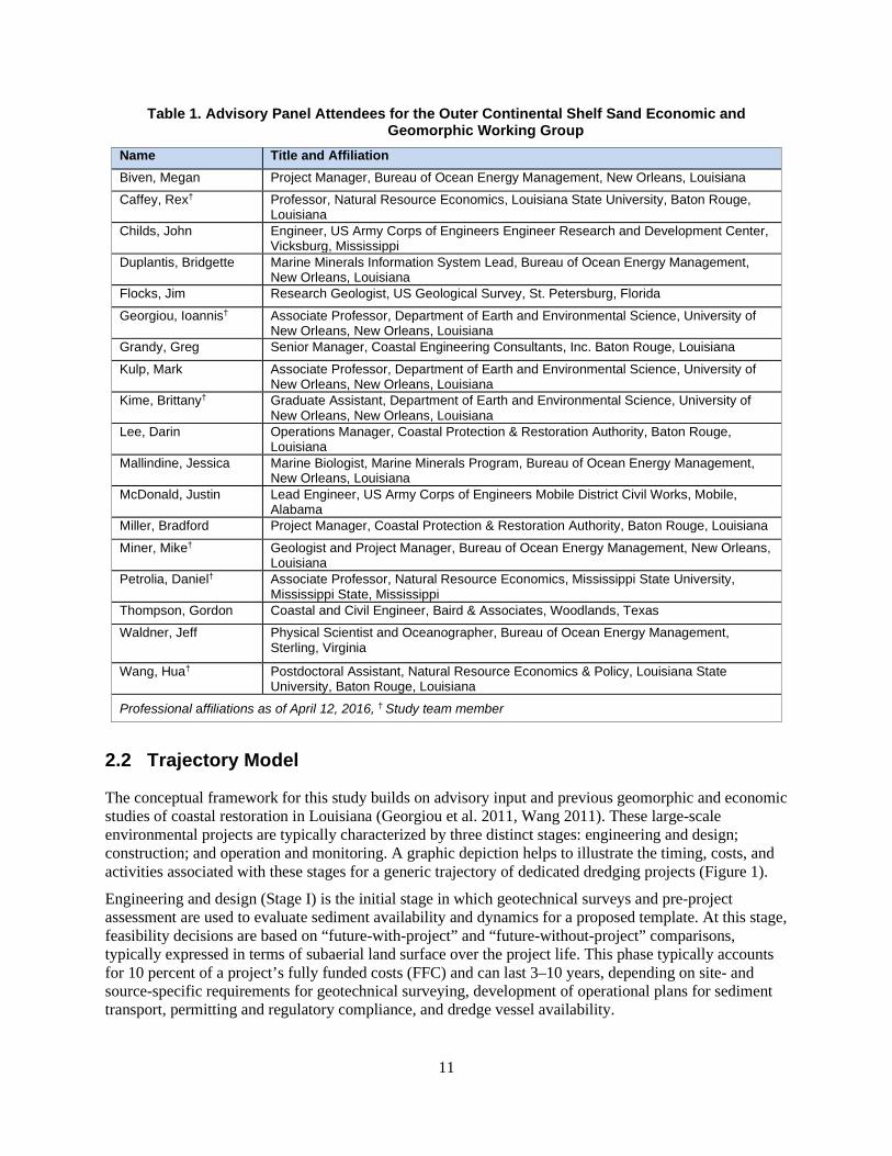
Initial meetings of the researchers involved in this project (study team) were heavily focused on the identification of relevant data and development of a common structure and language for the integrated analysis. The preliminary approach that resulted from those exchanges was presented to a project advisory committee convened at the University of New Orleans in year 1. The meeting consisted of 18 attendees, including 6 members of the study team and 13 external advisors from the public and private sector with expertise in coastal geomorphology, environmental engineering and management of state and federal dredging projects (Table 1).
During the meeting, the study team presented alternative frameworks for the study and a list of candidate projects under consideration as data sources for an integrated analysis. At the time of the meeting, 16 candidate projects had been identified for which relevant nearshore (NS) and Outer Continental Shelf (OCS) data were available for coastal Louisiana. Project advisors provided input that would lead to the identification of an additional 6 relevant projects for guiding the development of the geomorphic and economic sub-models. In terms of the analytical framework, the panel offered guidance on temporal and spatial scales and discussed key variables most likely to affect sediment-related performance and costs. Some of the more salient points that emerged from the integrated framework discussion are provided below. It is appropriate to simulate a standardized barrier island template and develop geomorphic and
economic projections based on data from previous projects using NS and OCS sediment sources.
Sediment dynamics should be modeled at the particle level, as opposed to total volume approach, given that sand quality will be highly variable between source locations .
Geomorphic simulations should focus on how sand quality affects project longevity at the site-level and the system-level. Simulations should address both chronic and acute forcing (storms).
Monetized benefits should derive from physical outputs (volume/area) of the geomorphic model and estimated on an annual net-basis (future-with minus future-without project).
Monetized cost estimates should be based on a statistical model derived from relevant data (e.g. final reports, contractor bids, and input from industry representatives).
Economic efficiency comparisons should not be based solely on sand as a commodity, but also on
the flow of ecosystems services generated by that sand throughout the project lifetime.
Different projects have different goals. Consider using alternative metrics of project performance and benefits (e.g. measuring project response at the site and system level and at subaerial and subaqueous contours).
Transferability of the knowledge base on this project is important. A valuable outcome would be the development of an integrated framework for decision-support that could be replicated in other coastal regions.
11
Table 1. Advisory Panel Attendees for the Outer Continental Shelf Sand Economic and Geomorphic Working Group
Name Title and Affiliation Biven, Megan Project Manager, Bureau of Ocean Energy Management, New Orleans, Louisiana Caffey, Rex† Professor, Natural Resource Economics, Louisiana State University, Baton Rouge,
Louisiana Childs, John Engineer, US Army Corps of Engineers Engineer Research and Development Center,
Vicksburg, Mississippi Duplantis, Bridgette Marine Minerals Information System Lead, Bureau of Ocean Energy Management,
New Orleans, Louisiana Flocks, Jim Research Geologist, US Geological Survey, St. Petersburg, Florida Georgiou, Ioannis† Associate Professor, Department of Earth and Environmental Science, University of
New Orleans, New Orleans, Louisiana Grandy, Greg Senior Manager, Coastal Engineering Consultants, Inc. Baton Rouge, Louisiana Kulp, Mark Associate Professor, Department of Earth and Environmental Science, University of
New Orleans, New Orleans, Louisiana Kime, Brittany† Graduate Assistant, Department of Earth and Environmental Science, University of
New Orleans, New Orleans, Louisiana Lee, Darin Operations Manager, Coastal Protection & Restoration Authority, Baton Rouge,
Louisiana Mallindine, Jessica Marine Biologist, Marine Minerals Program, Bureau of Ocean Energy Management,
New Orleans, Louisiana McDonald, Justin Lead Engineer, US Army Corps of Engineers Mobile District Civil Works, Mobile,
Alabama Miller, Bradford Project Manager, Coastal Protection & Restoration Authority, Baton Rouge, Louisiana Miner, Mike† Geologist and Project Manager, Bureau of Ocean Energy Management, New Orleans,
Louisiana Petrolia, Daniel† Associate Professor, Natural Resource Economics, Mississippi State University,
Mississippi State, Mississippi Thompson, Gordon Coastal and Civil Engineer, Baird & Associates, Woodlands, Texas Waldner, Jeff Physical Scientist and Oceanographer, Bureau of Ocean Energy Management,
Sterling, Virginia
Wang, Hua† Postdoctoral Assistant, Natural Resource Economics & Policy, Louisiana State University, Baton Rouge, Louisiana
Professional affiliations as of April 12, 2016, † Study team member
2.2 Trajectory Model
The conceptual framework for this study builds on advisory input and previous geomorphic and economic studies of coastal restoration in Louisiana (Georgiou et al. 2011, Wang 2011). These large-scale environmental projects are typically characterized by three distinct stages: engineering and design; construction; and operation and monitoring. A graphic depiction helps to illustrate the timing, costs, and activities associated with these stages for a generic trajectory of dedicated dredging projects (Figure 1).
Engineering and design (Stage I) is the initial stage in which geotechnical surveys and pre-project assessment are used to evaluate sediment availability and dynamics for a proposed template. At this stage, feasibility decisions are based on “future-with-project” and “future-without-project” comparisons, typically expressed in terms of subaerial land surface over the project life. This phase typically accounts for 10 percent of a project’s fully funded costs (FFC) and can last 3–10 years, depending on site- and source-specific requirements for geotechnical surveying, development of operational plans for sediment transport, permitting and regulatory compliance, and dredge vessel availability.

12
Project construction (Stage II) is a relatively brief period that accounts for the majority of FFC (85%). During this phase, an initial quantity of sediment from a designated source (Dredgeq) is mechanically transported to the project site and deposited within a bounded template to achieve a target level of post-settlement elevation (Targetq) per sponsor agency specifications. Construction is typically completed within a single year, although longer periods can be required depending on various factors, including: distance between source material and project footprint; project size and design; dredge capacity limitations; weather; and, critical habitat constraints that might limit operations during certain seasons.
Figure 1. Conceptual trajectory of dredge-based reclamation stages on a coastal barrier island.
Project operation and monitoring (Stage III) is the longest period and can range from 20–50 years depending on sponsor. During this phase, public benefits derive from an expanded barrier platform. A range of benefits have been used as justification for these projects; however, storm surge attenuation and provision of coastal habitat are two of the most frequently cited ecosystem services for coastal barrier systems (Petrolia and Kim 2009, Feagin et al. 2010, Barbier et al. 2011). And though there is some potential for volumetric and surface area increases of sediment due to longshore sediment transport processes at the site and system level, in a transgressive coast, most of these materials (and their associated benefits) are expected to diminish over time as restored land succumbs to physical forcing. Thus, the basic expectation is that project benefits will exceed project costs and the renourishment will sustain a subaerial template (Projectq) that have otherwise been lost over time (Controlq). Despite accounting for the lowest portion of FFC (5%), monitoring is critical for collecting the data needed to refine expectations and to improve the design and construction of future projects.
Figure 2 expands the basic trajectory with hypothesized responses for projects using NS- and OCS- sourced sediments. These curves approximate the observations of project managers and reflect two important tradeoffs with potential economic implications. First, while nearshore sediment sources may be less expensive to harvest and transport (given their proximity to project sites), they often contain a higher fraction of organic fines (mud) than OCS sources. Thus, for any given Targetq of sand, the volume of NS sediment dredged will typically exceed the volume of OCS sediment dredged, i.e. NSq> OCSq. Secondly, managers assert that OCS-sourced projects are typically more resilient over time than NS-source ones, thus OCSq’ > NSq’. In other words, increased resilience is attributed to the larger diameter of OCS sands, which can make them more resistant to the physical forces of coastal transport, erosion and storms (i.e., more energy is required for mobilization and transport). Less understood, however, is the degree to which these differences translate into economic efficiencies, and the extent to which any source-dependent trade-offs are affected by prolonged forcing and major storms events. Examining these questions requires the delineation of site and system boundaries and a mathematical framework for quantifying sediment dynamics within those boundaries.

13
Figure 2. Conceptual trajectories for dredge-based reclamation on a barrier island nourished with nearshore (NS) and outer continental shelf (OCS) sediments, including a storm event.
2.3 Boundary Model
Figure 3 delineates component boundaries and sand dynamics at the site and system level for dredge-based renourishment of a barrier template. For the purpose of this analysis, a “site” is defined as a distinct barrier island. Transport of sand into and out of the site affects the 2-dimensional area of the site, as defined by some vertical contour. Thus, for any given site, measures of surface area (e.g., acreage) increase as depth increases.
A project site may have one or more adjacent up-drift and down-drift sites associated with it, each with its own distinct boundary. A “barrier system” is defined as a set of one or more sites that stand in relation (up-drift or down-drift) to one another. Barrier systems are located within an active littoral zone characterized by subtidal transport of coastal sediments.
A unit of sand located at a position adjacent to, but external from, the vertical contour of a given site is considered to be outside of the site boundary. This designation is necessary for assessing which units of sand are to be counted as beneficial in terms of determining standing, discussed in more detail below.
Note that although a unit of sand outside a given boundary is not considered beneficial in a given period, that unit of sand may be transported (mechanically or naturally) at some later period to a location inside the boundary, at which point it would have standing, and would count as beneficial.
Note also that site boundaries allow for benefits to accrue at both subaerial and subaqueous contours, and that the value of the benefits attributed to a unit of sand at each of these two levels may differ.

14
Figure 3. Standard components and processes of sand transport for dredge-based reclamation of a barrier island system comprised of individual sites.
2.3.1 Sand Quantity
The quantity of sand in Stage III at a given site in a given period is the sum of the quantity of sand at the site in the previous period, any sand mechanically dredged from NS or OCS sources outside the system and placed within the site during the current period, the quantity of sand “captured” from adjacent sites in the current period due to natural transport, and the quantity of sand “lost” due to natural transport.
There is some set of functions that dictate how much sand accumulates (or sloughs off) at the site, and how much is recaptured from adjacent sites.
Note that the above description of “dredged” sand is expressed in terms of the quantity of sand placed, not the total quantity of sediment dredged, which is composed of some fraction of sand (beneficial) and mud (zero benefit) that varies by source location (see Targetq and Dredgeq designations in Stage II, Figure 1).1
2.3.2 Standing and Classification of Benefits
Only sand located within the benefit boundary of a given site is considered to have standing, where “standing” dictates which units of sand are counted as beneficial in a given time period. Standing is defined at both the site level and at the system level.
To facilitate policy discussion, benefits are divided into two classes. At the site level, benefits associated with pre-existing sand (i.e., sand present at a given site at period t = 0) and sand placed mechanically from outside the site boundary are classified as “direct” benefits. Benefits associated with sand recaptured at the site from outside the site boundary via natural transport are classified as “indirect” benefits.
At the system level, the classification of benefits is somewhat modified. For example, if sand were moved, either mechanically or naturally, from one site within the system to another within the system,
1 Dredge and. target quantities are addressed in Sections 3 and 4. If desirable, the model can be amended to include mud as also beneficial, with its own respective benefit values.

15
this would not result in any change of benefits, because the sand would move from one site with standing to another site also with standing.
Thus, at the system level, benefits associated with pre-existing sand and sand placed mechanically from outside the system boundary are classified as “direct” benefits. Benefits associated with the net quantity of sand recaptured across the entire system from outside the system via natural transport are classified as “indirect” benefits.
2.4 Mathematical Model
Formally, let the change in quantity of sand at site s at time t, stq∆ , be expressed as the sum of the
quantity of sand added mechanically in the current period, stm , and the net difference between the
quantity of sand added and lost via natural transport, stn . As Figure 3 indicates, sand added or lost via natural transport can originate either from other sites within the barrier system (up-drift or down-drift) or “vagrant” sand, i.e., sand from outside the barrier system, either from nearshore (littoral zone) or OCS sources. Thus, we may write
~s vst st stn n n= + (1)
where ~sstn represents the share originating from other sites within the barrier system ( ~ s indicating “not
s”) and vstn but these cannot be individually identified at the site level; we observe only a net gain or loss
of sand at a site at each period. Thus, we have:
st st stq m n∆ = + (2)
Summing expression (2) over all sites within the system, we have system quantity of sand at time t as:
( )1 1
S S
t st st sts s
Q q m n= =
∆ = ∆ = +∑ ∑ (3)
Within a defined barrier system, the sum of sand change via natural transport between all sites, is necessarily zero, i.e.:
~
10
Ss
sts
n=
=∑ (4)
Thus, at the barrier system level, any net change in sand quantities via natural transport is necessarily attributable to vagrant sand exchange with the larger littoral boundary and/or offshore zone (Figure 3).
Specification for Project Evaluation
Renourishment projects are typically conducted at a single site, with mechanical placement of sand at that site only. Further, project evaluation is typically based on the sand accrued at the project site only, ignoring any changes in sand accrual at other sites in the barrier system. Defining site 1s = as the project site, and recognizing that 0stm = for all 1s ≠ , we may rewrite (3) to separate what is typically evaluated, called here “direct”, from what is typically ignored, called here “indirect”.

16
1 1
1 2
S S
t st t t sts sDirect
Indirect
Q q m n n= =
∆ = ∆ = + +∑ ∑ (5)
Accounting for Subaqueous Quantities
If we assume that the benefits of a unit of sand are dependent upon whether that unit is subaerial or subaqueous, we may expand (1) into:
a a b bst st st st st
Subaerial Subaqueous
q m n m n∆ = + + + (6)
where the “a” superscript indicates “above the surface” (subaerial) and “b” indicates “below the surface” (subaqueous).
At the system level, substituting (6) into (5), we get:
1 1 1 1
1 2 2
S S Sa a b b a b
t st t t t t st sts s sDirect Subaerial Direct Subaqueous
Indirect Subaerial Indirect Subaqueous
Q q m n m n n n= = =
∆ = ∆ = + + + + +∑ ∑ ∑ (7)
where the first set of terms, “Direct Subaerial”, is what is included in a typical Stage III project performance evaluation, with all others ignored.
2.5 Summary
The graphical and mathematical framework outlined above establishes a conceptual model for examining the performance of barrier island renourishment projects in terms of sand quantity dynamics at the site and system level. Modeling the performance of that sand over time, however, requires a more specific delineation of the barrier island template, and geomorphic simulations to depict how sand of different quality responds to chronic and acute forcing.
17
3 Project Benefit Modeling
3.1 Geomorphic Data Synthesis and Simulation
Data for the development of a sub-model of project benefits were obtained from extant literature (i.e. scientific manuscripts and technical reports), geodatabases, and federal and/or state-owned sources related to coastal sediment inventories and dynamics. Examples of such work included citations of the location and extent of relict delta deposits, their proximity to the coastal zone, the potential availability of these deposits relative to the ongoing transgression of the Louisiana coast, chief drivers of nearshore sediment transports processes within the delta plain, and the role of coastal sediment sinks (Nairn et al. 2004, Miner et al. 2009a, Georgiou et al. 2011). Project performance parameters were developed from post-construction outcome monitoring and from consultation with project managers and engineers in the public and private sector. Such information included, but was not limited to: geotechnical and geophysical surveys, site- and technology-specific analyses of sediment delivery alternatives, and data from coast-wide reference monitoring systems and other systems with similar capabilities.
3.1.1 Sand Quality
The sediment characteristics of the Mississippi River Delta (MRD) region vary spatially as a function of geomorphology. Sand quality was accessed from Outer Continental Shelf (OCS) locations (e.g., Ship Shoal, Trinity Shoal, St. Bernard Shoals, etc.) using available borings and/or other available geophysical data. Information used in the analysis and comparison include among others median grain size diameter (d50), sorting, shape factor, kurtosis where available, mud content, etc. Similar analysis was used for sediment characteristics of sand in nearshore environments used previously for restoration projects, and to develop normalized plots comparing nearshore compared to OCS sediment quality. Because beachface, shoreface, and dune slopes are proportional to the sediment characteristics (Dean 1974, Dean and Darlymple 2002) an inventory of slopes in areas where restoration took place was developed to identify any correlations with the corresponding grain size diameter (James 1975).
3.1.2 Dredging Impacts
The presence (and geometry) of nearshore bars imposes a control on the available wave energy that arrives at a beach, as these bars often induced breaking of larger waves and hence limit the wave energy transmission for higher waves (Short 1992). Dredging immediately in front of barrier islands or beaches, is not very common in Louisiana, although several borrow pits where nearshore sediments were used are proximal to barriers, located within the active shoreface. Review of literature review and information synthesis from other states, and in particular Florida, was used to examine cases in which dredging takes place routinely following storms.
Kennedy et al. (2011) reported that, for open coast pits with large alongshore lengths, cross-shore infilling appeared to dominate over longshore infilling, but both processes may be of comparable importance in shorter pits. Infilling of three borrow pits adjacent to ebb shoals was found to be considerably larger than on open coasts, and, finally, the offshore pits experience more rapid bathymetric changes compared to nearshore pits. Kennedy et al. (2011) also reported that hurricanes have a significant effect on infilling rates, as did Miner et al. (2009b) during a survey of an ebb tidal delta along the Timbalier shoreline in 2004–2005. These findings were supplemented with a selection of wave simulations using the wave model (SWAN) in both stationary and non-stationary mode in a domain previously developed and validated by Georgiou et al. (2014). A series of hypothetical dredge pits were examined by adjusting the bathymetry at key environments, and performing simulations to compare with the baseline results.
18
3.1.3 Project Outcomes
An inventory of relevant projects that used both NS and OCS sands was developed to guide the development of time-dependent quantity estimates for the economic analysis. Quantity measures were reported volumetrically and in terms of subaerial land and the proximal subaqueous platform. The project database provided a 25–50 year window of historical bathymetry and topography from the corresponding period of each project, incorporated shoreline erosion rates (from BICM or other source, e.g., Barrier Shoreline Atlas), seafloor change analysis maps (Miner et al. 2012), cut-to-fill ratios, and other metrics of performance obtained from project monitoring reports. The challenge was to establish a continuous area function that accounted for the role of the shoreface and storm activity and reflected performance trends related to differential shoreface response, using BICM bathymetry (Miner et al. 2009c) and surface textural characteristics of the sediment (Kindinger et al. 2014).
3.1.4 Sediment Type Suitability
Based on results from the project inventory and data recovered from the literature and synthesis, a matrix was developed to categorize sediment type based on suitability for, or project type. Various grain sizes were evaluated for renourishment suitability for dunes, beach and back barrier platform. Because different templates produce different geomorphologies (given similar forcing), preferred sediment types can be determined based on the suitability of restoration targets and habitats. Geomorphic results provided baseline data to draw the first dependencies and state to complete the matrix. To ensure that model behavior is constrained, these simulations are supplemented with literature and results from locations where these sediment types are present with their respective habitat.
3.2 Model Domain and Set-up
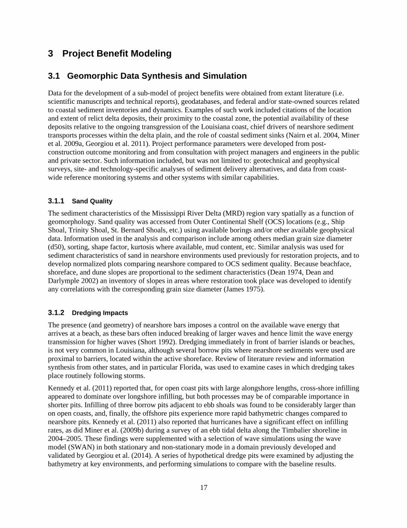
A final model grid was developed around a proxy barrier system based on the Isle Dernieres island chain using National Oceanic and Atmospheric Administration (NOAA) bathymetry from the 1980s. The system boundary consist of a 360 ha (subaerial) central barrier island with a large section (898 hecatares [ha]) of an up-drift barrier to the east and a smaller section (166 ha) of a down-drift barrier to the west. Additional components include tidal inlets, spit platforms, and areas ebb-delta, surf zone, and nearshore deposition. The bounded area represents a 50 km2 domain for the application of three-dimensional modeling with coupled waves, tidal currents and full sediment transport and morphology. The model is constructed with the Delft3D modeling suite and can be used to simulate cumulative erosion and deposition, with and without project-based nourishments at subaerial and subaqueous boundaries (Figure 4).
The domain is transected by 192 x 384 grid consisting of cells of varying resolution (~20m nearshore to 1 km offshore). Water is forced at offshore and lateral boundaries (~ 6 hours for waves, ~ 1 hour for water level) with a Neumann condition lateral using information from the Wave Information System (WIS) of the US Army Corps of Engineers and Port Fourchon NOAA tidal gauge. Changes in relative sea level are incorporated into the simulation based on forecast estimates provided by the Coastal Protection and Restoration Authority (CPRA) (2017). Sediment dynamics are depicted by a combined bedload/suspended load transport function (van Rijn 1984a and 1984b) using different sand classes to depict bathymetry updating (NS=156µm, OCS=160 µm, 165 µm, and 200µm). Morphodynamic upscaling was used which allows the model to extend bed-load and suspended load transport for wash-over, breaching, lateral migration, and sediment bypassing. The set-up simulates sand placement in terms of direct effects (central barrier) and total system effects (west, central, and east barriers) at elevation and depth contours of 1.0, 0.0, and -0.5 meters.
19
Figure 4. Model domain and system components used in geophysical simulations.
3.3 Model Scenarios and Semi-Empirical Results
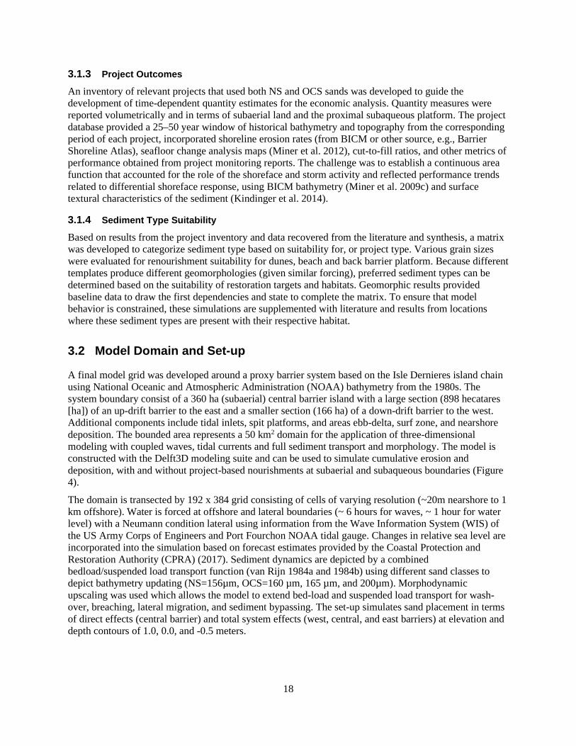
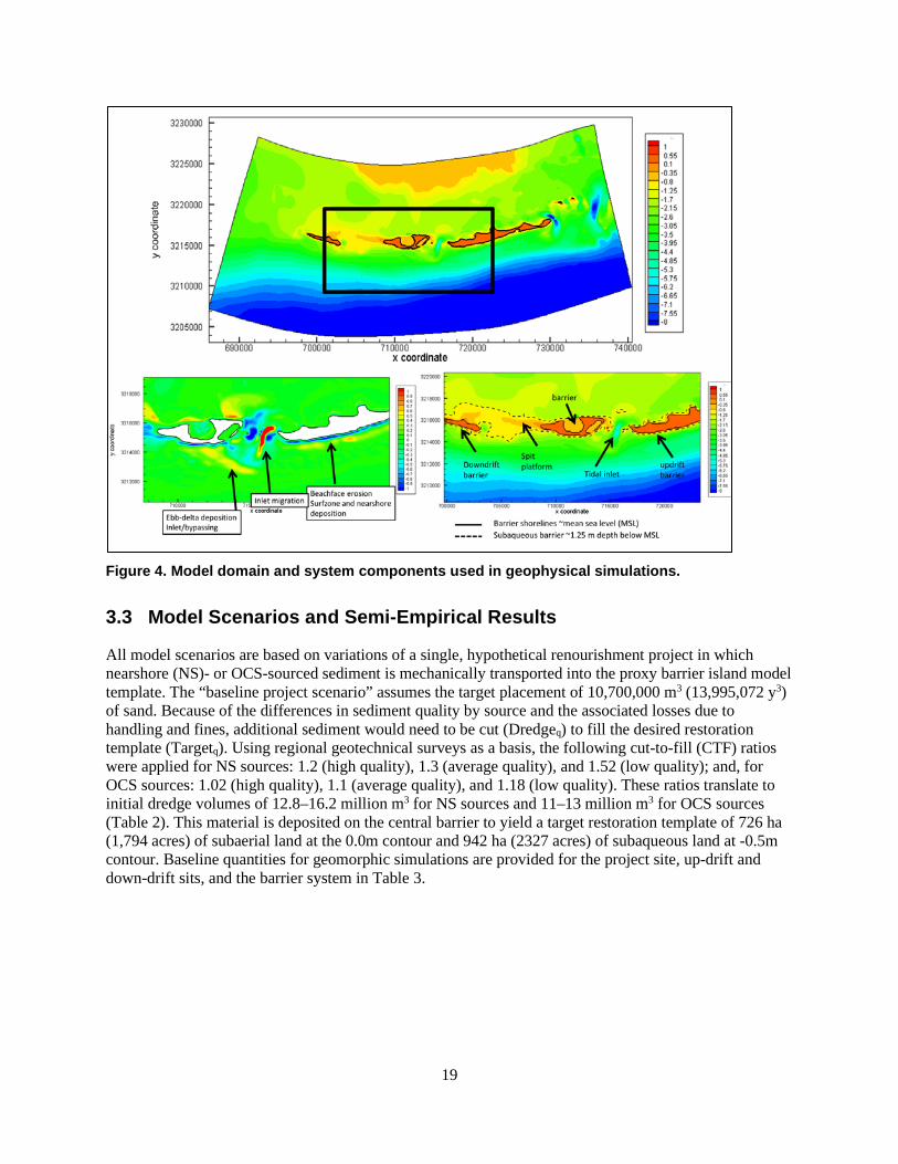
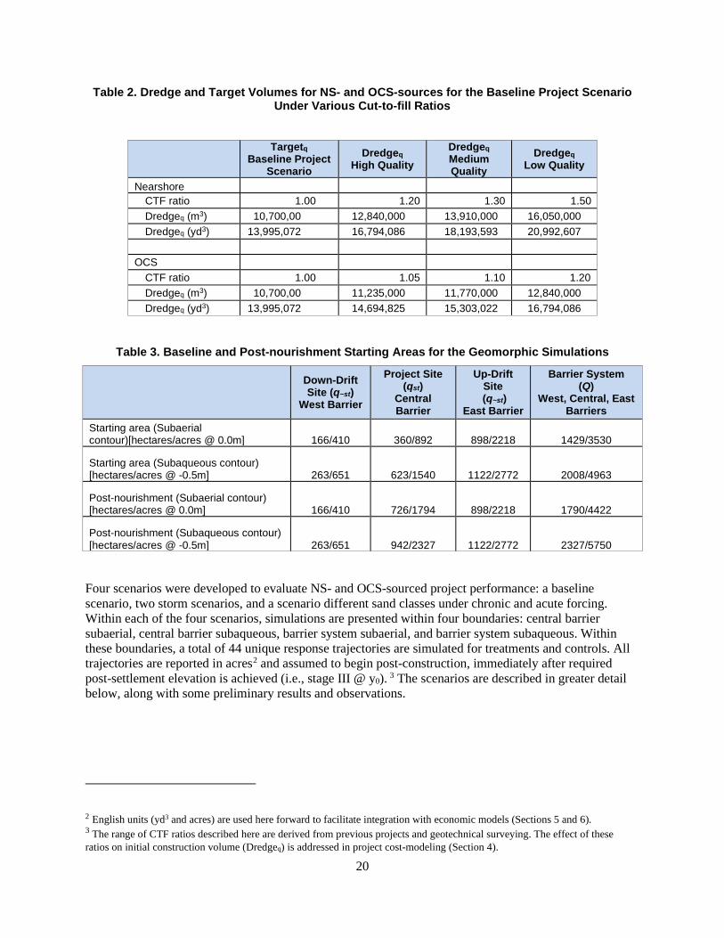
All model scenarios are based on variations of a single, hypothetical renourishment project in which nearshore (NS)- or OCS-sourced sediment is mechanically transported into the proxy barrier island model template. The “baseline project scenario” assumes the target placement of 10,700,000 m3 (13,995,072 y3) of sand. Because of the differences in sediment quality by source and the associated losses due to handling and fines, additional sediment would need to be cut (Dredgeq) to fill the desired restoration template (Targetq). Using regional geotechnical surveys as a basis, the following cut-to-fill (CTF) ratios were applied for NS sources: 1.2 (high quality), 1.3 (average quality), and 1.52 (low quality); and, for OCS sources: 1.02 (high quality), 1.1 (average quality), and 1.18 (low quality). These ratios translate to initial dredge volumes of 12.8–16.2 million m3 for NS sources and 11–13 million m3 for OCS sources (Table 2). This material is deposited on the central barrier to yield a target restoration template of 726 ha (1,794 acres) of subaerial land at the 0.0m contour and 942 ha (2327 acres) of subaqueous land at -0.5m contour. Baseline quantities for geomorphic simulations are provided for the project site, up-drift and down-drift sits, and the barrier system in Table 3.
20
Table 2. Dredge and Target Volumes for NS- and OCS-sources for the Baseline Project Scenario Under Various Cut-to-fill Ratios
Targetq Baseline Project
Scenario Dredgeq
High Quality Dredgeq Medium Quality
Dredgeq Low Quality
Nearshore CTF ratio 1.00 1.20 1.30 1.50 Dredgeq (m3) 10,700,00 12,840,000 13,910,000 16,050,000 Dredgeq (yd3) 13,995,072 16,794,086 18,193,593 20,992,607
OCS
CTF ratio 1.00 1.05 1.10 1.20 Dredgeq (m3) 10,700,00 11,235,000 11,770,000 12,840,000 Dredgeq (yd3) 13,995,072 14,694,825 15,303,022 16,794,086
Table 3. Baseline and Post-nourishment Starting Areas for the Geomorphic Simulations
Down-Drift Site (q~st)
West Barrier
Project Site (qst)
Central Barrier
Up-Drift Site
(q~st) East Barrier
Barrier System (Q)
West, Central, East Barriers
Starting area (Subaerial contour)[hectares/acres @ 0.0m] 166/410 360/892 898/2218 1429/3530
Starting area (Subaqueous contour) [hectares/acres @ -0.5m] 263/651 623/1540 1122/2772 2008/4963
Post-nourishment (Subaerial contour) [hectares/acres @ 0.0m] 166/410 726/1794 898/2218 1790/4422
Post-nourishment (Subaqueous contour) [hectares/acres @ -0.5m] 263/651 942/2327 1122/2772 2327/5750
Four scenarios were developed to evaluate NS- and OCS-sourced project performance: a baseline scenario, two storm scenarios, and a scenario different sand classes under chronic and acute forcing. Within each of the four scenarios, simulations are presented within four boundaries: central barrier subaerial, central barrier subaqueous, barrier system subaerial, and barrier system subaqueous. Within these boundaries, a total of 44 unique response trajectories are simulated for treatments and controls. All trajectories are reported in acres2 and assumed to begin post-construction, immediately after required post-settlement elevation is achieved (i.e., stage III @ y0). 3 The scenarios are described in greater detail below, along with some preliminary results and observations.
2 English units (yd3 and acres) are used here forward to facilitate integration with economic models (Sections 5 and 6). 3 The range of CTF ratios described here are derived from previous projects and geotechnical surveying. The effect of these ratios on initial construction volume (Dredgeq) is addressed in project cost-modeling (Section 4).
21
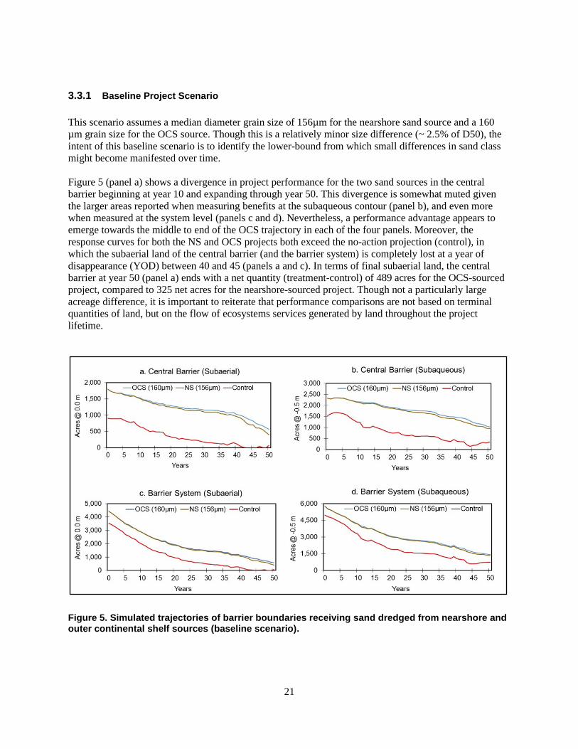
3.3.1 Baseline Project Scenario
This scenario assumes a median diameter grain size of 156µm for the nearshore sand source and a 160 µm grain size for the OCS source. Though this is a relatively minor size difference (~ 2.5% of D50), the intent of this baseline scenario is to identify the lower-bound from which small differences in sand class might become manifested over time. Figure 5 (panel a) shows a divergence in project performance for the two sand sources in the central barrier beginning at year 10 and expanding through year 50. This divergence is somewhat muted given the larger areas reported when measuring benefits at the subaqueous contour (panel b), and even more when measured at the system level (panels c and d). Nevertheless, a performance advantage appears to emerge towards the middle to end of the OCS trajectory in each of the four panels. Moreover, the response curves for both the NS and OCS projects both exceed the no-action projection (control), in which the subaerial land of the central barrier (and the barrier system) is completely lost at a year of disappearance (YOD) between 40 and 45 (panels a and c). In terms of final subaerial land, the central barrier at year 50 (panel a) ends with a net quantity (treatment-control) of 489 acres for the OCS-sourced project, compared to 325 net acres for the nearshore-sourced project. Though not a particularly large acreage difference, it is important to reiterate that performance comparisons are not based on terminal quantities of land, but on the flow of ecosystems services generated by land throughout the project lifetime.
Figure 5. Simulated trajectories of barrier boundaries receiving sand dredged from nearshore and outer continental shelf sources (baseline scenario).

22
3.3.2 Early Storm Scenario
In this scenario, baseline simulations (i.e., NS sand at 156µm, OCS sand at 160 µm) are punctuated by a major hurricane of Category 2 intensity on the Saffir-Simpson hurricane wind scale (National Hurricane Center 2020). Termed the “early storm scenario”, the intent is to examine how a major storm occurring early (year 5) in the 50-year trajectory would affect the performance of NS- and OCS-sourced projects. Acreage reductions are based on historical losses resulting from storms impacting the Isle Dernieres island chain, most notably Hurricane Lili in 2002 and Hurricane Gustav in 2008. Figure 6 depicts notable acreage reductions in year 5 within all four boundaries. And though there continues to be a slim advantage for the OCS-sourced project compared to the NS-sourced project on the central barrier (panel a), the divergence it is diminished, and is barely perceptible at the system level (panel c). Moreover, the terminal areas at year 50 on the central barrier are 130 and 225 net acres of subaerial land for NS and OCS- and sourced projects, respectively. This equates to a 60% and 54% reduction in remnant land remaining in the baseline scenario. Despite these impacts, the subaqueous projections for the central barrier (panel b) indicates that a considerable amount of sediment remains above the -0.5m contour, as indicated by terminal quantities of 690 and 828 net acres for NS- and OCS-sourced projects. And both projects remain effective in sustaining subaerial land compared to the no-action scenario (panel a) in which control trajectory is completely lost, with a YOD between years 30 and 35 (panels a & c)–10 years sooner than observed in the baseline scenario.
Figure 6. Simulated trajectories of barrier boundaries receiving sand dredged from nearshore and outer continental shelf sources (early storm scenario).

23
3.3.3 Late Storm Scenario
This set-up replicates the same conditions of the previous two scenarios (i.e., NS sand at 156µm, OCS sand at 160 µm, category 2 hurricane) but moves storm landfall to year 20. Figure 7 depicts notable acreage reductions in year 20 within all four boundaries. The terminal quantities of subaerial land at year 50 on the central barrier (panel a) is 250 and 360 net acres for NS- and OCS-sourced projects, respectively. This equates to 48% and 38% reductions in remnant land from the baseline, a reduction that is not quite as dramatic as seen in the early storm scenario. In each case (early and late storm), the OCS-sourced projects continued to outperform the NS-source projects. This result appears to confirm manager assertions that OCS-sourced projects perform better not only under chronic forcing, but also in terms of storm resilience. It is interesting to note, however, that this scenario results in the most grave outcome for a control simulation. The subaerial land of the central barrier is completely lost by year 30 (panel a) in the absence of restoration, indicating the potential for a looming threshold effect for non-restored barrier islands. And while a small recovery is evident between years 40 and 45 for the control simulation for all boundaries, it is short-lived. This apparent rebound likely reflects a simulated reworking the reworking of system sediments dispersed by the storm.
Figure 7. Simulated trajectories of barrier boundaries receiving sand dredged from nearshore and outer continental shelf sources (late storm scenario).

24
3.3.4 Larger Sand Scenario
This scenario expands the original baseline set-up by adding two additional OCS sand classes, one slightly larger (165 µm) and one much larger (200 µm). The intent of this scenario is to examine how modest to large increases (3%–20%) in sand diameter affect the long-term performance in OCS-sourced projects. Figure 8 depicts five trajectories in each boundary panel: the original three baseline simulations plus two additional simulations reflecting projects sourced with larger OCS sands. Because of the modest increase in size, the 165 µm project trajectory is difficult to discern from the baseline 160 µm trajectory. The 200 µm class, however, represents a much larger increase in sand quality (diameter) that translates to performance advantages clearly evident in all four boundary panels. For the 200 µm sand, there are 825 net acres of remnant subaerial land remaining in year 50 on the central barrier (panel a). This represents a near 70% increase over the baseline OCS-sourced project performance. The extent to which such performance advantages are possible is a function of the availability of, and feasibility of access to, large diameter sand deposits. Sands of 165–200 µm are not uncommon in the offshore shoals and Paleolithic stream channels of the Sabine Bank, Tiger and Trinity Shoal Complex, Ship Shoal Complex, and St. Bernard Shoal. Sediment distribution maps have estimated the total volume of these sources at OCS sand deposits sand at ~75 billion cubic meters (BCM), primarily (Finkl and Freeman 2014).
Figure 8 Simulated trajectories of barrier boundaries receiving sand dredged from nearshore and outer continental shelf sources (larger sand class scenario).

25
4 Project Cost Modeling
4.1 Data for the analysis
4.1.1 Project Reports
Data for the development of a sub-model of project costs were obtained from previously constructed restoration projects in coastal Louisiana. A list of “candidate projects” was developed with advisory panel input and with a focus on dedicated dredging efforts in the region similar to the proxy barrier system. A list of 22 barrier renourishment initiatives were identified for which nearshore (NS) (n=12) or Outer Continental Shelf (OCS) (n=10) sediments provided the primary source of dredge material for project construction efforts from 1997 to 2018 (Table 4).4
Most of these candidate projects (64%) were implemented with federal funds provided through the Coastal Wetland Planning Preservation and Restoration Act (CWPPRA). The remainder were funded by the Coastal Impact Assistance Program (CIAP), National Resource Damage Assessment (NRDA), National Fish and Wildlife Foundation (NFWF), State-Only projects (STATE),5 and Berm to Barrier (BERM)6 initiative.
Figure 9 provides a depiction of the locations of these candidate projects and borrow sites in coastal Louisiana. The graphic depicts that 20 of the 22 candidate projects are equally distributed within the coastal waters of the Barataria basin (10 projects) and the Terrebonne basin (10 projects). Restoration costs are captured for projects on Isles Dernieres (TE 20 and TE 24) - the basis for the proxy barrier island template described in Section 3. Similar projects to the east and west of Isles Dernieres provide additional sources of spatially-relevant costs data for economic modeling. Note that the borrow sites of OCS-sourced projects do not all appear to fall outside the state’s territorial waters. Candidate project designation in this study (i.e., NS or OCS) is delineated not only by distance, but also sand quality. Some of these projects have used relic deposits of large diameter, OCS-quality sand found relatively close to shore. Geotechnical surveys indicate, however, that such deposits are increasingly limited and that future sourcing of large-diameter sand will be reliant on deposits within shoals, channel and banks located well offshore.
4.1.2 Bid Data
Because of the large scale and budget of barrier island restoration projects, few candidate projects are available as the basis for predictive modeling. Additional information on project costs can be obtained through surveys of coastal dredging and engineering firms. The time required to collect such information (and its sensitivity), however, suggests that surveying would be unlikely to yield a sufficient amount of reliable information.
4 Costs data were extracted only from barrier shoreline and barrier island renourishment projects in coastal Louisiana. Interior, “marsh creation” projects were not included in the candidate project dataset. 5 In the years 2007, 2008, and 2009, the Louisiana State Legislature allocated $790 million in State surplus funds for use in coastal protection and restoration activities. This included both cost-sharing in other federal programs as well as the implementation of projects without a federal partner. 6 During the oil spill crisis in 2010, emergency dredging was used in an attempt to build sand berms to block oil from entering Louisiana’s coastal marshes. The CPRA has used material from those berms to renourish barrier island chains in the southeastern coast of the state.

26
Table 4. Candidate Projects for Development of a Representative Cost Model of Dedicated-dredging for Barrier Island and Shoreline Restoration in Coastal Louisiana (1990–2018)
ID Name Program Source* BA-38-1 Pelican Island Restoration CWPPRA OCS BA-40 Riverine Sand Mining/Scofield Island Restoration BERM/CWPPRA OCS BA-45 Caminada Headland Beach and Dune Restoration CIAP OCS BA-110 Shell Island East BERM Restoration NRDA OCS BA-111 Shell Island West NRDA Restoration NRDA OCS BA-143 Caminada Headland Beach and Dune Restoration INCR2 NFWF OCS CS-31 Holly Beach Sand Management CWPPRA OCS CS-33 Cameron Parish Shoreline Restoration CWPPRA OCS TE-48-2 Raccoon Island Shoreline Protection and Marsh Creation CWPPRA OCS TE-100 Caillou Lake Headlands Restoration NRDA OCS BA-30 East Grand Terre Island Restoration CIAP NS BA-35 Pass Chaland to Grand Bayou Pass Restoration CWPPRA NS BA-38-2 Chaland headland Restoration CWPPRA NS BA-76 Cheniere Ronquille Barrier Island Restoration CWPPRA NS TE-20 Isles Dernieres Restoration East Island CWPPRA NS TE-24 Isles Dernieres Restoration Trinity Island CWPPRA NS TE-
East Timbalier Island Sediment Restoration CWPPRA NS
TE-27 Whiskey Island Restoration CWPPRA NS TE-37 New Cut Dune and Marsh Restoration CWPPRA NS TE-40 Timbalier Island Dune and Marsh Creation CWPPRA NS TE-50 Whiskey Island Back Barrier Marsh Creation CWPPRA NS TE-52 West Belle Pass Barrier Headland Restoration CWPPRA NS * Categorization based on source material location and type
Previous economic research on coastal restoration in Louisiana has used commercial bid data as a means of expanding the number of usable observations for predictive modeling (Wang 2012, Caffey et al. 2014). State and federal agencies solicit formal bids from the private sector during the design, construction, and operation phases of coastal restoration projects. In responding to these public solicitations, private dredging and engineering firms develop competitive bids containing highly-detailed physical and financial projections. If accepted, a contractor’s bid is legally binding. Thus, the veracity of bid data is grounded in legal and economic consequences.
Appendix A contains commercial bids obtained from Louisiana Coastal Protection and Restoration Authority (CPRA) for the 22 candidate projects. The lists include 71 unique bids: 35 for OCS-sourced projects and 36 for NS-sourced projects. The average number of bids is 3 per project, with a range of 2–8 bids overall. Combined with final project data for the 22 candidate projects, this information expands the dataset to 93 useable observations.

27
Figure 9. Geographic locations of candidate projects (NS- and OC-sourced) for development of a dedicated dredging cost model for barrier shoreline and barrier island restoration in in Louisiana, 1997–2018.
Table 5 provides a more in-depth view of the physical characteristics and costs for the candidate projects. The NS- and OCS-sourced project types share some similarities in terms of dredge volumes and project size (e.g., 3.3–3.7 million y3 and 396–409 acres, respectively). Yet these similarities do not extend to project costs. At $59.7 million, the average OCS-sourced projects costs more than twice that of the average NS-sourced project.7 Because of their similar volumes and acreage, this translates to higher unit costs for sediment handling, such as a $17.20/y3 transport cost for OCS sediment compared to $8.05/y3 for NS sediment.8 The higher cost of OCS-sourced projects is due to the longer transport distances between projects and borrow sites. At 17.0 miles, the average transport distance of OCS-dredged sediment is more than five times that of NS-sourced projects (3.31 miles). Some of this difference is driven by recently constructed OCS projects with very long transport distances (e.g., 31 miles for BA-45 and 34.5 miles for BA-143).
7 Note the relatively small differences in average construction costs and project bids: +8% for NS bids and +2% for OCS bids. 8 All costs data contained in bids and project reports are reported in 2016 dollars as adjusted by the Civil Works Construction Cost Index System (CWCCIS).

28
Project ID Name
Sediment Quantity (y3)
Distance (miles)
Marsh (acres)
Beach/dune (acres)
Net Acres
Average Bid †
($)Construction*
Cost ($)$/acre $/y3
East Grand Terre Island 3,144,250 4 455 165 620 36,862,153 34,430,503 55,533 10.95
Pass Chaland to Grand Bayou Pass 5,098,651 8.5 226 124 350 44,184,104 39,725,976 113,503 7.79
Chaland headland Restoration 2,483,649 2 254 230 484 28,931,950 19,842,857 40,998 7.99
Cheniere Ronquille Barrier Island 2,631,400 2 274 137 411 30,948,091 39,725,976 96,657 15.1
Isles Dernieres Restoration East Island 3,900,000 1 40 202 242 14,352,760 15,105,896 62,421 3.87
Isles Dernieres Restoration Trinity Island 4,886,000 1 205 148 353 18,317,588 13,174,156 37,321 2.7
East Timbalier Island Sediment 2,643,437 2.5 161 56 217 17,834,696 14,970,412 68,988 5.66
Whiskey Island 2,338,632 3.5 269 254 523 18,365,011 12,115,143 23,165 5.18
New Cut Dune and Marsh 844,540 3 171 68 239 14,239,068 12,392,490 51,851 14.67
Timbalier Island Dune and Marsh Creation 4,600,000 2.7 264 209 473 17,852,837 19,007,027 40,184 4.13
Whiskey Island Back Barrier Marsh Creation 2,536,784 3.65 319 0 319 28,370,939 26,360,162 82,634 10.39
West Belle Pass Barrier Headland 4,161,226 5.9 334 183 517 36,140,135 33,834,071 65,443 8.13
3,272,381 3.31 248 148 396 25,533,278 23,390,389 61,558 8.05
BA-38-1 3,653,853 8.8 398 180 586 47,560,996 48,961,971 83,553 13.4
BA-40 3,587,081 22 273 261 534 67,565,293 54,741,557 102,512 15.26
BA-45 2,883,800 31 0 246 246 65,088,536 69,104,642 280,913 23.96
BA-110 2,576,000 17 136 141 277 34,756,177 49,186,764 177,570 19.09
BA-111 4,497,500 15.6 265 381 646 63,498,135 93,982,461 145,484 20.9
BA-143 4,941,900 34.5 0 489 489 142,445,762 121,367,379 248,195 24.56
CS-31 2,143,318 5 0 320 320 22,046,463 19,479,809 60,874 9.09
CS-33 1,932,470 21.2 0 267 267 50,785,300 42,507,050 159,202 22
TE-48-2 735,340 4 58 0 58 9,516,021 10,802,970 186,258 14.69
TE-100 9,691,800 7.1 150 512 662 104,106,209 87,304,094 131,879 9.01
3,664,306 17.00 128 280 409 60,736,889 59,743,870 157,644 17.2
*All costs in 2016 dollars, †Average of 3 bids per project
Nearshore (NS) sourced projects
Average NS
Outer Continental Shelf (OCS) sourced projectsPelican Island
BA-76
TE-20
TE-24
TE-25&30
TE-27
TE-37
BA-30
BA-35
Cameron Parish Shoreline
Raccoon Island Shoreline and Marsh Creation
Caillou Lake Headlands Restoration
Average OCS
BA-38-2
Riverine Sand Mining/Scofield Island
Caminada Headland Beach and Dune
Shell Island East BERM
Shell Island West NRDA
Caminada Headland Beach and Dune INCR2
Holly Beach Sand Management
TE-40
TE-50
TE-52
Table 5. Data from Candidate Projects for Development of a Representative Cost Model of Dedicated-dredging for Barrier Island and Shoreline Restoration in Coastal Louisiana (1990–2018)

29
It is important to note that the net acres constructed by the two project types are substantially different. The net acreage of the NS-sourced projects is marsh-dominated (63%), and the OCS-sourced projects are primarily for beach and dune renourishment (68%). This distinction is noteworthy in terms of the economics of sediment quantity (i.e., dredge volumes and cut-to-fill ratios) and sediment quality (i.e., sand performance and resilience of various sand grain sizes). Further analysis of these cost and benefit tradeoffs requires development of a predictive cost model based on the candidate project dataset.
4.2 Cost Modeling
4.2.1 Potential Variables
Project costs for dedicated dredging can vary considerably depending upon the location, quantity, quality, and transportation method and distance of source material. Additional cost considerations include dredging and placement restrictions pertaining to archeological concerns, endangered species, essential fish habitat; and challenges in working around existing oil and gas infrastructure (Michel et al. 2013). Costs can also be substantially dependent on dredge availability and capacity. Biven (2014) points out that only a small number of seaworthy reclamation vessels are available for US operations under the Jones Act of 1920 (P.L. 66-261). Most of these are hopper dredges (15), with a capacity less than 4,000 m3. Only three US dredges have capacities greater than 8,000 m3. Mobilizing large vessels within this small US fleet can be time consuming and result in high overhead costs. Finally, project costs can also be significantly affected by unique contractual details required by individual sponsor agencies (e.g., target elevation requirements, project timing limitations and payment mechanisms).
With these considerations in mind, potential variables for a multiple-regression model of project costs were identified through consultation with coastal scientists and restoration project managers. Potential factors examined by the study team are listed below, along with a brief description and the expected sign for all independent variables. Descriptive statistics for these variables are reported in Table 6.
Dependent Variables
• Project Construction Cost (CC): Stage II construction expenditures (2016 $) for completing the built portion of the restoration project. For candidate projects, CC has historically accounted for 85% of a project's fully funded cost.
• Project Fully Funded Cost (FFC): The total cost (2016 $) of a coastal restoration project (Stages I, II, and III). For candidate projects, FFC encompasses the costs of: engineering and design (~10%), construction (~85%) and operations and monitoring (~5%).
Independent Variables
• Dredge Volume (Dredgeq): The initial quantity (million y3) of sediment dredged (at a given cut-to-fill ratio) to achieve a post-settlement target volume of restoration (Targetq). Its expected sign is positive, given the more volume needed the higher construction cost is expected to be.
• Net Acres (Net acres): The net acres resulting from mechanically-placed sediment at a project site (see mst, equation 2). The expected sign is positive, given the more area needed the higher construction cost is expected to be.

30
Table 6. Project Cost Variables and Descriptive Statistics
Variable Description (units) Mean Std.Dev
Dependent
FFC Fully funded cost of a project ($)* 45,975,433 35,521,510 CC Construction cost of a project ($)* 40,400,000 32,600,000
Independent
Dredgeq Total dredged sediment (million y3) 3.66 1.79 NA Net Acres in project boundary @ y0 (acres) 398 160 Mob Overhead costs of equipment mobilization ($)* 5,266,983 3,709,377 Distance Borrow sites to project site (miles) 9.41 10.14 Distancesq Distance square (mile2) 190 337 Dune Average dune elevation (feet) 6.42 1.21 AD Access Dredging/Channels (y3) 76,237 218,618 OCS Sediment from outer-continental shelf (yes=1) 0.44 0.5 RH Deposited and harvested sediment (yes=1) 0.24 0.433 TES Endangered and Threatened Species (yes=1) 0.46 0.50 Payonfiill Payment Type ( Fill=1, Cut=0) 0.62 0.49 Basin Barataria (Reference group) 0.45 0.50
Calcasieu-Sabine 0.06 0.25 Terrebonne 0.48 0.50
Program BERM 0.03 0.18 CIAP 0.10 0.30
CWPPRA (Reference group) 0.61 0.49 NFWF 0.05 0.23 NRDA 0.17 0.38 STATE 0.03 0.18
* 2016 dollars
• Mobilization (Mob): Overhead expenditures (in 2016 $) usually occurring in stage I and II and
encompassing a wide range of activities associated with the transporting of large-scale dredge equipment to and from a project site, including the installation and removal of all on-site support facilities. Mob is expected to have a positive relationship with costs.
• Distance (Distance): The average distance (miles) from a sediment borrow site(s) to a project site. Its expected relationship with costs is positive. The longer the transport distance, the higher the project costs are expected to be.
• Distance Square (Distancesq): A square of distance (miles2) to examine a possible non-linear relationship between distance and project cost. Specifically, this variable considers whether construction cost increases (with distance) at a decreasing rate. In general, if the coefficient on Distance is expected to be positive, then Distancesq would be expected to be negative.
• Dune elevation (Dune): Most barrier island restoration projects include a dune element in construction. Dune elevation varies among projects based on a wide range of factors such as location, project size, forces of wind and waves, seasons. Dune elevation is measured as an average across a given site and measured in feet based on the standard North American Vertical Datum 1988 (NAVD88). Dune is expected have a positive relationship with cost in that higher

31
dune elevations require more sediment, which would result in higher project costs.
• Access Dredging (Access): The volume of dredging (y3) for a given project location required to open a corridor for heavy equipment or to provide a conduit for the distribution of sediment and nutrients. The expected effect on cost is positive.
• Outer-Continental Shelf (OCS): Projects in which the dredged sediment comes from an offshore borrow site beyond the littoral zone. OCS is treated as a binary variable (yes=1, otherwise 0) and is expected to be positively related to project cost.
• Rehandling (RH): Indicates whether the sediment dredged for a project was deposited in a temporary location and then re-suspended for transport to the project site (1=yes, otherwise 0). This variable is expected to increase project costs.
• Threatened or Endangered Species (TES): The presence of threatened or endangered species within or adjacent to a project site boundary can result in regulatory compliance costs associated with protection, abatement, mitigation and/or seasonal delays associated with migration and reproduction. The presence of any documented TES compliance activity is treated as a binary variable (yes=1) and is expected to be positively related to project costs.
• Payment Type (Pay-on-fill): For dredge projects, contractors usually receive payment in one of two ways: they are paid on either the cut or the fill. If they are paid on the cut, compensation is based on the amount of sediment removed from the borrow site (Dredgeq). If they are paid on the fill, compensation is based on a post-settlement elevation for the target project site (Targetq). For purposes of this analysis, Pay-on-fill is coded 1 if the contractor received payment on the fill and 0 otherwise. In general, payment on the fill is more costly because of sediment transport losses and sediment losses.
• Coastal Basin (Basin): The coastal basin from which candidate project data were derived (Barataria (Base), Terrebonne, or Calcasieu-Sabine). This categorical variable examines whether geographical location is related to project cost. The expected relationship between Basin and cost is unknown.
• Coastal Program (Program): Candidate projects were sponsored by six different coastal programs. For analysis purposes, coastal programs were categorized into six groups: (1) BERM; (2) CIAP; (3) CWPPRA (base), (4) NFWF, (5) NRDA, and (6) STATE. The expected relationship between Program and cost is unknown.
4.2.2 Empirical Results
Ordinary least squares (OLS) analysis was employed to estimate project construction costs from a total of 93 observations from NS- and OCS-sourced project data. For purpose of this study, the project construction costs are assumed to be associated with those potential variables mentioned in previous sub-section. The choice of independent variable was determined through a lengthy selection procedure. The preliminary regression model was estimated using all potential independent variables and variables were sequentially deleted until no further improvements in the model (i.e., variables that had the most explanatory power with economic considerations and no multicollinearity). The final multiple regression model was estimated with six variables. Thus, the conceptual cost relationship is given by

32
( , , , , , )qCC f Dredge Dist Distsq Dune Payonfill Program= (8)
where, Pcc is the project construction costs for a project (NS- or OCS-sourced) expressed in 2016 dollars based on both commercial bids and actual project cost data.
Data for the NS and OCS construction costs model were imported and analyzed in the statistical program Stata 13.1. The OLS model was estimated using Stata's “regress” routine. Results are presented in Table 7 with associated standard errors, t values, and p-values.
Table 7. Project Construction Cost Model Parameter Estimates Variable Parameter
Estimate Robust
Standard Error
t Value Pr > |t|
Dredgeq 5854.34*** 1041.42 5.62 0.000 Distance 3302.00*** 969.75 3.40 0.001 Distancesq -59.89** 28.56 -2.10 0.039 Dune 820.10 1037.75 0.79 0.432 Paytype 7983.27** 3580.62 2.23 0.029 Program
BERM -10240.96 6852.88 -1.49 0.139 CIAP 5697.69* 3112.83 1.83 0.071
CWPPRA (Reference group) NFWF 64210.22*** 12233.62 5.25 0.000 NRDA 8693.61** 3377.58 2.57 0.012
STATE -3931.34 4514.04 -0.87 0.386 Constant -15971.52 6636.24 -2.41 0.018 R-squared 0.93 Number of obs. 93
Note: Asterisks indicate levels of significance: *=0.1; **=0.05; ***=0.01.
The estimated marginal effect of an additional million cubic yards of sediment on total construction cost is highly significant and equal to $5,854, holding all other variables fixed. The significant coefficients of Distance and Distancesq indicate that construction costs increase an estimated $2,115 when the distance from the sediment borrow site to project site increases by one mile further than the mean distance of 9.41 miles. The negative and significant coefficient of distance square indicated that distance has a diminishing effect on total construction cost. The marginal effect with respect to Dune was positive but not significant.
The positive and statistically significant marginal effects with respect to payment type indicated that Payonfill plays an important role on the total construction cost. Contractors paid on the fill were found to receive $7,983 more than contractors who were paid on the cut. The marginal effect with respect to Program indicated that the coastal restoration projects initiated by BERM and STATE programs have lower construction cost relative to the base program category CWPPRA program, while CC is higher for those projects funded by CIAP, NFWF, and NRDA programs. The final equation is given by:

33
15971.52 5854.34* 3302* 59.89*820.10* 7983.27* 10240.96* 5697.69*64210.22* 8693.61* 3931.34*
qCC Dredge Distance DistancesqDune Payonfill BERM CIAP
NFWF NRDA STATE
= − + + −
+ + − ++ + −
(9)
4.2.3 Effects of Quantity and Distance
Table 8 includes output from a Relative Importance Metrics routine in R used to estimate the amount of variance in the dependent variable CC explained by the uncorrelated predictors of a multiple regression. The quantity of sediment (Dredgeq) and the length that it is transported (Distance), account for a combined 83% of the model’s variation (29% and 55%, respectively). 9
Table 8. Percent of Variation Explained by Individual Predictors in the Project Cost Model
Df Sum Sq Mean Sq F value Pr(>F) PctExp
Dredgeq 1 27,739,516,731 27,739,516,731 329.21 0 28.64
Dist 1 52,843,112,871 52,843,112,871 627.14 0 54.55
Distsq 1 164,386,776 164,386,776 1.95 0.1663 0.17
Program 5 8,434,949,063 1,686,989,813 20.02 0 8.71
Dune 1 187,574,861 187,574,861 2.23 0.1395 0.19
Payonfill 1 590,119,877 590,119,877 7 0.0098 0.61
Residuals 82 6,909,334,025 84,260,171 NA NA 7.13
Figure 10 illustrates the influence of these two dominant variables on construction costs as estimated by the regression model. Starting with the fill volume of the baseline scenario (Targetq = 13,995,072 yd3), the effects of volume increases on quantity (Dredgeq) can be observed for low, medium, and high cut-to-fill (CTF) ratios at various transport distances. Because of the significant and positive result for Payonfill in the model, we assume here that payment is on the fill. Thus, for the baseline scenario (Targetq= 13,995,072yd3), the initial volume of sand to be dredged (Dredgeq) must be adjusted upward to account for material losses due sediment quality differences. Inset values are used to highlight project costs for different CTF ratios at the borrow site distances of 3–5 miles and 15–20 miles for NS- and OCS-sourced projects, respectively. Construction costs for these inset examples ranges from $115–$145 million for NS-sourced projects and $129–$148 million for OCS-sourced projects.
9 PctExp provides only a general indication of the portion of variability explained by orthogonal predictors.

34
Figure 10. Model-estimated effects of distance and cut-to-fill ratio on construction cost under the baseline project scenario.
As indicated in Table 2, “low” quality source materials result in higher CTF ratios, but the difference between low and high material quality is borrow source-dependent. For this analysis, a CTF of 1.20 is simultaneously the highest quality for NS-sourced sediment (lowest CTF) and the lowest quality for OCS-sourced sediment (highest CTF). At this common ratio, an OCS-sourced project with a sediment transport distance of 20 miles costs $148 million compared to $115 million for the NS-source project at 3 miles (see black line common to both in Figure 10). Under this hypothetical case one might conclude, ceteris paribus, that the project with the shortest transport distance (lowest $/yd3) is the most efficient option. Such a conclusion would seem logical given that the NS-sourced project yields the same starting volume (See y0 in Figure 2) at a costs that is $33 million, or approximately 30% less than the OCS-sourced project of similar scale.
Project selection regimes within many large-scale restoration programs have historically been driven by the basic approach to cost-efficacy described above. Recall, however, that this study seeks to examine not only the economics of sediment quantity, but also the economics of sediment performance. To reiterate advisory panel guidance: Economic efficiency comparisons should not be based solely on sand as a commodity, but also on the flow of ecosystems services generated by that sand throughout the project lifetime. Developing a trajectory-based approach to project evaluation requires integration of the project cost model developed in this section with the benefit model of the previous section.
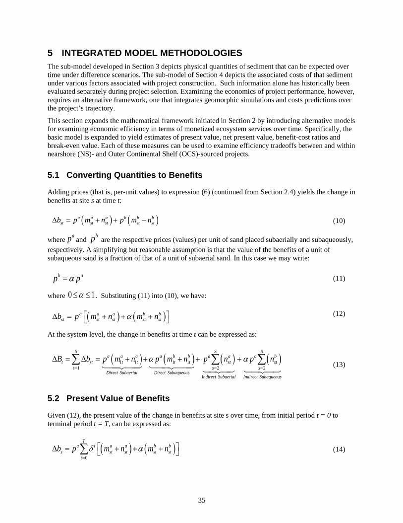
35
5 INTEGRATED MODEL METHODOLOGIES The sub-model developed in Section 3 depicts physical quantities of sediment that can be expected over time under difference scenarios. The sub-model of Section 4 depicts the associated costs of that sediment under various factors associated with project construction. Such information alone has historically been evaluated separately during project selection. Examining the economics of project performance, however, requires an alternative framework, one that integrates geomorphic simulations and costs predictions over the project’s trajectory.
This section expands the mathematical framework initiated in Section 2 by introducing alternative models for examining economic efficiency in terms of monetized ecosystem services over time. Specifically, the basic model is expanded to yield estimates of present value, net present value, benefit-cost ratios and break-even value. Each of these measures can be used to examine efficiency tradeoffs between and within nearshore (NS)- and Outer Continental Shelf (OCS)-sourced projects.
5.1 Converting Quantities to Benefits
Adding prices (that is, per-unit values) to expression (6) (continued from Section 2.4) yields the change in benefits at site s at time t:
( ) ( )a a a b b bst st st st stb p m n p m n∆ = + + + (10)
where ap and bp are the respective prices (values) per unit of sand placed subaerially and subaqueously, respectively. A simplifying but reasonable assumption is that the value of the benefits of a unit of subaqueous sand is a fraction of that of a unit of subaerial sand. In this case we may write:
b ap pα= (11)
where 0 1α≤ ≤ . Substituting (11) into (10), we have:
( ) ( )a a a b bst st st st stb p m n m nα ∆ = + + + (12)
At the system level, the change in benefits at time t can be expressed as:
( ) ( ) ( ) ( )1 1 1 11 2 2
S S Sa a a a b b a a a b
t st t t t t st sts s s
Direct Subaerial Direct SubaqueousIndirect Subaerial Indirect Subaqueous
B b p m n p m n p n p nα α= = =
∆ = ∆ = + + + + +∑ ∑ ∑
(13)
5.2 Present Value of Benefits
Given (12), the present value of the change in benefits at site s over time, from initial period t = 0 to terminal period t = T, can be expressed as:
( ) ( )0
Ta t a a b b
s st st st stt
b p m n m nδ α=
∆ = + + + ∑ (14)

36
where 11 r
δ =+
is the discount factor, and r is the discount rate. 10
At the system level, the present value of the change in benefits (PVB) over time, from initial period t = 0 to terminal period t = T, can be expressed as:
( ) ( )1 1 1 11 0 0 0
2 0 2 0
S T T Ta t a a a t b b
st t t t ts t t t
Direct Subaerial Direct Subaqueous
S T S Ta t a a t b
st sts t s t
Indirect Subaerial Indir
PVB b p m n p m n
p n p n
δ α δ
δ α δ
= = = =
= = = =
= ∆ = + + +
+ +
∑∑ ∑ ∑
∑∑ ∑∑
ect Subaqueous
(15)
If one is not interested in tracking changes in direct and indirect benefits separately, the above expression simplifies to:
( )1 11 0 1 0
S T S Ta t a a b b
st t st t sts t s t
PVB b p m n m nδ α= = = =
= ∆ = + + + ∑∑ ∑∑ (16)
again, recognizing that, at the system level, expression (4) holds, so that any change in sand quantities via natural transport is necessarily attributable to vagrant sand. Typical projects place sand in period 0t = only, such that in expressions (15) and (16), 1
ktm , ,k a b= , can be replaced with 10
km .
Based on geomorphic modeling barrier island area projections, the quantity of sand benefits could be converted to acreage basis. In this case, the present value of benefit can be expressed as
( )1 11 0
S Ta t a a b b
t st t sts t
PVB p ma na ma naδ α= =
= + + + ∑∑ (18)
where 1atma represents direct subaerial net acres with mechanical placement in the current period at the
project site. The expression of astna stands for indirect subaerial net acres via natural transport in the
current period from other sites within the system. And 1btma represents direct subaqueous net acres with
mechanical placement in the current period at the project site and bstna stands for indirect subaqueous net
acres via natural transport in the current period from other sites within the system.
10 If we wish to induce an added element of risk associated with future flows of benefits above and beyond those captured explicitly in the simulation model, we can inflate the discount rate, which, short of having specific info on risk, is, in effect, accounted for this way. This approach is used, for example, in the National Resource Damage Assessment (NRDA).

37
5.3 Present Value of Costs
As described in Figure 1, the associated project costs of engineering and design and operation and maintenance typically account for 10% and 5%, respectively, of total project costs. Although specific data for these two costs are unavailable, they can be derived algebraically as a function of construction costs
(CC), which accounts on average for 85% of a projects fully funded cost. In turn, construction costs are estimated from multiple-regression analysis of cost factors for OCS and NS projects (Section 4). The corresponding cost in period t for NS and OCS projects is given by the function:
( ) ( ) ( ) 1.18 ( )t t t t tFFC C ED C CC C OM C CC= + + = ∗ (19)
where FFC is the fully funded annual costs of a NS or OCS project in year t, inclusive of engineering and design (ED), construction costs (CC), and operation and maintenance (OM), Therefore, the present value of cost (PVC) function for NS and OCS projects can be expressed as:
0 01.18 ( )
T Tt t
t tt t
PVC FFC C CCδ δ= =
= ∗ = ∗ ∗∑ ∑ (20)
where t stands for the number of years of a project and range from 0 to 50. PVC is the total discounted
costs (in $) of a NS or OCS project during the project life. FFCt is the total annual costs of a NS or OCS
project in year t and δ is the discount factor.
5.4 Net Present Value Model
As stated in Section 1, the goal of this study is to provide a better understanding and quantification of the economic, ecologic, and geomorphic long-term benefits and costs of using OCS sediment compared to nearshore sediment for coastal restoration projects. The benefits and associated costs functions defined in Sections 3 and 4 can be integrated into a net present value (NPV) analysis for the two restoration methods over a given time period (50 years). The equation is given by:
( )0
1 11 0 1
( )
1.18 ( )
Tt
t tt
S T Ta t a a b b t
t st t st ts t t
NPV B C PVB PVC
p ma na ma na C CC
δ
δ α δ
=
= = =
= − = −
= + + + − ∗ ∗
∑
∑∑ ∑ (21)
where Bt is the sum of benefit in time t, Ct is the sum of cost in time t, δ is the discount factor and t is the year.
5.4.1 Benefit:Cost Ratio
The present value formulas for benefit and cost models in the net present valuation (Eq. 21) can be rewritten in as a benefit:cost ratio (BCR). This ratio allows for an alternative examination of project efficiency, with the underlying assumption that decision-makers should strive for projects in which benefits exceed costs, or BCR>1.0.

38
0
0
1.0
Tt
ttT
tt
t
BBCR
C
δ
δ
=
=
= >∑
∑ (22)
5.4.2 Ecosystem Service Valuation Challenges
The ecosystem services cited in association with barrier islands and shorelines typically include storm surge attenuation (disturbance regulation), habitat provision, and recreation. The integrated models depicted in equations 10–22 require an expression of those services in monetary terms. But the time and effort required for valuation of these benefits can be substantial. It is often infeasible to conduct targeted valuation studies in support of environmental policy analysis. Thus, under the PV, nre present value (NPV) and BCR approaches, ecosystem service values (ESV) must be specified from pre-existing studies. Within environmental economics, this extrapolation process is referred to as “benefit transfer”.
Richardson et al. (2015) provide an overview of the growing demand for monetized ESV estimates and the increasing use of benefit transfer within environmental policy. Guidelines are cited for facilitating more valid transfer of values between a study site and policy site, including: 1) the need for comparable scope, scale, and population; 2) recognizing differences in intermediate and final services; 3) and aggregation approaches to avoid double counting. The authors reference web-based databases that have emerged as a repository for monetized ESV estimates. Though these sites are increasingly used for benefit-cost analysis, the values they contain often vary by orders of magnitude for a given service. For example, the Gulf of Mexico Ecosystem Valuation Database cites ESV estimates ranging from $2.40–$13,360 per acre/year (US $2012 dollars) as the value of disturbance regulation from barrier islands and shorelines. Likewise, studies of the habitat provision of coastal wetlands are cited with estimates ranging from $1.77 to $7,854/acre/year (GecoServ 2019). Such large value ranges reflect the variety and complexity of non-market valuation methodology, which serves to compound the challenges of benefits transfer.
5.4.3 Break-Even Approach
Caffey et al. (2014) describe an alternative approach in which a break-even value for ecosystem services (EBEV) can be derived by setting the BCR ratio equal to 1.0 and solving for the average annual value that equates project benefits to costs over a given time period.
0
0
1.0
Tt
ttT
tt
t
BBCR
C
δ
δ
=
=
= =∑
∑ (23)
Substituting the present value of project costs and surface benefits into equation 23 yields:
0
11 0
1.18 ( )T
tt
ta S T
a t a at st
s t
C CCEBEV
p ma na
δ
δ
=
= =
∗ ∗=
+
∑
∑∑ (24)

39
where EBEVa is the annual break-even ecosystem service value for subaerial land. This condensed approach reflects the historic programmatic focus on surface-level project performance. Alternatively, if we want to examine performance of all mechanically placed material (both subaerial and subaqueous land), we can write:
( )0
1 11 0
1.18 ( )T
tt
tab S T
a t a a b bt st t st
s t
C CCEBEV
p ma na ma na
δ
δ
=
= =
∗ ∗=
+ + +
∑
∑∑ (25)
where EBEVab is the annual break-even ecosystem service value for subaerial and subaqueous land. Though equation 25 assumes no difference in the value of land above and below the surface, it yields a comparative metric for depicting project efficiency along a broader contour. With additional economic valuations (or sensitivity analysis) future iterations of the model could be parametrized to delineate separate values for subaqueous land (see equation 11-13).
Equations 24 and 25 allow for the estimation of project efficiency at two contours: direct effects (subaerial land above 0.0 m) and total effects (subaerial and subaqueous above -0.5m). This simple, yet effective method avoids the potential pitfalls of benefits transfer. Rather than specifying values from a suite of external studies, a project-specific EBEV is derived as a function of physical benefits and project costs over given time period.The estimate is based on a BCR of 1.0; it constitutes a useful efficiency metric–i.e., the minimum dollar value of ecosystem service benefits required to offset project costs. As an analytical metric, break-even value has long been used for examining economic efficiencies in the production of market-based goods and services. Its application in environmental policy can likewise yield valuable information on the relative efficiencies of a wide range of project alternatives (i.e., temporal, spatial, physical, technological, risk, etc.).

40
6 RESULTS
6.1 Model Scenarios and Semi-Empirical Results
In this section, the ecosystem break even value (EBEV) framework outlined in equations 24 and 25 is used to compare the economic performance of nearshore (NS)- and Outer Continental Shelf (OCS)-sourced projects in terms of monetized ecosystem services over a 50-year time span. Benefits are derived from net acreage calculations obtained from the geomorphic sub-model at the site and system level (future with project minus future without project). These benefits are combined with estimates from the project cost model as estimated for various sediment quantities, qualities, and transport distances. A range of EBEVs ($ per acre per year) is derived for each of the geomorphic simulations outlined in Section 3, including a baseline project scenario, two storm scenarios, and a larger sand class scenario. An “optional scenario” is added to better illustrate the economic benefits of sediment quality (sand diameter) under chronic and acute forcing. Table 9 contains a description of model assumptions for each of these scenarios in terms sediment quantity, quality, transport distance, and other factors related to project cost.
Table 9. Scenarios and Assumptions of the Ecosystem Break Even Value (EBEV) Model
Assumptions Baseline
Scenario Early Storm
Scenario Late Storm Scenario
Larger Sand Scenario
Targetq (million yd3) 14 14 14 14
Dredgeq Cut-To-Fill (ratio) NS OCS
1.2, 1.3, 1.5
1.05, 1.1, 1.2
1.2, 1.3, 1.5
1.05, 1.1, 1.2
1.2, 1.3, 1.5
1.05, 1.1, 1.2
1.2, 1.3, 1.5
1.05, 1.1, 1.2 Sand size (µm)
NS OCS
156 160
156 160
156 160
156 200
Boundaries: Direct & Indirect (Figure 3 areas)
Central, System (qst , Qt)
Central, System (qst , Qt))
Central, System (qst , Qt)
Central, System (qst , Qt)
Contours: Subaerial, subaqueous (m) 0.0, -0.5 0.0, -0.5 0.0, -0.5 0.0, -0.5
Sediment transport (miles) NS OCS
3–5 15–20
3–5 15–20
3–5
15–20
3–5
15–20
Project life (years) 50 50 50 50
Discount rate (%) 4 4 4 4
Payonfill (fill=1) 1 1 1 1
Dune elevation (feet) 6.4 6.4 6.4 6.4 Program (1-6) averaged averaged averaged averaged

41
6.1.1 Baseline Project Scenario The baseline scenario of section 3.3.1 is revisited below in Figure 11 to examine how small differences in sediment grain size (NS=156µm, OCS=160µm) interact with sediment quantity, distance and other variables to influence economic performance. The order of EBEV curves is similar in all four panels (a, b, c, d), indicating that increases in distance tend to increase cost, and increases in depth (contour) typically serve to decrease unit costs. The effects of changes in boundary level (central to system) are less notable, given that EBEV are calculated on a net-acre basis, and the underlying system is deteriorating. Therefore, the brunt of net change at for all boundaries is levels is primarily driven by the project. At common distances, NS-sourced projects with medium to high cut-tp-fill (CTF) ratios (1.3–1.5) are less efficient than OCS projects. Inset values are provided; however, to facilitate BEV comparisons at more relevant ranges of sediment transport. At a 3–5 mile range, NS projects with a CTF of 1.2–1.3 are more cost-effective than OCS projects with 10–15 miles transport and CTF of 1.1–1.2 (panel a). However, OCS projects with the highest quality borrow sites (CTF=1.05) yield a BEV range of $6,959-$6,982 at 15–10 miles, which is more efficient than the $7,527–$7,843 range at 3–5 miles from NS projects using the lowest quality borrow sites (CTF=1.50).
Figure 11. Ecosystem break-even values (EBEV) for NS- and OCS-soured projects at various boundaries, distances and cut-to-fill ratios (baseline scenario).

42
6.1.2 Early Storm Scenario
The disturbance regulation function of barrier islands is a primary focus of restoration mangers. Under typical meteorological conditions, these landforms serve as a buffer to chronic physical forcing (waves, tides, salinity), which helps in the protection of leeward shorelines and wetlands. Under more acute conditions, their role often described as “sacrificial”.
The panels of Figure 12 depict the economic aspects of simulations described in section 3.3.2. Recall that under the “early storm scenario”, the project site is assumed to take a direct hit from a Category 2 hurricane at y5. This impact reduces the amount of remnant subaerial land at y50 by 60% for the NS-sourced project, and 54% for the OCS-sourced project. As a result, the EBEV curves for subaerial land at the project site (panel a) increase by a range of $3000 to $4000 compared to the baseline scenario. As expected, efficiency losses are less pronounced at broader and deeper boundaries given the amount of sand remaining beneath the surface. As a result, the subaqueous contour of the barrier system (panel d) depicts a smaller efficiency loss, an increase of only $2700–$3000 in EBEV in panels b and d.
Figure 12. Ecosystem break-even values (EBEV) for NS- and OCS-sourced projects at various boundaries, distances and cut-to-fill ratios (early storm scenario, year 5).
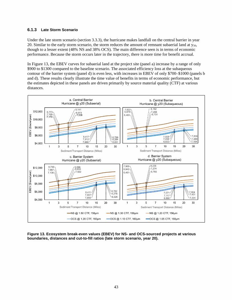
43
6.1.3 Late Storm Scenario
Under the late storm scenario (section 3.3.3), the hurricane makes landfall on the central barrier in year 20. Similar to the early storm scenario, the storm reduces the amount of remnant subaerial land at y50, though to a lesser extent (48% NS and 38% OCS). The main difference seen is in terms of economic performance. Because the storm occurs later in the trajectory, there is more time for benefit accrual. In Figure 13, the EBEV curves for subaerial land at the project site (panel a) increase by a range of only $900 to $1300 compared to the baseline scenario. The associated efficiency loss at the subaqueous contour of the barrier system (panel d) is even less, with increases in EBEV of only $700–$1000 (panels b and d). These results clearly illustrate the time value of benefits in terms of economic performance, but the estimates depicted in these panels are driven primarily by source material quality (CTF) at various distances.
Figure 13. Ecosystem break-even values (EBEV) for NS- and OCS-sourced projects at various boundaries, distances and cut-to-fill ratios (late storm scenario, year 20).
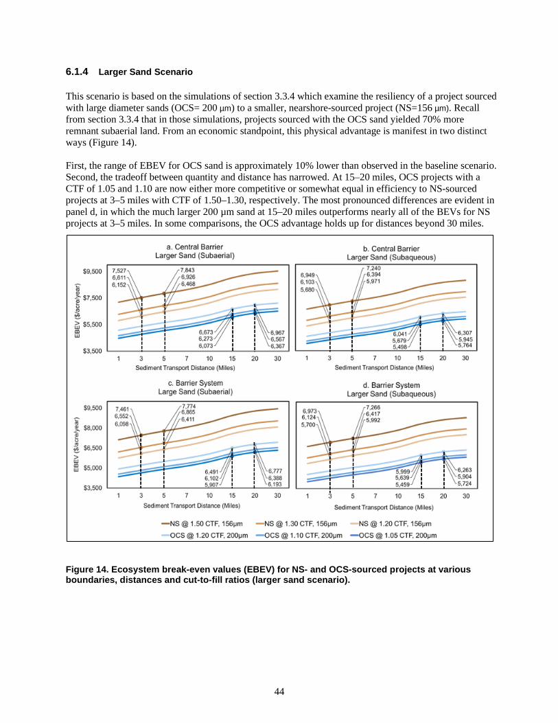
44
6.1.4 Larger Sand Scenario
This scenario is based on the simulations of section 3.3.4 which examine the resiliency of a project sourced with large diameter sands (OCS= 200 µm) to a smaller, nearshore-sourced project (NS=156 µm). Recall from section 3.3.4 that in those simulations, projects sourced with the OCS sand yielded 70% more remnant subaerial land. From an economic standpoint, this physical advantage is manifest in two distinct ways (Figure 14). First, the range of EBEV for OCS sand is approximately 10% lower than observed in the baseline scenario. Second, the tradeoff between quantity and distance has narrowed. At 15–20 miles, OCS projects with a CTF of 1.05 and 1.10 are now either more competitive or somewhat equal in efficiency to NS-sourced projects at 3–5 miles with CTF of 1.50–1.30, respectively. The most pronounced differences are evident in panel d, in which the much larger 200 µm sand at 15–20 miles outperforms nearly all of the BEVs for NS projects at 3–5 miles. In some comparisons, the OCS advantage holds up for distances beyond 30 miles.
Figure 14. Ecosystem break-even values (EBEV) for NS- and OCS-sourced projects at various boundaries, distances and cut-to-fill ratios (larger sand scenario).

45
7 SUMMARY AND CONCLUSIONS
7.1 Recap of Context and Approach
Forty percent of the US population resides in a contiguous band of counties at increasing risk from coastal land loss and storms. This threat is especially prominent in the Mississippi River delta plain (MRDP), where nearly 2,000 square miles of coastal land has been lost in the past century alone, primarily due to hydrologic modification, navigation canals, sediment starvation, subsidence, sea level rise, and climatic and geologic forcing. The outer boundary of this plain is bordered by a thin network of remnant delta lobes, the region’s barrier shorelines and islands.
In the past 30 years, more than $1 billion has been spent on projects designed to sustain this barrier system. Accordingly, the availability and suitability of sediment for renourishment projects has emerged as a major focus of restoration managers. Sediment for these projects has historically come from one of two primary sources. Nearshore (NS) sediment offers the economic advantage of proximity, but at the performance cost of smaller diameter sands with more organic fines. Outer Continental Shelf (OCS) sediments offers better performing, larger diameter sands with lower fines, but at higher transport costs due to distance. Previous economic comparisons of these sources have been piecemeal, focusing primarily on terminal quantities of sediment over a limited range of cost factors.
The goal of this project was to develop a more comprehensive framework for the assessment of NS and OCS sediment performance over time. A sub-model of project benefits was developed for a proxy barrier template based on the Isle Dernieres island chain. This geomorphic model simulates sediment transport within NS- and OCS-sourced projects under various scenarios of sediment quantity, quality, and meteorological forcing. A parallel sub-model of project cost was developed using bid and project data (n=93) for 22 barrier renourishment projects constructed in the Louisiana Coastal Zone. This statistical model estimates project costs, primarily as a function of sediment transport distance, sediment quantity, and authorizing program.
Options for integration of the geomorphic and cost sub-models are described mathematically for a variety of economic frameworks, each of which rely on the monetization of ecosystem service values (ESV). Because of the challenges associated with the valid transfer of values between a study site and policy site, ESVs in this study are not specified, but rather derived within a break-even value (BEV) framework. A series of five case scenarios is developed from which BEV curves are estimated at the site and system level, at subaerial and subaqueous contours, and for various combinations of sediment quality, quantity, and transport distance.
7.2 Primary Findings
Geomorphic simulations of sand transport within the proxy barrier template were developed to examine the performance of a 14 million yd3 renourishment project using NS sand of 156 µm and OCS sand of 160 µm. Under baseline conditions, the trajectory of subaerial land for the central barrier (project site) indicates a small advantage in resilience (increased volume and area) for the OCS sand. This divergence appears evident at year 10 and slowly expands through year 50. The advantage is less evident when measured at the system level and at subaqueous contours, primarily because of a dilution effects and the net export of vagrant sand from the proxy system over time. In terms of final subaerial land, the central barrier at y50 ends with a net quantity of 489 acres for the OCS-sourced project, compared to 325 net acres for the nearshore-sourced project. These remnant areas are reduced by 60% and 54%, respectively, under an early storm scenario (y5); and by 48% and 38% under a late storm scenario (y20). Performance advantages are clearly evident for larger OCS sands,

46
ranging from marginal improvements at 165 µm to substantial improvements at 200 µm. Projects sourced with 200 µm sand depict the largest divergence from the baseline, with 825 net acres of remnant subaerial land remaining in y50 on the central barrier, a near 70% increase over the performance compared to 160 µm sand. In all simulations, the project trajectories successfully maintain subaerial land, compared to the no action (control) in which the year of disappearance (YOD) ranged from 30 to 40 years.
Cost modelling for the baseline project yielded estimates ranging from $115 to $148 million for the target placement of 14 million y3 of material in y0. This cost range reflects a combination of two types of sediment quality (NS at 156 µm and OCS at 160 µm), 6 CTF ratios (1.05, 1.1, 1.2, 1.3, 1.4, and 1.5), and two transport distance ranges (3-5 miles for NS-sourced projects and 15-20 miles for OCS sourced projects). At 3–5 miles of transport, NS-sourced projects with a CTF of 1.2–1.5 of were 15–30% less expensive than the OCS projects with a CTF of 1.05–1.2 and distances of 15–20 miles. On a per unit basis, these costs equate to sediment placement costs of $8.20–$10.60/yd3.
Though placement costs is a metric that often dominates project selection, it reflects the value of sand as a commodity, and fails to fully account for the services generated throughout a project’s lifetime. An examination of project performance yields different results. Integration of benefit and cost sub models within a EBEV framework indicate that, despite having higher construction costs, the OCS-sourced projects actually out-perform NS-sourced projects in a number of cases, some of which involve large transport distances. Holding transport distance constant (3–5 miles for NS and 15–20 miles for OCS) allows for an assessment of the sediment quantity changes resulting from different CTF ratios. Under the baseline scenario, NS projects with a CTF of 1.2–1.3 were more cost-effective than OCS projects with a CTF of 1.1–1.2. However, OCS projects with the highest quality borrow sites (CTF=1.05) yielded a BEV range of $6,959–$6,982 at 15–10 miles, which is more efficient than the $7,527–$7,843 range at 3–5 miles from NS projects using the lowest quality borrow sites (CTF=1.50). Break-even values increased for all boundaries and contours under storm-punctuated. This reduction in efficiency is due to the net export of sand, and was found to be 20% greater for earlier (Y5) compared to later occurring storms (Y20). In short, the earlier a storm occurs in the trajectory, the less time there is for benefit accrual and the manifestation of any performance advantages due to sand quality (grain size). As expected, storm-induced efficiency losses were less noticeable beneath the surface, with subaqueous BEVs averaging 10% less than subaerial BEVs, compared to 5% lower in the baseline scenario. This outcome reflects an important finding from the geomorphic model: a substantial amount of remnant, subaqueous sand remains at subsurface contours after a storm. In each case (early and late storm), the OCS-sourced projects continued to outperform the NS-source projects in terms of physical resilience. This result appears to confirm manager assertions that OCS-sourced projects perform better under both chronic forcing and acute conditions. Isolating the effects of small differences in sediment quality (grain zize) on project performance requires holding sediment quantity constant. With both NS- and OCS-sourced projects modeled at a common CTF of 1.20, any economic effects of a 4 µm (2.5% larger) advantage from OCS sand are offset by the shorter transport distance (lower costs) for NS-sourced projects. This NS advantage narrows; however, under storm-punctuated scenarios, given the increased resilience of larger diameter sand. The economic implications of larger sands are more pronounced. The increased resilience of 200 µm sand (28% larger) results in two distinct advantages: 1) EBEVs that are 10% lower than OCS-sourced projects at 160 µm; and, 2) a substantial narrowing of the tradeoff between source material quality (CTF) and distance, with superior efficiency for all OCS projects at a moderate CTF of 1.10, and in some cases at a CTF of 1.20. The simulated performance of projects with OCS-sourced sand (200 µm, 15–20 miles) outperform nearly all of the NS projects at 3–5 miles. In some of the comparisons, this OCS efficiency advantage holds for distances exceeding 30 miles.

47
7.3 Limitations and Additional Research
Most of this analysis examines the physical and economic performance of a relatively small difference (4 µm) in sand diameter. It is important to note, however, that considerable time is required for quality differences to manifest at this range. Fifty-year trajectories are at the outer limit of coastal restoration planning, and many programs set the useful life of projects at 20 years. And while clear advantages are evident for OCS sands on the larger end of the D50 spectrum (200 µm), less is known about the performance of projects sourced with intermediate-sized sands (170–180 µm range). As a result, the current analysis constitutes a lower and upper bound of the economics of sand performance. Additional simulations would be required to for examining project performance over a wider range of sand classes and for alternative project periods.
Data for development of the cost model were limited and highly variable. The use of contractor bids expanded a dataset of 22 candidate projects into 93 useable observations. Though some might question the potential redundancies introduced by this process, no viable alternatives exist for this analysis. State and federal restoration mangers face similar limitations in the budgeting and allocation of funds for large-scale ecosystem restoration projects. Management of large-scale restoration projects requires systematic analysis of available costs and benefits, despite these limitations.
As currently structured, this analysis does not attempt to assign different ESVs for land above and beneath the water’s surface. The mechanics for this delineation; however, are described within the mathematical framework of section 5. The derivation of EBEV at subaerial and subaqueous boundaries (as used in this analysis) is merely intended to capture any areal effects resulting from net-transport of sand into or out of the proxy barrier system. Moreover, no attempt was made to assign (or derive) ESVs based on functional differences associated with disturbance regulation (surge attenuation) or habitat. Additional analysis would be required to examine how project efficiency varies with more depth-specific and material-specific delineations of ecosystem services.
Readers may question how the range of EBEVs estimated in the four scenarios compare to published ESV estimates for disturbance regulation and beach habitat. The insets highlighted in Figures 11–14 feature EBEVs ranging from a low of $5,459 (OCS, 200 µm, 1.05 CTF, 15 miles) to a high of $12,004 (NS, 156 µm, 5 miles, storm at y5). Though this is wide range, it is well within the bounds of published estimates of ecosystem values for any one service, and even more so with service aggregation. It is important to reiterate; however, the difference between EBEV estimates and net present value (NPV) estimates developed via benefit transfer. As derived estimates, EBEVs do not indicate whether a project should be built, or not. Instead, they serve as metrics of relative efficiency between and within project alternatives.
Finally, the integrated framework developed in this study could be replicated for the examination of important challenges facing state and federal restoration programs. With a modest amount of updating11, the model could be used to address a number of pertinent questions, including: What are the economic trade-offs of more regular maintenance compared to a sacrificial approach to barrier island renourishment? How do large scale dedicated dredging projects compare (economically) to more frequent renourishment efforts via smaller dredges? and What feasibility thresholds for restoration might exist given YOD projections for specific coastal barriers?
11 The time required for recalibration of sub-models of benefits and costs would depend on the context of any subsequent analysis, data availability, and processing capacity needed for updating geomorphic simulations.

48
7.4 Policy Implications
Nationwide, billions of dollars are being allocated for barrier island, shoreline, and beach renourishment. Since 1995, the Bureau of Ocean Energy Management (BOEM) has conveyed access to 162 million yd3
of sand for 56 projects in eight states. These projects have restored 343 miles of US shoreline and protected billions of dollars of coastal infrastructure and habitat. However, the availability and suitability of coastal sediments for dedicated dredging is a growing concern. This concern is especially prominent in the Gulf of Mexico region and in Louisiana in particular, where an estimated 90 million yd3 will be required in the next 50 years to address the state’s coastal land loss crisis. This demand is reflected in Louisiana’s 2017 Coastal Master Plan, which calls for more than $22 billion in expenditures for dedicated dredging projects during this same time period.
Sediment resource maps estimate the total volume of Louisiana-adjacent offshore surficial sand at nearly two billion cubic meters, with 60% of this material considered recoverable under current technological and regulatory constraints. Until recently, access to these OCS deposits was considered economically infeasible in comparison to lower quality, proximal sources. Traditional approaches to project evaluation have centered on the value of sediment as a commodity, with a focus on placement cost. The geomorphic and economic findings of this study, however, indicate that grain-size matters, and that a more comprehensive accounting of project performance beyond the fill template is required to maximize the return on coastal restoration spending
This study has provided a decision support tool for managers seeking more in-depth information on the economic trade-offs of various alternatives for dediciated dredging. The extent to which the framework is used will depend ultimately on its utility, which, in turn, hinges on the availability (and validity) of performance data from existing projects. Long-term monitoring of project performance, however, has historically received less than 5% of restoration budgeting. Project monitoring must be prioritized to ensure for adaptive management and improved efficiency of restoration programs in Louisiana, the Gulf of Mexico region and the coastlines of the US.

49
8 REFERENCES
Barbier EB, Hacker SD, Kennedy C, Koch EW, Stier BR, et al. 2011. The value of estuarine and coastal ecosystem services. Ecol Monogr. 81: 169–193.
Biven, M. 2014. A preliminary legal and cost analysis of rapid land-building technologies. [40 slides.] Presented at: State of the Coast Conference, March 18-20; 2014 New Orleans, LA.
Caffey RH, Wang H, Petrolia D. 2014. Trajectory economics: assessing the flow of ecosystem services from coastal restoration. Ecolog Econ. 100: 74-84.
Coastal Protection and Restoration Authority of Louisiana [CPRA]. 2017. Louisiana’s comprehensive master plan for a sustainable coast. Baton Rouge (LA): Coastal Protection and Restoration Authority. 93 p.
Dean RG. 1974. Compatibility of borrow material for beach fills. In: Proceedings of the Fourteenth International Conference on Coastal Engineering. Volume 1. Copenhagen, Denmark; June 24–28, 1974. New York (NY): American Society of Civil Engineers. p 1319–1330.
Feagin RA, Smith WK, Psuty NP, Young DR,Martinez ML, et al. 2010. Barrier islands: coupling anthropogenic stability with ecological sustainability. J Coast Res. 26(6): 987-992.
[GecoServ]. 2019. Gulf of Mexico Ecosystem services valuation database.Version 2.0. Corpus Christi (TX): Texas A&M University-Corpus Christi, Harte Research Institute for Gulf of Mexico Studies.
Georgiou IY, Weather HD, Kulp MK, Miner MD, Reed DJ (University of New Orleans, Pontchartrain Institute for Environmental Sciences, New Orleans, LA). 2011. Interpretation of regional sediment management pathways using subsurface geologic data, final report. New Orleans (LA): US army Corps of Engineers. Contract W912HX-09-2-0027. DOI 10.13140/RG.2.2.15432.47361. 33 p.
James WR, 1975. Techniques in evaluating suitability of borrow material for beach nourishment. Technical manual no. 60. Fort Belvoir (VA): US Army Corps of Engineering. 80 p.
Khalil SM, Finkl CW. 2009. Regional sediment management strategies for coastal restoration in Louisiana, USA. J Coast Res. 56: 1320-1324.
Khalil SM, Finkl CW, Roberts HH, Raynie RC. 2010. New approaches to sediment management on the inner continental shelf offshore coastal Louisiana. J Coast Res. 26: 591-604.
Merchant Marine Act of 1920, Jones Act: 46 USC § 50101.
Michel J, Bejarano AC, Peterson CH, Voss C (Research Planning, Inc.). 2013. Review of biological and biophysical impacts from dredging and handling of offshore sand. Herndon (VA): Bureau of Ocean Energy Management. 261 p. Contract No.: M11PD00219. Report No.: OCS Study BOEM 2013-0119.
Miner(a) MD, Kulp MA, FitzGerald DM, Flocks JG, Weathers HD. 2009. Delta lobe degradation and hurricane impacts governing large-scale coastal behavior, South-central Louisiana, USA. Geo-Mar Lett. 29(6): 441-453.

50
Miner (b) MD, Kulp MA, FitzGerald DM, Georgiou IY. 2009. Hurricane-associated ebb-tidal delta sediment dynamics: Geology. 37(9):851-854, doi: 10.1130/G25466A.1.
Miner (c) MD, Kulp M, Flocks J, Twichell D, Martinez L, et al (University of New Orleans Pontchartrain Institute for Environmental Sceinces, New Orleans LA; US Geological Survey, St. Peterbserg, FL; US Geological Survey, Woods Hole, MA). 2009. Louisiana Barrier Island comprehensive monitoring program, part 3: South-Central Louisiana and Northern Chandeleur Islands, bathymetry and historical seafloor change 1873–2006, part 2: bathymetry maps. Baton Rouge (LA): Louisiana Department of Natural Resources and US Army Corps of Engineers. 16 p. LDNR Interagency Agreement 2512-06-06.
Morton RA, Miller TL, Moore LJ. 2004. National assessment of shoreline change: part 1: historical shoreline changes and associated coastal land loss along the US Gulf of Mexico. St. Petersburg (FL): US Geological Survey, Center for Coastal and Watershed Studies. 44 p. Open File Report 2004-1043. https://pubs.usgs.gov/of/2004/1043/ofr-2004-1043.pdf .
Nairn RB, Langendyk SK, Michel J (Baird & Associate, Madison, Wisconsin, and Research Planning, Inc, Columbia, SC). 2004. Preliminary infrastructure stability study, offshore Louisiana. New Orleans (LA): US Department of the Interior, Minerals Management Service. 35 p. Contract No.: 35-0001-31051. Report No.: OCS Study MMS 2005-043.
National Hurricane Center (2020) Saffir-Simpson Hurricane Wind Scale. [accessed 2020 Feb 17]. https://www.nhc.noaa.gov/aboutsshws.php
National Oceanic and Atmospheric Administration and US Census Bureau. 2013. NOAA’s national coastal population report: population trends from 1970 to 2020. Washington (DC): National Oceanic and Atmospheric Administration, National Ocean Service. 22 p.
Richardson L, Loomis J, Kroeger T, Casey F. 2015. The role of benefit transfer in ecosystem service valuation. Ecol Econ. 115: 51-58.
Smith VK. 2018. Benefits transfer: current practice and prospects. Environ Res Econ. 69: 449–466.
van Rijn LC. 1984a. Sediment transport, part I: bed load transport. J Hydraul Eng. 110:1431-1456.
van Rijn LC. 1984b. Sediment transport, part II: suspended load transport. J Hydraul Eng. 110: 1631-1641.
Wang H. 2011. An economic assessment of competing technologies for coastal restoration [thesis]. Baton Rouge (LA): Louisiana State University.
Wang H, Caffey RH, Petrolia D.R. 2012. An economic assessment of competing technologies for coastal restoration. Southern Agricultural Economics Association (SAEA) 2012 Annual Meeting; February 4-7, 2012; Birmingham, Alabama. https://ageconsearch.umn.edu/record/119740
Woodward RT, Wui YS. 2001. The economic value of wetland services: a meta-analysis. Ecol Econ. 37:257–70.
Petrolia D, Kim T.G. 2009. What are barrier islands worth? Estimates of willingness to pay for restoration. Mar Res Econ. 24(2): 131-146.

51
Appendix A: Project Bid Data Table A1. Commercial Bid Data for NS-sources Dedicated-dredging Projects on Barrier Shorelines
and Island in Louisiana 1997–2018 (n=36)
Project ID Project Name Bid TBC ($) MM CYD BA-30 East Grand Terre Island Restoration 1 32,942,178 3.34 BA-30 East Grand Terre Island Restoration 2 35,787,671 3.34 BA-30 East Grand Terre Island Restoration 3 41,856,610 3.34 BA-35 Pass Chaland to Grand Bayou Pass Barrier Shoreline Restoration 1 49,004,367 5.21 BA-35 Pass Chaland to Grand Bayou Pass Barrier Shoreline Restoration 2 39,363,841 5.21 BA-38-2 Chaland headland Restoration 1 20,758,927 2.74 BA-38-2 Chaland headland Restoration 2 37,104,973 2.74 BA-76 Cheniere Ronquille Barrier Island Restoration 1 30,731,186 2.63 BA-76 Cheniere Ronquille Barrier Island Restoration 2 34,632,114 2.63 BA-76 Cheniere Ronquille Barrier Island Restoration 3 27,480,973 2.63 TE-20 Isles Dernieres Restoration East Island 1 11,847,227 3.60 TE-20 Isles Dernieres Restoration East Island 2 12,880,745 3.60 TE-20 Isles Dernieres Restoration East Island 3 12,173,192 3.60 TE-20 Isles Dernieres Restoration East Island 4 16,560,793 3.60 TE-20 Isles Dernieres Restoration East Island 5 13,670,979 3.60 TE-20 Isles Dernieres Restoration East Island 6 15,384,221 3.60 TE-20 Isles Dernieres Restoration East Island 7 16,152,462 3.60 TE-20 Isles Dernieres Restoration East Island 8 16,152,462 3.60 TE-24 Isles Dernieres Restoration Trinity Island 1 16,809,376 4.89 TE-24 Isles Dernieres Restoration Trinity Island 2 20,129,728 4.89 TE-24 Isles Dernieres Restoration Trinity Island 3 16,484,144 4.89 TE-24 Isles Dernieres Restoration Trinity Island 4 18,835,680 4.89 TE-24 Isles Dernieres Restoration Trinity Island 5 19,329,011 4.89 TE-27 Whiskey Island Restoration 1 15,271,243 3.70 TE-27 Whiskey Island Restoration 2 17,974,673 3.70 TE-27 Whiskey Island Restoration 3 19,050,007 3.70 TE-27 Whiskey Island Restoration 4 21,164,123 3.70 TE-37 New Cut Dune and Marsh Restoration 1 12,228,870 0.83 TE-37 New Cut Dune and Marsh Restoration 2 16,249,265 0.83 TE-40 Timbalier Island Dune and Marsh Creation 1 15,351,093 3.60 TE-40 Timbalier Island Dune and Marsh Creation 2 16,985,098 3.60 TE-40 Timbalier Island Dune and Marsh Creation 3 21,222,319 3.60 TE-50 Whiskey Island Back Barrier Marsh Creation 1 26,176,788 2.53 TE-50 Whiskey Island Back Barrier Marsh Creation 2 30,565,090 2.53 TE-52 West Belle Pass Barrier Headland Restoration 1 30,654,289 4.80 TE-52 West Belle Pass Barrier Headland Restoration 2 41,625,982 4.80

Table A2. Commercial Bid Data for OCS Sources Dedicated-dredging Projects on Barrier Shorelines and Island in Louisiana 1997–2018 (n=35)
Project ID Project Name Bid Bid Amount ($) MM cyds BA-38-1 Pelican Island Restoration 1 46,309,424 3.75 BA-38-1 Pelican Island Restoration 2 48,812,567 3.75 BA-40 Riverine Sand Mining/Scofield Island Restoration 1 48,792,190 3.39 BA-40 Riverine Sand Mining/Scofield Island Restoration 2 86,338,395 3.39 BA-45 Caminada Headland Beach and Dune Restoration 1 58,337,338 2.88 BA-45 Caminada Headland Beach and Dune Restoration 2 71,809,850 2.88 BA-45 Caminada Headland Beach and Dune Restoration 3 70,282,383 2.88 BA-45 Caminada Headland Beach and Dune Restoration 4 59,924,573 2.88 BA-110 Shell Island East BERM Restoration 1 34,400,181 1.70 BA-110 Shell Island East BERM Restoration 2 35,112,173 1.70 BA-111 Shell Island West NRDA Restoration 1 58,011,365 4.50 BA-111 Shell Island West NRDA Restoration 2 65,365,519 5.20 BA-111 Shell Island West NRDA Restoration 3 66,236,430 5.28 BA-111 Shell Island West NRDA Restoration 4 61,766,918 5.05 BA-111 Shell Island West NRDA Restoration 5 59,036,659 4.50 BA-111 Shell Island West NRDA Restoration 6 67,360,151 5.20 BA-111 Shell Island West NRDA Restoration 7 68,102,500 5.28 BA-111 Shell Island West NRDA Restoration 8 62,105,540 5.05 BA-143 Caminada Headland Beach and Dune Restoration INCR2 1 147,261,118 5.40 BA-143 Caminada Headland Beach and Dune Restoration INCR2 2 150,253,154 5.40 BA-143 Caminada Headland Beach and Dune Restoration INCR2 3 155,410,084 5.40 BA-143 Caminada Headland Beach and Dune Restoration INCR2 4 116,858,691 5.40 CS-31 Holly Beach Sand Management 1 24,563,544 2.27 CS-31 Holly Beach Sand Management 2 19,529,382 2.27 CS-33 Cameron Parish Shoreline Restoration 1 50,212,174 2.33 CS-33 Cameron Parish Shoreline Restoration 2 51,358,425 2.33 TE-25&30 East Timbalier Island Sediment Restoration 1 14,830,264 2.27 TE-25&30 East Timbalier Island Sediment Restoration 2 17,455,629 2.27 TE-25&30 East Timbalier Island Sediment Restoration 3 18,499,911 2.27 TE-25&30 East Timbalier Island Sediment Restoration 4 20,552,979 2.27 TE-48-2 Raccoon Island Shoreline Protection and Marsh Creation 1 5,889,249 0.64 TE-48-2 Raccoon Island Shoreline Protection and Marsh Creation 2 7,688,697 0.64 TE-48-2 Raccoon Island Shoreline Protection and Marsh Creation 3 14,970,118 0.64 TE-100 Caillou Lake Headlands Restoration 1 104,102,226 10.45 TE-100 Caillou Lake Headlands Restoration 2 104,110,192 10.45

Department of the Interior (DOI)
The Department of the Interior protects and manages the Nation's natural resources and cultural heritage; provides scientific and other information about those resources; and honors the Nation’s trust responsibilities or special commitments to American Indians, Alaska Natives, and affiliated island communities.
Bureau of Ocean Energy Management (BOEM)
The mission of the Bureau of Ocean Energy Management is to manage development of US Outer Continental Shelf energy and mineral resources in an environmentally and economically responsible way.
BOEM Environmental Studies Program
The mission of the Environmental Studies Program is to provide the information needed to predict, assess, and manage impacts from offshore energy and marine mineral exploration, development, and production activities on human, marine, and coastal environments. The proposal, selection, research, review, collaboration, production, and dissemination of each of BOEM’s Environmental Studies follows the DOI Code of Scientific and Scholarly Conduct, in support of a culture of scientific and professional integrity, as set out in the DOI Departmental Manual (305 DM 3).