economic base analysis using panel data regression:...
TRANSCRIPT

1
ECONOMIC BASE ANALYSIS USING PANEL DATA REGRESSION: A CASE STUDY OF THE FLORIDA REGIONAL ECONOMY
By
FAN LI
A THESIS PRESENTED TO THE GRADUATE SCHOOL OF THE UNIVERSITY OF FLORIDA IN PARTIAL FULFILLMENT
OF THE REQUIREMENTS FOR THE DEGREE OF MASTER OF SCIENCE
UNIVERSITY OF FLORIDA
2010

2
© 2010 Fan Li

3
To my beloved husband, Wei

4
5BACKNOWLEDGMENTS
I would like to express my most sincere appreciation to Dr. Timothy Fik, Dr. Grant I.
Thrall and Dr. Youliang Qiu, members of my advisory committee, for their academic support
and guidance through the completion of this study. I would like to give my special gratitude to
my advisor Dr. Timothy Fik, who is always ready, available and patient to help with academic
problems and discussion. I am also grateful for the help and encouragement from other
committee members, including Dr. Grant Thrall and Dr. Youliang Qiu. They provide insight,
suggestions and valuable feedback to my thesis.
I am thankful to all members of the Geography Department, faculty, staff and students for
creating a friendly atmosphere that makes every day of study so enjoyable. As an international
student, all members make me feel as if I am living and working in my home country. I also
express my special thanks to Dr. Peter Waylen and Dr. Youliang Qiu for their support and help
to my computer lab job. My dear friend, Anna Maria Szynizewska, work with me together to
find the data source. Yang Yang helps me with regression programming.
I also want to thank Dr. Chunrong Ai from Department of Economics and Dr. Alfonso
Flores-Lagunes from Department of Food and Resources Economics. Their Econometric
courses enable me to apply the regression models used in my research.
There are no words that could describe my gratitude to my husband Wei. If it wasn’t him
to encourage me to apply for Geography Department, I wouldn’t pursue a graduate study at such
an excellent American university. After I began my study in University of Florida, it is his
immense love and unconditional supports that make me get accustomed to life and study abroad.
Mostly I would like to thanks to his help in my thesis writing. He teaches me how to correct
thesis format that saved me many months of work on this thesis.

5
Finally, I would like to express my special gratitude to my family in China – my loving
parents and friends – for all their encouragement and support; something that I feel is very
strong, even though I am thousands of miles away from my home.

6
TABLE OF CONTENTS Upage
ACKNOWLEDGMENTS.................................................................................................................... 4
LIST OF TABLES................................................................................................................................ 8
LIST OF FIGURES .............................................................................................................................. 9
ABSTRACT ........................................................................................................................................ 11
CHAPTER
1 INTRODUCTION....................................................................................................................... 13
Overview and Problem Statement .............................................................................................. 13 Background .................................................................................................................................. 14 Research Objectives .................................................................................................................... 15
2 LITERATURE REVIEW ........................................................................................................... 17
Economic Base Theory ............................................................................................................... 17 Two Versions of Economic Base Model ................................................................................... 21 The Average Multiplier of the Economic Base Model ............................................................. 22 The Marginal Multiplier of Economic Base Model .................................................................. 25 The Procedure of Estimating Multipliers of Economic Base Model ....................................... 27
Survey Method ..................................................................................................................... 27 The Location Quotient Approach ....................................................................................... 28 Minimum Requirements ...................................................................................................... 31 Regression-based Approaches ............................................................................................ 32
3 METHODOLOGY ...................................................................................................................... 35
The Location Quotient Method .................................................................................................. 35 Ordinary Least Squares (OLS) ................................................................................................... 36 Linear Unobserved Effects Panel Data Models ........................................................................ 38
4 EXPLORATORY ECONOMIC BASE REGRESSION MODEL .......................................... 42
Initial Data Collection ................................................................................................................. 42 Regression Analysis .................................................................................................................... 44 Choosing a Scalar ........................................................................................................................ 81 Results and Discussion ............................................................................................................... 84
5 CONCLUSIONS ....................................................................................................................... 102

7
LIST OF REFERENCES ................................................................................................................. 106
BIOGRAPHICAL SKETCH ........................................................................................................... 109

8
6BLIST OF TABLES
UTableU Upage 3-1 OLS assumptions and possible solution ............................................................................... 37
4-1 Scalars and non-basic employment in year 1993 and 1997 by county ............................... 82
4-2 Ordinary least regression estimation result of years 1993 ................................................... 85
4-3 Ordinary least regression estimation result of years 1993 ................................................... 85
4-4 Ordinary least regression estimation result of year 1993 and 1997 .................................... 87
4-5 Test result of exogeneity of error term ................................................................................. 87
4-6 Panel data regression estimation result of year 1993 and 1997 without dummy variable .................................................................................................................................... 88
4-7 Panel data regression estimation result of year 1993 and 1997 with dummy variable ...... 97
4-8 Multipliers of OLS regression and panel data regression .................................................. 101

9
7BLIST OF FIGURES
UFigureU Upage 4-1 Total employment of Florida in different years by county A) 1993 B)1997 ..................... 45
4-2 Non-basic employment for primary sector of Florida in different years by county A)1993 B)1997 ....................................................................................................................... 47
4-3 Non-basic employment for construction sector of Florida in different years by county A)1993 B)199 ............................................................................................................ 49
4-4 Non-basic employment for manufacturing sector of Florida in different years by county A)1993 B)1997 .......................................................................................................... 51
4-5 Non-basic employment for transportation and public utilities sector of Florida in different years by county A)1993 B)1997 ............................................................................ 53
4-6 Non-basic employment for wholesale trade sector of Florida in different years by county A)1993 B)1997 .......................................................................................................... 55
4-7 Non-basic employment for retail trade sector of Florida in different years by county A)1993 B)1997 ....................................................................................................................... 57
4-8 Non-basic employment for finance, insurance and real estate sector of Florida in different years by county A)1993 B)1997 ............................................................................ 59
4-9 Non-basic employment for services sector of Florida in different years by county A)1993 B)1997 ....................................................................................................................... 61
4-10 Basic employment for primary sector of Florida in different years by county A)1993 B)1997..................................................................................................................................... 63
4-11 Basic employment for construction sector of Florida in different years by county A)1993 B)1997 ....................................................................................................................... 65
4-12 Basic employment for manufacturing sector of Florida in different years by county A)1993 B)1997 ....................................................................................................................... 67
4-13 Basic employment for transportation and public utilites sector of florida in different years by county A)1993 B)1997 ........................................................................................... 69
4-14 Basic employment for wholesale trade sector of Florida in different years by county A)1993 B)1997 ....................................................................................................................... 71
4-15 Basic employment for retail sector trade of Florida in different years by county A)1993 B)1997 ....................................................................................................................... 73

10
4-16 Basic employment for finance, insurance and real estate sector of Florida in different year by county A)1993 B)1997 ............................................................................................. 75
4-17 Basic employment for services sector of Florida in different years by county A)1993 B)1997..................................................................................................................................... 77
4-18 Social security payment by county of Florida in different years by county A)1993 B)1997..................................................................................................................................... 79
4-19 Normality test for different regression A)Year 1993 OLS regression B)Year 1997 OLS regression C)Both year 1993 and 1997 OLS regression D) Both year 1993 and 1997 panel data regression..................................................................................................... 89
4-20 Residual plots for different regression A)Year 1993 OLS regression B)Year 1997 OLS regression C)Both year 1993 and 1997 OLS regression D) Both year 1993 and 1997 panel data regression..................................................................................................... 91
4-21 Plots of fitted versus actual non-basic employment values for different regression A)Year 1993 OLS regression B)Year 1997 OLS regression C)Both year 1993 and 1997 OLS regression D) Both year 1993 and 1997 panel data regression ......................... 94
4-22 Map of coastal urban counties ............................................................................................... 96
4-23 Plots of fitted versus actual non-basic employment values for both year 1993 and year 1997 panel data regression with dummy variable ........................................................ 98

11
Abstract of Thesis Presented to the Graduate School of the University of Florida in Partial Fulfillment of the
Requirements for the Degree of Master of Science
ECONOMIC BASE ANALYSIS USING PANEL DATA REGRESSION: A CASE STUDY OF THE FLORIDA REGIONAL ECONOMY
By
Fan Li
August 2010 Chair: Timothy Fik Major: Geography
The main purpose of this research is to investigate and estimate the increase in total regional
employment as it relates to employment increases in specific economic sectors, using economic
base theory and a regional economic base model. Past empirical research in economic base
modeling typical relies on single year data and original least square (OLS) regression, with
unstable results that are possibly explained by the fact that the regression analysis is influenced
by abnormal value changes in one or more explanatory variables. As an alternative, this thesis
utilizes panel data regression with data for multiple years in an economic base analysis of Florida
employment patterns. Sector-specific employment multipliers are estimated and compared using
OLS and the panel data regression. Of the other widely used methodologies: the survey method,
location quotient (LQ) method, and minimum requirements (MR), regression analysis is the only
one which can estimate impact multipliers.
Regression models to estimate employment multipliers are typically divided into
disaggregate and aggregate models. The former can obtain the multiplier estimates for specific
industries, while the latter one independently cannot distinguish between different industries.
Hence, disaggregate regression models are widely used in economic base research. Unable to
account for economic spillover effects, such as cash flows or trans-boundary monetary transfers,

12
disaggregate regression models tend to have upwardly biased multipliers. It is necessary,
therefore, to apply scaling factors and utilize independent variables that capture the influence of
monetary transfers to account for such factors as unemployment and retirement benefits and
other state income sources in an effort to decrease bias in the modeling process. Transfer
payments, dividends, interest and rents, and social security benefits are considered in this
analysis, and prove to be effective in reducing the upward bias of multiplier estimates.
This research also examines the assumptions of original least square and alternatives, to test
for the potential violation of assumptions. In order to obtain reasonable and stable estimates of
multiplier related coefficients and avoid potential problems associated with endogenous error
terms, panel data regression is preferred to original least squares regression when data for more
than one sample time period is available.
The estimation results suggest that employment increases in wholesale trade can create most
total employment benefits in Florida’s regional economy, while job increases in the
transportation and public utility sector leads to relatively small job returns to Florida’s overall
regional economy. Comparison of results between ordinary least square regression based on a
single year sample and panel data regression using a two-year sample suggest that the latter can
avoid the impact of sudden and discontinue change in a regional economic trend. In short, the
panel regression approach is deemed as preferable over ordinary least square regression in the
estimation of employment multipliers.

13
0BCHAPTER 1 8BINTRODUCTION
15BOverview and Problem Statement
Employment patterns by industry or economic sector for sub-regions of a regional
economy are important indicators of regional economic growth and development. For example,
county employment patterns and industry mix are useful in assessing the degree to which a
county is reliant on specific industries when compared to an employment mix at the state or
national levels. The more employment in a given sector, relatively speaking, the more important
that sector is to the economic vitality of a regional economy. Furthermore, it is known that
overall employment levels may be a by product of supporting or linked industries that are known
to generate spin-off employment.
County-level economies typically have very different industry employment patterns than a
state-level economy. These patterns can offer insights as to the importance of various industries
or sectors to a county’s overall total employment and the extent to which key sectors have an
impact on regional economic development and the expansion of a region’s overall employment
base. Key sectors are generally referred to as the “economic base” of a regional economy. They
are the sectors that are most responsible for generating the majority of linked or spin-off
employment. The net benefits of a region’s economic base are generally distributed unevenly
over space, and it is useful to gather information from many sub-regions as to the overall
importance of various sectors to the regional economy at large.
Florida, nicknamed the "Sunshine State" because of its generally warm HclimateH, is ranked
as the fourth-most populous state in the U.S. according to the HUnited States Census Bureau H in
2008. Florida’s regional economy focuses on three leading industries; namely, tourism,
agriculture and mining. In the last fifty years, more and more retired people have moved and

14
relocated (permanently or seasonally) into the state. The influx of the elderly and retired brings a
large number of non-employment incomes to Florida in the form of transfer payments tied to
retirement accounts, social security, and interest, dividends and rents paid on investments. Non-
employment income in the form of transfer payments has had an enormous historical and
geographic impact on Florida’s regional economy. This impact sometimes clouds the nature of
how sector-specific industries affect total employment in any given sub-region. The nature of the
relationship between industrial employment and regional economic development in Florida is
investigated in this study, with acknowledgment that that transfer payments play a critical role in
influencing employment patterns. Hence, analysis of employment patterns and the identification
of a region’s economic base is understood as something that can be affected by transfer income.
Adjusting for transfer income, this study will focus on the estimation of economic base
multipliers – coefficients that embody the expansion effects of key sectors or industries that
contribute greatly to the state’s overall employment. More specifically, this study will seek to
compare several different methods and techniques for estimating multipliers and the inter-
relationships between the state’s economic sectors using county level data.
16BBackground
Warm weather and hundreds of miles of beaches attract about 60 million visitors to the
Sunshine State every year, so tourism replaces agriculture to makes up the largest economic
sector in the state economy. As such, much of Florida’s economy is tied to retail trade and
services. The second largest industry is HagricultureH. HCitrusH HfruitH, especially HorangesH, and various
winter vegetables play major roles in supporting the regional economy. Florida produces the
majority of citrus fruit grown in the U.S.; for example, in 2006, 67% of all citrus, 74% of
oranges, 58% of HtangerinesH, and 54% of HgrapefruitH came from growers in Florida. Hence,
employment activities in agricultural sectors are known to affect regional growth directly. The

15
extent to which a given industry affects a region’s total economy can vary dramatically
depending on that region’s industrial mix, and its overall impact on urban and regional
development is something that be estimated having knowledge of the inter-relationships or inter-
dependencies between industries and sectors. As a regional economy is highly dependent on
revenue from both industry mix and external sources, it is vital to understand the nature of the
influence of key economic sectors or industries as well as the effect of things like income
transfers. It is also important to determine the extent to which overall employment levels are
affected by key sectors or industries while accounting for the effects of income transfers.
17BResearch Objectives
The goal of this study is to identify the extent to which key sectors or industries affect
overall employment levels in the Florida economy, controlling for the effects of income transfers
and geographic variability in the inter-relationships between economic sectors. The analysis
takes into account both industrial employment patterns and underlying transfer payment impact
using county level data which links total employment to employment by sector. Total and
sector-specific employment data were chosen as they are widely used to measure the
development level of regional economy. A major task of this large interdisciplinary project is to
distinguish between import employment and export employment -- employment related to
income transfers versus that which is generated from a region’s economic base (also called an
export base), taking into account the transfer income factor (i.e., income generated from the
inflow of retirement dollars, investments, and other sources of personal revenue). The
importance of this factor can not be understated given the large proportion of elderly and retired
in Florida. Thus, it is recognized that the expansion of a region’s employment base is both tied
to industry mix and non-employment or transfer income. Transfer income is a crucial part of
state income, and cannot be ignored in the model. Failure to account for the transfer income

16
factor would ultimately result in biased and unreasonable estimates for economic base
multipliers and the degree to which specific industries or sectors contribute to the overall
employment base. Social security benefits are another non-employment revenue source. Social
security payments bring in money, stimulate demand for goods and services, and contribute to
overall employment growth. Therefore, a critical assessment of how key economic sectors
expand a regional economy must also address the importance of transfer incomes and social
security benefits.
In the estimation of economic base multipliers, which reveal the extent to which a sector
contributes to the expansion of the regional economy at large, several modeling and estimation
techniques will be compared with controls put in place to lessen bias and/or overstatement of the
impact. The research objectives of this thesis are two-fold: (1) to develop a regional economic
base model that incorporates the transfer income factor; and (2) using data for more than one
time period, demonstrate the effectiveness of panel data regression as a techniques that sidesteps
some of the limitations imposed by classic regression in the estimation of economic base
multipliers which describe the extent to which employment in key economic sectors contribute to
a region’s overall total employment (ceteris paribus).

17
1BCHAPTER 2 9BLITERATURE REVIEW
Economic base theory remains a respected field of study in geography and regional
economics. Economic base analysis offers an inexpensive yet reasonably accurate method to
assess small regional economic and employment impacts. The objective of economic base
analysis is to calculate regional multipliers that describe the extent to which employment or
income will grow as a function of new jobs added to a regional economy. The following section
provides a brief literature review of economic base theory, including related assumptions,
applicability and scale, and data requirements. Aggregate and disaggregate models are
discussed, as well as the derivation of multiplies; focusing on sector-specific application and
distinguishing between average multipliers and impact multipliers. The overview will highlight
the four most-commonly used methods of estimating economic base multipliers; namely, the
survey method, the location-quotient (LQ) method, minimum requirement (MR) method, and
regression-based approaches. It is noted that regression-based models tend to produce impact
multipliers, while the other methods are used to estimate average multipliers.
18BEconomic Base Theory
The history of the economics base concept dates back to the early 1900s. Early regional
economic analysts observed the duality of urban and regional economic activity, which includes
city-forming activities (characterized as the basic sector) and city-serving activities
(characterized as the non-basic sector) (Hewings 1985). The city-forming activities were said to
provide the reasons for the city’s existence; typically associated with export-oriented industries
that provided goods and services for markets both inside and outside the region. As these
industries satisfied demand outside the region, they were responsible for generating income from
sales related to exports. As such, these industries were viewed as responding to exogenous

18
demand and were labeled as basic to the survival of the region, with dollars generated from
export activities. By contrast, there were industries that were region serving in the sense that
they were associated with the sale of goods and services from one company in the region to
others inside the region. Hence, city-forming activities serviced the demand that was internal to
the region (demand generated by the local population), with money that was circulated and re-
circulated within the regions. To sum, basic or export-oriented activities were regarded as the
city forming and a direct result of external demand, while city-serving activities were there to
meet a region’s internal demand for non-exportable goods and services. The latter set of
activities and associated employment were in place for the maintenance and well-being of the
people inside the region – to satisfying its internal demand. The distinction between city-
forming and city serving activities is important in the sense that the regional employment base of
a region could then be broken down into basic employment (employment associated with export-
oriented activity) and non-basic employment (employment associated with meeting internal
demand). There is a fundamental assumption, central to the notion of the duality of regional
economic activity, that non-basic economic activity relies on basic economic activity (Andrews
1953) and that basic employment supports employment in non-basic sectors. This modeling
framework focuses on regional export activity as the primary determinant of local economy
growth. The theory also assumes that the money-generated by basic industry expands as it
circulates and re-circulates, creating non-basic jobs as money and income change hands – an
effect known as the multiplier effect (Fik, 2000). Note that the economic base models and input-
output models are different. While both modeling approaches can estimate the impact of a
change in employment, the former yields an aggregate overall impact, while the latter yields
sector-specific impacts (Billings 1969). Moreover, economic base models are computationally

19
less expensive in comparison to input-output models, a feature that explains why they are so
popular in the analysis of regional economic growth (Malecki 1991).
According to economic base framework, total economic activity, TE , is assumed to be
divided into non-basic economic activity, NE and basic economic activity BE , where NE is a
function of BE . More formally,
BNT EEE += (2-1) )( BN EfE = (2-2)
Note the narrow focus on exports and basic economic sectors as the engine of local
economy makes economic base theory lack the complexity to offer an adequate framework for
analyzing regional and sub-regional economic issues. The focus on exports only consider the
demand side, and excludes important supply-side factors (Blumenfeld 1955). Hence, the
assumption that basic economic activity is the predominant driver of regional economic change
minimizes the contribution that non-basic economic activity makes to regional growth and
development (Tiebout 1956). In an effort to expand the economic base model, other factors such
as transfer payments have been added (Mulligan 1987), as well as internal population growth
(Leichenko 2000). Discussions of the counter-veiling force of “leakage” – lost income due to
purchases made outside a regional economy by consumers who live in that region (Fik, 2000).
Many researches argued that economic base models are limited in their ability to forecast
long-run regional economic impacts as they focus on short-run expansion effects tied to export-
oriented income generation, while ignoring other important growth factors. Hildebrand and
Mace (1950) apply the familiar Keynesian equation:
)( MXGICY −+++= (2-3)

20
where Y denotes total regional income, which is divided into four parts: C, consumptions; I,
investment; G, government expenditures; and )( MX − exports minus imports. The Keynesian
equation suggests that regional export activity is only one of four other factors C, I, G and M
that explain regional growth and development; and hence, exports are not the only thing driving
economic growth. When relative factors C, I, G and M are held constant, economic base theory
and the Keynesian equation are congruent. Note that the short-run economy always assumes that
those four factors remain constant, so economic base models can be applied rather effectively to
estimate short-run changes, but should not be used to produce long-run forecasts. The additional
factors considered by Keynesian equation are related to both demand and supply. Thus, a more
detailed regional economic model would need to incorporate supply-side factors to anticipate
long-term changes; thus, making it non-traditional in the sense that it would also rely on su-pply
side patterns and trends. Theoretically, the most important determinate of a region’s long-run
development is the ability to attract capital and labor from outside into region. Such supply
accumulation would, in turn, stimulate export-oriented production sectors, thereby augmenting
export activity and bringing in exported-related revenues and income (North 1955). All in all,
the connection between the economic base model and the Keynesian equation has to do with
differences in social accounting techniques and the degree to which each model may be used
depending on the time horizon (short run versus long run), the geographic scale (the areal
coverage), and the type of impact assessment or forecast required. Roberts (2003) applied an
accounting model to quantify the relative importance of traditional and non-traditional elements
of economic base theory for local and regional economies in rural areas.
Due to its inherent simplicity of theoretical foundations, economic base theory,
nevertheless, does well to explain regional economic growth over the short-run. Input-output

21
models are typically preferred in cases involving complex inter-regional economic inter-
dependencies. Unfortunately, there is no clear boundary between two kinds of methods in terms
of which would be preferred as one increases the geographic scale of the analysis (Mulligan,
2009). It is safe to say that for short-run analyses, a traditional economic base analysis should
suffice if one operates under the assumption that factors such as Consumption, Investment,
Government expenditures, and Imports remain fairly constant over the period in question.
19BTwo Versions of Economic Base Model
Economic base models can be divided into two varieties: aggregate models and
disaggregate models. The distinction between them is that the aggregate model considers the
regional economy as a whole, while the disaggregate model identifies sectors or industries of
interest in a regional economy (Vias, Mulligan 1997). In additional to the model definition given
in equations (2-1) and (2-2), the following definitions are required for a disaggregate version of
the regional economic base model :
Bi
n
iB EE ∑
=
=1 (2-4a)
Ni
n
iN EE ∑
=
=1 (2-4b)
Ti
n
iT EE ∑
=
=1 (2-4c)
BiNiTi EEE += (2-5)
as defined for i = 1,…, n sectors, where the various relative industry-specific (i-th sector) figures
are summed to arrive at economy-wide figures for non-basic employment, basic employment,
and total employment.

22
The aggregate version of this model concentrates on the entire regional economy, and as
such fails to distinguish between the various impacts of basic economic activity change on
specific sectors or different industries that fall under the rubric of non-basic economic activity.
The aggregate model does identify dissimilarities of influence or the external industry-specific
demand on local economy (Mulligan 2009). Input-output models have clearly demonstrated that
regional changes in different export industries are likely to have different effects on a regional
economy, should one be able to trace the flow of income associated with exports and external
demand to inside economic activity.
Disaggregate regional economic base models represent an acceptable compromise between
aggregate models and the more computationally intensive and information-dense input-output
model. It extends the traditional economic base framework to include industry- or sector-
specific levels, a feature that has allowed these models to gain a broader acceptance (Loveridge
2004). Income data or employment data are widely used by researchers to measure the level of
regional economic activity by sector, thereby allowing the estimation of sector-specific
multipliers which describe the expected expansion in total income or employment for a given
change in income or employment in a given sector. Although it is recognized that employment
data fails to account adequately for productivity or wage/earnings differences between workers
employed in different industries (or even differences within the same industry or sector, across
various firms), employment data are widely used given their availability.
20BThe Average Multiplier of the Economic Base Model
After distinguishing basic and non-basic economic activity/employment, the economic base
model is then used to calculate an economic base multiplier. The average regional economic
base multiplier BM for the entire economy is calculated as:

23
B
N
B
TB
EE
EEM +== 1
(2-6)
which implies that each unit change in basic employment will lead to an BM employment
change in total employment and a B
N
EE change in non-basic employment. It is assumed that the
non-base/basic employment ratio B
N
EE
remains the same and that the impact trend is embodied in
the multiplier BM .
Practitioners frequently apply this multiplier to forecast the total employment impact of the
new establishment or the expansion of existing facilities. The multiplier is also used to predict
the total employment changes following an increase or decrease of export activity (and hence.
Describes the expansion or contraction potential of an employment change associated with a
change in exports, respectively). Large multiplier values indicate that export employment plays
a predominant role in the regional economy in terms of its ability to generate (or lose) jobs in the
non-basic sector(s). Once an estimate of an economic base multiplier is available, it is possible
to predict the future impact of a change in export-oriented employment on the total employment
within a regional economy (and the overall change in the employment in non-basic sectors).
More specifically, the change in total employment is equal to the multiplier times the change in
basic employment:
BBT EME ∆=∆ (2-7)
For example, if the current economy has 2,000 full-time workers employed in basic
(export-oriented) activities and 1,000 workers in non-basic basic the multiplier should be 1.5.
Then 50 new export jobs would create 25 non-basic jobs and 75 jobs in total. Equation (2-7)
supposes that the current BM can reflect the return of new basic employment change to total

24
employment. However, this impact might be understated as there is no evidence to support the
contention that the multiplier remains constant during the post-impact adjustment period. In
fact, empirical evidence suggests that the calculation of the multiplier in equation (2-6) will tend
to underestimate the multiplier effect and the overall economic impact. Therefore, the average
multiplier is widely applied in static regional economies rather than impact situations were an
economy is experience rapid growth. A shortcoming here is that the aggregate analysis cannot
identify which specific industries are associated with an additional X number of non-basic jobs,
though it is generally assumed that the expansion will take place in linked or interdependent
sectors.
By contrast, disaggregate economic base models benefit from the fact that they can produce
estimates of employment change associated with specific industry. If the industry-specific
assignment of additional non-basic job is equal with the current employment share of industry to
total economy, the expected change in local employment in an i th industry is:
NN
NiNi E
EEE ∆=∆ * (2-8)
So if the i th industry is responsible for 200 of 1,000 non-basic jobs in the current economy,
the practitioner expects that this industry to be allocated .20 (or 20%) of new X non-basic jobs
added to the economy. This assumption is also suspect given that shift of export employment
would simultaneously result in various industry employment shifts in the mix of non-basic
activities. Aggregate economic base models cannot distinguish between various shifts that might
take place in different industries or sectors as a result of an expansion of the regional
employment base associated with different basic sectors. If the multiplier is equal to 1.5, a shift
of 50=∆ BE export jobs both in 1st industry and in 2nd industry has the same anticipated result of

25
25 new non-basic jobs. Empirical evidence and common sense suggest that external demand of
two different industries will most likely produce dissimilar impacts in the regional economy.
Average economic base multipliers that depend on aggregate models do not fully express
the various influences of external demand on the local economy for goods and services produced
by different industries nor do they explain the different impacts of industry-specific export shifts
on a region’s economic/industry mix. By contrast, average multiplier obtained from the
disaggregate models provide better overall explanatory ability in terms of their ability to estimate
industry-specific differences and change. Average economic base multipliers, however, cannot
describe or forecast the complex dynamics of regional economic change as they relate to specific
sectors for changes that may be occurring simultaneously, and therefore, it is necessary to turn to
“marginal economic base multipliers” as a way to express regional adjustment and related
impacts in association with a given change in a region’s employment base.
21BThe Marginal Multiplier of Economic Base Model
Assume that a direct linear relationship exists between export-oriented activity and locally-
oriented activities, then following:
BN bEaE += (2-9)
where a is the autonomous component of non-basic employment and b is the marginal returns
of basic employment to non-basic employment. Hence, the marginal multiplier is:
bEEM
B
TI +=
∂∂
= 1)( (2-10)
The major difference between multipliers BM and IM is that the former represents the
average ratio while the latter one is marginal one. As a result, BM may be applied in static
economy, whereas IM may be applied in a dynamic economic setting. The marginal multiplier
is more valuable as a forecasting tool for economic impacts in comparison to the average

26
multiplier. Practitioners typically apply the marginal multipliers to forecast which industry
obtain the additional local employment as driven by the entire export-oriented employment shift
and to estimate the new local job creation that is linked to changes in industry-specific export
employment. The calculation of both BM and IM require estimation of the disaggregate model.
Let’s specify a liner relationship between total export activity and industry-specific local
activity. This can be formally expressed as
BiiNi EbaE += (2-11)
where ib is the marginal returns of entire basic employment to industry-specific non-basic
employment. Following this logic, the marginal multiplier is
biEEM
B
TIi +=
∂∂
= 1)( (2-12)
and represents the local employment change in an i th industry resulting from the each unit shift
in the total number of basic jobs.
Alternatively, a linear relationship between industry-specific export employment and total
local employment may be specified as
BNNBBBN EbEbEbEbaE +++++= ...332211 (2-13)
where ib is the marginal returns of industry-specific basic employment to total non-basic
employment as defined for i = 1,.., N industries. The marginal multiplier from this equation is
defined as
biEEM
B
TIi +=
∂∂
= 1)( (2-14)
and represents which the total local employment change associated with each unit shift of basic
employment in an i th industry. In short, either of these two methods could be used to estimate
the marginal multiplier.

27
22BThe Procedure of Estimating Multipliers of Economic Base Model
In order to estimate a regional economic base multiplier, it is important to determine how
much total employment in a given region is basic employment and how much is non-basic
employment. There are numerous methods to arrive at numerical values or estimates for basic
and non-basic employment.
30BSurvey Method
The Survey Method relies on a comprehensive survey of employers of all firms in a region
to identify approximately how much of each firm’s income is obtained from external sales versus
local sales. The proportion of sales revenue from export sales is assumed to be equal to the
proportion of basic employment. Suppose a firm generates 30% of its revenues from exports
sales, compared to 70% revenues from local sales, and 150 “full-time equivalent” (FTE)
employees (that is, a number of employees that total to an equivalent of 150 full-time
employees). Under such a scenario, it is assumed that there are 45 basic-sector employees and
105 non-basic sector employees (or 30% basic and 70% non-basic employees). Note that
standardized employment data must be transformed into FTEs as employment is typically
divided into three types: full-time, part-time and seasonal workers. All employment data should
be converted to a full-time equivalent (FTE) employment scale (Gibson and Worden, 1981).
Part-time employment is converted to FTE employment by summing the hours each employee
works and then dividing by 40 (assuming a standard workweek of 5 days at eight hours per day
or 40 hours). The number of weeks that seasonal employees work must be summed and divided
by 52 to estimate its contribution to FTE employment. When the data are in FTE format,
formula (2-6) can be applied to estimate the economic base multiplier. As mentioned before, this
approach can only be sued to estimate an average multiplier. The survey method is a least
preferred method as it requires a comprehensive survey of all companies in a study region; so it

28
is extremely time-consuming and costly. The quality of estimates obtained from this approach
depends greatly on the quality and accuracy of answers provided by survey respondents. Many
companies may be reluctant to reveal their sales data, and hence, there is a potential for under-
reporting or for firms to be uncooperative (Harris, Ebai & Shonkwiler 1998). Nevertheless, the
survey method is the most direct way to gather information on non-basic and basic employment
and does not rely on complex statistical techniques or mathematical transformations. It is a
technique that is effective in small communities or those settlements with a small number of
firms.
31BThe Location Quotient Approach
The location quotient (LQ) method of estimating economic base multipliers is more
elaborate in its design. The approach begins by assuming that that a given sub-region requires a
level of economic activity in an particular sector or industry that is directly proportional to the
national or regional economy at large (Isserman 1977a). Specifically, the method compares a
region’s observed industry employment or income concentration with that of a benchmark;
typically the concentration of employment or income that industry in the state or nation in which
the region is located in. The location quotient is a ratio of ratios, and may be defined as the ratio
of employment in sector i for region j divided by the ratio of employment in sector i for an
economy at a larger geographic scale. Specifically,
ee
EELQ i
j
ijij =
(2-15)
where j
ij
EE
and eei
are the ratios of employment in sector i to the total employment in sub-region
j and the larger geographic region, respectively. Once the value of ijLQ is estimated, non-basic
employment be easily identified. If 1>ijLQ , it means the proportion of i th sector employment to
29
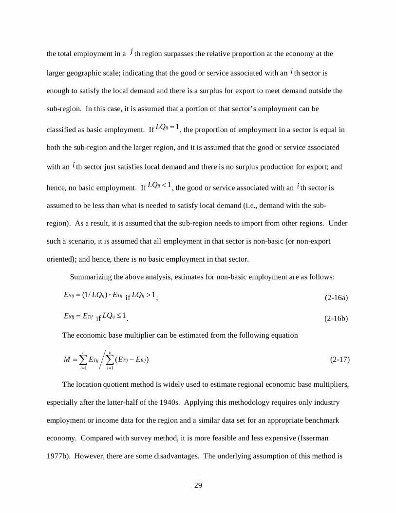
the total employment in a j th region surpasses the relative proportion at the economy at the
larger geographic scale; indicating that the good or service associated with an i th sector is
enough to satisfy the local demand and there is a surplus for export to meet demand outside the
sub-region. In this case, it is assumed that a portion of that sector’s employment can be
classified as basic employment. If 1=ijLQ , the proportion of employment in a sector is equal in
both the sub-region and the larger region, and it is assumed that the good or service associated
with an i th sector just satisfies local demand and there is no surplus production for export; and
hence, no basic employment. If 1<ijLQ , the good or service associated with an i th sector is
assumed to be less than what is needed to satisfy local demand (i.e., demand with the sub-
region). As a result, it is assumed that the sub-region needs to import from other regions. Under
such a scenario, it is assumed that all employment in that sector is non-basic (or non-export
oriented); and hence, there is no basic employment in that sector.
Summarizing the above analysis, estimates for non-basic employment are as follows:
TijijNij ELQE *)/1(= if 1>ijLQ ; (2-16a)
TijNij EE = if 1≤ijLQ . (2-16b)
The economic base multiplier can be estimated from the following equation
∑∑==
−=n
iBijTij
n
iTij EEEM
11)(
(2-17)
The location quotient method is widely used to estimate regional economic base multipliers,
especially after the latter-half of the 1940s. Applying this methodology requires only industry
employment or income data for the region and a similar data set for an appropriate benchmark
economy. Compared with survey method, it is more feasible and less expensive (Isserman
1977b). However, there are some disadvantages. The underlying assumption of this method is

30
weak as it is asserted that different economic regions adhere to the same benchmark; that is, have
the same minimum demand for a goods and services from a given industry or sector. In short, it
assumes that sector demand, in a relative sense, is spatially invariable across sub-regions and is
similar to that of the larger benchmark economy. The choice of a benchmark economy can also
impact the accuracy of the estimates; and a question arises as to whether it is advisable to use a
regional or national economy as a benchmark for a sub-region; especially as that region may be
highly specialized in terms of its industry mix and/or have a comparative or competitive
advantage in production that allows it achieve say economies of scale or exploit its geographic
location. When a region’s economy is compared with two benchmark economies, say at the state
and national levels, estimated basic and non-basic economic activity usually varies, and there is
no direct indicator for which estimate is more reflective of the region’s economic position.
Unfortunately, no wildly-applied standard is available by which to evaluate the benchmarks.
Consider the urban economy of Miami, Florida – a node that is recognized as a global city
because of its importance in several sectors including finance, commerce, media and
entertainment, and international trade. Miami is radically different in terms of its industry mix
than say the capital of Florida -- the city of Tallahassee, which focuses on education, government
administration, and agriculture. If the two cities’ economies are compared with the state level,
they will share the same benchmark to distinguish basic and non-basic economic activity in all
sectors. Yet obviously, Miami has a higher local minimum demand for finance, insurance, real
estate, retail trade and service, while Tallahassee has higher demand for public administration.
This inherent flaw can lead to multiplier estimates that are exceedingly large and over-estimated.
As an alternative benchmark by which to compare these two very different regional economies,
one could utilize information on sector activity for northern Florida and southern Florida and

31
obtain far more reasonable results as there would be less of a contrast in economic activity levels
across various sectors. Another disadvantage of the LQ method is that it fails to estimate the
marginal economic base multiplier. Recently, there has been an attempt to improve on
traditional location quotients estimates through the specification of the dynamic location quotient
(DLQ) method. This approach was developed to decompose regional employment into base and
non-basic components across multiple sectors using spatial and temporal data (Lego,
Gebremedhin & Cushing 2000).
32BMinimum Requirements
The minimum requirements (MR) method was popularized in 1960s and 1970s (Moore
1975). It is similar to the location quotient method in terms of distinguish sector activity by
comparing activity levels in the study area to a predetermined benchmark. In the minimum
requirements method, groups of regional economies or sub-regions with approximately similar
sizes are compared, and a sector’s minimum requirement is assumed to be the minimum level of
activity in those regions. It is assumed that this minimum level of employment observed within
the group is a level that satisfies internal demand. Furthermore, it is assumed that sub-regions
with greater activity than the observed minimum for a given economic sector must be exporting
goods or services. Excess sector employment (above the sector minimum), within a given size
class, is assumed to be basic employment. The minimum local benchmark for a given economic
sector, for a given size class, represents minimum non-basic employment inE min)( . Once these
values are determined for all sectors, the economic base multiplier is found from the following
expression:
∑
∑
=
=
−= n
iiNTi
n
iTi
EE
EM
0(min)
0
)(. (2-18)

32
As with the methods discussed earlier, the minimum requirements approach can only
estimate the average multiplier. The classification of the similar range regional economy makes
a significant influence on the accuracy of final result, so it is critical that care be taken to find
regional economies of similar size, though the same criticism can be levied as there is no reason
to believe that similar sized economies should have a similar industry mix. Some regions have
an inherent advantage based on location, natural resources, and/or other production advantages,
and even if similar in size will not necessarily share similar sector-specific production levels or
similar sector-specific demand. Researchers continue to discuss standards by which to evaluate
economies of similar size economy, but no agreement has been reach on exactly how to go about
justifying the minimum requirements benchmark. Nonetheless, tremendous strides have been
made in the estimation of multipliers using regression models of various kinds.
33BRegression-based Approaches
Regression analysis has been used effectively in the estimation of regional economic base
multipliers, yet is known that the type and quality of estimates depend on the specific regression
approach being applied regression model. The aggregate and disaggregate models represented
by equation (2-9), (2-11) and (2-13) can all be estimated using ordinary least square (OLS)
regression. This requires a survey and the gathering of a sample data, and then the use of OLS to
provide estimates of the coefficients of the model. Multipliers are then calculate from the
estimated coefficients using equations (2-10), (2-12) and (2-14). Typically, multiplier estimates
will be dramatically different from the method described above. Nevertheless, the regression-
based approaches have become quite popular in the economic base theory literature. The
regression-based approaches are also expandable, as illustrated by the seminal work of Mulligan
and Gibson (1987). Mulligan and Gibson emphasized the importance of including transfer
payments and have shown that the employment-derived estimates of economic base multipliers

33
tend to be biased upward unless the transfer payments are directly specified in the regression
model. Mulligan and Fik (1994) extended previous research using the Arizona Community Data
set, and distinguished between multipliers for different types of communities by introducing
dummy variables into the regression models. The estimation results have also been shown to be
dependent on Meta-analysis (Vollet, Bousset 2002). In this approach, a host of variables are
used to reflect characteristics of study regions and account for variability in population size and
the magnitude of the employment base, as well as the physical size of the study regions; and in
particular, how the economic base is determined, how it is expressed, and which statistic method
is applied, and how it might impact the accuracy of the model based on a multitude of variables.
As mentioned previously, the fundamental assumptions of economic base theory are at odds with
the Keynesian equation, something that researchers have made great efforts to correct in time-
series econometric applications. One very influential work was the use of bi-variate vector
autoregression (VAR). In this approach, sector employment levels were analyzed in the state of
Ohio, and its economic base was derived and evaluated using Granger causality tests and
interpreted dynamic base multipliers by impulse-response functions (Lesage, Reed 1989).
Although Krikelas (1992) argued that the identifying restrictions required to derive multiplier
estimates become arbitrary and the estimation procedure becomes unstable as the number of
sectors included in a VAR model is increased. Nevertheless, additional research in this area
supports the vector auto-regression approach. An interregional trade model from which testable
parameter restrictions for economic base theory were shown to be equivalent when subject to
Granger causality tests, suggest that economic base theory holds strongly for the crudest
definition of the base, in a study where the data set included the states of California,
Massachusetts and Texas (Nishiyama 1997).

34
Time-series procedures have also been applied in the estimation of economic base
multipliers, with moderate success. Separating the employment base into at least two sectors, a
shortcut method has been developed that utilizes both a structural adjustment procedure and a
time-adjustment procedure (Was and Mulligan, 1999; Mulligan, 2009). The first procedure
recognizes that each industry has a sector-specific assignment to the local employment base that
relies not only on the size of the regional economy but also its industrial mix and the degree of
industry concentration. The second procedure applies a time variable to control for dramatic
growth or depression of an economy in a particular year, using a variant of the VAR method.
These regression-based approaches represent the current trend in economic base research. They
represent flexible and expandable strategies for the estimation of coefficients and marginal
economic base multipliers and are methodologies that have potential forecasting abilities.
Regression-based procedures also offer the capacity to added more explanatory variables, such
as supply-side factors, regional characteristics, transfer payments and spillover incomes, leakage,
structural adjustment considerations, and time.

35
2BCHAPTER 3 10BMETHODOLOGY
This chapter discusses the methodology utilized to fulfill the research objectives stated in
Chapter1. In the first three sections of this chapter, employment data are used estimate economic
base multipliers using the location quotient (LQ) method to distinguish between basic and non-
basic employment, and a comparison of multiplier estimates from ordinary least squares (OLS)
regression and a linear unobserved effects panel data (PD) model. At the conclusion of this
chapter, alternative research models are proposed, with elaboration on the selection of variables
and potential data sources.
23BThe Location Quotient Method
The Location Quotient (LQ) method is commonly used to calculate an average economic
base multiplier. For our purposes here, it represents preliminary stage, as typically applied when
no industry-specific data regarding basic versus non-basic employment is available. In short, the
LQ method is a tool that provides sector-specific estimates for basic and non-basic employment,
under the usual assumptions. Given the lack of survey method data for counties in the state of
Florida, the LQ estimates will serve as important input for a regression-based approach that
compares the results of alternative estimators. The focus is on economic activity levels at the
county level, with the state of Florida used as a benchmark economy. It is well known that LQ
multipliers typically give large and bloated estimates when run at the regional level given that
much of sector-specific demand is satisfied by imports or supply coming from outside the region
and that some sectors are exporting across the regional boundary to satisfy non-internal demand
(Chiang 2009). Hence, it may be prudent not to use the actual location ratio as a benchmark, as
the LQ method would undoubtedly produce overstated multipliers. In order to make the
multiplier estimates more reasonable, a “scaling factor” could be employed. Any attempt,

36
however, to scale down the LQ multiplier estimates would run the risk of being viewed as
subjective as the choice of a scalar is not readily clear and for the simple fact that the scalar may
differ across locations. As such, we will turn to OLS estimators which rely on various statistical
properties in the estimation of multipliers.
24BOrdinary Least Squares (OLS)
This section introduces the single-equation linear model and the ordinary least squares
(OLS) estimators. It is the most basic estimation procedure in econometrics, yet it is known that
accurate application of OLS depends on meeting a series of strict assumptions (Hayshi, 2000).
Once one or more assumptions are violated, OLS method cannot obtain reasonable estimation
results. Consider a multivariate regression model of the variety
iikkiii xbxbxbay ε+++++= ...2211 (2-19) where b ’s are unknown parameters to be estimated and iε are unobserved error terms with
certain properties (as stated below). Note that the b ’s represent the marginal and separate
effects of regressors (the independent variables of the model). The error term represents the part
of the dependent variable left unexplained by the regressors. It can consist of a variety of things,
including omitted variables and measurement error. An explanatory variable kx is said to be
endogenous in the regression equation if is it correlated with ε . It is assumed that kx is exogenous
in regression equation. Endogenous variables are a common problem in OLS regression, and can
lead to violation of the assumptions of OLS regression.
Five assumptions of OLS may be summarized. First, the relationship between the
dependent variable and the regressors is linear; i.e., the model is linear in its parameters (or can
be specified in a linear form such as the model shown above). Second, variable matrix is full
rank, which implies that each column of regressors is linearly independent (assuming that multi-

37
collinear relations are not a problem). Third, the error term is strictly exogenous, stated as
formula 0),...,,( 21=ni xxxE ε , which indicates that regressors do not give information about the
expected value of the disturbance terms in the model. Fourth, the error terms satisfy conditional
homoscedasticity, where2
212 ),...,,( δε =ni xxxE (i.e, the error structure is such that it is of
constant variance). Fifth, the error terms are not dependent – that is, error is not spatially or
serially auto-correlated; and as such error covariance oxxxE nji =),...,,( 21εε .
The fourth and fifth assumptions define the format of the error term covariance matrix
with diagonal elements equal to 2δ and all non-diagonal elements equal to 0 (Greene 2000).
After OLS regression is applied, it is necessary to (a) check for outliers, (b) validate that the error
terms are normally distributed, (c) verify that multi-collinearity is not a problem, and (d) test for
serial or spatial autocorrelation in the residuals. When all assumptions of OLS are satisfied, the
estimators are said to be BLUE -- best linear (efficient and/or consistent) unbiased estimators.
However, it is common that one or more assumptions are violated. When this occurs it is useful
to apply a remedial measure or an alternative estimation technique. Table 3-1 provides an
overview of OLS assumptions and possible solutions and/or remedial measures.
Table 3-1. OLS assumptions and possible solution Assumption Violation Solution Linearity Nonlinearity Transformations (log, square, inverse, etc.) Full rank Multi-collinearity Delete one or more independent variable Exogeneity Endogeneity Instrumental Variables or TSLS Homescedasticity Heteroscedasticity GLS(WLS) or Robust Regression
No Autocorrelation
Temporal and/or Spatial Autocorrelation
GLS or spatial/temporal transformation Autoregressive models Spatial Econometric model

38
25BLinear Unobserved Effects Panel Data Models
This section highlights the advantages and problems of using “panel data”, and examines
two common methods for estimating linear unobserved effects in panel data (PD) models.
Before proceeding to review the panel data modeling approach, a short review of various
definitions as they pertain to regression data is necessary to panel data in its proper perspective.
A Hdata setH containing observations on a single phenomenon observed over multiple time
periods is called a “ Htime seriesH”. A data set containing observations on multiple phenomena
observed at a single point in time is called “ Hcross-sectionalH” (where each individual, sampling
unit, data point or polygon is observed only once). A data set containing observations on
multiple phenomena observed over multiple time periods is called “panel data” (which implies
that each individual, sampling unit, data point or polygon is observed in more than one time
period). Panel data analyses do not require that the time period in which different individuals or
sampling units are observed are exactly the same.
The major factor that distinguishes time-series data and cross-sectional data from panel data
is that both time-series and cross-sectional data are one-dimensional, while panel data is two-
dimensional (given that it is both spatial and temporal, and unrestricted in the temporal domain).
Time-series data suffers from its lack of spatial sensitivity and requires that observations be
equally spaced in time. Cross-sectional data analyses do not adequately capture the dynamics of
inter-relationships amongst variables as they occur across time and largely ignore the possibility
of consistency of phenomenon across the temporal domain. Cross-sectional data for a single
time period cannot adequately capture the aggregate effects inherent amongst variables or
phenomena and the inter-relationships that spans across multiple time periods. Panel data offers
an alternative that is widely used in economic analysis and can be viewed as offering information
that is spatial-temporal.

39
Consider the following linear panel data (PD) model, expressed as
itititititit xbxbxbay ε+++++= ...2211 (2-20)
where itx is a K*1 vector that contains observable variables that change across time t but not i ,
variables that change across i rather than t , and variables that change across i and t (Wooldridge,
2002). The error terms can be denoted as
itiit uc +=ε (2-20a)
where ic is the part of error term that changes across the individual rather than time, while itu is
the part of error term that change across both individual and time. Wooldridge (2002) states that
the component ic could be treated as a random variable or as a parameter that is to be estimated.
Accordingly, ic is divided into a “random effect” and a “fixed effect”, where the former means
zero correlation between the observed explanatory variables and the unobserved effect; that is,
0),( =iit cxCov ; while the latter means that correlation between the observed explanatory
variables and the unobserved effect is non-zero and allowed: 0),( ≠iit cxCov . In short, two
types of regression possibilities apply here: “random-effect methods” and “fixed-effect
methods”.
Recall that the fifth assumption of OLS regression states that no serial auto-correlation is
found in the error terms of the model, or 0)( 21 =xE ii εε . For the two time period panel data
model, because ic is unchanged across two time periods
0)()()()()(
])[(]))([()(
2112
21122121
≠=+++=
+++=++=
xccExuuExucExucExccE
xuucuucccExucucExE
iiiiiiiiii
iiiiiiiiiiiiii εε
(2-21)
where the assumption is that 0)()()()( 2112 ==++ xccExuuExucExucE iiiiiiii .
40
Viewed in this light, it is apparent that OLS regression cannot obtain “consistent” estimators. It
is necessary, therefore, to find an alternative method to OLS regression. Two commonly applied
alternatives are random-effects methods and fixed-effect methods. Both of these methods
assume that 0),( =iiit cxuE . The random effects method assumes that 0)( =ixciE , while the
fixed-effect method does not retain any such assumption.
Random effects methods belong to the family of “general least squares” (GLS) estimators;
techniques which utilize an unrestricted variance estimator as a transformer as a way to
overcome problems related to serial autocorrelation. The key issue is whether the random-
effects method should be applied in the panel data model given the assumption that
0),( =iiit cxuE (Baltagi 1995). In an economic base analysis using say two-years of data, ic can
be considered as part of various regional location factors such as the “weather” – a random effect
that is largely uncorrelated with industrial employment or export orientation. As such, the
random-effects methods can be used within a PD context.
Fixed-effects methods apply an internal transformation, where
iitiitiit uubxxyy −+−=− )( , (2-21)
and where ∑ =−=
T
t iti yTy1
1
, ∑ =−=
T
t iti xTx1
1
and T is the number of total periods. Note that the
component ic is deleted in the transformation process. This transformation is necessary to
ensure that the error term satisfies the assumptions of OLS regression; allowing OLS to obtain
consistent estimators.
Fixed-effects methods do not assume that 0),( =iiit cxuE . Note, however, that the
transformation depends on the difference between equation from one period and the average.

41
Hence, it is highly possible that the value of )( iit xx − is small but the value of iit uu − is
relatively large. If so, it would lead to a bias in estimation, something that would be especially
pronounced when the individual or sampling unit does not change much across time periods. To
illustrate the effectiveness of these methods, a two-period exploratory economic base model is
constructed and estimated using Florida employment data at the county level for the year 1993
and year 1997.

42
3BCHAPTER 4 11BEXPLORATORY ECONOMIC BASE REGRESSION MODEL
This chapter presents the statistical results of an exploratory economic base analysis of
the Florida economy using county level data (for n=67 counties). The first section provides an
overview of the employment data used in this study and the estimation of basic and non-basic
employment. Section two discusses the potential overestimation problem that is inherent to
economic base studies, and offers a potential solution – the use of various scaling factors to
deflate non-basic employment estimates. Lastly, the results of the regression analysis are
highlighted; comparing those obtained from ordinary least squares (OLS) regression and panel
data (PD) regression.
26BInitial Data Collection
Florida county-level industrial employment data were collect from the U.S. Census Bureau
website. Standard Industrial Classification of employment figures were obtained for nine
separate industries/sectors: (1) agricultural services, forestry, and fishing; (2) mining; (3)
construction; (4) manufacturing; (5) transportation & public utilities; (6) wholesale trade; (7)
retail trade; (8) finance, insurance and real estate; and (9) services, as well as employment
figures for unclassified establishments. Previous research, such as the economic base research of
communities in Arizona, combines employment in agricultural services, forestry and fishing, and
mining; defining it is as primary sector employment. This study follows this convention.
Using the reported employment data, estimates for basic and non-basic employment were
obtained using location quotient (LQ) method. A location quotient was calculated for each
county and each industrial sector using state level data as a benchmark. Recall that the LQ
method relies on the formulas listed in equations (2-15) to (2-17), where the ratio is the
proportion of a j-th county’s industry employment in a given i-th sector; a value that is compare j
ij
EE

43
to the proportion of employment associated with that sector as reported for the Florida economy
at large, . The LQ method is then used to estimate the amount of basic and non-basic
employment for each sector and each county. These estimates were then used in a disaggregated
model to estimate sector-specific economic base multipliers using various regression-based
models. Total employments by county of year 1993 and 1997 show in Figure 4-1. Estimated
non-basic employments for each sector by county of year 1993 and 1997 show from Figure 4-2
to Figure 4-9. Estimated basic employment for each sector by county of year 1993 and 1997
show from Figure 4-10 to Figure 4-17.
Accoriding to Figure 4-1a and Figure 4-1b, Orlando, Jaxsonville, Tampa, Miami,
St.Petersburg, West Beach and Boca Raton areas have relative large total emploment compared
with other regions. Non-basic employmenet and basic employment for sector from Figure 4-2 to
Figure 4-17 base on the location quotient method. From Figure 4-2 to Figure 4-9 show that non-
basic emploment of different sectors have disimilar spatial distribution by county, which is
probably not consistent with the spatial distribution of total employment. In Figure 4-2A,
Broward, Miami-Dade, Palm Beach, Orange, Pinellas,Hillsborough, Brevard and Duval counties
have largest total employment in 1993, however, on on hand, Brevard has medium non-basic
transportation employment in 1993 from Figure 4-5A, on the other hand, largest non-baic serives
employment in 1993 from Figure 4-9A is consitent with total employment.Therefore, the change
of non-basice employment of differents sectors should have disimilar return to total employment.
Some of the same sectors of year 1993 and 1997 shows disimilar employment distribution
by county, which implies that employment distribution by county of single year cannot
characterise that in long term. Therefore, panel data regression of mutliple years should instead
regression of single year to estimate the steady trend of regionl employment.
eei

44
Figure 4-18 shows social security payment of year 1993 and 1997 by county, which
shows same spatial distribution by county across years.
27BRegression Analysis
The disaggregate regression model which shows non-basic employment as a function of
basic employment by sector can be expressed as
SocibEbEbEbEbEbEbEbEbaE
Bserv
BfinaBretawholBtranBBmanuBconsBprimN
98
7654321
+
++++++++=
(4-1)
where denotes total non-basic employment in a j-th regional economic or county,
independent variables are the estimated basic employment of each industry/sector: agricultural
services, forestry, fishing and mining (prim); construction (cons); manufacturing (manu);
transportation and public utilities (tran); wholesale trade (whol); retail trade (reta); finance,
insurance, and real estate (fina); and services(serv). Note that the model is also expanded to
include social security benefits (soci), in thousands of dollars; a variable that is used as a
surrogate for income that creates a cash flow to regional economy and an expansion in sales and
services. The use of this surrogate helps to account for a source of state income that can
augment the non-basic sector. This especially important in the state of Florida were such a large
proportion of the population is 65 years of age or older, many of whom are retired and drawing
Social Security payments.
The sample database consists of data for n=67 Florida counties and data for two distinct
time periods (1993 and 1997). If one-year samples (for either year 1993 or year 1997) are
applied, the OLS regression model can be used. However, to obtain more stable and consistent
estimation of sector-specific economic base multipliers, data for these two time periods can be
combined using the panel data regression approach. Before this can be accomplished, the
dependent variable (county level non-basic employment) must be scaled back to account for

45
A Figure 4-1. Total employment of Florida in different years by county A) 1993 B)1997

46
B
Figure 4-1. Continued

47
A
Figure 4-2. Non-basic employment for primary sector of Florida in different years by county A)1993 B)1997

48
B
Figure 4-2. Continued

49
A
Figure 4-3. Non-basic employment for construction sector of Florida in different years by county A)1993 B)199

50
B
Figure 4-3.Continued

51
A
Figure 4-4. Non-basic employment for manufacturing sector of Florida in different years by county A)1993 B)1997

52
B
Figure 4-4. Continued

53
A Figure 4-5. Non-basic employment for transportation and public utilities sector of Florida in
different years by county A)1993 B)1997

54
B
Figure 4-5. Continued
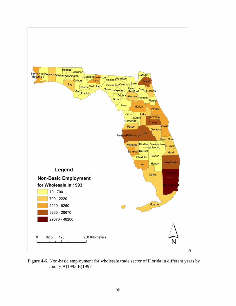
55
A
Figure 4-6. Non-basic employment for wholesale trade sector of Florida in different years by county A)1993 B)1997

56
B
Figure 4-6. Continued

57
A
Figure 4-7. Non-basic employment for retail trade sector of Florida in different years by county A)1993 B)1997

58
B
Figure 4-7. Continued

59
A
Figure 4-8. Non-basic employment for finance, insurance and real estate sector of Florida in different years by county A)1993 B)1997

60
B
Figure 4-8. Continued

61
A
Figure 4-9. Non-basic employment for services sector of Florida in different years by county A)1993 B)1997

62
B
Figure 4-9. Continued

63
A
Figure 4-10. Basic employment for primary sector of Florida in different years by county A)1993 B)1997

64
B
Figure 4-10. Continued

65
A
Figure 4-11. Basic employment for construction sector of Florida in different years by county A)1993 B)1997

66
B
Figure 4-11. Continued

67
A
Figure 4-12. Basic employment for manufacturing sector of Florida in different years by county A)1993 B)1997

68
B
Figure 4-12. Continued

69
A Figure 4-13. Basic employment for transportation and public utilites sector of florida in different
years by county A)1993 B)1997

70
B Figure 4-13. Continued

71
A Figure 4-14. Basic employment for wholesale trade sector of Florida in different years by county
A)1993 B)1997

72
B Figure 4-14. Continued

73
A Figure 4-15. Basic employment for retail sector trade of Florida in different years by county
A)1993 B)1997

74
B
Figure 4-15. Continued
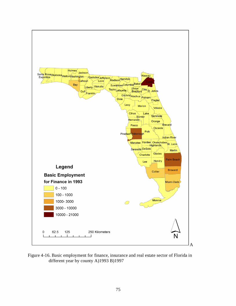
75
A
Figure 4-16. Basic employment for finance, insurance and real estate sector of Florida in different year by county A)1993 B)1997

76
B
Figure 4-16. Continued

77
A Figure 4-17. Basic employment for services sector of Florida in different years by county
A)1993 B)1997

78
B
Figure 4-17. Continued

79
A Figure 4-18. Social security payment by county of Florida in different years by county A)1993
B)1997

80
Figure 4-18. Continued

81
other non-employment related income and transfers which tend to bloat the non-basic sectors.
The choice of a scalar, while not obvious, is the focus of the next section.
28BChoosing a Scalar
If the regression model in previous section is applied directly, the estimation of sector-
specific coefficients would be very large. While the independent variables of the model may do
well in explaining employment related patterns, they lack in their ability to account for other
sources of personal or transfer payment income (e.g., investment income, dividends, interest and
rents, unemployment benefits, income from personal or corporate retirement accounts, money
spent by visitors to the state). Note that the dependent variable embodies both the impact of
employment income and non-employment income, and as such is typically thought of as
exaggerating the impact of basic employment. As such, there is a need to scale back the
estimates for non-basic employment to account for the impact of transfer payments.
Total personal income includes net earnings by place of residence; dividends, interest, and
rent; and personal current transfer receipts. The first part is from employment, while the second
and the third are from non-employment sources. Nontraditional sources of personal income and
transfers have become important in the economic base literature, especially in regions with high
population growth rates (Nelson, Beyers 1998); a feature that certainly applies to Sunshine State.
The ratio of net earnings to total personal income by county is applied as a scalar to the
dependent variable to account for the non-employment part of non-basic employment.
Numerical values for the scalar are presented in Table 4.1 for each of Florida’s 67 counties. This
scalar alone, however, is not sufficient in capturing the entire effect of income transfers as there
are also inherent via multiplier effects associated with income transfers that must be account for.
Furthermore, the scalar only decreases the initial non-basic employment figures, and ignores the
influence of state level non-employment income sources. Compared with other states in the

82
Table 4-1. Scalars and non-basic employment in year 1993 and 1997 by county County scalar 1 scalar 2 nonbasic in 1993 nonbasic in 1997 Alachua 0.65 0.8529 57107 66567 Baker 0.69 0.8529 2974 2956 Bay 0.63 0.8529 39872 45597 Bradford 0.68 0.8529 3068 3463 Brevard 0.59 0.8529 128870 137691 Broward 0.6 0.8529 463034 541136 Calhoun 0.59 0.8529 1365 1241 Charlotte 0.35 0.8529 21692 24698 Citrus 0.38 0.8529 17659 18615 Clay 0.73 0.8529 19526 22320 Collier 0.4 0.8529 56239 72960 Columbia 0.61 0.8529 10740 14044 Dade 0.62 0.8529 719150 740137 De Soto 0.55 0.8529 3778 3976 Dixie 0.52 0.8529 850 841 Duval 0.71 0.8529 291661 317162 Escambia 0.64 0.8529 88129 96929 Flagler 0.45 0.8529 5232 7281 Franklin 0.48 0.8529 1610 1800 Gadsden 0.64 0.8529 7610 7453 Gilchrist 0.66 0.8529 868 963 Glades 0.54 0.8529 269 1242 Gulf 0.56 0.8529 1583 1999 Hamilton 0.6 0.8529 1535 1453 Hardee 0.62 0.8529 2735 3109 Hendry 0.67 0.8529 4004 3793 Hernando 0.41 0.8529 16452 24306 Highlands 0.39 0.8529 15409 16688 Hillsborough 0.68 0.8529 366108 434392 Holmes 0.56 0.8529 1709 1903 Indian River 0.34 0.8529 25096 30632 Jackson 0.57 0.8529 7016 7083 Jefferson 0.63 0.8529 1633 1622 Lafayette 0.68 0.8529 418 487 Lake 0.48 0.8529 36262 41728 Lee 0.46 0.8529 103366 124288 Leon 0.72 0.8529 65815 74493 Levy 0.54 0.8529 3306 4037 Liberty 0.66 0.8529 578 568 Madison 0.58 0.8529 2178 2589 Manatee 0.5 0.8529 59985 79526 Marion 0.51 0.8529 48426 54307 Martin 0.37 0.8529 31768 36130 Monroe 0.48 0.8529 24340 26256

83
Table 4-1. Continued County scalar 1 scalar 2 nonbasic in 1993 nonbasic in 1997 Nassau 0.67 0.8529 8982 11287 Okaloosa 0.63 0.8529 40977 49660 Okeechobee 0.55 0.8529 5001 5344 Orange 0.7 0.8529 369316 453648 Osceola 0.67 0.8529 29503 36068 Palm Beach 0.46 0.8529 328170 389281 Pasco 0.48 0.8529 48966 56339 Pinellas 0.55 0.8529 306103 348737 Polk 0.61 0.8529 120189 133398 Putnam 0.54 0.8529 9134 10624 St.Johns 0.6 0.8529 23046 30035 St.Lucie 0.47 0.8529 32541 37475 Santa Rosa 0.69 0.8529 13465 15891 Sarasota 0.42 0.8529 95709 119964 Seminole 0.73 0.8529 87836 107294 Sumter 0.45 0.8529 3614 3703 Suwannee 0.58 0.8529 4769 5141 Taylor 0.61 0.8529 3082 3086 Union 0.69 0.8529 1291 1115 Volusia 0.5 0.8529 104654 118695 Wakulla 0.71 0.8529 1443 1686 Walton 0.57 0.8529 6119 7871 Washington 0.57 0.8529 2554 3272
U.S., Florida has a relatively large number of in-migrants and retirees that relocated to Florida
from other states. Subsequently, Florida has a large ratio of non-employment related income
when compared to other states, and conceivably an inordinate share and influx of external
income from sources that are varied categorically and geographically. Note that the ratio of net
earnings to total personal income in Florida is approximately 58%, while the ratio of net earnings
to total personal income of United States is 68%. Thus, the ratio of 58% to 68% (or .8529) is the
second scalar that can be used to deflate estimated non-basic employment. This second scalar
denotes the influence of state-level non-employment related income transfers that filter down on
average to county level economies. Therefore, the dependent variable in regression model
can be re-sated, adjusting for the impact of the two scalars:
βα **NN EE =×
(4-2)

84
where α is the ratio of net earnings to total personal income for each county and β is the scalar
of influence of the state level non-employment income. Note that the first scalar is different
across the counties, while the second scalar (without more detailed information) is assumed to be
constant across counties. Scaling back non-basic employment allows for more accurate sector-
specific multiplier estimates. Because of limitations in data sources, the scalars used in this study
were based on information for the closest year 1998.
29BResults and Discussion
The results of OLS estimation of the model illustrated in equation 4-1 using the modified
dependent variable from equation 4-2 for the year 1993 are shown Table 4-2. Except for the
primary sector, estimated coefficients are significant at 90% confidence level or higher. Basic
employment in wholesale trade is estimated to have the largest return to non-basic employment
in regional economy. One job increase in wholesale trade leads to approximately fourteen jobs in
non-basic sectors. Basic employment in construction; finance, insurance, and real estate; and
services also have large returns to non-basic employment, while basic employment of primary
sector industry and transportation have small returns to non-basic employment relative to other
sectors. For example, it is estimated that a one job increase in the primary sector leads to
approximately 2 jobs in non-basic sectors. The estimated coefficient associated with “soci”
implies that every additional $3,336 in social security benefits contributes roughly, on average, a
1 job increase in the non-basic sector of the regional economy.
The results of the OLS regression for the year 1997 are shown in Table 4-3. Note the
consistency in both the estimated values and the significance levels, with the exception of the
coefficient associated with primary sector industry (as it is now significant at the 95% confidence
level) and the increase in the coefficient associated with wholesale trade. The change in the

85
primary sector coefficient implies that a 1 job increase in the basic sector of Florida’s primary
industries leads to an estimated 9 job increase in non-basic sector employment. Note that this
coefficient is radically different form that which was estimated for 1993, which showed only a 2-
to-1 increase in non-basic employment for an additional basic job added to the economy. The
results also suggest the volatility that exists in year-to-year estimates. Note the jump in the
estimated coefficient for whole trade, from 12 to approximately 17. All in all, OLS estimation is
suspect as the sector-specific multipliers appear to remain somewhat exaggerated in spite of the
use of the scaling factors applied to the dependent variable.
Table 4-2. Ordinary least regression estimation result of years 1993 Coefficient Std.Err t-
test P>|t| 95% Conf. Interval
prim 2.253 3.534 0.64 0.526 -4.824 9.330 cons manu tran whol reta fina serv soci constant
8.085** 4.243*** 1.901**
12.076*** 3.182**
5.399*** 5.955*** 0.237***
-5704.684*
3.122 1.015 0.882 1.400 1.541 0.735 0.500 0.062
2732.42
2.59 4.18 2.16 8.62 2.06 7.34
11.90 3.85
-1.72
0.012 0.000 0.035 0.000 0.044 0.000 0.000 0.000 0.091
1.835 2.210 0.135 9.272 0.095 3.926 4.953 0.113
-10176
14.336 6.276 3.667
14.880 6.269 6.871 6.957 0.360
766.907
Table 4-3. Ordinary least regression estimation result of years 1993 Coefficient Std.Err t-
test P>|t| 95% Conf. Interval
prim 9.621** 3.736 2.58 0.013 2.141 17.102 cons manu tran whol reta fina serv soci constant
4.184* 1.593**
-1.747** 17.513*** 4.151*** 4.691*** 6.295*** 0.135**
-5011.103
2.334 1.092 1.028 1.635 1.345 0.595 0.412 0.058
3157.99
1.79 1.46
-1.70 10.71
3.09 7.88
15.28 2.34
-1.59
0.078 0.150 0.095 0.000 0.003 0.000 0.000 0.023 0.118
-.490 -.595
-3.806 14.238
1.458 3.450 5.470 0.020
-11334
8.858 3.780 0.312
20.788 6.844 5.883 7.120 0.250
1312.663 Note: *** indicates significant at the 0.01 level, ** indicates significant at the 0.05 level, * indicates significant at the 0.1 level. Adjust R2=0.948

86
The other obvious change from year 1993 to 1997 is that the sign of coefficient associated
with the transportation and public utility sector becomes negative (literally interpreted as
meaning a contraction of the non-basic sector for each additional job added in that sector). This
counterintuitive and illogical result means that a 1 job increase in the transportation and public
utility sector would lead to a decrease of two jobs overall in the regional economy. The results
for 1993 and 1997 show, nonetheless, that wholesale trade has the largest multiplier effect on
non-basic employment; something that is consistent in the estimation of both models. This result
is no surprise as wholesale trade represents an important industry as Florida maintains its
position as a key player in the global economy with its vibrant international shipping ports
located in Miami, Tampa, and Jacksonville. Employment in construction; finance, insurance,
and real estate; and services also have large return to non-basic employment. The estimated
coefficient for “soci” means that for every $1,896 dollar increase in social security benefits, one
additional non-basic job is added to the regional economy.
The regression analysis using the single-year samples cannot capture trends or the
adjustment of regional economies accurately, as the results are easily influenced by sudden
shocks or discontinuous changes that occur from one year to the next. This could explain why
the estimated coefficient associated with the primary industry in 1993 is not significant at even a
80% confidence level, even though it is represents one of the most important sectors in the state
of Florida (given that agriculture and mining activities generate a fairly large percentage of
income). The variability in single-year estimation can be overcome by applying a regression
platform that utilizes information for more than just one year. Table 4-4 lists the result of
ordinary least regression estimation for the years 1993 and 1997 combined. In this analysis, the
two sample years were combined and the model regressed without any classification. No

87
surprise that the estimated coefficients are located between the two single year estimates.
Nevertheless, the results are suspect and a test for exogeneity is necessary. Table 4-5 highlights
the results of exogeneity test on the error terms of the combined OLS model. The test depends
on the regression of error terms from the 1997 model (uhat) on error terms from the 1993 model
(uhat_1). The test results suggest that the coefficient is significant at 95% confident level, and
therefore, panel data (PD) regression should be applied instead of OLS regression on the two
year samples.
Table 4-4. Ordinary least regression estimation result of year 1993 and 1997 Coefficient Std.Err t-test P>|t| 95% Conf. Interval prim 5.282 2.611 2.02 0.045 .114 10.449 cons manu tran whol reta fina serv soci constant
5.189 2.911*** 0.082***
14.850*** 3.806*** 4.767*** 5.984*** 0.205***
-4881.392
1.851 0.750 0.676 1.078 0.993 0.462 0.315 0.040
2110.40
2.80 3.88 0.12
13.77 3.81
10.32 19.00
5.10 -2.31
0.006 0.000 0.903 0.000 0.000 0.000 0.000 0.000 0.022
1.526 -1.426 -1.256 12.716
1.828 3.853 5.360 0.126
-9058.46
8.853 4.395 1.421
16.985 5.784 5.681 6.607 0.285
-704.316 Note: *** indicates significant at the 0.01 level, ** indicates significant at the 0.05 level, * indicates significant at the 0.1 level. Adjust R2=0.946 Table 4-5. Test result of exogeneity of error term uhat Coefficient Std.Err t-test P>|t| uhat_1 0.563 0.101 5.59 0.000 constant -3365.202 3544.38 -0.9 0.346
The results for the panel data regression are shown in Table 4-6. Note that the estimated
coefficients for the primary and construction sectors are significant at 80% confidence level, and
the coefficients of all other industries are significant at 95% confidence level. Once again, the
largest estimated coefficient is for wholesale trade, which implies that one additional job in that
sector of wholesale trade will lead to approximately 11 additional non-basic jobs in the regional
economy at large. Retail trade, the service sector, and manufacturing are also important sectors,

88
with empirical results that are consistent with those reported by Fik et al (1991, 1993). The
smallest coefficients are associated with transportation and finance; not surprising, as Florida
does not actively engage in the building of public transportation (e.g., limited railway and
subway). All in all, the sector-specific multiplier estimates provide a glimpse of Florida’s
orientation toward a sales- and service-oriented economy, as discussed by Fik et al (1991). The
size of the multiplier estimates indicate that may still be slightly overstated, yet one could argue
Table 4-6. Panel data regression estimation result of year 1993 and 1997 without dummy variable
Coefficient Std.Err Z-test P>|Z| 95% Conf. Interval prim 5.483 4.072 1.35 0.178 -2.499 13.464 cons manu tran whol reta fina serv soci constant
3.311 4.019*** 2.768***
10.832*** 4.306*** 2.736*** 4.454*** 0.202***
-1336.749
2.137 1.307 1.059 1.702 1.201 0.685 0.396 0.046
3636.65
1.55 3.07 2.61 6.36 3.58 3.99
11.25 4.39
-0.37
0.121 0.002 0.009 0.000 0.000 0.000 0.000 0.000 0.713
-.877 -1.457
-.693 7.496 1.950 1.393 3.678 0.112
-8464.45
7.500 6.580 4.843
14.168 6.659 4.079 5.230 0.292
5790.9 Note: *** indicates significant at the 0.01 level, ** indicates significant at the 0.05 level, * indicates
significant at the 0.1 level. Wald Chi 2(9)=0629.42, Prob> Chi 2=0.000
that their relative proportion is fairly representative of Florida’s economic reality (with an
estimation bias that has been reduced), given that the transfer income effect has been largely
accounted for by scaling back non-basic employment levels.
In order to test if the above OLS regression and panel data regression is valid, error term
diagnostics for both OLS regression and panel data regression are applied. Normality test of
error term for residuals of year 1993 OLS regression, year 1997 OLS regression, both year 1993
and year 1997 OLS regression and panel data regression are showed in Figure 4-19a, 4-19b, 4-
19c and 4-19d respectively.

89
05.
0e-0
51.
0e-0
41.
5e-0
4D
ensi
ty
-50000 0 50000Residuals
A
05.
0e-0
51.
0e-0
41.
5e-0
4D
ensi
ty
-60000 -40000 -20000 0 20000 40000Residuals
B
Figure 4-19. Normality test for different regression A)Year 1993 OLS regression B)Year 1997 OLS regression C)Both year 1993 and 1997 OLS regression D) Both year 1993 and 1997 panel data regression
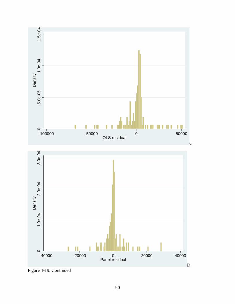
90
05.
0e-0
51.
0e-0
41.
5e-0
4D
ensi
ty
-100000 -50000 0 50000OLS residual
C
01.
0e-0
42.
0e-0
43.
0e-0
4D
ensi
ty
-40000 -20000 0 20000 40000Panel residual
D Figure 4-19. Continued

91
According to the normality tests figures, error terms of both OLS and panel data regression
show normally distributed. Peak density of error terms for both single year regression is located
in residual with value above 0, while peak density of error terms of panel data regression is
located in residual with value more closed to 0, so error terms of panel data regression show
more normally distributed.
Residual plots( fitted values versus residuals) for year 1993 OLS regression, year 1997 OLS
regression, both year 1993 and year 1997 OLS regression and panel data regression are showed
in Figure 4-20a, 4-20b, 4-20c and 4-20d respectively. Residual plots are applied to test
homoscedasticity assumption of regression.
-500
000
5000
0R
esid
uals
0 100000 200000 300000 400000Fitted values A
Figure 4-20. Residual plots for different regression A)Year 1993 OLS regression B)Year 1997 OLS regression C)Both year 1993 and 1997 OLS regression D) Both year 1993 and 1997 panel data regression

92
-100
000
-500
000
5000
0R
esid
uals
0 100000 200000 300000 400000Fitted values B
-100
000
-500
000
5000
0R
esid
uals
0 100000 200000 300000 400000Fitted values C
Figure 4-20. Continued

93
-400
00-2
0000
020
000
4000
0e[
coun
tyid
,t]
0 100000 200000 300000 400000Linear prediction D
Figure 4-20. Continued
While residual plots of OLS regression show obvious triangle-shade, residual plots of
panel data regression show probably random distributed if the upper and below outliers are
deleted. Therefore, all OLS regression estimates here suffer from heteroscedasticity problem.
Panel data regression also cannot avoid this problem, but alleviate to some extent according to
residual plots.
Plots of fitted versus actual values of the scaled non-basic employment for year 1993 OLS
regression, year 1997 OLS regression, both year 1993 and year 1997 OLS regression and panel
data regression are showed in Figure 4-21A, 4-21B, 4-21C and 4-21D respectively. All plots of
fitted versus actual non-basic employment values shows satisfied “goodness of fit” of the
economic base models, which implies that independent variables can explain scaled dependent

94
variables very well. However, figure 4-21D shows that fitted value of non-basic employment is
less than actual value of non-basic employment in the middle of plots. 0
1000
0020
0000
3000
0040
0000
Fitte
d va
lues
0 100000 200000 300000 400000NEB A
010
0000
2000
0030
0000
4000
00Fi
tted
valu
es
0 100000 200000 300000 400000NEB B
Figure 4-21. Plots of fitted versus actual non-basic employment values for different regression A)Year 1993 OLS regression B)Year 1997 OLS regression C)Both year 1993 and 1997 OLS regression D) Both year 1993 and 1997 panel data regression

95
010
0000
2000
0030
0000
4000
00Fi
tted
valu
es
0 100000 200000 300000 400000NEB C
010
0000
2000
0030
0000
4000
00Li
near
pre
dict
ion
0 100000 200000 300000 400000NEB D
Figure 4-21. Continued
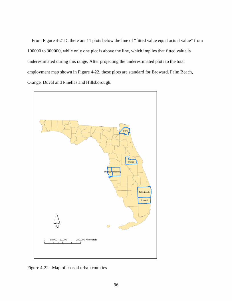
96
From Figure 4-21D, there are 11 plots below the line of “fitted value equal actual value” from
100000 to 300000, while only one plot is above the line, which implies that fitted value is
underestimated during this range. After projecting the underestimated plots to the total
employment map shown in Figure 4-22, these plots are standard for Broward, Palm Beach,
Orange, Duval and Pinellas and Hillsborough.
Figure 4-22. Map of coastal urban counties

97
Compared with Figures 4-1A and 4-1B, these counties are coincident with the counties that
have largest total employment except Miami-Dade, which actually is the plot above
NEB=400000 in Figure 4-21D. The common geographic characteristic of these 6 counties is that
all of them are coastal urban area. As tourist and wholesale trade are highly developing, coastal
and waterway resource boom the relative counties’ employment. Therefore, it is reasonable to
argue that the geography characteristic of coastal urban area should obtain more attention in the
model.
In order to eliminate the bias of estimates for these 6 counties, the original panel data
model should be added a new dummy variable “urban” defined as coastal urban counties,
including Broward, Palm Beach, Orange, Duval and Pinellas and Hillsborough. The result of
panel data regression estimation with dummy variable list in Table 4-7. Dummy variable is
positive significant at 1% level, which coincide with expected impact that coastal urban property
can increase the employment of county.
Table 4-7. Panel data regression estimation result of year 1993 and 1997 with dummy variable Coefficient Std.Err Z-test P>|Z| 95% Conf. Interval prim 2.220 2.320 0.95 0.340 -2.345 6.787 cons manu tran whol reta fina serv soci urban constant
3.987** 2.354*** 4.163*** 8.889*** 4.071***
-.087 2.752***
0.202* 109119.4***
-532.287
1.391 0.708 0.638 1.017 0.764 0.496 0.311 0.031
8501.87 1978.03
2.87 3.33 6.52 8.52 5.33
-0.17 8.85 2.72
12.83 -0.27
0.004 0.001 0.000 0.000 0.000 0.862 0.000 0.006 0.000 0.788
1.260 -0.997 2.912 6.675 2.573
-1.060 2.143 0.024
92456.1 -4409.16
6.715 3.741 5.413
10.662 5.569
.887 3.361 0.146
125782.8 3344.584
Note: *** indicates significant at the 0.01 level, ** indicates significant at the 0.05 level, * indicates significant at the 0.1 level. Wald Chi 2(10)=2558.00, Prob> Chi 2=0.000
Plots of fitted versus actual non-basic employment values for both year 1993 and year
1997 panel data regression with dummy variable show in Figure 4-23. In the middle, some plots

98
locate above the line of “fitted value equal actual value”, while others plots locate below the line,
which implies that estimation problem during range 100000 to 300000 is solved effectively.
Therefore, panel data model obtains better “goodness of fit” after dummy variable is added.
010
0000
2000
0030
0000
4000
00Li
near
pre
dict
ion
0 100000 200000 300000 400000NBE
Figure 4-23. Plots of fitted versus actual non-basic employment values for both year 1993 and year 1997 panel data regression with dummy variable
In order to further compare the estimation results of two panel data models, spatial
autocorrelation of error terms are considered. According to Moran’s I statistic test applying
“inverse distance” as conceptualized spatial relation, the spatial pattern of error terms of original
panel data model is random, while the spatial pattern of error terms of panel data model with
dummy variable is clustered in 10% significant level. Therefore, on one hand, the panel data
model with dummy variable “urban” has better estimation compared with original panel data
model, on the other hand, the panel data model with dummy variable suffer from spatial

99
autocorrelation of error term, while the original panel data model gets rid of the problem. It is
highly possible that dummy variable lead to such a problems, because some of coastal urban
counties are neighborhood.
According to test of exogeneity of error term and three comparison between OLS and
Panel data regression, estimates results depending on both OLS and panel data regression fit the
actual scaled non-basic employment to large extent, while compared with OLS regression, panel
data regression shows better results on test of normality, homoscedasticity and exogeneity.
Multipliers of each industry/sector, from Tables 4-2, 4-3, 4-6 and 4-7 are summarized in
Table 4-8. While the panel data results appear promising, the OLS estimates are most certainly
suspect given the dramatic differences that are observed between 1993 and 1997 in the
magnitude of the estimated coefficients. In 1993, the multiplier associated with the primary
sector is estimated at 3.253, smaller than that of the multiplier for the transportation and public
utility sector. This result does not make sense, because it is known that the agriculture industry
in Florida creates more employment opportunities than does public transportation. Moreover,
single equation estimation of multipliers for the year 1997 produced negative multipliers. This
result is somewhat of an absurdity as a job added to an economy cannot take away more than that
which it adds (as a generalization, any increase in income via a new job will undoubtedly
produce additional demand). By contrast, the panel data regression results seem to fall more in
line with expectations, producing positive multipliers across the board and coefficients that are of
a reasonable magnitude. Compared with regression estimates for a single year, panel data
regression provides a more consistent and even-handed estimation of multipliers across sectors,
avoiding the pitfall of abnormal disturbances associated with single year samples and illogical
results such as negative coefficients/multipliers.

100
From year 1993 to year 1997, wholesale trade, retail trade and services were responsible for
generating the greatest employment multiplier impacts. These results are undoubtedly tied to
Florida’s thriving tourist and recreation sectors, centered about the theme parks of Central
Florida and its bountiful parks and coastal amenities, not to mention its role as a leader in
international trade from import-export activities associated with the cities of Miami, Tampa, and
Jacksonville. These cities represent three of the most important hubs of southeast of U.S., and
link the U.S. economy to South America and the remainder of the global economy. Tourism, as
vital income source for Florida, represents an export-base in and of itself. Although no physical
products are being exported, tourist and recreation activity are services that provide a source of
entertainment and relaxation. Warm weather and hundreds of miles of beaches attract roughly
60 million visitors to Florida every year. HAmusement and theme parksH, in the HOrlandoH area,
make up a significant portion of that tourism. The HWalt Disney World ResortH is the largest
vacation resort in the world, consisting of four Htheme parksH and more than twenty hotels.
Universal studio also attracts a large number of tourists. Many beach towns, such as Daytona
Beach, Tampa, Fort Lauderdale, Sarasota, and Fort Myers are popular tourist destinations; and
attract year-round visitors and seasonal in-migrants from colder climates to the state during the
winter months. Therefore, it is no surprise that the retail and service sectors have relatively large
multipliers. While manufacturing in Florida account for less than 8% of the state’s total
employment, it is also very important as an impact industry with an estimated multiplier that is
larger than construction, transportation, and financial sectors.
The empirical results suggest that the regional economic bases multipliers associated with
the Florida economy are substantially larger than those estimated for various communities in the
state of Arizona (Mulligan, 1987). This is to be expected as Florida is more populated, more

101
export and tourist oriented, a large sink for retirees over the past several decades, and unique in
terms of its amenities and recreational possibilities from its natural, coastal and waterway
resources.
Table 4-8. Multipliers of OLS regression and panel data regression Sector
Year 1993
Year 1997
Two Years
Two Years with dummy prim
cons manu tran whol reta fina serv
3.253 9.085 5.243 2.901
13.076 4.182 6.399 6.955
10.621 5.184 2.593 -.747
18.513 5.151 5.691 7.295
6.583 4.431 5.019 3.768
11.832 5.406 3.736 5.454
3.220 4.987 3.354 5.163 9.889 5.071 0.913 3.852

102
4BCHAPTER 5 12BCONCLUSIONS
Job creation is a characteristic of basic industry. Activity and employment in basic sectors
are vital for economic growth, and basic employment plays a crucial role in contributing to the
growth of a regional economy by bringing in dollars from external sources. Economic base
multipliers estimate the impact that an influx of dollars has on the creation of jobs for each
additional job added to a given sector. Basic employment, in response to external demand for
goods and services, is responsible for creating additional jobs as income circulates and re-
circulates throughout a regional economy, and subsequently, as the employment base expands.
Quantitative models that attempt to estimate those multipliers through the disaggregation of
employment or income data must reckon with problems that are tied inherently to the nature of
sample data and to problems that arise from various estimation procedures. Economic base
models can be a quick, effective, and inexpensive way in which to ascertain the expansion
potential of various sectors or industries and their relative impact on a region’s economic growth.
This information is useful to policymakers and legislators in their attempt to construct economic
and development policies that could conceivably yield the biggest bang for the buck. Moreover,
economic base analysis and estimated multipliers are useful in explaining variability in regional
economic and employment growth rates (Malecki, 1991), factors that can be attributed to a
region’s economic or employment mix. As such, critical assessments of multipliers are needed
to ensure accurate and reasonable estimates. As part of this assessment, the techniques by which
multipliers are estimated must also be evaluated to lessen the chance of bias or misleading
results. This thesis has demonstrated that multiple-year panel data regression models offer a
useful alternative to OLS regression model as an estimation technique.

103
This study introduced economic base theory and methods used to distinguish between basic
and non-basic employment in a regional economy. It also gave an overview of the mechanics of
estimating employment multipliers using traditional and contemporary approaches. Discussion
focused on estimation techniques, assumptions, and the shortcomings of the traditional OLS
approach to estimating economic base multipliers. In addition, this study discussed the
difference between aggregate and disaggregate modeling. It also distinguished between average
multipliers and impact multipliers. Four commonly used methods of estimating economic base
multipliers were reviewed: the survey method, the location-quotient method, the minimum
requirements method, and linear regression-based alternatives. While the survey method is a
preferred approach, in that it is based on a comprehensive survey of all firms in all industries, it
is viewed as problematic and costly for large regions. The location-quotient (LQ) method and
minimum requirements methods, while easier in terms of data collection requirements, depend
on the choice of a benchmark (whose accuracy can be debated on several levels). The
regression-based approach is the most popular method by far, largely due to its accuracy and
forecasting ability. The largest difference between the regression-based approach and the other
three widely used methods is that regression approach allows for estimation of sector-specific
impact multipliers, while the other three index-driven approaches only produce average
multipliers.
In the methodology chapter, this study provided a comparison of two regression methods
that are used in the estimation of sector-specific multipliers – namely, original least square
regression and panel data regression. Non-basic employment figures were initially obtained
using the LQ method at the county level, with state-level employment figures as a benchmark.
These estimates were adjusted to account for the overstatement problem that is commonly

104
associated with the LQ method. Furthermore, this thesis offered a unique attempt as scaling
down estimates of non-basic employment (through the use of two scalars). This was done to
reduce the problem of overstating multipliers when non-basic employment levels are overstated
due to the effects of non-employment income or transfer payments. The two scalars, used to
adjust non-basic employment figures, were defined as (1) the ratio of net earnings to total
personal income of each county within the state, and (2) the ratio of the percentage of net
earnings to total personal income for Florida versus that of the U.S. at large. Non-basic
employment figures, as the dependent variable, were simply multiplied by the product of these
two scalars. The adjusted non-basic employment figures were then used as dependent variables
to estimate sector-specific multipliers. Apart from LQ-generated basic employment figures that
were calculated for each industry/sector (the explanatory variables of the model), social security
benefits were added as an additional surrogate variable on the right-hand side of the regression
equation given the state’s heavy reliance on this income source. These corrections were
necessary to account for the various factors related to non-employment income that typically
leads to overestimation of both non-basic employment and sector-specific multipliers.
It was shown that the panel data regression model for a two years sample yielded reasonable
more sensible results than single-year estimation using OLS regression. OLS residuals were also
shown to be suspect. Exogeneity tests on the residuals suggested that it was necessary to apply
panel data regression rather in the estimation of the disaggregated economic base model. It was
concluded that panel data regression offered a more even-handed and consistent estimation of
multipliers than those produced by OLS regression.
This study focused exclusively on county level employment patterns in the state of Florida
for the years 1993 and 1997. Reasonable economic base multiplier estimates were obtained using

105
the panel data approach for these years, though validation of the multiplier estimates represents
the next step in the scientific process. Further research on this topic could also consider
expanding the analysis to include more than two years to improve accuracy in the estimation of
sector-specific multipliers. Panel data regression could also be used to estimate economic base
multipliers for other states in the Southeast or the U.S. (and the results compared to estimates for
Florida). While this study applied transfer income related scalars and social security benefits as
a surrogate independent variable to weaken the influence of non-employment revenue sources,
further steps could be taken to scale down non-basic employment figures in places were there is
a secondary or overlapping multiplier effect associated with the indirect expansion related to
non-employment income (as might be in the case of Florida). Further inquires could also look at
various data transformations and alternative functional forms for the regression model. The
panel regression model could be further expanded to incorporate spatial or geographical effects
as suggested by Hanink (2007), who estimated multipliers as elasticities using regression
analyses to uncover the of the associations between retail trade earnings by place of work and
total income by place of residence across New England counties in 2002. As an extension,
further modeling efforts could consider spill-over and spill-inward effects across political
jurisdictions that are both part of the study region and part of the region(s) juxtaposed or adjacent
to the study region. Spatial autocorrelation problem of panel data model with dummy variable
“coastal urban” should be addressed. Lastly, a larger battery of regression diagnostics could be
performed to more fully inspect the error terms and to test model assumptions.

106
13BLIST OF REFERENCES
Andrews, R.B. 1953.Mechanics of the Urban Economic Base: A Classification of Base Types. Land Economics 29:343-50.
Baltagi, B.H. 1995. Econometric Analysis of Panel Data. New York: John Wiley and Sons.
Billings, R.B. 1969. The Mathematical Identity of the Multipliers Derived from the Economic Base Model and the Input-Output Model. Journal of Regional Science 9:471-73.
Blumenfeld, H. 1955. The Economic Base of the Metropolis: Critical Remarks on the "Basic - Nonbasic" Concept. Journal of the American Planning Association 21:114-32.
Chiang, S. 2009. Location Quotient and Trade. The Annals of Regional Science 43:399-414.
Fik, T.J., Amey, R.G, and Malecki, E.J. 1991. Changing Employment Profiles and Growth: An Economic Base Study of Florida Counties. Growth and Change 22:86-104. Fik, T.J., Malecki, E.J., and Amey, R.G. 1993. Trouble in Paradise? Employment Trends and Forecasts for a Service-Oriented Economy. Economic Development Quarterly 7:358-72.
Fik, T.J. 2000. The Geography of Economic Development: Regional Changes, Global Challenges. New York: McGraw-Hill.
Gibson, L.J. and Worden, M.A. 1981. Estimating the Economic Base Multiplier: A Test of Alternative Procedures. Economic Geography 57:146-59.
Greene, W.N. 2000. Econometric Analysis. Englewood Cliffs, NJ: Prentice-Hall.
Hanink, D.M. 2007. Spatial and Geographical Effects in Regional Multiplier Analysis. Environment and Planning A 39:748-62.
Harris, T.R., Ebai, G.E. and Shonkwiler, J.S. 1998. A Multidimensional Estimation of Export Base. The Journal of Regional Analysis & Policy 28:3-17.
Hayashi, F. 2000, Econometrics. New Jersey: Princeton University Press.
Hewings, G. 1985, Regional Input-output Analysis. Beverly Hills: Sage Publications.
Hildebrand, G.H. and Mace, A. 1950. The Employment Multiplier in an Expanding Industrial Market: Los Angeles County, 1940-47. The Review of Economics and Statistics 32:241-49.
Isserman, A.M.J. 1977a. A Bracketing Approach for Estimating Regional Economic Impact Multiplers and a Procedure for Assessing their Accuracy. Environment and Planning 9: 1003-11.
Isserman, A. 1977b. The Location Quotient Approach to Estimating Regional Economic Impacts. Journal of the American Planning Association 43:33-41.

107
Krikelas, A.C. 1992. Why Regions Grow: A Review of Research on the Economic Base Model. Economic Review of the Federal Reserve Bank of Atlanta 1992:16-29.
Lego, B., Gebremedhin, T. and Cushing, B. 2000 A Multi-Sector Export Base Model of Long-Run Regional Employment Growth. Agricultural and Resource Economics Review 29:192-97.
Leichenko, R.M. 2000. Exports, Employment, and Production: A Causal Assessment of U.S. States and Regions. Economic Geography 76:303-25.
Lesage, J. and Reed, D.J. 1989. The Dynamic Relationship between Export, Local, and Total Area Employment. Regional Science and Urban Economics 19:615-36.
Loveridge, S. 2004. A Typology and Assessment of Multi-Sector Regional Economic Impact Models. Regional Studies 38:305-17.
Malecki, E.J. 1991. Technology and Economic Development: The Dynamics of Local, Regional, and National Change. New York: John Wiley and Sons.
Moore, C.L. 1975. A New Look at the Minimum Requirements Approach to Regional Economic Analysis. Economic Geography 51:350-56.
Mulligan, G.F. and Gibson, L.J. 1984. Regression Estimates of Economic Base Multipliers for Small Communities. Economic Geography 60: 225-37.
Mulligan, G.F. 2009. Industry-Specific Employment Multipliers in U.S. Nonmetropolitan Economies. Studies in Regional Science 39:681-98.
Mulligan, G.F. 1987. Employment Multipliers and Functional Types of Communities: Effects of Public Transfer Payments. Growth and Change 18:1-11.
Mulligan, G. and Fik, T. 1994. Using Dummy Variables to Estimate Economic Base Multipliers. The Professional Geographer. 46:368-78.
Nelson, P.B. and Beyers, W.B. 1998. Using Economic Base Models to Explain New Trends in Rural Income. Growth and Change 29:295-318.
Nishiyama, Y. 1997. Exports Contribution to Economic Growth: Empirical Evidence for California, Massachusetts, and Texas, Using Employment Data. Journal of Regional Science 37:99-125.
North, D.C. 1955. Location Theory and Regional Economic Growth. The Journal of Political Economy 63:243-58.
Roberts, D. 2003. The Economic Base of Rural Areas: A SAM-Based Analysis of the Western Isles, 1997. Environment and Planning A 35:95-111.

108
Tiebout, C.M. 1956. Exports and Regional Economic Growth. The Journal of Political Economy 64:160-164.
Vias, A.C. and Mulligan, G.F. 1997. Disaggregate Economic Base Multipliers in Small Communities. Environment and Planning A 29: 955-74.
Vollet, D. and Bousset, J. 2002. Use of Meta-Analysis for the Comparison and Transfer of Economic Base Multipliers. Regional Studies 36: 481-94.
Was, A.C. and Mulligan, G.F. 1999. Integrating Economic Base Theory with Regional Adjustment Models: The Nonmetropolitan Rocky Mountain West. Growth and Change 30: 507-25.
Wooldridge, J.M. 2002. Econometric Analysis of Cross Section and Panel Data. Cambridge, MA: MIT Press.

109
14BBIOGRAPHICAL SKETCH
Fan Li was born in Xiangfan, China. She received a Bachelor of Engineering degree in
Information Engineering from Jinan University in 2007 and a master’s degree in industrial
economics from Jinan University in 2009.
Her interest in economic geography brought her to the University of Florida to pursue a
second master’s degree. She plans to continue her education at the University of Florida and
enter into a doctorate program in economics.