economic benefits of expanded infrastructure investment€¦ · cea • the economic benefits and...
TRANSCRIPT

The Council of Economic Advisers March 2018 September 29, 2017
The Economic Benefits and Impacts of Expanded Infrastructure Investment

CEA • The Economic Benefits and Impacts of Expanded Infrastructure Investment 1
Executive Summary
March 2018 In this paper, CEA investigates the likely impacts from a comprehensive public infrastructure
program. The program includes a 10-year, $1.5 trillion program of infrastructure investment as
well as new administrative and regulatory policies intended to increase efficiency and speed
delivery of infrastructure projects. CEA assesses the likely impacts of the program across three
key domains: GDP growth, time needed for project completion, and labor market opportunities
for infrastructure workers.
CEA estimates that a 10-year, $1.5 trillion program of infrastructure investment could
add between 0.1 and 0.2 percentage point to average annual real growth in gross
domestic product (GDP). We further argue that getting the greatest possible impact
from the program will require using our existing assets more efficiently, for example by
using congestion pricing to allocate scarce capacity to its best uses.
CEA notes that the average time needed to complete final Environmental Impact
Statements (EIS) reached 5.1 years for EIS completed in 2016, up from 4.7 years from
two years earlier. CEA also finds that the average time needed to approve pipeline
permit applications submitted to the Federal Energy Regulatory Commission (FERC)
has risen over time and estimates that the median days needed for approval of pipeline
project applications submitted in 2015 was 472 days. Speeding up the time needed to
complete infrastructure projects is valuable because it accelerates the receipt of project
benefits. CEA notes that the full Federal environmental and permitting process includes
many components, of which compliance with the National Environmental Policy Act
(NEPA) is only one element. Contingent on the projected impacts of a project, both the
lead Federal agency and other agencies may have to issue permits to satisfy Federal
laws, and each of those determinations would also be subject to a NEPA determination
by that agency. Overall, the entire process can include many studies and procedures
that occur prior to the initiation of one agency’s NEPA process and continue after that
agency’s NEPA process has concluded.
Expanded infrastructure investment would also have direct implications for American
workers. The President’s plan would likely result in the employment of 290,000 to
414,000 additional infrastructure workers, on average, over a 10-year window, although
these employment gains may be offset by losses elsewhere in the economy.
Infrastructure jobs are particularly lucrative for, and disproportionately employ,
workers with a high school degree or less. Infrastructure workers with a high school
degree or less earn 14 percent more in median hourly wages than non-infrastructure

CEA • The Economic Benefits and Impacts of Expanded Infrastructure Investment 2
occupations, while a subset of these workers, in skilled trades, obtain an even higher
median hourly earnings premium of 32 percent.

CEA • The Economic Benefits and Impacts of Expanded Infrastructure Investment 3
Introduction
America’s infrastructure needs an upgrade. In 2017, the American Society of Civil Engineers
(ASCE) gave the nation a grade of D+ in its most recent infrastructure report card, little changed
from previous years, and put a $4.6 trillion price tag on the investments that would be required
between 2016 and 2025 to bring the nation’s infrastructure assets to a state of good repair
across many sectors, including surface transportation, aviation, water utilities and water
resource management, and energy. Furthermore, the ASCE estimates that over the same 10
years, there will be an infrastructure funding gap of nearly $2.1 trillion, which will be
significantly reduced by the current infrastructure plan put forth by the Administration.
Without continued investment and maintenance, America’s infrastructure will continue to age
(Figure 1), deteriorate in quality and capacity, and gradually contribute less to American
output.
Figure 1. Average Age of Public Structures, 1956–2016 (Age, Years)
Source: Bureau of Economic Analysis.
Note: Water supply facilities and sewer systems exclude Federal structures—which account for at most 6 percent
of the value of their combined capital stock—because disaggregated Federal data are unavailable. Data for power
and transportation fixed assets begin in 1997 because disaggregated data are unavailable for years prior to 1997.
Transportation includes railroad transportation, local and interurban passenger transit, trucking and
warehousing, water transportation, transportation by air, pipelines, excluding natural gas, and transportation
services.
15
20
25
30
1956 1970 1984 1998 2012
Streets and Highways
Sewer
Systems
Water SupplyFaci lities
Transportation
Power
2016

CEA • The Economic Benefits and Impacts of Expanded Infrastructure Investment 4
Our Nation’s infrastructure—its roads, bridges, waterways, energy facilities,
telecommunications networks, and other public assets—support our economic activity, trade,
and commerce both domestically and abroad. However, recent decades have seen sustained
growth in the demand for infrastructure services that has not been met with corresponding
growth in and maintenance of their supply. Because infrastructure is not allocated through a
price system but through public investments, increased demand does not raise prices or give
signals about the value of increased supply. Because of this lack of supply response, we
systematically experience excess demand, overuse, and congestion—as, for example, on many
of our urban roads and highways. We allocate our existing infrastructure inefficiently, do not
properly maintain existing assets or invest to add needed capacity, and instead often
experience rising levels of congestion, delay, and quality degradation. In a nutshell, our
infrastructure assets, owned and funded by a complex mixture of Federal, State, and local
public entities as well as private sector stakeholders, are being used far beyond their intended
capacities and useful lives.
Congestion, crowding, and delays are evident on our roads (Figure 2A) and waterways (Figure
2B). The average annual congestion delay per auto commuter in the nation’s 471 urban areas
reached 42 hours in 2014 (TTI 2015). After placing a monetary value on lost time and wasted
fuel costs, the Texas A&M Transportation Institute estimates that urban congestion costs
totaled $160 billion in 2014, equivalent to almost a full point (0.9 percent) of gross domestic
product (GDP) in that year and far higher than the value measured 15 years prior. Similarly,
average delays at locks along the nation’s inland waterways system (IWS) have crept up from
under 1 hour per tow in 2009 to nearly 2.5 hours in 2016, despite a 9.2 percent decline in the
number of vessels served during this period.
Excess demand and service quality problems are not confined to the transportation sector. In
the water and wastewater sector, the U.S. Environmental Protection Agency (EPA) estimates
that $655 billion is needed over the course of 20 years to upgrade and replace infrastructure in
the water and wastewater sectors (EPA 2016). The $271 billion wastewater collection and
treatment facilities investment (EPA 2012), alongside a $384 billion drinking water investment
(EPA 2013), would reduce the risk of water loss from water main breaks and raw sewage
discharges into local water supplies, and improve overall water quality. Recent research
(Allaire, Wu, and Lall 2018) indicates that 9 percent of community water systems serving nearly
21 million people violated health-based water quality standards in 2015, with violation
incidence higher in rural areas than in urbanized areas.

CEA • The Economic Benefits and Impacts of Expanded Infrastructure Investment 5
Figure 2A. Congestion Delay per Urban Commuter and Costs, 1982–2014 (Hours) (Billions of 2014 U.S. Dollars)
Source: Texas A&M Transportation Institute.
Figure 2B. Average Delay at Locks along the Inland Waterway System, 1993–2016 (Hours)
Source: United States Army Corps of Engineers, Public Lock Usage Report.
Delay Per Commuter(Left Axis)
0
40
80
120
160
200
0
10
20
30
40
50
1980 1985 1990 1995 2000 2005 2010 2015
Total Cost(Right Axis)
2014
2016
0.0
0.4
0.8
1.2
1.6
2.0
2.4
2.8
1993 1998 2003 2008 2013

CEA • The Economic Benefits and Impacts of Expanded Infrastructure Investment 6
Upgrading our infrastructure and adding needed capacity can deliver meaningful
improvements in overall welfare. Reducing traffic congestion may raise productivity and
increase opportunities for leisure time, and improving water quality can deliver public health
benefits. The benefits from having more and higher quality infrastructure include what is paid
for that infrastructure as well as its value above and beyond those payments, or consumer
surplus. Further, “spillover” benefits may accrue to nonusers, and those represent potential
gains in social welfare as well. For example, a highway interchange project may lower travel
times along an entire travel corridor, not just on individual segments.
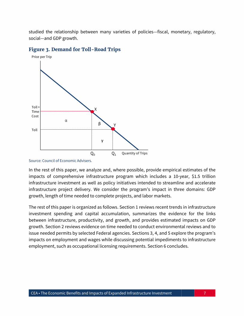
To illustrate some of these issues, consider Figure 3 below, which depicts the demand for
motor vehicle trips along a certain toll road. Trip price includes the toll plus the value of time
spent making the trip. Drivers choose to make Q0 trips, given initial values for the toll and the
time needed to drive the segment; this corresponds to point X on the demand schedule. Now
consider the value of some unspecified infrastructure improvement or expansion that
decreases the time needed to make the trip, and hence decreases the time cost facing
motorists. For simplicity, we assume that the time needed to travel drops to 0. Motorists will
respond to the decrease in total price per trip by increasing the number of trips made on the
toll road, from Q0 to Q1, corresponding to point Y. Motorists experience gains in consumer
surplus of α + β, where the first term, α, represents the increase in consumer surplus
experienced by motorists who previously chose to drive on that road segment (because they
now spend less time making their original number of trips), and the second term, β, represents
the consumer surplus experienced by motorists who now take additional trips on the road. Toll
revenues rise by γ, as more trips are now taken along the road. Thus, overall surplus, or social
welfare, has risen by α + β + γ, but any market-based measure, such as GDP, would include only
γ, the value of additional toll revenues.
This example illustrates the limitations of using transactions-based measures to trace the
effects of infrastructure investments. In the current example, area γ understates the true
welfare improvements coming from the project because it excludes consumer surplus
experienced by motorists.
Furthermore, while assessing benefits may be relatively straightforward for a specific asset or
project such as a toll road, doing so for an overall infrastructure investment program as a whole
is more difficult. Thus, economists often consider the relationship between infrastructure and
productivity or output, commonly measured by GDP. GDP’s limitations as a measure of
economic progress or well-being have been discussed at length elsewhere, and we simply note
here that GDP captures market transactions only, excludes household-based activities, and
fails to account for unpriced positive or negative externalities or for environmental
degradation. Despite its limitations as a measure of overall economic welfare or progress, GDP
offers a meaningful measure of an economy’s productive activities, and economists have long
CEA • The Economic Benefits and Impacts of Expanded Infrastructure Investment 7
studied the relationship between many varieties of policies—fiscal, monetary, regulatory,
social—and GDP growth.
Figure 3. Demand for Toll-Road Trips
Source: Council of Economic Advisers.
In the rest of this paper, we analyze and, where possible, provide empirical estimates of the
impacts of comprehensive infrastructure program which includes a 10-year, $1.5 trillion
infrastructure investment as well as policy initiatives intended to streamline and accelerate
infrastructure project delivery. We consider the program’s impact in three domains: GDP
growth, length of time needed to complete projects, and labor markets.
The rest of this paper is organized as follows. Section 1 reviews recent trends in infrastructure
investment spending and capital accumulation, summarizes the evidence for the links
between infrastructure, productivity, and growth, and provides estimated impacts on GDP
growth. Section 2 reviews evidence on time needed to conduct environmental reviews and to
issue needed permits by selected Federal agencies. Sections 3, 4, and 5 explore the program’s
impacts on employment and wages while discussing potential impediments to infrastructure
employment, such as occupational licensing requirements. Section 6 concludes.
Price per Trip
Quantity of Trips
α
γ
β
X
Y
Q0 Q1
Toll +
Time Cost
Toll

CEA • The Economic Benefits and Impacts of Expanded Infrastructure Investment 8
1. Infrastructure, Productivity, and Growth
A. How Public Sector Capital Affects Productivity and GDP Growth
An increased stock of public sector capital would mean increased flows of capital services
available to the economy’s workers, fueling GDP growth through at least two channels.1 First,
by raising the productivity of other factors of production (labor, private capital, and land),
increased public capital services encourage firms to increase their own investments and
expand economic activity. This indirect, or “crowding in,” effect has been identified in
numerous studies (e.g., Aschauer 1989; Abiad et al. 2016). A second, direct effect works through
increases in public capital services per employee hour, or public capital deepening, which
typically accounts for between 0.05 and 0.20 percentage point of growth in labor productivity—
not nearly as large as the impact of private sector capital accumulation, but nonetheless
important.2 Since 2007, public capital deepening has accounted for 0.15 percentage point of
the 1.2 percent growth in labor productivity (Figure 4). Although higher than the measured
values between 1973 and 2007, the contribution of public capital after 2007 is lower than the
measure from years prior to 1973.
Increasing infrastructure investment can generate additional economic output, but the
quantitative relationship will depend on many factors, including the responsiveness of output
to increases in public capital (the elasticity of output with respect to public sector capital), the
economy’s initial level of capital intensity, depreciation rates, how quickly assets can be
installed and brought into productive service, and even how the investments are financed.
Estimates of the marginal product of public sector capital vary. CBO (2016) estimates the real
marginal product at about 8 percent, while in 2016, CEA’s estimate was about 14 percent (CEA
2016a). Our updated preferred estimate is 12.9 percent, based on Bom and Ligthart’s (2014)
output elasticity estimate of 0.083 and current levels of public sector capital intensity (the ratio
1 In this analysis, we use the terms “infrastructure” and “public sector capital stock” interchangeably. In fact, a
sizeable share of infrastructure in the energy and communications sectors is privately owned. The research
findings referenced below focus on publicly owned capital stock, but, where appropriate, CEA applies those
findings to privately owned infrastructure assets as well. 2 Recall that labor productivity growth comes from growth in capital deepening, or the amount of private capital
services per labor input; growth in the skills of workers—often called a labor composition effect—and increased
overall efficiency, calculated as a residual and called total factor productivity. Historically, in the United States,
capital deepening has driven a significant share of labor productivity growth, though with a marked slowdown in
the post–Great Recession period. From 1953 to 2010, capital deepening accounted for more than 0.9 percentage
point of that era’s 2.2 percent labor productivity growth, but actually detracted from productivity growth from
2010 to 2015.

CEA • The Economic Benefits and Impacts of Expanded Infrastructure Investment 9
of nondefense public fixed assets to annual nominal GDP was .645 in 2016; hence the estimated
marginal product is 100 x (.083/.645)=12.9 percent).3
Figure 4. The Contribution of Public Capital to Productivity Growth, 1947–2016 (Percentage Points)
Sources: Bureau of Economic Analysis; Bureau of Labor Statistics; CEA calculations.
Applying CBO’s more conservative estimate of 8 percent, $100 billion in new public capital
stock would raise the level of annual GDP by $8.0 billion, while under CEA’s 12.9 percent
preferred estimate, the GDP increase would be $12.9 billion, or about 0.07 percent of GDP. This
additional capital stock would continue to generate additional GDP over time, though at a
decreasing rate because of depreciation of the installed public capital assets.
These calculations convert the stock of public sector capital, not annual infrastructure
spending, into estimated increases in output. The complete timeline and output implications
of increased infrastructure spending will depend on the timing of conceiving and constructing
infrastructure assets and bringing those assets into productive service, as well as the method
of financing the program and the depreciation rate of installed assets. Furthermore, an
increase in investment funds from the Federal government could lead to reductions in
resources provided by states and local governments if Federal money serves to crowd out
nonfederal support.
3Mathematically, the output elasticity equals the (marginal product of public capital) x (public sector capital
intensity), or ε= (dQ/dK)(K/Q); therefore, dividing both sides by the capital intensity yields (dQ/dK)= ε/((K/Q)).
2.80
1.44
2.67
1.19
0.18 0.10 0.060.15
0.0
1.0
2.0
3.0
1947–1973 1973–1995 1995–2007 2007–2016
Labor Productivity Growth Contribution of Public Capital (PP)

CEA • The Economic Benefits and Impacts of Expanded Infrastructure Investment 10
B. Evaluating a Program of Sustained Additional Infrastructure Investment
CEA has estimated the GDP impacts of a sustained $1.5 trillion infrastructure program spread
out over 10 years. Such a program would rely on Federal, State, and local government and
private sector resources to support increased investment in infrastructure. CEA assumes that
the full program would include $200 billion in Federal resources, matched by $1.3 trillion in
nonfederal resources coming from States and localities and the private sector, bringing the 10-
year total to $1.5 trillion.4 CEA uses a partial equilibrium model to estimate GDP impacts
relative to baseline under a range of parameter assumptions and different timing paths for the
infrastructure investments.5 CEA’s general approach was to use conservative parameter values
to avoid overstating impacts throughout.
In the short run, additional infrastructure spending may affect GDP in the year in which the
spending occurs, generating direct and possibly indirect (“multiplied”) effects on GDP. If the
increased spending is offset by equivalent increases in taxes or declines in spending, then these
short-run effects would likely be nil. However, to the extent that additional spending is
financed via increased deficits and the economy is below full employment, the infrastructure
spending here would represent net additions to government spending and could therefore
generate direct short-term spending impacts, which could then be amplified or diminished by
subsequent indirect impacts. In general, the sign and magnitude of these “fiscal multipliers”
remains a topic of active research, and recent evidence suggests that spending multipliers
exceed zero, meaning that the net impact of additional government spending is positive
(Auerbach and Gorodnichenko 2012; Ramey and Zubairy 2017). Auerbach and Gorodnichenko
find that these multipliers are larger during recessions, while Ramey and Zubairy find no
evidence that multipliers are higher during periods of slack. Abiad et al. (2014, 2016) find that
increased infrastructure spending, during recessions in particular, can raise GDP through
demand-side multiplier relationships.
In the long run, public capital deepening raises labor productivity and real output, driven by
the marginal product of public capital estimates discussed above. However, long-run impacts
may be attenuated by several factors. If the additional infrastructure investment spending is
financed purely by debt, then we may expect some “crowding out” to occur as interest rates
4The assumed timing of the investments over the 10 year period is based on Table S-2 from President Trump’s
proposed FY 2019 budget (https://www.whitehouse.gov/wp-content/uploads/2018/02/budget-fy2019.pdf).
Contributions from States and localities are assumed to be offset by tax or other revenue increases. 5 In large part, CEA’s analysis of the program is scalable, so that a larger or smaller program with a similar timing
profile would be expected to generate proportionally larger or smaller impacts on GDP. However, a significant
change in nonfederal resources may affect interest rates and crowding out, since States and localities typically
rely more heavily on budget-neutral funding plans for infrastructure.

CEA • The Economic Benefits and Impacts of Expanded Infrastructure Investment 11
rise and some amount of private sector spending, particularly fixed investment spending, is
curtailed.
Another potentially important factor affecting the output impacts of an infrastructure
investment program is the response of States and local governments to an infusion of
additional Federal funds for infrastructure investment. Such an increase could lead to
reductions in resources provided by States and local governments if Federal money serves to
crowd out nonfederal support. Note that even if the additional Federal funding takes the form
of matching grants, this “crowding out” effect can still occur if grant recipients are already
spending well in excess of their previously required matching funds. Under these
circumstances, recipients treat the additional grant funding as a simple increase in income and
may then choose to both increase overall spending on the target infrastructure assets and
decrease their own resources directed to those investments. State and local governments’
responses to additional Federal spending matter, because they are critical partners with the
Federal government, owning more than $6 of public infrastructure for every $1 of nondefense
capital stock owned by the Federal government.
Empirical evidence for the sign and size of this state and local crowding out effect is mixed. The
CBO estimates this crowding out effect at about one-third, implying that any sustained
increase in Federal funding of infrastructure would be offset by sizable displacement of
previous State and local government effort. In practice, the extent of displacement will be
driven by the details of specific legislative and funding proposals and how States and local
governments respond to the new programs and opportunities. However, the largest of the
programs within the President’s Infrastructure Plan, the Incentives program, has potential to
have minimal displacement effects. The program’s primary grant selection criterion is the
amount of new non-Federal revenue raised by the applicant for infrastructure investment,
providing a matching grant of up to 20 percent of such revenue.
Given these factors, we can estimate the long-run supply-side effects of a debt-financed, $1.5
trillion investment program. The CEA’s analysis of several different models indicates that these
supply-side effects would cumulatively add 0.2 to 0.4 percent to the level of real GDP over 10
years, depending on the marginal productivity of public capital. Further, depending on timing,
the extent of possible crowding out or, conversely, multiplier effects, and the marginal product
of public capital, CEA estimates the 10 year, $1.5 trillion infrastructure investment program
discussed above would add an average of 0.1 to 0.2 percentage point to annual growth in real
GDP. If investment is front-loaded, there is no crowding out, the fiscal multiplier is consistent
with Zandi (2012), and the marginal product of public capital is as reported in the 2016
Economic Report of the President (CEA 2016), we expect the average annual contribution to be
at the upper end of that range. With crowding out, no multiplier, and assuming the CBO

CEA • The Economic Benefits and Impacts of Expanded Infrastructure Investment 12
estimate of the marginal product of public capital, we expect the contribution to growth
instead to be closer to 0.1.
C. Using Existing Assets Efficiently
CEA also notes that getting the greatest possible impact of an infrastructure investment
program will depend on how we allocate our existing assets. When our existing roads,
waterways, and airports are crowded, for example, using time-varying prices or tolls to govern
access can increase efficiency and, in some cases, raise revenues needed to pay for operations
and maintenance of these assets as well. Time-varying tolls would encourage only users with
high valuations to use highly congested infrastructure assets during peak demand times,
improving efficiency.
The recent introduction of dynamic tolling along Interstate 66 in Northern Virginia offers an
example of how congestion pricing can improve travel times and raise revenues for
transportation projects. Preliminary figures from the Virginia Department of Transportation
indicate that morning rush-hour tolls averaged between $8.20 and $12.87 for the 10-mile
segment but that peak tolls reached $40.00 for a short time. Further, travel speeds in the tolled
lanes were far higher than during a comparable period a year earlier, and travel speed in the
non-tolled lanes as well as parallel roadways were similar or improved.
While efficiency (or surplus) is enhanced by such policies, it is possible that congestion pricing
may make some drivers worse off, particularly low-income drivers who may be priced out of
the tolled lanes (CBO 2009). Using toll revenues to improve other travel options, particularly
transit, can counteract this distributional effect, but most discussions of congestion pricing
acknowledge its potential to create both winners and losers from the policy. Even so, the lack
of appropriate congestion pricing mechanisms creates winners and losers as well, and some
evidence suggests that at least some low-income drivers in practice find tolled lanes worth
paying for (Federal Highway Administration, n.d.).
More evidence on distributional effects comes from studies of California’s State Route 91 tolled
express lanes, which show that at any given time about 25 percent of the vehicles in toll lanes
belong to high-income individuals, while the remaining 75 percent are low and middle-income
commuters. Based on research conducted by the state of California, pricing schemes do not
necessarily disadvantage low-income individuals. Assessments of State Route 91 has found
that low-income drivers do use express lanes and are as likely to endorse the use of express
lanes as drivers with higher incomes. As a matter of fact, over half of commuters with
household incomes under $25,000 a year approved of providing toll lanes (Department of
Transportation, 2000).
Furthermore, Hall (2015) shows that congestion pricing can be Pareto-improving, not just
potentially Pareto-improving, especially under conditions of bottleneck congestion, which

CEA • The Economic Benefits and Impacts of Expanded Infrastructure Investment 13
occurs when the number of vehicles that can use the road per unit of time (its “throughput”)
decreases. Bottleneck congestion occurs when traffic backs up at an exit ramp, slowing down
through traffic on the roadway. Tolling a portion of the highway’s lanes (value pricing) serves
to internalize both motorist travel time externalities as well as these bottleneck effects, raising
speeds on both the tolled and nontolled highway segments. When drivers differ in terms of
income and valuations of their time, partial time-varying tolls will raise welfare for drivers
along both the tolled and nontolled segments as long as high-income drivers use the highway
during rush hour. Under the policy, drivers “sort” into the road segments and are better off,
even before accounting for how toll revenues are spent.
A different variation on congestion pricing comes from San Francisco, which in 2011
established a pilot program, SFpark, in which 25 percent of city-controlled parking spaces had
parking rates that varied as demand for parking changed over time. This demand-responsive
pricing structure was intended to increase parking availability and decrease congestion due to
drivers “circling the block” to find a parking space. An early project evaluation of the pilot
(SFMTA 2014) found that the amount of time in which parking occupancy rates hit the target
range of 60 to 80 percent rose 31 percent in pilot areas, compared with an increase of only 6
percent in control areas. Further, the amount of time in which blocks had 90 to 100 percent
occupancy, so were “too full” to accommodate new arrivals, decreased 16 percent in pilot
neighborhoods, while increasing 51 percent in control areas. The project evaluation also
reported that greenhouse emissions decreased, traffic speed improved, and net parking
revenues rose slightly. Even sales taxes grew more in pilot areas compared with controls,
though the study could not rule out the difference was due to other factors distinguishing pilot
from control areas. After continued experimentation with this approach, the city has now
implemented dynamic pricing city wide, so that rates on all city-controlled parking spaces will
vary based on demand.
Finally, CEA notes that congestion or “peak load” pricing has long been successfully used by
public transit systems in many cities across the United States, and other infrastructure assets
offer plentiful opportunities to implement similar pricing structures. For example, the FAA
issued a proposed rule in 2015 which would have established a secondary market for airport
landing slots at Kennedy, LaGuardia, and Newark airports, though withdrew the proposal in
2016. Under the proposed rule, carriers would have been allowed to buy, sell, lease, and trade
slots.
On balance, these examples suggest that using time-varying prices to allocate access to scarce
public assets—such as roads, on-street parking spaces, or landing slots at airports—can have
positive impacts on welfare and economic activity and would make any given infrastructure
investment program that much more productive.

CEA • The Economic Benefits and Impacts of Expanded Infrastructure Investment 14
2. Regulatory and Environmental Review Processes
Complaints and concerns about conflicting, unduly complex, and uncoordinated rules and
regulations governing infrastructure investment have been expressed by many observers.
Implementing a more efficient and streamlined regulatory and environmental review process
can speed up the benefits of that improved infrastructure in terms of time savings, health
benefits, and business activity. Howard (2015) estimates that the costs of six-year long delays
in getting infrastructure projects completed costs the American economy $3.7 trillion, and the
ASCE (2016) estimated that failure to bring the nation’s infrastructure to a state of good repair
would impose GDP losses of almost $4 trillion in GDP by 2025, as business costs rise,
productivity falls, and employment and disposable incomes fall as well.
Lengthy project completion times, whether planned or not, can result in increased
construction costs, additional financing costs, and other business costs. However, the key
costs associated with lengthy project completion times come in the form of delayed enjoyment
of the benefits or value that the infrastructure would have provided had it been brought into
service sooner. These delayed benefits can include time savings, fuel cost savings, health
benefits, shipping costs—any number of positive impacts whose receipt is delayed. Consider a
project that delivers $X in benefits in perpetuity starting in year 0; that project’s present value
is $X(1 + 1/r), where r is the discount rate. A delay of one year in the project means benefits are
not realized until year 1, lowering the present value to $X/r. The difference in those present
values, $X, represents the cost of the one year delay.
In this example, the value of reducing the time needed for project completion depends on the
underlying present value of benefits generated by the project; the reduction in completion
time; and the discount rate. For example, as detailed further below, the average time needed
to complete a final Environmental Impact Statement (EIS) has risen and now exceeds 5 years.
Reducing the average time from 5 years to 2, 3, or even 4 years would add value, as benefits are
received earlier than under the status quo. Continuing our simple example, Figure 5 shows that
reducing the time needed for project completion from 5 years to 2 years generates an 8.0
percent increase in value at a 3 percent discount rate, but a 19.2 percent in value at a 9 percent
discount rate. At higher discount rates, the delay in receiving benefits is very costly in present
value terms.
In the rest of this section, we discuss Federal regulatory review requirements and processes
and present recent estimates of the length of time needed for some of these processes. The
limited evidence available suggests that permitting and review processes are taking
increasingly long periods of time to complete, extending the length of time between the start
of a project and its completion. CEA notes that several recent Federal actions have begun to
move in this direction, including President Trump’s August 15, 2017, Executive Order 13807 to
reduce unnecessary delays and barriers to infrastructure investment.

CEA • The Economic Benefits and Impacts of Expanded Infrastructure Investment 15
Figure 5. Value of Reducing Time to Completion from Current Levels (Percent of Project’s Present Value)
A. The Infrastructure Investment Process
It is important to note that Federal regulatory requirements are complex and often include the
need for project sponsors to apply for and receive one or more permits in order to move
forward with a project. State and local governments also establish and enforce their own
regulatory requirements, so there is no “one source” of regulatory authority and no “one type”
of environmental review. That said, GAO (2014) describes the basic process by which Federal
agencies meet their obligations under the National Environmental Protection Act (NEPA),
depicted in Figure 6 below.
The Federal environmental process for infrastructure projects typically involve multiple
Federal agencies For instance, with respect to a highway project using Federal grant funds
made available from the Federal Highway Administration (FHWA), the FHWA, as the primary
funding agency, would have to comply with NEPA by analyzing the environmental impacts of
the project and issuing the appropriate NEPA decision through a categorical exclusion
determination, finding of no significant impact, or record of decision. However, depending on
the impacts of the project, other agencies may have to issue permits in order for the project to
be fully authorized under Federal law, and each of those determinations would also be subject
to a NEPA reviewby that agency. Also, if the project involves funding from any other agencies,
then those agencies must also comply with NEPA. As such, the full federal environmental and
Years to Completion Source: CEA calculations.
0
2
4
6
8
10
12
14
16
18
20
2 3 4
3 Percent
5 Percent
7 Percent
9 Percent

CEA • The Economic Benefits and Impacts of Expanded Infrastructure Investment 16
permitting process for infrastructure projects involves many activities, studies and processes
that occur prior to the initiation of one agency’s NEPA process and continue after that agency’s
NEPA process has concluded—meaning that the overall time needed for project completion
exceeds the time needed to complete the NEPA process. The NEPA process is overseen by the
Council on Environmental Quality (CEQ), part of the Executive Office of the President.
Figure 6. Process for Implementing National Environmental Policy Act Requirements
Source: U.S. Government Accountability Office.
In brief, NEPA requires that Federal agencies evaluate the potentially significant environmental
impacts of proposed projects, with requirements to consider ecological, aesthetic, historic,
cultural, economic, social, and health effects (GAO 2014, p. 3). The initial step is typically to
determine whether a Categorical Exclusion (CE) applies, in which case no further analysis is
needed. If a CE does not apply, then the lead agency must complete either an Environmental
Assessment (EA) or an Environmental Impact Statement (EIS). If an EA is conducted and an
agency determines that the proposed project would have no significant impact (“Finding of No
Significant Impact”, or “FONSI”), the review process is complete. If, however, the agency
determines that there may be significant potential effects, then the agency must prepare the
more thorough EIS, which typically include a draft EIS, which is published and is used to solicit
comments and input from relevant stakeholders, followed by a final EIS. Agencies can skip the
EA and move directly to EIS.
Finding of No Significant Impact
Environmental Impact Statement
Categorical Exclusion
Environmental Assessment
Does A Categorical
Exclusion Exist for the
Proposed Action?
Are Potential
Environmental
Effects Significant?
Are There
Extraordinary
Circumstances?
Are Potential
Environmental
Effects Significant?
Proposed Action
(e.g., Road Maintenance)
No
Yes
YesNo
Yes
Unknown
Yes or
Maybe
No

CEA • The Economic Benefits and Impacts of Expanded Infrastructure Investment 17
In practice, little systematic data are available on the number and varieties of analyses
undertaken by Federal agencies under NEPA. According to the GAO (2014, p. 7):
“Government-wide data on the number and type of most NEPA analyses are not readily
available, as data collection efforts vary by agency….Agencies do not routinely track
the number of EAs or CEs, but CEQ estimates that EAs and CEs comprise most NEPA
analyses. EPA publishes and maintains government-wide information on EISs.”
Specifically, CEQ estimates that about 95 percent of NEPA analyses are CEs, less than 5 percent
are EAs, and less than 1 percent are EISs. In other words, by far the greatest share of proposed
projects are not subject to extensive and exhaustive reviews likely to take significant resources
and time to conduct. As a share of project dollars, however, EAs and EISs may be more
important, as larger projects are, other things equal, more likely to generate significant
impacts relevant under NEPA.
Conducting the required analyses and preparing these reviews can be costly and take many
years (GAO 2014; NAEP 2016), but limited specific data are available. GAO (2014, p. 15) reports
some agency-specific figures: for example, the average (median) time needed to complete EAs
by the Department of Energy was 13 (11) months in the 12 months ending March 31, 2013, and
the Forest Service took an average of about 18 months to complete its 501 EAs in fiscal year
2012. Completing CE determinations may take significantly less time than EAs, with reported
figures ranging from 1 or 2 days (Department of the Interior’s Office of Surface Mining) to nearly
180 days (Forest Service).
While CEs and some EAs may be straightforward and take little time to conduct, the average
number of years needed to complete a Final Environmental Impact Statement (EIS) has risen
over time, reaching 5.1 years in 2016, up from 4.7 years in 2014 (NAEP 2016). In 2016, almost 45
percent of all final EIS issued that year had taken five or more years to complete (from the date
of Notice of Intent to the date on which the final EIS was issued) (Figure 7).
Some additional data on length of time needed for environmental reviews comes from the
Federal Highway Administration (FHWA) and the GAO (2014, p. 10), which reported that
complex and expensive highway projects are likely to require EIS, with a median completion
time of over 7 years. EAs take less time to complete, ranging from 14 to 41 months, and CEs can
be done even more quickly, averaging 6 to 8 months. The FHWA estimated that in 2009, most
(96 percent) federal-aid highway projects required only a CE, with EAs and EISs accounting for
3 percent and 1 percent of projects, respectively. However, as mentioned above, the share of
projects by dollar value requiring an EIS would likely be significantly higher than 96 percent.
FHWA (2012) reports that CEs comprised between 90 and 90 percent of NEPA decisions, based
on a 2012 survey of 522 agencies regarding NEPA actions since 2005.

CEA • The Economic Benefits and Impacts of Expanded Infrastructure Investment 18
Figure 7. Years from Notice of Intent to Final EIS, 1997–2016 (Percent)
Years
Sources: National Association of Environmental Professionals, Annual NEPA Report, 2015, 2016; CEA
calculations.
B. Permitting Requirements
One specific and common project need is to obtain a permit from the U.S. Army Corps of
Engineers under Section 404 of the Clean Water Act. Ulibarri’s (2016) preliminary study of a
sample of permits for projects in California finds that the average number of days for a permit
decision is 427, with a median value of 314. That study also found that projects requiring
multiple permits did not experience increases in time needed for a decision, but projects
requiring consultation under Section 7 of the Endangered Species Act did, in fact, see an
increase in the number of days needed for the USACE’s permitting decision. Projects proposed
by public agencies (state or federal government) were also more likely to receive permits
quickly relative to a business or nonprofit organization.
Environmental reviews and studies take time to conduct, and project sponsors know this,
hence plan accordingly when assembling a project timeline. However, delays can and do
happen, though such delays are not always due to permitting problems. For example, one
recent industry study of highway projects in Texas between January 2012 and March 2014
(Beaty et al. 2016) found that environmental clearance problems accounted for 14.2 percent of
projects in the pre-construction phase; this compares with 10.7 percent of projects delayed for
funding problems. The authors reviewed 282 delayed projects and reported that projects with
0%
10%
20%
30%
40%
50%
0 to 1 1 to 2 2 to 3 3 to 4 4 to 5 5 or more
Average, 1997-2014 2015 2016
Years

CEA • The Economic Benefits and Impacts of Expanded Infrastructure Investment 19
environmental clearance delays at the district level had average delays of 243 days, or 8.1
months, but a median of only 4.5 months.
The energy sector also offers multiple examples of projects for which permitting and
environmental review concerns and potential delays are salient. Firms wishing to build
pipelines for natural gas must submit applications to the Federal Energy Regulatory
Commission (FERC). Data on such applications suggests that the time needed to approve such
applications has increased over time: applications approved in 2007-2010 took at an average
of 299 days to approve; by 2011-2014, that average had risen to 348 days; and over the 2015-
2017 period, rose even further to 380 (Figure 8).
Figure 8. Time for Pipeline Permit Approval, by Period of Initial Filing, 2007–2017 (Average Days from Application Date to Permit Issue)
Source: Federal Energy Regulatory Commission, Pipeline Approvals, CEA calculations.
These figures do not reflect applications that have been filed but are still open, or pending.
FERC’s data indicate that 65 permit applications were filed in calendar year 2015; of those 65,
49 had been approved by October 31, 2017, while the remaining 16 remained under review.
Using the Kaplan-Meier nonparametric estimate of survival time in the presence of censoring,
we estimate the median number of days until approval to be 472 days, meaning that half of all
applications have been approved by then.
While many factors likely affect the time needed to consider and ultimately approve a given
pipeline permit, one factor may be the number of different jurisdictions affected by the
proposed project. The FERC data indicate whether a proposed project crosses state
0
100
200
300
400
2007-2010 2011-2014 2015-2017

CEA • The Economic Benefits and Impacts of Expanded Infrastructure Investment 20
boundaries, and in fact, we find that interstate projects do have significantly longer approval
times. Figure 9 below shows the estimated cumulative probability of approval over time
functions for interstate projects (N = 28) and within-state projects (N = 37), and a log-rank test
of the hypothesis that the two groups have the same survival function (cumulative probability
of approval) suggests the difference is statistically significant at the .05 significance level.
Figure 9. Kaplan-Meier Estimated Probability of Approval for Applications Filed in 2015 (Cumulative Probability of Approval)
Days Elapsed from Initial Filing
We can also use these data to investigate the impact of speeding up permit approval times.
Figure 10 plots the baseline cumulative probability of approval along with alternative paths
based on an exponential decay hazard model fit with constants calibrated to the underlying
FERC data. Speeding up the approval process would lead to more pipeline projects being
brought into service sooner.
We cannot assess the value of speeding up permit approvals in this setting, as we lack
information on size, capacity, revenue or profit generation, or other measures that reflect the
value of bringing these assets into productive service sooner rather than later. Furthermore,
CEA notes that the optimal time needed will reflect a balance between the benefits of speedier
project approval and its potential costs (perhaps arising from a less-thorough or
comprehensive analysis) at the margin. A 30-day increase in time needed for a large, valuable
project may be more costly than a 60-day increase for a smaller, less valuable project. However,
0.00
0.25
0.50
0.75
1.00
0 200 400 600 800 1000
Interstate Pipelines
Non-Interstate Pipelines
Source: Federal Energy Regulatory Commission and CEA calculations.
Note: Data are all pipeline filings submitted to FERC in calendar year 2015.

CEA • The Economic Benefits and Impacts of Expanded Infrastructure Investment 21
Figure 11 below shows the impact of speedier approval times on the number of pipeline-days
in service, which is essentially a quantity measure representing the additional infrastructure
availability gained over a given permitting period due to the improved processing speeds. Over
a 1,000 day horizon, CEA estimates that doubling the speed of the permitting process would
increase total potential capacity of the project available over the period of development period
by 32 percent.
Figure 10. Improvement in Permitting Speed vs. Expected Time to Permit Approval in 2015, by Improvement over Baseline (Cumulative Probability of Approval)
Days Elapsed from Initial Filing
Source: Federal Energy Regulatory Commission.
Note: Data are all pipeline filings submitted to FERC in calendar year 2015 receiving approval by FERC’s latest 2017
review.
On balance, then, CEA’s review of available evidence suggests that the value of reducing
project completion times can be considerable. Streamlining and simplifying the many
environmental and regulatory review processes that affect the ability of investors to start and
complete projects in a timely fashion will mean earlier enjoyment of the benefits those projects
can deliver.
0.00
0.25
0.50
0.75
1.00
1 31 61 91 121
151
181
211
241
271
301
331
361
391
421
451
481
511
541
571
601
631
661
691
721
751
781
811
841
871
901
931
961
991
Baseline 1.25 1.5 1.75 2

CEA • The Economic Benefits and Impacts of Expanded Infrastructure Investment 22
Figure 11. Incremental Number of Pipeline-Days Gained Through Faster Permitting Process, by Improvement over Baseline (Net Days of Functionality Gained over Baseline Permitting Speed)
Days Elapsed from Initial Filing Source: Federal Energy Regulatory Commission.
Note: Data are all pipeline filings submitted to FERC in calendar year 2015.
3. Infrastructure Investment, Employment, and the Labor Market
In addition to raising U.S. productivity and competitiveness, a boost to infrastructure spending
would increase labor demand for workers with infrastructure-related skills, and we discuss the
characteristics of these workers more fully in this section.
A. Impact on Demand for Labor
Increased investment in the country’s infrastructure will result in an increase in the
employment of infrastructure workers. Using the GDP estimates from Section 1B above, we
estimate the change in infrastructure employment resulting from an additional $1.5 trillion
spent on infrastructure over a period of 10 years. Our estimates are based on the increase in
GDP that results from the spending itself, ignoring any employment responses to higher levels
of installed public capital and any employment multipliers to other sectors. The lower bound
of the estimated employment range reflects GDP impacts under the assumption of crowd-out
and the upper bound assumes no crowd-out. In addition to the crowd-out parameters, the net
employment effect of the spending package will also depend on any multipliers, on the
0
20
40
60
80
100
120
140
160
180
200
0 30 60 90 120
150
180
210
240
270
300
330
360
390
420
450
480
510
540
570
600
630
660
690
720
750
780
810
840
870
900
930
960
990
1.25
1.50
1.75
2.00

CEA • The Economic Benefits and Impacts of Expanded Infrastructure Investment 23
available labor supply when the spending is enacted, and on the reduction in economic activity
that accompanies either deficit spending or the revenue generation needed to fund the
investment. Thus, the increase in infrastructure employment estimated below may be
partially, or even fully, offset by job losses elsewhere in the economy, depending on these
effects.
The estimated increase in infrastructure employment is shown in Figure 12 below. Over the 10
year period, we estimate an average infrastructure employment effect of 290,000 to 414,000
jobs, depending on the parameters above. These estimates are an increase relative to the
baseline level of infrastructure employment that would otherwise have occurred, and the
employment effects end when the spending ends after year 10.
Figure 12. Additional Infrastructure Employment in Each Year, Relative to Baseline (Number of Jobs)
Source: CEA calculations.
Expanded infrastructure spending, and the jobs it entails, is likely to disproportionately favor
particular segments of the population. In February 2018, only 4.1 percent of U.S. labor force
participants reported being without a job. But the rate is substantially higher for workers with
less education, a trend that is apparent as far back as the collected series extends (1992).
Although the group with the fewest years of education reached a series low unemployment
rate in 2017, as of December, workers without a high school degree still had unemployment
Years after Start of Infrastructure Project
10-Year Average: 290K
10-Year Average: 414K
0
200
400
600
800
1 2 3 4 5 6 7 8 9 10
Lower Bound Upper Bound

CEA • The Economic Benefits and Impacts of Expanded Infrastructure Investment 24
rates 4.2 percentage points higher than workers with a bachelor’s degree, 6.3 and 2.1 percent,
respectively. Labor force participants with a high school degree but no college work had
unemployment rates of 4.2 percent in that month. Figure 13 shows the unemployment rate by
education level in the United States since 1992, when the series began.
Figure 13. U.S. Unemployment Rate by Education Level, 1992–2017 (Percent)
Source: Bureau of Labor Statistics.
Note: Series begins in January 1992.
B. Characteristics of Infrastructure Workers
To investigate the differential impact of enhanced infrastructure spending on different
educational attainment groups, we define a list of “infrastructure occupations” and provide
worker characteristics for all U.S. labor force participants in these occupations. A version of this
exercise, published in 2015 by Kane and Puentes, identifies a list of Census-defined 4-digit
North American Industry Classification System (NAICS) industry codes that are infrastructure-
related based on their definition of national infrastructure (Kane and Puentes 2015). Their list
includes industries that might benefit indirectly from improved infrastructure (for example,
freight transportation arrangements or rail transportation) but would not experience a direct
increase in economic activity from increased infrastructure spending. We identify a much
narrower list of 4-digit NAICS industry codes that would be the direct beneficiaries of additional
infrastructure spending likely to receive Congressional approval, dubbing these “infrastructure
industries.” The industry codes covered include 4-digit NAICS sectors related to heavy and civil
engineering construction (all sectors falling under NAICS 3-digit code 237000), including utility
Less than High
School
Dec-17
High SchoolSome
College
Bachelor's Degree
or more
0
3
6
9
12
15
18
1992 1997 2002 2007 2012 2017

CEA • The Economic Benefits and Impacts of Expanded Infrastructure Investment 25
system construction along with highway, street, and bridge construction, other specialty trade
contractors (NAICS code 238900), and remediation and other waste management services
(NAICS code 562900), including former industrial site cleanup. We then use National
Employment Matrix data for 2016 from the Bureau of Labor Statistics (BLS) on the occupation
distribution within these industries to define a set of occupations which comprise more than 1
percent of employment in at least one of these industries. The resulting set of 47 occupations
is refined further to exclude management occupations; job tasks for management occupations
are at least somewhat scalable, and employment in these occupations is more likely to be fixed
even under expanded economic activity in infrastructure construction.
The final defined set of “infrastructure occupations,” 31 in total (see Table 1), includes workers
who design and carry out infrastructure projects, including engineers, pipefitters, construction
laborers, etc. But it also includes transportation and warehousing occupations, along with
workers in installation, maintenance, and repair occupations. The list includes occupations for
which infrastructure industries comprise the majority of employment, along with occupations
for which infrastructure industries represent a small proportion of the overall industry
structure of employment.6 For example, both paving, surfacing, and tamping equipment
operators and pipelayers are overwhelmingly employed in the NAICS 3-digit heavy and civil
engineering construction sector, while electricians and plumbers are largely employed
elsewhere (in residential and building construction, for example) but nevertheless are critical
for the successful completion of infrastructure projects. Similarly, our occupation list includes
civil engineers although only a small share of civil engineers are directly employed in the
infrastructure sectors defined above.7 Of course, the set of occupations ultimately affected by
expanded infrastructure investment would depend on the particular set of investments
undertaken in any infrastructure legislative package, and the analysis in this report reflects
current infrastructure employment, not necessarily the footprint of future employment.
In 2016, the infrastructure occupations defined by this algorithm represented 1.2 million
workers in the defined set of infrastructure industries out of a total of 1.7 million workers in
these industries. Economy-wide, 13.8 million workers reported these as primary occupations.
Table 1 contains a list of defined infrastructure occupations and their broad occupation
categories, and Figure 14 shows the distribution of these workers across broad categories.
6 An alternative exercise would define “infrastructure occupations” as those where a majority of employment is in
an infrastructure industry. The conclusions in this report are remarkably similar under this alternative definition.
See also Kane and Puentes (2015), but note that the wage premia calculations in that report do not control for
gender and are, therefore, higher than those presented here. 7 A much larger number are employed in services industries, which would also experience increased demand with
expanded infrastructure. The 4-digit NAICS code encompassing engineering services is architectural, engineering,
and related services. Given this broad set of activities, this 4-digit category was not included in our list of direct
beneficiaries of an infrastructure package; civil engineering establishments are not separately identifiable. Civil
engineers, however, are an infrastructure occupation as defined above.

CEA • The Economic Benefits and Impacts of Expanded Infrastructure Investment 26
Nearly a million infrastructure workers were employed in construction and extraction
occupations in our defined set of infrastructure industries in 2016 while 156,700 hold
transportation and material moving jobs. The remainder are employed in installation,
maintenance and repair, business and financial occupations (in particular, cost estimators),
production, and architecture and engineering jobs.
Table 1. Infrastructure Occupations by Broad Category Installation, Maintenance
and Repair Construction and Extraction Transport and Material Moving
Business and Financial
Operations
First-line supervisors of mechanics, installers, and
repairers
First-line supervisors of construction trades and extraction
workers
Heavy and tractor-trailer truck drivers Cost estimators
Light truck or delivery services drivers
Mobile heavy equipment mechanics, except engines
Carpenters Crane and tower operators
Cement masons and concrete finishers
Excavating and loading machine and dragline operators
Electrical power-line installers and repairers
Construction laborers
Paving, surfacing, and tamping equipment operators
Laborers and freight, stock, and material movers, hand
Telecommunications line installers and repairers
Architecture and
Pile-driver operators Refuse and recyclable material
collectors Engineering
Maintenance and repair workers, general
Operating engineers and other construction equipment operators
Civil engineers
Electricians
Pipelayers
Plumbers, pipefitters, and
steamfitters
Fence erectors
Production Hazardous materials removal workers
Highway maintenance workers Welders, cutters, solderers, and brazers Rail-track laying and maintenance
equipment operators
Septic tank servicers and sewer pipe cleaners
Earth drillers, except oil and gas
Roustabouts, oil and gas
Source: BLS Occupation-Industry Matrix; CEA calculations.
Worker characteristics are obtained from the Current Population Survey (CPS), which provides
demographic information on the American population along with the stated occupation of
both employed and unemployed workers. Using the monthly CPS public use files for 2017 from
Integrated Public Use Microdata Series (IPUMS)-CPS, we compare the demographic
characteristics of labor force participants with infrastructure occupations to those reporting
other occupations in the survey.

CEA • The Economic Benefits and Impacts of Expanded Infrastructure Investment 27
Figure 14. Distribution of 1.2 Million Infrastructure Workers in Infrastructure Industries, 2016
Sources: BLS Occupation-Industry Matrix; CEA calculations.
Note: Job titles reflect 2010 Standard Occupational Classification (SOC) codes. For CPS analysis purposes, these
occupation codes are converted to CPS/Census coding using a crosswalk provided by BLS Office of Occupational
Statistics and Employment Projections.
The education composition of the infrastructure labor force differs notably from the labor force
at large; workers with less education are disproportionately employed in infrastructure
occupations (Figure 15). 62.0 percent of infrastructure workers in 2016 had a high school
degree or less, compared with 32.4 percent of the non-infrastructure labor force. Infrastructure
occupations and non-infrastructure occupations had a similar share of workers with some
college coursework but without a 4-year bachelor’s degree. Correspondingly, the share of
infrastructure occupation workers with a bachelor’s degree in 2017, 10.6 percent, was less than
one-third the rate for non-infrastructure occupation workers, 39.1 percent.
Additional characteristics of infrastructure occupation workers indicate a labor force
comprised mainly of men and with an age distribution similar to the labor force at large (Figure
16). While 49 percent of the U.S. labor force outside of infrastructure occupations is male, 93
percent of infrastructure occupation workers are male. Hispanics are over-represented in the
infrastructure labor force by approximately nine percentage points, while blacks are slightly
under-represented. Both differences are statistically significant. The age distribution is similar
between the infrastructure and non-infrastructure labor forces; the median age for both
groups is 41.
Construction and
Extraction (75.4%)
Transportation
and Material
Moving (12.5%)
Installation,
Maintenance, and
Repair (7.7%)
Business and
Financial Operations
(1.9%)
Production
(1.7%) Architecture and
Engineering (0.7%)

CEA • The Economic Benefits and Impacts of Expanded Infrastructure Investment 28
Figure 15. Educational Attainment, 2017 (Percentage of Labor Force Participants)
Sources: Current Population Survey; CEA calculations.
Figure 16. Gender, Race, Ethnicity, and Age, 2017 (Percentage of Labor Force Participants)
Sources: Current Population Survey; CEA calculations.
Bachelor's Degree or More
Some College
High School, No College
Less than High School
0
20
40
60
80
100
Infrastructure Occupations Non-Infrastructure Occupations
93
25
12
41
49
1613
41
0
25
50
75
100
Share Male Share Hispanic/Latino Share Black Median Age
Infrastructure Occupations Non-Infrastructure Occupations

CEA • The Economic Benefits and Impacts of Expanded Infrastructure Investment 29
C. Pool of Available Infrastructure Workers
To estimate potential worker availability for future infrastructure projects, we begin by
tabulating employment status in the Current Population Survey (CPS) for 2017. The
unemployment rate for experienced workers who reported having an infrastructure
occupation was 6.1 percent compared with 3.8 percent for non-infrastructure experienced
workers last year.8 CPS tabulations indicate that the unemployment rate for infrastructure
workers has been consistently higher than for all labor force participants since at least 2003,
and the gap between the two has averaged 3.4 percent between 2003 and 2017. Still, the
unemployment rate gap in 2017 between infrastructure and non-infrastructure workers was
somewhat larger than the gap in each year between 2005 and 2007 when the aggregate
unemployment rate had reached the lowest levels of the post-2001 business cycle. The
difference in unemployment rates between infrastructure and non-infrastructure labor force
participants in 2017, 2.3 percentage points, implies an excess supply of nearly 350,000
infrastructure workers who are not employed but are currently looking for a job. In other
words, if infrastructure labor force participants had the unemployment rate of their non-
infrastructure counterparts, nearly 350,000 additional infrastructure workers would be
employed.
However, these 350,000 infrastructure workers may not be sufficient to meet the increased
labor demand arising from an ambitious infrastructure investment program. Some of these
workers are temporarily unemployed while on layoff from a quasi-steady job. Further, the
geography and skill mix of these workers may not match the needs of expanded infrastructure
activity. Thus, there may be a need to retrain unemployed workers previously employed in
other sectors, new labor market entrants, and current labor force non-participants for careers
in infrastructure occupations. The latter group, consisting of individuals who have dropped out
of the labor force altogether, may be of special interest. Although labor market non-
participation is multi-causal, declining demand for lower-skilled workers is frequently
assigned some of the blame (CEA 2016b). Heightened demand for workers with less education,
and the associated increase in wages, may draw additional workers into the labor force,
particularly prime-aged men, whose recent labor force participation weakness has been
dubbed the problem of the “missing” men.
In order to bridge the gap between the set of potential workers, including those currently in
and out of the labor force, and the skill needs of infrastructure projects, the Federal
government could reconsider the current restrictions on Pell Grant eligibility. These grants,
8 The crosswalk from SOC codes in the National Employment Matrix to occupation codes in the CPS files is not perfect, and the
translation results in an over-definition of infrastructure occupations in the CPS due to aggregation of occupations in the CPS
occupation codes. As a result, for 2016, we identify 14.9 million infrastructure workers in the CPS files compared to 13.8 million
in the National Employment Matrix. The demographic characteristics and earnings premia presented in this report reflect the
characteristics of this broader group.

CEA • The Economic Benefits and Impacts of Expanded Infrastructure Investment 30
which are generally only available to students without a bachelor’s degree and who are
enrolled in programs with more than 600 clock hours of instruction over 15 weeks, do not
provide support to workers who require shorter-term investments, as some infrastructure jobs
would require. (See Section 5 for further discussion of licensing and credentialing in
infrastructure occupations.) Workforce Innovation and Opportunity Act funds can be used for
these short-term programs, but funds from this program are not dedicated to this purpose and
are therefore subject to competing priorities. Although it would require Congressional
approval, expanding Pell Grant eligibility to include investments in short-term training (or
retraining) programs would help ensure workers are not kept from infrastructure work due to
financial constraints.
4. The Wage Premium for Infrastructure Workers
Labor markets tend to reward educational attainment; bachelor’s degree holders have higher
wages than workers with some college who, in turn, out-earn high school degree holders, on
average. But there are other paths to higher wages other than formal education. For workers
with fewer years of schooling, the skilled trades occupations needed in infrastructure work are
one of those paths. To see this, we estimate an “earnings premium,” the additional income
earned in infrastructure relative to non-infrastructure occupations, given a worker’s sex, race,
and age. These premia are measured separately for workers with a high school degree or less
(“No College”), for workers with some college degree but no bachelor’s degree (“Some
College”) and for those with a bachelor’s degree, and we measure the premium at the 25th, 50th,
and 75th percentile of the education-specific income distribution.
We begin by measuring hourly wage premia, the additional per-hour monetary compensation
received by infrastructure workers after accounting for sex, race, age, and education level.
These premia do not reflect any differences in non-monetary compensation, such as
differences in benefits, and do not reflect differences in working conditions. Infrastructure
occupations likely carry a higher risk of physical injury, and those risks are not accounted for
in this exercise.
The results, contained in Figure 17, indicate a wage premium of 12 to 14 percent for
infrastructure workers with a high school degree or less in 2016 and 2017. The premium is
roughly the same across the wage distribution of these workers; at the median, infrastructure
jobs provide a 14.0 percent hourly wage boost to workers in this lowest educational attainment
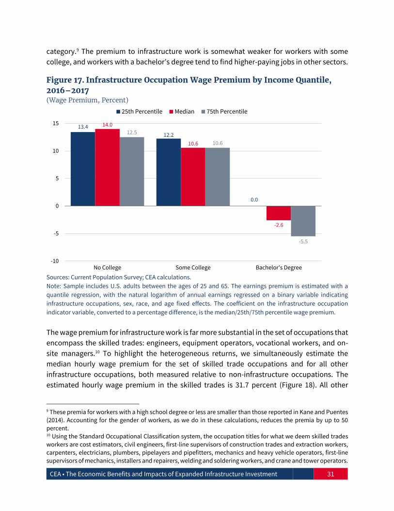
CEA • The Economic Benefits and Impacts of Expanded Infrastructure Investment 31
category.9 The premium to infrastructure work is somewhat weaker for workers with some
college, and workers with a bachelor’s degree tend to find higher-paying jobs in other sectors.
Figure 17. Infrastructure Occupation Wage Premium by Income Quantile, 2016–2017 (Wage Premium, Percent)
Sources: Current Population Survey; CEA calculations. Note: Sample includes U.S. adults between the ages of 25 and 65. The earnings premium is estimated with a
quantile regression, with the natural logarithm of annual earnings regressed on a binary variable indicating
infrastructure occupations, sex, race, and age fixed effects. The coefficient on the infrastructure occupation
indicator variable, converted to a percentage difference, is the median/25th/75th percentile wage premium.
The wage premium for infrastructure work is far more substantial in the set of occupations that
encompass the skilled trades: engineers, equipment operators, vocational workers, and on-
site managers.10 To highlight the heterogeneous returns, we simultaneously estimate the
median hourly wage premium for the set of skilled trade occupations and for all other
infrastructure occupations, both measured relative to non-infrastructure occupations. The
estimated hourly wage premium in the skilled trades is 31.7 percent (Figure 18). All other
9 These premia for workers with a high school degree or less are smaller than those reported in Kane and Puentes
(2014). Accounting for the gender of workers, as we do in these calculations, reduces the premia by up to 50
percent. 10 Using the Standard Occupational Classification system, the occupation titles for what we deem skilled trades
workers are cost estimators, civil engineers, first-line supervisors of construction trades and extraction workers,
carpenters, electricians, plumbers, pipelayers and pipefitters, mechanics and heavy vehicle operators, first-line
supervisors of mechanics, installers and repairers, welding and soldering workers, and crane and tower operators.
13.4
12.2
0.0
14.0
10.6
-2.6
12.5
10.6
-5.5
-10
-5
0
5
10
15
No College Some College Bachelor's Degree
25th Percentile Median 75th Percentile

CEA • The Economic Benefits and Impacts of Expanded Infrastructure Investment 32
infrastructure workers earn a median hourly wage premium of 8.1 percent. Still the premia for
both occupation categories are statistically significant at conventional levels (<1 percent).
Again, each of these estimated median hourly wage premia account for gender, age, and race,
and are only for workers who did not attend college.
Figure 18. Median Earnings Premium for Workers with a High School Degree or Less by Occupation Category, 2016–2017 (Wage Premium, Percent)
Sources: Current Population Survey; CEA calculations. Note: Sample includes U.S. adults between the ages of 25 and 65. The earnings premium is estimated with a
quantile regression, with the natural logarithm of annual earnings regressed on a binary variable indicating
infrastructure occupations, sex, race, and age fixed effects. The coefficient on the occupation indicator variable,
converted to a percentage difference, is the median wage premium.
In 2016, although infrastructure workers put in roughly the same number of hours each week
as the economy-wide average, they worked, on average, one fewer week than other workers,
potentially due to seasonality in work schedules or to weak labor demand. Survey responses
in the CPS regarding the reason for work absences indicate that infrastructure workers were
more than six times as likely to miss a week of work for slack work reasons than for weather.
Further, in 2016, infrastructure workers were more than twice as likely to miss work due to a
layoff, presumably reflecting weak demand, as were non-infrastructure workers.
As a result, infrastructure workers enjoy a smaller annual earnings premium than their hourly
wage premium would indicate. Our estimate of the 2016 median annual earnings premium for
infrastructure workers with a high school degree or less (8.5 percent) is still greater than half
31.7
8.1
0
5
10
15
20
25
30
35
Skilled Trades Workers Other Infrastructure Workers

CEA • The Economic Benefits and Impacts of Expanded Infrastructure Investment 33
the median hourly wage premium in 2016 and 2017 for these workers (14.0 percent, as in figure
17). Given the influence of weak demand on the number of weeks infrastructure workers
worked in 2016, enhanced demand from increased infrastructure spending may serve to even
out the work year for these workers, bringing annual earnings premia more in line with the
premia in hourly wages.11
5. Occupational Licensing
Labor markets for public infrastructure projects are affected by a number of specific rules. First,
workers in infrastructure occupations, much like the U.S. population at large, are frequently
subject to occupational licensing which inhibits the flow of workers across states. Second,
labor agreements and rules for publicly-funded projects, including the Federal Davis-Bacon Act
and its local variants, affect the wages of infrastructure workers and may result in hiring
processes that are skewed towards older, more experienced workers, making projects more
costly. Finally, less-prevalent project labor agreements set the terms of employment between
publicly-funded employers and workers in some states, including workers on Federal, State,
and local projects. In addition to wages and benefits, these agreements may sometimes
include mandates for union participation as a condition of employment on a public
infrastructure project.
One impediment to filling newly created infrastructure jobs is the country’s patchwork set of
occupational licensing requirements. In 2017, 23.8 percent of all U.S. labor force participants
reported having an active professional license or certification, while 21.2 percent of
infrastructure labor force participants reported the same. Civil engineers, electricians, and
pipelayers and plumbers had the highest licensing rate in 2017, with narly 50 percent of
workers in those occupations holding an active professional license or certification. Because
these licenses are largely granted by states (rather than being nationally recognized), licensing
inhibits the free flow of licensed workers across state boundaries to better match labor supply
to labor demand (Johnson and Kleiner 2017). Unless the geographic footprint and skill needs
of expanded infrastructure investments match the geographic distribution of currently
unemployed infrastructure workers, some reshuffling of workers across state lines may be
needed. The Federal government could encourage States to recognize out-of-state
occupational licenses in order to facilitate the movement of labor across state boundaries,
even if the recognition is only temporary. There is precedent for such an initiative; at the behest
11 These results are from the annual CPS-ASEC survey released in March. Data for 2017 are not currently available.
Annual and hourly earnings premia may also differ due to sampling variation between CPS ASEC and monthly
surveys.

CEA • The Economic Benefits and Impacts of Expanded Infrastructure Investment 34
of the Department of Defense, States have recognized occupational licenses issued in other
states for military spouses, who frequently must move across state lines.12
6. Conclusion
This report has described the nation’s infrastructure needs and the value of meeting them. An
ambitious infrastructure investment program is estimated to raise welfare, increase GDP, and
improve labor market opportunities and outcomes particularly for less educated workers.
While the particular structure and details of the infrastructure program ultimately adopted will
affect its subsequent future impacts, CEA believes the program’s overall value will be
considerable.
12 These waivers have been most frequent for teacher licenses, but licensure in healthcare occupations has also
been included in some states.

CEA • The Economic Benefits and Impacts of Expanded Infrastructure Investment 35
References
Abiad, A., Furceri, D., and Topalova, P. 2014. “IMF Survey: The Time is Right for an Infrastructure
Push.” International Monetary Fund: World Economic Outlook.
Abiad, A., Furceri, D., and Topalova, P. 2016. "The Macroeconomic Effects of Public Investment:
Evidence from Advanced Economies." Journal of Macroeconomics 50: 224-240.
Allaire, M., H. Wu, and U. Lall. 2018. “National trends in drinking water quality violations.”
Proceedings of the National Academy of Sciences February 27, 2018. 115 (9) 2078-2083.
American Society of Civil Engineers (ASCE). 2016. “Failure to Act: Closing the Infrastructure
Investment Gap for America’s Economic Future.” American Society of Civil Engineers,
Washington, DC.
American Society of Civil Engineers (ASCE). 2017. “Report Card History.”
Aschauer, D. A. 1989. "Is Public Expenditure Productive?" Journal of Monetary Economics 23(2):
177-200.
Auerbach, A.J. and Gorodnichenko, Y. 2012. “Measuring the Output Responses to Fiscal Policy.”
American Economic Journal 4(2): 1-27.
Beaty, C., Ellis D., Glover B., and Stockton B. 2016. “Assessing the Costs Attributed to Project
Delay During Project Pre-Construction Stages.” Texas A&M Transportation Institute, College
Station, TX.
Bom, P. and Ligthart, J. 2014. “What Have We Learned from Three Decades of Research on the
Productivity of Public Capital?” Journal of Economic Surveys 28(5): 889–916.
Bureau of Economic Analysis (BEA). “Chain-Type Quantity Indexes for Net Stock of Government
Fixed Assets.” National Data, Table 7.2B.
Bureau of Economic Analysis (BEA). “Chain-Type Quantity Indexes for Depreciation of
Government Fixed Assets.” National Data, Table 7.4B.
Bureau of Economic Analysis (BEA). “Current-Cost Average Age at Yearend of Government Fixed
Assets, 1925-1996.” National Data, Table 7.7A.
Bureau of Economic Analysis (BEA). “Current-Cost Average Age at Yearend of Government Fixed
Assets.” National Data, Table 7.7B.

CEA • The Economic Benefits and Impacts of Expanded Infrastructure Investment 36
Bureau of Economic Analysis (BEA). “Current-Cost Depreciation of Government Fixed Assets.”
National Data, Table 7.3B.
Bureau of Economic Analysis (BEA). “Current-Cost Net Stock of Government Fixed Assets, 1925-
1996.” National Data, Table 7.1A.
Bureau of Economic Analysis (BEA). “Current-Cost Net Stock of Government Fixed Assets.”
National Data, Table 7.1B.
Bureau of Economic Analysis (BEA). “Depreciation Estimates.”
Bureau of Economic Analysis (BEA). “Gross Domestic Product.” National Data, Table 1.1.5.
Bureau of Economic Analysis (BEA). “Investment in Government Fixed Assets.” National Data,
Table 7.5B.
Bureau of Economic Analysis (BEA). “Price Indexes for Government Consumption Expenditures
and Gross Investment.” National Data, Table 3.9.4.
Bureau of Labor Statistics (BLS). “Business and Nonfarm Business Sectors – November 2,
2017.” Labor Productivity and Costs.
Bureau of Labor Statistics (BLS). “Deciles of Income Before Taxes: Annual Expenditure Means,
Shares, Standard Errors, and Coefficients of Variation.” Consumer Expenditure Survey, 2016,
Table 1110.
Bureau of Labor Statistics (BLS). “Employment Status of the Civilian Noninstitutional
Population 16 Years and Over, 1982 to date.” Labor Force Statistics from the Current Population
Survey, Table A-1.
Bureau of Labor Statistics (BLS). “Employment Status of the Civilian Noninstitutional
Population 25 Years and Over by Educational Attainment, Seasonally Adjusted.” Labor Force
Statistics from the Current Population Survey, Table A-5.
Bureau of Labor Statistics (BLS). “Industry-Occupation Matrix Data, by Occupation.”
Employment Projections, Table 1.8.
Bureau of Labor Statistics (BLS). “May 2016 Occupation Profiles.” Occupational Employment
Statistics.
Congressional Budget Office (CBO). 2016. “The Macroeconomic and Budgetary Effects of
Federal Investment.”

CEA • The Economic Benefits and Impacts of Expanded Infrastructure Investment 37
Council of Economic Advisers (CEA). 2016a. “Chapter 6: The Economic Benefits of Investing in
U.S. Infrastructure.” Economic Report of the President.
Council of Economic Advisers (CEA). 2016b. “The Long-Term Decline in Prime-Age Male Labor
Force Participation.” Report.
Federal Highway Administration (FHA). 2017. “Urban Partnership Agreement Low-Income
Equity Concerns of U.S. Road Pricing Initiatives.”
Flood, S., King M., Ruggles S., and Warren, J. R. 2017. “Integrated Public Use Microdata Series,
Current Population Survey: Version 5.0.” IPUMS-Current Population Survey.
Howard, Philip K. 2015. “Two Years Not Ten Years: Redesigning Infrastructure Approvals.”
Common good, Brooklyn, NY.
Johnson, J. E. and Kleiner, M. M. 2017. “Is Occupational Licensing a Barrier to Interstate
Migration?” National Bureau of Economic Research.
Kane, J. and Puentes, R. 2015. “Expanding Opportunity through Infrastructure Jobs.”
Brookings Institution.
National Association of Environmental Professionals (NAEP). 2015. “NAEP Annual NEPA
Report—2014.”
National Association of Environmental Professionals (NAEP). 2017. “NAEP Annual NEPA
Report—2016.”
Ramey, V. A. and Zubairy, S. 2017. “Government Spending Multipliers in Good Times and in Bad:
Evidence from U.S. Historical Data.” National Bureau of Economic Research.
San Francisco Municipal Transportation Agency. 2014. “SFpark Pilot Project Evaluation.”
Texas A&M Transportation Institute (TTI). 2015. “Urban Mobility Scorecard 2015.”
Ulibarri, Nicola. 2016. “Streamlining Permitting Processes for Multi-Benefit Water Projects.”
University of California, Irvine, Department of Planning, Policy & Design: Irvine, Californias.
United States Army Corps of Engineers (USACE). “Lock Queue Report.” Lock Performance
Monitoring System.
United States Census Bureau. “Annual Social and Economic Supplement of the Current
Population Survey.”

CEA • The Economic Benefits and Impacts of Expanded Infrastructure Investment 38
United States Department of Defense (DOD). “Defense-State Liaison.”
United States Department of Labor (USDOL). “Davis-Bacon and Related Acts.”
United States Department of Labor (USDOL). 2017. “Dollar Threshold Amount for Contract
Coverage.”
United States Department of Transportation (USDOT). 2000. “Continuation Study to Evaluate
the Impacts of the SR 91 Value-Priced Express Lanes.”
United States Environmental Protection Agency (EPA). “Safe Drinking Water Information
System.” Ground Water and Drinking Water.
United States Environmental Protection Agency (EPA). 2012. “Clean Watersheds Needs Survey
2012.”
United States Environmental Protection Agency (EPA). 2013. “EPA Survey Shows $384 Billion
Needed for Drinking Water Infrastructure by 2030.”
United States Environmental Protection Agency (EPA). 2016. “The Time to Invest in America’s
Water Infrastructure is Now.”
United States Government Accountability Office (GAO). 2011. “Davis-Bacon Act:
Methodological Changes Needed to Improve Wage Survey.”
United States Government Accountability Office (GAO). 2014. “Little Information Exists on
NEPA Analyses.” GAO, GAO-14-370 National Environmental Policy Act.
United States Government Accountability Office (GAO). 2014. “Many Federal and State
Environmental Review Requirements Are Similar, and Little Duplication of Effort Occurs.” GAO,
GAO-15-71 State Highway Reviews.
Zandi, M. 2012. “Bolstering the Economy: Helping American Families by Reauthorizing the
Payroll Tax Cut and UI Benefits.”

ABOUT THE COUNCIL OF ECONOMIC ADVISERS
The Council of Economic Advisers, an agency within the Executive Office of the President, is charged with offering the President objective economic advice on the formulation of both domestic and international economic policy. The Council bases its recommendations and analysis on economic research and empirical evidence, using the best data available to support the President in setting our nation's economic policy.
www.whitehouse.gov/cea
March 2018