economic bulletin - june 2018 - bportugal.pt · sources: statistics portugal and banco de...
TRANSCRIPT

Economic BulletinJune 2018
Lisbon, 2018 • www.bportugal.pt
BANCO PORTUGALDE
E U R O S Y S T E M

Economic Bulletin | June 2018 • Banco de Portugal Av. Almirante Reis, 71 | 1150-012 Lisboa • www.bportugal.pt •
Edition Economics and Research Department • Design Communication and Museum Department | Design Unit
• Print run 25 • ISSN (print) 0872-9786 • ISSN (online) 2182-035X • Legal Deposit no. 241773/06
Contents
I Projections for the Portuguese economy: 2018-2020 | 5
1 Introduction | 7
2 International environment and technical assumptions | 9Box 1 • Projection assumptions | 12
3 Growth factors, demand and external accounts | 14
4 Labour market | 25
5 Prices | 27
6 Uncertainty and risks | 30
7 Conclusions | 32Box 2 • Medium-term fiscal outlook | 33
Box 3 • Recent developments in the market share of Portuguese exports | 38
Box 4 • Inflation developments in Portugal and the euro area: contributions from the procyclical and acyclical components | 43
Box 5 • Macroeconomic impact of a rise in global protectionist tensions | 47
II Special issue | 51
Household consumption inequality in Portugal | 53
III Series | 73
1 Quarterly series for the Portuguese economy: 1977-2017 | 75
2 Annual series on household wealth: 1980-2017 | 76

I Projections for the Portuguese economy:
2018-2020Box 1 Projection assumptions
Box 2 Medium-term fiscal outlook
Box 3 Recent developments in the market share of Portuguese exports
Box 4 Inflation developments in Portugal and the euro area: contributions from
the procyclical and acyclical components
Box 5 Macroeconomic impact of a rise in global protectionist tensions

Intr
oduc
tion
7
1 IntroductionThe projections for the Portu’guese economy presented in this Economic Bulletin indicate ongoing
expansion over the period 2018-20, although at a progressively slower pace. After growth of 2.7%
in 2017, Gross Domestic Product (GDP) should increase by 2.3% in 2018, 1.9% in 2019 and 1.7% in
2020 (Table I.1.1). The growth in 2018 is slightly above that published by the European Central Bank
(ECB) for the euro area as a whole and matches their projection for 2019 and 2020. In 2018, GDP
should recover to its level of before the international financial crisis in 2008 and reach around 5%
above that level in 2020.
Table I.1.1 • Projections of Banco de Portugal for 2018-2020 | Annual rate of change, in percentage
Weights 2017
EB June 2018 Projection March 2018
2017 2018 (p) 2019 (p) 2020 (p) 2017 2018 (p) 2019 (p) 2020 (p)
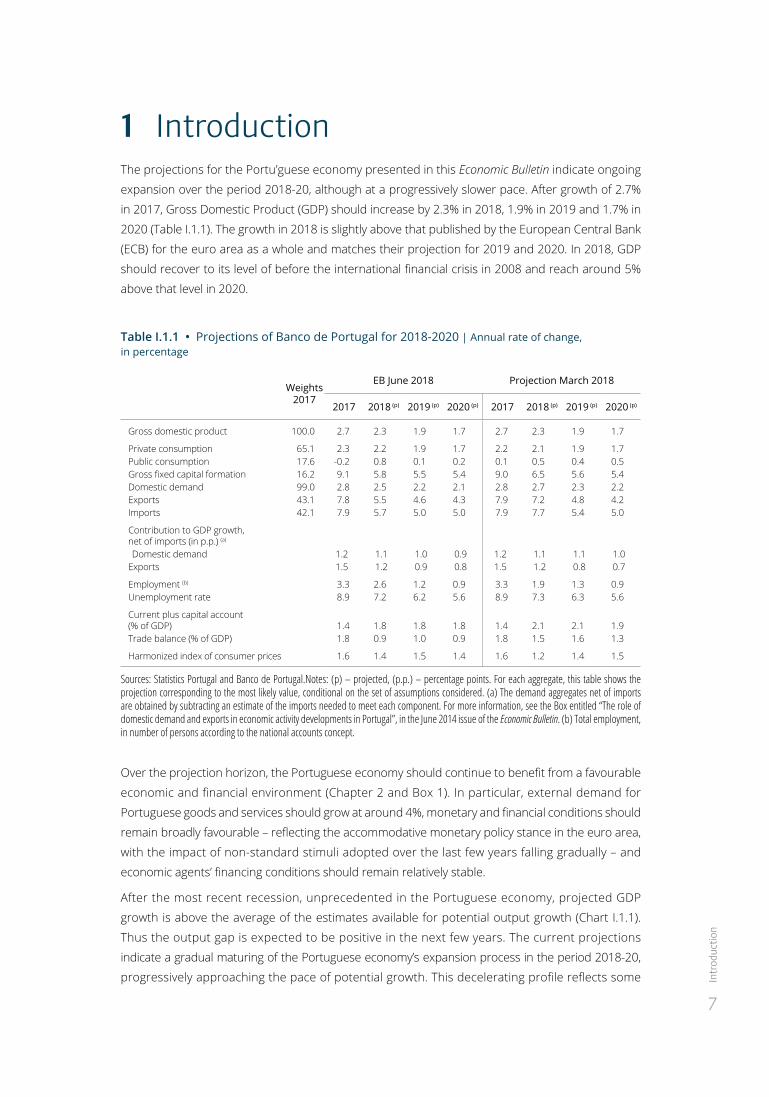
Gross domestic product 100.0 2.7 2.3 1.9 1.7 2.7 2.3 1.9 1.7
Private consumption 65.1 2.3 2.2 1.9 1.7 2.2 2.1 1.9 1.7Public consumption 17.6 -0.2 0.8 0.1 0.2 0.1 0.5 0.4 0.5Gross fixed capital formation 16.2 9.1 5.8 5.5 5.4 9.0 6.5 5.6 5.4Domestic demand 99.0 2.8 2.5 2.2 2.1 2.8 2.7 2.3 2.2Exports 43.1 7.8 5.5 4.6 4.3 7.9 7.2 4.8 4.2Imports 42.1 7.9 5.7 5.0 5.0 7.9 7.7 5.4 5.0
Contribution to GDP growth, net of imports (in p.p.) (a)
Domestic demand 1.2 1.1 1.0 0.9 1.2 1.1 1.1 1.0Exports 1.5 1.2 0.9 0.8 1.5 1.2 0.8 0.7
Employment (b) 3.3 2.6 1.2 0.9 3.3 1.9 1.3 0.9Unemployment rate 8.9 7.2 6.2 5.6 8.9 7.3 6.3 5.6
Current plus capital account (% of GDP) 1.4 1.8 1.8 1.8 1.4 2.1 2.1 1.9Trade balance (% of GDP) 1.8 0.9 1.0 0.9 1.8 1.5 1.6 1.3
Harmonized index of consumer prices 1.6 1.4 1.5 1.4 1.6 1.2 1.4 1.5
Sources: Statistics Portugal and Banco de Portugal.Notes: (p) – projected, (p.p.) – percentage points. For each aggregate, this table shows the projection corresponding to the most likely value, conditional on the set of assumptions considered. (a) The demand aggregates net of imports are obtained by subtracting an estimate of the imports needed to meet each component. For more information, see the Box entitled “The role of domestic demand and exports in economic activity developments in Portugal”, in the June 2014 issue of the Economic Bulletin. (b) Total employment, in number of persons according to the national accounts concept.
Over the projection horizon, the Portuguese economy should continue to benefit from a favourable
economic and financial environment (Chapter 2 and Box 1). In particular, external demand for
Portuguese goods and services should grow at around 4%, monetary and financial conditions should
remain broadly favourable – reflecting the accommodative monetary policy stance in the euro area,
with the impact of non-standard stimuli adopted over the last few years falling gradually – and
economic agents’ financing conditions should remain relatively stable.
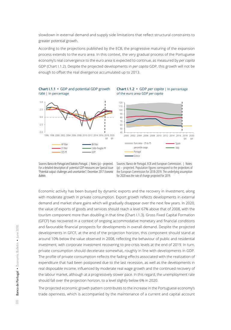
After the most recent recession, unprecedented in the Portuguese economy, projected GDP
growth is above the average of the estimates available for potential output growth (Chart I.1.1).
Thus the output gap is expected to be positive in the next few years. The current projections
indicate a gradual maturing of the Portuguese economy’s expansion process in the period 2018-20,
progressively approaching the pace of potential growth. This decelerating profile reflects some
Banc
o de
Por
tuga
l •
Eco
nom
ic B
ulle
tin •
Jun
e 20
18
8
slowdown in external demand and supply side limitations that reflect structural constraints to
greater potential growth.
According to the projections published by the ECB, the progressive maturing of the expansion
process extends to the euro area. In this context, the very gradual process of the Portuguese
economy’s real convergence to the euro area is expected to continue, as measured by per capita
GDP (Chart I.1.2). Despite the projected developments in per capita GDP, this growth will not be
enough to offset the real divergence accumulated up to 2013.
Chart I.1.1 • GDP and potential GDP growth rate | In percentage
Chart I.1.2 • GDP per capita | In percentage of the euro area GDP per capita
-5.0
-2.5
0.0
2.5
5.0
1996 1998 2000 2002 2004 2006 2008 2010 2012 2014 2016 2018 (p)
2020 (p)
HP filterCF filterCES PF
BK filterCobb-Douglas PF GDP
40
50
60
70
80
90
100
110
120
2000 2002 2004 2006 2008 2010 2012 2014 2016 2018(p)
2020(p)
Euro area − 25 to 75
percentile range
Portugal
Greece
Spain
Italy
Sources: Banco de Portugal and Statistics Portugal. | Notes: (p) – projected. For a detailed description of potential GDP measures see Special issue “Potential output: challenges and uncertainties”; December 2017 Economic Bulletin.
Sources: Banco de Portugal, ECB and European Commission. | Notes: (p) – projected. Population figures correspond to the projections of the European Commission for 2018-2019. The underlying assumption for 2020 was the rate of change projected for 2019.
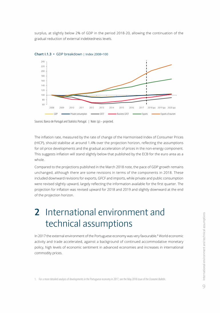
Economic activity has been buoyed by dynamic exports and the recovery in investment, along
with moderate growth in private consumption. Export growth reflects developments in external
demand and market share gains which will gradually disappear over the next few years. In 2020,
the value of exports of goods and services should reach a level 67% above that of 2008, with the
tourism component more than doubling in that time (Chart I.1.3). Gross Fixed Capital Formation
(GFCF) has recovered in a context of ongoing accommodative monetary and financial conditions
and favourable financial prospects for developments in overall demand. Despite the projected
developments in GFCF, at the end of the projection horizon, this component should stand at
around 10% below the value observed in 2008, reflecting the behaviour of public and residential
investment, with corporate investment recovering to pre-crisis levels at the end of 2019. In turn,
private consumption should decelerate somewhat, roughly in line with developments in GDP.
The profile of private consumption reflects the fading effects associated with the realization of
expenditure that had been postponed due to the last recession, as well as the developments in
real disposable income, influenced by moderate real wage growth and the continued recovery of
the labour market, although at a progressively slower pace. In this regard, the unemployment rate
should fall over the projection horizon, to a level slightly below 6% in 2020.
The projected economic growth pattern contributes to the increase in the Portuguese economy’s
trade openness, which is accompanied by the maintenance of a current and capital account
Inte
rnat
iona
l env
ironm
ent a
nd te
chni
cal a
ssum
ptio
ns
9
surplus, at slightly below 2% of GDP in the period 2018-20, allowing the continuation of the
gradual reduction of external indebtedness levels.
Chart I.1.3 • GDP breakdown | Index 2008=100
60
80
100
120
140
160
180
200
220
240
2008 2009 2010 2011 2012 2013 2014 2015 2016 2017 2018 (p) 2019 (p) 2020 (p)
GDP Private consumption GFCF Business GFCF Exports Exports of tourism
Sources: Banco de Portugal and Statistics Portugal. | Note: (p) – projected.
The inflation rate, measured by the rate of change of the Harmonised Index of Consumer Prices
(HICP), should stabilise at around 1.4% over the projection horizon, reflecting the assumptions
for oil price developments and the gradual acceleration of prices in the non-energy component.
This suggests inflation will stand slightly below that published by the ECB for the euro area as a
whole.
Compared to the projections published in the March 2018 note, the pace of GDP growth remains
unchanged, although there are some revisions in terms of the components in 2018. These
included downward revisions for exports, GFCF and imports, while private and public consumption
were revised slightly upward, largely reflecting the information available for the first quarter. The
projection for inflation was revised upward for 2018 and 2019 and slightly downward at the end
of the projection horizon.
2 International environment and technical assumptions
In 2017 the external environment of the Portuguese economy was very favourable.1 World economic
activity and trade accelerated, against a background of continued accommodative monetary
policy, high levels of economic sentiment in advanced economies and increases in international
commodity prices.
1. For a more detailed analysis of developments in the Portuguese economy in 2017, see the May 2018 issue of the Economic Bulletin.
Banc
o de
Por
tuga
l •
Eco
nom
ic B
ulle
tin •
Jun
e 20
18
10
Solid growth in world economic activity continued at the start of 2018, although a slight slowdown
was observed in major advanced economies. In the euro area, GDP decelerated to 0.4% (quarter-
on-quarter rate of change) in the first quarter of 2018, which compares with a 0.7% increase
in the previous period. This slowdown in real GDP growth followed strong increases in 2017
and is partly affected by idiosyncratic and temporary factors in some of the largest euro area
economies. In turn, short-term indicators for world trade also point to a deceleration at the start
of the year.
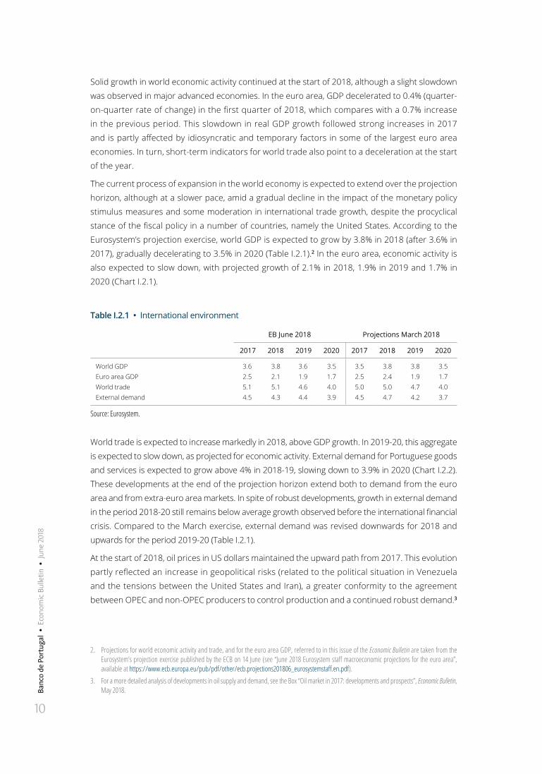
The current process of expansion in the world economy is expected to extend over the projection
horizon, although at a slower pace, amid a gradual decline in the impact of the monetary policy
stimulus measures and some moderation in international trade growth, despite the procyclical
stance of the fiscal policy in a number of countries, namely the United States. According to the
Eurosystem’s projection exercise, world GDP is expected to grow by 3.8% in 2018 (after 3.6% in
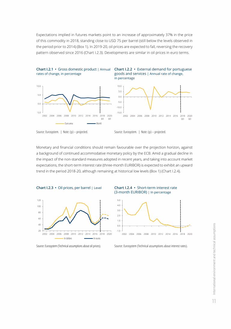
2017), gradually decelerating to 3.5% in 2020 (Table I.2.1).2 In the euro area, economic activity is
also expected to slow down, with projected growth of 2.1% in 2018, 1.9% in 2019 and 1.7% in
2020 (Chart I.2.1).
Table I.2.1 • International environment
EB June 2018 Projections March 2018
2017 2018 2019 2020 2017 2018 2019 2020
World GDP 3.6 3.8 3.6 3.5 3.5 3.8 3.8 3.5Euro area GDP 2.5 2.1 1.9 1.7 2.5 2.4 1.9 1.7World trade 5.1 5.1 4.6 4.0 5.0 5.0 4.7 4.0External demand 4.5 4.3 4.4 3.9 4.5 4.7 4.2 3.7
Source: Eurosystem.
World trade is expected to increase markedly in 2018, above GDP growth. In 2019-20, this aggregate
is expected to slow down, as projected for economic activity. External demand for Portuguese goods
and services is expected to grow above 4% in 2018-19, slowing down to 3.9% in 2020 (Chart I.2.2).
These developments at the end of the projection horizon extend both to demand from the euro
area and from extra-euro area markets. In spite of robust developments, growth in external demand
in the period 2018-20 still remains below average growth observed before the international financial
crisis. Compared to the March exercise, external demand was revised downwards for 2018 and
upwards for the period 2019-20 (Table I.2.1).
At the start of 2018, oil prices in US dollars maintained the upward path from 2017. This evolution
partly reflected an increase in geopolitical risks (related to the political situation in Venezuela
and the tensions between the United States and Iran), a greater conformity to the agreement
between OPEC and non-OPEC producers to control production and a continued robust demand.3
2. Projections for world economic activity and trade, and for the euro area GDP, referred to in this issue of the Economic Bulletin are taken from the Eurosystem’s projection exercise published by the ECB on 14 June (see “June 2018 Eurosystem staff macroeconomic projections for the euro area”, available at https://www.ecb.europa.eu/pub/pdf/other/ecb.projections201806_eurosystemstaff.en.pdf).
3. For a more detailed analysis of developments in oil supply and demand, see the Box “Oil market in 2017: developments and prospects”, Economic Bulletin, May 2018.
Inte
rnat
iona
l env
ironm
ent a
nd te
chni
cal a
ssum
ptio
ns
11
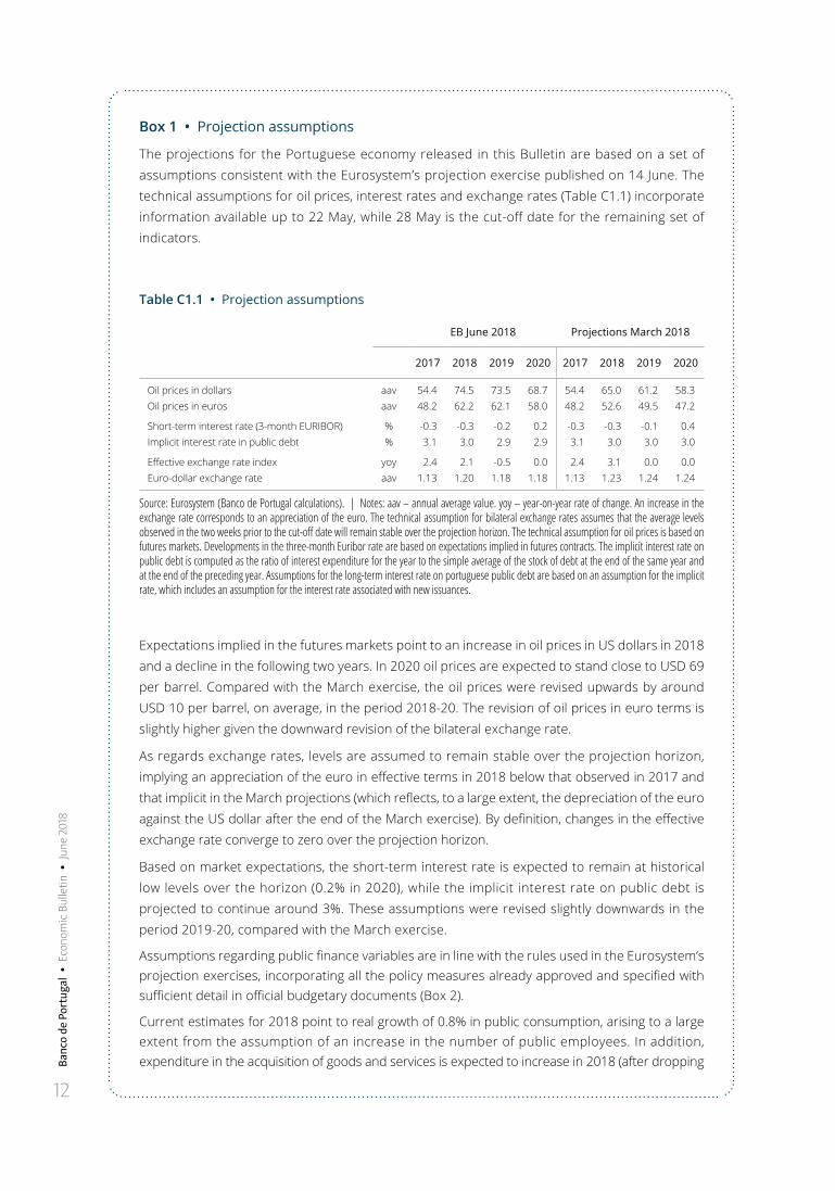
Expectations implied in futures markets point to an increase of approximately 37% in the price
of this commodity in 2018, standing close to USD 75 per barrel (still below the levels observed in
the period prior to 2014) (Box 1). In 2019-20, oil prices are expected to fall, reversing the recovery
pattern observed since 2016 (Chart I.2.3). Developments are similar in oil prices in euro terms.
Chart I.2.1 • Gross domestic product | Annual rates of change, in percentage
Chart I.2.2 • External demand for portuguese goods and services | Annual rate of change, in percentage
-5.0
0.0
5.0
10.0
2002 2004 2006 2008 2010 2012 2014 2016 2018(p)
2020(p)
Euro area World
-15.0
-10.0
-5.0
0.0
5.0
10.0
2002 2004 2006 2008 2010 2012 2014 2016 2018(p)
2020(p)
Source: Eurosystem. | Note: (p) – projected. Source: Eurosystem. | Note: (p) – projected.
Monetary and financial conditions should remain favourable over the projection horizon, against
a background of continued accommodative monetary policy by the ECB. Amid a gradual decline in
the impact of the non-standard measures adopted in recent years, and taking into account market
expectations, the short-term interest rate (three-month EURIBOR) is expected to exhibit an upward
trend in the period 2018-20, although remaining at historical low levels (Box 1) (Chart I.2.4).
Chart I.2.3 • Oil prices, per barrel | Level Chart I.2.4 • Short-term interest rate (3-month EURIBOR) | In percentage
20
40
60
80
100
120
2002 2004 2006 2008 2010 2012 2014 2016 2018 2020
In dollars In euros
-1.0
0.0
1.0
2.0
3.0
4.0
5.0
2002 2004 2006 2008 2010 2012 2014 2016 2018 2020
Source: Eurosystem (Technical assumptions about oil prices). Source: Eurosystem (Technical assumptions about interest rates).
12
Banc
o de
Por
tuga
l •
Eco
nom
ic B
ulle
tin •
Jun
e 20
18
Box 1 • Projection assumptions
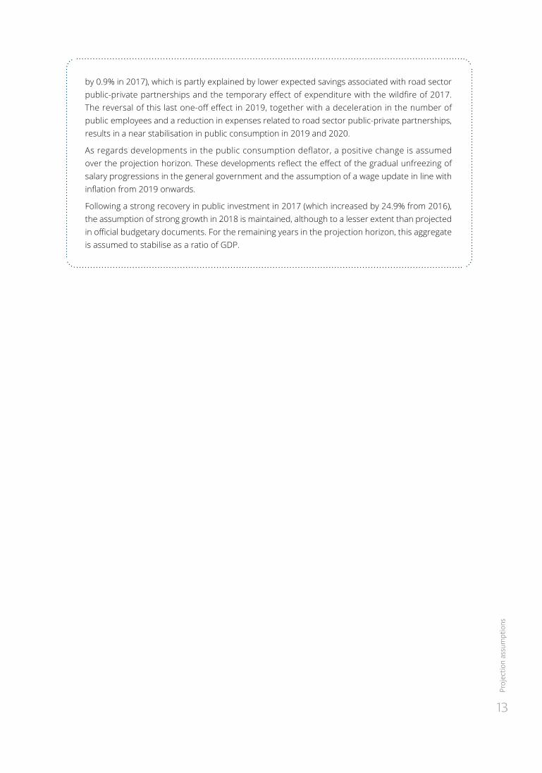
The projections for the Portuguese economy released in this Bulletin are based on a set of assumptions consistent with the Eurosystem’s projection exercise published on 14 June. The technical assumptions for oil prices, interest rates and exchange rates (Table C1.1) incorporate information available up to 22 May, while 28 May is the cut-off date for the remaining set of indicators.
Table C1.1 • Projection assumptions
EB June 2018 Projections March 2018
2017 2018 2019 2020 2017 2018 2019 2020
Oil prices in dollars aav 54.4 74.5 73.5 68.7 54.4 65.0 61.2 58.3Oil prices in euros aav 48.2 62.2 62.1 58.0 48.2 52.6 49.5 47.2
Short-term interest rate (3-month EURIBOR) % -0.3 -0.3 -0.2 0.2 -0.3 -0.3 -0.1 0.4Implicit interest rate in public debt % 3.1 3.0 2.9 2.9 3.1 3.0 3.0 3.0
Effective exchange rate index yoy 2.4 2.1 -0.5 0.0 2.4 3.1 0.0 0.0Euro-dollar exchange rate aav 1.13 1.20 1.18 1.18 1.13 1.23 1.24 1.24
Source: Eurosystem (Banco de Portugal calculations). | Notes: aav – annual average value. yoy – year-on-year rate of change. An increase in the exchange rate corresponds to an appreciation of the euro. The technical assumption for bilateral exchange rates assumes that the average levels observed in the two weeks prior to the cut-off date will remain stable over the projection horizon. The technical assumption for oil prices is based on futures markets. Developments in the three-month Euribor rate are based on expectations implied in futures contracts. The implicit interest rate on public debt is computed as the ratio of interest expenditure for the year to the simple average of the stock of debt at the end of the same year and at the end of the preceding year. Assumptions for the long-term interest rate on portuguese public debt are based on an assumption for the implicit rate, which includes an assumption for the interest rate associated with new issuances.
Expectations implied in the futures markets point to an increase in oil prices in US dollars in 2018 and a decline in the following two years. In 2020 oil prices are expected to stand close to USD 69 per barrel. Compared with the March exercise, the oil prices were revised upwards by around USD 10 per barrel, on average, in the period 2018-20. The revision of oil prices in euro terms is slightly higher given the downward revision of the bilateral exchange rate.
As regards exchange rates, levels are assumed to remain stable over the projection horizon, implying an appreciation of the euro in effective terms in 2018 below that observed in 2017 and that implicit in the March projections (which reflects, to a large extent, the depreciation of the euro against the US dollar after the end of the March exercise). By definition, changes in the effective exchange rate converge to zero over the projection horizon.
Based on market expectations, the short-term interest rate is expected to remain at historical low levels over the horizon (0.2% in 2020), while the implicit interest rate on public debt is projected to continue around 3%. These assumptions were revised slightly downwards in the period 2019-20, compared with the March exercise.
Assumptions regarding public finance variables are in line with the rules used in the Eurosystem’s projection exercises, incorporating all the policy measures already approved and specified with sufficient detail in official budgetary documents (Box 2).
Current estimates for 2018 point to real growth of 0.8% in public consumption, arising to a large extent from the assumption of an increase in the number of public employees. In addition, expenditure in the acquisition of goods and services is expected to increase in 2018 (after dropping
Proj
ectio
n as
sum
ptio
ns
13
by 0.9% in 2017), which is partly explained by lower expected savings associated with road sector public-private partnerships and the temporary effect of expenditure with the wildfire of 2017. The reversal of this last one-off effect in 2019, together with a deceleration in the number of public employees and a reduction in expenses related to road sector public-private partnerships, results in a near stabilisation in public consumption in 2019 and 2020.
As regards developments in the public consumption deflator, a positive change is assumed over the projection horizon. These developments reflect the effect of the gradual unfreezing of salary progressions in the general government and the assumption of a wage update in line with inflation from 2019 onwards.
Following a strong recovery in public investment in 2017 (which increased by 24.9% from 2016), the assumption of strong growth in 2018 is maintained, although to a lesser extent than projected in official budgetary documents. For the remaining years in the projection horizon, this aggregate is assumed to stabilise as a ratio of GDP.
Banc
o de
Por
tuga
l •
Eco
nom
ic B
ulle
tin •
Jun
e 20
18
14
3 Growth factors, demand and external accounts
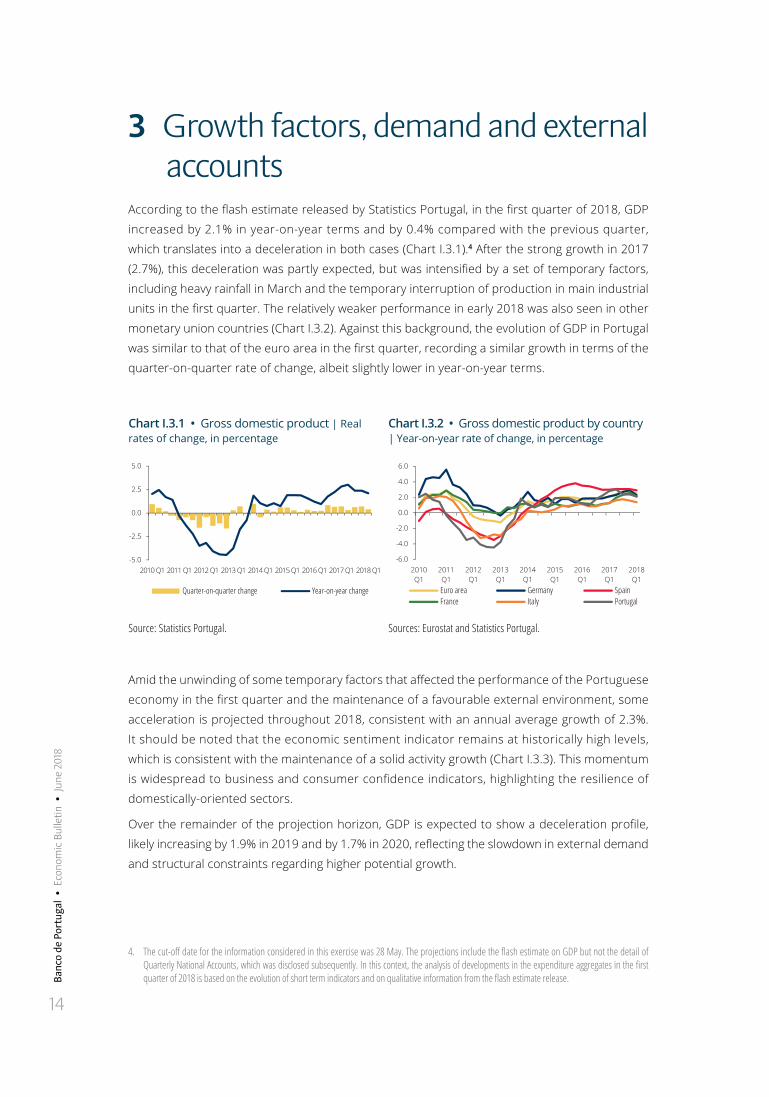
According to the flash estimate released by Statistics Portugal, in the first quarter of 2018, GDP
increased by 2.1% in year-on-year terms and by 0.4% compared with the previous quarter,
which translates into a deceleration in both cases (Chart I.3.1).4 After the strong growth in 2017
(2.7%), this deceleration was partly expected, but was intensified by a set of temporary factors,
including heavy rainfall in March and the temporary interruption of production in main industrial
units in the first quarter. The relatively weaker performance in early 2018 was also seen in other
monetary union countries (Chart I.3.2). Against this background, the evolution of GDP in Portugal
was similar to that of the euro area in the first quarter, recording a similar growth in terms of the
quarter-on-quarter rate of change, albeit slightly lower in year-on-year terms.
Chart I.3.1 • Gross domestic product | Real rates of change, in percentage
Chart I.3.2 • Gross domestic product by country | Year-on-year rate of change, in percentage
-5.0
-2.5
0.0
2.5
5.0
2010 Q1 2011 Q1 2012 Q1 2013 Q1 2014 Q1 2015 Q1 2016 Q1 2017 Q1 2018 Q1
Quarter-on-quarter change Year-on-year change
-6.0
-4.0
-2.0
0.0
2.0
4.0
6.0
2010Q1
2011Q1
2012Q1
2013Q1
2014Q1
2015Q1
2016Q1
2017Q1
2018Q1
Euro area Germany SpainFrance Italy Portugal
Source: Statistics Portugal. Sources: Eurostat and Statistics Portugal.
Amid the unwinding of some temporary factors that affected the performance of the Portuguese
economy in the first quarter and the maintenance of a favourable external environment, some
acceleration is projected throughout 2018, consistent with an annual average growth of 2.3%.
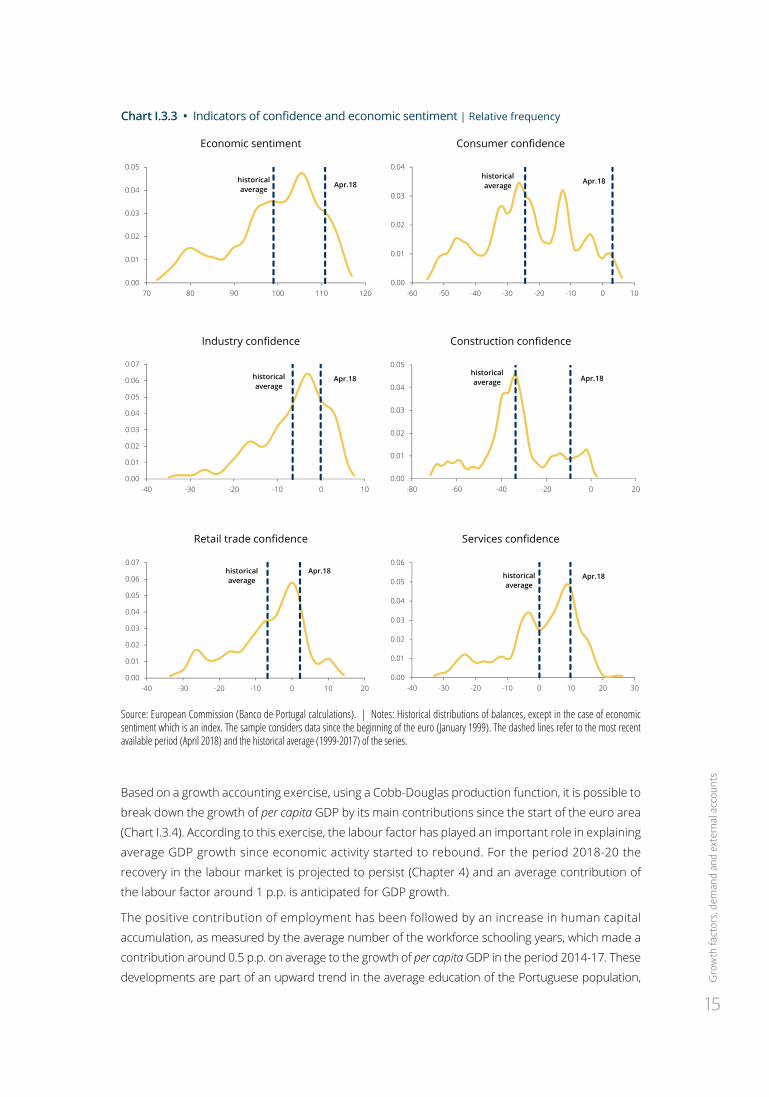
It should be noted that the economic sentiment indicator remains at historically high levels,
which is consistent with the maintenance of a solid activity growth (Chart I.3.3). This momentum
is widespread to business and consumer confidence indicators, highlighting the resilience of
domestically-oriented sectors.
Over the remainder of the projection horizon, GDP is expected to show a deceleration profile,
likely increasing by 1.9% in 2019 and by 1.7% in 2020, reflecting the slowdown in external demand
and structural constraints regarding higher potential growth.
4. The cut-off date for the information considered in this exercise was 28 May. The projections include the flash estimate on GDP but not the detail of Quarterly National Accounts, which was disclosed subsequently. In this context, the analysis of developments in the expenditure aggregates in the first quarter of 2018 is based on the evolution of short term indicators and on qualitative information from the flash estimate release.
Gro
wth
fact
ors,
dem
and
and
exte
rnal
acc
ount
s
15
Chart I.3.3 • Indicators of confidence and economic sentiment | Relative frequency
Economic sentiment Consumer confidence
0.00
0.01
0.02
0.03
0.04
0.05
70 80 90 100 110 120
historical average Apr.18
0.00
0.01
0.02
0.03
0.04
-60 -50 -40 -30 -20 -10 0 10
historical average Apr.18
Industry confidence Construction confidence
0.00
0.01
0.02
0.03
0.04
0.05
0.06
0.07
-40 -30 -20 -10 0 10
historical average
Apr.18
0.00
0.01
0.02
0.03
0.04
0.05
-80 -60 -40 -20 0 20
historical average Apr.18
Retail trade confidence Services confidence
0.00
0.01
0.02
0.03
0.04
0.05
0.06
0.07
-40 -30 -20 -10 0 10 20
historical average
Apr.18
0.00
0.01
0.02
0.03
0.04
0.05
0.06
-40 -30 -20 -10 0 10 20 30
historical average
Apr.18
Source: European Commission (Banco de Portugal calculations). | Notes: Historical distributions of balances, except in the case of economic sentiment which is an index. The sample considers data since the beginning of the euro (January 1999). The dashed lines refer to the most recent available period (April 2018) and the historical average (1999-2017) of the series.
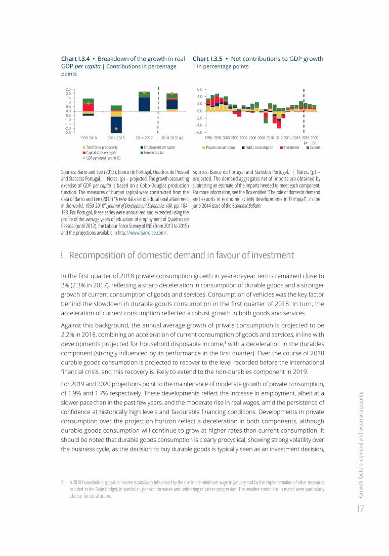
Based on a growth accounting exercise, using a Cobb-Douglas production function, it is possible to
break down the growth of per capita GDP by its main contributions since the start of the euro area
(Chart I.3.4). According to this exercise, the labour factor has played an important role in explaining
average GDP growth since economic activity started to rebound. For the period 2018-20 the
recovery in the labour market is projected to persist (Chapter 4) and an average contribution of
the labour factor around 1 p.p. is anticipated for GDP growth.
The positive contribution of employment has been followed by an increase in human capital
accumulation, as measured by the average number of the workforce schooling years, which made a
contribution around 0.5 p.p. on average to the growth of per capita GDP in the period 2014-17. These
developments are part of an upward trend in the average education of the Portuguese population,
Banc
o de
Por
tuga
l •
Eco
nom
ic B
ulle
tin •
Jun
e 20
18
16
which is still relatively low compared with the European standards5. In the coming years, this trend
is expected to persist, with an average contribution similar to that seen in the recent past. Human
capital is one of the main components when determining the growth pace of activity and appears to
be an element that can offset the negative effects of the demographic evolution over the long term,
which poses one of the major challenges to the potential growth of the Portuguese economy.6
Turning to the capital factor, it should be noted that in the period of economic recovery started
in mid- 2013, this factor made a virtually nil contribution to average GDP growth. Developments
in investment in the last two decades have contributed to the persistence of low capital levels
per employee, with important consequences for productivity and potential growth of the
Portuguese economy. Against this backdrop, Portugal has one of the lowest capital stock ratios
per employee among monetary union countries. Over the projection horizon, the capital stock
is expected to recover slightly, translating into a marginally positive contribution of this factor
to GDP growth. This recovery occurs against a backdrop of maintenance of the expansion
of corporate investment, which is an essential condition for sustained economic growth and
productivity growth economy-wide, as the incorporation of new technologies in the productive
process is made through capital.
Finally, it should be noted that after a zero contribution in the period 2014-17, total factor productivity,
obtained as a residual in this exercise, is likely to make a marginally positive contribution in the
coming years, reflecting, inter alia, better resource allocation in the economy following a process of
reorientation towards the sectors more exposed to international competition.
Chart I.3.5 illustrates developments in the Portuguese economy over the period 1995-2020 based
on the behaviour of the expenditure components. Since 2010 exports net of import content have
made a significant contribution to GDP growth, clearly above the net contribution of domestic
demand. The favourable performance of exports contrasts with that of the period prior to 2006,
in which domestic demand – and in particular private consumption – was the aggregate that
contributed the most to GDP growth. The decrease in the share of domestic demand in GDP
throughout the last decade is part of the need for fiscal adjustment and reduction of the private
sector indebtedness levels. The contribution of investment to GDP growth has strongly declined
since the start of the 2000s and more markedly during the recent crisis. From 2014 onwards this
trend recorded a reversal, in particular its corporate component.
Developments projected for the expenditure components over the period 2018-20 prolong the
recent trends and constitute a more sustainable growth pattern of the Portuguese economy
over the medium term, with an increase in the share of exports in GDP and with investment
growth, in particular of the corporate component, projected to recover towards the end of 2019
the level recorded before the international financial crisis. Over the projection horizon, the
average contribution of exports net of import content is expected to be broadly in line with the
net contribution of domestic demand.
5. See the box entitled “Evolution of labour force qualifications in Portugal”, Economic Bulletin, May 2018.6. See the Special issue entitled “Demographic transition and growth in the Portuguese economy”, Economic Bulletin, October 2015.
Gro
wth
fact
ors,
dem
and
and
exte
rnal
acc
ount
s
17
Chart I.3.4 • Breakdown of the growth in real GDP per capita | Contributions in percentage points
Chart I.3.5 • Net contributions to GDP growth | In percentage points
-2.5-2.0-1.5-1.0-0.50.00.51.01.52.02.5
1999-2010 2011-2013 2014-2017 2018-2020 (p)
Employment per capita Human capital
Total factor productivity Capital stock per capitaGDP per capita (arc, in %)
-6.0
-4.0
-2.0
0.0
2.0
4.0
6.0
1996 1998 2000 2002 2004 2006 2008 2010 2012 2014 2016 2018 (p)
2020 (p)
Private consumption Public consumption Investment Exports
Sources: Barro and Lee (2013), Banco de Portugal, Quadros de Pessoal and Statistics Portugal. | Notes: (p) – projected. The growth accounting exercise of GDP per capita is based on a Cobb-Douglas production function. The measures of human capital were constructed from the data of Barro and Lee (2013) “A new data set of educational attainment in the world, 1950-2010”, Journal of Development Economics 104, pp. 184-198. For Portugal, these series were annualized and extended using the profile of the average years of education of employment of Quadros de Pessoal (until 2012), the Labour Force Survey of INE (from 2013 to 2015) and the projections available in http://www.barrolee.com/.
Sources: Banco de Portugal and Statistics Portugal. | Notes: (p) – projected. The demand aggregates net of imports are obtained by subtracting an estimate of the imports needed to meet each component. For more information, see the Box entitled “The role of domestic demand and exports in economic activity developments in Portugal”, in the June 2014 issue of the Economic Bulletin.
Recomposition of domestic demand in favour of investment
In the first quarter of 2018 private consumption growth in year-on-year terms remained close to 2% (2.3% in 2017), reflecting a sharp deceleration in consumption of durable goods and a stronger growth of current consumption of goods and services. Consumption of vehicles was the key factor behind the slowdown in durable goods consumption in the first quarter of 2018. In turn, the acceleration of current consumption reflected a robust growth in both goods and services.
Against this background, the annual average growth of private consumption is projected to be 2.2% in 2018, combining an acceleration of current consumption of goods and services, in line with developments projected for household disposable income,7 with a deceleration in the durables component (strongly influenced by its performance in the first quarter). Over the course of 2018 durable goods consumption is projected to recover to the level recorded before the international financial crisis, and this recovery is likely to extend to the non-durables component in 2019.
For 2019 and 2020 projections point to the maintenance of moderate growth of private consumption, of 1.9% and 1.7% respectively. These developments reflect the increase in employment, albeit at a slower pace than in the past few years, and the moderate rise in real wages, amid the persistence of confidence at historically high levels and favourable financing conditions. Developments in private consumption over the projection horizon reflect a deceleration in both components, although durable goods consumption will continue to grow at higher rates than current consumption. It should be noted that durable goods consumption is clearly procyclical, showing strong volatility over the business cycle, as the decision to buy durable goods is typically seen as an investment decision,
7. In 2018 household disposable income is positively influenced by the rise in the minimum wage in January and by the implementation of other measures included in the State budget, in particular, pension increases and unfreezing of career progression. The weather conditions in march were particularly adverse for construction.
Banc
o de
Por
tuga
l •
Eco
nom
ic B
ulle
tin •
Jun
e 20
18
18
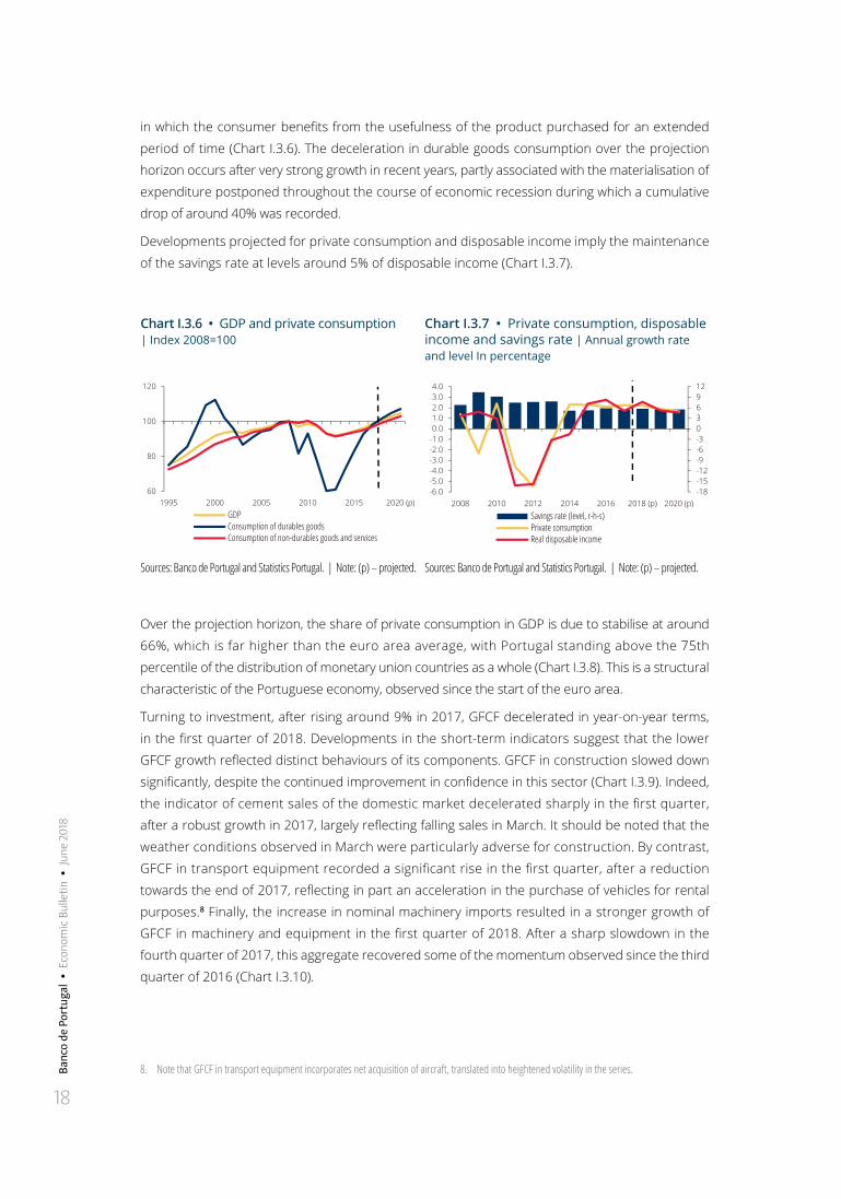
in which the consumer benefits from the usefulness of the product purchased for an extended
period of time (Chart I.3.6). The deceleration in durable goods consumption over the projection
horizon occurs after very strong growth in recent years, partly associated with the materialisation of
expenditure postponed throughout the course of economic recession during which a cumulative
drop of around 40% was recorded.
Developments projected for private consumption and disposable income imply the maintenance
of the savings rate at levels around 5% of disposable income (Chart I.3.7).
Chart I.3.6 • GDP and private consumption | Index 2008=100
Chart I.3.7 • Private consumption, disposable income and savings rate | Annual growth rate and level In percentage
60
80
100
120
1995 2000 2005 2010 2015 2020 (p)GDPConsumption of durables goodsConsumption of non-durables goods and services
-18-15-12-9-6-3036912
-6.0-5.0-4.0-3.0-2.0-1.00.01.02.03.04.0
2008 2010 2012 2014 2016 2018 (p) 2020 (p)Savings rate (level, r-h-s)Private consumptionReal disposable income
Sources: Banco de Portugal and Statistics Portugal. | Note: (p) – projected. Sources: Banco de Portugal and Statistics Portugal. | Note: (p) – projected.
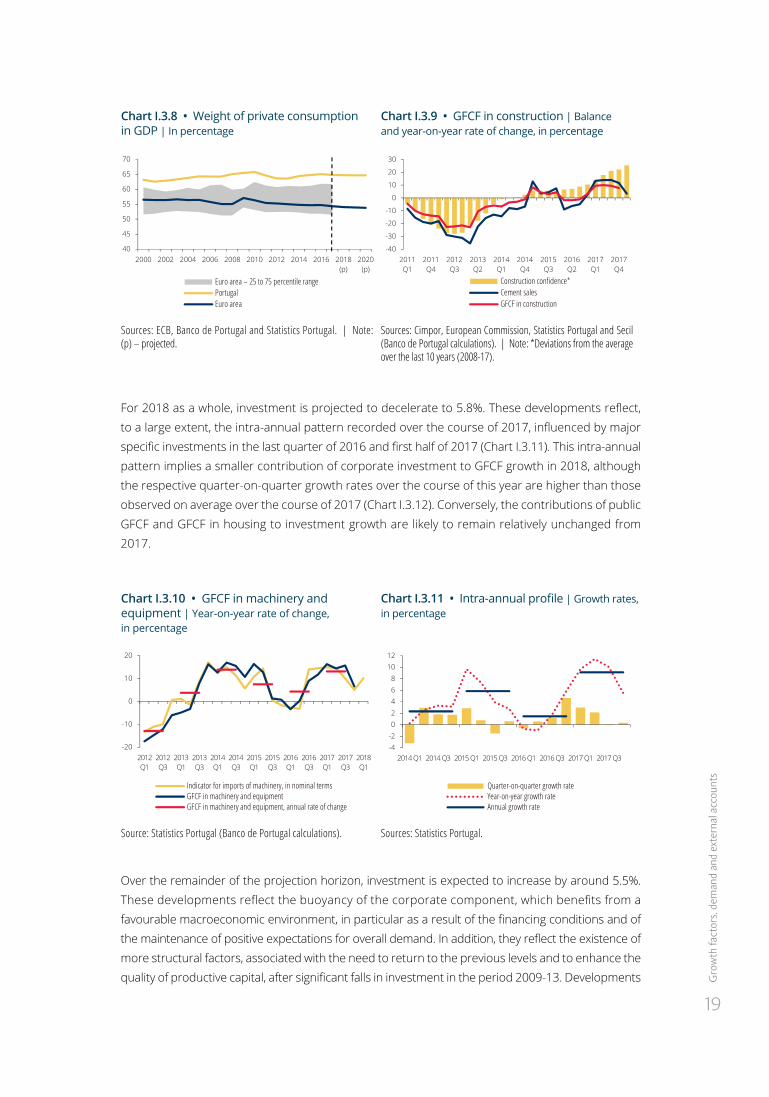
Over the projection horizon, the share of private consumption in GDP is due to stabilise at around
66%, which is far higher than the euro area average, with Portugal standing above the 75th
percentile of the distribution of monetary union countries as a whole (Chart I.3.8). This is a structural
characteristic of the Portuguese economy, observed since the start of the euro area.
Turning to investment, after rising around 9% in 2017, GFCF decelerated in year-on-year terms,
in the first quarter of 2018. Developments in the short-term indicators suggest that the lower
GFCF growth reflected distinct behaviours of its components. GFCF in construction slowed down
significantly, despite the continued improvement in confidence in this sector (Chart I.3.9). Indeed,
the indicator of cement sales of the domestic market decelerated sharply in the first quarter,
after a robust growth in 2017, largely reflecting falling sales in March. It should be noted that the
weather conditions observed in March were particularly adverse for construction. By contrast,
GFCF in transport equipment recorded a significant rise in the first quarter, after a reduction
towards the end of 2017, reflecting in part an acceleration in the purchase of vehicles for rental
purposes.8 Finally, the increase in nominal machinery imports resulted in a stronger growth of
GFCF in machinery and equipment in the first quarter of 2018. After a sharp slowdown in the
fourth quarter of 2017, this aggregate recovered some of the momentum observed since the third
quarter of 2016 (Chart I.3.10).
8. Note that GFCF in transport equipment incorporates net acquisition of aircraft, translated into heightened volatility in the series.
Gro
wth
fact
ors,
dem
and
and
exte
rnal
acc
ount
s
19
Chart I.3.8 • Weight of private consumption in GDP | In percentage
Chart I.3.9 • GFCF in construction | Balance and year-on-year rate of change, in percentage
40
45
50
55
60
65
70
2000 2002 2004 2006 2008 2010 2012 2014 2016 2018(p)
2020(p)
Euro area – 25 to 75 percentile rangePortugalEuro area
-40
-30
-20
-10
0
10
20
30
2011Q1
2011Q4
2012Q3
2013Q2
2014Q1
2014Q4
2015Q3
2016Q2
2017Q1
2017Q4
Construction confidence*Cement salesGFCF in construction
Sources: ECB, Banco de Portugal and Statistics Portugal. | Note: (p) – projected.
Sources: Cimpor, European Commission, Statistics Portugal and Secil (Banco de Portugal calculations). | Note: *Deviations from the average over the last 10 years (2008-17).
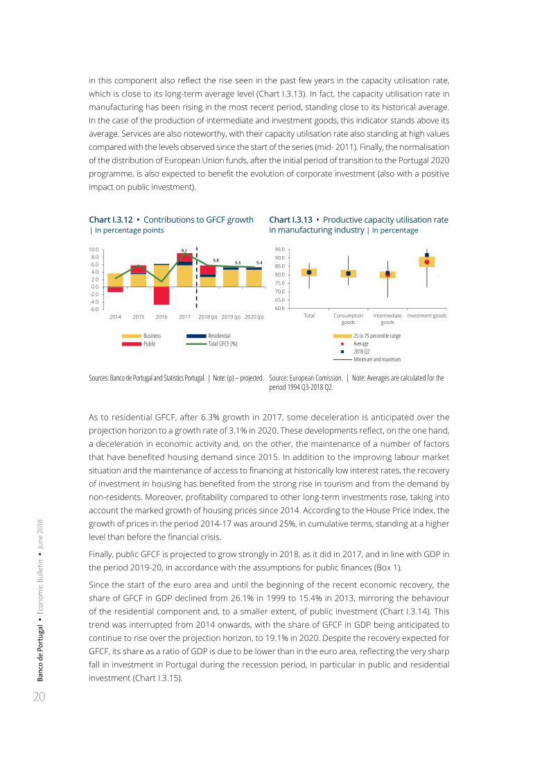
For 2018 as a whole, investment is projected to decelerate to 5.8%. These developments reflect, to a large extent, the intra-annual pattern recorded over the course of 2017, influenced by major specific investments in the last quarter of 2016 and first half of 2017 (Chart I.3.11). This intra-annual pattern implies a smaller contribution of corporate investment to GFCF growth in 2018, although the respective quarter-on-quarter growth rates over the course of this year are higher than those observed on average over the course of 2017 (Chart I.3.12). Conversely, the contributions of public GFCF and GFCF in housing to investment growth are likely to remain relatively unchanged from 2017.
Chart I.3.10 • GFCF in machinery and equipment | Year-on-year rate of change, in percentage
Chart I.3.11 • Intra-annual profile | Growth rates, in percentage
-20
-10
0
10
20
2012 Q1
2012 Q3
2013 Q1
2013 Q3
2014 Q1
2014 Q3
2015 Q1
2015 Q3
2016 Q1
2016 Q3
2017 Q1
2017 Q3
2018 Q1
Indicator for imports of machinery, in nominal termsGFCF in machinery and equipmentGFCF in machinery and equipment, annual rate of change
-4-202468
1012
2014 Q1 2014 Q3 2015 Q1 2015 Q3 2016 Q1 2016 Q3 2017 Q1 2017 Q3
Quarter-on-quarter growth rateYear-on-year growth rateAnnual growth rate
Source: Statistics Portugal (Banco de Portugal calculations). Sources: Statistics Portugal.
Over the remainder of the projection horizon, investment is expected to increase by around 5.5%. These developments reflect the buoyancy of the corporate component, which benefits from a favourable macroeconomic environment, in particular as a result of the financing conditions and of the maintenance of positive expectations for overall demand. In addition, they reflect the existence of more structural factors, associated with the need to return to the previous levels and to enhance the quality of productive capital, after significant falls in investment in the period 2009-13. Developments
Banc
o de
Por
tuga
l •
Eco
nom
ic B
ulle
tin •
Jun
e 20
18
20
in this component also reflect the rise seen in the past few years in the capacity utilisation rate, which is close to its long-term average level (Chart I.3.13). In fact, the capacity utilisation rate in manufacturing has been rising in the most recent period, standing close to its historical average. In the case of the production of intermediate and investment goods, this indicator stands above its average. Services are also noteworthy, with their capacity utilisation rate also standing at high values compared with the levels observed since the start of the series (mid- 2011). Finally, the normalisation of the distribution of European Union funds, after the initial period of transition to the Portugal 2020 programme, is also expected to benefit the evolution of corporate investment (also with a positive impact on public investment).
Chart I.3.12 • Contributions to GFCF growth | In percentage points
Chart I.3.13 • Productive capacity utilisation rate in manufacturing industry | In percentage
9.1
5.8 5.5 5.4
-6.0-4.0-2.00.02.04.06.08.0
10.0
2014 2015 2016 2017 2018 (p) 2019 (p) 2020 (p)
Business ResidentialPublic Total GFCF (%)
60.0
65.0
70.0
75.0
80.0
85.0
90.0
95.0
Total Consumptiongoods
Intermediategoods
Investment goods
25 to 75 percentile rangeAverage2018 Q2Minimum and maximum
Sources: Banco de Portugal and Statistics Portugal. | Note: (p) – projected. Source: European Comission. | Note: Averages are calculated for the period 1994 Q3-2018 Q2.
As to residential GFCF, after 6.3% growth in 2017, some deceleration is anticipated over the projection horizon to a growth rate of 3.1% in 2020. These developments reflect, on the one hand, a deceleration in economic activity and, on the other, the maintenance of a number of factors that have benefited housing demand since 2015. In addition to the improving labour market situation and the maintenance of access to financing at historically low interest rates, the recovery of investment in housing has benefited from the strong rise in tourism and from the demand by non-residents. Moreover, profitability compared to other long-term investments rose, taking into account the marked growth of housing prices since 2014. According to the House Price Index, the growth of prices in the period 2014-17 was around 25%, in cumulative terms, standing at a higher level than before the financial crisis.
Finally, public GFCF is projected to grow strongly in 2018, as it did in 2017, and in line with GDP in the period 2019-20, in accordance with the assumptions for public finances (Box 1).
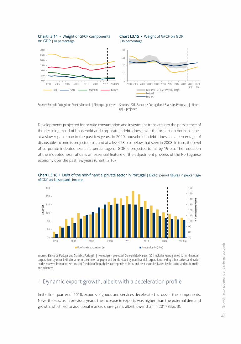
Since the start of the euro area and until the beginning of the recent economic recovery, the share of GFCF in GDP declined from 26.1% in 1999 to 15.4% in 2013, mirroring the behaviour of the residential component and, to a smaller extent, of public investment (Chart I.3.14). This trend was interrupted from 2014 onwards, with the share of GFCF in GDP being anticipated to continue to rise over the projection horizon, to 19.1% in 2020. Despite the recovery expected for GFCF, its share as a ratio of GDP is due to be lower than in the euro area, reflecting the very sharp fall in investment in Portugal during the recession period, in particular in public and residential investment (Chart I.3.15).
Gro
wth
fact
ors,
dem
and
and
exte
rnal
acc
ount
s
21
Chart I.3.14 • Weight of GFCF components on GDP | In percentage
Chart I.3.15 • Weight of GFCF on GDP | In percentage
0.0
5.0
10.0
15.0
20.0
25.0
30.0
1999 2002 2005 2008 2011 2014 2017 2020 (p)
Total Public Residential Business
10
15
20
25
30
2000 2002 2004 2006 2008 2010 2012 2014 2016 2018(p)
2020(p)
Euro area − 25 to 75 percentile range PortugalEuro area
Sources: Banco de Portugal and Statistics Portugal. | Note: (p) – projected. Sources: ECB, Banco de Portugal and Statistics Portugal. | Note: (p) – projected.
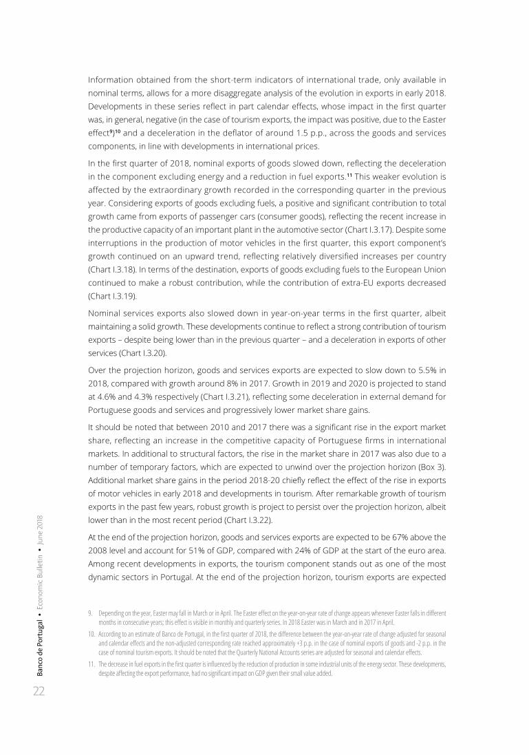
Developments projected for private consumption and investment translate into the persistence of the declining trend of household and corporate indebtedness over the projection horizon, albeit at a slower pace than in the past few years. In 2020, household indebtedness as a percentage of disposable income is projected to stand at a level 28 p.p. below that seen in 2008. In turn, the level of corporate indebtedness as a percentage of GDP is projected to fall by 19 p.p. The reduction of the indebtedness ratios is an essential feature of the adjustment process of the Portuguese economy over the past few years (Chart I.3.16).
Chart I.3.16 • Debt of the non-financial private sector in Portugal | End of period figures in percentage of GDP and disposable income
70
80
90
100
110
120
130
140
150
160
70
80
90
100
110
120
130
1999 2002 2008 2011 2014 2017 2020 (p)
In %
of d
ispo
sabl
e in
com
e
In %
of G
DP
2005
Non-financial corporations (a) Households (b) (r-h-s)
Sources: Banco de Portugal and Statistics Portugal. | Notes: (p) – projected. Consolidated values. (a) It includes loans granted to non-financial corporations by other institutional sectors; commercial paper and bonds issued by non-financial corporations held by other sectors and trade credits received from other sectors. (b) The debt of households corresponds to loans and debt securities issued by the sector and trade credit and advances.
Dynamic export growth, albeit with a deceleration profile
In the first quarter of 2018, exports of goods and services decelerated across all the components. Nevertheless, as in previous years, the increase in exports was higher than the external demand growth, which led to additional market share gains, albeit lower than in 2017 (Box 3).
Banc
o de
Por
tuga
l •
Eco
nom
ic B
ulle
tin •
Jun
e 20
18
22
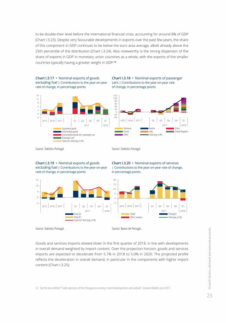
Information obtained from the short-term indicators of international trade, only available in nominal terms, allows for a more disaggregate analysis of the evolution in exports in early 2018. Developments in these series reflect in part calendar effects, whose impact in the first quarter was, in general, negative (in the case of tourism exports, the impact was positive, due to the Easter effect9)10 and a deceleration in the deflator of around 1.5 p.p., across the goods and services components, in line with developments in international prices.
In the first quarter of 2018, nominal exports of goods slowed down, reflecting the deceleration in the component excluding energy and a reduction in fuel exports.11 This weaker evolution is affected by the extraordinary growth recorded in the corresponding quarter in the previous year. Considering exports of goods excluding fuels, a positive and significant contribution to total growth came from exports of passenger cars (consumer goods), reflecting the recent increase in the productive capacity of an important plant in the automotive sector (Chart I.3.17). Despite some interruptions in the production of motor vehicles in the first quarter, this export component’s growth continued on an upward trend, reflecting relatively diversified increases per country (Chart I.3.18). In terms of the destination, exports of goods excluding fuels to the European Union continued to make a robust contribution, while the contribution of extra-EU exports decreased (Chart I.3.19).
Nominal services exports also slowed down in year-on-year terms in the first quarter, albeit maintaining a solid growth. These developments continue to reflect a strong contribution of tourism exports – despite being lower than in the previous quarter – and a deceleration in exports of other services (Chart I.3.20).
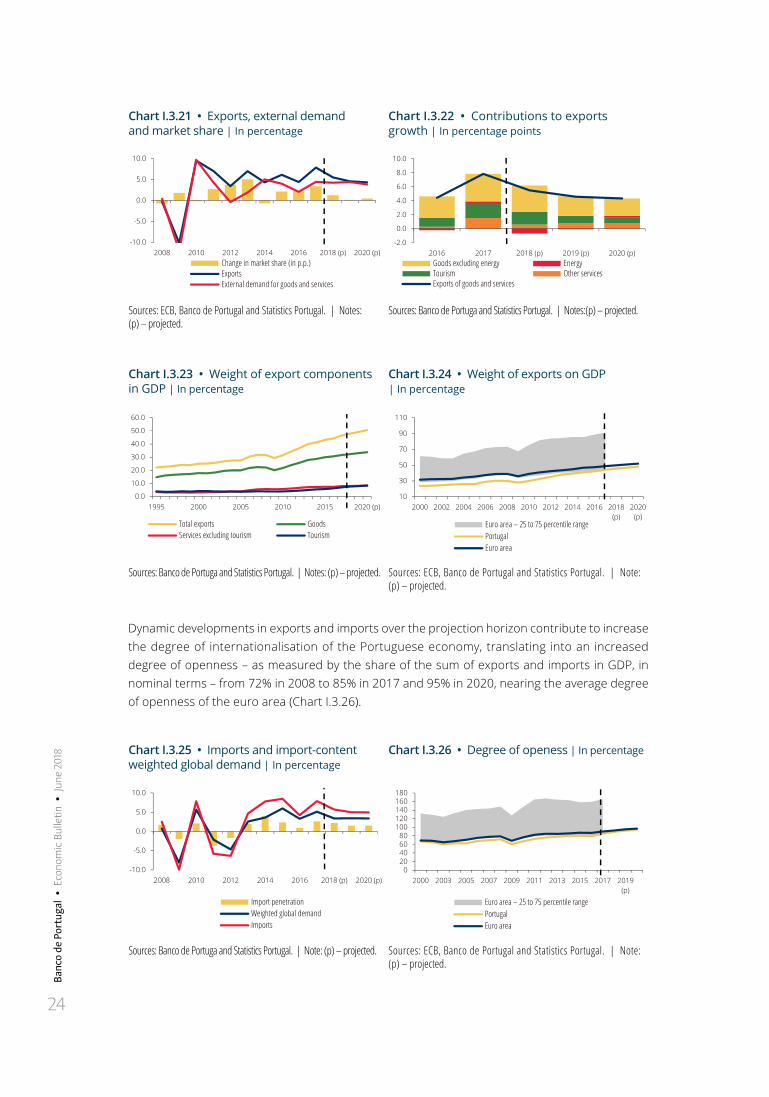
Over the projection horizon, goods and services exports are expected to slow down to 5.5% in 2018, compared with growth around 8% in 2017. Growth in 2019 and 2020 is projected to stand at 4.6% and 4.3% respectively (Chart I.3.21), reflecting some deceleration in external demand for Portuguese goods and services and progressively lower market share gains.
It should be noted that between 2010 and 2017 there was a significant rise in the export market share, reflecting an increase in the competitive capacity of Portuguese firms in international markets. In additional to structural factors, the rise in the market share in 2017 was also due to a number of temporary factors, which are expected to unwind over the projection horizon (Box 3). Additional market share gains in the period 2018-20 chiefly reflect the effect of the rise in exports of motor vehicles in early 2018 and developments in tourism. After remarkable growth of tourism exports in the past few years, robust growth is project to persist over the projection horizon, albeit lower than in the most recent period (Chart I.3.22).
At the end of the projection horizon, goods and services exports are expected to be 67% above the 2008 level and account for 51% of GDP, compared with 24% of GDP at the start of the euro area. Among recent developments in exports, the tourism component stands out as one of the most dynamic sectors in Portugal. At the end of the projection horizon, tourism exports are expected
9. Depending on the year, Easter may fall in March or in April. The Easter effect on the year-on-year rate of change appears whenever Easter falls in different months in consecutive years; this effect is visible in monthly and quarterly series. In 2018 Easter was in March and in 2017 in April.
10. According to an estimate of Banco de Portugal, in the first quarter of 2018, the difference between the year-on-year rate of change adjusted for seasonal and calendar effects and the non-adjusted corresponding rate reached approximately +3 p.p. in the case of nominal exports of goods and -2 p.p. in the case of nominal tourism exports. It should be noted that the Quarterly National Accounts series are adjusted for seasonal and calendar effects.
11. The decrease in fuel exports in the first quarter is influenced by the reduction of production in some industrial units of the energy sector. These developments, despite affecting the export performance, had no significant impact on GDP given their small value added.
Gro
wth
fact
ors,
dem
and
and
exte
rnal
acc
ount
s
23
to be double their level before the international financial crisis, accounting for around 8% of GDP (Chart I.3.23). Despite very favourable developments in exports over the past few years, the share of this component in GDP continues to be below the euro area average, albeit already above the 25th percentile of the distribution (Chart I.3.24). Also noteworthy is the strong dispersion of the share of exports in GDP in monetary union countries as a whole, with the exports of the smaller countries typically having a greater weight in GDP.12
Chart I.3.17 • Nominal exports of goods excluding fuel | Contributions to the year-on-year rate of change, in percentage points
Chart I.3.18 • Nominal exports of passenger cars | Contributions to the year-on-year rate of change, in percentage points
-3
0
3
6
9
12
15
2015 2016 2017 Q1 Q2 Q3 Q4 Q1
2017 2018Equipment goodsIntermediate goodsConsumption goods excl. passenger carsPassenger carsTotal excl. fuels (yoy, in %)
-40-20020406080100120
2015 2016 2017 Q1 Q2 Q3 Q4 Q1
2017 2018Germany Austria ChinaFrance Italy United KingdomOther Total (yoy, in %)
Source: Statistics Portugal. Source: Statistics Portugal.
Chart I.3.19 • Nominal exports of goods excluding fuel | Contributions to the year-on-year rate of change, in percentage points
Chart I.3.20 • Nominal exports of services | Contributions to the year-on-year rate of change, in percentage points
-5
0
5
10
15
2015 2016 2017 Q1 Q2 Q3 Q4 Q1
2017 2018Extra-EUIntra-EUTotal excl. fuels (yoy, in %)
-5
0
5
10
15
20
2015 2016 2017 Q1 Q2 Q3 Q4 Q1
2017 2018Travel TransportOther services Total (yoy, in %)
Source: Statistics Portugal. Source: Banco de Portugal.
Goods and services imports slowed down in the first quarter of 2018, in line with developments in overall demand weighted by import content. Over the projection horizon, goods and services imports are expected to decelerate from 5.7% in 2018 to 5.0% in 2020. The projected profile reflects the deceleration in overall demand, in particular in the components with higher import content (Chart I.3.25).
12. See the box entitled “Trade openness of the Portuguese economy: recent developments and outlook”, Economic Bulletin, June 2017.
Banc
o de
Por
tuga
l •
Eco
nom
ic B
ulle
tin •
Jun
e 20
18
24
Chart I.3.21 • Exports, external demand and market share | In percentage
Chart I.3.22 • Contributions to exports growth | In percentage points
-10.0
-5.0
0.0
5.0
10.0
2008 2010 2012 2014 2016 2018 (p) 2020 (p)Change in market share (in p.p.)ExportsExternal demand for goods and services
-2.0
0.0
2.0
4.0
6.0
8.0
10.0
2016 2017 2018 (p) 2019 (p) 2020 (p)Goods excluding energy EnergyTourism Other servicesExports of goods and services
Sources: ECB, Banco de Portugal and Statistics Portugal. | Notes: (p) – projected.
Sources: Banco de Portuga and Statistics Portugal. | Notes:(p) – projected.
Chart I.3.23 • Weight of export components in GDP | In percentage
Chart I.3.24 • Weight of exports on GDP | In percentage
0.0
10.0
20.0
30.0
40.0
50.0
60.0
1995 2000 2005 2010 2015 2020 (p)
Total exports GoodsServices excluding tourism Tourism
10
30
50
70
90
110
2000 2002 2004 2006 2008 2010 2012 2014 2016 2018(p)
2020(p)
Euro area – 25 to 75 percentile range PortugalEuro area
Sources: Banco de Portuga and Statistics Portugal. | Notes: (p) – projected. Sources: ECB, Banco de Portugal and Statistics Portugal. | Note: (p) – projected.
Dynamic developments in exports and imports over the projection horizon contribute to increase the degree of internationalisation of the Portuguese economy, translating into an increased degree of openness – as measured by the share of the sum of exports and imports in GDP, in nominal terms – from 72% in 2008 to 85% in 2017 and 95% in 2020, nearing the average degree of openness of the euro area (Chart I.3.26).
Chart I.3.25 • Imports and import-content weighted global demand | In percentage
Chart I.3.26 • Degree of openess | In percentage
-10.0
-5.0
0.0
5.0
10.0
2008 2010 2012 2014 2016 2018 (p) 2020 (p)
Import penetrationWeighted global demandImports
020406080100120140160180
2000 2003 2005 2007 2009 2011 2013 2015 2017 2019(p)
Euro area – 25 to 75 percentile range PortugalEuro area
Sources: Banco de Portuga and Statistics Portugal. | Note: (p) – projected. Sources: ECB, Banco de Portugal and Statistics Portugal. | Note: (p) – projected.
Labo
ur m
arke
t
25
Maintenance of the Portuguese economy’s net lending capacity
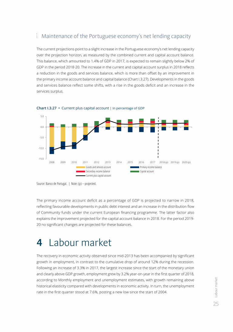
The current projections point to a slight increase in the Portuguese economy’s net lending capacity
over the projection horizon, as measured by the combined current and capital account balance.
This balance, which amounted to 1.4% of GDP in 2017, is expected to remain slightly below 2% of
GDP in the period 2018-20. The increase in the current and capital account surplus in 2018 reflects
a reduction in the goods and services balance, which is more than offset by an improvement in
the primary income account balance and capital balance (Chart I.3.27). Developments in the goods
and services balance reflect some shifts, with a rise in the goods deficit and an increase in the
services surplus.
Chart I.3.27 • Current plus capital account | In percentage of GDP
-15.0
-10.0
-5.0
0.0
5.0
2008 2009 2010 2011 2012 2013 2014 2015 2016 2017 2018 (p) 2019 (p) 2020 (p)
Goods and services account Primary income balanceSecondary income balance Capital accountCurrent plus capital account
Source: Banco de Portugal. | Note: (p) – projected.
The primary income account deficit as a percentage of GDP is projected to narrow in 2018,
reflecting favourable developments in public debt interest and an increase in the distribution flow
of Community funds under the current European financing programme. The latter factor also
explains the improvement projected for the capital account balance in 2018. For the period 2019-
20 no significant changes are projected for these balances.
4 Labour marketThe recovery in economic activity observed since mid-2013 has been accompanied by significant
growth in employment, in contrast to the cumulative drop of around 12% during the recession.
Following an increase of 3.3% in 2017, the largest increase since the start of the monetary union
and clearly above GDP growth, employment grew by 3.2% year-on-year in the first quarter of 2018,
according to Monthly employment and unemployment estimates, with growth remaining above
historical elasticity compared with developments in economic activity. In turn, the unemployment
rate in the first quarter stood at 7.6%, posting a new low since the start of 2004.
Banc
o de
Por
tuga
l •
Eco
nom
ic B
ulle
tin •
Jun
e 20
18
26
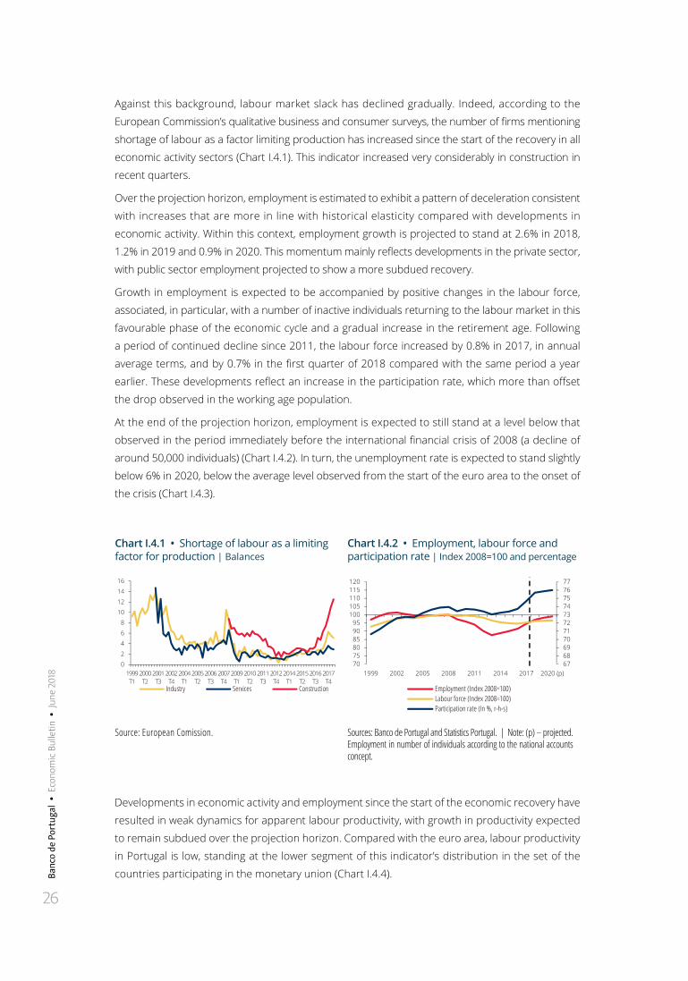
Against this background, labour market slack has declined gradually. Indeed, according to the
European Commission’s qualitative business and consumer surveys, the number of firms mentioning
shortage of labour as a factor limiting production has increased since the start of the recovery in all
economic activity sectors (Chart I.4.1). This indicator increased very considerably in construction in
recent quarters.
Over the projection horizon, employment is estimated to exhibit a pattern of deceleration consistent
with increases that are more in line with historical elasticity compared with developments in
economic activity. Within this context, employment growth is projected to stand at 2.6% in 2018,
1.2% in 2019 and 0.9% in 2020. This momentum mainly reflects developments in the private sector,
with public sector employment projected to show a more subdued recovery.
Growth in employment is expected to be accompanied by positive changes in the labour force,
associated, in particular, with a number of inactive individuals returning to the labour market in this
favourable phase of the economic cycle and a gradual increase in the retirement age. Following
a period of continued decline since 2011, the labour force increased by 0.8% in 2017, in annual
average terms, and by 0.7% in the first quarter of 2018 compared with the same period a year
earlier. These developments reflect an increase in the participation rate, which more than offset
the drop observed in the working age population.
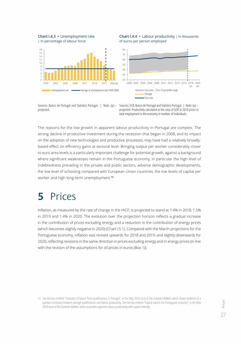
At the end of the projection horizon, employment is expected to still stand at a level below that
observed in the period immediately before the international financial crisis of 2008 (a decline of
around 50,000 individuals) (Chart I.4.2). In turn, the unemployment rate is expected to stand slightly
below 6% in 2020, below the average level observed from the start of the euro area to the onset of
the crisis (Chart I.4.3).
Chart I.4.1 • Shortage of labour as a limiting factor for production | Balances
Chart I.4.2 • Employment, labour force and participation rate | Index 2008=100 and percentage
0
2
4
6
8
10
12
14
16
1999 T1
2000 T2
2001 T3
2002 T4
2004 T1
2005 T2
2006 T3
2007 T4
2009 T1
2010 T2
2011 T3
2012 T4
2014 T1
2015 T2
2016 T3
2017 T4
Industry Services Construction
6768697071727374757677
707580859095
100105110115120
1999 2002 2005 2008 2011 2014 2017 2020 (p)
Employment (Index 2008=100)Labour force (Index 2008=100)Participation rate (In %, r-h-s)
Source: European Comission. Sources: Banco de Portugal and Statistics Portugal. | Note: (p) – projected. Employment in number of individuals according to the national accounts concept.
Developments in economic activity and employment since the start of the economic recovery have
resulted in weak dynamics for apparent labour productivity, with growth in productivity expected
to remain subdued over the projection horizon. Compared with the euro area, labour productivity
in Portugal is low, standing at the lower segment of this indicator’s distribution in the set of the
countries participating in the monetary union (Chart I.4.4).
Price
s
27
Chart I.4.3 • Unemployment rate | In percentage of labour force
Chart I.4.4 • Labour productivity | In thousands of euros per person employed
02468
1012141618
1999 2002 2005 2008 2011 2014 2017 2020 (p)
Unemployment rate Average of unemployment rate (1999-2008)
20
30
40
50
60
70
80
2000 2002 2004 2006 2008 2010 2012 2014 2016 2018(p)
2020(p)
Euro area − 25 to 75 percentile range PortugalEuro area
Sources: Banco de Portugal and Statistics Portugal. | Note: (p) – projected.
Sources: ECB, Banco de Portugal and Statistics Portugal. | Note: (p) – projected. Productivity calculated as the ratio of GDP at 2010 prices to total employment in the economy in number of individuals.
The reasons for the low growth in apparent labour productivity in Portugal are complex. The
strong decline in productive investment during the recession that began in 2008, and its impact
on the adoption of new technologies and productive processes, may have had a relatively broadly-
based effect on efficiency gains at sectoral level. Bringing output per worker considerably closer
to euro area levels is a particularly important challenge for potential growth, against a background
where significant weaknesses remain in the Portuguese economy, in particular the high level of
indebtedness prevailing in the private and public sectors, adverse demographic developments,
the low level of schooling compared with European Union countries, the low levels of capital per
worker and high long-term unemployment.13
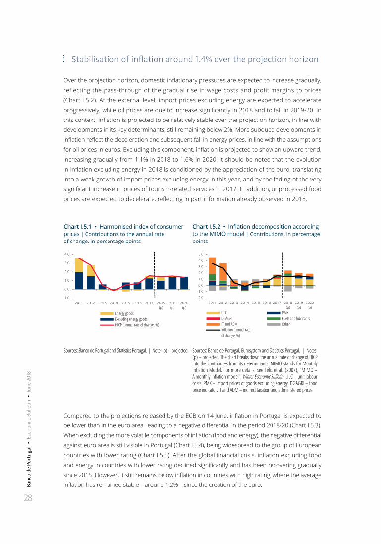
5 PricesInflation, as measured by the rate of change in the HICP, is projected to stand at 1.4% in 2018, 1.5%
in 2019 and 1.4% in 2020. The evolution over the projection horizon reflects a gradual increase
in the contribution of prices excluding energy and a reduction in the contribution of energy prices
(which becomes slightly negative in 2020) (Chart I.5.1). Compared with the March projections for the
Portuguese economy, inflation was revised upwards for 2018 and 2019, and slightly downwards for
2020, reflecting revisions in the same direction in prices excluding energy and in energy prices (in line
with the revision of the assumptions for oil prices in euros (Box 1)).
13. See the box entitled “Evolution of labour force qualifications in Portugal”, in the May 2018 issue of the Economic Bulletin, which shows evidence of a positive correlation between average qualifications and labour productivity. See the box entitled “Capital stock in the Portuguese economy”, in the May 2018 issue of the Economic Bulletin, which associates apparent labour productivity with capital intensity.
Banc
o de
Por
tuga
l •
Eco
nom
ic B
ulle
tin •
Jun
e 20
18
28
Stabilisation of inflation around 1.4% over the projection horizon
Over the projection horizon, domestic inflationary pressures are expected to increase gradually,
reflecting the pass-through of the gradual rise in wage costs and profit margins to prices
(Chart I.5.2). At the external level, import prices excluding energy are expected to accelerate
progressively, while oil prices are due to increase significantly in 2018 and to fall in 2019-20. In
this context, inflation is projected to be relatively stable over the projection horizon, in line with
developments in its key determinants, still remaining below 2%. More subdued developments in
inflation reflect the deceleration and subsequent fall in energy prices, in line with the assumptions
for oil prices in euros. Excluding this component, inflation is projected to show an upward trend,
increasing gradually from 1.1% in 2018 to 1.6% in 2020. It should be noted that the evolution
in inflation excluding energy in 2018 is conditioned by the appreciation of the euro, translating
into a weak growth of import prices excluding energy in this year, and by the fading of the very
significant increase in prices of tourism-related services in 2017. In addition, unprocessed food
prices are expected to decelerate, reflecting in part information already observed in 2018.
Chart I.5.1 • Harmonised index of consumer prices | Contributions to the annual rate of change, in percentage points
Chart I.5.2 • Inflation decomposition according to the MIMO model | Contributions, in percentage points
-1.0
0.0
1.0
2.0
3.0
4.0
2011 2012 2013 2014 2015 2016 2017 2018(p)
2019(p)
2020(p)
Energy goodsExcluding energy goodsHICP (annual rate of change, %)
-2.0
-1.0
0.0
1.0
2.0
3.0
4.0
5.0
2011 2012 2013 2014 2015 2016 2017 2018(p)
2019(p)
2020(p)
ULC PMXDGAGRI Fuels and lubricants
OtherIT and ADMInflation (annual rate of change, %)
Sources: Banco de Portugal and Statistics Portugal. | Note: (p) – projected. Sources: Banco de Portugal, Eurosystem and Statistics Portugal. | Notes: (p) – projected. The chart breaks down the annual rate of change of HICP into the contributes from its determinants. MIMO stands for Monthly Inflation Model. For more details, see Félix et al. (2007), “MIMO – A monthly inflation model”, Winter Economic Bulletin. ULC – unit labour costs. PMX – import prices of goods excluding energy. DGAGRI – food price indicator. IT and ADM – indirect taxation and administered prices.
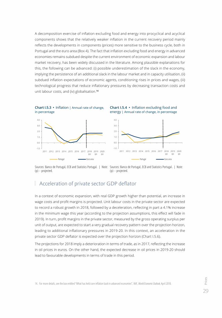
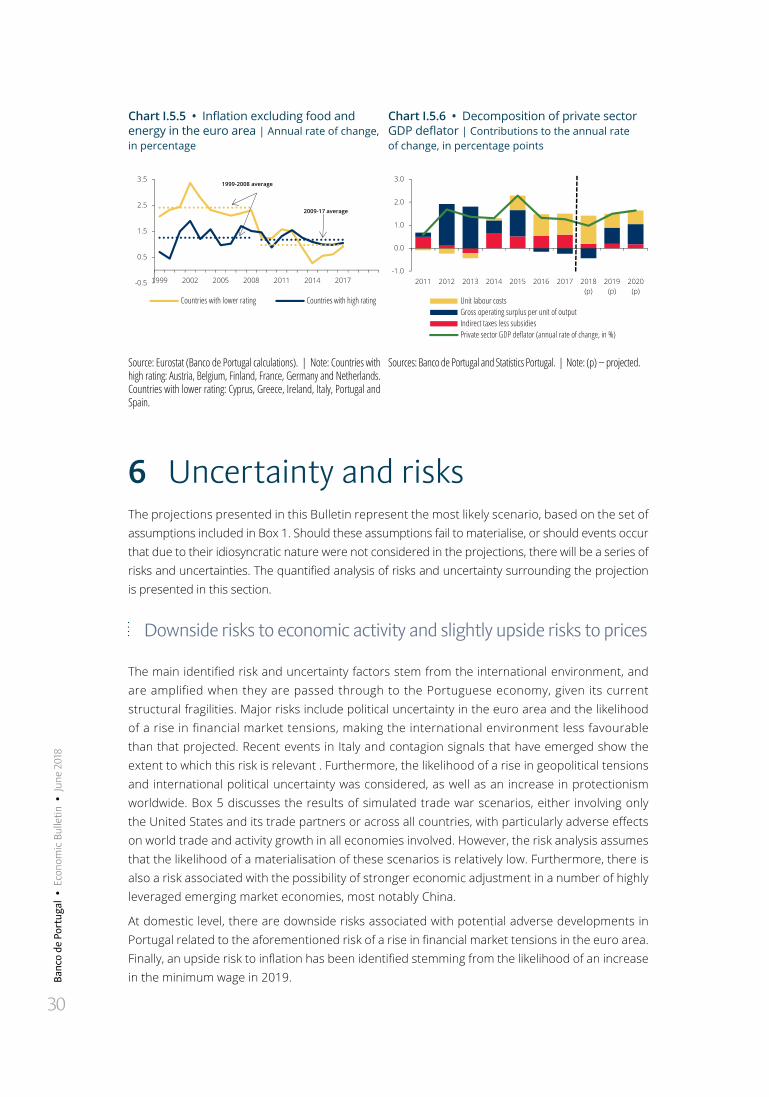
Compared to the projections released by the ECB on 14 June, inflation in Portugal is expected to
be lower than in the euro area, leading to a negative differential in the period 2018-20 (Chart I.5.3).
When excluding the more volatile components of inflation (food and energy), the negative differential
against euro area is still visible in Portugal (Chart I.5.4), being widespread to the group of European
countries with lower rating (Chart I.5.5). After the global financial crisis, inflation excluding food
and energy in countries with lower rating declined significantly and has been recovering gradually
since 2015. However, it still remains below inflation in countries with high rating, where the average
inflation has remained stable – around 1.2% – since the creation of the euro.
Price
s
29
A decomposition exercise of inflation excluding food and energy into procyclical and acyclical
components shows that the relatively weaker inflation in the current recovery period mainly
reflects the developments in components (prices) more sensitive to the business cycle, both in
Portugal and the euro area (Box 4). The fact that inflation excluding food and energy in advanced
economies remains subdued despite the current environment of economic expansion and labour
market recovery, has been widely discussed in the literature. Among plausible explanations for
this, the following can be advanced: (i) possible underestimation of the slack in the economy,
implying the persistence of an additional slack in the labour market and in capacity utilisation, (ii)
subdued inflation expectations of economic agents, conditioning rises in prices and wages, (iii)
technological progress that reduce inflationary pressures by decreasing transaction costs and
unit labour costs, and (iv) globalisation.14
Chart I.5.3 • Inflation | Annual rate of change, in percentage
Chart I.5.4 • Inflation excluding food and energy | Annual rate of change, in percentage
-1.0
0.0
1.0
2.0
3.0
4.0
2011 2012 2013 2014 2015 2016 2017 2018(p)
2019(p)
2020(p)
Portugal Euro area
-1.0
0.0
1.0
2.0
3.0
4.0
2011 2012 2013 2014 2015 2016 2017 2018(p)
2019(p)
2020(p)
Portugal Euro area
Sources: Banco de Portugal, ECB and Statistics Portugal. | Note: (p) – projected.
Sources: Banco de Portugal, ECB and Statistics Portugal. | Note: (p) – projected.
Acceleration of private sector GDP deflator
In a context of economic expansion, with real GDP growth higher than potential, an increase in
wage costs and profit margins is projected. Unit labour costs in the private sector are expected
to record a robust growth in 2018, followed by a deceleration, reflecting in part a 4.1% increase
in the minimum wage this year (according to the projection assumptions, this effect will fade in
2019). In turn, profit margins in the private sector, measured by the gross operating surplus per
unit of output, are expected to start a very gradual recovery pattern over the projection horizon,
leading to additional inflationary pressures in 2019-20. In this context, an acceleration in the
private sector GDP deflator is expected over the projection horizon (Chart I.5.6).
The projections for 2018 imply a deterioration in terms of trade, as in 2017, reflecting the increase
in oil prices in euros. On the other hand, the expected decrease in oil prices in 2019-20 should
lead to favourable developments in terms of trade in this period.
14. For more details, see the box entitled “What has held core inflation back in advanced economies”, IMF, World Economic Outlook, April 2018.
Banc
o de
Por
tuga
l •
Eco
nom
ic B
ulle
tin •
Jun
e 20
18
30
Chart I.5.5 • Inflation excluding food and energy in the euro area | Annual rate of change, in percentage
Chart I.5.6 • Decomposition of private sector GDP deflator | Contributions to the annual rate of change, in percentage points
-0.5
0.5
1.5
2.5
3.5
1999 2002 2005 2008 2011 2014 2017
Countries with lower rating Countries with high rating
2009-17 average
1999-2008 average
-1.0
0.0
1.0
2.0
3.0
2011 2012 2013 2014 2015 2016 2017 2018(p)
2019(p)
2020(p)
Unit labour costsGross operating surplus per unit of outputIndirect taxes less subsidiesPrivate sector GDP deflator (annual rate of change, in %)
Source: Eurostat (Banco de Portugal calculations). | Note: Countries with high rating: Austria, Belgium, Finland, France, Germany and Netherlands. Countries with lower rating: Cyprus, Greece, Ireland, Italy, Portugal and Spain.
Sources: Banco de Portugal and Statistics Portugal. | Note: (p) − projected.
6 Uncertainty and risksThe projections presented in this Bulletin represent the most likely scenario, based on the set of assumptions included in Box 1. Should these assumptions fail to materialise, or should events occur that due to their idiosyncratic nature were not considered in the projections, there will be a series of risks and uncertainties. The quantified analysis of risks and uncertainty surrounding the projection is presented in this section.
Downside risks to economic activity and slightly upside risks to prices
The main identified risk and uncertainty factors stem from the international environment, and are amplified when they are passed through to the Portuguese economy, given its current structural fragilities. Major risks include political uncertainty in the euro area and the likelihood of a rise in financial market tensions, making the international environment less favourable than that projected. Recent events in Italy and contagion signals that have emerged show the extent to which this risk is relevant . Furthermore, the likelihood of a rise in geopolitical tensions and international political uncertainty was considered, as well as an increase in protectionism worldwide. Box 5 discusses the results of simulated trade war scenarios, either involving only the United States and its trade partners or across all countries, with particularly adverse effects on world trade and activity growth in all economies involved. However, the risk analysis assumes that the likelihood of a materialisation of these scenarios is relatively low. Furthermore, there is also a risk associated with the possibility of stronger economic adjustment in a number of highly leveraged emerging market economies, most notably China.
At domestic level, there are downside risks associated with potential adverse developments in Portugal related to the aforementioned risk of a rise in financial market tensions in the euro area. Finally, an upside risk to inflation has been identified stemming from the likelihood of an increase in the minimum wage in 2019.
Unc
erta
inty
and
risk
s
31
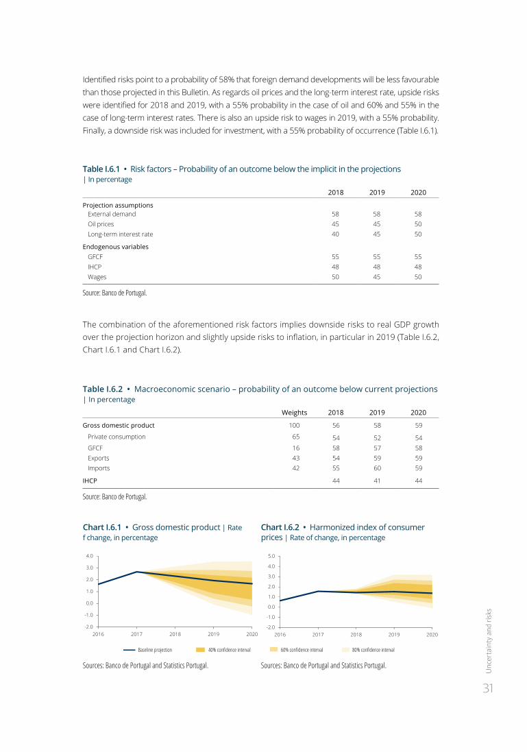
Identified risks point to a probability of 58% that foreign demand developments will be less favourable than those projected in this Bulletin. As regards oil prices and the long-term interest rate, upside risks were identified for 2018 and 2019, with a 55% probability in the case of oil and 60% and 55% in the case of long-term interest rates. There is also an upside risk to wages in 2019, with a 55% probability. Finally, a downside risk was included for investment, with a 55% probability of occurrence (Table I.6.1).
Table I.6.1 • Risk factors – Probability of an outcome below the implicit in the projections | In percentage
2018 2019 2020
Projection assumptionsExternal demand 58 58 58Oil prices 45 45 50Long-term interest rate 40 45 50
Endogenous variablesGFCF 55 55 55IHCP 48 48 48Wages 50 45 50
Source: Banco de Portugal.
The combination of the aforementioned risk factors implies downside risks to real GDP growth over the projection horizon and slightly upside risks to inflation, in particular in 2019 (Table I.6.2, Chart I.6.1 and Chart I.6.2).
Table I.6.2 • Macroeconomic scenario – probability of an outcome below current projections | In percentage
Weights 2018 2019 2020
Gross domestic product 100 56 58 59
Private consumption 65 54 52 54GFCF 16 58 57 58Exports 43 54 59 59Imports 42 55 60 59
IHCP 44 41 44
Source: Banco de Portugal.
Chart I.6.1 • Gross domestic product | Rate f change, in percentage
Chart I.6.2 • Harmonized index of consumer prices | Rate of change, in percentage
-2.0
-1.0
0.0
1.0
2.0
3.0
4.0
2016 2017 2018 2019 2020-2.0
-1.0
0.0
1.0
2.0
3.0
4.0
5.0
2016 2017 2018 2019 2020
ATENÇÃO: UMA VEZ QUE OS QUADROS I.6.1 E I.6.2 TINHAM OS VALORES ERRADOS E ESTE GRÁFICO FOI CALCULADOS A PARTIR DESSES QUADROS HNÃO NOS É POSSÍVEL VERIFICAR, UMA VEZ QUE ELE ESTÁ LIGADO A FICHEIRO QUE NÓS NÃO TEMOS ACESSO
Gross domestic product | Rate of change, in percentageGraf I.6.2
Baseline projection 40% confidence interval 60% confidence interval 80% confidence interval
-2.0
-1.0
0.0
1.0
2.0
3.0
4.0
2016 2017 2018 2019 2020
Sources: Banco de Portugal and Statistics Portugal. Sources: Banco de Portugal and Statistics Portugal.
Banc
o de
Por
tuga
l •
Eco
nom
ic B
ulle
tin •
Jun
e 20
18
32
7 ConclusionsAmid a favourable economic and financial environment, current projections point to the continued expansion in the Portuguese economy over the period 2018-20, although at a progressively slower pace, gradually approaching its potential growth.
Underlying projected developments is an increase in the weight of exports and investment (particularly corporate investment) in GDP and the continued recovery in the labour market, while the unemployment rate continued to follow a downward path. These developments are consistent with the maintenance of fundamental macroeconomic equilibria, namely as regards the Portuguese economy’s external surplus.
The projected deceleration profile of the economic activity over the forecast horizon reflects some slowdown in external demand and structural constraints to greater potential growth. Despite the macroeconomic adjustability of the Portuguese economy over the past few years and the sectoral restructuring based on the growing internationalisation of enterprises, major constraints to long-term growth persist.
The current cyclical situation should be seized to correct any remaining macroeconomic imbalances,
thus facilitating an increase in long-term growth in the Portuguese economy and bringing it closer
to the European income levels. In this context, investment must be increasingly channelled towards
the most productive sectors of the economy, to allow for the incorporation of new technology in
the production process and to increase capital per worker levels, which are among the lowest in the
Monetary Union. In a global economy, where growth hinges on technologically advanced industries
and innovation, low labour force skills are a major constraint to greater long-term growth. In this
context, it is essential to improve the skills of the Portuguese labour force, which, despite recent
progress, are still low compared to the EU average. The improvement in human capital may offset
the negative effects of long-term demographic developments. Another challenge is associated with
the labour market, in which a high percentage of long-term unemployment still persists. Against
this background, the decrease in the high prevalence of very long-term unemployment must be
at the forefront when designing unemployment-reducing policies. Finally, the efforts to reduce
the high leveraging of the public and private sectors must continue, with a view to decreasing the
Portuguese economy’s vulnerability to adverse shocks. The temporary nature of the current broad
range of non-standard monetary policy measures in the euro area and the persistence of downside
risks to activity, particularly related to the rise in geopolitical tensions and international political
uncertainty, emphasise the importance and urgency of structural progress in all these dimensions.
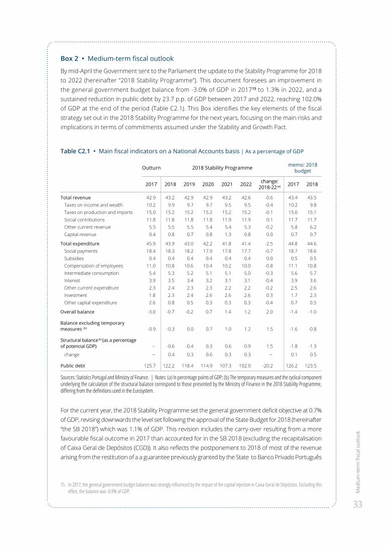
Med
ium
-ter
m fi
scal
out
look
33
Box 2 • Medium-term fiscal outlook
By mid-April the Government sent to the Parliament the update to the Stability Programme for 2018 to 2022 (hereinafter “2018 Stability Programme”). This document foresees an improvement in the general government budget balance from -3.0% of GDP in 201715 to 1.3% in 2022, and a sustained reduction in public debt by 23.7 p.p. of GDP between 2017 and 2022, reaching 102.0% of GDP at the end of the period (Table C2.1). This Box identifies the key elements of the fiscal strategy set out in the 2018 Stability Programme for the next years, focusing on the main risks and implications in terms of commitments assumed under the Stability and Growth Pact.
Table C2.1 • Main fiscal indicators on a National Accounts basis | As a percentage of GDP
Outturn 2018 Stability Programme memo: 2018 budget
2017 2018 2019 2020 2021 2022 change: 2018-22 (a) 2017 2018
Total revenue 42.9 43.2 42.9 42.9 43.2 42.6 -0.6 43.4 43.5Taxes on income and wealth 10.2 9.9 9.7 9.7 9.5 9.5 -0.4 10.2 9.8Taxes on production and imports 15.0 15.2 15.2 15.2 15.2 15.2 -0.1 15.0 15.1Social contributions 11.8 11.8 11.8 11.8 11.9 11.9 0.1 11.7 11.7Other current revenue 5.5 5.5 5.5 5.4 5.4 5.3 -0.2 5.8 6.2Capital revenue 0.4 0.8 0.7 0.8 1.3 0.8 0.0 0.7 0.7
Total expenditure 45.9 43.9 43.0 42.2 41.8 41.4 -2.5 44.8 44.6Social payments 18.4 18.3 18.2 17.9 17.8 17.7 -0.7 18.7 18.6Subsidies 0.4 0.4 0.4 0.4 0.4 0.4 0.0 0.5 0.5Compensation of employees 11.0 10.8 10.6 10.4 10.2 10.0 -0.8 11.1 10.8Intermediate consumption 5.4 5.3 5.2 5.1 5.1 5.0 -0.3 5.6 5.7Interest 3.9 3.5 3.4 3.2 3.1 3.1 -0.4 3.9 3.6Other current expenditure 2.3 2.4 2.3 2.3 2.2 2.2 -0.2 2.5 2.6Investment 1.8 2.3 2.4 2.6 2.6 2.6 0.3 1.7 2.3Other capital expenditure 2.6 0.8 0.5 0.3 0.3 0.3 -0.4 0.7 0.5
Overall balance -3.0 -0.7 -0.2 0.7 1.4 1.2 2.0 -1.4 -1.0
Balance excluding temporary measures (b) -0.9 -0.3 0.0 0.7 1.0 1.2 1.5 -1.6 -0.8
Structural balance (b) (as a percentage of potencial GDP) – -0.6 -0.4 0.3 0.6 0.9 1.5 -1.8 -1.3
change – 0.4 0.3 0.6 0.3 0.3 – 0.1 0.5
Public debt 125.7 122.2 118.4 114.9 107.3 102.0 -20.2 126.2 123.5
Sources: Statistics Portugal and Ministry of Finance. | Notes: (a) In percentage points of GDP; (b) The temporary measures and the cyclical component underlying the calculation of the structural balance correspond to those presented by the Ministry of Finance in the 2018 Stability Programme, differing from the definitions used in the Eurosystem.
For the current year, the 2018 Stability Programme set the general government deficit objective at 0.7% of GDP, revising downwards the level set following the approval of the State Budget for 2018 (hereinafter “the SB 2018”) which was 1.1% of GDP. This revision includes the carry-over resulting from a more favourable fiscal outcome in 2017 than accounted for in the SB 2018 (excluding the recapitalisation of Caixa Geral de Depósitos (CGD)). It also reflects the postponement to 2018 of most of the revenue arising from the restitution of a a guarantee previously granted by the State to Banco Privado Português
15. In 2017, the general government budget balance was strongly influenced by the impact of the capital injection in Caixa Geral de Depósitos. Excluding this effect, the balance was -0.9% of GDP.
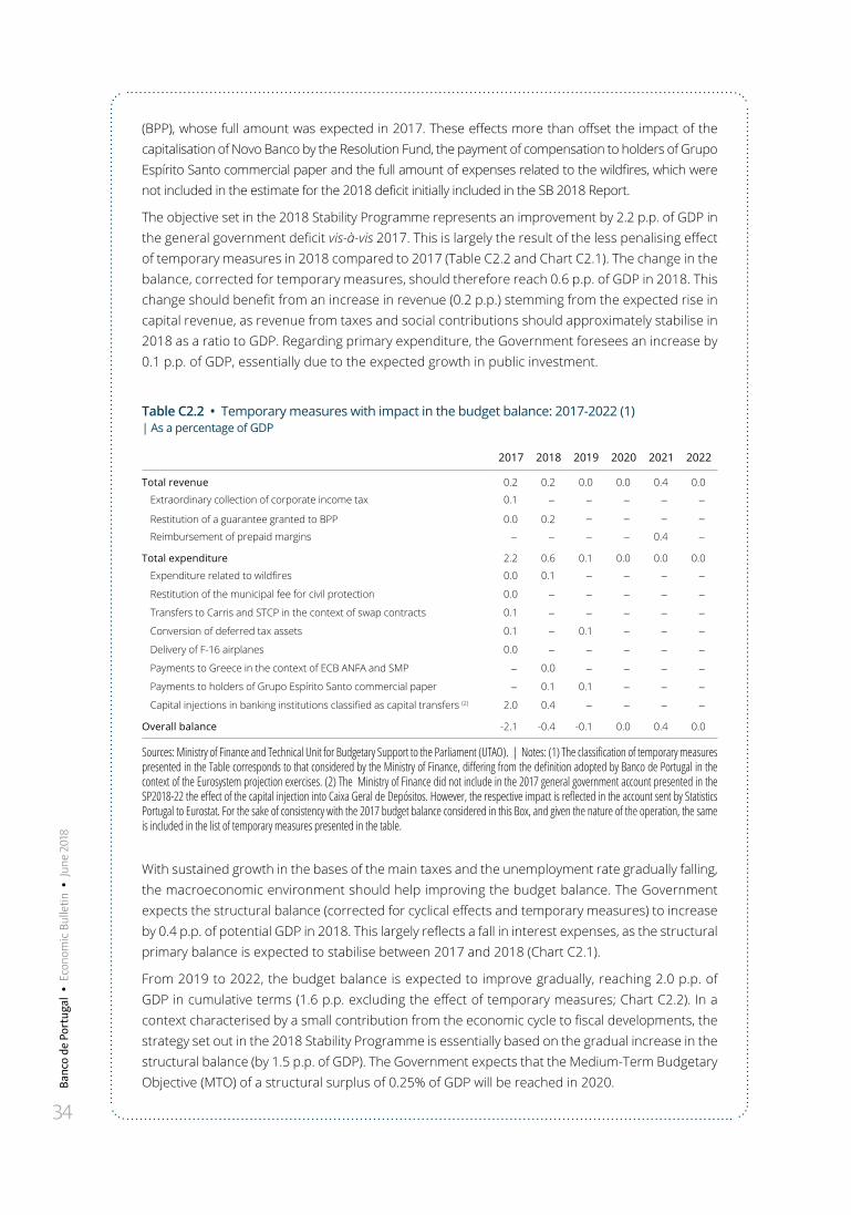
34
Banc
o de
Por
tuga
l •
Eco
nom
ic B
ulle
tin •
Jun
e 20
18
(BPP), whose full amount was expected in 2017. These effects more than offset the impact of the capitalisation of Novo Banco by the Resolution Fund, the payment of compensation to holders of Grupo Espírito Santo commercial paper and the full amount of expenses related to the wildfires, which were not included in the estimate for the 2018 deficit initially included in the SB 2018 Report.
The objective set in the 2018 Stability Programme represents an improvement by 2.2 p.p. of GDP in the general government deficit vis-à-vis 2017. This is largely the result of the less penalising effect of temporary measures in 2018 compared to 2017 (Table C2.2 and Chart C2.1). The change in the balance, corrected for temporary measures, should therefore reach 0.6 p.p. of GDP in 2018. This change should benefit from an increase in revenue (0.2 p.p.) stemming from the expected rise in capital revenue, as revenue from taxes and social contributions should approximately stabilise in 2018 as a ratio to GDP. Regarding primary expenditure, the Government foresees an increase by 0.1 p.p. of GDP, essentially due to the expected growth in public investment.
Table C2.2 • Temporary measures with impact in the budget balance: 2017-2022 (1) | As a percentage of GDP
2017 2018 2019 2020 2021 2022
Total revenue 0.2 0.2 0.0 0.0 0.4 0.0
Extraordinary collection of corporate income tax 0.1 – – – – –Restitution of a guarantee granted to BPP 0.0 0.2 – – – –Reimbursement of prepaid margins – – – – 0.4 –
Total expenditure 2.2 0.6 0.1 0.0 0.0 0.0
Expenditure related to wildfires 0.0 0.1 – – – –Restitution of the municipal fee for civil protection 0.0 – – – – –Transfers to Carris and STCP in the context of swap contracts 0.1 – – – – –Conversion of deferred tax assets 0.1 – 0.1 – – –Delivery of F-16 airplanes 0.0 – – – – –Payments to Greece in the context of ECB ANFA and SMP – 0.0 – – – –Payments to holders of Grupo Espírito Santo commercial paper – 0.1 0.1 – – –Capital injections in banking institutions classified as capital transfers (2) 2.0 0.4 – – – –
Overall balance -2.1 -0.4 -0.1 0.0 0.4 0.0
Sources: Ministry of Finance and Technical Unit for Budgetary Support to the Parliament (UTAO). | Notes: (1) The classification of temporary measures presented in the Table corresponds to that considered by the Ministry of Finance, differing from the definition adopted by Banco de Portugal in the context of the Eurosystem projection exercises. (2) The Ministry of Finance did not include in the 2017 general government account presented in the SP2018-22 the effect of the capital injection into Caixa Geral de Depósitos. However, the respective impact is reflected in the account sent by Statistics Portugal to Eurostat. For the sake of consistency with the 2017 budget balance considered in this Box, and given the nature of the operation, the same is included in the list of temporary measures presented in the table.
With sustained growth in the bases of the main taxes and the unemployment rate gradually falling, the macroeconomic environment should help improving the budget balance. The Government expects the structural balance (corrected for cyclical effects and temporary measures) to increase by 0.4 p.p. of potential GDP in 2018. This largely reflects a fall in interest expenses, as the structural primary balance is expected to stabilise between 2017 and 2018 (Chart C2.1).
From 2019 to 2022, the budget balance is expected to improve gradually, reaching 2.0 p.p. of GDP in cumulative terms (1.6 p.p. excluding the effect of temporary measures; Chart C2.2). In a context characterised by a small contribution from the economic cycle to fiscal developments, the strategy set out in the 2018 Stability Programme is essentially based on the gradual increase in the structural balance (by 1.5 p.p. of GDP). The Government expects that the Medium-Term Budgetary Objective (MTO) of a structural surplus of 0.25% of GDP will be reached in 2020.
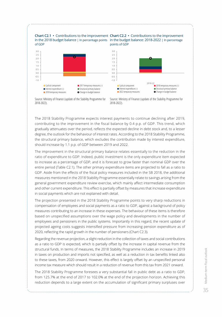
Med
ium
-ter
m fi
scal
out
look
35
Chart C2.1 • Contributions to the improvement in the 2018 budget balance | In percentage points of GDP
Chart C2.2 • Contributions to the improvement in the budget balance: 2018-2022 | In percentage points of GDP
-1.0
-0.5
0.0
0.5
1.0
1.5
2.0
2.5
3.0
Cyclical component 2017 temporary measures (-)Interest expenditure (-) Structural primary balance2018 temporary measures Change in budget balance
-1.0
-0.5
0.0
0.5
1.0
1.5
2.0
2.5
3.0
2018-22Cyclical component 2018 temporary measures (-)Interest expenditure (-) Structural primary balance2022 temporary measures Change in budget balance
Source: Ministry of Finance (update of the Stability Programme for 2018-2022).
Source: Ministry of Finance (update of the Stability Programme for 2018-2022).
The 2018 Stability Programme expects interest payments to continue declining after 2019, contributing to the improvement in the fiscal balance by 0.4 p.p. of GDP. This trend, which gradually attenuates over the period, reflects the expected decline in debt stock and, to a lesser degree, the outlook for the behaviour of interest rates. According to the 2018 Stability Programme, the structural primary balance, which excludes the contribution made by interest expenditure, should increase by 1.1 p.p. of GDP between 2019 and 2022.
The improvement in the structural primary balance relates essentially to the reduction in the ratio of expenditure to GDP. Indeed, public investment is the only expenditure item expected to increase as a percentage of GDP, and it is forecast to grow faster than nominal GDP over the entire period (Table C2.1). The other primary expenditure items are projected to fall as a ratio to GDP. Aside from the effects of the fiscal policy measures included in the SB 2018, the additional measures mentioned in the 2018 Stability Programme essentially relate to savings arising from the general government expenditure review exercise, which mainly affect intermediate consumption and other current expenditure. This effect is partially offset by measures that increase expenditure in social payments which are not explained with detail.
The projection presented in the 2018 Stability Programme points to very sharp reductions in compensation of employees and social payments as a ratio to GDP, against a background of policy measures contributing to an increase in these expenses. The behaviour of these items is therefore based on unspecified assumptions over the wage policy and developments in the number of employees and pensioners in the public systems. Importantly in this regard, the recent update of projected ageing costs suggests intensified pressure from increasing pension expenditure as of 2020, reflecting the rapid growth in the number of pensioners (Chart C2.3).
Regarding the revenue projection, a slight reduction in the collection of taxes and social contributions as a ratio to GDP is expected, which is partially offset by the increase in capital revenue from the structural funds. In terms of measures, the 2018 Stability Programme includes an increase in 2019 in taxes on production and imports not specified, as well as a reduction in tax benefits linked also to these taxes, from 2020 onward. However, this effect is largely offset by an unspecified personal income tax measure which should result in a reduction of revenue from this tax from 2021 onward.
The 2018 Stability Programme foresees a very substantial fall in public debt as a ratio to GDP, from 125.7% at the end of 2017 to 102.0% at the end of the projection horizon. Achieving this reduction depends to a large extent on the accumulation of significant primary surpluses over
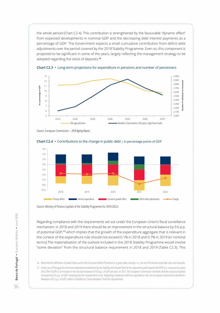
36
Banc
o de
Por
tuga
l •
Eco
nom
ic B
ulle
tin •
Jun
e 20
18
the whole period (Chart C2.4). This contribution is strengthened by the favourable “dynamic effect” from expected developments in nominal GDP and the decreasing debt interest payments as a percentage of GDP. The Government expects a small cumulative contribution from deficit-debt adjustments over the period covered by the 2018 Stability Programme. Even so, this component is projected to be significant in some of the years, largely reflecting the management strategy to be adopted regarding the stock of deposits.16
Chart C2.3 • Long-term projections for expenditure in pensions and number of pensioners
2,000
2,100
2,200
2,300
2,400
2,500
2,600
2,700
2,800
2,900
3,000
5
6
7
8
9
10
11
12
13
2016 2020 2030 2040 2050 2060 2070
Old-age pensions Number of pensioners (>65 years; right-hand scale)
As
a pe
rcen
tage
of G
DP
Num
ber
of in
divi
dual
s (in
tho
usan
d)
Source: European Commission – 2018 Ageing Report.
Chart C2.4 • Contributions to the change in public debt | In percentage points of GDP
-10.0
-8.0
-6.0
-4.0
-2.0
0.0
2.0
4.0
6.0
2018 2019 2020 2021 2022
Primary deficit Interest expenditure Economic growth effect Deficit-debt adjustments Change
Source: Ministry of Finance (update of the Stability Programme for 2018-2022).
Regarding compliance with the requirements set out under the European Union’s fiscal surveillance mechanism, in 2018 and 2019 there should be an improvement in the structural balance by 0.6 p.p. of potential GDP,17 which implies that the growth of the expenditure aggregate that is relevant in the context of the expenditure rule should not exceed 0.1% in 2018 and 0.7% in 2019 (in nominal terms).The materialisation of the outlook included in the 2018 Stability Programme would involve “some deviation” from the structural balance requirement in 2018 and 2019 (Table C2.3). This
16. Note that the definition of public debt used in the Excessive Deficit Procedure is a gross debt concept, i.e. not net of financial assets like cash and deposits.17. In the case of Portugal, the minimum adjustment established by the Stability and Growth Pact for the adjustment path towards the MTO (i.e. a structural surplus
of 0.25% of GDP) is an increase in the structural balance of 0.6 p.p. of GDP per year. In 2017, the European Commission estimates that the structural balance increased by 0.9 p.p. of GDP, meaning that this requirement is met. Regarding compliance with the expenditure rule, the European Commission identified a deviation of 0.5 p.p. of GDP, which it classified as “some deviation” from the requirement.
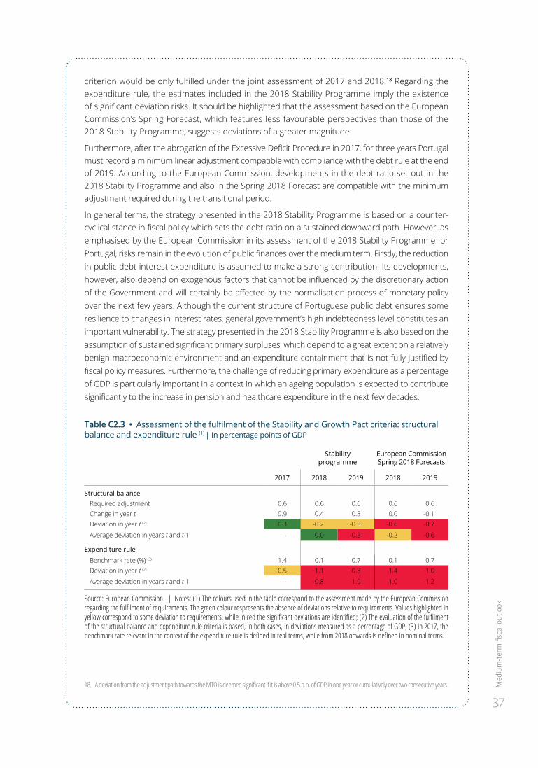
Med
ium
-ter
m fi
scal
out
look
37
criterion would be only fulfilled under the joint assessment of 2017 and 2018.18 Regarding the expenditure rule, the estimates included in the 2018 Stability Programme imply the existence of significant deviation risks. It should be highlighted that the assessment based on the European Commission’s Spring Forecast, which features less favourable perspectives than those of the 2018 Stability Programme, suggests deviations of a greater magnitude.
Furthermore, after the abrogation of the Excessive Deficit Procedure in 2017, for three years Portugal must record a minimum linear adjustment compatible with compliance with the debt rule at the end of 2019. According to the European Commission, developments in the debt ratio set out in the 2018 Stability Programme and also in the Spring 2018 Forecast are compatible with the minimum adjustment required during the transitional period.
In general terms, the strategy presented in the 2018 Stability Programme is based on a counter-cyclical stance in fiscal policy which sets the debt ratio on a sustained downward path. However, as emphasised by the European Commission in its assessment of the 2018 Stability Programme for Portugal, risks remain in the evolution of public finances over the medium term. Firstly, the reduction in public debt interest expenditure is assumed to make a strong contribution. Its developments, however, also depend on exogenous factors that cannot be influenced by the discretionary action of the Government and will certainly be affected by the normalisation process of monetary policy over the next few years. Although the current structure of Portuguese public debt ensures some resilience to changes in interest rates, general government’s high indebtedness level constitutes an important vulnerability. The strategy presented in the 2018 Stability Programme is also based on the assumption of sustained significant primary surpluses, which depend to a great extent on a relatively benign macroeconomic environment and an expenditure containment that is not fully justified by fiscal policy measures. Furthermore, the challenge of reducing primary expenditure as a percentage of GDP is particularly important in a context in which an ageing population is expected to contribute significantly to the increase in pension and healthcare expenditure in the next few decades.
Table C2.3 • Assessment of the fulfilment of the Stability and Growth Pact criteria: structural balance and expenditure rule (1) | In percentage points of GDP
Stability programme
European Commission Spring 2018 Forecasts
2017 2018 2019 2018 2019
Structural balanceRequired adjustment 0.6 0.6 0.6 0.6 0.6Change in year t 0.9 0.4 0.3 0.0 -0.1Deviation in year t (2) 0.3 -0.2 -0.3 -0.6 -0.7
Average deviation in years t and t-1 – 0.0 -0.3 -0.2 -0.6
Expenditure rule
Benchmark rate (%) (3) -1.4 0.1 0.7 0.1 0.7Deviation in year t (2) -0.5 -1.1 -0.8 -1.4 -1.0
Average deviation in years t and t-1 – -0.8 -1.0 -1.0 -1.2
Source: European Commission. | Notes: (1) The colours used in the table correspond to the assessment made by the European Commission regarding the fulfilment of requirements. The green colour respresents the absence of deviations relative to requirements. Values highlighted in yellow correspond to some deviation to requirements, while in red the significant deviations are identified; (2) The evaluation of the fulfilment of the structural balance and expenditure rule criteria is based, in both cases, in deviations measured as a percentage of GDP; (3) In 2017, the benchmark rate relevant in the context of the expenditure rule is defined in real terms, while from 2018 onwards is defined in nominal terms.
18. A deviation from the adjustment path towards the MTO is deemed significant if it is above 0.5 p.p. of GDP in one year or cumulatively over two consecutive years.
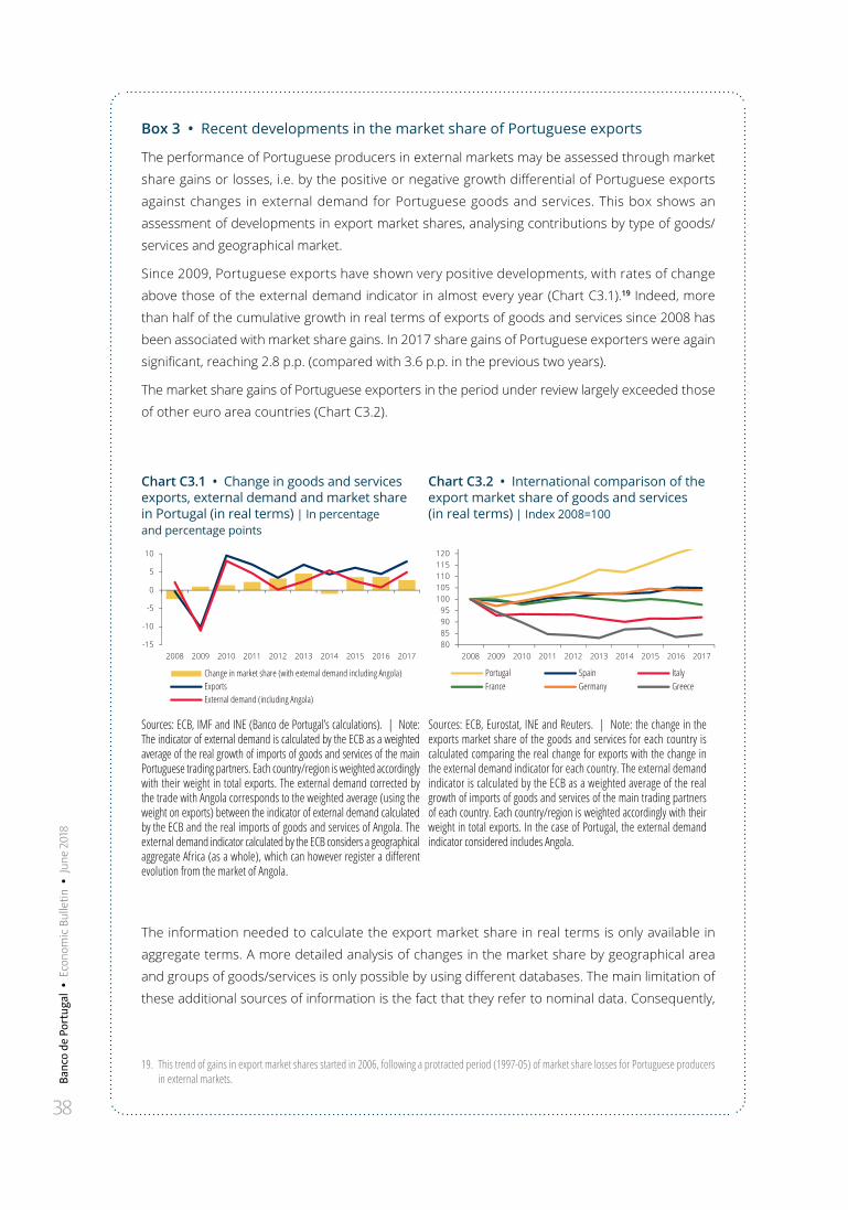
38
Banc
o de
Por
tuga
l •
Eco
nom
ic B
ulle
tin •
Jun
e 20
18
Box 3 • Recent developments in the market share of Portuguese exports
The performance of Portuguese producers in external markets may be assessed through market
share gains or losses, i.e. by the positive or negative growth differential of Portuguese exports
against changes in external demand for Portuguese goods and services. This box shows an
assessment of developments in export market shares, analysing contributions by type of goods/
services and geographical market.
Since 2009, Portuguese exports have shown very positive developments, with rates of change
above those of the external demand indicator in almost every year (Chart C3.1).19 Indeed, more
than half of the cumulative growth in real terms of exports of goods and services since 2008 has
been associated with market share gains. In 2017 share gains of Portuguese exporters were again
significant, reaching 2.8 p.p. (compared with 3.6 p.p. in the previous two years).
The market share gains of Portuguese exporters in the period under review largely exceeded those
of other euro area countries (Chart C3.2).
Chart C3.1 • Change in goods and services exports, external demand and market share in Portugal (in real terms) | In percentage and percentage points
Chart C3.2 • International comparison of the export market share of goods and services (in real terms) | Index 2008=100
-15
-10
-5
0
5
10
2008 2009 2010 2011 2012 2013 2014 2015 2016 2017
Change in market share (with external demand including Angola)ExportsExternal demand (including Angola)
80859095100105110115120
2008 2009 2010 2011 2012 2013 2014 2015 2016 2017
Portugal Spain ItalyFrance Germany Greece
Sources: ECB, IMF and INE (Banco de Portugal’s calculations). | Note: The indicator of external demand is calculated by the ECB as a weighted average of the real growth of imports of goods and services of the main Portuguese trading partners. Each country/region is weighted accordingly with their weight in total exports. The external demand corrected by the trade with Angola corresponds to the weighted average (using the weight on exports) between the indicator of external demand calculated by the ECB and the real imports of goods and services of Angola. The external demand indicator calculated by the ECB considers a geographical aggregate Africa (as a whole), which can however register a different evolution from the market of Angola.
Sources: ECB, Eurostat, INE and Reuters. | Note: the change in the exports market share of the goods and services for each country is calculated comparing the real change for exports with the change in the external demand indicator for each country. The external demand indicator is calculated by the ECB as a weighted average of the real growth of imports of goods and services of the main trading partners of each country. Each country/region is weighted accordingly with their weight in total exports. In the case of Portugal, the external demand indicator considered includes Angola.
The information needed to calculate the export market share in real terms is only available in
aggregate terms. A more detailed analysis of changes in the market share by geographical area
and groups of goods/services is only possible by using different databases. The main limitation of
these additional sources of information is the fact that they refer to nominal data. Consequently,
19. This trend of gains in export market shares started in 2006, following a protracted period (1997-05) of market share losses for Portuguese producers in external markets.
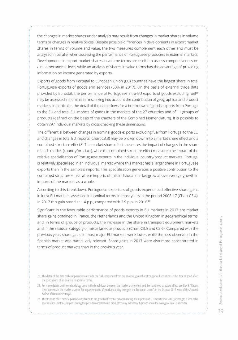
Rece
nt d
evel
opm
ents
in th
e m
arke
t sha
re o
f Por
tugu
ese
expo
rts
39
the changes in market shares under analysis may result from changes in market shares in volume
terms or changes in relative prices. Despite possible differences in developments in export market
shares in terms of volume and value, the two measures complement each other and must be
analysed in parallel when assessing the performance of Portuguese producers in external markets.
Developments in export market shares in volume terms are useful to assess competitiveness on
a macroeconomic level, while an analysis of shares in value terms has the advantage of providing
information on income generated by exports.
Exports of goods from Portugal to European Union (EU) countries have the largest share in total
Portuguese exports of goods and services (50% in 2017). On the basis of external trade data
provided by Eurostat, the performance of Portuguese intra-EU exports of goods excluding fuel20
may be assessed in nominal terms, taking into account the contribution of geographical and product
markets. In particular, the detail of the data allows for a breakdown of goods exports from Portugal
to the EU and total EU imports of goods in the markets of the 27 countries and of 11 groups of
products (defined on the basis of the chapters of the Combined Nomenclature). It is possible to
obtain 297 individual markets by cross-checking these dimensions.
The differential between changes in nominal goods exports excluding fuel from Portugal to the EU
and changes in total EU imports (Chart C3.3) may be broken down into a market share effect and a
combined structure effect.21 The market share effect measures the impact of changes in the share
of each market (country/product), while the combined structure effect measures the impact of the
relative specialisation of Portuguese exports in the individual country/product markets. Portugal
is relatively specialised in an individual market where this market has a larger share in Portuguese
exports than in the sample’s imports. This specialisation generates a positive contribution to the
combined structure effect where imports of this individual market grow above average growth in
imports of the markets as a whole.
According to this breakdown, Portuguese exporters of goods experienced effective share gains
in intra-EU markets, assessed in nominal terms, in most years in the period 2008-17 (Chart C3.4).
In 2017 this gain stood at 1.4 p.p., compared with 2.9 p.p. in 2016.22
Significant in the favourable performance of goods exports in EU markets in 2017 are market
share gains obtained in France, the Netherlands and the United Kingdom in geographical terms,
and, in terms of groups of products, the increase in the share in transport equipment markets
and in the residual category of miscellaneous products (Chart C3.5 and C3.6). Compared with the
previous year, share gains in most major EU markets were lower, while the loss observed in the
Spanish market was particularly relevant. Share gains in 2017 were also more concentrated in
terms of product markets than in the previous year.
20. The detail of the data makes it possible to exclude the fuel component from the analysis, given that strong price fluctuations in this type of good affect the conclusions of an analysis in nominal terms.
21. For more details on the methodology used in the breakdown between the market share effect and the combined structure effect, see Box 9, “Recent developments in the market share of Portuguese exports of goods excluding energy in the European Union”, in the October 2017 issue of the Economic Bulletin of Banco de Portugal.
22. The structure effect made a positive contribution to the growth differential between Portuguese exports and EU imports since 2013, pointing to a favourable specialisation in intra-EU exports during this period (concentration in product/country markets with growth above the average of total EU imports).
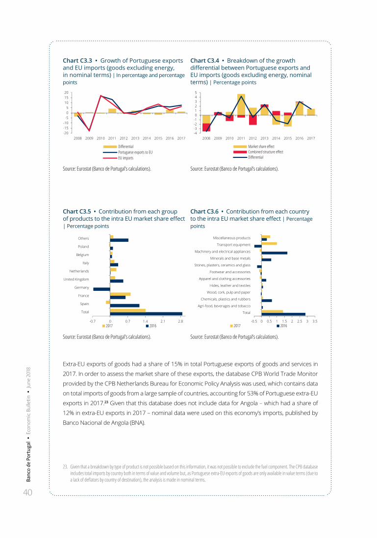
40
Banc
o de
Por
tuga
l •
Eco
nom
ic B
ulle
tin •
Jun
e 20
18
Chart C3.3 • Growth of Portuguese exports and EU imports (goods excluding energy, in nominal terms) | In percentage and percentage points
Chart C3.4 • Breakdown of the growth differential between Portuguese exports and EU imports (goods excluding energy, nominal terms) | Percentage points
-20-15-10-505101520
2008 2009 2010 2011 2012 2013 2014 2015 2016 2017
DifferentialPortuguese exports to EUEU imports
-4-3-2-1012345
2008 2009 2010 2011 2012 2013 2014 2015 2016 2017
Market share effectCombined structure effectDifferential
Source: Eurostat (Banco de Portugal’s calculations). Source: Eurostat (Banco de Portugal’s calculations).
Chart C3.5 • Contribution from each group of products to the intra EU market share effect | Percentage points
Chart C3.6 • Contribution from each country to the intra EU market share effect | Percentage points
-0.7 0 0.7 1.4 2.1 2.8
Total
Spain
France
Germany
United Kingdom
Netherlands
Italy
Belgium
Poland
Others
2017 2016-0.5 0 0.5 1 1.5 2 2.5 3 3.5
Total
Agri-food, beverages and tobacco
Chemicals, plastics and rubbers
Wood, cork, pulp and paper
Hides, leather and textiles
Apparel and clothing accessories
Footwear and accessories
Stones, plasters, ceramics and glass
Minerals and base metals
Machinery and electrical appliances
Transport equipment
Miscellaneous products
2017 2016
Source: Eurostat (Banco de Portugal’s calculations). Source: Eurostat (Banco de Portugal’s calculations).
Extra-EU exports of goods had a share of 15% in total Portuguese exports of goods and services in
2017. In order to assess the market share of these exports, the database CPB World Trade Monitor
provided by the CPB Netherlands Bureau for Economic Policy Analysis was used, which contains data
on total imports of goods from a large sample of countries, accounting for 53% of Portuguese extra-EU
exports in 2017.23 Given that this database does not include data for Angola – which had a share of
12% in extra-EU exports in 2017 – nominal data were used on this economy’s imports, published by
Banco Nacional de Angola (BNA).
23. Given that a breakdown by type of product is not possible based on this information, it was not possible to exclude the fuel component. The CPB database includes total imports by country both in terms of value and volume but, as Portuguese extra-EU exports of goods are only available in value terms (due to a lack of deflators by country of destination), the analysis is made in nominal terms.
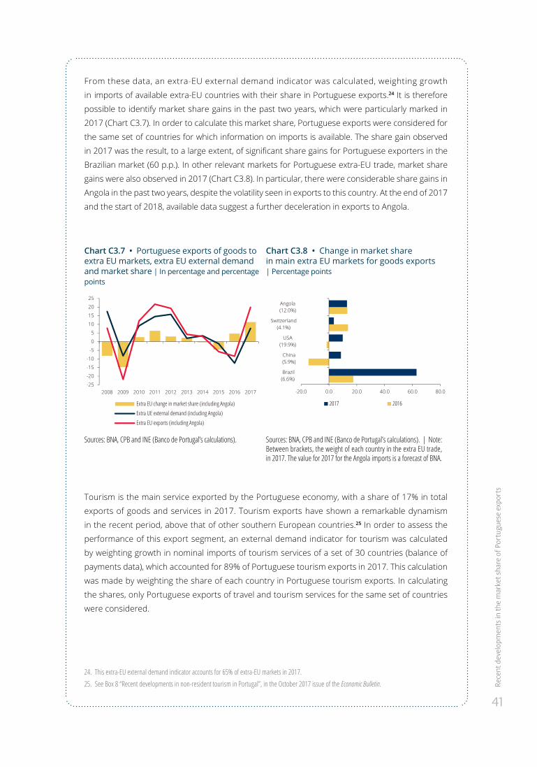
Rece
nt d
evel
opm
ents
in th
e m
arke
t sha
re o
f Por
tugu
ese
expo
rts
41
From these data, an extra-EU external demand indicator was calculated, weighting growth
in imports of available extra-EU countries with their share in Portuguese exports.24 It is therefore
possible to identify market share gains in the past two years, which were particularly marked in
2017 (Chart C3.7). In order to calculate this market share, Portuguese exports were considered for
the same set of countries for which information on imports is available. The share gain observed
in 2017 was the result, to a large extent, of significant share gains for Portuguese exporters in the
Brazilian market (60 p.p.). In other relevant markets for Portuguese extra-EU trade, market share
gains were also observed in 2017 (Chart C3.8). In particular, there were considerable share gains in
Angola in the past two years, despite the volatility seen in exports to this country. At the end of 2017
and the start of 2018, available data suggest a further deceleration in exports to Angola.
Chart C3.7 • Portuguese exports of goods to extra EU markets, extra EU external demand and market share | In percentage and percentage points
Chart C3.8 • Change in market share in main extra EU markets for goods exports | Percentage points
-25
-20
-15
-10
-5
0
5
10
15
20
25
2008 2009 2010 2011 2012 2013 2014 2015 2016 2017
Extra EU change in market share (including Angola)Extra UE external demand (including Angola)Extra EU exports (including Angola)
-20.0 0.0 20.0 40.0 60.0 80.0
Brazil (6.6%)
China(5.9%)
USA(19.9%)
Switzerland (4.1%)
Angola(12.0%)
2017 2016
Sources: BNA, CPB and INE (Banco de Portugal’s calculations). Sources: BNA, CPB and INE (Banco de Portugal’s calculations). | Note: Between brackets, the weight of each country in the extra EU trade, in 2017. The value for 2017 for the Angola imports is a forecast of BNA.
Tourism is the main service exported by the Portuguese economy, with a share of 17% in total
exports of goods and services in 2017. Tourism exports have shown a remarkable dynamism
in the recent period, above that of other southern European countries.25 In order to assess the
performance of this export segment, an external demand indicator for tourism was calculated
by weighting growth in nominal imports of tourism services of a set of 30 countries (balance of
payments data), which accounted for 89% of Portuguese tourism exports in 2017. This calculation
was made by weighting the share of each country in Portuguese tourism exports. In calculating
the shares, only Portuguese exports of travel and tourism services for the same set of countries
were considered.
24. This extra-EU external demand indicator accounts for 65% of extra-EU markets in 2017.25. See Box 8 “Recent developments in non-resident tourism in Portugal”, in the October 2017 issue of the Economic Bulletin.
42
Banc
o de
Por
tuga
l •
Eco
nom
ic B
ulle
tin •
Jun
e 20
18
In this export component, Portugal has also experienced very significant market share gains since
2009, with the exception of 2012 (Chart C3.9). These gains were particularly substantial in 2016
and 2017, with growth in Portuguese exports exceeding growth in external demand by 9.8 p.p.
and 14.3 p.p. respectively. An analysis by geographical market points to these gains having been
broadly-based across the main tourist source markets (Chart C3.10).
Results shown point to an improvement in competitiveness of Portuguese exports in the period
2009-17. Throughout this period, Portuguese exporters of goods and services obtained substantial
share gains in external markets, assessed in real terms (around 20%, in cumulative terms).26 The
market share gain continued to be significant in 2017. The analysis shown in this box points to the
market share gain in 2017 having been, to a large extent, associated with extraordinary growth in
tourism exports. As regards the share of goods exports, market share gains in 2017 are expected
to have been lower than in 2016, specifically in intra-EU markets, and relatively more concentrated
in a number of product markets, most notably transport equipment. In this regard, the increase in
production of a major car manufacturing unit had a sizeable impact on exports of this type of good at
the end of 2017 and in 2018. In extra-EU markets, Portuguese exporters experienced a considerable
increase in their sales and market share in 2017, although there is volatility associated with demand
from some of these markets.
Chart C3.9 • Portuguese tourism exports, tourism external demand and market share (in nominal terms) | In percentage and percentage points
Chart C3.10 • Change in market share in main markets - 2017 | Percentage points
-15
-10
-5
0
5
10
15
20
2009 2010 2011 2012 2013 2014 2015 2016 2017
Change in tourism market sharePortuguese tourism exportsTourism external demand
0 10 20 30
United Kingdom (17.1%)
France (16.4%)
Spain (13.2%)
Germany (11.4%)
USA (5.4%)
Netherlands (4.2%)
Brazil (3.8%)
Belgium (2.9%)
2017 2016
Sources: Eurostat, IMF and INE (Banco de Portugal’s calculations). Sources: Eurostat, IMF and INE (Banco de Portugal’s calculations). | Note: Between brackets, the weight of each country in total Portuguese tourism exports, in 2017.
26. For further analysis of the recent behaviour of Portuguese exporters using firm-level data, see Special Issue “Portuguese international traders: some facts about age, prices and markets”, in the October 2016 issue of the Economic Bulletin.
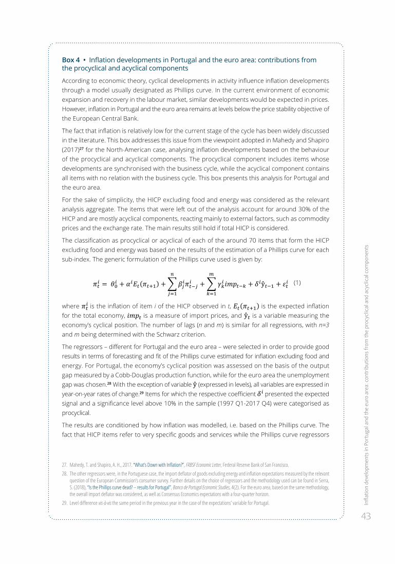
Infla
tion
deve
lopm
ents
in P
ortu
gal a
nd th
e eu
ro a
rea:
cont
ribut
ions
from
the
proc
yclic
al a
nd a
cycl
ical
com
pone
nts
43
Box 4 • Inflation developments in Portugal and the euro area: contributions from the procyclical and acyclical components
According to economic theory, cyclical developments in activity influence inflation developments through a model usually designated as Phillips curve. In the current environment of economic expansion and recovery in the labour market, similar developments would be expected in prices. However, inflation in Portugal and the euro area remains at levels below the price stability objective of the European Central Bank.
The fact that inflation is relatively low for the current stage of the cycle has been widely discussed in the literature. This box addresses this issue from the viewpoint adopted in Mahedy and Shapiro (2017)27 for the North-American case, analysing inflation developments based on the behaviour of the procyclical and acyclical components. The procyclical component includes items whose developments are synchronised with the business cycle, while the acyclical component contains all items with no relation with the business cycle. This box presents this analysis for Portugal and the euro area.
For the sake of simplicity, the HICP excluding food and energy was considered as the relevant analysis aggregate. The items that were left out of the analysis account for around 30% of the HICP and are mostly acyclical components, reacting mainly to external factors, such as commodity prices and the exchange rate. The main results still hold if total HICP is considered.
The classification as procyclical or acyclical of each of the around 70 items that form the HICP excluding food and energy was based on the results of the estimation of a Phillips curve for each sub-index. The generic formulation of the Phillips curve used is given by:
��� � ���� � ���������� ���������� ����� ������ � ��ŷ��� � ����
���
�
���
(1)
where
1
Caixa 3: Evolução da inflação em Portugal e na área do euro: contributo das componentes
procíclica e acíclica
De acordo com a teoria económica, os desenvolvimentos cíclicos da atividade têm influência na
evolução da inflação, através de uma relação habitualmente designada de curva de Phillips. No atual
contexto de expansão económica e recuperação do mercado de trabalho, esperar‐se‐ia uma evolução
semelhante do lado dos preços. No entanto, a inflação em Portugal e na área do euro permanece em
níveis inferiores ao objetivo de estabilidade de preços do Banco Central Europeu.
O facto de a inflação estar relativamente baixa para a fase do ciclo atual tem sido largamente debatido
na literatura. Esta caixa aborda esta questão de acordo com a perspetiva adotada em Mahedy e
Shapiro (2017)1 para o caso norte‐americano, analisando a evolução da inflação com base no
comportamento das componentes procíclica e acíclica. A componente procíclica inclui as rubricas que
têm uma evolução sincronizada com o ciclo económico e a componente acíclica contém todas as
rubricas sem relação com o ciclo económico. Nesta caixa, esta análise é feita para Portugal e para a
área do euro.
Por simplicidade, considerou‐se o Índice Harmonizado de preços no consumidor (IHPC) excluindo bens
alimentares e energéticos como o agregado de análise relevante. As rubricas que ficaram fora da
análise representam cerca de 30% do IHPC e são maioritariamente componentes acíclicas, reagindo
principalmente a fatores externos como os preços das matérias‐primas e taxa de câmbio. Os principais
resultados mantêm‐se se considerarmos o IHPC total.
A classificação de cada uma das cerca de 70 rubricas que compõem o IHPC excluindo os bens
alimentares e energéticos como procíclica ou acíclica teve como base os resultados da estimação de
uma curva de Phillips para cada subíndice. A formulação genérica da curva de Phillips utilizada é dada
por:
��� � �� � ��������� � ∑ ������� � ∑ �������� � �ŷ��� � ���������� (1)
onde ��� é a inflação da rubrica i do IHPC observada em t, �������� é a inflação esperada para o total da economia em t, ���� é uma medida de preços de importação e ŷ� é uma variável que mede a
posição cíclica da economia. O número de desfasamentos n e m é idêntico para todas as regressões,
sendo n=3 e m determinado com o critério de optimização de Schwarz.
1 Mahedy, T. e Shapiro, A. H., 2017. "What's Down with Inflation?", FRBSF Economic Letter, Federal Reserve Bank of San Francisco. https://ideas.repec.org/a/fip/fedfel/00150.html
is the inflation of item i of the HICP observed in t,
1
Caixa 3: Evolução da inflação em Portugal e na área do euro: contributo das componentes
procíclica e acíclica
De acordo com a teoria económica, os desenvolvimentos cíclicos da atividade têm influência na
evolução da inflação, através de uma relação habitualmente designada de curva de Phillips. No atual
contexto de expansão económica e recuperação do mercado de trabalho, esperar‐se‐ia uma evolução
semelhante do lado dos preços. No entanto, a inflação em Portugal e na área do euro permanece em
níveis inferiores ao objetivo de estabilidade de preços do Banco Central Europeu.
O facto de a inflação estar relativamente baixa para a fase do ciclo atual tem sido largamente debatido
na literatura. Esta caixa aborda esta questão de acordo com a perspetiva adotada em Mahedy e
Shapiro (2017)1 para o caso norte‐americano, analisando a evolução da inflação com base no
comportamento das componentes procíclica e acíclica. A componente procíclica inclui as rubricas que
têm uma evolução sincronizada com o ciclo económico e a componente acíclica contém todas as
rubricas sem relação com o ciclo económico. Nesta caixa, esta análise é feita para Portugal e para a
área do euro.
Por simplicidade, considerou‐se o Índice Harmonizado de preços no consumidor (IHPC) excluindo bens
alimentares e energéticos como o agregado de análise relevante. As rubricas que ficaram fora da
análise representam cerca de 30% do IHPC e são maioritariamente componentes acíclicas, reagindo
principalmente a fatores externos como os preços das matérias‐primas e taxa de câmbio. Os principais
resultados mantêm‐se se considerarmos o IHPC total.
A classificação de cada uma das cerca de 70 rubricas que compõem o IHPC excluindo os bens
alimentares e energéticos como procíclica ou acíclica teve como base os resultados da estimação de
uma curva de Phillips para cada subíndice. A formulação genérica da curva de Phillips utilizada é dada
por:
��� � �� � ��������� � ∑ ������� � ∑ �������� � �ŷ��� � ���������� (1)
onde ��� é a inflação da rubrica i do IHPC observada em t, �������� é a inflação esperada para o total da economia em t, ���� é uma medida de preços de importação e ŷ� é uma variável que mede a
posição cíclica da economia. O número de desfasamentos n e m é idêntico para todas as regressões,
sendo n=3 e m determinado com o critério de optimização de Schwarz.
1 Mahedy, T. e Shapiro, A. H., 2017. "What's Down with Inflation?", FRBSF Economic Letter, Federal Reserve Bank of San Francisco. https://ideas.repec.org/a/fip/fedfel/00150.html
is the expected inflation for the total economy,
1
Caixa 3: Evolução da inflação em Portugal e na área do euro: contributo das componentes
procíclica e acíclica
De acordo com a teoria económica, os desenvolvimentos cíclicos da atividade têm influência na
evolução da inflação, através de uma relação habitualmente designada de curva de Phillips. No atual
contexto de expansão económica e recuperação do mercado de trabalho, esperar‐se‐ia uma evolução
semelhante do lado dos preços. No entanto, a inflação em Portugal e na área do euro permanece em
níveis inferiores ao objetivo de estabilidade de preços do Banco Central Europeu.
O facto de a inflação estar relativamente baixa para a fase do ciclo atual tem sido largamente debatido
na literatura. Esta caixa aborda esta questão de acordo com a perspetiva adotada em Mahedy e
Shapiro (2017)1 para o caso norte‐americano, analisando a evolução da inflação com base no
comportamento das componentes procíclica e acíclica. A componente procíclica inclui as rubricas que
têm uma evolução sincronizada com o ciclo económico e a componente acíclica contém todas as
rubricas sem relação com o ciclo económico. Nesta caixa, esta análise é feita para Portugal e para a
área do euro.
Por simplicidade, considerou‐se o Índice Harmonizado de preços no consumidor (IHPC) excluindo bens
alimentares e energéticos como o agregado de análise relevante. As rubricas que ficaram fora da
análise representam cerca de 30% do IHPC e são maioritariamente componentes acíclicas, reagindo
principalmente a fatores externos como os preços das matérias‐primas e taxa de câmbio. Os principais
resultados mantêm‐se se considerarmos o IHPC total.
A classificação de cada uma das cerca de 70 rubricas que compõem o IHPC excluindo os bens
alimentares e energéticos como procíclica ou acíclica teve como base os resultados da estimação de
uma curva de Phillips para cada subíndice. A formulação genérica da curva de Phillips utilizada é dada
por:
��� � �� � ��������� � ∑ ������� � ∑ �������� � �ŷ��� � ���������� (1)
onde ��� é a inflação da rubrica i do IHPC observada em t, �������� é a inflação esperada para o total da economia em t, ���� é uma medida de preços de importação e ŷ� é uma variável que mede a
posição cíclica da economia. O número de desfasamentos n e m é idêntico para todas as regressões,
sendo n=3 e m determinado com o critério de optimização de Schwarz.
1 Mahedy, T. e Shapiro, A. H., 2017. "What's Down with Inflation?", FRBSF Economic Letter, Federal Reserve Bank of San Francisco. https://ideas.repec.org/a/fip/fedfel/00150.html
is a measure of import prices, and
1
Caixa 3: Evolução da inflação em Portugal e na área do euro: contributo das componentes
procíclica e acíclica
De acordo com a teoria económica, os desenvolvimentos cíclicos da atividade têm influência na
evolução da inflação, através de uma relação habitualmente designada de curva de Phillips. No atual
contexto de expansão económica e recuperação do mercado de trabalho, esperar‐se‐ia uma evolução
semelhante do lado dos preços. No entanto, a inflação em Portugal e na área do euro permanece em
níveis inferiores ao objetivo de estabilidade de preços do Banco Central Europeu.
O facto de a inflação estar relativamente baixa para a fase do ciclo atual tem sido largamente debatido
na literatura. Esta caixa aborda esta questão de acordo com a perspetiva adotada em Mahedy e
Shapiro (2017)1 para o caso norte‐americano, analisando a evolução da inflação com base no
comportamento das componentes procíclica e acíclica. A componente procíclica inclui as rubricas que
têm uma evolução sincronizada com o ciclo económico e a componente acíclica contém todas as
rubricas sem relação com o ciclo económico. Nesta caixa, esta análise é feita para Portugal e para a
área do euro.
Por simplicidade, considerou‐se o Índice Harmonizado de preços no consumidor (IHPC) excluindo bens
alimentares e energéticos como o agregado de análise relevante. As rubricas que ficaram fora da
análise representam cerca de 30% do IHPC e são maioritariamente componentes acíclicas, reagindo
principalmente a fatores externos como os preços das matérias‐primas e taxa de câmbio. Os principais
resultados mantêm‐se se considerarmos o IHPC total.
A classificação de cada uma das cerca de 70 rubricas que compõem o IHPC excluindo os bens
alimentares e energéticos como procíclica ou acíclica teve como base os resultados da estimação de
uma curva de Phillips para cada subíndice. A formulação genérica da curva de Phillips utilizada é dada
por:
��� � �� � ��������� � ∑ ������� � ∑ �������� � �ŷ��� � ���������� (1)
onde ��� é a inflação da rubrica i do IHPC observada em t, �������� é a inflação esperada para o total da economia em t, ���� é uma medida de preços de importação e ŷ� é uma variável que mede a
posição cíclica da economia. O número de desfasamentos n e m é idêntico para todas as regressões,
sendo n=3 e m determinado com o critério de optimização de Schwarz.
1 Mahedy, T. e Shapiro, A. H., 2017. "What's Down with Inflation?", FRBSF Economic Letter, Federal Reserve Bank of San Francisco. https://ideas.repec.org/a/fip/fedfel/00150.html
is a variable measuring the economy’s cyclical position. The number of lags (n and m) is similar for all regressions, with n=3 and m being determined with the Schwarz criterion.
The regressors – different for Portugal and the euro area – were selected in order to provide good results in terms of forecasting and fit of the Phillips curve estimated for inflation excluding food and energy. For Portugal, the economy’s cyclical position was assessed on the basis of the output gap measured by a Cobb-Douglas production function, while for the euro area the unemployment gap was chosen.28 With the exception of variable
1
Caixa 3: Evolução da inflação em Portugal e na área do euro: contributo das componentes
procíclica e acíclica
De acordo com a teoria económica, os desenvolvimentos cíclicos da atividade têm influência na
evolução da inflação, através de uma relação habitualmente designada de curva de Phillips. No atual
contexto de expansão económica e recuperação do mercado de trabalho, esperar‐se‐ia uma evolução
semelhante do lado dos preços. No entanto, a inflação em Portugal e na área do euro permanece em
níveis inferiores ao objetivo de estabilidade de preços do Banco Central Europeu.
O facto de a inflação estar relativamente baixa para a fase do ciclo atual tem sido largamente debatido
na literatura. Esta caixa aborda esta questão de acordo com a perspetiva adotada em Mahedy e
Shapiro (2017)1 para o caso norte‐americano, analisando a evolução da inflação com base no
comportamento das componentes procíclica e acíclica. A componente procíclica inclui as rubricas que
têm uma evolução sincronizada com o ciclo económico e a componente acíclica contém todas as
rubricas sem relação com o ciclo económico. Nesta caixa, esta análise é feita para Portugal e para a
área do euro.
Por simplicidade, considerou‐se o Índice Harmonizado de preços no consumidor (IHPC) excluindo bens
alimentares e energéticos como o agregado de análise relevante. As rubricas que ficaram fora da
análise representam cerca de 30% do IHPC e são maioritariamente componentes acíclicas, reagindo
principalmente a fatores externos como os preços das matérias‐primas e taxa de câmbio. Os principais
resultados mantêm‐se se considerarmos o IHPC total.
A classificação de cada uma das cerca de 70 rubricas que compõem o IHPC excluindo os bens
alimentares e energéticos como procíclica ou acíclica teve como base os resultados da estimação de
uma curva de Phillips para cada subíndice. A formulação genérica da curva de Phillips utilizada é dada
por:
��� � �� � ��������� � ∑ ������� � ∑ �������� � �ŷ��� � ���������� (1)
onde ��� é a inflação da rubrica i do IHPC observada em t, �������� é a inflação esperada para o total da economia em t, ���� é uma medida de preços de importação e ŷ� é uma variável que mede a
posição cíclica da economia. O número de desfasamentos n e m é idêntico para todas as regressões,
sendo n=3 e m determinado com o critério de optimização de Schwarz.
1 Mahedy, T. e Shapiro, A. H., 2017. "What's Down with Inflation?", FRBSF Economic Letter, Federal Reserve Bank of San Francisco. https://ideas.repec.org/a/fip/fedfel/00150.html
(expressed in levels), all variables are expressed in year-on-year rates of change.29 Items for which the respective coefficient ��� � ���� � ���������� ���������� ����� ������ � ��ŷ��� � ���
�
���
�
���
presented the expected signal and a significance level above 10% in the sample (1997 Q1-2017 Q4) were categorised as procyclical.
The results are conditioned by how inflation was modelled, i.e. based on the Phillips curve. The fact that HICP items refer to very specific goods and services while the Phillips curve regressors
27. Mahedy, T. and Shapiro, A. H., 2017. “What’s Down with Inflation?”, FRBSF Economic Letter, Federal Reserve Bank of San Francisco.28. The other regressors were, in the Portuguese case, the import deflator of goods excluding energy and inflation expectations measured by the relevant
question of the European Commission’s consumer survey. Further details on the choice of regressors and the methodology used can be found in Serra, S. (2018), “Is the Phillips curve dead? – results for Portugal”, Banco de Portugal Economic Studies, 4(2). For the euro area, based on the same methodology, the overall import deflator was considered, as well as Consensus Economics expectations with a four-quarter horizon.
29. Level difference vis-à-vis the same period in the previous year in the case of the expectations’ variable for Portugal.
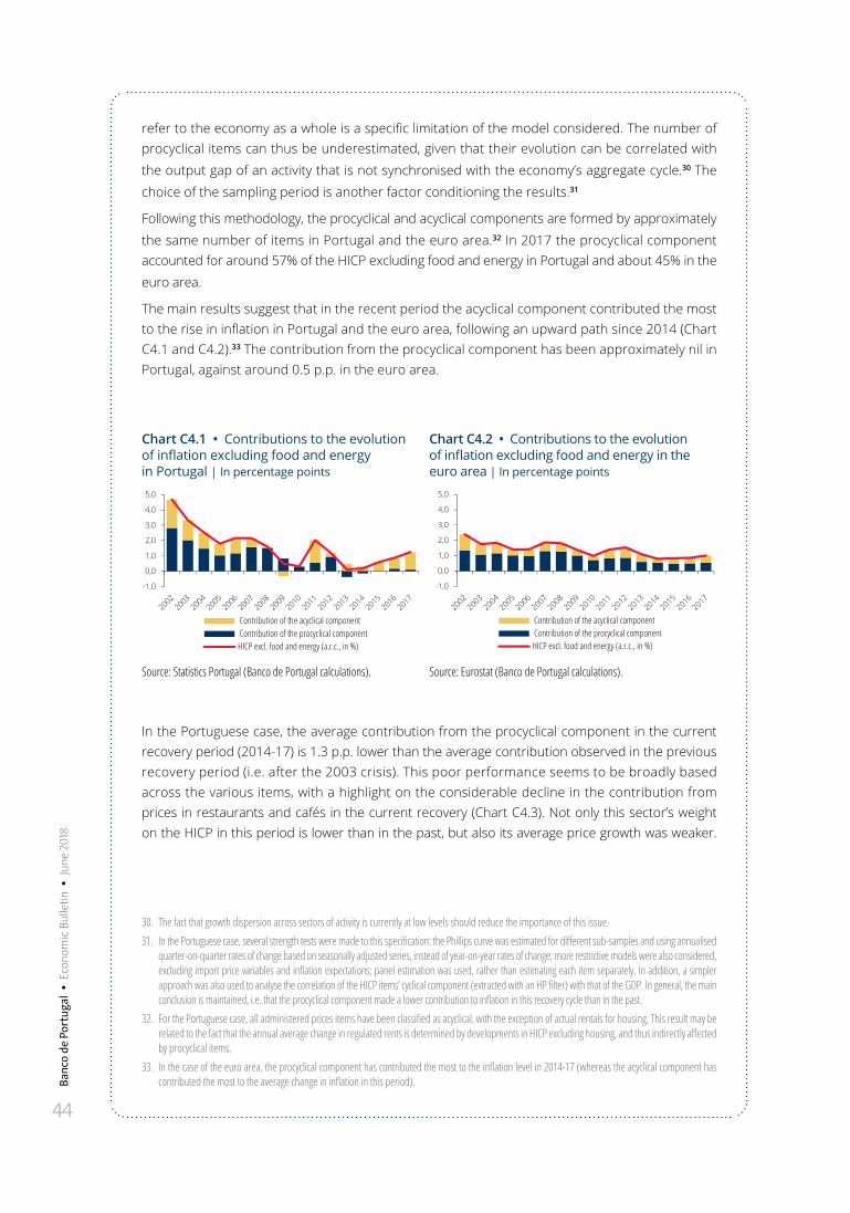
44
Banc
o de
Por
tuga
l •
Eco
nom
ic B
ulle
tin •
Jun
e 20
18
refer to the economy as a whole is a specific limitation of the model considered. The number of procyclical items can thus be underestimated, given that their evolution can be correlated with the output gap of an activity that is not synchronised with the economy’s aggregate cycle.30 The choice of the sampling period is another factor conditioning the results.31
Following this methodology, the procyclical and acyclical components are formed by approximately the same number of items in Portugal and the euro area.32 In 2017 the procyclical component accounted for around 57% of the HICP excluding food and energy in Portugal and about 45% in the euro area.
The main results suggest that in the recent period the acyclical component contributed the most to the rise in inflation in Portugal and the euro area, following an upward path since 2014 (Chart C4.1 and C4.2).33 The contribution from the procyclical component has been approximately nil in Portugal, against around 0.5 p.p. in the euro area.
Chart C4.1 • Contributions to the evolution of inflation excluding food and energy in Portugal | In percentage points
Chart C4.2 • Contributions to the evolution of inflation excluding food and energy in the euro area | In percentage points
-1,0
0,0
1,0
2,0
3,0
4,0
5,0
Contribution of the acyclical component Contribution of the procyclical componentHICP excl. food and energy (a.r.c., in %)
-1,0
0,0
1,0
2,0
3,0
4,0
5,0
Contribution of the acyclical component Contribution of the procyclical componentHICP excl. food and energy (a.r.c., in %)
Source: Statistics Portugal (Banco de Portugal calculations). Source: Eurostat (Banco de Portugal calculations).
In the Portuguese case, the average contribution from the procyclical component in the current recovery period (2014-17) is 1.3 p.p. lower than the average contribution observed in the previous recovery period (i.e. after the 2003 crisis). This poor performance seems to be broadly based across the various items, with a highlight on the considerable decline in the contribution from prices in restaurants and cafés in the current recovery (Chart C4.3). Not only this sector’s weight on the HICP in this period is lower than in the past, but also its average price growth was weaker.
30. The fact that growth dispersion across sectors of activity is currently at low levels should reduce the importance of this issue.31. In the Portuguese case, several strength tests were made to this specification: the Phillips curve was estimated for different sub-samples and using annualised
quarter-on-quarter rates of change based on seasonally adjusted series, instead of year-on-year rates of change; more restrictive models were also considered, excluding import price variables and inflation expectations; panel estimation was used, rather than estimating each item separately. In addition, a simpler approach was also used to analyse the correlation of the HICP items’ cyclical component (extracted with an HP filter) with that of the GDP. In general, the main conclusion is maintained, i.e. that the procyclical component made a lower contribution to inflation in this recovery cycle than in the past.
32. For the Portuguese case, all administered prices items have been classified as acyclical, with the exception of actual rentals for housing. This result may be related to the fact that the annual average change in regulated rents is determined by developments in HICP excluding housing, and thus indirectly affected by procyclical items.
33. In the case of the euro area, the procyclical component has contributed the most to the inflation level in 2014-17 (whereas the acyclical component has contributed the most to the average change in inflation in this period).
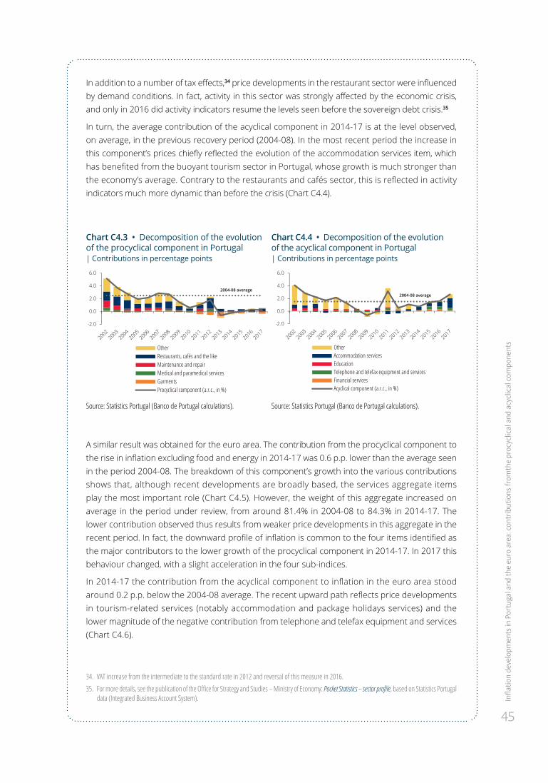
Infla
tion
deve
lopm
ents
in P
ortu
gal a
nd th
e eu
ro a
rea:
cont
ribut
ions
from
the
proc
yclic
al a
nd a
cycl
ical
com
pone
nts
45
In addition to a number of tax effects,34 price developments in the restaurant sector were influenced by demand conditions. In fact, activity in this sector was strongly affected by the economic crisis, and only in 2016 did activity indicators resume the levels seen before the sovereign debt crisis.35
In turn, the average contribution of the acyclical component in 2014-17 is at the level observed, on average, in the previous recovery period (2004-08). In the most recent period the increase in this component’s prices chiefly reflected the evolution of the accommodation services item, which has benefited from the buoyant tourism sector in Portugal, whose growth is much stronger than the economy’s average. Contrary to the restaurants and cafés sector, this is reflected in activity indicators much more dynamic than before the crisis (Chart C4.4).
Chart C4.3 • Decomposition of the evolution of the procyclical component in Portugal | Contributions in percentage points
Chart C4.4 • Decomposition of the evolution of the acyclical component in Portugal | Contributions in percentage points
-2.0
0.0
2.0
4.0
6.0
OtherRestaurants, cafés and the likeMaintenance and repairMedical and paramedical servicesGarmentsProcyclical component (a.r.c., in %)
2004-08 average
-2.0
0.0
2.0
4.0
6.0
OtherAccommodation servicesEducationTelephone and telefax equipment and servicesFinancial servicesAcyclical component (a.r.c., in %)
2004-08 average
Source: Statistics Portugal (Banco de Portugal calculations). Source: Statistics Portugal (Banco de Portugal calculations).
A similar result was obtained for the euro area. The contribution from the procyclical component to the rise in inflation excluding food and energy in 2014-17 was 0.6 p.p. lower than the average seen in the period 2004-08. The breakdown of this component’s growth into the various contributions shows that, although recent developments are broadly based, the services aggregate items play the most important role (Chart C4.5). However, the weight of this aggregate increased on average in the period under review, from around 81.4% in 2004-08 to 84.3% in 2014-17. The lower contribution observed thus results from weaker price developments in this aggregate in the recent period. In fact, the downward profile of inflation is common to the four items identified as the major contributors to the lower growth of the procyclical component in 2014-17. In 2017 this behaviour changed, with a slight acceleration in the four sub-indices.
In 2014-17 the contribution from the acyclical component to inflation in the euro area stood around 0.2 p.p. below the 2004-08 average. The recent upward path reflects price developments in tourism-related services (notably accommodation and package holidays services) and the lower magnitude of the negative contribution from telephone and telefax equipment and services (Chart C4.6).
34. VAT increase from the intermediate to the standard rate in 2012 and reversal of this measure in 2016.35. For more details, see the publication of the Office for Strategy and Studies – Ministry of Economy: Pocket Statistics – sector profile, based on Statistics Portugal
data (Integrated Business Account System).
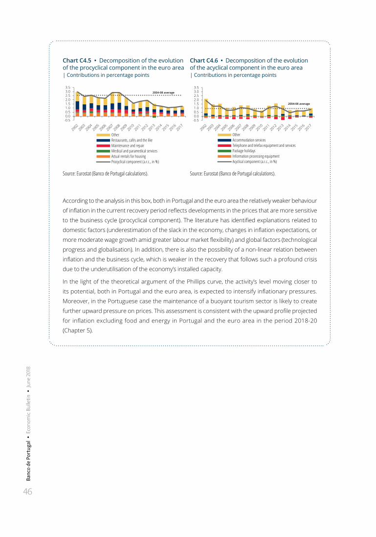
46
Banc
o de
Por
tuga
l •
Eco
nom
ic B
ulle
tin •
Jun
e 20
18
Chart C4.5 • Decomposition of the evolution of the procyclical component in the euro area | Contributions in percentage points
Chart C4.6 • Decomposition of the evolution of the acyclical component in the euro area | Contributions in percentage points
-0.50.00.51.01.52.02.53.03.5
OtherRestaurants, cafés and the likeMaintenance and repairMedical and paramedical servicesActual rentals for housingProcyclical component (a.r.c., in %)
2004-08 average
-0.50.00.51.01.52.02.53.03.5
OtherAccommodation servicesTelephone and telefax equipment and servicesPackage holidaysInformation processing equipmentAcyclical component (a.r.c., in %)
2004-08 average
Source: Eurostat (Banco de Portugal calculations). Source: Eurostat (Banco de Portugal calculations).
According to the analysis in this box, both in Portugal and the euro area the relatively weaker behaviour
of inflation in the current recovery period reflects developments in the prices that are more sensitive
to the business cycle (procyclical component). The literature has identified explanations related to
domestic factors (underestimation of the slack in the economy, changes in inflation expectations, or
more moderate wage growth amid greater labour market flexibility) and global factors (technological
progress and globalisation). In addition, there is also the possibility of a non-linear relation between
inflation and the business cycle, which is weaker in the recovery that follows such a profound crisis
due to the underutilisation of the economy’s installed capacity.
In the light of the theoretical argument of the Phillips curve, the activity’s level moving closer to
its potential, both in Portugal and the euro area, is expected to intensify inflationary pressures.
Moreover, in the Portuguese case the maintenance of a buoyant tourism sector is likely to create
further upward pressure on prices. This assessment is consistent with the upward profile projected
for inflation excluding food and energy in Portugal and the euro area in the period 2018-20
(Chapter 5).
Mac
roec
onom
ic im
pact
of a
rise
in g
loba
l pro
tect
ioni
st te
nsio
ns
47
Box 5 • Macroeconomic impact of a rise in global protectionist tensions
Underlying the projections in this Bulletin is an international environment where protectionist
tensions in international trade remain contained and trade disputes do not escalate. However, the
latest developments cast doubt on this assumption. The risks of greater protectionism in terms of
overall trade have risen, largely driven by the recent rhetoric and actions by the United States, as well
as by retaliatory threats by its trade partners. The US Administration has threatened to reverse trade
agreements and announced restrictions on imports, with the stated purpose of both reducing the
persistently increasing US external deficit and protecting output and employment in specific sectors.
Both theory and empirical evidence show that import barriers reduce the welfare of society and lead
to an inefficient allocation of resources, and are an inappropriate response to the challenges posed
by international trade (see Special issue “International trade: gains and challenges”, Economic Bulletin,
October 2017, Banco de Portugal).
In view of the growing risks from an intensification in protectionism, this box reviews two scenarios
where tensions escalate to a global-scale trade war. Its aim is to illustrate potential effects on
activity, trade flows and inflation at world level and, in particular, on the Portuguese economy.
The recent announcement by the United States of an increase in import tariffs on steel and
aluminium from several trade partners, as well as the latter’s retaliatory measures, should have
limited direct effects on world activity and trade, given that the share of imports from the US
and its partners affected by these tariffs is relatively small.36 However, they pose increased risks
of an escalation of trade disputes. In addition to these tariffs, the United States is paving the
way for the imposition of further constraints on trade with China following an investigation on
China’s intellectual property practices, which carries a high risk of retaliation by the Chinese
authorities. The US authorities are also looking into the possibility of increasing tariffs on
automobile imports from the European Union. Moreover, renegotiations of the North American
Free-Trade Agreement37 are under way, at the instance of the US. The country has also pulled
out of the Trans-Pacific Partnership.38 The US Administration has also taken a very critical view of
the role played by the World Trade Organisation, and expressed a preference for bilateral trade
agreements, which threatens multilateral free trade.
In this context, two alternative scenarios were taken into consideration. The first, of a limited
trade war, assumes an escalation of trade tensions between the US and all its trading partners.
In this scenario, the US increases import tariffs on all goods from third countries – which would
imply a rise in the export prices from such countries to the United States by approximately 10%
– and these economies retaliate, by imposing similar tariffs on imports from the US. The second
scenario assumes a generalized trade war, at global level, where all countries impose custom
duties on imports from all other countries, with an impact on international trade prices of around 10%.
36. However, the recent reduction in consumer confidence indicators among advanced economies may, to a certain extent, be associated with increased concerns of an escalation of trade disputes.
37. The North American Free-Trade Agreement (NAFTA) was signed by the US, Canada and Mexico (with Chile as an associate-member).38. The Trans-Pacific Partnership (TPP) is a trade agreement between twelve countries that border the Pacific Ocean (Australia, Brunei, Canada, Chile,
Japan, Malaysia, Mexico, New Zealand, Peru, Singapore, United States and Vietnam).
48
Banc
o de
Por
tuga
l •
Eco
nom
ic B
ulle
tin •
Jun
e 20
18
The probability of these alternative scenarios occurring is debateable, but clearly higher in the first case and relatively low for the generalized war scenario. The NiGEM model39 was used to simulate the global macroeconomic effects of these protectionist measures. The impact of the international environment on the Portuguese economy and of the imposition of tariffs to imports from Portugal’s trade partners was simulated by means of the main econometric model used by Banco de Portugal to produce medium-term projections for the Portuguese economy.
In both scenarios, the imposition of custom duties by the United States directly results in an increase in import prices. In other countries, the imposition of tariffs on imported products also results in an increase in import prices, to a lesser extent compared with the United States in the first scenario, but of a similar magnitude in the second scenario.40 The increase in import prices is mirrored, in the one hand, in a decline in world trade, with an impact on exports and the economic activity of the various countries and, on the other hand, a rise in domestic inflation, thereby reducing the purchasing power of economic agents and, consequently, private consumption. In response to the rise in inflation, the Federal Reserve and the monetary authorities of the other countries increase key interest rates, which is passed through to rates applied by banks on loans to enterprises and households. This increase in financing costs also has negative effects on investment and private consumption. The macroeconomic effects of an increase in tariffs on imports are, therefore, similar to those of a negative technological shock that results in higher price and reduced activity.
In the limited war scenario, world GDP declines by 0.7% at the end of the three-year horizon compared with the baseline scenario (Chart C5.1). World trade posts a cumulative reduction over the same period of nearly 3% compared to that projected in the baseline scenario. The results of the simulation show that activity decreases across all economies, with the United States being hit the hardest. The impact on economic activity across the various economies hinges on several factors, in particular, their size, degree of openness and share of their trade with the United States. In the generalized war scenario, the effects on GDP and world trade are far more severe, leading to a reduction of 2.5% and 9.6%, respectively, compared with the baseline scenario at the end of the projection horizon.41 Relative to the limited war scenario, the negative impact on
economic activity across all countries increases.
39. NiGEM is a model of the National Institute of Economic and Social Research (for more details on the model, see https://nimodel.niesr.ac.uk/). This multi-country macroeconometric model is particularly suited to simulate the effects of an increase in tariffs worldwide, as it provides a detailed modelling of trade and financial links between economies, in addition to the various options in simulation design. The version of the model used here is specifically designed to simulate the imposition of tariffs between the United States and all other countries/regions (US tariff and Brexit expanded model v.1.18). This version breaks down data by geographical origin/destination of US imports/exports, allowing the incorporation of shocks on export prices of individual countries to the US and export prices of the US to all other countries.
40. In the first scenario, the United States deal with higher tariffs on all of their exports, imposed by all their trade partners, while other countries are only faced with higher tariffs in their exports to the United States.
41. These results are similar to those discussed in “The war on trade: beggar thy neighbour, beggar thyself?” (National Institute Economic Review No. 244, May 2018), which used NiGEM to simulate an equivalent scenario. The results are also close to those obtained by the OECD, the IMF and the World Bank for similar scenario simulations. The OECD assumed a scenario in which major world economies – Europe, United States and China – impose higher trade barriers leading to a 10% increase in costs of trade against trade partners (Box 1.3. “The impact of changes in global trade costs”, OECD Economic Outlook, December 2016). In the simulations, based on the OECD METRO model, world GDP would decline by approximately 1.5% and world trade by more than 5%, with those economies that imposed new trade barriers being the most severely affected. The IMF undertakes a similar exercise, assuming that all countries in the world gradually increase tariff and non-tariff barriers in the course of three years against all of their trade partners, leading to a 10% increase in import prices (Scenario Box 1. “Tariff Scenarios”, IMF World Economic Outlook, October 2016). Using the GIMF model, this scenario implies a reduction in global activity of nearly 1.75% over five years compared with the baseline scenario, in which world trade falls by around 15% during the same period. The World Bank has also drawn up a simulation, according to which a global increase in tariffs of approximately 10% results in a global decline in welfare of 0.8% compared with the baseline scenario up to 2020, while trade flows decrease by 9% (Kutlina-Dimitrova and Lakatos (2017), “The Global Costs of Protectionism”, World Bank Policy Research Working Paper 8277).
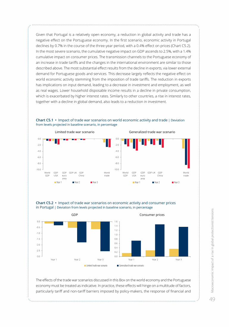
Mac
roec
onom
ic im
pact
of a
rise
in g
loba
l pro
tect
ioni
st te
nsio
ns
49
Given that Portugal is a relatively open economy, a reduction in global activity and trade has a negative effect on the Portuguese economy. In the first scenario, economic activity in Portugal declines by 0.7% in the course of the three-year period, with a 0.4% effect on prices (Chart C5.2). In the most severe scenario, the cumulative negative impact on GDP ascends to 2.5%, with a 1.4% cumulative impact on consumer prices. The transmission channels to the Portuguese economy of an increase in trade tariffs and the changes in the international environment are similar to those described above. The most substantial effect results from the decline in exports, via lower external demand for Portuguese goods and services. This decrease largely reflects the negative effect on world economic activity stemming from the imposition of trade tariffs. The reduction in exports has implications on input demand, leading to a decrease in investment and employment, as well as real wages. Lower household disposable income results in a decline in private consumption, which is exacerbated by higher interest rates. Similarly to other countries, a rise in interest rates, together with a decline in global demand, also leads to a reduction in investment.
Chart C5.1 • Impact of trade war scenarios on world economic activity and trade | Deviation from levels projected in baseline scenario, in percentage
Limited trade war scenario Generalized trade war scenario
-10.0
-8.0
-6.0
-4.0
-2.0
0.0
WorldGDP
GDPUSA
GDPeuroarea
GDP UK GDPChina
Worldtrade
Year 1 Year 2 Year 3
-10.0
-8.0
-6.0
-4.0
-2.0
0.0
WorldGDP
GDPUSA
GDPeuroarea
GDP UK GDPChina
Worldtrade
Year 1 Year 2 Year 3
Chart C5.2 • Impact of trade war scenarios on economic activity and consumer prices in Portugal | Deviation from levels projected in baseline scenario, in percentage
GDP Consumer prices
-3.0
-2.5
-2.0
-1.5
-1.0
-0.5
0.0
Year 1 Year 2 Year 3
Limited trade war scenario Generalised trade war scenario
0.0
0.2
0.4
0.6
0.8
1.0
1.2
1.4
1.6
Year 1 Year 2 Year 3-3.0
-2.5
-2.0
-1.5
-1.0
-0.5
0.0
Year 1 Year 2 Year 3
Limited trade war scenario Generalised trade war scenario
The effects of the trade war scenarios discussed in this Box on the world economy and the Portuguese economy must be treated as indicative. In practice, these effects will hinge on a multitude of factors, particularly tariff and non-tariff barriers imposed by policy-makers, the response of financial and
50
Banc
o de
Por
tuga
l •
Eco
nom
ic B
ulle
tin •
Jun
e 20
18
foreign exchange markets, the response of central banks, and fiscal policy measures adopted by
the various countries.
Furthermore, it should be noted that a greater degree of protectionism may affect the economies
involved via a series of additional channels. The simulations presented here do not take into
account possible impacts via uncertainty and confidence. Changes to trade policies and linkages,
even if merely in the form of a threat, may result in lower confidence or increased uncertainty,
which contributes to the amplification of negative effects on economic activity. The simulated
scenarios also fail to capture the degree of disruption and adjustment in global supply chains.
The impact of protectionist measures will tend to be amplified against a background of increased
economic integration and the growing importance of global supply chains (where the imposition of
tariffs on imports of intermediate goods hampers national industries). Finally, scenarios of higher
protectionism imply lower international competition and a reduction in specialisation possibilities,
which should have an impact on global productivity growth. This type of effect, which should be
more relevant in the medium run, is also not taken into account in the scenarios under review.42
These caveats suggest that results discussed in this Box may underestimate the adverse effects of
protectionist measures.
In sum, the protectionist threat, in particular with respect to an escalation of trade disputes, poses
a substantial downside risk to the world economic outlook. The increase in trade tariffs may have a
fairly negative impact on the Portuguese economy, given that its recent growth has largely hinged on
the buoyancy of exports.
42. For a reference that incorporates this type of effect in simulated scenarios of an increase in protectionism, see the background paper to the DNBulletin “Why protectionism does not work” (24 August 2017), or Bond, E. W., M. J. Crucini, T. Potter, and J. Rodrigue (May 2012), “Misallocation and productivity effects of the Smoot-Hawley Tariff.” NBER Working Paper No. 18034.
II Special issueHousehold consumption inequality
in Portugal

5353
Hou
seho
ld co
nsum
ptio
n in
equa
lity i
n Po
rtug
al
Household consumption inequality in Portugal
IntroductionThe debate around economic inequalities in Portugal has focused on the analysis of the distribution
of income and, occasionally, of wealth (Rodrigues et al., 2016 and Costa, 2017). However, economic
theory suggests that the distribution of consumption should be a better measure of the resources
available to households through life (Blundell and Preston, 1998). The joint analysis of consumption
and income allows to measure the persistence of shocks to income and can reveal consumption
smoothing mechanisms at each moment in time and over the life cycle (Attanasio and Pistaferri,
2016 and Meyer and Sullivan, 2018). Indeed, changes in income are transmitted to changes in
consumption through a network of social and household smoothing mechanisms, through the
access to the credit market, through the use of past savings and through the decisions of the
various members of the household in the labour market (Attanasio et al., 2002). As a result, the
dispersion of consumption across households may be more representative of the distribution of
well-being in an economy.
This Special issue aims to describe the inequality in consumption expenditure in Portugal based
on information from the Household Budget Surveys (hereinafter “HBS”), published by Statistics
Portugal (Statistics Portugal, 2002, 2012, 2017). These surveys allow combining information on
the distribution of consumption expenditure and income in Portugal, for a relatively long time
period (Alves, 2009). The current analysis will focus on the period between 2000 and 2015, the
year of the last available survey.
The high income inequality in the Portuguese economy compared to other European Union
countries is an established fact (Atkinson et al., 2017). However, evidence on the expenditure
inequality is rarer.1 This article aims to describe in detail the consumption distribution2 in Portugal,
as well as its developments over the last few years. The richness of the HBS microeconomic data
also allows analysing the breakdown of expenditures throughout the income and consumption
distribution, the joint profile of expenditure and income over the households’ life cycle, the
developments in the dispersion of income and expenditure as economic shocks accumulate, and
the role of education in determining these distributions.
The Special issue is structured as follows. The next section presents the data and methodological
choices adopted. Thereafter, inequality in the distribution of expenditure in Portugal in 2015 is
described according to different characteristics of the households. This is followed by an analysis of
the evolution of the expenditure inequality since the beginning of the euro area, with special emphasis
1. A set of experimental indicators published recently by Eurostat suggests that the inequality in expenditure in Portugal is also one of the highest in the euro area. This evidence is available here http://ec.europa.eu/eurostat/statistics-explained/index.php/Interaction_of_household_income,_consumption_and_wealth_-_statistics_on_main_results.
2. To be parsimonious, the terms “consumption” and “expenditure” will be used interchangeably to refer to households’ consumption expenditure.
5454
Banc
o de
Por
tuga
l •
Eco
nom
ic B
ulle
tin •
Jun
e 20
18
on the behaviour observed between the two latest surveys (2010 and 2015). These sections aim to
integrate the information on households’ expenditure and income, whenever relevant. Lastly, the
main conclusions are presented and some ideas are proposed for future research.
Data and conceptsThe main source used in the analysis is the Household Budget Survey. This survey is held every
five years by Statistics Portugal with the goal of supplying detailed information on household
expenditure. This is a very important statistical source both for the national accounts and for
calculating the consumer price index. Furthermore, this survey also provides information on income,
which makes it an important source for analysing households, in particular in the calculation of
inequality indicators. The latest survey, from 2015/2016, features data collected between March
2015 and March 2016 from a sample stratified by region, representative of households living in
Portugal. The statistical results of this survey, as well as the methodology and questionnaires, are
available from Statistics Portugal (2017). The number of households responding to the 2015/16
survey was 11,398, involving 26,889 individuals.
The microdata underlying this survey form the main statistical source for the description of the
dispersion of consumption in the latest period. For the purposes of analysing the evolution over
time, the data from two other surveys were also used: HBS 2010/2011 and HBS 2000. These
three surveys allow the analysis of changes taking place during implementation of the Economic
and Financial Assistance Programme to Portugal, as well as a longer-term comparison, from
the start of the euro area. To simplify the analysis, the expenditure data for HBS 2015/16 are
assumed to refer to 2015 (although the data collection period does not coincide exactly with
the calendar year). Similarly, the expenditure data for HBS 2010/2011 are presented as relating
to 2010, and those of HBS 2000 to 2000. The income data in each survey refers to the previous
calendar year, which explains why the time reference for the income data is that of the year
prior to that of the expenditure data (for example, in the case of HBS 2015/16, the income refers
to 2014). Households’ income corresponds approximately to the concept of disposable income
in the national accounts, in that it includes social transfers and is net of income tax and social
contributions.
In addition to monetary expenditure, households’ total expenditure includes the following items
comprised in the so-called non-monetary expenditure: self-consumption (self-produced goods),
self-supply (goods and services consumed freely in the family unit’s firms), owner-occupied
imputed rents (estimated value of house rent when the household owns the house or has free
accommodation), payments and salaries received in kind.3 As an alternative to the total expenditure
concept, monetary expenditure was analysed as well, which excludes those non-monetary items.
Similarly, monetary income may be calculated, since non-monetary income coincides with non-
monetary expenditure.
3. The households’ consumption expenditure concept in this survey is close to that of households’ final consumption expenditure of the national accounts, therefore goods and services provided freely by public entities are not considered in households’ consumption expenditure.
5555
Hou
seho
ld co
nsum
ptio
n in
equa
lityin
Por
tuga
l
It should be noted that total expenditure and total income calculated based on the HBS underestimate
the income and consumption calculated in Statistics Portugal’s national accounts. This accords with
analogous surveys for other countries (Attanasio and Pistaferri, 2016). As an example, in 2015,
consumption expenditure extrapolated from HBS to the population as a whole reaches around 70%
of households’ consumption presented in the annual national accounts. In the case of disposable
income, that level is at around 80%.
In this Special issue, all the data, both for expenditure and for income, are presented in real
terms, using the consumer price index as deflator4 and 2015 as the reference year for prices.
Furthermore, the expenditure and income data correspond to data per household and per
equalised adult. The calculation of the variables per equalised adult is based on the OECD-
modified equivalence scale, which gives a value of 1 to the household head, 0.5 to the other adults
and 0.3 to each child (individuals aged 13 or below are considered children of the household). This
equivalence scale was chosen due to existence of economies of scale within households, implying
that variables calculated per equivalent adult tend to be a better measure of economic well-being.
All the aggregated data presented below correspond to extrapolated data based on a sample
weight attributed to each household, supplied by Statistics Portugal.
The survey’s database also includes certain variables that allow households and the individuals to
be described, including region, age, professional situation or education level. The data presented
as the households’ characteristics (region, age group, education level) relate to the characteristics
of the household head.5 For example, the averages presented for expenditure per age group
refer to the average values of household expenditure per equalised adult, according to the age
group of the respective household head.
Description of inequality in household expenditure in 2015This section aims to describe the inequality in household expenditure, based on the latest wave
of the Household Budget Survey (HBS 2015/16). The analysis is based on a set of indicators
and measures relating to the distribution and dispersion of household expenditure, which were
chosen among the set of measures typically used in the literature. Although the focus of this
Special issue is expenditure inequality this analysis will be complemented whenever appropriate
by a description of income inequality, given that this is a key driver of households’ consumption
decisions.
Table 1 presents the averages, medians and some indicators of inequality for the expenditure
and income variables, both for total aggregates and for monetary aggregates (defined as indicated
in the previous section).
4. As a simplification, all aggregates were deflated using the total national consumer price index, not considering details by region and product.5. The household head is the individual with the greatest proportion of total net annual income in the family unit.
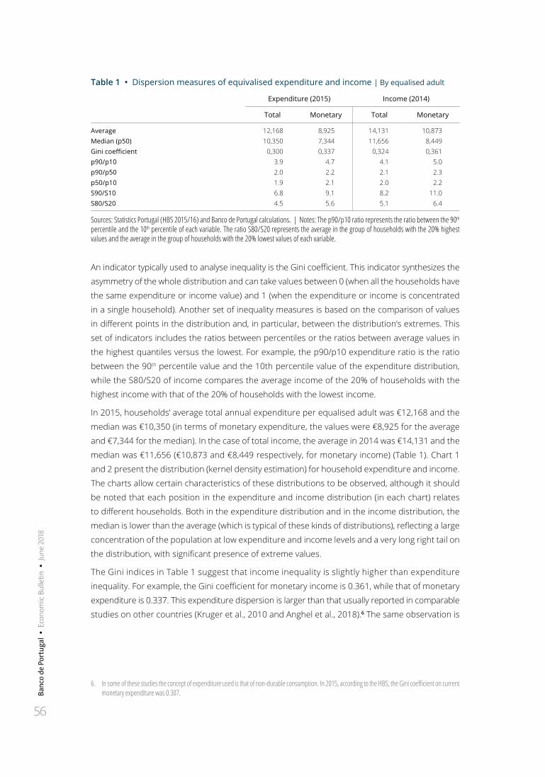
Banc
o de
Por
tuga
l •
Eco
nom
ic B
ulle
tin •
Jun
e 20
18
56
Table 1 • Dispersion measures of equivalised expenditure and income | By equalised adult
Expenditure (2015) Income (2014)
Total Monetary Total Monetary
Average 12,168 8,925 14,131 10,873Median (p50) 10,350 7,344 11,656 8,449Gini coefficient 0,300 0,337 0,324 0,361p90/p10 3.9 4.7 4.1 5.0p90/p50 2.0 2.2 2.1 2.3p50/p10 1.9 2.1 2.0 2.2S90/S10 6.8 9.1 8.2 11.0S80/S20 4.5 5.6 5.1 6.4
Sources: Statistics Portugal (HBS 2015/16) and Banco de Portugal calculations. | Notes: The p90/p10 ratio represents the ratio between the 90th percentile and the 10th percentile of each variable. The ratio S80/S20 represents the average in the group of households with the 20% highest values and the average in the group of households with the 20% lowest values of each variable.
An indicator typically used to analyse inequality is the Gini coefficient. This indicator synthesizes the
asymmetry of the whole distribution and can take values between 0 (when all the households have
the same expenditure or income value) and 1 (when the expenditure or income is concentrated
in a single household). Another set of inequality measures is based on the comparison of values
in different points in the distribution and, in particular, between the distribution’s extremes. This
set of indicators includes the ratios between percentiles or the ratios between average values in
the highest quantiles versus the lowest. For example, the p90/p10 expenditure ratio is the ratio
between the 90th percentile value and the 10th percentile value of the expenditure distribution,
while the S80/S20 of income compares the average income of the 20% of households with the
highest income with that of the 20% of households with the lowest income.
In 2015, households’ average total annual expenditure per equalised adult was €12,168 and the
median was €10,350 (in terms of monetary expenditure, the values were €8,925 for the average
and €7,344 for the median). In the case of total income, the average in 2014 was €14,131 and the
median was €11,656 (€10,873 and €8,449 respectively, for monetary income) (Table 1). Chart 1
and 2 present the distribution (kernel density estimation) for household expenditure and income.
The charts allow certain characteristics of these distributions to be observed, although it should
be noted that each position in the expenditure and income distribution (in each chart) relates
to different households. Both in the expenditure distribution and in the income distribution, the
median is lower than the average (which is typical of these kinds of distributions), reflecting a large
concentration of the population at low expenditure and income levels and a very long right tail on
the distribution, with significant presence of extreme values.
The Gini indices in Table 1 suggest that income inequality is slightly higher than expenditure
inequality. For example, the Gini coefficient for monetary income is 0.361, while that of monetary
expenditure is 0.337. This expenditure dispersion is larger than that usually reported in comparable
studies on other countries (Kruger et al., 2010 and Anghel et al., 2018).6 The same observation is
6. In some of these studies the concept of expenditure used is that of non-durable consumption. In 2015, according to the HBS, the Gini coefficient on current monetary expenditure was 0.307.
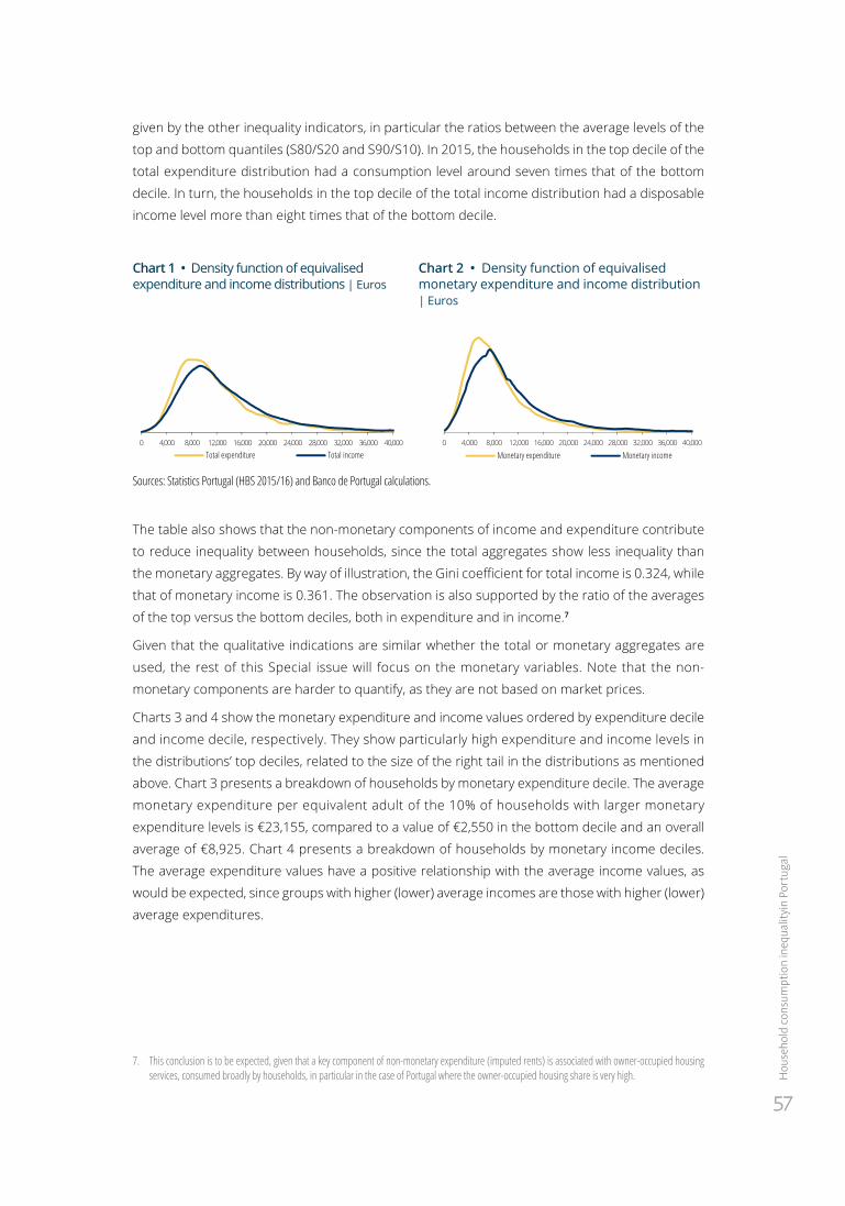
5757
Hou
seho
ld co
nsum
ptio
n in
equa
lityin
Por
tuga
l
given by the other inequality indicators, in particular the ratios between the average levels of the
top and bottom quantiles (S80/S20 and S90/S10). In 2015, the households in the top decile of the
total expenditure distribution had a consumption level around seven times that of the bottom
decile. In turn, the households in the top decile of the total income distribution had a disposable
income level more than eight times that of the bottom decile.
Chart 1 • Density function of equivalised expenditure and income distributions | Euros
Chart 2 • Density function of equivalised monetary expenditure and income distribution | Euros
0 4,000 8,000 12,000 16,000 20,000 24,000 28,000 32,000 36,000 40,000
Total expenditure Total income0 4,000 8,000 12,000 16,000 20,000 24,000 28,000 32,000 36,000 40,000
Monetary expenditure Monetary income
Sources: Statistics Portugal (HBS 2015/16) and Banco de Portugal calculations.
The table also shows that the non-monetary components of income and expenditure contribute
to reduce inequality between households, since the total aggregates show less inequality than
the monetary aggregates. By way of illustration, the Gini coefficient for total income is 0.324, while
that of monetary income is 0.361. The observation is also supported by the ratio of the averages
of the top versus the bottom deciles, both in expenditure and in income.7
Given that the qualitative indications are similar whether the total or monetary aggregates are
used, the rest of this Special issue will focus on the monetary variables. Note that the non-
monetary components are harder to quantify, as they are not based on market prices.
Charts 3 and 4 show the monetary expenditure and income values ordered by expenditure decile
and income decile, respectively. They show particularly high expenditure and income levels in
the distributions’ top deciles, related to the size of the right tail in the distributions as mentioned
above. Chart 3 presents a breakdown of households by monetary expenditure decile. The average
monetary expenditure per equivalent adult of the 10% of households with larger monetary
expenditure levels is €23,155, compared to a value of €2,550 in the bottom decile and an overall
average of €8,925. Chart 4 presents a breakdown of households by monetary income deciles.
The average expenditure values have a positive relationship with the average income values, as
would be expected, since groups with higher (lower) average incomes are those with higher (lower)
average expenditures.
7. This conclusion is to be expected, given that a key component of non-monetary expenditure (imputed rents) is associated with owner-occupied housing services, consumed broadly by households, in particular in the case of Portugal where the owner-occupied housing share is very high.
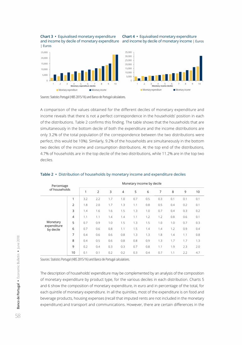
Banc
o de
Por
tuga
l •
Eco
nom
ic B
ulle
tin •
Jun
e 20
18
58
Chart 3 • Equivalised monetary expenditure and income by decile of monetary expenditure | Euros
Chart 4 • Equivalised monetary expenditure and income by decile of monetary income | Euros
0
5,000
10,000
15,000
20,000
25,000
1 2 3 4 5 6 7 8 9 10Monetary expenditure deciles
Monetary expenditure Monetary income
0
5,000
10,000
15,000
20,000
25,000
30,000
35,000
1 2 3 4 5 6 7 8 9 10Monetary income deciles
Monetary expenditure Monetary income
Sources: Statistics Portugal (HBS 2015/16) and Banco de Portugal calculations.
A comparison of the values obtained for the different deciles of monetary expenditure and
income reveals that there is not a perfect correspondence in the households’ position in each
of the distributions. Table 2 confirms this finding. The table shows that the households that are
simultaneously in the bottom decile of both the expenditure and the income distributions are
only 3.2% of the total population (if the correspondence between the two distributions were
perfect, this would be 10%). Similarly, 9.2% of the households are simultaneously in the bottom
two deciles of the income and consumption distributions. At the top end of the distributions,
4.7% of households are in the top decile of the two distributions, while 11.2% are in the top two
deciles.
Table 2 • Distribution of households by monetary income and expenditure deciles
Percentage of households
Monetary income by decile
1 2 3 4 5 6 7 8 9 10
Monetary expenditure
by decile
1 3.2 2.2 1.7 1.0 0.7 0.5 0.3 0.1 0.1 0.1
2 1.8 2.0 1.7 1.3 1.1 0.8 0.5 0.4 0.2 0.1
3 1.4 1.6 1.6 1.5 1.3 1.0 0.7 0.4 0.3 0.2
4 1.1 1.1 1.4 1.4 1.1 1.2 1.2 0.8 0.6 0.1
5 0.7 0.9 1.0 1.5 1.3 1.5 1.0 1.0 0.7 0.3
6 0.7 0.6 0.8 1.1 1.5 1.4 1.4 1.2 0.9 0.4
7 0.4 0.6 0.6 0.8 1.3 1.3 1.8 1.4 1.1 0.8
8 0.4 0.5 0.6 0.8 0.8 0.9 1.3 1.7 1.7 1.3
9 0.2 0.4 0.3 0.3 0.7 0.8 1.1 1.9 2.3 2.0
10 0.1 0.1 0.2 0.2 0.3 0.4 0.7 1.1 2.2 4.7
Sources: Statistics Portugal (HBS 2015/16) and Banco de Portugal calculations.
The description of households’ expenditure may be complemented by an analysis of the composition
of monetary expenditure by product type, for the various deciles in each distribution. Charts 5
and 6 show the composition of monetary expenditure, in euro and in percentage of the total, for
each quintile of monetary expenditure. In all the quintiles, most of the expenditure is on food and
beverage products, housing expenses (recall that imputed rents are not included in the monetary
expenditure) and transport and communications. However, there are certain differences in the
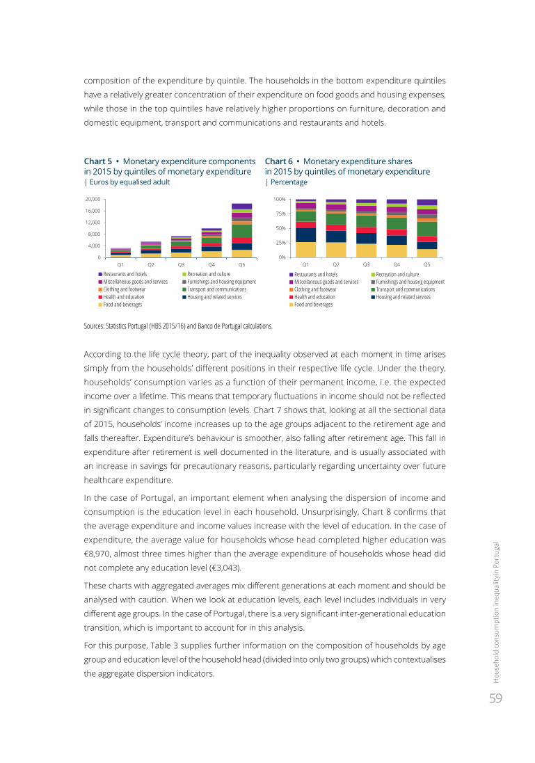
5959
Hou
seho
ld co
nsum
ptio
n in
equa
lityin
Por
tuga
l
composition of the expenditure by quintile. The households in the bottom expenditure quintiles
have a relatively greater concentration of their expenditure on food goods and housing expenses,
while those in the top quintiles have relatively higher proportions on furniture, decoration and
domestic equipment, transport and communications and restaurants and hotels.
Chart 5 • Monetary expenditure components in 2015 by quintiles of monetary expenditure | Euros by equalised adult
Chart 6 • Monetary expenditure shares in 2015 by quintiles of monetary expenditure | Percentage
0
4,000
8,000
12,000
16,000
20,000
Q1 Q2 Q3 Q4 Q5
Restaurants and hotels Recreation and cultureMiscellaneous goods and services Furnishings and housing equipmentClothing and footwear Transport and communicationsHealth and education Housing and related servicesFood and beverages
0%
25%
50%
75%
100%
Q1 Q2 Q3 Q4 Q5
Restaurants and hotels Recreation and cultureMiscellaneous goods and services Furnishings and housing equipmentClothing and footwear Transport and communicationsHealth and education Housing and related servicesFood and beverages
Sources: Statistics Portugal (HBS 2015/16) and Banco de Portugal calculations.
According to the life cycle theory, part of the inequality observed at each moment in time arises
simply from the households’ different positions in their respective life cycle. Under the theory,
households’ consumption varies as a function of their permanent income, i.e. the expected
income over a lifetime. This means that temporary fluctuations in income should not be reflected
in significant changes to consumption levels. Chart 7 shows that, looking at all the sectional data
of 2015, households’ income increases up to the age groups adjacent to the retirement age and
falls thereafter. Expenditure’s behaviour is smoother, also falling after retirement age. This fall in
expenditure after retirement is well documented in the literature, and is usually associated with
an increase in savings for precautionary reasons, particularly regarding uncertainty over future
healthcare expenditure.
In the case of Portugal, an important element when analysing the dispersion of income and
consumption is the education level in each household. Unsurprisingly, Chart 8 confirms that
the average expenditure and income values increase with the level of education. In the case of
expenditure, the average value for households whose head completed higher education was
€8,970, almost three times higher than the average expenditure of households whose head did
not complete any education level (€3,043).
These charts with aggregated averages mix different generations at each moment and should be
analysed with caution. When we look at education levels, each level includes individuals in very
different age groups. In the case of Portugal, there is a very significant inter-generational education
transition, which is important to account for in this analysis.
For this purpose, Table 3 supplies further information on the composition of households by age
group and education level of the household head (divided into only two groups) which contextualises
the aggregate dispersion indicators.
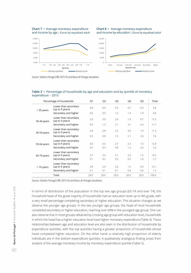
Banc
o de
Por
tuga
l •
Eco
nom
ic B
ulle
tin •
Jun
e 20
18
60
Chart 7 • Average monetary expenditure and income by age | Euros by equalised adult
Chart 8 • Average monetary expenditure and income by education | Euros by equalised adult
4,000
6,000
8,000
10,000
12,000
14,000
< 35 [35 - 44] [45 - 54] [55 - 64] [65 - 74] > 74
Monetary expenditure Monetary income
Age group
,0
5,000
10,000
15,000
20,000
25,000
None 1st Cycle 2nd Cycle 3rd Cycle Secondary Higher
Monetary expenditure Monetary income
Education level
Sources: Statistics Portugal (HBS 2015/16) and Banco de Portugal calculations.
Table 3 • Percentage of households by age and education and by quintile of monetary expenditure – 2015
Percentage of households Q1 Q2 Q3 Q4 Q5 Total
< 35 yearsLower than secondary (up to 9 years) 0.8 0.9 0.9 0.7 0.4 3.8
Secondary and higher 0.6 0.9 1.3 1.4 1.8 6.0
35-44 yearsLower than secondary (up to 9 years) 2.9 3.0 2.6 1.9 0.7 11.0
Secondary and higher 0.9 1.3 2.1 3.1 4.4 11.7
45-54 yearsLower than secondary (up to 9 years) 2.8 2.8 2.5 2.0 1.0 11.2
Secondary and higher 0.3 0.8 1.5 2.1 3.0 7.6
55-64 yearsLower than secondary (up to 9 years) 3.0 3.3 2.7 2.4 1.5 12.9Secondary and higher 0.2 0.3 0.8 1.2 2.6 5.2
65-74 yearsLower than secondary (up to 9 years) 3.7 3.5 3.1 2.6 1.5 14.5Secondary and higher 0.1 0.2 0.3 0.5 1.6 2.7
> 74 yearsLower than secondary (up to 9 years) 4.8 2.9 2.0 1.5 0.9 12.1Secondary and higher 0.1 0.1 0.1 0.4 0.6 1.3
Total 20.0 20.0 20.0 20.0 20.0 100.0
Sources: Statistics Portugal (HBS 2015/16) and Banco de Portugal calculations.
In terms of distribution of the population in the top two age groups (65-74 and over 74), the household head of the great majority of households had an education level up to 9th grade, with a very small percentage completing secondary or higher education. This situation changes as we observe the younger age groups. In the two younger age groups, the head of most households completed secondary or higher education, reaching over 60% in the youngest age group. One can also observe that in most groups obtained by crossing age group with education level, households in which the head has a higher education level have higher monetary expenditure (Table 4). These relationships between age and education level are also seen in the distribution of households by expenditure quintiles, with the top quintiles having a greater proportion of households whose head completed higher education. On the other hand, a relatively high proportion of elderly individuals are in the bottom expenditure quintiles. A qualitatively analogous finding arises from analysis of the average monetary income by monetary expenditure quintile (Table 5).
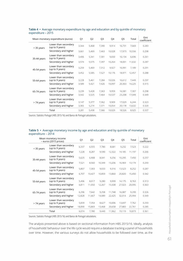
6161
Hou
seho
ld co
nsum
ptio
n in
equa
lityin
Por
tuga
l
Table 4 • Average monetary expenditure by age and education and by quintile of monetary expenditure – 2015
Mean monetary expenditure (euros) Q1 Q2 Q3 Q4 Q5 Total Gini coefficient
< 35 yearsLower than secondary (up to 9 years) 3,344 5,468 7,390 9,914 16,731 7,669 0.283
Secondary and higher 3,661 5,469 7,463 10,028 17,973 10,556 0.298
35-44 yearsLower than secondary (up to 9 years) 3,406 5,341 7,301 9,650 16,134 6,696 0.261
Secondary and higher 3,574 5,575 7,397 10,264 18,001 11,632 0.287
45-54 yearsLower than secondary (up to 9 years) 3,259 5,469 7,312 9,927 16,991 7,189 0.291
Secondary and higher 3,452 5,585 7,527 10,176 18,971 12,457 0.288
55-64 yearsLower than secondary (up to 9 years) 3,228 5,461 7,284 10,026 16,612 7,449 0.297Secondary and higher 3,589 5,421 7,426 10,097 20,363 14,225 0.315
65-74 yearsLower than secondary (up to 9 years) 3,239 5,428 7,363 9,959 16,581 7,307 0.298Secondary and higher 3,542 5,525 7,464 10,537 23,208 17,049 0.349
> 74 yearsLower than secondary (up to 9 years) 3,147 5,377 7,362 9,909 17,029 6,244 0.323Secondary and higher 3,365 5,274 7,371 10,054 20,178 13,632 0.320
Total 3,281 5,438 7,366 10,029 18,526 8,925 0.337
Sources: Statistics Portugal (HBS 2015/16) and Banco de Portugal calculations.
Table 5 • Average monetary income by age and education and by quintile of monetary expenditure – 2014
Mean monetary income – euros (2015 prices) Q1 Q2 Q3 Q4 Q5 Total Gini
coefficient
< 35 yearsLower than secondary (up to 9 years) 6,337 6,555 7,780 8,681 9,232 7,523 0.222
Secondary and higher 7,228 8,287 9,590 12,322 14,185 11,197 0.266
35-44 yearsLower than secondary (up to 9 years) 5,625 6,908 8,041 9,256 10,295 7,450 0.257
Secondary and higher 7,521 8,560 10,349 13,206 16,969 13,174 0.293
45-54 yearsLower than secondary (up to 9 years) 5,807 7,303 9,033 9,316 13,523 8,252 0.287
Secondary and higher 6,707 10,427 10,859 13,860 20,820 15,450 0.342
55-64 yearsLower than secondary (up to 9 years) 5,496 8,017 9,280 9,999 14,175 8,763 0.313Secondary and higher 6,811 11,050 12,267 15,508 27,023 20,095 0.363
65-74 yearsLower than secondary (up to 9 years) 6,296 7,642 9,258 11,748 16,087 9,299 0.326Secondary and higher 12,828 11,667 14,089 22,425 32,014 25,994 0.349
> 74 yearsLower than secondary (up to 9 years) 5,839 7,354 8,627 10,006 13,697 7,762 0.293
Secondary and higher 18,890 15,869 13,468 20,658 27,883 22,761 0.285
Total 6,074 7,780 9,440 11,962 19,119 10,873 0.361
Sources: Statistics Portugal (HBS 2015/16) and Banco de Portugal calculations.
The analysis presented above is based on sectional information from HBS 2015/16. Ideally, analysis of households’ behaviour over the life cycle would require a database tracking a panel of households over time. However, the various surveys do not allow households to be followed over time, as the
Banc
o de
Por
tuga
l •
Eco
nom
ic B
ulle
tin •
Jun
e 20
18
62
samples are independent between surveys. A way of resolving this problem is to define “synthetic” cohorts of households, based on their year of birth or, alternatively, the year of birth crossed with the education level. Using data from various HBS waves (in this case three surveys were used, the HBS 2000, HBS 2010 and HBS 2015), it is possible to track each cohort in the subsequent surveys and thereby evaluate the behaviour of their expenditure or income over the life cycle.
Charts 9 and 10 give the average monetary expenditure and income for the various cohorts (considering age groups between 25 and 74 years). The first cohort contains individuals born between 1935 and 1939 (which in the latest survey places them in the 70- to 74-year-old age group). The youngest cohort considered (born between 1985 and 1989), only has observations in HBS 2015 (in the 25- to 29-year-old age group). This generational analysis has several limitations, including greater statistical uncertainty due to the sample being restricted to relatively small subgroups of the population. Taking these limitations into account, the behaviour shown in the charts seems to confirm expectations. Indeed, the charts show that the average income values increase up to the 60- to 64-year-old age group, falling in the period following the typical retirement age. Expenditure also presents a (slightly) upward trend up to the 60- to 64-year-old age group but is more stable than income. After the age of 65, average expenditure, like income, declines, falling further in the 70- to 74-year-old age group.
Charts 11 and 12 divide the various cohorts into education levels. The indications of increasing monetary income up to retirement age are common across household segments with higher or lower education levels but the increase in income over the life cycle is sharper for households whose head has a higher education level. In turn, in both groups, the behaviour of expenditure was less pronounced. In the following section, this information will be analysed over time.
As noted above, the dispersion of income and consumption in Portugal is partly associated with the different position of the households in the life cycle, along with their respective educational level. However, most of the inequality observed in the Portuguese economy is not associated with households’ observable characteristics of this kind. A way to confirm this is to break down the inequality measures into population groups. The Gini coefficient cannot be broken down by population groups, therefore the mean logarithmic deviation will be used in the calculations that follow. Table 6 gives the breakdown of dispersion in households’ income and expenditure in the contribution arising on the one hand from differences in averages between age and education groups (between-group contribution) and on the other hand the dispersion within each one of those groups (within-group contribution). A granular disaggregation crossing age groups and education levels shows that most of the dispersion in consumption and income arises within each group and not between groups. Indeed the differences in the average expenditure between the various age groups and education levels (between-group contribution) represent less than one third of the total expenditure dispersion. In the case of income, the between-group contribution is slightly above one third.
This result suggests that there are unobservable factors, including the countless persistent shocks that affect households over the life cycle, which are behind most of the inequality observed in expenditure and income. This idea of individuals accumulating shocks, positive and negative, over their lifetime suggests that the dispersion of income and expenditure of their respective households should increase with age. This thesis, also present in the life-cycle theory, is confirmed in the last columns of Tables 4 and 5, except for in the highest age groups. In terms of cohorts, Charts 13 and 14 also confirm the increasing dispersion of households’ consumption and income over the working life of economic agents.
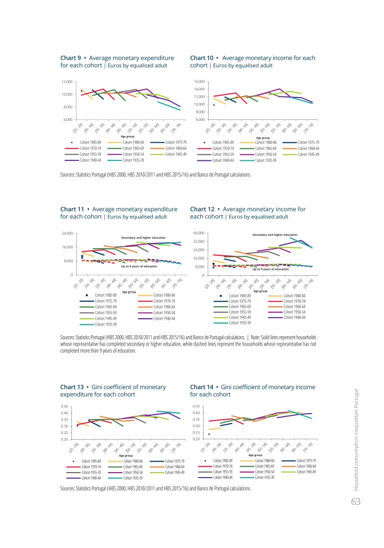
6363
Hou
seho
ld co
nsum
ptio
n in
equa
lityin
Por
tuga
l
Chart 9 • Average monetary expenditure for each cohort | Euros by equalised adult
Chart 10 • Average monetary income for each cohort | Euros by equalised adult
6,000
8,000
10,000
12,000
Age group
Cohort 1985-89 Cohort 1980-84 Cohort 1975-79Cohort 1970-74 Cohort 1965-69 Cohort 1960-64Cohort 1955-59 Cohort 1950-54 Cohort 1945-49Cohort 1940-44 Cohort 1935-39
6,000
8,000
10,000
12,000
14,000
16,000
Age group
Cohort 1985-89 Cohort 1980-84 Cohort 1975-79Cohort 1970-74 Cohort 1965-69 Cohort 1960-64Cohort 1955-59 Cohort 1950-54 Cohort 1945-49Cohort 1940-44 Cohort 1935-39
Sources: Statistics Portugal (HBS 2000, HBS 2010/2011 and HBS 2015/16) and Banco de Portugal calculations.
Chart 11 • Average monetary expenditure for each cohort | Euros by equalised adult
Chart 12 • Average monetary income for each cohort | Euros by equalised adult
,0
8,000
16,000
24,000
Age groupCohort 1985-89 Cohort 1980-84Cohort 1975-79 Cohort 1970-74Cohort 1965-69 Cohort 1960-64Cohort 1955-59 Cohort 1950-54Cohort 1945-49 Cohort 1940-44Cohort 1935-39
Secondary and higher education
Up to 9 years of education
,0
8,000
16,000
24,000
32,000
40,000
Age group
Cohort 1985-89 Cohort 1980-84Cohort 1975-79 Cohort 1970-74Cohort 1965-69 Cohort 1960-64Cohort 1955-59 Cohort 1950-54Cohort 1945-49 Cohort 1940-44Cohort 1935-39
Secondary and higher education
Up to 9 years of education
Sources: Statistics Portugal (HBS 2000, HBS 2010/2011 and HBS 2015/16) and Banco de Portugal calculations. | Note: Solid lines represent households whose representative has completed secondary or higher education, while dashed lines represent the households whose representative has not completed more than 9 years of education.
Chart 13 • Gini coefficient of monetary expenditure for each cohort
Chart 14 • Gini coefficient of monetary income for each cohort
0.20
0.25
0.30
0.35
0.40
0.45
Age group
Cohort 1985-89 Cohort 1980-84 Cohort 1975-79Cohort 1970-74 Cohort 1965-69 Cohort 1960-64Cohort 1955-59 Cohort 1950-54 Cohort 1945-49Cohort 1940-44 Cohort 1935-39
0.20
0.25
0.30
0.35
0.40
0.45
Age group
Cohort 1985-89 Cohort 1980-84 Cohort 1975-79Cohort 1970-74 Cohort 1965-69 Cohort 1960-64Cohort 1955-59 Cohort 1950-54 Cohort 1945-49Cohort 1940-44 Cohort 1935-39
Sources: Statistics Portugal (HBS 2000, HBS 2010/2011 and HBS 2015/16) and Banco de Portugal calculations.
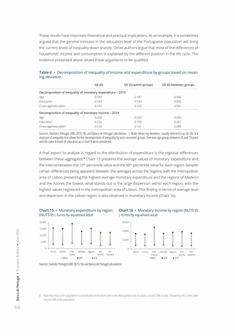
Banc
o de
Por
tuga
l •
Eco
nom
ic B
ulle
tin •
Jun
e 20
18
64
These results have important theoretical and practical implications. As an example, it is sometimes
argued that the general increase in the education level of the Portuguese population will bring
the current levels of inequality down sharply. Other authors argue that most of the differences of
households’ income and consumption is explained by the different position in the life cycle. The
evidence presented above allows these arguments to be qualified.
Table 6 • Decomposition of inequality of income and expenditure by groups based on mean log deviation
GE (0) GE (0) within-groups GE (0) between-groups
Decomposition of inequality of monetary expenditure – 2015Age 0.193 0.187 0.006Education 0.193 0.139 0.055Cross age/education 0.193 0.132 0.061
Decomposition of inequality of monetary income – 2014Age 0.226 0.220 0.006Education 0.226 0.159 0.067Cross age/education 0.226 0.141 0.085
Sources: Statistics Portugal (HBS 2015/16) and Banco de Portugal calculations. | Note: Mean log deviation, usually referred to as GE (0), is a measure of inequality that allows for the decomposition of inequality by socio-economic groups. Five-year age groups between 25 and 74 years and the same 6 levels of education as in chart 8 were considered.
A final aspect to analyse in regard to the distribution of expenditure is the regional differences
between these aggregates.8 Chart 15 presents the average values of monetary expenditure and
the interval between the 10th percentile value and the 90th percentile value for each region. Despite
certain differences being apparent between the averages across the regions, with the metropolitan
area of Lisbon presenting the highest average monetary expenditure and the regions of Madeira
and the Azores the lowest, what stands out is the large dispersion within each region, with the
highest values registered in the metropolitan area of Lisbon. This finding in terms of average level
and dispersion in the Lisbon region is also observed in monetary income (Chart 16).
Chart 15 • Monetary expenditure by region (NUTS II) | Euros by equalised adult
Chart 16 • Monetary income by region (NUTS II) | Euros by equalised adult
0
5,000
10,000
15,000
20,000
Norte Centro A.M. Lisboa
Alentejo Algarve R.A. Açores
R.A. Madeira
Mean p90 p10
0
10,000
20,000
30,000
Norte Centro A.M.Lisboa
Alentejo Algarve R.A.Açores
R.A.Madeira
Mean p90 p10
Sources: Statistics Portugal (HBS 2015/16) and Banco de Portugal calculations.
8. Note that most of the population is concentrated in the North and in the Metropolitan area of Lisbon, around 30% in each, followed by the Centre, with around 20% of the population.
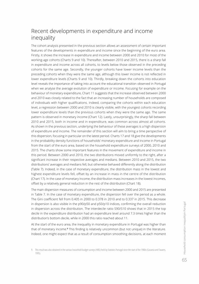
6565
Hou
seho
ld co
nsum
ptio
n in
equa
lityin
Por
tuga
l
Recent developments in expenditure and income inequalityThe cohort analysis presented in the previous section allows an assessment of certain important features of the developments in expenditure and income since the beginning of the euro area. Firstly, it shows the increase in expenditure and income between 2000 and 2010 for most of the working-age cohorts (Charts 9 and 10). Thereafter, between 2010 and 2015, there is a sharp fall in expenditure and income across all cohorts, to levels below those observed in the preceding cohorts for the same age. Secondly, the younger cohorts have lower income levels than the preceding cohorts when they were the same age, although this lower income is not reflected in lower expenditure levels (Charts 9 and 10). Thirdly, breaking down the cohorts into education level reveals the importance of taking into account the educational transition observed in Portugal when we analyse the average evolution of expenditure or income. Focusing for example on the behaviour of monetary expenditure, Chart 11 suggests that the increase observed between 2000 and 2010 was closely related to the fact that an increasing number of households are composed of individuals with higher qualifications. Indeed, comparing the cohorts within each education level, a regression between 2000 and 2010 is clearly visible, with the youngest cohorts recording lower expenditure levels than the previous cohorts when they were the same age. The same pattern is observed in monetary income (Chart 12). Lastly, unsurprisingly, the sharp fall between 2010 and 2015, both in income and in expenditure, was common across almost all cohorts. As shown in the previous section, underlying the behaviour of these averages is a high dispersion of expenditure and income. The remainder of this section will aim to bring a time perspective of this dispersion, focusing in particular on the latest period. Charts 17 and 18 give the developments in the probability density functions of households’ monetary expenditure and income in Portugal from the start of the euro area, based on the household expenditure surveys of 2000, 2010 and 2015. The charts show some important features in the movement of expenditure and income in this period. Between 2000 and 2010, the two distributions moved uniformly to the right, after a significant increase in their respective averages and medians. Between 2010 and 2015, the two distributions’ averages and medians fell, but otherwise behaved differently along the distribution (Table 7). Indeed, in the case of monetary expenditure, the distribution mass in the lowest and highest expenditure levels fell, offset by an increase in mass in the centre of the distribution (Chart 17). In the case of monetary income, the distribution mass increases in the lowest incomes, offset by a relatively general reduction in the rest of the distribution (Chart 18).
The main dispersion measures of consumption and income between 2000 and 2015 are presented in Table 7. In the case of monetary expenditure, the dispersion fell over the period as a whole. The Gini coefficient fell from 0.405 in 2000 to 0.378 in 2010 and to 0.337 in 2015. This decrease in dispersion is also visible in the p90/p50 and p50/p10 indices, confirming the overall reduction in dispersion across the distribution. The interdecile ratio S90/S10 shows that in 2015 the top decile in the expenditure distribution had an expenditure level around 7.3 times higher than the distribution’s bottom decile, while in 2000 this ratio reached about 11.
At the start of the euro area, the inequality in monetary expenditure in Portugal was higher than that of monetary income.9 This finding is relatively uncommon (but not unique) in the literature. Indeed, one might expect that as a result of consumption smoothing decisions, at each moment
9. This result was also obtained in the various household budget surveys (HBS) held by Statistics Portugal since the start of the 1980s (Gouveia and Tavares, 1995).
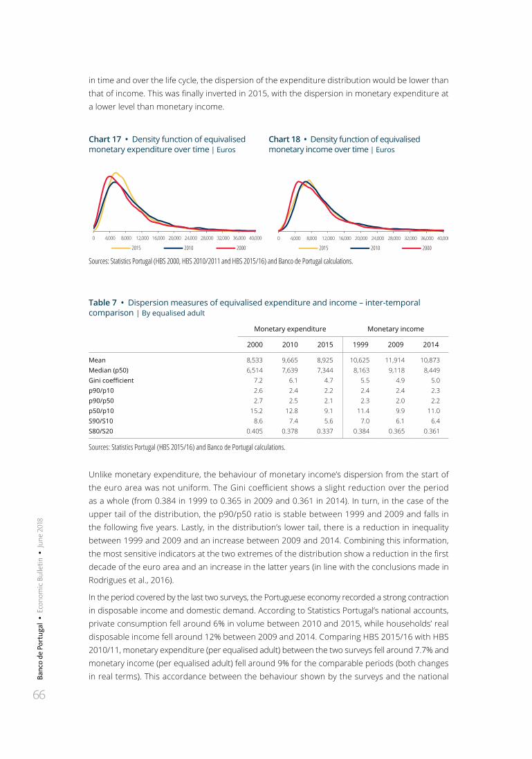
Banc
o de
Por
tuga
l •
Eco
nom
ic B
ulle
tin •
Jun
e 20
18
66
in time and over the life cycle, the dispersion of the expenditure distribution would be lower than that of income. This was finally inverted in 2015, with the dispersion in monetary expenditure at a lower level than monetary income.
Chart 17 • Density function of equivalised monetary expenditure over time | Euros
Chart 18 • Density function of equivalised monetary income over time | Euros
0 4,000 8,000 12,000 16,000 20,000 24,000 28,000 32,000 36,000 40,000
2015 2010 2000
0 4,000 8,000 12,000 16,000 20,000 24,000 28,000 32,000 36,000 40,000
2015 2010 2000
Sources: Statistics Portugal (HBS 2000, HBS 2010/2011 and HBS 2015/16) and Banco de Portugal calculations.
Table 7 • Dispersion measures of equivalised expenditure and income – inter-temporal comparison | By equalised adult
Monetary expenditure Monetary income
2000 2010 2015 1999 2009 2014
Mean 8,533 9,665 8,925 10,625 11,914 10,873Median (p50) 6,514 7,639 7,344 8,163 9,118 8,449Gini coefficient 7.2 6.1 4.7 5.5 4.9 5.0p90/p10 2.6 2.4 2.2 2.4 2.4 2.3p90/p50 2.7 2.5 2.1 2.3 2.0 2.2p50/p10 15.2 12.8 9.1 11.4 9.9 11.0S90/S10 8.6 7.4 5.6 7.0 6.1 6.4S80/S20 0.405 0.378 0.337 0.384 0.365 0.361
Sources: Statistics Portugal (HBS 2015/16) and Banco de Portugal calculations.
Unlike monetary expenditure, the behaviour of monetary income’s dispersion from the start of the euro area was not uniform. The Gini coefficient shows a slight reduction over the period as a whole (from 0.384 in 1999 to 0.365 in 2009 and 0.361 in 2014). In turn, in the case of the upper tail of the distribution, the p90/p50 ratio is stable between 1999 and 2009 and falls in the following five years. Lastly, in the distribution’s lower tail, there is a reduction in inequality between 1999 and 2009 and an increase between 2009 and 2014. Combining this information, the most sensitive indicators at the two extremes of the distribution show a reduction in the first decade of the euro area and an increase in the latter years (in line with the conclusions made in Rodrigues et al., 2016).
In the period covered by the last two surveys, the Portuguese economy recorded a strong contraction in disposable income and domestic demand. According to Statistics Portugal’s national accounts, private consumption fell around 6% in volume between 2010 and 2015, while households’ real disposable income fell around 12% between 2009 and 2014. Comparing HBS 2015/16 with HBS 2010/11, monetary expenditure (per equalised adult) between the two surveys fell around 7.7% and monetary income (per equalised adult) fell around 9% for the comparable periods (both changes in real terms). This accordance between the behaviour shown by the surveys and the national
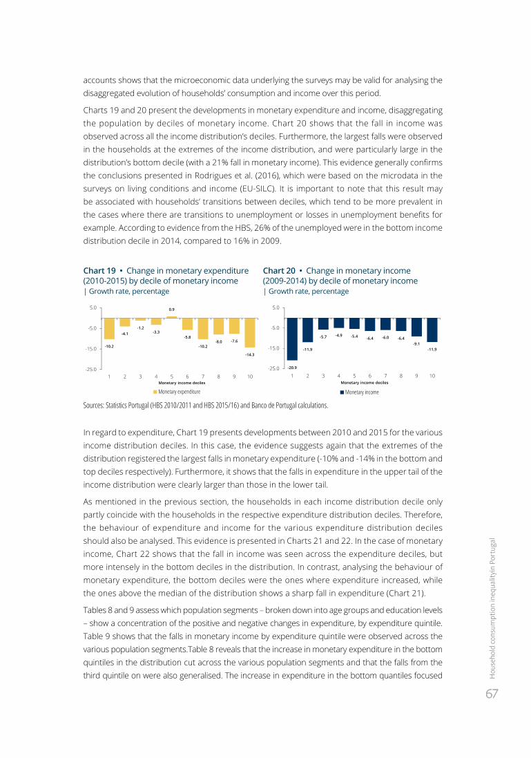
6767
Hou
seho
ld co
nsum
ptio
n in
equa
lityin
Por
tuga
l
accounts shows that the microeconomic data underlying the surveys may be valid for analysing the disaggregated evolution of households’ consumption and income over this period.
Charts 19 and 20 present the developments in monetary expenditure and income, disaggregating the population by deciles of monetary income. Chart 20 shows that the fall in income was observed across all the income distribution’s deciles. Furthermore, the largest falls were observed in the households at the extremes of the income distribution, and were particularly large in the distribution’s bottom decile (with a 21% fall in monetary income). This evidence generally confirms the conclusions presented in Rodrigues et al. (2016), which were based on the microdata in the surveys on living conditions and income (EU-SILC). It is important to note that this result may be associated with households’ transitions between deciles, which tend to be more prevalent in the cases where there are transitions to unemployment or losses in unemployment benefits for example. According to evidence from the HBS, 26% of the unemployed were in the bottom income distribution decile in 2014, compared to 16% in 2009.
Chart 19 • Change in monetary expenditure (2010-2015) by decile of monetary income | Growth rate, percentage
Chart 20 • Change in monetary income (2009-2014) by decile of monetary income | Growth rate, percentage
-10.2
-4.1-1.2
-3.3
0.9
-5.8
-10.2-8.0 -7.6
-14.3
-25.0
-15.0
-5.0
5.0
1 2 3 4 5 6 7 8 9 10
Monetary expenditureMonetary income deciles
-20.9
-11.9
-5.7 -4.9 -5.4 -6.4 -6.0 -6.4-9.1
-11.9
-25.0
-15.0
-5.0
5.0
1 2 3 4 5 6 7 8 9 10
Monetary income
Monetary income deciles
Sources: Statistics Portugal (HBS 2010/2011 and HBS 2015/16) and Banco de Portugal calculations.
In regard to expenditure, Chart 19 presents developments between 2010 and 2015 for the various income distribution deciles. In this case, the evidence suggests again that the extremes of the distribution registered the largest falls in monetary expenditure (-10% and -14% in the bottom and top deciles respectively). Furthermore, it shows that the falls in expenditure in the upper tail of the income distribution were clearly larger than those in the lower tail.
As mentioned in the previous section, the households in each income distribution decile only partly coincide with the households in the respective expenditure distribution deciles. Therefore, the behaviour of expenditure and income for the various expenditure distribution deciles should also be analysed. This evidence is presented in Charts 21 and 22. In the case of monetary income, Chart 22 shows that the fall in income was seen across the expenditure deciles, but more intensely in the bottom deciles in the distribution. In contrast, analysing the behaviour of monetary expenditure, the bottom deciles were the ones where expenditure increased, while the ones above the median of the distribution shows a sharp fall in expenditure (Chart 21).
Tables 8 and 9 assess which population segments – broken down into age groups and education levels – show a concentration of the positive and negative changes in expenditure, by expenditure quintile. Table 9 shows that the falls in monetary income by expenditure quintile were observed across the various population segments.Table 8 reveals that the increase in monetary expenditure in the bottom quintiles in the distribution cut across the various population segments and that the falls from the third quintile on were also generalised. The increase in expenditure in the bottom quantiles focused

Banc
o de
Por
tuga
l •
Eco
nom
ic B
ulle
tin •
Jun
e 20
18
68
on essential goods expenses, such as healthcare, education and other goods and services related to housing (Chart 23). In turn, the reduction in expenditure in the top quintiles came mainly from restaurants and hotels, transport and communications and leisure, recreation and culture.
Chart 21 • Change in monetary expenditure (2010-2015) by decile of monetary expenditure | Growth rate, percentage
Chart 22 • Change in monetary income (2010-2015) by decile of monetary expenditure | Growth rate, percentage
21.9
9.6
4.40.6
-2.5-5.9
-8.9-11.2 -12.5 -13.3-20.0
-10.0
0.0
10.0
20.0
30.0
1 2 3 4 5 6 7 8 9 10
Monetary expenditureMonetary expenditure deciles
-18.5
-9.8-11.8 -10.1
-6.9-4.2
-7.4-4.4 -5.4
-11.9-20.0
-10.0
0.0
10.0
20.0
30.0
1 2 3 4 5 6 7 8 9 10
Monetary incomeMonetary expenditure deciles
Sources: Statistics Portugal (HBS 2010/2011 and HBS 2015/16) and Banco de Portugal calculations.
Table 8 • Monetary expenditure growth, by age and education, by quintile of monetary expenditure
Rates of change (%) 2010-2015 Q1 Q2 Q3 Q4 Q5 Total
< 35 yearsLower than secondary (up to 9 years) 11.8 5.1 -3.7 -11.3 -4.9 -5.0
Secondary and higher 14.8 2.8 -4.2 -10.6 -16.1 -17.0
35-44 yearsLower than secondary (up to 9 years) 16.3 -0.9 -5.6 -12.4 -15.4 -19.0
Secondary and higher 5.9 3.7 -5.0 -9.6 -18.0 -21.3
45-54 yearsLower than secondary (up to 9 years) 6.5 1.6 -4.3 -10.1 -14.6 -15.1
Secondary and higher 6.2 4.6 -2.7 -8.4 -15.2 -21.3
55-64 yearsLower than secondary (up to 9 years) 8.8 3.4 -5.1 -11.3 -11.7 -11.9Secondary and higher 22.4 -3.2 -8.5 -12.0 -15.3 -20.1
65-74 yearsLower than secondary (up to 9 years) 14.9 2.6 -3.5 -10.4 -18.1 2.6Secondary and higher -4.4 6.9 -1.9 -5.5 -13.3 -9.0
> 74 yearsLower than secondary (up to 9 years) 19.3 2.5 -4.4 -10.9 -8.9 7.3Secondary and higher 1.6 -8.4 -4.9 -6.6 -12.1 -10.0
Sources: Statistics Portugal (HBS 2015/16) and Banco de Portugal calculations.
The surprising coexistence of falls in income with increases in expenditure in the bottom quintiles of the expenditure distribution requires two qualifications. First, the expenditure level in the distribution’s bottom deciles is very low (€2,500 of annual expenditure per equalised adult in the bottom decile), for which reason the increase observed – in terms of level – is also modest (Chart 23). Second, it is important to recall that the ordering of the households by expenditure and income deciles is very different, i.e. the households with the lowest expenditure levels are not necessarily those with the lowest incomes. The households in the bottom deciles of the expenditure distribution have positive savings levels on average (Chart 3). The increase in expenditure in these deciles between 2010 and
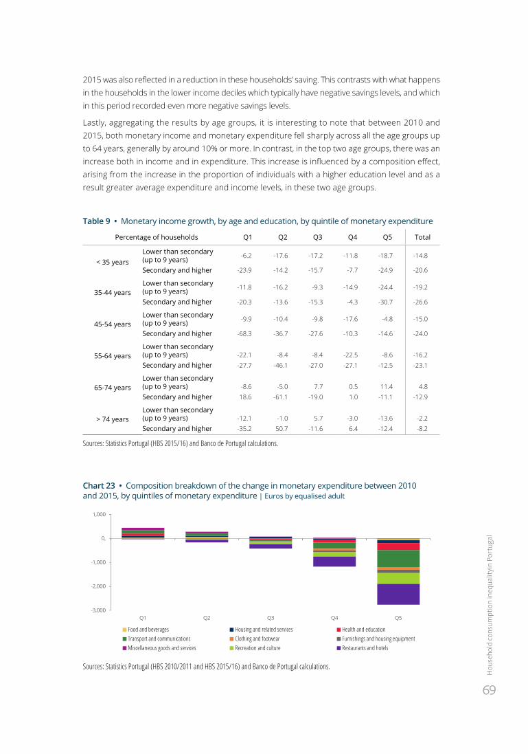
6969
Hou
seho
ld co
nsum
ptio
n in
equa
lityin
Por
tuga
l
2015 was also reflected in a reduction in these households’ saving. This contrasts with what happens in the households in the lower income deciles which typically have negative savings levels, and which in this period recorded even more negative savings levels.
Lastly, aggregating the results by age groups, it is interesting to note that between 2010 and 2015, both monetary income and monetary expenditure fell sharply across all the age groups up to 64 years, generally by around 10% or more. In contrast, in the top two age groups, there was an increase both in income and in expenditure. This increase is influenced by a composition effect, arising from the increase in the proportion of individuals with a higher education level and as a result greater average expenditure and income levels, in these two age groups.
Table 9 • Monetary income growth, by age and education, by quintile of monetary expenditure
Percentage of households Q1 Q2 Q3 Q4 Q5 Total
< 35 yearsLower than secondary (up to 9 years) -6.2 -17.6 -17.2 -11.8 -18.7 -14.8
Secondary and higher -23.9 -14.2 -15.7 -7.7 -24.9 -20.6
35-44 yearsLower than secondary (up to 9 years) -11.8 -16.2 -9.3 -14.9 -24.4 -19.2
Secondary and higher -20.3 -13.6 -15.3 -4.3 -30.7 -26.6
45-54 yearsLower than secondary (up to 9 years) -9.9 -10.4 -9.8 -17.6 -4.8 -15.0
Secondary and higher -68.3 -36.7 -27.6 -10.3 -14.6 -24.0
55-64 yearsLower than secondary (up to 9 years) -22.1 -8.4 -8.4 -22.5 -8.6 -16.2Secondary and higher -27.7 -46.1 -27.0 -27.1 -12.5 -23.1
65-74 yearsLower than secondary (up to 9 years) -8.6 -5.0 7.7 0.5 11.4 4.8Secondary and higher 18.6 -61.1 -19.0 1.0 -11.1 -12.9
> 74 yearsLower than secondary (up to 9 years) -12.1 -1.0 5.7 -3.0 -13.6 -2.2Secondary and higher -35.2 50.7 -11.6 6.4 -12.4 -8.2
Sources: Statistics Portugal (HBS 2015/16) and Banco de Portugal calculations.
Chart 23 • Composition breakdown of the change in monetary expenditure between 2010 and 2015, by quintiles of monetary expenditure | Euros by equalised adult
-3,000
-2,000
-1,000
0,
1,000
Q1 Q2 Q3 Q4 Q5
Food and beverages Housing and related services Health and educationTransport and communications Clothing and footwear Furnishings and housing equipmentMiscellaneous goods and services Recreation and culture Restaurants and hotels
Sources: Statistics Portugal (HBS 2010/2011 and HBS 2015/16) and Banco de Portugal calculations.
Banc
o de
Por
tuga
l •
Eco
nom
ic B
ulle
tin •
Jun
e 20
18
70
ConclusionsThis Special issue aimed to contribute to the debate on the economic inequalities in Portugal,
through the analysis of the distribution of consumption expenditure among households, jointly with
the distribution of income. The analysis was based on microeconomic information from various
household budget surveys held by Statistics Portugal. The main conclusions may be summarised in
the following points.
Inequality in the distribution of expenditure in Portugal is among the highest in the euro area. In
2015, the inequality in expenditure in Portugal was at levels only slightly below those of income.
The top decile of the monetary expenditure distribution represented about 20% of total monetary
expenditure. The households in this decile had monetary expenditure nine times higher on average
than that of the households in the bottom decile of the distribution. In terms of composition of
monetary expenditure, expenditures related to food and housing goods account for around half
of the consumption in the bottom expenditure deciles, while in the top deciles these aggregates
represent less than one third of total monetary expenditure.
In line with economic theory, expenditure’s behaviour is relatively smoother than that of income
over the life cycle. In the case of the Portuguese economy, this evidence should be interpreted in
the context of a profound educational transition, in which the youngest generations increasingly
have completed secondary or higher education and the older age groups are dominated by
qualifications beneath secondary level. This educational transition is very important given the
monotonic relationship observed between education level and households’ expenditure and
income levels. A part of the inequality observed in the Portuguese economy is thus attributable to
the households’ different positions in the life cycle combined with differences in their respective
education levels. However, these observable differences between the households only explain a
small part of the inequality in expenditure and income. In fact, most of the dispersion in expenditure
and income is observed within each of the age groups and education groups in the population,
which is likely to be associated with the accumulation of persistent economic shocks (positive and
negative) over the agents’ lives. This fact also explains the evidence showing that the dispersion in
expenditure and income increases over the working life of the agents, as propounded in economic
theory.
Comparison of the HBS surveys from the start of the euro area shows that in the first 15 years
of the monetary union, inequality in the distribution of monetary expenditure in Portugal fell
continuously. This conclusion is strongly supported across the different dispersion indicators,
both those that put greater weight in the centre of the distribution and those attributing greater
importance to differences in the extremes. In turn, the income inequality measures also fell up to
2009 but were relatively stable between 2009 and 2014. Over the last five years, the dispersion
of income also increased in the case of the indicators that focus on the differences between the
distribution’s extremes. Thus, while at the start of the euro area the dispersion of expenditure was
greater than the dispersion of income, in 2015 the dispersion of expenditure was below that of
income.
Although the HBS surveys are sectional, it is possible to track cohorts that represent households
when we combine the information from successive surveys over time. This analysis confirms the
idea that in 2015, each cohort – without exception – had a lower expenditure level than that of
7171
Hou
seho
ld co
nsum
ptio
n in
equa
lityin
Por
tuga
l
the older cohorts when they were the same age. This therefore confirms the idea of regression when the different cohorts are compared, both in terms of monetary expenditure and in terms of monetary income.
The period measured by the 2010 and 2015 surveys is particularly important material to analyse, as it saw real cumulative falls in consumption and income, unprecedented in recent history. When the information is analysed by monetary income deciles, the largest percentage falls in terms of monetary income were at the distribution’s extremes, with the largest in the lowest income decile. Regarding monetary expenditure, the largest falls were also at the distribution’s extremes, but more so in the top deciles of monetary income. When the households in the population are sorted by monetary expenditure deciles, the conclusion remains that the greatest falls in monetary income were observed at the distribution’s extremes. However, the evidence suggests that the monetary expenditure in the expenditure distribution’s bottom deciles increased in this period, in contrast to the fall in the distribution’s top deciles. This increase in expenditure in the bottom deciles in the distribution was mainly due to healthcare and transport expenses and other goods and services related to housing.
Economic inequality is a multi-dimensional concept. An integrated view of aspects such as income, consumption, wealth, leisure and access to public goods are an integral part of this concept. The integrated analysis of all these aspects is still an area with plenty of scope for progress in the theoretical and empirical literature (Aguiar and Hurst, 2017, Fisher et al., 2017). The same conclusion is valid for issues surrounding poverty, assessed from a broad perspective. These are important areas of research to be developed for the case of the Portuguese economy in the future.
ReferencesAguiar, M., and Bils, M. (2015). “Has Consumption Inequality Mirrored Income Inequality”, American Economic Review 105(9).
Aguiar, M. and Hurst, E. (2016). “The Macroeconomics of Time Allocation”, Handbook of Macroeconomics, Elsevier.
Alves, N. (2009). “New facts on poverty in Portugal”, Economic Bulletin of Banco de Portugal, Spring.
Anghel, B., Basso, H., Bover, O., Casado, J.M., Hospido, L., Izquierdo, M., Kataryniuk, A.L., Montero, J.M. and Vozmediano, E. (2018). “Income, consumption and wealth inequality in Spain”, Banco de Espana Occasional Paper No. 1806.
Atkinson, A., Guio, A-C. and Marlier, E. (eds.) (2017). “Monitoring social inclusion in Europe”, Eurostat Statistical Books.
Attanasio, O. and Pistaferri, L. (2016). “Consumption Inequality”, Journal of Economic Perspectives 30(2), 2016.
Attanasio, O., Berloffa, G., Blundell, R. and Preston, I. (2002). “From Earnings Inequality to Consumption Inequality”, Economic Journal 112 (478): C52–59.
Blundell, R., Pistaferri, L. and Preston, I. (2002). “Consumption Inequality and Partial Insurance”, American Economic Review, 98(5) 2008, 1887–1192.
Blundell, R. and Preston, I. (1998). “Consumption Inequality and Income Uncertainty”, Quarterly Journal of Economics 103, 603-640.
Banc
o de
Por
tuga
l •
Eco
nom
ic B
ulle
tin •
Jun
e 20
18
72
Costa, S. (2016). “Financial situation of the households in Portugal: an analysis based on the HFCS
2013”, Economic Studies, October, Banco de Portugal.
Fisher, J., D. Johnson, T. Smeeding, J. Thompson (2017). “Inequality in 3D: Income, consumption
and wealth”, Washington Center for Equitable Growth Working paper series, December.
Gouveia, M. and Tavares, J. (1995). “The Distribution of Household Income and Expenditure in
Portugal: 1980 and 1990”, Review of Income and Wealth 41(1), pp. 1-17.
Statistics Portugal (2002). Household Budget Survey 2000, 2002 Edition.
Statistics Portugal (2012). Household Budget Survey 2010/2011, 2012 Edition.
Statistics Portugal (2017). Household Budget Survey 2015/2016, 2017 Edition.
Krueger, D., Perri, F., Pistaferri, L. and Violante, G.L. (2010). “Cross Sectional Facts for Macroeconomists”,
Review of Economic Dynamics vol. 13(1), pp. 1-14.
Meyer, B. and Sullivan, J. (2018). “Consumption and income inequality in the US since the 60s”, Vox
article, 15 January.
Rodrigues, C.F. (coord), Figueras, R. and Junqueira, V. (2016). “Inequality of income and poverty
in Portugal”, Research Studies, Fundação Francisco Manuel dos Santos.
III Series1 Quarterly series for the Portuguese
economy: 1977-2017
2 Annual series on household wealth: 1980-2017

Qua
rter
ly se
ries f
or th
e Po
rtug
uese
eco
nom
y: 19
77-2
017
75
1 Quarterly series for the Portuguese economy: 1977-2017
As in previous years, this section discloses the update of the quarterly long series for the Portuguese
economy. These series are distributed in three blocks: expenditure, disposable income and labour
market.
The update released in this Bulletin maintains the same breakdown as the previous ones and
includes, for the first time, quarterly figures for 2017.1 The data is consistent with the latest version
of the Quarterly National Accounts published by Statistics Portugal on 30 May 2018 and mainly
follows the methodological procedures described in detail in Cardoso and Sequeira (2015).2
As regards the main expenditure components, the series for the period from 1995 onwards match
the quarterly data released by Statistics Portugal, both at current prices and in volume (chain-linked
volume data with reference year 2011).
In turn, disposable income series are adjusted for seasonal and calendar effects (whenever a
seasonal pattern was identified) and for this reason for the period from 1999 Q1 onwards, they may
differ from the ones published by Statistics Portugal (in the Quarterly Sector Accounts).
In the labour market block, series are grouped according to two different measures: full-time
equivalent (National Accounts concept) and thousands of individuals (Labour Force Survey concept).
Note that the series measured in thousands of individuals, as well as the unemployment rate series,
only differ from those published in the Labour Force Survey due to seasonal adjustments.
In general, seasonal adjustments were performed using the X13-ARIMA procedure (via the JDemetra+
software).
1. Quarterly series for the 1977-2017 period are only available in electronic format on Banco de Portugal’s webpage for this Economic Bulletin.2. Cardoso, F. and Sequeira, A. (2015), “Quarterly series for the Portuguese economy: 1977-2014”, Occasional Paper No. 1, Banco de Portugal.
Banc
o de
Por
tuga
l •
Eco
nom
ic B
ulle
tin •
Jun
e 20
18
76
2 Annual series on household wealth: 1980-2017
The annual series on household wealth, for the period 1980-2017, correspond to an update of the estimates published in the Economic Bulletin of June 2017. These wealth estimates, published annually,1 include the financial component (assets and liabilities) and housing (the main component of non-financial wealth). The concepts and methodology are identical to those described in Cardoso, F., Farinha, L. and Lameira, R. (2008).2
The financial series (assets and liabilities) presented here are consistent with the latest version of national financial accounts published by Banco de Portugal, which are available for the 1994-2017 period. The financial series for the period before 1994 were estimated using the implicit rates of change in the previous wealth series and obtained in accordance with the methodology described in detail in Cardoso, F. and Cunha, V. (2005).
The methodology used to estimate housing wealth is based on a method normally utilised to calculate capital stock estimates – the perpetual inventory method. This method consists in successively accumulating fixed capital investment (in this case, in housing), postulating reasonable hypotheses for its service life and depreciation method.
The series on housing wealth was adjusted, so as to incorporate for the 2000-2015 period the estimates of the housing capital stock, published for the first time by Statistics Portugal in November 2017.3 Estimates made available by Statistics Portugal do not include the value of land underlying housing (which is included in the wealth series published here). That value was estimated for the years under review. In order to estimate the value of land, we considered the ratio defined for tax purposes (regarding housing evaluations for the IMI – municipal property tax), which corresponds to 25% of the housing overall value. The remaining years of the long series of housing wealth (for the 1980-1999 and 2016-2017 periods) were calculated in compliance with the rates of change in the stock series obtained through the above-mentioned methodology, based on long series of GFCF in housing. The long series of GFCF in housing used to calculate the respective housing stock include the latest national accounts data (for the 1995-2017 period).
1. The series are only available in electronic format on Banco de Portugal’s webpage for this Economic Bulletin.2. Cardoso, F., Farinha, L. and Lameira, R. (2008), “Household wealth in Portugal: revised series”, Occasional Paper No. 1, Banco de Portugal. This
publication corresponds to the revised series previously published in Cardoso, F. and Cunha, V. (2005), “Household wealth in Portugal: 1980-2004” Working Paper No. 4, Banco de Portugal, where the calculation methodology is described in more detail.
3. Statistics Portugal (2018), “Capital stock (Base 2011) 2000-2015”, Press release of 24 November 2017.


www.bportugal.pt