economic consequence analysis of electric power
TRANSCRIPT

economic consequence analysis of electric power infrastructure disruptions
an analytical general equilibrium approach
Authors:
Ian Sue Wing1
Adam Z. Rose2
1Dept. Of Earth & Environment, Boston University
2Sol Price School of Public Policy and Center for Risk and Economic Analysis of Terrorism Attacks, University of Southern California
January 2018
The work described in this study was funded by the Transmission Planning and Technical Assistance
Division of the U.S. Department of Energy’s Office of Electricity Delivery and Energy Reliability under
Lawrence Berkeley National Laboratory Contract No. DE-AC02-05CH11231.

Economic Consequence Analysis of Electric Power Infrastructure Disruptions │1
Acknowledgements
The work described in this study was funded by the Transmission Planning and Technical Assistance
Division of the U.S. Department of Energy’s Office of Electricity Delivery and Energy Reliability under
Lawrence Berkeley National Laboratory Contract No. DE-AC02-05CH11231.

Economic Consequence Analysis of Electric Power Infrastructure Disruptions │2
Table of Contents
Acknowledgements ....................................................................................................................................... 1
Table of Contents .......................................................................................................................................... 2
Table of Figures ............................................................................................................................................. 3
List of Tables ................................................................................................................................................. 3
Acronyms and Abbreviations ........................................................................................................................ 4
1. Introduction ............................................................................................................................................ 5
2. Insights from Prior Research .................................................................................................................. 7
3. Methods ................................................................................................................................................. 9
3.1 An Analytical General Equilibrium Model ................................................................................... 9
3.2 Numerical Application: A Two-Week Power Outage in California’s Bay Area .......................... 13
4. Results .................................................................................................................................................. 15
4.1 No Substitution .......................................................................................................................... 15
4.2 Inherent Resilience Via Input Substitution ................................................................................ 15
4.3 Mitigation .................................................................................................................................. 19
5. Discussion and Conclusions .................................................................................................................. 23
6. References ............................................................................................................................................ 25
Economic Consequence Analysis of Electric Power Infrastructure Disruptions │3
Table of Figures
Figure 1. IMPACTS OF A TWO-WEEK ELECTRICITY INFRASTRUCTURE DISRUPTION ON THE BAY AREA ECONOMY: INHERENT RESILIENCE (% change in the value of each variable from its baseline level) . 19
Figure 2. ENERGY SUPPLY DISRUPTION MINIMIZING AND OPTIMAL BACKUP TECHNOLOGY PENETRATION (% change in backup capacity from its baseline level) ......................................................................... 20
List of Tables
Table 1. THE ANALYTICAL GENERAL EQUILIBRIUM MODEL ....................................................................... 10
Table 2. PARAMETERS OF THE NUMERICAL MODEL .................................................................................. 14
Table 3. EFFECTS OF BACKUP CAPACITY INVESTMENT ON THE CONSEQUENCES OF INFRASTRUCTURE DISRUPTION (median % change in the quantity of each variable from its baseline level, minimum and maximum values in square braces) ...................................................................................................... 22

Economic Consequence Analysis of Electric Power Infrastructure Disruptions │4
Acronyms and Abbreviations
CA DOF State of California Department of Finance
CAISO California Independent System Operator
CGE Computable general equilibrium
GE General equilibrium
NRC National Research Council
PE Partial equilibrium
USEOP United States Executive Office of the President

Economic Consequence Analysis of Electric Power Infrastructure Disruptions │5
1. Introduction
Electricity service providers take many steps to increase the reliability of their systems through
mitigation measures that reduces the frequency and magnitude of potential outages. These measures
include strengthening individual pieces of equipment and protecting system connectivity against
natural disasters, technological accidents and terrorist attacks (NRC, 2017). At the same time, direct
and indirect electricity customers pursue a range of measures to reduce their losses once the disruption
begins, which Rose (2007, 2017a) and others (e.g., Kajitani and Tatano, 2009; NRC, 2017) have
characterized as resilience. Some of these measures are inherent, or built into the production process,
such as the ability to substitute other power sources or the ability to shift operations to branch plants
out of the affected zone. Some require expenditures in advance of the disruption, such as the purchase
of storage batteries and back-up generators to be used once an outage commences. Still other actions
involve improvisation, or adaptive, resilience after the outage begins, such as conserving electricity at
greater levels than previously thought possible, altering production processes, finding new suppliers of
other critical inputs whose production has been disrupted by the outage, and recapturing lost
production once electricity is restored. Yet another strategy, more applicable to the electricity provider
is dynamic economic resilience, which refers to the acceleration of the pace of restoration of electricity
service. The distinction between reliability, as promoted by mitigation, and resilience is poignantly
stated in a recent NRC report: “Resilience is not the same as reliability. While minimizing the likelihood
of large-area, long-duration outages is important, a resilient system is one that acknowledges that such
outages can occur, prepares to deal with them, minimizes their impact when they occur, is able to
restore service quickly, and draws lessons from the experience to improve performance in the future”
(NRC, 2017, p. 10).1
In this paper we address three questions. First, we investigate the economy-wide impacts of a large-
scale disruption to electric power infrastructure. Second, we ask what effect mitigation and resilience
have on these impacts. Finally, we ask how the answers depend on key characteristics of the strategies
and of the affected economy. Previous research by the authors has demonstrated the methods for, and
elucidated the broader economic consequences of, incorporating these various risk reduction measures
into multi-sector computational general equilibrium (CGE) models of economies affected by disasters
(Rose et al., 2007; Sue Wing et al., 2016; Rose, 2017b). Energy-focused CGE models are the work-horse
1 Dozens of definitions of resilience have been offered along several dimensions. One important distinction is between
definitions that consider resilience to be any action that reduces risk (e.g., Bruneau et al., 2003; USEOP, 2013), including
those taken before, during and after an unforeseen event such as a power outage, and those that use the term narrowly
to include only actions taken after the event has commenced—acknowledging, however, that resilience is a process. The
latter definition does not ignore pre-event actions in building resilience capacity, such as in the advance purchase of
portable electricity generators, but notes that their implementation does not take place until after the outage has begun.
This is in contrast to mitigation, which is pre-outage investment intended to make a system more resistant, robust or
reliable (in standard engineering terminology) at the outset of the outage. Our definition simply chooses to focus on the
basic etymological root of resilience, “to rebound”, and thus emphasizes system or business continuity in the static sense
and recovery in the dynamic one (see also Greenberg et al., 2007; Wei et al., 2018). Note also that the emphasis on
actions after the outage begins shifts some of the attention away from the utility (supplier) and in the direction of its
customers (see Section 2).
Economic Consequence Analysis of Electric Power Infrastructure Disruptions │6
of assessments of these broader economic consequences of shocks or disruptions to energy supplies.
However, Sanstad (2015) identifies several shortcomings of previous applications of CGE modeling,
including the need for advances in the theory, clarification of important concepts (e.g., energy
conservation versus energy efficiency), and greater justifications for the parameter values of these
models. It is now common for such models to combine top-down representations of economic activity
with bottom-up detail in electricity generation technologies (see, e.g., Sue Wing, 2008). The resulting
disaggregated representations of electric power supply need to be constructed using numerical
calibration approaches that reconcile incommensurate data from economic accounts with engineering
specifications of the discrete technology options whose interactions will drive the model’s emergent
behavior. While the calibration process is relatively straightforward for aggregates of electric
generators with different technologies and/or fuels, it is extremely challenging to resolve the use of
inputs associated with elements of the transmission and distribution grid because of their network
(spatial) character.
This difficulty constitutes an important roadblock when investigation of disruption to electric power
supply from natural hazards and potential terrorist threats necessitates representations of elements of
the electric power system that are highly disaggregated. In particular, for any given downstream sector,
power generated by multiple, geographically dispersed generators upstream is conveyed by multiple
infrastructural assets to multiple electricity consuming entities located in different service territories.
This fundamental network structure of supply-demand linkages—and the allocation of electric power
flows to its various arcs, exists at geographic scales much finer than those at which economic models
simulate markets (e.g., individual counties). In addition, multi-sectoral economic models are ill-
equipped to represent the physical characteristics of power flows (e.g., Kirchhoff’s laws). Such details
are simulated with much greater fidelity by dedicated electricity sector techno-economic simulations
such as optimal power flow, economic dispatch or capacity expansion simulations. Moreover, these
types of models already exist and are routinely used by electricity system operators and balancing
authorities, and it is relatively straightforward to use them to quantify: (a) the magnitude of disruption
shocks—i.e., the extent of unserved load to various classes of customers, and (b) potential supply-side
resilience measures—i.e., ability for various deliberate investments in slack capacity or costly
interventions to manage the power system differently might be able reduce curtailments.
By contrast, explicit consideration of the foregoing details is rarely necessary for assessing the
downstream economy-wide impacts of the supply disruptions that these models would simulate as
emergent outcomes. The exception is the presence of strong feedbacks between downstream
responses to electricity supply curtailment and fundamental technological drivers of the disruption. Yet,
such feedbacks do not necessitate “hard” linkage (to say nothing of full integration) of multiple
simulation models based on fundamentally different paradigms. Models can be “soft” coupled using
emulation in conjunction with scenarios. In particular, one can envision the following three-step
assessment process:
(i) An optimal power flow model is used to simulate several scenarios of disruption while
incorporating mitigation activities of varying cost and effectiveness.
(ii) The simulation results are used to construct a reduced-form emulator of the envelope of

Economic Consequence Analysis of Electric Power Infrastructure Disruptions │7
resilience options, their opportunity costs, and their benefits in terms of moderating the
disruption (For recent efforts to construct reduced form emulators of economic models, see
Chen et al., 2017; Rose et al., 2017.)
(iii) The resulting vector of electricity supply curtailments, along with the response surface of
mitigation and resilience tactics and their bottom-up opportunity costs, are used in conjunction
with a multi-sector economic model to simulate the broader economic effects of power
disruptions.
The rest of the paper is organized as follows. Section 2 summarizes prior research on the economic
consequences of electricity outages, identifying key gaps in the existing literature. Motivated by these
opportunities, Section 3 provides a detailed description of our methodological approach, introducing
the analytical model which we solve, yielding our main results, and a numerical application of that
model: a two-week disruption in Bay-Area electricity infrastructure that reduces the latter’s annual
capacity by 4%. Analytical and numerical modeling results are presented in Section 4. Section 5
concludes with a brief discussion of caveats to the analysis and fruitful opportunities for future
research.
2. Insights from Prior Research
Nearly all of the early literature on the economic consequences electricity outages focused on standard
economic impacts and ways to reduce the probability and magnitude of these events before they took
place. As such, the major strategy was mitigation, which included such tactics as strengthening
equipment, improving connectivity, development of parallel systems, and having back-up equipment in
place. All of these tactics were essentially intended to enhance robustness/resistance of the electrical
system from the initial shock.
Much of the early economics literature focused on partial equilibrium (PE) analyses of electricity
providers or their customers. Except for a couple of studies of actual events, economy-wide losses were
typically not analyzed until the 1990s. They were, and continue to this day, to be measured primarily
with the common denominator of dollars in terms of gross output (sales revenue) or GDP. These
economy-wide or general equilibrium (GE) effects are of several types (Rose et al., 2007), involving
losses incurred by different actors:
Direct customers of the electricity service provider.
There is some dispute over whether these are considered GE or PE losses. In essence, customers
are the second major component of the electricity market in a PE sense, but much of the PE
literature focuses only on the supply side.
Downstream customers of disrupted firms, through their inability to source crucial inputs.
This and the other GE effects noted below set off a chain reaction beyond the PE effects.
Upstream suppliers of disrupted firms, via cancellation of orders for inputs.
Here too, this is transmitted through multiple rounds of interaction, though in this case in terms of
suppliers.

Economic Consequence Analysis of Electric Power Infrastructure Disruptions │8
All firms, via decreased consumer spending associated with a decreased wages and dividends of
firms directly affected by the electricity outage, as well as all other firms suffering negative GE
effects.
All firms, via decreased investment associated with decreased profits of firms suffering the
electricity outage and other firms negatively impacted by GE effects.
All firms, from cost (and ensuing price) increases from damaged equipment and other dislocations
(including uncertainty) that reduce the productivity of directly impacted firms.2
Sanstad (2016) and others have reviewed various modeling approaches to estimating the economy-
wide (typically at the regional level) impacts of electricity outages. The general leaning of these
assessments is that CGE models are the preferred approach. Input-output (I-O) models are limited by
their inherent linearity, lack of behavioral content and absence of considerations of prices and markets.
CGE models are able to maintain the best features of I-O models—sectoral detail and ability to trace
interdependencies—while overcoming these limitations. Macroeconometric models are especially
adept at forecasting, but often lack the detail needed in this area of inquiry and are less able than CGE
models to accommodate engineering data.
The most recent advances in modeling the economic consequences of electricity disruptions relates to
various types of resilience defined in the previous section (Rose, 2007, 2009; Kajitani and Tatano, 2008).
The focus here shifts to the customer side, since there are so many more tactics available, and they are
much less costly. For example, a good deal of conservation more than pays for itself (energy efficiency),
back-up generators are relatively inexpensive, shifting production to other facilities that have electricity
as well as excess capacity is relatively inexpensive, as is recapturing lost production at a later date by
working overtime and extra shifts. Moreover, most of these tactics need not be put in place before the
outage, but can simply be implemented on an as-needed basis once an outage occurs. These and other
resilience tactics are available to downstream customers as well, with the others including use of
inventories, input substitution, and relying more on imported goods from other regions or countries.
Rose and Liao (2005), Rose et al. (2007), Sue Wing et al. (2016), and Rose (2018) have shown how
various resilience tactics can be included in CGE models. For example, conservation can be included by
changing the productivity parameter of a production function, while inherent input substitution and
import substitution are an automatic aspect to this modeling approach, and adaptive input substitution
and import substitution can be modeled by altering the input substitution elasticities and Armington
elasticities, respectively. Several other resilience tactics, such as distributed generation and storage
batteries, can be modeled by simply reducing the electricity supply disruption in the first place or by
applying the production recapture factor to the initial results.
Several studies have measured the economic consequences of major electricity outages as summarized
in NRC (2017): the New England-East Canada Blackout of 1998 ($4 billion), the Northeast Blackout of
2 Various other types of effects are often referred to as indirect, such as those relating to health and safety. This
terminology and the lack of attention to these types of effects, is not to denigrate them but simply to note that they are
beyond the scope of this paper.

Economic Consequence Analysis of Electric Power Infrastructure Disruptions │9
2003 ($4 to $10 billion), and SuperStorm Sandy in 2013 ($14 to $26 billion). We note that most of these
studies did not explicitly model or estimate most types of resilience on either the supplier or customer
sites. Studies that have explicitly modeled various types of resilience include: the 1994 Northridge
Earthquake (Rose and Lim, 2002), the 2002 Southern California rolling blackouts (Rose et al., 2005), and
a hypothetical two-week shutdown of the Los Angeles (City) Department of Water and Power electricity
system due to a terrorist attack (Rose et al., 2007). These studies all found that resilience substantially
moderates losses, though the latter is likely to be overstated because the effects of potential rather
than actual implementation of resilience tactics are quantified.
Few studies have examined the impacts of long-term electricity outages. This phenomenon would best
be addressed by a dynamic CGE modeling approach. It would also place greater emphasis on dynamic
economic resilience, which Rose (2009, 2017) defines as investment in repair and reconstruction so as
to recover at an accelerated pace and decrease the duration of the outage in order to reduce losses. Of
course, repair and reconstruction efforts are also important for shorter outages, and a good deal of
literature has been developed to optimize restoration patterns, both to restore electricity and to
achieve various societal goals with respect to customer priorities (see, e.g., Çağnan et al., 2006). Finally,
we note that Rose (2009) has examined how resilience changes over time, with some tactics (e.g.,
Draconian conservation, inventories/storage) eroding and others (e.g., input substitution and
technological improvisation) increasing.
3. Methods
Our approach explicitly recognizes that the economic effects of power disruptions depend critically on
the geographically localized upstream topology of the affected electricity generation, transmission and
distribution network, as well as the downstream structural and resilience characteristics of the
economy that this network serves. This circumstance complicates broad assessment of blackouts in two
ways: it limits our ability to develop general insights, threatening to make any conclusions context-
specific, and it increases the fixed cost of undertaking numerical analyses by necessitating substantial
investments in data development and calibration to capture the specific local and/or regional
characteristics of electric power systems and the electricity-using economy. Our strategy for
surmounting these obstacles is to set up and solve an analytical model that abstracts from realistic
detail to capture the essence of the broader economic impacts in a manner that is simple, compelling,
and easily adapted to a wide range of circumstances that can potentially arise in specific geographic
locales.
3.1 An Analytical General Equilibrium Model
Our brutal abstraction is to reduce the supply side of the economy to two broad sectoral groupings,
electric power and the rest of the economy, indexed by 𝑗 = {𝐸,𝑁}, respectively. Output of the electric
power sector is indicated by 𝑞𝐸, and its price by 𝑝𝐸. Electricity production requires the input of
generation, transmission and distribution infrastructure capital. Denoted 𝑘, this input is assumed to be
a fixed factor with rate of return 𝑟. Electricity production also depends on the input of a composite

Economic Consequence Analysis of Electric Power Infrastructure Disruptions │10
factor, indicated by 𝑧𝐸. The factor is mobile among sectors, is in perfectly inelastic aggregate supply and
has a ruling price 𝑤. Output of the much larger rest-of-economy sector is indicated by 𝑞𝑁, and has a
price 𝑝𝑁. Rest-of-economy production relies on intermediate inputs of electricity, 𝑥, and inputs of the
composite factor, 𝑧𝑁. Production is assumed to be of the constant elasticity of substitution (CES)
variety, in electric power and the rest of the economy parameterized by technical coefficients 𝛼 and 𝛽
and elasticities of substitution 𝜎𝐸 and 𝜎𝑁, respectively. Infrastructure capital in the power sector and
electricity in the rest of economy are assumed to be necessary inputs, implying that 𝜎𝐸 , 𝜎𝑁 ∈ (0,1].
Electricity supply satisfies 𝑁’s intermediate demand as well as the demands final of final consumers,
denoted by 𝑐. Households also consume the entire rest-of-economy output. Households derive utility,
𝑢, from consumption of 𝑐 and 𝑞𝑁 and are endowed with CES preferences, parameterized by the
technical coefficient 𝜙 and elasticity of substitution 𝜎𝑈. Both inputs are assumed to be necessary,
implying that 𝜎𝑈 ∈ (0,1]. The variables, parameters and equations of the model are summarized in
Table 1.
Table 1. THE ANALYTICAL GENERAL EQUILIBRIUM MODEL
A. Variables
Electric
sector
Output
Rest of
economy
output
Electricity
infrastructure
Electricity
demand
Composite
factor
Utility Mitigation
Quantity �̂�𝐸 �̂�𝑁 �̂�∗ �̂�, �̂� �̂�𝐸 , �̂�𝑁 �̂� �̂�
Price �̂�𝐸 �̂�𝑁 �̂� �̂�
B. parameters
𝛼 Electricity sector infrastructure output elasticity 𝜎𝐸 Electricity sector elasticity of substitution
𝛽 Rest-of-economy sector electricity output elasticity 𝜎𝑁 Rest-of-economy elasticity of substitution
𝜆 Electricity sector share of aggregate factor supply 𝜎𝐶 Consumption elasticity of substitution
𝛾 Household share of aggregate electricity supply 𝜉 Power sector backup share of infrastructure
𝜙 Household electricity share of total expenditure 𝛿 Power sector backup share of factor input
𝜂 Factor-to-backup transformation elasticity
C. Model equations
Outage model with inherent resilience only
Electric power sector production function �̂�𝐸 = 𝛼�̂�∗ + (1 − 𝛼)�̂�𝐸 (1)
Rest-of-economy sector production function �̂�𝑁 = 𝛽�̂� + (1 − 𝛽)�̂�𝑁 (2)
Electric power sector zero profit condition �̂�𝐸 + �̂�𝐸 = 𝛼(�̂� + �̂�∗) + (1 − 𝛼)(�̂� + �̂�𝐸) (3)
Rest-of-economy sector zero profit condition �̂�𝑁 + �̂�𝑁 = 𝛽(�̂�𝐸 + �̂�) + (1 − 𝛽)(�̂� + �̂�𝑁) (4)
Elasticity of substitution in electricity production �̂�∗ − �̂�𝐸 = −𝜎𝐸(�̂� − �̂�) (5)
Elasticity of substitution in rest-of-economy production 𝑥 − �̂�𝑁 = −𝜎𝑁(�̂�𝐸 − �̂�) (6)
Household utility function �̂� = 𝜙�̂� + (1 − 𝜙)�̂�𝑁 (7)
Elasticity of substitution in final consumption �̂� − �̂�𝑁 = −𝜎𝐶(�̂�𝐸 − �̂�𝑁) (8)
Electricity supply-demand balance �̂�𝐸 = 𝛾�̂� + (1 − 𝛾)�̂� (9)
Composite factor supply-demand balance 𝜆�̂�𝐸 + (1 − 𝜆)�̂�𝑁 = 0 (10)
Alternative model with inherent and adaptive resilience
Electric power sector production function �̂�𝐸 = 𝛼(�̂� + 𝜉�̂�) + (1 − 𝛼) (�̂�𝐸 −𝛿
𝜂�̂�) (1’)

Economic Consequence Analysis of Electric Power Infrastructure Disruptions │11
Elasticity of substitution in electricity production (�̂� + 𝜉�̂�) − (�̂�𝐸 −𝛿
𝜂�̂�) = −𝜎𝐸(�̂� − �̂�) (5’)
Following Fullerton and Metcalf (2002) and Lanzi and Sue Wing (2013), the model of the economy is
posed as a system of log-linear equations in which a “hat” over a variable represents its logarithmic
differential (e.g., 𝑥 = 𝑑 log 𝑥 /𝑥), which can be interpreted as a fractional change from an initial
equilibrium level. On the supply side of the economy, producer behavior is captured by three sets of
equations: production functions (1)-(2), associated free-entry conditions guaranteeing zero economic
profit with perfectly competitive supply (3)-(4), and the definition of producers’ input substitution
possibilities (5)-(6). The demand side of the economy is represented by two equations, households’
utility function (7) and the definition of their elasticity of substitution (8). The supply and the demand
side of the economy are linked by the markets for electricity and rest-of-economy output. Producers
are linked to each other via input competition for fixed endowment of the composite factor. These
constraints are captured by the supply-demand balance conditions (9) and (10), respectively.
We assume that the economy is initially in equilibrium. The model’s system of algebraic equations
account for the economy-wide consequences of electricity supply interruptions through the channel of
a secular adverse shock to infrastructure capital, with the expected percentage loss in fixed factor
capacity given by �̂�∗ = 𝔼[�̂�] < 0. The solution to the algebraic system gives the expected economic
consequences of a blackout. The system is made up of the ten equations (1)-(10) in eleven unknowns
{�̂�𝐸 , �̂�, 𝑥, �̂�𝐸 , �̂�𝑁 , �̂�𝑁 , �̂�𝐸 , �̂�𝑁 , �̂�, �̂�, �̂�}. To close the model we treat the composite factor as the numeraire
commodity using the normalization �̂� = 0, which we include as an additional equation. This
approximation is valid where the value of electric power production (𝑝𝐸𝑞𝐸) is much smaller than that of
the rest of the economy (𝑝𝑁𝑞𝑁), which for regions in the United States is almost always true. In this
situation factor markets and prices will only be modestly impacted even in the event of a severe shock
to electricity infrastructure. This result is a system with as many equations as unknowns, in which
closed-form algebraic solutions for the latter can easily be obtained as functions of the shock, �̂�∗.
Notwithstanding the model’s abstract character, it has many advantages. Its solution is simple, in the
sense that although the unknown variables are generally complicated algebraic combinations of the
underlying parameters, the fundamental linearity of eqs. (1)-(10) guarantee that the resulting
expressions are linear functions of the initiating shock. The simple insight is that the combinations of
parameters whose values might differ according to the specific domain of any individual study can be
thought of as elasticities whose magnitudes (and, potentially, signs) will vary with the specific
circumstances of the shock and the impacted economy. The model’s simplicity and genericity enable it
to be flexibly parameterized to capture a broad range of economies at various geographic scales. This in
turn facilitates the expeditious creation of zeroth-order estimates of business interruption losses from
disruptions of different magnitudes. Moreover, doing so decouples economic consequence analysis
from detailed electric power system modeling, expediting assessment by enabling the two
investigations to proceed in parallel and have their results combined.
The model’s algebraic framework also enables us to explore the implications of inherent resilience and

Economic Consequence Analysis of Electric Power Infrastructure Disruptions │12
mitigation. On the supply side, inherent resilience is determined by the opportunities to substitute the
composite factor for damaged infrastructure capacity in 𝐸 and for scarce electricity in 𝑁, determined by
the values of 𝜎𝐸 and 𝜎𝑁. Symmetrically, on the demand side inherent resilience arises out of
consumers’ ability to substitute other goods and services for electricity as the latter’s supply is
curtailed, which is captured by the value of 𝜎𝑈. Turning to mitigation, power producers will attempt to
offset the negative economic impacts of blackouts via deliberate investments in backup generation,
transmission and distribution capacity, indicated generically by 𝑏. While inherent resilience is assumed
to be a costless property of the benchmark economy embodied in the elasticity of substitution
parameters, mitigation via backup investments incurs an opportunity cost.
We assume that the backup technology can be produced by investing a portion, 𝑧𝐸𝐵𝑎𝑐𝑘𝑢𝑝
, of the factor
input to the electricity sector. The net quantity of the factor available to produce power,
𝑧𝐸𝑁𝑒𝑡 = 𝑧𝐸 − 𝑧𝐸
𝐵𝑎𝑐𝑘𝑢𝑝
can be expressed in log differential form as
𝑧𝐸𝑁𝑒𝑡
𝑧𝐸(𝑑𝑧𝐸
𝑁𝑒𝑡
𝑧𝐸𝑁𝑒𝑡 ) = (
𝑑𝑧𝐸𝑧𝐸) −
𝑧𝐸𝐵𝑎𝑐𝑘𝑢𝑝
𝑧𝐸(𝑑𝑧𝐸
𝐵𝑎𝑐𝑘𝑢𝑝
𝑧𝐸𝐵𝑎𝑐𝑘𝑢𝑝 )
This investment yields backup capacity according to the elasticity of transformation, 𝜂:
𝑑𝑏 =𝜕𝑏
𝜕𝑧𝐸𝐵𝑎𝑐𝑘𝑢𝑝 𝑑𝑧𝐸
𝐵𝑎𝑐𝑘𝑢𝑝⇒𝑑𝑧𝐸
𝐵𝑎𝑐𝑘𝑢𝑝
𝑧𝐸𝐵𝑎𝑐𝑘𝑢𝑝 = (
𝜕𝑏
𝜕𝑧𝐸𝐵𝑎𝑐𝑘𝑢𝑝
𝑏
𝑧𝐸𝐵𝑎𝑐𝑘𝑢𝑝⁄ )
⏟ 𝜂
−1𝑑𝑏
𝑏⇒ �̂�𝐸
𝐵𝑎𝑐𝑘𝑢𝑝=1
𝜂�̂�
We exploit the simplifying assumption that the magnitude of backup investment is small compared to
the overall quantity of factor input (𝑧𝐸𝐵𝑎𝑐𝑘𝑢𝑝
/𝑧𝐸 = 𝛿 ≪ 1). The result is the approximation
�̂�𝐸𝑁𝑒𝑡 ≈ �̂�𝐸 − 𝛿�̂�𝐸
𝐵𝑎𝑐𝑘𝑢𝑝≈ �̂�𝐸 −
𝛿
𝜂�̂� (11)
which we substitute into the second terms on the right-hand side of eq. (1) and the left-hand side of eq.
(5). The backup technology provides the benefit of extra infrastructure capacity
𝑘𝑁𝑒𝑡 = 𝑘 + 𝑏
which in log differential form is given by
𝑘𝑁𝑒𝑡
𝑘(𝑑𝑘𝑁𝑒𝑡
𝑘𝑁𝑒𝑡) =
𝑑𝑘
𝑘+𝑏
𝑘(𝑑𝑘
𝑘)

Economic Consequence Analysis of Electric Power Infrastructure Disruptions │13
Assuming that the benchmark quantity of the backup technology constitutes a small fraction of
conventional capacity (𝑏/𝑘 = 𝜉 ≪ 1), we obtain the approximation
�̂�𝑁𝑒𝑡 ≈ �̂� + 𝜉�̂� (12)
which we substitute into the first term on the right-hand side of (1) and the left-hand side of (5).
As shown in Table 1, augmenting the model to incorporate adaptive resilience yields the new system of
equations (1’),(2)-(4),(5’) and (6)-(10). The number of equations is the same as before, but there is the
additional variable, �̂�, which makes the system under-determined. We therefore use the model to
explore how undertaking different levels of backup investment can moderate or exacerbate the adverse
consequences of an infrastructure shock, elucidate the economic consequences of various
combinations of �̂� and �̂�. A particular advantage of our simple analytical framework is that it enables us
to solve for the level of backup capital that can minimize disruption of operational infrastructure
(�̂�𝑁𝑒𝑡 → 0), the electricity supply (�̂�𝐸 → 0) or welfare losses (�̂� → 0) for a given expected curtailment of
infrastructure capacity. As we go on to illustrate, these criteria have different economic consequences.
3.2 Numerical Application: A Two-Week Power Outage in California’s Bay Area
As is common in theoretical studies, the model’s algebraic solutions can be challenging to interpret,
especially in cases where the responses of key variables cannot be unambiguously signed, with the
result that their direction of change depends on the parameters. To obtain addition insight, we
therefore numerically calibrate and simulate the model in an experiment that showcases its capabilities
for assessing the economic consequences of a shock to infrastructure. Our application is the impact of a
14-day disruption of electricity infrastructure in five counties of California’s Bay Area (Alameda, Contra
Costa, San Francisco, San Mateo). Using the simple assumption of constant daily average electricity
load, this interruption can be interpreted as a 4% reduction in the region’s annual electricity supply
capacity (�̂�∗ = −0.04).3 This shock is quite extreme. To put it in context, in the US Geological Survey’s
HayWired earthquake scenario, ground shaking, liquefaction, and subsequent fires and landslides
trigger immediate loss of power for 95% of customers in Alameda, with restoration of service to 83% of
customers within 7 days. Over the 6-month post-earthquake period, similar patterns of disruption and
recovery translate into integrated power supply losses of 3.9% in Alameda, 2.7% in Santa Clara, 2.5% in
Contra Costa, 1.8% in San Mateo, and 1.3% in San Francisco (Sue Wing et al, 2018).
Values for the economic parameters in Table 1 were calculated by aggregating social accounting
matrices for the five counties for the year 2012, constructed by the Minnesota IMPLAN Group. These
are summarized in Table 2. Electric power production is highly capital intensive, with inputs of capital
3 The scenario characterizes the physical impacts and economic consequences of a rupture of the Hayward Fault—see
Detweiler and Wein (2017).

Economic Consequence Analysis of Electric Power Infrastructure Disruptions │14
accounting for 42% of the sector’s output. We assume that the total value of various kinds of
infrastructure account for one quarter of this amount, which suggests an infrastructure share cum
output elasticity of just over 10%. As the Bay Area is a major hub of the digital economy, downstream
production activity served by the power sector is not only large by comparison—accounting for 99.6%
of the demand for the region’s endowment of primary factors, it is also responsible for the bulk of the
demand for electricity, accounting for 81% of supply in contrast to the residential sector’s 19%. In terms
of households’ expenditure, electricity makes up 1.4%, with the remainder allocated to consumption of
the output of industries in the rest-of-economy aggregate. Relative to other inputs to downstream
production, intermediate electricity plays an even smaller role, with a sectoral cost share of 0.6%.
Table 2. PARAMETERS OF THE NUMERICAL MODEL
𝛼 𝜆 𝛽 𝛾 𝜙 𝜉 𝜂 𝛿
0.104512 0.004106 0.004995 0.19208 0.014424 0.15 0.5-1.25 0.02
Our model’s highly aggregate and stylized character means that the parameters that determine the
opportunity cost and penetration of the backup technology will of necessity be less rigorously
empirically grounded. We assume that the backup technology’s share of infrastructure capacity in the
baseline equilibrium is 15%, the same as the operating reserve margin required by the California
Independent System Operator (CAISO). The elasticity of transformation between primary factors and
reserve generation, transmission and distribution capacity, as well as the benchmark share of the
power sector’s factor hiring allocated to provide these services, are both more speculative. For the
elasticity parameter we assume that, on one hand, power producers would be unwilling to sink
resources into the backup technology if such investment were not sufficiently productive (i.e., of
sufficient capacity to moderate the cost of adverse shocks), and, on the other hand, that if such
investments were highly productive firms would pursue them to such an extent as to render regulation
unnecessary. This in turn suggests that 𝜂 is neither highly inelastic nor highly elastic. Accordingly, we
consider values in the range 𝜂 ∈ [0.5,1.25] to be plausible. We calibrate the share based on the values
of the remaining parameters. The assumption that the benchmark prices of infrastructure and the
composite factor do not differ appreciably leads to the approximations 𝑘/𝑞𝐸 ≈ 𝛼 and 𝑧𝐸/𝑞𝐸 ≈ 1 − 𝛼.
We further assume that the productivity elasticity of backup investment is near unitary (𝜂 ≈ 1), which
allows us to express the latter as 𝑧𝐸𝐵𝑎𝑐𝑘𝑢𝑝
≈ 𝑏. Combining our approximations with the definition of the
share leads to
𝛿 =𝑧𝐸𝐵𝑎𝑐𝑘𝑢𝑝
/𝑞𝐸𝑧𝐸/𝑞𝐸
≈𝛼
1 − 𝛼
𝑧𝐸𝐵𝑎𝑐𝑘𝑢𝑝
𝑘≈
𝛼
1 − 𝛼
𝑏
𝑘=
𝛼
1 − 𝛼𝜉
which yields a plausible value of 0.0167. We round this result to 2%, which represents an upper bound,
given the uncertainties inherent in our calibration procedure.
We treat the elasticities of substitution as exogenous parameters whose values are simply assumed. At
the regional scale of our investigation, infrastructure capital is a necessary input to mains electricity

Economic Consequence Analysis of Electric Power Infrastructure Disruptions │15
supply, and power is a necessary input to both firms and households, which suggests that the values of
all elasticities are less than unity. The extreme technological difficulty of using other productive inputs
to substitute for infrastructure capacity in power generation, transmission and distribution suggests
that the inputs to the electricity sector are complements (𝜎𝐸 ≪ 1). Accordingly, for our model
simulations we consider low and high values for that sector’s elasticity of substitution, 𝜎𝐸 =
{0.01,0.25}. By contrast, firms and households both possess myriad opportunities to substitute other
inputs for mains electricity supply in response to supply curtailments and/or price increases. We
therefore consider substitution elasticities in the range 𝜎𝑁, 𝜎𝑈 ∈ [0.25,1].
4. Results
4.1 No Substitution
We begin by considering the extreme case where economic actors do not engage in substitution.
Although admittedly unrealistic, we note that this corresponds to the implicit assumptions underying PE
studies that treat prices, power sector output demands and/or inputs supplies as fixed. The
infrastructure disruption has straightforward economic consequences. If power producers do not react
to infrastructure curtailment by adjusting their factor usage, then the quantity of output declines
according to the product of the infrastructure output elasticity and the shock. Downstream, if neither
intermediate nor final consumers alter their demands for inputs of factors and the rest-of -economy
good (respectively), as the electricity supply declines, their electricity demands will decline by the same
percentage amount as the fall in supply. Accordingly, we have
�̂�𝐸 = 𝑥 = �̂� = 𝛼�̂�∗ < 0 (13)
while downstream output in the rest of the economy is reduced by the amount
�̂�𝑁 = 𝛼𝛽�̂�∗ < 0 (14)
triggering a welfare decline of
�̂� = 𝛼(𝜙 + (1 − 𝜙)𝛽)�̂�∗ < 0 (15)
With these responses our numerical parameterization implies that the impacts of a two-week
infrastructure disruption are modest: a slight decline in electricity supply and demand (0.4%), negligible
reduction in rest-of-economy output (0.002%), and a small welfare loss (0.19%).
4.2 Inherent Resilience Via Input Substitution
In the more realistic situation where producers and consumers do engage in substitution, the results
change dramatically. We begin by defining the quantity

Economic Consequence Analysis of Electric Power Infrastructure Disruptions │16
𝒟0 = (1 − 𝛼(1 − 𝜆))𝜎𝐸 + 𝛼(1 − 𝜆)(1 − 𝛾(1 − 𝛽))𝜎𝑁 + 𝛼(1 − 𝜆)𝛾(1 − 𝛽)𝜎𝑈 > 0
which plays the role of the denominator of the algebraic expressions of variable changes and is
unambiguously positive. The impact on power supply is unambiguously negative, as before,
�̂�𝐸 = 𝛼{𝜆𝜎𝐸 + (1 − 𝜆)(1 − 𝛾(1 − 𝛽))𝜎𝑁 + (1 − 𝜆)𝛾(1 − 𝛽)𝜎𝑈}𝒟0−1�̂� < 0 (16)
but here it is smaller in magnitude.4 A second unambiguous impact is an increase in the electricity price,
�̂�𝐸 = −𝛼𝒟0−1�̂� > 0 (17)
The impact on intermediate electricity use depends on the values of the parameters
𝑥 = 𝛼 {𝜆𝜎𝐸 + (1 − 𝜆(1 − 𝛾(1 − 𝛽))) 𝜎𝑁 − 𝛾𝜆(1 − 𝛽)𝜎𝑈}𝒟0−1�̂� (18)
The outcome depends on the competition for power between intermediate and final demands, which is
determined by the relative magnitudes of the elasticities of substitution. For curtailment of demand by
downstream firms, the restriction on the parameters is
𝜎𝑈 <1
𝛾(1 − 𝛽)𝜎𝐸 +
1 − 𝜆(1 − 𝛾(1 − 𝛽))
𝛾𝜆(1 − 𝛽)𝜎𝑁
suggesting that households’ elasticity of substitution between residential electric power and rest-of-
economy output must not be “too large”. If electric power and downstream producers’ outputs are
both necessary goods, the inequality above will be satisfied if the elasticities of substitution among
inputs to the producing sectors are sufficiently large that their weighted sum on the right-hand side
above exceeds unity.5
The sign of impacts on downstream economic output, residential electricity use and welfare are all
ambiguous as well:
�̂� = 𝛼 {𝜆𝜎𝐸 + (𝛽 − 𝜆(1 − 𝛾(1 − 𝛽))) 𝜎𝑁 + (1 − 𝛾𝜆)(1 − 𝛽)𝜎𝑈}𝒟0−1�̂� (19)
�̂�𝑁 = 𝛼{𝜆𝜎𝐸 + (𝛽 − 𝜆(1 − 𝛾(1 − 𝛽)))𝜎𝑁 − 𝛾𝜆(1 − 𝛽)𝜎𝑈}𝒟0−1�̂� (20)
�̂� = 𝛼 {𝜆𝜎𝐸 + (𝛽 − 𝜆(1 − 𝛾(1 − 𝛽))) 𝜎𝑁 + (𝜙 − 𝛾𝜆)(1 − 𝛽)𝜎𝑈}𝒟0−1�̂� (21)
4 The numerator and denominator have identical second and third terms. The magnitude of the impact on the power
sector is less negative because the magnitude of the first term in the denominator, (1 − 𝛼(1 − 𝜆))𝜎𝐸, exceeds that of the
first term in the numerator, 𝛼𝜆𝜎𝐸 . 5 Note that the weights on 𝜎𝐸 and 𝜎𝑁 are strictly positive.

Economic Consequence Analysis of Electric Power Infrastructure Disruptions │17
For these impacts to be negative, the main restriction on the parameter values that they share is that
the output elasticity of electricity in downstream production exceeds the share of the factor
endowment accounted for the power sector:
𝛽 > 𝜆1 − 𝛾
1 − 𝛾𝜆
Additional restrictions are, for welfare (21), the sufficient condition, 𝜙 > 𝛾𝜆, and, for rest-of-economy
output (20), the sufficient condition
𝜎𝑈 <1
𝛾(1 − 𝛽)𝜎𝐸 +
𝛽 − 𝜆(1 − 𝛾(1 − 𝛽))
𝛾𝜆(1 − 𝛽)𝜎𝑁
The essence of substitution’s moderating effect is that producers (consumers) are able to use relatively
larger quantities of factor (rest-of-economy) inputs in an attempt to compensate for declines in the
quantities of inputs of infrastructure or electricity. By eqs. (5), (6) and (8), the extent to which actors
adjust along these margins depends on the values of the elasticities of substitution, in conjunction with
general equilibrium feedback effects on prices that induce relative price changes. For the power sector,
the potential for adjustment is indicated by setting �̂�𝐸 = 0 in (1) and simplifying to obtain
−𝑑𝑧𝐸𝑑𝑘
= −(𝑧𝐸/𝑞𝐸𝑘/𝑞𝐸
)(𝑑𝑧𝐸𝑧𝐸
𝑑𝑘
𝑘⁄ ) ≈
𝛼 − 1
𝛼
�̂�𝐸
�̂�∗
= (1 − 𝛼)(1 − 𝜆){𝜎𝐸 − (1 − 𝛾(1 − 𝛽))𝜎𝑁 − 𝛾(1 − 𝛽)𝜎𝑈}𝒟0−1 (22)
which is positive so long as the factor-infrastructure elasticity of substitution is sufficiently large, i.e.,
𝜎𝐸 > (1 − 𝛾(1 − 𝛽))𝜎𝑁 + n𝛾(1 − 𝛽)𝜎𝑈
Applying similar mathematical arguments to eqs. (2) and (7) yield the potential adjustment by
downstream producers and consumers as
−𝑑𝑧𝑁𝑑𝑥
≈𝛽 − 1
𝛽
�̂�𝑁𝑥 =𝛽 − 1
𝛽{
𝜆𝜎𝐸 − 𝜆(1 − 𝛾(1 − 𝛽))𝜎𝑁 − 𝛾𝜆(1 − 𝛽)𝜎𝑈
𝜆𝜎𝐸 + (1 − 𝜆(1 − 𝛾(1 − 𝛽))) 𝜎𝑁 − 𝛾𝜆(1 − 𝛽)𝜎𝑈} (23)
−𝑑𝑞𝑁𝑑𝑐
≈𝜙 − 1
𝜙
�̂�𝑁�̂� =𝜙 − 1
𝜙{
𝜆𝜎𝐸 + (𝛽 − 𝜆(1 − 𝛾(1 − 𝛽))) 𝜎𝑁 − 𝛾𝜆(1 − 𝛽)𝜎𝑈
𝜆𝜎𝐸 + (𝛽 − 𝜆(1 − 𝛾(1 − 𝛽)))𝜎𝑁 + (1 − 𝜆𝛾)(1 − 𝛽)𝜎𝑈} (24)
Respectively, these expressions’ signs are positive for 𝜎𝑁 > 0 and 𝜎𝑈 > 0, and are negative only in the
limiting situations where electricity is strictly complementary to use of the factor in the case of

Economic Consequence Analysis of Electric Power Infrastructure Disruptions │18
producers, or rest-of-economy output in the case of consumers. The important implication is that
estimates of the economic consequences of outages should account for the tendency of the rest of the
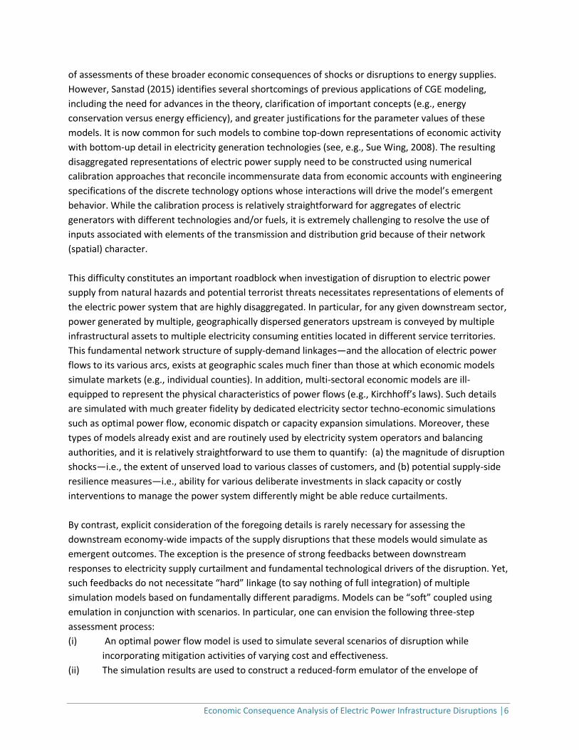
𝜎𝐸 = 0.01 𝜎𝐸 = 0.25
�̂�𝐸
�̂�𝐸
𝑥
�̂�
�̂�𝑁
�̂�

Economic Consequence Analysis of Electric Power Infrastructure Disruptions │19
Figure 1. IMPACTS OF A TWO-WEEK ELECTRICITY INFRASTRUCTURE DISRUPTION ON THE BAY AREA ECONOMY: INHERENT RESILIENCE (% change in the value of each variable from its baseline level)
economy to exploit any opportunity to replace relatively scarce and expensive power with other inputs
that are relatively abundant, and cheaper.
Figure 1 illustrates the net effects of these forces in our Bay Area disruption scenario. The response
surfaces make clear that while the impacts on variables’ percentage changes may be linear in the
initiating shock, they are nonlinear in the parameters. There are unambiguously negative impacts on
electricity supply (between -3.6% and -0.6%), intermediate and final electricity demands (-4% to -0.4%
and -8% to -0.5%), and welfare (-0.1% to -0.01%). Electricity power becomes unambiguously more
expensive (1.3% to greater than 10%), while the output of the rest of the economy contracts or expands
slightly depending on the combination of substitution elasticity values (between -0.06% and 0.002%).
With the exception of the electricity price, increases in the scope for producer and consumer
substitution shrink the absolute percentage magnitude of economic consequences. Under many
parameter combinations, this results in impacts that are smaller than the initiating shock. Not
surprisingly, this is overwhelmingly true for electric power producers’ ability to substitute factors for
infrastructure: the larger the value of 𝜎𝐸 the more the impacts shrink toward zero, and become linear in
the parameters. For the supply of, price of, and intermediate demand for, power, as well as rest-of-
economy output, the second strongest determinant of the response to a disruption is the rest of the
economy’s elasticity of substitution, whereas for final electricity demand and utility, this role is played
by the household elasticity of substitution. The results for �̂� indicate that the economy-wide benefit of
substitution is to moderate the welfare cost of the shock by at least an order of magnitude.
4.3 Mitigation
The counterfactual equilibrium of the model with backup investment is algebraically too complex to
yield clear analytical insights. Notwithstanding, it allows us to solve for changes in the quantity of
backup capacity that satisfy different criteria. We consider three cases. The first is the investment that
minimizes the loss of infrastructure capacity, which by (12) simply follows the fixed rule
�̂�𝐾0 = �̂�|�̂�𝑁𝑒𝑡=0
= −𝜉−1�̂�∗
The second is the investment that minimizes power supply disruption, which we find by setting �̂�𝐸 = 0
and solving for �̂� as a function of the parameters:6
�̂�𝐸0 = �̂�|�̂�𝐸=0
= −𝛼𝜂{𝜆𝜎𝐸 + (1 − 𝜆)(𝛾(1 − 𝛽)𝜎𝑈 + (1 − 𝛾(1 − 𝛽))𝜎𝑁)}𝒟1−1�̂�∗
6 In the polar case of no substitution, power producers do not adjust their gross factor input, and reduce their net factor
input by an amount that exactly offsets their allocation of resource to backup investment. The effect of mitigation is
therefore to simply replace �̂�∗ with �̂�∗ + 𝜉�̂� in eqs. (13)-(15), in the event of which the optimal backup is simply �̂� = �̂�𝐾0.

Economic Consequence Analysis of Electric Power Infrastructure Disruptions │20
Similarly, the third is investment that minimizes welfare loss, which we find by setting �̂� = 0 and solving
for �̂�:
�̂�𝑈0 = �̂�|�̂�=0
= 𝛼𝜂{𝜆𝜎𝐸 − 𝜆(𝛾(1 − 𝛽)𝜎𝑈 + (1 − 𝛾(1 − 𝛽))𝜎𝑁) + 𝛽𝜎𝑁 + (1 − 𝛽)𝜙𝜎𝑈}𝒟2−1�̂�∗
Here, the denominators 𝒟1 and 𝒟2 are complicated functions of the parameters.
𝜎𝐸 = 0.01 𝜎𝐸 = 0.25
�̂�𝐸0
�̂�𝑈0
Figure 2. ENERGY SUPPLY DISRUPTION MINIMIZING AND OPTIMAL BACKUP TECHNOLOGY PENETRATION (% change in backup capacity from its baseline level)
To understand the implications of these expressions we numerically parameterize them using values
from Table 1. Focusing on the role played by our technology parameters, we evaluate �̂�𝐸0 and �̂�𝑈0 at
representative values of the elasticities of substitution (𝜎𝑁 = 0.5, 𝜎𝑈 = 0.75) while varying the factor
elasticity of backup transformation and the baseline share of backup capacity. The results, shown in
Figure 2, highlight the nonlinear response of backup investment to these parameters. Under either
criterion, the optimal level of investment is for all practical purposes invariant over a wide range of
combinations of 𝜂 and 𝜉. The analytical solutions that underlie the figure indicate that in this region, the
elasticities of the response of backup capacity to the shock range from -6.6 to -7.2, which closely
parallel the value of the infrastructure disruption minimizing elasticity, above (1/𝜉 = 6.7). These
responses correspond to increases in backup capacity of around 27%.
As either the productivity of factors diverted to backup capacity additions or the baseline share of
backup capacity decline, the investment response becomes exponentially more sensitive, with values of
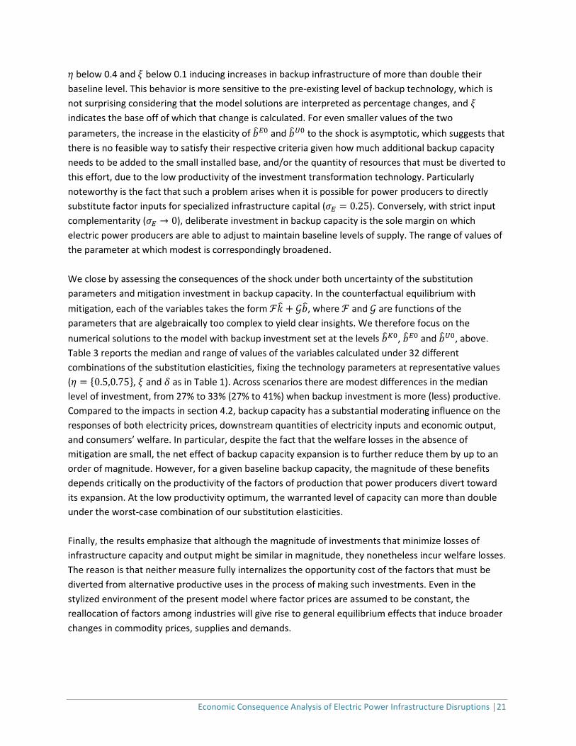
Economic Consequence Analysis of Electric Power Infrastructure Disruptions │21
𝜂 below 0.4 and 𝜉 below 0.1 inducing increases in backup infrastructure of more than double their
baseline level. This behavior is more sensitive to the pre-existing level of backup technology, which is
not surprising considering that the model solutions are interpreted as percentage changes, and 𝜉
indicates the base off of which that change is calculated. For even smaller values of the two
parameters, the increase in the elasticity of �̂�𝐸0 and �̂�𝑈0 to the shock is asymptotic, which suggests that
there is no feasible way to satisfy their respective criteria given how much additional backup capacity
needs to be added to the small installed base, and/or the quantity of resources that must be diverted to
this effort, due to the low productivity of the investment transformation technology. Particularly
noteworthy is the fact that such a problem arises when it is possible for power producers to directly
substitute factor inputs for specialized infrastructure capital (𝜎𝐸 = 0.25). Conversely, with strict input
complementarity (𝜎𝐸 → 0), deliberate investment in backup capacity is the sole margin on which
electric power producers are able to adjust to maintain baseline levels of supply. The range of values of
the parameter at which modest is correspondingly broadened.
We close by assessing the consequences of the shock under both uncertainty of the substitution
parameters and mitigation investment in backup capacity. In the counterfactual equilibrium with
mitigation, each of the variables takes the form ℱ�̂� + 𝒢�̂�, where ℱ and 𝒢 are functions of the
parameters that are algebraically too complex to yield clear insights. We therefore focus on the
numerical solutions to the model with backup investment set at the levels �̂�𝐾0, �̂�𝐸0 and �̂�𝑈0, above.
Table 3 reports the median and range of values of the variables calculated under 32 different
combinations of the substitution elasticities, fixing the technology parameters at representative values
(𝜂 = {0.5,0.75}, 𝜉 and 𝛿 as in Table 1). Across scenarios there are modest differences in the median
level of investment, from 27% to 33% (27% to 41%) when backup investment is more (less) productive.
Compared to the impacts in section 4.2, backup capacity has a substantial moderating influence on the
responses of both electricity prices, downstream quantities of electricity inputs and economic output,
and consumers’ welfare. In particular, despite the fact that the welfare losses in the absence of
mitigation are small, the net effect of backup capacity expansion is to further reduce them by up to an
order of magnitude. However, for a given baseline backup capacity, the magnitude of these benefits
depends critically on the productivity of the factors of production that power producers divert toward
its expansion. At the low productivity optimum, the warranted level of capacity can more than double
under the worst-case combination of our substitution elasticities.
Finally, the results emphasize that although the magnitude of investments that minimize losses of
infrastructure capacity and output might be similar in magnitude, they nonetheless incur welfare losses.
The reason is that neither measure fully internalizes the opportunity cost of the factors that must be
diverted from alternative productive uses in the process of making such investments. Even in the
stylized environment of the present model where factor prices are assumed to be constant, the
reallocation of factors among industries will give rise to general equilibrium effects that induce broader
changes in commodity prices, supplies and demands.

Economic Consequence Analysis of Electric Power Infrastructure Disruptions │22
Table 3. EFFECTS OF BACKUP CAPACITY INVESTMENT ON THE CONSEQUENCES OF INFRASTRUCTURE DISRUPTION (median % change in the
quantity of each variable from its baseline level, minimum and maximum values in square braces)
�̂� �̂�𝐸 �̂�𝐸 �̂� �̂�𝑁 �̂� �̂�
Inherent resilience via substitution only
— -2.1 2.7 -1.7 -0.0025 -1.4 -0.023
— [-3.7,-0.42] [1.3,12] [-4.2,-0.39] [-0.0065,0.0027] [-8.3,-0.34] [-0.12,-0.0081]
Backup investment that minimizes infrastructure disruption (�̂� = �̂�𝐾0)
𝜂 = 0.5
27 -0.083 0.24 -0.083 -0.0044 -0.096 -0.0059
— [-0.37,-0.035] [0.039,0.48] [-0.39,-0.026] [-0.0048,-0.0041] [-0.45,-0.015] [-0.011,-0.0046]
𝜂 = 0.75
27 -0.034 0.098 -0.034 -0.0029 -0.039 -0.0035
— [-0.15,-0.015] [0.015,0.19] [-0.16,-0.011] [-0.0031,-0.0028] [-0.19,-0.007] [-0.0055,-0.003]
Backup investment that minimizes electricity supply disruption (�̂� = �̂�𝐸0)
𝜂 = 0.5
32 — -0.0079 0 -0.0049 0 -0.0048
[27,38] — [-0.022,-0.0044] [-0.002,0.0009] [-0.0054,-0.0044] [-0.0038,0.0083] [-0.0054,-0.0043]
𝜂 = 0.75
29 — -0.0048 0 -0.003 0 -0.0029
[27,30] — [-0.012,-0.0029] [-0.0011,0.0005] [-0.0031,-0.0029] [-0.0022,0.0047] [-0.003-0.0028]
Backup investment that minimizes welfare loss (�̂� = �̂�𝑈0)
𝜂 = 0.5
41 0.37 -0.63 0.37 -0.0055 0.38 —
[28,110] [0.12,2.2] [-3.3,-0.31] [.076,2.6] [-0.012,-0.0039] [0.27,0.81] —
𝜂 = 0.75
33 0.21 -0.34 0.21 -0.0031 0.21 —
[27,48] [0.081,0.68] [-1,-0.2] [0.05,0.79] [-0.0036,-0.0024] [0.16,0.25] —

Economic Consequence Analysis of Electric Power Infrastructure Disruptions │23
5. Discussion and Conclusions
We have developed a simple analytical general equilibrium model of the economy-wide impacts of
electricity infrastructure disruptions. The model’s counterfactual equilibria throw into sharp relief two
key factors. The first is the role of substitution as an inherent resilience mechanism, which gives rise to
changes in commodity prices and quantities, and concomitant reductions in welfare, that are much
smaller in magnitude than the initiating shock. The second is the ability for deliberate investments in
mitigation to further dampen the consequent price and quantity changes, and ultimate welfare losses.
Additional insights were developed via a numerical case study investigating the consequences of a two-
week electricity infrastructure outage in California’s Bay Area. Inherent resilience and mitigation drive a
wedge between the initiating shock and the actual reduction in electricity supply. With substitution
alone, power output declines between -3.7% and -0.42%, the electricity price increases by 3% to 12%,
and intermediate and residential electricity use fall by -4.2% to -0.39% and . Mitigating these impacts by
expanding backup infrastructure capacity can reduce these effects by as much as two orders of
magnitude, and even nullify the loss in welfare.
In percentage terms the ultimate welfare impacts are small, ranging from -0.19% assuming no
substitution whatsoever to -0.0081%
The measure of welfare impact used here is a more theoretically consistent indicator of the economy-
wide burden of disruptions than commonly-used partial equilibrium measures of cost. To put our
results in context, we treat the change in utility as percentage equivalent variation, which we then
multiply by the combined annual personal income of our affected counties ($537 Bn in 2016). With no
substitution, this suggests a worst-case nominal economy-wide net cost of $1 Bn, which is reduced to
$123-644 M by inherent resilience due to substitution, $19-30 M with additional infrastructure
capacity-preserving backup investment, and $15-16 M with supply-preserving investment. By contrast,
applying an average $2/hour long-duration residential outage cost (e.g., Sullivan et al, 2015: Table 5-7)
to the 2.2 million households in our affected Bay Area counties (CA DOF, 2017) yields a cost of our
disruption scenario of $1.5 Bn in the residential sector alone! Disparities such as these points to the
need for research to reconcile costs derived from general equilibrium frameworks of the kind
developed here with bottom-up, partial equilibrium estimates of willingness to pay.
Turning to the supply side, it is more difficult to quantify what our results mean in terms of the direct
cost to power producers entailed in expanding backup capacity by the percentage amounts in Table 3.
This points to what is perhaps the most important limitation of this study: its stylized, highly simplified
character that requires additional research to be rendered consistent with the physical reality of the
power system. The latter is particularly relevant for our mitigation results, which rely on the artifice of a
monolithic backup technology. Detailed engineering and/or power system simulation studies to
elaborate the constituents of this black box, the manner in which their interactions determine backup
performance, and their operational and investment demands for different inputs—particularly capital,
can yield much needed empirical constraints on the values of the key uncertain parameters 𝜉, 𝛿 and 𝜂.

Economic Consequence Analysis of Electric Power Infrastructure Disruptions │24
Lastly, we take pains to acknowledge caveats to our economic model itself. A key omission is that it
ignores the income effects associated with changes in factor prices driven by shifts in the marginal
productivities of both the power sector infrastructure fixed factor and the intersectorally mobile
generic factor. In a regional economic system such price changes tend to be dampened by factor
movements across the regions’ boundaries, and we have eschewed explicit representation of these
economic processes for the sake of keeping the analysis simple and tractable. Our choices in this regard
also raise concerns that the model is insufficiently detailed in terms of the number of electricity using
sectors it represents, and, particularly, its omission of intermediate inputs to production, to be useful
for policy analysis. Furthermore, the model’s static character precludes its application to elucidate the
role of general equilibrium interactions in the dynamics of recovery from power disruption events, and
how they might influence the relative cost, effectiveness and desirability of different backup technology
options. All of the foregoing limitations can be expeditiously addressed through a program of research
to develop dynamic multi-sectoral (and perhaps additionally, multi-regional) CGE simulations and
couple them with techno-economic power system models. But in advance of such efforts, the type of
model developed here is sufficiently simple and flexible that it can be easily adapted to a broad range of
situations at a variety of geographic scales to provide first-order insights on the economic
consequences of long-term power disruptions.

Economic Consequence Analysis of Electric Power Infrastructure Disruptions │25
6. References
Bruneau, M., Chang, S., Eguchi, R., Lee, G., O’Rourke, T., Reinhorn, A., Shinozuka, M., Tierney, K.,
Wallace, W., and D. Von Winterfeldt. “A Framework to Quantitatively Assess and Enhance Seismic
Resilience of Communities.” Earthquake Spectra 19 (2003): 733–52.
Çağnan, Z., Davidson, R., and S. Guikema. “Post-Earthquake Restoration Planning for Los Angeles
Electric Power.” Earthquake Spectra 22(3) (2006): 589-608.
Detweiler, S.T. and A. Wein (eds.) The HayWired Earthquake Scenario. Earthquake hazards: U.S.
Geological Survey Scientific Investigations Report No. 2017-5013
(https://doi.org/10.3133/sir20175013v1), 2017.
Eto, J. H., LaCommare, K. H., Larsen, P., Todd, A., and E. Fisher. An Examination of Temporal Trends
in Electricity Reliability Based on Reports from US Electric Utilities. LBNL-5268E, Ernest Orlando
Lawrence Berkeley National Laboratory, Berkeley, CA (US), 2012.
Fullerton, D. and G. Metcalf. “Tax Incidence.” Handbook of Public Economics Vol. 4 (2002): 1787-
1872.
Greenberg, M., Mantell N., Lahr, M., Felder F., and R. Zimmerman. “Short and Intermediate
Economic Impacts of a Terrorist-Initiated Loss of Electric Power: Case Study of New Jersey.” Energy
Policy 35 (2007): 722-733.
National Research Council. Enhancing the Resilience of the Nation's Electricity System. Washington,
DC: National Academies Press, 2017.
Rose, A. “Economic Resilience to Natural and Man-Made Disasters: Multidisciplinary Origins
and Contextual Dimensions.” Environmental Hazards 7 (2007): 383-398.
Rose, A. Economic Resilience to Disasters. Community and Regional Resilience Institute Report No.
8, Oak Ridge National Laboratory, Oak Ridge, TN, 2009.
Rose, A. Benefit-Cost Analysis of Economic Resilience Actions, in S. Cutter (ed.) Oxford Research
Encyclopedia of Natural Hazard Science, New York: Oxford, 2007.
Rose, A. “Incorporating Cyber Resilience into Computable General Equilibrium Models,” in Y.
Okuyama and A. Rose (eds.), Modeling Spatial and Economic Impacts of Disasters, Heidelberg:
Springer, 2018.
Rose, A. and S. Liao. “Modeling Regional Economic Resilience to Disasters: A Computable General
Equilibrium Analysis of Water Service Disruptions.” Journal of Regional Science 45(1) (2005): 75-
112.

Economic Consequence Analysis of Electric Power Infrastructure Disruptions │26
Rose, A., Oladosu G., and S. Liao. “Business Interruption Impacts of a Terrorist Attack on the
Electric Power System of Los Angeles: Customer Resilience to a Total Blackout.” Risk Analysis 27(3)
(2007a), 513-31.
Rose, A., Oladosu G., and D. Salvino. “Economic Impacts of Electricity Outages in Los Angeles: The
Importance of Resilience and General Equilibrium Effects.” In M. A. Crew and M. Spiegel (eds.),
Obtaining the Best from Regulation and Competition. Springer Science, 2005.
Sanstad, A. Regional Economic Modeling of Electricity Supply Disruptions: A Review and Directions
for Future Research, Report No. LBNL- 1004426, Lawrence Berkeley National Laboratory, 2016.
(CA DOF) State of California, Department of Finance, E-5 Population and Housing Estimates for
Cities, Counties and the State–January 1, 2011- 2017. Sacramento, California, May 2017.
Sue Wing, Ian. (2008). “The Synthesis of Bottom-Up and Top-Down Approaches to Climate Policy
Modeling: Electric Power Technology Detail in a Social Accounting Framework.” Energy Economics
30 (2008): 547-573.
Sue Wing, I., D. Wei, A. Rose and A. Wein. Economic Impacts of the HayWired Earthquake Scenario.
Report to the US Geological Survey, 2018.
Sullivan, M.J, J. Schellenberg and M. Blundell, Updated Value of Service Reliability Estimates for
Electric Utility Customers in the United States, Report No. LBNL-6941E, Lawrence Berkeley National
Laboratory, 2015.
(USEOP) United States Executive Office of the President. Presidential Policy Directive – Critical
Infrastructure Security and Resilience. White House press release, February 12, 2013.