economic dynamics : theory and computation - · pdf fileeconomic dynamics theory and...
TRANSCRIPT

Economic Dynamics

Economic Dynamics
Theory and Computation
John Stachurski
The MIT PressCambridge, MassachusettsLondon, England

c© 2009 Massachusetts Institute of Technology
All rights reserved. No part of this book may be reproduced in any form by any electronic ormechanical means (including photocopying, recording, or information storage and retrieval)without permission in writing from the publisher.
MIT Press books may be purchased at special quantity discounts for business or salespromotional use. For information, please email [email protected] or write toSpecial Sales Department, The MIT Press, 55 Hayward Street, Cambridge, MA 02142.
This book was typeset in LATEX by the author and was printed and bound in the United Statesof America.
Library of Congress Cataloging-in-Publication Data
Stachurski, John, 1969–Economic dynamics : theory and computation / John Stachurski.
p. cm.Includes bibliographical references and index.ISBN 978-0-262-01277-5 (hbk. : alk. paper) 1. Statics and dynamics (Social sciences)—Mathematical models. 2.Economics—Mathematical models. I. Title.HB145.S73 2009330.1’519—dc22 2008035973
10 9 8 7 6 5 4 3 2 1

To Cleo


Contents
Preface xiii
Common Symbols xvii
1 Introduction 1
I Introduction to Dynamics 9
2 Introduction to Programming 112.1 Basic Techniques 11
2.1.1 Algorithms 112.1.2 Coding: First Steps 142.1.3 Modules and Scripts 192.1.4 Flow Control 21
2.2 Program Design 252.2.1 User-Defined Functions 252.2.2 More Data Types 272.2.3 Object-Oriented Programming 29
2.3 Commentary 33
3 Analysis in Metric Space 353.1 A First Look at Metric Space 35
3.1.1 Distances and Norms 363.1.2 Sequences 383.1.3 Open Sets, Closed Sets 41
3.2 Further Properties 443.2.1 Completeness 443.2.2 Compactness 46
vii

viii Contents
3.2.3 Optimization, Equivalence 483.2.4 Fixed Points 51
3.3 Commentary 54
4 Introduction to Dynamics 554.1 Deterministic Dynamical Systems 55
4.1.1 The Basic Model 554.1.2 Global Stability 594.1.3 Chaotic Dynamic Systems 624.1.4 Equivalent Dynamics and Linearization 66
4.2 Finite State Markov Chains 684.2.1 Definition 684.2.2 Marginal Distributions 724.2.3 Other Identities 764.2.4 Constructing Joint Distributions 80
4.3 Stability of Finite State MCs 834.3.1 Stationary Distributions 834.3.2 The Dobrushin Coefficient 884.3.3 Stability 904.3.4 The Law of Large Numbers 93
4.4 Commentary 96
5 Further Topics for Finite MCs 995.1 Optimization 99
5.1.1 Outline of the Problem 995.1.2 Value Iteration 1025.1.3 Policy Iteration 105
5.2 MCs and SRSs 1075.2.1 From MCs to SRSs 1075.2.2 Application: Equilibrium Selection 1105.2.3 The Coupling Method 112
5.3 Commentary 116
6 Infinite State Space 1176.1 First Steps 117
6.1.1 Basic Models and Simulation 1176.1.2 Distribution Dynamics 1226.1.3 Density Dynamics 1256.1.4 Stationary Densities: First Pass 129
6.2 Optimal Growth, Infinite State 133

Contents ix
6.2.1 Optimization 1336.2.2 Fitted Value Iteration 1356.2.3 Policy Iteration 142
6.3 Stochastic Speculative Price 1456.3.1 The Model 1456.3.2 Numerical Solution 1506.3.3 Equilibria and Optima 154
6.4 Commentary 156
II Advanced Techniques 157
7 Integration 1597.1 Measure Theory 159
7.1.1 Lebesgue Measure 1597.1.2 Measurable Spaces 1637.1.3 General Measures and Probabilities 1667.1.4 Existence of Measures 168
7.2 Definition of the Integral 1717.2.1 Integrating Simple Functions 1717.2.2 Measurable Functions 1737.2.3 Integrating Measurable Functions 177
7.3 Properties of the Integral 1787.3.1 Basic Properties 1797.3.2 Finishing Touches 1807.3.3 The Space L1 183
7.4 Commentary 186
8 Density Markov Chains 1878.1 Outline 187
8.1.1 Stochastic Density Kernels 1878.1.2 Connection with SRSs 1898.1.3 The Markov Operator 195
8.2 Stability 1978.2.1 The Big Picture 1978.2.2 Dobrushin Revisited 2018.2.3 Drift Conditions 2048.2.4 Applications 207
8.3 Commentary 210

x Contents
9 Measure-Theoretic Probability 2119.1 Random Variables 211
9.1.1 Basic Definitions 2119.1.2 Independence 2159.1.3 Back to Densities 216
9.2 General State Markov Chains 2189.2.1 Stochastic Kernels 2189.2.2 The Fundamental Recursion, Again 2239.2.3 Expectations 225
9.3 Commentary 227
10 Stochastic Dynamic Programming 22910.1 Theory 229
10.1.1 Statement of the Problem 22910.1.2 Optimality 23110.1.3 Proofs 235
10.2 Numerical Methods 23810.2.1 Value Iteration 23810.2.2 Policy Iteration 24110.2.3 Fitted Value Iteration 244
10.3 Commentary 246
11 Stochastic Dynamics 24711.1 Notions of Convergence 247
11.1.1 Convergence of Sample Paths 24711.1.2 Strong Convergence of Measures 25211.1.3 Weak Convergence of Measures 254
11.2 Stability: Analytical Methods 25711.2.1 Stationary Distributions 25711.2.2 Testing for Existence 26011.2.3 The Dobrushin Coefficient, Measure Case 26311.2.4 Application: Credit-Constrained Growth 266
11.3 Stability: Probabilistic Methods 27111.3.1 Coupling with Regeneration 27211.3.2 Coupling and the Dobrushin Coefficient 27611.3.3 Stability via Monotonicity 27911.3.4 More on Monotonicity 28311.3.5 Further Stability Theory 288
11.4 Commentary 293

Contents xi
12 More Stochastic Dynamic Programming 29512.1 Monotonicity and Concavity 295
12.1.1 Monotonicity 29512.1.2 Concavity and Differentiability 29912.1.3 Optimal Growth Dynamics 302
12.2 Unbounded Rewards 30612.2.1 Weighted Supremum Norms 30612.2.2 Results and Applications 30812.2.3 Proofs 311
12.3 Commentary 312
III Appendixes 315
A Real Analysis 317A.1 The Nuts and Bolts 317
A.1.1 Sets and Logic 317A.1.2 Functions 320A.1.3 Basic Probability 324
A.2 The Real Numbers 327A.2.1 Real Sequences 327A.2.2 Max, Min, Sup, and Inf 331A.2.3 Functions of a Real Variable 334
B Chapter Appendixes 339B.1 Appendix to Chapter 3 339B.2 Appendix to Chapter 4 342B.3 Appendix to Chapter 6 344B.4 Appendix to Chapter 8 345B.5 Appendix to Chapter 10 347B.6 Appendix to Chapter 11 349B.7 Appendix to Chapter 12 350
Bibliography 357
Index 367


Preface
The aim of this book is to teach topics in economic dynamics such as simulation, sta-bility theory, and dynamic programming. The focus is primarily on stochastic systemsin discrete time. Most of the models we meet will be nonlinear, and the emphasis ison getting to grips with nonlinear systems in their original form, rather than usingcrude approximation techniques such as linearization. As we travel down this path,we will delve into a variety of related fields, including fixed point theory, laws of largenumbers, function approximation, and coupling.
In writing the book I had two main goals. First, the material would present themodern theory of economic dynamics in a rigorous way. I wished to show that soundunderstanding of the mathematical concepts leads to effective algorithms for solvingreal world problems. The other goal was that the book should be easy and enjoy-able to read, with an emphasis on building intuition. Hence the material is drivenby examples—I believe the fastest way to grasp a new concept is through studyingexamples—and makes extensive use of programming to illustrate ideas. Runningsimulations and computing equilibria helps bring abstract concepts to life.
The primary intended audience is graduate students in economics. However, thetechniques discussed in the book add some shiny new toys to the standard tool kitused for economic modeling, and as such they should be of interest to researchersas well as graduate students. The book is as self-contained as possible, providingbackground in computing and analysis for the benefit of those without programmingexperience or university-level mathematics.
Part I of the book covers material that all well-rounded graduate students shouldknow. The style is relatively mathematical, and those who find the going hard mightstart by working through the exercises in appendix A. Part II is significantly morechallenging. In designing the text it was not my intention that all of those who readpart I should go on to read part II. Rather, part II is written for researchers and gradu-ate students with a particular aptitude for technical problems. Those who do read themajority of part II will gain a very strong understanding of infinite-horizon dynamicprogramming and (nonlinear) stochastic models.
xiii

xiv Preface
How does this book differ from related texts? There are several books on computa-tional macroeconomics and macrodynamics that have some similarity. In comparison,this book is not specific to macroeconomics. It should be of interest to (at least some)people working in microeconomics, operations research, and finance. Second, it ismore focused on analysis and techniques than on applications. Even when numericalmethods are discussed, I have tried to emphasize mathematical analysis of the algo-rithms, and acquiring a strong knowledge of the probabilistic and function-analyticframework that underlies proposed solutions.
The flip-side of the focus on analysis is that the models are more simplistic thanin applied texts. This is not so much a book from which to learn about economicsas it is a book to learn about techniques that are useful for economic modeling. Themodels we do study in detail, such as the optimal growth model and the commoditypricing model, are stripped back to reveal their basic structure and their links withone another.
The text contains a large amount of Python code, as well as an introduction toPython in chapter 2. Python is rapidly maturing into one of the major programminglanguages, and is a favorite of many high technology companies. The fact that Pythonis open source (i.e., free to download and distribute) and the availability of excellentnumerical libraries has led to a surge in popularity among the scientific community.All of the Python code in the text can be downloaded from the book’s homepage, athttp://johnstachurski.net/book.html.
MATLAB aficionados who have no wish to learn Python can still read the book.All of the code listings have MATLAB counterparts. They can be found alongside thePython code on the text homepage.
A word on notation. Like any text containing a significant amount of mathemat-ics, the notation piles up thick and fast. To aid readers I have worked hard to keepnotation minimal and consistent. Uppercase symbols such as A and B usually referto sets, while lowercase symbols such as x and y are elements of these sets. Functionsuse uppercase and lowercase symbols such as f , g, F, and G. Calligraphic letters suchas A andB represent sets of sets or, occasionally, sets of functions. Python keywordsare typeset in boldface. Proofs end with the symbol �.
I provide a table of common symbols on page xvii. Furthermore, the index beginswith an extensive list of symbols, along with the number of the page on which theyare defined.
In the process of writing this book I received invaluable comments and suggestionsfrom my colleagues. In particular, I wish to thank Robert Becker, Toni Braun, RogerFarmer, Onésimo Hernández-Lerma, Timothy Kam, Takashi Kamihigashi, NoritakaKudoh, Vance Martin, Sean Meyn, Len Mirman, Tomoyuki Nakajima, Kevin Reffett,Ricard Torres, and Yiannis Vailakis.
Many graduate students also contributed to the end product, including Real Arai,

Preface xv
Rosanna Chan, Katsuhiko Hori, Murali Neettukattil, Jenö Pál, and Katsunori Yamada.I owe particular thanks to Dimitris Mavridis, who made a large number of thoughtfulsuggestions on both computational and theoretical content; and to Yu Awaya, who—in a remarkable feat of brain-power and human endurance—read part II of the bookin a matter of weeks, solving every exercise, and checking every proof.
I have benefited greatly from the generous help of my intellectual elders and bet-ters. Special thanks go to John Creedy, Cuong Le Van, Kazuo Nishimura, and RabeeTourky. Extra special thanks go to Kazuo, who has helped me at every step of mypersonal random walk.
The editorial team at MIT Press has been first rate. I deeply appreciate their en-thusiasm and their professionalism, as well as their gentle and thoughtful criticism:Nothing is more valuable to the author who believes he is always right—especiallywhen he isn’t.
I am grateful to the Department of Economics at Melbourne University, the Centerfor Operations Research and Econometrics at Université Catholique de Louvain, andthe Institute for Economic Research at Kyoto University for providing me with thetime, space, and facilities to complete this text.
I thank my parents for their love and support, and Andrij, Nic, and Roman for thesame. Thanks also go to my extended family of Aaron, Kirdan, Merric, Murdoch, andSimon, who helped me weed out all those unproductive brain cells according to theprinciples set down by Charles Darwin. Dad gets an extra thanks for his long-runninginterest in this project, and for providing the gentle push that is always necessary fora task of this size.
Finally, I thank my beautiful wife Cleo, for suffering with patience and good hu-mor the absent-minded husband, the midnight tapping at the computer, the highsand the lows, and then some more lows, until the job was finally done. This book isdedicated to you.

Common Symbols
IID∼ F independent and identically distributed according to FN(μ, σ2) the normal distribution with mean μ and variance σ2
∼ F distributed according to FP(A) the set of all subsets of A‖x‖p the norm (∑k
i=1 xpi )
1/p on k
dp(x, y) the distance ‖x− y‖p on k
bS the set of bounded functions mapping S into‖ f ‖∞ the norm supx∈S | f (x)| on bS
d∞( f , g) the distance ‖ f − g‖∞ on bSbcS the continuous functions in bSibS the increasing (i.e., nondecreasing) functions in bSibcS the continuous functions in ibS
B(ε; x) the ε-ball centered on xB the indicator function of set B
B(S) the Borel subsets of SP(S) the distributions on Sδx the probability measure concentrated on xsS the simple functions on measure space (S,S )mS the measurable real-valued functions on (S,S )bS the bounded functions in mS
L1(S,S , μ) the μ-integrable functions on (S,S )L1(S,S , μ) the metric space generated byL1(S,S , μ)‖ f ‖1 the norm μ(| f |) on L1(S,S , μ)
d1( f , g) the distance ‖ f − g‖1 on L1(S,S , μ)D(S) the densities on SbM (S) the finite signed measures on (S,B(S))b�S the bounded, Lipschitz functions on metric space SdFM the Fortet–Mourier distance onP(S)
xvii

Chapter 1
Introduction
The teaching philosophy of this book is that the best way to learn is by example.In that spirit, consider the following benchmark modeling problem from economicdynamics: At time t an economic agent receives income yt. This income is split intoconsumption ct and savings kt. Savings is used for production, with input kt yieldingoutput
yt+1 = f (kt,Wt+1), t = 0, 1, 2, . . . (1.1)
where (Wt)t≥1 is a sequence of independent and identically distributed shocks. Theprocess now repeats, as shown in figure 1.1. The agent gains utility U(ct) from con-sumption ct = yt − kt, and discounts future utility at rate ρ ∈ (0, 1). Savings behavioris modeled as the solution to the expression
max(kt)t≥0
[∞
∑t=0
ρtU(yt − kt)
]
subject to yt+1 = f (kt,Wt+1) for all t ≥ 0, with y0 given
This problem statement raises many questions. For example, from what set of possiblepaths is (kt)t≥0 to be chosen? And how do we choose a path at the start of time suchthat the resource constraint 0 ≤ kt ≤ yt holds at each t, given that output is random?Surely the agent cannot choose kt until he learns what yt is. Finally, how does one goabout computing the expectation implied by the symbol ?
A good first step is to rephrase the problem by saying that the agent seeks a savingspolicy. In the present context this is a map σ that takes a value y and returns a numberσ(y) satisfying 0 ≤ σ(y) ≤ y. The interpretation is that upon observing yt, the agent’sresponse is kt = σ(yt). Next period output is then yt+1 = f (σ(yt),Wt+1), next period
1

2 Chapter 1
t+ 1
kt kt+1
ct+1ct
t
yt f (kt,Wt+1) = yt+1
Wt+1
Figure 1.1 Timing
savings is σ(yt+1), and so on. We can evaluate total reward as[∞
∑t=0
ρtU(yt − σ(yt))
]where yt+1 = f (σ(yt),Wt+1), with y0 given (1.2)
The equation yt+1 = f (σ(yt),Wt+1) is called a stochastic recursive sequence (SRS),or stochastic difference equation. As we will see, it completely defines (yt)t≥0 as asequence of random variables for each policy σ. The expression on the left evaluatesthe utility of this income stream.
Regarding the expectation , we know that in general expectation is calculated byintegration. But how are we to understand this integral? It seems to be an expectationover the set of nonnegative sequences (i.e., possible values of the path (yt)t≥0). Highschool calculus tells us how to take an integral over an interval, or perhaps over asubset of n-dimensional space n. But how does one take an integral over an (infinite-dimensional) space of sequences?
Expectation and other related issues can be addressed in a very satisfactory way,but to do so, we will need to know at least the basics of a branch of mathematics calledmeasure theory. Almost all of modern probability theory is defined and analyzed interms of measure theory, so grasping its basics is a highly profitable investment. Onlywith the tools that measure theory provides can we pin down the meaning of (1.2).1
Once the meaning of the problem is clarified, the next step is considering how tosolve it. As we have seen, the solution to the problem is a policy function. This is
1The golden rule of research is to carefully define your question before you start searching for answers.

Introduction 3
rather different from undergraduate economics, where solutions are usually numbers,or perhaps vectors of numbers—often found by differentiating objective functions. Inhigher level applied mathematics, many problems have functions as their solutions.
The branch of mathematics that deals with problems having functions as solutionsis called “functional analysis.” Functional analysis is a powerful tool for solving real-world problems. Starting with basic functional analysis and a dash of measure theory,this book provides the tools necessary to optimize (1.2), including algorithms andnumerical methods.
Once the problem is solved and an optimal policy is obtained, the income path(yt)t≥0 is determined as a sequence of random variables. The next objective is tostudy the dynamics of the economy. What statements can we make about what will“happen” in an economy with this kind of policy? Might it settle down into some sortof equilibrium? This is the ideal case because we can then make firm predictions. Andpredictions are the ultimate goal of modeling, partly because they are useful in theirown right and partly because they allow us to test theory against data.
To illustrate analysis of dynamics, let’s specialize our model so as to dig a littlefurther. Suppose now that U(c) = ln c and f (k,W) = kαW. For this very special case,no computation is necessary: pencil and paper can be used to show (e.g., Stokey andLucas 1989, §2.2) that the optimal policy is given by σ(y) = θy, where θ := αρ. From(1.2) the law of motion for the “state” variable yt is then
yt+1 = (θyt)αWt+1, t = 0, 1, 2, . . . (1.3)
To make life simple, let’s assume that lnWt ∼ N(0, 1). Here N(μ, v) represents thenormal distribution with mean μ and variance v, and the notation X ∼ F means thatX has distribution F.
If we take the log of (1.3), it is transformed into the linear system
xt+1 = b+ αxt + wt+1, where xt := ln yt, wt+1 ∼ N(0, 1), and b := α ln θ (1.4)
This system is easy to analyze. In fact every xt is normally distributed because x1 isnormally distributed (x0 is constant and constant plus normal equals normal), andmoreover xt+1 is normally distributed whenever xt is normally distributed.2
One of the many nice things about normal distributions is that they are determinedby only two parameters, the mean and the variance. If we can find these parameters,then we know the distribution. So suppose that xt ∼ N(μt, vt), where the constantsμt and vt are given. If you are familiar with manipulating means and variances, youwill be able to deduce from (1.4) that xt+1 ∼ N(μt+1, vt+1), where
μt+1 = b+ αμt and vt+1 = α2vt + 1 (1.5)
2Recall that linear combinations of normal random variables are themselves normal.

4 Chapter 1
xt ∼ N(−2, 0.8)
−3 −2 −1 0 10
0.1
0.2
0.3
0.4
0.5
Figure 1.2 Sequence of marginal distributions
Paired with initial conditions μ0 and v0, these laws of motion pin down the sequences(μt)t≥0 and (vt)t≥0, and hence the distribution N(μt, vt) of xt at each point in time. Asequence of distributions starting from xt ∼ N(−2, 0.8) is shown in figure 1.2. Theparameters are α = 0.4 and ρ = 0.75.
In the figure it appears that the distributions are converging to some kind of lim-iting distribution. This is due to the fact that α < 1 (i.e., returns to capital are dimin-ishing), which implies that the sequences in (1.5) are convergent (don’t be concernedif you aren’t sure how to prove this yet). The limits are
μ∗ := limt→∞ μt =
b1− α
and v∗ := limt→∞ vt =
11− α2 (1.6)
Hence the distribution N(μt, vt) of xt converges to N(μ∗, v∗).3 Note that this “equilib-rium” is a distribution rather than a single point.
All this analysis depends, of course, on the law of motion (1.4) being linear, andthe shocks being normally distributed. How important are these two assumptionsin facilitating the simple techniques we employed? The answer is that they are bothcritical, and without either one we must start again from scratch.
3What do we really mean by “convergence” here? We are talking about convergence of a sequence offunctions to a given function. But how to define this? There are many possible ways, leading to different no-tions of equilibria, and we will need to develop some understanding of the definitions and the differences.

Introduction 5
Figure 1.3 Stationary distribution
To illustrate this point, let’s briefly consider the threshold autoregression model
Xt+1 =
{A1Xt + b1 +Wt+1 if Xt ∈ B ⊂ n
A2Xt + b2 +Wt+1 otherwise(1.7)
Here Xt is n× 1, Ai is n× n, bi is n× 1, and (Wt)t≥1 is an IID sequence of normallydistributed random n× 1 vectors. Although for this system the departure from linear-ity is relatively small (in the sense that the law of motion is at least piecewise linear),analysis of dynamics is far more complex. Through the text we will build a set of toolsthat permit us to analyze nonlinear systems such as (1.7), including conditions usedto test whether the distributions of (Xt)t≥0 converge to some stationary (i.e., limiting)distribution. We also discuss how one should go about computing the stationary dis-tributions of nonlinear stochastic models. Figure 1.3 shows the stationary distributionof (1.7) for a given set of parameters, based on such a computation.
Now let’s return to the linear model (1.4) and investigate its sample paths. Fig-ure 1.4 shows a simulated time series over 250 periods. The initial condition is x0 = 4,and the parameters are as before. The horizontal line is the mean μ∗ of the station-ary distribution. The sequence is obviously correlated, and not surprisingly, showsno tendency to settle down to a constant value. On the other hand, the sample meanxt := 1
t ∑ti=1 xi seems to converge to μ∗ (see figure 1.5).
That this convergence should occur is not obvious. Certainly it does not followfrom the classical law of large numbers, since (xt)t≥0 is neither independent nor iden-tically distributed. Nevertheless, the question of whether sample moments convergeto the corresponding moments of the stationary distribution is an important one, withimplications for both theory and econometrics.

6 Chapter 1
Figure 1.4 Time series
Figure 1.5 Sample mean of time series
Introduction 7
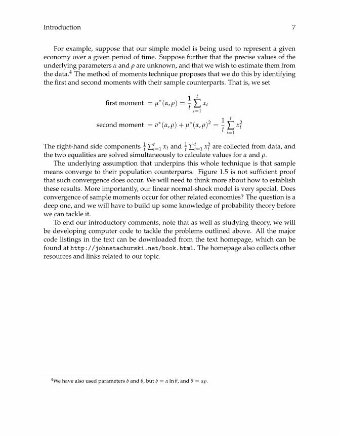
For example, suppose that our simple model is being used to represent a giveneconomy over a given period of time. Suppose further that the precise values of theunderlying parameters α and ρ are unknown, and that we wish to estimate them fromthe data.4 The method of moments technique proposes that we do this by identifyingthe first and second moments with their sample counterparts. That is, we set
first moment = μ∗(α, ρ) =1t
t
∑i=1
xt
second moment = v∗(α, ρ) + μ∗(α, ρ)2 =1t
t
∑i=1
x2t
The right-hand side components 1t ∑
ti=1 xt and 1
t ∑ti=1 x
2t are collected from data, and
the two equalities are solved simultaneously to calculate values for α and ρ.The underlying assumption that underpins this whole technique is that sample
means converge to their population counterparts. Figure 1.5 is not sufficient proofthat such convergence does occur. We will need to think more about how to establishthese results. More importantly, our linear normal-shock model is very special. Doesconvergence of sample moments occur for other related economies? The question is adeep one, and we will have to build up some knowledge of probability theory beforewe can tackle it.
To end our introductory comments, note that as well as studying theory, we willbe developing computer code to tackle the problems outlined above. All the majorcode listings in the text can be downloaded from the text homepage, which can befound at http://johnstachurski.net/book.html. The homepage also collects otherresources and links related to our topic.
4We have also used parameters b and θ, but b = α ln θ, and θ = αρ.


Part I
Introduction to Dynamics
9


Chapter 2
Introduction to Programming
Some readers may disagree, but to me computers and mathematics are like beer andpotato chips: two fine tastes that are best enjoyed together. Mathematics provides thefoundations of our models and of the algorithms we use to solve them. Computersare the engines that run these algorithms. They are also invaluable for simulation andvisualization. Simulation and visualization build intuition, and intuition completesthe loop by feeding into better mathematics.
This chapter provides a brief introduction to scientific computing, with special em-phasis on the programming language Python. Python is one of several outstandinglanguages that have come of age in recent years. It features excellent design, ele-gant syntax, and powerful numerical libraries. It is also free and open source, with afriendly and active community of developers and users.
2.1 Basic Techniques
This section provides a short introduction to the fundamentals of programming: al-gorithms, control flow, conditionals, and loops.
2.1.1 Algorithms
Many of the problems we study in this text reduce to a search for algorithms. Thelanguage we will use to describe algorithms is called pseudocode. Pseudocode is an in-formal way of presenting algorithms for the benefit of human readers, without gettingtied down in the syntax of any particular programming language. It’s a good habit tobegin every program by sketching it first in pseudocode.
11

12 Chapter 2
Our pseudocode rests on the following four constructs:
if–then–else, while, repeat–until, and for
The general syntax for the if–then–else construct is
if condition thenfirst sequence of actions
elsesecond sequence of actions
end
The condition is evaluated as either true or false. If found true, the first sequenceof actions is executed. If false, the second is executed. Note that the else statementand alternative actions can be omitted: If the condition fails, then no actions are per-formed. A simple example of the if–then–else construct is
if there are cookies in the jar theneat them
elsego to the shops and buy moreeat them
end
The while construct is used to create a loop with a test condition at the beginning:
while condition dosequence of actions
end
The sequence of actions is performed only if the condition is true. Once they arecompleted, the condition is evaluated again. If it is still true, the actions in the loopare performed again. When the condition becomes false the loop terminates. Here’san example:
while there are cookies in the jar doeat one
end
The algorithm terminates when there are no cookies left. If the jar is empty to beginwith, the action is never attempted.
The repeat–until construct is similar:

Introduction to Programming 13
repeatsequence of actions
until condition
Here the sequence of actions is always performed once. Next the condition ischecked. If it is true, the algorithm terminates. If not, the sequence is performedagain, the condition is checked, and so on.
The for construct is sometimes called a definite loop because the number of repe-titions is predetermined:
for element in sequence dodo something
end
For example, the following algorithm computes the maximum of a function f overa finite set S using a for loop and prints it to the screen.1
set c = −∞for x in S do
set c = max{c, f (x)}endprint c
In the for loop, x is set equal to the first element of S and the statement “setc = max{c, f (x)}” is executed. Next x is set equal to the second element of S, thestatement is executed again, and so on. The statement “set c = max{c, f (x)}” shouldbe understood to mean that max{c, f (x)} is first evaluated, and the resulting value isassigned to the variable c.
Exercise 2.1.1 Modify this algorithm so that it prints the maximizer rather than themaximum. Explain why it is more useful to know the maximizer.
Let’s consider another example. Suppose that we have two arrays A and B storedin memory, and we wish to know whether the elements of A are a subset of the ele-ments of B. Here’s a prototype algorithm that will tell us whether this is the case:
set subset = Truefor a in A do
if a /∈ B then set subset = Falseendprint subset
1That is, it displays the value to the user. The term “print” dates from the days when sending output tothe programmer required generating hardcopy on a printing device.

14 Chapter 2
Exercise 2.1.2 The statement “a /∈ B” may require coding at a lower level.2 Rewritethe algorithm with an inner loop that steps through each b in B, testing whether a = b,and setting subset = False if no matches occur.
Finally, suppose we wish to model flipping a biased coin with probability p ofheads, and have access to a random number generator that yields uniformly dis-tributed variates on [0, 1]. The next algorithm uses these random variables to generateand print the outcome (either “heads” or “tails”) of ten flips of the coin, as well as thetotal number of heads.3
set H = 0for i in 1 to 10 do
draw U from the uniform distribution on [0, 1]if U < p then // With probability p
print “heads”H = H + 1
else // With probability 1− pprint “tails”
endendprint H
Note the use of indentation, which helps maintaining readability of our code.
Exercise 2.1.3 Consider a game that pays $1 if three consecutive heads occur in tenflips and zero otherwise. Modify the previous algorithm to generate a round of thegame and print the payoff.
Exercise 2.1.4 Let b be a vector of zeros and ones. The vector corresponds to theemployment history of one individual, where 1 means employed at the associatedpoint in time, and 0 means unemployed. Write an algorithm to compute the longest(consecutive) period of employment.
2.1.2 Coding: First Steps
When it comes to programming, which languages are suitable for scientific work?Since the time it takes to complete a programming project is the sum of the time spentwriting the code and the time that a machine spends running it, an ideal languagewould minimize both these terms. Unfortunately, designing such a language is not
2Actually, in many high-level languages you will have an operator that tests whether a variable is amember of a list. For the sake of the exercise, suppose this is not the case.
3What is the probability distribution of this total?

Introduction to Programming 15
easy. There is an inherent trade-off between human time and computer time, due tothe fact that humans and computers “think” differently: Languages that cater more tothe human brain are usually less optimal for the computer and vice versa.
Using this trade-off, we can divide languages into (1) robust, lower level languagessuch as Fortran, C/C++, and Java, which execute quickly but can be a chore when itcomes to coding up your program, and (2) the more nimble, higher level “scripting”languages, such as Python, Perl, Ruby, Octave, R, and MATLAB. By design, theselanguages are easy to write with and debug, but their execution can be orders of mag-nitude slower.
To give an example of these different paradigms, consider writing a program thatprints out “Hello world.” In C, which is representative of the first class of languages,such a program might look like this:
#i n c l u d e <stdio.h>
i n t main( i n t argc , cha r *argv []) {printf("Hello world\n");r e t u r n 0;
}
Let’s save this text file as hello.c, and compile it at the shell prompt4 using the gcc(GNU project C) compiler:
gcc -o hello hello.c
This creates an executable file called hello that can be run at the prompt by typing itsname.
For comparison, let’s look at a “Hello world” program in Python—which is repre-sentative of the second class of languages. This is simply
print("Hello world")
and can be run from my shell prompt as follows:
python hello.py
What differences do we observe with these two programs? One obvious difference isthat the C code contains more boilerplate. In general, C will be more verbose, requir-ing us to provide instructions to the computer that don’t seem directly relevant to ourtask. Even for experienced programmers, writing boilerplate code can be tedious anderror prone. The Python program is much shorter, more direct, and more intuitive.
Second, executing the C program involves a two-step procedure: First compile,then run. The compiler turns our program into machine code specific to our operat-ing system. By viewing the program as a whole prior to execution, the compiler can
4Don’t worry if you aren’t familiar with the notion of a shell or other the details of the program. We arepainting with broad strokes at the moment.

16 Chapter 2
optimize this machine code for speed. In contrast, the Python interpreter sends indi-vidual instructions to the CPU for processing as they are encountered. While slower,the second approach is more interactive, which is helpful for testing and debugging.We can run parts of the program separately, and then interact with the results via theinterpreter in order to evaluate their performance.
In summary, the first class of languages (C, Fortran, etc.) put more burden on theprogrammer to specify exactly what they want to happen, working with the oper-ating system on a more fundamental level. The second class of languages (Python,MATLAB, etc.) shield the programmer from such details and are more interactive, atthe cost of slower execution. As computers have become cheaper and more powerful,these “scripting” languages have naturally become more popular. Why not ask thecomputer to do most of the heavy lifting?
In this text we will work exclusively with an interpreted language, leaving the firstclass of languages for those who wish to dig deeper. However, we note in passing thatone can often obtain the best of both worlds in the speed versus ease-of-use trade-off.This is achieved by mixed language programming. The idea here is that in a typicalprogram there are only a few lines of code that are executed many times, and it isthese bottlenecks that should be optimized for speed. Thus the modern method ofnumerical programming is to write the entire program in an interpreted languagesuch as Python, profile the code to find bottlenecks, and outsource those (and onlythose) parts to fast, compiled languages such as C or Fortran.5
The interpreted language we work with in the text is Python. However, MATLABcode is provided on the text homepage for those who prefer it. MATLAB has a gentlerlearning curve, and its numerical libraries are better documented. Readers who arecomfortable with MATLAB and have no interest in Python can skip the rest of this chapter.
Python is a modern and highly regarded object-oriented programming languageused in academia and the private sector for a wide variety of tasks. In addition tobeing powerful enough to write large-scale applications, Python is known for its min-imalist style and clean syntax—designed from the start with the human reader inmind. Among the common general-purpose interpreted languages (Perl, Visual Ba-sic, etc.), Python is perhaps the most suitable for scientific and numerical applications,with a large collection of MATLAB-style libraries organized primarily by the SciPyproject (scipy.org).6 The power of Python combined with these scientific librariesmakes it an excellent choice for numerical programming.
Python is open source, which means that it can be downloaded free of charge,7
and that we can peruse the source code of the various libraries to see how they work
5Another promising option is Cython, which is similar to Python but generates highly optimized C code.6See also Sage, which is a mathematical tool kit built on top of Python.7The main Python repositories are at python.org. Recently several distributions of Python that come
bundled with various scientific tools have appeared. The book home page contains suggestions and links.
Introduction to Programming 17
(and to make changes if necessary).Rather than working directly with the Python interpreter, perhaps the best way to
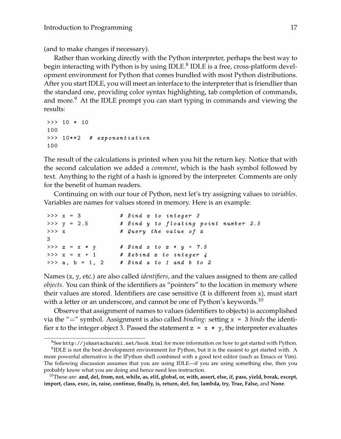
begin interacting with Python is by using IDLE.8 IDLE is a free, cross-platform devel-opment environment for Python that comes bundled with most Python distributions.After you start IDLE, you will meet an interface to the interpreter that is friendlier thanthe standard one, providing color syntax highlighting, tab completion of commands,and more.9 At the IDLE prompt you can start typing in commands and viewing theresults:
>>> 10 * 10100>>> 10**2 # exponentiation100
The result of the calculations is printed when you hit the return key. Notice that withthe second calculation we added a comment, which is the hash symbol followed bytext. Anything to the right of a hash is ignored by the interpreter. Comments are onlyfor the benefit of human readers.
Continuing on with our tour of Python, next let’s try assigning values to variables.Variables are names for values stored in memory. Here is an example:
>>> x = 3 # Bind x to integer 3>>> y = 2.5 # Bind y to floating point number 2.5>>> x # Query the value of x3>>> z = x * y # Bind z to x * y = 7.5>>> x = x + 1 # Rebind x to integer 4>>> a, b = 1, 2 # Bind a to 1 and b to 2
Names (x, y, etc.) are also called identifiers, and the values assigned to them are calledobjects. You can think of the identifiers as “pointers” to the location in memory wheretheir values are stored. Identifiers are case sensitive (X is different from x), must startwith a letter or an underscore, and cannot be one of Python’s keywords.10
Observe that assignment of names to values (identifiers to objects) is accomplishedvia the “=” symbol. Assignment is also called binding: setting x = 3 binds the identi-fier x to the integer object 3. Passed the statement z = x * y, the interpreter evaluates
8See http://johnstachurski.net/book.html for more information on how to get started with Python.9IDLE is not the best development environment for Python, but it is the easiest to get started with. A
more powerful alternative is the IPython shell combined with a good text editor (such as Emacs or Vim).The following discussion assumes that you are using IDLE—if you are using something else, then youprobably know what you are doing and hence need less instruction.
10These are: and, del, from, not, while, as, elif, global, or, with, assert, else, if, pass, yield, break, except,import, class, exec, in, raise, continue, finally, is, return, def, for, lambda, try, True, False, and None.
18 Chapter 2
the expression x * y on the right-hand side of the = sign to obtain 7.5, stores this re-sult in memory, and binds the identifier specified on the left (i.e., z) to that value.Passed x = x + 1, the statement executes in a similar way (right to left), creating anew integer object 4 and rebinding x to that value.
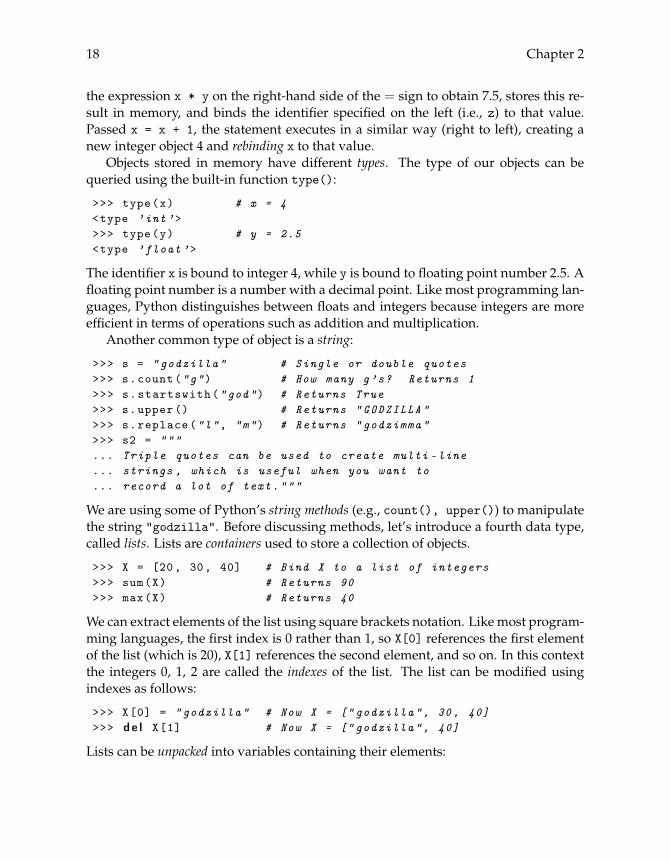
Objects stored in memory have different types. The type of our objects can bequeried using the built-in function type():
>>> type(x) # x = 4<type ’int’>>>> type(y) # y = 2.5<type ’float ’>
The identifier x is bound to integer 4, while y is bound to floating point number 2.5. Afloating point number is a number with a decimal point. Like most programming lan-guages, Python distinguishes between floats and integers because integers are moreefficient in terms of operations such as addition and multiplication.
Another common type of object is a string:
>>> s = "godzilla" # Single or double quotes>>> s.count("g") # How many g’s? Returns 1>>> s.startswith("god") # Returns True>>> s.upper() # Returns "GODZILLA">>> s.replace("l", "m") # Returns "godzimma">>> s2 = """... Triple quotes can be used to create multi -line... strings , which is useful when you want to... record a lot of text."""
We are using some of Python’s string methods (e.g., count(), upper()) to manipulatethe string "godzilla". Before discussing methods, let’s introduce a fourth data type,called lists. Lists are containers used to store a collection of objects.
>>> X = [20, 30, 40] # Bind X to a list of integers>>> sum(X) # Returns 90>>> max(X) # Returns 40
We can extract elements of the list using square brackets notation. Like most program-ming languages, the first index is 0 rather than 1, so X[0] references the first elementof the list (which is 20), X[1] references the second element, and so on. In this contextthe integers 0, 1, 2 are called the indexes of the list. The list can be modified usingindexes as follows:
>>> X[0] = "godzilla" # Now X = [" godzilla", 30, 40]>>> d e l X[1] # Now X = [" godzilla", 40]
Lists can be unpacked into variables containing their elements:

Introduction to Programming 19
>>> x, y = ["a", "b"] # Now x = "a" and y = "b"
We saw that Python has methods for operations on strings, as in s.count("g") above.Here s is the variable name (the identifier), bound to string "godzilla", and count()is the name of a string method, which can be called on any string. Lists also havemethods. Method calls on strings, lists and other objects follow the general syntax
identifier.methodName(arguments) # e.g., s.count ("g")
For example, X.append(3) appends 3 to the end of X, while X.count(3) counts thenumber of times that 3 occurs in X. In IDLE you can enter X. at the prompt and thenpress the TAB key to get a list of methods that can be applied to lists (more generally,to objects of type type(X)).
2.1.3 Modules and Scripts
There are several ways to interact with the Python interpreter. One is to type com-mands directly into the prompt as above. A more common way is to write the com-mands in a text file and then run that file through the interpreter. There are manyways to do this, and in time you will find one that best suits your needs. The easiest isto use the editor found in IDLE: Open up a new window under the ’File’ menu. Typein a command such as print("Hello world") and save the file in the current direc-tory as hello.py. You can now run the file by pressing F5 or selecting ’Run Module’.The output Hello world should appear at the command prompt.
A text file such as hello.py that is run through an interpreter is known as a script.In Python such files are also known as modules, a module being any file with Pythonfunctions and other definitions. Modules can be run through the interpreter usingthe keyword import. Thus, as well as executing hello.py using IDLE’s ’Run Module’command as above, we can type the following at the Python prompt:
>>> impor t hello # Load the file hello.py and run’Hello world’
When you first import the module hello, Python creates a file called hello.pyc, whichis a byte-compiled file containing the instructions in hello.py. Note that if you nowchange hello.py, resave, and import again, the changes will not be noticed becausehello.pyc is not altered. To affect the changes in hello.py, use reload(hello), whichrewrites hello.pyc.
There are vast libraries of Python modules available,11 some of which are bundledwith every Python distribution. A useful example is math:
>>> impor t math # Module math
11See, for example, http://pypi.python.org/pypi.

20 Chapter 2
>>> math.pi # Returns 3.1415926535897931>>> math.sqrt (4) # Returns 2.0
Here pi is a float object supplied by math and sqrt() is a function object. Collectivelythese objects are called attributes of the module math.
Another handy module in the standard library is random.
>>> impor t random>>> X = ["a", "b", "c"]>>> random.choice(X) # Returned "b">>> random.shuffle(X) # X is now shuffled>>> random.gammavariate (2, 2) # Returned 3.433472
Notice how module attributes are accessed using moduleName.identifier notation.Each module has it’s own namespace, which is a mapping from identifiers to objects inmemory. For example, pi is defined in the namespace of math, and bound to the float3.14 · · · 1. Identifiers in different namespaces are independent, so modules mod1 andmod2 can both have distinct attribute a. No confusion arises because one is accessedas mod1.a and the other is accessed as mod2.a.12
When x = 1 is entered at the command line (i.e., Python prompt), the identifierx is registered in the interactive namespace.13 If we import a module such as math,only the module name is registered in the interactive namespace. The attributes ofmath need to be accessed as described above (i.e, math.pi references the float objectpi registered in the math namespace).14 Should we wish to, we can however importattributes directly into the interactive namespace as follows:
>>> from math impor t sqrt , pi>>> pi * sqrt (4) # Returns 6.28...
Note that when a module mod is run from within IDLE using ’Run Module’, com-mands are executed within the interactive namespace. As a result, attributes of modcan be accessed directly, without the prefix mod. The same effect can be obtained at theprompt by entering
>>> from mod impor t * # Import everything
In general, it is better to be selective, importing only necessary attributes into theinteractive namespace. The reason is that our namespace may become flooded withvariable names, possibly “shadowing” names that are already in use.
12Think of the idea of a namespace as like a street address, with street name being the namespace andstreet number being the attribute. There is no confusion if two houses have street number 10, as long as wesupply the street names of the two houses.
13Internally, the interactive namespace belongs to a top-level module called __main__.14To view the contents of the interactive namespace type vars() at the prompt. You will see some stuff we
have not discussed yet (__doc__, etc.), plus any variables you have defined or modules you have imported.If you import math and then type vars(math), you will see the attributes of this module.

Introduction to Programming 21
Modules such as math, sys, and os come bundled with any Python distribution.Others will need to be installed. Installation is usually straightforward, and docu-mented for each module. Once installed, these modules can be imported just likestandard library modules. For us the most important third-party module15 is the sci-entific computation package SciPy, which in turn depends on the fast array processingmodule NumPy. The latter is indispensable for serious number crunching, and SciPyprovides many functions that take advantage of the facilities for array processing inNumPy, based on efficient C and Fortran libraries.16
Documentation for SciPy and NumPy can be found at the SciPy web site and thetext home page. These examples should give the basic idea:
>>> from scipy impor t *>>> integral , error = integrate.quad(sin , -1, 1)>>> minimizer = optimize.fminbound(cos , 0, 2 * pi)>>> A = array ([[1, 2], [3, 4]])>>> determinant = linalg.det(A)>>> eigenvalues = linalg.eigvals(A)
SciPy functions such as sin() and cos() are called vectorized (or universal) func-tions, which means that they accept either numbers or sequences (lists, NumPy arrays,etc.) as arguments. When acting on a sequence, the function returns an array obtainedby applying the function elementwise on the sequence. For example:
>>> cos([0, pi , 2 * pi]) # Returns array ([ 1., -1., 1.])
There are also modules for plotting and visualization under active development.At the time of writing, Matplotlib and PyX are popular and interact well with SciPy.A bit of searching will reveal many alternatives.
2.1.4 Flow Control
Conditionals and loops can be used to control which commands are executed and theorder in which they are processed. Let’s start with the if/else construct, the generalsyntax for which is
i f <expression >: # If <expression > is true , then<statements > # this block of code is executed
e l s e :<statements > # Otherwise , this one
The else block is optional. An expression is any code phrase that yields a value whenexecuted, and conditionals like if may be followed by any valid expression. Expres-sions are regarded as false if they evaluate to the boolean value False (e.g., 2 < 1),
15Actually a package (i.e., collection of modules) rather than a module.16For symbolic (as opposed to numerical) algebra see SymPy or Sage.
22 Chapter 2
to zero, to an empty list [], and one or two other cases. All other expressions areregarded as true:
>>> i f 42 and 99: print("foo") # Both True , prints foo>>> i f [] or 0.0: print("bar") # Both False
As discussed above, a single = is used for assignment (i.e., binding an identifier to anobject), rather than comparison (i.e., testing equality). To test the equality of objects,two equal signs are used:
>>> x = y = 1 # Bind x and y to 1>>> i f x == y: print("foobar") # Prints foobar
To test whether a list contains a given element, we can use the Python keyword in:
>>> 1 i n [1, 2, 3] # Evaluates as True>>> 1 not i n [1, 2, 3] # Evaluates as False
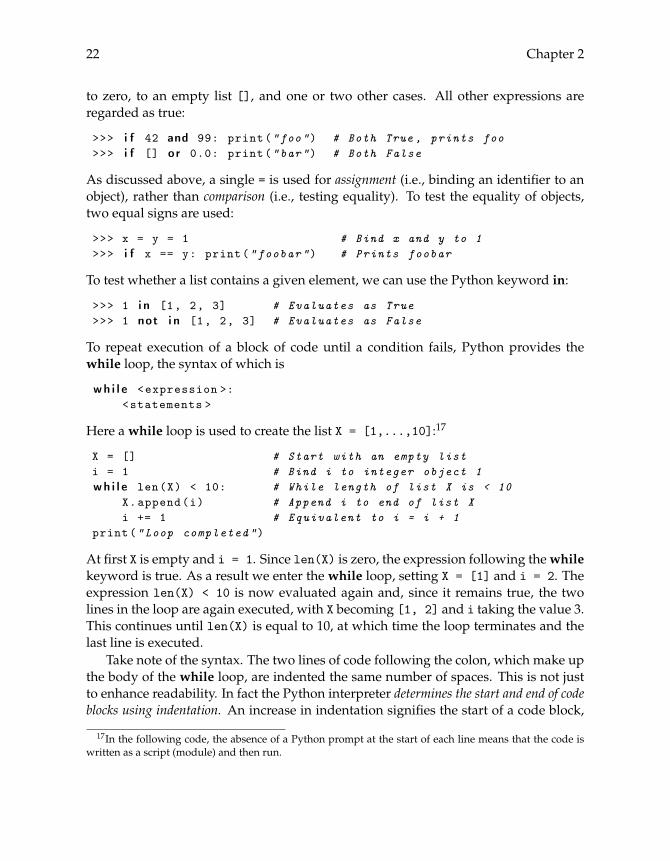
To repeat execution of a block of code until a condition fails, Python provides thewhile loop, the syntax of which is
wh i l e <expression >:<statements >
Here a while loop is used to create the list X = [1,...,10]:17
X = [] # Start with an empty listi = 1 # Bind i to integer object 1wh i l e len(X) < 10: # While length of list X is < 10
X.append(i) # Append i to end of list Xi += 1 # Equivalent to i = i + 1
print("Loop completed")
At first X is empty and i = 1. Since len(X) is zero, the expression following thewhilekeyword is true. As a result we enter the while loop, setting X = [1] and i = 2. Theexpression len(X) < 10 is now evaluated again and, since it remains true, the twolines in the loop are again executed, with X becoming [1, 2] and i taking the value 3.This continues until len(X) is equal to 10, at which time the loop terminates and thelast line is executed.
Take note of the syntax. The two lines of code following the colon, which make upthe body of the while loop, are indented the same number of spaces. This is not justto enhance readability. In fact the Python interpreter determines the start and end of codeblocks using indentation. An increase in indentation signifies the start of a code block,
17In the following code, the absence of a Python prompt at the start of each line means that the code iswritten as a script (module) and then run.
Introduction to Programming 23
whereas a decrease signifies its end. In Python the convention is to use four spaces toindent each block, and I recommend you follow it.18
Here’s another example that uses the break keyword. We wish to simulate therandom variable T := min{t ≥ 1 : Wt > 3}, where (Wt)t≥1 is an IID sequence ofstandard normal random variables:
from random impor t normalvariateT = 1wh i l e 1: # Always true
X = normalvariate (0, 1) # Draw X from N(0,1)i f X > 3: # If X > 3,
print(T) # print the value of T,break # and terminate while loop.
T += 1 # Else T = T + 1, repeat
The program returns the first point in time t such that Wt > 3.Another style of loop is the for loop. Often for loops are used to carry out oper-
ations on lists. Suppose, for example, that we have a list X, and we wish to create asecond list Y containing the squares of all elements in X that are strictly less than zero.Here is a first pass:
Y = []f o r i i n range(len(X)): # For all indexes of X
i f X[i] < 0:Y.append(X[i]**2)
This is a traditional C-style for loop, iterating over the indexes 0 to len(X)-1 of the listX. In Python, for loops can iterate over any list, rather than just sequences of integers(i.e., indexes), which means that the code above can be simplified to
Y = []f o r x i n X: # For all x in X, starting with X[0]
i f x < 0:Y.append(x**2)
In fact, Python provides a very useful construct, called a list comprehension, that allowsus to achieve the same thing in one line:
Y = [x**2 f o r x i n X i f x < 0]
A for loop can be used to code the algorithm discussed in exercise 2.1.2 on page 14:
subset = Truef o r a i n A:
18In text files, tabs are different to spaces. If you are working with a text editor other than IDLE, youshould configure the tab key to insert four spaces. Most decent text editors have this functionality.
24 Chapter 2
i f a not i n B:subset = Fa l s e
print(subset)
Here A and B are expected to be lists.19
We can also code the algorithm on page 14 along the following lines:
from random impor t uniformH, p = 0, 0.5 # H = 0, p = 0.5f o r i i n range (10): # Iterate 10 times
U = uniform(0, 1) # U is uniform on (0, 1)i f U < p:
print("heads")H += 1 # H = H + 1
e l s e :print("tails")
print(H)
Exercise 2.1.5 Turn the pseudocode from exercise 2.1.3 into Python code.
Python for loops can step through any object that is iterable. For example:
from urllib impor t urlopenwebpage = urlopen("http :// johnstachurski.net")f o r line i n webpage:
print(line)
Here the loop acts on a “file-like” object created by the call to urlopen(). Consult thePython documentation on iterators for more information.
Finally, it should be noted that in scripting languages for loops are inherentlyslow. Here’s a comparison of summing an array with a for loop and summing withNumPy’s sum() function:
impor t numpy , timeY = numpy.ones (100000) # NumPy array of 100 ,000 onest1 = time.time() # Record times = 0f o r y i n Y: # Sum elements with for loop
s += yt2 = time.time() # Record times = numpy.sum(Y) # NumPy’s sum() functiont3 = time.time() # Record timeprint((t2 -t1)/(t3-t2))
19Actually they are required to be iterable. Also note that Python has a set data type, which will performthis test for you. The details are omitted.

Introduction to Programming 25
On my computer the output is about 200, meaning that, at least for this array of num-bers, NumPy’s sum() function is roughly 200 times faster than using a for loop. Thereason is that NumPy’s sum() function passes the operation to efficient C code.
2.2 Program Design
The material we have covered so far is already sufficient to solve useful programmingproblems. The issue we turn to next is that of design: How to construct programsso as to retain clarity and readability as our projects grow. We begin with the idea offunctions, which are labeled blocks of code written to perform a specific operation.
2.2.1 User-Defined Functions
The first step along the road to good program design is learning to break your pro-gram up into functions. Functions are a key tool through which programmers imple-ment the time-honored strategy of divide and conquer: problems are broken up intosmaller subproblems, which are then coded up as functions. The main program thencoordinates these functions, calling on them to do their jobs at the appropriate time.
Now the details. When we pass the instruction x = 3 to the interpreter, an integer“object” with value 3 is stored in the memory and assigned the identifier x. In a similarway we can also create a set of instructions for accomplishing a given task, store theinstructions in memory, and bind an identifier (name) that can be used to call (i.e., run)the instructions. The set of instructions is called a function. Python supplies a numberof built-in functions, such as max() and sum() above, as well as permitting users todefine their own functions. Here’s a fairly useless example of the latter:
de f f(x, y): # Bind f to a function thatprint(x + y) # prints the value of x + y
After typing this into a new window in IDLE, saving it and running it, we can thencall f at the command prompt:
>>> f(2,3) # Prints 5>>> f("code ", "monkey") # Prints "code monkey"
Take note of the syntax used to define f. We start with def, which is a Python keywordused for creating functions. Next follows the name and a sequence of arguments inparentheses. After the closing bracket a colon is required. Following the colon wehave a code block consisting of the function body. As before, indentation is used todelimit the code block.
Notice that the order in which arguments are passed to functions is important. Thecalls f("a", "b") and f("b", "a") produce different output. When there are many

26 Chapter 2
arguments, it can become difficult to remember which argument should be passedfirst, which should be passed second, and so on. In this case one possibility is to usekeyword arguments:
de f g(word1="Charlie ", word2="don’t ", word3="surf."):print(word1 + word2 + word3)
The values supplied to the parameters are defaults. If no value is passed to a givenparameter when the function is called, then the parameter name is bound to its defaultvalue:
>>> g() # Prints "Charlie don’t surf">>> g(word3="swim") # Prints "Charlie don’t swim"
If we do not wish to specify any particular default value, then the convention is to useNone instead, as in x=None.
Often one wishes to create functions that return an object as the result of theirinternal computations. To do so, we use the Python keyword return. Here is anexample that computes the norm distance between two lists of numbers:
de f normdist(X, Y):Z = [(x - y)**2 f o r x, y i n zip(X, Y)]r e t u r n sum(Z)**0.5
We are using the built-in function zip(), which allows us to step through the x, ypairs, as well as a list comprehension to construct the list Z. A call such as
>>> p = normdist(X, Y) # X, Y are lists of equal length
binds identifier p to the value returned by the function.It’s good practice to include a doc string in your functions. A doc string is a string
that documents the function, and comes at the start of the function code block. Forexample,
de f normdist(X, Y):"Computes euclidean distance between two vectors."Z = [(x - y)**2 f o r x, y i n zip(X, Y)]r e t u r n sum(Z)**0.5
Of course, we could just use the standard comment notation, but doc strings havecertain advantages that we won’t go into here. In the code in this text, doc strings areused or omitted depending on space constraints.
Python provides a second way to define functions, using the lambda keyword.Typically lambda is used to create small, in-line functions such as
f = lambda x, y: x + y # E.g. f(1,2) returns 3

Introduction to Programming 27
Note that functions can return any Python object, including functions. For exam-ple, suppose that we want to be able to create the Cobb–Douglas production functionf (k) = Akα for any parameters A and α. The following function takes parameters(A, α) as arguments and creates and returns the corresponding function f :
de f cobbdoug(A, alpha ):r e t u r n lambda k: A * k**alpha
After saving and running this, we can call cobbdoug at the prompt:
>>> g = cobbdoug(1, 0.5) # Now g(k) returns 1 * k**0.5
2.2.2 More Data Types
We have already met several native Python data types, such as integers, lists andstrings. Another native Python data type is the tuple:
>>> X = (20, 30, 40) # Parentheses are optional
Tuples behave like lists, in that one can access elements of the tuple using indexes.Thus X[0] returns 20, X[1] returns 30, and so on. There is, however, one crucial dif-ference: Lists are a mutable data type, whereas tuples (like strings) are immutable. Inessence, mutable data types such as lists can be changed (i.e., their contents can be al-tered without creating a new object), whereas immutable types such as tuples cannot.For example, X[0] = 3 raises an exception (error) if X is a tuple. If X is a list, then thesame statement changes the first element of X to 3.
Tuples, lists, and strings are collectively referred to as sequence types, and theysupport a number of common operations (on top of the ability to access individualelements via indexes starting at zero). For example, adding two sequences concate-nates them. Thus (1, 2) + (3, 4) creates the tuple (1, 2, 3, 4), while "ab" +"cd" creates "abcd". Multiplication of a sequence by an integer n concatenates withn copies of itself, so [1] * 3 creates [1, 1, 1]. Sequences can also be unpacked: x, y= (1, 2) binds x to 1 and y to 2, while x, y = "ab" binds x to "a" and y to "b".
Another useful data type is a dictionary, also known as a mapping, or an asso-ciative array. Mathematically, a dictionary is just a function on a finite set, where theprogrammer supplies the domain of the function plus the function values on elementsof the domain. The points in the domain of a dictionary are referred to as its keys. Adictionary d is created by specifying the key/value pairs. Here’s an example:
>>> d = {"Band": "AC/DC", "Track": "Jailbreak"}>>> d["Track"]"Jailbreak"

28 Chapter 2
Mutable case:
Immutable case:
[1]
1
2
1
x = y = [1]
x = y = 1 y = 2
y[0] = 2
x
y
[2]x
y
x
y
x
y
Figure 2.1 Mutable and immutable types
Just as lists and strings have methods that act on them, dictionaries have dictionarymethods. For example, d.keys() returns the list of keys, and d.values() returns thelist of values. Try the following piece of code, which assumes d is as defined above:
>>> f o r key i n d.keys (): print(key , d[key])
Values of a dictionary can be any object, and keys can be any immutable object.This brings us back to the topic of mutable versus immutable. A good under-
standing of the difference between mutable and immutable data types is helpful whentrying to keep track of your variables. At the same time the following discussion isrelatively technical, and can probably be skipped if you have little experience withprogramming.
To begin, consider figure 2.1. The statement x = y = [1] binds the identifiers xand y to the (mutable) list object [1]. Next y[0] = 2 modifies that same list object,so its first (and only) element is 2. Note that the value of x has now changed, since theobject it is bound to has changed. On the other hand, x = y = 1 binds x and y to animmutable integer object. Since this object cannot be altered, the assignment y = 2rebinds y to a new integer object, and x remains unchanged.20
A related way that mutable and immutable data types lead to different outcomesis when passing arguments to functions. Consider, for example, the following codesegment:
20You can check that x and y point to different objects by typing id(x) and id(y) at the prompt. Theirunique identifier (which happens to be their location in memory) should be different.

Introduction to Programming 29
de f f(x):x = x + 1r e t u r n x
x = 1print(f(x), x)
This prints 2 as the value of f(x) and 1 as the value of x, which works as follows: Afterthe function definition, x = 1 creates a global variable x and binds it to the integer object1. When f is called with argument x, a local namespace for its variables is allocated inmemory, and the x inside the function is created as a local variable in that namespaceand bound to the same integer object 1. Since the integer object is immutable, thestatement x = x + 1 creates a new integer object 2 and rebinds the local x to it. Thisreference is now passed back to the calling code, and hence f(x) references 2. Next,the local namespace is destroyed and the local x disappears. Throughout, the global xremains bound to 1.
The story is different when we use a mutable data type such as a list:
de f f(x):x[0] = x[0] + 1r e t u r n x
x = [1]print(f(x), x)
This prints [2] for both f(x) and x. Here the global x is bound to the list object [1].When f is called with argument x, a local x is created and bound to the same listobject. Since [1] is mutable, x[0] = x[0] + 1 modifies this object without changingits location in memory, so both the local x and the global x are now bound to [2]. Thusthe global variable x is modified by the function, in contrast to the immutable case.
2.2.3 Object-Oriented Programming
Python supports both procedural and object-oriented programming (OOP). While anyprogramming task can be accomplished using the traditional procedural style, OOPhas become a central part of modern programming design, and will reward even thesmall investment undertaken here. It succeeds because its design pattern fits wellwith the human brain and its natural logic, facilitating clean, efficient code. It fitswell with mathematics because it encourages abstraction. Just as abstraction in math-ematics allows us to develop general ideas that apply in many contexts, abstractionin programming lets us build structures that can be used and reused in different pro-gramming problems.
Procedural programming is based around functions (procedures). The programhas a state, which is the values of its variables, and functions are called to act on these
30 Chapter 2
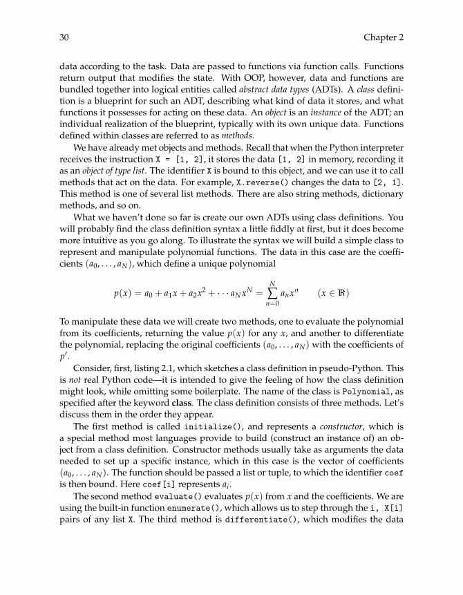
data according to the task. Data are passed to functions via function calls. Functionsreturn output that modifies the state. With OOP, however, data and functions arebundled together into logical entities called abstract data types (ADTs). A class defini-tion is a blueprint for such an ADT, describing what kind of data it stores, and whatfunctions it possesses for acting on these data. An object is an instance of the ADT; anindividual realization of the blueprint, typically with its own unique data. Functionsdefined within classes are referred to as methods.
We have already met objects and methods. Recall that when the Python interpreterreceives the instruction X = [1, 2], it stores the data [1, 2] in memory, recording itas an object of type list. The identifier X is bound to this object, and we can use it to callmethods that act on the data. For example, X.reverse() changes the data to [2, 1].This method is one of several list methods. There are also string methods, dictionarymethods, and so on.
What we haven’t done so far is create our own ADTs using class definitions. Youwill probably find the class definition syntax a little fiddly at first, but it does becomemore intuitive as you go along. To illustrate the syntax we will build a simple class torepresent and manipulate polynomial functions. The data in this case are the coeffi-cients (a0, . . . , aN), which define a unique polynomial
p(x) = a0 + a1x+ a2x2 + · · · aNxN =N
∑n=0
anxn (x ∈ )
To manipulate these data we will create two methods, one to evaluate the polynomialfrom its coefficients, returning the value p(x) for any x, and another to differentiatethe polynomial, replacing the original coefficients (a0, . . . , aN) with the coefficients ofp′.
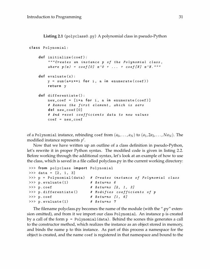
Consider, first, listing 2.1, which sketches a class definition in pseudo-Python. Thisis not real Python code—it is intended to give the feeling of how the class definitionmight look, while omitting some boilerplate. The name of the class is Polynomial, asspecified after the keyword class. The class definition consists of three methods. Let’sdiscuss them in the order they appear.
The first method is called initialize(), and represents a constructor, which isa special method most languages provide to build (construct an instance of) an ob-ject from a class definition. Constructor methods usually take as arguments the dataneeded to set up a specific instance, which in this case is the vector of coefficients(a0, . . . , aN). The function should be passed a list or tuple, to which the identifier coefis then bound. Here coef[i] represents ai.
The second method evaluate() evaluates p(x) from x and the coefficients. We areusing the built-in function enumerate(), which allows us to step through the i, X[i]pairs of any list X. The third method is differentiate(), which modifies the data
Introduction to Programming 31
Listing 2.1 (polyclass0.py) A polynomial class in pseudo-Python
c l a s s Polynomial:
de f initialize(coef):"""Creates an instance p of the Polynomial class ,where p(x) = coef [0] x^0 + ... + coef[N] x^N."""
de f evaluate(x):y = sum(a*x**i f o r i, a i n enumerate(coef))r e t u r n y
de f differentiate ():new_coef = [i*a f o r i, a i n enumerate(coef)]# Remove the first element , which is zerod e l new_coef [0]# And reset coefficients data to new valuescoef = new_coef
of a Polynomial instance, rebinding coef from (a0, . . . , aN) to (a1, 2a2, . . . ,NaN). Themodified instance represents p′.
Now that we have written up an outline of a class definition in pseudo-Python,let’s rewrite it in proper Python syntax. The modified code is given in listing 2.2.Before working through the additional syntax, let’s look at an example of how to usethe class, which is saved in a file called polyclass.py in the current working directory:
>>> from polyclass impor t Polynomial>>> data = [2, 1, 3]>>> p = Polynomial(data) # Creates instance of Polynomial class>>> p.evaluate (1) # Returns 6>>> p.coef # Returns [2, 1, 3]>>> p.differentiate () # Modifies coefficients of p>>> p.coef # Returns [1, 6]>>> p.evaluate (1) # Returns 7
The filename polyclass.py becomes the name of the module (with the “.py” exten-sion omitted), and from it we import our class Polynomial. An instance p is createdby a call of the form p = Polynomial(data). Behind the scenes this generates a callto the constructor method, which realizes the instance as an object stored in memory,and binds the name p to this instance. As part of this process a namespace for theobject is created, and the name coef is registered in that namespace and bound to the
32 Chapter 2
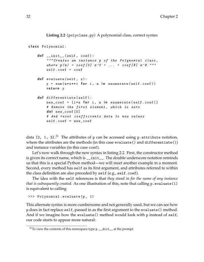
Listing 2.2 (polyclass.py) A polynomial class, correct syntax
c l a s s Polynomial:
de f __init__(self , coef):"""Creates an instance p of the Polynomial class ,where p(x) = coef [0] x^0 + ... + coef[N] x^N."""self.coef = coef
de f evaluate(self , x):y = sum(a*x**i f o r i, a i n enumerate(self.coef))r e t u r n y
de f differentiate(self):new_coef = [i*a f o r i, a i n enumerate(self.coef)]# Remove the first element , which is zerod e l new_coef [0]# And reset coefficients data to new valuesself.coef = new_coef
data [2, 1, 3].21 The attributes of p can be accessed using p.attribute notation,where the attributes are the methods (in this case evaluate() and differentiate())and instance variables (in this case coef).
Let’s now walk through the new syntax in listing 2.2. First, the constructor methodis given its correct name, which is __init__. The double underscore notation remindsus that this is a special Python method—we will meet another example in a moment.Second, every method has self as its first argument, and attributes referred to withinthe class definition are also preceded by self (e.g., self.coef).
The idea with the self references is that they stand in for the name of any instancethat is subsequently created. As one illustration of this, note that calling p.evaluate(1)is equivalent to calling
>>> Polynomial.evaluate(p, 1)
This alternate syntax is more cumbersome and not generally used, but we can see howp does in fact replace self, passed in as the first argument to the evaluate() method.And if we imagine how the evaluate() method would look with p instead of self,our code starts to appear more natural:
21To view the contents of this namespace type p.__dict__ at the prompt.

Introduction to Programming 33
de f evaluate(p, x):y = sum(a*x**i f o r i, a i n enumerate(p.coef))r e t u r n y
Before finishing, let’s briefly discuss another useful special method. One rather un-gainly aspect of the Polynomial class is that for a given instance p correspondingto a polynomial p, the value p(x) is obtained via the call p.evaluate(x). It wouldbe nicer—and closer to the mathematical notation—if we could replace this with thesyntax p(x). Actually this is easy: we simply replace the word evaluate in listing 2.2with __call__. Objects of this class are now said to be callable, and p(x) is equivalentto p.__call__(x).
2.3 Commentary
Python was developed by Guido van Rossum, with the first release in 1991. It is nowone of the major success stories of the open source model, with a vibrant communityof users and developers. van Rossum continues to direct the development of the lan-guage under the title of BDFL (Benevolent Dictator For Life). The use of Python hasincreased rapidly in recent years.
There are many good books on Python programming. A gentle introduction isprovided by Zelle (2003). A more advanced book focusing on numerical methods isLangtangen (2008). However, the best place to start is on the Internet. The Pythonhomepage (python.org) has links to the official Python documentation and varioustutorials. Links, lectures, MATLAB code, and other information relevant to this chap-ter can be found on the text home page, at http://johnstachurski.net/book.html.
Computational economics is a rapidly growing field. For a sample of the literature,consult Amman et al. (1996), Heer and Maussner (2005), Kendrick et al. (2005), orTesfatsion and Judd (2006).

Chapter 3
Analysis in Metric Space
Metric spaces are sets (spaces) with a notion of distance between points in the spacethat satisfies certain axioms. From these axioms we can deduce many properties relat-ing to convergence, continuity, boundedness, and other concepts needed for the studyof dynamics. Metric space theory provides both an elegant and powerful frameworkfor analyzing the kinds of problems we wish to consider, and a great sandpit for play-ing with analytical ideas: A careful read of this chapter should strengthen your abilityto read and write proofs.
The chapter supposes that you have at least some exposure to introductory realanalysis or advanced calculus. A review of this material is given in appendix A. Onthe other hand, if you are already familiar with the fundamentals of metric spaces,then the best approach is to skim through this chapter quickly and return as necessary.
3.1 A First Look at Metric Space
Consider the set k, a typical element of which is x = (x1, . . . , xk), where xi ∈ .These elements are also called vectors. There are a number of important “topological”notions we need to introduce for k. These notions concern sets and functions on orinto such space. In order to introduce them, it is convenient to begin with the conceptof euclidean distance between vectors: Define d2 : k × k → by
d2(x, y) :=: ‖x− y‖2 :=
[k
∑i=1
(xi − yi)2]1/2
(3.1)
Doubtless you have met with this notion of distance before. You might know that itsatisfies the following three conditions:
35
36 Chapter 3
1. d2(x, y) = 0 if and only if x = y,
2. d2(x, y) = d2(y, x), and
3. d2(x, y) ≤ d2(x, v) + d2(v, y).
for any x, y, v ∈ k. The first property says that a point is at zero distance fromitself, and also that distinct points always have positive distance. The second propertyis symmetry, and the third—the only one that is not immediately apparent—is thetriangle inequality.
These three properties are fundamental to our understanding of distance. In factif you look at the proofs of many important results—for example, the proof that everycontinuous function f from a closed bounded subset of k to has a maximizer anda minimizer—you will notice that no other properties of d2 are actually used.
Now it turns out that there are many other “distance” functions we can imposeon k that also satisfy properties 1–3. Any proof for the euclidean (i.e., d2) case thatonly uses properties 1–3 continues to hold for other distances, and in certain problemsalternative notions of distance are easier to work with. This motivates us to generalizethe concept of distance in k.
While we are generalizing the notion of distance between vectors in k, it is worththinking about distance between other kinds of objects. If we could define the distancebetween two (infinite) sequences, or between a pair of functions, or two probabilitydistributions, we could then give a definition for things like the “convergence” ofdistributions discussed informally in chapter 1.
3.1.1 Distances and Norms
Here is the key definition:
Definition 3.1.1 A metric space is a nonempty set S and a metric or distance ρ : S× S→such that, for any x, y, v ∈ S,
1. ρ(x, y) = 0 if and only if x = y,
2. ρ(x, y) = ρ(y, x), and
3. ρ(x, y) ≤ ρ(x, v) + ρ(v, y).
Apart from being nonempty, the set S is completely arbitrary. In the context ofa metric space the elements of the set are usually called points. As in the case ofeuclidean distance, the third axiom is called the triangle inequality.
An immediate consequence of the axioms in definition 3.1.1 (which are sometimesreferred to as the Hausdorff postulates) is that ρ(x, y) ≥ 0 for any x, y ∈ S. To see this,

Analysis in Metric Space 37
note that if x and y are any two points in S, then 0 = ρ(x, x) ≤ ρ(x, y) + ρ(y, x) =ρ(x, y) + ρ(x, y) = 2ρ(x, y). Hence ρ(x, y) ≥ 0 as claimed.
The space ( k, d2) is a metric space, as discussed above. The most important caseis k = 1, when d2(x, y) reduces to |x− y| for x, y ∈ . The notation ( , | · |) will be usedto denote this one-dimensional space.
Many additional metric spaces on k are generated by what is known as a norm:
Definition 3.1.2 A norm on k is a mapping k � x �→ ‖x‖ ∈ such that, for anyx, y ∈ k and any γ ∈ ,
1. ‖x‖ = 0 if and only if x = 0,
2. ‖γx‖ = |γ|‖x‖, and
3. ‖x+ y‖ ≤ ‖x‖+ ‖y‖.Each norm ‖ · ‖ on k generates a metric ρ on k via ρ(x, y) := ‖x− y‖.
Exercise 3.1.3 Show that ρ is indeed a metric, in the sense that it satisfies the threeaxioms in definition 3.1.1.
Exercise 3.1.4 Let ‖ · ‖ be a norm on k. Show that for any x, y ∈ k we have |‖x‖ −‖y‖| ≤ ‖x− y‖.
The most important norm on k is ‖x‖2 := (∑ki=1 x
2i )
1/2, which generates theeuclidean distance d2. A class of norms that includes ‖ · ‖2 as a special case is thefamily ‖ · ‖p defined by
‖x‖p :=
(k
∑i=1|xi|p
)1/p
(x ∈ k) (3.2)
where p ≥ 1. It is standard to admit p = ∞ in this family, with ‖x‖∞ := max1≤i≤k |xi|.Proving that ‖ · ‖p is indeed a norm on k for arbitrary p ≥ 1 is not difficult, but
neither is it entirely trivial. In particular, establishing the triangle inequality requiresthe services of Minkowski’s inequality. The latter is found in any text covering normsand is omitted.
Exercise 3.1.5 Prove that ‖ · ‖p is a norm on k for p = 1 and p = ∞.
The class of norms ‖ · ‖p gives rise to the class of metric spaces ( k, dp), wheredp(x, y) := ‖x− y‖p for all x, y ∈ k.
So far all our spaces have involved different metrics on finite-dimensional vectorspace. Next let’s consider an example of a “function space.” Let U be any set, let bUbe the collection of all bounded functions f : U → (i.e., supx∈U | f (x)| < ∞), and let
d∞( f , g) :=: ‖ f − g‖∞ := supx∈U| f (x)− g(x)| (3.3)

38 Chapter 3
x
x1
x2
xN
{y | ρ(x, y) < ε}
Figure 3.1 Limit of a sequence
The space (bU, d∞) is a metric space. The reader can verify the first two propertiesof the definition of a metric space. The triangle inequality is verified as follows. Letf , g, h ∈ bU. Pick any x ∈ U. We have
| f (x)− g(x)| ≤ | f (x)− h(x)|+ |h(x)− g(x)| ≤ d∞( f , h) + d∞(h, g)
Since x is arbitrary, we obtain d∞( f , g) ≤ d∞( f , h) + d∞(h, g).1
3.1.2 Sequences
Let S = (S, ρ) be a metric space. A sequence (xn) ⊂ S is said to converge to x ∈ Sif, for all ε > 0, there exists an N ∈ such that n ≥ N implies ρ(xn, x) < ε. Inother words (xn) converges to x if and only if the real sequence ρ(xn, x) → 0 in asn → ∞ (see §A.2 for more on real sequences). If this condition is satisfied, we writelimn→∞ xn = x, or xn → x. The point x is referred to as the limit of the sequence.Figure 3.1 gives an illustration for the case of two-dimensional euclidean space.
Theorem 3.1.6 A sequence in (S, ρ) can have at most one limit.
Proof. You might like to try a proof by contradiction as an exercise. Here is a directproof. Let (xn) be an arbitrary sequence in S, and let x and x′ be two limit points. Wehave
0 ≤ ρ(x, x′) ≤ ρ(x, xn) + ρ(xn, x′) ∀ n ∈1As an aside, you may have noticed that the metric space (bU, d∞) seems to be defined by a “norm”
‖ f ‖∞ := supx∈U | f (x)|. This is not a norm in the sense of definition 3.1.2, as that definition requires that theunderlying space is k , rather than bU. However, more general norms can be defined for abstract “vectorspace,” and ‖ · ‖∞ is a prime example. The details are omitted: See any text on functional analysis.

Analysis in Metric Space 39
a
f
f + ε
f − ε
b
Figure 3.2 An ε-ball for d∞
From theorems A.2.12 and A.2.13 (page 330) we have ρ(x, x′) = 0. Therefore x = x′.(Why?)
Exercise 3.1.7 Let (xn) and (yn) be sequences in S. Show that if xn → x ∈ S andρ(xn, yn)→ 0, then yn → x.
One of the most important creatures defined from the distance function is the hum-ble open ball. The open ball or ε-ball B(ε; x) centered on x ∈ S with radius ε > 0 is theset
B(ε; x) := {z ∈ S : ρ(z, x) < ε}In the plane with ρ = d2 the ε-ball is a circle; in 3 it is a sphere. Figure 3.2 gives avisualization of the ε-ball around f ∈ (b[a, b], d∞).
Exercise 3.1.8 Let (xn) ⊂ S and x ∈ S. Show that xn → x if and only if for all ε > 0,the ball B(ε; x) contains all but finitely many terms of (xn).
A subset E of S is called bounded if E ⊂ B(n; x) for some x ∈ S and some (suitablylarge) n ∈ . A sequence (xn) in S is called bounded if its range {xn : n ∈ } is abounded set.
Exercise 3.1.9 Show that every convergent sequence in S is also bounded.
Given sequence (xn) ⊂ S, a subsequence is defined analogously to the case of realsequences: (yn) is called a subsequence of (xn) if there is a strictly increasing functionf : → such that yn = x f (n) for all n ∈ . It is common to use the notation (xnk )to denote a subsequence of (xn).

40 Chapter 3
Exercise 3.1.10 Show that for (xn) ⊂ S, xn → x for some x ∈ S if and only if everysubsequence of (xn) converges to x.
For the euclidean space ( k, d2) we have the following result:
Lemma 3.1.11 A sequence (xn) = (x1n, . . . , xkn) in ( k, d2) converges to x = (x1, . . . , xk) ∈
k if and only if xjn → xj in = ( , | · |) for all j in 1, . . . , k.
Proof. For j in 1, . . . , k we have |xjn − xj| ≤ d2(xn, x). (Why?) Hence if d2(xn, x) → 0,then |xjn − xj| → 0 for each j. For the converse, fix ε > 0 and choose for each j in1, . . . , k an Nj ∈ such that n ≥ Nj implies |xjn − xj| < ε/
√k. Now n ≥ maxj Nj
implies d2(xn, x) ≤ ε. (Why?)
Lemma 3.1.11 is important, and you should try sketching it for the case k = 2 tobuild intuition. We will see that in fact the same result holds not just for d2, but for themetric induced by any norm on k.
Let S and Y be two metric spaces. Parallel to §A.2.3, define f : S ⊃ A → Y to becontinuous at a ∈ A if for every sequence (xn) in A converging to a we have f (xn) →f (a) inY, and continuous on Awhenever it is continuous at every a ∈ A. For the samef : A→ Y and for a ∈ A, we say that y = limx→a f (x) if f (xn)→ y for every sequence(xn) ⊂ A with xn → a. Clearly, f is continuous at a if and only if limx→a f (x) = f (a).
Example 3.1.12 Let S be a metric space, and let x be any given point in S. The mapS � x �→ ρ(x, x) ∈ is continuous on all of S. To see this, pick any x ∈ S, and any(xn) ⊂ S with xn → x. Two applications of the triangle inequality yield
ρ(x, x)− ρ(xn, x) ≤ ρ(xn, x) ≤ ρ(xn, x) + ρ(x, x) ∀ n ∈Now take the limit (i.e., apply theorem A.2.12 on page 330).
Exercise 3.1.13 Let f (x, y) = x2 + y2. Show that f is a continuous function from( 2, d2) into ( , | · |).2
Throughout the text, if S is some set, f : S→ , and g : S→ , then f + g denotesthe function x �→ f (x) + g(x) on S, while f g denotes the function x �→ f (x)g(x) on S.
Exercise 3.1.14 Let f and g be as above, and let S be a metric space. Show that if fand g are continuous, then so are f + g and f g.
Exercise 3.1.15 A function f : S→ is called upper-semicontinuous (usc) at x ∈ S if,for every xn → x, we have lim supn f (xn) ≤ f (x); and lower-semicontinuous (lsc) if,for every xn → x, we have lim infn f (xn) ≥ f (x). Show that f is usc at x if and only if− f is lsc at x. Show that f is continuous at x if and only if it is both usc and lsc at x.
2Hint: Use lemma 3.1.11.

Analysis in Metric Space 41
3.1.3 Open Sets, Closed Sets
Arbitrary subsets of arbitrary spaces can be quite unruly. It is useful to identifyclasses of sets that are well-behaved, interacting nicely with common functions, andco-operating with attempts to measure them, or to represent them in terms of simplerelements. In this section we investigate a class of sets called the open sets, as well astheir complements the closed sets.
Let’s say that x ∈ S adheres to E ⊂ S if, for each ε > 0, the ball B(ε; x) contains atleast one point of E;3 and that x is interior to E if B(ε; x) ⊂ E for some ε > 0.4 A set E ⊂S is called open if all points in E are interior to E, and closed if E contains all points thatadhere to E. In the familiar metric space ( , | · |), canonical examples are the intervals(a, b) and [a, b], which are open and closed respectively.5 The concepts of open andclosed sets turn out to be some of the most fruitful ideas in all of mathematics.
Exercise 3.1.16 Show that a point in S adheres to E ⊂ S if and only if it is the limit ofa sequence contained in E.
Theorem 3.1.17 A set F ⊂ S is closed if and only if for every convergent sequence entirelycontained in F, the limit of the sequence is also in F.
Proof. Do the proof as an exercise if you can. If not, here goes. Suppose that F isclosed, and take a sequence in F converging to some point x ∈ S. Then x adheres to Fby exercise 3.1.16, and is therefore in F by definition. Suppose, on the other hand, thatthe limit of every convergent sequence in F belongs to F. Take any x ∈ S that adheresto F. By exercise 3.1.16, there is a sequence in F converging to it. Therefore x ∈ F, andF is closed.
Open sets and closed sets are closely related. In fact we have the following funda-mental theorem:
Theorem 3.1.18 A subset of an arbitrary metric space S is open if and only if its complementis closed, and closed if and only if its complement is open.
Proof. The proof is a good exercise. If you need a start, here is a proof that G openimplies F := Gc closed. Take (xn) ⊂ F with xn → x ∈ S. We wish to show that x ∈ F.In fact this must be the case because, if x /∈ F, then x ∈ G, in which case there is anε > 0 such that B(ε, x) ⊂ G. (Why?) Such a situation is not possible when (xn) ⊂ Fand xn → x. (Why?)
3In some texts, x is said to be a contact point of E.4Try sketching some examples for the case of ( 2, d2).5If you find it hard to verify this now, you won’t by the end of the chapter.

42 Chapter 3
We call D(ε; x) := {z ∈ S : ρ(z, x) ≤ ε} the closed ε-ball centered on x. EveryD(ε; x) ⊂ S is a closed set, as anticipated by the notation. To see this, take (an) ⊂D(ε; x) converging to a ∈ S. We need to show that a ∈ D(ε; x) or, equivalently, thatρ(a, x) ≤ ε. Since ρ(an, x) ≤ ε for all n ∈ , since limits preserve orders and sincey �→ ρ(y, x) is continuous, we have ρ(a, x) = lim ρ(an, x) ≤ ε.
Exercise 3.1.19 Likewise every open ball B(ε; x) in S is an open set. Prove this directly,or repeat the steps of the previous example applied to B(ε; x)c.
You will not find it difficult to convince yourself that if (S, ρ) is any metric space,then the whole set S is itself both open and closed. (Just check the definitions care-fully.) This can lead to some confusion. For example, suppose that we consider themetric space (S, | · |), where S = (0, 1). Since (0, 1) is the whole space, it is closed. Atthe same time, (0, 1) is open as a subset of ( , | · |). The properties of openness andclosedness are relative rather than absolute.
Exercise 3.1.20 Argue that for any metric space (S, ρ), the empty set ∅ is both openand closed.
Exercise 3.1.21 Show that if (S, ρ) is an arbitrary metric space, and if x ∈ S, then theset {x} is always closed.
Theorem 3.1.22 If F is a closed, bounded subset of ( , | · |), then sup F ∈ F.
Proof. Let s := sup F. Since F is closed it is sufficient to show there exists a sequence(xn) ⊂ F with xn → s. (Why?) By lemma A.2.19 (page 332) such a sequence exists.
Exercise 3.1.23 Prove that a sequence converges to a point x if and only if the sequenceis eventually in every open set containing x.
Exercise 3.1.24 Prove: If {Gα}α∈A are all open, then so is ∪α∈AGα.
Exercise 3.1.25 Show that if A is finite and {Gα}α∈A is a collection of open sets, then∩α∈AGα is also open.
In other words, arbitrary unions and finite intersections of open sets are open. Butbe careful: An infinite intersection of open sets is not necessarily open. For example,consider the metric space ( , | · |). If Gn = (−1/n, 1/n), then ∩n∈ Gn = {0} because
x ∈ ∩nGn ⇐⇒ − 1n
< x <1n∀ n ∈ ⇐⇒ x = 0
Exercise 3.1.26 Show that ∩n∈ (a− 1/n, b+ 1/n) = [a, b].
Exercise 3.1.27 Prove that if {Fα}α∈A are all closed, then so is ∩α∈AFα.
Analysis in Metric Space 43
Exercise 3.1.28 Show that if A is finite and {Fα}α∈A is a collection of closed sets, then∪α∈AFα is closed. On the other hand, show that the union ∪n∈ [a+ 1/n, b− 1/n] =(a, b). (Why is this not a contradiction?)
Exercise 3.1.29 Show that G ⊂ S is open if and only if it can be formed as the unionof an arbitrary number of open balls.
The closure of E is the set of all points that adhere to E, and is written cl E. In viewof exercise 3.1.16, x ∈ cl E if and only if there exists a sequence (xn) ⊂ E with xn → x.The interior of E is the set of its interior points, and is written int E.
Exercise 3.1.30 Show that cl E is always closed. Show in addition that for all closedsets F such that F ⊃ E, cl E ⊂ F. Using this result, show that cl E is equal to theintersection of all closed sets containing E.
The last exercise tells us that the closure of a set is the smallest closed set thatcontains that particular set. The next one shows us that the interior of a set is thelargest open set contained in that set.
Exercise 3.1.31 Show that int E is always open. Show also that for all open sets G suchthat G ⊂ E, int E ⊃ G. Using this result, show that int E is equal to the union of allopen sets contained in E.
Exercise 3.1.32 Show that E = cl E if and only if E is closed. Show that E = int E ifand only if E is open.
Open sets and continuous functions interact very nicely. For example, we have thefollowing fundamental theorem.
Theorem 3.1.33 A function f : S → Y is continuous if and only if the preimage f−1(G) ofevery open set G ⊂ Y is open in S.
Proof. Suppose that f is continuous, and let G be any open subset of Y. If x ∈ f−1(G),then x must be interior, for if it is not, then there is a sequence xn → x where xn /∈f−1(G) for all n. But, by continuity, f (xn) → f (x), implying that f (x) ∈ G is notinterior to G. (Why?) Contradiction.
Conversely, suppose that the preimage of every open set is open, and take any{xn}n≥1 ∪ {x} ⊂ S with xn → x. Pick any ε-ball B around f (x). The preimage f−1(B)is open, so for N sufficiently large we have xn ∈ f−1(B) for all n ≥ N, in which casef (xn) ∈ B for all n ≥ N.
Exercise 3.1.34 Let S, Y, and Z be metric spaces, and let f : S → Y and g : Y → Z.Show that if f and g are continuous, then so is h := g ◦ f .
44 Chapter 3
Exercise 3.1.35 Let S = k, and let ρ∗(x, y) = 0 if x = y and 1 otherwise. Provethat ρ∗ is a metric on k. Which subsets of this space are open? Which subsets areclosed? What kind of functions f : S → are continuous? What kinds of sequencesare convergent?
3.2 Further Properties
Having covered the fundamental ideas of convergence, continuity, open sets andclosed sets, we now turn to two key concepts in metric space theory: completenessand compactness. After stating the definitions and covering basic properties, we willsee how completeness and compactness relate to existence of optima and to the theoryof fixed points.
3.2.1 Completeness
A sequence (xn) in metric space (S, ρ) is said to be a Cauchy sequence if, for all ε > 0,there exists an N ∈ such that ρ(xj, xk) < ε whenever j ≥ N and k ≥ N . A subset Aof a metric space S is called complete if every Cauchy sequence in A converges to somepoint in A. Often the set A of interest is the whole space S, in which case we say thatS is a complete metric space. As discussed in §A.2, the set of reals ( , | · |) has thisproperty. Many other metric spaces do not.
Notice that completeness is intrinsic to a given set A and a metric ρ on A. Eitherevery Cauchy sequence in (A, ρ) converges or there exists a Cauchy sequence thatdoes not. On the other hand, openness and closedness are relative properties. The setA := [0, 1) is not open as a subset of ( , | · |), but it is open as a subset of ( +, | · |).
The significance of completeness is that when searching for the solution to a prob-lem, it sometimes happens that we are able to generate a Cauchy sequence whose limitwould be a solution if it does in fact exist. In a complete space we can rest assuredthat our solution does exist as a well-defined element of the space.
Exercise 3.2.1 Show that a sequence (xn) in metric space (S, ρ) is Cauchy if and onlyif limn→∞ supk≥n ρ(xn, xk) = 0.
Exercise 3.2.2 Show that if a sequence (xn) in metric space (S, ρ) is convergent, thenit is Cauchy. Show that if (xn) is Cauchy, then it is bounded.
Which metric spaces are complete? Observe that while = ( , | · |) is complete,subsets of may not be. For example, consider the metric space (S, ρ) = ((0,∞), | ·|). Some manipulation proves that while (xn) = (1/n) is Cauchy in S, it convergesto no point in S. On the other hand, for (S, ρ) = ( +, | · |) the limit point of the

Analysis in Metric Space 45
sequence (1/n) is in S. Indeed this space is complete, as is any closed subset of .More generally,
Theorem 3.2.3 Let S be a complete metric space. Subset A ⊂ S is complete if and only if itis closed as a subset of S.
Proof. Let A be complete. To see that A is closed, let (xn) ⊂ A with xn → x ∈ S.Since (xn) is convergent it must be Cauchy (exercise 3.2.2). Because A is complete wehave x ∈ A. Thus A contains its limit points, and is therefore closed. Conversely,suppose that A is closed. Let (xn) be a Cauchy sequence in A. Since S is complete,(xn) converges to some x ∈ S. As A is closed, the limit point x must be in A. Hence Ais complete.
The euclidean space ( k, d2) is complete. To see this, observe first that
Lemma 3.2.4 A sequence (xn) = (x1n, . . . , xkn) in ( k, d2) is Cauchy if and only if each
component sequence xjn is Cauchy in = ( , | · |).The proof of lemma 3.2.4 is an exercise.6 The lemma is important because it implies
that ( k, d2) inherits the completeness of (axiom A.2.4, page 328):
Theorem 3.2.5 The euclidean space ( k, d2) is complete.
Proof. If (xn) is Cauchy in ( k, d2), then each component is Cauchy in = ( , | · |),and, by completeness of , converges to some limit in . It follows from lemma 3.1.11that (xn) is convergent in ( k, d2).
Recall that (bU, d∞) is the bounded real-valued functions f : U → , endowedwith the distance d∞ defined on page 37. This space also inherits completeness from
:
Theorem 3.2.6 Let U be any set. The metric space (bU, d∞) is complete.
Proof. Let ( fn) ⊂ bU be Cauchy. We claim the existence of a f ∈ bU such thatd∞( fn, f ) → 0. To see this, observe that for each x ∈ U we have supk≥n | fn(x) −fk(x)| ≤ supk≥n d∞( fn, fk) → 0, and hence ( fn(x)) is Cauchy (see exercise 3.2.1). Bythe completeness of , ( fn(x)) is convergent, and we define a new function f ∈ bUby f (x) = limn→∞ fn(x).7
To show that d∞( fn, f ) → 0, fix ε > 0, and choose N ∈ such that d∞( fn, fm) <ε/2 whenever n,m ≥ N. Pick any n ≥ N. For arbitrary x ∈ U we have | fn(x) −fm(x)| < ε/2 for all m ≥ n, and hence, taking limits with respect to m, we have| fn(x)− f (x)| ≤ ε/2. Since x was arbitrary, d∞( fn, f ) ≤ ε/2 < ε.
6Hint: You might like to begin by rereading the proof of lemma 3.1.11.7Why is f ∈ bU (i.e., why is f bounded on U)? Consult exercise 3.2.2.
46 Chapter 3
This is a good opportunity to briefly discuss convergence of functions. A sequenceof functions ( fn) from arbitrary set U into converges pointwise to f : U → if| fn(x) − f (x)| → 0 as n → ∞ for every x ∈ U; and uniformly if d∞( fn, f ) → 0.Pointwise convergence is certainly important, but it is also significantly weaker thanconvergence in d∞. For example, suppose that U is a metric space, that fn → f , andthat all fn are continuous. It might then be hoped that the limit f inherits continuityfrom the approximating sequence. For pointwise convergence this is not generallytrue,8 while for uniform convergence it is:
Theorem 3.2.7 Let ( fn) and f be real-valued functions on metric space U. If fn is continuouson U for all n and d∞( fn, f )→ 0, then f is also continuous on U.
Proof. Take (xk) ⊂ U with xk → x ∈ U. Fix ε > 0. Choose n ∈ such that | fn(x)−f (x)| < ε/2 for all x ∈ U. For any given k ∈ the triangle inequality gives
| f (xk)− f (x)| ≤ | f (xk)− fn(xk)|+ | fn(xk)− fn(x)|+ | fn(x)− f (x)|∴ | f (xk)− f (x)| ≤ | fn(xk)− fn(x)|+ ε (k ∈ )
From exercise A.2.28 (page 333) we have 0 ≤ lim supk | f (xk)− f (x)| ≤ ε. Since ε isarbitrary, lim supk | f (xk)− f (x)| = limk | f (xk)− f (x)| = 0.
Now let’s introduce another important metric space.
Definition 3.2.8 Given any metric space U, let (bcU, d∞) be the continuous functionsin bU endowed with the same metric d∞.
Theorem 3.2.9 The space (bcU, d∞) is always complete.
Proof. This follows from theorem 3.2.3 (closed subsets of complete spaces are com-plete), theorem 3.2.6 (the space (bU, d∞) is complete) and theorem 3.2.7 (which impliesthat the space bcU is closed as a subset of bU).
3.2.2 Compactness
Now we turn to the notion of compactness. A subset K of S = (S, ρ) is called precom-pact in S if every sequence contained in K has a subsequence that converges to a pointof S. The set K is called compact if every sequence contained in K has a subsequencethat converges to a point of K. (Thus every compact subset of S is precompact in S,and every closed precompact set is compact.) Compactness will play a major role inour analysis. As we will see, the existence of a converging subsequence often allowsus to track down the solution to a difficult problem.
8A counterexample is U = [0, 1], fn(x) = xn, f (x) = 0 on [0, 1) and f (1) = 1.

Analysis in Metric Space 47
As a first step, note that there is another important characterization of compact-ness, which at first sight bears little resemblance to the sequential definition above. Tostate the theorem, recall that for a set K in S, an open cover is a collection {Gα} of opensubsets of S such that K ⊂ ∪αGα. The cover is called finite if it consists of only finitelymany sets.
Theorem 3.2.10 A subset K of an arbitrary metric space S is compact if and only if everyopen cover of K can be reduced to a finite cover.
In other words, a set K is compact if and only if, given any open cover, we can dis-card all but a finite number of elements and still cover K. The proof of theorem 3.2.10can be found in any text on real analysis.
Exercise 3.2.11 Exhibit an open cover of k that cannot be reduced to a finite subcover.Construct a sequence in k with no convergent subsequence.
Exercise 3.2.12 Use theorem 3.2.10 to prove that every compact subset of a metricspace S is bounded (i.e., can be contained in an open ball B(n; x) for some x ∈ S andsome (suitably large) n ∈ ).
Exercise 3.2.13 Prove that every compact subset of a metric space is closed.
On the other hand, closed and bounded subsets of metric spaces are not alwayscompact.
Exercise 3.2.14 Let (S, ρ) = ((0,∞), | · |), and let K = (0, 1]. Show that although K is aclosed, bounded subset of S, it is not precompact in S.
Exercise 3.2.15 Show that every subset of a compact set is precompact, and everyclosed subset of a compact set is compact.
Exercise 3.2.16 Show that in any metric space the intersection of an arbitrary numberof compact sets and the union of a finite number of compact sets are again compact.
Exercise 3.2.17 For a more advanced exercise, you might like to try to show thatthe closure of a precompact set is compact. It follows that every precompact set isbounded. (Why?)
When it comes to precompactness and compactness, the space ( k, d2) is ratherspecial. For example, the Bolzano–Weierstrass theorem states that
Theorem 3.2.18 Every bounded sequence in euclidean space ( k, d2) has at least one con-vergent subsequence.
48 Chapter 3
Proof. Let’s check the case k = 2. Let (xn) = (x1n, x2
n) ⊂ ( 2, d2) be bounded. Since(x1
n) is itself bounded in (why?), we can find a sequence n1, n2, . . . =: (nj) such that(x1
nj) converges in (theorem A.2.10, page 330). Now consider (x2nj). This sequence is
also bounded, and must itself have a convergent subsequence, so if we discard moreterms from n1, n2, . . . =: (nj) we can obtain a subsubsequence (ni) ⊂ (nj) such that(x2
ni ) converges. Since (ni) ⊂ (nj), the sequence (x1ni ) also converges. It follows from
lemma 3.1.11 (page 40) that (xni ) converges in ( k, d2).
The next result (called the Heine–Borel theorem) follows directly.
Theorem 3.2.19 A subset of ( k, d2) is precompact in ( k, d2) if and only if it is bounded,and compact if and only if it is closed and bounded.
As we have seen, some properties of ( k, d2) carry over to arbitrary metric spaces,while others do not. For example, we saw that in an arbitrary metric space, closedand bounded sets are not necessarily compact. (This has important implications forthe theory of Markov chains developed below.) However, we will see in §3.2.3 thatany metric d on k induced by a norm (see definition 3.1.2 on page 37) is “equivalent”to d2, and that, as a result, subsets of ( k, d) are compact if and only if they are closedand bounded.
3.2.3 Optimization, Equivalence
Optimization is important not only to economics, but also to statistics, numerical com-putation, engineering, and many other fields of science. In economics, rationality isthe benchmark assumption for agent behavior, and is usually imposed by requiringagents solve optimization problems. In statistics, optimization is used for maximumlikelihood and other related procedures, which search for the “best” estimator in someclass. For numerical methods and approximation theory, one often seeks a simple rep-resentation fn of a given function f that is the “closest” to f in some suitable metricsense.
In any given optimization problem the first issue we must confront is whether ornot optima exist. For example, a demand function is usually defined as the solutionto a consumer optimization problem. It would be awkward then if no solution tothe problem exists. The same can be said for supply functions, or for policy functions,which return the optimal action of a “controller” faced with a given state of the world.Discussions of existence typically begin with the following theorem:
Theorem 3.2.20 Let f : S → Y, where S and Y are metric spaces and f is continuous. IfK ⊂ S is compact, then so is f (K), the image of K under f .

Analysis in Metric Space 49
Proof. Take an open cover of f (K). The preimage of this cover under f is an opencover of K (recall theorem 3.1.33 on page 43). Since K is compact we can reduce this toa finite cover (theorem 3.2.10). The image of this finite cover under f contains f (K),and hence f (K) is compact.
Exercise 3.2.21 Give another proof of theorem 3.2.20 using the sequential definitionsof compactness and continuity.
The following theorem is one of the most fundamental results in optimization the-ory. It says that in the case of continuous functions on compact domains, optimaalways exist.
Theorem 3.2.22 (Weierstrass) Let f : K → , where K is a subset of arbitrary metric space(S, ρ). If f is continuous and K is compact, then f attains its supremum and infimum on K.
In other words, α := sup f (K) exists, and, moreover, there is an x ∈ K such thatf (x) = α. A corresponding result holds for the infimum.
Proof. Regarding suprema, the result follows directly from theorem 3.2.20 combinedwith theorem 3.1.22 (page 42). By these theorems you should be able to show thatα := sup f (K) exists, and, moreover, that α ∈ f (K). By the definition of f (K), there isan x ∈ K such that f (x) = α. This proves the assertion regarding suprema. The proofof the assertion regarding infima is similar.
In general, for f : S → , a value y ∈ is called the maximum of f on A ⊂ S iff (x) ≤ y for all x ∈ A and f (x) = y for some x ∈ A. At most one maximum exists.The maximizers of f on A are the points
argmaxx∈A
f (x) := {x ∈ A : f (x) = y} = {x ∈ A : f (z) ≤ f (x) for all z ∈ A}
Minima and minimizers are defined in a similar way.With this notation, we can restate theorem 3.2.22 as follows: If K is compact and
f : K → is continuous, then K contains at least one maximizer and one minimizerof f on K. (Convince yourself that this is so.)
Exercise 3.2.23 Let f : K → , where K is compact and f is continuous. Show that iff is strictly positive on K, then inf f (K) is strictly positive.
As an application of theorem 3.2.22, let’s show that all norms on k induce essen-tially the same metric space. We begin with a definition: Let S be a nonempty set,and let ρ and ρ′ be two metrics on S. We say that ρ and ρ′ are equivalent if there existconstants K and J such that
ρ(x, y) ≤ Kρ′(x, y) and ρ′(x, y) ≤ Jρ(x, y) for any x, y ∈ S (3.4)
50 Chapter 3
The notion of equivalence is important because equivalent metrics share the sameconvergent sequences and Cauchy sequences, and the metric spaces (S, ρ) and (S, ρ′)share the same open sets, closed sets, compact sets and bounded sets:
Lemma 3.2.24 Let ρ and ρ′ be equivalent on S, and let (xn) ⊂ S. The sequence (xn) ρ-converges to x ∈ S if and only if it ρ′-converges to x.9
Proof. If ρ(xn, x)→ 0, then ρ′(xn, x) ≤ Jρ(xn, x)→ 0, and so forth.
Exercise 3.2.25 Let ρ and ρ′ be equivalent on S, and let (xn) ⊂ S. Show that (xn) isρ-Cauchy if and only if it is ρ′-Cauchy.10
Exercise 3.2.26 Let ρ and ρ′ be equivalent on S, and let A ⊂ S. Show that A is ρ-complete if and only if it is ρ′-complete.
Exercise 3.2.27 Let ρ and ρ′ be equivalent on S. Show that (S, ρ) and (S, ρ′) share thesame closed sets, open sets, bounded sets and compact sets.
Exercise 3.2.28 Let ρ and ρ′ be equivalent on S, and let f : S → = ( , | · |). Showthat f is ρ-continuous if and only if it is ρ′-continuous.
Exercise 3.2.29 Let S be any nonempty set, and let ρ, ρ′, and ρ′′ be metrics on S.Show that equivalence is transitive, in the sense that if ρ is equivalent to ρ′ and ρ′ isequivalent to ρ′′, then ρ is equivalent to ρ′′.
Theorem 3.2.30 All metrics on k induced by a norm are equivalent.
Proof. The claim is that if ‖ · ‖ and ‖ · ‖′ are any two norms on k (see definition 3.1.2on page 37), and ρ and ρ′ are defined by ρ(x, y) := ‖x − y‖ and ρ′(x, y) := ‖x − y‖′,then ρ and ρ′ are equivalent. In view of exercise 3.2.29, it is sufficient to show that anyone of these metrics is equivalent to d1. To check this, it is sufficient (why?) to showthat if ‖ · ‖ is any norm on k, then there exist constants K and J such that
‖x‖ ≤ K‖x‖1 and ‖x‖1 ≤ J‖x‖ for any x ∈ k (3.5)
To check the first inequality, let ej be the j-th basis vector in k (i.e., the j-th componentof vector ej is 1 and all other components are zero). Let K := maxj ‖ej‖. Then for anyx ∈ k we have
‖x‖ = ‖x1e1 + · · · xkek‖ ≤k
∑j=1‖xjej‖ =
k
∑j=1|xj|‖ej‖ ≤ K‖x‖1
9Here ρ-convergence means convergence in (S, ρ), etc., etc.10Hint: Try a proof using exercise 3.2.1 (page 44).

Analysis in Metric Space 51
To check the second inequality in (3.5), observe that x �→ ‖x‖ is continuous on ( k, d1)because if xn → x in d1, then
|‖xn‖ − ‖x‖| ≤ ‖xn − x‖ ≤ K‖xn − x‖1 → 0 (n→ ∞)
Now consider the set E := {x ∈ k : ‖x‖1 = 1}. Some simple alterations to the-orem 3.2.19 (page 48) and the results that lead to it show that, just as for the caseof ( k, d2), closed and bounded subsets of ( k, d1) are compact.11 Hence E is d1-compact. It now follows from theorem 3.2.22 that x �→ ‖x‖ attains its minimum on E,in the sense that there is an x∗ ∈ E with ‖x∗‖ ≤ ‖x‖ for all x ∈ E. Clearly, ‖x∗‖ �= 0.(Why?) Now observe that for any x ∈ k we have
‖x‖ =∥∥∥∥ x‖x‖1
∥∥∥∥ ‖x‖1 ≥ ‖x∗‖‖x‖1Setting J := 1/‖x∗‖ gives the desired inequality.
3.2.4 Fixed Points
Next we turn to fixed points. Fixed point theory tells us how to find an x that solvesTx = x for some given T : S → S.12 Like optimization it has great practical impor-tance. Very often the solutions of problems we study will turn out to be fixed pointsof some appropriately constructed function. Of the theorems we treat in this section,one uses convexity and is due to L. E. J. Brouwer while the other two are contractionmapping arguments: a famous one due to Stefan Banach and a variation of the latter.
Incidentally, fixed point and optimization problems are closely related. When westudy dynamic programming, an optimization problem will be converted into a fixedpoint problem—in the process yielding an efficient means of computation. On theother hand, if T : S → S has a unique fixed point in metric space (S, ρ), then findingthat fixed point is equivalent to finding the minimizer of g(x) := ρ(Tx, x).
So let T : S → S, where S is any set. An x∗ ∈ S is called a fixed point of T on S ifTx∗ = x∗. If S is a subset of , then fixed points of T are those points in S where Tmeets the 45 degree line, as illustrated in figure 3.3.
Exercise 3.2.31 Show that if S = and T : S → S is decreasing (x ≤ y impliesTx ≥ Ty), then T has at most one fixed point.
11Alternatively, you can show directly that ( k , d2) and ( k , d1) are equivalent by establishing (3.5) for‖ · ‖ = ‖ · ‖2. The first inequality is already done, and the second follows from the Cauchy–Schwartzinequality (look it up).
12It is common in fixed point theory to use upper case symbols like T for the function, and no bracketsaround its argument. One reason is that S is often a space of functions, and standard symbols like f and gare reserved for the elements of S.

52 Chapter 3
45 degree line
x∗ = Tx∗
T
Figure 3.3 Fixed points in one dimension
A set S ⊂ k is called convex if for all λ ∈ [0, 1] and a, a′ ∈ S we have λa+ (1− λ)a′ ∈S. Here is Brouwer’s fixed point theorem:
Theorem 3.2.32 Consider the space ( k, d), where d is the metric induced by any norm.13
Let S ⊂ k, and let T : S → S. If T is continuous and S is both compact and convex, then Thas at least one fixed point in S.
The proof is neither easy nor central to these notes, so we omit it14 and move onto contraction mappings. Let (S, ρ) be a metric space, and let T : S→ S. The map T iscalled nonexpansive on S if
ρ(Tx, Ty) ≤ ρ(x, y) ∀ x, y ∈ S (3.6)
It is called contracting on S if
ρ(Tx, Ty) < ρ(x, y) ∀ x, y ∈ S with x �= y (3.7)
It is called uniformly contracting on S with modulus λ if 0 ≤ λ < 1 and
ρ(Tx, Ty) ≤ λρ(x, y) ∀ x, y ∈ S (3.8)
Exercise 3.2.33 Show that if T is nonexpansive on S then it is also continuous on S(with respect to the same metric ρ).
13All such metrics are equivalent. See theorem 3.2.30.14You might like to sketch the case S = [0, 1] to gain some intuition.
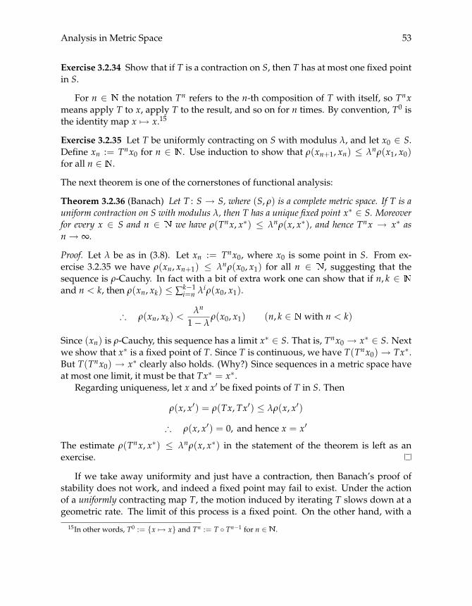
Analysis in Metric Space 53
Exercise 3.2.34 Show that if T is a contraction on S, then T has at most one fixed pointin S.
For n ∈ the notation Tn refers to the n-th composition of T with itself, so Tnxmeans apply T to x, apply T to the result, and so on for n times. By convention, T0 isthe identity map x �→ x.15
Exercise 3.2.35 Let T be uniformly contracting on S with modulus λ, and let x0 ∈ S.Define xn := Tnx0 for n ∈ . Use induction to show that ρ(xn+1, xn) ≤ λnρ(x1, x0)for all n ∈ .
The next theorem is one of the cornerstones of functional analysis:
Theorem 3.2.36 (Banach) Let T : S → S, where (S, ρ) is a complete metric space. If T is auniform contraction on S with modulus λ, then T has a unique fixed point x∗ ∈ S. Moreoverfor every x ∈ S and n ∈ we have ρ(Tnx, x∗) ≤ λnρ(x, x∗), and hence Tnx → x∗ asn→ ∞.
Proof. Let λ be as in (3.8). Let xn := Tnx0, where x0 is some point in S. From ex-ercise 3.2.35 we have ρ(xn, xn+1) ≤ λnρ(x0, x1) for all n ∈ , suggesting that thesequence is ρ-Cauchy. In fact with a bit of extra work one can show that if n, k ∈and n < k, then ρ(xn, xk) ≤ ∑k−1
i=n λiρ(x0, x1).
∴ ρ(xn, xk) <λn
1− λρ(x0, x1) (n, k ∈ with n < k)
Since (xn) is ρ-Cauchy, this sequence has a limit x∗ ∈ S. That is, Tnx0 → x∗ ∈ S. Nextwe show that x∗ is a fixed point of T. Since T is continuous, we have T(Tnx0)→ Tx∗.But T(Tnx0) → x∗ clearly also holds. (Why?) Since sequences in a metric space haveat most one limit, it must be that Tx∗ = x∗.
Regarding uniqueness, let x and x′ be fixed points of T in S. Then
ρ(x, x′) = ρ(Tx, Tx′) ≤ λρ(x, x′)
∴ ρ(x, x′) = 0, and hence x = x′
The estimate ρ(Tnx, x∗) ≤ λnρ(x, x∗) in the statement of the theorem is left as anexercise.
If we take away uniformity and just have a contraction, then Banach’s proof ofstability does not work, and indeed a fixed point may fail to exist. Under the actionof a uniformly contracting map T, the motion induced by iterating T slows down at ageometric rate. The limit of this process is a fixed point. On the other hand, with a
15In other words, T0 := {x �→ x} and Tn := T ◦ Tn−1 for n ∈ .
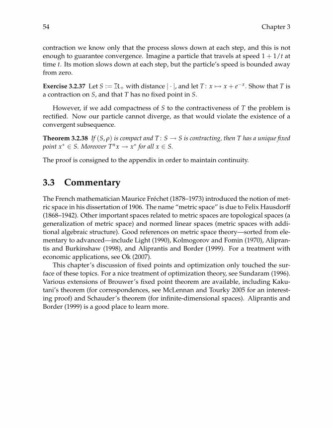
54 Chapter 3
contraction we know only that the process slows down at each step, and this is notenough to guarantee convergence. Imagine a particle that travels at speed 1 + 1/t attime t. Its motion slows down at each step, but the particle’s speed is bounded awayfrom zero.
Exercise 3.2.37 Let S := + with distance | · |, and let T : x �→ x+ e−x. Show that T isa contraction on S, and that T has no fixed point in S.
However, if we add compactness of S to the contractiveness of T the problem isrectified. Now our particle cannot diverge, as that would violate the existence of aconvergent subsequence.
Theorem 3.2.38 If (S, ρ) is compact and T : S→ S is contracting, then T has a unique fixedpoint x∗ ∈ S. Moreover Tnx → x∗ for all x ∈ S.
The proof is consigned to the appendix in order to maintain continuity.
3.3 Commentary
The French mathematician Maurice Fréchet (1878–1973) introduced the notion of met-ric space in his dissertation of 1906. The name “metric space” is due to Felix Hausdorff(1868–1942). Other important spaces related to metric spaces are topological spaces (ageneralization of metric space) and normed linear spaces (metric spaces with addi-tional algebraic structure). Good references on metric space theory—sorted from ele-mentary to advanced—include Light (1990), Kolmogorov and Fomin (1970), Alipran-tis and Burkinshaw (1998), and Aliprantis and Border (1999). For a treatment witheconomic applications, see Ok (2007).
This chapter’s discussion of fixed points and optimization only touched the sur-face of these topics. For a nice treatment of optimization theory, see Sundaram (1996).Various extensions of Brouwer’s fixed point theorem are available, including Kaku-tani’s theorem (for correspondences, see McLennan and Tourky 2005 for an interest-ing proof) and Schauder’s theorem (for infinite-dimensional spaces). Aliprantis andBorder (1999) is a good place to learn more.
Chapter 4
Introduction to Dynamics
4.1 Deterministic Dynamical Systems
Having covered programming and metric spaces in some depth, we now possess am-ple tools for analysis of dynamics. After starting with deterministic dynamical sys-tems, setting up the basic theory and the notion of stability, we turn to stochasticmodels, where evolution of the state variable is affected by noise. While deterministicsystems are clearly a kind of stochastic system (with zero-variance noise), we will seethat the converse is also true: Stochastic models can be embedded in the determin-istic framework. Through this embedding we can study the dynamic properties ofstochastic systems using our knowledge of the deterministic model.
4.1.1 The Basic Model
Suppose that we are observing the time path of some variable x in a metric space S. Att, the current state of the system is denoted by xt. Assume that from the current state xtwe can compute the time t+ 1 value xt+1 by applying a map h. That is, xt+1 = h(xt).The two primitives that make up this system are S and h:
Definition 4.1.1 A dynamical system is a pair (S, h), where S = (S, ρ) is an arbitrarymetric space and h is a map from S into itself.
By the n-th iterate of x ∈ S under hwe mean hn(x). It is conventional to set h0(x) :=x. The trajectory of x ∈ S under h is the sequence (ht(x))t≥0. As before, x∗ ∈ S isa fixed point of h in S if h(x∗) = x∗. Fixed points are also said to be stationary orinvariant under h.1 Figure 4.1 illustrates the dynamics of one particular map h on 2
1Similar terminology applies to sets. For example, if h(A) ⊂ A, then A is said to be invariant under h.
55
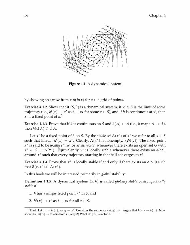
56 Chapter 4
Figure 4.1 A dynamical system
by showing an arrow from x to h(x) for x ∈ a grid of points.
Exercise 4.1.2 Show that if (S, h) is a dynamical system, if x′ ∈ S is the limit of sometrajectory (i.e., ht(x) → x′ as t → ∞ for some x ∈ S), and if h is continuous at x′, thenx′ is a fixed point of h.2
Exercise 4.1.3 Prove that if h is continuous on S and h(A) ⊂ A (i.e., h maps A → A),then h(cl A) ⊂ cl A.
Let x∗ be a fixed point of h on S. By the stable set Λ(x∗) of x∗ we refer to all x ∈ Ssuch that limt→∞ ht(x) = x∗. Clearly, Λ(x∗) is nonempty. (Why?) The fixed pointx∗ is said to be locally stable, or an attractor, whenever there exists an open set G withx∗ ∈ G ⊂ Λ(x∗). Equivalently x∗ is locally stable whenever there exists an ε-ballaround x∗ such that every trajectory starting in that ball converges to x∗:
Exercise 4.1.4 Prove that x∗ is locally stable if and only if there exists an ε > 0 suchthat B(ε, x∗) ⊂ Λ(x∗).
In this book we will be interested primarily in global stability:
Definition 4.1.5 A dynamical system (S, h) is called globally stable or asymptoticallystable if
1. h has a unique fixed point x∗ in S, and
2. ht(x)→ x∗ as t→ ∞ for all x ∈ S.
2Hint: Let xt := ht(x), so xt → x′. Consider the sequence (h(xt))t≥1. Argue that h(xt) → h(x′). Nowshow that h(xt)→ x′ also holds. (Why?!) What do you conclude?

Introduction to Dynamics 57
Figure 4.2 Global stability
Exercise 4.1.6 Prove that if x∗ is a fixed point of (S, h) to which every trajectory con-verges, then x∗ is the only fixed point of (S, h).
Figure 4.2 helps to visualize the concept of global stability, plotting 20 individualtrajectories of a stable map h on 2. Figure 4.3 also illustrates global stability, in thiscase for the one-dimensional system (S, h), where S := (0,∞) and h(k) := sAkα withs ∈ (0, 1], A > 0 and α ∈ (0, 1). The system represents a simple Solow–Swan growthmodel, where next period’s capital stock h(k) is the savings rate s times current outputAkα. The value A is a productivity parameter and α is the capital intensity. Figure 4.3is called a 45 degree diagram. When the curve h lies above (resp., below) the 45 degreeline we have h(k) > k (resp., h(k) < k), and hence the trajectory moves to the right(resp., left). Two trajectories are shown, converging to the unique fixed point k∗.
Regarding local stability of (S, h) when S is an open subset of , it is well-knownthat
Lemma 4.1.7 If h is a map with continuous derivative h′ and x∗ is a fixed point of h with|h′(x∗)| < 1, then x∗ is locally stable.
The most enthusiastic readers might like to attempt a proof, although the lemmais not particularly central to what follows.
Example 4.1.8 Consider a growth model with “threshold” nonconvexities of the formkt+1 = sA(kt)kαt , where s ∈ (0, 1] and k �→ A(k) is some increasing function with

58 Chapter 4
k∗ kt
kt+1
Figure 4.3 45 degree diagram
A(k) > 0 when k > 0. Suppose, for example, that A is a step function of the form
A(k) =
{A1 if 0 < k < kbA2 if kb ≤ k < ∞
Here kb is a “threshold” value of capital stock, and 0 < A1 < A2. Let k∗i be thesolution to k = sAikα for i = 1, 2 when it exists. A plot is given in figure 4.4 for thecase where k∗1 < kb < k∗2. The two fixed points k∗1 and k∗2 are local attractors, as can beverified from lemma 4.1.7. Long-run outcomes depend on initial conditions, and forthis reason the model is said to exhibit path dependence.
Exercise 4.1.9 A dynamical system (S, h) is called Lagrange stable if every trajectoryis precompact in S. In other words, the set {hn(x) : n ∈ } is precompact for everyx ∈ S.3 Show that if S is a closed and bounded subset of n, then (S, h) is Lagrangestable for any choice of h.
Exercise 4.1.10 Give an example of a dynamical system (S, h) where S is unboundedbut (S, h) is Lagrange stable.
Exercise 4.1.11 Let S = , and let h : → be an increasing function, in the sensethat if x ≤ y, then h(x) ≤ h(y). Show that every trajectory of h is a monotone sequencein (either increasing or decreasing).
3Equivalently every subsequence of the trajectory has a convergent subsubsequence.

Introduction to Dynamics 59
k∗1 k∗
2kb kt
kt+1
Figure 4.4 Threshold externalities
Exercise 4.1.12 Now order points in n by setting x ≤ y whenever xi ≤ yi for i in{1, . . . , n} (i.e., each component of x is dominated by the corresponding componentof y). Let S = n, and let h : S → S be monotone increasing. (The definition is thesame.) Show that the same result no longer holds—h does not necessarily generatemonotone trajectories.
4.1.2 Global Stability
Global stability will be a key concept for the remainder of the text. Let’s start ourinvestigation of global stability by looking at linear (more correctly, affine) systems inone dimension.
Exercise 4.1.13 Let S = ( , | · |) and h(x) = ax+ b. Prove that
ht(x) = atx+ bt−1
∑i=0
ai (x ∈ S, t ∈ )
(Hint: Use induction.) From this expression, prove that (S, h) is globally stable when-ever |a| < 1, and exhibit the fixed point.
Exercise 4.1.14 Show that the condition |a| < 1 is also necessary, in the sense that if|a| ≥ 1, then (S, h) is not globally stable. Show, in particular, that ht(x0) converges tox∗ := b/(1− a) only if x0 = x∗.

60 Chapter 4
In exercise 4.1.13 we found a direct proof of global stability for our affine systemwhen |a| < 1. For more complex systems direct methods are usually unavailable,and we must deploy more powerful machinery, such as Banach’s fixed point theorem(theorem 3.2.36 on page 53).
Exercise 4.1.15 Let (S, h) be as in exercise 4.1.13. Using theorem 3.2.36, prove that(S, h) is globally stable whenever |a| < 1.
Exercise 4.1.16 Let S := (0,∞) with ρ(x, y) := | ln x − ln y|. Prove that ρ is a metricon S and that (S, ρ) is a complete metric space.4 Consider the growth model kt+1 =h(kt) = sAkαt in figure 4.3, where s ∈ (0, 1], A > 0 and α ∈ (0, 1). Convert this into adynamical system on (S, ρ), and prove global stability using theorem 3.2.36.
Next we consider linear systems in n. In general, a function h : n → n is calledlinear if
h(αx+ βy) = αh(x) + βh(y) ∀ x, y ∈ n ∀ α, β ∈ (4.1)
It can be shown that every such h is continuous. If E is an n× n matrix, then the mapon n defined by x �→ Ex is linear. In fact it can be shown that for all linear mapsh : n → n there exists a matrix Eh with h(x) = Ehx for all x ∈ n. An affine systemon n is a map h : n → n given by
h(x) = Ex+ b where E is an n× n matrix and b ∈ n
To investigate this system, let ‖ · ‖ be any norm on n, and define
λ := max{‖Ex‖ : x ∈ n, ‖x‖ = 1} (4.2)
Exercise 4.1.17 If you can, prove that the maximum exists. Using the properties ofnorms and linearity of E, show that ‖Ex‖ ≤ λ‖x‖ for all x ∈ n. Show in additionthat if λ < 1, then ( n, h) is globally stable.
Let’s look at an application of these ideas. In a well-known paper, Long andPlosser (1983) studied the modeling of business cycles using multisector growth mod-els. After solving their model, they find a system for log output given by yt+1 =Ayt + b. Here A = (aij) is a matrix of input/output elasticities across sectors, and ytis a 6× 1 vector recording output in agriculture, mining, construction, manufactur-ing, transportation and services.5 Using cost share data and the hypothesis of perfect
4Hint: Take a Cauchy sequence (xn) in (S, ρ), and map it into (ln xn), which is a sequence in ( , | · |).Prove this sequence is Cauchy in ( , | · |), and therefore converges to some y ∈ . Now prove that xn → ey
in (S, ρ).5In their model b is random, but let’s ignore this complication for now.

Introduction to Dynamics 61
competition, the authors calculate A to be given by
A = (aij) =
⎛⎜⎜⎜⎜⎜⎜⎝
0.45 0.00 0.01 0.21 0.10 0.160.00 0.09 0.04 0.17 0.05 0.490.00 0.01 0.00 0.42 0.12 0.090.06 0.03 0.01 0.46 0.06 0.130.00 0.00 0.02 0.12 0.10 0.320.02 0.02 0.06 0.20 0.09 0.38
⎞⎟⎟⎟⎟⎟⎟⎠
Exercise 4.1.18 Prove that Long and Plosser’s system is stable in the following way:Let A = (aij) be an n× n matrix where the sum of any of the rows of A is strictly lessthan 1 (i.e., maxi αi < 1, where αi := ∑j |aij|). Using the norm ‖ · ‖∞ in (4.2), show thatfor A we have λ < 1. Now argue that in Long and Plosser’s model, (yt) convergesto a limit y∗, which is independent of initial output y0, and, moreover, is the uniquesolution to the equation y∗ = Ay∗ + b.6
Exercise 4.1.19 Let B = (bij) be an n× n matrix where the sum of any of the columnsof B is strictly less than 1 (i.e., maxj β j < 1, where β j := ∑i |bij|). Using the norm ‖ · ‖1in (4.2), show that for B we have λ < 1. Conclude that if h(x) = Bx+ b, then ( n, h)is globally stable.
The following results will be needed later in the text:
Exercise 4.1.20 Suppose that h is uniformly contracting on complete space S, so (S, h)is globally stable. Prove that if A ⊂ S is nonempty, closed and invariant under h (i.e.,h(A) ⊂ A), then the fixed point of h lies in A.
Lemma 4.1.21 Let (S, h) be a dynamical system. If h is nonexpansive and (S, hN) is globallystable for some N ∈ , then (S, h) is globally stable.
Proof. By hypothesis, hN has a unique fixed point x∗ in S, and hkN(x)→ x∗ as k → ∞for all x ∈ S. Pick any ε > 0, and choose k ∈ so that ρ(hkN(h(x∗)), x∗) < ε. Then
ρ(h(x∗), x∗) = ρ(h(hkN(x∗)), x∗) = ρ(hkN(h(x∗)), x∗) < ε
It follows that x∗ is a fixed point of h. (Why?)Stability: Fix x ∈ S and ε > 0. Choose k ∈ so that ρ(hkN(x), x∗) < ε. Then
nonexpansiveness implies that for each n ≥ kN,
ρ(hn(x), x∗) = ρ(hn−kN(hkN(x)), x∗) ≤ ρ(hkN(x), x∗) < ε
In other words, (S, h) is globally stable.
6You are proving d∞-convergence of trajectories, but this is equivalent to d2-convergence by theo-rem 3.2.30.
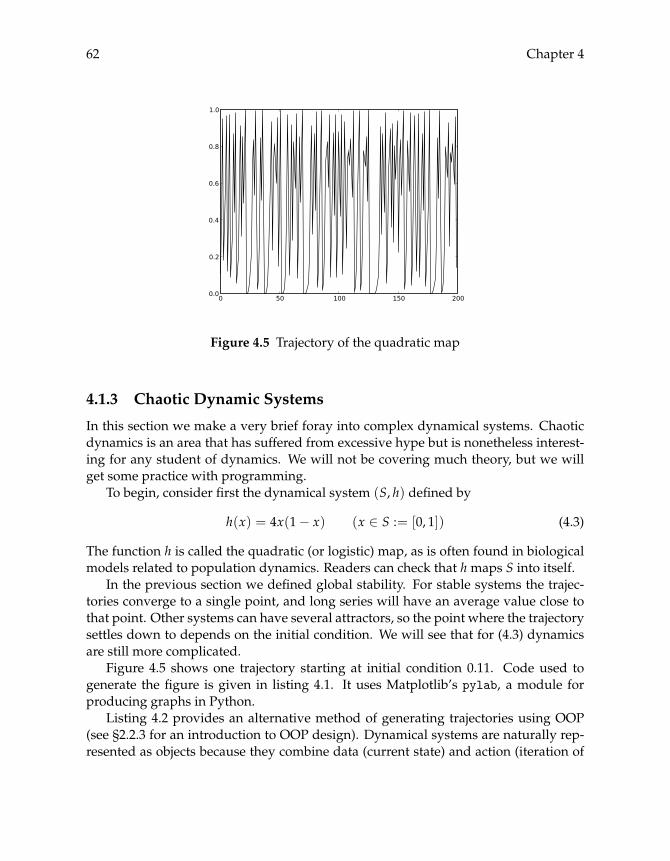
62 Chapter 4
Figure 4.5 Trajectory of the quadratic map
4.1.3 Chaotic Dynamic Systems
In this section we make a very brief foray into complex dynamical systems. Chaoticdynamics is an area that has suffered from excessive hype but is nonetheless interest-ing for any student of dynamics. We will not be covering much theory, but we willget some practice with programming.
To begin, consider first the dynamical system (S, h) defined by
h(x) = 4x(1− x) (x ∈ S := [0, 1]) (4.3)
The function h is called the quadratic (or logistic) map, as is often found in biologicalmodels related to population dynamics. Readers can check that h maps S into itself.
In the previous section we defined global stability. For stable systems the trajec-tories converge to a single point, and long series will have an average value close tothat point. Other systems can have several attractors, so the point where the trajectorysettles down to depends on the initial condition. We will see that for (4.3) dynamicsare still more complicated.
Figure 4.5 shows one trajectory starting at initial condition 0.11. Code used togenerate the figure is given in listing 4.1. It uses Matplotlib’s pylab, a module forproducing graphs in Python.
Listing 4.2 provides an alternative method of generating trajectories using OOP(see §2.2.3 for an introduction to OOP design). Dynamical systems are naturally rep-resented as objects because they combine data (current state) and action (iteration of

Introduction to Dynamics 63
Listing 4.1 (quadmap1.py) Trajectories of the quadratic map
from pylab impor t plot , show # Requires Matplotlib
datapoints = [] # Stores trajectoryx = 0.11 # Initial conditionf o r t i n range (200):
datapoints.append(x)x = 4 * x * (1 - x)
plot(datapoints)show()
the map). Here we define a class DS that is an abstraction of a dynamical system. Theclass definition is relatively self-explanatory. Although the use of OOP is perhaps ex-cessive for this simple problem, one can see how abstraction facilitates code reuse: DScan be used to generate trajectories for any dynamical system. An example of usageis given in listing 4.3.
Notice that in figure 4.5 the trajectory continues to traverse through the space with-out settling down. Some experimentation shows that this happens for many initialconditions (but not all—does the map have any fixed points?). Moreover a slightvariation in the initial condition typically leads to a time series that bears no clearresemblance to the previous one.
Science and mathematics are all about simplification and reduction. For example,with a globally stable system we can usually focus our attention on the steady state.(How does this state fit with the data?) From this perspective figure 4.5 is a littledistressing. Unless the initial conditions are very special and can be known exactly, itseems that long run outcomes cannot be predicted.7 However, this conclusion is toopessimistic, as the next exercise illustrates.
Exercise 4.1.22 Using your preferred plotting tool, histogram some trajectories gener-ated by the quadratic map, starting at different initial conditions. Use relatively longtrajectories (e.g., around 5,000 points), and a fine histogram (about 40 bins). Whatregularities can you observe?
Incidentally, the time series in figure 4.5 looks quite random, and in exercise 4.1.22we treated the trajectory in a “statistical” way, by computing its histogram. Is there in
7Which is problematic for a scientific study—what falsifiable implications can be drawn from thesemodels?

64 Chapter 4
Listing 4.2 (ds.py) An abstract dynamical system
c l a s s DS:
de f __init__(self , h=None, x=None):"""Parameters: h is a function and x is a numberin S representing the current state."""self.h, self.x = h, x
de f update(self):"Update the state of the system by applying h."self.x = self.h(self.x)
de f trajectory(self , n):"""Generate a trajectory of length n, startingat the current state."""traj = []f o r i i n range(n):
traj.append(self.x)self.update ()
r e t u r n traj
Listing 4.3 (testds.py) Example application
from ds impor t DS # Import from listing 4.2
de f quadmap(x):r e t u r n 4 * x * (1 - x)
q = DS(h=quadmap , x=0.1) # Create an instance q of DST1 = q.trajectory (100) # T1 holds trajectory from 0.1
q.x = 0.2 # Reset current state to 0.2T2 = q.trajectory (100) # T2 holds trajectory from 0.2
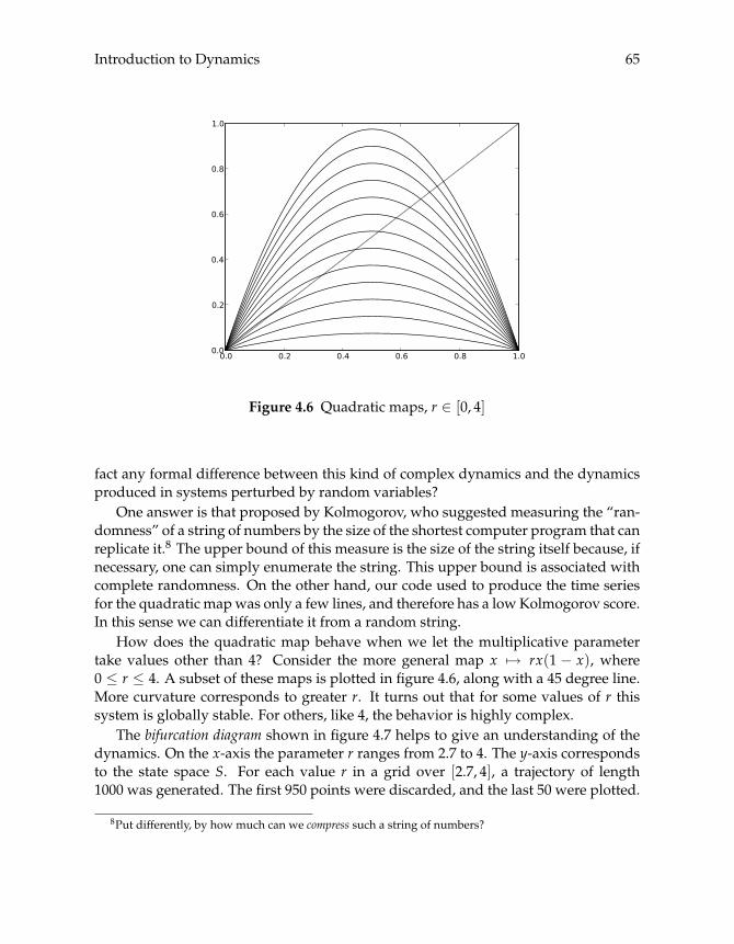
Introduction to Dynamics 65
Figure 4.6 Quadratic maps, r ∈ [0, 4]
fact any formal difference between this kind of complex dynamics and the dynamicsproduced in systems perturbed by random variables?
One answer is that proposed by Kolmogorov, who suggested measuring the “ran-domness” of a string of numbers by the size of the shortest computer program that canreplicate it.8 The upper bound of this measure is the size of the string itself because, ifnecessary, one can simply enumerate the string. This upper bound is associated withcomplete randomness. On the other hand, our code used to produce the time seriesfor the quadratic map was only a few lines, and therefore has a low Kolmogorov score.In this sense we can differentiate it from a random string.
How does the quadratic map behave when we let the multiplicative parametertake values other than 4? Consider the more general map x �→ rx(1 − x), where0 ≤ r ≤ 4. A subset of these maps is plotted in figure 4.6, along with a 45 degree line.More curvature corresponds to greater r. It turns out that for some values of r thissystem is globally stable. For others, like 4, the behavior is highly complex.
The bifurcation diagram shown in figure 4.7 helps to give an understanding of thedynamics. On the x-axis the parameter r ranges from 2.7 to 4. The y-axis correspondsto the state space S. For each value r in a grid over [2.7, 4], a trajectory of length1000 was generated. The first 950 points were discarded, and the last 50 were plotted.
8Put differently, by how much can we compress such a string of numbers?

66 Chapter 4
Figure 4.7 Bifurcation diagram
For r ≤ 3, interior points converge to a unique interior steady state. For r ∈ (3, 1 +√6], the state eventually oscillates between two “periodic attractors.” From there
the number of periodic attractors increases rapidly, and the behavior of the systembecomes correspondingly more “chaotic.”
Exercise 4.1.23 Reproduce figure 4.7 using Python to generate the data and your pre-ferred plotting tool.
4.1.4 Equivalent Dynamics and Linearization
In general, nonlinear models are much more difficult to analyze than linear models,leading researchers to approximate nonlinear models with linearized versions. Thelatter are usually obtained by a first-order Taylor expansion. Since fixed points are thenatural focus of analysis, it is standard to take expansions around fixed points.
Let us see how this is done in the one-dimensional case. Let (S, h) be a dynamicalsystem where S is an open subset of , and h is continuously differentiable, withderivative h′ on S. Pick any a ∈ S. The first-order Taylor expansion around a is themap h1 defined by
h1(x) = h(a) + h′(a)(x− a) (4.4)
Notice that h1 is an affine function on with h(a) = h1(a). Clearly, h1 approximates
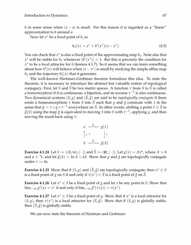
Introduction to Dynamics 67
h in some sense when |x − a| is small. For this reason it is regarded as a “linear”approximation to h around a.
Now let x∗ be a fixed point of h, so
h1(x) = x∗ + h′(x∗)(x− x∗) (4.5)
You can check that x∗ is also a fixed point of the approximating map h1. Note also thatx∗ will be stable for h1 whenever |h′(x∗)| < 1. But this is precisely the condition forx∗ to be a local attractor for h (lemma 4.1.7). So it seems that we can learn somethingabout how ht(x) will behave when |x− x∗| is small by studying the simple affine maph1 and the trajectory ht1(x) that it generates.
The well-known Hartman–Grobman theorem formalizes this idea. To state thetheorem, it is necessary to introduce the abstract but valuable notion of topologicalconjugacy. First, let S and S be two metric spaces. A function τ from S to S is calleda homeomorphism if it is continuous, a bijection, and its inverse τ−1 is also continuous.Two dynamical systems (S, g) and (S, g) are said to be topologically conjugate if thereexists a homeomorphism τ from S into S such that g and g commute with τ in thesense that g = τ ◦ g ◦ τ−1 everywhere on S. In other words, shifting a point x ∈ S tog(x) using the map g is equivalent to moving x into S with τ−1, applying g, and thenmoving the result back using τ:
xg−−−−→ g(x)�⏐⏐τ−1
⏐⏐�τ
xg−−−−→ g(x)
Exercise 4.1.24 Let S := ((0,∞), | · |) and S := ( , | · |). Let g(x) = Axα, where A > 0and α ∈ , and let g(x) = ln A+ αx. Show that g and g are topologically conjugateunder τ := ln.
Exercise 4.1.25 Show that if (S, g) and (S, g) are topologically conjugate, then x∗ ∈ Sis a fixed point of g on S if and only if τ(x∗) ∈ S is a fixed point of g on S.
Exercise 4.1.26 Let x∗ ∈ S be a fixed point of g and let x be any point in S. Show thatlimt→∞ gt(x) = x∗ if and only if limt→∞ gt(τ(x)) = τ(x∗).
Exercise 4.1.27 Let x∗ ∈ S be a fixed point of g. Show that if x∗ is a local attractor for(S, g), then τ(x∗) is a local attractor for (S, g). Show that if (S, g) is globally stable,then (S, g) is globally stable.
We can now state the theorem of Hartman and Grobman:
68 Chapter 4
Theorem 4.1.28 (Hartman–Grobman) Let S be an open subset of , let h : S → S be acontinuously differentiable function, let x∗ ∈ S be a fixed point of h, and let h1 be the Taylorapproximation in (4.5). If |h′(x∗)| �= 1, then there exists an open set G containing x∗ suchthat h and h1 are topologically conjugate on G.9
Be careful when applying this theorem, which is one of the most misused math-ematical results in all of economics. It provides only a neighborhood of S such thatbehavior of the approximation is qualitatively similar to that of the original system. Asit stands, the Hartman–Grobman theorem provides no basis for quantitative analysis.
4.2 Finite State Markov Chains
Next we start our journey into the world of stochastic dynamics. Stochastic dynamicsis a technically demanding field, mainly because any serious attempt at probabilitytheory on general state spaces requires at least a modicum of measure theory. Fornow we concentrate on finite state spaces, where measure theory is unnecessary. How-ever, our treatment of finite state stochastic dynamics is geared in every way towardbuilding understanding, intuition, notation and tools that will be used in the general(uncountable state) case.
4.2.1 Definition
We begin with a state space S, which is a finite set {x1, . . . , xN}. A typical elementof S is usually denoted by x, rather than a symbol such as xi or xn. This makes ournotation more consistent with the continuous state theory developed below. The setof distributions on S will be denotedP(S), and consists of all functions φ : S→ withφ(x) ≥ 0 for all x ∈ S, and ∑x∈S φ(x) = 1. In general, φ(x) will correspond to theprobability attached to the point x in the state space under some given scenario.10
A quick digression: Although φ has been introduced as a function from S to ,one can also think of it as a vector under the one-to-one correspondence
P(S) � φ↔ (φ(x))x∈S := (φ(x1), . . . , φ(xN)) ∈ N (4.6)
Under the correspondence (4.6), the collection of functionsP(S) becomes a subset ofthe vector space N—in particular, the elements of N that are nonnegative and sumto one. This set is called the unit simplex, and is illustrated for the case of N = 3 infigure 4.8.
The basic primitive for a discrete time Markov process on S is a stochastic kernel,the definition of which is as follows.
9To see why |h′(x∗)| �= 1 is important, consider the case of h(x) = arctan(x).10What we call a distribution here is also referred to as a probability mass function.

Introduction to Dynamics 69
Figure 4.8 The unit simplex with N = 3
Definition 4.2.1 A stochastic kernel p is a function from S× S into [0, 1] such that
1. p(x, y) ≥ 0 for each (x, y) in S× S, and
2. ∑y∈S p(x, y) = 1 for each x ∈ S.
In other words, the function S � y �→ p(x, y) ∈ is an element ofP(S) for all x ∈ S.This distribution is represented by the symbol p(x, dy) in what follows.
As well as being a function, the distribution p(x, dy) can be viewed as a row11
vector (p(x, x1), . . . , p(x, xN)) in N , located in the unit simplex, and these rows canbe stacked horizontally to produce an N × N matrix with the property that each rowis nonnegative and sums to one:
p =
⎛⎜⎝
p(x1, dy)...
p(xN , dy)
⎞⎟⎠ =
⎛⎜⎝
p(x1, x1) · · · p(x1, xN)...
...p(xN , x1) · · · p(xN , xN)
⎞⎟⎠ (4.7)
Conversely, any square N × N matrix that is nonnegative and has all rows summingto one defines a stochastic kernel. However, when we move on to infinite state spacesthere is no concept of matrices, and hence most of the theory is stated in terms ofkernels.
11When treating distributions as vectors it is traditional in the Markov chain literature to regard them asrow vectors.
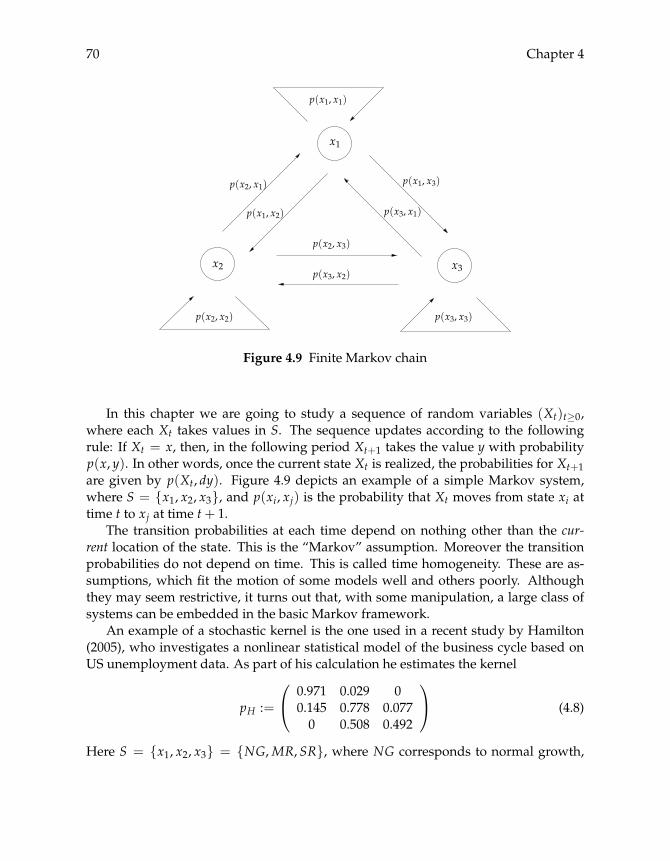
70 Chapter 4
p(x2, x1)
x1
x2 x3
p(x1, x2)
p(x2, x3)
p(x3, x2)
p(x3, x1)
p(x1, x3)
p(x1, x1)
p(x3, x3)p(x2, x2)
Figure 4.9 Finite Markov chain
In this chapter we are going to study a sequence of random variables (Xt)t≥0,where each Xt takes values in S. The sequence updates according to the followingrule: If Xt = x, then, in the following period Xt+1 takes the value y with probabilityp(x, y). In other words, once the current state Xt is realized, the probabilities for Xt+1are given by p(Xt, dy). Figure 4.9 depicts an example of a simple Markov system,where S = {x1, x2, x3}, and p(xi, xj) is the probability that Xt moves from state xi attime t to xj at time t+ 1.
The transition probabilities at each time depend on nothing other than the cur-rent location of the state. This is the “Markov” assumption. Moreover the transitionprobabilities do not depend on time. This is called time homogeneity. These are as-sumptions, which fit the motion of some models well and others poorly. Althoughthey may seem restrictive, it turns out that, with some manipulation, a large class ofsystems can be embedded in the basic Markov framework.
An example of a stochastic kernel is the one used in a recent study by Hamilton(2005), who investigates a nonlinear statistical model of the business cycle based onUS unemployment data. As part of his calculation he estimates the kernel
pH :=
⎛⎝ 0.971 0.029 0
0.145 0.778 0.0770 0.508 0.492
⎞⎠ (4.8)
Here S = {x1, x2, x3} = {NG, MR, SR}, where NG corresponds to normal growth,

Introduction to Dynamics 71
MR to mild recession, and SR to severe recession. For example, the probability oftransitioning from severe recession to mild recession in one period is 0.508. The lengthof the period is one month.
For another example of a Markov model, consider the growth dynamics study ofQuah (1993), who analyzes the evolution of real GDP per capita relative to the worldaverage for a “typical” country (e.g., Xt = 2 implies that income per capita for thecountry in question is twice the world average at time t). A natural state space is +,but to simplify matters Quah discretizes this space into five bins that correspond tovalues for relative GDP of 0 to 0.25, 0.25 to 0.5, 0.5 to 1, 1 to 2 and 2 to ∞ respectively.He then calculates the stochastic kernel by setting p(x, y) equal to the fraction of timesthat a country, finding itself in state x, subsequently makes the transition to state y.12
The result of this calculation is
pQ :=
⎛⎜⎜⎜⎜⎝
0.97 0.03 0.00 0.00 0.000.05 0.92 0.03 0.00 0.000.00 0.04 0.92 0.04 0.000.00 0.00 0.04 0.94 0.020.00 0.00 0.00 0.01 0.99
⎞⎟⎟⎟⎟⎠ (4.9)
For example, the probability of our typical country transitioning from the lowest binto the second lowest bin in one year is 0.03.
Algorithm 4.1 Simulation of a Markov chain
draw X0 ∼ ψ and set t = 0while True do // "while True" means repeat forever
draw Xt+1 ∼ p(Xt, dy)set t = t+ 1
end
Let us now try to pin down the definition of a Markov chain (Xt)t≥0 correspondingto a given stochastic kernel p. It is helpful to imagine that we wish to simulate (Xt)t≥0on a computer. First we draw X0 from some predetermined initial condition ψ ∈P(S).As p(x, dy) gives the transition probabilities for Xt+1 conditional on Xt = x, we nowdraw X1 from p(X0, dy). Taking the result X1, we then draw X2 from p(X1, dy), andso on. This is the content of algorithm 4.1, as well as the next definition.
Definition 4.2.2 Let ψ ∈ P(S). A sequence of S-valued random variables (Xt)t≥0 iscalled Markov-(p,ψ) if
12His data span the period 1962 to 1984, and have a sample of 118 countries. The transitions are over aone year period. The model is assumed to be stationary (transition probabilities do not vary with time), soall of the transitions (1962 to 1963, 1963 to 1964, etc.) can be pooled when calculating transition probabilities.

72 Chapter 4
1
1.5
2
2.5
3
0 200 400 600 800 1000
Figure 4.10 Simulation of the chain
1. at time zero, X0 is drawn from ψ, and
2. at time t+ 1, Xt+1 is drawn from p(Xt, dy).
If ψ(x) = 1 for some x ∈ S, then (Xt)t≥0 is called Markov-(p, x).
Let’s try simulating a Markov-(p,ψ) chain. One method is given in listing 4.4.The function sample() defined at the top is used to generate draws from a givenfinite distribution using the inverse transform algorithm.13 Next we define a class MC,which is similar to the class DS in listing 4.2 (page 64). An instance is initialized witha stochastic kernel p and an initial state X. The kernel p should be such that p[x] is asequence representing p(x, dy)—see listing 4.5 for an example. The method update()updates the current state using sample(), drawing Xt+1 from p(Xt, dy).14
In listing 4.5 an instance h of MC is created for Hamilton’s stochastic kernel pH ,and the sample_path() method is used to produce some time series. In the code,genfinitemc is the name of the file in listing 4.4. Figure 4.10 shows a simulated series.
4.2.2 Marginal Distributions
Let (Xt)t≥0 be Markov-(p,ψ). For every t ∈ , let ψt ∈ P(S) denote the distributionof Xt. That is, ψt(y) is the probability that Xt = y, given that X0 is draw from initial
13There are existing libraries that can do this job, but the technique used in sample() is something wewill revisit later on (see algorithm 5.3 on page 109), and we present it here for future reference. Don’t beconcerned if the logic is not yet clear.
14All of this code is written for clarity rather than speed, and is suitable only for small state spaces. Seethe text home page for more efficient methods.

Introduction to Dynamics 73
Listing 4.4 (genfinitemc.py) Finite Markov chain
from random impor t uniform
de f sample(phi):"""Returns i with probability phi[i], where phi is anarray (e.g., list or tuple)."""a = 0.0U = uniform (0,1)f o r i i n range(len(phi)):
i f a < U <= a + phi[i]:r e t u r n i
a = a + phi[i]
c l a s s MC:"""For generating sample paths of finite Markov chainson state space S = {0,...,N-1}."""
de f __init__(self , p=None, X=None):"""Create an instance with stochastic kernel p andcurrent state X. Here p[x] is an array of length Nfor each x, and represents p(x,dy).The parameter X is an integer in S."""self.p, self.X = p, X
de f update(self):"Update the state by drawing from p(X,dy)."self.X = sample(self.p[self.X])
de f sample_path(self , n):"""Generate a sample path of length n, starting fromthe current state."""path = []f o r i i n range(n):
path.append(self.X)self.update ()
r e t u r n path

74 Chapter 4
Listing 4.5 (testgenfinitemc.py) Example application
from genfinitemc impor t sample , MC # Import from listing 4.4
pH = ((0.971 , 0.029, 0.000) ,(0.145 , 0.778 , 0.077) ,(0.000 , 0.508 , 0.492))
psi = (0.3, 0.4, 0.3) # Initial conditionh = MC(p=pH, X=sample(psi)) # Create an instance of class MCT1 = h.sample_path (1000) # Series is Markov -(p, psi)
psi2 = (0.8, 0.1, 0.1) # Alternative initial conditionh.X = sample(psi2) # Reset the current stateT2 = h.sample_path (1000) # Series is Markov -(p, psi2)
distribution ψ, and that the chain subsequently follows Xt+1 ∼ p(Xt, dy). This dis-tribution is sometimes called the marginal or unconditional distribution of Xt. We canunderstand it as follows: Generate n independent realizations of Xt, and calculate thefraction that takes the value y. Call this number ψn
t (y). The probability ψt(y) can bethought of as the limit of ψn
t (y) as n→ ∞.
A method for computing the fraction ψnt (y) is given in algorithm 4.2. In the algo-
rithm, the instruction draw X ∼ p(X, dy) should be interpreted as: Draw a randomvariable Y according to the distribution p(X, dy) and then set X = Y. Also, {Xi
t = y}is an indicator function, equal to one when Xi
t = y and zero otherwise.
Algorithm 4.2 Approximate marginal distribution
for i in 1 to n dodraw X ∼ ψ
for j in 1 to t dodraw X ∼ p(X, dy)
endset Xi
t = Xendreturn (1/n)∑n
i=1 {Xit = y}
Introduction to Dynamics 75
Exercise 4.2.3 Implement algorithm 4.2 for Hamilton’s Markov chain.15 Set ψ =(0, 0, 1), so the economy starts in severe recession with probability one. Computean approximation to ψt(y), where t = 10 and y = NG. For sufficiently large n youshould get an answer close to 0.6.
Exercise 4.2.4 Rewrite algorithm 4.2 using a counter that increments by one wheneverthe output of the inner loop produces a value equal to y instead of recording the valueof each Xi
t.
Now consider again a Markov-(p,ψ) chain (Xt)t≥0 for arbitrary stochastic kernelp and initial condition ψ. As above, let ψt ∈ P(S) be the marginal distribution of Xt.From ψt and our complete description of the dynamics in p, it seems possible that wewill be able to calculate the distribution of Xt+1. That is to say, we might be able tolink ψt and ψt+1 using p. That we can in fact construct such a recursion is one of themost fundamental and important properties of Markov chains.
To begin, pick any y ∈ S. Using the law of total probability (see §A.1.3), we candecompose the probability that Xt+1 = y into conditional parts as follows:
{Xt+1 = y} = ∑x∈S
{Xt+1 = y |Xt = x} · {Xt = x}
Rewriting this statement in terms of our marginal and conditional probabilities gives
ψt+1(y) = ∑x∈S
p(x, y)ψt(x) (y ∈ S) (4.10)
This is precisely the kind of recursion we are looking for. Let’s introduce some addi-tional notation to help manipulate this expression.
Definition 4.2.5 Given stochastic kernel p, the Markov operator corresponding to p isthe map M sendingP(S) � ψ �→ ψM ∈P(S), where ψM is defined by
ψM(y) = ∑x∈S
p(x, y)ψ(x) (y ∈ S) (4.11)
The notation appears unusual, in the sense that we normally writeM(ψ) instead ofψM for the image of ψ under a mapping M. However, such notation is traditional inthe Markov literature. It reminds us that applying the Markov operator to a distribu-tion ψ ∈P(S) is just postmultiplication of the row vector (ψ(x))x∈S by the stochastickernel (viewed as a matrix).
15Ideally you should add the extra functionality to the class MC rather than writing it specifically forHamilton’s chain. Note that in Python, if Y is a sequence containing observations of Xt, then Y.count(y)gives the number of elements equal to y.
76 Chapter 4
Combining (4.10) and (4.11), we obtain the fundamental recursion
ψt+1 = ψtM (4.12)
Check this carefully until you feel comfortable with the notation.This representation (4.12) is easy to manipulate. For example, suppose that we
want to calculate ψj+k from ψj. Clearly,
ψj+k = ψj+k−1M = (ψj+k−2M)M = ψj+k−2M2 = · · · = ψjMk
whereMm is them-th composition of the mapMwith itself. In particular, setting j = 0and k = t, we have Xt ∼ ψMt when X0 ∼ ψ. Let’s state these results as a theorem:
Theorem 4.2.6 Let (Xt)t≥0 be Markov-(p,ψ), and letM be the Markov operator correspond-ing to p. If ψt is the marginal distribution of Xt for each t, then ψt+1 = ψtM and ψt = ψMt.
To illustrate these ideas, consider again the kernel pQ calculated by Danny Quah,and let MQ be the Markov operator. We can evaluate probabilities of different out-comes for a given country over time by iteratively applyingMQ to an initial conditionψ, generating the sequence (ψMt
Q). Figure 4.11 shows the elements ψM10Q , ψM60
Q , andψM160
Q of this sequence. In the top graph, the country in question is initially in thepoorest group, so ψ = (1, 0, 0, 0, 0). The bottom graph shows the corresponding ele-ments when the initial condition is reset to ψ = (0, 0, 0, 1, 0).
4.2.3 Other Identities
Let’s think a bit more about the iterates of the Markov operator M. To begin, fix akernel p with Markov operator M and define the t-th order kernel pt by
p1 := p, pt(x, y) := ∑z∈S
pt−1(x, z)p(z, y) ((x, y) ∈ S× S, t ∈ )
Exercise 4.2.7 Show that pt is in fact a stochastic kernel on S for each t ∈ . (Hint:Use induction.)
To interpret pt, we can use the following lemma:
Lemma 4.2.8 If M is the Markov operator defined by stochastic kernel p on S, then its t-thiterateMt is the Markov operator defined by pt, the t-th order kernel of p. In other words, forany ψ ∈P(S) we have
ψMt(y) = ∑x∈S
pt(x, y)ψ(x) (y ∈ S)

Introduction to Dynamics 77
0.0
0.2
0.4
0.6
0.8
t = 10
0.0
0.2
0.4
0.6
0.8
t = 60
0.0
0.2
0.4
0.6
0.8
t = 160
0.0
0.2
0.4
0.6
0.8
t == 10
0.0
0.2
0.4
0.6
0.8
t == 600.0
0.2
0.4
0.6
0.8t == 160
Figure 4.11 Top: X0 = 1. Bottom: X0 = 4

78 Chapter 4
We prove only the case t = 2 here, and leave the full proof for the reader. (Hint:Use induction.) Pick any ψ ∈P(S) and any y in S. Then
ψM2(y) = ((ψM)M)(y) = ∑z∈S
p(z, y)ψM(z)
= ∑z∈S
p(z, y) ∑x∈S
p(x, z)ψ(x)
= ∑x∈S∑z∈S
p(x, z)p(z, y)ψ(x) = ∑x∈S
p2(x, y)ψ(x)
Now let δx ∈P(S) be the distribution that puts all mass on x ∈ S (i.e., δx(y) = 1 ify = x and zero otherwise). Applying lemma 4.2.8 with ψ = δx, we obtain δxMt(y) =pt(x, y) for all y ∈ S. In other words, the distribution pt(x, dy) is precisely δxMt, which weknow is the distribution of Xt when X0 = x. More generally, pk(x, y) is the probabilitythat the state moves from x now to y in k steps:
pk(x, y) = {Xt+k = y |Xt = x} (x, y ∈ S, k ∈ )
and pk(x, dy) is the conditional distribution of Xt+k given Xt = x.
Exercise 4.2.9 Let t ∈ . Show that if p is interpreted as the matrix in (4.7), thenpt(x, y) is the (x, y)-th element of its t-th power.
Now let’s introduce another operation for the Markov operator M. So far we haveM acting on distributions to the left, as in ψM(y) = ∑x p(x, y)ψ(x). We are also goingto let M act on functions to the right, as in
Mh(x) = ∑y∈S
p(x, y)h(y) (x ∈ S) (4.13)
where h : S → is any function. Thus M takes a given function h on S and sends itinto a new function Mh on S. In terms of matrix algebra, this is pre-multiplication ofthe column vector (h(y))y∈S by the matrix (4.7).
To understand (4.13), recall that if Y is a random variable on S with distributionφ ∈ P(S) (i.e., {Y = y} = φ(y) for all y ∈ S) and h is a real-valued function onS, then the expectation h(Y) of h(Y) is the sum of all values h(y) weighted by theprobabilities {Y = y}:
h(Y) := ∑y∈S
h(y) {Y = y} = ∑y∈S
φ(y)h(y)
In terms of vectors we are just computing inner products.It is now clear that Mh(x) = ∑y∈S p(x, y)h(y) should be interpreted as the expec-
tation of h(Xt+1) given Xt = x. Analogous to the result in lemma 4.2.8, we have
Mth(x) = ∑y∈S
pt(x, y)h(y) (x ∈ S, t ∈ ) (4.14)

Introduction to Dynamics 79
Since pt(x, dy) is the distribution of Xt given X0 = x, it follows that Mth(x) is theexpectation of h(Xt) given X0 = x.
Exercise 4.2.10 Using induction, confirm the claim in (4.14).
Now the finishing touches. Fix an initial condition ψ ∈ P(S), a function h asabove and a k ∈ . Define
ψMkh := ∑y∈S∑x∈S
pk(x, y)ψ(x)h(y) (4.15)
In terms of linear algebra, this expression can be thought of as the inner product ofψMk and h. Since ψMk is the distribution of Xt+k when Xt ∼ ψ, (4.15) gives us theexpectation of h(Xt+k) given Xt ∼ ψ. In symbols,
ψMkh = [h(Xt+k) |Xt ∼ ψ] (4.16)
Exercise 4.2.11 Confirm the Chapman–Kolmogorov equation, which states that for anyk, j ∈ ,
pk+j(x, y) = ∑z∈S
pj(z, y)pk(x, z) ((x, y) ∈ S× S)
The listing below provides suggested code for implementing the operator ψ �→ψM given a kernel p. (The map h �→ Mh can be implemented in similar fashion.)From NumPy we import dot(), which performs matrix multiplication (NumPy mustbe installed for this to work). The second line imports the class DS from listing 4.2.Next we set up Hamilton’s kernel and use it to define the corresponding Markovoperator as a function acting on distributions. Using the class DS, we compute 100elements of the sequence (ψMt)t≥0.
from numpy impor t dot # Matrix multiplicationfrom ds impor t DS # Dynamical system classpH = ((0.971 , 0.029, 0.000) , # Hamilton ’s kernel
(0.145 , 0.778 , 0.077) ,(0.000 , 0.508 , 0.492))
psi = (0.3, 0.4, 0.3) # Initial conditionM = lambda phi: dot(phi , pH) # Define Markov operatormarkovds = DS(h=M, x=psi) # Instance of class DST = markovds.trajectory (100) # Compute trajectory
Exercise 4.2.12 Suppose that the business cycle evolves according to Hamilton’s ker-nel pH on S = {NG, MR, SR}, and that a firm makes profits {1000, 0,−1000} in thesethree states. Compute expected profits at t = 5, given that the economy starts in NG.How much do profits change when the economy starts in SR?
80 Chapter 4
Exercise 4.2.13 Compute expected profits at t = 1000 for each of the three possibleinitial states. What do you notice?
Exercise 4.2.14 Suppose now that the initial state will be drawn according to ψ =(0.2, 0.2, 0.6). Compute expected profits at t = 5 using (4.16).
4.2.4 Constructing Joint Distributions
Let’s now consider the joint distributions of a Markov-(p,ψ) process (Xt)t≥0. Wewould like to understand more about probabilities not just for individual elements ofthe sequence such as Xt, but rather for a collection of elements. For example, how dowe compute the probability that (Xt,Xt+1) = (x, y), or that Xj ≤ x for j ≤ t?
Consider first the pair (X0,X1), which can be thought of as a single bivariate ran-dom variable taking values in S2 := S× S. Thus the joint distribution is an element ofP(S2). A typical element of S2 is a pair (x0, x1), where xi ∈ S.16 We wish to find theprobability {X0 = x0,X1 = x1}.
To begin, pick any (x0, x1) ∈ S2, and let
q2(x0, x1) := {X0 = x0,X1 = x1} = {X0 = x0} ∩ {X1 = x1}From (A.2) on page 325, for any events A and B we have (A ∩ B) = (A) (B | A).It follows that
q2(x0, x1) = {X0 = x0} {X1 = x1 |X0 = x0} = ψ(x0)p(x0, x1)
Similarly, the distribution q3 ∈P(S3) of (X0,X1,X2) is
q3(x0, x1, x2) = {X0 = x0,X1 = x1,X2 = x2}= {X0 = x0,X1 = x1} {X2 = x2 |X0 = x0,X1 = x1}= ψ(x0)p(x0, x1)p(x1, x2)
Notice that we are using {X2 = x2 |X0 = x0,X1 = x1} = p(x1, x2). This is reason-able because, if X1 = x1, then X2 ∼ p(x1, dy).
Continuing along the same lines yields the general expression
qT+1(x0, . . . , xT) = ψ(x0)T−1
∏t=0
p(xt, xt+1) (4.17)
To evaluate the probability of a given path x0, . . . , xT for some stochastic kernel p andinitial condition ψ, we can use a function such as
16A word on notation: Superscripts represent time, so x0 ∈ S is a typical realization of X0, x1 ∈ S is atypical realization of X1, and so on.
Introduction to Dynamics 81
de f path_prob(p, psi , X): # X a sequence giving the pathprob = psi[X[0]]f o r t i n range(len(X) - 1):
prob = prob * p[X[t], X[t+1]]r e t u r n prob
Here p is such that p[x, y] corresponds to p(x, y),17 while psi[x] represents theprobability of initial state x according to ψ, and X is a sequence representing the pathwe wish to evaluate.
Exercise 4.2.15 Show that for Hamilton’s kernel pH and ψ = (0.2, 0.2, 0.6), the proba-bility of path (NG, MR,NG) is 0.000841.
Exercise 4.2.16 Note that qT+1(x0, . . . , xT) = qT(x0, . . . , xT−1)p(xT−1, xT) also holdsfor each T and each path. Readers familiar with recursive function calls can try rewrit-ing path_prob() using recursion.
From our expression for qT+1 in (4.17) we can also compute the probabilities ofmore complex events. By an event is meant any subset B of ST+1. For example,
B := {(x0, . . . , xT) ∈ ST+1 : xt ≤ xt+1 for t = 0, . . . , T − 1}is an event. It consists of all paths (x0, . . . , xT) in ST+1 that are increasing (i.e., nonde-creasing). To obtain the probability of any such event B we just sum qT+1(x0, . . . , xT)over all distinct paths in B.
One important special case is events of the form
D0 × · · · × DT = {(x0, . . . , xT) ∈ ST+1 : xt ∈ Dt for t = 0, . . . , T}where Dt ⊂ S for each t. Then {(X0, . . . ,XT) ∈ D0×· · ·×DT} = ∩t≤T {Xt ∈ Dt},and for this kind of event the following lemma applies:
Lemma 4.2.17 If D0, . . . ,DT is any collection of subsets of S, then
∩t≤T {Xt ∈ Dt} = ∑x0∈D0
ψ(x0) ∑x1∈D1
p(x0, x1) · · · ∑xT∈DT
p(xT−1, xT)
Proof. For any such sets Dt, the probability ∩t≤T {Xt ∈ Dt} can be computed bysumming over distinct paths:
∩t≤T {Xt ∈ Dt} = ∑(x0,...,xT)∈D0×···×DT
qT+1(x0, . . . , xT)
= ∑x0∈D0
· · · ∑xT∈DT
qT+1(x0, . . . , xT)
The last step now follows from the expression for qT+1 in (4.17).17For example, p might be implemented as a 2D NumPy array. Alternatively, you can use a sequence of
sequences (e.g., list of lists), in which case change p[x, y] to p[x][y].
82 Chapter 4
Exercise 4.2.18 Returning to Hamilton’s kernel pH , and using the same initial con-dition ψ = (0.2, 0.2, 0.6) as in exercise 4.2.15, compute the probability that the econ-omy starts and remains in recession through periods 0, 1, 2 (i.e., that xt �= NG fort = 0, 1, 2). [Answer: 0.704242]
Another way to compute this probability is via Monte Carlo:
Exercise 4.2.19 Generate 10,000 observations of (X0,X1,X2), starting at the same ini-tial condition ψ = (0.2, 0.2, 0.6). Count the number of paths that do not enter state NGand divide by 10,000 to get the fraction of paths that remain in recession. This fractionconverges to the probability of the event, so you should get approximately the samenumber as you found in exercise 4.2.18.
Now let’s think a little bit about computing expectations. Recall the firm in exer-cise 4.2.12. If the firm operates up until period T, and if the interest rate is equal to r,then the net present value (NPV) of the firm is the expected sum of discounted profits
Π(X0, . . . ,XT) where Π(X0, . . . ,XT) :=T
∑t=0
ρth(Xt)
and ρ := 1/(1 + r). Expectations for finite state spaces are found by summing valuesweighted by probabilities. In this case,
Π(X0, . . . ,XT) =∑Π(x0, . . . , xT)qT+1(x0, . . . , xT) =:∑Π(x)qT+1(x)
where the sum is over all x ∈ ST+1.
Exercise 4.2.20 Compute the NPV when T = 2 and r = 0.05. Take the same initialcondition as in exercise 4.2.15. [Answer: −396.5137]
For larger T and S this kind of computation is problematic. For example, if S hasten elements and T = 100, then we must sum Π(x)qT+1(x) over 10100 paths.
Exercise 4.2.21 If the computer can evaluate one billion (109) paths per second, howmay years will it take to evaluate all of the paths? Compare this with current estimatesof the age of the universe.
In high dimensions, expectations are often best evaluated via Monte Carlo.
Exercise 4.2.22 Redo exercise 4.2.20 using Monte Carlo. Generate 10,000 observationsof the path (X0,X1,X2) and evaluate average profits.
Actually the computational problem we have been discussing can be greatly sim-plified in this particular case by linearity of expectations, which gives
Π =
[T
∑t=0
ρth(Xt)
]=
T
∑t=0
ρt h(Xt) =T
∑t=0
ρtψMth

Introduction to Dynamics 83
The second equality (linearity of ) can be proved from the definition of the joint dis-tribution, but we treat it in much greater generality below. The third equality followsfrom (4.16) on page 79.
Exercise 4.2.23 Redo exercise 4.2.20 using this last expression, taking parameters T, r,and ψ as given in that exercise. Next plot expected profits against T. After how manyperiods (for what value of T) will the firm’s expected profits be positive?
4.3 Stability of Finite State MCs
In chapter 1 we investigated a Markovian model where the distribution for log incomeconverges to a unique distribution N(μ∗, v∗), independent of initial conditions. Thisbehavior means that knowledge of the limiting distribution gives us a great deal ofpredictive power in terms of likelihoods for long-run outcomes. In fact stability alsogives us a number of statistical properties that are central to time series econometrics.As a result, we are motivated to study when one does observe stability, beginningwith the case of finite state Markov chains.
To start the ball rolling, consider again the sequences of distributions in figure 4.11(page 77). What happens if we extend the time horizon? In other words, what sort oflimiting properties, if any, do these sequences possess? Figure 4.12 repeats the samedistribution projections, but this time for dates t = 160, t = 500, and t = 1, 000.Looking at the top graph for starters, note that after about t = 500 there seems to bevery little change in ψt. In other words, it appears that the sequence (ψt) is converging.Interestingly, the sequence in the bottom graph seems to be converging to the samelimit.
Perhaps we are again observing a form of global stability? It turns out that we are,but to show this we must first define stability for Markov chains and derive theoremsthat allow us to establish this property.
4.3.1 Stationary Distributions
Recall that a dynamical system (U, h) consists of a metric space U and a map h : U →U. Recall also the definition of the Markov operator M corresponding to a givenstochastic kernel p: Given ψ ∈ P(S), the operator M is a map sending ψ into ψM,where ψM(y) = ∑x∈S p(x, y)ψ(x) for each y ∈ S. What we are going to do now isview (P(S),M) as a dynamical system in its own right (recalling that trajectories ofthe form (ψMt)t≥0 correspond to the sequence of marginal distributions for a Markov-(p,ψ) process (Xt)t≥0; see page 76). To do this, we need to introduce a metric onP(S),and also establish that M does indeed sendP(S) into itself.

84 Chapter 4
0.0
0.2
0.4
0.6
0.8
t = 160
0.0
0.2
0.4
0.6
0.8
t = 500
0.0
0.2
0.4
0.6
0.8
t = 1000
0.0
0.2
0.4
0.6
0.8
t = 160
0.0
0.2
0.4
0.6
0.8
t = 5000.0
0.2
0.4
0.6
0.8t = 1000
Figure 4.12 Top: X0 = 1. Bottom: X0 = 4
Introduction to Dynamics 85
Exercise 4.3.1 Confirm that ψM ∈P(S) whenever ψ ∈P(S).
To setP(S) up as a metric space, we define
‖ψ‖1 := ∑x∈S|ψ(x)| for each ψ ∈P(S), and d1(ψ,ψ′) := ‖ψ− ψ′‖1
If one views P(S) as the unit simplex in N rather than as a space of functions (seethe correspondence (4.6) on page 68), then our norm and distance are just the regular‖ · ‖1 norm (see page 37) and d1 distance on N . Viewed in this way,P(S) is a closedand bounded subset of ( N , d1), and therefore both compact and complete.18
Exercise 4.3.2 Let ψ1,ψ2 ∈ P(S), and for each A ⊂ S let Ψi(A) := ∑x∈A ψi(x) =the probability of A ⊂ S according to distribution ψi. Show that ‖ψ1 − ψ2‖1 =2 supA⊂S |Ψ1(A)−Ψ2(A)|.19
To illustrate the dynamical system (P(S),M) and its trajectories, consider Hamil-ton’s kernel pH and the corresponding operator MH . HereP(S) can be visualized asthe unit simplex in 3. Figure 4.13 shows four trajectories (ψMt
H) generated by iter-ating MH on four different initial conditions ψ. All trajectories converge toward thebottom right-hand corner. Indeed, we will prove below that (P(S),MH) is globallystable.
Exercise 4.3.3 Let M be the Markov operator determined by an arbitrary stochastickernel p. Show that M is d1-nonexpansive onP(S), in the sense that for any ψ,ψ′ ∈P(S) we have d1(ψM,ψ′M) ≤ d1(ψ,ψ′).
Let us now turn to the existence of fixed points for the system (P(S),M). ForMarkov chains, fixed points are referred to as stationary distributions:
Definition 4.3.4 A distribution ψ∗ ∈ P(S) is called stationary or invariant for M ifψ∗M = ψ∗. In other words, ψ∗ is a stationary distribution for M if it is a fixed point ofthe dynamical system (P(S),M).
If ψ∗ is stationary for M, if M corresponds to kernel p, if (Xt)t≥0 is Markov-(p,ψ),and if Xt has distribution ψ∗ for some t, then Xt+1 has distribution ψt+1 = ψtM =
18Interested readers are invited to supply the details of the argument. The connection between the func-tion space (P(S), d1) and the unit simplex in ( N , d1) can be made precise using the concept of isomor-phisms. Metric spaces (S, ρ) and (S′, ρ′) are said to be isometrically isomorphic if there exists a bijectionτ : S → S′ such that ρ(x, y) = ρ′(τ(x), τ(y)) for all x, y ∈ S. In our case, the bijection in question is (4.6)on page 68. If (S, ρ) and (S′, ρ′) are isometrically isomorphic, then (S, ρ) is complete if and only if (S′, ρ′) iscomplete, and compact if and only if (S′, ρ′) is compact.
19Hint: The set that attains the supremum in this expression is A := {x ∈ S : ψ1(x) ≥ ψ2(x)}. Makeuse of the fact that ∑x∈A(ψ1(x) − ψ2(x)) = ∑x∈Ac (ψ2(x) − ψ1(x)). (Why?) Now decompose the sum in‖ψ1 − ψ2‖1 into a sum over A and Ac.
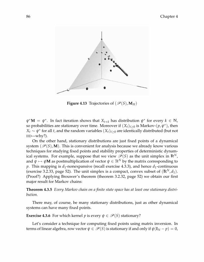
86 Chapter 4
Figure 4.13 Trajectories of (P(S),MH)
ψ∗M = ψ∗. In fact iteration shows that Xt+k has distribution ψ∗ for every k ∈ ,so probabilities are stationary over time. Moreover if (Xt)t≥0 is Markov-(p,ψ∗), thenXt ∼ ψ∗ for all t, and the random variables (Xt)t≥0 are identically distributed (but notIID—why?).
On the other hand, stationary distributions are just fixed points of a dynamicalsystem (P(S),M). This is convenient for analysis because we already know varioustechniques for studying fixed points and stability properties of deterministic dynam-ical systems. For example, suppose that we view P(S) as the unit simplex in N ,and ψ �→ ψM as postmultiplication of vector ψ ∈ N by the matrix corresponding top. This mapping is d1-nonexpansive (recall exercise 4.3.3), and hence d1-continuous(exercise 3.2.33, page 52). The unit simplex is a compact, convex subset of ( N , d1).(Proof?) Applying Brouwer’s theorem (theorem 3.2.32, page 52) we obtain our firstmajor result for Markov chains:
Theorem 4.3.5 Every Markov chain on a finite state space has at least one stationary distri-bution.
There may, of course, be many stationary distributions, just as other dynamicalsystems can have many fixed points.
Exercise 4.3.6 For which kernel p is every ψ ∈P(S) stationary?
Let’s consider a technique for computing fixed points using matrix inversion. Interms of linear algebra, row vector ψ ∈P(S) is stationary if and only if ψ(IN− p) = 0,
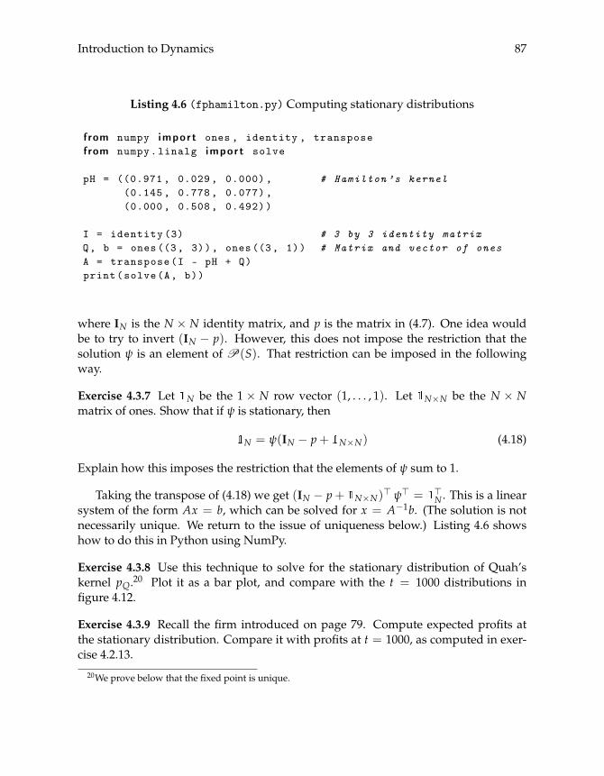
Introduction to Dynamics 87
Listing 4.6 (fphamilton.py) Computing stationary distributions
from numpy impor t ones , identity , transposefrom numpy.linalg impor t solve
pH = ((0.971 , 0.029, 0.000) , # Hamilton ’s kernel(0.145 , 0.778 , 0.077) ,(0.000 , 0.508 , 0.492))
I = identity (3) # 3 by 3 identity matrixQ, b = ones((3, 3)), ones((3, 1)) # Matrix and vector of onesA = transpose(I - pH + Q)print(solve(A, b))
where IN is the N × N identity matrix, and p is the matrix in (4.7). One idea wouldbe to try to invert (IN − p). However, this does not impose the restriction that thesolution ψ is an element of P(S). That restriction can be imposed in the followingway.
Exercise 4.3.7 Let N be the 1 × N row vector (1, . . . , 1). Let N×N be the N × Nmatrix of ones. Show that if ψ is stationary, then
N = ψ(IN − p+ N×N) (4.18)
Explain how this imposes the restriction that the elements of ψ sum to 1.
Taking the transpose of (4.18) we get (IN − p+ N×N)� ψ� = �N . This is a linear
system of the form Ax = b, which can be solved for x = A−1b. (The solution is notnecessarily unique. We return to the issue of uniqueness below.) Listing 4.6 showshow to do this in Python using NumPy.
Exercise 4.3.8 Use this technique to solve for the stationary distribution of Quah’skernel pQ.20 Plot it as a bar plot, and compare with the t = 1000 distributions infigure 4.12.
Exercise 4.3.9 Recall the firm introduced on page 79. Compute expected profits atthe stationary distribution. Compare it with profits at t = 1000, as computed in exer-cise 4.2.13.
20We prove below that the fixed point is unique.
88 Chapter 4
Exercise 4.3.10 According to the definition of the stationary distribution, if ψ∗ is sta-tionary for pH and if X0 ∼ ψ∗, then Xt ∼ ψ∗ for all t. Using algorithm 4.2 (page 74),check this for pH by drawing X0 from the stationary distribution calculated in list-ing 4.6 and then computing an approximation to the distribution ψT of XT whenT = 20.
4.3.2 The Dobrushin Coefficient
Now let’s consider convergence to the stationary distribution. We continue to im-pose onP(S) the distance d1 and study the dynamical system (P(S),M). By defini-tion 4.1.5, the system (P(S),M) is globally stable if
1. it has a unique fixed point (stationary distribution) ψ∗ ∈P(S), and
2. d1(ψMt,ψ∗) := ‖ψMt − ψ∗‖1 → 0 as t→ ∞ for all ψ ∈P(S).
The second condition implies that if (Xt)t≥0 is Markov-(p,ψ) for some ψ ∈P(S),then the distribution of Xt converges to ψ∗.21
Exercise 4.3.11 Exercise 4.3.6 asked you to provide an example of a kernel whereglobal stability fails. Another is the “periodic” Markov chain
p =(
0 11 0
)
Show that ψ∗ := (1/2, 1/2) is the unique stationary distribution. Give a counterex-ample to the claim ‖ψMt − ψ∗‖1 → 0 as t→ ∞, ∀ψ ∈P(S).
How might one check for stability of a given kernel p and associated dynamicalsystem (P(S),M)? Exercise 4.3.3 suggests the way forward: M is nonexpansive onP(S), and if we can upgrade this to a uniform contraction then Banach’s fixed pointtheorem (page 53) implies that (P(S),M) is globally stable, and that convergence toequilibrium takes place at a geometric rate.
Which kernels will we be able to upgrade? Intuitively, stable kernels are thosewhere current states have little influence on future states. An extreme example iswhere the distributions p(x, dy) are all equal: p(x, dy) = q ∈ P(S) for all x ∈ S. Inthis case the current state has no influence on tomorrow’s state—indeed, the resultingprocess is IID with Xt ∼ q for all t. The Markov operator satisfies ψM = q for allψ ∈P(S) (check it), and (P(S),M) is globally stable.
A less extreme case is when the distributions p(x, dy) are “similar” across x ∈S. One similarity measure for two distributions p(x, dy) and p(x′, dy) is ∑y p(x, y) ∧
21In this context, global stability is sometimes referred to as ergodicity.
Introduction to Dynamics 89
p(x′, y), where a ∧ b := min{a, b}. If p(x, dy) = p(x′, dy) then the value is one. If thesupports22 of p(x, dy) and p(x′, dy) are disjoint, then the value is zero. This leads usto the Dobrushin coefficient, which measures the stability properties of a given kernelp.
Definition 4.3.12 Given stochastic kernel p, the Dobrushin coefficient α(p) is definedby
α(p) := min
{∑y∈S
p(x, y) ∧ p(x′, y) : (x, x′) ∈ S× S
}(4.19)
Exercise 4.3.13 Prove that 0 ≤ α(p) ≤ 1 always holds.
Exercise 4.3.14 Show that α(p) = 1 if and only if p(x, dy) is equal to a constant distri-bution q ∈P(S) for every x ∈ S.
Exercise 4.3.15 Show that α(p) = 0 for the periodic kernel in exercise 4.3.11, and forp corresponding to the identity matrix.
Exercise 4.3.16 Distributions φ and ψ are said to overlap if there exists a y such thatφ(y) > 0 and ψ(y) > 0. Show that α(p) > 0 if and only if for each pair (x, x′) ∈ S× Sthe distributions p(x, dy) and p(x′, dy) overlap.
The following result links the Dobrushin coefficient to stability via Banach’s fixedpoint theorem (page 53).
Theorem 4.3.17 If p is a stochastic kernel on S with Markov operatorM, then
‖φM− ψM‖1 ≤ (1− α(p))‖φ− ψ‖1 ∀ φ,ψ ∈P(S)
Moreover this bound is the best available, in the sense that if λ < 1− α(p), then there existsa pair φ,ψ inP(S) such that ‖φM− ψM‖1 > λ‖φ− ψ‖1.
The first half of the theorem says that if α(p) > 0, then M is uniformly contracting(for the definition see page 52) with modulus 1− α(p). Since (P(S), d1) is complete,Banach’s fixed point theorem then implies global stability of (P(S),M). The secondpart of the theorem says that this rate 1− α(p) is the best available, which in turn sug-gests that the Dobrushin coefficient is a good measure of the stability properties of M.For example, if α(p) = 0, then we can be certain M is not a uniform contraction.
Some intuition for theorem 4.3.17 and it’s stability implications was discussedabove. The coefficient is large (close to one) when all distributions p(x, dy) are similaracross x, and the current state has little influence on future states. This is the stablecase. The coefficient is zero when there exists states x and x′ such that p(x, dy) and
22The support of φ ∈P(S) is {y ∈ S : φ(y) > 0}.

90 Chapter 4
p(x′, dy) have disjoint support, as with the identity kernel and the periodic kernel.More intuition on the link between positivity of α(p) and stability is given in the nextsection.
The proof of theorem 4.3.17 is given in the appendix to this chapter. The fact that1 − α(p) is the best rate possible may suggest to you that the proof is not entirelytrivial. Indeed this is the case. We have to do better than crude inequalities. All butthe most enthusiastic readers are encouraged to skip the proof and move to the nextsection.
4.3.3 Stability
Let p be a stochastic kernel on S. If α(p) > 0, then (P(S),M) is globally stable byBanach’s fixed point theorem. In fact we can say a bit more. We now present our mainstability result for finite chains, which clarifies the relationship between the Dobrushincoefficient and stability.
Theorem 4.3.18 Let p be a stochastic kernel on S with Markov operator M. The followingstatements are equivalent:
1. The dynamical system (P(S),M) is globally stable.
2. There exists a t ∈ such that α(pt) > 0.
Another way to phrase the theorem is that (P(S),M) is globally stable if and onlyif there is a t ∈ such that, given any pair of states x, x′, one can find at least onestate y such that pt(x, y) and pt(x′, y) are both positive. Thus, if we run two Markovchains from any two starting points x and x′, there is a positive probability that thechains will meet. This is connected with global stability because it rules out the kind ofbehavior seen in example 4.1.8 (page 57), where initial conditions determine long-runoutcomes.
Exercise 4.3.19 Consider the periodic kernel in exercise 4.3.11. Show that α(pt) = 0for every t ∈ .
Exercise 4.3.20 Prove that if minx∈S pt(x, y) =: ε > 0 for some y ∈ S, then α(pt) ≥ ε,and hence (P(S),M) is globally stable.
Exercise 4.3.21 Stokey and Lucas (1989, thm. 11.4) prove that (P(S),M) is globallystable if there exists a t ∈ such that ∑y∈S minx∈S pt(x, y) > 0. Show how this resultis implied by theorem 4.3.18.
Exercise 4.3.22 Prove theorem 4.3.18. To show that (2) implies (1), use Lemma 4.2.8(page 76) and Theorem 4.3.17. To show that (1) implies (2), let ψ∗ be the stationary

Introduction to Dynamics 91
distribution. Note that ∃y ∈ S with ψ∗(y) > 0. Argue that pt(x, y)→ ψ∗(y) for any x.Using finiteness of S, show that there is a t ∈ with minx∈S pt(x, y) > 0. Concludethat α(pt) > 0.
Let’s consider how to apply theorem 4.3.18. In view of exercise 4.3.20, if thereexists a y with p(x, y) > 0 for all x ∈ S, then α(p) > 0 and global stability holds. Acase in point is Hamilton’s kernel (4.8) on page 70, which is globally stable as a resultof the strict positivity of column two.
Next consider Quah’s kernel pQ (page 71). We know from theorem 4.3.5 that atleast one stationary distribution exists, and we calculated a stationary distribution inexercise 4.3.8. We should now check that there are not many stationary distributions—otherwise exhibiting one of them is not very interesting. Also, the stationary distribu-tion becomes a better predictor of outcomes if we know that all trajectories convergeto it.
Exercise 4.3.23 Show that the Dobrushin coefficient α(pQ) is zero.
Since α(pQ) = 0, let’s look at the higher order iterates. In his study Quah calculatesthe 23rd-order kernel
p23Q =
⎛⎜⎜⎜⎜⎝
0.61 0.27 0.09 0.03 0.000.37 0.32 0.20 0.09 0.020.14 0.23 0.31 0.25 0.070.04 0.11 0.25 0.39 0.220.00 0.01 0.04 0.12 0.82
⎞⎟⎟⎟⎟⎠ (4.20)
Exercise 4.3.24 Show that α(p23Q ) > 0.
Exercise 4.3.25 As (P(S),MQ) is globally stable, we can iterate MQ on any initialcondition ψ to calculate an approximate fixed point ψ∗. Take ψ = (1, 0, 0, 0, 0) as yourinitial condition and iterate until d1(ψMt
Q,ψMt+1Q ) < 0.0001. Compare your result
with that of exercise 4.3.8.
Exercise 4.3.26 Code a function that takes a kernel p as an argument and returns α(p).Write another function that repeatedly calls the first function to compute the smallestt ≥ 1 such that α(pt) > 0, and prints that t along with the value α(pt). Include amaximum value T such that if t reaches T the function terminates with a message thatα(pt) = 0 for all t ≤ T. Now show that the first t such that α(ptQ) > 0 is 2.
One interesting fact regarding stationary distributions is as follows: Let p be akernel such that (P(S),M) is globally stable, and let ψ∗ be the unique stationarydistribution. Let (Xt)t≥0 be Markov-(p, x), where ψ∗(x) > 0. The return time to x isdefined as the random variable
τ(x) := inf{t ≥ 1 : Xt = x}
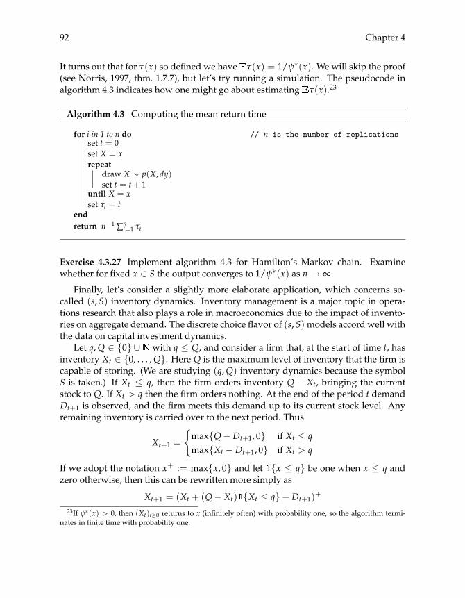
92 Chapter 4
It turns out that for τ(x) so defined we have τ(x) = 1/ψ∗(x). We will skip the proof(see Norris, 1997, thm. 1.7.7), but let’s try running a simulation. The pseudocode inalgorithm 4.3 indicates how one might go about estimating τ(x).23
Algorithm 4.3 Computing the mean return time
for i in 1 to n do // n is the number of replicationsset t = 0set X = xrepeat
draw X ∼ p(X, dy)set t = t+ 1
until X = xset τi = t
endreturn n−1 ∑n
i=1 τi
Exercise 4.3.27 Implement algorithm 4.3 for Hamilton’s Markov chain. Examinewhether for fixed x ∈ S the output converges to 1/ψ∗(x) as n→ ∞.
Finally, let’s consider a slightly more elaborate application, which concerns so-called (s, S) inventory dynamics. Inventory management is a major topic in opera-tions research that also plays a role in macroeconomics due to the impact of invento-ries on aggregate demand. The discrete choice flavor of (s, S) models accord well withthe data on capital investment dynamics.
Let q,Q ∈ {0} ∪ with q ≤ Q, and consider a firm that, at the start of time t, hasinventory Xt ∈ {0, . . . ,Q}. Here Q is the maximum level of inventory that the firm iscapable of storing. (We are studying (q,Q) inventory dynamics because the symbolS is taken.) If Xt ≤ q, then the firm orders inventory Q − Xt, bringing the currentstock to Q. If Xt > q then the firm orders nothing. At the end of the period t demandDt+1 is observed, and the firm meets this demand up to its current stock level. Anyremaining inventory is carried over to the next period. Thus
Xt+1 =
{max{Q− Dt+1, 0} if Xt ≤ qmax{Xt − Dt+1, 0} if Xt > q
If we adopt the notation x+ := max{x, 0} and let {x ≤ q} be one when x ≤ q andzero otherwise, then this can be rewritten more simply as
Xt+1 = (Xt + (Q− Xt) {Xt ≤ q} − Dt+1)+
23If ψ∗(x) > 0, then (Xt)t≥0 returns to x (infinitely often) with probability one, so the algorithm termi-nates in finite time with probability one.

Introduction to Dynamics 93
or, if hq(x) := x+ (Q− x) {x ≤ q} is the stock on hand after orders for inventory arecompleted, as
Xt+1 = (hq(Xt)− Dt+1)+
We assume throughout that (Dt)t≥1 is an IID sequence taking values in {0} ∪ ac-cording to distribution b(d) := {Dt = d} = (1/2)d+1.
Exercise 4.3.28 Let S = {0, 1, . . . ,Q}. Given an expression for the stochastic kernelp(x, y) corresponding to the restocking policy q.24
Exercise 4.3.29 LetMq be the corresponding Markov operator. Show that (P(S),Mq)is always globally stable independent of the precise values of q and Q. Let ψ∗q denote thestationary distribution corresponding to threshold q. Show numerically that if Q = 5,then
ψ∗2 = (0.0625, 0.0625, 0.125, 0.25, 0.25, 0.25)
Now consider profits of the firm. To minimize the number of parameters, supposethat the firm buys units of the product for zero dollars and marks them up by one dol-lar. Revenue in period t is min{hq(Xt),Dt+1}. Placing an order for inventory incursfixed cost C. As a result profits for the firm at time t are given by
πq(Xt,Dt+1) = min{hq(Xt),Dt+1} − C {Xt ≤ q}If we now sum across outcomes for Dt+1 taking Xt = x as given, then we get
gq(x) := [πq(x,Dt+1)] =∞
∑d=0
πq(x, d)b(d) =∞
∑d=0
πq(x, d)2d+1
which is interpreted as expected profits in the current period when the inventory stateXt is equal to x.
Exercise 4.3.30 One common performance measure for an inventory strategy (in thiscase, a choice of q) is long-run average profits, which is defined here as gq(X) whenX ∼ ψ∗q (i.e., ∑x∈S gq(x)ψ∗q (x)). Show numerically that according to this performancemeasure, when Q = 20 and C = 0.1, the optimal policy is q = 7.
4.3.4 The Law of Large Numbers
Let’s end our discussion of stability by investigating some probabilistic properties ofsample paths. In particular, we investigate the law of large numbers (LLN) in thecontext of Markov chains.
24Hint: If a is any integer and D has the distribution b defined above, then what is the probability that(a− D)+ = y? You might find it convenient to first consider the case y = 0 and then the case y > 0.

94 Chapter 4
In algorithm 4.2 (page 74) we computed an approximation to the marginal distri-bution ψt via Monte Carlo. The basis of Monte Carlo is that if we sample indepen-dently from a fixed probability distribution and count the fraction of times that anevent happens, that fraction converges to the probability of the event (as determinedby this probability distribution). This is more or less the frequentist definition of prob-abilities, but it can also be proved from the axioms of probability theory. The theoremin question is the law of large numbers (LLN), a variation of which is as follows:
Theorem 4.3.31 If F is a cumulative distribution function on , (Xt)t≥1IID∼ F, and h : →
is a measurable function with∫ |h(x)|F(dx) < ∞, then
1n
n
∑i=1
h(Xi)→ h(X1) :=:∫h(x)F(dx) as n→ ∞ with probability one (4.21)
This result is fundamental to statistics. It states that for IID sequences, samplemeans converge to means as the sample size gets large. Later we will give a for-mal definition of independence and prove a version of the theorem. At that time theterm “measurable function” and the nature of probability one convergence will bediscussed. Suffice to know that measurability of h is never a binding restriction forthe problems we consider.
Example 4.3.32 If (Xi)ni=1 are independent standard normal random variates, thenaccording to theorem 4.3.31 we should find that n−1∑n
i=1 X2i → 1. (Why?) You can try
this out in Python using some variation of
>>> from random impor t normalvariate>>> Y = [normalvariate (0, 1)**2 f o r i i n range (10000)]>>> sum(Y) / 10000
Another use of the LLN: Suppose that we wish to compute h(X), where h is somereal function. One approach would be to use pen and paper plus our knowledge ofcalculus to solve the integral
∫ ∞−∞ h(x)F(dx). In some situations, however, this is not
so easy. If instead we have access to a random number generator that can generateindependent draws X1,X2, . . . from F, then we can produce a large number of draws,take the mean of the h(Xi) terms, and appeal to (4.21).
In (4.21) the sequence of random variables is IID. In some situations the LLN ex-tends to sequences that are neither independent nor identically distributed. For ex-ample, we have the following result concerning stable Markov chains:
Theorem 4.3.33 Let S be finite, let ψ ∈P(S), let p be a stochastic kernel on S with α(pt) >0 for some t ∈ , and let h : S→ . If (Xt)t≥0 is Markov-(p,ψ), then
1n
n
∑t=1
h(Xt)→ ∑x∈S
h(x)ψ∗(x) as n→ ∞ with probability one (4.22)

Introduction to Dynamics 95
where ψ∗ is the unique stationary distribution of p.
The left-hand side is the average value of h(Xt), and the right-hand side is theexpectation of h(X) when X ∼ ψ∗. Note that the result holds for every initial conditionψ ∈P(S).
The proof of theorem 4.3.33 requires more tools than we have in hand.25 The intu-ition is that when the chain is globally stable, Xt is approximately distributed accord-ing to ψ∗ for large t. In addition the stability property implies that initial conditionsare unimportant, and for the same reason Xt has little influence on Xt+k for large k.Hence there is a kind of asymptotic independence in the chain. Together, these twofacts mean that our chain approximates the IID property that drives the LLN.
If h(x) = 1 if x = y and zero otherwise (i.e., h(x) = {x = y}), then (4.22) becomes
1n
n
∑t=1
h(Xt) =1n
n
∑t=1{Xt = y} → ψ∗(y) as n→ ∞ (4.23)
This provides a new technique for computing the stationary distribution, via MonteCarlo. Exercise 4.3.34 illustrates.
Exercise 4.3.34 Let pH be Hamilton’s kernel, and let h(x) = 1 if x = NG and zerootherwise. Take any initial condition, and draw a series of length 50,000. Compute theleft-hand side of (4.22). Compare it with the right-hand side, which was calculated inlisting 4.6 on page 87.
When the state space is small, this is a less efficient technique for computing thestationary distribution than the algebraic method used in listing 4.6. However, thecomputational burden of the algebraic method increases rapidly with the size of thestate space. For large or infinite state spaces, a variation of the LLN technique used inexercise 4.3.34 moves to center stage. See §6.1.3 for details.26
The importance of theorem 4.3.33 extends beyond this new technique for comput-ing stationary distributions. It provides a new interpretation for the stationary distri-bution: If we turn (4.23) around, we get
ψ∗(y) � fraction of time that (Xt) spends in state y
This is indeed a new interpretation of ψ∗, although it is not generally valid unless thechain in question is stable (in which case the LLN applies).
Exercise 4.3.35 Give an example of a kernel p and initial condition ψ where this inter-pretation fails.
25A weak version of theorem 4.3.33 is proved in §11.1.1.26The look-ahead method introduced in §6.1.3 concerns infinite state spaces, but it can be applied to finite
state spaces with the obvious modifications.

96 Chapter 4
In the preceding discussion, h was an indicator function, which reduced the dis-cussion of expectations to one of probabilities. Now let’s consider more general ex-pectations.
Exercise 4.3.36 Recall the firm introduced on page 79. Extending exercise 4.3.34, ap-proximate expected profits at the stationary distribution using theorem 4.3.33. Com-pare your results to those of exercise 4.3.9.
Thus the LLN provides a new way to compute expectations with respect to station-ary distributions. However, as was the case with probabilities above, it also providesa new interpretation of these expectations when the Markov chain is stationary. Forexample, if h denotes profits as above, then we have
∑x∈S
h(x)ψ∗(x) � long-run average profits
Again, this interpretation is valid when the chain in question is stationary, but maynot be valid otherwise.
4.4 Commentary
Regarding deterministic, discrete-time dynamical systems, a good mathematical in-troduction is provided by Holmgren (1996), who treats elementary theory, topologicalconjugacy, and chaotic dynamics. For dynamics from an economic perspective, see,for example, Stokey and Lucas (1989), Azariadis (1993), de la Fuente (2000), Turnovsky(2000), Shone (2003), Ljungqvist and Sargent (2004), Caputo (2005), or Gandolfo (2005).
The threshold externality model in example 4.1.8 is a simplified version of Azari-adis and Drazen (1990). See Durlauf (1993) for a stochastic model with multiple equi-libria.
Our discussion of chaotic dynamics lacked any economic applications, but plentyexist. The Solow–Swan model produces chaotic dynamics with some minor modifi-cations (e.g., Böhm and Kaas 2000). Moreover rational behavior in infinite-horizon,optimizing models can lead to chaos, cycles, and complex dynamics. See, for exam-ple, Benhabib and Nishimura (1985), Boldrin and Montrucchio (1986), Sorger (1992),Nishimura et al. (1994), Venditti (1998), or Mitra and Sorger (1999). For more dis-cussion of complex economic dynamics, see Grandmont (1985), Chiarella (1988), Ga-lor (1994), Medio (1995), Brock and Hommes (1998), Barnett and Serletis (2000), orKikuchi (2008).
Two good references on finite state Markov chains are Norris (1997) and Häg-gström (2002). These texts provide a more traditional approach to stability of Markovchains based on irreducibility and aperiodicity. It can be shown that every irreducible

Introduction to Dynamics 97
and aperiodic Markov chain is globally stable, and as a result satisfies the conditionsof theorem 4.3.18 (in particular, α(pt) > 0 for some t ∈ ). The converse is not true,so theorem 4.3.18 is more general.
The Dobrushin coefficient was introduced by Dobrushin (1956). For an alternativediscussion of the Dobrushin coefficient in the context of finite state Markov chains, seeBremaud (1999).
The treatment of (s, S) dynamics in §4.3.3 is loosely based on Norris (1997). Foranother discussion of inventory dynamics see Stokey and Lucas (1989, sec. 5.14). Aninteresting analysis of aggregate implications is Nirei (2008). A modern treatment ofdiscrete adjustment models can be found in Stokey (2008).


Chapter 5
Further Topics for Finite MCs
We have now covered the fundamental theory of finite state Markov chains. Next letus turn to more applied topics. In §5.1 below we consider the problem of dynamicprogramming, that is, of controlling Markov chains through our actions in order toachieve a given objective. In §5.2 we investigate the connection between Markovchains and stochastic recursive sequences.
5.1 Optimization
In this section we take our first look at stochastic dynamic programming. The term“dynamic programming” was coined by Richard Bellman in the early 1950s, and per-tains to a class of multistage planning problems. Because stochastic dynamic pro-gramming problems typically involve Markov chains, they are also called Markovdecision problems, Markov control problems, or Markov control processes. We willfocus on solving a simple example problem, and defer the more difficult proofs untilchapter 10.
5.1.1 Outline of the Problem
Our objective is to model the behavior of Colonel Kurtz, who can be found on a smallisland in the Nung river living on catfish. The local catfish bite only at dawn, and theColonel bags a random quantity W ∈ {0, . . . , B}, W ∼ φ. Catfish spoil quickly in thetropics, lasting only if refrigerated. The Colonel has limited refrigeration facilities: Amaximum of M fish can fit into his freezer. We let Xt be the stock of fish at noon onday t, from which a quantity Ct is consumed. The remainder Rt = Xt − Ct is frozen.Following the next morning’s fishing trip, the state is Xt+1 = Rt +Wt+1.
99
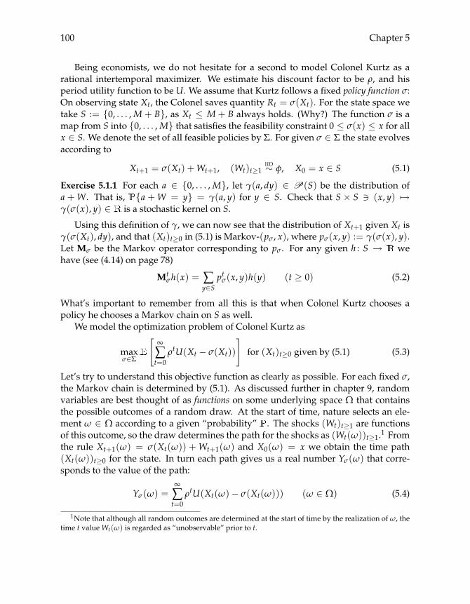
100 Chapter 5
Being economists, we do not hesitate for a second to model Colonel Kurtz as arational intertemporal maximizer. We estimate his discount factor to be ρ, and hisperiod utility function to be U. We assume that Kurtz follows a fixed policy function σ:On observing state Xt, the Colonel saves quantity Rt = σ(Xt). For the state space wetake S := {0, . . . , M + B}, as Xt ≤ M + B always holds. (Why?) The function σ is amap from S into {0, . . . , M} that satisfies the feasibility constraint 0 ≤ σ(x) ≤ x for allx ∈ S. We denote the set of all feasible policies by Σ. For given σ ∈ Σ the state evolvesaccording to
Xt+1 = σ(Xt) +Wt+1, (Wt)t≥1IID∼ φ, X0 = x ∈ S (5.1)
Exercise 5.1.1 For each a ∈ {0, . . . , M}, let γ(a, dy) ∈ P(S) be the distribution ofa +W. That is, {a +W = y} = γ(a, y) for y ∈ S. Check that S × S � (x, y) �→γ(σ(x), y) ∈ is a stochastic kernel on S.
Using this definition of γ, we can now see that the distribution of Xt+1 given Xt isγ(σ(Xt), dy), and that (Xt)t≥0 in (5.1) is Markov-(pσ, x), where pσ(x, y) := γ(σ(x), y).Let Mσ be the Markov operator corresponding to pσ. For any given h : S → wehave (see (4.14) on page 78)
Mtσh(x) = ∑
y∈Sptσ(x, y)h(y) (t ≥ 0) (5.2)
What’s important to remember from all this is that when Colonel Kurtz chooses apolicy he chooses a Markov chain on S as well.
We model the optimization problem of Colonel Kurtz as
maxσ∈Σ
[∞
∑t=0
ρtU(Xt − σ(Xt))
]for (Xt)t≥0 given by (5.1) (5.3)
Let’s try to understand this objective function as clearly as possible. For each fixed σ,the Markov chain is determined by (5.1). As discussed further in chapter 9, randomvariables are best thought of as functions on some underlying space Ω that containsthe possible outcomes of a random draw. At the start of time, nature selects an ele-ment ω ∈ Ω according to a given “probability” . The shocks (Wt)t≥1 are functionsof this outcome, so the draw determines the path for the shocks as (Wt(ω))t≥1.1 Fromthe rule Xt+1(ω) = σ(Xt(ω)) +Wt+1(ω) and X0(ω) = x we obtain the time path(Xt(ω))t≥0 for the state. In turn each path gives us a real number Yσ(ω) that corre-sponds to the value of the path:
Yσ(ω) =∞
∑t=0
ρtU(Xt(ω)− σ(Xt(ω))) (ω ∈ Ω) (5.4)
1Note that although all random outcomes are determined at the start of time by the realization of ω, thetime t value Wt(ω) is regarded as “unobservable” prior to t.
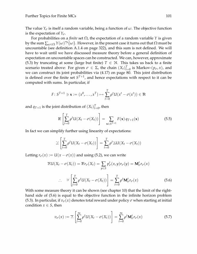
Further Topics for Finite MCs 101
The value Yσ is itself a random variable, being a function of ω. The objective functionis the expectation of Yσ.
For probabilities on a finite set Ω, the expectation of a random variable Y is givenby the sum∑ω∈Ω Y(ω) {ω}. However, in the present case it turns out thatΩmust beuncountable (see definition A.1.4 on page 322), and this sum is not defined. We willhave to wait until we have discussed measure theory before a general definition ofexpectation on uncountable spaces can be constructed. We can, however, approximate(5.3) by truncating at some (large but finite) T ∈ . This takes us back to a finitescenario treated above: For given σ ∈ Σ, the chain (Xt)Tt=0 is Markov-(pσ, x), andwe can construct its joint probabilities via (4.17) on page 80. This joint distributionis defined over the finite set ST+1, and hence expectations with respect to it can becomputed with sums. In particular, if
F : ST+1 � x := (x0, . . . , xT) �→T
∑t=0
ρtU(xt − σ(xt)) ∈
and qT+1 is the joint distribution of (Xt)Tt=0, then[T
∑t=0
ρtU(Xt − σ(Xt))
]= ∑
x∈ST+1
F(x) qT+1(x) (5.5)
In fact we can simplify further using linearity of expectations:[T
∑t=0
ρtU(Xt − σ(Xt))
]=
T
∑t=0
ρt U(Xt − σ(Xt))
Letting rσ(x) := U(x− σ(x)) and using (5.2), we can write
U(Xt − σ(Xt)) = rσ(Xt) = ∑y∈S
ptσ(x, y)rσ(y) = Mtσrσ(x)
∴[
T
∑t=0
ρtU(Xt − σ(Xt))
]=
T
∑t=0
ρtMtσrσ(x) (5.6)
With some measure theory it can be shown (see chapter 10) that the limit of the right-hand side of (5.6) is equal to the objective function in the infinite horizon problem(5.3). In particular, if vσ(x) denotes total reward under policy σ when starting at initialcondition x ∈ S, then
vσ(x) :=
[∞
∑t=0
ρtU(Xt − σ(Xt))
]=
∞
∑t=0
ρtMtσrσ(x) (5.7)
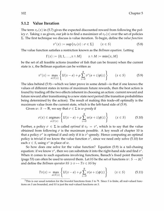
102 Chapter 5
5.1.2 Value Iteration
The term vσ(x) in (5.7) gives the expected discounted reward from following the pol-icy σ. Taking x as given, our job is to find a maximizer of vσ(x) over the set of policiesΣ. The first technique we discuss is value iteration. To begin, define the value function
v∗(x) := sup{vσ(x) : σ ∈ Σ} (x ∈ S) (5.8)
The value function satisfies a restriction known as the Bellman equation. Letting
Γ(x) := {0, 1, . . . , x ∧M} x ∧M := min{x, M}be the set of all feasible actions (number of fish that can be frozen) when the currentstate is x, the Bellman equation can be written as
v∗(x) = maxa∈Γ(x)
{U(x− a) + ρ
B
∑z=0
v∗(a+ z)φ(z)
}(x ∈ S) (5.9)
The idea behind (5.9)—which we later prove in some detail—is that if one knows thevalues of different states in terms of maximum future rewards, then the best action isfound by trading off the two effects inherent in choosing an action: current reward andfuture reward after transitioning to a new state next period (the transition probabilitiesbeing determined by the action). The result of making this trade-off optimally is themaximum value from the current state, which is the left-hand side of (5.9).
Given w : S→ , we say that σ ∈ Σ is w-greedy if
σ(x) ∈ argmaxa∈Γ(x)
{U(x− a) + ρ
B
∑z=0
w(a+ z)φ(z)
}(x ∈ S) (5.10)
Further, a policy σ ∈ Σ is called optimal if vσ = v∗, which is to say that the valueobtained from following σ is the maximum possible. A key result of chapter 10 isthat a policy σ∗ is optimal if and only if it is v∗-greedy. Hence computing an optimalpolicy is trivial if we know the value function v∗, since we need only solve (5.10) foreach x ∈ S, using v∗ in place of w.
So how does one solve for the value function? Equation (5.9) is a tail-chasingequation: if we know v∗, then we can substitute it into the right-hand side and find v∗.When it comes to such equations involving functions, Banach’s fixed point theorem(page 53) can often be used to unravel them. Let bS be the set of functions w : S→ ,2
and define the Bellman operator bS � v �→ Tv ∈ bS by
Tv(x) = maxa∈Γ(x)
{U(x− a) + ρ
B
∑z=0
v(a+ z)φ(z)
}(x ∈ S) (5.11)
2This is our usual notation for the bounded functions from S to . Since S is finite, all real-valued func-tions on S are bounded, and bS is just the real-valued functions on S.
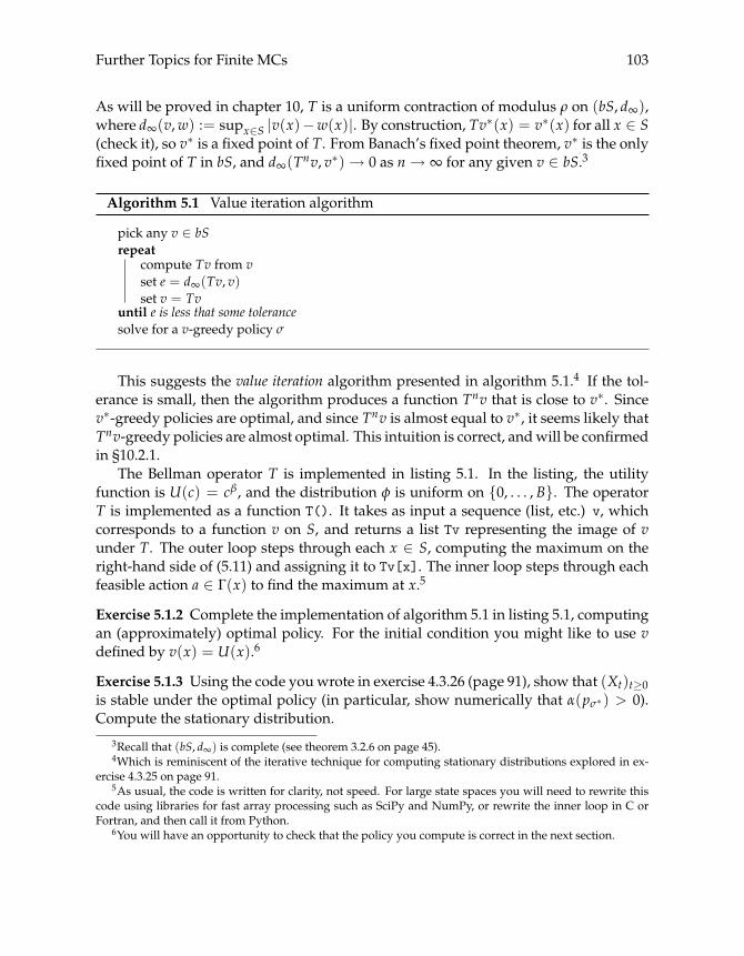
Further Topics for Finite MCs 103
As will be proved in chapter 10, T is a uniform contraction of modulus ρ on (bS, d∞),where d∞(v,w) := supx∈S |v(x)−w(x)|. By construction, Tv∗(x) = v∗(x) for all x ∈ S(check it), so v∗ is a fixed point of T. From Banach’s fixed point theorem, v∗ is the onlyfixed point of T in bS, and d∞(Tnv, v∗)→ 0 as n→ ∞ for any given v ∈ bS.3
Algorithm 5.1 Value iteration algorithm
pick any v ∈ bSrepeat
compute Tv from vset e = d∞(Tv, v)set v = Tv
until e is less that some tolerancesolve for a v-greedy policy σ
This suggests the value iteration algorithm presented in algorithm 5.1.4 If the tol-erance is small, then the algorithm produces a function Tnv that is close to v∗. Sincev∗-greedy policies are optimal, and since Tnv is almost equal to v∗, it seems likely thatTnv-greedy policies are almost optimal. This intuition is correct, and will be confirmedin §10.2.1.
The Bellman operator T is implemented in listing 5.1. In the listing, the utilityfunction is U(c) = cβ, and the distribution φ is uniform on {0, . . . , B}. The operatorT is implemented as a function T(). It takes as input a sequence (list, etc.) v, whichcorresponds to a function v on S, and returns a list Tv representing the image of vunder T. The outer loop steps through each x ∈ S, computing the maximum on theright-hand side of (5.11) and assigning it to Tv[x]. The inner loop steps through eachfeasible action a ∈ Γ(x) to find the maximum at x.5
Exercise 5.1.2 Complete the implementation of algorithm 5.1 in listing 5.1, computingan (approximately) optimal policy. For the initial condition you might like to use vdefined by v(x) = U(x).6
Exercise 5.1.3 Using the code you wrote in exercise 4.3.26 (page 91), show that (Xt)t≥0is stable under the optimal policy (in particular, show numerically that α(pσ∗) > 0).Compute the stationary distribution.
3Recall that (bS, d∞) is complete (see theorem 3.2.6 on page 45).4Which is reminiscent of the iterative technique for computing stationary distributions explored in ex-
ercise 4.3.25 on page 91.5As usual, the code is written for clarity, not speed. For large state spaces you will need to rewrite this
code using libraries for fast array processing such as SciPy and NumPy, or rewrite the inner loop in C orFortran, and then call it from Python.
6You will have an opportunity to check that the policy you compute is correct in the next section.
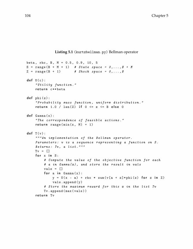
104 Chapter 5
Listing 5.1 (kurtzbellman.py) Bellman operator
beta , rho , B, M = 0.5, 0.9, 10, 5S = range(B + M + 1) # State space = 0,...,B + MZ = range(B + 1) # Shock space = 0,...,B
de f U(c):"Utility function."r e t u r n c**beta
de f phi(z):"Probability mass function , uniform distribution."r e t u r n 1.0 / len(Z) i f 0 <= z <= B e l s e 0
de f Gamma(x):"The correspondence of feasible actions."r e t u r n range(min(x, M) + 1)
de f T(v):"""An implementation of the Bellman operator.Parameters: v is a sequence representing a function on S.Returns: Tv, a list."""Tv = []f o r x i n S:
# Compute the value of the objective function for each# a in Gamma(x), and store the result in valsvals = []f o r a i n Gamma(x):
y = U(x - a) + rho * sum(v[a + z]*phi(z) f o r z i n Z)vals.append(y)
# Store the maximum reward for this x in the list TvTv.append(max(vals))
r e t u r n Tv

Further Topics for Finite MCs 105
5.1.3 Policy Iteration
Another common technique for solving dynamic programming problems is policy it-eration, as presented in algorithm 5.2.7 This technique is easy to program, and is of-ten faster than value iteration. It has the nice feature that for finite state problemsthe optimal policy is computed exactly (modulo numerical error) in finite time (theo-rem 10.2.6, page 244).
Algorithm 5.2 Policy iteration algorithm
pick any σ ∈ Σrepeat
compute vσ from σ
compute a vσ-greedy policy σ′set e = σ− σ′set σ = σ′
until e = 0
First, an arbitrary policy σ is chosen. Next, one computes the value vσ of thispolicy. From vσ a vσ-greedy policy σ′ is computed:
σ′(x) ∈ argmax0≤a≤x∧M
{U(x− a) + ρ
B
∑z=0
vσ(a+ z)φ(z)
}(x ∈ S)
and e records the deviation between σ and σ′. If the policies are equal the loop termi-nates. Otherwise we set σ = σ′ and iteration continues.
The most difficult part of coding this algorithm is to compute the value of a givenpolicy (i.e., compute vσ from σ). Listing 5.2 gives one method for accomplishing this,based on evaluating the right-hand side of (5.6) with large T. It starts with two importstatements. First we import zeros, dot and array from numpy. The first is for creatingarrays of zeros, the second is for matrix multiplication, and the third is for convertingother data types such as lists into NumPy arrays. Second, we import some primitivesfrom kurtzbellman, which is listing 5.1.
Next we define the function value_of_policy(), which takes an array sigma rep-resenting a feasible policy σ ∈ Σ as its argument, and returns a NumPy array v_sigma,which represents vσ. At the start of the function we create a 2D array p_sigma corre-sponding to the stochastic kernel pσ(x, y) := γ(σ(x), y) defined above. From thatarray we create a function M_sigma() corresponding to Mσ. In addition we createthe array r_sigma(), which corresponds to rσ. Finally, we step through 50 terms ofρtMt
σrσ, adding each one to the return value.7Sometimes called Howard’s policy improvement algorithm.
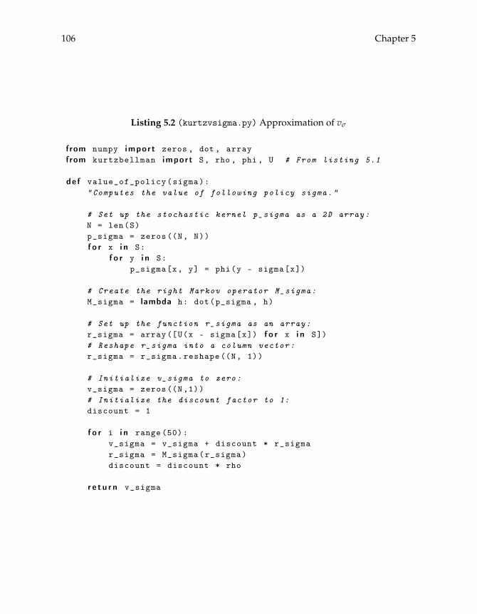
106 Chapter 5
Listing 5.2 (kurtzvsigma.py) Approximation of vσ
from numpy impor t zeros , dot , arrayfrom kurtzbellman impor t S, rho , phi , U # From listing 5.1
de f value_of_policy(sigma):"Computes the value of following policy sigma."
# Set up the stochastic kernel p_sigma as a 2D array:N = len(S)p_sigma = zeros((N, N))f o r x i n S:
f o r y i n S:p_sigma[x, y] = phi(y - sigma[x])
# Create the right Markov operator M_sigma:M_sigma = lambda h: dot(p_sigma , h)
# Set up the function r_sigma as an array:r_sigma = array([U(x - sigma[x]) f o r x i n S])# Reshape r_sigma into a column vector:r_sigma = r_sigma.reshape ((N, 1))
# Initialize v_sigma to zero:v_sigma = zeros((N,1))# Initialize the discount factor to 1:discount = 1
f o r i i n range (50):v_sigma = v_sigma + discount * r_sigmar_sigma = M_sigma(r_sigma)discount = discount * rho
r e t u r n v_sigma

Further Topics for Finite MCs 107
Exercise 5.1.4 Complete the implementation of algorithm 5.2. The resulting policyshould be the same as the one you computed in exercise 5.1.2.
5.2 MCs and SRSs
In this section we investigate the connection between Markov chains generated bystochastic kernels on one hand, and stochastic recursive sequences (stochastic differ-ence equations) on the other. We will see that to each Markov chain there correspondsat least one stochastic recursive sequence (in fact there are many). This provides uswith new ways of analyzing and simulating Markov chains.
5.2.1 FromMCs to SRSs
When we start studying processes on infinite state spaces we will often be interestedin stochastic recursive sequences (SRSs). In the finite case, a typical SRS has the form
Xt+1 = F(Xt,Wt+1), X0 ∼ ψ ∈P(S), F : S× Z → S (5.12)
where (Wt)t≥1 is a sequence of independent shocks taking values in arbitrary set Z.As discussed in §5.1.1, the shocks Wt are to be thought of as functions on a commonspace Ω. At the start of time, nature selects an ω ∈ Ω according to the probability
. This provides a complete realization of the path (Wt(ω))t≥1. The value ω alsodetermines X0, with {ω : X0(ω) = xi} = ψ(xi). Given (Wt(ω))t≥1 and X0(ω), weconstruct the corresponding time path (Xt(ω))t≥0 by
X1(ω) = F(X0(ω),W1(ω)), X2(ω) = F(X1(ω),W2(ω)), etc.
The idea that all uncertainty is realized at the start of time by a single observation ωfrom Ω is a convenient mathematical fiction. It’s as if we could draw an entire path(Wt(ω))t≥1 by a single call to our random number generator. However, you can men-tally equate the two approaches by thinking of ω as being realized at the beginningof our simulation. Generating n random numbers can be thought of as observing thefirst n observations of the sequence. The default behavior of most random numbergenerators is to produce (quasi) independent sequences of shocks.
Given the SRS (5.12) we obtain a stochastic kernel p on S by
p(x, y) = {F(x,Wt) = y} := {ω ∈ Ω : F(x,Wt(ω)) = y}In fact, we can also go the other way, representing any Markov-(p,ψ) process by anSRS such as (5.12). This is useful for simulation, and for gaining a deeper understand-ing of the probabilistic structure of dynamics.
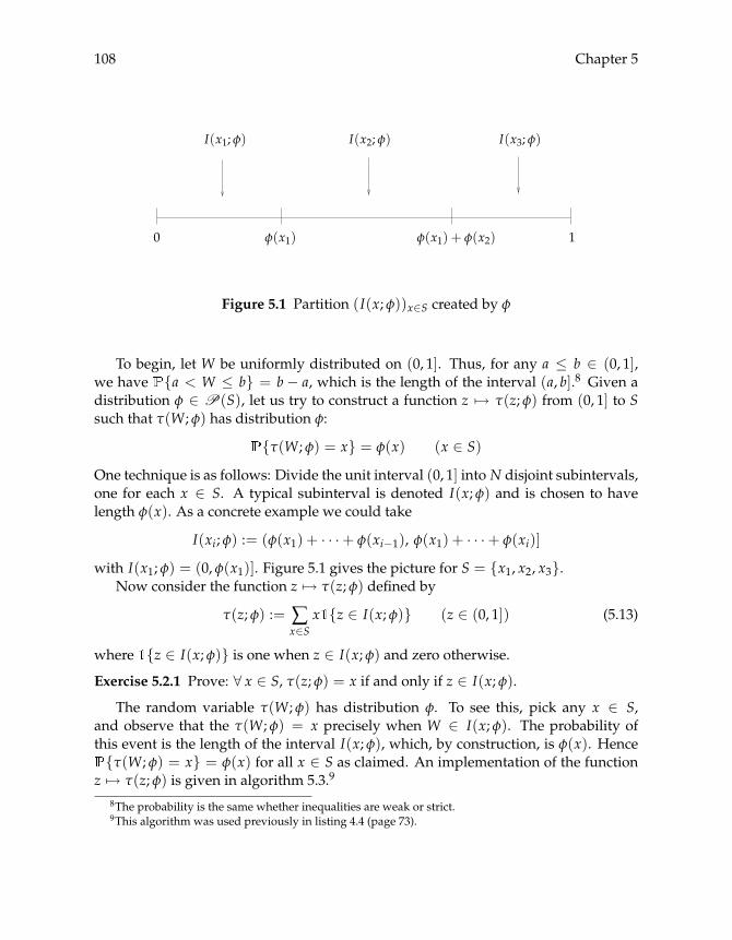
108 Chapter 5
φ(x1) φ(x1) + φ(x2)0 1
I(x1; φ) I(x2; φ) I(x3; φ)
Figure 5.1 Partition (I(x; φ))x∈S created by φ
To begin, let W be uniformly distributed on (0, 1]. Thus, for any a ≤ b ∈ (0, 1],we have {a < W ≤ b} = b− a, which is the length of the interval (a, b].8 Given adistribution φ ∈ P(S), let us try to construct a function z �→ τ(z; φ) from (0, 1] to Ssuch that τ(W; φ) has distribution φ:
{τ(W; φ) = x} = φ(x) (x ∈ S)
One technique is as follows: Divide the unit interval (0, 1] into N disjoint subintervals,one for each x ∈ S. A typical subinterval is denoted I(x; φ) and is chosen to havelength φ(x). As a concrete example we could take
I(xi; φ) := (φ(x1) + · · ·+ φ(xi−1), φ(x1) + · · ·+ φ(xi)]
with I(x1; φ) = (0, φ(x1)]. Figure 5.1 gives the picture for S = {x1, x2, x3}.Now consider the function z �→ τ(z; φ) defined by
τ(z; φ) := ∑x∈S
x {z ∈ I(x; φ)} (z ∈ (0, 1]) (5.13)
where {z ∈ I(x; φ)} is one when z ∈ I(x; φ) and zero otherwise.
Exercise 5.2.1 Prove: ∀ x ∈ S, τ(z; φ) = x if and only if z ∈ I(x; φ).
The random variable τ(W; φ) has distribution φ. To see this, pick any x ∈ S,and observe that the τ(W; φ) = x precisely when W ∈ I(x; φ). The probability ofthis event is the length of the interval I(x; φ), which, by construction, is φ(x). Hence{τ(W; φ) = x} = φ(x) for all x ∈ S as claimed. An implementation of the function
z �→ τ(z; φ) is given in algorithm 5.3.9
8The probability is the same whether inequalities are weak or strict.9This algorithm was used previously in listing 4.4 (page 73).

Further Topics for Finite MCs 109
Algorithm 5.3 The function z �→ τ(z; φ)
read in zset a = 0for x in S do
if a < z ≤ a+ φ(x) then return xa = a+ φ(x)
end
With these results we can represent any Markov-(p,ψ) chain as an SRS. By defini-tion, such a chain obeys X0 ∼ ψ and Xt+1 ∼ p(Xt, dy) for t ≥ 0. To write this as astochastic recursive sequence, let (Wt)t≥0 be a IID and uniform on (0, 1], and let
X0 = τ(W0;ψ), Xt+1 = τ(Wt+1; p(Xt, dy)) (5.14)
The second equality can be rewritten as
Xt+1 = F(Xt,Wt+1) where F(x, z) := τ(z; p(x, dy)) (5.15)
You should convince yourself that if W is uniform on (0, 1], then F(x,W) has distri-bution p(x, dy), and that the sequence (Xt)t≥0 generated by (5.14) and (5.15) obeysX0 ∼ ψ and Xt+1 ∼ p(Xt, dy) for t ≥ 0.
Listing 5.3 provides some code for creating F from a given kernel p. The ker-nel p is represented as a sequence of sequences (see, e.g., the definition of the ker-nel on page 79). A call such as F = createF(p) assigns to F the function F(x, z) =τ(z; p(x, dy)).
Exercise 5.2.2 Use listing 5.3 to reimplement Hamilton’s Markov chain as a stochasticrecursive sequence. Verify that the law of large numbers still holds by showing that1n ∑
nt=1 {Xt = y} → ψ∗(y) as n → ∞. (The right-hand side of this equality can be
calculated by listing 4.6. Now calculate the left using listing 5.3 and compare.)
Incidentally, SRSs are sometimes referred to as iterated function systems. In thisframework one thinks of updating the state from Xt to Xt+1 by the random functionFWt+1 := F(·,Wt+1). Although we are now dealing with “random functions,” whichsounds rather fancy, in practice the only change is a notational one: Xt+1 = FWt+1(Xt)as compared to (5.12). The main advantage is that we can now write
Xt = FWt ◦ FWt−1 ◦ · · · ◦ FW1(X0) = FWt ◦ FWt−1 ◦ · · · ◦ FW1(τ(W0;ψ))
We see that Xt is just a fixed function of the shocks up to time t.
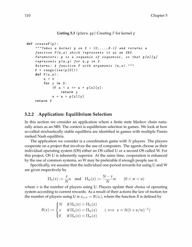
110 Chapter 5
Listing 5.3 (p2srs.py) Creating F for kernel p
de f createF(p):"""Takes a kernel p on S = {0,...,N-1} and returns afunction F(x,z) which represents it as an SRS.Parameters: p is a sequence of sequences , so that p[x][y]represents p(x,y) for x,y in S.Returns: A function F with arguments (x,z)."""S = range(len(p[0]))de f F(x,z):
a = 0f o r y i n S:
i f a < z <= a + p[x][y]:r e t u r n y
a = a + p[x][y]r e t u r n F
5.2.2 Application: Equilibrium Selection
In this section we consider an application where a finite state Markov chain natu-rally arises as an SRS. The context is equilibrium selection in games. We look at howso-called stochastically stable equilibria are identified in games with multiple Paretoranked Nash equilibria.
The application we consider is a coordination game with N players. The playerscooperate on a project that involves the use of computers. The agents choose as theirindividual operating system (OS) either an OS called U or a second OS called W. Forthis project, OS U is inherently superior. At the same time, cooperation is enhancedby the use of common systems, so W may be preferable if enough people use it.
Specifically, we assume that the individual one-period rewards for using U and Ware given respectively by
Πu(x) :=xNu and Πw(x) :=
N − xN
w (0 < w < u)
where x is the number of players using U. Players update their choice of operatingsystem according to current rewards. As a result of their actions the law of motion forthe number of players using U is xt+1 = B(xt), where the function B is defined by
B(x) :=
⎧⎪⎨⎪⎩N if Πu(x) > Πw(x)x if Πu(x) = Πw(x) (⇐⇒ x = N(1 + u/w)−1)0 if Πu(x) < Πw(x)
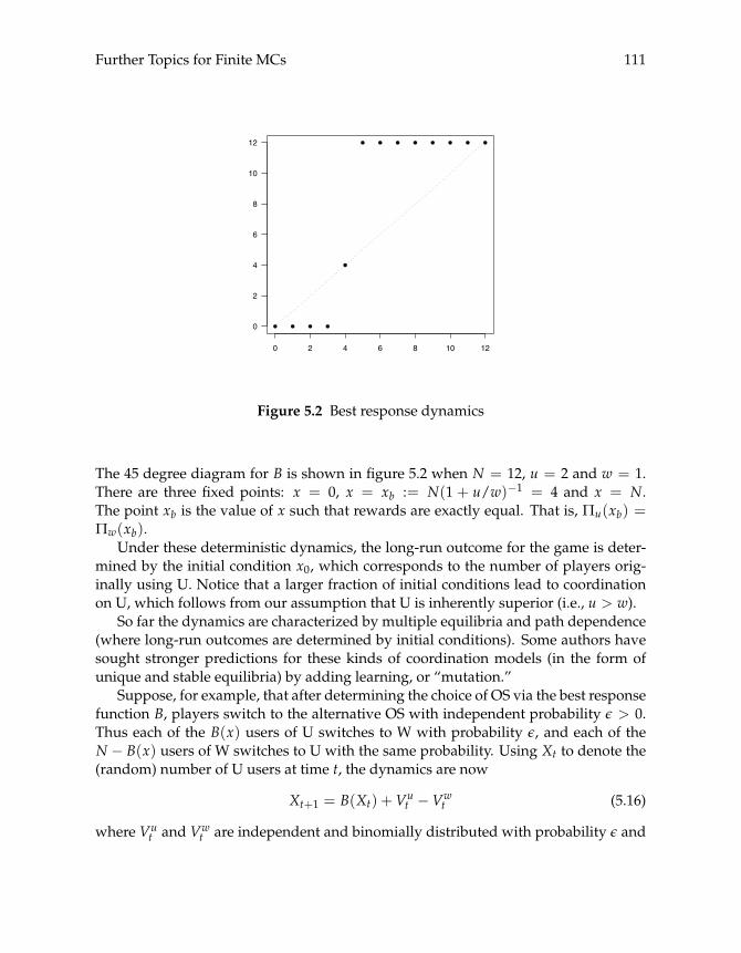
Further Topics for Finite MCs 111
0 2 4 6 8 10 12
0
2
4
6
8
10
12
● ● ● ●
●
● ● ● ● ● ● ● ●
Figure 5.2 Best response dynamics
The 45 degree diagram for B is shown in figure 5.2 when N = 12, u = 2 and w = 1.There are three fixed points: x = 0, x = xb := N(1 + u/w)−1 = 4 and x = N.The point xb is the value of x such that rewards are exactly equal. That is, Πu(xb) =Πw(xb).
Under these deterministic dynamics, the long-run outcome for the game is deter-mined by the initial condition x0, which corresponds to the number of players orig-inally using U. Notice that a larger fraction of initial conditions lead to coordinationon U, which follows from our assumption that U is inherently superior (i.e., u > w).
So far the dynamics are characterized by multiple equilibria and path dependence(where long-run outcomes are determined by initial conditions). Some authors havesought stronger predictions for these kinds of coordination models (in the form ofunique and stable equilibria) by adding learning, or “mutation.”
Suppose, for example, that after determining the choice of OS via the best responsefunction B, players switch to the alternative OS with independent probability ε > 0.Thus each of the B(x) users of U switches to W with probability ε, and each of theN − B(x) users of W switches to U with the same probability. Using Xt to denote the(random) number of U users at time t, the dynamics are now
Xt+1 = B(Xt) +Vut −Vw
t (5.16)
where Vut and Vw
t are independent and binomially distributed with probability ε and

112 Chapter 5
sizes N − B(Xt) and B(Xt) respectively.10 Here Vut is the number of switches from W
to U, while Vwt is switches from U to W.
With the addition of random “mutation,” uniqueness and stability of the steadystate is attained:
Exercise 5.2.3 Let p(x, y) := {Xt+1 = y |Xt = x} be the stochastic kernel corre-sponding to the SRS (5.16), let M be the Markov operator, and let S := {0, . . . ,N}.Argue that for any fixed ε ∈ (0, 1), the system (P(S),M) is globally stable.
Let ψ∗ε be the unique stationary distribution for ε ∈ (0, 1). It has been shown (seeKandori, Mailath, and Rob 1993) that as ε→ 0, the distribution ψ∗ε concentrates on thePareto dominant equilibrium N (i.e., ψ∗ε (N) → 1 as ε → 0). The interpretation is thatfor low levels of experimentation or mutation, players rarely diverge from the mostattractive equilibrium.
This concentration on N can be observed by simulation: Let (Xεt )
nt=0 be a time
series generated for some fixed ε ∈ (0, 1). Then the law of large numbers (theo-rem 4.3.33, page 94) implies that for large n,
n−1n
∑t=1{Xε
t = N} � ψ∗ε (N)
Figure 5.3 shows a simulation that gives n−1∑nt=1{Xε
t = N} as ε ranges over theinterval [0.001, 0.1]. The parameters are N = 12, u = 2 and w = 1. The series length nused in the simulation is n = 10, 000. The figure shows that steady state probabilitiesconcentrate on N as ε→ 0.
Exercise 5.2.4 Replicate figure 5.3. Generate one time series of length n = 10, 000 foreach ε, and plot the fraction of time each series spends in state N.
5.2.3 The Coupling Method
Much of the modern theory of Markov chains is based on probabilistic methods (asopposed to analytical techniques such as fixed point theory). A prime example iscoupling. Found in many guises, coupling is a powerful and elegant technique forstudying all manner of probabilistic phenomena. It has been used to prove stability ofMarkov processes since the masterful work of Wolfgang Doeblin (1938).
We will use coupling to prove global stability of Markov chains for which the Do-brushin coefficient is strictly positive, without recourse to the contraction mappingargument employed in theorem 4.3.18 (page 90). Our main aim is to provide the basic
10A binomial random variable with probability p and size n counts the number of successes in n binarytrials, each with independent success probability p.
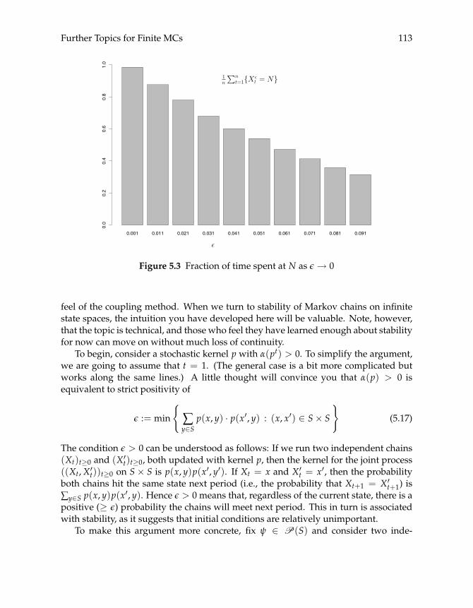
Further Topics for Finite MCs 113
0.001 0.011 0.021 0.031 0.041 0.051 0.061 0.071 0.081 0.091
0.0
0.2
0.4
0.6
0.8
1.0
ε
1n
∑nt=1{Xε
t = N}
Figure 5.3 Fraction of time spent at N as ε→ 0
feel of the coupling method. When we turn to stability of Markov chains on infinitestate spaces, the intuition you have developed here will be valuable. Note, however,that the topic is technical, and those who feel they have learned enough about stabilityfor now can move on without much loss of continuity.
To begin, consider a stochastic kernel p with α(pt) > 0. To simplify the argument,we are going to assume that t = 1. (The general case is a bit more complicated butworks along the same lines.) A little thought will convince you that α(p) > 0 isequivalent to strict positivity of
ε := min
{∑y∈S
p(x, y) · p(x′, y) : (x, x′) ∈ S× S
}(5.17)
The condition ε > 0 can be understood as follows: If we run two independent chains(Xt)t≥0 and (X′t)t≥0, both updated with kernel p, then the kernel for the joint process((Xt,X′t))t≥0 on S× S is p(x, y)p(x′, y′). If Xt = x and X′t = x′, then the probabilityboth chains hit the same state next period (i.e., the probability that Xt+1 = X′t+1) is∑y∈S p(x, y)p(x′, y). Hence ε > 0 means that, regardless of the current state, there is apositive (≥ ε) probability the chains will meet next period. This in turn is associatedwith stability, as it suggests that initial conditions are relatively unimportant.
To make this argument more concrete, fix ψ ∈ P(S) and consider two inde-
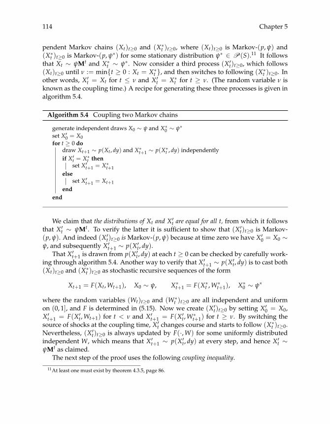
114 Chapter 5
pendent Markov chains (Xt)t≥0 and (X∗t )t≥0, where (Xt)t≥0 is Markov-(p,ψ) and(X∗t )t≥0 is Markov-(p,ψ∗) for some stationary distribution ψ∗ ∈ P(S).11 It followsthat Xt ∼ ψMt and X∗t ∼ ψ∗. Now consider a third process (X′t)t≥0, which follows(Xt)t≥0 until ν := min{t ≥ 0 : Xt = X∗t }, and then switches to following (X∗t )t≥0. Inother words, X′t = Xt for t ≤ ν and X′t = X∗t for t ≥ ν. (The random variable ν isknown as the coupling time.) A recipe for generating these three processes is given inalgorithm 5.4.
Algorithm 5.4 Coupling two Markov chains
generate independent draws X0 ∼ ψ and X∗0 ∼ ψ∗set X′0 = X0for t ≥ 0 do
draw Xt+1 ∼ p(Xt, dy) and X∗t+1 ∼ p(X∗t , dy) independentlyif X′t = X∗t then
set X′t+1 = X∗t+1else
set X′t+1 = Xt+1
endend
We claim that the distributions of Xt and X′t are equal for all t, from which it followsthat X′t ∼ ψMt. To verify the latter it is sufficient to show that (X′t)t≥0 is Markov-(p,ψ). And indeed (X′t)t≥0 is Markov-(p,ψ) because at time zero we have X′0 = X0 ∼ψ, and subsequently X′t+1 ∼ p(X′t, dy).
That X′t+1 is drawn from p(X′t, dy) at each t ≥ 0 can be checked by carefully work-ing through algorithm 5.4. Another way to verify that X′t+1 ∼ p(X′t, dy) is to cast both(Xt)t≥0 and (X∗t )t≥0 as stochastic recursive sequences of the form
Xt+1 = F(Xt,Wt+1), X0 ∼ ψ, X∗t+1 = F(X∗t ,W∗t+1), X∗0 ∼ ψ∗
where the random variables (Wt)t≥0 and (W∗t )t≥0 are all independent and uniformon (0, 1], and F is determined in (5.15). Now we create (X′t)t≥0 by setting X′0 = X0,X′t+1 = F(X′t,Wt+1) for t < ν and X′t+1 = F(X′t,W∗t+1) for t ≥ ν. By switching thesource of shocks at the coupling time, X′t changes course and starts to follow (X∗t )t≥0.Nevertheless, (X′t)t≥0 is always updated by F(·,W) for some uniformly distributedindependent W, which means that X′t+1 ∼ p(X′t, dy) at every step, and hence X′t ∼ψMt as claimed.
The next step of the proof uses the following coupling inequality.
11At least one must exist by theorem 4.3.5, page 86.
Further Topics for Finite MCs 115
Lemma 5.2.5 If X and Y are any random variables taking values in S and having distribu-tions φX and φY respectively, then
‖φX − φY‖∞ := maxx∈S|φX(x)− φY(x)| ≤ {X �= Y}
Intuitively, if the probability that X and Y differ is small, then so is the distancebetween their distributions. An almost identical proof is given later in the book so weomit the proof here.12
Let’s apply lemma 5.2.5 to X′t and X∗t . Since X′t ∼ ψMt and X∗t ∼ ψ∗,
‖ψMt − ψ∗‖∞ ≤ {X′t �= X∗t }We wish to show that the right-hand side of this inequality goes to zero, and this iswhere the reason for introducing X′t becomes clear. Not only does it have the distri-bution ψMt, just as Xt does, but also we know that if X′t is distinct from X∗t , then Xj andX∗j are distinct for all j ≤ t. Hence {X′t �= X∗t } ≤ ∩j≤t {Xj �= X∗j }.13 Therefore
‖ψMt − ψ∗‖∞ ≤ ∩j≤t {Xj �= X∗j } (5.18)
Thus, to show that ψMt converges to ψ∗, it is sufficient to demonstrate that the prob-ability of Xj and X∗j never meeting prior to t goes to zero as t→ ∞. And this is wherepositivity of ε in (5.17) comes in. It means that there is an ε chance of meeting at eachtime j, independent of the locations of Xj−1 and X∗j−1. Hence the probability of nevermeeting converges to zero. Specifically,
Proposition 5.2.6 We have ∩j≤t {Xj �= X∗j } ≤ (1− ε)t for all t ∈ .
It follows from proposition 5.2.6 and (5.18) that if ε is strictly positive, then ‖ψMt−ψ∗‖∞ → 0 at a geometric rate.
Proof of proposition 5.2.6. The process (Xt,X∗t )t≥0 is a Markov chain on S× S. A typicalelement of S × S will be denoted by (x, s). In view of independence of (Xt)t≥0 and(X∗t )t≥0, the initial condition of (Xt,X∗t )t≥0 is ψ × ψ∗ (i.e., {(X0,X∗0 ) = (x, s)} =(ψ× ψ∗)(x, s) := ψ(x)ψ∗(s)), while the stochastic kernel is
k((x, s), (x′, s′)) = p(x, x′)p(s, s′)
To simplify notation let’s write (x, s) as x so that k((x, s), (x′, s′)) can be expressedmore simply as k(x, x′), and set D := {(x, s) ∈ S× S : x = s}. Evidently
∩j≤t {Xj �= X∗j } = ∩j≤t {(Xj,X∗j ) ∈ Dc}12See lemma 11.3.2 on page 273.13If A and B are two events with A ⊂ B (i.e., occurrence of A implies occurrence of B), then (A) ≤ (B).
See chapter 9 for details.

116 Chapter 5
In view of lemma 4.2.17 this probability is equal to
∑x0∈Dc
(ψ× ψ∗)(x0) ∑x1∈Dc
k(x0, x1) · · · ∑xt−1∈Dc
k(xt−2, xt−1) ∑xt∈Dc
k(xt−1, xt) (5.19)
Now consider the last term in this expression. We have
∑xt∈Dc
k(xt−1, xt) = 1− ∑xt∈D
k(xt−1, xt)
But from the definitions of k and D we obtain
∑xt∈D
k(xt−1, xt) = ∑(xt ,st)∈D
p(xt−1, xt)p(st−1, st) = ∑y∈S
p(xt−1, y)p(st−1, y)
∴ ∑xt∈D
k(xt−1, xt) ≥ ε
∴ ∑xt∈Dc
k(xt−1, xt) ≤ 1− ε
Working back through (5.19) and applying the same logic to each term shows that(5.19) is less than (1− ε)t. This proves the proposition.
5.3 Commentary
Much of the early theory of dynamic programming is due to Bellman (1957). A goodintroduction to dynamic programming in discrete state environments can be foundin Puterman (1994). An overview with applications is given in Miranda and Fackler(2002, ch. 7). Further references can be found in the commentary to chapters 6 and 10.
The representation of Markov chains as stochastic recursive sequences in §5.2.1 isloosely based on Häggström (2002, ch. 3). The application in §5.2.2 is from Kandori,Mailath, and Rob (1993). The approach to coupling in §5.2.3 is somewhat nonstan-dard. More information can be found in the commentary to chapter 11.
Chapter 6
Infinite State Space
In this chapter we begin working with stochastic systems on infinite state space. Whilea completely rigorous treatment of this area requires measure theory (chapter 7 andonward), we can build a good understanding of the key topics (dynamics, optimiza-tion, etc.) by heuristic arguments, simulation, and analogies with the finite case.Along the way we will meet some more challenging programming problems.
6.1 First Steps
In this section we study dynamics for stochastic recursive sequences (SRSs) taking val-ues in . Our main interest is in tracking the evolution of probabilities over time, asrepresented by the marginal distributions of the process. We will also look at station-ary distributions—the infinite state analogue of the stationary distributions discussedin §4.3.1—and how to calculate them.
6.1.1 Basic Models and Simulation
Our basic model is as follows: Let the state space S be a subset of and let Z ⊂ .Let F : S× Z → S be a given function, and consider the SRS
Xt+1 = F(Xt,Wt+1), X0 ∼ ψ, (Wt)t≥1IID∼ φ (6.1)
Here (Wt)t≥1IID∼ φ means that (Wt)t≥1 is an IID sequence of shocks with cumulative
distribution function φ. In other words, {Wt ≤ z} = φ(z) for all z ∈ Z. Likewise ψis the cumulative distribution function of X0, and X0 is independent of (Wt)t≥1. Notethat Xt and Wt+1 are independent, since Xt depends only on the initial condition andthe shocks W1, . . . ,Wt, all of which are independent of Wt+1.
117

118 Chapter 6
Example 6.1.1 Consider a stochastic version of the Solow–Swan growth model, whereoutput is a function f of capital k and a real-valued shockW. The sequence of produc-tivity shocks (Wt)t≥1 is IID∼ φ. Capital at time t+ 1 is equal to that fraction s of outputthat was saved last period, plus undepreciated capital, giving law of motion
kt+1 = F(kt,Wt+1) := s f (kt,Wt+1) + (1− δ)kt (6.2)
Consumption is given by ct = (1− s) f (kt,Wt+1). The production function satisfiesf : 2
+ → + and f (k, z) > 0 whenever k > 0 and z > 0. For the state space we canchoose either S0 = + or S = (0,∞), while Z := (0,∞).
Exercise 6.1.2 Show that if k ∈ S0 (resp., S) and z ∈ Z, then next period’s stock F(k, z)is in S0 (resp., S).
Example 6.1.3 Let Z = S = , and consider the smooth transition threshold autore-gression (STAR) model
Xt+1 = g(Xt) +Wt+1, (Wt)t≥1IID∼ φ (6.3)
g(x) := (α0 + α1x)(1− G(x)) + (β0 + β1x)G(x)
Here G : S → [0, 1] is a smooth transition function, such as the logistic function, satis-fying G′ > 0, limx→−∞ G(x) = 0 and limx→∞ G(x) = 1.
Code for simulating time series from an arbitrary SRS is given in listing 6.1. Thelisting defines a class SRS implementing the canonical SRS in (6.1).1 The behavior ofthe class is similar to that of the class MC in listing 4.4 (page 73), and the methods areexplained in the doc strings.
Listing 6.2 provides an example of usage. The code creates an instance of SRS,corresponding to the Solow model (6.2) when f (k,W) = kαW and lnWt ∼ N(0, σ2).The two sample paths generated by this code are shown in figure 6.1.
Exercise 6.1.4 Repeat exercise 5.2.2 on page 109 using the class SRS.
Returning to the SRS (6.1), let’s consider the distribution of Xt for arbitrary t ∈ .This distribution will be denoted by ψt, and you can think of it for now as a cumulativedistribution function (i.e., ψt(x) is the probability that Xt ≤ x). It is also called themarginal distribution of Xt; conceptually it is equivalent to its discrete state namesakethat we met in §4.2.2.
In order to investigate ψt via simulation, we need to sample from this distribution.The simplest technique is this: First draw X0 ∼ ψ and generate a sample path stop-ping at time t. Now repeat the exercise, but with a new set of draws X0,W1, . . . ,Wt,
1The benefit of designing an abstract class for SRSs is code reuse: The class can be used to study anysystem. Readers are encouraged to add functionality to the class as they do the exercises in the chapter.

Infinite State Space 119
Listing 6.1 (srs.py) Simulation of SRSs
c l a s s SRS:
de f __init__(self , F=None, phi=None, X=None):"""Represents X_{t+1} = F(X_t , W_{t+1}); W ~ phi.Parameters: F and phi are functions , where phi()returns a draw from phi. X is a number representingthe initial condition."""self.F, self.phi , self.X = F, phi , X
de f update(self):"Update the state according to X = F(X, W)."self.X = self.F(self.X, self.phi())
de f sample_path(self , n):"Generate path of length n from current state."path = []f o r i i n range(n):
path.append(self.X)self.update ()
r e t u r n path
Listing 6.2 (testsrs.py) Example application
from srs impor t SRS # Import from listing 6.1from random impor t lognormvariate
alpha , sigma , s, delta = 0.5, 0.2, 0.5, 0.1# Define F(k, z) = s k^alpha z + (1 - delta) kF = lambda k, z: s * (k**alpha) * z + (1 - delta) * klognorm = lambda: lognormvariate (0, sigma)
solow_srs = SRS(F=F, phi=lognorm , X=1.0)P1 = solow_srs.sample_path (500) # Generate path from X = 1solow_srs.X = 60 # Reset the current stateP2 = solow_srs.sample_path (500) # Generate path from X = 60

120 Chapter 6
Figure 6.1 Time series plot
leading to a new draw of Xt that is independent of the first. If we do this n times, weget n independent samples X1
t , . . . ,Xnt from the target distribution ψt. Algorithm 6.1
contains the pseudocode for this operation. Figure 6.2 is a visualization of the algo-rithm after 3 iterations of the outer loop.
Exercise 6.1.5 Investigate the mean of ψt for the Solow–Swan model when f (k,W) =kαW and lnWt ∼ N(0, σ2). Carry out a simulation with k0 = 1, t = 20, δ = 0.1,s = 1/2, σ2 = 0.2 and α = 0.3. Draw n = 1000 samples. Compute kt using thestatistic n−1∑n
i=1 kit. Explain how theorem 4.3.31 on page 94 justifies your statistic.
Exercise 6.1.6 Repeat exercise 6.1.5, but now setting s = 3/4. How does your estimatechange? Interpret.
Exercise 6.1.7 Repeat exercise 6.1.5, but now set k0 = 5, k0 = 10, and k0 = 20. To theextent that you can, interpret your results.
Exercise 6.1.8 Repeat exercise 6.1.5, but now set t = 50, t = 100, and t = 200. Whathappens to your estimates? Interpret.
Exercise 6.1.9 Repeat exercise 6.1.7, but with t = 200 instead of t = 20. Try to interpretyour results.

Infinite State Space 121
Algorithm 6.1 Draws from the marginal distribution
for i in 1 to n dodraw X from the initial condition ψ
for j in 1 to t dodraw W from the shock distribution φ
set X = F(X,W)endset Xi
t = Xendreturn (X1
t , . . . ,Xnt )
time
X2t
X1t
X3t
0 t
Figure 6.2 Sampling from the marginal distribution

122 Chapter 6
Recall that if X1, . . . ,Xn is a sample of IID random variables, then the sample meanis defined as Xn := 1
n ∑ni=1 Xi, while the sample variance is
σ2n :=
1n− 1
n
∑i=1
(Xi − Xn)2
Assuming that the second moment of Xi is finite, the central limit theorem and aconvergence result often referred to as Slutsky’s theorem give
√n(Xn − X1)
σn
d→ N(0, 1) as n→ ∞, where σn :=√σ2n
Exercise 6.1.10 Based on this fact, construct a 95% confidence interval for your esti-mate of kt. (Use the parameters from exercise 6.1.5.)
Exercise 6.1.11 Consider the same model as in exercise 6.1.5, but now set δ = 1. Theclassical golden rule optimization problem is to choose the savings rate s in the Solow–Swan model to maximize steady state consumption. Let’s consider the stochastic ana-logue. The simplest criterion is to maximize expected steady state consumption. Forthis model, by t = 100 the distribution of cj varies little for j ≥ t (we’ll learn moreabout this later on). As such, let’s consider c100 as expected steady state consump-tion. Compute n = 5, 000 observations of c100, and take the sample average to obtainan approximation of the expectation. Repeat for s in a grid of values in (0, 1). Plot thefunction, and report the maximizer.
6.1.2 Distribution Dynamics
While the mean conveys some information about the random variable kt, at times wewish to know about the entire (cumulative) distribution ψt. How might one go aboutcomputing ψt by simulation?
The standard method is with the empirical distribution function, which, for indepen-dent samples (Xi)ni=1 of random variable X ∈ , is given by
Fn(x) :=1n
n
∑i=1{Xi ≤ x} (x ∈ ) (6.4)
Thus Fn(x) is the fraction of the sample that falls below x. The LLN (theorem 4.3.31,page 94) can be used to show that if X has cumulative distribution F, then Fn(x) →F(x) with probability one for each x as n → ∞.2 These results formalize the funda-mental idea that empirical frequencies converge to probabilities when the draws areindependent.
2Later we will cover how to do these kinds of proofs. In this case much more can be proved—interestedreaders should refer to the Glivenko–Cantelli theorem.

Infinite State Space 123
Listing 6.3 (ecdf.py) Empirical distribution function
c l a s s ECDF:
de f __init__(self , observations):self.observations = observations
de f __call__(self , x):counter = 0.0f o r obs i n self.observations:
i f obs <= x:counter += 1
r e t u r n counter / len(self.observations)
An implementation of the empirical distribution function is given in listing 6.3,based on a class called ECDF.3 The class is initialized with samples (Xt)nt=1 stored ina sequence (list or tuple) called observations, and an instance is created with a callsuch as F = ECDF(data). The method __call__ evaluates Fn(x) for a given value of x.(Recall from §2.2.3 that __call__ is a special method that makes an instance F callable,so we can evaluate Fn(x) using the simple syntax F(x).) Here is an example:
from ecdf impor t ECDF # Import from listing 6.3from random impor t uniformsamples = [uniform(0, 1) f o r i i n range (10)]F = ECDF(samples)F(0.5) # Returned 0.29F.observations = [uniform(0, 1) f o r i i n range (1000)]F(0.5) # Returned 0.479
Figure 6.3 gives four plots of the empirical distribution function corresponding to thetime t distribution of the Solow–Swan model. The plots are for n = 4, n = 25, n = 100,and n = 5, 000. The parameters are k0 = 1, t = 20, δ = 0.1, s = 1/2, σ2 = 0.2, andα = 0.3.
Exercise 6.1.12 Add a method to the ECDF class that uses Matplotlib to plot the em-pirical distribution over a specified interval. Replicate the four graphs in figure 6.3(modulo randomness).
Consider now a variation of our growth model with additional nonlinearities. In
3As usual, the code is written for clarity rather than speed. See the text home page for more optimizedsolutions.

124 Chapter 6
10 15 20 25
0.0
1.0
k
10 15 20 25
0.0
1.0
k
10 15 20 25
0.0
1.0
k
10 15 20 25
0.0
1.0
k
n = 4 n = 25
n = 100 n = 5000
Figure 6.3 Empirical distribution functions
example 4.1.8 (page 57) we looked at a model with “threshold” nonconvexities. Astochastic version is
kt+1 = sA(kt)kαt Wt+1 + (1− δ)kt (6.5)
where the shock is assumed to be lognormally distributed (and independent), and Ais the step function
A(k) = A1 {0 < k < kb}+ A2 {kb ≤ k < ∞} =
{A1 if 0 < k < kbA2 if kb ≤ k < ∞
with kb ∈ S = (0,∞) interpreted as the threshold, and 0 < A1 < A2.Figures 6.4 and 6.5 each show two time series generated for this model, with initial
conditions k0 = 1 and k0 = 80. The parameters for figure 6.4 are set at α = 0.5,s = 0.25, A1 = 15, A2 = 25, σ2 = 0.02, and kb = 21.6, while for figure 6.5, kb =24.1. Notice how initial conditions tend to persist, although time series occasionallycross the threshold kb—what might be referred to in physics as a “phase transition.”Informally, the state variable moves from one locally attracting region of the statespace to another.
Exercise 6.1.13 Compute the empirical distribution functions at t = 100 for the two

Infinite State Space 125
Figure 6.4 Persistence in time series
sets of parameters used in figures 6.4 and 6.5. Plot the functions and interpret theirshapes.
Aside from computing the distributions, another interesting question is: How longdo we expect it to take on average for the transition (crossing of the threshold kb) tooccur for an economy with initial condition k0 = 1? More mathematically, what is theexpectation of τ := inf{t ≥ 0 : kt > kb} when regarded as a random variable on ?(Here τ is usually called the first passage time of (kt)t≥0 to (kb,∞).)
Exercise 6.1.14 Using α = 0.5, s = 0.25, A1 = 15, A2 = 25, σ2 = 0.02, k0 = 1 andkb = 21.6, compute an approximate expectation of τ by sample mean. (Set n = 5, 000.)Do the same for kb = 24.1, which corresponds to figure 6.5. How does your answerchange? Interpret.
6.1.3 Density Dynamics
Now let’s look more deeply at distribution dynamics for SRSs, with an emphasis ondensity dynamics. In reading this section, you should be aware that all densities createdistributions but not all distributions are created by densities. If f is a density functionon , then F(x) :=
∫ x−∞ f (u)du is a cumulative distribution function. However, if F is
a cumulative distribution function with jumps—corresponding to positive probability
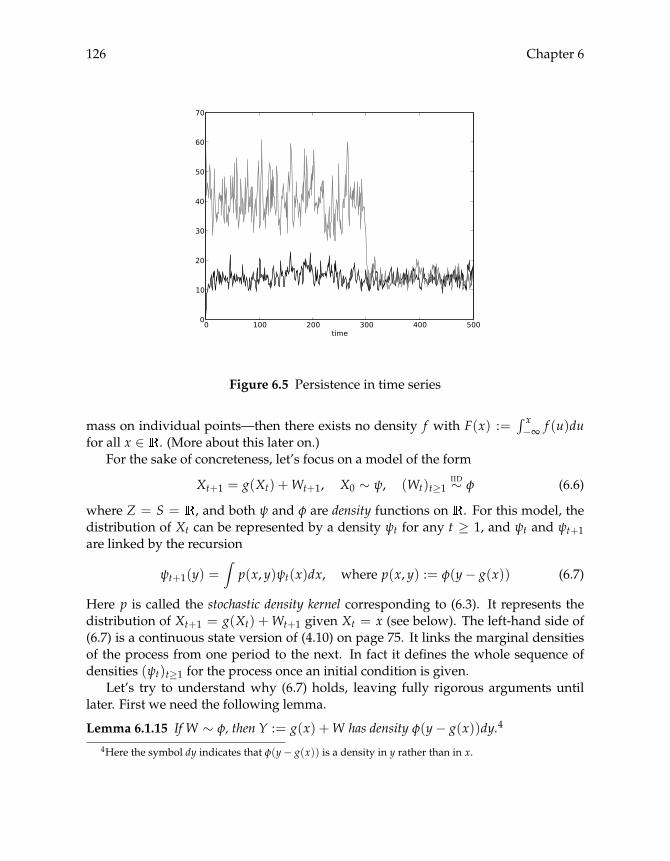
126 Chapter 6
Figure 6.5 Persistence in time series
mass on individual points—then there exists no density f with F(x) :=∫ x−∞ f (u)du
for all x ∈ . (More about this later on.)For the sake of concreteness, let’s focus on a model of the form
Xt+1 = g(Xt) +Wt+1, X0 ∼ ψ, (Wt)t≥1IID∼ φ (6.6)
where Z = S = , and both ψ and φ are density functions on . For this model, thedistribution of Xt can be represented by a density ψt for any t ≥ 1, and ψt and ψt+1are linked by the recursion
ψt+1(y) =∫
p(x, y)ψt(x)dx, where p(x, y) := φ(y− g(x)) (6.7)
Here p is called the stochastic density kernel corresponding to (6.3). It represents thedistribution of Xt+1 = g(Xt) +Wt+1 given Xt = x (see below). The left-hand side of(6.7) is a continuous state version of (4.10) on page 75. It links the marginal densitiesof the process from one period to the next. In fact it defines the whole sequence ofdensities (ψt)t≥1 for the process once an initial condition is given.
Let’s try to understand why (6.7) holds, leaving fully rigorous arguments untillater. First we need the following lemma.
Lemma 6.1.15 If W ∼ φ, then Y := g(x) +W has density φ(y− g(x))dy.4
4Here the symbol dy indicates that φ(y− g(x)) is a density in y rather than in x.
Infinite State Space 127
Proof. Let F be the cumulative distribution function (cdf) of Y, and let Φ be the cdfcorresponding to φ (i.e., Φ′ = φ). We have
F(y) = {g(x) +W ≤ y} = {W ≤ y− g(x)} = Φ(y− g(x))
The density of Y is F′(y) = φ(y− g(x)) as claimed.
Returning to (6.7), recall that if X and Y are random variables with joint densitypX,Y(x, y), then their marginal densities satisfy
pX(x) =∫
pX,Y(x, y)dy, pY(y) =∫
pX,Y(x, y)dx
Moreover the conditional density pY|X(x, y) of Y given X = x is given by
pY|X(x, y) =pX,Y(x, y)pX(x)
(x, y ∈ S)
Some simple manipulations now yield the expression
pY(y) =∫
pY|X(x, y)pX(x)dx (y ∈ S)
We have almost established (6.7). Letting Xt+1 = Y and Xt = X, we have
ψt+1(y) =∫
pXt+1|Xt(x, y)ψt(x)dx (y ∈ S)
The function pXt+1|Xt(x, y) is the density of g(Xt) +Wt+1 given Xt = x, or, more sim-
ply, the density of g(x) +Wt+1. By lemma 6.1.15, this is φ(y− g(x)) =: p(x, y), con-firming (6.7).
Now let’s look at the dynamics implied by the law of motion (6.7). The initialcondition is ψ0 = ψ, which is the density of X0 (regarded as given). From this initialcondition, (6.7) defines the entire sequence (ψt)t≥0. There are a couple of ways that wecan go about computing elements of this sequence. One is numerical integration. Forexample, ψ1 could be calculated by evaluating ψ1(y) =
∫p(x, y)ψ(x)dx at each y ∈ S.
Come to think of it, though, this is impossible: there is an infinity of such y. Instead,we would have to evaluate on a finite grid, use our results to form an approximationψ1 of ψ1, then do the same to obtain ψ2, and so on.
Actually this process is not very efficient, and it is difficult to obtain a measure ofaccuracy. So let’s consider some other approaches. Say that we wish to compute ψt,where t is a fixed point in time. Since we know how to compute empirical distributionfunctions by simulation, we could generate n observations of Xt (see algorithm 6.1),compute the empirical distribution function Fnt , and differentiate Fnt to obtain an ap-proximation ψn
t to ψt.
128 Chapter 6
It turns out that this is not a good plan either. The reason is that Fnt is not differen-tiable everywhere on S. And although it is differentiable at many points in S, at thosepoints the derivative is zero. So the derivative of Fnt contains no information aboutψt.5
Another plan would be to generate observations of Xt and histogram them. Thisis a reasonable and common way to proceed—but not without its flaws. The mainproblem is that the histogram converges rather slowly to its target ψt. This is becausehistograms have no notion of neighborhood, and do not make use of all knowledgewe have at hand. For example, if the number of bins is large, then it is often the casethat no points from the sample will fall in certain bins. This may happen even for binsclose to the mean of the distribution. The result is a “spiky” histogram, even when thetrue density is smooth.6
We can include the prior information that the density of ψt is relatively smoothusing Parzen windows, or nonparametric kernel density estimates. The kernel densityestimate fn of unknown density f from observations (Yi)ni=1 is defined as
fn(x) :=1
n · δnn
∑i=1
K(x−Yiδn
)(x ∈ ) (6.8)
where K is some density on , and δn is either a parameter or a function of the data,usually referred to as the bandwidth.
Essentially, fn is a collection of n “bumps,” one centered on each data point Yi.These are then summed and normalized to create a density.
Exercise 6.1.16 Using a suitable change of variables in the integral, show that fn is adensity for every n.
The bandwidth parameter plays a role similar to the number of bins used in thehistogram: A high value means that the densities we place on each data point are flatwith large tails. A low value means they are concentrated around each data point,and fn is spiky.
Exercise 6.1.17 Implement the nonparametric kernel density estimator (6.8) using astandard normal density for K. Base your code on the empirical distribution functionclass in listing 6.3. Generate a sample of 100 observations from the standard normaldistribution and plot the density esimate for bandwidth values 0.01, 0.1, and 0.5.
Although the nonparametric kernel density estimator produces good results in abroad range of environments, it turns out that for the problem at hand there is a better
5Readers familiar with the theory of ill-posed problems will have a feel for what is going on here. Thedensity computation problem is ill-posed!
6We get ψt by integrating ψt−1 with respect to a kernel φ(y− g(x)), and functions produced in this wayare usually smooth rather than spiky.
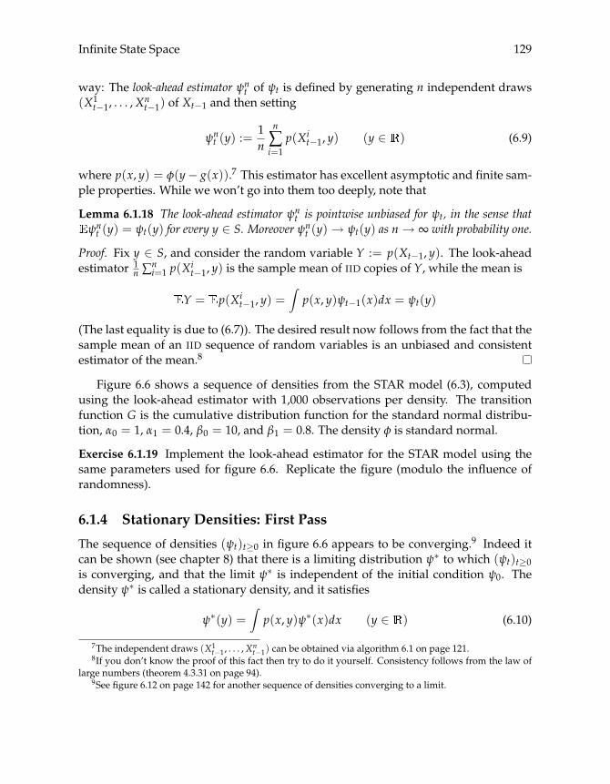
Infinite State Space 129
way: The look-ahead estimator ψnt of ψt is defined by generating n independent draws
(X1t−1, . . . ,X
nt−1) of Xt−1 and then setting
ψnt (y) :=
1n
n
∑i=1
p(Xit−1, y) (y ∈ ) (6.9)
where p(x, y) = φ(y− g(x)).7 This estimator has excellent asymptotic and finite sam-ple properties. While we won’t go into them too deeply, note that
Lemma 6.1.18 The look-ahead estimator ψnt is pointwise unbiased for ψt, in the sense that
ψnt (y) = ψt(y) for every y ∈ S. Moreover ψn
t (y)→ ψt(y) as n→ ∞ with probability one.
Proof. Fix y ∈ S, and consider the random variable Y := p(Xt−1, y). The look-aheadestimator 1
n ∑ni=1 p(X
it−1, y) is the sample mean of IID copies of Y, while the mean is
Y = p(Xit−1, y) =
∫p(x, y)ψt−1(x)dx = ψt(y)
(The last equality is due to (6.7)). The desired result now follows from the fact that thesample mean of an IID sequence of random variables is an unbiased and consistentestimator of the mean.8
Figure 6.6 shows a sequence of densities from the STAR model (6.3), computedusing the look-ahead estimator with 1,000 observations per density. The transitionfunction G is the cumulative distribution function for the standard normal distribu-tion, α0 = 1, α1 = 0.4, β0 = 10, and β1 = 0.8. The density φ is standard normal.
Exercise 6.1.19 Implement the look-ahead estimator for the STAR model using thesame parameters used for figure 6.6. Replicate the figure (modulo the influence ofrandomness).
6.1.4 Stationary Densities: First Pass
The sequence of densities (ψt)t≥0 in figure 6.6 appears to be converging.9 Indeed itcan be shown (see chapter 8) that there is a limiting distribution ψ∗ to which (ψt)t≥0is converging, and that the limit ψ∗ is independent of the initial condition ψ0. Thedensity ψ∗ is called a stationary density, and it satisfies
ψ∗(y) =∫
p(x, y)ψ∗(x)dx (y ∈ ) (6.10)
7The independent draws (X1t−1, . . . ,X
nt−1) can be obtained via algorithm 6.1 on page 121.
8If you don’t know the proof of this fact then try to do it yourself. Consistency follows from the law oflarge numbers (theorem 4.3.31 on page 94).
9See figure 6.12 on page 142 for another sequence of densities converging to a limit.
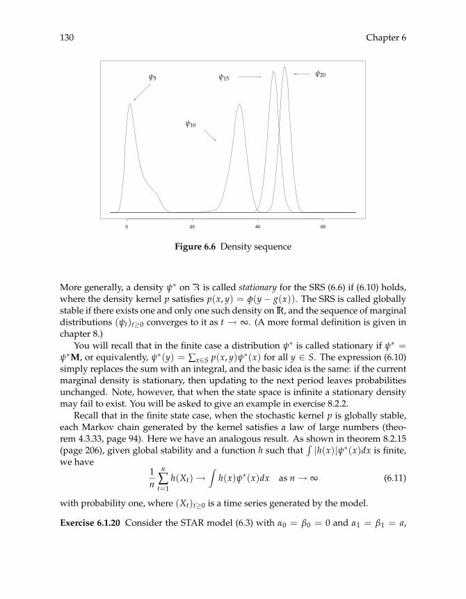
130 Chapter 6
0 20 40 60
ψ5 ψ15
ψ10
ψ20
Figure 6.6 Density sequence
More generally, a density ψ∗ on is called stationary for the SRS (6.6) if (6.10) holds,where the density kernel p satisfies p(x, y) = φ(y− g(x)). The SRS is called globallystable if there exists one and only one such density on , and the sequence of marginaldistributions (ψt)t≥0 converges to it as t → ∞. (A more formal definition is given inchapter 8.)
You will recall that in the finite case a distribution ψ∗ is called stationary if ψ∗ =ψ∗M, or equivalently, ψ∗(y) = ∑x∈S p(x, y)ψ∗(x) for all y ∈ S. The expression (6.10)simply replaces the sum with an integral, and the basic idea is the same: if the currentmarginal density is stationary, then updating to the next period leaves probabilitiesunchanged. Note, however, that when the state space is infinite a stationary densitymay fail to exist. You will be asked to give an example in exercise 8.2.2.
Recall that in the finite state case, when the stochastic kernel p is globally stable,each Markov chain generated by the kernel satisfies a law of large numbers (theo-rem 4.3.33, page 94). Here we have an analogous result. As shown in theorem 8.2.15(page 206), given global stability and a function h such that
∫ |h(x)|ψ∗(x)dx is finite,we have
1n
n
∑t=1
h(Xt)→∫h(x)ψ∗(x)dx as n→ ∞ (6.11)
with probability one, where (Xt)t≥0 is a time series generated by the model.
Exercise 6.1.20 Consider the STAR model (6.3) with α0 = β0 = 0 and α1 = β1 = a,

Infinite State Space 131
where a is a constant with |a| < 1. Suppose that φ is standard normal. We will see laterthat this is a stable parameter configuration, and ψ∗ = N(0, 1/(1− a2)) is stationaryfor this kernel. From (6.11) we have
1n
n
∑t=1
X2t �
11− α2 for large n
Write a simulation that compares these two expressions for large n.
The LLN gives us a method to investigate the steady state distribution ψ∗ for glob-ally stable systems. For example, we can form the empirical distribution function
Fn(x) :=1n
n
∑t=1{Xt ≤ x} =
1n
n
∑t=1
(−∞,x](Xt) (x ∈ )
where (−∞,x](y) = 1 if y ≤ x and zero otherwise and (Xt)t≥0 is a simulated time se-ries generated by the model. The empirical distribution function was discussed previ-ously in §6.1.2. We will see in what follows that
∫(−∞,x](y)ψ∗(y)dy is the probability
that a draw from ψ∗ falls below x. In other words, F(x) :=∫
(−∞,x](y)ψ∗(y)dy is thecumulative distribution function associated with ψ∗. Setting h = (−∞,x] in (6.11), wethen have Fn(x)→ F(x) with probability one, ∀x ∈ , and the empirical distributionfunction is consistent for F.
Exercise 6.1.21 Use the empirical distribution function to compute an estimate of Ffor (6.3) under the same parameters used in figure 6.6.
There is, however, a more powerful technique for evaluating ψ∗ when global sta-bility holds. Taking our simulated time series (Xt)nt=1, define
ψ∗n(y) :=1n
n
∑t=1
p(Xt, y) (y ∈ ) (6.12)
This expression is almost identical to the look-ahead estimator developed in §6.1.3(see (6.9) on page 129), with the difference being that the random samples are now asingle time series rather than repeated draws at a fixed point in time. To study theproperties of ψ∗n, observe that for any fixed y ∈ S, the LLN (6.11) gives us
ψ∗n(y) :=1n
n
∑t=1
p(Xt, y)→∫
p(x, y)ψ∗(x)dx = ψ∗(y)
where the last equality is by (6.10). Thus ψ∗n(y) is consistent for ψ∗(y).In fact much stronger results are true, and ψ∗n is an excellent estimator for ψ∗ (see,
e.g., Stachurski and Martin 2008). The reason is that while estimators such as Fn use
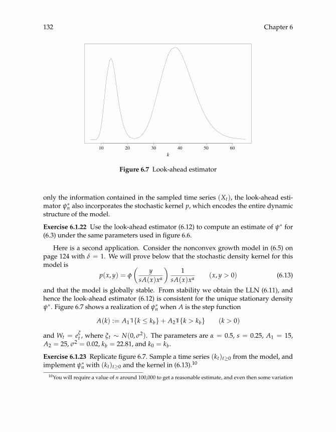
132 Chapter 6
10 20 30 40 50 60
k
Figure 6.7 Look-ahead estimator
only the information contained in the sampled time series (Xt), the look-ahead esti-mator ψ∗n also incorporates the stochastic kernel p, which encodes the entire dynamicstructure of the model.
Exercise 6.1.22 Use the look-ahead estimator (6.12) to compute an estimate of ψ∗ for(6.3) under the same parameters used in figure 6.6.
Here is a second application. Consider the nonconvex growth model in (6.5) onpage 124 with δ = 1. We will prove below that the stochastic density kernel for thismodel is
p(x, y) = φ
(y
sA(x)xα
)1
sA(x)xα(x, y > 0) (6.13)
and that the model is globally stable. From stability we obtain the LLN (6.11), andhence the look-ahead estimator (6.12) is consistent for the unique stationary densityψ∗. Figure 6.7 shows a realization of ψ∗n when A is the step function
A(k) := A1 {k ≤ kb}+ A2 {k > kb} (k > 0)
and Wt = eξt , where ξt ∼ N(0, σ2). The parameters are α = 0.5, s = 0.25, A1 = 15,A2 = 25, σ2 = 0.02, kb = 22.81, and k0 = kb.
Exercise 6.1.23 Replicate figure 6.7. Sample a time series (kt)t≥0 from the model, andimplement ψ∗n with (kt)t≥0 and the kernel in (6.13).10
10You will require a value of n around 100,000 to get a reasonable estimate, and even then some variation

Infinite State Space 133
6.2 Optimal Growth, Infinite State
Let’s now look at a simple optimal growth model on an infinite state space. We willcompute the optimal policy for the model numerically using value iteration and policyiteration. We also study via simulation the dynamics of the model under that policy.
6.2.1 Optimization
Consider again the optimal growth model discussed in chapter 1. At time t an agentreceives income yt, which is split into consumption ct and savings kt. Given kt, outputat t + 1 is yt+1 = f (kt,Wt+1), where (Wt)t≥1 is IID and takes values in Z := (0,∞)according to density φ. The agent’s behavior is specified by a policy function σ, whichis a map from S := + to satisfying 0 ≤ σ(y) ≤ y for all y ∈ S. The valueσ(y) should be interpreted as the agent’s choice of savings when income = y, while0 ≤ σ(y) ≤ y is a feasibility constraint ensuring that savings is nonnegative and doesnot exceed income. The set of all such policies will be denoted by Σ.
As with the finite state case, choice of a policy function σ ∈ Σ also determines anSRS for the state variable, given by
yt+1 = f (σ(yt),Wt+1), (Wt)t≥1IID∼ φ, y0 = y (6.14)
where y is initial income. Letting U be the agent’s utility function and ρ ∈ (0, 1) bethe discount factor, the agent’s decision problem is
maxσ∈Σ
vσ(y), where vσ(y) :=
[∞
∑t=0
ρtU(yt − σ(yt))
](6.15)
Here vσ(y) is the expected discounted value of following policy σ when initial incomeis y0 = y. For now we assume that U : + → + is bounded and continuous, andthat f : + × Z → + is continuous.
As discussed in the finite case—see §5.1.1, and in particular the discussion sur-rounding (5.4) on page 100—a rigorous definition of the expectation in (6.15) requiresmeasure theory. The details are deferred until chapter 10. Among other things, wewill see that the expectation can be passed through the sum to obtain
vσ(y) =∞
∑t=0
ρt U(yt − σ(yt)) (y ∈ S = +) (6.16)
will be observable over different realizations. This is due to the nonlinearity in the model and resultingslow convergence.
134 Chapter 6
This expression is simpler to interpret, with each term U(yt−σ(yt)) defined in termsof integrals over . Specifically, we integrate the function y �→ U(y − σ(y)) withrespect to the marginal distribution ψt of yt, where yt is defined recursively in (6.14).
Given vσ in (6.16), we can define the value function v∗ in exactly the same wayas (5.8) on page 102: v∗(y) := sup{vσ(y) : σ ∈ Σ}.11 Just as in §5.1.2, the valuefunction satisfies a Bellman equation: Letting Γ(y) := [0, y] be the feasible savingschoices when income is y, we have
v∗(y) = maxk∈Γ(y)
{U(y− k) + ρ
∫v∗( f (k, z))φ(z)dz
}(y ∈ S) (6.17)
The intuition behind (6.17) is similar to that for the finite state Bellman equation onpage 102, and won’t be repeated here. A proof that v∗ satisfies (6.17) will be providedvia theorem 10.1.11 on page 234. In the same theorem it is shown that v∗ is continuous.
Recall that bcS is the set of continuous bounded real-valued functions on S. Givena w ∈ bcS, we say that σ ∈ Σ is w-greedy if
σ(y) ∈ argmaxk∈Γ(y)
{U(y− k) + ρ
∫w( f (k, z))φ(z)dz
}(y ∈ S) (6.18)
Later in the text we will see that continuity of w implies continuity of the objectivefunction in (6.18), and since Γ(y) is compact, the existence of a maximizer σ(y) foreach y is guaranteed by theorem 3.2.22 (page 49).
We will also prove that a policy σ∗ is optimal in terms of maximizing expected dis-counted rewards if and only if it is v∗-greedy (theorem 10.1.11). In view of continuityof v∗ and the previous comment regarding existence of maximizers, this result showsthat at least one optimal policy exists. Moreover we can compute σ∗ by first solvingfor v∗ and then obtaining σ∗ as the maximizer in (6.18) with v∗ in place of w.
In order to compute v∗, we define the Bellman operator T, which maps w ∈ bcSinto Tw ∈ bcS via
Tw(y) = maxk∈Γ(y)
{U(y− k) + ρ
∫w( f (k, z))φ(z)dz
}(y ∈ S) (6.19)
We prove in chapter 10 that T is a uniform contraction of modulus ρ on the metricspace (bcS, d∞), where d∞(v,w) := supy∈S |v(y) − w(y)|. In view of Banach’s fixedpoint theorem (page 53), T then has a unique fixed point v ∈ bcS, and Tnv → v in d∞as n → ∞ for all v ∈ bcS. Moreover it is immediate from the definition of T and theBellman equation that Tv∗(y) = v∗(y) for all y ∈ S, so v = v∗. We conclude that alltrajectories of the dynamical system (bcS, T) converge to v∗.
11From boundedness of U it can be shown that this supremum is taken over a bounded set, and hence v∗is well defined. See exercise 10.1.8 on page 233. We treat unbounded rewards in §12.2.
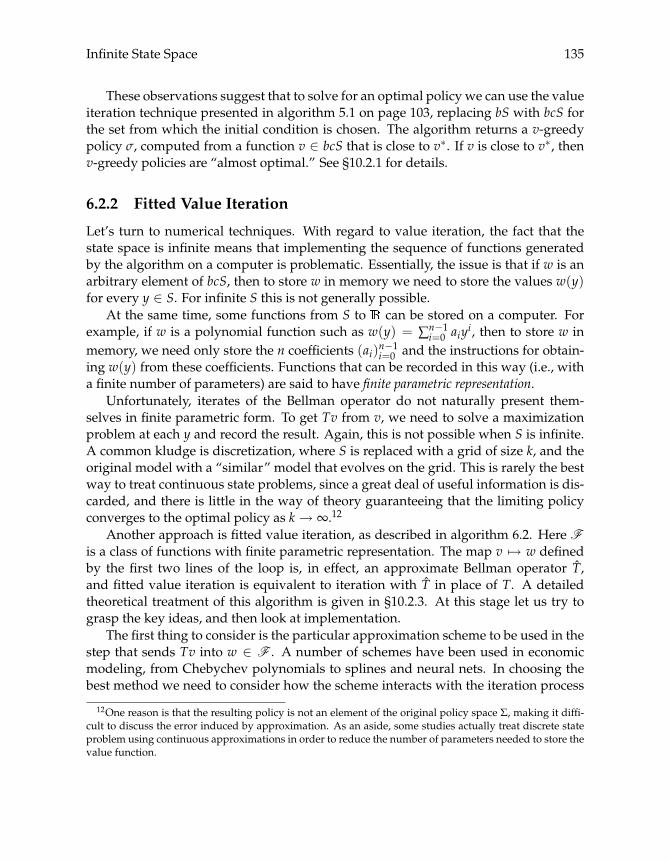
Infinite State Space 135
These observations suggest that to solve for an optimal policy we can use the valueiteration technique presented in algorithm 5.1 on page 103, replacing bS with bcS forthe set from which the initial condition is chosen. The algorithm returns a v-greedypolicy σ, computed from a function v ∈ bcS that is close to v∗. If v is close to v∗, thenv-greedy policies are “almost optimal.” See §10.2.1 for details.
6.2.2 Fitted Value Iteration
Let’s turn to numerical techniques. With regard to value iteration, the fact that thestate space is infinite means that implementing the sequence of functions generatedby the algorithm on a computer is problematic. Essentially, the issue is that if w is anarbitrary element of bcS, then to store w in memory we need to store the values w(y)for every y ∈ S. For infinite S this is not generally possible.
At the same time, some functions from S to can be stored on a computer. Forexample, if w is a polynomial function such as w(y) = ∑n−1
i=0 aiyi, then to store w inmemory, we need only store the n coefficients (ai)n−1
i=0 and the instructions for obtain-ing w(y) from these coefficients. Functions that can be recorded in this way (i.e., witha finite number of parameters) are said to have finite parametric representation.
Unfortunately, iterates of the Bellman operator do not naturally present them-selves in finite parametric form. To get Tv from v, we need to solve a maximizationproblem at each y and record the result. Again, this is not possible when S is infinite.A common kludge is discretization, where S is replaced with a grid of size k, and theoriginal model with a “similar” model that evolves on the grid. This is rarely the bestway to treat continuous state problems, since a great deal of useful information is dis-carded, and there is little in the way of theory guaranteeing that the limiting policyconverges to the optimal policy as k→ ∞.12
Another approach is fitted value iteration, as described in algorithm 6.2. Here Fis a class of functions with finite parametric representation. The map v �→ w definedby the first two lines of the loop is, in effect, an approximate Bellman operator T,and fitted value iteration is equivalent to iteration with T in place of T. A detailedtheoretical treatment of this algorithm is given in §10.2.3. At this stage let us try tograsp the key ideas, and then look at implementation.
The first thing to consider is the particular approximation scheme to be used in thestep that sends Tv into w ∈ F . A number of schemes have been used in economicmodeling, from Chebychev polynomials to splines and neural nets. In choosing thebest method we need to consider how the scheme interacts with the iteration process
12One reason is that the resulting policy is not an element of the original policy space Σ, making it diffi-cult to discuss the error induced by approximation. As an aside, some studies actually treat discrete stateproblem using continuous approximations in order to reduce the number of parameters needed to store thevalue function.

136 Chapter 6
Algorithm 6.2 Fitted value iteration
initialize v ∈ bcSrepeat
sample the function Tv at finite set of grid points (yi)ki=1use the samples to construct an approximation w ∈ F of Tvset e = d∞(v,w)set v = w
until e is less that some tolerancesolve for a v-greedy policy σ
used to compute the fixed point v∗. A scheme that approximates individual functionswell with respect to some given criterion does not always guarantee good dynamicproperties for the sequence (Tnv)n≥1.
To try to pin down a suitable technique for approximation, let’s decompose T intothe action of two operators L and T. First T is applied to v—in practice Tv is evaluatedonly at finitely many points—and then an approximation operator L sends the resultinto w = Tv ∈ F . Thus, T = L ◦ T. Figure 6.8 illustrates iteration of T.
We aim to choose L such that (1) the sequence (Tnv)n≥1 converges, and (2) thecollection of functions F is sufficiently rich that the limit of this sequence (whichlives in F ) can be close to the fixed point v∗ of T (which lives in bcS).13 The richnessof F depends on the choice of the approximation scheme and the number of gridpoints k in algorithm 6.2. In the formal results presented in §10.2.3, we will see thatthe approximation error depends on d∞(Lv∗, v∗), which indicates how well v∗ can beapproximated by an element ofF .
Returning to point (1), any serious attempt at theory requires that the sequence(Tnv)n≥1 converges in some sense as n → ∞. In this connection, note the followingresult.
Exercise 6.2.1 Let M and N be operators sending metric space (U, d) into itself. Showthat if N is a uniform contraction with modulus ρ and M is nonexpansive, then M ◦ Nis a uniform contraction with modulus ρ.
As T is a uniform contraction on (bcS, d∞), we see that T is uniformly contractingwhenever L is nonexpansive on (bcS, d∞). While for some common approximationarchitectures this fails, it does hold for a number of useful schemes. When attentionis restricted to these schemes the sequence (Tnv)n≥1 is convergent by Banach’s fixedpoint theorem, and we can provide a detailed analysis of the algorithm.
13More correctly, the limit of the sequence lives in clF ⊂ bcS.

Infinite State Space 137
F
T L TL
bcS
T Tv
Figure 6.8 The map T := L ◦ T
w
LwLv
v
x2 x3x1
Figure 6.9 Approximation via linear interpolation

138 Chapter 6
Listing 6.4 (lininterp.py) An interpolation class
from scipy impor t interp
c l a s s LinInterp:"Provides linear interpolation in one dimension."
de f __init__(self , X, Y):"""Parameters: X and Y are sequences or arrayscontaining the (x,y) interpolation points."""self.X, self.Y = X, Y
de f __call__(self , z):"""If z is a float (or integer) returns a float;if z is a sequence or array returns an array."""i f isinstance(z, int) or isinstance(z, float):
r e t u r n interp ([z], self.X, self.Y)[0]r e t u r n interp(z, self.X, self.Y)
Let’s move on to implementation, deferring further theory until §10.2.3. The ap-proximation scheme we will use is piecewise linear interpolation, as shown in fig-ure 6.9. (Outside the set of grid points, the approximations are constant.) With ref-erence to the figure, it is not difficult to see that for any v,w ∈ bcS, and any x in thedomain, we have
|Lv(x)− Lw(x)| ≤ sup1≤i≤k
|v(xi)− w(xi)| ≤ ‖v− w‖∞
Taking the supremum over x gives ‖Lv− Lw‖∞ ≤ ‖v−w‖∞, so L is nonexpansive onbcS.
Consider the class LinInterp in listing 6.4. This class provides an interface toSciPy’s interp() function, which implements linear interpolation. The latter is calledusing syntax interp(Z, X, Y), where X and Y are arrays of equal length providingthe (x, y) interpolation points, and Z is an array of arbitrary points where the inter-polant is to be evaluated. The call returns an array of length len(Z) containing theseevaluations.
The class LinInterp makes two modifications. First, an object of class LinInterpstores the interpolation points X and Y internally, so after instantiation of the objectwith these arrays, evaluations of the interpolant can be obtained without having topass the interpolation points each time. Second, we may wish to evaluate the inter-
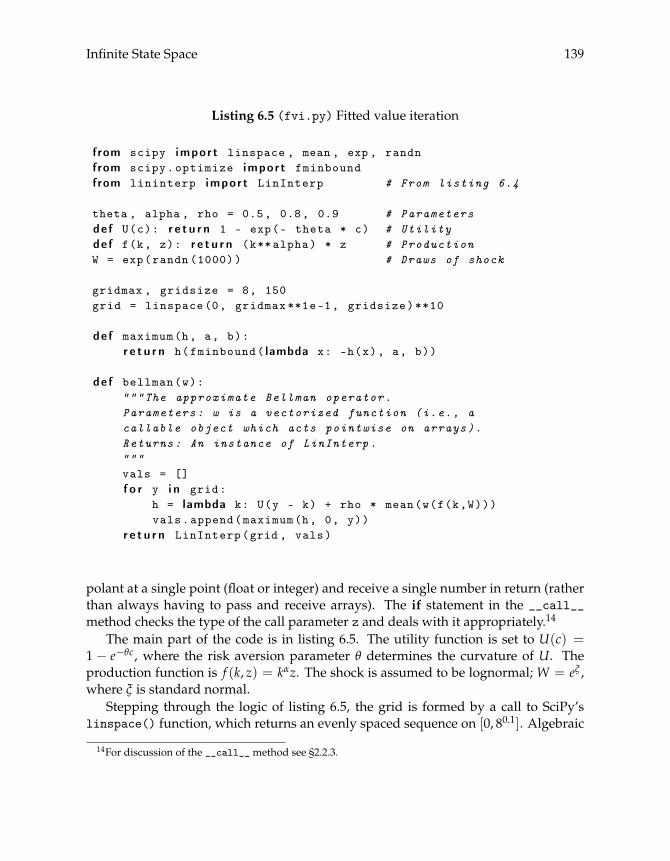
Infinite State Space 139
Listing 6.5 (fvi.py) Fitted value iteration
from scipy impor t linspace , mean , exp , randnfrom scipy.optimize impor t fminboundfrom lininterp impor t LinInterp # From listing 6.4
theta , alpha , rho = 0.5, 0.8, 0.9 # Parametersde f U(c): r e t u r n 1 - exp(- theta * c) # Utilityde f f(k, z): r e t u r n (k** alpha) * z # ProductionW = exp(randn (1000)) # Draws of shock
gridmax , gridsize = 8, 150grid = linspace(0, gridmax **1e-1, gridsize)**10
de f maximum(h, a, b):r e t u r n h(fminbound( lambda x: -h(x), a, b))
de f bellman(w):"""The approximate Bellman operator.Parameters: w is a vectorized function (i.e., acallable object which acts pointwise on arrays).Returns: An instance of LinInterp."""vals = []f o r y i n grid:
h = lambda k: U(y - k) + rho * mean(w(f(k,W)))vals.append(maximum(h, 0, y))
r e t u r n LinInterp(grid , vals)
polant at a single point (float or integer) and receive a single number in return (ratherthan always having to pass and receive arrays). The if statement in the __call__method checks the type of the call parameter z and deals with it appropriately.14
The main part of the code is in listing 6.5. The utility function is set to U(c) =1 − e−θc, where the risk aversion parameter θ determines the curvature of U. Theproduction function is f (k, z) = kαz. The shock is assumed to be lognormal; W = eξ ,where ξ is standard normal.
Stepping through the logic of listing 6.5, the grid is formed by a call to SciPy’slinspace() function, which returns an evenly spaced sequence on [0, 80.1]. Algebraic
14For discussion of the __call__ method see §2.2.3.
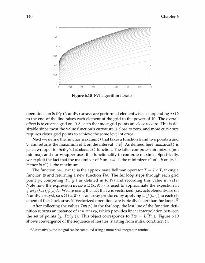
140 Chapter 6
0
0.25
0.5
0.75
1
1.25
1.5
0 0.25 0.5 0.75 1 1.25 1.5 1.75 2
Figure 6.10 FVI algorithm iterates
operations on SciPy (NumPy) arrays are performed elementwise, so appending **10to the end of the line raises each element of the grid to the power of 10. The overalleffect is to create a grid on [0, 8] such that most grid points are close to zero. This is de-sirable since most the value function’s curvature is close to zero, and more curvaturerequires closer grid points to achieve the same level of error.
Next we define the function maximum() that takes a function h and two points a andb, and returns the maximum of h on the interval [a, b]. As defined here, maximum() isjust a wrapper for SciPy’s fminbound() function. The latter computes minimizers (notminima), and our wrapper uses this functionality to compute maxima. Specifically,we exploit the fact that the maximizer of h on [a, b] is the minimizer x∗ of −h on [a, b].Hence h(x∗) is the maximum.
The function bellman() is the approximate Bellman operator T = L ◦ T, taking afunction w and returning a new function Tw. The for loop steps through each gridpoint yi, computing Tw(yi) as defined in (6.19) and recording this value in vals.Note how the expression mean(w(f(k,W))) is used to approximate the expection in∫w( f (k, z))φ(z)dz. We are using the fact that w is vectorized (i.e., acts elementwise on
NumPy arrays), so w(f(k,W)) is an array produced by applying w( f (k, ·)) to each el-ement of the shock array W. Vectorized operations are typically faster than for loops.15
After collecting the values Tw(yi) in the for loop, the last line of the function defi-nition returns an instance of LinInterp, which provides linear interpolation betweenthe set of points (yi, Tw(yi)). This object corresponds to Tw = L(Tw). Figure 6.10shows convergence of the sequence of iterates, starting from initial condition U.
15Alternatively, the integral can be computed using a numerical integration routine.

Infinite State Space 141
0
1
2
3
4
0 0.5 1 1.5 2 2.5 3 3.5 4
45 degreesy �→ σ(y)y �→ f(σ(y),m)
Figure 6.11 Approximate optimal policy
We can now compute a greedy policy σ from the last of these iterates, as shownin figure 6.11; along with the function y �→ f (σ(y),m), where m is the mean of theshock. If the shock is always at its mean, then from every positive initial condition theincome process (yt)t≥0 would converge to the unique fixed point at � 1.25. Noticethat when income is low, the agent invests all available income.
Of course, what happens when the shock is at its mean gives us little feel for thetrue dynamics. To generate the sequence of densities corresponding to the processyt+1 = f (σ(yt),Wt+1), we can use the look-ahead estimator (6.9) on page 129. To usethe theory developed there it is easiest to operate in logs. Given our parameterizationof f , taking logs of both sides of yt+1 = f (σ(yt),Wt+1) = σ(yt)αWt+1 yields
xt+1 = α ln σ(exp(xt)) + wt+1 := g(xt) + wt+1
where xt := ln yt, wt := lnWt and g(x) := α ln σ(exp(x)). This SRS is of the form (6.6)on page 126, and the look-ahead estimator of the density ψt of xt can be computed via
ψnt (y) :=
1n
n
∑i=1
p(xit−1, y) (y ∈ ) (6.20)
where p(x, y) = φ(y − g(x)) and (xit−1)ni=1 is n independent draws of xt−1 starting
from a given initial condition x0. Here φ is the density of wt—in this case it’s N(0, 1).Figure 6.12 shows the densities ψ1 to ψ15 starting at x0 ≡ −7.5 and using n = 1, 000.
Exercise 6.2.2 Using your preferred plotting utility and extending the code in list-ing 6.5, replicate figures 6.10 through 6.12. Starting from initial condition U, about

142 Chapter 6
−10 −7.5 −5 −2.5 0 2.5 50
0.05
0.1
0.15
0.2
0.25
0.3
0.35
Figure 6.12 Densities of the income process
30 iterates of T produces a good approximation of v∗. When you compute the densi-ties via the look-ahead estimator, try experimenting with different initial conditions.Observe how the densities always converge to the same limit.
6.2.3 Policy Iteration
Recall that in §5.1.3 we solved the finite state problem using a second algorithm, calledpolicy iteration. (See in particular algorithm 5.2 on page 105.) We can do the samething here, although we will need to use approximation techniques similar to thosewe used for fitted value iteration. The basic idea is presented in algorithm 6.3. (Inpractice, the functions vσ and σ will have to be approximated at each step.)
Algorithm 6.3 Policy iteration algorithm
pick any σ ∈ Σrepeat
compute vσ from σ
solve for a vσ-greedy policy σ′set σ = σ′
until until some stopping condition is satisfied

Infinite State Space 143
The theory behind policy iteration is presented in §10.2.2. In this section our inter-est will be in implementation. When considering implementation the most difficultpart is to compute vσ from σ (i.e., to calculate the value of a given policy). Let’s thinkabout how we might do this given the definition vσ(y) = ∑∞t=0 ρ
t U(yt − σ(yt)) in(6.16).
Fix y and consider the evaluation of vσ(y). We need to sum the terms U(yt −σ(yt)) discounted by ρt, at least for all t ≤ T where T is large. How should weevaluate U(yj− σ(yj)) for fixed j? One idea would be to use Monte Carlo. The initialcondition is y, and from there the process (yt)t≥0 follows the SRS in (6.14). We cangenerate n independent observations y1
j , . . . , ynj of yj using a version of algorithm 6.1
(page 121). The mean n−1∑ni=1 U(yij − σ(yij)) is close to U(yj − σ(yj)) for large n.16
While Monte Carlo methods can be useful for high-dimensional problems, thisapproach is not the easiest to implement. The reason is that even if we obtain goodapproximations to U(yt− σ(yt)) for each t and then sum them (discounting by ρt) toobtain vσ(y), we have only obtained an evaluation of the function vσ at a single pointy. But for algorithm 6.3 we need to evaluate vσ at every point y (or at least on a gridof points so we can approximate vσ).
Rather than us going down this path, consider the following iterative technique.For given σ ∈ Σ, define the operator Tσ that sends w ∈ bcS into Tw ∈ bcS by
Tσw(y) = U(y− σ(y)) + ρ∫w( f (σ(y), z))φ(z)dz (y ∈ S) (6.21)
For us the pertinent features of Tσ are summarized in the following result.
Lemma 6.2.3 For each σ ∈ Σ, the operator Tσ is a uniform contraction on (bcS, d∞), and theunique fixed point of Tσ in bcS is vσ.
The proof is not overly difficult but does involve some measure theory. As suchwe defer it until §10.1.3. What is important for us now is that from any initial guessv ∈ bcS we have Tnσ v → vσ so, by iterating with Tσ, we can obtain an approximationto vσ. In doing so we need to approximate at each iteration, just as we did for fittedvalue iteration (algorithm 6.2, but with Tσ in place of T). Listing 6.6 provides animplementation of this scheme, along with some additional routines.
The first line of the listing imports everything from the module fvi, which isthe file in listing 6.5. This provides the primitives of the model and the grid. Nextsome functions are imported from scipy. The first function maximizer() is similar tomaximum() in listing 6.5 but returns maximizers rather than maxima.
16An alternative Monte Carlo strategy would be to use the densities computed by the look-ahead estima-tor (see figure 6.12). Numerical integration of y �→ U(y− σ(y)) with respect to the density of yj then givesanother approximation to U(yj − σ(yj)).
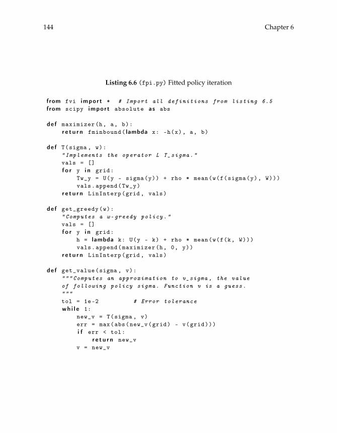
144 Chapter 6
Listing 6.6 (fpi.py) Fitted policy iteration
from fvi impor t * # Import all definitions from listing 6.5from scipy impor t absolute as abs
de f maximizer(h, a, b):r e t u r n fminbound( lambda x: -h(x), a, b)
de f T(sigma , w):"Implements the operator L T_sigma."vals = []f o r y i n grid:
Tw_y = U(y - sigma(y)) + rho * mean(w(f(sigma(y), W)))vals.append(Tw_y)
r e t u r n LinInterp(grid , vals)
de f get_greedy(w):"Computes a w-greedy policy."vals = []f o r y i n grid:
h = lambda k: U(y - k) + rho * mean(w(f(k, W)))vals.append(maximizer(h, 0, y))
r e t u r n LinInterp(grid , vals)
de f get_value(sigma , v):"""Computes an approximation to v_sigma , the valueof following policy sigma. Function v is a guess."""tol = 1e-2 # Error tolerancewh i l e 1:
new_v = T(sigma , v)err = max(abs(new_v(grid) - v(grid)))i f err < tol:
r e t u r n new_vv = new_v

Infinite State Space 145
The function T takes functions sigma and w, representing σ and w respectively, andreturns Tσw as an instance of the class LinInterp defined in listing 6.4. The code isrelatively self-explanatory, as is that for the function get_greedy(), which takes as itsargument a function w and returns a w-greedy policy as an instance of LinInterp.
The function get_value is used to calculate vσ from σ. It takes as arguments thefunctions sigma and v, which represent σ and a guess for vσ. We then iterate on thisguess with Tσ (actually L ◦ Tσ where L is the linear interpolation operator) to obtainan approximation to vσ. Iteration proceeds until the maximum distance over the gridpoints between the new and previous iterate falls below some tolerance.
Exercise 6.2.4 Compute an approximate optimal policy from listing 6.6. Check thatthis policy is similar to the one you computed in exercise 6.2.2.17
6.3 Stochastic Speculative Price
This section applies some of the ideas we have developed to the study of prices in acommodity market with consumers and speculators. After specifying and solving themodel, we will also investigate how the solution can be obtained using the optimalgrowth model of §6.2. In this way, we will see that the optimal growth model, whichat first pass seems rather limited, can in fact be applied to the study of decentralizedeconomies with a large number of agents.
6.3.1 The Model
Consider a market for a single commodity, whose price is given at t by pt. The “har-vest” of the commodity at time t is Wt. We assume that the sequence (Wt)t≥1 is IID
with common density function φ. The harvests take values in S := [a,∞), wherea > 0. The commodity is purchased by “consumers” and “speculators.” We assumethat consumers generate demand quantity D(p) corresponding to price p. Regardingthe inverse demand function D−1 =: P we assume that
Assumption 6.3.1 The function P : (0,∞) → (0,∞) exists, is strictly decreasing andcontinuous, and satisfies P(x) ↑ ∞ as x ↓ 0.
Speculators can store the commodity between periods, with It units purchased inthe current period yielding αIt units in the next, α ∈ (0, 1). For simplicity, the risk freeinterest rate is taken to be zero, so expected profit on It units is
t pt+1 · αIt − pt It = (α t pt+1 − pt)It17Hint: Suppose that σn is the policy computed at the n-th iteration. A good initial condition for the guess
of vσn in get_value() is vσn−1 .

146 Chapter 6
Here t pt+1 is the expectation of pt+1 taken at time t. Speculators are assumed to berisk neutral. Nonexistence of arbitrage requires that
α t pt+1 − pt ≤ 0 (6.22)
Profit maximization gives the additional condition
α t pt+1 − pt < 0 implies It = 0 (6.23)
We also require that the market clears in each period. Supply Xt is the sum αIt−1 +Wt of carryover by speculators and the current harvest, while demand is D(pt) + It(i.e., purchases by consumers and speculators). The market equilibrium condition istherefore
αIt−1 +Wt =: Xt = D(pt) + It (6.24)
The initial condition X0 ∈ S is treated as given.Now to find an equilibrium. Constructing a system (It, pt,Xt)t≥0 for investment,
prices, and supply that satisfies (6.22)–(6.24) is not trivial. Our path of attack will beto seek a system of prices that depend only on the current state. In other words, we take afunction p : S → (0,∞) and set pt = p(Xt) for every t. The vector (It, pt,Xt)t≥0 thenevolves as
pt = p(Xt), It = Xt − D(pt), Xt+1 = αIt +Wt+1 (6.25)
For given X0 and exogenous process (Wt)t≥1, the system (6.25) determines the timepath for (It, pt,Xt)t≥0 as a sequence of random variables. We seek a p such that (6.22)and (6.23) hold for the corresponding system (6.25).18
To this end, suppose that there exists a particular function p∗ : S → (0,∞) satisfy-ing
p∗(x) = max{α
∫p∗(αI(x) + z)φ(z)dz, P(x)
}(x ∈ S) (6.26)
whereI(x) := x− D(p∗(x)) (x ∈ S) (6.27)
It turns out that such a p∗ will suffice, in the sense that (6.22) and (6.23) hold for thecorresponding system (6.25). To see this, observe first that19
t pt+1 = t p∗(Xt+1) = t p∗(αI(Xt) +Wt+1) =∫
p∗(αI(Xt) + z)φ(z)dz
18Given (6.25) we have Xt = It + D(pt), so (6.24) automatically holds.19If the manipulations here are not obvious don’t be concerned—we will treat random variables in detail
later on. The last inequality uses the fact that if U and V are independent and V has density φ then theexpectation of h(U,V) given U is
∫h(U, z)φ(z)dz.
Infinite State Space 147
Thus (6.22) requires that
α∫
p∗(αI(Xt) + z)φ(z)dz ≤ p∗(Xt)
This inequality is immediate from (6.26). Second, regarding (6.23), suppose that
α∫
p∗(αI(Xt) + z)φ(z)dz < p∗(Xt)
Then by (6.26) we have p∗(Xt) = P(Xt), whence D(p∗(Xt)) = Xt, and It = I(Xt) = 0.(Why?) In conclusion, both (6.22) and (6.23) hold, and the system (It, pt,Xt)t≥0 is anequilibrium.
The only issue remaining is whether there does in fact exist a function p∗ : S →(0,∞) satisfying (6.26). This is not obvious, but can be answered in the affirmativeby harnessing the power of Banach’s fixed point theorem. To begin, let C denote theset of decreasing (i.e., nonincreasing) continuous functions p : S → with p ≥ Ppointwise on S.
Exercise 6.3.2 Argue that C ⊂ bcS, the set of all bounded continuous functions fromS into .
Exercise 6.3.3 Show that if (hn) ⊂ C and d∞(hn, h) → 0 for some function h ∈ bcS,then h is decreasing and dominates P.
Lemma 6.3.4 The metric space (C , d∞) is complete.
Proof. By theorem 3.2.3 on page 45 (closed subsets of complete spaces are complete)and the completeness of bcS (theorem 3.2.9 on page 46) we need only show that C isclosed as a subset of bcS. This follows from exercise 6.3.3.
As C is complete, it provides a suitable space in which we can introduce an opera-tor from C to C and—appealing to Banach’s fixed point theorem—show the existenceof an equilibrium. The idea is to construct the operator such that (1) any fixed pointsatisfies (6.26), and (2) the operator is uniformly contracting on C . The existence of anoperator satisfying conditions (1) and (2) proves the existence of a solution to (6.26).
So let p be a given element of C , and consider the new function on S constructedby associating to each x ∈ S the real number r satisfying
r = max{α
∫p(α(x− D(r)) + z)φ(z)dz, P(x)
}(6.28)
We denote the new function by Tp, where Tp(x) is the r that solves (6.28), and regardT as an operator sending elements of C into new functions on S. It is referred to belowas the pricing functional operator.

148 Chapter 6
Theorem 6.3.5 The following results hold:
1. The pricing functional operator T is well-defined, in the sense that Tp(x) is a uniquelydefined real number for every p ∈ C and x ∈ S. Moreover
P(x) ≤ Tp(x) ≤ v(x) := max{α
∫p(z)φ(z)dz, P(x)
}(x ∈ S)
2. T maps C into itself. That is, T(C ) ⊂ C .The proof is only sketched. You might like to come back after reading up on mea-
sure theory and fill out the details. To start, let p ∈ C and x ∈ S. Define
hx(r) := max{α
∫p(α(x− D(r)) + z)φ(z)dz, P(x)
}(P(x) ≤ r ≤ v(x))
Although we skip the proof, this function is continuous and decreasing on the inter-val [P(x), v(x)]. To establish the claim that there is a unique r ∈ [P(x), v(x)] satisfying(6.28), we must show that hx has a unique fixed point in this set. As hx is decreas-ing, uniqueness is trivial.20 Regarding existence, it suffices to show that there existnumbers r1 ≤ r2 in [P(x), v(x)] with
r1 ≤ hx(r1) and hx(r2) ≤ r2
Why does this suffice? The reason is that if either holds with equality then we aredone, and if both hold inequalities are strict, then we can appeal to continuity of hxand the intermediate value theorem (page 335).21
A suitable value for r1 is P(x). (Why?) For r2 we can use v(x), as
hx(r2) = max{α
∫p(α(x− D(r2)) + z)φ(z)dz, P(x)
}
≤ max{α
∫p(z)φ(z)dz, P(x)
}= v(x) = r2
The claim is now established, and with it part 1 of the theorem.To prove part 2, we must show that Tp (1) dominates P, (2) is decreasing on S, and
(3) is continuous on S. Of these, (1) is implied by previous results, while (2) and (3)hold but proofs are omitted—we won’t cover the necessary integration theory untilchapter 7.22
20This was discussed in exercise 3.2.31 on page 51.21Can you see why? Apply the theorem to g(r) = r− h(r).22The proof of (3) uses theorem B.1.4 on page 341.
Infinite State Space 149
Exercise 6.3.6 Verify that if p∗ is a fixed point of T, then it solves (6.26).
Theorem 6.3.7 The operator T is a uniform contraction of modulus α on (C , d∞).
It follows from theorem 6.3.7 that there exists a unique p∗ ∈ C with Tp∗ = p∗. Inview of exercise 6.3.6, p∗ satisfies (6.26), and we have solved our existence problem.Thus it only remains to confirm theorem 6.3.7, which can be proved using Blackwell’ssufficient condition for a uniform contraction. To state the latter, consider the met-ric space (M, d∞), where M is a subset of bU, the bounded real-valued functions onarbitrary set U.
Theorem 6.3.8 (Blackwell) Let M be a subset of bU with the property that u ∈ M andγ ∈ + implies u+ γ U ∈ M. If T : M→ M is monotone and
∃ λ ∈ [0, 1) s.t. T(u+ γ U) ≤ Tu+ λγ U ∀ u ∈ M and γ ∈ + (6.29)
then T is uniformly contracting on (M, d∞) with modulus λ.
Monotonicity means that if u, v ∈ M and u ≤ v, then Tu ≤ Tv, where all inequal-ities are pointwise on U. The proof of theorem 6.3.8 is given in on page 344, and wenow return to the proof of theorem 6.3.7.
Exercise 6.3.9 Let h1 and h2 be decreasing functions on S with (necessarily unique)fixed points x1 and x2. Show that if h1 ≤ h2, then x1 ≤ x2.
Using this exercise it is easy to see that T is a monotone operator on C : Pick anyp, q ∈ C with p ≤ q, and any x ∈ S. Let r �→ hp(r) be defined by
hp(r) := max{α
∫p(α(x− D(r)) + z)φ(z)dz, P(x)
}
and let hq(r) be defined analogously. Clearly, Tp(x) is the fixed point of r �→ hp(r),as is Tq(x) the fixed point of r �→ hq(r). Since hp(r) ≤ hq(r) for all r, it must be thatTp(x) ≤ Tq(x). As x was arbitrary we have Tp ≤ Tq.
To apply Blackwell’s condition, we need to show in addition that if p ∈ C andγ ∈ +, then (1) p+ γ S ∈ C , and (2) there exists a λ < 1 independent of p and γand having the property
T(p+ γ S) ≤ Tp+ λγ S (6.30)
Statement (1) is obviously true. Regarding statement (2), we make use of the followingeasy lemma:
Lemma 6.3.10 Let a, b, and c be real numbers with b ≥ 0. We have
max{a+ b, c} ≤ max{a, c}+ b
150 Chapter 6
If you’re not sure how to prove these kinds of inequalities, then here is how theyare done: Observe that both
a+ b ≤ max{a, c}+ b and c ≤ max{a, c}+ b
∴ max{a+ b, c} ≤ max{a, c}+ b
To continue, let p and γ be as above, and let q := p+ γ S. Pick any x ∈ S. Let rp standfor Tp(x) and let rq stand for Tq(x). We have
rq = max{α
∫q(α(x− D(rq)) + z)φ(z)dz, P(x)
}
≤ max{α
∫q(α(x− D(rp)) + z)φ(z)dz, P(x)
}
= max{α
∫p(α(x− D(rp)) + z)φ(z)dz+ αγ, P(x)
}
≤ max{α
∫p(α(x− D(rp)) + z)φ(z)dz, P(x)
}+ αγ
= rp + αγ
Here the first inequality follows from the fact that rp ≤ rq (since p ≤ q and T ismonotone), and the second from lemma 6.3.10.
We have show that T(p+ γ S)(x) ≤ Tp(x) + αγ. Since x is arbitrary and α < 1,the inequality (6.30) is established with λ := α.
6.3.2 Numerical Solution
In this section we compute the rational expectations pricing functional p∗ numericallyvia Banach’s fixed point theorem. To start, recall that in §6.3.1 we established theexistence of a function p∗ : S → (0,∞) in C satisfying (6.26). In the proof, p∗ wasshown to be the fixed point of the pricing operator T : C � p �→ Tp ∈ C . In view ofBanach’s theorem we have d∞(Tnp, p∗) → 0 as n → ∞ for any p ∈ C , so a naturalapproach to computing p∗ is by iterating on an arbitrary element p of C (such as P).In doing so, we will need to approximate the iterates Tnp at each step, just as for fittedvalue iteration (algorithm 6.2, page 136). As before we use linear interpolation, whichis nonexpansive with respect to d∞.
So suppose that p ∈ C and x ∈ S are fixed, and consider the problem of obtain-ing Tp(x), which, by definition, is the unique r ∈ [P(x), v(x)] such that (6.28) holds.Regarding this r,
Exercise 6.3.11 Show that r = P(x) whenever α∫p(z)φ(z)dz ≤ P(x).

Infinite State Space 151
Exercise 6.3.12 Show that if α∫p(z)φ(z)dz > P(x), then r satisfies
r = α∫
p(α(x− D(r)) + z)φ(z)dz
Algorithm 6.4 Computing Tp(x)
evaluate y = α∫p(z)φ(z)dz
if y ≤ P(x) then return P(x)else
define h(r) = α∫p(α(x− D(r)) + z)φ(z)dz
return the fixed point of h in [P(x), y]end
Together, exercises 6.3.11 and 6.3.12 suggest the method for finding r presented inalgorithm 6.4, which returns Tp(x) given p and x. An implementation of the algo-rithm is given in listing 6.7. The demand curve D is set to 1/x, while for the shock weassume thatWt = a+ cBt, where Bt is beta with shape parameters (5, 5). The functionfixed_point() computes fixed points inside a specified interval using SciPy’s brentqroot-finding algorithm. The function T() implements algorithm 6.4.23
Once we can evaluate Tp(x) for each p and x, we can proceed with the iterationalgorithm, as shown in algorithm 6.5. A sequence of iterates starting at P is displayedin figure 6.13.
Algorithm 6.5 Computing the pricing function
set p = Prepeat
sample Tp at finite set of grid points (xi)ki=1use samples to construct linear interpolant q of Tpset p = q
until a suitable stopping rule is satisfied
Exercise 6.3.13 Implement algorithm 6.5 and replicate figure 6.13.24
23Although the else statement from algorithm 6.4 is omitted in the definition of T(), it is unnecessarybecause the last two lines in the definition of T() are only executed if the statement y <= P(x) is false. Notealso that the function p() passed to T() must be vectorized.
24Hint: You can use the LinInterp class in listing 6.4 (page 138) for interpolation.
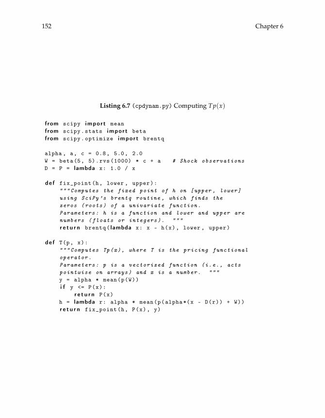
152 Chapter 6
Listing 6.7 (cpdynam.py) Computing Tp(x)
from scipy impor t meanfrom scipy.stats impor t betafrom scipy.optimize impor t brentq
alpha , a, c = 0.8, 5.0, 2.0W = beta(5, 5).rvs (1000) * c + a # Shock observationsD = P = lambda x: 1.0 / x
de f fix_point(h, lower , upper):"""Computes the fixed point of h on [upper , lower]using SciPy ’s brentq routine , which finds thezeros (roots) of a univariate function.Parameters: h is a function and lower and upper arenumbers (floats or integers). """r e t u r n brentq( lambda x: x - h(x), lower , upper)
de f T(p, x):"""Computes Tp(x), where T is the pricing functionaloperator.Parameters: p is a vectorized function (i.e., actspointwise on arrays) and x is a number. """y = alpha * mean(p(W))i f y <= P(x):
r e t u r n P(x)h = lambda r: alpha * mean(p(alpha*(x - D(r)) + W))r e t u r n fix_point(h, P(x), y)

Infinite State Space 153
Figure 6.13 The trajectory TnP
Given p∗, we have a dynamic system for quantities defined by
Xt+1 = αI(Xt) +Wt+1, (Wt)t≥1IID∼ φ (6.31)
where I(x) := x− D(p∗(x)). As shown in §6.1.3, the distribution ψt of Xt is a densityfor each t ≥ 1, and the densities satisfy
ψt+1(y) =∫
p(x, y)ψt(x)dx (y ∈ S)
where p(x, y) = φ(y− αI(x)), and φ is the density of the harvest Wt.25
Exercise 6.3.14 We will see later that the process (6.31) is stable, with a unique sta-tionary density ψ∗, and that the look-ahead estimator given in (6.12) on page 131 canbe used to estimate it. Using this estimator, show graphically that for these particularparameter values, speculators do not affect long-run probabilities for the state, in thesense that ψ∗ � φ.26
25We regard φ as defined on all of , and zero off its support. Hence, if y < αI(x), then p(x, y) = 0.26The latter is the distribution that prevails without speculation.

154 Chapter 6
6.3.3 Equilibria and Optima
In §6.3.1 we used Banach’s fixed point theorem to show the existence of a pricingfunctional p∗ such that the resulting system for prices and quantities was a competi-tive equilibrium. There is another way we can obtain the same result using dynamicprogramming and the optimal growth model. Solving the problem this way illustratesone of the many fascinating links between decentralized equilibria and optimality.
Before getting started we are going to complicate the commodity pricing modelslightly by removing the assumption that the interest rate is zero. With a positive andconstant interest rate r, next period returns must be discounted by ρ := 1/(1 + r). Asa result the no arbitrage and profit maximization conditions (6.22) and (6.23) become
ρα t pt+1 − pt ≤ 0 (6.32)
ρα t pt+1 − pt < 0 implies It = 0 (6.33)
As in §6.3.1 we seek a pricing function p∗ such that the system
pt = p∗(Xt), It = Xt − D(pt), Xt+1 = αIt +Wt+1 (6.34)
satisfies (6.32) and (6.33). This can be accomplished directly using the fixed point ar-guments in §6.3.1, making only minor adjustments to incorporate ρ. However, insteadof going down this path we will introduce a fictitious planner who solves the optimalgrowth model described in §6.2.1. Through a suitable choice of primitives, we showthat the resulting optimal policy can be used to obtain such a p∗. Since the optimalpolicy exists and can be calculated, p∗ likewise exists and can be calculated.
Regarding the planner’s primitives, the production function f is given by f (k, z) =αk+ z; the discount factor is ρ := 1/(1+ r); the utility functionU is defined byU(c) :=∫ c0 P(x)dx, where P is the inverse demand function for the commodity pricing model;
and the distribution φ of the shock is the distribution of the harvest.We assume that P is such that U is bounded on +. By the fundamental theorem
of calculus we have U′ = P. The conditions of assumption 6.3.1 on page 145 alsohold, and as a result the function U is strictly increasing, strictly concave and satisfiesU′(c) ↑ ∞ as c ↓ 0. We remove the assumption in §6.3.1 that the shock is boundedaway from zero, as this restriction is not needed.
Using the arguments in §6.2.1, we know that there exists at least one optimal policy.In fact concavity of the primitives implies that there is only one such policy. (For theproof, see §12.1.2.) The policy, denoted simply by σ, is v∗-greedy, which is to say that
σ(x) = argmax0≤k≤x
{U(x− k) + ρ
∫v∗( f (k, z))φ(z)dz
}(6.35)
Infinite State Space 155
for all x. One can also show that v∗ is differentiable with (v∗)′(x) = U′(x− σ(x)), andthat the objective function in (6.35) is likewise differentiable. Using these facts andtaking into account the possibility of a corner solution, it can be shown that σ satisfies
U′ ◦ c(x) ≥ ρ∫U′ ◦ c[ f (σ(x), z)] f ′(σ(x), z)φ(z)dz ∀ x ∈ S (6.36)
Moreover if the inequality is strict at some x > 0, then σ(x) = 0. Here c(x) := x− σ(x)and f ′(k, z) is the partial derivative of f with respect to k. This is the famous Euler(in)equality, and full proofs of all these claims can be found via propositions 12.1.23and 12.1.24 in §12.1.2.
The main result of this section is that by setting p∗ equal to marginal utility ofconsumption we obtain an equilibrium pricing functional for the commodity pricingmodel.
Proposition 6.3.15 If p∗ is defined by p∗(x) := U′ ◦ c(x) :=: U′(c(x)), then the systemdefined in (6.34) satisfies (6.32) and (6.33).
Proof. Substituting the definition of p∗ into (6.36) we obtain
p∗(x) ≥ ρ∫
p∗[ f (σ(x), z)] f ′(σ(x), z)φ(z)dz ∀ x ∈ S
with strict inequality at x implying that σ(x) = 0. Using f (k, z) = αk+ z this becomes
p∗(x) ≥ ρα∫
p∗(ασ(x) + z)φ(z)dz ∀ x ∈ S
Now observe that since c(x) = x− σ(x), we must have
p∗(x) = U′(x− σ(x)) = P(x− σ(x)) ∀ x ∈ S
∴ D(p∗(x)) = x− σ(x) ∀ x ∈ S
Turning this around, we get σ(x) = x−D(p∗(x)), and the right-hand side is preciselyI(x). Hence σ = I, and we have
ρα∫
p∗(αI(x) + z)φ(z)dz− p∗(x) ≤ 0 ∀ x ∈ S
with strict inequality at x implying that I(x) = 0. Since this holds for all x ∈ S, itholds at any realization Xt ∈ S, so
ρα∫
p∗(αI(Xt) + z)φ(z)dz− p∗(Xt) ≤ 0
with strict inequality implying I(Xt) = 0. Substituting It and pt from (6.34), and usingthe fact that
t pt+1 =∫
p∗(αI(Xt) + z)φ(z)dz
as shown in §6.3.1, we obtain (6.32) and (6.33).
156 Chapter 6
6.4 Commentary
Further theory and applications of stochastic recursive sequences in economics andfinance can be found in Sargent (1987), Stokey and Lucas (1989), Farmer (1999), Duffie(2001), Miranda and Fackler (2002), Adda and Cooper (2003), or Ljungqvist and Sar-gent (2004). The simulation-based approach to computing marginal and stationarydensities of stochastic recursive sequences in §6.1.3 and §6.1.4 was proposed by Glynnand Henderson (2001), and a detailed analysis of the technique and its properties canbe found in Stachurski and Martin (2008).
The one-sector, infinite horizon, stochastic optimal growth model in §6.2 is essen-tially that of Brock and Mirman (1972). Related treatments can be found in Mirmanand Zilcha (1975), Donaldson and Mehra (1983), Stokey and Lucas (1989), Amir (1996),and Williams (2004). A survey of the field is given in Olsen and Roy (2006). Fordiscussion of the stability properties of the optimal growth model, see §12.1.3. Thecommentary to that chapter contains additional references.
We saw in §6.3.3 that optimal policies for the growth model coincide with the mar-ket equilibria of certain decentralized economies. For more discussion of the links be-tween dynamic programming and competitive equilibria, see Stokey and Lucas (1989,ch. 16), or Bewley (2007). Seminal contributions to this area include Samuelson (1971),Lucas and Prescott (1971), Prescott and Mehra (1980), and Brock (1982).
Under some variations to the standard environment (incomplete markets, produc-tion externalities, distortionary taxes, etc.), equilibria and optima no longer conincide,and the problem facing the researcher is to find equilibria rather than optimal poli-cies. For a sample of the literature, see Huggett (1993), Aiyagari (1994), Greenwoodand Huffman (1995), Rios-Rull (1996), Krusell and Smith (1998), Kubler and Schmed-ders (2002), Reffett and Morand (2003), Krebs (2004), Datta et al. (2005), Miao (2006),and Angeletos (2007).
The commodity price model studied in §6.3 is originally due to Samuelson (1971),who connected equilibrium outcomes with solutions to dynamic programming prob-lems. Our treatment in §6.3.1 and §6.3.2 follows Deaton and Laroque (1992), whowere the first to derived the equilibrium price directly via Banach’s fixed point theo-rem. The technique of iterating on the pricing functional is essentially equivalent toColeman’s algorithm (Coleman 1990). For more on the commodity pricing model, see,for example, Scheinkman and Schectman (1983) or Williams and Wright (1991).

Part II
Advanced Techniques
157


Chapter 7
Integration
Measure and integration theory are among the foundation stones of modern mathe-matics, and particularly those fields of concern to us. Measure theory also has a rep-utation for being difficult, and indeed it is both abstract and complex. However, witha little bit of effort and attention to the exercises, you will find that measure-theoreticarguments start to seem quite natural, and that the theory has a unique beauty of itsown.
Before attempting this chapter you should have a good grounding in basic realanalysis. Anyone who has solved most of the exercises in appendix A should be upto the task.
7.1 Measure Theory
In this first section we give a brisk introduction to measure theory. The longer proofsare omitted, although a flavor of the arguments is provided. If you read this sectioncarefully you will have a good feel for what measure theory is about, and for whythings are done the way that they are.
7.1.1 Lebesgue Measure
To understand integration, we need to know about Lebesgue measure. The basicproblem of Lebesgue measure is how to assign to each subset of k (each elementof P( k)) a real number that will represent its “size” (length, area, volume) in themost natural sense of the word.1 For a set like (a, b] ⊂ 1 there is no debate: The
1Recall that P(A) denotes the set of all subsets of the set A.
159
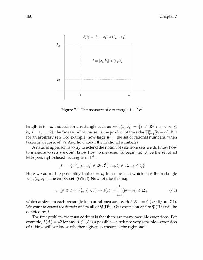
160 Chapter 7
�(I) = (b1− a1)× (b2− a2)
a2
b2
a1 b1
I = (a1, b1]× (a2, b2]
Figure 7.1 The measure of a rectangle I ⊂ 2
length is b − a. Indeed, for a rectangle such as ×ki=1(ai, bi] = {x ∈ k : ai < xi ≤
bi, i = 1, . . . , k}, the “measure” of this set is the product of the sides∏ki=1(bi − ai). But
for an arbitrary set? For example, how large is , the set of rational numbers, whentaken as a subset of ? And how about the irrational numbers?
A natural approach is to try to extend the notion of size from sets we do know howto measure to sets we don’t know how to measure. To begin, let J be the set of allleft-open, right-closed rectangles in k:
J := {×ki=1(ai, bi] ∈ P( k) : ai, bi ∈ , ai ≤ bi}
Here we admit the possibility that ai = bi for some i, in which case the rectangle×ki=1(ai, bi] is the empty set. (Why?) Now let � be the map
� : J � I = ×ki=1(ai, bi] �→ �(I) :=
k
∏i=1
(bi − ai) ∈ + (7.1)
which assigns to each rectangle its natural measure, with �(∅) := 0 (see figure 7.1).We want to extend the domain of � to all of P( k). Our extension of � to P( k) will bedenoted by λ.
The first problem we must address is that there are many possible extensions. Forexample, λ(A) = 42 for any A /∈J is a possible—albeit not very sensible—extensionof �. How will we know whether a given extension is the right one?
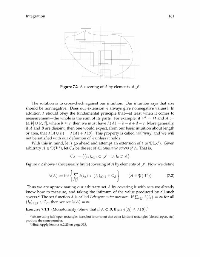
Integration 161
Figure 7.2 A covering of A by elements ofJ
The solution is to cross-check against our intuition. Our intuition says that sizeshould be nonnegative. Does our extension λ always give nonnegative values? Inaddition λ should obey the fundamental principle that—at least when it comes tomeasurement—the whole is the sum of its parts. For example, if k = and A :=(a, b] ∪ (c, d], where b ≤ c, then we must have λ(A) = b− a+ d− c. More generally,if A and B are disjoint, then one would expect, from our basic intuition about lengthor area, that λ(A ∪ B) = λ(A) + λ(B). This property is called additivity, and we willnot be satisfied with our definition of λ unless it holds.
With this in mind, let’s go ahead and attempt an extension of � to P( k). Givenarbitrary A ∈ P( k), let CA be the set of all countable covers of A. That is,
CA := {(In)n≥1 ⊂J : ∪n In ⊃ A}Figure 7.2 shows a (necessarily finite) covering of A by elements ofJ . Now we define
λ(A) := inf
{∑n≥1
�(In) : (In)n≥1 ∈ CA
}(A ∈ P( k)) (7.2)
Thus we are approximating our arbitrary set A by covering it with sets we alreadyknow how to measure, and taking the infimum of the value produced by all suchcovers.2 The set function λ is called Lebesgue outer measure. If ∑n≥1 �(In) = ∞ for all(In)n≥1 ∈ CA, then we set λ(A) = ∞.
Exercise 7.1.1 (Monotonicity) Show that if A ⊂ B, then λ(A) ≤ λ(B).3
2We are using half-open rectangles here, but it turns out that other kinds of rectangles (closed, open, etc.)produce the same number.
3Hint: Apply lemma A.2.25 on page 333.

162 Chapter 7
Exercise 7.1.2 (Sub-additivity) Show that if A and B are any two subsets of k, thenλ(A ∪ B) ≤ λ(A) + λ(B).4
Exercise 7.1.3 Extend sub-additivity to countable sub-additivity if you can: Show thatfor any (An) ⊂ P( ) we have λ(∪nAn) ≤ ∑n λ(An).5
Before we go on, we need to consider whether Lebesgue outer measure is actuallyan extension of �—the function defined onJ—to P( k). Clearly, λ is a well definedfunction on P( k) (why?), but does it actually agree with the original function � onJ ? In other words, we need to check that λ assigns “volume” to rectangles.
Lemma 7.1.4 λ : P( k)→ [0,∞] defined in (7.2) agrees with � onJ .
Although the result seems highly likely, the proof is not entirely trivial. It can befound in any text on measure theory.
Now the task is to see whether λ agrees with our intuition in the ways that we dis-cussed above (nonnegativity, additivity, etc.). Nonnegativity is obvious, but when itcomes to additivity we run into problems: Additivity fails. In 1905 G. Vitali succeededin constructing sets A, B ∈ P( ) that are so nasty and intertwined that λ(A)+λ(B) >λ(A ∪ B).6
Well, we said at the start that we were not prepared to accept the validity of ourextension unless it preserves additivity. So must (7.2) be abandoned? It might seemso, but no obvious alternatives present themselves.7 The solution of Henri Lebesguewas to restrict the domain of the set function λ to exclude those nasty sets that causeadditivity to break down. The method succeeds because the sets remaining in thedomain after this exclusion process turn out to be all those sets we will ever need in dayto day analysis.
The actual restriction most commonly used in modern texts is due to the Greekmathematician Constantin Carathéodory, who considers the class of sets A ∈ P( k)satisfying
λ(B) = λ(B ∩ A) + λ(B ∩ Ac) for all B ∈ P( k) (7.3)
This collection of sets is denoted by L and called the Lebesgue measurable sets. Therestriction of λ toL is called Lebesgue measure.
Exercise 7.1.5 Show that k ∈ L and∅ ∈ L . Using monotonicity and sub-additivity,show that if N ⊂ and λ(N) = 0, then N ∈ L .
4Hint: Fix ε > 0 and choose covers (IAn )n≥1 and (IBn )n≥1 of A and B respectively such that ∑n �(IAn ) ≤λ(A) + ε/2 and ∑n �(IBn ) ≤ λ(B) + ε/2. Now consider (∪n IAn ) ∪ (∪n IBn ) as a cover of A ∪ B.
5Hint: Fix ε > 0 and choose for each An a cover (Inj )j≥1 such that ∑j �(Inj ) ≤ λ(An) + ε2−n. Nowconsider ∪n ∪j Inj as a cover of ∪nAn.
6His construction uses the dreaded Axiom of Choice.7We could try approximating sets from the inside (“inner” measure rather than outer measure), but this
is less convenient and it turns out that the same problem reappears.
Integration 163
Our first important observation is that Lebesgue measure is additive onL . In factone of the central facts of measure theory is that, restricted to this domain, λ is not justadditive, but countably additive (definition below). This turns out to be crucial whentrying to show that λ interacts well with limiting operations. Equally important,L isvery large, containing the open sets, closed sets, countable sets, and more.8
Let’s state without proof the countable additivity property of λ onL .
Theorem 7.1.6 (Countable additivity) If (An)n≥1 is a disjoint sequence in L , in thatAi ∩ Aj = ∅ whenever i �= j, then λ(∪nAn) = ∑n≥1 λ(An).9
Exercise 7.1.7 Show that countable additivity implies (finite) additivity.10
Exercise 7.1.8 Prove that for any A, B ∈ L with A ⊂ B and λ(B) < ∞ we haveλ(B \ A) = λ(B)− λ(A).
To learn a bit more about the properties of λ, consider the following exercise: Weknow that {x} ∈ L for all x ∈ k becauseL contains all closed sets. Let’s show thatλ({x}) = 0 for any point x ∈ . It is enough to show that for any ε > 0, we can finda sequence (In)n≥1 ⊂ J containing x and having ∑n≥1 �(In) ≤ ε. (Why?) So picksuch an ε, and take a cover (In)n≥1 such that the first rectangle I1 satisfies I1 � x and�(I1) ≤ ε, and then In = ∅ for n ≥ 2. Now ∑n≥1 �(In) ≤ ε as required.
Exercise 7.1.9 Show that λ( k) = ∞.11
Exercise 7.1.10 Using countable additivity and the fact that singletons {x} have zeromeasure, show that countable sets have zero measure.12
You may be wondering if there are uncountable sets of measure zero. The answeris yes. An often cited example is the Cantor set, which can be found in any text onmeasure theory.
7.1.2 Measurable Spaces
We mentioned above that the set of Lebesgue measurable sets L contains all of thesets we typically deal with in analysis, In addition it has nice “algebraic” properties.In particular, it is a σ-algebra:
8For the definition of countable (and uncountable) sets see page 322.9The value +∞ is permitted here. Also, readers might be concerned that for an arbitrary sequence
(An)n≥1 ⊂ L the union ∪nAn may not be inL , in which case λ(∪nAn) is not defined. In fact the union isalways inL as we will see below.
10Hint: We must show that λ(∪Nn=1An) = ∑Nn=1 λ(An) for any finite collection of disjoint sets (An)Nn=1.
Try thinking about the countable sequence (Bn)n≥1 where Bn = An for n ≤ N and Bn = ∅ for n > N.11Hint: Using lemma 7.1.4 and monotonicity (exercise 7.1.1), show that λ( k) is bigger than any real
number.12This implies that in we must have λ( ) = 0. By additivity, then, λ( ) = λ( c). In this sense there
are “many more” irrational numbers than rational numbers.
164 Chapter 7
Definition 7.1.11 Let S be any nonempty set. A family of sets S ⊂ P(S) is called aσ-algebra if
1. S ∈ S ,
2. A ∈ S implies Ac ∈ S , and
3. if (An)n≥1 is a sequence with An inS for all n, then ∪nAn ∈ S .
The pair (S,S ) is called a measurable space, and elements of S are called measur-able sets. The second and third properties are usually expressed by saying that thecollectionS is “closed” or “stable” under complementation and countable unions, inthe sense that these operations do not take us outside the collectionS . From De Mor-gan’s law (∩nAn)c = ∪nAc
n, we see thatS is also stable under countable intersections.(Why?) Finally, note that ∅ ∈ S .
An example of a σ-algebra on S is P(S). This is true for every set S. For example,if A ∈ P(S), then Ac := {x ∈ S : x /∈ A} is also a subset of S by its very definition.On the other hand, the collection O of open subsets of is not a σ-algebra because itis not stable under the taking of complements.
Incidentally, the concept of σ-algebras plays a major role in measure theory, andthese collections of sets sometimes seem intimidating and abstract to the outsider.But the use of σ-algebras is less mysterious than it appears. When working with aσ-algebra, we know that if we start with some measurable sets, take unions, thencomplements, then intersections, and so on, the new sets we create are still measur-able sets. By definition, σ-algebras are stable under the familiar set operations, so weneed not worry that we will leave our safe environment when using these standardoperations.
Exercise 7.1.12 Check that {∅, S} is a σ-algebra on S for any set S. Show that, on theother hand,J is not a σ-algebra on k.
Exercise 7.1.13 If {Sα}α∈Λ is any collection of σ-algebras on S, then their intersection∩αSα is all B ⊂ S such that B ∈ Sα for every α ∈ Λ. Show that ∩αSα is itself aσ-algebra on S.
One of the most common ways to define a particular σ-algebra is to take a collec-tion C of subsets of S, and consider the smallest σ-algebra that contains this collection.
Definition 7.1.14 If S is any set and C is any collection of subsets of S, then the σ-algebra generated by C is the smallest σ-algebra on S that contains C , and is denoted byσ(C ). More precisely, σ(C ) is the intersection of all σ-algebras on S that contain C . Ingeneral, if σ(C ) = S , then C is called a generating class forS .
Integration 165
Exercise 7.1.15 Show that if C is a σ-algebra, then σ(C ) = C , and that if C and D aretwo collections of sets with C ⊂ D , then σ(C ) ⊂ σ(D).
Now let’s return to the Lebesgue measurable sets. As discussed above, it can beshown that L is a σ-algebra, and that it contains all the sets we need in day-to-dayanalysis.13 In fact L contains more sets than we actually need, and is not easily ab-stracted to more general spaces. As a result we will almost invariably work with asmaller domain called the Borel sets, and denoted B( k). The collection B( k) isjust the σ-algebra generated by the open subsets of k.14 More generally,
Definition 7.1.16 Let S be any metric space. The Borel sets on S are the sets B(S) :=σ(O), where O is the open subsets of S.
Exercise 7.1.17 Explain whyB(S) must contain the closed subsets of S.
In the case of S = k this collectionB( k) is surprisingly large. In fact it is quitedifficult to construct a subset of k that is not inB( k). MoreoverB( k) is a subsetof L , and hence all of the nice properties that λ has on L it also has on B( k). Inparticular, λ is countably additive onB( k).
Exercise 7.1.18 Show that ∈ B( ).15
The following theorem gives some indication as to why the Borel sets are so naturaland important to analysis.
Theorem 7.1.19 Let O , C andK be the open, closed and compact subsets of k respectively.We have
B( k) := σ(O) = σ(C ) = σ(K ) = σ(J )
Let’s just show thatB( k) = σ(K ). To see thatB( k) ⊃ σ(K ), note thatB( k)is a σ-algebra containing all the closed sets, and hence all the compact sets. (Why?) Inwhich case it also contains σ(K ). (Why?) To show thatB( k) ⊂ σ(K ), it suffices toprove that σ(K ) contains C . (Why?) To see that σ(K ) contains C , pick any C ∈ Cand let Dn := {x ∈ k : ‖x‖ ≤ n}. Observe that Cn := C ∩ Dn ∈ K for every n ∈(why?), and that C = ∪nCn. Since Cn ∈ K for all n, we have C = ∪nCn ∈ σ(K ), aswas to be shown.
Exercise 7.1.20 Let A be the set of all open intervals (a, b) ⊂ . Show that σ(A ) =B( ).16
13To prove that L is a σ-algebra, one can easily check from the definition (7.3) that ∈ L and thatA ∈ L implies Ac ∈ L . To show thatL is stable under countable unions is a bit more subtle and the proofis omitted.
14The open subsets of k are determined by the euclidean metric d2. But any metric defined from a normon k gives us the same open sets (theorem 3.2.30), and hence the same Borel sets.
15Hint: Singletons are closed, and = a countable union of singletons.16You should be able to show that σ(A ) ⊂ σ(O). To show that σ(O) ⊂ σ(A ) it is sufficient to prove that

166 Chapter 7
7.1.3 General Measures and Probabilities
Measure theory forms the foundations of modern probability. Before we study this inearnest, let’s think a little bit about why it might be fruitful to generalize the concept of“measures.” To start, imagine a space S, which you might like to visualize as a subsetof the plane 2. Like a satellite photograph of the earth at night, the space is sprinkledwith lots of tiny glowing particles. If we take a region E of the space S, you might askhow many of these particles are contained in E, or alternatively, what fraction of thetotal quantity of the particles are in E?
Let μ be a set function on P(S) such that μ(E) is the fraction of particles in E. Itseems that μ is going to be nonnegative, monotone (E ⊂ F implies μ(E) ≤ μ(F)), andadditive (E, F disjoint implies μ(E ∪ F) = μ(E) ∪ μ(F)), just as the Lebesgue measureλwas. So perhaps μ is also some kind of “measure,” and can be given a neat treatmentby using similar ideas.
These considerations motivate us to generalize the notion of Lebesgue measurewith an abstract definition. As is always the case in mathematics, abstracting in aclever way will save us saying things over and over again, and lead to new insights.
Definition 7.1.21 Let (S,S ) be a measurable space. A measure μ on (S,S ) is a func-tion fromS to [0,∞] such that
1. μ(∅) = 0, and
2. μ is countably additive: If (An) ⊂ S is disjoint, then μ(∪nAn) = ∑n μ(An).
The triple (S,S , μ) is called a measure space.
Exercise 7.1.22 Show that if there exists an A ∈ S with μ(A) < ∞, then (2) implies(1).17
Exercise 7.1.23 Show that (2) implies monotonicity: If E, F ∈ S and E ⊂ F, thenμ(E) ≤ μ(F).
Exercise 7.1.24 Show that a measure μ on S is always sub-additive: If A and B are anyelements ofS (disjoint or otherwise), then μ(A ∪ B) ≤ μ(A) + μ(B).
Let (An)n≥1 ⊂ S have the property that An+1 ⊂ An for all n ∈ , and let A :=∩nAn. We say that the sequence (An)n≥1 decreases down to A, and write An ↓ A.On the other hand, if An+1 ⊃ An for all n ∈ and A := ∪nAn, then we say that(An)n≥1 increases up to A, and write An ↑ A. For such “monotone” sequences of sets,an arbitrary measure μ on (S,S ) has certain continuity properties, as detailed in thenext exercise.σ(A ) contains the open sets. (Why?) To do so, use the fact that every open subset of can be expressed asthe countable union of open intervals.
17In this sense (1) is just to rule out trivial cases, and (2) is the real condition of interest.

Integration 167
Exercise 7.1.25 Let (An)n≥1 be a sequence inS . Show that
1. if An ↑ A, then μ(An) ↑ μ(A),18 and
2. if μ(A1) < ∞ and An ↓ A, then μ(An) ↓ μ(A).19
Example 7.1.26 Consider the measurable space ( ,P( )) formed by the set of nat-ural numbers and the set of all its subsets. On this measurable space define thecounting measure c, where c(B) is simply the number of elements in B, or +∞ if B isinfinite. With some thought you will be able to convince yourself that c is a measureon ( ,P( )).20
Exercise 7.1.27 Let (an) ⊂ +. Let μ be defined on ( ,P( )) by μ(A) = ∑n∈A an.Show that μ is a measure on ( ,P( )).
Let’s now specialize this to “probability measures,” which are the most importantkind of measures for us after Lebesgue measure. In what follows (S,S ) is any mea-surable space.
Definition 7.1.28 A probability measure μ is a measure on (S,S ) such that μ(S) = 1.The triple (S,S , μ) is called a probability space. The set of all probability measures on(S,S ) is denoted byP(S,S ). When S is a metric space, elements ofP(S,B(S)) arecalled Borel probability measures. For brevity we will writeP(S,B(S)) asP(S).
In the context of probability theory, a set E in S is usually called an event, andμ(E) is interpreted as the probability that when uncertainty is realized the event Eoccurs. Informally, μ(E) is the probability that x ∈ E when x is drawn from the set Saccording to μ. The empty set ∅ is called the impossible event, and S is called the certainevent.
Defining μ on a σ-algebra works well in terms of probabilistic intuition. For exam-ple, the impossible and certain events are always in S . Also, we want Ec to be in Swhenever E is: If the probability of E occurring is defined, then so is the probabilityof E not occurring. And if E and F are in S , we want E ∩ F ∈ S so that we cantalk about the probability that both E and F occur, and so forth. These properties areassured by the definition of σ-algebras.
Given measurable space (S,S ) and point x ∈ S, the Dirac probability measure δx ∈P(S,S ) is the distribution that puts all mass on x. More formally, δx(A) = A(x) forall A ∈ S .
Exercise 7.1.29 Confirm that δx is a probability measure on (S,S ).18Hint: Let B1 = A1 and Bn = An \ An−1 for n ≥ 2. Show that (Bn) is a disjoint sequence with ∪kn=1Bn =
Ak and ∪nBn = A. Now apply countable additivity.19Hint: Use part 1 of the exercise.20When we come to integration, series of real numbers will be presented as integrals of the counting
measure. Repackaging summation as integration may not sound very useful, but actually it leads to ahandy set of results on passing limits through infinite sums.
168 Chapter 7
7.1.4 Existence of Measures
Suppose that we release at time zero a large number of identical, tiny particles intowater at a location defined as zero, and then measure the horizontal distance of theparticles from the origin at later point in time t. As Albert Einstein pointed out, theindependent action of the water molecules on the particles and the central limit theo-rem tell us that, at least in this idealized setting, and at least for E = (a, b] ∈ J , thefraction of the total mass contained in E should now be approximately
μ(E) = μ((a, b]) =∫ b
a
1√2πt
exp−x2
2tdx (7.4)
One can think of μ(E) as the probability that an individual particle finds itself in E attime t.
In (7.4) we have a way of computing probabilities for intervals (a, b] ∈ J , butno obvious way of measuring the probability of more complex events. For example,what is μ( ), where is the rational numbers? Measuring intervals is all well andgood, but there will certainly be times that we want to assign probabilities to morecomplex sets. In fact we need to do this to develop a reasonable theory of integration.
How to extend μ from J to a larger class of subsets of ? Taking our cue fromthe process for Lebesgue measure, we could assign probability to an arbitrary set Aby setting
μ∗(A) := inf ∑n≥1
μ(In) = inf ∑n≥1
∫ bn
an
1√2πt
exp−x2
2tdx (A ⊂ ) (7.5)
where the infimum is over all sequences of intervals (In)n≥1, with In := (an, bn] ∈Jfor each n, and with the sequence covering A (i.e., ∪n In ⊃ A). This extension wouldbe suitable if (1) it agrees with μ onJ , and (2) it is a measure, at least when restrictedto a nice subset of P( ) such asB( ). Being a measure implies attractive propertiessuch as nonnegativity, monotonicity and additivity.21
Instead of dealing directly with μ, let’s look at this extension process in an abstractsetting. As with all abstraction, the advantage is that we can cover a lot of cases in onego. The disadvantage is that the statement of results is quite technical. It is providedmainly for reference purposes, rather than as material to be worked through step bystep. The idea is to formulate a system for constructing measures out of set functionsthat behave like measures (i.e., are countably additive) on small, concrete classes ofsets called semi-rings.
21For probabilities, monotonicity should be interpreted as follows: A ⊂ B means that whenever A hap-pens, B also happens. In which case B should be at least as likely to occur as A, or μ∗(A) ≤ μ∗(B).Additivity is familiar from elementary probability. For example, the probability of getting an even numberwhen you roll a dice is the probability of getting a 2 plus that of getting a 4 plus that of getting a 6. (Notethat monotonicity is implied by nonnegativity and additivity—see exercise 7.1.23).
Integration 169
Definition 7.1.30 Let S be a nonempty set. A nonempty collection of subsets R iscalled a semi-ring if, given arbitrary sets I and J inR, we have
1. ∅ ∈ R,
2. I ∩ J ∈ R, and
3. I \ J can be expressed as a finite union of elements ofR.
The definition is not particularly attractive, but all we need to know at this stageis thatJ , the half-open rectangles ×k
i=1(ai, bi] in k, form a semi-ring. Although theproof is omitted, a little thought will convince you thatJ is a semi-ring when k = 1.You might like to give a sketch of the proof for the case of 2 by drawing pictures.
We now give a general result for existence of measures. Let S be any nonemptyset, and letR be a semi-ring on S. A set function μ : R → [0,∞] is called a pre-measureonR if μ(∅) = 0 and μ(∪n In) = ∑n μ(In) for any disjoint sequence (In)n≥1 ⊂ R with∪n In ∈ R. For any A ⊂ S, let CA be the set of all countable covers of A formed fromelements ofR. That is,
CA := {(In)n≥1 ⊂ R : ∪n In ⊃ A}Now define the outer measure generated by μ as
μ∗(A) := inf
{∑n≥1
μ(In) : (In)n≥1 ∈ CA
}(A ∈ P(S)) (7.6)
The restriction of μ∗ to σ(R) turns out to be a measure, and is typically denoted simplyby μ. Formally,
Theorem 7.1.31 Let S be any nonempty set and let R be a semi-ring on S. If μ is a pre-measure onR, then the outer measure (7.6) agrees with μ onR and is a measure on (S, σ(R)).If there exists a sequence (In) ⊂ R with ∪n In = S and μ(In) < ∞ for all n, then theextension is unique in the sense that if ν is any other pre-measure that agrees with μ on R,then its extension agrees with μ on all of σ(R).
The proof is quite similar to the construction of Lebesgue measure sketched in§7.1.1. First one defines the outer measure μ∗ by (7.6). Since μ∗ is not necessarilyadditive over all of P(S) (think of the case of Lebesgue measure), we then restrictattention to those sets S that satisfy Carathéodory’s condition: All A ∈ P(S) suchthat
μ∗(B) = μ∗(B ∩ A) + μ∗(B ∩ Ac) for all B ∈ P(S) (7.7)
It can be proved that S is a σ-algebra containing R, and that μ∗ is a measure on S .Evidently σ(R) ⊂ S (why?), and the restriction of μ∗ to σ(R) is simply denoted byμ.
170 Chapter 7
Let’s consider applications of theorem 7.1.31. One is Lebesgue measure on k. Forthe semi-ring we takeJ . It can be shown that � defined onJ by (7.1) on page 160 isa pre-measure. As a result � extends uniquely to a measure on σ(J ) = B( k). Thisgives us Lebesgue measure onB( k).
A second application is probabilities on , such as the Gaussian probability de-fined in (7.4). Recall that F : → is called a cumulative distribution function on
if it is nonnegative, increasing, right-continuous, and satisfies limx→−∞ F(x) = 0and limx→∞ F(x) = 1. We imagine F(x) represents the probability that random vari-able X takes values in (−∞, x]. More generally, for interval (a, b] the probability thatX ∈ (a, b] is given by F(b)− F(a).
Fix any distribution function F, and let J be the semi-ring of all intervals (a, b],where a ≤ b. Although the proof is not trivial, one can show using the properties of Fthat μF : J → + defined by
μF((a, b]) = F(b)− F(a)
is a pre-measure onJ . Clearly, there exists a sequence (In) ⊂J with ∪n In = andμF(In) < ∞ for all n. As a result there exists a unique extension of μF to a measureon σ(J ) = B( ) with μF(A) := inf∑n≥1(F(bn) − F(an)) for all A ∈ B( ). Theinfimum is over all sequences of intervals (In) with In := (an, bn] ∈J for each n and∪n In ⊃ A.
It follows that to each cumulative distribution function on there corresponds aunique Borel probability measure. Conversely, suppose that μ ∈ P( ), and let F bedefined by F(x) = μ((−∞, x]) for x ∈ .
Exercise 7.1.32 Show that F is a cumulative distribution function on .
Putting this together and filling in some details, one can show that
Theorem 7.1.33 There is a one-to-one pairing between the collection of all distribution func-tions on and P( ), the set of all Borel probability measures on . If F is a distributionfunction, then the corresponding probability μF satisfies
μF((−∞, x]) = F(x) (x ∈ )
Let’s look back and see what we have accomplished. The main result here is the-orem 7.1.31, which helps us construct measures. To understand it’s importance, sup-pose that we propose a would-be measure such as (7.4). To check that this is indeeda measure on the Borel sets is a tough ask. After all, what does an arbitrary Borel setlook like? But to show that μ((a, b]) =
∫ ba (2πt)−1/2e−x2/2tdx is a pre-measure on the
nice semi-ring J of intervals (a, b] is much easier. Once this is done theorem 7.1.31can be applied.

Integration 171
7.2 Definition of the Integral
Elementary calculus courses use the Riemann definition of integrals. As a result of itsconstruction the Riemann integral is inherently limited, in terms of both its domainof definition and its ability to cope with limiting arguments. We want to construct anintegral that extends the Riemann integral to a wider domain, and has nice analyticalproperties to boot. With this goal in mind, let’s start to develop a different theory ofintegration (the Lebesgue theory), beginning with the case of functions from to ,and working up to more abstract settings.
7.2.1 Integrating Simple Functions
Let’s start with the easiest case. A simple function is any real-valued function takingonly finitely many different values. Consider a simple function s : → that takesvalues α1, . . . , αN on a corresponding disjoint intervals I1, . . . , IN inJ . Exploiting theassumption that the intervals are disjoint, the function s can be expressed as a linearcombination of indicator functions: s = ∑N
n=1 αn In .22 Take a moment to convince
yourself of this.Since our integral is to be an extension of the Riemann integral, and since the Rie-
mann integral of s is well defined and equal to the sum over n of αn times the lengthof In, the Lebesgue integral must also be
λ(s) :=:∫sdλ :=
N
∑n=1
αn(bn − an) =N
∑n=1
αnλ(In) (7.8)
where λ on the right-hand side is the Lebesgue measure.The symbol
∫sdλ is reminiscent of the traditional notation
∫s(x)dx. Using dλ
reminds us that we are integrating with respect to Lebesgue measure. Later, moregeneral integrals are defined. The alternative notation λ(s) for the integral of functions with respect to measure λ is also common. It reminds us that we are defining a mapthat sends functions into numbers.
Little effort is needed to shift our theory up from to k. For a function s : k →defined by s = ∑N
n=1 αn In , where each In = ×ki=1(ai, bi] is an element of J ⊂
P( k) and the rectangles are disjoint, we set
λ(s) :=:∫sdλ :=
N
∑n=1
αnλ(In) (7.9)
Here λ on the right-hand side is Lebesgue measure on k. Figure 7.3 shows an exam-ple of such a function s on 2.
22In other words, s(x) = ∑Nn=1 αn In (x) for every x ∈ , where In (x) = 1 if x ∈ In and zero otherwise.

172 Chapter 7
Figure 7.3 A simple function on the plane
Having defined an integral for simple functions that are constant on rectangles,the next step is to extend the definition to the B( k)-simple functions sB( k), eachof which takes only finitely many values, but on Borel sets rather than just rectangles.More succinctly, sB( k) is all functions of the form ∑N
n=1 αn Bn , where the Bn’s aredisjoint Borel sets. For now let’s think about nonnegative simple functions (αn ≥ 0 forall n), the set of which we denote sB( k)+. A natural extension of our integral (7.9)to sB( k)+ is given by
λ(s) :=:∫sdλ :=
N
∑n=1
αnλ(Bn) (7.10)
This is already a generalization of the Riemann integral. For example, the Riemannintegral is not defined for , which is an element of sB( )+. Note also that λ(s) =∞ is a possibility, and we do not exclude this case.
Exercise 7.2.1 Explain why the integral of is zero.
So far we have defined integrals of (finite-range) functions defined over k, whereintegration was with respect to Lebesgue measure. Next, just as we abstracted fromLebesgue measure to arbitrary measures, let us now introduce integrals of simplefunctions using general measures.
Suppose that we have a measure μ on an arbitrary measurable space (S,S ). Wecan define the real-valued simple functions sS on (S,S ) in the same way that we
Integration 173
defined the Borel simple functions sB( k) on k, replacing B( k) with S in thedefinition. In other words, sS is those functions of the form s = ∑N
n=1 αn An , wherethe sets A1, . . . , AN are disjoint and An ∈ S for all n. The set sS + is the nonnegativefunctions in sS .
By direct analogy with (7.10), the integral of s ∈ sS + is defined as
μ(s) :=:∫sdμ :=
N
∑n=1
αnμ(An) (7.11)
To give an illustration of (7.11), consider an experiment where a point ω is selectedfrom some set Ω according to probability measure . Here is defined on some σ-algebra F of subsets of Ω, and (E) is interpreted as the probability that ω ∈ E foreach E ∈ F . Suppose that we have a discrete random variable X taking ω ∈ Ω andsending it into one of N values. Specifically, X sends points in An ∈ F into αn ∈ ,where A1, . . . , AN is a partition of Ω. Intuitively, the expectation of X is then
N
∑n=1
αn Prob{X = αn} =N
∑n=1
αn Prob{ω ∈ An} =N
∑n=1
αn (An)
Comparing the right-hand side of this expression with (7.11), it becomes clear that theexpectation of X is precisely the integral (X) :=:
∫Xd . A more traditional notation
is X. We will come back to expectations later on.Returning to general (S,S , μ), integrals of simple functions have some useful
properties.
Proposition 7.2.2 For s, s′ ∈ sS + and γ ≥ 0, the following properties hold:
1. γs ∈ sS + and μ(γs) = γμ(s).
2. s+ s′ ∈ sS + and μ(s+ s′) = μ(s) + μ(s′).
3. If s ≤ s′ pointwise on S, then μ(s) ≤ μ(s′).
We say that on sS + the integral μ is positive homogeneous, additive, and mono-tone respectively. The full proofs are a bit messy and not terribly exciting so we omitthem.
Exercise 7.2.3 Prove part 1 of proposition 7.2.2. Prove parts 2 and 3 in the special casewhere s = α A and s′ = β B.
7.2.2 Measurable Functions
So far we have extended the integral to sS +. This is already quite a large class offunctions. The next step is to extend it further by a limiting operation (a method of
174 Chapter 7
definition so common in analysis!). To do this, we need to define a class of functionsthat can be approximated well by simple functions. This motivates the definition of ameasurable function:
Definition 7.2.4 Let (S,S ) and (R,R) be two measurable spaces, and let f : S → R.The function f is called S ,R-measurable if f−1(B) ∈ S for all B ∈ R. If (R,R) =( ,B( )), then f is called S -measurable. If, in addition, S is a metric space andS = B(S), then f is called Borel measurable.
While this definition is very succinct, it is also rather abstract, and the implicationsof measurability are not immediately obvious. However, we will see that—for thekinds of functions we want to integrate—measurability of a function f is equivalentto the existence of a sequence of simple functions (sn)n≥1 that converges to f in asuitable way (see lemma 7.2.11 below). We will then be able to define the integral of fas the limit of the integrals of the sequence (sn)n≥1.
Exercise 7.2.5 Show that if (S1,S1), (S2,S2) and (S3,S3) are any three measurablespaces, f : S1 → S2 is S1,S2-measurable and g : S2 → S3 is S2,S3-measurable, thenh := g ◦ f : S1 → S3 isS1,S3-measurable.
With measure theory the notation keeps piling up. Here is a summary of the nota-tion we will use for functions from (S,S ) into :
• mS is defined to be theS -measurable functions on S,
• mS + is defined to be the nonnegative functions in mS , and
• bS is defined to be the bounded functions in mS .
Exercise 7.2.6 Let S be any set. Argue that every f : S→ isP(S)-measurable, whileonly the constant functions are {S,∅}-measurable.
Exercise 7.2.7 Let (S,S ) be any measurable space. Show that sS ⊂ mS .
The following lemma is very useful when checking measurability. The proof istypical of measure-theoretic arguments.
Lemma 7.2.8 Let (E,E ) and (F,F ) be two measurable spaces, and let f : E → F. Let G bea generator of F , in the sense that σ(G ) = F . Then f is E ,F -measurable if and only iff−1(B) ∈ E for all B ∈ G .Proof. Necessity is obvious. Regarding sufficiency, let
M := {B ∈ F : f−1(B) ∈ E }
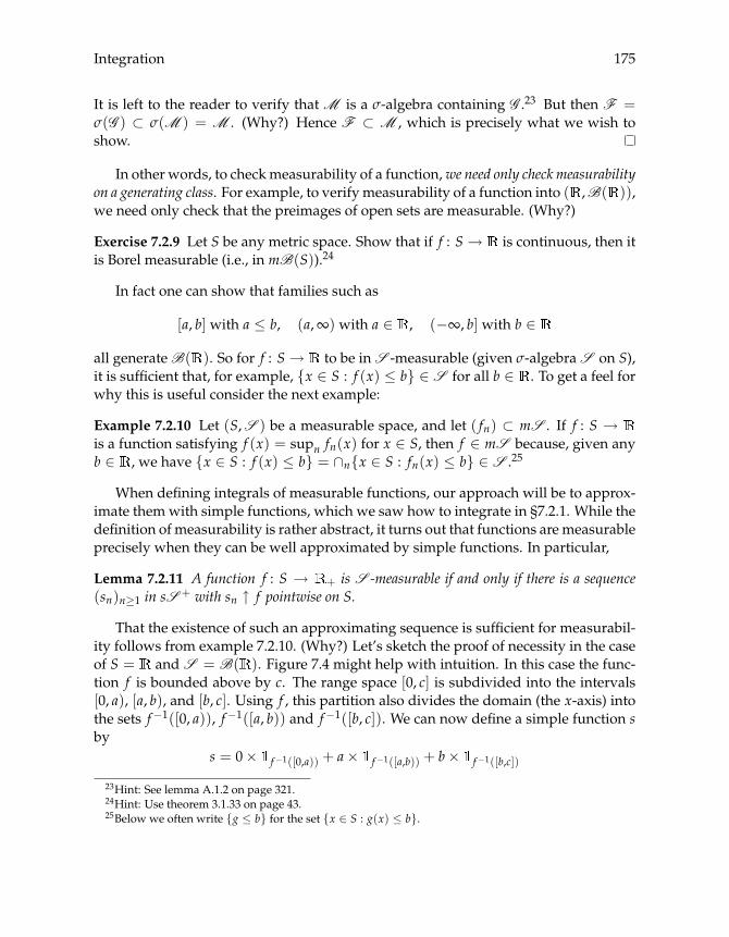
Integration 175
It is left to the reader to verify that M is a σ-algebra containing G .23 But then F =σ(G ) ⊂ σ(M ) = M . (Why?) Hence F ⊂ M , which is precisely what we wish toshow.
In other words, to check measurability of a function,we need only check measurabilityon a generating class. For example, to verify measurability of a function into ( ,B( )),we need only check that the preimages of open sets are measurable. (Why?)
Exercise 7.2.9 Let S be any metric space. Show that if f : S→ is continuous, then itis Borel measurable (i.e., in mB(S)).24
In fact one can show that families such as
[a, b] with a ≤ b, (a,∞) with a ∈ , (−∞, b] with b ∈
all generateB( ). So for f : S→ to be inS -measurable (given σ-algebraS on S),it is sufficient that, for example, {x ∈ S : f (x) ≤ b} ∈ S for all b ∈ . To get a feel forwhy this is useful consider the next example:
Example 7.2.10 Let (S,S ) be a measurable space, and let ( fn) ⊂ mS . If f : S →is a function satisfying f (x) = supn fn(x) for x ∈ S, then f ∈ mS because, given anyb ∈ , we have {x ∈ S : f (x) ≤ b} = ∩n{x ∈ S : fn(x) ≤ b} ∈ S .25
When defining integrals of measurable functions, our approach will be to approx-imate them with simple functions, which we saw how to integrate in §7.2.1. While thedefinition of measurability is rather abstract, it turns out that functions are measurableprecisely when they can be well approximated by simple functions. In particular,
Lemma 7.2.11 A function f : S → + is S -measurable if and only if there is a sequence(sn)n≥1 in sS + with sn ↑ f pointwise on S.
That the existence of such an approximating sequence is sufficient for measurabil-ity follows from example 7.2.10. (Why?) Let’s sketch the proof of necessity in the caseof S = and S = B( ). Figure 7.4 might help with intuition. In this case the func-tion f is bounded above by c. The range space [0, c] is subdivided into the intervals[0, a), [a, b), and [b, c]. Using f , this partition also divides the domain (the x-axis) intothe sets f−1([0, a)), f−1([a, b)) and f−1([b, c]). We can now define a simple function sby
s = 0× f−1([0,a)) + a× f−1([a,b)) + b× f−1([b,c])
23Hint: See lemma A.1.2 on page 321.24Hint: Use theorem 3.1.33 on page 43.25Below we often write {g ≤ b} for the set {x ∈ S : g(x) ≤ b}.
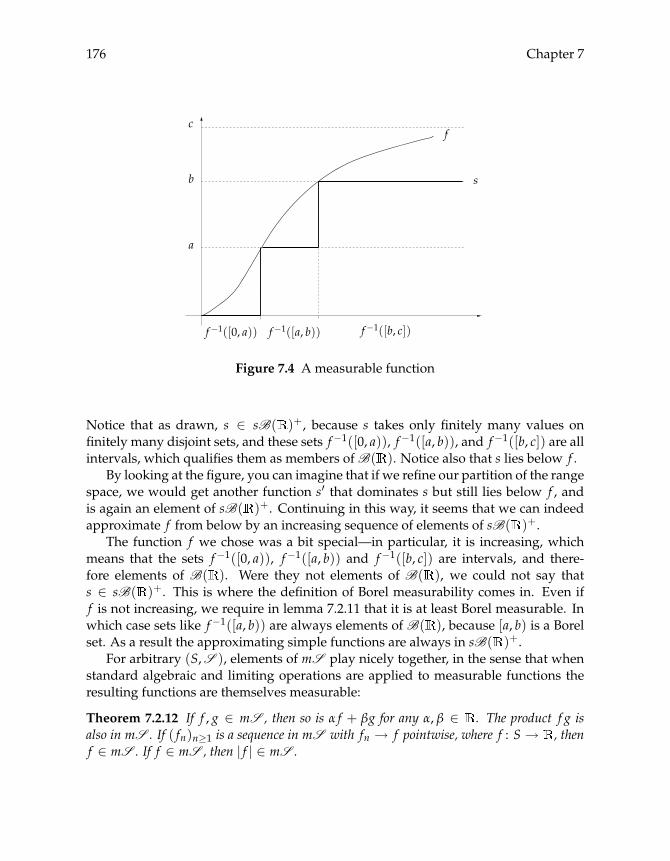
176 Chapter 7
b
f
s
c
a
f−1([b, c])f−1([0, a)) f−1([a, b))
Figure 7.4 A measurable function
Notice that as drawn, s ∈ sB( )+, because s takes only finitely many values onfinitely many disjoint sets, and these sets f−1([0, a)), f−1([a, b)), and f−1([b, c]) are allintervals, which qualifies them as members ofB( ). Notice also that s lies below f .
By looking at the figure, you can imagine that if we refine our partition of the rangespace, we would get another function s′ that dominates s but still lies below f , andis again an element of sB( )+. Continuing in this way, it seems that we can indeedapproximate f from below by an increasing sequence of elements of sB( )+.
The function f we chose was a bit special—in particular, it is increasing, whichmeans that the sets f−1([0, a)), f−1([a, b)) and f−1([b, c]) are intervals, and there-fore elements of B( ). Were they not elements of B( ), we could not say thats ∈ sB( )+. This is where the definition of Borel measurability comes in. Even iff is not increasing, we require in lemma 7.2.11 that it is at least Borel measurable. Inwhich case sets like f−1([a, b)) are always elements ofB( ), because [a, b) is a Borelset. As a result the approximating simple functions are always in sB( )+.
For arbitrary (S,S ), elements of mS play nicely together, in the sense that whenstandard algebraic and limiting operations are applied to measurable functions theresulting functions are themselves measurable:
Theorem 7.2.12 If f , g ∈ mS , then so is α f + βg for any α, β ∈ . The product f g isalso in mS . If ( fn)n≥1 is a sequence in mS with fn → f pointwise, where f : S → , thenf ∈ mS . If f ∈ mS , then | f | ∈ mS .
Integration 177
Exercise 7.2.13 Show that if f ∈ mS , then | f | ∈ mS .26
7.2.3 Integrating Measurable Functions
Now we are ready to extend our notion of integral from simple functions to measur-able functions. Let (S,S , μ) be any measure space and consider first integration of anonnegative measurable function f : S→ + (i.e., an element of mS +). We define theintegral of f on S with respect to μ by
μ( f ) :=:∫
f dμ := limn→∞ μ(sn) where (sn)n≥1 ⊂ sS + with sn ↑ f (7.12)
We are appealing to lemma 7.2.11 for the existence of at least one sequence (sn)n≥1 ⊂sS + with sn ↑ f . Note that μ(sn) always converges in [0,∞] as a result of monotonic-ity (see proposition 7.2.2).
Regarding notation, all of the following are common alternatives for the integralμ( f ):
μ( f ) :=:∫
f dμ :=:∫
f (x)μ(dx)
In the case of Lebesgue measure we will also use∫f (x)dx:
λ( f ) :=:∫
f dλ :=:∫
f (x)λ(dx) :=:∫
f (x)dx
Isn’t it possible that the number we get in (7.12) depends on the particular approx-imating sequence (sn)n≥1 that we choose? The answer is no. If (sn)n≥1 and (s′n)n≥1are two sequences in sS + with sn ↑ f and s′n ↑ f , then μ(sn) and μ(s′n) always havethe same limit.27 The number given by taking any of these limits is in fact equal to
sup{μ(s) : s ∈ sS +, 0 ≤ s ≤ f
} ∈ [0,∞] (7.13)
Example 7.2.14 Recall the counting measure c on ( ,P( )) introduced on page 167.A nonnegative function f : → + is just a nonnegative sequence, and we em-phasize this by writing f as ( fn). Since is paired with its power set (the set ofall subsets), there is no issue with measurability—all such functions (sequences) aremeasurable.
The function ( fn) is simple if it takes only finitely many values. Suppose in partic-ular that fn = 0 for all n ≥ N ∈ . Then, by the definition of the integral on simplefunctions,
c( f ) :=:∫
f dc =N
∑n=1
fn c(n) =N
∑n=1
fn
26Hint: Use the fact that g ∈ mS whenever {g ≤ b} ∈ S for all b ∈ .27The reason that the approximating sequence in (7.12) is required to be monotone is to ensure that this
independence holds. The proof is not difficult but let’s take it as given.

178 Chapter 7
so integration with respect to c is equivalent to summation.Now consider the case of a general nonnegative sequence f = ( fn). For simple
functions converging up to f we can take f N := ( f Nn ), which is defined as equal to fnif n ≤ N and to zero if n > N. In light of (7.12) we have
c( f ) :=:∫
f dc = limN→∞
∫f Ndc = lim
N→∞
N
∑n=1
fn
which is the standard definition of the infinite series ∑n fn. Again, integration withrespect to c is equivalent to summation.
So far we have only defined the integral of nonnegative measurable functions.Integration of general measurable functions is also straightforward: Split the functionf into its positive part f+ := max{0, f } and its negative part f− := max{0,− f }, sof = f+ − f−. Then set
μ( f ) := μ( f+)− μ( f−) (7.14)
The only issue here is that we may end up with the expression ∞−∞, which is defi-nitely not allowed—in this case the integral is not defined.
Definition 7.2.15 Let (S,S , μ) be a measure space, and let f ∈ mS . The function f iscalled integrable if both μ( f+) and μ( f−) are finite. If f is integrable, then its integralμ( f ) is given by (7.14). The set of all integrable functions on S is denotedL1(S,S , μ),or simplyL1(μ).
How do we define integration of a function f ∈ L1(μ) over a subset E of S, ratherthan over the whole space? The answer is by setting∫
Ef dμ :=
∫E f dμ :=: μ( E f )
Here the function E f evaluated at x is the product E(x) · f (x).Although we omit the proof, if f is a continuous real function on with the
property that f = 0 outside an interval [a, b]—so that the Riemann integral is well-defined—then λ( f ) is precisely the Riemann integral of f on [a, b]. We can go aheadand integrate f as our high school calculus instinct tells us to. Hence we have suc-ceeded in extending the elementary integral to a larger class of functions.
7.3 Properties of the Integral
Having defined the abstract Lebesgue integral, let’s now look at some of its proper-ties. As we will see, the integral has nice algebraic properties, and also interacts wellwith limiting operations. Section §7.3.1 focuses on nonnegative functions, while §7.3.2treats the general case.

Integration 179
7.3.1 Basic Properties
Recall that functions constructed from measurable functions using standard algebraicand limiting operations are typically measurable (theorem 7.2.12). This leads us toconsider the relationship between the integrals of the original functions and the inte-grals of the new functions. For example, is the integral of the sum of two measurablefunctions equal to the sum of the integrals? And is the integral of the limit of mea-surable functions equal to the limit of the integrals? Here is a summary of the keyresults:
Theorem 7.3.1 Given an arbitrary measure space (S,S , μ), the integral has the followingproperties on mS +:
M1. If A ∈ S and f := A, then μ( A) = μ(A).
M2. If f = ∅ ≡ 0, then μ( f ) = 0.
M3. If f , g ∈ mS + and α, β ∈ +, then μ(α f + βg) = αμ( f ) + βμ(g).
M4. If f , g ∈ mS + and f ≤ g pointwise on S, then μ( f ) ≤ μ(g).
M5. If ( fn)n≥1 ⊂ mS +, f ∈ mS + and fn ↑ f , then μ( fn) ↑ μ( f ).Property M1 is immediate from the definition of the integral, and M2 is immediate
from M1. Properties M3 and M4 can be derived as follows:
Exercise 7.3.2 Using proposition 7.2.2 (page 173), show that if γ ∈ + and f ∈ mS +,then μ(γ f ) = γμ( f ). Show further that if f , g ∈ mS +, then μ( f + g) = μ( f ) + μ(g).Combine these two results to establish M3.
Exercise 7.3.3 Prove M4.28
Property M5 is fundamental to the success of Lebesgue’s integral, and is usuallyreferred to as the monotone convergence theorem (although we give a more generalresult with that name below). Note that μ( f ) = ∞ is permitted. The proof of M5 isbased on countable additivity of μ, and is one of the reasons that countable additivity(as opposed to finite additivity) is so useful. You can consult any book on measuretheory and integration to see the proof.
The next result clarifies the relationship between measures and integrals.
Theorem 7.3.4 Let (S,S ) be any measurable space. For each measure μ : S � B �→μ(B) ∈ [0,∞], there exists a function μ : mS + � f �→ μ( f ) ∈ [0,∞] with properties M1–M5. Conversely, each function μ : mS + → [0,∞] satisfying properties M2–M5 creates aunique measure on (S,S ) via M1.
28Hint: Use the expression for the integral in (7.13).
180 Chapter 7
One can think of a measure μ on (S,S ) as a kind of “pre-integral,” defined on thesubset of mS + that consists of all indicator functions (the integral of A being μ(A)).The process of creating an integral on mS + via simple functions and then monotonelimits can be thought of as one that extends the domain of μ from indicator functions inmS + to all functions in mS +.
Exercise 7.3.5 Show that if μ : mS + → [0,∞] satisfies M2–M5, then the map μ : S →[0,∞] defined by μ(A) = μ( A) is a measure onS .29
Exercise 7.3.6 Use M1–M5 to prove the previously stated result (see exercise 7.1.25 onpage 167) that if (En) ⊂ S with En ⊂ En+1 for all n, then μ(∪nEn) = limn→∞ μ(En).30
Lemma 7.3.7 Let A, B ∈ S , and let f ∈ mS +. If A and B are disjoint, then∫A∪B
f dμ =∫Af dμ+
∫Bf dμ
Proof. We have A∪B f = ( A + B) f = A f + B f . Now apply M3.
One of the most important facts about the integral is that integrating over sets ofzero measure cannot produce a positive number:
Theorem 7.3.8 If f ∈ mS +, E ∈ S , and μ(E) = 0, then∫E f dμ = 0.
Proof. Since f ∈ mS +, there is a sequence (sn)n≥1 ⊂ sS + with sn ↑ f , and henceEsn ↑ E f .31 But
Esn =K
∑k=1
αk( E · Ak ) =K
∑k=1
αk E∩Ak
∴ μ( Esn) =K
∑k=1
αkμ(E ∩ Ak) = 0 ∀ n ∈
since μ(E) = 0. By property M5, we have μ( E f ) = limn→∞ μ( Esn) = 0.
7.3.2 Finishing Touches
Let (S,S , μ) be any measure space. By using the five fundamental properties M1–M5,one can derive the classical theorems about integrals on L1(μ) := L1(S,S , μ). Thenext few results show that many results from the previous section that hold for non-negative functions also hold for the (not necessarily nonnegative) elements ofL1(μ).
29Hint: Regarding countable additivity, if (An) ⊂ S are disjoint then ∪nAn = ∑n An .30Hint: Use the fact that ∪nEn = limn→∞ En pointwise on S.31That is, the convergence E(x)sn(x) → E(x)sn(x) holds at each point x ∈ S, and that E(x)sn(x) gets
progressively larger with n for each x ∈ S.

Integration 181
To state the results we introduce the concept of properties holding “almost every-where.” Informally, if f , g ∈ mS and P(x) is a statement about f and g at x (e.g.,f (x) = g(x) or f (x) ≤ g(x)), then we will stay f and g have property P μ-almosteverywhere (μ-a.e.) whenever the set of all x such that P(x) fails has μ-measure zero.For example, if the set of x ∈ S such that f (x) �= g(x) has measure zero then f and gare said to be equal μ-a.e. In addition we say that fn → f μ-a.e. if lim fn = f μ-a.e.This sounds a bit complicated, but the basic idea is that null sets don’t matter whenit comes to integration, so it’s enough for properties to hold everywhere except on anull set.
Theorem 7.3.9 Let f , g ∈ L1(μ), and let α, β ∈ . The following results hold:
1. α f + βg ∈ L1(μ) and μ(α f + βg) = αμ( f ) + βμ(g).
2. If E ∈ S with μ(E) = 0, then∫E f dμ = 0.
3. If f ≤ g μ-a.e., then μ( f ) ≤ μ(g).
4. | f | ∈ L1(μ), and |μ( f )| ≤ μ(| f |).5. μ(| f |) = 0 if and only if f = 0 μ-a.e.
This list is not minimal. For example, part 2 follows from parts 4 and 5. Part1 follows from the definitions and M3 (i.e., linearity of the integral on the space ofnonnegative measurable functions). See, for example, Dudley (2002, thm. 4.1.10). Part2 can also be obtained from the identity f = f+ − f−, part 1 and theorem 7.3.8:
μ( E f ) = μ( E f+ − E f−) = μ( E f+)− μ( E f−) = 0− 0
Exercise 7.3.10 Prove that if μ(E) = 0 and f ∈ L1(μ), then∫Ec f dμ =
∫f dμ, and if
f , g ∈ L1(μ) with f = g μ-a.e., then μ( f ) = μ(g).32
Exercise 7.3.11 Prove part 3 using properties M1–M5.33
Exercise 7.3.12 Prove part 4 using the identity | f | = f+ + f−.
Regarding part 5, suppose that f �= 0 on a set E with μ(E) > 0. We will prove thatμ(| f |) > 0. To see this, define En := {x : | f (x)| > 1/n}. Observe that En ⊂ En+1for each n, and that E = ∪nEn. From exercise 7.1.25 (page 167) there is an N withμ(EN) > 0. But then μ(| f |) ≥ μ( EN | f |) ≥ μ(EN)/N > 0. The converse implicationfollows from exercise 7.3.10.
Now we come to the classical convergence theorems for integrals, which can bederived from M1–M5. They are among the foundation stones of modern real analysis.
32Hint: Let E be the set on which f and g disagree. Then Ec f = Ec g.33Hint: Convert to a statement about nonnegative functions. Note that if f ≤ g μ-a.e., then Ec f+ +Ec g− ≤ Ec g+ + Ec f−, where E is all x such that f (x) > g(x).

182 Chapter 7
Theorem 7.3.13 (Monotone convergence theorem) Let (S,S , μ) be a measure space, andlet ( fn)n≥1 be a sequence in mS . If fn ↑ f ∈ mS μ-almost everywhere and μ( f1) > −∞,then limn→∞ μ( fn) = μ( f ).34
Theorem 7.3.14 (Dominated convergence theorem) Let (S,S , μ) be a measure space, letg ∈ L1(μ) and let ( fn)n≥1 ⊂ mS with | fn| ≤ g for all n. If fn → f μ-almost everywhere,then f ∈ L1(μ) and limn→∞ μ( fn) = μ( f ).
It’s almost impossible to overemphasize what a useful result the dominated con-vergence theorem is, and the proof can be found in any text on measure theory. For aneat little illustration, consider
Corollary 7.3.15 Consider the collection of real sequences
a = (a1, a2, . . .), ak = (ak1, ak2, . . .) (k ∈ )
Suppose that ak is dominated pointwise by a sequence b = (bn) for all k, in the sense that|akn| ≤ bn for all k, n. Suppose further that limk→∞ akn = an for each n. If ∑n bn < ∞, then
limk→∞ ∑n≥1
akn = ∑n≥1
limk→∞
akn = ∑n≥1
an
Proof. Apply the dominated convergence theorem with (S,S , μ) = ( ,P( ), c),where c is the counting measure (recall example 7.2.14).
Let’s conclude with the topic of image measures. To define image measures, let(S,S , μ) be any measure space, let (S′,S ′) be a measurable space, and let T : S → S′beS ,S ′-measurable. If E is some element ofS ′, then T−1(E) ∈ S , so μ ◦ T−1(E) =μ(T−1(E)) is well defined. In fact E �→ μ ◦ T−1(E) is a measure on (S′,S ′), called theimage measure of μ under T. Figure 7.5 provides a picture. The value of μ ◦ T−1(E) isobtained by pulling E back to S and evaluating with μ.
Exercise 7.3.16 Show that μ ◦ T−1 is indeed a measure on (S′,S ′).35
The following result shows how to integrate with image measures:36
Theorem 7.3.17 Let (S,S , μ) be any measure space, let (S′,S ′) be a measurable space, letT : S → S′ be a measurable function, and let μ ◦ T−1 be the image measure of μ under T.If w : S′ → is S ′-measurable and either w is nonnegative or μ(|w ◦ T|) is finite, thenμ ◦ T−1(w) = μ(w ◦ T), where the first integral is over S′ and the second is over S.
One application of this theorem is when μ is Lebesgue measure, and μ ◦ T−1 ismore complex. If we don’t know how to integrate with respect to this new measure,we can use the change of variable to get back to an integral of the form
∫f dμ.
34In fact, for this theorem to hold the limiting function f need not be finite everywhere (or anywhere) onS. See Dudley (2002, thm. 4.3.2).
35You might find it useful to refer to lemma A.1.2 on page 321.36A full proof can be found in Dudley (2002, thm. 4.1.11).
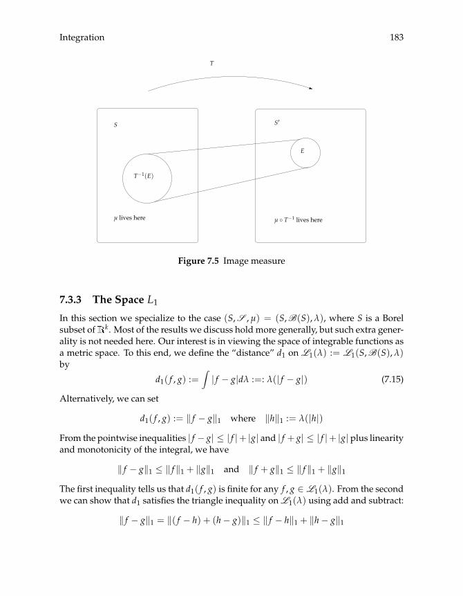
Integration 183
E
T
T−1(E)
S S′
μ ◦ T−1 lives hereμ lives here
Figure 7.5 Image measure
7.3.3 The Space L1
In this section we specialize to the case (S,S , μ) = (S,B(S),λ), where S is a Borelsubset of k. Most of the results we discuss hold more generally, but such extra gener-ality is not needed here. Our interest is in viewing the space of integrable functions asa metric space. To this end, we define the “distance” d1 on L1(λ) := L1(S,B(S),λ)by
d1( f , g) :=∫| f − g|dλ :=: λ(| f − g|) (7.15)
Alternatively, we can set
d1( f , g) := ‖ f − g‖1 where ‖h‖1 := λ(|h|)From the pointwise inequalities | f − g| ≤ | f |+ |g| and | f + g| ≤ | f |+ |g| plus linearityand monotonicity of the integral, we have
‖ f − g‖1 ≤ ‖ f ‖1 + ‖g‖1 and ‖ f + g‖1 ≤ ‖ f ‖1 + ‖g‖1The first inequality tells us that d1( f , g) is finite for any f , g ∈ L1(λ). From the secondwe can show that d1 satisfies the triangle inequality onL1(λ) using add and subtract:
‖ f − g‖1 = ‖( f − h) + (h− g)‖1 ≤ ‖ f − h‖1 + ‖h− g‖1

184 Chapter 7
Since d1 satisfies the triangle inequality it seems plausible that d1 is a metric (see thedefinition on page 36) on L1(λ). However, there is a problem: We may have f �=g and yet d1( f , g) = 0, because functions that are equal almost everywhere satisfy∫ | f − g|dλ = 0. (Why?) For example, when S = , the functions and 0 := ∅ areat zero distance from one another. Hence (L1(λ), d1) fails to be a metric space. Ratherit is what’s called a pseudometric space:
Definition 7.3.18 A pseudometric space is a nonempty set M and a function ρ : M ×M→ such that, for any x, y, v ∈ M,
1. ρ(x, y) = 0 if x = y,
2. ρ(x, y) = ρ(y, x), and
3. ρ(x, y) ≤ ρ(x, v) + ρ(v, y).
In contrast to a metric space, in a pseudometric space distinct points are permittedto be at zero distance from one another.
Exercise 7.3.19 On the space 2 consider the function ρ(x, y) = |x1 − y1|, where x1and y1 are the first components of x = (x1, x2) and y = (y1, y2) respectively. Showthat ( 2, ρ) is a pseudometric space.
It is not difficult to convert a pseudometric space into a metric space: We simplyregard all points at zero distance from each other as the same point. In other words,we partition the original space into equivalence classes of points at zero distance fromone another, and consider the set of these classes as a new space. Figure 7.6 illustratesfor the space in exercise 7.3.19.
The distance between any two equivalence classes is just the distance betweenarbitrarily chosen members of each class. This value does not depend on the particularmembers chosen: If x and x′ are equivalent, and y and y′ are equivalent, then ρ(x, y) =ρ(x′, y′) because
ρ(x, y) ≤ ρ(x, x′) + ρ(x′, y′) + ρ(y′, y)= ρ(x′, y′) ≤ ρ(x′, x) + ρ(x, y) + ρ(y, y′) = ρ(x, y)
The space of equivalence classes and the distance just described form a metric space.In particular, distinct elements of the derived space are at positive distance from oneanother (otherwise they would not be distinct).
The metric space derived from the pseudometric space (L1(λ), d1) is traditionallydenoted (L1(λ), d1), and has a major role to play in the rest of this book.37 Since twofunctions inL1(λ) are at zero distance if and only if they are equal almost everywhere,
37To simplify notation, we are using the symbol d1 to represent distance on both spaces.

Integration 185
equivalence classes
x1
x2
Figure 7.6 Equivalence classes for ( 2, ρ)
the new space (L1(λ), d1) consists of equivalences classes of functions that are equalalmost everywhere.
A density on S is a nonnegative measurable function that integrates to one. Weare interested in describing the set of densities as a metric space, with the intention ofstudying Markov chains such that their marginal distributions evolve in the space ofdensities. The densities are embedded into L1(λ) as follows:
Definition 7.3.20 The space of densities on S is written as D(S) and defined by
D(S) := { f ∈ L1(λ) : f ≥ 0 and ‖ f ‖1 = 1}In the definition, f is actually an equivalence class of functions f ′, f ′′, etc., that are
all equal almost everywhere. The statement f ≥ 0 means that all of these functionsare nonnegative almost everywhere, while ‖ f ‖1 = 1 means that all integrate to one.(More generally, if f ∈ L1(λ), then ‖ f ‖1 is the integral of the absolute value of anyelement in the equivalence class.)
Theorem 7.3.21 The spaces (L1(λ), d1) and (D(S), d1) are both complete.
A proof of completeness of (L1(λ), d1) can be found in any good text on measuretheory. Completeness of (D(S), d1) follows from the fact that D(S) is closed as a subsetof (L1(λ), d1) and theorem 3.2.3 (page 45). The proof that D(S) is closed is left as anexercise for enthusiastic readers.
Densities are used to represent distributions of random variables. Informally, thestatement that X has density f ∈ D(S) means that X is in B ⊂ S with probability
186 Chapter 7
∫B f ′(x)dx :=:
∫B f ′ dλ, where f ′ is some member of the equivalence class. Note that
it does not matter which member we pick, as all give the same value here. In this senseit is equivalence classes that represent distributions rather than individual densities.
Finally, Scheffés identity provides a nice quantitative interpretation of d1 distancebetween densities: For any f and g in D(S),
‖ f − g‖1 = 2× supB∈B(S)
∣∣∣∣∫Bf (x)dx−
∫Bg(x)dy
∣∣∣∣ (7.16)
It follows that if ‖ f − g‖1 ≤ ε, then for any event B of interest, the deviation in theprobability assigned to B by f and g is less than ε/2.38
7.4 Commentary
The treatment of measure theory and integration in this chapter is fairly standardamong modern expositions. There are many excellent references with which to roundout the material. Good starting points are Williams (1991) and Taylor (1997). Alipran-tis and Burkinshaw (1998) is more advanced, and contains many exercises. The booksby Pollard (2002), Dudley (2002), and Schilling (2005) are also highly recommended.
38A proof of this identity is given later in a more general context (see lemma 11.1.29).
Chapter 8
Density Markov Chains
In this chapter we take an in-depth look at Markov chains on state space S ⊂ n withthe property that conditional (and hence marginal) distributions can be representedby densities. These kinds of processes were previously studied in chapter 6. Now thatwe have measure theory under our belts, we will be able to cover a number of deeperresults.
Not all Markov chains fit into the density framework (see §9.2 for the general case).For those that do, however, the extra structure provided by densities aids us in analyz-ing dynamics and computing distributions. In addition densities have a concretenessthat abstract probability measures lack, in the sense that they are easy to represent vi-sually. This concreteness makes them a good starting point when building intuition.
8.1 Outline
We start with the basic theory of Markov chains with density representations. Afterdefining density Markov chains, we will illustrate the connection to stochastic recur-sive sequences (stochastic difference equations). In §8.1.3 we introduce the Markovoperator for the density case, and show how the marginal distributions of a densityMarkov chain can be generated by iterating on the Markov operator. This theoryclosely parallels the finite case, as discussed in §4.2.2.
8.1.1 Stochastic Density Kernels
We met some examples of density kernels in chapter 6. Let’s now give the formaldefinition of a density kernel.
187
188 Chapter 8
Definition 8.1.1 Let S be a Borel subset of n. A stochastic density kernel on S is a Borelmeasurable function p : S× S→ + such that
∫p(x, y)dy :=:
∫p(x, y)λ(dy) :=: λ(p(x, ·)) = 1 for all x ∈ S (8.1)
In particular, the function y �→ p(x, y) is a density for each x ∈ S. We can thinkof p as a family of density functions, one for each point in the state space. In whatfollows, we will use the notation p(x, y)dy to represent the density function y �→ p(x, y).A second point is that S× S is a subset of 2n, and Borel measurability of p refers toBorel subsets of this space. In practice, one rarely encounters stochastic kernels whereBorel measurability is problematic.
To illustrate the definition, consider the kernel p defined by
p(x, y) =1√2π
exp(− (y− ax− b)2
2
)((x, y) ∈ S× S = × )
In other words, p(x, y)dy = N(ax+ b, 1). The kernel is presented visually in figure 8.1.Each point on the x-axis picks out a distribution N(ax+ b, 1), which is represented asa density running along the y-axis. In this case a is positive, so an increase in x leads toan increase in the mean of the corresponding density p(x, y)dy, and the density putsprobability mass on larger y.
From an initial condition ψ ∈ D(S) and a density kernel p, we can generate aMarkov chain (Xt)t≥0. Here is a definition paralleling the finite case (page 71):
Definition 8.1.2 Let ψ ∈ D(S). A random sequence (Xt)t≥0 on S is called Markov-(p,ψ) if
1. at time zero, X0 is drawn from ψ, and
2. at time t+ 1, Xt+1 is drawn from p(Xt, y)dy.
In the case of the kernel p(x, y)dy = N(ax + b, 1), we draw X0 from some givenψ and then, at each time t, draw Xt+1 ∼ N(aXt + b, 1). Listing 8.1 generates oneobservation (of length 100) for the process when ψ = N(0, 1). An observation (samplepath) is shown in figure 8.2.
There is another way to visualize the dynamics associated with our stochastic ker-nel. Recall the 45 degree diagram technique for studying univariate deterministicdynamic systems we introduced in figure 4.3 (page 58). Now consider figure 8.3, eachpanel of which shows a series generated by the kernel p(x, y)dy = N(ax + b, 1). Thekernel itself is represented in the graphs by shading. You should understand thisshading as a “contour” representation of the 3D graph in figure 8.1, with lighter areascorresponding to higher probability. For each graph the sequence of arrows traces out

Density Markov Chains 189
xdy
prob
Figure 8.1 The stochastic kernel p(x, y)dy = N(ax+ b, 1)
an individual time series. The initial condition is X0 = −4, and X1 is then drawn fromN(aX0 + b, 1). We trace this value back to the 45 degree line to obtain the distributionfor X2 ∼ N(aX1 + b, 1), and so on.
When most of the probability mass lies above the 45 degree line, the value of thestate tends to increase. When most is below the 45 degree line, the value tends todecrease. The actual outcome, however, is random, depending on the sequence ofdraws that generate the time series.
8.1.2 Connection with SRSs
Suppose that we wish to investigate a stochastic recursive sequence (SRS) where thestate space S is a Borel subset of n, Z is a Borel subset of k, F : S× Z → S is a givenfunction, and
Xt+1 = F(Xt,Wt+1), X0 ∼ ψ ∈ D(S), (Wt)t≥1IID∼ φ ∈ D(Z) (8.2)
We would like to know when there exists a stochastic density kernel p on S that repre-sents (8.2), in the sense that (Xt)t≥0 defined in (8.2) is Markov-(p,ψ). Put differently,we wish to know when there exists a density kernel p such that, for all x ∈ S,
p(x, y)dy = the density of F(x,W) when W ∼ φ (8.3)

190 Chapter 8
Listing 8.1 (ar1.py) Simulation of (Xt)t≥0 for p(x, y)dy = N(ax+ b, 1)
from random impor t normalvariate as N
a, b = 0.5, 1 # ParametersX = {} # An empty dictionary to store pathX[0] = N(0, 1) # X_0 has distribution N(0, 1)
f o r t i n range (100):X[t+1] = N(a * X[t] + b, 1)
Figure 8.2 Time series

Density Markov Chains 191
−4 −2 0 2 4
−4
−2
02
4
x
dy
−4 −2 0 2 4
−4
−2
02
4
x
dy
Figure 8.3 Two time series
192 Chapter 8
Such a p will do the job for us because, if the state Xt arrives at any x ∈ S, thendrawing Xt+1 from p(x, y)dy is—by definition of p—probabilistically equivalent todrawing Wt+1 from φ and setting Xt+1 = F(x,Wt+1).
The reason for our interest in this question is that the theory of Markovian dy-namics is more easily developed in the framework of stochastic kernels than in thatof SRSs such as (8.2). This is largely because the stochastic density kernel capturesthe stochastic law of motion for the system in one single object. To apply the theorydeveloped below, it is necessary to be able to take a given model of the form (8.2) andobtain its density kernel representation.
The existence of a stochastic density kernel p satisfying (8.3) is not guaranteed, asnot all random variables have distributions that can be represented by densities. Letus try to pin down simple sufficient conditions implying that F(x,W) can be repre-sented by a density.
Here is a more general question: If Y is a random variable on S, when does thereexist a density φ ∈ D(S) such that φ representsY in the sense that, for every B ∈ B(S),the number
∫B φdλ :=:
∫B φ(x)dx gives the probability that Y ∈ B? In essence the
answer is that Y must not take values in any Lebesgue null set with positive probability. Tosee this, suppose that N ∈ B(S) with λ(N) = 0 and Y ∈ N with positive probability.Then regardless of which φ ∈ D(S) we choose, theorem 7.3.8 implies that
∫N φ(x)dx =
0, and hence φ does not represent Y.Now let us consider the distribution of Y = F(x,W), W ∼ φ ∈ D(Z). The follow-
ing theorem, though not as general as some, will be sufficient for our purposes:
Theorem 8.1.3 Let W be a random variable on n with density φ, let γ ∈ n, and let Γ bean n× n matrix. If det Γ �= 0, then Y = γ+ ΓW has density φY on n, where
φY(y) := φ(Γ−1(y− γ))|det Γ−1| (y ∈ n)
Why is det Γ �= 0 required? If det Γ = 0 then Y = γ + ΓW takes values in asubspace of dimension less than n. In n, such subspaces have Lebesgue measurezero. Hence Y takes values in a Lebesgue null set with positive probability, in whichcase it cannot be represented by a density.
Before looking at the proof, let’s see how we can use the theorem. In §8.1.1 welooked at a process (Xt)t≥0 defined by kernel p(x, y)dy = N(ax + b, 1). This corre-sponds to the SRS
Xt+1 = aXt + b+Wt+1, (Wt)t≥1IID∼ φ = N(0, 1)
In other words, p(x, y)dy = N(ax + b, 1) is the density of Y = ax + b + W whenW ∼ φ. This claim is easily verified. From theorem 8.1.3 the density φY ofY is φY(y) =

Density Markov Chains 193
φ(y− ax− b). Since φ = N(0, 1), this becomes
φY(y) =1√2π
exp(− (y− ax− b)2
2
)= N(ax+ b, 1)
Exercise 8.1.4 Consider the n-valued SRS
Xt+1 = AXt + b+Wt+1, (Wt)t≥1IID∼ φ ∈ D( n) (8.4)
where A is an n× n matrix and b is an n× 1 vector. Show that the stochastic densitykernel corresponding to this model is p(x, y) = φ(y− Ax− b).
Exercise 8.1.5 Consider the well-known threshold autoregression model (Chan andTong 1986). The model is a nonlinear AR(1) process
Xt+1 =K
∑k=1
(AkXt + bk) Bk (Xt) +Wt+1, (Wt)t≥1IID∼ φ ∈ D( n) (8.5)
where Xt takes values in n, the family of sets (Bk)Kk=1 is a (measurable) partition ofn, and (Ak)Kk=1 and (bk)Kk=1 are n× n-dimensional matrices and n× 1-dimensional
vectors respectively. The idea is that when Xt is in the region of the state space Bk,the state variable follows the law of motion AkXt + bk. Show that the correspondingdensity kernel is
p(x, y) = φ
[y−
K
∑k=1
(Akx+ bk) Bk (x)
](8.6)
Example 8.1.6 Consider again the Solow–Swan model. Set δ = 1 and f (k,W) =f (k)W. In other words, the state evolves according to
kt+1 = s f (kt)Wt+1, (Wt)t≥1IID∼ φ (8.7)
Suppose that s > 0 and f (k) > 0 whenever k > 0, and take S = Z = (0,∞). We wishto determine the stochastic density kernel p(x, y)dy; equivalently, we wish to find thedensity φY of the random variable Y = s f (x)W when x ∈ S is fixed and W ∼ φ.
The only obstacle to applying theorem 8.1.3 in this case is that Z is a proper subsetof , not itself. Hence φ is not necessarily defined on all of . However, we can getaround this easily enough by setting φ = 0 on the complement (−∞, 0] of Z.
When x ∈ S is fixed, s f (x) is a strictly positive constant, and from theorem 8.1.3the density of Y = s f (x)W is
p(x, y) = φ
(y
s f (x)
)1
s f (x)(8.8)
194 Chapter 8
Exercise 8.1.7 Consider again example 8.1.6, but this time with δ < 1. In other words,(kt)t≥0 evolves according to
kt+1 = s f (kt)Wt+1 + (1− δ)kt, (Wt)t≥1IID∼ φ
Show that the stochastic density kernel is now given by
p(x, y) = φ
(y− (1− δ)x
s f (x)
)1
s f (x)(8.9)
Notice that if y < (1− δ)x, then φ is evaluated at a negative number. This is whywe need to extend φ to all of , with φ(z) = 0 for all z ≤ 0.
Exercise 8.1.8 In §6.1.2 we considered a stochastic threshold externality model withmultiple equilibria, with law of motion for capital given by
kt+1 = sA(kt)kαt Wt+1, (Wt)t≥1IID∼ φ (8.10)
Here k �→ A(k) is any function with A(k) > 0 when k > 0. Set Z = S = (0,∞). Derivethe stochastic density kernel p corresponding to this model.
Now let’s sketch the proof of theorem 8.1.3. We will use the following standardchange-of-variable result:
Theorem 8.1.9 Let A and B be open subsets of k, and let T : B → A be a C1 bijection. Iff ∈ L1(A,B(A),λ), then∫
Af (x)dx =
∫Bf ◦ T(y) · |det JT(y)|dy (8.11)
Here JT(y) is the Jacobian of T evaluated at y, and C1 means that T is continuouslydifferentiable on B.1
Example 8.1.10 Let A = , let B = (0,∞), and let Tx = ln(x). Then |det JT(y)| =1/y, and for any measurable f on with finite integral we have
∫f (x)dx =
∫(0,∞)
f (ln y)1ydy
Now suppose we have a random variable W with density φ ∈ D( n), and wetransform W with some function h to create a new random variable Y = h(W). Inthe case of theorem 8.1.3 the transformation h is the linear function z �→ γ+ Γz. Thefollowing generalization of theorem 8.1.3 holds:
1theorem 8.1.9 is actually a special case of theorem 7.3.17 on page 182.

Density Markov Chains 195
Theorem 8.1.11 Let S and T be open subsets of n, and let W be a random vector on S,distributed according to density φ on S. Let Y = h(W), where h : S → T is a bijection andthe inverse h−1 is a C1 function. In that case Y is a random vector on T with density φY,where
φY(y) := φ(h−1(y)) · |det Jh−1(y)| (y ∈ T) (8.12)
The proof can be constructed along the following lines: The statement that φY isthe density of Y means that {Y ∈ B} =
∫B φY(y)dy holds for every B ∈ B(T). By an
application of theorem 8.1.9 we get
{Y ∈ B} = {W ∈ h−1(B)}=
∫h−1(B)
φ(x)dx =∫Bφ(h−1(y))|det Jh−1(y)|dy =
∫BφY(y)dy
8.1.3 The Markov Operator
Let p be a density kernel on S ∈ B( n), let ψ ∈ D(S) be an initial condition, andlet (Xt)t≥0 be Markov-(p,ψ). As usual, let ψt be the (marginal) distribution of Xtfor each t ≥ 0. In §6.1.3 we saw that if X and Y are random variables on S withmarginals pX and pY, and if pY|X is the conditional density of Y given X, then pY(y) =∫pY|X(x, y)pX(x)dx for all y ∈ S. Letting Xt+1 = Y and Xt = X, we obtain
ψt+1(y) =∫
p(x, y)ψt(x)dx (y ∈ S) (8.13)
Equation (8.13) is just (6.7) on page 126, translated to a more general setting. It is thecontinuous state version of (4.10) on page 75 and the intuition is roughly the same:The probability of being at y tomorrow is the probability of moving from x today to ytomorrow, summed over all x and weighted by the probability ψt(x)dx of observingx today.
Now define an operator M sending ψ ∈ D(S) into ψM ∈ D(S) by
ψM(y) =∫
p(x, y)ψ(x)dx (y ∈ S) (8.14)
This operator is called the Markov operator corresponding to stochastic density kernelp, and parallels the definition of the Markov operator for the finite state case given onpage 75. As in that case, M acts on distributions (densities) to the left rather than theright, and is understood as updating the distribution of the state: If the state is cur-rently distributed according to ψ then next period its distribution is ψM. In particular,(8.13) can now be written as
ψt+1 = ψtM (8.15)

196 Chapter 8
This a density version of (4.12) on page 76. Iterating backward we get the representa-tion ψt = ψMt for the distribution of Xt given X0 ∼ ψ.
Technical note: An element of D(S) such as ψ is actually an equivalence class offunctions on S that are equal almost everywhere—see §7.3.3. This does not causeproblems for the definition of the Markov operator, since applying M to any elementof the equivalence class yields the same function: If ψ′ and ψ′′ are equal off a null setE, then the integrands in (8.14) are equal off E for every y, and hence both integrate tothe same number. Thus ψM in (8.14) is a well-defined function on S, and we embedit in D(S) by identifying it with the equivalence class of functions to which it is equalalmost everywhere.
That M does in fact map D(S) into itself can be verified by showing that ψM isnonnegative and integrates to 1. That ψM integrates to 1 can be seen by changing theorder of integration:
∫ψM(y)dy =
∫ ∫p(x, y)ψ(x)dxdy =
∫ [∫p(x, y)dy
]ψ(x)dx
Since∫p(x, y)dy = 1 and
∫ψ(x)dx = 1, the proof is done. Regarding nonnegativity,
fix any y ∈ S. Since p ≥ 0 and since ψ ≥ 0 almost everywhere, the integrand in (8.14)is nonnegative almost everywhere, and ψM(y) ≥ 0.
Before moving on let us briefly investigate the iterates of the Markov operator M.Recall that when we studied finite Markov chains, the t-th order kernel pt(x, y) wasdefined by
p1 := p, pt(x, y) := ∑z∈S
pt−1(x, z)p(z, y)
Analogously, let p be a stochastic density kernel p, and define a sequence (pt)t≥1 ofkernels by
p1 := p, pt(x, y) :=∫
pt−1(x, z)p(z, y)dz (8.16)
Below pt is called the t-th order density kernel corresponding to p. As in the finite statecase, pt(x, y)dy can be interpreted as the distribution (density) of Xt when X0 = x.
Exercise 8.1.12 Using induction, verify that pt is density kernel on S for each t ∈ .
Lemma 8.1.13 IfM is the Markov operator associated with stochastic density kernel p on S,then Mt is the Markov operator associated with pt. In other words, for any ψ ∈ D(S), wehave
ψMt(y) =∫
pt(x, y)ψ(x)dx (y ∈ S)
This lemma is the continuous state version of lemma 4.2.8 on page 76. Essentiallyit is telling us what we claimed above: that pt(x, y)dy is the distribution of Xt givenX0 = x. The proof is an exercise.
Density Markov Chains 197
Given any kernel p on S, the Markov operator M is always continuous on D(S)(with respect to d1). In fact it is nonexpansive. To see this, observe that for any φ,ψ ∈D(S), we have
‖φM− ψM‖1 =∫ ∣∣∣∣
∫p(x, y)(φ(x)− ψ(x))dx
∣∣∣∣ dy≤
∫ ∫p(x, y)|φ(x)− ψ(x)|dxdy
=∫ ∫
p(x, y)dy|φ(x)− ψ(x)|dx = ‖φ− ψ‖1
8.2 Stability
Let’s now turn to the topic of stability. The bad news is that for density Markov chainson infinite state spaces, the theory is considerably more complex than for the finitecase (see §4.3.3). The good news is that we can build on the intuition gained fromstudying the finite case, and show how the concepts can be extended to cope with in-finite state spaces. After reviewing the density analogue of the Dobrushin coefficient,we look at drift conditions that keep probability mass within a “bounded” regionof the state space as the Markov chain evolves. Combining drift conditions with aconcept related to positivity of the Dobrushin coefficient, we obtain a rather generalsufficient condition for stability of density Markov chains, and apply it to several ap-plications.
8.2.1 The Big Picture
Before plunging into the formal theory of stability, we are going spend some timebuilding intuition. In particular, we would like to know under what circumstancesstability will fail, with the aim of developing conditions that rule out these kinds ofcircumstances. This section considers these issues in a relatively heuristic way. Webegin with the definitions of stationary densities and global stability.
Let p be a stochastic density kernel on S, and let M be the corresponding Markovoperator. As before, S is a Borel subset of n endowed with the standard euclideanmetric d2. Since M sends D(S) into D(S), and since D(S) is a well-defined metricspace with the distance d1 (see §7.3.3), the pair (D(S),M) is a dynamical system in thesense of chapter 4. The trajectory (ψMt)t≥0 of a point ψ ∈ D(S) corresponds to thesequence of marginal distributions for a Markov-(p,ψ) process (Xt)t≥0.
Now consider the stability properties of the dynamical system (D(S),M). We areinterested in existence of fixed points and global stability. A fixed point ψ∗ of M is
198 Chapter 8
also called a stationary density, and, by definition, satisfies
ψ∗(y) =∫
p(x, y)ψ∗(x)dx (y ∈ S)
Exercise 8.2.1 Consider the linear AR(1) model
Xt+1 = aXt +Wt+1, (Wt)t≥1IID∼ φ = N(0, 1) (8.17)
with |a| < 1. The corresponding density kernel is p(x, y)dy = N(ax, 1). Using penciland paper, show that the normal density N(0, 1/(1− a2)) is stationary for this kernel.
In the finite state case every Markov chain has a stationary distribution (theo-rem 4.3.5, page 86). When S is not finite, however, stationary distributions can eas-ily fail to exist. Consider, for example, the model (8.17) with α = 1, which is calleda random walk. With a bit of thought, you will be able to convince yourself thatXt ∼ N(X0, t), and hence
pt(x, y) =1√2πt
exp(−(y− x)2
2t
)((x, y) ∈ × )
Exercise 8.2.2 Show that p has no stationary distribution by arguing that if ψ∗ is sta-tionary, then
ψ∗(y) =∫
pt(x, y)ψ∗(x)dx (t ∈ , y ∈ )
in which case the dominated convergence theorem implies that ψ∗(y) = 0 for ally ∈ . (Contradicting what?)
Translated to the present context, global stability of (D(S),M) is equivalent to theexistence of a unique stationary density ψ∗ such that
ψMt → ψ∗ in d1 as t→ ∞ for every ψ ∈ D(S)
Let’s try to work out when such stability can be expected. First, we have to rule out thekind of behavior exhibited by the random walk above. In this case the density of Xtbecomes more and more spread out over . In fact ψt converges to zero everywherebecause
ψt(y) = (ψMt)(y) =∫
pt(x, y)ψ(x)dx → 0 (t→ ∞)
for all y ∈ by the dominated convergence theorem.A similar problem arises when densities are diverging off to the right or the left, as
illustrated in figure 8.4. In either case probability mass is escaping from the “center”of the state space. In other words, it is not concentrating in any one place.
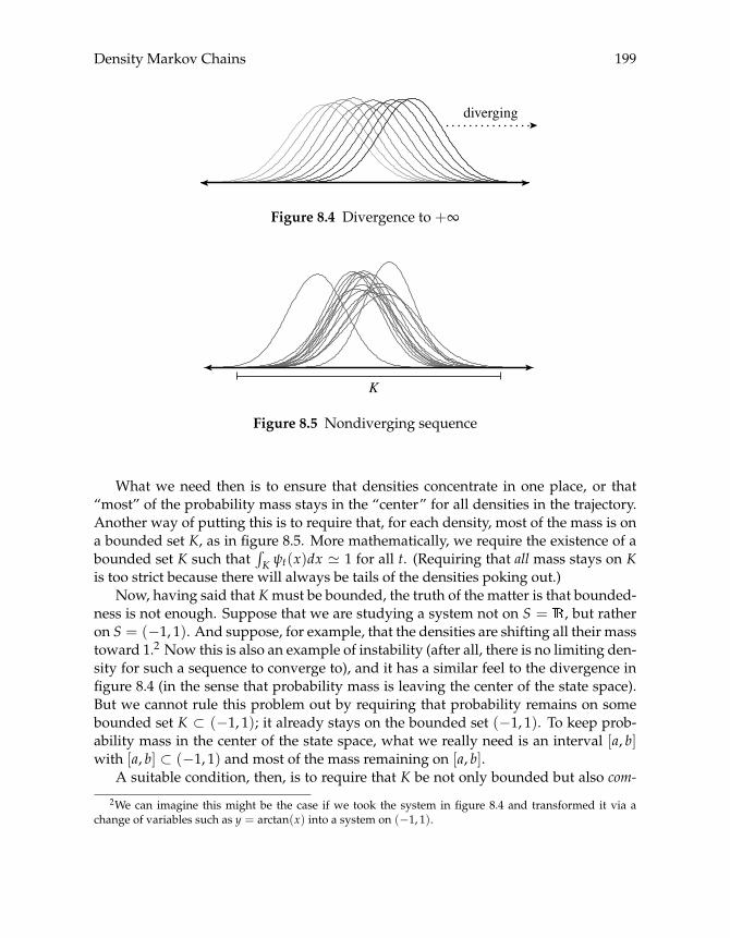
Density Markov Chains 199
diverging
Figure 8.4 Divergence to +∞
K
Figure 8.5 Nondiverging sequence
What we need then is to ensure that densities concentrate in one place, or that“most” of the probability mass stays in the “center” for all densities in the trajectory.Another way of putting this is to require that, for each density, most of the mass is ona bounded set K, as in figure 8.5. More mathematically, we require the existence of abounded set K such that
∫K ψt(x)dx � 1 for all t. (Requiring that all mass stays on K
is too strict because there will always be tails of the densities poking out.)Now, having said that K must be bounded, the truth of the matter is that bounded-
ness is not enough. Suppose that we are studying a system not on S = , but ratheron S = (−1, 1). And suppose, for example, that the densities are shifting all their masstoward 1.2 Now this is also an example of instability (after all, there is no limiting den-sity for such a sequence to converge to), and it has a similar feel to the divergence infigure 8.4 (in the sense that probability mass is leaving the center of the state space).But we cannot rule this problem out by requiring that probability remains on somebounded set K ⊂ (−1, 1); it already stays on the bounded set (−1, 1). To keep prob-ability mass in the center of the state space, what we really need is an interval [a, b]with [a, b] ⊂ (−1, 1) and most of the mass remaining on [a, b].
A suitable condition, then, is to require that K be not only bounded but also com-
2We can imagine this might be the case if we took the system in figure 8.4 and transformed it via achange of variables such as y = arctan(x) into a system on (−1, 1).

200 Chapter 8
h
ah
bh
kt
kt+1
Figure 8.6 Multiple invariant sets
pact. That is, we require that most of the probability mass stays on a compact subsetof S. For example, we might require that, given any ε > 0, there is a compact setK ⊂ S such that
∫K ψt(x)dx ≥ 1− ε for all t. Indeed this is precisely the definition of
tightness, and we will see it plays a crucial role in what follows.Tightness is necessary for stability, but it is not sufficient. For example, consider
the model represented in figure 8.6, which is a stochastic version of the model in ex-ample 4.1.8 (page 57). The deterministic model is kt+1 = h(kt) := sA(kt)kαt , andthe function h is the bold curve in figure 8.6. The stochastic version is given bykt+1 = Wt+1h(kt), where the shock sequence (Wt)t≥1 is supported on a boundedinterval [a, b]. The functions k �→ ah(k) and k �→ bh(k) are represented by dashedlines.
A little thought will convince you that the two intervals marked in the figure areinvariant sets, which is to say that if the state enters either of these sets, then it cannotescape—it remains there with probability one. As a result global stability fails, eventhough tightness appears likely to hold. (It does, as we’ll see later on.)
The problem here is that there is insufficient mixing for global stability to obtain.What we need, then, is a condition to ensure sufficient mixing, as well as a conditionfor tightness. Finally, we need a minor technical condition called uniform integrabilitythat ensures trajectories do not pile up on a set of measure zero—as does, for example,the sequence of densities N(0, 1/n)—in which case the limiting distribution cannot berepresented by a density, and hence does not exist in D(S).
We now turn to a formal treatment of these conditions for stability.
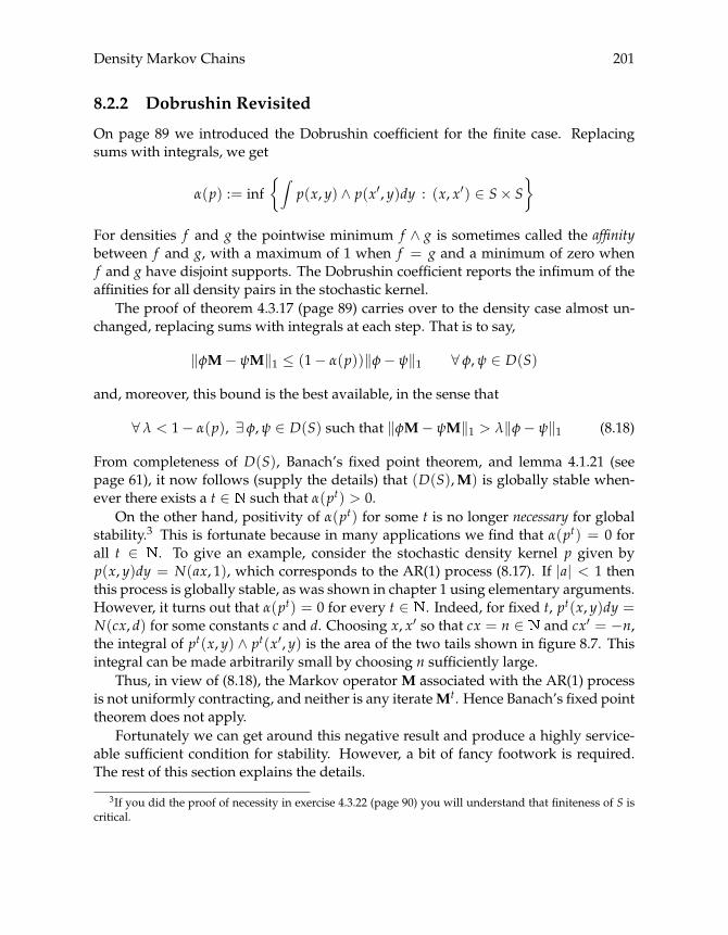
Density Markov Chains 201
8.2.2 Dobrushin Revisited
On page 89 we introduced the Dobrushin coefficient for the finite case. Replacingsums with integrals, we get
α(p) := inf{∫
p(x, y) ∧ p(x′, y)dy : (x, x′) ∈ S× S}
For densities f and g the pointwise minimum f ∧ g is sometimes called the affinitybetween f and g, with a maximum of 1 when f = g and a minimum of zero whenf and g have disjoint supports. The Dobrushin coefficient reports the infimum of theaffinities for all density pairs in the stochastic kernel.
The proof of theorem 4.3.17 (page 89) carries over to the density case almost un-changed, replacing sums with integrals at each step. That is to say,
‖φM− ψM‖1 ≤ (1− α(p))‖φ− ψ‖1 ∀ φ,ψ ∈ D(S)
and, moreover, this bound is the best available, in the sense that
∀ λ < 1− α(p), ∃ φ,ψ ∈ D(S) such that ‖φM− ψM‖1 > λ‖φ− ψ‖1 (8.18)
From completeness of D(S), Banach’s fixed point theorem, and lemma 4.1.21 (seepage 61), it now follows (supply the details) that (D(S),M) is globally stable when-ever there exists a t ∈ such that α(pt) > 0.
On the other hand, positivity of α(pt) for some t is no longer necessary for globalstability.3 This is fortunate because in many applications we find that α(pt) = 0 forall t ∈ . To give an example, consider the stochastic density kernel p given byp(x, y)dy = N(ax, 1), which corresponds to the AR(1) process (8.17). If |a| < 1 thenthis process is globally stable, as was shown in chapter 1 using elementary arguments.However, it turns out that α(pt) = 0 for every t ∈ . Indeed, for fixed t, pt(x, y)dy =N(cx, d) for some constants c and d. Choosing x, x′ so that cx = n ∈ and cx′ = −n,the integral of pt(x, y) ∧ pt(x′, y) is the area of the two tails shown in figure 8.7. Thisintegral can be made arbitrarily small by choosing n sufficiently large.
Thus, in view of (8.18), the Markov operator M associated with the AR(1) processis not uniformly contracting, and neither is any iterateMt. Hence Banach’s fixed pointtheorem does not apply.
Fortunately we can get around this negative result and produce a highly service-able sufficient condition for stability. However, a bit of fancy footwork is required.The rest of this section explains the details.
3If you did the proof of necessity in exercise 4.3.22 (page 90) you will understand that finiteness of S iscritical.
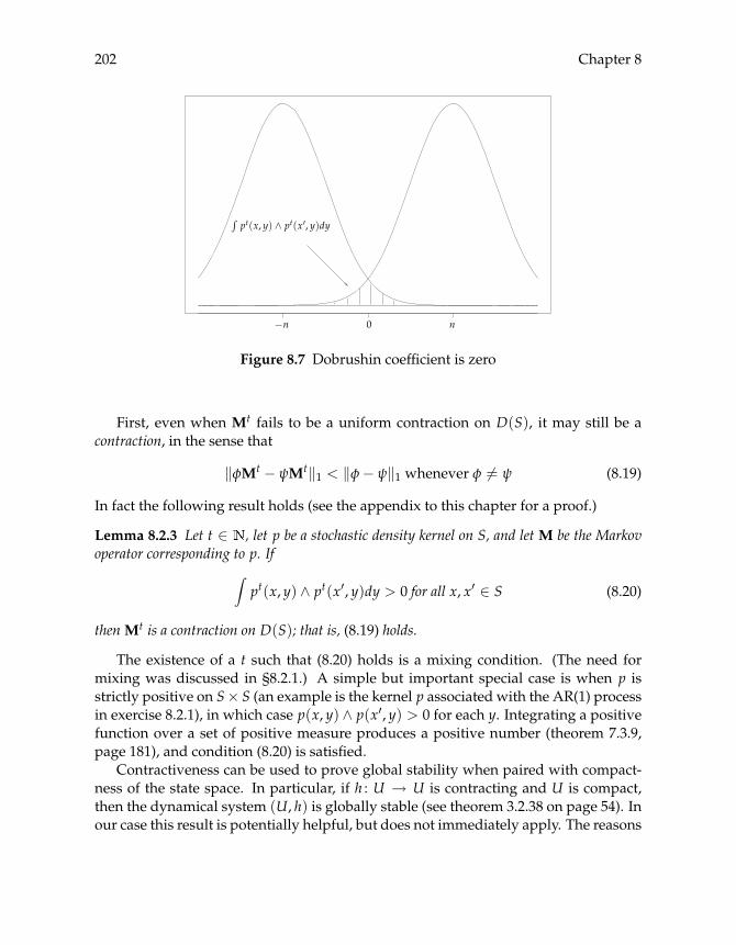
202 Chapter 8
−n 0
∫pt(x, y) ∧ pt(x′, y)dy
n
Figure 8.7 Dobrushin coefficient is zero
First, even when Mt fails to be a uniform contraction on D(S), it may still be acontraction, in the sense that
‖φMt − ψMt‖1 < ‖φ− ψ‖1 whenever φ �= ψ (8.19)
In fact the following result holds (see the appendix to this chapter for a proof.)
Lemma 8.2.3 Let t ∈ , let p be a stochastic density kernel on S, and let M be the Markovoperator corresponding to p. If∫
pt(x, y) ∧ pt(x′, y)dy > 0 for all x, x′ ∈ S (8.20)
thenMt is a contraction on D(S); that is, (8.19) holds.
The existence of a t such that (8.20) holds is a mixing condition. (The need formixing was discussed in §8.2.1.) A simple but important special case is when p isstrictly positive on S× S (an example is the kernel p associated with the AR(1) processin exercise 8.2.1), in which case p(x, y) ∧ p(x′, y) > 0 for each y. Integrating a positivefunction over a set of positive measure produces a positive number (theorem 7.3.9,page 181), and condition (8.20) is satisfied.
Contractiveness can be used to prove global stability when paired with compact-ness of the state space. In particular, if h : U → U is contracting and U is compact,then the dynamical system (U, h) is globally stable (see theorem 3.2.38 on page 54). Inour case this result is potentially helpful, but does not immediately apply. The reasons
Density Markov Chains 203
is that when S is infinite, D(S) = (D(S), d1) is not compact. The next two exerciseshelp to illustrate why this is so.
Exercise 8.2.4 Let S = , and let (φn)n≥1 ⊂ D(S) be given by φn := [n,n+1). Showthat d1(φn, φm) = 2 whenever n �= m. Conclude that this sequence has no subsequenceconverging to a point in D(S).
Exercise 8.2.5 Let S = (0, 1), and let (φn)n≥1 ⊂ D(S) be given by φn := n · (0,1/n).Suppose that d1(φn, φ) → 0 for some φ ∈ D(S). Using your measure-theoretic bag oftricks, show that λ(φ) = 0, contradicting φ ∈ D(S). You have now shown that thesequence itself cannot converge to any point in D(S). Argue that the same is true forany subsequence.
Fortunately there is a way around this problem created by lack of compactnessof D(S). Recall from exercise 4.1.9 (page 58) that a dynamical system (U, h) is calledLagrange stable if every trajectory is precompact in U. Lagrange stability is weakerthan compactness of U,4 but it turns out that if (U, h) is contracting and Lagrange stablethen it is globally stable.5
So suppose that (8.20) holds for some t ∈ , and hence Mt is contracting. Ifwe can prove that all trajectories of (D(S),M) are precompact, then all trajectoriesof (D(S),Mt) are also precompact (subsets of precompact sets are precompact), and(D(S),Mt) is globally stable. Finally, lemma 4.1.21 (page 61) implies that if (D(S),Mt)is globally stable, then so is (D(S),M). Let’s record this as a theorem.
Theorem 8.2.6 Let (D(S),M) be Lagrange stable. If Mt is a contraction for some t ∈ ,then (D(S),M) is globally stable.
But how to prove precompactness of trajectories? We need the following two def-initions:
Definition 8.2.7 Let M be a subset of D(S). The collection of densities M is calledtight if
∀ ε > 0, ∃ a compact set K ⊂ S such that supψ∈M
∫Kcψ(x)dx ≤ ε
It is called uniformly integrable if
∀ ε > 0, ∃ δ > 0 such that λ(A) < δ implies supψ∈M
∫Aψ(x)dx ≤ ε
4If U is compact then (U, h) is always Lagrange stable (why?), but the converse is not true (example?).5Proof: Fix x ∈ U, and define Γ(x) to be the closure of {hn(x) : n ∈ }. The set Γ(x) is a compact subset
of U. (Why?) Moreover h sends Γ(x) into itself (see exercise 4.1.3, page 56). Hence (Γ(x), h) is a dynamicalsystem where h is contracting and Γ(x) is compact, implying the existence of a unique fixed point x∗ ∈ Γ(x)with hn(x) → x∗ (theorem 3.2.38, page 54). Finally, h has at most one fixed point in U by contractivenessover U. Therefore x∗ does not depend on x, and (U, h) is globally stable.
204 Chapter 8
Here λ is Lebesgue measure. Essentially, tightness rules out the violation of com-pactness seen in exercise 8.2.4, while uniform integrability rules out that seen in ex-ercise 8.2.5. Tightness and uniform integrability are important to us because of thefollowing result:
Theorem 8.2.8 Let p be a stochastic density kernel on S, and let M be the correspondingMarkov operator. Let ψ ∈ D(S). If the sequence (ψMt)t≥0 is both tight and uniformlyintegrable, then it is also precompact in D(S).
While the proof is omitted, those readers familiar with functional analysis will un-derstand that tightness and uniform integrability together imply weak precompact-ness in L1. Further, the fact that M is an integral operator means it is sufficientlysmoothing that it sends weakly precompact sets into (strongly) precompact sets. Theproof of the latter result can be found in Lasota (1994, thm. 4.1).
8.2.3 Drift Conditions
How might one verify the tightness and uniform integrability of a given trajectory(ψMt)t≥0? Tightness is usually established using drift inequalities. We will use avariety that rely on the concept of norm-like functions (Meyn and Tweedie 1993):
Definition 8.2.9 A measurable function w : S → + is called norm-like if all of itssublevel sets (i.e., sets of the form Ca := {x ∈ S : w(x) ≤ a}, a ∈ +) are precompactin (S, d2).
Example 8.2.10 Let S = n, and let w(x) := ‖x‖, where ‖ · ‖ is any norm on n (def-inition 3.1.2, page 37). This function w is norm-like on S because the sublevel sets ofw are bounded with respect to the metric induced by ‖ · ‖, and hence bounded for d2(theorem 3.2.30, page 50). For subsets of ( n, d2), boundedness implies precompact-ness (theorem 3.2.19, page 48).
We can now state our drift condition:
Definition 8.2.11 Let p be a stochastic density kernel on S. We say that p satisfiesgeometric drift to the center if there exists a norm-like function w on S and positiveconstants α < 1 and β < ∞ such that∫
w(y)p(x, y)dy ≤ αw(x) + β (x ∈ S)
As we will see, this condition is often easy to check in applications. Moreover
Proposition 8.2.12 If p satisfies geometric drift to the center, then (ψMt) is tight for everyψ ∈ D(S).
Density Markov Chains 205
The proof is given in the appendix to the chapter, but the intuition is not difficult:Under geometric drift, the ratio
∫w(y)p(x, y)dy/w(x) is dominated by α+ β/w(x).
Norm-like functions tend to get large as x moves away from the center of the statespace, so if x is sufficiently far from the center, then α+ β/w(x) < 1. In which case∫w(y)p(x, y)dy, the expectation of w(Xt+1) given Xt = x, is less than w(x). This
in turn means that probability mass is moving back toward the center, where w issmaller. Keeping probability mass in the center of the state space is the essence oftightness.
Let’s conclude this section by showing that the AR(1) model
Xt+1 = aXt + b+Wt+1, (Wt)t≥1IID∼ φ = N(0, 1), |a| < 1
is Lagrange stable. Since its stochastic kernel
p(x, y) = φ(y− ax− b), φ(z) :=1√2π
exp(−z2/2)
is strictly positive on × (and hence its Markov operator is contracting), this im-plies global stability.
Regarding tightness, let w be the norm-like function | · |. The change of variablez = y− ax− b gives∫|y|p(x, y)dy =
∫|y|φ(y− ax− b)dy
=∫|ax+ b+ z|φ(z)dz ≤ α|x|+ β, α := |a|, β := |b|+
∫|z|φ(z)dz
Since |a| < 1 the geometric drift condition is satisfied, and, in view of proposition8.2.12, every trajectory is tight.
Only uniform integrability of trajectories remains to be checked. To do this, pickany ψ ∈ D(S). Observe there is a constant K such that p(x, y) ≤ K for every x, y.Hence, for any A ∈ B( ), t ∈ ,
∫AψMt(y)dy =
∫A
[∫p(x, y)ψMt−1(x)dx
]dy
=∫ [∫
Ap(x, y)dy
]ψMt−1(x)dx ≤
∫Kλ(A)ψMt−1(x)dx = Kλ(A)
Now fix ε > 0. If λ(A) < ε/K, then∫A ψM
t(y)dy < ε, independent of t. Henceuniform integrability of (ψMt)t≥0 is established. Theorem 8.2.8 now tells us that(D(S),M) is Lagrange stable, and hence globally stable.
We will see in the next section that these ideas can be used to prove the stabilityof much more complex models. Before discussing applications in earnest, let’s try to
206 Chapter 8
package our results in a simple format. On the Lagrange stability side, we can makeour life easier with the following result:
Proposition 8.2.13 Let ψ ∈ D(S), let p be a stochastic density kernel on S, and let M bethe corresponding Markov operator. If the sequence (ψMt)t≥0 is tight, and in addition thereexists a continuous function m : S → such that p(x, y) ≤ m(y) for all x, y ∈ S, then(ψMt)t≥0 is also uniformly integrable.
The proof is an extension of the proof of uniform integrability of the AR(1) systemabove, where we used the fact that p is bounded above by a constant (which is cer-tainly a continuous function). It is given in the appendix to the chapter and should beskipped on first pass.
Now let’s put this all together:
Theorem 8.2.14 Let p be a stochastic density kernel on S, and let M be the correspondingMarkov operator. If
1. ∃ t ∈ such that∫pt(x, y) ∧ pt(x′, y)dy > 0 for all (x, x′) ∈ S× S,
2. p satisfies geometric drift to the center, and
3. ∃ a continuous m : S→ such that p(x, y) ≤ m(y) for all x, y ∈ S,
then the dynamical system (D(S),M) is globally stable.
Proof. In view of theorem 8.2.6, we need only show that (ψMt)t≥0 is precompact forevery ψ ∈ D(S). So pick any ψ ∈ D(S). Since p satisfies geometric drift, (ψMt)t≥0 istight. By proposition 8.2.13 it is also uniformly integrable, and therefore precompact(theorem 8.2.8).
Just as for the finite state case, stability is connected with the law of large numbers(recall theorem 4.3.33 on page 94). For example, take the stochastic recursive sequence
Xt+1 = F(Xt,Wt+1), X0 ∼ ψ, (Wt)t≥1IID∼ φ (8.21)
where the state space S is a Borel subset of n, Z is a Borel subset of k, φ ∈ D(Z)and ψ ∈ D(S). Let kernel p represent this SRS on S in the sense of (8.3) on page 189.Let M be the corresponding Markov operator. We have the following result:
Theorem 8.2.15 Let h : S → be a Borel measurable function, and let (Xt)t≥0, the kernelp and the Markov operator M be as above. If (D(S),M) is globally stable with stationarydistribution ψ∗, then
1n
n
∑t=1
h(Xt)→∫h(x)ψ∗(x)dx as n→ ∞
with probability one whenever∫ |h(x)|ψ∗(x)dx is finite.
Density Markov Chains 207
The meaning of probability one convergence will be discussed later, but for nowyou can understand it as it sounds: The probability of generating a path (Wt)t≥1 suchthat this convergence fails is zero. Notice that convergence holds independent of theinitial condition ψ.
The proof of the theorem is beyond the scope of this book. See Nummelin (1984,prop. 6.3) and Meyn and Tweedie (1993, thm. 17.1.7). Note that theorem 8.2.15 justifiesthe stationary density look-ahead estimator introduced in §6.1.4, at least when stabil-ity holds. Also, as we saw in the finite state case, the LLN leads to a new interpretationof the stationary density that is valid in the globally stable case:
∫Bψ∗(x)dx � the fraction of time that (Xt)t≥0 spends in B
for any B ∈ B(S). To see this, take h = B. Then theorem 8.2.15 gives
1n
n
∑t=1
h(Xt) =1n
n
∑t=1
B(Xt)→∫Bψ∗(x)dx as n→ ∞ (8.22)
8.2.4 Applications
Let’s turn to applications. To start, recall the model of commodity dynamics withspeculation discussed in §6.3.2. The state evolves according to
Xt+1 = αI(Xt) +Wt+1, (Wt)t≥1IID∼ φ
where I is the equilibrium investment function defined in (6.27), page 146. Supposefor now that φ is a lognormal density. The stochastic kernel is
p(x, y) = φ(y− αI(x)) ((x, y) ∈ S× S)
where φ(z) = 0 when z < 0. The state space is S = +.This model is easily seen to be globally stable. Regarding condition 1 of theo-
rem 8.2.14, pick any x, x′ ∈ S. Let E be all y ∈ S such that y > αI(x) and y > αI(x′).On E the function y �→ p(x, y) ∧ p(x′, y) is strictly positive, and integrals of strictlypositive functions on sets of positive measure are positive (theorem 7.3.9, page 181).Hence condition 1 holds for t = 1.
Regarding condition 2, let w(x) = x. This function is norm-like on S. (Proof?)Moreover geometric drift to the center holds because, using the change of variablez = y− αI(x),
∫yp(x, y)dy =
∫yφ(y− αI(x))dy = αI(x) +
∫zφ(z)dz ≤ αx+
∫zφ(z)dz

208 Chapter 8
Condition 3 is trivial because p(x, y) ≤ K for some constant K, and constant functionsare continuous. Hence global stability holds.
Next, recall the STAR model of example 6.1.3, where Z = S = , and the stateevolves according to
Xt+1 = g(Xt) +Wt+1, (Wt)t≥1IID∼ φ ∈ D( ) (8.23)
with g(x) := (α0 + α1x)(1− G(x)) + (β0 + β1x)G(x). Here G : S → [0, 1] is a smoothtransition function satisfying G′ > 0, limx→−∞ G(x) = 0, and limx→∞ G(x) = 1.Suppose that φ is bounded, everywhere positive on ,
γ := |α1| ∨ |β1| < 1, and∫|z|φ(z)dz < ∞
Exercise 8.2.16 Show that under these assumptions there exists a constant c such that|g(x)| ≤ γ|x|+ c for all x ∈ S = .
Since the stochastic density kernel p(x, y) = φ(y − g(x)) is strictly positive onS× S, condition 1 of theorem 8.2.14 holds. Regarding condition 2, set w(x) = |x|. Thechange of variable z = y− g(x) gives∫|y|p(x, y)dy =
∫|y|φ(y− g(x))dy =
∫|g(x) + z|φ(z)dz ≤ γ|x|+ c+
∫|z|φ(z)dz
Since γ < 1, condition 2 is satisfied.Condition 3 is trivial because φ and hence p are bounded by some constant K.
Setting m(y) = K for all y gives a continuous upper bound.As another application, consider again the threshold autoregression model, where
S = Z = n, and
Xt+1 =K
∑k=1
(AkXt + bk) Bk (Xt) +Wt+1, (Wt)t≥1IID∼ φ ∈ D( n)
In exercise 8.1.5 you showed that the stochastic kernel is given by
p(x, y) = φ
[y−
K
∑k=1
(Akx+ bk) Bk (x)
]((x, y) ∈ S× S) (8.24)
Assume that φ is strictly positive on n, bounded, and that∫ ‖z‖φ(z)dz < ∞ for some
norm ‖ · ‖ on n. Conditions 1 and 3 of theorem 8.2.14 can be verified in much thesame way as the previous example. Regarding condition 2, let γk be a real numbersuch that ‖Akx‖ ≤ γk‖x‖ for all x. Assume that γ := maxk γk < 1. Then, using a

Density Markov Chains 209
change of variable again,
∫‖y‖p(x, y)dy =
∫ ∥∥∥∥∥K
∑k=1
(Akx+ bk) Bk (x) + z
∥∥∥∥∥ φ(z)dz≤
K
∑k=1‖Akx+ bk‖ Bk (x) +
∫‖z‖φ(z)dz
≤K
∑k=1
γk‖x‖ Bk (x) +K
∑k=1‖bk‖+
∫‖z‖φ(z)dz
≤ γ‖x‖+ β, β :=K
∑k=1‖bk‖+
∫‖z‖φ(z)dz
Since γ < 1 and ‖ · ‖ is norm-like, condition 2 is also satisfied, and the model isglobally stable.
Before starting the next application, let’s think a little more about norm-like func-tions (i.e., nonnegative functions with precompact sublevel sets). For the metric space( n, d2) we can equate precompactness with boundedness (theorem 3.2.19, page 48).For S ⊂ n, bounded subsets of (S, d2) are not necessarily precompact (e.g., see ex-ercise 3.2.14 on page 47), making precompactness and hence the norm-like propertyharder to check. The next result gives some guidance when S is an open interval in .The proof is an exercise.
Lemma 8.2.17 If S = (u, v), where u ∈ {−∞} ∪ and v ∈ {+∞} ∪ , then w : S→ +is norm-like if and only if limx→u w(x) = limx→v w(x) = ∞.6
As a consequence w(x) := | ln x| is a norm-like function on S = (0,∞). We exploitthis fact below.
Now for the last application. In exercise 8.1.8 you derived the stochastic kernelfor the nonconvex growth model kt+1 = sA(kt)kαt Wt+1, where S = Z = (0,∞) and(Wt)t≥1 is IID with density φ ∈ D(Z). It has the form
p(x, y) = φ
(y
sA(x)xα
)1
sA(x)xα((x, y) ∈ S× S) (8.25)
Suppose that A takes values in [a1, a2] ⊂ S and that α < 1. Regarding the densityφ, assume that φ is strictly positive on (0,∞), that
∫ | ln z|φ(z)dz is finite, and thatφ(z)z ≤ M for some M < ∞ and all z ∈ (0,∞). For example, the lognormal densitysatisfies all of of these conditions.
6Here limx→a f (x) = ∞ means that for any xn → a and any M ∈ , there exists an N ∈ such thatn ≥ N implies f (xn) ≥ M. Hint: Show that K ⊂ S is precompact in S if and only if no sequence in Kconverges to either u or v.

210 Chapter 8
Now let’s check the conditions of theorem 8.2.14. Condition 1 holds because p isstrictly positive on S× S. Regarding condition 2, set w(x) = | ln x|, so
∫w(sA(x)xαz)φ(z)dz =
∫| ln s+ ln A(x) + α ln x+ ln z|φ(z)dz
≤ | ln s|+ | ln A(x)|+ α| ln x|+∫| ln z|φ(z)dz
Setting β := | ln s|+ max{| ln a1|, | ln a2|}+∫ | ln z|φ(z)dz we obtain
∫w(sA(x)xαz)φ(z)dz ≤ α| ln x|+ β = αw(x) + β
Since w is norm-like on (0,∞), condition 2 is proved.Finally, consider condition 3. Given any x and y in S we have
p(x, y) = p(x, y)yy
= φ
(y
sA(x)xα
)y
sA(x)xα1y≤ M
y
Since m(y) := M/y is continuous on S, condition 3 is satisfied.
8.3 Commentary
The material in this chapter draws heavily on Lasota and Mackey (1994), and alsoon a slightly obscure but fascinating paper of Lasota (1994). Theorem 8.2.14 is fromMirman, Reffett, and Stachurski (2005). More details on the theory and an applicationto optimal growth can be found in Stachurski (2002). See also Stachurski (2003).
Chapter 9
Measure-Theoretic Probability
In the first few decades of the twentieth century, mathematicians realized that throughmeasure theory it was possible to place the slippery subject of probability in a com-pletely sound and rigorous framework, where manipulations are straightforward andpowerful theorems can be proved. This integration of probability and measure yieldeda standard language for research in probability and statistics shared by mathemati-cians and other scientists around the world. A careful read of this chapter will providesufficient fluency to understand and participate in their conversation.
9.1 Random Variables
The language of probability begins with random variables and their distributions.Let’s start with a detailed treatment of these topics, beginning with basic definitionsand moving on to key concepts such as expectations and independence.
9.1.1 Basic Definitions
In probability theory, the term random variable is just another way of saying F -measurable real-valued function on some measure space (Ω,F ). In other words, arandom variable on (Ω,F ) is a map X : Ω → with the property that X−1(B) ∈ Ffor all B ∈ B( ). For historical reasons random variables are typically written withupper-case symbols such as X and Y, rather than lower-case symbols such as f andg. The measurable space (Ω,F ) is usually paired with a probability measure (seepage 167), which assigns probabilities to events E ∈ F .
Why restrict attention toF -measurable functions? Well, suppose that is a prob-ability on (Ω,F ). We can think of a draw from as an experiment that results in a
211
212 Chapter 9
nonnumerical outcome ω ∈ Ω, such as “three heads and then two tails.” In order tomake the outcome of this experiment more amenable to analysis, we specify a func-tion X : Ω → that maps outcomes into numbers. Suppose further that we wish toevaluate the probability that X ≥ a, or
{ω ∈ Ω : X(ω) ≥ a} :=: {X ≥ a} :=: X−1([a,∞))
Since is only defined on the sets in F , this requires X−1([a,∞)) ∈ F . The latter isguaranteed byF -measurability of X.
Actually, the definition of random variables as real-valued functions is not generalenough for our purposes. We need to consider random “objects,” which are like (real-valued) random variables except that they take values in other spaces (such as n, orabstract metric space). Some authors use the term “random object,” but we will callthem all random variables:
Definition 9.1.1 Let (Ω,F , ) be a probability space, and let (S,S ) be any mea-surable space. An S-valued random variable is a function X : Ω → S that is F ,S -measurable: X−1(B) ∈ F whenever B ∈ S . The distribution of X is the uniquemeasure μX ∈P(S,S ) defined by
μX(B) := (X−1(B)) = {ω ∈ Ω : X(ω) ∈ B} (B ∈ S )
Note that μX , which gives the probability that X ∈ B for each B ∈ S , is justthe image measure ◦ X−1 of under X (see page 183 for a discussion of imagemeasures). Distributions play a central role in probability theory.
A quick but important point on notation: In probability theory it is standard to usethe abbreviation {X has property P} for the set {ω ∈ Ω : X(ω) has property P}. Wewill follow this convention. Similarly, {X ∈ A} is the indicator function for the set{ω ∈ Ω : X(ω) ∈ A}.Exercise 9.1.2 Let S be a metric space, and let (Ω,F ) be any measurable space. Letf : Ω→ S beF ,B(S)-measurable, and let g : S→ be a continuous function. Showthat X := g ◦ f is a random variable on (Ω,F ).
The integral of a real-valued random variable X on (Ω,F , ) is called its expecta-tion, and written (X) or just X. That is,
X :=∫X d :=:
∫X(ω) (dω) :=: (X)
The definition on the far right is the linear functional notation for the integral, whichI personally prefer, as it eliminates the need for the new symbol , and forces us tospecify the underlying probability whenever we want to take expectations. However,

Measure-Theoretic Probability 213
the notation is more traditional, and is used in all of what follows—albeit with someresentment on my part.
Our definition of has a sound probabilistic interpretation. If X is simple, takingvalues α1, . . . , αN on A1, . . . , AN respectively, then the expectation X = ∑n αn (An),which is the sum of all possible values taken by the random variable X multiplied bythe probability that each such value occurs. If X is not simple, then to calculate ex-pectation we approximate X by simple functions (see page 177), in which case similarintuition applies.
Exercise 9.1.3 Consider the probability space (S,S , δz), where δz is the degenerateprobability measure introduced in §7.1.3. The expectation of f ∈ mS + is f :=∫f dδz. Intuitively, f = f (z), since we are sure that δz will pick out the point z.
Confirm this intuition.
There is a close connection between distributions and expectations:
Theorem 9.1.4 If X is an S-valued random variable on (Ω,F , ) with distribution μX ∈P(S,S ), and if w ∈ mS is nonnegative or |w(X)| < ∞, then
w(X) :=∫w ◦ X d =
∫w dμX :=: μX(w) (9.1)
This is just a special case of theorem 7.3.17 on page 182, which gives∫w dμX :=
∫w d( ◦ X−1) =
∫w ◦ X d
Let (Ω,F , ) be a probability space, let X be a real-valued random variable onthis space, and let k ∈ . The k-th moment of X is (Xk), which may or may not existas an expectation. By definition, existence of the expectation requires that |X|k < ∞.The elementary inequality aj ≤ ak + 1 for all j ≤ k and a ≥ 0 can be used to provethat if j ≤ k and the k-th moment is finite, then so is the j-th: By the previous boundwe have |X|j ≤ |X|k + Ω, where the inequality is understood to hold pointwise onΩ (i.e., for all ω ∈ Ω). Referring to properties M1–M5 of the integral (page 179), weconclude that |X|j ≤ |X|k + 1 < ∞.
Let X and Y be real-valued random variables with finite second moment. Thevariance of X is the real number Var(X) := [(X − X)2], while the covariance of Xand Y is
Cov(X,Y) := [ (X− X)(Y− Y) ]
Exercise 9.1.5 Show that if X has finite second moment and if a and b are constants,then Var(aX + b) = a2 Var(X). Show in addition that if Cov(X,Y) = 0, then Var(X +Y) = Var(X) + Var(Y).
214 Chapter 9
In the results that follow, we will often need to say something along the lines of “letX be a random variable on (Ω,F , ) taking values in (S,S ) and having distributionμ.” It is fortunate then that:
Theorem 9.1.6 Given any measurable space (S,S ) and μ ∈ P(S,S ), there exists a prob-ability space (Ω,F , ) and a random variable X : Ω→ S such that X has distribution μ.
Exercise 9.1.7 Prove theorem 9.1.6 by setting (Ω,F , ) = (S,S , μ) and X = theidentity map on S. Show, in particular, that X is measurable and has distribution μ.
Sometimes it’s useful to construct a supporting probability space a little more ex-plicitly. Consider an arbitrary distribution in P( ), which can be represented by acumulative distribution function H.1 For simplicity, we assume that H is strictly in-creasing (a discussion of the general case can be found in Williams 1991, ch. 3). LetX : (0, 1) → be the inverse of H: X = H−1. Then X is a random variable on(Ω,F , ) = ((0, 1),B(0, 1),λ) with distribution H. (Here λ is Lebesgue measure.)
Leaving measurability as an exercise, let’s confirm that X has distribution H. Fixz ∈ . Note that for each u ∈ (0, 1) we have X(u) ≤ z if and only if u ≤ H(z), andhence
{X ≤ z} := {u ∈ (0, 1) : X(u) ≤ z}= {u ∈ (0, 1) : u ≤ H(z)} = λ((0,H(z)]) = H(z)
Thus X has distribution H, as was to be shown.Next we introduce Chebychev’s inequality, which allows us to bound tail probabili-
ties in terms of expectations—the latter being easier to calculate in many applications.
Theorem 9.1.8 Let X be an S-valued random variable on (Ω,F , ). If h : S → + is ameasurable function and δ ∈ , then δ {h(X) ≥ δ} ≤ h(X).
Proof. Observe that h(X) ≥ h(X) {h(X) ≥ δ} ≥ δ {h(X) ≥ δ} pointwise on Ω.Now integrate, using properties M1–M5 as required.
Two special cases are used repeatedly in what follows: First, if X is a nonnegativerandom variable then setting h(x) = x gives
{X ≥ δ} ≤ Xδ
(δ > 0) (9.2)
Second, application of the bound to Y := X− X with h(x) = x2 gives
{|X− X| ≥ δ} = {(X− X)2 ≥ δ2} ≤ Var(X)δ2 (δ > 0) (9.3)
As we will see, (9.3) can be used to prove a law of large numbers.1Recall theorem 7.1.33 on page 170.
Measure-Theoretic Probability 215
9.1.2 Independence
We have already used the concept of independence repeatedly in the text. It’s nowtime for a formal definition.
Definition 9.1.9 Random variables X and Y taking values in (S,S ) and (T,T ) re-spectively are said to be independent whenever
{X ∈ A} ∩ {Y ∈ B} = {X ∈ A} · {Y ∈ B} for all A ∈ S and B ∈ T
More generally, a finite collection of random variables X1, . . . ,Xn with Xi taking val-ues in (Si,Si) is called independent if
∩ni=1 {Xi ∈ Ai} =n
∏i=1
{Xi ∈ Ai} =n
∏i=1
μXi (Ai) (9.4)
for any sets with Ai ∈ Si. An infinite collection of random variables is called inde-pendent if any finite subset of the collection is independent.
In (9.4), the right-hand side is the product of the marginal distributions. Hencethe joint distributions of independent random variables are just the product of theirmarginals. The next result extends this “independence means multiply” rule fromprobabilities to expectations.
Theorem 9.1.10 If X and Y are independent real-valued random variables with |X| < ∞and |Y| < ∞, then |XY| < ∞ and (XY) = X Y.
Exercise 9.1.11 Show that if X and Y are independent, then Cov(X,Y) = 0.
One important consequence of independence is the following result
Theorem 9.1.12 (Fubini) Let X and Y be as above, and let S and T be subsets of n and k
respectively. Let h ∈ bB(S× T) or mB(S× T)+. In other words, h is a either a bounded ora nonnegative Borel measurable function on the space where the pair (X,Y) takes values. If Xand Y are independent, then
h(X,Y) =∫ ∫
h(x, y)μX(dx)μY(dy) =∫ ∫
h(x, y)μY(dy)μX(dx)
Things start to get interesting when we have an infinite number of random vari-ables on the one probability space indexed by a value that often represents time. Thesecollections of random variables are called stochastic processes. A formal definitionfollows.
216 Chapter 9
Definition 9.1.13 Let (S,S ) be a measurable space, and let (Ω,F , ) be a probabilityspace. By an S-valued stochastic process we mean a tuple
(Ω,F , , (Xt)t∈ )
where is an index set such as or and (Xt)t∈ is a family of S-valued randomvariables Xt all defined on (Ω,F , ).
With stochastic processes the ideas is that, at the “start of time,” a point ω is se-lected by “nature” from the set Ω according to the probability law (i.e., (E) is theprobability that ω ∈ E). This is a once-off realization of all uncertainty, and Xt(ω)simply reports the time t outcome for the variable of interest, as a function of thatrealization.
The simplest kind of stochastic processes are the IID processes:
Definition 9.1.14 An S-valued stochastic process (Ω,F , , (Xt)t∈ ) is called inde-pendent and identically distributed (IID) if the sequence (Xt)t∈ is independent andeach Xt has the same distribution, in the sense that
{Xt ∈ B} = {Xs ∈ B} for any s, t ∈ and any B ∈ S
For an IID process, any event that occurs at each t with nonzero probability occurseventually with probability one. To see this, suppose that (Ω,F , , (Xt)t∈ ) is a IID,and that the common distribution of each Xt is μ ∈ P(S,S ). Consider a set A ∈ Swith μ(A) > 0.
Exercise 9.1.15 Show that {Xt /∈ A, ∀t ∈ } ⊂ ∩t≤T{Xt /∈ A} for all T ∈ .2
Using this relation, show that {Xt /∈ A, ∀t ∈ } ≤ (1 − μ(A))T for all T ∈ .Conclude that this probability is zero, and hence that Xt ∈ A for at least one t ∈with probability one.
9.1.3 Back to Densities
We have mentioned a few times that some but not all distributions can be representedby densities. Let’s now clarify exactly when distributions do have density representa-tions, as well as collecting some miscellaneous facts about densities.
Let S be a Borel subset of n. Recall that a density on S is a function φ ∈ mB(S)+
with the property that∫φ(x)dx :=:
∫φdλ :=: λ(φ) = 1. The set of all densities on
S is denoted by D(S). Each density φ ∈ D(S) creates a distribution μφ ∈ P(S) viaμφ(B) =
∫B φ(x)dx.
2Remember that these are subsets of Ω.
Measure-Theoretic Probability 217
Exercise 9.1.16 Confirm that this μφ is countably additive.3
Sometimes we can go the other way, from distributions to associated density. Inparticular, suppose that S ∈ B( n), and let μ ∈ P(S). The distribution μ is said tohave a density representation φ if φ ∈ D(S) and
μ(B) =∫Bφ(x) dx (B ∈ B(S)) (9.5)
However, the pairing of D(S) and P(S) in (9.5) is not a one-to-one correspondence.Every density creates a distribution, but there are distributions inP(S) without suchan “integral” representation by an element of D(S). Here is an example:
Exercise 9.1.17 Let a ∈ , and let δa be the element ofP( ) that puts unit mass on a.That is, δa(B) = 1 if a ∈ B and zero otherwise. Argue that there is no φ ∈ D( ) suchthat δa(B) =
∫B φ(x)dx for all B ∈ B( ).4
So when do density representations exist? The following rather fundamental the-orem answers that question. The proof is omitted, but you can find it in any text onmeasure theory.
Theorem 9.1.18 (Radon–Nikodym) Let μ ∈ P(S), where S ∈ B( n), and let λ be theLebesgue measure. The distribution μ has a density representation if and only if μ(B) = 0whenever B ∈ B(S) and λ(B) = 0.
When densities exist, they can make our life much easier. The next theorem indi-cates how density representations can be used to compute expectations by changingthe measure used to integrate from a given distribution to Lebesgue measure. Oftenthe transformation results in a standard Riemann integral, which can be solved usingcalculus.
Theorem 9.1.19 Let S ∈ B( n). If distribution μ ∈ P(S) has density representationφ ∈ D(S), and if h ∈ bB(S) or h ∈ mB(S)+, then
μ(h) =∫h(x)φ(x)dx (9.6)
Proof. The proof follows a very standard argument, and is probably worth readingthrough at least once. Let’s focus on the case of h ∈ bB(S). Suppose first that h = B,where B ∈ B(S). For such an h the equality (9.6) holds by (9.5). Now suppose that
3Hint: If (Bn) is a disjoint sequence of sets, show that ∪Bn = ∑∞n Bn . Complete the proof usingproperties M1–M5 of the integral.
4Hint: Recall from theorem 7.3.9 that if λ(B) = 0, then∫B φ(x)dx = 0.

218 Chapter 9
h is a simple function: h ∈ sB(S), h = ∑Nn=1 αn Bn , Bn ∈ B(S). Since the integral is
linear, we have
μ
(N
∑n=1
αn Bn
)=
N
∑n=1
αnμ( Bn) =N
∑n=1
αn
∫Bn(x)φ(x)dx =
∫ N
∑n=1
αn Bn(x)φ(x)dx
In other words, (9.6) holds for h ∈ sB(S). Now let h ∈ bB(S) with h ≥ 0. Bylemma 7.2.11 (page 175) there is a sequence (sk) ⊂ sB(S)+ with sk ↑ h. Since (9.6)holds for each sk, we have
μ(sk) =∫sk(x)φ(x)dx (k ∈ )
Taking limits with respect to k and using the monotone convergence theorem gives(9.6). Finally, for general h ∈ bB(S), we have h = h+ − h−, and another applicationof linearity completes the proof.
9.2 General State Markov Chains
It’s time to develop a general theory of Markov chains on uncountably infinite statespaces.5 In chapter 8 we covered uncountable state spaces when the stochastic (den-sity) kernel was a family of densities p(x, y)dy, one for each x in the state space. Wenow drop the assumption that these distributions can be represented as densities andpermit them to be arbitrary probability measures.
9.2.1 Stochastic Kernels
For discrete time Markov chains of all shapes and forms, the most important primitiveis the stochastic kernel.6 You have already met some stochastic kernels: The first wasthe finite kernel p, living on a finite set S, with the property that p(x, y) ≥ 0 and∑y∈S p(x, y) = 1. The second was the density kernel p(x, y)dy on a Borel subset S ofk. Here is the general (i.e., probability measure) case:
Definition 9.2.1 Let S be a Borel subset of n. A stochastic kernel on S is a family ofprobability measures
P(x, dy) ∈P(S) (x ∈ S)
where x �→ P(x, B) is Borel measurable for each B ∈ B(S).7
5In order to be consistent with earlier theory and what lies ahead, we stick to state spaces that are subsetsof k . The theory for abstract measure spaces differs little.
6Stochastic kernels are also called Markov kernels, or transition probability functions.7This last property is just a regularity condition to make sure that various integrals we want to use will
make sense.
Measure-Theoretic Probability 219
Each finite kernel p on finite S defines a general kernel P on S by
P(x, B) = ∑y∈B
p(x, y) (x ∈ S, B ⊂ S)
Each density kernel p on Borel set S ⊂ n defines a general kernel P on S by
P(x, B) =∫Bp(x, y)dy (x ∈ S, B ∈ B(S))
The next definition provides a link between Markov chains and kernels.
Definition 9.2.2 Let ψ ∈ P(S). A stochastic process (Xt)t≥0 on S is called Markov-(P,ψ) if
1. at time zero, X0 is drawn from ψ, and
2. at time t+ 1, Xt+1 is drawn from P(Xt, dy).
If ψ = δx for some x ∈ S, then we say (Xt)t≥0 is Markov-(P, x).
While this definition is intended to parallel the finite and density case definitionsgiven on pages 71 and 188 respectively, it is time to address an issue that needs clarifi-cation: If the Markov-(P,ψ) process (Xt)t≥0 is to be regarded a stochastic process, then,by definition of stochastic processes (see page 216) it must be a sequence of S-valuedrandom variables, all defined on a common probability space (Ω,F , ). In the defini-tion above no probability space is mentioned, and it is not clear how (Xt)t≥0 is definedas a sequence of functions from Ω to S.
While construction of the underlying probability space can be undertaken withoutany additional assumptions—interested readers are referred to Pollard (2002, §4.8)or Shiryaev (1996, p. 249)—the construction is usually redundant in economic appli-cations because Markov chains typically present themselves in the form of stochas-tic recursive sequences (SRSs). Such representations simultaneously determine thestochastic kernel P, provide the probability space (Ω,F , ), and furnish us with therandom variables (Xt)t≥0 living on that space. Let’s see how this works, starting withthe following definition.
Definition 9.2.3 Let S ∈ B( n), Z ∈ B( k), φ ∈ P(Z), and ψ ∈ P(S). Let F : S×Z → S be Borel measurable. The canonical stochastic recursive sequence (Xt)t≥0 isdefined by
Xt+1 = F(Xt,Wt+1), (Wt)t≥1IID∼ φ, X0 ∼ ψ (9.7)
The random variables (Wt)t≥1 and X0 are defined on a common probability space(Ω,F , ) and are jointly independent.
220 Chapter 9
In the definition, each Xt is defined as a random variable on (Ω,F , ) as follows:Given ω ∈ Ω, we have (Wt(ω))t≥1 and X0(ω). From these, (Xt(ω))t≥0 is recursivelydetermined by
Xt+1(ω) = F(Xt(ω),Wt+1(ω))
Note that according to the definition, Xt is a function only of X0 andW1, . . . ,Wt. HenceXt and the current shock Wt+1 are independent.
There is a unique stochastic kernel P on S that represents the dynamics impliedby F and φ. To define P, we need to specify P(x, B) for arbitrary x ∈ S and B ∈B(S), corresponding to the probability that Xt+1 ∈ B given Xt = x. Since Xt+1 =F(Xt,Wt+1), we get
P(x, B) = {F(x,Wt+1) ∈ B} = B[F(x,Wt+1)]
(Recall that the expectation of an indicator function is equal to the probability of theevent it refers to.) Since Wt+1 is distributed according to φ ∈P(Z), this becomes
P(x, B) =∫
B[F(x, z)]φ(dz) (x ∈ S, B ∈ B(S)) (9.8)
The integral is over the space Z on which the shock is defined.In what follows, whenever we introduce a Markov-(P,ψ) process (Xt)t≥0, it will be
implicitly assumed that P is derived from the canonical SRS via (9.8), and that (Xt)t≥0is the sequence of random variables defined recursively in (9.7). This way, (Xt)t≥0is always a well-defined stochastic process living on the probability space (Ω,F , )that supports the shocks (Wt)t≥1 and initial condition X0.8
Example 9.2.4 In §6.1 we introduced a stochastic Solow–Swan growth model whereoutput is a function f of capital k and a real-valued shockW. The sequence of produc-tivity shocks (Wt)t≥1 is IID with distribution φ ∈P( ). Capital at time t+ 1 is equalto that fraction s of output saved last period, plus undepreciated capital. As a resultkt follows the law
kt+1 = s f (kt,Wt+1) + (1− δ)kt (9.9)
Let f : +× → +. A suitable state space is S = +, and the shock space is Z = .We set
F(x, z) = s f (x, z) + (1− δ)x
8Two technical notes: Given a distribution φ on Z, there always exists a probability space (Ω,F , ) andan independent sequence of random variables (Wt)t≥1 on (Ω,F , ) such that the distribution of Wt is φ(i.e., ◦W−1
t = φ) for each t. See, for example, Pollard (2002, §4.8). Second, there is no loss of generality inassuming the existence of an SRS representation for a given kernel P on S. In fact every kernel on S can beshown to have such a representation. See Bhattacharya and Majumdar (2007, §3.8) for details.

Measure-Theoretic Probability 221
which clearly maps S× Z into S. Using (9.8), the “Solow-Swan stochastic kernel” isgiven by
P(x, B) =∫
B(s f (x, z) + (1− δ)x)φ(dz)
Example 9.2.5 Consider the deterministic model Xt+1 = h(Xt). Since P(x, B) is theprobability that Xt+1 ∈ B given Xt = x, we can set P(x, B) = B(h(x)) = h−1(B)(x).
9
Example 9.2.6 Consider the linear model with correlated shocks given by
Yt+1 = αYt + ξt+1
ξt+1 = ρξt +Wt+1
where all variables take values in and (Wt)t≥1 is IID according to φ ∈ P( ).Although (Yt)t≥0 is not itself a Markov chain, the bivariate process given by Xt :=(Yt, ξt) is Markov on 2. It is a special case of the canonical SRS defined in (9.7), withS = 2, Z = and
F(x, z) = F[(y, ξ), z] =(
αy+ ρξ + zρξ + z
)
If max{|α|, |ρ|} < 1, then the model has certain stability properties elaborated onbelow.
Figures 9.1–9.3 give some idea of the dynamics for (Yt)t≥0 that can arise in thelinear correlated shock model. In figure 9.1 the shocks Wt are identically zero and theparameters α and ρ are negative, causing oscillation. In figures 9.2 and 9.3 the shock isN(0, 0.25) and the parameters α and ρ are nonnegative. In figure 9.2 the coefficient ρis relatively large, leading to strong autocorrelation, while in 9.3 we set ρ = 0. In thiscase the shocks are IID, (Yt)t≥0 is Markovian, and the autocorrelation is weaker.
Example 9.2.7 This next example is the so-called AR(p) model. It demonstrates thatMarkov models are more general than they first appear. Suppose that the state vari-able X takes values in , that (Wt) is an independent and identically distributed se-quence in , and that
Xt+1 = a0Xt + a1Xt−1 + · · ·+ ap−1Xt−p+1 +Wt+1 (9.10)
Define Yt := (Xt,Xt−1, . . . ,Xt−p+1), and consider the system
Yt+1 =
⎛⎜⎜⎜⎝a0 a1 . . . ap−2 ap−11 0 . . . 0 0...0 0 . . . 1 0
⎞⎟⎟⎟⎠Yt +
⎛⎜⎜⎜⎝
10...0
⎞⎟⎟⎟⎠Wt+1 (9.11)
9Another path to the same conclusion is by considering Xt+1 = h(Xt) + Wt+1 where Wt = 0 withprobability one and then appealing to (9.8).
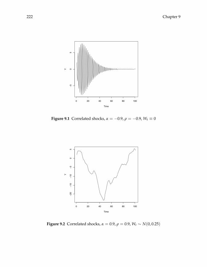
222 Chapter 9
0 20 40 60 80 100
−5
05
Time
Y
Figure 9.1 Correlated shocks, α = −0.9, ρ = −0.9, Wt ≡ 0
0 20 40 60 80 100
−20
−15
−10
−5
05
Time
Y
Figure 9.2 Correlated shocks, α = 0.9, ρ = 0.9, Wt ∼ N(0, 0.25)

Measure-Theoretic Probability 223
0 20 40 60 80 100
−1
01
23
Time
Y
Figure 9.3 Correlated shocks, α = 0.9, ρ = 0.0, Wt ∼ N(0, 0.25)
The process (9.11) is an SRS with a well-defined stochastic kernel. At the same time,the first element of Yt follows the process in (9.10).
9.2.2 The Fundamental Recursion, Again
On page 68 we showed that for a finite state Markov chain (Xt)t≥0 with Markov oper-ator M, the sequence of marginal distributions (ψt)t≥0 satisfies ψt+1 = ψtM. An anal-ogous recursion was obtained for the density case by defining the density Markovoperator ψM(y) =
∫p(x, y)ψ(x)dx. Since a measure kernel P generalizes the finite
and density kernels, perhaps we can identify the general rule.To begin, let S be a Borel subset of n, let P be a stochastic kernel on S, and let
(Xt)t≥0 be Markov-(P,ψ) for some ψ ∈P(S). Writing ψt ∈P(S) for the distributionof Xt, we claim that the sequence (ψt)t≥0 ⊂P(S) satisfies
ψt+1(B) =∫P(x, B)ψt(dx) (B ∈ B(S)) (9.12)
The intuition is the same as for the finite case: The probability that Xt+1 ∈ B is theprobability that Xt goes from x into B, summed across all x ∈ S, weighted by theprobability ψt(dx) that Xt takes the value x.
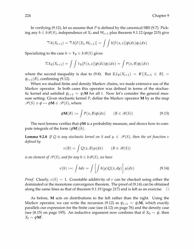
224 Chapter 9
In verifying (9.12), let us assume that P is defined by the canonical SRS (9.7). Pick-ing any h ∈ bB(S), independence of Xt and Wt+1 plus theorem 9.1.12 (page 215) give
h(Xt+1) = h[F(Xt,Wt+1)] =∫ ∫
h[F(x, z)]φ(dz)ψt(dx)
Specializing to the case h = B ∈ bB(S) gives
B(Xt+1) =∫ ∫
B[F(x, z)]φ(dz)ψt(dx) =∫P(x, B)ψt(dx)
where the second inequality is due to (9.8). But B(Xt+1) = {Xt+1 ∈ B} =ψt+1(B), confirming (9.12).
When we studied finite and density Markov chains, we made extensive use of theMarkov operator. In both cases this operator was defined in terms of the stochas-tic kernel and satisfied ψt+1 = ψtM for all t. Now let’s consider the general mea-sure setting: Given stochastic kernel P, define the Markov operator M by as the mapP(S) � φ �→ φM ∈P(S), where
φM(B) :=∫P(x, B)φ(dx) (B ∈ B(S)) (9.13)
The next lemma verifies that φM is a probability measure, and shows how to com-pute integrals of the form (φM)(h).
Lemma 9.2.8 If Q is any stochastic kernel on S and μ ∈ P(S), then the set function νdefined by
ν(B) =∫Q(x, B)μ(dx) (B ∈ B(S))
is an element ofP(S), and for any h ∈ bB(S), we have
ν(h) :=:∫hdν =
∫ [∫h(y)Q(x, dy)
]μ(dx) (9.14)
Proof. Clearly, ν(S) = 1. Countable additivity of ν can be checked using either thedominated or the monotone convergence theorem. The proof of (9.14) can be obtainedalong the same lines as that of theorem 9.1.19 (page 217) and is left as an exercise.
As before, M acts on distributions to the left rather than the right. Using theMarkov operator, we can write the recursion (9.12) as ψt+1 = ψtM, which exactlyparallels our expression for the finite case (see (4.12) on page 76) and the density case(see (8.15) on page 195). An inductive argument now confirms that if X0 ∼ ψ, thenXt ∼ ψMt.

Measure-Theoretic Probability 225
Example 9.2.9 In the case of the deterministic dynamical system Xt+1 = h(Xt), recallthat P(x, B) = B(h(x)). Now suppose that X0 = x (i.e., X0 ∼ δx). Our intuition tellsus that the distribution of X1 must then be δh(x), and indeed
δxM(B) =∫
B(h(x))δx(dx) = B(h(x)) = δh(x)(B)
∴ δxM = δh(x)
Iterating forward, we find that Xt ∼ δxMt = δht(x), as expected.
Given a kernel P, the higher order kernels (Pt)t≥1 are defined by
P1 := P, Pt(x, B) :=∫P(z, B)Pt−1(x, dz) (x ∈ S, B ∈ B(S))
These kernels are defined so that Pt(x, B) gives the probability of moving from x intoB in t steps, and Pt(x, dy) is the distribution of Xt given X0 = x. To see this, observethat the distribution of Xt given X0 = x is precisely δxMt, so we are claiming that
δxMt(B) = Pt(x, B) (x ∈ S, B ∈ B(S), t ∈ )
This claim is a special case of the more general statement
φMt(B) =∫Pt(x, B)φ(dx) (φ ∈P(S), B ∈ B(S), t ∈ )
which says that Mt, the t-th iterate of M, is the Markov operator corresponding to thet-th-order kernel Pt.10 For the proof we refer to theorem 9.2.15 below.
9.2.3 Expectations
As before, let bB(S) be all the bounded measurable functions on S. We now introducea second operator, also called the Markov operator and also denoted by M, whichsends h ∈ bB(S) into Mh ∈ bB(S), where
Mh(x) :=∫h(y)P(x, dy) (x ∈ S) (9.15)
Intuitively, Mh(x) represents the expectation of h(Xt+1) given Xt = x. This is thesame interpretation as the finite case, where we defined Mh(x) = ∑y∈S h(y)p(x, y).
We now have M acting on measures to the left and functions to the right. This isanalogous to the finite state notation, where ψM is the row vector ψ postmultiplied
10This (unsurprising) result is the measure analogue of the density case stated in lemma 8.1.13 (page 196).
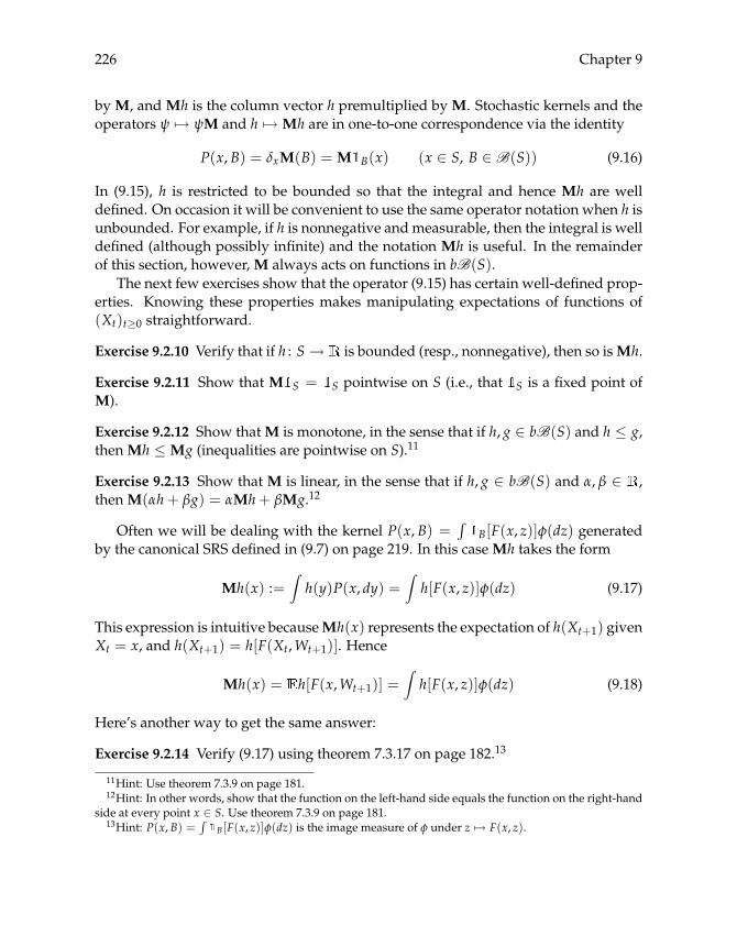
226 Chapter 9
by M, and Mh is the column vector h premultiplied by M. Stochastic kernels and theoperators ψ �→ ψM and h �→ Mh are in one-to-one correspondence via the identity
P(x, B) = δxM(B) = M B(x) (x ∈ S, B ∈ B(S)) (9.16)
In (9.15), h is restricted to be bounded so that the integral and hence Mh are welldefined. On occasion it will be convenient to use the same operator notation when h isunbounded. For example, if h is nonnegative and measurable, then the integral is welldefined (although possibly infinite) and the notation Mh is useful. In the remainderof this section, however, M always acts on functions in bB(S).
The next few exercises show that the operator (9.15) has certain well-defined prop-erties. Knowing these properties makes manipulating expectations of functions of(Xt)t≥0 straightforward.
Exercise 9.2.10 Verify that if h : S→ is bounded (resp., nonnegative), then so isMh.
Exercise 9.2.11 Show that M S = S pointwise on S (i.e., that S is a fixed point ofM).
Exercise 9.2.12 Show that M is monotone, in the sense that if h, g ∈ bB(S) and h ≤ g,then Mh ≤ Mg (inequalities are pointwise on S).11
Exercise 9.2.13 Show that M is linear, in the sense that if h, g ∈ bB(S) and α, β ∈ ,then M(αh+ βg) = αMh+ βMg.12
Often we will be dealing with the kernel P(x, B) =∫
B[F(x, z)]φ(dz) generatedby the canonical SRS defined in (9.7) on page 219. In this case Mh takes the form
Mh(x) :=∫h(y)P(x, dy) =
∫h[F(x, z)]φ(dz) (9.17)
This expression is intuitive becauseMh(x) represents the expectation of h(Xt+1) givenXt = x, and h(Xt+1) = h[F(Xt,Wt+1)]. Hence
Mh(x) = h[F(x,Wt+1)] =∫h[F(x, z)]φ(dz) (9.18)
Here’s another way to get the same answer:
Exercise 9.2.14 Verify (9.17) using theorem 7.3.17 on page 182.13
11Hint: Use theorem 7.3.9 on page 181.12Hint: In other words, show that the function on the left-hand side equals the function on the right-hand
side at every point x ∈ S. Use theorem 7.3.9 on page 181.13Hint: P(x, B) =
∫B[F(x, z)]φ(dz) is the image measure of φ under z �→ F(x, z).

Measure-Theoretic Probability 227
The t-th iterate Mth of h under M can be represented in terms of Pt:
Mth(x) =∫h(y)Pt(x, dy) (x ∈ S) (9.19)
We state a more general result immediately below (theorem 9.2.15). Before doing so,note that since Pt(x, dy) is the distribution of Xt given X0 = x, it follows from (9.19)that Mth can be interpreted as the conditional expectation
Mth(x) = [h(Xt) |X0 = x] (9.20)
Theorem 9.2.15 Let P be a stochastic kernel on S. IfM is the correspondingMarkov operator,then for every φ ∈P(S), h ∈ bB(S) and t ∈ , we have
(φMt)(h) = φ(Mth) =∫ [∫
h(y)Pt(x, dy)]φ(dx)
We are using the linear functional notation for the first two integrals. In traditionalnotation,
(φMt)(h) =∫h(y)(φMt)(dy) and φ(Mth) =
∫(Mth)(x)φ(dx)
Theorem 9.2.15 connects the iterates of φ �→ φM and those of h �→ Mh.14
Proof of theorem 9.2.15. Consider the case t = 1. We have
φ(Mh) =∫Mh(x)φ(dx) =
∫ [∫h(y)P(x, dy)
]φ(dx) = φM(h)
where the final equality is due to (9.14). It is an exercise for the reader to extend thisto general t using induction.
9.3 Commentary
The first monograph to exposit the measure-theoretic foundations of probability isKolmogorov (1956)—originally published in 1933—which provides excellent histori-cal perspective, and is still well worth reading. For general references on measure-theoretic probability, see Williams (1991), Breiman (1992), Shiryaev (1996), Durrett(1996), Taylor (1997), Pollard (2002), Dudley (2002), and Schilling (2005).
For further background on general state Markov chains see Breiman (1992, ch. 7),Meyn and Tweedie (1993, ch. 3), Durrett (1996, ch. 5), and Taylor (1997, ch. 3). Fora reference with economic applications see Stokey and Lucas (1989, ch. 8). Stabilityof general state Markov chains is discussed in chapter 11, and the commentary at theend of the chapter contains more pointers to the literature.
14There is an obvious parallel with the finite case. See (4.16) on page 79.


Chapter 10
Stochastic DynamicProgramming
In this chapter we continue our study of intertemporal decision problems begun in§5.1 and §6.2, working our way through a rigorous treatment of stochastic dynamicprogramming. Intertemporal problems are challenging because they involve opti-mization in high dimensions; in fact the objective function is often defined over aspace of infinite dimension.1 We will see that studying the theory behind dynamicprogramming is valuable not only for the understanding it provides, but also for de-veloping numerical solution methods. Value iteration and policy iteration are themost common techniques, and convergence of the algorithms is covered in some de-tail.
10.1 Theory
Our first step is to give a careful definition of the problem. Once the definition is inplace we will go on to state and prove the basic principle of optimality for (infinitehorizon, stationary) stochastic dynamic programs.
10.1.1 Statement of the Problem
For an infinite horizon stochastic dynamic program (SDP), the scenario is one whereactions taken by an agent affect the future path of a state variable. Actions are spec-
1We have not defined infinite-dimensional space, which is an algebraic concept, but spaces of sequencesand spaces of functions typically have this property.
229
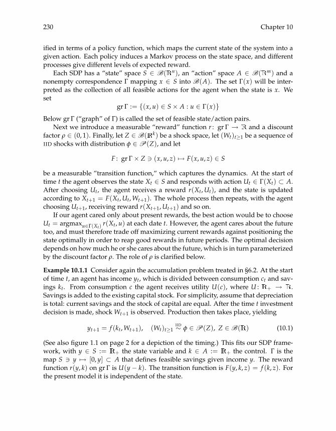
230 Chapter 10
ified in terms of a policy function, which maps the current state of the system into agiven action. Each policy induces a Markov process on the state space, and differentprocesses give different levels of expected reward.
Each SDP has a “state” space S ∈ B( n), an “action” space A ∈ B( m) and anonempty correspondence Γ mapping x ∈ S into B(A). The set Γ(x) will be inter-preted as the collection of all feasible actions for the agent when the state is x. Weset
gr Γ := {(x, u) ∈ S× A : u ∈ Γ(x)}Below gr Γ (“graph” of Γ) is called the set of feasible state/action pairs.
Next we introduce a measurable “reward” function r : gr Γ → and a discountfactor ρ ∈ (0, 1). Finally, let Z ∈ B( k) be a shock space, let (Wt)t≥1 be a sequence ofIID shocks with distribution φ ∈P(Z), and let
F : gr Γ× Z � (x, u, z) �→ F(x, u, z) ∈ S
be a measurable “transition function,“ which captures the dynamics. At the start oftime t the agent observes the state Xt ∈ S and responds with action Ut ∈ Γ(Xt) ⊂ A.After choosing Ut, the agent receives a reward r(Xt,Ut), and the state is updatedaccording to Xt+1 = F(Xt,Ut,Wt+1). The whole process then repeats, with the agentchoosing Ut+1, receiving reward r(Xt+1,Ut+1) and so on.
If our agent cared only about present rewards, the best action would be to chooseUt = argmaxu∈Γ(Xt) r(Xt, u) at each date t. However, the agent cares about the futuretoo, and must therefore trade off maximizing current rewards against positioning thestate optimally in order to reap good rewards in future periods. The optimal decisiondepends on how much he or she cares about the future, which is in turn parameterizedby the discount factor ρ. The role of ρ is clarified below.
Example 10.1.1 Consider again the accumulation problem treated in §6.2. At the startof time t, an agent has income yt, which is divided between consumption ct and sav-ings kt. From consumption c the agent receives utility U(c), where U : + → .Savings is added to the existing capital stock. For simplicity, assume that depreciationis total: current savings and the stock of capital are equal. After the time t investmentdecision is made, shock Wt+1 is observed. Production then takes place, yielding
yt+1 = f (kt,Wt+1), (Wt)t≥1IID∼ φ ∈P(Z), Z ∈ B( ) (10.1)
(See also figure 1.1 on page 2 for a depiction of the timing.) This fits our SDP frame-work, with y ∈ S := + the state variable and k ∈ A := + the control. Γ is themap S � y �→ [0, y] ⊂ A that defines feasible savings given income y. The rewardfunction r(y, k) on gr Γ is U(y− k). The transition function is F(y, k, z) = f (k, z). Forthe present model it is independent of the state.
Stochastic Dynamic Programming 231
Clearly, some states in S are more attractive than others. High income positions uswell in terms of future consumption. Hence a trade off exists between consuming now,which gives current reward, and saving, which places us at a more attractive point inthe state space tomorrow. Such trade-offs are the essence of dynamic programming.
Example 10.1.2 Now consider the same model but with correlated shocks. That is,yt+1 = f (kt, ηt+1), where ηt+1 = g(ηt,Wt+1), g : + × + → +. This also fitsthe SDP framework, with the only modification being that the state space has twoelements (y, η) ∈ S := + × +, and the transition function F is
F : (y, η, k, z) �→(
f (k, g(η, z))g(η, z)
)
The feasible correspondence Γ is the map sending (y, η) into [0, y].
Returning to the general case, at minimum we need some regularity assumptionson the primitives that will ensure that at least one solution to the SDP exists:
Assumption 10.1.3 The map r : gr Γ→ is continuous and bounded.
Assumption 10.1.4 Γ : S→ B(A) is continuous and compact valued.2
Assumption 10.1.5 gr Γ � (x, u) �→ F(x, u, z) ∈ S is continuous, ∀z ∈ Z.
These continuity and compactness assumptions are all about guaranteeing exis-tence of maximizers. For us the important implication of assumption 10.1.5 is that forany w ∈ bcS, the function
gr Γ � (x, u) �→∫w[F(x, u, z)]φ(dz) ∈
is continuous. To see this, take any (xn, un) ⊂ gr Γ converging to some arbitrary(x, u) ∈ gr Γ, and any w ∈ bcS. We need to show that∫
w[F(xn, un, z)]φ(dz)→∫w[F(x, u, z)]φ(dz) (n→ ∞)
You can verify this using the dominated convergence theorem (page 182).
10.1.2 Optimality
In order to construct a sensible optimization problem, we will restrict the agent topolicies in the set of stationary Markov policies.3 For such a policy, the agent makes ex-actly the same decision after observing Xt = x as after observing Xt′ = x at some later
2For the definition of continuity for correspondences and a simple sufficient condition see page 339.3In fact it can be shown that every reasonable optimal policy is of this type.

232 Chapter 10
date t′. This is intuitive because when looking toward the infinite future, the agentfaces exactly the same trade-off (i.e., maximizing current rewards versus positioningthe state attractively next period), independent of whether the time is t or t′.
Under a stationary Markov policy, the agent’s behavior is described by a Borelmeasurable function σ mapping each possible x ∈ S into a feasible action u ∈ Γ(x).The interpretation is that if the current state is x ∈ S, then the agent responds withaction σ(x) ∈ Γ(x). We let Σ denote the set of all Borel measurable σ : S → A withσ(x) ∈ Γ(x) for all x ∈ S. In what follows we refer to Σ simply as the set of feasiblepolicies.
For each σ ∈ Σ, we obtain a stochastic recursive sequence
Xt+1 = F(Xt, σ(Xt),Wt+1), (Wt)t≥1IID∼ φ (10.2)
for the state (Xt)t≥0, and hence a stochastic kernel Pσ(x, dy) on S given by
Pσ(x, B) :=∫
B[F(x, σ(x), z)]φ(dz) (x ∈ S, B ∈ B(S))
We denote by Mσ the corresponding Markov operator. It is also convenient to definethe function
rσ : S � x �→ r(x, σ(x)) ∈so that rσ(x) is the reward at x when the agent follows policy σ. Using operatornotation, expected rewards next period under policy σ can be expressed as
Mσrσ(x) =∫rσ(y)Pσ(x, dy) =
∫rσ[F(x, σ(x), z)]φ(dz) (x ∈ S)
where the last equality follows from (9.17) on page 226.The shocks (Wt)t≥1 are defined on a fixed probability space (Ω,F , ). Eachω ∈ Ω
picks out a sequence (Wt(ω))t≥1. Combining this sequence with an initial conditionX0 = x ∈ S and a policy σ yields a path (Xt(ω))t≥0 for the state:
Xt+1(ω) = F(Xt(ω), σ(Xt(ω)),Wt+1(ω)), X0(ω) = x
The reward corresponding to this path is random variable Yσ : Ω→ ,
Yσ(ω) :=∞
∑t=0
ρtrσ(Xt(ω)) (ω ∈ Ω)
Exercise 10.1.6 Using boundedness of r, prove that this random variable is well de-fined, in the sense that the sum converges for each ω ∈ Ω.4
4Hint: if (xn) is any sequence in and ∑n |xn| converges, then so does ∑n xn.
Stochastic Dynamic Programming 233
The optimization problem for the agent is maxσ∈Σ Yσ. More precisely, if we set
vσ(x) := Yσ :=:
[∞
∑t=0
ρtrσ(Xt)
]:=:
∫ [∞
∑t=0
ρtrσ(Xt(ω))
](dω)
and define the value function v∗ : S→ as
v∗(x) = supσ∈Σ
vσ(x) (x ∈ S) (10.3)
then a policy σ∗ ∈ Σ is called optimal if it attains the supremum in (10.3) for everyx ∈ S. In other words, σ∗ ∈ Σ is optimal if and only if vσ∗ = v∗.
Exercise 10.1.7 Using the dominated convergence theorem, show that we can ex-change limit and integral to obtain
vσ(x) :=
[∞
∑t=0
ρtrσ(Xt)
]=
∞
∑t=0
ρt rσ(Xt)
Now if h ∈ bB(S), then we can express h(Xt) as Mtσh(x), where Mt
σ is the t-thiterate of the Markov operator Mσ and X0 = x (see (9.20) on page 227). As a result vσcan be written as
vσ(x) =∞
∑t=0
ρtMtσrσ(x) (x ∈ S) (10.4)
As an aside, note that by theorem 9.2.15 (page 227), we have
Mtσrσ(x) = (δxMt
σ)(rσ) =∫rσ(y)Ptσ(x, dy) (x ∈ S) (10.5)
Thus each policy σ ∈ Σ creates a Markov chain (Xt)t≥0 starting at x, with correspond-ing marginal distributions (δxMt
σ)t≥0. By integrating each distribution with rσ, thereward corresponding to σ, and computing the discounted sum, we obtain a value forthe policy. This is our objective function, to be maximized over σ ∈ Σ.
Exercise 10.1.8 Show that the sup in (10.3) is well-defined for each x ∈ S.
Definition 10.1.9 Given w ∈ bB(S), we define σ ∈ Σ to be w-greedy if
σ(x) ∈ argmaxu∈Γ(x)
{r(x, u) + ρ
∫w[F(x, u, z)]φ(dz)
}(x ∈ S) (10.6)
Lemma 10.1.10 Let assumptions 10.1.3–10.1.5 hold. If w ∈ bcS, then Σ contains at leastone w-greedy policy.
234 Chapter 10
The proof of this lemma is harder than it looks: On one hand, Since w ∈ bcS,assumption 10.1.5 implies that the objective function on the right-hand side of (10.6)is continuous with respect to u for each x. Since the constraint set Γ(x) is compact, asolution to the maximization problem exists. Thus for every x we can find at least oneu∗x that attains the maximum, and the map x �→ u∗x certainly defines a function σ fromS→ A satisfying (10.6). On the other hand, for this “policy” to be in Σ it must be Borelmeasurable. Measurability is not immediately clear.
Fortunately there are “measurable selection” theorems stating that under the cur-rent assumptions we can find at least one such x �→ u∗x that is measurable. We omitthe details, referring interested readers to Aliprantis and Border (1999, §17.3).5
We are now ready to state our main result on dynamic programming:
Theorem 10.1.11 Under assumptions 10.1.3–10.1.5, the value function v∗ is the uniquefunction in bB(S) that satisfies
v∗(x) = supu∈Γ(x)
{r(x, u) + ρ
∫v∗[F(x, u, z)]φ(dz)
}(x ∈ S) (10.7)
Moreover v∗ ∈ bcS. A feasible policy is optimal if and only if it is v∗-greedy. At least one suchpolicy exists.
Before turning to the proof let’s make some brief comments and discuss an easyapplication. As a preliminary observation, note that in view of (10.7), a policy σ ∈ Σis v∗-greedy if and only if
v∗(x) = r(x, σ(x)) + ρ∫v∗[F(x, σ(x), z)]φ(dz) (x ∈ S) (10.8)
In operator notation, this translates to v∗ = rσ + ρMσv∗.Next let’s discuss how theorem 10.1.11 can be applied. One use is as a sufficient
condition: We will see below that v∗ can be computed using value iteration. Withv∗ in hand, one can then compute a v∗-greedy policy. Assuming Borel measurability,we have found an optimal policy. The second way that we can use the theorem is as anecessary condition for optimality. For example, suppose that we want to know aboutthe properties of optimal policies. We know that if σ∗ is optimal, then it satisfies (10.8).We can (and do) use this to deduce facts about σ∗.
As an application of theorem 10.1.11, consider again the optimal growth examplediscussed on page 230. Recall that the state variable is income y ∈ S := +, thecontrol is savings k ∈ A := +, the feasible correspondence is Γ(y) = [0, y], thereward function is r(y, k) = U(y− k), and the transition function is F(y, k, z) = f (k, z).
5In many of the applications considered here, solutions of the form x �→ u∗x described above are easilyseen to be measurable (being either continuous or monotone).
Stochastic Dynamic Programming 235
The shocks (Wt)t≥1 are independent and take values in Z ⊂ according to φ ∈P(Z).
Assumption 10.1.12 The map U : + → + is bounded and continuous. The func-tion f is measurable and maps + × Z into +. For each fixed z ∈ Z, the mapk �→ f (k, z) is continuous.
A feasible savings policy σ ∈ Σ is a Borel function from S to itself such that σ(y) ∈[0, y] for all y. Every σ ∈ Σ defines a process for income via
yt+1 = f (σ(yt),Wt+1) (10.9)
The corresponding stochastic kernel Pσ on S is given by
Pσ(y, B) =∫
B[ f (σ(y), z)]φ(dz) (y ∈ S, B ∈ B(S))
Proposition 10.1.13 Under assumption 10.1.12, the value function v∗ is continuous, and isthe unique function in bB(S) that satisfies
v∗(y) = max0≤k≤y
{U(y− k) + ρ
∫v∗[ f (k, z)]φ(dz)
}(y ∈ S)
At least one optimal policy exists. Moreover a policy σ∗ is optimal if and only if it satisfies
v∗(y) = U(y− σ∗(y)) + ρ∫v∗[ f (σ∗(y), z)]φ(dz) (y ∈ S)
Exercise 10.1.14 Verify proposition 10.1.13 using assumption 10.1.12. In particular,show that assumptions 10.1.3–10.1.5 on page 231 all hold.
10.1.3 Proofs
Let’s turn to the proof of theorem 10.1.11. As a preliminary step, we introduce twoimportant operators and investigate their properties. Many proofs in dynamic pro-gramming can be reduced to simple manipulations using these maps.
Definition 10.1.15 The operator Tσ : bB(S)→ bB(S) is defined for all σ ∈ Σ by
Tσw(x) = r(x, σ(x)) + ρ∫w[F(x, σ(x), z)]φ(dz) (x ∈ S)
Further, the Bellman operator T : bB(S)→ bB(S) is defined by
Tw(x) = supu∈Γ(x)
{r(x, u) + ρ
∫w[F(x, u, z)]φ(dz)
}(x ∈ S)

236 Chapter 10
Using the Bellman operator we can restate the first part of theorem 10.1.11 as: v∗is the unique fixed point of T in bB(S).
Exercise 10.1.16 Show that both Tσ and T do in fact send bB(S) into itself. (Onlyadvanced students need worry about measurability. Just show that the images ofbounded functions are bounded.) If you need a hint on how to tackle T, refer tolemma A.2.31 on page 334.
Recalling the definition vσ := ∑∞t=0 ρtMt
σrσ, our first result is as follows:
Lemma 10.1.17 For every σ ∈ Σ, the operator Tσ is uniformly contracting on (bB(S), d∞),with
‖Tσw− Tσw′‖∞ ≤ ρ‖w− w′‖∞ ∀w,w′ ∈ bB(S) (10.10)
and the unique fixed point of Tσ in bB(S) is vσ. In addition Tσ is monotone on bB(S), in thesense that if w,w′ ∈ bB(S) and w ≤ w′, then Tσw ≤ Tσw′.
Here inequalities such as w ≤ w′ are pointwise inequalities on S.
Proof. The proof that Tσ is monotone is not difficult, and is left to the reader (youmight want to use monotonicity of Mσ, as in exercise 9.2.12, page 226). Regarding theclaim that Tσvσ = vσ, pointwise on S we have
vσ =∞
∑t=0
ρtMtσrσ = rσ +
∞
∑t=1
ρtMtσrσ = rσ + ρMσ
∞
∑t=0
ρtMtσrσ = rσ + ρMσvσ = Tσvσ
The only tricky part of this argument is passing Mσ through the limit in the infinitesum. Justifying this is a good exercise for the reader who wants to improve his or herfamiliarity with the dominated convergence theorem.
The proof that Tσ is uniformly contracting is easy. Pick any w,w′ ∈ bB(S). Makinguse of the linearity and monotonicity of Mσ, we have
|Tσw− Tσw′| = |ρMσw− ρMσw′| = ρ|Mσ(w− w′)|≤ ρMσ|w− w′| ≤ ρMσ‖w− w′‖∞ S = ρ‖w− w′‖∞
pointwise on S. The inequality (10.10) now follows.
Next we turn to the Bellman operator.
Lemma 10.1.18 The operator T is uniformly contracting on (bB(S), d∞), with
‖Tw− Tw′‖∞ ≤ ρ‖w− w′‖∞ ∀w,w′ ∈ bB(S) (10.11)
In addition T is monotone on bB(S), in the sense that if w,w′ ∈ bB(S) and w ≤ w′, thenTw ≤ Tw′.
Stochastic Dynamic Programming 237
Proof. The proof of the second claim (monotonicity) is easy and is left to the reader.Before starting the proof of (10.11), we make the following observation: If w,w′ ∈bB(S), then
| supw− supw′| ≤ sup |w− w′| =: ‖w− w′‖∞ (10.12)
To see this, pick any such w,w′. We have
supw = sup(w− w′ + w′) ≤ sup(w− w′) + supw′ ≤ sup |w− w′|+ supw′
∴ supw− supw′ ≤ sup |w− w′|The same argument reversing the roles of w and w′ finishes the job.
Now consider (10.11). For any w,w′ ∈ bB(S) and any x ∈ S, the deviation|Tw(x)− Tw′(x)| is equal to∣∣∣∣sup
u
{r(x, u) + ρ
∫w[F(x, u, z)]φ(dz)
}− sup
u
{r(x, u) + ρ
∫w′[F(x, u, z)]φ(dz)
}∣∣∣∣Using (10.12), we obtain
|Tw(x)− Tw′(x)| ≤ ρ supu
∣∣∣∣∫{w[F(x, u, z)]− w′[F(x, u, z)]}φ(dz)
∣∣∣∣≤ ρ sup
u
∫|w[F(x, u, z)]− w′[F(x, u, z)]|φ(dz)
≤ ρ supu
∫‖w− w′‖∞φ(dz) = ρ‖w− w′‖∞
Taking the supremum over x ∈ S gives the desired inequality.6
Exercise 10.1.19 Give an alternative proof that T is a uniform contraction of modulusρ by applying theorem 6.3.8 (page 149).
Now we turn to the first claim in theorem 10.1.11. In operator notation, this trans-lates to the following assertion:
Lemma 10.1.20 The value function v∗ is the unique fixed point of T in bB(S). Moreoverv∗ ∈ bcS.
Proof. Since T is uniformly contracting on the complete space (bB(S), d∞), it followsfrom Banach’s fixed point theorem (theorem 3.2.36) that T has one and only one fixedpoint w∗ in bB(S).7 It remains to show that w∗ ∈ bcS and w∗ = v∗.
6This proof is due to Hernández-Lerma and Lasserre (1996, lmm. 2.5).7Why is (bB(S), d∞) complete? Since (bS, d∞) is complete (theorem 3.2.6) and closed subsets of complete
spaces are complete (theorem 3.2.3), one need only show that bB(S) is a closed subset of (bS, d∞). This canbe proved via theorem 7.2.12 on page 176.

238 Chapter 10
To show that w∗ ∈ bcS, it is sufficient to prove that bcS is a closed subset of bB(S),and that T maps bcS into itself (see exercise 4.1.20 on page 61). That bcS is a closed sub-set of bB(S) was proved in theorem 3.2.7 (page 46). That T sends bcS into bcS followsfrom Berge’s theorem. (Given w ∈ bcS, Tw is continuous by assumptions 10.1.3–10.1.5and Berge’s theorem (page 340). Boundedness is clear.) Hence w∗ ∈ bcS as claimed.
Next we show that w∗ = v∗. To begin, note that by lemma 10.1.10 there exists apolicy σ ∈ Σ satisfying Tw∗ = Tσw∗. (Why?) For this policy σ we have w∗ = Tw∗ =Tσw∗. But vσ is the only fixed point of Tσ, so w∗ = vσ. In which case w∗ ≤ v∗, sincevσ ≤ v∗ for any σ ∈ Σ. It remains only to check that w∗ ≥ v∗ also holds.
To do this, pick an arbitrary σ ∈ Σ, and note that w∗ = Tw∗ ≥ Tσw∗. Iterating onthis inequality and using the monotonicity of Tσ, we obtain w∗ ≥ Tkσw∗ for all k ∈ .Taking limits and using the fact that Tkσw∗ → vσ uniformly and hence pointwise, wehave w∗ ≥ vσ. Since σ is arbitrary it follows that w∗ ≥ v∗. (Why?) Therefore w∗ = v∗as claimed.
Our next task is to verify the claim that policies are optimal if and only if they arev∗-greedy.
Lemma 10.1.21 A policy σ ∈ Σ is optimal if and only if it is v∗-greedy.
Proof. Recall that σ is v∗-greedy if and only if it satisfies (10.8), which in operatornotation becomes v∗ = Tσv∗. This is equivalent to the statement vσ = v∗, since vσ isthe unique fixed point of Tσ. But vσ = v∗ says precisely that σ is optimal.
The last claim in theorem 10.1.11 is that at least one optimal policy exists. This nowfollows from lemma 10.1.10.
10.2 Numerical Methods
Numerical solution of dynamic programming problems is challenging and, at thesame time, of great practical significance. In earlier chapters we considered tech-niques for solving SDPs numerically, such as value iteration and policy iteration. Inthis section we look more deeply at the theory behind these iterative methods. Thealgorithms are shown to converge globally to optimal solutions.
10.2.1 Value Iteration
Consider the SDP defined in §10.1. The fact that the Bellman operator is a uniformcontraction on bcS for which v∗ is the fixed point gives us a natural way to approx-imate v∗: Pick any v0 ∈ bcS and iterate the Bellman operator until Tnv0 is close to
Stochastic Dynamic Programming 239
Algorithm 10.1 Value iteration algorithm
read in initial v0 ∈ bcS and set n = 0repeat
set n = n+ 1set vn = Tvn−1, where T is the Bellman operator
until a stopping rule is satisfiedsolve for a vn-greedy policy σ (cf., definition 10.1.9)return σ
v∗. This suggests the algorithm for computing (approximately) optimal policies pre-sented in algorithm 10.1.
Algorithm 10.1 is essentially the same as the earlier value iteration algorithms pre-sented on page 103, although we have added the index n in order to keep track ofthe iterates. Since vn = Tnv0 converges to v∗, after sufficiently many iterations theresulting policy σ should have relatively good properties, in the sense that vσ � v∗.8
Two obvious questions arise: First, what stopping rule should be used in the loop?We know that vn → v∗, but v∗ is not observable. How can we measure the distancebetween v∗ and vn for given n? Second, for given vn, how close to being optimal is thevn-greedy policy σ that the algorithm produces? These questions are answered in thenext theorem.
Theorem 10.2.1 Let v0 ∈ bcS. Fix n ∈ , and let vn := Tnv0, where T is the Bellmanoperator. If σ ∈ Σ is vn-greedy, then
‖v∗ − vσ‖∞ ≤ 2ρ1− ρ
‖vn − vn−1‖∞ (10.13)
The next corollary follows directly (the proof is an exercise).
Corollary 10.2.2 Let (vn)n≥0 be as in theorem 10.2.1. If (σn)n≥0 is a sequence in Σ suchthat σn is vn-greedy for each n ≥ 0, then ‖v∗ − vσn‖∞ → 0 as n→ ∞.
The proof of theorem 10.2.1 is given at the end of this section. Before turning to it,let us make some comments on the theorem.
First, theorem 10.2.1 bounds the deviation between the vn-greedy policy σ and theoptimal policy σ∗ in terms of their value. The value of σ∗ is given by vσ∗ , which bydefinition is equal to v∗. As a result we can say that given any initial condition x,
vσ∗(x)− vσ(x) = |vσ∗(x)− vσ(x)| ≤ ‖v∗ − vσ‖∞ ≤ 2ρ1− ρ
‖vn − vn−1‖∞8Of course if vn is exactly equal to v∗, then σ is optimal, and vσ = v∗.
240 Chapter 10
Of course one can also seek to bound some kind of geometric deviation between σand σ∗, but in applications this is usually less important than bounding the differencebetween their values.
Second, the usefulness of this theorem comes from the fact that ‖vn − vn−1‖∞ isobservable. In particular, it can be measured at each iteration of the algorithm. Thisprovides a natural stopping rule: Iterate until ‖vn− vn−1‖∞ is less than some toleranceε, and then compute a vn-greedy policy σ. The policy satisfies ‖v∗ − vσ‖∞ ≤ 2ρε/(1−ρ).
Third, the bound (10.13) is often quite conservative. From this perspective, the-orem 10.2.1 might best be viewed as a guarantee that the output of the algorithmconverges to the true solution—such a guarantee is indispensable for numerical algo-rithms in scientific work.
Finally, on a related point, if you wish to supply bounds for a particular solutionyou have computed, then relative optimality bounds are easier to interpret. A relativebound establishes that an approximate optimal policy earns at least some fraction(say, 95%) of maximum value. Here is an example: Suppose that the reward functionis nonnegative, so vσ and v∗ are nonnegative on S.9 Suppose further that we choosev0 to satisfy 0 ≤ v0 ≤ v∗, in which case 0 ≤ vn ≤ v∗ for all n ∈ by monotonicity ofT. By (10.13) and the fact that vn ≤ v∗, we have
‖vn − vn−1‖∞ ≤ η =⇒ v∗(x)− vσ(x)v∗(x) ≤ 2ρ
1− ρ· η
vn(x)=: αn(η, x) (10.14)
In other words, if one terminates the value iteration at ‖vn − vn−1‖∞ ≤ η, then theresulting policy σ obtains at least (1 − αn(η, x)) × 100% of the total value availablewhen the initial condition is x.
Let’s finish with the proof of theorem 10.2.1:
Proof of theorem 10.2.1. Note that
‖v∗ − vσ‖∞ ≤ ‖v∗ − vn‖∞ + ‖vn − vσ‖∞ (10.15)
First let’s bound the first term on the right-hand side of (10.15). Using the fact that v∗is a fixed point of T, we get
‖v∗ − vn‖∞ ≤ ‖v∗ − Tvn‖∞ + ‖Tvn − vn‖∞ ≤ ρ‖v∗ − vn‖∞ + ρ‖vn − vn−1‖∞
∴ ‖v∗ − vn‖∞ ≤ ρ
1− ρ‖vn − vn−1‖∞ (10.16)
9Since r is already assumed to be bounded, there is no loss of generality in taking r as nonnegative, inthe sense that adding a constant to r produces a monotone transformation of the objective function vσ(x),and hence does not alter the optimization problem.
Stochastic Dynamic Programming 241
Now consider the second term on the right-hand side of (10.15). Since σ is vn-greedy,we have Tvn = Tσvn, and
‖vn − vσ‖∞ ≤ ‖vn − Tvn‖∞ + ‖Tvn − vσ‖∞ ≤ ‖Tvn−1 − Tvn‖∞ + ‖Tσvn − Tσvσ‖∞∴ ‖vn − vσ‖∞ ≤ ρ‖vn−1 − vn‖∞ + ρ‖vn − vσ‖∞
∴ ‖vn − vσ‖∞ ≤ ρ
1− ρ‖vn − vn−1‖∞ (10.17)
Together, (10.15), (10.16), and (10.17) give us (10.13).
10.2.2 Policy Iteration
Aside from value function iteration, there is another iterative procedure called policyiteration, which we first met in §5.1.3. In this section we describe policy iteration, andsome of its convergence properties. The basic algorithm is presented in algorithm 10.2.
Algorithm 10.2 Policy iteration algorithm
read in an initial policy σ0 ∈ Σset n = 0repeat
evaluate vσn := ∑∞t=0 ρtMt
σn rσncompute a vσn -greedy policy σn+1 ∈ Σset n = n+ 1
until a stopping rule is satisfiedreturn σn
It turns out that the sequence of functions vσn produced by algorithm 10.2 con-verges to v∗, and, with a sensible stopping rule, the resulting policy is approximatelyoptimal. Let’s clarify these ideas, starting with the following observation:
Lemma 10.2.3 If (σn)n≥0 is a sequence in Σ generated by the policy iteration algorithm, thenvσn ≤ vσn+1 holds pointwise on S for all n.
Proof. Pick any x ∈ S and n ∈ . By definition,
σn+1(x) ∈ argmaxu∈Γ(x)
{r(x, u) + ρ
∫vσn [F(x, u, z)]φ(dz)
}
From this and the fact that vσ = Tσvσ for all σ ∈ Σ, we have
vσn(x) = r(x, σn(x)) + ρ∫vσn [F(x, σn(x), z)]φ(dz)
≤ r(x, σn+1(x)) + ρ∫vσn [F(x, σn+1(x), z)]φ(dz)
242 Chapter 10
Rewriting in operator notation, this inequality becomes vσn ≤ Tσn+1vσn . Since Tσn+1
is monotone (lemma 10.1.17), iteration with Tσn+1 yields vσn ≤ Tkσn+1vσn for all k ∈ .
Taking limits, and using the fact that Tkσn+1vσn → vσn+1 uniformly and hence pointwise
on S, we obtain the conclusion of the lemma.
It turns out that just as the value iteration algorithm is globally convergent, so toois the policy iteration algorithm.
Theorem 10.2.4 If (σn)n≥0 ⊂ Σ is a sequence generated by the policy iteration algorithm,then ‖vσn − v∗‖∞ → 0 as n→ ∞.
Proof. Let wn := Tnvσ0 , where T is the Bellman operator, and, as usual, T0 is theidentity map. Since vσn ≤ v∗ for all n ≥ 0 (why?), it is sufficient to prove that wn ≤ vσnfor all n ≥ 0. (Why?) The claim is true for n = 0 by definition. Suppose that it is truefor arbitrary n. Then it is true for n+ 1, since
wn+1 = Twn ≤ Tvσn = Tσn+1vσn ≤ Tσn+1vσn+1 = vσn+1
You should not have too much trouble verifying these statements.
The rest of this section focuses mainly on policy iteration in the finite case, whichwe treated previously in §5.1.3. It is proved that when S and A are finite, the exactoptimal policy is obtained in finite time.
Lemma 10.2.3 tells us that the value of the sequence (σn) is nondecreasing. In fact,if σn+1 cannot be chosen as equal to σn, then the value increase is strict. On the otherhand, if σn+1 can be chosen as equal to σn, then we have found an optimal policy. Thenext lemma makes these statements precise.
Lemma 10.2.5 Let (σn) be a sequence of policies generated by the policy iteration algorithm.If σn+1 cannot be chosen as equal to σn, in the sense that there exists an x ∈ S such that
σn(x) /∈ argmaxu∈Γ(x)
{r(x, u) + ρ
∫vσn [F(x, u, z)]φ(dz)
}
then vσn+1(x) > vσn(x). Conversely, if σn+1 can be chosen as equal to σn, in the sense that
σn(x) ∈ argmaxu∈Γ(x)
{r(x, u) + ρ
∫vσn [F(x, u, z)]φ(dz)
}∀ x ∈ S
then vσn = v∗ and σn is an optimal policy.

Stochastic Dynamic Programming 243
Proof. Regarding the first assertion, let x be a point in S with
r(x, σn+1(x)) + ρ∫vσn [F(x, σn+1(x), z)]φ(dz)
> r(x, σn(x)) + ρ∫vσn [F(x, σn(x), z)]φ(dz)
Writing this in operator notation, we have Tσn+1vσn(x) > Tσnvσn(x) = vσn(x). Butlemma 10.2.3 and the monotonicity of Tσn+1 now yield
vσn+1(x) = Tσn+1vσn+1(x) ≥ Tσn+1vσn(x) > vσn(x)
Regarding the second assertion, suppose that
σn(x) ∈ argmaxu∈Γ(x)
{r(x, u) + ρ
∫vσn [F(x, u, z)]φ(dz)
}∀ x ∈ S
It follows that
vσn(x) = r(x, σn(x)) + ρ∫vσn [F(x, σn(x), z)]φ(dz)
= maxu∈Γ(x)
{r(x, u) + ρ
∫vσn [F(x, u, z)]φ(dz)
}
for every x ∈ S. In other words, vσn is the fixed point of the Bellman operator. Inwhich case vσn = v∗, and the proof is done.
Algorithm 10.3 Policy iteration, finite case
read in initial σ0 ∈ Σset n = 0repeat
set n = n+ 1evaluate vσn−1 = ∑∞t=0 ρ
tMtσn−1
rσn−1
taking σn = σn−1 if possible, compute a vσn−1 -greedy policy σnuntil σn = σn−1return σn
Algorithm 10.3 adds a stopping rule to algorithm 10.2, which is suitable for thefinite case. The algorithm works well in the finite state/action case because it alwaysterminates in finite time at an optimal policy. This is the content of our next theorem.

244 Chapter 10
Theorem 10.2.6 If S and A are finite, then the policy iteration algorithm always terminatesafter a finite number of iterations, and the resulting policy is optimal.
Proof. First note that if the algorithm terminates at n with σn+1 = σn, then this pol-icy is optimal by the second part of lemma 10.2.5. Next suppose that the algorithmnever terminates, generating an infinite sequence of policies (σn). At each stage n thestopping rule implies that σn+1 cannot be chosen as equal to σn, and the first part oflemma 10.2.5 applies. Thus vσn < vσn+1 for all n (i.e., vσn ≤ vσn+1 and vσn �= vσn+1 ).But the set of maps from S to A is clearly finite, and hence so is the set of functions{vσ : σ ∈ Σ}. As a result such an infinite sequence is impossible, and the algorithmalways terminates.
10.2.3 Fitted Value Iteration
In §6.2.2 we began our discussion of fitted value iteration and presented the mainalgorithm. Recall that to approximate the image Tv of a function v we evaluatedTv at finite set of grid points (xi)ki=1 and then used these samples to construct anapproximation to Tv. In doing so, we decomposed T into the two operators L and T:First T is applied to v at each of the grid points, and then an approximation operatorL sends the result into a function w = Tv = L(Tv). Thus T := L ◦ T :=: LT. We sawthat LT is uniformly contracting whenever L is nonexpansive with respect to d∞.
In general, we will consider a map L : bB(S) → F ⊂ bB(S) where, for eachv ∈ bB(S), the approximation Lv ∈ F is constructed based on a sample (v(xi))ki=1 ongrid points (xi)ki=1. In addition, L is chosen to be nonexpansive:
‖Lv− Lw‖∞ ≤ ‖v− w‖∞ ∀ v,w ∈ bB(S) (10.18)
Example 10.2.7 (Piecewise constant approximation) Let (Pi)ki=1 be a partition of S, inthat Pm ∩ Pn = ∅ when m �= n and S = ∪ki=1Pi. Each Pi contains a single grid point xi.For any v : S→ we define v �→ Mv by
Mv(x) =k
∑i=1
v(xi) Pi (x) (x ∈ S)
Exercise 10.2.8 Show that for any w, v ∈ bB(S) and any x ∈ S we have
|Mw(x)−Mv(x)| ≤ sup1≤i≤k
|w(xi)− v(xi)|
Using this result, show that the operator M is nonexpansive on (bB(S), d∞).
Stochastic Dynamic Programming 245
Example 10.2.9 (Continuous piecewise linear interpolation) Let’s focus on the one-dimensional case. Let S = [a, b], and let the grid points be increasing:
x1 < . . . < xk, x1 = a and xk = b
Let N be the operator that maps w : S → into its continuous piecewise affine inter-polant defined by the grid. That is to say, if x ∈ [xi, xi+1] then
Nw(x) = λw(xi) + (1− λ)w(xi+1) where λ :=xi+1 − xxi+1 − xi
Exercise 10.2.10 Show that for any w, v ∈ bB(S) and any x ∈ S we have
|Nw(x)− Nv(x)| ≤ sup1≤i≤k
|w(xi)− v(xi)|
Using this result, show that N is nonexpansive.
Algorithm 10.4 FVI algorithm
read in initial v0 ∈ bB(S) and set n = 0repeat
set n = n+ 1sample Tvn−1 at a finite set of grid pointscompute Tvn−1 = LTvn−1 from the samplesset vn = Tvn−1
until the deviation ‖vn − vn−1‖∞ falls below some tolerancesolve for a vn-greedy policy σ
Our algorithm for fitted value iteration is given in algorithm 10.4. It terminatesin finite time for any strictly positive tolerance, since T is a uniform contraction. Thepolicy it produces is approximately optimal, with the deviation given by the followingtheorem. (The proof is given in the appendix to this chapter.)
Theorem 10.2.11 Let v0 ∈ F and let vn := Tnv0, where T := LT and L : bB(S) → F isnonexpansive. If σ ∈ Σ is vn-greedy, then
‖v∗ − vσ‖∞ ≤ 2(1− ρ)2
× (ρ‖vn − vn−1‖∞ + ‖Lv∗ − v∗‖∞)
Most of the comments given after theorem 10.2.1 (page 239) apply to theorem10.2.11. In particular, the bound is conservative, but it shows that the value of σcan be made as close to that of σ∗ as desired, provided that L can be chosen so that

246 Chapter 10
‖Lv∗ − v∗‖∞ is arbitrarily small. In the case of continuous piecewise linear interpola-tion on S = [a, b] this is certainly possible.10
10.3 Commentary
A first-rate theoretical treatment of stochastic dynamic programming can be foundin the two monographs of Hernández-Lerma and Lasserre (1996, 1999). Also recom-mended are Bertsekas (1995) and Puterman (1994). From the economics literature see,for example, Stokey and Lucas (1989) or Le Van and Dana (2003). All these sourcescontain extensive references to further applications.
Additional discussion of fitted value iteration with nonexpansive approximatorscan be found in Gordon (1995) and Stachurski (2008). For alternative discussions ofvalue iteration, see, for example, Santos and Vigo-Aguiar (1998) or Grüne and Semm-ler (2004).
Value iteration and policy iteration are two of many algorithms proposed in theliterature. Other popular techniques include projection methods, Taylor series ap-proximation (e.g., linearization), and parameterized expectations. See, for example,Marcet (1988), Tauchen and Hussey (1991), Judd (1992), Den Haan and Marcet (1994),Rust (1996), Judd (1998), Christiano and Fisher (2000), McGrattan (2001), Uhlig (2001),Maliar and Maliar (2005), or Canova (2007). Marimon and Scott (2001) is a usefulsurvey, while Santos (1999) and Aruoba et al. (2006) provide numerical comparisons.
Dynamic programming has many interesting applications in economics that wewill have little chance to discuss. Two unfortunate omissions are industrial orga-nization (e.g., Green and Porter 1984, Hopenhayn 1992, Ericson and Pakes 1995, orPakes and McGuire 2001) and search theory (see McCall 1970 for an early contri-bution and Rogerson et al. 2005 for a recent survey). For some earlier classics themacroeconomics literature, try Lucas and Prescott (1971), Hall (1978), Lucas (1978),Kydland and Prescott (1982), Brock (1982), or Mehra and Prescott (1985). Dechert andO’Donnell (2006) provide a nice application of dynamic programming to environmen-tal economics.
10This is due to continuity of v∗, which always holds under our assumptions. When v∗ is continuous on[a, b] it is also uniformly continuous, which is to say that for any ε > 0 there is a δ > 0 such that |v∗(x)−v∗(y)| < ε whenever |x − y| < δ. From this property it is not too difficult to show that given any ε > 0,a sufficiently fine grid will yield a continuous piecewise affine interpolant Lv∗ such that ‖v∗ − Lv∗‖∞ < ε.See, for example, Bartle and Sherbet (1992).

Chapter 11
Stochastic Dynamics
It’s now time to give a treatment of stability for general Markov chains on uncountablyinfinite state spaces. Although the stability theory we used to study the finite case(chapter 4) and the density case (chapter 8) does not survive the transition withoutsome modification, the underlying ideas are similar, and connections are drawn atevery opportunity. Throughout this chapter we take S to be a Borel subset of n.
11.1 Notions of Convergence
Before considering the dynamics of general state Markov chains, we need to developnotions of convergence that apply to the measure (as opposed to finite probability ordensity) setting. Along the way we will cover some fundamental results in asymptoticprobability, including the weak and strong laws of large numbers for IID sequences.
11.1.1 Convergence of Sample Paths
Recall that an S-valued stochastic process is a tuple (Ω,F , , (Xt)t∈ ) where (Ω,F )is a measurable space, is a probability on (Ω,F ), is an index set such as or ,and (Xt)t∈ is a family of S-valued random variables on (Ω,F ). Various notions ofconvergence exist for stochastic processes. We begin with almost sure convergence.
Definition 11.1.1 Let (Ω,F , , (Xt)t≥1) be an S-valued stochastic process and let Xbe an S-valued random variable on (Ω,F , ). We say that (Xt)t≥1 converges almostsurely (alternatively, with probability one) to X if{
limt→∞Xt = X
}:=
{ω ∈ Ω : lim
t→∞Xt(ω) = X(ω)}
= 1
247
248 Chapter 11
In the language of §7.3.2, almost sure convergence is just convergence -almost ev-erywhere.
Almost sure convergence plays a vital role in probability theory, although you maywonder why we don’t just require that convergence occurs for every ω ∈ Ω, insteadof just those ω in a set of probability one. The reason is that convergence for everypath is too strict: In almost all random systems, aberrations can happen that causesuch convergence to fail. Neglecting probability zero events allows us to obtain muchmore powerful conclusions.
Exercise 11.1.2 Expectations are not always very informative measures of stochasticprocesses dynamics. For example, consider a stochastic process with probability space((0, 1),B(0, 1),λ) and random variables Xn := n2
(0,1/n). Show that Xn → 0 almostsurely, while Xn ↑ ∞.
Here is another important notion of convergence of random variables:
Definition 11.1.3 Let (Ω,F , , (Xt)t≥1) and X be as above. We say that (Xt)t≥1 con-verges in probability to X if, for all ε > 0,
limt→∞ {‖Xt − X‖ ≥ ε} := lim
t→∞ {ω ∈ Ω : ‖Xt(ω)− X(ω)‖ ≥ ε} = 0
Convergence in probability is weaker than almost sure convergence:
Lemma 11.1.4 If Xt → X almost surely, then Xt → X in probability.
Proof. Fix ε > 0. Since Xt → X almost surely, {‖Xt − X‖ ≥ ε} → 0 -almosteverywhere on Ω. (Why?) An application of the dominated convergence theorem(page 182) now gives the desired result.
The converse is not true. It is an optional (and nontrivial) exercise for you to con-struct a stochastic process that converges to some limit in probability, and yet fails toconverge to that same limit almost surely.
Exercise 11.1.5 The sets in definition 11.1.3 are measurable. Show, for example, that ifS = and ε > 0, then {|Xn − X| ≥ ε} ∈ F .
Let’s discuss some applications of almost sure convergence and convergence inprobability. Let (Xt)t≥1 be a real-valued stochastic process on (Ω,F , ) with commonexpectation m. Define Xn := n−1∑n
t=1 Xt. The (weak) law of large numbers (WLLN)states that under suitable assumptions the sample mean Xn converges in probabilityto m as n→ ∞. We begin with the case m = 0.

Stochastic Dynamics 249
Exercise 11.1.6 We will make use of the following identity, the proof of which is leftas an exercise (use induction):
for all (a1, . . . , an) ∈ n,
(n
∑i=1
ai
)2
= ∑1≤i,j≤n
aiaj =n
∑j=1
n
∑i=1
aiaj
Exercise 11.1.7 Suppose the real, zero-mean sequence (Xt)t≥1 satisfies
1. Cov(Xi,Xj) = 0 for all i �= j, and
2. Cov(Xi,Xi) = Var(Xi) = X2i ≤ M for all i ∈ .
Show that Var(Xn) ≤ M/n for all n ∈ . (Regarding the first property, we usuallysay that the sequence is pairwise uncorrelated.)
Exercise 11.1.8 Now prove that the WLLN holds for this sequence. As a first step,show that {|Xn| ≥ ε} ≤ M/(nε2).1 Conclude that Xn converges to zero in proba-bility as n→ ∞.
This result can be extended to the case m �= 0 by considering the zero-mean se-quence Yt := Xt −m. This gives us
Theorem 11.1.9 Let (Ω,F , , (Xt)t≥1) be a real-valued stochastic process with commonmean m. If (Xt)t≥1 is pairwise uncorrelated and Var(Xt) ≤ M for all t, then Xn → m inprobability. In particular,
{|Xn −m| ≥ ε} ≤ Mnε2 (ε > 0, n ∈ ) (11.1)
When the sequence is independent a stronger result holds:
Theorem 11.1.10 Let (Ω,F , , (Xt)t≥1) be a real-valued stochastic process. If (Xt)t≥1 isIID and |X1| < ∞, then Xn → m almost surely.
Theorem 11.1.10 is called the strong law of large numbers (SLLN). A version of thistheorem was stated previously on page 94. For a proof, see Dudley (2002, thm. 8.3.5).
How about stochastic processes that are correlated, rather than IID? We have al-ready presented some generalizations of the SLLN that apply to Markov chains (the-orem 4.3.33 on page 94 and theorem 8.2.15 on page 206). Although the proofs of thesestrong LLNs are beyond the scope of this book, let’s take a look at the proof of a weakLLN for correlated processes. (Readers keen to progress can skip to the next sectionwithout loss of continuity.) We will see that the correlations Cov(Xi,Xi+k) must con-verge to zero in k sufficiently quickly. The following lemma will be useful:
1Hint: Use the Chebychev inequality (see page 214).

250 Chapter 11
Lemma 11.1.11 Let (βk)k≥1 be a sequence in +, and let (Ω,F , , (Xt)t≥1) be a real-valued stochastic process such that Cov(Xi,Xi+k) ≤ βk for all i ≥ 1. If (βk)k≥0 satisfies∑k≥1 βk < ∞, then Var(Xn)→ 0 as n→ ∞.
Proof. We have
Var
(1n
n
∑i=1
Xi
)=
1n2 ∑
1≤i,j≤nCov(Xi,Xj)
=1n2
n
∑i=1
Cov(Xi,Xi) +2n2 ∑
1≤i<j≤nCov(Xi,Xj)
≤ 2n2 ∑
1≤i≤j≤nCov(Xi,Xj) =
2n2
n−1
∑k=0
n−k∑i=1
Cov(Xi,Xi+k)
∴ Var
(1n
n
∑i=1
Xi
)≤ 2
n2
n−1
∑k=0
(n− k)βk ≤ 2n
n−1
∑k=0
βk ≤ 2n
∞
∑k=0
βk → 0
Now we can give a weak LLN for correlated, non-identically distributed randomvariables:
Theorem 11.1.12 Let (Ω,F , , (Xt)t≥1) be a real-valued stochastic process. If
1. Cov(Xi,Xi+k) ≤ βk for all i ≥ 1 where ∑k≥0 βk < ∞, and
2. Xn → m ∈ as n→ ∞,
then Xn → m in probability as n→ ∞.
Proof. Note that Xn → m implies Xn → m. Now fix ε > 0 and choose N ∈ suchthat | Xn −m| ≤ ε/2 whenever n ≥ N. If n ≥ N, then
{|Xn −m| ≥ ε} ⊂ {|Xn − Xn|+ | Xn −m| ≥ ε} ⊂ {|Xn − Xn| ≥ ε/2}
∴ {|Xn −m| ≥ ε} ≤ {|Xn − Xn| ≥ ε/2} (n ≥ N)
This is sufficient because |Xn − Xn| → 0 in probability when n → ∞ as a result ofthe Chebychev inequality
{|Xn − Xn| ≥ ε} ≤ Var(Xn)ε2
and the fact that Var(Xn)→ 0 by lemma 11.1.11.

Stochastic Dynamics 251
Theorem 11.1.12 can be used to prove a weak version of the SLLN stated in theo-rem 4.3.33 (page 94). Let S be a finite set, let p be a stochastic kernel on S such that theDobrushin coefficient α(p) is strictly positive, let ψ∗ be the unique stationary distribu-tion for p, and let h : S→ be any function.
Exercise 11.1.13 Show that if T is a uniform contraction with modulus γ and fixedpoint x∗ on metric space (U, ρ), then for any given x ∈ U we have ρ(Tkx, x∗) ≤γkρ(x, x∗) . Conclude that there exist two constants M < ∞ and γ ∈ [0, 1) satisfying
∑y∈S|pk(x, y)− ψ∗(y)| ≤ Mγk for any k ∈ and any x ∈ S
Exercise 11.1.14 Let m := ∑y∈S h(y)ψ∗(y) be the mean of h with respect to ψ∗. Usingexercise 11.1.13, show that there are constants K < ∞ and γ ∈ [0, 1) such that
∣∣∣∣∣∑y∈S h(y)pk(x, y)−m
∣∣∣∣∣ ≤ Kγk for any k ∈ and any x ∈ S
Now consider a Markov-(p,ψ∗) chain (Xt)t≥0, where the initial condition has beenset to the stationary distribution in order to simplify the proof. In particular, we haveh(Xt) = m for all t. Regarding the covariances,
Cov(h(Xi), h(Xi+k)) = ∑x∈S∑y∈S
[h(x)−m][h(y)−m] {Xi+k = y,Xi = x}
= ∑x∈S∑y∈S
[h(x)−m][h(y)−m]pk(x, y)ψ∗(x)
= ∑x∈S
[h(x)−m]ψ∗(x) ∑y∈S
[h(y)−m]pk(x, y)
where the second equality is due to
{Xi+k = y,Xi = x} = {Xi+k = y |Xi = x} {Xi = x}
Exercise 11.1.15 Using these calculations and the result in exercise 11.1.14, show thatthere are constants J < ∞ and γ ∈ [0, 1) such that
|Cov(h(Xi), h(Xi+k))| ≤ Jγk for any i, k ≥ 0
Exercise 11.1.16 Show that the process (h(Xt))t≥0 satisfies the conditions of theo-rem 11.1.12.

252 Chapter 11
11.1.2 Strong Convergence of Measures
Now let’s turn to another kind of convergence: convergence of the distribution of Xnto the distribution of X. Since distributions are measures, what we are seeking hereis a metric (and hence a concept of convergence) defined on spaces of measures. Inthis section we discuss so-called strong convergence (or total variation convergence)of measures. The next section discusses weak convergence.
When defining strong convergence, it is useful to consider not only standard non-negative measures but also signed measures, which are countably additive set func-tions taking both positive and negative values.
Definition 11.1.17 Let S be a Borel measurable subset of n. A (Borel) signed measureμ on a S is a countably additive set function from B(S) to : Given any pairwisedisjoint sequence (Bn) ⊂ B(S), we have μ(∪nB) = ∑n μ(Bn). The set of all signedmeasures on S will be denoted by bM (S).2
Exercise 11.1.18 Show that for any μ ∈ bM (S) we have μ(∅) = 0.
Addition and scalar multiplication of signed measures is defined setwise, so (αμ+βν)(B) = αμ(B) + βν(B) for μ, ν ∈ bM (S) and scalars α, β. Notice that the differenceμ− ν of any two finite (nonnegative) measures is a signed measure. It turns out thatevery signed measure can be represented in this way:
Theorem 11.1.19 (Hahn–Jordan) For each μ ∈ bM (S) there exists sets S− and S+ inB(S) with S− ∩ S+ = ∅, S− ∪ S+ = S,
• μ(B) ≥ 0 whenever B ∈ B(S) and B ⊂ S+, and
• μ(B) ≤ 0 whenever B ∈ B(S) and B ⊂ S−.
As a result, μ can be expressed as the difference μ+ − μ− of two finite nonnegative measuresμ+ and μ−, where
• μ+(B) := μ(B ∩ S+) for all B ∈ B(S), and
• μ−(B) := −μ(B ∩ S−) for all B ∈ B(S).
The set S+ is called a positive set for μ and S− is called a negative set. They are uniquein the sense that if A and B are both positive (negative) for μ, then the set of points in Aor B but not both has zero μ-measure. The first part of the theorem (decomposition ofS) is called the Hahn decomposition, while the second (decomposition of μ) is calledthe Jordan decomposition. The proof of the Hahn decomposition is not overly difficultand can be found in almost every text on measure theory. The Jordan decompositionfollows from the Hahn decomposition is a straightforward way:
2Notice that our signed measures are required to take values in . For this reason some authors callbM (S) the set of finite (or bounded) signed measures.

Stochastic Dynamics 253
Exercise 11.1.20 Show that μ = μ+ − μ− holds setwise onB(S).
Exercise 11.1.21 Verify that μ+ and μ− are measures on (S,B(S)). Show that theequalities μ(S+) = maxB∈B(S) μ(B) and μ(S−) = minB∈B(S) μ(B) both hold.
Exercise 11.1.22 Show that if S+ (resp., S−) is positive (resp., negative) for μ, then S−(resp., S+) is positive (resp., negative) for −μ.
Exercise 11.1.23 Let f ∈ mB(S) with λ(| f |) < ∞. Let μ(B) := λ( B f ). Show that μ ∈bM (S). Show that if S+ := {x ∈ S : f (x) ≥ 0} and S− := {x ∈ S : f (x) < 0}, then S+
and S− form a Hahn decomposition of S with respect to μ; and that μ+(B) = λ( B f+)and μ−(B) = λ( B f−). Show that the L1 norm of f is equal to μ+(S) + μ−(S).
The final result of the last exercise suggests the following generalization of L1 dis-tance from functions to measures:
Definition 11.1.24 The total variation norm of μ ∈ bM (S) is defined as
‖μ‖TV := μ+(S) + μ−(S) = μ(S+)− μ(S−)
where S+ and S− are as in theorem 11.1.19. The function
dTV(μ, ν) := ‖μ− ν‖TV (μ, ν in bM (S))
is a metric on bM (S), and (bM (S), dTV) is a metric space.
Exercise 11.1.25 Prove that for μ ∈ bM (S), the norm ‖μ‖TV = maxπ∈Π ∑A∈π |μ(A)|,where Π is the set of finite measurable partitions of S.3
Exercise 11.1.26 Verify that dTV is a metric on bM (S).
One of the nice things about the Jordan decomposition is that we can define inte-grals with respect to signed measures with no extra effort:
Definition 11.1.27 Let h ∈ mB(S), let μ ∈ bM (S) and let μ+, μ− be the Jordan de-composition of μ. We set μ(h) := μ+(h)− μ−(h) whenever at least one term is finite.
For given stochastic kernel P, we can define the Markov operator as a map overthe space of signed measures in the obvious way:
μM(B) =∫P(x, B)μ(dx) =
∫P(x, B)μ+(dx)−
∫P(x, B)μ−(dx)
where μ ∈ bM (S) and B ∈ B(S). The next lemma can be used to show that M isnonexpansive on (bM (S), dTV).
3Hint: The maximizer is the partition π := {S+, S−}.

254 Chapter 11
Lemma 11.1.28 We have ‖μM‖TV ≤ ‖μ‖TV for any μ ∈ bM (S).
Proof. If S+ and S− are the positive and negative sets for μM, then
‖μM‖TV = μM(S+)− μM(S−) =∫P(x, S+)μ(dx)−
∫P(x, S−)μ(dx)
By the definition of the integral with respect to μ, this becomes∫P(x, S+)μ+(dx)−
∫P(x, S+)μ−(dx)−
∫P(x, S−)μ+(dx) +
∫P(x, S−)μ−(dx)
∴ ‖μM‖TV ≤∫P(x, S+)μ+(dx) +
∫P(x, S−)μ−(dx)
The last term is dominated by μ+(S) + μ−(S) =: ‖μ‖TV .
Total variation distance seems rather abstract, but for probabilities it has a veryconcrete alternative expression.
Lemma 11.1.29 If φ and ψ are probability measures, then
dTV(φ,ψ) := ‖φ− ψ‖TV = 2 supB∈B(S)
|φ(B)− ψ(B)|
This equivalence makes the total variation distance particularly suitable for quan-titative work. The proof is in the appendix to this chapter.
Theorem 11.1.30 The metric spaces (bM (S), dTV) and (P(S), dTV) are both complete.
Proof. See, for example, Stokey and Lucas (1989, lem. 11.8).
11.1.3 Weak Convergence of Measures
Although total variation distance is pleasingly quantitative and important for theanalysis of Markov chains, it does not cover all bases. We will also consider anothertype of convergence, known to probabilists as weak convergence. The next exercisestarts the ball rolling.
Exercise 11.1.31 Let S = , let φn = δ1/n and let φ = δ0. Show that for each n ∈we have supB∈B(S) |φn(B)− φ(B)| = 1. Conclude that dTV(φn, φ) → 0 fails for thisexample.
This negative result is somewhat unfortunate in that δ1/n seems to be convergingto δ0. To make the definition of convergence more accommodating, we can abandonuniformity, and simply require that φn(B) → φ(B) for all B ∈ B(S). This is usually
Stochastic Dynamics 255
known as setwise convergence. However, a little thought will convince you that thesequence treated in exercise 11.1.31 still fails to converge setwise.
Thus we need to weaken the definition further by requiring that φn(B) → φ(B)holds only for a certain restricted class of sets B ∈ B(S): We say that φn → φ weaklyif φn(B) → φ(B) for all sets B ∈ B(S) such that φ(cl B \ int B) = 0. In fact this isequivalent to the following—more convenient—definition.
Definition 11.1.32 The sequence (φn) ⊂P(S) is said to converge to φ ∈P(S) weaklyif φn(h) → φ(h) for every h ∈ bcS, the bounded continuous functions on S. If (Xn) isa sequence of random variables on S, then Xn → X weakly (or, in distribution; or, inlaw) means that the distribution of Xn converges weakly to that of X.
Weak convergence is more in tune with the topology of S than setwise conver-gence. The next exercise illustrates.
Exercise 11.1.33 Show that δ1/n → δ0 holds for weak convergence.
Exercise 11.1.34 Convergence in probability implies convergence in distribution.4
Show that the converse is not true.5
Actually, when testing weak convergence, we don’t in fact need to test conver-gence at every h ∈ bcS. There are various “convergence determining classes” of func-tions, convergence over each element of which is sufficient for weak convergence. Oneexample is ibcS, the increasing functions in bcS:
Theorem 11.1.35 Let (φn) and φ be elements ofP(S). We have φn → φ weakly if and onlyif φn(h)→ φ(h) for all h ∈ ibcS.6
Readers may be concerned that limits under weak convergence are not unique, inthe sense that there may exist a sequence (φn) ⊂ P(S) with φn → φ and φn → φ′weakly, where φ �= φ′. In fact this is not possible, as can be shown using the followingresult:
Theorem 11.1.36 Let φ,ψ ∈P(S). The following statements are equivalent:
1. φ = ψ
2. φ(h) = ψ(h) for all h ∈ bcS
3. φ(h) = ψ(h) for all h ∈ ibcS
4The proof is not trivial. See, for example, Dudley (2002, prop. 9.3.5).5Hint: What happens in the case of an IID sequence?6See Torres (1990, cor. 6.5).
256 Chapter 11
If it can be shown that the third statement implies the first, then the rest of thetheorem is easy. A proof that such an implication holds can be found in Torres (1990,thms. 3.7 and 5.3).
Exercise 11.1.37 Using theorem 11.1.36, show that if (φn) ⊂ P(S) is a sequence withφn → φ and φn → φ′ weakly, then φ = φ′.
When S = , weak convergence implies convergence of distribution functions inthe following sense:
Theorem 11.1.38 Let (φn) and φ be elements ofP( ), and let (Fn) and F be their respectivedistribution functions. If φn → φ weakly, then Fn(x) → F(x) in for every x ∈ suchthat F is continuous at x.7
One reason weak convergence is so important in probability theory is the magnif-icent central limit theorem, which concerns the asymptotic distribution of the samplemean Xn := n−1∑n
t=1 Xt.8
Theorem 11.1.39 Let (Xt)t≥1 be an IID sequence of real-valued random variables. If μ :=X1 and σ2 := VarX1 are both finite, then n1/2(Xn − μ) converges weakly to N(0, σ2).
While not obvious from the definition, it turns out that weak convergence onP(S)can be metrized, in the sense that there exists a metric ρ on P(S) with the propertythat φn → φ weakly if and only if ρ(φn, φ)→ 0. Actually there are several, and all areat least a little bit complicated. We will now described one such metric, known as theFortet–Mourier distance.
Recall that a function h : S → is called Lipschitz if there exists a K ∈ suchthat |h(x)− h(y)| ≤ Kd2(x, y) for all x, y ∈ S. Let b�S be the collection of boundedLipschitz functions on S, and set
‖h‖b� := supx∈S|h(x)|+ sup
x �=y
|h(x)− h(y)|d2(x, y)
(11.2)
The Fortet–Mourier distance between φ and ψ inP(S) is defined as
dFM(φ,ψ) := sup{|φ(h)− ψ(h)| : h ∈ b�S, ‖h‖b� ≤ 1} (11.3)
It can be shown that dFM so constructed is indeed a metric, and does metrize weakconvergence as claimed.9
7For a proof see, for example, Taylor (1997, prop. 6.2.3). The converse is not true in general, but ifFn(x)→ F(x) in for every x ∈ such that F is continuous at x then φn(h)→ φ(h) for every h ∈ bcS suchthat h(S \ K) = {0} for some compact K ⊂ S.
8For a proof see, for example, Taylor (1997, thm. 6.7.4.).9See, for example, Dudley (2002, thm. 11.3.3).

Stochastic Dynamics 257
There is a large and elegant theory of weak convergence, most of which would takeus too far afield. We will content ourselves with stating Prohorov’s theorem. It turnsout thatP(S) is dFM-compact if and only if S is compact. Prohorov’s theorem can beused to prove this result, and also provides a useful condition for (pre)compactness ofsubsets ofP(S) when S is not compact.
Definition 11.1.40 A subset M of P(S) is called tight if, for each ε > 0, there is acompact K ⊂ S such that φ(S \ K) ≤ ε for all φ ∈M .10
Theorem 11.1.41 (Prohorov) The following statements are equivalent:
1. M ⊂P(S) is tight.
2. M is a precompact subset of the metric space (P(S), dFM).
For a proof, see Pollard (2002, p. 185) or Dudley (2002, ch. 11).
11.2 Stability: Analytical Methods
We are now ready to tackle some stability results for general state Markov chains. Inthis section we will focus on analytical techniques related to the metric space theoryof chapter 3. In §11.3 we turn to more probabilistic methods.
11.2.1 Stationary Distributions
When we discussed distribution dynamics for a stochastic kernel p on a finite statespace, we regarded the Markov operator M corresponding to p (see page 75) as pro-viding a dynamical system of the form (P(S),M), whereP(S) was the set of distri-butions on S. The interpretation was that if (Xt)t≥0 is Markov-(p,ψ), then ψMt is thedistribution of Xt. A fixed point of M was called a stationary distribution.
A similar treatment was given for the density case (chapter 8), where we con-sidered the dynamical system (D(S),M). Trajectories correspond to sequences ofmarginal densities, and a fixed point of M in D(S) is called a stationary density.
For the general (i.e., measure) case, where S is a Borel subset of n, P is an arbitrarystochastic kernel and M is the corresponding Markov operator (see page 224), weconsider the dynamical system (P(S),M), withP(S) denoting the Borel probabilitymeasures on S. The metric imposed on P(S) is either dTV or dFM (see §11.1.2 and§11.1.3 respectively). A distribution ψ∗ ∈ P(S) is called stationary if ψ∗M = ψ∗;equivalently ∫
P(x, B)ψ∗(dx) = ψ∗(B) (B ∈ B(S))
10This is a generalization of the definition given for densities on page 203.

258 Chapter 11
Exercise 11.2.1 Consider the deterministic model Xt+1 = Xt. Show that for this modelevery ψ ∈P(S) is stationary.11
In this section we focus on existence of stationary distributions using continuityand compactness conditions. Regarding continuity,
Definition 11.2.2 Let P be a stochastic kernel on S, and let M be the correspondingMarkov operator. We say that P has the Feller property if Mh ∈ bcS whenever h ∈ bcS.
The Feller property is usually easy to check in applications. To illustrate, recall ourcanonical SRS defined in (9.7) on page 219.
Lemma 11.2.3 If x �→ F(x, z) is continuous on S for all z ∈ Z, then P is Feller.
Proof. Recall from (9.17) on page 226 that for any h ∈ bB(S), and in particular forh ∈ bcS, we have
Mh(x) =∫h[F(x, z)]φ(dz) (x ∈ S)
So fix any h ∈ bcS. We wish to show that Mh is a continuous bounded function.Verifying boundedness is left to the reader. Regarding continuity, fix x0 ∈ S and takesome xn → x0. For each z ∈ Z, continuity of x �→ F(x, z) and h gives us h[F(xn, z)]→h[F(x0, z)] as n→ ∞. Since h is bounded the conditions of the dominated convergencetheorem (page 182) are all satisfied. Therefore
Mh(xn) :=∫h[F(xn, z)]φ(dz)→
∫h[F(x0, z)]φ(dz) =: Mh(x0)
As x0 was arbitrary, Mh is continuous on all of S.
The Feller property is equivalent to continuity of ψ �→ ψM in (P(S), dFM):
Lemma 11.2.4 A stochastic kernel P with Markov operator M is Feller if and only if ψ �→ψM is weakly continuous as a map fromP(S) toP(S).
Proof. Suppose first that M is Feller. Take any (ψn) ⊂ P(S) with ψn → ψ ∈ P(S)weakly. We must show that ψnM(h) → ψM(h) for every h ∈ bcS. Pick any such h.Since Mh ∈ bcS, theorem 9.2.15 (page 227) gives
ψnM(h) = ψn(Mh)→ ψ(Mh) = ψM(h) (n→ ∞)
The reverse implication is left as an exercise.12
We can now state the well-known Krylov–Bogolubov existence theorem, the proofof which is given in the appendix to this chapter.
11Hint: See example 9.2.5 on page 221.12Hint: Try another application of theorem 9.2.15.

Stochastic Dynamics 259
Theorem 11.2.5 (Krylov–Bogolubov) Let P be a stochastic kernel on S, and let M be thecorresponding Markov operator. If P has the Feller property and (ψMt)t≥0 is tight for someψ ∈P(S), then P has at least one stationary distribution.13
Remark 11.2.6 If S is compact, then every subset ofP(S) is tight (why?), and henceevery kernel with the Feller property on S has at least one stationary distribution. Thisis theorem 12.10 in Stokey and Lucas (1989).
There are many applications of theorem 11.2.5 in economic theory, particularly forthe case where the state space is compact. In fact it is common in economics to assumethat the shocks perturbing a given model are bounded above and below, preciselybecause the authors wish to obtain a compact state space. (Actually such strict re-strictions on the shocks are usually unnecessary: we can deal with unbounded shocksusing drift conditions as discussed below.)
Example 11.2.7 Consider again the commodity pricing model, which was shown tobe stable when the shock is lognormal in §8.2.4. The law of motion for the model isXt+1 = αI(Xt) +Wt+1 with shock distribution φ ∈ P(Z). The Feller property holdsbecause I is continuous (see the definition on page 146). Suppose now that Z := [a, b]for positive constants a ≤ b.14 Define S := [a, b/(1− α)]. It is an exercise to showthat if x ∈ S and z ∈ Z, then αI(x) + z ∈ S. Hence the compact set S can be chosenas a state space for the model, and, by the Krylov–Bogolubov theorem, at least onestationary distribution ψ∗ exists. It satisfies
ψ∗(B) =∫ [∫
B[αI(x) + z]φ(dz)]ψ∗(dx) (B ∈ B(S)) (11.4)
If S is not compact, then to establish existence via the Krylov–Bogolubov theorem,we need to show that at least one trajectory ofM is tight. Fortunately we already knowquite a bit about finding tight trajectories, at least in the density case. For example, un-der geometric drift to the center every trajectory is tight (proposition 8.2.12, page 204).In the general (i.e., measure rather than density) case a similar result applies:
Lemma 11.2.8 LetM be a subset ofP(S). If there exists a norm-like function15 w on S suchthat supψ∈M ψ(w) < ∞, thenM is tight.16
Proof. Let M := supψ∈M ψ(w), and fix ε > 0. Pick any ψ ∈M . We have
ψ{x ∈ S : w(x) > k} ≤ ψ(w)k≤ M
k∀ k ∈
13That is, M has at least one fixed point inP(S).14Since Z is compact, one often says that φ has compact support.15Recall that a function w : S → + is called norm-like when all sublevel sets are precompact. See
definition 8.2.9 on page 204.16Actually the converse is also true. See Meyn and Tweedie (1993, lem. D.5.3).
260 Chapter 11
where the first inequality follows from w ≥ k {x ∈ S : w(x) > k}. Since ψ is arbitrary,
supψ∈M
ψ{x ∈ S : w(x) > k} ≤ Mk
∀ k ∈
For sufficiently large k the left-hand side is less than ε. Defining C := w−1([0, k]),we can write this as supψ∈M ψ(Cc) < ε. Since w is norm-like, we know that C isprecompact. By exercise 3.2.17 on page 47, there is a compact set K with C ⊂ K, orKc ⊂ Cc. But then ψ(Kc) ≤ ψ(Cc) ≤ ε for all ψ ∈M .
The easiest way to apply lemma 11.2.8 is via a drift condition:
Lemma 11.2.9 Let P be a stochastic kernel on S with Markov operatorM, and let ψ ∈P(S).If there exists a norm-like function w on S and constants α ∈ [0, 1) and β ∈ + with
Mw(x) ≤ αw(x) + β (x ∈ S) (11.5)
then there exists a ψ ∈P(S) such that the trajectory (ψt) := (ψMt) is tight.
The intuition is similar to that for proposition 8.2.12 (page 204).
Proof. Let ψ := δx for some x ∈ S. Using theorem 9.2.15 (page 227) and then mono-tonicity property M4 of the integral, we have
ψt(w) = (ψt−1M)(w) = ψt−1(Mw) ≤ ψt−1(αw+ β) = αψt−1(w) + β
From this bound one can verify (use induction) that
ψt(w) ≤ αtψ(w) +β
1− α= αtw(x) +
β
1− α∀ t ∈
Tightness of (ψt) now follows from lemma 11.2.8.
11.2.2 Testing for Existence
Let’s investigate how one might use lemma 11.2.9 in applications. First we can repack-age the results of the previous section as a corollary that applies to the canonical SRSgiven in (9.7) on page 219. The proof is an exercise.
Corollary 11.2.10 If x �→ F(x, z) is continuous on S for each z ∈ Z, and there exists anorm-like function w on S and constants α ∈ [0, 1) and β ∈ + with∫
w[F(x, z)]φ(dz) ≤ αw(x) + β (x ∈ S) (11.6)
then at least one stationary distribution exists.
Stochastic Dynamics 261
Example 11.2.11 Let S = Z = n, and let F(x, z) = Ax + b+ z, where A is an n× nmatrix and b is an n× 1 vector. Let φ ∈ P(Z). Suppose that for some norm ‖ · ‖ onS we have λ := sup{‖Ax‖ : ‖x‖ = 1} < 1, and in addition
∫ ‖z‖φ(dz) < ∞. Usingexercise 4.1.17 (page 60), we have
∫‖Ax+ ‖b‖+ z‖φ(dz) ≤ ‖Ax‖+ ‖b‖+
∫‖z‖φ(dz) ≤ λ‖x‖+ ‖b‖+
∫‖z‖φ(dz)
Setting α := λ and β := ‖b‖+ ∫ ‖z‖φ(dz) gives the drift condition (11.6). It is left asan exercise to show that the Feller property holds. Since ‖ · ‖ is norm-like on S (seeexample 8.2.10), a stationary distribution exists.
Example 11.2.12 Let S = Z = n, and let F(x, z) = G(x) + z, where G : n → n is acontinuous function with the property that for some M < ∞ and some α < 1 we have‖G(x)‖ ≤ α‖x‖ whenever ‖x‖ > M. In other words, when x is sufficiently far fromthe origin, G(x) is closer to the origin than x. Also note that L := sup‖x‖≤M ‖G(x)‖ isfinite because continuous functions map compact sets into compact sets. By consider-ing the two different cases ‖x‖ ≤ M and ‖x‖ > M, you should be able to show that‖G(x)‖ ≤ α‖x‖+ L for every x ∈ n. As a result
∫‖G(x) + z‖φ(dz) ≤ ‖G(x)‖+
∫‖z‖φ(dz) ≤ α‖x‖+ L+
∫‖z‖φ(dz)
If∫ ‖z‖φ(dz) < ∞, then the drift condition (11.6) holds. As the Feller property clearly
holds a stationary distribution must exist.
Exercise 11.2.13 Show that example 11.2.11 is a special case of example 11.2.12.
Exercise 11.2.14 Consider the log-linear Solow–Swan model kt+1 = skαt Wt+1. SetS = Z = (0,∞), and assume α < 1 and | lnWt| < ∞. One way to show exis-tence of a stationary distribution is by way of taking logs and converting our log-linear system into a linear one. Example 11.2.11 then applies. However, this stillleaves the task of showing that existence of a stationary distribution for the linearmodel implies existence of a stationary distribution for the original model. Instead oflog-linearizing, prove the existence of a stationary distribution directly, by applyingcorollary 11.2.10.17
Finally, let’s treat the problem of existence in a more involved application. Theapplication requires an extension of lemma 11.2.9 on page 260. A proof can be foundin Meyn and Tweedie (1993, thm. 12.1.3).
17Hint: Use w(x) = | ln x| as the norm-like function.

262 Chapter 11
Lemma 11.2.15 Let P be a stochastic kernel on S with Markov operator M, and let ψ ∈P(S). If P has the Feller property, and in addition there exists a norm-like function w on Sand constants α ∈ [0, 1) and β ∈ + with
Mtw(x) ≤ αw(x) + β (x ∈ S) (11.7)
for some t ∈ , then P has at least one stationary distribution.
As an application, consider the SRS with correlated shocks defined by
Xt+1 = g(Xt) + ξt+1 and ξt+1 = Aξt +Wt+1 (11.8)
Here Xt and ξt both take values in k, and (Wt)t≥1 is an k valued IID sequencewith distribution φ ∈ P( k). The matrix A is k × k, while g : k → k is Borelmeasurable. Although (Xt)t≥0 is not generally Markovian, the joint process (Xt, ξt)t≥0is Markovian in S := k × k. The associated stochastic kernel is
P((x, ξ), B) =∫
B[g(x) + Aξ + z, Aξ + z]φ(dz) ((x, ξ) ∈ S, B ∈ B(S))
If g is a continuous function, then in view of lemma 11.2.15 a stationary distributionwill exist for Pwhenever the drift condition (11.7) holds. That this drift condition doeshold under some restrictions is the content of the next proposition.
Proposition 11.2.16 Let ‖ · ‖ be any norm on k. Let ρ be a constant such that A satisfies‖Ax‖ ≤ ρ‖x‖ for all x ∈ k, and let w be the norm-like function w(x, ξ) = ‖x‖+ ‖ξ‖. Setμ := ‖W1‖. If μ < ∞, ρ < 1, and there exists constants λ ∈ [0, 1) and L ∈ + such that
‖g(x)‖ ≤ λ‖x‖+ L (x ∈ k)
then there exists constants t ∈ , α ∈ [0, 1) and β ∈ + such that (11.7) holds.
Proof. Consider the joint process (Xt, ξt)t≥0 from constant initial condition (x0, ξ0) ∈S. From the definition of the SRS and the growth condition on g, we have
‖Xt+1‖ ≤ λ ‖Xt‖+ L+ ‖ξt+1‖ and ‖ξt+1‖ ≤ ρ ‖ξt‖+ μ
From these bounds one can see (use induction) that for any t ≥ 0,
‖Xt‖ ≤ λt‖x0‖+ L1− λ
+t−1
∑i=0
λi ‖ξt−i‖ (11.9)
and‖ξt‖ ≤ ρt‖ξ0‖+ μ
1− ρ(11.10)
Stochastic Dynamics 263
Substituting (11.10) into (11.9) and rearranging gives
‖Xt‖ ≤ λt‖x0‖+ L1− λ
+μ
(1− λ)(1− ρ)+
t−1
∑i=0
λiρt−i‖ξ0‖ (11.11)
Adding (11.10) and (11.11), we obtain
‖Xt‖+ ‖ξt‖ ≤ λt‖x0‖+ ρt‖ξ0‖+t−1
∑i=0
λiρt−i‖ξ0‖+ β
where β is a constant. Since limt→∞ ∑t−1i=0 λ
iρt−i = 0, we can choose a t ∈ such that
ρt +t−1
∑i=0
λiρt−i < 1
Letting α be the maximum of this term and λt, we obtain
‖Xt‖+ ‖ξt‖ ≤ α‖x0‖+ α‖ξ0‖+ β
This inequality is equivalent to the claim in the proposition.
11.2.3 The Dobrushin Coefficient, Measure Case
Now let’s turn to the problem of uniqueness and stability of stationary distributions.As a first step we discuss a contraction mapping approach based on the Dobrushin co-efficient. As we saw in §8.2.2, for unbounded state spaces this approach is not alwayssuccessful. Nevertheless, it provides a useful departure point, and the basic ideas willlater be extended to handle more general models.
Let S be a Borel subset of n. For stochastic kernel P with a density representationp (i.e., P(x, dy) = p(x, y)dy for all x ∈ S), the Dobrushin coefficient was defined in§8.2.2 as
α(p) := inf{∫
p(x, y) ∧ p(x′, y)dy : (x, x′) ∈ S× S}
(11.12)
The corresponding Markov operator is a uniform contraction of modulus 1− α(p) on(D(S), d1) whenever α(p) > 0.
The concept of the Dobrushin coefficient can be extended to kernels without den-sity representation. To do so we need a notion equivalent to the affinity measure∫f ∧ g between densities f and g used in (11.12). Since f ∧ g is the largest function
less than both f and g, it is natural to extend this idea by considering the largest mea-sure less than two given measures μ and ν.18 Such a measure is called the infimum ofμ and ν, and denoted by μ ∧ ν.
18The ordering is setwise: μ ≤ ν if μ(B) ≤ ν(B) for all B ∈ B(S).
264 Chapter 11
Things are not quite as simple as the density case. In particular, it is not correctto define μ ∧ ν as the set function m : B �→ μ(B) ∧ ν(B). The reason is that m is notalways additive, and hence fails to be a measure (example?) However, the infimum oftwo measures does always exists:
Lemma 11.2.17 If μ ∈ bM (S) and ν ∈ bM (S), then there exists a unique element ofbM (S), denoted here by μ ∧ ν, such that
1. both μ ∧ ν ≤ μ and μ ∧ ν ≤ ν, and
2. if κ ∈ bM (S) and both κ ≤ μ and κ ≤ ν, then κ ≤ μ ∧ ν.Proof. Let S+ be a positive set for μ− ν, and let S− be a negative set (for definitions,see page 252). It follows that if B ∈ B(S) and B ⊂ S+, then μ(B) ≥ ν(B), while ifB ⊂ S−, then ν(B) ≥ μ(B). Now set
(μ ∧ ν)(B) := μ(B ∩ S−) + ν(B ∩ S+)
Evidently μ ∧ ν is countably additive. That μ ∧ ν ≤ μ is immediate:
μ(B) = μ(B ∩ S−) + μ(B ∩ S+) ≥ μ(B ∩ S−) + ν(B ∩ S+)
The proof that μ ∧ ν ≤ ν is similar. To check the second claim, let κ ∈ bM (S) withκ ≤ μ and κ ≤ ν. Then
κ(B) = κ(B ∩ S−) + κ(B ∩ S+) ≤ μ(B ∩ S−) + ν(B ∩ S+)
Hence κ ≤ μ ∧ ν, as was to be shown.
Exercise 11.2.18 Show that if μ is a probability with density f , and ν has density g,then μ ∧ ν has density f ∧ g.
For probabilities μ and ν, the value (μ ∧ ν)(S) is sometimes called the affinity be-tween μ and ν, and is a measure of similarity.
Exercise 11.2.19 Show that (μ ∧ ν)(S) = minπ ∑A∈π μ(A) ∧ ν(A) for any μ and ν inP(S), where the minimum is over all finite measurable partitions π of S.19 Show thatthe affinity between μ and ν has a maximum value of 1, which is attained if and onlyif μ = ν.
We can now define the Dobrushin coefficient for general kernel P.
19Here μ(A) ∧ ν(A) is a simple infimum in , rather than in bM (S). Hint: For the minimizer considerπ = {S+, S−}, where S+ and S− are as in the proof of lemma 11.2.17.
Stochastic Dynamics 265
Definition 11.2.20 Let P be a stochastic kernel on S. Writing Px ∧ Px′ for the infimummeasure P(x, dy) ∧ P(x′, dy), the Dobrushin coefficient of P is defined as
α(P) := inf { (Px ∧ Px′)(S) : (x, x′) ∈ S× S }When P(x, dy) = p(x, y)dy, this reduces to (11.12) above, while if S is finite and P
is defined by a finite kernel p (i.e., P(x, B) = ∑y∈B p(x, y) for all x ∈ S and B ⊂ S),then it reduces to the definition given on page 89.
As for the finite and density cases, the Dobrushin coefficient is closely connectedto stability. In fact the following theorem holds:
Theorem 11.2.21 Let P be a stochastic kernel on S with Markov operatorM. For every pairφ,ψ inP(S) we have
‖φM− ψM‖TV ≤ (1− α(P))‖φ− ψ‖TVMoreover this bound is the best available, in the sense that if λ < 1− α(P), then there existsa pair φ,ψ inP(S) such that ‖φM− ψM‖TV > λ‖φ− ψ‖TV.
This result closely parallels the result in theorem 4.3.17, page 89. The proof issimilar to the finite case (i.e., the proof of theorem 4.3.17) and as such is left to theenthusiastic reader as an exercise. The intuition behind the theorem is also similar tothe finite case: The affinity (Px ∧ Px′)(S) is a measure of the similarity of the kernelsP(x, dy) and P(x′, dy). If all the kernels are identical then α(P) = 1 andM is a constantmap—the ultimate in global stability. More generally, high values of α(P) correspondto greater similarity across the kernels, and hence more stability.
The first half of theorem 11.2.21 says that if α(P) > 0, then M is a uniform contrac-tion with modulus 1− α(P) on P(S). Since (P(S), dTV) is a complete metric space(theorem 11.1.30), it follows that (P(S),M) is globally stable whenever α(Pt) > 0 forsome t ∈ .20 Let us record these findings as a corollary.
Corollary 11.2.22 Let P be a stochastic kernel on S, and letM be the associated Markov oper-ator. If α(Pt) > 0 for some t ∈ , then (P(S),M) is globally stable with unique stationarydistribution ψ∗. Moreover if h : S → is a measurable function satisfying ψ∗|h| < ∞ andψ ∈P(S), then any Markov-(P,ψ) chain (Xt)t≥0 satisfies
1n
n
∑t=1
h(Xt)→ ψ∗(h) with probability one as n→ ∞ (11.13)
The second part of the corollary, which is a law of large numbers for Markovchains, follows from global stability. The proof is omitted, but interested readers canconsult Meyn and Tweedie (1993, ch. 17).
20This follows from Banach’s fixed point theorem, nonexpansiveness of M with respect to dTV (seelemma 11.1.28 on page 254) and lemma 4.1.21 on page 61.

266 Chapter 11
Example 11.2.23 Consider the well-known stability condition
∃m ∈ , ν ∈P(S), ε > 0 such that Pm(x, dy) ≥ εν ∀ x ∈ S (11.14)
Here Pm(x, dy) ≥ εν means that Pm(x, B) ≥ εν(B) for all B ∈ B(S). If this conditionholds, then α(Pm) > 0 and (P(S),M) is globally stable, as the next exercise asks youto confirm.
Exercise 11.2.24 Show that if (11.14) holds, then α(Pm) ≥ ε.
The condition (11.14) is particularly easy to verify when Pm(x, dy) puts uniformlypositive probability mass on a point z ∈ S, in the sense that
∃ z ∈ S, γ > 0 such that Pm(x, {z}) ≥ γ ∀ x ∈ S (11.15)
It turns out that if (11.15) holds, then (11.14) holds with ν := δz and ε := γ. To see this,pick any x ∈ S and any B ∈ B(S). If z ∈ B, then
Pm(x, B) ≥ Pm(x, {z}) ≥ γ = εν(B)
On the other hand, if z /∈ B, then Pm(x, B) ≥ 0 = εν(B). Thus Pm(x, B) ≥ εν(B) forall x ∈ S and B ∈ B(S) as claimed.
Example 11.2.25 Stokey and Lucas (1989, p. 348) use the following condition for sta-bility, which they refer to as condition M: There exists a m ∈ and an ε > 0 such thatfor any A ∈ B(S), either Pm(x, A) ≥ ε for all x ∈ S or Pm(x, Ac) ≥ ε for all x ∈ S.This condition is stricter than α(Pm) > 0, as the next exercise asks you to confirm.
Exercise 11.2.26 Show that if condition M holds, then α(Pm) ≥ ε.21
We saw in §8.2.2 that when the state space is unbounded, existence of a t ∈ suchthat α(Pt) > 0 often fails (recall the discussion of the AR(1) model in that section). Inthat case the method for establishing global stability discussed in this section cannotbe applied. However, as we will see, the basic ideas can be extended to a wide varietyof problems—including those on unbounded spaces.
11.2.4 Application: Credit-Constrained Growth
In this section we apply the stability condition in corollary 11.2.22 to a model of eco-nomic growth under credit constraints due to Matsuyama (2004), which tries to recon-cile classical and structuralist views on the effects of global financial market integra-tion. The classical view is that such integration fosters growth of developing countries
21Hint: For any x, x′ ∈ S we have (Px ∧ Px′ )(S) = Pm(x, S−) + Pm(x′, S+), where S− and S+ are negativeand positive for Pm(x, dy)− Pm(x′, dy) respectively. Now use the fact that S+ = (S−)c.
Stochastic Dynamics 267
by giving them access to scarce capital. Structuralists argue that poorer economieswould not be able to compete with richer countries in global financial markets, andthat the gap between rich and poor may even be magnified.
We will not delve into the many economic ideas that are treated in the paper. In-stead our focus will be on technical issues, in particular, on analyzing the dynamics ofa small open economy model constructed by Matsuyama. The model has been slightlymodified to better suit our purposes.
To begin, consider a small open economy populated by agents who live for two pe-riods. Agents supply one unit of labor when young and consume only when old. Eachsuccessive generation has unit mass. At the start of time t a shock ξt is realized andproduction takes place, combining the current aggregate stock of capital kt suppliedby the old with the unit quantity of labor supplied by the young.22 The resulting out-put is yt = f (kt)ξt, where the production function f : + → + is increasing, strictlyconcave, differentiable, and f ′(x) ↑ ∞ as x ↓ 0. The shocks (ξt)t≥0 are IID on +. Forconvenience we set ξt = 1.23
Factor markets are competitive, paying young workers the wage wt := w(kt)ξt,where
w(k) := f (k)− k f ′(k) (k ∈ +)
and a gross return on capital given by f ′(kt)ξt. Since the old supply kt units of capitalto production, the sum of factor payments exhausts aggregate income.24
After production and the distribution of factor payments, the old consume anddisappear from the model, while the young take their wage earnings and invest them.In doing so, the young have two choices:
1. a loan to international investors at the risk free gross world interest rate R, or
2. an indivisible project, which takes one unit of the consumption good and returnsin the next period Q units of the capital good.
The gross rate of return on the second option, measured in units of the consumptiongood, is Qf ′(kt+1)ξt+1. In this expression, kt+1 is the outcome of investment in theproject by the young. Factors of production are not internationally mobile, and FDI isruled out.
Agents are assumed to be risk neutral, and as a result they invest in the projectuntil the expected rate of return Qf ′(kt+1) is equal to the risk-free rate. Thus kt+1 isdetermined by the equation
R = Qf ′(kt+1) (11.16)
22Capital depreciates fully between periods, so capital stock is equal to investment.23If the mean differs from one then this constant can be absorbed into the production function. Thusξt = 1 is essentially a finite first-moment assumption.24That is, kt f ′(kt)ξt + w(kt)ξt = yt.
268 Chapter 11
We assume that Qf ′(Q) ≤ R so that if every young agent starts a project, then thereturn to projects is driven below that of the risk-free rate.
We have already constructed a dynamic model, with (kt)t≥0 converging immedi-ately to the (constant) solution to (11.16). To make matters more interesting, however,let’s investigate how the model changes when capital markets are imperfect. The im-perfection we consider is a constraint on borrowing, where lending is dependent onthe provision of collateral.
When wt < 1, young agents who start projects must borrow 1 − wt at the riskfree rate R. As a result their obligation at t + 1 is given by R(1− wt). Against thisobligation, borrowers can only credibly pledge a fraction λ ∈ [0, 1] of their expectedearnings Qf ′(kt+1). This results in the borrowing constraint
R(1− wt) ≤ λQf ′(kt+1)
This constraint is binding only if 1− wt > λ, or, as a restriction on wt, if wt < 1−λ; otherwise, agents are able to choose the unconstrained equilibrium value of kt+1defined in (11.16). If the constraint is in fact binding, then it holds with equality
R =λ
1− wtQ f ′(kt+1)
Combining this with (11.16), we can write the equation that determines kt+1 as
R = θ(wt)Qf ′(kt+1), θ(w) :=
{λ/(1− w) if w < 1− λ
1 otherwise(11.17)
The function w �→ θ(w) is shown in figure 11.1. It is monotone increasing andtakes values in the interval [λ, 1]. The determination of next period’s capital stockkt+1 is depicted in figure 11.2 as the value of k at which the curve k �→ θ(wt)Qf ′(k)intersects the horizontal line R. This value is the solution to (11.17).
Let g := ( f ′)−1 be the inverse function of f ′. The constants a and b in the figureare defined by
a := g(
RλQ
)and b := g
(RQ
)The lower bound a is the quantity of domestic capital at t + 1 when wt = 0. In thiscase the entire cost of the project must be financed by borrowing, and kt+1 solvesR = λQf ′(kt+1). The upper bound b is the unconstrained solution (11.16). As is clearfrom these two figures, higher wages increases θ, which increases kt+1.
Using g, we can write the stochastic law of motion for (kt)t≥0 as the SRS
kt+1 = g(
Rθ(w(kt)ξt)Q
)(11.18)
A suitable state space for this SRS is provided by the interval S = [a, b]:

Stochastic Dynamics 269
1− λ
w
θ(w)
λ
1
0
θ
Figure 11.1 The function θ(w)
kQ
λQf ′(k)
θ(wt)Qf ′(k)
Qf ′(k)
R
a bkt+1
Return on investment
Figure 11.2 Determination of kt+1

270 Chapter 11
Exercise 11.2.27 Show that if kt ∈ S and ξt ∈ +, then kt+1 ∈ S.
The corresponding stochastic kernel P on S is defined by
P(x, B) =∫
B
[g
(R
θ(w(x)z)Q
)]φ(dz) (x ∈ S, B ∈ B(S))
where φ is the common distribution of the shocks (ξt)t≥0.Global stability holds whenever α(P) > 0 (corollary 11.2.22). To show that α(P) >
0, we can use the condition
∃ z ∈ S, γ > 0 such that P(x, {z}) ≥ γ ∀ x ∈ S
presented in (11.15) on page 266. For the z in this expression we use b, the upperbound of S = [a, b]. For γ we set
γ := {w(a)ξt ≥ 1− λ} = φ
{z ∈ + : z ≥ 1− λ
f (a)− a f ′(a)
}
We assume φ is such that γ > 0. It remains to be shown that P(x, {b}) ≥ γ for all x ∈S. To see that this is the case, note that by monotonicity we have P(x, {b}) ≥ P(a, {b})for all x ∈ S. The latter quantity P(a, {b}) is the probability of jumping from thelowest state a to the highest in state b (the unconstrained equilibrium) in one period.This occurs whenever θ(w(a)ξt) = 1, which in turn holds when w(a)ξt ≥ 1− λ. Theprobability of this event is precisely γ, and P(x, {b}) ≥ γ for all x is now verified.
Although global stability holds, this general result masks important differences inthe dynamics that occur when the parameters are varied. To gain some understandingof these differences let us compute the stationary distribution ψ∗ and see how it isaffected by variation in parameters.
The stationary distribution is not a density (it puts positive mass on b) and henceone cannot use the look-ahead estimator (6.12) introduced on page 131. Instead weuse the empirical cumulative distribution function
F∗n (x) :=1n
n
∑t=1{kt ≤ x} =
1n
n
∑t=1
[0,x](kt) (x ∈ S)
where (kt)t≥0 is a time series generated from (11.18). From the LLN result (11.13) onpage 265, we have
limn→∞ F∗n (x) =
∫[0,x](y)ψ
∗(dy) = ψ∗{y : y ≤ x} =: F∗(x)
with probability one, where the far right-hand side function F∗ is defined to be thecumulative distribution corresponding to the probability measure ψ∗. Thus the esti-mator F∗n of F∗ converges at each point in the state space with probability one.

Stochastic Dynamics 271
λ = 0.52
S
λ = 0.5
λ = 0.48
λ = 0.44
1
0a b
Figure 11.3 Estimates of F∗ for different λ
Figure 11.3 shows four observations of F∗n , each generated with individual timeseries of length 5,000. The four observations correspond to different values of thecredit constraint parameter λ, as shown in the figure.25 Notice that the stationarydistributions are very sensitive to λ, with probability mass rapidly shifting towardthe unconstrained equilibrium state b as λ increases.
Exercise 11.2.28 Use the LLN to estimate ψ∗({b}) for different values of λ. Graphthese values against λ as λ varies over [0.4, 0.6].26
11.3 Stability: Probabilistic Methods
So far our techniques for treating stability of Markov chains have been mainly ana-lytical. Now it’s time to treat probabilistic methods, which are perhaps even morefundamental to modern Markov chain theory. As you will see, the flavor of the proofsis quite different. This unusual taste has limited the diffusion of probabilistic methodsinto economics. However, a bit of study will illustrate how powerful—and beautiful—these ideas can be.
25The model is otherwise defined by f (k) = kα, α = 0.6, R = 1, Q = 2 and ln ξt ∼ N(μ, σ2), whereσ = 0.1 and μ = −σ2/2 (which gives ξt = 1).
26In view of the LLN, ψ∗({b}) can be interpreted as the fraction of time that (kt)t≥0 spends at the uncon-strained equilibrium b over the long run.

272 Chapter 11
Underlying most probabilistic methods is the notion of coupling. Coupling is usedto make assertions about a collection of distributions by constructing random vari-ables on a common probability space that (1) have these distributions, and (2) alsohave certain properties useful for establishing the assertion one wishes to prove. Inthe case of Markov chains the distributions in question are usually the stationary dis-tribution ψ∗ and the marginal distribution ψMt, and the assertion one seeks to proveis that ‖ψMt − ψ∗‖ → 0 as t→ ∞.
At this stage you might like to review the material in §5.2.3, which uses couplingto prove the stability of finite state Markov chains. However, the next section can beread independently of §5.2.3, and despite the infinite state space, is perhaps a littleeasier to follow.
11.3.1 Coupling with Regeneration
Let us begin by reconsidering stability of the commodity pricing model. This modelhas a regenerative structure making it particularly well suited to illustrating the fun-damentals of coupling. The commodity pricing model was shown to be globally stablein §8.2.4 when the harvest (i.e., shock) process is lognormally distributed. Let us nowprove that global stability holds when the harvest is distributed according to a generalBorel probability measure φ (as opposed to a density).
In §6.3.1 we assumed that the shock is bounded away from zero in order to set upa contraction mapping argument in a space of bounded functions. Now we assumethat Wt has compact support [0, b]. The contraction mapping arguments of §6.3.1 canbe maintained if P(0) < ∞, where P is the inverse demand function. Assume this tobe the case.
The law of motion for the commodity pricing model is of the form
Xt+1 = αI(Xt) +Wt+1, (Wt)t≥1IID∼ φ, X0 ∼ ψ
where I is the equilibrium investment function in (6.27), page 146. As usual, we as-sume that X0 is independent of (Wt)t≥1. The shocks (Wt)t≥1 and the initial conditionX0 are random variables on some probability space (Ω,F , ). The stochastic kernelP is given by
P(x, B) :=∫
B[αI(x) + z]φ(dz) (x ∈ S, B ∈ B(S))
and the Markov operator M is defined in the usual way. In example 11.2.7 (page 259)we saw that S := [0, s] is a valid state space for this model when s := b/(1− α), andthat a stationary distribution ψ∗ ∈P(S) always exists. When discussing stability, wewill use the metric
‖μ− ν‖ := supB∈B(S)
|μ(B)− ν(B)| (11.19)

Stochastic Dynamics 273
onP(S), which is proportional to total variation distance (see page 254).
Theorem 11.3.1 If φ(z0) > 0 whenever z0 > 0, then (P(S),M) is globally stable. In factthere exists a k ∈ and a δ < 1 such that
‖ψMt×k+1 − ψ∗‖ ≤ δt for all ψ ∈P(S), t ∈ (11.20)
It is an exercise to show that (11.20) implies global stability of (P(S),M).27 Theproof of (11.20) is based on the following inequality, a version of which was previouslydiscussed in lemma 5.2.5 (page 115):
Lemma 11.3.2 If X and Y are two random variables on (Ω,F , ) with X ∼ ψX ∈ P(S)and Y ∼ ψY ∈P(S), then
‖ψX − ψY‖ ≤ {X �= Y} (11.21)
Intuitively, if the probability that X and Y differ is small, then so is the distancebetween their distributions. The beauty of lemma 11.3.2 is that it holds for any X andY with the appropriate distributions, and careful choice of these random variables canyield a tight bound.
Proof. Pick any B ∈ B(S). We have
{X ∈ B} = {X ∈ B} ∩ {X = Y}+ {X ∈ B} ∩ {X �= Y}, and
{Y ∈ B} = {Y ∈ B} ∩ {X = Y}+ {Y ∈ B} ∩ {X �= Y}Since {X ∈ B} ∩ {X = Y} = {Y ∈ B} ∩ {X = Y}, we have
{X ∈ B} − {Y ∈ B} = {X ∈ B} ∩ {X �= Y} − {Y ∈ B} ∩ {X �= Y}
∴ {X ∈ B} − {Y ∈ B} ≤ {X ∈ B} ∩ {X �= Y} ≤ {X �= Y}Reversing the roles of X and Y gives
| {X ∈ B} − {Y ∈ B}| ≤ {X �= Y}
Since B is arbitrary, we have established (11.21).
Our strategy for proving theorem 11.3.1 is as follows: Given the harvest process(Wt)t≥1, let (Xt)t≥0 and (X∗t )t≥0 be defined by
Xt+1 = αI(Xt) +Wt+1, X0 ∼ ψ and X∗t+1 = αI(X∗t ) +Wt+1, X∗0 ∼ ψ∗
27Hint: Use nonexpansiveness. See lemma 11.1.28 on page 254.
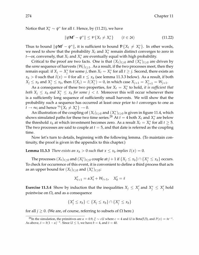
274 Chapter 11
Notice that X∗t ∼ ψ∗ for all t. Hence, by (11.21), we have
‖ψMt − ψ∗‖ ≤ {Xt �= X∗t } (t ∈ ) (11.22)
Thus to bound ‖ψMt − ψ∗‖, it is sufficient to bound {Xt �= X∗t }. In other words,we need to show that the probability Xt and X∗t remain distinct converges to zero int—or, conversely, that Xt and X∗t are eventually equal with high probability.
Critical to the proof are two facts. One is that (Xt)t≥0 and (X∗t )t≥0 are driven bythe same sequence of harvests (Wt)t≥1. As a result, if the two processes meet, then theyremain equal: if Xj = X∗j for some j, then Xt = X∗t for all t ≥ j. Second, there exists anxb > 0 such that I(x) = 0 for all x ≤ xb (see lemma 11.3.3 below). As a result, if bothXj ≤ xb and X∗j ≤ xb, then I(Xj) = I(X∗j ) = 0, in which case Xj+1 = X∗j+1 = Wj+1.
As a consequence of these two properties, for Xt = X∗t to hold, it is sufficient thatboth Xj ≤ xb and X∗j ≤ xb for some j < t. Moreover this will occur whenever thereis a sufficiently long sequence of sufficiently small harvests. We will show that theprobability such a sequence has occurred at least once prior to t converges to one ast→ ∞; and hence {Xt �= X∗t } → 0.
An illustration of the coupling of (Xt)t≥0 and (X∗t )t≥0 is given in figure 11.4, whichshows simulated paths for these two time series.28 At t = 4 both Xt and X∗t are belowthe threshold xb at which investment becomes zero. As a result Xt = X∗t for all t ≥ 5.The two processes are said to couple at t = 5, and that date is referred as the couplingtime.
Now let’s turn to details, beginning with the following lemma. (To maintain con-tinuity, the proof is given in the appendix to this chapter.)
Lemma 11.3.3 There exists an xb > 0 such that x ≤ xb implies I(x) = 0.
The processes (Xt)t≥0 and (X∗t )t≥0 couple at j+ 1 if {Xj ≤ xb}∩ {X∗j ≤ xb} occurs.To check for occurrence of this event, it is convenient to define a third process that actsas an upper bound for (Xt)t≥0 and (X∗t )t≥0:
X′t+1 = αX′t +Wt+1, X′0 = s
Exercise 11.3.4 Show by induction that the inequalities Xj ≤ X′j and X∗j ≤ X′j holdpointwise on Ω, and as a consequence
{X′j ≤ xb} ⊂ {Xj ≤ xb} ∩ {X∗j ≤ xb}
for all j ≥ 0. (We are, of course, referring to subsets of Ω here.)
28In the simulation, the primitives are α = 0.9, ξ ∼ cU where c = 4 and U is Beta(5,5), and P(x) = se−x .As above, s = b(1− α)−1. Since U ≤ 1, we have b = 4, and s = 40.

Stochastic Dynamics 275
5 10 15 20 25
time
Xt
X∗t
xb
Figure 11.4 Coupling of (Xt)t≥0 and (X∗t )t≥0 at t = 5
Given that if (Xt)t≥0 and (X∗t )t≥0 meet they remain equal, and given that X′j ≤ xbimplies Xj+1 = X∗j+1, we have
X′j ≤ xb for some j ≤ t =⇒ Xt+1 = X∗t+1
In terms of subsets of Ω, this can be stated as
∪j≤t{X′j ≤ xb} ⊂ {Xt+1 = X∗t+1}∴ ∪j≤t {X′j ≤ xb} ≤ {Xt+1 = X∗t+1}∴ {Xt+1 �= X∗t+1} ≤ ∩j≤t {X′j > xb}
The probability of the event ∩j≤t{X′j > xb} can be bounded relatively easily. Indeedsuppose that harvests Wn+1 to Wn+k are all below z0, where k and z0 are chosen tosatisfy
αks+ z01− αk
1− α≤ xb (11.23)
Since the harvests are all below z0, we have
X′j ≤ αX′j−1 + z0 j = n+ 1, . . . , n+ k
Combining these k inequalities gives
X′n+k ≤ αkX′n + z01− αk
1− α≤ αks+ z0
1− αk
1− α≤ xb

276 Chapter 11
where the last inequality follows from (11.23). Thus a sequence of k harvests below z0forces (X′t)t≥0 below xb by the end of the sequence. For dates of the form t× k thereare t nonoverlapping sequences of k consecutive harvests prior to t× k. Let Ei be theevent that the i-th of these t sequences has all harvests below z0:
Ei = ∩i×kj=k×(i−1)+1{Wj ≤ z0} i = 1, . . . , t
If X′j never falls below xb in the period up to t × k, then none of the events Ei hasoccurred.
∴ ∩j≤t×k{X′j > xb} ⊂ ∩ti=1Eci
∴ {Xt×k+1 �= X∗t×k+1} ≤ ∩j≤t×k {X′j > xb} ≤ ∩ti=1 Eci
Since the sequences of harvests that make up each Ei are nonoverlapping, these eventsare independent, and ∩ti=1 E
ci = ∏t
i=1(1− (Ei)).
∴ {Xt×k+1 �= X∗t×k+1} ≤t
∏i=1
(1− (Ei)) = (1− φ(z0)k)t
We have now established (11.20) and hence theorem 11.3.1.
11.3.2 Coupling and the Dobrushin Coefficient
Let S ∈ B( n), and let P be an arbitrary stochastic kernel on S. In the previoussection S was a subset of , and P had the attractive property that for any x, x′ in[0, xb] ⊂ S, P(x, dy) = P(x′, dy). Such a set is called an atom of P. Existence of an atomto which the state returns regularly makes coupling particularly simple: Wheneverthe two chains (Xt)t≥0 and (X∗t )t≥0 in §11.3.1 enter the atom simultaneously they canbe coupled.
Unfortunately, most Markov chains studied in economic applications fail to havethis structure. However, it turns out that with a little bit of trickery one can constructcouplings for many chains without using atoms. In this section we discuss the casewhere P has a positive Dobrushin coefficient. As we show, positivity of the Dobrushincoefficient is very closely connected with the possibility of successful coupling.
Understanding the connection between coupling and the Dobrushin coefficientis satisfying because the latter plays such an important role in analytical proofs ofstability. Coupling will shine a light on the role of the Dobrushin coefficient from anew angle. More importantly, the basic idea behind the coupling proof we use herecan be generalized to a large number of different models.
As in §11.3.1, we will endow P(S) with the metric defined by (11.19), which isproportional to total variation distance. Our main result is as follows:
Stochastic Dynamics 277
Proposition 11.3.5 Let ψ,ψ′ ∈ P(S). If α(P) is the Dobrushin coefficient for P and M isthe corresponding Markov operator, then
‖ψMt − ψ′Mt‖ ≤ (1− α(P))t (t ∈ )
If α(P) = 0, then this inequality is trivial. On the other hand, if α(P) > 0, thenfor any initial conditions ψ and ψ′, we have ‖ψMt − ψ′Mt‖ → 0 at a geometric rate.In particular, if ψ′ = ψ∗ is stationary, then ‖ψMt − ψ∗‖ → 0. Note also that we areproving nothing new here. Theorem 11.2.21 yields the same result. What is new is theproof—which is radically different.
Since the proposition is trivial when α(P) = 0, we assume in all of what followsthat α(P) is strictly positive. To make the proof, we will build two processes (Xt)t≥0and (X′t)t≥0 such that the distribution ψt of Xt is ψMt and the distribution ψ′t of X′t isψ′Mt. In view of lemma 11.3.2 (page 273), we then have
‖ψMt − ψ′Mt‖ ≤ {Xt �= X′t} (11.24)
Given (11.24) it is sufficient to show that {Xt �= X′t} ≤ (1 − α(P))t. The trick tothe proof is constructing (Xt)t≥0 and (X′t)t≥0 in a rather special way. In particular,we build these processes so that there is an independent α(P) probability of meetingat every step, and, moreover, once the processes meet (i.e., Xj = X′j for some j) theyremain coupled (i.e., Xt = X′t for all t ≥ j). It then follows that if Xt �= X′t, then thetwo processes have never met, and the probability of this is less than (1− α(P))t.
While (Xt)t≥0 and (X′t)t≥0 are constructed in a special way, care must be taken thatψt = ψMt and ψ′t = ψ′Mt remains valid. This requires that X0 ∼ ψ, X′0 ∼ ψ′, and,recursively, Xt+1 ∼ P(Xt, dy) and X′t+1 ∼ P(X′t, dy). That such is the case does notappear obvious from the construction, but at the end of our proof we will verify thatit is.
In order to construct the processes (Xt)t≥0 and (X′t)t≥0, it is convenient to intro-duce some additional notation. First, let
γ(x, x′) := (Px ∧ Px′)(S) ((x, x′) ∈ S× S)
be the affinity between P(x, dy) and P(x′, dy), so α(P) = infx,x′ γ(x, x′). Evidentlyγ(x, x′) ≥ α(P) > 0 for every x and x′.
Next let us define three new functions from S× S×B(S) to [0, 1] by
ν(x, x′, B) :=(Px ∧ Px′)(B)
γ(x, x′)
μ(x, x′, B) :=P(x, B)− (Px ∧ Px′)(B)
1− γ(x, x′)

278 Chapter 11
μ′(x, x′, B) :=P(x′, B)− (Px ∧ Px′)(B)
1− γ(x, x′)
Crucially, ν(x, x′, dy), μ(x, x′, dy) and μ′(x, x′, dy) are all probability measures on S. Inparticular, ν(x, x′, B), μ(x, x′, B) and μ′(x, x′, B) are nonnegative for all B ∈ B(S); andν(x, x′, S) = μ(x, x′, S) = μ′(x, x′, S) = 1. The next exercise asks you to show that thisis the case.
Exercise 11.3.6 Prove that ν(x, x′, dy), μ(x, x′, dy) and μ′(x, x′, dy) are probability mea-sures on S for every (x, x′) ∈ S× S such that γ(x, x′) < 1.29
Algorithm 11.1 Coupling algorithm
draw X0 ∼ ψ and X′0 ∼ ψ∗set t = 0while True do
if Xt = X′t thendraw Z ∼ P(Xt, dy) and set Xt+1 = X′t+1 = Z
elsedraw Ut+1 independently from Uniform(0, 1)if Ut+1 ≤ γ(Xt,X′t) then // with probability γ(Xt,X′t)
draw Z ∼ ν(Xt,X′t, dy) and set Xt+1 = X′t+1 = Zelse // with probability 1− γ(Xt,X′t)
draw Xt+1 ∼ μ(Xt,X′t, dy)draw X′t+1 ∼ μ′(Xt,X′t, dy)
endendset t = t+ 1
end
We are now ready to build the processes (Xt)t≥0 and (X′t)t≥0. This is done inalgorithm 11.1. The while loop in the algorithm is an infinite loop. If at time t we haveXt �= X′t, then a uniform random variable Ut+1 is drawn to determine the next action.The probability that Ut+1 ≤ γ(Xt,X′t) is γ(Xt,X′t), and if this occurs, then both Xt+1and X′t+1 are set equal to a single draw from ν(Xt,X′t, dy). Otherwise, they are drawnfrom μ(Xt,X′t, dy) and μ′(Xt,X′t, dy) respectively. All random variables are assumedto live on probability space (Ω,F , ).
Our first claim is that for the processes (Xt)t≥0 and (X′t)t≥0 we have
{Xt �= X′t} ≤ (1− α(P))t (t ∈ ) (11.25)
29Note that γ(x, x′) > 0 by assumption.

Stochastic Dynamics 279
The proof is not difficult: Fix any t ∈ . Observe that if Uj ≤ γ(Xj−1,X′j−1) for justone j ≤ t, then the two processes couple and Xt = X′t. So, if Xt �= X′t, then we musthave Uj > γ(Xj−1,X′j−1) for all j ≤ t. Since γ(Xj−1,X′j−1) ≥ α(P), and since (Ut)t≥1
is IID and uniformly distributed on (0, 1), the probability of this event is no more than(1− α(P))t. As t is arbitrary, the proof of (11.25) is now done.
In view of (11.25), proposition 11.3.5 will be established if we can verify (11.24); inother words, we need to show that
‖ψMt − ψ′Mt‖ ≤ {Xt �= X′t}
As discussed above, this is implied by lemma 11.3.2 (page 273), provided that thedistributions of Xt and X′t are ψMt and ψ′Mt respectively. Since X0 ∼ ψ and X′0 ∼ ψ′certainly hold, we need only show that Xt+1 ∼ P(Xt, dy) and X′t+1 ∼ P(X′t, dy) ateach step.
To see that this is the case, suppose that at time t we have (Xt,X′t) = (x, x′). Weclaim that after the next iteration of algorithm 11.1, the probability that Xt+1 ∈ B isP(x, B), while the probability that X′t+1 ∈ B is P(x′, B). Let’s focus for now on theclaim that the probability that Xt+1 ∈ B is P(x, B).
Suppose first that x �= x′. If γ(x, x′) = 1, then Xt+1 is drawn from ν(x, x′, dy)with probability one. But γ(x, x′) = 1 implies that P(x, dy) = P(x′, dy), and henceν(x, x′, dy) = P(x, dy) = P(x′, dy). In particular, the probability that Xt+1 ∈ B isP(x, B). On the other hand, if γ(x, x′) < 1, then Xt+1 is drawn from ν(x, x′, dy) withprobability γ(x, x′), and from μ(x, x′, dy) with probability 1− γ(x, x′). As a result theprobability that Xt+1 ∈ B is
γ(x, x′)ν(x, x′, B) + (1− γ(x, x′))μ(x, x′, B)
A look at the definitions of ν and μ confirms that this is precisely P(x, B).The argument that X′t+1 ∈ B with probability P(x′, B) is almost identical.Finally, suppose that x = x′. Then Xt+1 ∼ P(x, dy), so clearly Xt+1 ∈ B with
probability P(x, B). Also X′t+1 = Xt+1, so X′t+1 ∈ B with probability P(x, B). But sincex′ = x, we have P(x′, B) = P(x, B). Hence the probability that X′t+1 ∈ B is P(x′, B).The proof is done.
11.3.3 Stability via Monotonicity
Economic models often possess a degree of monotonicity in the laws of motion. Ifa nice property such as monotonicity holds, then we would like to exploit it whenconsidering stability. The question of when monotone stochastic systems are stable isthe topic of this section.
280 Chapter 11
Consider again our canonical SRS introduced on page 219. To reiterate, the statespace S is a Borel subset of n and the shock space Z is a Borel subset of k . TheSRS is described by a (Borel) measurable function F : S × Z → S and a distributionφ ∈P(Z), where
Xt+1 = F(Xt,Wt+1), (Wt)t≥1IID∼ φ, X0 ∼ ψ ∈P(S) (11.26)
The sequence of shocks (Wt)t≥1 and the initial condition X0 live on a common proba-bility space (Ω,F , ) and are mutually independent. The stochastic kernel for (11.26)is given by
P(x, B) =∫
B[F(x, z)]φ(dz) (x ∈ S, B ∈ B(S)) (11.27)
Let M be the corresponding Markov operator, so ψ∗ is stationary for (11.26) if andonly if ψ∗M = ψ∗.
Definition 11.3.7 The SRS (11.26) is said to be monotone increasing if, for all z ∈ Z,30
F(x, z) ≤ F(x′, z) whenever x ≤ x′ (11.28)
Example 11.3.8 Consider the one-dimensional linear system
Xt+1 = αX +Wt+1, (Wt)t≥1IID∼ φ ∈P( ) (11.29)
where S = Z = and F(x, z) = αx+ z. This SRS is monotone increasing if and onlyif α ≥ 0.
Exercise 11.3.9 Suppose that (11.26) is monotone increasing, and h : S → . Showthat if h ∈ ibS, then Mh ∈ ibS.31
Exercise 11.3.10 A set B ⊂ S is called an increasing set if x ∈ B and x′ ∈ S withx ≤ x′ implies x′ ∈ B. Show that B ⊂ S is an increasing set if and only if B ∈ ibS.(Since P(x, B) = M B(x), it follows that x �→ P(x, B) is increasing whenever B is anincreasing set. What is the intuition?)
Returning to the general SRS (11.26), let’s assume that at least one stationary dis-tribution ψ∗ exists, and see what conditions we might need to obtain uniqueness andstability of ψ∗ under the hypothesis of monotonicity. In this section stability of ψ∗ willhave the slightly nonstandard definition
∀ψ ∈P(S), (ψMt)(h)→ ψ∗(h) as t→ ∞ for all h ∈ ibS (11.30)
30Our order on n is the usual one: (xi)ni=1 ≤ (yi)ni=1 if xi ≤ yi for all i with 1 ≤ i ≤ n.31As usual, ibS denotes the increasing bounded functions h : S→ .
Stochastic Dynamics 281
To understand condition (11.30), recall that a sequence (μn) ⊂ P(S) converges toμ ∈P(S) weakly if μn(h)→ μ(h) as n→ ∞ for all h ∈ bcS. Moreover, to verify weakconvergence, it suffices to check μn(h) → μ(h) only for h ∈ ibcS (theorem 11.1.35,page 255). Since ibcS ⊂ ibS, the convergence in (11.30) is stronger than ψMt → ψ∗weakly. Finally, (11.30) implies uniqueness of ψ∗, as follows from the next exercise.
Exercise 11.3.11 Show that if ψ∗∗ ∈ P(S) satisfies ψ∗∗M = ψ∗∗ and (11.30) holds,then ψ∗∗ and ψ∗ must be equal.32
Now let (Wt)t≥1 and (W ′t )t≥1 be jointly independent IID processes on Z, both dis-tributed according to φ and defined on the common probability space (Ω,F , ). Us-ing these two independent shock processes, we can introduce a condition that is suf-ficient for stability of monotone systems.
Definition 11.3.12 The SRS (11.26) is called order mixing if, given any two independentinitial conditions X0 and X′0, the processes (Xt)t≥0 and (X′t)t≥0 defined by Xt+1 =F(Xt,Wt+1) and X′t+1 = F(X′t,W ′t+1) satisfy
∪t≥0 {Xt ≤ X′t} = ∪t≥0 {X′t ≤ Xt} = 1 (11.31)
Exercise 11.3.13 Prove: ∪t≥0 {Xt ≤ X′t} = 1 iff limT→∞ ∩t≤T {Xt � X′t} = 0.33
Paired with monotonicity, order mixing is sufficient for stability. In particular, wehave the following result:
Theorem 11.3.14 Suppose that (11.26) has at least one stationary distribution ψ∗ ∈ P(S).If it is monotone increasing and order mixing, then ψ∗ is the only stationary distribution, andmoreover ψ∗ is globally stable in the sense of (11.30).
The proof is given at the end of §11.3.4. For now let us consider how to apply thisresult. To do so, it is necessary to develop sufficient conditions for order mixing thatare easy to check in applications. One set of conditions that implies order mixing isthat introduced by Razin and Yahav (1979), and extended and popularized by Stokeyand Lucas (1989) and Hopenhayn and Prescott (1992). Following Stokey and Lucas(1989, assumption 12.1), suppose that S = [a, b] := {x ∈ n : a ≤ x ≤ b} for fixeda, b ∈ n, and that
∃ m ∈ , c ∈ S, ε > 0 such that Pm(a, [c, b]) ≥ ε and Pm(b, [a, c]) ≥ ε (11.32)
Let’s consider this condition in our setting, where P is the kernel (11.27) and (11.26) ismonotone increasing.
32Hint: See theorem 11.1.36 on page 255.33Hint: Use exercise 7.1.25 on page 167. Note that all sets are subsets of Ω.
282 Chapter 11
Exercise 11.3.15 Show that under (11.32) the kernel P satisfies Pm(x, [c, b]) ≥ ε andPm(x, [a, c]) ≥ ε for all x ∈ S.34
If (11.26) satisfies (11.32), then it is order mixing. To get a feel for the proof, supposethat (11.32) holds with m = 1, and consider the probability that there exists a t ≥ 0with Xt ≤ X′t. In light of exercise 11.3.13, to show this probability is one, it is sufficientto show that limT→∞ (ET) = 0, where ET := ∩t≤T{Xt � X′t}. The probability ofXt ≤ X′t given (Xt−1,X′t−1) = (x, x′) is
{F(x,Wt) ≤ F(x′,W ′t )} ≥ {F(x,Wt) ≤ c} ∩ {F(x′,W ′t ) ≥ c}= {F(x,Wt) ≤ c} {F(x′,W ′t ) ≥ c}= P(x, [a, c])P(x′, [c, b]) ≥ ε2
Hence for each t the probability of Xt ≤ X′t occurring is at least ε2, independent of thelagged value of the state. One can then show that the probability (ET) of this eventnever occurring prior to T is ≤ (1− ε2)T → 0.35 From exercise 11.3.13 we then have∪t≥0 {Xt ≤ X′t} = 1. A similar argument establishes ∪t≥0 {Xt ≥ X′t} = 1, and
hence order mixing.Condition (11.32) can be restrictive, as the state space must be of the form {x ∈
n : a ≤ x ≤ b}. To devise a weaker set of sufficient conditions, we introduce theconcept of order inducing sets and order norm-like functions.
Definition 11.3.16 A C ∈ B(S) is called order inducing for kernel P if there exists ac ∈ S and an m ∈ such that
infx∈C
Pm(x, {z : z ≤ c}) > 0 and infx∈C
Pm(x, {z : z ≥ c}) > 0
A measurable function v : S → + is called order norm-like for P if every sublevel setof v is order inducing for P.36
Example 11.3.17 Continuing with the model (11.29) in example 11.3.8, suppose that{Wt ≤ d} > 0 and {Wt ≥ d} > 0 for all d ∈ S = . Then every set of the form
[−b, b] is order inducing with m = 1 and c = 0. To see this, pick any b ≥ 0. Forx ∈ [−b, b] we have
P(x, {z : z ≤ 0}) = {αx+W ≤ 0} = {W ≤ −αx} ≥ {W ≤ −αb}which is positive. The proof that infx∈C P(x, {z : z ≥ 0}) > 0 is similar.
Since all sets of the form [−b, b] are order inducing, it follows that v(x) = |x| isorder norm-like for this model. (Why?)
34Hint: Use exercise 11.3.10.35A complete proof can be made along the lines of of proposition 5.2.6, or using conditional expectations.
See also Kamihigashi and Stachurski (2008).36Recall that the sublevel sets of v are sets of the form {x ∈ S : v(x) ≤ a} for a ∈ +.
Stochastic Dynamics 283
Exercise 11.3.18 Show that all measurable subsets of order inducing sets are orderinducing. Show that v : S→ + is order norm-like if and only if there exists a K ∈ +such that {x ∈ S : v(x) ≤ a} is order inducing for all a ≥ K.
We can now state the following sufficient condition for order mixing:
Theorem 11.3.19 If there exists an order norm-like function v for (11.26) and constantsα ∈ [0, 1) and β ∈ + such that∫
v[F(x, z)]φ(dz) ≤ αv(x) + β (x ∈ S) (11.33)
then (11.26) is order mixing.
The intuition is that under (11.33) there is drift back to (sufficiently large) sub-level sets of v, which are order inducing. When two independent chains (Xt)t≥0 and(X′t)t≥0 enter such an order inducing set, there is a positive probability of the orderingsXt ≤ X′t and Xt ≥ X′t occurring within m periods. Repeated over an infinite horizon,these orderings eventually occur with probability one. For a proof, see Kamihigashiand Stachurski (2008).
Example 11.3.20 Continuing with example 11.3.17, we saw that v(x) = |x| is ordernorm-like for this model. If |Wt| < ∞ and |α| < 1, then the model is order mixing,since for any x ∈ S,∫
v[F(x, z)]φ(dz) =∫|αx+ z|φ(dz) ≤ |α|v(x) +
∫|z|φ(dz)
11.3.4 More on Monotonicity
Let’s now turn to a less trivial example of how monotonicity and order mixing canbe used to establish stability.37 Recall the stochastic Solow–Swan growth model dis-cussed in example 9.2.4, page 220, with law of motion
kt+1 = s f (kt)Wt+1 + (1− δ)kt (11.34)
and increasing production function f : + → + with f (k) > 0 for all k > 0. The pro-ductivity shock Wt and the capital stock kt take values in Z := S := (0,∞), while theparameters satisfy s ∈ (0, 1) and δ ∈ (0, 1]. The model (11.34) is monotone increasingin the sense of definition 11.3.7.
Let’s look for conditions under which (11.34) is order mixing. For simplicity we as-sume that δ = 1.38 We suppose further that limk→0 f (k)/k = ∞, and limk→∞ f (k)/k =
37See also §12.1.3, which treats the optimal growth model using monotonicity.38The case δ < 1 can be accommodated at the cost of a longer proof.

284 Chapter 11
0. (More traditional Inada conditions can be used if f is assumed to be differentiable.)Regarding the distribution φ, we assume that both Wt and (1/Wt) are finite, andthat {Wt ≤ x} and {Wt ≥ x} are strictly positive for every x ∈ S.39
First let’s show that all closed intervals [a, b] ⊂ S are order inducing for this model.To do so, pick any a ≤ b. Fix any c ∈ S. It suffices to show that infa≤x≤b P(x, [c,∞)) >0 and likewise for (0, c]. Given our assumptions on φ, for any x ∈ [a, b] we have
P(x, [c,∞)) = {s f (x)Wt+1 ≥ c}= {Wt+1 ≥ c/(s f (x))} ≥ {Wt+1 ≥ c/(s f (a))} > 0
A similar argument gives infa≤x≤b P(x, (0, c]) > 0.Now consider the function v(x) := 1/x + x. Since sublevel sets of v are closed
intervals in S, the function v is order norm-like on S.
Exercise 11.3.21 Suppose that f is unbounded, and f (0) = 0. Show that neither x �→ xnor x �→ 1/x are order norm-like for (11.34).
To complete the proof of stability, we must show that the drift condition (11.33)holds for v. That is, we need to establish the existence of an α ∈ [0, 1) and a β ∈ +such that
Mv ≤ αv+ β when v(x) = x+1x
(11.35)
where M is the Markov operator defined by Mh(x) =∫h[s f (x)z]φ(dz). To this end,
suppose that we can establish the existence of α1, α2 ∈ [0, 1) and β1, β2 ∈ + with
Mv1 ≤ α1v1 + β1 and Mv2 ≤ α2v2 + β2 (11.36)
where v1(x) = x and v2(x) = 1/x. Then since v = v1 + v2, adding across the twoinequalities in (11.36) gives the desired inequality (11.35) because
Mv = M(v1 + v2) = Mv1 +Mv2 ≤ α1v1 + β1 + α2v2 + β2 ≤ αv+ β
when α := max{α1, α2} and β := β1 + β2. In other words, to establish the driftcondition (11.35) and hence order mixing, it is sufficient to establish separately the twodrift conditions in (11.36). Intuitively, the drift condition on v1 prevents divergence to+∞, which the condition on v2 prevents divergence to zero.
Let’s attempt to establish the two inequalities in (11.36), starting with the left-handside (i.e., the inequality Mv1 ≤ α1v1 + β1).
39We require a lot of mixing for global stability because f is not assumed to be concave. In fact f can berather arbitrary, and the deterministic model (i.e., Wt ≡ 1 for all t) can have many fixed points.

Stochastic Dynamics 285
Exercise 11.3.22 Fix any constant α1 ∈ (0, 1). Using the assumption limx→∞ f (x)/x =0, establish the existence of a γ ∈ S satisfying
s f (x) W1 ≤ α1x ∀ x > γ
Using monotonicity of f , show further that there is a β1 ∈ + with
s f (x) W1 ≤ β1 ∀ x ≤ γ
Based on these two inequalities, conclude that
Mv1(x) = s f (x) W1 ≤ α1x+ β1 = α1v1(x) + β1 ∀ x ∈ S
The last exercise establishes the first of the two inequalities in (11.36). The nextexercise establishes the second inequality.
Exercise 11.3.23 Fix any constant α2 ∈ (0, 1). Using the assumption limx→0 f (x)/x =∞, establish the existence of a γ ∈ S satisfying[
1s f (x)W1
]≤ α2
1x
∀ x < γ
Using monotonicity of f , show there exists a β2 ∈ + with[1
s f (x)W1
]≤ β2 ∀ x ≥ γ
Based on these two inequalities, conclude that
Mv2(x) =[
1s f (x)W1
]≤ α2
1x
+ β2 = α2v2(x) + β2 ∀ x ∈ S
Thus the second inequality in (11.36) also holds, and theorem 11.3.19 implies thatunder our assumptions the stochastic Solow–Swan growth model is order mixing.Since it is also monotone increasing, theorem 11.3.14 implies that should any station-ary distribution ψ∗ ∈ P(S) exist, that stationary distribution would be unique andglobally stable in the sense of (11.30). If f is continuous, then since v is also norm-like(as well as order norm-like, see lemma 8.2.17 on page 209), existence of ψ∗ followsimmediately from corollary 11.2.10.
To complete this section, let’s give the proof of theorem 11.3.14. Using the two in-dependent series (Wt)t≥1 and (W ′t )t≥1 in the definition of order mixing, algorithm 11.2defines four processes, denoted by (Xt)t≥0, (X′t)t≥0, (XL
t )t≥0 and (XUt )t≥0.40 The pro-
cess (Xt)t≥0 is the original SRS in (11.26), with initial condition ψ. The process (X′t)t≥0
40Formally, ω ∈ Ω is drawn at the start of time according to , thereby determining the initial conditionsX0(ω) and X′0(ω), and the shock realizations (Wt(ω))t≥1 and (W ′t (ω))t≥1. These in turn determine therealizations of all other random variables.
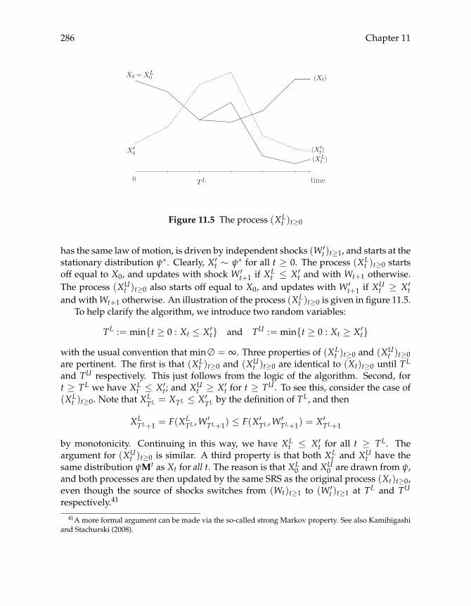
286 Chapter 11
(X ′t)(XL
t )
TL time
(Xt)
0
X ′0
X0 = XL0
Figure 11.5 The process (XLt )t≥0
has the same law of motion, is driven by independent shocks (W ′t )t≥1, and starts at thestationary distribution ψ∗. Clearly, X′t ∼ ψ∗ for all t ≥ 0. The process (XL
t )t≥0 startsoff equal to X0, and updates with shock W ′t+1 if XL
t ≤ X′t and with Wt+1 otherwise.The process (XU
t )t≥0 also starts off equal to X0, and updates with W ′t+1 if XUt ≥ X′t
and withWt+1 otherwise. An illustration of the process (XLt )t≥0 is given in figure 11.5.
To help clarify the algorithm, we introduce two random variables:
TL := min{t ≥ 0 : Xt ≤ X′t} and TU := min{t ≥ 0 : Xt ≥ X′t}with the usual convention that min∅ = ∞. Three properties of (XL
t )t≥0 and (XUt )t≥0
are pertinent. The first is that (XLt )t≥0 and (XU
t )t≥0 are identical to (Xt)t≥0 until TL
and TU respectively. This just follows from the logic of the algorithm. Second, fort ≥ TL we have XL
t ≤ X′t; and XUt ≥ X′t for t ≥ TU . To see this, consider the case of
(XLt )t≥0. Note that XL
TL = XTL ≤ X′TL by the definition of TL, and then
XLTL+1 = F(XL
TL ,W′TL+1) ≤ F(X′TL ,W
′TL+1) = X′TL+1
by monotonicity. Continuing in this way, we have XLt ≤ X′t for all t ≥ TL. The
argument for (XUt )t≥0 is similar. A third property is that both XL
t and XUt have the
same distribution ψMt as Xt for all t. The reason is that XL0 and XU
0 are drawn from ψ,and both processes are then updated by the same SRS as the original process (Xt)t≥0,even though the source of shocks switches from (Wt)t≥1 to (W ′t )t≥1 at TL and TU
respectively.41
41A more formal argument can be made via the so-called strong Markov property. See also Kamihigashiand Stachurski (2008).

Stochastic Dynamics 287
Algorithm 11.2 Four (F, φ) processes
generate independent draws X0 ∼ ψ and X′0 ∼ ψ∗set XL
0 = XU0 = X0
for t ≥ 0 dodraw Wt+1 ∼ φ and W ′t+1 ∼ φ independentlyset Xt+1 = F(Xt,Wt+1) and X′t+1 = F(X′t,W ′t+1)if XL
t ≤ X′t thenset XL
t+1 = F(XLt ,W ′t+1)
elseset XL
t+1 = F(XLt ,Wt+1)
endif XU
t ≥ X′t thenset XU
t+1 = F(XUt ,W ′t+1)
elseset XU
t+1 = F(XUt ,Wt+1)
endend
Now to the proof. Pick any h ∈ ibS. We wish to show that (ψMt)(h) → ψ∗(h)as t → ∞. Order mixing tells us precisely that {TL < ∞} = 1, or {TL ≤ t} → 1as t → ∞. Note that TL ≤ t implies XL
t ≤ X′t, and since h is increasing, this impliesh(XL
t ) ≤ h(X′t). Therefore
h(XLt ) {TL ≤ t} ≤ h(X′t) {TL ≤ t}
∴ h(XLt ) {TL ≤ t} ≤ h(X′t) {TL ≤ t} (11.37)
Using {TL ≤ t} → 1 and taking the limit superior now gives
lim supt→∞
h(XLt ) ≤ lim sup
t→∞h(X′t) (11.38)
where the precise derivation of (11.38) is left until the end of the proof. To continue,since X′t ∼ ψ∗ for all t, the right-hand side is just ψ∗(h). And since XL
t ∼ ψMt for all t,we have proved that
lim supt→∞
(ψMt)(h) ≤ ψ∗(h)
By a similar argument applied to XUt instead of XL
t , we obtain
ψ∗(h) ≤ lim inft→∞ (ψMt)(h)

288 Chapter 11
It now follows that limt→∞(ψMt)(h) = ψ∗(h), and since h is an arbitrary element ofibS, the claim in (11.30) is established.
To end the section, let’s see how (11.38) is derived. We have
lim supt→∞
h(XLt ) ≤ lim sup
t→∞h(XL
t ) {TL ≤ t}+ lim supt→∞
h(XLt ) {TL > t}
Since h is bounded the last term is zero, and hence
lim supt→∞
h(XLt ) ≤ lim sup
t→∞h(XL
t ) {TL ≤ t} ≤ lim supt→∞
h(X′t) {TL ≤ t} = ψ∗(h)
where the second inequality is due to (11.37), and the final equality holds because
h(X′t) {TL ≤ t} = h(X′t)− h(X′t) {TL > t} = ψ∗(h)− h(X′t) {TL > t}
and boundedness of h gives h(X′t) {TL > t} → 0 as t→ ∞.
11.3.5 Further Stability Theory
In the theory covered so far, we have illustrated how stability problems in unboundedstate spaces can be treated using drift conditions. Drift conditions were used in §8.2.3for existence, uniqueness, and stability in the density case, in §11.2.1 for existence inthe general (i.e., measure) case, and in §11.3.3 for stability in the general case undermonotonicity. It would be nice to add a stability result suitable for unbounded spaces(i.e., using drift) that requires neither density assumptions nor monotonicity. Let usnow address this gap, providing a result for the general case that gives existence,uniqueness, and stability without specifically requiring continuity, monotonicity ordensities. While full proofs are beyond the scope of this text, an intuitive explanationbased on coupling and the Dobrushin coefficient is provided.
Let P be a stochastic kernel on S ∈ B( n). In §11.3.2 we showed how processeson S can be coupled when the Dobrushin coefficient is strictly positive, and how thiscoupling can be used to prove stability. However, we know that on unbounded statespace the Dobrushin coefficient α(P) of P is often zero.42 The problem is that α(P) isdefined as the infimum of the affinities γ(x, x′) := (Px ∧ Px′)(S) over all (x, x′) pairsin S× S. The affinity is close to one when P(x, dy) and P(x′, dy) put probability massin similar areas, and converges to zero as their supports diverge. If S is unbounded,then as the distance between x and x′ increases without bound, it is likely that thesupports of P(x, dy) and P(x′, dy) also diverge from one another, and γ(x, x′) can bemade arbitrarily small. The end result is α(P) = 0.
42Recall the example shown in figure 8.7 on page 202.
Stochastic Dynamics 289
If α(P) = 0, then the coupling result in §11.3.2 fails. To see this, recall that the proofis based on the bound
‖ψMt − ψ′Mt‖ ≤ {Xt �= X′t} (11.39)
where (Xt)t≥0 and (X′t)t≥0 are processes with X0 ∼ ψ, X′0 ∼ ψ′, Xt+1 ∼ P(Xt, dy)and X′t+1 ∼ P(X′t, dy). To show that {Xt �= X′t} → 0 as t → ∞, we constructed thesequences (Xt)t≥0 and (X′t)t≥0 using algorithm 11.1, where the probability of couplingat t+ 1 is γ(Xt,X′t) ≥ α(P). This gave the bound {Xt �= X′t} ≤ (1− α(P))t.
Of course, if α(P) = 0, then this bound has no bite. However, there is a wayto extend our stability result to such cases. The basic idea is as follows: While theinfimum of γ(x, x′) may be zero when taken over all of S× S, it may well be a positivevalue ε when taken over C × C, where C is some bounded subset of S. If such a Cexists, then we can modify our strategy by attempting to couple the chains only whenboth are in C. In this case the probability of coupling at t+ 1 is γ(Xt,X′t) ≥ ε.
This idea is illustrated in algorithm 11.3. (Compare with algorithm 11.1.)
Algorithm 11.3 Coupling with drift
draw X0 ∼ ψ, X′0 ∼ ψ∗ and set t = 0while True do
if Xt = X′t thendraw Z ∼ P(Xt, dy) and set Xt+1 = X′t+1 = Z
elseif Xt ∈ C and X′t ∈ C then
draw Ut+1 from the uniform distribution on (0, 1)if Ut+1 ≤ γ(Xt,X′t) then // with probability γ(Xt,X′t)
draw Z ∼ ν(Xt,X′t, dy) and set Xt+1 = X′t+1 = Zelse // with probability 1− γ(Xt,X′t)
draw Xt+1 ∼ μ(Xt,X′t, dy) and X′t+1 ∼ μ′(Xt,X′t, dy)end
elsedraw Xt+1 ∼ P(Xt, dy) and X′t+1 ∼ P(X′t, dy)
endendset t = t+ 1
end
The algorithm can be made to work along the following lines: Suppose that thekernel P and the set C are such that (Xt)t≥0 and (X′t)t≥0 return to C infinitely oftenwith probability one. Each time both chains return to C simultaneously, there is an εprobability of coupling. From this it can be shown that {Xt �= X′t} → 0 as t → ∞,

290 Chapter 11
which implies stability via (11.39).The formal arguments are not trivial, and rather than attempting such a proof
here, we present instead some standard results that can be understood using the sameintuition. In particular, we will be looking for (1) a set C ⊂ S such that the infimumof γ(x, x′) on C × C is positive, and (2) some kind of drift condition ensuring thechain returns to C infinitely often. These conditions capture the essence of stability onunbounded state spaces: mixing at the center of the state sufficient to rule out multiplelocal equilibria, and drift back to the center sufficient to rule out divergence.
Before presenting these standard results, it might be helpful to consider an exam-ple for which there exists a set C ⊂ S such that the infimum of γ(x, x′) on C × C ispositive:
Example 11.3.24 Consider again the STAR model discussed in §8.2.4, where Z = S =, and the state evolves according to
Xt+1 = g(Xt) +Wt+1, (Wt)t≥1IID∼ φ ∈ D(S) (11.40)
The kernel P corresponding to this model is of the form P(x, dy) = p(x, y)dy, wherep(x, y) = φ(y− g(x)). The affinities are given by
γ(x, x′) =∫
p(x, y) ∧ p(x′, y)dy =∫φ(y− g(x)) ∧ φ(y− g(x′))dy
Suppose that φ and g are both continuous, and that φ is strictly positive on , in whichcase
S× S � (x, y) �→ p(x, y) = φ(y− g(x)) ∈is continuous and positive on S× S. It follows that for any compact set C, the infimumof (x, y) �→ p(x, y) on C× C is greater than some δ > 0. But then
γ(x, x′) =∫
p(x, y) ∧ p(x′, y)dy ≥∫Cp(x, y) ∧ p(x′, y)dy ≥ δλ(C) =: ε
for any (x, x′) ∈ C× C. If λ(C) > 0, then inf(x,x′)∈C×C γ(x, x′) ≥ ε > 0.
The set C is called a small set. The traditional definition is as follows:
Definition 11.3.25 Let ν ∈ P(S) and let ε > 0. A set C ∈ B(S) is called (ν, ε)-smallfor P if for all x ∈ C we have
P(x, A) ≥ εν(A) (A ∈ B(S))
C is called small for P if it is (ν, ε)-small for some ν ∈P(S) and ε > 0.

Stochastic Dynamics 291
This definition works for us because if C is small, then the infimum of γ on C× Cis strictly positive. In particular, if C is (ν, ε)-small, then the infimum is greater thanε. The proof is left as an exercise:
Exercise 11.3.26 Show that if C is (ν, ε)-small for kernel P, then γ(x, x′) := (Px ∧Px′)(S) ≥ ε for any x, x′ in C.
Exercise 11.3.27 Show that every measurable subset of a small set is small.
Exercise 11.3.28 Show that if P(x, dy) = p(x, y)dy for some density kernel p, then C ∈B(S) is small for P whenever there exists a measurable g : S→ + with
∫g(y)dy > 0
and p(x, y) ≥ g(y) for all x ∈ C and y ∈ S.
Exercise 11.3.29 Consider the stochastic kernel P(x, dy) = p(x, y)dy = N(ax, 1),which corresponds to a linear AR(1) process with normal shocks. Show that everybounded C ⊂ is a small set for this process.
Now let’s introduce a suitable drift condition.
Definition 11.3.30 The kernel P satisfies drift to a small set if there exists a small set C,a measurable function v : S→ [1,∞) and constants λ ∈ [0, 1) and L ∈ + such that
Mv(x) ≤ λv(x) + L C(x) (x ∈ S) (11.41)
Drift to a small set is not dissimilar to our other drift conditions. In this case, if thecurrent state Xt is at some point x /∈ C, then since λ < 1, the next period expectation[v(Xt+1) |Xt = x] of the “Lyapunov function” v is a fraction of the current value
v(x). Since v ≥ 1, this cannot continue indefinitely, and the state tends back towardC.43
Sometimes the following condition is easier to check than (11.41).
Lemma 11.3.31 Suppose that there exists a measurable function v : S → + and constantsα ∈ [0, 1) and β ∈ + such that
Mv(x) ≤ αv(x) + β (x ∈ S) (11.42)
If all sublevel sets of v are small, then P satisfies drift to a small set.44
Exercise 11.3.32 Prove lemma 11.3.31. Show that we can assume without loss of gen-erality that v in the lemma satisfies v ≥ 1.45 Now show that if we pick any λ ∈ (α, 1),set C := {x : v(x) ≤ β/(λ− α)} and L := β, then v, C, λ, and L satisfy the conditionsof definition 11.3.30.
43Condition (11.41) corresponds to (V4) in Meyn and Tweedie (1993, §15.2.2).44Recall that the sublevel sets of v are sets of the form {x ∈ S : v(x) ≤ K}, K ∈ +.45Show that if the lemma holds for some v, α and β then it also holds for the function v′ := v + 1 and
constants α′ := α and β′ = β+ 1.

292 Chapter 11
Finally, to present the main result, we need two definitions that appear frequentlyin classical Markov chain theory. The first is aperiodicity:
Definition 11.3.33 A kernel P is called aperiodic if P has a (ν, ε)-small set C withν(C) > 0.46
Exercise 11.3.34 Continuing exercise 11.3.28, suppose there is a C ∈ B(S) and mea-surable g : S → + with
∫g(y)dy > 0 and p(x, y) ≥ g(y) for all x ∈ C and y ∈ S.
Show that if∫C g(x)dx > 0, then P is aperiodic.
Definition 11.3.35 Let μ ∈ P(S). The kernel P is called μ-irreducible if, for all x ∈ Sand B ∈ B(S) with μ(B) > 0, there exists a t ∈ with Pt(x, B) > 0. P is calledirreducible if it is μ-irreducible for some μ ∈P(S).
Let P be a stochastic kernel on S. LetM be the corresponding Markov operator, andletP(S) be endowed with the total variation metric. We can now state the followingpowerful stability result:
Theorem 11.3.36 If P is irreducible, aperiodic and satisfies drift to a small set, then the system(P(S),M) is globally stable with unique stationary distribution ψ∗ ∈ P(S). Moreover ifv is the function in definition 11.3.30 and h : S → is any measurable function satisfying|h| ≤ v, then
1n
n
∑t=1
h(Xt)→ ψ∗(h) with probability one as n→ ∞ (11.43)
Finally, if h2 ≤ v, then there is a σ ∈ + with
√n
(1n
n
∑t=1
h(Xt)− ψ∗(h))→ N(0, σ2) weakly as n→ ∞ (11.44)
For a proof of theorem 11.3.36, the reader is referred to Meyn and Tweedie (1993,thms. 16.0.1 and 17.0.1), or Roberts and Rosenthal (2004, thms. 9 and 28). The proofsin the second reference are closer to the coupling intuition provided in algorithm 11.3.
Remark 11.3.37 Under the conditions of theorem 11.3.36 it is known that ψ∗(v) < ∞,so |h| ≤ v implies ψ∗(|h|) < ∞. Actually this last restriction is sufficient for h to satisfythe LLN (11.43).
Remark 11.3.38 Why is aperiodicity required in theorem 11.3.36? To gain some intu-ition we can refer back to algorithm 11.3. Under the conditions of theorem 11.3.36 wehave drift back to a small set, which corresponds to C in algorithm 11.3. Each time
46Our definition corresponds to what is usually called strong aperiodicity. See Meyn and Tweedie (1993,ch. 5).
Stochastic Dynamics 293
the chains both return to C there is an opportunity to couple, and with enough suchopportunities the probability of not coupling prior to t converges to zero in t. At issuehere is that the chains must not only drift back to C, they must also return to C at thesame time. With periodic chains this can be problematic because starting at differentpoints in the cycle can lead to infinitely many visits to C by both chains that nevercoincide.
Let’s try to apply theorem 11.3.36 to the STAR model in (11.40). We assume thatthe function g in (11.40) is continuous and satisfies
|g(x)| ≤ α|x|+ c (x ∈ S = )
for some α < 1 and c ∈ +, that the density φ is continuous and everywhere positiveon , and that |W1| =
∫ |z|φ(z)dz < ∞.
Exercise 11.3.39 Show that the corresponding kernel P is irreducible on S = .47
Next let’s prove that every compact C ⊂ S is small for P. Since measurable subsetsof small sets are themselves small (exercise 11.3.27), we can assume without loss ofgenerality that the Lebesgue measure λ(C) of C is strictly positive. (Why?) Now setδ := min{p(x, y) : (x, y) ∈ C× C}. The quantity δ is strictly positive. (Why?) Finally,let g := δ C.
Exercise 11.3.40 Show that C and g satisfy the all of the conditions in exercises 11.3.28and 11.3.34.
From exercise 11.3.40 we conclude that all compact sets are small, and, moreover,that P is aperiodic. To verify theorem 11.3.36, it remains only to check drift to a smallset holds. In view of lemma 11.3.31, it is sufficient to exhibit a function v : S→ + andconstants α ∈ [0, 1), β ∈ + such that all sublevel sets of v are compact and the driftin (11.42) holds. The condition (11.42) has already been shown to hold for v(x) :=|x| in §8.2.4. Moreover the sublevel sets of v are clearly compact. The conditions oftheorem 11.3.36 are now verified.
11.4 Commentary
The outstanding reference for stability of Markov chains in general state spaces isMeyn and Tweedie (1993). (At the time of writing, a second edition is reportedlyin production through Cambridge University Press.) Another good reference on thetopic is Hernández-Lerma and Lasserre (2003). Bhattacharya and Majumdar (2007)
47Hint: Show first that if x ∈ S and B ∈ B(S) has positive Lebesgue measure, then P(x, B) > 0. Now letf ∈ D(S), and let μ ∈P(S) be defined by μ(B) =
∫B f (x)dx. Show that P is μ-irreducible.

294 Chapter 11
give a general treatment of Markov chains with extensive discussion of stability. Foran application of Meyn and Tweedie’s ideas to time series models, see Kristensen(2007).
I learned about the Dobrushin coefficient and its role in stability through read-ing lecture notes of Eric Moulines, and about coupling via Lindvall (1992), Rosenthal(2002), and Roberts and Rosenthal (2004). The idea of using coupling to prove stabilityof Markov chains is due to the remarkable Wolfgang Doeblin (1938). The link betweenthe Dobrushin coefficient and coupling in §11.3.2 is my own work, extending similarstudies by the authors listed above. While I was unable to find this line of argumentelsewhere, I certainly doubt that it is new.
The monotonicity-based approach to stability introduced in §11.3.3 is due to Kami-higashi and Stachurski (2008). For other monotonicity-based treatments of stability,see Razin and Yahav (1979), Bhattacharya and Lee (1988), Hopenhayn and Prescott(1992), or Zhang (2007).
In this chapter we gave only a very brief discussion of the central limit theorem forMarkov chains. See Meyn and Tweedie (1993) for standard results, and Jones (2004)for a survey of recent theory.
Chapter 12
More Stochastic DynamicProgramming
In this chapter we treat some extensions to the fundamental theory of dynamic pro-gramming, as given in chapter 10. In §12.1 we investigate how additional structurecan be used to obtain new results concerning the value function and the optimal pol-icy. In §12.2 we show how to modify our earlier optimality results when the rewardfunction is not bounded.
12.1 Monotonicity and Concavity
In many economic models we have more structure at our disposal than continuity andcompactness (assumptions 10.1.3–10.1.5, page 231), permitting sharper characteriza-tions of optimal actions and more efficient numerical algorithms. Often this additionalstructure is in the form of monotonicity or convexity. We begin by discussing mono-tonicity.
12.1.1 Monotonicity
Let’s recall some definitions. Given vectors x = (x1, . . . , xn) and y = (y1, . . . , yn) inn, we say that x ≤ y if xi ≤ yi for 1 ≤ i ≤ n; and x < y if, in addition, we have
x �= y. A function w : n ⊃ E → is called increasing on E if, given x, x′ ∈ E withx ≤ x′, we have w(x) ≤ w(x′); and strictly increasing if x < x′ implies w(x) < w(x′).A correspondence Γ from E to any set A is called increasing on E if Γ(x) ⊂ Γ(x′)whenever x ≤ x′. A set B ⊂ E is called an increasing subset of E if B is an increasing
295

296 Chapter 12
function on E; equivalently, if x ∈ B and x′ ∈ E with x ≤ x′ implies x′ ∈ B. It is calleda decreasing subset of E if x′ ∈ B and x ∈ E with x ≤ x′ implies x ∈ B. For convexE ⊂ n, a function w : E→ is called concave if,
λw(x) + (1− λ)w(y) ≤ w(λx+ (1− λ)y) ∀ λ ∈ [0, 1] and x, y ∈ E
and strictly concave if the inequality is strict for all x �= y and all λ ∈ (0, 1).In all of this section, S ∈ B( n) and A ∈ B( k). Furthermore the set S is assumed
to be convex. We will be working with an arbitrary SDP (r, F, Γ, φ, ρ) that obeys ourusual assumptions (page 231). The state space is S, the action space is A, and theshock space is Z. Finally, ibcS is the increasing bounded continuous functions on S.
Exercise 12.1.1 Show that ibcS is a closed subset of (bcS, d∞).1 The same is not truefor the strictly increasing bounded continuous functions. (Why?)
Our first result gives sufficient conditions for the value function associated withthis SDP to be increasing on S.
Theorem 12.1.2 The value function v∗ is increasing on S whenever Γ is increasing on S and,for any x, x′ ∈ S with x ≤ x′, we have
1. r(x, u) ≤ r(x′, u) for all u ∈ Γ(x), and
2. F(x, u, z) ≤ F(x′, u, z) for all u ∈ Γ(x), z ∈ Z.
Proof. In the proof of lemma 10.1.20 (page 237) we saw that the Bellman operator Tsatisfies T : bcS → bcS. Since ibcS is a closed subset of bcS and since v∗ is the fixedpoint of T, we need only show that T : ibcS → ibcS. (Recall exercise 4.1.20, page 61.)To do so, take any x and x′ in S with x ≤ x′ and fix w ∈ ibcS. Let σ be w-greedy(definition 10.1.9, page 233) and let u∗ = σ(x). From w ∈ ibcS and our hypotheses weobtain
Tw(x) = r(x, u∗) + ρ∫w[F(x, u∗, z)]φ(dz)
≤ r(x′, u∗) + ρ∫w[F(x′, u∗, z)]φ(dz)
≤ maxΓ(x′)
{r(x′, u) + ρ
∫w[F(x′, u, z)]φ(dz)
}=: Tw(x′)
where the second inequality follows from the assumption that Γ is increasing. (Why?)We conclude that Tw ∈ ibcS, and hence so is v∗.
1Hint: Recall that if fn → f uniformly, then fn → f pointwise.
More Stochastic Dynamic Programming 297
Exercise 12.1.3 Show that if, in addition to the hypotheses of the theorem, x < x′implies r(x, u) < r(x′, u), then v∗ is strictly increasing.2
Exercise 12.1.4 Recall the optimal growth model, with S = A = +, Γ(y) = [0, y]and gr Γ = all pairs (y, k) with k ∈ [0, y]. The reward function is given on gr Γ byr(y, k) := U(y− k), where U : + → . The transition function is F(y, k, z) = f (k, z).The shocks (Wt)t≥1 are independent and takes values in Z ⊂ according to φ ∈P(Z). Let the conditions of assumption 10.1.12 be satisfied (see page 235). Show thatthe value function v∗ is increasing whenever U is, and strictly increasing when U is.(Notice that monotonicity of the production function plays no role.)
Next let’s consider parametric monotonicity. The question is as follows: Supposethat an objective function has maximizer u. If one now varies a given parameter inthe objective function and maximizes again, a new maximizer u′ is determined. Doesthe maximizer always increase when the parameter increases? The connection to dy-namic programming comes when the state variable is taken to be the parameter andthe corresponding optimal action is the maximizer. We wish to know when the op-timal action is monotone in the state. Monotone policies are of interest not only fortheir economic interpretation but also because they can speed up algorithms for ap-proximating optimal policies.
Definition 12.1.5 Let Γ and gr Γ be as above. A function g : gr Γ→ satisfies increas-ing differences on gr Γ if, whenever x, x′ ∈ S with x ≤ x′ and u, u′ ∈ Γ(x) ∩ Γ(x′) withu ≤ u′, we have
g(x, u′)− g(x, u) ≤ g(x′, u′)− g(x′, u) (12.1)
The function is said to satisfy strictly increasing differences on gr Γ if the inequality (12.1)is strict whenever x < x′ and u < u′.
Intuitively, the impact of increasing the argument from u to u′ has more effect ong when the parameter x is larger. The requirement u, u′ ∈ Γ(x) ∩ Γ(x′) ensures that gis properly defined at all the points in (12.1).
Example 12.1.6 Consider the optimal growth model of exercise 12.1.4. If U is strictlyconcave, then r(y, k) = U(y− k) has strictly increasing differences on gr Γ. To see this,pick any y, y′, k, k′ ∈ + with y < y′, k < k′ and k, k′ ∈ Γ(y) ∩ Γ(y′) = [0, y]. We areclaiming that
U(y− k′)−U(y− k) < U(y′ − k′)−U(y′ − k)
or alternatively,
U(y− k′) +U(y′ − k) < U(y′ − k′) +U(y− k) (12.2)2Hint: Show that the result Tw(x) ≤ Tw(x′) in the proof of the theorem can be strengthened to Tw(x) <
Tw(x′). Hence T sends ibcS into the strictly increasing bounded continuous functions. Since v∗ ∈ ibcS itfollows that Tv∗ is strictly increasing. But then v∗ is strictly increasing. (Why?!)
298 Chapter 12
It is left as an exercise for the reader to show that strict concavity of U implies that foreach λ ∈ (0, 1) and each pair x, x′ with 0 ≤ x < x′ we have
U(x) +U(x′) < U(λx+ (1− λ)x′) +U(λx′ + (1− λ)x)
This yields (12.2) when
λ :=k′ − k
y′ − y+ k′ − k, x := y− k′, x′ := y′ − k
Exercise 12.1.7 Show that if g : gr Γ → satisfies strictly increasing differences ongr Γ and h : gr Γ → satisfies increasing differences on gr Γ, then g + h satisfiesstrictly increasing differences on gr Γ.
We now present a parametric monotonicity result in the case where the actionspace A is one-dimensional. Although not as general as some other results, it turnsout to be useful, and the conditions in the theorem are relatively easy to check inapplications. In the statement of the theorem we are assuming that A ⊂ , g : gr Γ→
, and argmaxu∈Γ(x) g(x, u) is nonempty for each x ∈ S.
Theorem 12.1.8 Suppose that g satisfies strictly increasing differences on gr Γ, that Γ isincreasing on S, and that Γ(x) is a decreasing subset of A for every x ∈ S. Let x, x′ ∈ S withx ≤ x′. If u is a maximizer of a �→ g(x, a) on Γ(x) and u′ is a maximizer of a �→ g(x′, a) onΓ(x′), then u ≤ u′.
Proof. When x = x′ the result is trivial, so take x < x′. Let u and u′ be as in thestatement of the theorem. Suppose to the contrary that u > u′. Since Γ is increasing,we have Γ(x) ⊂ Γ(x′), and hence both u and u′ are in Γ(x′). Also, since u′ < u ∈ Γ(x),and since Γ(x) is a decreasing set, both u and u′ are in Γ(x). It then follows fromstrictly increasing differences that
g(x′, u)− g(x′, u′) > g(x, u)− g(x, u′)
However, from u ∈ Γ(x′), u′ ∈ Γ(x) and the definition of maxima,
g(x′, u′)− g(x′, u) ≥ 0 ≥ g(x, u′)− g(x, u)
∴ g(x′, u)− g(x′, u′) ≤ g(x, u)− g(x, u′)
Contradiction.
We can now derive a general parametric monotonicity result for SDPs.

More Stochastic Dynamic Programming 299
Corollary 12.1.9 Let (r, F, Γ, φ, ρ) define an SDP satisfying the conditions in theorem 12.1.2.If in addition Γ(x) is a decreasing subset of A for every x ∈ S, r satisfies strictly increasingdifferences on gr Γ, and, ∀w ∈ ibcS,
gr Γ � (x, u) �→∫w[F(u, x, z)]φ(dz) ∈
satisfies increasing differences on gr Γ, then every optimal policy is monotone increasing on S.
Proof. Let v∗ be the value function for this SDP, and set
g(x, u) := r(x, u) + ρ∫v∗[F(x, u, z)]φ(dz)
on gr Γ. If a policy is optimal, then it maximizes a �→ g(x, a) over Γ(x) for each x ∈ S.Hence we need only verify the conditions of theorem 12.1.8 for our choice of g and Γ.The only nontrivial assertion is that g satisfies strictly increasing differences on gr Γ.This follows from exercise 12.1.7 and the fact that v∗ ∈ ibcS (see theorem 12.1.2).
From corollary 12.1.9 it can be shown that investment in the optimal growth modelis monotone increasing whenever U is increasing and strictly concave. In particular,no shape restrictions on f are necessary.
Exercise 12.1.10 Verify this claim.
12.1.2 Concavity and Differentiability
Next we consider the role of concavity and differentiability in dynamic programs.This topic leads naturally to the Euler equation, which holds at the optimal policywhenever the solution is interior and all primitives are sufficiently smooth. Althoughwe focus on the growth model, many other models in economics have Euler equa-tions, and they can be derived using steps similar to those shown below. Detailedproofs are provided, although most have been consigned to the appendix to this chap-ter.
To begin, let C ibcS denote the set of all concave functions in ibcS, where the latteris endowed as usual with the supremum norm d∞.
Exercise 12.1.11 Show that the set C ibcS is a closed subset of ibcS.
Our first result gives conditions under which the value function v∗ is concave.Here v∗ corresponds to our canonical SDP (r, F, Γ, φ, ρ) that obeys the standard as-sumptions (page 231).
Theorem 12.1.12 Let the conditions of theorem 12.1.2 hold. If, in addition,

300 Chapter 12
1. gr Γ is convex,
2. r is concave on gr Γ, and
3. (x, u) �→ F(x, u, z) is concave on gr Γ for all z ∈ Z,
then the value function v∗ is concave. In particular, we have v∗ ∈ C ibcS.Proof. By theorem 12.1.2, T : ibcS→ ibcS and v∗ ∈ ibcS. We wish to show additionallythat v∗ ∈ C ibcS. Analogous to the proof of theorem 12.1.2, since C ibcS is a closedsubset of ibcS, it suffices to show that T maps C ibcS into itself. So let w ∈ C ibcS.Since Tw ∈ ibcS, we need only show that Tw is also concave. Let x, x′ ∈ S, and letλ ∈ [0, 1]. Set x′′ := λx+ (1− λ)x′. Let σ be a w-greedy policy, let u := σ(x), and letu′ := σ(x′). Define u′′ := λu+ (1− λ)u′. Condition 1 implies that u′′ ∈ Γ(x′′), andhence
Tw(x′′) ≥ r(x′′, u′′) + ρ∫w[F(x′′, u′′, z)]φ(dz)
Consider the two terms on the right-hand side. By condition 2,
r(x′′, u′′) ≥ λr(x, u) + (1− λ)r(x′, u′)
By condition 3 and w ∈ C ibcS,∫w[F(x′′, u′′, z)]φ(dz) ≥
∫w[λF(x, u, z) + (1− λ)F(x′, u′, z)]φ(dz)
≥ λ∫w[F(x, u, z)]φ(dz) + (1− λ)
∫w[F(x′, u′, z)]φ(dz)
∴ Tw(x′′) ≥ λTw(x) + (1− λ)Tw(x′)
Hence Tw is concave on S, Tw ∈ C ibcS, and v∗ is concave.
Exercise 12.1.13 Show that if, in addition to the hypotheses of the theorem, r is strictlyconcave on gr Γ, then v∗ is strictly concave.3
Exercise 12.1.14 Consider again the stochastic optimal growth model (see exercise12.1.4 on page 297 for notation and assumption 10.1.12 on page 235 for our assump-tions on the primitives). Suppose that the utility function U is strictly increasing andstrictly concave, in which case v∗ is strictly increasing (exercise 12.1.4) and any optimalinvestment policy is increasing (exercise 12.1.10). Show that if, in addition, k �→ f (k, z)is concave on + for each fixed z ∈ Z, then v∗ is also strictly concave.
Under the present assumptions one can show that for the optimal growth modelthe optimal policy is unique. Uniqueness in turn implies continuity. The details areleft for you:
3Hint: The argument is similar to that of exercise 12.1.3.

More Stochastic Dynamic Programming 301
Exercise 12.1.15 Let [a, b] ⊂ , where a < b, and let g : [a, b] → . Show that if gis strictly concave, then g has at most one maximizer on [a, b]. Show that under theconditions of exercise 12.1.14, there is one and only one optimal policy for the growthmodel. Show that in addition it is continuous everywhere on S.4
Now let’s turn to the Euler equation. First we need to strengthen our assumptions;in particular, we need to ensure that our primitives are smooth.
Assumption 12.1.16 For each z ∈ Z, the function k �→ f (k, z) is concave, increas-ing, and differentiable, while z �→ f (k, z) is Borel measurable for each k ∈ +. Theutility function U is bounded, strictly increasing, strictly concave and differentiable.Moreover
limk↓0
f ′(k, z) > 0 ∀ z ∈ Z, and limc↓0
U′(c) = ∞
Here and below, f ′(k, z) denotes the partial derivative of f with respect to k. SinceU is bounded we can and do assume that U(0) = 0.5
Under the conditions of assumption 12.1.16, we know that the value function isstrictly concave and strictly increasing, while the optimal policy is unique, increasing,and continuous. More can be said. A preliminary result is as follows.
Proposition 12.1.17 Let assumption 12.1.16 hold, and let w ∈ C ibcS. If σ is w-greedy, thenσ(y) < y for every y > 0.
The proof can be found in the appendix to this chapter. We are now ready to statea major differentiability result.
Proposition 12.1.18 Let w ∈ C ibcS and let σ be w-greedy. If assumption 12.1.16 holds,then Tw is differentiable at every y ∈ (0,∞), and moreover
(Tw)′(y) = U′(y− σ(y)) (y > 0)
Concavity plays a key role in the proof, which can be found in the appendix to thechapter.6
Corollary 12.1.19 Let σ be the optimal policy. If assumption 12.1.16 holds, then v∗ is differ-entiable and (v∗)′(y) = U′(y− σ(y)) for all y > 0.
That corollary 12.1.19 follows from proposition 12.1.18 is left as an exercise.
4Hint: Regarding continuity, see Berge’s theorem (page 340).5Adding a constant to an objective function (in this case the function σ �→ vσ(y)) affects the maximum
but not the maximizer.6The argument is one of the class of so-called “envelope theorem” results. There is no one envelope
theorem that covers every case of interest, so it is worth going over the proof to get a feel for how the bitsand pieces fit together.
302 Chapter 12
Exercise 12.1.20 Show using corollary 12.1.19 that optimal consumption is strictlyincreasing in income.
There is another approach to corollary 12.1.19, which uses the following lemmafrom convex analysis.
Lemma 12.1.21 If g : + → is concave, and on some neighborhood N of y0 ∈ (0,∞)there is a differentiable concave function h : N → with h(y0) = g(y0) and h ≤ g on N,then g is differentiable at y0 and g′(y0) = h′(y0).
Exercise 12.1.22 Prove proposition 12.1.18 using lemma 12.1.21.
We have been working toward a derivation of the Euler (in)equality. In our state-ment of the result, σ := σ∗ is the optimal policy and c(y) := y − σ(y) is optimalconsumption.
Proposition 12.1.23 Let y > 0. Under assumption 12.1.16, we have
U′ ◦ c(y) ≥ ρ∫U′ ◦ c[ f (σ(y), z)] f ′(σ(y), z)φ(dz) (y > 0) (12.3)
When is the Euler inequality an equality? Here is one answer:
Proposition 12.1.24 Under the additional assumption f (0, z) = 0 for all z ∈ Z, we haveσ(y) > 0 for all y > 0, and the Euler inequality always holds with equality. On the otherhand, if the inequality is strict at some y > 0, then σ(y) = 0.
The proofs of these propositions are in the appendix to this chapter.
12.1.3 Optimal Growth Dynamics
Next we consider dynamics of the growth model when agents follow the optimalpolicy. We would like to know whether the system is globally stable, and, in addi-tion, whether the resulting stationary distribution is nontrivial in the sense that it isnot concentrated on zero. The problem is not dissimilar to that for the Solow–Swanmodel treated in §11.3.4. However, the fact that the savings rate is endogenous andnonconstant means that we will have to work a little harder. In particular, we need toextract any necessary information about savings from the Euler equation.
Throughout this section we will suppose that the conditions of assumption 12.1.16all hold, and moreover that f (0, z) = 0 for all z ∈ Z. Together, these conditions,proposition 12.1.17, and proposition 12.1.24 give us interiority of the optimal policyand the Euler equality
U′ ◦ c(y) = ρ∫U′ ◦ c[ f (σ(y), z)] f ′(σ(y), z)φ(dz) (y > 0)

More Stochastic Dynamic Programming 303
We study the process (yt)t≥0 generated by the optimal law of motion
yt+1 = f (σ(yt),Wt+1) (Wt)t≥1IID∼ φ ∈P(Z) (12.4)
For our state space S we will use (0,∞) rather than +. The reason is that whenS = + the degenerate measure δ0 ∈ P(S) is stationary for (12.4). Hence any proofof existence based on a result such as the Krylov–Bogolubov theorem is entirely re-dundant. Moreover global convergence to a nontrivial stationary distribution is im-possible because δ0 will never converge to such a distribution. Hence global stabilitynever holds. Third, if we take S := (0,∞), then any stationary distribution we canobtain must automatically be nontrivial.
To permit (0,∞) to be the state space, we require that f (k, z) > 0 whenever k > 0and z ∈ Z. (For example, if f (k, z) = kαz and Z = (0,∞) then this assumption holds.)Observe that since σ(y) > 0 for all y ∈ S = (0,∞), we then have f (σ(y), z) ∈ S forall y ∈ S and z ∈ Z. Hence S is a valid state space for the model. Observe also that ifwe permit f (k, z) = 0 independent of k for z in a subset of Z with φ-measure ε > 0,then {yt �= 0} ≤ (1− ε)t for all t, and yt → 0 in probability. (Why?) Under suchconditions a nontrivial steady state cannot be supported.
To keep our assumptions clear let’s now state them formally.
Assumption 12.1.25 All the conditions of assumption 12.1.16 hold. Moreover for anyz ∈ Z, f (k, z) = 0 if, and only if, k = 0.
Let us begin by considering existence of a (nontrivial) stationary distribution. Wewill use the Krylov–Bogolubov theorem; in particular, corollary 11.2.10 on page 260.The corollary requires that y �→ f (σ(y), z) is continuous on S for each z ∈ Z, and thatthere exists a norm-like function w on S and nonnegative constants α and β with α < 1and
Mw(y) =∫w[ f (σ(y), z)]φ(dz) ≤ αw(y) + β ∀ y ∈ S (12.5)
Since σ is continuous on S (see exercise 12.1.15 on page 301), y �→ f (σ(y), z) is contin-uous on S for each z ∈ Z. Thus it remains only to show that there exists a norm-likefunction w on S and nonnegative constants α and β with α < 1 such that (12.5) holds.
In this connection recall from lemma 8.2.17 on page 209 that w : S → + is norm-like on S if and only if limx→0 w(x) = limx→∞ w(x) = ∞. So suppose that we have twononnegative real-valued functions w1 and w2 on Swith the properties limx→0 w1(x) =∞ and limx→∞ w2(x) = ∞. Then the sum w := w1 + w2 is norm-like on S. (Why?) If,in addition,
Mw1 ≤ α1w1 + β1 and Mw2 ≤ α2w2 + β2 pointwise on S (12.6)
for some α1, α2, β1, β2 with αi < 1 and βi < ∞, then w = w1 + w2 satisfies (12.5), asthe next exercise asks you to confirm.

304 Chapter 12
Exercise 12.1.26 Using linearity of M and assuming (12.6), show that w satisfies (12.5)for α := max{α1, α2} and β := β1 + β2.
The advantage of decomposing w in this way stems from the fact that we mustconfront two rather separate problems. We are trying to show that at least one trajec-tory of distributions is tight, keeping almost all of its mass on a compact K ⊂ S. Atypical compact subset of S is a closed interval [a, b] with 0 < a < b < ∞. Thus werequire positive a such that almost all probability mass is above a, and finite b suchthat almost all mass is less than b. In other words, income must neither collapse to-ward zero nor drift out to infinity. The existence of a w1 with limx→0 w1(x) = ∞ andMw1 ≤ α1w1 + β1 prevents drift to zero, and requires that the agent has sufficient in-centives to invest at low income levels. The existence of a w2 with limx→∞ w2(x) = ∞and Mw2 ≤ α2w2 + β2 prevents drift to infinity, and requires sufficiently diminishingreturns.
Let’s start with the first (and hardest) problem, that is, guaranteeing that the agenthas sufficient incentives to invest at low income levels. We need some kind of Inadacondition on marginal returns to investment. In the deterministic case (i.e., f (k, z) =f (k)) a well-known condition is that limk↓0 ρ f ′(k) > 1, or limk↓0 1/ρ f ′(k) < 1. Thismotivates the following assumption:
Assumption 12.1.27 Together, φ, ρ and f jointly satisfy
limk↓0
∫ 1ρ f ′(k, z)φ(dz) < 1
With this assumption we can obtain a function w1 with the desired properties, asshown in the next lemma. (The proof is straightforward but technical, and can befound in the appendix of this chapter.)
Lemma 12.1.28 For w1 := (U′ ◦ c)1/2 there exist positive constants α1 < 1 and β1 < ∞such thatMw1 ≤ α1w1 + β1 pointwise on S.
Now let’s turn to the second problem, which involves bounding probability massaway from infinity via diminishing returns. We assume that
Assumption 12.1.29 There exists constants a ∈ [0, 1) and b ∈ + such that∫f (k, z)φ(dz) ≤ ak+ b ∀ k ∈ S (12.7)
This is a slightly nonstandard and relatively weak diminishing returns assump-tion. Standard assumptions forcing marginal returns to zero at infinity can be shownto imply assumption 12.1.29.
We now establish the complementary result for a suitable function w2.
More Stochastic Dynamic Programming 305
Lemma 12.1.30 For w2(y) := y there exist positive constants α2 < 1 and β2 < ∞ such thatMw2 ≤ α2w2 + β2 pointwise on S.
Exercise 12.1.31 Prove lemma 12.1.30 using assumption 12.1.29.
Since limx→0 w1(x) = ∞ and limx→∞ w2(x) = ∞, we have proved the followingresult:
Proposition 12.1.32 Under assumptions 12.1.25–12.1.29 there exists a norm-like functionw on S and nonnegative constants α and β with α < 1 and β < ∞ such thatMw ≤ αw+ βpointwise on S. As a result the optimal income process (12.4) has at least one nontrivialstationary distribution ψ∗ ∈P(S).
Having established existence, let us now consider the issue of global stability. Thisproperty can be obtained quite easily if the shocks are unbounded (for example, mul-tiplicative, lognormal shocks). If the shocks are bounded the proofs are more fiddly,and interested readers should consult the commentary at the end of this chapter.7
Assumption 12.1.33 For each k > 0 and each c ∈ S both { f (k,W) ≥ c} and{ f (k,W) ≤ c} are strictly positive.
Proposition 12.1.34 If, in addition to the conditions of proposition 12.1.32, assumption12.1.33 holds, then the optimal income process is globally stable.
Proof. We will show that the function w in proposition 12.1.32 is also order norm-like(see definition 11.3.16 on page 282). Since y �→ f (σ(y), z) is monotone increasing thisis sufficient for the proof (see theorems 11.3.14 and 11.3.19 in §11.3.3). As a first step,let’s establish that all intervals [a, b] ⊂ S are order inducing for the growth model. Todo so, pick any a ≤ b. Fix any c ∈ S. In view of assumption 12.1.33,
∀ y ∈ [a, b], { f (σ(y),Wt+1) ≥ c} ≥ { f (σ(a),Wt+1) ≥ c} > 0
∴ infa≤y≤b
P(y, [c,∞)) > 0
A similar argument shows that infa≤y≤b P(y, (0, c]) > 0. Therefore [a, b] is order in-ducing. Now since any sublevel set of w is contained in a closed interval [a, b] ⊂ S(why?), and since subsets of order inducing sets are order inducing, it follows thatevery sublevel set of w is order inducing. Hence w is order norm-like, as was to beshown.
7Don’t be afraid of assuming unbounded shocks—this is just a modeling assumption that approximatesreality. For example, the normal distribution is often used to model human height, but no one is claimingthat a 20 meter giant is going to be born.

306 Chapter 12
12.2 Unbounded Rewards
One weakness of the dynamic programming theory provided in chapter 10 is that thereward function is must be bounded. This constraint is violated in many applications.The problem of a potentially unbounded reward function can sometimes be rectifiedby compactifying the state space so that the (necessarily continuous) reward functionis automatically bounded on the state (despite perhaps being unbounded on a largerdomain). In other situations such tricks do not work, or are ultimately unsatisfying interms of the model they imply.
Unfortunately, there is no really general theory of dynamic programming withunbounded rewards. Different models are tackled in different ways, which is time-consuming and intellectually unrewarding. Below we treat perhaps the most generalmethod available, for programs with reward and value functions that are boundedwhen “weighted” by some function κ. We travel to the land of weighted supremumnorms, finding an elegant technique and the ability to treat quite a large class of mod-els.
Should you seek to use this theory for a given application, you will quickly dis-cover that while the basic ideas are straightforward, the problem of choosing a suitableweighting function can be quite tricky. We give some indication of how to go aboutthis using our benchmark example: the optimal growth model.
12.2.1 Weighted Supremum Norms
To begin, let κ be a function from S to such that κ ≥ 1. For any other v : S → ,define the κ-weighted supremum norm
‖v‖κ := supx∈S|v(x)|κ(x)
=∥∥∥ vκ
∥∥∥∞
(12.8)
Definition 12.2.1 Let bκS be the set of all v : S → such that ‖v‖κ < ∞. We refer tothese functions as the κ-bounded functions on S. On bκS define the metric
dκ(v,w) := ‖v− w‖κ = ‖v/κ − w/κ‖∞Define also bκB(S) := bκS ∩ mB(S) and bκcS := bκS ∩ cS. In other words, bκB(S)is the κ-bounded functions on S that are also (Borel) measurable, and bκcS is the κ-bounded functions on S that are also continuous.
Exercise 12.2.2 Show that v ∈ bκS if and only if v/κ ∈ bS.
Exercise 12.2.3 Show that bB(S) ⊂ bκB(S) and bcS ⊂ bκcS.
Exercise 12.2.4 Confirm that (bκS, dκ) is a metric space.
More Stochastic Dynamic Programming 307
It is a convenient fact that dκ-convergence implies pointwise convergence. Pre-cisely, if (wn) is a sequence in bκS and dκ(wn,w)→ 0 for some w ∈ bκS, then wn(x)→w(x) for every x ∈ S. To see this, pick any x ∈ S. We have
|wn(x)/κ(x)− w(x)/κ(x)| ≤ ‖wn − w‖κ → 0
∴ |wn(x)− w(x)| ≤ ‖wn − w‖κκ(x)→ 0
The next lemma states that the usual pointwise ordering on bκS is “closed” withrespect to the dκ metric. The proof is an exercise.
Lemma 12.2.5 If (wn) is a dκ-convergent sequence in bκS with wn ≤ w ∈ bκS for all n ∈ ,then limwn ≤ w.
The space (bκS, dκ) and its closed subspaces would not be of much use to us shouldthey fail to be complete. Fortunately all the spaces of κ-bounded functions are com-plete under reasonable assumptions.
Theorem 12.2.6 The space (bκS, dκ) is a complete metric space.
Proof. Let (vn) be a Cauchy sequence in (bκS, dκ). It is left to the reader to show that(vn/κ) is then Cauchy in (bS, d∞). Since the latter space is complete, there exists somefunction v ∈ bS with ‖vn/κ− v‖∞ → 0. We claim that v · κ ∈ bκS and ‖vn − v · κ‖κ →0, in which case the completeness of (bκS, dκ) is established. That vκ ∈ bκS followsfrom boundedness of v. Moreover,
‖vn − vκ‖κ = ‖vn/κ − (vκ)/κ‖∞ = ‖vn/κ − v‖∞ → 0 (n→ ∞)
The completeness of (bκS, dκ) is now verified.
Exercise 12.2.7 Show that if κ is Borel measurable, then bκB(S) is a closed subset of(bκS, dκ), and that if κ is continuous, then bκcS is a closed subset of (bκS, dκ).8 Nowprove the following theorem:
Theorem 12.2.8 If κ is measurable, then (bκB(S), dκ) is complete. If κ is continuous, then(bκcS, dκ) is complete.
The following result is a useful extension of Blackwell’s sufficient condition, whichcan be used to establish that a given operator is a uniform contraction on bκS.
Theorem 12.2.9 Let T : bκS→ bκS be a monotone operator, in the sense that v ≤ v′ impliesTv ≤ Tv′. If, in addition, there is a λ ∈ [0, 1) such that
T(v+ aκ) ≤ Tv+ λaκ for all v ∈ bκS and a ∈ + (12.9)
then T is uniformly contracting on (bκS, dκ) with modulus λ.8Hint: Pointwise limits of measurable functions are measurable. Uniform limits of continuous functions
are continuous.

308 Chapter 12
Exercise 12.2.10 Prove this result by modifying the proof of theorem 6.3.8 (page 344)appropriately.
12.2.2 Results and Applications
Let S, A, r, F, Γ, and ρ again define an SDP, just as in §10.1. Let gr Γ have its previousdefinition. However, instead of assumptions 10.1.3–10.1.5 on page 231, we assume thefollowing:
Assumption 12.2.11 The reward function r is continuous on gr Γ.
Assumption 12.2.12 Γ : S→ B(A) is continuous and compact valued.
Assumption 12.2.13 gr Γ � (x, u) �→ F(x, u, z) ∈ S is continuous for all z ∈ Z.
The only difference so far is that r is not required to be bounded. For our lastassumption we replace boundedness of r by
Assumption 12.2.14 There exists a continuous function κ : S → [1,∞) and constantsR ∈ + and β ∈ [1, 1/ρ) satisfying the conditions
supu∈Γ(x)
|r(x, u)| ≤ Rκ(x) ∀ x ∈ S (12.10)
supu∈Γ(x)
∫κ[F(x, u, z)]φ(dz) ≤ βκ(x) ∀ x ∈ S (12.11)
In addition the map (x, u) �→ ∫κ[F(x, u, z)]φ(dz) is continuous on gr Γ.
Remark 12.2.15 Actually it is sufficient to find a continuous nonnegative function κ sat-isfying the conditions of assumption 12.2.14. The reason is that if κ is such a function,then κ := κ + 1 is a continuous function that is greater than 1 and satisfies the condi-tions of the assumption with the same constants R and β. You may want to check thisclaim as an exercise.
In applications the difficulty is in constructing the required function κ. The follow-ing example illustrates how this might be done:
Example 12.2.16 Consider again the stochastic optimal growth model, this time satis-fying all of the conditions in assumption 10.1.12 (page 235) apart from boundednessof U. Instead U is required to be nonnegative. In addition we assume that
κ(y) :=∞
∑t=0
δt U(yt) < ∞ (y ∈ S) (12.12)

More Stochastic Dynamic Programming 309
Here δ is a parameter satisfying ρ < δ < 1, and (yt)t≥0 is defined by
yt+1 = f (yt,Wt+1) and y0 = y (12.13)
The process (yt) is an upper bound for income under the set of feasible policies. It isthe path for income when consumption is zero in each period.
We claim that the function κ in (12.12) satisfies all the conditions of assumption12.2.14 for the optimal growth model.9 In making the argument, it is useful to defineN to be the Markov operator corresponding to (12.13). Hopefully it is clear to you thatfor this operator we have U(yt) = NtU(y) for each t ≥ 0, so κ can be expressed as∑t δ
tNtU.
Lemma 12.2.17 The function κ in (12.12) is continuous and increasing on +.
The proof can be found in the appendix to this chapter. Let us show instead that theconditions of assumption 12.2.14 are satisfied, beginning with (12.10). In the optimalgrowth model r(x, u) = U(y− k) and Γ(x) = Γ(y) = [0, y]. Since U is increasing andnonnegative, we have
supu∈Γ(x)
|r(x, u)| = sup0≤k≤y
U(y− k) ≤ U(y) ≤ κ(y)
Thus (12.10) holds with R = 1. Now let’s check that (12.11) also holds. Observe that
sup0≤k≤y
∫κ( f (k, z))φ(dz) ≤
∫κ( f (y, z))φ(dz) = Nκ(y)
where we are using the fact that κ is increasing on S. Now
Nκ = N∞
∑t=0
δtNtU =∞
∑t=0
δtNt+1U = (1/δ)∞
∑t=0
δt+1Nt+1U ≤ (1/δ)κ
∴ sup0≤k≤y
∫κ( f (k, z))φ(dz) ≤ βκ(y), where β := 1/δ
Since δ was chosen to satisfy ρ < δ < 1, we have 1 ≤ β < 1/ρ as desired.Finally, to complete the verification of assumption 12.2.14, we need to check that
(x, u) �→ ∫κ[F(x, u, z)]φ(dz) is continuous, which in the present case amounts to
showing that if (yn, kn) is a sequence with 0 ≤ kn ≤ yn and converging to (y, k),then ∫
κ( f (kn, z))φ(dz)→∫κ( f (k, z))φ(dz)
Evidently z �→ κ( f (kn, z)) is dominated by κ( f (y, z)), where y := supn kn, and anapplication of the dominated convergence theorem completes the proof.
9In view of remark 12.2.15 we need not verify that κ ≥ 1.

310 Chapter 12
Returning to the general case, as in chapter 10 we define the function vσ by
vσ(x) :=∞
∑t=0
ρtrσ(Xt) for x ∈ S, where Xt+1 = F(Xt, σ(Xt),Wt+1) with X0 = x
Unlike the situation where r is bounded, this expression is not obviously finite, oreven well defined. Indeed it is not clear that ∑∞t=0 ρ
trσ(Xt(ω)) is convergent at eachω ∈ Ω. And even if this random variable is well defined and finite, the expectationmay not be.10
To start to get a handle on the problem, let’s prove that
Lemma 12.2.18 For all x ∈ S and all σ ∈ Σ we have |rσ(Xt)| ≤ Rβtκ(x).
Proof. That |rσ(Xt)| = Mtσ|rσ| ≤ Rβtκ pointwise on S can be proved by induction.
For t = 0 we have |rσ(x)| ≤ Rκ(x) by (12.10). Suppose in addition thatMtσ|rσ| ≤ Rβtκ
holds for some arbitrary t ≥ 0. Then
Mt+1σ |rσ| = MσMt
σ|rσ| ≤ MσRβtκ = RβtMσκ ≤ Rβt(βκ) = Rβt+1κ
where the second inequality follows from (12.11).
Lemma 12.2.19 For each σ ∈ Σ and x ∈ S we have ∑∞t=0 ρt|rσ(Xt)| < ∞.
Proof. Pick any σ ∈ Σ and x ∈ S. Using the monotone convergence theorem followedby lemma 12.2.18, we obtain
∞
∑t=0
ρt|rσ(Xt)| =∞
∑t=0
ρt |rσ(Xt)| ≤∞
∑t=0
ρtRβtκ(x)
Since ρ · β < 1 the right-hand side is finite, as was to be shown.
This lemma implies that limT→∞ ∑Tt=0 ρ
trσ(Xt(ω)) exists (and hence the infinitesum is well defined) for -almost every ω ∈ Ω. The reason is that a real-valued series∑t at converges whenever it converges absolutely, that is, when ∑t |at| < ∞. This ab-solute convergence is true of ∑t ρ
trσ(Xt(ω)) for -almost every ω by lemma 12.2.19and the fact that a random variable with finite expectation is finite almost every-where.11 It also implies via the dominated convergence theorem (why?) that we canpass expectation through infinite sum to obtain our previous expression for vσ:
vσ(x) :=
[∞
∑t=0
ρtrσ(Xt)
]=
∞
∑t=0
ρtMtσrσ(x)
We will need the following lemma, which is proved in the appendix to this chapter:10It may be infinite or it may involve an expression of the form ∞−∞.11For a proof of this last fact, see Schilling (2005, cor. 10.13).
More Stochastic Dynamic Programming 311
Lemma 12.2.20 Let assumptions 12.2.11–12.2.14 all hold. If w ∈ bκcS, then the mapping(x, u) �→ ∫
w[F(x, u, z)]φ(dz) is continuous on gr Γ.
Parallel to definition 10.1.9 on page 233, for w ∈ bκB(S) we say that σ ∈ Σ isw-greedy if
σ(x) ∈ argmaxu∈Γ(x)
{r(x, u) + ρ
∫w[F(x, u, z)]φ(dz)
}(x ∈ S) (12.14)
Lemma 12.2.21 Let assumptions 12.2.11–12.2.14 hold. If w ∈ bκcS, then Σ contains at leastone w-greedy policy.
The proof follows from lemma 12.2.20, and is essentially the same as that of lemma10.1.10 on page 233. We can now state the main result of this section.
Theorem 12.2.22 Under assumptions 12.2.11–12.2.14, the value function v∗ is the uniquefunction in bκB(S) satisfying
v∗(x) = supu∈Γ(x)
{r(x, u) + ρ
∫v∗[F(x, u, z)]φ(dz)
}(x ∈ S) (12.15)
Moreover v∗ ∈ bκcS. A feasible policy is optimal if and only if it is v∗-greedy. At least onesuch policy exists.
12.2.3 Proofs
Let’s turn to the proof of theorem 12.2.22. In parallel to §10.1, let Tσ : bκB(S) →bκB(S) be defined for all σ ∈ Σ by
Tσw(x) = r(x, σ(x)) + ρ∫w[F(x, σ(x), z)]φ(dz) = rσ(x) + ρMσw(x)
and let the Bellman operator T : bκB(S)→ bκB(S) be defined by
Tw(x) = supu∈Γ(x)
{r(x, u) + ρ
∫w[F(x, u, z)]φ(dz)
}(x ∈ S)
Exercise 12.2.23 Show that both Tσ and T do in fact send bκB(S) into itself. (In par-ticular, show that the images of κ-bounded functions are κ-bounded.) Lemma A.2.31on page 334 might be useful in the case of T.
Lemma 12.2.24 Let γ := ρβ. For every σ ∈ Σ, the operator Tσ is uniformly contracting onthe metric space (bκB(S), dκ), with
‖Tσw− Tσw′‖κ ≤ γ‖w− w′‖κ ∀w,w′ ∈ bκB(S) (12.16)
and the unique fixed point of Tσ in bκB(S) is vσ. In addition Tσ is monotone on bκB(S), inthe sense that if w,w′ ∈ bB(S) and w ≤ w′, then Tσw ≤ Tσw′.

312 Chapter 12
Proof. The proof that Tσ is monotone is left to the reader. The proof that Tσvσ =vσ is identical to the proof in §10.1 for bounded r. The proof that Tσ is a uniformcontraction goes as follows: Pick any w,w′ ∈ bκB(S). Making use of the linearity andmonotonicity of Mσ, we have
|Tσw− Tσw′| = |ρMσw− ρMσw′| = ρ|Mσ(w− w′)|≤ ρMσ|w− w′| ≤ ρ‖w− w′‖κMσκ ≤ ρβ‖w− w′‖κκ
The rest of the argument is an exercise.
Next we turn to the Bellman operator.
Lemma 12.2.25 The operator T is uniformly contracting on (bκB(S), dκ), with
‖Tw− Tw′‖κ ≤ γ‖w− w′‖κ ∀w,w′ ∈ bκB(S) (12.17)
where γ := ρβ. In addition T is monotone on bκB(S), in the sense that if w,w′ ∈ bκB(S)and w ≤ w′, then Tw ≤ Tw′.
Exercise 12.2.26 Prove lemma 12.2.25. In particular, prove that T is uniformly con-tracting with modulus γ by applying theorem 12.2.9 (page 307).
The proof of theorem 12.2.22 now follows from lemmas 12.2.24 and 12.2.25 in analmost identical fashion to the bounded case (see §10.1.3). The details are left to thereader.
12.3 Commentary
Monotonicity in parameters is a major topic in mathematical economics and dynamicprogramming. Useful references include Lovejoy (1987), Puterman (1994), Topkis(1998), Hopenhayn and Prescott (1992), Huggett (2003), Amir (2005), and Mirman etal. (2008). See Amir et al. (1991) for an early analysis of monotone dynamic program-ming and optimal growth.
Our treatment of concavity and differentiability is standard. The classic referenceis Stokey and Lucas (1989). Corollary 12.1.19 is due to Mirman and Zilcha (1975). Theconnection between lemma 12.1.21 and differentiability of the value function is dueto Benveniste and Scheinkman (1979), and is based on earlier results in Rockafellar(1970).
Global stability of the stochastic optimal growth model under certain Inada-typeconditions was proved by Brock and Mirman (1972). See also Mirman (1970, 1972,1973), Mirman and Zilcha (1975), Hopenhayn and Prescott (1992), Stachurski (2002),Nishimura and Stachurski (2004), Zhang (2007), Kamihigashi (2007), or Chatterjee and

More Stochastic Dynamic Programming 313
Shukayev (2008). The techniques used here closely follow Nishimura and Stachurski(2004).
Our discussion of unbounded dynamic programming in §12.2 closely follows thetheory developed in Hernández-Lerma and Lasserre (1999, ch. 8). Boyd (1990) is anearly example of the weighted norm approach in economics, with an application torecursive utility. See also Becker and Boyd (1997). Le Van and Vailakis (2005) is amore recent treatment of the same topic. Stokey and Alvarez (1998) use weightednorm techniques for dynamic programs with certain homogeneity properties. Seealso Rincon-Zapatero and Rodriguez-Palmero (2003).


Part III
Appendixes
315


Appendix A
Real Analysis
This appendix reviews some bits and pieces from basic real analysis that are usedin the book. If you lack background in analysis, then it’s probably best to parse thechapter briefly and try some exercises before starting the main body of the text.
A.1 The Nuts and Bolts
We start off our review with fundamental concepts such as sets and functions, andthen move on to a short discussion of probability on finite sample spaces.
A.1.1 Sets and Logic
Pure mathematicians might tell you that everything is a set, or that sets are the onlyprimitive (i.e., the only mathematical objects not defined in terms of something else).We won’t take such a purist view. For us a set is just a collection of objects viewed as awhole. Functions are rules that associate elements of one set with elements of another.
Examples of sets include , , and , which denote the natural numbers (i.e.,positive integers), the integers, and the rational numbers respectively. The objectsthat make up a set are referred to as its elements. If a is an element of A we writea ∈ A. The set that contains no elements is called the empty set and denoted by ∅. SetsA and B are said to be equal if they contain the same elements. Set A is called a subsetof B (written A ⊂ B) if every element of A is also an element of B.1 Clearly, A = B ifand only if A ⊂ B and B ⊂ A.
1Something to ponder: In mathematics any logical statement that cannot be tested is regarded as (vacu-ously) true. It follows that ∅ is a subset of every set.
317
318 Appendix A
If S is a given set, then the collection of all subsets of S is itself a set. We denote itby P(S).
The intersection A ∩ B of two sets A and B consists of all elements found in both Aand B; A and B are called disjoint if A ∩ B = ∅. The union of A and B is the set A ∪ Bconsisting of all elements in at least one of the two. The set-theoretic difference A \ B isdefined as
A \ B := {x : x ∈ A and x /∈ B}In the case where the discussion is one of subsets of some fixed set A, the differenceA \ B is called the complement of B and written Bc.
If A is an arbitrary “index” set so that {Kα}α∈A is a collection of sets, then wedefine
∩α∈AKα := {x : x ∈ Kα for all α ∈ A}and
∪α∈AKα := {x : there exists an α ∈ A such that x ∈ Kα}The same collection {Kα}α∈A is called pairwise disjoint if any pair Kα,Kβ with α �= β isdisjoint.
The following two equalities are known as de Morgan’s laws:
1. (∪α∈AKα)c = ∩α∈AKcα
2. (∩α∈AKα)c = ∪α∈AKcα
Let’s see how we prove these kinds of set equalities by going through the proof of thefirst one slowly. Let A := (∪α∈AKα)c and B := ∩α∈AKc
α. Take some arbitrary elementx ∈ A. Since x ∈ A, it must be that x is not in Kα for any α. In other words, x ∈ Kc
α forevery α. But if this is true, then, by the definition of B, we see that x ∈ B. Since x wasarbitrary, we have A ⊂ B. Similar reasoning shows that B ⊂ A, and hence A = B.
As we go along, fewer of these steps will be spelled out, so read the proof througha few times if the method does not seem obvious. You will get used to this way ofthinking.
The Cartesian product of sets A and B is the set of ordered pairs
A× B := {(a, b) : a ∈ A, b ∈ B}
For example, if A is the set of outcomes for a random experiment (experiment A), andB is the set of outcomes for a second experiment (experiment B), then A × B is theset of all outcomes for the experiment C, which consists of first running A and thenrunning B. The pairs (a, b) are ordered, so (a, b) and (b, a) are not in general the samepoint. In the preceding example this is necessary so that we can distinguish betweenthe outcomes for the first and second experiment.

Real Analysis 319
Infinite Cartesian products are also useful. If (An) is a collection of sets, one foreach n ∈ , then
×n≥1An := {(a1, a2, . . .) : an ∈ An}If An = A for all n, then ×n≥1A is often written as A .
So much for sets. Now let’s very briefly discuss logic and the language of mathe-matics. We proceed in a “naive” way (rather than axiomatic), with the idea of quicklyintroducing the notation and its meaning. If you are not very familiar with formalmathematics, I suggest that you skim through, picking up the basic points and com-ing back if required.
Logic starts with the notion of mathematical statements, which we denote withcapital letters such as P or Q. Typical examples are
P = the area of a rectangle is the product of its two sides
Q = x is strictly positive
Next we assign truth values to these statements, where each statement is labeled either“true” or “false.” A starting point for logic is the idea that every sensible mathematicalstatement is either true or false. The truth value of “maybe” is not permitted.
In general, mathematical statements should not really be thought of as inherentlytrue or false. For example, you might think that P above is always a true statement.However, it is better to regard P as consistent with the natural world in certain ways,and therefore a useful assumption to make when performing geometric calculations.At the same time, let’s not rule out the possibility of assuming that P is false in orderto discover the resulting implications.
Simply put, a lot of mathematics is about working out the consistency of giventruth values assigned to collections of mathematical statements. This is done accord-ing to the rules of logic, which are indeed quite logical. For example, if a statement Pis labeled as true, then its negation ∼ P is false, and ∼ (∼ P) must have the same truthvalue as P.
Statements can be combined using the elementary connectives “and” and “or.” State-ment “P and Q” is true if both P and Q are true, and false otherwise. Statement“P or Q” is false if both P and Q are false, and true otherwise. You might try to con-vince yourself that
∼ (A or B) ≡ (∼ A) and (∼ B) & ∼ (A and B) ≡ (∼ A) or (∼ B)
where the notation P ≡ Q means that P and Q are logically equivalent (i.e., always havethe same truth value).
Another form of relationship between statements is implication. For example, sup-pose that we have sets A and B with A ⊂ B. Let P be the statement x ∈ A and Q be
320 Appendix A
the statement x ∈ B. If P is labeled as true, then Q must also be true, since elementsof A are also elements of B. We say that P implies Q (alternatively: if P, then Q), andwrite P =⇒ Q.
Sometimes it is not so easy to see that P =⇒ Q. Mathematical proofs typicallyinvolve creating a chain of statements R1, . . . ,Rn with
P =⇒ R1 =⇒ · · · =⇒ Rn =⇒ Q
Often this is done by working forward from P and backward from Q, and hoping thatyou meet somewhere in the middle. Another strategy for proving that P =⇒ Q is toshow that ∼ Q =⇒ ∼ P.2 For if the latter holds then so must P =⇒ Q be valid, forwhen P is true Q cannot be false (if it were, then P could not be true).
The universal quantifier ∀ (for all) and the existential quantifier ∃ (there exists) areused as follows. If P(α) is statement about an object α, then
∀ α ∈ Λ, P(α)
means that for all elements α of the set Λ, the statement P(α) holds.
∃ α ∈ Λ such that P(α)
means that P(α) is true for at least one α ∈ Λ. The following equivalences hold:
∼ [∀ α ∈ Λ, P(α)] ≡ ∃ α ∈ Λ such that ∼ P(α), and
∼ [∃ α ∈ Λ such that P(α)] ≡ ∀ α ∈ Λ, ∼ P(α)
A.1.2 Functions
A function f from set A to set B, written A � x �→ f (x) ∈ B or f : A → B, is a ruleassociating to each and every one of the elements a in A one and only one elementb ∈ B.3 The point b is also written as f (a), and called the image of a under f . ForC ⊂ A, the set f (C) is the set of all images of points in C, and is called the image of Cunder f . Formally,
f (C) := {b ∈ B : f (a) = b for some a ∈ C}Also, for D ⊂ B, the set f−1(D) is all points in A that map into D under f , and iscalled the preimage of D under f . That is,
f−1(D) := {a ∈ A : f (a) ∈ D}2The latter implication is known as the contrapositive of the former.3Some writers refer to a function f by the symbol f (x), as in “the production function f (x) is increas-
ing. . . ,” or similar. Try not to follow this notation. The symbol f (x) represents a value, not a function.
Real Analysis 321
When D consists of a single point b ∈ B we write f−1(b) rather than f−1({b}). Ingeneral, f−1(b) may contain many elements of A or none.
Let S be any set. For every A ⊂ S, let S � x �→ A(x) ∈ {0, 1} be the function thattakes the value 1 when x ∈ A and zero otherwise. This function is called the indicatorfunction of A.
Exercise A.1.1 Argue that Ac = S− A holds pointwise on S (i.e., Ac(x) = S(x)−A(x) at each x ∈ S). In what follows we usually write S simply as 1. Argue further
that if A1, . . . , An is a collection of subsets, then maxi Ai = 1−∏i Aci.
A function f : A → B is called one-to-one if distinct elements of A are alwaysmapped into distinct elements of B, and onto if every element of B is the image underf of at least one point in A. A function that is both one-to-one and onto is called abijection.
You will be able to verify that f : A→ B is a bijection if and only if f−1(b) consistsof precisely one point in A for each b ∈ B. In this case f−1 defines a function from Bto A by setting f−1(b) equal to the unique point in A that f maps into b. This functionis called the inverse of f . Note that f ( f−1(b)) = b for all b ∈ B, and that f−1( f (a)) = afor all a ∈ A.
New functions are often defined from old functions by composition: If f : A → Band g : B → C, then g ◦ f : A → C is defined at x ∈ A by (g ◦ f )(x) := g( f (x)). It iseasy to check that if f and g are both one-to-one and onto, then so is g ◦ f .
Preimages and set operations interact nicely. For example, if f : A→ B, and E andF are subsets of B, then
f−1(E ∪ F) = f−1(E) ∪ f−1(F)
To see this, suppose that x ∈ f−1(E ∪ F). Then f (x) ∈ E ∪ F, so f (x) ∈ E or f (x) ∈ F(or both). Therefore x ∈ f−1(E) or x ∈ f−1(F), whence x ∈ f−1(E) ∪ f−1(F). Thisproves that f−1(E ∪ F) ⊂ f−1(E) ∪ f−1(F). A similar argument shows that f−1(E ∪F) ⊃ f−1(E) ∪ f−1(F), from which equality now follows.
More generally, we have the following results. (Check them.)
Lemma A.1.2 Let f : A→ B, and let E and {Eγ}γ∈C all be arbitrary subsets of B.4 We have
1. f−1(Ec) = [ f−1(E)]c,
2. f−1(∪γEγ) = ∪γ f−1(Eγ), and
3. f−1(∩γEγ) = ∩γ f−1(Eγ).
The forward image is not as well behaved as the preimage.
4Here C is any “index” set.
322 Appendix A
Exercise A.1.3 Construct an example of sets A, B,C,D, with C,D ⊂ A, and functionf : A→ B, where f (C ∩ D) �= f (C) ∩ f (D).
Using the concept of bijections, let us now discuss some different notions of in-finity. To start, notice that it is not always possible to set up a bijection between twosets. (Consider the case where one set has two elements and the other has one—try tofind a bijection.) When a bijection does exist, the two sets are said to be in one-to-onecorrespondence, or have the same cardinality. This notion captures the idea that the twosets “have the same number of elements,” but in a way that can be applied to infinitesets.
Definition A.1.4 A nonempty set A is called finite if it has the same cardinality as theset {1, 2, . . . , n} for some n ∈ . Otherwise, A is called infinite. If A is either finiteor in one-to-one correspondence with , then A is called countable. Otherwise, A iscalled uncountable.5
The distinction between countable and uncountable sets is important, particularlyfor measure theory. In the rest of this section we discuss examples and results for thesekinds of properties. The proofs are a little less than completely rigorous—sometimesall the cases are not covered in full generality—but you can find formal treatments inalmost all textbooks on real analysis.
An example of a countable set is E := {2, 4, . . .}, the even elements of . We canset up a bijection f : → E by letting f (n) = 2n. The set O := {1, 3, . . .} of oddelements of is also countable, under f (n) = 2n− 1. These examples illustrate thatfor infinite sets, a proper subset can have the same cardinality as the original set.
Theorem A.1.5 Countable unions of countable sets are countable.
Proof. Let An := (a1n, a2
n, . . .) be a countable set, and let A := ∪n≥1An. For simplicitywe assume that the sets (An) are all infinite and pairwise disjoint. Arranging theelements of A into an infinite matrix, we can count them in the following way:
a11 → a2
1 a31 → · · ·
↙ ↗a12 a2
2 · · ·↓ ↗a13
......
This system of counting provides a bijection with .
5Sets we are calling countable some authors refer to as at most countable.
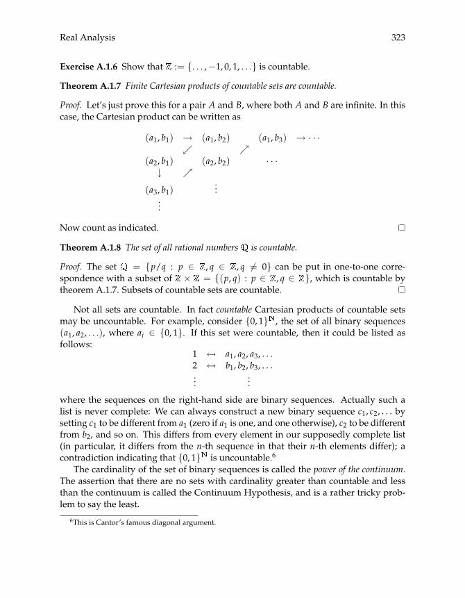
Real Analysis 323
Exercise A.1.6 Show that := {. . . ,−1, 0, 1, . . .} is countable.
Theorem A.1.7 Finite Cartesian products of countable sets are countable.
Proof. Let’s just prove this for a pair A and B, where both A and B are infinite. In thiscase, the Cartesian product can be written as
(a1, b1) → (a1, b2) (a1, b3) → · · ·↙ ↗
(a2, b1) (a2, b2) · · ·↓ ↗
(a3, b1)...
...
Now count as indicated.
Theorem A.1.8 The set of all rational numbers is countable.
Proof. The set = {p/q : p ∈ , q ∈ , q �= 0} can be put in one-to-one corre-spondence with a subset of × = {(p, q) : p ∈ , q ∈ }, which is countable bytheorem A.1.7. Subsets of countable sets are countable.
Not all sets are countable. In fact countable Cartesian products of countable setsmay be uncountable. For example, consider {0, 1} , the set of all binary sequences(a1, a2, . . .), where ai ∈ {0, 1}. If this set were countable, then it could be listed asfollows:
1 ↔ a1, a2, a3, . . .2 ↔ b1, b2, b3, . . ....
...
where the sequences on the right-hand side are binary sequences. Actually such alist is never complete: We can always construct a new binary sequence c1, c2, . . . bysetting c1 to be different from a1 (zero if a1 is one, and one otherwise), c2 to be differentfrom b2, and so on. This differs from every element in our supposedly complete list(in particular, it differs from the n-th sequence in that their n-th elements differ); acontradiction indicating that {0, 1} is uncountable.6
The cardinality of the set of binary sequences is called the power of the continuum.The assertion that there are no sets with cardinality greater than countable and lessthan the continuum is called the Continuum Hypothesis, and is a rather tricky prob-lem to say the least.
6This is Cantor’s famous diagonal argument.

324 Appendix A
A.1.3 Basic Probability
In this section we briefly recall some elements of probability on finite sets. Considera finite set Ω, a typical element of which is ω. A probability on Ω is a function fromP(Ω), the set of all subsets of Ω, into [0, 1] with properties
1. (Ω) = 1, and
2. if A, B ⊂ Ω and A ∩ B = ∅, then (A ∪ B) = (A) + (B).
The pair (Ω, ) is sometimes called a finite probability space. Subsets ofΩ are also calledevents. The elements ω that make up Ω are the primitive events, while general B ⊂ Ωis a composite event, consisting of M ≤ #Ω primitive events.7 The number (B) is the“probability that event B occurs.” In other words, (B) represents the probability thatwhen uncertainty is resolved and some ω ∈ Ω is selected by “nature,” the statementω ∈ B is true.
Exercise A.1.9 Let p : Ω→ [0, 1], where ∑ω∈Ω p(ω) = 1, and let
(B) := ∑ω∈B
p(ω) (B ⊂ Ω) (A.1)
Show that properties (1) and (2) both hold for defined in (A.1).
The next few results follow easily from the definition of a probability.
Lemma A.1.10 If A ⊂ Ω, then (Ac) = 1− (A).
Proof. Here of course Ac := Ω \ A. The proof is immediate from (1) and (2) abovebecause 1 = (Ω) = (A ∪ Ac) = (A) + (Ac).
Exercise A.1.11 Prove that (∅) = 0. Prove that if A ⊂ B, then (B \ A) = (B)−(A). Prove further that if A ⊂ B, then (A) ≤ (B).
The idea that if A ⊂ B, then (A) ≤ (B) is fundamental. Event B occurs when-ever A occurs, so the probability of B is larger. Many crucial ideas in probability boildown to this one point.
Exercise A.1.12 Prove that if A and B are (not necessarily disjoint) subsets of Ω, then(A ∪ B) ≤ (A) + (B). Construct an example of a probability and subsets A, B
such that this inequality is strict. Show that in general, (A ∪ B) = (A) + (B)−(A ∩ B).7If A is a set, then #A denotes the number of elements in A.
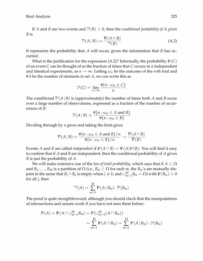
Real Analysis 325
If A and B are two events and (B) > 0, then the conditional probability of A givenB is
(A | B) :=(A ∩ B)
(B)(A.2)
It represents the probability that A will occur, given the information that B has oc-curred.
What is the justification for the expression (A.2)? Informally, the probability (C)of an event C can be thought of as the fraction of times that C occurs in n independentand identical experiments, as n → ∞. Letting ωn be the outcome of the n-th trial and#A be the number of elements in set A, we can write this as
(C) = limn→∞
#{n : ωn ∈ C}n
The conditional (A | B) is (approximately) the number of times both A and B occurover a large number of observations, expressed as a fraction of the number of occur-rences of B:
(A | B) � #{n : ωn ∈ A and B}#{n : ωn ∈ B}
Dividing through by n gives and taking the limit gives
(A | B) � #{n : ωn ∈ A and B}/n#{n : ωn ∈ B}/n → (A ∩ B)
(B)
Events A and B are called independent if (A ∩ B) = (A) (B). You will find it easyto confirm that if A and B are independent, then the conditional probability of A givenB is just the probability of A.
We will make extensive use of the law of total probability, which says that if A ⊂ Ωand B1, . . . , BM is a partition of Ω (i.e., Bm ⊂ Ω for each m, the Bm’s are mutually dis-joint in the sense that Bj ∩ Bk is empty when j �= k, and ∪Mm=1Bm = Ω) with (Bm) > 0for all j, then
(A) =M
∑m=1
(A | Bm) · (Bm)
The proof is quite straightforward, although you should check that the manipulationsof intersections and unions work if you have not seen them before:
(A) = (A ∩ ∪Mm=1Bm) = (∪Mm=1(A ∩ Bm))
=M
∑m=1
(A ∩ Bm) =M
∑m=1
(A | Bm) · (Bm)
326 Appendix A
Now consider a random variable taking values in some collection of numbers S. For-mally, a random variable X is a function from the sample space Ω into S. The idea isthat “nature” picks out an element ω inΩ according to some probability. The randomvariable now sends this ω into X(ω) ∈ S. We can think of X as “reporting” the out-come of the draw to us in a format that is more amenable to analysis. For example,Ω might be a collection of binary sequences, and X translates these sequences into(decimal) numbers.
Each probability on Ω and X : Ω→ S induces a distribution8 φ on S via
φ(x) = {ω ∈ Ω : X(ω) = x} (x ∈ S) (A.3)
Exercise A.1.13 Show that φ(x) ≥ 0 and ∑x∈S φ(x) = 1.
In what follows we will often write the right-hand side of (A.3) simply as {X =x}. Please be aware of this convention. We say that X is distributed according to φ,and write X ∼ φ.
An aside: If you stick to elementary probability, then you may begin to feel that thedistinction between the underlying probability and the distribution φ of X is largelyirrelevant. Why can’t we just say that X is a random variable with distribution φ, andY is another random variable with distribution ψ? The meaning of these statementsseems clear, and there is no need to introduce and Ω, or to think about X and Y asfunctions.
The short answer to this question is that it is often useful to collect different ran-dom variables on the one probability space defined by Ω and . With this constructone can then discuss more complex events, such as convergence of a sequence of ran-dom variables on (Ω, ) to yet another random variable on (Ω, ).
Next we define expectation. Let X : Ω → S and let be a probability on Ω. Theexpectation X of X is given by
X := ∑ω∈Ω
X(ω) {ω} (A.4)
Exercise A.1.14 Prove that if X ∼ φ, then X = ∑x∈S xφ(x).9 Prove the more generalresult that if Y = h(X) for some real-valued function h of X (i.e., h : S→ ), then
Y := ∑ω∈Ω
h(X(ω)) {ω} = ∑x∈S
h(x)φ(x) (A.5)
8What we call a distribution here is often referred to as a probability mass function.9Hint: Divide Ω into sets Bx for x ∈ S, where Bx := {ω ∈ Ω : X(ω) = x}.

Real Analysis 327
A.2 The Real Numbers
As usual, denotes the so-called real numbers, which you can visualize as the “con-tinuous” real line. We will make use of several of its properties. One property worthmentioning before we start is that the set is uncountable. This can be proved by show-ing that is in one to one correspondence with the set of all binary sequences—whichwere shown to be uncountable in §A.1.2. (For the correspondence, think of the waythat computers represent numbers in binary form.) also has certain algebraic, order,and completeness properties, which we now detail.
A.2.1 Real Sequences
In what follows, if x ∈ then |x| denotes its absolute value. For any x, y ∈ thetriangle inequality |x+ y| ≤ |x|+ |y| holds.
Exercise A.2.1 Show that if a, b and x are any real numbers, then
|a− b| ≤ |a− x|+ |x− b| and | |x| − |a| | ≤ |x− a| (A.6)
A subset A of is called bounded if there is an M ∈ such that |x| ≤ M, allx ∈ A. The ε-ball or ε-neighborhood around a ∈ is the set of points x ∈ suchthat |a − x| < ε.10 An X-valued sequence is a function from the natural numbers
:= {1, 2, . . .} to nonempty set X, traditionally denoted by notation such as (xn). Itis called a real sequence when X ⊂ . A real sequence (xn) called bounded if its rangeis a bounded set (i.e., ∃M ∈ such that |xn| ≤ M for all n ∈ ).
A real sequence (xn) is said to be convergent if there is an x ∈ such that, givenany ε > 0, we can find an N ∈ with the property |xn − x| < ε whenever n ≥N. This property will often be expressed by saying that (xn) is eventually in anyε-neighborhood of x. The point x is called the limit of the sequence, and we writelimn→∞ xn = x or xn → x as n→ ∞.
This definition of convergence can be a little hard to grasp at first. One way isto play the “ε,N game.” If I claim that a sequence is convergent, then, for every ε-neighborhood you give me, I commit to providing you with an index N such thatall points further along the sequence than the N-th one (i.e., points xN , xN+1, . . .) arein that ε-neighborhood. For example, consider xn = 1/n2. I claim xn converges tozero. When you give me ε = 1/3, I can give you N = 2, because n ≥ 2 impliesxn = 1/n2 ≤ 1/4 < ε. In fact I can give you an “algorithm” for generating such an N:Given ε > 0, take any N ∈ greater than 1/
√ε.
Sometimes the “points” ∞ and −∞ can are regarded as limits of sequences. Inwhat follows, we will say that xn → ∞, or limn xn = ∞, if for each M ∈ there is an
10This “ball” will look more ball-like once we move to higher dimensional spaces.
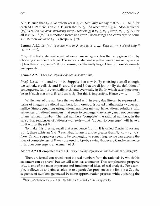
328 Appendix A
N ∈ such that xn ≥ M whenever n ≥ N. Similarly we say that xn → −∞ if, foreach M ∈ there is an N ∈ such that xn ≤ −M whenever n ≥ N. Also, sequence(xn) is called monotone increasing (resp., decreasing) if xn ≤ xn+1 (resp, xn+1 ≤ xn) forall n ∈ . If (xn) is monotone increasing (resp., decreasing) and converges to somex ∈ , then we write xn ↑ x (resp., xn ↓ x).Lemma A.2.2 Let (xn) be a sequence in , and let x ∈ . Then xn → x if and only if|xn − x| → 0.
Proof. The first statement says that we can make |xn − x| less than any given ε > 0 bychoosing n sufficiently large. The second statement says that we can make ||xn − x| −0| less than any given ε > 0 by choosing n sufficiently large. Clearly, these statementsare equivalent.
Lemma A.2.3 Each real sequence has at most one limit.
Proof. Let xn → a and xn → b. Suppose that a �= b. By choosing ε small enough,we can take ε-balls Ba and Bb around a and b that are disjoint.11 By the definition ofconvergence, (xn) is eventually in Ba and eventually in Bb. In which case there mustbe an N such that xN ∈ Ba and xN ∈ Bb. But this is impossible. Hence a = b.
While most of the numbers that we deal with in every day life can be expressed interms of integers or rational numbers, for more sophisticated mathematics does notsuffice. Simple equations using rational numbers may not have rational solutions, andsequences of rational numbers that seem to converge to something may not convergeto any rational number. The real numbers “complete” the rational numbers, in thesense that sequences of rationals—or reals—that “appear to converge” will have alimit within the set .
To make this precise, recall that a sequence (xn) in is called Cauchy if, for anyε > 0, there exists an N ∈ such that for any n and m greater than N, |xn − xm| < ε.Now Cauchy sequences seem to be converging to something, so we can express theidea of completeness of —as opposed to —by saying that every Cauchy sequencein does converge to an element of .
Axiom A.2.4 (Completeness of ) Every Cauchy sequence on the real line is convergent.
There are formal constructions of the real numbers from the rationals by which thisstatement can be proved, but we will take it as axiomatic. This completeness propertyof is one of the most important and fundamental ideas of real analysis. For exam-ple, it allows us to define a solution to a particular problem as the limit of a Cauchysequence of numbers generated by some approximation process, without fearing the
11Using (A.6), show that if ε < |a− b|/2, then x ∈ Ba and x ∈ Bb is impossible.
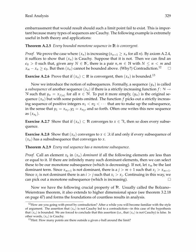
Real Analysis 329
embarrassment that would result should such a limit point fail to exist. This is impor-tant because many types of sequences are Cauchy. The following example is extremelyuseful in both theory and applications:
Theorem A.2.5 Every bounded monotone sequence in is convergent.
Proof. We prove the case where (xn) is increasing (xn+1 ≥ xn for all n). By axiom A.2.4,it suffices to show that (xn) is Cauchy. Suppose that it is not. Then we can find anε0 > 0 such that, given any N ∈ , there is a pair n,m ∈ with N ≤ n < m andxm − xn ≥ ε0. But then (xn) cannot be bounded above. (Why?) Contradiction.12
Exercise A.2.6 Prove that if (xn) ⊂ is convergent, then (xn) is bounded.13
Now we introduce the notion of subsequences. Formally, a sequence (yn) is calleda subsequence of another sequence (xn) if there is a strictly increasing function f : →
such that yn = x f (n) for all n ∈ . To put it more simply, (yn) is the original se-quence (xn) but with some points omitted. The function f picks out a strictly increas-ing sequence of positive integers n1 < n2 < · · · that are to make up the subsequence,in the sense that y1 = xn1 , y2 = xn2 , and so forth. Often one writes this new sequenceas (xnk ).
Exercise A.2.7 Show that if (xn) ⊂ converges to x ∈ , then so does every subse-quence.
Exercise A.2.8 Show that (xn) converges to x ∈ if and only if every subsequence of(xn) has a subsubsequence that converges to x.
Theorem A.2.9 Every real sequence has a monotone subsequence.
Proof. Call an element xk in (xn) dominant if all the following elements are less thanor equal to it. If there are infinitely many such dominant elements, then we can selectthese to be our monotone subsequence (which is decreasing). If not, let xm be the lastdominant term. Since xm+1 is not dominant, there is a j > m+ 1 such that xj > xm+1.Since xj is not dominant there is an i > j such that xi > xj. Continuing in this way, wecan pick out a monotone subsequence (which is increasing).
Now we have the following crucial property of . Usually called the Bolzano–Weierstrass theorem, it also extends to higher dimensional space (see theorem 3.2.18on page 47) and forms the foundations of countless results in analysis.
12How are you going with proof by contradiction? After a while you will become familiar with the styleof argument. The assertion that (xn) is not Cauchy led to a contradiction—in this case of the hypothesisthat (xn) is bounded. We are forced to conclude that this assertion (i.e., that (xn) is not Cauchy) is false. Inother words, (xn) is Cauchy.
13Hint: How many points are there outside a given ε-ball around the limit?

330 Appendix A
Theorem A.2.10 Every bounded sequence in has a convergent subsequence.
Proof. Take a given sequence in . By theorem A.2.9, the sequence has a monotonesubsequence, which is a sequence in its own right. Evidently this sequence is alsobounded. By theorem A.2.5, every bounded monotone sequence converges.
The next result is important in practice, and the proof is an exercise.
TheoremA.2.11 Let (xn) and (yn) be two sequences in , with lim xn = x and lim yn = y.If xn ≤ yn for all n ∈ , then x ≤ y.14
Often when we use this result one sequence will be a constant. For example, ifxn ≤ b for all n ∈ , then lim xn ≤ b. Note that taking limits does not preserve strictordering! For example, 1/n > 0 for all n, but limn 1/n > 0 is false.
Theorem A.2.12 Let (xn), (yn) and (zn) be three sequences in , with xn ≤ yn ≤ zn forall n ∈ . If xn → a and zn → a both hold, then yn → a.
Proof. Fix ε > 0. We can choose an N ∈ such that if n ≥ N, then xn > a− ε andzn < a+ ε. (Why?) For such n we must have |yn − a| < ε.
You might have thought it would be simpler to argue that, since xn ≤ yn ≤ zn forall n, we have lim xn ≤ lim yn ≤ lim zn from theorem A.2.11. But this is not permissi-ble because we did not know at the start of the proof that lim yn exists. Theorem A.2.11expressly requires that the limits exist. (This is an easy mistake to make.)
Theorem A.2.13 Let (xn) and (yn) be real sequences. If xn → x and yn → y, then xn +yn → x+ y.
Proof. Fix ε > 0. By the triangle inequality,
|(xn + yn)− (x+ y)| ≤ |xn − x|+ |yn − y| (A.7)
Choose N ∈ such that |xn − x| < ε/2 whenever n ≥ N, and N′ ∈ such that|yn − y| < ε/2 whenever n ≥ N′. For n ≥ max{N,N′}, the right-hand side of (A.7) isless than ε.
Exercise A.2.14 Show that if a ∈ and xn → x, then axn → ax.
Theorem A.2.15 Let (xn) and (yn) be real sequences. If xn → x and yn → y, then xnyn →xy.
14Hint for the proof: Suppose that x > y. Take ε-balls around each point that do not intersect. (Convinceyourself that this is possible.) Now try to contradict xn ≤ yn for all n.
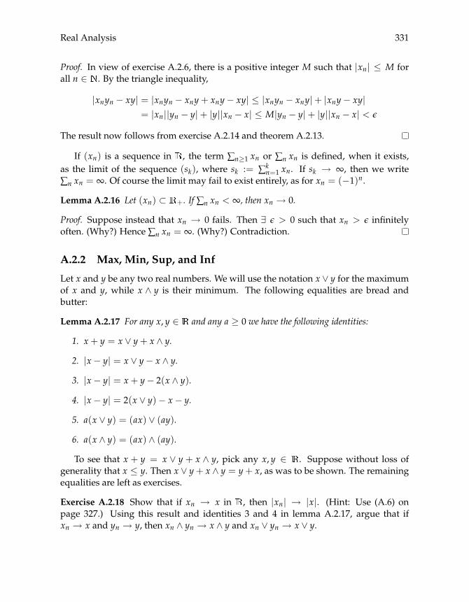
Real Analysis 331
Proof. In view of exercise A.2.6, there is a positive integer M such that |xn| ≤ M forall n ∈ . By the triangle inequality,
|xnyn − xy| = |xnyn − xny+ xny− xy| ≤ |xnyn − xny|+ |xny− xy|= |xn||yn − y|+ |y||xn − x| ≤ M|yn − y|+ |y||xn − x| < ε
The result now follows from exercise A.2.14 and theorem A.2.13.
If (xn) is a sequence in , the term ∑n≥1 xn or ∑n xn is defined, when it exists,as the limit of the sequence (sk), where sk := ∑k
n=1 xn. If sk → ∞, then we write∑n xn = ∞. Of course the limit may fail to exist entirely, as for xn = (−1)n.
Lemma A.2.16 Let (xn) ⊂ +. If ∑n xn < ∞, then xn → 0.
Proof. Suppose instead that xn → 0 fails. Then ∃ ε > 0 such that xn > ε infinitelyoften. (Why?) Hence ∑n xn = ∞. (Why?) Contradiction.
A.2.2 Max, Min, Sup, and Inf
Let x and y be any two real numbers. We will use the notation x ∨ y for the maximumof x and y, while x ∧ y is their minimum. The following equalities are bread andbutter:
Lemma A.2.17 For any x, y ∈ and any a ≥ 0 we have the following identities:
1. x+ y = x ∨ y+ x ∧ y.2. |x− y| = x ∨ y− x ∧ y.3. |x− y| = x+ y− 2(x ∧ y).4. |x− y| = 2(x ∨ y)− x− y.
5. a(x ∨ y) = (ax) ∨ (ay).
6. a(x ∧ y) = (ax) ∧ (ay).
To see that x + y = x ∨ y + x ∧ y, pick any x, y ∈ . Suppose without loss ofgenerality that x ≤ y. Then x ∨ y+ x ∧ y = y+ x, as was to be shown. The remainingequalities are left as exercises.
Exercise A.2.18 Show that if xn → x in , then |xn| → |x|. (Hint: Use (A.6) onpage 327.) Using this result and identities 3 and 4 in lemma A.2.17, argue that ifxn → x and yn → y, then xn ∧ yn → x ∧ y and xn ∨ yn → x ∨ y.

332 Appendix A
If A ⊂ , the maximum of A, when it exists, is a number m ∈ A with a ≤ m for alla ∈ A. The minimum is defined analogously. For any finite collection of real numbers,the maximum and minimum always exist. For infinite collections this is not the case.To deal with infinite sets we introduce the notion of suprema and infima.
Given a set A ⊂ , an upper bound of A is any number u such that a ≤ u for alla ∈ A. If s ∈ is an upper bound for A and also satisfies s ≤ u for every upper boundu of A, then s is called the supremum of A. You will be able to verify that at most onesuch s exists. We write s = sup A.
Lemma A.2.19 Suppose that s is an upper bound of A. The following statements are thenequivalent:
1. s = sup A.
2. s ≤ u for all upper bounds u of A.
3. ∀ ε > 0, ∃ a ∈ A with a > s− ε.
4. There exists a sequence (an) ⊂ A with an ↑ s.Exercise A.2.20 Prove lemma A.2.19.
Exercise A.2.21 Show that sup(0, 1) = 1 and sup(0, 1] = 1. Show that if a set Acontains one of its upper bounds u, then u = sup A.
Theorem A.2.22 Every nonempty subset of that is bounded above has a supremum in .
The proof is omitted, but this is in fact equivalent to axiom A.2.4. Either one can betreated as the axiom. They assert the “completeness” of the real numbers.
If A is not bounded above, then it is conventional to set sup A := ∞. With thisconvention, the following statement is true:
Lemma A.2.23 If A, B ⊂ with A ⊂ B, then sup A ≤ sup B.
Proof. If sup B = ∞ the result is trivial. Suppose instead that B is bounded above,and let b := sup B, a = sup A. By lemma A.2.19, there is a sequence (an) ⊂ A withan ↑ a. But b is an upper bound for A (why?), so an ≤ b for all n. It now follows fromtheorem A.2.11 that a = lim an ≤ b.
For A ⊂ a lower bound of A is any number l such that a ≥ l for all a ∈ A. Ifi ∈ is an lower bound for A and also satisfies i ≥ l for every lower bound l of A,then i is called the infimum of A. At most one such i exists. We write i = inf A. Everynonempty subset of bounded from below has an infimum.
Exercise A.2.24 Let A be bounded below. Show that i = inf A if and only if i is a lowerbound of A and, for each ε > 0, there is an a ∈ A with a < i+ ε.
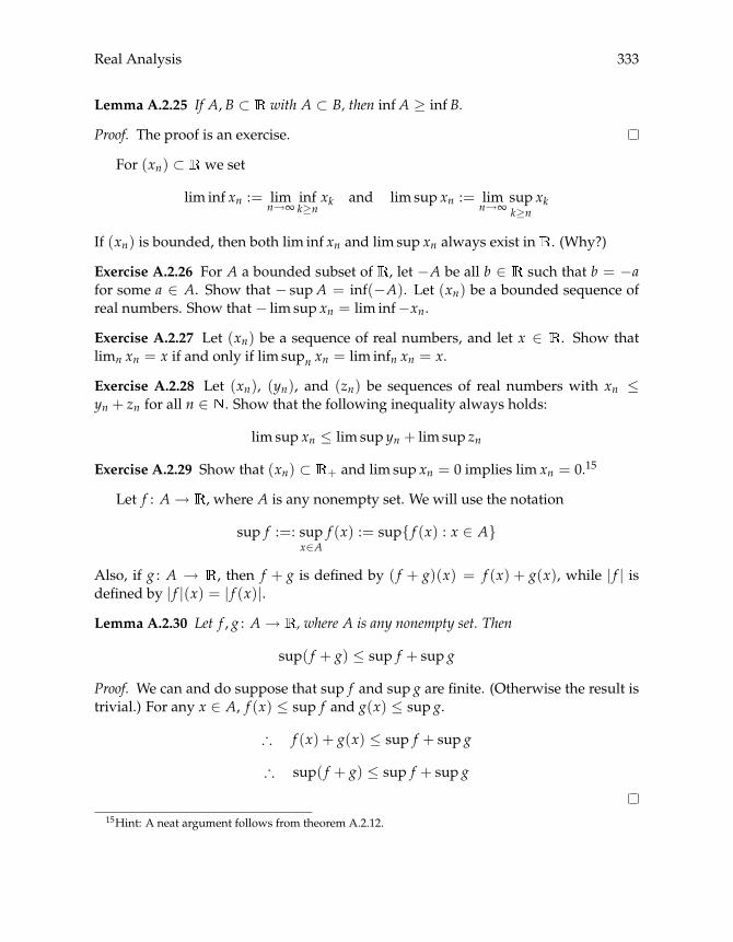
Real Analysis 333
Lemma A.2.25 If A, B ⊂ with A ⊂ B, then inf A ≥ inf B.
Proof. The proof is an exercise.
For (xn) ⊂ we set
lim inf xn := limn→∞ inf
k≥nxk and lim sup xn := lim
n→∞ supk≥n
xk
If (xn) is bounded, then both lim inf xn and lim sup xn always exist in . (Why?)
Exercise A.2.26 For A a bounded subset of , let −A be all b ∈ such that b = −afor some a ∈ A. Show that − sup A = inf(−A). Let (xn) be a bounded sequence ofreal numbers. Show that − lim sup xn = lim inf−xn.Exercise A.2.27 Let (xn) be a sequence of real numbers, and let x ∈ . Show thatlimn xn = x if and only if lim supn xn = lim infn xn = x.
Exercise A.2.28 Let (xn), (yn), and (zn) be sequences of real numbers with xn ≤yn + zn for all n ∈ . Show that the following inequality always holds:
lim sup xn ≤ lim sup yn + lim sup zn
Exercise A.2.29 Show that (xn) ⊂ + and lim sup xn = 0 implies lim xn = 0.15
Let f : A→ , where A is any nonempty set. We will use the notation
sup f :=: supx∈A
f (x) := sup{ f (x) : x ∈ A}
Also, if g : A → , then f + g is defined by ( f + g)(x) = f (x) + g(x), while | f | isdefined by | f |(x) = | f (x)|.Lemma A.2.30 Let f , g : A→ , where A is any nonempty set. Then
sup( f + g) ≤ sup f + sup g
Proof. We can and do suppose that sup f and sup g are finite. (Otherwise the result istrivial.) For any x ∈ A, f (x) ≤ sup f and g(x) ≤ sup g.
∴ f (x) + g(x) ≤ sup f + sup g
∴ sup( f + g) ≤ sup f + sup g
15Hint: A neat argument follows from theorem A.2.12.

334 Appendix A
Lemma A.2.31 If f : A→ , then | sup f | ≤ sup | f |.Proof. We can and do suppose that sup | f | < ∞. Evidently sup f ≤ sup | f |.16 Tocomplete the proof, we need only show that − sup f ≤ sup | f | also holds. This is thecase because
0 = sup(− f + f ) ≤ sup(− f ) + sup f ≤ sup | f |+ sup f
Exercise A.2.32 Show via counterexample that the statement | sup f | = sup | f | doesnot hold in general.
Let A ⊂ . A function f : A → is called monotone increasing on A if, wheneverx, y ∈ A and x ≤ y, we have f (x) ≤ f (y). It is called monotone decreasing if, wheneverx ≤ y, we have f (x) ≥ f (y). We say strictly monotone increasing or strictly monotonedecreasing if the previous inequalities can be replaced with strict inequalities.
Exercise A.2.33 Let S be any set, let g : S → , and let x be a maximizer of g on S,in the sense that g(x) ≥ g(x) for all x ∈ S. Prove that if f : → is monotoneincreasing, then x is a maximizer of f ◦ g on S.
A.2.3 Functions of a Real Variable
Let’s recall some basics about functions when send subsets of into . Below wedefine such concepts as continuity, differentiability, convexity, and concavity. If youare rusty on these definitions, then it is probably worth skim-reading this section andcompleting a few of the exercises.
Let A ⊂ and let f , g : A → . As usual, the sum of f and g is the functionf + g defined by ( f + g)(x) := f (x) + g(x). Similarly, the product f g is defined by( f g)(x) := f (x)g(x). The product of real number α and f is the function (α f )(x) :=α f (x). Recall that f is called bounded if its range is a bounded set (i.e., ∃M ∈ suchthat | f (a)| ≤ M for all a ∈ A).
Exercise A.2.34 Show that if f and g are bounded and α ∈ , then f + g, f g, and α fare also bounded functions.
Function f : A → is said to be continuous at a ∈ A if for every sequence (xn) inA converging to a we have f (xn) → f (a). (Sketch it.) It is called continuous on A (orjust continuous) whenever it is continuous at every a ∈ A. Continuity of functionscaptures the idea that small changes to the input do not lead to sudden jumps in the
16Pick any x ∈ A. Then f (x) ≤ | f (x)| ≤ sup | f |. Since x is arbitrary, sup f ≤ sup | f |.

Real Analysis 335
output. Notice that in requiring that f (xn)→ f (a) for each xn → a, we require that notonly does f (xn) actually converge for each choice of xn → a, but all these sequencesconverge to the same limit, and moreover that limit is f (a).
Exercise A.2.35 Prove carefully that the functions f (x) = x + 1 and g(x) = x2 arecontinuous. Give an example of a function that is not continuous, showing how itfails the definition.
More generally, for the same f : A→ and for a ∈ A, we say that y = limx→a f (x)if f (xn) → y for every sequence (xn) ⊂ A with xn → a. Note that limx→a f (x) maynot exist. It may be the case that different sequences converging to a yield differentlimits for the sequence f (xn), or indeed that f (xn) does not converge at all. But thisnew notation is useful because we can now say that f is continuous at a if and only iflimx→a f (x) exists and is equal to f (a).
Exercise A.2.36 Show that if f and g are continuous functions and α ∈ , then f + g,f g and α f are also continuous.
Exercise A.2.37 A function f : A → is said to be continuous from the left at x ∈ Aif f (xn) → f (x) for every sequence xn ↑ x; and continuous from the right at x ∈ Aif f (xn) → f (x) for every sequence xn ↓ x. Clearly, a function continuous at x isboth continuous from the left at x and continuous from the right at x. Show that theconverse also holds.17
One of the many delightful results concerning continuous functions is the inter-mediate value theorem:
Theorem A.2.38 Let f : [a, b] → , where a < b. If f is continuous on [a, b] and f (a) <0 < f (b), then there exists an s ∈ (a, b) with f (s) = 0.
Proof. Let A := {x ∈ [a, b] : f (x) < 0}, and let s be the supremum of this set. (Whycan we be sure that such a supremum exists?) We claim that f (s) = 0. To see whythis must be the case, observe that since s = sup A there exists a sequence (xn) withf (xn) < 0 and xn ↑ s. (Why?) By continuity of f , we have lim f (xn) = f (s). Butf (xn) < 0 for all n, so lim f (xn) ≤ 0. Hence f (s) ≤ 0. On the other hand, since s is anupper bound of A, we know that x > s implies x /∈ A, in which case f (x) ≥ 0. Takea strictly decreasing sequence (xn) in (s, b] with xn ↓ s. (Convince yourself that sucha sequence does exist.) As f (xn) ≥ 0 for all n it follows that lim f (xn) = f (s) ≥ 0.Therefore f (s) = 0.
Exercise A.2.39 Using theorem A.2.38 (the result, not the proof), show that the sameresult holds when f (b) < 0 < f (a).
17Hint: You might like to make use of exercise A.2.8 and theorem A.2.9.
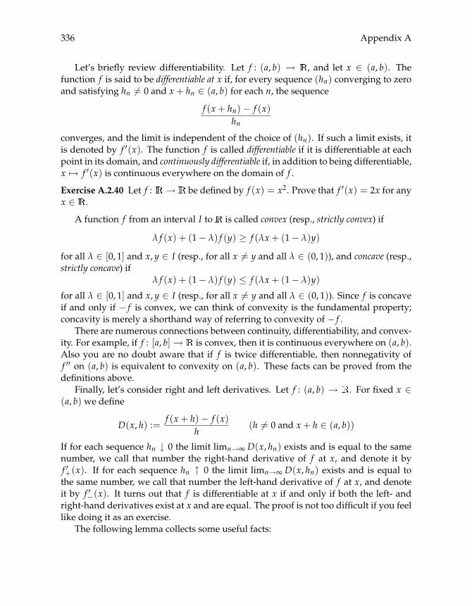
336 Appendix A
Let’s briefly review differentiability. Let f : (a, b) → , and let x ∈ (a, b). Thefunction f is said to be differentiable at x if, for every sequence (hn) converging to zeroand satisfying hn �= 0 and x+ hn ∈ (a, b) for each n, the sequence
f (x+ hn)− f (x)hn
converges, and the limit is independent of the choice of (hn). If such a limit exists, itis denoted by f ′(x). The function f is called differentiable if it is differentiable at eachpoint in its domain, and continuously differentiable if, in addition to being differentiable,x �→ f ′(x) is continuous everywhere on the domain of f .
Exercise A.2.40 Let f : → be defined by f (x) = x2. Prove that f ′(x) = 2x for anyx ∈ .
A function f from an interval I to is called convex (resp., strictly convex) if
λ f (x) + (1− λ) f (y) ≥ f (λx+ (1− λ)y)
for all λ ∈ [0, 1] and x, y ∈ I (resp., for all x �= y and all λ ∈ (0, 1)), and concave (resp.,strictly concave) if
λ f (x) + (1− λ) f (y) ≤ f (λx+ (1− λ)y)
for all λ ∈ [0, 1] and x, y ∈ I (resp., for all x �= y and all λ ∈ (0, 1)). Since f is concaveif and only if − f is convex, we can think of convexity is the fundamental property;concavity is merely a shorthand way of referring to convexity of − f .
There are numerous connections between continuity, differentiability, and convex-ity. For example, if f : [a, b]→ is convex, then it is continuous everywhere on (a, b).Also you are no doubt aware that if f is twice differentiable, then nonnegativity off ′′ on (a, b) is equivalent to convexity on (a, b). These facts can be proved from thedefinitions above.
Finally, let’s consider right and left derivatives. Let f : (a, b) → . For fixed x ∈(a, b) we define
D(x, h) :=f (x+ h)− f (x)
h(h �= 0 and x+ h ∈ (a, b))
If for each sequence hn ↓ 0 the limit limn→∞ D(x, hn) exists and is equal to the samenumber, we call that number the right-hand derivative of f at x, and denote it byf ′+(x). If for each sequence hn ↑ 0 the limit limn→∞ D(x, hn) exists and is equal tothe same number, we call that number the left-hand derivative of f at x, and denoteit by f ′−(x). It turns out that f is differentiable at x if and only if both the left- andright-hand derivatives exist at x and are equal. The proof is not too difficult if you feellike doing it as an exercise.
The following lemma collects some useful facts:

Real Analysis 337
Lemma A.2.41 If f is concave on (a, b), then f ′+ and f ′− exist everywhere on (a, b). For eachx ∈ (a, b),
f ′+(x) = suph>0
D(x, h) and f ′−(x) = infh<0
D(x, h)
Moreover f ′+ ≤ f ′− everywhere on (a, b). If f ′+(x) = f ′−(x) at some point x ∈ (a, b), then fis differentiable at x, and f ′(x) = f ′+(x) = f ′−(x).
Exercise A.2.42 Prove lemma A.2.41. First show that when f is concave, D(x, h) is de-creasing in h. Next apply existence results for limits of monotone bounded sequences.


Appendix B
Chapter Appendixes
B.1 Appendix to Chapter 3
Let us briefly discuss the topic of parametric continuity. The question we address iswhether or not the solution to a given optimization problem varies continuously withthe parameters that define the problem. The classic theorem in this area is Berge’stheorem of the maximum. You should familiarize yourself at least with the statementof the theorem.
To begin, let A and B be two sets. A function Γ from A into P(B) (i.e., into thesubsets of B) is called a correspondence from A to B. Correspondences are often usedto define constraint sets. For example, a ∈ A might be the price of a commodity, ora level of wealth, and Γ(a) ⊂ B is the budget set associated with that value of theparameter.
Now suppose that A and B are metric spaces, and let Γ be a correspondence fromA to B. We say that Γ is compact-valued if Γ(a) is a compact subset of B for everya ∈ A, and nonempty if Γ(a) �= ∅ for every a ∈ A. A nonempty compact-valuedcorrespondence Γ from A to B is called upper-hemicontinuous at a ∈ A if, for eachsequence (an) ⊂ A with an → a, and each sequence (bn) ⊂ B with bn ∈ Γ(an) forall n ∈ , the sequence (bn) has a convergent subsequence whose limit is in Γ(a).It is called lower-hemicontinuous at a if, for each (an) ⊂ A with an → a and eachb ∈ Γ(a), there is a sequence (bn) ⊂ B with bn ∈ Γ(an) for all n ∈ , and bn → bas n → ∞. Finally, Γ is called continuous at a if it is both upper-hemicontinuous andlower-hemicontinuous at a. It is called continuous if it is continuous at a for eacha ∈ A.
The following lemma treats an important special case:
339
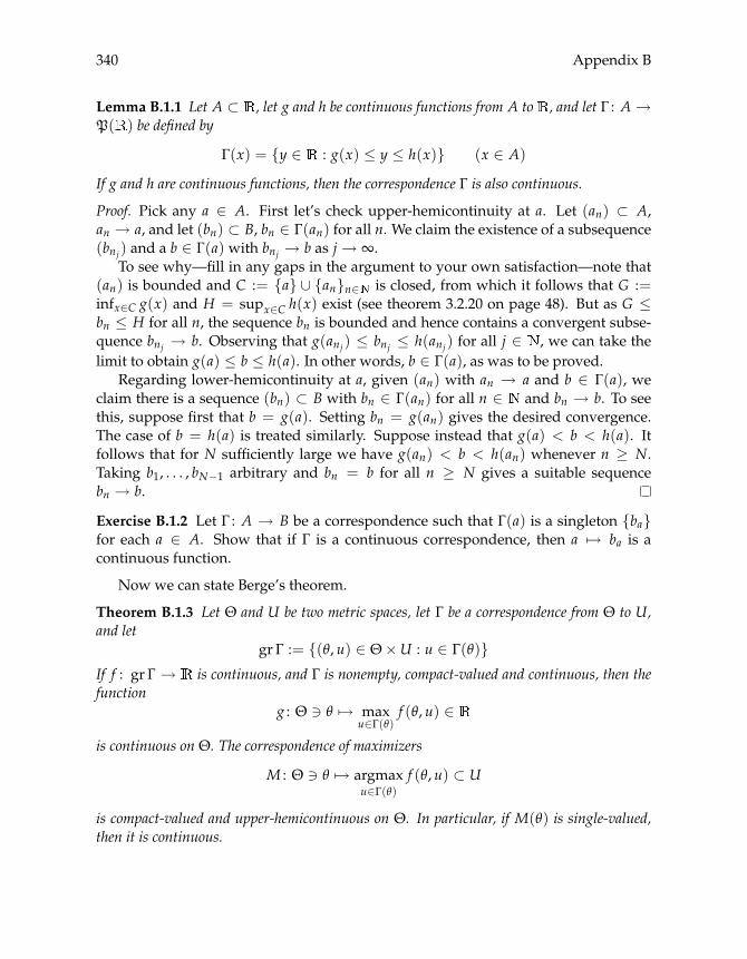
340 Appendix B
Lemma B.1.1 Let A ⊂ , let g and h be continuous functions from A to , and let Γ : A→P( ) be defined by
Γ(x) = {y ∈ : g(x) ≤ y ≤ h(x)} (x ∈ A)
If g and h are continuous functions, then the correspondence Γ is also continuous.
Proof. Pick any a ∈ A. First let’s check upper-hemicontinuity at a. Let (an) ⊂ A,an → a, and let (bn) ⊂ B, bn ∈ Γ(an) for all n. We claim the existence of a subsequence(bnj) and a b ∈ Γ(a) with bnj → b as j→ ∞.
To see why—fill in any gaps in the argument to your own satisfaction—note that(an) is bounded and C := {a} ∪ {an}n∈ is closed, from which it follows that G :=infx∈C g(x) and H = supx∈C h(x) exist (see theorem 3.2.20 on page 48). But as G ≤bn ≤ H for all n, the sequence bn is bounded and hence contains a convergent subse-quence bnj → b. Observing that g(anj) ≤ bnj ≤ h(anj) for all j ∈ , we can take thelimit to obtain g(a) ≤ b ≤ h(a). In other words, b ∈ Γ(a), as was to be proved.
Regarding lower-hemicontinuity at a, given (an) with an → a and b ∈ Γ(a), weclaim there is a sequence (bn) ⊂ B with bn ∈ Γ(an) for all n ∈ and bn → b. To seethis, suppose first that b = g(a). Setting bn = g(an) gives the desired convergence.The case of b = h(a) is treated similarly. Suppose instead that g(a) < b < h(a). Itfollows that for N sufficiently large we have g(an) < b < h(an) whenever n ≥ N.Taking b1, . . . , bN−1 arbitrary and bn = b for all n ≥ N gives a suitable sequencebn → b.
Exercise B.1.2 Let Γ : A → B be a correspondence such that Γ(a) is a singleton {ba}for each a ∈ A. Show that if Γ is a continuous correspondence, then a �→ ba is acontinuous function.
Now we can state Berge’s theorem.
Theorem B.1.3 Let Θ and U be two metric spaces, let Γ be a correspondence from Θ to U,and let
gr Γ := {(θ, u) ∈ Θ×U : u ∈ Γ(θ)}If f : gr Γ → is continuous, and Γ is nonempty, compact-valued and continuous, then thefunction
g : Θ � θ �→ maxu∈Γ(θ)
f (θ, u) ∈
is continuous on Θ. The correspondence of maximizers
M : Θ � θ �→ argmaxu∈Γ(θ)
f (θ, u) ⊂ U
is compact-valued and upper-hemicontinuous on Θ. In particular, if M(θ) is single-valued,then it is continuous.

Chapter Appendixes 341
In the theorem, continuity of f on gr Γ means that if (θ, u) ∈ gr Γ and (θn, un) is asequence in gr Γ with (θn, un) → (θ, u), then f (θn, un) → f (θ, u). (This is a strongerrequirement than assuming f is continuous in each individual argument while theother is held fixed.) The theorem is well-known to economists, and we omit the proof.See Aliprantis and Border (1999, thm. 16.31), or Stokey and Lucas (1989, thm. 3.6).
The next result is a direct implication of Berge’s theorem B.1.3 but pertains to para-metric continuity of fixed points.
Theorem B.1.4 Let Θ, U and Γ be as in theorem B.1.3. Let g : gr Γ→ U, and let
F(θ) := {u ∈ U : u = g(θ, u)} (θ ∈ Θ)
If F(θ) is nonempty for each θ ∈ Θ, g is continuous on gr Γ, and Γ is nonempty, compact-valued and continuous, then θ �→ F(θ) is compact-valued and upper-hemicontinuous on Θ.In particular, if F(θ) is single-valued, then it is continuous.
Proof. Continuity of g on gr Γ means that if (θ, u) ∈ gr Γ and (θn, un) is a sequence ingr Γ with (θn, un)→ (θ, u), then g(θn, un)→ g(θ, u). Let f : gr Γ→ be defined by
f (θ, u) = −ρ(u, g(θ, u))
where ρ is the metric on U. You will be able to show that f is also continuous ongr Γ. Theorem B.1.3 then implies that θ �→ M(θ) is compact-valued and upper-hemi-continuous, where M(θ) is the set of maximizers argmaxu∈Γ(θ) f (θ, u).
Now pick any θ ∈ Θ. As F(θ) is assumed to be nonempty, the set of maximizersof f and fixed-points of g coincide. That is, M(θ) = F(θ). Since θ is arbitrary, Mand F are the same correspondence on Θ, and θ �→ F(θ) is also compact-valued andupper-hemicontinuous.
Next we turn to the
Proof of theorem 3.2.38. Uniqueness is by exercise 3.2.34. To prove existence, definer : S → by r(x) = ρ(Tx, x). It is not too difficult to show that r is continuous (withrespect to ρ). Since S is compact, r has a minimizer x∗. But then Tx∗ = x∗ must hold,because otherwise
r(Tx∗) = ρ(TTx∗, Tx∗) < ρ(Tx∗, x∗) = r(x∗)
contradicting the definition of x∗.Next we show that Tnx → x∗ as n→ ∞ for all x ∈ S. To see this, pick any x ∈ S and
consider the real sequence (αn) defined by αn := ρ(Tnx, x∗). Since T is contracting,the sequence (αn) is monotone decreasing, and therefore converges (why?) to somelimit α ≥ 0. I claim that α = 0.

342 Appendix B
To see this, we can argue as follows: By compactness of S the sequence (Tnx) hasa subsequence (Tn(k)x) with Tn(k)x → x′ for some x′ ∈ S. It must be the case thatρ(x′, x∗) = α. The reason is that y �→ ρ(y, x∗) is continuous as a map from S to(example 3.1.12 on page 40). Hence ρ(Tn(k)x, x∗) → ρ(x′, x∗). But ρ(Tn(k)x, x∗) → αand sequences have at most one limit, so ρ(x′, x∗) = α.
It is also the case that ρ(Tx′, x∗) = α. To see this, note that by continuity of T wehave
T(Tn(k)x) = Tn(k)+1x → Tx′
Since y �→ ρ(y, x∗) is continuous, we have ρ(Tn(k)+1x, x∗) → ρ(Tx′, x∗). At the sametime, ρ(Tn(k)+1x, x∗)→ α is also true, so ρ(Tx′, x∗) = α.
We have established the existence of a point x′ ∈ S such that both ρ(x′, x∗) andρ(Tx′, x∗) are equal to α. If α > 0 the points x′ and x∗ are distinct, implying
α = ρ(x′, x∗) > ρ(Tx′, Tx∗) = ρ(Tx′, x∗) = α
Contradiction.
B.2 Appendix to Chapter 4
We now provide the proof of theorem 4.3.17 on page 89. To begin our proof, considerthe following result:
Lemma B.2.1 If φ and ψ are elements ofP(S) and h : S→ +, then∣∣∣∣∣∑x∈S h(x)φ(x)− ∑x∈S h(x)ψ(x)
∣∣∣∣∣ ≤ 12
supx,x′|h(x)− h(x′)| · ‖φ− ψ‖1
Proof. Let ρ(x) := φ(x)− ψ(x), ρ+(x) := ρ(x) ∨ 0, ρ−(x) := (−ρ(x)) ∨ 0. It is left tothe reader to show that ρ(x) = ρ+(x)− ρ−(x), that |ρ(x)| = ρ+(x) + ρ−(x), and that∑x∈S ρ+(x) = ∑x∈S ρ−(x) = (1/2)‖ρ‖1.
In view of the equality |a− b| = a ∨ b− a ∧ b (lemma A.2.17, page 331), we have∣∣∑ hφ−∑ hψ∣∣ =
∣∣∑ hρ∣∣ =
∣∣∑ hρ+ −∑ hρ−∣∣
=(∑ hρ+
) ∨ (∑ hρ−
)− (∑ hρ+
) ∧ (∑ hρ−
)Consider the two terms to the right of the last equality. If sup h := supx∈S h(x) andinf h := infx∈S h(x), then the first term satisfies(
∑ hρ+) ∨ (∑ hρ−
) ≤ (sup h∑ ρ+
) ∨ (sup h∑ ρ−
)= sup h
(∑ ρ+
) ∨ (∑ ρ−
)= sup h
‖ρ‖12
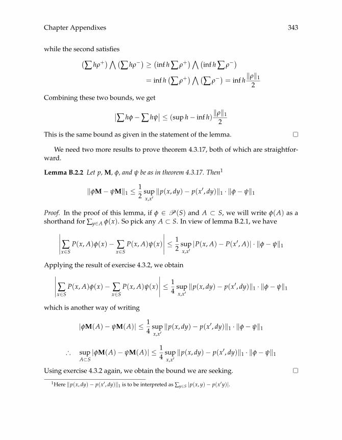
Chapter Appendixes 343
while the second satisfies(∑ hρ+
) ∧ (∑ hρ−
) ≥ (inf h∑ ρ+
) ∧ (inf h∑ ρ−
)= inf h
(∑ ρ+
) ∧ (∑ ρ−
)= inf h
‖ρ‖12
Combining these two bounds, we get
∣∣∑ hφ−∑ hψ∣∣ ≤ (sup h− inf h)
‖ρ‖12
This is the same bound as given in the statement of the lemma.
We need two more results to prove theorem 4.3.17, both of which are straightfor-ward.
Lemma B.2.2 Let p,M, φ, and ψ be as in theorem 4.3.17. Then1
‖φM− ψM‖1 ≤ 12
supx,x′‖p(x, dy)− p(x′, dy)‖1 · ‖φ− ψ‖1
Proof. In the proof of this lemma, if φ ∈ P(S) and A ⊂ S, we will write φ(A) as ashorthand for ∑y∈A φ(x). So pick any A ⊂ S. In view of lemma B.2.1, we have
∣∣∣∣∣∑x∈S P(x, A)φ(x)− ∑x∈S
P(x, A)ψ(x)
∣∣∣∣∣ ≤ 12
supx,x′|P(x, A)− P(x′, A)| · ‖φ− ψ‖1
Applying the result of exercise 4.3.2, we obtain∣∣∣∣∣∑x∈S P(x, A)φ(x)− ∑x∈S
P(x, A)ψ(x)
∣∣∣∣∣ ≤ 14
supx,x′‖p(x, dy)− p(x′, dy)‖1 · ‖φ− ψ‖1
which is another way of writing
|φM(A)− ψM(A)| ≤ 14
supx,x′‖p(x, dy)− p(x′, dy)‖1 · ‖φ− ψ‖1
∴ supA⊂S|φM(A)− ψM(A)| ≤ 1
4supx,x′‖p(x, dy)− p(x′, dy)‖1 · ‖φ− ψ‖1
Using exercise 4.3.2 again, we obtain the bound we are seeking.
1Here ‖p(x, dy)− p(x′, dy)‖1 is to be interpreted as ∑y∈S |p(x, y)− p(x′y)|.
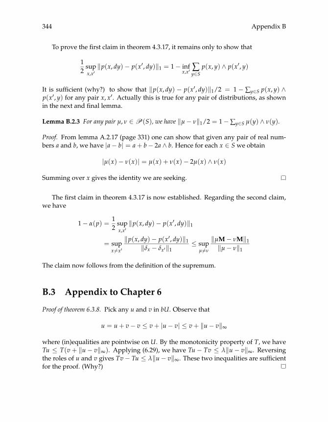
344 Appendix B
To prove the first claim in theorem 4.3.17, it remains only to show that
12
supx,x′‖p(x, dy)− p(x′, dy)‖1 = 1− inf
x,x′ ∑y∈Sp(x, y) ∧ p(x′, y)
It is sufficient (why?) to show that ‖p(x, dy) − p(x′, dy)‖1/2 = 1 − ∑y∈S p(x, y) ∧p(x′, y) for any pair x, x′. Actually this is true for any pair of distributions, as shownin the next and final lemma.
Lemma B.2.3 For any pair μ, ν ∈P(S), we have ‖μ− ν‖1/2 = 1−∑y∈S μ(y) ∧ ν(y).
Proof. From lemma A.2.17 (page 331) one can show that given any pair of real num-bers a and b, we have |a− b| = a+ b− 2a ∧ b. Hence for each x ∈ S we obtain
|μ(x)− ν(x)| = μ(x) + ν(x)− 2μ(x) ∧ ν(x)
Summing over x gives the identity we are seeking.
The first claim in theorem 4.3.17 is now established. Regarding the second claim,we have
1− α(p) =12
supx,x′‖p(x, dy)− p(x′, dy)‖1
= supx �=x′
‖p(x, dy)− p(x′, dy)‖1‖δx − δx′ ‖1
≤ supμ �=ν
‖μM− νM‖1‖μ− ν‖1
The claim now follows from the definition of the supremum.
B.3 Appendix to Chapter 6
Proof of theorem 6.3.8. Pick any u and v in bU. Observe that
u = u+ v− v ≤ v+ |u− v| ≤ v+ ‖u− v‖∞
where (in)equalities are pointwise on U. By the monotonicity property of T, we haveTu ≤ T(v+ ‖u− v‖∞). Applying (6.29), we have Tu− Tv ≤ λ‖u− v‖∞. Reversingthe roles of u and v gives Tv− Tu ≤ λ‖u− v‖∞. These two inequalities are sufficientfor the proof. (Why?)

Chapter Appendixes 345
B.4 Appendix to Chapter 8
First let us prove lemma 8.2.3, beginning with some preliminary discussion: We canextend M to act on all functions f in L1(S) by setting fM(y) :=
∫p(x, y) f (x)dx. The
inequality ‖ fM‖1 ≤ ‖ f ‖1 always holds. Under the following condition it is strict:
Lemma B.4.1 Let f ∈ L1(S). Then ‖ fM‖1 < ‖ f ‖1 if and only ifλ[( f+M) ∧ ( f−M)] > 0
Proof. In view of lemma A.2.17 (page 331) the pointwise inequality
| fM| = | f+M− f−M| = f+M+ f−M− 2( f+M) ∧ ( f−M)
holds. Integrating over S and making some simple manipulations, we have
‖ fM‖1 = λ( f+) + λ( f−)− 2λ[( f+M) ∧ ( f−M)]
∴ ‖ fM‖1 = ‖ f ‖1 − 2λ[( f+M) ∧ ( f−M)]
The proof is done.
Proof of lemma 8.2.3. Note that it is sufficient to prove the stated result for the caset = 1 because if it holds at t = 1 for an arbitrary kernel q and its associated Markovoperator N, then it holds for q := pt, and the Markov operator associated with pt isMt (lemma 8.1.13, page 196).
So choose any distinct φ,ψ ∈ D(S), and let f := φ− ψ. In view of lemma B.4.1 wewill have ‖φM− ψM‖1 < ‖φ− ψ‖ whenever∫ [(∫
p(x, y) f+(x)dx) ∧ (∫
p(x, y) f−(x)dx)]
dy > 0 (B.1)
With a little bit of effort one can show that, for each y ∈ S, we have(∫p(x, y) f+(x)dx
) ∧ (∫p(x′, y) f−(x′)dx′
)
≥∫ ∫
p(x, y) ∧ p(x′, y) f+(x) f−(x′)dxdx′
Integrating over y shows that (B.1) dominates∫ ∫ [∫p(x, y) ∧ p(x′, y)dy
]f+(x) f−(x′)dxdx′
Since the inner integral is always positive by hypothesis, and both f+ and f− arenontrivial (due to distinctness of φ and ψ), this term is strictly positive. Lemma 8.2.3is now established.

346 Appendix B
Proof of proposition 8.2.12. In lemma 11.2.9 it is shown that if λ(w · φ) < ∞ and thegeometric drift condition holds then (φMt)t≥0 is tight. It remains to establish thisresult for general ψ ∈ D(S). We establish it via the following two claims:
1. The set D0 of all φ ∈ D(S) with λ(w · φ) < ∞ is dense in D(S).2
2. If there exists a sequence (φn) ⊂ D(S) such that (φnMt)t≥0 is tight for eachn ∈ and d1(φn,ψ)→ 0, then (ψMt)t≥0 is tight.
The two claims are sufficient because if claim 1 holds, then there is a dense subsetD0 of D(S) such that trajectories starting from D0 are all tight. Since D0 is dense, theexistence of a sequence with the properties in claim 2 is assured.
Regarding the first claim, let Cn := {x : w(x) ≤ n} and pick any φ ∈ D(S).Define φn := an Cnφ, where an is the normalizing constant 1/λ( Cnφ). It can be veri-fied that the sequence (φn) lies in D0 and converges pointwise to φ. Scheffè’s lemma(see Taylor, 1997, p. 186) implies that for densities pointwise convergence implies d1convergence. Since φ is an arbitrary density, D0 is dense.
Regarding claim 2, pick any ε > 0, and choose n such that d1(φn,ψ) ≤ ε/2. Non-expansiveness of M implies that d1(φnMt,ψMt) ≤ ε/2 for all t. Since (φnMt) is tight,there exists a compact set K such that λ( KcφnMt) ≤ ε/2 for all t. But then
λ( KcψMt) = λ( Kc |ψMt − φnMt + φnMt|) ≤ d1(ψMt, φnMt) + λ( KcφnMt) ≤ ε
for all t ∈ . Hence (ψMt)t≥0 is tight as claimed.
Proof of proposition 8.2.13. Fix ε > 0. We claim the existence of a δ > 0 such that∫A ψM
t(x)dx < ε whenever λ(A) < δ. Since (ψMt)t≥0 is tight, there exists a compactset K such that
λ( KcψMt) :=:∫KcψMt dλ <
ε
2∀ t ∈ (B.2)
For any Borel set A ⊂ S the decomposition∫AψMt dλ =
∫A∩K
ψMt dλ+∫A∩Kc
ψMt dλ (B.3)
holds. Consider the first term in the sum. We have∫A∩K
(ψMt)(x)λ(dx) =∫A∩K
[∫p(x, y)(ψMt−1)(x)λ(dx)
]λ(dy)
=∫ [∫
A∩Kp(x, y)λ(dy)
](ψMt−1)(x)λ(dx)
2A subset A of a metric space U is called dense in U if every element of U is the limit of a sequence in A.
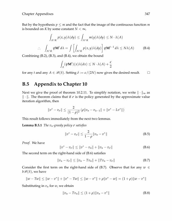
Chapter Appendixes 347
But by the hypothesis p ≤ m and the fact that the image of the continuous function mis bounded on K by some constant N < ∞,∫
A∩Kp(x, y)λ(dy) ≤
∫A∩K
m(y)λ(dy) ≤ N · λ(A)
∴∫A∩K
ψMt dλ =∫ [∫
A∩Kp(x, y)λ(dy)
]ψMt−1 dλ ≤ Nλ(A) (B.4)
Combining (B.2), (B.3), and (B.4), we obtain the bound∫A(ψMt)(x)λ(dx) ≤ N · λ(A) +
ε
2
for any t and any A ∈ B(S). Setting δ := ε/(2N) now gives the desired result.
B.5 Appendix to Chapter 10
Next we give the proof of theorem 10.2.11. To simplify notation, we write ‖ · ‖∞ as‖ · ‖. The theorem claims that if σ is the policy generated by the approximate valueiteration algorithm, then
‖v∗ − vσ‖ ≤ 2(1− ρ)2
(ρ‖vn − vn−1‖+ ‖v∗ − Lv∗‖)
This result follows immediately from the next two lemmas.
Lemma B.5.1 The vn-greedy policy σ satisfies
‖v∗ − vσ‖ ≤ 21− ρ
‖vn − v∗‖ (B.5)
Proof. We have‖v∗ − vσ‖ ≤ ‖v∗ − vn‖+ ‖vn − vσ‖ (B.6)
The second term on the right-hand side of (B.6) satisfies
‖vn − vσ‖ ≤ ‖vn − Tvn‖+ ‖Tvn − vσ‖ (B.7)
Consider the first term on the right-hand side of (B.7). Observe that for any w ∈bB(S), we have
‖w− Tw‖ ≤ ‖w− v∗‖+ ‖v∗ − Tw‖ ≤ ‖w− v∗‖+ ρ‖v∗ − w‖ = (1 + ρ)‖w− v∗‖Substituting in vn for w, we obtain
‖vn − Tvn‖ ≤ (1 + ρ)‖vn − v∗‖ (B.8)
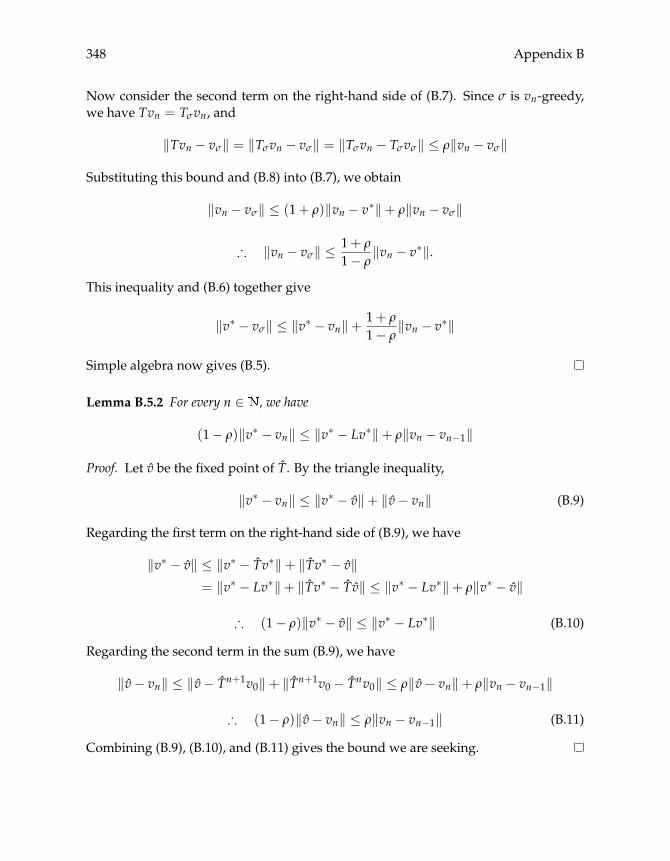
348 Appendix B
Now consider the second term on the right-hand side of (B.7). Since σ is vn-greedy,we have Tvn = Tσvn, and
‖Tvn − vσ‖ = ‖Tσvn − vσ‖ = ‖Tσvn − Tσvσ‖ ≤ ρ‖vn − vσ‖
Substituting this bound and (B.8) into (B.7), we obtain
‖vn − vσ‖ ≤ (1 + ρ)‖vn − v∗‖+ ρ‖vn − vσ‖
∴ ‖vn − vσ‖ ≤ 1 + ρ
1− ρ‖vn − v∗‖.
This inequality and (B.6) together give
‖v∗ − vσ‖ ≤ ‖v∗ − vn‖+ 1 + ρ
1− ρ‖vn − v∗‖
Simple algebra now gives (B.5).
Lemma B.5.2 For every n ∈ , we have
(1− ρ)‖v∗ − vn‖ ≤ ‖v∗ − Lv∗‖+ ρ‖vn − vn−1‖
Proof. Let v be the fixed point of T. By the triangle inequality,
‖v∗ − vn‖ ≤ ‖v∗ − v‖+ ‖v− vn‖ (B.9)
Regarding the first term on the right-hand side of (B.9), we have
‖v∗ − v‖ ≤ ‖v∗ − Tv∗‖+ ‖Tv∗ − v‖= ‖v∗ − Lv∗‖+ ‖Tv∗ − Tv‖ ≤ ‖v∗ − Lv∗‖+ ρ‖v∗ − v‖
∴ (1− ρ)‖v∗ − v‖ ≤ ‖v∗ − Lv∗‖ (B.10)
Regarding the second term in the sum (B.9), we have
‖v− vn‖ ≤ ‖v− Tn+1v0‖+ ‖Tn+1v0 − Tnv0‖ ≤ ρ‖v− vn‖+ ρ‖vn − vn−1‖
∴ (1− ρ)‖v− vn‖ ≤ ρ‖vn − vn−1‖ (B.11)
Combining (B.9), (B.10), and (B.11) gives the bound we are seeking.
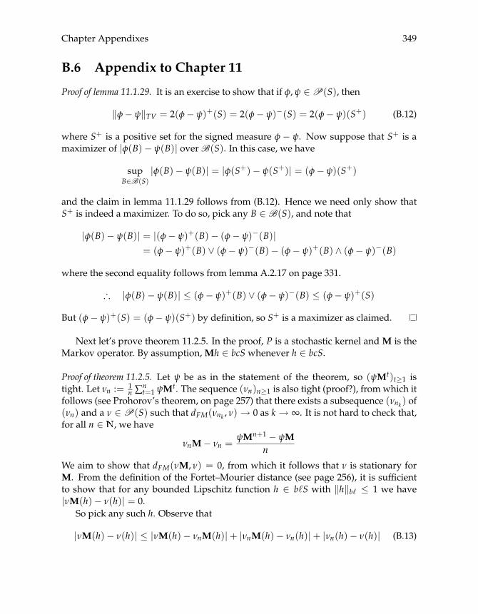
Chapter Appendixes 349
B.6 Appendix to Chapter 11
Proof of lemma 11.1.29. It is an exercise to show that if φ,ψ ∈P(S), then
‖φ− ψ‖TV = 2(φ− ψ)+(S) = 2(φ− ψ)−(S) = 2(φ− ψ)(S+) (B.12)
where S+ is a positive set for the signed measure φ − ψ. Now suppose that S+ is amaximizer of |φ(B)− ψ(B)| overB(S). In this case, we have
supB∈B(S)
|φ(B)− ψ(B)| = |φ(S+)− ψ(S+)| = (φ− ψ)(S+)
and the claim in lemma 11.1.29 follows from (B.12). Hence we need only show thatS+ is indeed a maximizer. To do so, pick any B ∈ B(S), and note that
|φ(B)− ψ(B)| = |(φ− ψ)+(B)− (φ− ψ)−(B)|= (φ− ψ)+(B) ∨ (φ− ψ)−(B)− (φ− ψ)+(B) ∧ (φ− ψ)−(B)
where the second equality follows from lemma A.2.17 on page 331.
∴ |φ(B)− ψ(B)| ≤ (φ− ψ)+(B) ∨ (φ− ψ)−(B) ≤ (φ− ψ)+(S)
But (φ− ψ)+(S) = (φ− ψ)(S+) by definition, so S+ is a maximizer as claimed.
Next let’s prove theorem 11.2.5. In the proof, P is a stochastic kernel and M is theMarkov operator. By assumption, Mh ∈ bcS whenever h ∈ bcS.
Proof of theorem 11.2.5. Let ψ be as in the statement of the theorem, so (ψMt)t≥1 istight. Let νn := 1
n ∑nt=1 ψM
t. The sequence (νn)n≥1 is also tight (proof?), from which itfollows (see Prohorov’s theorem, on page 257) that there exists a subsequence (νnk ) of(νn) and a ν ∈P(S) such that dFM(νnk , ν) → 0 as k → ∞. It is not hard to check that,for all n ∈ , we have
νnM− νn =ψMn+1 − ψM
n
We aim to show that dFM(νM, ν) = 0, from which it follows that ν is stationary forM. From the definition of the Fortet–Mourier distance (see page 256), it is sufficientto show that for any bounded Lipschitz function h ∈ b�S with ‖h‖b� ≤ 1 we have|νM(h)− ν(h)| = 0.
So pick any such h. Observe that
|νM(h)− ν(h)| ≤ |νM(h)− νnM(h)|+ |νnM(h)− νn(h)|+ |νn(h)− ν(h)| (B.13)

350 Appendix B
for all n ∈ . All three terms on the right-hand side of (B.13) converge to zero alongthe subsequence (nk), which implies |νM(h)− ν(h)| = 0. To see that this is the case,consider the first term. We have
|νM(h)− νnkM(h)| = |ν(Mh)− νnk (Mh)| → 0
where the equality is from the duality property in theorem 9.2.15 (page 227), and con-vergence is due to the fact that Mh is bounded and continuous, and dFM(νnk , ν) → 0as k→ ∞.
Consider next the second term in (B.13). That |νnkM(h)− νnk (h)| converges to zeroas k→ ∞ follows from the bound
|νnkM(h)− νnk (h)| =1nk|ψMnk+1(h)− ψM(h)| ≤ 2
nk
That the final term in the sum (B.13) converges to zero along the subsequence (nk) istrivial, and this completes the proof of theorem 11.2.5.
Proof of lemma 11.3.3. The xb that solves P(xb) = α∫p∗(z)φ(dz) satisfies D(αP(0)) ≤
xb because P(xb) = α∫p∗(z)φ(dz) ≤ αp∗(0) = αP(0). Here we are using the fact that
p∗(0) = P(0).3 Also D(αP(0)) > 0 because D(P(0)) = 0 and D is strictly decreasing.Since xb ≥ D(αP(0)), we have shown that xb > 0.
We claim in addition that if x ≤ xb, then p∗(x) = P(x) and I(x) = 0. That p∗(x) =P(x) implies I(x) = 0 is immediate from the definition: I(x) = x − D(p∗(x)) (seepage 146). Hence we need only prove that when x ≤ xb we have p∗(x) = 0. But ifx ≤ xb, then P(xb) ≤ P(x), and hence
P(x) ≥ α∫
p∗(z)φ(dz) ≥ α∫
p∗(αI(x) + z)φ(dz)
That p∗(x) = P(x) is now clear from the definition of p∗.4
B.7 Appendix to Chapter 12
Proof of proposition 12.1.17. Pick any y > 0 and define the h : [0, y]→ by
h(k) := U(y− k) +W(k), W(k) := ρ∫w[ f (k, z)]φ(dz)
3To prove this, one can show via (6.28) on page 147 that if p ≤ P(0), then Tp ≤ P(0), from which itfollows that p∗ = limn TnP ≤ P(0). Therefore p∗(0) ≤ P(0). On the other hand, p∗ ≥ P, so p∗(0) ≥ P(0).Hence p∗(0) = P(0).
4For the definition refer to (6.26) on page 146.
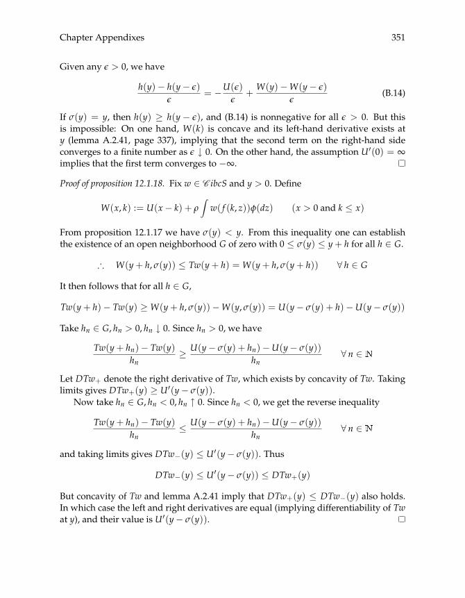
Chapter Appendixes 351
Given any ε > 0, we have
h(y)− h(y− ε)ε
= −U(ε)ε
+W(y)−W(y− ε)
ε(B.14)
If σ(y) = y, then h(y) ≥ h(y − ε), and (B.14) is nonnegative for all ε > 0. But thisis impossible: On one hand, W(k) is concave and its left-hand derivative exists aty (lemma A.2.41, page 337), implying that the second term on the right-hand sideconverges to a finite number as ε ↓ 0. On the other hand, the assumption U′(0) = ∞implies that the first term converges to −∞.
Proof of proposition 12.1.18. Fix w ∈ C ibcS and y > 0. Define
W(x, k) := U(x− k) + ρ∫w( f (k, z))φ(dz) (x > 0 and k ≤ x)
From proposition 12.1.17 we have σ(y) < y. From this inequality one can establishthe existence of an open neighborhood G of zero with 0 ≤ σ(y) ≤ y+ h for all h ∈ G.
∴ W(y+ h, σ(y)) ≤ Tw(y+ h) = W(y+ h, σ(y+ h)) ∀ h ∈ G
It then follows that for all h ∈ G,
Tw(y+ h)− Tw(y) ≥W(y+ h, σ(y))−W(y, σ(y)) = U(y− σ(y) + h)−U(y− σ(y))
Take hn ∈ G, hn > 0, hn ↓ 0. Since hn > 0, we have
Tw(y+ hn)− Tw(y)hn
≥ U(y− σ(y) + hn)−U(y− σ(y))hn
∀ n ∈
Let DTw+ denote the right derivative of Tw, which exists by concavity of Tw. Takinglimits gives DTw+(y) ≥ U′(y− σ(y)).
Now take hn ∈ G, hn < 0, hn ↑ 0. Since hn < 0, we get the reverse inequality
Tw(y+ hn)− Tw(y)hn
≤ U(y− σ(y) + hn)−U(y− σ(y))hn
∀ n ∈
and taking limits gives DTw−(y) ≤ U′(y− σ(y)). Thus
DTw−(y) ≤ U′(y− σ(y)) ≤ DTw+(y)
But concavity of Tw and lemma A.2.41 imply that DTw+(y) ≤ DTw−(y) also holds.In which case the left and right derivatives are equal (implying differentiability of Twat y), and their value is U′(y− σ(y)).
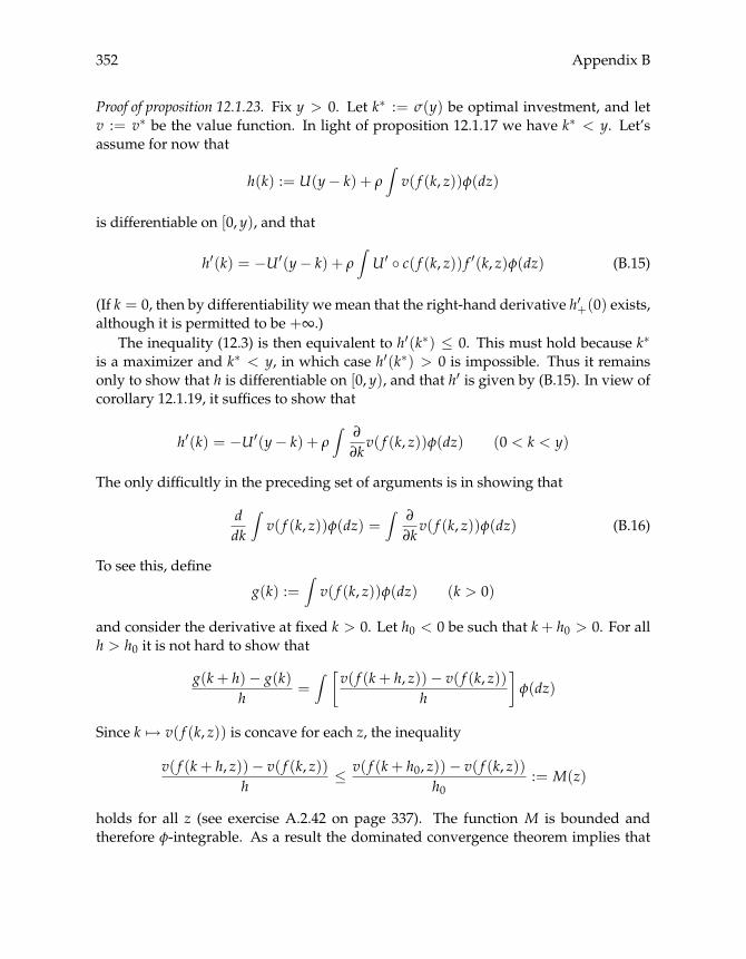
352 Appendix B
Proof of proposition 12.1.23. Fix y > 0. Let k∗ := σ(y) be optimal investment, and letv := v∗ be the value function. In light of proposition 12.1.17 we have k∗ < y. Let’sassume for now that
h(k) := U(y− k) + ρ∫v( f (k, z))φ(dz)
is differentiable on [0, y), and that
h′(k) = −U′(y− k) + ρ∫U′ ◦ c( f (k, z)) f ′(k, z)φ(dz) (B.15)
(If k = 0, then by differentiability we mean that the right-hand derivative h′+(0) exists,although it is permitted to be +∞.)
The inequality (12.3) is then equivalent to h′(k∗) ≤ 0. This must hold because k∗is a maximizer and k∗ < y, in which case h′(k∗) > 0 is impossible. Thus it remainsonly to show that h is differentiable on [0, y), and that h′ is given by (B.15). In view ofcorollary 12.1.19, it suffices to show that
h′(k) = −U′(y− k) + ρ∫
∂
∂kv( f (k, z))φ(dz) (0 < k < y)
The only difficultly in the preceding set of arguments is in showing that
ddk
∫v( f (k, z))φ(dz) =
∫∂
∂kv( f (k, z))φ(dz) (B.16)
To see this, define
g(k) :=∫v( f (k, z))φ(dz) (k > 0)
and consider the derivative at fixed k > 0. Let h0 < 0 be such that k+ h0 > 0. For allh > h0 it is not hard to show that
g(k+ h)− g(k)h
=∫ [
v( f (k+ h, z))− v( f (k, z))h
]φ(dz)
Since k �→ v( f (k, z)) is concave for each z, the inequality
v( f (k+ h, z))− v( f (k, z))h
≤ v( f (k+ h0, z))− v( f (k, z))h0
:= M(z)
holds for all z (see exercise A.2.42 on page 337). The function M is bounded andtherefore φ-integrable. As a result the dominated convergence theorem implies that

Chapter Appendixes 353
for hn → 0 with hn > h0 and hn �= 0 we have
g(k) = limn→∞
∫ [v( f (k+ hn, z))− v( f (k, z))
hn
]φ(dz)
=∫
limn→∞
[v( f (k+ hn, z))− v( f (k, z))
hn
]φ(dz)
=∫
∂
∂kv( f (k, z))φ(dz)
The last equality is due to the fact that k �→ v( f (k, z)) is differentiable in k for eachz.
Proof of proposition 12.1.24. Starting with the second claim, in the notation of the proofof proposition 12.1.23, we are claiming that if h′(k∗) < 0, then k∗ = 0. This followsbecause if k∗ > 0, then k∗ is interior, in which case h′(k∗) = 0.
The first claim will be established if, whenever f (0, z) = 0 for each z ∈ Z, we have0 < σ(y) for all y > 0. (Why?) Suppose instead that σ(y) = 0 at some y > 0, so
v(y) = U(y) + ρ∫v[ f (0, z)]φ(dz) = U(y) (B.17)
where we have used U(0) = 0. Define also
vξ := U(y− ξ) + ρ∫v[ f (ξ, z)]φ(dz) (B.18)
where ξ is a positive number less than y. Using optimality and the fact that U(y) =v(y), we get
0 ≤ v(y)− vξξ
=U(y)−U(y− ξ)
ξ− ρ
∫ v[ f (ξ, z)]ξ
φ(dz) ∀ ξ < y
Note that the first term on the right-hand side of the equal sign converges to the finiteconstant U′(y) as ξ ↓ 0. We will therefore induce a contradiction if the second term(i.e., the integral term) converges to plus infinity. Although our simple version of themonotone convergence theorem does not include this case, it is sufficient to show thatthe integrand converges to infinity as ξ ↓ 0 for each fixed z; interested readers shouldconsult, for example, Dudley (2002, thm. 4.3.2).5 To see that this is so, observe that forany z ∈ Z,
limξ↓0
v[ f (ξ, z)]ξ
= limξ↓0
v[ f (ξ, z)]f (ξ, z)
f (ξ, z)ξ≥ lim
ξ↓0U[ f (ξ, z)]f (ξ, z)
f (ξ, z)ξ→ ∞
We have used here the fact that v ≥ U pointwise on S.5We are using the fact that the integrand increases monotonically as ξ ↓ 0 for each fixed z, as follows
from concavity of f in its first argument, and the fact that the value function is increasing.
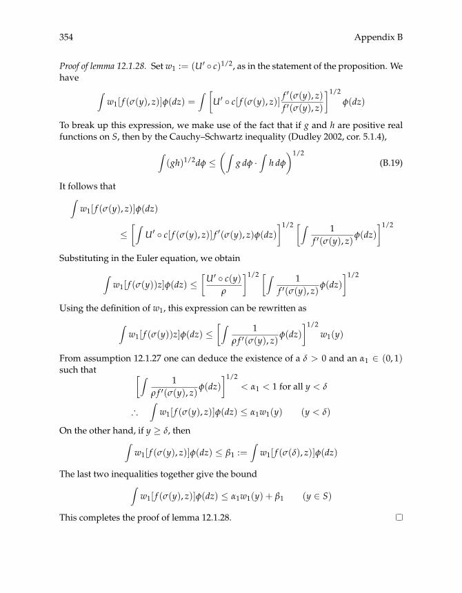
354 Appendix B
Proof of lemma 12.1.28. Set w1 := (U′ ◦ c)1/2, as in the statement of the proposition. Wehave
∫w1[ f (σ(y), z)]φ(dz) =
∫ [U′ ◦ c[ f (σ(y), z)] f
′(σ(y), z)f ′(σ(y), z)
]1/2
φ(dz)
To break up this expression, we make use of the fact that if g and h are positive realfunctions on S, then by the Cauchy–Schwartz inequality (Dudley 2002, cor. 5.1.4),
∫(gh)1/2dφ ≤
(∫g dφ ·
∫h dφ
)1/2(B.19)
It follows that∫w1[ f (σ(y), z)]φ(dz)
≤[∫
U′ ◦ c[ f (σ(y), z)] f ′(σ(y), z)φ(dz)]1/2 [∫ 1
f ′(σ(y), z)φ(dz)]1/2
Substituting in the Euler equation, we obtain
∫w1[ f (σ(y))z]φ(dz) ≤
[U′ ◦ c(y)
ρ
]1/2 [∫ 1f ′(σ(y), z)φ(dz)
]1/2
Using the definition of w1, this expression can be rewritten as
∫w1[ f (σ(y))z]φ(dz) ≤
[∫ 1ρ f ′(σ(y), z)φ(dz)
]1/2w1(y)
From assumption 12.1.27 one can deduce the existence of a δ > 0 and an α1 ∈ (0, 1)such that [∫ 1
ρ f ′(σ(y), z)φ(dz)]1/2
< α1 < 1 for all y < δ
∴∫w1[ f (σ(y), z)]φ(dz) ≤ α1w1(y) (y < δ)
On the other hand, if y ≥ δ, then∫w1[ f (σ(y), z)]φ(dz) ≤ β1 :=
∫w1[ f (σ(δ), z)]φ(dz)
The last two inequalities together give the bound∫w1[ f (σ(y), z)]φ(dz) ≤ α1w1(y) + β1 (y ∈ S)
This completes the proof of lemma 12.1.28.
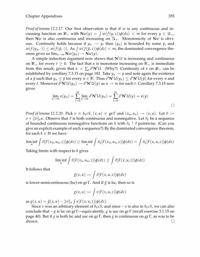
Chapter Appendixes 355
Proof of lemma 12.2.17. Our first observation is that if w is any continuous and in-creasing function on + with Nw(y) =
∫w( f (y, z))φ(dz) < ∞ for every y ∈ +,
then Nw is also continuous and increasing on +. Monotonicity of Nw is obvi-ous. Continuity holds because if yn → y, then (yn) is bounded by some y, andw( f (yn, ·)) ≤ w( f (y, ·)). As
∫w( f (y, z))φ(dz) < ∞, the dominated convergence the-
orem gives us limn→∞Nw(yn)→ Nw(y).A simple induction argument now shows that NtU is increasing and continuous
on + for every t ≥ 0. The fact that κ is monotone increasing on + is immediatefrom this result, given that κ = ∑t δ
tNtU. (Why?) Continuity of κ on + can beestablished by corollary 7.3.15 on page 182. Take yn → y and note again the existenceof a y such that yn ≤ y for every n ∈ . Thus δtNtU(yn) ≤ δtNtU(y) for every n andevery t. Moreover δtNtU(yn) → δtNtU(y) as n → ∞ for each t. Corollary 7.3.15 nowgives
limn→∞ κ(yn) =
∞
∑t=0
limn→∞ δ
tNtU(yn) =∞
∑t=0
δtNtU(y) = κ(y)
Proof of lemma 12.2.20. Pick v ∈ bκcS, (x, u) ∈ gr Γ and (xn, un) → (x, u). Let v :=v+ ‖v‖κκ. Observe that v is both continuous and nonnegative. Let vk be a sequenceof bounded continuous nonnegative functions on S with vk ↑ v pointwise. (Can yougive an explicit example of such a sequence?) By the dominated convergence theorem,for each k ∈ we have
lim infn
∫v[F(xn, un, z)]φ(dz) ≥ lim inf
n
∫vk[F(xn, un, z)]φ(dz) =
∫vk[F(x, u, z)]φ(dz)
Taking limits with respect to k gives
lim infn
∫v[F(xn, un, z)]φ(dz) ≥
∫v[F(x, u, z)]φ(dz)
It follows thatg(x, u) :=
∫v[F(x, u, z)]φ(dz)
is lower-semicontinuous (lsc) on gr Γ. And if g is lsc, then so is
g(x, u) :=∫v[F(x, u, z)]φ(dz)
as g(x, u) = g(x, u)− ‖v‖κ∫κ[F(x, u, z)]φ(dz).
Since v was an arbitrary element of bκcS, and since −v is also in bκcS, we can alsoconclude that −g is lsc on gr Γ—equivalently, g is usc on gr Γ (recall exercise 3.1.15 onpage 40). But if g is both lsc and usc on gr Γ, then g is continuous on gr Γ, as was to beshown.


Bibliography
Adda, J., and R. Cooper. 2003. Dynamic Economics: Quantitative Methods and Applications. Cam-bridge: MIT Press.
Aiyagari, S. R. 1994. Uninsured idiosyncratic risk and aggregate saving. Quarterly Journal ofEconomics 109: 659–684.
Aliprantis, C. D., and K. C. Border. 1999. Infinite Dimensional Analysis. New York: Springer.
Aliprantis, C. D., and O. Burkinshaw. 1998. Principles of Real Analysis. London: Academic Press.
Alvarez, F., and N. L. Stokey. 1998. Dynamic programming with homogeneous functions.Journal of Economic Theory 82: 167–89.
Amir, R. 1997. A new look at optimal growth under uncertainty. Journal of Economic Dynamicsand Control 22: 67–86.
Amir, R. 2005. Supermodularity and complementarity in economics: An elementary survey.Southern Economic Journal 71: 636–60.
Amir, R., L. J. Mirman, and W. R. Perkins. 1991. One-sector nonclassical optimal growth: Opti-mality conditions and comparative dynamics. International Economic Review 32: 625–44.
Amman, H. M., D. A. Kendrick, and J. Rust, eds. 1990. Handbook of Computational Economics.Burlington, MA: Elsevier.
Angeletos, G-M. 2007. Uninsured idiosyncratic investment risk and aggregate saving. Reviewof Economic Dynamics 10: 1–30.
Aruoba, S. B., J. Fernàndez-Villaverde, and J. Rubio-Ramírez. 2006. Comparing solution meth-ods for dynamic equilibrium economies. Journal of Economic Dynamics and Control 30: 2447–508.
Azariadis, C. 1993. Intertemporal Macroeconomics. New York: Blackwell.
Azariadis, C., and A. Drazen. 1990. Threshold externalities in economic development. QuarterlyJournal of Economics 105: 501–26.
Barnett, W. A., and A. Serletis. 2000. Martingales, nonlinearity, and chaos. Journal of EconomicDynamics and Control 24: 703–24.
Bartle, R., and D. Sherbet. 1992. Introduction to Real Analysis. New York: Wiley.
357

358 Bibliography
Becker, R. A., and J. H. Boyd. 1997. Capital Theory, Equilibrium Analysis and Recursive Utility.New York: Blackwell.
Bellman, R. E. 1957. Dynamic Programming. Princeton: Princeton University Press.
Benhabib, J., and K. Nishimura. 1985. Competitive equilibrium cycles. Journal of EconomicTheory 35: 284–306.
Benveniste, L. M. , and J. A. Scheinkman. 1979. On the differentiability of the value function indynamic models of economics. Econometrica 47: 727–32.
Bertsekas, D. P. 1995. Dynamic Programming and Optimal Control. New York: Athena Scientific.
Bewley, T. 2007. General Equilibrium, Overlapping Generations Models, and Optimal Growth Theory.Cambridge: Harvard University Press.
Bhattacharya, R. N., and O. Lee. 1988. Asymptotics of a class of Markov processes which arenot in general irreducible. Annals of Probability 16: 1333–47.
Bhattacharya, R., and M. Majumdar. 2007. Random Dynamical Systems: Theory and Applications.Cambridge: Cambridge University Press.
Böhm, V., and L. Kaas. 2000. Differential savings, factor shares, and endogenous growth cycles.Journal of Economic Dynamics and Control 24: 965–80.
Boldrin, M., and L. Montrucchio. 1986. On the indeterminacy of capital accumulation paths.Journal of Economic Theory 40: 26–39.
Boyd, J. H. 1990. Recursive utility and the Ramsey problem. Journal of Economic Theory 50:326–45.
Breiman, L. 1992. Probability. SIAM Classics in Applied Mathematics, Philadelphia: SIAM.
Bremaud, P. 1999. Markov Chains. New York: Springer.
Brock, W. A., and L. J. Mirman. 1972. Optimal economic growth and uncertainty: The dis-counted case. Journal of Economic Theory 4: 479–513.
Brock, W. A. 1982. Asset prices in a production economy. In Economics of Information and Uncer-tainty. J. J. McCall, ed. Chicago: University of Chicago Press, pp. 1–43.
Brock, W. A., and C. H. Hommes. 1998. Heterogeneous beliefs and routes to chaos in a simpleasset pricing model. Journal of Economic Dynamics and Control 22: 1235–74.
Canova, F. 2007. Methods for Applied Macroeconomic Research. Princeton: Princeton UniversityPress.
Caputo, M. R. 2005. Foundations of Dynamic Economic Analysis: Optimal Control Theory and Appli-cations. Cambridge: Cambridge University Press.
Chan, K. S., and H. Tong. 1986. On estimating thresholds in autoregressive models. Journal ofTime Series Analysis 7: 179–90.
Chatterjee, P., and M. Shukayev. 2008. Note on a positive lower bound of capital in the stochas-tic growth model. Journal of Economic Dynamics and Control 32: 2137–47.

Bibliography 359
Chiarella, C. 1988. The cobweb model its instability and the onset of chaos. Economic Modelling5: 377–84.
Christiano, L. J., and J. D. M. Fisher. 2000. Algorithms for solving dynamic models with occa-sionally binding constraints. Journal of Economic Dynamics and Control 24: 1179–232.
Coleman, W. J. 1990. Solving the stochastic growth model by policy-function iteration. Journalof Business and Economic Statistics 8: 27–29.
Datta, M., L. J. Mirman, O. F. Morand, and K. Reffett. 2005. Markovian equilibrium in in-finite horizon economies with incomplete markets and public policy. Journal of MathematicalEconomics 41: 505–44.
Deaton, A., and G. Laroque. 1992. On the behavior of commodity prices. Review of EconomicStudies 59: 1–23.
Dechert, W. D., and S. I. O’Donnell. 2006. The stochastic lake game: A numerical solution.Journal of Economic Dynamics and Control 30: 1569–87.
Den Haan, W. J., and A. Marcet. 1994. Accuracy in simulations. Review of Economic Studies 61:3–17.
Dobrushin, R. L. 1956. Central limit theorem for nonstationary Markov chains. Theory of Proba-bility and its Applications 1: 65–80.
Doeblin, W. 1938. Exposé de la theorie des chaîns simples constantes de Markov à un nombrefini d’états. Revue Mathematique de l’Union Interbalkanique 2: 77–105.
Donaldson, J. B., and R. Mehra. 1983. Stochastic growth with correlated production shocks.Journal of Economic Theory 29: 282–312.
Dudley, R. M. 2002. Real Analysis and Probability. Cambridge: Cambridge University Press.
Duffie, D. 2001. Dynamic Asset Pricing Theory. Princeton: Princeton University Press.
Durlauf, S. 1993. Nonergodic economic growth. Review of Economic Studies 60: 349–66.
Durrett, R. 1996. Probability: Theory and Examples. New York: Duxbury Press.
Ericson, R., and A. Pakes. 1995. Markov-perfect industry dynamics: A framework for empiricalwork. Review of Economic Studies 62: 53–82.
Farmer, R. E. A. 1999. The Macroeconomics of Self-Fulfilling Prophecies. Cambridge: MIT Press.
de la Fuente, A. 2000. Mathematical Methods and Models for Economists. Cambridge: CambridgeUniversity Press.
Galor, O. 1994. A two-sector overlapping generations model: A global characterization of thedynamical system. Econometrica 60: 1351–86.
Gandolfo, G. 2005. Economic Dynamics: Study Edition. New York: Springer.
Glynn, P. W., and S. G. Henderson. 2001. Computing densities for Markov chains via simula-tion. Mathematics of Operations Research 26: 375–400.
Gordon, G. J. 1995. Stable function approximation in dynamic programming. Mimeo. Carnegie–Mellon University.
360 Bibliography
Grandmont, J-M. 1985. On endogenous competitive business cycles. Econometrica 53: 995–1046.
Green, E. J., and R. H. Porter. 1984. Noncooperative collusion under imperfect price informa-tion. Econometrica 52: 87–100.
Greenwood, J., and G. W. Huffman. 1995. On the existence of nonoptimal equilibria. Journal ofEconomic Theory 65: 611–23.
Grüne, L., and W. Semmler. 2004. Using dynamic programming with adaptive grid scheme foroptimal control. Journal of Economic Dynamics and Control 28: 2427–56.
Häggström, O. 2002. Finite Markov Chains and Algorithmic Applications. Cambridge: CambridgeUniversity Press.
Hall, R. E. 1978. Stochastic implications of the life cycle-permanent income hypothesis: Theoryand evidence. Journal of Political Economy 86: 971–87.
Hamilton, J. D. 2005. What’s real about the business cycle? Federal Reserve Bank of St. LouisReview. July–August: 435–52.
Heer, B., and A. Maussner. 2005. Dynamic General Equilibrium Modelling. New York: Springer.
Hernández-Lerma, O., and J. B. Lasserre. 1996. Discrete Time Markov Control Processes: BasicOptimality Criteria. New York: Springer.
Hernández-Lerma, O., and J. B. Lasserre. 1999. Further Topics on Discrete Time Markov ControlProcesses. New York: Springer.
Hernández-Lerma, O., and J. B. Lasserre. 2003. Markov Chains and Invariant Probabilities. Boston:Birkhäuser.
Holmgren, R. A. 1996. A First Course in Discrete Dynamical Systems. New York: Springer.
Hopenhayn, H. A. 1992. Entry, exit, and firm dynamics in long run equilibrium. Econometrica60: 1127–50.
Hopenhayn, H. A., and E. C. Prescott. 1992. Stochastic monotonicity and stationary distribu-tions for dynamic economies. Econometrica 60: 1387–1406.
Huggett, M. 1993. The risk-free rate in heterogeneous-agent incomplete-insurance economies.Journal of Economic Dynamics and Control 17: 953–969.
Huggett, M. 2003. When are comparative dynamics monotone? Review of Economic Dynamics 6:1–11.
Jones, G. L. 2004. On the Markov chain central limit theorem. Probability Surveys 1: 299–320.
Judd, K. L. 1992. Projection methods for solving aggregate growth models. Journal of EconomicTheory 58: 410–52.
Judd, K. L. 1998. Numerical Methods in Economics. Cambridge: MIT Press.
Kamihigashi, T. 2007. Stochastic optimal growth with bounded or unbounded utility and withbounded or unbounded shocks. Journal of Mathematical Economics 43: 477–500.
Kamihigashi, T., and J. Stachurski. 2008. Asymptotics of stochastic recursive economies undermonotonicity. Mimeo. Kyoto University.
Bibliography 361
Kandori, M., G. J. Mailath, and R. Rob. 1993. Learning, mutation and long run equilibria ingames. Econometrica 61: 29–56.
Kendrick, D. A., P. R. Mercado, and H. M. Amman. 2005. Computational Economics. Princeton:Princeton University Press.
Kikuchi, T. 2008. International asset market, nonconvergence, and endogenous fluctuations.Journal of Economic Theory 139: 310–34.
Kolmogorov, A. N. 1955. Foundations of the Theory of Probability. Chelsea, NY: Nathan Morrison.
Kolmogorov, A. N., and S. V. Fomin. 1970. Introductory Real Analysis. New York: Dover Publi-cations.
Krebs, T. 2004. Non-existence of recursive equilibria on compact state spaces when markets areincomplete. Journal of Economic Theory 115: 134–50.
Kristensen, D. 2007. Geometric ergodicity of a class of Markov chains with applications to timeseries models. Mimeo. University of Wisconsin.
Krusell, P., and A. Smith. 1998. Income and wealth heterogeneity in the macroeconomy. Journalof Political Economy 106: 867–96.
Krylov, N., and N. Bogolubov. 1937. Sur les properties en chaine. Comptes Rendus Mathematique204: 1386–88.
Kubler, F., and K. Schmedders. 2002. Recursive equilibria in economies with incomplete mar-kets. Macroeconomic Dynamics 6: 284–306.
Kydland, F., and E. C. Prescott. 1982. Time to build and aggregate fluctuations. Econometrica 50:1345–71.
Langtangen, H. P. 2008. Python Scripting for Computational Science. New York: Springer.
Lasota, A. 1994. Invariant principle for discrete time dynamical systems. Universitatis Iagelloni-cae Acta Mathematica 31: 111–27.
Lasota, A., and M. C. Mackey. 1994. Chaos, Fractals and Noise: Stochastic Aspects of Dynamics.New York: Springer.
Le Van, C., and R-A. Dana. 2003. Dynamic Programming in Economics. New York: Springer.
Le Van, C., and Y. Vailakis. 2005. Recursive utility and optimal growth with bounded or un-bounded returns. Journal of Economic Theory 123: 187–209.
Light, W. 1990. Introduction to Abstract Analysis. Oxford, UK: Chapman and Hall.
Lindvall, T. 1992. Lectures on the Coupling Method. New York: Dover Publications.
Ljungqvist, L., and T. Sargent. 2004. Recursive Macroeconomic Theory. Cambridge: MIT Press
Long, J., and C. Plosser. 1983. Real business cycles. Journal of Political Economy 91: 39–69.
Lovejoy, W. 1987. Ordered solutions for dynamic programs. Mathematics of Operations Research12: 269–76.
Lucas, R. E., Jr., and E. C. Prescott. 1971. Investment under uncertainty. Econometrica 39: 659–81.

362 Bibliography
Lucas, R. E., Jr. 1978. Asset prices in an exchange economy. Econometrica 46: 1429–45.
Maliar, L., and S. Maliar. 2005. Solving nonlinear dynamic stochastic models: An algorithmcomputing value function by simulations. Economics Letters 87: 135–40.
Marcet, A. 1988. Solving nonlinear models by parameterizing expectations. Mimeo. CarnegieMellon University.
Marimon, R., and A. Scott, eds. 2001. Computational Methods for the Study of Dynamic Economies.Oxford: Oxford University Press.
Matsuyama, K. 2004. Financial market globalization, symmetry-breaking, and endogenous in-equality of nations. Econometrica 72: 853–84.
McCall, J. J. 1970. Economics of information and job search. Quarterly Journal of Economics 84:113–26.
McGrattan, E. R. 2001. Application of weighted residual methods to dynamic economic models.In Computational Methods for the Study of Dynamic Economies. R. Marimon and A. Scott, eds.Oxford: Oxford University Press, pp. 114–43.
McLennan, A., and R. Tourky. 2005. From imitation games to Kakutani. Mimeo. University ofMelbourne.
Medio, A. 1995. Chaotic Dynamics: Theory and Applications to Economics. Cambridge: CambridgeUniversity Press.
Mehra, R., and E. C. Prescott. 1985. The equity premium: A puzzle. Journal of Monetary Eco-nomics 15: 145–61.
Meyn, S. P., and R. L. Tweedie. 1993. Markov Chains and Stochastic Stability. London: Springer.
Miao, J. 2006. Competitive equilibria of economies with a continuum of consumers and aggre-gate shocks. Journal of Economic Theory 128: 274–98.
Miranda, M., and P. L. Fackler. 2002. Applied Computational Economics and Finance. Cambridge:MIT Press.
Mirman, L. J. 1970. Two essays on uncertainty and economics. PhD Thesis, University ofRochester.
Mirman, L. J., 1972. On the existence of steady state measures for one sector growth modelswith uncertain technology. International Economic Review 13: 271–86.
Mirman, L. J. 1973. The steady state behavior of a class of one sector growth models withuncertain technology. Journal of Economic Theory 6: 219–42.
Mirman, L. J., and I. Zilcha. 1975. On optimal growth under uncertainty. Journal of EconomicTheory 11: 329–39.
Mirman, L. J., O. F. Morand, and K. L. Reffett. 2008. A qualitative approach to Markovianequilibrium in infinite horizon economies with capital. Journal of Economic Theory 139: 75–98.
Mirman, L. J., K. Reffett, and J. Stachurski. 2005. Some stability results for Markovian economicsemigroups. International Journal of Economic Theory 1: 57–72.

Bibliography 363
Mitra, T., and G. Sorger. 1999. Rationalizing policy functions by dynamic optimization. Econo-metrica 67: 375–92.
Nirei, M. 2008. Aggregate fluctuations of discrete investments. Mimeo. Carleton University.
Nishimura, K., G. Sorger, and M. Yano. 1994. Ergodic chaos in optimal growth models withlow discount rates. Economic Theory 4: 705–17.
Nishimura, K., and J. Stachurski. 2005. Stability of stochastic optimal growth models: A newapproach. Journal of Economic Theory 122: 100–18.
Norris, J. R. 1997. Markov Chains. Cambridge: Cambridge University Press.
Nummelin, E. 1984. General Irreducible Markov Chains and Nonnegative Operators. Cambridge:Cambridge University Press.
Ok, E. A. 2007. Real Analysis with Economic Applications. Princeton: Princeton University Press.
Olsen, L., and S. Roy. 2006. Theory of stochastic optimal growth. InHandbook of Optimal Growth,vol. 1. C. Le Van, R-A. Dana, T. Mitra and K. Nishimura, eds. New York: Springer, pp. 297–335.
Pakes, A., and P. McGuire. 2001. Stochastic algorithms, symmetric Markov perfect equilibriaand the curse of dimensionality. Econometrica 69: 1261–81.
Pollard, D. 2002. A User’s Guide to Measure Theoretic Probability. Cambridge: Cambridge Univer-sity Press.
Prescott, E. C., and R. Mehra. 1980. Recursive competitive equilibrium: The case of homoge-neous households. Econometrica 48: 1365–79.
Puterman, M. 1994. Markov Decision Processes: Discrete Stochastic Dynamic Programming. NewYork: Wiley.
Quah, D. T. 1993. Empirical cross-section dynamics in economic growth. European EconomicReview 37: 426–34.
Razin, A., and J. A. Yahav. 1979. On stochastic models of economic growth. International Eco-nomic Review 20: 599–604.
Reffett, K., and O. F. Morand. 2003. Existence and uniqueness of equilibrium in nonoptimalunbounded infinite horizon economies. Journal of Monetary Economics 50: 1351–73.
Rios-Rull, V. 1996. Life-cycle economies with aggregate fluctuations. Review of Economic Studies63: 465–90.
Rincon-Zapatero, J. P., and C. Rodriguez-Palmero. 2003. Existence and uniqueness of solutionsto the Bellman equation in the unbounded case. Econometrica 71: 1519–55.
Roberts, G. O., and J. S. Rosenthal. 2004. General state space Markov chains and MCMC algo-rithms. Probability Surveys 1: 20–71.
Rockafellar, R. T. 1970. Convex Analysis. Princeton: Princeton University Press.
Rogerson, R., R. Shimer, and R. Wright. 2005. Search-theoretic models of the labor market: Asurvey. Journal of Economic Literature 43: 959–88.

364 Bibliography
Rosenthal, J. S. 2002. Quantitative convergence rates of Markov chains: A simple account.Electronic Communications in Probability 7: 123–28.
Rust, J. 1996. Numerical dynamic programming in economics. In Handbook of ComputationalEconomics. H. Amman, D. Kendrick, and J. Rust, eds. Burlington, MA: Elsevier, pp. 619–729.
Sargent, T. J. 1987. Dynamic Macroeconomic Theory. Cambridge: Harvard University Press.
Santos, M. S., and J. Vigo-Aguiar. 1998. Analysis of a numerical dynamic programming algo-rithm applied to economic models. Econometrica 66: 409–26.
Santos, M. 1999. Numerical solutions of dynamic economic models. In Handbook of Macroeco-nomics, vol. 1A. J. B. Taylor and M. Woodford, eds. Burlington, MA: Elsevier, pp. 311–86.
Scheinkman, J. A., and J. Schectman. 1983. A simple competitive model with production andstorage. Review of Economic Studies 50: 427–41.
Schilling, R. L. 2005. Measures, Integrals and Martingales. Cambridge: Cambridge UniversityPress.
Shiryaev, A. N. 1996. Probability. New York: Springer.
Shone, R. 2003. Economic Dynamics: Phase Diagrams and their Economic Application. Cambridge:Cambridge University Press.
Stachurski, J. 2002. Stochastic optimal growth with unbounded shock. Journal of Economic The-ory 106: 40–65.
Stachurski, J. 2003. Economic dynamical systems with multiplicative noise. Journal of Mathe-matical Economics 39: 135–52.
Stachurski, J., and V. Martin. 2008. Computing the distributions of economics models via sim-ulation. Econometrica 76: 443–50.
Stachurski, J. 2008. Continuous state dynamic programming via nonexpansive approximation.Computational Economics 31: 141–60.
Samuelson, P. A. 1971. Stochastic speculative price. Proceedings of the National Academy of Science68: 335–7.
Sorger, G. 1992. On the minimum rate of impatience for complicated optimal growth paths.Journal of Economic Theory 56: 160–79.
Stokey, N. L. 2008. The Economics of Inaction. Princeton: Princeton University Press.
Stokey, N. L., and R. E. Lucas, with E. C. Prescott. 1989. Recursive Methods in Economic Dynamics.Cambridge: Harvard University Press.
Sundaram, R. K. 1996. A First Course in Optimization Theory. Cambridge: Cambridge UniversityPress.
Tauchen, G., and R. Hussey. 1991. Quadrature-based methods for obtaining approximate solu-tions to nonlinear asset pricing models. Econometrica 59: 371–96.
Taylor, J. C. 1997. An Introduction to Measure and Probability. New York: Springer.

Bibliography 365
Tesfatsion, L., and K. L. Judd, eds. 2006. Handbook of Computational Economics, Volume 2: Agent-Based Computational Economics. Burlington, MA: Elsevier.
Topkis, D. 1998. Supermodularity and Complementarity. Princeton: Princeton University Press.
Torres, R. 1990. Stochastic dominance. Mimeo. Northwestern University.
Turnovsky, S. 2000. Methods of Macroeconomic Dynamics. Cambridge: MIT Press.
Uhlig, M. 2001. A toolkit for analysing nonlinear dynamic stochastic models easily. In Computa-tional Methods for the Study of Dynamic Economies. R. Marimon and A. Scott, eds. Oxford: OxfordUniversity Press, pp. 30–62.
Venditti, A. 1998. Indeterminacy and endogenous fluctuations in a two-sector optimal growthmodel with externalities. Journal of Economic Behavior and Organization 33: 521–42.
Williams, D. 1991. Probability with Martingales. Cambridge, UK: Cambridge University Press.
Williams, N. 2004. Small noise asymptotics for a stochastic growth model. Journal of EconomicTheory 119: 271–98.
Williams, J. C., and B. C. Wright. 1991. Storage and Commodity Markets. Cambridge: CambridgeUniversity Press.
Zelle, J. M. 2003. Python Programming: An Introduction to Computer Science. Wilsonville, OR:Franklin Beedle and Associates.
Zhang, Y. 2007. Stochastic optimal growth with a non-compact state space. Journal of Mathemat-ical Economics 43: 115–29.


Index
A \ B, 318B(ε; x), 39D(S), 185D(ε; x), 42L1, 184Px ∧ Px′ , 265S+, S−, etc., 252T, Bellman op., 235Tσ, 235A, B, etc., 321, 317, 317
Σ, set of policies, 232, 317B(S),B( ), etc., 165C ibcS, 299δx, δz, etc., 78, 167ε-ball, 39∃, 320∀, 320γ(x, x′), 277gr Γ, 230=⇒ , 319κ-bounded, 306L , Lebesgue measurable sets, 162L1, 178μ-a.e., 181μ′(x, x′, dy), 277μ( f ), λ( f ), etc., 177μ(x, x′, dy), 277μ+, μ−, etc., 252
ν(x, x′, dy), 277P(S), 68, 167P(U), P(S), etc., 318σ-algebra, 164σ(C ), σ(O), etc., 164bU, bS, etc., 37b�S, 256bM (S), 252bS , bB(S), etc., 174bκS, 306bκB(S), 306bκcS, 306bcU, bcS, etc., 46dFM, 256d∞, 38dκ , 306f ◦ g, 321f+, f−, etc., 178ibcS, 255mS , mB(S), etc., 174mS +, 174rσ, 232sS , sB(S), etc., 172sS +, sB(S)+, etc., 172w-greedy, 102, 134, 233, 311x ∨ y, 331x ∧ y, 33145 degree diagram
deterministic model, 57stochastic model, 188
Additivity, 161
367

368 Index
Adherence, 41Affinity
between densities, 201between measures, 264
Almost everywhere, 181Aperiodicity, 96, 292AR(p) model, 221Atom, 276Attractor, 56, 62Attribute, 19
Banach’s fixed point theorem, 53Banach, S., 51Bellman equation, 102, 134, 234, 311Bellman operator, 102, 134, 235, 311Bellman, R., 99Berge’s theorem, 340Bifurcation diagram, 65Bijection, 321Binding, 17Blackwell’s condition, 149, 307Bolzano–Weierstrass thm., 47, 329Borel measurable, 174Borel sets, 165Boundedness
in , 327in metric space, 39
break, 23Brouwer’s fixed point thm., 52Brouwer, L.E.J., 51
C language, 15__call__, 33Carathéodory’s condition, 162Cardinality, 322Cartesian product, 318Cauchy sequence, 44, 328Central limit theorem
IID, 122, 256Markov, 292, 294
Change-of-variable, 194Chaotic dynamics, 62Chapman–Kolmogorov eq., 79Chebychev’s inequality, 214class, 30Class, Python, 29Closed ball, 42Closed set, 41Closure, 43Compact-valued, 339Compactness
and fixed points, 52, 54and optima, 49and small sets, 293and the Borel sets, 165definition, 46in ( k, d2), 48of state space, 259
Complement, 318Completeness
definition, 44of (C , d∞), 147of (P(S), dTV), 254of ( k, d2), 45of (bcU, d∞), 46of (bU, d∞), 45of (D(S), d1), 185of (L1(λ), d1), 185of , 328
Concatenation, 27Concavity, 295, 336Condition M, 266Conditional probability, 325Constructor, 30Continuity
in metric space, 40of correspondences, 339of real functions, 334open sets definition, 43
Continuum, 323

Index 369
Contracting, 52Contrapositive, 320Convergence
almost sure, 247in , 327in metric space, 38in probability, 248pointwise, 46, 307setwise, 255uniform, 46weak, 255with prob. one, 247
Convexfunction, 336set, 52
Coordination game, 110Correlated shocks, 221, 231, 262Correspondence, 339Countable, 322Countable additivity, 163Countable cover, 161, 169Counting measure, 167, 177Coupling, 272
finite case, 112inequality, 114, 273time, 114
Covariance, 213Credit constraints, 266Cython, 16
de Morgan’s laws, 318Decreasing
function, 295set, 295
def, 25Density, 185
existence of, 217expectation w.r.t., 217kernel, see Stochastic kernel
Dictionary, Python, 27
Differentiability, 336Diminishing returns, 4, 304Dirac probability, 167Distance, 36Distribution
finite, 68function, 170joint, 80marginal, 72, 76, 118, 223of a random variable, 212stationary, see Stationaryunconditional, 72
Dobrushin coefficientand coupling, 276density case, 201finite case, 89measure case, 265
Doc string, 26Doeblin, W., 112, 294Dominated convergence thm., 182Drift condition
density case, 204for monotone systems, 283measure case, 260to a small set, 291
DS (class name), 62Dynamical system, 55
Empirical distribution, 122, 131, 270Equivalence class, 184Equivalence of metrics, 49Euclidean distance, 35Euler (in)equality, 302Expectation
finite, 326general, 212
Expression, Python, 21
Feasible policy, see PolicyFeller property, 258

370 Index
Financial markets, 266First passage time, 125Fitted value iteration, 135, 244Fixed point, 51, 55for, 23Fortet–Mourier distance, 256Fréchet, M., 54Fubini’s theorem, 215Function
mathematical, 320Python, 25
Generating class, 164, 175Geometric drift, see Drift cond.Greedy policy, see w-greedy
Hahn–Jordan theorem, 252Hamilton’s kernel, 70Hartman–Grobman theorem, 67Hausdorff, F., 36, 54Heine–Borel thm., 48Hemicontinuity, 339Homeomorphism, 67
Identifier, 17IDLE, 17if/else, 21IID, 216Image (of a set), 320Image measure, 182, 212Immutable, 27Imperfect markets, 268Inada condition, 284, 304Increasing
correspondence, 295function, 58, 295set, 280, 295
Increasing differences, 297Independence, 215Indicator function, 321Infimum
of a subset of , 332of two measures, 264
__init__, 32Instance, 29Integrable function, 178Interior, 43Interior Point, 41Intermediate value thm., 335Intersection, 318Invariant
point, 55set, 55
Inventory dynamics, 92Inverse function, 321IPython, 17Irreducibility, 96, 292Iterate, 55Iterated function system, 109
Jordan decomposition, 252
Krylov–Bogolubov thm., 259
Lagrange stability, see Stabilitylambda, 26Law of large numbers
correlated, 250IID, 94, 249Markov, density, 206Markov, finite, 94, 251Markov, general, 265, 292
Law of Total Probability, 325Lebesgue
integral, 177, 178measurable set, 162measure, 162, 169outer measure, 161
Left derivative, 336Liminf, 333Limit
in , 327

Index 371
in metric space, 38Limsup, 333Linear systems, 59Linearization, 66LinInterp (class name), 138Lipschitz function, 256List comprehension, 23List, Python, 18LLN, see Law of large numbersLogic, 319Look-ahead estimator
marginal distribution, 128, 141stationary distribution, 131
Loopfor, 13, 23while, 12, 22
Lower bound, 332Lower-semicontinuity, 40
Markov chaindensity case, 188finite, 71general case, 219periodic, 88
Markov operatorcontinuity w.r.t. dFM, 258contraction properties, 89, 201, 265density case, 195finite state, 75, 78for SRS, 226general case, 224, 225
math, Python module, 19MATLAB, 16Matplotlib, 21, 62Matsuyama, K., 266Maximizer, 49Maximum, 49MC (class name), 72Measurable
function, 174, 176
selection, 234set, 164space, 164
Measure, 166probability, 167signed, 252
Measure space, 166Method, 29Metric, 36Metric space, 36Minimizer, 49Minimum, 49Mixing, 200, 202Module, 19Monotone convergence thm., 182Monotone sequence, 327Monotone subseq., 329Monotonicity
and stability, 279in parameters, 297of an SRS, 280of functions, 58of measures, 166of optimal policies, 299of the Bellman operator, 236
Mutable, 27
Namespace, 20Negative set, 252Nonconvex growth model
density kernel, 194deterministic, 57simulation, 124stability, 209
Nonexpansiveness, 52and approximation, 136, 244of M w.r.t. d1, 85, 196of M w.r.t. dTV , 253
Norm, 37Norm-like function, 204, 259

372 Index
NumPy, 21
Object, Python, 17, 29Object-oriented programming, 29One-to-one, 321Onto, 321Open ball, 39Open cover, 47Open set, 41Optimal growth
concavity of v∗, 300drift condition, 303monotonicity, 297, 299optimization, 230, 234outline, 133stability, 302, 305uniqueness of policy, 301
Optimal policydefinition, 102, 134, 233monotonicity of, 299
Order inducing, 282Order mixing, 281, 283Order norm-like, 282Outer measure, 169
Parametric continuity, 339Parametric monotonicity, 298Path dependence, 58, 111Policy
feasible, 232interiority, 301optimal, see Optimal policysavings, 1, 133stationary Markov, 231
Policy iteration, 105, 142, 241Positive set, 252Pre-measure, 169Precompactness
and Lagrange stability, 58and norm-like functions, 204
and Prohorov’s theorem, 257definition, 46of densities, 204
Preimagedefinition, 320rules concerning, 321
Probabilityfinite, 324measure, 167
Probability space, 167Prohorov’s theorem, 256Pseudocode, 11Pseudometric space, 184Pylab, 62PyX, 21
Quadratic map, 62Quah’s kernel, 71
random, Python module, 20Random variable, 212Real
numbers, 327sequence, 327
Regeneration, 272return, 26Return time, 91Reward function, 230Riemann integral, 171, 178Right derivative, 336
Sage, 16Scheffés identity, 186SciPy, 21Script, 19SDP, 229self, 32Semi-ring, 169Sequence, 38, 327Signed measure, see MeasureSimple function, 171, 172

Index 373
Small set, 290Solow–Swan
density kernel, 193deterministic, 57simulation, 118stationary distribution, 261stochastic kernel, 220stochastic stability, 283
SRS, see Stochastic recursive seq.SRS (class name), 118Stability
global, 56, 88, 90, 198Lagrange, 58, 203local, 56
Stationarydensity, 129, 197distribution, 85, 257point, 55
Stochastic kerneldensity, 126, 188finite, 68for SRS, 220general case, 218higher order, 76, 196, 225
Stochastic process, 216, 247Stochastic recursive sequence
and density kernel, 189canonical, 219finite case, 107on , 117simulation of, 118
Strict concavity, 295, 301Strictly increasing diff., 297String, 18Sub-additivity, 162, 166Subsequence
in , 329in metric space, 39
Supremum, 332
Taylor expansion, 66Threshold autoregression
density kernel, 193stability, 208STAR, 118, 208, 290, 293
Tightnessof densities, 200, 203of measures, 257, 259
Topological conjugacy, 67Total variation norm, 253Trajectory, 55Transition function, 230Triangle inequality, 36, 183Tuple, Python, 27
Unbounded rewards, 306Uncountable, 322Uniform integrability, 203Uniformly contracting, 52Union, 318Unit simplex, 68Unpacking, 18Upper bound, 332Upper-semicontinuity, 40
Value functionconcavity of, 299definition, 102, 134, 233differentiability of, 301monotonicity of, 296
Value iteration, 103, 239Variable, Python, 17Variance, 213Vector, 35Vectorized function, 21
Weak convergence, see ConvergenceWeierstrass theorem, 49Weighted supremum norm, 306while, 22