economic evaluations of health technologies
TRANSCRIPT

Ana Bobinac
Economic evaluations of health technologies: insights into the measurement and valuation of benefits

Funding
The research described in this thesis was financially supported by Astra-Zeneca, GlaxoSmith-
Kline, Janssen-Cilag, Merck and Pfizer BV.
Bobinac, A.
Economic evaluations of health technologies: insights into the measurement and valuation
of benefits. Dissertation Erasmus University Rotterdam, the Netherlands
© A. Bobinac, 2012
All rights reserved. No part of this publication may be reproduced, stored in a retrieval system,
or transmitted, in any form or by any means, electronically, mechanically, by photo- copying,
recording, or otherwise, without the prior written permission of the author.
Printing & Layout: Optima Grafische Communicatie, Rotterdam, the Netherlands
Cover: Optima Grafische Communicatie, Rotterdam, the Netherlands
ISBN: 978-94-6169-250-4

Economic evaluations of health technologies:
insights into the measurement and valuation of benefits
Economische evaluaties van zorgtechnologieën: inzichten in de meting en waardering van baten
Thesis
to obtain the degree of Doctor from the
Erasmus University Rotterdam
by command of the
rector magnificus
Professor dr. H.G. Schmidt
and in accordance with the decision of the Doctorate Board.
The public defense shall be held on
11th of May 2011 at 11:30 hrs.
by
Ana Bobinac
born in Rijeka, Croatia
institute of Health Policy and Management
Erasmus university Rotterdam

doctoral committee
Promotors: Prof. dr. W.B.F. Brouwer
Prof. dr. F.F.H. Rutten
Co-promotor: dr. N.J.A. Van Exel
Other members: Prof. dr. E.K.A. Van Doorslaer
Prof. dr. J.A. Olsen
Prof. dr. C. Donaldson

There is a crack in everything - that is how the light gets in
(Leonard Cohen)
I dedicate this book to my father and the Little Dragon.

Chapters of this doctoral dissertation are based on following papers:
Bobinac A, Van Exel NJA, Rutten FFH, Brouwer WBF (2010) Caring for and caring about:
disentangling the family effect and the caregiving effect. Journal of Health Economics 29:
549-556. (Chapter 2)
Bobinac A, Van Exel NJA, Rutten FFH, Brouwer WBF (2011) Health effects in significant others:
Separating family and care giving effects. Medical Decision Making 31: 292-298. (Chapter 3)
Bobinac A, Van Exel NJA, Rutten FFH, Brouwer WBF (2010) Willingness to pay for a QALY:
the individual perspective. Value in Health 13: 1046–1055. (Chapter 4)
Bobinac A, van Exel NJA, Rutten FFH, Brouwer WBF (2012) Get more, pay more? An elabo-
rate test of construct validity of willingness to pay per QALY estimates obtained through
contingent valuation. Journal of Health Economics 31: 158-168. (Chapter 5)
Bobinac A, van Exel NJA, Rutten FFH, Brouwer WBF (2011) Deriving individual willingness
to pay for health gains under uncertainty. Submitted (Chapter 6)
Bobinac A, van Exel NJA, Rutten FFH, Brouwer WBF (2011) Inquiry into the relationship
between the equity weights and the value of a QALY. Value in Health, resubmitted after
second revision (Chapter 7)
Bobinac A, Van Exel NJA, Rutten FFH, Brouwer WBF (2011) Valuing QALY gains applying a
societal perspective. Submitted (Chapter 8)
Bobinac A, Brouwer WBF, Van Exel NJA (2011) Societal discounting and growing healthy
life expectancy – an empirical investigation. Health Economics 20: 111-119. (Chapter 9)

TABlE oF ConTEnTs
1 general introduction
1.1 introduction 131.2 The scope of benefits in economic evaluations 161.3 The value of health 171.4 distributional concerns in healthcare and
the value of a QAlY 191.5 The value of future health benefits in the light of
growing life expectancy in the population 201.6 The aim of the thesis 221.7 Research questions and the outline of the thesis 22
2 CARing FoR And CARing ABouT: disEnTAngling THE CAREgiving EFFECT And THE FAMilY EFFECT
2.1 introduction 272.2 Methods 29
2.2.1 The dependent variable: Wi 30
2.2.2 The explanatory variables 31
2.2.3 Empirical specification and hypotheses 33
2.2.4 The data 33
2.2.5 The analysis 342.3 Results 352.4 discussion 38
3 HEAlTH EFFECTs in signiFiCAnT oTHERs: sEPARATing FAMilY And CAREgiving EFFECTs
3.1 introduction 453.2 Methods 46
3.2.1 operationalized variables 473.2.2 Model specification and hypotheses 473.2.3 The data 483.2.4 The analysis 48
3.3 Results 503.4 discussion 51

4 WillingnEss To PAY FoR A QuAliTY-AdjusTEd liFE YEAR: THE individuAl PERsPECTivE
4.1 introduction 574.2 Methods 59
4.2.1 survey instrument 594.2.2 design of scenarios 624.2.3 The analysis 63
4.3 Results 65
4.3.1 WTP for non-health items 654.3.2 QAlY weights 654.3.3 Patterns in WTP answers 664.3.4 Maximum WTP per QAlY 664.3.5 subgroup Analyses 674.3.6 What would you not pay? 674.3.7 Theoretical validity 69
4.4 discussion 704.5 Appendix 4A 75
5 gET MoRE, PAY MoRE? An ElABoRATE TEsT oF ConsTRuCT vAlidiTY oF WillingnEss To PAY PER QAlY EsTiMATEs oBTAinEd THRougH ConTingEnT vAluATion
5.1 introduction 815.2 Methods 83
5.2.1 survey instrument 845.2.2 Analyses of hypotheses 87
5.3 Results 905.4 discussion 97
6 dERiving individuAl WillingnEss To PAY FoR HEAlTH gAins undER unCERTAinTY
6.1 introduction 1056.2 Methods 107
6.2.1 description of the questionnaire 1076.2.2 scenario design 1096.2.3 Computation of expected QAlY gains 1106.2.4 Probability weighting 1116.2.5 Construct validity 112

6.3 Results 113
6.3.1 Patterns in WTP data 1146.3.2 Average WTP per QAlY estimates 1156.3.3 Construct and theoretical validity of
WTP and WTP per QAlY estimates and influence of the income constraint 117
6.3.4 The comparison with WTP per QAlY obtained under certainty 120
6.4 discussion 1206.5 Appendix 6A 125
7 inQuiRY inTo THE RElATionsHiP BETWEEn EQuiTY WEigHTs And THE vAluE oF THE QAlY
7.1 introduction 1337.2 The context of the equity-efficiency trade-off 1367.3 Which distributional concerns matter? 1387.4 Estimates of the iCER threshold 1427.5 discussion 146
8 vAluing QAlY gAins APPlYing A soCiETAl PERsPECTivE
8.1 introduction 1518.2 Methods 1528.3 Results 1548.4 discussion 1588.5 Appendix 8A 160
9 disCounTing FuTuRE HEAlTH gAins: An EMPiRiCAl EnQuiRY inTo THE inFluEnCE oF gRoWing liFE ExPECTAnCY
9.1 introduction 1679.2 The experiment 1689.3 Results 1709.4 discussion 1739.5 Appendix 9A 175

10 gEnERAl disCussion
10.1 introduction 17910.2 The spillover effects of patient’s health 17910.3 Considerations and limitations 18110.4 value of a QAlY 18210.5 Considerations and limitations 18510.6 Time preferences in the context of growing life expectancy 18710.7 Considerations and limitations 18710.8 Final remarks 188
suMMARY 189
sAMEnvATTing 193
ACknoWlEdgEMEnTs 199
ABouT THE AuTHoR 201
PHd PoRTFolio 203
lisT oF TABlEs 207
lisT oF FiguREs 209
lisT oF REFEREnCEs 211

Chapter 1general introduction


General introduction 13
11.1 inTRoduCTion
Economic evaluations have been applied in the field of healthcare for several decades
with the principle aim of improving the economic efficiency of resource allocation, i.e.,
help maximizing benefits from available (and constrained) resources. Broadly speaking,
“economic evaluation is the comparative analysis of alternative courses of action in terms
of both their costs and consequences” (Drummond et al., 1997). Economic evaluations
became reasonably well-accepted in the decision-making process within the systems of
different countries because they offer a promise of a systematic and transparent framework
for deciding which intervention - among alternative interventions - to fund from a restricted
budget. That is, once efficacy and effectiveness have been established, decision-makers can
decide between competing interventions based on their relative cost-effectiveness and thus
maximize the aggregate (value of) health benefits attained.
In recent years, the most common types of economic evaluation in healthcare have been
cost-effectiveness analysis (CEA) and its sub-form, cost-utility analysis (CUA). Both types
of analysis evaluate (at least) two alternative interventions in terms of their incremental
benefits and costs, and summarize the result in an incremental cost-effectiveness ratio (or
ICER). The ICER thus represents the additional costs per additional health unit produced by
one intervention in comparison to another. While the costs can be calculated using similar
methods, the main difference between the two types of evaluations is the method used to
describe the benefits. In CEA, the benefits of an intervention are measured in natural units
such as lives saved or life years gained and the task of an economist performing the evaluation
is to estimate the cost per unit of outcome achieved – the cost per life saved, for instance.
CEA, however, does not permit a direct comparison of costs and benefits across interven-
tions yielding different outcomes (for instance, cases prevented vs. life years gained) but is
restricted to the comparisons of relative (technical) efficiency in the same disease area using
disease-specific outcome measures1. To avoid the problem of non-comparability, benefits
in CUA are expressed in terms of Quality-adjusted Life Years (QALYs), an index comprising
both length and quality of life. Although this has been debated (e.g., Mooney, 1989;
Neumann and Greenberg, 2009), it is generally assumed that the QALY is a comprehensive
measure of health that captures enough aspects of health to be considered an appropriate
instrument for measuring outcomes in the field of curative healthcare. In theory, all health
benefits (life years gained and cases prevented alike) could be expressed as QALYs, and all
intervention outcomes (i.e., ICERs) would be mutually comparable. A cost-utility analysis
thus evaluates two (alternative) interventions in terms of incremental QALYs and costs and
again summarizes the result in an ICER representing the cost per QALY gained. Theoretically,
1. Technical efficiency refers to maximizing the level of output from a given level of input.

14 Chapter 1
and assuming all relevant information is available and captured in a CUA, the use of a single
measure of health helps decision-makers address both technical and allocative efficiency2.
The cost–utility framework is now accepted as the reference case for healthcare economic
evaluation in jurisdictions such as the UK, the Netherlands, Canada, and Australia. Through-
out this thesis we will use the terms economic evaluations, cost-effectiveness analysis and
cost-utility analysis interchangeably, as is commonly done. The notion of the ICER will thus
always relate to the incremental cost per QALY gained, unless explicitly stated otherwise.
Economic evaluations can take various perspectives, most commonly either a (narrow)
healthcare system perspective or a broader, societal perspective. It has been argued that
all relevant costs and effects should be included in deliberation and analysis (Gold et
al., 1996), regardless of where they fall. This would imply the use of the societal per-
spective in economic evaluations. From such a broad perspective, a general decision
rule for judging healthcare interventions can be formalized as (Claxton et al., 2010):
(1) v * [∆h - ∆ch
k - cc] > 0
where ∆h denotes the patient’s incremental QALY gain and ∆ch denotes the incremental
costs falling on the healthcare budget. In Equation (1), k represents the opportunity cost of
displacing one unit of health elsewhere in the healthcare system or, alternatively, a reciprocal
of a shadow price of the budget constraint (Gravelle et al., 2007). It can be seen as the
correction factor for healthcare costs, intended to ensure a true reflection of opportunity
costs within the healthcare sector in case of fixed (and, in a conventional economic sense,
non-optimal) budgets. ∆cc denotes the net consumption cost of an intervention, which, if
positive, indicates net consumption losses to the wider economy and, if negative, indicates
net consumption benefits to the wider economy. The sign will depend on aspects like the
treated patient population, the intervention under study and the illness it is aimed at. Finally,
v is a monetary valuation of health, or the consumption value of health, representing the rate
at which the society is willing to trade health and consumption (i.e., amount of consumption
equivalent to 1 unit of health). The decision rule described in Equation (1) basically compares
the costs and benefits of the intervention, and indicates that the latter need to exceed the
former in order for the intervention to be deemed welfare improving.
2. Interventions compete for implementation; allocative efficiency is achieved when it is impossible to increase overall benefits produced by the healthcare system by reallocating resources between interventions. This occurs when the ratio of marginal benefits to marginal costs is equal across healthcare interventions in the system.

General introduction 15
1Equation (1) can be rewritten as:
(2) ∆cc
∆h - ∆ch
k
< v
This shows that the consumption costs incurred divided by the units of health gained
(which is the amount gained minus the amount displaced), or equivalently, the amount of
consumption costs per unit of health gained, should not exceed the consumption value of a
unit of health, in order for a program to be considered welfare improving. Therefore, in this
thesis, v is seen as the appropriate threshold to be used to judge the ICERs of interventions
in a societal welfare assessment3.
Note that the correction factor k has also been labeled as the cost-effectiveness threshold
(Claxton et al., 2010). This difference in terminology seems related to differences between
schools of thought regarding the appropriate decision-making context, the maximand and,
hence, the scope of economic evaluations. This discourse is not the focus here, however.
For the ease of notation and flow of argumentation, in this thesis we will simply consider v
to be equal to k and focus (amongst other things) on eliciting v4. In that simplified context,
we consider the healthcare budget to be flexible and, in a conventional sense, optimal (so
that the cost-effectiveness of marginal spending in the healthcare sector, k, equals the
societal value placed on a gained QALY, v). Thus, if v = k, we can rewrite Equation (1) as:
(3) v * [∆h - ∆ch
v ] - ∆cc > 0
and rearrange it to obtain the common and here relevant decision rule for CEA:
(4) ∆ch + ∆cc
∆h < v
3. Even when all costs would fall on the healthcare budget instead of a wider economy, the displaced health still needs to be valued (if only in relative terms) given that not all health gains carry the same value (e.g., Dolan et al., 2005).
4. k is a question of fact, v is a question of value (Claxton et al., 2010). k currently is also largely unknown and assessing it requires a different empirical approach than the one used here to asses v (primarily, the knowledge of the cost-effectiveness of marginal unit of spending in the healthcare sector, e.g., Martin et al., 2008). If v is not equal to k, it becomes relevant to determine k in addition to v.

16 Chapter 1
Equation (4) shows the CEA decision rule that is (implicitly) used henceforth in this thesis. It
describes the general condition under which an intervention can be considered cost-effective,
or welfare improving, i.e., if the incremental costs incurred to produce incremental health
benefits do not exceed the social value of health.
Although numerous economic evaluations are published every year, and the methodology
has advanced over time, there remain many important challenges and methodological gaps
(e.g., Gravelle et al., 2007; Claxton et al., 2010; McCabe et al., 2008; Koopmanschap et
al., 2008; Drummond et al, 2009; Dolan and Edlin, 2002; Gyrd-Hansen, 2005). That can
partly explain why, in spite of the evidence that decision-makers do realize the value of
cost-effectiveness information to the policy process (Drummond et al., 1997; Hoffman and
von der Schulenburg, 2000), the role played by economic evaluations in healthcare decision-
making is still limited. This thesis focuses on some of the caveats of economic evaluations,
all basically related to the question of determining the benefits of healthcare interventions.
Notably, we address the issue of the scope of benefits encompassed within the evaluations
(the scope of ∆h); the lack of valid empirical estimates of the consumption value of health,
v; the lack of a distinct relationship between the v and relevant distributional concerns that
also play a role in societal decision-making; and, finally, the issue of the value of health of
future generations in the light of growing population’s life expectancy.
In the next sections, the above-mentioned topics are further introduced, in the order in
which they will be covered in the following chapters. First we address the issue of the scope
of benefits to be encompassed in economic evaluations. Second, the empirical investigation
into the value of health is highlighted. Next, we focus on the equity concerns in economic
evaluations and their relationship with the relevant decision rule. Finally, we address the
issue of the appropriate discount rate for health in light of the growing life expectancy in
the population.
1.2 THE sCoPE oF BEnEFiTs in EConoMiC EvAluATions
Economic evaluations, both in theory and in practice, typically treat patients as isolated
individuals (Brouwer and Koopmanschap, 2000; Basu and Meltzer, 2000). In terms of the
notation of Equation (4), ∆h typically contains information about the benefits achieved in
patients only, through some intervention, and disregards the benefits achieved in relevant
others. However, already in 1996, the US Panel on cost-effectiveness in health and medicine
(Gold et al., 1996) recognized that healthcare affects “significant others” as well as patients.
Significant others are persons belonging to the social environment of the patient, usually
sharing emotional or family ties, such as informal caregivers and close family members. The

General introduction 17
1Panel encouraged analysts to “think broadly” about including the effects on “health-related
quality of life” of significant others into economic evaluations, explicitly mentioning caregiv-
ers and family members as possible sources of additional health effects. In other words,
healthcare may improve the health status of patients and therewith their well-being, but also
affect, consequently, the health and well-being of the people in their social environment (Basu
and Meltzer, 2005; Dixon et al., 2006; Burton et al., 2008). If these health and well-being
gains are substantial, neglecting them in economic evaluations could potentially result in
suboptimal allocation decisions. However, the evidence on the existence or relative size of
these “spillover effects” in significant others is scarce in the current literature (examples
include Becker, 1976; Boulding, 1981; Basu and Meltzer, 2005; Brouwer et al., 2009).
The appropriate inclusion of spillover effects in economic evaluations primarily requires clarity
regarding their nature and source. They can be measured as health or well-being effects,
depending on the scope of the particular analysis. In this thesis it is argued and demonstrated
that the health and well-being spillover effects in significant others may stem from two
distinct sources, termed: (i) the caregiving effect and (ii) the family effect. The caregiving
effect results from providing informal care, i.e., caring for someone who is ill has an indirect
yet potentially significant effect on the health and well-being of the informal caregiver. The
family effect refers to the fact that we care about other people and their health; our children
and our parents, for instance. This effect therefore entails a direct influence of the health
of a patient on the health or well-being of a significant other.
In Chapters 2 and 3 of this thesis, we argue and provide supporting evidence for the
claim that the spillover effects in significant others - separated into the caregiving and the
family effect - are indeed relevant and should be systematically considered within economic
evaluations. Ignoring these effects in significant others could lead to economic evaluations
systematically misrepresenting the real gain of any health intervention and potentially
misguiding allocation decisions. To our knowledge, an in-depth analysis of such spillover
effects has not yet been performed.
1.3 THE vAluE oF HEAlTH
In some jurisdictions, such as the Netherlands, and as a part of the reimbursement appraisal
process, the ICER of a new intervention is (or should be) compared to a threshold value (or a
range of values). In line with the decision rule previously described, if the ICER falls below the
threshold value, the new intervention can be considered a good investment and considered
for reimbursement. In fact, without explicating some threshold value(s), economic evaluation
cannot be considered a proper decision-making tool, as it lacks a systematic and universally

18 Chapter 1
recognizable criterion for the assessment of its result (Johannesson and Meltzer, 1998). This
criterion is here taken to be best represented by the monetary threshold, v, which can be
empirically determined by setting it at the value that society attaches to health. The ICER
threshold can then be defined as the maximum (societal) willingness to pay (WTP) for an
additional QALY and an intervention can be considered cost-effective if the ICER falls below
the relevant estimate of WTP per QALY. Thus, WTP per QALY is a monetary valuation of
health, revealing the rate of substitution between health and consumption in the population.
In this thesis, we aim at obtaining valid estimates of WTP per QALY in the Dutch population.
However, it is clear that setting the size of the cost-effectiveness threshold is, in the end, (also)
a political decision that may embody other social obligations, values and principles. Thus,
the main purpose of empirically estimating the value of a QALY in this thesis is to inform
the debate about the size of the threshold used in the Netherlands. The importance of such
investigation is supported by the lack of empirical underpinning (Rawlins and Culyer, 2004;
Eichler et al., 2004) of the threshold values currently used in every day practice of appraisal
processes, both by the Dutch and other regulatory bodies (such as the National Institute
for Health and Clinical Excellence (NICE) in the UK, Swedish Pricing and Reimbursement
board, Pharmaceutical Benefits Advisory Committee in Australia). Obtaining valid empirical
estimates of WTP per QALY would signal a “beginning of a real public discourse on processes
for deciding what healthcare services are worth paying for” (Weinstein, 2008) and serve as
a valuable input in setting the appropriate cost-effectiveness threshold(s).
Another, more methodological purpose is to conduct an empirical inquiry into the contingent
valuation technique as an appropriate method for obtaining valid estimates of WTP per
QALY and, hence, its capability of informing the debate about the threshold. Our approach
consists of several steps in which differently specified contingent valuation studies were
carried out sequentially, starting off with individual valuations under certainty and ultimately
ending with social valuations under uncertainty. Since each consecutive study varied as little
as possible from the previous one, direct comparisons between their results were possible.
Comparisons were focused both on the size of WTP per QALY estimates obtained under
different assumptions and on a thorough investigation of their validity. In that sense, our
approach is unique in the literature.
In terms of sequence, the individual WTP per QALY values under certainty were estimated
first (Chapter 4), followed by the individual values obtained under uncertainty (Chapter 6)
and, finally, the social values under uncertainty (Chapter 8). Detailed attention (particularly
in Chapter 5) was devoted to the underexplored topic of construct validity of WTP per QALY
estimates. This is an important standard for determining the usefulness of WTP per QALY
estimates in healthcare decision-making.

General introduction 19
11.4 disTRiBuTionAl ConCERns in HEAlTHCARE And
THE vAluE oF A QAlY
As already indicated, the aim underlying CUAs is to increase the economic efficiency of
resource allocation, i.e., to maximize the amount of health from available resources. The
implicit “equity approach” (equity being defined in terms of distributional fairness) within
common CUAs is fully driven by efficiency: the resources are allocated to those interventions
(and therefore illnesses and patients) where the most health can be produced. Thus, the
usual health maximization principle that follows from the aim of increasing efficiency
intrinsically favors interventions (and patients) that generate most health from a unit of
investment. However, this approach has been contested since other characteristics of
patients (for example, age), or the pre- and post-intervention levels of well-being (Rawls,
1971), are not considered in common economic evaluations, which is (partly) at odds
with societal preferences and societal concerns for – what can be considered as - a fairer
distribution of health and healthcare5. Thus, the aim of increasing equity captures the
notion that “economic efficiency”, as the primary goal of healthcare policy, may not be a
full representation of societal distributional preferences (e.g., Culyer et al., 2007). There is
a large body of literature supporting allocation decisions taking the relative societal value
of QALYs in different populations into account (Gyrd-Hansen, 2005; Smith and Richardson,
2005; Van Houtven, 2006; Dolan et al., 2005; Weinstein, 2008). Within the framework
of economic evaluations, this would imply assigning more weight or value to health gains
achieved in certain subgroups (on basis of the characteristics of the patients, treatments
or illnesses involved), and steering more resources in their direction, even though, ceteris
paribus, they may not be the most efficient QALY producers.
Within the simple decision-making framework of economic evaluations given in Equation
(4), this can be formalized as:
(5) ∆ch + ∆cc
∆hi
< vi
where ∆hi denotes the incremental QALY gain of type i and vi denotes the value attached
to an additional unit of QALYs of type i. With type i, we here denote the “equity segment”
to which the QALY gain and thus the corresponding value vi belong. Equation (5) shows
that the costs incurred to produce QALYs of “equity type i” should not exceed the value
5. Note that an equitable distribution of health only partly depends on the healthcare system, i.e., on the distribution of healthcare (e.g., Sen, 2002).

20 Chapter 1
per QALY of that type (vi). Current practice of economic evaluations, however, commonly
deals with a single threshold for all QALY gains, under the assumption that “every QALY
is a QALY”, or the equity notion that all QALY gains are equally valuable regardless of the
context in which they are gained. Even when institutions (such as NICE) work with a range
of threshold values, instead of a single value, there is no clear indication of which ∆hi (or
QALYi) should be compared to which value vi within the threshold’s range. If different
thresholds for different QALY gains exist, and empirical and observational data are pointing
in that direction (Dolan et al., 2005; NICE, 2008; Towse, 2009), these thresholds may need
to be explicitly specified.
This, obviously, raises many issues. Chapter 7 of this thesis provides a review of the literature
focusing on three particular questions. Notably, given the empirical literature on social
preferences, should resources be distributed based solely on efficiency grounds or (also) on
the basis of some equity consideration(s), and which one(s)? Second, what are the available
methods for explicitly incorporating equity considerations into the CEA framework? (As with
the size of the threshold, considerations for equity should be made explicit since someone
always bears the opportunity cost of healthcare provision.) Finally, what is the relationship
between equity or distributional concerns on one hand and the societal value of QALYs,
vi, on the other, and how is that relationship treated in the health economics literature?
This final question, to the best of our knowledge, has not been thoroughly explored in the
literature but is becoming increasingly important in light of the increasing empirical interest
in equity-related concerns as well as the nature and height of the ICER threshold. Chapter
7 investigates these three questions, specifically focusing on how the empirical literature
estimating the ICER threshold “treats” different distributional considerations.
1.5 THE vAluE oF FuTuRE HEAlTH BEnEFiTs in THE ligHT oF gRoWing liFE ExPECTAnCY in THE PoPulATion
The discount rates for health reflect the weight given to future versus present health gains.
Discounting future health benefits considerably affects the outcomes of economic evalu-
ations and, potentially, the resource allocation within the healthcare sector. For example,
the question of investing in the curative or preventive care is heavily influenced by how we
weight future health relative to current. The appropriate discount rate for future health is
still a matter of debate (e.g., Harvey, 1994; Olsen, 1993b; Cairns, 1994; Van Hout, 1998;
Gravelle and Smith, 2001; Brouwer et al., 2005; Claxton et al., 2006; Gravelle et al., 2007).

General introduction 21
1Using the simple CEA decision-making framework of Equation (6) in which the costs of the
intervention are incurred now but the benefits are achieved (at one point t) in the future,
∆h needs to be discounted at an appropriate rate, such that:
(6) ∆ch + ∆cc
[∆ht ]
(1 + r)t
< v
where r is the discount rate for health and ∆ht is the health gain at the time t. Since economic
evaluations seek to inform social decisions regarding the allocation of healthcare resources,
it has been suggested that the appropriate discount rates for health should also reflect social
time preference (Gold et al., 1996; Ramsey, 1928).
Present-biased preferences in the distribution of any good, including health, may primarily
stem from efficiency reasons (i.e., pure time preference – people simply like now over later
(for good things at least) – and diminishing marginal utility of a good - if one already has
more of something, an additional unit is valued less; see e.g., Gravelle and Smith, 2001; Van
Hout, 1998). If the growth in health over time is anticipated (i.e., people living longer and
healthier over time), next to these efficiency reasons there might also be equity reasons for
preferring current health over future health, since the current generations are then, relatively
speaking, worse off than the future ones. In the context of social choices about healthcare
interventions, these considerations jointly imply that decision-makers may assign higher
weight to present QALYs than future QALYs because of pure time preference and, when
(healthy) life expectancy is anticipated to grow, because of efficiency considerations (i.e.,
diminishing marginal utility; e.g., Gravelle and Smith, 2001; Van Hout, 1998) and equity
considerations (i.e., preferences for equal distribution of health across generations; e.g.,
Arrow et al., 1996, p.130; Michelbach et al., 2003; Spackman 2004).
However, despite its theoretical relevance, growth in healthy life expectancy is rarely alluded
to in empirical elicitations of social time preference for health. The effect of (anticipated)
growth in (healthy) life expectancy on empirically elicited social time preference for health,
therefore, remains unclear. In Chapter 9 of this thesis, we present the results of an empirical
test of the influence of the growth in life expectancy on social preference for the intertem-
poral distribution of health.

22 Chapter 1
1.6 THE AiM oF THE THEsis
The overall aim of this thesis is to address several methodological issues related to the
measurement and valuation of benefits in economic evaluations of healthcare technologies.
The issues addressed can be separated in several subheadings: the issue of the scope of
benefits to be included in economic evaluations (i.e., measuring and valuing the health
and well-being of “significant others” alongside patients’), the issue of valuing health
gains in monetary terms, the issue of valuing (or weighting) health of future generations
versus current generations and the issue of valuing the health gains in one group in society
relative to those gained in other groups. This thesis provides an empirical inquiry into
the above-mentioned issues of value in health. In doing so, it yields insight in terms of
outcome and methodology, and discusses the implications for economic evaluations in
healthcare. By improving the methodology of economic evaluations, ultimately, this thesis
hopes to contribute to a stronger, more decisive role of economic evaluations in healthcare
decision-making processes.
1.7 REsEARCH QuEsTions And THE ouTlinE oF THE THEsis
Given the background presented under previous subheadings, specific research questions
can be formulated. These research questions contribute to the overall aim of this thesis, as
indicated above.
a. Does a patient’s health affect the well-being of significant others? If so, can we distinguish
between different sources of that effect?
b. Does a patient’s health affect the health status of significant others? Can we disentangle
the source of the effect?
c. What is the average value of QALY gains, derived under certainty from the individual
perspective, in the Netherlands?
d. How valid are the individual WTP per QALY estimates obtained under certainty?
e. What is the average value of an individual QALY gain obtained under uncertainty in the
Netherlands and how valid are these estimates?
f. What is the relationship between distributional concerns and the social value of QALYs,
in theory and in empirical studies?
g. What is the value of a QALY elicited from a societal perspective?
h. How does the growth in life expectancy of future generations affect the discount rate
applied to future health?

General introduction 23
1Each chapter of this thesis answers a particular research question. The outline of this thesis
is highlighted below.
Chapters 2 and 3 will address the issue of the scope of benefits to be included in economic
evaluations. Two distinct research questions (aan db) are addressed in these chapters. Chapter
2 focuses on the well-being effects of patients’ health on informal caregivers and write
attempts to find supporting evidence for the claim that these well-being effects stem from
two distinct sources, termed the family effect and the caregiving effect. Such well-being
spillover effects of patient’s health significant others are relevant for the general discussion
about the scope of benefits included in economic evaluations and the practice of conducting
economic evaluations from the societal perspective.
Chapter 3 investigates whether patient’s health can affect also the health of informal
caregivers. It is investigated whether these effects also stem from two distinct sources: the
family and the caregiving effect. Confirming such effects on health of significant others has
important implications also for economic evaluations taking a narrower healthcare system
perspective.
Chapter 4 investigates individual valuations of health gains, derived under certainty (research
question c). Relevant values are obtained using the contingent valuation, a common method
for deriving monetary valuations of health gains. We compare our empirical findings to those
currently available in the literature and discuss the most important implications.
Chapter 5 subsequently focuses on the validity of the estimates presented in Chapter 4
(research question d). This chapter also considers the standard for judging validity of WTP
per QALY estimates and the implications of obtaining (in)valid empirical estimates of WTP
for their usefulness in healthcare decision-making.
Chapter 6 discusses research question e by presenting a study that derived the willingness to
pay for a QALY from an individual perspective under uncertainty. Introducing decision-making
under risk in a contingent valuation implies dealing with probabilities in a theoretically sound
manner, which has consequences both for the estimates of the value of a QALY and the
validity of these estimates. Chapter 6 provides an in-depth empirical inquiry into these issues.
Chapter 7 of this thesis presents an overview of the literature on the issues of distributional
concerns in healthcare and the methods for their inclusion in economic evaluations with
the aim of understanding how the empirical literature eliciting WTP per QALY estimates
addresses relevant distributional considerations. In light of the recent empirical interest in

24 Chapter 1
equity-related concerns as well as the nature and height of the ICER threshold, this question
is one of great interest (research question f).
Chapter 8 presents the final step in the series of empirical studies on WTP per QALY. It reports
on the valuation of QALY gains from a societal perspective, under uncertainty (research
question g). Such valuations can be considered especially relevant in the context of collectively
funded healthcare systems. Different estimates (relating to different operationalisations of
“social value”) are presented and their validity discussed.
Chapter 9 addresses research question h by presenting the results of an empirical test of
the influence of the growth in life expectancy on discount rates for health.
Finally, Chapter 10 discusses the findings of this thesis.

Chapter 2Caring for and caring about: disentangling the caregiving effect and the family effect
Chapter based on: Bobinac A, Van Exel NJA, Rutten FFH, Brouwer WBF (2010) Caring for and caring about: disentangling the family effect and the caregiving effect. Journal of Health Economics 29: 549-556.

26 Chapter 2
suMMARY
Besides patients’ health and well-being, healthcare interventions may affect the well-being
of significant others. Such “spillover effects” in significant others may be distinguished
in two distinct effects: (i) the caregiving effect and (ii) the family effect. The first refers
to the welfare effects of providing informal care, or, in other words, the effects of caring
for someone who is ill. The second refers to a direct influence of the health of a patient
on others’ well-being, i.e., the effects of caring about other people. Using a sample of
Dutch informal caregivers and care recipients we found that both effects exist and may
be comparable in size. Our results, while explorative, indicate that economic evaluations
adopting a societal perspective should include both the family and the caregiving effects
measured in the relevant individuals.

Caring for and caring about: disentangling the caregiving effect and the family effect 27
2
2.1 inTRoduCTion
It is increasingly recognized that patients should not be treated as isolated individuals in
economic evaluations (Brouwer and Koopmanschap, 2000; Basu and Meltzer, 2005). The
US Panel (Gold et al., 1996), for instance, recognized that healthcare affects “significant
others” as well as patients themselves, and encouraged analysts to “think broadly” about
including the effects on “health-related quality of life” of significant others.6 Furthermore,
healthcare may induce changes in the general welfare of the patient and his or her social
environment (Basu and Meltzer, 2005; Dixon et al., 2006; Burton et al., 2008). If, for instance,
we imagine what it means to parents to see their child relieved of suffering and illness, it is
clear that these welfare gains can be substantial. Still, such well-being effects in significant
others are typically neglected in economic evaluations, resulting in potentially suboptimal
decisions from a societal perspective. Appropriate inclusion of such effects, however, requires
clarity regarding their nature, relevance, and source. In this study, we argue and provide
supporting evidence that such “spillover effects” (Basu and Meltzer, 2005) in significant
others are indeed relevant and may stem from two distinct sources: (i) the caregiving effect
and (ii) the family effect.
The caregiving effect refers to the welfare effects of providing informal care, i.e., the effects
of caring for someone who is ill. The patient’s degree of illness and care dependency thus has
an indirect yet uncontroversially significant effect on the welfare of the informal caregiver
(e.g., Brouwer et al., 2006a). Inclusion of informal care(givers) in economic evaluation has
been repeatedly encouraged in the literature (Smith and Wright, 1994; Gold et al., 1996;
Brouwer et al., 1999), which now offers ample evidence regarding its effects. Informal care
involves sacrifices in time (opportunity costs), (un)pleasant activities (process (dis)utility),
physical and emotional strain (health losses), social isolation (loss of well-being), et cetera.
Several methods of including informal care in economic evaluations have been proposed
albeit they differ greatly with respect to the aspect of informal care they value (Van den Berg
et al., 2004 and Koopmanschap et al., 2008 summarize the recent discussions).
The family effect (Brouwer et al., 1999) refers to the fact that we care about other people
and their health (Becker, 1976; Boulding, 1981; Basu and Meltzer, 2005) - our children
and our parents, for instance. This effect therefore entails a direct influence of the health
of a patient on the welfare of a significant other. Indeed, Burton et al. (2008), studying
parents of children with disabilities, noted that parental well-being is likely to be directly
affected by concern for the child’s well-being. Moreover, Basu and Meltzer (2005) argued
6. Note that the US Panel limits effects on significant others to health effects only, in line with their definition of the societal perspective.

28 Chapter 2
that health economic evaluations treat patients as “isolated individuals and neglect the
effects of improvement in patients’ health on the welfare of their family members.” They
demonstrated how the welfare of family members could be directly and indirectly affected
by improvements in the health of a patient, as well as found empirical support that such
spillover effects may affect treatment decisions. While acknowledging the equity dilemma
related to the inclusion of these effects7, they conclude “cost-effectiveness analyses may
better reflect the full costs and benefits of medical interventions if they incorporate these
family effects.” Such claims align with taking a societal perspective in economic evaluation
and welfare maximization, and have been made before (Brouwer et al., 1999; Brouwer,
2006). It is, however, crucial to avoid double-counting in the final analysis (Bergstrom, 2006).
The caregiving effect by definition is present in people providing informal care, regardless
of their relationship to the patient. The family effect, on the other hand, is present in a
larger group of people who have a social relationship with someone who is ill, whether or
not they provide care. Typically, economic evaluations will ignore both the family and the
caregiving effects on the well-being of significant others. While informal caregivers are
increasingly recognized as an important group of significant others, family members are
not. This means that when spillover other effects are included in an economic evaluation,
they probably refer to informal caregivers. Informal care is, however, usually provided by
the patient’s family and friends because of the social relationship between patient and
caregiver, meaning that the caregiving and family effects will normally both be present in
informal caregivers. Depending on the measurement method, therefore, the well-being
effects in informal caregivers may comprise both the caregiving and the family effect. For
instance, Van den Berg and Ferrer-i-Carbonell (2007) applied the well-being method to value
informal care, deriving a monetary value of informal care from the self-reported happiness
of caregivers. Given that caregivers are often partners or blood relatives of the patients,
their happiness is likely to be influenced by both the caregiving and the family effect,
unless some adjustment is made. Van den Berg and Ferrer-i-Carbonell (2007) found that
the monetary value of providing an extra hour informal care is higher if the care recipient
is a family member, and argue that this may be the case because “emotional involvement
(...) reduces caregivers’ well-being considerably.”8 They do not, however, explicitly correct
7. Inclusion of spillover effects may make the treatment of people without relatives less “worthwhile” than those with many relatives and friends. The equity implications of inclusion may cause people to object to the consideration of these effects (Basu and Meltzer, 2005). Moreover, one may feel that the aim and boundaries of the healthcare sector contradict inclusion (Brouwer et al., 2006b). Still, it is clear that a complete welfare economic evaluation of some health technology would require the inclusion of all relevant welfare effects, i.e., both the caregiving and family effects.
8. Similarly, caregiving has been shown to be more likely to be associated with psychological distress for caregivers who are caring for a disabled child, spouse, or parent (e.g., Marks, 1998), which again may pick up a family rather than a caregiving effect.

Caring for and caring about: disentangling the caregiving effect and the family effect 29
2
the monetary value of informal care for the family effect. A recently developed instrument
to measure care-related quality of life, the CarerQol (Brouwer et al., 2006b), also uses a
happiness scale as outcome. Here again, both effects can influence the rating. When using
other valuation methods such as contingent valuation or discrete choice experiments, similar
problems may occur. For instance, when an additional hour of informal care is valued, we
do not know whether respondents associated (explicitly or implicitly) an additional hour of
informal care with a worsened health status of the patient.
This implies that if the family and caregiving effects are conflated in the measurement of
well-being, the family effect may be attributed to informal care and valued only in studies
in which informal care is significantly present. In other cases, where informal care is not
significantly present, the family effect goes unnoticed. This can obviously lead to misleading
conclusions and suboptimal decisions, as it may bias the results of an economic evaluation
towards certain illnesses or groups of patients (Brouwer, 2006). This study aims to establish
the existence of the caregiving and family effects in a sizeable and homogenous sample of
Dutch caregivers and to estimate the relative size of these effects.
2.2 METHods
We set out to establish the (independent and separable) existence of the caregiving effect
and the family effect in informal caregivers. That is, controlling for other variables (own
health, socio-economic characteristics and so on) we wish to demonstrate the existence of
the caregiving effect (the effect of the burden of providing care on caregivers’ well-being) and
the family effect (the direct influence of the health of the patient on caregivers’ wellbeing).
In general terms our model is:
Wi = f(Hp, Bi, Xi)
where Wi is the well-being of the informal caregiver, defined as function of the health of
the care recipient (Hp), the caregiving burden experienced by the caregiver (Bi), and a vector
of characteristics of the caregiver (Xi); subscript i denotes the caregiver and p the related
care recipient. The variables are explained in more detail below.

30 Chapter 2
2.2.1 The dependent variable: Wi
Subjective well-being was assessed with a self-report happiness scale. Informal caregivers
were asked to indicate how happy they currently felt on a simple visual analogue scale
ranging from 0 (completely unhappy) to 100 (completely happy) (figure 2a).
Completely
unhappy
Completely
happy
0 10 20 30 40 50 60 70 80 90 100
Figure 2a: Happiness or subjective well-being (Wi) scaleQuestion posed: “Please indicate with a “X” on the scale below how happy you feel at the moment.”
The measurement of happiness is one particular operationalization of the concept of utility
or well-being, and not an uncontroversial one. Nonetheless, in recent years the measurement
of happiness seems to have become increasingly popular and economists increasingly appear
to acknowledge the usefulness of happiness data at both the micro and macro levels.9
Ferrer-i-Carbonell and Frijters, for instance, indicate that the answer to (different types
of) happiness questions describing general satisfaction can be interpreted as “a positive
monotonic transformation of an underlying metaphysical concept called welfare” (Ferrer-
i-Carbonell and Frijters, 2004).10 Subjective well-being has thus been used in economics to
address and explore a range of issues (Oswald, 1997; Easterlin, 2001; DiTella et al., 2001;
Frey and Stutzer, 2001; Ferrer-i-Carbonell and Van Praag, 2002; Frey and Stutzer, 2002;
Frijters et al., 2004; Van Praag and Ferreri-Carbonell, 2004; Ferrer-i-Carbonell, 2005; Bell and
Blanchflower, 2007). For example, Ferrer-i-Carbonell and Van Praag (2002) estimated the
income equivalent of health satisfaction changes and Van den Berg and Ferrer-i-Carbonell
(2007) employed the same unitary scale in their attempt to determine a monetary value of
informal care. Abdel-Khalek (2006) has summarized evidence of concurrent, convergent,
and divergent validity of the instrument as reliable, valid and viable in community surveys.
9. From 2001 to 2005, more than 100 articles, analyzing self-reported life satisfaction or happiness data, were listed in EconLit, up from just 4 in the period 1990 to 1995 (Kahneman and Krueger, 2006).
10. DiTella and MacCulloch (2006) likewise stress that happiness scores measure true internal utility with some noise, but the signal-to-noise ratio in the available data is sufficiently high to make empirical research productive.

Caring for and caring about: disentangling the caregiving effect and the family effect 31
2
2.2.2 The explanatory variables
The size of the family effect was assessed through Hp, the health of the patient, which was
measured using the EuroQoL-5D (EuroQol Group, 1990) and valued using the Dutch tariffs
(Lamers et al., 2006). The caregiving effect was assessed through the number of tasks
performed by the caregiver, using a pre-specified list of 16 tasks (Van Exel et al., 2002).11
Although associated with subjective caregiver burden (measured using the SRB, Van Exel et
al., 2004a; 2005), the variable is independent of the personal characteristics of caregivers,
which also influence well-being, and therefore describes the objective burden of caregiving.
If inserted in the model, subjective measures could be correlated with the error term and
thus be endogenous.
Other determinants of subjective well-being included in the model concerned characteristics
of the caregiver (Xi): age, gender, health (assessed using the EuroQoL-5D), marital status,
having children, level of education, employment status12 and the level of net monthly
household income.13 Income and age were converted into natural logarithms to capture
the usual assumption of diminishing marginal utility of income and decreasing marginal
effects of age on happiness.
In addition, caregivers were asked to report the health problems of the care recipient
as mental, physical or both. The variables do not capture the health status but different
ranges (types) of caring duties and possible frustrations of dealing with specific illnesses
(like Alzheimer’s). Indeed, the caregivers of relatives with mental illnesses reported higher
levels of psychological distress than others (Andren and Elmstahl, 2007). Summary statistics
are presented in table 2a.
11. Time spent on (1) preparing food and drinks, (2) housecleaning, (3) laundering, ironing, and sewing, (4) providing for or playing with the children, (5) groceries and shopping, (6) odd jobs and gardening; time spent on assistance with (7) personal hygiene, (8) visiting the toilet, (9) indoor mobility, (10) eating and drinking, (11) outdoor mobility, (12) social visits and outings, (12) contacts with healthcare (e.g., visits to hospital or GP), (14) arranging assistive devices, home adaptations, and professional care, (15) financial administration and insurance; and time spent on (16) social support.
12. We hypothesize that caregiving might have a negative consequence for employed persons as a result of taking up multiple role responsibilities. For further discussion see for example Marks (1998).
13. The income question in the questionnaire was posed in intervals. The mean of the interval was taken as an approxi-mation of the income of the respondent because the intervals presented in the questionnaire were fairly small. For individuals in the lowest and highest category, household income was set at ¤360 and 3,375, respectively. This is approximately two-thirds lower or higher than the lowest and the highest income category, respectively. Other values were also tested but did not bring significant changes to the results (values include 10% and 20% larger or smaller than ¤ 360 and 3,375).

32 Chapter 2
Table 2a: Summary statistics (n = 1,190)
Variable Mean SD Min Max
Characteristics of caregivers
Age 55.3 12.4 17 88
Gender (female) 0.62
Marital status (married or living together as partners, yes) 0.84
Children (yes) 0.80
Health status (EQ-5D Dutch tariff) 0.80 0.2 -0.1 1
Subjective well-being 61.3 20.3 0 100
Level of education (yes):
- Lower vocational or primary school 0.31
- Middle vocational or secondary school 0.47
- Higher vocational or academic 0.22
Employment status (yes):
- Employed 0.37
- Unemployed 0.14
- Retired 0.16
- Housewife/househusband 0.33
Net monthly household income (mean) €1725.1 872.2 350 3300
Net monthly household income (interval distribution, yes) - €360 - €612.5 - €787.5 - €987.5 - €1315.5 - €1865.5 - €3375
0.030.050.050.130.270.280.19
Characteristics of patients
Health status (EQ-5D) 0.40 0.3 -0.3 1
Type of health problem (yes):
- Physical 70
- Mental 9
- Physical and mental 21
Caregiving situation
Number of tasks performed daily 8.10 3.6 0 15

Caring for and caring about: disentangling the caregiving effect and the family effect 33
2
2.2.3 Empirical specification and hypotheses
Given the operationalization of the variables, the empirical specification of model 1 is
written as:
(1) Wi = α + β1*Hp + β2*Bi + β3*Hi + β4*agei + β5*genderi + β6*marital statusi +
β7*childreni + β8*education leveli + β9*employment statusi + β10*incomei +
β11*type of health problemp + ℮i
We hypothesize that in (1) the relation between Wi and Hp will be positive, that is, the
informal caregiver will experience a well-being gain as the patient’s health improves (family
effect). On the other hand, when the burden of caring (Bi) increases Wi is expected to drop
and the caregiver will experience a happiness loss (caregiving effect).
To investigate how the family effect may be conflated with the caregiving effect, we used
a model that omitted the (β1*Hp) factor of model (1). Comparison of the results of models
(1) and (2) will reveal whether the family effect is conflated with the caregiving effect when
it is not explicitly accounted for. This illustrates the need for correction for the family effect
when using well-being based methods for valuing informal care. We hypothesize that in
(2) the coefficient of B1 will be of the same sign as in (1) but enlarged, picking up a part of
the family effect.
2.2.4 The data
We conducted the analysis on a cross-sectional data set collected in the Netherlands in two
studies by means of two separate but highly comparable postal questionnaires. Respondents
were informal caregivers and recipients recruited through local informal care support centers
throughout the Netherlands and the Dutch association of care budget-holders Per Saldo14
(Van Exel et al., 2002; Van den Berg et al., 2002). The sample is a non-representative con-
venience sample anticipated to consist of relatively burdened informal caregivers. Separate
14. The personal care budget (also known as cash benefits, consumer directed services or direct payments) is a scheme that provides people entitled to home care with a right to choose between receiving the care in kind or a personal budget to contract care providers (Kremer, 2006; Wiener et al., 2003). The size of the budget is determined by the type and amount of care the patient is entitled to based on a formal assessment and a comprehensive tariff system. Budget holders can use a limited amount to compensate informal caregivers for their time and effort.

34 Chapter 2
questionnaires were used for informal caregivers and care recipients.15 A total of 1468
caregivers and 834 care recipients returned the questionnaire. As we used data from both
questionnaires (i.e., information from both caregivers and patients), our sample size was
834. After reducing the sample to the most common form of informal caring, i.e., that
provided by family members, partners, and/or household members and default deletion
of observations missing a value for any model variable, 595 observations (71%) remained
for analysis (combining information therefore from 1190 questionnaires). The sample was
reduced to the common form of caregiving because effects, outcomes, and perceptions are
likely to be affected by the strength of the relationship between care recipient and caregiver
(Walker et al., 1995; McConaghy and Caltabiano, 2005).
2.2.5 The analysis
While psychologists and sociologists usually interpret happiness scores as cardinal and
comparable across respondents, economists usually prefer an ordinal interpretation of
utility scores (see for example Ng (1997) for a broader discussion). This implies that the
relative difference between happiness scores is unknown, but all respondents share the
same interpretation of the answer. Discussion regarding the appropriateness of the two
interpretations and use of utility scores is ongoing but the practical problem of comparability
of happiness scores seems to be less pronounced when happiness scores are measured in
groups (DiTella and MacCulloch, 2006) and only minor differences in results between the
two approaches have been found (Ferrer-i-Carbonell and Frijters, 2004). To investigate the
importance of a priori assumptions of either cardinality or ordinality, we estimated both the
linear and the ordered probit regressions and compared the results.
The data was analyzed in statistical software STATA version 10. Ramsey’s test checked for
misspecification of the models, Variance Inflation Factor (VIF) showed if the variance of the
coefficient estimate was inflated by multicollinearity and the Breusch–Pagan/Cook–Weisberg
test was used to detect heteroskedasticity. We tested for combined effects and correlations
between the key variables and coefficients both within the models and between models (1)
and (2). All explanatory variables were examined for possible nonlinear relationships with
the explained variable. The stability of the results was further tested by running the models
on different subsets of the data, obtained by imputing missing values of several variables,
using different algorithms.16
15. Respondents were instructed to complete the questionnaires independently whenever possible.
16. Mean and median values of variables and imputing new values conditional on other variables in the database.

Caring for and caring about: disentangling the caregiving effect and the family effect 35
2
Standardization of coefficients (βstd) provided insight into the relative sizes of coefficients.
Finally, as Kahneman and Krueger (2006) have emphasized, the effect of the exact setting
of questions on happiness in surveys on the subsequently reported happiness could be
considerable. We presented the respondents with the happiness scale only after questioning
them about the caregiving situation and the subjective burden of care (CSI scale). We
assumed that these preliminary questions put all caregivers in a similar contextual frame,
adding to the validity of the results.
2.3 REsulTs
Our sample comprised mostly burdened caregivers in relatively good health who provided
on average almost eight tasks per patient. Often, informal caregivers were married females
in their mid-fifties. Higher educated people were slightly overrepresented in the sample and
37% of the respondents were employed. The distribution of happiness scores (Wi) in the
sample of informal caregivers ranged from 0 to 100, averaging 61 (table 2a). Most happiness
scores were in the range between 50 and 80; 34% reported happiness scores lower than
50, and only 8% higher than 80. This is considerably lower than the Dutch population at
large. According to the World Database of Happiness, mean happiness scores ranged from
7.3 to 7.6 on a 0–10 scale (years 2002–2006) (Veenhoven, 2008). This supports the view
that illness has a negative bearing on both patient and loved one (Carnwath and Johnson,
1987; Bugge et al., 1999).17 Informal caregivers seemed to be in good health (mean EQ-5D
score 0.82) and, as expected, care recipients in poor health (mean EQ-5D score 0.40). They
were usually physically or both mentally and physically ill. Only a marginal proportion of
care recipients had no physical illness.
The results for models 1 and 2 are presented in table 2b. In line with earlier findings
(Ferrer-i-Carbonell and Frijters, 2004), only marginal differences in trade-offs between
variables were observed between the ordered probit and linear regressions, indicating that
indifference curves of linear and ordered regressions are very similar. We therefore report
only the results of linear regressions. Linear specifications were found to be statistically
significant. The highest predictor of personal well-being is the respondent’s own health.
Ramsey’s RESET test and link test showed no misspecification of the models (p < 0.76) and
VIF test revealed no multicolliniarity (all VIF < 2; condition number = 2.66). Breusch–Pagan/
Cook–Weisberg test offered signs of heteroskedasticity, corrected by Long and Ervin’s HC3
correction for non-specified heteroskedasticity.
17. Note, however, that our sample differs from the Dutch general population in more respects than only the fact that they are informal caregivers.

36 Chapter 2
As hypothesized (model 1), we found a statistically significant (p < 0.001) and positive
relationship between Wi and Hp. Informal caregivers’ well-being is thus positively associated
with patient health, confirming the notion of the family effect. The relationship between Wi
and Bi was negative (p < 0.01). This suggests that an increase in the number of caregiving
tasks brings on a loss of happiness (as has been reported by Silliman et al., 1986; Anderson
et al., 1995; Scholte op Reimer et al., 1998), confirming the notion of the caregiving effect.
The findings thus confirm our main hypotheses. The standardized coefficients (βstd) show
that (at the mean) the positive effect of an improvement in the patient’s health, the family
effect, is comparable to the negative caregiving effect. This indicates that, in this sample,
neglecting the family effect in an economic evaluation is equivalent to neglecting the
similarly-sized caregiving effect on well-being. The Hp and Bi coefficients are statistically
different (p = 0.01).18
18. Similar-sized beta coefficients prompted additional tests of the relationship between the two key variables. They showed that Hp and Bi coefficients are only marginally correlated (r = 0.1383) and that the interaction term between Hp and Bi is statistically insignificant (p > 0.05). The combined linear effect of the parameters confirmed the statisti-cal difference between the two coefficients (p = 0.01).
Table 2b: Empirical estimation of models 1 and 2 (n = 1,190)
Model 1 Model 2
β t P>|t| βstd β t P>|t| βstd
Health patient (Hp; Family effect) 6.42 2.37 0.018 0.09
Number of tasks (Bi; Caregiving effect) -0.57 -2.58 0.010 -0.10 -0.74 -3.29 0.001 -0.13
Health status (EQ-5D) 37.48 6.94 0.000 0.36 38.53 7.22 0.000 0.37
Log (age) -8.95 -2.48 0.013 -0.10 -8.56 -2.38 0.018 -0.10
Gender (male) 2.16 1.36 0.175 0.05 1.85 1.17 0.242 0.04
Marital status (married or cohabitating) -4.32 -1.52 0.130 -0.08 -4.02 -1.40 0.160 -0.07
Children (yes) 1.38 0.63 0.532 0.03 1.23 0.55 0.582 0.02
Level of education (yes):
- Lower vocational or primary school 5.65 2.27 0.023 0.13 5.50 2.20 0.028 0.12
- Middle vocational or secondary school 3.83 1.80 0.073 0.09 3.91 1.83 0.068 0.09
- Higher vocational or academic (baseline) - - - - - - - -
Employed (yes) -1.56 -0.83 0.405 -0.04 -1.79 -0.97 0.335 -0.04
Log (household income) 3.90 2.28 0.023 0.10 4.08 2.37 0.018 0.10
Health problem(yes):
- Mental -8.22 -3.14 0.002 -0.12 -7.53 -2.86 0.004 -0.11
- Both mental and physical -3.88 -1.93 0.054 -0.08 -3.92 -1.95 0.052 0.08
Constant 39.76 2.19 0.029 - 40.06 2.20 0.028 -
Adjusted R2 0.22 0.22
Note: “βstd” = standardized coefficient.

Caring for and caring about: disentangling the caregiving effect and the family effect 37
2
Some of the other explanatory variables were also clearly associated with caregivers’ well-
being. As expected, the effects of their own health on happiness were positive (p < 0.05);
age was negatively associated with happiness (p < 0.05); household income was positively
associated with well-being (poorer people in our sample reported lower happiness scores
than richer people, c.p.). Interestingly, higher educated respondents reported, on average,
lower levels of happiness than lower educated respondents. It may well be the case that
aspiration levels regarding how to live one’s life and opportunity costs of time rise with
education; having to circumstantially provide informal care may therefore have greater impact
on the well-being of higher rather than lower educated people. Higher educated people
have been found to be more distressed than lower educated individuals when confronted
with unemployment (Clark and Oswald, 1994). The type of illness of the care recipient also
proved to be important, i.e., providing informal care to a person with “mental” or with
“mental and physical illness” has a statistically significant negative impact on well-being
as compared to care recipients with (only) physical problems; this is in line with findings
from a study using a subset of the same data (Van den Berg and Ferrer-i-Carbonell, 2007).19
Gender, marital status, and having children were not significantly related to caregivers’
well-being in our sample.
Model 2 reveals the changes in size and significance of other coefficients when the family
effect (Hp) is not explicitly accounted for. Among other things, we observed a stronger
caregiving effect, i.e., a larger influence of the number of caregiving tasks on the wellbeing
of caregivers. A likely explanation is that the caregiving effect takes over a part of the
explanatory power of the family effect. The difference between the coefficients of Bi in
models (1) and (2) was statistically significant (p = 0.02). The standardized coefficient (βstd)
of the caregiver effect (the number of tasks performed) increased by some 30% in model
2 compared to model 1. Ignoring the family effect thus results in overstating the size of
the effect of caregiving effect burden on well-being – and therefore the monetary value
of informal care – by some 30%. The stability of the other relationships across the two
models provides an indication of the reliability of our results. No statistical differences were
found between coefficients in models (1) and (2) at 5% level (lowest p > 0.08), except – as
mentioned above – between coefficients of Bi in models (1) and (2) (p = 0.02). Importantly,
all of the above results were stable across larger subsamples of the data created by imputing
missing values on several variables.
19. Based on correlation coefficients and other data inspection, the variable “having both a mental and physical illness” is considerably closer to the variable “physical illness”, rather than being a “sum” of both mental and physical illness. We should therefore not look at these three variables in cardinal but more descriptive terms.

38 Chapter 2
2.4 disCussion
It has been argued repeatedly that broader effects of healthcare interventions should be
incorporated in economic evaluations. This holds for both welfare effects in patients (apart
from health) and broader effects on significant others. At least on a theoretical level, one
important group of significant others – informal caregivers – is gaining attention, although
in practice the group is still often ignored. A broader group of significant others, for instance
family members, is seldom even mentioned, at both the theoretical and empirical level (e.g.,
Basu and Meltzer, 2005).
Here we concentrated on demonstrating the existence of the caregiving effect and the
family effect in a sample of Dutch caregivers. Our aim was to demonstrate the importance
of disentangling these two effects and provide an indication of their relative sizes. Our
results revealed that, controlling for personal characteristics of respondents, the well-being
of informal caregivers is statistically significantly associated with the health of the patient
(family effect) and the number of caregiving tasks (caregiving effect). In our sample, the family
effect was almost as large as the caregiving effect. This estimate lends support to the view
that an economic evaluation adopting the societal perspective should include both effects.
Our study also reveals a considerable overestimation of the caregiving effect (around 30%)
when the family effect in caregivers is not specifically accounted for. If the caregiving effect
is to be valued separately from other effects (whether or not those other effects are also
included in the analysis), it is important to value informal care in such a way that conflation
with the family effect is avoided. In short, if the family effect is attributed to informal care
and valued only in studies in which informal care is significantly present, it can obviously
lead to misleading conclusions and suboptimal decisions. For example, if we were to value
informal care in our sample using model (2), it would obviously have a higher value, the use
of which is inconsistent if we do not also take account of the family effect on non-caregivers.
Using the specification in model (1), such inconsistency is avoided and it leaves open the
possibility of valuing the family effect separately (if so desired).
Based on our results, we cannot claim a causal relationship between variables. Causality
needs to be confirmed in longitudinal and experimental studies, using various samples and
various caregiving, non-caregiving, and disease contexts. Regarding the relative sizes of the
family and caregiving effects, it appears plausible that these will vary across disease and
age groups. In extreme cases, there will be no caregiving effect but only a family effect,
usually where patients are fully dependent on formal care. Our sample mostly consisted
of elderly caregivers providing informal care to an elderly loved one over a long period of
time. In many cases, therefore, the underlying illnesses are probably not life threatening,

Caring for and caring about: disentangling the caregiving effect and the family effect 39
2
but chronic or slowly progressive. It may be expected that the family effect is relatively large
in cases where patients suffer from acute and terminal diseases, and where the patient is
relatively young. This needs to be examined further. Therefore, our results must be seen as
a first step in the quest to disentangle and quantify two distinct effects of patients’ health
on the well-being of significant others.
A few limitations of this study need to be mentioned. First, some may question the use
of a simple happiness scale as indication of well-being. DiTella and MacCulloch (2006)
have argued that whether reported happiness represents an indication of actual welfare
can be derived from how it relates to other variables. Our results are encouraging in that
respect and indicate that our interpretation of the happiness data as a measure of welfare
is plausible. Second, we had no information regarding the well-being of non-caregiving
family members. Future studies may investigate the well-being of these family members to
explore the family effect in non-caregivers. Third, sample characteristics, such as duration
of caring or ethnicity and cultural background may have further implications for the relative
size of the caregiving and the family effects and the generalizability of our findings to other
settings. It appears unlikely, however, that the evidence provided here for the existence of
the two distinct effects would not be generalizable. Fourth, we estimated the well-being
effects in caregivers and family members themselves. It could be argued that, from an
ex ante perspective, this may have led to an underestimation of well-being losses due to
adaptation and coping. People adapt to difficult circumstances, be it their own health, the
health of a loved one, or a straining caregiving situation. It would be interesting to see how
members of the general public valued family and caregiving effects from such an ex ante
perspective. Finally, general confounding effects deserve to be mentioned. For example,
whether good health explains happiness or whether happy individuals also evaluate their
health relatively positively is difficult to assess. The observed stability in the relations between
the dependent and explanatory variables in different specifications of the models (not all
of which presented here) is encouraging. Replication of this study and confirmation of its
findings in other samples remains warranted, however.
If confirmed, the implications of our findings for economic evaluations will depend to a great
extent on the perspective taken in the evaluation. In some jurisdictions, such as England
and Wales where the National Institute for Health and Clinical Excellence (NICE) operates,
the perspective of the economic evaluation is largely restricted to health effects (in patients
and caregivers) and costs falling within the care sector. In that case, the well-being effects
described in this study may fall outside the scope of analysis. However, if caregiving or the
family effect resulted in health changes in caregivers or other family members, the effects

40 Chapter 2
would be relevant.20 Basically, much of the reasoning in this study then applies to the health
of caregivers and family members and the possibility of conflating the two in caregivers.
A first indication of the existence of these two effects on health was also provided (study
reported in Chapter 3).
For evaluations taking a broader perspective, two views may be taken. It appears that there
is considerable (theoretical) consensus for including informal care in economic evaluations.
The well-being effects of informal care can thus be considered important for economic
evaluations that take a societal perspective. The findings in this study show that the valu-
ation and inclusion of such effects need to be carried out carefully to avoid conflating the
caregiving effect with the family effect. Whether to express the caregiving effect in monetary
or other terms will depend on the type of economic evaluation performed. Regarding the
family effect, there is less consensus that it should be included in economic evaluations
partly because of the scope of an evaluation (which normally focuses on health) and partly
because it has not been addressed in literature that often. If one wishes to narrow the scope
of effects considered in an economic evaluation by arbitrarily (but deliberately) leaving out
certain effects, one may consider family effects outside the scope. From a traditional welfare
economic perspective, however, a non-negligible family effect should not go unnoticed.
Ignoring real benefits from improving the health of a patient could result in suboptimal
decisions and may prevent us from understanding caregivers’ and patients’ decisions (Basu
and Meltzer, 2005). Again, the question of how to include (or exclude, for that matter) such
effects remains open and depends on the type of evaluation used. As it is the case with
other effects included in societal cost-effectiveness analysis (such as productivity costs), the
inclusion of the family effect may have debatable equity implications. For that reason, one
may opt to exclude family effects from the analysis. Policy-makers would then, however,
remain ignorant of some real effects. An alternative is to include the effects and inform
policy-makers about the implications of doing so. The latter seems more in line with the
role of an analyst (Brouwer et al., 2008a).
Our research has ultimately shown that patients should not be seen as isolated individuals.
Their health affects the well-being of others, both indirectly through caregiving and directly
through the bonds of love, family, and friendship. While the exact way to include such
effects in economic evaluations remains debatable, a strong claim can be made for giving
more consideration to both effects. There is something to be gained from moving beyond
20. A considerable body of research suggests health effects of caregiving on informal caregivers (Beach and Schulz, 2000; Marks, 1998). Some of these studies also give the impression that the family effect on health is actually being measured more than anything else (Brouwer, 2006). It appears important, therefore, to take seriously the statement made by the US Panel in 1996 that we should think broadly about including the effects on “health-related quality of life” of significant others (Gold et al., 1996).

Caring for and caring about: disentangling the caregiving effect and the family effect 41
2
our normal preoccupation with patients alone and begin to seriously consider significant
others as well. Their well-being counts and, therefore, should be counted.


Chapter 3Health effects in significant others: separating family and caregiving effects
Chapter based on:Bobinac A, Van Exel NJA, Rutten FFH, Brouwer WBF (2011) Health effects in significant others: Separating family and caregiving effects. Medical Decision Making 31: 292-298.

44 Chapter 3
suMMARY
Changes in the health of patients may affect the health of so-called “significant others” in 2
distinct ways. First, an individual may provide informal care to the patient and be burdened
by the process of caregiving. We label this indirect effect of a patient’s health on the health
of the caregiver the caregiving effect. Second, a person may suffer from health losses because
someone in his or her social environment is ill, regardless of his or her caregiving status.
The health of the patient then directly affects the health of this significant other, which we
label the family effect. We investigate the occurrence of the family and caregiving effect
in a convenience sample of Dutch caregivers and care recipients. The family effect was
approximated by the health status of the patient and the caregiving effect by the number of
the caregiving tasks provided. It was assumed that caregivers’ health is positively associated
with patients’ health (the family effect) and negatively associated with caregiving burden
(the caregiving effect). Relationships are studied using multivariate regressions. Our results
support the existence of both types of health effects. The analysis shows that the two effects
are separable and independently associated with the health of caregivers. Not accounting
for the family effect conflates the caregiving effect.
If the goal of healthcare policy is to optimize health, all-important effects should be captured.
The scope of economic evaluations should also include health effects in significant others.
This study suggests that significant others include both caregivers and broader groups of
affected individuals, such as family members.

Health effects in significant others: separating family and caregiving effects 45
3
3.1 inTRoduCTion
A common viewpoint is that economic evaluations should take a societal perspective (Gold
et al., 1996). This implies that all relevant costs and (health) effects should be taken into
account, regardless of where they fall. While for costs there remains some controversy as
to whether a broad societal perspective is indeed desirable (Brouwer et al., 2006a), there
appears to be little discussion of whether all health effects should be counted in an economic
evaluation. Currently, economic evaluations of healthcare interventions usually treat patients
as isolated individuals (Basu and Meltzer, 2005) in determining the relevant health effects.
This may be problematic because (changes in) the health of patients may also affect the
health of others substantially (Gold et al., 1996; Schulz and Beach, 1999; Wyller et al., 2003;
Yamazaki et al., 2005; Allik et al., 2006; McCusker et al., 2007).
In 1996, the US Panel (Gold et al., 1996) acknowledged that relevant health effects exist
in patients and in “significant others.” They encouraged analysts to “think broadly” about
including these broader health effects in economic evaluations, explicitly mentioning caregiv-
ers and family members as possible sources of additional health effects. However, evidence
to date on the existence and size of the health effects in such significant others is scarce. In
this study, we argue that health effects in significant others stem from two distinct sources:
the caregiving effect and the “family effect.” The caregiving effect on health is the effect
on health induced by the burden of informal care. Inherently, this effect is only present in
caregivers and may be considerable, as has been noted in the literature (Schulz and Beach,
1999; Brouwer et al., 2004; Treasure, 2004). The other effect on health, the family effect,
is induced by the mere fact that someone in one’s social environment is ill. That is, the
anxiety, worry, grief, and so on related to the illness of a loved one may directly result in
reduced health in significant others (Yamazaki et al., 2006). This effect has received less
attention in the literature so far (Brouwer et al., 2009; Brouwer, 2006; Davidson and Levin,
2010) and little empirical investigation. Given its nature, the family effect may operate not
only in caregivers but also in a broader group of family members and friends, regardless of
caregiving status. While the caregiving effects are restricted to people providing informal care
to a sufficient extent, the family effect is restricted to the group of people with a sufficiently
strong social connection to the patient.21
The investigation of health effects in significant others and attempts to include them in
economic evaluations are only just commencing (NICE, 2009; Dixon et al., 2006; Davidson
21. It is, in fact, conceivable that there is a threshold in the strength of the social relationship above which a family effect would be present, ceteris paribus. Below this threshold, there would be no family effects. The type and severity of the illness may also play a role in this context.

46 Chapter 3
and Levin, 2010). This inclusion is by no means simple as the relationship between patient
health and the health of significant others may be complex and nonlinear. Without including
health effects on significant others, however, the total health effect of interventions may
be miscalculated when substantial caregiving and family effects indeed exist. Moreover, in
cases where health effects in significant others are measured, usually only (primary) informal
caregivers are considered (NICE, 2009). The health effects measured in caregivers will,
however, normally comprise both a caregiving and a family effect because many caregivers
are family members of the patients they care for. If the two distinct health effects are not
disentangled properly when considering health effects in caregivers, the caregiving effect
on health may be conflated with the family effect and therefore be overestimated. At the
same time, family effects in a broader group of affected individuals (i.e., family and friends
of the patient) are often ignored. This again may unduly bias the results of an economic
evaluation towards certain illnesses and groups of patients (Brouwer, 2006).
This chapter presents the results of an exploratory study investigating whether the health
status of caregivers is associated with caregiving burden and with the health status of the
patient. To our knowledge, this study is the first attempt to empirically disentangle the
associations between the caregiving burden (or the caregiving effect) and the health of the
patient (or the family effect) as they affect the health of the caregiver.22
3.2 METHods
We model the health status of an informal caregiver (Hi) as:
Hi = f(Hp, Bi, Xi)
where Hp is the health of the patient, Bi is the caregiving burden experienced by the caregiver,
and Xi is a vector of characteristics of the caregiver; subscript i denotes the caregiver and
p the related care recipient.
22. In this study, we aim at establishing associations between effects, not causality; “effect” is a label for health benefits occurring in different groups of significant others.

Health effects in significant others: separating family and caregiving effects 47
3
3.2.1 operationalized variables
The health of the caregiver (Hi) and the care recipient (Hp) were measured using the EuroQoL-
VAS (or EQ-VAS, EuroQol Group, 1990). The caregiving effect (Bi) was assessed as the number
of tasks performed by the caregiver, using a prespecified list of 16 tasks (Van Exel et al,
2002). This measure is an objective account of burden and as such considerably reduces
the risk of endogeneity. The measure of burden correlates strongly with other relevant and
more subjective measures of caregiver burden, such as the self-rated burden (SRB) and
the Caregiver Strain Index (CSI) (Van Exel et al., 2004a; 2005). Measured characteristics of
the caregiver (Xi) include age, gender, having children, level of education, the level of net
monthly household income23, number of months providing informal care, and the type of
relationship between the caregiver and the patient. Socioeconomic determinants of health
status were included in the model on the basis of common evidence from the literature on
socioeconomic determinants of health (Contoyannis and Jones, 2004; Isaacs and Schroeder,
2004) and availability in the data set. Total number of months providing informal care was
included to capture the effect of the duration of caregiving on the health status of the
caregiver to correct for the level of coping. A dummy “related to patient” was added to the
model to control for possible differences in the health status of caregivers who are blood
relatives to the patients and those who are not thus controlling for a (potential) common
determinant of health of patients and caregivers.
3.2.2 Model specification and hypotheses
The first empirical specification of the model can be written as:
(1) Hi = α + β1*Hp + β2*Bi + β3*total months providing carei,p + β4*agei + β5*genderi
+ β6*childreni + β7*education leveli + β8* log(incomei) + β9* relationship
with patienti + β10*(total months providing carei,p)2 + β11* (agei)
2 + ℮i
23. The income question in the questionnaire was posed in intervals. The mean of the interval was taken as an ap-proximation of the income of the respondent because the intervals presented in the questionnaire were fairly small. For individuals in the lowest and highest category, household income was set at 360 (equaling 2/3 of maximum income level in lowest interval) and ¤ 3,375 (equaling 3/2 of minimum income level in highest interval), respectively. Other values were also tested but did not bring significant changes to the results (values include 10% and 20% larger or smaller than ¤ 360 and 3,375).

48 Chapter 3
We hypothesize that in model (1) β1 will be positive, and β2 will be negative. That is, the
informal caregiver will experience a gain in health when the patient’s health improves (the
gain is the family effect), and a loss in health when the burden of caring increases (i.e., the
caregiving effect).
To investigate the consequence of ignoring the family effect on the size of the caregiving
effect, we also estimated nested model 2 in which the term β1*Hp was omitted. Comparison
of the results of models 1 and 2 will reveal whether the family effect, when it is not explicitly
accounted for, conflates the caregiving effect. We hypothesize that in model 2, β1 will be
positive and significantly larger than in model 1.
3.2.3 The data
We fitted the models to a cross-sectional data set previously collected in the Netherlands in
2 studies by means of 2 separate but highly comparable postal questionnaires (Van Exel et
al., 2004b; Van den Berg et al., 2002; Van den Berg and Ferrer-i-Carbonell, 2007). The data
collection was conducted among informal caregivers and recipients approached through local
informal care support centres throughout the Netherlands and the Dutch association of care
budget holders Per Saldo24. Thus, the sample is a non-representative convenience sample
of relatively burdened informal caregivers. Separate questionnaires were used for informal
caregivers and care recipients; respondents were instructed to complete the questionnaires
independently whenever possible. A total of 1468 caregivers and 834 care recipients returned
the questionnaire. As we used matched data from both questionnaires (i.e., information
from both caregivers and patients), the sample size was 834. Due to missing variables, the
sample was reduced to 751 pairs of questionnaires. Table 3a reveals the characteristics of
the sample.
3.2.4 The analysis
The data were analyzed using STATA version 10. After inspecting the relations between key
variables, the models were estimated by multiple linear regressions corrected for hetero-
skedasticity. All explanatory variables were examined for possible nonlinear relationships
24. The personal care budget (also known as cash benefits, consumer-directed services, or direct payments) is a scheme that provides people entitled to home care with a right to choose between receiving the care in kind or a personal budget to contract care providers (Kremer, 2006; Wiener et al., 2003). The size of the budget is determined by the type and amount of care the patient is entitled to based on a formal assessment and a comprehensive tariff system. Budget holders can use a limited amount to compensate informal caregivers for their time and effort.

Health effects in significant others: separating family and caregiving effects 49
3
to the dependent variable. Within models, we tested for equality, combined effects, and
correlations between the coefficients (parameters). Between models 1 and 2, we tested for
statistical difference between the parameters. The stability of the results was further tested
by imputing missing values of the main variables Hp and Bi in the total sample (n = 834) and
subsequently running the models using these additional observations25. We used a Ramsey
test to check for misspecification of the models, variance inflation factor (VIF) to indicate
problems related to the variance of the coefficient being inflated by multicollinearity, and
the Breusch-Pagan/ Cook-Weisberg test to detect heteroskedasticity.
25. Mean and median values of variables and imputing new values conditional on other variables in the database.
Table 3a: Summary statistics (n = 1,502)
Variable Mean SD Min Max
Characteristics of caregivers
Age 54.5 12.8 17 88
Gender (female) 0.63
Marital status (married or living together as partners, yes) 0.82
Children (yes) 0.78
Health status (EQ-VAS score) 75.3 16.4 0 100
Level of education (yes):
- Lower vocational or primary school 0.33
- Middle vocational or secondary school 0.46
- Higher vocational or academic 0.21
Net monthly household income (average) €1725.1 872.2 350 3300
Net monthly household income (interval distribution, yes)
- €360
- €612.5
- €787.5
- €987.5
- €1315.5
- €1865.5
- €3375
0.03
0.05
0.05
0.13
0.27
0.28
0.19
Characteristics of patients
Health status (EQ-VAS) 48.4 20.7 0 100
Age 59.1 21.3 3 99
Caregiving situation
Total months caregiving 181.9 141.3 1 360
Caring for blood-related family (yes) 35
Hours providing care a week 54.8 34.9 1 126
Number of tasks performed daily 7.83 3.67 0 15

50 Chapter 3
3.3 REsulTs
The sample comprised, on average, relatively young and burdened caregivers (table 3a).
Mean age was 54.5 years. Caregivers - predominately female - performed on average 8
care tasks a day, for a period of 15 years. They were in relatively good health (mean EQ-VAS
score of 73.3), unlike care recipients (mean EQ-VAS score of 48.3). 35% of the caregivers
provided care to a blood relative.
Table 3b presents the estimation results for models 1 and 2. Adjusted R2 of 8% to 10%
is common in the literature on this subject, employing comparable variables (Marimoto et
al., 2003). The Ramsey RESET test and link test showed no misspecification of the models
(p < 0.76), and the VIF test revealed no multicollinearity (VIF < 2.11; condition number =
2.77 for all but the variables inserted as squares). The Breusch-Pagan/Cook-Weisberg test
indicated signs of heteroskedasticity, which we corrected by Long and Ervin’s HC3 correction
for non-specified heteroskedasticity (Long and Ervin, 2000).
As hypothesized (model 1), we found a statistically significant positive relationship between
Hi and Hp (β1 = 0.17; p = 0.01), even when controlling for other determinants of health
Table 3b: Empirical estimation of models 1 and 2 (n = 1,502).
Model 1 Model 2
β t P>|t| βstd β t P>|t| βstd
Health patient (Hp; Family effect) 0.13 4.15 0.00 0.17
Number of tasks (Bi; Caregiving effect) -0.41 -2.40 0.02 -0.09 -0.48 -2.72 0.01 -0.11
Age -0.86 -3.18 0.02 -0.67 -0.98 -3.56 0.00 -0.76
Age squared 0.01 2.37 0.02 0.51 0.01 2.76 0.01 0.60
Gender (male) 2.10 1.61 0.11 0.06 1.99 1.49 0.14 0.06
Children (yes) 2.04 1.22 0.22 0.05 2.27 1.34 0.181 0.06
Level of education (yes):
- Lower vocational or primary school 0.00 0.00 0.99 0.00 -0.01 -0.01 0.995 -0.00
- Middle vocational or secondary school 1.36 0.86 0.39 0.04 1.42 0.89 0.374 0.04
- Higher vocational or academic (baseline) - - - - - - - -
Log (household income) 4.28 3.60 0.00 0.14 4.34 3.63 0.00 0.14
Caring for blood-related family (yes) -1.84 -1.31 0.19 -0.05 -0.89 -0.65 0.52 -0.03
Total months caregiving -0.03 -1.62 0.11 -0.30 -0.04 -1.84 0.07 -0.34
Total months caregiving squared 0.00 1.57 0.12 0.29 0.00 1.85 0.07 0.34
Constant 67.26 6.26 0.00 .- 76.30 7.08 0.00 .-
Adjusted R2 0.11 0.08
Note: Dependent variable is the health of the caregiver measured with EQ-VAS. “βstd” = standardized coefficient.

Health effects in significant others: separating family and caregiving effects 51
3
such as age and the objective burden of care. We found a statistically significant negative
relationship between Hi and Bi (β2 = -0.09; p = 0.017).
The non-standardized coefficients, ceteris paribus, reveal that an improvement for a patient
of 1 point on the EQ-VAS leads to an increase of 0.13 on the caregiver’s EQ-VAS. All other
things being equal, when one additional caregiving task is performed, the caregiver’s
EQ-VAS score drops by 0.41. The standardized coefficients suggest that (ceteris paribus,
at the mean, in this sample and context) the family effect is significantly stronger than the
caregiving effect (p = 0.002).
All explanatory variables were examined for possible nonlinear relationships with the de-
pendent variable. Caregiver age affected caregiver health at a decreasing rate (p = 0.02).
Household income was positively associated with health status (p = 0.003). Gender and
having children were not significantly related to caregivers’ health. Other socioeconomic
variables, such as martial status, were also tested in exploratory analyses but were not found
to be significant predictors. Blood relation between patients and caregivers did not affect
the family effect, indicating the interdependence between patient and caregiver health in
this sample most probably was not of genetic origin.
Model 2 (table 3b) shows the changes in size and significance of other coefficients when
the family effect (Hp) is not explicitly accounted for. We observed a larger caregiving effect
in model 2 (β1 = -0.11 vs. –0.09 in model 1; p = 0.037). Ignoring the family effect overstates
the size of the effect of caregiver burden on health by some 10%. No other significant
differences were found between coefficients in models 1 and 2. All results were stable
across the data sets that included imputed missing values of the main variables Hp and Bi.
3.4 disCussion
This exploratory study was motivated by the argument that if the aim of healthcare interven-
tions is to maximize health, health effects of interventions in significant others also need to
be considered in order to make optimal decisions. Thus, it is important to determine who
the relevant significant others are and which effects they incur.
We have argued that a patient’s health may affect the health of significant others in 2 distinct
ways: directly through the family effect because people care about each other’s health,
and indirectly through the caregiving effect because of the burden of caregiving. Although
research on the caregiving effect has had yielded important knowledge (e.g., Hughes et al.,
1999; Tooth et al., 2005; Schulz and Martire, 2004), the results reported here highlight the

52 Chapter 3
fact that health effects may arise not only because of providing care (nor only, therefore, in
caregivers) but also from the social relationship between the patients and family members
and friends (and therefore in a broader range of significant others). The presence of a family
effect not only has implications for how to measure (and value) the caregiving effect but
also has clear implications for the practice of economic evaluations. Before turning to these,
some caution is warranted in using or generalizing the results.
First of all, current study was a cross-sectional study in a convenience sample of caregivers.
This obviously limits the conclusions we can draw, for instance, because we cannot correct
for baseline health (the health status before caregiving or the illness of the patient). Ideally,
future studies should use larger longitudinal data sets to further address the causality of
the relationships. We cannot claim causal relationships on the basis of the current data set.
Secondly, in spite of the efforts to lessen the problem, current results might have been
influenced by endogeneity stemming from several sources. Genetic factors could have
influenced the health of the caregivers and patients simultaneously, even if only 35% of
the sample shares a genetic base. However, we lacked adequate instrumental variables
representing health in the data. Thus, we introduced a dummy in models 1 and 2 that
controlled for a genetic relationship between caregivers and patients and found no effect
of common genetic base. As an alternative, we estimated models 1 and 2 on a sub-sample
of caregivers providing care to spouses (no genetic root), but the results (not presented
here) led to comparable conclusions, providing some assurance that genetic factors did not
influence the results. Confounding might have also been caused by common exogenous
factors (such as pollution), although we considered it unlikely that this would be very
influential in the Dutch context. In fact, the correlation between the health of patients
and caregivers is comparable in size in the sample of caregivers who cohabitate and those
who do not. Other exogenous factors are not expected to be very influential either, given
that the models controlled for the most important socioeconomic characteristics (income,
education) that are known to be highly correlated with lifestyle variables (like adequate
housing or nutrition).
The non-representative sample and selection bias limit the generalizability of the conclusions.
Our findings should be replicated using a representative sample of caregivers, including those
with more or fewer health problems or fewer problems with caregiving (i.e., those who did
not require support centers for help). Furthermore, it would be of interest to explore cultural
factors that may play a role in how informal care (and illness) is experienced in different
settings. Finally, the current study investigated only caregivers. It would be of considerable
interest to investigate the existence of the family effect in non-caregiving significant others.

Health effects in significant others: separating family and caregiving effects 53
3
Taking the above into consideration, our findings indicate that health problems in patients
may well have spillover effects in terms of health in significant others. An economic evaluation
that wishes to consider all relevant health effects, regardless of where they occur, should
consider the possibility that relevant health changes may occur in significant others. The
health effects in caregivers are expected to be larger than in other significant others because
caregivers will typically experience both the caregiving and the family effect. Still, the health
effects in loved ones of patients may be considerable.
This raises the question of how, whether, and when health outcomes should be measured in
caregivers and other significant others as well as in patients. When health gains in significant
others in relation to those in patients are nonnegligible, suboptimal decisions may be made
if significant others are ignored. The family effect may, for instance, be expected to be larger
in more extreme situations like diseases involving young children or terminally ill patients.
However, there is as yet little evidence regarding health effects in caregivers and the variation
thereof that could be used in economic evaluation.
As Brouwer and others (2009) point out, simply adding a constant caregiving effect to the
patient effects to account for the informal care spillover health effect is not a reliable method
to include the health effects in significant others in economic evaluations. The relationship
between the health of significant others and patients will probably be more complex. An
improvement in the health of patients may reduce informal care needs but could also prolong
the period that a patient stays home rather than being institutionalized (e.g., in the case
of dementia). Therefore, improved health of the patient may even lead to lower health in
the caregiver through the caregiving effect. In addition, threshold effects may exist; small
amounts of informal care may not affect caregivers’ health.
In economic evaluations, can health effects in significant others simply be added to health
effects in patients? Although reporting such effects separately is important, combining health
effects in the final economic evaluation may be acceptable when all effects are measured
in a similar way. For example, using generic health measures such as the EuroQol-5D health
effects in significant others can be expressed in terms of QALYs. An open question is whether
such instruments are sensitive enough to capture these health effects. We experimented
with an alternative specification of the health status using the Dutch EuroQol-5D tariffs
(or EQ-5D tariffs; EuroQol Group (1990)) but found no significant association between the
health of the caregiver and the care recipient. Possibly, the EQ-5D tariffs poorly represent
the health of caregivers (and patients) in the current sample, majority of which suffer from
psychological and mental problems that are not well captured in EQ-5D tariffs but could be
described by EQ-VAS. Neumann and others (1999) also reported insensitivity of the HUI2

54 Chapter 3
instrument in this context. Including the health effects in significant others may also have
equity implications that need to be considered.
If the main findings of this study are confirmed, they will give additional weight to the call
of the US Panel (Gold et al., 1996) for including effects on health-related quality of life of
significant others in economic evaluations. A good way to start is to include measurement
of the health of significant others and caregivers in ongoing studies whenever such effects
are expected to be relevant. In that way, the knowledge regarding these spillover effects
will increase, more tailored advice as to their inclusion can be provided, and the neglect of
important health effects in economic evaluations can be avoided.

Chapter 4Willingness to pay for a Quality-adjusted Life Year: the individual perspective
Chapter based on: Bobinac A, Van Exel NJA, Rutten FFH, Brouwer WBF (2010) Willingness to pay for a QALY: the individual perspective. Value in Health 13: 1046-1055.

56 Chapter 4
suMMARY
The aim of this study was to elicit the individual willingness to pay (WTP) for a Quality-adjusted
Life Year (QALY). In a Web-based questionnaire containing contingent valuation exercises,
respondents valued health changes in five scenarios. In each scenario, the respondents
first valued two health states on a visual analog scale (EQ-VAS) and expressed their WTP
for avoiding a decline in health from the better health state to the worse, using a payment
scale followed by a bounded open contingent valuation question. WTP per QALY was
calculated for QALY gains calculated using EQ-VAS valuations, as well as the Dutch EQ-5D
tariffs, the two steps in the WTP estimations and each scenario. Heterogeneity in WTP
per QALY ratios was examined from the perspective of: 1) household income; and 2) the
level of certainty in WTP indicated by respondents. Theoretical validity was analyzed using
clustered multivariate regressions. A total of 1091 respondents, representative of the Dutch
population, participated in the survey. Mean WTP per QALY was €12,900 based on EQ-VAS
valuations, and €24,500 based on the Dutch EuroQoL tariffs. WTP per QALY was strongly
associated with income, varying from €5000 in the lowest to €75,400 in the highest income
group. Respondents indicating higher certainty exhibited marginally higher WTP. Regression
analyses confirmed expected relations between WTP per QALY, income, and other personal
characteristics. Individual WTP per QALY values elicited in this study are similar to those
found in comparable studies. The use of individual valuations in social decision-making
deserves attention, however.

Willingness to pay for a Quality-adjusted Life Year: the individual perspective 57
4
4.1 inTRoduCTion
Decisions regarding reimbursement and allocation of funds within the healthcare budget
increasingly are influenced by the results of cost-effectiveness analysis (CEA). CEA evaluates
two or more alternative interventions in terms of their benefits (expressed in a nonmonetary
measure) and costs, and summarizes the result in an incremental cost-effectiveness ratio
(ICER). The ICER represents the additional costs per additional health unit produced by one
intervention in comparison to another. A common measure of health in this context is the
Quality-adjusted Life Year (QALY), which comprises both length and quality of life. When
using the QALY as outcome measure, the ICER represents the ratio of incremental costs per
QALY gained. Typically, an intervention is considered cost-effective if the ICER falls below
certain cost-effectiveness “threshold,” indicating some monetary value of a QALY. Some
10 years ago, Johannesson and Meltzer (1998) argued that without explicating such a
threshold value, CEA cannot be considered a proper decision-making tool, as it would lack
a systematic and universally recognizable decision criterion.
Recent literature has seen a lively debate on implicit and explicit cost-effectiveness
threshold(s), although without reaching consensus on the nature or height of an appropriate
monetary value of a QALY (McCabe at al., 2008; Devlin and Parkin, 2004; Shiroiwa et al.,
2009; Appleby et al., 2007; Culyer, 2002; Culyer et al., 2007). In the mean time, various
institutions and governmental bodies (such as the National Institute for Health and Clinical
Excellence (NICE) in the UK, Swedish Pricing and Reimbursement board, Pharmaceutical
Benefits Advisory Committee in Australia, CVZ in The Netherlands) have adopted threshold
values in the process of optimizing the allocation of healthcare resources, albeit sometimes
implicitly and inconsistently. The acceptable ranges of the monetary value of a QALY used in
such decision-making, however, appear to be broad and tend to lack empirical underpinning
(Rawlins and Culyer, 2004; Eichler et al., 2004). This underlines the importance of further
investigating the monetary value of a QALY.
The apparent reluctance to research and estimate a “true” value of a QALY has its roots in
various arguments and in empirical, theoretical, and methodological challenges inherent to
the process of obtaining such a number. For example, there is evidence that the willingness
to pay (WTP) for a QALY is not constant and is dependent on the size, duration, and type
of the health gain (Dolan and Edlin, 2002; Hammit, 2002; Gyrd-Hansen, 2005; Smith and
Richardson, 2005; Van Houtven, 2006; Pinto Prades et al., 2009). It might thus be impossible
to elicit a unique individual WTP for a QALY, as suggested for example by Bleichrodt and
Quiggin (1999). Matters are additionally complicated by the societal context of decision-
making in healthcare. From the societal perspective, which aligns with the decision-maker’s
approach, the beneficiaries from healthcare services need not be the payers of those services

58 Chapter 4
and therefore characteristics other than the size of the health gain may play a role in the
valuation of QALYs. A review by Dolan et al. (2005), for instance, showed the age of the
beneficiary to be an important equity consideration that ought to be included in the social
valuations of publicly provided healthcare services. The discrepancy between individual and
societal valuations, elicited from an ex ante or ex post perspective, could be considerable
(O’Brien and Gafni, 1996).
In spite of these problems, it is important to continue research in this area and work toward
a higher level of transparency and consistency in societal decision-making. Seeking to find
appropriate monetary values for QALY gains should not be seen as necessarily attempting
to establish a firm link between CBA and CEA, but rather as an aid to decision-makers
(Gyrd-Hansen, 2005). Indeed, Weinstein (2008) recently concluded “it is time to lay to rest
the mythical $50,000 per QALY standard and begin a real public discourse on processes for
deciding what healthcare services are worth paying for.”
This study aimed at eliciting the first empirical estimate of the monetary value of a QALY
in the Netherlands. In doing so, it applies a carefully designed questionnaire, which draws
on previous studies in this field. Specifically, it uses a contingent valuation approach, from
the individual perspective and under certainty, to answer how much are Dutch citizens
willing to pay for a QALY gain. This is one of three ways of determining what the optimal
cost-effectiveness threshold should be (McCabe et al., 2008). First, the threshold can be
inferred from previous decisions taken by leading institutions such as NICE (Devlin and
Parkin, 2004; Rawlins and Culyer, 2004). Second, it can be set to exhaust an exogenously
determined budget (Culyer, 2002). Third, it can be set by identifying the marginal value the
society attaches to health. While WTP is a common way of deriving the value of a commodity,
only a few studies have applied it in this area (Pinto Prades et al., 2009; Gyrd-Hansen, 2003;
King et al., 2005; Byrne et al., 2005). This study offers a more comprehensive approach to
WTP elicitation, in terms of the number of health states valued (in absolute terms and per
respondent; e.g., Pinto Prades et al., 2009; Gyrd-Hansen, 2003; King et al., 2005), ensuring
a good coverage of the QALY scale. The two-step elicitation method WTP used in this
study, using a payment scale (PS) followed by a bounded direct follow-up question, is also
more comprehensive than was usually applied, because it combines two (linked) elicitation
questions in order to arrive at a more precise estimate of the maximum WTP. This was done
to combine the ease of a PS with the precision of an open-ended (OE) format. Moreover,
throughout, the study applies several different ways of mitigating the hypothetical nature
of the exercise. Finally, the robustness of the findings was ensured by sample properties
and size, arguably leading to larger generalizability of the results.

Willingness to pay for a Quality-adjusted Life Year: the individual perspective 59
4
Conversely, like previous studies, the current study employs the individual perspective
to WTP elicitation. It is the first step in a larger research effort, designed to estimate the
societal value of a QALY in the Netherlands. As a part of a larger study, current results offer
a reference point for future findings and give important practical insight on how to derive
the appropriate values to be used in social decision-making.
4.2 METHods
WTP for a QALY was elicited in a representative sample of the general public in the
Netherlands, by means of contingent valuation. Former research showed that the general
population (i.e., a heterogeneous, less health-literate sample) elicits more certain, and less
volatile health valuations and WTP estimates than patient and/or decision-maker groups
(Jansen et al., 2000). A professional Internet sampling company recruited the respondents
and administered the questionnaire in October 2008 through the Internet. Participants did
not receive direct monetary compensation, but a small sum was donated to a charity of
their choice, upon completion of the questionnaire.
4.2.1 survey instrument
In the introduction to the questionnaire, the respondents were briefed about the purpose
and content of the questionnaire, and, to help them understand the WTP exercises, were
offered three “warm-up” WTP questions for non-health-related items: 1) a car; 2) housing;
and 3) a pair of shoes). Next, the respondents were asked to describe their own health
status using the EQ-5D profile and to rate own health, perfect health, and death on the
EQ-VAS (King et al., 2005). The respondents had the possibility to adapt the ratings until
final confirmation was given.
After this introduction, the respondents solved five choice scenarios. Each scenario contained
two EQ-5D health profiles or health states (please note, scenario design is discussed below).
The respondents were asked which of the two health states they considered as the better
one (figure 4A.1 in Appendix) and then requested to place the two health states on a
visual analog scale (EQ-VAS) showing their previous valuations of current health, death,
and perfect health (figure 4A.2 in Appendix). Next, the respondents were asked to imagine
being in the health state they had chosen as the better one and to indicate their WTP to
avoid spending 1 year in the health state they had chosen as the worse. This health loss
(or the difference between the better and the worse health state in the scenario) could be
avoided by taking a painless medicine of unspecified properties once a month, for which

60 Chapter 4
one had to pay out-of-pocket in 12 monthly installments (table 4A.1 in Appendix reveals
the wording of the question translated to English). The vehicle of health improvement was
only described as “painless medicine” in order to remove any possible contamination of
the health gain evaluation according to the means by which that improvement would be
brought about (Smith, 2001).
Next, the WTP was elicited in a two-step procedure: first, a PS (Donaldson et al., 1995;
Donaldson et al., 1997a; Donaldson et al., 1997b; Olsen and Donaldson, 1998; Gibb et
al., 1998) was offered, followed by a bounded “OE” question. The boundaries in the “OE”
question were determined by the amounts the respondents had indicated to certainly pay
or certainly not pay in the PS phase.
In particular, in the first step, the respondents were presented with an ordered low-to-high
PS of monthly installments (in €: 0, 10, 15, 25, 50, 75, 100, 125, 150, 250, 300, 500, 750,
1000, 1500, 2500), and asked to indicate the maximum amount they would certainly pay
(figure 4A.3 in Appendix) and the first amount they would certainly not pay (figure 4A.4 in
Appendix, Donaldson et al., 1997b). By asking the respondents to identify all the amounts
they would certainly pay and those that they would certainly not pay, the method provided
information about the range of values over which people are uncertain (Dubourg et al.,
1997). In the second step, the respondents were presented with a bounded direct OE
follow-up question and asked to indicate the maximum amount they would pay if asked to
do so right now. This maximum WTP was deemed as the appropriate estimate to be used
in the calculation of the WTP for a QALY, and is our central WTP estimate. This estimate
was bounded by the higher and the lower value the respondents previously chose on the PS
(figure 4A.5 in Appendix). The combination of two WTP questions, although in the context
of a bidding game, was applied before (Bhatia and Fox-Rushby, 2002; 2003). The two-step
contingent valuation approach was applied to arrive at a directly and precisely indicated
estimate of the maximum WTP within a range of WTP which was informed by the results
from the less precise, but informative and easy-to-use PS. This two-step approach also added
information and potentially robustness to current findings because the respondents used
two different valuation techniques within one questionnaire. The benefit of employing two
different WTP formats, although in a context of two entirely separate WTP questions, was
investigated by Johnson et al. (2000).
Attention was also given to reducing the hypothetical bias inherent in contingent valuation
exercises, through ex ante and ex post mitigation (Blomquist et al., 2009). Ex ante, the
respondents were reminded to take their household income into consideration when solving
the exercise (Arrow et al., 1993). Moreover, the visual image of health states rated on the
EQ-VAS remained present on the right-hand side of the screen, as a reminder of the size

Willingness to pay for a Quality-adjusted Life Year: the individual perspective 61
4
of the health gain being valued (figure 4A.3 and figure 4A.4 in Appendix). Ex post, the
respondents were asked on which element of household spending they would economize
in order to be able to pay for the painless medicine (answer options were: 1) food; 2)
clothing; 3) entertainment; 4) sport; 5) savings; 6) charity; and 7) other) (Smith, 2006). To
avoid respondent fatigue and repetition, this was asked only at the end of the first of the
five scenarios. Finally, the respondents were asked to indicate the level of certainty in the
answer provided. They were asked to imagine having to pay the stated amount in reality,
and immediately, and the options included: 1) totally sure I would pay the stated amount; 2)
pretty sure I would pay the stated amount; 3) neither sure nor unsure I would pay the stated
amount (maybe yes, maybe no); 4) probably not pay the stated amount; or 5) surely not pay
the states amount. This follow-up question was introduced to identify a subset of responses
whose valuations may more closely reflect their “true” WTP (Smith, 2006; Blumenschein et
al., 2001; Poe et al., 2002). Nevertheless, being surer in the valuation does not necessarily
imply that the elicited value is “true” or that it necessarily reflects the revealed preference.
It is only assumed that the stated WTP will probably deviate more from “true” WTP when
the respondents are less sure about their answers.
When the respondents chose €0 as their maximum WTP, they were asked to indicate the
reason behind this preference (answer options were: 1) I am unable to pay more than €0;
2) avoiding the worse health state and remaining in the better health state in not worth
more than €0 to me; 3) I am not willing to pay out of ethical considerations; 4) something
else [with open text field for explanation]; options 1) and 2) were considered as true WTP,
options 3) and 4) as a protest answer).
The scenarios were presented in a random order to the respondents as to control for possible
order bias, although such effects may not be entirely possible to eradicate (Bateman and
Jones, 2003). Still, by adopting a randomized order, the potential bias was distributed more or
less evenly across the blocks. Following the main part of the questionnaire, the respondents
were asked about their socio-economic and demographic characteristics.
The questionnaire was pilot tested in a random sample of 100 respondents in order to
determine the plausibility and clarity of the tasks, the feasibility of the questionnaire as
a whole, and to test the range of the PS. The respondents had several opportunities to
express their opinion about the tasks at hand. The results of the pilot showed that the
questionnaire was clear and feasible, with no evidence to support the claim that the task was
found unrealistic. Moreover, the two-step contingent valuation exercise proved feasible. The
results of the pilot did point out that the distribution and spread of the PS were not optimal;
the initial scale encompassed three value categories above €2,500 (€5,000, €7,500, and
€10,000), which were never chosen. To avoid loss of information and possible anchoring to

62 Chapter 4
exaggerated high values, the maximum was set at €2,500 for the main study and additional
value categories were added to the scale around the most frequently chosen values.
4.2.2 design of scenarios
Forty-two health states were paired into 29 choice scenarios (table 4A.2 in Appendix)
representing a fair spread of QALY gains across the utility plane (Figure 4a). The majority of
the pairs were originally applied for deriving the UK tariffs for the EQ-5D (Kind et al., 1998),
and 16 out of the 29 pairs were also applied in deriving the Dutch tariffs (Lamers et al.,
2006). The few scenarios that were not applied in deriving the UK or the Dutch tariffs were
chosen for the purpose of testing other hypotheses, on which the current study does not
focus. The 29 scenarios were split into 10 blocks of five scenarios, and randomly assigned
to a bit more than 100 respondents per block. Two scenarios per block were randomly
assigned to one of the 10 blocks, and three were purposefully selected into blocks. These
scenarios were assigned to blocks in order to ensure that in each block, the respondents
encountered health gains situated on the low, middle, and high end of the utility scale
(according to Dutch EQ-5D tariffs). Given the design, the changes in health between two
health states (according to Dutch EQ-5D tariffs) ranged from 0.004 to 0.738 QALY, with a
mean of 0.23 and a median of 0.161 QALY. Several scenarios were designed such that one
health state was unambiguously better than the other.Chapter 4 figure
-0,2
0
0,2
0,4
0,6
0,8
1
-0,2 0 0,2 0,4 0,6 0,8 1
utility_HS1
utility_HS2
Figure 4a: Spread of gains across the utility plane

Willingness to pay for a Quality-adjusted Life Year: the individual perspective 63
4
QALY gains were calculated using the Dutch EQ-5D tariffs (Lamers et al., 2006) and the
sample specific EQ-VAS scores. The sample-specific EQ-VAS scores (Xrescaled) were calculated
in a rescaling procedure26 based on the formula:
(1) X rescaled = X RAW - X MEAN of DEATH
X MEAN of PERFECT HEALTH - X MEAN of DEATH
where Xraw denotes the health state’s EQ-VAS score read from the questionnaire; Xmean of death
and Xmean of perfect health denote the mean scores of “death” and “perfect health” in the sample.
Combining the highest (€2,500) and the lowest values (€10) of the PS with the minimum
(0.004) and the maximum (0.738) QALY gains defined by the design produces an implicit
maximum WTP of €7,500,000 (2,500/0.004 * 12) and an implicit minimum WTP of €163
(10/0.738 * 12) (table 4A.2 in Appendix).27
4.2.3 The analysis
WTP per QALY was calculated as the ratio of the WTP for avoiding the move from the better
to the worse health state to the QALY difference between the two health states. This ratio
was calculated for two utility elicitation techniques (EQ-5D tariffs and EQ-VAS scores),
two WTP elicitation techniques (PS and “bounded” OE formats), and for each of the five
scenarios (taking the means of ratios of each individual scenario). The approach of taking
the mean of ratios accounts for the individual variation in the marginal utility of income
and the overall heterogeneity in preferences because individual’s WTP for a QALY is directly
imputed into the calculation of the mean. The most relevant WTP per QALY estimate was
calculated based on valuations from the bounded direct “OE” follow-up question.
The heterogeneity in WTP per QALY ratios was primarily examined from the perspective of:
1) the level of household income, using the income categories presented in table 4a, and
2) the level of certainty in the WTP answers, by comparing the sample average WTP per
QALY to the WTP per QALY of the respondents indicating the highest levels of certainty
(pretty sure and totally sure).
26. The rescaling procedure was intended to correct for the EQ-VAS end-points being labelled as “best imaginable health” and “worst imaginable health” rather than “death” and “perfect health” to allow for health states worse than death.
27. The ratio was multiplied by 12 because we asked about the monthly installment and a yearly health gain.
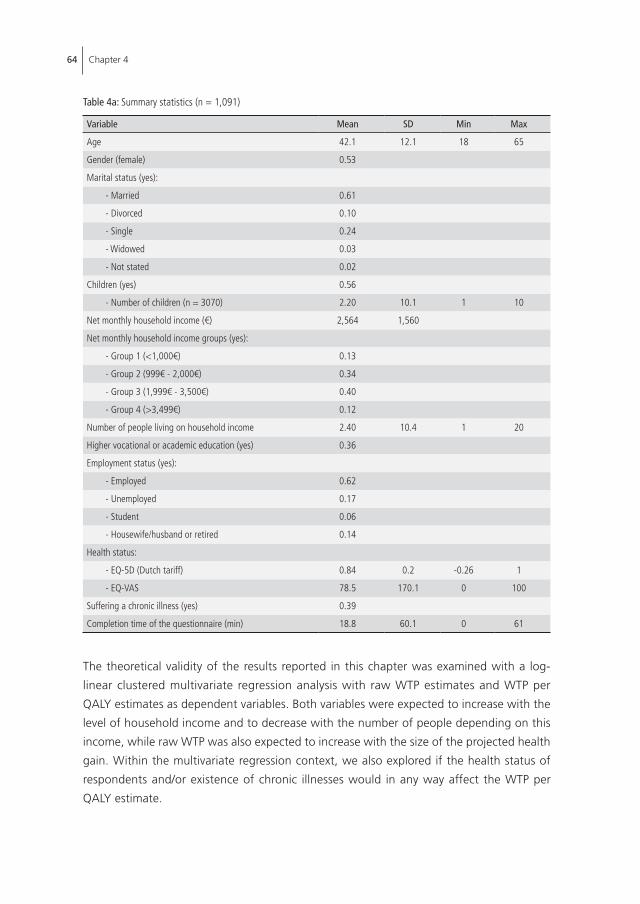
64 Chapter 4
The theoretical validity of the results reported in this chapter was examined with a log-
linear clustered multivariate regression analysis with raw WTP estimates and WTP per
QALY estimates as dependent variables. Both variables were expected to increase with the
level of household income and to decrease with the number of people depending on this
income, while raw WTP was also expected to increase with the size of the projected health
gain. Within the multivariate regression context, we also explored if the health status of
respondents and/or existence of chronic illnesses would in any way affect the WTP per
QALY estimate.
Table 4a: Summary statistics (n = 1,091)
Variable Mean SD Min Max
Age 42.1 12.1 18 65
Gender (female) 0.53
Marital status (yes):
- Married 0.61
- Divorced 0.10
- Single 0.24
- Widowed 0.03
- Not stated 0.02
Children (yes) 0.56
- Number of children (n = 3070) 2.20 10.1 1 10
Net monthly household income (€) 2,564 1,560
Net monthly household income groups (yes):
- Group 1 (<1,000€) 0.13
- Group 2 (999€ - 2,000€) 0.34
- Group 3 (1,999€ - 3,500€) 0.40
- Group 4 (>3,499€) 0.12
Number of people living on household income 2.40 10.4 1 20
Higher vocational or academic education (yes) 0.36
Employment status (yes):
- Employed 0.62
- Unemployed 0.17
- Student 0.06
- Housewife/husband or retired 0.14
Health status:
- EQ-5D (Dutch tariff) 0.84 0.2 -0.26 1
- EQ-VAS 78.5 170.1 0 100
Suffering a chronic illness (yes) 0.39
Completion time of the questionnaire (min) 18.8 60.1 0 61

Willingness to pay for a Quality-adjusted Life Year: the individual perspective 65
4
Separate regressions were conducted for each of the utility and WTP elicitation techniques.
Variables and their associations were compared using parametric and nonparametric tests.
The results of the PS were tested for order bias by comparing the WTP estimates between
samples that solved the same blocks of scenarios in different orders. The specification of
the PS, and the mid-point and end-point bias, were investigated by examining response
patterns on the PS, both in the pilot and the main study. The relationship between EQ-VAS
and EQ5D tariffs was checked for consistency. All analysis was conducted using STATA for
Windows version 10.
4.3 REsulTs
One thousand ninety-one respondents, representative of the Dutch population according
to age (18–65 years), sex, and education, participated in the survey. The description of the
sample is given in table 4a. The respondents were predominately married, employed, and in
very good health (EQ-5D 0.84; EQ-VAS 78.5) (39% of the sample reported suffering from
a chronic condition, and although the severity of the condition was not specified, given
the average score on the EQ-VAS and EQ-5D tariff, we can assume that the respondents
predominately suffered from very mild or mild chronic conditions.). The sample average
net household income of €2564 a month, with an average of 2.44 household members
depending on that income, adequately represents the Dutch national figures for 2008
(CBS, 2009).
4.3.1 WTP for non-health items
As shown in table 4a, the respondents gave plausible estimates of WTP for a car (mean
€10,900, median €7,000), a pair of shoes (mean €109, median €80), and housing (mean
€201,600, median €200,000) of their choice. From this, we inferred that the respondents
understood the exercise, although the focal point of the exercise - health - may be more
difficult to value, as normal (direct) market prices are absent.
4.3.2 QAlY weights
The correlation between QALY weights obtained from the EQ-VAS scores and the Dutch
EQ-5D tariffs was low (r = 0.24). The average health gain was 0.23 based on EQ-5D tariffs
and 0.33 (SD 0.29; median 0.25) based on the EQ-VAS. There is a statistically significant
difference between them (p = 0.02). The tests of consistency between EQ-VAS and the

66 Chapter 4
Dutch EQ-5D tariffs conducted on the level of particular health states showed that the
two valuation techniques especially provided similar valuations for health states situated
in the middle range of the utility scale. It was tested and confirmed that the better health
states received, on average, higher valuations on the EQ-VAS. The respondents reversed
the ranking (or valued the obviously worse health state higher on the EQ-VAS) on average
in only 7% of scenarios.
4.3.3 Patterns in WTP answers
Data inspection did not disclose any unusual patterns. Less than 1.5% of the respondents
chose the highest level offered on the PS (€2,500). Sixty-two respondents indicated, in
one or more scenarios, that they would not pay more than €0 for a health gain (only 23
respondents indicated €0 in all five scenarios). No consistent relationship was found between
the size of the health gain, household income, and zero WTP. The interpretations of zero
WTP were uniformly distributed among the offered explanations, and protest answers were
observed in only 1.4% of all scenarios. We therefore proceeded with the analysis without
specifically considering (or excluding) these responses.
The distribution of the certainty in the provided answers revealed that the majority of
respondents (56%) was either pretty or totally sure that they would actually pay the stated
amount for the specified health gain; 33% indicated uncertainty, 8% was not very sure
they would pay, and 3% indicated they were unsure they would pay. The majority of the
respondents would give up charitable donations or savings if they needed to pay for the
medicine out-of-pocket.
Test results did not indicate that the mid-point or range bias played a noteworthy role. The
results show a highly left-skewed distribution of values chosen from the PS. Although the
results did not concentrate at one particular amount on the scale, the majority of values
chosen on the scale fell between €50 and €200. Finally, the tests showed that WTP per
QALY elicited when the scenario offering the largest gain was presented first in a block did
not differ from WTP per QALY estimates elicited when the scenario offering the smallest
gain was presented first, thus refuting the order bias.
4.3.4 Maximum WTP per QAlY
The estimates of WTP per QALY varied considerably with the method of calculation. Table
4b provides the breakdown of WTP per QALY values according to: 1) the source of health
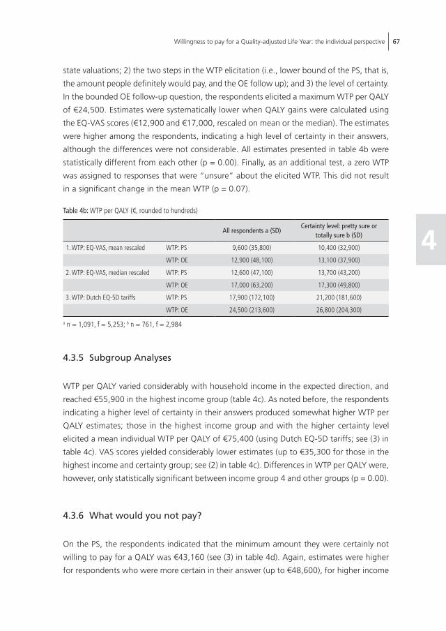
Willingness to pay for a Quality-adjusted Life Year: the individual perspective 67
4
state valuations; 2) the two steps in the WTP elicitation (i.e., lower bound of the PS, that is,
the amount people definitely would pay, and the OE follow up); and 3) the level of certainty.
In the bounded OE follow-up question, the respondents elicited a maximum WTP per QALY
of €24,500. Estimates were systematically lower when QALY gains were calculated using
the EQ-VAS scores (€12,900 and €17,000, rescaled on mean or the median). The estimates
were higher among the respondents, indicating a high level of certainty in their answers,
although the differences were not considerable. All estimates presented in table 4b were
statistically different from each other (p = 0.00). Finally, as an additional test, a zero WTP
was assigned to responses that were “unsure” about the elicited WTP. This did not result
in a significant change in the mean WTP (p = 0.07).
Table 4b: WTP per QALY (€, rounded to hundreds)
All respondents a (SD)Certainty level: pretty sure or
totally sure b (SD)
1. WTP: EQ-VAS, mean rescaled WTP: PS 9,600 (35,800) 10,400 (32,900)
WTP: OE 12,900 (48,100) 13,100 (37,900)
2. WTP: EQ-VAS, median rescaled WTP: PS 12,600 (47,100) 13,700 (43,200)
WTP: OE 17,000 (63,200) 17,300 (49,800)
3. WTP: Dutch EQ-5D tariffs WTP: PS 17,900 (172,100) 21,200 (181,600)
WTP: OE 24,500 (213,600) 26,800 (204,300)
a n = 1,091, f = 5,253; b n = 761, f = 2,984
4.3.5 subgroup Analyses
WTP per QALY varied considerably with household income in the expected direction, and
reached €55,900 in the highest income group (table 4c). As noted before, the respondents
indicating a higher level of certainty in their answers produced somewhat higher WTP per
QALY estimates; those in the highest income group and with the higher certainty level
elicited a mean individual WTP per QALY of €75,400 (using Dutch EQ-5D tariffs; see (3) in
table 4c). VAS scores yielded considerably lower estimates (up to €35,300 for those in the
highest income and certainty group; see (2) in table 4c). Differences in WTP per QALY were,
however, only statistically significant between income group 4 and other groups (p = 0.00).
4.3.6 What would you not pay?
On the PS, the respondents indicated that the minimum amount they were certainly not
willing to pay for a QALY was €43,160 (see (3) in table 4d). Again, estimates were higher
for respondents who were more certain in their answer (up to €48,600), for higher income

68 Chapter 4
Tabl
e 4c
: WTP
per
QAL
Y di
ffere
ntia
ted
by in
com
e gr
oups
and
leve
ls of
cer
tain
ty (€
, rou
nded
to h
undr
eds)
Inco
me
grou
ps (S
D)In
com
e gr
oups
and
cer
tain
ty le
vel:
pret
ty s
ure
or to
tally
sur
e (S
D)
1 a
2 b
3 c
4 d
1 e
2 f
3 g
4 h
1. W
TP: E
Q-V
AS, m
ean
resc
aled
WTP
: PS
5,00
0 (1
2,90
0)8,
200
(41,
100)
8,80
0 (2
2,10
0)20
,800
(60,
900)
5,00
0 (7
,600
)8,
500
(30,
100)
9,10
0 (1
9,60
0)22
,200
(63,
600)
WTP
: OE
8,00
0 (2
7,30
0)11
,400
(63,
500)
11,9
00 (2
8,50
0)25
,200
(62,
000)
6,70
0 (1
0,50
0)11
,100
(42,
100)
11,5
00 (2
2,40
0)26
,900
(64,
200)
2. W
TP: E
Q-V
AS, m
edia
n re
scal
edW
TP: P
S6,
500
(17,
000)
10,8
00 (5
4,00
0)11
,500
(29,
100)
27,3
00 (8
0,00
0)6,
600
(9,9
00)
11,1
00 (3
9,60
0)12
,000
(25,
700)
29,1
00 (8
3,60
0)
WTP
: OE
10,5
00 (3
6,00
0)15
,000
(83,
500)
15,7
00 (3
7,50
0)33
,200
(81,
600)
8800
(13,
900)
14,7
00 (5
5,30
0)15
,100
(29,
400)
35,3
00 (8
4,40
0)
3. W
TP: D
utch
EQ
-5D
tarif
fsW
TP: P
S8,
200
(34,
100)
14,3
00 (1
78,3
00)
15,1
00 (9
0,70
0)47
,100
(349
,200
)8,
000
(29,
600)
11,1
00 (4
7,90
0)17
,400
(111
,900
)63
,900
(426
,200
)
WTP
: OE
12,6
00 (2
87,6
00)
18,0
00 (1
82,4
00)
21,1
00 (1
28,4
00)
55,9
00 (3
69,0
00)
11,1
00 (4
1,30
0)15
,100
(60,
000)
22,9
00 (1
56,3
00)
75,4
00 (4
50,0
00)
a n =
139
, f =
672
; b n =
371
, f =
1,8
06; c n
= 4
40, f
= 2
,117
; d n =
134
, f =
658
; e n =
86,
f =
318
; f n =
248
, f =
964
; g n =
317
, f =
1,2
62; h n
= 1
07, f
= 4
40
Tabl
e 4d
: WTP
per
QAL
Y up
per b
ound
, ave
rage
and
diff
eren
tiate
d by
inco
me
grou
ps a
nd le
vels
of c
erta
inty
(€, r
ound
ed to
hun
dred
s)
All r
espo
nden
ts a
(SD)
Cert
aint
y le
vel:
pret
ty o
r to
tally
sur
e b (S
D)
Inco
me
grou
ps (S
D)In
com
e gr
oups
and
cer
tain
ty le
vel:
pret
ty o
r tot
ally
sur
e (S
D)
1 c2
d3
e4
f1 f
2 h
3 i
4 j
1. W
TP: E
Q-V
AS, m
ean
resc
aled
23,8
00(7
5,80
0)22
,500
(56,
200)
18,0
00(9
2,30
0)22
,400
(85,
000)
22,1
00(5
7,30
0)39
,150
(81,
200)
12,5
00(2
1,10
0)20
,400
(63,
800)
20,0
00(4
2,90
0)41
,000
(80,
700)
2. W
TP: E
Q-V
AS, m
edia
n re
scal
ed31
,300
(99,
700)
29,5
00(7
3,90
0)23
,700
(121
,400
)29
,400
(111
,700
)29
,100
(75,
300)
51,5
00(1
06,8
00)
16,4
00(2
7,70
0)26
,800
(838
00)
26,3
00(5
6,40
0)54
,000
(106
,100
)
3. W
TP: D
utch
EQ
-5D
tarif
fs43
,160
(308
,500
)48
,600
(351
,000
)45
,800
(412
,900
)33
,000
(264
,400
)37
,800
(210
,000
)86
,100
(502
,900
)44
,400
(421
,600
)32
,700
(265
,000
)39
,000
(248
,900
)11
4,90
0(6
12,7
00)
a n =
1,0
91, f
= 5
,253
; b n =
761
, f =
2,9
84;c n
= 1
39, f
= 6
72; d n
= 3
71, f
= 1
,806
; e n =
440
, f =
2,1
17; f n
= 1
34, f
= 6
58; g n
= 8
6, f
= 3
18; h n
= 2
48, f
= 9
64; I n
= 3
17, f
= 1
,262
; j n =
107,
f =
44

Willingness to pay for a Quality-adjusted Life Year: the individual perspective 69
4
groups (up to €86,100), and these characteristics combined (up to €114,900). Using EQ-
VAS scores in the calculation of the amount the respondents were not willing to pay for a
particular gain yields the estimate of up to €54,000 (i.e., (2) in table 4d).
4.3.7 Theoretical validity
Table 4e presents the results of multivariate logarithmic regressions with raw WTP values
and WTP per QALY estimates as dependent variables. T-tests showed that all independent
variables were statistically significant (at 1 or 5% level), and F-test showed that the regression
equations were statistically significant at any regular level. Results for health gains computed
using median-rescaled EQ-VAS scores were omitted because they are highly comparable to
the mean-rescaled ones.
Table 4e: Multivariate clustered regression analysis with “raw” WTP and WTP per QALY estimates as the dependent variable
WTP: PS WTP: OE WTP: PS WTP: OE
β SE P>|t| β SE P>|t| β SE P>|t| β SE P>|t|
DV: Log (WTP)
QALY gain: Log (EQ-VAS) 0.05 0.02 0.06 0.06 0.03 0.02
QALY gain: EQ-5D 0.13 0.05 0.02 0.13 0.06 0.04
Log (household income) 0.74 0.07 0.00 0.81 0.09 0.00 0.73 0.07 0.00 0.79 0.09 0.00
Log (age) -0.21 0.1 0.03 -0.33 0.11 0.00 -0.21 0.09 0.02 -0.33 0.11 0.00
Higher vocationalor academic education (yes)
0.25 0.07 0.00 0.23 0.07 0.00 0.25 0.06 0.00 0.22 0.07 0.00
Number of people livingon household income
-0.07 0.02 0.00 -0.09 0.03 0.00 -0.07 0.02 0.00 -0.08 0.03 0.00
Constant -0.55 0.57 0.34 -0.42 0.67 0.53 -0.58 0.56 0.29 -0.37 0.67 0.58
Adjusted R2 0.11 0.12 0.12 0.18
DV: Log (WTP per QALY)
Log (household income) 0.71 0.08 0.00 0.78 0.10 0.00 0.72 0.07 0.00 0.79 0.10 0.00
Log (age) -0.24 0.11 0.00 -0.35 0.12 0.00 -0.28 0.10 0.01 -0.40 0.11 0.00
Higher vocational oracademic education (yes)
0.31 0.08 0.00 0.29 0.08 0.00 0.20 0.07 0.00 0.18 0.08 0.02
Number of people livingon household income
-0.07 0.03 0.01 -0.08 0.03 0.01 -0.07 0.03 0.01 -0.08 0.03 0.01
Constant 3,6 0.65 0.00 3,7 0.73 0.00 3,7 0.59 0.00 3,8 0.70 0.00
Adjusted R2 0.07 0.08 0.06 0.06
n 4,841 4,982 5,029 5,184
The results are in line with a priori expectations; the WTP and WTP per QALY estimates were
positively associated with the size of the health gain and household income, and negatively

70 Chapter 4
associated with the number of household members supported by the household income.
In both sets of regressions, WTP increased with the level of education (e.g., Zethraeus,
1998) and decreased with age. Current health status, being chronically ill and subjective life
expectancy, was not associated with raw WTP or WTP per QALY (regressions not presented
here). The adjusted R2 were low, similar to related work (King et al., 2005).
4.4 disCussion
Recently, more empirical research to determine the monetary value of a QALY has been
called for and initiated (Weinstein, 2008; Gyrd-Hansen, 2003; Mason et al., 2008a, 2008b;
EUROVAQ, 2009). In this context, we estimated the first monetary value of a QALY in The
Netherlands, using a comprehensive valuation exercise from the individual perspective. The
results show that the maximum WTP for a QALY, derived through aggregating and averaging
individual responses, is €24,500.
As we have shown, however, the estimates of the WTP per QALY can vary substantially,
depending on the specific sub-groups and methods of calculation. In terms of the latter,
using the EQ-VAS valuations of the health changes rather than the TTO tariffs, resulted
in an average estimate of €12,900. Such a discrepancy between TTO-based values and
VAS-based values of the maximum WTP per QALY has been noted before (Lundberg et al.,
1999). Indeed, the two techniques are known to yield different estimates, but the debate
regarding their acceptability or accuracy is well beyond the scope of this study (Parkin and
Devlin (2006) bring the discussion on EQ-VAS). For the current purpose, we consider the
EuroQoL-5D tariffs to be more relevant because they are most commonly used and derived
in a standardized way. In terms of the former, valuations of subgroups stratified by income
level and level of certainty, proved to differ substantially. The richest, most certain subgroup
elicited a considerably higher WTP per QALY (i.e., €75,400; their upper-bound estimate
using the PS is €114,900). It seems important to stress these variations and to be careful
with terms as “the value” of a QALY. Similarly, the standard deviations around the WTP
estimates were considerable, indicating a large variation in preferences. The level of variation
was lowest for the lower-bound estimates of WTP (i.e., highest amount people certainly
would pay, as indicated on the PS) and it increased with the size of WTP. Moreover, it is
also important to note that the individual valuations can be combined in different ways to
come to a value of a QALY. Aggregating in a different way than the one chosen here (i.e.,
taking the mean of ratios) is likely to result in different estimates of WTP per QALY. Such
methodological aspects of deriving monetary values from the “raw material” deserve more
attention, especially because there appears to be no guidance or consensus on this topic.

Willingness to pay for a Quality-adjusted Life Year: the individual perspective 71
4
The results presented here align with the relevant range of the cost-effectiveness threshold
of £20,000 to £30,000 (or €23,300 to €35,000) used by NICE in recent years (McCabe et al.,
2008) and the most commonly cited threshold of €20,000 in The Netherlands (e.g., Brouwer
et al., 2008b). Similar results were recently derived from the existing value of preventing
a statistical fatality in the UK context, with estimates ranging between £23,199 (€26,877)
and £40,029 (€46,375) per QALY (Mason et al., 2008b). Gyrd-Hansen (2003), using a DCE
approach and TTO utilities, estimated a WTP per QALY of €12,000 in the general population
of Denmark for relatively small-sized health gains. King et al. (2005) reported on WTP per
QALY ratios obtained in three distinct patient populations. Using EQ-VAS, Standard Gamble,
and TTO to elicit utilities, they found a maximum WTP per QALY ranging from $12,500
(€9500) to $32,000 (€24,500). Recently, Shiroiwa et al. (2009) estimated the WTP for an
additional year of survival in full health, and found that the mean WTP per QALY ranged
from £23,000 (€26,600) in the UK, AU$64,000 (Australia; €36,600) to US$62,000 (USA;
€44,000). Seemingly, the available empirical estimates range roughly between €10,000 and
€45,000 - aligning with the lower- and upper-bound estimates for the full sample obtained
in the current study.
We note that several methodological issues that deserve attention may have influenced our
results. First is the range of values offered on the PS (Whynes et al., 2004; Frew et al., 2003).
We carefully pre-tested the range of the scale in a pilot study and, to minimize the mid-point
bias, employed a two-question procedure in using the PS. The majority of values chosen on
the scale fell between €50 and €200. The end-point bias could be rejected, because only a
few respondents (in less than 1.5% of scenarios) opted for the highest amount offered on
the scale (€2,500). Nevertheless, some concerns remain with the range of the scale because
the results could not be compared to results from a scale of a different range. The range
may thus be limiting both the WTP estimates and the difference between WTP per QALY
values stemming from the PS and the bounded OE question. Nevertheless, the use of a
two-step procedure in deriving WTP estimates proved feasible and helpful, yet it must be
noted that using other elicitation techniques may result in different estimates of WTP. This
seems an important area for further research.
Furthermore, it could be argued that the respondents’ ability to pay constrained the monetary
value of a QALY, especially in light of non-marginal health gains employed. Nevertheless,
the data show that this too could only be a minor problem. The average maximum WTP
for an average gain of 0.33 (EQ-VAS) or 0.23 (EQ-5D tariffs) was €174 a month, while the
average net monthly household income was €2,564. This suggests that the respondents
were not bidding to the point of a catastrophic payment (i.e., spending on average 6.79%
of the monthly household income) or that the ability to pay limited the expressed WTP. Still,
employing marginal gains would decrease such concerns even further, which could result

72 Chapter 4
in higher estimates of WTP. In that sense, our estimates might be seen as lower bounds of
the WTP per QALY. Nevertheless, using marginal increments could raise questions regarding
the extrapolation of obtained WTP estimates to scenarios in which non-marginal health
improvements are relevant (Gyrd-Hansen, 2003). Second, the respondents only valued
potential health improvements and not potential mortality reduction. While many healthcare
interventions are indeed aimed at improving quality of life rather than reducing mortality,
which emphasizes the relevance of the here presented figures, obtaining estimates in the
context of mortality reduction remains important. It is likely that such estimates would be
higher than the ones presented here (Bleichrodt and Quiggin, 1999; Mason et al., 2008a).
Such scenarios would, unlike the ones used in this study, require valuations under risk rather
than under certainty. While this has advantages such as marginality when using small risks,
it also entails disturbing elements like risk weighting, which would need to be accounted
for in analyzing the results. Third, the choice of the payment vehicle and frequency could
be another important contextual determinant of the size of WTP per QALY estimate. In
this study, WTP was elicited in relation to actual use of the intervention (as opposed to an
“insurance” context) and payments phrased as monthly outlays (as opposed to, for instance,
a lump sum). Although individuals in the Netherlands are somewhat acquainted with paying
out-of-pocket for healthcare (according to OECD (2009), 8% of all healthcare is financed
out-of-pocket) and increasingly so since the introduction of a mandatory deductible (Holland
et al., 2009), it remains unclear to what extent the type of payment seemed realistic to
respondents. A similar issue has been reported by (Skjoldborg and Gyrd-Hansen, 2003), and
it limits the applicability of the results. Phrasing the payments in terms of a lump sum might
have produced more conservative estimates because it does not offer the opportunity of
spreading the burden over time (Carson, 2000), but could induce problems of ability to pay
and budget constraints. Fourth, the relative position of the respondent’s own health and
the health states valued could have affected the WTP valuations because some health states
could have been considered as a relative gain or a loss. Although most respondents’ own
health was evaluated higher than the health states presented in the questionnaire, in the
analysis, we took the usual assumption that, given the instructions, own health is, in fact,
irrelevant for the valuation. The data did not allow a firm test of whether this assumption
actually holds. Similarly, the style or framing of the WTP question (i.e., valuing gains in
health as opposed to valuing avoiding a loss in health) could have had an effect on WTP.
Although these issues, and the scale of their impact, are beyond the scope of this study,
they remain interesting empirical and theoretical questions. Finally, an important limitation
of this study (and other preference elicitation studies) is the hypothetical nature of the
exercise. Similar to other studies, the respondents might have found it difficult to imagine
being in a health state other than what they have experienced. The same holds for other
elements of our questionnaire (for instance, the concept of painless cure or the duration
of health loss of precisely 12 months). Regardless of the effort put into increasing realism

Willingness to pay for a Quality-adjusted Life Year: the individual perspective 73
4
and reducing the hypothetical bias (through ex ante and ex post mitigation), it is uncertain
whether the elicited WTP corresponds to the real (revealed) WTP. Some have indicated that
the subgroup of most certain respondents would produce an estimate of WTP that is fairly
close to “real” WTP (Blumenschein et al., 2008). In this study, this implies that a slightly
higher estimate of WTP per QALY - €26.800 instead of €24.500 - would be relevant (table
4b). Given that the two estimates are not considerably different, that only one is informed by
all respondents and that it has been recommended (Arrow et al., 1993) to use conservative
estimates in contingent valuation studies, we have focused here on the estimate of €24.500.
Encouragingly, as seen above, these results compare well to the relevant range of the most
often-cited cost- effectiveness threshold.
Some issues need to be addressed concerning the use of the figures presented here in the
context of health policy. First, the figures are lower than some thresholds that have been
mentioned elsewhere, such as the $50,000 or $100,000 threshold in the US context or,
for instance, the upper limit of €80,000 proposed in The Netherlands by an important
advisory body RVZ (2009). Moreover, they are lower than what we infer from a part of the
value-of-life literature (Hirth et al., 2000) and lower than the estimates of WTP for a life-year
saved (Braithwaite et al., 2008). Such large variations, undoubtedly fuelled by underlying
methodological differences, exist and need to be explicitly addressed before recommending
the use of particular thresholds in health policy. One of the key normative and methodological
issues is the perspective from which the appropriate height of the cost-effectiveness threshold
needs to be determined (Dolan et al., 2003). This appears to be an essential element in future
theoretical and empirical work. For instance, the €80,000 threshold in The Netherlands was
not proposed as a fixed threshold, but as the maximum of a range. Importantly, this range
does not increase with individual valuations (such as income in the current study), yet is
increasing with more socially driven considerations, namely disease severity, which can be
seen as an equity consideration (Stolk et al., 2004). NICE, perhaps somewhat similar, asks
that a technology with the ICER of over £20,000 per QALY needs to make explicit references
to “the particular features of the condition and population receiving the technology” as
to increase its chances of being accepted (NICE, 2004). Recently, NICE even indicated that
certain interventions (for example, lifesaving cancer drugs) may be approved in spite of less
favorable cost-effectiveness (NICE, 2008; Towse, 2009).
Equity considerations thus appear to play a role in societal decisions. Indeed, when looking
at the literature regarding “equity weights,” this becomes even clearer (e.g., Williams and
Cookson, 2000; Dolan et al., 2005). People attach weights to health gains according to
the “the particular features of the condition and population receiving the technology”,
it seems. Importantly, though, such preferences are most likely not reflected in individual

74 Chapter 4
valuations of own health gains. This raises the issue of usefulness of individual valuations
in the current context.
If we are, however, to consider individual valuations of health gains as relevant for societal
decisions on the allocation of health- care resources, the question of how to use these
individual valuations is important. For example, in this study, we find a great variation
in WTP across income groups. The average individual threshold of €24,500 is therefore
only the “right” valuation for a small group of individuals. From a traditional normative
welfare economic viewpoint, it is easy to argue that simply taking the average can result
in systematically “wrong” decisions. Indeed, applying such a cost-effectiveness threshold
“unduly” restricts the provision of expensive interventions to the rich part of the population
(as true benefits are higher than projected), while it “unduly” grants them to poorer groups
(because the true benefits are lower than projected). A similar argument extends to the
use of the mean monetary value of premature fatality (i.e., value of a statistical life) as a
threshold in economic evaluations done by the UK Department of Transport.
This practice resembles an implicit weighting procedure (of valuations), from an individual
perspective. While we may wish to do so for many reasons, welfarist or extra-welfarist
(Brouwer et al., 2008a), the justification for using the average (as opposed to the median
or the maximum) needs to be clear, and still is not (e.g., Baker et al., 2008).
If, on the contrary, we expect that individual valuations of own health gains may not be
directly relevant for the societal decisions we are faced with, it may be worthwhile attempting
to directly elicit something like the “societal WTP for a QALY.” Such an ex-ante value should
be the focus of future research. In our view, it should include aspects like option value and
solidarity, and would be allowed to vary with characteristics of the beneficiaries of healthcare
interventions such as disease severity and age (instead of income). Indeed, in the context of
the collective decisions in the healthcare sector involving (risk and income) solidarity, one
may consider valuations directly derived from a societal perspective to be more relevant
for the question at hand. This then allows a direct link between equity weights and the
value of QALY gains, as well as a transparent public discourse (if not consensus) on what
the desirable weights should be. It does require, however, that such valuation studies be
appropriately designed, also in order to be able to interpret the results straightforwardly.
It seems, therefore, that the quest of finding appropriate monetary values is just beginning.
While this study hopes to have contributed in this quest, it is clear that important normative
and methodological issues need to be addressed before the results can be used in a policy
context.

Willingness to pay for a Quality-adjusted Life Year: the individual perspective 75
4
4.5 APPEndix 4A
Figure 4A.1: Ranking two health statesThe wording of the task in English: “Imagine yourself in either of the two health states. Which of the two you find better?”
Figure 4A.2: Rating the two health states on an EQ-VAS showing previous valuations of death, perfect health and own healthThe wording of the task in English: “Place the two health states on the rating scale”
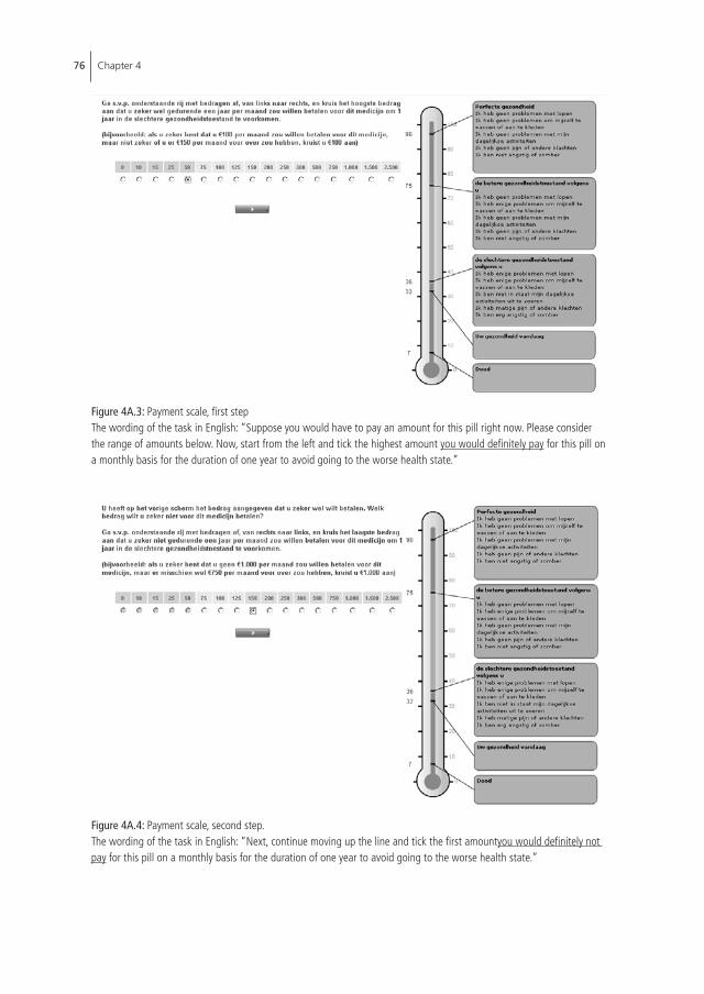
76 Chapter 4
Figure 4A.3: Payment scale, first stepThe wording of the task in English: “Suppose you would have to pay an amount for this pill right now. Please consider the range of amounts below. Now, start from the left and tick the highest amount you would definitely pay for this pill on a monthly basis for the duration of one year to avoid going to the worse health state.”
Figure 4A.4: Payment scale, second step.The wording of the task in English: “Next, continue moving up the line and tick the first amountyou would definitely not pay for this pill on a monthly basis for the duration of one year to avoid going to the worse health state.”

Willingness to pay for a Quality-adjusted Life Year: the individual perspective 77
4
Figure 4A.5: Open-ended format.The wording of the task in English: “You have indicated that you would definitely pay €50 and definitely not pay €150 to avoid experiencing the worse health state for one year and remaining in the better health state. Please write in the amount (between €50 and €150) that most closely approximates the maximum you would be willing to pay per month to avoid going to the worse health state?”

78 Chapter 4
Table 4A.2: Design of the choice scenarios, levels of risk and expected QALY gain
Choice scenario Health state 1 Health state 2 Health gain
1 22222 11131 0.203
2 33232 33323 0.017
3 21312 12111 0.369
4 22323 21312 0.369
5 22323 12111 0.738
6 21232 32211 0.246
7 11112 22121 0.008
8 11122 22122 0.118
9 21323 22233 0.300
10 22331 21133 0.186
11 21111 12121 0.132
12 23232 32232 0.055
13 11312 11113 0.144
14 12311 11211 0.341
15 32311 12311 0.161
16 32311 11211 0.502
17 21111 12211 0.078
18 32313 32331 0.004
19 11211 22211 0.118
20 23313 11133 0.084
21 11121 22112 0.156
22 12223 13332 0.137
23 11312 11211 0.383
24 11332 11312 0.329
25 11332 11211 0.712
26 21222 33321 0.412
27 22222 13311 0.083
28 11112 22112 0.118
29 33212 32223 0.217
*Risk reduction to zero in Que1, halved in Que2.
Table 4A.1: The wording of WTP question in English
Please suppose you are in the health state that you assessed as the better one but face moving to the worse health state tomorrow. If you do not avoid this deterioration, you will certainly remain in the worse health state for one year. After this year, you will return to the better health state.You can avoid this health deterioration completely by taking a medicine (with no side effects) each month. You will then certainly remain in the better health state. You must pay for this medicine yourself, directly from your (net monthly household) income.Please have your ability to pay (given your household income) in mind!!

Chapter 5Get more, pay more? An elaborate test of construct validity of willingness to pay per QALY estimates obtained through contingent valuation
Chapter based on: Bobinac A, Van Exel NJA, Rutten FFH, Brouwer WBF (2011) , pay more? An elaborate test of construct validity of willingness to pay per QALY estimates obtained through contingent valuation. Journal of Health Economics 31: 158-168.

80 Chapter 5
suMMARY
Estimates of WTP per QALY can be taken as an indication of the monetary value of health
gains, which may carry information regarding the appropriate height of the cost-effectiveness
threshold. Given the far-reaching consequences of choosing a particular threshold, and thus
the potential relevance of WTP per QALY estimates, it is important to address the validity
of these estimates. This study addresses this issue. Our findings offer little support to the
validity of WTP per QALY estimates obtained in this study. Implications for general WTP per
QALY estimates and further research are discussed.

81
5
Get more, pay more? An elaborate test of construct validity of willingness to pay per QALY estimates obtained through contingent valuation
5.1 inTRoduCTion
Economic evaluations inform allocation decisions in the healthcare sector by evaluating
alternative interventions in terms of costs and benefits, typically expressed in non-monetary
terms such as Quality-adjusted Life Years (QALYs) and summarized in an incremental cost-
effectiveness ratio (ICER). Common decision rules indicate that an intervention is “good
value for money” if the ICER falls below the relevant cost-effectiveness threshold, which
represents the relevant value of a health gain within a specific decision-making context.
The nature and height of the threshold can vary with the normative rule adopted (Claxton
et al., 2010). It can be viewed as representing opportunity costs of spending within the
healthcare sector or as the (monetary) value society places on marginal health gains. If the
second, perhaps more common, viewpoint is taken, the monetary value of the QALY can
be empirically estimated with some preference elicitation method, the most prominent of
which is contingent valuation (CV), or the willingness-to-pay (WTP) method, which has been
applied several times in this context (Gyrd-Hansen, 2003; King et al, 2005). The important
consequence of choosing a particular threshold – and thus the potential relevance of the
WTP per QALY estimates – calls for addressing the issue of validity28 of WTP per QALY
estimates. When such estimates are intended to inform decision-making in the healthcare
sector, they need to be robust. Issues of validity and reliability thus have more than merely
academic interest (Bateman and Brouwer 2006).
Broadly speaking, the validity of WTP estimates refers to whether the estimates concur with
the underlying economic theory, i.e., the neoclassical theory of consumer behavior, which
predicts that larger gains result in higher WTP, ceteris paribus. Validity can thus be judged
by considering the robustness of WTP to changes in the QALY gains offered (for instance,
by varying the size of the quality improvement or the duration of the health gains). While
theory predicts that WTP should increase with increasing QALY gains, it does not predict
the exact size of the increase (Fisher, 1996; Bateman and Brouwer, 2006). The relationship
between WTP and QALY gains is expected to be increasing yet concave, such that an increase
in the QALY gain offered yields a less than proportional increase in WTP (Bradford, 1972;
Smith, 2005; Olsen et al., 2004a). This is mainly due to diminishing marginal utility of health
and the income effect (where an increasing WTP takes a higher proportion of income and
decreases the ability to pay (Flores and Carson, 1997; Smith, 2005)).
28. Validity is about whether the measure reflects what it intends to (i.e., accuracy), as opposed to reliability, which deals with whether the instrument measures something other than random noise (i.e., reproducibility) (Jorgensen et al., 2004).

82 Chapter 5
WTP estimates have been criticized for their insensitivity to scale, implying that they do not
vary “meaningfully” with the quantity of the offered good. Given that a non-proportional
increase is expected theoretically, the degree of robustness must also be evaluated to allow
more general claims about the validity of WTP estimates. In other words, finding a significant
(and positive) coefficient of the health gain (or income) in a linear regression explaining
the variance in WTP, usually termed “theoretical validity” (e.g., Ryan, 2004; Lienhoop and
MacMillian, 2007), is a necessary but not sufficient condition for a more general claim about
validity. Indeed, the appropriate sign does not necessarily imply that the associated variation is
“practically meaningful” or, as it also has been labeled, “theoretically plausible” (Olsen et al.,
2004a), let alone that the estimates can be directly applied in decision-making. Results that
cannot be shown to be theoretically invalid may thus still be considered practically irrelevant.
Judging whether results are practically meaningful, i.e., whether the size of the coefficient is
deemed appropriate, requires a judgment that is normative and not directly informed by theory
(Hammitt and Graham, 1999). This issue has yet to receive due attention in the literature. It
has, for instance, been suggested that WTP estimates for small risk reductions need to be
near-proportional (increasing and strictly concave) to the size of the risk reduction (NOAA,
1993; Hammitt and Graham, 1999). Although perhaps somewhat restrictive, the condition of
near-proportionality might thus be appropriate in establishing what practically meaningful (i.e.,
“theoretically plausible”) refers to. We will use this benchmark here as well. Still, obviously,
when one exactly considers something to be near-proportional, is again somewhat arbitrary.
Although the validity of WTP estimates for goods other than health has attracted considerable
attention (Desvousges et al., 1993; McFadden and Leonard, 1993; Jones-Lee et al., 1995;
Carson and Mitchell, 1995; Frederick and Fischoff, 1998; Hammitt and Graham, 1999;
Smith, 2001; Van Exel et al., 2006; Van Houtven et al., 2006; Smith and Sach, 2009; Baker
et al., 2010), in-depth empirical interest in the validity of WTP for changes in health per se
is limited (Olsen et al., 2004a; Smith, 2005; Yeung et a, 2003), particularly when health is
expressed in terms of QALYs. (A notable exception is Pinto Prades et al., 2009.) Validity, in
that sense, is not thoroughly addressed also in studies reporting the WTP per QALY estimates
(e.g., Shiroiwa et al., 2010; Donaldson et al., 2011). Given the commonness of using QALYs
as a measure of health gains and the increased interest in the monetary value of QALYs,
however, such studies appear warranted.
This study contributes to the literature by extensively exploring the validity of WTP per QALY
estimates, using a data set explicitly designed to (1) estimate the WTP per QALY and (2)
test the various aspects of this estimate’s validity. We define validity in terms of “construct

83
5
Get more, pay more? An elaborate test of construct validity of willingness to pay per QALY estimates obtained through contingent valuation
validity” (Jakobsson and Dragun, 1996), which encompasses scale sensitivity of WTP29 and
the related sub-additive impartiality (or “part-whole” bias). The latter refers to the fact that
the WTP for the same quantity of some good is typically less when this quantity is offered
as a whole, and more when it is offered in separately valued parts. The design of this study
allows validity testing along both dimensions of a QALY (length and quality of life), within
and between-blocks of data, and on aggregate and sub-group levels, thus allowing us to
account for the underlying heterogeneity in preferences. Particular hypothesis are described
in the Methods section.
5.2 METHods
This study uses a contingent valuation (CV) data set from a representative sample of the Dutch
population aged 18 to 65, designed to estimate the WTP for a QALY from the individual
perspective under certainty and to test the construct validity of WTP per QALY estimates.
(Chapter 4 brings more details on data collection.) A professional Internet sampling company
recruited respondents and administered the questionnaire online. Completion was rewarded
by a small sum donated to a charity of choice.
The construct validity of WTP per QALY estimates was tested using the following hypotheses:
Hypothesis I: WTP is sensitive to scale in terms of quality of life. That is, for a given duration,
a larger gain in quality of life should result in a higher WTP, both between and within-blocks.
The sensitivity will be evaluated in terms of theoretical validity and practical meaningfulness.
Hypothesis II: WTP is sensitive to scale in terms of duration. Within-blocks, for a given gain
in quality of life, a longer duration of the gain should result in a higher WTP. The sensitivity
will be evaluated in terms of theoretical validity and practical meaningfulness.
Hypothesis III: Subgroup-level data exhibits an increased level of sensitivity, relative to
average-level data. That is, in specific subgroups WTP is more sensitive to changes in the
size of the offered gain, both between and within-blocks.
29. This data set was previously used by Bobinac et al. (2010), a study reported in Chapter 4, for the purpose of reporting and discussing average WTP per QALY estimates while this study reports on testing the validity of the WTP per QALY estimates through examining the relationship between the WTP estimates and the QALY gains. Since the QALY is the outcome of interest, we will not address the sensitivity to scope in this study (i.e., sensitivity to a range of goods on offer).

84 Chapter 5
Hypothesis IV: WTP per QALY estimates are affected by the sub-additivity bias. Within-blocks,
the sum of the values attached to two smaller QALY gains are expected to exceed that
attached to the sum of these gains when valued jointly.
A significant difference between the WTP for smaller and larger gains is a necessary condition
for establishing construct validity, but it need not be a sufficient one. A more definite test
would be disproving the sub-additivity bias, i.e., finding a “near-proportional” relationship
between WTP estimates and the size of the health gains on offer, thus establishing a (near)
additive relationship between them.
5.2.1 survey instrument
42 health states, described using the EuroQoL-5D system (or EQ-5D; EuroQol Group, 1999),
were paired into 29 scenarios (table 4A.2 in Appendix 4A). Many of the selected health
states were originally applied in deriving the national tariffs for the EQ-5D (Kind et al.,
1998; Lamers et al., 2006) or applied by Gyrd-Hansen (2003) to estimate the WTP per
QALY in Denmark. The 29 scenarios, representing a fair spread of QALY gains across the
Table 5a: Scenario design
Scenario 1-3 Scenario 4: Pairing and duration in blocks
Scenario HS1 HS2HS1
(tariff)HS2
(tariff)QALY gain
Durationin years
1 2 3 4 5 6 7 8 9 10
Block1-4
1 21312 12111 0.478 0.847 0.369 1 3 5**
2 22323 21312 0.109 0.478 0.369 1 3* 5
3 22323 12111 0.109 0.847 0.738 1
Block5-7
1 12311 11211 0.556 0.897 0.341 1 3
2 32311 12311 0.395 0.556 0.161 1 3 5
3 32311 11211 0.395 0.897 0.502 1
Block8-10
1 11312 11211 0.514 0.897 0.383 1 3
2 11332 11312 0.185 0.514 0.329 1 3 5
3 11332 11211 0.185 0.897 0.712 1
* The “3” indicates that respondents in block 1 (see column in table), in addition to the three scenarios listed in columns 2-4 of the table, evaluated a fourth scenario, which was identical to scenario 2 (see row in table) in terms of the health states presented but differed in terms of duration (i.e. 3 years instead of 1 year). ** The “5” indicates that respondents in block 4 (see column in table), in addition to the three scenarios listed in columns 2-4 of the table, evaluated a fourth scenario, which was identical to scenario 1 (see row in table) in terms of the health states presented but differed in terms of duration (i.e. 5 years instead of 1 year).

85
5
Get more, pay more? An elaborate test of construct validity of willingness to pay per QALY estimates obtained through contingent valuation
utility range, were (with some overlap) assigned to 10 different blocks of six scenarios.
Respondents solved one randomly assigned block. Four out of six scenarios from each
block are relevant for this study as they were specifically designed and combined to test the
construct validity of WTP per QALY estimates. In particular, the first two scenarios in each
block represented smaller health gains that, according to Dutch EQ-5D tariffs (Lamers et al.,
2006), added up to a larger health gain presented in the third scenario (table 5a). Health
gains in different scenarios purposefully started either low or in the middle of the QALY
scale, ending either in the middle or high on the scale. To avoid specific dimensions of the
EQ-5D to dominate the results, the dimensions that constitute a quality of life gain within
scenarios were varied.30 In each block, one scenario was repeated as the fourth scenario,
but now with a longer duration (that is, 3 or 5 years instead of 1 year; see the right-hand
side of table 5a). The combinations of health states and durations were chosen to ensure
comparability across blocks.
The two remaining scenarios were not purposefully designed to test construct validity but
for the calculation of individual WTP per QALY under certainty.
Respondent-specific health state valuations were obtained from the visual analog scale
(EQ-VAS), as these represent the gains that were actually valued, in two steps.31 First,
respondents rated their current health, death, and perfect health on the VAS bounded by
end-points labeled “best imaginable health” and “worst imaginable health”. This allowed
for health states worse than death. Second, respondents indicated which of two presented
health states in each scenario was better and then rated the two states on the EQ-VAS
showing the previous valuations of current health, death and perfect health, thus providing
a valuation context. Respondents were instructed to imagine being in the better health state
and to indicate their WTP to avoid one year in the health state they chose as worse. The
health loss, presented as a difference between the two health states, could be avoided by
taking a painless medicine for which one had to pay out-of-pocket in 12 monthly installments
(avoiding the need to correct for discounting).
WTP was elicited in a two-step procedure: a payment scale (PS) (Donaldson et al., 1995;
Olsen and Donaldson, 1998), followed by a bounded open-ended (OE) question. Respondents
were first presented with an ordered low-to-high payment scale of monthly installments32
30. I.e., in the first four blocks quality of life changed between the two health states along all the EQ5D dimensions; in blocks 5-7 quality of life gains were achieved in the mobility, self-care and daily activities segments and in blocks 8-10 the gain is achieved in the “mental” dimensions of pain and anxiety.
31. EQ-VAS was used instead of a TTO or SG because it is easier to use, especially in the context of self-completion, which was deemed an important consideration in a large and complex, web-based questionnaire such as this one.
32. Monthly installments were: €0; 10; 15; 25; 50; 75; 100; 125; 150; 250; 300; 500; 750; 1,000; 1,500; 2,500

86 Chapter 5
and asked to indicate the maximum amount they would certainly pay and the minimum
amount they would certainly not pay (Donaldson et al., 1997b). Together, the two answers
provided a range of values for which people were uncertain (Dubourg et al., 1997). Secondly,
respondents were given a bounded OE follow-up question, asking them to indicate the
maximum amount they would pay if asked to do so right now, within the boundaries they
had indicated in the first step. This two-step approach was applied to arrive at a more precise
and robust estimate of the maximum WTP. A combination of WTP elicitation methods,
although in different settings, was applied before (Bhatia and Fox-Rushby, 2003; Cameron
and Quiggin, 1994; Johnson et al., 2000).
For the purpose of reducing the hypothetical bias inherent to CV exercises (Blomquist et al.,
2009), respondents were, ex ante, reminded to take their net monthly household income
into consideration when solving the exercise (NOAA, 1993). The image of the health states
valued on the EQ-VAS remained present on the screen as a reminder of the size of the gain
being valued. Ex post, respondents were asked which part of household spending they
would economize on to pay for the health gain33 (NOAA, 1993) and to indicate how sure
they were about their stated WTP.34 Finally, if respondents chose €0 as their maximum WTP,
they were asked to indicate an explanation.35
The questionnaire was pilot-tested in a sample of 100 respondents to determine the plausibil-
ity and clarity of the tasks, the feasibility of the questionnaire, and test the range of the
payment scale. Respondents could express their opinion about the tasks at hand but none
of the comments pointed to the task being too difficult or unrealistic. Combined with a
low dropout rate and reasonable completion time, it was judged that respondents were
capable of understanding and solving the tasks at hand. The pilot, however, showed that
the payment scale was not optimal since the values above €2,500 were never chosen. To
avoid the loss of information and possible anchoring to exaggeratedly high values, the
maximum was lowered to €2,500 and amounts added around the most frequent values.
Scenarios were presented in random order to optimally control for possible order bias
(Bateman and Jones, 2003). Following the questionnaire, respondents were asked about
their socio-economic and demographic characteristics.
33. Answer options were (i) food; (ii) clothing; (iii) entertainment; (iv) sports; (v) savings; (vi) charity and (vii) other (Smith, 2006).
34. Answer options were (i) totally sure; (ii) pretty sure; (iii) maybe yes, maybe no; (iv) probably not and (v) surely not.
35. Answer options were: (i) I am unable to pay more than €0; (ii) avoiding the worse health state and remaining in the better health state is not worth more than €0 to me; (iii) I am not willing to pay out of ethical considerations and (iv) other (with an open text field for explanation). Options (i) and (ii) were considered “true zero” WTPs, whereas for options (iii) and (iv) this is less clear.

87
5
Get more, pay more? An elaborate test of construct validity of willingness to pay per QALY estimates obtained through contingent valuation
5.2.2 Analyses of hypotheses
The sample-specific utility weights were calculated in a rescaling procedure intended to
correct for the EQ-VAS end-points not being labeled as “death” and “perfect health” but
“best imaginable health” and “worst imaginable health”, based on the formula:
(1) X rescaled = X RAW - X MEAN of DEATH
X MEAN of PERFECT HEALTH - X MEAN of DEATH
The QALY gains were calculated as the difference between the EQ-VAS and EQ-5D weights
of the two health states, respectively. The average, point estimates of the WTP per QALY
were calculated as an average of the ratios between the open-ended (OE) WTP answer and
the QALY gain, for every data row, using the sample-specific EQ-VAS scores. Discount rates
for health were obtained by asking respondents about their indifference between 10 days
of illness next month and another period of illness in 3 or 5 years time.
The distributional properties of WTP estimates were analyzed using Kurtosis and Shapiro-
Wilk tests for normality. The hypotheses were tested using the parametric t-test on log-
transformed and non-transformed WTP estimates, and the non-parametric Mann-Whitney
u-test (Yeung et al., 2003). Particular attention was paid to testing the income variable and
its effect on the WTP per QALY estimates. Due to multiple observations per respondent,
all tests were repeated to check for clustering effects. Statistical analyses were performed
in STATA version 11.
Table 5b summarizes the hypothesis and their related tests. For all hypotheses testing, the
change in WTP was evaluated in terms of its sign, size and practical meaningfulness (i.e.,
theoretical plausibility), relative to the change in the size of the health gain. In particular,
sensitivity to scale was examined in terms of quality of life (Hypothesis I), both between and
within blocks. Between blocks, the statistical differences between WTP estimates for different
gains was tested under the premise that different samples elicit similar WTP for similar gains
and statistically different WTP for gains of different sizes (e.g., comparing scenarios 1 across
blocks; table 5a). The within-block tests were performed to reveal whether respondents,
when faced with consecutive health gains varying in size, assigned a statistically significantly
(and meaningfully) higher WTP to higher gains. In terms of table 5a, we tested whether,
for example, scenarios 1 and 2 yielded lower and statistically different WTP estimates than
those obtained in scenario 3.

88 Chapter 5
Tabl
e 5b
: A s
umm
ary
of te
sts
and
hypo
thes
is
Desc
riptio
nM
ain
feat
ures
A pr
iori
expe
ctat
ions
Test
s
Hypo
thes
is I
WTP
is s
ensit
ive
to s
cale
in
term
s of
qua
lity
of li
fe.
Qua
lity
of li
fe v
arie
s, du
ratio
n co
nsta
nt (1
yea
r).
1.
Larg
er q
ualit
y of
life
gai
ns s
houl
d re
sult
in h
ighe
r WTP
.2.
Be
twee
n-bl
ocks
: diff
eren
t sub
-sam
ples
sol
ving
diff
eren
t blo
cks
elici
t sim
ilar a
nd n
ot s
tatis
tical
ly di
ffere
nt W
TP fo
r sim
ilar g
ains
, an
d la
rger
and
sta
tistic
ally
diffe
rent
WTP
for g
ains
of l
arge
r size
in
term
s of
qua
lity
of li
fe.
3.
With
in-b
lock
s: re
spon
dent
s so
lvin
g a
singl
e bl
ock
offe
ring
cons
ecut
ive
heal
th g
ains
var
ying
in s
ize a
ssig
n a
high
er a
nd
stat
istica
lly d
iffer
ent W
TP to
the
high
er g
ain
in te
rms
of q
ualit
y of
lif
e.
The
diffe
renc
es in
WTP
est
imat
es te
sted
usin
g pa
ram
etric
t-te
st o
n W
TP d
ata,
par
amet
ric
t-tes
t on
log-
trans
form
ed W
TP d
ata
and
the
non-
para
met
ric M
ann-
Whi
tney
u-te
st, a
pplie
d w
ithin
and
bet
wee
n-bl
ocks
.
Hypo
thes
is II
WTP
is s
ensit
ive
to s
cale
in
term
s of
dur
atio
n.Q
ualit
y of
life
con
stan
t, du
ratio
n va
ries
(3 o
r 5 y
ears
).
4.
Long
er d
urat
ion
of g
ains
sho
uld
resu
lt in
hig
her W
TP.
5.
With
in-b
lock
s: re
spon
dent
s, so
lvin
g a
singl
e bl
ock
offe
ring
cons
ecut
ive
heal
th g
ains
var
ying
in s
ize, a
ssig
n a
high
er a
nd
stat
istica
lly d
iffer
ent W
TP to
gai
ns w
ith lo
nger
dur
atio
n.
The
diffe
renc
es in
WTP
est
imat
es te
sted
usin
g pa
ram
etric
t-te
st o
n W
TP d
ata,
par
amet
ric
t-tes
t on
log-
trans
form
ed W
TP d
ata
and
the
non-
para
met
ric M
ann-
Whi
tney
u-te
st, a
pplie
d be
twee
n-bl
ocks
.
Hypo
thes
is II
I
Subg
roup
-leve
l dat
a ex
hibi
ts in
crea
sed
leve
l of
sen
sitiv
ity, r
elat
ive
to
aver
age-
leve
l dat
a
Mai
n fe
atur
es e
qual
to
thos
e of
Hyp
othe
sis I
and
Hypo
thes
is II.
Subg
roup
s:(i)
leve
ls of
hou
seho
ld in
com
e an
d (ii
) lev
els
of c
erta
inty
in
the
WTP
ans
wer
s
6.
In li
ne w
ith e
xpec
tatio
ns o
f Hyp
othe
sis I
and
Hypo
thes
is II.
Repe
at th
e te
sts
of H
ypot
hesis
1 a
nd
Hypo
thes
is II
on s
ubgr
oup
leve
l dat
a.
Hypo
thes
is IV
WTP
est
imat
es a
re
affe
cted
by
the
sub-
addi
tivity
bia
s
Qua
lity
of li
fe v
arie
s, du
ratio
n co
nsta
nt (1
yea
r).
7.
The
sum
of t
he W
TP fo
r tw
o sm
alle
r QAL
Y ga
ins
exce
eds
the
WTP
fo
r the
sum
of t
hose
gai
ns.
8.
With
in-b
lock
s: re
spon
dent
s, so
lvin
g a
singl
e bl
ock
offe
ring
cons
ecut
ivel
y tw
o sm
alle
r hea
lth g
ains
and
one
hea
lth g
ain
equa
l to
the
sum
of t
he s
mal
ler h
ealth
gai
ns, a
ssig
n a
prop
ortio
nally
sm
alle
r WTP
for t
o th
e sm
alle
r gai
ns th
an to
the
larg
er g
ain,
and
th
e W
TP e
stim
ates
for t
he s
mal
ler g
ains
add
up
to th
e W
TP o
f the
la
rger
gai
n.
The
diffe
renc
es in
WTP
est
imat
es te
sted
usin
g pa
ram
etric
t-te
st o
n W
TP d
ata,
par
amet
ric
t-tes
t on
log-
trans
form
ed W
TP d
ata
and
the
non-
para
met
ric M
ann-
Whi
tney
u-te
st, a
pplie
d w
ithin
-blo
cks.

89
5
Get more, pay more? An elaborate test of construct validity of willingness to pay per QALY estimates obtained through contingent valuation
Because the scenarios were presented consecutively to respondents - potentially drawing
attention to the size of the health gain - one could expect the within-blocks tests to be more
likely to detect a (meaningful) increase in WTP estimates (given the increase in health gains)
(Kahneman et al., 1999; Hammitt and Graham, 1999; Olsen et al., 2004a).
Sensitivity to scale in terms of duration (Hypothesis II) was examined within blocks. Health
gains of longer duration were expected to be valued statistically significantly (and meaning-
fully) higher (table 5a).
Sensitivity to scale was further examined in subgroups of respondents with different (i) levels
of net monthly household income36 and (ii) reported levels of certainty in the WTP answers
(Johannesson et al., 1999), thus addressing Hypothesis III. Subgroup analysis was performed
using both within-blocks and between-blocks tests. With respect to income, the sensitivity
to scale was expected to increase with the absolute level of income but decrease with the
proportion of income sacrificed, regardless of its absolute level, thus disclosing the “income
effect”. In terms of expressed certainty, we expected that higher levels of certainty would
be associated with more sensitivity due to more reasoned responses.
Sub-additivity (Hypothesis IV) was examined by comparing WTP for the health gain in
scenario 3 of each block with the sum of WTP estimates for the health gains in scenarios 1
and 2 (table 5a). (Recall that the two smaller gains added up to the larger gain in terms of
Dutch EQ-5D tariffs.) We expected the sum of the value assigned to two smaller gains (in
the first two scenarios) to exceed the value assigned to the summed gain in scenario 337.
Validity was further explored with multivariate regressions, using the QALY gain as the
independent variable, along with the most common socio-economic factors. WTP per QALY
was not used as the dependent variable since the focus here is on the determinants of the
variance in the WTP, especially those stemming from the changes in the size of the QALY
gain. Finally, the results were tested for specific framing effects: order bias was tested by
considering the strength of correlation between the mean WTP estimates across all scenarios
and the WTP assigned in the first scenario presented to a respondent; learning bias was
36. Income groups were defined by the national income distribution, such that the poorest (household income <€1,000 per month) and the wealthiest (>€3,500 per month) groups comprised 13% and 12% of the sample, respectively, while two middle groups comprised 35% and 40% of the sample.
37. In additional analyses, the individuals were assigned to one of three sub-additivity categories: positive “scope” (the sum of the values assigned to the parts exceeded the value assigned to the whole), negative “scope” (the sum of the values assigned to the parts was lower than the value assigned to the whole), and neutral “scope” (the sum of the values assigned to the parts equaled the value assigned to the whole).

90 Chapter 5
tested by inspecting improvement in sensitivity to scale in scenarios presented later in the
questionnaire, after respondents gathered some experience answering questions.
5.3 Results
1,091 respondents representative of the Dutch population in terms of age (from 18 to 65
years of age), gender, and education participated in the survey (table 5c). On average, 2.44
people shared an average net monthly household income of €2,564, adequately representing
the Dutch national figures for 2008 (CBS, 2009).
Most respondents exhibited a positive WTP for health gains. 62 respondents indicated, in
one or more scenarios, that they would not pay more than €0 for a health gain (only 23
respondents indicated €0 in all 5 scenarios).38 Given the small number of zeros, further
analysis was performed including “zero value” respondents.
The sample-specific EQ-VAS scores were rescaled on the mean and median scores for perfect
health and death (90 and 0, and 84 and 15.4, respectively). Since the mean scores exhibited
larger variation in estimates and fit the EQ-5D tariffs better than median scores (i.e., were
more similar), only these are presented henceforth.
Overall, QALY gains based on sample-specific EQ-VAS scores were somewhat lower than
those based on Dutch EQ-5D tariffs, with one notable exception (scenario 2 in blocks 5-7,
table 5d). In most scenarios one health state was unambiguously better than the other. We
tested and confirmed that the better health states systematically received higher average
valuations on the EQ-VAS - respondents reversed the ranking in fewer than 5% of scenarios.
However, the correlation between EQ-5D tariffs and sample-specific EQ-VAS scores was
relatively low (r = 0.24, p = 0.02). Although the average ratio between QALY gains based
either on existing tariffs or the EQ-VAS scores was 0.97, the dispersion of estimates around
the ratio of 1 is considerable (table 5d). Since the EQ-VAS QALY gains represent the estimates
that respondents themselves provided and subsequently valued through the WTP exercise,
these estimates will be used henceforth.
38. Explanations for not paying more than zero were fairly equally distributed between the four possibilities on offer (i.e., around 25% each of the four explanations). A difficult issue is always how to interpret zero answers, even in light of the provided explanations. We could not investigate this further, but it may well be that these respondents were simply not prepared to express their health gain preferences along the chosen valuation instrument. Given the small amount of zeros and the negligible influence on results, and the difficulty in labeling zero’s as true “protest answers”, we decided to include them in further analyses. It seems, however, that more research in this area is warranted.

91
5
Get more, pay more? An elaborate test of construct validity of willingness to pay per QALY estimates obtained through contingent valuation
Table 5c: Summary statistics (n = 1,091)
Variable Mean SD Min Max
Age 42.1 12.1 18 65
Gender (female) 0.53
Marital status (yes):
- Married 0.61
- Divorced 0.10
- Single 0.24
- Widowed 0.03
- Not stated 0.02
Children (yes) 0.56
- Number of children (n = 3,070) 2.23 10.1 1 10
Net monthly household income (€) 2,564 1,560
Net monthly household income groups (yes):
- Group 1 (<1,000€) 0.13
- Group 2 (999€ - 2,000€) 0.34
- Group 3 (1,999€ - 3,500€) 0.40
- Group 4 (>3,499€) 0.12
Number of people living on household income 2.44 10.4 1 20
Higher vocational or academic education (yes) 0.36
Employment status (yes):
- Employed 0.62
- Unemployed 0.17
- Student 0.06
- Housewife/husband or retired 0.14
Health status:
- EQ-5D (Dutch tariff) 0.84 0.2 -0.26 1.00
- EQ-VAS 78.5 170.1 0 100
Suffering a chronic illness (yes) 0.39
Subjective life expectancy 81.9 11.2 30 120
Completion time of the questionnaire (min) 18.8 60.1 9 61
Levels of certainty (%)
- Totally sure 0.14
- Pretty sure 0.42
- Maybe yes, maybe no 0.33
- Probably not 0.08
- Surely not 0.03

92 Chapter 5
The results of tests for sensitivity to scale in terms of quality of life (Hypothesis I) are presented
in table 5d. As could be expected, the WTP data was skewed and thus the parametric t-test
on log-transformed data and the non-parametric Mann-Whitney u-tests were applied.
With respect to within-block analysis, the parametric and non-parametric tests revealed no
statistical difference between mean WTP estimates for gains of comparable size in scenarios
1 and 2 in all blocks. Although there is no statistically significant difference between mean
WTP estimates, the gains situated lower on the scale systematically received a higher WTP
relative to similarly sized gains positioned higher on the scale. This may signal that a given
health gain is considered more valuable when attained low on the QALY scale.
When testing sensitivity to scale by comparing the valuations in scenarios 1 and 2 with those
in scenario 3 (representing a considerably higher gain), a (marginally) statistically significant
difference between WTP for smaller and larger gains was only observed in blocks 8-10 (p
= 0.1 for scenario 1 vs. 3, using the parametric test). In terms of practically meaningful
(or “theoretically plausible”) increases in WTP, however, it appears implausibly low when
compared to the increase in the health gain on offer. Indeed, an increase in the health gain
of 50% (from 0.310 in scenario 1 to 0.442 in scenario 3) resulted in an increase in WTP of
no more than €7 per month (+3.6%). In other blocks, no significant differences between
the values in scenarios 1 and 2 and those in scenario 3 were detected.
We explored whether the differences between the valuations obtained in different scenarios
would be more pronounced on the subgroup level (using within-block tests in subgroups).
Table 5d: Results of the scale sensitivity test: scenarios with health gains of different size and equal duration. WTP per QALY estimates rounded to hundreds (all monetary values expressed in €)
Scenario
nHS1
(tariff)HS2
(tariff)
QALY gain
(tariff)
Valuation using EQ-VAS (rescaled) WTP (month)WTP per
QALY
HS1 HS2QALY gain*
Ratio** Mean (SD) Median Mean
Block 1-4 1 444 0.478 0.847 0.369 0.412 0.719 0.348 0.94 150(319) 75 8,300
2 444 0.109 0.478 0.369 0.305 0.530 0.268 0.73 170 (349) 75 16,200
3 444 0.109 0.847 0.738 0.303 0.737 0.476 0.64 174 (358) 75 6,800
Block 5-7 1 329 0.556 0.897 0.341 0.402 0.728 0.337 0.99 167 (318) 100 13,600
2 329 0.395 0.556 0.161 0.262 0.570 0.340 2.11 178 (320) 100 12,000
3 329 0.395 0.897 0.502 0.256 0.743 0.496 0.99 197 (366) 100 7,600
Block 8-10 1 318 0.514 0.897 0.383 0.465 0.748 0.310 0.81 167 (353) 75 11,900
2 318 0.185 0.514 0.329 0.323 0.570 0.294 0.89 196 (360) 100 15,200
3 318 0.185 0.897 0.712 0.319 0.719 0.442 0.62 203 (385) 100 9,000
*Gains were calculated for each individual and then averaged; therefore the difference between two gains on average is not equal to the average gain presented in this column. ** Ratio of QALY gain estimated using EQ-VAS to QALY gain by tariff.

93
5
Get more, pay more? An elaborate test of construct validity of willingness to pay per QALY estimates obtained through contingent valuation
The results indicated that “highly certain “respondents exhibited only a marginally higher
level of sensitivity to scale: a statistically significant difference was observed between scenario
1 and scenarios 2 and 3 in blocks 8-10 (p = 0.02 and 0.01, respectively) and between
scenarios 1 and 3 in blocks 5-7 (p = 0.05). These respondents were on average younger (p
= 0.00), in better health (p = 0.00), more often employed (p = 0.00), and devoted more time
to the questionnaire (p = 0.00). No difference in sensitivity to scale was detected between
respondents belonging to different income groups, an issue further explored below.
Between-block tests revealed no statistical differences in WTP for similar gains in scenarios
1 and 2 across blocks (table 5d). For gains of 0.268 to 0.348, the WTP ranged from €150 to
€167 per month. We can interpret this result in different ways. First, it might be encouraging
that, when presented with gains of similar size, different samples elicit similar WTP estimates.
On the other hand, it may be that a fluctuation of €17 per month between groups compared
to a fluctuation in health gain of 0.08 QALY indicates an insensitivity to scale. (The difference
between the highest and lowest health gains was 29.9%, with a corresponding increase
in WTP of 11.3%). However, a significant difference in WTP estimates for health gains in
scenarios 3 was found across blocks, although these gains were also comparable in size. This
result prompted additional investigation, since it might be caused by income constraints,
given that the gains in scenario 3 were relatively large. However, we found that the majority
of WTP-to-income ratios were fairly low (mean = 7.4%, median = 3.6%). We also found
that respondents who elicited bids corresponding to an above average WTP-to-income ratio
(and thus more closely approached the income constraint) did not exhibit lower variability in
WTP estimates than other respondents (Smith, 2005). Budget constraints are thus unlikely
to explain such findings.39
Table 5e shows the sensitivity with respect to duration (Hypothesis II). The mean WTP values
somewhat increased when the duration increased but the increase was mostly statistically
insignificant (p = 0.09 or higher), both when using non-parametric or parametric tests and
in both subgroups. In fact, median values were almost identical between smaller and larger
gains, emphasizing the degree of insensitivity. Seemingly, respondents were able to assign
similar values to similarly sized gains in two different scenarios (even though they were not
specifically informed about the equality of health states) but failed to assign significantly
higher values to benefits that lasted longer. For instance, in Block 1 respondents valued a
39. We also investigated the ratio between WTP for the larger gains in scenario 3 and smaller gains in scenario 1 in all blocks for respondents with an income below the mean and median as well as those above. If budget constraints played a substantial role, the ratio would be expected to be considerably larger for respondents with a higher income, because their ability to express a “true” WTP would be less constrained. Such a finding would indicate the influence of a budget constraint (Pinto Prades et al., 2009). In our study, the ratio turned out to be 1.10 for low-income respondents and 1.28 for high-income respondents, a 16.6% difference in response variation. This was modest constraints were a main driver of our results.

94 Chapter 5
health improvement of similar size in scenarios 2 and 4 (EQ-VAS gains of 0.224 and 0.220,
respectively) and elicited an almost equal mean WTP for both gains (€194 and €196,
respectively). However, the duration of the gain in scenario 4 is three times longer than
in scenario 2 (table 5e) and, therefore, the total (undiscounted) gain in scenario 4 is three
times higher than in scenario 2. An increase in WTP of €2 seems, besides being statistically
insignificant, practically meaningless (or theoretically implausible), adding to the negative
evidence on sensitivity to scale of WTP per QALY estimates.
The sub-additivity bias (Hypothesis IV) was confirmed. Note that in all blocks, scenarios 1 to
3 used three distinct health states. If we label them, ordered from lowest- to highest-ranked
health states A, B and C, scenario 1 valued the distance from A to B, scenario 2 from B to
C and scenario 3 from A to C. Since we randomized the order of the different scenarios,
the three health states were all valued twice (in other words, in each scenario in which
they appeared). If the valuations of the health states had been equal in both valuations,
Table 5e: Scale sensitivity test: scenarios with health gains of equal size and different duration. WTP per QALY estimates rounded to hundreds (€)
Scenario
n HS1 (tariff)
HS2 (tariff)
QALY
gain
Duration
Valuation using EQ-VAS (rescaled)
WTP (month)WTP per
QALY
HS1 HS2 QALY gain Mean (SD) Median Mean
Block 1 2 113 0.109 0.478 0.369 1 0.29 0.514 0.224 194 (460) 80 21,400
4 113 0.109 0.478 0.369 3 0.284 0.504 0.22 196 (447) 70 5,900
Block 2 2 110 0.109 0.478 0.369 1 0.30 0.54 0.24 127 (157) 75 10,400
4 110 0.109 0.478 0.369 5 0.311 0.53 0.219 169 (301) 75 2,900
Block 3 1 110 0.478 0.847 0.369 1 0.41 0.751 0.341 168 (308) 80 8,100
4 110 0.478 0.847 0.369 3 0.41 0.734 0.324 199 (368) 100 4,600
Block 4 1 111 0.478 0.847 0.369 1 0.424 0.71 0.286 92 (90) 75 5,500
4 111 0.478 0.847 0.369 5 0.418 0.734 0.316 107 (116) 70 1,200
Block 5 2 109 0.395 0.556 0.161 1 0.28 0.55 0.27 159 (206) 100 11,900
4 109 0.395 0.556 0.161 3 0.29 0.546 0.256 158 (169) 120 5,700
Block 6 2 110 0.395 0.556 0.161 1 0.24 0.59 0.35 182 (360) 100 13,900
4 110 0.395 0.556 0.161 5 0.255 0.552 0.297 211 (435) 100 3,300
Block 7 1 110 0.556 0.897 0.341 1 0.393 0.78 0.387 176 (350) 100 13,900
4 110 0.556 0.897 0.341 3 0.44 0.80 0.36 146 (260) 100 4,500
Block 8 1 108 0.514 0.897 0.383 1 0.47 0.75 0.28 121 (210) 58 8,200
4 108 0.514 0.897 0.383 3 0.48 0.75 0.27 129 (181 75 2,900
Block 9 2 109 0.185 0.514 0.329 1 0.32 0.59 0.27 202 (374) 100 14,200
4 109 0.185 0.514 0.329 3 0.32 0.56 0.24 216 (374 120 6,300
Block 10 2 101 0.185 0.514 0.329 1 0.315 0.55 0.235 223 (400) 105 17,900
4 101 0.185 0.514 0.329 5 0.296 0.56 0.264 249 (432) 101 2,400

95
5
Get more, pay more? An elaborate test of construct validity of willingness to pay per QALY estimates obtained through contingent valuation
the distance on the EQ-VAS from A to C in scenario 3 should equal the sum of the distance
between A and B in scenario 1 and B and C in scenario 3. As we can see from table 5d, this
was not the case. In scenario 3, the distance between A and C was smaller than the sum of
A to B and B to C (in scenarios 1 and 2). (For example, 0.348 + 0.268 is more than 0.467 in
block 1-4, table 5d). The difference was not caused by different EQ-VAS valuations of the
highest (C) and lowest (A) health states (which were valued almost identically both times),
but by a difference in valuation of the middle health state (B) in scenarios 1 and 2 (with
mean EQ-VAS scores of 0.42 and 0.55). This may be caused by a combination of ceiling
effects and the wish to clearly differentiate between health states on the EQ-VAS scale.
Analyzing the WTP for the two smaller gains makes it clear that, even considering the fact
that the EQ-VAS gains valued in scenarios 1 and 2 may exceed the EQ-VAS gain valued
in scenario 3 (even though the two extreme health states were of identical value in the
different scenarios), there is clear evidence for a sub-additivity bias. For instance, considering
block 1-4 (table 5d), the WTP for the integral gain between the two extreme health states
in scenario 3 (€174) is far lower than the valuations of the smaller gains in scenarios 1
and 2 (€150 and €170, respectively). In fact, only 28 respondents (2.5%) indicated neutral
“scope” on one or more occasions such that the valuations of the parts actually added up
to the valuation of the whole.
Multivariate regression models are presented in table 5f. The signs of coefficients aligned
with a priori expectations. The size of coefficients (0.05 and 0.06 in models 1 and 2),
however, indicated a clearly non-proportional relationship between WTP and the size of
the health gain. The sign and the relationship between the main variables remained stable
when introducing other variables in the regression (model 2, table 5f; Olsen et al., 2004a;
King et al., 2005). Such results emphasize that while the relationship between WTP and
size of the health gain (both per year and in terms of duration) is in the expected direction
(i.e., “theoretically valid”), the size of the coefficients raise important questions about the
practical meaningfulness or “theoretical plausibility” of the results.
As expected, given the findings already presented, the WTP per QALY estimates varied
considerably with the changes in the size of the gain, both when the quality of life and the
duration varied. For example, the gain of around 0.34 received in three different scenarios
a WTP per QALY of €8,300, €13,600 and €12,000. Such values are comparable to others
reported in the literature (e.g., King et al., 2005; Byrne et al., 2005; Gyrd-Hansen, 2003),
while they seem to be on the lower end of values commonly proposed for use in decision-
making (Bobinac et al., 2010 reported in Chapter 4). The gains of different duration received
even inversely related estimates: gains of higher duration (3 or 5 years) received up to five
times smaller WTP per QALY estimates than gains of shorter duration. For example, in

96 Chapter 5
block 1, WTP per QALY was €21,400 when the gain lasted 1 year but only €5,900 when
3 years. On average, discount rates for health were 14% and 23% for the 5- and 3-year
time span, respectively. However, while mitigating the differences somewhat, these discount
rates cannot explain the observed differences in the estimates of WTP for the gains of such
different duration or, consequently, the differences in WTP per QALY between different
gain durations.
Median values were (predominately) independent of the size of the gain (reported before,
for instance, by Norinder et al., 2001). The variation of the means around the medians
suggests a high variability in results and, indirectly, non-normality of the distributions. Since
each respondent solved multiple tasks, all tests were repeated to account for clustering,
i.e., multiple valuations from the same subject tend to be positively correlated due to the
common subject-specific characteristics such as age, income, and cultural factors. Clustered
t-tests showed that this did not significantly impact the results. We also tested for learning
effects, but found no indication that respondents became more sensitive to changes in the
size of the gain in consecutive exercises. Finally, we found no evidence of an ordering bias
in our study.
Table 5f: Multivariate clustered regression analysis with “raw” WTP estimates as the dependent variable (n = 4,018)
DV: Log (WTP)Model 1 Model 2
β RSE P>|t| β RSE P>|t|
QALY gain: Log (EQ-VAS) 0.05 0.03 0.07 0.06 0.03 0.02
Log (duration) 0.03 0.02 0.04 0.04 0.02 0.02
Net monthly household monthly income groups (yes):
- Group 1 (<1,000€) - - -
- Group 2 (999€ - 2,000€) 0.37 0.12 0.00
- Group 3 (1,999€ - 3,500€) 0.72 0.12 0.00
- Group 4 (>3,499€) 1.34 0.16 0.00
Log (age) -0.34 0.11 0.00
University education (yes) 0.26 0.07 0.00
Number of people living on household income -0.07 0.03 0.01
Gender (female) 0.14 0.07 0.04
Constant 4.52 0.05 0.00 5.22 0.4 0.00
Adjusted R2 0.01 0.01
Note: “RSE” = Robust standard error

97
5
Get more, pay more? An elaborate test of construct validity of willingness to pay per QALY estimates obtained through contingent valuation
5.4 discussion
Depending on the normative framework and decision rules adopted (Claxton et al., 2010),
the monetary value of a QALY can be seen as representing the appropriate cost-effectiveness
threshold or, if not directly informative in that context, at least provide an opportunity for
public discourse on healthcare limits and decisions (Gyrd-Hansen, 2005; Weinstein, 2008).
However, before estimates can be considered useful for decision-making or even public debate,
evidence regarding their validity must be provided. Here, we have empirically explored the
construct validity of individual WTP per QALY estimates using a large-scale study designed to
obtain monetary values for health gains and to explicitly test several aspects of validity (i.e.,
Bobinac et al. (2010) reported in Chapter 4). However, our results relate to only one study
using a specific design and methods to obtain both WTP estimates and QALY gain estimates.
Although these methods are not uncommon in this stream of literature and the results thus
seem relevant to the general discussion on the validity of WTP per QALY estimates, applying
different methods may lead to different results (for example by using EQ-VAS, OE and PS,
or the choice of particular 29 scenarios). The level of insensitivity, however, seems hardly
explainable only by the choice of the methods. This is emphasized by the fact that WTP per
QALY estimates are reasonably similar to earlier studies in this area (Chapter 4).
Overall, current results lend relatively little support to the validity of WTP per QALY estimates
obtained this way. The relationship between WTP and QALYs was clearly not “nearly pro-
portional” (NOAA, 1993; Hammitt and Graham, 1999). In fact, only sporadic statistically
significant differences between WTP estimates for smaller and larger health gains were
found. Complete insensitivity in terms of duration is especially worrisome since it appears
less cognitively demanding to exhibit sensitivity in case of unidimensional differences (e.g.,
1 vs. 5 years) between scenarios than in the case of multidimensional health gains. This
clear lack of sensitivity, even in the context of a questionnaire that enabled respondents to
indicate their WTP while seeing the QALY gain under valuation on the screen, as a reminder
of its size, is worrisome. The insensitivity of “raw” WTP is directly reflected in WTP per QALY
estimates and their sensitivity, and it is worrisome that WTP per QALY estimates depend on
the size of the gain on offer.
The results of this study largely confirm the existence of the sub-additivity bias. While not
unexpected (although relatively new in this specific context), the magnitude of the differences
between the sum of two smaller gains and the integral gain was indeed considerable and
raises clear questions on how to infer an accurate value for a health gain.
Larger scale sensitivity, in terms of the statistical difference between WTP estimates for smaller
and larger gains of equal duration, was found in the subgroup of respondents with a higher

98 Chapter 5
level of certainty in their WTP values. This indicates the importance of subgroup analyses
because sample-average sensitivity tests might lead to over-restrictive conclusions regarding
validity (e.g., Heberlein et al., 2005). However, the extent of the scale sensitivity only marginally
improved in the subgroup. If, alternatively, a much larger sensitivity was found among more
certain respondents, it would support the idea that only WTP estimates obtained in that
subgroup are practically useful since these (hypothetical) estimates were found to approach
the revealed WTP more closely (Johannesson et al., 1999; Blumenschein et al., 2001).
Budget constraints do not appear to have caused the insensitivity (even though the health
gains on offer were not marginal). The observed increases in WTP for larger health gains were
very small compared to the increase in health gains, raising obvious questions regarding the
practical meaningfulness or theoretical plausibility of the estimates. This is compounded by
the fact that our results were in line with previous studies reporting a nonlinear relationship
between WTP and QALY gains (even for changes that might be considered marginal; Smith,
2005). Some studies have reported an overall insensitivity to scale (e.g., Olsen et al., 2004a);
in some, WTP even appears to decrease as the health benefit increases (Pinto Prades et al.,
2009).
The lack of validity observed in this study could stem from several sources, among which
are design-related problems (despite careful consideration of various aspects of study design
and pilot-testing) and problems in the properties of and relationship between WTP and
QALY. With respect to the first problem, there are different ways in which the estimates of
the WTP per QALY can be obtained and it is useful to investigate whether some (design)
approaches perform better, in terms of validity, than others. It might be hypothesized that
replacing the EQ-VAS with either TTO or SG, changing particular features of the CV or
choosing different scenarios may have improved the validity. For example, the EuroQoL-5D
description system might not have provided enough information for respondents to fully
appreciate the severity of health states in a web-based questionnaire. Thus, respondents’
answers may have been less thoughtful and more heuristic in nature than would otherwise
be the case. Since the study was not repeated, the quality (or reliability) of the contingent
market could not be tested further. Although “non-realism” is a notable problem in CV
exercises, we avoided it as much as possible through ex post and ex ante mitigation. A partial
solution to invalidity caused by such procedural problems would be to strongly emphasize
the differences in outcomes (Arrow, 1993; Corso et al., 2001). Therefore, in this study
the gain on the EQ-VAS scale achieved with a certain payment was shown and alluded to
throughout the WTP exercise.40 If knowing and thinking more about the good in question
40. Providing respondents with an opportunity to form more stable preferences by restating them in repeated interviews is another option. Heberlein et al. (2001) and Macmillan et al. (2006) are among many who have found that WTP

99
5
Get more, pay more? An elaborate test of construct validity of willingness to pay per QALY estimates obtained through contingent valuation
leads to more valid results then researchers might also consider using a more health literate
population in future WTP studies. This raises an important, more general dilemma regarding
the validity of WTP estimates. It may well be that the validity of WTP responses may be
better in some subgroups than in a representative sample of the general population. The
question then is, would it be appropriate to focus on sub-groups (losing representativeness)
or a representative sample (losing validity)?
Importantly, validity was investigated only in the context of the current study and its specific
design. It would be relevant to compare the outcome of validity tests in empirical studies
that also estimated the WTP per QALY but chose other designs (for example, Johannesson
and Johansson, 1997; Olsen and Donaldson, 1998; Gyrd-Hansen, 2003). However, available
empirical studies scarcely report in-depth validity checks, with the exception of Pinto Prades
et al. (2009) who reported results quite similar to ours, if not “worse”. In particular, WTP
per QALY in that study varied inversely with the magnitude of health gains and there was
evidence of ordering effects and insensitivity of WTP to the duration of the period of payment.
Pinto Prades and colleagues (2009) employed a Standard Gamble (SG) and a card sorting
procedure to obtain QALY weights and WTP estimates, respectively, which is different than
the procedure employed here. However, this approach did not lead to an increase in the
level of validity, lending additional support to the suggestion that problems observed here
go beyond design-related issues, including using more sophisticated methods such as SG
to obtain health state valuations rather than the EQ-VAS.
The problems in the properties of and the relationship between WTP and QALY, as estimated
here, raise three noteworthy issues. First, we used the EQ-VAS as a means of health state
valuation. Not only has the relevance of EQ-VAS valuations sometimes been disputed (detailed
discussion in Parkin and Devlin (2006)), here it may have resulted in some noteworthy
response patterns. Due to randomization of the scenarios (causing some respondents to
start with scenario 3 rather than 1 or 2), all respondents had to value the three health
states twice. As mentioned, the EQ-VAS valuation of the two extreme health states (i.e.,
the lowest one in scenarios 1 and 3 and the highest one in scenarios 2 and 3) were nearly
identical at the two valuation moments. However, the middle health state was valued clearly
differently between the two moments. Perhaps respondents tried to clearly differentiate
between the health states on the EQ-VAS while simultaneously being influenced by ceiling
effects of the EQ-VAS. The latter implies that shifting the extreme health states further
downward or upward was not an option, so that that placement of the middle state had
to be shifted between scenarios 1 and 2. This implies that the sub-additivity testing in this
changed significantly when respondents were given additional information and time to think about an unfamiliar environmental good, thus better forming their preferences. This seems to be an interesting line for future research.

100 Chapter 5
study was imperfect in terms of indicated utility distance (although correct in terms of the
described health gain). Although important to note, the result does not seem to have caused
the observed insensitivity. It may, however, have contributed to the observed sub-additivity
bias, as the largest EQ-VAS gain (in scenario 3) was lower than the sum of the two smaller
EQ-VAS gains (in scenarios 1 and 2). It may also have influenced the relative valuations of
QALY gains high and low on the scale.
Second, generally, WTP may measure broader outcomes than the QALY does, and therefore, a
(nearly) proportional relationship between the two quantities need not exist. Given that there
may be more associated with improved health than health-related utility, the relationship
between WTP and QALY gains may seem to behave unexpectedly. It seems unlikely, however,
that such considerations could explain the results presented here in a convincing manner.
It is hard to see for instance how it would explain that an additional 0.2 QALY gain would
yield a €20 increase in monthly WTP in a sample of the Dutch population. In fact, it would
rather be expected to induce an increased sensitivity of WTP per QALY estimates for (some
ranges of) health gains.
Third, generally speaking, there is a difference between valuations focusing on health states
(after which the size of a health gain is calculated) and WTP valuations, which directly
value a health change. In contrast to a health state valuation exercise, respondents in any
WTP exercise have the opportunity to consider both the origin and destination of the gain,
potentially influencing their valuation (Weinstein et al., 2009). It seems that using different
procedures to value changes thus may hamper the comparison of methods and influence
the observed validity of WTP per QALY estimates. This issue may be related to recent debates
regarding the optimal way to value health improvements (Nord et al., 2008; Drummond et
al., 2009). Moreover, differences between valuation methods could arise if the properties
underlying the conventional QALY model do not hold. It has been suggested, therefore, that
researchers consider nonlinear specifications of the QALY model to see if it adds to validity
of findings (Pinto Prades et al., 2009). Although clearly important, the results of this study
seem unexplainable solely by violations of the QALY model.
Given the evidence regarding problems with the CV method in general and in the context
of health gains specifically, the question of whether current results indeed do not reflect
inherent problems with the method seems justified. Hammitt and Graham (1999), considering
WTP for risk reductions, note “… additional research on improving the application of CV
to health risk is warranted. We test several variations in CV instrument design, but obtain
only modest improvements in sensitivity to probability” (p. 34). In that sense, comparing
the validity of different methods to derive monetary values for a QALY (WTP, DCE, etc.)
may be an interesting issue for further research (Tilling et al., 2010). This study has at least

101
5
Get more, pay more? An elaborate test of construct validity of willingness to pay per QALY estimates obtained through contingent valuation
emphasized that caution is required in directly considering outcomes of WTP per QALY
estimates – including those published in Bobinac et al. (2010) – when studies fail to provide
convincing and extensive evidence on the validity of such estimates. While we do not wish
to imply that practically meaningful WTP estimates cannot be established, in spite of the
results presented here or those presented in Pinto Prades et al. (2009), the findings reported
in this study provide an indication of the type and extent of problems in similar studies
and the depth of inquiry required to make claims about the validity of results. Theoretical
validity is a relatively undemanding requirement, but insufficient to demonstrate construct
validity. If sound estimates of WTP for health gains are sought, it is pivotal to understand
the insensitivity of the estimates as reported here, and, if possible, to unravel (and ideally
counter) its causes. Whether this is possible has, in fact, been doubted (e.g., Kahneman et
al., 1999). Further methodological analysis and testing thus seems necessary to investigate
whether and how the CV method can meaningfully inform healthcare decision-making
(Klose, 1999). Possibly, validity testing should become an integral part of piloting a CV study
since at that stage there is still room for improvement.
For now, the theoretical validity and especially the practical meaningfulness or theoretical
plausibility of WTP estimates for health gains in general appear to be insufficiently demon-
strated in order to consider current estimates useful for informing policy-making or public
debate. Future studies need to convince readers not only of the theoretical validity of the
estimates of the value per QALY, but also of their construct validity, that is, their theoretical
plausibility. In that sense, it is critical to pay more attention to such aspects in future studies
in order to get more valid results: pay more, get more, therefore.


Chapter 6Deriving individual willingness to pay for health gains under uncertainty
Chapter based on: Bobinac A, Van Exel NJA, Rutten FFH, Brouwer WBF (2011) Deriving individual willingness to pay for health gains under uncertainty. Submitted

104 Chapter 6
suMMARY
There is an increasing interest in the monetary value of health gains. Past studies commonly
derived willingness to pay (WTP) for certain health gains, expressed in a commonly used
health outcome measure - the Quality-adjusted Life Year (QALY). Obtaining valid WTP
estimates, however, proves to be difficult. Here we present the results of a study estimating
the individual WTP per QALY under uncertainty and demonstrate the impact of probability
weighting on WTP per QALY estimates. Our estimates of the value of a QALY are in the range
of €80,000 to €110,000. The validity of these estimates, applying probability weighting,
appears to be good.

Deriving individual willingness to pay for health gains under uncertainty 105
6
6.1 inTRoduCTion
Policy-makers in the healthcare sector increasingly use information from economic evaluations
to optimize the allocation of scarce healthcare resources. Health economic evaluations
normally avoid attaching a monetary value to health gains since expressing the value of
health in monetary terms tends to be a contentious matter. The preferred type of economic
evaluation used in the healthcare sector is cost-utility analysis (CUA), in which two or more
alternative interventions are compared in terms of their costs and their health effects. These
health effects are typically expressed in terms of Quality-Adjusted Life Years (QALYs), a utility
measure of health comprising length and quality of life. The utility value of a year in full health
is normalized to 1, and that of one year in the state “dead” is normalized to zero. Most
health states receive a value in between 0 and 1, but very poor health states may be valued
negatively (i.e., worse than death) (Dolan, 1997; Lamers et al., 2006). The results of a CUA
are presented as an incremental cost-effectiveness ratio (ICER), a measure summarising the
incremental costs and health benefits (expressed as QALY gains) of an intervention relative
to an adequate comparator, without alluding to the monetary value of the health gains.
It is easy to demonstrate that this type of economic evaluation is, in fact, a partial economic
evaluation. Assume we compare two interventions yielding costs and health gains only in
the current year t. The common welfare economic evaluation would require the benefits of
moving from one to the other intervention to exceed the costs (e.g., Gravelle et al., 2007):
(1) vt * ∆ht > ∆ct
In (1), vt denotes the consumption value per unit of health (QALY) at time t, ∆ht indicates
the change in the number of QALYs at time t, and ∆ct denotes the change in costs at time
t. The term vt * ∆ht thus denotes the monetary benefits of the QALYs gained at time t.
Equivalently, (1) can be rewritten as:
(2) ∆ct∆ht
< vt
This expression indicates that the costs to produce one additional QALY should not exceed
the value of a QALY, a rather standard requirement. Current cost-utility analyses focus only
on the ICER, the left hand side of (2). However, to be useful for decision-making on the
funding of new healthcare technologies, an ICER needs to be judged (explicitly or implicitly)

106 Chapter 6
against a threshold indicating the value of a QALY. After all, only if the ICER falls below this
threshold, an intervention can be considered welfare improving. The contentious topic of
establishing a monetary value for health gains can therefore not be avoided.
It needs noting that this threshold can be viewed in several ways (Claxton et al., 2010). A
common interpretation, and the one used here, is that it reflects the consumption value
a society places on marginal health gains, i.e., the monetary value society is willing to pay
(or the consumption it is willing to forego) to obtain an extra unit of health (i.e., a QALY).
Under that definition, the appropriate height of the threshold is essentially an empirical
question. Given the importance of choosing a particular CUA threshold for healthcare
decision-making, thorough empirical inquiries into the willingness to pay for a QALY remain
high on the agenda. Eliciting a unique estimate of the WTP per QALY is, however, theoretically
and practically problematic (e.g., Bleichrodt and Quiggin, 1999; Gyrd-Hansen, 2005; Pinto
Prades et al., 2009; Gyrd-Hansen and Kjær, 2011). This may partly explain why published
estimates from empirical studies (e.g., King et al., 2005; Gyrd-Hansen, 2003; Bobinac et al.,
2010; Shiroiwa et al., 2009; Olsen and Donaldson, 1998; Donaldson et al., 2011; Byrne et
al., 2005) have not been adopted in any direct sense by policy-makers.
Therefore, improving design features of empirical studies, such that they provide policy-
makers with more valid and useful estimates, remains an important field of research (Bobinac
et al., 2011). Here, we aim to contribute to that field, using the well-established contingent
valuation (CV) method to derive a monetary value of health gains.41 Two important features
in designing and conducting such studies deserve particular attention. First, empirical studies
estimating the WTP for a QALY rarely include decision-making under uncertainty, even
though uncertainty about future events is a crucial aspect in real-life decision-making. In
the context of uncertainty, the effect of the nonlinear sensitivity towards probabilities on
WTP per QALY estimates needs to be addressed (e.g., Quiggin, 1981; Yaari 1987; Starmer
and Sugden, 1989; Luce and Fishburn, 1991; Tversky and Kahneman 1992; Bleichrodt,
2001). The effect of this probability weighting on WTP per QALY estimates has remained
underexplored (e.g., Bleichrodt and Eeckhoudt, 2006), also in the few studies deriving WTP
per QALY estimates under risk (e.g., Donaldson et al., 2011). A second feature deserving
attention is that existing studies rarely investigate (or report) the validity42 of the presented
WTP estimates. Although this seems crucial, especially if the estimates are to inform actual
decision-making (e.g., Carson, 2000; Pinto Prades et al., 2009; Bobinac et al., 2011), validity
41. For other methods used to derive monetary values for QALYs see, e.g., McCabe et al (2008) and Mason et al. (2008).
42. Here validity is defined in terms of construct validity, especially the sensitivity of WTP estimates to the size of the good on offer.

Deriving individual willingness to pay for health gains under uncertainty 107
6
tests have not been performed before in a WTP per QALY study involving uncertainty and
correcting for probability weighting.
Here we present the results of a study addressing the abovementioned issues. We estimate
individual WTP per QALY obtained under uncertainty, and investigate the influence of
probability weighting on WTP per QALY estimates and the degree of construct validity of
these estimates. An additional feature of this study is that we are able to compare these
estimates and their validity with individual WTP per QALY estimates under certainty elicited
in a highly comparable study (Bobinac et al., 2010; 2011).
6.2 METHods
In order to study the willingness to pay for QALY gains under uncertainty, we designed a
questionnaire to be completed online. We describe the design of the questionnaire and the
data analysis in this section.
6.2.1 description of the questionnaire
The questionnaire was administered online in April 2010. A professional Internet sampling
company recruited a representative sample of the Dutch population. Respondents did not
receive any financial incentive themselves, however, upon completion of the questionnaire
a small sum was donated to a charity of the participant’s choice. The respondents were
first informed about the purpose and content of the research and were then offered two
“warm-up” WTP questions for non-health related items (a car and a pair of shoes). They
were asked to describe their current health using the EuroQoL-5D descriptive system (EQ-5D;
EuroQol Group, 1999) asking about problems (i.e., no, some, or severe problems) in five
health domains: mobility; self-care; daily activities; pain and other complaints; anxiety and
depression. Next they were asked to rate their current health, perfect health and death on a
Visual Analogue Scale (EQ-VAS) ranging from worst imaginable (score 0) to best imaginable
health (score 100) (an example of the EQ-VAS scale used in Appendix 6A).
In the introduction to the questionnaire we included a graphical explanation of the concept
of risk and probability to improve respondents’ understanding of the risk reduction in the
WTP questions that followed43. A 10 by 10 matrix of green dots was used to represent a
43. A visual aid using dots in explaining the concept of risk was demonstrated to increase the validity of WTP responses by Corso et al. (2001). Our design of this graphical explanation was similar to that used in the recent EuroVaQ

108 Chapter 6
hundred people (figure 6A.6 in Appendix). An accompanying textbox explained that each
dot represented an individual “just like you”. To demonstrate the meaning of, for example
a 40% chance of becoming ill, we asked respondents to click on one of the green dots (by
clicking the selected dot was marked with an “X”). Respondents were then told that the
computer would randomly select 40 of the hundred dots and turn them red, and that the
chance that the dot they marked would turn red therefore was 40 in 100, or 40%. The
same example was repeated with the probability of 1%.
Respondents were subsequently randomly assigned to a scenario consisting of two EQ-5D
health states (figure 6A.1 in Appendix; design is described in more detail below) and asked
to indicate which of the two health states they considered better. Next, they were asked to
rate both health states on a EQ-VAS scale ranging from worst imaginable to best imaginable
health (figure 6A.2 in Appendix). Then, they were asked to imagine being in the better
health state, and to indicate their WTP for reducing the probability of spending one year in
the worse health state, starting the next day44. The expected gain (or, actually, the expected
avoided loss) to be valued thus consisted of the difference in utility value between the two
health states (i.e., a difference in the quality of life, or QOL), combined with the stated
duration of illness (1 year) and the probability of the health decrement. Two WTP questions
followed (hereafter labeled as Que1 and Que2) varying only in terms of the size of the risk
reduction (table 6A.1 in Appendix). Respondents were instructed that the probability of
illness (i.e., the probability of the QOL decrement occurring) could be reduced by taking a
medicine once a month during that 1 year, which they would have to pay for out-of-pocket
in 12 monthly installments.45 They were reminded that a risk of, for instance, 10% could
be thought of as having a 10 in 100 chance of the health decrement occurring and a 90 in
100 chance of no health decrement.
A two-step procedure was applied in eliciting WTP, to add precision and robustness to the
estimate of maximum WTP 46 (Bobinac et al., 2010; 2011). First, respondents were presented
with an ordered low-to-high payment scale (PS) of monthly installments47 and asked to
indicate the maximum amount they would certainly pay, and the minimum amount they
project, see http://research.ncl.ac.uk/eurovaq/EuroVaQ_Final_Publishable_Report_and_Appendices.pdf
44. In the previous studies, reported in Chapters 4 and 5, respondents were asked to imagine being in the better health state and to indicate their WTP to avoid one year in the worse health state, starting the next day with certainty.
45. The vehicle to prevent deterioration of health was described as “a medicine (with no side effects)” to impede contamination of the health effect by how this effect would be brought about (Smith, 2001).
46. The combination of two WTP questions has been applied before, although in the context of a bidding game (e.g., Bhatia and Fox-Rushby, 2003; Cameron and Quiggin, 1994). The benefit of employing different WTP formats was investigated by Johnson et al. (2000).
47. The range of the payment scale was (€): 0; 10; 15; 25; 50; 75; 100; 125; 150; 250; 300; 500; 750; 1,000; 1,500; 2,500

Deriving individual willingness to pay for health gains under uncertainty 109
6
would certainly not pay, to reduce the probability of illness (figure 6A.3 and figure 6A.4 in
Appendix), providing a range of uncertainty values (Donaldson et al., 1995; Gibb et al., 1998;
Dubourg et al., 1997). The combination of the lowest and highest values of the payment
scale with the minimum and maximum expected QALY gains determined the implicit range
of possible WTP per QALY estimates (minimum €1,818 per QALY; maximum €15,000,000
per QALY48). Second, respondents were presented with a bounded direct open-ended (OE)
follow-up question and asked to indicate the maximum amount they would indeed pay
if asked to do so right now. The boundaries of the OE question were determined by their
response to the PS question (figure 6A.5 in Appendix). The answer to the OE question was
taken as the appropriate estimate of the individual maximum WTP for a QALY and thus
used for the calculation of the average WTP per QALY in this study.
To increase the chance of obtaining reliable estimates, the respondents were reminded to
take their household income into consideration when solving the exercise (Arrow et al,
1993). The visual image of the health states rated on the EQ-VAS remained in view on the
right-hand side of the screen during the WTP exercise as a reminder of the size of the health
gain being valued. Ex post, respondents were asked how confident they were about their
WTP49. Those who chose €0 as their maximum WTP were asked why50. Finally, we asked
for respondents’ socio-economic and demographic data.
The questionnaire was pilot-tested on a random sample of 100 respondents to determine
feasibility and to test the range of the payment scale. A low dropout rate, reasonable
completion time, and plausible answer patterns implied that respondents had no obvious
difficulties with understanding and solving the tasks at hand. Respondents had the op-
portunity to comment on the questionnaire and tasks at the end of the pilot but gave no
indication that the tasks were too demanding or considered unrealistic.
6.2.2 scenario design
Respondents were randomly assigned to one of 29 designed choice scenarios (consisting
of two health states; table 6A.2 in Appendix). These 29 scenarios used a total of 42 health
states (i.e., some health states were used in more than one scenario). The health states were
48. €1,818 = (10 / 0.066) * 12; €15,000,000 = (2,500 / 0.002) * 12. The ratio is multiplied by 12 to account for monthly instalments paid over a one year period.
49. Answer options were: (i) totally sure; (ii) pretty sure; (iii) maybe yes, maybe no; (iv) probably not; (v) surely not.
50. Answer options were: (i) I am unable to pay more than €0; (ii) Avoiding the worse health state and remaining in the better health state in not worth more than €0 to me; (iii) I am not willing to pay out of ethical considerations; and (iv) Other [open text field for explanation].

110 Chapter 6
described using the EQ-5D descriptive system and represented a fair spread of health states,
ranging from very poor to very good. The health states were previously used for deriving
the British (Kind et al., 1996) and Dutch (Lamers et al., 2006) EQ-5D tariffs and used by
Gyrd-Hansen (2003) in her study of the WTP per QALY in Denmark. Some health states and
scenarios were added explicitly to test construct validity. Most scenarios were designed such
that one health state was unambiguously better than the other51.
In Que1 respondents were asked to indicate their WTP to reduce the probability of the QOL
decrement to zero (e.g., from a 50% chance to a 0% chance). In Que2 respondents were
asked to indicate their WTP to reduce the probability of the QOL decrement by a half (e.g.,
from a 50% chance to a 25% chance) (table 6A.1 in Appendix). We used four distinct
probability combinations: (i) 50% to 0% (Que 1) and 50% to 25% (Que2), (ii) 10% to
0% and 10% to 5%; (iii) 4% to 0% and 4% to 2%; (iv) 2% to 0% and 2% to 1% (table
6A.1 and 6A.2 in Appendix). In order to ensure the valuation of sufficiently small (marginal)
expected gains, smaller probabilities were generally combined with larger potential health
decrements, and vice versa (table 6A.2 in Appendix). The wording between Que1 and Que2
did not vary nor emphasize the difference between questions in the probability reduction
on offer (table 6A.1 in Appendix). In order to test whether larger gains would result in
higher WTP estimates (i.e., sensitivity testing), several scenarios with the same probability
level were designed such that they shared one of the two health states, either the better
or the worse one.
6.2.3 Computation of expected QAlY gains
Assuming zero discounting, the expected QALY gain (i.e., the avoided loss) in each scenario
was calculated using the utility difference between the two health states in each scenario
(i.e., the QOL decrement), multiplied by the stated duration of illness (one year) and the
reduction in the probability of moving from the better to the worse health state. The utility
value of the difference between the two health states was determined using the Dutch
EQ-5D tariffs (Lamers et al., 2006) as well as the VAS scores provided by respondents. The
sample-specific VAS scores (Xrescaled) were calculated as52:
(3) X rescaled = X RAW - X MEAN of DEATH
X MEAN of PERFECT HEALTH - X MEAN of DEATH
51. The difference between the health states being larger than 0.2 QALYs according to the Dutch tariffs.
52. The rescaling procedure corrected for the VAS end-points being labelled as “best imaginable health” and “worst imaginable health” rather than “death” and “perfect health”, allowing for health states worse than death.

Deriving individual willingness to pay for health gains under uncertainty 111
6
where Xraw denotes the EQ-VAS score for the health state obtained from respondents, and
Xmean of death and Xmean of perfect health the EQ-VAS scores for the states of “death” and “perfect
health”, respectively. The (non-weighted) expected QALY gain in each scenario was fairly
marginal, ranging from 0.002 to 0.066 (Appendix, table 6A.2). This range of values provides
variation and helps to ensure constant marginal utility of income across respondents,
circumventing the effect of income constraints on the size and variation in WTP. The average
WTP per QALY was calculated as the average of the ratios between the open-ended (OE)
WTP answer and the expected QALY gain. For comparison, this ratio was also calculated
using the maximum amount people were sure that they would pay as indicated on the
payment scale (PS). Furthermore, we examined the variation in responses by relating them
to (i) the level of certainty regarding WTP answers, (ii) the level of household income, and
(iii) individual health status.
6.2.4 Probability weighting
The expected QALY gains were computed using non-weighted probabilities (i.e., those
presented in the questionnaire) and weighted probabilities. Probabilities were weighted to
correct for the commonly observed fact that respondents tend to overweight small prob-
abilities and underweight large probabilities (Tversky and Kahneman, 1992; Camerer and
Ho, 1994; Camerer, 1995; Starmer, 2000; Abdellaoui, 2000; Bleichrodt and Pinto Prades,
2000). Such violations of expected utility theory are especially prevalent in studies offering
low-probability, high-consequence events (Shaw and Woodward, 2008), as partly the case in
our study, and might lead to biased WTP estimates if ignored. Previous studies have shown
the importance of non-linear probability weighting in explaining choices regarding health, life
and death (Bleichrodt and Pinto Prades, 2000) and in other contexts (e.g., Camerer, 2000).
We used three different specifications of the probability weighting functions to investigate
the impact of the non-linear probability weighting on WTP per QALY estimates (table
6a): the one-parameter Tversky and Kahneman (1992) function (TK), the two-parameter
Gonzalez and Wu (1999) function (GW), and the one-parameter Prelec (1998) function (P).
The TK and P functions were estimated using function parameters estimated by Bleichrodt
and Pinto Prades (2000) in the medical decision-making domain. The GW function was
estimated using the Adbellaoui (2000) parameters for losses, obtained in the context of
monetary decision-making. Because the probabilities used in this study are mostly small, the
weighting procedures mostly increased the size of probabilities (table 6a).

112 Chapter 6
Table 6a: Probability weighting functions and parameter estimates
Non-weighted probabilities
Weighted probabilities
Functional form 1(Tversky and Kahneman,
1992)
Functional form 2(Prelec, 1998)
Functional form 3(Gonzalez and Wu, 1999)
w(p) =
pγ
[pγ + (1 - p)γ] 1γ
w(p) = exp(-(-ln p)α) w(p) = δpγ
[δpγ + (1 - p)]γ
Parameter estimate (Bleichrodt and Pinto
Prades, 2000):γ = 0.674 for losses
Parameter estimate (Bleichrodt and Pinto Prades,
2000):α = 0.533
Parameter estimates (Abdellaoui, 2000):
δ = 0.84, γ = 0.65 for losses
Probability combination 1:
Que1 0.50 0.45 0.44 0.46
Que2 0.25 0.29 0.31 0.30
Probability combination 2:
Que1 0.10 0.17 0.21 0.17
Que2 0.05 0.11 0.17 0.11
Probability combination 3:
Que1 0.04 0.10 0.16 0.10
Que2 0.02 0.06 0.13 0.06
Probability combination 4:
Que1 0.02 0.06 0.13 0.06
Que2 0.01 0.04 0.11 0.04
6.2.5 Construct validity
The construct validity of WTP per QALY estimates was tested by examining the sensitivity
of the “raw” WTP estimates (i.e., those obtained directly from the open-ended question)
to the change in the size of the expected QALY gain on offer as in Chapter 5. The variation
in the size of the expected QALY gains stemmed from either changes in the size of QOL
decrement, or from changes in the size of the risk reduction. Larger expected gains were
expected to receive statistically higher WTP values than smaller ones, and the relationship
between the size of the gain and WTP was anticipated to be concave, i.e., non-proportional53.
In particular, we examined whether respondents provided a statistically significantly higher
53. Due to the valuations of marginal expected QALY gains and the assumption of the constant marginal utility of income across respondents in our study, a concave relationship between WTP and the expected QALY gain can primarily be ascribed to the diminishing marginal utility of health (e.g., Bradford, 1972; Smith, 2005; Olsen et al., 2004).
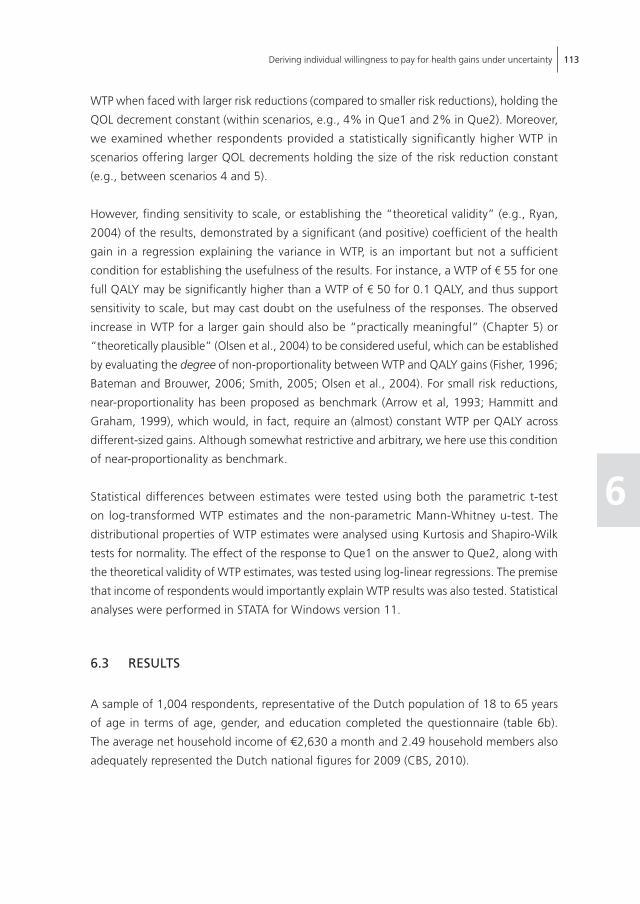
Deriving individual willingness to pay for health gains under uncertainty 113
6
WTP when faced with larger risk reductions (compared to smaller risk reductions), holding the
QOL decrement constant (within scenarios, e.g., 4% in Que1 and 2% in Que2). Moreover,
we examined whether respondents provided a statistically significantly higher WTP in
scenarios offering larger QOL decrements holding the size of the risk reduction constant
(e.g., between scenarios 4 and 5).
However, finding sensitivity to scale, or establishing the “theoretical validity” (e.g., Ryan,
2004) of the results, demonstrated by a significant (and positive) coefficient of the health
gain in a regression explaining the variance in WTP, is an important but not a sufficient
condition for establishing the usefulness of the results. For instance, a WTP of ¤ 55 for one
full QALY may be significantly higher than a WTP of ¤ 50 for 0.1 QALY, and thus support
sensitivity to scale, but may cast doubt on the usefulness of the responses. The observed
increase in WTP for a larger gain should also be “practically meaningful” (Chapter 5) or
“theoretically plausible” (Olsen et al., 2004) to be considered useful, which can be established
by evaluating the degree of non-proportionality between WTP and QALY gains (Fisher, 1996;
Bateman and Brouwer, 2006; Smith, 2005; Olsen et al., 2004). For small risk reductions,
near-proportionality has been proposed as benchmark (Arrow et al, 1993; Hammitt and
Graham, 1999), which would, in fact, require an (almost) constant WTP per QALY across
different-sized gains. Although somewhat restrictive and arbitrary, we here use this condition
of near-proportionality as benchmark.
Statistical differences between estimates were tested using both the parametric t-test
on log-transformed WTP estimates and the non-parametric Mann-Whitney u-test. The
distributional properties of WTP estimates were analysed using Kurtosis and Shapiro-Wilk
tests for normality. The effect of the response to Que1 on the answer to Que2, along with
the theoretical validity of WTP estimates, was tested using log-linear regressions. The premise
that income of respondents would importantly explain WTP results was also tested. Statistical
analyses were performed in STATA for Windows version 11.
6.3 REsulTs
A sample of 1,004 respondents, representative of the Dutch population of 18 to 65 years
of age in terms of age, gender, and education completed the questionnaire (table 6b).
The average net household income of €2,630 a month and 2.49 household members also
adequately represented the Dutch national figures for 2009 (CBS, 2010).

114 Chapter 6
6.3.1 Patterns in WTP data
The WTP responses showed a highly left-skewed distribution. Most values (79%) were
fairly well-dispersed within the range of €0 to €300. Only 1.3% of respondents indicated
the highest level offered on the payment scale as their maximum WTP (€2,500) and 87
respondents indicated in one or more scenarios a WTP of €0 (while only 24 indicated €0
Table 6b: Summary statistics (n = 1,004)
Variable Mean SD Min Max
Age 40.1 12.8 18 65
Gender (female) 0.50
Marital status (yes):
- Married 0.59
- Divorced 0.08
- Single 0.26
- Widowed 0.02
- Not stated 0.05
Children (yes) 0.51
- Number of children (n = 3070) 2.07 1.09 1 10
Net monthly household income (€) 2,630 1,560 999 10,000
Net monthly household income groups (yes):
- Group 1 (<1,000€) 0.14
- Group 2 (999€ - 2,000€) 0.34
- Group 3 (1,999€ - 3,500€) 0.37
- Group 4 (>3,499€) 0.15
Number of people living on household income 2.49 1.08 1 20
Level of education (yes):
- Higher vocational or academic 0.35
- Middle vocational or secondary school 0.52
- Lower vocational or primary school 0.13
Employment status (yes):
- Employed 0.62
- Unemployed 0.18
- Student 0.09
- Housewife/husband or retired 0.11
Health status:
- EQ-5D (Dutch tariff) 0.85 0.23 -0.329 1
- EQ-VAS 78.8 17.6 0 100
WTP for a car 16,300 60,300 0 1,000.000
WTP for a pair of shoes 200 1,200 0 23,400

Deriving individual willingness to pay for health gains under uncertainty 115
6
in both Que1 and Que2).54 As noted before, most scenarios were designed in such a way
that one health state was unambiguously better than the other. In more than 96% of the
scenarios, the respondents ranked the health states accordingly. 42.8% of the respondents
indicated to be either “pretty” or “totally” sure that they would pay the stated amount for
the specified health gain, while 15.8% indicated that they would probably or surely not do
so. Seven data points were missing for Que2.
6.3.2 Average WTP per QAlY estimates
The WTP per QALY estimates obtained using the EQ-VAS scores were comparable to the results
obtained using the EQ-5D tariffs, diverging about 10% in size, and supported largely the same
conclusions regarding explanatory variables for WTP per QALY estimates and their sensitivity to
scale. Since the results using the EQ-5D tariffs are more commonly used in this context and are
better suited for generalization because these tariffs were derived using the common health
valuation technique of time trade-off, only these results are reported henceforth.
The average estimates of WTP per QALY (OE) were calculated using the responses to both Que1
and Que2 (table 6c). The maximum average WTP per QALY without correcting for probability
weighting was €250,500, but when corrected for probability weighting ranged between
€80,800 and €113,000. The estimates obtained using the TK and the GW functions were
almost identical, in spite of different function specifications and origins of parameter estimates.
Because of this similarity, and because the TK function was estimated using health domain
specific parameters (Bleichrodt and Pinto Prades, 2006), the GW estimates are not presented
henceforth. The P function yielded the largest expected QALY gain in the denominator (0.036)
and, therefore, resulted in the most conservative estimates of WTP per QALY (€80,800).
The WTP per QALY (PS) estimates were about 45 percent lower, which is logical considering
that this PS estimate constituted the lower bound of the OE follow-up question. Given
the skewedness of the data, median values of WTP per QALY were lower than the means,
although of similar relative sizes.
Table 6d shows the breakdown of WTP per QALY (OE) values according to respondents’ levels
of health, certainty regarding responses and household income. Especially income shows a clear
pattern in both means and medians, with higher valuations for higher income groups (p < 0.05).
54. The reasons for zero WTP were uniformly distributed among the explanations. No consistent relationship was found between the size of the health ain, household income, and zero WTP. Given the low number of zero’s, we decided to retain them in further analyses.

116 Chapter 6
Tabl
e 6c
: Ave
rage
WTP
for a
QAL
Y es
timat
es fr
om Q
ue1
and
Que
2 co
mbi
ned,
for a
ll fu
nctio
ns (€
, rou
nded
to h
undr
eds)
Expe
cted
QAL
Y ga
inW
TP p
er Q
ALY:
PS
WTP
per
QAL
Y: O
E
Mea
n (S
D)M
inM
axM
edia
nM
ean
(SD)
Min
Max
Med
ian
Mea
n (S
D)M
inM
axM
edia
n
Non
-wei
ghte
d re
sults
(NW
)
0.01
2(0.
012)
0.00
10.
070.
008
174,
900
(451
,900
)0
5,97
6,10
052
,800
250,
500
(542
,200
)0
5,97
6,10
081
,300
Wei
ghte
d re
sults
*
- GW
func
tion
0.02
2 (0
.011
)0.
001
0.06
0.02
378
,000
(172
,900
)0
1,47
0,00
024
,300
113,
200
(224
,100
)0
1,62
0,10
036
,900
- TK
func
tion
0.02
2 (0
.011
)0.
001
0.06
0.02
275
,900
(168
,600
)0
1,40
7,80
024
,800
110,
100
(218
,900
)0
1,54
4,50
037
,900
- P fu
nctio
n0.
036
(0.0
2)0.
001
0.09
0.03
455
,400
(131
,700
)0
1,24
1,60
015
,500
80,8
00 (1
77,1
00)
01,
480,
000
23,5
00
*GW
= G
onza
les
and
Wu
(199
9); T
K =
Tve
rsky
and
Kah
nem
an (1
992)
; P =
Pre
lec
(199
8).
Tabl
e 6d
: WTP
per
QAL
Y by
hea
lth s
tatu
s, ce
rtain
ty le
vel a
nd in
com
e gr
oup
(n =
200
1; in
€, r
ound
ed to
hun
dred
s)
Varia
ble
n (%
yes
)W
TP p
er Q
ALY
OE
(NW
)W
TP p
er Q
ALY
OE
(TK)
WTP
per
QAL
Y O
E (P
)
Mea
n (S
D)M
edia
nM
ean
(SD)
Med
ian
Mea
n (S
D)M
edia
n
Heal
th s
tatu
s (E
Q-5
D)<
0.51
116
1 (8
.0)
344,
500
(898
,000
)61
,500
126,
400
(271
,500
)26
,200
82,2
00 (1
72,6
00)
17,9
00
0.51
1 - 0
.737
198
(9.9
)27
6,00
0 (5
07,1
00)
87,0
0011
7,00
0 (2
10,7
00)
36,1
0083
,400
(165
,600
)24
,500
>0.
737
1,64
2 (8
2.1)
238,
200
(497
,700
)83
,000
107,
600
(214
,100
)37
,600
80,4
00 (1
79,0
00)
23,8
00
Certa
inty
leve
l- S
urel
y no
t85
(4.2
)41
7,20
0 (1
,083
,000
)28
,900
150,
400
(327
,200
)19
,300
96,5
00 (2
11,3
00)
11,4
00
- Pro
babl
y no
t23
1 (1
1.5)
247,
900
(540
,800
)80
,000
110,
000
(214
,900
)37
,100
81,2
00 (1
69,5
00)
24,1
00
- May
be y
es, m
aybe
no
852
(42.
6)27
6,50
0 (5
80,0
00)
88,0
0012
2,20
0 (2
35,6
00)
41,1
0090
,200
(193
,400
)25
,200
- Pre
tty s
ure
yes
623
(31.
1)21
6,20
0 (3
51,0
00)
94,0
0099
,100
(182
,000
)41
,500
74,5
00 (1
62,4
00)
28,1
00
- Tot
ally
sure
yes
210
(10.
5)18
1,90
0 (5
10,8
00)
25,4
0077
,100
(192
,900
)10
,100
54,8
00 (1
36,0
00)
7,00
0
Inco
me
grou
p<
€1,0
0027
4 (1
3.7)
138,
500
(250
,700
)42
,000
58,4
00(1
24,5
00)
18,1
0041
,800
(109
,000
)12
,500
€1,0
00 -
€1,9
9968
4 (3
4.2)
190,
000
(411
,100
)65
,600
88,7
00 (1
85,7
00)
27,5
0067
,800
(160
,400
)19
,300
€2,0
00 -
€3,4
9974
1 (3
7.0)
258,
000
(500
,000
)10
0,00
011
2,65
5 (2
09,5
00)
44,6
0082
,100
(170
,900
)27
,900
≥€3
,500
302
(15.
1)47
1,60
0 (9
11,5
00)
135,
200
199,
000
(326
,800
)59
,600
142,
700
(259
,100
)40
,300

Deriving individual willingness to pay for health gains under uncertainty 117
6
Respondents expressing higher levels of certainty generally indicated lower WTP per QALY
estimates55. The group indicating “maybe yes, maybe no” disturbs this pattern somewhat56 (p
< 0.05). The medians show a more mixed pattern as well. Finally, respondents who reported
being in relatively poor health indicated a higher average WTP per QALY compared to
respondents in relatively good health for the non-weighted results and the correction using
the TK function. For the P function as well as the medians, this pattern was not observed.
6.3.3 Construct and theoretical validity of WTP and WTP per QAlY estimates and influence of the income constraint
Table 6e presents the results of sensitivity tests, keeping QOL changes constant and varying
the size of risk reduction. The average WTP response in Que157, offering the larger gain,
was statistically significantly larger than that in Que2 (€185 > €132, ratio 0.71, p = 0.00).
Without correcting for probability weighting, the ratio between the health gains in Que1 and
Que2 is 0.5, as implied by the design of the questionnaire (since probability of health reduction
halved between Que1 and Que2). This means that a reduction of 50% in expected health
gain resulted in a reduction in WTP of 29%, which is concave (and thus theoretically valid) but
hardly can be considered as near-proportional (and thus practically meaningful). Correcting
for probability weighting, the ratios of the health gains were somewhat higher (0.67 and 0.8
55. It has been observed before that higher certainty results in lower WTP estimates (e.g., Blumenschein et al., 2009), but this is not always the case (e.g., Chapter 4).
56. This may indicate that this category should not be interpreted as lying in between “probably not” and “pretty sure”, but may signal a more fundamental uncertainty.
57. The “raw” WTP estimates are presented as monthly payments as they were elicited in the questionnaire and not yearly estimates by multiplying raw values by 12. Although the expected QALY gain is a yearly one, multiplying by 12 would not have changed the relevant ratios.
Table 6e: Que1 (n = 1004) and Que2 (n = 997) separately (€, rounded to hundreds)
VariableQue1 Que2 Que2/Que1
Mean (p)Que2/Que1 Median (p)Mean (SD) Median Mean (SD) Median
Raw WTP: OE 185 (383) 80 132 (285) 50 0.71 (0.00) 0.63
Health gain (EQ-5D) - NW function 0.016 (0.014) 0.012 0.008 (0.007) 0.006 0.50 (0.00) 0.50
- TK function 0.027 (0.012) 0.025 0.018 (0.008) 0.017 0.67 (0.00) 0.70
- P function 0.040 (0.021) 0.036 0.032 (0.017) 0.027 0.80 (0.00) 0.75
WTP per QALY: OE - NW function 207,800 (443,000) 71,400 293,400 (623,600) 88,700 1.42 (0.00) 1.24
- TK function 106,500 (212,000) 35,700 113,600 (225,600) 38,300 1.10 (0.23) 1.10
- P function 84,100 (179,700) 25,400 77,600 (174,400) 21,700 0.91 (0.21) 0.85

118 Chapter 6
for the TK and P function, respectively). When using the TK function, a 33% reduction in
expected health gain resulted in a 29% reduction in WTP. This is concave and may be considered
near-proportional. When using the P function, a 20% reduction in expected health gain was
accompanied by a 29% reduction in WTP. Although this is close to near-proportional (but less
so than when using the TK function), it also represents a non-concave relationship, which is
reflected in the fact that the WTP per QALY for Que2 is lower than that for Que1 when using
the P function (table 6e). Median values showed very similar ratios.
Judging from these ratio differences, sensitivity was higher when the probabilities were weighted
according to a weighting function, further supporting the idea that non-linear weighting is
“empirically important in explaining choice behaviour” (Harless and Camerer, 1994). Especially
the application of the TK function results in WTP estimates that were near-proportional, so that
their sensitivity to scale may be considered practically meaningful. The results when using the
P-function were also close to near-proportional, but showed a (slight) non-concave pattern,
which emphasizes the importance of choosing an appropriate weighting function.
Table 6e also shows the mean WTP per QALY estimates obtained in Que1 and Que2
separately. Although these estimates are not particularly useful for testing the sensitivity
to scale (because they incorporate both the WTP and the scale, i.e., the expected QALY
gain), they are indicative of the stability of mean WTP per QALY estimates across different
expected gains. WTP per QALY estimates were almost identical between Que1 and Que2
when we corrected for probability weighting, but statistically significantly different (p =
0.00) without the correction. This indicates insensitivity when not correcting for probability
weighting, since, from a theoretical and practical perspective, the average point WTP per
QALY estimate should not depend on variation of the expected gain. In other words, WTP
should be adjusted to the gain on offer, leading to a more or less constant WTP per QALY
estimate across different QALY gains. Importantly, this may hold only for marginal gains
such as the ones offered here. (This issue is further addressed below.)
WTP results were also compared within 4 distinct pairs of scenarios offering different QOL
decrements but using identical risk reductions. Most of the higher expected gains received
higher and statistically different WTP estimates, although WTP and the expected gains were
not as proportional as when the size of the risk reduction varied. This finding can perhaps
be attributed to a small sample size solving each scenario (n = 35) and, hence, the influence
of lone outlying values on the results. Thus, although the comparisons between scenario
results yielded favourable results, their interpretation should be approached with caution.
Table 6f presents log-linear regressions, with log-WTP estimates as the dependent variable.
Independent variables were potential determinants of WTP, including the size of the QALY

Deriving individual willingness to pay for health gains under uncertainty 119
6
gain on offer (NW and TK) and log-income. (The results of the P function were similar to
those of the TK function and thus not shown.)
Table 6f: Multivariate regressions on cumulative data when probabilities are non-weighted (NW) and when probabilities are weighted (Tversky and Kahneman function, TK)
DV: Log (WTP)Model 1: NW Que1 & Que2 Model 2: TK Que1 & Que2
β RSE P>|t| βstd β RSE P>|t| βstd
QALY gain: Log (EQ-5D) 0.17 0.04 0.000 0.10 0.18 0.05 0.000 0.09
Certainty level 0.02 0.03 0.640 0.01 0.01 0.03 0.700 0.01
Health status (EQ-5D Dutch tariff) -0.26 0.15 0.093 -0.04 -0.26 0.15 0.094 -0.04
Age -0.09 0.02 0.000 -0.81 -0.09 0.02 0.000 -0.81
Age squared 0.00 0.00 0.000 0.66 0.00 0.00 0.000 0.66
Gender (female) 0.14 0.06 0.029 0.05 0.12 0.06 0.052 0.04
Children under 18 (yes) 0.22 0.09 0.009 0.07 0.22 0.09 0.009 0.07
Higher vocational or academic education (yes) 0.09 0.07 0.162 0.03 0.10 0.07 0.151 0.03
Employment status (yes)
- Unemployed -0.27 0.10 0.004 -0.07 -0.28 0.10 0.004 -0.08
- Student 0.08 0.10 0.562 0.02 0.10 0.11 0.496 0.02
- Housewife/husband or retired 0.01 0.11 0.920 0.00 0.01 0.11 0.890 0.00
- Employed (baseline) - - - - - - - -
Number of people living on household income -0.03 0.03 0.227 -0.03 -0.03 0.03 0.216 -0.03
Log (monthly income) 0.58 0.07 0.000 0.22 0.58 0.07 0.000 0.22
Constant 2.69 0.70 0.000 2.60 0.70 0.000
Adjusted R2 0.11 0.11
n 1,853 1,854
Note: “RSE” = robust standard error. “βstd” = standardized coefficient.
All covariates (table 6f) were tested for non-linearity (using quadratic terms) and relevant
interactions (which were excluded when found insignificant). The log-linear regression results
indicate that all variables carry the expected sign (e.g., WTP increases with income, the size
of the gain and the level of education and certainty), confirming the theoretical validity of
the WTP per QALY estimates. The relationship between age and WTP was negative and
non-linear, as observed before (e.g., Liu, 2004).
We also tested whether income constraints influenced our results, by examining the ratios
between the WTP for larger gains in Que1 and smaller gains in Que2 for respondents both
below and above the mean and median income (as in Flores and Carson, 1997; Smith, 2005).
If budget constraints played a role, the ratio is expected to be larger for higher income
respondents because their ability to express a “true” WTP is less constrained (Pinto Prades

120 Chapter 6
et al., 2009). In our study, the ratio was 1.52 for low-income and 1.29 for high-income
respondents, indicating a larger variation in WTP among low incomes, and thus refuting
the relevance of the budget constraint.
6.3.4 The comparison with WTP per QAlY obtained under certainty
The design of the current study was identical to that reported in Chapters 4 and 5, except
in two aspects: (i) we introduced uncertainty and (ii) we reduced the number of WTP
questions from five to two, decreasing the (potential) cognitive burden of the exercise. All
other aspects of the WTP question, scenario design and sample representativeness were
kept constant to ensure comparability between the results. Notwithstanding, the results
presented here differed considerably from those in previous chapters, both in terms of point
estimates and construct validity. The average point estimate of WTP per QALY estimate in
Chapter 4, also based on the Dutch EQ5D tariffs, was much lower than those reported
here (i.e., €24,500)58. In terms of validity, only sporadic statistically significant differences
between WTP for considerably smaller and larger gains were found in Chapter 5, both
when expected gains varied in terms of QOL and gain duration. Income did not appear to
be a constraining factor in either study. These differences signal an important and striking
effect of introducing uncertainty (and probability weighting corrections) in eliciting WTP for
health improvements, particularly in the size of estimates, but also in terms of their validity.
6.4 disCussion
Cost-utility analysis is becoming increasingly important source of information for decision-
makers in the healthcare sector. In order to be able to assess whether an intervention can
be considered welfare improving, the results of such analyses need to be judged against a
threshold, representing the value of health (or, more generally, of a QALY). Valid estimates
of the value of a QALY are, however, still lacking.
Using a large representative sample of the Dutch population, we estimated the individual ex
ante WTP per QALY under uncertainty. Furthermore, we investigated how different specifica-
tions of probability weighting functions affect these WTP per QALY estimates, and their
construct validity. Given the dominant theory of decision-making under risk (e.g., Quiggin,
58. This estimate is, however, comparable to findings of similar studies that used either the CV or DCE methodology, also under certainty. In fact, the available empirical estimates of the individual WTP per QALY under certainty range roughly between €10,000 and €45,000 in the literature (e.g., Gyrd-Hansen, 2003; King et al, 2005; Shiroiwa et al., 2009) – aligning with the lower and upper bound estimates for the full sample obtained in Chapter 4.

Deriving individual willingness to pay for health gains under uncertainty 121
6
1981; Starmer and Sugden, 1989; Tversky and Kahneman 1992), and the results regarding
sensitivity to scale of the different estimates obtained here, it appears that the WTP per QALY
estimates corrected for probability weighting have better validity and are more practically
meaningful than the non-weighted estimates. These WTP per QALY estimates, ranging from
€80,000 to €110,000 per QALY and comparing well to some recent figures in the literature
(e.g., the maximum threshold of €80,000 proposed in the Netherlands by RVZ (2006)), may
inform policy-makers further regarding the value placed on health gains by society.
The finding that the construct validity of estimates corrected for probability weighting appears
to be relatively good as compared to non-corrected estimates supports the relevance of
probability weighting in deriving WTP estimates obtained under uncertainty. Not accounting
for probability weighting not only resulted in an apparent overestimation of the monetary
value of health gains (with a factor 2 to 3 in this study), but also in less favourable conclusions
regarding the validity of responses. Given concerns about the validity of existing WTP per
QALY estimates (those expressed in Chapter 5 and other work, e.g., Pinto Prades et al.,
2009), our findings may be considered encouraging. The estimates demonstrate theoretical
validity and the near-proportional relationship between expected gains and WTP also supports
their practical meaningfulness (Chapter 5). Many previous studies showed less favourable
results (e.g., Smith, 2005; Van Houtven et al., 2006; Jones-Lee et al., 1995). Nevertheless,
confirmation of our findings in future empirical studies and in different settings is pivotal
and we still need to be cautious in interpreting our findings, as discussed below.
Our results highlight a number of important issues. First, we found clear heterogeneity
in WTP responses. For instance, as expected, WTP increases with income and decreases
with health status. Whether and how such heterogeneity should be reflected in healthcare
decision-making is an issue that goes beyond the scope of this paper, but clearly relates to
notions of equity that are central in the healthcare sector (Brouwer et al., 2008). Moreover,
one may consider the estimates from respondents who were more certain about their
answers to be a closer representation of the real WTP (as opposed to a hypothetical WTP;
e.g., Johannesson et al., 1999; Blumenschein et al., 2001) than those obtained in less certain
respondents. Using only the responses of participants who were pretty or totally sure of
their response (see Table 4) would result in a WTP per QALY estimate somewhere between
€64,000 (correcting for probability weighting with the P function) and €87,000 (correcting
for probability weighting with the TK function). However, using only a selection of responses
obviously may decrease the representativeness of the results. It is worth noting that we did
not observe higher levels of sensitivity among more certain respondents, unlike reported in
previous studies (e.g., Johannesson et al., 1999; Blumenschein et al., 2001).

122 Chapter 6
Second, applying different probability weighting functions resulted in different WTP per
QALY estimates. In our study, the weighting functions of Tversky and Kahneman (1992)
and Gonzalez and Wu (1999) produced similar results. Their use improved the conclusions
in terms of sensitivity to scale, yielding a near-proportional relationship between size of
the health gain and the elicited WTP. The Prelec (1998) function caused the results to be
closer to proportionality than without weighting, but performed less well than the other
two weighting functions as it resulted in a – less plausible – modestly convex relationship
between size of the health gain and WTP. Clearly, therefore, while correcting for probability
weighting appears advisable, more research is warranted into the appropriate weighting
functions to be applied in this context.
Third, comparison of our results to those from a very similar study, but valuing health gains
under certainty (reported in Chapters 4 and 5), showed significant differences in obtained
WTP per QALY estimates and their construct validity. The introduction of risk in WTP exercises,
apart from making the choice tasks more realistic, can thus be considered influential on the
obtained results. The higher WTP per QALY estimates produced here appear to result from
the fact that, while “raw” WTP responses were comparable between studies, the uncertainty
introduced here decreased the size of the expected QALY gain in the denominator59. The
higher sensitivity to scale observed in this study may be due to the reduced number of the
WTP questions presented to respondents (i.e., 2 rather than 5) and to the fact that the two
questions related to a single scenario, differing only in the risk of the health decrement (as
compared to 5 distinct scenarios60). The lower cognitive burden may thus have made it easier
for respondents to exhibit a higher level of sensitivity. Alternatively, it could be said that
it was easy for respondents to fixate on the halving of the probability. We note, however,
that simply halving the stated WTP by participants in response to halving the probability of
health loss would have resulted, unlike what we observed here, in more sensitivity in the
non-weighted estimates than in those corrected for probability weighting. In addition, only
varying the size of the health gain also resulted in significantly different WTP responses.
This implies that there is more sensitivity in the estimates than only invoked by adjusting
WTP for (halving) probabilities61. In that sense, the sensitivity observed here is encouraging
59. The average (and certain) gain was 0.12 QALYs in the study of Bobinac et al (2010; 2011), reported in Chapters 4 and 5 This implies similarly sized health changes as used in the current study. However, here they are multiplied by the relevant risk of health deterioration.
60. The first two scenarios represented smaller health gains that, according to Dutch EQ-5D tariffs, added up to a larger health gain presented in the third scenario. The fourth scenario was a repetition of one of the offered scenarios, but with longer duration of benefits.
61. Chapter 5 reports that sensitivity was also not found when comparing two WTP questions varying only in gain duration (1 vs. 5 years). This is an equally straightforward task.

Deriving individual willingness to pay for health gains under uncertainty 123
6
and suggests that WTP elicited under uncertainty may in fact lead to more valid answers,
possibly because it increases the realism of the contingent market62.
A number of limitations of our study need to be mentioned. First, our sample was representa-
tive of the 18- to 65-year-old Dutch population in terms of age, gender and education, but
not in terms of health status. This might impede generalizability of our results. Note that
respondents were asked to imagine being in the better of the two health states presented
in a scenario, which should have rendered own health irrelevant. In other words, the
position of the initial and potential health state presented in the scenarios should not have
been influenced by own health, and whether these health states constituted a gain or a
loss, relative to own health. Our data did however not allow a firm test of this assumption.
Similarly, the levels of risk presented here were meant to be strictly exogenous. The ability to
self-protect against health deterioration (a component of realized risk faced by the individual;
e.g., Bateman et al., 2005; Shogren and Crocker, 1991) should therefore be irrelevant
for WTP estimates. If the probabilities of health deterioration used by respondents were,
nonetheless, partly endogenous, it would be inappropriate to treat them as exogenous in
econometric models (e.g., Konishi and Adachi, 2010) and future research might explore
models estimating WTP per QALY that include perceived (subjective) risks (e.g., Viscusi and
Evans, 1998; Riddel and Shaw, 2006).
Second, some design-specific choices may have affected our results. For example, the
range of the payment scale may have influenced (the variation in) WTP per QALY estimates,
although probably only marginally, given the few maximum choices. The choice of the
payment vehicle is also important. We elicited WTP by an out-of-pocket payment and not
as an increase in insurance premium. Although Dutch citizens are somewhat acquainted
with paying out-of-pocket for healthcare (8% of all healthcare is financed out of pocket
(OECD, 2009)) – and increasingly so since the introduction of a mandatory deductible
(Holland et al., 2009) – it is unclear to what extent out-of-pocket payments seemed realistic
to respondents (e.g., Skjoldborg and Gyrd-Hansen, 2003). Neither the study nor the pilot,
however, indicated great difficulties in that respect. Moreover, the finding of relatively good
sensitivity to scale when lowering the probability of health deterioration may not be observed
when increasing (e.g., doubling) the probability of health deterioration. People may more
easily lower subsequent WTP answers than increase subsequent WTP answers (proportional
to the gain on offer). Unfortunately, we could not test this further here. Another point is
that we asked respondents to value avoidance of potential health losses. Framing similar
62. Working with probabilities is cognitively demanding. Here, however, we found no evidence that the probabilities caused problems for the respondents; no evidence was found of failure to distinguish between risk reductions of different sizes (Hammitt & Graham, 1999), nor of many (seemingly) random answers, protest responses, etc. (Carson, 2000).

124 Chapter 6
questions as health gains could yield different, presumably lower WTP per QALY estimates.
Finally, our design combined lower probabilities with larger health gains, vice versa. This
resulted in less variation in the QALY gains presented in the WTP exercises. In case WTP
would be insensitive to the size of QALY gains, our design might still have yielded relatively
favourable results and fairly constant WTP per QALY estimates. However, the (variation
in) gains were larger when correcting for probability weighting, and we observed better
sensitivity after correction. This implies that our findings are not a mere artefact of design.
Confirming these findings using different designs is however advocated.
Third, respondents only valued potential QOL improvements, not potential mortality reduc-
tions. While many healthcare interventions indeed aim to improve QOL rather than to reduce
mortality – thereby emphasizing the relevance of the figures presented here, obtaining
estimates in the context of mortality reduction remains important. Such estimates would
likely be higher than those presented here.
Finally, the mean estimates of WTP per QALY in our study were shown to vary with various
factors (among which the weighting function used). Although a discussion on the appropriate
weighting function to be used in this context is beyond the scope of this paper, it seems
important to note that one single weighting function may not apply to all people. Similarly,
individual valuations can be combined in different ways to come to a mean value of a QALY.
Aggregating in different ways, (for example, taking the mean of ratios rather the ratio of
means) might result in different estimates of WTP per QALY (Gyrd-Hansen and Kjær, 2011).
Also, by focusing on individual valuations of health improvements, important elements like
solidarity – so central in many healthcare systems – are not considered. Deriving societal
estimates of WTP per QALY, in which such notions are captured, is another future challenge.
Ideally, the QALY value would be allowed to vary with characteristics of the beneficiaries
such as disease severity and age (instead of income or health status). This would allow a
more direct link between equity considerations and the value of QALY gains, as well as a
transparent public discourse (if not consensus) on what equity weights should be.
In conclusion, this study has highlighted the importance of correcting for probability weight-
ing in WTP studies involving uncertainty. Moreover, given the reasonable support of their
validity, the estimates derived while correcting for probability weighting provide valuable
input for the debate on the consumption value of health (e.g., Claxton et al., 2010). While
decision-makers should not apply these estimates without further research and consideration,
since strictly individual valuations may not carry all relevant information and values for societal
decision-making (Smith, 2007), the current estimates may provide a good and informed
basis for further discussion and study of this important topic.

Deriving individual willingness to pay for health gains under uncertainty 125
6
6.5 APPEndix 6A
Table 6A.1: The wording of WTP question in English
Que1
Please suppose you are in the health state that you assessed as the better one but face the risk of moving to the worse health state tomorrow. If this health deterioration happens, you will remain in the worse health state for one year. After this year, you will return to the better health state.The risk of deterioration you face is x%. This means that you have x in 100 chance of moving to the worse state and y (100-x) in 100 chance of remaining in the better state.You can avoid this risk of health deterioration completely (reduce x% to 0%) by taking a medicine (with no side effects) each month. You will then certainly remain in the better health state. You must pay for this medicine yourself, directly from your (net monthly household) income.Please have your ability to pay (given your household income) in mind!!
Que2
Please suppose you are in the health state that you assessed as the better one but face the risk of moving to the worse health state tomorrow. If this health deterioration happens, you will remain in the worse health state for one year. After this year, you will return to the better health state.The risk of deterioration you face is x%. This means that you have x in 100 chance of moving to the worse state and y (100-x) in 100 chance of remaining in the better state.You can reduce this risk of health deterioration by taking a medicine (with no side effects) each month. As a result, your risk of moving to the worse health state will be halved from x% to x/2%. You must pay for this medicine yourself, directly from your (net monthly household) income.Please have your ability to pay (given your household income) in mind!!

126 Chapter 6
Table 6A.2: Design of the choice scenarios, levels of risk and expected QALY gain
Choice scenario Health state 1 Health state 2 Level of risk
Expected QALY gain*
If riskreduced to 0
If riskhalved
1 22222 11131 10% 0.021 0.0105
2 33232 33323 50% 0.009 0.0045
3 21312 12111 2% 0.0074 0.0037
4 22323 21312 2% 0.0074 0.0037
5 22323 12111 2% 0.015 0.0075
6 21232 32211 4% 0.0092 0.0046
7 11112 22121 10% 0.008 0.004
8 11122 22122 10% 0.012 0.006
9 21323 22233 4% 0.012 0.006
10 22331 21133 4% 0.0075 0.00375
11 21111 12121 50% 0.066 0.033
12 23232 32232 50% 0.028 0.014
13 11312 11113 10% 0.0144 0.0072
14 12311 11211 2% 0.0068 0.0034
15 32311 12311 10% 0.0161 0.008
16 32311 11211 2% 0.010 0.005
17 21111 12211 50% 0.039 0.0195
18 32313 32331 50% 0.002 0.001
19 11211 22211 4% 0.0047 0.0024
20 23313 11133 50% 0.042 0.021
21 11121 22112 10% 0.016 0.008
22 12223 13332 10% 0.014 0.007
23 11312 11211 2% 0.0077 0.0039
24 11332 11312 4% 0.0132 0.0066
25 11332 11211 2% 0.0142 0.0071
26 21222 33321 2% 0.0082 0.0041
27 22222 13311 50% 0.0415 0.0208
28 11112 22112 4% 0.0047 0.0024
29 33212 32223 4% 0.0087 0.0044
* Risk reduction to zero in Que1, halved in Que2.
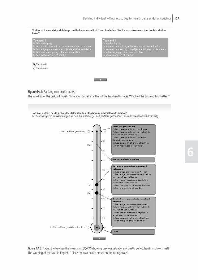
Deriving individual willingness to pay for health gains under uncertainty 127
6
Figure 6A.1: Ranking two health statesThe wording of the task in English: “Imagine yourself in either of the two health states. Which of the two you find better?”
Figure 6A.2: Rating the two health states on an EQ-VAS showing previous valuations of death, perfect health and own healthThe wording of the task in English: “Place the two health states on the rating scale”

128 Chapter 6
Figure 6A.3: Payment scale, first stepThe wording of the task in English: “Suppose you would have to pay an amount for this pill right now. Please consider the range of amounts below. Now, start from the left and tick the highest amount you would definitely pay for this pill on a monthly basis for the duration of one year to avoid going to the worse health state.”
Figure 6A.4: Payment scale, second step.The wording of the task in English: “Next, continue moving up the line and tick the first amountyou would definitely not pay for this pill on a monthly basis for the duration of one year to avoid going to the worse health state.”

Deriving individual willingness to pay for health gains under uncertainty 129
6
Figure 6A.5: Open-ended format.The wording of the task in English: “You have indicated that you would definitely pay €50 and definitely not pay €150 to avoid experiencing the worse health state for one year and remaining in the better health state. Please write in the amount (between €50 and €150) that most closely approximates the maximum you would be willing to pay per month to avoid going to the worse health state?”
Figure6 A.6: Graphical explanation of the concept of riskThe wording of the task in English: “Now imagine that in this group of 100 people the probability that someone becomes ill is 40%. In other words, 40 people will become ill and 60 people will not. To get an idea of what it means for the probability that you will be one of the people becoming ill, choose a green dot and click on it. The probability of the dot you selected changing colour is 40 to 100.”


Chapter 7Inquiry into the relationship between equity weights and the value of the QALY
Chapter based on: Bobinac A, van Exel NJA, Rutten FFH, Brouwer WBF (2011) Inquiry into the relationship between the equity weights and the value of a QALY. Resubmitted after second revision

132 Chapter 7
suMMARY
A commonly held view of the decision rule in economic evaluations in healthcare is that the
final incremental cost-effectiveness ratio (ICER) needs to be judged against some threshold,
which is equal for all QALY gains. This reflects the assumption that “a QALY is a QALY”
no matter who receives it, or the equity notion that all QALY gains are equally valuable,
regardless of the context in which they are realized. However, if such an assumption does
not adequately reflect the distributional concerns in society, different thresholds could be
used for different QALY gains, whose relative values can be seen as “equity weights”. In
spite of such a clear relationship between equity or distributional concerns on the one hand
and the social value of QALYs on the other, it is interesting to explore how that relationship
has been treated in the health economics literature – especially in light of the lively recent
empirical interest in equity-related concerns as well as the nature and height of the ICER
threshold. This study investigates the “common ground” between the two streams of
literature and considers how the empirical literature estimating the ICER threshold treats
existing distributional considerations.

Inquiry into the relationship between equity weights and the value of the QALY 133
7
7.1 inTRoduCTion
Some form of rationing or priority setting in the healthcare sector is inevitable given finite
resources. In such a context, efficiency and equity are two important objectives. The goal of
maximizing efficiency in resource allocation can be restated as maximizing the amount of
health produced per Euro spent (Wagstaff, 1991). Under such a maximand, scarce resources
are allocated to patient groups and interventions that produce the most health per unit
invested, and steered away from those that produce less. To inform social decisions in health
and increase the efficiency in the use of resources, policy-makers in some countries rely
on the results of economic evaluations, often in the form of a cost-utility analysis (CUA).
The results of a CUA are commonly summarized in an incremental cost-effectiveness ratio
(ICER) - a measure of the additional costs and benefits of the intervention relative to an
adequate comparator. In a CUA, benefits are expressed in terms of Quality-adjusted Life
Years, or QALYs. The meaning and acceptability of any ICER is determined by judging it
in relation to some monetary threshold value, whose nature is a matter of debate (e.g.,
Claxton et al., 2010). Here we consider it to represent the monetary value society places on
a QALY.63 The ICER threshold then defines the monetary value below which an intervention
can be considered efficient (or welfare improving) and above which it is not. The implicit
equity approach commonly taken in a CUA is to assign equal value to each QALY, irrespec-
tive of the characteristics of recipients or the intervention (i.e., “a QALY is a QALY”). This
approach has been the topic of much debate, also because it seems partly at odds with
another equity approach - the explicit concern for an increasingly equitable distribution of
health and healthcare64, implying different values for different QALYs (i.e., “a QALY is not a
QALY”). This explicit concern for equity is reflected in assigning differing weights to QALYs
depending on the recipients’ or interventions’ characteristics.
Equity is a broad notion comprising many aspects and is best seen as a multidimensional
concept (e.g., Culyer and Wagstaff, 1993; Culyer, 2001; Sen, 2002; Tsuchiya and Dolan,
2009). Striving for an equitable distribution of health and healthcare mostly is a reflection of
societal preferences for the distribution of health(care). The common notion of “economic
efficiency” may, however, not fully represent such societal preferences (e.g., Nord, 1995;
Dolan, 1998; Wagstaff and van Doorslaer, 2000; Dolan et al., 2005). In fact, there is a
large body of literature suggesting that the allocation decisions in healthcare should take
the relative social value of QALYs in different populations into account. This supports the
63. Moreover, for ease of expression, we will assume that the budget is flexible and, in a conventional sense, optimal, so that the cost-effectiveness of marginal spending in the healthcare sector equals the societal value placed on a gained QALY.
64. Note that an equitable distribution of health only partly depends on the healthcare system, i.e., on the distribution of healthcare (Sen, 2002).

134 Chapter 7
notion that a QALY is not a QALY regardless of who gets it (e.g., Tsuchiya and Dolan, 2009;
Dolan, 1998; Williams, 1997; Bleichrodt, 1997; Olsen, 2000; Rodriguez Miguez and Pinto
Prades, 2002; Dolan and Olsen, 2001; Coast, 2004; Dolan, 2011; Schwappach, 2002;
Schwappach, 2003; Polsky, 2005; Stolk et al., 2005; Tsuchiya and Dolan, 2005; Tsuchiya
and Dolan, 2007; Cookson et al., 2008). Within the framework of economic evaluations,
this implies assigning more weight to QALYs achieved in certain subgroups. Subsequently,
more resources will be steered in their direction, ceteris paribus, even though they may not
be the most efficient QALY producers.
On what basis QALYs are to be weighted depends on the particular argument that determines
what is unfairly unequal, i.e., which characteristics of patients or illnesses are perceived to
make someone worse-off (in terms of health) by members of society and thus more deserving
of health improvements. Which characteristics of patients or illnesses should determine the
weight attached to health gains, and which notions are defendable and consistent with
moral arguments, intuitions, observable societal values and judgments, is a matter of current
discussion and investigation (e.g., Olsen et al., 2003; Nord, 2005).
Some form of a trade-off between the objectives of efficiency and equity can ensure both
are incorporated into priority setting (Wagstaff, 1991) and into economic evaluations. If
adequately addressed, the trade-off would provide decision-makers with more information
relevant to healthcare decisions (Dowie, 1998). One important issue is how to make this
trade-off explicit, transparent, and systematic rather than a matter of intuition and implicit
values. If we consider economic evaluation a helpful tool in healthcare decision-making, one
condition for a sound and explicit equity-efficiency trade-off is a thoughtful incorporation
of equity concerns in economic evaluations. In that sense, it is important to consider the
decision-making framework of CUA, written as:
(1) vi * ∆hi - ∆c < v
where vi is the value attached to an additional unit of QALYs of type i, Δhi denotes the
incremental QALY gain of type i and Δc denotes all incremental costs of the intervention.
Type i denotes the “equity segment” to which the QALY gain, and thus the corresponding
value vi belong. The common decision rule in economic evaluations is for benefits to outweigh
costs, and thus equation (1) can be rewritten as:
(2) ∆c∆hi
< vi

Inquiry into the relationship between equity weights and the value of the QALY 135
7
which shows that the costs incurred to produce QALYs of equity type i should not exceed
the value per QALY of type i. Often, one threshold is used for all QALY gains under the
assumption that “a QALY is a QALY”, or the equity notion that all QALY gains are equally
valuable regardless of their context. If such an assumption does not adequately reflect
distributional concerns in society, different thresholds can be used for different QALY gains
whose relative values can be seen as “equity weights”. Therefore, a clear relationship exists
between equity or distributional concerns on one hand and the social value of QALYs on
the other. This study focuses on that relationship.
The relationship between the threshold and distributional concerns already exists, albeit
sometimes implicitly. NICE, for instance, requests that a technology with an ICER of over
£20,000 per QALY reference “the particular features of the condition and population receiv-
ing the technology” to increase its chances of being reimbursed (NICE, 2004). Seemingly,
therefore, if the condition or population appeals to certain notions of deservingness, the
ICER threshold might be higher. Recently, NICE even indicated that certain interventions
(e.g., life-prolonging) might be approved despite less favorable cost-effectiveness (NICE,
2008; Towse, 2009; Rawlins et al., 2010), depending on the context in which such QALYs
are gained. In the Netherlands, rather than formulating an exception to a more or less
fixed threshold, a general rule has been formulated highlighting the relationship between
equity concerns and the QALY value. Based on a specific notion of equitable distribution of
health (care), the threshold varies with the severity of the disease (e.g., Stolk et al., 2004).
Although the distributional concerns and the ICER threshold are related in practice, as shown
in the examples above, it is interesting to explore how that relationship has been treated in
the health economics literature - especially in light of recent and lively empirical interest in
equity-related concerns as well as the nature and height of the ICER threshold. This study
investigates the “common ground” between the empirical literature on estimating the
monetary value of a QALY, which is seen here as the appropriate ICER threshold, and the
literature on distributional considerations in allocating health and healthcare. For example,
do existing studies allude to or discuss the variations in ICER threshold estimates stemming
from possible distributional concerns, such as health status, socio-economic characteristics,
or healthcare consumption history? Have any empirical studies estimated the value of QALY
gains achieved in different segments of the population, where the segments were defined in
terms of equity-relevant characteristics (e.g., age or severity of illness)? Current study looks
to answer these questions by providing a thematic (rather than systematic) overview of the
empirical literature on prominent distributional concerns and the empirical literature on the
ICER threshold, and to establish their complementarity. For recent systematic reviews of the
literature regarding equity considerations we refer to Dolan et al. (2005) and Schwappach
(2002).

136 Chapter 7
7.2 THE ConTExT oF THE EQuiTY-EFFiCiEnCY TRAdE-oFF
The trade-off between equity and efficiency, apparently supported by both healthcare
policy-makers and the citizens they serve (NICE, 2005; Drummond and McGuire, 2001;
Schwappach, 2002; Dolan et al., 2005), enables maximization of equity-adjusted health
outcomes. This suggests that some health is sacrificed to reach higher levels of equity in
the distribution of health and healthcare. The total sum of the health gains achieved in the
population may then be less than what is attainable. The question of how to incorporate
the trade-off between the goals of equity and efficiency in economic evaluations remains
unanswered, however. A first issue in this context is whether the trade-off between equity
and efficiency within (decision-making based on) economic evaluations should be achieved
in a quantitative or in a qualitative manner (e.g., Cookson et al., 2009). In the former, equity
is used to adjust either the applied threshold or calculated ICER explicitly and quantitatively.
In the latter approach, the emphasis is much more on the process of decision-making and
gathering relevant background information on the equity relevant characteristics of the
disease, the intervention and the target population. It thus provides decision-makers with
a descriptive review of potentially relevant information on equity-related impacts alongside
“standard” economic evaluation results. Information can be provided on aspects such as the
patterns and causes of the health inequality in question, the relative importance of reducing
it (i.e., different stakeholders’ views), and the effects on related interventions in other
settings (Cookson et al., 2009). Reimbursement decisions could then take account of this
information, along with the intervention’s cost-effectiveness, but it is left to the policy-makers
to decide on their relative importance. For instance, the rankings of interventions based
on their ICERs can be reordered on the basis of qualitative information about the values
and priorities expressed by the public (e.g., as in the “Oregon experiment” (Tangs et al.,
1996)). Appraisal phases in the full process of decision-making, like used in the UK and the
Netherlands, also may be seen as qualitative approaches that account for non-quantified,
yet important aspects in reaching a final decision.
The most prominent quantitative approachesare equity weighting and multi-criteria decision
analysis (for the latter see Baltussen et al., 2006; Beaten et al., 2010). Equity weighting allows
a quantitative adjustment of the estimated ICER to account for equity concerns, which is the
focus here. Equity weights (e.g., Bleichrodt et al., 2004; Bleichrodt et al., 2005; Murray and
Lopez, 1994; Murray and Acharya, 1997; Rodriguez Miguez and Pinto Prades, 2002) are a
way of attributing more or less importance (or value) to health benefits achieved in some
circumstances relative to others. They can be estimated in several ways, such as through
willingness to pay (WTP) exercises, through person trade-off exercises or through conjoint
analysis (e.g., Nord, 1995; Dolan et al., 2005; Dolan and Green, 1998; Lancsar et al., 2011).
The obtained weights or values can subsequently be applied within economic evaluations

Inquiry into the relationship between equity weights and the value of the QALY 137
7
either by adjusting the QALY gains within the ICER or by adjusting the ICER threshold. The
two approaches should yield mathematically equal outcomes. This can be highlighted using
an example taken from a study of Wailoo et al. (2009). Imagine an intervention generating 5
additional QALYs in a patient group for whom an equity weight of 1.5 is considered applicable
relative to some base case. This implies that the intervention yields 7.5 equity-weighted
QALYs. With an additional cost of not more than £150,000, this would be considered a
cost-effective intervention, assuming a threshold of £25,000 (since £150,000 / 7.5QALYs
is £20,000 per QALY, which is below the threshold). The alternative approach is to adjust
the monetary threshold. For instance, if an intervention generates 5 additional QALYs at an
additional cost of £150,000, the ICER £30,000 per QALY (£150,000 / 5 QALYs) would be
judged again against the appropriate threshold in that context. Given the relative value of
the health gains in this context (i.e., the equity weight of 1.5), the appropriate threshold
would be £37,500 (that is, 1.5 times £25,000). Again, the new intervention would be
deemed cost-effective since the ICER falls below this threshold.
In general terms, we can fix the threshold value (vi) in the conventional decision rule (2) by
allowing equity weights on the left hand side, reflecting the relative value of QALYs gained
relative to the reference QALY value (v*):
(3) ∆c
αi * ∆hi
< v *
where ai is the relative value of the QALY compared to the reference QALY, i.e., vi/v*. Using
a fixed threshold with equity weights is thus essentially equal to using a flexible threshold
and no equity weights. While this notion need not be surprising, and seems to be implicitly
assumed in earlier work (e.g., Nord, 1996), for the purpose of the current study it is ap-
propriate to explicate this.
However, having a set of weights to apply within the CUA framework will be useful only
in conjunction with an ICER threshold that represents a known (reference or baseline)
case in terms of equity. In the above example, if the weight of 1.5 is to have its desired
meaning, the reference case receiving a weight of 1 needs to be fully specified with respect
to the equity-relevant characteristics of patients and/or their illness. Likewise, the average
£20,000 threshold is useful in conjunction with weights only when it is specified to the
reference case the value actually refers to. Only with a clear link between equity weights
and the threshold value can the weights be applied in a meaningful way within the decision
framework related to economic evaluation. A lack of clarity about what the reference cases
for either the weights or the threshold refer to precludes using the weights meaningfully

138 Chapter 7
within a full decision framework. Thus, to establish a link between the ICER threshold and
the distributional concerns, it is necessary to consider which distributional concerns matter
and to obtain or define a reference ICER threshold in relation to such concerns. We next
highlight distributional concerns in such contexts and then turn our attention to empirical
estimates of the ICER threshold.
7.3 WHiCH disTRiBuTionAl ConCERns MATTER?
The choice of equity-relevant characteristics, or the aspects determining who is worse-off,
depends on the justification or different ethical arguments for preferential treatment of
some people over others. Generally, the worse-off may be considered entitled to preferential
treatment because they suffer undeserved relative deprivation and usually have more urgent
needs (Brock, 2001). Although consensus on favoring worse-off groups or those subject
to greater inequality in the situation of scarcity seems to exist, debate on the appropriate
argument for deciding who should be regarded as more deprived and what actually is
considered inequitable is ongoing (e.g., Olsen et al., 2003; Nord, 2005).
Several characteristics of patients and illnesses have been put forward as possible criteria
(Schwappach, 2002; Olsen et al., 2003; Dolan et al., 2055; Shah, 2009). The issue regarding
who is worse-off has been mostly defined and discussed in terms of illness severity and
age. Three types of personal characteristics have most frequently been discussed (Olsen
et al., 2003): those that place the person in a causal relationship with the illness, i.e., the
extent to which a particular illness might have been influenced by a person’s own actions
(such as smoking); those that refer to a person’s relations to other people in society (such
as having children); and, finally, those that are “embodied” in a person’s “self” - physically,
intellectually or attitudinally (such as gender or sexual orientation). Social preferences
regarding such distributional concerns have been investigated empirically, both in isolation
and in a multi-attribute setting (e.g., Schwappach, 2003; Ratcliffe, 2000; Ratcliffe et al.,
2005; Ottersen et al., 2008), as general principles or as an issue within the context of a
particular intervention. Respondents in these empirical studies usually answered questions
about whether and to what extent a particular characteristic of patients or illness should be
relevant in prioritizing scarce resources. Important to the context of the current study, these
empirical studies did not elicit equity weights by deriving some type of willingness to pay for
different QALY gains, (or differing WTP estimates for QALYs achieved in different segments
of the population) but mostly traded off health gains in groups of beneficiaries (e.g., younger
versus older patients) without any reference to the threshold value. Therefore, they did
not establish a direct relationship between the ICER threshold and equity concerns. If one

Inquiry into the relationship between equity weights and the value of the QALY 139
7
would do so for one of the relevant groups, thus establishing an anchor point, the equity
weights would subsequently reveal the implied value of health gains in all other segments.
Severity of illness emerges as the most important discriminator between care recipients. This
has been noted in empirical studies reporting experimental and attitudinal data (e.g., Nord,
2005; Nord, 1993a, 1993b; Ubel, 1999; Bowling et al., 2002; Gyrd-Hansen, 2004). Severity
is usually defined in terms of the pre-treatment health state of patients or the expected QALY
profile in the case of no treatment (i.e., future health prospect). The value of the health gain
was commonly found to be higher in persons whose initial health state was worse, ceteris
paribus (Nord et al., 1999; Dolan and Cookson, 2000; Dolan and Tsuchiya, 2005; Green,
2009; Dolan and Olsen, 2001; Olsen et al., 2003) and in those with the worst prospective
health if left untreated (Dolan and Olsen, 2001). Patients with moderate health problems
who improve considerably with treatment, therefore, may not necessarily be favored over
patients with severe health problems who improve less with treatment (e.g., Ubel, 1999;
Oddsson, 2003).
Such rules, however, often come with particular exceptions. For instance, there may be a
threshold effect (Camidge, 2005). Prognosis without treatment, for example, may not be so
important for patients gaining only a very small amount of health due to a new treatment.
Similarly, little support was found for programs that provided some improvement yet left
patients in relatively poor health states after treatment (Roberts et al., 1999). People also
appear to prefer larger gains for fewer people to smaller gains for more people, even if in the
latter case the aggregate health gain is larger. The threshold for preferring a concentration
of benefits when the magnitude of individual health gains is not thinly spread across many
individuals may vary among populations (Mortimer, 2006; Olsen, 2000; Rodriguez Miguez
and Pinto Prades, 2002). This might be due to small gains not having the required “welfare
significance” and a meaningful benefit (Mortimer, 2006). In relation to life years, Dolan and
Cookson (2000) found that people were willing to make health gain trade-offs between
patient groups only once the differences in the number of life years gained exceeded a
certain threshold.
Age is the next most important equity consideration, and can be closely related to the severity
argument. The concern for age was famously operationalized with the fair innings argument
of Alan Williams (1997), proposing that everyone is entitled to a certain (quality-adjusted) life
span, labeled “fair innings”. In general, young patients are considered worse off since they
have not yet had their fair share of life. The conventional fair innings “ageism” (Tsuchiya,
2000; Tsuchiya et al., 2003) says that those people reaching their fair innings should be
given a weight of 1 in the priority-setting calculus, and individuals with poorer lifetime
prospects than the fair innings should be given a relative weight larger than 1. However,

140 Chapter 7
age weights might also have other justifications – weighting the young higher than the old
could actually be supported both by equity and efficiency arguments (Tsuchiya, 1999; Murray
and Lopez, 1994). Among the efficiency arguments, most prominent ones account for the
fact that the young contribute more to society (in economic terms, have young children,
etc.) and the old usually have lower capacity to benefit in terms of future life years and
propensity toward co-morbidity (Edlin et al., 2008). These are labeled productivity ageism
and health maximization ageism (Tsuchiya et al., 2003; Stolk et al., 2004). To account for it,
Murray and Lopez (1994) suggest ‘unequal age weights as an attempt to capture different
social roles at different ages’. It is important to disentangle the different motives - equity
or efficiency-related - behind preferential treatment of the young over the old. Opposing
views have also been expressed, however.65
Furthermore, Stolk and colleagues (2004) operationalized the concept of “proportional
shortfall”, which poses that priority should be determined by the proportion of QALYs that
people lose relative to their remaining life expectancy due to some illness. Proportional
shortfall compares individuals in relative terms to determine who is worse off. Based on an
empirical study Stolk et al. (2005) report that people’s preferences for who to treat were
most in line with the fair innings argument, followed by the proportional shortfall criterion,
and then the severity of illness criterion. Similar findings were also reported Tsuchiya and
colleagues (2003).
Another equity consideration may be culpability, the extent to which a particular illness
might be due to one’s own actions (e.g., smoking). People may consider it fair to allocate
resources away from those who can (somehow) be held responsible for their illness in favor
of people not responsible for theirs. Cappelen and Norheim (2006) have shown, using an
example of dental services, that there may be a limited but significant role for individual
responsibility (culpability) in healthcare prioritization. However, although several studies found
that people were in favor of discriminating against those whose ill health is considered to be
partly self-inflicted (Ubel et al, 2001; Furnham et al., 2000; Cappelen and Norheim, 2006),
the view provoked discussion (e.g., Dolan and Cookson, 2000). The dissent is caused by
difficulties in discerning the factors outside of self-control from those that are controllable;
even negligence might not be fully under our control. Unhealthy habits like smoking,
for example, can be predetermined by socio-economic status, undermining rather than
promoting the idea of fairness when distributing according to the principle of culpability.
65. Edlin et al. (2008) brought an extensive review on cost-effectiveness and ageism. The topic has also been discussed by other authors, for instance, Cohen-Almagor (2002) and Werntoft et al. (2007).

Inquiry into the relationship between equity weights and the value of the QALY 141
7
Other personal characteristics that also have been mentioned as bases for prioritization
include: relations with other people, societal position, and personal characteristics (Olsen
et al., 2003). With respect to the first two, it seems that the external effects of an illness on
others may be seen as a reason for differential priority. For instance, priority could be given
to married people, people with dependents, breadwinners (Williams, 1988; Dolan et al.,
1999; Nord et al., 1995; Olsen and Richardson, 1998). Some of these reasons may lead to an
accumulation of equity weights in specific groups (for example, married breadwinners with
dependents), which may or may not be desirable. With respect to personal characteristics,
the findings are inconclusive. Some studies indicate that respondents prefer treatment of
men to women, while others find the opposite; and some studies report lower priority for
homosexuals (Dolan et al., 1999). These results foremost highlight the need to distinguish
between desirable and undesirable preferences (i.e., “laundered preferences”, Olsen et
al., 2003).
Several studies have calculated the weights to be used in equity-efficiency and equity-equity
trade-offs (e.g., Busschbach et al., 1993; Nord et al., 1996; Nord, 1995; Bleichrodt et al.,
2005; Murray and Acharya, 1997). For example, Nord and colleagues (1996) derived weights
for life years gained at ages 10, 20, 60 and 80 of 1.1, 1.0, 0.4 and 0.1 respectively – indicating
a more than a tenfold differential between the most and least preferred age groups. Lancsar
et al. (2011) used a discrete choice experiment to derive distributional weights for QALYs
based on both age and disease severity. Their results suggested that the QALYs should be
weighted in only a small number of specific cases, and that in those cases the weights would
be relatively small. Due to methodological differences and the design and focus of empirical
studies, however, no consensus on the size and the basis for weights for any of the mentioned
equity-relevant characteristics currently exists. Application of explicit quantitative weights in
decision-making seems uncommon, although the WHO operationalized age weighting in its
calculation of Disability-adjusted Life Years (DALYs) (Murray and Acharya, 1997). Moreover,
there is no wider consensus on the appropriate normative arguments underlying equity
weights and the suitable methods for eliciting them (Cookson et al., 2009; Wailoo et al.,
2009; Williams and Cookson, 2000). Some countries, such as the Netherlands, appear to
be moving towards applying equity weights more formally. Then, obviously, the relation
between weights and the threshold value becomes especially important. We next examine
whether the estimates of the monetary value of health gains reported in the empirical
literature address the link between the threshold and different equity concerns.

142 Chapter 7
7.4 EsTiMATEs oF THE iCER THREsHold
In considering the link between equity and the ICER threshold, it is important to recognize
that both reflect societal preferences. However, the individual and the societal perspective
in estimating the value of health can lead to different conclusions. Society, for example,
may value a gain in the 100-year-old less than a gain in the 20-year-old, but, for various
reasons, the 100-year-old might value her own QALY gain higher than a 20-year-old. Empirical
studies estimating the ICER threshold (i.e., the value of a QALY, v) can thus be evaluated in
terms of their usefulness to societal decision-making, particularly in terms of whether they
take the societal perspective in obtaining the v and if they specify the properties of vi. The
perspective taken by an empirical study also determines the degree to which equity-related
characteristics are relevant and can be addressed.
As discussed, the ICER threshold could be viewed and empirically determined in several
ways (e.g., McCabe et al., 2008; Mason et al., 2008b). The most prominent viewpoint
and most frequently used approach to estimate the height of the ICER threshold in the
empirical literature is setting it at the monetary value society attaches to health, i.e., at the
maximum (societal) WTP for a QALY. Several studies have been designed to estimate this
value (Johannesson and Johansson, 1997; Johnson et al., 2000; Olsen and Donaldson, 1998;
Blumenschein and Johannesson, 1998; Zethraeus, 1998; Lundberg et al, 1999; Cunningham
and Hunt, 2000; Gyrd-Hansen, 2003; King et al., 2005; Byrne et al., 2005; Donaldson et
al., 2011; Shiroiwa et al., 2010 and Bobinac et al., 2010 reported here in Chapter 4). Table
7a shows the details and the wide range of results.
Most studies used the public as their sample. This can be considered more useful to societal
decision-makers since the influence of coping and adaptation in the valuations can be
avoided and the marginal income utility between payers (i.e., the general public) and
decision-makers in healthcare can be equalized. The studies, however, almost exclusively
took the individual perspective when estimating WTP values (i.e., WTP for respondents’ own
health) and ignored broader societal perspectives (the full framework of perspectives given
by Dolan and colleagues (2003)). They also mostly employed an ex post approach, asking
respondents to imagine having a clear need for treatment, and not the ex ante approach
asking respondents about their willingness to pay for potential health improvements.
However, an argument can be made in favor of the ex ante approach, because it involves
decision-making under risk and thus better aligns with common real-life choices. Moreover,
under the assumption of certainty and with sufficient severity of illness, marginal utility of
income will not remain stable, imminent death being the extreme example. If the possible
health gain is large enough, WTP can be entirely determined by ability to pay. Under
certainty, therefore, it is difficult to value larger health gains. Introducing risk might solve

Inquiry into the relationship between equity weights and the value of the QALY 143
7these problems but only if the WTP question is posed in the context of a sufficiently small
risk of future health deterioration.
Gyrd-Hansen (2003) and Bobinac et al. (2010), reported in Chapter 4, are examples of studies
employing the individual ex post individual approach to estimating WTP per QALY. In both
studies, representative samples from the public were used; health gains were defined in terms
of avoiding a health loss and the payment vehicle defined as an out-of-pocket payment.
Gyrd-Hansen (2003) used conjoint analysis and the value of the QALY was estimated at
DKK 88,000 (€13,000). Although the offered gains were relatively small, both studies
discussed whether the average health gain of about 0.1 QALYs was small enough to avoid
affecting the marginal utility of income and approach the respondents’ income constraint.
For example, Bobinac et al. (2010), reported in Chapter 5, carried out extensive testing of
Table 7a: WTP per QALY studies
Study (year)Surveypopulation
CurrencyWTP per QALY (as reported in the paper)
WTP per QALY, in 2010 €, adjusted for inflation
Zethraeus (1998) Patient SEK 118,400 - 156,100 16,000 - 21,500
Blumenschein and Johannesson (1998)
Patient US$ 7,000 - 46,000 7,300 - 48,200
Cunningham and Hunt (2000) Patient £ 506 700
King et al (2005) Patient US$ 12,500 - 32,000 10,900 - 28,000
Johnson et al. (1998) General public Can$ 14,000 9,500
Johannesson and Johansson (1997)
General public SEK 5,000 - 9,000 670 - 1,200
Olsen and Donaldson (1998) General public NOK 0.2 - 6.7 0.8
Gyrd-Hansen (2003) General public DKK 88,000 10,900
Byrne et al (2005) General public US$ 1,221-6,197 1,100 - 5,400
Donaldson et al. (2011) General public UK £ 17,980 - 265,000 23,000 - 340,000
Shiroiwa et al. (2009) General public
UK £AU$US$
UK £AU$US$
UK £AU$US$
WTP individual:23,00064,00062,000
WTP family:26,00078,00069,000
WTP social:38,00089,00096,000
30,00043,00050,000
34,00052,40055,000
50,00060,00077,000
Bobinac et al., 2010 (Chapter 4) General public € 12,900 - 24,500 13,000 - 25,000

144 Chapter 7
the constraining effect of income on WTP estimates. Although they found no evidence of
lower variability of WTP in lowest versus highest income groups, the issue remains open.
A study by Donaldson et al. (2011) was formulated as both an ex ante and an ex post
individual question (i.e., valuing an uncertain and a certain gain, respectively). The study
involved a representative sample and formulated the question in terms of out-of-pocket
payments. WTP to reduce risk of life-threatening events was close to €83,000 per QALY,
compared to around €42,000 for a life-extending QALY. Estimating gains from improvements
in QoL with no increase in number of remaining years produced a value of about €12,000
per QALY. This suggests that the thresholds of rare and more highly valued (life-saving) QALYs
could be different from the individual perspective than the more common QoL-enhancing
QALYs. But, since this study also took an individual perspective, it did not explicitly consider
the variation in WTP estimates given differences in beneficiaries’ characteristics.
While varying in methods and designs, the above studies all used a fully individual perspective,
that is, elicited a WTP for personal health gains. Since such studies, by definition, cannot
address societal equity concerns, we next highlight studies that take a broader perspective.
Shiroiwa et al. (2009) elicited ex post out-of-pocket WTP for a full additional year of
survival in perfect health, in several different countries. The research used a double-bound
conjoint analysis and WTP for QALY estimates ranged between €27,000 and €53,000 per
QALY. Interestingly, Shiroiwa et al. (2009) added two societal WTP questions: WTP for
an additional QALY for an unidentified family member (WTPfam) and society’s WTP for an
additional QALY for an anonymous person (WTPsoc). The WTPsoc estimate was, however, not
a proper (societal) WTP question, since respondents were not asked to pay for the health
gains in others but rather were asked what they thought the society should pay for those
gains. The study showed that WTP for a personal health gain generally is less than both
WTPfam and WTPsoc. The authors explain these findings by caring externalities and altruistic
motives. However, given that both WTPfam and WTPsoc were estimated for an unidentified
individual, it is not clear which family or society member the respondents had in mind
and thus how the valuations of health gains varied with characteristics of the recipients.
For example, were WTP estimates higher when children were considered, or parents with
little children or some more severely ill family member? This makes it difficult to link these
findings to equity concerns.
Olsen and Donaldson (1998) provide a good example of a study that, at least implicitly,
incorporated equity considerations in a WTP per QALY exercise. The paper reports the WTP
for three different healthcare programs. Respondents were asked for their willingness to
contribute to each program through extra, earmarked taxation, given some (communal)
probability of benefitting from the intervention. They were instructed about (1) the pro-

Inquiry into the relationship between equity weights and the value of the QALY 145
7
gram to which resources could be allocated (either an emergency helicopter service, a hip
replacement operation and a coronary artery bypass; all programs cost 10 million NOK but
yield different number of QALY gains), (2) the hypothetical patients’ initial health problems
and the health states after treatment, (3) the duration of the improvement, and (4) the
characteristics of those benefiting (age, sex and where they live). The paper compared the
WTP values with the QALYs gained from each program to learn whether, and why, the
two valuation techniques resulted in different program rankings. Arguably, WTP per QALY
can differ between programs based on characteristics other than their health enhancing
capabilities (e.g., option value, “rescue service”, life-extending vs. quality-of-life enhancing
intervention and the characteristics of beneficiaries such as age). Results confirmed this
intuition. The observed WTP per QALY was smallest for hip replacements, arguably because
the intervention does not save lives, while it was highest for the emergency helicopter service.
This supports the view that a QALY gained from a life-saving intervention (i.e., preventing
imminent death, relating to the “rule of rescue”) may be valued more than a QALY from
a life-extending or quality-of-life-improving intervention (e.g., Nord, 1993a; Ubel, 1999).
In conclusion, the link between equity and QALY value is not commonly investigated, high-
lighting an important area for future research in which it might be wise to draw lessons from
the existing literature. First, it would be interesting to investigate WTP per QALY estimates
from a social or social-inclusive-personal perspective rather than the individual perspective
(Dolan et al., 2003). The individual approach might be relevant in settings in which users
directly pay the full costs of an intervention (through user charges or private insurance), and in
situations when care is viewed as an individual good (Olsen and Donaldson, 1998). However,
the approach may be seen as less relevant for societal decision-making, where the wider
community pays for healthcare on the basis of solidarity, where healthcare is considered to
have utility-bearing characteristics in the form of “caring externalities” (Culyer, 1971; Dolan
et al., 2003), and where equity plays an important role. The appropriate payment vehicle in
that context would be the health insurance premium or taxes (e.g., Olsen and Donaldson,
1998; Olsen et al., 2004b). An exercise incorporating such a payment vehicle, in combination
with a broader perspective, would (arguably) yield the most relevant “social value” of a
QALY, i.e., the amount of own consumption individuals are willing to sacrifice through a
collective contribution to pay for QALY gains achieved somewhere in society. However, to
date, no empirical study has incorporated all of these properties and directly obtained the
social WTP per QALY. Although warranted, such results are thus not yet available, sustaining
the gap between the threshold value and equity weights.

146 Chapter 7
7.5 disCussion
The aim of this study was to explore the relationship between distributional preferences in
healthcare resource allocation and the monetary value of a QALY (the ICER threshold). So
far, no attempts have been made to establish a firm link between the two topics, such as
through some value of QALY gains in some reference category. This is important since both
equity concerns and the ICER threshold are relevant from a societal perspective and feed into
the same CUA decision framework. Although several empirical studies have demonstrated
the importance of equity considerations in the context of healthcare decisions, the literature
estimating the WTP per QALY is primarily focused on individual values. It is not clear how
useful such estimates are to societal decision-makers or how these individual valuations
relate to the societal decision-making context. Little is directly known, therefore, about the
(potential) variation in WTP per QALY estimates caused by differences in equity characteristics
of the recipients of such QALY gains or the broader circumstances.
To some extent, the current state of affairs can be attributed to a lack of consensus on
the most relevant distributional concerns and their mutual interactions. Empirical studies
regarding equity weights can be individually selected to support specific viewpoints, but,
on average, there is no strong consensus on exactly which distributional concerns should be
used in healthcare decisions. In fact, a wide range of distributional concerns is considered
under the label “equity concerns”. It seems important to stress, however, that whether
some of these equity considerations would actually contribute to higher levels of equity in
healthcare or health if used in decision-making is highly controversial.
In practice, several equity characteristics of beneficiaries might be relevant at the same
time (e.g., young individuals who have children and a severe disease partly caused by risky
behavior), requiring knowledge about how the equity characteristics are to interact in
decisions. In case equity weights would enter the decision framework for all considerations
independently, it is not clear whether they should be used in a multiplicative, additive, or
other form (Rivlin, 2000; Wailoo et al., 2009).
The literature offers a wide range of estimates for the value of a QALY (e.g., Hirth et al.,
2000; Mason et al, 2008a) due in part to differences in sources of valuations, study designs,
and health gains valued. Still, most studies use an individual perspective in valuing health
gains, which makes alluding to equity concerns difficult if not impossible. The few studies
that take a broader view commonly do not explicitly address equity issues, making it difficult
to explain the results in relation to specific equity considerations.

Inquiry into the relationship between equity weights and the value of the QALY 147
7
As indicated in the introduction, here we have taken the view that the appropriate ICER
threshold reflects the population’s willingness to pay for an additional QALY. This view does
not require the budget to be set optimally (in a conventional sense) and the opportunity costs
within the healthcare sector (i.e., the marginal cost-effectiveness of displaced spending) to
be explicitly accounted for (Gravelle et al., 2007). Alternatively, and related to a different
view of the appropriate decision context, the threshold can be seen as a representation
of the opportunity costs of displaced spending within the healthcare system with a fixed
budget constraint. The two approaches are fundamentally different (e.g., Claxton et al.,
2010). In both contexts, however, equity weights could be applied. When dealing with a
situation of opportunity costs within the healthcare sector, it is important that the equity
weights should be applied not only to the health gains achieved by implementing a new
intervention (on which the focus has been in this study) but also to the health foregone
when displacing current interventions (Wailoo et al., 2009).
Two ways of moving forward appear particularly feasible. The first is to attempt to establish
a reference value for a QALY gained in a specific segment of the population, predefined in
terms of relevant equity characteristics. Existing reports on relative equity weights – related
to the characteristics of the reference segment - would subsequently supply the relevant
height of the threshold for other groups of beneficiaries. An alternative approach would
be to directly elicit a social WTP for QALY gains, dependent on specific characteristics of
an intervention and its beneficiaries. Instead of separately eliciting equity weights and the
ICER threshold and then applying the weights within the ICER or threshold, it might be
more useful to combine the two procedures and simultaneously elicit segment-specific
thresholds, i.e., the QALY’s social value for the relevant “equity segments” of society. The
segments would be based on normatively agreed upon equity-relevant characteristics of
beneficiaries. An outcome could be a cross-sectional table of WTP values that vary with to
the beneficiary’s characteristics. The decision-maker could then directly apply the adequate
threshold to, for example, a 10-year-old mildly ill child. The implied equity weights could
be calculated, although because of the varying thresholds, they need not be applied to the
threshold or the QALY gains within the ICER.
What is clear is that, while equity weights and threshold values have a definite theoretical link,
it is nearly absent in empirical work in a direct sense. This important conclusion inherently calls
for more research. In order to move forward in the field, we must normatively establish which
equity considerations should play a role in allocating healthcare from a societal perspective.
As indicated above, not all elicited “equity” preferences seem appropriate to normative
decisions and the consequences of using specific weights warrant clear justification. It seems
that the label “equity weights” is currently used more broadly than perhaps is appropriate.
We should note in that context that, while equity weights have a positive connotation, their

148 Chapter 7
use would not produce winners only. Normatively considering age as an important equity
consideration, for instance, can ultimately lead to reduced health(care) for the elderly (e.g.,
Bowling, 1999; Bramstedt, 2003). Defending such outcomes based on equity considerations
will at least require an open debate and justification. Otherwise, allocating resources away
from any segment of the society seems inappropriate.
Finally, although the distributional concerns and the ICER threshold are relevant to decision-
makers and fit within the same economic evaluation framework, the empirical and even the
normative literature by and large treat the two topics separately. To create a decision-making
framework that balances equity and efficiency in healthcare, the gap between the two
must be bridged.

Chapter 8Valuing QALY gains applying a societal perspective
Chapter based on: Bobinac A, Van Exel NJA, Rutten FFH, Brouwer WBF (2011) Valuing QALY gains applying a societal perspective. Submitted

150 Chapter 8
suMMARY
Interpreting the outcomes of economic evaluations requires an appropriately defined
threshold. A common view is that this threshold should represent the (consumption) value
a society attaches to health gains. So far, empirical estimates of this value have focused
almost exclusively on (average) individual valuations of own health gains. In this study we
present first empirical estimates of health gain valuations from a societal perspective, elicited
under uncertainty. Most relevant estimations obtained in a representative sample from the
Dutch population (n = 1004), corrected for probability weighting, range from €52,000 when
gains will not occur in the individual herself to €83,000 when they might. The construct
validity of these empirical estimates is insufficient. Further investigation of societal valuations
of health gains appears useful in the context of collectively funded healthcare systems.

Valuing QALY gains applying a societal perspective 151
8
8.1 inTRoduCTion
Economic evaluations aim to inform decision-makers on the optimal allocation of scarce
resources. In the healthcare sector, results from economic evaluations are used in decisions
regarding the funding or reimbursement of healthcare interventions. In such decisions the
outcomes of an evaluation, often expressed as incremental costs per Quality-adjusted Life
Year (QALY) gained, need to be judged against some “threshold”. The nature and height
of this threshold has received quite some attention (e.g., Hirth et al., 2001; Grosse, 2008;
Claxton et al., 2010). One common interpretation of the threshold is that it represents the
monetary (or consumption) value of QALY gains (Gravelle et al., 2007). Then, only when
the incremental costs per gained QALY are below this threshold, an intervention can be
regarded cost-effective and to offer “value for money”. Knowledge of the monetary value
of a QALY is therefore important, but still relatively scarce. Moreover, available estimates
have limited usefulness because of their very diverse origins, broad ranges (e.g., Hirth et
al., 2001; Mason et al., 2008a) and doubtful validity (Pinto Prades et al., 2009; Chapter 5).
The need for useful estimates of the value of QALY gains therefore remains.
An important, yet frequently neglected question in this context is what perspective should
be taken in valuing health gains. So far, studies have almost exclusively taken an individual
perspective, asking respondents to value changes in their own health. While this may
provide important information, it is questionable whether such valuations also represent
the most relevant information for societal decision-making about interventions delivered
through collectively funded healthcare. For this purpose, the “social value” of a QALY may
be considered more relevant than individual values, revealing only how much of their own
consumption individuals are willing to give up to improve their own health. The social value
of a QALY, on the other hand, can be defined as the amount of own consumption individuals
are willing to forego in order to contribute to a health gain achieved in society. Although
social values can be seen as representing averages of individual valuations66, we use it here
to represent the value of QALY gains generated through a collectively funded healthcare
system and gained by members of society in need of treatment (which may include the
payer, or not). Social valuations may be lower or higher than individual valuations. Lower
in relation to end-of-life treatments, for instance, in which case individual valuations may
be (extremely) high due to diminishing marginal utility of income. Or higher, for instance,
when, based on equity considerations society is willing to pay more for health improvements
in certain groups (for instance, severely ill children) than individual budgets of these patients
would allow.
66. The appropriate method of calculating such figures and averaging is debatable.

152 Chapter 8
Social values seem particularly relevant in the context of collectively funded healthcare
systems reflecting broader objectives and principles than purely individual ones (such as
“communaritism” or solidarity; Barry, 1999; Dolan et al., 2003). This study represents a
first attempt to move beyond the individual perspective and elicit social valuations of health
gains. It is explicitly intended as a first step, but hopes to stimulate more investigation and
debate in this important area.
8.2 METHods
In order to investigate the social value of QALY gains empirically, an online contingent
valuation study was conducted in a representative sample of the Dutch population, through
a professional sampling agency. Two WTP questions were used to elicit different social
values of a QALY: the “social value” (SOC; representing the value of an expected QALY gain
achieved in others) and the “social-inclusive-individual value” (SII; representing the value
of an expected QALY gain in others or the individual herself) (Dolan et al., 2003). Applying
these two ex ante perspectives enabled the valuation of the externality value and option
value, and their combination67.
Respondents were asked to imagine that the entire Dutch population was in a relative good
health state, and that half of the population was at risk of some health deterioration that
would last for 1 year. This risk of health deterioration was specified with varying percentages
(table 8A.1 in Appendix). Respondents were asked to indicate their WTP for a treatment
that would eliminate the risk of moving from the better to the worse health state for one
year. In one version of the questionnaire respondents were instructed they belonged to the
risk group (SII), in the other that they did not (SOC).
The elicitation of WTP values was the same as in Chapter 6. The concept of risk was explained
using a visual aid (figure 8A.4 in Appendix). WTP was elicited in a two-step approach.
Respondents first indicated the highest amount they would certainly pay and the lowest
amount they would certainly not pay on a payment scale (PS) (figure 8A.1 and 8A.2 in
Appendix). Second, respondents indicated their exact WTP for avoiding the health decline,
falling within the range specified in the first step, in an open-ended format (OE) (figure 8A.3
in Appendix). The payment vehicle was described as an increase in their monthly health
67. A health gain carries an externality value either due to altruism (subsidy or the “warm glow” motive) or due to reducing own risk of contagion (encompassed both in SOC and SII). Option value denotes the value of treatment availability in circumstances of uncertainty regarding future health needs (encompassed within SII).

Valuing QALY gains applying a societal perspective 153
8
insurance premium68. Respondents were told that all eligible members of the population
(above 18 years of age) would be required to pay the additional premium. The questionnaire
was pilot-tested in a random sample of 100 respondents.
We used 42 health states in the questionnaire, described using the EQ-5D system (EuroQol
Group, 1999). These were paired into 29 scenarios69, representing different health quality
(QOL) decrements. Larger QOL decrements were combined with smaller probabilities of
occurring, and vise versa, to obtain marginal expected QALY gains. Based on Dutch EQ-5D
tariffs (Lamers et al., 2006), the expected QALY gains ranged between 0.002 and 0.066
(table 8A.2 in Appendix). Scenarios were randomly assigned either to the SOC or SII question,
respecting the scenario balance, and then randomly assigned to respondents.
Total number of expected QALYs (TEQ) in each scenario was calculated as:
(1) TEQ = (U(HS1) - U(HS2)) * p * 16,500,000 * 0.5
where U(HS1)–U(HS2) is the QOL decrement based on Dutch EQ-5D tariffs and p the
presented probability of the specific decrement occurring in half of the Dutch population (i.e.,
16,500,000*0.5). For analyses, p was used both directly (i.e., the percentage as presented in
the questionnaire) and as a weighted probability. Two one-parameter probability-weighting
functions were employed (table 8a), the Tversky and Khaneman (1992) function (TK) and
the Prelec (1998) function (P), using the parameters (for health) estimated by Bleichrodt and
Pinto Prades (2000). A study by Bobinac et al. (2011), reported in Chapter 6, used these
functions in the context of individual valuations of QALY gains and showed that correcting
for probability weighting improved the validity of WTP responses.
The average WTP per QALY was then calculated as:
(2) WTP per QALY = <OE(WTP)
TEQ > * 12 * 13,260,000
68. Health insurance was described as social (community-based) health insurance, typical in the Dutch setting, For more discussion on the potential differences between social insurance and taxation healthcare financing in this context see Olsen et al., (2004).
69. The majority of scenarios was also applied in deriving the national EQ-5D tariffs (Lamers et al., 2006) or applied in other studies (Gyrd-Hansen, 2003).

154 Chapter 8
where <WTP/TEQ> presents the average of the ratios between the OE WTP estimate and TEQ
for every data row, multiplied by 12 (as we asked about a monthly premium increase) and
the number of eligible health insurance premium payers in the Netherlands (≈13,260,000).
Estimates of the SOC and SII values were tested using parametric t-tests on log-transformed
WTP and non-parametric Mann-Whitney u-tests on non-transformed data. Sensitivity to
scale was tested by examining the sensitivity of OE WTP estimates to the quantity of health
gain on offer (e.g., Chapter 5). We tested whether larger (smaller) gains received statistically
different and proportionally higher (lower) WTP values. Theoretical validity was tested within
a log-linear regression, all using STATA version 11.
8.3 REsulTs
The SOC and SII questions were solved by 500 respondents each and both subgroups were
representative of the Dutch population in terms of age (18-65), education, income and
gender (table 8b).
Table 8a: Probability weighting
Non-weighted probabilities Weighted probabilities
Functional form 1(Tversky and Kahneman, 1992):
Functional form 2(Prelec, 1998):
w(p) =
pγ
[pγ + (1 - p)γ] 1γ
w(p) = exp(-(-ln p)α)
Parameter estimate (Bleichrodt and Pinto Prades, 2000):γ = 0.674 for losses
Parameter estimate (Bleichrodt and Pinto Prades, 2000):α = 0.533
Probability combination 1:
Que1 0.50 0.45 0.44
Que2 0.25 0.29 0.31
Probability combination 2:
Que1 0.10 0.17 0.21
Que2 0.05 0.11 0.17
Probability combination 3:
Que1 0.04 0.10 0.16
Que2 0.02 0.06 0.13
Probability combination 4:
Que1 0.02 0.06 0.13
Que2 0.01 0.04 0.11

Valuing QALY gains applying a societal perspective 155
8
Table 8c shows SOC and SII WTP per QALY estimates, obtained from an open-ended (OE)
question, both weighted (TK and P functions) and non-weighted, on average and by certainty
level and income group. Average OE WTP values for an average non-weighted QALY gain
of 0.008 was €29 in SOC and €48 in SII (p = 0.00 for parametric and non-parametric tests).
SOC WTP per QALY was systematically lower than SII (ranges €52,200 to €119,600 versus
€59,200 to €188,900), both when correcting for probability weighting and not (table 8c).
Table 8b: Summary statistics (n = 1,004)
Variable Mean SD Min Max
Age 40.1 12.8 18 65
Gender (female) 0.50
Marital status (yes):
- Married 0.59
- Divorced 0.08
- Single 0.26
- Widowed 0.02
- Not stated 0.05
Children (yes) 0.51
- Number of children (n = 3070) 2.07 1.09 1 10
Net monthly household income (€) 2,630 1,560 999 10,000
Net monthly household income groups (yes):
- Group 1 (<1,000€) 0.14
- Group 2 (999€ - 2,000€) 0.34
- Group 3 (1,999€ - 3,500€) 0.37
- Group 4 (>3,499€) 0.15
Number of people living on household income 2.49 1.08 1 20
Level of education (yes):
- Higher vocational or academic 0.35
- Middle vocational or secondary school 0.52
- Lower vocational or primary school 0.13
Employment status (yes):
- Employed 0.62
- Unemployed 0.18
- Student 0.09
- Housewife/husband or retired 0.11
Health status:
- EQ-5D (Dutch tariff) 0.85 0.23 -0.329 1
- EQ-VAS 78.8 17.6 0 100
WTP for a car (€) 16,300 60,300 0 1,000.000
WTP for a pair of shoes 200 1,200 0 23,400

156 Chapter 8 Valuing QALY gains applying a societal perspective 157
8
Tabl
e 8c
: Ope
n-en
ded
(OE)
SO
C an
d SI
I WTP
per
QAL
Y es
timat
es, w
eigh
ted
(TK
and
P fu
nctio
ns) a
nd n
on-w
eigh
ted,
on
aver
age
and
by c
erta
inty
leve
l and
inco
me
grou
p (€
, rou
nded
to
hund
reds
).
SOC
SII
nW
TP p
er Q
ALY
OE
NW
(SD)
WTP
per
QAL
YO
E TK
(SD)
WTP
per
QAL
YO
E P
(SD)
nW
TP p
er Q
ALY
OE
NW
(SD)
WTP
per
QAL
YO
E TK
(SD)
WTP
per
QAL
YO
E P
(SD)
Aver
ages
504
119,
600
(307
,800
)65
,100
(213
,300
)52
,200
(198
,000
)50
018
8,90
0 (4
81,1
00)
83,2
00 (3
09,1
00)
59,2
00 (2
84,3
00)
Subg
roup
ana
lysis:
Certa
inty
leve
l- S
urel
y no
t22
50,0
00 (1
65,5
00)
15,2
00 (5
0,20
0)8,
000
(26,
200)
1835
0,72
3 (7
73,4
00)
118,
700
(284
,400
)70
,100
(183
,400
)
- Pre
tty s
ure
not
3888
,800
(183
,100
)35
,700
(87,
800)
25,2
00 (7
7,10
0)22
76,7
00 (1
34,3
00)
41,7
00 (9
2,80
0)34
,400
(89,
300)
- May
be y
es, m
aybe
no
199
130,
100
(291
,800
)73
,100
(198
,500
)61
,100
(184
,200
)19
521
3,80
0 (5
28,3
00)
91,6
00 (3
26,7
00)
66,8
00 (3
02,8
00)
- Pre
tty s
ure
yes
179
121,
100
(316
,324
)63
,300
(242
,200
)51
,700
(232
,500
)19
117
3,60
0 (4
66,2
00)
76,9
00 (3
37,1
00)
58,1
00 (3
22,3
00)
- Tot
ally
sure
yes
6612
5,20
0 (4
11,0
00)
68,5
00 (2
37,7
00)
56,8
00 (2
16,4
00)
7415
6,00
0 (3
42,4
00)
65,5
00 (1
87,5
00)
47,0
00 (1
65,9
00)
Inco
me
grou
p<
€10
0082
85,7
00 (1
56,4
00)
37,3
00 (7
5,00
0)27
,000
(60,
800)
5610
6,40
0 (1
92,0
00)
48,0
00 (1
35,5
00)
36,3
00 (1
29,8
00)
€100
0 - €
1,99
916
910
8,40
0 (3
03,8
00)
57,5
00 (1
91,1
00)
47,0
00 (1
77,5
00)
174
161,
400
(480
,900
)69
,500
(325
,700
)51
,100
(306
,100
)
€2,0
00 -
€3,4
9917
512
6,50
0 (2
88,9
00)
66,0
00 (2
11,3
00)
53,7
00 (2
02,0
00)
196
192,
000
(531
,500
)82
,000
(339
,600
)60
,100
(316
,900
)
≥ €
3,50
078
164,
300
(446
,700
)99
,700
(318
,800
)86
,200
(298
,900
)74
307,
700
(408
,500
)12
9,70
0 (2
46,1
00)
93,4
00 (2
18,3
00)

156 Chapter 8 Valuing QALY gains applying a societal perspective 157
8
Tabl
e 8d
: Mul
tivar
iate
regr
essio
ns fo
r SII
and
SOC
sepa
rate
ly, n
on-w
eigh
ted
(NW
) and
wei
ghte
d (T
K an
d P
func
tion)
SII N
WSO
C N
WSI
I TK
SOC
TKSI
I PSO
C P
DV: L
og (W
TP)
βRS
EP>
|t|β
RSE
P>|t|
βRS
EP>
|t| β
RSE
P>|t|
βRS
EP>
|t| β
RSE
P>|t|
QAL
Y ga
in: L
og (E
Q-5
D)0.
180.
090.
06-0
.08
0.08
0.28
0.0
50.
110.
65 -0
.11
0.08
0.18
-0.0
90.
060.
16 -0
.05
0.06
0.33
Heal
th s
tatu
s (E
Q-5
D)-0
.27
0.31
0.38
0.1
0.32
0.75
-0.2
70.
310.
37 0
.12
0.32
0.78
-0.2
90.
310.
33 0
.12
0.32
0.71
Age
-0.0
30.
040.
43-0
.04
0.04
0.27
-0.0
30.
040.
46 -0
.04
0.04
0.29
-0.0
40.
040.
38 -0
.04
0.04
0.28
Age
squa
red
0.00
20.
005
0.74
0.00
30.
004
0.41
0.0
0.00
0.78
0.0
0.0
0.43
0.0
0.0
0.64
0.0
00.
000.
43
Gen
der (
fem
ale)
-0.0
20.
130.
870.
140.
130.
3-0
.02
0.13
0.86
0.1
40.
130.
28 -0
.03
0.13
0.79
0.1
40.
130.
3
Child
ren
unde
r 18
(yes
)0.
180.
180.
310.
010.
180.
960.
180.
180.
32 0
.01
0.18
0.95
0.1
90.
180.
28 0
.02
0.18
0.91
High
er v
ocat
iona
l or
acad
emic
educ
atio
n (y
es)
-0.0
80.
140.
58-0
.02
0.14
0.88
-0.1
0.14
0.48
-0.0
30.
140.
84 -0
.10
0.14
0.47
-0.0
30.
140.
84
Empl
oym
ent s
tatu
s (y
es)
- U
nem
ploy
ed-0
.24
0.2
0.23
-0.1
10.
20.
58-0
.24
0.21
0.23
-0.1
0.2
0.61
-0.2
60.
20.
19 -0
.10.
20.
61
- S
tude
nt0.
650.
30.
028
-0.2
0.27
0.47
0.66
0.3
0.03
-.2
0.27
0.47
0.6
50.
30.
03 -0
.21
0.27
0.43
- H
ouse
wife
or
hous
ehus
band
0.33
0.25
0.18
-0.1
0.21
0.64
0.35
0.25
0.16
-0.0
10.
20.
67 0
.31
0.25
0.21
-0.0
90.
20.
64
- E
mpl
oyed
(bas
elin
e)-
--
--
--
--
--
--
--
--
-
Num
ber o
f peo
ple
livin
g on
hou
seho
ld in
com
e-0
.09
0.05
0.08
-0.0
60.
060.
27-0
.09
0.05
0.08
-0.0
60.
060.
28 -0
.09
0.05
0.08
-0.0
60.
060.
25
Log
(mon
thly
inco
me)
0.68
0.14
0.0
0.21
0.13
0.09
90.
690.
140.
0 0
.21
0.13
0.1
0.6
80.
140.
00 0
.21
0.13
0.10
Cons
tant
-0.0
21.
550.
991.
611.
360.
239
-0.7
91.
520.
6 1
.51
1.36
0.27
-1.1
71.
460.
43 1
.82
1.32
0.17
Adju
sted
R2
0.11
0.09
0.10
0.10
0.11
0.09
n46
544
646
544
646
544
6

158 Chapter 8
Respondents who were relatively uncertain about their answers and those who reported
lower income also reported lower WTP. 93 respondents indicated €0 WTP (9%).70 The elicited
WTP did not vary proportionally with the size of the QALY gain on offer, both in the SII and
SOC questions, indicating poor sensitivity to scale. This insensitivity was also found when
only the probability varied. Consequently, WTP per QALY estimates varied considerably across
QALY gains of different sizes. Place on the scale (“medical necessity”) did not appear to
affect the valuations. Correcting for probability weighting could not explain the insensitivity.
Log-linear regressions supported the notion of insensitivity to scale and revealed that SOC
WTP estimates were - in fact - not affected by the size of the QALY gain on offer (p = 0.28,
table 8d). The coefficient of the QALY gain in SII preformed somewhat better (p = 0.06).
These results were similar with a correction for probability weighting.
Income constraints were an unlikely source of insensitivity given the marginality of the
presented health gains and also given the similarity in ratios of WTP for larger and smaller
gains for respondents with an income below and above the mean and median.71
8.4 disCussion
There has been surprisingly little empirical effort to derive the WTP per QALY from a societal
perspective. Smith (2007) is a noteworthy exception, although not directly valuing QALYs.
While the dominant interest in strictly individual valuations of own health gains may be
related to a traditional tenet of individual sovereignty, i.e., that the individual is the best
judge of her own welfare, it seems that social values may be particularly informative in the
context of collectively funded healthcare systems. They can reflect equity considerations
important in healthcare decision-making (Chapter 7) and incorporate concerns for the
well-being of others, although caution is warranted not to double-count (Bergstrom, 2006).
The ex ante SII insurance perspective may be considered most relevant in estimating the
willingness to pay for health gains in a collectively funded system. A purely individual misses
out on important notions of equity, solidarity and altruism, while a SOC perspective ignores
the self-regarding option value. The SII perspective combines the individual’s self-interest
with the concern for others and aligns well with the context of the social insurance system.
70. Respondents were asked about their reason for opting for a zero WTP. Their responses were uniformly distributed among available explanations (I am unable to pay more than €0; The health gain is not worth more than €0 to me; I am not willing to pay out of ethical considerations; Other) and zero WTP was not systematically related to income level or the size of the gain on offer.
71. If the hypothesis of the “income effect” (Flores and Carson, 1997; Smith, 2005) holds, this ratio should have been larger for higher income respondents, because their ability to express a “true” WTP was less constrained (Pinto Prades et al., 2009).

Valuing QALY gains applying a societal perspective 159
8
This study was a first attempt to derive the value of QALY gains from a societal perspective
and it had some clear limitations (such as offering only one WTP question per respondent).
Still, the absolute sizes of the average SOC and SII estimates were not implausible (€52,000
to €83,000 per QALY) and in fact close to commonly used figures in the Netherlands (Van
de Wetering et al., 2011). The fact that the SII estimates were consistently higher than the
SOC estimates also was encouraging. However, both estimates failed basic sensitivity to
scale tests. Satisfying this criterion is essential when the estimates are supposed to inform
policy-making, especially since similarly derived, individual valuations of own health gains
have been shown sensitive to scale (i.e., as in the study reported in Chapter 6). The observed
insensitivity is less surprising for SOC values, given that these might be interpreted as a
referendum about the externality value of health gains. WTP estimates then may reflect the
worth of having a collective healthcare system as such (e.g., Hurley, 2000) rather than the
value of the health gain on offer. It has also been argued that the SOC perspective relates
to an “act of giving” through which respondents buy moral satisfaction (Kahneman and
Knetsch, 1992; Andreoni 1990; Olsen, 1997) but not an indication of the monetary value
of the underlying gains. In that sense, it may be seen as encouraging that the SII valuations
perform somewhat better in terms of sensitivity, although still not sufficiently so (e.g., Chapter
5) - in spite of the self-interest. Without qualitative data, the reasons for this result remain
unclear. Therefore, this study hopes to encourage the debate and research in the important
area of eliciting relevant valuations of health gains for use in societal decision-making about
interventions in healthcare.

160 Chapter 8
8.5 APPEndix 8A
Table 8A.1: The wording of WTP question in English
SII Please suppose the entire Dutch population is in the health state you assessed as the better one.Half of the population is at risk of going to the worse health state due to some virus. If this health deterioration happens, half of the population will remain in the worse health state for one year. After the year, they will return to the better health state.The other half is not at risk of the virus. The risk and no-risk groups are otherwise identical in all respects.
Please imagine you are a part of this risk group.
The risk of health deterioration can be avoided completely (x% reduced to 0%) by taking a medicine (with no side effects) each month. One will then certainly remain in the better health state. All eligible members of the population (above 18 years of age) are required to pay an additional premium to finance this medicine.Please have your ability to pay (given your net monthly household income) in mind!!
SOC Please suppose the entire Dutch population is in the health state you assessed as the better one.Half of the population is at risk of going to the worse health state due to some virus. If this health deterioration happens, half of the population will remain in the worse health state for one year. After the year, they will return to the better health state.The other half is not at risk of the virus. The risk and no-risk groups are otherwise identical in all respects.
Please imagine you are not a part of this risk group.
The risk of health deterioration can be avoided completely (x% reduced to 0%) by taking a medicine (with no side effects) each month. One will then certainly remain in the better health state. All eligible members of the population (above 18 years of age) are required to pay an additional premium to finance this medicine.Please have your ability to pay (net monthly given your household income) in mind!!
Note: in SII and SOC x = 50%, 10%, 4% or 2%

Valuing QALY gains applying a societal perspective 161
8
Table 8A.2: Design of the choice scenarios, levels of risk and expected QALY gain
Choice scenario Health state 1 Health state 2 Level of risk Expected QALY gain*
If riskreduced to 0
If riskhalved
1 22222 11131 10% 0.021 0.0105
2 33232 33323 50% 0.009 0.0045
3 21312 12111 2% 0.0074 0.0037
4 22323 21312 2% 0.0074 0.0037
5 22323 12111 2% 0.015 0.0075
6 21232 32211 4% 0.0092 0.0046
7 11112 22121 10% 0.008 0.004
8 11122 22122 10% 0.012 0.006
9 21323 22233 4% 0.012 0.006
10 22331 21133 4% 0.0075 0.00375
11 21111 12121 50% 0.066 0.033
12 23232 32232 50% 0.028 0.014
13 11312 11113 10% 0.0144 0.0072
14 12311 11211 2% 0.0068 0.0034
15 32311 12311 10% 0.0161 0.008
16 32311 11211 2% 0.010 0.005
17 21111 12211 50% 0.039 0.0195
18 32313 32331 50% 0.002 0.001
19 11211 22211 4% 0.0047 0.0024
20 23313 11133 50% 0.042 0.021
21 11121 22112 10% 0.016 0.008
22 12223 13332 10% 0.014 0.007
23 11312 11211 2% 0.0077 0.0039
24 11332 11312 4% 0.0132 0.0066
25 11332 11211 2% 0.0142 0.0071
26 21222 33321 2% 0.0082 0.0041
27 22222 13311 50% 0.0415 0.0208
28 11112 22112 4% 0.0047 0.0024
29 33212 32223 4% 0.0087 0.0044
* Risk reduction to zero in Que1, halved in Que2.

162 Chapter 8
Figure 8A.1: Payment scale, first stepThe wording of the task in English: “Suppose you would have to pay an amount for this pill right now. Please consider the range of amounts below. Now, start from the left and tick the highest amount you would definitely pay for this pill on a monthly basis for the duration of one year to avoid going to the worse health state.”
Figure 8A.2: Payment scale, second step.The wording of the task in English: “Next, continue moving up the line and tick the first amountyou would definitely not pay for this pill on a monthly basis for the duration of one year to avoid going to the worse health state.”

Valuing QALY gains applying a societal perspective 163
8
Figure 8A.3: Open-ended format.The wording of the task in English: “You have indicated that you would definitely pay €50 and definitely not pay €150 to avoid experiencing the worse health state for one year and remaining in the better health state. Please write in the amount (between €50 and €150) that most closely approximates the maximum you would be willing to pay per month to avoid going to the worse health state?”
Figure 8A.4: Graphical explanation of the concept of riskThe wording of the task in English: “Now imagine that in this group of 100 people the probability that someone becomes ill is 40%. In other words, 40 people will become ill and 60 people will not. To get an idea of what it means for the probability that you will be one of the people becoming ill, choose a green dot and click on it. The probability of the dot you selected changing colour is 40 to 100.”


Chapter 9Discounting future health gains: an empirical enquiry into the influence of growing life expectancy
Chapter based on: Bobinac A, Brouwer WBF, Van Exel NJA (2011) Societal discounting and growing healthy life expectancy – an empirical investigation. Health Economics 20: 111-119.

166 Chapter 9
suMMARY
We tested the influence of the growth in life expectancy over time on social time preferences
for health. Growing life expectancy of future generations should raise social discount rates
for health because of diminishing marginal utility of additional health gains and equity
reasons reflecting the desire for a more equitable distribution of benefits over genera-
tions. This influence has, however, been largely ignored in empirical studies. We provide a
first comprehensive analysis of how time preferences for health gains vary with projected
growth rates, indicating the importance of subjective expectations about the growth in life
expectancy in the elicitation of social time preference. Six hundred and fifty-six respondents,
representative of the Dutch population, completed one of four questionnaires, differing in the
projected growth in life expectancy. Results showed that individuals discount future health
gains at different rates, depending on the latency period and on the projected or expected
growth in life expectancy. As hypothesized, discount rates increased with higher growth
rates. The association between observed discount rates and expectations regarding future life
expectancy was confirmed, suggesting that discount rates for health may depend on future
life expectancy. In light of these results, specifying life expectancy of future generations in
time preference exercises appears appropriate.

Discounting future health gains: an empirical enquiry into the influence of growing life expectancy 167
9
9.1 inTRoduCTion
Discounting is a matter of much controversy in health economic literature. Choosing dif-
ferent discount rates for costs and effects considerably influences the results of economic
evaluations of healthcare technologies, emphasizing their relevance (Olsen, 1993a; Cairns,
2001; Severens and Milne, 2004; Bos et al., 2005; Brouwer et al., 2005; Frederick, 2006).
Examples of topics that have been fiercely debated are (1) what the discount rates should
be for costs and effects in economic evaluations, (2) whether the rates should be equal for
costs and effects, and (3) whether they should be constant over time (e.g., Harvey, 1994;
Olsen, 1993b; Cairns, 1994; Van Hout, 1998; Gravelle and Smith, 2001; Brouwer et al.,
2005; Claxton et al., 2006; Gravelle et al., 2007).
Since economic evaluations seek to inform social decisions regarding the allocation of
healthcare resources and ideally take a societal perspective, appropriate rates should at least
reflect social time preference (Gold et al., 1996). While the definition and underpinning
of social time preference remains in discussion (e.g., Layard and Glaister, 1994), a com-
mon formal definition of social time preference (STP) is provided by the Ramsey equation
(Ramsey, 1928; Feldstein, 1964, 1965; Arrow and Kurz, 1970; Bradford, 1975; HM Treasury
Guidelines, 2003):
(1) STP = ρ + εχ gχ
where ρ denotes pure time preference, εx denotes the elasticity of the marginal utility of
the good x (with the sign reversed) and gx is the growth rate of good x. This equation was
recently also derived by Gravelle and Smith (2001) from a common social welfare function.
Equation (1) indicates two reasons for present-biased preferences for the distribution of a
good: pure time preference and diminishing marginal utility (in case more of that good is
available in the future).72,73 Baumol (1968, p. 800), Spackman (2004) and others indicated
that when growth in x is anticipated, equity considerations may also lead to present-biased
preferences (for example, by raising the value of εx).
In the context of social choices about healthcare technologies this means that people may
give present QALYs higher weight than future QALYs because of pure time preference and,
when (healthy) life expectancy is anticipated to grow, because of efficiency considerations
72. If the growth rate of some good is zero, the only reason to prefer it now rather than later is pure time preference.
73. Van Hout (1998) noted that if growth rates differ between goods, discount rates might also differ.

168 Chapter 9
(i.e., diminishing marginal utility; see for instance Gravelle and Smith, 2001 and Van Hout,
1998) and equity considerations (i.e., preference for equal distribution of health across
generations; see for example Arrow et al., 1996, p.130; Michelbach et al., 2003, Spackman
2004). Despite its theoretical relevance, growth in life expectancy is rarely alluded to in
empirical elicitations of social time preference for health.74 Polinder et al. (2005) have briefly
touched upon the subject but with limited and inconclusive results. The effect of (anticipated)
growth in (healthy) life expectancy on empirically elicited social time preference for health
therefore remains unclear.
In this study we present the results of an empirical test of the influence of explicit projections
of growth in life expectancy on social preference for the intertemporal distribution of
health, addressing two questions: Do preferences for current or future health gains vary
with different projections of growth in life expectancy? And when growth of life expectancy
is not mentioned explicitly, what is the effect of subjective expectations on social time
preferences for health?
9.2 THE ExPERiMEnT
A web-based questionnaire was designed to elicit time preference for health gains in 5,
10, 20, and 40 years’ time relative to a current gain. Four versions of the questionnaire
were distributed, differing only in the projection of future life expectancy (the wording
given in table 9A.1 of Appendix). The first three questionnaires projected the growth in
life expectancy explicitly: no growth, moderate growth, and rapid growth, respectively.
The fourth questionnaire was silent with respect to growth in life expectancy, but enquired
about respondents’ own expectations of future life expectancy after the elicitation exercise.
In order to elicit social rather than individual time preference, respondents were asked to
take a social decision-maker’s perspective, that is, to make decisions on behalf of society,
excluding oneself. General demographic information was also gathered.
The discount rates were calculated on the basis of the formula:
(2) rh = χh
1000 1t
74. Environmental economics is a contrasting example (Nordhaus, 1993; Manne and Richels, 1995).

Discounting future health gains: an empirical enquiry into the influence of growing life expectancy 169
9
where Xh represents the future amount of healthy life years gained elicited by the respondent
to make her indifferent between a program yielding 1,000 healthy life years now and a
delayed program yielding Xh healthy life years after a delay of t years (t being 5, 10, 20 or
40 years).
The data were collected from the general public in a sample representative of the 2004
Dutch population in terms of age (18–65), gender, and level of education. A total of
656 respondents completed one of the four questionnaires. A response was regarded
inconsistent if the answer to the open-ended follow-up question (table 9A.1 of Appendix)
did not align with the respondent’s prior program choices more than once. As a result, 49
respondents (7.4%), fairly equally distributed demographically and over the four versions
of the questionnaire, were excluded from further analysis. The final sample for analysis
therefore consisted of 607 respondents. Table 9a provides basic information for the sample.
We tested for equality of variances and used a one-way parametric ANOVA/Bonferroni table
and a multivariate Spearman Rank Correlation Test to analyze possible associations between
the growth in life expectancy and societal time preference for future health gains. Linear
regression was used to test whether growth in life expectancy (projected or expected) was
associated with observed discount rates.
Table 9a: Summary statistics (n = 607)
Variable n (%)
Gender (female) 304 (50)
Age groups (yes):
- Group 1 (<30) 141 (23)
- Group 2 (29-50) 249 (41)
- Group 3 (>49) 217 (36)
Level of education (yes):
- Lower vocational or primary school 116 (19)
- Middle vocational or secondary school 339 (56)
- Higher vocational or academic 152 (25)
Health status (yes):
- Group 1 (<0.5) 64 (11)
- Group 2 (0.49-0.8) 127 (20)
- Group 3 (>0.79) 416 (69)

170 Chapter 9
9.3 REsulTs
Table 9b shows that the majority of respondents elicited a positive time preference for health,
indicating that they valued current health gains higher than future gains; a considerable
number of respondents elicited zero time preference, indicating that they were indifferent
to current and future (equally-sized) health gains. We did not observe negative time prefer-
ence.75 The share of responses with a positive time preference was positively associated with
75. Note that this finding has to be considered in light of the social decision-making context of this study. It has been found in previous studies (for instance by Kapteyn and Teppa, 2003) that individuals may prefer increasing rather than decreasing consumption paths, which would indicate negative time preference. However, such findings appear to be influenced by habit formation and reference points (i.e., “normal” patterns of consumption), which were not expected to be significant in the context of the current study.
Table 9b: Mean and median elicited discount rates in the different questionnaires
Questionnaire* VariableDelay period
5 years 10 years 20 years 40 years
1. No growth(n = 152)
Time preference† - positive 80 (52.6) 84 (55.3) 85 (55.9) 86 (56.8)
- none 72 (47.4) 68 (44.7) 67 (44.1) 66 (43.4)
Discount rate‡
12.5% (18.3%) 0.0%
9.3% (10.8%) 4.1%
5.7% (6.4%) 2.8%
3.3% (3.7%) 1.7%
2. Moderate growth(n = 156)
Time preference† - positive 82 (52.6) 88 (56.4) 92 (58.9) 98 (62.8)
- none 74 (47.4) 68 (43.6) 64 (41.1) 58 (37.2)
Discount rate‡
14.1% (19.4%) 1.9%
9.2% (11.1%) 4.1%
6.0% (6.9%) 3.5%
3.7% (4.1%) 1.7%
3. Rapid growth(n = 146)
Time preference† - positive 80 (54.8) 86 (58.2) 95 (65.1) 97 (66.4)
- none 66 (44.2) 60 (41.8) 51 (34.9) 49 (33.6)
Discount rate‡
16.0% (17.3%) 8.4%
11.4% (11.8%) 9.6%
7.9% (7.2%) 8.4%
4.9% (4.4%) 5.3%
4. Silent(n = 153)
Time preference† - positive 105 (68.6) 125 (81.7) 127 (83) 122 (79.7)
- none 48 (31.4) 28 (18.3) 26 (16) 31 (20.3)
Discount rate‡
22.4% (18.3%) 24.6%
18.3% (11.9%) 22.3%
11.6% (7.2%) 14.5%
7.1% (4.9%) 8.9%
* The following life expectancy growth scenarios were projected to respondents in the four questionnaires: (1) constant life expectancy of 79 years; (2) life expectancies of 79.5, 80, 81 and 83 at t = 5, 10, 20 and 40 respectively; (3) life expectancies of 80, 81, 93 and 87 at t = 5, 10, 20 and 40 respectively; (4) life expectancy was not mentioned, but elicited afterwards. † N (%). ‡ Mean (SD) median.

Discounting future health gains: an empirical enquiry into the influence of growing life expectancy 171
9
life expectancy, either projected (questionnaire versions 1, 2, and 3) or subjective (version
4), and the delay period. Silence regarding future life expectancy apparently increased the
emphasis on current gains.
We checked the data for the most common heuristics in these types of exercises. We found
that 83 respondents (13.7%) had used a specific decision heuristic.76These observations were
however retained. Excluding these respondents from analysis did not alter our conclusions,
but did result in lower discount rates in all delay periods (p < 0.05). No other remarkable
patterns were observed.
Table 9b also shows the implicit discount rates. The values indicate that discount rates for
future health gains decline with the delay period and increase with projected future life
expectancy. The decline of discount rates with the delay period (figure 9a) is commonly
observed in empirical research (Cairns and Van der Pol, 2000; Read, 2001; Rubinstein, 2003).
We found high-positive intrapersonal correlations between discount rates for different
delays, indicating that people systematically exhibit a certain time preference. In addition,
we found that the discount rates increased with the projected growth in life expectancy.
76. They responded that 1000 life years gained now would equal 5000 life years in 5 years, 10 000 life years in 10 years, and so on. This heuristic was used more often for higher projected growth rates of life expectancy and peaked in the questionnaire that was silent about life expectancy. Respondents younger than 30 or older than 60 were most likely to use this decision heuristic, but neither their education level nor health status differed from other respondents.
0%
5%
10%
15%
20%
25%
5 10 15 20 25 30 35 40
delay period (years)
disc
ount
rate
silent
rapid growthmoderate growthno growth
Figure 9a: Mean discount rates in the four versions of the questionnaires for delay periods of 5, 10, 20, and 40 years

172 Chapter 9
The explicit mention of growth in life expectancy thus influenced social time preference,
but differences did not reach statistical significance until delays of 20 years and beyond (p
> 0.05) (table 9b), indicating that some kind of threshold level may apply. When compared
to the “silent” version of the questionnaire, explicit mention of future life expectancy
substantially and significantly lowered elicited discount rates (p-value ranging from 0.00 to
0.09). This confirms the finding of Polinder et al. (2005). Table 9c shows that people have
positive subjective expectations regarding the growth in life expectancy.
Table 9d: Can the variance in elicited discount rates be attributed to (subjective expectations of) future life expectancy? (n = 562)
Delay period
5 years 10 years 20 years 40 years
β P>|t| β P>|t| β P>|t| β P>|t|
Gender (female) 0.017 0.499 -0.005 0.604 -0.002 0.706 -0.002 0.671
Age -0.0002 0.713 -0.001 0.094 -0.0002 0.321 -0.00005 0.748
Level of education (yes):
- Lower vocational or primary school (baseline)
- - - - - - - -
- Middle vocational or secondary school
0.018 0.390 0.016 0.232 0.018 0.023 0.014 0.007
- Higher vocational or academic
0.011 0.654 0.019 0.212 0.016 0.089 0.010 0.075
Health status (EQ-VAS) 0.001 0.136 0.000 0.397 0.000 0.690 0.000 0.843
Future life expectancy* 0.004 0.667 0.009 0.005 0.004 0.000 0.001 0.000
Constant -0.205 0.774 -0.577 0.020 -0.264 0.003 -0.086 0.000
Adjusted R2 -0.0032 0.01 0.026 0.03
Note: * The four sub-samples received different life expectancy growth scenarios: a no growth, a moderate growth, a rapid growth and a silent scenario [see note to Table 9b for more details].
Table 9c: Subjective expectations of life expectancy and implied growth rates in questionnaire 4 (n = 153)
Life expectancy Mean SD Min MaxImplied growth in life expectancy
Delay period (%) Yearly (%)
In 5 years 79.1 7.17 20 85 0.26 0.05
In 10 years 80.5 7.30 22 90 9.15 0.91
In 20 years 82.8 7.26 40 105 8.82 0.44
In 40 years 85.5 11.21 22 120 5.17 0.13

Discounting future health gains: an empirical enquiry into the influence of growing life expectancy 173
9
Of the questionnaire 4 respondents, 72% indicated a posteriori that they had considered
expected future life expectancy in eliciting time preference.77 We tested the strength of
associations between observed discount rates and (projected or subjective) expectations
regarding future life expectancy.78 Linear regression disclosed an association between life
expectancy and discount rates, supporting the hypothesis that discount rates for health
may be dependent on future life expectancy (table 9d). While we did not find a significant
effect for the 5-year delay period, which again signals the possible existence of a threshold
effect, growth in life expectancy resulted in higher discount rates in all other delay periods
(p < 0.01). Some studies have found the level of education (e.g., Viscusi and Moore, 1989)
or health status (e.g., Becker and Mulligan, 1997) to be associated with time preference.
These relationships were here found to be weak, at best.
9.4 disCussion
This study presents a first test of how explicit projections of growth in life expectancy may
affect social time preference for health. As discussed, social discount rates are expected to
increase - at least theoretically - with growing life expectancy for reasons of efficiency and
equity. The test, here conducted on a sizeable sample representative of the Dutch population,
showed that people tend to discount future health gains higher when the future beneficiaries
are anticipated to be better off in terms of health, confirming the aforementioned hypothesis.
In addition, being silent in the questionnaire about the life expectancy of future beneficiaries
resulted in considerably higher discount rates, even compared to fairly high projections of
life expectancy (i.e., questionnaire version 3, “rapid growth”).
A few limitations of this study should be mentioned. Its foundation was a web-based
single-country survey using life years to measure health gain and life expectancy to express
health differences between beneficiaries over time. Johannesson and Johansson (1996)
have demonstrated that phrasing and framing can explain differences in elicited discount
rates. Caution is therefore warranted in generalizing the results. Further tests of the influ-
ence of life expectancy on social time preference are encouraged. Phrasing and framing
notwithstanding, the results of this study fall reasonably in line with those from previous
studies: the magnitude of the discount rates, the large variation around the means, and
the shape of the discounting function are all rather common. We could ascribe the large
77. Although some subjective expectations were not in line with objective projections, excluding outliers did not alter our findings. Therefore no respondents were excluded on this basis.
78. For this analysis, we included all respondents from questionnaires 1 to 3 and their projected life expectancies as well as the 72% of questionnaire 4 respondents who considered subjective life expectancy in their elicitation of discount rates (562 respondents in total.

174 Chapter 9
interpersonal variation in elicited values to individual differences in time preference, but also
to various decision heuristics or low degree of understanding of the exercise that do not
reflect real differences in preferences but reduce the validity of the results. Re-examination
of the data after various alterations such as eliminating extreme values, however, showed
little change in mean and median values, and the main findings remained intact. On the
other hand, the same was true with respect to the inconsistent responses excluded from
the analysis; re-examination including these responses showed very similar results as well.79
Our findings suggest that life expectancy of future beneficiaries matters in the empirical
elicitation of social time preference for reasons of efficiency and equity, both normatively
and empirically. It seems theoretically appropriate to argue that the explicit mention of
future life expectancy based on actual forecasts would lead to more reasonable and precise
estimates of social time preference. However, replications of this test - perhaps using
healthy life expectancy - are necessary to learn whether explicit or silent framing yields
more accurate results.
Finally, respondents were asked to take a social decision-maker’s perspective. While we
found that increasing life expectancy was associated with higher societal time preference
for reasons of efficiency and equity, this need not be the case for individual time preference.
On the contrary, individual time preference may be expected to fall in light of increasing life
expectancy, at least when the increase for the individual is perceived to be large enough.
Furthermore, if people learn that their subjective perceptions regarding (remaining) life
expectancy are substantially biased - which may well be the case (Brouwer and Van Exel,
2005) - explicit mention of the objective projections may also affect individual time prefer-
ence. How individual and social time preferences interact in that context is an additional
and interesting topic for further research.
79. The absolute mean difference compared to the values in table 9b was +0.04% (min -0.3%; max +0.5%).

Discounting future health gains: an empirical enquiry into the influence of growing life expectancy 175
9
9.5 APPEndix 9A
Table 9A.1: The wording of questions 1 - 4 in English
All respondents first asked to indicate whether they preferred producing 1,000 additional life years in current beneficiaries (1 additional year for 1,000 people) or the same amount in future beneficiaries (or to be indifferent between these options). Subsequently, when preferring one of the two, they had to indicate (in an open-ended procedure) the number of life years produced in the future that would be equally good as producing 1,000 now (or vice versa).
The four questionnaires were designed as follows:
Questionnaire 1 explicitly indicated that the life expectancy remained stable over time, by mentioning the same life expectancy for current beneficiaries and future beneficiaries (i.e., a priori life expectancy is 79 years for all beneficiaries).
Questionnaire 2 explicitly projected a moderately growing life expectancy over time, by mentioning a lower a priori life expectancy for current beneficiaries than for future beneficiaries (with a higher a priori life expectancy for more distant beneficiaries: 79 for current beneficiaries; 79,5 at t=5; 80 at t=10; 81 at t=20 and 84 at t=40).
Questionnaire 3 was identical to questionnaire 2 but now explicitly projected a rapidly growing life expectancy over time: 79 for current beneficiaries; 80 at t=5; 81 at t=10; 83 at t=20 and 87 at t=40).
Questionnaire 4 did not allude to the life expectancy of the different beneficiaries whatsoever, but, after having completed the questions regarding time preference did ask respondents to state their own expectations regarding future longevity and whether they had considered this in their time preference elicitation.


Chapter 10General discussion


General discussion 179
10
10.1 inTRoduCTion
The aim of this doctoral dissertation was to address several methodological gaps related to
the measurement and valuation of benefits in economic evaluations of healthcare technolo-
gies. The following paragraphs present a discussion of our main findings and, in a concise
manner, answer the research questions posed in the Introduction. As indicated, the research
questions can be grouped based on the following themes: the spillover effects of patients’
health, the monetary valuation of QALY gains, and time preference in the context of growing
life expectancy. Next to discussing the main findings, we will also highlight some important
considerations and limitations of our results, and draw attention to relevant questions for
future research.
10.2 THE sPillovER EFFECTs oF PATiEnT’s HEAlTH
Chapters 2 and 3 answered research questions a and b, respectively:
a: “Does a patient’s health affect the well-being of significant others? If so, can we distin-
guish between different sources of that effect?”
b: “Does a patient’s health affect the health status of significant others? Can we disentangle
the source of the effect?”
The results presented in these chapters showed that a change in a patient’s health is related
to, and can significantly affect the health and well-being of “significant others”, i.e., relevant
individuals in patient’s social circle. Chapters 2 and 3 presented empirical evidence showing
that an increase in patient’s health can have beneficial spillover effects on the well-being
and the health status of significant others, respectively. We have argued for the inclusion
of such spillover effects in economic evaluations as a new standard, whenever relevant,
because ignoring important benefits (in patients or elsewhere) could lead to misguiding
allocation decisions. In other words, without including the spillover effects of patient’s
health on significant others, the total health (or well-being) effect of an intervention may be
underestimated, causing allocation decisions to be based on incomplete cost-effectiveness
data and, therefore, biased towards certain groups of patients or illnesses.
The decision to include either the well-being or the health effects of patient’s health in
significant others depends on the perspective employed in a particular economic evaluation.
If the societal perspective is taken, it seems appropriate to include the broader well-being
effects in the evaluation. It is important to note that the focus on broader well-being effects
can also be important for patients, although this is commonly ignored. Alternatively, if a

180 Chapter 10
narrower healthcare perspective is employed, it seems more appropriate to account only
for the health effects in significant others.
The appropriate inclusion of spillover effects in economic evaluations requires clarity regarding
their nature and source. This topic has received almost no attention in the literature. In this
dissertation, it has been argued that spillover effects may stem from two distinct sources,
termed: (i) the caregiving effect and (ii) the family effect. The caregiving effect was defined
as the indirect effect of a patient’s health on the health or well-being of informal caregivers,
caused by the physical strain and burden of providing informal care. The family effect was
defined as the direct effect of patient’s illness on the health or well-being of family members,
stemming from the emotional suffering, anxiety and grief that the illness of a loved one can
generate in significant others, including their informal caregivers. Thus, the caregiving effect
can only be present in caregivers while the family effect can be present both in caregivers
and in a wider circle of significant others.
Our empirical work confirmed the existence of both the caregiving effect and the family
effect. Using a sizable sample of the Dutch caregivers, we showed that the two effects
independently influenced the well-being (Chapter 2) and the health status (Chapter 3)
of caregivers. The relative sizes of the family effect and the caregiving effect were both
instances quite similar. We hypothesized that when the two effects are not disentangled, the
caregiving effect could be overestimated, picking up a (considerable) part of the influence
of the family effect on either the well-being or the health status of informal caregivers. Our
results confirmed this hypothesis, showing that the caregiving effect can be overstated by
30% when measured in terms of well-being and around 10% when measured in terms of
the health status of informal caregivers. Thus, since it is most common to measure health
or well-being of informal caregivers, failing to disentangle the two effects is likely to result
in an overestimation of the caregiving effect, while the impact of the family effect remains
largely ignored. In other cases, where informal care is not significantly present, the family
effect would even go unnoticed. Such inconsistent practice can lead to suboptimal decisions.
Like in the case of ignoring relevant effects altogether, accounting for only some effects in
significant others (for instance, only the caregiving effect) or effects in some significant others
(for instance, only in caregivers) may bias the decisions based on the results of economic
evaluations towards certain illnesses and groups of patients. Given that the inclusion of
informal care can have a major bearing on the potential cost-effectiveness of social care
interventions, it is necessary to ensure consistency in the practice of accounting for spillover
effects of patient’s health on significant others.

General discussion 181
10
10.3 ConsidERATions And liMiTATions
The evidence presented in Chapters 2 and 3 confirms that patients should not be treated
as isolated individuals in economic evaluations (Gold et al., 1996) since there indeed are
important spillover effects of (changes in) patient’s health on significant others. Our results
thus support the idea of broadening the benefit side of economic evaluations but emphasize
the need for understanding (and carefully disentangling) between different types of effects
of patient’s health on others, before including them into economic evaluations.
The question of how to include these broader effects in economic evaluations remained
open in our work, and it constitutes an interesting area for future research. In our view, a
general framework and set of guidelines for including these broader effects in economic
evaluations is required. This deserves attention in future empirical and theoretical work, as
such guidelines are currently not available. Subsequently, more context-specific guidelines
could be developed, where necessary, aimed at helping analysts and practitioners involved
in economic evaluations in particular disease areas or patient populations. These guidelines
would necessarily have to account for the differences in perspectives taken in economic
evaluations in different jurisdictions, due to their inherently differing view on the scope of
benefits. In some jurisdictions, such as England and Wales where the National Institute for
Health and Clinical Excellence (NICE) operates, the perspective of economic evaluations is
largely restricted to health effects (in patients and caregivers) and costs falling within the
healthcare sector. In that case, the evaluation may be restricted to capturing health changes in
caregivers and family members. When a broader, societal perspective is advocated, like in the
Dutch setting, the evaluation may be standardized in such a way that all relevant well-being
effects are (also) captured. The way to include such effects in common evaluations and
how to combine them with health effects, should be further explored. Such considerations
deserve more attention when thinking about developing guidelines for including broader
benefits into economic evaluations.
It has to be acknowledged that the results reported in Chapters 2 and 3 are based on
a relatively large cross-sectional data set, containing only the information about Dutch
informal caregivers. Future empirical work would benefit from using larger empirical datasets,
preferably longitudinal panels, containing information about caregivers and family members,
allowing the investigation of spillover effects in greater detail and with more certainty.
Ideally, the results presented in Chapter 2 and 3 would be confirmed in such settings.
Additional empirical information on family members could also add to our understanding of
the impact in particular circumstances, such as in the context of different diseases (chronic,
progressive or acute, life threatening, etc.) or different age groups of the involved patients
(young children or the elderly, for instance). This is especially important in determining the

182 Chapter 10
relative size of the family and the caregiving effects. Moreover, the provision of informal care
may be endogenous to caregivers’ health. In other words, the health status of significant
others may affect the individual and family decision on who provides informal care as
well as whether and how long the caregiver can continue providing care. This further
emphasizes the importance of using an adequate database and modeling techniques (the
instrumental variable approach, for instance) to uncover the true health and well-being
effects in significant others.
The most important message is that ignoring (any) real benefits from improving the health
of patients can result in misrepresenting the gains of health technologies. If measurable
benefits exist, ignoring them undermines the quality of allocation decisions based on
economic evaluations.
10.4 vAluE oF A QAlY
A valid estimate of the monetary value of health gains is an important element in the debate
about the appropriate size of the cost-effectiveness threshold. Although an estimate of the
monetary value of a health gain could be obtained in several ways, the most prominent
approach is equating it to the maximum (social) willingness to pay (WTP) for an additional
unit of health, commonly expressed in terms of QALYs. The social WTP per QALY thus
reveals the rate at which society is willing to trade off consumption and health. Within
the common framework of economic evaluations, the social WTP per QALY represents the
cost-effectiveness threshold.
One of the aims of this thesis was to estimate and investigate the social monetary value of
a QALY. Chapters 4 to 8 have dealt with the topic of the value of QALY gains (answering
the five related research questions, c to g:
c: “What is the average value of QALY gains, derived under certainty from the individual
perspective, in the Netherlands?”
d: “How valid are the individual WTP per QALY estimates obtained under certainty?”
e: “What is the average value of an individual QALY gain obtained under uncertainty in
the Netherlands and how valid are these estimates?”
f: “What is the relationship between distributional concerns and the social value of QALYs,
in theory and in empirical studies?”
g: “What is the value of a QALY elicited from a societal perspective?”

General discussion 183
10
To investigate the social WTP per QALY, we designed a series of consecutive studies – starting
off with the basic, individual WTP per QALY values (Chapter 4) and progressing towards
more direct social values (Chapter 8). All studies employed the contingent valuation method,
which was chosen because of its longstanding and widespread use in the field of health
economics (and beyond, e.g., in environmental and transport economics).
The studies were designed to vary as little as possible in each consecutive step, facilitating
adequate comparisons of their findings. The comparisons between consecutive contingent
valuation studies were focused both on the size of the WTP per QALY estimates and on the
level of their validity (especially in Chapters 5 and 6). The step-wise approach taken in this
thesis also allowed investigating the impact that different design-related properties and
assumptions underlying contingent valuations can have on WTP estimates.
The study presented in Chapter 4 (research question c) was designed as a first step in
studying WTP per QALY. Its design conformed to the standard practice of estimating WTP
per QALY in the empirical literature (i.e., estimating the value of a QALY under certainty
and from an individual perspective) and thus, to some extent, served as a reference point
for the subsequent work. The average value of ¤ 24,000 per QALY was in line with the
ranges available from the empirical literature using contingent valuations (Shiriowa et al.,
2009; King et al., 2005).
Chapter 5 showed that the individual values obtained in Chapter 4, however, failed to exhibit
the necessary degree of construct validity to be considered useful in policy-making (research
question d). In other words, WTP did not respond in a “practically meaningful” manner to
changes in the size of the QALY gains on offer (i.e., the changes in WTP, given the changes
in the size of the gain, were not near-proportional). The estimates obtained in Chapter 4
have been shown to be “theoretically valid”, thus satisfying the common and widely cited
criterion for establishing the “goodness” of WTP results. However, Chapter 5 argued that
this is a necessary but not a sufficient condition for more general claims about the validity of
WTP estimates or, as a consequence, about their usefulness in decision-making. The results
reported in Chapter 5 call for more rigorous validity testing in future WTP studies, also in
order to judge their practical relevance.
The usefulness of values obtained in Chapter 4, but also in most other empirical work
published on this topic, may also be questioned in light of the chosen design, as these
values were derived under certainty. Such practice is contrary to common real-life contexts in
which decisions regarding health often involve uncertainty. The second WTP study (Chapter
6, research question e) estimated the value of a QALY in the Dutch population using the
same question format as in Chapter 4, but now involving uncertainty regarding future health

184 Chapter 10
gains. It was found that the appropriate estimate of the individual monetary value of a QALY,
under uncertainty, lies between ¤ 80,000 and ¤ 110,000, on average. This range of values
was obtained using different specifications of probability weighting functions that account
for common violations of expected utility – the non-linear sensitivity towards probabilities
where people tend to overestimate small risks and underestimate large ones (Starmer and
Sugden, 1989a; Tversky and Kahneman 1992). Unlike those obtained under certainty,
these estimates exhibited a considerable degree of construct validity. Thus, if individual
values would be considered acceptable for the use in societal decision-making, the values
obtained in Chapter 6 could be considered relevant for the debate about the appropriate
size of the cost-effectiveness threshold in the Netherlands. It is interesting to note that the
range of ¤ 80,000 to ¤ 110,000 per QALY aligns reasonably well with the recently proposed
(maximum) threshold value for the Netherlands (RVZ, 2006).
However, it can be argued that individual valuations of QALY gains may not form a sound
basis for societal decision-making, whether estimated under certainty or uncertainty, because
(1) they cannot accommodate wider distributional concerns relevant in healthcare distribu-
tion and (2) cannot account for all potential sources of value of health relevant to societal
decision-makers (such as, for instance, caring externalities). Hence, in Chapter 7 (addressing
research question f) we reviewed the literature on WTP per QALY and the literature on
relevant distributional concerns in healthcare, with the aim of finding “common grounds”.
We found that, although the distributional concerns and the monetary value of health fit
within the same framework for economic evaluations, the empirical (and even normative)
literature largely treats these two topics separately. This implies that the empirical literature
on valuing QALY gains largely neglects broader distributional concerns. The reported averages
thus implicitly assume that all QALY gains have an equal value regardless of where they
fall, although this is contrary to societal preferences about the distribution of health and
healthcare (e.g., Dolan et al., 2005). Ignoring the distributional preferences in WTP per QALY
exercises appears primarily related to the individual perspective taken in the vast majority
of empirical exercises.
Therefore, we attempted to obtain a more direct estimation of WTP per QALY from a societal
perspective, which is a novelty in this stream of the literature. Chapter 8 (research question
g) reported the social WTP per QALY, defined as the amount of own consumption individuals
are willing to sacrifice in the form of a collective contribution in order to obtain a QALY
in some member of society. One may claim that such values align more closely with the
context of societal decision-making in jurisdictions such as the Netherlands, where decisions
regarding the expansion of the basic benefits package (resulting in additional health gains
in some members of society) are collectively paid for by all contributing members of society,
on the basis of solidarity.

General discussion 185
10
The social values reported in Chapter 8 ranged between ¤ 52,000 and 83,000 per QALY,
which is somewhat lower than the individual values reported in Chapter 6, but clearly higher
than those reported in Chapter 4. These values were, however, shown to lack a sufficient
degree of validity. Arguably, the social values reported in Chapter 8 might be interpreted
to some extent as a referendum about the value of having a collective healthcare system
as such (Hurley, 2000) rather than the value of the health gain on offer, partly explaining
their lack of validity. This limits the usefulness of comparing the results of Chapters 6 and
8. The challenge for future work appears to be to obtain more valid responses to WTP per
QALY estimates from a societal perspective.
10.5 ConsidERATions And liMiTATions
The inquiry into to WTP per QALY reported in this thesis has lead to several conclusions.
Given our findings - especially those in Chapter 6 - the contingent valuation can be considered
a useful tool for establishing valid WTP estimates, although this is not automatically the case.
Our findings can serve as an incentive for further use of the contingent valuation technique
in determining public preferences in the field of healthcare and, more specifically, in studies
aimed at informing the debate regarding the appropriate height of the cost-effectiveness
threshold. Validity tests are crucial in that context. More generally, the evidence on construct
validity should become a standard criterion in judging the usefulness of the results of any
contingent valuation (and other preference elicitation studies for that matter). This criterion
can serve as a quality-discriminator between empirical studies. Current standards for testing
validity do not seem rigorous enough. If valuations of health gains in contingent valuation
studies comprise decision-making under risk, which appears advisable given our findings,
the probabilities should be treated in the appropriate manner (i.e., by correcting for prob-
ability weighting). Validity checks are also (and even especially) important for the relatively
underexplored issue of estimating WTP per QALY from a societal perspective. There, it needs
to be ensured that the resulting WTP per QALY estimates actually reflect the value of the
health gain on offer and not other sources of value, for instance, the worth of having a
collective healthcare system as such.
It would certainly be interesting to investigate to what extent our results can be replicated
in other settings. As a consideration for future research, it would be interesting to estimate
the broader, social WTP per QALY estimates that would explicitly account for the most
relevant distributional concerns, such as severity of illness or the age of beneficiaries. Which
distributional concerns are “most relevant” remains open to debate, as shown in Chapter
7. This would entail estimating the WTP for a QALY gain achieved in different segments of

186 Chapter 10
society, where the segments would be defined on the basis of the distributional concerns
(i.e., characteristics of interventions or patients). The current literature commonly suggests
a different approach - eliciting the weights for the distributional concerns separately from
the ICER threshold, and only subsequently combining the two within CUA. Alternatively,
as suggested in Chapter 7, it might be useful to combine the two procedures and elicit
segment-specific thresholds simultaneously, i.e., the social value of a QALY gain in different
“equity segments”. An outcome could be a cross-sectional table of WTP values that vary with
distributional concerns. For instance, the decision-maker could directly apply the adequate
threshold to, for instance, an intervention generating an additional QALY in 10-year-old
mildly ill children, thus enhancing the level of transparency in healthcare decision-making.
Several caveats of the methods used to estimate the value of the QALY in this dissertation
need to be noted. Primarily, in the process of our study design and calculations, different
(scientific) value judgments had to be made. That is, deciding for a particular perspective or
design property is not simply a technical question but quite often also a more fundamental
question of value. These judgments, as can be expected, affected our results.
Throughout this doctoral dissertation we assumed that v (i.e., the consumption value of
health) could adequately be estimated using the contingent valuation approach, among
other techniques that have been developed for measuring the monetary value of health
outcomes. We assumed that the willingness to pay to avoid adverse health changes is an
appropriate formulation in that context. Another assumption was that WTP estimates can
be adequately estimated in the general public and be obtained by averaging the results
(in one particular way) across all respondents. These respondents, however, hold different
positions in the income distribution, making the average estimate of the value of a QALY
not only irrelevant for all but the “average person” in society but also dependent on the
income distribution. We also assumed (and advocated) that the societal perspective is the
appropriate perspective that should ultimately be adopted in the estimation of the value
of health and that distributional concerns (the appropriate ones) should be accounted for
within that framework. These assumptions can be (and are) questioned, however. Although
the value of v is a necessary piece of the distributional matrix (as the appropriate indication
of the trade-off between health and consumption), it could be determined in other ways as
well. For instance, it could be set based on a consensus value of some informed discussion,
derived from past decisions of legitimate institutions, or averaged only across the population
at a “majority’s” part of the income distribution. Claiming that v should necessarily be
estimated in the manner presented here, or in any other way for that matter, is a question
of value - one that transcends this thesis. The fact is that the choices made and the approach
taken here are not uncommon and their longstanding use in health economic research
practice adds weight to our findings.

General discussion 187
10
Finally, the rate at which the society is willing to trade between health and consumption can
be interpreted as a (two factor) social welfare function (SWF). Here, we do not attempt to
answer the question of the possibility, desirability or legitimacy of specifying such a function.
On the contrary, we believe that the role of economic evaluations is not to prescribe social
choice but to inform it. Hence, the aim of estimating the WTP per QALY in this dissertation is
to provide a basis for deliberation, rather than making normative claims about social welfare.
10.6 TiME PREFEREnCEs in THE ConTExT oF gRoWing liFE ExPECTAnCY
Chapter 9 answers research question h:
h: “How does the growth in life expectancy of future generations affect the discount rate
applied to future health?”
This chapter presented a test of how implicit and explicit projections of growth in life
expectancy affect social time preference for health. The test was conducted in a sizeable
sample representative of the Dutch population and showed, as expected, that people tend
to discount future health gains higher when the future beneficiaries are anticipated to be
better off in terms of health.
Our findings suggest that the life expectancy of future beneficiaries matters in empirical
elicitations of social time preference, potentially for reasons of efficiency and equity. This
empirical finding is in line with normative notions regarding the social discount rate. In that
context, it seems appropriate to argue that the explicit mentioning of future life expectancy
based on actual forecasts would lead to more reasonable and precise estimates of social
time preference.
10.7 ConsidERATions And liMiTATions
Although we found that increasing life expectancy was associated with higher societal time
preference, arguably both for reasons of efficiency and equity, this need not be the case
for individual time preference. On the contrary, individual time preference may be expected
to fall in light of increasing life expectancy, at least when the increase for the individual is
perceived to be large enough. This raises the interesting question of how individual and social
time preferences interact and which of the two should be used in societal decision-making.
These questions, which go beyond the current thesis, represent interesting and important
areas for further research.

188 Chapter 10
10.8 FinAl REMARks
The aim of this dissertation was to address several methodological gaps related to the
measurement and valuation of benefits in economic evaluations of healthcare technologies.
The presented findings are relevant from both a theoretical as well as a practical viewpoint,
and can be helpful to researchers and decision-makers in the field of healthcare. We hope
that the insights of this thesis will inspire further research in the important domain of valuing
benefits of healthcare technologies.
Many questions have, however, remained unanswered. The question of finding a valid
estimate of the social WTP per QALY and the question of the most appropriate way of
broadening the benefit side of economic evaluations are two important ones, which need
to be answered in future research. Some issues will be hard to resolve in any definite sense.
For instance, as indicated earlier, the question of the possibility, desirability or legitimacy
of constructing a (two-component) social welfare function will likely remain a matter of
debate. Moreover, some issues will involve value judgments on which agreement will be
difficult to achieve, if at all possible.
This general observation should not, however, be equated with skepticism about the value
of our findings or, more generally, about the value of future research in the area health
valuation. It is only a reminder - along many discussed in the chapters of this thesis - of
the difficulties we face in our attempt to improve decision-making processes in healthcare.
However, the fact that decisions regarding healthcare distribution need to be made, in
spite of any methodological difficulty here mentioned, underlines the importance of further
advancing economic evaluations and their role in healthcare decision-making. We can only
hope this thesis contributes to that goal.

Summary 189
suMMARY
By providing information on cost-effectiveness of health technologies, economic evaluations
aim to optimize resource allocation within healthcare systems. However, the role played
by economic evaluations in the practice of healthcare decision-making remains limited,
partly due to unresolved methodological issues. In this thesis, we focused on some of
these issues, primarily related to the measurement and valuation of benefits in economic
evaluations of health technologies. More precisely, in this dissertation we addressed four
issues: (i) the scope of benefits encompassed in evaluations; (ii) the value of health and the
lack of valid empirical estimates thereof; (iii) the relationship between the value of health
and equity concerns; and, finally, (iv) the value of health of future generations in light of
increasing life expectancy in the population. Our aim was to advance the understanding of
these important topics and hence contribute both to the methodological development of
economic evaluations and to their usefulness for healthcare decision-making.
In Chapters 2 and 3 of the dissertation, we addressed the scope of benefits encompassed in
economic evaluations. In the vast majority of economic evaluations, the benefits of health
technologies are currently confined to the benefits achieved in patients, although the
evidence indicates that patients’ illness may affect the health and well-being of the people
in their social environment, i.e., their ‘significant others’. Hence, it can be argued that
healthcare interventions improve not only the health status of patients, and therewith their
well-being, but simultaneously may increase the health and well-being of these significant
others. If these broader social benefits of healthcare interventions are substantial, neglecting
them in economic evaluations could potentially result in suboptimal allocation decisions.
As we demonstrated in this thesis, improvements in patients’ health can indeed have
positive spillover effects on the health and well-being of significant others. In Chapters
2 and 3, we also showed that these spillover effects are not uniform but comprise two
distinct effects: the caregiving effect and the family effect. The former refers to the effect
of providing informal care on the significant other, or, in other words, the effect of caring
for a patient. Providing informal care can be burdensome and thus significantly affect the
caregiver’s health and well-being. The latter effect refers to a direct influence of the health
of a patient on the health and well-being of significant others, i.e., the effects of caring
about other people. The results presented in Chapters 2 and 3 of this thesis support the
claim that the spillover effects in significant others, stemming from the caregiving and the
family effect, can indeed be relevant and should thus be systematically considered within
economic evaluations. Ignoring these broader effects may lead to economic evaluations
systematically misrepresenting the full benefits of a healthcare intervention and potentially
misguiding allocation decisions. Future research should advance our understanding of these

190 Summary
effects by providing causal evidence, but also focus on advancing the methodology that will
enable systematic inclusion of broader benefits into economic evaluations.
In Chapters 4 to 8 of this dissertation we addressed the monetary value of health and the
validity of such estimates. This is an important issue in healthcare decision-making, because
the monetary value of health, expressed as the maximum (societal) willingness to pay (WTP)
for a health gain, can be used as the threshold value in judging cost-effectiveness ratios of
healthcare interventions. In this thesis we addressed the question: how much is a health
gain worth and how can this value be established, validly?
We explored this issue from different perspectives and under different assumptions, using
the contingent valuation method. We designed a sequence of empirical studies, building up
from individual value of a QALY reported in Chapter 4 to broader, social values of a QALY
as reported in Chapter 8. The variations in the design of consecutive studies also enabled
addressing some important methodological questions, such as the impact of probability
weighting on estimates of the value of a QALY derived under risk. All studies were conducted
using sizeable and representative samples of the Dutch population.
In Chapter 4, we reported the value of a QALY obtained from an individual perspective and
under certainty. The design of this study conformed to the standard practice of estimating
WTP per QALY in the empirical literature and thus, to some extent, served as a reference
point for the subsequent work. Using different valuation methods, the range of estimates
of the value of a QALY reported in Chapter 4 averaged between €12,000 and €24,000.
The validity of these estimates, and their usefulness for healthcare decision-making, was
discussed in Chapter 5. The estimates of WTP were shown to be theoretically valid but not
sufficiently sensitive to scale and, thus, not practically useful to healthcare decision-makers.
Based on these findings we argued that rigorous validity tests (including the analysis of the
degree of validity) should become an integral part of preference-based studies, including
contingent valuations, in order to establish the usefulness of their results for informing
healthcare decision-making.
In Chapter 6 we explored the value of a QALY obtained from the individual perspective, but
now under uncertainty. Here, we found that the estimates of the value of a QALY ranged
between €80,000 and €110,000. These values were obtained using different specifications
of probability weighting functions, which we used to correct responses for the nonlinear
treatment of probabilities (overestimating small risks and underestimating high risks) by
respondents, a common violation of expected utility theory. Unlike those obtained under
certainty, the estimates that were corrected for probability weighting exhibited a consider-

Summary 191
able degree of sensitivity to scale. Thus, if average individual valuations of (marginal and
expected) health gains would be considered to form an acceptable basis for healthcare
decision-making, the values obtained in Chapter 6 could be considered as a relevant source
of information in setting a cost-effectiveness threshold in the Netherlands. Overall, these
findings support further use of the contingent valuation method, used in a context of
uncertainty, to investigate public preferences in the field of healthcare.
It could be argued, however, that individual valuations of QALY gains are not the most
appropriate basis for societal decision-making, whether estimated under certainty or uncer-
tainty, because (1) they cannot accommodate wider equity concerns relevant in healthcare
distribution and (2) cannot account for all potential sources of value of health relevant to
societal decision-makers (such as, for instance, caring externalities). Indeed, research has
shown that people prefer distributions of health(care) that reflect equity concerns over
ones that exclusively focus on efficiency. This should translate into different valuations of
health gains in different situations (in terms of equity characteristics). We therefore explored
whether, and how, equity concerns were reflected in current estimates of the monetary
value of a QALY and the size of the cost-effectiveness threshold. In Chapter 7 we reviewed
the empirical literature on WTP per QALY and the literature on the most prominent equity
concerns in healthcare, with the aim of finding their “common ground”. This relationship is
especially important in light of the increasing empirical interest in both ‘equity weights’ and
the nature and height of the cost-effectiveness threshold. We found that, although both
topics fit within the same framework for economic evaluations, the empirical (and even the
normative) literature largely treats them separately. This implies that the current empirical
literature on the value of a QALY does not reflect societal preferences about the distribution
of heath and healthcare. Primarily, an individual perspective is taken in the vast majority of
empirical exercises deriving valuations of health gains, which precludes the consideration
of equity concerns. Future research aimed at valuing health gains but taking a societal
perspective in doing so, is therefore encouraged. Such studies could incorporate explicit
information about equity-related issues, thus addressing the valuation of health gains and
societal preferences for an equitable distribution of healthcare more coherently. This may
for instance result in equity segment-specific cost-effectiveness thresholds, which is similar
to the model currently proposed for use by the Health Insurance Board in the Netherlands.
In Chapter 8 of this thesis, we investigated the WTP per QALY from a societal perspective
and under uncertainty. The social WTP per QALY was defined as the contribution members
of a society are willing to make to a collective health care system in order to obtain a QALY in
some member of society (not necessarily herself, thus introducing the “caring externality”).
Arguably, such values align more closely with the context of societal decision-making in
jurisdictions such as the Netherlands, where decisions regarding the expansion of the basic

192 Summary
benefits package (resulting in additional health gains in some members of society) are col-
lectively paid for by all contributing members of society, on the basis of solidarity. The social
values reported in Chapter 8 ranged between €52,000 and €83,000 per QALY, somewhat
lower than the individual values reported in Chapter 6. The values were also corrected
for probability weighting, again using different specifications of probability weighting
functions. These social values were, however, shown to lack a sufficient degree of validity
to be considered “practically useful”, according to the definition introduced in Chapter 5.
Arguably, the social values reported in Chapter 8, to some extent, might have reflected the
value of having a collective healthcare system as such, rather than only the value of the
health gain on offer. This limited the usefulness of comparing the results of Chapters 6 and
8. For the moment, obtaining valid WTP per QALY estimates from a societal perspective,
explicitly addressing equity-related concerns, remains a challenge for future work.
In Chapter 9, we explored the effect of the (anticipated) growth in (healthy) life expectancy
on social time preference for health. Our findings suggest that the life expectancy of future
beneficiaries matters in empirical elicitations of social time preference, potentially for reasons
of efficiency and equity. It seems appropriate to argue that the explicit mentioning of
future life expectancy based on actual forecasts would lead to more reasonable and precise
estimates of social time preference for health.
The aim of this dissertation was to address several methodological gaps related to the
measurement and valuation of benefits in economic evaluations of healthcare technologies.
The insights of this thesis are novel in many respects and they will, hopefully, inspire further
research since many questions remained unanswered. The question of finding a valid estimate
of the social WTP per QALY and the question of the most appropriate way of broadening
the benefit side of economic evaluations are two important ones. Although some issues
will remain hard to resolve in any definite sense, as they involve value judgments on which
there is little agreement, this thesis hopes to add to the knowledge on valuing benefits in
healthcare and the usefulness of economic evaluations in decision-making.

Samenvatting 193
sAMEnvATTing
Door het verstrekken van informatieover de kosteneffectiviteitvan zorgtechnologieën, tracht
men de allocatie van schaarse middelen binnen de gezondheidszorg te optimaliseren. Echter,
de rol van economischeevaluaties bij praktische besluitvorming in de gezondheidszorg blijft
tot dusver beperkt, onder andere vanwege onopgeloste methodologischeproblemen. In dit
proefschrift hebben we ons gericht op een aantal van deze kwesties,, waarbij met name op
de meting en waardering van de baten van zorgtechnologieën in economischeevaluaties is
ingegaan. Om precies te zijn, in deze dissertatiehebben we vier onderwerpen aan de orde
gesteld: (i) welke baten zouden moeten worden meegenomenin economische evaluaties;
(ii) de waarde van gezondheiden het gebrek aan valide empirische schattingen daarvan;
(iii) de relatietussen de waarde van gezondheiden rechtvaardigheidsoverwegingen;en (iv)
de bepaling van de huidige waarde van toekomstige gezondheid in het licht van een
stijgende levensverwachting. Hiermee hebben wij getracht het inzicht in deze belangrijke
onderwerpen te vergroten en bij te dragen aan zowel de methodologische ontwikkeling
van economischeevaluaties, als aan hun praktische bruikbaarheid voor besluitvorming in
de gezondheidszorg.
In de hoofdstukken 2 en 3 van deze dissertatiehebben wij aandacht besteed aan de vraag
welke baten zouden moeten worden meegenomenin economischeevaluaties. In de overgrote
meerderheid van huidige economischeevaluaties worden de baten van zorgtechnologie-
enbeperkt tot de gezondheidseffecten bij patiënten, terwijlde ziekte van patiëntenook de
gezondheiden het welzijn van mensen in hun sociale omgeving (familie en vrienden) kan
beïnvloeden. Men kan stellen dat zorginterventies niet slechts de gezondheidstoestandvan
patiënten verbeteren (en daarmee hun welzijn),maar tegelijkertijd ook de gezondheiden
het welzijn van hun naasten. Als deze bredere maatschappelijke baten van zorginterven-
tiesaanzienlijk zijn, zou het veronachtzamen ervan in economischeevaluaties tot suboptimale
allocatiebeslissingen kunnen leiden.
In dit proefschrift hebben we laten ziendat verbeteringen in de gezondheid van patiënten
inderdaad positieve neveneffecten kunnen hebben op de gezondheid en het welzijn van
hun naasten. In de hoofdstukken 2 en 3 lieten we ook zien dat deze neveneffecten uit
twee afzonderlijke effecten bestaan: het mantelzorgeffect en het familie-effect. Het eerst-
genoemde effect treedt op als gevolg van het verlenen van informele zorgaan een naaste,
ofwel het effect van het zorgenvooreen patiënt. Het verlenen van informele zorg kan zwaar
zijn en dus de gezondheid en het welzijn van de zorgverlener aanzienlijk beïnvloeden.Het
familie-effect verwijst naar een rechtstreekse invloed van de gezondheidvan een patiënt op
de gezondheiden het welzijn van naasten, ofwel de effecten van het gevenom een patiënt.
De in hoofdstuk 2 en 3 gepresenteerde resultaten ondersteunen de stelling dat beide effecten

194 Samenvatting
die optreden in naasten van patiënten, inderdaad relevant kunnen zijn en dus systematisch
meegenomen zouden moeten worden in economischeevaluaties. Het negeren van deze
bredere effecten kan ertoe leiden dat in een economische evaluatie niet de volledige baten
van een zorginterventieworden weergegeven. Suboptimale allocatiebeslissingen kunnen
hiervan het gevolg zijn. Toekomstig onderzoek zou zich moeten richten op het aantonen
van de causaliteit van deze effecten, en op het verbeteren van de methoden waarmee
het systematisch meten en waarderen van deze bredere baten in economischeevaluaties
mogelijk wordt gemaakt.
In de hoofdstukken 4 toten met 8 van deze dissertatiehebben we de monetaire waardering
van gezondheidswinst, uitgedrukt als de maximale (maatschappelijke) betalingsbereidheid
voor een eenheid gezondheidswinst, en de validiteit van dergelijke schattingen behandeld. Dit
is een belangrijk thema voor besluitvorming in de gezondheidszorg, omdat deze monetaire
waarde van gezondheidgebruikt kan worden als drempelwaarde bij het beoordelen van
kosteneffectiviteitsratio’svan zorginterventies. In dit proefschrift hebben we daarom de
volgende vraag aan de orde gesteld: hoeveel is gezondheidswinst waard, en hoe kan deze
waarde op valide wijze worden vastgesteld?
Wij hebben dit vraagstuk vanuit verschillende gezichtspunten en met behulp van uiteenlo-
pende onderzoeksopzetten bestudeerd, daarbij steeds gebruik makend van de contingent
valuation methode. We hebben een reeks samenhangende empirische studies ontwikkeld,
die opbouwen van het bepalen van de individuele waardering van een voor kwaliteit
aangepast levensjaar (QALY), zoals gerapporteerd in hoofdstuk 4,tot het bepalen van een
ruimere, maatschappelijke waardering van een QALY, zoals gerapporteerd in hoofdstuk
8. De verschillen in opzet tussen de opeenvolgende studies maakten het ook mogelijk
om bepaalde belangrijke methodologische kwesties te bestuderen,zoals de invloed van
kansweging op de waarde van een QALY, wanneer deze onder onzekerheid is vastgesteld.
Alle studies werden uitgevoerd met behulp van grote en representatieve steekproeven uit
de Nederlandse bevolking.
In hoofdstuk 4 hebben we de waarde van een QALY gerapporteerd, verkregen vanuit
een individueel perspectiefen onder zekerheid. De opzet van deze studie was in over-
eenstemming met de standaard praktijk in de empirische literatuur voor het schatten van
de betalingsbereidheid voor een QALY. Deze waardering diende, tot op zekere hoogte,
als een referentiepunt voor de studies die in volgende hoofdstukken besproken worden.
Gebruikmakend van verschillende aannames in de berekening, varieerden de schattingen
van de waarde van een QALY tussen €12.000 en €24.000.
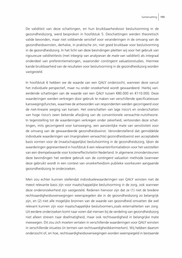
Samenvatting 195
De validiteit van deze schattingen, en hun bruikbaarheidvoor besluitvorming in de
gezondheidszorg, werd besproken in hoofdstuk 5. Deschattingen werden theoretisch
valide bevonden, maar niet voldoende sensitief voor veranderingen in de omvang van de
gezondheidswinsten, derhalve, in praktische zin, niet goed bruikbaar voor besluitvorming
in de gezondheidszorg. In het licht van deze bevindingen pleitten wij voor het gebruik van
rigoureuze validiteittests (met inbegrip van analysevan de mate van validiteit) als integraal
onderdeel van preferentiemetingen, waaronder contingent valuationstudies. Hiermee
kande bruikbaarheid van de resultaten voor besluitvorming in de gezondheidszorg worden
vastgesteld.
In hoofdstuk 6 hebben we de waarde van een QALY onderzocht, wanneer deze vanuit
het individuele perspectief, maar nu onder onzekerheid wordt gewaardeerd. Hierbij vari-
eerdende schattingen van de waarde van een QALY tussen €80.000 en €110.000. Deze
waarderingen werden verkregen door gebruik te maken van verschillende specificatiesvan
kanswegingsfuncties, waarmee de antwoorden van respondenten werden gecorrigeerd voor
de niet-lineaire weging van kansen. Het overschatten van lage risico’s en onderschatten
van hoge risico’s iseen bekende afwijking van de conventionele verwachte-nutstheorie.
In tegenstelling tot de waarderingen verkregen onder zekerheid, vertoonden deze schat-
tingen, mits gecorrigeerd voor kansweging, een aanzienlijke mate van sensitiviteit voor
de omvang van de gewaardeerde gezondheidswinst. Veronderstellend dat gemiddelde
individuele waarderingen van (marginaleen verwachte) gezondheidswinst een acceptabele
basis vormen voor de (maatschappelijke) besluitvorming in de gezondheidszorg, lijken de
waarderingen gepresenteerd in hoofdstuk 6 een relevanteinformatiebron voor het vaststellen
van een drempelwaarde voor kosteneffectiviteitin Nederland. In algemene zinondersteunen
deze bevindingen het verdere gebruik van de contingent valuation methode (wanneer
deze gebruikt wordt in een context van onzekerheid)om publieke voorkeuren aangaande
gezondheidszorg te onderzoeken.
Men zou echter kunnen stellendat individuelewaarderingen van QALY winsten niet de
meest relevante basis zijn voor maatschappelijke besluitvorming in de zorg, ook wanneer
deze onderonzekerheid zijn vastgesteld. Redenen hiervoor zijn dat ze (1) niet de bredere
rechtvaardigheidsoverwegingen weerspiegelen die in de gezondheidszorg zo belangrijk
zijn, en (2) niet alle mogelijke bronnen van de waarde van gezondheid omvatten die wel
relevant kunnen zijn voor maatschappelijke besluitvormers,zoals externaliteiten van zorg.
Uit eerdere onderzoeken komt naar voren dat mensen bij de verdeling van gezondheidszorg
niet alleen streven naar doelmatigheid, maar ook rechtvaardigheid in belangrijke mate
meewegen. Dit zou zich moeten vertalen in verschillende waarderingen voor QALY winsten
in verschillende situaties (in termen van rechtvaardigheidskenmerken). Wij hebben daarom
onderzocht of, en hoe, rechtvaardigheidsoverwegingen worden weerspiegeld in bestaande

196 Samenvatting
schattingen van de monetairewaarde van QALYs, en in de hoogte van de drempelwaarde
voor kosteneffectiviteit.
In hoofdstuk 7 hebben we de empirische literatuur over de monetaire waardering van de
QALY én die over(prominente) rechtvaardigheidsopvattingen in de gezondheidszorgonder-
zocht, met de bedoeling om de “gemeenschappelijke deler” tussen deze twee stromen
literatuur te vinden. De relatietussen opvattingen over rechtvaardigheid en de waarde van
de QALY is vooral belangrijk in het licht van de toenemende empirische interessein beide
aspecten. Hoewel beide onderwerpen gerelateerd zijn in de gebruikelijke beslisregel achter
economischeevaluaties, bleek uit hoofdstuk 7 dat de empirische (en zelfs de normatieve)
literatuur beide aspecten grotendeels afzonderlijk behandelt. Dit betekent dat de huidige
empirisch literatuur over de waarde van een QALY niet de maatschappelijke voorkeuren
betreffende een rechtvaardige verdeling van gezondheid en zorgweerspiegelt. In verreweg
de meeste empirische studies naar de waarde van gezondheidswinst wordt namelijk een
individueel perspectief gehanteerd, wat de beschouwing van gangbare overwegingen over
rechtvaardigheid uitsluit. Onderzoek gericht op het waarderen van gezondheidswinst vanuit
een maatschappelijk perspectief wordt dan ook aangemoedigd. In zulk onderzoek zou
expliciete informatie kunnen worden verschaft over de relevante rechtvaardigheidsaspecten,
waardoor de waardering van gezondheidswinst en de voorkeuren voor een eerlijke verdeling
van gezondheid en zorg meer samenhangend kunnen worden onderzocht. Op deze wijze
kunnen bijvoorbeeld specifieke drempelwaarden voor kosteneffectiviteit worden vastgesteld
voor specifieke doelgroepen en contexten, op basis van rechtvaardigheidsoverwegingen.
Een dergelijke aanpak lijkt op het beslismodel dat thans wordt voorgesteld door het College
voor Zorgverzekeringen in Nederland.
In hoofdstuk 8 hebben we de betalingsbereidheid voor een QALY vanuit maatschappelijk
perspectief en onder onzekerheid onderzocht. De maatschappelijke betalingsbereidheid
per QALY werd gedefinieerd als de (gemiddelde) bijdrage die leden van een samenleving
bereid zijn te leveren aan een collectiefgezondheidszorgsysteem ten einde een QALY te
winnen in een lid van die maatschappij. Dit betreft niet noodzakelijkerwijs de respondent
zelf, waardoor ook altruïstische en rechtvaardigheidsvoorkeuren meegewogen kunnen
worden. Dergelijke waarderingen lijken meer in lijn met maatschappelijke besluitvorming
in de zorgbetreffende de uitbreiding van een basispakket zorgvoorzieningen dat, zoals in
Nederland het geval, collectief wordt gefinancierd, op basis van solidariteit. De in hoofdstuk
8 gerapporteerde maatschappelijke waarderingenvarieerden van €52,000 tot €83,000 per
QALY, en waren daarmee iets lager dan de individuele waarderingen uithoofdstuk 6. De
waarderingen werden ook hier gecorrigeerd voor kansweging, waarbij weer verschillende
specificaties van kanswegingsfuncties werden gebruikt.Deze maatschappelijkewaarderingen
bleken echter een onvoldoende mate van validiteit te vertonen om beschouwd te worden

Samenvatting 197
als praktisch bruikbaar, volgens de definitiegeïntroduceerd in hoofdstuk 5. De waarden
gerapporteerd in hoofdstuk 8 weerspiegelen mogelijk tot op zekere hoogte de waardering
van het hebben van een collectiefzorgsysteem, in plaats van alleende gepresenteerde gezond-
heidswinst. Dit belemmert een zinvolle vergelijking van de resultaten uit de hoofdstukken
6 en 8.Het verkrijgen van valide schattingen van de waarde van QALY winsten vanuit een
maatschappelijk perspectief, waarbij ook expliciet rechtvaardigheidsoverwegingen worden
meegewogen, blijft daarmee een uitdaging voor toekomstig onderzoek.
In hoofdstuk 9 hebben wij het effect onderzocht van de (geanticipeerde) groei in de (ge-
zonde) levensverwachting op de maatschappelijke tijdsvoorkeur voor gezondheid. Onze
bevindingen suggereren dat de levensverwachting van toekomstige generaties van belang
is, mogelijk vanwege zowel doelmatigheids- als rechtvaardigheidsoverwegingen. Bij de
meting van maatschappelijke tijdsvoorkeur voor gezondheidis het expliciet benoemen van
de levensverwachting van toekomstige generaties, gebaseerd op feitelijke voorspellingen,
aan te bevelen, aangezien het tot meer zinvolle en nauwkeurige schattingen kan leiden.
Het doel van dit proefschrift was om in te gaan op diverse methodologische problemen
met betrekking tot de meting en waardering van baten in economischeevaluaties van
gezondheidszorgtechnologieën. De inzichten die uit dit proefschrift naar voren komen zijn in
meerdere opzichten vernieuwend en zullen, naar wij hopen, inspireren tot verder onderzoek,
aangezien nog veel vragen onbeantwoord blijven. Het vinden van een valide schatting
van de maatschappelijkebetalingsbereidheid voor een QALY alsmede de meest geschikte
manier om de batenzijde van economischeevaluaties uit te breiden, zijn twee belangrijke
vraagstukken. Hoewel bepaalde vragen moeilijk eenduidig oplosbaar zijn - aangezien het
normatieve kwesties betreffen waarover geen overeenstemming bestaat -hopen wij dat dit
proefschrift bijdraagt aan de kennis over het waarderen van baten van gezondheidszorgen
de bruikbaarheid van economischeevaluaties in besluitvorming in de zorg.


Acknowledgements 199
ACknoWlEdgEMEnTs
The work put into this thesis, and the process of developing into a researcher was not
(always) easy or straightforward, but I have enjoyed every moment. This was possible due
to three unstoppable forces. First, the inspiration I found in my parents. Second, the support
I found in my supervisors. Third, the comfort I found in my friends. For this, and more, I
am forever in their debt.
To my parents - my mother, prof. dr. Dragica Bobinac and my father, dr. Damir Bobinac. You
have been, and are, my rock, my shelter, my light when all else faded. Nema rijeci kojima
bih vam se mogla zahvaliti za sve sto ste za mene u zivotu ucinili.
To my supervisors – prof. dr. Werner Brouwer, prof. dr. Frans Rutten and dr. Job van Exel.
This is an opportunity for me to thank you, from the bottom of my heart, for everything
you have done for me over the last years.
Werner, you have been a great supervisor and a professional role model, guiding me through
the labyrinth that is the PhD, and posting clues when required. Your ideas, dedication and
patience made all the difference in my work. I will always remember this stage of my life as
a great learning period, primarily because of your unselfish contribution to my professional
development, always conveyed with enthusiasm that kept my spirit high. Dear Job, the same
applies to you! I thank you dearly for all your encouragement, understanding and friendship.
Prof. Rutten, thank you very much for your kindness and support.
Although not among my supervisors, I would also like to thank prof. dr. Eddy van Doorslaer
for all his kind help and advice.
To my friends - who understood and shared the pain and the joy of the past few years - I
am thankful for their friendship. Without your shoulder to cry on and a heart to lean on, I
might not have made it!
For the “technical support”, I have two acknowledgements. First, I would like to thank my
colleagues and fellow PhDs at iBMG for creating a lovely work atmosphere I enjoyed very
much! Special thanks to my colleagues form the seventh floor for their unselfish help and
a friendly hand when I needed it, especially mrs. Elif Pelit-Cekic.
Finally, I would like to thank the funders of the Broader Social Benefits project (which
resulted in thesis Chapters 2 to 8) for their financial support: Astra-Zeneca, GlaxoSmithKline,

200 Acknowledgements
Janssen-Cilag, Merck and Pfizer BV. I am grateful to the representatives of these companies
for their cooperation, their useful comments and suggestions.

About the author 201
ABouT THE AuTHoR
Ana Bobinac was born on the 14th of April 1980 in Rijeka, Croatia. She studied Economics
(International business major) at the University of Rijeka. In 2004, after graduating with a
Master of Arts in Economics, Ana took a position at the Institute for Public Health in Rijeka
where she developed an interest in Health Economics. In 2005, Ana enrolled into the Master
of Science in Health Economics program at Erasmus University. Her study in Rotterdam
was financially supported by the Croatian Ministry of Science through their “Scholarship
for excellence”. After obtaining her Masters degree, Ana became a PhD candidate at the
Institute of Health Policy and Management (iBMG) at Erasmus University, working on the
research project “Broader Social Benefits”. As an external advisor to the Croatian HTA board,
she participated in developing Croatian national HTA guidelines. In 2011, Ana received an
award from the Dutch Society for Technology Assessment in Healthcare (NVTAG) for the
best paper published by a young researcher in the domain of the society. She has published
her work in the Journal of Health Economics, Medical Decisions Making, Health Economics
and other relevant journals.
Currently, Ana holds a postdoctoral position at the Institute of Health Policy and Management
in Rotterdam. She has a son, Peter.


PhD Portfolio 203
Phd PoRTFolio
PhD Student: Ana Bobinac
Department: Institute of Health Policy and Management
PhD period: 2007-2012
Promotors: prof. dr. Werner Brouwer
prof. dr. Frans Rutten
Co-promotor: dr. Job van Exel
Training courses Year
Discrete choice experiments - Erasmus University, Rotterdam (course
given by prof. dr. John Rose of Melbourne University)
Modern statistical methods - NIHES, Erasmus MC, Rotterdam
International comparison of healthcare systems - NIHES, Erasmus MC,
Rotterdam
Academic writing - Erasmus University, Rotterdam
Economic policy evaluation - ISS, den Haag
2008
2009
2010
2010
2011
invited presentations
1st Annual meeting of the Croatian Society for Pharmacoeconomics,
Rijeka, Croatia
iBMG alumni workshop, Erasmus University Rotterdam
2010
2011

204 PhD Portfolio
Presentations at conferences (with a discussant) Year
1st Dutch Health Economics Study Group (LoLa HESG), Utrecht, the
Netherlands
3rdAmerican Society of Health economics conferences (ASHE), Ithaca,
USA
2nd Dutch Health Economics Study Group (LoLa HESG), Maastricht, the
Netherlands
UK Health Economics Study Group (UK HESG), York, UK
2009
2010
2010
2011
Presentations at conferences
6thWorld congress of the International Health Economics Association
(IHEA), Copenhagen, Denmark
7thEuropean Conference on Health Economics (ECHE), Rome, Italy
7thWorld congress of the International Health Economics Association
(IHEA), Toronto, Canada
2007
2008
2011
Poster presentations at conferences
11th European congressof the International Society for Pharmacoeco-
nomics and Outcomes Research (ISPOR), Paris, France
2009
Teaching
Discrete choice experiments, topic within the course Advanced
Economic Evaluations (Health economics Master program at Erasmus
University Rotterdam)
Contingent analysis, topic within the course Health Technology As-
sessment (Health economics Master program at Erasmus University
Rotterdam)
2008/2009
2008/2009
and
2009/2010
PhD Portfolio 205
Thesis supervision Year
Supervised and co-supervise Health economics Master theses 2009 - 2011
Publications not included in thesis
van Exel NJA, Bobinac A, Koopmanschap MA, Brouwer WBF (2008) The invisible hands
made visible: recognizing the value of informal care in healthcare decision-making.
Expert Review of Pharmacoeconomics and Outcomes Research 8: 557-561
van Exel NJA, Bobinac A, Koopmanschap MA, Brouwer WBF (2007) Providing informal
care: a burden and a blessing. Geneva Association Information Newsletter: Health and
Ageing 16: 10-13
Awards
Dutch Society for Technology Assessment in Healthcare (NVTAG) award
for the best paper published by a young researcher in the domain of
the society
2011


List of tables 207
lisT oF TABlEs
Table 2a: Summary statistics (n = 1,190) 32
Table 2b: Empirical estimation of models 1 and 2 (n = 1,190) 36
Table 3a: Summary statistics (n = 1,502) 49
Table 3b: Empirical estimation of models 1 and 2 (n = 1,502). 50
Table 4a: Summary statistics (n = 1,091) 64
Table 4b: WTP per QALY (€, rounded to hundreds) 67
Table 4c: WTP per QALY differentiated by income groups and levels of
certainty (€, rounded to hundreds) 68
Table 4d: WTP per QALY upper bound, average and differentiated by
income groups and levels of certainty (€, rounded to hundreds) 68
Table 4e: Multivariate clustered regression analysis with “raw” WTP and
WTP per QALY estimates as the dependent variable 69
Table 4A.1: Wording of WTP questions 78
Table 4A.2: Design of the choice scenarios, levels of risk and expected QALY gain 78
Table 5a: Scenario design 84
Table 5b: A summary of tests and hypothesis 88
Table 5c: Summary statistics (n = 1,091) 91
Table 5d: Results of the scale sensitivity test: scenarios with health gains of
different size and equal duration. WTP per QALY estimates rounded
to hundreds (all monetary values expressed in €) 92
Table 5e: Scale sensitivity test: scenarios with health gains of equal size and
different duration. WTP per QALY estimates rounded to hundreds (€) 94
Table 5f: Multivariate clustered regression analysis with “raw”
WTP estimates as the dependent variable (n = 4,018) 96
Table 6a: Probability weighting functions and parameter estimates 112
Table 6b: Summary statistics (n = 1,004) 114
Table 6c: Average WTP for a QALY estimates from Que1 and Que2 combined,
for all functions (€, rounded to hundreds) 116
Table 6d: WTP per QALY by health status, certainty level and
income group (n = 2001; in €, rounded to hundreds) 116
Table 6e: Que1 (n = 1004) and Que2 (n = 997) separately
(€, rounded to hundreds) 117
Table 6f: Multivariate regressions on cumulative data when probabilities are non-
weighted (NW) and when probabilities are weighted
(Tversky and Kahneman function, TK) 119
Table 6A.1: Wording of WTP questions 125
Table 6A.2: Design of the choice scenarios, levels of risk and expected QALY gain 126

208 List of tables
Table 7a: WTP per QALY studies 143
Table 8a: Probability weighting 154
Table 8b: Summary statistics (n = 1,004) 155
Table 8c: Open-ended (OE) SOC and SII WTP per QALY estimates, weighted
(TK and P functions) and non-weighted, on average and by
certainty level and income group (€, rounded to hundreds). 156
Table 8d: Multivariate regressions for SII and SOC separately,
non-weighted (NW) and weighted (TK and P function) 157
Table 8A.1: Wording of WTP questions 160
Table 8A.2: Design of the choice scenarios, levels of risk and expected QALY gain 161
Table 9a: Summary statistics (n = 607) 171
Table 9b: Mean and median elicited discount rates in the different questionnaires 170
Table 9c: Subjective expectations of life expectancy and
implied growth rates in questionnaire 4 (n = 153) 172
Table 9d: Can the variance in elicited discount rates be attributed to
(subjective expectations of) future life expectancy? (n = 562) 172
Table 9A.1: Wording of questions 1 - 4 175

List of figures 209
lisT oF FiguREs
Figure 4a: Spread of gains across the utility plane 62
Figure 4A.1: Ranking two health states 75
Figure 4A.2: Rating the two health states on an EQ-VAS showing previous
valuations of death, perfect health and own health 75
Figure 4A.3: Payment scale, first step 76
Figure 4A.4: Payment scale, second step. 76
Figure 4A.5: Open-ended format. 77
Figure 6A.1: Ranking two health states 127
Figure 6A.2: Rating the two health states on an EQ-VAS showing previous
valuations of death, perfect health and own health 127
Figure 6A.3: Payment scale, first step 128
Figure 6A.4: Payment scale, second step. 128
Figure 6A.5: Open-ended format. 129
Figure 6A.6: Graphical explanation of the concept of risk 129
Figure 8A.1: Payment scale, first step 162
Figure 8A.2: Payment scale, second step. 162
Figure 8A.3: Open-ended format. 163
Figure 8A.4: Graphical explanation of the concept of risk 163
Figure 9a: Mean discount rates in the four versions of the questionnaires
for delay periods of 5, 10, 20, and 40 years 171


List of references 211
lisT oF REFEREnCEs
Abdel-Khalek A (2006) Measuring happiness with a single-item scale. Social Behaviour and Personality
34: 139-150.
Abdellaoui M (2000) Parameter-free elicitation of utility and probability weighting functions. Manage-
ment Science 46: 1497-1512.
Allik H, Larsson JO, Smedje H (2006) Health-related quality of life in parents of school-age children
with Asperger syndrome or high-functioning autism. Health and Quality of Life Outcomes 4: 1.
Anderson C, Linto J, Stewart-Wynne EG (1995) A population-based assessment of the impact and
burden of caregiving for long-term stroke survivors. Stroke 26: 843-849.
Andren S, Elmstahl S (2007) Relationships between income, subjective health and caregiver burden in
caregivers of people with dementia in group living care; a cross-sectional community-based study.
International Journal of Nursing Studies 44: 435-446.
Andreoni J (1990) Impure altruism and donations to public goods: a theory of warm-glow giving. The
Economic Journal 100: 464– 477.
Appleby J, Devlin N, Parkin D (2007) NICE’s cost effectiveness threshold. British Medical Journal 335:
358–359.
Arrow KJ, Cline WR, Mäler KG, Squitieri R, Stiglitz JE (1996) Intertemporal equity discounting and
economic efficiency. In: Bruce JP, Haites EF (eds) Economic and social dimensions of climate change.
Contribution of working Group III to the Second assessment report of the Intergovernmental panel
on climate change. Cambridge: Cambridge University Press.
Arrow KJ, Kurz M (1970) Public investment, the rate of return, and optimal fiscal investment. Balti-
more: Johns Hopkins.
Arrow KJ, Solow R, Leamer E, Radner R, Schuman H (1993) Report of the NOAA Panel on contingent
valuation. Federal Register 58: 4601–4614.
Baeten S, Baltussen R, Uyl-de Groot C, Bridges J, Niessen L (2010) Incorporating equity-efficiency
interactions in cost-effectiveness analysis-three approaches applied to breast cancer control. Value
in Health 13: 573-579.
Baker R, Chilton S, Jones-Lee M, Metcalf H (2008) Valuing lives equally: defensible premise or unwar-
ranted compromise? Journal of Risk and Uncertainty 36: 125–138.
Baker R, Currie GR, Donaldson C (2010) What needs to be done in contingent valuation: have Smith
and Sach missed the boat? Health Economics, Policy and Law 5: 113-121.
Baltussen R, Stolk E, Chisholm D, Aikins M (2006) Towards a multi-criteria approach for priority set-
ting: an application to Ghana. Health Economics 15: 689–696.
Barry BM (1989) A treatise on social justice. Theories of Justice, vol. I. Berkeley: University of California
Press.
Basu A, Meltzer D (2005) Implications of spillover effects within the family for medical cost-effective-
ness analysis. Journal of Health Economics 224: 751–773.
Bateman IJ, Brouwer R (2006) Consistency and construction in stated WTP for health risk reductions.
A novel scope sensitivity test. Resource and Energy Economics 28: 199-214.
212 List of references
Bateman IJ, Brouwer R, Georgiou S, Hanley N, Machado F, Mourato S, Saunders C (2005) A “natural
experiment” approach to contingent valuation of private and public UV health risk reduction
strategies in low and high risk countries. Environmental and Resource Economics 31: 47-72.
Bateman IJ, Jones AP (2003) Contrasting conventional with multi-level modeling approaches to meta-
analysis: Expectation consistency in U.K. woodland recreation values. Land Economics 79: 235-258.
Baumol WJ (1968) On the social rate of discount. American Economic Review 58: 788-802.
Beach SR, Schulz R (2000) Is care giving a risk factor for mortality? Geriatric Times 1: 26-27.
Becker GS (1997) Altruism, egoism and genetic fitness: economics and sociobiology. Journal of Eco-
nomic Literature 14: 817-826.
Becker GS, Mulligan CB (1997) The endogenous determination of time preferences. Quarterly Journal
of Economics 112: 729-758.
Bell D, Blanchflower CG (2007) The Scots may be brave but they are neither healthy nor happy.
Scottish Journal of Political Economy 54: 166–194.
Bergstrom TC (2006) Benefit-cost in a benevolent society. American Economic Review 96: 339-351.
Bhatia MR, Fox-Rushby JA (2003) Validity of willingness to pay: hypothetical versus actual payment.
Applied Economics Letters 10: 737–740.
Bleichrodt H (1997) Health utility indices and equity considerations. Journal of Health Economics 16:
65-91.
Bleichrodt H, Crainich D, Eeckhoudt L (2003) Comorbidities and the willingness to pay for health
improvements. Journal of Public Economics 87: 2399-2406.
Bleichrodt H, Diecidue E, Quiggin J (2004) Equity weights in the allocation of healthcare: the rank-
dependent QALY model. Journal of Health Economics 23: 157-171.
Bleichrodt H, Doctor JN, Stolk E (2005) A nonparametric elicitation of the equity-efficiency tradeoff in
cost-utility analysis. Journal of Health Economics 24: 655-678.
Bleichrodt H, Eeckhoudt L (2006) Willingness to pay for reductions in health risk when probabilities are
distorted. Health Economics 15: 211-214.
Bleichrodt H, Pinto Prades JL (2000) A parameter-free elicitation of the probability weighting function
in medical decision analysis. Management Science 46: 1485-1496.
Bleichrodt H, Quiggin J (1999) Life-cycle preferences over consumption and health: when is cost-
effectiveness analysis equivalent to cost-benefit analysis? Journal of Health Economics 18: 681-708.
Blomquist G, Blumenschein K, Johannesson M (2009) Eliciting willingness to pay without bias using
follow-up certainty statements: comparisons between probably/definitely and a 10-point certainty
scale. Environmental Resource Economics 43: 473–502.
Blumenschein K, Johannesson M (1998) Relationship between quality of life instruments, health-state
utilities and willingness to pay in patients with asthma. Annals of Allergy Asthma Immunology 80:
189–194.

List of references 213
Blumenschein K, Johannesson M, Yokoyama KK, Freeman PR (2001) Hypothetical versus real willing-
ness to pay in the healthcare sector: results from a field experiment. Journal of Health Economics
20: 441-457.
Bobinac A, Brouwer WBF, Van Exel NJA (2011) Societal discounting and growing healthy life expec-
tancy – an empirical investigation. Health Economics 20: 111-119. (Chapter 9)
Bobinac A, Van Exel NJA, Rutten FFH, Brouwer WBF (2010) Caring for and caring about: disentangling
the family effect and the caregiving effect. Journal of Health Economics 29: 549-556. (Chapter 2)
Bobinac A, Van Exel NJA, Rutten FFH, Brouwer WBF (2010) Willingness to pay for a QALY: the indi-
vidual perspective. Value in Health 13: 1046–1055. (Chapter 4)
Bobinac A, van Exel NJA, Rutten FFH, Brouwer WBF (2011) Inquiry into the relationship between the
equity weights and the value of a QALY. Submitted (Chapter 7)
Bobinac A, van Exel NJA, Rutten FFH, Brouwer WBF (2011) Get more, pay more? An elaborate test of
construct validity of willingness to pay per QALY estimates obtained through contingent valuation.
Journal of Health Economics 31: 158-168.(Chapter 5)
Bobinac A, van Exel NJA, Rutten FFH, Brouwer WBF (2011) Moving towards valid estimates of individual
willingness to pay for a QALY: using uncertainty and probability weighting. Submitted (Chapter 6)
Bobinac A, Van Exel NJA, Rutten FFH, Brouwer WBF (2011) Health effects in significant others: Sepa-
rating family and care giving effects. Medical Decision Making 31: 292-298. (Chapter 3)
Bobinac A, Van Exel NJA, Rutten FFH, Brouwer WBF (2011) Valuing QALY gains applying a societal
perspective. Submitted (Chapter 8)
Bos JM, Postma MJ, Lieven A (2005) Discounting health effects in pharmacoeconomic evaluations:
current controversies. Pharmacoeconomics 23: 639-649.
Boulding KE (1981) A preface to grants economics: the economy of love and fear. New York: Praeger
Publishers.
Bowling A (1999) Ageism in cardiology. British Medical Journal 319: 1353–1355.
Bowling A, Mariotto A, Evans O (2002) Are older people willing to give up their place in the queue for
cardiac surgery to a younger person? Age and Ageing 31: 187–192.
Bradford DF (1972) Benefit–cost analysis and demand curves for public goods. Kyklos 23: 775–791.
Bradford DF (1975) Constraints on government investment opportunities and the choice of discount
rate. American Economic Review 6: 887–899.
Braithwaite RS, Meltzer DO, King JT Jr, Leslie D, Roberts M (2008) What does the value of modern
medicine say about the $50,000 per Quality-adjusted Life Year decision rule? Medical Care 4:
349–359.
Bramstedt KA (2003) Aortic valve replacement in the elderly: frequently indicated yet frequently
denied. Gerontology 49: 46–49.
Brock D (2001) Priority to the worst off in healthcare resource prioritization. In: Battin M, Rhodes R,
Silvers A (eds) Healthcare and social justice. New York: Oxford University Press.
Brouwer WBF (2006) Too important to ignore – informal caregivers and other significant others.
Pharmacoeconomics 24:39-41.
Brouwer WBF, Culyer AJ, Van Exel NJA, Rutten FFH (2008a) Welfarism vs. extra-welfarism. Journal of
Health Economics 27: 325–338.

214 List of references
Brouwer WBF, Van Exel NJA, Baker R, Donaldson C (2008b) The new myth: the social value of the
QALY. Pharmacoeconomics 26: 1–4.
Brouwer WBF, Koopmanschap MA (2000) On the economic foundations of CEA. Ladies and gentle-
men, take your positions! Journal of Health Economics 19: 439-459.
Brouwer WBF, Niessen L, Postma M, Rutten FFH (2005) Need for differential discounting of costs and
health effects in cost effectiveness analyses. British Medical Journal 331: 446-448.
Brouwer WBF, Tilford M, Van Exel NJA (2009) Incorporating caregiver and family effects in economic
evaluations of child health. In: Ungar W (eds) Economic Evaluation in Child Health. Oxford: Oxford
University Press.
Brouwer WBF, Van Exel NJA (2005) Expectations regarding length and health related quality of life:
some empirical findings. Social Science and Medicine 61: 1083-1094.
Brouwer WBF, Van Exel NJA, Baltussen RMPM, Rutten FFH (2006a) A dollar is a dollar is a dollar: or is
it? Value Health 9: 341–347.
Brouwer WBF, Van Exel NJA, Van Gorp B, Redekop K (2006b) The CarerQol: A new instrument to
measure care-related quality of life of informal caregivers for use in economic evaluations. Quality
of Life Research 15: 1005-1021.
Brouwer WBF, Van Exel NJA, Koopmanschap MA, Rutten FFH (1999) The valuation of informal care in
economic appraisal; a consideration of individual choice and societal costs of time. International
Journal of Technology Assessment in Health Care 15: 147-160.
Brouwer WBF, Van Exel NJA, Van de Berg B, Koopmanschap MA, Dinant H, Van den Bos GAM (2004)
The burden of caregiving: evidence on objective burden, subjective burden and quality of life
impacts in informal caregivers for patients with rheumatoid arthritis. Arthritis Care and Research
51: 570–577.
Bugge C, Alexander H, Hagen S (1999) Stroke patients’ informal caregivers. Patient, caregiver, and
service factors that affect caregiver strain. Stroke 30: 1517–1523.
Burton P, Lethbridge L, Phipps S (2008) Children with disabilities and chronic conditions and longer-
term parental health. Journal of Socio-Economics 37: 1168-1186.
Busschbach JJV, Hessing DJ, Charro FT (1993) The utility of health at different stages in life: a quantita-
tive approach. Social Science and Medicine37: 153–158.
Byrne MM, O’Malley K, Suarez-Almazor M (2005) Willingness to pay per Quality-Adjusted Life Year in
a study of knee osteoarthritis. Medical Decision Making 25: 655-666.
Cairns J (1994) Valuing future benefits. Health Economics 2: 221-229.
Cairns J (2001) Discounting in economic evaluation. In: Drummond MF, McGuire A (eds) Economic
Evaluation in Health Care: Merging Theory with Practice. Oxford: Oxford University Press.
Cairns J, Van der Pol M (2000) Valuing future private and social benefits: The discounted utility model
versus hyperbolic discounting models. Journal of Economic Psychology 21: 191-205.
Camerer CF (1999) Individual decision-making. In: Kagel JH, Roth AE (eds) Handbook of Experimental
Economics. New Jersey: Princeton University Press.
Camerer CF, Ho T (1994) Violations of the betweenness axiom and nonlinearity in probability. Journal
of Risk and Uncertainty 8: 167-196.
Camerer CF (2000) Prospect theory in the wild: Evidence from the field. In: Kahneman D, Tversky A
(eds) Choices, values, and frames (pp. 288-300). Cambridge: Cambridge University Press.

List of references 215
Cameron AT, Quiggin J (1994) Estimation using contingent valuation data from a “Dichotomous
choice with follow-Up” questionnaire. Journal of Environmental Economics and Management 27:
218–234.
Camidge R, Walker A, Oliver JJ, Nussey F, Maxwell S, Jodrell D, Webb DJ (2005) Prognosis without
treatment as a modifier in health economic assessments. British Medical Journal 330: 1382-1384.
Cappelen A, Norheim O (2006) Responsibility, fairness and rationing in healthcare. Health Policy 76:
312–319.
Carnwath TC, Johnson DA (1987) Psychiatric morbidity among spouses of patients with stroke. British
Medical Journal 294: 409– 411.
Carson R (2000) Contingent Valuation: a user’s guide. Environmental Science and Technology 34:
1413-1418.
Carson R, Mitchell R (1995) Sequencing and nesting in contingent valuation surveys. Journal of Envi-
ronmental Economics and Management 28: 155-173.
CBS. Available from: http://www.cbs.nl/en-GB/menu/cijfers/ kerncijfers/default.htm
Clark AE, Oswald AJ (1994) Unhappiness and unemployment. The Economic Journal 104: 648-659.
Claxton K, Paulden M, Gravelle H, Brouwer WBF, Culyer AJ (2011) Discounting and decision-making in
the economic evaluation of healthcare technologies. Health Economics 20: 2-15.
Claxton K, Sculpher M, Culyer A, McCabe C, Briggs A, Akehurst R, Buxton M, Brazier J (2006) Dis-
counting and cost-effectiveness in NICE - stepping back to sort out a confusion. Health Economics
15: 1-4.
Claxton K, Walker S, Palmer S, Sculpher M (2010) Appropriate perspectives for healthcare decisions.
Centre for Health Economics, University of York. CHE Research Paper 54.
Coast J (2004) Is economic evaluation in touch with society’s health values? British Medical Journal
329: 1233-1236.
Cohen-Almagor R (2002) A critique of Callahan’s utilitarian approach to resource allocation in health-
care. Issues in Law and Medicine 17: 247-261.
Contoyannis P, Jones AM (2004) Socio-economic status, health and lifestyle. Journal of Health Eco-
nomics 23: 965–995.
Cookson R, Drummond M, Weatherly H (2009) Explicit incorporation of equity considerations into
economic evaluation of public health interventions. Health Economics, Policy and Law 4: 231-245.
Cookson R, McCabe C, Tsuchiya A (2008) Public healthcare resource allocation and the rule of rescue.
Journal of Medical Ethics 34: 540-544.
Corso P, Hammitt J, Graham J (2001) Valuing mortality-risk reduction: using visual aids to improve the
validity of contingent valuation. Journal of Risk and Uncertainty 23: 165-184.
Culyer AJ (1971) The nature of the commodity healthcare and its efficient allocation. Oxford Economic
Papers 23: 189-211.
Culyer AJ (2001) Equity – some theory and its policy implications. Journal of Medical Ethics 27:
275–283.
Culyer AJ (2002) Introduction. In: Towse A, Pritchard C, Devlin N (eds) Cost-Effectiveness Threshold:
Economic and Ethical Issues. London: King’s Fund and Office of Health Economics.

216 List of references
Culyer AJ, McCabe C, Briggs A, Claxton K, Buxton M, Akehurst R, Sculpher M, Brazier J (2007)
Searching for a threshold not setting one: the role of the National Institute for Health and Clinical
Excellence. Journal of Health Services Research and Policy 12: 56-58.
Culyer AJ, Wagstaff A (1993) Equity and equality in health and healthcare. Journal of Health Econom-
ics 12: 431-457.
Cunningham SJ, Hunt NP (2000) Relationship between utility values and willingness to pay in patients
undergoing orthognathic treatment. Community Dental Health 17: 92–96.
Davidson T, Levin LA (2010) Is the societal approach wide enough to include relatives? Incorporating
relatives’ costs and effects in a CEA. Applied Health Economics and Health Policy 8: 25–35.
Desvousges WH, Johnson FR, Dunford RW, Boyle KJ, Hudson SP, Wilson KN (1993) Measuring natural
resource damages with contingent valuation: tests of validity and reliability. In: Hausman JA (ed)
Contingent Valuation: a critical assessment. Amsterdam: Elsevier Science Publishers.
Devlin N, Parkin D (2004) Does NICE have a cost effectiveness threshold and what other factors
influence its decisions? A binary choice analysis. Health Economics 13: 437–452.
DiTella R, MacCulloch RJ (2006) Some Uses of Happiness Data in Economics. The Journal of Economic
Perspectives 20: 25-46.
DiTella R, MacCulloch RJ, Oswald AJ (2001) Preferences over inflation and unemployment; Evidence
from surveys of subjective well-being. American Economic Review 91: 335-341.
Dixon S, Walker M, Salek S (2006) Incorporating carer effects into economic evaluation. Pharmaco-
economics 24: 43–53.
Dolan P (1998) The measurement of individual utility and social welfare. Journal of Health Economics
17: 39- 52.
Dolan P (2001) Utilitarianism and the measurement and aggregation of Quality-adjusted Life Years.
Healthcare Analysis 9: 65-76.
Dolan P, Cookson R (2000) A qualitative study of the extent to which health gain matters when
choosing between groups of patients. Health Policy 51: 19–30.
Dolan P, Cookson R, Ferguson B (1999) Effect of discussion and deliberation on the public’s views of
priority setting in healthcare: focus group study. British Medical Journal 318: 916–919.
Dolan P, Edlin R (2002) Is it really possible to build a bridge between cost–benefit analysis and cost-
effectiveness analysis? Journal of Health Economics 21: 827–843.
Dolan P, Green C (1998) Using the person trade-off approach to examine differences between indi-
vidual and social values. Health Economics 7: 307–312.
Dolan P, Olsen JA (2001) Equity in health: the importance of different health streams. Journal of Health
Economics 20: 823-834.
Dolan P, Olsen JA, Menzel P, Richardson J (2003) An inquiry into the different perspectives that can be
used when eliciting preferences in health. Health Economics 12: 545–551.
Dolan P, Shaw R, Tsuchiya A, Williams A (2005) QALY maximisation and people’s preferences: a meth-
odological review of the literature. Health Economics 14: 197-208.
Dolan P, Tsuchiya A (2005) Health priorities and public preferences: the relative importance of past
health experience and future health prospects. Journal of Health Economics 24: 703–714.

List of references 217
Donaldson C, Baker R, Mason H, Jones-Lee M, Lancsar E, Wildman J, Bateman I, Loomes G, Robinson
A, Sugden R, Pinto Prades JL, Ryan M, Shackley P, Smith R (2011) The social value of a QALY: raising
the bar or barring the raise? BMC Health Services Research 11: 8.
Donaldson C, Shackley P, Abdalla M (1997a) Using willingness to pay to value close substitutes: carrier
screening for cystic fibrosis revisited. Health Economics 6: 145–159.
Donaldson C, Thomas R, Torgerson D (1997b) Validity of open-ended and payment scale approaches
to eliciting willingness to pay. Applied Economics 29: 79–84.
Donaldson, C, Shackley P, Abdalla M, Miedzybrodzka Z (1995) Willingness to pay for antenatal carrier
screening for cystic fibrosis. Health Economics 4: 439–452.
Dowie J (1998) Towards the equitable efficient and transparently decidable use of public funds in the
deep blue millennium. Health Economics 7: 93-104.
Drummond M, Brixner D, Gold M, Kind P, McGuire A, Nord E and Consensus Development Group
(2009) Toward a Consensus on the QALY. Value in Health 12: 31–35.
Drummond M, McGuire A (2001) Economic evaluation in healthcare. Merging theory and practice.
London, Office of Health Economics.
Drummond MF, O’Brien B, Stoddart GL, Torrance GW (1997) Methods for the economic evaluation of
healthcare programmes. Oxford: Oxford University Press.
Dubourg WR, Jones-Lee MW, Loomes G (1997) Imprecise preferences and survey design in contingent
valuation. Economica 64: 681-702.
Easterlin RA (2001) Income and happiness: Towards a unified theory. The Economic Journal 111:
465-484.
Edlin R, Round J, McCabe C, Sculpher M, Claxton K, Cookson R (2008) Cost-effectiveness analysis and
ageism: a review of the theoretical literature. Leeds Institute of Health Sciences.
Eichler HG, Kong SX, Gerth WC, Mavros P, Jonsson B (2004) Use of cost-effectiveness analysis in
healthcare resource allocation decision-making: how are cost-effectiveness thresholds expected to
emerge? Value Health 7: 518–528.
EUROVAQ project. from: http://research.ncl.ac.uk/ eurovaq/
Feldstein MS (1964) The social time preference discount rate in cost benefit analysis. Economic Journal
74: 360–379.
Feldstein MS (1965) The derivation of social time preference rates. Kyklos 18: 277–287.
Ferrer-i-Carbonell A (2005) Income and well-being: An empirical analysis of the comparison income
effect. Journal of Public Economics 89: 997-1019.
Ferrer-i-Carbonell A, Frijters P (2004) How important is methodology for the estimates of the determi-
nants of happiness? The Economic Journal 114: 641-659.
Ferrer-i-Carbonell A, Van Praag BMS (2002) The subjective costs of health losses due to chronic dis-
eases. An alternative model for monetary appraisal. Health Economics 11: 709-722.
Fisher AC (1996) The conceptual underpinnings of the contingent valuation method. In: Bjornstad
DJ, Kahn JR (eds) The contingent valuation of environmental resources: methodological issues and
research needs. Cheltenham: Edward Elgar.
Flores N, Carson R (1997) The relationship between the income elasticities of demand and willingness
to pay. Journal of Environmental Economics and Management 33: 287-295.

218 List of references
Frederick S (2006) Valuing future life and future lives: A framework for understanding discounting.
Journal of Economic Psychology 27: 667-680.
Frederick S, Fischhoff B (1998) Scope insensitivity in elicited valuations. Risk, Decision and Policy 3:
109-123.
Frew EJ, Whynes DK, Wolstenholme J (2003) Eliciting willingness to pay: comparing closed-ended with
open-ended and payment scale formats. Medical Decision Making 23: 150–159.
Frey BS, Stutzer A (2001) Happiness and economics. Princeton: Princeton University Press.
Frey BS, Stutzer A (2002) What can economists learn from happiness research? Journal of Economic
Literature 40: 402-435.
Frijters P, Haisken-DeNew JP, Shields MA (2004) Money does matter! Evidence from increasing real
incomes and life satisfaction in East Germany following reunification. American Economic Review
94: 730-740.
Furnham A, Simmons K, McClelland A (2000) Decisions concerning the allocation of scarce medical
resources. Journal of Social Behavior and Personality 15: 185–200.
Gibb S, Donaldson C, Henshaw R (1998) Assessing strength of preference for abortion method using
willingness to pay. Journal of Advanced Nursing 27: 30–36.
Gold MR, Siegel JE, Russell LB, Weinstein MC (1996) Cost-effectiveness in health and medicine.
Oxford: Oxford University Press.
Gonzalez R, G Wu (1999) On the form of the probability weighting function. Cognitive Psychology
38: 129-166.
Gravelle H, Brouwer WBF, Niessen LW, Postma MJ, Rutten FFH (2007) Discounting in economic evalu-
ations: stepping forward towards optimal decision rules. Health Economics 16: 307-317.
Gravelle H, Smith D (2001) Discounting for health effects in cost-benefit and cost-effectiveness analy-
sis. Health Economics 10: 587-599.
Green C (2009) Investigating public preferences on “severity of health” as a relevant condition for
setting healthcare priorities. Social Science and Medicine 68: 2247–2255.
Grosse SD (2008) Assessing cost effectiveness in healthcare: the history of the $50,000 per QALY
threshold. Expert Reviews of Pharmacoeconomics and Outcomes Research 8: 165-178.
Gyrd-Hansen D (2003) Willingness to pay for a QALY. Health Economics 12: 1049-1060.
Gyrd-Hansen D (2004) Investigating the social value of health changes. Journal of Health Economics
23: 1101–1116.
Gyrd-Hansen D (2005) Willingness to pay for a QALY: theoretical and methodological issues. Pharma-
coeconomics 23: 423-432.
Gyrd-Hansen D, Kjær T (2011) Disentangling WTP per QALY data: different analytical approaches,
different answers. Health Economics in press
Hammitt JK (2002) QALY versus WTP. Risk Analysis 22: 985–1001.
Hammitt JK, Graham JD (1999) Willingness to pay for health protection: inadequate sensitivity to
probability? Journal of Risk and Uncertainty 18: 32-62.
Harless DW, Camerer CF (1994) The predictive utility of generalized expected utility theories. Econo-
metrica 62: 1251–1289.

List of references 219
Harvey CM (1994) The reasonableness of non-constant discounting. Journal of Public Economics 53:
31-51.
Heberlein TA, Wilson MA, Bishop RC, Schaeffer NC (2005) Rethinking the scope test as a criterion for
validity in contingent valuation. Journal of Environmental Economics and Management 50: 1-22.
Hirth RA, Chernew ME, Miller E, Fendrick AM, Weissert WG (2000) Willingness to pay for a Quality-
adjusted Life Year: in search of a standard. Medical Decision Making 20: 332-342.
HM Treasury Guidelines, 2003. http://www.hm-treasury.gov.uk/d/Ch_10_Philibert_3.pdf
Hoffman C, von der Schulenberg JMG (2000) The influence of economic evaluation studies on
decision-making: A European Survey. Health Policy 52: 179–192.
Holland J, Van Exel NJA, Schut FT, Brouwer WBF (2009) Some pain, no gain. Experiences with the
no-claim rebate in the Dutch healthcare system. Health Economics, Policy and Law 4: 405-424.
Hughes SL, Giobbie-Hurder A, Weaver FM, Kubal JD, Henderson W (1999) Relationship between
caregiver burden and health- related quality of life. Gerontologist 39: 534–545.
Hurley J (2000) An overview of the normative economics of the health sector. In: Culyer AJ, Newhouse
JP (eds) Handbook of Health Economics, vol 1A. Amsterdam: Elsevier.
Isaacs SL, Schroeder SA (2004) Class: the ignored determinant of the nation’s health. New England
Journal of Medicine 351: 1137–1142.
Jakobsson K, Dragun J (1996) Contingent Valuation and Endangered Species. Cheltenham, UK and
Brookfield, US: Edward Elgar.
Jansen SJ, Stiggelbout AM, Wakker PP, Nooij MA, Noordijk EM, Kievit J (2000) Unstable preferences:
a shift in valuation or an effect of the elicitation procedure? Medical Decision Making 20: 62–71.
Johannesson M, Blomquist GC, Blumenschein K, Johansson P, Liljas B, O’Conor RM (1999) Calibrat-
ing hypothetical willingness to pay responses. Journal of Risk and Uncertainty 18: 21-32.
Johannesson M, Johansson PO (1996) The discounting of lives saved in future generations - some
empirical results. Health Economics 5: 329-332.
Johannesson M, Johansson PO (1997) Is the valuation of a QALY gained independent of age? Journal
of Health Economics 16: 589-599.
Johannesson M, Meltzer D (1998) Editorial: some reflections on cost-effectiveness analysis. Health
Economics 7: 1-7.
Johnson R, Banzhaf M, Desvouges W (2000) Willingness to pay for improved respiratory and car-
diovascular health: a multiple-format stated-preference approach. Health Economics 9: 295–317.
Jones-Lee M, Loomes G, Philips P (1995) Valuing the prevention of non-fatal road injuries: contingent
valuation vs. standard gambles. Oxford Economic Papers 47: 676-695.
Jorgensen BS, Syme GJ, Smith LM, Bishop BJ (2004) Random error in willingness to pay measurement:
a multiple indicators, latent variable approach to the reliability of contingent values. Journal of
Economic Psychology 25: 41–59.
Kahneman D, Knetsch JL (1992) Valuing public goods: the purchase of moral satisfaction. Journal of
Environmental Economics and Management 22: 57–70.
Kahneman D, Krueger AB (2006) Developments in the measurement of subjective well-being. Journal
of Economic Perspectives 20: 3-24.

220 List of references
Kahneman D, Ritov I, Schkade D (1999) Economic preferences or attitude expressions? An analysis of
dollar responses to public issues. Journal of Risk and Uncertainty 19: 203-235.
Kahneman D, Tversky A (1979) Prospect theory: an analysis of decision under risk. Econometrica 47:
263-291.
Kapteyn A, Teppa F (2003) Hypothetical intertemporal consumption choices. Economic Journal 11:
140-152.
Kind P, Dolan P, Gudex C, Williams A (1998) Variations in population health status: results from a
United Kingdom national questionnaire survey. British Medical Journal 316: 736–741.
King JT Jr, Tsevat J, Lave JR, Roberts MS (2005) Willingness to pay for a Quality-adjusted Life Year:
implications for societal healthcare resource allocation. Medical Decision Making 25: 667–677.
Klose T (1999) The contingent valuation method in healthcare. Health Policy 47: 97-123.
Konishi Y, Kenji A (2011) A framework for estimating willingness to pay to avoid endogenous environ-
mental risks. Resource and Energy Economics 33: 130-154.
Koopmanschap MA, NJA Van Exel, B Van den Berg, WBF Brouwer (2008) An overview of methods
and applications to value informal care in economic evaluation of healthcare. Pharmacoeconomics
26: 269-280.
Kremer M (2006) Consumers in charge of care: the Dutch personal budget and its impact on the
market, professionals and the family. European Societies 8: 385–401.
Lamers LM, McDonnell J, Stalmeier PFM, Krabbe PFM, Busschbach JJV (2006) The Dutch Tariff: Results
and arguments for an effective design for national EQ-5D valuations studies. Health Economics
215: 1121-1132.
Lancsar E, Wildman JC, Donaldson C, Ryan M, Baker R (2011) Deriving distributional weights from
QALYs through discrete choice experiments. Journal of Health Economics 30: 466–478.
Layard R, Glaister S (1994) Cost-Benefit Analysis (2nd edition). Cambridge: Cambridge University
Press.
Lienhoop N, MacMillan D (2007) Valuing wilderness in Iceland: Estimation of WTA and WTP using the
market stall approach to contingent valuation. Land Use Policy 24: 289-295.
Liu L (2004) Comorbidities and the willingness to pay for reducing the risk of a targeted disease:
introducing endogenous effort for risk reduction. Health Economics 13: 493-498.
Long JS, Ervin LH (2000) Using heteroscedasticity consistent standard errors in the linear regression
model. American Statistician 54: 217–224.
Luce DR, Fishburn PC (1994) Rank- and sign-dependent linear utility models for finite first-order
gambles. Journal of Risk and Uncertainty 4: 29-59.
Lundberg L, Johannesson M, Silverdahl M, Hermansson C, Lindberg M (1999) Quality of life, health-
state utilities and willingness to pay in patients with psoriasis. British Journal of Dermatology 141:
1067-1075.
MacMillan D, Hanley N, Lienhoop N (2006) Contingent valuation: environmental polling or preference
engine. Ecological Economics 60: 299–307.
Manne AS. Richels R (1995) MERGE: A model for evaluating regional and global effects of GHGs
reduction policies. Energy Policy 23: 17-34.
Marks NF (1998) Does It Hurt to Care? Care giving, work-family conflict, and midlife well-being.
Journal of Marriage and the Family 60: 951-966.

List of references 221
Martin S, Rice N, Smith PC (2008) Does healthcare spending improve health outcomes? Evidence from
English programme budgeting data. Journal of Health Economics 27: 826-842.
Mason H, Baker R, Donaldson C (2008a) Willingness to pay for a QALY: past, present and future.
Expert Reviews of Pharmacoeconomics and Outcomes Research 8: 575–582.
Mason H, Jones-Lee M, Donaldson C (2008b) Modeling the monetary value of a QALY: a new ap-
proach based on UK data. Health Economics 18: 933-950.
McCabe C, Claxton K, Culyer AJ (2008) The NICE cost-effectiveness threshold: what it is and what that
means. Pharmacoeconomics 26: 733-744.
McConaghy R, Caltabiano ML (2005) Caring for a person with dementia: exploring relationships
between perceived burden, depression, coping and well-being. Nursing and Health Sciences 7:
81-91.
McCusker J, Latimer E, Cole M, Ciampi A, Sewitch M (2007) Major depression among medically ill
elders contributes to sustained poor mental health in their informal caregivers. Age Ageing 36:
400–406.
McFadden D, Leonard G (1993) Issues in the Contingent Valuation of Environmental Goods: Meth-
odologies for Data Collection and Analysis. In: Hausman JA (ed) Contingent valuation: a critical
assessment. Amsterdam: Elsevier.
Michelbach PA, Scott JT, Matland RE, Bornstein BH (2003) Doing Rawls justice: an experimental study
of income distribution norms. American Journal of Political Science 47: 523–539.
Mooney G (1989) QALYs: are they enough? A health economist’s perspective. Journal of Medical
Ethics 15: 148-152.
Morimoto T, Schreiner AS, Asano H (2003) Caregiver burden and health-related quality of life among
Japanese stroke caregivers. Age and Ageing 32: 218–223.
Mortimer D (2006) The value of thinly spread QALYs. Pharmacoeconomics 24: 845-853.
Murray CJL, Acharya AK (1997) Understanding DALYs. Journal of Health Economics 16: 703–730.
Murray CJL, Lopez AD (1994) Global comparative assessments in the health sector: disease burden,
expenditures and intervention packages. World Health Organization (WHO): Geneva.
Neumann PJ, Greenberg D (2009) Is The United States ready for QALYs? Health Affairs 28: 1366-1371.
Neumann PJ, Kuntz KM, Leon J, Araki SS, Hermann RC, Hsu MA (1999) Health utilities in Alzheimer’s
disease: a cross-sectional study of patients and caregivers. Medical Care 37: 27-32.
Ng YK (1997) A case for happiness, cardinalism and interpersonal comparability.The Economic Journal
107: 1848-1858.
NICE (2004) Guide to the Methods of Technology Appraisal. National Institute for Clinical Excellence:
London. ( from: www.nice.org.uk.)
NICE (2005) Social value judgements. Principles for the development of NICE guidance. National
Institute for Health and Clinical Excellence: London. ( from: www.nice.org.uk.)
NICE (2008) Appraising life-extending, end of life treatments. National Institute for Health and Clinical
Excellence: London. ( from: www.nice.org.uk.)
NICE (2009) TA111 Alzheimer’s disease: Donepezil, Galantamine, Rivastigmine (Review) and Me-
mantine. Guidance (amended August 2009). London: National Institute for Health and Clinical
Excellence; 2009. (Available from: URL:http://www.nice.org.uk/nicemedia/pdf/TA111Guidance-
AmendedAug09.pdf)

222 List of references
NOAA Panel (Available from: (http://www.cbe.csueastbay.edu/~alima/courses/4306/articles/
NOAA%%20on%%20contingent%%20valuation%%201993.pdf.)
Nord E (1993a) The relevance of health state after treatment in prioritizing between different patients.
Journal of Medical Ethics 19: 37–42
Nord E (1993b) The trade-off between severity of illness and treatment effect in cost–value analysis of
healthcare. Health Policy 24: 227–238.
Nord E (1995) The person-trade-off approach to valuing healthcare programs. Medical Decision Mak-
ing 15: 201–208.
Nord E (1999) Cost-Value Analysis in Health Care: Making Sense of QALYs. New York: Cambridge
University Press.
Nord E (2005) Concerns for the worse off: fair innings versus severity. Social Science and Medicine
60: 257-263.
Nord E, Daniels N, Kamlet M (2008) QALYs: some challenges. Value in Health 12: 10–15.
Nord E, Pinto Prades JL, Richardson J, Menzel P, Ubel P (1999) Incorporating societal concerns for
fairness in numerical valuations of health programmes. Health Economics 8: 25–39.
Nord E, Richardson J, Street A, Kuhse H, Singer (1996) The significance of age and duration of effect
in social evaluation of healthcare. Healthcare Analysis 4: 103–111.
Nord E, Richardson J, Street A, Kuhse H, Singer P (1995) Maximizing health benefits vs egalitarianism:
an Australian survey of health issues. Social Science and Medicine 41: 1429–1437.
Nordhaus W (1993) Rolling the ‘DICE’: an optimal transition path for controlling greenhouse gases’.
Resource and Energy Economics 15: 27-50.
Norinder A, Krister H, Ulf P (2001) Scope and scale insensitivities in a contingent valuation study of risk
reductions. Health Policy 57: 141-153.
O’Brien B, Gafni A (1996) When do the “dollars” make sense? Toward a conceptual framework for
contingent valuation studies in healthcare. Medical Decision Making 6: 288-299.
Oddsson K (2003) Assessing attitude towards prioritizing in healthcare in Iceland. Health Policy 66:
135–146.
OECD statistics (Available from: http://stats.oecd.org/WBOS/ index.aspx)
Olsen JA (1993a). On what basis should health be discounted? Journal of Health Economics 12: 39-53.
Olsen JA (19993b) Time preferences for health gains: an empirical investigation. Health Economics 2:
257-265.
Olsen JA (1997) Aiding priority setting in healthcare: Is there a role for the Contingent Valuation
method? Health Economics 6: 603-612.
Olsen JA (2000) A note on eliciting distributive preferences for health. Journal of Health Economics
19: 541-550.
Olsen JA, Donaldson C (1998) Helicopters, hearts and hips: using willingness to pay to set priorities for
public sector healthcare programmes. Social Science and Medicine 46: 1–12.
Olsen JA, Donaldson C, Pereira J (2004a) The insensitivity of ‘willingness-to-pay’ to the size of the
good: New evidence for healthcare. Journal of Economic Psychology 25: 445-460.
Olsen JA, Kidholm K, Donaldson C, Shackley P (2004b) Willingness to pay for public healthcare: a
comparison of two approaches. Health Policy 70: 217 – 228.

List of references 223
Olsen JA, Richardson J (1998) Priority setting in the public health service: Results of an Australian
survey. Technical Report 9, Centre for Health Program Evaluation, Monash University, Melbourne.
Olsen JA, Richardson J, Dolan P, Menzel P (2003) The moral relevance of personal characteristics in
setting healthcare priorities. Social Science and Medicine 57: 1163-1172.
Oswald AJ (1997) Happiness and economic performance. The Economic Journal 107: 1815-1831.
Ottersen T, Mbilinyi D, Maestad O, Norheim OF (2008) Distribution matters: Equity considerations
among health planners in Tanzania. Health Policy 85: 218–227.
Parkin D, Devlin N (2006) Is there a case for using visual analogue scale valuations in cost-utility
analysis? Health Economics 15: 653-664.
Pinto Prades JL, Loomes G, Brey R (2009) Trying to estimate a monetary value for the QALY. Journal of
Health Economics 28: 553-562.
Poe G, Clark JE, Rondeau D, Schulze WD (2002) Provision point mechanisms and field validity tests of
contingent valuation. Environmental and Resource Economics 23: 105–131.
Polinder S, Meerding WJ, Van Exel J, Brouwer WBF (2005) Societal discounting of health effects in
cost-effectiveness analyses: the influence of life expectancy. Pharmacoeconomics 23: 791-802.
Polsky D (2005) Does willingness to pay per Quality-adjusted Life Year bring us closer to a useful
decision rule for cost-effectiveness analysis? Medical Decision Making 25: 605-606.
Prelec D (1998) The probability weighting function. Econometrica 66: 497-528.
Quiggin J (1981) Risk perception and risk aversion among Australian farmers. Australian Journal of
Agricultural Economics 25: 160-169.
Ramsey FP (1928) A mathematical theory of saving. Economic Journal 38: 543-559.
Ratcliffe J (2000) Public preferences for the allocation of donor liver grafts for transplantation. Health
Economics 9: 137–148.
Ratcliffe J, Buxton M, Young T, Longworth L (2005) Determining priority for liver transplantation: a
comparison of cost per QALY and discrete choice experiment-generated public preferences. Ap-
plied Health Economics and Health Policy 4: 249-255.
Rawlins MD, Barnett D, Stevens A (2010) Pharmacoeconomics: NICE’s approach to decision making.
British Journal of Clinical Pharmacology 70: 346-349.
Rawlins MD, Culyer AJ (2004) National Institute for Clinical Excellence and its value judgments. British
Medical Journal 329: 224–227.
Rawls J (1971) A Theory of Justice. Cambridge: Harvard University Press.
Read D (2001) Is time-discounting hyperbolic or subadditive? Journal of Risk and Uncertainty 23: 5-32.
Riddel M, Shaw WD (2006) A theoretically consistent empirical model of non-expected utility: an
application to nuclear waste transportation. Journal of Risk and Uncertainty 32: 131–150.
Rivlin MM (2000) Why the fair innings argument is not persuasive. BMC Medical Ethics 1: 1.
Roberts T, Bryan S, Heginbotham C, McCallum A (1999) Public involvement in healthcare priority
setting: an economic perspective. Health Expectations 2: 235–244.
Rodriguez Miguez E, Pinto Prades JL (2002) Measuring the social importance of concentration or
dispersion of individual health benefits. Health Economics 11: 43–53.
Rubinstein A (2003) Economics and psychology? The case of hyperbolic discounting. International
Economic Review 44: 1207-1216.

224 List of references
RVZ Council for Public Health and Health Care. Sensible and sustainable care. Zoetermeer, Nether-
lands: Council for Public Health and Health Care (RVZ), 2006. [in Dutch]
Ryan M (2004) A comparison of stated preference methods for estimating monetary values. Health
Economics 13: 291-296.
Scholte op Reimer WJM, de Haan RJ, Rijnders PT, Limburg M, Van den Bos GAM (1998) The burden of
care giving in partners of long-term stroke survivors. Stroke 29: 1605-1611.
Schulz R, Beach SR (1999) Caregiving as a risk factor for mortality: the caregiver health effects study.
JAMA 282: 2215–2219.
Schulz R, Martire LM (2004) Family caregiving of persons with dementia: prevalence, health effects,
and support strategies. American Journal of Geriatric Psychiatry 12: 240–249.
Schwappach DL (2002) Resource allocation, social values and the QALY: a review of the debate and
empirical evidence. Health Expectations 5: 210–222.
Schwappach DL (2003) Does it matter who you are or what you gain? An experimental study of
preferences for resource allocation. Health Economics 12: 255-267.
Sen A (2002) Why health equity? Health Economics 11: 659–666.
Severens JL, Milne RJ (2004) Discounting Health Outcomes in Economic Evaluation: The Ongoing
Debate. Value in Health 7: 397-401.
Shah KK (2009) Severity of illness and priority setting in healthcare: A review of the literature. Health
Policy 93: 77-84.
Shaw WD, Woodward RT (2008) Why environmental and resource economists should care about
non-expected utility models. Resource and Energy Economics 30: 66-89.
Shiroiwa T, Sung Y, Fukuda T, Lang H, Bae S, Tsutani K (2010) International survey on willingness-
to-pay (WTP) for one additional QALY gained: what is the threshold of cost effectiveness? Health
Economics 4: 422-437.
Shogren JF, Crocker TD (1991) Risk, self-protection, and ex ante economic value. Journal of Environ-
mental Economics and Management 20: 1-15.
Silliman RA, Fletcher RH, Earp JL, Wagner EH (1986) The families of elderly stroke patients: Effects of
home care. Journal of The American Geriatrics Society 34: 643-648.
Skjoldborg US, Gyrd-Hansen D (2003) Conjoint analysis. The cost variable: an Achilles’ heel? Health
Economics 12: 479-491.
Smith K, Wright K (1994) Informal care and economic appraisal: A discussion of possible methodologi-
cal approaches. Health Economics 3: 137-148.
Smith RD (2001) The relative sensitivity of willingness-to-pay and time-trade-off to changes in health
status: an empirical investigation. Health Economics 10: 487–497.
Smith RD (2005) Sensitivity to scale in contingent valuation: the importance of the budget constraint.
Journal of Health Economics 24: 519–529.
Smith RD (2006) It’s not just what you do, it’s the way that you do it: the effect of different payment
card formats and survey administration on willingness to pay for health gain. Health Economics
15: 281-293.
Smith RD (2007) Use, option and externality values: are contingent valuation studies in healthcare
misspecified? Health Economics 16: 861–869.

List of references 225
Smith RD, Richardson J (2005) Can we estimate the “social” value of a QALY? Four core issues to
resolve. Health Policy 74: 77–84.
Smith RD, Sach TH (2010) Contingent valuation: what needs to be done? Health Economics, Policy
and Law 5: 91-111.
Spackman M (2004) Time discounting and of the cost of capital in government. Fiscal Studies 25:
467-518.
Starmer C (2000) Developments in non-expected utility theory: the hunt for a descriptive theory of
choice under risk. Journal of Economic Literature 38: 332–382.
Starmer C, Sugden R (1989a) Probability and juxtaposition effects: an experimental investigation of
the common ratio effect. Journal of Risk and Uncertainty 2: 159–178.
Starmer C, Sugden R (1989b) Violations of the independence axiom in common ratio problems: An
experimental test of some competing hypotheses. Annals of Operations Research 19: 79-101.
Stolk EA, Pickee SJ, Ament AH, Busschbach JJ (2005) Equity in healthcare prioritisation: an empirical
inquiry into social value. Health Policy 74: 343-355.
Stolk EA, van Donselaar G, Brouwer WBF, Busschbach JJV (2004) Reconciliation of economic concerns
and health policy: illustration of an equity adjustment procedure using proportional shortfall.
Pharmacoeconomics 22: 1097-1107.
Tengs TO, Meyer G, Siegel JE, Pliskin JS, Graham JD, Weinstein MC (1996) Oregon’s Medicaid ranking
and cost-effectiveness: is there any relationship? Medical Decision Making 16: 99-107.
The EuroQol Group (1999) EuroQol – a new facility for the measurement of health related quality of
life. Health Policy 16: 199–208.
Tilling C, Krol M, Tsuchiya A, Brazier J, Van Exel NJA, Brouwer WBF (2009) Measuring the value of life:
Exploring a new method for deriving the monetary value of a QALY. University of Sheffield Working
Paper 09-14, Sheffield University.
Tooth L, Mckenna K, Barnett A, Prescott C, Murphy S (2005) Caregiver burden, time spent caring and
health status in the first 12 months following stroke. Brain Injury 19: 963–974.
Towse A (2009) Should NICE’s threshold range for cost per QALY be raised? Yes. British Medical
Journal 338: 181.
Treasure J (2004) Review: exploration of psychological and physical health differences between care-
givers and non-caregivers. Evidence Based Mental Health 7: 28.
Tsuchiya A (2000) QALYs and ageism: philosophical theories and age weighting. Health Economics 9:
57-68.
Tsuchiya A, Dolan P (2005) The QALY model and individual preferences for health states and health
profiles over time: a systematic review of the literature. Medical Decision Making 25: 460-467.
Tsuchiya A, Dolan P (2007) Do NHS clinicians and members of the public share the same views about
reducing inequalities in health? Social Science and Medicine 64: 2499-2503.
Tsuchiya A, Dolan P (2009) Equality of what in health?: Distinguishing between outcome egalitarian-
ism and gain egalitarianism. Health Economics 18: 147-159.
Tsuchiya A, Dolan P, Shaw R (2003) Measuring people’s preferences regarding ageism and health:
Some methodological issues and some fresh evidence. Social Science and Medicine 57: 687-696.
Tsuchiya A (1999) Age-related preferences and age weighting health benefits. Social Science and
Medicine 48: 267-276.

226 List of references
Tversky AD, Kahneman D (1992) Advances in prospect theory: cumulative representation of uncer-
tainty. Journal of Risk and Uncertainty 15: 297-323.
Ubel PA (1999) How stable are people’s preferences for giving priority to severely ill patients? Social
Science and Medicine 49: 895–903.
Ubel PA, Jepson C, Baron J, Mohr T, McMorrow S, Asch DA (2001) Allocation of transplantable organs:
do people want to punish patients for causing their illness? Liver Transplant 7: 600–607.
Van de Wetering L, Stolk EA, Van Exel NJA, Brouwer WBF (2011) Balancing equity and efficiency in
delineating the Dutch basic benefits package using the principle of proportional shortfall. European
Journal of Health Economics in press
Van den Berg B, Brouwer WBF, Koopmanschap MA (2004) Economic valuation of informal care. An
overview of methods and applications. European Journal of Health Economics 5: 36-45.
Van den Berg B, Ferrer-i-Carbonell A (2007) Monetary valuation of informal care: the well-being valu-
ation method. Health Economics 16: 1227-1244.
Van den Berg B, Van Exel NJA, Koopmanschap MA, Van den Bos GAM, Brouwer WBF (2002) Informal
Care and Personal Care Budget: A Situational Sketch of Informal Care Providers Reached via the
Dutch Association of Care Budget Holders. Report no. 02.59. Rotterdam: iMTA Rotterdam, Eras-
mus MC (Available from: URL: www.imta.nl/publications/0259.html)
Van Exel NJA, Brouwer WBF, Van den Berg B, Koopmanschap MA (2006) With a little help from an
anchor: Discussion and evidence of anchoring effects in contingent valuation. Journal of Socio-
Economics 35: 836-853.
Van Exel NJA, Koopmanschap MA,Van den Berg B, Brouwer WBF, Van den Bos GAM (2005) Burden of
informal care giving for stroke patients: identification of caregivers at risk of adverse health effects.
Cerebrovascular Diseases 19: 11-17.
Van Exel NJA, Scholte op Reimer WJM, Brouwer WBF, Van den Berg B, Van den Bos GAM, Koopman-
schap MA (2004a) Instruments for assessing the burden of informal caregiving for stroke patients
in clinical practice: a comparison of CSI, CRA, SCQ and self-rated burden. Clinical Rehabilitation
18: 203–214.
Van Exel NJA, Van den Bos GAM, Van den Berg B, Koopmanschap MA, Brouwer WBF (2004b) What
really matters: an inquiry into the relative importance of dimensions of care giving burden. Clinical
Rehabilitation 18: 683-693.
Van Exel NJA, Van den Berg B, Koopmanschap MA, Van den Bos GAM, Brouwer WBF (2002) Informal
Care in the Netherlands: A Situational Sketch of Informal Care Providers Reached via Informal Care
Support Centres. Report no. 02.58b. Rotterdam: iMTA Rotterdam, Erasmus MC (Available from:
URL: www.imta.nl/publications/0258b.html)
Van Hout BA (1998) Discounting costs and effects: a reconsideration. Health Economics 7: 581-594.
Van Houtven G, Powers J, Jessup A, Yang J (2006) Valuing avoided morbidity using meta-regression
analysis: what can health status measures and QALYs tell us about WTP? Health Economics 15:
775-795.
Van Praag BMS, Ferrer-i-Carbonell A (2007) Happiness Quantified: A Satisfaction Calculus Approach.
Oxford: Oxford University Press.
Veenhoven R (2008) World Database of Happiness, Distributional Findings in Nations. Erasmus Univer-
sity Rotterdam (Available at: www.worlddatabaseofhappiness.eur.nl)

List of references 227
Viscusi KW, Moore MJ (1989) Rates of time preference and valuations of the duration of life. Journal
of Public Economics 38: 297-317.
Viscusi WK, Evans WN (1998) Estimation of revealed probabilities and utility functions for product
safety decisions. Review of Economics and Statistics 80: 28-33.
Wagstaff A (1991) QALYs and the equity-efficiency trade-off. Journal of Health Economics 10: 21-41.
Wagstaff A, Van Doorslaer E (2000) Measuring and testing for inequity in the delivery of healthcare.
Journal of Human Resources 35: 716-733.
Wailoo A, Tsuchiya A, McCabe C (2009) Weighting must wait: incorporating equity concerns into
cost-effectiveness analysis may take longer than expected. Pharmacoeconomics 27: 983-989.
Walker AJ, Pratt CC, Eddy L (1995) Informal care giving to aging family members: A critical review.
Family Relations 44: 402-411.
Weinstein M (2008) How much are Americans willing to pay for a Quality-adjusted Life Year? Medical
Care 46: 343-345.
Weinstein M, McGuire A, Torrance G (2009) QALYs: the basics. Value in Health 12: S5–S9.
Werntoft E, Hallberg IR, Edberg AK (2007) Prioritisation and resource allocation in healthcare. The
views of older people, receiving continuous public care and service. Health Expectations 10: 117-
128.
Whynes DK, Wolstenholme JL, Frew EJ (2004) Evidence of range bias in contingent valuation payment
scales. Health Economics 13: 183–190.
Wiener J, Tilly J, Evans Cuellar A (2003) Consumer-Directed Home Care in the Netherlands, England
and Germany. Report no. 2003-12. Washington, DC: AARP Public Policy Institute.
Williams A (1997) Intergenerational equity: an exploration of the ‘fair innings’ argument. Health
Economics 6: 117-132.
Williams A (1998) Ethics and efficiency in the provision of healthcare. In: Bell M, Mendus S (eds)
Philosophy and Medical Welfare. Cambridge: Cambridge University Press.
Williams A, Cookson R (2000) Equity in health. In: Culyer AJ, Newhouse JP (eds) Handbook of Health
Economics. Amsterdam: Elsevier.
Wyller TB, Thommessen B, Sodring KM, Sveen U, Pettersen AM, Bautz-Holter E, Laake K (2003)
Emotional well- being of close relatives to stroke survivors. Clinical Rehabilitation 17: 410–417.
Yaari ME (1987) The dual theory of choice under risk. Econometrica 55: 95-115.
Yamazaki S, Sokejima S, Mizoue T, Eboshida A, Fukuhara S (2005) Health-related quality of life of
mothers of children with leukemia in Japan. Quality of Life Research 14: 1079-1085.
Yeung R, Smith RD, McGhee SM (2003) Willingness to pay and size of health benefit: an integrated
model to test for ‘sensitivity to scale’. Health Economics Letters 12: 791–796.
Zethraeus N (1998) Willingness to pay for hormone replacement therapy. Health Economics 7: 31-38.