economic factors that influence soybean and canola prices
TRANSCRIPT
The University of MaineDigitalCommons@UMaine
Electronic Theses and Dissertations Fogler Library
2001
Economic factors that influence soybean andcanola pricesLei Cui
Follow this and additional works at: http://digitalcommons.library.umaine.edu/etd
Part of the Agribusiness Commons, and the Agricultural and Resource Economics Commons
This Open-Access Thesis is brought to you for free and open access by DigitalCommons@UMaine. It has been accepted for inclusion in ElectronicTheses and Dissertations by an authorized administrator of DigitalCommons@UMaine.
Recommended CitationCui, Lei, "Economic factors that influence soybean and canola prices" (2001). Electronic Theses and Dissertations. 540.http://digitalcommons.library.umaine.edu/etd/540

ECONOMIC FACTORS THAT INFLUENCE
SOYBEAN AND CANOLA PRICES
BY
Lei Cui
B.S. Beijing Normal University, P.R.China, 1997
A THESIS
Submitted in Partial Fulfillment of the
Requirements for the Degree of
Master of Science
(in Resource Economics and Policy)
The Graduate School
The University of Maine
August, 2001
Advisory Committee:
James D. Leiby, Associate Professor of Resource Economics and Policy, Advisor
Mario F. Teisl, Assistant Professor of Resource Economics and Policy
Kathleen P. Bell, Assistant Professor of Resource Economics and Policy

ECONOMIC FACTORS THAT INFLUENCE SOYBEAN AND CANOLA PRICES
By Lei Cui
Thesis Advisor: Dr. James Leiby
An Abstract of the Thesis Presented in Partial Fulfillment of the Requirements for the
Degree of Master of Science (in Resource Economics and Policy)
August, 2001
The USDA Agricultural Research Service is examining the feasibility and
profitability of growing Canola and soybeans in potato rotation systems. The study
described in this thesis is part of this research program. The primary objective of this
research is to look for economic factors that influence soybean and Canola prices.
Canola is a new oilseed crop to the U.S. Since the Food and Drug Administration
approved its use as edible food, Canola production in the US . has increased
tremendously. Because only 11 years of data are available on Canola consumption and
production in the U.S., it is difficult to empirically analyze Canola prices. Fortunately, we
find that Canola and soybean prices are highly correlated. As a result, if we can explain
the determinants of soybean prices, we can discover information about the determinants
of Canola prices. In this study, we concentrate on soybean price movements, make
inferences about Canola prices.
We establish a simultaneous model of the U.S. soybean market and study factors
affecting soybean prices within this economic structure. Our model is based primarily on
the USDA CROPS Model developed by Houck, et al.

Our results indicate that soybean price is positively affected by a time trend variable,
expected wholesale price of corn oil, expected real expenditures spent on food, expected
variable cost of growing soybeans, and one-year lagged farm-level corn price, but
negatively affected by one-year lagged soybean price, one-year lagged wheat price, and
one-year lagged acreage of soybeans. Using the Canola and soybean price relationship,
we infer how these economic factors affect Canola price. With the reduced form, we can
forecast the future price of both Canola and soybeans.

ACKNOWLEDGMENTS
I would like to thank Dr. Leiby, Dr. Teisl and Dr. Bell for being on this thesis
committee. I would especially like to thank my advisor James Leiby, for his remarkable
patience and countless hours spent during the process of conducing researches, revising
models and writing this thesis.
I would also like to thank my friends, both in China and in the U.S., who encouraged
me during the last two years. I especially thank my husband, Hanxing Yu, for his love,
understanding and support all the time. Finally, I would like to thank my parents. Their
care and love are the sources of my courage.
.. 11

TABLE OF CONTENTS
.. ACKNOWLEDGEMETNS ...................................................................... 11
LIST OF TABLES ................................................................................. vi
LIST OF FIGURES ................................................................................. ix
Chapter
1 . INTRODUCTION ............................................................................ 1
Statement of Problem ......................................................................... 1
Background .................................................................................... 5
Summary ....................................................................................... 8
2 . USDA CROPS MODEL FOR THE U.S. SOYBEANMARKET ..................... 9
The Demand Side for Soybeans in the CROPS Model ................................. 10
Aggregated Demand for Soybeans in the U.S. ............................... 10
Variable Definitions ............................................................. 11
Simultaneous Equations for the Demand Side of Soybean Market ....... 11
The Supply Side for Soybeans in the CROPS Model ................................. 16
Joining Demand and Supply Sides Together ........................................... 18
Some Criticisms Regarding the CROPS Model ....................................... 19
Summary .................................................................................... 22
.
3 . EMPIRICAL MODEL AND DATA ..................................................... 23
Reasons for using A Simultaneous Equation System .................................. 23
The Demand Side of Soybean Market ................................................... 24
Soy Meal Market ................................................................. 26
Soy Oil Market ...................................................................
Stock Demand .................................................................... 29
The Supply Side of Soybeans ............................................................ 29
Product Supply and Acreage Response ....................................... 29
Factors Relating to Acreage Response Model ................................ 31
Technical and Physical Relationships ................................................... 33
Price Linkage Equation ......................................................... 33
Ratio of Soy Oil/Meal Produced to Soybeans Crushed ..................... 34
Market Equilibrium Identities ............................................................ 34
27
Summary .................................................................................... 36
4 . EMPIRICAL RESULTS ............................................................... 37
Statistical Methods and Estimation Results ........................................... 37
........................................................................ Results Discussion 41
Elasticity Analysis of Soybean Demand and Supply ........................ 41
Reduced Form of Soybean Farm Level Prices .............................
Forecast Soybean Prices ...................................................... 46
Applying the Forecast Results to Canola Prices ............................. 47
43
Summary ................................................................................. 49
iv
5 . SUMMARY AND CONCLUSIONS ................................................ 50
Summary ................................................................................. 50
Conclusions .............................................................................. 51
REFERENCES ............................................................................... 52
APPENDICES ................................................................................ 54
Appendix A . Formulation of Distributed Lag Models ................. 55
Appendix B . Identification in Simultaneous System and
Two-Stage-Least-Squares Estimates ..................... 65
Appendix C . Comparison of OLS Estimates with Two-Stage-Least-Squares Estimates in the Simultaneous Equation Model for the Soybean Market ............................................ 68
Appendix D . Procedure of Obtaining the Reduced Form for Farm-Level Soybean Prices (PS) ........................ 72
BIOGRAPHY OF THE AUTHOR ...................................................... 74
V
LIST OF TABLES
Table 1 .l .
, Table 2.1.
Table 3.1.
Table 3.2.
Table 3.3.
Table 3.4.
Table 3.5.
Table 3.6.
Table 3.7
Table 4.1.
Table 4.2.
Regression Results Comparing Soybean and Canola Prices . . . . . . . . . . . ... 4
Variable Definitions in The CROPS Model.. . . . . . . . . . . . . . . . . . . . . . . . . . . . . . . . 12
Summary Statistics for Variables Used in the Equation of
Soybean Export Demand (Equation 3.1) . . . . . . . . . . . . . . . . . . . . . . . . . . . . . . . . .... 25
Summary Statistics for Variables Used in the Equation of
Soy Meal Demand (Equation 3.2) . . . . . . . . . . . . . . . . . . . . . . . . . . . . . . . . . . . . . . . . . .. 26
Summary Statistics for Variables Used in the Equation of
Soy Meal Export Demand (Equation 3.3) . . . . . . . . . . . . . . . . . . . . . . . . . . . . . . . . . . 27
Summary Statistics for Variables Used in the Equation of
Domestic Soy Oil Demand (Equation 3.4) . . .. . . . . . . . . . . . . . . . . . . . . . . . . . .. . ... 28
Summary Statistics for Variables Used in Equation of
Soy Oil Export Demand (Equation 3.5) . . . . . . . . . . . . .. . . . . . . . . . . . . . . . . . . . . . . . . 28
Summary Statistics for Variables Used in Acreage Response
Equation (Equation 3.6) . . . . . . . . . . . . . . . . . . . . . . . . . . . . . . . . . . . . . . . . . . . . . . . . . . . . . . . .. . 33
Summary Statistics for Variables Used in Identity Equations
(Equation 3.10 through 3.12) . . . . . . . . . . . . . . . . . . . . . . . . . . . . . . . . . . . . . . . . . . . . . . . ... 36
Parameter Estimates for Equation (4.1)
- U.S. Soy Meal Demand, QMD.. . . . . . . . . . . . . . . . . . . . . . . . . . . . . . . . . . . . . . . . ... . . .. 39
Parameter Estimates for Equation (4.2)
- U.S. Soy Oil Demand, QOD.. .. . .. . .. . . . . . . . .. . . . . . . . . . . . . . .. . .... . . . . . . . . . . . 39
vi

Table 4.3.
Table 4.4.
Table 4.5.
Table 4.6.
Table 4.7.
Table 4.8.
Table 4.9.
Table 4.10.
Table 4.1 1.
Table 4.12.
Table 4.13.
Parameter Estimates for Equation (4.3)
- U.S. Soybean Export Demand, QSX . . . . . . . . . . . . . . . . . . . . . . . . . . . . . . . . . . . .
Parameter Estimates for Equation (4.4)
- U.S. Soy Meal Exports, QMX . . . . . . . . . . . . . . . . . . . . . . . . . . . . . . . . . . . . . . . . . ... . .. 40
Parameter Estimates for Equation (4.5)
- U.S. Soy Oil Exports, QOX . . . . . . . . . . . . . . . . . . . . . . . . . . . . . . . . . . . .. . . . . . . . . . . . . 40
39
Parameter Estimates for Equation (4.6)
Soy Meal Produced (QMP) Regressed on Soybeans Crushed (QSC)
(with no intercept) . . .. . . . . . . . . . . .. . .... . . . . . . . .. . . . . . . . .. . . . . .. . . . . .. . . . . .. . . . . ..
Parameter Estimates for Equation (4.7)
Soy Oil Produced (QOP) Regressed on Soybeans Crushed (QSC)
(with no intercept) . . .. . .. . .. . .. . .. . . . . .. . . . . . . . . . . .. . . . . ... . . . . . . . . . . . . . .. . . . . . . . . 40
Parameter Estimates for Equation (4.8) - Wholesale Soy Meal Price (PM)
And Wholesale Soy Oil Price (PO) Regressed on Farm-level
Soybean Price (PS) . . . . . . . . .. . .. . .. . .. . . . . . . . . . . .. . . . . . . . . . . . . . . . . . . . . . . . . . ... . .. 40
Parameter Estimate for Equation (4.12)
- Soybean Acreage Response Model . . . . . . . . . . . . . . . . . . . . . . . . . . . . . . . . . . . . . . ... 41
Elasticity of Soy Oil Domestic Demand
Computed at Mean Levels . . .. . . . . .. . .. . .. . .. . . . . . . . .. . . . . .. . . . . . . . . . . . . . . . . . . . .. 42
Elasticity of Soy Oil Export Demand Computed at Mean Levels.. . . . . . . . . 42
Elasticity Soybean Acreage Computed at Mean Levels . . . . . . . . .. . . . . . . . ... 43
Soybean Farm Level Price With Respect to
Some of the Right-hand-side Variables . . . . . . . . . . . . . . . . . . . . . . . . . . . . . . . . . . . . . . .. 44
40
vii
Table A. 1. Summary Statistics for Soybean Prices from 1965 to 1998
(Prices are adjusted with CPI, 1999=100) ............................ 62
Table A.2. Parameter Estimates of Polynomial Distributed Lag Structures
For Soybeans, Soy Oil and Meal
(numbers in parentheses are standard errors) ................................. 62
Table C. 1. Compare OLS Estimates and Two-Stage-Least-Squares Estimates
for Equations in the Simultaneous System In Our Model
(numbers in parentheses are standard errors) ................................ 7 1
... Vll l

Figure 1.1.
Figure 1.2.
Figure 1.3.
Figure 1.4.
Figure 1.5.
Figure 3.1.
Figure 4.1.
Figure 4.2.
Figure A. 1.
LIST OF FIGURES
U.S. Average Annual Farm Level Canola Seed Price and Soybean Price
From 1991 to 1999.. .. . .... .... ......... ... . .. . ..... . .. ... . .. ... . .. . .. . .. . .. . ... . 2
U.S. Average Annual Canola Oil Price and soy Oil Price
From 1989 to 1999 ...... . .. . .. . .. ... ......... . .. . ..... . .. . .. . ... .. . .. . .. . .. . .. . .. 2
U.S. Average Annual Canola Meal Price and Soy Meal Price
From 1989 to 1999 .......... ... . .. . .. ......... . .. . ..... . .. ... . ... .. . .. ... . .. . ...
U.S. Canola Production
From 1991 to 2000 . . . . . . . . . . . . . . . . . . . . . . . . . . . . . . . . . . . . . . ... . . . . . . . . . . . . . . . . . . . . .... 6
U.S. Soybean Production and Exports
From 1970 to 1998 .... . .. . . . . . . . . . . . . . .. . . . . . . . . . . .. . . . . .. . . . . . . . . . . . . . . . . . . . . . . ... 7
South American Soybean Export Share in the International
Soybean Market (1995 - 1999) . . . . . . . . . . . ... . . . . . . . . . . . . . . . . . . . . . . . . . . . . . . . . ... 25
Forecast Farm-Level Soybean Price from 199 1 to 1998 . . . . . . . . . . . . . . . . . . . . .47
Forecast Canola Price from 1991 to 1998 . . . . . . . . . . . . . . . . . . . . . . . . . . . . . . . . ... 48
Forecast Real Soybean Prices from 1990 to 1998
With Polynomial Distributed Lag Structure . . . . . . . . . . . . . . . . . . . . . . . . . . . . . . . . . 64
3
ix

Chapter 1
INTRODUCTION
Statement of Problem
In order to identify more profitable potato rotations, the Agricultural Research
Service of the USDA is conducting a study of the feasibility of growing soybeans and
Canola in a potato rotation system. This thesis is part of that project. Here we attempt to
determine what economic factors influence the price of soybeans and Canola and then
explain how soybean and Canola prices move with respect to these factors.
Canola is a relatively new oilseed crop in the United States. It was not approved for
food use in the U.S. until 1985. Current price data for Canola available from USDA are
annual prices from 1989 to 2000, insufficient for a rigorous empirical analysis.
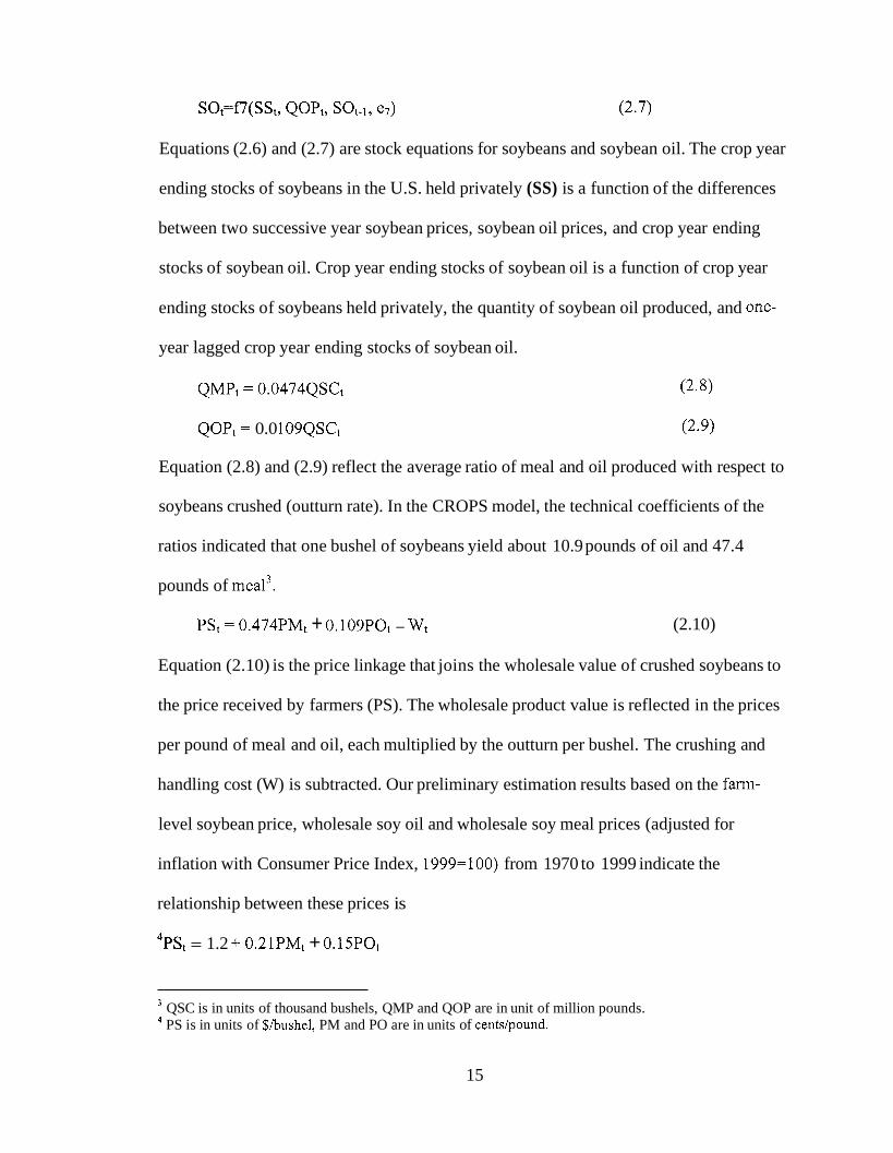
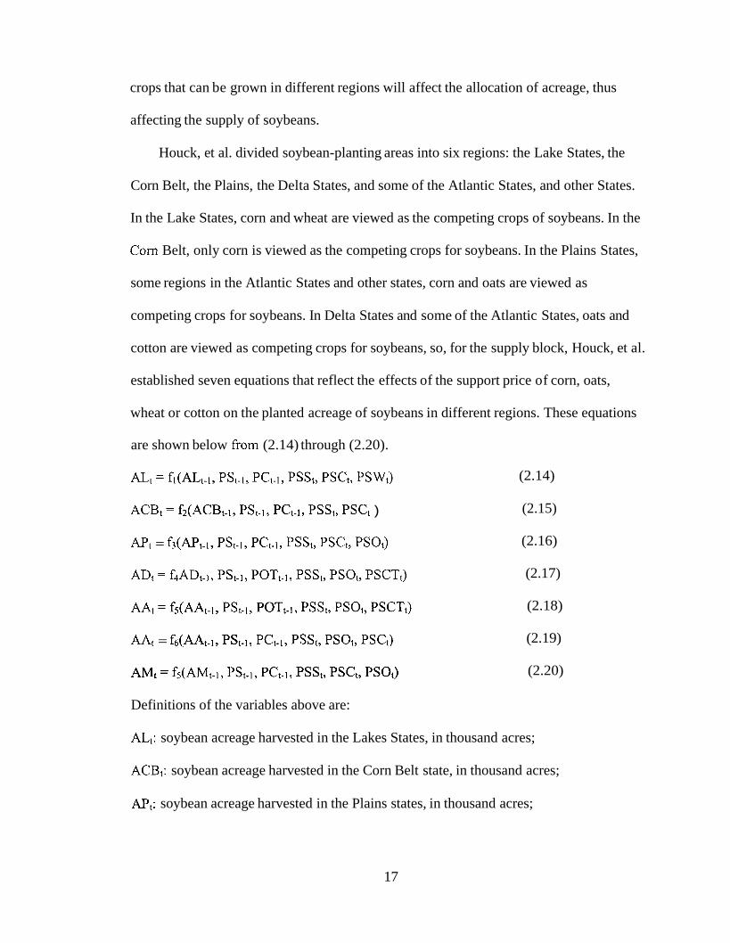
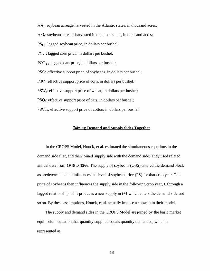
Fortunately, we find that the prices of Canola and soybeans move quite similarly. This is
displayed in Figure 1.1, Figure 1.2 and Figure 1.3.
1

Figure 1.1: U.S. Average Annual Farm Level Canola Seed Price and Soybean Price From 1991 to 1999
350
300
250
200
150
100
50
C
$/metric ton
U.S.Soybean Bean Price _ _ _ _ _ U.S.Canola Seed Price
1988 1989 1990 1991 1992 1993 1994 1995 1996 1997 1998 1999 2000
Year (Source: USDA Agricultural Statistics, various year) (Prices are adjusted with Consumer Price Index. 1999=100)
Figure 1.2: U.S. Average Annual Canola Oil Price and Soy Oil Price From 1989 to 1999
$/metric ton
"1
400 5m1 U.S. Soybean Oil Price
200
3001 . . _ I _ - U.S. Canola Oil Price
1988 1989 1993 1991 1992 1993 1994 1995 1596 1997 1998 1999 2000
(Source: USDA Agricultural Statistics, various years, prices are adjusted with Consumer Price Index. 1999=100) Year
2
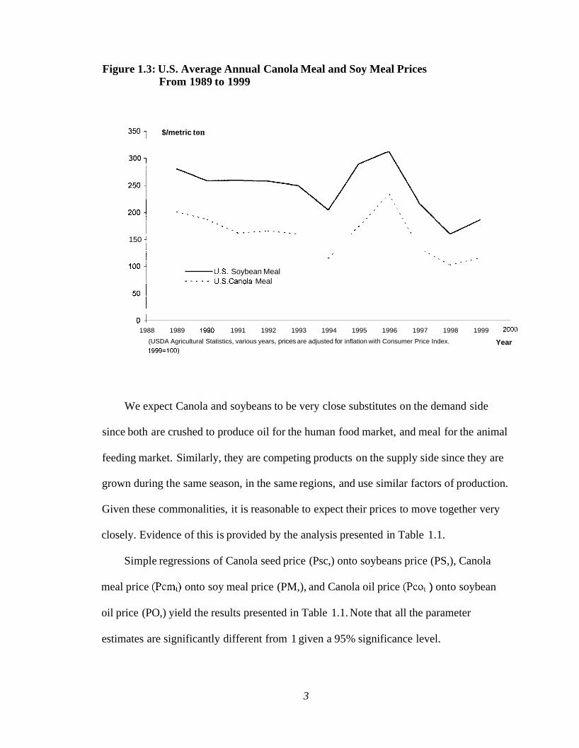
Figure 1.3: U.S. Average Annual Canola Meal and Soy Meal Prices From 1989 to 1999
350 1 $/metric ton
300 1
150 A j
US. Soybean Meal U.S.Canola Meal _ . _ . _
50 i 0 4 1988 1989 1990 1991 1992 1993 1994 1995 1996 1997 1998 1999 2000
(USDA Agricultural Statistics, various years, prices are adjusted for inflation with Consumer Price Index. 1999=100)
Year
We expect Canola and soybeans to be very close substitutes on the demand side
since both are crushed to produce oil for the human food market, and meal for the animal
feeding market. Similarly, they are competing products on the supply side since they are
grown during the same season, in the same regions, and use similar factors of production.
Given these commonalities, it is reasonable to expect their prices to move together very
closely. Evidence of this is provided by the analysis presented in Table 1.1.
Simple regressions of Canola seed price (Psc,) onto soybeans price (PS,), Canola
meal price (Pcm,) onto soy meal price (PM,), and Canola oil price (Pco, ) onto soybean
oil price (PO,) yield the results presented in Table 1.1. Note that all the parameter
estimates are significantly different from 1 given a 95% significance level.
3
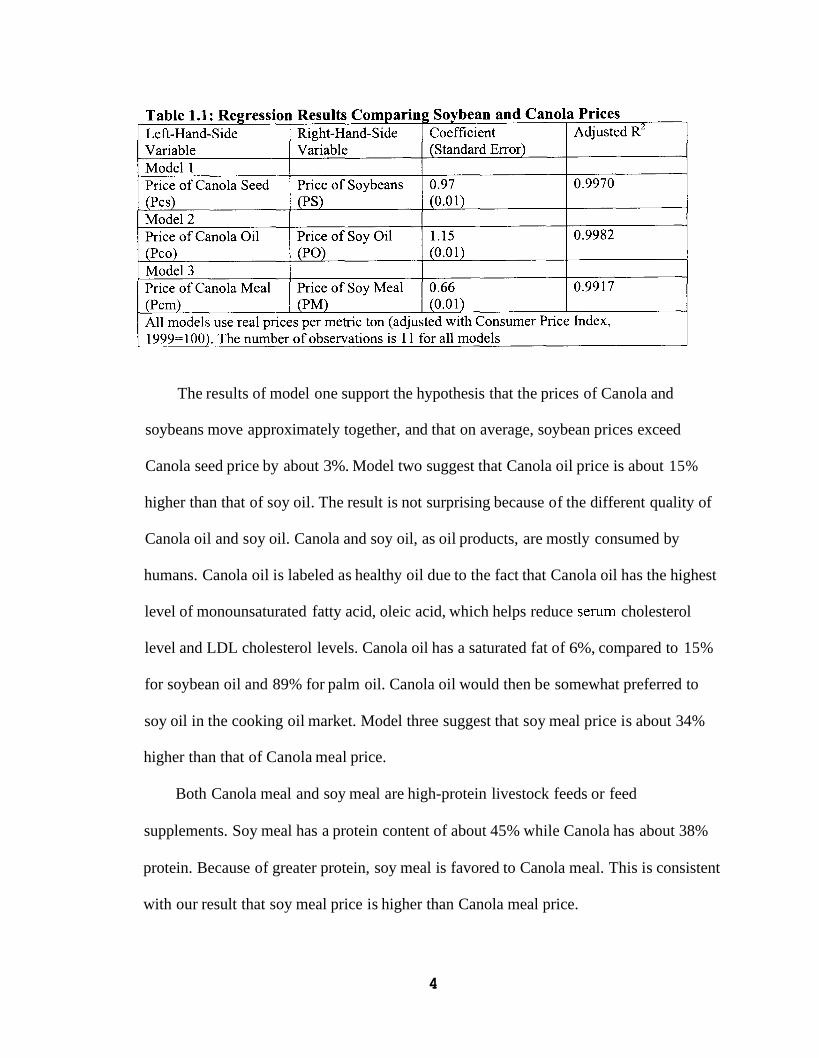
The results of model one support the hypothesis that the prices of Canola and
soybeans move approximately together, and that on average, soybean prices exceed
Canola seed price by about 3%. Model two suggest that Canola oil price is about 15%
higher than that of soy oil. The result is not surprising because of the different quality of
Canola oil and soy oil. Canola and soy oil, as oil products, are mostly consumed by
humans. Canola oil is labeled as healthy oil due to the fact that Canola oil has the highest
level of monounsaturated fatty acid, oleic acid, which helps reduce serum cholesterol
level and LDL cholesterol levels. Canola oil has a saturated fat of 6%, compared to 15%
for soybean oil and 89% for palm oil. Canola oil would then be somewhat preferred to
soy oil in the cooking oil market. Model three suggest that soy meal price is about 34%
higher than that of Canola meal price.
Both Canola meal and soy meal are high-protein livestock feeds or feed
supplements. Soy meal has a protein content of about 45% while Canola has about 38%
protein. Because of greater protein, soy meal is favored to Canola meal. This is consistent
with our result that soy meal price is higher than Canola meal price.
4
From the discussions above, we see that Canola and soybeans have similar
processing, end-use purposes, and are substitutable for each other in the oil and meal
markets. So it is likely that their prices are highly correlated. Thus we can understand
how one price moves by examining the other. In this way, we can transform our problem
of examining Canola price movements to examining soybean price movements. Because
data for U.S. Canola are from a very short time series, we will, in this thesis, concentrate
on the soy market. From the soy market we can reasonably infer the price movements of
Canola.
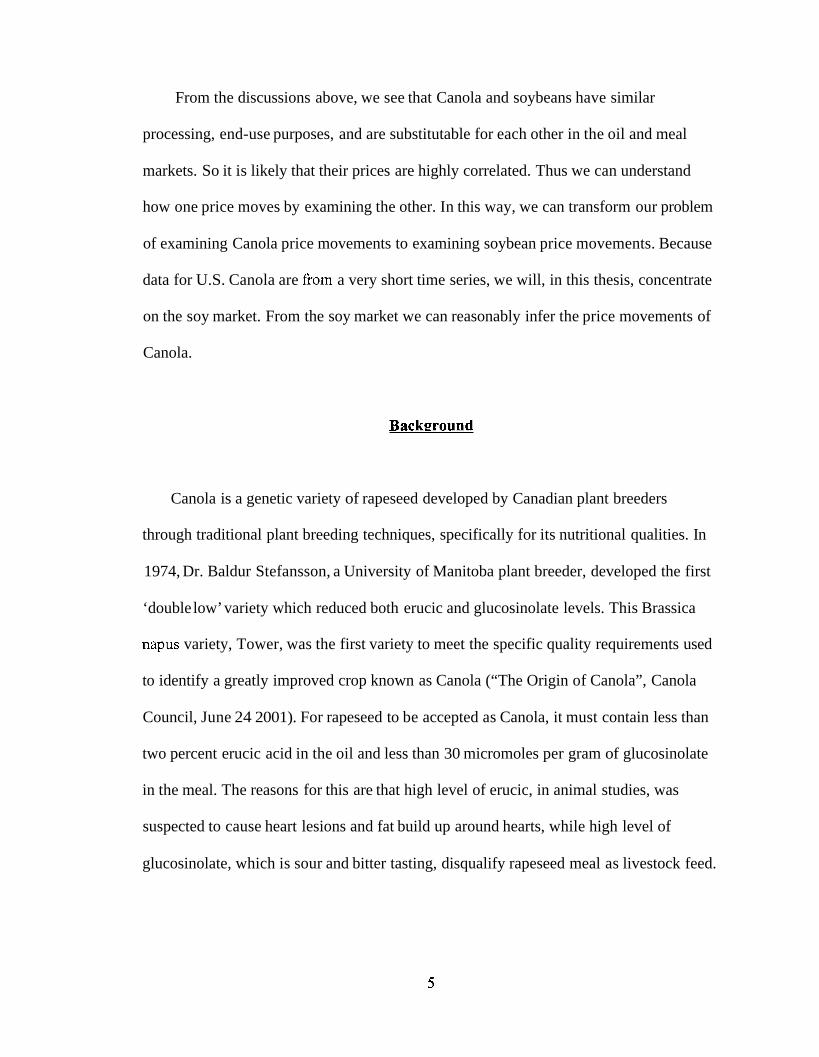
Backwound
Canola is a genetic variety of rapeseed developed by Canadian plant breeders
through traditional plant breeding techniques, specifically for its nutritional qualities. In
1974, Dr. Baldur Stefansson, a University of Manitoba plant breeder, developed the first
‘double low’ variety which reduced both erucic and glucosinolate levels. This Brassica
napus variety, Tower, was the first variety to meet the specific quality requirements used
to identify a greatly improved crop known as Canola (“The Origin of Canola”, Canola
Council, June 24 2001). For rapeseed to be accepted as Canola, it must contain less than
two percent erucic acid in the oil and less than 30 micromoles per gram of glucosinolate
in the meal. The reasons for this are that high level of erucic, in animal studies, was
suspected to cause heart lesions and fat build up around hearts, while high level of
glucosinolate, which is sour and bitter tasting, disqualify rapeseed meal as livestock feed.
5

The United States has relatively a short history of growing and consuming Canola.
But since the approval of Canola being used in edible products by the Food and Drug
Administration in 1985, domestic production has increased greatly. The implementation
of the 1990 Farm Bill also contributed to the increase of Canola growing (Lordkipanidze
et al. and Ames et al). Two aspects of its legislation: planting flexibility and oilseeds
marketing provisions encouraged farmers to expand acreage of Canola. In turn, the
production of Canola has increased tremendously. According to data from USDA, U.S.
Canola production increased by over 950% from 1991 to 2000. (See Figure 1.4)
Figure 1.4: U.S. Canola Production from 1991 to 2000
2000 4
i 1500 1 1 0 0 0 1
I 5 0 0 4
The soybean is often called the miracle crop. It is the world’s foremost provider of
protein and oil. Soybean cultivation was first recorded in 2828 B.C. in China (Jordan,
Houck, et al.). Soybeans and their products have been important sources of protein for
millions of Chinese and other Oriental people for nearly 5000 years.
6

The Soybean was first introduced into the United States in 1804 (Jordan et al.),
primarily for use as a forage crop. In 1921, the growing American soybean industry was
provided tariff protection. Since the 1950’s, the U.S. has become the world’s largest
soybean producer and exporter. Figure 1.5 shows the production and exports of U.S.
soybeans from 1970 to 1998.
Figure 1.5: U.S. Soybean Production and Exports from 1970 to 1998
180000
160000
140000
120000
100000
80000
60000
40000
20000
0
Million Pounds
Total Production
Total Exports _ _ - - -
_ I , - . - , ,.. . .
1965 1970 1975 1980 1985 1990 1995 2000
(Source: USDA Agricultural Statistics various years) Year
7

Summary
This chapter provides background information on Canola and soybean production in
the United States and stated our objective of studying Canola and soybeans prices.
Because the U.S. has relatively a short history of growing Canola, it is difficult to
perform a rigorous empirical analysis of Canola prices. Fortunately, we find that Canola
and soybean prices are highly correlated. By studying soybean prices, we can also learn
about Canola prices. Chapter Two provides a model of soybean prices, developed in the
1960’s. Chapter Three provides our updated model of these prices, based on the
information in Chapter Two.
8
Chapter 2
USDA CROPS MODEL FOR U.S. SOYBEAN MARKET
Preliminary empirical estimates based on pure time series analysis do not provide
insight into soybean future prices and cannot pick up the turning points of soybean prices
when used for forecasts, although the pure time series structure itself fits the data well
(See Appendix A). We will study soybean prices within economic structures. In this
Chapter, we first review the work of Houck, Ryan, and Subotnik in their study of a
simultaneous equations model for the U.S soybean market. Some criticisms to their
model will be raised, which make necessary significant modifications to the model.
Multi-equation econometric models have been used by a number of researchers to
analyze the structure and operation of the soybean market. These models have grown in
complexity, as their components have become more representative of the total soybean
market. The dynamic supply and demand model of the U.S. Soybean Market is one such
model. Houck, Ryan and Subotnik( 1971) presented a multi-equation model of soybean
prices that for the first time took both supply and demand into consideration. In their
study, the meshing of both supply and demand relationships is undertaken with special
attention to policy variables. Their work is frequently referred to as the USDA CROPS
Model (Jordan, et al.). The CROPS model is composed of two “blocks”, which are
constituted of the behavioral and technical relationships on the demand supply sides of
soybeans.
9

The Demand Side for Soybeans in the CROPS Model
Aggregated Demand for Soybeans in the U.S.
Meal and oil are joint products from the crushing of soybeans. The ratio of soy oil
and meal crushed from soybeans with respect to soybeans crushed is relatively fixed.
Thus meal and oil supplies are tightly linked to each other and to the quantities of
soybeans crushed.
Soybeans, meal and oil have multiple uses: domestic (crush), export, and inventory.
Thus, multiple-market outlets are available for all three products. The three are
interdependent with larger economic sectors. Once crushed, the meal and oil components
enter market channels that are essentially independent of each other. Each of these is part
of a complex economic sector in which competition and substitution among commodities
are important. Soy meal is one of several high-protein feed products for the livestock
sector. Soy oil is one of many edible vegetable oils in the fats and oils complex. Soybeans
are a specific oilseed in a worldwide network of competing oil-bearing products. Prices
and product flows of soybeans, meal and oil are determined simultaneously because of
the joint-product relationship.
It is indicated in the CROPS model that the total demand of soybeans at the farm
level is an aggregated demand of U.S crushing demand, export demand, and other
demands'. The U.S. soybean crushing demand is a summation of the total wholesale soy
meal and soy oil demand. The export soybean demand is reflected by foreign soybean
demand, soy oil demand and soy meal demand. The foreign soybean oil demand is
Other demands include government purchases of soybeans and demand for stocks of soybeans. I
10
expressed in two parts: P.L. 480 concessional sales and commercial exports through
normal trade channels.
Variable Definitions
Houck (et al.) formulated a thirteen-equation model for the demand side of
soybeans in the U.S. These equations ((2.1) through (2.13)) are shown below and
discussions of the variables chosen are also presented. Table 2.1 provides variable
definitions.
Simultaneous Equations for the Demand Side of Soybean Market
Each equation (From equation (2.1) to (2.13)) will be discussed in detail.
QMDt=fi(PMt, Qpt, LVt, QDPt, el) (2.1 1
Equation (3.1) is the domestic soy meal demand. Since the feed outlet overwhelmingly
dominates the U.S. soy meal market, the domestic soy meal demand is a total of several
derived demands that reflect the variables having a major impact on soybean-meal
demand originating in the feed-livestock sector. The quantity of soy meal demanded
(QMD) is expressed jointly in a function with the wholesale meal price (PM) and several
other predetermined variables. The quantity supplied of other high-protein feeds (QP) is
included to capture the substitution effects of other high protein feeds like cottonseed
meal, linseed meal, tankage, and meat scraps (Houck, et al.). The livestock production
units2 of hogs, cattle and poultry (LV) is included as these livestock are consumers of soy
meal. Their influence in this equation is analogous to the population effect in a primary
demand equation (Houck, et al.). The variable QOP represents the estimated percentage
of digestible protein in concentrate rations for livestock and poultry (QDP). QOP is an
A livestock production unit is approximately 1000 pounds of animal live weight. 2
11
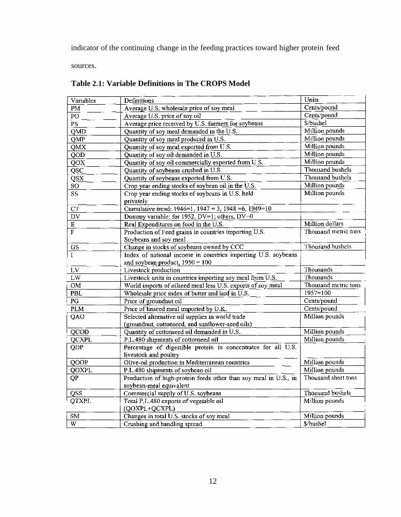
indicator of the continuing change in the feeding practices toward higher protein feed
sources.
Table 2.1: Variable Definitions in The CROPS Model
12
QODt=fi(POt, QCODt, PBLt, Et, e2) (2.2)
Equation (2.2) represents the domestic demand for soybean oil. This is also a
combination of several derived demand functions. The quantity of soybean oil demanded
(QOD) is expressed jointly in a function with the price of crude soy oil (PO) and several
other predetermined variables. The domestic utilization of cottonseed oil (QCOD) is
included to account for the substitution effects. A wholesale price index of butter and lard
in the U.S. (PBL ) (1957 is used as base year, 1957=100) is included to account for the
influence of animal fats and oils on soy oil demand (Houck, et al.). The total yearly-
deflated expenditure (E) on food in the U.S. is included to account for the changes in both
population and individual incomes (Houck, et al.).
QSXt=f3(PSPMt, LW/Ft, Tt, e3) (2.3)
Equation (2.3), the foreign demand for soybeans (QSX) faced by exporters is the sum of
the derived demands for soybean-using products by foreign buyers. The major source of
demand for soybeans in world markets is for crushing. As foreign buyers can substitute
bean purchases for purchases of soy meal and/or soy oil, the ratio of the price of soybeans
to the price of soy meal (PSPM) is included to capture this competitive effect (Houck, et
al.). The ratio of the livestock units on hand in the importing countries to the quantity of
feed grains produced in the importing countries (LW/F) is included to represent the effect
analogous to a per capita income effect in a primary demand function (Houck, et al.)(We
do not agree with this analogy). A time trend variable (T) is in the Model to capture the
changes in processing technology (Houck, et al.).
QOXt=f4(POPGty It, QTXPLt, Q O W , DVt, QAOt, e4) (2.4)
Equation (2.4) is the foreign demand for soybean oil. The quantity demanded for soybean
13

oil in the international markets (QOX) is a sum of derived demands for oil-using products
faced by foreign oil importers. As groundnut oil is a major competitor for soybean oil in
the international market, the price ratio of soybean oil to groundnut oil (POPG) is
included to capture this substitution effect (Houck, et al.). An index of personal income in
foreign importing nations (I) is included to capture the income change effects in the
soybean oil importing countries. QTXPL represented the quantity of concessional oil
exported through P.L. 480. It was hypothesized that some substitution would occur
through concessional export (Houck, et al.). Olive-oil production (QOOP) is included to
account the competing effects of olive oil from Mediterranean countries in world cooking
oil export market (Houck, et al.). Other oil supplies (QAO), groundnut, cottonseed and
sunflower-seed oils, are also included to represent substitutes for soy oil in the
international market (Houck, et al.). A dummy variable (DV) is included to account for a
special trade limitation imposed by the Spanish government in 1952 (Houck, et al.).
QMXt=f5(PM/PLMt, LW/Ft, OMt, CTt, es) (2.5)
Equation (2.5) represents the quantity of meal exports (QMX). The price ratio of soy
meal price to linseed meal price (PM, PLM) is to capture the substitutability between soy
meal and linseed meal in the international feed market (Houck, et al). LW/F is the ratio
of the livestock units in the importing countries to feed grains produced in these countries
(Houck, et al.). OM is the quantity of other oilseed meal imported by the importing
countries. It stands for the competing effects of other oilseed-meal imports. CT is a
cumulative trend that reflect changes in livestock-feed practices in the importing
countries (Houck, et al.).
SSt=f6(PSt - PSt-1, Pot - Pot-1, Sot, QSSt, e6) (2.6)
14
SOt=f7(SSt, QOPt, Sot-1, e7) (2.7)
Equations (2.6) and (2.7) are stock equations for soybeans and soybean oil. The crop year
ending stocks of soybeans in the U.S. held privately (SS) is a function of the differences
between two successive year soybean prices, soybean oil prices, and crop year ending
stocks of soybean oil. Crop year ending stocks of soybean oil is a function of crop year
ending stocks of soybeans held privately, the quantity of soybean oil produced, and one-
year lagged crop year ending stocks of soybean oil.
QMP, = 0.0474QSCt (2.8)
QOP, = 0.0 109QSCt (2.9)
Equation (2.8) and (2.9) reflect the average ratio of meal and oil produced with respect to
soybeans crushed (outturn rate). In the CROPS model, the technical coefficients of the
ratios indicated that one bushel of soybeans yield about 10.9 pounds of oil and 47.4
pounds of meal3.
PSt = 0.474PMt + 0.109POt - Wt (2.10)
Equation (2.10) is the price linkage that joins the wholesale value of crushed soybeans to
the price received by farmers (PS). The wholesale product value is reflected in the prices
per pound of meal and oil, each multiplied by the outturn per bushel. The crushing and
handling cost (W) is subtracted. Our preliminary estimation results based on the farm-
level soybean price, wholesale soy oil and wholesale soy meal prices (adjusted for
inflation with Consumer Price Index, 1999=100) from 1970 to 1999 indicate the
relationship between these prices is
4PSt = 1.2 + 0.21PMt + O.15POt
QSC is in units of thousand bushels, QMP and QOP are in unit of million pounds. PS is in units of $/bushel, PM and PO are in units of centslpound.
15

QSSt = QSCt +QSXt +SSt - SSt-1 +GSt (2.11)
QMPt = QMDt+QMXt+SMt (2.12)
QOPt = QODt + QOXt + Sot - Sot-, + QOXPLt
Equations (2.1 1) through (2.13) are the market equilibrium identities that ensure that
(2.13)
the total demand for beans, meal and oil in all outlets are equivalent to total supplies for
each crop year. According to the aggregated soybean demand framework, in equation
(2.1 1) the commercial supply of U.S. soybeans (QSS) equals the total of quantity of
soybeans crushed in the U.S. (QSC), quantity of soybeans exported as whole beans
(QSX), the difference of two successive crop years ending stocks of soybeans
(SSt - SSt-,) and the change in stocks of soybeans owned by the CCC (USDA
Commodity Credit Corporation) (Houck, et al.). In equation (2.12), the quantity of soy
meal produced in the U.S. equals the summation of quantity of soybean demanded,
quantity of soybean export and change in the total U.S. stocks of soy meal. In equation
(2.13), the quantity of soybean oil production is a summation of the quantity of domestic
soybean oil demanded, soybean oil exported, the differences between two successive
crop year ending stocks of soybean oil, and total P.L. 480 exports of vegetable oil.
The Supplv Side for Soybeans in the CROPS Model
On the supply side of soybeans in the U.S. market, the Model stressed particular
interest on the support prices and acreage restrictions for competing crops. Regional
supplies of soybeans are taken into consideration. Different effective support price for
16
crops that can be grown in different regions will affect the allocation of acreage, thus
affecting the supply of soybeans.
Houck, et al. divided soybean-planting areas into six regions: the Lake States, the
Corn Belt, the Plains, the Delta States, and some of the Atlantic States, and other States.
In the Lake States, corn and wheat are viewed as the competing crops of soybeans. In the
Corn Belt, only corn is viewed as the competing crops for soybeans. In the Plains States,
some regions in the Atlantic States and other states, corn and oats are viewed as
competing crops for soybeans. In Delta States and some of the Atlantic States, oats and
cotton are viewed as competing crops for soybeans, so, for the supply block, Houck, et al.
established seven equations that reflect the effects of the support price of corn, oats,
wheat or cotton on the planted acreage of soybeans in different regions. These equations
are shown below from (2.14) through (2.20).
ALt = fl(ALt-1, PSt-1, PCt-1, PSSt, PSCt, PSWt)
ACBt = fZ(ACBt-1, PSt-1, PCt-I, PSSt, PSCt )
A p t = f3(APt-,, PSt-1, PCt-1, PSSt, PSCt, PSOt)
ADt = f4ADt-1, PSt-1, POTt-1, PSSt, PSOt, PSCTt)
AAt = fs(AAt-1, PSt-1, POTt-I, PSSt, PSOt, PSCTt)
AAt = fs(AAt-1, PSt-1, PCt-1, PSSt, PSOt, PSCt)
(2.14)
(2.15)
(2.16)
(2.17)
(2.18)
(2.19)
= fs(Mt-1, PSt-1, PCt-1, Psst, PSCt, PSOt) (2.20)
Definitions of the variables above are:
ALt: soybean acreage harvested in the Lakes States, in thousand acres;
ACBt: soybean acreage harvested in the Corn Belt state, in thousand acres;
Apt: soybean acreage harvested in the Plains states, in thousand acres;
17
AA,: soybean acreage harvested in the Atlantic states, in thousand acres;
AMt: soybean acreage harvested in the other states, in thousand acres;
PSt-, : lagged soybean price, in dollars per bushel;
PCt-l : lagged corn price, in dollars per bushel;
POT t-l : lagged oats price, in dollars per bushel;
PSSt: effective support price of soybeans, in dollars per bushel;
PSCt: effective support price of corn, in dollars per bushel;
PSWt: effective support price of wheat, in dollars per bushel;
PSOt: effective support price of oats, in dollars per bushel;
PSCTt: effective support price of cotton, in dollars per bushel.
Joininp Demand and Supply - Sides Together
In the CROPS Model, Houck, et al. estimated the simultaneous equations in the
demand side first, and then joined supply side with the demand side. They used related
annual data from 1946 to 1966. The supply of soybeans (QSS) entered the demand block
as predetermined and influences the level of soybean price (PS) for that crop year. The
price of soybeans then influences the supply side in the following crop year, t, through a
lagged relationship. This produces a new supply in t+l which enters the demand side and
so on. By these assumptions, Houck, et al. actually impose a cobweb in their model.
The supply and demand sides in the CROPS Model are joined by the basic market
equilibrium equation that quantity supplied equals quantity demanded, which is
represented as:
18

(Yieldt)(At) = QOPt + QMPt + QSSt
where Yield is the average yield of soybeans, A is the aggregated acreage of soybeans
planted.
Before they studied the price movements by joining the supply and demand,
Houck, et al. ran the simultaneous equations for the demand side and equations for the
supply side of soybeans separately. For the demand side, the results showed that, except
for variables LV, E, QOCD, T, I, QTXPL, QOOP, QAO, OM, QSS, SS, QOP, and Sot-,,
other structural estimates are all statistical significant given a 5% level of significance.
For the supply side, only one-year lagged acreage in the six regions is not statistically
significant at a 5% level.
Houck, et al. then aggregated the supply side to a national level by summing the six
regional functions and rearrange the appropriate terms, and joined the supply side to the
demand side to study the price of soybeans.
Some Criticisms Regarding - the CROPS Model
Although the parameter estimates Houck, et al. obtained from the two-stage-least
squares estimate method fit the data they used well with high R squares, there are some
apparent problems with their model.
First of all, Houck, et al. did not include the supply side within the simultaneous
equation system. They only set up the simultaneous equations system to describe the
demand side of soybeans market, and obtained the parameter estimates without
considering the supply side of soybeans. According to microeconomic theory, since price
19

is the simultaneous result of supply and demand, it is more appropriate to study the
demand side together with the supply side.
Second, some of the variables in the CROPS model do not reflect standard
microeconomic theory. In the equation for soy meal demand (equation 2.1),
Houck, et al. used the quantity supplied of other high-protein feeds (QP) to account for
the substitution effects for soy meal in livestock feeds market. Generally, however, the
prices of substitutes, not the quantities, are included in demand equations to account for
substitution effects. The same criticism applies also to the quantity of other oil supplies
(QAO) in soy oil export demand equation (equation 2.4). As we have noted, that Houck,
et al. used price ratios like PSPM (soybean price with respect to soy meal price), PO/PG
(soy oil price with respect to groundnut price) to account for the substitution effects of
soy meal for soybeans, grountnut oil for soy oil, however, this is not a general practice in
microeconomic theory. Houck, et al. included the ratio of livestock units to the feeding
grains in the soybean importing countries (LW/F) in the equation of soybean export
demand (equation 2.3) as a variable analogous to the per capita income effect in a
primary demand function Houck, et al. However, this does not seem to be a reasonable
analogy. In the soy meal demand equation, the variable QOP (percentage of digestible
protein in the concentrate ratios for livestock and poultry) is included as an indicator of
the continuing change in the feeding practices toward higher protein feeds sources. This
variable makes sense, however, it is not a very good one. A time trend variable may
perform better to account for the development of higher quality livestock feeds.
Third, since the CROPS Model was established in the late 1960’s, the U.S. has
experienced great changes in its own market, consumption behavior, trade policies,
20
foreign business partners, and the world economic situation. Thus, some of the variables
used in CROPS Model may not be relevant or applicable for soybean study today. In the
demand equation of soy oil, Houck, et al. includes the price index of butter and lard to
account for an animal fats substitution effect for soy oil. However, during the last three
decades, the U.S. consumption pattern has been shifted away fi-om diets rich in animal fat
to more health diets of h i t s , cereal, vegetables and so on. Thus, the animal fat index may
not be an important variable for soybean studies today. The concessional oil exported
through P.L.4805 was an important variable during the time period when the CROPS
Model was established. However oil exported through P.L.480 is now so small a fraction
of soy oil exports that it can be safely ignored. Houck, et al. considered stocks in the
models for soybeans and soy oil. However, the USDA commodity policies regarding
inventories have been far less active than they were for the period of time when this
model was established (1 946 to 1966), and preliminary estimates suggest that changes in
stocks are effectively random. Thus it is reasonable to include stock changes merely as
data in market equilibrium equations.
Based on these criticisms, it is necessary to make modifications and establish a more
applicable model that adheres better to economic theory.
P.L. 480 (Public Law 480 is also known as Food for Peace Program. 5
21

Summarv
In this chapter, we have reviewed the USDA CROPS Model of the U.S. soybean
market developed by Houck, et al. Each equation and variable are discussed in great
detail. We then raised some criticisms regarding that model. Based on these criticisms, it
is necessary for us to make some reasonable modifications to develop our own model. In
the next chapter, such a model is established and each variable will be explained.
22

Chapter 3
EMPIRICAL MODEL AND DATA
In Chapter Two, we reviewed the CROPS model of the U.S. soybean market from
post-World I1 to the 1970's. This chapter will modify that model and develop the
empirical framework for our study describing the U.S. soybean markets of more recent
years. Some new variables are included.
The data used in this study are from USDA Agricultural Statistics (various years).
They are annual data that cover 29 years (1970 to 1998). All prices are adjusted for
inflation with the Consumer's Price Index (1999=100).
Reasons For UsinP - A Simultaneous Equation System
Four major ideas underpin the simultaneous equation system used for our model.
Meal and oil are joint products from the crushing of soybeans, thus meal and oil supplies
are tightly linked to each other and to the quantity of soybeans crushed in the United
States. Multiple-market outlets are available for all three products. These market channels
are essentially independent of each other. However, prices and product flows of
soybeans, meal and oil are determined simultaneously because of the joint-product
relationship. The market for soybeans is actually the aggregate of the three markets for
soybeans, soy meal and soy oil. These markets can also be grouped into domestic and the
international markets. Thus, in our analysis, we establish a simultaneous system of
23
equations to describe soybeans and its products market both in the U.S. and in the rest of
the world.
The Demand Side of Soybean Market
Soybean Market
Our preliminary estimates suggest that soybeans are crushed to about 49% soy meal
and 21% soy oil. U.S. domestic demand for soybeans primarily comes from the demand
for these products. We will not establish an equation specifically for the domestic
soybean market, since it is implicit in the oil and meal demands.
The major source of demand for soybeans in the world market is for crushing, thus
foreign buyers can buy soybeans or soy meal/oil. For the equation of the world demand
for soybeans, we include variables of soybean price and soy meal price to capture these
substitute effects. Another variable included is the South American export of soybeans.
South American soybean exports have been increasing steadily. Figure 3.1 shows the
increasing share of South American soybean exports in the international soybean export
market.
The increase of the South American soybean exports is expected to continue due to
the increasing production of soybeans in South American counties. Relatively high yield,
cheap labor cost and cheap land have been favorable to the soybeans production in the
South American countries since the 1970's (Frederick). Based on our analysis for soybean
export market, we establish an equation for soybean export demand equation, as shown in
equation (3.1)
24

Figure 3.1: South American Soybean Exports Share In the International Soybean Market (1995 to 1999)
Variables Unit N Mean Soybean Price (PS) $/bushel 29 10.65 Soy Meal Price (PM) Centslpound 29 16.17 South American Soybeans 000 metric tons 29 24464 Export (SX) Soybeans Exported (QSX) Million pounds 29 41 127
35.00%
30.00%
25.00%
20.00%
15.00%
10.00%
5.00%
0.00%
Std Dev 4.06 6.96 14825
9253
1995 1996 1997
Year
(Source: USDA Agricultural Statistics 1995 to 2000)
1998 1999 2000
where, QSX is the quantity of soybeans demanded by -Jreign buyers, PS is tile farm-
level soybean price, PM is the wholesale price of soy meal, and SX is the South
American soybean exports, t represents years from 1970 to 1998 (1 970=1). Table 3.1
provides the summary statistics for variables used in this equation.
25
Soy Meal Market
Variables Unit N Quantity of Meal Million pounds 29 Demanded (QMD) Price of Soy Meal (PM) Centdpound 29 Price of Corn Meal Centdpound 29 (PCOM) Livestock Units (AF) 000 animal units 29
Domestic demand for soy meal derives from the demand for livestock meat since
Mean Std Dev 25910 5967
16317 6.56 13.61 5332
66950 5959
livestock are the primarily consumers of soy meal. The number of livestock units4 in the
U.S. (AF) is therefore included as a population shifter. In the livestock feed market, soy
meal has some substitutes, for example corn meal, cottonseed meal, etc. We assume only
the corn meal to be the substitute for soy meal in this thesis, and use the price of corn
meal as an independent variable to capture substitution effects5. A time trend variable is
used to capture the effects of the development of higher quality of livestock feeds
livestock feeds market. Based on these assumptions, domestic demand for soy meal is
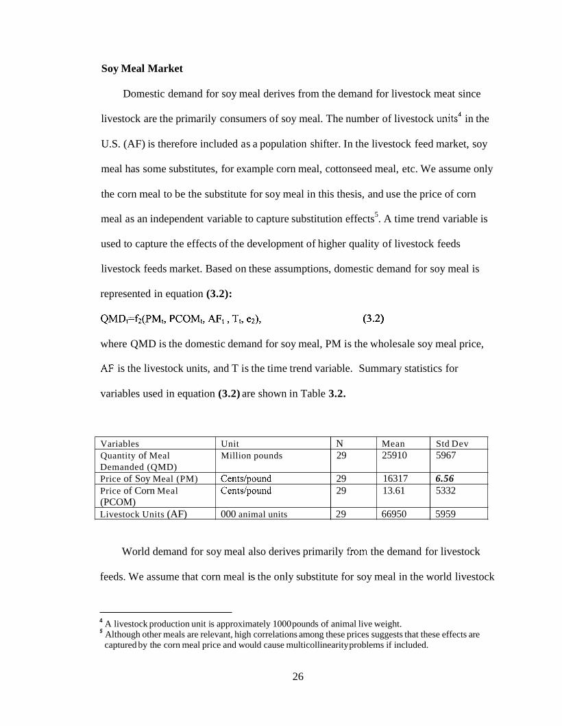
represented in equation (3.2):
(3.2)
where QMD is the domestic demand for soy meal, PM is the wholesale soy meal price,
AF is the livestock units, and T is the time trend variable. Summary statistics for
variables used in equation (3.2) are shown in Table 3.2.
World demand for soy meal also derives primarily from the demand for livestock
feeds. We assume that corn meal is the only substitute for soy meal in the world livestock
A livestock production unit is approximately 1000 pounds of animal live weight. Although other meals are relevant, high correlations among these prices suggests that these effects are captured by the corn meal price and would cause multicollinearity problems if included.
4
5
26

feed market (See Footnote 5). Prior to the 1 9 6 0 ’ ~ ~ some soybean importing counties
bought only meal. Since that time, most importers have begun crushing domestically,
thus, a time trend variable is used to account for these changes. The export demand for
soy meal is therefore represented in equation (3.3).
QMXt=f3(PMt, PCOMt, Tt, e3), (3.3)
where QMX is the quantity of soy meal demanded by foreign buyers, PM is the
wholesale soybean price, PCOM is the wholesale price of corn meal, T is the time trend
Variables Unit N Mean Export Demand for Soy Million pounds 29 601 1 Meal Demanded (QMX) Price of Soy Meal (PM) Centdpound 29 16.17 Price of Corn Meal Centdpound 29 13.61 (PCOM)
variable. Summary statistics for variables used in equation (3.3) are provided in Table
Std Dev 1181
6.56 5.32
3.3.
Table 3.3: Summary Statistics for Variables Used in the Equation of Soy Meal
(Source: USDA Agricultural Statistics, various years)
Soy Oil Market
In both the domestic and world markets, soy oil is used primarily as cooking oil.
Although soy oil also has nonfood uses, such as soap, paints, drying oils, and plastics,
these outlets are a very small share of the total soy oil market, thus, are not considered
here.
For the equation of domestic soy oil demand, we assume that corn oil6 is the only
substitute for soy oil, thus corn oil price is included to account for the substitution effect.
in the cooking oil market. A variable of the total annual real expenditures on food in the
Although other oils are relevant, high correlations among these prices suggests that these effects are 6
captured by the corn oil price and would cause multicollinearity problems if included.
27
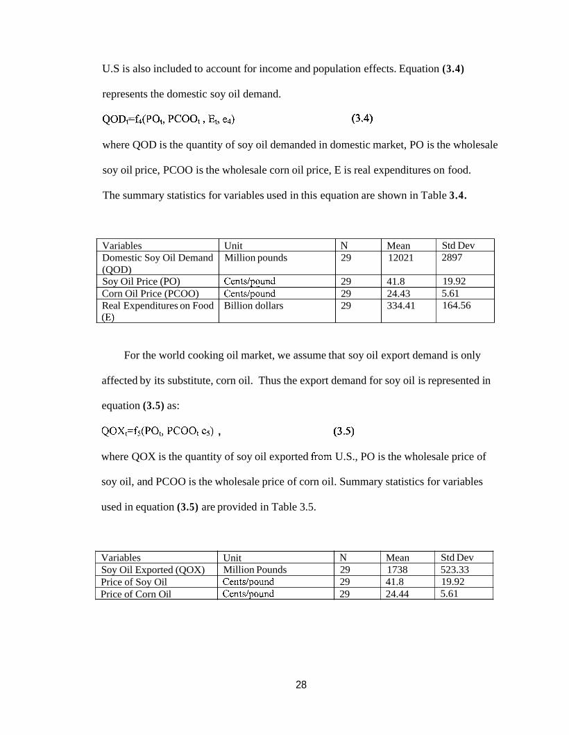
U.S is also included to account for income and population effects. Equation (3.4)
represents the domestic soy oil demand.
QODt=f4(POt, PCOOt, b, e4) (3.4)
where QOD is the quantity of soy oil demanded in domestic market, PO is the wholesale
Variables Unit N Mean Domestic Soy Oil Demand Million pounds 29 1202 1 (QOD) Soy Oil Price (PO) Centdpound 29 41.8 Corn Oil Price (PCOO) Centdpound 29 24.43 Real Expenditures on Food Billion dollars 29 334.41 (E)
soy oil price, PCOO is the wholesale corn oil price, E is real expenditures on food.
Std Dev 2897
19.92 5.61 164.56
The summary statistics for variables used in this equation are shown in Table 3.4.
Variables Unit N Mean Soy Oil Exported (QOX) Million Pounds 29 1738 Price of Soy Oil Centdpound 29 41.8 Price of Corn Oil Centdpound 29 24.44
Std Dev 523.33 19.92 5.61
For the world cooking oil market, we assume that soy oil export demand is only
affected by its substitute, corn oil. Thus the export demand for soy oil is represented in
equation (3.5) as:
QOX,=fS(PO,, PCOOt es) , (3.5)
where QOX is the quantity of soy oil exported from U.S., PO is the wholesale price of
soy oil, and PCOO is the wholesale price of corn oil. Summary statistics for variables
used in equation (3.5) are provided in Table 3.5.
28

Stock Demand
As we have mentioned in Chapter Two, in the CROPS Model, Houck, et al.
considered the demand for soybean, soy oil and soy meal stocks as endogenous variables.
However, the USDA commodity policies regarding inventories have been far less active
than they were for the period of time for which the CROPS Model was estimated (1 946
to 1966). Preliminary estimates suggested that changes in stocks are effectively random.
We therefore use stocks for soybeans, soy oil and soy meal merely as data in the
equilibrium equation.
The Supply Side of Soybeans
On the supply side of soybeans, we use an acreage response model, just as did
Houck, et al., but we make some changes to his original model. Since the implementation
of the 1990 Farm Bill, farmers have been granted planting flexibility so some variables in
his model are not as important as they were during the late 1960’s when Houck, et al.
established the CROPS Model. To begin, we first review some theories on product
supply and acreage response.
Product Supply and Acreage Response
The traditional production function can be derived from firm’s profit maximizing
rule. Assume that the firm’s economic profit is a function of output price, inputs and their
wages and other nonprice factors:
n= P*Q-(La*A+CLiXi ) ,
29
where P is the output price, A is the acreage, Xi is the ith input employed, La is the wage
for crop land, Li is the wage for the ith other input. By transforming the equation above,
we may represent Q as:
Q =&(A, X Z),
where Z is the vector of other factors.
We obtain the factor demand functions from the first order conditions of the profit
function and substitute it into the production function above and get the firm’s supply
function as follows:
Qs =f s (Pp C, z), where C represents a generalized vector of factor costs.
Farmers are faced with uncertainty regarding the quantities supplied (Qs in the above
equation). There are at least two sources of the uncertainty, the unpredictable variation of
yield and differences between planned and planted acreage. The yield is uncertain
because it is affected by weather and other uncontrollable factors, so it is hard for farmers
to adjust their production precisely. However, since they have more control over the
acreage than production, farmers usually can adjust their acreage allocated to a crop. In
this sense, acreage is a better index of the producers’ reactions to price changes than is
production. Thus acreage planted, rather than production, is often used to formulate the
farmer’s response in both theory and application. The acreage response model is:
A=L(P, c, Z),
Planted acreage is not a perfect proxy for production. Cassels describes two
problems with the approximation. First, the weather and other problems may cause
farmers to be unable to fully plant their planned acreage or to h l ly harvest planted
30

acreage. Second, the acreage gives no indication of the response that is made through
increased or decreased intensity of cultivation. Nerlove (1958) and later Behramn specify
two additional inadequacies of the approximation. First, the land is an heterogenous
factor. Each piece of land drawn into production of a particular crop or released from
production has either higher or lower fertility than the acres already in production or
remaining in production. Second, the land is only one of many inputs in agriculture. All
these inputs might not increase or decrease proportionately, thus the output per unit of
any one input changes. Nerlove and Behrman also compare the elasticity of planned
output and planned acreage to illustrate the discrepancy between planned output and
planned acreage. They find that relative magnitudes of these two elasticities are hard to
identify.
In spite of this imperfect approximation, the planted acreage may be the best
available indication of supply response because acreage changes are the primary means to
control production while yields may vary through changes in intensity or uncontrollable
factors. It is thus reasonable to focus on an acreage model of a crop supply, rather than
the more standard direct supply response.
Factors Relating to Acreage Response Model
In our model on the supply side of soybean beans, the acreage response model is a
function expressed in equation (3.6) as
At = f6 (At-1, PSt-1, COSTt, PWt-1, PCORNt.1, e6), (3.6)
where A is the acreage allocated to planting soybean, PS is the farm-level soybean price,
COST is the production cost, PW, and PCORN are farm-level prices of wheat and corn.
The subscript t represents time period t, and t-1 represents one-year lag.
31

One-year lagged acreage is included to account for the effects of asset fixity on
production. Farmers tend to establish a fixed ratio of equipment to acreage. As this
equipment is of low salvage value, it makes no sense for farmers to decrease acreage
often; on the other hand, when the equipment is used at capacity, one unit increase in
acreage will require large amount of increase in equipment. Thus asset fixity inhibits
increases in acreage also.
Cassels, in his supply response literature in 1933, concludes that the acreage
response to price approach based on the past experience with respect to prices is more
practical than other approaches. The output price of the current year is unknown to
farmers when they make their planting decisions. So farmers respond to price signals
other than current year’s actual observed price. For simplicity reasons, we assume that
farmers have nabe expectations for farm-level soybean prices.
Production Cost (COST) is another important factor in production. U.S. Department
of Agriculture estimates of variable costs of production for selected field crops are
considered the best available estimates for production costs for corn and soybean
(Shideed and White). The index of prices paid by fanners for production items, interest,
taxes, and wage rates was used to adjust the cost values for the study period in this study.
We assume that cost is known when the planting decisions are made.
Farm level expected prices for corn, and wheat are included here to capture the
competing crop effects. Opportunity cost is another important determinant in production.
Some previous studies included the prices of competing crops when they analyzed the
production. Love and Willette, for example, include competing crops in their model of
potato acreage response. In our model, we include corn and wheat as the competing crops
32

or joint crops with soybeans. The effects are reflected by the changes of acreages
Variable Cost
allocated to soybeans with respect to the changes of the price of corn and wheat. For
COST $/acre (adjusted by 29 3285 46 1 producer price index, 1990 -1992 =loo)
simplicity, we assume that farmers make acreage decisions based on last years’ corn and
Yield Farm-level soybean price Farm-level corn price Farm-level wheat price
wheat farm-level prices. Summary statistics of the variables we include in the acreage
Y Poundslacre 29 1893 PS $/bushel 29 11 PCORN $/bushel 29 3.38 PW $/bushel 29 4.76
response model are provided in Table 3.6.
Table 3.6: Summary Statistics for Variables Used in Acreage Response Equation (Equation 3.6)
I Variables I Unit I N I Mean I StdDev I
I ArrPnwe I A I Million acres I 2 9 159.10
I271 1 =-p---j 7.64
(Source: USDA Agricultural Statistics various years)
Technical and Physical Relationships
That, discussed above, forms the behavioral equations in our model of the soybean
demand side. These equations indicate the formal constraints on the variables we use in
the model. Besides these, we also must identify the technical and physical relationships to
ensure that market supply of soybeans equals market demand.
Price Linkage Equation
A price linkage equation between the fm-level price of soybean and wholesale
price and soy meal and soy oil takes the form of:
PSt=f(PMt, pot, e7), (3-7)
33
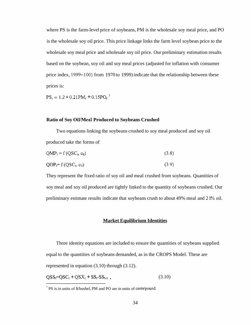
where PS is the farm-level price of soybeans, PM is the wholesale soy meal price, and PO
is the wholesale soy oil price. This price linkage links the farm level soybean price to the
wholesale soy meal price and wholesale soy oil price. Our preliminary estimation results
based on the soybean, soy oil and soy meal prices (adjusted for inflation with consumer
price index, 1999=100) from 1970 to 1999) indicate that the relationship between these
prices is:
PSt = 1.2 + 0.21PMt + O.15POt
Ratio of Soy OiYMeal Produced to Soybeans Crushed
Two equations linking the soybeans crushed to soy meal produced and soy oil
produced take the forms of
QMPt = f (QSCt, e8) (3.8)
QOPt= f (QSCt, e9) (3.9)
They represent the fixed ratio of soy oil and meal crushed from soybeans. Quantities of
soy meal and soy oil produced are tightly linked to the quantity of soybeans crushed. Our
preliminary estimate results indicate that soybeans crush to about 49% meal and 2 1 % oil.
Market Equilibrium Identities
Three identity equations are included to ensure the quantities of soybeans supplied
equal to the quantities of soybeans demanded, as in the CROPS Model. These are
represented in equation (3.10) through (3.12).
QSSt=QSC, + QSXt + SSt-SSt-1 , (3.10)
’ PS is in units of $/bushel, PM and PO are in units of centslpound.
34

QMPt=QMDt+QMXt+SMt-SMt-l , (3.1 1)
QOPt=QODt+QOXt+S Ot- S Ot- 1 , (3.12)
Equation (3.10) represents soybeans market equilibrium. On the left hand side, QSS is the
market supply of soybeans, which is expressed by
QSSt = (At)(Yieldt),
in which Yield is assumed to be constant and take value of the average yield of soybeans
in the U.S. from 1970 to 1998 (1891 pounds/acre)'. On the right-hand-side of equation
(3.1 l), QSC is quantity of soybeans crushed; QSX is the quantity of soybeans exported.
SS, -SSt-l represents the stock changes. Equation (3.12) represents the market
equilibrium for soy meal. On the left-hand-side of the equation, QMP is the quantity of
soy meal produced. It equals the sum of the quantity of meal domestically demanded
(QMD), quantity of meal exported (QMX), and the changes of soy meal stocks (SMt-
SM,-1). Equation (3.12) represents market equilibrium for soy oil. The quantity of soy oil
produced (QOP) is equal to total of the quantity of soy oil domestically demanded
(QMD), quantity of soy oil exported (QOX), and soy oil stock changes (SOt-SOt-I).
Summary statistics for the variables used in the identity equations are provided in Table
3.7.
Soybean yield in the U.S. has increase from 1970 to 1998. However, yields vary slightly since the 1990's, 8
thus, we will take the average of the yields from 1990 to 1998 as the constant (2204 poundacre).
35
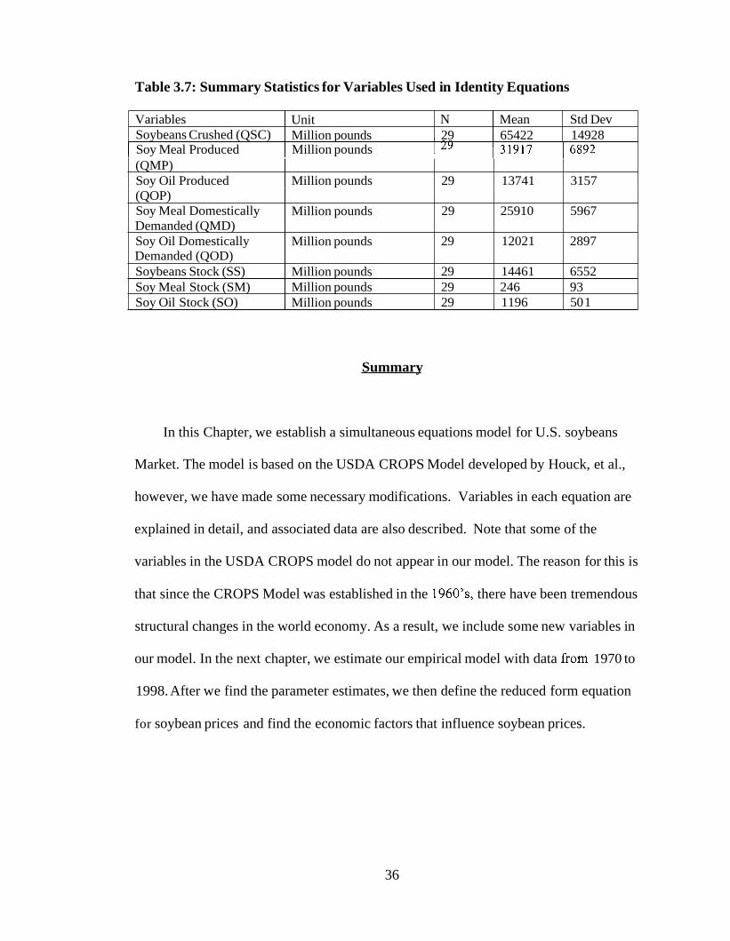
Table 3.7: Summary Statistics for Variables Used in Identity Equations
Variables Unit N Mean Soybeans Crushed (QSC) Million pounds 29 65422
Std Dev 14928 I Soy Meal Produced I Million pounds I 29 I31917 I6892
(QMP) Soy Oil Produced Million pounds 29 13741 3157 (QOP) Soy Meal Domestically Demanded (QMD) Soy Oil Domestically Demanded (QOD) Soybeans Stock (SS)
Soy Oil Stock (SO) Soy Meal Stock (SM)
Summary
Million pounds 29 25910 5967
Million pounds 29 12021 2897
Million pounds 29 14461 6552
Million pounds 29 1196 50 1 Million pounds 29 246 93
In this Chapter, we establish a simultaneous equations model for U.S. soybeans
Market. The model is based on the USDA CROPS Model developed by Houck, et al.,
however, we have made some necessary modifications. Variables in each equation are
explained in detail, and associated data are also described. Note that some of the
variables in the USDA CROPS model do not appear in our model. The reason for this is
that since the CROPS Model was established in the 1960’s, there have been tremendous
structural changes in the world economy. As a result, we include some new variables in
our model. In the next chapter, we estimate our empirical model with data from 1970 to
1998. After we find the parameter estimates, we then define the reduced form equation
for soybean prices and find the economic factors that influence soybean prices.
36

Chapter 4
EMPIRICAL RESULTS
In Chapter Three, a simultaneous equation model describing the U.S. soybean
market was developed and each explanatory variable was discussed in some detail. In
Chapter Four, we report the estimation results and discuss the reduced form estimates of
the model. Finally, these results are applied to the U.S. Canola market.
Statistical Methods And Estimation Results
In Chapter Three, we develop a simultaneous model for both demand and supply
sides of the soybean market. This simultaneous system is presented below, where
variables marked by * are exogenous variables.
QMDt=al l+a12PMt + a13PCOM*t + a ~ 4 F * ~ +alsTt* + el , (4-1)
QODt=a21 + a22POt +cc~~PCOO*~+ a24E*t + e2 , (4.2)
QSXt=a31 + a32PS+a33PMt + ~t34SX*~+ e3 , (4.3)
QMXt=a41 + a42PMt + CC~~PCOM*~+ a44Tt*+ e4, (4.4)
QOXt=a51 + as2PMt + a53PCOO*t+ a54T*t+ e5 , (4.5)
QMPF a61QsCt + e6 , (4-6)
QOPt = a71QSCt +e7, (4.7)
PSt=CY.sl +a82PMt+ag3POt +eg , (4.8)
QSStZQSCt + QSXt + SS*t-SS*t-l , (4.9)
QMPt=QMDt+QMXt+SM*t-SM*t-I , (4.10)
37

QOPt=QODt+QOX+SO * t- S 0" t- 1 , (4.1 1)
At= a91+a92A*t_l+a93PS*t_l+a94PCORN*t_l + a95PW*t-l+a96COST*t+e9 , (4.12)
QSSt=2204At , (4.13)
All error terms in the above equations are assumed to be normally distributed with zero
means and constant variances. Recall that endogenous variables in the system are
QMD (quantity of soy meal demanded in the domestic market), QOD (quantity of
soybean oil demanded in the domestic market), QSX (quantity of soybeans demanded by
foreign buyers), QMX (quantity of soy meal exported), QOX (quantity of soy oil
exported), QMP(quantity of meal produced), QOP(quantity of oil produced), PS (farm
level soybean price), PM (wholesale soy meal price), and PO (wholesale soy oil price),
and QSS (soybeans supply).
The exogenous variables are, AFt (animal units), T, (a time trend variable), PCOO,
(the price of corn oil), PCOMt (the price of corn meal), Et (real expenditures on food),
SX, (South American soybeans exports), SSt (soybean stocks), SMt (soy meal stocks),
and SOt (soy oil stocks), A,(soybean acreage), PCORNt (farm level price of corn), PW,
(farm level price of wheat), COSTt (Variable cost of growing soybeans), At-l(one-year
lagged acreage of soybeans) and Pt-l (one-year lagged farm-level soybean price).
As the simultaneous system is over-identified (See Appendix B), OLS estimates are
biased and inconsistent. They tend to overestimate the parameter estimates, but
underestimate the intercepts, however, by using two-stage-least squares method, we can
estimate parameters that are more likely to be consistent and efficient. A two-stage least
square method is used to estimate the coefficients in this simultaneous system (See
Appendix B).
38
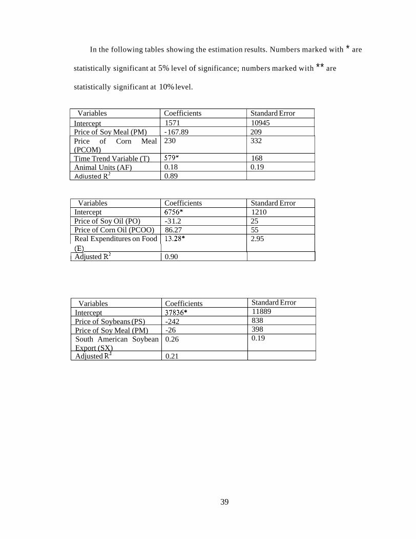
In the following tables showing the estimation results. Numbers marked with * are
statistically significant at 5% level of significance; numbers marked with ** are
statistically significant at 10% level.
Variables Coefficients Standard Error Intercept 1571 10945 Price of Soy Meal (PM) - 167.89 209 Price of Corn Meal (PCOM) Time Trend Variable (T) Animal Units (AF) Adiusted R2
230 332
579* 168 0.18 0.19 0.89
Variables Coefficients Standard Error Intercept 6756* 1210
Price of Corn Oil (PCOO) 86.27 55 Price of Soy Oil (PO) -3 1.2 25
Real Expenditures on Food 13.28* 2.95
I Adjusted R’ I 0.90
Variables Coefficients Intercept 37836* Price of Soybeans (PS) -242 Price of Soy Meal (PM) South American Soybean 0.26 Export (SX)
-26
Adjusted R2 0.21
Standard Error 11889 838 398 0.19
39

Variables Intercept Price of Soy Meal (PM) Price of Corn Meal (PCOM) Time Trend Variable (T) Adiusted R2
Coefficients Standard Error 2712 2006 -97.16 108.36 182.95 173.27
119.11* 50.1 0.29
Table 4.6: Parameter Estimates for Equation (4.6) - Soy Meal Produced (QMP)
Variables Coefficients Standard Error Intercept 998* 444
Adjusted R2 0.21
Price of Soy Oil (PO) -10.87* 5.05 Price of Corn Oil (PCOO) 47.9* 18.3
[ Variables 1 Coefficients I Standard Error Soy Meal Crushed Adjusted R2
Table 4.7: Parameter Estimates for Equation (4.7) - Soy Oil Produced (QOP)
0.49* 0.003 0.99
I Variables 1 Coefficients 1 Standard Error Soy Oil Crushed Adjusted R2
Table 4.8: Parameter Estimates for Equation (4.8) -Wholesale Soy Meal Price (PM) And Wholesale Soy Oil Price (PO) Regressed on Farm-level Soybean
0.21* 0.0016 0.99
Variables coefficients Intercept 1.2**
Standard Error 0.62
40
Price of Soy Meal (PM) Price of Soy Oil (PO) Adjusted R2
0.21* 0.046 0.15* 0.016 0.91

Table 4.9: Parameter Estimates for Equation (4.12)-Soybean Acreage
Variables Intercept
Coefficients Standard Error 84858* 12576
One-year lagged Acreage (At.1) One-year lagged Farm level price of soybeans (PSt-I) One-year Lagged Farm level price of wheat (PWt-1) One-year lagged Farm level price of corn (PCORN, 1)
Variable cost (COST) Adiusted R2
Results Discussion
0.24* 0.10
443.19* 162.14
1580.79* 487.86
-1 103* 763
-14.79* 2.47 0.90
Elasticity Analysis of Soybean Demand and Supply
The elasticities of soybean demand and supply are calculated at mean levels. The
general formula we use is
Exl,x2 = (&1/&2)(Mean of x2Mean of x l )
in which, the elasticity of x l with respect to x2 ( E , I , ~ ~ ) equals to the percentage changes
of x l with respect to x2 (&l/&2) times the ratio of the mean of x2 to the mean of x l .
Table 4.10 presents the elasticity of domestic soy oil demanded with respect to real
expenditures on food computed at mean level. One percentage increase in the real
expenditures on food (E) will increase the quantity of soy oil demanded by 0.36%. The
sign is of our expectation. Increases in expenditures on food are expected to increase the
quantities of soy oil demanded.
41
I Soy Oil Demand
Real Expenditures on I Food (E)
(QOD) 0.36
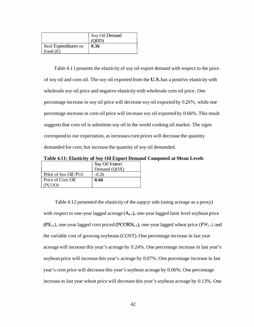
Table 4.1 1 presents the elasticity of soy oil export demand with respect to the price
Price of Corn Oil (PCOO)
of soy oil and corn oil. The soy oil exported from the U.S. has a positive elasticity with
0.66
wholesale soy oil price and negative elasticity with wholesale corn oil price. One
percentage increase in soy oil price will decrease soy oil exported by 0.26%’ while one
percentage increase in corn oil price will increase soy oil exported by 0.66%. This result
suggests that corn oil is substitute soy oil in the world cooking oil market. The signs
correspond to our expectation, as increases corn prices will decrease the quantity
demanded for corn, but increase the quantity of soy oil demanded.
Table 4.11: Elasticity of Soy Oil Export Demand Computed at Mean Levels 1 SOY Oil ~xp01-t I Demand (QOX) I -0.26 Price of Sov Oil (PO)
Table 4.12 presented the elasticity of the supply side (using acreage as a proxy)
with respect to one-year lagged acreage (At-l), one-year lagged farm level soybean price
(PSt-l), one-year lagged corn priced (PC0RNt-,), one-year lagged wheat price (PW,,) and
the variable cost of growing soybeans (COST). One percentage increase in last year
acreage will increase this year’s acreage by 0.24%. One percentage increase in last year’s
soybean price will increase this year’s acreage by 0.07%. One percentage increase in last
year’s corn price will decrease this year’s soybean acreage by 0.06%. One percentage
increase in last year wheat price will decrease this year’s soybean acreage by 0.13%. One
42
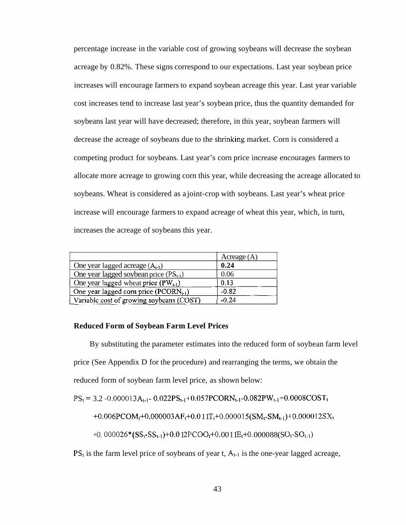
percentage increase in the variable cost of growing soybeans will decrease the soybean
acreage by 0.82%. These signs correspond to our expectations. Last year soybean price
Acreage (A) 0.24
One year lagged soybean price (PSJ 0.06 One year lagged acreage (At-])
increases will encourage farmers to expand soybean acreage this year. Last year variable
cost increases tend to increase last year’s soybean price, thus the quantity demanded for
soybeans last year will have decreased; therefore, in this year, soybean farmers will
decrease the acreage of soybeans due to the shnking market. Corn is considered a
competing product for soybeans. Last year’s corn price increase encourages farmers to
allocate more acreage to growing corn this year, while decreasing the acreage allocated to
soybeans. Wheat is considered as a joint-crop with soybeans. Last year’s wheat price
increase will encourage farmers to expand acreage of wheat this year, which, in turn,
increases the acreage of soybeans this year.
I One vear lawed wheat mice (PW,,)
Reduced Form of Soybean Farm Level Prices
By substituting the parameter estimates into the reduced form of soybean farm level
price (See Appendix D for the procedure) and rearranging the terms, we obtain the
reduced form of soybean farm level price, as shown below:
PSt = 3.2 -0.00001 3At-l- 0.022PSt~~+0.057PCORNt~~-0.082PW~~~+0.0008COST~
+0.006PCOM~+0.000003AF,+O.O 1 1 Tt+0.00001 S(SM~-SM~-I)+O.OOOO 12SXt
+O. 000026* (S St-S St- 1)+0.0 1 2PCOOt+O. 00 1 1 Et+O. 0000 8 8 (S Ot-S Ot- 1)
PSt is the farm level price of soybeans of year t, At-l is the one-year lagged acreage,
43
PSt-, is the one-year lagged farm-level soybean price, PCORNt-l is the one-year lagged
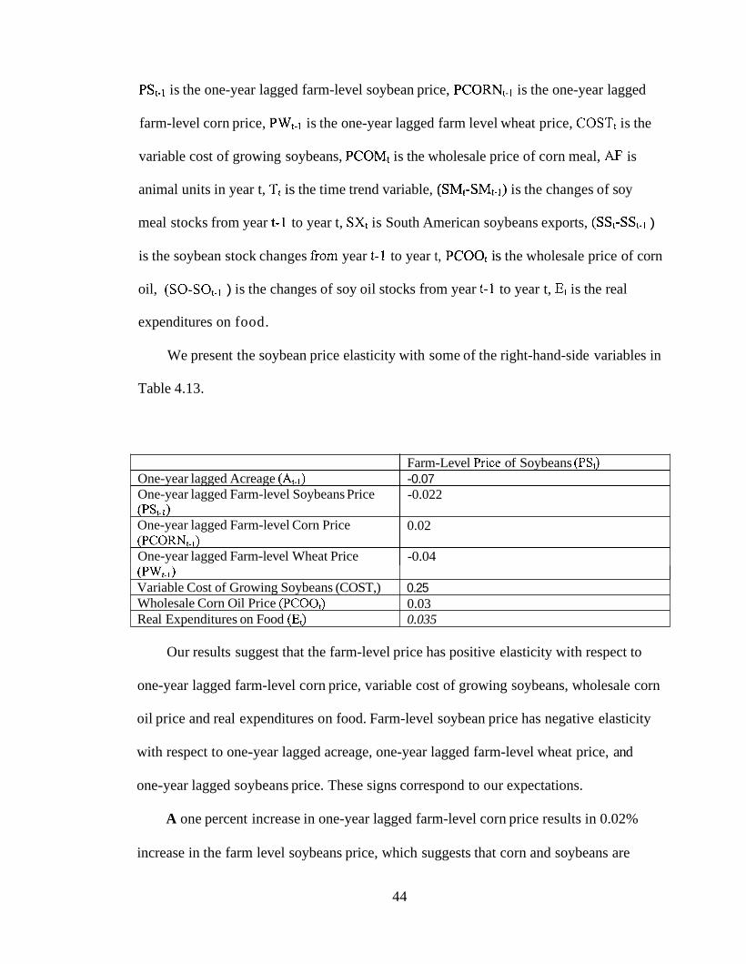
One-year lagged Acreage (At-,) One-year lagged Farm-level Soybeans Price (PSt-d One-year lagged Farm-level Corn Price (PCORN,,) One-year lagged Farm-level Wheat Price
farm-level corn price, PWt-l is the one-year lagged farm level wheat price, COSTt is the
Farm-Level Pnce of Soybeans (PS,)
-0.022
0.02
-0.04
-0.07
variable cost of growing soybeans, PCOMt is the wholesale price of corn meal, AF is
(PW, 1 ) Variable Cost of Growing Soybeans (COST,) Wholesale Corn Oil Price (PCOO,) Real Expenditures on Food (E,)
animal units in year t, Tt is the time trend variable, (SMt-SMt-l) is the changes of soy
0.25 0.03 0.035
meal stocks from year t-1 to year t, SXt is South American soybeans exports, (SSt-SSt.l )
is the soybean stock changes from year t-1 to year t, PCOOt is the wholesale price of corn
oil, (SO-SOt.l ) is the changes of soy oil stocks from year t-1 to year t, Et is the real
expenditures on food.
We present the soybean price elasticity with some of the right-hand-side variables in
Table 4.13.
Our results suggest that the farm-level price has positive elasticity with respect to
one-year lagged farm-level corn price, variable cost of growing soybeans, wholesale corn
oil price and real expenditures on food. Farm-level soybean price has negative elasticity
with respect to one-year lagged acreage, one-year lagged farm-level wheat price, and
one-year lagged soybeans price. These signs correspond to our expectations.
A one percent increase in one-year lagged farm-level corn price results in 0.02%
increase in the farm level soybeans price, which suggests that corn and soybeans are
44

competing crops. The increases in last year’s corn price will encourage farmers to
allocate more acreage to corn this year, while less for soybeans, thus the production of
soybeans of this year is expected to deceases which, in turn, decreases the quantities of
soybean supplied this year. The farm-level soybean prices of this year will increase as a
result.
A one percent increase in corn oil price increases the farm-level soybean price by
0.03%. As corn oil and soy oil are substitutes in the cooking oil market, increases in the
price of corn oil will decrease the quantities of corn oil demanded, but increase the
quantity of soy oil demanded, which in turn increases the soy oil price. As soy oil is a
joint product of soybeans and soybean farm-level price is positively related to soy oil
price, the soybean farm-level price will increase as a result.
A one percent increase in the variable cost of growing soybeans will increase
expected farm-level soybean price by 0.25%. Variable cost increases decreases the
soybeans supplied, which increases the soybean prices, assuming a finite negative
demand elasticity.
A one percent increase in real expenditures on food will increase the soybean farm-
level price by 0.035%. Increase in food expenditures increases the quantities of soy oil
demanded, which in turn increases the soy oil price. As the farm-level soybean price is
positively related to soy oil wholesale price, the soybean price is also driven up.
A one percent increase in acreage of soybeans of last year decreases the farm-level
soybean price this year by 0.07%. Increases in last year’s acreage increase the expected
quantity of soybeans supplied, which decreases the expected farm-level soybean price.
45
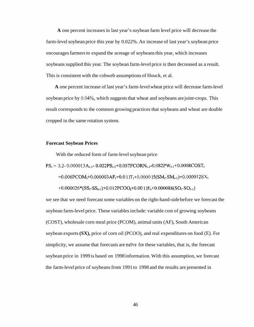
A one percent increases in last year’s soybean farm level price will decrease the
farm-level soybean price this year by 0.022%. An increase of last year’s soybean price
encourages farmers to expand the acreage of soybeans this year, which increases
soybeans supplied this year. The soybean farm-level price is then decreased as a result.
This is consistent with the cobweb assumptions of Houck, et al.
A one percent increase of last year’s farm-level wheat price will decrease farm-level
soybean price by 0.04%, which suggests that wheat and soybeans are joint-crops. This
result corresponds to the common growing practices that soybeans and wheat are double
cropped in the same rotation system.
Forecast Soybean Prices
With the reduced form of farm-level soybean price
PSt = 3.2- 0.000013At-1- 0.022PS~~~+0.057PCORNt~~-0.082PW~~~+0.0008COST~
+0.006PCOM~+O.000003AF~+0.0 1 1 Tt+0.0000 1 S(SM~-SM~_I)+O.OOOO 12SXt
+0.000026*(SSt-SSt.1)+0.0 12PCOOt+0.00 1 1 Et+0.000088(SOt-SOt-1)
we see that we need forecast some variables on the right-hand-side before we forecast the
soybean farm-level price. These variables include: variable cost of growing soybeans
(COST), wholesale corn meal price (PCOM), animal units (AF), South American
soybean exports (SX), price of corn oil (PCOO), and real expenditures on food (E). For
simplicity, we assume that forecasts are naWe for these variables, that is, the forecast
soybean price in 1999 is based on 1998 information. With this assumption, we forecast
the farm-level price of soybeans from 1991 to 1998 and the results are presented in
46

Figure 4.1. Note that both the observed and forecast prices are real prices adjusted for
inflation with CPI (1999=100).
Figure 4.1: Forecast Farm-Level Soybean Price From 1991 to 1998
6
forecast observed
1989 1990 1991 1992 1993 1994 1995 1996 1997 1998 1999 Year
(Source: USDA Agricultural Statistics, various years) (Prices are adjusted with CPI, 1999=100)
Applying the Forecast Results to Canola Prices
Recall in Chapter One, we found the relationsh,,, between Canola and soybean
prices as:
Psct=0.974PSt,
in which Psc is the Canola farm-level price and PS is the soybean farm-level price.
Nearly 99% of the variation in Canola farm-level price can be explained by the soybean
farm-level price; if we can explain how the soybean farm-level price moves, we can
47

explain how the Canola farm-level price moves. We can substitute the forecast result for
soybeans into the relationship between Canola and soybean prices; thus, each parameter
in the soybean price reduced form is proportioned by 0.974. Figure 4.2 presents the
Canola forecast price from 1991 to 1998. Observed Canola price of the same years are
also presented in the same figure. Note that prices here are real prices adjusted with CPI
(1999=100).
Figure 4.2: Forecast Canola Price from 1991 to 1998
n a 4 forecast
observed _ _ _ _ _
3 i
year 0 1 1989 1990 1991 1992 1993 1994 1995 1996 1997 1998 1999
(Source: USDA Agricultural Statistics, various years) (Prices are adjusted with CPI, 1999=100)
Our results suggest that the forecast results farm-level soybean price and Canola price
roughly captures the movements of the two prices.
48

Summary
In this chapter, we estimated a simultaneous system of soybeans using two-stage-
least-squares estimate method. We find some variables that significantly influence the
soybean market and the supply of soybeans. By substituting the parameter estimates into
the reduced form of farm-level soybean price, we are able to forecast soybeans price and
the Canola prices. Our forecast results suggest that with economic structure, we can
roughly capture the movements for soybean price from 199 1 to 1998.
49

Chapter 5
SUMMARY AND CONCLUSIONS
Summary
The focus of this study is to identify economic factors that influence soybean and
Canola prices. These results are expected to be used to answer whether it is feasible to
grow soybeans or Canola as rotation crops in a potato rotation system. Because the
United States has limited data on Canola, we attempt to characterize the determinants of
Canola prices by studying soybean prices. The reason for this is that Canola prices and
soybean prices are highly correlated. Through analysis, we find that Canola seed price is
about 97% soybean price; Canola oil price is about 1.15 times the soy oil price and
Canola meal price is about 66% soy meal price. We consider an economic structure to
study how the soybean prices are affected by economic factors.
Houck, Ryan, and Subotnik established a famous USDA CROPS Model for the U.S.
soybean and its products market in the late 1960’s. This model basically studies the
soybean market from the demand side. Market supply of soybeans is considered as an
exogenous variable. Houck, et al. imposed a cobweb model for soybeans prices in their
model. Primarily based on the CROPS Model, we made some necessary modifications
and established our own model for this thesis. In our model, the stock demands for
soybeans, soy meal and soy oil are considered constant due to the fact that the USDA
commodity policies regarding inventories have been far less active than they were for the
period of time when Houck, et al, established his model (1946 to 1966). Stock demand is
50

used in the identity equation to ensure that the supply of soybeans equals the demand. By
a two-stages-least-squares estimation method, we obtain the parameters for a reduced
form for soybean price. With these results and the former relationship between soybean
price and Canola price, we are able to explain how the canola price is affected by
economic factors and to forecast Canola price.
Conclusions
Several conclusions can be drawn from this study. First, soybean prices and Canola
prices are highly correlated and move closely. Second, we can use a simultaneous
equation system for studying the farm-level soybean prices. We find that soybean prices
are positively affected by: animal units (AF), wholesale corn oil price (PCOO), and real
expenditures on food (E), time trend variable (T), the variable cost of growing soybeans
and stock changes of soybeans, soybean oil and soy meal. Farm-level price of soybeans is
negatively affected by one-year lagged farm level soybean price, one-year lagged farm-
level wheat price and one-year lagged soybean acreage. Third, assume that the
relationship of these economic factors between soybean farm-level price also hold for
Canola, with the relationship of Canola and soybean price we obtained in Chapter One,
we can explain how Canola prices are affected by these same economic factors. Finally,
based on one-year lagged information of the economic variables on the right hand sides
of the reduced form we obtain for soybeans, we can forecast soybeans and Canola future
prices. Our forecast results suggest that with economic structure, we may roughly capture
the price movements of soybean price and Canola prices.
51
REFERENCES
Almon, S. “The Distributed Lag Between Capital Appropriations and Expectations.” Econometrica, 33 (1965):178 -196.
Ames, G.C.W., Shumaker, G.A. and Myneni, G. “Cross-Hedging as a Pricing Strategy for Alternative Crops: The Case of Southeastern Canola.” Journal of International Food and Agricultural Marketing. 4, 3 (1992): 25 - 43.
Arrow K.J. and Nerlove, M. “A Note on Expectations and Stability.” Econometrica. 26 (1956): 297 - 305.
Behrman, J.R. Supply Response in Underdeveloped Agriculture: A Case Study of Four Maior Annual Crops in Thailand. Amsterdam: North-holland Publishing Company. 1968.
Cagan, P. “The Monetary Dynamics of Hyper-Inflation.” in (ed.) M.Friedman, Studies in the Quality Theorv of Money. Chicago: University of Chicago Press. (1956): 25-1 17.
Cassels, J.M. “The Nature of Statistical Supply Curves.” Journal of Farm Economics 15( 1993): 378-387.
Cooperative Extension, University of Maine, Soybean Information Packet. Feb. 1998.
Enthoven, A.C. and Arrow, K.J. “A Theorem on Expectations and the Stability of Equilibrium.” Econometrica. 26 (1956): 288-293.
Frederick, R. “South American Competition Likely Here to Stay” Department of Agricultural Economics, University of Nebraska-Lincoln http://ianrhome. unl. edu/static/O 1 0503 0. shtml. (May 03, 200 1)
Goodwin, R.M. “Dynamical Coupling with Especial Reference to Markets Having Production Lags.” Econometrica. 1 5 (1 947): 18 1-204.
Griffiths, E. W, Hill, R.C, and Judge, G.G. Learning - and Practicing - Econometrics. New York. John Wiley & Sons. 1993.
Houck, J.P., Ryan, M.E. and Subotnik. A. Soybeans and Their Products: Markets, Models, and Policy. Minneapolis. University of Minnesota Press 1972.
52
Jordan, E.J., and Schupp, A.R. “An Econometric Analysis of the Soybean Market with Emphasis on Farm Level Price Prediction.” D.A.E. Research Report - Department of Agricultural Economics and Agribusiness, Louisiana State University, Louisiana Agricultural Experiment Station. Baton Rouge, La. : The Station August 1985.
Judge G. G., Carter, H.R., Griffiths, E. W., Helmut, L. and Lee, T.C. Introduction to the Theory and Practice of Econometrics. New York. John Wiley & Sons. 1982.
Metzler, L.A. “The Nature and Stability of Inventory Cycles.” Review of Economic Statistics. 23 (1941): 113-129.
Muth, J.F. “Rational Expectations and the Theory of Price Movements.” Econometrica 29 (1 96 1): 3 15-335.
Lordkipanidze N, Epperson J.E., Ames, G. C.W. “An Economic Analysis Of Import Demand for Canola Oil in the United States.” Journal of International Food and Agribusiness Marketing. 9(4) (1998): 23-34.
Nerlove, M. “Estimates of the Elasticities of Supply of Selected Agricultural Commodities.” Journal of Farm Economics. 38 (1956): 496-509.
Nerlove, M. The Dynamics of Supply: Estimation of Farmers’ Response to Price. Baltimore: The Johns Hopkins Press, 1958:
Nerlove, M. “The Dynamics of Supply: Retrospect and Prospect.” American Journal of Agricultural Economics 61 (1979): 874-888.
Pindyck, R.S. and Rubinfeld, D.L. Econometric Models and Economic Forecasts. New York: McGraw - Hill Company. 1976.
SAS Institute Inc. SAS/ETS: User’s Guide. Version 8.1. 1999-2000.
Shideed, K.H. and White, F.C. “Alternative Forms of Price Expectations in Supply Analysis for U.S. Corn and Soybean Acreages.” Western Journal of Agricultural Economics. 14 (1989): 281-292.
USDA. Agricultural - Statistics. 1960 to 1990
“The Origin of Canola.” www.canola-counci1.org. (June 24,2001)
Wallis, K.F., “Multiple Time Series Analysis and the Final Form of Econometric Models.” Econometrica. 45 (1977): 1481-1497.
53

APPENDICES
54

Appendix A
FORMULATION OF DISTRIBUTED LAG MODELS
In this Appendix, we first review some of the expectation theories. We then use
Polynomial distributed lag structures to study the soybean price movements. We will
present the results of forecasting annual soybean prices from 1970 to 1998 by using
second degree, 4-year lag polynomial distributed lag structures.
Expectation Theories
Extrapolative Expectations
In 1941, Metzler presented a model using a coefficient of expectation, as an
alternative to a naive expectation model. His model later was used by Goodwin (1 947)
and subsequently analyzed by Enthoven and Arrow (1956). Their work developed the
theory of extrapolative expectation, for which they defined the expected price as
i j *=p,-1+ ?7Pl-I-Pt-2),
where I; * is the expected price for period t at period t- 1, Pt-l the observed price in period
t-1 , Pt-z the observed price in period t-2, and q Metzler’s coefficient of expectation.
The purpose of the extrapolative expectations model is to modify the cobweb theory
to take into account the most recent trends in prices. Metzler compares his coefficient of
expectation to Hick’s elasticity of expectation and concludes that his coefficient of
expectation plus one is exactly Hick’s elasticity. However, this comparison lacks
theoretical appeal.
55

Adaptive Expectations
Based on Hicks’ definition of elasticity of expectation, the adaptive expectations
models first appear in Cagan (1956). Under the adaptive expectations hypothesis, the
individuals are assumed to revise their expectations according to their most recent
experience :
P*-P( t-1 )*=P(Pt-l -P*(t-I ,).
where P* is the expected price for period t at period t-1, P*t-l the expected price for
period t-1 at period t-2, , Pt-l the observed price in period t-1 and p the coefficient of
expectation and O<P<l. Rearrange the terms of both sides and we can get:
Pt*-( 1 -P)P,-, *=PPt_1.
Replacing (1 -p) by h and introducing the lag operator V so that VJxt = Xt-j, we obtain
(1 -hV)P,*=( 1 -h)Pt-l, so that
Pt* =[(l-h)/((l-hV)]P,+
So long as -l<h<l, we can expand l/((l-hV) as l+hV+h2V2+. . . and thus express Pt* as
Pt* = (l-h)ChkPt-l-k , where k>=O.
By transformation, the expected price in adaptive expectation can be expressed by
an infinite weighted average of past-realized prices with weights that decline
geometrically with the lag.
Nerlove (1958) developed the idea of an expected price using the adaptive
expectations model. Adaptive expectations have been popular for their simplicity since
maximum-likelihood estimates for h can be obtained easily and because such models
appear to work well in a number of empirical studies.
56
Although adaptive expectation is widely used, there are still several unsolved
problems that make the concept questionable. The first problem is that there is no real
theoretical justification for the model. Besides, much of the criticism of the adaptive
expectation theory has to do with its implication of a geometrically decaying lag
structure.
Muth’s Rational Expectations
As we have indicated above that the extrapolative expectations and adaptive
expectations models lack theoretical justification. Muth developed an expectations model
that eliminates the theoretical weakness common to the previous theories of expectation
formation.
Muth’s theory is based on three hypotheses about individual behavior:
“1). Information is scarce, and the economic system generally does not waste it. 2). The way expectations are formed depends specially on the structure of the relevant system describing the economy. 3) A ‘public prediction,’ in the sense of Grunberg and Modigliani.. ., will have no substantial effect on the operation of the economic system (unless it is based on inside information)” (Muth, p.3 16)
Muth’s theory implies that expectations are based on information, which is assumed
to be costless to obtain and to be generated according to perceptible forces. For example,
if a producer operating under free competition has some idea of market conditions, he
will use the information available to him about demand and supply conditions in
generating his expectations about the relevant variables for decision purposes.
By applying his theory to price expectations, Muth introduced three simplifying
assumptions: random disturbances are normal; certainty equivalents exist for the variable
57
to be predicted; and the equations of the system, including the expectation formulas are
linear. He assumed that the market equations take the form
PDt= -ppt (1)
PSt-=ypte + et (2)
PDt=PSt (3)
Where PS, represents the number of units produced in a period lasting as long as the
production lag, pt is the market price in the tth period, p t is the market price expected to
prevail during the tth period on the basis of information available through the (t-1)’s t
period, ef is an error term which represents all kinds of undetermined variations in yields.
By solving the equilibrium of supply and demand, Muth generated the relationship
between pt, market price in the tth period and p: , the market price expected to prevail
during the tth period on the basis of information available through the (t-1)’s t period, in
the form o f :
Pt = (-y/P)pte-(l/P)et.
The error term is unknown at the time the production decisions are made, but it is known
at the time the commodity is purchased in the market. The prediction of the model is
found by replacing the error term by its expected value, conditional on past events.
Assume there is no serial correlation among errors, we have the expected value of the
error term, E(et)=O and we can obtain the expected value of price in the tth period
E@J= (-y/P)pt“.
This result is of great importance because if the predictions of the theory were
substantially better than the expectations of the firms, then there would be opportunities
for the “insider” to profit from the knowledge, by possible inventory speculation, or by
58
selling a price forecasting service to the firms. The profit opportunities would no longer
exist if the aggregate expectation of the firms is the same as the prediction of the theory,
which is:
E@d= E(Pte).
From an economic view of point, Muth’s rational expectations, compared with other
expectation theories, are more consistent with the underlying structure of economic
behavior, while alternative models of expectations (cobweb, extrapolative, and adaptive)
are not necessarily compatible with the economic behavior implied by the underlying
economic structure. If forecast efficiency is the criterion, rational expectations are always
empirically better than any other expectation theories (Wallis). Rational expectations are
attractive in that economic behavior is directly incorporated in their definition, and it is
that makes expectations depend on the parameters of the model itself.
Theoretically satisfactory as it is, rational expectations also present problems in use.
From the technical viewpoint, rational expectations are more difficult to estimate than
other alternatives. To obtain rational expectations in our model, it must be solved for the
expected values of the uncertain variables. Although this solution is linear in the
exogenous variables, the coefficients are combinations of the structural parameters that
are generally not linear. The identification problem is also associated with rational
expectations and poses a difficulty for using rational expectations models. A third
possible problem with rational expectations is the evidence of serial correlation in the
structural disturbance. Imposing the assumption that random disturbances are not enough
to simplify estimation. If there is serial correlation, then the estimate of the error term (e)
is not rational.
59
Almon Polynomial Distributed Lag
Due to the difficulty of estimation or identification of the expectation theories we
discussed above, we will focus on polynomial distributed lags in this part and investigate
its significance to our study.
Almon used nonsample information about the distributed lag weights to improve the
precision of estimation. In her study of the relationship between capital appropriation and
capital expenditures, Almon assumed that a smooth pattern of lag weights could be
approximated by a polynomial of relatively low order. Her insight indicates that the lag
weights don’t necessarily decline geometrically with time, but can be specified by a
continuous function.
The general polynomial structure can be expressed as
Yt =a+p(wlXt-1+w2Xt-2+. . .wtXt-,,)+Et ,
where, w represents polynomial distributed lags weights in the fhction of the lag index-
variable u,
t = n.. ... T
w, = 1I-J +hlU+h2U2+h3U3+. . .hqUq ,
in which, u is the lag index (eg. 1 lag, u=O, 2 lags, u=l), q is the degree of polynomial.
The error term Et is assumed to be normal distributed with zero means.
Assume a second degree polynomial (q=2) distributed lag structure. The weight is
then represented as:
w, = ho +h1u+h2u2 U=O, 1,2, . . ., n
We have considerable flexibility involved in specifying a polynomial distributed lag
model. Usually a third-degree or a fourth degree polynomial will provide a sufficiently
accurate approximation to the lag structure. Almon assumed that a second-degree
60
polynomial distributed lag can sufficiently approximate the lag structure in her study of
capital appropriations. The choice of length of lag depends more on the nature of the
problem being specified, so that useful rules of thumb are not available. (Pindyck, 2 1 1)
A polynomial distributed lag provides a more flexible lag structure. And the
decision regarding the lag length is a subjective decision’. We can choose appropriate
order and lags for the convenience of estimation. So it is a feasible model for our
empirical study in this thesis.
A Pure Time Series Analysis of Soybean Prices
We assume that a second degree, four-year lag polynomial distributed lag structure
sufficiently approximates the lag structures for studying soybean prices. In the
polynomial distributed lag structure in our study, we will define the weights as
wt=ho+hl t+h2t2, (t=O, 1,2,3), in which
t is the lag index (eg. 1 lag, t=O, 2 lags, t=1) and w is the weight.
The soybean prices can be expressed as
PSt=al+PI 1 ho3PSt-1 +P2l(ho3+hl3+h23)PSt-2
+P31(h03+2h13+4h23)PS~-3+P41(h03+3h13+9h23) PSt-4+el
PMt=a2+P 12h02PMt-1 +P22(h02+h12+h22)PMt-2
+P32(ho2+2h12+4h22)PMt-3+P42(h02+3h12+9h22) PMt-4+e2
pOt=a3+P 13blPOt-1 +P23(h01 +A1 1 +h21)POt-2
+P33(h01+2h11+4h21)PO~-3+P43(h01+3hl l+gh21) POt-4+e3
An F-test can be employed to test the length of lags (Judge et al. 1982) 9
61
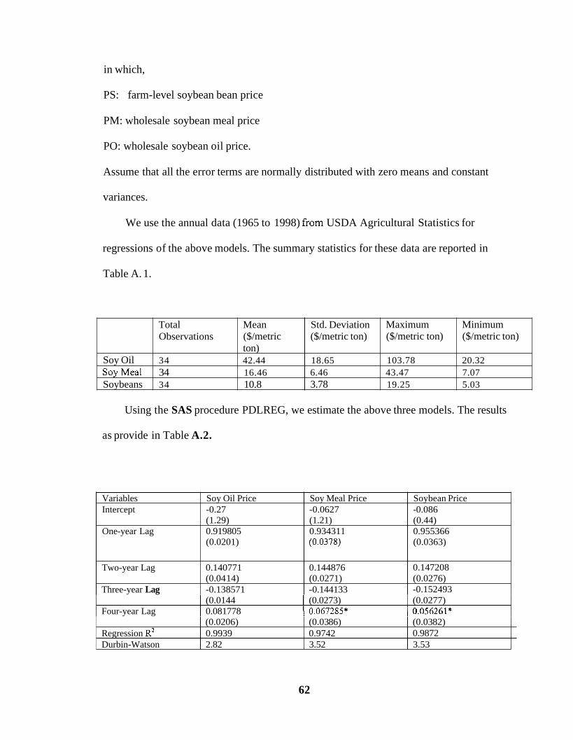
in which,
Soy Oil SoyMeal Soybeans
PS: farm-level soybean bean price
Total Mean Std. Deviation Maximum Minimum Observations ($/metric ($/metric ton) ($/metric ton) ($/metric ton)
34 42.44 18.65 103.78 20.32 34 16.46 6.46 43.47 7.07 34 10.8 3.78 19.25 5.03
ton)
PM: wholesale soybean meal price
Variables Soy Oil Price Soy Meal Price Intercept -0.27 -0.0627
(1.29) (1.21) One-year Lag 0.919805 0.9343 1 1
(0.0201) (0.0378)
Two-year Lag 0.140771 0.144876 (0.04 14) (0.0271)
Three-year Lag -0.138571 -0.144133
PO: wholesale soybean oil price.
Soybean Price
(0.44) 0.955366 (0.0363)
0.147208 (0.0276)
-0.086
-0.152493
Assume that all the error terms are normally distributed with zero means and constant
Regression R2 Durbin-Watson
variances.
(0.0206) (0.03 8 6) (0.03 82) 0.9939 0.9742 2.82 3.52 3.53
0.9872
We use the annual data (1965 to 1998) from USDA Agricultural Statistics for
regressions of the above models. The summary statistics for these data are reported in
Table A. 1.
Using the SAS procedure PDLREG, we estimate the above three models. The results
as provide in Table A.2.
I (0.0144 I (0.0273) I (0.0277) Four-year Lag 1 0.081778 I 0.067285* 10.056261*
62

Given a 5% level, all parameter estimates are significant except for four-year lag
terms for soy meal and soybeans. Also, Durbin-Watson values indicate that
autocorrelation does not seem to be a problem for these estimators. As all of the
regression R2’s are as high 99%, we can say that nearly all of the variation of the left-
hand-side variables is explained by the variations in the right-hand-side variables.
From the above estimation results, we can weigh the soybean prices on their four-
year lag prices as shown below.
Pot= -0.27+0.9198PO~~~+O.1408POt-~ - 0. 1386POt-3 + 0.082POt4
PMt= -0.0627+PMt-,+0.1449PMt-2 - 0.1441PM,-3 + 0.0673PMt-4
PS,=-0.086+0.9554PSt-1+0.1472PSt-2 - 0.1525PSt-3 + 0.056PSt-4
(A. 1)
(A.2)
(A.3)
Note that the forecast procedure and results are similar for the three prices, we will only
present soybean price analysis in this appendix.
Based on the estimation results, we use equation (A.3) to forecast soybean prices
from 1990 to 1998. The forecast results indicate only slight variations and provides little
insight into future price. Figure A. 1 presented the forecasting results for farm-level
soybean bean prices.
Since forecast results indicated that pure time series analysis doesn’t capture the
structure of movements of soybean prices. It is necessary to consider an economic
structure to study the economic factors that influence the soybean prices.
63
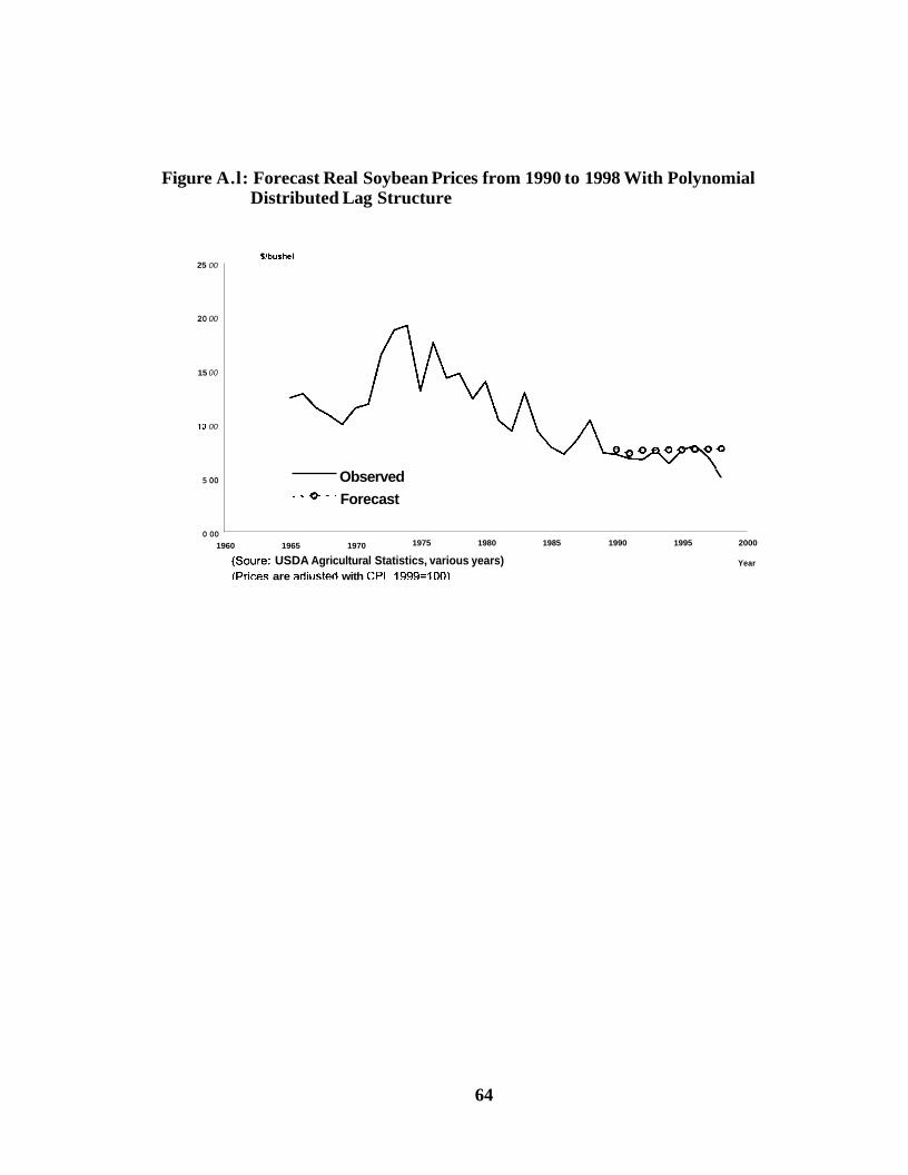
Figure A.l: Forecast Real Soybean Prices from 1990 to 1998 With Polynomial Distributed Lag Structure
Shushel 25 00
20 00
15 00
10 00
5 00
0 00
Observed - - - ’ Forecast
\
1975 1980 1985 1990 1995 2000 1960 1965 1970
(Soure: USDA Agricultural Statistics, various years) IPrirss are adiusted with CPI 1999=100\
Year
64

Appendix B
Identification in Simultaneous System and Two-Stage Least Square Estimates
Counting Rules and Rank Rules
Counting rules (Order rules) state that in the tth equation of a simultaneous system,
if the sum of the number of endogenous variables in this equation and the number of
exogenous variables is less than the total number of exogenous variables in the whole
system plus 1, the equation is over-identified; if it equals to the total number of
exogenous variables plus 1, the equation is just identified; if it is larger than the total
number of exogenous variables plus 1, the equation is under-identified (Griffiths, et al.).
Recall that the simultaneous equation system in our model is:
QMDt=a~l+a12PMt +a13PCOMt +al4AFt +al5T + a16e1 ,
QODt=a21 + a22POt +a23PCOOt+ ~~24Et + ~ 2 5 ~ ,
QSXt=a31 + a32PS+a33PMt + a34SXt+ a35e3 ,
QMXt=a41 + a42PMt + a43PCOMt+ a44T+ e4,
QOXt=asl + a52PMt + a53PCOOt+ a54T+ e5 ,
QMPt= %1QSCt + a61e6 ,
QOPt = a7iQsct +a71e7,
PSt=agl+ag2PMt+ag3POt +a81 eg ,
QSSt=QSCt + QSXt + SSt-SSt-I ,
QMPt=QMDt+QMXt+SMt-SMt-, ,
QOPt=QODt+QOX+SOt-SOt-l ,
At= a 9 1 +CX~~A*~- I +a93PS*t-l+a94PCORN*t-l + ~t~~PW*~-l+a96COST*~+e9
65

Endogenous variables are QMD, QOD, QSX, QMX, QOX, QOP, QMP, QSC, PS, PM
and PO. Other variables are all exogenous variables and the total number of exogenous
variables in the system is fifteen. For equation (l), number of endogenous variables in
this equation is two; number of exogenous variables in this equation is three. As five
(2+3=5) is less than fourteen (15-1=14), equation (1) is over-identified. Applying the
same rule to the following equations in the system (except for the identity equation), we
see that all the equations in the system are over-identified.
Counting rules are only necessary conditions for identification. Sufficient (rank)
conditions require that for the ith equation, no linear combination of the other equations
in the simultaneous system can produce the ith equation. In our simultaneous system, this
is apparently true. So the simultaneous equations of our model are over-identified.
Two Stage Least Square Estimates
Griffin, Hill, and Judge (1993) explained that for the over-identified simultaneous
system, indirect least squares and the instrumental variable method do not yield unique
estimates; these estimates are consistent but not efficient due to the problem of
correlation between the random variables and the error terms in the over-identified
system. Two-stage-least-squares estimates may be used to provide a consistent and
unbiased estimator. They use an example to state the procedure.
Suppose a statistical model for demand and supply takes the forms:
Pt=P 1 i f Y i 2 Q t + P 12pst+Pi3dit+ei t , and
Qt=P21+Yi2Pt+P24p~+e2t .
66

Let Pt=ylt, Qt=y2t, pst=x2,, d i t=~3~, pft=qt and xlt represent the intercept variable, they
rewrite the equations for a sample of T observations as:
yI=y2y12 + xIplL+X2p12+x3p13+el 9 and (Example 1)
y2=y1y12 + x1P21+~4p24+e2. (Example 2)
They first concentrate on the supply equation (example 2). Since the endogenous variable
yl is correlated with e2 and thus yield biased and inconsistent estimates by using least
squares estimator method. From the reduced form equation for y1, they get the least
square estimator for parameters in y1, and they substitute the predictions of y1 back into
y2, and get the new formulation of y2 that takes forms of:
y2=2’262 +ey2,
where 2’2 is the vector of the right-hand-side variables in y2 after the replacement. By the
replacement, a new error term is obtained in y2 (e’2) that depends on the reduced form
residuals for y1 and the original error term in y2. The advantage of the new formulation is
that when observation sample T becomes very large, new right-hand side variables
(variables in vector Z’2) and error terms (e’2) in y2 become uncorrelated. Consequently,
the least squares estimator in the new formulation may be used to provide a consistent
estimator of 62.
67
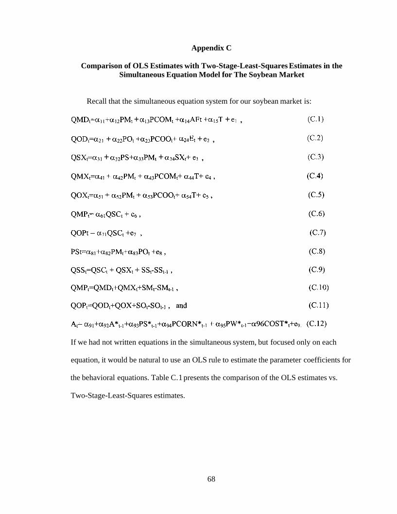
Appendix C
Comparison of OLS Estimates with Two-Stage-Least-Squares Estimates in the Simultaneous Equation Model for The Soybean Market
Recall that the simultaneous equation system for our soybean market is:
QMDt=all+a12PMt + a13PCOMt +al4AFt +alsT + el , (C.1)
QODt=a21 + a22POt +cx~~PCOO~+ + e2 , (C.2)
QSXt=a31 + a32PS+a33PMt + a34SXt+ e3 , (C.3)
If we had not written equations in the simultaneous system, but focused only on each
equation, it would be natural to use an OLS rule to estimate the parameter coefficients for
the behavioral equations. Table C. 1 presents the comparison of the OLS estimates vs.
Two-Stage-Least-Squares estimates.
68

Table C.l: Compare OLS Estimates and Two-Stage Least Square Estimates for Equations in the Simultaneous System In Our Model (Numbers in the Parentheses Are Standard Errors)
(AF) (0.195) (0.19) ' Adjusted R2 0.8909 0.89
Oil (QOD) ~ Constant 16412.14* 16759*
(1089.97) (1210) Price of Soy Oil (PO) -21.2 -3 1.2
, (20) (25) Price of Corn Oil (PCOO) 68.4 86.27
OLS Estimates
(1 0743) Constant 2280
Price of Soy Meal (PM) -1 18
Domestic Demand for Soy I
2SLS Estimates 1571 (10945) -167
Price of Corn Meal (PCOM)
Time Trend Variable (T)
Number of Animal Units
15 8 230 (264.9) (332) 574.94 579* (167.35) (1 68) 0.176 0.18
Real Expenditures on Food (E) (48.64) (55) 14.37* 13.28*
69
. _
Adjusted R2 (2.45) (2.95) 0.9017 0.90

Table C1: (Corztinued) I U.S. Soybean Export
Constant
Price of Soybeans (PS)
41681* (11212) -558.92 . ,
Price of Soy Meal (PM) (729.14) 29.05
RL I 0.2274 U.S. Soy Meal Export
South American Soybean Ex~ort (SX)
37836* 11889
0.2155 (0.1849)
(838) -26
Price of Soy Meal (PM)
Price of Corn Meal (PCOM)
Time Trend Variable (T)
Adjusted R2
9 (1 930) (2006)
(81.6) ( 1 08.3 6) 141.52 182.25 (138.3 1) (173.27) 113.88* 119.1 1* (48.42) 0.248 0.29
-68.84 -97.16
Demand (QMX) Constant I 2923.12 I2712 1
Price of Soy Oil (PO)
Price of Corn Oil (PCOO)
(442.92) (444) -9.06** -10.87* (4.85) (5.05) 45.84* 47.9*
(QOX) Constant I 975.66* I998*
Adjusted R2 ( 1 8.1 9) 0.17 0.21
(1 8.3)
QOP 0.2096* (0.001 86)
Adjusted R2 0.9978
1 Soy Meal Produced I
0.21* (0.0016) 0.99
(QMP) QMP I0.48628* I 0.49*
70
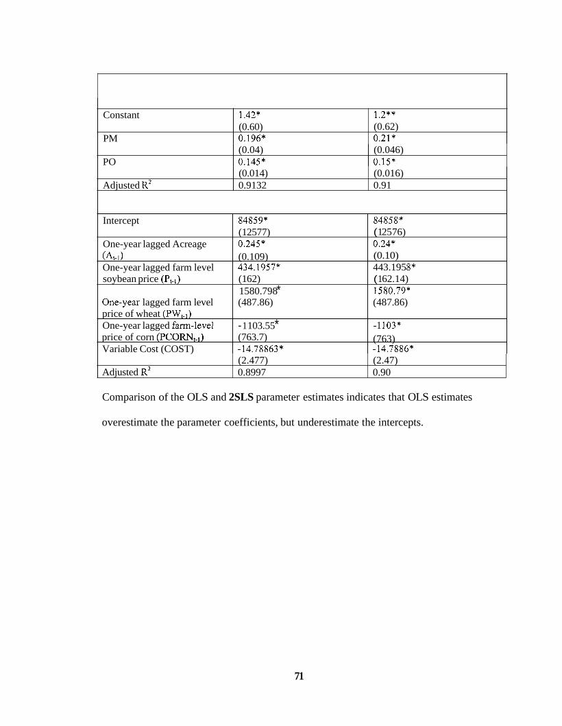
Constant 1.42* (0.60)
PM 0.196*
1.2** (0.62) 0.21*
PO (0.04) (0.046) 0.145* 0.15*
Comparison of the OLS and 2SLS parameter estimates indicates that OLS estimates
Adjusted R2
overestimate the parameter coefficients, but underestimate the intercepts.
(0.014) (0.016) 0.9132 0.91
71
Intercept 84859* (1 2577)
One-year lagged Acreage 0.245*
One-year lagged farm level 434.1957* soybean price (P,.J (1 62)
1580.798 * One-year lagged farm level (487.86) price of wheat (PW,,)
price of corn (PCORNt..l) (763.7)
(At- I 1 (0.109)
One-year lagged farm-level - 1 103.55 *
Variable Cost (COST) - 14.78863*
84858* ( 1 25 76) 0.24*
443.195 8* ( 1 62.14) 1580.79* (48 7.8 6)
(0.10)
-1 103* (763) -14.7886*
Adjusted R2 (2.477) (2.47) 0.8997 0.90
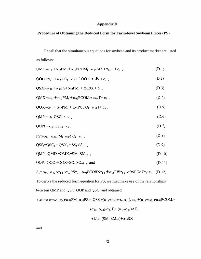
Appendix D
Procedure of Obtaining the Reduced Form for Farm-level Soybean Prices (PS)
Recall that the simultaneous equations for soybean and its product market are listed
as follows:
QMDt=al l+a12PMt + a13PCOMt +al4AFt +alsT + el , (D.1)
QODt=a21 + az2POt +a23PCOOt+ + e2 , (D.2)
QSXt=a31 + a32PS+a33PMt + a34SXt+ e3 , 03.3)
QMXt=a41 + a42PMt + a43PCOMt+ a44T+ e4 , 03.4)
Q0Xt=a5l + a52PMt + a53PCOOt+ a54T+ e5 , (D.5)
QMPt= a61QsCt + e6 , (D.6)
QOPt = a71QSCt +e7, (D .7)
PSt=agl+as2PMt+ag3POt +eg , (D.8)
QSSt=QSCt + QSXt + SSt-SSt-1 , 03.9)
QMPt=QMDt+QMXt+SMt-SMt-l , (D. 10)
QOPt=QODt+QOX+SOt-SOt-l , and (D. 1 1)
At= a 9 1 +a92A*t-l +a93PS*t-~+a94PCORN*t-I + a9~PW*~-l +a96COST*,+eg. (D. 12)
To derive the reduced form equation for PS, we first make use of the relationships
between QMP and QSC, QOP and QSC, and obtained
-(a 12+a52+a61 a34)/a61 PMt-a32PSt=-QSSt+(a 1 1+a51+a61 a 3 I)/ % + ( a 13+a53)/a61PCOMt+
(a 15+a54)/a61 Tt+ (a1 4 / a 6 l )mt
+I / a 6 1 (SMt-SMt-l)+a35SXt
and
72
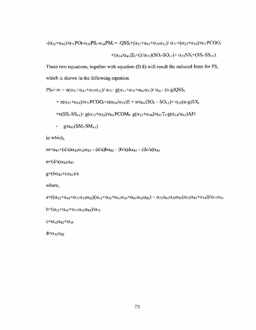
73
BIOGRAPHY OF THE AUTHOR
Lei Cui was born in Nanjing, Jiangsu, P.R.China on July 6 , 1975. She graduated
from the Affiliated Middle School of Nanjing Normal University in 1993 and attended
Bejing Normal University in the same year. She received her Bachelor of Science in
Economics in July 1997. She was enrolled for graduate study in agricultural production
and marketing at the University of Maine in September 1999 and served as a research
assistant in the Department of Resource Economics and Policy.
Lei is a candidate for a Master of Science degree in Resource Economics and Policy
from the University of Maine in August, 2001.
74