economic geography, jobs, and regulations: the...
TRANSCRIPT
Economic Geography, Jobs, and Regulations: The Value of Land and Housing
Nils Kok Maastricht University
Netherlands [email protected]
Paavo Monkkonen University of Hong Kong
Hong Kong [email protected]
John M. Quigley University of California
Berkeley, CA [email protected]
February 2011
Analyses of the determinants of land prices in urban areas typically base inferences on housing transactions which combine payments for land and long-lived improvements. These inferences, in turn, are based upon assumptions about the production function for housing and the appropriate aggregation of non-land inputs. In contrast, we investigate directly the determinants of urban land prices. We assemble more than 7,000 land transactions in the San Francisco Bay Area during the 1990-2009 period, and we analyze the link between the physical access of sites, the topographical and demographic characteristics of their local environment, and the prices of vacant land on those sites. We investigate in detail the link between variations in the quality of public services and the value of developable land. Most importantly, our analysis documents the powerful link between variations in the regulatory environment within a metropolitan area and the prices commanded by raw land as an input to residential or commercial development. Finally, we relate these large variations in land prices to the prices paid by consumers for housing in the region.
JEL Codes: D40, L51, R31
Keywords: Geography, Housing Supply, Land Prices, Land-Use Regulation
Financial support for this research was provided by the Berkeley Program for Housing and Urban Policy and the European Property Research Institute at Maastricht University. Kok is supported by a VENI grant from the Dutch Science Foundation (NWO). We are grateful for the comments of Jan Brueckner, Morris Davis, Albert Saiz, and Gene Smolensky, participants at the 2011 ASSA Meetings, and at seminars at UBC and Berkeley.
1
I. Introduction
The price of land is a basic indicator of the attractiveness and the economic value
of a specific site and of the amenities available at that location. These amenities can
include a diverse collection of attributes, ranging from the productivity of a rural site in
agriculture to the quality of an urban neighborhood surrounding a given location. In
urban areas, variations in the price of land may reflect local externalities and
governmental policies as well as the locational and geographical advantages of particular
sites.
Variations in the price of land within urban areas also affect the cost of housing
within metropolitan areas, as well as spatial variations in the density of population and
housing (and the capital intensity of non-residential properties as well). Substitution in
the production of residential (and non-residential) property means that, in any cross
section, intra-metropolitan variations in the price of housing and commercial property
will be less pronounced than intra-urban variations in land prices.1
There is a large and impressive literature on the determinants of rural land values
in the US (e.g., Goodwin, et al, 2003, Alston, 1986), facilitated by the availability of land
price data through the National Agricultural Statistics Service of the US Department of
Agriculture and more recently its Agricultural Resource Management Survey.
Yet there is no comparable body of empirical evidence on the determinants of
urban land values. For the most part, land values are estimated from variations in the
selling prices of housing by making assumptions about the production function for
1 As shown forty years ago by Muth (1968), substitution in production implies that the intra-urban gradient of land prices will be steeper than the gradient of housing prices.
2
housing.2 (See Davis and Heathcote, 2007, for a particularly careful and important
application of this reasoning.) This methodology does not account for variations in the
land component of housing output within metropolitan regions,3 and it does not account
for factors which may distinguish the value of land at the intensive margin from the value
of land at the extensive margin, i.e., the difference between the value of an additional unit
of land for a built-up property and the value of marginal land in lots of newly-constructed
housing. (See Sundling and Swoboda, 2009, or Glaeser and Gyourko, 2003, for a
discussion.)
But of course the most important reason why the value of urban land is
problematic is the dearth of direct observations on sales of urban land, sales which are
less common in built-up urban areas than in the rural hinterland. This is well-known to
those who have analyzed urban land and housing markets, and it is a key reason why
ingenious indirect methods have been developed. For example, Davis and Heathcote
(2007) observe that:
“…with the exception of land sales at the undeveloped fringes of metro areas—where land is relatively cheap—there are very few direct observations of land prices from vacant lot sales, because most desirable residential locations have already been built on (p 2595).”
They note further that their indirect approach to measuring land prices is intended
“to circumvent this potentially intractable measurement problem.”
However, a recent descriptive analysis of land prices in the New York
metropolitan area by Haughwout, et al (2008) reported that more than 1,600 land sales
2 There are also a few analyses of small samples of teardowns (i.e., redevelopment parcels) to investigate the value of land in built-up urban areas. See Rosenthal and Helsley (1994). 3 For example, Davis and Palumbo (2008) estimate land values over time for 46 US cities by relying upon indices of aggregate house prices, assumptions about production relationships, and the creative measurement of residential capital.
3
took place in the Bronx, Brooklyn, Manhattan and Queens during the seven-year period
1999 to 2006. Indeed, the authors reported that there were almost 90 transactions of
vacant land each year in the 23 square miles of Manhattan, the most densely-populated
county in the United States and one of the most intensely developed areas of the world.
The work reported by Haughwout, et al (2008) is based on a rather unusual source of
micro data which we exploit further.
The sales prices of parcels of vacant land and “teardown” parcels are recorded by
city and county assessors. These transactions form the basis for property tax liabilities in
most jurisdictions. For obvious reasons, these transactions are ignored by the firms which
produce indices of housing prices and which market statistical analyses of local or
metropolitan-wide housing prices (e.g., the S&P Case Shiller products). However, this
urban land price information is recorded on a regular basis by the CoStar Group.4 In this
paper, we use this data source in an extensive analysis of land price determination in the
San Francisco Bay Area in California.
The San Francisco Bay Area has historically had the highest housing prices in the
US, and the rate of increase in housing prices has been among the highest experienced by
any large US metropolitan area, at least until the recent collapse in the US housing
market. Within the Bay Area, there is substantial variation in the economic and
geographical conditions affecting land parcels, not only proximity to jobs and economic
conditions, but also wide variations in topography – in elevation and proximity to water,
4 Data from CoStar on the hedonic and financial characteristics of commercial office buildings have formed the basis for several recent microeconomic analyses of US property markets (e.g., Eichholtz, et al, 2010, Fuerst and McAllister, 2011); a subset of the CoStar data was exploited by Haughwout, et al (2008) in their analysis of land prices in New York. After this paper was completed, we became aware of two recent working papers which rely upon aggregates of CoStar land data: Albouy and Ehrlich (2011); and Nichols, Oliner and Mulhall (2010).
4
open space, and natural amenities, as well as earthquake risk. As with most metropolitan
areas in the US, the region is segregated by race and income, and land parcels may be
exposed to different levels of public services. The availability of detailed data on the
transactions prices of vacant land and teardown properties, geocoded to locations,
supports a detailed examination of the relationship between the physical and economic
geography of the region and land values.
Importantly, the Bay Area is infamous for a restrictive pattern of land-use
regulation which varies according to the unfettered choices of the different cities in the
region (See Quigley, et al, 2009). In the empirical analysis below, we utilize quite
detailed survey data on land-use regulations in the 110 independent jurisdictions in the
Bay Area to investigate the linkage between these regulations and land prices, and
ultimately housing prices.
Our findings show the importance of the geographical level of analysis in
understanding the relationship between land-use regulations and housing prices. This
complements recent work by, for example, Albert Saiz (2010) who relates land
availability to regulation, calculating the average elasticity of housing supply at the
metropolitan level. We measure topography, geography, and regulation at the level of the
land parcel, and we relate these factors to land prices and housing prices within a large
number of independent land use jurisdictions of a single metropolitan area. The power to
regulate land use is wielded by city governments in most states, and our analysis provides
some evidence on the importance of intra-metropolitan variation in regulation and its
effect upon land values.
5
We then link land values to house values, using a large sample of sales of single-
family housing in the San Francisco Bay Area. We find that changes in typography,
geography, and land use regulation have quite large effects on the value of houses sold in
the region, in part because local land-use regulation is so pervasive and in part because
land values represent such a large fraction of house values in the San Francisco Bay Area.
Section II describes the key sources of land price data and the measures of
physical and economic geography used in the analysis. Section III relates variation in
land prices to our intra-urban measures of economic geography, and section IV relates
variation in land prices within the metropolitan region to variations in local regulation. In
Section V, which analyzes the relation between housing values and land values, we make
the linkage to the work by Saiz (2010) and Davis and Palumbo (2008) more explicit, and
we note the complimentarity in approaches. Section VI is a brief conclusion.
II. Data on Land Prices and their Determinants
A. Land Prices
The proprietary data on land prices in the San Francisco Bay Area that we rely
on5 are widely used by commercial real estate agents throughout the US, for example, in
keeping abreast of market developments and in assisting clients in negotiating leases.
We utilize the historical file of land sales for the nine-county San Francisco Bay
Area as of January 1, 2010. Most of these land sales had been reported by brokers and
other market participants. The file includes the address of each parcel, its size in square
5 The complete database includes information on about 2.4 million commercial land parcels and properties, their locations and their hedonic characteristics, as well as the current tenancy and rental terms, and the recent sales prices for these properties. About eleven percent of these commercial parcels are classified as “land.” In addition, purchases of other properties are identified as “land” when the buyer is primarily (continued at bottom of next page)
6
feet, and its selling price. The data consist of 7,278 observations on land sales in the San
Francisco Bay Area between 1990 and 2010.6
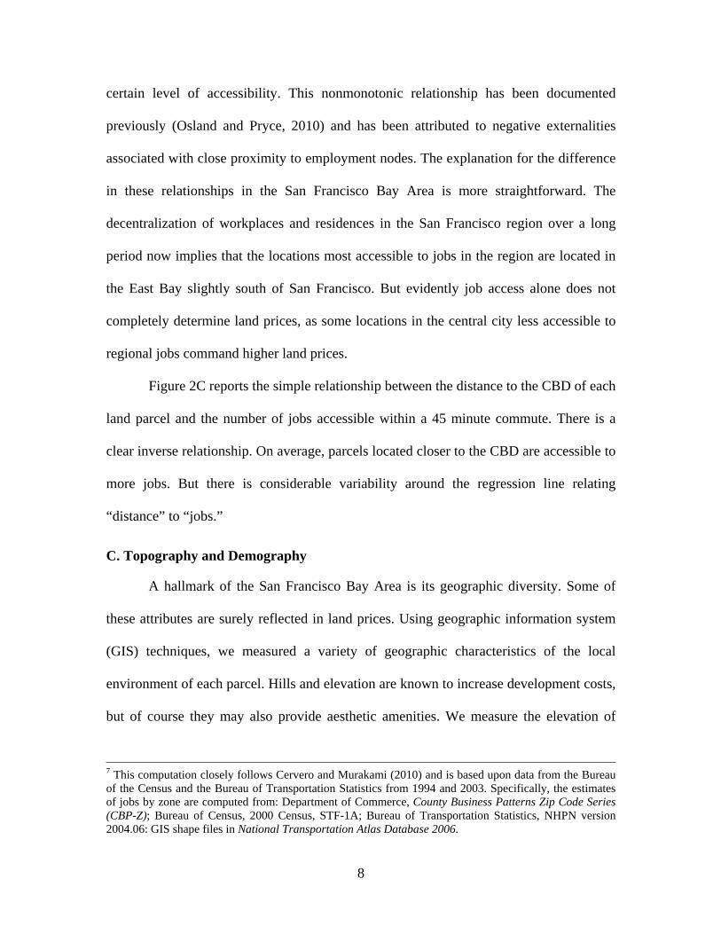
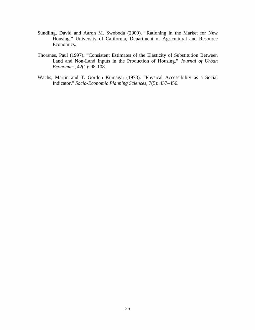
Figure 1 reports the geographic distribution of our sample of land sales in the nine
counties of the San Francisco Bay Area. The dark grey areas denote incorporated cities;
this distinction will be exploited further in the analysis below.
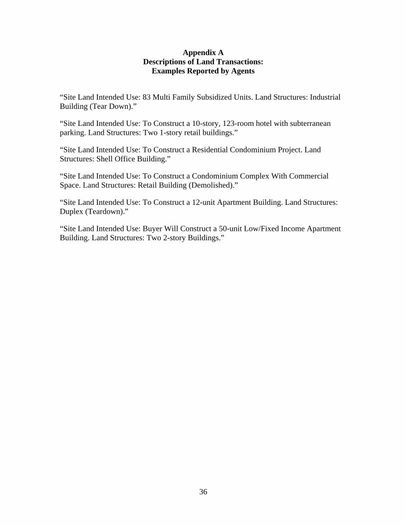
The correspondents reporting information on land sales are encouraged to submit
descriptions of the land transactions. A sample of these descriptions is included in
Appendix A. From these unstructured narratives, we classified the current condition of
these parcels into four categories (i.e., “raw,” “rough graded,” “fully improved,” and
“previously developed” land). The proposed use of these parcels is classified into eight
categories (i.e., “hold for development,” “single family,” “commercial,” “industrial,”
“multi family,” “mixed use,” “public space,” and “public facilities”). These categories,
current condition and anticipated use, are presumably important determinants of the
cross-sectional variation in land prices.
Due to non-responses and ambiguities, we were only able to identify the current
condition and expected use of the land parcels for about 84 percent of the sales.
B. Job Access
From the coordinates of the street address for each parcel, we matched each site to
the most important geographical determinant of urban land value, namely its location
relative to the commercial center of the region (the Central Business District, CBD).
interested in development or redevelopment of the parcel and any unoccupied structures it contains. (Sales of these latter parcels are called “teardowns.”) 6 Specifically, the data include all sales of less than 1,000,000 square feet of land which could be matched to the topographical, census, and regulatory data described in Section III. The overwhelming majority of the observations excluded from analysis consist of sales of vineyards or farmlands at the periphery of the nine-county region (according to the narrative descriptions reported at the time of sale).
7
Access, location relative to the CBD, is measured by the airline distance to San
Francisco’s Ferry Building in the heart of the downtown financial district.
Although this simple measure of employment access is widely recognized, the
decentralization of workplaces in US cities has rendered it less meaningful as a measure
of employment accessibility over time. In the nine-county San Francisco Bay Area, for
example, by 2003 only fourteen percent of jobs were located in the central city of San
Francisco. In recognition of these spatial developments, we also measure access to jobs in
a more sophisticated way.
The employment access of each parcel is measured by estimating the number of
jobs located within 45 minutes of travel time on the metropolitan highway network
system using an isochrone or “cumulative opportunity” measure. This technique,
originally developed by Wachs and Kumagai (1973), sums all jobs that can be reached
within a given travel time accounting for the location of employment, distance, and the
road network.7
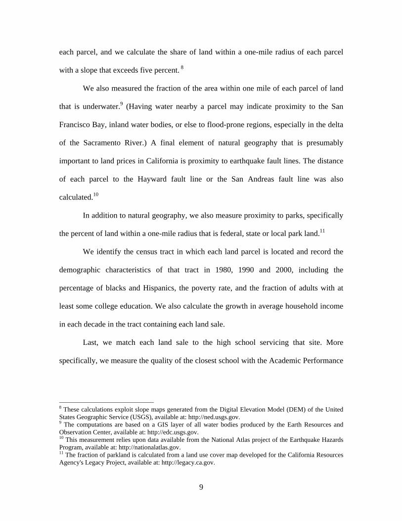
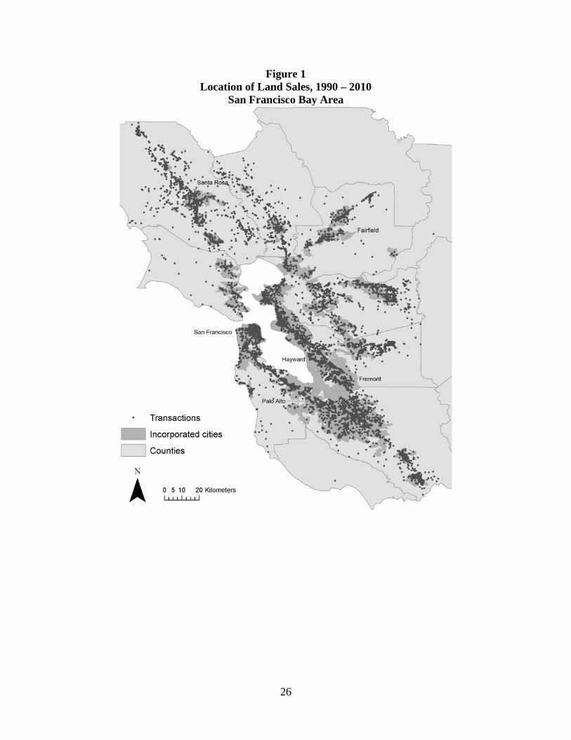
Figure 2A reports the simple bivariate relationship between each of these two
measures and the selling price of land parcels (per square foot) in San Francisco during
the 1990-2010 period. The relationship between land prices and distance to the CBD
conforms to the traditional pattern and can be approximated crudely by a negative
exponential. The relationship between access to jobs and land prices (presented in Figure
2B) is more complex, taking a concave (almost parabolic) shape. Prices increase as job
accessibility grows in an almost exponential pattern, but then drop off sharply beyond a
8
certain level of accessibility. This nonmonotonic relationship has been documented
previously (Osland and Pryce, 2010) and has been attributed to negative externalities
associated with close proximity to employment nodes. The explanation for the difference
in these relationships in the San Francisco Bay Area is more straightforward. The
decentralization of workplaces and residences in the San Francisco region over a long
period now implies that the locations most accessible to jobs in the region are located in
the East Bay slightly south of San Francisco. But evidently job access alone does not
completely determine land prices, as some locations in the central city less accessible to
regional jobs command higher land prices.
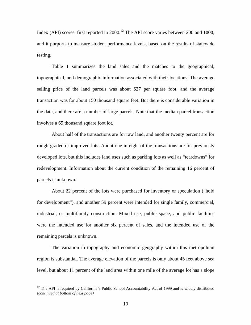
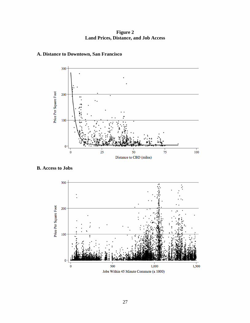
Figure 2C reports the simple relationship between the distance to the CBD of each
land parcel and the number of jobs accessible within a 45 minute commute. There is a
clear inverse relationship. On average, parcels located closer to the CBD are accessible to
more jobs. But there is considerable variability around the regression line relating
“distance” to “jobs.”
C. Topography and Demography
A hallmark of the San Francisco Bay Area is its geographic diversity. Some of
these attributes are surely reflected in land prices. Using geographic information system
(GIS) techniques, we measured a variety of geographic characteristics of the local
environment of each parcel. Hills and elevation are known to increase development costs,
but of course they may also provide aesthetic amenities. We measure the elevation of
7 This computation closely follows Cervero and Murakami (2010) and is based upon data from the Bureau of the Census and the Bureau of Transportation Statistics from 1994 and 2003. Specifically, the estimates of jobs by zone are computed from: Department of Commerce, County Business Patterns Zip Code Series (CBP-Z); Bureau of Census, 2000 Census, STF-1A; Bureau of Transportation Statistics, NHPN version 2004.06: GIS shape files in National Transportation Atlas Database 2006.
9
each parcel, and we calculate the share of land within a one-mile radius of each parcel
with a slope that exceeds five percent. 8
We also measured the fraction of the area within one mile of each parcel of land
that is underwater.9 (Having water nearby a parcel may indicate proximity to the San
Francisco Bay, inland water bodies, or else to flood-prone regions, especially in the delta
of the Sacramento River.) A final element of natural geography that is presumably
important to land prices in California is proximity to earthquake fault lines. The distance
of each parcel to the Hayward fault line or the San Andreas fault line was also
calculated.10
In addition to natural geography, we also measure proximity to parks, specifically
the percent of land within a one-mile radius that is federal, state or local park land.11
We identify the census tract in which each land parcel is located and record the
demographic characteristics of that tract in 1980, 1990 and 2000, including the
percentage of blacks and Hispanics, the poverty rate, and the fraction of adults with at
least some college education. We also calculate the growth in average household income
in each decade in the tract containing each land sale.
Last, we match each land sale to the high school servicing that site. More
specifically, we measure the quality of the closest school with the Academic Performance
8 These calculations exploit slope maps generated from the Digital Elevation Model (DEM) of the United States Geographic Service (USGS), available at: http://ned.usgs.gov. 9 The computations are based on a GIS layer of all water bodies produced by the Earth Resources and Observation Center, available at: http://edc.usgs.gov. 10 This measurement relies upon data available from the National Atlas project of the Earthquake Hazards Program, available at: http://nationalatlas.gov. 11 The fraction of parkland is calculated from a land use cover map developed for the California Resources Agency's Legacy Project, available at: http://legacy.ca.gov.
10
Index (API) scores, first reported in 2000.12 The API score varies between 200 and 1000,
and it purports to measure student performance levels, based on the results of statewide
testing.
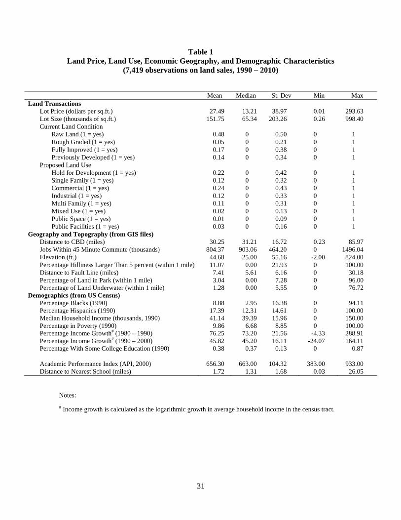
Table 1 summarizes the land sales and the matches to the geographical,
topographical, and demographic information associated with their locations. The average
selling price of the land parcels was about $27 per square foot, and the average
transaction was for about 150 thousand square feet. But there is considerable variation in
the data, and there are a number of large parcels. Note that the median parcel transaction
involves a 65 thousand square foot lot.
About half of the transactions are for raw land, and another twenty percent are for
rough-graded or improved lots. About one in eight of the transactions are for previously
developed lots, but this includes land uses such as parking lots as well as “teardowns” for
redevelopment. Information about the current condition of the remaining 16 percent of
parcels is unknown.
About 22 percent of the lots were purchased for inventory or speculation (“hold
for development”), and another 59 percent were intended for single family, commercial,
industrial, or multifamily construction. Mixed use, public space, and public facilities
were the intended use for another six percent of sales, and the intended use of the
remaining parcels is unknown.
The variation in topography and economic geography within this metropolitan
region is substantial. The average elevation of the parcels is only about 45 feet above sea
level, but about 11 percent of the land area within one mile of the average lot has a slope
12 The API is required by California’s Public School Accountability Act of 1999 and is widely distributed (continued at bottom of next page)
11
greater than five percent. The land sales are, on average, seven and a half miles from the
Hayward Fault (which last ruptured violently in 1987) or the San Andreas Fault (the
epicenter of the great 1906 earthquake). On average, about three percent of land located
within a mile of these land sales lies within state or local parkland; only a small fraction
of nearby surface area is underwater.
III. Land Prices and Economic Geography
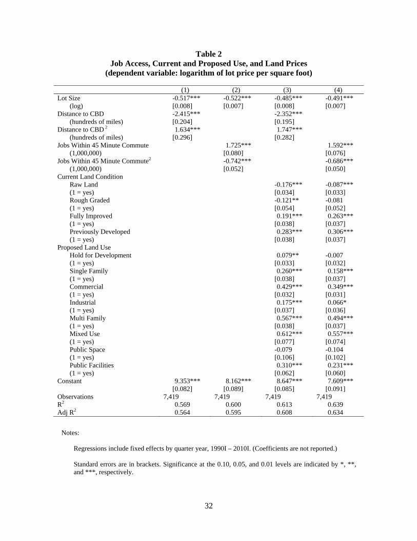
Table 2 reports the relationships between land prices and the accessibility
measures noted above. The table relates the logarithm of land prices per square foot to the
most straightforward measures - access to jobs and to the CBD - as well as the current
land condition and the proposed usage. These regressions also include fixed effects for
each quarter year, from 1990:I through 2010:I.
Lot size and the distance to the CBD (as well as the indicators for each quarter
year) explain more than half of the variation in vacant land prices per square foot. The
substitution of the job access measure for the simple distance measure increases the
explained variance to sixty percent. The current land condition and the proposed land use
are also important; when the estimates of current land condition and contemplated usage
are taken into account, the simple model explains 61-64 percent of the variation in land
prices.
Not surprisingly, raw land sells at a significant discount relative to fully improved
lots. Ceteris paribus, previously-developed lots sell at a 4-9 percent premium over the
latter. Compared to the unknown category, lots purchased for investment inventories are
sold at a slight premium, while land parcels intended for specific development activities
to the public. Data are available at: http://www.cde.ca.gov/ta/ac/ap .
12
are sold for a greater premium, especially those intended for commercial, multifamily, or
mixed use. Parcels intended for use as public open space (i.e., parks) are sold at a
considerable discount.
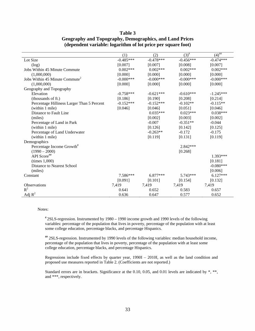
Table 3 reports further analysis of the relationship between land prices and the
topographic and demographic measures described above. The regressions also include
fixed effects for each quarter, 1990-2010, and the indicators of land condition and
proposed use as reported in Table 2. The results in Table 3 show that lots at higher
elevations sell for somewhat less, and those on hilly terrain sell for a considerable
discount. Presumably, construction is considerably more expensive when (parts of) lots
must be graded. Land further from major earthquake fault lines is more valuable; a one-
mile increase in distance to the fault line increases the value of land by 1-2 percent,
ceteris paribus. Land in very close proximity to water is less valuable. Clearly, elements
of topography and economic geography have important influences on the price of land.
The results in Table 3 also confirm the importance of local demographics in
affecting land values. Areas where household income was anticipated to grow between
1990 and 2000 (as instrumented by census tract income growth between 1980 and 1990)
registered much higher land values. Land parcels serviced by a better local school (as
reported by the Academic Performance Index of the school and instrumented by census
tract demographic data measured in 1990) are much more valuable. Parcels closer to
those schools are also more valuable. These findings about schools and land prices are
consistent with the well-documented relationship between school quality, test scores, and
house prices (see for example Black, 1999, and Figlio and Lucas, 2004).
13
IV. Land Prices and Political Economy
In many states, cities are afforded great freedom to regulate land use and to award
or deny developers the right to build at any location. Several studies have attempted to
characterize these regulations and to develop simple measures of land-use regulation
from the many details specified in land-use statutes and in practice. A series of surveys
designed by economists at Wharton have created a taxonomy of restrictive regulatory
practices in US cities. (These efforts are summarized in Gyourko, et al, 2008.) These
surveys have been used to estimate the restrictiveness of land-use regulation in U.S.
metropolitan areas.13
In California, prior studies by Glickfeld and Levine in 1988 and again in 1992
elicited a series of procedural and attitudinal responses to questions about local
development and regulation from the Planning Director or a comparable official in each
California city.14 In subsequent work, Quigley, et al (2004) used statistical techniques to
aggregate the detailed responses documented by Glickfeld and Levine to two indexes:
one measuring the “restrictiveness” of each jurisdiction (including, for example
restrictions on the numbers of building permits issued); and one measuring the
“hospitality” of each jurisdiction to development (including, for example, the
implementation of regulatory “fast tracking”). These indexes were used in an analysis of
demographic trends in cities in Southern California.
More recently, the MacArthur Foundation sponsored a detailed investigation of
the regulatory structure of the San Francisco Bay Area conducted at Berkeley in 2007.
13 By the Wharton calculations, the San Francisco metropolitan area ranks sixth among 47 US metropolitan areas in terms of the restrictiveness of land use (Gyourko, et al, 2008, p. 713). 14 The survey was administered by the League of California Cities, and this insured a high response rate. Details of this survey and a complete set of survey responses may be found in Glickfeld and Levine (1992).
14
This analysis included surveys of developers and market intermediaries as well as
interviews and surveys of Planning Directors and other officials in the cities within the
nine-county San Francisco Bay Area.15
We matched our dataset of 7,419 sales of land parcels to the attributes of local
regulation measured by Glickfeld and Levine in 1994 for the cities in which these parcels
were located. We also matched these land sales to the four most salient measures of land-
use restrictiveness derived from the analysis of land-use restrictiveness in the San
Francisco Bay Area conducted in 2007. First, we measured the number of independent
reviews and approvals required before issuance of a building permit.16 Second, we
measured the number of separate reviews by municipal authorities required to approve a
zoning change.17 Third, the survey obtained estimates of the average delay in months
between the time a request was made for building and the time a decision was reached –
for standard development projects, for those requiring a zoning change, and for those
involving an entire subdivision. We use the average delay in months. Fourth, we use a
measure of political influence which rated stakeholders in the development process in
terms of their involvement in land-use decisions.18
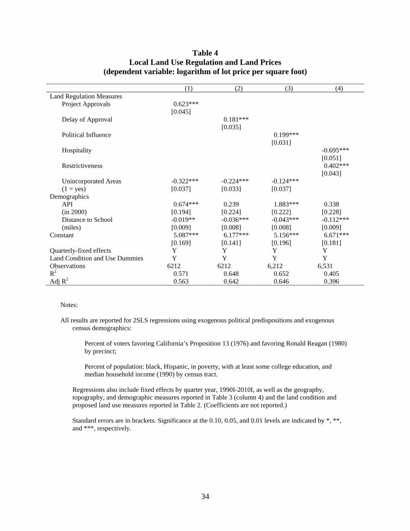
Table 4 presents regressions relating these measures of land-use restrictiveness to
the price per square foot of vacant land, holding constant the other important
determinants of land values noted previously. Measures of land use restrictions are
15 These data were used in a recent comparative analysis of land use regulation and economic development (see Glaeser and Quigley, 2009, Quigley and Raphael, 2005, Quigley, Raphael, and Rosenthal, 2009). 16 As many as eleven different reviews by municipal authorities may be required for issuance of a building permit, depending upon the jurisdiction – separate reviews by the planning commission, the architectural and design review board, the parking authorities, etc. 17 Again, one or more of a large number of independent entities may be required to concur; on average six concurrences are required in the jurisdictions in San Francisco Bay Area.
15
normalized to a mean of zero and a standard deviation of one. Because the restrictiveness
of regulation is endogenous, we use instrumental variables to estimate the models in
Table 4. As instruments we use the popular vote on California’s Proposition 13 (in favor
of a substantial property tax rollback) in the 1978 state election, by precinct, and the
popular vote for Ronald Reagan (against President Jimmy Carter) in the 1980 national
election, also by precinct.
The popular votes on these measures are clearly exogenous to the land-use
regulations observed in 1992 and 2007. On average, 65 percent of Bay Area voters
favored Proposition 13 in 1978, and 46 percent favored Reagan in the 1980 election.
As the results show, the stringency of regulations has a powerful effect upon the
prices of vacant land in the San Francisco Bay Area, even when controlling for locational
and geographic characteristics of the land site. The number of reviews and approvals
required for issuance of a building permit or zoning change, delay in project approval,
and stronger political influence all contribute to higher land prices, and these measures
are highly correlated across jurisdictions. If the number of independent reviews required
for approval of a general construction project were increased by one standard deviation
in each of the political jurisdictions in the Bay Area (and the delay and influence
measures were increased concomitantly), it is estimated that average land prices in the
region would further increase by 62 percent. If the average delay in the approval of
residential construction projects (currently a little more than a year) were increased by
one standard deviation in each jurisdiction (about eight months), the model estimates that
average land prices would be increased by about 18 percent. These findings confirm early
18 Complete details on these surveys, the specific questions addressed, and a complete set of survey (continued at bottom of next page)
16
evidence by Glaeser, et al (2005), who document the impact of development restrictions
on condominium prices in New York City.
V. Land Prices and House Prices
A. The Influence of Economic Geography and Regulation
The empirical analyses presented in Tables 2-4 permit us to explore the
relationship between the determinants of land prices within the San Francisco
metropolitan area and the effects of these factors on the prices for housing paid by
consumers at various locations in the region. This analysis has parallels with Saiz’s
(2010) aggregate analysis across 95 MSAs; both emphasize the importance of physical
geography and regulation in housing market outcomes. However, Saiz’s analysis is based
upon stronger behavioral assumptions (e.g., exogeneity in metropolitan populations
across thirty years) and theoretical assumptions (e.g., the forms of utility functions), as
well as cruder measurements (e.g., regulatory variables are measured at the metropolitan
level of aggregation). But in return for these more heroic assumptions, Saiz is able to
report estimates of house price elasticities across a national sample of housing markets.
The most important difference between this analysis and that of Saiz is the
geographical level of aggregation. The power to regulate land use and the variation in
land-use regulation occurs at the local level, suggesting that intra-metropolitan variation
is important in considering the impacts of regulation on prices. As noted in Table 4, we
find substantial differences within a metropolitan housing market in the effects of
economic geography, public services, and especially land use regulation upon land prices.
responses is reported in Quigley, Raphael, and Rosenthal (2007).
17
We explore further the link between individual house values and land prices using
the simple framework emphasized by Davis and Palumbo (2008), in which the value of
any house (Vi) is simply the sum of the physical capital embedded in that house (Ki) and
the land it occupies ( Li ), where stocks of capital and land are valued at current prices
( pk , pl):
(1) Vi = pkKi + plLi
For each of the 110 cities in the nine-county Bay Area region during the period
1990-2010, we obtained data on the number of single-family house sales, the average
selling price and lot size, by quarter year.19 We estimated predicted land prices for each
city and quarter year from the regressions reported in Table 4 and then computed the
average land values of single-family house sales by multiplying the average lot size with
the corresponding predicted land price in the same city and quarter year. From equation
(1), we computed the average value of the housing capital transacted by simply
subtracting the predicted value of land.
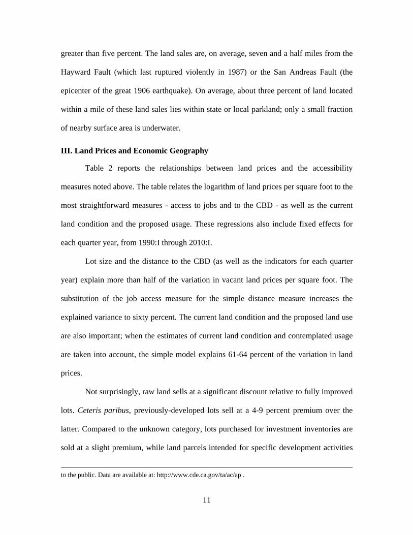
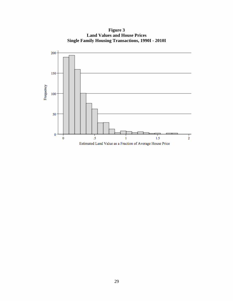
Figure 3 reports the frequency distribution of land values in the San Francisco
Bay Area as a fraction of average house sales.20 For the average house sale in the region,
the underlying land value represents about 34 percent of the selling price, and this
fraction has been increasing over time. For sales during the 1990-1995 period, land
values averaged about 31 percent of house values; for sales during the 2005-2010 period,
land values averaged 43 percent of house values. Presumably, this increase in land values
reflects increases in population and incomes in the region, together with the increased
costs of topography, demography and local regulation documented here. The reported
19 Data were obtained from DataQuick in August 2010.
18
fractions are large compared to the conventional wisdom (e.g., Thornses, 1997) which
suggests that land values are about twenty percent of housing values.21
The regressions relating the linkage between geography, demography, land-use
regulation and land values support an analysis of the importance of these factors in
affecting housing values in the region. We use the regression results reported in Tables 2-
4 to estimate changes in the land prices for each of the residential parcels in the sample
under changed economic conditions. These changes in land prices are then used to
estimate changes in house values employing the identity reported in equation (1).
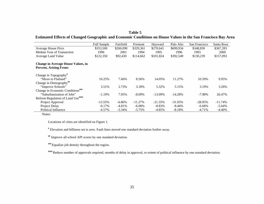
Table 5 summarizes a set of counterfactual estimates,22 for the Bay Area, for the
central city, and for a number of specific suburban jurisdictions which are identified in
Figure 1. The first three rows present the average house prices and the average
corresponding land values. Land sales are not uniformly distributed over the 1990-2010
time period. The median year of sale is reported for the transactions in each of the cities
noted in the table.
The lower part of the table reports the average percentage change of house values
attributable to the change in the value of the land input (from equation 1), under different
scenarios. If the characteristic hilliness of the Bay Area were eliminated and the threat of
earthquake removed, average house values in the region would be increased by about 10
percent, or $36,000. These increments to housing values vary substantially across the
20 House values and land values are weighted by the number of sales reported, by city and quarter year. 21 However, using less precise data on residential capital, Davis and Palumbo (2008) estimate land’s average share of home values within the city of San Francisco at about 75 percent in 1984 and 89 percent in 2004. 22 Note that these counterfactual estimates assume an “open” economy with free mobility, consistent with the results reported in Tables 2-4 and also with the model developed by Saiz (2010).
19
region with the underlying topography, reaching fourteen percent in the City of Hayward,
epicenter of the Hayward fault.
If the quality of the Bay Area’s public schools were increased by one standard
deviation, or 16 percent (as proxied by the 2000 API score for each school), average
house values are estimated to increase by about $12,000.
If job locations were completely decentralized throughout the region, the
aggregate effect upon house values would be negligible. But, of course, this average
masks a great deal of variation across cities. Housing prices in cities like Palo Alto and
Hayward, close to current concentrations of workplaces, would decline substantially
while housing prices in more rural suburbs currently far from job concentrations, such as
Santa Rosa and Fairfield, would increase markedly. Job access matters.
The estimated effects of reductions in the current regulatory restrictiveness of
land-use regulations upon housing values are quite large indeed. For example, a one-
standard-deviation reduction in the extent of delay between application and approval for
residential construction in Bay Area jurisdictions (about eight months) would increase the
affordability of housing by $22,000, with very much larger effects in Palo Alto.
Similarly, a one-standard-deviation reduction in the number of independent reviews
required for approval of a general construction project in Bay Area communities (about
three independent public reviews) would decrease average house prices by about fourteen
percent. Affordability in traditionally more restricted areas, like the city of San Francisco
and Palo Alto, would increase by more than double that number. Restrictive land use
regulation strongly affects land and housing prices.
B. Summary
20
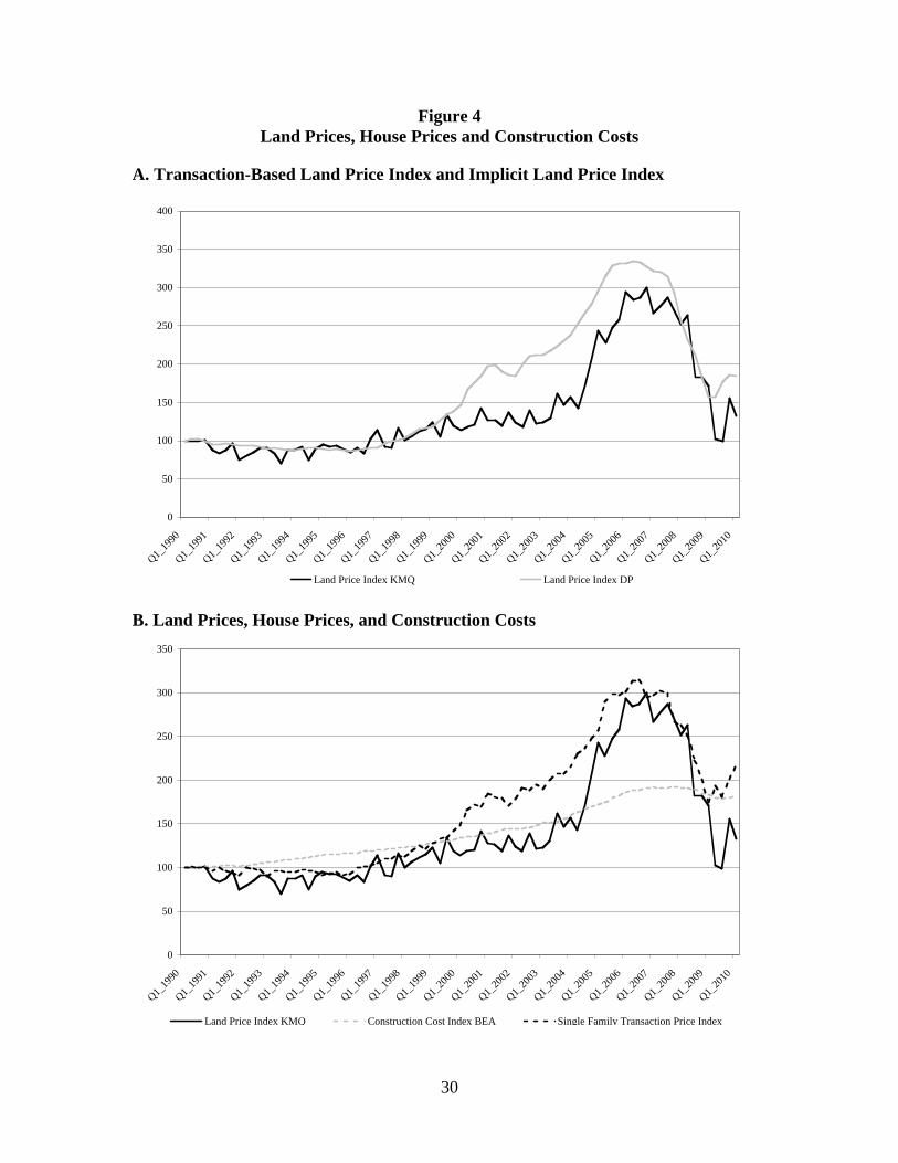
We summarize the link between land prices, house prices and capital costs in
Figure 4. The graph summarizes the aggregate index of land prices derived in our
analysis, holding constant the economic geography and the condition of the individual
land parcels, and compares this to the cruder index published by Davis and Palumbo
(2008). We also compare the land price index to the home price index produced by Case-
Shiller for the Bay Area, using repeat sales of single-family housing,23 and the
construction cost index produced by the Bureau of Economic Analysis.
Figure 4A shows that the transactions-based land index behaves differently when
compared to the Davis-Palumbo (DP) index based on inferred land prices. In particular,
the DP index displays a lower volatility, probably because the latter relies upon changes
in capital costs, which move slowly over time. More importantly, the transactions-based
land price index lags behind the DP index in the early years of the recent price boom.
This difference is due to the dependence of the DP index on housing prices, which is
evident when compared with the Case-Shiller house price index presented in Figure 4B.
The transactions-based land index fluctuates around the Case-Shiller house price
index, until the start of the recent housing bubble. Even though home prices increased
substantially, the price of transacted land remained relatively stable for several years
before catching up at the end of 2004. This lag quite possibly reflects the demand for real
capital created by the abundant availability of financing at very low cost. Alternatively, it
may reflect the real time necessary to obtain building permits to develop otherwise raw
land.
23 Our own estimates, based on a simple hedonic price index (calculated using DataQuick transactions data by city by quarter year) for the nine counties in the Bay Area, are indistinguishable from the Case-Shiller repeat sales index.
21
VII. Conclusion
Analyses of the determinants of land prices in urban areas typically base
inferences on housing transactions which combine payments for land and long-lived
improvements. These inferences, in turn, are based upon assumptions about the
production function for housing and the appropriate aggregation of non-land inputs. In
contrast, this paper exploits micro data on a large sample of land prices in one
metropolitan region – San Francisco – to analyze the link between land values and the
geographic characteristics of land, the quality of the immediate neighborhoods in which it
is located, and the circumstances under which its use is regulated.
We find that intra-urban variations along these dimensions are important
determinants of land prices. Topography (e.g., hilliness, elevation, earthquake fault lines,
etc.) has a significant influence on land prices; jobs in the nearby area, income growth,
and school quality are strongly and positively related to the price of land. We also find
that these variations in land prices have large effects upon regional housing prices.
Moreover, the geographic variation in the restrictiveness of the legal and
regulatory environment, measured by delay in the approval of zoning changes and
construction projects and the influence of stakeholders in the development process,
greatly affects the value of land, and this is reflected in the transaction prices of single-
family homes. These are large effects on house values, in part because local land-use
regulation is so pervasive and in part because land values represent such a large fraction
of house values in the San Francisco Bay Area.
Finally the paper illustrates the substantial complementarity between intra- and
inter-metropolitan analyses of the price and supply impacts of land-use regulations.
Within a single metropolitan area – and across regional markets -- land and housing

22
prices vary quite substantially in response to topographical and natural barriers and in
response to highly localized regulation of land use.
23
References
Albouy, David and Gabriel Ehrlich (2011). “Metropolitan Land Values and Housing Productivity.” University of Michigan.
Alston, Julian M. (1986). “An Analysis of Growth in U.S. Farmland Prices: 1963-82.” American Journal of Agricultural Economics, 68(1): 1-9.
Black, Sandra. (1999). “Do Better Schools Matter? Parental Valuation of Elementary Education.” Quarterly Journal of Economics, 114(2): 577-600.
Cervero, Robert and Jin Murakami (2010). “Effects of Built Environments on Vehicle Miles Traveled: Evidence from 370 US Urbanized Areas.” Environment and Planning A, 42: 400-418.
Davis, Morris A. and Jonathan Heathcote (2007). “The Price and Quantity of Residential Land in the United States.” Journal of Monetary Economics, 54(8): 2595-2620.
Davis, Morris A. and Michael G. Palumbo (2008). “The Price of Residential Land in Large US Cities.” Journal of Urban Economics, 63(1): 352-384.
Eichholtz, Piet M.A., Kok, Nils and Quigley, John M. (2010). “Doing Well by Doing Good: Green Office Buildings.” American Economic Review, 100(5): 2494-2511.
Figlio, David N. and Maurice E. Lucas (2004). “What's in a Grade? School Report Cards and the Housing Market.” American Economic Review, 94(3): 591-604.
Fuerst, Franz and Patrick McAllister. (2011). “Green Noise or Green Value? Measuring the Effects of Environmental Certification on Office Values.” Real Estate Economics, forthcoming.
Glaeser, Edward L. and Joseph Gyourko (2003). “The Impact of Building Restrictions on Housing Affordability.” Federal Reserve Bank of New York Economic Policy Review, 9(2): 21-39.
Glaeser, Edward L., Joseph Gyourko and Raven Saks (2005). “Why is Manhattan So Expensive? Regulation and the Rise in House Prices.” Journal of Law and Economics, 48(2): 331-370.
Glaeser, Edward L. and John M. Quigley (eds.) (2009). Housing Markets and the Economy. Cambridge, MA: Lincoln Institute of Land Policy.
Glickfeld, Madelyn and Ned Levine (1992). Regional Growth, Local Reaction: The Enactment and Effects of Local Growth Control and Management Measures in California. Cambridge, MA: Lincoln Institute of Land Policy.
24
Goodwin, Barry K., Ashok K. Mishra and François N. Ortalo-Magné (2003). “What’s Wrong with Our Models of Agricultural Land Values?” American Journal of Agricultural Economics, 85(3): 744-752.
Green, Richard K., Stephen Malpezzi and Stephen K. Mayo (2005). “Metropolitan-Specific Estimates of the Price Elasticity of Supply of Housing, and Their Sources.” American Economic Review, 95(2): 334-339.
Gyourko, Joseph, Albert Saiz and Anita Summers (2008). “A New Measure of the Local Regulatory Environment for Housing Markets: The Wharton Residential Land Use Regulatory Index.” Urban Studies, 45(3): 693-729.
Haughwout, Andrew, James Orr and David Bedoll (2008). “The Price of Land in the New York Metropolitan Area.” Federal Reserve Bank of New York Current Issues in Economics and Finance, 14(3): 1-7.
Muth, Richard F. (1968). Cities and Housing. Chicago: University of Chicago Press.
Nichols, Joseph B., Stephen D. Oliner and Michael R. Mulhall (2010). “Commercial and Residential Land Prices Across the United States.” Federal Reserve Board, Finance and Economics Discussion Series 1020-16, Washington, D.C.
Osland, Liv and Gwilym Pryce (2010). “Housing Prices and Multiple Employment Nodes: Is the Relationship NonMonotonic?” paper presented at the Cambridge Centre for Housing and Planning Research Conference, Housing: The Next 20 Years, Sept. 16-17, Cambridge, UK.
Quigley, John M. and Steven Raphael (2005). “Regulation and the High Cost of Housing in California.” American Economic Review, 95(2): 323-328.
Quigley, John M., Steven Raphael and Larry A. Rosenthal (2004). “Local Land-use Controls and Demographic Outcomes in a Booming Economy.” Urban Studies, 41(2): 389-421.
_____ (2007). “Measuring Land-Use Regulation: An Examination of the San Francisco Bay Area, 1992-2007.” Professional Report No. P07-002, Part 1. Berkeley, California: Berkeley Program on Housing and Urban Policy.
_____ (2009). “Measuring Land-Use Regulations and Their Effects in the Housing Market.” in E.L. Glaeser and J.M. Quigley, eds., Housing Markets and the Economy. Cambridge, MA: Lincoln Institute of Land Policy.
Rosenthal, Stuart S. and Robert W. Helsley (1994), “Redevelopment and the Urban Land Price Gradient.” Journal of Urban Economics 35(2): 182-200.
Saiz, Albert (2010). “The Geographic Determinants of Housing Supply.” Quarterly Journal of Economics, 125(3): 1253-1296.
25
Sundling, David and Aaron M. Swoboda (2009). “Rationing in the Market for New Housing.” University of California, Department of Agricultural and Resource Economics.
Thorsnes, Paul (1997). “Consistent Estimates of the Elasticity of Substitution Between Land and Non-Land Inputs in the Production of Housing.” Journal of Urban Economics, 42(1): 98-108.
Wachs, Martin and T. Gordon Kumagai (1973). “Physical Accessibility as a Social Indicator.” Socio-Economic Planning Sciences, 7(5): 437–456.
26
Figure 1 Location of Land Sales, 1990 – 2010
San Francisco Bay Area
27
Figure 2 Land Prices, Distance, and Job Access
A. Distance to Downtown, San Francisco
B. Access to Jobs
28
C. Accessibility to Jobs and Distance to Downtown
29
Figure 3 Land Values and House Prices
Single Family Housing Transactions, 1990I - 2010I
30
Figure 4 Land Prices, House Prices and Construction Costs
A. Transaction-Based Land Price Index and Implicit Land Price Index
B. Land Prices, House Prices, and Construction Costs
0
50
100
150
200
250
300
350
400
Q1_19
90
Q1_19
91
Q1_19
92
Q1_19
93
Q1_19
94
Q1_19
95
Q1_19
96
Q1_19
97
Q1_19
98
Q1_19
99
Q1_20
00
Q1_20
01
Q1_20
02
Q1_20
03
Q1_20
04
Q1_20
05
Q1_20
06
Q1_20
07
Q1_20
08
Q1_20
09
Q1_20
10
Land Price Index KMQ Land Price Index DP
0
50
100
150
200
250
300
350
Q1_19
90
Q1_19
91
Q1_19
92
Q1_19
93
Q1_19
94
Q1_19
95
Q1_19
96
Q1_19
97
Q1_19
98
Q1_19
99
Q1_20
00
Q1_20
01
Q1_20
02
Q1_20
03
Q1_20
04
Q1_20
05
Q1_20
06
Q1_20
07
Q1_20
08
Q1_20
09
Q1_20
10
Land Price Index KMQ Construction Cost Index BEA Single Family Transaction Price Index
31
Table 1 Land Price, Land Use, Economic Geography, and Demographic Characteristics
(7,419 observations on land sales, 1990 – 2010)
Mean Median St. Dev Min Max
Land Transactions Lot Price (dollars per sq.ft.) 27.49 13.21 38.97 0.01 293.63 Lot Size (thousands of sq.ft.) 151.75 65.34 203.26 0.26 998.40 Current Land Condition
Raw Land (1 = yes) 0.48 0 0.50 0 1 Rough Graded (1 = yes) 0.05 0 0.21 0 1 Fully Improved (1 = yes) 0.17 0 0.38 0 1 Previously Developed (1 = yes) 0.14 0 0.34 0 1
Proposed Land Use Hold for Development (1 = yes) 0.22 0 0.42 0 1 Single Family (1 = yes) 0.12 0 0.32 0 1 Commercial (1 = yes) 0.24 0 0.43 0 1 Industrial (1 = yes) 0.12 0 0.33 0 1 Multi Family (1 = yes) 0.11 0 0.31 0 1 Mixed Use (1 = yes) 0.02 0 0.13 0 1 Public Space (1 = yes) 0.01 0 0.09 0 1 Public Facilities (1 = yes) 0.03 0 0.16 0 1
Geography and Topography (from GIS files) Distance to CBD (miles) 30.25 31.21 16.72 0.23 85.97 Jobs Within 45 Minute Commute (thousands) 804.37 903.06 464.20 0 1496.04 Elevation (ft.) 44.68 25.00 55.16 -2.00 824.00 Percentage Hilliness Larger Than 5 percent (within 1 mile) 11.07 0.00 21.93 0 100.00 Distance to Fault Line (miles) 7.41 5.61 6.16 0 30.18 Percentage of Land in Park (within 1 mile) 3.04 0.00 7.28 0 96.00 Percentage of Land Underwater (within 1 mile) 1.28 0.00 5.55 0 76.72
Demographics (from US Census) Percentage Blacks (1990) 8.88 2.95 16.38 0 94.11 Percentage Hispanics (1990) 17.39 12.31 14.61 0 100.00 Median Household Income (thousands, 1990) 41.14 39.39 15.96 0 150.00 Percentage in Poverty (1990) 9.86 6.68 8.85 0 100.00 Percentage Income Growth# (1980 – 1990) 76.25 73.20 21.56 -4.33 288.91 Percentage Income Growth# (1990 – 2000) 45.82 45.20 16.11 -24.07 164.11 Percentage With Some College Education (1990) 0.38 0.37 0.13 0 0.87 Academic Performance Index (API, 2000) 656.30 663.00 104.32 383.00 933.00 Distance to Nearest School (miles) 1.72 1.31 1.68 0.03 26.05
Notes:
# Income growth is calculated as the logarithmic growth in average household income in the census tract.
32
Table 2 Job Access, Current and Proposed Use, and Land Prices
(dependent variable: logarithm of lot price per square foot)
(1) (2) (3) (4) Lot Size -0.517*** -0.522*** -0.485*** -0.491***
(log) [0.008] [0.007] [0.008] [0.007] Distance to CBD -2.415*** -2.352***
(hundreds of miles) [0.204] [0.195] Distance to CBD 2 1.634*** 1.747***
(hundreds of miles) [0.296] [0.282] Jobs Within 45 Minute Commute 1.725*** 1.592***
(1,000,000) [0.080] [0.076] Jobs Within 45 Minute Commute2 -0.742*** -0.686***
(1,000,000) [0.052] [0.050] Current Land Condition
Raw Land -0.176*** -0.087*** (1 = yes) [0.034] [0.033] Rough Graded -0.121** -0.081 (1 = yes) [0.054] [0.052] Fully Improved 0.191*** 0.263*** (1 = yes) [0.038] [0.037] Previously Developed 0.283*** 0.306*** (1 = yes) [0.038] [0.037]
Proposed Land Use Hold for Development 0.079** -0.007 (1 = yes) [0.033] [0.032] Single Family 0.260*** 0.158*** (1 = yes) [0.038] [0.037] Commercial 0.429*** 0.349*** (1 = yes) [0.032] [0.031] Industrial 0.175*** 0.066* (1 = yes) [0.037] [0.036] Multi Family 0.567*** 0.494*** (1 = yes) [0.038] [0.037] Mixed Use 0.612*** 0.557*** (1 = yes) [0.077] [0.074] Public Space -0.079 -0.104 (1 = yes) [0.106] [0.102] Public Facilities 0.310*** 0.231*** (1 = yes) [0.062] [0.060]
Constant 9.353*** 8.162*** 8.647*** 7.609*** [0.082] [0.089] [0.085] [0.091] Observations 7,419 7,419 7,419 7,419 R2 0.569 0.600 0.613 0.639 Adj R2 0.564 0.595 0.608 0.634
Notes:
Regressions include fixed effects by quarter year, 1990I – 2010I. (Coefficients are not reported.) Standard errors are in brackets. Significance at the 0.10, 0.05, and 0.01 levels are indicated by *, **, and ***, respectively.
33
Table 3 Geography and Topography, Demographics, and Land Prices
(dependent variable: logarithm of lot price per square foot)
(1) (2) (3)# (4)## Lot Size -0.485*** -0.478*** -0.456*** -0.474***
(log) [0.007] [0.007] [0.008] [0.007] Jobs Within 45 Minute Commute 0.002*** 0.002*** 0.002*** 0.002***
(1,000,000) [0.000] [0.000] [0.000] [0.000] Jobs Within 45 Minute Commute2 -0.000*** -0.000*** -0.000*** -0.000***
(1,000,000) [0.000] [0.000] [0.000] [0.000] Geography and Topography
Elevation -0.758*** -0.621*** -0.610*** -1.245*** (thousands of ft.) [0.186] [0.190] [0.208] [0.214] Percentage Hilliness Larger Than 5 Percent -0.152*** -0.152*** -0.102** -0.115** (within 1 mile) [0.046] [0.046] [0.051] [0.046] Distance to Fault Line 0.035*** 0.023*** 0.038*** (miles) [0.002] [0.003] [0.002] Percentage of Land in Park -0.007 -0.351** -0.044 (within 1 mile) [0.126] [0.142] [0.125] Percentage of Land Underwater -0.263** -0.172 -0.175 (within 1 mile) [0.119] [0.131] [0.119]
Demographics Percentage Income Growth# 2.842*** (1990 – 2000) [0.268] API Score## 1.393*** (times 1,000) [0.181] Distance to Nearest School -0.080*** (miles) [0.006]
Constant 7.586*** 6.877*** 5.743*** 6.127*** [0.091] [0.101] [0.154] [0.132] Observations 7,419 7,419 7,419 7,419 R2 0.641 0.652 0.583 0.657 Adj R2 0.636 0.647 0.577 0.652
Notes:
# 2SLS-regression. Instrumented by 1980 – 1990 income growth and 1990 levels of the following variables: percentage of the population that lives in poverty, percentage of the population with at least some college education, percentage blacks, and percentage Hispanics.
## 2SLS-regression. Instrumented by 1990 levels of the following variables: median household income, percentage of the population that lives in poverty, percentage of the population with at least some college education, percentage blacks, and percentage Hispanics.
Regressions include fixed effects by quarter year, 1990I – 2010I, as well as the land condition and proposed use measures reported in Table 2. (Coefficients are not reported.) Standard errors are in brackets. Significance at the 0.10, 0.05, and 0.01 levels are indicated by *, **, and ***, respectively.
34
Table 4 Local Land Use Regulation and Land Prices
(dependent variable: logarithm of lot price per square foot)
(1) (2) (3) (4) Land Regulation Measures
Project Approvals 0.623*** [0.045] Delay of Approval 0.181*** [0.035] Political Influence 0.199***
[0.031] Hospitality -0.695*** [0.051] Restrictiveness 0.402*** [0.043] Unincorporated Areas -0.322*** -0.224*** -0.124*** (1 = yes) [0.037] [0.033] [0.037]
Demographics API 0.674*** 0.239 1.883*** 0.338 (in 2000) [0.194] [0.224] [0.222] [0.228] Distance to School -0.019** -0.036*** -0.043*** -0.112*** (miles) [0.009] [0.008] [0.008] [0.009]
Constant 5.087*** 6.177*** 5.156*** 6.671*** [0.169] [0.141] [0.196] [0.181] Quarterly-fixed effects Y Y Y Y Land Condition and Use Dummies Y Y Y Y Observations 6212 6212 6,212 6,531 R2 0.571 0.648 0.652 0.405 Adj R2 0.563 0.642 0.646 0.396
Notes: All results are reported for 2SLS regressions using exogenous political predispositions and exogenous
census demographics:
Percent of voters favoring California’s Proposition 13 (1976) and favoring Ronald Reagan (1980) by precinct; Percent of population: black, Hispanic, in poverty, with at least some college education, and median household income (1990) by census tract.
Regressions also include fixed effects by quarter year, 1990I-2010I, as well as the geography, topography, and demographic measures reported in Table 3 (column 4) and the land condition and proposed land use measures reported in Table 2. (Coefficients are not reported.) Standard errors are in brackets. Significance at the 0.10, 0.05, and 0.01 levels are indicated by *, **, and ***, respectively.
35
Table 5 Estimated Effects of Changed Geographic and Economic Conditions on House Values in the San Francisco Bay Area
Notes:
Locations of cities are identified on Figure 1.
# Elevation and hilliness set to zero. Fault lines moved one standard deviation further away. ## Improve all school API scores by one standard deviation.
### Equalize job density throughout the region.
#### Reduce number of approvals required, months of delay in approval, or extent of political influence by one standard deviation.
Full Sample Fairfield Fremont Hayward Palo Alto San Francisco Santa Rosa Average House Price $353,500 $260,090 $329,361 $270,641 $699,934 $348,830 $367,283 Median Year of Transaction 1996 2001 1994 1995 1996 1993 2000 Average Land Value $122,350 $92,430 $114,662 $101,824 $392,549 $130,239 $157,093 Change in Average House Values, in Percent, Arising From:
Change in Topography# “Move to Flatland” 10.25% 7.66% 8.56% 14.05% 11.27% 10.59% 9.95%
Change in Demography## “Improve Schools” 3.51% 2.73% 3.18% 5.32% 5.15% 3.19% 3.26%
Change in Economic Conditions### “Suburbanization of Jobs” -1.19% 7.05% -8.09% -13.09% -14.28% -7.98% 26.47%
Reform Regulation of Land Use#### Project Approval -13.55% -6.86% -11.27% -21.35% -31.93% -28.95% -11.74% Project Delay -6.17% -4.81% -6.08% -8.83% -8.44% -6.68% -5.64% Political Influence -4.57% -3.34% -3.75% -4.85% -8.18% -4.71% -4.40%
36
Appendix A Descriptions of Land Transactions:
Examples Reported by Agents
“Site Land Intended Use: 83 Multi Family Subsidized Units. Land Structures: Industrial Building (Tear Down).”
“Site Land Intended Use: To Construct a 10-story, 123-room hotel with subterranean parking. Land Structures: Two 1-story retail buildings.”
“Site Land Intended Use: To Construct a Residential Condominium Project. Land Structures: Shell Office Building.”
“Site Land Intended Use: To Construct a Condominium Complex With Commercial Space. Land Structures: Retail Building (Demolished).”
“Site Land Intended Use: To Construct a 12-unit Apartment Building. Land Structures: Duplex (Teardown).”
“Site Land Intended Use: Buyer Will Construct a 50-unit Low/Fixed Income Apartment Building. Land Structures: Two 2-story Buildings.”