Economic Impacts of the Arkstorm Scenario 1

Ian Sue Wing1; Adam Z. Rose2; and Anne M. Wein3 2

3

Abstract 4

We estimate the business interruption (BI) impacts of ARkStorm, a severe winter storm scenario 5

developed by the U.S. Geological Survey and partners. BI stems from loss of building function, lost 6

productivity of agricultural land, and reduced lifeline services. We develop a dynamic computable 7

general equilibrium model of the California economy to perform this economic consequence analysis. 8

Economic resilience in the form of input and import substitution is inherent in the model’s equilibrium 9

solution, and we also adjust its parameterization to reflect other forms of resilience such as production 10

recapture and lifeline importance. Varying assumptions about the timing and source of funds for 11

reconstruction results in a range of recovery paths. Five years after the storm, flood-induced building 12

damage is the overwhelming source of GDP losses, timely and partially externally-funded reconstruction 13

mitigates impacts by approximately 50%, and the economy is not guaranteed to return to its baseline 14

GDP trajectory. Our methodology serves as a template for assessing the macroeconomic consequences 15

of disasters and the influence of resilience in reducing BI losses. 16

Subject Headings 17

California ARkstorm; winter storm hazard; flood and wind damages, economic impacts; business 18

interruption; economic resilience; computable general equilibrium models; sensitivity analysis; 19

reconstruction funding 20

Introduction 21

This paper estimates the business interruption impacts that arise from the ARkStorm (severe 22

winter storm) Scenario developed by the U.S. Geological Survey (USGS). ARkStorm refers to 23

1 Associate Professor, Dept. of Earth & Environment, Boston Univ., 675 Commonwealth Ave., Boston MA 02215. Email: isw@bu.edu 2 Research Professor, Coordinator for Economics, Center for Risk and Economic Analysis of Terrorism Events, Price School of Public Policy, Univ. of Southern California, Ralph and Goldy Lewis Hall 230, Los Angeles, CA 90089-0626. Email: Adam.Rose@usc.edu 3 Operations Research Analyst, Western Geographic Science Center, U.S. Geological Survey, 345 Middlefield Rd., Menlo Park, CA 94303. Email: awein@ugsg.gov

“Atmospheric River”, a meteorological phenomenon that brings large masses of moist air to California, 24

resulting in intense winter rainstorms/snowstorms lasting several weeks. It is considered a once in every 25

500 to 1,000 year event. Such a series of storms took place during the winter of 1861-62, though with 26

minimal economic damage due to the state’s relatively small population, infrastructure and economic 27

activity at the time. A lengthy series of major winter storms also took place during the winter of 2010-28

11, though at less than catastrophic levels. ARkstorm hazards include flooding and wind damage in the 29

short term and landslide damage in the long term. The major impacted regions of California from 30

ARkStorm would likely include its principal urban areas—especially the Sacramento Delta, with its low-31

lying land and aging dam/levee protection system, and densely developed and flood-exposed Orange, 32

Los Angeles, and Santa Clara counties—as well as California's Central Valley, the major agricultural 33

region west of the Rockies (Porter et al. 2011). 34

Economic impacts stem from simultaneous damage to buildings, agricultural lands, and several 35

types of infrastructure. Our business interruption (BI) estimates include not only direct impacts that 36

manifest themselves at the precise location and time that damage occurs, but also indirect impacts 37

stemming from consequent disruptions of the interdependent activities of businesses and households 38

throughout the economy. The direct BI estimates are based on calculations of loss of building function, 39

loss of productivity on agricultural land, and reduction of lifeline services from damaged infrastructure. 40

They are translated into decreases in the capital stock or direct declines in the productivity of firms’ 41

output, as appropriate, across 29 sectors of the economy. 42

Our indirect BI loss estimates are derived from a dynamic computable general equilibrium (CGE) 43

model of the California economy. CGE models are state-of-the-art economic tools that calculate the 44

commodity and factor prices and activity levels of firms and households that equalize supply and 45

demand across all markets in the economy (Shoven and Whalley 1992). They are based on the 46

behavioral responses of representative producers and consumers to market price signals within the 47

limits of the economy’s aggregate endowment of productive factors (e.g., capital and labor), and 48

capture both the technical interdependence between economic actors in terms of production inputs 49

and sales of product, as well as market activity and interactions through prices and substitution 50

responses. The model we develop is dynamic, solving for the equilibrium of the economy on a 6-month 51

time-step. 52

Hazard Loss Estimation 53

Basic Considerations 54

Business interruption (BI) losses, refer to the reduction in the flow of goods and services 55

produced by property (capital stock). This stock/flow distinction is fundamental in economics, with flow 56

measures such as gross domestic product (GDP) having long held a dominant position in evaluating the 57

performance of an economy and the well-being of its population. Direct and indirect versions of both 58

categories of losses are prevalent. Direct property damage refers to the effects of flooding, winds, and 59

landslides while collateral, or indirect, property damage is exemplified by toxic releases from HAZMAT 60

facilities damaged by the hazards. Such indirect property damages have been identified under 61

environmental and health issues in the ARkStorm USGS open-file report (Porter et al. 2010), but not 62

with enough specificity to evaluate their economic impacts. Direct BI refers to the immediate reduction 63

or cessation of economic production in a damaged production facility or in one cut off from a utility 64

lifeline. Indirect BI stems from the interdependencies of the economy in the form of “multiplier” effects 65

associated with the supply- or customer chain of the directly affected business or through the general 66

equilibrium effects of market interactions. The reader is referred to Rose (2004a) for an exposition of 67

these concepts and to European Union (2003), MMC (2005), National Research Council (2006) and Rose 68

et al. (2007) for examples of their application. 69

70

An important consideration is that nearly all direct property and ancillary (or indirect) property 71

damage takes place during the time span of the winter storm (with the exception of some deep-seated 72

landslides. BI, being a flow variable, however, manifests itself over a longer time period than storm 73

related damage. It begins when the damages from flooding, wind, and landslides occur and continues 74

until the built environment is repaired and reconstructed to some desired or feasible level (not 75

necessarily pre-disaster status) and a normal business environment is restored. As such, BI is 76

complicated because it is highly influenced by the choices of private and public decision makers about 77

the pattern of recovery, including repair and reconstruction. As in the ShakeOut (catastrophic Southern 78

California Earthquake) scenario (Jones et al. 2008; Rose et al. 2010), the aggregate magnitude of BI can 79

rival that of property damage. Also, embodied technological progress suggests that more rapid 80

investment during reconstruction which replaces old, less efficient capital with new, more efficient 81

capital can potentially generate a temporary increase in aggregate productivity that offsets some loses 82

in the long-run. However, the magnitude of this effect is challenging to estimate, because of its 83

substantial variation with the type of capital assets being replaced, and therefore with the identities of 84

the sectors suffering physical capital damage. 85

More recently, the loss estimation framework has been expanded in several ways, with the term 86

economic consequence analysis used to highlight this broader scope (Rose 2009). The main extension is 87

the incorporation of the loss reduction strategy of resilience, in both static and dynamic forms. We 88

define static economic resilience as the ability of an entity or system to maintain function (e.g., continue 89

producing) when shocked by the types of disruptions outlined above (see also Rose 2004b, 2009). It thus 90

reflects the fundamental economic problem of efficient resource allocation, which is exacerbated in the 91

context of disasters. This aspect is interpreted as static because the flexibility to engage in substitution 92

on the demand side can make an economy resilient without repair and reconstruction activities, which 93

affect not only the current level of economic activity but also its future time path. Another key feature 94

of static economic resilience is that it is primarily a demand-side phenomenon involving users of inputs 95

(customers) rather than producers (suppliers). This is in contrast to supply-side considerations, which 96

definitely require the repair or reconstruction of critical inputs. By contrast, dynamic resilience is the 97

speed at which an entity or system recovers from a severe shock to achieve a desired state. This also 98

subsumes the concept of mathematical or system stability, as it implies the tendency of the system to 99

“bounce back” to the equilibrium from which it was perturbed. This version of resilience is relatively 100

more complex, because it encompasses long-term investment, which is intimately related to decisions 101

about repair and reconstruction. 102

Throughout, we are careful to distinguish stock from flow effects and direct from indirect losses. 103

We factor in BI associated with interdependent infrastructure failures. We include some major sources 104

of resilience in the aftermath of disasters, including static resilience strategies of substitution responses 105

to price signals and the ability to recapture lost production through overtime or extra shifts. 106

Conduits of Economic Shocks 107

Our focus is on the following conduits of shocks to the economic system arising from damages 108

to the built environment:6 109

I. Direct damages to 110

6 There does not need to be actual damage for economic losses to occur—see, e.g., Dixon et al. (2010). Evacuation prior to disaster can cause even greater BI losses than a small version of the event itself. Also, some buildings can be closed for business because of their proximity to damaged structures. Some infrastructure services may be shut down as a precautionary measure as well.

a. buildings and content from flood 111

b. building damage from wind 112

II. crops, fruit and nut trees, and agricultural lands from flood 113

III. Direct lifeline service outages for: 114

a. Electric power systems 115

b. Water systems 116

c. Wastewater treatment systems 117

d. Telecommunication systems 118

. 119

Our results are presented in terms of several economic impact indicators. We first present them 120

in terms of property damage (loss of asset values). We also calculate the results in terms of state gross 121

domestic product (GDP). The term “gross” here refers to the fact that depreciation (i.e., wear-and-tear 122

or obsolescence of fixed capital assets) is included, although intermediate goods are not. 123

The Dynamic Computable General Equilibrium Model 124

A CGE model is a stylized computational representation of the circular flow of the economy. It 125

solves for the set of commodity and factor prices and the set of activity levels of firms’ outputs and 126

households’ incomes that equalize supply and demand across all markets in the economy (Sue Wing 127

2009, 2011). The model developed for this study divides California’s economy into 58 counties, each of 128

which is modeled as an open economy with 29 industry sectors and households in nine different income 129

categories. The industry aggregation is chosen to approximate the occupancy classes in HAZUS, the 130

expert system used to calculate the building repair costs caused by ARkStorm’s floods and wind. Each 131

sector is modeled as a representative firm characterized by a constant elasticity of substitution (CES) 132

technology, which produces a single good or service. The households in each income class are modeled 133

as a single representative agent with CES preferences and a constant marginal propensity to save and 134

invest out of income. The government is represented in a simplified fashion. Its role in the circular flow 135

of the economy is passive: collecting taxes from industries and passing some of the resulting revenue to 136

the households as a lump-sum transfer, in addition to purchasing commodities to create a composite 137

government good, which is also consumed by the households. Two factors of production are 138

represented within the model: labor—whose endowments respond to changes in the wage rate, and 139

capital,—which, over the time-step on which equilibrium is computed, is assumed to be sector-specific 140

and immobile among industries and counties. Productive factors are owned by the representative 141

agents, who “rent” them out to the firms in exchange for factor income.9 Each county engages in trade 142

with the rest of California, the rest of the U.S. and the rest of the world according to the Armington 143

(1969) specification in which imports from other counties, and states and the rest of the world, are 144

imperfect substitutes for goods produced locally. 145

The static component of the model computes the prices and quantities of goods and factors that 146

bring supply and demand into line across all markets in the economy, subject to constraints on the 147

external balance of payments. This equilibrium sub-model is embedded within a dynamic process, 148

which, on a 6-month time-step, specifies exogenous improvements in firms’ productivity, increases 149

households’ supply of labor according to the exogenous growth of the population, and updates 150

household’s capital endowments based on investment-driven accumulation of the stocks of capital. The 151

impacts of a severe storm are modeled as exogenous negative shocks to sectors’ capital stocks, 152

generating concomitant reductions in the county-through-household endowments of sector-specific 153

capital input. 154

The model is formulated as a mixed complementarity problem using the MPSGE subsystem for 155

the General Algebraic Modeling System (GAMS) software (Rutherford 1999; Brooke et al. 1998) and is 156

solved using the PATH solver (Ferris et al. 2000). The model’s algebraic structure is numerically 157

calibrated using county-level IMPLAN social accounting matrices for the state of California for the year 158

2007 (Minnesota IMPLAN Group 2007). The key parameters of the model are summarized in an 159

Appendix (available upon request), which also provides the sectoring scheme. 160

We model the consequences of storm’s damage impacts as an array of initial declines in sectoral 161

capital stocks, which induce intra- and inter-sectoral substitution adjustments by producers and 162

consumers, in addition to changes in the prices of commodities and factors. The result is a new 163

equilibrium with reduced aggregate expenditure and investment, which generates contemporaneous 164

losses of consumer welfare (relative to the model’s baseline solution), as well as slower growth of 165

investment and stocks of capital. The latter ends up adversely affect the path of the economy’s 166

endowment of capital input and its productive capacity in subsequent periods. This dynamic impact is a 167

crucial source of hysteresis in the losses caused by physical storm damage, which only occurs in the first 168

period of the simulation. Symmetrically, the principal channel through which repair and reconstruction 169

9 In the model capital is treated as sectorally and geographically immobile over the course of the 6-month period over which it solves for equilibrium. By contrast, to reflect the prevalence of commuting, labor is assumed to be sectorally and geographically mobile, employable by firms within as well as outside a particular agent’s county of residence.

investments dampen the persistence of losses is the output- and income-enhancing effect of restoring 170

firms’ productive capacity. 171

Methodological Details for Individual Loss Categories 172

In addition to the IMPLAN social accounting matrix, other data are critical for evaluating 173

economic impacts and resilience associated with disasters. These include inventory data on both the 174

built environment (commercial and industrial property, residences, and infrastructure) and the natural 175

environment. Also needed is a set of damage functions that translate changes in the physical 176

environment into property damage and loss of function. One such source is FEMA’s Hazards United 177

States-Multi-Hazard (HAZUS-MH) System (Federal Emergency Management Agency [FEMA] 2008). This 178

is a large expert system that integrates detailed data on the built environment at the small-area level, a 179

set of damage functions, and GIS capability to estimate direct dollar values of building repair costs and 180

forgone sales revenue10 . 181

Estimation of the main conduits of business interruption are described in Porter et al. (2010) and 182

applied as follows: 183

I. Flood damaged buildings. The flooded building damage estimates were calculated using 184

HAZUS equations. . However, there is a substantial overlap between the forgone gross 185

sales revenue estimates and the declines in production that would be determined by 186

the CGE model in response to reductions in the capital stock and the supply of capital 187

input. Consequently, we concluded that imposing additional, exogenously-determined 188

output reductions (e.g., FEMA 2009, Chapter 7) onto the system of markets being 189

simulated would result in widespread double counting—and thus overestimation—of 190

losses. For this reason we captured the effects of flooding on the sectors in the 191

economic simulation purely through damage to the capital stock, expressed as 192

percentages of the benchmark value of building assets by HAZUS occupancy class and 193

county. Within the CGE model, the initial-period sectoral capital stocks and endowments 194

of capital input were decremented by the same proportions as the shocks thus 195

calculated. 196

10 For details, see the HAZUS flood technical manual (FEMA, n.d.: Chapter 14). These figures include output losses for non-residential occupancy classes and nursing homes, imputed output losses for rental and owner-occupied structures in residential occupancy classes, and the opportunity cost of additional flooded building downtime (due to dry out and clean up, inspection, permitting and ordinance approval, contractor availability and HAZMAT delay).

II. Wind damaged buildings. Building wind damages are also calculated using HAZUS 197

equations. We applied the same procedure using proportional capital stocks developed 198

for flooding. 199

III. Damages to agricultural commodities. An adaptation of the methodology developed for 200

the Delta Risk Management Strategy (United Research Services and Jack R. Benjamin & 201

Associates 2008) was used to estimate agricultural damages. Field repair costs were 202

calculated for annual and perennial crops and livestock. In addition, forgone income was 203

calculated for flooded annual crops; perennial crops flooded for two weeks or more 204

incurred crop replacement costs and forgone income for up to five years; and the 205

replacement value of livestock (dairies, feedlots, poultry) at risk was estimated in areas 206

flooded to a depth of at least six feet. As these calculations assumed no damage to 207

agricultural capital stocks, we were satisfied that imposing the output losses directly in 208

the CGE model would not result in double counting of damages. Accordingly, the dollar 209

values of forgone output were expressed as percentages of the total value of the crops 210

in each county, and the resulting trajectories of fractional reductions in output were 211

imposed within the CGE model as adverse neutral shocks to the productivity of 212

agricultural sectors. By neutral we mean that the shock equiproportionally reduces the 213

productivity of all inputs to agriculture, so that the sectoral output is reduced by that 214

same percentage. 215

IV. One feature of the computations for most of the infrastructure categories considered 216

in our analysis is the timing of disruptions. The percentage of customers affected by 217

lifeline outages is not constant but decreases over time as services are restored. Like 218

buildings, wind and flood damages to infrastructure were assessed, the dominant 219

cause of damage identified for the different types of infrastructure in each county, 220

and service reduction and restoration curves developed based on panel discussions 221

and expert opinion. Electric power. Tthe pattern of electric power restoration 222

(percentage of electricity services recovered in individual restoration periods) differed 223

by county and ranged from .2% to 69% of customers initially out of service, with most 224

counties experiencing complete restoration of service within one month except for a 225

handful of outliers that required six months to fully restore power to its customer base. 226

The power outages were localized to counties because generation capacity sited “high 227

and dry” was not considered to be a limiting factor. Each county restoration curve was 228

transformed into semi-annual power shortages for each occupancy class by: (i) 229

integrating under the inverse of each county restoration curve to estimate the 230

percentage of county customers not served during each quarter, (ii) weighting this 231

percentage by the proportion of occupancy class square footage in the county, and (iii) 232

summing up weighted county power shortages for each occupancy class. 233

V. Water. BI losses stemming from disruption of the water system were estimated in a 234

manner similar to the power system, except that flooding was the only cause of 235

damage. Consequently, forty-two counties were not affected by water supply 236

disruptions. Based on the proportion of water treatment plants inundated, the 237

remaining counties have disrupted water services to 10-60% of their customers, with 238

complete restoration of service within three months. 239

VI. Waste water. The estimation of BI losses stemming from wastewater disruption follows 240

the procedure used for the water system. Forty-one counties were not affected by 241

waste water treatment disruptions. The remaining counties presented disrupted waste 242

water services to 17-100% of its customers with service completely restored within one 243

month. 244

VII. Telecommunications. The estimation of BI losses stemming from disruption of the 245

telecommunications system from flood and wind damage follows our procedures for the 246

power system. All counties experience reduced telecommunication services affecting 2-247

25% of customers for up to 7 days. 248

As with other categories of damage, lifeline losses (IV-VII) are first expressed in percentage terms before 249

being imposed within the CGE model as adverse neutral productivity shocks on the Armington supplies 250

of utility services in each county. 251

Resilience 252

This study incorporates static resilience options, and we perform sensitivity analysis on the dynamic 253

aspect of recovery. Only a limited number of static resilience options were incorporated, albeit those 254

that have been found to have the greatest potential for reducing BI losses (see, e.g., Rose et al. 2007). 255

The primary source of static resilience is “production rescheduling”, the ability of firms to work overtime 256

or extra shifts after they have repaired or replaced the necessary plant and equipment and their 257

employees and critical inputs become available once more.. 258

Production rescheduling is incorporated in HAZUS’ DELM module through the inclusion of 259

production “recapture factors” (RFs), scaling parameters that represent the percentage of direct gross 260

output losses that can be recovered at a later date. The original HAZUS RFs range from 0.30 to 0.99. 261

Manufacturing enterprises that produce non-perishable commodities are at the high end, while sectors 262

producing perishables (e.g., agricultural) or non-essential services (e.g., entertainment) are at the lower 263

end of the scale. These RFs are subject to the caveat that they are applicable only for three months with 264

no effect thereafter. This is meant to reflect the fact that customers will grow increasingly impatient as 265

their orders go unfilled. Accordingly, we adjusted the HAZUS RFs downward by a linear decay rate of 266

25% for every three-month period during the first year, so that recapture becomes zero by the second 267

year. In our view, this reflects a more realistic situation in which customers become increasingly 268

impatient over time, canceling larger numbers of orders as delays mount (Rose 2009; Rose et al. 2011). 269

Our use of the percentage of capital stock destroyed as our measure of reduced productive 270

capacity collapses the entire shock to the economy into the first period of our simulation, which 271

prevents recapture from offsetting losses that persist beyond the initial period, biasing downward our 272

estimates of the impact of resilience. Our remedy is to reinterpret HAZUS’ time-varying RFs as applying 273

not to sectors’ output but to their productive capacity, which we define as the flow of services from 274

those capital assets which survive the initial destructive event. The key effect of production rescheduling 275

is therefore to temporarily increase the productivity of these capital services, with the result that 276

counties’ capital input measured in efficiency units no longer decline in lock-step with the storm-related 277

losses in their underlying capital stocks. 278

A second type of resilience is infrastructure “importance.” The term stems from ATC-25 (1991), 279

which convened a panel of experts to advance hazard loss estimation. One of the contributions was to 280

identify the percentage of a sector’s business operations that does not depend on a specific category of 281

infrastructure. Thus, even if there is a lifeline outage, a portion of the sector can keep operating. We did 282

not include Importance in our analysis, however, because of the dominant impact of flood building 283

damage, which renders separability of production activities moot during correlated water and 284

wastewater service disruptions. 285

The market system itself is a major source of resilience. Price increases signal that resources 286

have become scarcer, and thereby have a higher value, and that we should reallocate inputs 287

accordingly. Accordingly, it bears noting that not all price increases represent gouging, and our CGE 288

simulations indicate what increases are warranted on the basis of economic efficiency. The CGE model 289

also incorporates substitution possibilities as part of the production function of individual businesses. 290

Finally, it bears emphasizing that in the absence of detailed information we have often employ 291

scalar or linear relationships to characterize resilience. Notwithstanding this, we acknowledge that there 292

is likely to be a threshold at which even resilience is eroded, beyond which the economic system will be 293

overwhelmed and rendered much less able to return to its pre-disaster equilibrium. This has been the 294

case for Hurricane Katrina, and is likely to be the case for some areas hit by ARkStorm. 295

Benchmark Macroeconomic Impacts 296

In this section, we summarize the macroeconomic impacts of the ARkStorm Scenario as 297

estimated in the CGE model results. First, we present GDP losses for both the pure damage effects and 298

for the case where we factor in reconstruction spending. Results for the “no reconstruction, no 299

recapture” case are used in this summary because they represent the gross damage from the storm. 300

Below, we simulate additional “with recapture” and “with reconstruction” cases, which incorporate 301

production rescheduling as an additional margin of adjustment and include the offsetting stimulus of 302

financing of repair investments from outside of the affected region. We then present the results of 303

sensitivity analyses related to direct loss estimates, reconstruction timing, and the extent to which 304

reconstruction spending offsets ordinary investment. BI losses are presented in two ways. The first are 305

calculated relative to California’s projected business as usual (BAU) trajectory of GDP, which in the 306

absence of any catastrophic storm or other major shock increases at an annual average rate of 1.7%, or 307

8.7% over the 5-year simulation horizon. The second set of BI loss estimates is calculated relative to the 308

pre-storm GDP of $945 billion for the initial 6-month period of the simulation (this reflects California’s 309

2007 annual GDP of $1.89 trillion). There is no consensus on which of the two approaches best reflects 310

losses, so we have opted to present both, which can be thought of as long- and short-run estimates, 311

respectively. 312

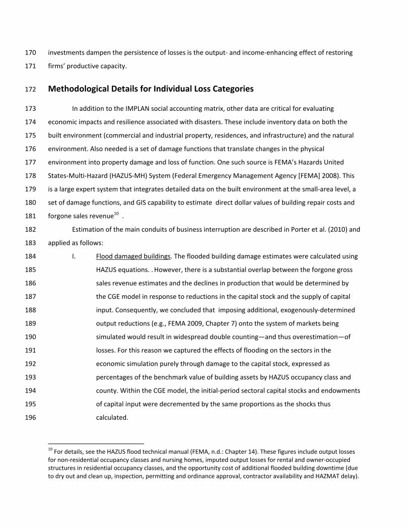
Figs. 1 and 2 illustrate the temporal patterns of ARkStorm’s impacts, in terms of the 313

contributions of individual components of damage to the path of California’s GDP in the aftermath of 314

the storm, as well as the business interruption losses incurred during the recovery to the pre-storm level 315

of income (the “loss triangle”). The impacts of wind damage to buildings and damage to crops and utility 316

lifelines are all generally small and are broadly similar in terms of the magnitude of their long-run effects 317

on GDP. By contrast, building flood damage has a large and persistent impact, representing a one-time 318

downward shift in the growth path of the economy. This trajectory is closely tracked by our base case 319

simulation, in which damages in all four of these categories are imposed simultaneously. Interestingly, 320

the path of GDP implied by the sum of the individual damage components falls short of our base case. 321

The implication is that ex-post summation of the various categories of damages overstates the true 322

simultaneous impact, principally because producers and consumers are able to adjust to temporary 323

lifeline outages and reduced supplies of agricultural goods by engaging in substitution within and across 324

counties, in response to the storm’s differential impacts on the relative prices of input commodities and 325

factors. In the present setting, the difference in the resulting estimate is substantial, ranging from 6% in 326

the initial period to 33% at the end of the 5-year simulation horizon. Nevertheless, in every case 327

ARkStorm’s long-run impact is to move the economy to a lower growth path that parallels the slight 328

exponential GDP increase in the BAU trajectory. 17 The key implication of the CGE model’s supply-driven 329

framework is that without reconstruction of destroyed capital or some other exogenous infusion of 330

resources there is no mechanism by which the economy can recoup BI-related forgone output and 331

investment on its own. The result that business-as-usual levels of output and income are never re-332

attained within our evaluation time-frame. 333

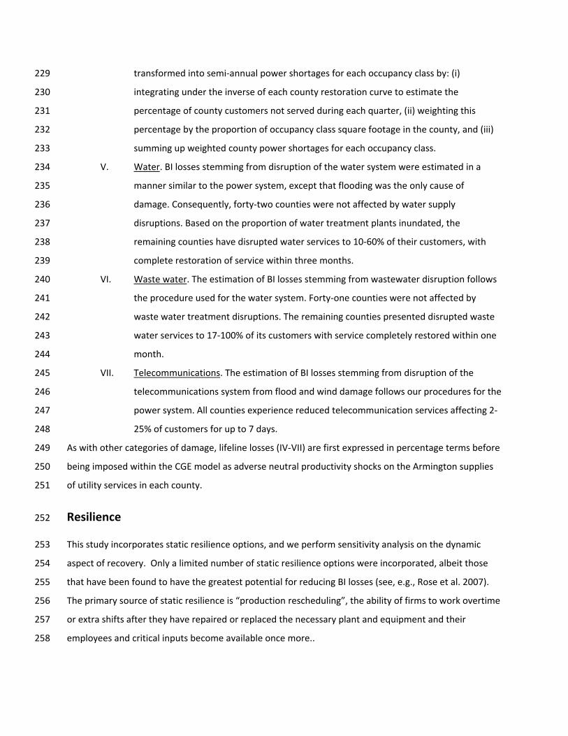
Fig. 2 provides a clearer picture of the differences among the lifeline, building wind damage and 334

agricultural impacts. Here, near-term losses are the value of forgone output over the period of recovery 335

to the pre-event level of GDP, given by the area of the triangle bounded by the axes and the trajectories 336

in the figure. Losses from agriculture damage vastly exceed those from the first two damage 337

components, because of the small magnitude of wind damage and the fact that lifeline losses attenuate 338

quickly. The corollary is that the hysteresis introduced by the very large loss of capital—and productive 339

capacity—due to flooding is the principal driver of overall losses, whether estimated as the short-run 340

loss triangle in Fig. 2 or as the area between BAU and post-event trajectories of GDP in Fig. 1. One final 341

noteworthy feature of Fig. 2 is the difference between the simultaneous and sum-of-damage loss 342

measures indicated by the solid and dashed heavy lines. After the first 6 months, losses in the latter 343

measure increase slightly before declining, reflecting the additional drag on the economy’s output from 344

persistent lifeline and agriculture damages. The simultaneous damages measure highlights the fact that 345

in cases such as this where the persistent effects are small, they can be counteracted by variable input 346

substitution. 347

The main results of our analysis are summarized in Table 1. . The first numerical column lists 348

property damage estimates developed by other research team members (see Porter et al. 2011). The 349

total is $353.6 billion (2007 dollars). The second column tabulates the loss estimates which form the 350

17 In a recursive-dynamic model with constant marginal propensity to save of the kind used here, a one-time loss of a portion of the capital stock shifts the economy onto a lower trajectory of output and capital accumulation. Holding constant other economic forces, output growth will resume at the rate that prevailed prior to the shock, but with smaller values of all economic quantities.

inputs to the CGE model, computed by normalizing the quantities in column 1 by their respective totals 351

and multiplying the result by the corresponding economic quantities in the CGE model. The difference 352

from column 1 highlights the fact that HAZUS’ “bottom-up” calculations based on estimates of the book 353

value of asset stocks produce results are largely incommensurate with the “top-down” macroeconomic 354

input-output accounts used to calibrate CGE models. While this divide is precisely what our data 355

translation procedures in Section IV attempts to bridge, we in no way expect the methodology 356

developed here to be the last word on this issue. Rather, our results are an invitation to economists and 357

engineers to jointly advance the methodological underpinnings of economic loss calculations. 358

Total BI losses relative to the BAU trajectory of the California economy are presented in column 359

3. When computed on a sum-of-damage-components basis, losses amount to $386.6 billion, similar in 360

magnitude to the losses tabulated in column 2 and some 9% larger than total property damage in 361

column 1. By far the largest component (nearly 65% of the total) is attributable to flooding. Losses from 362

Wind, Agriculture (damage to crops and arable land), and lifeline disruption are roughly equivalent.. 363

Some BI losses, such as those associated with Levee Repair and Relocation were not computed, but are 364

not likely to exceed their property damage counterparts, and thus do not represent any major omission 365

in the estimates. Total BI losses relative to the Pre-Storm GDP are presented in column 4. They amount 366

to $115.7 billion, 35% of the size of the estimates in column 1. Here, flood losses are an even higher 367

percentage of the total (90%). To put these results in perspective, the estimates in columns 1-4 would 368

render ARkStorm the largest disaster ever to hit the US. Property damages in column 1 are more than 369

three times those of Hurricane Katrina, as are the BI losses, which are more than three times those of 370

the September 11, 2001 World Trade Center attacks (Rose et al. 2009; Rose and Blomberg 2010). The 371

property losses from ARkStorm exceed the property damage estimates of the ShakeOut scenario 372

(approximately $100 billon). ShakeOut BI estimates were about $67 billion but were computed relative 373

to the pre-event GDP only. Moreover they were computed for a much smaller region (8 counties in 374

southern California). 375

In percentage terms, the summed BI losses represent 4.4% of GDP for the BAU Trajectory and 376

2.1% of pre-event GDP, comparable to the 4% loss in gross regional product incurred by ShakeOut. Note 377

that although total BI in column 3 is nearly four times as great as that in column 4, the percentage 378

relative to the baseline is less than twice as large, a result which reflects the consistent upward trend of 379

GDP in the various scenarios in Figs. 1 and 2. Even in the absence of dedicated reconstruction 380

investment, economic growth does resume after the shock to the economy, leading to more rapid decay 381

of losses relative to the Pre-Event GDP level, which causes the economic base for the calculation of 382

losses in column 4 to be much smaller than that used to compute losses for column 3. 383

Relative to pre-event GDP (column 4) and BAU trajectory (column 3) simultaneous losses are 384

41% and 29% lower than the corresponding sum-of-damage-components estimates, respectively. 385

Interestingly, the disparity between the simultaneous impacts underscores the difference in the 386

dynamic effects of storm damage. The absence of substitution reflected in the sum-of-damage-387

components estimate suggests a sub-optimal response by economic actors that implicitly leaves fewer 388

resources available for contemporaneous investment, leading to a diminished pace of capital 389

accumulation that places the economy on a growth path that is not just lower, but also slower. Thus, as 390

reinforced by Fig. 2, both the distance and the area between the trajectories of losses (indicated 391

respectively by the heavy solid and dashed lines) grows as time goes on. Consequently, the areas of two 392

near-term loss triangles are closer to one another in size than the corresponding trapezoids of GDP 393

losses relative to the BAU scenario over the entire simulation horizon. 394

Columns 5 and 6 summarize the results of these scenarios assuming producers’ ability to recoup 395

losses through recapture. While production rescheduling has a slight effect on the costs of agricultural 396

and lifeline damage, it has a more substantial mitigating impact on the present value of wind and 397

particularly flood losses, to the tune of $1.8 billion and $29.5 billion, respectively. Recapture lowers both 398

the sum-of-damage-components and simultaneous-damage loss estimates by 8%, to $358.8 billion and 399

$249.3 billion. The impact on losses computed relative to pre-event GDP is more pronounced because 400

recapture is confined to the initial 12-month period after the storm, with a larger effect on the near-401

term loss triangle than on costs incurred over the longer simulation horizon. Present value losses are 402

23% lower when computed on a sum-of-damage-components basis, and 34% lower when all damages 403

are imposed simultaneously. The difference in these figures primarily reflects the larger loss triangle in 404

the former case, consistent with Fig. 2. 405

Sensitivity Analyses 406

We also performed several sensitivity tests on the base case simultaneous results. First, the 407

direct property damage/lifeline outage estimates were increased and decreased by 25% relative to their 408

base levels. This broad range is admittedly impressionistic. but our intent is to shed light on the potential 409

impact of uncertainty in the magnitude of the meteorological forcing (i.e., a larger or smaller storm). 410

As well, we simulated the effects of reconstruction investment on the economy following 411

ARkStorm. Our base case with reconstruction assumes full repair of wind and flood damage to the 412

capital stock by 24 months after the storm, with reconstruction spending making up lump sum 413

quantities of investment in the amount of 50% of initial capital losses 6-12 months after the storm, and 414

25% of capital losses in each of the subsequent semi-annual periods. Crucially, our default assumption is 415

that 50% of the funds for repair and reconstruction come from within California (via household savings 416

and retained earnings of businesses), and 50% flow in from outside (principally insurance payments and 417

federal government assistance). The use of domestic or “internal” funds displaces ordinary investment 418

in plant and equipment and residential structures, while “external” financing from outside California 419

results in a pure additive boost to the state’s productive capacity, with no opportunity cost. In particular, 420

we assume that every dollar of internal capital formation is purchased at the cost of more than a dollar’s 421

worth of principal and interest payments over the remainder of the simulation horizon, which dampens 422

the overall stimulus effect of repair and reconstruction in the long run.18 We quantify the importance of 423

this effect by performing sensitivity analyses around our equal division of financing between California 424

and rest-of-world sources, simulating cases with 75%-25% and 25%-75% internal-external financing 425

splits, as well as our 50%-50% base case with a 6-month delay in the availability of reconstruction funds. 426

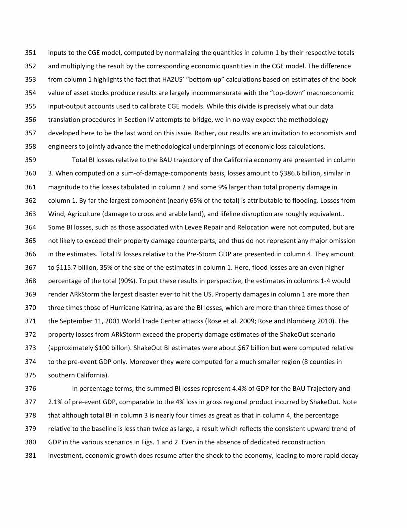
Fig. 3 shows the strong influence of production recapture (which takes place at a declining rate 427

during the first 12 months after the disaster). It also shows that the results are more sensitive to initial 428

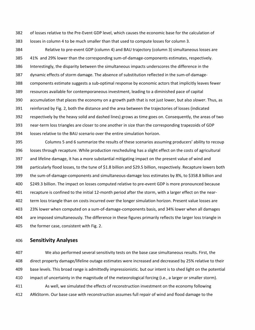
property damage (from storms of different magnitudes) than to the influence of reconstruction. Fig. 4 429

presents sensitivity analyses for the geographic origin of financing of reconstruction and for the effect of 430

delays in reconstruction. The former is far less influential on GDP losses than the latter. 431

The impact of scaling the various damage components is straightforward, shifting the base case 432

GDP trajectory upward or downward to the tune of $7 billion in each period (Fig. 3). More interesting is 433

the effect of reconstruction investment, the sign of which depends critically on the fraction of 434

reconstruction spending sourced internally (Fig. 4). Relative to the no reconstruction, no recapture base 435

case, our 50%-50% financing scenario generates savings of $3 billion 6-12 months after the storm, a 436

beneficial effect that decays linearly as time proceeds. The largest savings are an upward shift of GDP by 437

$8.5 billion to$15 billion, which arise when 75% of the cost of capital stock reconstruction comes from 438

outside California. Conversely, imposing a mandate that these economic actors raise these funds 439

internally exacerbates the long-run reduction in GDP, shifting it downward by $2 billion to $12 billion. 440

18 We assumed that each tranche of reconstruction spending was first distributed among counties in proportion to their aggregate capital stock damage, and then among the sectors within each county in proportion to their pre-event shares of capital. The resulting increment to investment stimulated additional growth in counties’ sectoral capital stocks. In simulating internal financing we made the simplest possible assumptions that the costs are distributed across households according to their ownership shares of California’s pre-event aggregate capital endowment, and are incurred at the opportunity cost of investment goods.

This additional loss stems from the resources dissipated in financing investment at a higher rate than in 441

the base case. For this reason, the need to rely heavily on domestic financing sources would seem to 442

militate against such a program of reconstruction, as economic actors would find it more cost-effective 443

to simply pursue a slower pace of investment, capital accumulation and economic growth, trading off 444

savings from avoided capital adjustment costs against forgone output at the margin. 445

The sensitivity results are summarized in Table 2. For the BAU Trajectory case, the 25% higher 446

(lower) direct damage case yielded an increase (decrease) in total BI losses of 22.9% (22.6%), indicating 447

that aggregate losses increase approximately linearly with the magnitude of the shock. Measured in 448

terms of pre-event GDP, the corresponding losses increase by 42.8% and decline by 36.7%, an 449

asymmetry reflecting the predominance of persistent capital stock and investment related damages 450

(with larger loss triangles) relative to shorter term lifeline and agriculture related damages. It is 451

straightforward to show that if the average rate of growth of aggregate GDP is invariant to the 452

magnitude of the overall shock, the area of the loss triangle varies approximately with the square of the 453

initial damage. Consequently, the same percentage increase and decrease in initial damage generate a 454

different percentage increase and decrease in the size of the loss triangle. 455

Under our default financing assumptions, reconstruction lowers the present value of BI losses by 456

6% over the 5-year horizon, to $257.4 billion and by 14% when measured relative to pre-event GDP, to 457

$57.9 billion. This more elastic near-term response is symptomatic of the drag on the economy created 458

by the additional expenditure necessary to finance the domestic component of reconstruction. While 459

the supplemental investment provided by the principal stimulates a rapid increase in the economy’s 460

productive capacity and output in early periods, the associated financing charges reduce the resources 461

available for investment over the entire horizon, slowing the growth of output in later periods. 462

Rows E, F and G illustrate the sensitivity to our assumption of a 50%-50% internal-external 463

financing split. As expected a larger share of external financing reduces the quantity of investment 464

principal and the stream of internal financing payments, and long-term drag on economic growth. The 465

sensitivity of losses to financing assumptions are larger when calculated over the entire simulation 466

horizon than over the short-run loss triangle. Losses for 75%-25% internal-external case were estimated 467

to be $343 billion, one-third higher than in the 50%-50% case. Symmetrically, losses in the 25%-75% 468

internal-external case are one third lower. Recasting these figures in terms of recovery to pre-event 469

GDP, financing 75% of reconstruction through domestic sources is accompanied by 48% higher BI losses 470

than in row E ($85.9 billion), while having to finance only 25% internally reduces BI losses by one quarter 471

($43.3 billion). 472

Row H assumes a 6-month delay in reconstruction spending, which generates a 7% increase in BI 473

losses over row E, to $275.2 billion, while losses relative to pre-event GDP increase by 10%, to $63.8 474

billion.. Delayed reconstruction lengthens the lag between the initial capital stock losses and the 475

compensating output-expanding stimulus, increasing the size of the near-term loss triangle. In addition 476

to forcing the economy to forgo six months of higher output, our assumption of a fixed-end date for 477

reconstruction financing translates into a shorter sequence of larger payments, which further attenuates 478

long-term economic growth. The former lump-sum loss outweighs the latter amortized loss, resulting in 479

a front-loaded BI cost that is larger in present value terms. Lastly, rows D and I summarize the results of 480

simulations with recapture as a point of comparison. In row D, the mitigating effects of recapture alone 481

offset BI by a somewhat larger amount than our reconstruction case with 50% internal financing.. 482

Overall, the sensitivity results exhibit a modest range of variation, which gives us confidence in 483

the robustness of our base case loss estimates. The key insight from the difference in the savings due to 484

recapture versus reconstruction investment is that time is of the essence in disaster recovery. The 485

biggest benefit of resilience derives from components whose mitigating effects kick in quickly after the 486

event. Recapture’s larger effect in both the short- and the long run arises from its ability to offset 487

damage to productive capacity in the first post-storm period that is not only large but carries the 488

heaviest weight in our present value calculation. This mitigates the large drop in initial output that 489

would otherwise occur, and indirectly cushions the shock to investment, which makes available a larger 490

supply of capital—facilitating the generation of more output—in every subsequent period. Finally, our 491

analysis indicates that even a very high level of external financing is not sufficient to completely shift the 492

economy back to its BAU trajectory of growth, as has been the case in a small percentage of disaster 493

aftermaths (e.g., the Northridge Earthquake). 494

Conclusion 495

We have estimated the economic impacts of ARkStorm to potentially much more than one 496

hundred billion dollars over a five-year period. There are uncertainties in the cost estimates (noted as 497

ranges for lifelines and agricultural damages). However, the relative order of magnitude of the results is 498

likely representative of the domination of flooded building damages and economic impacts followed by 499

lifeline services, water service in particular. Although agricultural impacts are estimated as relatively 500

light, they are of a much greater scale than experienced during previous California storms. 501

The novel aspect of this study is its use of a computable general equilibrium approach to 502

systematically characterize and quantify the economic consequences of the full spectrum of individual 503

but overlapping impacts of a large-scale natural disaster. The input-output approaches utilized by 504

ShakeOut and similar studies (for reviews see Okuyama and Chang 2004; Okuyama 2007) have difficulty 505

capturing the feedback effects of property damage, temporary interruptions in labor supplies, and 506

hysteretic adverse productivity shocks on prices, producers’ and consumers’ substitution responses, and 507

concomitant intersectoral supply-demand adjustments across the economy. Distinctly, prior CGE 508

analyses of the effects of disasters either limit consideration of impacts to a fairly narrow range of 509

damage categories (e.g., Rose et al. 1997; Rose and Liao 2005; Rose et al. 2007), or express the shock to 510

the economy in a highly aggregate fashion with little differentiation among different types of damage 511

(e.g., Selcuk and Yeldan 2001; Narayan 2003), potentially leading to under- or double-counting of 512

impacts (respectively) and their associated macroeconomic costs. within a CGE framework , remaining 513

issues depend on empirical characterization of technological progress from innovations embodied in 514

new capital, changes in household savings rates in the post-disaster economic environment, geographic 515

relocation of firms, and optimal use of reconstruction investment.. Bearing these issues in mind, our key 516

contribution is the development of algorithms for translating the outputs of geospatial engineering 517

models of disaster damage (HAZUS) into sequences of shocks to capital stocks and productivity in 518

various industry sectors that can be employed as inputs to economic impact assessment simulations. By 519

addressing several of the methodological concerns outlined in Rose (2004) and Okuyama (2007), the 520

current advance provides a roadmap for refining future estimates of both the macroeconomic costs of 521

disasters and the influence of resilience in reducing economic losses. 522

Acknowledgements 523

The authors thank many other research team members involved in the ARkStorm Scenario, most 524

notably Keith Porter, for providing data and other assistance during the course of this research. We 525

acknowledge the help of Dan Wei of USC and Laura Dinitz with some of the data refinement and 526

processing. We appreciate the insightful review comments from Wade Martin and Philip Ganderton. 527

References 528

Applied Technology Council. (1991). “Seismic vulnerability and impacts of disruptions of utility lifelines in 529

the conterminous United States.” Report ATC-25, Redwood, CA: Applied Technology Council. 530

Brooke, A., Kendrick, D., Meeraus, A., and Raman, R. (1998). GAMS: A User’s Guide, Washington DC: 531

GAMS Corp. 532

Chang, S. E., Pasion, C., Tatebe, K., and Ahmad, R. (2008). “Linking lifeline infrastructure performance 533

and community disaster resilience: models and multi-stakeholder processes.” MCEER-08-0004. 534

Dixon, P. B., Lee, B., Muehlenbeck, T., Rimmer, M. T., Rose, A., and Verikios, G. (2010). “An H1N1 535

epidemic in the US: Analysis using a quarterly CGE model,” Journal of Homeland Security and 536

Emergency Management 7(1): Article 75. 537

European Union. (2003). Proceedings of the Joint NEDEIS and University of Twente Workshop: In Search 538

of a Common Methodology for Damage Estimation, Bruxelles: Office for Official Publications of the 539

European Communities. 540

Federal Emergency Management Agency (FEMA). (2008). Earthquake loss estimation methodology 541

HAZUS-MH MR3 (HAZUS). Washington, DC: National Institute of Building Sciences. 542

Federal Emergency Management Agency (FEMA). (2009). Multi-hazard loss estimation methodology 543

flood model HAZUS®MH MR4, <http://www.fema.gov/library/viewRecord.do?id=3726>. 544

Ferris, M. C., Munson, T. S., and Ralph, D. (2000). “A homotopy method for mixed complementarity 545

problems based on the PATH Solver”, Numerical Analysis, D. F. Griffiths and G. A. Watson, eds., 546

Chapman and Hall, London, 143-167. 547

Jones, L. M., Bernknopf, R., Cox, D., Goltz, J., Hudnut, K., Mileti, D., Perry, S., Ponti, D., Porter, K., Reichle, 548

M., Seligson, H., Shoaf, K., Treiman, J., and Wein, A. (2008), “The ShakeOut Scenario.” U.S. 549

Geological Survey Open File Report 2008-1150 and California Geological Survey Preliminary Report 550

25, version 1.0, <http://pubs.usgs.gov/of/2008/1150>. 551

Minnesota IMPLAN Group (MIG). (2006). Impact Analysis for Planning (IMPLAN) System, Stillwater, MN. 552

Multihazard Mitigation Council (MMC). (2005). “Natural hazard mitigation saves: Independent study to 553

assess the future benefits of hazard mitigation activities, study documentation, vol. 2.” Report to the 554

Federal Emergency Management Agency by the Applied Technology Council, National Institute of 555

Building Sciences, Washington, DC. 556

National Research Council. (2005). Improved seismic monitoring--Improved decision-making: Assessing 557

the value of reduced uncertainty, National Academy Press, Washington, DC. 558

Porter, K., Wein, A., Alpers, C., Baez, A., Barnard, P., Carter, J., Corsi, A., Costner, J., Cox, D., Das, T., 559

Dettinger, M., Done, J., Eadie, C., Eymann, M., Ferris, J., Gunturi, P., Hughes, M., Jarrett, R., Johnson, 560

L., Dam Le-Griffin, H., Mitchell, D., Morman, S., Neiman, P., Olsen, A., Perry, S., Plumlee, G., Ralph, 561

M., Reynolds, D., Rose, A., Schaefer, K., Serakos, J., Siembieda, W., Stock, J., Strong, D., Sue Wing, I., 562

Tang, A., Thomas, P., Topping, K., and Wills, C.; Jones, Lucile, Chief Scientist, Cox, Dale, Project 563

Manager (2011). “Overview of the ARkStorm Scenario.” U.S. Geological Survey Open-File Report 564

2010-1312, <http://pubs.usgs.gov/of/2010/1312/>. 565

Rose, A. (2004a). “Economic principles, issues, and research priorities of natural hazard loss estimation.” 566

Modeling of spatial economic impacts of natural hazards, Y. Okuyama and S. Chang, eds., Springer, 567

Heidelberg. 568

Rose, A. (2004b). “Defining and measuring economic resilience to disasters.” Disaster Prevention and 569

Management, 13, 307-14. 570

Rose, A. (2009). “Economic resilience to disasters.” Community and Regional Resilience Institute Report 571

No. 8. 572

Rose, A., and Liao, S. Y. (2005). “Modeling regional economic resilience to disasters: A computable 573

general equilibrium analysis of water service disruptions.” Journal of Regional Science, 45, 75-112. 574

Rose, A., Wei, D., and Wein, A. (2011). “Economic impacts of the ShakeOut.” Earthquake Spectra Special 575

Issue on the ShakeOut Scenario, 27(2), 539-57. 576

Rose, A., Oladosu, G., Lee, B., and Beeler-Asay, G. (2009). “The economic impacts of the 2001 terrorist 577

attacks on the World Trade Center: A computable general equilibrium analysis.” Peace Economics, 578

Peace Science, and Public Policy, 15(2), Article 4. 579

Rose, A., Porter, K., Dash, N., Bouabid, J., Huyck, C., Whitehead, J., Shaw, D., Eguchi, R., Taylor, 580

C., McLane, T., Tobin, L.,Ganderton, P., Godschalk, D., Kiremidjian, A., Tierney, K., and West, 581

C. (2007). ”Benefit-Cost Analysis of FEMA Hazard Mitigation Grants.” Nat. Hazards Rev., 8(4), 97–582

111. 583

Rutherford, T.F. (1999). “Applied general equilibrium modeling with MPSGE as a GAMS subsystem: An 584

overview of the modeling framework and syntax,” Computational Economics, 14, 1-46. 585

Sue Wing, I. (2009). “Computable general equilibrium models for the analysis of economy-environment 586

interactions.” Research tools in natural resource and environmental economics, A. Batabyal and P. 587

Nijkamp, eds., World Scientific, Hackensack. 588

Sue Wing, I. (2010). “ARkStorm computable general equilibrium model documentation,” Boston 589

University, Boston, MA. 590

Tierney, K. (1997). “Impacts of recent disasters on businesses: The 1993 Midwest floods and the 1994 591

Northridge earthquake.” Economic consequences of earthquakes: Preparing for the unexpected, B. 592

Jones, ed., National Center for Earthquake Engineering Research, Buffalo, NY. 593

United Research Services and Jack R. Benjamin & Associates. (2008). “Delta Risk Management Strategy 594

(DRMS), Phase 1: Final risk analysis report.” Rep. Prepared for California Department of Water 595

Resources. <http://www.water.ca.gov/floodsafe/fessro/levees/drms/phase1_information.cfm> 596

(Feb. 1, 2013). 597

Wein, A., and Rose, A. (2011). “Economic resilience lessons from the ShakeOut Earthquake Scenario.” 598

Earthquake Spectra, 27(2), 559-73. 599

Table 1. Summary of ARkStorm Property Damage and Business Interruption for California, Without Reconstruction (billion 2007 $)

Property Damage

Business Interruptiona

Without Recapture With Recapture (1)

HAZUS/ DWR models

(2) CGE

modelb

(3) Relative to

projected GDP

(4) Relative to

pre-event GDP

(5) Relative to

projected GDP

(6) Relative to

pre-event GDP Building Flood Damage 195.0c 376.6 270.5 [3.1%] 62.5 [1.8%] 246.0 [2.8%] 42.6 [1.2%] related content damage 103.0 Building Wind Damage 5.6 4.7 40.8 [0.5%] 1.7 [0.2%] 39.0 [0.4%] 0.3 [0.03%] Agricultural Damaged 3.6e 1.3a 38.5 [0.4%] 1.5 [0.07%] 37.3 [0.4%] 0.6 [0.07%] Lifeline Damage 6.9f,g,h 0.5a 36.8 [0.4%] 0.04 [0.005%] 36.5 [0.4%] 0.02 [0.002%] Levee Repair/Island Dewatering 0.5i n.a.j n.a. n.a. n.a. n.a. Relocation 39.0k n.a.l n.a. n.a. n.a. n.a. Sum of Damage Categories

353.6 383.0 386.6 [4.4%] 115.7 [2.1%] 358.8 [4.1%] 89.3 [1.3%] Simultaneous Impact of Damages 274.6 [3.1%] 67.6 [1.9%] 249.3 [2.8%] 44.4 [1.2%] a Present value calculation using a 5% discount rate. Absolute and percentages losses calculated relative to the present value of real GDP in the BAU scenario. b These numbers represent HAZUS and DWR losses normalized by their respective benchmark values to generate percentage shocks, which are then multiplied by the relevant economic quantities in the CGE model see Section IV for details). c Weather and flood warning (of at least 48) hours could reduce building and content damages by $30 billion, while demand surge could increase property repair cost by $70 billion (Porter, 2011). d Agricultural costs pertain to field damage, crop and livestock replacement and forgone income from crop losses. e Agricultural losses increase to $6.8 billion for high-end range of flood duration estimate f Power system repair cost estimates range from $0.3-$3 billion. g Water system repair cost estimate ranges from $1-10 billion. h Highway repair cost estimate ranges from $2-3 billion. i Levee repair and dewatering costs pertain to the levees and islands in the San Joaquin Delta only. j Potentially, levee repair and Island dewatering time could increase BI losses by increasing agricultural damages. k $39 billion relocation costs calculated using HAZUS formulas, $25 billion for relocation of residences, $11 billion for relocation of commercial establishments, and the remainder for industry, education, religion and agricultural occupancy classes. l Indirect effects of relocation have not been evaluated; building service interruption multipliers have not been developed for the flood module of HAZUS-MH.

Table 2. Present Value of Absolute and Percentage GDP Losses (5% discount rate)

Relative to BAU GDP Trajectory

Relative to Pre-Event GDP Level

(billion 2007$) (%) (billion 2007$) (%) A. Base case damages

(no recapture, no reconstruction) 274.6 3.1 67.6 1.9

B. 125% x all base case damages 337.4 3.8 96.5 2.1 C. 75% x all base case damages 212.5 2.4 42.8 1.5 D. Base case damages with recapture

(no reconstruction) 249.3 2.8 44.4 1.2

E. Base case damages with reconstruction (50%-50% internal-external financing)

257.4 2.9 57.9 1.6

F. Base case damages with reconstruction (75%-25% internal-external financing)

343.0 3.9 85.9 1.9

G. Base case damages with reconstruction (25%-75% internal-external financing)

170.0 1.9 43.3 1.6

H. Base case damages with reconstruction (delayed 6 months)

275.2 3.1 63.8 1.7

I. Base case damages with recapture and reconstruction (50%-50% internal-

external financing)

236.4 2.7 38.5 1.1

Fig. 1. ARk

kStorm impaccts on the trajectory of semmi-annual reaal GDP

Fig. 2. ARk

kStorm semi--annual losses

s and recoverry relative to

pre-event GDDP

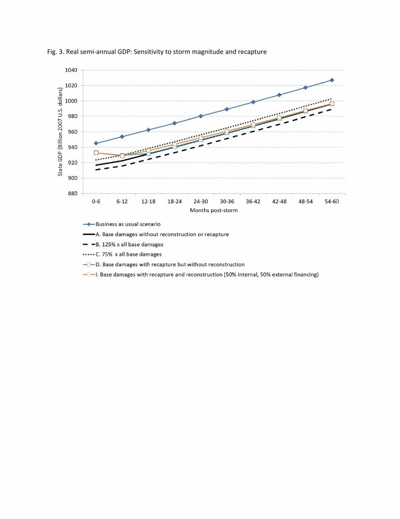
Fig. 3. Reaal semi-annuaal GDP: Sensittivity to stormm magnitude and recapturre

Fig. 4. Sem

mi-annual reaal GDP: Sensittivity to reconnstruction andd its financingg