economic model for optimal flood risk transfer · economic model for optimal flood risk transfer...

i

Economic Model for Optimal Flood Risk Transfer By

Lyndsey Blanche Croghan

B.S. (Oregon State University) 2010

THESIS

Submitted in partial satisfaction of the requirements for the degree of

MASTER OF SCIENCE

in

Civil Engineering

in the

OFFICE OF GRADUATE STUDIES

of the

UNIVERSITY OF CALIFORNIA

DAVIS

Approved:

Jay R Lund, Chair

Beth A Faber

Fabian Bombardelli

Committee in Charge

2013

ii

Lyndsey Blanche Croghan Civil Engineering

Economic Model for Optimal Flood Risk Transfer Abstract

This thesis examines the concepts of economic flood risk transformation and transference among floodplain users. Risk transference shifts flood damages among locations or floodplain users. Risk transformation changes the frequency of flood damage across low and higher consequence outcomes. These phenomena are explained by modeling the economically optimal distribution of flood damages between floodplains on opposite river banks. A hypothetical river reach is used as an example, where a city lies on one side of the reach and agricultural land on the other. Levee heights on either riverbank are optimized for the least total cost. Reduction in total flood risk can occur from transferring risk from the urban side to the rural side of the river. Risk transfer can reduce overall flood damages, but can increase individual damages. Compensation for transferred risks can improve conditions for all parties.

iii

Table of Contents Abstract ......................................................................................................................................................... ii

1 Introduction ..................................................................................................................................... 1

2 Shifting Flood Risk ............................................................................................................................ 2

2.1 Presenting Risk ...................................................................................................................... 2

2.2 Risk Transfer .......................................................................................................................... 3

2.3 Risk Transformation .............................................................................................................. 4

2.4 Flood Risk Management Policy ............................................................................................. 5

3 Example and Methods ..................................................................................................................... 6

3.1 Methods ................................................................................................................................ 7

4 Levee System Design & Risk Transfer and Transformation ............................................................. 9

4.1 Equal Levee System Design Heights .................................................................................... 10

4.1.1 Society Optimal Levees ....................................................................................................... 11

4.1.2 Agriculture Optimal Levees ................................................................................................. 11

4.1.3 City Optimal Levees ............................................................................................................. 12

4.1.4 Comparisons ....................................................................................................................... 12

4.2 Unequal Levee System Design Heights ............................................................................... 13

4.2.1 Society Optimal Unequal Levees ......................................................................................... 13

4.2.2 Agriculture Optimal Unequal Levees .................................................................................. 17

4.2.3 City Optimal Unequal Levees .............................................................................................. 18

4.2.4 Total Value Net Benefits ..................................................................................................... 18

4.2.5 Risk Transformation ............................................................................................................ 19

5 Flood Damage Compensation ........................................................................................................ 19

5.1 Example ............................................................................................................................... 21

6 Conclusions, Limitations, and Further Research ............................................................................ 23

6.1 Conclusions ......................................................................................................................... 23

6.2 Limitations ........................................................................................................................... 24

6.2.1 Failure Before Overtopping................................................................................................. 24

6.2.2 Damage Estimation ............................................................................................................. 24

6.3 Further Research ................................................................................................................. 25

References .................................................................................................................................................. 26

iv

List of Figures

Figure 1 FD curve indicating the effects of risk transfer and transformation (Jonkman, 2008) ................... 2

Figure 2 Consequences of levee raising on the right bank of a river ............................................................ 3

Figure 3 FD Curve: Transformation of risk to lower probability events ....................................................... 5

Figure 4 Plan view of example river reach .................................................................................................... 6

Figure 5 Profile view of varying levee height relationships .......................................................................... 8

Figure 6 Log-Pearson Type III flow frequency distribution ........................................................................... 9

Figure 7 Optimal equal levee height for agriculture to city damages $100:$500 million .......................... 10

Figure 8 Optimal unequal lower levee height for agriculture to city damages $100:$500 ........................ 14

Figure 9 Minimum total cost of optimal levee pairs ................................................................................... 15

Figure 10 Project costs for $100 and $500 million in possible damages .................................................... 16

Figure 11 Total cost surface of unequal levee pairs for $100:$500 million in possible damages .............. 17

v

List of Tables

Table 1 Assumed parameter values .............................................................................................................. 9

Table 2 Society optimal equal levee heights............................................................................................... 11

Table 3 Optimal equal levee heights from rural perspective ..................................................................... 12

Table 4 Urban optimal equal levee heights ................................................................................................ 12

Table 5 Summary of optimal equal levee heights ....................................................................................... 13

Table 6 Society optimal unequal levee heights .......................................................................................... 15

Table 7 Rural optimal unequal levee heights.............................................................................................. 18

Table 8 Urban optimal unequal levee heights ............................................................................................ 18

Table 9 Optimal total net benefits of each design case .............................................................................. 19

Table 10 Methods for raising compensation funding ................................................................................. 21

Table 11 Society optimal unequal levee heights with easement purchase ................................................ 22

Table 12 Society optimal unequal levee heights with disaster relief ......................................................... 23

1

1 Introduction

Flood risk is defined as the product of flood event probability and resulting damage. Typically, risk increases with land development. Despite best efforts to reduce peak flow frequencies using flood control structures, damage potential often tends to increase faster. Non-structural actions such as evacuation plans, emergency notification systems, or enhanced flood safety awareness can help curb some types of risk by reducing potential damage. However, flood management actions also change how risk is distributed. Risk transformation and risk transference describe changes in flood location, frequency, and damage for flood management systems. As individuals strive to reduce their own risk, it may increase risk for others, with either a net increase or decrease in overall flood risk.

Understanding risk transference and transformation enables flood control districts, property owners, private businesses, and local, state, and federal governments to make more informed flood management decisions. For example, the Sacramento River bypass system in California’s Central Valley shifted floodwaters from high risk urban areas to low risk agricultural lands, particularly flood bypass areas, where flood easements were purchased (Kelley, 1989). These risk transformations and transference were understood and compensated. Transfer of risk occurs when damages increase in one location because a flood control structure decreases damages in another location that is hydraulically connected. Risk transformation occurs when flood consequences change due to a change in the frequency and magnitude of events.

Despite the desire to protect against all flood damage, shifting flood risk is often more beneficial than reducing it overall. Trading flood risk, like air pollution in an emissions market or water in a water market, can allow individuals or groups to compensate one another for flood damage shifts and interactions (Chang, 2008). Also, society may find it acceptable to compensate individuals for small flood damages incurred so larger damages are avoided. In either case, economic models can simulate damage estimates for various flood management cases. In turn, the results can help inform managers about where flood control is most valuable by the standards of the affected populations.

While total flood risk includes risk to life, an economic model only measures the economic risk of flooding. Economic risk is the direct and indirect monetary consequences of flooding and is usually calculated at a societal level (Vrijling, 2011). Damages are summed across many individual flood losses over a region. These regions can vary in size depending on the relationship between individuals in the floodplain. For example, the Columbia River reservoir system in the US Pacific Northwest spans several states and parts of Canada and was built to reduce flood risk for many communities. The Sacramento bypass system provides more local protection as floodwaters are diverted out of stream before reaching high risk communities.

Understanding economic risk is important for measuring the benefits of flood management actions. Cost-benefit analysis quantitatively compares the risks of a variety of actions or decisions and their costs, helping decision makers to choose appropriate actions. The economic model developed here compares the benefits of decreased overall economic risk to the cost of increasing individual risk. This is accomplished by calculating the expected value of damages associated with each combination of levee heights on either side of a river. As flood protection levels increase from the base case, the transformation of economic risk can inform the ultimate flood management decision (Jonkman, 2008)

This study develops a model of flood risk transference and transformation to find an optimal levee system capacity near a high risk urban community. First, risk transformation and transference are discussed, followed by a description of the study area. The assumptions and methods for developing the model are listed. Results of the model are presented and analyzed to identify optimal distributions of flood risk within the study area. Resulting insights and conclusions are then discussed.

2

2 Shifting Flood Risk

In current literature, a distinction is made between flood management actions that reduce flooding probability and those that reduce the consequences of flooding (Chang, 2008; Escuder-Bueno, 2012; Etkin, 1999; Jonkman, 2008; Vrijling, 2001; Lund, 2012). Here, changing flooding probabilities is referred to as risk transformation and changing the users or locations affected is risk transfer. These actions both reduce and shift flood risks from a base case. The distinction is important to decision makers who must balance the interests of different stakeholders with the physical and fiscal constraints of their floodplain. For urban areas bisected by a river, levee strengthening may be the only option and could transform risk to less frequent and larger floods if development continues. If spatial planning has left adequate room, however, floodwaters could be diverted to lower consequence areas thereby transferring the risk to other individuals or unoccupied areas, even while reducing total risk.

2.1 Presenting Risk

Frequency-Damage (FD) curves can help describe the process of risk transfer. An FD curve illustrates the relationship between frequency and damages at a local or societal level. In Figure 1, plotting damages against the annual probability of exceedance shows how consequences change with flood frequency. Jonkman (2008) identifies how shifts in risk are demonstrated on an FD curve. Flood management actions that change the probability of an event cause the curve to move along the probability axis. Actions that change the consequences of an event result in the FD curve shifting left or right along the damages axis.

Integrating an FD curve over the range of floods yields the Expected Annual Damages (EAD), or the mean of the damage distribution. In Equation 1, EAD is the sum product of flood damages, D(Q), and their flood probability, P(Q), over all flows, Q.

𝐸𝐴𝐷 = ∫ 𝐷(𝑄)𝑃(𝑄)𝑑𝑄∞0 Equation (1)

The EAD represents the long term average possible damages to a floodplain or group of users that have some level of protection. Therefore, a change in EAD is the measureable effect of risk transfer and transformation. Comparing EAD before and after implementation of a new flood management project indicates where and by how much risk has changed.

Figure 1 FD curve indicating the effects of risk transfer and transformation (Jonkman, 2008)

1.00E-08

1.00E-07

1.00E-06

1.00E-05

1.00E-04

1.00E-03

1.00E-02 10 100 1000 10000

Prob

abili

ty o

f Exc

eeda

nce,

/yr

Damages, $k/event

Actions to reduce the consequences

Actions to reduce the probability

3

2.2 Risk Transfer

When a flood control structure protects a specific area or damage category (population, property, etc.) it can increase flood risk for other areas or users. For example, higher levees on one side of a river increase flood damages on the other side of the river where floodwaters will overtop the lower levees more frequently and extensively. Retaining major floods in reservoirs similarly increases damages around the reservoir rim to avoid larger economic damages downstream. And containing floodwaters in a channel with high levees on both sides passes more flow faster, reducing flood wave attenuation and causing higher flood peaks for downstream users.

Using the example of constructing higher levees on one side of a river (the right side), risk is transferred when flood damage decreases on the right side of the river, but increases on the left side. The corresponding FD curve for the right side shifts down the probability axis. The higher right bank levees reduce probability of consequences from smaller floods, but may increase consequences for larger floods as the floodplain develops over time (Figure 2b). This causes the FD curve to shift to the right on the damages axis, beyond the initial maximum damage. In Figure 2b, the same larger low exceedance event now has greater consequences associated with it while smaller high exceedance events have much fewer consequences than before.

Figure 2 Consequences of levee raising on the right bank of a river

(Figure 2a Left bank FD Curve, Figure 2b Right bank FD curve)

A different FD curve applies to the left side of the river. The FD curve in Figure 2a indicates larger consequences for infrequent floods and much more damages from more frequent floods. This is because the risk of flooding is shifted from the right side of the river to the left by the levee improvements only on the right bank (Escuder-Bueno, 2012). In other words, the higher right bank levees push floodwaters away from one side of the river to the opposite floodplains. The left side of the river will experience more flooding when overtopping of the left bank levee occurs because flow will only be allowed on that side by the higher right bank levee; flood frequency has not increased, but the consequences per flood event have.

When floodwaters are transferred from one group of users to another, compensation can be made in different ways. For example, when the US Army Corps of Engineers designs a new off-stream floodway to reduce damages for downstream users, they can purchase, from upstream users, the right to flood their lands. The right is known as a flowage easement and it prohibits construction or maintenance of structures for habitation or that reduce flood storage or conveyance capacity. State and local flood

1.0E-08

1.0E-07

1.0E-06

1.0E-05

1.0E-04

1.0E-03

1.0E-02 $10 $100 $1,000 $10,000

Floo

d Fr

eque

ncy,

/yr

Damages, $k

Before After 1.0E-08

1.0E-07

1.0E-06

1.0E-05

1.0E-04

1.0E-03

1.0E-02 $10 $1,000 $100,000

Floo

d Fr

eque

ncy,

/yr

Damages, $k

Before After

4

control agencies also use easements to increase regional flow capacity. Because no development may occur in an easement, they often consist of agricultural or habitat land. The Yolo Bypass on the Sacramento River, for example, is largely agricultural but is also home to the Yolo Bypass Wildlife Area that supports migrating water fowl and native fisheries.

Risk transfer compensation also occurs internationally as in the case of the Columbia River Treaty between the United States and Canada. Under the agreement, Canada built three dams to provide flood storage in the upper reaches of the river basin and the US developed a reservoir that crosses the border and backs into Canada 42 miles. In exchange for the increased flood protection, the US paid Canada a total of $64.4 million for the estimated flood damages prevented. Canada also received the right to half of the additional potential hydropower benefits generated in the lower reaches of the Columbia due to flow regulation by the reservoirs, but sold the rights to various US power companies for $254 million. Combined, the payments helped Canada fund the development of three Treaty dams in the 1960s and 70s (Hyde, 2010).

2.3 Risk Transformation

Transformation of risk describes flood management actions that change the probabilities of flood events or consequences. Some risk that would have occurred during a given event of some frequency is shifted to larger and smaller events. An increase in consequence of large floods often is a byproduct of society protecting itself against the lesser, more frequent floods (Etkin, 1999). Risk transformation is most common in areas where new levee construction or strengthening has encouraged economic development. With the promise of greater flood protection, new homes, businesses, and infrastructure are built behind levees that were originally only designed to withstand up to a specific flood event. If the design flood is ever exceeded, the consequences would be much greater once there is added development behind the levees. By decreasing the probability of events below the design flood, development is encouraged and risk is transformed to events larger than the design flood.

Risk transformation can increase long term vulnerability by non-structural flood management actions as well. For example, local governments are required by the US National Flood Insurance Program (NFIP) to use zoning or other actions to restrict development in a designated flood hazard area, often the 100-year floodway. But they are not bound to such actions in the remainder of a floodplain that may be susceptible to larger events (Burby, 2001). During these larger floods, floodplain occupants will experience greater damages because they were not prepared for flooding. By choosing not to develop in a more frequent floodway, but allowing development in a less frequent floodway, this community has transformed their flood risk from smaller and more frequent to larger and less frequent events.

Figure 3 graphically illustrates transformation of risk: the FD curve is shifted down the probability axis. With levee improvements, damages are reduced for more frequent events though often increased at less frequent events. Again, better protection can encourage growth in a floodplain and cause more damages for large floods. In Figure 3, this explains the extension of the transformed FD curve past the maximum damages of the original FD curve.

Risk transformation can be examined in a stepwise fashion as a portfolio of risk reduction actions is implemented. Each has a level of protection corresponding to a specific probability of failure. Once that failure is reached, consequences increase quickly until the next reduction action becomes effective. Some actions may be more effective than others, but cause larger increases in consequences. For example, more damage occurs after the exceedance of a dam than the exceedance of a small scale drainage system (Figure 3). Risk transformation is a tradeoff: smaller and frequent flood damages are avoided while larger floods that exceed low probabilities of failure are more devastating.

5

Figure 3 FD Curve: Transformation of risk to lower probability events

2.4 Flood Risk Management Policy

For communities in known floodplains, improving or expanding existing flood control systems is important for encouraging economic development. An increasing knowledge of floodplain characteristics and flood frequencies, and wide variety of modern management techniques, creates a diverse decision making process to address improvements. Flood risk management policy seeks to provide a framework for this process so the effects on flood risk are duly accounted for during project design. The following section explores flood risk management policies, how they become policy, and issues with regulating flood risk.

In the United States, federal policy addressing risk transfer is administered by FEMA and USACE criteria that describe the design, construction, evaluation, operation, and maintenance of federally funded levees and reservoirs. In particular, some assumptions in hydraulic modeling must be made during the design of levee projects. Hydraulic models quantify the effect of a proposed levee project on a current or new flood management system. In urban areas, levee projects usually include sufficient levee freeboard over the desired design flood capacity to account for uncertainty in flood probability estimates, as well as wind-driven waves. In nonurbanized areas, a minimum crown elevation is required and overtopping of these levees is acceptable in the hydraulic model. This overtopping is simulated by weir behavior for nonurbanized levees, assuming no breach up to a design flood, and models the transfer of risk away from urban areas. Furthermore, non-project levees (those not funded but that affect project design) in nonurbanized areas must be modeled at existing height and also serve as weirs in the system (CA DWR, 2012).

Policies that seek to control the shift of flood risk do not occur without demand for upgrading flood control systems (Chang & Leentvaar, 2008). And any upgrades should be cost efficient in terms of damages reduced compared to costs incurred (transferred damages, construction, etc.) (Vrijling, 2001; Jonkman, 2008). If it were more cost effective to allow flooding of agricultural land on one side of a river, for example, and compensation was available, then demand would shift towards levee strengthening on the other side of the river. Or a community within a floodplain may find it economically efficient to build a levee system to protect against frequent flooding. In both cases, demand for reducing overall flood consequences precedes new policy and management actions.

1.0E-08

1.0E-07

1.0E-06

1.0E-05

1.0E-04

1.0E-03

1.0E-02 $10 $100 $1,000 $10,000 $100,000 $1,000,000

Floo

d Fr

eque

ncy,

/yr

Damages, $k

Maximum channel capacity

Reservoir Capacity

Drainage system capacity

Floodplain development

6

These reduced consequences are shared at a societal level, but might not seem or be fair to the individual. Socioeconomics affects risk transfer. A more affluent region will have higher flood risk due to the higher values of property, homes, and businesses. In a purely economic flood risk transfer model, areas of low value would be sacrificed for a net decrease in overall consequences. In turn, taking on additional flood risk would further decrease the value of development in the flood prone areas and make future economic growth difficult (Johnson, Penning-Roswell & Parker, 2007). Therefore, if society decides to protect higher value areas at the expense of lower value areas, a mechanism to compensate individuals for their increased flood risk can facilitate implementation.

The NFIP requires flood insurance of property owners within a floodplain and demonstrates the idea that institutional support facilitates the transference of risk. By delineating the 100-year floodplain and requiring flood insurance, the NFIP theoretically encourages individuals to seek federally funded flood protection to move out of the floodplain (or reduce their damages due to flooding) and decrease overall risk. Additionally, the actions or regulations of public agencies that favor returning floodplains to a more natural state or leaving more room for rivers to overflow also affect how flood risk is managed. The flood management policies of the State of California in the Sacramento Valley, for example, reflect this idea of spatial planning that incorporates flooding. As the view of controlling the rivers within the valley gave way to planning around inevitable flooding, bypass systems were built and levees set back. Now the risk from more frequent and smaller floods is reduced, but as development in the Valley continues to increase, so does risk associated with larger floods (Kelley, 1989).

As was the case in the Sacramento Valley, the timing of floods has a major effect on risk management policies and is an important mechanism for instigating policy change. Lange and Garrelts (2007) found that for two flood management cases in Germany, the only one in which policy changed was where local communities had suffered a large flood. Spurred on by recent events and an election, politicians passed new legislation requiring more floodplain designation, additional flood retention areas, and increased public awareness. Most importantly, new policy called for a basin-wide coordinated flood protection plan on the premise that every flood control structure built upstream can increase risk downstream. Recognizing that flood risk could be transferred became a critical component of flood management policy.

3 Example and Methods

Consider a hypothetical river network where several smaller tributaries and numerous watersheds feed into a large river prone to major flooding during one season each year. In a particular river reach, a large city lies on one side of the river while the other side is mainly agricultural and with a small population (Figure 4). The levees along this reach need improvement to meet new design flow standards, which would require raising levees on the urban side of the river. Initially, levee heights on both sides are roughly the same.

Currently there are no weirs or bypasses along this reach of the river to divert floodwaters so both sides of the river receive similar flooding. However, the total flood risk is much higher on the urban side because of higher urban damage potential. Raising urban levees above

Figure 4 Plan view of example river reach

7

rural levees would transfer floodwaters and decrease overall flood damages. The optimal design height of each levee depends on levee costs and reduction in economic flood damages, though modeling several levee height combinations will explore different levels of consequences.

To measure the benefits of levee improvement in this example flood plain, a base case is established using current conditions. The base case is the estimated annual urban and agricultural damages given equal levee heights and calculated for the range of potential peak flows. From here, the benefits of levee heightening can be measured as the reduction in EAD from the base conditions. The next section describes the methods used to calculate current and future damages and the benefits of levee improvement.

3.1 Methods

Flood damage to residential, commercial, industrial, and public infrastructure can be estimated using a stage-damage relationship developed for a specific flood plain or structure type. For simplicity in calculating EAD, total potential damages on each side of the river are constant for any levee overtopping and are weighted by the exceedance probability of the design flow for a particular levee height (Equation 2). In the initial case where levee heights are equal, damages are summed for the city and agricultural land to simulate simultaneous and complete levee system overtopping. By proposing levee improvements, either the urban or rural levee will be overtopped; only when levees are of equal height will overtopping occur on both sides. This means that damages will be reduced to one side of the river or the other except when levee heights are the same – then the greatest damages will occur. Flood risk and EAD simplifies to Equation 2 in this case.

𝐷𝑎𝑚𝑎𝑔𝑒𝑠,𝐷(𝐻) = 𝑃(𝑞(𝐻)) ∗ 𝐷 Equation (2)

𝐻𝑅 < 𝐻𝑈 𝐷𝑎𝑚𝑎𝑔𝑒𝑠 = 𝑃(𝑞(𝐻𝑅)) ∗ 𝐷𝑅

𝐻𝑅 = 𝐻𝑈 𝐷𝑎𝑚𝑎𝑔𝑒𝑠 = 𝑃(𝑞(𝐻𝑅)) ∗ (𝐷𝑅 + 𝐷𝑈)

𝐻𝑅 > 𝐻𝑈 𝐷𝑎𝑚𝑎𝑔𝑒𝑠 = 𝑃(𝑞(𝐻𝑈)) ∗ 𝐷𝑈

𝑞(𝐻) = design flow as a function of levee height (Manning’s equation)

𝑃(𝑞(𝐻)) = exceedance probability of design flow 𝑞(𝐻)

𝐷 = constant total damage potential for land use type (𝐷𝑈 for urban, 𝐷𝑅 for rural)

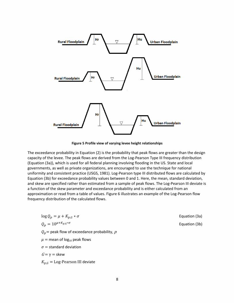
Figure 5 depicts the varying relationship between the urban and rural levees and helps illustrate where damages occur based on the constraining levee. The top graphic shows the case where the city levee heights are raised above the agriculture levees. The middle illustration depicts the initial state of the levee system and the last graphic shows the possibility of higher rural levees.

8

Figure 5 Profile view of varying levee height relationships

The exceedance probability in Equation (2) is the probability that peak flows are greater than the design capacity of the levee. The peak flows are derived from the Log-Pearson Type III frequency distribution (Equation (3a)), which is used for all federal planning involving flooding in the US. State and local governments, as well as private organizations, are encouraged to use the technique for national uniformity and consistent practice (USGS, 1981). Log-Pearson type III distributed flows are calculated by Equation (3b) for exceedance probability values between 0 and 1. Here, the mean, standard deviation, and skew are specified rather than estimated from a sample of peak flows. The Log-Pearson III deviate is a function of the skew parameter and exceedance probability and is either calculated from an approximation or read from a table of values. Figure 6 illustrates an example of the Log-Pearson flow frequency distribution of the calculated flows.

log𝑄𝑝 = 𝜇 + 𝐾𝑝,𝐺 ∗ 𝜎 Equation (3a)

𝑄𝑝 = 10𝜇+𝐾𝑝,𝐺∗𝜎 Equation (3b)

𝑄𝑝= peak flow of exceedance probability, p

𝜇 = mean of log10 peak flows

𝜎 = standard deviation

G = γ = skew

𝐾𝑝,𝐺 = Log-Pearson III deviate

9

Figure 6 Log-Pearson Type III flow frequency distribution

Now, flood damages can be estimated from levee overtopping probability and a reliable base case of the situation can be developed for a risk transfer comparison to any proposed levee system improvement. Levee improvements are also analyzed in terms of the cost of heightening levees and the benefits of decreased flood risk. The construction cost of increasing both urban and rural levee heights is calculated by unit cost per cubic meter of fill and discounted for a very long levee life (Equation (6)). Levee cost is then added to flood damages from Equation (2) for the total cost of each combination of city and agriculture levee design heights (Equation (7)). Optimal design heights will occur when damages are reduced enough that raising the levees only increases total cost.

𝐿𝑒𝑣𝑒𝑒 𝐶𝑜𝑠𝑡,𝐶(𝐻𝑅 ,𝐻𝑈) = 𝑇𝑜𝑡𝑎𝑙 𝑙𝑒𝑣𝑒𝑒 𝑣𝑜𝑙𝑢𝑚𝑒 ∗ 𝑈𝑛𝑖𝑡 𝑐𝑜𝑠𝑡 ∗ 𝐷𝑖𝑠𝑐𝑜𝑢𝑛𝑡 𝑟𝑎𝑡𝑒 Equation (4)

𝑇𝑜𝑡𝑎𝑙 𝐶𝑜𝑠𝑡 = 𝐷(𝐻) + 𝐶(𝐻𝑅 ,𝐻𝑈) Equation (5)

4 Levee System Design & Risk Transfer and Transformation

A levee system for the example reach is designed to maximize the sum of EAD and levee construction cost. These are calculated for a range of levee heights up to 25 meters and in increments of 0.25 meters. Total levee cost is determined by unit cost per cubic meter of fill for the levee dimensions listed in Table 1. Also in the table are the assumed parameters for calculation of maximum channel flow, above which damages occur. The last column lists hypothetical potential economic damages for the city and agriculture and their estimated annual discount rate.

Table 1 Assumed parameter values

Manning’s n 0.04 Crown width 7 m Annual discount rate 5%Width 200 m Wet & Dry slope 1.5 City $500 millionEnergy slope 0.0001 Length 20000 m Agriculture $100-$500 millionNormal stage 1.5 m Unit cost $30/m3

Channel Characteristics Levee Characteristics Potential Economic Damages

First, the agricultural and city levees are set to equal heights to simulate the initial condition where levees were originally built to protect agricultural lands on both sides of the river. Optimal levee heights

99 90 75 50 25 10 5 2 1 0.5 0.2 100

1000

10000

Peak

Flo

w, c

ms

Percent Chance Exceedance

10

for the overall society, the city, and the rural area are found for several possible rural potential damages between $100 and $500 million and constant urban potential damages of $500 million. Then, total costs are minimized for combinations of different levee heights and ratios of potential damages. Minimizing costs for unequal levees demonstrates the benefits of transferring risk and the effect on agricultural and city flood damages.

4.1 Equal Levee System Design Heights

To compare the costs and benefits of levee improvements, the initial flood damage condition is modeled with the same city and agriculture levee heights. Construction costs from Equation 4 and EAD from Equation 2 for a range of possible floods are calculated for each levee height and then summed for total cost (Equation 5). Diminishing EAD represents the benefits of flood protection to the system and construction is the cost of protection. The relationship between the benefits and costs for potential agriculture damages of $100 million and city damages of $500 million is illustrated in Figure 7, assuming equal levee heights.

Figure 7 Optimal equal levee height for agriculture to city damages $100:$500 million

The figure shows how levee construction costs and EAD change with increasing levee height and in turn, how the total cost is affected. As EAD is reduced towards zero, the total cost becomes purely a function of construction cost and there is no more utility to heightening levees. The minimum point on the Total Cost curve indicates the optimal levee height at the societal level and occurs where the utility is greatest. Total cost is minimized across all land use types as if damages and costs were shared equally while levees above this height are decreasing in utility. Annual damages are also separated by type to illustrate the relative contribution each land use makes to the total cost of the system.

$-

$20

$40

$60

$80

$100

$120

$140

$160

$180

$200

0 5 10 15 20 25

Cost

, mill

ion

$

Levee Height, m

Levee Cost Total Society Cost City EAD Ag EAD

Optimal city only height Optimal society height

Optimal agricultural only height

11

4.1.1 Society Optimal Levees

For potential rural and urban damages of $100 and $500 million, respectively, the society optimal height is 14.5 meters for equal levee heights with a cost of about $25 million. Table 2 tabulates optimal levee heights (for 0.25m height increments) for different potential agriculture damages. The optimal height is the same for the first two agriculture values then increases and stays constant for each of the next three values. The optimal levee height rises once agricultural damage potential reaches $300 million, then agriculture EAD drops with a higher levee. But, agriculture EAD continues to increase while levees do not change because the potential damage changes. The city EAD does not change as long as levee height does not change, but it does decrease when height increases. This is because potential city damages remain constant at $500 million so higher levees can only decrease EAD.

Table 2 Society optimal equal levee heights

Ag City Ag City Total Levee Cost Total100$ 500$ 14.50 1.00$ 5.00$ 6.00$ 25.01$ 31.01$ 200$ 500$ 14.50 2.00$ 5.00$ 7.00$ 25.01$ 32.01$ 300$ 500$ 15.75 1.50$ 2.50$ 4.00$ 28.94$ 32.94$ 400$ 500$ 15.75 2.00$ 2.50$ 4.50$ 28.94$ 33.44$ 500$ 500$ 15.75 2.50$ 2.50$ 5.00$ 28.94$ 33.94$

Potential Damage Total ValueEADOptimal Levee Height

Results for minimized equal levee heights protecting both urban and rural land uses indicate that to avoid large EAD for a city, levee heights and costs must be relatively high. Table 2 shows that EAD can be low, but for levee costs between $25 and $29 million. Also for low rural value relative to urban value ($100:$500), there is a disparity in EAD when levee heights are the same. Even though both areas in the floodplain may receive the same amount of flooding, damages are far less on the agricultural side. Requiring equal levee heights favors the agricultural side of the river. The difference in EAD decreases as agricultural value increases and the difference reaches zero when value is the same. At that point, the risk is so great on both sides of the river that higher levees are needed just to keep larger flows from leaving the channel at all.

4.1.2 Agriculture Optimal Levees

To further appreciate the factors that influence levee system design, it is important to look at optimal heights purely from the individual rural or urban perspectives. Separate simulations of the agriculture and city areas are especially useful for understanding the economic pressures that drive levee construction or maintenance policy. For example, it may be difficult to raise funds for levee improvements in a shared floodplain if farmers feel that annualized construction costs exceed the premium to insure their crops. While farmers would realize the benefits of better flood protection, it is not logical to pay for levees if another source of benefits (insurance) has lower cost. Understanding what ‘optimal levee height’ means to various parties involved in an improvement project can be critical to its success.

From the agriculture perspective, the best levee heights are listed in Table 3 for the same changing damage values (for 0.25m levee height increments). The best height is selected for minimum rural damages and construction of both levees to an equal height. This means that if agricultural communities had complete project control over both levees, these lower levee heights would be chosen with higher EAD in every case. The rural communities would not see enough benefits to pay more for construction

12

costs, even if potential flood damages are higher. This is especially apparent in the table where potential damages are equal ($500 million each) and still a lower levee cost is preferred over lower total costs. The agriculture optimal levee height is also shown relative to the society optimal in Figure 8 for the $100:$500 case.

Table 3 Optimal equal levee heights from rural perspective


Potential Damage Total ValueEAD Optimal Levee Height

Studying optimal levee heights separately illustrates the game theory of levee heights: each bank sequentially designs and builds a height optimal for itself over time. In this case, the rural bank increases height in response to changes in damage potential. In the next section, the city optimal heights are presented for $500 million in damage potential.

4.1.3 City Optimal Levees

On the city side of the river, the best levee height is listed in Table 4 (for 0.25m height increments) and illustrated in Figure 8. Because potential city damages are the same for all cases, the optimal levee height does not change. From the urban point of view when damages can reach $500 million, 13.5m is the most cost efficient height. And although possible damages are increasing on the agriculture side, they do not affect the cost of protection for the city.

Table 4 Urban optimal equal levee heights


Potential Damage Total ValueEAD Optimal Levee Height

Table 4 also shows that as long as potential damages are higher on the city side of the river, the city will prefer the cost of higher levees rather than suffering more damages. Consequently, agricultural communities receive more flood protection than they would build on their own, and total costs are lower on both sides of the river than for the rural design case. But, levee heights are less than the societal optimum (Table 2) because agricultural damages are not considered in the city perspective.

4.1.4 Comparisons

Comparing optimal equal levee heights for society and rural and urban communities shows that when construction costs are shared in society, total costs are lower. Total costs are less because users can afford much higher levees and improved flood protection. For example, when potential agriculture and

13

city damages are $100 and $500 million, the optimal rural channel capacity is 3075 cubic meters per second (cms) and the optimal society channel capacity is 5182 cms. Sharing costs provides more protection for rural communities by over 2000 cms while saving $4.5 million in local damages and more than $10 million over the entire floodplain.

Table 5 summarizes optimal heights, local EAD, and total cost from each perspective. City levees more closely match society optimal levees because potential city damages are greater. When the city is only concerned with its own EAD, though, levee heights are lower and constrained by cost. In turn, this increases damages compared to the society optimal levees. The difference between the society and urban conditions represents a change in contributors to levee costs when including or excluding users from agricultural communities. When society pays the cost of flood protection, it enables the city to afford a higher level of protection. The ability to increase construction costs and the larger effect city damages have on total society costs also explains why levee height does not change for the first society optimal cases. The cost efficient height minimizes EAD for the city and in the process, agricultural communities receive greater protection. Only when rural damage potential nears the urban value is more protection optimal.

Table 5 Summary of optimal equal levee heights

Ag City Ag City Society Ag City Society Rural City Society100$ 500$ 10.25 13.50 14.50 5.50$ 7.50$ 6.00$ 41.76$ 31.07$ 31.01$ 200$ 500$ 12.25 13.50 14.50 5.00$ 7.50$ 7.00$ 36.15$ 32.57$ 32.01$ 300$ 500$ 12.25 13.50 15.75 7.50$ 7.50$ 4.00$ 38.65$ 34.07$ 32.94$ 400$ 500$ 13.50 13.50 15.75 6.00$ 7.50$ 4.50$ 35.57$ 35.57$ 33.44$ 500$ 500$ 13.50 13.50 15.75 7.50$ 7.50$ 5.00$ 37.07$ 37.07$ 33.94$

Potential Damage Optimal Local EADEqual Optimal Heights Optimal Total Value

4.2 Unequal Levee System Design Heights

Unequal levee heights create economic opportunities, but involve more flood risk transfer effects. As before, the total cost of levee construction and EAD is minimized for increasing potential agriculture damages and constant potential city damages. In these cases, though, levee heights can differ so there are many combinations of different heights on the urban and rural sides of the river. When one levee is higher, all damages occur on the opposite side and EAD is a function of the shortest levee. The best overall cost levees occur at the pair of heights with the lowest total cost.

4.2.1 Society Optimal Unequal Levees

The optimal society, agriculture, and city levee heights for $100 and $500 million in potential damages are illustrated in Figure 9. The figure shows, from each perspective, where flood damages occur when levees are raised on one side of the river. The society optimal height is 10.25m on the agriculture side and 10.5m on the city side. Since there is a 0.25m difference (driven by the 0.25m levee height increment used) between the optimal levee pair, only the lower (constraining) optimal levee is plotted. The difference in height means that damages only occur on the rural side of the river and EAD only includes rural damages. The city and agriculture optimal heights indicate that from those perspectives, the best height combination is 0.0m and 0.25m, shifting all damage to the opposite bank in ease case. EAD differs drastically between the cases, though, with $499 million on the urban side when rural levees are higher and only $99.9 million on the rural side when urban levees are higher.

14

Figure 8 Optimal unequal lower levee height for agriculture to city damages $100:$500

(Higher levee is incrementally higher)

A benefit of the unequal levee model is the ability to move damages to one side to greatly reduce larger EAD. Therefore, equal levee pairs are never optimal in terms of reducing cost – but close levee pairs often are. Figure 9 shows how minimum total cost changes with changing pairs of society optimal rural and urban levee heights for each ratio of agriculture to city damage potential. In the model, optimal levee pairs are always the minimum increment of 0.25m apart, with the higher levee on the urban side. The curves in Figure 9 illustrate how total cost for each levee pair decreases to a low point at the optimal pair, which is further right along the horizontal axes for increasing potential agricultural damage. Each curve does end at the same total cost where EAD is very nearly zero and levee cost is the only component of the total.

$-

$20

$40

$60

$80

$100

$120

0 2 4 6 8 10 12 14 16

Cost

, mill

ion

$

Lower Levee Height, m

Total Cost Total EAD Levee Cost

Society solution ($19 million, 10.25m ag levee)

Agriculture only solution ($499 million, 0.0m city levee)

City only solution ($99 million, 0.0m ag levee)

15

Figure 9 Minimum total cost of optimal levee pairs

The actual society optimal unequal levees for each potential agriculture damage level are listed in Table 6. Heights are higher for the city and lower for the agricultural land with a consistent 0.25 meter difference. Because the city levees are taller, EAD is a function of the rural levee height and possible rural damages. EAD diminishes when levee height rises and EAD grows when levee height stays the same while possible agricultural damages increase. For example, raising agriculture levee height from 10.25 to 12.25 meters and 12.25 to 13.5 meters causes EAD to decline but when height stays at 12.25 or 13.5m during an increase in potential agricultural damages, EAD grows. Total cost always increases because levee construction costs are greater and more influential than EAD and increase regularly with levee height.

Table 6 Society optimal unequal levee heights

Ag City Ag City EAD for Ag Levee Total100$ 500$ 10.25 10.50 5.50$ 14.05$ 19.55$ 200$ 500$ 12.25 12.50 5.00$ 18.98$ 23.98$ 300$ 500$ 12.25 12.50 7.50$ 18.98$ 26.48$ 400$ 500$ 13.50 13.75 6.00$ 22.43$ 28.43$ 500$ 500$ 13.50 13.75 7.50$ 22.43$ 29.93$

Potential Damage Levee Height Value

Compared to the equal levee heights in the previous section, unequal heights are less in total cost and construction. But the resulting EAD changes depending on the combination of agricultural value and levee height. For example, the $100:$500 optimal equal height (Table 2) has a higher EAD of $6 million and the EAD for the $100:$500 optimal unequal height (Table 6) is $5.5 million, even though the equal

0 2 4 6 8 10 12 14 16

$-

$50

$100

$150

$200

$250

$300

0.25 2.25 4.25 6.25 8.25 10.25 12.25 14.25 16.25

Rural Levee Height, m

Min

imum

Tot

al C

ost,

$ M

illio

n

Urban Levee Height, m

$100:$500

$300:$500

$500:$500

$200:$500

$400:$500

16

levees are more than 4m higher. However, the $300:$500 equal height EAD is less at $4 million than the unequal height EAD of $7.5 million. This happens again for the $400:$500 ratio and $500:$500 ratio levees. In the unequal case, EAD is greater but only on the agriculture side because the difference in height transfers floodwaters to the agriculture side and away from the higher value city. The savings from constructing lower levees also contributes to the lower total cost.

For a growing community on one side of a river, building high levees on both sides does not necessarily decrease risk. Rather than raising all levees, a smarter system design would be to keep levees lower and unequal. Also, the society optimal unequal heights for the agriculture levees are the same as those calculated from the optimal agriculture equal levee height cases. This suggests that levees be constructed to minimize total damages on the side of the river with lowest damage potential and raised just higher on the side with the greater damage potential.

Levee heights correspond to design flows with an exceedance probability of their own in the Log-Pearson Type III flood frequency distribution. Therefore, risk can be represented as a function of flow, as in Figure 10, to illustrate the probable costs of flood events. For increasing exceedance probability (decreasing peak flow), cost actually decreases. Though large floods cause greater damages, the small likelihood of such an event means that expected cost is relatively low. The optimal equal and unequal levee heights are indicated on a secondary axis and they relate to an exceedance probability of the levee design flow.

Figure 10 Project costs for $100 and $500 million in possible damages

The costs plotted in Figure 10 are for $100 and $500 million in possible damages and the equal and unequal levee height cases. The equal levee cost curves show total cost for each height combination of rural and urban levees. These costs are greater for every possible flood event than for the unequal

2 4 6 8 10 12 14 16 18

22 24

0.0001

0.001

0.01

0.1

1

$0.01 $0.10 $1.00 $10.00 $100.00 $1,000.00

Exce

edan

ce P

roba

bilit

y, /

yr

Cost, million $/yr

Equal Damages Unequal Damages Equal Total Cost

Unequal Total Cost Equal Construction Unequal Construction

Leve

e He

ight

, m

Optimal Unequal Height (rural levee, 10.25m)

Optimal Equal Height (14.5m)

17

levees. Each point on the cost curves for the unequal levees is the minimum total cost from each column (or row) of the matrix of simulated levee pairs.

The matrix of simulated levee pairs is a square matrix with each row and column corresponding to a 0.25 meter increase in levee height. At each junction, total cost is calculated based on the levee heights and the logic in Equation (2) for calculating possible damages. Figure 11 represents the surface of total costs as a contour plot and shows bins of cost for each combination of levee heights.

Figure 11 Total cost surface of unequal levee pairs for $100:$500 million in possible damages

The diagonal line down the center of the plot is the space where levee heights are equal and total cost is dramatically larger. The lowest costs over the entire space occur on either side of the diagonal line where levee heights are not equal, but very close. The highest costs occur when either levee height is 0 meters and damages are high, and when both levees are very tall and construction costs are high. Costs are also higher along the rural levee axis than the urban levee axis because damages transferred to the city are greater than costs transferred to agricultural land.

4.2.2 Agriculture Optimal Unequal Levees

Levee heights optimized in the interest of rural communities transfer all damages to the urban side of the river. Table 7 lists the rural optimal unequal levee heights and corresponding costs, which are extremely high. From the rural side, the low cost alternative is a very short levee and no levee at all on

0 4.25

8.5 12.75

17 21.25

$-

$100

$200

$300

$400

$500

$600

0 1.

75

3.5

5.25

7

8.75

10

.5

12.2

5 14

15

.75

17.5

19

.25

21

22.7

5 24

.5

Tota

l Cos

t, $

mill

ion

Rural Levee Height, m

Urban Levee Height, m

$- - $100 $100 - $200 $200 - $300 $300 - $400 $400 - $500 $500 - $600 Millions

18

the urban side. Levee construction is cheap and all EAD occurs on the city side. When levee heights can be unequal, the agricultural levee need only be just higher than the city levee.

Table 7 Rural optimal unequal levee heights

Ag City Ag City EAD for City Levee Cost to Ag Total100$ 500$ 0.25 0.00 499.75$ 0.06$ 499.81$ 200$ 500$ 0.25 0.00 499.75$ 0.06$ 499.81$ 300$ 500$ 0.25 0.00 499.75$ 0.06$ 499.81$ 400$ 500$ 0.25 0.00 499.75$ 0.06$ 499.81$ 500$ 500$ 0.25 0.00 499.75$ 0.06$ 499.81$


4.2.3 City Optimal Unequal Levees

Mirroring the rural users, the urban optimal unequal levees are very short for the city and nonexistent on the agricultural land. Table 8 lists the urban optimal levee pairs and corresponding costs. In this case, risk is transferred to rural users and EAD increases with increasing agricultural value. In reality, an urban community in a floodplain would construct levees and not rely on a 0.25m levee for protection because all damages would not be so completely transferred. However, this analysis does illustrate that the levee heights are cost efficient when they are very similar, but not equal. Costs are the same when potential damages are equal, though, because EAD on either side of the river is the same. From an economic standpoint, it makes no difference which side of the river risk is transferred to, as long as the opposite side is spared damages and total cost is not double.

Table 8 Urban optimal unequal levee heights

Ag City Ag City EAD for Ag Levee Cost to City Total100$ 500$ 0.00 0.25 99.95$ 0.06$ 100.01$ 200$ 500$ 0.00 0.25 199.90$ 0.06$ 199.96$ 300$ 500$ 0.00 0.25 299.85$ 0.06$ 299.91$ 400$ 500$ 0.00 0.25 399.80$ 0.06$ 399.86$ 500$ 500$ 0.00 0.25 499.75$ 0.06$ 499.81$


4.2.4 Total Value Net Benefits

For each levee height condition, the project net benefits are calculated as the difference in initial EAD and levee cost and remaining EAD for each level of agricultural value. The net benefits of each ratio of potential damages and from each perspective for both equal and unequal optimal levee heights are listed in Table 9. The projects with the lowest benefits are the unequal levees from the agriculture and city perspectives, because the levee heights are only 0 and 0.25m. All equal height scenarios are very similar in value since reducing damages on both sides of the river is important for reducing overall cost. In contrast, the society optimal unequal height benefits are much larger than the agriculture and city benefits, and greatest overall all height conditions.

19

Table 9 Optimal total net benefits of each design case

Ag City Ag City Society Ag City Society100$ 500$ 558$ 569$ 569$ 100$ 500$ 580$ 200$ 500$ 664$ 667$ 668$ 200$ 500$ 676$ 300$ 500$ 761$ 766$ 767$ 300$ 500$ 773$ 400$ 500$ 864$ 864$ 866$ 400$ 500$ 871$ 500$ 500$ 962$ 962$ 966$ 500$ 500$ 970$

Net Benefits Equal Optimal Heights Net Benefits Unequal Optimal HeightsPotential Damage

Comparing the monetary benefits of each levee project can help planners select optimal alternatives. Table 9 shows for which levee heights floodplain users can see the greatest cost savings and experience the most efficient use of their resources. Besides illustrating the best economic decision, net benefit also shows the next best alternatives when factors other than economics are important. For risk transfer, the issue is whether the cost savings can justify the intentional flooding of a user’s property. So while it is optimal to society to flood just agricultural land, the values in Table 9 show that the benefits of equal levee heights are not much less. This information can be important when discussing compensation for flood transfer and can help answer the question of which is more economically efficient: accepting fewer net benefits or adding compensation to the optimal project alternative.

4.2.5 Risk Transformation

This analysis has mainly focused on risk transfer and not transformation, which is the increase in risk for larger floods and decrease for smaller floods. Risk transformation can be demonstrated by a simple example of a small community with $100 million in potential damages, 10-year (0.1 chance exceedance) level of protection, and $10 million in EAD. When a levee improvement project raises levees to a 100-year (0.01 chance exceedance) level of protection, EAD is reduced to $1 million. With the increased protection, the small community grows over time into a large city with $500 million in potential damages. Because the 100-year level of protection has not changed with the growth of the community, EAD increases to $5 million. While EAD is still less than before levee improvement, it does grow after the project for the same level of protection. Just after the improvement, EAD is $1 million for the 100-year flood, but over time, EAD becomes $5 million for the same flood. Risk is transformed from small and more frequent (10-year) floods where single event consequences are lower ($100 million) to larger and less frequent (100-year) floods where single event consequences are greater ($500 million). The FD curve for this situation is similar to that in Figures 2b and 3.

5 Flood Damage Compensation

Transferring flood risk from users in economically high value communities to those in low value areas can reduce total levee system costs. However, users in low value rural areas would require compensation for the increase in flood risk in their part of the floodplain. What is financially optimal for the flood management system will not necessarily seem fair to all users. Compensation for risk transfer currently takes many forms that can be broadly organized into two categories: flood recovery assistance and easement options. The former is reactive while the latter can be preemptive. Each kind of compensation has benefits and drawbacks.

In the US, a prominent form of compensatory flood relief is disaster assistance, available from many agencies including the Federal Emergency Management Agency (FEMA), the Natural Resources

20

Conservation Service (NRCS), the National Flood Insurance Program (NFIP) and the Internal Revenue Service (IRS) as well as state and local agencies. FEMA provides assistance to floodplain users after flooding to aid in relocation or repairs, especially for the prevention of future damages. Most funds are loans administered by the Small Business Administration while some funds are granted by the Individual and Households Program on a case-by-case basis. The IRS also provides tax relief for victims of severe flood events. FEMA grants and IRS relief are taxpayer funded, though, and there is a limit to available assistance. But, this assistance can be in addition to any funds distributed by the NFIP for floodplain users with federal flood insurance.

The NRCS provides flood damage assistance in a different way by removing hazards that remain right after a flood. Because a large part of the mission of the NRCS is soil conservation, funds are available at a community or regional scale to prevent erosion and increase runoff retention. In doing so, floodplain users receive the benefits of emergency flood action, though assistance is not directly to an individual. The NRCS also administers the Emergency Watershed Protection Program – Floodplain Easement Option (EWP-FPE) when purchasing an easement at the time of flooding is a more economical and reasonable alternative to recovery measures. If a user’s land is eligible, the NRCS can pay up to 100% of easement value, restoration, and/or structure value if the owner decides to have it demolished. So at a time of flooding, residents in a floodplain have many options for emergency funds, though not all are guaranteed.

A method of flood risk transfer compensation that can occur before a flood is an easement purchase. Easements are common tools used by many US agencies for a variety of reasons including increasing flood storage and natural habitat as well as wetland restoration. The terms of an easement also vary depending on the purchasing agency. The NRCS, for example, purchases easements for restoration purposes and allows landowners control of access and water rights, but no agricultural rights. USACE easements, however, are merely a right to flood and agriculture is a common land use in these floodplains (specifically crops and rotations designed around seasonal flooding). Easements purchased by the NRCS and USACE both prohibit the construction or maintenance of structures and even encourage demolition, in the case of wetland restoration by the NRCS. Local agencies also purchase easements, often for the dual purpose of habitat restoration and flood storage, as in the case of the Sacramento River bypasses (Kelley, 1989).

While flood easements effectively compensate floodplain users for damages, they also discourage any development or increase in damage potential. For example, the Birds Point -New Madrid Floodway is a flood easement below Cairo, Illinois designed to relieve pressure in the Mississippi River levee system. In 1937, just after the appropriate easements were purchased, a major flood necessitated the breach of the Birds Point levee below Cairo and the floodway was inundated, flooding homes and fields. After the flood, many users retired from the floodplain for fear of future flooding and only repaired remaining farming structures. Users that remained experienced a prolonged period when the floodway was not used and mistakenly assumed it would never again be used. So when the floodway was inundated in 2011 to transfer risk away from Cairo, the development that had occurred during the previously dry years was damaged. Now, any users planning to rebuild in the floodway may only do so by building homes on stilts or elevated ground, mostly at their expense, per the easement agreement with the USACE (Morton & Olson, 2013).

The Birds Point – New Madrid floodway speaks to the point of fair flood risk management. Although the USACE did compensate land owners for floodway rights, the floodplain was originally occupied mainly by sharecroppers and this group bore most of the damages from the 1937 flood (Morton & Olson, 2013).

21

Even though compensation was given for risk transfer, the victims of flooding received none of the benefits. While sharecropping has died out, land and structures in an easement still carry a notice about flooding, thereby discouraging potential land buyers and lowering property values (Johnson, Penning-Roswell & Parker, 2007). So when low value land is identified for the construction of a floodway, the land is kept at a lower value and at a disadvantage to owners who may have only been able to afford the land originally because it was less expensive.

Funding from any of the sources listed here is ultimately derived from taxpayers, either at a federal, state or local level, but could also be raised from assessments on better protected floodplain users whose property values increase. There are different ways the funds can be raised and disbursed, though, and some methods are more common at different governmental levels. Table 11 lists several ways that flood management funds are raised in the US for disaster relief, new projects, and improvements. These methods are not currently used for compensation of risk transfer explicitly, but can be applied to the situation since compensation is basically another project cost.

Table 10 Methods for raising compensation funding

Funding Method Description

State Bonds Sold by a state to fund local projects through a grant application process; theoretically repaid with project benefits at the end of the bond term

Assessments Property taxes levied by local governments to users who benefit from proposed flood management projects

Federal Agencies Grants and loans available for local projects, paid for by appropriations

Loans Available between project stakeholders at a more local level; can be restricted by regulations and difficult to negotiate

Cost Sharing Very common tool between federal, state, and local interests where each funds a certain percentage of total project costs

Legislation Funds directly appropriated to a specific project due to extreme circumstances; can be provoked by large and devastating events

5.1 Example

In the previous risk transfer analysis, compensation costs are not included in the total cost of each levee pair. These costs can be difficult to account for when they are usually funded by all taxpayers, administered at a federal level, and vary on a case-by-case basis. But in an effort to simulate levee design with compensation, a one-time cost is included in the model. Table 12 lists the society optimal unequal levee heights with compensation included in total cost. The compensation represents the city purchasing an agriculture easement, 𝐶(𝐸), for 50% of the agricultural value, annually discounted at 5%.

𝐶(𝐸) = (𝐷𝑅 ∗ 50%) ∗ 5% Equation (8)

𝑇𝑜𝑡𝑎𝑙 𝐶𝑜𝑠𝑡 = 𝐷(𝐻) + 𝐶(𝐻𝑅 ,𝐻𝑈) + 𝐶(𝐸) Equation (9)

22

Table 11 Society optimal unequal levee heights with easement purchase

Ag City Ag City EAD Levee Easement Total Net Benefit100$ 500$ 10.25 10.50 5.50$ 14.1$ 2.50$ 22.05$ 577.95$ 200$ 500$ 12.25 12.50 5.00$ 19.0$ 5.00$ 28.98$ 671.02$ 300$ 500$ 12.25 12.50 7.50$ 19.0$ 7.50$ 33.98$ 766.02$ 400$ 500$ 13.50 13.75 6.00$ 22.4$ 10.00$ 38.43$ 861.57$ 500$ 500$ 13.50 13.75 7.50$ 22.4$ 12.50$ 42.43$ 957.57$


Compensation for an easement, while relatively high, does not affect optimal heights because the same cost is added on at every levee pair. Levee construction is a similar one time annualized cost, but it varies with height and therefore affects total cost differently. Because the easement price is a percentage of land value, the cost increases with damage potential faster than levee costs. By $500 million in possible agriculture damages, the total cost is more than double the cost without the easement (Table 2) and there is no reason for an easement purchase when land values are the same. In terms of net benefits, the project is never better with the easement than without, but at $100 million in possible agriculture damages, benefits are greater than for equal levee heights. Benefits decrease considerably with increasing agriculture value which suggests that using easements for compensation is detrimental to project cost. Assuming random failures, it might be more efficient to build equal levees without risk transfer so damages occur on both sides of the river and payment from one side to the other is not an issue.

In the case of the Birds Point – New Madrid Floodway, the floodway had already been purchased by the 1937 flood. In the years after the flood, though, improvements were proposed at key locations in the levee system. If the optimization model used here is applied to this new levee project, easement costs are not a factor, but relief assistance to users in the floodway can be. The assistance, 𝐶(𝑅), represents a credit to the total cost equation rather than a cost since users are receiving the relief amount, not losing the amount (Equation 10). Therefore, project designers could theoretically plan a disaster relief amount into the model.

𝑇𝑜𝑡𝑎𝑙 𝐶𝑜𝑠𝑡 = 𝐷(𝐻) + 𝐶(𝐻𝑅 ,𝐻𝑈) − 𝐶(𝑅) Equation (10)

After the 2011 flood of the Birds Point – New Madrid Floodway, almost $1.25 million in federal disaster relief was granted to the community of Pinhook, Missouri. This amount is used in this model to simulate assistance at all increments of agriculture value. The amount is relatively small because it reinforces the concept of an empty flood easement. Legally, users in an easement have already received flood damage compensation when they sold the right to flood to the USACE and users remain in the easement at their own risk. Table 13 lists the society optimal unequal levee heights incorporating an estimated disaster relief payment.

23

Table 12 Society optimal unequal levee heights with disaster relief

Ag City Ag City EAD Levee Relief Total Net Benefit100$ 500$ 10.25 10.50 5.50$ 14.1$ (1.25)$ 18.3$ 581.70$ 200$ 500$ 12.25 12.50 5.00$ 19.0$ (1.25)$ 22.7$ 677.27$ 300$ 500$ 12.25 12.50 7.50$ 19.0$ (1.25)$ 25.2$ 774.77$ 400$ 500$ 13.50 13.75 6.00$ 22.4$ (1.25)$ 27.2$ 872.82$ 500$ 500$ 13.50 13.75 7.50$ 22.4$ (1.25)$ 28.7$ 971.32$


Again, optimal levee heights are the same with disaster compensation as without it, though total costs are less. Relief assistance is deducted from the total cost, assuming it can come from funding sources outside of the project. The urban area does not pay relief to the rural area, unlike the easement example where a purchase by the urban area is considered a part of the levee improvement project. However, it would be difficult to estimate relief assistance in a project design, from an engineering and from a social standpoint. The USACE, for example, does not allow projections of future values when designing flood management projects. Nor would floodplain users approve of a project alternative that sacrificed their property for such little assistance. Though in the case of easements, the government can condemn property or use eminent domain to acquire property rights involuntarily from an owner at ‘fair market value.’ Fair market value will often include some future value of development.

6 Conclusions, Limitations, and Further Research

6.1 Conclusions

This model provides insight into the economic, social, and political issues that often arise when discussing flood risk management. Economically, transferring risk away from urban areas maximizes benefits while minimizing project costs. When levees are built to unequal heights along a river reach, the total value cost of the project is less than if the levees are of equal height. The relative difference in height is small though – the levee on the greater value side of the river need only be just higher than the levee on the lower value side to transfer flow. This ability to move flow, and damages, to one side is the benefit of unequal levees. Any unequal levee pair will follow this behavior, but to minimize total value cost, levees on the lower value side should be constructed to minimize EAD on that same side. Then the benefits of risk transfer can outweigh the costs.

This study has shown that sharing a project among users lowers total cost. But, modeling the optimal conditions from the perspective of rural and urban communities in a floodplain does help understand the motivation of each user. When levee heights are equal, rural communities are less likely to pay more for construction costs even if total estimated flood damages are larger with shorter levees because the potential damages for communities is low. Urban communities, however, will prefer the cost of higher levees over more damages because the potential for damage is greater. In this case, the cost efficient levee height also provides sufficient protection for rural communities and when rural communities grow, higher levees are needed. Raising levees does not necessarily decrease risk, though, as risk can be transformed to larger events.

A smart system design keeps heights unequal, rather than higher equal levees that cost more. For unequal levees, the side with the shorter levee sees an increase in flood risk because overtopping occurs for smaller floods and flooding is sustained longer at each event, though total cost is lower because of

24

lower construction cost. The other side reaps the benefits of decreased risk. But when potential damages are equal on either side of the river, it does not matter which side of the river risk is transferred to. As long as only one user is flooded and the other spared damages, total consequences will not double.

The height difference of unequal levee pairs and compensation are other factors that affect total cost. The best levee pairs are 0.25m unequal and at greater heights because channel capacity is larger and EAD is less. In terms of compensation, the cost increases the total value of a project, but does not affect optimal levee heights. Adding compensation either as a fixed value or a percentage of land value does not alter optimization calculations, for the way this model is set up. The cost could be a function of damages specific to a flood event, but this is beyond the scope of the model.

Socially, risk transfer is a difficult policy to implement. Communities that take on risk from flood management projects should not necessarily have to sacrifice their property. Although a purely economic model suggests low value areas in a floodplain be flooded for a net decrease in overall consequences, the socioeconomic impacts are not factored in. Low value communities that risk is transferred to could see further decline in property values, hindering future growth. Conversely, when a levee improvement project increases flood protection for a community, there will be a desire to develop behind the levee, increasing risk. Development can be discouraged by building codes and insurance requirements, but again at the detriment to residents of the area. These conditions exemplify the complex affects on society when a change in risk occurs as a result of a new flood management project.

While flood management policy can dictate that new projects reach maximum net benefits, it can also facilitate compensation to users taking on risk. In the US, some disaster relief is available to communities affected by flood risk transfer. However, a large part of flood management policy is about vacating floodways of damage-prone activities. It is more cost effective to allow flooding of agricultural land with no occupants than rural land with occupants. So it has been the policy to purchase easements from floodplain users and discourage additional development.

6.2 Limitations

6.2.1 Failure Before Overtopping

A major limitation of this model is the assumption that levees only fail by overtopping. While this thesis examines the economics of risk transfer, not levee failure modes, the behavior of a levee during a flood does affect the consequences of the event. For example, the failure of a levee before overtopping will transfer waters to the failed side and away from the intact levee. When heights are the same, failure of both levees at the same time becomes unlikely. One levee fails first and reduces the load on the other levee. In the case studied here, a failure of the urban levee would result in larger than estimated city damages and less than estimated agriculture damages.

6.2.2 Damage Estimation

A more accurate method for estimating flood damages for events with given probabilities of exceedance is to model a specific area with an inventory of infrastructure and an official stage-damage relationship. A risk model was used by Escuder-Bueno et al (2012) to study the effects of non structural management measures on consequence reduction; and by Vrijling (2001) and Jonkman et al (2008) for the probabilistic design of levees. The USACE maintains models for estimating flood impacts on Corps projects using local structure inventories, population estimates, and depth-damage curves. These

25

models have drawbacks, but can estimate detailed flood consequences for specific events whereas this model measures the probability of complete damage only for events that are larger than levee capacity.

6.3 Further Research

As cities along major rivers continue to grow, finding the space to transfer floodwaters to may become difficult without spatial planning policies. Planning now for future growth could be critical to avoiding major flooding disasters. Estimating future conditions is uncertain, though, as is estimating flood events and consequences. Incorporating uncertainty into flood management policy compels designers to understand levels of protection and the risk inherent to a project. This increased understanding of risk is crucial for measuring its changes and impacts throughout a floodplain.

Future research into flood risk transfer and transformation can prove instrumental for implementing flood risk management policy that effectively addresses social impacts. The peripheral economic changes that occur over time when risk is shifted are especially uncertain. A systematic study of long term effects would provide insight into the transformation of risk and the relative success of flood management strategies. Research into the motivations and awareness of floodplain users would also contribute to a well rounded study of shifting flood risk. Economic models such as the one presented here can only show one aspect of the flood management issue. To design sustainable projects, a more complete understanding of the impacts to the economy, society, and even the environment that flood risk transfer and transformation poses is paramount to future success.

26

References

Burby, Raymond J. (2001) Flood Insurance and floodplain management: the US experience. Environmental Hazards 3, 111-122.

CA Department of Water Resources. (2010) State Plan of Flood Control Facilities: Descriptive Document. 3-40-3-44.

CA Department of Water Resources. (2012) Urban Levee Design Criteria.

DWR Division of Flood Management. (2010) Fact Sheet: Sacramento River Flood Control Project Weirs and Flood Relief Structures.

Chang, Chiung-Ting, Leentvarr, J. (2008) Risk trading in transboundary flood management: Case study of the Dutch and German Rhine. Journal of Flood Risk Management 1:3, 133-141.

Escuder-Bueno, I., Castillo-Rodriguez, J.T., Zechner, S., Jöbstl, C., Perales-Momparler, S., Petaccia, G. (2012) A quantitative flood risk analysis methodology for urban areas with integration of social research data. Natural Hazards and Earth System Sciences 12, 2843-63.

Etkin, David. (1999) Risk transference and related trends: driving forces towards more mega-disasters. Environmental Hazards1, 69-75.

Hyde, John M. (2010) Columbia River Treaty Past and Future. http://www.crt2014-2024review.gov

Johnson, Clare, Penning-Rowsell, Edmund, & Parker, Dennis. (2007) Natural and Imposed Injustices: The Challenges in Implementing ‘Fair’ Flood Risk Management Policy in England. The Geographical Journal 173(4), 374-390.

Jonkman, Sebastiaan N., Kok, Matthijs, & Vrijling, Johannes K. (2008) Flood Risk Assessment in the Netherlands: A Case Study for Dike Ring South Holland. Risk Analysis 28(5), 1357-1373.

Kelley, Robert. (1989) Battling the Inland Sea: Floods, public policy, and the Sacramento Valley, 1850-1986. Berkeley: University of California Press.

Klijn, Frans, van Buuren, Michael, & van Rooij, Sabine A.M. (2004) Flood-risk Management Strategies for an Uncertain Future: Living with Rhine River Floods in The Netherlands. Ambio 33(3), 141-147.

Lund, Jay R. (2012) Flood Management in California. Water 4(1), 157-169.

Lange, Hullmuth & Garrelts, Heiko. (2007) Risk Management at the Science-Policy Interface: Two Contrasting Cases in the Field of Flood Protection in Germany. Journal of Environmental Policy & Planning 9(3-4), 263-279.

Morton, Lois Wright, Olson, Kenneth R. (2013) Birds Point – New Madrid Floodway: Redesign, reconstruction, and restoration. Journal of Soil and Water Conservation 68(2), 35A-40A

Plate, Erich J. (2002) Flood risk and flood management. Journal of Hydrology 267, 2-11.

US Department of the Interior Geological Survey (USGS) (1981) Guidelines for Determining Flood Flow Frequency. Bulletin 17b of the Hydrology Subcommittee of the Interagency Advisory Committee on Water Data.

Vrijling, J.K. (2001) Probabilistic design of water defense systems in The Netherlands. Reliability Engineering and System Safety 74, 337-344.

Vrijling, J.K., Schweckendiek, T., & Kanning, W. (2011) Safety Standards of Flood Defenses. Proc. International Symposium on Geotechnical Safety and Risk.

http://www.crt2014-2024review.gov/

economic model for optimal flood risk transfer · economic model for optimal flood risk transfer...

Documents