Economic News and the Yield Curve:

Evidence from the U.S. Treasury Market

Pierluigi Balduzzi, Edwin J. Elton, and T. Clifton Green*

First draft: November, 1996

This version: July, 1999

AbstractThis paper examines newly-available intra-day data from the interdealer government bond market to investigatethe effects of economic-news announcements on prices, trading volume, and bid-ask spreads. The use of this newdata set together with data on market expectations allows us to obtain new and different results regarding whichannouncements are important relative to previous studies. In fact, this is the first paper to separate out the effectsof concurrent announcements, the first to measure the intra-day price impact of announcements, and the first tostudy the effect of announcements on bid-ask spreads and trading volume. We find a total of seventeen economicannouncements to have a significant impact on the price of at least one of the following instruments: a three-month bill, a two- and ten-year note, and a thirty-year bond. Eight of them significantly affect all instruments. Forannouncements that have a significant impact on prices, the impact generally occurs within one minute after theannouncement. We explore these effects further for the ten-year note and the three-month bill, for theannouncements that significantly affect their prices. We find a strong association between announcements andtrading volume. Bid-ask spreads widen immediately after most economic announcements, but then return tonormal levels within 5 to 15 minutes. For almost all announcements, volatility is significantly higher after therelease.

JEL # G14

* Balduzzi is with the Finance Department of the Carroll School of Management of Boston College. Elton iswith the Finance Department of the Stern School of Business, New York University. Green is with theFinance Department of the Goizueta Business School of Emory University. This research was initiated whileBalduzzi and Green were affiliated with NYU. Corresponding author: Pierluigi Balduzzi, Carroll School ofManagement, Boston College, Chestnut Hill, MA 02167.

The authors thank Yakov Amihud, Dave Backus, Kit Baum, Kobi Boudoukh, Young Ho Eom, Mike Fleming,Silverio Foresi, Ming Huang, Luanne Isherwood, Eric Jaquier, Bob Murphy, Matt Richardson, Eli Remolona,Bill Silber, Greg Udell, and seminar participants at NYU, Dartmouth College, University of Utah, BostonCollege, the 1997 WFA meetings, the Norwegian School of Management (BI), and the Stockholm School ofEconomics for helpful comments. The authors also thank GovPX for making their data set available and SteveWeiss of C-Scape Consulting for his great patience and competence in producing the codes used to parse thedata. Financial support from New York University, the Salomon Brothers Center, and Boston College isgratefully acknowledged. Green also wishes to thank Nasdaq for financial assistance.

Economic News and the Yield Curve:

Evidence from the U.S. Treasury Market

Abstract

This paper examines newly-available intra-day data from the interdealer government bond market to investigatethe effects of economic-news announcements on prices, trading volume, and bid-ask spreads. The use of this newdata set together with data on market expectations allows us to obtain new and different results regarding whichannouncements are important relative to previous studies. In fact, this is the first paper to separate out the effectsof concurrent announcements, the first to measure the intra-day price impact of announcements, and the first tostudy the effect of announcements on bid-ask spreads and trading volume. We find a total of seventeen economicannouncements to have a significant impact on the price of at least one of the following instruments: a three-month bill, a two- and ten-year note, and a thirty-year bond. Eight of them significantly affect all instruments. Forannouncements that have a significant impact on prices, the impact generally occurs within one minute after theannouncement. We explore these effects further for the ten-year note and the three-month bill, for theannouncements that significantly affect their prices. We find a strong association between announcements andtrading volume. Bid-ask spreads widen immediately after most economic announcements, but then return tonormal levels within 5 to 15 minutes. For almost all announcements, volatility is significantly higher after therelease.

JEL # G14

2

1. Introduction

The secondary market for U.S. Treasury securities is the largest and most active single financial

market in the world. As of December 1994, private investors and institutions held $2,754 billion

worth of U.S. Treasury securities.1 Average daily trading is in the order of $100 billion per day.

Hence, understanding the functioning of this market is of crucial importance for academics,

policy-makers, and practitioners.

It is a well-established paradigm in finance that asset prices are affected by the arrival of

“news.” Unanticipated changes in underlying variables can affect the cash-flows provided by an

asset as well as the discount factors used to value the cash-flows. In the case of U.S. government

debt, the variables likely to be relevant for pricing are those that characterize the general

macroeconomic environment. In fact, unlike stocks and corporate bonds, there is little, if any,

asset-specific information concerning Treasury securities.

Thus far, the lack of available data on the intra-day behavior of prices in the secondary market

for U.S. government debt has made it difficult to study the impact of economic news on interest

rates. Normally, several announcements and other news reach the market during any given day,

making it hard to attribute price behavior to any one of them using daily return data.

We use intra-day price information, together with data on economic announcements and

expectations, to differentiate between contemporaneous announcements and to determine which

announcements significantly affect prices, the size and sign of the price response, as well as how

quickly the new information is incorporated into Treasury prices. In addition to price data, our data set

contains information on trading volume and bid-ask spreads, enabling us to also investigate the effects

of different announcements on trading volume and bid-ask spreads.

There are at least three aspects of this study that are different and new relative to the existing

literature that looks at intra-day price data. First, we utilize expectations data to calculate surprises in

1 Treasury Bulletin, December 1994.

3

the economic announcements.2 This allows us to relate price reactions to the surprise component of the

announcement, and assess the different impact of announcements which occur simultaneously. This

differentiates us from the studies of intra-day price behavior by Ederington and Lee (1993), Harvey and

Huang (1993), and Fleming and Remolona (1999), which focus on price volatility and use dummy

variables as regressors. These dummies take a value of one when a given economic variable is

announced. If two or more economic variables are always released at the same time (Civilian

Unemployment rate and Nonfarm Payrolls, for example), the corresponding dummies are perfectly

correlated, and it is impossible to separate the effects of the different announcements.

Second, we utilize data from the interdealer or inner market. These data have several advantages

relative to data from the futures market: i) futures contracts have delivery options which complicate the

analysis; ii) futures-market data do not contain bid-ask and trade volume information; and iii) the inner

market trades around-the-clock, and hence we are able to consider the effects of announcements that

take place when both domestic and foreign futures markets are closed.

Third, we study the differential impact of announcements on instruments of different maturity.

Specifically, we consider the most-recently issued three-month bills, two-year notes, ten-year

notes, and thirty-year bonds. These maturities were selected for two reasons. First, at least the

first three of these instruments are very liquid. Second, modern bond-pricing models describe

interest rates as functions of one, two, or three factors, and the rates that we study are those

normally used in testing these models. For example, a single factor is typically identified with the

short-term rate as in the traditional one-factor models of Cox, Ingersoll, and Ross (1985) and

Vasicek (1977). A second factor has been identified with the long-term rate as in Brennan and

Schwartz (1979), the spread between the short and the long-term rate as in Elton, Gruber, and

Mei (1996) and Schaefer and Schwartz (1984), or a time-varying central tendency of the short-

term rate, which in turn is proxied by a linear combination of two intermediate-maturity yields as

in Balduzzi, Das, and Foresi (1998).

2 There is ample evidence that unanticipated information moves asset prices, since anticipated news is already

incorporated into prices. The original study demonstrating this behavior for common equity is Elton, and Gruber(1972). This has been followed by nearly 500 other studies in the common equity area; see the I/B/E/S researchbibliography by Brown (1996) and the associated overview for a history of these studies.

4

The main findings of our analysis can be summarized as follows. First, we that find eight economic

surprises have a significant impact on the price of the three-month bill, the two- and ten-year note, and

the thirty-year bond. Surprises also explain a substantial portion of price volatility around

announcement times (up to 67%). Second, the Nonfarm Payroll component of the employment

announcement is by far the most important announcement. Also, surprises in procyclical indicators

(e.g. Nonfarm Payrolls) affect bond prices negatively, while surprises in counter-cyclical indicators (e.g.

Initial Jobless Claims) affect bond prices positively. Third, the adjustment of prices to news is extremely

quick. In the case of the ten-year note (which is representative of the behavior of intermediate- and

long-term bonds), only five announcements (out of 16) induce a significant price reaction beyond one

minute after the release. Fourth, for the ten-year note and the three-month bill, we also find a strong

association between news releases and trading volume. Fifth, bid-ask spreads on the three-month bill

and the ten-year note widen at the time of the announcement, but then revert to their usual magnitude

immediately after. Finally, for almost all announcements that significantly affect prices, the volatility of

the three-month bill and the ten-year note prices is significantly higher after the announcement.

The paper is organized as follows: Section 2 describes the data set. Section 3 studies the effects of

announcements on prices. Section 4 studies the effects of announcements on trading activity: trading

volume, bid-ask spreads, and price volatility. Section 5 concludes.

2. The Data

This section describes the data set used in the empirical analysis: the GovPX bond price data and the

MMS forecast survey data. We also perform some tests to assess the properties of the MMS survey

data.

2.1 Bond Prices

Our primary data set contains bid and ask quotes, trade prices, and trading volume for Treasury bills,

notes, and bonds in the interdealer broker market. The data set covers the period from July 1, 1991 to

September 29, 1995, and includes data over all 24 hours.

5

According to the Federal Reserve Bulletin (September 1993), roughly 62% of the March-May

1993 Treasury security transactions in the secondary market occurred between dealers; that is, within

the inner market. Treasury dealers trade with one another mainly through intermediaries, called

interdealer brokers. Dealers use intermediaries, rather than trading directly with each other, in order to

maintain anonymity. Six of the seven main interdealer brokers3 provide price information to the firm

GovPX (the exception is Cantor Fitzgerald). In turn, GovPX provides price information directly to

Treasury bond dealers and to other traders through financial news providers, such as Bloomberg.

Daily trading volume in the most recently issued securities, “on-the-run” or “active” issues, is

measured in the billions of dollars, and the number of transactions in the active issues recorded by

GovPX is in the order of three to seven hundred a day. Bid-ask spreads are also very narrow for all

securities averaging 5.3 cents for 100 dollars of price.

Dealers leave firm quotes with the brokers, along with the largest size that they are willing to trade.

The best quotes across all the participating primary dealers as well as the size of the order the quotes

are good for are posted on the GovPX screen. Thus, the posted quotes are also the prices at which

actual trading takes place. At a minimum, these quotes are good for one million dollars, and normal

units are in millions of dollars.

2.2 Survey and Announcement Data

The data on economic announcements and expectations are from Money Market Services (MMS), a

San Francisco-based corporation which has conducted telephone surveys since late 1977. The MMS

data are the most commonly used data in studies of economic announcements. Edison (1996), Hakkio

and Pearce (1985), Ito and Roley (1987), Hardouvelis (1988), McQueen and Roley (1993), and Urich

and Wachtel (1984) are some of the many previous studies that have used the MMS data to calculate

the surprise component in economic announcements.

MMS conducts a survey of about forty money market managers on the Friday of the week before

the release of each variable under consideration. MMS reports the median forecast from the survey.

3 Garban, EJV, Fundamental, Liberty, RMJ, and Hilliard Farber. These intermediaries handle about 70% of the

trading volume.

6

The announcement of a given economic variable typically occurs on the same day of the week. For

example, the employment figure is always released on a Friday; the PPI figure is usually released on

Thursday or Friday; and the Index of Leading Indicators figure is mainly announced on Wednesdays or

Fridays. Thus, the distance in days between the time of the MMS survey and the announcement of the

corresponding economic variable does not vary much; the standard deviation of this distance ranges

from a minimum of 0.85 days for Consumer Confidence to a maximum of 1.69 days for Construction

Spending. Moreover, these news releases tend to be concentrated in the last two days of the week. So,

the distance between survey and announcement also tends to be the same across announcements. For

21 of the 26 announcements, the average number of days between survey and release is between five

and six.

The 26 economic news announcements that we consider are shown in Table 1.4 This is a more

comprehensive set of economic announcements than in any existing study. As shown in Table 1, twelve

of the announcements occur at 8:30 a.m., two at 9:15 a.m., eight at 10 a.m., one at 2 p.m., and three at

4:30 p.m.5 Most of the announcements are made monthly, although M1, M2, M3 and Initial Jobless

Claims figures are announced weekly. Table 1 also shows the number of times an announcement

coincided with another announcement. For example, Nonfarm Payrolls and the Civilian Unemployment

rate are always announced at the same time. Table 1 also reports the units used to measure the

announced figures. Levels are reported as units, dollars, or as percentages. Changes are reported as

either absolute in units or dollars, or as a percentage change from the previous observation.

2.3 Properties of the MMS Survey Data

We had two main concerns regarding the MMS data. First, although these data have been widely used,

we would like to provide some direct evidence of their accuracy. Second, new information may reach

4 For most monthly announcements, we have 51 observations. We lose one observation in the case of the Index

of Leading Indicators, and Personal Consumption and Personal Income, because of the timing of the releases. Wealso lose two observations (219 rather than 221) for a weekly announcement, Initial Jobless Claims, since theLabor Department started releasing this figure beginning July 18, 1991.

5 The dates of the announcements reported by MMS were checked against the dates recorded by SalomonBrothers. The few discrepancies were then verified against the information from Business Week, in “The WeekAhead” section, which confirmed the information from Salomon Brothers. The times of the announcements arethose recorded by Salomon Brothers.

7

the market between the time of the survey and the release, and this information may affect

expectations.

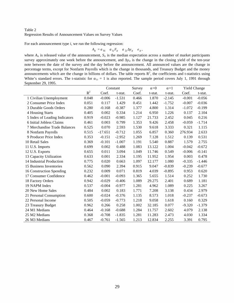
Table 2 reports the results of a regression of the actual announcement, Ai, on the median forecast

of the MMS survey, Fi, and the change in the ten-year note yield from the time of the survey to the

time of the announcement, ∆y:6

ittiiti0iit eyFA +∆α+α+α= 21 (1)

Several announcement series are announced in levels and are very persistent. In order to make the

regressions meaningful, Ai and Fi are measured in percentage changes of the announced value,

except for those announcements already reported in differences. These are Nonfarm Payroll

(reported as the difference in thousands), and Treasury Budget and the money supply

announcements (reported as the difference in billions of dollars). For these announcements, the

numbers used in the regressions are differences (not percentage change).

The regression model in Equation (1) allows us to test several hypotheses. First, if there is

information content in the MMS survey data, we would expect the coefficient estimates α1i to be

positive and significant. Second, if the survey information is unbiased, we would expect the α0i

coefficient estimates to be zero, and the slope terms α1i to be one. Finally, if expectations are revised

between the survey and the announcement, there should be a price change at the time of the revision,

and we should see a relationship between the change in yield and the announcement.7

Now consider the regression results reported in Table 3. The adjusted R-squared is higher than

50% in the majority of the regressions. In all but two cases, the α1i coefficient estimate is significantly

different from zero.8 Moreover, the intercept terms are not significantly different from zero in 21 out of

6 We used the ten-year yield, rather than a shorter maturity rate, because we found that short-term rates do not

respond as significantly to economic announcements.7 Since the change in yield during the week preceding the announcement might be only a noisy indicator of the

revision of expectations, we also considered as explanatory variables the surprise components of all otherannouncements released between the date of the survey and the announcement. These surprises are defined as inEquation (3). The results are essentially unchanged. In particular, the slope coefficients on the announcementforecasts are almost identical, with only four coefficients differing in magnitude by more than 0.1. Since the resultsof this second set of tests are so similar, we decided not to report them in the paper.

8 Here, and in the remaining of the paper, a coefficient is denoted significant if its t-statistic differs from zeroin a two-tailed test at the 5% level. Since in all regressions there are at least 30 observations, the corresponding

8

26 regressions. Also, we cannot reject the hypothesis that the survey enters with a coefficient of unity

in 17 out of 26 regressions. This is strong evidence that the survey data that we use contains real

information about the variable being forecasted, and in most cases this is an unbiased forecast.

Moreover, in 20 of 26 cases, the estimate of the coefficient on the yield change is insignificant. And

even when the yield change is significant, in four of the six cases we later show that the announcement

significantly affects all note and bond prices (e.g. Nonfarm Payroll). Thus, we may also conclude that

the revision of expectations between survey and release is not a major issue.

These results complement the findings of Pearce and Roley (1985) who test the properties of the

MMS survey data for money supply, industrial production, unemployment, PPI, and CPI. They find a

significant bias only in the industrial production forecasts. They also note that the survey data is more

accurate than autoregressive models by virtue of lower mean squared errors.9

Regardless of the results above, it is possible that the surprise components in the announcements is

measured with error. Since the surprises are then used as regressors in our tests, these errors-in-

variables induce a bias towards zero in the coefficients, as well as inflate the standard errors of the

estimates. Hence, t-statistics are biased towards zero. This affects the interpretation of our results in the

following sense: the actual significance level of the tests may be higher than what we report.

3. Economic News and Bond Prices

This section explains the methodology used to evaluate the impact of the different announcements on

bond prices. We then study which announcements have a significant effect on bond prices, and the

speed at which new information is incorporated into prices. We also discuss the size of the effect of the

various announcements.

critical values can be read off the table for the normal distribution, and they equal ± 1.96. Moreover, all regressiont-statistics use White’s standard error estimates to correct for heteroskedasticity of unknown form.

9 McQueen and Roley (1993) perform similar tests for a different sample period, and they also conclude that thesurvey data generally have smaller mean squared errors than autoregressive models.

9

3.1 Methodology

Let Fi denote the median of the MMS forecast survey and Ai the released value for announcement i.

We measure the surprise in the announcement i as:

Ei = Ai - Fi (2)

Since units of measurement differ across economic variables, we divide the surprises by their standard

deviation across all observations to facilitate interpretation. Our “standardized” surprise measure is:

SE

ii

i= σ (3)

Thus, when regressing bond returns on surprises, the regression coefficient is the change in return for a

one standard-deviation change in the surprise. Since the standard deviation σ i is constant across all the

observations for a given announcement i , this adjustment does not affect either the significance of the

estimates or the fit of the regressions. The only reason for the standardization is that it allows us to

compare the size of regression coefficients associated with surprises in different announcements.

To analyze the effect of economic news on bond prices, we regress price changes on the surprise in

the economic variable being studied and the surprises in variables announced simultaneously.10,11

itti

K

k i,+kiti0i5it5it30it eSS)/PP(Pk

+++=− ∑ =−− 1 11 βββ (4)

where

10 One instance were including all simultaneously announced surprises is problematic is the case of Imports,

Exports, and Merchandise Trade Balance. The three announcements are released at the same time, andMerchandise Trade Balance is simply the difference between Exports and Imports. Hence, in the regressions forImports and Exports we exclude the Trade Balance. In the Trade Balance regression, we exclude Imports andExports. This accounts for the small differences in R2 reported in Table 3.

11 One potential concern is that the impact of economic announcements may change over time. Although wewould not expect substantial variation during the 1991-1995 time period we consider, which witnessed a gradualeconomic expansion, we explore this possibility using the approach of Almeida, Goodhart, and Payne (1998) andallow for differential impacts for each year in our sample. We conduct tests using data for the ten-year note andexamine the fifteen announcements that significantly affect its price. Taking 1991 as the reference year, we testedwhether the responses in the remaining four years were significantly different, for a total of 60 tests. Only in 22cases do we reject the null of equality of the response at the 5% level, and the pattern of the rejections is quiteerratic. We regard this as very weak evidence of time variation during our sample. In addition, we only have fewobservations for each year, which it makes the estimation of these differential effects problematic. Hence, in whatfollows we assume the announcement responses are constant over time.

10

1. P30it is the price thirty minutes after announcement i at time t. Prices are measured as the averagebetween the bid and ask quotes.

2. P-5it is the price 5 minutes before the announcement at time t.12

3. β1i is the sensitivity of the price to the announcement.

4. k denotes the k-th announcement concurrent with announcement i, and K is the total number ofconcurrent announcements.

5. tikS is the standardized surprise in the k-th announcement concurrent with announcement i at time

t.

6. β k i+1, is the sensitivity of the price to the k-th announcement concurrent with announcement i.

As an example of the methodology, consider the employment announcement. From Table 1 we

know that the Civilian Unemployment rate and the Nonfarm Payroll figures are always announced at

the same time. Moreover, the two announcements concur with the Index of Leading Indicators seven

times, and once with Initial Jobless Claims. We include a concurrent announcement in the regression if

it occurs at least 10 percent of the times the announcement under analysis is released. Hence, for the

Civilian Unemployment rate we include two concurrent announcements, K = 2 , and we run the

regression

(P P ) / P S S301t 51t 51t 01 11 1t− = + + + +− − β β β β21 8 31 5 1t t tS e (5)

The subscripts 1, 8, and 5, correspond to the announcements as numbered in Table 1; that is, 1

represents the Civilian Unemployment rate, 8 represents the Nonfarm Payroll, and 5 represents the

Index of Leading Indicators. This regression has 51 observations.

12 We ran identical regressions using price changes from 5 minutes before to 1, 2, 3, 4, 5, 10, 15, 20, and 25

minutes after the announcement. Shortly, we will show that price changes are extremely rapid in this market, withmost of the impact in the first minute after the release. We find no additional price change after 25 minutes. Thusour choice of 30 minutes should capture all of the relevant price change.

11

3.2 Which Economic Announcements Affect Prices?

Table 3 presents the estimation results for the four instruments: three-month bill, two-year note, ten-

year note, thirty-year bond. The table shows slope coefficients, t-statistics and R-squared estimates.

Intercept terms are not reported, since they are rarely significant. For example, in the case of the ten-

year note, only three of the 26 intercept terms are significant. The main results are as follows:

First, the prices of the four instruments react significantly to eight announcements. These eight

announcements are Durable Goods Orders, Housing Starts, Initial Jobless Claims, Nonfarm Payrolls,

Producers Price Index, Consumer Confidence, NAPM Index, and New Home Sales. In addition, three

announcements affect the prices of three instruments, Consumer Price Index and M2, the longest three

and Retail Sales, the shortest three.13 One other, Capacity Utilization, only affects the price of the two

intermediate notes. The differential effect on different segments of the yield curve could be the result of

chance, or it could be that different announcements systematically affect in different ways short- versus

long-term expectations.

To explore this issue further, we regressed price changes on announcement surprises and included

the price change of a bond of different maturity as an additional independent variable. When we regress

note and bond returns on the 3-month bill return, the surprises that are significant maintain their

significance. For example, when we regress the 30-year bond return on announcement surprises and

the 3-month bill return, 7 of 10 announcements are still significant. When we run the same regression

for the 10-year note, 12 of 16 announcements maintain their significance. And for the 2-year note only

one announcement loses significance. When we regress the note and bond returns on other note or

bond returns, most significant announcements loose there significance. The number of announcements

that remain significant ranges from one (when we regress the 30 year on the 2 year) to four (when we

regress the 10 year on the 2 year). Thus, the return on any intermediate or long maturity instrument

seems to serve as a factor for the returns on other intermediate and long maturity instruments, but the

13 It is worth noting that the estimates in the Initial Jobless Claims and M2 regression may tend to be more

precise than in other regressions simply because of the larger number of observations (they are weekly, rather thanmonthly announcements).

12

3-month bill return does not. These results support the statement that at least two factors are needed to

model the yield curve.

Second, the R-squared for the significant announcements can be quite high. For instance, in the

case of the two-year note, the R-squared for the employment announcement (Civilian Unemployment

and Nonfarm Payrolls) is 67.7%. This indicates that a substantial portion of price volatility around

announcement time is explained by the surprises.

Third, it is important to note how we have been able to separate the effects of variables announced

concurrently by using our surprise data, and how it is the availability of the MMS forecast data that

allows us to calculate surprises.14 Consider, for example, Nonfarm Payrolls and the Civilian

Unemployment rate. These announcements are always released together at 8:30 a.m. Thus, without

knowing the surprise components of the two announcements, there is no way to separate their

influence. However, examining Table 4 shows that the surprises in the Civilian Unemployment rate

affect prices much less than surprises in Nonfarm Payrolls. What we have shown is that it is the

Nonfarm Payroll figure that affects bond prices, while the Civilian Unemployment rate is much less

important. Also, consider the National Association of Purchasing Managers (NAPM) Index and

Construction Spending. Previous studies (e.g. Ederington and Lee, 1993, and Fleming and Remolona,

1996) have not attempted to distinguish between the effects of the two 10:00 a.m. announcements, and

therefore find them equally important. Once again, examining Table 1 shows that 43 out of 50 times

they are announced at the same time. Using our surprise data, we are able to show that it is the NAPM

Index and not Construction Spending that affects prices. In fact, not only are the sensitivities for

Construction Spending insignificant across instruments of different maturity, but they vary in sign.

Again, this shows the importance of using surprise data in comparing announcement effects.

Fourth, we find that for most announcements the size of the effect increases with the maturity of

the instrument. For the Nonfarm Payroll announcement, for example, the surprise coefficient (in

absolute value) increases from 0.013 for the three-month bill, to 0.0160 for the two-year note, to 0.416

14 This would be true even if there were no simultaneous announcements.

13

for the ten-year note, to 0.592 for the thirty-year bond.15 This is consistent with the notion that longer

maturity bond prices are more volatile (duration increases with maturity ).

3.3 Some Further Discussion

Of the eleven announcements that significantly affect the prices of at least three maturities, two

describe the situation in the labor market (Initial Jobless Claims and Nonfarm Payrolls), two describe

the inflationary process (CPI and PPI), one describes the state of consumer demand (Durable Goods

Orders and Retail Sales), two describe the state of the real estate market (Housing Starts and New

Home Sales), two describe the perceived state of the economy (Consumer Confidence and NAPM

Index), and one describes the conditions of the money market (M2 medians). Of the announcements

that significantly affect the prices of less than three of the five instruments, one describes the labor

market (Civilian Unemployment rate), three describe the state of the economy (Capacity Utilization,

Industrial Production, and Factory Orders), and two describe foreign trade (Merchandise Trade

Balances and U.S. Exports).16

It is also interesting to provide an interpretation for the lack of significance of some of the

economic announcements. For example, the reason for the lack of impact of the Index of Leading

Indicators may have to do with the fact the Index is a weighted average of 11 components.17 While the

market may find some of the components relevant for pricing, this information might be confused by

the other components of the index. The lack of significance of U.S. Imports may be attributed to the

fact that these announcements have implications both for aggregate economic activity and for foreign

exchange rates, and thus convey a mixed signal. In addition, the Treasury Budget announcements are

also not significant, probably because they are related to one component only of total aggregate

demand. The reason why the market reacts to M2, but not to M1 and to M3, is that both M1 and M3

15 All of these coefficients are negative.16 Of these announcements, Retail Sales, Capacity Utilization, and Industrial Production have a significant

impact on the prices of both the two- and ten-year note.17 The eleven components of the index are: the average workweek, weekly jobless claims, new orders for

consumer goods, vendor performance, contracts and orders for new plant and equipment, building permits,changes in unfilled durable goods orders, sensitive material prices, stock prices, real money supply (M2), andconsumer expectations.

14

are viewed as not having a stable relationship with nominal GNP.18 Indeed, this result is consistent with

the findings of Hallman, Porter, and Small (1991), who document a long-run link between M2 and the

price level for the 1955-1988 period.

For the ten announcements that significantly effect the prices of all notes and bond prices, we

calculated the average yield changes induced by the announcements for the different maturities. For all

announcements, the absolute yield change for one standard deviation of surprise is largest for the two-

year note, and smallest for the thirty-year bond. This is consistent with the notion of the short rate

being stationary around a long-run mean: in equilibrium, the longer the maturity of the rate, the smaller

the variability (see, for example, Cox, Ingersoll, and Ross, 1985). The (absolute) size of the yield

changes reflects the price effects documented above. One standard deviation of Nonfarm Payroll

Surprise induces the largest change in the ten-year yield, 5.6 basis points, while one standard deviation

of M2 Medians induces the smallest change, 0.3 basis points.

It is also interesting to examine how some of our results would differ if daily, rather than intra-day,

price data had been used. For this purpose, we also estimated a regression model analogous to that in

Equation (2), but where the intra-day price change is replaced by the daily one as the dependent

variable.19 Of the ten announcements that we find significant for all note and bond prices, three would

not be significant if we used daily data: Initial Jobless Claims, Housing Starts, and M2 Medians. This is

not surprising, since the standard error of the slope estimates increases with the variability of the

residual in the regression. As the time window around the announcement widens, the variability of the

residual term also increases, because a smaller portion of price variability can be explained by any given

announcement. Hence, as we move from intra-day to daily data, the statistical significance of some

announcements gets lost.

Perhaps more importantly, when the time window is widened announcements that are not

significant may erroneously show up as significant. Consider the situation where two announcements

18 Interestingly, the correlations between surprises in the three monetary aggregates are not very high. In fact,

the highest correlation coefficient is between surprises in M2 and M3, 0.7. Hence, the lack of significance ofsurprises in M1 and M3 cannot be attributed to a problem of multicollinearity.

19 The daily price change is defined as the change between 6:00 p.m. the day before the announcement and6:00 p.m. on the announcement day.

15

are often released on the same day, but at different times during the day, and assume that the market

reacts significantly only to the first of the two announcements, although the two surprises are

correlated. Using daily data, the second announcement may seem to be significant, when in fact it is

not. The only way to avoid this "spurious significance" is to include in the daily regressions all

announcements that took place on the days when the primary announcement of interest was released.

This is much more cumbersome than controlling only for the concurrent announcements, as in the

present study. And in fact, the existing studies of announcement effects which use daily data control

only for a few, if any, of the announcements that take place on the same day.20

The importance of looking at intra-day data is also supported by the evidence in Section 3.5 below.

There, we show that most announcements that significantly affect the price of the ten-year note, do so

within one minute of the release, and all but one have no impact after 25 minutes from the release.

3.4 Sign and Size of Response

Commentaries in the financial press explain the reaction of the bond market to economic news mainly

in terms of revisions of inflationary expectations, where, in accord with a Phillips-curve view, inflation

is perceived to be positively correlated with economic activity. Our results are consistent with this

interpretation. Procyclical variables, such as Nonfarm Payrolls, affect bond prices negatively, while

counter-cyclical variables, such as Initial Jobless Claims, have a positive impact on prices.21

Regarding the size of the price reaction, the following discussion concentrates on the behavior of

the price of the ten-year note, which is representative of the behavior of intermediate- and long-term

bond prices. The 16 economic announcements that significantly affect the ten-year note have differing

impacts in terms of the magnitude of price changes. Per unit of standard deviation of surprise, the most

important is Nonfarm Payrolls. To gain some idea of the importance of this announcement, note that

the standard deviation of the daily percentage price change for the ten-year note is 0.47%. Thus, a one

standard deviation surprise in nonfarm payrolls, corresponding to an increase in nonfarm payrolls of

20 Hardouvelis (1988), for example, controls for only 15 of all the announcements that may be released during

a given day.21 King and Watson (1994, 1996) document the existence of an inflation-output and an inflation-

unemployment trade-off in U.S. post-war data.

16

110,000, leads to a price change of about 89% of the normal daily volatility of price changes.22 Next in

importance is PPI. A one standard deviation surprise in PPI, corresponding to a .24% monthly

variation in the index, leads to a price change of about 39% of the normal daily volatility. CPI, Durable

Goods Orders, Retail Sales, NAPM Index, and Consumer Confidence are of roughly equal importance.

These announcements induce price changes that range from 25 to 30% of daily volatility. Initial Jobless

Claims, Capacity Utilization, Industrial Production, and New Home Sales have effects between 12 and

19% of daily volatility. Finally, Factory Orders, and M2 Medians have the smallest effect on bond

prices, with effects between four and nine percent of daily volatility.23

3.5 Speed of Impact

One interesting issue to investigate, in addition to the size of the response, is how quickly bond prices

react to economic news announcements. As in the previous section, we concentrate on the behavior of

the price of the ten-year note. Table 4 presents the results of the following regression

itti

K

1k i,+kiti0iitit30it eSS)/PP(Pk

+++=− ∑ = 11 γγγττ (4)

where P itτ is the price τ minutes after the announcement. The regression is performed for the 16

significant announcements identified in Table 3. The endpoint of the horizon used to calculate rates of

return is kept constant, while the beginning of the horizon, τ, is changed from -2, two minutes before

the release, to +25, 25 minutes after the announcement. This allows us to identify the lowest value of

τ for which the price reaction is not significant. This corresponds to the time period needed for the

surprise to be fully incorporated into prices.

22 The second column of Table 3 reports the standard deviation of the surprises for each variable. This,

together with the economic units reported in Table 1, facilitates an economic interpretation of the results.23 In order to examine whether the announcement effects are different across maturities, we calculate the

covariance matrix of the estimates of the slope coefficients for the four regressions (one for each maturityconsidered). We then construct Wald tests to examine whether the responses are statistically different acrossmaturities for the eight announcements that have a significant impact on all bond prices. For each announcement,we perform individual pair-wise tests that the coefficients are equal, as well as a joint test that all coefficients areequal. Out of a total of 56 tests (48 pair-wise tests and 8 joint tests) only in six cases do we fail to reject that thecoefficients are different at the 5% level. Hence, we conclude that the null hypothesis that the effect is the sameacross maturities is strongly rejected.

17

Of the 16 announcements, only five significantly affect prices on or after τ = 1: Merchandise Trade

Balances, U.S. Exports, Capacity Utilization, Factory Orders, and NAPM Index. None are significant

beyond 15=τ . Thus, even for these six announcements information is rapidly incorporated into prices.

Moreover, the pattern of significance for Merchandise Trade Balances, U.S. Exports, and Factory

Orders is erratic, which casts some doubt on the relevance of these delayed price effects.

The high speed of adjustment is also documented by the graphs reported in Figure 1, which shows

the average percentage price change of the ten-year note in response to the first four significant

announcements released at 8:30 a.m. The figure also shows that the reaction of prices to positive and

negative surprises is roughly symmetric.

4 Economic News and Bond Trading

This section studies the effects of economic announcements on trading volume, bid-ask spreads, and

price volatility. In this analysis, we focus on the three-month bill and the ten-year note whose price

behavior is representative of short-term and intermediate-to-long-term instruments, respectively. We

also concentrate on the announcements that significantly affect the price of the two instruments.24,25

4.1 Trading Volume

Table 5 presents the ratio of the average trading volume over different intervals preceding and

following announcement times to the average volume over the same interval on days when no

announcement took place. Ratios are reported for the ten-year note and the three-month bill.

24 In a related paper, Fleming and Remolona (1999) examine intra-day trading activity in the vicinity of

scheduled announcements. Since they only consider one year of data, they pool observations across the threeannouncements they examine. In addition, they only consider one instrument, the five-year note. The generalpattern of their results is similar to ours. However, as our findings indicate, there is substantial variation in theresults across announcements and maturities that is missed by their analysis.

25 We do not report the results for announcements that do not have a significant impact on prices. The impactof these announcements depends on the amount of overlap with other announcements and the importance of theconcurrent announcements. For example, consider the Treasury Budget and Business Inventory announcements,which do not have a significant price effect and have no concurrent announcement (see Table 1). The bid-askspread and price volatility of the ten-year note are unaffected by these two announcements, while trading volume isslightly higher than normal for Business Inventories. In contrast, the Index of leading Indicators, which also has aninsignificant price effect, is concurrent with a number of important announcements and shows patterns in tradingvolume, bid-ask spread, and volatility, similar to the concurrent announcements.

18

We also ran regressions of volume against the absolute size of economic surprises, in the same

way as we did with bond returns. We found little evidence of a statistically reliable relation

between trading volume and the size of the surprises, even for the announcements that

significantly affect bond prices. This is not surprising, since volume should reflect disagreement

among investors concerning the price adjustment.26 This disagreement need not be directly related

to the size of the surprise. In fact, while a large surprise may induce investors to revise their priors

in the same manner, and hence triggers little trade, a small surprise may generate wide

disagreement, and hence triggers a large surge in trading activity.

For the ten-year note, we find consistent patterns of volume for each of the announcements which

have a significant impact on prices, with the exception of Consumer Confidence. In the five minutes

before the announcement, volume is either not different from or significantly less than trading volume

on non-announcement days. Within the first five minutes after the announcement, trading volume

grows to about 1.7 times the average volume for that time period on non-announcement days. The

volume ratio continues to grow in the following ten minutes, up to almost twice the size of the non-

announcement average, but then declines after another 15 minutes, while still remaining above

normal.27 For the three-month bill, we also find that volume is substantially higher around

announcements, although the pattern is somewhat erratic.

It is also interesting to compare the different effects of announcements on trading volume and on

prices. First, the effects of announcements on trading volume differ much less than the effects on

prices. Consider, for example, the ten-year note. From Table 3 we see that a one standard deviation

surprise in Nonfarm Payroll triggers a price change which is more than 20 times larger than the effect

of a one standard deviation surprise in M2 Medians. However, the largest increment in trading volume

during the interval of 5 to 15 minutes after the announcement (the PPI announcement) is less than

twice as big as the smallest increment (the money announcement).

26 This interpretation dates back to Beaver (1968).27 This pattern is strongest for the 8:30 a.m. announcements. Trading volume around this time cannot be

influenced by announcements released earlier on that day, since there are none. Conversely, trading volume later inthe day might be higher than normal even if there are no announcements at that time, because of announcementsreleased earlier that day.

19

Second, the announcements that affect prices most are not those that have the greatest effect on

volume. Consider again the ten-year note and trading volume during the interval of 5 to 15 minutes

after the announcement. The Nonfarm Payroll-Civilian Unemployment announcement has only the

fourth largest effect on volume. From Table 3 we know that the Nonfarm Payroll surprise has, by far,

the largest effect on prices. We also found that several of the announcements that exhibit significant

increases in volume at some point after their release time are also announcements for which the surprise

does not appear to affect prices (these results are not reported in the table).28

Third, the effects of announcements on volume persist even beyond 30 minutes after the release,

yet we know from Table 4 that for most of the announcements that significantly affect the price of the

ten-year note, the impact is exhausted within the first minute after the release.

The discussion above highlights the fact that trading volume behaves somewhat independently of

price changes. As in French and Roll (1986), we can distinguish between public information which

affects prices with little or no trading, and private information which only affects prices through

trading. Hence, the evidence that we collected suggests that public information plays a dominant role in

the adjustment of bond prices after economic announcements.

4.2 Bid-Ask Spreads

Table 6 presents the ratio between the average bid-ask spread at different times before and after the

announcement and the average bid-ask spread at the same times during non-announcement days for the

ten-year note and for the three-month bill.29 The average spreads are 2.6 cents and 0.26 cents per one

hundred dollars price, for the bill and the note, respectively.

For most announcements, for both the ten-year note and the three-month bill, we find a significant

widening of the spread exactly at the time when the announcement is made. The spread then reverts to

its normal values after five to fifteen minutes.

28 In a sense, this is not very surprising when we consider the number of times non-significant announcements

overlap with announcements that do move prices. Even the observed trading volume after the 9:15 a.m. announcementsmay be affected by important announcements released 45 minutes earlier.

29 Once again, we find no relation between the size of the bid-ask spread and the surprise component of theannouncement.

20

There are several theories that predict this response. First there is an asymmetric information

argument that predicts a widening of the spread because of the fear on the part of market makers that

traders may be better informed (Glosten and Milgrom, 1985, and Glosten, 1987). Since there should be

no leakage of information before announcements are made, and since information relevant to the bond

market is quickly disseminated in a widespread manner, asymmetry arises not because different

information is received by traders, but because traders may have differing ability to process the

information. A second argument that suggests bid-ask spreads will widen around announcements relies

on the interpretation of bid-ask spreads as an “option to trade” offered by the market maker to traders

(Copeland and Galai, 1983, and Ho and Stoll, 1981). The price of the option to trade is the bid-ask

spread itself. As volatility increases because of the announcement, the value of the option increases, and

this is reflected by a widening of the spread.

As with trading volume, it is interesting to compare the effects of announcements on bid-ask

spreads to those on prices and volume. First, the Nonfarm Payrolls announcement induces both the

largest price adjustment and the largest widening of the bid-ask spread. This is true for both the ten-

year note and the three-month T-bill. Second, in the case of the ten-year note, the quick reversion of

bid-ask spreads to normal values mirrors the quick adjustment of prices to news. This is not surprising,

since the need on the part of market makers to protect themselves from informed traders should be

exhausted as soon as prices have adjusted to their new “equilibrium” values.

4.3 Price Volatility

We also examine price volatility around announcements. We measure this by the ratio of the mean

absolute value of price changes on announcement days over the mean absolute value of price

changes on non-announcement days, during the same time interval.30 The time intervals that we

consider start with 30 to 5 minutes before the announcements and end with 45 to 60 minutes after

the announcements.

30 By standardizing the announcement-day volatility by non-announcement-day volatility at the same time of

the day, we adjust for possible systematic intraday volatility patterns. The presence of such patterns in the bondfutures market is examined in Bollerslev, Cai, and Song (1999).

21

For both the ten-year note and the three-month bill, the relative size of the volatility effects

reflects the relative size of the price effects documented in Section 3. For example, for the ten-

year note, during the time interval 0 to 5 minutes after the announcement, the largest increases in

price volatility are for the employment announcement and for the PPI announcement, with ratios

of 10.2 and 6, respectively. For the three-month bill, the largest increase in price volatility also

corresponds to the employment announcement, with a ratio of 19.2 for the same time interval.

It is worth noting that for many of the announcements the volatility effects persist for up to 60

minutes after the release of the announcement. For example, for the ten-year note volatility is still

more than twice the normal during the time interval 30 to 45 minutes after the employment

announcement. This persistence is similar to the persistence in trading volume discussed earlier

and is in contrast to the rapid adjustment of prices to new information.

We may conclude that price volatility reflects both the adjustment of prices to news as well as

the mere impact of trading volume. In fact, there are several announcements that do not

significantly affect prices (and hence are not reported in Table 7) that lead to significant increases

in price volatility.

5. Conclusions

This paper examines the effect of economic announcements on the price, volume, bid-ask spread and

price volatility of Treasury securities. To analyze price effects, we use intra-day data of bid and ask

quotes from the inner market for U.S. government bonds. Our database provides a continuous posting

of bids and asks, and the trading around announcement times is sufficiently intense that in most cases

there are multiple trades every minute. This allows us to measure impact on price at very short

intervals. Many announcements are made concurrently. By using a database on forecasts, we are able

to measure the surprise component of an announcement. This allows us to separate out the impact of

concurrent announcements. While previous researchers have grouped simultaneous announcements

together, we find that in several cases of important announcement pairs only one of the two announce-

ments has a significant impact on prices. Because of our ability to separate out the impact of concurrent

announcements, and because we analyze intra-day price data, the announcements that we find

22

important differ from what other researchers have found. We find that most economic announcements

are incorporated in bond prices within one minute of the announcement for most significant

announcements. This implies that the inner market for U.S. government bonds is highly efficient.

We also consider the effects of announcements on transaction volume, bid-ask spreads, and price

volatility. We find that the patterns of trading volume are quite different from those in prices, thus

suggesting that private information and differences in opinion only play a minor role in the market for

U.S. Treasuries. Bid-ask spreads tend to widen significantly immediately after the announcement, and

then to quickly revert to their normal values, which is consistent with the quick reaction of prices to

news. The behavior of price volatility is also consistent with the price reactions that we document.

23

Appendix: Bond Price Data

The GovPX data set is relatively new. Thus, in this appendix we will provide some additional details

about it and make some comparisons to better known data sets. Additional details can be found in

Elton and Green (1998) and Fleming (1997).

GovPX distributes its information through on-line vendors, by sending out a digital ticker feed. We

were given digital backup copies of the feed. The data provides a precise history of the tick-by-tick

information sent to traders. Since the purpose of the digital feed is to refresh vendors’ screens, the data

must be processed before it can be effectively analyzed. GovPX’s digital ticker feed contains a time

stamp which is the actual time, rounded to the closest second, when the message reaches the computer

terminals. It is the arrival of the information to the screen that determines the time stamping. The

messages reach screens every 60 seconds (give or take one second). Hence, we have 60 24 1440× =

messages each day, although some of the messages are simply “refreshers” and do not change any of

the existing information on the screen for some bonds.

It is important to note that the GovPX data reports continuously the best price quotes collected by

the major brokers among all the primary dealers, where the quotes are binding. All other sources

currently available only report end-of-day prices and collect data from a smaller pool of dealers. For

example, the CRSP data consists of the quotes from one dealer only, Salomon Brothers, until 1962.

After 1962, CRSP began using data collected by the Federal Reserve Bank of New York, which, in

turn, over the time frame of this study, are an average of the price quotes from five primary dealers.31

The Wall Street Journal, on the other hand, reports the quotes posted by one of the brokers only,

Cantor Fitzgerald, which are collected through a Dow Jones subsidiary, Telerate. Hence, the price data

collected by GovPX provide a better representation of the market for U.S. Treasury securities than the

data provided by these other sources.

It is worth noting that the only other existing source of intra-day bond data is the futures market.

However, much of the analysis performed in this paper would not be possible with futures data. In

particular, intra-day information on bid-ask spreads and trading volume is not available for the futures

31 Recently the Federal Reserve Bank of New York began using GovPX data as their primary source, so that

the CRSP data is also currently based on the GovPX data set.

24

markets. For example, the data provided by the Chicago Board of Trade is tick-by-tick data:

transaction prices which are recorded separately only if there was a change in price. Bid-ask quotes,

successive trades at the same price, and trade volume are not recorded. Also, futures contracts have

delivery options that make it hard to determine exactly the maturity of the instrument to be traded at a

forward date. This is especially true for the bond futures contract, that has bonds with maturities

ranging from 15 to 30 years as the deliverable instrument. Finally, the GovPX data provides around-

the-clock price and trade volume information. This makes it possible to study the effects of

announcements that take place when domestic and foreign futures markets are closed. This is the case

of the money supply announcements which are released on Thursdays at 4:30 p.m. Eastern Time.32 In

fact, trading in London (LIFFE) stops at 11:10 a.m., while trading in New York (AMEX) and Chicago

(CBOT, CBOE) stops at 3:00 p.m., and evening trading in Chicago (CBOT) only resumes after 6:00

p.m. (7:00 p.m. when daylight saving time is in effect).

32 Throughout the paper times are to be interpreted as Eastern Standard Time.

25

References

Almeida, A., C. Goodhart, and R. Payne (1998). "The Effects of Macroeconomic News on High-Frequency Exchange Rate Behavior." Journal of Financial and Quantitative Analysis 33, 383-408.

Balduzzi, P., Das, S. R., and Foresi, S. (1996). “The Central Tendency: A Second Factor in BondYields.” Review of Economics and Statistics 80, 62-72.

Beaver, W.H. (1968). “The Information Content of Annual Earnings Announcements.” In EmpiricalResearch in Accounting: Selected Studies, supplement to The Journal of Accounting Research,67-92.

Bollerslev, T., J. Cai, and F. M. Song (1999). "Intraday Periodicity, Long Memory Volatility, andMacro Announcements in the U.S. Treasury Bond Market." Mimeo, City University of HongKong.

Brennan, M.J. and Schwartz, E. S. (1979). “A Continuous Time Approach to the Pricing of Bonds.”Journal of Banking and Finance 3, 133-156.

Brown, L. D. (1996). I/B/E/S Research Bibliography, I/B/E/S International Inc., New York.

Copeland, T. E., and Galai, D. (1983). “Information Effects of the Bid-Ask Spread.” Journal ofFinance, 38, 1457-1469.

Cox, J. C., Ingersoll, J. E., and Ross, S. A. (1985). “A Theory of the Term Structure of InterestRates.” Econometrica, 53, 385-407.

Duffie, D. (1996). "Special Repo Rates." Journal of Finance, 51, 1533-1562.

Ederington, L. H. and Lee, J. H. (1993). “How Markets Process Information: News Releases andVolatility.” The Journal of Finance, 48, 1161-1191.

Edison, H.J. (1996). “The Reaction of Exchange Rates and Interest Rates to News Releases.”International Finance Discussion Paper No. 570, Board of Governors of the Federal ReserveSystem.

Elton, E. J., and T.C. Green (1998). "Tax and Liquidity Effects in Pricing Government Bonds."Journal of Finance, 53, 1533-1562.

Elton, E. J., and Gruber, M. J. (1972). “Earnings Estimation and the Accuracy of Expectational Data.”Management Science, 18, Vol. 2, 409-424.

26

Elton, E. J., Gruber, M. J., and Mei, J. (1996). “Return Generating Process and the Determinants ofRisk Premiums.” Journal of Banking and Finance, 20, 1251-69.

Federal Reserve Bulletin, September 1993, Board of Governors of the Federal Reserve, WashingtonD.C.

Fleming, M. J. (1997). "The Round-the-Clock Market for U.S. Treasury Securities." Federal ReserveBank of New York Economic Policy Review (December), 31-50.

Fleming, M. J., and Remolona, E. M. (1999). “Price Formation and Liquidity in the U.S. TreasuryMarket: The Response to Public Information.” Journal of Finance forthcoming.

French, K., and R. Roll (1986), “Stock Return Variances: The Arrival of Information and the Reactionof Traders.” Journal of Financial Economics, 17, 5-26.

Glosten, L. R., and Milgrom, P. R. (1985). “Bid, Ask, and Transaction Prices in a Specialist Marketwith Heterogeneously Informed Traders.” Journal of Financial Economics, 14, 71-100.

Glosten, L. R. (1987). “Components of the Bid-ask Spread and the Statistical Properties ofTransaction Prices.” Journal of Business 42, 1293-1307.

Hakkio, C. S., and Pearce D. K. (1985). “The reaction of Exchange Rates to Economic News.”Economic Inquiry 23, 621-636.

Hallman, J. H., Porter, R. D., and Small, D.H. (1991). “Is the Price Level Tied to the M2 MonetaryAggregate in the Long Run?” American Economic Review 81, 841-858.

Hardouvelis, G. A. (1988). “Economic News, Exchange Rates and Interest Rates.” Journal ofInternational Money and Finance, 7, 23-35.

Harvey, C. R. and Huang, R. D. (1993). “Public Information and Fixed Income Volatility.” Mimeo,Duke University.

Ho, T. and Stoll, H. R. (1981). “Optimal Dealer Pricing Under Transactions and Return Uncertainty.”Journal of Financial Economics, 9, 47-73.

Ito, T., and Roley, V. V. (1987). “News from the U.S. and Japan: Which Moves the Yen/DollarExchange Rate?” Journal of Monetary Economics 19, 255-277.

King, R. G., and Watson, M. (1994). “Money, Prices, Interest Rates, and the Business Cycle.”Carnagie-Rochester Conference Series on Public Policy 41, 157-219.

27

King, R. G., and Watson, M. (1996). “Money, Prices, Interest Rates, and the Business Cycle.” Reviewof Economics and Statistics 78, 35-53.

McQueen, G., and Roley, V.V. (1993). “Stock Prices, News, and Business Conditions.” The Review ofFinancial Studies, 6, 683-707.

Pearce, D. K., and Roley, V. V. (1985). “Stock Prices and Economic News.” Journal of Business 58,49-67.

Schaefer, S. M. and Schwartz, E. S. (1984). “A Two-Factor Model of the Term Structure: AnApproximate Analytical Solution.” Journal of Financial and Quantitative Analysis, 19, 413-424.

Urich, T., and Wachtel, P. (1984). “The Effects of Inflation and Money Supply Announcements onInterest Rates.” Journal of Finance 39, 1177-1188.

Vasicek, O. (1977). “An Equilibrium Characterization of the Term Structure.” Journal of FinancialEconomics, 5, 177-188.

Treasury Bulletin, December 1994, Treasury Department, Washington D.C.

28

Table 1Contemporaneous Announcement Releases

The table contains the time each announcement is released, the reported units for that announcement, and thenumber of times each economic announcement is released concurrently with other announcements for the 27economic announcements considered in the study. The sample period covers July 1, 1991 through September 29,1995.

8:30a.m. Announcements 1 2 3 4 5 6 7 8 9 10 11 121 Civilian Unemployment (% Level) 51 0 0 0 7 1 0 51 0 0 0 02 Consumer Price Index (% Change) 0 51 0 5 0 11 5 0 0 18 5 43 Durable Goods Orders (% Change) 0 0 51 0 0 14 0 0 0 0 0 04 Housing Starts (Millions of Units) 0 5 0 51 0 8 0 0 0 0 1 15 Index of Leading Indicators (% Change) 7 0 0 0 50 4 0 7 0 0 0 06 Initial Jobless Claims – weekly (Thousands) 1 11 14 8 4 219 19 1 18 19 22 227 Merchandise Trade Balances ($ Billions) 0 5 0 1 0 22 51 0 0 0 51 518 Nonfarm Payrolls (Change in Thousands) 51 0 0 0 7 1 0 51 0 0 0 09 Producer Price Index (% Change) 0 0 0 0 0 18 0 0 51 14 0 0

10 Retail Sales (% Change) 0 18 0 0 0 19 0 0 14 51 0 011 U.S. Imports ($ Billions) 0 5 0 1 0 22 51 0 0 0 51 5112 U.S. Exports ($ Billions) 0 5 0 1 0 22 51 0 0 0 51 51

9:15a.m. Announcements 13 1413 Capacity Utilization (% Level) 51 5114 Industrial Production (% Change) 51 51

10:00a.m. Announcements 15 16 17 18 19 20 21 2215 Business Inventories (% Change) 51 0 0 0 0 0 0 016 Construction Spending (% Change) 0 51 1 0 43 1 5 517 Consumer Confidence (% Level) 0 1 51 0 1 10 0 018 Factory Orders (% Change) 0 0 0 51 3 0 2 219 NAPM Index (Index Value) 0 43 1 3 51 1 5 520 New Home Sales (In Thousands) 0 1 10 0 1 51 7 721 Personal Consumption (% Change)a 0 5 0 2 5 7 50 5022 Personal Income (% Change)a 0 5 0 2 5 7 50 50

2:00p.m. Announcements 2323 Treasury Budget (Change in $ Billions) 51

4:30p.m. Announcements 25 26 2724 M1 Medians - weekly (Change in $ Billions) 221 221 22125 M2 Medians - weekly (Change in $ Billions) 221 221 22126 M3 Medians - weekly (Change in $ Billions) 221 221 221

aPersonal Consumption and Personal Income began being reported at 8:30 a.m. in January of 1994.

29

Table 2Regression Results of Announcement Values on Survey Values

For each announcement type i, we run the following regression:

,210 ititiitiiit yFA εααα +∆++=

where Ait is released value of the announcement, Sit is the median expectation across a number of market participantssurvey approximately one week before the announcement, and ∆yit is the change in the closing yield of the ten-yearnote between the date of the survey and the day before the announcement. All announced values are the change inpercentage terms, except for Nonfarm Payrolls which is the change in thousands, and Treasury Budget and the moneyannouncements which are the change in billions of dollars. The table reports R2, the coefficients and t-statistics usingWhite’s standard errors. The t-statistic for α1i = 1 is also reported. The sample period covers July 1, 1991 throughSeptember 29, 1995.

Constant Survey α=0 α=1 Yield ChangeR2 Coef. t-stat. Coef. t-stat. t-stat. Coef. t-stat.

1 Civilian Unemployment 0.048 -0.006 -1.531 0.466 1.870 -2.145 -0.001 -0.0562 Consumer Price Index 0.051 0.117 1.429 0.451 1.442 -1.752 -0.007 -0.0363 Durable Goods Orders 0.280 -0.168 -0.387 1.377 4.800 1.314 -1.072 -0.1994 Housing Starts 0.405 0.002 0.334 1.214 6.950 1.226 0.137 2.1045 Index of Leading Indicators 0.919 -0.023 -0.985 1.127 21.733 2.452 0.045 0.2166 Initial Jobless Claims 0.461 0.003 0.799 1.353 9.426 2.458 -0.059 -1.7147 Merchandise Trade Balances 0.525 0.070 2.593 1.530 9.618 3.333 0.321 1.1158 Nonfarm Payrolls 0.515 -17.651 -0.712 1.055 6.857 0.360 276.934 2.6339 Producer Price Index 0.353 -0.151 -2.952 1.269 7.128 1.512 0.139 0.531

10 Retail Sales 0.369 -0.101 -1.007 1.191 5.540 0.887 1.579 2.75511 U.S. Imports 0.699 0.002 0.488 1.083 13.122 1.004 -0.042 -0.67212 U.S. Exports 0.655 0.011 3.094 1.049 11.746 0.549 -0.006 -0.14113 Capacity Utilization 0.633 0.001 2.334 1.195 11.952 1.954 0.003 0.47814 Industrial Production 0.775 0.020 0.663 1.097 12.177 1.080 -0.335 -1.44615 Business Inventories 0.562 0.090 2.394 0.915 9.047 -0.839 -0.239 -0.67716 Construction Spending 0.232 0.009 0.071 0.819 4.039 -0.895 0.953 0.62017 Consumer Confidence 0.462 -0.001 -0.093 1.365 5.655 1.514 0.252 1.73018 Factory Orders 0.942 -0.029 -0.406 1.089 29.275 2.401 0.689 1.18119 NAPM Index 0.537 -0.004 -0.977 1.281 4.962 1.089 0.225 3.26720 New Home Sales 0.484 0.002 0.183 1.771 7.208 3.138 0.434 2.97921 Personal Consumption 0.600 -0.024 -0.376 1.135 8.573 1.018 -0.237 -0.67322 Personal Income 0.505 -0.059 -0.773 1.218 9.058 1.618 0.160 0.32923 Treasury Budget 0.962 0.266 0.258 1.002 32.185 0.077 -9.320 -1.37924 M1 Medians 0.464 -0.168 -0.688 1.284 11.757 2.602 4.079 2.13825 M2 Medians 0.368 -0.708 -1.835 1.281 11.283 2.473 4.030 1.33426 M3 Medians 0.467 -0.761 -1.565 1.213 12.834 2.255 3.391 0.795

30

Table 3The Effect of Announcement Surprises at Different Points on the Yield Curve

For each instrument and for each announcement type i, we run the following regression:

,/)( 1 ,1105530 ittiikitiiititit eSSPPPk

Kk +∑++=− = +−− βββ

where P30it is the price of the instrument 30 minutes after the announcement i, Sit is the surprise for announcement type i standardized by σi2, the standard deviation of all

surprises for that type. The subscript k denotes other announcements released at the same time as announcement i. The table reports σi2, the coefficient β1i, and the t-statistic

using White’s standard errors. R2 for the regression is also reported. The sample covers July 1, 1991 through September 29, 1995.3 Month Bill 2 Year Note 10 Year Note 30 Year Bond

Surprise Surprise Surprise Surpriseσi

2 Coef. t-stat. R2 Coef. t-stat R2 Coef. t-stat R2 Coef. t-stat R2

1 Civilian Unemployment 0.169 0.004 1.818 0.644 0.053 2.631 0.677 0.112 1.761 0.607 -0.003 -0.028 0.5672 Consumer Price Index 0.126 -0.001 -1.538 0.162 -0.033 -3.345 0.281 -0.142 -3.637 0.374 -0.205 -2.587 0.4463 Durable Goods Orders 2.735 -0.004 -2.928 0.481 -0.056 -5.201 0.552 -0.118 -4.442 0.399 -0.211 -5.622 0.4984 Housing Starts 0.070 -0.002 -2.824 0.335 -0.031 -4.435 0.453 -0.075 -2.424 0.181 -0.119 -3.298 0.2275 Index of Leading Indicators 0.153 -0.001 -1.750 0.697 -0.006 -0.954 0.772 -0.029 -1.669 0.678 -0.019 -0.449 0.0036 Initial Jobless Claims 19.550 0.001 3.055 0.031 0.020 5.317 0.097 0.057 3.792 0.068 0.052 3.026 0.0517 Merchandise Trade Balances 1.443 0.000 0.261 0.004 0.005 0.830 0.043 0.052 2.064 0.109 0.051 1.297 0.0378 Nonfarm Payrolls 109.920 -0.014 -5.802 0.644 -0.160 -7.763 0.677 -0.416 -6.189 0.607 -0.592 -5.386 0.5679 Producer Price Index 0.242 -0.002 -2.755 0.371 -0.044 -5.504 0.448 -0.184 -5.093 0.473 -0.333 -5.825 0.437

10 Retail Sales 0.496 -0.003 -3.692 0.346 -0.037 -2.944 0.320 -0.117 -3.080 0.390 -0.122 -1.607 0.17511 U.S. Imports 1.391 0.000 -0.136 0.004 0.001 0.186 0.057 0.031 1.146 0.117 0.024 0.638 0.03512 U.S. Exports 1.203 0.000 -0.258 0.004 -0.008 -1.370 0.057 -0.058 -2.525 0.117 -0.054 -1.862 0.03513 Capacity Utilization 0.318 -0.002 -1.894 0.195 -0.029 -3.599 0.269 -0.070 -2.548 0.232 -0.055 -1.884 0.13514 Industrial Production 0.196 0.000 -0.040 0.195 -0.010 -1.545 0.269 -0.054 -2.804 0.232 -0.053 -1.693 0.13515 Business Inventories 0.243 0.000 -0.017 0.000 0.000 0.053 0.000 0.017 0.705 0.014 0.040 1.131 0.05716 Construction Spending 0.933 0.000 0.000 0.267 0.002 0.332 0.569 0.018 0.614 0.408 -0.002 -0.052 0.43217 Consumer Confidence 5.065 -0.002 -3.967 0.458 -0.031 -4.023 0.352 -0.109 -3.968 0.326 -0.088 -2.417 0.23918 Factory Orders 0.500 0.000 -0.594 0.007 -0.007 -1.356 0.026 -0.040 -2.649 0.091 -0.034 -1.286 0.01719 NAPM Index 2.183 -0.002 -4.728 0.324 -0.061 -7.248 0.575 -0.147 -4.821 0.392 -0.233 -6.290 0.41220 New Home Sales 61.490 -0.001 -4.697 0.314 -0.031 -4.897 0.352 -0.089 -4.070 0.252 -0.152 -4.039 0.25421 Personal Consumption 0.187 0.000 0.982 0.065 -0.003 -0.327 0.031 -0.017 -0.492 0.062 0.011 0.391 0.00622 Personal Income 0.309 0.001 1.604 0.065 -0.011 -1.038 0.031 -0.047 -1.275 0.062 -0.012 -0.361 0.00623 Treasury Budget 5.029 0.000 -0.734 0.012 0.002 0.526 0.010 -0.002 -0.217 0.000 -0.005 -0.374 0.00224 M1 Medians 3.063 -0.001 -1.014 0.008 -0.002 -1.479 0.295 -0.006 -1.524 0.170 -0.011 -1.894 0.11425 M2 Medians 5.098 0.002 0.627 0.008 -0.011 -3.989 0.295 -0.020 -3.138 0.170 -0.028 -2.264 0.11426 M3 Medians 6.759 -0.003 -0.929 0.008 -0.004 -1.844 0.295 -0.002 -0.414 0.170 0.005 0.568 0.114

31

Table 4Speed of Adjustment to New Economic Information

For each announcement i, we run the following regression:

,/)( 1 ,11030 ittiikitiiititit eSSPPPk

Kk +∑++=− = +γγγττ

where P30it is the price of the ten-year note 30 minutes after announcement i, Pτti is the price of the ten year note τ minutes afterthe announcement, Sit is the standardized surprise for announcement type i, and k denotes other announcements occurring atthe same time as announcement i. A number of different time horizons τ are chosen to measure price changes, with theendpoint of each price change being fixed at 30 minutes after the announcement. The table reports the coefficient γ1i for eachtime horizon for all announcements found to be significant for the ten-year note. Under each coefficient is the t-statistic usingWhite’s standard errors. The sample coves July 1, 1991 through September 29, 1995.

-2 -1 0 1 2 3 4 5 10 15 20 252 Consumer Price Index -0.107 -0.102 -0.011 -0.016 -0.015 -0.005 -0.012 0.002 -0.011 0.008 0.008 0.003

-2.945 -2.078 -0.306 -0.517 -0.587 -0.170 -0.370 0.064 -0.404 0.406 0.413 0.224

3 Durable Goods Orders -0.115 -0.126 -0.095 0.013 0.003 -0.003 0.000 -0.005 -0.001 -0.006 -0.002 -0.004-4.429 -4.780 -3.852 0.650 0.161 -0.213 0.020 -0.266 -0.117 -1.022 -0.460 -0.644

4 Housing Starts -0.098 -0.107 -0.051 -0.037 -0.036 -0.035 -0.020 -0.022 -0.007 -0.012 -0.008 0.001-4.792 -5.334 -1.693 -1.697 -1.737 -1.706 -1.127 -1.282 -0.490 -0.979 -0.912 0.212

6 Initial Jobless Claims 0.062 0.068 0.027 -0.007 -0.003 0.001 0.006 0.003 0.000 0.000 -0.005 -0.0044.731 4.877 2.303 -0.491 -0.280 0.143 0.723 0.387 -0.075 -0.001 -1.272 -1.510

7 Merchand. Trade Bal. 0.021 0.043 0.024 0.032 0.022 0.038 0.019 0.017 0.020 0.021 0.011 0.0071.275 1.969 1.030 2.094 1.655 2.560 1.215 1.116 1.520 2.711 1.660 1.160

8 Nonfarm Payrolls -0.365 -0.373 -0.213 -0.126 -0.045 -0.036 -0.021 -0.039 -0.012 0.018 0.049 0.043-6.048 -6.878 -3.055 -1.331 -0.853 -0.711 -0.436 -0.964 -0.388 1.066 1.370 1.112

9 Producer Price Index -0.175 -0.160 -0.052 -0.008 0.016 0.000 -0.001 -0.005 -0.004 -0.004 -0.004 -0.007-5.173 -3.748 -1.281 -0.271 0.532 -0.008 -0.084 -0.353 -0.344 -0.196 -0.210 -0.838

10 Retail Sales -0.119 -0.147 -0.093 -0.024 -0.031 -0.052 -0.039 -0.041 -0.020 0.003 0.001 0.001-3.203 -3.689 -2.512 -0.771 -0.966 -1.947 -1.378 -1.843 -0.846 0.174 0.034 0.097

12 U.S. Exports -0.056 -0.055 -0.039 -0.026 -0.024 -0.031 -0.020 -0.026 -0.027 -0.025 -0.011 -0.008-3.417 -2.857 -1.762 -1.932 -1.809 -2.326 -1.362 -1.636 -2.042 -3.678 -1.568 -1.266

13 Capacity Utilization -0.073 -0.076 -0.047 -0.039 -0.041 -0.052 -0.046 -0.045 -0.023 -0.013 -0.013 -0.016-2.615 -2.717 -2.417 -2.109 -2.034 -2.686 -2.181 -2.113 -1.441 -1.118 -1.503 -3.267

14 Industrial Production -0.055 -0.054 -0.031 -0.007 -0.007 -0.008 -0.004 -0.010 -0.011 -0.007 -0.011 -0.004-2.971 -2.929 -1.765 -0.478 -0.408 -0.589 -0.253 -0.619 -0.637 -0.547 -1.127 -0.516

17 Consumer Confidence -0.098 -0.082 -0.041 0.018 -0.002 -0.001 0.004 0.000 -0.003 0.002 -0.011 -0.012-3.537 -3.250 -1.878 0.618 -0.102 -0.037 0.171 0.000 -0.137 0.156 -0.902 -1.297

18 Factory Orders -0.035 -0.031 -0.023 -0.017 -0.024 -0.022 -0.022 -0.023 -0.018 -0.005 -0.003 -0.003-2.416 -1.984 -1.560 -1.268 -1.911 -1.910 -1.959 -1.994 -1.542 -0.610 -0.433 -0.590

19 NAPM Index -0.152 -0.145 -0.101 -0.108 -0.078 -0.079 -0.067 -0.054 -0.050 -0.029 -0.026 0.000-5.369 -5.082 -4.741 -3.438 -3.597 -3.419 -3.084 -2.725 -2.750 -2.623 -1.710 0.006

20 New Home Sales -0.091 -0.090 -0.071 -0.011 -0.020 -0.026 -0.021 -0.017 0.002 -0.009 -0.004 -0.004-4.136 -4.031 -3.051 -0.569 -1.316 -1.661 -1.242 -1.075 0.144 -0.627 -0.460 -0.615

25 M2 Medians -0.017 -0.017 -0.016 -0.008 0.004 0.003 0.001 0.005 0.000 0.004 0.008 0.002-2.847 -2.851 -2.401 -1.479 0.466 0.283 0.056 0.543 -0.091 1.151 1.044 1.014

32

Table 5Mean Trading Volume of Announcement and Nonannouncement Days

Mean trading volume is calculated around announcements and compared to the mean trading volume at the sametime of day on nonannouncement days. Announcements that are usually released alone are considered inisolation. Announcements that are frequently released at the same time are grouped together. The table reports theratio of mean volume on announcement days over the mean volume on nonannouncement days. Reported belowthe ratio is the t-statistic for a test that the two means are equal. Panel A reports the results for the announcementsfound to have a significant impact on the ten-year note. Panel B reports the results for the three-month bill. Thesample covers July 1, 1991 through September 29, 1995.Panel A: Ten-Year Note

-30 to -5 -5 to 0 0 to 5 5 to 15 15 to 30 30 to 45 45 to 602 Consumer Price Index 1.583 0.850 1.916 2.380 1.890 1.932 1.699

4.371 -1.183 6.607 11.497 8.611 8.794 6.4283 Durable Goods Orders 1.048 0.683 1.547 1.713 1.416 1.201 1.114

0.375 -2.532 4.000 6.198 4.197 2.079 1.1154 Housing Starts 1.102 0.777 1.571 1.821 1.480 1.446 1.303

0.806 -1.753 4.325 7.002 4.793 4.479 2.9316 Initial Jobless Claims 1.121 0.753 1.466 1.741 1.500 1.398 1.279

1.639 -3.584 5.917 10.165 7.867 6.658 4.5979 Producer Price Index 1.539 0.885 2.040 2.533 2.063 1.756 1.621

4.107 -0.894 7.201 12.269 9.730 7.347 5.54710 Retail Sales 1.540 0.730 1.955 2.391 1.923 1.875 1.551

4.105 -2.158 6.748 11.523 8.756 8.526 5.263

1 Civilian Unemployment and 1.438 0.728 1.615 2.355 2.377 2.127 1.7688 Nonfarm Payrolls 3.298 -2.113 4.414 11.469 13.183 11.151 7.203

7 Merchandise Trade Balances, 1.295 0.704 1.359 1.764 1.356 1.430 1.34811 U.S. Imports, and 2.147 -2.369 2.757 6.466 3.559 4.415 3.30112 U.S. Exports

13 Capacity Utilization and 1.289 1.138 1.771 1.916 1.777 1.458 1.50714 Industrial Production 3.048 1.046 4.734 7.113 6.811 4.001 4.615

17 Consumer Confidence 1.058 1.405 1.795 1.767 1.704 1.391 1.2400.567 2.665 5.391 6.436 5.837 3.609 2.285

18 Factory Orders 1.324 1.163 1.742 1.706 1.657 1.436 1.3243.127 1.103 5.301 5.933 5.330 3.835 2.971

20 New Home Sales 1.190 1.158 1.923 1.923 1.537 1.339 1.3961.826 1.044 6.456 7.603 4.482 3.070 3.759

16 Construction Spending and 0.964 1.208 1.665 1.822 1.616 1.468 1.31319 NAPM Index -0.382 1.430 4.929 6.984 5.279 4.377 3.148

24 M1 Medians, 1.291 1.215 1.272 1.549 1.400 1.373 1.38325 M2 Medians, and 3.793 1.631 2.036 4.910 4.149 2.907 0.33926 M3 Medians

33

Table 5 (continued)Panel B: Three-Month Bill

-30 to -5 -5 to 0 0 to 5 5 to 15 15 to 30 30 to 45 45 to 603 Durable Goods Orders 1.029 0.679 2.420 1.657 1.471 1.172 1.358

0.080 -0.705 2.464 2.176 1.435 0.681 1.2544 Housing Starts 1.308 1.060 2.581 2.175 1.935 0.908 2.129

0.844 0.123 2.606 3.645 2.798 -0.382 3.5606 Initial Jobless Claims 0.860 0.971 1.662 1.522 1.283 1.141 1.616

-0.765 -0.112 2.111 2.534 1.586 1.007 3.4769 Producer Price Index 1.524 1.394 2.137 1.468 1.851 1.418 2.041

1.422 0.820 2.053 1.525 2.470 1.643 3.08910 Retail Sales 1.108 1.035 1.193 1.364 1.412 1.493 1.630

0.308 0.074 0.377 1.231 1.270 1.953 2.158

1 Civilian Unemployment and 1.664 1.391 0.854 1.754 1.271 1.752 1.5048 Nonfarm Payrolls 1.806 0.775 -0.286 2.265 0.831 2.891 1.794

17 Consumer Confidence 1.177 2.323 1.547 1.875 2.160 2.500 1.4630.710 2.256 1.504 2.773 3.843 4.453 1.469

20 New Home Sales 0.906 1.525 1.241 1.336 1.411 1.205 1.190-0.406 0.946 0.679 1.139 1.579 0.792 0.640

16 Construction Spending and 1.055 1.035 1.791 1.404 1.582 1.170 0.80519 NAPM Index 0.251 0.068 1.673 1.406 2.090 0.688 -0.707

34

Table 6Mean Bid-Ask Spreads on Announcement and Nonannouncement Days

Mean percentage bid-ask spread is calculated around announcements and compared to the mean bid-ask spreadvolume at the same time of day on nonannouncement days. Announcements that are usually released alone areconsidered in isolation. Announcements that are frequently released at the same time are grouped together. The tablereports the ratio of mean bid-ask spread on announcement days over the mean bid-ask spread on nonannouncementdays. Reported below the ratio is the t-statistic for a test that the two means are equal. Panel A reports the results forthe announcements found to have a significant impact on the ten-year note. Panel B reports the results for the three-month bill. The sample covers July 1, 1991 through September 29, 1995.Panel A: Ten-Year Note

-30 -5 0 5 15 30 45 602 Consumer Price Index 0.815 1.020 2.517 0.898 0.885 0.847 1.033 1.087

-1.783 0.211 8.941 -0.821 -1.050 -1.385 0.324 0.7593 Durable Goods Orders 0.999 0.886 2.132 1.008 0.842 0.897 1.004 1.089

-0.006 -1.280 7.624 0.067 -1.457 -0.969 0.038 0.7924 Housing Starts 0.790 1.177 1.758 1.025 0.854 0.988 0.980 0.909

-2.063 1.615 6.222 0.208 -1.371 -0.111 -0.201 -0.8286 Initial Jobless Claims 0.919 1.018 1.853 0.989 0.972 0.894 0.981 1.064

-1.325 0.322 8.627 -0.159 -0.265 -1.779 -0.341 0.5019 Producer Price Index 0.947 0.982 2.061 1.331 0.857 1.076 1.084 0.942

-0.510 -0.189 6.944 2.686 -1.271 0.655 0.818 -0.53210 Retail Sales 0.832 1.012 2.298 0.932 0.778 1.022 1.147 1.071

-1.647 0.131 7.433 -0.566 -2.028 0.195 1.425 0.621

1 Civilian Unemployment and 0.842 1.274 5.459 1.937 1.040 1.288 1.527 1.2188 Nonfarm Payrolls -1.581 2.516 12.421 6.925 0.364 2.491 4.444 1.925

7 Merchandise Trade Balances, 0.965 1.034 1.672 0.795 1.026 0.929 1.265 0.92311 U.S. Imports, and -0.320 0.382 5.094 -1.784 0.236 -0.658 2.478 -0.71612 U.S. Exports

13 Capacity Utilization and 0.907 1.034 1.840 1.256 1.027 0.962 1.130 0.90714 Industrial Production -0.849 0.326 6.460 2.271 0.244 -0.392 1.332 -0.974

17 Consumer Confidence 0.942 0.906 1.406 0.977 1.184 1.019 1.226 0.900-0.535 -0.985 3.385 -0.237 1.836 0.207 2.425 -1.055

18 Factory Orders 0.931 1.060 1.215 0.904 0.812 1.028 0.905 0.883-0.632 0.620 2.070 -1.041 -1.994 0.310 -1.092 -1.203

20 New Home Sales 0.751 1.060 1.516 1.375 1.019 1.068 1.170 0.889-2.221 0.627 4.279 3.698 0.201 0.767 1.835 -1.150

16 Construction Spending and 0.859 0.904 1.524 0.982 1.029 1.076 1.048 0.82219 NAPM Index -1.400 -1.064 4.642 -0.198 0.326 0.904 0.561 -1.965

24 M1 Medians, 1.020 0.903 1.242 1.062 1.116 1.079 0.961 0.81425 M2 Medians, and 0.358 -1.125 3.140 0.552 1.661 1.027 -0.479 -1.16626 M3 Medians

35

Table 6 (continued)Panel B: Three-Month Bill

-30 -5 0 5 15 30 45 603 Durable Goods Orders 0.872 0.773 1.124 1.537 0.901 1.007 0.922 0.834

-0.874 -1.760 0.851 3.314 -0.609 0.040 -0.535 -1.1864 Housing Starts 0.835 0.659 0.960 0.871 0.790 0.808 0.777 0.840

-1.232 -2.765 -0.273 -0.854 -1.290 -1.146 -1.525 -1.1436 Initial Jobless Claims 1.031 0.804 1.152 1.247 0.962 0.891 0.966 0.829

0.385 -2.856 1.832 2.528 -0.420 -1.199 -0.402 -2.1979 Producer Price Index 0.784 0.758 1.323 1.490 1.419 1.167 0.925 0.977

-1.504 -1.890 2.205 3.052 2.429 0.959 -0.511 -0.16910 Retail Sales 0.826 0.686 1.431 1.759 1.211 0.788 1.096 1.067

-1.347 -2.462 2.923 4.375 1.291 -1.290 0.643 0.444

1 Civilian Unemployment and 0.938 1.236 1.329 2.981 2.598 2.035 1.944 1.6298 Nonfarm Payrolls -0.378 1.631 2.025 10.135 7.743 5.578 5.702 4.114

17 Consumer Confidence 0.634 0.870 1.128 1.342 0.960 0.832 0.735 1.050-2.569 -0.920 0.868 2.418 -0.302 -1.244 -2.100 0.398

20 New Home Sales 0.796 1.034 1.306 1.531 1.261 1.178 1.188 1.037-1.442 0.245 2.085 3.691 1.629 1.317 1.459 0.286

16 Construction Spending and 1.000 1.101 1.492 1.892 1.386 1.136 1.033 0.83219 NAPM Index 0.003 0.733 3.397 5.772 2.943 1.112 0.284 -1.460

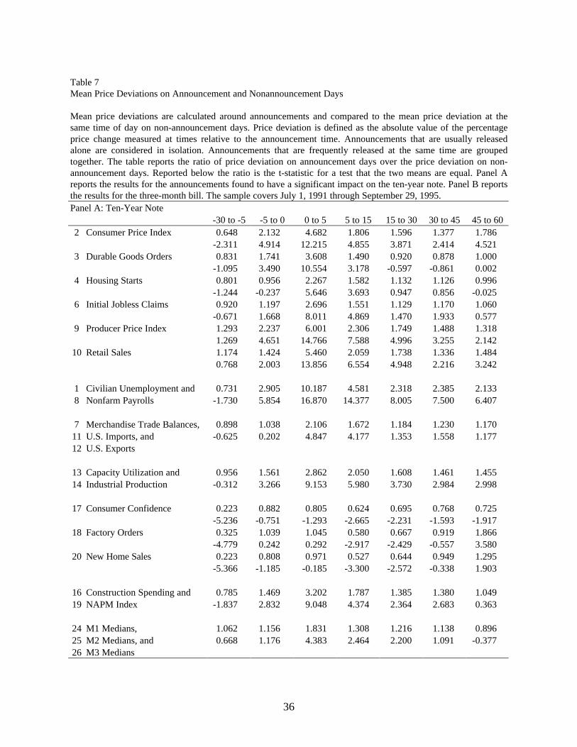
36

Table 7Mean Price Deviations on Announcement and Nonannouncement Days

Mean price deviations are calculated around announcements and compared to the mean price deviation at thesame time of day on non-announcement days. Price deviation is defined as the absolute value of the percentageprice change measured at times relative to the announcement time. Announcements that are usually releasedalone are considered in isolation. Announcements that are frequently released at the same time are groupedtogether. The table reports the ratio of price deviation on announcement days over the price deviation on non-announcement days. Reported below the ratio is the t-statistic for a test that the two means are equal. Panel Areports the results for the announcements found to have a significant impact on the ten-year note. Panel B reportsthe results for the three-month bill. The sample covers July 1, 1991 through September 29, 1995.Panel A: Ten-Year Note

-30 to -5 -5 to 0 0 to 5 5 to 15 15 to 30 30 to 45 45 to 602 Consumer Price Index 0.648 2.132 4.682 1.806 1.596 1.377 1.786

-2.311 4.914 12.215 4.855 3.871 2.414 4.5213 Durable Goods Orders 0.831 1.741 3.608 1.490 0.920 0.878 1.000

-1.095 3.490 10.554 3.178 -0.597 -0.861 0.0024 Housing Starts 0.801 0.956 2.267 1.582 1.132 1.126 0.996

-1.244 -0.237 5.646 3.693 0.947 0.856 -0.0256 Initial Jobless Claims 0.920 1.197 2.696 1.551 1.129 1.170 1.060

-0.671 1.668 8.011 4.869 1.470 1.933 0.5779 Producer Price Index 1.293 2.237 6.001 2.306 1.749 1.488 1.318

1.269 4.651 14.766 7.588 4.996 3.255 2.14210 Retail Sales 1.174 1.424 5.460 2.059 1.738 1.336 1.484

0.768 2.003 13.856 6.554 4.948 2.216 3.242

1 Civilian Unemployment and 0.731 2.905 10.187 4.581 2.318 2.385 2.1338 Nonfarm Payrolls -1.730 5.854 16.870 14.377 8.005 7.500 6.407

7 Merchandise Trade Balances, 0.898 1.038 2.106 1.672 1.184 1.230 1.17011 U.S. Imports, and -0.625 0.202 4.847 4.177 1.353 1.558 1.17712 U.S. Exports

13 Capacity Utilization and 0.956 1.561 2.862 2.050 1.608 1.461 1.45514 Industrial Production -0.312 3.266 9.153 5.980 3.730 2.984 2.998

17 Consumer Confidence 0.223 0.882 0.805 0.624 0.695 0.768 0.725-5.236 -0.751 -1.293 -2.665 -2.231 -1.593 -1.917

18 Factory Orders 0.325 1.039 1.045 0.580 0.667 0.919 1.866-4.779 0.242 0.292 -2.917 -2.429 -0.557 3.580

20 New Home Sales 0.223 0.808 0.971 0.527 0.644 0.949 1.295-5.366 -1.185 -0.185 -3.300 -2.572 -0.338 1.903

16 Construction Spending and 0.785 1.469 3.202 1.787 1.385 1.380 1.04919 NAPM Index -1.837 2.832 9.048 4.374 2.364 2.683 0.363

24 M1 Medians, 1.062 1.156 1.831 1.308 1.216 1.138 0.89625 M2 Medians, and 0.668 1.176 4.383 2.464 2.200 1.091 -0.37726 M3 Medians

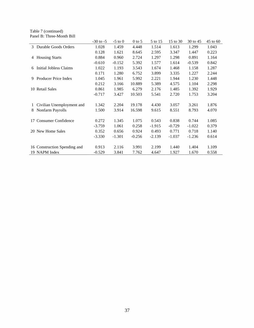
37

Table 7 (continued)Panel B: Three-Month Bill

-30 to -5 -5 to 0 0 to 5 5 to 15 15 to 30 30 to 45 45 to 603 Durable Goods Orders 1.028 1.459 4.448 1.514 1.613 1.299 1.043

0.128 1.621 8.645 2.595 3.347 1.447 0.2234 Housing Starts 0.884 0.960 2.724 1.297 1.298 0.891 1.164

-0.610 -0.152 5.392 1.577 1.614 -0.539 0.8426 Initial Jobless Claims 1.022 1.193 3.543 1.674 1.468 1.158 1.287

0.171 1.280 6.752 3.899 3.335 1.227 2.2449 Producer Price Index 1.045 1.961 5.992 2.221 1.944 1.230 1.448

0.212 3.166 10.889 5.389 4.575 1.104 2.29810 Retail Sales 0.861 1.985 6.279 2.176 1.485 1.392 1.929

-0.717 3.427 10.503 5.541 2.720 1.753 3.204

1 Civilian Unemployment and 1.342 2.204 19.178 4.430 3.057 3.261 1.8768 Nonfarm Payrolls 1.500 3.914 16.598 9.615 8.551 8.793 4.070

17 Consumer Confidence 0.272 1.345 1.075 0.543 0.838 0.744 1.085-3.759 1.061 0.258 -1.915 -0.729 -1.022 0.379

20 New Home Sales 0.352 0.656 0.924 0.493 0.771 0.718 1.140-3.330 -1.301 -0.256 -2.139 -1.037 -1.236 0.614

16 Construction Spending and 0.913 2.116 3.991 2.199 1.440 1.404 1.10919 NAPM Index -0.529 3.841 7.762 4.647 1.927 1.670 0.558

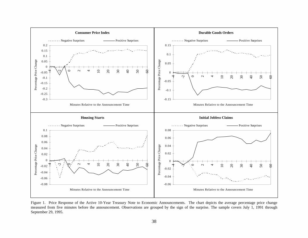
38

Consumer Price Index

-0.3

-0.25

-0.2

-0.15

-0.1

-0.05

0

0.05

0.1

0.15

0.2-4 -2 0 2 4 10 20 30 40 50 60

Minutes Relative to the Announcement Time

Negative Surprises Positive Surprises

Perc

enta

ge P

rice

Cha

nge

Durable Goods Orders

-0.15

-0.1

-0.05

0

0.05

0.1

0.15

-4 -2 0 2 4 10 20 30 40 50 60

Minutes Relative to the Announcement Time

Negative Surprises Positive Surprises

Perc

enta

ge P

rice

Cha

nge

Housing Starts

-0.08

-0.06

-0.04

-0.02

0

0.02

0.04

0.06

0.08

0.1

-4 -2 0 2 4 10 20 30 40 50 60

Minutes Relative to the Announcement Time

Negative Surprises Positive Surprises

Perc

enta

ge P

rice

Cha

nge

Initial Jobless Claims

-0.06

-0.04

-0.02

0

0.02

0.04

0.06

0.08

-4 -2 0 2 4 10 20 30 40 50 60

Minutes Relative to the Announcement Time

Negative Surprises Positive Surprises

Perc

enta

ge P

rice

Cha

nge

Figure 1. Price Response of the Active 10-Year Treasury Note to Economic Announcements. The chart depicts the average percentage price changemeasured from five minutes before the announcement. Observations are grouped by the sign of the surprise. The sample covers July 1, 1991 throughSeptember 29, 1995.