Economic Science and Political Influence

Gilles Saint-Paul

To cite this version:

Gilles Saint-Paul. Economic Science and Political Influence. PSE Working Papers n2012-41.2012. <halshs-00759057>

HAL Id: halshs-00759057

https://halshs.archives-ouvertes.fr/halshs-00759057

Submitted on 29 Nov 2012

HAL is a multi-disciplinary open accessarchive for the deposit and dissemination of sci-entific research documents, whether they are pub-lished or not. The documents may come fromteaching and research institutions in France orabroad, or from public or private research centers.

L’archive ouverte pluridisciplinaire HAL, estdestinee au depot et a la diffusion de documentsscientifiques de niveau recherche, publies ou non,emanant des etablissements d’enseignement et derecherche francais ou etrangers, des laboratoirespublics ou prives.

WORKING PAPER N° 2012 – 41

Economic Science and Political Influence

Gilles Saint-Paul

JEL Codes : A11, E6

Keywords: Ideology ; Macroeconomic Modelling ; Self-con.rming equilibria ;Polarization ; Autocoherent Models ; Intellectual Competition ; Degenerative Research Programs ; Identification

PARIS-JOURDAN SCIENCES ECONOMIQUES48, BD JOURDAN – E.N.S. – 75014 PARIS

TÉL. : 33(0) 1 43 13 63 00 – FAX : 33 (0) 1 43 13 63 10

www.pse.ens.fr

CENTRE NATIONAL DE LA RECHERCHE SCIENTIFIQUE – ECOLE DES HAUTES ETUDES EN SCIENCES SOCIALES

ÉCOLE DES PONTS PARISTECH – ECOLE NORMALE SUPÉRIEURE – INSTITUT NATIONAL DE LA RECHERCHE AGRONOMIQUE

Economic Science and Political In�uence

Gilles Saint-Paul�

November 27, 2012

ABSTRACTWhen policymakers and private agents use models, the economists who de-

sign the model have an incentive to alter it in order infuence outcomes in afashion consistent with their own preferences. I discuss some consequences ofthe existence of such ideological bias. In particular, I analyze the role of mea-surement infrastructures such as national statisticall institutes, the extent towhich intellectual competition between di¤erent schools of thought may lead topolarization of views over some parameters and at the same time to consensusover other parameters, and �nally how the attempt to preserve in�uence canlead to degenerative research programs.JEL: A11, E6Keywords: Ideology, Macroeconomic modelling, Self-con�rming equilibria,

polarization, autocoherent models, intellectual competition, degenerative re-search programs, identi�cation

�Paris School of Economics, New York University Abu Dhabi and Toulouse School ofEconomics. This paper is the text of my EEA Congress Schumpeter Lecture, Malaga, August2012. I am grateful to the President of the EEA, Jordi Gali, for giving me the opportunity topresent this work at the congress. This research has bene�tted from comments from seminarparticipants at Princeton, Yale, CERGE, Venice University, Toulouse School of Economics,the European Summer Symposium in Macroeconomics 2011, Gerzensee, and the InternationalSeminar on Macroeconomics 2011, Malta.

1

1 Introduction

In the standard approach to political economy, agents di¤er in their preferences.

These preferences in turn are aggregated by some political mechanism, which

leads to public decisions being made. From such a perspective, an interest group

can in�uence outcomes only by acquiring more weight in the political process,

for example through campaign contributions.

Yet another important element is the debate on the actual e¤ects of policies.

We observe that people di¤er in their beliefs about how policies relate to out-

comes, because there exists no �rm, agreed upon theory that would pin down

those mechanisms. This in turn opens the door for interest groups to participate

in the debate so as to in�uence beliefs in a self-serving fashion. It then follows

that, in addition to politicians, another class of people will naturally play a

key role in public decision making: the intellectuals. In particular, given that

arguably most decisions made by governments are economic in nature � from

aggregate demand management down to pricing of public utilities, allocating

health expenditure, or the cost-bene�t analysis of public works �we expect a

prominent role to be ascribed to economists.

Controversies about how the economy works have important consequences

for which policies should be prescribed. And one may like such policies more

or less, not only because of one�s beliefs about how they work, but also due to

one�s preferences or self-interest.

For example, how much the government should be involved in macroeco-

nomic management depends on certain properties of the economy: Is there

slack, or are resources fully utilized? Are expectations adaptive or rational?

Are �uctuations chie�y driven by supply shocks or demand shocks? Is the

Keynesian multiplier high or low? The extent to which the economy will be

macro-managed by the government depends on the answers one gives to those

questions. That is, they depend on the theory, in a way tyically summarized in

2

Table 1. Depending on one�s tastes for government intervention, then, one may

favor one theory or another.1

[TABLE 1 HERE]

Consider another example: Should there be a minimum wage, and how high

should it be? Again, the answer depends on our views on the functioning of the

labor market. We are more likely to be in favor of high minimum wages if we

believe �rms have monopsony power (and that is the main thrust of Card and

Krueger�s (1994) new economics of the minimum wage), because then wages are

below the marginal product of labor and jobs won�t be destroyed if they go up,

and if we think the elasticity of labor demand is low, because then minimum

wages entail a low cost in terms of foregone jobs. Furthermore, minimum wages

clearly have distributive consequences, so that some social groups will favor

them and others oppose them2 . Clearly, the former will bene�t if more people

hold views like those in the �rst column of Table 2, because such views are likely

to lead to policy choices in favor of a high minimum wage.

[TABLE 2 HERE]

Real world examples of views of the world being polarized along ideological

lines are common. We may mention the recent US controversy about the size

of the Keynesian multiplier, where more conservative economists aligned with

the former Republican administration argued that the multiplier was low, while

those aligned with the Democratic party considered it was high. Similarly, in

France the labor unions protested against the publication in the national statis-

tican institute journal of a study (Laroque and Salanié, 2000) which concluded

1Throughout this paper I will assume that agents have instrinsic tastes for the level ofgovernment intervention. This could be interpreted as deeper beliefs regarding the natureand e¢ cacy of government, but it can also be interpreted as a short cut for the welfare ofspecial interests, that is, people whose economic activity is more dependent on governmentinvolvement in the economy will bene�t more from such involvement.

2At least this will be the case if no other, more e¢ cient �scal instrument can be used forthe bene�t of the winners of such policies. See Acemoglu and Robinson (2001) and Saint-Paul(2000).

3

that hundreds of thousands of jobs were lost because of the minimum wage,

while promoting alternative studies which did not reach such conclusions. Yet

we also observe, in addition to polarization, some degree of agreement, often

after a convergence process over time. We would like to explain why there is

more consensus on some aspects of the model than others, in light of our view

that beliefs are shaped by self-interest.

2 In�uencing outcomes through beliefs

I now turn to the question of how experts can in�uence outcomes. A charis-

matic guru could in principle promote a view of the world which is demonstrably

false and yet wield in�uence. But here we are talking about scientists and we

must impose discipline upon the set of theories that they may formulate. In

physics, all competing theories, including the correct one, must be observation-

ally equivalent, otherwise some would be rejected by the data. In economics,

things are more complex because beliefs a¤ect outcomes through the formation

of expectations by private agents and the design of government policies, which

is precisely the source of the intellectuals�political power3 . In other words, the

data themselves depend on which model is believed by the agents. Nevertheless,

it makes sense to impose the restriction that any perceived model must match

those data. This means that the economy must be in a self-con�rming equi-

librium (SCE, as in Fudenberg and Levine (1993,2007)) where beliefs may be

incorrect but are nevertheless con�rmed in equilibrium. Only a deviation from

the equilibrium path would reveal that beliefs are wrong. In the context I am

dealing with here, to support such an SCE, the model must be autocoherent: If

everybody uses it to form their expectations, then it matches the corresponding

equilibrium probability distribution of the observables4 .

3MacKenzie (2008) documents the performative aspects of economic theory in the �nancialsector.

4See Saint-Paul (2012a) for an exploration of the properties of those models.

4

This means that the model is observationally equivalent to the correct model

in the equilibrium where people use it. Figure 1 illustrates this concept. Suppose

that the model consists of two parameters, a and b: In general people may believe

that the values of those parameters are a and b; which may di¤er from their

correct values. On �gure 1, the correct model is represented by point CM while

point "1" represents an alternative, incorrect model. The locus IM(1) is the set

of "identi�ed" models in the equilibrium where people use model 1 to form their

expectations. This locus contains more than one point, which means that the

model is under-indenti�ed; of course the correct model CM explains the data

in any equilibrium, so it lies on IM(1)5 . As drawn, locus IM(1) goes through

1. This means that this equilibrium is self-con�rming, i.e. that the model is

autocoherent. We can draw the locus of autocoherent models AC, i.e. the set of

models X such that X 2 IM(X). As long as AC is not reduced to CM, there

exist self-con�rming equilbria supported by incorrect beliefs about the way the

economy works. Again that is possible because the model is under-identi�ed.

Note that in that equilibrium, model 2 is also observationally equivalent to

model 1 (and to the correct model). Therefore, an economist could credibly

claim that it is correct. But if people were to believe him, they would act

di¤erently and the equilibrium would change. In that new equilibrium, the set

of identi�ed models is now IM(2) instead of IM(1)6 . Since point 2 is not on

IM(2), model 2 is not autocoherent. It is self-defeating: the data would reject it

5Here we need to be more precise: what explains the data in any equilibrium such as1 is the correct model of how the economy works conditional on expectations formation andpolicy choices, supplemented with the correct description of expectations formation and policychoices in that equilibrium, i.e. supplemented with the correct assumption that people usethe incorrect perceived model to make choices.On the other hand, a model is autocoherent if the (incorrect) assumption that it describes

the behavior of the economy conditional on policies and expectations formation, along withthe assumption that it is used to form expectations and policies, explains the data, in anequilibrium where it is indeed used to form expectations and policies � implying that thesecond assumption is correct.Implicitly, when one moves along the IM(1) locus, it is common knowledge that people use

the perceived model 1. Therefore, a point along that locus is a model which explains the datain equilibrium 1, under the joint assumption that it is the correct one and that people usemodel 1 to form expectations and policies.

6Since CM is the correct model, it explains the data in all equilibria. Therefore CM is onthe IM(2) locus as well.

5

if everybody believed it. An economist promoting model 2 remains scienti�cally

credible only as long as people do not believe him. Finally, for the sake of

completeness, we may also consider the set of models that are economically

equivalent to model 1. That is the set of models that would deliver the same

equilibrium if people believed them. It is drawn as EE(1) on �gure 1. Model 3

is on EE(1) and delivers the same equlibrium if people use it rather than model

1, but in that equilibrium, the set of models that describe the observables is

given by IM(1), and since model 3 does not lie on that locus it is again not

autocoherent7 .

The preceding literature has produced some important examples of such self-

con�rming equilibria. Piketty (1995) studies a model of income inequality and

redistribution where people may believe either that "luck" is the key determi-

nant of income, or that "e¤ort" is the important variable. Any of those two

beliefs is self-con�rming because of its policy consequences. In the "luck" equi-

librium, people vote for a high level of redistribution; e¤ort is then low and so

is the share of income inequality explained by e¤ort, which validates the belief

that luck matters more. The opposite holds in the other equilibrium8 .

Sargent (2008) studies a situation where the policy maker has some beliefs

regarding the (local) slope of the output/in�ation trade-o¤. These beliefs make

it optimal to select a given point on that trade-o¤, which is the equilibrium

point of the economy. As long as the economy remains at that point (and since

it is supposedly optimal, there is no reason to deviate from it), the slope of the

Phillips curve is unobserved. Consequently the initial beliefs about its slope are

7As discussed in Saint-Paul (2012b, 2012c), if people have to form expectations of observ-able variables and the rational expectations equilibrium (REE) is unique, instead of a modelpeople can just use the relevant moments to form their expectations and this is enough forthe economy to be at the REE. All autocoherent models are then economically equivalent tothe correct one and there is no scope for the expert to in�uence outcomes.This is a situation where the reduced form model is enough to form one�s expectations.

Lucas and Sargent (1979) argue that in practice that is unlikely to be the case as far asthe policymaker is concerned. Hence the utmost importance of the identifying assumptionsunderlying structural identi�cation of the parameters.

8This mechanism has then been re-examined by Benabou and Ok (2001), Alesina andAngeletos (2005).

6

unchanged and the equilibrium is self-con�rming.

What is missing from those examples is a positive theory of which perceived

model is actually used. My objective is to lay the steps for such a theory9 .

In the next section I will lay out a simple model of macro stabilization policy

that has been fully analyzed in Saint-Paul (2012b), and which delivers some

plausible predictions on how an economist�s ideological bias would in�uence his

models. I will then extend it to study some aspects of the interplay between

political economy and the evolution of scienti�c paradigms. That is, in a world

of self-interested experts seeking to achieve in�uence so as to make the world

more palatable to their tastes, how do we expect science to evolve? I will in

particular address the following questions:

� How do theory and measurement interact? How many resources will be

spent on measurement, and is this amount right? How will theory react

to the accuracy of measurement?

� What are the e¤ects of intellectual competition between several school of

thoughts? Do we expect polarization or consensus?

� How will experts try to preserve in�uence when new data are inconsistent

with their model? How will the theory evolve in response to such events?

3 The self-interested expert: A simple macro-economic example

I now brie�y discuss a variant of the model studied in Saint-Paul (2012b) which

is useful to illustrate the optimal choice of a perceived model by a self-interested9For Marxists such as Lucaks and Gramsci, ideology necessarily re�ects the interests of the

"dominant class". Yet this ignores that this "dominant class" is heterogeneous. Exportersand importers have con�icting interests, and similarly for savers who hold nominal bonds andfear in�ation vs. bankers who want credit to �ow as free as possible.Furthermore, in a democratic society, competition for devising the "dominant" ideology is

open. There is no presumption that the dominant ideology will be that of the dominant class,unless we specify how the dominant class achieves intellectual domination. Clearly Hayek(1949) believed that intellectual domination did not coincide with economic domination.

7

expert facing autocoherence constraints.

I consider an economy where the government attempts to stablize aggregate

demand shocks. As those are not directly observed, it needs to make inferences

and for this it will use a "perceived model". The perceived model is determined

by an expert who is fully believed by the government. In particular there is

no scope for the government to reverse engineer the statements of the expert,

contrary to the cheap talk literature (Crawford and Sobel, 1982). This is be-

cause the government knows neither the expert�s preferences and is incapable

of forming priors with respect to the correct model.

The government�s objective is the following:

minE(y2 + 'g2);

where y is a measure of GDP and g a measure of government spending. The

greater the parameter '; the more reluctant the government is to use active

stabilization policy. It is therefore natural to interpret governments with a

higher value of ' as being more conservative.

The equilibrium of the economy is determined by the following two equations:

y = ag + u+ v; (1)

z = !u+ ":

The �rst equation can be interpreted as an aggregate demand curve. The

variables u and v are two independent, normally distributed shocks with zero

means and variances �2u and �2v: I will label u a "demand shock" and v a "supply

shock". The parameter a is the response of output to government expenditures.

It is natural to call it the "Keynesian multiplier". The second equation de-

termines z; a signal that the government observes prior to setting the level of

expenditure g: This signal has noise "; which has a zero mean, is normally dis-

tributed, independent of u and v and has a variance equal �2": The parameter

8

! describes how sensitive the signal is to the demand shock. The greater !; the

better the signal.

The preceding equations describe how the economy is objectively working.

That disturbances have a zero mean and are independent is common knowledge.

The correct model can be summarized as a quintuple (a; !; �2u; �2v; �

2"): In what

follows I will normalize the correct values of ! and �2u to ! = �2u = 1:

Instead of the correct model, the government uses a perceived model which

has the same speci�cation as the correct one but may have di¤erent parameter

values. For reasons that will be clear later, I will assume that the value of

�2" is common knowledge. Therefore the perceived model can be described

as a quintuple (a; !; �2u; �2v; �

2"); where, throughout the text, hats will denote

perceived values. Since the correct value of �2" is common knowledge, it appears

without a hat.

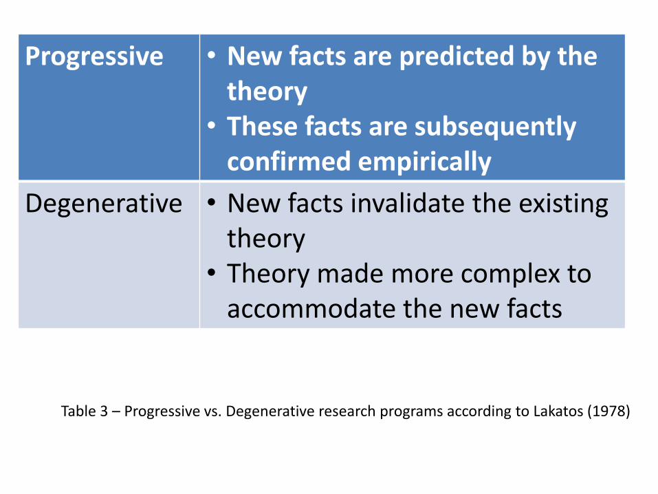
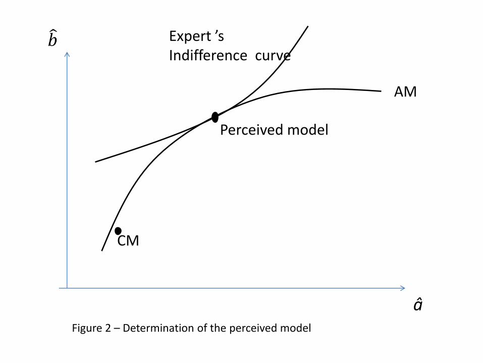
The perceived model is set by an economist who (i) knows the correct model

but chooses to report a potentially incorrect one, (ii) has preferences that may

di¤er from those of the government, and (iii) can only choose an autocoherent

model, otherwise the economy could not be in a SCE, as the model would be

invalidated by the data. Thus, as illustrated on �gure 2 in the two dimensional

case, the economist picks his most preferred perceived set of parameters so as

to maximize his utility function subject to the autocoherence constraints. Here

I will assume that the economist�s objective is

minE(y2 + �'g2):

Therefore, the economist is more (resp. less) conservative than the govern-

ment if and only if �' > ' (resp. �' < ').

[FIGURE 2 HERE]

It is interesting to note that this same simple model could be given a totally

di¤erent interpretation and thus applied to a di¤erent kind of policy decision.

9

For example we could interpret g as an indicator negatively related to the min-

imum wage (such as � lnw if w denotes the minimum wage), a as the absolute

value of the relevant elasticity of labor demand, and y as the level of unskilled

employment. In such a world, the greater '; the more the government prefers

stable wages over stable employment, which may be interpreted as being more

favorable to unions10 .

To solve this model, we need to derive optimal government policy, then we

need to compute the autocoherence constraints, and �nally we need to solve for

the economist�s optimal perceived model.

3.1 Optimal government policy

It is easy to see11 that the optimal value of g is given by

g = z;

with

= � a!�2u(!2�2u + �

2")('+ a

2): (2)

We observe that ; the degree of stabilization, only depends on the perceived,

rather than correct, parameters (with the exception of �2" which is common

knowledge). The absolute value of is larger, i.e. there is more stabilization,

the less conservative the government (the smaller '), and the larger the per-

ceived Keynesian multiplier a; as long as a <p':12 However for a >

p' the

converse holds: beyond that threshold an "income e¤ect" dominates, by which

less activism is needed to achieve a given level of output stability.

10Under such an interpretation a greater value of ' now means that the government ismore "left-wing", under the traditional view that unions are left-wing.11For details, see Saint-Paul (2012b). All the computations for the present pa-

per are in an Appendix available from the author or directly at http://saint-paul.zxq.net/research/Schumpeter%20lecture%20appendix%20computations.pdf12This can be checked by straightforward di¤erentiation of (2).

10

3.2 Autocoherence

A consequence of the government pursuing the optimal policy is that g is col-

inear with z: Therefore, despite that the vector of observables (y; z; g) is three

dimensional, we can reduce it to a two-dimensional vector (y; z): This vector is

normally distributed with zero mean. Any autocoherent model must replicate

the distribution of the observables. This means that if people use this model

(under the assumption that it is common knowledge that everybody uses it)

in order to predict this distribution, the prediction is correct. Here this means

that we must match the variance-covariance matrix of (y; z); that is

Ey2 = Ey2;

Ezy = Ezy;

Ez2 = Ez2 = 1 + �2":

In those formulas, E denotes the mathematical expectation of a variable

computed using the perceived model, whereas E denotes the actual mathemat-

ical expectation in equilibrium, given that the economy is driven by the actual

parameter values while policy is driven by the perceived model.

There are three autocoherence constraints while the perceived model has

four free parameters. This leaves one degree of freedom to the economist to

choose the perceived model. Computations show that this can be reexpressed

as a trade-o¤ between a and ! given by

! ='+ aa

'+ a2: (3)

3.3 The economist�s optimal perceived model

We now turn to the economist�s optimal perceived model. Here it is useful to

note that policy is reduced to one parameter, the degree of stabilization ; and

that the economist has one degree of freedom in choosing the perceived model.

This means that the economist can induce the value of that he would pick

11

if he were a dictator, that is, the one corresponding to the use of the correct

model and the preferences of the economist:

E = �a

(1 + �2")(�'+ a2): (4)

In the sequel, I will label such a situation as "quasi-dictatorship". Equating

to E and using the autocoherence conditions allows us to compute the perceived

model. A central aspect is that it satis�es the following condition:

a = a'

�': (5)

That is, quite naturally, conservative economists tend to understate the value

of the Keynesian multiplier, so as to induce less stabilization. Left-wing econo-

mists do the reverse13 . Furthermore, the gap between the actual and perceived

Keynesian multipliers is equal to the preference gap between the economist and

the government. If the economist is aligned with the government (' = �'), then

the correct model is revealed. Finally, we can also show that a more left-wing

economist will (i) understate the sensitivity of the signal to demand shocks !

(from (3)), (ii) overstate the variance of demand shocks �2u; and (iii) understate

the variance of supply shocks �2v:14

Note that if policy were responsive to another driving variable in addition to

the demand signal z; then the vector of observables would be 6-dimensional. In

such a case the economist would not have enough degrees of freedom and would

be constrained to reveal the correct model. We will return to that later.13Note though that this holds regardless of the value of a: It is also be true if a >

p', i.e.

if the "income e¤ect" dominates. This is because in such a zone the autocoherence conditionimplies a strong positive link between a and �2u : that is, any empirically plausible model witha higher Keynesian multiplier must also have a greater variance of demand shocks. The latter,by itself, tends to induce a greater absolute value for : This is the channel through whichmore left-wing economists induce more stabilization by claiming that a is large, even thoughthe e¤ect of a alone tends to discourage stabilization due to the dominant income e¤ect.14See the computational appendix.

12

4 From theory to measurement

In the preceding discussion, policy is driven by a theory. But policy can be

operational only if theory is supplemented by measurement. And, as measure-

ment is costly, one must decide how much resources to allocate to measurement,

that is, what to measure and how precisely to measure it. These choices will be

driven by theory: Theory will tell us which variables should be measured most

precisely because they matter most for policy.

For example, in a vivid account, Bos (2011) illustrates how the Keynesian

paradigm in�uenced the design of national accounts:

The Keynesian type of analysis established a direct link between

economic theory and national accounting as both came to use the

same macro-economic identities. A direct e¤ect on national account-

ing was that another de�nition of national income and product be-

came most popular:(. . . ). Net national income at factor costs was

more and more replaced by gross national income at market prices.

The Keynesian type of analysis also threw a new light on the role

of the government.(. . . ) This induced the introduction of accounting

per sector, in particular the introduction of a government sector.

(. . . ) Keynes (. . . ) clearly saw the importance of national ac-

counting for planning a national economy in times of war as well of

peace.

� Bos (2011)

Clearly, di¤erent policy paradigms will lead to di¤erent measurement strate-

gies. For example, a "libertarian paradigm", based, say, on the ethical system

proposed by Nozick (1977), will not pay so much attention to aggregate variables

such as GDP or unemployment. Instead, it will attempt to track how well prop-

erty rights are enforced, and possibly to reconstruct the alllocation of resources

13

that would prevail if property rights had been respected in the past, in order

to restore this allocation. As another example, recent proponents of paternal-

ist policies based on happiness economics, such as Easterlin (2001) or Layard

(2007) will insist on measuring happiness and the importance of behavioural

biases instead of, or in addition to, GDP. Indeed the UK government, follow-

ing those authors, is implementing a system for measuring happiness, which

will presumably trigger policy decisions that were not conceivable absent such

a system15 .

The preceding framework delivers some insights about the determnation of

macroeconomic theory whenever it is supplemented by public decisions about

measurement. In our simple example, we can assume that the government

can spend resources in order to better measure the demand shock. Let us

assume that one can pick the variance of the noise to the signal z; �2"; provided

one pays a cost16 c2=�2": That is, the government�s objective function is now

minE(y2+'g2)+c2=�2"; while that of the economist is minE(y2+�'g2)+c2=�2":

Hence, we now treat �2" as policy parameter set by the government prior to

the realization of the equilibrium (which is consistent to our prior assumption

that it is common knowledge). This means that if we denote by U ['; ; a; �2"]

the utility of the government as a function of its preference parameter, its sta-

bilization policy, its beliefs, and its measurement policy, the latter will satisfy

the following �rst-order condition:

@

@�2"U ['; ; a; �2"] = 0:

We can check that this FOC is equivalent to

�'+ a2

� 2 =

c2

(�2")2 :

15See for example http://www.guardian.co.uk/news/datablog/2011/jul/25/wellbeing-happiness-o¢ ce-national-statistics16Given the Gaussian structure of the model, one would face an identical problem if, in the

fashion of Sims (2003), one faced a cost expressed in terms of the mutual information betweenthe signal z and the shock u:

14

Using (2) and the autocoherence conditions we can re-express the optimal

measurement as a function of the perceived Keynesian multiplier only:

�2"1 + �2"

=c('+ aa)

ap'+ a2

: (6)

The RHS is increasing in ' : More conservative governments invest less

in measuring the demand shock because they are less keen on stabilizing the

economy17 . It is also decreasing in a : The greater the perceived Keynesian

multiplier, the more we want to stabilize and the more we want to measure the

demand shock18 . Also, from (2) we also know that is larger in absolute value,

the smaller �2": This is fundamentally because the cross-partial@2U@ @�2"

is positive

and it is a quite general property of Bayes�law: the lower the noise, the more

sensitive our inference is to the signal, and therefore the more we react to the

signal. As a result, there exists a measurement multiplier for any change in

the perceived model. For a given �2"; stabilization policy becomes more active

whenever the perceived Keynesian multiplier a goes up. But this also induces

greater e¤orts at measuring the demand shock, which leads the government to

stabilize even more.

In general the economist would like the government to pursue a di¤erent

level of measurement. The economists�optimality condition for �2" is

�2"1 + �2"

=cp�'+ a2

a: (7)

Suppose the economist is a conservative, i.e. �' > '. Then he would like

to spend less resources on measurement should the government use the correct

model. But, at the same time, the economist convinces the government to use

too small a Keynesian multiplier, which in itself leads to undermeasurement of

the demand shock. We therefore have two con�icting e¤ects: The government

17This is true provided '=2 + a(a� a=2) > 0; which generally holds as long as a is not toosmall or ' not too small.18This is because always increases with a, even for a >

p'; once one takes into account

all the autocoherence conditions.

15

is more left-wing than the economist (the preference e¤ect), but has a more

right-wing view of the world than it really is (the belief e¤ect), precisely due to

the in�uence of the economist.

Which e¤ect dominates? Suppose the economist sets the perceived model

optimally as above, taking the government�s measurement policy, i.e. the value

of �2"; as given. This would be the case in a Nash equilibrium where the gov-

ernment sets and �2" while the economists sets the perceived model simulta-

neously. Then again (5) will hold and substituting into (6) we now have

�2"1 + �2"

=c('�'2 + a2'�')

a'p'�'2 + a2'2

:

The RHS can be shown to be larger than that of (7) for �' > '. This means

that at the perceived model derived in the preceding section, the government

will spend too few resources on measurement compared to what the economist

would do if he were a dictator. That is, the belief e¤ect dominates the preference

e¤ect. Consequently, if the economist takes this into account when setting the

perceived model, he will try to mitigate it by reporting a Keynesian multiplier

closer to the truth. This will occur, for example, in a Stackelberg equilibrium

where the economist �rst selects the perceived model and the government then

determines the stabilization level and the precision of the demand signal.

Therefore, that an underreported Keynesian multiplier generates a downward

bias in measurement will bring the perceived model closer to the correct one.

Note though that if instead the preference e¤ect dominated, then the opposite

would be true: The economist would be even more biased so as to reduce (if he

is conservative) the resources spent on measuring the demand shock, in addition

to inducing less stablization.

16

5 Intellectual competition

The assumption that beliefs are set by a single, highly in�uential intellectual is

obviously quite stark, although it may capture some speci�c historical period,

like the pre-1972 macroeconomic policy paradigm which was heavily in�uenced

by Keynesian ideas, the import substitution model of economic development

which was popular in Latin America19 , or the case of highly ideological totalitar-

ian regimes such as the Soviet Union. In many other cases, though, economists

(and other social scientists) inevitably di¤er in their views. There are di¤er-

ent schools of thought with di¤erent followers, and these schools of thoughts

compete for scienti�c recognition and in�uence over policies and outcomes.

We can use the above framework to analyze the role of competing theories.

In the same logic as above, I am going to assume that, in any equilibrium,

any theory which is believed by some people is capable of explaining the data.

This is a natural generalization of the autocoherence property. Again, that

several theories may explain the same data is possible because the model is

underindenti�ed, and it implies that in any equilibrium, all theories are equally

good. In other words, competition for scienti�c recognition has eliminated all

the theories that do not explain the data. What remains is the attempt by each

school to in�uence outcomes through the design of their theory. This in�uence

comes from the fact that each theory is followed by a number of people, or

equivalently has a certain "weight", and these respective weights are re�ected

in the average belief of society, which we can approximmate as an average of

the di¤erent schools�models. That is illustrated on Figure 3 in the case of two

schools, on which I will henceforth focus. There are two theories, represented

by points 1 and 2. Society believes in some average model A, which re�ects the

weight of each theory � as these weights vary, the average model lies on some

"contract curve" S. The greater the weight of theory 2, the closer A will be to

2 on S. Given that average belief, there is an average action which determines19See Dosman, ed. (2006)

17

the equilibrium. In that equilibrium, the set of identi�ed models is IM(A). Any

theory that survives must lie on IM(A). Note that the average model itself will

not generally be consistent with the data �it is o¤ IM(A). The "average model"

is just a short-cut to represent how beliefs are aggregated between the di¤erent

schools; there is nobody who actually uses it and therefore it does not have to

explain the data.

[FIGURE 3 HERE]

More speci�cally, in the preceding example, each school i would have a

theory summarized by (ai; !i; �2ui; �2vi; �

2"); and the equilibrium will be as if the

perceived model were a = a�1a1��2 ; ! = !�1!

1��2 ; and so on. Again we can ask the

question: How will the di¤erent schools�models depend on their preferences?

Instead of autocoherence constraints, each school must now design its model so

as to match the data in an equilibrium where people use the average model.

Then we can show that instead of the autocoherence trade-o¤ (3) school 1 faces

the constraint

!1 � 1 =!1a(a� a1)!('+ a2)

; (8)

and similarly for school 2.

5.1 Polarization

It is natural to assume that the schools play a Nash equilibrium, i.e. take

the other school�s model as given. Each school will then set its own model

by maximizing its utility subject to the data matching constraints such as (8).

Note that the schools do not derive utility from their own model, what they

really care about is the average model, since it is the one used by the policy

maker when setting the level of public expenditures20 . Given school 2�s model,

20Again, the "policy maker" is a metaphor for the decision process. There is no agent whobelieves in model A since it does not explain the data, only the compromise between di¤erentfactions that have a say in policy leads to the same policy that a unitary government withthe same preferences and a belief in model A would choose.

18

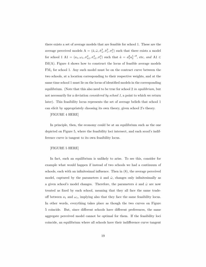
there exists a set of average models that are feasible for school 1. These are the

average perceived models A = (a; !; �2u; �2v; �

2") such that there exists a model

for school 1 A1 = (a1; !1; �2u1; �

2v1; �

2") such that a = a�1a

1��2 ; etc, and A1 2

IM(A). Figure 4 shows how to construct the locus of feasible average models

FM1 for school 1. Any such model must be on the contract curve between the

two schools, at a location corresponding to their respective weights, and at the

same time school 1 must lie on the locus of identi�ed models in the corresponding

equilibrium. (Note that this also need to be true for school 2 in equilibrium, but

not necessarily for a deviation considered by school 1, a point to which we return

later). This feasibility locus represents the set of average beliefs that school 1

can elicit by appropriately choosing its own theory, given school 2�s theory.

[FIGURE 4 HERE]

In principle, then, the economy could be at an equilibrium such as the one

depicted on Figure 5, where the feasibility loci intersect, and each scool�s indif-

ference curve is tangent to its own feasibility locus.

[FIGURE 5 HERE]

In fact, such an equilibrium is unlikely to arise. To see this, consider for

example what would happen if instead of two schools we had a continuum of

schools, each with an in�nitesimal in�uence. Then in (8), the average perceived

model, captured by the parameters a and !; changes only in�nitesimally as

a given school�s model changes. Therefore, the parameters a and ! are now

treated as �xed by each school, meaning that they all face the same trade-

o¤ between a1 and !1; implying also that they face the same feasibility locus.

In other words, everything takes place as though the two curves on Figure

5 coincide. But, since di¤erent schools have di¤erent preferences, the same

aggregate perceived model cannot be optimal for them. If the feasibility loci

coincide, an equilibrium where all schools have their indi¤erence curve tangent

19

to their feasibility locus at the average perceived model cannot arise. In a

similar fashion, getting back to the two schools case, we can consider what

happens if their preferences di¤er marginally from those of the government,

that is '1 � '2 � ': In such a situation, it is natural to assume that they

will choose models that also marginally di¤er from the truth. A �rst-order

apprroximation of (8) around the correct model (i.e. around a = a and ! = 1)

is

!1 � 1 =!1a(a� a1)'+ a2

:

This formula tells us that at a �rst-order approximation, the trade-o¤ be-

tween !i and ai does not depend on the average perceived model. This is because

the deviation between the average perceived model and the correct model only

has second order e¤ects. Since the correct model is the same for both schools

and independent of their perceived models, they again face the same trade-o¤

between !i and ai; as in the case with a continuum of schools. This again rules

out an interior equilibrium where the average perceived model is optimal for

both schools.

What do we, then, expect to observe? In equilibrium, each school will try to

choose a corner solution, that is a point on the common feasibility locus which

is as extreme as possible. For example school one will pick a theory with the

largest possible value of a1; while school 2 will pick a theory with the smallest

possible value of a2: In other words, intellectual competition between schools of

thought who try to in�uence outcomes generates polarized views. The reason

is that they are trying to manipulate the same average perceived beliefs and

have di¤erent targets for those. This is very similar to a game where each player

announces a number between 0 and 100 and each derive utility from the average

of these two numbers. As long as the two players have di¤erent preferences about

that average, the Nash equilibrium is such that one player announces 0 and the

20

other announces 100. This is true even though their preferences may be quite

close: we expect to observe polarized views among economists who may in the

end only marginally di¤er in their preferences.

Such polarized views are not unseen. During the early nineties, the contro-

versies between "fresh water" and "salt water" macroeconomists were polarized:

the former emphasized the role of supply shocks in business cycles considerably,

while the latter were very dismissive about such views21 . Similarly, the recent

multiplier controversy is arguably polarized, with prominent economists being

in favor of either "large" (i.e. 2) or "small" (i.e. 0.5) multipliers, with few views

in the middle22 .

Note however that here we reach the limits of the assumption that the in-

tellectuals are naively believed by their followers. Even if one does not have the

required knowledge to reverse engineer their statements, the mere observation of

polarized views indicates to the policymakers that they are being manipulated.

This surely puts limits on the degree of polarization that one should observe,

but to know more about that we would need to work with a more complex

model where the policymakers could detect manipulation despite not knowing

the correct model nor the experts�preferences, which would open the door for

an economist with a less extreme model to enter the market and steal followers

from the extremists. On the other hand, we may also explore the idea that

extreme views may survive because they are more parsimonious and because

they generate more clear-cut prescriptions for actions.

5.2 Mutation-proofness and consensus

A general theme of the approach I am discussing is that variation in policy

regimes generally change the equilibrium, which increases the amount of data

21An account of these controversies can be found in Blanchard (2009), who also notes theirtendency to erode over time and for consensus to emerge.22See Batini et al. (2012). Intuitively, a crisis leads people to dismiss previous data; this

increases the degrees of freedom of the intellectuals, and therefore the scope for controversy.

21

that any acceptable model has to explain: such a model now has to replicate the

relevant moments for each policy regime. Consequently, the set of autocoherent

models is reduced: changes in policy regimes act as a natural experiment which

increases the number of parameters that are identi�ed. I will discuss these issues

to a greater extent in the next section, but they are also relevant to intellectual

competition.

When a school considers deviating and picking a di¤erent model, it faces the

constraint that its alternative model must explain the data, taking into account

that as a result of its deviation, the equilibrium will change due to changes in

average beliefs. But this change in equilibrium will then typically make the

models of other schools invalid, and our school can very well live with that23 .

This means that by deviating, any school, by changing average beliefs, can force

a "natural experiment" that would invalidate the other schools�models. This

is somewhat problematic for our equilibrium concept, because then there is no

reason why, upon my deviating, my competitors�models should be continue to

be believed.

This suggests that it makes sense to consider "mutation-proof" strategies,

that is to impose that any theory explains the data regardless of the beliefs

promoted by competing theories. This is a strong restriction because it does

not restrict the competing theories to be mutation proof themselves; that is, it

allows for my competitors to hold demonstrably false views, assuming that they

are charismatic enough to nevertheless have followers. It would be interesting

to relax such a strong concept of mutation proofness, but here it is enough to

illustrate my point.

We can rewrite Equation (8) as

!1 � 1 =!1(a

�1a1��2 )(a� a1)

(!�1!1��2 )('+ (a�1a

1��2 )2)

:

23Note however that if it takes into account the consequences of a competing school beingabandoned as a result of its own deviation (such as more people adopting its own model), itwill pick a di¤erent model since the set of feasible average perceived models is changed.

22

In a mutation-proof equilibrium, this has to hold for any competing model

(a2; !2); not just for the equilibrium one. Clearly, this can be the case only if

a = a1 and ! = !1: The correct model must now be reavealed.

More generally, though, it may be that mutation-proofness does not yield

enough constraints to force to reveal the correct model. In such cases it will

induce the economist to reveal some parameters (or perhaps a combination of

parameters), while at the same time the tendencies for polarization on other

parameters will remain. Thus we see how intellectual competition generates

forces towards polarization as well as consensus, although here consensus arises

over the correct model, because mutation proofness compels the schools to come

up with more robust theories, rather than out of a need to conform to the views

of others.

6 Degenerative research programs

In the preceding discussion, I implicitly assumed that the correct model�s spec-

i�cation was common knowledge, by imposing that any perceived model should

have the same structure as the correct one and di¤er from it only because it

has di¤erent parameter values. But of course in reality the correct speci�cation

is unknown, so that a self-serving expert could pick his speci�cation so as to

preserve or achieve in�uence. Indeed, a measure of the degree of in�uence is

I = A�B � C; (9)

where A is the number of independent parameters of my model, B is the number

of autocoherence conditions, and C the number of policy parameters set by the

government. Generally, if I � 0; the expert is a quasi-dictator. On the other

hand, if I � �C; the expert is forced to reveal the correct model.

Let us go back to the remark, made in the preceding section, that policy

regime changes generate new observations that make it more di¢ cult for my

23

model to match the data. This means that we expect B to increase each time

there is a regime change. Let us hold A and C �xed. If regime changes happen

with a non zero probability, if there is an arbitrarily large number of potential

policy regimes, and if one does not forget the data, then at some point I will

fall to �C and the expert�s in�uence will vanish.

However, if we now assume that the correct value of A is not know, there is

now a natural way for the expert to preserve his in�uence, by making the model

more complex, i.e. by adding parameters, so that A could increase over time in

line with B: In a dynamic fashion, the expert�s model could be rejected after

a policy regime change (or any other natural experiment), and he would come

up with a more complicated model that would explain the new data in addition

to the old ones. One may wonder why anydoby would still believe him, rather

that say a competitor. However it does not really matter to us whether we are

talking about the initial expert or a competitor, as long as the competitor is

also self-interested and has to come up with an equally complex model in order

to explain the data.

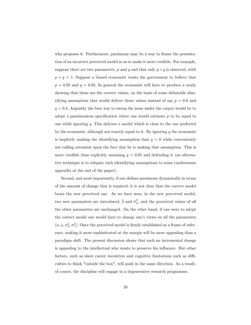
Therefore we expect self-interested experts to make their model more com-

plex over time in order to preserve in�uence. This is similar to the notion of a

degenerative research program discussed by Lakatos (1978), a follower of Kuhn

(1962). The distinction between progressive and degenerate research programs,

according to Lakatos, is summarized in Table 3.

[TABLE 3 HERE]

6.1 A simple example

Let us illustrate this point in the context of our simple framework. In our model,

part of the reason why the government does not know the correct Keynesian

multiplier is that according to its beliefs it is pursuing an optimal stabilization

policy, by which public expenditures are colinear with the signal z: Suppose we

24

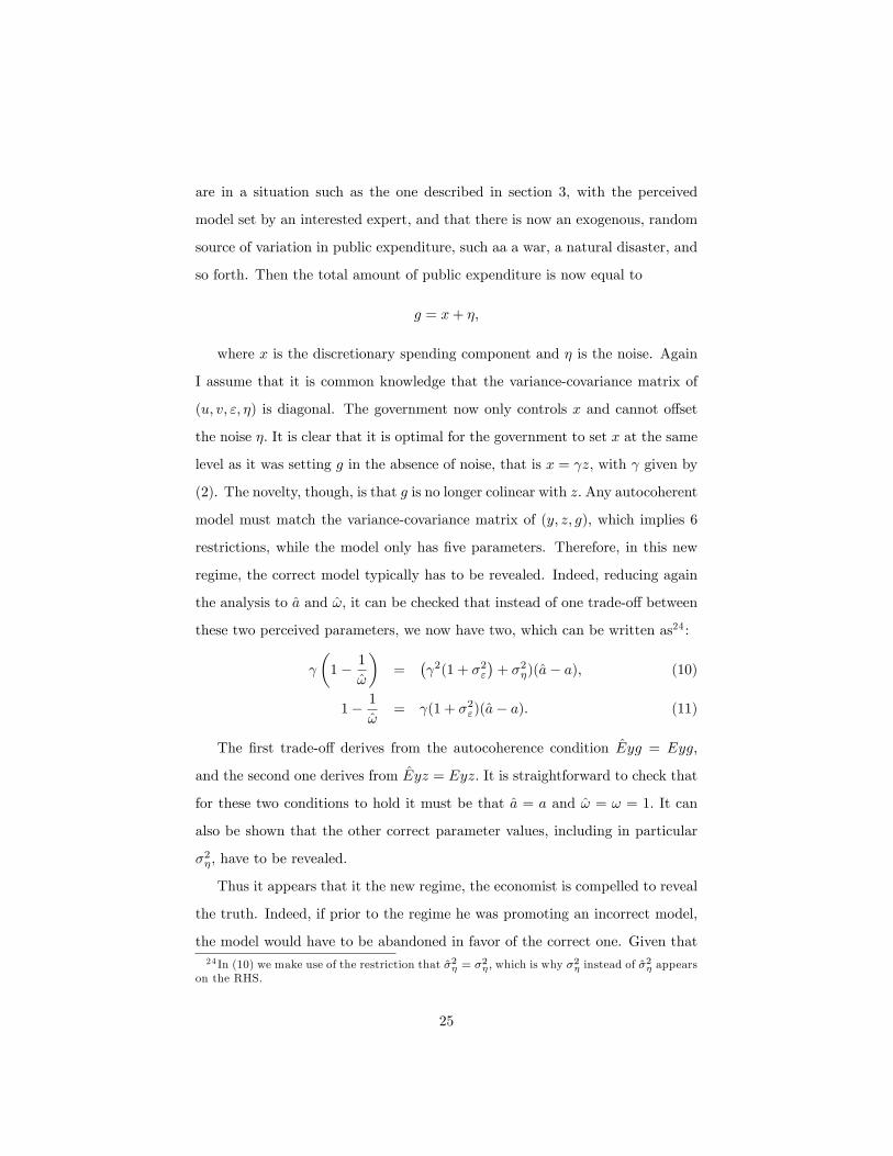
are in a situation such as the one described in section 3, with the perceived

model set by an interested expert, and that there is now an exogenous, random

source of variation in public expenditure, such aa a war, a natural disaster, and

so forth. Then the total amount of public expenditure is now equal to

g = x+ �;

where x is the discretionary spending component and � is the noise. Again

I assume that it is common knowledge that the variance-covariance matrix of

(u; v; "; �) is diagonal. The government now only controls x and cannot o¤set

the noise �: It is clear that it is optimal for the government to set x at the same

level as it was setting g in the absence of noise, that is x = z; with given by

(2). The novelty, though, is that g is no longer colinear with z: Any autocoherent

model must match the variance-covariance matrix of (y; z; g); which implies 6

restrictions, while the model only has �ve parameters. Therefore, in this new

regime, the correct model typically has to be revealed. Indeed, reducing again

the analysis to a and !; it can be checked that instead of one trade-o¤ between

these two perceived parameters, we now have two, which can be written as24 :

�1� 1

!

�=

� 2(1 + �2"

�+ �2�)(a� a); (10)

1� 1

!= (1 + �2")(a� a): (11)

The �rst trade-o¤ derives from the autocoherence condition Eyg = Eyg;

and the second one derives from Eyz = Eyz: It is straightforward to check that

for these two conditions to hold it must be that a = a and ! = ! = 1: It can

also be shown that the other correct parameter values, including in particular

�2�, have to be revealed.

Thus it appears that it the new regime, the economist is compelled to reveal

the truth. Indeed, if prior to the regime he was promoting an incorrect model,

the model would have to be abandoned in favor of the correct one. Given that24 In (10) we make use of the restriction that �2� = �

2� ; which is why �

2� instead of �

2� appears

on the RHS.

25

in any case the preceding model has to be abandoned, though, the economist

may consider other options than revealing the correct model that may preserve

his in�uence. In particular, as long as the correct speci�cation is not common

knowledge (and there is no reason why it should be since a speci�cation funda-

mentally is an intellectual construct), the economist can preserve his in�uence

by making the model more complex, that is, by increasing the number of para-

meters A so as to o¤set the increase in the number of autocoherence conditions

B:

Suppose then that upon invalidation of the preceding perceived model in

the new regime, the economist now modi�es it marginally and claims that the

random component of public expenditures has a di¤erent multiplier from the

systematic one. That is indeed plausible, since under rational expectations

surprises generally have di¤erent e¤ects from anticipated shocks. That is, output

determination is now

y = ax+ b� + u+ v;

where the correct parameter values are such that b = a but the economist can

pick b di¤erent from a: It is then easy to see that the autocoherence condition

(10) becomes

�1� 1

!

�=� 2(1 + �2"

�+ �2�)(a� a) + �2�(b� a); (12)

while the other autocoherence condition (11), i.e. Eyz = Eyz; is unchanged, as

it does not involve b since it is common knowledge that the shocks (u; v; "; �) are

uncorrelated. Furthermore it must still be that �2� = �2�; which comes from the

fact that x is observed and the variance of g has to be matched. Therefore (12)

de�nes a trade-o¤ between the three perceived parameters a; b; and !: Given a

choice for a and ! that matches (11), the economist can now freely pick b to

match (12). Therefore, the economist can preserve his in�uence by using the

new, less parsimonious model and act again as a quasi-dictator.

In fact, it turns out that the economists cannot lie about b: Substituting

26

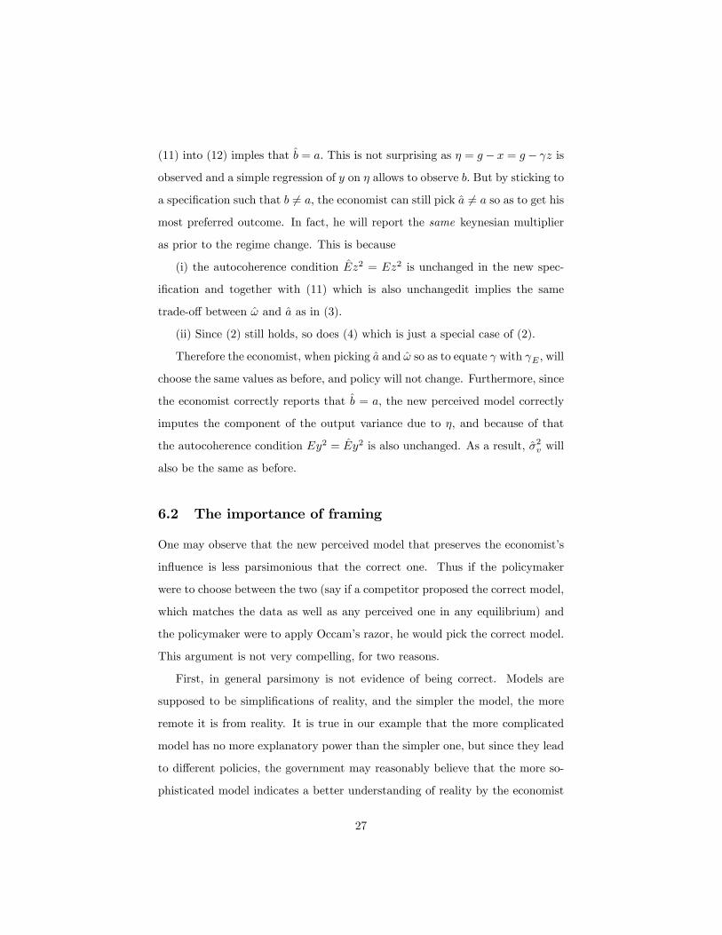
(11) into (12) imples that b = a: This is not surprising as � = g � x = g � z is

observed and a simple regression of y on � allows to observe b: But by sticking to

a speci�cation such that b 6= a; the economist can still pick a 6= a so as to get his

most preferred outcome. In fact, he will report the same keynesian multiplier

as prior to the regime change. This is because

(i) the autocoherence condition Ez2 = Ez2 is unchanged in the new spec-

i�cation and together with (11) which is also unchangedit implies the same

trade-o¤ between ! and a as in (3).

(ii) Since (2) still holds, so does (4) which is just a special case of (2).

Therefore the economist, when picking a and ! so as to equate with E ; will

choose the same values as before, and policy will not change. Furthermore, since

the economist correctly reports that b = a; the new perceived model correctly

imputes the component of the output variance due to �; and because of that

the autocoherence condition Ey2 = Ey2 is also unchanged. As a result, �2v will

also be the same as before.

6.2 The importance of framing

One may observe that the new perceived model that preserves the economist�s

in�uence is less parsimonious that the correct one. Thus if the policymaker

were to choose between the two (say if a competitor proposed the correct model,

which matches the data as well as any perceived one in any equilibrium) and

the policymaker were to apply Occam�s razor, he would pick the correct model.

This argument is not very compelling, for two reasons.

First, in general parsimony is not evidence of being correct. Models are

supposed to be simpli�cations of reality, and the simpler the model, the more

remote it is from reality. It is true in our example that the more complicated

model has no more explanatory power than the simpler one, but since they lead

to di¤erent policies, the government may reasonably believe that the more so-

phisticated model indicates a better understanding of reality by the economist

27

who proposes it. Furthermore, parsimony may be a way to frame the presenta-

tion of an incorrect perceived model so as to make it more credible. For example,

suppose there are two parameters, p and q and that only p+ q is observed, with

p + q = 1: Suppose a biased economist wants the government to believe that

p = 0:95 and q = 0:05: In general the economist will have to produce a study

showing that these are the correct values, on the basis of some debatable iden-

tifying assumption that would deliver those values instead of say p = 0:6 and

q = 0:4: Arguably the best way to sweep the issue under the carpet would be to

adopt a parsimonious speci�cation where one would estimate p to be equal to

one while ignoring q: This delivers a model which is close to the one preferred

by the economist, although not exactly equal to it. By ignoring q the economist

is implictly making the identifying assumption that q = 0 while conveniently

not calling attention upon the fact that he is making that assumption. This is

more credible than explicitly assuming q = 0:05 and defending it (an alterna-

tive technique is to relegate such identi�ying assumptions to some cumbersome

appendix at the end of the paper).

Second, and most importantly, if one de�nes parsimony dynamically in terms

of the amount of change that is required, it is not clear that the correct model

beats the new perceived one. As we have seen, in the new perceived model,

two new paramaters are introduced, b and �2�; and the perceived values of all

the other parameters are unchanged. On the other hand, if one were to adopt

the correct model one would have to change one�s views on all the parameters

(a; !; �2u; �2v): Once the perceived model is �rmly established as a frame of refer-

ence, making it more sophisticated at the margin will be more appealing than a

paradigm shift. The present discussion shows that such an incremental change

is appealing to the intellectual who wants to preserve his in�uence. But other

factors, such as sheer career incentives and cognitive limitations such as di¢ -

culties to think "outside the box", will push in the same direction. As a result,

of course, the discipline will engage in a degenerative research programme.

28

What is key here is that a frame of reference is a set of identifying assump-

tions. Thus, in the preceding example, the amendment to the existing model

� the "discovery" that random shifts in public expenditures have a di¤erent

multiplier � could rationally be presented as a new �nding, as long as it is

considered, explicitly or implicitly, that it is "known" that the multiplier for

systematic expenditure shifts is equal to a25 : Arnold Kling (2011) expresses his

sceptical views about such a process:

�Because of the need to impose strong priors, the structural ap-

proach is nothing but a roundabout way of communicating the way

you believe the economy works. The estimated equations are not be-

ing used to discover relationships. Instead, the equations are being

used by the econometrician to communicate to others the econome-

trician�s beliefs about how the economy ought to work. To a �rst

approximation, using structural estimates is no di¤erent from creat-

ing a simulation model out of thin air by making up the parameters.�

Kling (2011).

Kling also describes three main strategies that were used to preserve the

dominant paradigm in the face of new contradictory evidence (such as the drift

in the Phillips curve): "dropping old data; add factors; and lagged dependent

variables.". Clearly the last two practices can be interpreted in light of Lakatos�s

views regarging degenerative research programme. A similar account of macro-

econometric practice can be found in Lucas and Sargent (1979).:

"The track record of the major econometric models is (...) very

poor.(...). Moreover, this di¢ culty is implicitly acknowledged by

model builders thelmselves, who routinely employ an elaborate sys-

25 In a similar vein, Lucas and Sargent (1979) describe how the postulates from the Gen-eral Theory, such as those regarding the demand for money or the consumption function,were systematically used as (unwarranted, in their view) identifying assumptions in structuralmacroeconometric modelling.

29

tem of add factors in forecasting, in an attempt to o¤set the contin-

uing drift of the model away from the actual series."

Lucas and Sargent (1979)

Note that there are other mechanisms for preserving an existing paradigm.

For example Cogley and Sargent (2005) argue that the old Phillips curve hy-

pothesis was only discarded by policymakers in favor of the natural rate one in

the late 1970s, despite that its likelihood was (in their view) quite low as early

as 1970. Their idea, borrowed from Hansen and Sargent�s (2005) robust control

theory, is that the old Phillips curve view delivered the worst case scenario of

a painful disin�ation; under robust control, a lot of weght is given to the worst

case scenario even though the model that delivers it is unlikely26 . From our

perspective, this suggests that the expert can strategically use the policymaker

tendencies toward prudence, by devising a model such that policy deviations

from the expert�s preferred outcome are very costly, i.e. acting as a doomsayer.

Indeed, revising one�s model to make it more dramatic may be viewed as one

instance of a degenerative research programme.

7 Conclusion

A scienti�c paradigm is necessary to set a framework for scienti�c progress. Sim-

ilarly, an economic paradigm is necessary for policy to be conducted. But are

economic paradigms neutral or do they re�ect an agenda? Here I have explored

the latter possibility, on the basis of two stark simplifying assumptions. The

�rst assumption is that the policymaker naively accepts the model presented to

him by the economists. The second assumption is that the economist knows the

correct model and cynically reports an incorrect (but unfalsi�able) one. The

analysis hopefully delivers some interesting insights about how interest groups

may a¤ect beliefs even in the case where those are embodied in sophisticated

26This view is consistent with the historical account of De Long (1996).

30

theories validated by the data. But it leaves many questions open to future

research. One will need to relax these two assumptions in order to better un-

derstand how people pick the theories they use and how political preferences

shape the views of the intellectuals in a sophisticated fashion. Also, we need to

understand why some theories (such as the Keynesian one), rather than com-

peting ones, become the dominant paradigm, and why and when a paradigm is

eventually abandoned.

31

REFERENCES

Acemoglu, Daron and James A. Robinson (2001), "Ine¢ cient Redistribu-

tion", American Political Science Review, Vol. 95, No. 3, pp. 649-661

Alesina Alberto and George-Marios Angeletos (2005). "Fairness and Redis-

tribution," American Economic Review, vol. 95(4), pages 960-980

Batini Nicoletta, Giovanni Callegari and Giovanni Melina, "Successful Aus-

terity in the United States, Europe and Japan", IMF Working Paper, 2012

Bénabou Roland and Efe A. Ok (2001). "Social Mobility And The Demand

For Redistribution: The Poum Hypothesis," Quarterly Journal of Economics,

vol. 116(2), pages 447-487, May.

Blanchard, Olivier, 2009. "The State of Macro," Annual Review of Eco-

nomics, Annual Reviews, vol. 1(1), pages 209-228, 05.

Bos, Frits (2011), "Three centuries of macro-economic statistics" Eagle Eco-

nomic & Statistics Working Paper 2011-02

Card, David & Krueger, Alan B, 1994. "Minimum Wages and Employment:

A Case Study of the Fast-Food Industry in New Jersey and Pennsylvania,"

American Economic Review, vol. 84(4), pages 772-93, September.

Cogley, Timothy and Thomas J. Sargent, (2005). "The conquest of US

in�ation: Learning and robustness to model uncertainty," Review of Economic

Dynamics, vol. 8(2), pages 528-563, April.

Crawford, Vincent P. and Joel Sobel (1982) Strategic Information Transmis-

sion" Econometrica, Vol. 50, No. 6 (Nov.), pp. 1431-1451

De Long, J. Bradford (1997), "America�s Peacetime In�ation: The 1970s,"

in Christina D. Romer and David H. Romer, Editors, Reducing In�ation: Mo-

tivation and Strategy University of Chicago Press (1997)

Dosman, Edgar J., ed. (2006), Raul Prebisch: Power, Principle and the

Ethics of Development, Washington DC: IDB-INTAL

Easterlin, R. (2001), �Income and Happiness: Towards a Uni�ed Theory�,

Economic Journal, 111 (473), 465-84.

32

Fudenberg. D. and D.K. Levine (1993) �Self-Con�rming Equilibrium�Econo-

metrica, 61 , 523-546.

� � � � � � � � � � � (2009), "Self-con�rming equilibrium and

the Lucas critique" Journal of Economic Theory 144 issue 6 p. 2354-2371

Hansen, L. P. and T. J. Sargent (2005a). "Robust estimation and control

under commitment." Journal of Economic Theory 124, 258�301.

Hayek, Friedrich, (1949), "The Intellectuals and Socialism", University of

Chicago Law Review

Kling, Arnold (2009), "Macroeconometrics: The lost history",

arnoldkling.com/essays/macroeconometrics.doc

Kuhn, T.S. The Structure of Scienti�c Revolutions. Chicago: University of

Chicago Press, 1962.

Lakatos Imre (1978), The Methodology of Scienti�c Research Programmes:

Philosophical Papers Volume 1. Cambridge: Cambridge University Press

Laroque, Guy and Bernard Salanié, (2000),� Une décomposition du non

emploi en France �, Economie et statistique, 331

Layard, Richard, (2007). �Happiness and the Teaching of Values.�Centre-

Piece 18-23.

Lucas, R. and T. Sargent (1979), "After Keynesian Macroeconomics", Fed-

eral Reserve Bank of Minneapolis Quarterly Review; spring, 1-16

MacKenzie, Donald (2008), An Engine, Not a Camera. How Financial Mod-

els Shape Markets. Cambridge MA: MIT Press

Nozick, R., (1977), Anarchy, State and Utopia. New York: Basic Books

Piketty, Thomas, (1995) "Social Mobility and Redistributive Politics", Quar-

terly Journal of Economics

Saint-Paul, Gilles (2000), The political economy of labour market institu-

tions. Oxford: Oxford University Press

� � � � � � � �(2012a) "Some properties of autocoherent models", work-

ing paper, TSE and CEPR

33

� � � � � � � �(2012b) "Toward a Political Economy of Macroeconomic

Thinking" in J. Frenkel and C. Pissarides, eds, International Seminar on Macro-

economics 2011 (p. 249 - 284), University of Chicago Press for NBER

� � � � � � � �(2012c) "The scope for ideological bias in structural macro-

economic models", working paper, TSE and NBER

Sargent, Thomas (2008), "Evolution and Intelligent Design", American Eco-

nomic Review, 98(1), 5-37

Sims Christopher A., "Implications of rational inattention", Journal of Mon-

etary Economics 50 (2003) 665�690

.

34

Pro State Contra State Slack Equilibrium

Adaptive Expectations

Rational expectations

Demand shocks Supply shocks

High Keynesian Multiplier

Low Keynesian Multiplier

Table 1 – Macroeconomic views and preferences for state intervention

Pro Contra Monopsony Competition

Low labour demand elasticity

High labour demand elasticity

Table 2 -- Views on the labor market and preferences for high minimum wages

Progressive • New facts are predicted by the theory

• These facts are subsequently confirmed empirically

Degenerative • New facts invalidate the existing theory

• Theory made more complex to accommodate the new facts

Table 3 – Progressive vs. Degenerative research programs according to Lakatos (1978)

â

CM

2

1

3

AM

IM(1)

EE(1)

IM(2)

Figure 1 – Autocoherent models

â

CM

AM

Figure 2 – Determination of the perceived model

Perceived model

Expert ’s Indifference curve

â

CM

2

1

IM(A)

Figure 3 – Two schools of thought

A

â

CM

2

1

IM(A)

Figure 4 – The feasible average models locus

A

1’

B IM(B)

FM1

â Figure 5 -- Interior equilibrium

FM2 FM1

IC1

IC2