economics 306 a01: international economicsweb.uvic.ca/~bscarfe/international economics.pdf · ·...
TRANSCRIPT

Economics 306 – A01: International Economics
Summer term 2008: MTWRF 10:30-12:30 in CLEA311
Instructor: Brian L. Scarfe
Business telephone: 360-0300; e-mail: [email protected]
Office hours: MTWRF 9:15-10:15 in BEC 328; tel: 721-6520
Required Text: Paul R. Krugman and Maurice Obstfeld, International Economics:
Theory and Policy, eighth edition, Addison-Wesley, 2008, ISBN
0-321-49304-4
Given the condensed nature of summer session courses, we will only be able to cover the
main highlights of the International Economics syllabus. The course will move quickly
through the following topics. Students are strongly advised to keep their reading of the
textbook and lecture notes on pace.
Lecture outline: Text chapters
May 12-16: Part One: International Trade Theory (5 classes) Ch. 1-7
May 12: Introduction and Overview: Main Themes, Gravity Model Ch. 1 and 2
May 13: Comparative Advantage: the Ricardian Model Ch. 3
May 14: The Heckscher-Ohlin Factor Proportions Model Ch. 4
May 15: The Standard Trade Model: Growth, Terms of Trade Ch. 5
May 16: Economies of Scale, Intra-Industry Trade and Factor Mobility Ch. 6 and 7
May 20-22: Part Two: International Trade Policy (3 classes) Ch. 8-11
May 20: Instruments of Trade Policy: Tariffs Ch. 8
May 21: Other Instruments of Trade Policy: Worked Examples Ch. 9
May 22: Free Trade versus Protectionism: Customs Unions Ch. 10 and 11
May 23 (Friday): Midterm Examination (40 marks)
May 26-29: Part Three: Exchange Rates and Open-Economy
Macroeconomics (4 classes) Ch. 12-17
May 26: The Balance of Payments and Exchange Rates Ch. 12 and 13
May 27: The Asset Approach: Money, Interest Rates and Exchange Rates Ch. 14
May 28: Real Exchange Rates and Purchasing Power Parity Ch. 15
May 29: Macro-Economic Adjustment under Flexible Exchange Rates:
The Marshall-Lerner Condition and the Current Account Ch. 16
May 30-June 3: Part Four: International Macroeconomic Policy
(3 classes) Ch. 18-22
May 30: Fixed Exchange Rates and Macro-Economic Adjustment Ch. 17 and 18
June 2: External and Internal Balance: Exchange Rate Regimes and
Optimal Currency Areas Ch. 19 and 20
June 3: International Capital Markets and International Debt Problems Ch. 21 and 22
June 4 (Wednesday): Final Examination (60 marks)

Examinations and Grading Equivalencies:
Midterm examination (1 hr, 45 min): 40% Final examination (1 hr, 45 min): 60%
A+ = 90-100% A = 85-89% A- = 80-84% B+ = 75-79%
B = 70-74% B- = 65-69% C+ = 60-64% C = 55-59%
D = 50-54% F = 0-49%
Plagiarism and cheating: Students are expected to observe the same standards of scholarly
integrity as their academic and professional counterparts. Students who are found to have
engaged in unethical academic behaviour, including the practices described on pages 31-32
of the calendar, are subject to penalty by the University.
Inclusivity and diversity: The University of Victoria is committed to providing an
environment that affirms and promotes the dignity of human beings of diverse backgrounds
and needs.
Workshop Questions: Workshop questions will be taken up in class from time to time.
Students are advised to work on these questions in advance of the workshops.
Workshop One, for in class discussion on Wednesday, May 14
This question is essentially similar to problems 1 to 5 on p. 52 of the textbook.
Two countries, Home and Foreign, trade apples and bananas in a Ricardian trade world.
Home has 1,200 units of labour available, and requires 3 units of labour to produce one
tonne of apples and 2 units of labour to produce one tonne of bananas. Foreign has 800
units of labour available, and requires 5 units of labour to produce one tonne of apples and
1 unit of labour to produce one tonne of bananas.
(a) Construct graphically the world relative supply curve which relates the relative price of
apples to the relative quantity of apples produced.
(b) On the same graph, draw the world relative demand curve under the assumption that (in
both countries) expenditure is equally divided between the two goods, so that p(A) Q(A) =
p(B) Q(B), where p(A) and p(B) are the prices of apples and bananas, and Q(A) and Q(B)
are the overall quantities of apples and bananas produced (and consumed), respectively.
(c) Calculate the values of p(A)/p(B), Q(A) and Q(B) in trading equilibrium.
(d) Based upon comparative advantage theory, which country exports apples (how many
tonnes?), and which country exports bananas (how many tonnes?), in trading equilibrium?
(e) Calculate the increased volumes of apples and bananas that become available in trading
equilibrium when compared with the pre-trade situation, and thereby demonstrate that there
are consumption gains from trade (how are these gains shared between the two countries?).
Answer Guide: Workshop One
(a) The relative supply curve is horizontal at p(A)/p(B) = 3/2 (the relative cost ratio in
Home), has a vertical section at Q(A)/Q(B) = ½ (when all Home labour is allocated to

apples, and all Foreign labour is allocated to bananas), and has a further horizontal section
at p(A)/p(B) = 5/1 (the relative cost ratio in Foreign).
(b) The relative demand curve is a rectangular hyperbola which intersects the relative
supply curve in the vertical section.
(c) In trading equilibrium, p(A)/p(B) = 2, Q(A) = 400 tonnes, and Q(B) = 800 tonnes.
(d) As expected from the theory of comparative advantage, Home will export apples and
Foreign will export bananas. If D(A) and D(B) are Home’s consumption of apples and
bananas, respectively, then p(A) D(A) = p(B) D(B) and p(A) [ 400 – D(A)] = p(B) D(B). It
follows that D(A) = 200, and D(B) = 400. Thus, Home will export 200 tonnes of apples in
exchange for 400 tonnes of bananas, which are imported from Foreign.
(e) However, in the pre-trade situation at a relative cost ratio of 3/2, Home produces 200
tonnes of apples and 300 tonnes of bananas, fully employing 1,200 units of labour. In the
pre-trade situation at a relative cost ratio of 5/1, Foreign produces 80 tonnes of apples and
400 tonnes of bananas, fully employing 800 units of labour. Free trade increases the
overall production of apples from 280 tonnes to 400 tonnes, with all of the additional 120
tonnes consumed by Foreign. Free trade also increases the overall production of bananas
from 700 tonnes to 800 tonnes, with all of the additional 100 tonnes consumed by Home.
Workshop Two, for in class discussion on Wednesday, May 21
A country imports 3 billion barrels of crude oil per year and domestically produces another
3 billion barrels of crude oil per year. The world price of crude oil is $18 per barrel.
Assuming linear schedules, economists estimate the price elasticity of domestic supply to
be 0.25 and the price elasticity of domestic demand to be - 0.10 in the neighbourhood of the
current equilibrium.
(a) Assuming that the world price of crude oil does not change when the country imposes a
$6 per barrel import duty on crude oil, determine the domestic price, and the three
quantities: domestic consumption, domestic production, and import volume after the
imposition of the import duty.
(b) Calculate the impact on producer surplus, consumer surplus, and government revenues.
Also calculate the net social benefits associated with the imposition of the import duty.
(c) and (d) Redo the calculations under (a) and (b) on the assumption that the reduction in
the country’s demand for crude oil reduces the world price by $2 per barrel.
(e) By how much does the “terms of trade effect” of the import duty offset the efficiency
losses (i.e., what are the net social benefits to the importing country)? If foreign exporters
also had standing, would overall welfare be increased?
Answer Guide: Workshop Two
(a) A small open economy is a price-taker for its imports in the world market place. Since
none of the tariff incidence can be shifted backwards to foreign producers, the whole
burden of an import tariff falls on domestic consumers. In this case, the domestic price of
crude oil rises by $6 per barrel from $18 to $24. The resulting change in domestic quantity

supplied is given by 0.25 x 3 x 6/18 = 0.25 bbls (billion barrels), resulting in 3.25 bbls
being the new quantity supplied. The resulting change in domestic quantity demanded is
given by – 0.10 x 6 x 6/18 = - 0.20 bbls, resulting in 5.80 bbls being the new quantity
demanded. As a result, imports fall by 0.45 bbls to 2.55 bbls.
(b) The positive effect on producer surplus is given by area a in the diagram. This area is
equal to (3 + 3.25) x 6/2 = $18.75 b. The negative effect on consumer surplus is given by
area a+b+c+d in the diagram. This area is equal to (6 + 5.80) x 6/2 = $35.40 b. The
positive effect on net government revenues is given by area c in the diagram. This area is
equal to (5.80 – 3.25) x 6 = $15.30 b.
The net social benefits associated with the imposition of the import duty are negative,
and equal in size to area b+d in the diagram. This deadweight loss of $1.35 b. is made up
of a combination of the production side efficiency loss, area b in the diagram, which is
equal to (3.25 – 3) x 6/2 = $0.75 b, and the consumption side efficiency loss, area d in the
diagram, which is equal to (6 – 5.80) x 6/2 = $0.60 b.
(c) When the economy is no longer a price-taker in the world market place for its crude oil
imports, and the world price falls by $2 per barrel in response to the imposition of the
import duty, the domestic price rises by only $4 per barrel. As a result, the quantities
supplied, demanded, and imported all need to be recalibrated. The new quantity supplied is
3 + 0.25 x 3 x 4/18 = 3.17 bbls. The new quantity demanded is 6 – 0.10 x 6 x 4/18 = 5.87
bbls. As a result, imports fall by only 0.30 bbls to 2.70 bbls.
(d) The change in producer surplus is equal to (3 + 3.17) x 4/2 = $12.33 b. The change in
consumer surplus is equal to - (6 + 5.87) x 4/2 = - $23.73 b. The change in government
revenues is equal to (5.87 – 3.17) x 6 = $16.20 b. Notice that only 2/3s of this revenue is
raised from domestic consumers, while the remaining 1/3 is raised from foreign producers.
Thus, there is a terms of trade gain of $5.40 b. Net social benefits are equal to $4.80 b.
(e) The producer and consumer side efficiency losses are, respectively, equal to (3.17 – 3) x
4/2 = $0.34 b. and (6 – 5.87) x 4/2 = $0.26 b. The terms of trade gain exceeds the
deadweight efficiency loss by $5.40 b. - $0.60 b. = $4.80 b. or by the net social benefits.
However, the terms of trade gain to the importing country implies a terms of trade loss to
foreign exporters, so that if these exporters had standing there would be an overall welfare
loss. This loss would consist of the producer side and consumer side efficiency losses in
the importing country and two similar losses in the exporting country.
Workshop Three, for in class discussion on Thursday, May 22
Work through questions 1-4 and 7 on pp. 201-2 of the Textbook
Answer Guide: Workshop Three
Question One:
The relevant diagram is Figure 8-4, as adapted in the attached schematic. Home’s import
demand schedule is D – S = 80 – 40P. In the absence of trade, the price of wheat in Home
would be $2 per bushel.

Question Two:
Foreign’s export supply schedule is S* - D* = - 40 + 40P. In the absence of trade, the price
of wheat in Foreign would be $1 per bushel. In free trade equilibrium, one must have D – S
= S* - D*, and thus that 80 – 40P = - 40 + 40P. It follows that the world equilibrium price
of wheat is P = $1.50 per bushel. Home produces 50 bushels of wheat, consumes 70
bushels, and imports 20 bushels from Foreign. Foreign produces 70 bushels of wheat,
consumes 50 bushels, and exports 20 bushels to Home.
Question Three:
Now suppose that Home places a specific duty of $0.50 on wheat imports. This creates a
wedge between the Home and Foreign wheat prices such that P(H) = P(F) + 0.50. When
Home’s import demand is now equated to Foreign’s export supply, one has 80 – 40P(H) =
-40 + 40[P(H) - 0.50]. This equation solves for P(H) = $1.75 per bushel of wheat, so that
P(F) = $1.25 per bushel. Home now produces 55 bushels of wheat, consumes 65 bushels,
and imports 10 bushels from Foreign. Foreign produces 65 bushels of wheat, consumes 55
bushels, and exports 10 bushels to Home. The volume of trade has been cut in half by the
imposition of the import duty, as illustrated in the attached diagram. The welfare
implications for Home and Foreign are as follows:
Welfare effects for Home
Gain in producer surplus: area a (50 + 55) x 0.25/2 = $13.125
Loss in consumer surplus: area a+b+c+d (65 + 70) x 0.25/2 = $16.875
Tariff revenue gain: area c+e (65 – 55) x 0.50 = $ 5.000
Net social benefit: area e-b-d = $ 1.250
Terms of trade gain: area e (65 – 55) x 0.25 = $ 2.500
Production efficiency loss: area b (55 – 50) x 0.25/2 = $ 0.625
Consumption efficiency loss: area d (70 – 65) x 0.25/2 = $ 0.625
Welfare effects for Foreign
Gain in consumer surplus: area a* (50 + 55) x 0.25/2 = $13.125
Loss in producer surplus: area a*+b*+c*+d* (65 + 70) x 0.25/2 = $16.875
Net social loss: area b*+c*+d* = $ 3.750
Term of trade loss: area c* = area e (65 – 55) x 0.25 = $ 2.500
Consumption efficiency loss: area b* (55 – 50) x 0.25/2 = $ 0.625
Production efficiency loss: area d* (70 – 65) x 0.25/2 = $ 0.625
World welfare implications
Net social loss: area b+d+b*+d* = $ 2.500
Although Home gains at the expense of Foreign when a tariff is imposed on wheat imports,
the distortion to the world market place generates a net social loss from a world perspective.
Question Four:
When Foreign is ten times as large as before, its export supply function becomes S* - D* =
- 400 + 400P. In the absence of trade, the price of wheat in Foreign would be $1 per bushel.
In free trade equilibrium, one must have D – S = S* - D*, and thus that 80 – 40P = - 400 +
400P. It follows that the world equilibrium price of wheat is P = $1.091 per bushel. Home
produces 41.8 bushels of wheat, consumes 78.2 bushels, and imports 36.4 bushels from
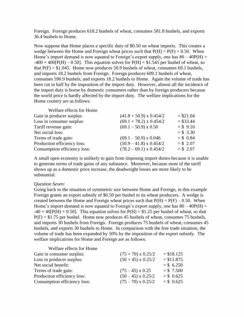
Foreign. Foreign produces 618.2 bushels of wheat, consumes 581.8 bushels, and exports
36.4 bushels to Home.
Now suppose that Home places a specific duty of $0.50 on wheat imports. This creates a
wedge between the Home and Foreign wheat prices such that P(H) = P(F) + 0.50. When
Home’s import demand is now equated to Foreign’s export supply, one has 80 – 40P(H) =
-400 + 400[P(H) – 0.50]. This equation solves for P(H) = $1.545 per bushel of wheat, so
that P(F) = $1.045. Home now produces 50.9 bushels of wheat, consumes 69.1 bushels,
and imports 18.2 bushels from Foreign. Foreign produces 609.1 bushels of wheat,
consumes 590.9 bushels, and exports 18.2 bushels to Home. Again the volume of trade has
been cut in half by the imposition of the import duty. However, almost all the incidence of
the import duty is borne by domestic consumers rather than by foreign producers because
the world price is hardly affected by the import duty. The welfare implications for the
Home country are as follows:
Welfare effects for Home
Gain in producer surplus: (41.8 + 50.9) x 0.454/2 = $21.04
Loss in consumer surplus: (69.1 + 78.2) x 0.454/2 = $33.44
Tariff revenue gain: (69.1 – 50.9) x 0.50 = $ 9.10
Net social loss: = $ 3.30
Terms of trade gain: (69.1 – 50.9) x 0.046 = $ 0.84
Production efficiency loss: (50.9 – 41.8) x 0.454/2 = $ 2.07
Consumption efficiency loss: (78.2 – 69.1) x 0.454/2 = $ 2.07
A small open economy is unlikely to gain from imposing import duties because it is unable
to generate terms of trade gains of any substance. Moreover, because most of the tariff
shows up as a domestic price increase, the deadweight losses are more likely to be
substantial.
Question Seven:
Going back to the situation of symmetric size between Home and Foreign, in this example
Foreign grants an export subsidy of $0.50 per bushel to its wheat producers. A wedge is
created between the Home and Foreign wheat prices such that P(H) = P(F) – 0.50. When
Home’s import demand is now equated to Foreign’s export supply, one has 80 – 40P(H) =
-40 + 40[P(H) + 0.50]. This equation solves for P(H) = $1.25 per bushel of wheat, so that
P(F) = $1.75 per bushel. Home now produces 45 bushels of wheat, consumes 75 bushels,
and imports 30 bushels from Foreign. Foreign produces 75 bushels of wheat, consumes 45
bushels, and exports 30 bushels to Home. In comparison with the free trade situation, the
volume of trade has been expanded by 50% by the imposition of the export subsidy. The
welfare implications for Home and Foreign are as follows:
Welfare effects for Home
Gain in consumer surplus: (75 + 70) x 0.25/2 = $18.125
Loss in producer surplus: (50 + 45) x 0.25/2 = $11.875
Net social benefit: = $ 6.250
Terms of trade gain: (75 – 45) x 0.25 = $ 7.500
Production efficiency loss: (50 – 45) x 0.25/2 = $ 0.625
Consumption efficiency loss: (75 – 70) x 0.25/2 = $ 0.625

Welfare effects for Foreign
Gain in producer surplus: (75 + 70) x 0.25/2 = $18.125
Loss in consumer surplus: (50 + 45) x 0.25/2 = $11.875
Government subsidy outlay: (75 – 45) x 0.50 = $15.000
Net social loss: = $ 8.750
Terms of trade loss: (75 – 45) x 0.25 = $ 7.500
Consumption efficiency loss: (50 – 45) x 0.25/2 = $ 0.625
Production efficiency loss: (75 – 70) x 0.25/2 = $ 0.625
World welfare implications:
Net social loss: = $ 2.500
Although Home gains substantially at the expense of Foreign when a subsidy is granted on
wheat exports, the distortion to the world market place generates a net social loss from a
world perspective. It should, however, be noted that an export subsidy is a particularly
perverse form of industrial protection from the perspective of the subsidising country, in
large part because an export subsidy is costly to government and turns the terms of trade
against the subsidising country. The relevant diagram is Figure 8-11.
Workshop Four, for in class discussion on Wednesday, May 28
This assignment expands upon problem 6 on page 345 of the textbook.
Suppose that the US dollar interest rate and the pound sterling interest rate are the same, 5
percent per year, but that there is a risk premium of 1 percent associated with holding
sterling rather than US dollars over the year.
(a) What is the relationship (in percentage terms) between the current equilibrium
dollar/pound exchange rate and its expected future level?
(b) If the expected future exchange rate is $1.52 per pound, what is the equilibrium
dollar/pound (spot) exchange rate?
Now suppose that the expected future exchange rate, $1.52 US per pound, remains constant
as Britain’s interest rate rises to 10 percent per year.
(c) If the US interest rate also remains constant, what is the new equilibrium dollar/pound
exchange rate?
(d) What is the expected rate of return over the year from holding a sterling deposit in a
London bank?
Now suppose that the actual exchange rate at the end of the year turns out to be $1.55 US
per pound.
(e) By how much does the actual return over the year from holding a sterling deposit in
London exceed or fall short of the expected rate of return? Would the actual dollar/pound
exchange rate rise or fall if, in response to the falsification of their expectations, currency
traders adapted their view of the expected future exchange rate towards the observed year
end outcome of $1.55 US per pound?
Answer Guide: Workshop Four
(a) The relevant formula is the uncovered interest rate parity formula:
E = E(e) (1+R*) / (1+R) (1+q),

where E is the spot exchange rate in US dollars per pound, E(e) is the expected exchange
rate at the end of the year, R* is the pound interest rate per annum in London, R is the
dollar interest rate per annum in New York, and q is the risk premium on holding pounds
rather than US dollars. Thus, when R* = R = 5% and q = 1%, the pound must be expected
to appreciate by 1% per annum. That is, E(e) must exceed E by 1%.
(b) The equilibrium spot exchange rate would be $1.505 US per pound, consistent with an
expected pound appreciation of 1% per annum, given E(e) = $1.52 US per pound.
(c) If the expected exchange rate remains at $1.52 US per pound, and the pound interest
rate rises from 5% to 10%, then the uncovered interest parity formula is satisfied only if the
current exchange rate changes such that there is an expected appreciation of the dollar equal
to approximately 4%. More precisely, this will occur when the exchange rate rises to $1.58
US per pound (a depreciation of the US dollar against the pound).
(d) The expected rate of return over the year from holding a sterling deposit in a London
bank is 6% per annum, which is the US dollar interest rate in New York plus the sterling
risk premium.
(e) If the actual exchange rate at the end of the year is $1.55 US per pound, the actual return
on holding a sterling deposit in a London bank would be approximately 8%, which exceeds
the expected rate of return by 2%. If currency traders adapt their view of the expected
future exchange rate towards the observed year end outcome of $1.55 US per pound, the
dollar/pound exchange rate would appreciate.

Economics 306: International Economics: Lecture Notes
Course Overview
International economics involves the study of the issues arising from economic interactions
among sovereign nations. This study centres around seven main themes:
The gains from international trade
Explanations of the pattern of trade
Ricardian productivity differences
The Heckscher-Ohlin factor proportions model
The standard trade model
Product differentiation and scale economies
Technological convergence and capital mobility
The impact of protectionist devices
Import duties/tariffs
Export subsidies
Quantitative restrictions/quotas
Voluntary export restraints
Customs unions and free trade areas
The balance of payments
Export and import flows and the current account
Asset transactions and the capital account
Exchange reserves and official settlements balances
Exchange rate determination
The interest rate parity relationship
Real exchange rate movements
Terms of trade effects
Macroeconomic adjustment
Flexible exchange rate regimes
Fixed exchange rate regimes
Employment fluctuations and price inflation
International policy co-ordination
The international capital market
The first three themes focus on real transactions and flows of imports and exports in the
international trading system. The final four themes relate to international monetary
economics.
The volume of trade between any two countries depends positively upon their economic
size and negatively on the distance (and therefore the associated transportation costs)
between them, as captured by the log-linear gravity equation:
ln T(i,j) = ln A + a ln Y(i) + b ln Y(j) - c ln D(i,j) + u(i,j) ,
where T(i,j) is the total trade value (exports plus imports) between countries i and j, Y(i)
and Y(j) are the gross domestic products of countries i and j, respectively, D(i,j) is the
distance between the two countries (or their central trading hubs), u(i,j) is an error term, A
is a constant, and a, b and c are positive parameters (or regression coefficients).
The gravity model has also been used to demonstrate that borders matter. That is to say,
the intensities of economic exchange within and across national borders are remarkably
dissimilar. Economic linkages are much tighter within, than among, nation-states. For
example, if the model was applied to the trade of British Columbia with other Canadian
provinces and individual US states, it would under-predict BC’s actual trade with Canadian
provinces and over-predict BC’s actual trade with most US states. The opposite effects
would be observed for the trade of Washington State.
There are many reasons why borders matter. These reasons are associated with transactions
costs, differential access to information, institutional differences, separate currencies, home
biases in preferences, and various barriers to the free flow of trade across international
boundaries. While strong, the forces of globalization do not seem to lead to a borderless
world.
Part One: International Trade Theory
Ricardo’s model of comparative advantage
The fundamental concept on which the theory of international trade is based is the principle
of comparative advantage. This principle may be defined by the statement that trade will
be mutually advantageous whenever the relative prices of various commodities differ from
country to country before trade by an amount great enough to over-offset the costs of
transferring the commodities in question from one country to another. A country will
export those goods that it produces relatively cheaply before trade in exchange for imports
of those goods that it produces relatively expensively before trade. This process of
profitable exchange leads countries to specialise (not necessarily completely) in the
production of those commodities in which they have a comparative advantage. A country
has a comparative advantage in producing a good if the opportunity cost of producing that
good in terms of other goods is lower in that country than it is in other countries.
The theory of international trade suggests that there are basically three reasons why the
relative production costs of various commodities might differ among countries. These are
(a) different resource endowments, (b) different production functions, and (c) different
scales of output. The Ricardian model of comparative advantage focuses on the second of
these reasons and, in particular, differences in relative labour-productivities in different
activities. To export those commodities in the production of which labour-productivity is
relatively high in exchange for those whose production exhibits relatively low labour-
productivity results in a gain in real income for a trading country. Thus, there are gains to
be made from international trade.
Consider an economy with a finite supply of labour that produces and consumes two
commodities, wine and cheese. The production possibility frontier may be written as:
a(L,C) Q(C) + a(L,W) Q(W) < L,
where L is labour supply, Q(C) is cheese output (measured on the horizontal axis), Q(W) is
wine output (measured on the vertical axis), a(L,C) is the unit labour requirement in the

production of cheese, and a(L,W) is the unit labour requirement in the production of wine.
Notice that a(L,C) is the reciprocal of the productivity of labour in cheese production, and
a(L,W) is the reciprocal of the productivity of labour in wine production. The absolute
slope of the production possibility frontier is the opportunity cost of cheese in terms of
wine, namely a(L,C)/a(L,W), which measures the number of litres of wine the economy
would have to give up in order to produce an extra kilogram of cheese.
If our simple economy (called Home) produces both goods, then the relative price of cheese,
p(C)/p(W), is equal to the unit labour requirement ratio, a(L,C)/a(L,W). However, if the
relative price of cheese exceeds its opportunity cost, the economy will specialise in cheese
production, while if the relative price of cheese is less than its opportunity cost, the
economy will specialise in wine production.
Now introduce a second country, called Foreign, which also has a production possibility
frontier of the form:
a*(L*,C) Q*(C) + a*(L*,W) Q*(W) < L*,
where the *-notation refers to the foreign country. Now assume that a(L,C)/a(L,W) <
a*(L*,C)/a*(L*,W) or, equivalently, that a(L,C)/a*(L*,C) < a(L,W)/a*(L*,W). This
assumption implies that the production possibility frontier for Foreign is steeper than the
production possibility frontier for Home, that Foreign has a higher opportunity cost of
cheese production than Home, that Home’s relative productivity in cheese production is
higher than it is in wine production, that Home has a comparative advantage in cheese
production, and that if trade opens up between Home and Foreign, Home will export cheese
to Foreign while importing wine. Notice that all four labour requirement coefficients are
necessary to determine comparative advantage and the direction of trade.
Demonstrate trading equilibrium in terms of the relative price and quantity of cheese
produced and consumed. See text, diagram 3-3. Note that in trading equilibrium the
relative price of cheese, p(C)/p(W) is bounded by a(L,C)/a(L,W) and a*(L*,C)/a*(L*,W).
Demonstrate also that there are gains from trade. These gains are shared between Home
and Foreign except where one of the two countries does not completely specialise, and the
relative price of cheese remains equal to that country’s labour requirement ratio.
The gains from trade depend upon comparative advantage and not upon absolute advantage.
If Home has an absolute productivity advantage in the production of both goods, it will
have a higher wage rate than Foreign. Home’s relative wage rate, w/w*, will lie between
Home’s productivity advantage in its exported good and its productivity advantage in its
imported good. The competitive advantage of an industry depends not only on its
productivity relative to the foreign industry, but also on the domestic wage rate relative to
the foreign wage rate. Finally, if there are many possible goods, j = 1…n, Home will
export all those goods for which w a(L,j) < w* a(L*,j), and import all those goods for
which w a(L,j) > w* a(L*,j). Thus, if goods are ordered by the productivity ratios,
a(L*,j)/a(L,j), then w/w* will determine where along this ordering the cut will occur
between Home’s potential exports and Home’s potential imports. Home will have a cost
advantage in any good for which its relative productivity is higher than its relative wage,
and Foreign will have a cost advantage in the other goods. However, if transport costs are
introduced, some commodities will become non-traded goods.

The Heckscher-Ohlin factor proportions model
Whereas the Ricardian model of comparative advantage focuses on differences in
production functions and, more explicitly, on differences in labour productivity as an
explanation of trade patterns, the Heckscher-Ohlin model focuses on differences in factor
endowments. A country will export those commodities which use intensively its relatively
abundant factor. Underlying this model are two key assumptions: (a) goods may be
ordered unambiguously by factor- intensities, and (b) countries have different factor
endowments.
Let there be two factors of production, land (N) and labour (L), which can be used in the
production of food (F) and cloth (C). Food production is land-intensive relative to cloth
production, which is labour-intensive. That is to say, the ratio of labour to land used in the
production of cloth is higher than the ratio of labour to land used in the production of food.
Thus,
a(L,C)/a(N,C) > a(L,F)/a(N,F),
where a(i,j) refers to the amount of factor i that is used in the production of one unit of good
j, where i = labour (L) or land (N), and j = cloth (C) or food (F). There are now two
resource constraints, which may be written as:
a(L,C) Q(C) + a(L,F) Q(F) < L, and
a(N,C) Q(C) + a(N,F) Q(F) < N,
where Q(C) and Q(F) refer to the outputs of cloth and food, respectively.
If each of the a(i,j)’s were fixed technical coefficients, the production possibilities frontier
would consist of two straight lines, one representing the labour constraint and the other
representing the land constraint. There would be a kink in the production possibilities locus
where these two constraint functions intersect. However, if there is a choice of technique,
with the a(i,j)’s depending upon relative factor input prices, then the production
possibilities frontier will be a downwards sloping line which is convex outwards from the
origin. The opportunity cost of cloth in terms of food (the absolute slope of the production
possibilities frontier) increases as the economy produces more cloth and less food. An
increase in the relative price of cloth, p(C)/p(F), would generate such a shift in production
volumes. The maximisation of production value requires that the opportunity cost of cloth
production be equated to the relative price of cloth.
Although cost minimisation implies that both a(L,C)/a(N,C) and a(L,F)/a(N,F) will
decrease if the wage paid for labour (w) rises relative to the rental price of land (r), we will
continue to assume that a(L,C)/a(N,C) > a(L,F)/a(N,F). It follows that the relative price of
cloth, p(C)/p(F) will increase as w/r increases. This is because an increase in the cost of
labour has a larger impact on the price of cloth than it has on the price of food. Taken in
reverse, an increase in p(C)/p(F) will redistribute factor income towards labour.
An increase in the supply of labour will lead to a biased expansion of production
possibilities, with the production possibilities frontier shifting outwards much more
prominently in the direction of cloth production. Indeed, if relative prices remain constant,
full employment of both factors of production would require an increase in cloth production
and a decrease in food production. However, prices may not remain constant in the face of
the increased labour supply. In particular, the relative price of labour, w/r, and the relative
price of cloth, p(C)/p(F), may fall in response to the increased availability of both labour
and cloth. It follows that a country with a relatively abundant supply of labour is likely to
be relatively effective at (and, thus, have a comparative advantage in) producing labour-
intensive goods.
Now consider a trading situation in which Home has a higher ratio of labour to land than
does Foreign. Thus, L/N > L*/N*. Home’s production possibility frontier is skewed
towards cloth production, while Foreign’s is skewed towards food production. Assuming
that Home and Foreign have similar demand functions for cloth and food, the pre-trade
relative price of cloth will be lower in Home than in Foreign. Thus, Home will begin to
export cloth and import food from Foreign. Moreover, Home’s food import quantity will
be equal to p(C)/p(F) times Home’s cloth export quantity, a fundamental budget constraint.
Countries tend to export goods whose production is intensive in factors with which they are
abundantly endowed. International trade in goods indirectly implies the international
exchange of factor services. More labour is embodied in Home’s exports than in its
imports.
On the assumption that both countries continue to produce both goods, as relative product
prices converge, relative factor prices will also tend to converge. w/r will rise in Home,
while w*/r* will fall in Foreign, implying a tendency towards international factor price
equalisation. In reality, however, factor price equalisation may be less likely than it
appears to be within the Heckscher-Ohlin model because (a) complete specialisation may
occur if factor endowments are very different, (b) production functions may differ
internationally because of technological leads and lags, and because the quality of factor
inputs may differ across countries and/or productive sectors, (c) transportation costs and
other impediments to trade may prevent full commodity price equalisation, and (d) factor-
intensity orderings may not be unambiguous.
Although there will be overall income gains from international trade, there will be changes
in income distribution that imply gains for some factors and losses for others. In particular,
each country’s abundant factor will receive an income gain, while its scarce factor will
experience an income loss. However, since trade expands a country’s overall consumption
possibilities in the sense that it would be possible to increase consumption of both goods, it
is clear that the gainers could fully compensate the losers and still have left-over gains.
Despite income distribution effects, there are gains to be achieved from international trade.
The expansion of the economy’s choices implies that it is always possible to redistribute
income in such a way that everyone gains from trade. Free trade satisfies the normal cost-
benefit criterion. Nevertheless, arguments over trade policies often reflect distributional
concerns.

The standard trade model
The standard trade model is agnostic as to whether trade patterns are determined by
Ricardian differences in production technologies or by Heckscher-Ohlinian differences in
factor endowments. The standard trade model is built on four key relationships: (a) the
relationship between the production possibility frontier and the relative supply curve; (b)
the relationship between relative prices and relative demand; (c) the determination of world
equilibrium by world relative supply and world relative demand; and (d) the effect of the
terms of trade – the price of a country’s exports divided by the price of its imports – on a
nation’s welfare.
The standard trade model proceeds in diagrammatic terms; see text figures 5-3, which
illustrates a trading equilibrium with a given terms of trade, and 5-4, which illustrates the
effects of a change in the terms of trade. The production and consumption points for a
given country must lie on an iso-value line, or budget constraint line, of the form:
p(C) Q(C) + p(F) Q(F) = p(C) D(C) + p(F) D(F),
where D(C) and D(F) are, respectively, the quantities of cloth and food consumed. The
budget constraint line may also be written as:
p(F) [D(F) – Q(F)] = p(C) [ Q(C) – D(C)],
so that import value equals export value. An increase in the terms of trade increases a
country’s welfare, while a decline in the terms of trade reduces its welfare. In trading
equilibrium, relative prices are determined by the intersection of the upward-sloping world
relative supply curve for cloth with the downward-sloping world relative demand curve for
cloth.
Export-biased growth tends to worsen a growing country’s terms of trade, to the benefit of
the rest of the world; import-biased growth tends to improve a growing country’s terms of
trade at the rest of the world’s expense. Thus, the effects of economic growth on the
welfare of the Home country will normally be as follows:
(a) Export-biased growth in Home’s production possibilities: normally positive
(b) Import-biased growth in Home’s production possibilities: positive
(c) Export-biased growth in Foreign’s production possibilities: positive
(d) Import-biased growth in Foreign’s production possibilities: normally negative
An income transfer worsens the donor’s terms of trade if the donor has a higher propensity
to spend on its export good than the recipient, i.e. if there is home country preference in
demand functions, as may be implied by the presence of non-traded goods.
For large countries, import tariffs improve the country’s terms of trade. The welfare
consequences depend upon the net effect of the terms of trade improvement when offset by
the efficiency losses associated with tariff-induced price distortions. For small price-taker
countries, import tariffs may not affect the terms of trade, while tariff-induced price
distortions generate a welfare loss. Export subsidies normally lower a country’s terms of
trade as well as generating efficiency losses; welfare is unambiguously reduced. Trade
barriers also have impacts on the internal distribution of income.
The Heckscher-Ohlin model assumes that factors are mobile between production sectors
within countries, but internationally immobile. An alternative model, the specific factors
model, separates factor inputs into three types: (a) specific resource inputs that are
immobile between production sectors, (b) generic inputs such as labour which are mobile
between sectors, but immobile internationally, and (c) capital, which is assumed to be
mobile between countries. Assume that the economy has three sectors: (a) an export sector
uses a specific natural resource (such as timber lands), labour and capital to produce a
tradable output (such as lumber), (b) an import-competing sector uses labour and capital,
plus a different specific factor, as inputs, and (c) a non-traded goods sector uses labour and
capital, but no specific factors, to produce its output. The non-traded good is taken to be
the numeraire, so that its price is unity.
There are three exogenous world prices: (a) the price of the country’s exports, (b) the price
of the country’s imports, and (c) the world price of capital funds. There are three
endogenous prices: (a) the rental price of resource inputs, (b) the price the specific factor
used in the import-competing sector, and (c) the wage of labour. Exports are resource
intensive, while imports are intensive in the use of the alternative specific factor.
Within this model, an increase in the world price of capital funds will lower the domestic
wage rate, but have ambiguous impacts on the rental price of resource inputs and the price
of the specific factor used in the import-competing sector. This ambiguity can be sorted out
if more is specified about the capital/labour ratios that pertain to these sectors in
comparison to the non-traded goods sector. Resource production often involves capital-
intensive techniques so that, in this case, the rental price of resource inputs would fall in
response to an increase in the world price of capital funds.
Also within this model, an increase in the world price of a tradable commodity will have an
impact on the associated specific factor price which is magnified in proportional terms, but
will have no impact on the price of specific factors that do not enter the cost function for
the commodity, or on the price of a generic factor such as labour. Thus, changes in the
terms of trade (the relative price of the resource-related export commodity relative to the
price of imported goods) will have important effects on internal income distribution, and
especially on the welfare of specific factor owners, while changes in the world price of
capital funds will have important effects on labour income, as well as on the level of
employment if wage rates are inflexible.
Product differentiation and scale economies
The third explanation of trade patterns is economies of scale. Scale economies are an
important explanation of intra-industry trade, whereas factor endowments and
technological differences may explain inter-industry trade. Internal economies of scale
occur at the firm level, and give rise to imperfectly competitive markets. These markets
often exhibit product differentiation, with consumers benefiting from the variety of goods
that are made available through trade. External economies of scale occur at the industry
level and are largely based upon synergistic relationships among firms. These synergistic
relationships may involve (a) specialised suppliers, (b) labour market pooling, and (c)
knowledge spill-overs.

We turn first to a model involving internal economies of scale and monopolistic
competition. Assuming that the representative firm faces a downward-sloping but linear
demand curve, one has:
Q = S/n – bS(P – P*),
where Q is quantity demanded, P is the firm’s price, P* is average price charged by the
firm’s competitors, S is total industry sales or overall market size, n is the number of firms
in the industry, and b is a positive parameter which measures the responsiveness of the
firm’s sales to its own price, given S and P*. Now let a = S/n + bSP*. It follows that PQ =
(a – Q)Q / bS, and that MR = (a – 2Q)/bS = P – Q/bS, where MR is marginal revenue.
Assuming also that the representative firm experiences both fixed costs and constant
marginal costs, the firm’s average cost (AC) function may be written as:
AC = c + F/Q,
where F is fixed costs, Q is output, and c is marginal (and average variable) costs. Setting
MR = c to maximise profits, one discovers that:
P = c + (Q / bS).
With symmetry among firms so that P = P* and Q = S/n, this expression becomes:
P = c + 1 / bn.
The larger is the number of firms competing within the industry, the smaller will each
firm’s price be. Also, with symmetry among firms, average costs may be re-written as:
AC = c + nF/S.
The larger is the number of firms in the industry, the less will scale economies be exploited,
and the higher will average costs be. If there is free entry into the industry, profits will be
driven to zero, with P = AC. Industry equilibrium thus implies that 1/bn must be equated to
nF/S, so that the equilibrium number of firms in the industry is equal to the square root of
S/bF.
The division of labour is limited by the extent of the market. However, when trade is
opened up in a monopolistically competitive industry, overall market size expands. This
increases the number of firms that can be profitably sustained within the industry, permits
these firms to take advantage of more scale economies, lowers the prices of products, and
expands the variety of products available to consumers. Because of economies of scale,
neither country is able to produce the full range of manufactured products by itself; thus,
although both countries may produce some manufactures, they will be producing different
things. Two-way trade, or intra-industry trade, occurs in manufactured goods. Whereas
inter-industry trade reflects comparative advantage, either based on Ricardian technological
differences or Heckscher-Ohlinian factor endowments, intra-industry trade reflects
economies of scale. Although there are overall gains to be made from both kinds of trade,
intra-industry trade is much less likely than inter-industry trade to have significant effects
on the distribution of income among productive factors. Examples: the formation of the
European Common Market, and the North American Auto Pact of 1964.

Dumping is a form of international price discrimination which occurs in oligopolistic
industries. Dumping occurs when it is possible for a firm to segment its markets and
proceed to sell its products at a lower price in foreign markets than in domestic markets.
Since profit maximising price discrimination requires marginal revenue to be equated in all
markets in which the firm’s output is sold, the lower price should be charged in the market
where the elasticity of demand is higher. Because greater competition is likely to exist for
a firm’s products in foreign markets than in domestic markets, the elasticity of demand is
likely to be greater in the foreign market. In terms of the linear demand curve used
previously, where MR = P – Q/bS, the lower price would be charged where Q/bS is smaller.
Given home market preference, this is most likely to be the foreign market. Thus, firms
have an incentive to dump products in the foreign market whenever the responsiveness of
quantity sold to price is greater in that market than at home.
The US International Trade Administration regards dumping as an unfair trading practice,
and often assesses anti-dumping duties against foreign firms that are alleged to be dumping
products into the US market. However, in many cases anti-dumping duties, like the
countervailing duties that are applied in the case of alleged foreign subsidies, are really
another example of trade protection.
External economies are observed when industrial clustering leads to lower costs for all
firms within the cluster. The main reasons why costs might fall when similar firms cluster
together in one location relate to the emergence of specialised suppliers, to labour market
pooling, and to knowledge spill-overs – the diffusion of new technological ideas occurs
more quickly among firms which are in close proximity to each other. All three reasons
generate synergism among firms within the cluster. Example: Silicon Valley in California.
External economies give rise to first-mover advantages, and make it more difficult for
potential competitors in other locations to break into the market. Learning-by-doing effects,
where costs fall in response to cumulative output, give rise to the phenomenon of dynamic
increasing returns. Infant-industry protection is sometimes justified on the assumption that
costs will fall as experience rises.
Technological convergence and capital mobility
International factor mobility may be either a complement to, or a substitute for,
international trade in goods and services. If the basis for the international exchange of final
commodities resides in differences in factor endowments as in Heckscher-Ohlinian trade
theory, allowing these factors to move directly between countries obviates the need for
commodity trade. However, if the basis for trade lies in other reasons (technological
differences, as in Ricardian trade theory, increasing returns to scale, etc.) trade by itself will
tend to raise the return to factors used intensively in each nation’s export sector. Factor
mobility that responds to such differences adds a factor endowment basis for expanded
commodity trade.
Sometimes the international mobility of factors is a prerequisite for the development of
commodity trade, particularly where extractive industries are concerned. On the other hand,
deliberate protectionist policies may reduce trade significantly if they encourage the flow of
capital to avoid the tariff barriers. Thus, foreign investment may serve to expand
production of a nation’s exportables, or serve to encourage production of importables.

International factor mobility responds to perceived differences in factor returns among
countries, and leads to the convergence of factor prices. International factor mobility also
increases world income, but there may be important distributional consequences. In
general, there are more important barriers to international factor mobility, perhaps with the
exception of capital mobility, than there are to the movement of goods and services in
international trade. There is limited mobility of labour between countries, and virtually no
mobility of land-based natural resources.
International capital mobility reflects borrowing and lending transactions between countries,
and gives rise to inter-temporal exchanges. Real interest rates are the key price variable
which influences these transactions. The number of units of future consumption that must
be foregone to obtain an additional unit of present consumption is equal to 1+r, where r is
the real interest rate. Alternatively, the relative price of future consumption is 1/(1+r).
Countries with a relatively low rate of interest will export capital by lending to foreign
countries. Countries with a relatively high rate of interest will import capital by borrowing.
Look at relevant diagrams.
Multinational enterprises choose to locate their operations in more than one country, and by
so doing are involved in the transfer of their core competencies and/or proprietary
technologies for use in other countries. They are, therefore, an important vehicle for
international technology transfers.
Technological convergence may be said to occur whenever the underlying technology of a
“less advanced economy” becomes more similar to that of a “more advanced economy”
through a process of technological diffusion. Recent empirical research related to (a) the
explanation of observed differences in postwar growth rates among advanced economies,
and (b) the explanation of observed changes in the pattern of international trade among
advanced economies in the postwar period, seems to suggest the following broad
generalisation, namely, that it is difficult, if not impossible, to explain either the differences
in growth rates or the changes in trade patterns if one starts from the supposition that, sector
by sector, these economies employ the same average levels of technological know-how at
any given point of time.
When the production function in any given productive sector is defined in terms of the
average degree of application of technological knowledge to production processes within
the sector, this production function will generally be observed to differ from one economy
to another. But these differences in sectoral production functions (or technological leads
and lags) among advanced economies do not remain unchanged through time. Indeed, the
effects generated by intertemporal changes in these sectoral differences are, in combination,
largely responsible for the observed differences in overall rates of economic growth and for
the observed changes in broad trading patterns.
This broad generalisation suggests that the comparative advantage positions underlying the
exchange of manufactured products are largely acquired through the combined processes of
technological change and capital accumulation. These processes are at the same time
responsible for the determination of overall rates of economic growth. Moreover, just as
comparative advantage positions can be acquired they can also be lost as the application of
technological knowledge becomes more widely diffused among trading economies. While

an original innovation may lead to a short term or medium term technological advantage,
the ensuing diffusion process tends to reduce this advantage. Such a diffusion process may
be called technological convergence.
The process of technological convergence involves the diffusion of the usage of “best-
practice techniques” across the various producers of a particular commodity, in whichever
countries these producers are located. This diffusion process normally implies some degree
of “anti-import bias” in the pattern of productivity improvements introduced by countries
which are, on the whole, importers of new techniques of production, and makes it
progressively more difficult for a country which is largely an exporter of new production
techniques to continue exporting relatively large quantities of commodities in the
production of which initially possesses a comparative advantage. Illustrate why this is
likely to be the case when diffusion processes lead to “catching up”.
Economies that grow rapidly through the reduction of an existing productivity gap
experience higher rates of return on capital investment and higher rates of capital
accumulation than a slower growing economy with a higher level of productivity. If long
term direct foreign investment responds to relative rates of return, capital will flow from a
slower growing more advanced economy to faster growing less advanced economies, this
flow tending to equalise rates of return among the countries under consideration.
International technological diffusion and international capital mobility go hand in hand,
with a major vehicle being the multinational enterprise.
In addition to the “anti-import bias” problem associated with the process of technological
convergence, an initial technological leader may also be faced with a transfer problem
associated with its long term capital outflows. The appropriate response to these two
related problems would be an overall reduction in the real exchange rate (the external value
of the technological leader’s currency adjusted for relative price levels). However,
eventually the growth rates of “catch-up” economies will slow down from their higher
levels as the process of technological convergence runs its course.
Part Two: International Trade Policy
Import duties/tariffs
A tariff is a tax levied when a good is imported. Specific duties, taxes or tariffs differ from
ad valorem duties. A specific duty involves a fixed charge for each unit of goods imported,
and tends to be independent of the point along the transportation and distribution network
at which the duty is levied. Ad valorem duties involve a percentage charge on the value of
the imported goods, and their impact depends upon where along the transportation and
distribution network the duty is levied. The cyclical impact of specific tariffs also differs
from the cyclical impact of ad valorem tariffs. An ad valorem duty that raises the same
amount of revenues as a specific duty in a normal or average market will raise larger
revenues in a buoyant market where goods prices are high, and smaller revenues in a down
market where goods prices are low. The burden of ad valorem duties on the market place is
higher than that of specific duties in buoyant markets, but is smaller than that of specific
duties in down markets. The distribution of the burden across high value products and low
value products within the same commodity class also differs between specific tariffs and ad
valorem tariffs. A blended tariff system could have the form T = a + bP, where T refers to

tariff revenues per unit, P refers to product price, and the parameters (a and b) refer to the
specific and ad valorem components, respectively. The blended tariff rate, t = T/P, would
then be equal to b + a/P.
If there are no impediments to trade, the equation of world demand to world supply
establishes an equilibrium price. In a two country world, equilibrium implies that the sum
of Home and Foreign demand must be equal to the sum of Home and Foreign supply. Thus,
the world market price is established where Home’s import demand (Home demand minus
Home supply) is equal to Foreign’s export supply (Foreign supply minus Foreign demand).
See diagrams 8-1, 8-2 and 8-3.
When Home implements an import tariff, a wedge is created between the Home and
Foreign market prices. The import tariff raises the price in Home and (except where Home
is a small price-taking country) lowers the price in Foreign. The volume traded declines.
See diagrams 8-4 and 8-5. The incidence or burden of the tariff is shared between Home
and Foreign in a manner which depends upon the elasticity of Home import demand and
the elasticity of Foreign export supply. There are also deadweight efficiency losses
associated with tariff distortions. As a result, import tariffs fail the cost-benefit test from a
world point of view. Home producers and Foreign consumers gain while Home consumers
and Foreign producers lose, but the overall net gain is negative. This negative effect is
exacerbated if Foreign retaliates to Home’s tariff by imposing protective tariffs on its
imports from Home. On the other hand, there are gains from trade from a world
perspective if one moves from tariff protection to free trade.
Whether or not Home gains or loses from implementing an import tariff depends upon the
size of the deadweight efficiency losses it incurs in relationship to the extent to which the
burden of the tariff is passed back to Foreign exporters (the terms of trade gain). Using a
cost-benefit analysis framework, Home’s net social benefits (NSB) from tariff
implementation are equal to NSB = dCS + dPS + dGR, where dCS is the change in
consumer surplus, dPS is the change in producer surplus, and dGR is the change in
government revenues associated with the tariff. The consumer surplus loss will inevitably
be larger than the producer surplus gain, and the government revenue gain may or may not
offset the difference. A small open economy will generally lose by imposing a tariff on
imports, because there will be little or no terms of trade gain. See diagrams 8-9 and 8-10.
Work through examples, including the effects of the imposition of tariffs on petroleum
imports and the impact of US countervailing duties on Canadian softwood lumber. In this
context, discuss the concept of effective protection, and why Canada needs to maintain log
export controls as long as the US continues to impose tariffs on softwood lumber imports.
Export subsidies
Export subsidies always fail the cost-benefit criterion. The wedge created between
domestic and foreign prices is associated with the diversion of production to the foreign
market. As a result, the exporting country creates a consumer surplus loss for domestic
consumers and a producer surplus gain for domestic producers, accompanied by a drain
from government revenues. There are again deadweight losses from the subsidy distortion,
to which must be added a terms of trade loss. See diagram 8-11.

On the other hand, an export tax can generate a terms of trade gain for an exporting country.
The effects of an export tax are similar to the effects of an import duty, but with the
important difference that the tax revenues accrue to the government of the exporting
country rather than to the government of the importing country.
Quantitative restrictions/quotas
Like a tariff, an import quota raises the domestic price of the imported good. However,
rather than generating tariff revenues for government, an import quota generates quota rents
for those companies who hold import licences, or quota rights. If these licences are held by
domestic importers, then the importing country may experience a gain or a loss from
imposing quotas depending upon the balance between efficiency losses and terms of trade
gains. However, if the import licences are held by foreign exporters, the importing country
suffers a net loss from a cost-benefit perspective. See diagram 8-13.
Voluntary export restraints
Voluntary export restraints are usually imposed at the request of an importing country.
However, from a cost-benefit perspective the request makes little sense because the
importing country suffers a terms of trade loss as well as the usual efficiency losses from
market distortion. The exporting country may enjoy a terms of trade gain, with its
exporters enjoying rents that arise from the restraints. Indeed, voluntary export restraints
operate like import quotas where the quota rights (or import licences) are assigned to
foreign exporters. As one form of managed trade, multilateral export restraints are often
called orderly marketing agreements.
Other trade policy instruments include local content requirements and national procurement,
regulated product standards and red-tape barriers, and export credit subsidies. The
summary table, 8-1, should be studied in detail. Although the effects on national welfare of
tariffs and import quotas are ambiguous (except for small countries where national welfare
falls), the effects on national welfare of export subsidies and voluntary export restraints are
negative. From a cost-benefit perspective, free trade should be preferred to protectionism.
Moreover, when monopoly power exists within a country, free trade can help to reduce this
power. Free trade is therefore a useful form of industrial policy.
Free trade versus protectionism
The case for free trade is based upon (a) economic efficiency gains through the harnessing
a comparative advantage and the avoidance of market distortions, (b) scale economies,
longer production runs, and enhanced product variety, (c) greater opportunities for learning
and innovation, and (d) the fact that retaliatory trade protection is a negative sum game.
The case against free trade is based upon (a) the terms of trade argument (optimum tariff
argument) for protection, (b) domestic market failure (second best arguments, including
infant industry arguments for protection), and (c) income distribution concerns. However,
it is always preferable to deal with market failures as directly as possible, because indirect
policy responses lead to unintended distortions of incentives elsewhere in the economy.
Thus, trade policies justified by domestic market failure are never the most efficient
response; they are always “second best” rather than “first best” policies. Indeed, most

deviations from free trade are adopted not because their benefits exceed their costs but
because the public fails to understand their true cost.
Movements towards free trade normally require international negotiation in which import
protection is traded off for export access, and the avoidance of trade wars. This process
mobilises the collective support of exporters and the general public to overcome the
concentrated lobbies of import competing industries and the workers they employ.
Customs unions and free trade areas
Trade liberalisation rounds under the General Agreement of Tariffs and Trade (GATT), and
now the World Trade Organisation (WTO) normally involve multilateral tariff reductions
based upon most favoured nation clauses. However, preferential trading agreements in the
form of customs unions and free trade areas are also permitted under the GATT/WTO.
Whereas a customs union involves a common set of external tariffs, which must be
determined by prior negotiation, a free trade area does not. The management of a free trade
area therefore requires a elaborate set of “rules of origin”. The European Community is a
customs union, while NAFTA is a free trade area. Preferential trading agreements involve
trade creation among the members of the customs union or free trade area, and trade
diversion from non-members of the preferential trading agreement. Welfare implications
involve balancing the gains from trade creation against the losses from trade diversion. The
gains are likely to exceed the losses if most of the trade creation effects involve intra-
industry trade based upon economies of scale, longer production runs, and increased
consumer choice.
Miscellaneous trade issues
The rationale for strategic trade policy in industrialised countries is based upon two kinds
of market failure. One of these is the inability of firms in high-technology industries to
capture or appropriate the externality benefits of contributions to knowledge that spill-over
to other firms. The other is the presence of monopoly profits in highly concentrated
oligopolistic firms. However, entry deterrence (i.e. a head start) seems to be required if a
subsidy is to generate an addition to oligopoly profits that exceed the subsidy, and the
whole strategy risks retaliatory activity (e.g. Boeing vs. Airbus, Embraer vs Bombardier).
Import-substituting industrialisation based upon the infant industry argument, which was
popular in developing countries during the first 30 postwar years, has largely been
superseded by export-orientated industrialisation during later years due to the example set
by a group of high performance Asian economies. The pre-conditions for rapid growth
through technological convergence appear to be: (a) the existence of a productivity gap to
be exploited, (b) the ability to invest in new capital equipment of the latest vintage (which
itself requires a high rate of savings), (c) the existence of a reasonable infrastructure of
social overhead facilities, including educational facilities, (d) a labour force with a
reasonably high level of education and skills, (e) the ability to release labour resources from
less productive sectors, including agriculture, (f) wage rates and labour income at a level
which creates a market for mass produced goods, (g) alert entrepreneurs and dynamic
management, and (h) respect for international comparative advantages and openness to
international trade. A threshold level of per capita income may be required before take-off
can occur.

The effects of globalisation on the real incomes of low-wage workers in both developing
and industrialised countries have given rise to various concerns. However, some of these
concerns are not well founded in economic logic. In developing countries, low-wage
workers would be worse off without the ability to work in growing export industries (e.g.
Mexico’s maquiladoras). In industrialised countries, it is technological change rather than
international trade which appears to be the main driving force behind labour market duality
(high wage, high skilled jobs versus low wage, low skilled jobs). Debate continues to
occur over whether labour standards and environmental standards should be included as a
component in trade negotiations.
Part Three: Exchange Rates and Open-Economy Macroeconomics
Export and import flows and the current account of the balance of payments
The national income accounting identity for an open economy may be written as:
Y = C + I + G + EX – IM,
where Y stands for gross national product, I for investment, G for government expenditure,
EX for exports and IM for imports. Within this identity, the difference between the value
of goods and services that are exported, EX, and the value of goods and services that are
imported, IM, equals the current account balance, CA = EX – IM. If EX > IM, the current
account is said to be in surplus, while if EX < IM, the current account is said to be in deficit.
A current account deficit implies that domestic absorption, or C + I + G, exceeds gross
national product, Y, and that the economy is spending more on imports than it is earning
from its exports. The economy is therefore borrowing from foreigners and reducing its net
foreign wealth. A current account surplus implies that domestic absorption is smaller than
gross national product, and that the economy is spending less on imports than it is earning
on exports. The economy is therefore lending to foreigners and increasing its net foreign
wealth.
Now define national saving, S, as the sum of private sector saving, SP = Y – T - C, and
public sector saving, SG = T – G, where T refers to tax revenues. Public sector saving will
be negative if government expenditure, G, exceeds tax revenues, T, so that the
government’s fiscal accounts are in deficit. It follows that national saving is the difference
between gross national product and the sum of private and public consumption
expenditures. Thus, S = Y – C – G, from which it follows that:
S = I + CA, where CA = EX – IM.
A country that saves more than it invests at home will be building up its stock of net
foreign wealth by running a current account surplus. A country whose domestic investment
exceeds national savings will be running a current account deficit and thereby financing
part of its investment needs by borrowing foreign savings.
Another way of looking at these accounting identities is to note that:
CA = SP – I – (G – T),

from which it becomes evident that, depending upon its private saving and investment
decisions, an economy that runs a large government sector deficit may find that deficit
mirrored in a current account deficit. The large US current account deficit reflects a
deficiency in national saving relative to investment. Part of the explanation of the shortfall
in national saving is the size of the government sector deficit. This is known as the twin
deficits problem. On the other side of the Pacific, China and Japan are generating large
current account surpluses because their national savings exceed their domestic investments.
In a sense, they are currently financing the US government deficit.
Asset transactions and the capital account of the balance of payments
The balance of payments records all transactions that occur between the Home country and
foreign countries. All transactions that result in a payment to foreigners (for example,
import purchases) are recorded as a debit (or negative) item in the balance of payments,
while all transactions that result in receipts from foreigners (for example, export sales) are
recorded as a credit (or positive) item in the balance of payments. Since export values and
import values are recorded in the balance of payments, the balance of payments includes
the current account.
Notice, however, that export values include exports of both goods and services, where
services include tourist services provided to foreign visitors and income receipts that
represent a return on the Home country’s foreign asset holdings. Similarly, import values
include imports of both goods and services, where services include the tourist services
provided when Home country residents visit foreign lands and income payments that
represent a return on foreign investments in the Home country. It follows that the current
account balance is a more inclusive concept than the merchandise trade balance, which
usually refers to the difference between the value of goods exports and the value of goods
imports.
The balance of payments also includes a capital account. (Although the textbook follows
US guidelines and distinguishes a capital account from an asset account, Canada does not
follow this classification, so we will treat the two accounts as merged.) The capital
account includes all exchanges of capital assets between the Home country and foreign
countries. If Canadians purchase US government bonds, or a condominium in the French
Riviera, this represents a capital outflow and would be recorded as a debit item in the
capital account. If foreigners purchase shares in well known Canadian companies, or a
chalet at Whistler, BC, the associated capital inflow would be recorded as a credit item in
the capital account. More generally, capital outflows are associated with an increase in
foreign assets held by residents of the Home country, while capital inflows are associated
with an increase in Home country assets held by residents of foreign countries.
Exchange reserves and official settlements balances
The balance of payments includes both the current account and the capital account. Double
entry accounting principles ensure that a current account surplus implies a capital account
deficit and that a current account deficit implies a capital account surplus. Current account
surpluses are lent back to foreign countries through capital outflows. Current account
deficits are covered by borrowing from foreign countries through capital inflows. In this
accounting sense, the balance of payments always balances.
However, included within the capital account are official settlement transactions. Central
banks hold exchange reserve accounts which are comprised of short term money market
instruments (such as Treasury bills) denominated in foreign currencies, normally US dollars,
euros, pounds, or yen. Thus, official settlements transactions involve the purchase or sale
of foreign exchange reserves by a country’s central bank. Official purchases of foreign
exchange reserves imply that the balance of payments would otherwise have been in overall
surplus had these purchases not occurred. Official sales of foreign exchange reserves imply
that the balance of payments would otherwise have been in overall deficit had these sales
not occurred. Thus, one may write:
dRH = CA + NF,
where dRH is the change in official holdings of foreign exchange reserves, CA is the
current account balance, and NF is net capital inflows excluding official settlement
transactions. If there is no official intervention in the foreign exchange market, dRH = 0,
and thus CA = - NF. A current account surplus, CA > 0, is associated with a net capital
outflow, so that NF < 0. A current account deficit, CA < 0, is associated with a net capital
inflow, so that NF > 0.
However, if CA + NF > 0, official foreign exchange reserve holdings must be increasing,
while if CA + NF < 0, official foreign exchange reserve holdings must be decreasing. (In
the case of a reserve currency country such as the United States, it may be that foreign
central banks, in aggregate, increase their holdings of US dollar exchange reserve assets
when the US balance of payments is in overall deficit, and decrease their holdings of US
dollar exchange reserve assets when the US balance of payments is in overall surplus.)
Exchange rate determination: the interest rate parity relationship
The price of one currency in terms of another is called an exchange rate. In a world with n
currencies, there are n-1 independent exchange rates. Since the US dollar is the most
universally traded currency, and since foreign central banks hold much of their exchange
reserves in short-term US dollar denominated assets, such as US Treasury bills, we will
normally use the term exchange rate to refer to the US dollar price of a unit of another
country’s currency. Thus, it costs approximately $0.89, $1.28, $0.87, $1.89 and $0.81 US
dollars to purchase one Canadian dollar, one euro, 100 yen, one pound, and one Swiss franc,
respectively. These exchange rates imply various currency cross-rates. For example, the
Canadian dollar price of one euro is approximately $1.44 Canadian, which can be obtained
by dividing the US dollar price of one euro by the US dollar price of one Canadian dollar
(i.e. $1.28 US / euro divided by $0.89 US / Can$ = $1.44 Can$ / euro). Arbitrage
operations keep currency cross-rates in line at all times. Although foreign exchange
transactions can occur anywhere in the world, the world’s most important foreign exchange
market continues to be in London, England.
This way of viewing exchange rates implies that, from the US perspective, an exchange rate
is the price of a unit of foreign exchange. Thus, the Canadian dollar appreciates in terms of
US dollars when its value moves upwards from $0.78 US/Can$ to $0.82 US/Can$, and
depreciates when the opposite movement occurs. Note, however, that from a Canadian
perspective the price of foreign exchange falls from $1.28 Can/US$ to $1.22 Can/US$ as

the Canadian dollar appreciates in this range, while rising as the Canadian dollar
depreciates in this range.
An appreciation of a country’s currency raises the relative price of its exports and lowers
the relative price of its imports. Thus, when a country’s currency appreciates, foreigners
pay more for the country’s products and domestic consumers pay less for foreign products.
Conversely, a depreciation lowers the relative price of a country’s exports and raises the
relative price of its imports. Thus, when a country’s currency depreciates, foreigners find
that its exports are cheaper and domestic residents find that imports from abroad are more
expensive.
The asset approach to foreign exchange rate determination begins from the proposition that,
among those assets that relate to the same risk and liquidity class, individuals prefer to hold
the assets which offer the highest expected real rate of return. Consider, then, the choice
between investing for a year in a secure US dollar bank deposit versus investing in a secure
bank deposit denominated in euros. If R is the rate of interest paid on the US dollar bank
deposit, then at the end of the year, each dollar invested will return 1 + R dollars.
Alternatively, if R* is the rate of interest paid on the euro bank deposit, and z is the
expected rate of appreciation in the exchange rate over the course of the year (where the
exchange rate is the price of euros in terms of US dollars), then each dollar that is converted
into euros at the beginning of the year, invested in a euro bank deposit, and reconverted
back into US dollars at the end of the year, will return (1 + R*)(1 + z) dollars. If there is to
be no incentive for investors to switch between these two alternative assets, they must
generate the same rate of return. Thus, asset market equilibrium implies that:
(1 + R) = (1 + R*) (1 + z) and, therefore, that R* = (R – z) / (1 + z).
This formula is known as the interest parity condition, which says that the foreign
exchange market is in equilibrium when deposits in both currencies offer the same expected
rate of return. Assuming that z is relatively small, the previous formulas may be
approximated by the formula, R = R* + z. Thus, asset market equilibrium implies that the
rate of interest on euro deposits plus the expected rate of appreciation of the euro relative to
the dollar must be equal to the rate of interest on US dollar deposits.
Now let z = [E(e) – E] / E, where E is the spot (or current) exchange rate at the beginning
of the year, and E(e) is the exchange rate that market participants at the beginning of the
year expect to occur at the end of the year. It follows that 1 + z = E(e) / E and, therefore,
that the formula for determining the current exchange rate may be written as:
E = E(e) (1 + R*) / (1 + R) or, alternatively, (1 + R) = E(e) (1 + R*) / E.
Given an initial interest rate differential, an increase in the expected US dollar price of
euros must increase the current exchange rate for euros in terms of US dollars. Given the
expected future exchange rate, an increase in the interest rate differential in favour of
Europe must increase the current exchange rate for euros in terms of US dollars. Moreover,
if the interest rate on euro deposits exceeds (falls short of) that on US dollar deposits, then
the current exchange rate must be at a level from which the euro is expected to depreciate
(appreciate). A country that maintains relatively high interest rates is essentially
compensating for the expected future depreciation of the external value of its currency.

It follows from these statements that the behaviour of exchange rates in response to changes
in monetary tightness or monetary ease will exhibit overshooting. An increase in European
interest rates will increase the current exchange rate (the US dollar price of euros) to a level
from which it is expected to fall, while a decrease in European interest rates will decrease
the current exchange rate to a level from which it is expected to rise. All of these points
may be illustrated in diagrams that relate the exchange rate (the US dollar price of euros) to
expected rates of return in US dollar terms on euro and dollar deposits. See, for example,
diagrams 13-4, 13-5, and 13-6.
Finally, assuming (as we have done) that foreign and domestic deposits are equally risky
(there is no differential risk premium), the forward exchange rate (the contracted US price
today of euros to be delivered in the future) is an unbiased predictor of the expected future
exchange rate. However, if for whatever reason it is more risky to hold euro deposits than
US dollar deposits, then not only will euro-zone interest rates tend to exceed US interest
rates when there is no expectation of a change in currency values, but also the forward rate
will tend to be a downwards biased predictor of the expected future exchange rate. In fact,
if q is the risk premium on holding euros, and E(f) is the forward price of euros, then E(e) =
E(f) (1 + q). In this situation, asset market equilibrium implies that:
E = E(e) (1+R*) / (1+R) (1+q) or, alternatively, E(e) (1+R*) / E = (1+R) (1+q),
which we will now call the uncovered interest parity condition. An increase in the risk
premium associated with holding euro deposits relative to holding US dollar deposits will
need to be compensated by a higher expected return on euro deposits relative to US dollar
deposits. The alternative covered (or hedged) interest parity condition is:
E = E(f) (1+R*) / (1+R).
Thus, if R* > R, euros are trading at a forward discount, [E(f) – E] / E < 0, whereas if R* <
R, euros are trading at a forward premium, [E(f) – E] / E > 0.
Money, interest rates, and exchange rates
An exchange rate is the relative price of one country’s money in terms of another’s. Thus,
factors which affect a country’s money supply and/or demand have powerful effects on the
exchange rate for its currency. Monetary developments influence the exchange rate both by
changing interest rates and by changing people’s expectations about future exchange rates.
Moreover, expectations about future exchange rates are influenced by expectations about
the future purchasing power of a country’s money, which itself reflects output price
developments that are themselves influenced by changes in money supply and/or demand.
As is well known, money serves as (a) a medium of exchange, (b) a unit of account, and (c)
a store of value. Money is the most liquid of all assets, where an asset is said to be liquid if
it is readily realisable (or converted into other asset forms) at short notice without
significant cost. Thus, the demand for money is essentially the demand for liquidity. The
supply of money, defined as the sum of currency outstanding and commercial bank deposits
on which cheques can be written, is determined by the actions of the country’s central bank.
When the central bank increases (decreases) its asset holdings by open market purchases
(sales) of government bonds, the domestic money supply will increase (decrease).

The demand for money depends positively on the economy’s price level, P, and on the
economy’s overall level of real output, Y, and negatively on the interest rate, R, which
measures the opportunity cost of holding money rather than an interest-bearing asset.
Money demand is assumed to respond proportionately to movements in the price level, so
that the demand for money may be written as:
M(d) = P L(Y, R),
where M(d) is money demand, P is the price level, and L(Y, R) is the demand for real
balances, or for money of constant purchasing power. Monetary equilibrium occurs when
money demand is equal to the money supply, M(s), so that:
M(s) = M(d) = P L(Y, R) or, alternatively, M(s)/ P = M(d)/ P = L(Y, R).
Given the level of output, Y, an increase in the supply of real balances, M(s)/P, will lower
the rate of interest, R, whereas a decrease in the real money supply will raise the rate of
interest. Given the real money supply, an increase (decrease) in the level of output will
expand (contract) the transactions demand for real balances and lead to an increase
(decrease) in the rate of interest. The relevant diagrams are 14-3, 14-4 and 14-5.
An increase in a country’s money supply causes its currency to depreciate in the foreign
exchange market, while a reduction in the money supply causes its currency to appreciate.
When the domestic money supply increases, downward pressure is placed on the domestic
interest rate. Given an unchanged foreign interest rate, the lower domestic interest rate is
only compatible with the interest parity condition if the domestic currency is expected to
appreciate (that is, the price of foreign exchange is expected to fall, so that E(e) < E).
Given the expected exchange rate, this can only occur if the external value of the domestic
currency falls (that is, E increases). Another way of looking at this point is to note that a
lower anticipated return on domestic assets would lead to substantial short-term capital
outflows seeking higher foreign returns, and these outflows (sales of domestic assets in
order to purchase foreign assets) push the external value of the domestic currency
downwards (and the price of foreign exchange upwards) in the foreign exchange market.
On the other hand, when the domestic money supply decreases, upward pressure is placed
on the domestic interest rate. Given an unchanged foreign interest rate, the higher domestic
interest rate is only compatible with the interest parity condition if the domestic currency is
expected to depreciate (that is, the price of foreign exchange is expected to rise, so that
E(e) > E). Given the expected exchange rate, this can only occur if the external value of
the domestic currency rises (that is, E decreases). Another way of looking at this point is to
note that a higher anticipated return on domestic assets would lead to substantial short-term
capital inflows seeking higher domestic returns, and these inflows (sales of foreign assets in
order to purchase domestic assets) push the external value of the domestic currency
upwards (and the price of foreign exchange downwards) in the foreign exchange market.
Thus, when M(s) increases, one should observe that R falls and E (the price of foreign
exchange) rises, whereas when M(s) decreases, one should observe that R rises and E falls.
However, an increase in the foreign money supply would reduce both R* and E, as the
domestic currency appreciates, while a decrease in the foreign money supply would raise

both R* and E, as the domestic currency depreciates. It follows that relative money
supplies are an important determinant of foreign exchange rates, and that the exchange
values of currencies issued by countries experiencing higher money supply growth rates
will tend to depreciate over time. Diagrams 14-6, 14-8, and 14-9 illustrate these points.
It should be noted that the repercussions we have illustrated so far are short-run in nature,
because they assume that output, Y, the price level, P, and the expected exchange rate, E(e),
all remain unchanged in response to money supply changes. In the long-run, however,
money supply changes lead to proportional changes in the price level, where one of the
prices that is proportionately affected is the price of foreign exchange. Thus, a permanent
increase in a country’s money supply causes a proportional long-run depreciation of its
currency against foreign currencies. Similarly, a permanent decrease in a country’s money
supply causes a proportional long-run appreciation of its currency against foreign
currencies.
Prices tend to be sticky in the short-run and flexible in the long-run. Unlike the exchange
rate, prices do not jump immediately in response to monetary changes. Despite the short-
run stickiness of price levels, however, money supply increases create immediate demand
and cost pressures that eventually lead to future increases in the price level. These
pressures come from (a) excess demand for output and labour, (b) increases in commodity
prices, which do move with flexibility in response to changes in demand and supply, and (c)
the destabilisation of inflationary expectations.
Because the price level is sticky in the short-run, the response path of the economy to a
permanent increase in the money supply involves (a) an initial fall in interest rates, which
gradually return to their original level as prices rise over time, and (b) an initial fall in the
value of the currency to a level from which it is expected to appreciate. Although long-run
equilibrium implies a lower value of the currency, the initial fall in currency value is larger
than the long-run fall. The exchange rate overshoots its eventual equilibrium level along
the adjustment path. The relevant diagrams are figures 14-12 and 14-13.
Real exchange rate movements
The real exchange rate is a broad summary measure of the prices of one country’s goods
and services relative to another’s. If P is the domestic price level and P* is the foreign
price level, then P*E / P is the relative price of foreign goods in terms of domestic goods.
Notice that the nominal exchange rate, E, which measures the price of foreign currency in
terms of domestic currency, is a central element in the real exchange rate. The real
exchange rate measures the number of units of domestic production that are required to
purchase one unit of foreign production.
An increase in the real exchange rate implies a depreciation in the purchasing power of
domestic products over foreign products. Foreign products are thus becoming relatively
more expensive to purchase than domestic products, and there will be a tendency to
substitute domestic products for foreign products. The real exchange rate will rise over
time whenever the difference between the foreign inflation rate and the domestic inflation
rate is less than fully offset by a decline in the exchange value of the foreign currency.

A decrease in the real exchange rate implies an appreciation in the purchasing power of
domestic products over foreign products. Foreign products are thus becoming relatively
cheaper to purchase than domestic products, and there will be a tendency to substitute
foreign products for domestic products. The real exchange rate will fall over time if the
difference between the domestic and foreign inflation rates is less than fully offset by a
decline in the exchange value of the domestic currency.
Deviations in the real exchange rate from unity imply deviations from purchasing power
parity. Put differently, the purchasing power parity value of the nominal exchange rate
would be given by the equation, P*E = P. If this equation were to hold, it would assert that,
when measured in terms of the same currency, the price levels in the foreign and domestic
countries are equal. The purchasing power of a US dollar would be the same in Europe as
it is in the United States. Although there are good reasons to believe that, transport costs
and trade impediments apart, the law of one price should hold across countries for
individual commodities, there are several reasons why purchasing power parity does not
seem to hold at the level of broad price level aggregates. These reasons include: (a) the
market basket of goods and services included in aggregate price indices differs across
countries, (b) the domestic price level will place a heavier weight on commodities produced
and consumed at home, while the foreign price level will place a heavier weight on
commodities produced and consumed in the foreign country, (c) there are many goods and
services that are not traded between countries, and (d) transport costs and other trade
impediments interact with oligopolistic and monopolistic practices, such as pricing to
market, so as to distort the competitive norm of the law of one price. For example, the
purchasing power of the US dollar in developing countries usually exceeds its purchasing
power in the United States because labour-intensive non-traded goods and services are
cheaper in developing countries because wage rates are relatively low there.
Both monetary and real shocks will affect the value of the real exchange rate, P*E / P. If
these shocks are transitory in nature, the effects on P*E / P will tend to be self- reversing.
In addition, the short-run effects of permanent changes in relative money supplies will tend
to be self-reversing in the longer-run. There is, therefore, some tendency for the real
exchange rate to return to a long-run equilibrium value when initially perturbed by money
supply changes that turn out to be permanent. This tendency is consistent with the concept
of relative (as opposed to absolute) purchasing power parity. However, real shocks that
turn out to be permanent will alter the long-run equilibrium value of the real exchange rate.
Prominent among real shocks are changes in relative prices, or terms of trade changes.
Consider the response path of two countries that are engaged in international trade to a
permanent increase in the money supply in the home country, while the foreign money
supply is held constant. In the short-run, the domestic interest rate will fall and the price of
foreign exchange (the nominal exchange rate) will increase to a level from which it
expected to depreciate. As domestic prices gradually adjust in response to the monetary
expansion, the domestic interest rate will begin to return to its initial value, and the nominal
exchange rate will move downwards towards a long-run equilibrium value which is higher
than its initial value. Notice again that exchange rate over-shooting occurs along the
response path.

In the final equilibrium, the domestic price level will have risen in proportion to the
increase in the home country’s money supply, and the nominal exchange rate will have
fallen in the same proportion. While the real exchange rate initially increases in response to
the domestic money supply increase, in the final equilibrium the real exchange rate returns
to its initial value. P and E are both proportionately higher, leaving P*E / P unchanged. If
economic agents understand the process involved, it would be rational for them to form
expectations of the nominal exchange rate that are based on relative purchasing power
parity considerations.
We will see later that the initial increase in the real exchange rate leads to a temporary
expansion in the trade balance, and that the resulting expansion in aggregate demand is one
of the forces that drives up prices in the domestic economy. Another force is the increased
price of imported goods and services, perhaps including raw material inputs, in response to
the higher price of foreign exchange. Thus, both demand-pull and cost-push forces
affecting the domestic price level are set in play in response to the initial money supply
increase.
With the foreign money supply held constant, a permanent decrease in the home country’s
money supply works in the opposite direction. Domestic price deflation and a matching
appreciation of the home country currency would be the eventual outcome. Moreover, the
domestic economy can, in principle, insulate its price level from an increase in the foreign
price level that is induced by foreign monetary expansion by appreciating the external value
of its currency, so that a falling E offsets a rising P*.
The impacts of a permanent shift in relative money supply growth rates (as opposed to
levels) may also be analysed, but to do so requires consideration of the Fisher effect. The
Fisher effect states that an increase in an economy’s expected inflation rate will be reflected
in a one-for-one manner in the economy’s interest rates. Nominal interest rates embody a
premium for expected inflation which compensates lenders for the falling value of money
in response to ongoing inflation. The real interest rate is approximately equal to the
nominal interest rate less the expected rate of price inflation. More precisely, if x is the
expected rate of price inflation and R is the nominal interest rate, then the real interest rate
is equal to r = (1+R)/(1+x) – 1, or r = (R – x)/(1+x).
Suppose now that expected inflation in the foreign economy is equal to x*. Then the real
interest rate in the foreign economy is r* = (1+R*)/(1+x*) – 1, or r* = (R* – x*)/(1+x*),
where R* is the nominal interest rate in the foreign country. If the home and foreign
countries have the same real rate of interest, then (1+r) = (1+r*), from which it follows that
(1+R)/(1+x) is equal to (1+R*)/(1+x*). But when differential risk is ignored, the interest
parity condition implies that (1+R) = (1+R*) (1+z), where z = [E(e) – E] / E is the expected
rate of appreciation of the foreign currency. It follows that:
E(e) / E = (1+z) = (1+x)/(1+x*) and, hence, that z = (x – x*) / (1+x*).
Assuming that x* is fairly small, this equation says that the expected rate of appreciation of
the foreign currency is equal to the difference between the expected rate of inflation in the
domestic economy and the expected rate of inflation in the foreign economy. The currency
of a country whose price level is expected to increase faster than the price level of its
trading partners will be expected to experience a depreciation in the value of its currency

that is equal to the difference in inflation rates. The resulting nominal exchange rate
adjustment will maintain the real exchange rate at a given level, consistent with the
maintenance of relative purchasing power parity. (It should be noted that there is a two-
way relationship between the maintenance of relative purchasing power parity and the
equivalence of real interest rates in the two trading countries. More generally, relative
movements in real interest rates will be associated with changes in the real exchange rate.)
One may now consider the impact of a permanent shift in relative money supply growth
rates. The long run effects of an increase in the domestic money supply growth rate
relative to the foreign money supply growth rate are to generate a higher rate of inflation in
the domestic economy, raise the nominal interest rate in the domestic economy above that
in the foreign economy due to the Fisher effect, and lead to a continuous depreciation in the
value of the domestic currency, while real interest rates and the real exchange rate remain
unchanged. The relevant diagram is figure 15-1.
Terms of trade effects
Unlike permanent monetary shocks, permanent real shocks will have a lasting effect on the
real exchange rate. Suppose that there is an increase in world demand for the types of
goods and services that the US exports relative to the demand for the types of goods and
services that it imports. This increase will lead to an increase in the price of US exports
relative to the price of its imports. A movement in the terms of trade (the relative price of
US exports relative to its imports) that is favourable to the US economy occurs. As a result,
P*E / P must decrease, implying a real appreciation of the US dollar. If overall price
levels remain roughly unchanged, the real appreciation will be accompanied by an increase
in the external value of the US dollar. On the other hand, a decrease in world demand for
the types of goods and services that the US exports relative to the demand for the types of
goods and services that it imports will lead to an unfavourable movement in the US terms
of trade. As a result, P*E / P must increase, implying a real depreciation of the US dollar.
If overall price levels remain roughly unchanged, the real depreciation will be accompanied
by a decrease in the external value of the US dollar. If the process of technological
convergence implies “anti-import biased” growth in “catch-up” countries, then the
technological leading country will experience real depreciation. However, the effects of
changes in national output, and output growth rates, will be discussed more generally below.
Terms of trade effects are particularly important to understanding Canadian dollar
exchange rate movements. Indeed, given the importance of natural resource based
commodities in the Canada’s export trade, the Canadian dollar is sometimes referred to as a
“commodity currency”. Various authors, with relatively more or less success, have tried to
explain movements in Canada’s real exchange rate using variables such as a raw materials
price index relative to the prices of all other goods (a proxy for the Canadian terms of trade),
and the real interest rate differential between Canada and the United States. More recently,
the high prices being received for exports of crude petroleum and natural gas have been one
of the explanations of Canadian dollar appreciation. Since the appreciation has also been a
real one, cost-price pressure has been placed on Canadian sectors other than its energy
producing sector.

The real income of a small open economy such as Canada can move differentially in
relationship to its real output if the terms of trade change substantially. Real income equals
money income divided by the consumer price index. Money income equals the overall
volume of output times the average price at which output is sold. The price of exportables
enters the overall output price, whereas the price of importables enters the consumer price
index. Hence, if the terms of trade improve, output prices increase relative to the consumer
price index, and real income goes up in relationship to real output. On the other hand, if the
terms of trade decline, output prices fall relative to the consumer price index, and real
income falls in relationship to real output. The specific factors model can be helpful in
analysing terms of trade effects for a small open economy.
In summary, when all disturbances are monetary in nature, nominal exchange rates reflect
relative purchasing power parity in the long run. In the long run, a monetary disturbance
affects only the general purchasing power of a currency, and this change in purchasing
power is equally reflected in the currency’s value in terms of both domestic and foreign
goods. However, when disturbances occur in output markets, including situations
involving terms of trade changes, nominal exchange rates are unlikely to reflect purchasing
power parity. Real appreciation or depreciation is likely to be observed in response to real
shocks.
Macroeconomic adjustment: flexible exchange rate regimes
In terms of units of domestic output, the current account balance of the home country may
be written as:
CA = EX - IM = X(P*E / P, Y*, Y),
where X refers to net exports, which are a function of the real exchange rate, P*E / P,
foreign output, Y*, and domestic output, Y. An increase in foreign output will expand the
home country’s net exports because export demand increases. For Canada, US gross
national product provides a good proxy for foreign output. An increase in domestic output
will lower net exports because import demand increases. The impact of the real exchange
rate on net exports is usually assumed to be positive because of substitution effects. That is
to say, if the relative price of foreign goods and services increases, substitution effects will
lead to larger purchases of domestic goods and services in both the home and foreign
markets. As a result, export quantities will rise and import quantities will fall. Provided
that these substitution effects are large enough to overcome the fact that import prices are
rising relative to domestic output prices, net exports will increase in response to an increase
in the real exchange rate, P*E / P.
The exact condition that needs to hold for net exports to respond positively to the real
exchange rate is known as the Marshall-Lerner elasticity condition. Let the current account
balance (or more strictly the merchandise trade balance) be written in units of domestic
output as x – qm, where x measures physical exports, m measures physical imports, and q
measures the real exchange rate, or the price of foreign products (including imports)
relative to the price of domestic products (including exports). The derivative of x – qm
with respect to q is equal to dx/dq – qdm/dq – m. We are interested in whether this
derivative is positive or negative. Now dx/dq = e(x) x/q, where e(x) is the elasticity of
demand for exports, which is positive since q is the inverse of the relative price of exports.

Moreover, dm/dq = - e(m) m/q, where e(m) > 0 is the absolute value of the elasticity of
demand for imports. It follows that the derivative of x –qm with respect to q is equal to e(x)
x/q + e(m) m – m. If it is assumed that trade is initially balanced so that x – qm = 0, the
sign of the derivative will be positive if and only if:
e(x) + e(m) > 1.
This is the Marshall-Lerner condition. It says that the home country’s trade balance will
improve in response to an increase in the real exchange rate (a real depreciation for the
home country) if and only if there are sufficient substitution possibilities between home and
foreign goods and services, as measured by the elasticities of export and import demand, to
overcome the fact that imported goods and services become more expensive for domestic
consumers.
Empirical estimates of trade elasticities suggest that, for most countries, the Marshall-
Lerner condition is satisfied in both the short-run and the long-run. However, since
substitution effects take time to materialise, impact elasticities may be insufficient. If this
is the case, the trade balance will weaken in response to a real depreciation of the country’s
currency before it eventually strengthens. This response pattern is known as the J-curve
effect. Thus, except over short time periods, real depreciation is likely to improve the trade
balance while real appreciation is likely to worsen it. The impact on the current account
will correspond to the impact on the trade balance in most instances, with the possible
exception of countries with a large external indebtedness which is denominated in foreign
currencies. In this case, an increased burden of interest payments may offset the positive
trade balance effects that real depreciation brings about.
The current account balance is an important component of the aggregate demand for an
open economy’s output. Indeed, aggregate demand may be written as:
D = C(Y – T) + I(r) + G + X(P*E / P, Y*, Y),
where consumption, C, is a positive function of deposable income, Y – T, with less than
unit slope, investment, I, is a function of the real interest rate, r = (R – x)/(1 + x),
government expenditure, G, and taxes, T, are taken to be autonomous, and net exports, X,
are a function of the real exchange rate, P*E / P, foreign output, Y*, and domestic output, Y,
as previously outlined. It is assumed that the Marshall-Lerner elasticity condition holds, so
that a real depreciation (appreciation) of the home currency raises (lowers) aggregate
demand for home output.
Equilibrium output occurs when aggregate demand, D, is equal to domestic output, Y. An
increase in D will lead to a corresponding increase in Y, while a decrease in D will lead to a
corresponding decrease in Y. Notice that there is a positive transmission mechanism from
movements in foreign output, Y*, to movements in domestic output, Y, which works
through the current account balance. In addition, an increase (decrease) in the real
exchange rate, P*E / P, will cause an upward (downward) shift in aggregate demand, and
therefore an expansion (contraction) in domestic output. These responses illustrate two of
the ways in which the US economy dog wags the Canadian economy tail.

The short-run behaviour of an open economy under flexible exchange rates may be
described by three equations. These equations describe the conditions for equilibrium in
the output market, the money market and the foreign exchange market, respectively. The
three equations are:
Y = D = C(Y – T) + I(R) + G + X(P*E / P, Y*, Y),
M(s) = M(d) = P L(Y, R), and
E = E(e) (1 + R*) / (1 + R) (1 + q).
In the short-run, prices are taken to be given and, thus, the inflation rate is taken to be zero
so that the nominal and real interest rates coincide (R = r). To keep matters simple, we
assume that the risk premium, q, is also zero, and that the expected exchange rate, E(e), is
predetermined. M(s), G and T are policy variables, which are also taken to be
predetermined. Finally, one should note that all three foreign variables, Y*, P*, and R*,
have an impact on the equilibrium equations, indicating that there are important linkages
(or transmission mechanisms) between the rest of the world and the economy being
analysed. Given the small open economy assumption, however, all foreign variables are
taken to be exogenously determined. The three endogenous variables are output, Y, the
interest rate, R, and the exchange rate, E.
There are two different diagrammatic ways of analysing this three equation equilibrium
system. One of these is the standard IS-LM diagram, which works with Y and R as the
primary variables, with movements in E taken to be behind the scene. The other of these is
the AA-DD diagram, which works with Y and E as the primary variables, with movements
in R taken to be behind the scene. We begin by considering the IS-LM diagram.
In the IS-LM diagram, output, Y, appears on the horizontal axis, and the interest rate, R,
appears of the vertical axis. The LM curve depicts all Y, R combinations at which the
money market is in equilibrium. The LM curve is drawn up for a given real money supply,
M(s)/ P, and is an upward sloping line in Y, R space. The upward slope of the LM curve
reflects the fact that higher levels of output expand the transactions demand for money,
which leads to tighter credit conditions if the money supply remains unchanged.
The IS curve depicts all Y, R combinations at which the output market and the foreign
exchange market are in equilibrium. The IS curve is drawn up for given foreign variables,
and given domestic fiscal policy, and is a downward sloping line in Y, R space. The
downward slope of the IS curve relates to two separate forces. First, a reduction in interest
rates stimulates additional investment activity. Secondly, a reduction in domestic interest
rates in relationship to foreign interest rates will reduce the external value of the domestic
currency. That is to say, it will increase the nominal exchange rate (the price of foreign
exchange, E) relative to the expected exchange rate, which may temporarily be taken to be
given. The resulting increase in the real exchange rate, P*E / P, will expand the current
account balance. Both the increase in the volume of exports relative to imports, and the
increase in investment activity, will generate an increase in domestic output in the short-run.
Of course, although the nominal exchange rate adjusts quickly in response to relative
interest rate movements, both processes may be subject to response lags. Investment may
expand only gradually in response to a decrease in the domestic interest rate, and the

current account balance may expand only gradually in response to an increase in the real
exchange rate (or even contract initially if substitution effects take time, as illustrated by
the J-curve effect).
Simultaneous equilibrium in all three markets occurs at the intersection of the IS and LM
curves. It should, nevertheless, be pointed out that although the expected exchange rate,
E(e), may not be affected by temporary shocks to the equilibrium situation, it will be
affected by permanent shocks. An increase in E(e) will shift the IS curve to the right, while
a decrease in E(e) will shift the IS curve to the left. As a result, permanent changes in the
money supply have a larger impact on the level of output than temporary changes, while
permanent changes in fiscal policy have a smaller impact on the level of output than
temporary changes. These consequences arise from the fact that changes in E(e) tend to
generate further changes in E in the same direction.
The relevant diagrams for analysing shifts in domestic monetary and fiscal policy are A-2
and A-3. In diagram A-2, a temporary increase in the domestic money supply shifts the
LM curve to the right, lowering the domestic interest rate, increasing the price of foreign
exchange, and increasing the volume of output. A permanent increase in the money supply
will also increase the expected exchange rate, E(e), leading to a rightward shift in the IS
curve, which tends to increase output further due to additional exchange rate changes, while
the interest rate moves back towards its original level. Perhaps with some lag, upwards
pressure on the domestic price level will also be observed. As prices increase, real balances
will begin to fall back towards their initial level. This will ultimately reduce the impact on
output and interest rates, as the LM and IS curves both begin shifting back towards their
original positions. All of the movements described in this paragraph would proceed in
reverse in response to a reduction in the domestic money supply.
In diagram A-3, a temporary increase in government expenditure (or reduction in taxes)
shifts the IS curve to the right. Domestic output and interest rates both increase, while the
price of foreign exchange falls. The expansionary impact of fiscal policy is limited by
crowding out effects on both private investment and the trade balance. Permanent fiscal
expansion will also lower the expected exchange rate, E(e), leading to further crowding out
effects as the IS curve moves back towards its initial position. Indeed, a permanent fiscal
expansion has no effect on domestic output or the interest rate. All of the movements
described in this paragraph would proceed in reverse in response to fiscal contraction.
It follows that, when exchange rates are flexible, monetary policy has powerful short-run
effects on the volume of domestic output, and therefore on employment, while fiscal policy
has limited power. Fiscal policy does affect the composition of the balance of payments
and, eventually, the country’s net foreign indebtedness position. Indeed, while the effects
of fiscal expansion tend to appreciate the external value of the domestic currency (that is,
generate a fall in E), the long-run impact of a sustained build-up of foreign indebtedness
may be to depreciate the domestic currency, due to the increasing debt service burden on
the current account of the balance of payments.
The alternative diagrammatic treatment of simultaneous short-run equilibrium in the output
market, the money market and the foreign exchange market uses the AA and DD
relationships. The AA curve represents asset market equilibrium, and depicts all those

combinations of output and the exchange rate at which the domestic money market and the
foreign exchange market are simultaneously in equilibrium. The AA curve is downward
sloping in Y, E space, and is drawn up on the assumption that real balances, M(s)/ P, the
expected exchange rate, E(e), and the foreign interest rate, R*, are given.
The downward slope of the AA curve relates to the fact that a higher level of output is
associated with a larger transactions demand for money, and therefore with higher domestic
interest rates. Higher domestic interest rates are only compatible with equilibrium in the
foreign exchange market if the domestic currency is expected to depreciate. Given the
expected exchange rate, this can only occur if the nominal exchange rate (that is, the price
of foreign exchange) is lower than it was previously. This is illustrated in Figure 16-6. For
asset markets to remain in equilibrium, a rise in domestic output must be accompanied by
an appreciation of the domestic currency (a fall in the price of foreign exchange), all else
equal, and a fall in domestic output must be accompanied by a depreciation of the domestic
currency (a rise in the price of foreign exchange).
The AA curve will shift to the right (left) if the volume of real balances, M(s)/ P, increases
(decreases). The AA curve will also shift to the right if either the expected exchange rate,
E(e), or the foreign interest rate, R*, increases (decreases). The reason for this is that either
of these changes will, other things equal, increase (decrease) the price of foreign exchange
that is associated with any given level of output. The linkage here is that increases
(decreases) in either E(e) or R* tend to generate capital outflows (inflows), with resulting
impacts on the foreign exchange rate.
The DD curve represents output market equilibrium, and depicts all those combinations of
output and the exchange rate that are consistent with output market equilibrium. The DD
curve is upward sloping in Y, E space, and is drawn up on the assumption that fiscal policy
(government expenditure and taxation), investment demand, the home and foreign price
levels, foreign output, and relative product demands (and, thus, the terms of trade) are given.
Any disturbance that raises aggregate demand for domestic output shifts the DD schedule
to the right; any disturbance that lowers aggregate demand shifts the DD schedule to the
left.
The upward slope of the DD curve relates to the effects of changes in the nominal exchange
rate on changes in the real exchange rate (P*E / P, given P and P*), and to the effects of
changes in the real exchange rate on the current account balance. It is assumed that the
Marshall-Lerner elasticity condition holds, so that the current account balance increases in
response to an increase in the real exchange rate (a real depreciation of the home currency).
Thus, all else equal, any rise (fall) in the real exchange rate, P*E / P, will cause an upward
(downward) shift in the aggregate demand function and an expansion (contraction) in the
level of domestic output. This is illustrated in Figure 16-4.
One may now put the DD and AA schedules together into one diagram. Simultaneous
short-run equilibrium in the asset and output markets occurs at the intersection of the DD
and AA schedules, as illustrated in Figure 16-8. A temporary increase in the money supply
will shift the AA schedule to the right and lead to an increase in both the exchange rate (the
price of foreign currency) and the level of domestic output. The causal sequence is that the
money supply increase lowers domestic interest rates and, thereby, depreciates the domestic

currency to a level from which it is expected to appreciate. The depreciation of the
domestic currency expands the trade balance, and the resulting increase in aggregate
demand leads to an increase in domestic output.
A permanent increase in the money supply also raises the expected exchange rate, E(e), and
this further increases the nominal exchange rate, so that the short-run effects of a permanent
increase in the money supply are larger than the short-run effects of a temporary increase.
However, the expansionary effects of a permanent increase in the money supply will begin
to place upward pressure on domestic prices. Thus, the initial increase in real money
balances will gradually reverse itself, with the AA schedule moving back to the left as in
Figure 16-15. In addition, the initial increase in the real exchange rate will reverse itself as
the domestic price level rises. Thus, the DD schedule will also move to the left. In the
ultimate equilibrium, the real exchange rate and the level of output will return to their initial
levels, but the nominal exchange rate (E, the price of foreign exchange) will be higher than
its initial level, but lower than the temporary level reached before domestic prices started to
adjust. This overshooting phenomenon relates to the fact that the impact of the permanent
increase in the money supply on interest rates is also self-reversing. The causal sequences
emanating from temporary and permanent decreases in the domestic money supply
essentially work in the opposite direction.
Temporary and permanent fiscal policy changes may also be analysed within the AA-DD
framework. Expansionary fiscal policy shifts the DD curve to the right. As a result, the
level of output rises while the price of foreign exchange falls. The impact on output levels
is, however, damped by the crowding out effects of government expenditure increases
(and/or taxation reductions) that occur through the impacts of exchange rate movements on
the trade balance, and interest rate movements on investment demand. Working in reverse,
contractionary fiscal policy shifts the DD curve to the left. As a result, the level of output
falls while the price of foreign exchange rises.
Nevertheless, fiscal policy changes that become permanent lead to self-reversing effects on
output because the expected exchange rate, E(e), adjusts, generating larger effects on the
nominal exchange rate and, thus, complete crowding out of the fiscal policy changes. As a
result, the AA curve must also shift (to the left for a permanent fiscal expansion, and to the
right for a permanent fiscal contraction, as illustrated in Figure 16-16). Effects on the
composition of the balance of payments remain. Expansionary fiscal policy reduces the
current account balance, while dis-absorption through fiscal contraction may be necessary
to augment the current account balance. On the other hand, monetary expansion
(contraction) generally augments (reduces) the current account balance through real
depreciation (appreciation) of the home currency, at least until the real exchange rate is
restored to its initial position through adjustments in the domestic price level.
Macroeconomic adjustment: fixed exchange rate regimes
The impact of monetary and fiscal policies under a fixed exchange rate regime differs from
their impact under a flexible exchange rate regime. Fixed exchange rates were the norm
under the historic gold standard regime, during the 1920s, and under the Bretton Woods
system that operated internationally between 1945 and the beginning of the 1970s.
Regional currency areas and many developing countries still operate with fixed (or pegged)

exchange rates today. Moreover, most countries operate with managed floating exchange
rates in which foreign exchange market intervention (the buying and selling of foreign
exchange reserves) is frequently used to prevent the exchange rate from moving too quickly
in one direction or the other. Monetary authorities often “lean against the wind” in order to
stabilise the foreign exchange market. Understanding how fixed exchange rate systems
operate is useful for understanding the nature and implications of exchange market
intervention.
The most important lesson to be learned about fixed exchange rates is that the monetary
authorities of a small open economy give up control over the domestic money supply by
pegging the value of the currency to an external benchmark, usually the currency of a large
trading partner such as the United States. Unless a rigid system of exchange controls is
applied, fixed exchange rates are incompatible with monetary independence. Monetary
policy is essentially held hostage to keeping the external value of the currency from
changing. If the monetary authorities want to maintain a fixed external value of the
currency, they need to forego control over the domestic money supply, whereas if they wish
to control the domestic money supply, they need to forego control over the currency’s
external value.
When the foreign exchange rate is fixed, and market participants expect it to remain fixed,
E = E(e), and the interest parity condition becomes:
(1 + R) = (1 + R*) (1 + q), or R* = (R – q) / (1 + q),
where R is the domestic interest rate, R* is the foreign interest rate, and q is now the risk
premium associated with holding domestic rather than foreign assets. Except for a possible
risk premium, the domestic interest rate is equal to the foreign interest rate. If a small open
economy pegs the external value of its currency to the currency of a larger trading partner,
the small open economy essentially becomes an interest rate taker. For example, if the
Canadian dollar was pegged to the US dollar (as it was during the period 1961-1970), then
Canadian interest rates would essentially be determined in New York. Canadian monetary
policy would be held hostage to the maintenance of interest rate parity with the United
States.
Consider the implications of a tightening (loosening) of US monetary policy. As the US
money supply contracts (expands), US interest rates will increase (decrease). The further
consequences of these changes may also reduce (augment) US output and prices. However,
the immediate repercussion on Canada works through induced capital outflows (inflows)
due to the high substitutability between domestic and foreign capital assets. The induced
capital outflows (inflows) imply excess demand for (supply of) foreign exchange, and the
residual seller (buyer) of foreign exchange must be the Canadian foreign exchange
equalisation account, which is run by the Bank of Canada on behalf of the Government of
Canada. As the Bank of Canada sells (buys) foreign exchange assets, it automatically
reduces (augments) its holdings of foreign exchange reserves. The open market sale
(purchase) of assets by the Bank of Canada reduces (augments) the Canadian money supply.
Through this process, the change in the US money supply generates a corresponding
change in the Canadian money supply. Under a fixed exchange rate system, US monetary
contraction (expansion) leads to Canadian monetary contraction (expansion).
Further light can be shone on this monetary transmission mechanism by considering the
combined balance sheet of the Bank of Canada and the foreign exchange equalisation
account.
Assets Liabilities
Foreign exchange reserve assets Deposits held by commercial banks
Domestic assets (government bonds) Currency in circulation
Central bank liabilities are the base of the monetary pyramid (or high powered money). It
follows that as the central bank sells (buys) foreign exchange reserve assets, it must
automatically generate a contraction (expansion) in the domestic money supply through the
usual commercial bank reserve multiplier process. Any central bank sale (purchase) of
assets automatically results in a decrease (increase) in the domestic money supply.
In the short run, the central bank can prevent a change in its foreign exchange reserve
holdings from affecting the domestic money supply by making offsetting changes to its
domestic asset holdings. Such a process is called sterilisation of the foreign exchange
intervention. For example, if there is excess demand for (supply of) foreign exchange, the
central bank can provide additional (soak up) foreign exchange, while simultaneously
buying (selling) domestic government bonds in the market place. However, this process
cannot be continued for very long. By preventing the domestic interest rate from matching
the foreign interest rate, the central bank leaves in place a reason for there to be large-scale
capital outflows or inflows.
As sustained capital outflows (inflows) generate an ongoing run-down (run-up) of the
central bank’s holdings of foreign exchange reserves, foreign exchange market participants
will be presented with a one-way bet that the central bank will be unable to maintain the
fixed exchange rate. A sustained run-down (run-up) of the central bank’s foreign exchange
reserve holdings will generate an increase (decrease) in E(e), the expected price of foreign
exchange. The resulting currency crisis will generate a stark choice for the monetary
authorities: either stop sterilising the foreign exchange losses (gains) or allow the domestic
currency to be devalued (revalued), that is for E to rise (fall) by a discrete interval.
Devaluation (revaluation) of the domestic currency creates large gains for currency
speculators who wind up buying low and selling high, and correspondingly large losses for
the monetary authorities.
More generally, when sterilisation does not occur under fixed exchange rates, overall
balance of payments deficits (surpluses) lead to monetary contraction (expansion). This is
just as it was under the historic gold standard, where money supplies were backed by gold
reserve holdings and foreign exchange took the form of gold. A country that ran a balance
of payments deficit (surplus) would lose (gain) gold holdings to (from) other countries.
Balance of payments equilibrium would be restored through a Humean adjustment process
as contractionary (expansionary) pressure was placed on countries that lost (gained) gold
reserves. Domestic inflation would ultimately undermine the mercantilist objective of
always running a trade surplus.
Under flexible exchange rates, the money supply may be taken to be predetermined, while
the exchange rate is an endogenous variable. Under fixed exchange rates, by contrast, the
exchange rate is predetermined, while the money supply is an endogenous variable. Events

that would lead to depreciation (appreciation) of the domestic currency under flexible
exchange rates, would lead to monetary contraction (expansion) under fixed exchange rates.
Moreover, devaluation (revaluation) of the domestic currency from one fixed exchange rate
to another has similar implications to monetary expansion (contraction) under flexible
exchange rates.
Under fixed exchange rates, any attempt to increase (decrease) the money supply in
relationship to the level that is necessary to maintain the fixed exchange rate will either be
self-reversing or incompatible with the existing exchange rate peg. As long as the
exchange rate is fixed, central bank monetary policy tools are powerless to affect the
economy’s money supply or its output level. The relevant AA-DD diagram is Figure 17-2.
Under fixed exchange rates, monetary policy (open market operations) can affect the level
of foreign exchange reserve holdings but nothing else.
However, under fixed exchange rates, fiscal policy becomes an effective device for internal
stabilisation purposes. Whereas under flexible exchange rates, the effectiveness of fiscal
policy was undermined by strong crowding out effects operating through the domestic
interest rate and the foreign exchange rate, under fixed exchange rates a fiscal expansion
(contraction) induces a simultaneous monetary expansion (contraction) which is necessary
to prevent domestic interest rates and the external value of the currency from increasing
(decreasing). Put differently, fiscal expansion (contraction) places upwards (downwards)
pressure on domestic interest rates, leading to capital inflows (outflows) that generate
excess supply of (demand for) foreign exchange. Since the central bank must act as the
residual buyer (seller) of foreign exchange, the result is an increase (decrease) in the
domestic money supply. The relevant AA-DD diagram is Figure 17-3.
If a permanent increase in government expenditure leads to a continuing fiscal deficit, the
increasing public debt burden may increase the risk premium (or sovereign risk) on holding
domestic rather than foreign assets. Moreover, if the debt build-up is largely financed by
foreign purchases of domestic bonds and international debt service charges escalate, foreign
bondholders may eventually become concerned about the future value of the currency. E(e)
may rise relative to E, generating an expectation of future devaluation. The expectation of
a future devaluation of the home currency causes a balance of payments crisis marked by a
sharp fall in foreign exchange reserves (or capital flight) and an increase in the domestic
interest rate above the world interest rate. Similarly, an expected revaluation causes an
abrupt rise in foreign exchange reserves together with a fall in the home interest rate below
the world rate.
Most of our analysis has dealt with a small open economy. However, for a large open
economy, such as the United States, which has emerged as a reserve currency country,
some additional comments are necessary. The main comment relates to the asymmetric
position of the reserve centre. Provided that all other countries are willing to hold short-
term reserve currency assets, and their central banks run monetary policies which maintain
the system of fixed exchange rates, the reserve currency country does not have to intervene
in the foreign exchange market. Indeed, it can follow a policy of benign neglect of its own
balance of payments situation. In addition, as foreign countries expand their holdings of
exchange reserves, the reserve currency country earns seigniorage that allows it to purchase

imported goods and services without directly paying for them in terms of exported goods
and services.
However, in these circumstances it is essential that the reserve currency country provide a
price-stable anchor for the world economy. The fact that the United States failed to provide
such an anchor in the late 1960s and early 1970s led to the breakdown of the Bretton
Woods fixed exchange rate system, and to the emergence of managed flexible exchange
rates as the predominant exchange rate system in the industrialised world. In retrospect, it
is not surprising that the Bretton Woods system broke down under inflationary conditions.
Under a fixed exchange rate system, there are three basic transmission mechanisms through
which inflation in a major trading partner gets imported into the domestic economy. The
first is through demand-pull linkages or substitution effects which work through the current
account of the balance of payments. The second is through cost-push linkages and cost-of-
living effects resulting from the rise in the price of imported materials. The third is through
monetary linkages or overall balance of payments effects.
Through these three linkages, foreign inflation will eventually be fully transmitted to the
domestic economy. Indeed, a country which tries to prevent inflation at home while
inflation is going on abroad cannot succeed in the longer run unless it is willing to alter its
foreign exchange rate. So long as the rate is kept fixed the central bank is bound to lose
control over the money supply, and therefore over the level of total spending. It follows
from this that a rational anti-inflationary stabilisation policy for any small open economy
requires, as a necessary ingredient, a willingness to allow the domestic currency to
appreciate whenever foreign inflation rates are accelerating to levels which are
incompatible with the norms established for the rate of domestic price inflation. To
maintain a fixed exchange rate in the face of fluctuations in the rate of world price inflation
is to keep the big lever tied behind ones back and, thus, to make it exceedingly difficult to
stabilise the domestic economy.
We are now in a position to provide a broad summary of the medium term effects of
various external and internal shocks on the basic macroeconomic variables of a small open
economy that operates under a managed flexible exchange rate regime. Under a managed
flexible exchange rate regime, the monetary authorities may decide to moderate the
exchange rate impacts of particular economic shocks that might lead to the appreciation
(depreciation) of the domestic currency by permitting some of the impact to come out as an
increase (decrease) in the money supply. When the authorities so choose to “lean against
the wind”, the resulting exchange rate regime operates as a halfway house between the
flexible and fixed exchange rate regimes. The broad summary is presented in tableau form.
Each row of the tableau considers the causal linkages pertaining to a different economic
shock, while the implications for the key domestic macro-economic variables are provided
in the different columns of the tableau. The signs relate to the directional impact on the
variable in question. Economic shocks in the opposite direction would change all of the
signs in the tableau.

Output (Y) & Prices (P) Interest Exchange
Employment & Wages Rates (R) Rate (E)
Money Supply Increase
[M(s) up] + + - +
Government Expenditure
Increase (G up) + + + -
Cost Increasing Shock to
Wage/Price Nexus - + + -
Export Demand
Expansion (Y* up) + ? - -
Foreign Price Level
Increase (P* up) 0 + 0 -
Foreign Interest Rate
Increase (R* up) - ? + +
Foreign Money Supply
Increase [M*(s) up] + + - -
Foreign Gov’t Expenditure
Increase (G* up) ? ? + +
One should work through each of these economic shocks to make sure one understands the
causal linkages that are involved. It should be noted that most of the listed economic
shocks affect the demand side of the economy, and thus tend to move domestic output and
the price level in the same direction. The exception pertains to the impact of cost
increasing shocks, which affect the supply side of the economy, and therefore tend to move
domestic output and the price level in opposite directions. The price-quantity movements
that are observed as the economy responds to an adverse supply-side shock are thus
associated with the phenomenon of inflationary recession (or stagflation). Inflationary
recession may also be observed as the delayed response to a previous demand expansion if
price movements lag behind quantity movements as the economy adjusts to demand-side
shocks.
It should also be noted that domestic shocks tend to move interest rates and the external
value of the domestic currency in the same direction. This response occurs because higher
(lower) domestic interest rates stimulate capital inflows (outflows) that tend to appreciate
(depreciate) the external value of the domestic currency. Put differently, domestic shocks
that increase (decrease) interest rates tend to lower (raise) the price of foreign exchange (the
nominal exchange rate). However, foreign shocks tend to move domestic interest rates in
the opposite direction to the external value of the domestic currency. This response occurs
because capital outflows (inflows) that put downwards (upwards) pressure on the external
value of the domestic currency may need to be kept in check by an increase (decrease) in
domestic interest rates. Put differently, foreign shocks that increase (decrease) the price of
foreign exchange (the nominal exchange rate) tend to raise (lower) domestic interest rates.
Foreign shocks, however, do not usually take the form of isolated changes in either Y*, P*,
or R*. Foreign shocks are more likely to involve combinations of changes in Y*, P* and
R*. For example, increases in the foreign money supply will expand Y* and P* while
lowering R*, while decreases in the foreign money supply will reduce Y* and P* while
raising R*. Under fixed exchange rates, these impacts will be mirrored in the domestic

economy as the domestic money supply moves in the same direction as the foreign money
supply. Under flexible exchange rates, the domestic economy can be at least partially
insulated from the effects of foreign monetary expansion (contraction) by allowing the
domestic currency to appreciate (depreciate), that is by allowing the nominal exchange rate
(E) to fall (rise).
The directional effects of changes in foreign fiscal policy on the domestic economy are
more difficult to sign than the effects of changes in the foreign money supply. However,
foreign fiscal expansion (contraction) will put upwards (downwards) pressure on foreign
interest rates. The higher (lower) interest rates will induce capital inflows into (outflows
from) the foreign economy, which generate pressure for the nominal exchange rate (E) to
appreciate (depreciate). Interest rates in the smaller home country will need to increase
(decrease) to offset these capital flows, especially if the domestic monetary authorities wish
to prevent the nominal exchange rate from moving too far. The impact on the home
country’s output and prices remains ambiguous because the impact on aggregate demand
which occurs through the trade balance goes in the opposite direction to the impact which
occurs through domestic investment.
Part Four: International Macroeconomic Policy
Employment fluctuations and price inflation
Macroeconomic policy in an open economy has two basic goals: maintaining full
employment with price stability (or internal balance), and avoiding excessive imbalances in
its international payments (external balance). The means for achieving internal and
external balance simultaneously differ between fixed and flexible exchange rates. Under
the postwar Bretton Woods system, financial discipline was to be maintained through a
system of fixed (or pegged) exchange rates. However, countries that found themselves in
fundamental disequilibrium were permitted to adjust the pegged value of their US dollar
exchange rate through devaluations or revaluations, which were to be used sparingly.
Under fixed exchange rates, monetary policy is tied to the maintenance of the fixed
exchange rate (and thus the overall state of the balance of payments), and thus is not free to
be used to meet either internal balance (full employment with price stability) or external
balance (a viable current account balance, or other compositional target for the balance of
payments). Fiscal policy might, therefore, provide insufficient instruments for achieving
both internal and external balance.
Four zones of discomfort can be identified. The first of these combines substantial
unemployment with a current account surplus. Here, expansionary fiscal policy may not
only reduce unemployment, but also move the current account back towards balance. The
second zone of discomfort couples excess demand and inflationary pressures with a current
account deficit. Here, fiscal contraction may not only serve to curtail demand, but would
also help to reduce the current account deficit. However, what does one do if excess
demand and inflationary pressures are coupled with a large current account surplus (the
third zone of discomfort), or substantial unemployment is coupled with a large current
account deficit (the fourth zone of discomfort)? Under both of these circumstances, it turns
out that expenditure-switching policies are required in addition to expenditure-changing
policies. In particular, in the third discomfort zone, upwards revaluation of the domestic

currency needs to be considered in addition to fiscal contraction, while in the fourth
discomfort zone, devaluation of the domestic currency may be necessary in addition to
fiscal expansion. The relevant diagram is Figure 18-2.
The “beggar my neighbour” devaluations of the 1930s depression years resulted because
many countries found themselves in the fourth discomfort zone, while Keynesian fiscal
policy was not yet in fashion. Indeed, the postwar Bretton Woods system, and with it the
International Monetary Fund as an international lender of last resort, were established
largely to prevent a repeat of the 1930s situation.
When the United States failed to provide a price-stable anchor to the Bretton Woods system
during the late 1960s and early 1970s, many countries found themselves in the third
discomfort zone. In the face of these inflationary pressures, many pegged rates were
ultimately abandoned, which ushered in the floating exchange rate system of the later
postwar period.
The case for floating exchange rates rests upon three important principles: monetary policy
autonomy (the freeing of an additional instrument to meet the objectives of internal and
external balance), symmetry in the adjustment processes to surpluses and deficits and
between the reserve currency country and all other countries, and the use of exchange rates
as automatic stabilisers that would reduce the occurrence of currency crises.
In principle, flexible exchange rates can provide an important insulating device in the face
of foreign shocks, whether these shocks are monetary (e.g. foreign inflation) or real (e.g.
terms of trade changes). For example, if world demand for the home country’s exports falls
(rises), the terms of trade shock can be partially offset by depreciation (appreciation) of the
domestic currency, thereby preventing output from falling (rising) as much as it would
under fixed exchange rates. Indeed, adjustment to terms of trade shocks requires changes
in the real exchange rate. If the nominal exchange rate is held constant, the required real
exchange rate adjustment is forced to occur through domestic inflation or deflation, which
may be a much more painful process.
The case against floating exchange rates relates to discipline effects, possible destabilising
speculation, trade effects through price uncertainty and higher transactions costs, and lack
of economic policy coordination. In addition, the gains associated with enhanced monetary
autonomy may be partly illusory. Moreover, the economy may be more unstable in the
face of domestic (as opposed to foreign) shocks. This explains why smaller developing
countries often choose to peg their currencies to an external island of stability.
Nevertheless, between industrialised countries and/or trading blocks with well-developed
and integrated capital markets, flexible exchange rates seem to work sufficiently well that
today there seem to be few viable alternatives.
The most important recent experiment with fixed exchange rates involves the European
monetary system, which has emerged into a single currency, called the euro, from a
currency block with fixed parities all of which floated together (as a “snake”) in
relationship to the US dollar, British pound and Japanese yen. Key currencies within the
“snake” included the Deutschemark and (to a lesser extent) the French franc. European
monetary cooperation has been driven by the desire to enhance Europe’s role in the world
monetary system, and to turn the European Union into a truly unified market. Less

disciplined members of the European monetary system believed that the credibility of their
domestic monetary management would be enhanced by the discipline imposed by joining
the “snake”, essentially pegging their currencies to the Deutschemark as an island of
monetary stability. Not surprisingly, as they have moved towards a common monetary
policy, members of the European monetary system have, as time has gone on, experienced
converging inflation rates (see Figure 20-2).
The Maastricht Treaty established the principles underlying the formation of a common
currency area, with the euro replacing the national currencies of the signing partners. These
principles were strengthened by the Stability and Growth Pact. Together, these principles
place considerable constraints on fiscal and debt management policies among the signing
partners. A new monetary institution, the European Central Bank, was created to manage
monetary policy within the euro-area. The central banks of the signing partners now
operate more or less like the regional branches of the US Federal Reserve System. How
does the theory of optimum currency areas apply to European monetary integration?
The theory of optimum currency areas predicts that fixed exchange rates are most
appropriate for areas that are closely integrated through international trade and factor
movements. More particularly, the formation of a monetary union may make sense if much
of the trade between the potential members is intra-industry trade, rather than inter-industry
trade, so that substantial movements in the terms of trade between the potential members
are unlikely. The formation of a monetary union may also make sense if there are
reasonable possibilities for labour to migrate between the potential members. On the other
hand, monetary union between countries which have very different resource endowments
and comparative advantages, and between which labour mobility is difficult if not
impossible, is unlikely to be warranted, and could indeed prove costly from a
macroeconomic adjustment perspective.
A high degree of economic integration between a country and a fixed exchange rate area
magnifies the monetary efficiency gain (reduction in transactions costs) that the country
reaps when it fixes its exchange rate against the area’s currencies. However, fixing the
exchange rate will be associated with an economic stability loss because monetary policy
instruments can no longer be used to meet stabilisation objectives. The insulating
properties of a flexible exchange rate are no longer available when the exchange rate is
pegged to the currencies of the monetary union. These properties are particularly useful in
the face of substantial demand shifts (asymmetric shocks) that lead to terms of trade
changes. It is nevertheless the case that a high degree of economic integration between a
country and the fixed exchange rate area that it joins reduces the resulting economic
stability loss due to output market disturbances. This is particularly the case if fiscal
federalism ties (and associated transfers of the equalisation type) provide a form of income
insurance among the members of a monetary union.
The decision whether or not to join a monetary union requires one to weigh the potential
monetary efficiency gains against the potential economic stability losses. The textbook
provides a diagrammatic presentation of this decision in Figure 20-5. The textbook also
suggests that the European monetary union is not an optimum currency area. Some of the
reasons for this conclusion are (a) substantial impediments that regulations have imposed
on labour market adjustment within many Western European countries, let alone between

countries, (b) substantial differences in economic structure between northern European
countries, the Mediterranean countries of southern Europe, and the ex-Comecon countries
of eastern Europe (the minority of whom are currently in the euro-zone), (c) restrictions
imposed on fiscal policies through the Stabilisation and Growth Pact, and (d) the difficulty
of finding a common monetary policy that would be appropriate to all euro-zone member
countries over time. The politics of European integration seem to have dominated the
economics since, for several countries within the European monetary union, economic
stability losses seem to outweigh monetary efficiency gains, and it is notable that Britain
and the Scandinavian countries have not, as yet, joined the euro-zone, although all but
Norway are members of the European Community. The lessons for Canada, when coupled
with Canada’s long experience with managing a flexible exchange rate regime, suggest that
forming a monetary union with the United States is unlikely to pass the cost-benefit
analysis test. Indeed, given its regional production structure differences, Canada itself
sometimes appears to be larger than an optimum currency area.
International policy co-ordination and the international capital market
There are three types of gains from international trade: gains accruing when current goods
and services are exchanged, gains accruing when current goods and services are exchanged
for assets, and gains accruing when assets are exchanged for assets. The first category
includes the standard gains from merchandise trade. The second category involves gains
from inter-temporal trade, or international borrowing and lending contracts. The third
category (along with the second) involves the international capital market. International
asset for asset exchanges reflect the portfolio diversification need to minimise the financial
risk associated with the maintenance of a given average rate of return on an asset portfolio.
Freedom of international capital movements as an objective is compatible with either (a)
fixed exchange rates, or (b) monetary policy orientated towards domestic goals, but not
both. The simultaneous pursuit of both (a) and (b) would require the implementation of a
rigid set of exchange controls that would seriously curtail capital mobility.
The international capital market has grown by leaps and bounds in the postwar period. The
development of electronic communications technology has essentially made this market
both instantaneous and never closed. Offshore currency trading activities (as in the so-
called Euro-dollar market) have also greatly expanded. Regulatory asymmetries exist
between domestic money market management and the management of offshore currency
trading. Deposit insurance, statutory reserve requirements, bank capitalisation and asset
requirements, commercial bank supervision, and lender of last resort facilities are all
significantly less in evidence for offshore (foreign currency) deposits than for domestic
deposits. The growth of the international capital market has increased the need for
international regulatory co-operation, and for orderly monetary adjustment when required.
Co-ordinated intervention in foreign exchange markets is sometimes warranted if
substantial imbalances in trade and payments occur, while the International Monetary Fund
(IMF) continues to be an important source of liquidity when temporary currency crises
occur.
The combined forces of technological convergence and capital accumulation have led to
some tendency for per capita real income convergence between the emergent newly
industrialised countries (particularly in Eastern Asia) and Western economies. However,

there is less evidence of “catch-up” elsewhere in the developing world. Industrialisation
via the development of import-competing industries behind high tariff barriers has turned
out to be much less successful than industrialisation via export-expansion that is based
upon existing or recently-acquired comparative advantages.
The absence of development success in some countries has been related to (a) excessive
government control of the economy (e.g. experiments with socialism in several African
countries), (b) high inflation due to the monetisation of government debt and the absence of
effective taxation systems, (c) weak development of domestic financial markets, (d)
exchange controls to defend temporarily pegged exchange rates, (e) poor terms of trade for
primary agricultural commodities due in part to farm subsidies in the Western world, and (f)
corruption and black market emergence. The vicious and tragic cycle of poverty and
disease, lack of available domestic savings to support investment in capital goods, social
infrastructure, health care, and K-12 education, and continued poverty and disease is
particularly evident in sub-Saharan Africa.
International lending to developing countries is impeded by country-specific risk premiums
that may reflect the likelihood of debt default, so that the relief of international debt
burdens for the poorest developing countries has become of vital importance. This is
particularly important because much of the debt of developing countries is denominated in
foreign currencies so that the debt burden increases as currency devaluation occurs.
Devaluation may often be triggered by a collapse in the terms of trade for one of the
country’s major export commodities; indeed, several of the poorer developing countries are
virtual monocultures, exhibiting very little export diversification. The expansion of
international equity investment as an alternative to increased international debt borrowing
is of vital importance (and may sometimes be facilitated by debt-equity swaps), while
targeted foreign aid flows also appear to be essential.
The key formula that is involved in external debt management is as follows:
d(D/Y)/dt = (R – G) (D/Y) – B/Y,
where D/Y is the ratio of external debt (D) to gross national product (Y), d(D/Y)/dt is the
time rate of change of D/Y, B/Y is the ratio of the trade balance (exports minus imports) to
gross national product, R is the interest rate on external debt, and G = dY/Ydt is the
economy’s output growth rate. (For consistency, both R and G must either be interpreted in
real terms or in nominal terms; they cannot be mismatched.) This formula is easily derived
from the basic equation that dD/dt = RD – B; the change in external debt equals debt
service payments plus any new borrowing required to finance a trade deficit (- B).
If R exceeds G, as will normally be the case, stabilisation of the D/Y ratio implies that the
economy must generate a sufficiently large trade surplus, which in turn implies that
domestic absorption must be smaller than gross national product. Although loan
restructuring may temporarily ease a developing country’s debt burden by lowering the
interest rate (R), continued open access of developing countries to the markets of the
industrialised world is essential if the world debt problem is to be manageable. However, if
existing global imbalances lead to high world interest rates, the possibility of recession
and/or a rise in protectionism, international attempts to ease the debt burden of developing
countries would be seriously undermined.

From a financial management perspective, developing countries need to (a) keep inflation
under control, (b) choose the right exchange rate regime, (c) recognise the central
importance of banking institutions, (d) sequence reform measures in an appropriate way, (e)
understand the importance of contagion, or the spill-over of financial crises from one
developing country to another, and (f) recognise the macroeconomic policy trilemma that
only two of monetary policy independence, stability in the exchange rate, and free
movement of capital are compatible with each other.
Monetary policy autonomy is compatible with exchange rate stability only if binding
capital controls are implemented. Monetary autonomy is compatible with free capital
mobility only if the exchange rate is allowed to float. Exchange rate stability and free
capital mobility are compatible only if the exchange rate is fixed, and can be expected to
remain fixed, which may require the establishment of a currency board. The relevant
diagram is Figure 22-2. However, there are substantial grounds for pegging the external
value of the currency to a market basket of currencies rather than a single currency, given
the volatility of exchange rates between the US dollar, the euro, the pound and the yen.
China is cautiously moving from a monetary system which combines a fixed US dollar
exchange rate for the remnimbi or yuan with exchange controls on capital movements, to a
monetary system which combines an exchange rate that is adjusted in response to
movements in a market basket of currencies with increased freedom in the mobility of
financial capital. It will be interesting to see how this new experiment works out, and
whether or not it helps to resolve existing global imbalances in an orderly fashion.

Ricardo and Comparative Advantage: A Worked Example
Unit Labour Requirements Labour Availability
Clothing Widgets
Home 1 2 120
Foreign 6 3 180
Relative demand function (both countries): p(C)C = 2 p(W)W
Home has an absolute advantage in the production of clothing
and widgets, but a comparative advantage in the production of
clothing. Foreign has a comparative advantage in the
production of widgets.
Before trade, the relative price of clothing, p(C)/p(W), is 0.5 in
Home, and Home produces 80 units of clothing and 20 units of
widgets. Solution: 1C + 2W = 120, and 2W = C p(C)/p(W).
Thus, with p(C)/p(W) = 0.5, C = 80 and W = 20. In Foreign, the
pre-trade relative price of cloth is 2.0, and 20 units of each good
are produced. Solution: 6C + 3W = 180, and 2W = C p(C)/p(W).
Thus, with p(C)/p(W) = 2.0, C = 20 and W = 20.
After trade, the relative price of clothing is 1.0. World clothing
production (all in Home) is 120 units, and world widget
production (all in Foreign) is 60 units. Solution: C = 120, W =
60, and 2W = C p(C)/p(W). Hence, p(C)/p(W) = 1.0.
In trading equilibrium, Home consumes 80 units of clothing and
exports 40 units to Foreign in exchange for 40 units of widgets.
Foreign consumes 20 units of widgets and exports 40 units in
exchange for 40 units of clothing. Solution: X(C) = M(W) =
D(W) = 0.5 D(C) = 0.5[120 – X(C)]. Thus, 120 = 3X(C), and X(C)
= 40.
The relative wage between Home and Foreign is 3 to 1, given
Home’s productivity advantage. Notice that 6/1 > 3/1 > 3/2.
However, both countries gain from specialisation and trade.
The four relevant diagrams pertaining to this example have
been drawn on the blackboard. These diagrams also illustrate
the following points.
An increase in the relative supply of Home labour implies an
increase in the relative supply of clothing, since Home has a
comparative advantage in clothing production. As a result, both
the relative wage in Home and the relative price of clothing
decrease. A limit on these wage and price movements occurs
when Home ceases to be completely specialised in clothing
production, producing both clothing and widgets, and no longer
shares in the gains from trade.
An increase in the relative demand for clothing implies an
increase in the relative demand for Home labour, again since
Home has a comparative advantage in clothing production. As a
result, both the relative price of clothing and the relative wage in
Home increase. A limit on these wage and price movements
occurs when Foreign ceases to be completely specialised in
widget production, producing both widgets and clothing, and no
longer shares in the gains from trade.
Both of these points illustrate the importance of relative price
(or terms of trade) movements.
Understanding the concept of comparative advantage helps to
explode three myths about international trade. The myths are:
(a) Free trade is beneficial only if your country is strong enough
to stand up to foreign competition (the productivity and
competitiveness argument);
(b) Foreign competition is unfair and hurts other countries when
it is based on low wages (the pauper labour argument); and
(c) Trade exploits a country and makes it worse off if its workers
receive much lower wages than workers in other nations (the
exploitation argument).

Heckscher-Ohlin Trade Theory: A Worked Example
Factor requirements Home’s Factor
Wheat Cloth Endowments
Land 2 1 60
Labour 1 2 60
Commodity prices 1.0 1.4
If production costs are equal to output prices, the wage rate (w)
for labour will be 0.6 and the rental rate (r) on land will be 0.2.
Solution: 2r + w = 1 and r + 2w = 1.4 imply w = 0.6 and r = 0.2.
Changes in product prices lead to changes in factor prices. If the
price of cloth were to fall from 1.4 to 1.1, the wage rate would
fall to 0.4, while the rental rate on land would rise to 0.3.
Solution: 2r + w = 1 and r + 2w = 1.1 imply w = 0.4 and r = 0.3.
If land and labour are both fully employed, then the outputs of
wheat and cloth will both be equal to 20 units. Solution: 2Q(W)
+ Q(C) = 60 and Q(W) + 2Q(C) = 60 imply Q(W) = Q(C) = 20.
Changes in factor endowments lead to changes in output
quantities. Suppose that Home’s labour supply expands by 25%
to 75 units. If relative prices remain constant, then full
employment of both factors would imply an expansion in cloth
production to 30 units and a contraction in wheat production to
15 units. Solution: 2Q(W) + Q(C) = 60 and Q(W) + 2 Q(C) = 75
imply Q(W) = 15 and Q(C) = 30. Home would have a “vent for
surplus” in cloth production, making it more likely that Home
will export cloth in exchange for imports of wheat.
However, relative prices may not remain constant. A downwards
adjustment in the wage-rental ratio may lead to substitution of
labour for land in the production processes for both wheat and
cloth. This would make it easier to employ the expanded labour
supply without as much change in relative outputs, but the
direction of the required adjustment is clear.

Increasing Returns and Intra-Industry Trade
Demand Function: Q = S/n - bS(P - P*),
where S is industry output, P* is average industry price, n is the
number of firms, P is firm price, Q is firm output, and b
measures the responsiveness of firm output to variations in firm
price relative to average industry price.
Cost Function: AC = c + F/Q,
where AC is average cost, c is marginal cost (and average
variable cost), F is fixed cost, and Q is firm output, so that F/Q is
average fixed cost.
Profit maximisation implies setting marginal revenue (MR)
equal to marginal cost, where MR = P – Q/Sb. Hence,
P = c + Q/Sb.
Symmetry across firms implies that Q = S/n. Hence,
P = c + 1/bn. In addition, AC = c + nF/S. Thus, when the
industry breaks even, P = AC, and the equilibrium number of
firms, n, is equal to the square root of S/bF.
When market size increases, the number of firms (n) rises less
than proportionally, since firm size also increases. Costs and
prices fall due to increasing returns. Product variety expands.
Example Home Market Foreign Market Integrated
Before Trade Before Trade Market
Total sales 900,000 1,600,000 2,500,000
No. of firms 6 8 10
Sales per firm 150,000 200,000 250,000
Average cost 10,000 8,750 8,000
Average price 10,000 8,750 8,000
This example uses the data points: c = 5,000, F = 750,000,000,
and b = 1/30,000.

Free Trade versus Protection
The economic case for free trade is based upon:
(a) economic efficiency gains through the harnessing of comparative
advantages and the avoidance of market distortions;
(b) scale economies, longer production runs, and enhanced product
variety;
(c) greater opportunities for learning and innovation; and
(d) the fact that retaliatory trade protection is a negative sum game.
The economic case against free trade is based upon:
(a) the terms of trade argument (optimum tariff argument) for
protection;
(b) domestic market failure (second best arguments, including the
infant industry and strategic trade policy arguments for protection);
and
(c) employment and income distribution concerns.

The Behaviour of Natural Resource Commodity Markets
Let the flow demand (e) for a natural resource commodity be a positive function of world
income (y) and a negative function of world price (p). Thus, e = F(p, y). Let the flow
supply (q) for a natural resource commodity be a positive function of world price (p) and a
negative function of factor input costs (w). Thus, q = G(p, w).
Let the change (ds/dt) in the actual inventory stock (s) of the natural resource commodity
be equal to the difference between flow supply and flow demand. Thus, ds/dt = q – e.
Stocks will change as long as q differs from e, and will stop changing whenever flow
equilibrium, given by the condition q = e, occurs. It follows from these assumptions that
ds/dt = G(p, w) – F(p, y), so that ds/dt is an increasing function of p, and a decreasing
function of both w and y. This function may also be written as ds/dt = H(p, w, y), where
the partial derivatives are +, - , and -, respectively.
Let the expected price of the commodity (p*) depend, in rational expectation fashion, on
the condition for flow equilibrium. Thus, p* is determined by the condition G(p*, w) =
F(p*, y), or H(p*, w, y) = 0. It follows that p* is a positive function of both w and y. It
also follows that inventory stocks will rise or fall in response to the sign of the price
discrepancy, p – p*. A price above the flow equilibrium price will lead to stock build-ups,
while a price below the flow equilibrium price will lead to stock reductions.
Let the desired inventory stock (s*) of the natural resource commodity (the stock that
market participants want to hold) have a transactions component that is a positive function
of world income (y) and a negative function of factor input costs (w), and a speculative
component which is a positive function of the difference between the expected price (p*) of
the commodity and the actual price (p) of the commodity, and a negative function of the
cost of carrying the inventory stock, as measured by the rate of interest (r). Thus, s* =
J(p*- p, r, w, y), so that if p* increases relative to p, a larger capital gain, or a smaller
capital loss, from holding the inventory stock would be expected, making the stock
temporarily more desirable to hold, given r, w and y.
Let actual prices rise or fall in response to the difference between desired inventory stocks
(s*) and actual inventory stocks (s). Thus, dp/dt = k(s* - s), where k measures the speed of
the price response. Prices will change as long as s* differs from s, and will stop changing
whenever stock equilibrium, given by the condition s* = s, occurs. Substituting for s* in
dp/dt = k(s* - s), one obtains a second dynamic equation of the form
dp/dt = k[J(p*- p, r, w, y) – s], where the partial derivatives of the J-function are,
respectively, +, -, -, and +.
The complete dynamic system thus takes the form:
ds/dt = H(p, w, y), where H(p*, w, y) = 0, and dp/dt = k[J(p*- p, r, w, y) – s],
so that ds/dt takes the sign of p – p*, while dp/dt takes the sign of s* - s. Various diagrams
may be used to describe the behaviour of prices (p) and inventory stocks (s) within this
system, and the manner in which the system responds to changes in the exogenous
variables, such as the rate of interest (r), factor input costs (w), and world income (y).

National Income Accounting Identity
Y = C + I + G + EX – IM,
where Y = gross domestic product, C + I + G = domestic absorption,
and EX – IM = CA = current account balance.
CA = EX – IM > 0 iff Y > C + I + G.
Savings, Investment and the Current Account Balance
S = SP + SG = (Y – T – C) + (T – G), so that
S = I + CA, where CA = EX – IM, and
CA = SP – I – (G – T).
Asset Transactions and Exchange Reserve Holdings
dRH = CA + NF, where dRH is the change in official holdings of
foreign exchange reserves, CA is the current account balance, and
NF is net capital inflows (the capital account balance).
The Balance of Payments
Exports – Imports = Current A/C (CA)
+ + +
Capital Inflows – Capital Outflows = Capital A/C (NF)
= = =
Sources of For Exch – Uses of For Exch = Official Settle-
ments A/C (dRH)
Uncovered Interest Parity Condition
(1 + R) = E(e) (1 + R*) / E, or E = E(e) (1 + R*) / (1 + R),
assuming no differential risk. With differential risk,
(1 + R) (1 + q) = E(e) (1 + R*) / E, or
E = E(e) (1 + R*) / (1 + R) (1 + q),
where q is the risk premium on holding foreign assets.

Worked Exercise on Exchange Rates
(a) Suppose that the uncovered interest parity condition holds, so
that
E = E(e) (1+R*) / (1+R) (1+q),
where E is the spot exchange rate in US dollars per 100 Mexican
pesos, E(e) is the exchange rate that is expected to occur at the end
of the year, R* is the Mexican interest rate per annum, R is the US
dollar interest rate per annum, and q is the risk premium on holding
pesos rather than US dollars.
(b) If the US dollar interest rate is 4%, the Mexican peso interest rate
is 9%, and the risk premium associated with holding pesos rather
than US dollars is equivalent to 3% per annum, what is the
relationship (in percentage terms) between the current equilibrium
dollar/peso exchange rate and its expected future level?
E(e)/E = (1.04) (1.03) / (1.09) = 0.983.
The Mexican peso is expected to depreciate by 1.7% per annum.
Thus, if the expected exchange rate is $9.83 per 100 pesos, the spot
exchange rate would be $10.00 per 100 pesos.
(c) Now suppose that the expected exchange rate remains constant at
$9.83 per 100 pesos as the peso interest rate rises to 12% per annum.
If the US interest rate remains constant, what is the new dollar/peso
exchange rate?
E = $9.83 (1.12) / (1.04) (1.03) = $10.28.
The peso rises from $10.00 per 100 pesos to $10.28 per 100 pesos,
or by roughly 3% over its initial value. Other things being equal, an
increase in a country’s interest rate will lead to an appreciation in the
external value of the country’s currency (that is, a decline in the
price of foreign exchange).

NAFTA: The North American Free Trade Agreement
(One of the best references on NAFTA is the 1994 CD Howe
Institute book, The NAFTA: What’s In, What’s Out, What’s Next, by
Lipsey, Schwanen, and Wonnacott.)
NAFTA refers to the Free Trade Area that includes Canada, the
United States and Mexico. NAFTA came into effect on January 1,
1994, and is the successor to the Free Trade Agreement between the
U.S. and Canada, which dates back to January 1, 1989.
NAFTA is one of four major preferential trading agreements. The
other three are:
European Union (EU), which now includes 25 member
countries having expanded in stages from the original six (Belgium,
France, Germany, Italy, Luxembourg and the Netherlands), with
Austria joining during the 1996 enlargement; 12 of the 15 countries
that were members in 1996 have now adopted the Euro as their
internal currency unit (Denmark, Sweden and the United Kingdom
remain outside the Euro zone);
Association of Southeast Asian Nations (ASEAN), which now
includes 10 members having expanded from the original six (Brunei,
Indonesia, Malaysia, Philippines, Singapore, and Thailand); Taiwan
is not a member of ASEAN; and
Mercosur, which currently has four South American members
(Argentina, Brazil, Paraguay and Uruguay).
NAFTA is a Free Trade Area. It is neither a Customs Union, nor a
Common Market. Whereas a customs union involves a common set
of external tariffs, which must be determined by prior negotiation, a
free trade area does not. The management of a free trade area
therefore requires an elaborate set of “rules of origin”. Unrestricted
factor mobility is the feature that takes a common market (e.g. the
precursor to the European Union) beyond a customs union.
However, language, cultural barriers and mobility costs continue to
affect inter-country labour mobility within the European Union.

Preferential trading agreements involve trade creation among the
members of the common market, customs union or free trade area,
and trade diversion from non-members of the preferential trading
agreement. Welfare implications involve balancing the gains from
trade creation against the losses from trade diversion. The gains are
likely to exceed the losses if most of the trade creation effects
involve intra-industry trade based upon economies of scale, longer
production runs, and increased consumer choice, rather than inter-
industry trade based upon differences in factor endowments.
Canada’s interests in NAFTA are complementary to its interests in
liberalised multilateral trade under the auspices of the World Trade
Organisation. From a trade perspective, we have no interest in a
trade-diverting “fortress North America”. Our offshore trade ties are
too important to us.
Canada had several objectives in entering a free trade agreement
with the United States, and in the expansion to NAFTA:
to permit the Canadian economy to become more efficient by
exposing the Canadian economy to the greater competition and scale
economies (including longer production runs) that a larger market
area provides;
to enable Canada to exploit further her comparative advantages
through increased specialisation;
to reduce the need to fight continual battles to counter U.S.
protectionist measures and maintain market access, and improve the
mechanisms through which disputes may be settled; and
to counter the development of an undesirable “hub and spoke”
trading system under which the U.S. has bilateral free trade
agreements with several partners that do not share free trade
agreements with each other; having entered a free trade area with the
U.S., Canada had little choice but to be a partner in the expansion to
NAFTA, because otherwise its attractiveness as an investment
location would have been reduced.
The key provisions of NAFTA include:
eliminating all tariffs on trade in goods among the three
countries, while clarifying “rules of origin”;
liberalising trade in services (including transportation,
communications, and financial services);
providing greater access to government procurement contracts;
providing protection for investors against discriminatory
practices by imposing “national treatment” standards;
reducing restrictions on foreign direct investment in most
sectors (exclusions include airlines and communications in the U.S.,
petroleum in Mexico, cultural industries in Canada);
easing restrictions in a limited way on inter-country labour
mobility for white collar jobs; no easing for blue collar jobs;
improving protection of intellectual property rights;
recognising the right of each country to adopt health, safety
and environmental standards within its own territory;
allowing for the continuation of various “supply management”
programs;
establishing a dispute settlement mechanism; however, no
agreement was struck on what constitutes a countervailable subsidy
under each country’s trade remedy laws (e.g., softwood lumber
dispute).
To counter the concerns of loss of sovereignty, one notes that:
much of the foreign control of Canada’s manufacturing
industry occurred as a result of the Canadian tariff as subsidiaries
were created by foreign multinationals to avoid tariff protection on
production directed at Canadian consumers;
Canada is already constrained in meeting its taxation and
regional development objectives by her close integration into the
world (or New York) capital market;
Canada’s social welfare programs were not on the table when
either the U.S./Canada free trade agreement or NAFTA were
negotiated.

Ross Perot’s “giant sucking sound” prediction of substantial losses
of U.S. jobs to low wage workers in Mexico does not seem to have
materialised. More generally, labour market adjustments have not
been as wrenching, or costly, as some had feared.
Sectoral considerations: agriculture, energy, forest products,
minerals, automobiles and parts, precision instruments, electronic
equipment, consumer products.
Non-discriminatory pricing, proportional market access rules, and
resource-sharing principles: the energy sector
Contingent protection: anti-dumping and countervailing duties: the
softwood lumber dispute
Summary data on Canadian trade patterns: implications of the
gravity model: borders still matter
Trade and mobility implications of 9/11/2001, terrorism, and
homeland security
Exchange rate regimes and the currency issue: would the Euro
experiment make any sense for NAFTA?
Two basic propositions about foreign exchange rate changes
Short-run movements in foreign exchange rates are intimately
related to interest rate differentials among countries, while long-run
movements are intimately related to anticipated differences in rates
of price inflation.
Proposition One:
Other things being equal, the short-run effects of an increase
(decrease) in the domestic money supply (Ms) will be to lower (raise)
domestic interest rates (R) and to put upwards (downwards) pressure
on the price of foreign exchange (E); that is, the domestic currency
will tend to depreciate (appreciate) in market value.

Proposition Two:
In the longer term, a sustained increase (decrease) in the domestic
money supply (Ms) will increase (decrease) the domestic price level
(P) and lead to an expectation that the domestic currency will
depreciate (appreciate) in value; that is, that the price of foreign
exchange (E) will rise (fall).
In consequence, the real exchange rate (P*E/P) will tend to return to
its initial value, given the foreign price level (P*), because the
movements in P and E will tend to offset each other. “Mean
reversion” in the real exchange rate in response to monetary changes
embodies the concept of relative purchasing power parity.
The Case for Flexible Exchange Rates
Monetary policy autonomy (instrument restoration)
Symmetry in adjustment processes
(a) reserve currency countries
(b) deficit countries versus surplus countries
Exchange rates as automatic stabilisers
(a) insulation from foreign shocks
(b) easing the pain from required changes in the real
exchange rate (avoiding the need for wage deflation)
The Case for Fixed Exchange Rates
Imposition of monetary discipline
Insulation from domestic shocks by pegging to an island of
stability (appropriate and inappropriate pegs)
Lower transactions costs for the trade sector

National Income Accounting and the Balance of Payments
Borrowers and lenders:
Trade balance Net debt service Net capital Net int’l
Receipts Inflows Indebtedness
Immature debtor - - + increasing
Mature debtor + - - decreasing
Net foreign
Wealth
Immature creditor + + - increasing
Mature creditor - + + decreasing
Savings, investment and global imbalances
Foreign Exchange Market
Three kinds of exchange rate risk:
(a) transactions exposure
(b) translation exposure
(c) economic exposure
Forward exchange rates and hedging
Covered (or hedged) interest parity condition
(1+R) = E(f) (1+R*) / E
Asset market equilibrium and the foreign exchange market
Uncovered interest parity condition
(1+R) (1+q) = E(e) (1+R*) / E, or
E = E(e) (1+R*) / (1+R) (1+q).
Exchange rate (un)predictability
The Concept of the Real Exchange Rate
Proposition One: Ms changes affect R and, thus, E
Capital flight: E(e) falls or q rises, leading to either E down, or R* up, or both.
Proposition Two: E adjusts to compensate for differential inflation
Prices and the exchange rate: mean reversion of P*E/P
Exchange rate movements in response to monetary and real shocks
The real exchange rate and the current account balance
Fiscal policy and the current account balance
Developing Countries and the World Debt Problem
d(D/Y)/dt = (R – G) (D/Y) – B/Y,
where D/Y is the ratio of external debt (D) to output (Y), B/Y is the ratio of the trade
balance (exports less imports) to output, R is interest rate on debt, and G is growth rate.
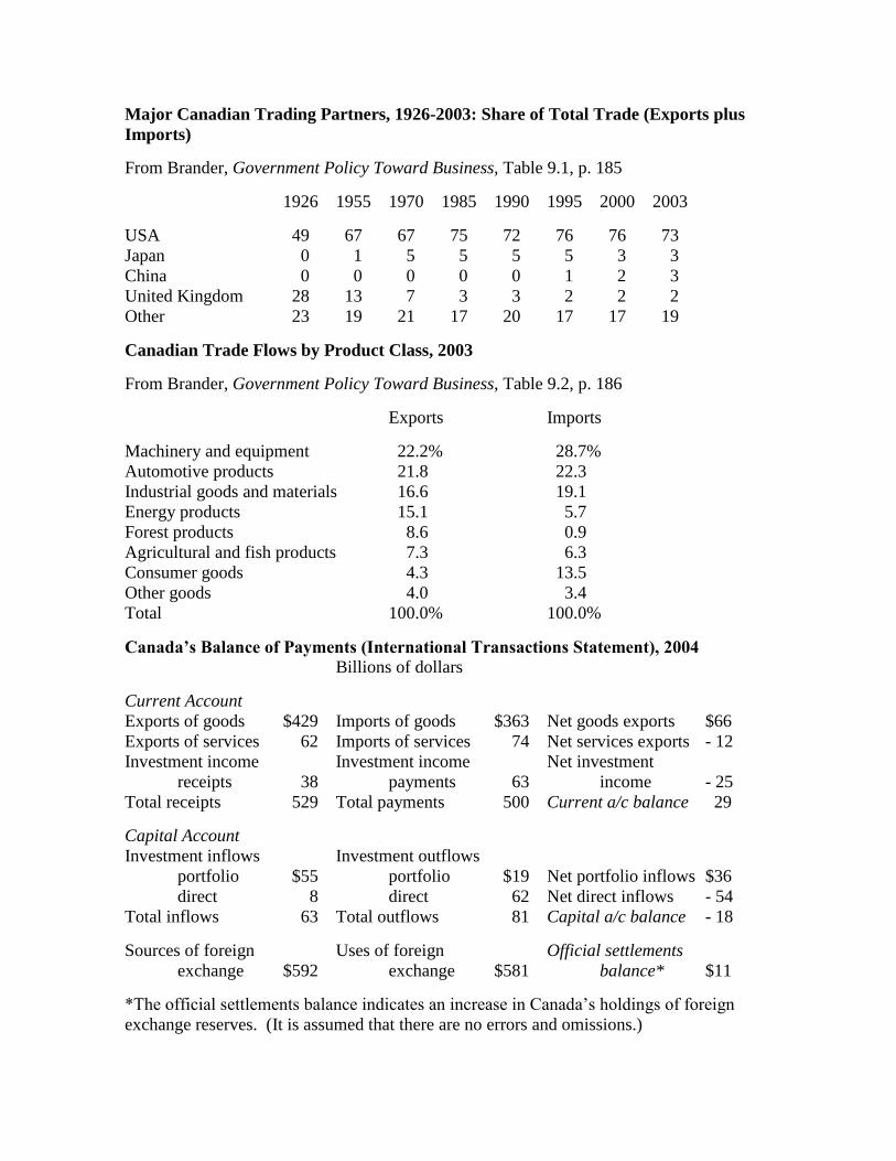
Major Canadian Trading Partners, 1926-2003: Share of Total Trade (Exports plus
Imports)
From Brander, Government Policy Toward Business, Table 9.1, p. 185
1926 1955 1970 1985 1990 1995 2000 2003
USA 49 67 67 75 72 76 76 73
Japan 0 1 5 5 5 5 3 3
China 0 0 0 0 0 1 2 3
United Kingdom 28 13 7 3 3 2 2 2
Other 23 19 21 17 20 17 17 19
Canadian Trade Flows by Product Class, 2003
From Brander, Government Policy Toward Business, Table 9.2, p. 186
Exports Imports
Machinery and equipment 22.2% 28.7%
Automotive products 21.8 22.3
Industrial goods and materials 16.6 19.1
Energy products 15.1 5.7
Forest products 8.6 0.9
Agricultural and fish products 7.3 6.3
Consumer goods 4.3 13.5
Other goods 4.0 3.4
Total 100.0% 100.0%
Canada’s Balance of Payments (International Transactions Statement), 2004
Billions of dollars
Current Account
Exports of goods $429 Imports of goods $363 Net goods exports $66
Exports of services 62 Imports of services 74 Net services exports - 12
Investment income Investment income Net investment
receipts 38 payments 63 income - 25
Total receipts 529 Total payments 500 Current a/c balance 29
Capital Account
Investment inflows Investment outflows
portfolio $55 portfolio $19 Net portfolio inflows $36
direct 8 direct 62 Net direct inflows - 54
Total inflows 63 Total outflows 81 Capital a/c balance - 18
Sources of foreign Uses of foreign Official settlements
exchange $592 exchange $581 balance* $11
*The official settlements balance indicates an increase in Canada’s holdings of foreign
exchange reserves. (It is assumed that there are no errors and omissions.)

Compensation in 26 countries: Ratios of CEO Pay to Manufacturing Employee Pay
Derived from Hill, Global Business Today, Table 16.3, p. 548. These data, for 2003-4,
relate to companies with annual sales of about $500 million.
Japan 9.5 Taiwan 14.5 Korea 14.8
Belgium 16.0 France 17.2 Sweden 17.6
Netherlands 18.3 New Zealand 19.5 Switzerland 19.8
Germany 21.3 China (Shanghai) 21.6 Spain 21.8
Australia 22.0 Italy 23.7 Canada 24.5
United Kingdom 27.9 China (Hong Kong) 35.7 United States 44.0
Venezuela 40.8 Argentina 45.7 Malaysia 49.9
Singapore 54.9 India 56.7 Brazil 61.5
Mexico 63.1 South Africa 72.2
Although there may be few firms with annual sales of $500 million in several of the
developing countries, these data nevertheless suggest that income inequality is greater in
many developing countries than in many Western countries, particularly including
European countries, while (from these data) the most egalitarian society appears to be Japan
(where labour turn-over is also traditionally slower). However, income distribution in the
United States appears to be less equal than that in other advanced countries, while there
may be some spill-over implications of this phenomenon to other English-speaking
countries.