economics a textbook - welcome igcse | dr ...€¢ production possibilities • law of increasing...
TRANSCRIPT

© Skanda Kumarasingam 2009 Page 1
ECONOMICS A TEXTBOOK
SKANDA Kumarasingam

© Skanda Kumarasingam 2009 Page 2
In memory of my father
Viswalingam Kumarasingam

© Skanda Kumarasingam 2009 Page 3
Contents in Brief Introduction
About the Author
Part 1- Micro Economics
Chapter 1- Basic Concepts and Ideas of Economics Chapter 2- Price Theory Chapter 3- Price Elasticity and Marginal Revenue Chapter 4- Cost of Production Chapter 5- Product Price and Output in Pure Competition Chapter 6- Product Price and Output in a Pure Monopoly Chapter 7- The Prices and Employment of Resources
Part 2- Macro Economics
Chapter 8- National Income Accounting Chapter 9- Macroeconomic Analysis- Aggregate Demand and Aggregate Supply
Chapter 10- National Income Analysis
Chapter 11- International Trade and Balance of Payments Chapter 12- Money and Banking: Fiscal and Monetary Policy

© Skanda Kumarasingam 2009 Page 4
Contents in Detail Introduction
About the Author
Part 1- Micro Economics
Chapter 1- Basic Concepts and Ideas of Economics
• Problem of scarcity
• Needs and wants
• Resources or factors of production
• Goods and services
• Efficient economies
• Production possibilities
• Law of increasing opportunity cost
• Efficient and inefficient points on the production possibilities curve
• Circular flow diagram
• The economic questions
• Review (chapter summary)
• Answers to review questions
Chapter 2- Price Theory
• Demand
• Law of demand
• Differences between demand and quantity demanded( compiling the determinants of demand)
• Supply
• Law of supply
• Differences between supply and quantity supplied( compiling determinants of supply)

© Skanda Kumarasingam 2009 Page 5
• Demand and supply( finding the market equilibrium for an individual product)
• Changes in the equilibrium
• Review( chapter summary)
• Answers to review questions Chapter 3- Price Elasticity and Marginal Revenue
• Elasticity and its calculation
• Revenue
• Elasticity of supply
• Marginal revenue
• Review( chapter summary)
• Answers to review questions
Chapter 4- Cost of Production
• Economic costs and economic profits
• Cost schedules and curves
• Marginal cost and marginal product
• law of diminishing returns
• Average costs
• Long run cost curves
• Review (chapter summary)
• Answers to review questions Chapter 5- Product Price and Output in Pure Competition
• Features of perfect competition and assumptions
• Short run cost of production
• The firm’s supply curve

© Skanda Kumarasingam 2009 Page 6
• Long run cost of production
• Review (chapter summary)
• Answers to review questions
Chapter 6- Product Price and Output in a Pure Monopoly
• Features and assumptions of a pure monopoly
• Short-run cost curves
• Long run cost curves
• Review ( chapter summary)
• Answers to Review questions Chapter 7- The Prices and Employment of Resources
• Types of resource employers and their markets
• Perfectly competitive resource employers selling in a perfectly competitive environment
• Perfectly competitive resource employers selling in an imperfectly competitive environment
• Important features of a perfectly competitive resource market
• Monopsonists
• Firms where all resources are variable
• Review questions
• Answers to review questions

© Skanda Kumarasingam 2009 Page 7
Part 2- Macro Economics
Chapter 8- National Income Accounting
• Purposes of national income accounting
• Gross domestic product
• Adjusting for gross domestic product
• Review( chapter summary)
• Answers to review questions Chapter 9- Macroeconomic Analysis- Aggregate Demand and Aggregate Supply
• The basic ideas of macroeconomic analysis
• Aggregate demand and reasons for the downward sloping curve
• Changes in the quantity of real output demanded and changes in aggregate demand
• Aggregate supply
• Changes in the quantity of real output supplied and changes in the aggregate supply
• Equilibrium
• Inflation and unemployment
• Review questions
• Answers to review questions Chapter 10- National Income Analysis
• The purposes of national income analysis
• Assumptions
• Consumption and savings
• Gross investment
• Marginal and average consumption and savings
• Understanding gross investment using graphical presentations
© Skanda Kumarasingam 2009 Page 8
• Two sector economy
• Effects of multiplier
• Open economy with foreign trade
• Government expenditure and taxes in an open economy
• Review questions
• Answers to review questions Chapter 11- International Trade and Balance of Payments
• Fundamental questions of trade
• Law of comparative advantage
• Importance of specialization
• Terms of trade
• Foreign exchange
• Law of demand and supply for foreign exchange
• Balance of payment
• Review( chapter summary)
• Answers to review questions Chapter 12- Money and Banking: Fiscal and Monetary Policy
• Roles of money
• Components of money and money-supply
• Demand for money
• Equilibrium money-supply and demand
• Commercial banks
• The commercial banking system
• Federal Reserve Bank
• Policies

© Skanda Kumarasingam 2009 Page 9
• Review (chapter summary)
• Answers to review questions

© Skanda Kumarasingam 2009 Page 10
Introduction This book is like no other. I say this boldly because as a teacher and lecturer in economics for over ten years at Post-graduate and Under-graduate levels I am yet to see a book of this nature. We know that the average economics book will have about 500 pages or more (some over a 1500 pages) and most of them would include over explanations, repetition, articles, information, case studies, examples or metaphors which only go to confuse the simple concepts that we need to be aware of so that we will be able to evaluate this world better from an economic standpoint. After all this has always been the core objective of studying economics in all most all courses. If you think critically you will see that in many subjects to understand it better you need to understand the concepts only. Once the concepts have been clearly understood the topics and the overall subject becomes easy to digest. Understanding core concepts has become the new way of super-learning. One method of super-learning suggests that a teacher (or facilitator) should only be involved in spending about 10 percent of their time that is given to lecture an economic course (or any course for that matter) explaining only the core concepts well. Once the concepts have been well understood the student will then be able to read any chapter and be able to understand it well. However when the overall concept or the picture is not given the student will have to laboriously go through an economic text book which often looks as big as a dictionary to unearth the concepts. Most often they give up and muddle through with little understanding of the topics or overall subject. Their intention then becomes know something to just pass the examination. As previously explained as a teacher, lecturer and facilitator for over 10 years teaching not only economics but many management, accounting and finance related subjects I have realized that there remains a huge gap in books which explain the concepts very clearly and fast. In this book I have just done this and this is why I say that this book is like no other. In nearly 10 days at the most you will be able to go through this book very quickly which consists of just 150 pages of text explaining to you very clearly and succinctly the key points and core concepts of this rather confusing and difficult subject. The rest of the pages (approximately around 75 pages more) include pictures and diagrams to explain the concepts even better. Eventually you will not even have to read the notes. Just look at the pictures, graphs and schedules to understand the whole subject. Then read the review or summary at the end of the chapter to tie up all loose ends. Once the concepts have been grasped you will be able to tackle your complex economics textbooks that have been often recommended by university professors in a fairly easy manner. So in this book I have avoided explanations of certain unnecessary areas, padding it with case studies, paper articles and long drawn examples. However I have used clear examples to explain the concepts extremely well. Note that this book is not a short notes book in economics. Each concept or key point has been explained very clearly. All of us understand that people learn well when given the information or the data in very small doses. The small steps that you take will seem simple and familiar to you. Developing on these basic ideas we will then move towards more complex often perplexing and unfamiliar ideas. In this way you will be able to grasp very difficult and complex ideas in economics fairly simply. You will also note that this concept book has been developed in such a way so that every paragraph will highlight small but new information. In the following paragraph a new idea or concept is developed based on the idea in the previous paragraph, schedule or curve.

© Skanda Kumarasingam 2009 Page 11
All of us consider that people learn better when they are actively involved. To get you actively involved it (the book) asks you to fill schedules', draw graphs and pictures and write your own observations before it is told or taught. Try not to look at the suggested answers or completed schedules provided just below the activity until you have made genuine effort completing it. The answers are given just after simply because I do not want to waste your time by asking you to check at the end of the book for the answers. In this way you will realize that economics is easy to study and understand. You also analyze and synthesize the subject as you move along. This book has been written in such a manner so that it will work as your personal tutor. So first it will tell you about certain concepts, then ask you about them and finally answer it or correct it. Say for example first it will explain a simple concept then ask you to fill a schedule or draw a graph or picture or write your observations. Then I will give you the right observations so that you can check your understanding as you go along. Since this is your personal trainer you are not obliged to work fast. The concepts are easy to understand and it is believed that you should work at your own speed. Somehow if you are hard pressed for time you can still go through the whole book in less than 10 days and you will have all the concepts you need to know about economics at your fingertips. Please remember that the essence of learning is understanding and mastering these concepts very well. Once the concepts are embedded into your mind you will be able not only to understand but also answer all questions using your intelligence remembering to blend it with the theoretical frameworks. You should note that this book has been written in such a way as people generally talk. So the reading is less strenuous and easy to understand. As far as possible I have not used jargon. However like all specialized subjects jargon is necessary evil and so has introduced such words but first explaining them in simple English. At the end of the chapters there are a series of review tests. These review tests are simple questions which you will be able to fill out fast. These will highlight all the major points that you need to know and will help you to round-off or tie up the knowledge you have gained by studying the specific chapter. This is indeed your chapter summary. So I have not provided a chapter summary. You have written one yourself. I believe that this book should have a wide readership. This has been written with a lot of focus on students who will be exposed to the subject for the first time or being introduced to the subject before have not really grasp the ideas or the concepts well. This can involve advanced level students, students taking bachelor's courses where economics is a subject, professional examinations and those studying for their Masters of Business Administration. Particularly those who are studying for their Masters of Business Administration come from many fields such as medicine, engineering and the arts. These students generally were never taught economics before. At the master's level the subject is taught at its most complex offering and those who have not understood the subject well or do not understand the concepts well are forced to study a fairly complex economics test book having about 500-1500 pages making the concepts impossible to understand in the process. We also know that students are hard pressed for time and there is a dearth of good economics lecturers and teachers. I believe that this book will be the answer to such readership. However to obtain complete knowledge about economics this book on concepts is insufficient. This will only help to lift the initial fog that surrounds the subject. Once the concepts have been well understood you should read the recommended textbook to obtain a fully rounded understanding. I believe that as you seek to understand the world where we are all time poor with a great yearning for simplicity this book serves its purpose well. I hope that this book will benefit you by helping you to prune the many trees that may temporarily block your vision and enable you to behold a single coherent forest. Skanda Kumarasingam Sydney Australia 31 December 2009

© Skanda Kumarasingam 2009 Page 12
About the Author
Skanda Kumarasingam was a facilitator to many distinguished foreign Masters and Bachelors programmes offered in Sri Lanka by the American Central University (USA), American City University (USA), Troy State University (USA), University of Manipal (India), Curtin University of Technology (Australia) and Leeds Metropolitan University (UK). He also possesses vast primary research skills and has supervised over thirty five theses writing for MBA programs. He was a corporate coach specializing in finance, operations and change management through the Centre for International Education and Training from the Torrens Valley TAFE –South Australia and EdExcel of UK. In the past Skanda lectured/facilitated study programs leading to the professional examinations conducted by the Institute of Chartered Accountants of Sri Lanka, Society of Certified Management Accountants of Sri Lanka, Association of Accounting Technicians of Sri Lanka, Sri Lanka Institute of Marketing, Chartered Institute of Marketing (UK), Association of Business Executives (UK) and Institute of Chartered Secretaries and Administrators (UK). Skanda counts over 10 years of lecture and facilitation experience. Before becoming fully involved in education he was a senior manager and professional primarily in general management and management accounting roles either with profit centre responsibility or in supporting senior managers with profit responsibilities. He has held senior management roles in KPMG (Audit and Consulting), Coke (Regional Internal Auditor and Leader- Financial Impact Teams in the Asian Region), PepsiCo, Marks and Spenser (UK) , Gap(Singapore), Next (Singapore) and Ernst and Young (Business Training Centre- Kingdom of Bahrain).

© Skanda Kumarasingam 2009 Page 13
Skanda has over 15 years experience in senior management and professional business training roles. During this period Skanda developed many tools and techniques to aid management in managing and controlling costs and improving profits. His models which include the Profit Maps (for profit improvement and cost reduction) and the LEAST Tax Model (for proactive tax planning) have been widely used in many organizations and its branches and sub-units saving them large amounts of dollars in costs and dramatically improving profits.
Skanda is a qualified Chartered and Management Accountant. He earned his MBA from the University of Lincoln UK. He has many professional qualifications in Quality Management, Supply Chain Management and Taxation.
Skanda is the author of four books - The Profit Maps Model, The Profit Maps Model Workbook, Personal Tax Planning and Economics- A Textbook. The first two books have been used in workshops and training sessions by him with great success. These two books and the Personal Tax Planning book have been widely distributed in e-book form and made use by many organizations and individuals. The Economics textbook was adopted in many teaching institutions where Skanda was a lecturer. All these books are available free for reading (without abbreviation) in the Scribd website. His ideas on profit improvement cost reduction can be found on his web-site www.profitmaps.com.au. Skanda can be contacted by email on [email protected]. Skanda lives with his wife Anne and two daughters Ramita and Sahana in Sydney, Australia.

© Skanda Kumarasingam 2009 Page 14
Part 1- Micro Economics

© Skanda Kumarasingam 2009 Page 15
Chapter 1
Basic Concepts and Ideas of Economics Learning Outcomes
• To understand the basic economic terms and concepts such as scarcity, unlimited needs and wants, resources in economics, goods and services and to develop a basic definition of economics as a science
• To appreciate the role or contribution of the study of economics in creating efficient economies
• Understanding the concept of production possibilities and using it to learn the law of increasing opportunity cost
• To develop a simple understanding of a society or economy using the circular flow diagram. More complex versions are developed later in this book.
• Understanding the meaning and relevance of the economic questions that every society must answer
• Summarize what was learnt in this chapter by asking relevant questions in the review section to tie up all the loose ends. Using the answers that have been provided subsequently to these review questions you will have a complete and comprehensive summary to study this chapter.
Chapter Outline
• Problem of scarcity
• Needs and wants
• Resources or factors of production
• Goods and services
• Efficient economies
• Production possibilities
• Law of increasing opportunity cost
• Efficient and inefficient points on the production possibilities curve
• Circular flow diagram
• The economic questions
• Review (chapter summary)
• Answers to review questions

© Skanda Kumarasingam 2009 Page 16
Scarcity (The Theme of Economics)
Let us say for example a college student has the following expenses for a given month in USD Food 110 Housing 100 Clothing 030 Recreation 040 Laundry 030 Miscellaneous expenses 020 Total 330 However the above college student has only USD 300. From this we can note that the available resources or money that she has is limited compared to her needs. So we can also say that the available resources are scarce compared to her needs. The problem facing this college student is not at all uncommon. Everybody in the society faces this problem. This problem that the society faces is that its needs and wants are unlimited compared to the scarce resources that are available in society. This problem is called the problem of scarcity. Because of this economics is the study of understanding and solving the problem of scarcity. In fact economics is also defined this way. Needs and Wants
There is however a difference between needs and wants. Needs are goods and services that people require so that their basic requirements are met and that they will be able to survive in society. However once their basic needs are met they tend to become much more desirous of wanting goods and services which are not required for survival but may be required for purposes of status etc. The requirement for such products and services are called wants. Resources are Factors of Production
We also need to understand that scarce resources need not always be money. In economics scarce resources are basically the factors of production which include land, labor, capital and entrepreneurship. The scarce resources are used to produce the goods and services that the society wants. Goods and Services
Goods and services can be tangible or intangible. Tangible goods are those which you can touch and feel such as a pound of bread or a table or chair. Intangibles are services such as getting a haircut or cleaning your teeth from a dentist. Services cannot be touched but can only be felt and so are called intangibles. Some goods are also called free goods when given by nature and available in abundance and free to use. Nobody owns them and they are not transacted in a market. Sunlight and river and sea water may be examples of this. On the other hand economic goods are owned by somebody, transacted in a market and not available in abundance. All economic goods (consumer goods and capital goods) are examples of economic goods Efficient Economies
If a society needs to reduce the gap between its unlimited needs and wants and the products or services it can produce based on the scarce resources it has it should become a very efficient economy. Such an economy is called a fully efficient economy. But we need to know that even in a

© Skanda Kumarasingam 2009 Page 17
fully efficient economy even though we may be able to produce more goods and services we still will not be able to meet human demands which are unlimited. All that we are saying is that we will be able to reduce the gap if society is fully efficient. Next we need to consider what we mean by an efficient economy. Efficient economies are capable of producing more goods and services by their capability of using all resources that are available so that there are no idle resources. Also note such a society should be able to use the best available technology to produce the goods and services. In a society which is capable of using all its resources and that there are no idle resources such a society is called a society which has full employment. You should note clearly that as far as economics is concerned full employment not only means full employment of labor but full employment of all the resources (factors of production) that are required to make goods and services. Technology is the means or methods that are used by businesses to convert inputs to outputs. A society should use the best available technology to produce its goods and services and if it does so such a society is called as having full production. You are thus required to note the subtle difference between full employment and full production very carefully. So we can summarize that a fully efficient economy = full employment+ full production Production Possibilities
Due to the concept of scarcity there are certain other ideas in economics which we need to be introduced to. To do this well we need to first understand what we mean by the production possibilities curve or production possibilities frontier or production possibilities schedule. They all mean one and the same. Given below is a production possibilities schedule. This is prepared assuming that the economy is a fully efficient economy and so all the resources are used and the best possible technology is employed. Also the production possibilities schedule is prepared for a period of time when resources or technology will not change.
Combinations
Products
A
B C D E F G H I J K
Food
0 1 2 3 4 5 6 7 8 9 10
Clothing
100 99 96 91 84 75 64 51 36 19 0
Opportunity cost of producing food
Opportunity cost of producing clothes
This also tells us that this economy produces two kinds of goods which are food and clothing. This economy is capable of producing different combinations of food and clothing and these combinations are given from A to K. We can also observe that at any combination such as at combination C this

© Skanda Kumarasingam 2009 Page 18
economy is able to produce 2 units of food and 96 units of clothing using its fixed resources and technology at this given time. We also note that as the production of food keeps increasing the production of clothing has to reduce and vice versa. This is because as assumed the resources are fixed so to produce more food we need to shift resources from clothing to the production of food. Because of this shift production of clothing will obviously reduce. It is also clear that to produce more of something we need to give up the production of something else. So we need to make a choice. Wherever there are choices to be made there is obviously a cost. In economics this cost is called an economic cost. All economic costs are opportunity costs. Opportunity cost means what you give up to get something. In the above schedule we can say that the opportunity cost of producing food is how many units of clothing you will have to give up. Similarly the opportunity cost of producing clothing is how many units of food you will have to give up. For example to produce one unit of food (say from point A to Point B) we need to give up the production of clothing by one unit. So the opportunity cost of producing one unit of food is one unit of clothing that was given up. Using this explanation you are now required to fill up all the blanks (the last two rows) in the above schedule When you completed the last two rows of the production possibilities schedule it should be like this
Combinations Products
A B C D E F G H I J K
Food - 1 2 3 4 5 6 7 8 9 10
Clothing 100 99 96 91 84 75 64 51 36 19 -
Opportunity cost of producing food
- 1 3 5 7 9 11 13 15 17 19
Opportunity cost of producing clothes
1.00 0.33 0.20 0.14 0.11 0.09 0.08 0.07 0.06 0.05 -
You might now ask which is the best combination of all the combinations that have been given in the production possibilities schedule. The production possibilities schedule does not reveal which is the best combination but it only reveals what combinations are possible given the resources and technology at a particular time when these are fully employed and technology is at full production. Law of Increasing Opportunity Costs
We can also note from the completed production possibilities curve above that when production increases of a particular commodity the opportunity cost also increases. This is called the law of increasing opportunity costs. Let me now explain why the law of increasing opportunity cost is true. Let us say for example in our hypothetical economy or society that has been depicted by the production possibilities schedule above we have 100 laborers and half of this labour is involved in the production of clothing and the other half in the production of food. We also assume that those who are involved in the production of food are experts in its production and those who are involved in the production of clothing are skilled in their own field. Let us also say that the other resource which is capital includes 50 sewing machines and 50 tractors. The 50 sewing machines obviously are involved in the production of clothing and 50 tractors are involved in the production of food.

© Skanda Kumarasingam 2009 Page 19
Now if we move from one combination to the other we need to also shift these resources. However we also know that these resources specialize in the production of either food or clothing. When we want to produce more of clothing we will then shift most of the resources which are capable of producing food to the production of clothing. This will obviously be inefficient as those who are experts in the production of food will be incompetent in the production of clothing and that tractors cannot be used in the production of clothing. Another thing that we see is that the increased labour in clothing will now be using the limited number of sewing machines that are available and so will have to wait for a long time until a machine becomes free for them to use. This will also make them more disorganized. So even though we know that production increases when more resources are used we need to shift more and more resources to produce this increase. This explains how the law of increasing opportunity cost works. Efficient and Inefficient Points on the Production Possibility Curve
Using our production possibilities schedule let us now prepare a production possibilities curve. For no obvious reason let us plot food on the Y axis and clothing on the X axis. Now draw this graph in the space provided below. On this graph note combination F as indicated on the production possibilities schedule.
To the left of this production possibilities mark a point L. We can easily say that point L is a possible combination that can be achieved but it is inefficient. The more efficient production will involve moving this point towards the production possibilities curve. Note that to become fully efficient we need to move towards the production possibilities curve and the opportunity cost of doing this is zero. The only reason why we are unable to achieve this is because there are either unemployed resources or underemployment of the right technology. If we are able to overcome this problem of unemployment of resources or the underemployment of technology we will be able to move towards the most efficient production point which is on the production possibilities curve at the given time. We can also mark a point M which is on the right side of the production possibilities curve. We should note that this point is impossible to achieve with the fixed resources and the given technology. The only way the production possibilities curve can shift or move towards point M is if it shifts outwards to the right. This will take time to achieve and can only be achieved by increasing the resources or improving technology so that such technology will be able to increase output for one unit of input. We also know that the production possibilities curve is a negative curve. We say the graph is negative when the relationship is an inverse relationship. This relationship can be noted by finding out what the opportunity cost is. The opportunity cost can be derived by calculating the slope of this curve.

© Skanda Kumarasingam 2009 Page 20
Slope of any curve is calculated as rise over run(Y axis over X axis). You will also note that if you calculate opportunity costs at different points that it is not constant but increasing as the law of increasing opportunity cost dictates in any given society. Your completed production possibilities graph should look like this
Production possibilities
0
2
4
6
8
10
12
- 10 20 30 40 50 60 70 80 90 100 110
clothing
food
FL
M
Circular Flow Diagram
Let us now try to draw this diagram in the space below using the information and descriptions that are provided. Read them carefully and you will be able to develop a very good understanding of how certain essential ideas of economics operate.

© Skanda Kumarasingam 2009 Page 21
Draw 2 boxes and label one as business firms and the other as households Inside the box marked business firms also mark that the business produces goods and services Inside the box for households indicate that it involves families and individuals. You may also mark in the box that their needs and wants are unlimited. On the upper part of this box you may mark that households are the owners of all resources in a given society. Draw an arrow from households to the business firms connecting the top parts of the two boxes drawn. You may mark this as the movement of resources. At the bottom part draw another arrow from business firms to households and mark this as the movement of goods and services. These two arrows indicate that resources are moving from households which own them to business firms which convert them to goods and services and transfer them back to households to fulfill their unlimited needs and wants. This flow is called the real flow as it involves the flow of resources and the flow of goods and services. Also on the top part of the diagram draw another arrow from business firms to the households and mark it as money. In a similar manner on the bottom half draw another arrow from households to business firms and mark it again as money. These two arrows indicate another flow which is called the money flow. The money flow operates because when resources are purchased by business firms they will pay the household's money. Using this money the households will purchase the goods and services that have been produced by the business firms. We note that when money flows from business firms to households it is a cost to the business firm for buying the resources and it is an income to the households because they are able to sell their resources. Alternatively when money flows from households to business firms it is expenditure for the household for the purchase of goods and services and it is the receipt to the business firm. Also from the diagram note that there two kinds of markets in any given society. One of them is called the resource market where buyers and sellers meet to sell resources and to purchase resources. This is obviously indicated in this diagram on the top part. In any given market there would be buyers and sellers and transactions taking place. In the Resource market the buyers are called the demanders and the sellers are called the suppliers. The buyers or the demanders of resources are the business firms and the sellers or the suppliers are the owners of these resources or the households. We can also observe from this diagram that there is another market which is called the product market. In this product market the buyers or demanders are the households who demand the goods and services to fulfill their unlimited needs and wants and the sellers or the suppliers are the business firms which produce and supply these goods and services. You may now ask the obvious question whether we really need business firms in society. This is because all the households pool their resources and can thus produce goods and services which again flow back to the households. The question is why it should flow to and from business firm. The answer to this question is simple and logical. The main reason why a business firm is established in society is usually because most businesses specialize in the production of a single or a few products and services. Because of this they are able to become fully efficient. So the use of a business firm in society might help it to become more efficient which is capable of using all the available resources at a given time and using the best available technology. This will obviously create more goods and services and may be able to fulfill more of the unlimited needs and wants of households.

© Skanda Kumarasingam 2009 Page 22
Another advantage of business firms is that this helps all resources to be pooled. Otherwise every household will try to be a Jack of all trades and may become very inefficient in trying to fulfill their unlimited needs and wants. However when they start working as team (in business units) productivity and efficiency increases as a better blend of resources (factors of production) is put to work. The next question we need to ask is why we need money. Why cannot households provide the resources and in turn obtain the goods and services which they might want. However this easier said than done. Obviously there are certain disadvantages of not using money and the effect of it on trading is well known. When barter trading is involved money is not exchanged but goods and services are exchanged for resources. However the problem of breaking down such resources or trying to sell certain resources to firms which may not actually want them create major problems which only money can solve The Economic Questions
Now let us look at the major economic questions every society needs to answer. These questions need to be answered because there is scarcity of resources and this leads us to make certain choices. Answering or trying to solve these problems involves the process of answering these economic questions. The questions that we want to ask are as follows
• What to produce?
• How to produce?
• For whom produce?
• What to do to ensure full employment and full production of resources and technology?
• How to improve the flexibility of resources? What to produce? In the production possibilities schedule we note that a particular society produces either food or clothing assuming it is what they want. However societies can decide what they need to consume. So rather than food and clothing it may be wine and rice, chicken and pears or shoes and chocolates. Once it is decided what to produce the society also needs to decide what combination of these goods and services it needs to produce. Obviously we know that the production possibilities schedule will only highlight the combinations that are possible but it does not tell us the ideal combination. Society must decide what is ideal for its needs and then tell it to the businesses so that they would able to produce the goods and services and supply it to them We also know that in this problem of what to produce it involves moving resources from one product to the other which also creates increasing opportunity costs How to produce? This involves how the society allocates resources and what best technology to use so that it will be capable of becoming a fully efficient economy

© Skanda Kumarasingam 2009 Page 23
For whom to produce? This involves answering the question of whom should we produce for and what proportions do these people get of the product and services that have been produced What to do to ensure full employment and full production? For full employment to occur those who are willing to work or provide the resources should be capable of work and able to provide the resources. Say for example that there are 100 workers and 80 of them want to work whereas 20 of them would not like to work. In such a society we can say when 80 people are employed there is full employment and when there are 70 people employed there is unemployment. Deciding on the best available technology does not mean that we have to use the best in the world or the latest technology. We need to decide on the ideal technology which may be either labor-intensive of machine intensive. How to improve the flexibility of resources? Say for example if the production possibilities schedules shifts are due to improving technology the other resources should be capable of working and becoming more flexible with this new technology. If they are not flexible the new technology will not give the required efficiency levels and so this society will not be able to enjoy more goods and services with the limited resources it has. Alternatively if the society decides to go from one combination to the other as its needs and wants have changed the resources it employs must be flexible enough move towards the production of the desired goods and services. If these resources are incapable of moving towards the production of the more desirable goods the society will not be able to enjoy the goods and services it requires fulfilling its current needs and wants.
Review (Once complete you can use this as the chapter summary or round-up) Question 1 Every society finds that it’s.......................are scarce because.......................................................................... ………………………………………………………………………………………………………………… Question 2 Economics is the social science that studies how society uses its scarce resources to produce the............... and.......................that....................... ………..human wants Question 3 For the economy to be efficient there must be both.......................and ....................................in the economy. Full employment means that…………………………………………………………………………………... ………………………………………………………………………………………………………………… Full production means that……………………………………………………………………………………. ………………………………………………………………………………………………………………… Question 4 The opportunity cost of producing a good or service is.................................................................................. …………………………………………………………………………………………………………………and as the production of a good increases the opportunity cost of producing it....................................

© Skanda Kumarasingam 2009 Page 24
Question 5 The law of increasing opportunity costs is the tendency for the..........................cost of producing a good or service to increase when the production of that good or service ...........................; the opportunity cost increases because as an additional resource is employed the extra output that is produced.....................................; and the extra output produced decreases because the additional resources are employed along with........................ quantities of other resources Question 6 A point that lies to the right or above and economy's production possibilities curve represents a combination of goods that the economy......................produce with its fix resources and technology. A point that lies to the left or below its production possibilities curve represents a combination of goods it...........................produces Question 7 A point to the Left of the production possibilities curve represents a combination that is produced when there is ..................................... or.............................. in the economy Right of the curve represents a combination that cannot be produced unless the economy...................... or........................................ Question 8 Eliminating the underemployment or unemployment of resources enables the economy to increase its production of a good at an opportunity cost of......................... Increasing its resources on improving its technology enables it to increase the production of a good at an opportunity cost of............................... Question 9 We have now encountered five fundamental economic questions for which every society must find answers. A society must decide ............................to produce ................to produce it .....................................................................to produce these goods and services What it needs to do to ensure the………………………………..... of its resources What it must do if the economy is to be......................... Question 10 In the circular flow diagram there are two groups represented and two flows shown. The two groups are....................................................................... The two flows are the.........................flow and the..........................flow Question 11 In the real flow.....................flow from.........................to................................and..........................flow from........................... to......................................... In the money flow monies flow from.............................to........................in payment for resources and the monies in this flow are the...........................of households and the..........................of firms Monies flow from.......................to...........................in payment for goods and services and the monies in this flow are the .......................................of households and the...................... of firms Question 12 The dual role of Households is………………………………………………………………………………………………….. Firms is………………………………………………………………………………………………………...

© Skanda Kumarasingam 2009 Page 25
Question 13 The two types of markets in the economy are the .............................. markets and the............................ markets Question 14 In the resource markets of the economy firms are the.................. and households are the.......................... In the product markets of the economy firms are the............................... and households are the......................

© Skanda Kumarasingam 2009 Page 26
Answers
Suggested answers to the above questions are given. The answers are provided sequentially in the same order you will fill the blanks or select from a choice in the brackets) Question 1 Resources The wants of society are unlimited Question 2 Goods and services Satisfy Question 3 Full employment Full production The economy employs all its resources It uses the best methods (Technology) to produce goods and services Question 4 The amount of other goods that must be sacrificed Increases Question 5 Opportunity Increases Decreases Fixed Question 6 Cannot Can Question 7 Unemployment(less than full employment) Underemployment(less than full production) Increases its resources Improves its technology Question 8 Zero Zero
Question 9 What How For whom Full employment Flexible Question 10 Households and business firms Real Money Question 11 Resources Households Business firms Goods and services Business firms Households Business firms Households Incomes Costs Households Business firms Expenditures Receipts Question 12 To furnish resources and use goods and services To employ resources and produce goods and services Question 13 Resource Product Question 14 Demanders (buyers) Suppliers (sellers) Suppliers (sellers) Demanders (buyers)

© Skanda Kumarasingam 2009 Page 27
Chapter 2
Price Theory Learning Outcomes
• To understand what demand and supply mean in economics and then to develop the law of demand and the law of supply from this understanding
• To understand what determines or changes demand and supply.
• To understand the differences between change in demand( or supply) and the change in quantity demanded ( quantity supplied)
• To combine our understanding of demand and supply and to note how markets determine the equilibrium quantity and price.
• To appreciate what effects do changes in demand and supply( or quantity demanded and quantity supplied) may have on the equilibrium point ( equilibrium price or equilibrium quantity)
• To summarize our understanding of the chapter by completing the answers to the Review questions. The review questions have been framed in such a way so that you may be able to use it as the summary of the chapter. This is the primary reason why a chapter summary has not been complied or given as it will lead to a repetition.
Chapter Outline
• Demand
• Law of demand
• Differences between demand and quantity demanded( compiling the determinants of demand)
• Supply
• Law of supply
• Differences between supply and quantity supplied( compiling determinants of supply)
• Demand and supply( finding the market equilibrium for an individual product)
• Changes in the equilibrium
• Review( chapter summary)
• Answers to review questions

© Skanda Kumarasingam 2009 Page 28
Demand Demand is a schedule. This schedule is prepared for a period of time. This schedule has two columns which are price and quantity demanded. To prepare this schedule we need to interview many people and ask them how many of a given product or service they would consume at the given prices. Hence initially we will be tabulating the individual demand schedules. The individual demanders are given as A, B, C and D in the schedule below. Adding all these individuals demand schedules we can produce the demand schedule for the market. This is done obviously for a period of time. Fill in the gaps to complete the demand schedule
Demand Schedule for Milk
Week June 8-14, 2006
Price A B C D Quantity Demanded(A+B+C+D)
1.3 100 300 800 1300
1.2 125 125 925 1400
1.1 150 150 250 1500
1.0 175 175 275 975
0.9 200 200 300 1700
0.8 225 225 1025 1800
0.7 250 350 1050 1900
Write your observations of the above schedule……………………………………………………………….. ………………………………………………………………………………………………………………… ………………………………………………………………………………………………………………… ………………………………………………………………………………………………………………… This is the completed schedule
Demand Schedule for Milk
Week June 8-14, 2006
Price A B C D Quantity Demanded
1.30 100 100 300 800 1,300
1.20 125 125 225 925 1,400
1.10 150 150 250 950 1,500
1.00 175 175 275 975 1,600
0.90 200 200 300 1,000 1,700
0.80 225 225 325 1,025 1,800
0.70 250 250 350 1,050 1,900
Thus if we are to define demand it would be as follows, Demand is a schedule of quantity demanded versus price for a specific period of time. Demand also means the desire to own something and having the ability to purchase it. The above schedule could obviously be incorporated into a graph. In this graph the Y axis will have the price and the X axis will have the quantity demanded. This curve which is drawn from the demand schedule is called the demand curve.

© Skanda Kumarasingam 2009 Page 29
In the space provided draw the market demand curve for milk.
Your completed graph should look this way
Demand schedule for milk
-
0.20
0.40
0.60
0.80
1.00
1.20
1.40
1,200 1,300 1,400 1,500 1,600 1,700 1,800 1,900 2,000
quantity demanded
pric
e
Law of Demand
Using the schedule and graph, we can observe what is called the law of demand. According to the law of demand there is an inverse or opposite relationship between price and the quantity demanded. We can see that lower the price charged the quantity demanded is high or vice versa. There are two reasons for the law of demand to operate this way. The first reason is called a substitute effect and the second reason is called the income effect. Let me now explain to you the substitute effect. A substitute product is something that the consumer will consume in place of the given product and will not notice any major difference in utility or satisfaction at the given prices. For example substitute products maybe tea and coffee or butter and margarine. Let us say hamburgers and steak are perfect substitutes. If the price of a hamburger is held constant and the price of steak reduces and if people do not know or observe a difference in utility (a measuring scale of satisfaction) they would obviously shift from hamburgers to eating more steak.

© Skanda Kumarasingam 2009 Page 30
Give 3 more examples of substitute products ………………………………………………………………………………………………………………… ………………………………………………………………………………………………………………… ………………………………………………………………………………………………………………… The other reason for the law of demand to work is the income effect. Say for example a person earns 10,000 /= in a given period and uses it to purchase bread only. A loaf of bread costs 100/=. Hence the person will be able to consume hundred loaves of bread. However if the price of bread increases to 200/= this person will have to consume less bread. Conversely if the price per leaf reduced to 50/= the number of loaves consumed in the given period will be ………………………………….. The two reasons for the law of demand to operate reinforce one another. These reasons give the consumer the belief or feeling richer as they can consume more with the same level of income.
Difference between Demand and Quantity Demanded
Now let us look at the difference between demand and quantity demanded. According to the definition of demand we know it is the schedule of quantity demanded vs. price at a specific time. Hence the change in demand has got to be a change in the schedule. There are many reasons for the demand to change. The reasons are called the determinants of demand and there are five of them. They are as follows
1. Number of buyers It is clear that the total demand schedule is prepared based on the number of people in the market who desire to have the product and have the capability to purchase it. If the number of such consumers increases this will have an effect on the total demand for the product in the market. This will increase the demand for the product. Alternatively if the number of buyers reduces the total demand schedule which is prepared by adding all the individual buyers’ demands in the market is affected and the demand will reduce.
2. Taste This means that certain people buy products based on their taste preferences and fashions of the time. If people eventually do not like the taste of a product they will buy less of it or stop buying this product. If they like the taste of it they will continue to buy more of it. Also if a product is fashionable during the current times more people will purchase them and if it is going out of fashion will purchase less of it.
3. Income When the income of consumers increases they have more purchasing power to purchase many products. This means when income increases the demand for superior goods and normal goods should increase. However when income increases the demand for inferior products will reduce. Provide 3 examples of superior goods ………………………………………………………………………... ………………………………………………………………………………………………………………… Provide 3 examples of normal goods ………………………………………………………………………... ………………………………………………………………………………………………………………… Provide 3 examples of inferior goods ………………………………………………………………………... …………………………………………………………………………………………………………………
4. Price of related goods As far as demand is concerned related products are substitutes and complements. Substitutes are products which can satisfy the consumers’ current need or want by giving them the required utility

© Skanda Kumarasingam 2009 Page 31
or satisfaction at the same level for the required price. Examples of such substitute products are tea and coffee. Provide 3 examples of substitutes ………………………………………………………………………... ………………………………………………………………………………………………………………… ………………………………………………………………………………………………………………… On the other hand complementary products are consumed together. One product cannot be consumed without the other such as guns and bullets, film roles and camera or tires and tubes. Provide 3 examples of complementary goods ………………………………………………………………. ………………………………………………………………………………………………………………… Intuitively we can say when the price of a particular substitute increases the demand for the given product will increase. So for example if the price of coffee increases more people will start drinking tea and hence the demand for tea will increase. On the other hand if the price of a complementary product increases the demand for the product will obviously reduce.
5. Expectations This is based on what the prices will be in the future. For example in certain cases due to taxation and so on prices tend to increase. If the consumer believes that the prices will increase in the future he will purchase the product immediately thus increasing the demand for the product. When there is a change in demand which is basically due to the determinants of demand causing this the demand schedule and the demand curve will either increase or decrease. If we look at the demand curve we can see that an increasing demand will shift the demand curve to the right and a decrease in demand will shift the curve to the left.
Demand for Milk
Quantity Demanded in the Months in 2005
Price July August September
1.3 4000 4500 3500
1.2 5000 5500 4500
1.1 6000 6500 5500
1.0 7000 7500 6500
0.9 8000 8500 7500
0.8 9000 9500 8500
0.7 10000 10500 9500
Draw the related demand curves for the months of July August and September and state if demand increased or decreased compared to July 2005

© Skanda Kumarasingam 2009 Page 32
Your completed graph should look like this
Quantity demanded in the months of 2005
-
0.20
0.40
0.60
0.80
1.00
1.20
1.40
3,00
0
3,50
0
4,00
0
4,50
0
5,00
0
5,50
0
6,00
0
6,50
0
7,00
0
7,50
0
8,00
0
8,50
0
9,00
0
9,50
0
10,0
00
10,5
00
11,0
00
quantity demanded
quan
tity
supp
lied
September July August
Now let us look at the change in quantity demanded. Quantity demanded can only change when there is a change in the quantity demanded and this is caused by the movement along the demand curve. The only reason why this can happen is because of a change in price. Thus we can conclude that price does not cause a change in demand. It only causes a change in the quantity demanded.
Supply
We can now analyze supply the same way we analyzed demand. We can start off by saying that supply is schedule. This schedule is prepared for a period of time. Supply in a market is caused by the producers who are willing to produce the supply and have the capability to produce it. Hence we can say that individual’s supply schedule is bought about by plotting the prices and tabulating the quantities the suppliers will be willing to produce and sell at those prices. Obviously the suppliers will only produce and supply if they are going to make a profit. Hence if the cost of producing a product is higher than the price that will be offered in the market they will not produce it. However as the price keeps increasing this will help to cover the cost and make a profit. At this point they will start producing and selling. As suppliers are keen on profit and higher the profit (assuming that the cost remains constant) they will be willing to produce more and sell more of this product. The tabulation of all these individual suppliers supply schedules will form the total quantity supplied in the market.
© Skanda Kumarasingam 2009 Page 33
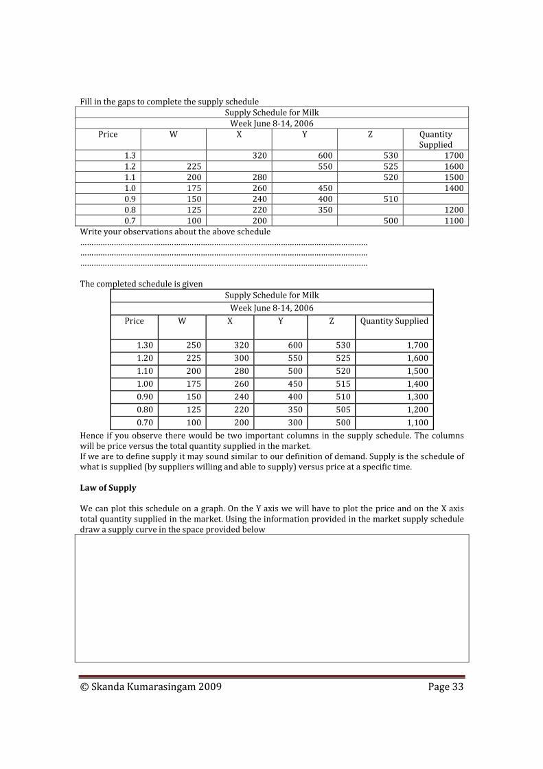
Fill in the gaps to complete the supply schedule
Supply Schedule for Milk
Week June 8-14, 2006
Price W X Y Z Quantity Supplied
1.3 320 600 530 1700
1.2 225 550 525 1600
1.1 200 280 520 1500
1.0 175 260 450 1400
0.9 150 240 400 510
0.8 125 220 350 1200
0.7 100 200 500 1100
Write your observations about the above schedule ………………………………………………………………………………………………………………… ………………………………………………………………………………………………………………… ………………………………………………………………………………………………………………… The completed schedule is given
Supply Schedule for Milk
Week June 8-14, 2006
Price W X Y Z Quantity Supplied
1.30 250 320 600 530 1,700
1.20 225 300 550 525 1,600
1.10 200 280 500 520 1,500
1.00 175 260 450 515 1,400
0.90 150 240 400 510 1,300
0.80 125 220 350 505 1,200
0.70 100 200 300 500 1,100
Hence if you observe there would be two important columns in the supply schedule. The columns will be price versus the total quantity supplied in the market. If we are to define supply it may sound similar to our definition of demand. Supply is the schedule of what is supplied (by suppliers willing and able to supply) versus price at a specific time. Law of Supply
We can plot this schedule on a graph. On the Y axis we will have to plot the price and on the X axis total quantity supplied in the market. Using the information provided in the market supply schedule draw a supply curve in the space provided below

© Skanda Kumarasingam 2009 Page 34
Supply schedule of milk
-
0.20
0.40
0.60
0.80
1.00
1.20
1.40
1,100 1,200 1,300 1,400 1,500 1,600 1,700 1,800
quantity supplied
pric
e
This curve which would be an upward sloping curve is called the supply curve. Observing the graph and the supply curve or even the supply schedule we will be able to state the law of supply. The law of supply is basically when the price increases the quantity supplied in the market will also increase and vice versa. The basic reason for the law of supply to work is the profit motive. Difference between Supply and Quantity Supplied Now let us look at the differences between changes in supply and quantity supplied. A change in supply means a change in the supply schedule or curve. A change in supply is caused mainly by six reasons and these reasons are called the determinants of supply. They are as follows
1. Number of suppliers in the market When the number of suppliers in the market increases this will obviously increase the individual supply curves which are ultimately added up to obtain the total market supply curve.
2. Resource prices Resources are used to produce goods and services. These resources which are called the factors of production may increase or decrease in price. If the price of these resources increases the cost of producing the goods or services will also increase. If we are unable to increase the prices to cover these cost increases we will end up with a lesser profit. As profit is a major motive for the supply the supplier will reduce production as he is not motivated any more. Conversely if the resource prices decreases the cost of production will reduce. This will obviously increase the profit margin of the product. This will induce the producer of the goods or services to produce more as the more he supplies he will be able to make more profits
3. Technology Technology reduces the cost of production. This is because if we are able to use the right kind of technology we can increase the efficiency and effectiveness. Obviously this will lead to higher profits for the supplier. As the major motive of the supplier is profit he will be highly motivated to produce more and sell more as he will begin earning a higher profit.

© Skanda Kumarasingam 2009 Page 35
4. Taxes and subsidies
Increases in taxes increase the cost or reduce the income that is available to the producer. When the taxes are high profit margins will be low and this will de-motivate the supplier. Hence she will supply less of the products. Alternately subsidies are provided by the government to reduce the cost of producing the goods or services. If the cost of production goes down it will increase the profit margins to the supplier and she will be motivated to produce more of the goods and supply it.
5. Price of related goods Prices of related goods are different to the related goods we looked at when we were studying the determinants of demand. In the determinants of demand related goods were substitutes and complementary products. However when studying the determinants of supply related goods mean what the supplier can produce with the given factors of production compared to the current product. When they can easily shift resources (very flexible resources) they will be motivated to shift its use towards products and services which give them a higher profit margin.
6. Future expectations If the supplier believes that the product will be able to command a higher price in the future they may temporarily stop supplying it. This is because by holding on to the sale and if the price increases they will be able to sell it at a higher price thus increasing their profits. Say for example the possibility of forming and becoming a member of a cartel such as OPEC (Organization for Petroleum Exporting Countries) However if they believe that the prices will fall in the future due to competition they will do their best to sell the product as fast as possible.
Supply for Milk
Quantity Supplied in the Months in 2005
Price July August September
1.3 8000 7500 8500
1.2 7000 6500 7500
1.1 6000 5500 6500
1.0 5000 4500 5500
0.9 4000 3500 4500
0.8 3000 2500 3500
0.7 2000 1500 2500
Draw the related supply curves for the months of July August and September and state if supply increased or decreased compared to July 2005

© Skanda Kumarasingam 2009 Page 36
This is the completed graph
Quantity supplied in months in 2005
0.00
0.20
0.40
0.60
0.80
1.00
1.20
1.40
0
500
1000
1500
2000
2500
3000
3500
4000
4500
5000
5500
6000
6500
7000
7500
8000
8500
9000
quantity supplied
pric
e
August September July
Determinants of supply cause the supply curve to increase or decrease. Looking at the supply curve we can say an increase in supply would shift the supply curve to your right and a decrease in supply would shift the curve towards the left. The reason for change in quantity supplied is only due to a change in price. Prices do not cause the change in supply but only cause a change in quantity supplied. This will cause the movement along the supply curve.
Demand and Supply
Previously we have been looking at the demand individually and supply individually. However demand and supply curves need to interact in the market so that the market will be able to determine the price. This is called the price mechanism and it is explained below
Demand and Supply of Milk
Week June 8-14, 2006
Quantity demanded Price Quantity supplied Notes
1300 1.3 1700
1400 1.2 1600
Quantity supplied is >quantity demanded so it is a surplus
1500 1.1 1500 Equilibrium point
1600 1.0 1400
1700 0.9 1300
1800 0.8 1200
1900 0.7 1100
Quantity supplied< quantity demanded so it is shortage
If we look at the schedule above we can see at price 1.1 the quantity demanded and the quantity supplied are the same. There is only one such point. This single point is called the point of

© Skanda Kumarasingam 2009 Page 37
equilibrium. The price at this point is called the equilibrium price and the quantity is called the equilibrium quantity. At equilibrium quantity there are no shortages or excesses of the product in the market. Above the equilibrium point we can note that the quantity supplied is greater than the quantity demanded. This creates a surplus situation. Suppliers will then reduce prices by providing discounts or free issues so that they may be able to sell off all the quantity. If the product is not sold off immediately or cannot be sold this will become a cost. Hence the suppliers will reduce the prices to sell off all the quantity they have. If we look below the equilibrium point in the schedule we will observe that the quantity supplied is less than the quantity demanded. This will then cause a shortage in the market. As there is a shortage, buyers will offer increased prices to encourage the sellers to sell the small quantity available to them. This will force the prices upwards until it reaches the equilibrium point. At the equilibrium point the demanders of the product need not pay any more as all they want can be purchased at a given price. They would be foolish to increase the price anymore as all they want can be purchased at the equilibrium price. In the same way at the equilibrium point the suppliers need not reduce the prices as all they have could be sold off at this given price. They would be foolish to reduce this price anymore to sell off everything they have. This can also be shown using a graphical presentation. According to the graphical presentation the point at which the demand and the supply curve intersect is called the equilibrium point. We will be able to read the equilibrium price along the Y axis and the equilibrium quantity along the X axis. Now draw the demand and supply curves together based on information in the above schedule on equilibrium in the space provided
On this graph or curve mark the equilibrium point, the equilibrium price, the equilibrium quantity, two price point to explain a shortage and surplus. The completed graph is given now for you to check your own answer

© Skanda Kumarasingam 2009 Page 38
Demand and supply of milk
0.00
0.20
0.40
0.60
0.80
1.00
1.20
1.40
1100 1200 1300 1400 1500 1600 1700 1800 1900 2000
quantity demanded and quantity supplied
pric
e
Quantity demande
Quantity supplied
Changes in the Equilibrium Point
Finally we need to look at how the equilibrium point would change based on the change in demand or supply. However we need to do this very carefully if we use the graphical presentation as the graphs can give you conflicting answers. Look at the example below
• If the demand increases the equilibrium price will increase and the equilibrium quantity will also increase.
• If demand decreases the equilibrium price will decrease and the equilibrium quantity will also decrease
• If supply increases the equilibrium price will reduce and equilibrium quantity will increase
• If supply reduces the equilibrium price will increase and the equilibrium quantity will reduce.
Draw four graphs to explain the above truths in the space provided below and give your observations on them.

© Skanda Kumarasingam 2009 Page 39
Now work out the following examples to note how the equilibrium points will change
1. Increase in demand and an increase in supply- this can have two variations where there is a small increase in demand and there is a big increase in supply or where there is a small increase in supply and a big increase in demand.
2. You cannot use graphs as it will give you to conflicting answers. Hence if you are to use a graph to find out the right answer we need to know the size of change in demand and supply or both of them.
3. Increase in demand and a decrease in supply. 4. Decrease in demand and a decrease in supply
Review (Once complete you can use this as the chapter summary or round-up) Question 1 Explain what demand is…………………………………………………………………………… ……………………………………………………………………………………………………………….. ……………………………………………………………………………………………………………….. ……………………………………………………………………………………………………………….. ……………………………………………………………………………………………………………….. Question 2 State the law of demand…………………………………………………………………………… ……………………………………………………………………………………………………………….. ……………………………………………………………………………………………………………….. ……………………………………………………………………………………………………………….. ……………………………………………………………………………………………………………….. Question 3 Explain what the demand curve is……………………………………………………………… ……………………………………………………………………………………………………………….. ……………………………………………………………………………………………………………….. ……………………………………………………………………………………………………………….. ………………………………………………………………………………………………………………..

© Skanda Kumarasingam 2009 Page 40
Question 4 What's the difference between demand and quantity demanded……………….. ……………………………………………………………………………………………………………….. ……………………………………………………………………………………………………………….. ……………………………………………………………………………………………………………….. ……………………………………………………………………………………………………………….. Question 5 What is supply………………………………………………………………………………………… ……………………………………………………………………………………………………………….. ……………………………………………………………………………………………………………….. ……………………………………………………………………………………………………………….. ……………………………………………………………………………………………………………….. Question 6 State the law of supply……………………………………………………………………………… ……………………………………………………………………………………………………………….. ……………………………………………………………………………………………………………….. ……………………………………………………………………………………………………………….. ……………………………………………………………………………………………………………….. Question 7 What is the difference between supply and quantity supplied…………………… ……………………………………………………………………………………………………………….. ……………………………………………………………………………………………………………….. ……………………………………………………………………………………………………………….. ……………………………………………………………………………………………………………….. Question 8 What is the difference between a change in supply and change in the quantity supplied……………........................................................................................................................ ……………………………………………………………………………………………………………….. ……………………………………………………………………………………………………………….. ……………………………………………………………………………………………………………….. ……………………………………………………………………………………………………………….. ……………………………………………………………………………………………………………….. Question 9 Explain an increase and decrease in supply……………………………………………… ……………………………………………………………………………………………………………….. ……………………………………………………………………………………………………………….. ……………………………………………………………………………………………………………….. ……………………………………………………………………………………………………………….. ……………………………………………………………………………………………………………….. Question 10 Both demand and supply are expressed as schedules or curves. During a specific period of time the demand schedule indicates the.............................. and the supply schedule indicates the.................................. at various prices in the schedule. Question 11 Both demand and supply have their laws. Between price and quantity demanded there is a............ relationship and between price and quantity supplied there is a...................... relationship

© Skanda Kumarasingam 2009 Page 41
Both demand and supply may be graphed. The demand curve slopes.................................... and the supply curve slopes............................................... Question 12 Both demand and supply may change. An increase in demand or supply means that the quantities in the schedule have.............................. causing the curve to move to the.................................. the decrease in demand or supply means that the quantities in the schedule have.............................. causing the curves to move to the................................. Question 13 In your own words define equilibrium price…………………………………………….. ……………………………………………………………………………………………………………….. ……………………………………………………………………………………………………………….. ……………………………………………………………………………………………………………….. ……………………………………………………………………………………………………………….. Question 14 In your own words define equilibrium quantity………………………………………… ……………………………………………………………………………………………………………….. ……………………………………………………………………………………………………………….. ……………………………………………………………………………………………………………….. ……………………………………………………………………………………………………………….. Question 15 Demand and supply as we have discovered determine what the price of a commodity will be and how much of that commodity will be bought and sold. The price which will be charged for a commodity in a competitive market is called be................................ price. The quantity of the commodities which will be bought and sold is called the............................... quantity. Question 16 Suppose the actual price being charged for a commodity was not its equilibrium price. Why would the actual price of the commodity move towards its equilibrium price? If this actual price started out above the equilibrium price than........................................................................................ ……………………………………………………………………………………………………………….. ……………………………………………………………………………………………………………….. ……………………………………………………………………………………………………………….. If this actual price started out below the equilibrium price than......................... ……………………………………………………………………………………………………………….. ……………………………………………………………………………………………………………….. ……………………………………………………………………………………………………………….. Question 17 If you plot demand and supply on a graph what does the point where the two curves cross indicate……………………………………………………………………………………………………. ……………………………………………………………………………………………………………….. ……………………………………………………………………………………………………………….. ……………………………………………………………………………………………………………….. ……………………………………………………………………………………………………………….. ………………………………………………………………………………………………………………..

© Skanda Kumarasingam 2009 Page 42
Question 18 Complete the table below using + for an increase or - for a decrease or a? for indeterminate.
Upon equilibrium Effect of
Price Quantity
Increase in both demand and supply
Decrease in both demand and supply
Increase in demand and decrease in supply
Decrease in demand and an increase in supply

© Skanda Kumarasingam 2009 Page 43
Answers
Suggested answers to the above questions are given. The answers are provided sequentially in the same order you will fill the blanks or select from a choice in the brackets
Question 1 A schedule showing the quantities demanded of a commodity at various prices during some specific period of time assuming determinants do not change Question 2 Price and quantity demanded are inversely related to each other (as price increases quantity demanded decrease and vice versa) Question 3 A graph of demand (of the demand schedule) Question 4 Demand is the schedule or curve while quantity demanded is the amount that will be purchased at some specific price in the schedule Question 5 A schedule of the quantities supplied at various prices during a specific period of time Question 6 The direct relation between price and quantity supplied (when price increases quantity supplied increases and vice versa) Question 7 Supply is a schedule and quantity supplied is the amount offered for sale at a particular price Question 8 A change in supply is a change in the schedule while a change in quantity supplied is the result of a price change
Question 9 When supply increases (decreases) the quantities supplied at each price increase (decrease) Question 10 Quantity demanded Quantity supplied Question 11 Inverse Direct Downward Upward Question 12 Increased Right Decreased Left Question 13 The price at which the quantity demanded of a commodity = the quantity supplied Question 14 The quantity demanded and the quantity supplied at the equilibrium price Question 15 Equilibrium Equilibrium Question 16 There would be a surplus of the commodity and the suppliers would bid the prices downward There would be a shortage of the commodity and the buyers would bid the price upward Question 17 The equilibrium price and equilibrium quantity Question 18 Question mark and + Question mark and- + And question mark - And question mark

© Skanda Kumarasingam 2009 Page 44
Chapter 3
Price Elasticity and Marginal Revenue
Learning Outcomes
• To understand the economic concepts of elasticity (or sensitivity) and the approach to calculating it. The types of elasticity and the basic formula for calculating it using the mid-point method or the average method giving reasons why the traditional method of calculating it is not right.
• To understand what is meant by revenue the means of calculating it.
• To study the relationship between revenue and elasticity to maximize profit .This is the basic objective of any organization from an economic standpoint.
• to understand the basic concepts behind the elasticity of supply and how total revenue is affected by the elasticity of supply
• To learn the concepts behind marginal revenue. To also identify the relationship between total revenue, marginal revenue, average revenue, price, the demand curve and the elasticity
• To identify the relationship between marginal revenue and elasticity for imperfectly competitive sellers and perfectly competitive sellers
• Review questions that are given to summarize the core concepts of this chapter. When you complete (answer) these questions and update it by the correcting errors by checking the right answers to Review questions you will have a comprehensive chapter summary from this.
• Answers to Review questions Chapter Outline
• Elasticity and its calculation
• Revenue
• Elasticity of supply
• Marginal revenue
• Review( or a summary)
• Answers to Review questions

© Skanda Kumarasingam 2009 Page 45
Elasticity and its Calculation
We have already learnt two of the most important and basic tools in economics which are demand and supply. Along with these two ideas or tools we have also learnt the laws pertaining to them which are the law of demand and the law of supply. To understand micro economics even better there are two other related ideas which you need to know along with demand and supply. They are the concepts of elasticity and marginal revenue. In this chapter we will understand these two concepts. What you learn from this chapter will be used to understand other micro economic concepts which are based on the cost of production, product price and output in pure competitive industries and product price and output in monopolies. Elasticity in demand tells us about the relative sensitivity or the responsiveness of one variable compared to another. In this instance relative sensitivity will mean how the change in price will have an effect on the quantity that is demanded. Some also call this the price elasticity of demand. Price elasticity of demand is also called the elasticity coefficient and is calculated as % change in quantity demanded divided by the % change in price. What this means is that when price changes by 1% (the denominator) what is the amount of change taking place on the numerator which is the quantity demanded. If the numerator (% change in quantity demanded) changes by a larger amount compared to the denominator (% change in price) we say that demand is elastic and if vice-versa it is inelastic. So to calculate the price elasticity of demand first we need to find out about the percentage change in price and the percentage change in quantity demanded using a demand schedule. In the space given write the general formula for elasticity based on the description in the previous paragraphs
To calculate a change in price we need to use two points from the demand schedule. You should always remember that whenever we talk of change we are talking about a change taking place between two points or numbers. However to calculate the percentage change in price we divide change in price by the price before the change. Likewise to calculate the change in quantity demanded we need to use two points from the demand schedule. Having done this we can then calculate the percentage change in quantity demanded by dividing the change in quantity by the quantity before the change. However this leads us to a problem which will be highlighted by filling the schedule given next. To fill these schedules you will start off from the top from A onwards and then calculate the elasticity of demand. You already know how to calculate % changes in price and % changes in quantity demanded by reading the earlier paragraphs.

© Skanda Kumarasingam 2009 Page 46
Change Change Points Price Quantity demanded From –To % change
in price From –
To % change in
quantity
Elasticity coefficient
A 7.50 0 - -
B 7.00 1 A to B A to B
C 6.50 2 B to C B to C
D 6.00 3 C to D C to D
E 5.50 4 D to E D to E
F 5.00 5 E to F E to F
G 4.50 6 F to G F to G
H 4.00 7 G to H G to H
I 3.50 8 H to I H to I
J 3.00 9 I to J I to J
K 2.50 10 J to K J to K
The completed schedule will look like this
Change Change Points Price Quantity demanded From –
to % change in price
From – to
% change in quantity
Elasticity coefficient
A 7.50 - - - - - -
B 7.00 1 A to B 6.67 A to B - -
C 6.50 2 B to C 7.14 B to C 100.00 14.00
D 6.00 3 C to D 7.69 C to D 50.00 6.50
E 5.50 4 D to E 8.33 D to E 33.33 4.00
F 5.00 5 E to F 9.09 E to F 25.00 2.75
G 4.50 6 F to G 10.00 F to G 20.00 2.00
H 4.00 7 G to H 11.11 G to H 16.67 1.50
I 3.50 8 H to I 12.50 H to I 14.29 1.14
J 3.00 9 I to J 14.29 I to J 12.50 0.88
K 2.50 10 J to K 16.67 J to K 11.11 0.67
Once this is done you will now start filling the second schedule from the bottom from point G to A and note the elasticity’s at each different point. You will note that there are differences in the price elasticity of demand when you start from point A and move towards point G and when you initiate from G and go towards point A.
Change Change Points Price Quantity demanded From –to % change
in price From –
to % change in
quantity
Elasticity coefficient
A 7.50 0 B to A B to A
B 7.00 1 C to B C to B
C 6.50 2 D to C D to C
D 6.00 3 E to D E to D
E 5.50 4 F to E F to E
F 5.00 5 G to F G to F
G 4.50 6 H to G H to G
H 4.00 7 I to H I to H
I 3.50 8 J to I J to I
J 3.00 9 K to J K to J
K 2.50 10 - -

© Skanda Kumarasingam 2009 Page 47
The completed schedule will look like this
Change Change
Points Price Quantity
demanded From –to
% change in price
From – to
% change in quantity
Elasticity coefficient
A 7.50 - B to A 7.14 B to A 100.00 14.00
B 7.00 1 C to B 7.69 C to B 50.00 6.50
C 6.50 2 D to C 8.33 D to C 33.33 4.00
D 6.00 3 E to D 9.09 E to D 25.00 2.75
E 5.50 4 F to E 10.00 F to E 20.00 2.00
F 5.00 5 G to F 11.11 G to F 16.67 1.50
-G 4.50 6 H to G 12.50 H to G 14.29 1.14
H 4.00 7 I to H 14.29 I to H 12.50 0.88
I 3.50 8 J to I 16.67 J to I 11.11 0.67
J 3.00 9 K to J 20.00 K to J 10.00 0.50
K 2.50 10 - - - - -
To overcome this apparent contradiction economists use what is called the mid-point method which is explained to you now. Using the midpoint method you will note that we will be able to arrive at the same answer irrespective of whether we are moving from point A towards point G or from point G towards point A. To calculate the elasticity of demand using the midpoint method we need to divide the percentage change in price by the percentage change in quantity demanded as previously noted. However in the calculation of these percentage changes lies the difference. When calculating the percentage change in price we divide the change in price by using the averages (sometimes called the averages method because of this) of the two prices amongst this change. Likewise when calculating the percentage change in quantity demanded we divide the change in quantity demanded by using the averages of the two quantities demanded amongst the change. Filling the schedule in the next page will highlight to you how this is done. Use the information from the above schedules. In the space below draw a graph and on the X axis plot the quantity demanded and on the Y axis plot the price. Using this demand curve how do you find the price elasticity of demand or the elasticity coefficient? Does the elasticity coefficient differ at different points of the graph?

© Skanda Kumarasingam 2009 Page 48
Price Quantity demanded
Change in quantity demanded
Mid-point of quantity demanded
% change in quantity demanded
Change in price
Mid-point of price
% change in price
Elasticity coefficient
Elastic or inelastic or unit elastic?
Total revenue Price X quantity demanded
Marginal revenue Δ TR Δ TQ
Average revenue TR TQ
A 7.50 0
B 7.00 1
C 6.50 2
D 6.00 3
E 5.50 4
F 5.00 5
G 4.50 6
H 4.00 7
I 3.50 8
J 3.00 9
K 2.50 10
Please remember that in the future when we talk about calculating the elasticities of demand or supply we will always be using the mid-point method. In the space provided below write your observations from the schedule ……………………………………………………………… …………………………………………………………………………………………………………………………………………………………………………... …………………………………………………………………………………………………………………………………………………………………………... …………………………………………………………………………………………………………………………………………………………………………... …………………………………………………………………………………………………………………………………………………………………………...

© Skanda Kumarasingam 2009 Page 49
Turn to the next page to see if you completed the chart properly
Total revenue
Marginal revenue
Average revenue
Price Quantity
demanded
Change in quantity
demanded
Mid-point of quantity demanded (average quantity)
% change in quantity demanded
Change in price
Mid-point of
price (average
price)
% change in price
Elasticity coefficient Price X
quantity demanded
Δ TR Δ TQ
TR TQ
A 7.50 - - - - - - - - - - -
B 7.00 1 1.00 0.50 200.00 0.50 7.25 6.90 29.00 7.00 7.00 7.00
C 6.50 2 1.00 1.50 66.67 0.50 6.75 7.41 9.00 13.00 6.00 6.50
D 6.00 3 1.00 2.50 40.00 0.50 6.25 8.00 5.00 18.00 5.00 6.00
E 5.50 4 1.00 3.50 28.57 0.50 5.75 8.70 3.29 22.00 4.00 5.50
F 5.00 5 1.00 4.50 22.22 0.50 5.25 9.52 2.33 25.00 3.00 5.00
G 4.50 6 1.00 5.50 18.18 0.50 4.75 10.53 1.73 27.00 2.00 4.50
H 4.00 7 1.00 6.50 15.38 0.50 4.25 11.76 1.31 28.00 1.00 4.00
I 3.50 8 1.00 7.50 13.33 0.50 3.75 13.33 1.00 28.00 - 3.50
J 3.00 9 1.00 8.50 11.76 0.50 3.25 15.38 0.76 27.00 (1.00) 3.00
K 2.50 10 1.00 9.50 10.53 0.50 2.75 18.18 0.58 25.00 (2.00) 2.50

© Skanda Kumarasingam 2009 Page 50
Having calculated the elasticity of demand which is sometimes called the elasticity coefficient we observed that at different points in the schedule that the elasticity coefficient is different. If the percentage change in quantity demanded is greater than the percentage change in price elasticity of demand or the elasticity coefficient with be greater than one. In such instances we say that elasticity is sensitive. When the % change in quantity demanded is less than the percentage change in price elasticity of demand or the elasticity coefficient is less than one and so we call it as insensitive. We also note that the elasticity coefficient can take an amount which is less than one, greater than one or equal to one. Let us first try to understand what they mean. When the elasticity coefficient is greater than one whenever there is a percentage change in price this will lead to a larger percentage change in the quantity demanded. So for example if the price elasticity coefficient is 2 and we need to increase the quantity demanded by 10% we need to change the percentage increase in prices by 5%. Wherever the price elasticity of demand or the elasticity coefficient is greater than one we call this as price elastic. We also note that this is usually at higher prices from the schedule Where the price elasticity of demand is less than one or the elasticity coefficient is less than one we say that the demand is price inelastic and it is usually achieved at lower prices. There is also a unique point which we know (and can see too at point I) from the schedule above where the price elasticity of demand or the elasticity coefficient is equal to one. This is called a point where demand is unit elastic. At this point say when price reduces by 3% the quantity demanded will increase by 3%. Revenue
You may now wonder why elasticity is an important concept in economics and in the study of demand and supply. This can be answered by filling the total revenues column in the schedule given. Total revenue is calculated by multiplying the unit price by the quantity demanded. We also can call total revenue as total receipts.
Total Revenue = Unit price X quantity demanded (or supplied)
Where the elasticity coefficient is greater than one we can say when there is a drop in price the total revenue will increase and where there is a price increase the total revenue will drop. Say for example if an individual firm is interested in increasing its total receipts or revenue it will have to sell a higher quantity. When the elasticity coefficient is > 1 it can do this by a small percentage change in price. This concept is often ideal for firms which sell luxury goods. These firms will suffer a large quantity decrease when the prices increase by a small percentage because their elasticity coefficient is greater than one. Alternatively when the elasticity coefficient is less than one we see that when prices decreased total revenue decreases and when prices increase total revenues will increase. Look at the bottom of the schedule to identify this. This is true for items such as wheat and medicinal drugs. When elasticity coefficient is less than one we note that when there is a percentage increase in price that there is a smaller percentage drop in the quantity demanded. So because of this the total revenue will increase. Such firms would be foolish to reduce prices to increase quantity demanded. Even though the quantity demanded increases (by a smaller %) because there is a % drop in price this will go on to reduce the total revenue thus reducing the total economic profits that it can earn which is the main objective of any firm in our society

© Skanda Kumarasingam 2009 Page 51
Elasticity of Supply
Now let us look at the elasticity of supply. Fill out the schedule provided below. Where you have to compute the elasticity of supply or the elasticity coefficient of supply you are to use the mid-point method only. Here again you will observe from this schedule that the elasticity of supply is either greater than one, equal to one or less than one. Where this is greater than one it is because this is elastic supply. Where it is equal to one it is called unit elastic and where it is less than one it is inelastic. You will also notice on this schedule that supply is elastic at higher prices and tends to fall as the prices drop. Alternately we can say that inelasticity reduces and it becomes more elastic as the prices increase.
Price Quantity supplied
% change in quantity supplied
% change in price
Elasticity coefficient of supply using
mid-point method
Total revenue = price X quantity
supplied
7.50 10
7.00 09
6.50 08
6.00 07
5.50 06
5.00 05
4.50 04
4.00 03
3.50 02
3.00 01
2.50 00
We can also calculate the sellers total revenue by multiplying the prices with the quantity supplied. So when prices increase total revenue will increase and when prices drop the total revenue will drop. This is because whenever prices increase the quantity supplied will also increase. Note this difference with what happens to the demand schedule that was provided above. That is total revenue always increases irrespective of the elasticity coefficient of supply. ………………………………………………………………………………………………………………… ………………………………………………………………………………………………………………… The above schedule when complete should be like this
Price Quantity supplied
% change in quantity supplied
% change in price
Elasticity coefficient of supply using mid-
point method Total revenue
7.50 10 75.00
7.00 9 10.53 6.90 1.53 63.00
6.50 8 11.76 7.41 1.59 52.00
6.00 7 13.33 8.00 1.67 42.00
5.50 6 15.38 8.70 1.77 33.00
5.00 5 18.18 9.52 1.91 25.00
4.50 4 22.22 10.53 2.11 18.00
4.00 3 28.57 11.76 2.43 12.00
3.50 2 40.00 13.33 3.00 7.00
3.00 1 66.67 15.38 4.33 3.00
2.50 - 200.00 18.18 11.00 -

© Skanda Kumarasingam 2009 Page 52
Marginal Revenue
Imperfectly Competitive Seller
We study marginal revenue from the viewpoint of the individual firm or the seller. The seller is in an imperfectly competitive market or a perfectly competitive market. In an imperfectly competitive market the seller will have to decrease their prices if they wish to sell a larger quantity. So the above schedule is a demand schedule faced by an imperfectly competitive supplier or firm. In the above demand schedule you are now required to fill the marginal revenue and the average revenue columns. Marginal revenue is calculated between two points from the schedule. It is calculated as change in total revenue divided by the change in total quantity. Average revenue is calculated as total revenue divided by total quantity. Write the formula for marginal revenue
Write the formula for average revenue
We can observe certain interesting facts from the completed schedule about marginal revenue. Can you identify some of them?...................................................................................................... ………………………………………………………………………………………………………………… ………………………………………………………………………………………………………………… ………………………………………………………………………………………………………………… ………………………………………………………………………………………………………………… ………………………………………………………………………………………………………………… ………………………………………………………………………………………………………………… ………………………………………………………………………………………………………………… First when the prices decrease the quantity demanded increases as this firm is in an imperfectly competitive industry and so needs to reduce prices to increase the quantity demanded as the law of demand dictates. When this happens we also note that the marginal revenue decreases. We also note that marginal revenue is always less than the price We see that price = demand curve = average revenue Then when the elasticity coefficient is greater than one which is usually the case at higher prices giving us higher total revenue marginal revenue is always positive. When the elasticity coefficient is less than one which is usually the case at lower prices the total revenue decreases and marginal revenue is negative. Where elasticity is equal to one total revenue is constant and marginal revenue is equal to zero. You are now required to draw a graph. On the X axis you should have the quantity demanded and of the Y axis you have the total revenue, price (average revenue) and marginal revenue.

© Skanda Kumarasingam 2009 Page 53
Now write your observations about this graph in the space provided below…………………………………. ………………………………………………………………………………………………………………… ………………………………………………………………………………………………………………… ………………………………………………………………………………………………………………… ………………………………………………………………………………………………………………… ………………………………………………………………………………………………………………… ………………………………………………………………………………………………………………… ………………………………………………………………………………………………………………… You will observe that total revenue starts off from zero keeps increasing to a point an eventually starts decreasing. You will note that the marginal revenue curve is below the demand curve(demand curve = average revenue). The marginal revenue line cuts the X axis where total revenue is at its maximum. Once the marginal revenue is below the X axis or becomes negative the total revenue starts to reduce. Where marginal revenue cuts the X axis the elasticity of demand or the elasticity coefficient is equal to one To the left of this point you will realize that total revenue increases because marginal revenue is > 0 and price elasticity of demand is greater than one and thus elastic. To the right of this point you will note that total revenue decreases because marginal revenue is negative and also the price elasticity of demand is inelastic. This is briefly how the chart should look

© Skanda Kumarasingam 2009 Page 54
Total-average and marginal revenue
(5.00)
-
5.00
10.00
15.00
20.00
25.00
30.00
- 1 2 3 4 5 6 7 8 9 10 11
quantity demanded
pric
e,to
tal r
even
ue,m
argi
nal
reve
nue,
aver
age
reve
nue
TR
AR
MR
We need to also understand the relationship between total revenue and marginal revenue. This is highlighted by the simple example that has been given below
Price Quantity demanded Total revenue = P X Qd Marginal revenue
5 3 15 -
4 4 16 1
You will note that in this table when price reduced the reduction is total revenue from the first three units were $1 each (since price decreased from five to four). Because of this change the drop in total revenue for the first three units was $1 multiplied by three units which is equal to three dollars. However we note that because the firm reduced its price by $1 it was able to increase the quantity demanded and thus supplied by one unit and was able to sell this extra unit at $4. So overall because of this price change we have increased our total revenue by $1 which is equal to the marginal revenue. This is what happens when the price elasticity of demand or demand coefficient is elastic.
When price was 5 per unit total revenue was 5 X 3 units sold (refer to the second row)
15
When price reduced to 4 per unit total revenue from these 3 units sold was 4 X 3
12
Because price reduced to 4 per unit we sold an extra unit ,so the extra revenue was 4 X 1
04
Since price reduced from 5 to 4 total revenue was 12+04
16
So the increase compared to the original situation when we sold 3 units @ 5 is 16-15= is called marginal revenue
01
Now let us look at this table.
Price Quantity demanded Total revenue = P X Qd Marginal revenue
5 3 15 -
2 4 08 (7)

© Skanda Kumarasingam 2009 Page 55
When price was 5 per unit total revenue was 5 X 3 units sold (refer to the second row)
15
When price reduced to 2 per unit total revenue from these 3 units sold was 2 X 3
06
Because price reduced to 2 per unit we sold an extra unit ,so the extra revenue was 2 X 1
02
Since price reduced from 5 to 2 total revenue was 06+02
08
So the increase compared to the original situation when we sold 3 units @ 5 is 08-15= is called marginal revenue
(07)
Another way to understand the above working table is now given. You will see that to increase the unit sold by one (from 3 to 4) we have to decrease the price from five to two. Because of this change in price the loss on total revenue for the first three units which we were able to sell initially at five and now we can only sell at $2 is equal to 3 units (originally sold) multiplied by 3(drop in prices) which is equal to $9. We also note that because of this a drop in price even though we are able to sell one more unit and this generates an additional $2 overall the total revenue decreased by seven which is equal to the marginal revenue. The marginal revenue is negative when the price elasticity of demand or elasticity coefficient is inelastic or less than one. Perfectly Competitive Seller
The individual demand curve faced by a farmer who produces wheat is given below. Now fill out the schedule
Price Quantity demanded
Elasticity coefficient
Total revenue Marginal revenue
Average revenue
7.50 0
7.50 1
7.50 2
7.50 3
7.50 4
7.50 5
7.50 6
7.50 7
7.50 8
7.50 9
7.50 10
Write down your observations in the space provided below………………………… ………………………………………………………………………………………………………………… ………………………………………………………………………………………………………………… ………………………………………………………………………………………………………………… You will note that price is decided by the market and taken by the firm (a price taker) the firm can sell all it can produce and so the total revenue increases. Marginal revenue is constant Marginal revenue is always positive Demand is perfectly elastic. This is said to be perfectly elastic when elasticity of demand or the demand coefficient is equal to infinite
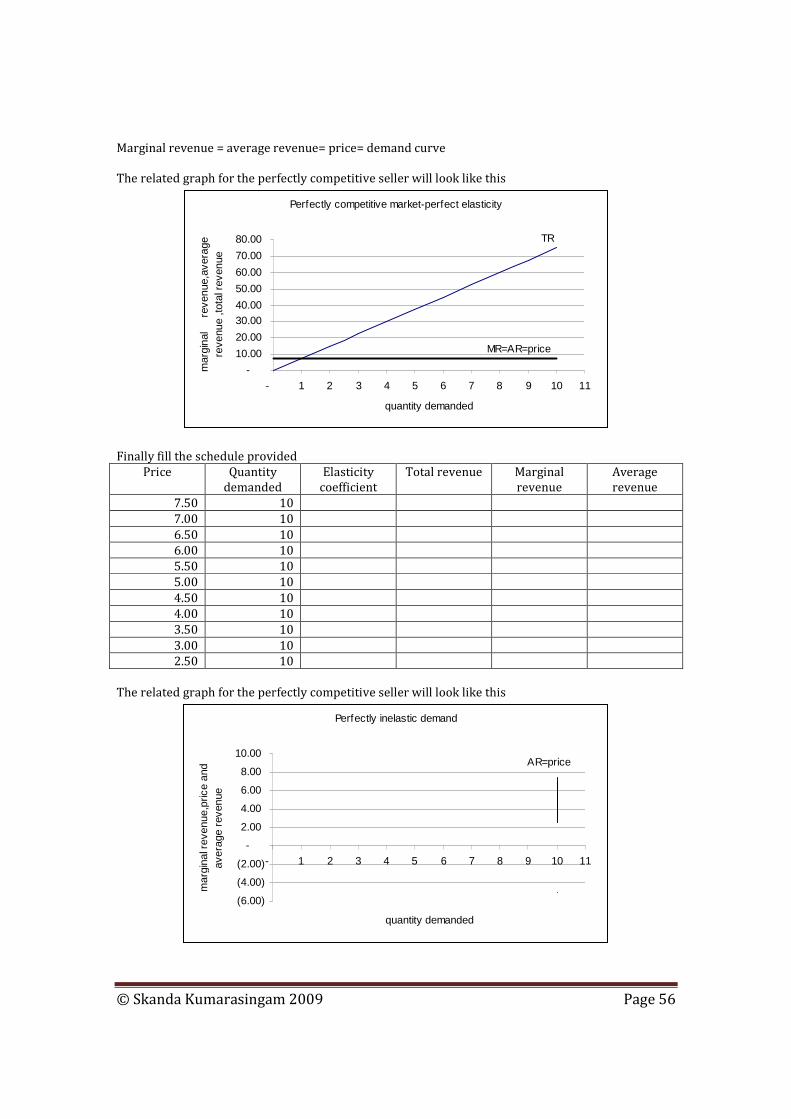
© Skanda Kumarasingam 2009 Page 56
Marginal revenue = average revenue= price= demand curve The related graph for the perfectly competitive seller will look like this
Perfectly competitive market-perfect elasticity
-
10.00
20.00
30.00
40.00
50.00
60.00
70.00
80.00
- 1 2 3 4 5 6 7 8 9 10 11
quantity demanded
mar
gina
l
reve
nue,
aver
age
reve
nue
,tota
l rev
enue
TR
MR=AR=price
Finally fill the schedule provided
Price Quantity demanded
Elasticity coefficient
Total revenue Marginal revenue
Average revenue
7.50 10
7.00 10
6.50 10
6.00 10
5.50 10
5.00 10
4.50 10
4.00 10
3.50 10
3.00 10
2.50 10
The related graph for the perfectly competitive seller will look like this
Perfectly inelastic demand
(6.00)
(4.00)
(2.00)
-
2.00
4.00
6.00
8.00
10.00
- 1 2 3 4 5 6 7 8 9 10 11
quantity demanded
mar
gina
l rev
enue
,pric
e an
d av
erag
e re
venu
e
AR=price

© Skanda Kumarasingam 2009 Page 57
This schedule may be true for inferior goods. You will note that even if the individual firm reduces its price it will not be able to increase the quantity demanded and the quantity supplied. This is called perfectly inelastic where the price elasticity of demand is always equal to zero. In this situation Price = average revenue Marginal revenue is always negative (it is a dot or speck on the graph and hence not visible). Review
Question 1 Using the method employed by economists and the following two lines from a demand schedule
Price Quantity demanded
5.50 750
4.50 850
The percentage change in price is................... and the percentage change in quantity is................. Question 2 To compute the elasticity of demand coefficient we must divide.......................... …………………………………………by................................................................ Question 3 Demand is Elastic when the coefficient is……………………………. Inelastic when the coefficient is………………………….. Unit elastic when the coefficient is………………………. Question 4 For demand to be price elastic the percentage change in quantity demanded must be................... than the percentage change in price. When the percentage change in quantity demanded is..................... than the percentage change in price, demand is price inelastic Question 5 When demand is Price elastic, total receipts........................ if price rises and ......................................if prices fall Price inelastic, total receipts...................... if price rises and ............................... if price falls. Unit elastic, total receipts......................... when price rises or falls Question 6 To review what we have learnt about the elasticity of supply let us feel the following table
When supply is The elasticity (of supply) coefficient is
When price falls total receipts
Elastic
Inelastic
Unit elastic
Question 7 For supply to be elastic, the percentage change in quantity supplied must be.................. than the percentage change in price. When supply is inelastic the percentage change in price is................................than the percentage change in quantity supplied.

© Skanda Kumarasingam 2009 Page 58
Question 8 We have examined marginal revenue from the viewpoint of the individual (perfectly/ imperfectly) competitive seller which finds that it must.......................the price charged in order to sell more of a commodity. Question 9 Marginal revenue is the amount by which....................increases when the seller sells....................more unit of a commodity. Marginal revenue is A positive amount when demand is price......................... A negative amount when demand is price...................... Zero when demand is.................... Question 10 Except for the first unit sold marginal revenue is..................... than the price at which the commodity is sold. As the firm increases its sales marginal revenue................................. Question 11 If demand is Price elastic and the firm sells an extra unit total revenue will.............................. Price inelastic and the firm sells an extra unit total revenue will....................... Unit elastic and the firm sells one extra unit total revenue will........................ Question 12 A perfectly competitive seller can sell as little or as much as it wants of a commodity at a..........................price because the demand for the commodity sold is............................................... Question 13 As a result it finds that marginal revenue is (positive/ negative/ zero) and (decreases/ constant) when sales increase and are equal to.............................. Question 14 Whenever it sells an additional unit of the commodity total revenue...............by an amount which is equal to both................................and ……………………. Answers
Suggested answers to the above questions are given. The answers are provided sequentially in the same order you will fill the blanks or select from a choice in the brackets
Question 1 20 12.50 Question 2 The percentage change in quantity demanded The percentage change in price Question 3 > 1 < 1 Equal to one
Question 4 Greater Less Question 5 Fall or decrease Rise or increase Rise or increase Fall or decrease Do not change Question 6 > 1 and falls Less than one and falls Equal to one and falls Question 7 Greater Greater

© Skanda Kumarasingam 2009 Page 59
Question 8 Imperfectly Lower (decreases) Question 9 Total receipts One Elastic Inelastic Of unit elasticity Question 10 Less Decreases Question 11 Increase Decrease Remain constant Question 12 Constant (fixed) Perfectly elastic Question 13 Positive Constant Price of the Commodity Question 14 Increases Price Marginal revenue

© Skanda Kumarasingam 2009 Page 60
Chapter 4
Cost of Production
Learning Outcomes
• To understand the meaning of economic costs which are considered opportunity costs and why they are more important than the accountant's cost to make proper decisions
• To appreciate the meaning of economic profits and learn how they are calculated and why they are more important than the accountant's profit to make proper decisions
• To appreciate different types of total costs (total fixed, total variable and mixed costs) and their relationships to one another
• To understand the idea of marginal in economics. Then to develop the idea of marginal cost and marginal product and to understand the relationship between them
• Using marginal cost and marginal product we need to develop the law of diminishing returns.
• Appreciate what average costs are and their types (average fixed, average variable and average total )and combine this understanding with all types of marginal costs and all types of total costs
• Understand how the long run cost curves are developed
• To summarize our understanding of the chapter by completing the answers to the Review questions. The review questions have been framed in such a way so that you may be able to use it as the summary of the chapter. This is the primary reason why a chapter summary has not been complied or given as it will lead to a repetition.
Chapter Outline
• Economic costs and economic profits
• Cost schedules and curves
• Marginal cost and marginal product
• law of diminishing returns
• Average costs
• Long run cost curves
• Review (chapter summary)
• Answers to Review questions

© Skanda Kumarasingam 2009 Page 61
Economic Costs and Economic Profits
In economics all costs are considered to be opportunity costs. Such opportunity costs are again divided into two which are called explicit cost and implicit costs. Explicit cost is easy to understand as it involves payment of cash to outsiders of the firm for the purchase of factors of production. This means that such payments are made to non-owners of the enterprise or the firm. Give five examples of explicit costs ………………………………………………………………………………………………………………… ………………………………………………………………………………………………………………… ………………………………………………………………………………………………………………… ………………………………………………………………………………………………………………… Implicit cost is somewhat difficult to understand. What this means is basically you will have to give up something to get something and what you give up is also a cost. Usually it is what you give up to gain something else from the current business. These are also called non expenditure costs as cash payments are not made. This is also incurred by the owners of the firm or owners of the resources who put it to start their own self employment or entrepreneurial enterprise. Example of such implicit cost could be
• Income lost (if you did not go into self-employment) by working for somebody else
• Use of your own funds to start and run the business and hence you will lose the interest that you may be earning if this money was kept in a bank savings account.
Give five examples of implicit costs ………………………………………………………… ………………………………………………………………………………………………………………… ………………………………………………………………………………………………………………… ………………………………………………………………………………………………………………… In short owner’s income must cover all costs to ensure they make normal profits to keep them content in economic terms. Such profit in economics is called economic profits and they are different to what the accountants’ profits are. The following example will explain this.
Description Accountants profit calculation(USD)
Economists profit calculation (USD)
Sales 1000 1000
Cost of goods sold (explicit ) 800 800
Gross margin 200 200
Other explicit costs 100 100
Accountants profit 100 100
Implicit costs - 50
Economic profit - (when this is above zero it is called pure or economic profit and when it is zero it
is called normal profits)50
As you may see there are two types of profits from an economic point of view. The normal profit which is often the usual profit enterprises will end up earning in the long run. Most often organizations or individuals when they get into certain industries as pioneers they will obviously be making pure or economic profits. However when others notice that somebody is making pure or economic profits they too will be motivated to shift their resources to these industries. Eventually the pioneers will have to reduce selling prices so that they can remain competitive. The reduction in selling prices will continue until the firm eventually ends up making profits which are equal to normal profits. However if this normal profit turns to be negative the enterprise would be wise to shift the resources back to a more lucrative industry or business.

© Skanda Kumarasingam 2009 Page 62
Cost Schedule and Curve
To understand the different types of costs in economics next look at the schedule below. Please remember all costs identified in this are economic costs. This means the total fixed cost (TFC) includes implicit and explicit cost. In this manner total variable cost (TVC) will also include both implicit and explicit costs. Even though this will not be stated over and over again as an economist this is an agreed consideration. Total fixed cost is defined as economic costs that cannot be increased in the short run. That is it does not vary with output. Examples of total fixed costs in the short run could be rent paid for premises, leases for motor cars, fixed rental paid on mobile bills and telephone bills and fixed salary paid to executives and managers. Total variable cost can be defined as economic costs that can be increased or decreased in the short run. That is total variable cost varies with output. Examples of total variable costs will be direct materials, direct labor paid on a piece rate basis, and direct overheads. Provide 3 more examples from a marketing or personal perspective………………………………………………………………………………………….. ………………………………………………………………………………………………………………… ………………………………………………………………………………………………………………… Total cost is made up by adding total fixed cost and total variable cost. Total cost can also be called a mixed cost because it incorporates both fixed and variable cost. You might have observed in real life that such costs are also possible. Vehicle running costs and payment of mobile bills are such examples. Can you think at least three more of them………………………………………………………………………………………………………… ………………………………………………………………………………………………………………… …………………………………………………………………………………………………………………
Total cost = total variable cost + total fixed cost
Reading the definitions provided above about TFC, TVC and TC complete this schedule
Short-Run Costs of Production Schedule
Output TFC TVC Total Costs (TC)
0
00 200
1
40
2
60
3
90
4
200 130
5
180
6
240
7
310
8
390

© Skanda Kumarasingam 2009 Page 63
The above schedule is called the short run cost of production schedule. This schedule primarily talks about the output and the total cost incurred at these various outputs. Once completed it should look like this
Short-Run Costs of Production Schedule
Output in units TFC TVC Total Costs (TC)
- 200 - 200
1 200 40 240
2 200 60 260
3 200 90 290
4 200 130 330
5 200 180 380
6 200 240 440
7 200 310 510
8 200 390 590
Using the above definitions of total fixed costs and total variable cost we can then define what short term means in economics. In economics the short term means a period of time where certain costs will remain fixed and certain costs will vary with output. Obviously the cost that will remain fixed will be the total fixed costs and those that will vary will be the total variable cost. Based on the above schedule you are now required to draw the cost curves. On the Y axis have the costs and on the X axis have total output. Draw the total cost, total variable cost, and the total fixed cost curves.
Write your observations about the curves in the space provided below……… ………………………………………………………………………………………………………………… ………………………………………………………………………………………………………………… ………………………………………………………………………………………………………………… …………………………………………………………………………………………………………………

© Skanda Kumarasingam 2009 Page 64
………………………………………………………………………………………………………………… ………………………………………………………………………………………………………………… You might have observed that the total fixed cost curve is a straight line. However the total cost and the total variable cost curves are upwards sloping. Can you determine what the reasons may be? ………………………………………………………………………………………………………………… ………………………………………………………………………………………………………………… ………………………………………………………………………………………………………………… ………………………………………………………………………………………………………………… Did your completed cost curves look like this?
Cost curves
-
100
200
300
400
500
600
700
- 1 2 3 4 5 6 7 8 9
output in units
tota
l fi
xed
cost
, tot
al v
aria
ble
cost
and
tota
l cos
t
TC
TFC
TVC
To understand the reasons we need to understand two more economic concepts which are called marginal product and marginal cost. Marginal Cost and Marginal Product
Marginal in economics means the amount of change that takes place because of a unit change in a factor that drives the change. Say for example total cost will change when the output changes. Hence marginal cost means a change in total cost because of the one unit change in the output. Write the formula for marginal cost
Similarly we can say that the number of units produced increases when inputs required to produce it are increased. So marginal product will be the change in number of units produced (output) because of one unit change in the input of a given resource.

© Skanda Kumarasingam 2009 Page 65
Write the formula for marginal product
Now in the schedule provided you are required to complete the marginal cost and the marginal product columns.
Output TFC TVC Total Costs (TC)
Marginal cost
Input Need in kg
Marginal product
- 00 200 -
1 40 0.04
2 60 0.06
3 90 0.09
4 200 130 0.13
5 180 0.18
6 240 0.24
7 310 0.31
8 390 0.39
Using the data that was derived from the above schedule you are now required to draw the marginal cost and the marginal product curves in the space provided below.
Write your observations of these curves …………………………………………………… ………………………………………………………………………………………………………………… ………………………………………………………………………………………………………………… ………………………………………………………………………………………………………………… ………………………………………………………………………………………………………………… ………………………………………………………………………………………………………………… …………………………………………………………………………………………………………………
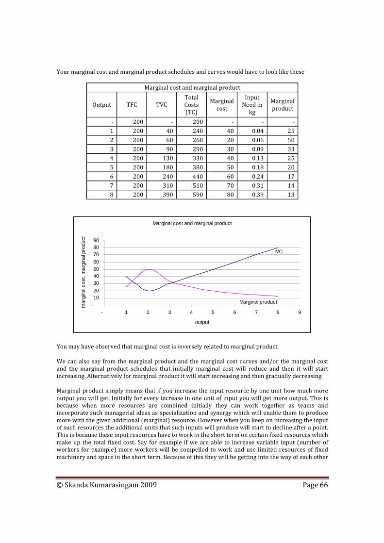
© Skanda Kumarasingam 2009 Page 66
Your marginal cost and marginal product schedules and curves would have to look like these
Marginal cost and marginal product
Output TFC TVC Total Costs (TC)
Marginal cost
Input Need in
kg
Marginal product
- 200 - 200 - - -
1 200 40 240 40 0.04 25
2 200 60 260 20 0.06 50
3 200 90 290 30 0.09 33
4 200 130 330 40 0.13 25
5 200 180 380 50 0.18 20
6 200 240 440 60 0.24 17
7 200 310 510 70 0.31 14
8 200 390 590 80 0.39 13
Marginal cost and marginal product
-1020
30405060
708090
- 1 2 3 4 5 6 7 8 9
output
mar
gina
l cos
t, m
argi
nal p
rodu
ct
MC
Marginal product
You may have observed that marginal cost is inversely related to marginal product. We can also say from the marginal product and the marginal cost curves and/or the marginal cost and the marginal product schedules that initially marginal cost will reduce and then it will start increasing. Alternatively for marginal product it will start increasing and then gradually decreasing. Marginal product simply means that if you increase the input resource by one unit how much more output you will get. Initially for every increase in one unit of input you will get more output. This is because when more resources are combined initially they can work together as teams and incorporate such managerial ideas as specialization and synergy which will enable them to produce more with the given additional (marginal) resource. However when you keep on increasing the input of such resources the additional units that such inputs will produce will start to decline after a point. This is because these input resources have to work in the short term on certain fixed resources which make up the total fixed cost. Say for example if we are able to increase variable input (number of workers for example) more workers will be compelled to work and use limited resources of fixed machinery and space in the short term. Because of this they will be getting into the way of each other
© Skanda Kumarasingam 2009 Page 67
or will have to wait until certain machinery become free to do their work. As the numbers increase their work will obviously slowdown. If you understand how marginal product will increase and eventually decrease because the additional input resource will have to work on limited fixed resources in the short term you can now intuitively explain how marginal cost will tend to reduce and increase subsequently. Marginal cost is the additional cost incurred to produce one more unit. When the input resources are very efficient (increasing marginal product) at the beginning the marginal cost (of producing the next unit) should obviously come down. And as the input resources eventually become very inefficient since they will have to work on limited fixed resources in the short term to produce the next unit we will have to include more inputs which will thus increase the marginal cost as output increases. Now you should be able to identify that the marginal cost can also be found from the slope of the total cost and the total variable cost. The slope on any curve is found by its rise over run(X axis change / Y axis change). At any given point this slope will indicate the marginal cost. Please remember that the marginal cost will not remain constant at all the points in the graph and it will be different at various output levels. This is obvious if you really look at the schedule. Looking at the curve you will observe that initially total cost and total variable cost slopes are somewhat less steep. This is when marginal cost is low and reducing. After a point the slope will become steeper and continue to become much steeper as the output increases. This is the reason for the total cost and total variable cost curves to curve upwards. These curve upwards simply because marginal cost keeps increasing as output increases. Law of Diminishing Returns
This can be explained by understanding what marginal product means. Marginal product can also mean how much additional output an increase in variable resources (input) can produce in the short run. It was also observed that it will increase and then decrease as the variable resource needs to work on fixed facilities in the short term. This is called the law of diminishing returns and this affects all firms in the short term. Average Costs
• Average fixed costs is calculated as total fixed cost/total output
• Average variable cost is calculated as total variable cost/total output
• Average total cost is calculated as total cost/total output
• Average total cost is the summation of average fixed cost plus average variable cost. How do you calculate the average age of the class...........................................................................................? How do you calculate your average salary for last year…...............................................................................?

© Skanda Kumarasingam 2009 Page 68
Using the above definitions complete the schedule.
Output TFC TVC Total Costs (TC)
Marginal cost
Input Need
Marginal product
Average fixed cost
Average variable
cost
Average total cost
0 00 200
1 40 0.04
2 60 0.06
3 90 0.09
4 200 130 0.13
5 180 0.18
6 240 0.24
7 310 0.31
8 390 0.39
Once the schedule is completed in the space provided draw a graph which will only incorporate marginal cost, average total cost, average variable cost and average fixed cost.

© Skanda Kumarasingam 2009 Page 69
Your completed schedule and average cost curves (with marginal cost incorporated) should look like this
Types of costs in economics
Output TFC TVC Total Costs (TC)
Marginal cost
Input Need
Marginal product
Average fixed cost
Average variable
cost
Average total cost
- 200 - 200 - - - - -
1 200 40 240 40 0.04 25 200 40 240
2 200 60 260 20 0.06 50 100 30 130
3 200 90 290 30 0.09 33 67 30 97
4 200 130 330 40 0.13 25 50 33 83
5 200 180 380 50 0.18 20 40 36 76
6 200 240 440 60 0.24 17 33 40 73
7 200 310 510 70 0.31 14 29 44 73
8 200 390 590 80 0.39 13 25 49 74
Cost curves
-102030405060708090
100110120130140150160170180190200210220230240250260
- 1 2 3 4 5 6 7 8 9
output
aver
age
tota
l cos
t,ave
rage
var
iabl
e co
st,a
vera
ge fi
xed
cost
an
d m
argi
nal c
ost
ATC
AFC
AVC
MC
Observations on the graph Marginal cost curve is below the average variable cost and the average total cost curves when they are decreasing

© Skanda Kumarasingam 2009 Page 70
Marginal cost curve is above the average variable cost and the average total cost curves when they are increasing The distance between the average total cost and the average variable cost at any given output level will be equal to the average fixed cost at that particular output level. This is simply because average fixed cost plus average variable cost is equal to average total cost. The marginal cost curve intersects with average total cost and the average variable cost curves at their lowest points. Marginal cost intersects with the average total cost at a higher output level than the output level at average variable cost. At the points of intersection marginal cost = average variable cost and marginal cost = average total cost Average fixed cost will keep reducing as the output increases but it will never reach zero. It will only reach zero at infinity. Explain the relationship between Marginal costs and average variable and average total cost by the following example You have played 250 cricket matches and your batting average per innings is 30. How will it change if the scores in the next few innings increase or decrease………………………………………………………....... …………………………………………………………………………………………………………………………………………………………………………………………………………………………………… Long Run Cost Curves
In the short run all economic costs can be divided into fixed and variable. However in the long run all costs are variable. In fact this is the way long term is defined. The long run cost schedule is developed from the short-term cost schedules as explained. Using the explanation provided below complete the schedule
Short run cost of production schedules
Average total costs in the short term Output
Plant 1 Plant 2 Plant 3
Long run average total
cost
Plant used
100 3.00 4.00 7.00
200 2.00 3.00 6.00
300 1.50 2.00 5.00
400 2.00 1.00 4.00
500 3.00 0.50 3.00
600 4.00 0.75 2.00
700 5.00 2.00 1.00
800 6.00 3.00 2.00
900 7.00 4.00 3.00
1000 8.00 5.00 4.00
According to the schedule you will note that for certain output levels certain plants have the least average total cost in the short term. So if a person wants to produce hundred units of output she should select plant1 and another person who wants to produce 400 units should select plant2. If a

© Skanda Kumarasingam 2009 Page 71
producer is interested at an output level of 800 she should then select plant3. As it was stated in the long run all costs are variable and so the producer can select between plants unlike in the short term. You may have observed that the long run average total cost is built up from the short run average total cost of producing a given quantity. You may have also observed that the long run average total cost could have two columns. They are output vs. the long run average total cost. The completed chart of the long run costs is given below
Short run cost of production schedules
Average total costs in the short term
Output
Plant 1 Plant 2 Plant 3
Long run
average total cost
Plant used
100 3.00 4.00 7.00 3.00 1
200 2.00 3.00 6.00 2.00 1
300 1.50 2.00 5.00 1.50 1
400 2.00 1.00 4.00 1.00 2
500 3.00 0.50 3.00 0.50 2
600 4.00 0.75 2.00 0.75 2
700 5.00 2.00 1.00 1.00 3
800 6.00 3.00 2.00 2.00 3
900 7.00 4.00 3.00 3.00 3
1,000 8.00 5.00 4.00 4.00 3
You are now required to draw the long run average total cost curves based on the data provided in the above schedule.

© Skanda Kumarasingam 2009 Page 72
Initially the long run average total cost will keep reducing. This is called increasing economies of scale. Then the curve reaches the minimum point and then it starts increasing. This is when diseconomies of scale set in. The reason for diseconomies of scale to set in is not because variable resources will have to work on fixed resources like in the short term. In the long run as all costs are variable this explanation is not possible and accurate. I believe in the long run for diseconomies of scale to set in would be because more resources will have to be brought in which are incapable of producing the given product and are specialized in the production of something else. Also operating resources which may then become scarcer will be costly and time-consuming to extract such as the cost of obtaining petroleum. Its costs have increased as man has to draw it out of more difficult locations now. The completed long run cost curve is given. Check your own graph with this
Long run cost curve
-1.002.003.004.005.006.007.008.009.00
- 200 400 600 800 1,000 1,200
output
shor
t run
ave
rage
cos
ts o
f pla
nt
1,2
and
3 an
d lo
ng r
un c
ost
curv
e
SR-AC of plant 1
SR-AC of plant 2
SR-AC of plant 3
LR-AC
For purposes of practice complete the schedule below and draw all the related curves and explain them in detail.
Output TFC TVC Total Costs (TC)
Marginal cost
Input Need
Marginal product
Average fixed cost
Average variable cost
Average total cost
000 00 400 -
100 500 0.05
200 900 0.09
300 1500 0.15
400 2400 0.24
500 3500 0.35
600 4800 0.48
700 6300 0.63
800 8000 0.80

© Skanda Kumarasingam 2009 Page 73
The completed chart is provided at the end of the review with the related graphs
Review (Once complete you can use this as the chapter summary or round-up) Question 1 All costs in economics include both..................... and ..........................for both are............................... costs. Question 2 That the total variable cost and total cost curves are not straight lines is fairly obvious. The short run is defined as any………………... of time in which some of the firm's resources are........................... and some are....................... As a result in the short run some costs are....................................... costs and the rest are....................................... Question 3 A firm’s total variable cost + total fixed cost are equal to its......................... costs. As output decreases there will be a decrease in................................................. and no change in..................................... as output increases will all three increase? ...................................... Question 4 A cost schedule indicates the cost of producing at different levels of.............................................. Question 5 In graphing cost schedules we plot...............................on the horizontal axis and................................ on the vertical axis Question 6 In constructing a graph of marginal cost we use the horizontal axis to plot........................- just as we did when we graphed total costs. On the vertical axis we plot...................................................... Question 7 Marginal cost is the amount by which.......................................... increases when the firm increases its ........................................by............................................. Question 8 As any firm expands its production in the short run it finds that marginal cost at the first ....................................... and thereafter............................................... The marginal cost curve at first slopes.............................and thereafter slopes............................................... Question 9 Marginal cost is defined as………………………………………………………………………… ………………………………………………………………………………………………………………… ………………………………………………………………………………………………………………… ………………………………………………………………………………………………………………… ………………………………………………………………………………………………………………… Question 10 Marginal product is defined as…………………………………………………………………… ………………………………………………………………………………………………………………… ………………………………………………………………………………………………………………… ………………………………………………………………………………………………………………… …………………………………………………………………………………………………………………

© Skanda Kumarasingam 2009 Page 74
Question 11 State the law of diminishing returns…………………………………………………………… ………………………………………………………………………………………………………………… ………………………………………………………………………………………………………………… ………………………………………………………………………………………………………………… ………………………………………………………………………………………………………………… Question 12 As the firm's output increases marginal product will………………………………… ………………………………………………………………………………………………………………… ………………………………………………………………………………………………………………… ………………………………………………………………………………………………………………… ………………………………………………………………………………………………………………… Marginal cost will therefore……………………………………………………………………… ………………………………………………………………………………………………………………… ………………………………………………………………………………………………………………… ………………………………………………………………………………………………………………… ………………………………………………………………………………………………………………… As a result total variable cost and total cost will………………………………………… ………………………………………………………………………………………………………………… ………………………………………………………………………………………………………………… ………………………………………………………………………………………………………………… ………………………………………………………………………………………………………………… Question 13 In your words explain how you compute or determine Average fixed cost…………………………………………………………………………………………….. Average variable cost……………………………………………………………………………………….. Average total cost……………………………………………………………………………………………... Question 14 As a firm increases its output in the short run what happens to Average fixed cost…………………………………………………………………………………………….. Average available cost……………………………………………………………………………………… Average total cost……………………………………………………………………………………………... Question 15 In your words Why does average fixed cost always decrease when the firm increases its output? ………………………………………………………………………………………………………………… ………………………………………………………………………………………………………………… ………………………………………………………………………………………………………………… ………………………………………………………………………………………………………………… Why does average variable cost at first decrees and then increase? …………… ………………………………………………………………………………………………………………… ………………………………………………………………………………………………………………… ………………………………………………………………………………………………………………… ………………………………………………………………………………………………………………… Question 16 In the short run some of a firm's costs are fixed and average fixed cost decreases as the firm expand its output. As a result average variable cost will start to increase (before/ after) average total cost starts to increase and the output at which average total cost is a minimum is (greater/ less) than the output at which average variable cost is a minimum
© Skanda Kumarasingam 2009 Page 75
Question 17 In the long run all costs are.............................because all resources are........................................ The long run average cost of producing a certain amount of a product is equal to the............................... short run cost of producing that quantity of the product. As the firm expands its production in the long run average cost will at first.............................because of the...................... of scale. Thereafter average cost will.............................due to the...................................of scale.

© Skanda Kumarasingam 2009 Page 76
Answers
Suggested answers to the above questions are given. The answers are provided sequentially in the same order you will fill the blanks or select from a choice in the brackets
Question 1 Explicit Implicit Opportunity Question 2 Variable Fixed Variable Fixed Question 3 Total Total variable cost and total cost Total fixed cost No Question 4 Output or production Question 5 Output or production Cost Question 6 Output or production Marginal cost Question 7 Total variable cost or total cost Output or production One additional unit Question 8 Decreases Increases Downward Upward Question 9 The amount by which total variable cost or total cost increases when the firm increases its output by one unit
Question 10 The amount by which total output increases when the firm increases the employment of a variable input by one unit Question 11 As the firm increases its employment of available input the marginal product of that input will at first increase and then decrease Question 12 At first increases and then decrease At first decreases and then increase At first increase by amounts that become smaller and then increase by amounts that become larger Question 13 Total fixed cost/ output Total variable cost/ output Total cost/ output or add average fixed cost and the average variable cost Question 14 Decrease Decreases and then increases Decreases and then increases Question 15 Total fixed cost is being divided by larger and larger outputs Marginal cost at first is less than average variable cost causing the average variable cost to fall. As marginal cost increases it becomes > average variable cost causing the average variable cost to increase Question 16 Before Greater Question 17 Variable Variable Minimum Decrease Economies Increase Diseconomies

© Skanda Kumarasingam 2009 Page 77
Output TFC TVC Total Costs (TC)
Marginal cost
Input Need in
kg
Marginal product
Average fixed cost
Average variable
cost
Average total cost
- 400 - 400 - - - - -
100 400 500 900 5 0.05 20.00 4 5 9
200 400 900 1,300 4 0.09 25.00 2 5 7
300 400 1,500 1,900 6 0.15 16.67 1 5 6
400 400 2,400 2,800 9 0.24 11.11 1 6 7
500 400 3,500 3,900 11 0.35 9.09 1 7 8
600 400 4,800 5,200 13 0.48 7.69 1 8 9
700 400 6,300 6,700 15 0.63 6.67 1 9 10
800 400 8,000 8,400 17 0.80 5.88 1 10 11
Marginal cost and marginal product curves
-
5
10
15
20
25
30
- 100 200 300 400 500 600 700 800 900
output
mar
gina
l cos
t and
mar
gina
l pr
oduc
t MC
MP
Average and marginal costs
-
2
4
6
8
10
12
14
16
18
- 100 200 300 400 500 600 700 800 900
output
aver
age
varia
ble
cost
,ave
rage
fixe
d co
st,
aver
age
tota
l cos
t and
mar
gina
l cos
t
MC
AFC
ATC AVC

© Skanda Kumarasingam 2009 Page 78
Chapter 5
Product Price and Output in Pure Competition
Learning Outcomes
• To comprehend the important features of perfect competition and firms operating in a perfectly competitive environment
• Develop the major assumptions made and give their rationale when studying markets
• To understand short-run costs related to production in a perfectly competitive market. To appreciate the relationships that are involved in various types of revenues( total, average and marginal) and different types of costs such as total, average and marginal
• Understand the difference between the industry demand curve and the firm's demand curve
• Using the cost curves that will be developed build up the firm's supply curve. Appreciate the fact that the marginal cost curve is equal to the supply curve of the firm
• Understand how the market equilibrium is arrived at in a perfectly competitive market and the relationship of the market equilibrium price to the firm's price as a price taker
• Appreciate the differences with the short-run cost of production and the concepts behind long run cost of production
• To summarize our understanding of the chapter by completing the answers to the Review questions. The review questions have been framed in such a way so that you may be able to use it as the summary of the chapter. This is the primary reason why a chapter summary has not been complied or given as it will lead to a repetition.
Chapter Outline
• Features of perfect competition and assumptions
• Short run cost of production
• The firm’s supply curve
• Long run cost of production
• Review (or chapter summary)
• Answers to Review questions

© Skanda Kumarasingam 2009 Page 79
Features of Pure Competition and Assumptions
A supplier or producer of goods and services is interested in making the highest profit possible. However profit depends on the price you get for the product in the market and the total quantity that can be produced and sold. We should also note that price and total quantity produced depends on the cost of production, demand for the product or service in the market, the industry in which the supplier operates and whether it operates in a competitive environment or is it a monopolist and finally whether we are considering the short run or the long run to evaluate profits. In this chapter we will be looking at competitive industries and how firms in such industries try to maximize profits. Competitive environments or businesses have the following features
• There are a large number of small firms
• These firms are so small that they cannot affect the prices in the market. That is they accept the market equilibrium price and are called price takers. Price takers cannot affect prices in the market but can only change the quantity they produce. If they increase the price the buyers will buy elsewhere. However if they reduce the price they can sell all they want (have produced) but will make lesser profits. So to maximize profits or reduce losses such firms are advised to sell at the markets established or equilibrium price.
• All firms produce an identical product in the industry
• In the long term there are no barriers to entry. We have defined long run as when all economic costs are variable and there is nothing called a fixed cost. We can also give another definition of long term as a period of time when the number of firms in the industry can increase or decrease. In the short term there are barriers to entry.
• There is perfect information in the market and so the buyers will not pay a higher price to purchase a product from a particular supplier.
• Firms in these industries do not make an economic profit and so the best they can hope for is to make normal profits.
• The competitive firms marginal cost is equal to the price of the product in the market which is in turn equal to the marginal revenue.
When we are in the process of studying product prices and outputs we need to make certain general assumptions.
• Whether it is a competitive market or monopolistic market every firm intends to make the highest profit possible or to reduce their losses
• Cost of production of the firm does not vary whether the firm operates in a competitive environment or whether they are a monopolist
• Buyers in the market are numerous and very large. So no one buyer can influence the price or the output.
Short Run Costs of Production
Using your understanding of what was studied before and also by looking carefully at the second row of the schedule provided in the next page complete it. Once this is done please check your answers with the answer provided in the page after it.

© Skanda Kumarasingam 2009 Page 80
Short Run Cost of Production Schedule for a Firm in a Competitive Industry Output Total
fixed cost
Total variable cost
Total cost
Marginal cost
Average fixed cost
Average variable cost
Average total cost
Total revenue P= 250
Marginal revenue
Average revenue
Economic profit or loss
Total revenue P= 180
Economic profit or loss
Total revenue P= 140
Economic profit or loss
Total revenue P= 233
Economic profit or loss
Q Remains constant
Varies with activity
TFC+ TVC
Δ TC Δ TQ
TFC TQ
TVC TQ
TC TQ
P X Q Δ TR Δ TQ
TR TQ
TR-TC or (AR-AC) Q
0 200 000
1 200 175
2 200 300
3 200 500
4 200 800
5 200 1200
6 200 1700
7 200 2300

© Skanda Kumarasingam 2009 Page 81
Completed schedule will look like this.
Output Total fixed cost
Total variable
cost
Total cost
Marginal cost
Average fixed cost
Average variable
cost
Average total cost
Total revenue P= 250
Marginal revenue
Average revenue
Economic profit or
loss
Total revenue P= 180
Economic profit or
loss
Total revenue P= 140
Economic profit or
loss
Total revenue P=
233
Economic profit or loss
Δ TC TFC TVC TC Δ TR TR Q
Remains constant
Varies with
activity
TFC+ TVC Δ TQ TQ TQ TQ
P X Q Δ TQ TQ
TR-TC or (AR-AC) Q
P X Q
- 200 - 200 - - - - - - - (200) - (200) - (200) - (200)
1 200 175 375 175 200.00 175 375 250 250 250 (125) 180 (195) 140 (235) 233 (142)
2 200 300 500 125 100.00 150 250 500 250 250 - 360 (140) 280 (220) 466 (34)
3 200 500 700 200 66.67 167 233 750 250 250 50 540 (160) 420 (280) 699 (1)
4 200 800 1,000 300 50.00 200 250 1,000 250 250 - 720 (280) 560 (440) 932 (68)
5 200 1,200 1,400 400 40.00 240 280 1,250 250 250 (150) 900 (500) 700 (700) 1,165 (235)
6 200 1,700 1,900 500 33.33 283 317 1,500 250 250 (400) 1,080 (820) 840 (1,060) 1,398 (502)
7 200 2,300 2,500 600 28.57 329 357 1,750 250 250 (750) 1,260 (1,240) 980 (1,520) 1,631 (869)
Keep reviewing this sheet (schedule) as you go through the observations.

© Skanda Kumarasingam 2009 Page 82
Observations from the Above Schedule
• Total cost is equal to total variable cost + total fixed cost.
Cost curves
-
500
1,000
1,500
2,000
2,500
3,000
- 1 2 3 4 5 6 7 8
quantity
tota
l fix
ed c
ost,
tota
l var
iabl
e co
st,to
tal c
ost
TFC
TCTVC
• When total revenue is greater than total cost you will make a profit. Where total-revenue is equal
to total cost it is called the break-even situation. When total revenue is less than total cost it is a loss situation
Break even chart
(1,000)
(800)
(600)
(400)
(200)
-
200
400
600
800
1,000
1,200
1,400
1,600
1,800
2,000
2,200
2,400
2,600
2,800
- 1 2 3 4 5 6 7 8
quantity
tota
l cos
t,tot
al r
even
ue,e
cono
mic
pro
fit
TC
TR
Economic prof it
maximum economic prof it of 50
• In the above graph there are two break even points (where economic profit is equal to zero). Identify the points and mark them on the graph and write the reason for it in the space ……………………………………………………………………………………………………………………………………………………………………………………………………………………………………………………………………………………………………

© Skanda Kumarasingam 2009 Page 83
……………………………………………………………………………………………………………………………………………………………………………………………………………………………………………………………………………………………………
• Marginal cost is at its minimum at125. Marginal cost reduces as output increases up to a point and then increases thereafter as the output increases.
Marginal cost
-
100
200
300
400
500
600
700
- 1 2 3 4 5 6 7 8
quantity
mar
gina
l cos
t
• Average variable cost is at its lowest at two units of output and it is equal to 150.
• Average total cost is at its minimum when the output is three units and is equal to 233
Average Costs
-
50.00
100.00
150.00
200.00
250.00
300.00
350.00
400.00
- 1 2 3 4 5 6 7 8
quantity
aver
age
fixed
cos
t,ave
rage
va
riabl
e co
st a
nd a
vera
ge to
tal
cost
ATC
AVC
AFC

© Skanda Kumarasingam 2009 Page 84
• Marginal cost curve intersects the average variable cost and average total costs at its lowest points
Marginal and average cost curves
-
100
200
300
400
500
600
700
- 1 2 3 4 5 6 7 8
quantity
mar
gina
l cos
t,ave
rage
tota
l cos
t an
d av
erag
e va
riabl
e co
st MC
ATC
AVC
• Marginal revenue is equal to average revenue and that is equal to the price of the product. This is only true when the firm operates in a competitive industry. If a schedule is prepared using output and price which is = average revenue which is also = marginal revenue this will become the firms demand curve. If this schedule is drawn on a graph where output is given in the X axis and market price (which is equal to the firms price as it is a price taker and is a constant) in the Y axis this will form the firms demand curve. This demand curve is horizontal to the X axis. Such a demand curve is called a perfectly elastic demand curve.
Revenue curves
-
500
1,000
1,500
2,000
- 1 2 3 4 5 6 7 8
quantity
tota
l rev
enue
,mar
gina
l rev
enue
an
d av
erag
e re
venu
e
TR
AR=MR=price
• When the market price is equal to 250 the highest economic profit is equal to 50 and earned when the output is 3 units. It can also be observed that as long as the marginal revenue is more than the marginal cost the economic loss is reduced or profits increased. However when marginal cost is higher than the marginal revenue the firm will start making economic losses. Hence the advice would be to keep on producing as long as the marginal revenue is > marginal cost. In this manner the firm will be able to reduce its economic loss or to increase its profit.

© Skanda Kumarasingam 2009 Page 85
Marginal revenue and marginal cost
(1,000)
(800)
(600)
(400)
(200)
-
200
400
600
800
- 1 2 3 4 5 6 7 8 9
quantity
mar
gina
l rev
enue
,mar
gina
l cos
t an
d ec
onom
ic p
rofit
MC
MR
Economic profit
• We can also observe when the price is equal 250 the highest economic profit is earned when the average total cost is at its lowest which is equal to 233. This leads us to another interesting observation about the competitive industry. There is economic profit when the price is above the minimum average total cost and the maximum economic profit is derived where the average total cost is at its minimum of 233. You will make economic losses when the price is below the average total cost. When the price is equal to the minimum average total cost it is a break even situation ( no profit –no loss )
Profit maximization output w hen price >ATC
(900)
(800)
(700)
(600)
(500)
(400)
(300)
(200)
(100)
-
100
200
300
400
500
600
700
- 1 2 3 4 5 6 7 8 9
quantity
mar
gina
l rev
enue
,eco
nom
ic
pro
fit,m
argi
nal c
ost,a
vera
ge
varia
ble
cost
and
ave
rage
tota
l cos
t
MC
ATC
MR=ARAVC
Economic profit

© Skanda Kumarasingam 2009 Page 86
• When the market price is equal to 180 the firm will never make an economic profit. As stated earlier the market price which is equal to the marginal revenue is always below marginal cost. Hence where marginal cost is greater than marginal revenue no profits can be made. However close examination of the economic profit column will indicate that as long or as the firm produces up to 2 units the economic loss is reduced. Hence this firm is advised to produce up to 2 units rather than shutting it down. Shutting the factory or the firm down will incur an economic loss of 200. However if the firm or the factory is kept open and it produces up to 2 units its economic loss will reduce to 140 compared to an economic loss of 200. You may wonder why this will happen. In such cases we will have to see what happens to the average variable cost. The average variable cost is at its lowest at 150. In a case where the firm always makes economic losses because marginal cost is greater than marginal revenue it should still continue to produce as long as it's price is > the average variable cost. The extra revenue which is called the contribution (price minus variable cost) will help the firm to reduce the economic loss which it will suffer if was kept closed. If the firm is kept closed the loss incurred will be equal to the total fixed cost ( in this case 200)
Economic profit /loss analysis w hen price is greater than minimum average variable cost but low er than the minimum average total cost
-1400
-1300
-1200
-1100
-1000
-900
-800
-700
-600
-500
-400
-300
-200
-100
0
100
200
300
400
500
600
700
(1) - 1 2 3 4 5 6 7 8 9
quantity
mar
gina
l rev
enue
,eco
nom
ic p
rofit
,mar
gina
l cos
t,ave
rage
va
riabl
e co
st a
nd a
vera
ge to
tal c
ost
economic profit
MC
MR
ATC
AVC
• At a price of 140 the firm will never make an economic profit. You will also observe that the
market price is less than the average total cost and hence there is no way in which this firm will ever make an economic profit or a normal profit. You will also observe that the market price is always lower than the average variable cost. When the market price is below the average variable cost the firm is advised to shut down the factory. This is because when the factory shuts down the maximum loss that can be incurred is equal to the total fixed cost of 200. As long as this firm produces outputs the losses will be greater than the total fixed costs of 200 which is incurred when it is kept shut.

© Skanda Kumarasingam 2009 Page 87
Economic profit analysis w hen price(140)is below minimum average variable cost
-1500
-1400
-1300
-1200
-1100
-1000-900
-800
-700
-600
-500
-400
-300
-200
-100
0
100
200300
400
500
600
700
800
- 1 2 3 4 5 6 7 8
quantity
mar
gina
l rev
enue
,eco
nom
ic p
rofit
,mar
gina
l cos
t,ave
rage
var
iabl
e co
st a
nd a
vera
ge to
tal c
ost
economic profit
MC
ATC
AR=140AVC
• In this schedule total fixed cost, total variable cost and total cost are all economic costs and not
the accountants cost. You may remember from your previous studies in economics (previous chapters) that economic cost is opportunity cost which in turn embeds implicit and explicit costs.
• One of the most important things that you will learn in this schedule is that the revenue that is earned by selling each and every unit is constant. However we know from previous studies about the demand schedules and /or demand curves that we need to reduce prices if we are interested in selling more units.
• When we are studying firms in competitive industries we need to remember that there are two types of demand curves or schedules. There is one demand curve or schedule for the whole market or industry and there is one more for the individual firm. The total demand curve for the whole market or industry is a downward sloping demand curve as we have studied. That is in a competitive market if all firms are interested to sell a higher quantity the prices will have to come down.
• However the demand curve for the individual firm is different. It is a perfectly elastic demand curve. A perfectly elastic demand is one that is parallel to the X axis in the graph. This means that the individual firm can sell any number of units at a given fixed price. This is because for the individual firm in a competitive industry the price is established by the market. This price is established by the market demand and market supply curves and found at the equilibrium point. However once the market equilibrium point is decided this will give the market price for the product at a particular time and the total quantity that will be demanded in this market. Each

© Skanda Kumarasingam 2009 Page 88
and every individual firm is so small that it cannot influence the price by increasing its output. This means at a given price the individual firm which is very small and its output being very insignificant in this market can produce whatever they want and sell all of it at the market equilibrium price. This is the reason why the demand curve for the individual firm is horizontal to the X axis in a graph.
• Thus it can be concluded that the law of demand is not violated. This means the law of demand is relevant in the market to establish the market demand (quantity demanded) and the market equilibrium price. Once this price has been decided this price will remain constant at whatever quantity the individual firm operating in the competitive industry decides to produce and sell. Hence the two types of demand curves that we come across when we are studying competitive industries are one for the markets and one for the individual (and insignificant in terms of output) firm.
• From the above schedule we can see the highest profit the individual firm can make is 50 at a price of 250. The quantity or output is equal to three units. However a closer look will tell you that this point is not equal to the highest revenue generating point. You should always remember that firms are not interested to maximize revenue but rather to maximize profits. Hence the highest revenue generating quantity will not always give you the highest or the profit maximizing quantity.
The Firms Supply Curve
Using the schedule and/or graphs with the observations outlined above we can develop the following schedule for the individual firm in a competitive environment
Price Quantity produced to maximize economic profit or reduce economic losses
140 0
180 2
233 3
250 3
300 4
400 5
500 6
600 7
This schedule shows us the price versus the quantity produced by an individual firm in the competitive industry or environment. These quantities that are produced are where marginal cost = marginal revenue (visually check it on the graphs again) and situations where either economic profits are maximized for economic losses reduced. A careful look will tell you that this individual firm will be able to produce the given quantities at those given prices as it is in the best interest of this firm. A schedule which gives price versus quantity produced in a given period is often called the supply schedule. Hence the marginal cost schedule or curve of the firm is identical to the supply schedule or curve of the individual firm.
Marginal cost curve = firms supply curve
In this manner the supply schedules for all firms in the industry can be added together. This will give us the industry's supply schedule or curve. Let us say that there are 1000 firms with the same cost

© Skanda Kumarasingam 2009 Page 89
structure in this industry. Using this assumption we will now be able to develop the supply schedule for the industry which is given.
Price Quantity produced by all firms in the market
140 0
180 2000
233 3000
250 3000
300 4000
400 5000
500 6000
600 7000
Market Equilibrium
We can now include the market supply schedule or curve with the market demand schedule or curve which may look like this
Quantity demanded
Price Quantity supplied
8000 140 0
7500 180 2000
7000 233 3000
6500 250 3000
6000 300 4000
5000 400 5000
4000 500 6000
3000 600 7000
At a price of 400 the quantity supplied and quantity demanded are equal and this is called the equilibrium point. This price will be called the equilibrium price and it is the price takers price in the competitive industry. Draw the market demand and supply curves and indicate the equilibrium point and equilibrium quantity and equilibrium price. Next to this graph draw the firms demand curve.

© Skanda Kumarasingam 2009 Page 90
This is the way the above graph should look
Market demand and market supply
-
100
200
300
400
500
600
700
- 1,000 2,000 3,000 4,000 5,000 6,000 7,000 8,000 9,000
quantity
pric
e
market demand market supply
Long Run
In the long run the following assumptions can be made
• All costs are variable. Hence total variable cost ( no fixed costs as fixed costs in the short-term also become variable) is equal to the total cost.
• We can also form another definition of short-term and long term. The short-term is a period of time during which the number of firms does not change in a competitive industry. Hence the definition for long -term can be stated as a period of time during which the number of firms can change in a competitive industry.
• In the long run firms will enter the industry when they can make economic profits. This is possible when the price which is always equal to marginal revenue is > average total cost.
• In the long run firms will leave the industry when they make an economic loss. This happens when price which is always equal to marginal revenue is < average total cost.
• However when price which is always equal to marginal revenue is equal to the average total cost you will make zero economic profits which is also called normal profits.
Now let the supply increase as shown in the final two columns of the schedule
Quantity demanded
Price Quantity supplied –original data
Quantity supplied- increases at various price point (S2)
Quantity supplied- increases at various price point (S3)
8000 140 0 0 0
7500 180 2000 3000 4000
7000 233 3000 4000 5000
6500 250 3000 4000 6500
6000 300 4000 6000 6900
5000 400 5000 6000 7300
4000 500 6000 7000 8000
3000 600 7000 8000 9000

© Skanda Kumarasingam 2009 Page 91
Change in market supply
-
100
200
300
400
500
600
700
- 1,000 2,000 3,000 4,000 5,000 6,000 7,000 8,000 9,000 10,000
quantity
pric
e
market demandmarket supply S2 S3
On the same graph show the increases in supply as increased in the final two columns. Show the new equilibrium points on the graph. Next to this graph juxtaposition the firms graph showing the MC, ATC and various demand curves (the price = MR=AR curves). Show in the graph how profit per unit will be calculated at the original and new equilibrium prices. Show the ranges where economic profits are made, where you need to produce to reduce economic losses and where you should not produce but shut the factory down to keep the economic loss at a minimum (equivalent to the total fixed cost.)
Review (Once complete you can use this as the chapter summary or round-up) Question 1 In a purely competitive industry the price of the product and the marginal revenue from the sale of each additional units are.......................................... and the demand for the product produced by each firm is....................................................................................................... Question 2 To maximize its total economic profits or minimize its total economic losses a firm will produce all units of its product which have a..................................... > or equal to their.........................................provided the price of the product is > or equal to..........................................

© Skanda Kumarasingam 2009 Page 92
Question 3 If the price of the product in the short run is > Minimum average total cost the firm will produce at a.................................................. > Minimum average variable cost and less than minimum average total cost the firm will produce an economic......................................... Less than minimum average variable cost the firm will................................and its total loss will be equal to its............................................... Question 4 The purely competitive firm’s short run supply schedule is its ...................................schedule above the minimum.................................. Product prices must............................................to induce the firm to supply a greater quantity of its product because the marginal cost of producing the product......................... Question 5 Demand and supply determine the equilibrium price and equilibrium quantity in a purely competitive industry. In the short run the supply schedule for the industry is found by............................ the........................ schedules of all firms in the industry. The equilibrium price of the product is the price at which the total quantity supplied by all firms is...............................to the total quantity........................................ The equilibrium quantity is the total quantity demanded and supplied at the equilibrium..................................... Question 6 The equilibrium price is also equal to the........................ the individual firm can obtain from the sale of one additional unit of its product. So the firm will produce so long as................................has not become > the product price Question 7 In the short run the firms in an industry will earn an economist profit if the product price is....................................and the will suffer an economic loss if it is ......................... than................................ In no case however with the firm's loss exceed it’s............................ Question 8 In the long run the entire firms’s.......................and ...............................are variable. Also firms are able to......................................and to...............................a purely competitive industry Question 9 Firms will enter an industry when............................................................................... and they will leave an industry when.................................................................................................. Question 10 The entry of new firms into an industry causes the supply of the product to.........................................., the price of the product to...........................................and the economic profits in the industry to............................................... On the other hand the exit of old firms from an industry causes the supply of the product to............................, the price of the product to.................................... and the economic losses in the industry to.......................................... Question 11 When a competitive industry is in long-run equilibrium firms tend neither to ............................................................. the industry because economic profits and losses in the industry are.................................. Question 12 In long run equilibrium the product price is equal to both................................. and .................................... and long run average total cost is......................................................

© Skanda Kumarasingam 2009 Page 93
Answers
Suggested answers to the above questions are given. The answers are provided sequentially in the same order you will fill the blanks or select from a choice in the brackets Question 1 = or same as Perfectly elastic (such that the product price is not affected by the output of any one firm) Question 2 Marginal revenue (or price) Marginal cost The minimum average variable cost Question 3 Profit Loss Close down (produce nothing) Total fixed cost Question 4 Marginal cost Average variable cost Increase Increases Question 5 Adding or totaling Supply Equal Demanded Price
Question 6 Marginal revenue Marginal cost Question 7 Greater Less Minimum average total cost Total fixed cost Question 8 Resources Costs Enter Leave Question 9 Firms in the industry are earning economic profits They are suffering economic losses Question 10 Increase Decrease Decrease Decrease Increase Decrease Question 11 Enter nor to leave 0 Question 12 Long run average total cost Long run marginal cost
© Skanda Kumarasingam 2009 Page 94
Chapter 6
Product Price and Output in a Pure Monopoly
Learning Outcomes
• To understand the important features of a pure monopoly market
• To appreciate the common assumptions that are made when studying different types of markets and in particular to a pure monopoly
• To understand different types of short-run cost curves such as the total cost curves, marginal cost curves and the average cost curves in relation to a pure monopoly
• To identify the relationships between different types of cost curves and different types of revenue( such as marginal revenue, average revenue and total revenue)
• To understand the difference between short run and long run cost curves. To be aware of how long run economic profits are made in the pure monopoly market
• To summarize our understanding of the chapter by completing the answers to the Review questions. The review questions have been framed in such a way so that you may be able to use it as the summary of the chapter. This is the primary reason why a chapter summary has not been complied or given as it will lead to a repetition.
Chapter Outline
• Features and assumptions of a pure monopoly
• Short-run cost curves
• Long run cost curves
• Review ( chapter summary)
• Answers to Review questions

© Skanda Kumarasingam 2009 Page 95
Features and Assumptions of a Pure Monopoly
Very few industries operate in a pure monopoly. In a pure monopoly the firm which operates is often called a price maker. Accordingly the demand curve of the market is equal to the demand curve of the company or the firm. This is the reason why we call a company which operates in a pure monopoly as a price maker. Before the start off this chapter we need to understand certain features of a pure monopoly. They are as follows
• There will be only one firm which operates in this industry. Because of this in a pure monopoly the firm becomes the industry. In short the firm’s demand and supply curves become the industry demand and supply curves.
• The firm produces the product of the industry
• There are no close substitutes to this product which is produced by the pure monopoly firm
• There is always barriers to entry If you review the features very carefully you will understand that the market demand curve is equal to the company's demand curve, unlike in a pure competitive situation. In the pure competitive industry there are two types of demand curves. There is the demand curve for the market which closely follows the law of demand and as such the price and quantity demanded have an inverse relationship. However the demand curve of the individual firm is horizontal and is called a perfectly elastic demand curve since the firm is very small in the purely competitive environment and so it will be able to sell whatever output it produces at the market equilibrium price. On the other hand in a pure monopoly the demand curve of the firm and the industry follow the law of demand and so the price and the quantity demanded have an inverse relationship. In short the industry’s demand curve is the firm's demand curve and they do follow the law of demand Before studying this chapter which is related to understanding the price and output in the purely monopolistic environment we need to make certain assumptions. The assumptions are similar to the assumptions we made when we were studying a firm in a purely competitive environment.
• Whether the firm operates in a purely competitive environment or a monopolistic environment the objective of the firm is to maximize economic profits or to reduce its economic losses.
• Cost of production does not differ whether the firm operates in a competitive environment or in a monopolistic environment
• Large number of buyers will be in the market. Hence no buyer can influence the price or the quantity or both of it.
Short Run Cost Curves(Please see next page)

© Skanda Kumarasingam 2009 Page 96
Price Output Total fixed cost
Total variable
cost
Total cost Marginal cost
Average fixed cost
Average variable
cost
Average total cost
Total revenue
Marginal revenue
Average revenue
Economic profit or
loss
TFC+TVC Δ TC Δ output
TFC TQ
TVC TQ
TC TQ
Q X P Δ TR Δ output
TR TQ
TR-TC
1200 0 100 0
1100 1 400
1000 2 600
900 3 900
800 4 1300
700 5 1800
600 6 2400
500 7 3100
400 8 3900
300 9 4800
200 10 5800
Fill in all the blanks of the above schedule. You can use the help provided in the second row of the schedule. Write your observations in the space ……………………………………………………………………………………………………………………………………………………………………………………………………………………………………………………………………………………………………………………………………………………………………………………………………………………………………………………………………………………………………………………………………………………………………………………………………………………………………………………………………………………………………………………………………………………………………………………………………………………………………………………………………………………………………………………………………………………………………………………………………………………………………………………………… The completed schedule is given in the next page. Do not turn to it until you complete the above.

© Skanda Kumarasingam 2009 Page 97
Price Output Total fixed cost
Total variable
cost
Total cost
Marginal cost
Average fixed cost
Average variable
cost
Average total cost
Total revenue
Marginal revenue
Average revenue
Economic profit or
loss
Δ TC TFC TVC TC Δ TR TR TFC+TVC
Δ output TQ TQ TQ Q X P
Δ output TQ TR-TC
1,200 - 100 - 100 - - - - - - (100)
1,100 1 100 400 500 400 100.00 400 500 1,100 1,100 1,100 600
1,000 2 100 600 700 200 50.00 300 350 2,000 900 1,000 1,300
900 3 100 900 1,000 300 33.33 300 333 2,700 700 900 1,700
800 4 100 1,300 1,400 400 25.00 325 350 3,200 500 800 1,800
700 5 100 1,800 1,900 500 20.00 360 380 3,500 300 700 1,600
600 6 100 2,400 2,500 600 16.67 400 417 3,600 100 600 1,100
500 7 100 3,100 3,200 700 14.29 443 457 3,500 (100) 500 300
400 8 100 3,900 4,000 800 12.50 488 500 3,200 (300) 400 (800)
300 9 100 4,800 4,900 900 11.11 533 544 2,700 (500) 300 (2,200)
200 10 100 5,800 5,900 1,000 10.00 580 590 2,000 (700) 200 (3,900)

© Skanda Kumarasingam 2009 Page 98
Observations from the above schedule
• Total revenue is maximized when total revenue is equal to 3600 and when the selling price is 600 and 6 units are sold. However the revenue maximizing point is not the profit maximizing point.
• Economic profit is maximized (at 1800) when total revenue is 3200 and when the selling price is 800 per unit and 4 units are sold. We should always keep in mind that the main objective of any firm is to maximize its economic profit or to reduce its economic losses.
Total revenue and economic profit
(4,500)(4,000)(3,500)(3,000)(2,500)(2,000)(1,500)(1,000)
(500)-500
1,0001,5002,0002,5003,0003,5004,000
- 1 2 3 4 5 6 7 8 9 10 11
output
tota
l rev
enue
and
eco
nom
ic p
rofit
TR
Economic profit
• Even though it may not be very clear from the above schedule profit is always maximized when marginal revenue is equal to marginal cost. This is made clear in a graph
Marginal cost ,marginal revenue and economic profit
(4,500)
(4,000)
(3,500)
(3,000)
(2,500)
(2,000)
(1,500)
(1,000)
(500)
-
500
1,000
1,500
2,000
2,500
- 1 2 3 4 5 6 7 8 9 10 11
output
mar
gina
l rev
enue
,mar
gina
l cos
t and
ec
onom
ic p
rofit
economic profit
MCMR

© Skanda Kumarasingam 2009 Page 99
• The firm should continue to produce as long as marginal revenue is greater than marginal cost. In this way the firm will be able to keep on adding to the economic profit as every unit will generate more revenue compared to the additional costs. This is indicated very clearly at all the points which are above the profit maximizing point in the above schedule.
• However if the market price(or average revenue) is less than 800 per unit the firm may still have to produce so that it can reduce its economic losses. You will note that just below the price of 800 the economic profits keep reducing (economic profit curve reaches a maximum and turns to become downward sloping). However the firm should continue to produce the given output stated at the market equilibrium price (even if that is below the ideal market price of 800 as the firm will have to accept the market equilibrium price)which is also equal to the firm's equilibrium price.
Understanding profit maximization or loss minimization
(4,500)
(4,000)
(3,500)
(3,000)
(2,500)
(2,000)
(1,500)
(1,000)
(500)
-
500
1,000
1,500
2,000
2,500
- 1 2 3 4 5 6 7 8 9 10 11
output
aver
age
reve
nue,
aver
age
tota
l cos
t,ave
rage
var
iabl
e co
st,a
vera
ge fi
xed
cost
and
eco
nom
ic p
rofit
economic profit
AR
AFC
AVC and ATC (almost overlapping)
• You will also observe when price (or average revenue) is equal to 400 per unit and output is
eight the firm starts making economic losses which are > the total fixed costs. If this happens the firm should stop producing. Under no circumstances should a firm produce if the loss is going to be greater than the total fixed cost. This is because even if the firm shuts down its operations in the short term the maximum loss it can suffer will be 200 which is equal to the total fixed costs. It will be very unwise to produce and sell anything over seven units as this will only increase its economic losses over its total fixed cost.
• Another interesting way to find out when the firm should stop its production and shut down is when the average variable cost is more than the price offered. Thus we can say that as long as price is over average variable cost we need to produce so that we can increase the economic profit or reduce economic losses.
• We will observe that as long as price is greater than average total cost we will be making an economic profit

© Skanda Kumarasingam 2009 Page 100
Long Run
Now let us see how some of the concepts can change when we look at the long run schedules or curves. Essentially they will remain the same and there is very little more to study compared to the short run curves or schedules. But the primary difference that we will observe from the schedule is that in the long run all costs are variable and so the concept of fixed cost thus becomes irrelevant.
Price Output Total variable cost= TC
Marginal cost
Average total cost
Total revenue
Marginal revenue
Average revenue
Economic profit
Δ TC Δ output
TC TQ
P X Q Δ TR Δ output
TR TQ
TR-TC
1100 3 1200
1000 4 1500
900 5 1700
800 6 1800
700 7 2000
600 8 2300
500 9 2700
400 10 3200
300 11 3800
200 12 4500
Write your observations of the chart in this space ……………………………………… ………………………………………………………………………………………………………………… ………………………………………………………………………………………………………………… ………………………………………………………………………………………………………………… ………………………………………………………………………………………………………………… ………………………………………………………………………………………………………………… ………………………………………………………………………………………………………………… …………………………………………………………………………………………………………………

© Skanda Kumarasingam 2009 Page 101
This is how the completed chart will look like
Price Output
Total variable
cost= TC
Marginal cost
Average total cost
Total revenue
Marginal revenue
Average revenue
Economic profit
Δ TC TC Δ TR TR
Δ output TQ P X Q
Δ output TQ TR-TC
1,100 3 1,200 - - - - - (1,200)
1,000 4 1,500 300 375 4,000 4,000 1,000 2,500
900 5 1,700 200 340 4,500 500 900 2,800
800 6 1,800 100 300 4,800 300 800 3,000
700 7 2,000 200 286 4,900 100 700 2,900
600 8 2,300 300 288 4,800 (100) 600 2,500
500 9 2,700 400 300 4,500 (300) 500 1,800
400 10 3,200 500 320 4,000 (500) 400 800
300 11 3,800 600 345 3,300 (700) 300 (500)
200 12 4,500 700 375 2,400 (900) 200 (2,100)
• So you will see that total revenue is maximized when it is 4900 where the price per unit is 700 and 7 units are sold. As we always know that the object of the firm is either to increase its economic profits or as far as possible to reduce its economic losses. So the firm will not be interested in maximizing total revenue but rather to maximize its total economic profits. This point is reached when the price is 800 and when 6 units are sold generating an economic profit of 3000.
Total revenue and economic profits compared
(2,500)(2,000)(1,500)(1,000)
(500)-500
1,0001,5002,0002,5003,0003,5004,0004,5005,0005,500
- 1 2 3 4 5 6 7 8 9 10 11 12 13
output
tota
l rev
enue
and
eco
nom
ic p
rofit
TReconomic prof it
• At this profit maximizing point we will also note that marginal revenue is equal to marginal cost.

© Skanda Kumarasingam 2009 Page 102
Identif ication of profit maximization
(2,500)
(2,000)
(1,500)
(1,000)
(500)
-
500
1,000
1,500
2,000
2,500
3,000
3,500
4,000
4,500
- 1 2 3 4 5 6 7 8 9 10 11 12 13
output
mar
gina
l rev
enue
,mar
gina
l cos
t and
eco
nom
ic
prof
itMR
MC
Economic profit
• In a similar manner to the short run schedule we can say that a firm should continue to produce
as long as its marginal revenue is > its marginal cost. As long as marginal revenues are greater than marginal cost the firm will keep on producing so that it can maximize its economic profits.
• However in certain situations the equilibrium price the market sets may be lower than what the firm desires. In such a situation the firm will continue to produce as long as the revenue per unit or the price is greater than the average total cost. As long as average total cost is greater than the price the firm will make an economic profit or will be able to reduce its economic losses.
• Finally if the average total cost is greater than the price set in the market which is the equilibrium price the firm is advised to shut down its operations. Because if it continues to produce when the average total cost is greater than the price its economic losses will be greater than when shutting down its operations when its economic losses are zero. We say this because we are now considering the long term curves or the schedule and this does not incorporate or does not recognize the idea of fixed costs as all costs in the long run are variable.

© Skanda Kumarasingam 2009 Page 103
Identif ication of profit maximization or loss minimization
(2,500)
(2,000)
(1,500)
(1,000)
(500)
-
500
1,000
1,500
2,000
2,500
3,000
3,500
- 1 2 3 4 5 6 7 8 9 10 11 12 13
output
aver
age
reve
nue,
aver
age
tota
l cos
t and
ec
onom
ic p
rofit
economic profit
AR
ATC
Review (Once complete you can use this as the chapter summary or round-up) Question 1 To maximize total economic profit or to minimize total economic losses a pure monopolist will produce as long as.......................is > or equal to...............................the price it charges is the price it’s.......................schedule tells it is the price at which its total output can be sold. Question 2 In the short run, a monopolist will Earn a profit if the price is (greater/ lesser) than average total cost Suffer a loss if the price is (greater/ lesser) than average total cost Close down if price is less than................................. Never have total losses >.............................. Question 3 A monopolist (does/ does not) charge the highest price it can get, it (does/ does not) earn the largest possible profit on each unit produced and (always earns/ does not always earn) and economy profit in the short run Question 4 In order to maximize total economic profit the pure monopolist in the long run will produce how much of its product........................................................................................................................................................... ………………………………………………………………………………………………………………… Question 5 In the long run the typical monopolistic firm (Will/ will not) earn total profit (Will/ will not) produce the output at which the long run average total cost is at a minimum (Sell/ does not sell) its product at a price which equals the long run marginal cost of the last year it produced.
© Skanda Kumarasingam 2009 Page 104
Answers
Suggested answers to the above questions are given. The answers are provided sequentially in the same order you will fill the blanks or select from a choice in the brackets Question 1 Marginal revenue Marginal cost Demand Question 2 Greater Less Average variable cost Total fixed cost
Question 3 Does not Does not Does not always earn Question 4 So long as marginal revenue is > or equal to long run marginal cost Question 5 Will Will not Does not sell

© Skanda Kumarasingam 2009 Page 105
Chapter 7
The Prices and Employment of Resources Learning Outcomes
• To develop a general understanding of the types of resource employers and what types of markets they obtain these resources from.
• To understand from what types of markets the different types of resources employers obtain these resources from and how it determines the way they compete either in a perfectly competitive environment or in an imperfectly competitive environment
• To understand how firms operate in a perfectly competitive resource market
• To learn how the laws of demand and the laws of supply operate in a perfectly competitive resource market
• To be aware of a different type of resource employer called Monopsonists
• Using what was learnt in this chapter to consider how firms should maximize economic profits when all resources are variable which is most often closer to reality
• Review questions which once complete will be used as chapter summary. This will be used for study purposes. All the answers are provided subsequently to these review questions.
Chapter Outline
• Types of resource employers and their markets
• Perfectly competitive resource employers selling in a perfectly competitive environment
• Perfectly competitive resource employers selling in an imperfectly competitive environment
• Important features of a perfectly competitive resource market
• Monopsonists
• Firms where all resources are variable
• Review questions
• Answers to review questions

© Skanda Kumarasingam 2009 Page 106
Types of Resource Employers and Their Markets
Organizations need to know how much to produce. To do so they will also need to know how much of different resources are needed. How much to produce and how much resources to use will depend on the demand and supply of the resources that are required as inputs, whether this resource market is perfectly competitive (where there are a large number of buyers and no one buyer will not be able to impact the price or the output of the resource due to their insignificant size) or imperfectly competitive such as for a Monopsonist (where one firm employs all of the resources) and finally if one or all resources are variable. Before starting our discussions we also need to know two important assumptions. Firstly the aim of any firm in society is to maximize its economic profits or to minimize economic losses and secondly the numbers of suppliers are so large that no one supplier can affect the prices. This chapter is analyzed on the basis of the number of resources that are variable in the firm's input. Firstly we look at a firm when only one resource is variable. These single resource variable firms have been further categorized such as
• Perfectly competitive employers selling in a perfectly competitive environment
• Perfectly competitive employers selling in an imperfectly competitive market
• Some features of a perfectly competitive resource market
• Monopsonist Having looked at the one variable resource firm we will then look at firms where all resources become variable which is more often the case. However what we study about the single resource firm highlights lots of important economic concepts. So again if we are to clarify matters a perfectly competitive employer means an environment or society in which there are a large number of firms employing a particular resource that we are studying and the firm due to its insignificant size will not be able to affect the resource price or the output quantity supplied. The Monopsonists however operates in an imperfectly competitive environment and differs from a perfectly competitive employer. Such a firm can only employ the given variable resource by paying more if it requires additional inputs. Please remember we will study the Monopsonists categorized as a one variable resource firm. Whatever type the employer may be in the resource market they will also have to sell their products primarily in two types of markets. These markets would likely be perfectly competitive markets or imperfectly competitive markets. We need to know this because at the end of this chapter we will try to analyze how such firms can maximize their economic profits or minimize their economic losses. To do this we will also need to know how total receipts on revenue are earned. This obviously depends on how much you can sell and at what prices. This again depends on the kind of market the seller or the employer is placed within. One Variable Resource
Perfectly Competitive Employers who are also Perfectly Competitive Sellers
Given is a production schedule of a firm which sells plastic cups. This firm will be able to sell all the plastic cups it can produce at a constant selling price because it operates in a perfectly competitive market. In the short run to increase production this firm will have to increase the number of laborers (or their time)

© Skanda Kumarasingam 2009 Page 107
In the short run the fixed resources are plant and raw materials You are required to fill the schedule using the information and guidelines provided below and also by reading carefully row two of the schedule. Guide to filling the schedule
• Marginal product (MP) is calculated as change in total output /change in the total number of workers
• Total revenue (TR) is calculated by multiplying the unit selling price by the total output (assuming of course that all that is produced can be sold)
• Marginal revenue product (MRP) is calculated as change in total revenue/change in the number of workers. Essentially this tells us how much additional revenue an extra worker brings to the organization.
• Total cost is calculated (TC) as the number of workers multiplied by the unit cost of labour which is U.S dollars 7.5. As stated before this firm operates in a perfectly competitive resource market (and called a perfectly competitive resource employer) is able to hire as many laborers as it wants at a constant price of U.S dollars 7.5 a day.
• Marginal resource cost (MRC) is calculated as change in total cost/change in the number of workers. Essentially marginal resource cost increases if the firm employs one additional unit of the resource. The resource in this case is the number of laborers
• Economic profit is calculated by deducting total cost from total revenue.
• Once complete the schedule should look like what appears in the page next to the schedule you completed. Do not turn to this until you have filled the schedule yourself.

© Skanda Kumarasingam 2009 Page 108
No of laborers
Output Marginal product
Total revenue
@ 1 dollar
Marginal revenue product
Total cost @
7.50 dollar
Marginal resource
cost
Economic profit
Total cost @ 6
dollar
Marginal resource
cost
Economic profit
Total cost @ 5
dollar
Marginal resource
cost
Economic profit
Δ Total output Δ Total labour
Price X output
Δ Total revenue Δ Total labour
Cost X output
Δ Total cost
Δ Total labour
TR-TC
4 40
5 48
6 55
7 61
8 66
9 70
10 73
11 75
12 76
Now write your observations from the schedule………………………………………………………………………………………………… …………………………………………………………………………………………………………………………………………………………………………... …………………………………………………………………………………………………………………………………………………………………………... …………………………………………………………………………………………………………………………………………………………………………... …………………………………………………………………………………………………………………………………………………………………………... …………………………………………………………………………………………………………………………………………………………………………... …………………………………………………………………………………………………………………………………………………………………………... …………………………………………………………………………………………………………………………………………………………………………... …………………………………………………………………………………………………………………………………………………………………………...

© Skanda Kumarasingam 2009 Page 109
No of laborers
Output Marginal product
Total revenue
@ 1 dollar
Marginal revenue product
Total cost @
7.50 dollar
Marginal resource
cost
Economic profit
Total cost @
6 dollar
Marginal resource
cost
Economic profit
Total cost @
5 dollar
Marginal resource
cost
Economic profit
Δ Total output
Δ Total revenue
Δ Total cost
Δ Total labour
Price X output Δ Total
labour
Cost X output Δ Total
labour
TR-TC
4 40 40.00 30.00 10.00 24.00 16.00 20.00 20.00
5 48 8.00 48.00 8.00 37.50 7.50 10.50 30.00 6.00 18.00 25.00 5.00 23.00
6 55 7.00 55.00 7.00 45.00 7.50 10.00 36.00 6.00 19.00 30.00 5.00 25.00
7 61 6.00 61.00 6.00 52.50 7.50 8.50 42.00 6.00 19.00 35.00 5.00 26.00
8 66 5.00 66.00 5.00 60.00 7.50 6.00 48.00 6.00 18.00 40.00 5.00 26.00
9 70 4.00 70.00 4.00 67.50 7.50 2.50 54.00 6.00 16.00 45.00 5.00 25.00
10 73 3.00 73.00 3.00 75.00 7.50 (2.00) 60.00 6.00 13.00 50.00 5.00 23.00
11 75 2.00 75.00 2.00 82.50 7.50 (7.50) 66.00 6.00 9.00 55.00 5.00 20.00
12 76 1.00 76.00 1.00 90.00 7.50 (14.00) 72.00 6.00 4.00 60.00 5.00 16.00

© Skanda Kumarasingam 2009
Observations from the schedule are,
• You would have noted that when the number of workers or laborers is increased total production or output also increases and vice versa
• When the number of workers increases total production of output increases but marginal product decreases and vice versa
Total product and marginal product
-
5
10
15
20
25
30
35
40
45
50
55
60
65
70
75
80
- 2 4 6 8 10 12 14
no of w orkers
tota
l pro
duct
ion
(out
put)
and
mar
gina
l pro
duct
total product
marginal product
• When the number of workers increases total revenue also increases and vice versa
• When the number of workers increases marginal revenue product decreases and vice versa

© Skanda Kumarasingam 2009
Total revenue and marginal revenue product
-
10.00
20.00
30.00
40.00
50.00
60.00
70.00
80.00
- 2 4 6 8 10 12 14
no of w orkers
tota
l rev
enue
and
mar
gina
l rev
enue
pro
duct
total revenue
marginal revenue product
• Marginal revenue product= marginal product x selling price. In a perfectly competitive seller's market marginal revenue is equal to the selling price. In a perfectly competitive seller's market we can conclude that marginal revenue product must be equal to marginal product multiplied by marginal revenue (since marginal revenue is equal to the selling price). So Marginal revenue product= marginal product x marginal revenue.
• When the number of workers increases total cost also increases and vice versa
• Marginal resource cost is always equal to 7.5 in a perfectly competitive resource market
• Marginal resource cost is always equal to the price of the resource
Total cost and marginal resource cost
-
10.00
20.00
30.00
40.00
50.00
60.00
70.00
80.00
90.00
100.00
- 2 4 6 8 10 12 14
no of w orkers
tota
l cos
t and
mar
gina
l res
ourc
e co
st total cost
marginal resource cost =price of the resource

© Skanda Kumarasingam 2009
• Economic profits are maximized when the firm hires six workers. We also note that economic profits increase up to a point and then decreases.
• To find the profit maximizing point we need to identify where marginal revenue product is equal to marginal resource cost. As long as marginal revenue product is greater than marginal resource cost the firm will continue to produce as this will keep on increasing its total economic profits.
• However when marginal revenue product is less than the marginal resource cost the firm should stop producing as the more it produces its total economic losses will increase or its total economic profit will decrease. Hence the ideal point which maximizes economic profit or minimizes economic losses would be when marginal revenue product is equal to marginal resource cost.
Economic profit maximization
(16.00)
(14.00)
(12.00)
(10.00)
(8.00)
(6.00)
(4.00)
(2.00)
-
2.00
4.00
6.00
8.00
10.00
12.00
- 1 2 3 4 5 6 7 8 9 10 11 12 13
no of labourers
econ
omic
pro
fit,m
argi
nal r
even
ue p
rodu
ct a
nd
mar
gina
l res
ourc
e co
st
MRC
MRP
economic profit
• Using the above observations where economic profit is maximized when marginal revenue product = marginal resource cost every firm will try to employ the number of workers at this point. So in the given schedule above where marginal revenue product = marginal resource cost which is approximately U.S dollars 7.5 we note that the number of workers the firm should hire is 6. We can also see that we will be able to prepare a schedule where marginal resource cost vs. the number of workers a firm employs at its profit maximization. This schedule then becomes the demand schedule of labor.
• Using the above observations prepare a schedule of price of labor (which is equal to the marginal resource cost) versus the number of workers. The number of workers selected will be when marginal revenue product is equal to marginal resource cost which is at the profit maximization point. This schedule is called the demand schedule of labor. Fill the schedule given

© Skanda Kumarasingam 2009
Demand schedule of labour for a perfectly competitive employer
Price of labor= MRC and where MRC= MRP
No of workers
8
7
6
5
4
3
2
1
The completed schedule should look like this
Demand schedule of labour for a perfectly competitive employer
Price of labor= MRC and where MRC=
MRP No of workers
8 5
7 6
6 7
5 8
4 9
3 10
2 11
1 12
• We can also see that the economic profit maximizing point is not where total revenue is maximized. We should note very carefully that the intention of any firm from an economic viewpoint is not to increase total revenue but rather to maximize its total economic profits.
Perfectly Competitive Employers who are Imperfectly Competitive Sellers
As already explained we know who perfectly competitive employers are. However we need to know what imperfectly competitive means. Imperfectly competitive sellers are those who if they wish to sell more will have to reduce their selling prices or if they wish to sell less will need to increase their prices. Fill up the schedule that is provided and in the space provided below write your observations

© Skanda Kumarasingam 2009 Page 114
No of workers
Output Marginal product
Price per book
Total revenue
Marginal revenue product
Marginal revenue
Total cost @ 160 a day
for a worker
Marginal resource
cost
Economic profit
4
160 4.00
5
240 3.80
6
310 3.60
7
370 3.40
8
420 3.20
9
460 3.00
10
490 2.88
11
510 2.80
12
520 2.76
Now write your observations from the schedule…………………………………………………………………………………………………… …………………………………………………………………………………………………………………………………………………………………………... …………………………………………………………………………………………………………………………………………………………………………... …………………………………………………………………………………………………………………………………………………………………………... …………………………………………………………………………………………………………………………………………………………………………... …………………………………………………………………………………………………………………………………………………………………………... …………………………………………………………………………………………………………………………………………………………………………... …………………………………………………………………………………………………………………………………………………………………………... The completed chart is provided in the next page. You should complete it before you check the answers.

© Skanda Kumarasingam 2009 Page 115
No of workers
Output Marginal product
Price per
book
Total revenue
Marginal revenue product
Marginal revenue
Total cost @ 160 a
day for a worker
Marginal resource
cost
Economic profit
4 160 - 4.00 640.00 - - 640.00 - -
5 240 80.00 3.80 912.00 272.00 3.40 800.00 160.00 112.00
6 310 70.00 3.60 1,116.00 204.00 2.91 960.00 160.00 156.00
7 370 60.00 3.40 1,258.00 142.00 2.37 1,120.00 160.00 138.00
8 420 50.00 3.20 1,344.00 86.00 1.72 1,280.00 160.00 64.00
9 460 40.00 3.00 1,380.00 36.00 0.90 1,440.00 160.00 (60.00)
10 490 30.00 2.88 1,411.20 31.20 1.04 1,600.00 160.00 (188.80)
11 510 20.00 2.80 1,428.00 16.80 0.84 1,760.00 160.00 (332.00)
12 520 10.00 2.76 1,435.20 7.20 0.72 1,920.00 160.00 (484.80)
Some of the observations that you might have seen are as follows
• When the number of workers increases the marginal revenue product reduces and the marginal product also reduces and vice versa
• To sell more units and to increase total revenue the firm will have to reduce its selling prices and vice versa
• Marginal revenue is less than the price of selling the additional unit
• Marginal revenue product= marginal product x marginal revenue
• When the number of workers increases marginal revenue product will decrease. This is because marginal product and marginal revenue also reduces. In the equation where marginal revenue product= marginal product X marginal revenue, if marginal product and marginal revenue decrease logic tells us that marginal revenue product should obviously reduce.
• Marginal resource cost is always equal to 160. This is because the firm operates in a perfectly competitive employer environment and so is able to hire or employ its variable inputs at a constant price whatever quantity it may require.

© Skanda Kumarasingam 2009 Page 116
Economic profit maximization
(600.00)
(500.00)
(400.00)
(300.00)
(200.00)
(100.00)
-
100.00
200.00
300.00
400.00
- 1 2 3 4 5 6 7 8 9 10 11 12 13
no of w orkers
econ
omic
pro
fit,m
argi
nal r
even
ue
prod
uct,m
argi
nal r
esou
rce
cost MRC
MRP
economic prof it
• We also note that profit is maximized when there are 6 laborers or workers. This is
approximately where marginal revenue product= marginal resource cost.
• We also note where marginal revenue product is greater than marginal resource cost the firm should continue to produce as it will maximize its economic profits. Alternatively where marginal revenue product is less than a marginal resource cost it should not produce as it will only increase the economic loss. The ideal situation would be to produce until marginal revenue product is equal to marginal resource cost and once this point is reached to stop.
• If profits are to be maximized then marginal revenue product should be equaled to marginal resource cost. We will now compile a schedule having two columns. The first column will tell us how much the firm will be willing to pay per unit of Resource( in this case price per labor or wage rate) and the second column will have the number of workers at the economic profit maximization point. This schedule now becomes the demand schedule for labor. Please note that this schedule highlights two points where economic profits are maximized. Economic profits are maximized when marginal revenue product = marginal resource cost.
Demand schedule of labour for an imperfectly competitive seller
Price per labour=MRC and where MRP=MRC
No of workers
142.00
86.00
36.00
31.20
16.80
7.20

© Skanda Kumarasingam 2009 Page 117
The completed schedule is given next
Demand schedule of labour for an imperfectly competitive seller
Price per labour=MRC and where MRP=MRC
No of workers
142.00 7.00
86.00 8.00
36.00 9.00
31.20 10.00
16.80 11.00
7.20 12.00
• Say for example in the above schedule (not given in the schedule but you should be able to figure it out yourself from the previous graph) we note that if marginal resource cost is equal to 160 the ideal profit maximizing number of workers to hire would be six . This is the approximate point where marginal revenue product is equal to marginal resource cost.
Perfectly Competitive Resource Markets
Irrespective of whether the firm sells in a perfectly competitive environment or in an imperfectly competitive environment it may still operate in a perfectly competitive resource market. We will now be able to develop from the individual demand schedules prepared above by adding all such firms schedules to obtain the market demand schedule for labor.
Combined demand and supply schedules of the market
No of workers demanded Price of resource or wage rate No of workers supplied
5000 8.00 9000
6000 7.00 8000
7000 6.00 7000
8000 5.00 6000
9000 4.00 5000
10000 3.00 4000
11000 2.00 3000
12000 1.00 2000
if you plot the demand and supply from the schedule above on a graph (on the X axis you will have the quantity demanded or the quantity supplied and on the Y axis you will have the price or the wage rate) you will note that the market demand schedule is a downward sloping demand curve and the market supply schedule is upward sloping. Both the market demand schedule and the market supply schedules obey the law of demand and the law of supply respectively. Once the market equilibrium point has effectively decided what the equilibrium price is going to be in the market the firm will be able to employ as much of this resource as it wants at this fixed price. This is because there are two demand schedules (one for the firm and the other is the market demand schedule) faced by an organization or firm in a perfectly competitive resource market. Since in a perfectly competitive resource market the employer is of an insignificant size they will not be

© Skanda Kumarasingam 2009 Page 118
able to or need not pay more or less than the given market equilibrium price as it can employ all it wants at the given market equilibrium price. In the schedule above you will note that the equilibrium point is reached when the wage rate or the resource price is equal to six and the quantity demanded and the quantity supplied are 7000 each. The quantity demanded is based on the business needs and the quantity supplied (like the supply of all resources in the society) is provided by the households. We can say that the equilibrium price is six and the equilibrium quantity is 7000. This is derived from the market demand and supply schedules. Now that the labor price paid in this market is six and so the individual firm will hire the required number of laborers it wants at this price to maximize its economic profits. The quantity that it will employ is the point where marginal revenue product is equal to the marginal resource cost= 6. Draw the market demand and supply curves and the firms demand curve for labour showing the above stated relationships
Here is the completed graph
Market demand and supply of labour(resource)
0
1
2
3
4
5
6
7
8
9
0 1000 2000 3000 4000 5000 6000 7000 8000 9000 10000 11000 12000 13000
no of w orkers demanded and no of w orkers supplied
pric
e of
res
ourc
e or
labo
ut r
ate w orkers demanded w orkers supplied
equilibrium point

© Skanda Kumarasingam 2009 Page 119
Monopsonists
These are firms which operate in an imperfectly competitive resource market. However they could be selling their products either in a perfectly competitive market or an imperfectly competitive market. Fill out the schedule that is provided below and write your observations in the space provided below
Wage rate Quantity of labor
Total cost Marginal resource cost
Marginal Revenue product
Economic profit
4.00 0 0
5.60 1 21.60
7.20 2 20.80
8.80 3 20.00
10.40 4 19.20
12.00 5 18.40
13.60 6 17.60
15.20 7 16.80
16.80 8 16.00
Write your observations…………………………………………………………………………… ………………………………………………………………………………………………………………… ………………………………………………………………………………………………………………… ………………………………………………………………………………………………………………… ………………………………………………………………………………………………………………… ………………………………………………………………………………………………………………… ………………………………………………………………………………………………………………… ………………………………………………………………………………………………………………… The completed schedule is given
Wage rate
Quantity of labor
Total cost
Marginal resource
cost
Marginal Revenue product
Economic profit
4.00 - - -
5.60 1 5.60 5.60 21.60
7.20 2 14.40 8.80 20.80
8.80 3 26.40 12.00 20.00
10.40 4 41.60 15.20 19.20
12.00 5 60.00 18.40 18.40 maximize
13.60 6 81.60 21.60 17.60
15.20 7 106.40 24.80 16.80
16.80 8 134.40 28.00 16.00

© Skanda Kumarasingam 2009 Page 120
Some of the observations would be
• Except for the first worker marginal resource cost is always > the price of the product.
• When the number of workers increases the marginal resource cost also increases and vice versa
• Marginal resource cost is greater than the price of labor. This could be explained say for example if we increased the number of workers from two to three. In such an instance the third worker has to be paid U.S dollars 8.80 a day. Because this new (additional) worker is paid U.S. dollars 8.80 a day the previous two workers who were being paid U.S. dollars 7.20 a day may become dissatisfied and so their wage rate should also be increased from 7.20 to 8.80 which amounts to an increase of U.S dollars 1.60 a person a day. If we take both the workers this increases cost by 1.60 x 2= 3.2. If the increase of the two previous workers wage rate is equaled to the new worker's wage rate of 8.80 a day we can see that the marginal resource cost has increased by a total of 12.00 which is more than the price of labor paid for the third worker.
• We also say that the firm should continue to produce as long as its marginal revenue product is greater than its marginal resource cost and should not produce when its marginal resource cost is greater than its marginal revenue product. Profit will be maximized when marginal resource cost is equal to marginal revenue product.
• By observing the marginal revenue product which has been given we will not be able to find out whether the firm operates as a perfectly competitive supplier or as an imperfectly competitive supplier. Even though we may not know this we are actually not interested in doing this as it will serve no extra purpose.
• As previously done if we prepare a schedule with two columns with the first column having the marginal resource cost and the second having the number of workers we can develop the demand schedule for labor. Always remember that the firm will select the number of workers which will maximize its economic profits which is obviously where marginal resource cost= marginal revenue product. Fill this up yourself.
Demand schedule of labour for a Monopsonist
Price per labour=MRC and where MRP=MRC
No of workers
21.60 1
20.80 2
20.00
19.20
18.40
17.60
16.80
16.00

© Skanda Kumarasingam 2009 Page 121
Here is the above schedule now complete
Demand schedule of labour for a Monopsonist
Price per labour=MRC and where MRP=MRC
No of workers
21.60 1
20.80 2
20.00 3
19.20 4
18.40 5
17.60 6
16.80 7
16.00 8
All Resources are Variable
This is a more realistic situation than those that were discussed above. However some of the lessons that were learnt are of profound importance where we considered a single resource. For instance we have often seen many firms large and small which are perplexed and confused to note that even though their total revenues have increased their total economic profits have been constant or reduced. This is a sad state of affairs as this can only happen to firms which are run by those who do not have a good grounding in economics. I will explain the ideas in relation to a firm where all its resources are variable by looking at a simple example which will gradually explain to you certain profound truths about businesses. Say for example that in a given city there is a wastepaper collector firm which collects waste papers and sells it to wastepaper dealers. The only two resources it uses are trucks and common labor. The firm will be able to collect more waste paper provided it can hire more trucks and employ more labor. The firm let us say can hire any number of trucks it wants at U.S dollars 24 per day. Hence U.S dollars 24 becomes the marginal resource cost of trucks. The firm can also employ more labor by paying U.S dollars 12 a day for a person. So we can say the marginal resource cost of labor is equal to U.S dollars 12. We also know that when resources are increased marginal product decreases. Let me first explain why this will happen. Let us also assume that this wastepaper collector operates in a perfectly competitive environment and so is able to supply a pound of wastepaper at 4 cents. We also know that marginal revenue product= marginal product x marginal revenue (4 cents). As stated in a perfectly competitive environment marginal revenue will be constant and in such a scenario if marginal product reduces due to the employment of more resources marginal revenue product will obviously reduce. Let us now look at the current practice of this firm. It uses two workers in every truck and there are four trucks. Because there are four trucks there will be eight workers since each truck will employ two workers. The total cost will be 4 trucks x U.S dollars 24 each + 8 workers x U.S dollars 12= U.S dollars 192.

© Skanda Kumarasingam 2009 Page 122
Let us also assume that in this given situation or its current practice the firm is able to collect 10,000 lbs. of waste paper giving it a total revenue of U.S dollars 400. So we could say the current profit is equal to total revenue less total cost (400-192) = U.S dollars 208. Can this firm increase its economic profits? To do so it might have to do two things. They are
• Collect more wastepaper with its current cost of U.S dollars 192 or
• Collect the current amount of waste paper which a lesser total cost. The firm also faces the following schedules for trucks and the number of workers
Trucks= marginal resource cost = 24 Workers or labour =marginal resource cost= 12
No of trucks Marginal resource product
No of workers Marginal resource product
1 64 7 33
2 56 8 30
3 48 9 27
4 40 10 24
5 32 11 21
6 24 12 18
7 18 13 15
8 12 14 12
9 4 15 9
Work out a scenario where the firm will reduce one truck from its current level of four and increase the number of workers by two from its current level of eight. Does this increase the total cost? What would happen to total revenue? And the economic profits?
You will observe (if you have worked it out of course) that the firm is able to increase its economic profits by U.S dollars 11 with the same overall total cost. Hence there must be a rule which tells us what proportions of resources to use. The rule is simple. Use more of the resource with a higher marginal revenue product/ marginal resource cost and less of the resources with a lower marginal revenue product/ marginal resource cost until both become equal This rule will only tell us what proportions of the resources should be used to maximize profits. However what amount of resources to use will not be highlighted by this rule. The next rule which will tell us this is already known to us. Even when all resources are variable a firm should continue to produce as long as its marginal revenue product is > marginal resource cost of producing it. Its economic profit will be maximized when its marginal revenue product is equal to marginal resource cost or when marginal revenue product/marginal resource cost is equal to one. Obviously when

© Skanda Kumarasingam 2009 Page 123
marginal revenue product is less than marginal resource cost it should not produce as this only lead to reducing economic profits. You are now required to calculate what this maximum economic profit would be giving clear workings for it. (The answer is U.S dollars 382)
Review (Once complete you can use this as the chapter summary or round-up) Question 1 The marginal revenue product of a resource is the amount by which..............increases when the firm..........................................................................and is equal to the.................of the last unit of the resource multiplied by the.........................from the sale of one more unit of its product Question 2 When the firm sells its product in a perfectly competitive market and the marginal product is decreasing the firm finds that the price at which it sells its product and ............................are equal. Marginal revenue product will also (increase/ decrease) Question 3 Marginal resource cost is the amount by which the...................of a resource increases when the firm employs.................................. When a firm can employed as little or as much of a resource as it desires without affecting its market price the marginal resource cost is equal to................................................. Question 4 To maximize its total profit or minimize its loss a firm with hire all units of a resource which have a ...................... > or equal to their.................................... and will not hire any units of a resource which have a................. >than their.............................. Question 5 Regardless of whether a firm sells its product in a perfectly or imperfectly competitive market marginal revenue product=...................................x.............................. and marginal revenue product........................ when the firm uses more of the resource. Question 6 Both perfectly and imperfectly competitive sellers of a product hire all units of a resource which have a.................... >or equal to their................................and they do not hire units of a resource which have a..............................> than their.................................... Question 7 Beyond some level of employment marginal revenue product decreases as the firm increases its employment of a resource. The perfectly competitive seller of a product finds that marginal revenue product decreases because.................decreases. The imperfectly competitive seller also finds that marginal revenue product decreases because both ......................... and ...................... decrease Question 8 Any firm's demand schedule for a variable resource is it’s .......................schedule for that resource Question 9 In a perfectly competitive resource market there are a (large/ small) number of employers or demanders of the resource. By itself each employer is(able/ unable) to affect the market price of the resource

© Skanda Kumarasingam 2009 Page 124
Question 10 To find the market demand for a resource we.............................the demands of all firms using the resource. Question 11 The equilibrium price of any resource in a perfectly competitive market is the price at which the total quantity...........................is equal to the total quantity............................................. The total amount of the resource employed by all users is....................................or …………………………at the equilibrium price. Question 12 A Monopsonist finds that if it wishes to increase the amount of a variable resource it employs it must.................................the price it pays for each unit of the resource. As a result of this finding the marginal resource cost is..........................than the price paid for the resource and will..........................when the Monopsonist increases its employment of the resource Question 13 In your own words How much of a variable Resource will the Monopsonist employ? ………………………………………………………………………………………………………………… ………………………………………………………………………………………………………………… ………………………………………………………………………………………………………………… ………………………………………………………………………………………………………………… ………………………………………………………………………………………………………………… What price will it pay for each unit of the resource? ………………………………………………………………………………………………………………… ………………………………………………………………………………………………………………… ………………………………………………………………………………………………………………… ………………………………………………………………………………………………………………… Question 14 A perfectly competitive employer of a variable resource finds that it can hire as few or as many units of the resources it wishes at a .......................price. As a result the marginal resource cost is......................the market price of the resource Question 15 Because the perfectly competitive employer hires all units of the variable resource which have a....................... >or equal to their market price the firm's......................schedule is its...............schedule for that resource Question 16 The total or market demand schedule for a resource hired by a perfectly competitive employer is found by........................................................................................................................................................................ ………………………………………………………………………………………………………………… ………………………………………………………………………………………………………………… Question 17 This market demand schedule along with the supply schedule for the resource determines the equilibrium..............................of the resource. This equilibrium price in turn is the price at which each perfectly competitive employer can hire all it wishes of the resource and is equal to the.........................of that resource

© Skanda Kumarasingam 2009 Page 125
Question 18 When resources are employed in the best proportion...........................................................................are equal Question 19 If the marginal revenue product/ marginal resource cost ratio is not the same for all resources and the firm substitutes' more of the high ratio resources for less of the low ratio resources either the firm's total revenue will...................................while total cost remains constant or its total cost will................................while total revenue remains constant. Question 20 In short using resources in the best proportion means that the firm gets the most.......................for the amount it spends on resources or it is able to obtain its total revenue at the least................................ Question 21 So if a firm is to maximize its profits it must use resources in the........................................................ This is called the least cost rule. Question 22 Using A and B to stand for two different variable resources A and B are employed in the least cost proportion when marginal revenue product of A/ marginal resource cost of A is ................................. marginal revenue product of B / marginal Resource cost of B Question 23 When A and B is used in the profit maximizing amounts marginal revenue product of A is .................. marginal resource cost of A and marginal revenue product of B is ........................... marginal resource cost of B Question 24 For example suppose the marginal revenue product of A and the marginal resource cost of A are equal when they're both 3. This means that marginal revenue product of A/ marginal resource cost of A will be equal to 3 divided by 3 or equal to........................ Question 25 So to use of variable resources in both the best proportion and in the amounts that will maximize profits marginal revenue product/ marginal resource cost ratio for all resources must be equal to..................... Question 26 To maximize its total profit a firm must higher each variable Resource up to the amount at which it’s.........................and .....................................are............................. Question 27 To hire variable resources in the best proportion the marginal revenue product/ marginal resource cost ratio for each resource is....................................

© Skanda Kumarasingam 2009 Page 126
Answers
Suggested answers to the above questions are given. The answers are provided sequentially in the same order you will fill the blanks or select from a choice in the brackets Question 1 Total revenue Employs one more unit of the resource Marginal product Marginal revenue Question 2 Marginal revenue Decrease Question 3 Total cost One more unit of the resource The market price of the resource Question 4 Marginal revenue product Marginal resource cost Marginal resource cost Marginal revenue product Question 5 Marginal product Marginal revenue Decreases Question 6 Marginal revenue product Marginal Resource cost Marginal Resource cost Marginal revenue product Question 7 Marginal product Marginal product Marginal revenue Question 8 Marginal revenue product Question 9 Large Unable Question 10 Add Question 11 Demand
Supplied The quantity demanded or supplied at the equilibrium price Question 12 Increase Greater Increase Question 13 All units which have a marginal revenue product > or equal to their marginal resource cost (or up to the amount at which marginal revenue product and marginal resource cost are equal) The price which will enable it to employ that amount of the resource Question 14 Constant or fixed Equal to Question 15 Marginal revenue product Marginal revenue product Demand Question 16 Totaling the demand schedules of these employers Question 17 Price Marginal resource cost Question 18 The marginal revenue product divided by the marginal resource cost ratios of all resources Question 19 Increase Decrease Question 20 Total revenue Total cost Question 21 Best proportions Question 22 Equal to

© Skanda Kumarasingam 2009 Page 127
Question 23 Equal to Equal to Question 24 1 Question 25 1 Question 26 Marginal revenue product Marginal resource cost Equal Question 27 Equal

© Skanda Kumarasingam 2009 Page 128
Part 2- Macro Economics

© Skanda Kumarasingam 2009 Page 129
Chapter 8
National Income Accounting Learning Outcomes
• To understand the importance and the purposes of national income accounting
• To understand the different methods of calculating national income and how different methods should finally end up giving us the same answers
• To understand the importance of the different components of national income
• To recognize the importance of adjusting for gross domestic product to identify the true growth or the real gross domestic product of an economy
• Summarize the chapter using the answer key provided so that you may be able to use it for revision purposes
Chapter Outline
• Purposes of national income accounting
• Gross domestic product
• Adjusting for gross domestic product
• Review
• Answers to Review questions

© Skanda Kumarasingam 2009 Page 130
Purposes of National Income Accounting
We all know that owners of businesses require accounting information so that they will know how the business has performed between the current year and the previous year or how its performance has varied over the years and finally how to improve it. Likewise the members of a society (or nation) are also interested how the society performed economically between the current year and last year, between a number of years and finally how to improve it. To facilitate the members of the society or its government (formed by members of the society joining hands to look after the welfare of the society) to do this well economists prepare what is called national income accounting which comprises five important measures. They are
• Gross domestic product (GDP)
• Net domestic product (NDP)
• National income
• Personal income
• Disposable income Gross Domestic Product
This measures the market value of all the goods and services that have been produced by an economy. Let us say for example that there is a small society or nation which has just one farm family who are the owners of the factors of production. The business unit obviously consists of the farm. During the year the production was
• 8 pairs of shoes made
• 800 loaves of bread
• 1 irrigation ditch
• 30 wood cut and stacked for future use as fuel
• 98 haircuts given to the family members
• 52 laundries As you can see the above was the production of this small society or community or nation in a given year. So this could be called as the gross domestic product of the society. However we have a problem. Say for example if this society was fairly complex and involved the production of millions of different types of products and services it may be impossible to say what the gross domestic product was as we will have to list out all these items that were produced and the quantities that were produced. To overcome this problem we have to convert these different products so that we may be able to add them all up and you have one composite figure as the gross domestic product. This is done by multiplying the year's production by the market values. Please note for this calculation we only use the market values which may be derived by comparing prices in other societies or economies. If we are able to do this we will be able to calculate the gross domestic product of the society in a given year as follows
Good or service produced Quantity Market price per unit (MP)
Total price Quantity X MP
8 pairs of shoes made 8 20.00
800 loaves of bread 800 0.50
1 irrigation ditch 1 600.00
30 wood cut and stacked for future use as fuel
30 12.00
98 haircuts given to the family members 98 4.00
52 laundries 52 10.00
Gross domestic product in values
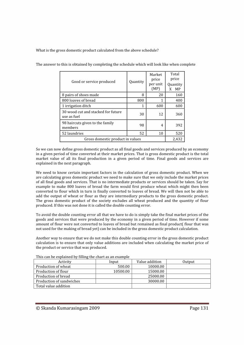
© Skanda Kumarasingam 2009 Page 131
What is the gross domestic product calculated from the above schedule? The answer to this is obtained by completing the schedule which will look like when complete
Total price
Good or service produced Quantity
Market price
per unit (MP)
Quantity X MP
8 pairs of shoes made 8 20 160
800 loaves of bread 800 1 400
1 irrigation ditch 1 600 600
30 wood cut and stacked for future use as fuel
30 12 360
98 haircuts given to the family members
98 4 392
52 laundries 52 10 520
Gross domestic product in values 2,432
So we can now define gross domestic product as all final goods and services produced by an economy in a given period of time converted at their market prices. That is gross domestic product is the total market value of all its final production in a given period of time. Final goods and services are explained in the next paragraph. We need to know certain important factors in the calculation of gross domestic product. When we are calculating gross domestic product we need to make sure that we only include the market prices of all final goods and services. That is no intermediate products or services should be taken. Say for example to make 800 loaves of bread the farm would first produce wheat which might then been converted to flour which in turn is finally converted to loaves of bread. We will then not be able to add the output of wheat or flour as they are intermediary products to the gross domestic product. The gross domestic product of the society excludes all wheat produced and the quantity of flour produced. If this was not done it is called the double counting error. To avoid the double counting error all that we have to do is simply take the final market prices of the goods and services that were produced by the economy in a given period of time. However if some amount of flour were not converted to loaves of bread but remained as final product( flour that was not used for the making of bread yet) can be included in the gross domestic product calculation. Another way to ensure that we do not make this double counting error in the gross domestic product calculation is to ensure that only value additions are included when calculating the market price of the product or service that was produced. This can be explained by filling the chart as an example
Activity Input Value addition Output
Production of wheat 500.00 10000.00
Production of flour 10500.00 15000.00
Production of bread 25000.00
Production of sandwiches 30000.00
Total value addition

© Skanda Kumarasingam 2009 Page 132
Gross domestic product is equal to the value addition or the final value of the output. Are these amounts equal to one another?................................................. The answer to this is obtained by completing the schedule above which will look like this when complete
Activity Input Value
addition Output
Production of wheat 500 10,000 10,500
Production of flour 10,500 15,000 25,500
Production of bread 25,500 25,000 50,500
Production of sandwiches 50,500 30,000 80,500
Total value addition 80,000
Total value addition=final output - input (80500-500)
80,000
You will also note from the initial example that the irrigation ditch and the 30 wood cut and stacked for future use as fuel in the first chart are considered as investments. The other products and services were consumed. In the space provided below draw a simple two sector economy (which has only households and business firms just like our farm family and the farm as the business unit) and show the flow of the factors of production from households to business firms. In the same diagram shows the flow of goods and services from the business firms to the household.
In our example the household is the farm house and the business firm is the farm itself. We can simply say that in this economy where there is only one household everything that was produced in this society would be consumed or invested (saved) by the household. This simply becomes the income that the household earns by providing the factors of production to the business firm or the farm. What is the amount of investment and what is the amount of consumption by this economy in the given year? Investment was………………and consumption was……………….both totaling to the gross domestic product of this simple society or nation.

© Skanda Kumarasingam 2009 Page 133
Write this in notation form in the box below
We also note that the irrigation ditch might not actually belong to a particular household but to all members of the society. When something belongs to all members of the society we say that it belongs to the government. So we can say that the gross domestic product is equal to the investments that are made by the household + consumption of goods and services+ assets created or consumed by the government (or for the government). Write this in notation form in the box below
Sometimes we know that this asset creation by the government is done by collecting taxes from the households. So from this we will be able to say that the gross domestic product is equal to the incomes of all the households in the society. Hence gross domestic product must be equal to the gross income of all the households. We can calculate income of an economy or society as the addition of net incomes of all families + taxes collected by the government to create assets for joint ownership or for consumption of a joint nature. Write this in notation form in the box below
Let us now say that this simple economy is going to trade with the rest of the word. This is simply because this economy may be producing more than it requires and so it may be able to sell this excess quantity to the rest of the world to earn an additional income. This additional income can then be used to import certain goods and services which could be used either as input for production or as consumption. Let us say that the business firms produce goods and services that are worth at market prices = U.S dollars 1000. This we can then say is the gross domestic product of the economy which must be also equal to the income of the society.
• Households consumed 300
• They invested 200
• Paid to government as taxes 100 which it then uses to produce joint assets or for a joint consumption.
This leaves the consumer an additional…………….in excess of their needs. This they will export to the rest of the world. Using this money or foreign exchange that has been earned by way of exports the society imports let us say goods and services worth 280. The net difference between exports and imports is equal to 400-280= U.S dollars 120 and is called net exports.

© Skanda Kumarasingam 2009 Page 134
The formula for next exports is calculated as
Let us again say that like in the previous paragraph that the society is left with 400 in excess of its needs. It then imports goods and services worth 500 either for consumption or as input for further production. If we now calculate the net export figure it will be 400-500= (U.S dollars 100). When net export is negative like in this example it simply means that this society or nation has taken a loan from the rest of the world. This is a simple indication that shows what the society has consumed over what was produced by it. If a society is going to consume more than what it has produced it obviously has to do so by taking a loan from the rest of the world. This is when the net export amount is a negative figure. So in a society where there are households + governments + trade with the external world by exports and imports the gross domestic product will be calculated as follows
Gross domestic product = investment made by households+ consumption of the society+ tax levied by the government to create joint assets or for the purpose of joint consumption+ net exports
However if we are going to use the income method it will be net income of families + taxes paid to the government.
Having understood the basics of gross domestic product calculation we are confronted with a small problem. The problem is that economists use different words or complex jargon in the components of the above two equations. This is explained in the table that is provided below
In simple English Economic jargon
Consumption Personal consumption
Investment Gross domestic investment
Government Government purchases
Net exports Net exports
National Income (income of all people or members of the nation or the given society)
The calculation of gross domestic product using the income method involves an understanding of nine components. Some of these components are usually called the national income and is based on the income earned by the members of the society as suppliers of resources within the country and abroad. Essentially this is income earned by individuals. Income earned by individuals who are the owners of the factors of production and the suppliers of the factors of production earn their income in the following manner
• Suppliers of labor will earn compensation from employment. This compensation has two components which are
1. salary and wages 2. wage supplements( employer contributions to pensions and other funds)
• The suppliers of land and related resources such as raw materials will earn rent income

© Skanda Kumarasingam 2009 Page 135
• The suppliers of capital which may be in the form of either money or machinery will earn an interest income
• The suppliers of entrepreneurship will earn profits. We also need to know whether this profit is earned by a sole proprietor or a shareholder in a corporate firm. If the person is a sole proprietor all profits will belong to her. However if it is a shareholder in a corporate firm the corporate profits will be split into three further components which are
1. Dividends which is the received component of the profit 2. Tax on the corporate income which is paid to the government to create joint assets or
for the purpose of joint consumption 3. Undistributed income which is the profit that is retained by the business so that it may
be able to use it for future expansion and growth. Thus the seven components that makes the national income and is given in the table below
Components of national income ( earned by individuals)
Labour Land Capital Entrepreneurial ability
Salaries and wages
Wage supplements
Rent Interest Distributed profit(dividend)
Corporate taxes
Retained profit
1 2 3 4 5 6 7
Having understood seven of the components out of the nine that are involved in gross domestic product calculation there are two more components which are classified as non-income charges. These two items are not earned by the individuals or the households in the society. They are
• Depreciation which is the reimbursement to the suppliers of capital and is considered as a consumption of fixed capital. Please remember reimbursement is not equal to income.
• Indirect business taxes which are the income earned by the government The addition of all these nine components will comprise gross national product
Gross national product
National income( earned by members of the economy) Non-income charges(not earned by members of the society
Labour Land Capital Entrepreneurial ability
Salaries and wages
Wage supplements
Rent Interest Distributed profit(dividend)
Corporate taxes
Retained profit
Depreciation (consumption of fixed capital)
Indirect business taxes
From the above amount we need to deduct the net income earned abroad to arrive at the gross domestic product. Net income earned abroad is calculated by deducting income earned by the members of the nation or society from foreign nations (which is not a part of the gross domestic product as it was income earned by producing goods and services in another economy by the members of the society or the nation) from the income earned by foreigners within the society or the nation (even though the income goes to a foreigner it was earned in the country for producing goods and services within its boundaries)

© Skanda Kumarasingam 2009 Page 136
From the gross national product if we deduct the net income earned abroad we arrive at the gross domestic product of the society or nation
Gross national product
National income( earned by members of the economy)
Non-income charges(not earned by members of the society
Net income earned abroad Deduct- foreign income by locals Add- income of foreigners in the society
Gross domestic product
Net Domestic Product
The second component in national income accounting is net domestic product. Net domestic product is calculated as gross domestic product less input required for producing the gross domestic product. In the gross domestic product calculation we do not include or deduct the inputs that were used to produce the goods and services. However in the net domestic product calculation we consider the market value of the input.
Net domestic product= gross domestic products – inputs
The input usually considered is depreciation or consumption of fixed capital. Usually this means
Net domestic product = gross domestic product- depreciation (or consumption of fixed capital)
Say for example a farm society harvests 50,000 bushels of wheat and sells 49,000 bushels. So the gross investment is 1000 bushels. The gross domestic product will be the market price of the final goods which are equal to 50,000 bushels of wheat multiplied by the market price of wheat. However to obtain the number of 50,000 bushels of wheat the farm had to sow 400 bushels of seeds. Sometimes we say that this input as stated above is often considered to be consumption of capital goods or depreciation. So we will be able to calculate net private domestic investment (or simply net investment) as gross private domestic investment - depreciation
Net private domestic investment (net investment) = gross private domestic investment (gross investment) – depreciation
From the schedule below you will note two interesting ways of calculating the net domestic product.
Method 1 Method 2
Personal consumption 350 350
Gross domestic investment 75 37
Government purchases 110 110
Net exports 5 5
Gross domestic product 540
Depreciation 38 0
Net private domestic investment= gross domestic investment – depreciation = ( 75-38)=37

© Skanda Kumarasingam 2009 Page 137
Net domestic product 502 502
Two other ways of calculating national income based on gross domestic product and net domestic product are 1. National income can also be calculated as
National income= gross domestic product- non-income charges+ net income from abroad
Non income charges include depreciation (consumption of capital goods) + indirect taxes 2. Another way of calculating national income is
National income= gross national product- indirect taxes+ net income from abroad
Both these methods should be obvious when you study the table providing both methods of calculating net domestic product. Personal Income and Disposable Income
National income as stated before is income earned by all resource suppliers in a given society. This includes
• Compensation for employment which incorporates salaries and wages + wage and salary supplements paid by the employer
• Rent
• Interest
• Proprietors income or corporate income ( which has three components namely dividends + corporate taxes+ retained profits)
You may see from the above that even though the national income is earned by the suppliers of the resources who are the owners of the factors of production or the households they do not actually receive all that they earn. For example corporate income simply means only the dividend component to the shareholder and so they lose out on corporate taxes and do not receive anything immediate from the undistributed corporate profits portion. We also know that due to certain social security contributions which have to be paid by the employee (it may be deducted from their salaries and wages that are paid to them) or the employer (to a pension fund and so they will not receive money immediately). So we can say
National income- corporate taxes- undistributed corporate profits- social security contributions= earned and receive income
Sometimes to the earned and received income we may have to add something unusual. Sometimes resource suppliers or owners of the factors of production receive money which they have not earned. This may be in the form of government subsidies or business gifts. These are called transfer payments. To the earned and received income if we add the transfer payments we get what is called personal income of all of households.

© Skanda Kumarasingam 2009 Page 138
Personal income= earned and received income – transfer payments
Now we need to know what people or members of the society do with this income or how do they spend it. There are three things that members of a society can do with their personal income.
• They pay personal income taxes
• Use it for personal consumption
• Use it for personal savings Whatever the members of the Society use for personal consumption and personal savings is called the disposable income. Finally this is the amount that is available for them to spend. Another way of stating this is personal income minus personal taxes= disposable income
Personal income – personal taxes = disposable income
Personal consumption + personal savings = disposable income
Adjusting for Gross Domestic Product
This is important because changes in market prices can distort the gross domestic product from one year to another. Say for example last year the economy produced thousand bushels at the market price of U.S dollars 40 per bushel. So the total market value of the production was U.S dollars 40,000. Let us say in the current year too the number of units produced were thousand bushels but at the market rate of U.S dollars 50 per unit. Hence the total value of production was U.S dollars 50,000. From the above example we know that the market value of all production has increased from U.S dollars 40,000 to 50,000. However we also know that even though the market values increased production has not increased and has remained constant at thousand bushels. To calculate the output we need to divide total market value by the market price. This will tell us the output or GDP in units. However this can only be done if the economy produces one product or service. We also know that this is far from reality. To overcome this problem economists have a method. This involves the calculation of an index. Say for example in 1933 which is the base year a packet of cigarettes cost 20¢. In 1941 a packet of cigarettes costs 24¢. If we consider 1933 to be the base year 20¢ will be indexed as 100. If 20¢ is indexed at 100 then 24¢ will be indexed as 120. That is price increased by 20 percent compared to the base year or 1941 prices are 120% of 1933 price. This index is called the GDP deflator. The gross domestic product deflator or the GDP deflator is not the consumer price index which is used to calculate inflation. Once this index has been calculated which is also called the GDP deflator which can now be used to calculate the market price of each and every item from the base year terms. However the GDP deflator has to be calculated for each and every item that the economy produces. Work out the schedule that is provided below using 1982 as the base year to calculate the adjusted GDP.
Year GDP Price index Real GDP

© Skanda Kumarasingam 2009 Page 139
1929 103 12.3
1933 56 9.4
1941 91 10.7
1982 4540 100.0
The adjusted GDP or the adjusted gross domestic product tells us how GDP has grown without considering the impact of changes in market prices. This will help us to calculate and compare the performance of an economy from one year to another in a more meaningful manner. If we were unable to calculate the real GDP we may think that the economy is actually growing since the GDP is increasing but it may be because of an increase in market prices and not due to increase in quantity or output. Only an increase in quantity produced can improve the real GDP of an economy. The adjusted GDP table should look like this
Year GDP Price index
Real GDP
1929 103 12.30 837
1933 56 9.40 596
1941 91 10.70 850
1982 4,540 100.00 4,540
Review (Once complete you can use this as the chapter summary or round-up) Question 1 For a self-sufficient farm family its gross domestic product or GDP is the...................................................... ………………………………………………………………………………………………………………… ………………………………………………………………………………………………………………… ………………………………………………………………………………………………………………… Question 2 The family’s GDP (does/ does not) equal its total output of final goods and services and (does/ does not) equal the family's total income. Question 3 Some of this GDP was output which the family......................during the year. The rest of the output was..................... for use during some later years. Adding up the incomes of all members of the family tells us the size of the family’s............................. Question 4 We must add.................items to compute gross domestic product or GDP. Two of these items do not represent the incomes of individuals who supply the economy with resources. These two items are called................................charges. They are depreciation and..................................................... Finally we must subtract one item which is.......................................... Question 5 Some of these items are the incomes earned by those who provide the economy with labor, land, and entrepreneurial ability. The income of those who supply Labor is called.......................... Land is called........................... Capital is called........................

© Skanda Kumarasingam 2009 Page 140
Entrepreneurial ability is called..................................... Question 6 The compensation of employees, the income earned by labor results in one of the items we add to measure GDP. This item is made up of two sub-items-…………………………..and. .......................................: and....................................................................................................................................................................... Question 7 Profit, the income earned by entrepreneurial ability falls into four categories. One of these four categories is the income of owners of business firms which are not corporations. This is called............................................ 3 of these four categories make up the income of owners of business firms which are corporations. These three are............................................................................... and........................................... Question 8 The NDP is calculated as............................................................................................................ ………………………………………………………………………………………………………………… ………………………………………………………………………………………………………………… ………………………………………………………………………………………………………………… ………………………………………………………………………………………………………………… Question 9 The NDP = the GDP.................................................................................. Using the income approach what items do you add to find the NDP?........................................................................................................... ………………………………………………………………………………………………………………… ………………………………………………………………………………………………………………… ………………………………………………………………………………………………………………… ………………………………………………………………………………………………………………… Question 10 What is net private domestic investment?-………………………………………………… ………………………………………………………………………………………………………………… ………………………………………………………………………………………………………………… ………………………………………………………………………………………………………………… ………………………………………………………………………………………………………………… Question 11 NPDI (net private domestic investment) =GPDI (gross private domestic investment)............................................................ Using the expenditures approach what items do you add to find the NDP?-………………………………………………………………………………………… ………………………………………………………………………………………………………………… ………………………………………………………………………………………………………………… ………………………………………………………………………………………………………………… ………………………………………………………………………………………………………………… Question 12 Net income is the income (earned/ actually received) by those who provide the economy with economic..................................... Net domestic product = gross domestic product minus................................... Net income = net domestic product minus .................................... and plus.......................................... Net income can be computed via the income approach by adding.................. (How many?)items

© Skanda Kumarasingam 2009 Page 141
Question 13 The items we add to find net income by the income approach include all of the nine we added to compute the gross domestic product except those two which together are called.......................................................... These seven items which constitute the incomes earned by the four kinds of economic resources and the 4 in comes are called.......................................................................................................... and............................ Question 14 Personal income is the income which is (earned/ received) and national income is the income which is (earned/ received) Question 15 Personal income can be calculated either by adding the following items.......... ………………………………………………………………………………………………………………… ………………………………………………………………………………………………………………… ………………………………………………………………………………………………………………… …………………………………………………………………………………………………………………or by adding the following three items............................................................................................................... ………………………………………………………………………………………………………………… ………………………………………………………………………………………………………………… ………………………………………………………………………………………………………………… ………………………………………………………………………………………………………………… Question 16 Personal income can also be determined by subtracting……………………………………………………… ............................................................................................................................................................................…………………………………………………………………………………………………………………………………………………………………………………. …………………………………………………………………………………………………………………from the national income and then adding......................................................................................................... Question 17 You just cannot trust the GDP figures to tell you what happened to the economy's total output unless you first.......................these figures to take into account the changes that may have occurred in the level of...........................................over the years. We do this by dividing the GDP by the..................................................for that year and then multiplying by............................ Question 18 We also learned that inflation is a ........................... and deflation is a..................................in the..................... level.
Answers
Suggested answers to the above questions are given. The answers are provided sequentially in the same order you will fill the blanks or select from a choice in the brackets
Question 1 Total market value of all the final goods and services produced during the year
Question 2 Does Does Question 3 Consumed Invested Gross domestic product (or output or income)

© Skanda Kumarasingam 2009 Page 142
Question 4 Income 9 Net income Indirect business Net national income earned abroad Question 5 Compensation of employees Rent Interest Profit Question 6 Wages Salaries Wage and salary supplements Question 7 Proprietors’ income Corporate income taxes Dividends Undistributed corporate profits Question 8 The market value of the final goods and services produced during a year less the capital used up during the year Question 9 Less depreciation All items that are added to find the gross domestic product except depreciation Question 10 The capital goods produced during a year less the capital goods worn out Question 11 Less depreciation Personal consumption expenditures, net private domestic investment, government purchases, net exports Question 12 Earned Resources
Depreciation Indirect business taxes Net national income earned abroad 7 Question 13 Non- income Chargers Compensation of employees, rent, interest, profits Question 14 Received Earned Question 15 Compensation of employees Rents Interest Proprietors’ income Dividends Transfer payments Less social security contributions Or Personal savings Personal taxes Personal consumption expenditure Question 16 Social Security contributions Corporate income taxes Undistributed corporate profits Transfer payments Question 17 Adjust Prices Price index 100 Question 18 Rise Fall Price

© Skanda Kumarasingam 2009 Page 143
Chapter 9
Macroeconomic Analysis- Aggregate Demand and
Aggregate Supply
Learning Outcomes
• Using the basic understanding obtained from microeconomics about the demand and supply curves of individual products and services we now try to understand how the same concepts can be applied at the macroeconomic level. Also we try to understand how the microeconomic situation differs or complements the macroeconomic situation.
• To understand the reasons why the aggregate demand curve is a downward sloping demand curve. This will help us to appreciate that the reasons for the aggregate demand curve to slope downwards is not the same as mentioned in explaining the reasons for the downward sloping demand curve of an individual product or service.
• To appreciate and understand what changes the quantity of real output demanded and changes in aggregate demand.
• To learn the special features and the reasons for the peculiar shape of the aggregate supply curve
• To appreciate and understand what changes the quantity of real output supplied and changes in aggregate supply
• To appreciate the outcomes when the aggregate demand curve and the aggregate supply curve intersect at the equilibrium point and what happens when aggregate demand is more than the aggregate supply or vice versa
• To understand what causes inflation and unemployment and to appreciate the link between them. The two important reasons for inflation being demand pull and cost push which are caused by changes in aggregate demand and aggregate supply respectively. To use the graphical means to understand it
• Finally to prepare your own set of review notes by answering the questions set in review questions.
Chapter Outline
• The basic ideas of macroeconomic analysis
• Aggregate demand and reasons for the downward sloping curve
• Changes in the quantity of real output demanded and changes in aggregate demand
• Aggregate supply
• Changes in the quantity of real output supplied and changes in the aggregate supply
• Equilibrium

© Skanda Kumarasingam 2009 Page 144
• Inflation and unemployment
• Review questions and answers to review questions
The Basic Ideas of Macroeconomic Analysis
We have already understood how output of a commodity varies with prices for an individual product or service. This we can understand by studying the price of the commodity (think of it as a product or service) and the output of the commodity by establishing their demand and supply schedules. Once we have established the demand and supply schedules or curves of an individual commodity we can then find the equilibrium point which determines the price of the commodity and the output of the commodity at a given time. However we may also be able to draw the demand and supply schedules for the whole economy. Such a demand curve is called the aggregate demand curve and such a supply curve is called the aggregate supply curve. These curves are established by adding up all the market demand and the market supply schedules of all types of products and services respectively to obtain the aggregate demand and the aggregate supply schedules. From these schedules we can then draw the aggregate demand and aggregate supply curves. This curve is drawn by plotting the price levels (rather than the price like in the individual demand and supply graphs) in the economy along the Y axis and real GDP along the X axis. Real GDP (gross domestic product) means the actual output not considering increases in market prices. So real GDP shows us by how much the output of the economy as increased or decreased irrespective of any change in the market prices of all the products and services that were produced in the given economy or society. In macroeconomic analysis we would like to know why output or real GDP and price levels keep changing. There are many reasons for them and having a good understanding of it will help the economists to develop better plans to overcome the issues related to inefficiency, inflation and unemployment. Aggregate Demand and Reasons for the Downward Sloping Curve
This is a schedule between price levels of an economy and the real GDP. Usually the aggregate demand schedule will show an inverse relationship between price levels and the real GDP. That is when price levels increase real GDP will reduce and vice versa. So we can say that the aggregate demand curve is a downward sloping curve. Now why does the price levels and real GDP have an inverse relationship? Unlike for the individual demand curve or schedule the reasons are not the income effect or the substitution effect. These do not apply when we are dealing with aggregates. The demand curve of an individual commodity is affected by the income effect. Say for example if a person's monthly income is equal to U.S dollars 1,000.00 and a loaf of bread is equal to U.S dollars 10.00. If this person only consumes bread he will be able to consume 100 loaves of bread. If the price
© Skanda Kumarasingam 2009 Page 145
of bread increases from U.S dollars 10 to U.S dollars 20 and there is no change in his monthly income he will have to consume 50 loaves of bread. This is the income effect for an individual product. However this explanation is not viable then we are dealing with aggregate demand as real GDP means in other words national income. When we talk about real GDP along the aggregate demand curve it is obvious that real output has increased. So a movement along the demand curve indicates increasing aggregate incomes which is not a feasible explanation. The demand curve of an individual commodity is also affected by the substitution effect. In short the substitution effect affects individual products when the price of a particular product increases whilst its substitute’s price remains constant. So if the price of a particular product increases consumers of this particular product will move over to consuming more of the substitute and less of the particular product. Hence the quantity demanded for the particular product will decrease when there is a price increase. However when we consider the aggregate demand curve we can observe that along the demand curve all prices are generally falling and so all products will become cheaper. Hence again this explanation is not feasible when analyzing aggregate demand. However there are three valid and plausible reasons which tell us why the aggregate demand curve is downward sloping. They are
• The wealth or real balance effect
• Interest rates effect
• Foreign purchases effect Let us now look at each of them in turn. Say for example in a given society its members will hold assets. When there is a general decrease in price levels and if there is no fall in the value of these assets the members of the society may be able to consume more by selling off the assets they hold. Stated another way the value of assets remains constant or increases but price levels of goods and services decrease. This will increase the real balances of the assets and will make the consumers and firms feel they have become richer. When consumers and firms become richer or feel that way they tend to spend more. This increases their spending and so increases the real GDP. This is called the wealth or real balance effect If the price levels decrease in the economy it will decrease the demand for money. When the demand for money is reduced the interest rate which is the price paid for money will also decrease. When the cost of borrowing money is cheaper because of the reduction in the interest rate members of the society (households and even businesses) will tend to spend more. Spending more will increase the real GDP. This is called the interest rates in effect When the price levels decrease in a given society its production or output of goods and services become cheaper to foreigners. When the foreigners compare prices in their economy and realize that it is more expensive they will start importing from the given society. Hence the society’s net exports will increase. An increase in net exports can only occur due to an increase in real GDP. This is called the foreign purchases effect. These are the three reasons why the aggregate demand curve is downward sloping or has an inverse relationship between price levels and real GDP.
Changes in the Quantity of Real Output Demanded and Changes in Aggregate Demand
When studying the demand curve or schedule of a single product or commodity we distinguished between change in quantity demanded and change in demand. Likewise when we are studying aggregate demand we need to look at
• Changes in the quantity of real output demanded
• Changes in aggregate demand

© Skanda Kumarasingam 2009 Page 146
Changes in the quantity of real output demanded can only occur due to a change in the price levels. As explained before price levels can only change due to the wealth or real balance effect, interest rates effect and the foreign purchases effect. Changes in aggregate demand will shift the aggregate demand curve from the original aggregate demand curve either to the left or the right. Such changes in aggregate demand are due to a change in the determinants of aggregate demand. These determinants of aggregate demand are
• Consumption
• Gross investment
• Government spending
• Net exports First let us look at consumption. This again is affected by
• The change in real consumer wealth
• Change in consumer real income
• Change in indebtedness
• Changes in personal income taxes If we look at the change in real consumer wealth this can occur due to gifts or inheritance. Please note that this is not the wealth effect which is caused by a change in the price level. Wealth effect tries to explain why the aggregate demand curve is downward sloping. So if the real consumer wealth increases the consumer may be willing to buy more. This will increase aggregate demand and shift the aggregate demand curve to the right. If an increase in consumer real income (increase in income after deducting the effects of inflation) takes place the members of the society will decide to consume more and hence will be spending extra. This will cause the aggregate demand to increase and the aggregate demand curve will shift towards the right. When indebtedness increases it reduces the spending of the society. The society will be keener to pay off the loans rather than to spend whatever they have earned. So when the spending reduces the aggregate demand curve will shift to the left indicating that there is a reduction in the aggregate demand. When personal income taxes reduce it will increase the take home pay of the members of the society. This will lead to willingness by the consumer to buy further and to spend additionally. This will shift the aggregate demand curve to the right Next we have to look at gross investment which is another determinant of aggregate demand. This again is affected by
• The cost of borrowing money
• Expectations of future profits
• Business taxes
• New technology
• Recession Now let us look at each of them in turn If the cost of borrowing money reduces it will become cheaper to borrow money. This will increase the gross investment and so shift the aggregate demand curve to the right

© Skanda Kumarasingam 2009 Page 147
When business firms expect the economy to do well and have high expectations of future profits they will increase gross investment so that this new capital (property, plant and equipment) will be able in turn to increase or create this expected future profit. This additional investment will shift the aggregate demand curve to the right. In the same manner if members of the society or households also expect their profits or income to increase they too will tend to invest more. This will also shift the aggregate demand curve to the right. When business taxes increases it reduces the profit after tax. When profits reduce gross investments will reduce because businesses are not interested to produce when economic profits are low. This will shift the aggregate demand curve to the left. When new technology is introduced it often improves efficiency and productivity. When efficiency and productivity increases the cost of producing goods and services will reduce which in turn will increase the economic profits. So business firms will invest in this new technology increasing the gross investments. This increase in gross investments will also increase aggregate demand and so the aggregate demand curve will shift to the right. In times of great recession there will often be excess capacity in the production plants or factories of the business firms. So there is no need to increase plant size. This will mean that gross investment need not take place. Hence this will decrease the aggregate demand and so shift the aggregate demand curve to the left. Another determinant of aggregate demand is government spending. When government spending increases it tends to increase the gross investment or consumption. This is on the assumption that taxes and /or interest rates do not increase. In such a scenario aggregate demand will increase and move the aggregate demand curve to the right. The final determinant of aggregate demand is net exports. There are two reasons why net exports may drive the aggregate demand. The first reason may be a change in the national income of other countries. When the national income of other countries or nations increases it increases the demand for exports in the particular society that is being studied. When demand for exports increases it also increases aggregate demand and so will shift the aggregate demand curve to the right. However if there is recession abroad it will reduce the demand for exports. This reduction in exports will also reduce the aggregate demand in the particular society that is being studied and so will shift its aggregate demand curve to the left. The next reason why net exports may drive aggregate demand is when real interest rates in the society increases. When the real interest rate (nominal interest rate quoted by financial institutions less average inflation premium/rate) increases it also increases the demand for the bonds and debentures that are issued in this society that is being studied. To purchase more of these bonds foreigners will require paying for them in the society's particular currency. So the demand for the currency of the society will increase. We need to understand that a currency in a country is a normal good and the price you pay for it is the exchange rate you have to pay to obtain it. So when the demand for the currency of the society increases the price will increase compared to the foreign currencies. This will make the particular currency of the society appreciate in value. When the currency of the society appreciates in value exports become more expensive to foreigners. When exports become more expensive to foreigners they will export less of the products and services produced by the society. The Society in turn will increase its imports as it is cheaper compared to the goods and services produced within the country. For these reasons net exports will reduce. This reduction in net exports will also reduce the aggregate demand and shift the aggregate demand curve to the left.

© Skanda Kumarasingam 2009 Page 148
Aggregate Supply
This curve or schedule shows us the relationship between price levels and real GDP (aggregate supply). The real GDP being the aggregate supply. If we plot this on graph on the X axis we will have real GDP and on the Y axis the price levels. The aggregate supply curve is of a particular and peculiar shape. It starts off being perfectly inelastic and is parallel to the X axis. After a particular point it is an upward sloping aggregate supply curve. However when real GDP reaches the full employment level the aggregate supply curve turns vertical and becomes perfectly inelastic. In the space given below try drawing a typical aggregate supply curve from the description. After that is given a typical aggregate supply curve. Check yours with it
Aggregate supply
0
2
4
6
8
10
12
14
16
18
20
0 2 4 6 8 10 12 14 16 18 20 22 24 26 28 30
aggregate supply
pric
e le
vel
Keynesian range
intermediate range
classical range
The initial part of the curve which is perfectly elastic and so parallel to the X axis happens when there is severe depression or recession in the economy. This particular range is also called the Keynesian range since this British economist (John Maynard Keynes) studied the causes and remedies of

© Skanda Kumarasingam 2009 Page 149
unemployment and recession. In this range suppliers will be willing to supply even though they do not expect price levels to increase. It is also unnecessary for price levels to increase and so they remain constant. The reasons why price levels need not increase are as follows
• The first reason is since there is severe depression and unemployment workers will accept jobs without increases in their wages or salaries. So the cost of production is low and remains constant and the supplier will still be able to make profits even without an increase in the overall price levels.
• The next reason is due to severe depression most business firms’ production plants or factories will work well below capacity. So they can produce and sell as they will not need to be motivated by higher prices to increase production. Whatever they produce will earn those economic profits and in difficult times the suppliers or producers should be happy with whatever they make as economic profits.
These are the reasons why real GDP will increase but price levels will remain constant at the Keynesian range. The next part of the aggregate supply curve is upward sloping just like the normal supply curve of a particular or single commodity. This is called the intermediate range since it is between the Keynesian range and the classical range. The classical range is where the aggregate supply curve reaches full employment level (Yf) and is perfectly inelastic. In the intermediate range to increase real GDP we need to increase the price levels. There are two reasons why when price levels increase real GDP also increases.
• The first reason is as production increases certain types of labor and raw materials will become short supplied. So the business firm will need to pay them a higher price if it is interested in purchasing a larger quantity. This will obviously increase the costs. So to make economic profits you will need to increase the prices.
• The second reason is as production increases and unemployment reduces (obviously when production increases factories will require more people to work for them thus reducing unemployment) all machines will have to work harder to produce a larger quantity that now needs to be supplied. Due to this reason old or existing machines will break more often and will cost extra to repair and maintain. So you need to have a higher economic profit to induce the move towards full production.
The final part of the aggregate supply curve is perfectly inelastic. At this point there is employment of all resources and so you cannot increase the real GDP at that given moment in time. At this point it is the maximum the economy is able to produce. This is also called the classical range. The classical economists believe that all economies will tend to produce its full employment output. At this level even if price levels increases the society or nation cannot increase its real GDP as all resources are working at their maximum efficiency and availability. Changes in the Quantity of Real Output Supplied and Changes in Aggregate Supply
In a similar manner to the aggregate demand curve there will also be a movement along the aggregate supply curve. This occurs due to changes in real GDP or price levels when all other determinants of aggregate supply remain constant. These determinants change the unit cost of production. When this happens this will either increase or decrease the economic profit. When this happens the aggregate supply curve changes or shifts to
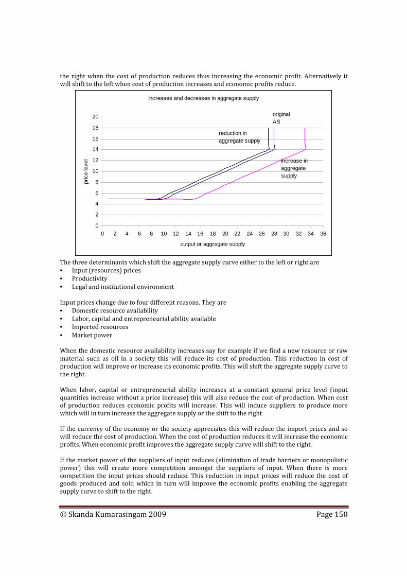
© Skanda Kumarasingam 2009 Page 150
the right when the cost of production reduces thus increasing the economic profit. Alternatively it will shift to the left when cost of production increases and economic profits reduce.
Increases and decreases in aggregate supply
0
2
4
6
8
10
12
14
16
18
20
0 2 4 6 8 10 12 14 16 18 20 22 24 26 28 30 32 34 36
output or aggregate supply
pric
e le
vel
reduction in aggregate supply
increase in aggregate supply
original AS
The three determinants which shift the aggregate supply curve either to the left or right are
• Input (resources) prices
• Productivity
• Legal and institutional environment Input prices change due to four different reasons. They are
• Domestic resource availability
• Labor, capital and entrepreneurial ability available
• Imported resources
• Market power When the domestic resource availability increases say for example if we find a new resource or raw material such as oil in a society this will reduce its cost of production. This reduction in cost of production will improve or increase its economic profits. This will shift the aggregate supply curve to the right. When labor, capital or entrepreneurial ability increases at a constant general price level (input quantities increase without a price increase) this will also reduce the cost of production. When cost of production reduces economic profits will increase. This will induce suppliers to produce more which will in turn increase the aggregate supply or the shift to the right If the currency of the economy or the society appreciates this will reduce the import prices and so will reduce the cost of production. When the cost of production reduces it will increase the economic profits. When economic profit improves the aggregate supply curve will shift to the right. If the market power of the suppliers of input reduces (elimination of trade barriers or monopolistic power) this will create more competition amongst the suppliers of input. When there is more competition the input prices should reduce. This reduction in input prices will reduce the cost of goods produced and sold which in turn will improve the economic profits enabling the aggregate supply curve to shift to the right.

© Skanda Kumarasingam 2009 Page 151
The second determinant of aggregate supply is productivity. Productivity means the increase in output by using a given level of inputs. When this increases you are able to produce more at the same cost or same amount of inputs. This will reduce the cost of production and increase the economic profit. When the economic profit increases the aggregate supply curve will shift to the right. The final determinant of aggregate supply is the legal and institutional environment. This has two other elements which are taxes and subsidies and government regulations. When taxes increase it increases the cost of production which in turn reduces the economic profits which leads to the aggregate supply reducing and thus shifting the curve to the left. Alternatively when subsidies increase this will reduce the cost of production which in turn improves or increases the economic profits. This increase in economic profits will induce the aggregate supply curve to shift to the right. An increase in government regulations will increase paperwork to many business firms. This will obviously increase the cost of production or of running a business. When the cost of production increases we know that the company profits will have to reduce thus shifting the aggregate supply curve to the left Equilibrium
In the space provided draw a typical aggregate supply curve. In the intermediate range of this aggregate supply curve draw an aggregate demand curve. This means the aggregate demand curve will intersect the aggregate supply curve at the intermediate range. The intersecting point is called the equilibrium point. The equilibrium price level at this point let us says is P2. Mark another point above the equilibrium point called P3. Mark another point P1 below the equilibrium price level of P2.

© Skanda Kumarasingam 2009 Page 152
This is how your graph should have looked.
Equilibrium aggregate demand and supply in the intermediate range
0
2
4
6
8
10
12
14
16
18
20
0 2 4 6 8 10 12 14 16 18 20 22 24 26 28 30
aggregate demand and aggregate supply
pric
e le
vel
aggregate supply
aggregate demand
p2 equilibrium price
p1
p3
excess
shortage
At the price level of P1 you will note that the aggregate demand is more than the aggregate supply. When this happens there will be a shortage. When there is shortage buyers will bid prices upwards. This increases the economic profits to the suppliers so they will produce more until the equilibrium point is reached. At a price level P3 we note that the aggregate supply is > the aggregate demand. When this happens there are two things that can happen.
• In the first case as suppliers have overproduced they will have to reduce prices (discounts or free-issues) to sell these excess quantities. When prices reduce the demand tends to increase until the equilibrium point is reached.
• However in the second case suppliers do not reduce prices to sell the excess but they will store the product and sell it eventually. So the prices do not reduce. This is called the ratchet effect. According to the ratchet effect price level is flexible upwards and inflexible downwards. That is the suppliers will not reduce the prices to sell the excess quantity.
Inflation and Unemployment
Inflation simply means the rise in the price level of an economy. It is similar to an increase in the equilibrium change in price for an individual commodity(product or service) . So it can be understood using the aggregate demand and aggregate supply curves. When inflation is affected due to the aggregate demand curve we call it as demand pull inflation and when inflation is due to a change in the aggregate supply curve we name it as cost push inflation. First let us look at how inflation and unemployment are affected due to a change in the aggregate demand. In the space provided draw a typical aggregate supply curve.

© Skanda Kumarasingam 2009 Page 153
Now draw an aggregate demand curve in the Keynesian range. Draw another aggregate demand curve showing that aggregate demand has increased on the same range. Obviously the new aggregate demand curve will shift to the right. We can say that at this range that there is no change in the price levels so there cannot be inflation. However employment has increased as real GDP has increased. When real GDP increases output improves or increases and to accommodate this increase in output business firms will have to employ more workers. This will reduce unemployment.
Next in the intermediate range of the aggregate supply curve draw an aggregate demand curve. Draw another aggregate demand curve showing that aggregate demand has increased on the same range. In the intermediate range when aggregate demand increases price levels also increases and so it is inflationary. Also it can be seen that real GDP increases and hence employment increases. Thus we can conclude that in the intermediate range when the aggregate demand increases it increases the price levels or inflation and also the real GDP and thus increases employment. Finally in the classical range draw an aggregate demand curve. Draw another aggregate demand curve showing that aggregate demand has increased on the same range. In the classical range we know price levels have obviously increased and so it is inflationary. However we also note that there is no change in real GDP and so there cannot be change in employment. This is because at full employment level there cannot be a change in the real GDP. Whenever price levels increase due to a change in aggregate demand it is called the demand pull inflation. Demand pull inflation occurs at the intermediate range and the classical range. Employment increases at the Keynesian range and the intermediate range because there is an increase in the real GDP. However in the classical range employment does not increase or unemployment does not reduce since there will be no change in the real GDP.

© Skanda Kumarasingam 2009 Page 154
The graph drawn by you should ideally look like this
Inflation and GDP
0
2
4
6
8
10
12
14
16
18
20
0 2 4 6 8 10 12 14 16 18 20 22 24 26 28 30 32
aggregate demand and supply
pric
e le
vels
the original aggregate demand curves in each range is on the left and w hen increased moves to the right
Keynesian range
intermediate range
classical range
Now in the space provided draw the typical aggregate supply curve.
Draw 3 aggregate demand curves intersecting the aggregate supply curve at the Keynesian range, intermediate range and the classical range respectively. Now draw another aggregate supply curve to the left of the original aggregate supply curve. Looking to this graph we will be able to determine the causes of cost push inflation which is caused by a shift of the aggregate supply curve towards the left of the original aggregate supply curve. At all three ranges (Keynesian, intermediate and classical) we note that price levels increase and real GDP reduces. We can also say that at all three ranges or levels this leads to inflation and it also increases unemployment since real GDP reduces. Ideally your graph should like this

© Skanda Kumarasingam 2009 Page 155
Reduction in aggregate supply and its impact on inflation and unemployment (GDP)
0
1
2
3
4
5
6
7
8
9
10
11
12
13
14
15
16
17
18
19
0 5 10 15 20 25 30 35
aggregate demand and aggregate supply
pric
e le
vels
original aggregate supply curve
reduction in aggregate supply
Finally let us look at the scenario where aggregate demand has increased and aggregate supply has reduced. You should be now able to complete this on your own. In the space provided below draw the typical aggregate supply curve and an aggregate demand curve which intersects at the intermediate range and also at the classical range. Draw two more aggregate demand curves to the right of the original aggregate demand curves that were drawn in the intermediate range and the classical range. Now draw another aggregate supply curve to the left of the original aggregate supply curve.

© Skanda Kumarasingam 2009 Page 156
Inflation and GDP
0123456789
10111213141516171819
0 2 4 6 8 10 12 14 16 18 20 22 24 26 28 30 32
aggregate demand and supply
pric
e le
vels
Keynesian range
intermediate range
classical range
We note that in the intermediate range when aggregate demand increases and aggregate supply reduces from the original points
• There is an increase in price level which causes inflation
• There is an increase in real GDP
• There is an increase in employment We note that in the classical range when the aggregate demand increases and aggregate supply reduces from the original points
• Price level increases due to increases in costs causing inflation
• Real GDP reduces
• There is a reduction in employment What happens at the classical range is called stagflation. This is a major problem for politicians as everything that can go wrong in the economy happens here. There is inflation, real GDP or output of the economy has reduced and unemployment is on the rise. However what happens at the intermediate range may be acceptable to the members of the society who elect the government. Even though there is an increase in inflation there is also an increase in real GDP or output and also an increase in employment.
Review (Once complete you can use this as the chapter summary or round-up)
Question 1 When the price level falls real balances (rise/fall) consumers and firms find themselves (richer/ poorer) and (increase/ decrease) their spending, and the real gross domestic product (increases/ decreases) and vice versa
© Skanda Kumarasingam 2009 Page 157
When the price level falls the demand for money( rises/ falls) the rate of interest( increases/ decreases) spending sensitive to changes in the rate of interest( expands/ contracts) and the real gross domestic product( increases/ decreases) and vice versa When the price level falls, the nation's goods and services become relatively (more expensive/ cheaper) to foreigners and foreign goods and services become relatively (more expensive/ cheaper) to the nationals. Thus net exports (increases/ decreases) and the real gross domestic product (increases/ decreases) and vice versa. Question 2 The factors that influence the amount of real output that consumers, businesses, governments and foreigners wish to buy at each price level are called the………………………………………........................ Question 3 Changes in spending caused by a change in one or more of the determinants of demand lead to (movement along/ shift of) the aggregate demand curve. Question 4 An increase in spending shifts the aggregate demand curve to the............................................................ A decrease in spending shifts the aggregate demand curve to the...................................... In both cases we are assuming that the change in spending (was/ was not) caused by a change in the price level. Question 5 There are along the aggregate supply curve (1 / 2 / 3 / 4) ranges. In the Keynesian range the curve is............................................................... In the classical range it is.......................................... In the intermediate range it is................................... Question 6 The aggregate supply curve is horizontal when the economy is (at full employment/ in severe recession or depression/ between these two extremes) It is vertical when the economy is..........................................................................and it is up sloping when the economy is.......................................... Question 7 To summarize the effects of increases in aggregate demand complete the table below. Use + to mean increase, -to mean a decrease and 0 to mean no change
On the Effect of an increase in aggregate demand in the Price level Real gross domestic product
Keynesian range
Intermediate range
Classical range
Question 8 An increase in total or aggregate spending at any price level will increase the real gross domestic product the spenders in the economy wish to have produced. The total spending = consumption + gross investment + government spending + net exports. Therefore the real gross domestic product demanded to increase when.........................or........................ or............................... or............................... increase and vice versa Question 9 What might cause consumption to increase? If the wealth of consumers increases they will spend (more/ less) for consumption If personal taxes increase, take home income (increases/ decreases) and consumption will (increase/ decrease)
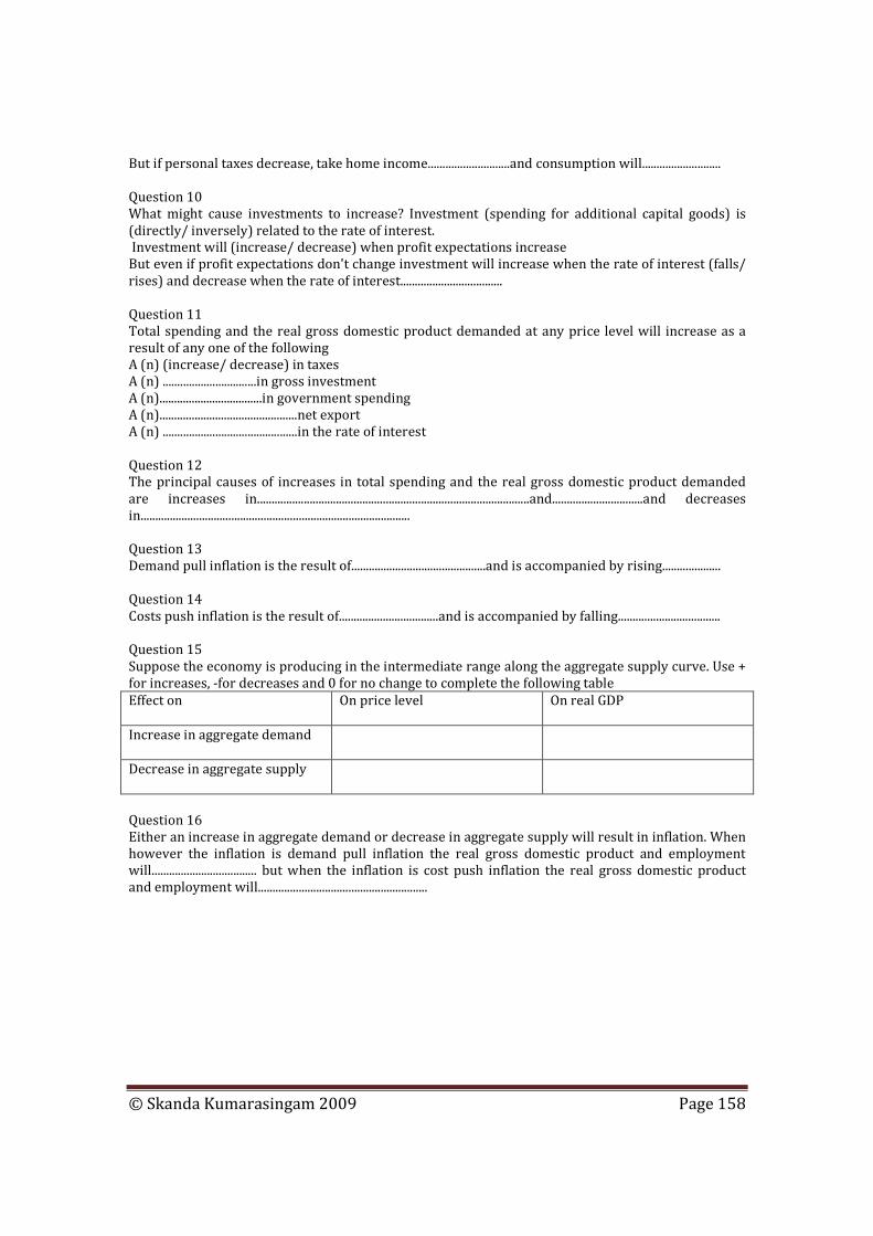
© Skanda Kumarasingam 2009 Page 158
But if personal taxes decrease, take home income............................and consumption will........................... Question 10 What might cause investments to increase? Investment (spending for additional capital goods) is (directly/ inversely) related to the rate of interest. Investment will (increase/ decrease) when profit expectations increase But even if profit expectations don't change investment will increase when the rate of interest (falls/ rises) and decrease when the rate of interest................................... Question 11 Total spending and the real gross domestic product demanded at any price level will increase as a result of any one of the following A (n) (increase/ decrease) in taxes A (n) ................................in gross investment A (n)...................................in government spending A (n)...............................................net export A (n) ..............................................in the rate of interest Question 12 The principal causes of increases in total spending and the real gross domestic product demanded are increases in.............................................................................................and...............................and decreases in............................................................................................ Question 13 Demand pull inflation is the result of..............................................and is accompanied by rising.................... Question 14 Costs push inflation is the result of..................................and is accompanied by falling................................... Question 15 Suppose the economy is producing in the intermediate range along the aggregate supply curve. Use + for increases, -for decreases and 0 for no change to complete the following table
Effect on On price level On real GDP
Increase in aggregate demand
Decrease in aggregate supply
Question 16 Either an increase in aggregate demand or decrease in aggregate supply will result in inflation. When however the inflation is demand pull inflation the real gross domestic product and employment will.................................... but when the inflation is cost push inflation the real gross domestic product and employment will..........................................................

© Skanda Kumarasingam 2009 Page 159
Answers
Suggested answers to the above questions are given. The answers are provided sequentially in the same order you will fill the blanks or select from a choice in the brackets Question 1 Rise Richer Increase Increases Falls Decreases Expands Increases Cheaper More expensive Increase Increases Question 2 Determinants of demand Question 3 Shift of Question 4 Right Left Was not Question 5 3 Horizontal Vertical Up sloping Question 6 In severe recession or depression At full employment Between these two extremes Question 7 0 and + + and + + and 0
Question 8 Gross investment Government purchases Net exports Question 9 More Decreases Decrease Increases Increase Question 10 Inversely Increase Falls Rises Question 11 Decrease Increase Increase Increase And decrease Question 12 Consumption Gross investment Government purchases Net exports The rate of interest Question 13 An increase in aggregate demand Real gross domestic product and employment Question 14 A decrease in aggregate supply Real gross domestic product and employment Question 15 + and + + and- Question 16 Increase Decrease

© Skanda Kumarasingam 2009 Page 160
Chapter 10
National Income Analysis Learning Outcomes
• To appreciate the major purposes and reasons for studying national income analysis using national income accounting
• To appreciate the assumptions that are made when studying national income accounting and national income analysis
• To learn the determinants of consumption and savings and the relationship between consumption and savings
• To understand the nature of gross investment undertaken by business firms
• To appreciate the concepts of marginal and average propensity to consume and save. This will be further highlighted through graphical presentations to show the relationship between them.
• To understand the nature of a two sector economy
• To learn the concept behind the multiplier effect and how the multiplier effect determines important equilibrium points in relation to national income analysis.
• To learn how an open economy with foreign trade operates
• To appreciate how government expenditures and taxes work in an open economy
• To summarize the chapter by completing the review questions to which the answers are provided subsequently.
Chapter Outline
• The purposes of national income analysis
• Assumptions
• Consumption and savings
• Gross investment
• Marginal and average consumption and savings
• Understanding gross investment using graphical presentations
• Two sector economy
• Effects of multiplier
• Open economy with foreign trade

© Skanda Kumarasingam 2009 Page 161
• Government expenditure and taxes in an open economy
• Review questions and answers to review questions
The Purposes of National Income Analysis
We have already seen and studied how national income is calculated. Having already got a basic grounding on the calculation (accounting) part we will now endeavor to understand in a much broader manner what national income analysis is all about. The main purpose of national income analysis is to measure the overall performance of the economy. This we do by using the real gross domestic product. Calculating the gross domestic product was called national income accounting and was already covered in a previous chapter. Real gross domestic product means that changes in price levels are not considered. Gross domestic product also means the domestic output of an economy in a given period of time. We also have another purpose in studying national income analysis because we want to know what determines the size of the gross domestic product. This is also called the theory of employment because the size of an economy's gross domestic product will determine how many workers will be employed to earn this gross domestic product. Apart from these reasons we are also interested to know why real gross domestic product changes from one year to another. Before we study national income analysis there are primarily certain principles and assumptions we need to state again .However some of them you have already learnt when studying national income accounting. Assumptions
We know that gross domestic product depends on how much people want to spend in an economy on goods and services. So we can say that when spending increases or there is anticipation for spending (called as planned expenditure or aggregate expenditure) we can say that the gross domestic product will increase. We also know that there are four types of people or institutions which are involved in spending in an economy. They are consumers, business firms, the government, and foreigners who spend in our domestic economy. So we can say
Aggregate expenditure or planned expenditure= consumption+ gross investment+ government expenditure+ net exports
• Consumption expenditure or spending is by consumers in the economy
• Gross investment is made by business firms

© Skanda Kumarasingam 2009 Page 162
• Government expenditure is purchases made by the government
• Net exports involves how much foreigners spend from our domestic production (exports less imports)
We also make another major assumption when we study national income analysis. From our studies of national income accounting we know that
• Gross domestic product-Net factor income from abroad= Net domestic product
• Net domestic product-Depreciation= National income
• National income-Deductions such as taxes on businesses+ Transfer payments= Personal income
• Personal income- Income taxes= Disposable income
• Disposable income= Consumption + Savings The assumption that we make here is from the above equations. If the following are considered to be zero then gross domestic products must be equal to disposable income.
• Net factor income from abroad
• Depreciation
• Deductions such as taxes on businesses and transfer payments
• Income taxes.
We can also say that when the above items are zero gross domestic product= net domestic product= national income= personal income= disposable income.
Consumption and Savings
Having clearly understood what the assumptions are now let us try to analyze a little more how consumer expenditure is greatly influenced by disposable income. To understand this we need to know that there are certain factors which are called income determinants and non-income determinants. The change in disposable income is called the income determinant of consumption. When there is a change in disposable income the movement is along the consumption or savings curve. This is also called change in the amount consumed and is very similar to a change in quantity demanded. Because the change in quantity demanded can only occur due to price changes and the movement is along the demand curve. Like in our studies of demand where there are determinants of demand there are also non-income determinants of consumption and savings. They are as follows 1. When price levels or prices increase in the given economy consumption and savings will reduce.
This is to be expected when disposable income is held constant. Obviously when prices increase for products and services people will be able to consume less goods and services and will also be able to save less because they will have less money to do so unless they sacrifice on their current living standards. We can so conclude that there is an indirect relationship between price levels and consumption and between price levels and savings.
2. When there is expectations of price increases people will consume immediately. This means that
when the expectations of price increases savings will reduce as people want to consume more immediately rather than save. So when expectations of price increases there is a direct relationship between consumption and increases in expectations of prices and there is an indirect relationship between expectations of price increases and savings.

© Skanda Kumarasingam 2009 Page 163
3. When personal debts of consumers increase there is a tendency for them to save more so that
they will be able to pay the debt as soon as possible. So we can say that there is a direct relationship between personal debt and savings. Obviously when people save more they will be able to consume less and so there is an inverse relationship between personal debt and consumption.
4. The other non-income determinant of consumption and savings is wealth. The amount of wealth
people have induces them to consume more and they will be obliged to save less. This means that there is a direct relationship between wealth and consumption and an indirect relationship between wealth and savings.
We need to understand that when there is a change in the non-income determinants of consumption and savings there will be a shift of consumption or savings on the graph. This is called a change in consumption or savings just like a change in demand. You will be able to understand about these changes when we start talking about the related graphs involving consumption and savings in a moment. Revisit the previous paragraphs so that you are able to comprehend them better after studying the schedules and graphs. Gross Investment (Expenditure by Business Units)
We also know that business firms spend in the form of gross investments. Business firms usually invest in buildings and equipment and also in different types of capital goods. Gross investment less replacement of old investment will give us the net investment. However, as far as spending is concerned in an economy we are interested in the gross investment. Gross investment is done based on future expectations. Business firms will consider the incremental profits. As we already know incremental profits are calculated as marginal revenue-marginal cost. If there is a high expectation that there will be incremental profits in the future business firms will invest in new equipment and so on so that they will be able to reap the benefits of a higher profit. Please remember when we are analyzing national income we are always interested in planned expenditure or aggregate expenditure and not the past expenditures. Aggregate and planned expenditure mean one and the same. Interestingly we also know that one of the major cost components of investments or any business is the payment of interest for capital. We already know that lower the interest rate lower will be the cost of production. Lower the cost of production we know that economic profits will be higher. When there is a high expectation of economic profits investment will obviously increase. So we may say that there is an inverse relationship between interest (which is the price paid for money or capital) and gross investment. We need to be careful because when there is a purchase of capital equipment involving borrowed funds there is an explicit interest cost. However if we use our own funds to purchase capital equipment there is an implicit cost of the interest forgone. Marginal and Average Consumption and Savings
Now let us try to understand what we have studied so far in this chapter and also what determines the size of real gross domestic product and how real gross domestic product changes from year to year with the use of schedules and graphs.

© Skanda Kumarasingam 2009 Page 164
Let us first look at how the disposable income of consumers is used for consumption and savings. As stated earlier in our assumption we know that disposable income is equal to the gross domestic product. Fill the schedule on the next page. To do this you need to use the information that is provided To do this it is assumed that disposable income is equal to the gross domestic product.
Disposable income (or real gross domestic product) = consumption+ savings
Average propensity to consume= consumption/ disposable income
Average propensity to consume simply means that from total disposable income how much you are willing to spend on consumption.
Average propensity to save= savings/ disposable income
Average propensity to save simply means that from total income how much you are willing to save. We already know that consumers can only do two things with their disposable income which is either to consume or to save. Which means of a given disposable income they will consume a part of it (which is called the average propensity to consume) and save the balance (which is called the average propensity to save) So we can say that
Average propensity to consume+ Average propensity to save=100%.
If given as a rate it will total to one. we also need to remember that from our understanding of the non-income determinants of consumption and savings that the average propensity to consume and the average propensity to save will depend on these factors and need not always be uniform throughout different levels of gross domestic product in the economy. This is clearly seen when you observe it from the schedule. Now we need to be introduced to another concept which is called the marginal propensity to consume and the marginal propensity to save.
Marginal propensity to consume = change in consumption/ change in disposable income
This simply means that when there is a change in the disposable income by how much does a change in consumption take place.
Marginal propensity to save= change in savings/ change in disposable income
This simply means that when that is a change in the disposable income by how much does a change in savings takes place

© Skanda Kumarasingam 2009 Page 165
We can also say when disposable income changes or increases by some amount this additional amount can only be consumed or saved. This need not be constant throughout the range of different gross domestic products in the economy (or the disposable income). So we may be able to conclude that
Marginal propensity to consume+ marginal propensity to save=100%
When given in rates it will total to one.

© Skanda Kumarasingam 2009 Page 166
Real gross domestic product= disposable income
Consumption Savings Average propensity to
consume
Average propensity to save
Marginal propensity to
consume
Marginal propensity to save
Disposable income less consumption
Consumption Disposable income
Savings Disposable
income
Δ in consumption Δ in disposable
income
Δ in consumption Δ in disposable
income
50 60
100 100
150 140
200 180
250 220
300 260
350 300
400 340
In the space provided write your observations about the above schedule………………………………………………………… ………………………………………………………………………………………………………………………………………………………………………....... ………………………………………………………………………………………………………………………………………………………………………....... ………………………………………………………………………………………………………………………………………………………………………....... ………………………………………………………………………………………………………………………………………………………………………....... ………………………………………………………………………………………………………………………………………………………………………....... ………………………………………………………………………………………………………………………………………………………………………....... ………………………………………………………………………………………………………………………………………………………………………....... ………………………………………………………………………………………………………………………………………………………………………....... ………………………………………………………………………………………………………………………………………………………………………....... ………………………………………………………………………………………………………………………………………………………………………....... Now turn to the next page to check your answers

© Skanda Kumarasingam 2009 Page 167
Real gross domestic product=
disposable income
Consumption Savings Average
propensity to consume
Average propensity
to save
Marginal propensity to consume
Marginal propensity
to save
Consumption Savings Δ in
consumption Δ in
consumption
Disposable income less
consumption Disposable income
Disposable income
Δ in disposable
income
Δ in disposable
income
50 60 (10) - - - -
100 100 - 1.00 - 0.80 0.20
150 140 10 0.93 0.07 0.80 0.20
200 180 20 0.90 0.10 0.80 0.20
250 220 30 0.88 0.12 0.80 0.20
300 260 40 0.87 0.13 0.80 0.20
350 300 50 0.86 0.14 0.80 0.20
400 340 60 0.85 0.15 0.80 0.20
From the above schedule we may be able to extract a consumption schedule which shows the relationship between disposable income (gross domestic product) and consumption. From the same schedule we may extract a saving schedule which shows the relationship between disposable income (gross domestic product) and savings Using this information draw a graph in the space provided below. On the X axis you will have disposable income or real gross domestic product and of the Y axis you will have the following 1. Consumption 2. Savings 3. Disposable income= consumption + savings
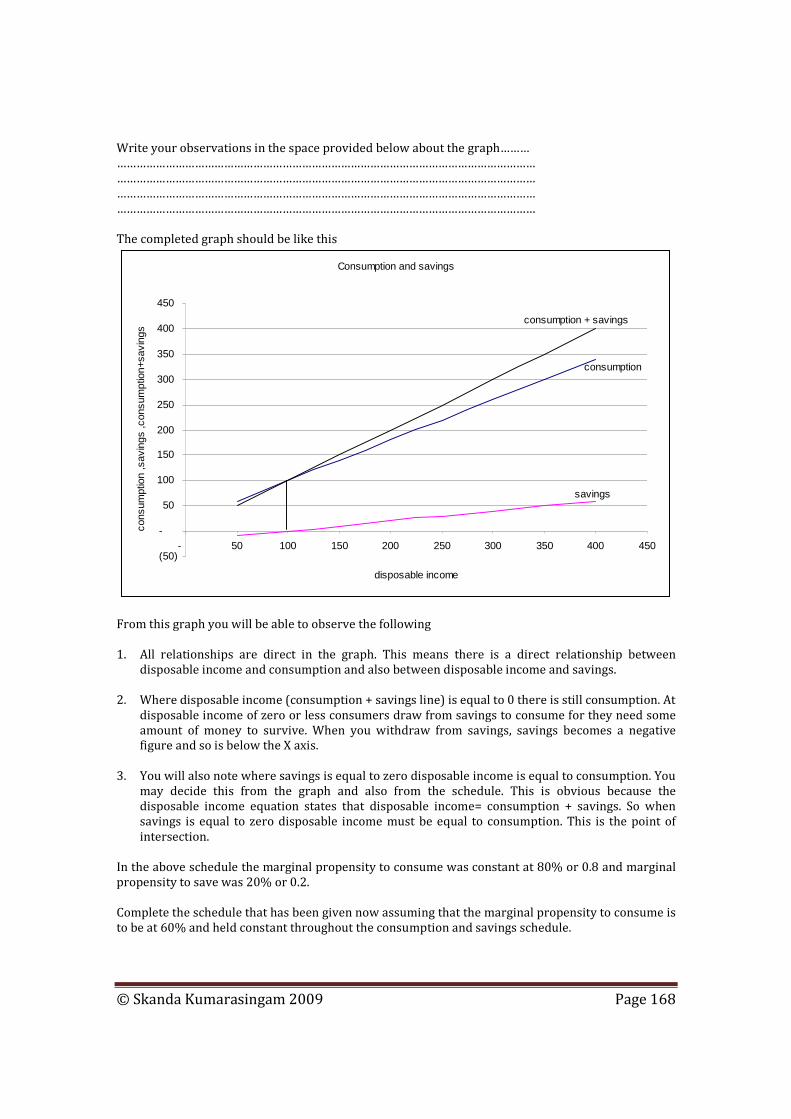
© Skanda Kumarasingam 2009 Page 168
Write your observations in the space provided below about the graph……… ………………………………………………………………………………………………………………… ………………………………………………………………………………………………………………… ………………………………………………………………………………………………………………… ………………………………………………………………………………………………………………… The completed graph should be like this
Consumption and savings
(50)
-
50
100
150
200
250
300
350
400
450
- 50 100 150 200 250 300 350 400 450
disposable income
cons
umpt
ion
,sav
ings
,con
sum
ptio
n+sa
ving
s
consumption + savings
consumption
savings
From this graph you will be able to observe the following 1. All relationships are direct in the graph. This means there is a direct relationship between
disposable income and consumption and also between disposable income and savings. 2. Where disposable income (consumption + savings line) is equal to 0 there is still consumption. At
disposable income of zero or less consumers draw from savings to consume for they need some amount of money to survive. When you withdraw from savings, savings becomes a negative figure and so is below the X axis.
3. You will also note where savings is equal to zero disposable income is equal to consumption. You
may decide this from the graph and also from the schedule. This is obvious because the disposable income equation states that disposable income= consumption + savings. So when savings is equal to zero disposable income must be equal to consumption. This is the point of intersection.
In the above schedule the marginal propensity to consume was constant at 80% or 0.8 and marginal propensity to save was 20% or 0.2. Complete the schedule that has been given now assuming that the marginal propensity to consume is to be at 60% and held constant throughout the consumption and savings schedule.

© Skanda Kumarasingam 2009 Page 169
Marginal propensity to consume is to be 0.80 throughout and constant at all
levels of gross domestic product
Marginal propensity to consume is to be 0.60 throughout and constant at all
levels of gross domestic product
Gross domestic product or disposable
income Consumption Savings
Consumption savings
50 50 50 -
100 80 60 40
150
200
250
300
350
400
Using the information from the schedule above draw a graph where on the X axis you have disposable income and on the Y axis you have the following
• Consumption ( when marginal propensity to consume is 0.80 and 0.60)
• Savings ( when marginal propensity to save is 0.20 and 0.40)
• Disposable income= Consumption + Savings
The completed chart should look like this
Marginal propensity to consume is to be 0.80
throughout and constant at all levels of gross domestic
product
Marginal propensity to consume is to be 0.60
throughout and constant at all levels of gross domestic
product
Gross domestic
product or disposable
income
Consumption=C1 Savings=S1 Consumption=C2 Savings=S2
50 50 - 50 -
100 80 20 60 40
150 120 30 90 60
200 160 40 120 80
250 200 50 150 100
300 240 60 180 120
350 280 70 210 140
400 320 80 240 160

© Skanda Kumarasingam 2009 Page 170
The graph when drawn for the above should be like this
consumption and savings
-
50
100
150
200
250
300
350
- 50 100 150 200 250 300 350 400 450
disposable income
cons
umpt
ion
and
savi
ngs
C1
C2
S2
S1
You will note that if the scales on the X axis and the Y axis are drawn having equal intervals in numbering (like in the above graph having intervals of 50 each) the disposable income line is a 45 degree line which commences from zero. This graph will show you the relationship that takes effect when there is a change in non-income determinants. This is because these curves will show you the movement of the consumption or the savings curves either to the left or right from the original curves which occur due to a change in the non-income determinants. You will also be able to note that where the disposable income line intersects with the consumption line the related savings line intersects the X axis. This is because only where savings is equal to zero (point of intersection on the X axis) does disposable income equal consumption since disposable income = consumption + savings. This is where the disposable income line intersects with the consumption line. Understanding Gross Investment Using Graphical Presentation
In the space provided draw a graph which shows the relationship between the interest rate on the Y axis and the gross investment on the X axis. Show when there is an increase in gross investment and also when there is a decrease in gross investment. You will note that this will look very similar to a demand curve. In fact this is the demand curve of gross investment. What we have essentially plotted is gross investment demand versus the price for the use of capital or interest rate. This is very similar to plotting demand for any product versus price.

© Skanda Kumarasingam 2009 Page 171
The above graph should be like the one below
Relationship of interest rate and gross investment
-
1
2
3
4
5
6
7
8
9
- 5 10 15 20 25 30 35
gross investment
rate
of i
nter
est
gross investment
reduction increase
Now in the space given draw on the X axis the real gross domestic product and on the Y axis gross investment. If there is a direct relationship between gross investment and real gross domestic product the curve will be upward sloping. This is called induced demand. This happens when increased gross domestic product leads to higher revenue which in turn leads to higher profits. When there is anticipation of higher profits obviously the gross investment will increase since you need to have the right capital equipment with you to reap the benefits of a high anticipated economic profit or revenue as explained previously.

© Skanda Kumarasingam 2009 Page 172
The above graph should look like this
Induced gross investment
0
10
20
30
40
50
60
70
0 20 40 60 80 100 120 140
gross domestic product
gros
s in
vest
men
t
There is also another type investment which is called as autonomous investment. This is not dependent on real gross domestic product and so is a straight line and is parallel to the X axis. In the space below draw the relationship between autonomous investment and gross domestic product. On the X axis you will have real gross domestic product and on the Y axis you will have gross investment.
You will see the relationship of autonomous investment with gross domestic product in the graph below
Autonomous gross investment
0
5
10
0 20 40 60 80 100 120 140
gross investment
gros
s in
vest
men
t

© Skanda Kumarasingam 2009 Page 173
Two Sector Economies
Having studied how consumers and business firms behave individually we are now in a position to combine business firms and households (which comprise consumers who are either families or individuals living in the economy) to study how they interact with one another in a two sector economy. We already know that consumers will use the disposable income to buy products and services for consumption or to save. Business firms will invest. Let us now try to complete the schedule that is provided to obtain a better understanding of how a two sector economy operates. The information required to complete this schedule is provided now
• Gross domestic product = disposable income (refer back to the assumptions made)
• This disposable income can only be used for consumption or savings and nothing else by the consumer
• Autonomous investment= 25. We already know when we talk about autonomous investment there will be no change in the investment even if there is a change in the gross domestic product.
• Aggregate expenditure or planned expenditure= consumption+ gross investment
• Unintended gross investment or disinvestment = gross domestic product- aggregate expenditure (or planned expenditure)

© Skanda Kumarasingam 2009 Page 174
Gross
domestic product or disposable
income
Consumption Savings Autonomous gross
investment
Aggregate expenditure
(planned expenditure)
Unintended gross
investment or disinvestment
Autonomous gross
investment
Aggregate expenditure
(planned expenditure)
Autonomous gross
investment
Aggregate expenditure
(planned expenditure)
Is a constant Consumption + gross
investment
Gross domestic product less
aggregate expenditure
Is a constant Consumption + gross
investment
Is a constant Consumption + gross
investment
300 295
25 30 20
325 315
25 30 20
350 335
25 30 20
375 355
25 30 20
400 375
25 30 20
425 395
25 30 20
450 415
25 30 20
475 435
25 30 20
In the space provided write your observations about the above schedule……………………………………………………………… ………………………………………………………………………………………………………………………………………………………………………....... ………………………………………………………………………………………………………………………………………………………………………....... ………………………………………………………………………………………………………………………………………………………………………....... ………………………………………………………………………………………………………………………………………………………………………....... ………………………………………………………………………………………………………………………………………………………………………....... ………………………………………………………………………………………………………………………………………………………………………....... ………………………………………………………………………………………………………………………………………………………………………....... ………………………………………………………………………………………………………………………………………………………………………....... ………………………………………………………………………………………………………………………………………………………………………....... ……………………………………………………………………………………………………………………………………………………………………….......

© Skanda Kumarasingam 2009 Page 175
Now turn to the next page to see how this chart is completed Gross domestic product or disposable income
Consumption Savings Autonomous gross investment
Aggregate expenditure (planned expenditure)
Unintended gross investment or disinvestment
Autonomous gross investment
Aggregate expenditure (planned expenditure)
Autonomous gross investment
Aggregate expenditure (planned expenditure)
Is a constant Consumption + gross investment
Gross domestic product less aggregate expenditure
Is a constant Consumption + gross investment
Is a constant Consumption + gross investment
300
295
5
25
320 (20)
30
325 20
315
325
315
10
25
340 (15)
30
345 20
335
350
335
15
25
360 (10)
30
365 20
355
375
355
20
25
380 (5)
30
385 20
375
400
375
25
25
400 - 30
405 20
395
425
395
30
25
420 5
30
425 20
415
450
415
35
25
440 10
30
445 20
435
475
435
40
25
460 15
30
465 20
455

© Skanda Kumarasingam 2009 Page 176
Observations from the schedule
• Gross domestic product (disposable income) and (consumption + gross investment) when tabulated together is called the aggregate expenditure schedule.
• In a two sector economy you have consumers and firms only. So aggregate expenditure or planned expenditure is = consumption + gross investment
• Aggregate expenditure( what consumers and businesses want to spend) should be equal to the gross domestic product( what producers of consumer goods and capital goods want to produce and sell)
• Due to this reason if aggregate expenditure (or planned expenditure) is > the gross domestic product business firms will want to produce more because there is a need (planned expenditure) which is higher than what is being produced and sold now. So suppliers will want to produce more (increase real gross domestic product) to sell more and make more economic profits. This happens at points where unintended gross investment or disinvestment is less than zero or negative. The opposite happens when unintended gross investment or disinvestment is greater than zero. This is because when production (real gross domestic product) is > what business firms and consumers plan to spend (aggregate expenditure or planned expenditure). In such a situation there will be over production which will lead to losses to the supplier (producer of consumer and capital goods) as they will not be able to sell what they produce in excess. So they will reduce production and reduce unintended gross investment until aggregate expenditure is equal to gross domestic product.
• Where gross domestic product is equal to aggregate expenditure you will note that there is no unintended gross investment or disinvestment in the economy. This is the position or point which every economy will try to reach. This is called the equilibrium gross domestic product.
• So we can say at the equilibrium gross domestic product that equilibrium gross domestic product= consumption + gross investment
• At equilibrium gross domestic product we also know that savings = gross investment Using the information that was obtained from the schedule draw a graph in the space provided below. On the X axis you will have real gross domestic product. On the Y axis you should have the following
1. gross domestic product= disposable income= consumption + savings 2. aggregate expenditure( planned expenditure)= consumption + gross investment 3. consumption 4. savings 5. autonomous gross investment

© Skanda Kumarasingam 2009 Page 177
At the equilibrium gross domestic product from the graph
• The gross domestic product (consumption + savings) = aggregate expenditure
• Savings= Gross investment
Equilibrium point identif ication
-
50
100
150
200
250
300
350
400
450
500
300 320 340 360 380 400 420 440 460 480 500
gross domestic product
cons
umpt
ion
+ sa
ving
s,ag
greg
ate
expe
nditu
re,c
onsu
mpt
ion,
savi
ngs,
gro
ss in
vest
men
t
consumption+ savings
consumption + Ig
consumptio
savings
Ig

© Skanda Kumarasingam 2009 Page 178
Also from the graphs we can note that the distance between the (consumption + savings) line and the consumption line will give you the savings at a particular real gross domestic product From the graph we can note that the distance between the (consumption + gross investment) line and the consumption line will give you the gross investment at a particular real gross domestic product
Gross investment= Savings is the equilibrium point
At the equilibrium point we know that consumption+ gross investment = consumption + savings As consumption is common on both sides of the equation we can then conclude that gross investment = savings. Effects of the Multiplier
Now go back to the schedule and complete the columns where autonomous investment is equal to 30 and aggregate expenditure when gross investment increases to 30. In a similar manner complete the columns where autonomous gross investment is equal to 20 and aggregate expenditure when gross investment reduces to 20. Identify the new equilibrium gross domestic product. The equilibrium gross domestic product is where gross domestic product is equal to aggregate expenditure (planned expenditure) You will note when gross investment increases by five (from 25 to 30) equilibrium gross domestic product increased by 25. In a similar manner you will note when gross investment reduced by five (from 25 to 20) equilibrium gross domestic product reduced by 25 So we can say that gross domestic product changes by a multiple when there is a change of 5 in gross investments, gross domestic product increases or reduces by 25. This is called the multiplier effect We can say
Increase in gross domestic product= Increase in gross investment X Multiplier
The multiplier is calculated as follows
Multiplier =1/ Marginal propensity to save
Or
Multiplier =1/ (1- Marginal propensity to consume)
Let me now explain to you how the multiplier effect works. This is best explained by the table that has been completed in the next page. However to understand this will also have to understand how

© Skanda Kumarasingam 2009 Page 179
the columns in the table are completed. It involves a series of steps and is circular in nature. Here is the explanation first in pictorial form
Multiplier Effect of Gross Investment Increase by 5
Round Increase in Increase in Increase in
Gross Consumption Savings
Domestic (GDP X MPC)
Product MPC=0.80
1 5.00 4.00 1.00
2 4.00 3.20 0.80
3 3.20 2.56 0.64
4 2.56 2.05 0.51
5 2.05 1.64 0.41
6 1.64 1.31 0.33
7 1.31 1.05 0.26
8 1.05 0.84 0.21
9 0.84 0.67 0.17
10 0.67 0.54 0.13
11 0.54 0.43 0.11
12 0.43 0.34 0.09
13 0.34 0.27 0.07
14 0.27 0.22 0.05
15 0.22 0.18 0.04
16 0.18 0.14 0.04
Gross domestic product increases
by 5
Consumption increases by 5 X
Marginal propensity to
consume
Aggregate expenditure
increases by 5 (Gross Investment
+ consumption)
Disposable income increases by 5
When gross investment increases by 5

© Skanda Kumarasingam 2009 Page 180
17 0.14 0.11 0.03
18 0.11 0.09 0.02
19 0.09 0.07 0.02
20 0.07 0.06 0.01
21 0.06 0.05 0.01
22 0.05 0.04 0.01
23 0.04 0.03 0.01
24 0.03 0.02 0.01
25 0.02 0.02 0.00
26 0.02 0.02 0.00
27 0.02 0.01 0.00
28 0.01 0.01 0.00
29 0.01 0.01 0.00
30 0.01 0.01 0.00
31 0.01 0.00 0.00
Total 24.98 19.98 5.00
Say 25.00 20.00 5.00
1. Let us say that gross investment increases by five. 2. This will increase aggregate expenditure by five because aggregate expenditure is equal to
consumption + gross investment.
3. When aggregate expenditure increases by five we can say that the equilibrium gross domestic product will also increase by five.
4. Obviously when gross domestic product increases by five disposable income which is equal
to gross domestic product should also increase by five.
5. When disposable income increases by five consumption will increase by five multiplied by the marginal propensity to consume. In this case it is 5 X 0.8=4
6. When consumption increases by an amount which is equal to disposable income multiplied
by the marginal propensity to consume(4 as noted above) it will go on to increase the aggregate expenditure since aggregate expenditure = gross investment + consumption.
7. This cycle will continue but the amount that is fed in by consumption will keep reducing
with every cycle because the amount that is spent is equal to the new disposable income multiplied by the marginal propensity to consume. Finally when this amount reaches zero the cycle will stop.
8. When the cycle stops you will also understand that savings is equal to gross investment. This
is something that we already know from the schedule, equations and the graph we have already drawn.
Open Economy
Now let us look at an open economy which comprises trade with the external world or outside the economy. Fill the schedule that is provided in the next page.

© Skanda Kumarasingam 2009 Page 181
X denotes exports and it is equal to 30. Calculate the aggregate expenditure (or planned expenditure) which is equal to consumption+ gross investment + exports. With only exports the equilibrium gross domestic product is equal to 610. At the equilibrium gross domestic product we also note that
• Gross domestic product = aggregate expenditure
• Consumption + savings= consumption+ gross investment + exports
• So we can say that savings = gross investment plus exports You should be able to identify the above from the schedule M denotes imports. Imports simply mean what we spend on goods and services that have been produced in other economies.
Net exports = Export-Imports
Imports are deducted from exports and we use the net export figure when calculating aggregate expenditure as it (that is imports) is not spent on our economy. Also because our economy does not produce the imported goods and services it cannot form a part of the economy’s gross domestic product We can now extend the equations as follows
Aggregate expenditure= Consumption+ Gross investment + Net exports

© Skanda Kumarasingam 2009 Page 182
Gross domestic product
Consumption Savings Gross autonomous investment
(Ig)
Aggregate expenditure
(AE)
Exports(X) Aggregate expenditure with exports
Imports (M)
Net exports
(Xn)
Aggregate expenditure with
net exports
GDP C S= GDP-C Ig =Constant =20
AE = C + Ig X=Constant = 30
AE = C +Ig + X X-M AE = C+ Ig + Xn
450
432 27
460
440 30
470
448 33
490
464 39
510
480 45
530
496 51
550
512 57
570
528 63
590
544 69
610
560 75
630
576 81
Note your observations in the space given. Note carefully what happens to the equilibrium gross domestic product before exports are introduced, after exports are introduced and when net exports (exports less imports) are introduced……………………………………………… …………………………………………………………………………………………………………………………………………………………………………... …………………………………………………………………………………………………………………………………………………………………………... …………………………………………………………………………………………………………………………………………………………………………... …………………………………………………………………………………………………………………………………………………………………………... …………………………………………………………………………………………………………………………………………………………………………... Turn to the next page to see the completed chart

© Skanda Kumarasingam 2009 Page 183
Gross domestic product
Consumption Savings Gross autonomous investment
(Ig)
Aggregate expenditure
(AE)
Exports(X) Aggregate expenditure with exports
Imports (M)
Net exports
(Xn)
Aggregate expenditure
with net exports
GDP C S= GDP-C Ig =Constant =20
AE = C + Ig X=Constant = 30
AE = C +Ig + X X-M AE = C+ Ig + Xn
450
432
18
20
452 30
482
27
3
455
460
440
20
20
460 30
490
30
-
460
470
448
22
20
468 30
498
33
(3)
465
490
464
26
20
484 30
514
39
(9)
475
510
480
30
20
500 30
530
45
(15)
485
530
496
34
20
516 30
546
51
(21)
495
550
512
38
20
532 30
562
57
(27)
505
570
528
42
20
548 30
578
63
(33)
515
590
544
46
20
564 30
594
69
(39)
525
610
560
50
20
580
30
610
75
(45)
535
630
576
54
20
596 30
626
81
(51)
545

© Skanda Kumarasingam 2009 Page 184
At equilibrium we know that gross domestic product = Aggregate expenditure. At this point, Consumption + Savings = Consumption + Gross investment + Exports- Imports Savings= Gross investment + Exports- Imports (eliminating consumption from both sides of the equation)
Savings+ Imports= Gross investment + Exports (rearranging the above equation)
Savings plus imports are called leakages whereas aggregate investment and exports are called injections.
We can also say savings = gross investment + net exports
We also know when exports of 30 are introduced gross domestic product increases by 150(from 460 to 610). You can observe this from the schedule above. This is called the multiplier effect. Where there are no imports the multiplier = 1/ marginal propensity to save OR 1/ (1- marginal propensity to consume)
However in an open economy the multiplier is modified to become1/ (marginal propensity to save + marginal propensity to import)
Marginal propensity to import= change in import/ change in gross domestic product (or changes in disposable income)
Now fill the next detailed schedule that is provided. You will note two important rules which are given below Rule 1-Equal increases in consumption (or gross investment or exports) or an equal or similar reduction in savings (or imports) will have an equal impact on aggregate expenditure or gross domestic product at the equilibrium point. That is a similar reduction in withdrawals or a similar increase in injections will not cause the equilibrium gross domestic product to change. Like stated before withdrawals are savings and imports and the injections are gross investment and exports Rule 2-Increase in gross domestic product at the equilibrium point is equal to the Change in the aggregate expenditure X open economy multiplier.
The open economy multiplier= 1/ (Marginal propensity to save + marginal propensity to import)

© Skanda Kumarasingam 2009 Page 185
Gross domestic product = disposable income
Consumption (C) where marginal propensity to consume = 0.80
Savings(S) Autonomous gross investment(Ig) of 20
Exports (X) held constant at 30
Imports (M)
Net exports (Xn) Xn=X-M
Aggregate Expenditure = C+Ig+Xn
New Aggregate Expenditure = C+Ig+Xn Where Ig increases from 20 to 30 (by 10)
New Aggregate Expenditure = C+Ig+Xn Where X increases from 30 to 40 (by 10)
New Aggregate Expenditure = C+Ig+Xn Where M reduces by 10
New Aggregate Expenditure = C+Ig+Xn Where C increases by 10 or S reduces by 10
420 408 18
430 416 21
440 24
450 27
460 30
470 33
480 36
490 39
500 42
510 45
520 48
530 51
540 54
550 57
560 60
570 63
580 66
590 69
600 72
610 75
620 78
630 81
Note how the two rules operate from the schedule in your own words………………………………………………………………………………………………… …………………………………………………………………………………………………………………………………………………………………………... …………………………………………………………………………………………………………………………………………………………………………... …………………………………………………………………………………………………………………………………………………………………………...

© Skanda Kumarasingam 2009 Page 186
Net exports (Xn)
New Aggregate Expenditure =
C+Ig+Xn
New Aggregate
Expenditure = C+Ig+Xn
New Aggregate
Expenditure = C+Ig+Xn
New Aggregate
Expenditure = C+Ig+Xn
Gross domestic product = disposable
income
Consumption (C) where marginal
propensity to consume =
0.80
Savings(S)
Autonomous gross
investment(Ig) of 20
Exports (X) held
constant at 30
Imports (M)
Xn=X-M
Aggregate Expenditure
= C+Ig+Xn
Where Ig increases from 20
to 30 (by 10)
Where X increases
from 30 to 40 (by 10)
Where M reduces by
10
Where C increases by
10 or S reduces by
10
420 408 12 20 30 18 12 440 450 450 450 450
430 416 14 20 30 21 9 445 455 455 455 455
440 424 16 20 30 24 6 450 460 460 460 460
450 432 18 20 30 27 3 455 465 465 465 465
460 440 20 20 30 30 - 460 470 470 470 470
470 448 22 20 30 33 (3) 465 475 475 475 475
480 456 24 20 30 36 (6) 470 480 480 480 480
490 464 26 20 30 39 (9) 475 485 485 485 485
500 472 28 20 30 42 (12) 480 490 490 490 490
510 480 30 20 30 45 (15) 485 495 495 495 495
520 488 32 20 30 48 (18) 490 500 500 500 500
530 496 34 20 30 51 (21) 495 505 505 505 505
540 504 36 20 30 54 (24) 500 510 510 510 510
550 512 38 20 30 57 (27) 505 515 515 515 515
560 520 40 20 30 60 (30) 510 520 520 520 520
570 528 42 20 30 63 (33) 515 525 525 525 525
580 536 44 20 30 66 (36) 520 530 530 530 530
590 544 46 20 30 69 (39) 525 535 535 535 535
600 552 48 20 30 72 (42) 530 540 540 540 540
610 560 50 20 30 75 (45) 535 545 545 545 545
620 568 52 20 30 78 (48) 540 550 550 550 550

© Skanda Kumarasingam 2009 Page 187
Government Expenditure and Taxes in the Open Economy
Now finally let us consider an economy bringing in the government. The government will be involved in the economy by spending called the government expenditure and taxation (or transfer payments which follow the reverse rules of taxation) Before taxation is introduced gross domestic product (or disposable income) is used for consumption and savings. After the government introduces tax disposable income can only do three things which are 1. Consumption 2. Savings 3. Pay taxes Consumption and savings are affected by the marginal propensity to consume and the marginal propensity to save. Taxes increase or decrease the disposable income.
Aggregate expenditure= consumption+ gross investment+ net exports+ government expenditure
Consumption, gross investment, net exports and government expenditure have multiplier effects.
Gross domestic product = disposable income = consumption + savings + tax
Aggregate expenditure= consumption + gross investment+ net exports+ government expenditure
At equilibrium gross domestic product = aggregate expenditure Consumption + savings+ tax= consumption+ gross investment + net exports + government expenditure Savings+ tax= gross investment + net exports + government expenditure (eliminating consumption from both sides of the equation)
Savings and taxation are withdrawals
Gross investment, net exports and government expenditure are injections
You will be able to find the answers to the questions given below by completing the schedule and studying them carefully. What happens to the equilibrium gross domestic product when there is no taxation? ………………………………………………………………………………………………………………… ………………………………………………………………………………………………………………… …………………………………………………………………………………………………………………

© Skanda Kumarasingam 2009 Page 188
What happens to the equilibrium gross domestic product when there is taxation of 10? ………………………………………………………………………………………………………………… ………………………………………………………………………………………………………………… ………………………………………………………………………………………………………………… Next what happens to the equilibrium gross domestic product if the government decides to spend 18 in the economy? ……………………………………………………………………………………………………... ………………………………………………………………………………………………………………… ………………………………………………………………………………………………………………… ………………………………………………………………………………………………………………… Tax multiplier= regular multiplier-1 Find out what happens when tax increases by 10 and government expenditure also increases by 10 to the equilibrium gross domestic product. This is called the rule for equal increases. What is this rule? ………………………………………………………………………………………………………………… ………………………………………………………………………………………………………………… ………………………………………………………………………………………………………………… ………………………………………………………………………………………………………………… ………………………………………………………………………………………………………………… Find out what happens to the equilibrium across domestic product when taxes reduced by 6 and the government expenditures increased by5. This will tell us the net result rule. What is it? ………………………………………………………………………………………………………………… ………………………………………………………………………………………………………………… ………………………………………………………………………………………………………………… …………………………………………………………………………………………………………………
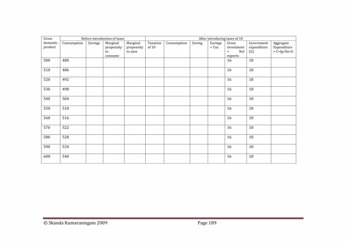
© Skanda Kumarasingam 2009 Page 189
Before introduction of taxes After introducing taxes of 10 Gross domestic product
Consumption Savings Marginal propensity to consume
Marginal propensity to save
Taxation of 10
Consumption Saving Savings + Tax
Gross investment + Net exports
Government expenditure (G)
Aggregate Expenditure = C+Ig+Xn+G
500 480
16 18
510 486
16 18
520 492
16 18
530 498
16 18
540 504
16 18
550 510
16 18
560 516
16 18
570 522
16 18
580
528 16 18
590
534 16 18
600
540 16 18

© Skanda Kumarasingam 2009 Page 190
Equal increases in taxation and government expenditure of 10 compared to previous schedule=rule of equal increases
Unequal changes where tax reduced by 6 and government expenditure rose by 5= net results rule
Gross domestic product Taxation Consumption Savings Gross
investment + Net exports
Government expenditure (G)
Aggregate Expenditure = C+Ig+Xn+G
Tax reduced by 6
New consumption when tax is 14
New savings when tax is 14
Government expenditure increased by 5
New aggregate expenditure = C+Ig+Xn+G
500
20 460 16 28 14 33
510
20 466 16 28 14 33
520
20 472 16 28 14 33
530
20 478 16 28 14 33
540
20 484 16 28 14 33
550
20 490 16 28 14 33
560
20 496 16 28 14 33
570
20 502 16 28 14 33
580
20 508 16 28 14 33
590
20 514 16 28 14 33
600
20 520 16 28 14 33
The answers to the above two graphs are provided below

© Skanda Kumarasingam 2009 Page 191
Before introduction of taxes After introducing taxes of 10
Gross domestic product Consumption Savings
Marginal propensity to
consume
Marginal propensity to save
Taxation of 10
Consumption
Saving Savings +
Tax
Gross investment + Net exports
Government expenditure
(G)
Aggregate Expenditure
= C+Ig+Xn+G
500 480 20 10 474 16 26 16 18 508
510 486 24 0.60 0.40 10 480 20 30 16 18 514
520 492 28 0.60 0.40 10 486 24 34 16 18 520
530 498 32 0.60 0.40 10 492 28 38 16 18 526
540 504 36 0.60 0.40 10 498 32 42 16 18 532
550 510 40 0.60 0.40 10 504 36 46 16 18 538
560 516 44 0.60 0.40 10 510 40 50 16 18 544
570 522 48 0.60 0.40 10 516 44 54 16 18 550
580 528 52 0.60 0.40 10 522 48 58 16 18 556
590 534 56 0.60 0.40 10 528 52 62 16 18 562
600 540 60 0.60 0.40 10 534 56 66 16 18 568

© Skanda Kumarasingam 2009 Page 192
Equal increases in taxation and government expenditure of 10 compared to previous schedule=rule of equal increases
Unequal changes where tax reduced by 6 and government expenditure rose by 5= net results rule
New aggregate
expenditure =
Gross domestic product
Taxation Consumption Savings
Gross investment
+ Net exports
Government expenditure
(G)
Aggregate Expenditure
= C+Ig+Xn+G
Tax reduced
by 6
New consumption when tax is
14
New savings when tax is
14
Government expenditure
increased by 5
C+Ig+Xn+G
500 20 460 20 16 28 504 14 464 22 33 513
510 20 466 24 16 28 510 14 470 26 33 519
520 20 472 28 16 28 516 14 476 30 33 525
530 20 478 32 16 28 522 14 482 34 33 531
540 20 484 36 16 28 528 14 488 38 33 537
550 20 490 40 16 28 534 14 494 42 33 543
560 20 496 44 16 28 540 14 500 46 33 549
570 20 502 48 16 28 546 14 506 50 33 555
580 20 508 52 16 28 552 14 512 54 33 561
590 20 514 56 16 28 558 14 518 58 33 567
600 20 520 60 16 28 564 14 524 62 33 573

© Skanda Kumarasingam 2009 Page 193
Review
Question 1 In your own words how would you define or compute The average propensity to consume…………………………………………………………… ………………………………………………………………………………………………………………… The average propensity to save………………………………………………………………… ………………………………………………………………………………………………………………… The marginal propensity to consume………………………………………………………… ………………………………………………………………………………………………………………… The marginal propensity to save………………………………………………………………… ………………………………………………………………………………………………………………… Question 2 The average propensity to consume tends to (increase/ decrease) as disposable income increases and vice versa. The average propensity to save tends to (rise/ fall) as the disposable income rises and vice versa. The average propensity to consume plus the average propensity to save are equal to....................... %. The marginal propensity to consume plus the marginal propensity to save are equal to....................... % Question 3 The average propensity to consume (can/ cannot) be greater than one. The average propensity to save is less than zero when the amount of savings is (more/ less) than zero. Their average propensity to consume is > 1 when consumption is (more/ less) than disposable income Question 4 The rate of interest is the price paid for the......... of..........................., is a (cost/ revenue/ profit) for a firm and is (directly/ inversely) related to the amount of gross investment Question 5 When a firm Borrows money to spend for capital goods it (does/ does not) have an interest cost. Uses its own money for more capital it (does/ does not) have to consider the cost of using its money to acquire capital Question 6 Gross investment will.................. in the economy when the interest rate increases and vice versa. To increase gross investment the rate of interest must............................. Question 7 If gross investment increases when the gross domestic product increases investment is said to be......................... If investment is autonomous as gross domestic product increases gross investment will (increase/ decrease/ remain constant) Question 8 The aggregate expenditures schedule indicates the total amount of spending for................ and for......................... at various levels of................................. Question 9 The equilibrium gross domestic product can be discovered either by finding the gross domestic product at which...................=......................... or the gross domestic product at which............................ =............................... Because the gross domestic product is another name for the domestic output of the economy and the total amount of spending in the economy are its aggregate expenditures for goods and services when

© Skanda Kumarasingam 2009 Page 194
the economy produces its equilibrium gross domestic product the..................... is equal to the........................... made by consumers and business firms for goods and services Question 10 At gross domestic products > the equilibrium gross domestic product, gross domestic product is.................than consumption + gross investment and savings is............. than gross investment At gross domestic products less than the equilibrium gross domestic product, gross domestic product is..........................than consumption + gross investment and savings is...................... than gross investment Question 11 Business firms are motivated by their desire for profits. Therefore when consumption + gross investment is greater than gross domestic product they will.................. their production and the gross domestic product. Similarly they will decrease their production and the............... whenever total spending for........................ and.................... is (>/ <) the gross domestic product Question 12 When gross investment increases by 3, gross domestic product will (increase/ decrease) by (more/ less) than 3. And were gross investment to decrease by 5 gross domestic product (rises/falls) by (more/ less) than 5. Question 13 This tendency for gross domestic product to change in the same direction as the change in gross investment although by a greater amount is called the................................ Question 14 The size of the multiplier is equal to 1 divided by either.............................or.............................. Question 15 If the multiplier was 4 and gross investment was to rise by 20 the gross domestic product would expand by..................... Question 16 When the multiplier is 3 a 75 fall in gross domestic product tells us that investment has..................... by.......................... Question 17 When there is foreign spending for a nation's goods and services the equilibrium gross domestic product is the gross domestic product at which aggregate.................................. and total.............................are equal Question 18 At the equilibrium gross domestic product, gross domestic product =. .................................+....................................+............................. Consumption +....................are also equal to.........................+....................................+...................... Therefore savings = ........................+........................ Question 19 When the marginal propensity to consume this 0.70 the multiplier is equal to............................and a 9 decrease in exports will cause the equilibrium gross domestic product to (rise/ fall) by..................................

© Skanda Kumarasingam 2009 Page 195
Question 20 When an economy is opened to foreign trade exports is added to consumption and gross investment as a new component of aggregate................................and imports is added to savings as a new...................... from the income stream Question 21 The open economy multiplier =......................... it has a value (higher than/ lower than/ the same as) the closed economy multiplier because imports like savings is............................................................................... ………………………………………………………………………………………………………………… Question 22 At the equilibrium level of gross domestic product that is when total output =..............................., savings+ imports=.............................+...................................even when savings (is/ is not) equal to gross investment and imports (is/ is not) equal to........................... Question 23 When there is government purchasing of goods and services the equilibrium gross domestic product is the gross domestic product at which aggregate.............................. and ............................... are equal Question 24 At the equilibrium gross domestic product, gross domestic product =..................................+.......................+..............................+......................... Consumption+.......................... are also equal to..................................+............................................+.........................+.................................. Therefore savings =.........................+................................+..................................... Question 25 When government purchases increases, gross domestic product will (increase/ decrease) by an amount (>/ <) the increase in government purchases or spending Question 26 When the marginal propensity to consume is 0.70 the multiplier is equal to.............................and a 20 decrease in government spending will cause the equilibrium gross domestic product to (rise/fall) by.................................... Question 27 Look at the following table
Gross domestic product Consumption Savings
550 500 50
560 508 52
570 516 54
580 524 56
The marginal propensity to consume is equal to.................... The spending multiplier is therefore equal to.............................. If gross investment plus net exports were 50 the equilibrium gross domestic product would be........................... Question 28 Now forget the schedule in the proceeding paragraph. Remember only that the spending multiplier is five and that when gross investment+ net export is 50 the equilibrium gross domestic product is550. Step-by-step let us put government into the picture. If government spending increases from 0 to 30 the equilibrium gross domestic product rises from 500 to..........................

© Skanda Kumarasingam 2009 Page 196
Question 29 Now suppose government levies taxes of 40. The equilibrium gross domestic product will fall to.................................. Question 30 Finally let us have the government making transfer payments of 10. The equilibrium gross domestic product will now be................................. Question 31 If the government believed that the gross domestic product of 580 was 40 too high it could lower it to 540 in any of the three ways By (raising/ lowering) taxes by................. By (raising/ lowering) its purchases of goods and services by....................... Or by (raising/ lowering) its transfer payments by................................
Answers
Suggested answers to the above questions are given. The answers are provided sequentially in the same order you will fill the blanks or select from a choice in the brackets
Question 1 A percentage or fraction of disposable income spent for consumption (consumption/disposable income) A percentage or fraction of disposable income saved (savings/disposable income) A percentage or fraction of change in disposable income spent for consumption (change in consumption/change in disposable income) A percentage or fraction of change in disposable income saved (change in savings/change in disposable income) Question 2 Decrease Rise 100 100 Question 3 Can Less More Question 4 Use Money Cost Inversely
Question 5 Does Does Question 6 Decrease Fall or decrease Question 7 Induced Remain constant Question 8 Consumption Investment Gross domestic product Question 9 Gross domestic product Consumption Gross investment Savings Gross investment Domestic output Aggregate expenditures Question 10 Greater Greater Less Less Question 11 Increase Gross domestic product Consumption Gross investment Less

© Skanda Kumarasingam 2009 Page 197
Question 12 Increase More Fall More Question 13 Multiplier effect Question 14 Marginal propensity to save Or 1- marginal propensity to consume Question 15 80 Question 16 Fallen 25 Question 17 Expenditures Production Question 18 Consumption Gross investment Exports Savings Consumption Gross investment Exports Gross investments Exports Question 19 3.33 Fall 30 Question 20 Expenditures Leakage Question 21 1/ (marginal propensity to save+ marginal propensity to import) Lower than A subtraction from spending on domestic production (leakage) Question 22 Aggregate expenditures Gross investment
Exports Is not Is not Exports Question 23 Expenditures Gross domestic product Question 24 Consumption Gross investment Net exports Government spending Savings Consumption Gross investment Net exports Government purchases (spending) Gross investment Net exports Government spending Question 25 Increase Greater Question 26 3.33 Fallen 66.66 Question 27 0.80 5 550 Question 28 700 Question 29 540 Question 30 580 Question 31 Raising 10 Lowering 8 Lowering 10

© Skanda Kumarasingam 2009 Page 198
Chapter 11
International Trade and Balance of Payments Learning Outcomes
• To understand the fundamental reasons why trade takes place between individuals or businesses and between one nation and another and to appreciate that these reasons are common whether it is between individuals or businesses or one nation and another
• To understand the concept of the law of comparative advantage which provides the first fundamental reason for trade
• To appreciate the importance of specialization which provides the second fundamental reason for trade
• To learn what the terms of trade are so that we will be capable of understanding the third fundamental reason for trade
• To understand what foreign-exchange means and its features and principle concepts
• To learn the law of demand and supply for foreign exchange which explains as to how market forces determine the foreign exchange rates
• To learn the importance of balance of payments and how it is managed by governments
• Review questions which will help to summarize the complete chapter so that you will be capable of using it for revision. The suggested answers for these review questions are provided.
Chapter Outline
• Fundamental questions of trade
• Law of comparative advantage
• Importance of specialization
• Terms of trade
• Foreign exchange
• Law of demand and supply for foreign exchange
• Balance of payment
• Review( chapter summary)
• Answers to review questions

© Skanda Kumarasingam 2009 Page 199
Fundamental Questions of Trade
Every nation in this world (there are approximately 180 of them) have citizens, business firms and a government within them. The citizens, business firms and the government buy and sell goods and services amongst themselves. However we have also seen that a particular nation may also buy goods and services from other countries and sell its products and services to them. International trade simply means trade between two nations or amongst many nations. Even though trade takes place between different nations buyers buy and sellers sell for the same reason like we do within the domestic market of our country. We need to now understand why trade takes place between different nations. To understand why trade takes place between two nations we also ask the question why do people or citizens of a country and business firms trade amongst one another within a nation. The simple answer you can give for this is that each individual or business firm will specialize in making one single or a few commodities (or products) and /or services and may not produce most of the other goods and services that they/it needs and consumes. So trading between one another is useful as it helps the producer of a particular commodity (or product) or service to sell the surplus to others and to buy from them what they produce in excess so that they are able to fulfill a wider variety of their needs. To understand trade and particularly international trade we need to ask three important questions. They are fundamental questions not only to understand international trade but also trade between members of a society or business firms within a nation. These fundamental questions are
• What commodity (product) will each nation or an individual specialize in making?
• Why should an individual or nations specialize?
• When nations on individuals specialize and trade what would be the terms of trade? Law of Comparative Advantage (What to specialize in?)
In trying to develop answers to the above three questions we have to gain an understanding on an important economic concept called the law of comparative advantage. Look at the table provided for a country called Tasmania. You will identify from the previous studies that this table is the production possibilities schedule. Tasmania is able to produce only two different items which are corn and wheat using specific resources it has. The production possibilities schedule is prepared assuming that the economy is a fully efficient economy and so all the resources it has are used and the best possible technology is employed. Also the production possibilities schedule is prepared for a period of time when resources or technology will not change.
Combinations of production possibilities Product
A B C D E F G H I
Corn 0 50 100 150 200 250 300 350 400
Wheat 1200 1050 900 750 600 450 300 150 0
Opportunity cost of producing corn (in wheat)
Opportunity cost of producing wheat (in corn)

© Skanda Kumarasingam 2009 Page 200
Tasmania is capable of producing either corn or wheat in different combinations. We also note that as the production of a particular commodity keeps increasing the production of the other has to reduce and vice versa. So we need to make a choice. Wherever there are choices to be made there is obviously a cost. In economics any cost is called an economic cost. All economic costs are also called opportunity costs. Opportunity cost means what you give up to get something. In the above schedule we can say that the opportunity cost of producing wheat is how many units of corn Tasmania will have to give up. Similarly the opportunity cost of producing corn is how many units of wheat it will have to give up. Fill in the opportunity costs in the above schedule. We can observe that if Tasmania wants to increase the production of corn by 50 units it will have to give up 150 units of wheat. Hence the opportunity cost of producing one unit of corn is equal to three units of wheat that have been given up. We can also observe that if Tasmania wants to increase the production of wheat by 150 units it will have to give up 50 units of corn. Hence the opportunity cost of one unit of wheat must be equal to 0.33 units of corn. Here is the above chart completed where opportunity costs are incorporated
Combinations of production possibilities-Tasmania Product
A B C D E F G H I
Corn - 50 100 150 200 250 300 350 400
Wheat 1,200 1,050 900 750 600 450 300 150 -
Opportunity cost of producing corn( in wheat)
- 3 3 3 3 3 3 3 3
Opportunity cost of producing wheat( in corn)
0.33 0.33 0.33 0.33 0.33 0.33 0.33 0.33 -
Now let us look at the production possibilities schedule of another country called Stanford.
Combinations of production possibilities Product
A B C D E F
Corn 0 90 180 270 360 450
Wheat 1800 1440 1080 720 360 0
Opportunity cost of producing corn(in wheat)
Opportunity cost of producing wheat(in corn)
We can observe that in Stanford to produce 90 units of corn it has to give up 360 units of wheat. This means the opportunity cost of producing one unit of corn is equal to four units of wheat. We also serve that in Stanford to increase the production of wheat by 360 units it needs to give up the production of 90 units of corn. Hence the opportunity cost of producing one unit of wheat is equal to0.25 units of corn.
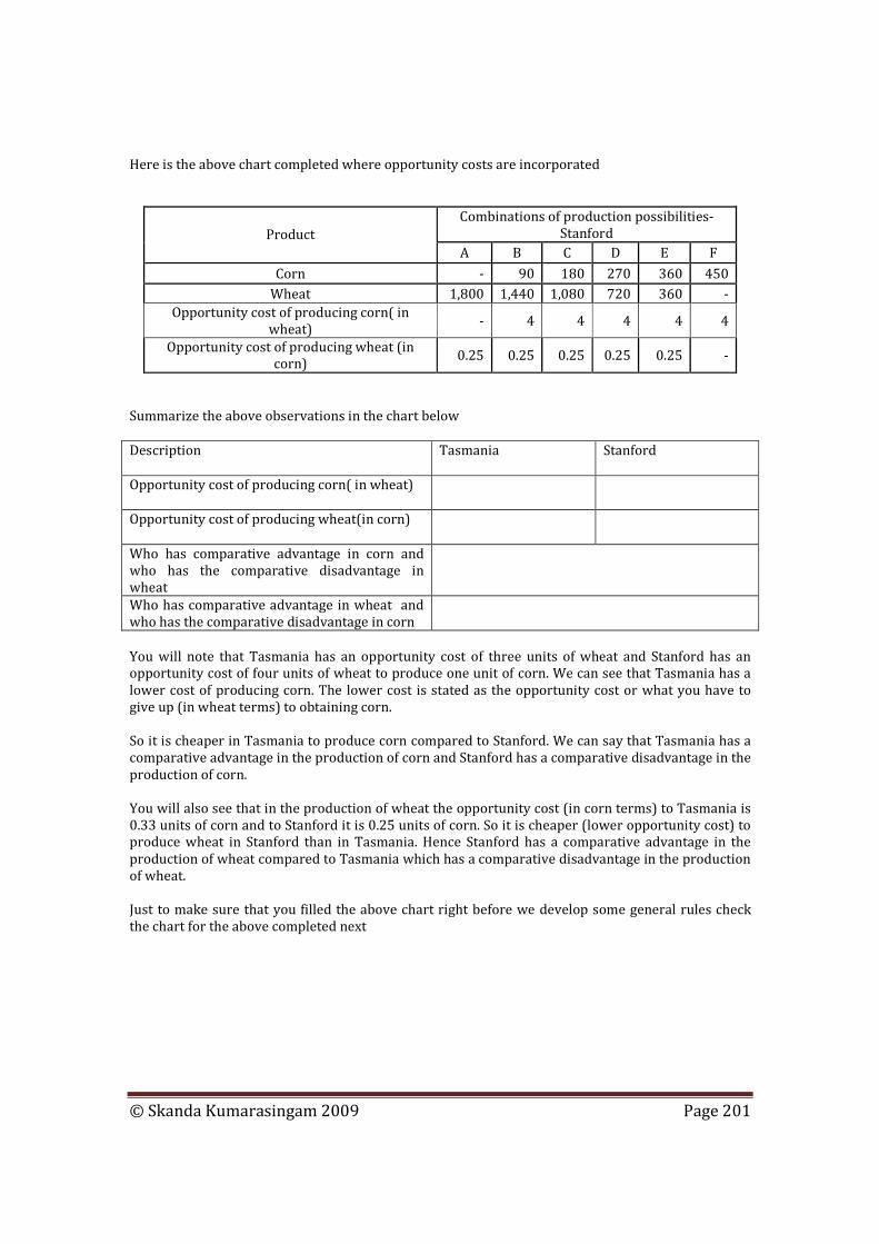
© Skanda Kumarasingam 2009 Page 201
Here is the above chart completed where opportunity costs are incorporated
Combinations of production possibilities-Stanford Product
A B C D E F
Corn - 90 180 270 360 450
Wheat 1,800 1,440 1,080 720 360 -
Opportunity cost of producing corn( in wheat)
- 4 4 4 4 4
Opportunity cost of producing wheat (in corn)
0.25 0.25 0.25 0.25 0.25 -
Summarize the above observations in the chart below
Description
Tasmania Stanford
Opportunity cost of producing corn( in wheat)
Opportunity cost of producing wheat(in corn)
Who has comparative advantage in corn and who has the comparative disadvantage in wheat
Who has comparative advantage in wheat and who has the comparative disadvantage in corn
You will note that Tasmania has an opportunity cost of three units of wheat and Stanford has an opportunity cost of four units of wheat to produce one unit of corn. We can see that Tasmania has a lower cost of producing corn. The lower cost is stated as the opportunity cost or what you have to give up (in wheat terms) to obtaining corn. So it is cheaper in Tasmania to produce corn compared to Stanford. We can say that Tasmania has a comparative advantage in the production of corn and Stanford has a comparative disadvantage in the production of corn. You will also see that in the production of wheat the opportunity cost (in corn terms) to Tasmania is 0.33 units of corn and to Stanford it is 0.25 units of corn. So it is cheaper (lower opportunity cost) to produce wheat in Stanford than in Tasmania. Hence Stanford has a comparative advantage in the production of wheat compared to Tasmania which has a comparative disadvantage in the production of wheat. Just to make sure that you filled the above chart right before we develop some general rules check the chart for the above completed next

© Skanda Kumarasingam 2009 Page 202
Description Tasmania Stanford
Opportunity cost of producing corn 3.00 4.00
Opportunity cost of producing wheat 0.33 0.25
Who has comparative advantage in corn and who has the comparative disadvantage in wheat
Tasmania
Who has comparative advantage in wheat and who has the comparative disadvantage in corn
Stanford
From the above observations we will now be able to develop two important rules. They are
• Rule 1 When two nations or two individuals produce two commodities (or products) one has a comparative advantage on one product and a comparative disadvantage on the other product. The other nation or individual will have a comparative disadvantage on the product which has a comparative advantage in the other nation (or by the first individual) and comparative advantage on the product which has a comparative disadvantage in the other nation(or by the first individual)
• Rule 2 Produce where you have a comparative advantage and do not produce when you have a comparative disadvantage. The second rule leads us to what is called specialization. This answers the first important question of what to specialize in. The Importance of Specialization
Now let us try to answer the second question which is why nations or individuals need to specialize
To understand the second question fill the chart below
Country Corn Wheat Point on production possibility curve
Tasmania
100 900 C
Stanford
270 720 D
Total
We observe from the above chart that if trade does not take place between Tasmania and Stanford Tasmania produces at point C and Stanford producers at point D. However if each nation considers the idea of comparative advantage and produces what they have a comparative advantage in Tasmania will only produce corn and Stanford will only produce wheat. What would be the total quantity of corn that will be produced by Tasmania and the total quantity of wheat that will be produced by Stanford? …………………………………………………… ………………………………………………………………………………………………………………… …………………………………………………………………………………………………………………

© Skanda Kumarasingam 2009 Page 203
Compared to the prior situation where both nations produced a combination of corn and wheat by how many units will the total output of corn and wheat increase by if each nation identified what comparative advantage is and produced only either wheat or corn?................................................................................................................................................. ………………………………………………………………………………………………………………… ………………………………………………………………………………………………………………… These questions can be answered by looking at the above chart completed as shown
Country Corn Wheat Point on
production possibility curve
Tasmania 100 900 C
Stanford 270 720 D
Total 370 1,620
We note that both nations can produce more with the same resources if they become aware of and operate by the law of comparative advantage. This leads to the efficient use of resources. So the primary advantages of adhering to the law of comparative advantage are
• Greater production from the same amount of resources
• More efficient use of resources These primarily are the reasons why nations or individuals need to specialize Terms of Trade
Having answered the second question now we have to answer the third question which is what the terms of trade are between two nations or between two individuals. Terms of trade is an important idea since if both nations wish to consume both corn and wheat will have to exchange the excess quantity of what they produce compared to their needs to obtain the quantity of what is produced in excess in the other nation. To do so international trade will have to take place and there must be an exchange system. This exchange system will tell us how much( maximum limit) of corn will Tasmania give up to obtain a unit of wheat and how many units of wheat (maximum limit) will Stanford give up to obtain one unit of corn. Striking a price is called the terms of trade. This strike price must be below the opportunity cost of producing the commodity (product) on its own. Let us say for example that Tasmania is willing to sell 30 units of corn to obtain 150 units of wheat. We can then say that Stanford must be willing to sell 150 units of wheat to obtain 30 units of corn. Fill the chart below.
Tasmania sells 30 units of corn for 150 units of wheat
So the exchange will be for one unit of corn Tasmania needs
units of wheat
Opportunity cost of one unit of corn to Tasmania is
units of wheat

© Skanda Kumarasingam 2009 Page 204
Stanford sell 150 units of wheat for 30 units of corn
So the exchange will be for one unit of wheat Stanford needs units of corn
Opportunity cost of one unit of wheat to Stanford is units of corn
Here is the above chart now completed
Tasmania sells 30 units of corn for 150 units of wheat
So the exchange will be for one unit of corn Tasmania needs 5 units of wheat
Opportunity cost of one unit of corn to Tasmania is 3 units of wheat
Stanford sell 150 units of wheat for 30 units of corn
So the exchange will be for one unit of wheat Stanford needs 1/5 units of corn
(0.2)
Opportunity cost of one unit of wheat to Stanford is 1/4 units of corn(0.25)
You will note from this chart that Tasmania is willing to sell one unit of corn for five units of wheat. Stanford is able to sell one unit of wheat for 0.2 units of corn. Do you think these two options are one and the same? …………………………………………………………………………………………… ………………………………………………………………………………………………………………… ………………………………………………………………………………………………………………… However to convince Tasmania to sell one unit of corn and obtain five units of wheat it has to compare its opportunity cost of producing one unit of wheat. We know that to produce one unit of wheat Tasmania has to give up 0.33 units of wheat. If the opportunity cost is more than the strike price then Tasmania will agree to sell. Otherwise it will be cheaper for Tasmania to produce its own wheat. To convince Stanford to sell one unit of wheat to obtain 0.2 units of corn it has to compare its opportunity cost of producing one unit of corn. The opportunity cost of producing one unit of corn to Stanford is 4 units of wheat. Stanford will only agree to trade if the terms of trade are less than the opportunity cost of producing one unit of corn by itself. If this is not so it is more expensive for Stanford to trade because it can produce it at a lower opportunity cost. We cannot state at what price the terms of trade should be. We can only say what range it should be. We can simply say the range should be in this case where one unit of corn fetches anything between three and four units of wheat. So you can see that the terms of trade are based on a price range and open to negotiation. Let us say in this instance the terms of trade was settled at 3.33 units of wheat for one unit of corn.

© Skanda Kumarasingam 2009 Page 205
Let us say based on the terms of trade Tasmania decides to sell 300 units of corn. It will get 1000 units of wheat. Based on the terms of trade Stanford will have to sell 1000 units of wheat and obtain 300 units of corn. Using this information complete the chart.
Consumption before international trade
Consumption based on the law of comparative advantage
Increase in consumption due to international trade
Country
Corn Wheat Corn Wheat Corn Wheat
Tasmania(Point C of the PPC)
Stanford(Point D of PPC)
Here is the above now completed
Consumption before
international trade
Consumption based on the
law of comparative
advantage
Increase in consumption
due to international
trade Country
Corn Wheat Corn Wheat Corn Wheat
Tasmania(Point C of the PPC) 100 900 100 1,000 - 100
Stanford(Point D of PPC) 270 720 300 800 30 80
You will observe that before trade Tasmania was able to produce and consume hundred units of corn and 900 units of wheat. When there is trade between the two countries Tasmania is able to consume 100 units of corn and 1000 units of wheat. So there is an increase in consumption of 100 units of wheat. Similarly Stanford before trade was able to produce and consume 270 units of corn and 720 units of wheat. Because of trade Stanford is now able to consume 300 units of corn and 800 units of wheat. There is an increase of 30 units of corn and 80 units of wheat since trade between these two nations took place. Now we can observe that trade will only take place if the exchange prices are within the terms of trade. If trade takes place it is advantageous for both nations. This is not only when trade takes place between nations but also when trade takes place between business firms or individuals or between two parties. However to operate at a country level International trade must take place. In international trade each country will export the excess quantity produced compared to their needs and import the other countries products and services which it requires but does not produce in the quantity it needs. Foreign Exchange
When trade within a nation takes place individuals or business firms will sell products and services which they specialize in making and obtain money in exchange. This currency or money is used to buy other goods and services that they require and/or do not produce. However when there is trade between two nations we are confronted with another problem. The problem is each nation has its own currency and will pay by this currency (its own currency) when it

© Skanda Kumarasingam 2009 Page 206
buys goods and services. However the nation or a country (the individuals and business firms within them) that obtains this currency (by selling their goods and services) will not be able to use it within its own nation as it will not be the currency of exchange within its boundaries. To understand how foreign exchange and foreign-exchange markets operate let us now look at a simple example. The two nations (or nationals) involved are Americans and Englishmen. The Americans want to buy a shipment of cars (say 100 cars) that has been produced in the United Kingdom by Englishmen. So the American buyer will use the U.S. dollar to pay for the purchase of the car. However the Englishmen use and only accept the United Kingdom Sterling pounds. So the American will have to use the U.S. dollars to purchase Sterling pounds. This is done in a particular market which is called the foreign exchange market. The amount of U.S. dollars that the American will have to give up is called the exchange rate. In other words foreign exchange rate simply means how much we need to pay (in our own currency) to obtain one unit of the foreign-currency. Now we can say in this example that Americans are the demanders of sterling pounds and suppliers of U.S. dollars in this particular foreign-exchange transaction. That is the American will use the U.S. dollars that he has (as the supplier) and demand (to purchase) Sterling pounds. Alternatively Englishmen will have to supply the Sterling pounds to this foreign exchange market. If this was not done the American will not be able to obtain sterling pounds as only Englishmen can supply this to the foreign-exchange market. So they are called the suppliers of Sterling pounds. However Englishmen will not supply sterling pounds unless they're interested in obtaining the U.S. dollar to purchase something else from the Americans. Hence they will now become the demanders of the U.S. dollar. As previously stated the foreign exchange rate is how much we need to pay of our own currency to obtain one unit of the foreign-currency. In other words this is the price paid for the other currency. Price (exchange rate) depends on the demand and supply for a particular currency in the foreign-exchange market. Complete the chart below
Rate of exchange for sterling pounds ( in U.S dollars
Rate of exchange for U.S. dollars ( in sterling pounds
5 1/5
4
3
2
1
Did the completed chart look like this? It should
Rate of exchange for sterling pounds ( in U.S dollars)
Rate of exchange for U.S. dollars ( in sterling pounds
5 0.20
4 0.25
3 0.33
2 0.50
1 1.00

© Skanda Kumarasingam 2009 Page 207
You will note from the above chart that the rates of exchange are inversely related. That is the rate of exchange for a sterling pound reduces when the rate of exchange for U.S. dollars increases and vice versa. As stated before the exchange rate or price paid to obtain the other currency depends on the demand and supply for the currency. We need to understand that foreign exchange is also a commodity or normal good. Note the schedule given next. This explains to us the quantity demanded for sterling pounds and the quantity supplied for sterling pounds along with their prices or foreign-exchange rates. The equilibrium point is reached when the foreign exchange rate settles at 4 U.S. dollars per sterling pound. This is called the equilibrium point since the quantity demanded for sterling pounds and the quantity supplied for sterling pounds is one and the same at 600 units.
Quantity demanded for sterling pounds
Foreign exchange Quantity supplied for sterling pounds
400 5.00 800
500 4.50 700
600 4.00 600
700 3.50 500
800 3.00 400
900 2.50 300
1000 2.00 200
Foreign exchange demand and supply
-
1
2
3
4
5
6
- 200 400 600 800 1,000 1,200
quantity demanded and quantity supplied for sterling pounds
fore
ign
exch
ange
quantity supplied
quantity demanded
This as you can see also follows the law of demand and the law of supply. We can observe when the foreign-exchange rate increases the quantity demanded reduce and vice versa. Likewise when the foreign exchange rate increases the quantity supplied also increases and vice versa. Let us say that if a person purchases 600 units of Sterling pounds at the equilibrium price they will have to give up 2400 U.S. dollars. This is calculated as 600 sterling pounds multiplied by the exchange rate of 4 U.S. dollars to a sterling pound. Let us now look at the demand for Sterling pounds for exchange in U.S. dollars and the supply of Sterling pounds for exchange in U.S. dollars.

© Skanda Kumarasingam 2009 Page 208
From an American viewpoint we note that demand for sterling pounds for exchange in U.S. dollars can occur for four reasons. They are 1. Demand by American importers (or purchasers) of goods and services produced in the United
Kingdom by Englishmen. Such goods are mostly consumer goods. However there are also instances where capital goods are purchased from the United Kingdom. Apart from goods, services are also purchased from Englishmen. Such services may be tourism, insurances, purchase of films and royalty paid to writers of books. If Americans want to purchase the goods or services they will demand the Sterling pound and exchange it for the U.S. dollar. Using these sterling pounds they will be able to buy what they want from Englishmen.
2. If Americans want to give a loan to Englishmen then too the Americans will demand Sterling
pounds for exchange in U.S. dollars. This is because the Englishmen will need it in Sterling pounds to make use of it.
3. If Americans decide to gift to Englishmen they will have to give it in Sterling pounds. Hence the
Americans will demand sterling pounds for exchange in U.S. dollars because the gift to be useful to the Englishmen must be in Sterling pounds so that they maybe able to use it to purchase goods and services of their desire or need.
4. Finally Englishmen who export money to the United States of America (by way of a loan which
will attract interest or purchase stocks or shares in companies in the United States which will attract dividend payments) expect their income received in the form of interest or dividends to be in Sterling pounds. So the American firm which has obtained the loan or capital from the Englishmen will demand sterling pounds for exchange in U.S. dollars to pay them
Again from an American viewpoint we note that the supply of Sterling pounds for exchange in U.S. dollars can happen for four important reasons. They are 1. Englishmen will also import goods and services that are produced in the United States of
America. Such Englishmen or British firms will supply sterling pounds for exchange in U.S. dollars since the American firms or individual will need to be paid in their currency of choice which is the U.S. dollars.
2. The next reason is if Americans export money to the United Kingdom the U.K. firm will need it in
Sterling pounds since it can only use Sterling pounds within its boundaries. So the Americans will have to find suppliers of Sterling pounds for exchange in U.S. dollars.
3. Another reason is if Englishmen decide to give gifts to the Americans. In this instance the
Americans will look for suppliers of Sterling pounds for exchange in U.S. dollars. Once the U.S. dollars have been obtained it will then be transferred to the Americans
4. Finally when Americans export money to the United Kingdom either to give a loan to a firm or
individual in the United Kingdom or to invest in the shares or stocks of an English company the Americans will demand interest and dividends respectively. This dividend and interest payment should be made to the Americans in U.S. dollars. To facilitate this firms will have to supply the Sterling pounds for exchange into U.S. dollars. Once the U.S. dollars have been obtained it will then be transferred to the Americans.
Law of Demand and the Law of Supply for Foreign-Exchange
Let us say the price of a car in the United Kingdom this 5000 sterling pounds. If the exchange rate is three U.S. dollars per sterling pound the American will have to pay 15000 U.S. dollars to purchase this car. However if the exchange rate is two U.S. dollars per sterling pound the American will have to pay 10,000 U.S. dollars only .

© Skanda Kumarasingam 2009 Page 209
When the price or exchange rate increases the demand for UK goods in the United States of America reduce. However when the price or exchange-rate reduces the demand for U.K good and services will increase. To the American it becomes cheaper to purchase the car when the exchange rate is lower. So more Americans will now decide to buy cars that have been made in the United Kingdom. To do so the Americans will require or demand more sterling pounds for exchange in U.S. dollars. This will increase the demand for sterling pounds. Eventually this increased demand will increase the prices thus following or complying with the law of demand. Balance of Payments
This is the annual record of a nation's trade or transactions with the rest of the world. This will also show the shortage or excess of foreign-currency in the country. The balance of payment has two major components which are the current account and the capital account. First let us look at the current account. The current account can again be divided into four separate components. They are
1. The balance of trade( visible trade) 2. Balance of services( invisible trade) 3. Net investment income 4. Net transfers
The balance of trade and the balance of services when added together will form the balance of goods and services Balance of trade records a nation's transactions in relation to exports of goods less the imports of goods The balance of services will record a country's transactions in relation to exports of services less the imports of services Net investment income is the dividends that will be received for having invested in the shares of foreign companies minus dividends that have to be paid by the business firms (within the nation) to foreigners for having invested in the shares of local companies. Another form of net investment income is interest. This is received when members of the nation (the government, individuals or business units) give out loans to foreigners and paid when government, citizens or business firms obtain loans from foreign nationals. Net transfers are the final component of the current account. This considers the gifts, pensions, foreign aid and allowances that are transacted between the nation’s individuals and business units and foreign nationals. The next major component of the balance of payment is the capital account. This records the inflows and outflows between the nation’s individuals and business units with foreign nationals (and nations) in relation to the purchase of liquid capital for buying and selling real and financial assets. Some examples of financial assets are bonds, debentures and shares. Real assets will include property plant and equipment. When the inflows are larger than the outflows it shows a desire by foreign nationals to hold more of the nation’s assets. This will lead to an increase in the quantity demanded for the nation’s foreign exchange because it is required to purchase these liquid real and financial assets. This will increase the price for the nation’s currency.

© Skanda Kumarasingam 2009 Page 210
When the price of the nation’s currency increases because foreign nationals prefer to hold the nation’s assets this will have a negative effect on the balance of goods and services in the current account. When the price or the exchange rate increases for the nations currency it will make exports more expensive to foreign nationals and imports cheaper to the citizens of the nation. This means less will be exported and more will be imported which may create a negative balance of goods and services. A negative balance is considered unfavorable and a positive balance is considered favorable. When we add the final totals of the current account and the capital account we will obtain the balance of payment of the nation for a particular period of time. The balance of payments can either be a positive figure or zero but never a negative figure. It will never be a negative figure simply because even before the balance of payment becomes negative the government of the nation will understand that this situation will arise. To absorb this situation the government will supply currencies from its reserve so that the price of the nation's currency will fall and so the current account deficit will not rise or remain small at its best.
Balance of Payment
Current Account Capital Account
Balance of goods and services
Balance of trade Balance of services
Net investment income
Net transfers
Net flow of Real assets
Net flow of financial assets
Export of goods
Import of goods
Export of services
Import of services
Dividends and Interest
Gifts Pensions Foreign aid allowances
Property Plant Equipment
Stocks Bonds Debentures
Review (Once complete you can use this as the chapter summary or round-up) Question 1 Here is a problem you can work to review your understanding of the principles of comparative advantage. The production possibilities tables for South Africa and North America follow
South Africa
Steel (tons) 150 100 50 0
Oats (carloads) 0 20 40 60
North America
Steel (tons) 180 120 60 0
Oats (carloads) 0 30 60 90
South Africa finds that the opportunity cost of 1 ton of steel is...............................................and of one carload of oats is............................................... Question 2 North America’s opportunity cost of 1 ton of steel is....................................................and of one carload of oats is.........................

© Skanda Kumarasingam 2009 Page 211
Question 3 ..........................................has a comparative advantage in steel and ..........................................has a comparative advantage in oats.....................................will specialize in the production of............................... and .....................................in................................. Question 4 North America will exchange its (steel/ oats) for South Africa’s (steel/ oats) The terms of trade will lie between .........................and ........................ carload of oats for 1 ton of steel ...........................and.......................... tons of steel for one carload of oats Question 5 Specialization based on the principle of comparative advantage enables the two nations to....................................their combined production of steel and oats without an increase in the resources available to them. Question 6 A West German wishing to buy wine in France will be a (demander/ supplier) of German deutsche marks and a (demander/ supplier) of French francs. A French firm that wants to buy coal in West Germany will demand (French francs/ deutsche marks) and supply (French francs/ Deutsche marks) Question 7 Another name for foreign money is........................................................ The rate of the exchange is the.......................paid to obtain.............................. unit(s) of foreign money Question 8 If 5 French francs can be exchanged for one U.S. dollar the rate of exchange for the dollar is..................... French francs. If the rate of exchange for the deutsche mark is 40 cents (in United States of America currency) the rate of exchange for the dollar is......................... Deutsche marks. Question 9 The rate of exchange for any foreign money depends upon the............................for and the.......................of that money. The equilibrium exchange rate for the French franc will be the rate at which the quantity of French francs.................................. equals the quantity of French francs.............................. Question 10 The four groups that demand pounds and supply dollars are
• Americans who wish to (export/ import) goods and services
• Englishmen who............................the use of money and are being paid interest and dividends.
• Americans who wish to make financial investments in England by buying......................... and making........................ in England
• Americans who want to...................... money to persons or institutions in England Question 11 The suppliers of pounds and the demanders of dollars are Englishmen who import............................and.................................... Americans to export the.................................of money and are being paid interest and dividends Englishmen who wish to (buy/ sell) stocks or (make/ obtain) loans in the United States Englishmen who want to (make/ receive) gifts of money

© Skanda Kumarasingam 2009 Page 212
Question 12 Now let us understand why the laws of demand and of supply apply to foreign-exchange. Use a + to indicate an increase and a - sign to indicate a decrease. An increase in the rate of exchange for the pound will.................................. the rate of exchange for the dollar.............................. the pound price of American goods and services, and ........................... the dollar price of English goods and services. Question 13 As a result of this increase in the rate of exchange for the pound The quantity of American commodities demanded by the English will..................................... and the quantity of English commodities demanded by the American’s will.................................... The quantity of pounds supplied by Englishmen will ordinarily...................................and the quantity of pounds demanded by the Americans will............................. Question 14 Look at this international balance of payments of a Western European country (in U.S. dollars-billions)
Merchandise exports 17
Merchandise imports 16
Balance of trade
Exports of services 3
Imports of services 1
Balance on goods and services
Net investment income +3
Net transfers -1
Balance on current account
Capital inflows 6
Capital outflows 8
Balance on capital account
Current capital account balance
Official reserves
Insert the correct figures in the six blanks (where the items are given in bold) on the right side of the table Question 15 The country had a balance of payments..................................... Question 16 From the figures it is apparent that the country is a net (exporter/ importer) of capital and is a net international................................. Question 17 It is also apparent the country (increased/ decreased) its official reserves by..............billion and thereby acted to put (up/ down) ward pressure on the foreign exchange rate for its currency. Question 18 If the country had not acted to absorb the 3 billion payments surplus in its official reserves by buying them with its own currency, the excess( supply of/ demand for) foreign currency would have put( up-ward/ down-ward) pressure on the foreign exchange rate for its currency until net exports of goods and services (increased/ decreased) by..................billion. The current and capital account balance then would have become.............................billion.

© Skanda Kumarasingam 2009 Page 213
Question 19 Exports and other transactions that increase the supply of foreign-exchange demanding a country's own currency in foreign-exchange markets put..................................pressure on the rate of exchange for its currency and are shown as (+/-) figure, while imports and other transactions increase the supply of the country's own currency in foreign-exchange markets and put..................................... pressure on its rate of exchange are shown as a.........................figure Question 20 When a country increases its official reserves this is shown in the balance of payments as a ...................................figure because to increase these reserves the central bank has to buy them with........................................................ Thus its supply in the foreign exchange markets is........................................and this puts.............................pressure on its rate of exchange Question 21 When imports are greater than exports a nation has a balance of trade..................................... This is indicated by a (+/-) and means that the nation has earned (more/ less) foreign exchange than it has spent. Question 22 If a nation had a balance of trade of U.S. dollars +6, it had trade................... and it’s......................... were > it’s............................... Question 23 If the figure given for official reserves in the balance of payments is U.S. dollars +7 billion this means the country had a balance of..................................( surplus/ deficit) of U.S. dollars ............................ billion
Answers
Suggested answers to the above questions are given. The answers are provided sequentially in the same order you will fill the blanks or select from a choice in the brackets Question 1 2/5 carload of oats 2-1/2 tons of steel Question 2 1/2 carload of oats 2 tons of steel Question 3 South Africa North America Oats Steel Question 4 Oats
Steel 2/5 and 1/2(either order) 2-1/2 and 2(either order) Question 5 Increase Question 6 Supplier Demander Deutsche marks Francs Question 7 Foreign exchange Price One Question 8 5 2-1/2 Question 9 Demand
Supply Demanded Supplied Question 10 Import Exporter Stocks Loans Give Question 11 Goods Services Use By Make Make Question 12 - - +

© Skanda Kumarasingam 2009 Page 214
Question 13 + - + - Question 14 +1 +3 +5 -2 +3 -3 Question 15 Surplus Question 16 Exporter Creditor Question 17 Increased 3 Downward Question 18 Supply of Upward Decreased 3 Question 19 Upward + Downward - Question 20 Its own currency Increase to Downward Question 21 Deficit - Less Question 22 Surplus Exports Imports Question 23 Payments
Deficit 7

© Skanda Kumarasingam 2009 Page 215
Chapter 12
Money and Banking: Fiscal and Monetary Policy
Learning Outcomes
• To understand the roles of money and its important features and purposes
• To understand what components make up money and to understand how money-supply operates
• To understand what causes the demand for money. There are two reasons which cause the demand for money namely the transactions demand for money and the asset demand for money.
• To identify the equilibrium point for money-supply and demand so that the equilibrium interest rate (price of money) in the economy is established
• to understand how commercial banks operate including the art and science of credit creation and destruction
• To learn the components of a balance sheet of a commercial bank
• To understand how multiple deposit expansion is possible by the commercial banking system
• To understand the role of the Federal Reserve Bank in controlling( including the methods) of money-supply and shaping the monetary policies of the government
• To appreciate the roles of government policies. This includes monetary policies and fiscal policies. Fiscal policies are again divided into two which includes demand management policies and supply-side fiscal policies. we need to understand the differences between these types policies
• Review or chapter summary.
• Answers to Review questions Chapter Outline
• Roles of money
• Components of money and money-supply
• Demand for money
• Equilibrium money-supply and demand
• Commercial banks
• The commercial banking system

© Skanda Kumarasingam 2009 Page 216
• Federal Reserve Bank
• Policies
• Review (Chapter summary)
• Answers to review questions
The Roles of Money
First let us look at what money is and its roles in society. Money is a medium of exchange .This is because it is more convenient to use money rather than barter for exchanging goods and services which was the ancient practice. In the system of bartering we will not be able to sell the product or service that we manufacture in exchange to obtaining something else unless both parties agree and are willing to accept the goods or services produced by the other. However we see that in most situations this does not happen. Also dividing or splitting the goods or services may become difficult in the system of bartering. Say for example if you have a cow to sell but require 10 eggs which are produced in my farm you will have to exchange the cow to obtain the 10 eggs. To you this may not look a sufficient exchange. However money tends to solve these problems. Due to these reasons money has been successful as a medium of exchange. Money functions as a store of value. What they mean by this is you will be able to save it for the future. Money is a measure of value. It helps you to determine how much a particular good or service or an asset is worth. Money helps us to account for all economic activities. This is because you will be able to convert different products and services which have different measurement units (kilogram, liters, units, bales so on) into money terms and so will help you to add and deduct them. This will also help you to evaluate different businesses by enabling you to add different items of costs and revenues and assets and liabilities together for purposes of accounting. However one of the most important reasons for studying what money is is because how much money there is in the economy determines two importance features in a given economy. They are 1. How much money there is in the economy determines how large the gross domestic product of
the economy will be. 2. The other reason is how much money there is in the economy determines how much of the
resources will be employed or unemployed. Remember when we talk of employment we talk about the employment of all resources and not only the employment of labor.
Let me now explain to you in a little more detail what was meant in the previous two paragraphs or points. You will note that how much money there is in the economy will affect the interest rates. What the interest rate is will determine how much business firms will invest. When business firms invest (gross investment) according to the expenditure method this will increase the gross domestic product. When the gross domestic product increases it requires a high level of employment of all resources or a reduction in the unemployment of all resources. This shows the relationship between how large the gross domestic product and how much of the resources will be employed or unemployed in the economy based on the amount of money that is circulating in the economy.
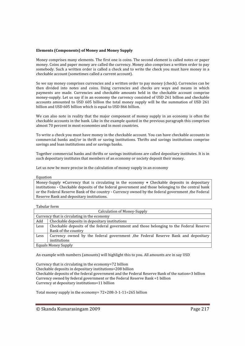
© Skanda Kumarasingam 2009 Page 217
Elements (Components) of Money and Money Supply
Money comprises many elements. The first one is coins. The second element is called notes or paper money. Coins and paper money are called the currency. Money also comprises a written order to pay somebody. Such a written order is called a check and to write the check you must have money in a checkable account (sometimes called a current account). So we say money comprises currencies and a written order to pay money (check). Currencies can be then divided into notes and coins. Using currencies and checks are ways and means in which payments are made. Currencies and checkable amounts held in the checkable account comprise money-supply. Let us say if in an economy the currency consisted of USD 261 billion and checkable accounts amounted to USD 605 billion the total money supply will be the summation of USD 261 billion and USD 605 billion which is equal to USD 866 billion. We can also note in reality that the major component of money supply in an economy is often the checkable accounts in the bank. Like in the example quoted in the previous paragraph this comprises almost 70 percent in most economies and in most countries. To write a check you must have money in the checkable account. You can have checkable accounts in commercial banks and/or in thrift or saving institutions. Thrifts and savings institutions comprise savings and loan institutions and or savings banks. Together commercial banks and thrifts or savings institutions are called depositary institutes. It is in such depositary institutes that members of an economy or society deposit their money. Let us now be more precise in the calculation of money supply in an economy Equation
Money-Supply =Currency that is circulating in the economy + Checkable deposits in depositary institutions - Checkable deposits of the federal government and those belonging to the central bank or the Federal Reserve Bank of the country - Currency owned by the federal government ,the Federal Reserve Bank and depositary institutions.
Tabular form
Calculation of Money-Supply
Currency that is circulating in the economy
Add Checkable deposits in depositary institutions
Less Checkable deposits of the federal government and those belonging to the Federal Reserve Bank of the country
Less Currency owned by the federal government ,the Federal Reserve Bank and depositary institutions
Equals Money Supply
An example with numbers (amounts) will highlight this to you. All amounts are in say USD Currency that is circulating in the economy=72 billion Checkable deposits in depositary institutions=208 billion Checkable deposits of the federal government and the Federal Reserve Bank of the nation=3 billion Currency owned by federal government or the Federal Reserve Bank =1 billion Currency at depositary institutions=11 billion Total money supply in the economy= 72+208-3-1-11=265 billion

© Skanda Kumarasingam 2009 Page 218
Money-supply that is calculated based on the above formula is called M1. There are also other types of money supply which are M2 and M3. These are much broader definitions of money supply and their calculations vary between countries at times and so will not be covered here. The reason why currency deposited in institutions which amount to USD 11 billion is deducted from the above formula is because such money has already been accounted for when calculating the checkable deposits in depository institutions which amount to 208 billion. We need to understand that currency at depository institutions is only for safekeeping and it belongs to the members of the economy or society who have put their money in a checkable account in a depository institution. So this money does not belong to the depositary institution. So we deduct this amount to avoid double counting. Demand for Money
Now let us see how the demand for money is created. Let us say a particular individual named Ralph Roberts has a monthly income of U.S. dollars 2500. Usually from this monthly income he saves 20%. This amount which is saved from the monthly income is called the marginal propensity to save. Marginal propensity to save simply means how much of the total income individuals will save. We have understood more about the marginal propensity to save when we learnt about national income analysis. If Ralph Roberts saves 20% of his monthly income because his marginal propensity to save is 20% he will have 80 percent left for consumption. This 80 percent is called the marginal propensity to consume. The 20% that Ralph Roberts saves is equal to U.S. dollars 500. This is money which is used as a store of value. The 80 percent that Ralph Roberts uses for consumption is equal to U.S. dollars 2000 and is used as a medium of exchange to buy the goods and services that Ralph Robert requires. If the monthly income increases from U.S. dollars 2500 to U.S dollars 3000 and the marginal propensity to consume remains at 80% and the marginal propensity to save is equal to 20% what is the amount that will be saved and what is the amount that he will spend for consumption? ………………………………………………………………………………………………………………… ………………………………………………………………………………………………………………… We also need to be thoughtful about another idea which is the average possession of money. Say for example that Ralph Roberts when earning a monthly income of U.S dollars 2500 spent U.S. dollars 2000 for consumption. Ralph Robert had U.S. dollars 2000 at the beginning of the month and if he uses up the full amount by the end of the month the amount that he will have in his possession will be 0. So we say the average possession of money is equal to (2000+0)/2= U.S. dollars 1000. This average amount of money that is in his possession for the purpose of consumption is called the transaction demand for money. We did note that the transaction demand for money has a direct relationship with income. To find out whether this is so see what happens to the average amount that is held in possession when Ralph Roberts income increases from U.S. dollars 2500 to U.S. dollars 3000.

© Skanda Kumarasingam 2009 Page 219
We also know when members of an economy use a higher amount for consumption this will improve the economy’s or the society's nominal GDP which is directly proportional to the transaction demand for money. In the space provided draw a graph depicting on the X axis the nominal gross domestic product (income of all citizens) and on the Y axis the transaction demand for money.
Your graph should look like this
Transaction demand for money
0
100
200
300
400
500
600
0 200 400 600 800 1000 1200 1400 1600
nominal GDP(in billions)
tran
sact
ion
dem
and
for
mon
ey(a
vera
ge m
oney
peo
ple
wan
t to
hold
for
tran
sact
ions
)
Now let us see what happens with the amount that is saved. We got as far as knowing that when Ralph Roberts savings increased from U.S. dollars 500 to U.S. dollars 600 when his monthly income increased from U.S. dollars 2500 to U.S. dollars 3000 whilst the marginal propensity to save remained constant at 0.2 or 20%. Like it was stated before savings show us how money is used as a store of value. Such money that is saved can either be held as money itself or in your checkable deposit account. However when such

© Skanda Kumarasingam 2009 Page 220
money that is saved is held in the form of money itself or in the checkable deposit account it does not earn interest. However holding the amount of money that is saved in your possession in the form of money itself or in the checkable deposit account is often called the asset demand for money. However if such money is held in the form of a bond, a debenture or in a savings account in a depository institution this will earn interest on the amount that has been invested or deposited. If you do not invest the money you save in an interest-bearing asset you will lose out the interest which you could have been earning otherwise. Higher the interest rate that is offered by the depositary institutions the cost of holding money or depositing them in checkable deposit accounts (which do not give interest on the balance) also increases. The cost of holding money is equal to the opportunity cost. In this instance the opportunity cost is the interest that is forgone. We can thus say that there really is an inverse relationship between the interest rate and the asset demand for money. To depict it draw a graph in the space. On the X axis you will have the asset demand for money (Da) and on the Y axis interest rate (the price of money)
The interest rate versus the asset demand for money graph will look like this
Asset demand for money
0
5
10
15
20
25
30
0 100 200 300 400 500 600 700 800 900
asset demand for money
inte
rest
rat
e
Now we will be able to find out how the demand for money is created. Demand for money is equal to the transaction demand for money and the asset demand for money.

© Skanda Kumarasingam 2009 Page 221
Demand for money= Transaction demand for money + Asset demand for money
Transaction demand for money (Dt) has a direct relationship with the nominal gross domestic product and is based on the marginal propensity to consume The asset demand for money (Da) has an inverse relationship with the interest rate which is the price paid for the use of money and is based on the marginal propensity to save. Equilibrium Money Supply and Demand
Now let us see how the supply of money interacts with the demand for money to create the equilibrium interest rate which is the price paid for money. In the graph that is showed it is assumed that at a given period of time the nominal gross domestic product and the transaction demand for money are held constant.
Demands for money and money supply
0
5
10
15
20
25
30
0 200 400 600 800 1000 1200
demands for money and money supply
inte
rest
rat
e
Transaction demand
Supply of money
asset demand for money
demand for money
You will note that when the nominal gross domestic product increases the transaction demand for money curve shifts to the right ( or should shift outwards) which in turn increases the demand for money which in turn increases the interest rate and vice versa. From this we also note that there is a direct relationship between the nominal gross domestic product and the interest rate. We also note from the above graph that money supply at a given time is fixed and so the line depicting the supply of money is vertical and is parallel to the Y axis. It will also be noted that when the supply of money increases this curve will shift to the right (or outward) reducing the interest rate and vice versa. So we can conclude that the supply of money is inversely related to the interest-rate. From the previous two paragraphs we can now state that There is a direct relationship between the nominal gross domestic product and the interest rate There is an inverse relationship between the supply of money and the interest rate. We can now see where demand for money = supply of money and it is at the equilibrium point. This point indicates to us the equilibrium interest rate or the price that has to be paid for the use of money.

© Skanda Kumarasingam 2009 Page 222
We may finally conclude that nominal gross domestic product = real gross domestic product X price level. From the above equation we can state that when the real gross domestic product and / or the price level increases the interest rate also increases. This is to be expected as the interest rate is the price paid for the use of money. Commercial Banks
Supply of money to a large extent is determined by the operations of the commercial banks in a given society or economy. This is because commercial banks are able to create money or to destroy money. Creation of money increases the supply of money and the destruction of money reduces the supply of money. Money is created when commercial banks make loans. Money is destroyed when loans are repaid and new loans are not issued in place of it. Apart from commercial banks any institution which can be categorized as depositary institutions can also be involved in the creation of money to increase the supply of money and be involved in the destruction of money to reduce the supply of money. Please remember that in the process of creation of money and in the destruction of money it is usually the checkable accounts that get involved as it is a large proportion of the money supply. To understand this process of the creation of money and the destruction of money we first need to understand how the balance sheet of a bank will look like. Even though it may not be repeated for every balance sheet given please note that all amounts are in billions of USD.
Balance Sheet of First National Bank
Things owned Things owed
Assets Liabilities and Funds
Banks Reserves Liabilities
Cash(currency in the vault) 100 Demand deposits 2100
Deposit at Federal Reserve Bank 500 Time deposits 200
Total Reserves 600 Total deposits 2300
Other Assets Net Worth
Loans 1000 Share Capital + Reserves 200
Securities in government securities 900
Total Other Assets 1900 Net Worth 200
Total assets 2500 Liabilities and Funds 2500
Looking at this balance sheet we can say that on the right side of the balance sheet we can observe what the bank owes others. These are often called as liabilities and net worth. Liabilities include demand deposits (which are non-interest bearing checkable accounts) and time deposits (where the bank has to pay interest but no checks can the written and usually where the bank can take time to settle or payback). Net worth can be calculated as total assets minus total liabilities. This is the amount that is available to the owners of the business or the owners of the Bank.

© Skanda Kumarasingam 2009 Page 223
On the left side of the balance sheet you will see the things that are owned by the Bank. Whatever the bank owns is called assets. Assets mainly comprise of four components. The first component is cash (currency held in the vault) and is held by the Bank because it needs to meet the day to day operations and the payments of depositors and for check payments. The second component is deposits held at the Federal Reserve Bank. This amount needs to be held at the Federal Reserve Bank (Central Bank or Bankers Bank in an economy) by law and is a percentage of the total deposits which include demand deposit and time deposits. This percentage is often called the reserve ratio. So we may say that the reserve ratio is equal to a percentage of the deposits.
The required reserve (deposit at the Federal Reserve Bank) = deposits x Reserve ratio
Combining the cash that is held in the vault + the deposit at the Federal Reserve Bank we call it as the reserves of the bank. The third asset that is held is the loans that are given to the customers of the bank. The forth asset that is held is Securities in government bonds and Treasury bills. The third and fourth assets are revenue generating or interest income earning assets of the bank. The third and the fourth assets are combined and labeled as the other assets of the bank. However the first two assets which comprise cash or currency held in the vault + deposit at the Federal Reserve Bank do not give the bank an income. However they need to be held to meet the day-to-day needs of the deposit holders and for check payments (when those who hold checkable accounts make a written order to the bank to pay from their checkable account). This is the balancing act of maximizing profits whilst maintaining liquidity (ability to meet payments).
Using the new summarized classifications for the assets and liabilities of the bank fill in the blanks to create the new summarized balance sheet.
Balance Sheet of First National Bank
Things owned Things owed
Assets Liabilities and Funds
Reserves 600 Deposits 2300
Other Assets 1900 Net Worth 200
Total assets 2500 Liabilities and Funds 2500
Now look at this banks original balance sheet which is in summarized form. You will note that the actual reserves are 145, other assets 480 demand deposits 600 and net worth 25. Let us say that the reserve ratio is 15%.
Balance Sheet of First National Bank
Things owned Things owed
Assets Liabilities and Funds
Reserves 145 Deposits 600
Other Assets 480 Net Worth 25
Total assets 625 Liabilities and Funds 625

© Skanda Kumarasingam 2009 Page 224
Reserve Ratio =15%
the actual reserve is 145
Required reserve = 600 x 15%=90
Excess reserves=145-90=55
Using this excess reserve the bank will be able to create money and thus increase the supply of money in the market. The excess reserve is the amount it can loan out in a safe manner or use it to buy extra security in Treasury bills and government bonds. So in other words the additional money a single bank can create depends on the excess reserves it has which it will use to give out loans or buy securities in Treasury bills or government bonds. When loans are given which are equal to the excess reserve of 55 as in the above example the bank will initially deposit this money in the demand deposit account of the customer. This will increase the demand deposit from 600 to 655. On the left side of the balance sheet the other assets (loans given to customers) will increase by 55 and become 535. At this point you will note that the bank has succeeded in creating money and increasing the money supply as the demand deposit which belongs to the customer has increased by the excess reserves of the bank. Now in the space provided below re-draw the balance sheet after the loan was granted. This is an intermediate balance sheet and temporary in nature
Balance Sheet of First National Bank
Things owned Things owed
Assets Liabilities and Funds
Reserves 145 Deposits(600+55) 655
Other Assets(480+55) 535 Net Worth 25
Total assets 680 Liabilities and Funds 680
After the loan is granted the loan amount is deposited in the demand deposit account of the customer. The customer will withdraw this money or give a check (which is the written demand to the Bank to pay) to another person. When this money is withdrawn or a check is presented for payment the bank will need to make the payment. Let us say in this instance the customer or the borrower takes the whole amount of the loan from his demand deposit account. When this transaction takes place obviously the demand deposit amount will reduce from 655 to 600 and the Bank will have to pay out this money from the currency in the vault which will go to reduce the reserves of the bank by an equal amount. Now the final balance sheet will look like this.
Balance Sheet of First National Bank
Things owned Things owed
Assets Liabilities and Funds
Reserves(145-55) 90 Deposits (655-55) 600
Other Assets 535 Net Worth 25
Total assets 625 Liabilities and Funds 625
Reserve Ratio =15%
the actual reserve is 90
Required reserve = 600 X 15%=90
Excess reserves= 0

© Skanda Kumarasingam 2009 Page 225
You will note that the reserves are equal to 90. This is the amount that needs to be maintained by the bank so that it does not violate the banking law. This is calculated as demand deposit x reserve ratio= 600 x 15%=90. Now let us see how when a loan is repaid supply of money is reduced. Let us say in this example that the loan repayment was 50. Check out the balance sheets given to understand this.
Balance Sheet of First National Bank
Things owned Things owed
Assets Liabilities and Funds
Reserves 90 Deposits (600-50) 550
Other Assets (535-50) 485 Net Worth 25
Total assets 575 Liabilities and Funds 575
Reserve Ratio =15%
the actual reserve is 90
Required reserve = 550 X 15%=82.5
Excess reserves= 7.5
This loan has to be repaid from the demand deposit account of the customer or the borrower and so the balance will fall from 600 to 550. This has destroyed the supply of money by 50 which is equal to the amount of the loan that was repaid. On the left side of the balance sheet you will note the adjustment is a reduction in the other assets (loans given to customers) by 50. Now let us look at an example where a bank tries to grant a loan > its reserve ratio. The balance sheet of the bank before the grant of the loan of 100 is given in the space.
Balance Sheet of First National Bank
Things owned Things owed
Assets Liabilities and Funds
Reserves 145 Deposits 600
Other Assets 480 Net Worth 25
Total assets 625 Liabilities and Funds 625
Reserve Ratio =15%
the actual reserve is 145
Required reserve = 600 X 15%=90
Excess reserves= 55
The reserve ratio is equal to 15%. Calculate the actual reserves, required reserves and the excess reserves. The excess reserve that has been calculated (which is 55) is the amount that it can safely loan. However the Bank has decided to give a loan of 100. In the space provided below draw the new balance sheet after the loan of 100 is granted. This is only a temporary balance sheet
Balance Sheet of First National Bank
Things owned Things owed
Assets Liabilities and Funds
Reserves 145 Deposits (600+100) 700
Other Assets (480+100) 580 Net Worth 25
Total assets 725 Liabilities and Funds 725

© Skanda Kumarasingam 2009 Page 226
Now in the space provided redraw the final balance sheet after the customer withdraws this loan from his demand deposit account.
Balance Sheet of First National Bank
Things owned Things owed
Assets Liabilities and Funds
Reserves (145-100) 45 Deposits 600
Other Assets 580 Net Worth 25
Total assets 625 Liabilities and Funds 625
Reserve Ratio =15%
the actual reserve is 45
Required reserve = 600 X 15%=90
Excess reserves= (45)-called the negative excess reserve
On this final balance sheet calculate how much the required ratio should be and if there is a shortfall or excess. You will note that there is a shortfall as when the demand deposit is equal to600 the bank's reserves should be 15 percent of this which must be 90. However the amounts in the reserves are equal to only 45. So the bank has violated the banking law.
Now let us see how new money is created when the bank buys government securities and how money is destroyed when it sells government securities. Look at the balance sheet that has been provided below. Please note that the banks should not buy securities from other banks or the Federal Reserve Bank if the process is to create new money but only from the general public and those outside the banking system.
Balance Sheet of First National Bank
Things owned Things owed
Assets Liabilities and Funds
Reserves 145 Deposits 600
Other Assets 480 Net Worth 25
Total assets 625 Liabilities and Funds 625
Reserve Ratio =15%
the actual reserve is 145
Required reserve = 600 X 15%=90
Excess reserves= 55
For this balance sheet you are required to calculate the actual reserves, required reserves and the excess reserve. The reserve ratio is equal to 15%. Let us say the bank buys securities worth 55. When it buys securities it will give a check to the seller from the bank's own account which will be one of the accounts in the demand deposit account of the bank. The banks banker is obviously itself! This will increase the demand deposit of the bank by55 and increase the other assets (Securities in Treasury bills) by a similar amount and so the bank's balance sheet will balance. You will note that because the demand deposit has increased by 55 new money has been created. This new money that is created is equal to the excess reserves as calculated above. In the space provided complete the new balance sheet of the bank based on the information that has been given after the purchase of securities.

© Skanda Kumarasingam 2009 Page 227
Balance Sheet of First National Bank
Things owned Things owed
Assets Liabilities and Funds
Reserves 145 Deposits (600+55) 655
Other Assets (480+55) 535 Net Worth 25
Total assets 680 Liabilities and Funds 680
Once the seller withdraws (or presents the check) to the bank the deposits will fall by a further 55 to 600 and reserves by 55 to 90. Then the reserve ratio will be 600 X 15% = 90 just the way we want it. The bank now decides after purchasing securities for 55 to sell off securities worth 40. When it sells off security it destroys money and so will reduce the supply of money in the market. Obviously when securities are sold the other assets of the bank will reduce by the said amount and also the demand deposit account will reduce by the same amount. In the space provided below complete the final balance sheet after the bank has sold securities worth 40. You can see that the demand deposit has reduced from 655 to 615.
Balance Sheet of First National Bank
Things owned Things owed
Assets Liabilities and Funds
Reserves 145 Deposits (655-40) 615
Other Assets (535-40) 495 Net Worth 25
Total assets 640 Liabilities and Funds 640
The Commercial Banking System
Commercial banks in a society or economy are responsible for the multiple deposit expansion or the multiple creation of money. Before we understand how this operates we need to know certain basic facts. These basic facts are 1. Individual banks will increase the supply of money by its excess reserves only or else will break
the law and so will not engage in doing this 2. When one bank loses its reserves another bank will gain it. This is because when the check is
paid the demand deposit account will fall by that amount and also the reserves will fall by the same amount as the bank has to use the money in the vault to pay it. This money that has been paid will be deposited in another person's bank account who will receive this check from the first banks customer. This will continue thus creating money supply in a multiple manner.
This is explained by filling up the worksheet that is provided. Let us say there are three banks which are called the First National Bank, the Second National Bank and the Third National Bank. Each of them has a reserve ratio of 20% as they all do business in a particular economy Now go ahead and fill up the blanks (or understand how they are derived) using the information that has been provided.

© Skanda Kumarasingam 2009 Page 228
First National Bank Calculate first the actual reserves the required reserves and the excess reserves.
Balance Sheet of First National Bank
Things owned Things owed
Assets Liabilities and Funds
Reserves 2000 Deposits 9500
Other Assets 8000 Net Worth 500
Total assets 10000 Liabilities and Funds 10000
Reserve Ratio =20%
the actual reserve is 2000
Required reserve = Deposits X Reserve Ratio=9500 X 20%=1900
Excess reserves= actual ratio - required ratio=100
Complete the second balance sheet (temporary) if the bank gives a loan equal to the excess reserves. What is the increase in the supply of money?
Balance Sheet of First National Bank
Things owned Things owed
Assets Liabilities and Funds
Reserves 2000 Deposits (9500+100) 9600
Other Assets (8000+100) 8100 Net Worth 500
Total assets 10100 Liabilities and Funds 10100
Once the loan has been granted the borrower will spend it by writing checks. To settle this loan the bank will have to pay cash or currency. Using this information complete the third balance sheet.
Balance Sheet of First National Bank
Things owned Things owed
Assets Liabilities and Funds
Reserves 1900 Deposits 9500
Other Assets 8100 Net Worth 500
Total assets 10000 Liabilities and Funds 10000
Reserve Ratio =20%
the actual reserve is 1900
Required reserve = Deposits X Reserve Ratio=9500 X 20%=1900
Excess reserves= actual ratio - required ratio=0
Recalculate the required reserves and find out if there are any excess reserves. Ideally there will be no excess reserves and the required reserves are maintained thus not violating the banking laws of the society as seen above. The payee from the first bank will deposit this 100 in her account which is in the Second National Bank. Second National Bank Look at the original balance sheet of this bank. Calculate the actual reserves the required reserves and the excess reserves. We can say that since there are no excess reserves the bank will not be able to give new loans.

© Skanda Kumarasingam 2009 Page 229
Balance Sheet of Second National Bank
Things owned Things owed
Assets Liabilities and Funds
Reserves 1000 Deposits 5000
Other Assets 4300 Net Worth 300
Total assets 5300 Liabilities and Funds 5300
Reserve Ratio =20%
the actual reserve is 1000
Required reserve = Deposits X Reserve Ratio=5000 X 20%=1000
Excess reserves= actual ratio - required ratio=0
Now let us assume that the money that was withdrawn from the demand deposit of the First National Bank is to be deposited in the second National Bank. Complete the second balance sheet showing how it will look when the amount that was withdrawn from the demand deposit of the First National Bank is deposited in the second National Bank. Once this amount has been deposited in the second National Bank calculate the actual reserves the required reserves and the excess reserves.
Balance Sheet of Second National Bank
Things owned Things owed
Assets Liabilities and Funds
Reserves (1000+100) 1100 Deposits (5000+100) 5100
Other Assets 4300 Net Worth 300
Total assets 5400 Liabilities and Funds 5400
Reserve Ratio =20%
the actual reserve is 1100
Required reserve = Deposits X Reserve Ratio=5100 X 20%=1020
Excess reserves= actual ratio - required ratio=80
Now that the Second National Bank has an excess reserve of 80 it will now be able to give new loans to this amount and thus increase the supply of money by this amount. Assuming that the Second National Bank will give this loan and increase the money supply you are now required to draw the third balance sheet after the loan has been granted.
Balance Sheet of Second National Bank
Things owned Things owed
Assets Liabilities and Funds
Reserves 1100 Deposits (5100+80) 5180
Other Assets (4300+80) 4380 Net Worth 300
Total assets 5480 Liabilities and Funds 5480
Once the loan has been granted the borrower will spend it by writing checks for this amount. Now complete the final balance sheet for the second National Bank when the borrower of the loan pays money by writing checks to others.

© Skanda Kumarasingam 2009 Page 230
Balance Sheet of Second National Bank
Things owned Things owed
Assets Liabilities and Funds
Reserves (1100-80) 1020 Deposits (5180-80) 5100
Other Assets 4380 Net Worth 300
Total assets 5400 Liabilities and Funds 5400
Reserve Ratio =20%
the actual reserve is 1020
Required reserve = Deposits X Reserve Ratio=5100 X 20%=1020
Excess reserves= actual ratio - required ratio=0
See what the required reserves are and if there are any excess reserves in the final balance sheet that you have completed for the second National Bank. Hopefully you would arrive where the excess reserves equal to zero. Third National Bank Using the same methodology that was highlighted to complete the balance sheets of the Second National Bank complete all the balance sheets for the Third National Bank in the same manner. Look at the original balance sheet of this bank. Calculate the actual reserves the required reserves and the excess reserves. We can say that since there are no excess reserves the bank will not be able to give new loans.
Balance Sheet of Third National Bank
Things owned Things owed
Assets Liabilities and Funds
Reserves 1200 Deposits 6000
Other Assets 5000 Net Worth 200
Total assets 6200 Liabilities and Funds 6200
Reserve Ratio =20%
the actual reserve is 1200
Required reserve = Deposits X Reserve Ratio=6000 X 20%=1200
Excess reserves= actual ratio - required ratio=0
Now let us assume that the money that was withdrawn from the demand deposit of the Second National Bank (which was 80) is to be deposited in the Third National Bank. Complete the second balance sheet showing how it will look when the amount that was withdrawn from the demand deposit of the Second National Bank is deposited in the Third National Bank. Once this amount has been deposited in the Third National Bank calculate the actual reserves the required reserves and the excess reserves.
Balance Sheet of Third National Bank
Things owned Things owed
Assets Liabilities and Funds
Reserves (1200+80) 1280 Deposits (6000+80) 6080
Other Assets 5000 Net Worth 200
Total assets 6280 Liabilities and Funds 6280
Reserve Ratio =20%
the actual reserve is 1280
Required reserve = Deposits X Reserve Ratio=6080 X 20%=1216
Excess reserves= actual ratio - required ratio=64

© Skanda Kumarasingam 2009 Page 231
Now that the Third National Bank has an excess reserve of 64 it will now be able to give new loans to this amount and thus increase the supply of money by this amount. Assuming that the Third National Bank will give this loan and increase the money supply you are now required to draw the third balance sheet after the loan has been granted.
Balance Sheet of Third National Bank
Things owned Things owed
Assets Liabilities and Funds
Reserves 1280 Deposits 6144
Other Assets 5064 Net Worth 200
Total assets 6344 Liabilities and Funds 6344
Once the loan has been granted the borrower will spend it by writing checks for this amount. Now complete the final balance sheet for the Third National Bank when the borrower of the loan pays money by writing checks to others.
Balance Sheet of Third National Bank
Things owned Things owed
Assets Liabilities and Funds
Reserves (1280-64) 1216 Deposits (6144-64) 6080
Other Assets 5064 Net Worth 200
Total assets 6280 Liabilities and Funds 6280
Reserve Ratio =20%
the actual reserve is 1216
Required reserve = Deposits X Reserve Ratio=6080 X 20%=1216
Excess reserves= actual ratio - required ratio=0
See what the required reserves are and if there are any excess reserves in the final balance sheet that you have completed for the Third National Bank. Hopefully you would arrive where the excess reserves equal to zero. We can see that Required Reserve = Deposit X reserve Ratio Required Ratio when increased by 100 will increase deposits by 500 as the reserve ratio is equal to 20%. So when the excess reserve is 100 the deposit should increase by 5 times and so the money supply should also increase by this amount. Now complete the schedule that is provided based on the balance sheets of the First National Bank, Second National Bank and the Third National Bank and what you learnt from the above formula.

© Skanda Kumarasingam 2009 Page 232
Schedule of Multiple Deposit Expansion
Bank Excess Increase in Increase in Description Cumulative
Reserves Deposits money supply increase in
money supply
1 100 - 100.00 excess reserve of 100 100
2 - 80 80.00 excess reserve of 80 180
3 - 64 64.00 And so on 244
4 - 51 51.20 295
5 - 41 40.96 336
6 - 33 32.77 369
7 - 26 26.21 395
8 - 21 20.97 416
9 - 17 16.78 433
10 - 13 13.42 446
11 - 11 10.74 457
12 - 9 8.59 466
13 - 7 6.87 473
14 - 5 5.50 478
15 - 4 4.40 482
16 - 4 3.52 486
17 - 3 2.81 489
18 - 2 2.25 491
19 - 2 1.80 493
20 - 1 1.44 494
21 - 1 1.15 495
22 - 1 0.92 496
23 - 1 0.74 497
24 - 1 0.59 498
25 - 0 0.47 498
26 - 0 0.38 498
27 - 0 0.30 499
28 - 0 0.24 499
29 - 0 0.19 499
30 - 0 0.15 499
31 - 0 0.12 500
From the schedule you will be able to observe how much excess money will be created in the economy when multiple deposit expansion or the multiple creation of money takes place. The increase in money supply becomes smaller and smaller and the cumulative amount (money created) settled at USD 500. However to do this you need not always complete the full schedule as there is a simple formula. However before understanding this simple formula we need to understand how the concept works. This is the reason why the schedule was filled first. The formula is
The increase in the supply of money= monetary multiplier x excess reserves

© Skanda Kumarasingam 2009 Page 233
Please note only then you have excess reserves can the supply of money increase because when there are excess reserves the bank will be able to give out more loans or buy more security.
The monetary multiplier = 1/ reserve ratio
The monetary multiplier and the reserve ratio have an inverse relationship. Look at the consolidated balance sheet of all banks that have been provided below. The reserve ratio is 20 %. Calculate the actual reserves the required reserves and the excess reserves.
Consolidated Balance Sheet of All Banks
Things owned Things owed
Assets Liabilities and Funds
Reserves 35 Deposits 150
Other Assets 120 Net Worth 5
Total assets 155 Liabilities and Funds 155
Reserve Ratio =20%
the actual reserve is 35
Required reserve = Deposits X Reserve Ratio=150 X 20%=30
Excess reserves= actual ratio - required ratio=5
Using this information calculate by how much the supply of money will increase in the economy. Increase in money supply = monetary multiplier X excess reserves = 1/ reserve ratio X excess reserves = 1/0.20 X 5 = 5 X 5 = 25 You will also note that the supply of money will reduce if there is a negative excess reserve. Negative excess reserves are created when the bank loans out a larger amount than it should. The amount it can legally loan out is equal to the demand deposit x reserve ratio. Usually when there are negative excess reserves the bank will overcome the situation by not giving out new loans when old loans are repaid. This is explained in the balance sheets below
Consolidated Balance Sheet of All Banks
Things owned Things owed
Assets Liabilities and Funds
Reserves 18 Deposits 100
Other Assets 87 Net Worth 5
Total assets 105 Liabilities and Funds 105
Reserve Ratio =20%
the actual reserve is 18
Required reserve = Deposits X Reserve Ratio=100 X 20%=20
Excess reserves= actual ratio - required ratio=(2) – is a negative excess reserve
Reduction in money supply = monetary multiplier X negative excess reserves = 1/ reserve ratio X negative excess reserves = 1/0.20 X 5 = 5 X (2) = (10) This amount of (10) when repaid as a loan the bank will not give out new loans. This is shown in the next balance sheet after a loan of 10 is repaid.

© Skanda Kumarasingam 2009 Page 234
Consolidated Balance Sheet of All Banks
Things owned Things owed
Assets Liabilities and Funds
Reserves 18 Deposits (100-90) 90
Other Assets (87-10) 77 Net Worth 5
Total assets 95 Liabilities and Funds 95
Reserve Ratio =20%
the actual reserve is 18
Required reserve = Deposits X Reserve Ratio=90 X 20%=18
Excess reserves= actual ratio - required ratio=0
So to summarize complete this schedule
Increase in money supply Reduction in money supply
Grant new loans to the amount of excess reserves
No new loans are granted when loans are repaid
Buy government securities except from other banks or Federal Reserve Bank to the amount of excess reserves
Sell government securities expect from anyone in the banking system
Federal Reserve Bank
The Federal Reserve Bank is primarily involved in the control of the supply of money in the market. The supply of money in the market needs to be controlled to achieve full employment of all resources and stable prices. What we mean by stable prices is there should be low inflation. There are three ways in which the Federal Reserve Bank will try to achieve this. However all of them involve the control of the amount of excess reserves in commercial banks. This can be accomplished by 1. Changing the reserve ratio 2. Changing the discount rate( the discount rate is the interest charged by the Federal Reserve Bank
from commercial banks when they borrow from the Federal Bank) 3. Engage in open market operations( this involves buying and selling government securities) Now let us look at each one of them individually and how they help to control the supply of money in the given economy. Changing the Reserve Ratio We know from our previous discussions that when the reserve ratio is increased it reduces the supply of money and vice versa. We also know that supply of money equals excess reserves multiplied by the monetary multiplier. We also know that the monetary multiplier is equal to1/the reserve ratio. So when there is a change in the reserve ratio it obviously affects the excess reserves and also the monetary multiplier (The monetary multiplier is inversely related to the reserve ratio)

© Skanda Kumarasingam 2009 Page 235
Let us look at an instance when the supply of money increases. When the supply of money increases interest rates will come down because interest rate is the price paid for the use of money. So the price to buy money reduces when the supply of money increases in the economy. When the interest rate reduces many people will borrow including business firms and gross investments in the economy will increase. When the gross investment increases it not only increases spending but as more production will be involved there will also be increased consumption. So we can conclude that when the supply of money increases spending in the economy will also increase. There is a direct relationship between the supply of money and spending. However this direct relationship impacts upon inflation and unemployment. Refer to the chapter on aggregate demand and supply to fully understand this. Inflation is caused by too much spending and unemployment is caused by too little spending. So to reduce inflation we will need to reduce the supply of money and to reduce unemployment we will have to increase the supply of money. You will see that when we do one thing such as reducing the supply of money it will reduce inflation but at the same time it will also increase unemployment and a vice versa. Change the discount rate As explained before the discount rate is the interest charged by the Federal Reserve Bank from commercial banks when they borrow from the Federal Reserve Bank. When the discount rate increases commercial banks will borrow less as it is more expensive to acquire money. However when the discount rate reduces it is much cheaper to acquire money and so the commercial banks will be willing to take a larger loan from the Federal Reserve Bank. When commercial banks borrow from the Federal Bank this is added to the deposit at the Federal Bank of the individual banks balance sheet. This is a borrowing and so is a liability and will be shown on the right side of the individual banks' balance sheet. Look at the balance sheet of a bank that is given below which has a reserve ratio of 20%.
Balance Sheet of Third National Bank
Things owned Things owed
Assets Liabilities and Funds
Reserves 100 Deposits 500
Other Assets 450 Borrowings from Federal Reserve Bank 10
Net Worth 40
Total assets 550 Liabilities and Funds 550
Let us say that the discount rate reduced from 9% to 8% and this induced the bank to borrow 3 billion more from the Federal Reserve Bank. Using this information now complete the intermediate balance sheet that is shown. You will now see that there is an excess reserve of 3 and when the monetary multiplier is equal to 5 (calculated as 1/0.20) the supply of money will increase by 15.

© Skanda Kumarasingam 2009 Page 236
Balance Sheet of Third National Bank
Things owned Things owed
Assets Liabilities and Funds
Reserves (100+3) 103 Deposits 500
Other Assets 450 Borrowings from Federal Reserve Bank(10+3)
13
Net Worth 40
Total assets 553 Liabilities and Funds 553
Reserve Ratio =20%
the actual reserve is 103
Required reserve = Deposits X Reserve Ratio=500 X 20%=100
Excess reserves= actual ratio - required ratio=3
We know that when the supply of money increases it also increases inflation and reduces unemployment. Now let us say if the discount rate increased from 9% to 10% and the individual bank decides to reduce its borrowings from the Federal Reserve Bank from 10 to 6. It will be repaying 4. Now calculate how much the actual reserves the required reserves and the excess reserves are. You will note that there is negative excess reserve. The monetary multiplier is calculated as shown before and is equal to5. Since there is a negative excess reserve the supply of money will reduce by the negative excess reserve multiplied by the reserve ratio which is equal to 20. So the demand deposit account will reduce from500 to 480.
Balance Sheet of Third National Bank
Things owned Things owed
Assets Liabilities and Funds
Reserves (100-4) 96 Deposits 500
Other Assets 450 Borrowings from Federal Reserve Bank(10-4)
6
Net Worth 40
Total assets 546 Liabilities and Funds 546
Reserve Ratio =20%
the actual reserve is 96
Required reserve = Deposits X Reserve Ratio=500 X 20%=100
Excess reserves= actual ratio - required ratio=(4) negative excess reserve
Engage in open market operations The Federal Reserve Bank engages in open market operations by buying and selling government securities such as Treasury bills and gilt edged securities. Usually the government securities have a face value and it is sold at a lower price than the face value. At maturity the full face value is paid to by the government. When the Federal Reserve Bank reduces the prices the difference between the selling price and face value will increase (this is the profit margin which increases) and is more profitable for the commercial banks to buy it. So the Federal Reserve Bank can sell the securities without problems. In the same manner when the Federal Reserve Bank increases the prices the difference between the selling price and face value will reduce and will not be very profitable for the commercial banks to

© Skanda Kumarasingam 2009 Page 237
hold them. So they will try to sell them. Using this methodology the Federal Reserve Bank induces the commercial banks to buy and sell government securities. Let me now try to explain this to you by an example. Given is a balance sheet of a bank with the reserve ratio of 25%.
Balance Sheet of Third National Bank
Things owned Things owed
Assets Liabilities and Funds
Reserves 150 Deposits 600
Other Assets 500 Net Worth 50
Total assets 650 Liabilities and Funds 650
Reserve Ratio =25%
the actual reserve is 150
Required reserve = Deposits X Reserve Ratio=600 X 25%=150
Excess reserves= actual ratio - required ratio=0
When the Federal Reserve Bank buys securities worth 10 the Federal Reserve Bank will give money after accepting the security ( the paper) that was sold. This will increase the reserves of the bank (cash) by 10 and also reduce the other assets (Securities in Treasury bills) by 10. Now draw the new balance sheet. Calculate the actual reserves, required reserves and the excess reserve. Using this information and calculating the monetary multiplier calculate the increase in the supply of money.
Balance Sheet of Third National Bank
Things owned Things owed
Assets Liabilities and Funds
Reserves (150+10) 160 Deposits 600
Other Assets (500-10) 490 Net Worth 50
Total assets 650 Liabilities and Funds 650
Reserve Ratio =25%
the actual reserve is 160
Required reserve = Deposits X Reserve Ratio=600 X 25%=150
Excess reserves= actual ratio - required ratio=10
Increase in money supply = monetary multiplier X excess reserves = 1/ reserve ratio X excess reserves = 1/0.25 X 10 = 4 X 10 = 40 Now let us assume a different situation where the Federal Reserve Bank will sell securities worth 8 to the commercial bank. When this happens the bank will have to pay the Federal Reserve Bank from its reserves (cash). This will reduce the reserves of the bank but increase the other assets (Securities in Treasury bills). Now in this new balance sheet calculate the actual reserve, required reserves and the excess reserves. You will note that there is a negative excess reserve. Using this information and the monetary multiplier that was calculated before calculate the reduction in the supply of money.
Balance Sheet of Third National Bank
Things owned Things owed
Assets Liabilities and Funds
Reserves (150-8) 142 Deposits 600
Other Assets (500+8) 508 Net Worth 50
Total assets 650 Liabilities and Funds 650

© Skanda Kumarasingam 2009 Page 238
Reserve Ratio =25%
the actual reserve is 142
Required reserve = Deposits X Reserve Ratio=600 X 25%=150
Excess reserves= actual ratio - required ratio=(8)
Decrease in money supply = monetary multiplier X negative excess reserves = 1/ reserve ratio X excess reserves = 1/0.25 X (8) = 4 X 8 = (32) You will note that the Federal Reserve Bank by increasing the prices of the securities is able to buy back securities which can increase the supply of money and vice versa. Now let us try to see what will happen if the Federal Reserve Bank sells to individuals and business firms and buys from individuals and business firms rather than from other commercial banks. Now I will explain to you what will happen if the Federal Reserve Bank buys the securities from the individual or the business firms. Look at the balance sheet of a particular bank with a reserve ratio of 25%.
Balance Sheet of Third National Bank
Things owned Things owed
Assets Liabilities and Funds
Reserves 150 Deposits 600
Other Assets 500 Net Worth 50
Total assets 650 Liabilities and Funds 650
Reserve Ratio =25%
the actual reserve is 150
Required reserve = Deposits X Reserve Ratio=600 X 25%=150
Excess reserves= actual ratio - required ratio=0
Assume that the Federal Reserve Bank buys securities worth 10 from the public (individuals+ business firms). The person who sells it will take money from the Federal Reserve Bank and will deposit it in the demand deposit account of the bank. This will increase the demand deposit by 10 and also increase the reserves of the bank by 10. Now complete the intermediate balance sheet of the bank. You will note that once this is done the available reserve is much more than the required reserve and so there will be excess reserves.
Balance Sheet of Third National Bank
Things owned Things owed
Assets Liabilities and Funds
Reserves (150+10) 160 Deposits (600+10) 610
Other Assets 500 Net Worth 50
Total assets 660 Liabilities and Funds 660
Reserve Ratio =25%
the actual reserve is 160
Required reserve = Deposits X Reserve Ratio=610 X 25%=152.5
Excess reserves= actual ratio - required ratio=7.5
Increase in money supply = monetary multiplier X excess reserves + increase in demand deposit = 1/ reserve ratio X excess reserves + increase in demand deposit = 1/0.25 X 7.5 = 4 X 7.5 = 30 + (610-600) =30+ 10 = 40

© Skanda Kumarasingam 2009 Page 239
Calculate the available reserves, required reserves and the excess reserve. Using this information and also by calculating the monetary multiplier you will be able to find by how much the supply of money increases in the economy. You will see that the amount is the same as if the Federal Reserve Bank was buying from another commercial bank. Now in the same manner workout what would happen if the Federal Reserve Bank sells securities worth 8 to members of the public. Complete the intermediate balance sheet that is provided and also by how much the supply of money will reduce in the economy.
Balance Sheet of Third National Bank
Things owned Things owed
Assets Liabilities and Funds
Reserves (150-8) 142 Deposits (600+10) 592
Other Assets 500 Net Worth 50
Total assets 642 Liabilities and Funds 642
Reserve Ratio =25%
the actual reserve is 142
Required reserve = Deposits X Reserve Ratio=592 X 25%=148
Excess reserves= actual reserve - required reserve=(6)
Decrease in money supply = monetary multiplier X negative excess reserves + increase in demand deposit = 1/ reserve ratio X negative excess reserves + increase in demand deposit = 1/0.25 X (6) = 4 X (6) = (24) + (600-592) = (24) + (8) = (30) Policies
The government has two types of policies which it implements to achieve certain ends in society or in the economy. The policies are fiscal policy and monetary policy We have already looked at how the monetary policies are implemented through the Federal Reserve Bank. This as a policy involves the control of the supply of money by using the Federal Reserve Bank. Now let us look at what the fiscal policy is. The fiscal policy talks about changes in government spending and in taxation. When the government increases it’s spending by giving subsidies, grants and gifts to the public it increases the supply of money. Alternatively if it reduces the spending it reduces the supply of money. Another way in which the fiscal policies are implemented is by taxation. When the government increases the taxation the amount of money that is available for spending is reduced (as more money is sucked in by the government) reducing the supply of money. If the government reduces taxes there will be more money with the people as they have to pay a lesser amount in taxes and so it will increase the supply of money. Fiscal policies are also called as demand management policies since it affects the aggregate demand in the economy. Let us now try to understand this demand management policy a little better by looking at the graph below The completed graphs should ideally look like this

© Skanda Kumarasingam 2009 Page 240
Demand management
0
2
4
6
8
10
12
14
16
18
0 2 4 6 8 10 12 14 16 18
real GDP
pric
e le
vel
AD1AD2
AD3
AD4
AD5
AD6
You will see that the aggregate supply curve is parallel to the X axis in the Keynesian range. In this range you will note that if the government increases its spending or reduces the taxation the supply of money will also increase. This increase in the supply of money will increase the aggregate demand and shift the curve from its original position to the right (AD1 to AD2). When this happens the real gross domestic product increases but the price level remains constant. When the price level remains constant there is no inflation and there is real growth. Now when we look at the intermediate range we see a somewhat different picture. In the intermediate range when the government increases it’s spending or reduces taxation the supply of money will obviously increase and so move the aggregate demand curve from AD3 to AD4. We can say that the real gross domestic product increases and also the price level increases. This increase in price levels will cause inflation. Now let us look at what happens in the classical range. Ideally in the classical range the government should do nothing or will not do anything. Say for example if the government increases its spending or reduces taxation it will increase the supply of money and so the aggregate demand will increase from AD5 to AD6. When this happens real gross domestic product will remain constant and the price levels will increase. This is why if the economy is in the classical range the government should do nothing. However even if the government will not do anything the public will consume more or gross investments will increase thus moving the aggregate demand from AD5 to AD6. We need to study what happened at the classical range in a little more detail as in this situation stagflation can occur. Stagflation is a situation where there is no growth in the economy but price levels will keep increasing and so unemployment will increase or remain constant. This is a difficult situation for any government to grapple with. Look at the graph pertaining to the classical range only

© Skanda Kumarasingam 2009 Page 241
0
5
10
15
20
25
30
0 5 10 15 20 25 30
real GDP
pric
e le
vel
p2
p3
p4
Yb Ya Yf
AS3 AS2 AS1
AD5 AD6
In the classical range we need to be interested as to what happens to price levels. If prices are flexible than it will reduce or increase. However if prices are inflexible prices will move upwards but will not reduce. If the government is successful in reducing AD6 to AD5 it will reduce the price levels but the real gross domestic product will remain constant. However for this to happen prices must be flexible and should move downwards. In other words suppliers should be willing to reduce prices. However if prices are inflexible when aggregate demand reduces from AD6 to AD5 the supplier's will also reduce aggregate supply from AS1 to AS2. When this happens you will see that the prices will remain constant real GDP will reduce from Yf to Ya. This is the situation where stagflation occurs and it is also called the ratchet effect. Thirdly in such a scenario if the government increases costs to firms by increasing taxes and interest rates (using the monetary policy) let us see what will happen. If this happens suppliers will further reduce the aggregate supply from AS2 to AS3. This is the worst that can happen because real gross domestic product reduces and price levels increase. Supply-side fiscal policies As it has been noted before the demand side fiscal policies could only do the following 1. If it increased employment(reducing unemployment) by increasing real gross domestic product
(because increasing productivity requires more use of resources) the price levels will also increase causing inflation
2. Alternatively if it reduced employment and also reduced the real gross domestic product the
price levels will reduce reducing the inflation in the economy. This is not good news for governments as they want to increase employment (or reduce unemployment) and GDP whilst at the same time reduce price levels or inflation. However as we have seen this cannot be achieved by demand side fiscal policies.

© Skanda Kumarasingam 2009 Page 242
To overcome this situation we use what is called the supply-side fiscal policies. According to this the government will do anything to lower the cost of production (increasing profitability to suppliers or producers) and so increase the aggregate supply in the economy. Let me now explain to you this better by the graph below.
Supply side fiscal policies
0123456789
101112131415161718
0 2 4 6 8 10 12 14
real GDP
pric
e le
vel
AS1 AS2
AD1 AD2
You will note that the original equilibrium point where AD1 intersects with AS1 the price level was 8 and real gross domestic product was 8. When you have a new demand side policy you will only try to increase the aggregate demand from AD1 to AD2. However when you have the supply-side policy you will try to increase the aggregate supply from AS1 to AS2. When this happens you will note that the new equilibrium price level is at 7 and the new equilibrium real gross domestic product is 9. You can now see that real gross domestic product increases and the same time price levels reduce because of supply-side fiscal policies. To achieve this and increase aggregate supply in the economy the government should do anything that is possible to lower the cost of production or doing business so that business firms will be highly motivated by the large profits they could earn and so will increase the aggregate supply. Cost of production can be reduced by the following means
• Reduce taxation on business firms
• Reduce regulations on business firms as costs increase when documentation is increased to prove adherence to the laws enforced by the government
• Provide tax incentives for people to work more, take more risks and to use new technology
• Reduce interest rates
• Improve the quality of the workforce so that when the output increases per worker productivity improves and increases profits ( skills development + improved education to be in line with the changing needs of businesses + tax rebate or incentives on training programmes)

© Skanda Kumarasingam 2009 Page 243
• Provide banking facilities in rural areas and infrastructure development (For a greater analysis of how to improve aggregate demand and aggregate supply revisit the chapter on Macro-Economic Analysis)
Review (Once complete you can use this as the chapter summary or round-up) Question 1 In any country the money-supply consists of the..........................and the........................................ that are not owned by the.................................the federal...................................and the federal.................................. banks Question 2 The rate of interest is determined by.................................................................................................................. ………………………………………………………………………………………………………………… The total demand for money is the sum of the.....................................and the....................................demand At any time the money-supply is............................ Question 3 The transactions demand is.............................related to...................................... The asset demand is.......................related to............................................. Question 4 The equilibrium rate of interest is the rate at which........................................................................................... ………………………………………………………………………………………………………………… The equilibrium rate of interest will increase when either the money supply........................... or the nominal gross domestic product......................................... This increase in the rate of interest will tend to........................... investment spending and therefore to.............................the real gross domestic product produced in the economy. A decrease in the rate of interest will occur when either............................... or................................. and this decrease in the rate of interest will have the following effects on investment and the real gross domestic product: ........................................................... Question 5 To simplify our discussion of how banks create and destroy money let us pretend that commercial banks accept only demand deposits. Our abbreviated balance sheet will now look like this (converting all former time deposits to demand deposits)
Assets Liabilities and net worth
Reserves 600 Demand deposits 2300
Other assets 1900 Net worth 200
Total 2500 Total 2500
Let us briefly review what these items on the balance sheet represent. The assets which are income earning are it’s (reserves/ other assets) and the assets which are not income earning are it’s (reserves/ other assets) Question 6 Other assets are the....................and ...............................which the bank owns. Reserves are the......................................it has in its vaults and the........................it has at the............................................

© Skanda Kumarasingam 2009 Page 244
Question 7 Commercial banks create money when they make................or when they buy.......................from the public. Money is destroyed when loans are...........................or when commercial banks.......................securities to the public Question 8 The amount of new loans a bank can safely make and the amount of securities it can safely buy are equal to it’s................................................... Question 9 Commercial banks required reserves are equal to........................................................................................... Its excess reserves are equal to........................................................................................................................... Question 10 If a commercial bank lends more than the amount of its excess reserves it may soon find itself with (positive/negative / zero) excess reserves. But if it limits itself to lending only the amount of its excess reserves its excess reserves will never be (positive/negative/zero) Question 11 What happens to the size of the country's money supply if a commercial bank Sells 20,000 in securities to buyers other than the federal government or other banks?.................................... ………………………………………………………………………………………………………………… Accepts a repayment of an 800 loan?................................................................................................................. ………………………………………………………………………………………………………………… Makes a new loan of 1500?............................................................................................................................... ………………………………………………………………………………………………………………… Buys 12000 of securities from sellers other than the federal government or other banks?................................ ………………………………………………………………………………………………………………… Question 12 To increase the money supply commercial banks must either make (more/ fewer) loans or (buy/sell) securities from the public. And to decrease the money-supply banks should either make (more/ fewer) loans or (buy/sell) securities to the public Question 13 For every dollar of excess reserves an individual commercial bank can increase the money supplied by (more than $1 / by exactly $1) and the commercial banking system can increase the money supply by (more than $1 / exactly $1) Question 14 Whenever single commercial bank loses 500 in reserves and demand deposits because borrowers have written checks which were deposited in other banks the other banks gain........................................................ ………………………………………………………………………………………………………………… Question 15 The size of the monetary multiplier can be found by....................................................... The relationship between the reserve ratio and the monetary multiplier is one which is (direct/ inverse)

© Skanda Kumarasingam 2009 Page 245
Question 16 With the following reserve ratios and excess reserves tell what will happen to the money-supply
Money supply will Reserve ratio Excess reserves
Increase or decrease? Amount of increase or decrease
16.667 -5
33.334 3
25.000 8
12.500 -4
Question 17 The commercial banking system expands the money-supply when it............................................................... ………………………………………………………………………………………………………………… ……………………………………………………………………………………………………………and reduces the money-supply when it..................................................................................................................... ………………………………………………………………………………………………………………… ………………………………………………………………………………………………………………… Question 18 When the Federal Reserve Bank buys securities from the commercial banks their excess reserves............... and the money-supply........................................... When the Federal Reserve banks sell securities to the commercial banks their excess reserves................................. and the money-supply............................ Question 19 When the Federal Reserve Bank wishes to decrease the money-supply it must......................... securities. When it wishes to increase the money-supply it must..................................securities in the open market Question 20 In using open market operations to achieve stable prices and full employment the Federal Reserve Bank buy securities in times of( inflation/ unemployment) to( expand/ contract) the money-supply and sells securities in periods of( inflation/ unemployment) to( expand/ contract) the money-supply Question 21 The Federal Reserve Bank has three controls it can use to change the supply of money. It changes the................... it changes the............................ and it buys or sells.......................in the open market Question 22 In times of inflation the Federal Reserve Bank desires that the money-supply...................... in order to..................... total spending in the economy. To do this it might............................... the reserve ratio............................... the discount rate or..................... securities in the open market Question 23 When there is unemployment in the economy the Federal Reserve Bank wishes to................... total spending in the economy by.................................... the money-supply. To bring this result the Federal Reserve Bank might................... the reserve ratio............................... the discount rate or.............................. securities in the open market Question 24 In raising the reserve ratio the Federal Reserve Bank not only (increases/ decreases) the amount of its excess reserves but also (increases/ decreases) the size of the monetary multiplier

© Skanda Kumarasingam 2009 Page 246
Question 25 In selling securities in the open market it makes( little difference/ a great deal of difference) as far as the total effect on the money-supply is concerned whether the Federal Reserve Bank sells to commercial banks or to the general public. Question 26 If the Federal Reserve Bank wishes to buy securities in the open market it will.................. the price it is willing to pay for the securities Question 27 When the supply of money increases the rate of interest in the economy will (rise/ fall) and total spending- especially investment spending- will (expand/ contract) and vice versa Question 28 By controlling the money-supply the Federal Reserve Bank is also able to affect the rate of............................... To raise this rate the Federal Reserve Bank needs to........................ the supply of money. And to lower it the Federal Reserve Bank must......................................the money-supply Question 29 Decreases in the rate of interest will.............................. total spending and increases in the interest rate will......................... total spending Question 30 Demand management policies are an effective way of increasing real gross domestic product and employment when the economy is producing along the Keynesian range of the aggregate supply curve. Government may increase aggregate demand by............................................................................................... Real gross domestic product and employment will rise and unemployment will therefore................... and the price level will........................................ But when the economy is in the intermediate range while an increase in aggregate demand will.............................real gross domestic product and employment and .............................. it will also.............................the price level in the economy Question 31 To deal with inflation when the economy is operating in the classical range the government might decrease aggregate demand or take the steps needed to prevent an increase in aggregate demand. To do this it would.................................................................................................................................................................. When prices are flexible downward only the........................................... would decline. But if prices are inflexible downward the......................................and employment would decline and unemployment would......................... Question 32 Stagflation is....................................................................................................................................................... ………………………………………………………………………………………………………………… ……………………………………………………………………………………………………………and is the result of.................................................................................................................................................... Question 33 To increase real gross domestic product and reduce unemployment without increasing the price level the government should seek to.............................and for this purpose utilize.................................... policies Question 34 A supply-side policy is a policy which reduces the....................................... of producing goods and services

© Skanda Kumarasingam 2009 Page 247
Answers
Suggested answers to the above questions are given. The answers are provided sequentially in the same order you will fill the blanks or select from a choice in the brackets Question 1 Currency Checkable deposits Depositary institutions Government Federal Reserve banks Question 2 The money-supply and the demand for money Transactions Asset Fixed Question 3 Directly The nominal gross domestic product Inversely The rate of interest Question 4 The money-supply is equal to the quantity of money demanded Decreases Increases Decrease Decrease The money-supply increases The nominal gross domestic product decreases Increase both Question 5 Other assets Reserves Question 6 Loans Securities Currency Deposits Federal Reserve Question 7 Loans Securities Repaid Sell
Question 8 Excess Reserves Question 9 Its deposits X the reserve ratio Its actual reserves-its required reserves Question 10 Negative Negative Question 11 It decreases by 20,000 It decreases by 800 It increases by 1500 Increases by 12,000 Question 12 More Buy Fewer Sell Question 13 $1 More than $1 Question 14 500 in reserves and demand deposits Question 15 Dividing one by the reserve ratio Inverse Question 16 Decrease by 30 Increase by 9 Increase by 32 Decrease by 32 Question 17 Makes new loans or buys securities from the public Does not make new loans as old ones are repaid or sell securities to the public Question 18 Increase Increases or expands Decrease Decreases or contracts

© Skanda Kumarasingam 2009 Page 248
Question 19 Sell Buy Question 20 Unemployment Expand Inflation Contract Question 21 Reserve ratio Discount rate Securities Question 22 Decrease Decrease Increase Increase Sell Question 23 Increase Increasing Decrease Decrease Buy Question 24 Decreases Decreases Question 25 Little difference Question 26 Raise
Question 27 Fall Expand Question 28 Interest Decrease Increase Question 29 Increase Decrease Question 30 Increasing government spending or money-supply or decreasing taxes Fall Remain constant Increase Decrease Raise Question 31 Decrease government spending or supply of money or increase tax Price level Real gross domestic product Rise Question 32 A rise in the price level accompanied by a fall in real gross domestic product (the rise in unemployment) A decrease in aggregate supply Question 33 Increase aggregate supply Supply side Question 34 Costs