Economics Definitions, Methods, Models, and Analysis

Procedures for Homeland Security Applications

Prepared for The Science and Technology Directorate, U.S. Department of Homeland Security

Chemical Sector and Resilience Project

Prepared by Mark A. Ehlen, Ph.D. – Chief Economist, NISAC at Sandia National Laboratories

With Contributions by

Verne W. Loose, Ph.D., Senior Economist Braeton J. Smith, Economist

Vanessa N. Vargas, Economist Drake E. Warren, Ph.D., Economist

P. Sue Downes, Analyst Eric D. Eidson, Programmer

Greg E. Mackey, Programmer Computational Economics Group

January 29, 2010

2

This page intentionally blank

3

Economics Definitions, Methods, Models, and Analysis Procedures for Homeland Security Applications

Prepared for

The Science and Technology Directorate, U.S. Department of Homeland Security Chemical Sector and Resilience Project

Prepared by

Mark A. Ehlen – Chief Economist, NISAC at Sandia National Laboratories

With Contributions by Verne W. Loose, Ph.D., Senior Economist

Vanessa N. Vargas, Economist Braeton J. Smith, Economist

Drake E. Warren, Ph.D., Economist P. Sue Downes, Analyst

Eric D. Eidson, Programmer Greg E. Mackey, Programmer

Computational Economics Group

January 29, 2010

Abstract

This report gives an overview of the types of economic methodologies and models used by Sandia economists in their consequence analysis work for the National Infrastructure Simulation & Analysis Center and other DHS programs. It describes the three primary resolutions at which analysis is conducted (microeconomic, mesoeconomic, and macroeconomic), the tools used at these three levels (from data analysis to internally developed and publicly available tools), and how they are used individually and in concert with each other and other infrastructure tools.

4

This page intentionally blank

5

Table of Contents 1. Introduction 10

1.1 Role of Economics Analysis in NISAC Consequence Analysis 10 1.2 Sandia’s Role in Infrastructure-Related Economic Impacts Analysis 10 1.3 The General NISAC Economic Analysis Approach 11 1.4 Example Homeland Security Economics Analyses 12 1.5 Purpose of this Report 13

2. Foundational Economic-Analysis Definitions and Concepts 14 2.1 Resolution of Analysis 14

2.1.1 Microeconomics 15 2.1.2 Mesoeconomics 16 2.1.3 Macroeconomics 16

2.2 Infrastructure Dependencies and their Effects on Economic Impacts 17 2.3 Different Classes of Economic Impacts 17

2.3.1 Regional Direct and Indirect Impact Zones 18 2.3.2 Economic-Impact Networks 19 2.3.3 Direct, Indirect, and Induced Economic Impacts 21 2.3.4 Static versus Dynamic Economic-Impact Estimates 22

3. Economic Models 24 3.1 FASTMap 24

3.1.1 Theoretical Foundations 25 3.1.2 The FASTMap Economic Data Model 25 3.1.3 Analysis Steps 26 3.1.4 Verification and Validation Issues 26 3.1.5 Summary 27

3.2 REAcct 27 3.2.1 Theoretical Foundations 28 3.2.2 The REAcct Model 31 3.2.3 Analysis Steps 33 3.2.4 Verification and Validation Issues 35 3.2.5 Summary 35

3.3 N-ABLE™ 36 3.3.1 Theoretical Foundations 36 3.3.2 The Economic Network Model 40 3.3.3 Analysis Steps 43 3.3.4 Verification and Validation Issues 45 3.3.5 Summary 50

3.4 REMI 50 3.4.1 Theoretical Foundations 51 3.4.2 Analysis Steps 51 3.4.3 Step 1: Develop a Set of REMI Inputs (Pre-Modeling) 51 3.4.4 Step 2: Conduct REMI Simulations 51 3.4.5 Verification and Validation Issues 53

4. Example Comprehensive Economic Consequence Analysis 54 4.1 Regional and National Macroeconomic Impacts 59

6

4.2 Commodities Exported from and Imported to the Affected Region 63 4.3 Chemical Industry Supply Chain Impacts 65 4.4 National Chlorine Supply Chain 68

4.4.1 Small Businesses and Insured Losses 79

5. Summary and Conclusions 82 5.1 Summary 82 5.2 Conclusions 82

References 83

Appendix A - N-ABLE™ Software Classes 90 5.1 AgentLib Software Classes 90

5.1.1 Software Goals 92 5.1.2 Modeling Framework 93 5.1.3 Execution Engine 98 5.1.4 Simulation Input 106 5.1.5 Simulation Output 108 5.1.6 Some Conclusions 112

5.2 N-ABLE™ Library of Economics Classes 112 5.2.1 Economic Agents 113 5.2.2 Buyers 115 5.2.3 Sellers 117 5.2.4 Ordering Process 118 5.2.5 Warehouse 119 5.2.6 Accountant 120 5.2.7 Regions and Markets 120 5.2.8 Productions 121 5.2.9 Social Networks 123 5.2.10 Data Output and the Economic Data Reporter 123 5.2.11 Shipping Cost 123 5.2.12 Locations 125 5.2.13 Transportation Modeling 126 5.2.14 Converting the ORNL CTA Graphs for Use in N-ABLE™ 138

7

List of Figures

Figure 1. General NISAC Fast-Analysis Process ................................................................................11

Figure 2. Relationships between Micro, Meso, and Macroeconomic Resolutions ..............................14

Figure 3. Example Areas of Direct (colored) and Indirect (gray) Impacts of a Hurricane ..................18

Figure 4. Input-Output Network: N-ABLE Manufactured Food Supply Chain ..................................19

Figure 5. N-ABLE™ Economic Network of Milk & Milk Products Producers and Consumers: Baseline Conditions .........................................................................................................20

Figure 6. N-ABLE™ Economic Network of Milk & Milk Products Producers: Disruption Conditions ............................................................................................................................................21

Figure 7: Hurricane Outage Areas .......................................................................................................33

Figure 8: GDP Reduction by County and Two-Digit NAICS Industry ...............................................34

Figure 9: Direct GDP Reduction, By County ......................................................................................35

Figure 10. EconomicAgent Class ........................................................................................................42

Figure 11. N-ABLE Model Viewer .....................................................................................................44

Figure 12. Sample N-ABLE™ Commodity Network .........................................................................47

Figure 13. Sample N-ABLE™ Markets ..............................................................................................48

Figure 14. N-ABLE™ Road and Rail Networks .................................................................................49

Figure 15. Major REMI Economic Variable Categories and Relationships. .......................................51

Figure 16. Economic Impacts are measured as Difference between Alternative (with Disruption) and Baseline Forecasts .....................................................................................................52

Figure 17. General NISAC Consequence Analysis Process ................................................................54

Figure 18. NOAA Katrina Forecast (August 27, 2005) .......................................................................56

Figure 19. Probabilistic Damage Contours (August 27, 2005) ............................................................56

Figure 20: Forecast Outage Areas: Category 5 Hurricane Estimates ..................................................57

Figure 21: Lost GDP, by County: Category 5 Katrina Hurricane Estimates .......................................58

Figure 22: Direct and Total Economic Impacts, by Directly Impacted State: Category 5 Hurricane Katrina Estimates ................................................................................................................59

Figure 23: Changes in State GDP: 2005 ..............................................................................................61

Figure 24: Chemical Facilities in Hurricane Damage Area .................................................................63

Figure 25. Bulk Chlorine Market: Baseline and Disruption Conditions .............................................70

Figure 26. Bottled Chlorine Market: Baseline and Disruption Conditions .........................................71

Figure 27. Transportation Use, Chlorine Value Chain: Baseline/Disruption ......................................72

Figure 28. Bulk Chlorine Production: Relative Production Rates (as diameter) .................................74

Figure 29. Bulk Chlorine Demand (as diameter) and Shipments (as height): Baseline/Disruption..............................................................................................................................75

Figure 30. Bottled Chlorine Production (as diameter) .........................................................................76

Figure 31. Bottled Chlorine Demand (as diameter) & Shipments (as height): Baseline/Disruption..............................................................................................................................77

8

Figure 32. Macroeconomic Measures: Chlorine Value Chain .............................................................79

Figure 33: Number of Affected Firms with < 100 Employees, by County .........................................80

Figure 34. N-ABLE™ Suite of Software Functions ............................................................................90

Figure 35. AgentLib Agents Scheduling an Event on Event Calendar ................................................93

Figure 36. AgentComponents within the AgentLib Agent .................................................................94

Figure 37. AgentLib BBoard ...............................................................................................................95

Figure 38. Synchronizing BBoards Across Processes .........................................................................96

Figure 39. CoffeeLand Example ..........................................................................................................97

Figure 40. Scheduling Parallel Events Across Agents.........................................................................99

Figure 41. Ring and Star Exchange Topologies ................................................................................104

Figure 42. Relationship of AgentLib and N-ABLE™ Classes ..........................................................113

Figure 43. N-ABLE™ EconomicAgent ............................................................................................114

Figure 44. Source Producer Economic Agent....................................................................................114

Figure 45. Sink Consumer Economic Agent .....................................................................................115

Figure 46. Buyer, Seller, and Market Classes ....................................................................................115

Figure 47. Flow of Ordering Process .................................................................................................119

Figure 48. Market Example ...............................................................................................................121

Figure 49. N-ABLE™ Production Manager Classes .........................................................................121

Figure 50. Production, Production Manager, and Social Network Classes in N-ABLE™ ...............122

Figure 51. Translating economic agents to networks ........................................................................126

Figure 52. Master Shipper..................................................................................................................127

Figure 53. Shipping component classes .............................................................................................128

Figure 54. States of a Package ...........................................................................................................130

Figure 55. N-ABLE™ Implementation of CTA Intermodal Network ..............................................139

List of Tables

Table 1. NISAC Economic-Impact Analyses ......................................................................................12

Table 2. REAcct Required Data and Sources ......................................................................................32

Table 3. Supply Chain Data in Chemical Data Model .........................................................................40

Table 4. Input and Output Variables for V&V, by Software Class .....................................................45

Table 5. Factors Influencing Hurricane Katrina Impacts .....................................................................59

Table 6: Comparison of Macroeconomic Estimates ............................................................................61

Table 7: Commodities Exported from Impacted Region: Hurricane Katrina ......................................64

Table 8: Commodities Imported from Impacted Region: Hurricane Katrina .....................................64

Table 9: Affected Chemical Production .............................................................................................67

Table 10: NAICS Codes Definitions ..................................................................................................68

Table 11: Top Industries Impacted by Damage to Chemical Industry ................................................68

9

Table 12: Estimated Number of Impacted Small Businesses (< 100 Employees) ..............................80

10

1. Introduction

1.1 Role of Economics Analysis in NISAC Consequence Analysis

Over the past seven years, the National Infrastructure Simulation & Analysis Center has been developing and applying infrastructure and economics models, simulations, and other tools to the consequence analysis of a wide range of natural and man-made disruptive events. Most of this work has been done in direct response to requests for analysis from the U.S. Department of Homeland Security (DHS). In some cases, existing models and analysis approaches can be applied, but often the required models do not exist and new models and tools need to be developed. In these latter cases, significant work is being done to develop, validate, and directly apply new infrastructure and economic models and tools.

Economic impact analysis is a central, recurring, and typically required component of these DHS consequence analyses. A considerable strength of this component is that, regardless of the particular disruptive event, critical infrastructure, region, or sector of the country, economic impact is the single common measure of the event’s impact on the United States. Commonly used economic measures include lost national GDP (gross domestic product), employment, and personal income. Furthermore, economic impact estimates allow government policy makers to compare the relative importance of, say, hurricanes versus pandemics, and to determine whether a particular disruptive event is important enough at a national level to require federal assistance.

1.2 Sandia’s Role in Infrastructure-Related Economic Impacts Analysis

In its work through NISAC and other DHS programs, Sandia National Laboratories economists have developed a unique set of capabilities for conducting infrastructure-related economic impact analysis. First, primarily within NISAC, Sandia economists work side-by-side with the critical infrastructure subject-matter experts to understand in great detail how disruptions to critical infrastructure (and their infrastructure interdependencies) directly impact the economy, e.g., how an electric power outage impacts individual firms, their suppliers, customers, in-bound and out-bound shipments, and employees, either through loss of direct power, communications, transportation assets (e.g., railroads, highways, ports, pipelines), or combination of these. This detailed understanding of the “mechanics” of an economic disruption allows Sandia economists to select the best economic level of detail, economic analysis framework, tools, and measures of impact.

Second, Sandia economists have to-date conducted well over 120 detailed economic analyses, across a wide range of disruptive events, each with a unique set of impact questions to be answered. This broad analytical experience allows them to compare and cross-validate the data, models, and model results used in each analysis. Finally, the majority of economic analysis is for real world events and is conducted in “real time;” this acute responsiveness has given Sandia economists a honed set of skills for synthesizing, from a real scenario and detailed set of questions from DHS, a multi-model

11

approach to giving comprehensive, cross-validated, high-to-low-resolution estimates of economic impact.

1.3 The General NISAC Economic Analysis Approach

To assess the impacts of a given NISAC scenario, Sandia economists follow an economic analysis procedure that is part of a larger NISAC fast-analysis procedure (Figure 1), which is designed to divide the overall DHS request into parts that can be analyzed individually and later combined into a single impacts report.

Figure 1. General NISAC Fast-Analysis Process

The economics questions are grouped according to whether they pertain to individual firms and households (microeconomic); supply chains, value chains, and regional markets (mesoeconomic); or the aggregate regional or national economy (macroeconomic). The respective micro/meso/macro economic impact tools are then applied. In some cases, the particular scenario question is answered by analyzing FASTMap data and other databases; in most other cases, detailed economic models or tools are applied. In these latter cases, significant pre-modeling must occur, where data and economics expertise are used to prepare the inputs to the models and tools. For example, while the NISAC version of the REMI model1 can model many different structure changes to the U.S. macroeconomy, it cannot directly capture the effects of lost transportation, power, POL, and communications assets on economic firms, say, within the path of hurricane. To determine these particular direct structural changes to the economy, significant work must be done by Sandia economists to translate these infrastructure impacts, as well as other direct impacts such as increases in energy prices

1 As detailed later, the REMI model is a publicly available macroeconomic simulation tool available from Regional Economic Models, Inc., 433 West Street, Amherst, MA 02001, accessed at http://www.remi.com on January 4, 2010.

12

or changes in consumer purchasing, into economic changes that can be modeled by REMI.2

In many cases, the same data sources are used in different economic models, allowing for cross-validation of the different models generated from this data. In the course of these analyses, Sandia economists and the CIKR subject-matter experts cross-compare their impact estimates to ensure consistency. The set of results that come from these micro/meso/macro-economic analysis paths are then compiled and compared to ensure that the coupled set of answers is internally consistent, and the economic results are then compiled with the infrastructure impact results and related back to the original overall set of DHS scenario questions.

1.4 Example Homeland Security Economics Analyses

As shown in Figure 1, a particular request for analysis of a scenario is presented as a detailed set of questions about impacts to infrastructure and the economy; these questions are grouped by infrastructure type (e.g., Energy, Transportation, Information Technology, Chemical) and the economy. To illustrate the range of economics analyses Sandia economists have conducted, Table 1 lists many of the NISAC scenarios for which it has conducted economic impact analysis.

Table 1. NISAC Economic-Impact Analyses

NISAC Hurricane Scenarios. Hurricane Isabel, landfall September 18, 2003, at Drum Inlet, Outer Banks, North Carolina Hurricane Francis, landfall September 6, 2004 near the mouth of the Aucilla River, Big Bend Region,

Florida Hurricane Ivan, initial landfall September 16, 2004 at Gulf Shores, Alabama Hurricane Jeanne, landfall September 26, 2004 on the East Coast of Florida Hurricane Dennis, landfall, July 10, 2005 at Santa Rosa Island, Florida Hurricane Emily, landfall, July 18, 2005 at Yucatan Peninsula, Mexico Hurricane Katrina, initial landfall August 25,2005 near the border between Miami-Dade and Broward

counties, Florida; second landfall was August 29, 2005 near Buras, Louisiana Hurricane Ophelia, landfall September 14-15, 2005 along coastal area from Wilmington, NC to

Morehead City, NC Hurricane Rita, landfall September 24, 2005 Sabine Pass near Texas-Louisiana border Hurricane Wilma, landfall October 24, 2005 at southwestern Florida near Cape Romano Hurricane Ernesto, landfall August 30, 2006 at Plantation Key, Florida Hurricane Flossie, mid-August 2007, never made landfall Hurricane Dean, landfall August 22, 2007 at Tecolutla, Mexico Hurricane Dolly, landfall July 23, 2008 at South Padre Island, Texas Hurricane Bertha, July 21, 2008 never made landfall Tropical Storm Edouard, landfall August 5, 2008 at the McFaddin National Wildlife Refuge between

High Island and Sabine Pass, Texas Hurricane Gustav, landfall September 1, 2008 at Cocodrie, Louisiana Hurricane Hanna, landfall September 6, 2008 near the North and South Carolina border Hurricane

Ike, landfall September 14, 2008 along the northern end of Galveston Island, Texas

National Level Exercises (NLEs)

2 As such, then this pre-modeling is categorically different from the process of making assumptions about model parameters before running a model. Because Sandia economists are given a set of scenario data and questions to answer and these questions are answered by a set of models, the single scenario must be “transformed” into direct economic impacts that each model can use as inputs.

13

Senior Officials Exercise (SOE) IV, August, 2004 Senior Officials Exercise (SOE) V Top Officials) (TOPOFF) 3, August 2005 Top Officials (TOPOFF) 4 Ardent Sentry, May 2007 National Level Exercise (NLE)-2, May 2008 National Level Exercise (NLE)-09, March 2009 Principals Level Exercise (PLE) 2-09, April 2009 Eagle Horizon 2009 NLE, June 2009 Visualization and Modeling Working group (VMWG) Exercise, February 2008 Visualization and Modeling Working group (VMWG) Exercise, June 2008 Visualization and Modeling Working group (VMWG) Exercise, March 2009

Other NISAC Scenarios Minneapolis I35W Bridge Collapse, August 2, 2007 Enbridge crude oil pipeline explosion, November 29,2007 Upper Missouri River Flooding, June 2008 2009 Presidential Inauguration, January 2009 Super Bowl February 2009 Southeast drought analysis, October 2007 California fires, October 2007 H1N1 flu pandemic, Spring 2009

1.5 Purpose of this Report

The purpose of this report is give a detailed overview of the economic methods, tools, and related procedures Sandia economists use to conduct homeland security consequence analysis. First, it describes in economic detail the types of homeland scenarios and economic-impact questions answered by Sandia economists within NISAC and for other homeland security-related customers; these questions can be categorized as either (1) microeconomic in nature, that is, being concerned with economic impacts to individual business firms and households and their survivability during and after disruption; (2) mesoeconomic in nature, that is, being concerned with how these firms and households interact on a one-to-one basis, through economic networks (supply chains, value chains, commodity markets, global trade) and their use of critical infrastructure; and (3) macroeconomic in nature, that is being concerned with regional, state, or national aggregate economic relationships. Grouping the overall set of questions this way allows the Sandia economists to answer them with the appropriate data and tools developed for the particular level of resolution. Second, it describes the primary tools used and then how these tools are applied to representative questions.

Section 2 describes the three main categories of analysis, and summarizes with a long example list of the types of questions that fit into each of the categories. Section 3 gives a detailed overview of each of the primary data models and economic models used. Section 3 describes how each is used the context of a representative analysis procedure that takes a disruption scenario and data to construct an economic impact calculation. Section 5 summarizes and concludes.

14

2. Foundational Economic-Analysis Definitions and Concepts

2.1 Resolution of Analysis

Sandia economists have conducted over 120 detailed economic impact analyses that cover a broad range of scenarios and use a comprehensive set of economic techniques. To improve the overall economic impact analysis, the components of each analysis (if not the entire analysis) are grouped according to one of three major economic analysis domains – microeconomics (individual firms and households), mesoeconomics3 (supply chains, value chains,4 and markets), and macroeconomics (aggregate output, employment, income, and prices) – which ultimately drives the economic assumptions made, the modeling approach used, the software and other tools applied, and specific measures of economic impact reported.

Figure 2. Relationships between Micro, Meso, and Macroeconomic Resolutions

Figure 2 illustrates the basic distinctions and relationships between these three approaches. As indicated by the red squares, an individual firm or household is the definitive unit of microeconomic analysis. As indicated by the orange, specific sets of

3 A number of economists will argue that mesoeconomics, as an area of economics, is in its infancy and is not as clearly defined as microeconomics and macroeconomics. It does, however, provide a conceptual middle-tier analysis domain, distinct from the other two disciplines, for assessing interactions between economic firms and households (i.e., economic networks), many of which are the forces that drive important macroeconomic relationships. 4 For the discussion herein, the distinction made between supply chains and value chains is that a supply chain is the set of suppliers, facilities, transportation, and customers of a single company, while a value chain is the set of firms and their supply chains that make up a particular economic sector, e.g., the Chemical Sector Critical Infrastructure.

15

economically related firms and end-consumers are the definitive unit of mesoeconomic analysis, and finally, the entire collection of firms and households is the unit for macroeconomic analysis.

To help understand how these three approaches are used together, each is defined and described below sufficiently (but not completely) to understand the relative meaning and advantages of each, how the disruption scenario questions can be categorized using these approaches, and what their results look like.

2.1.1 Microeconomics

Microeconomics, a long-standing traditional area of economics, is concerned with the economic behaviors of individual economic firms and households, in particular how their decision-making affects the quantity and prices of the goods and services they buy and sell in markets.5 Much of microeconomic theory focuses on how households make purchasing decisions based on their household income and market prices, and on how firms make production and market price decisions based on availability of input goods and competition with other firms in the market place.

The majority of mathematical or computable microeconomic models are calculus-based constrained optimization problems with closed form solutions. For firms, these problems are of the form, “maximize profits subject to market prices,” or “minimize costs subject to production technologies and sales amounts,” and so on. Household problems are generally of the form, “maximize household utility subject to household income and market prices.” These classes of models help analysts determine what will happen to firm production and household utility if there is a significant change in the availability or price (or both) of goods and services, such as occurs when there is a significant disruptive event.

Due to the many types of real economic firms and their production and market decisions (e.g., an automotive manufacturing firm is very different from a restaurant, which is very different from a productive farm, and so on), there are few off-the-shelf software models or tools for quantitatively analyzing microeconomic impacts. For these analyses, Sandia economists use the above microeconomic concepts to assess impacts. For example, NISAC analysis of a disruptive event includes the general assessment of whether households can still work (to produce household income), can purchase goods and services (and if not, what effect this will have on its ability function as a household), and what effect will significant changes in household behavior (increases in the purchase or stockpiling of particular goods) will have on economic markets. The analysis will also include the general assessment of whether firms that are directly impacted by the disruptive event (e.g., firms in the direct damage path of a hurricane) can still purchase input goods and services, produce output and other value add, can still sell and deliver its

5 For more details on the formal definition of microeconomics, see, for example, The MIT Dictionary of Modern Economics, Fourth Edition (D.W. Pearce, Ed.), Cambridge, MT: The MIT Press, 1992. For details on traditional calculus-based microeconomic optimization problems and solution procedures, see Chiang, A.C., Fundamental Methods of Mathematical Economics, Second Edition, New York, NY: McGraw-Hill Book Company, 1974.

16

goods and services in markets, and if not, then what impacts this will have on supply and demand in broader economic markets.

As described below, Sandia economists do use the NISAC FASTMap (Section 3.1) and FAIT (Section 3.2) tools to assess some of the microeconomic impacts, such as to identify numbers of firms (by economic sector) and households in the directly impacted areas.

2.1.2 Mesoeconomics

Mesoeconomics, a new area of economics, is concerned with the economic activity and forces in the middle (or “meso”) layer between individual microeconomic activity (individual firms and households) and aggregate macroeconomic activity (national output, employment, income).6 In the context of Sandia economic analysis, the “unit of analysis” is primarily the economic networks between different firms (e.g., the vertically integrated chain of individual petrochemical firms), and households (who are the end consumers of these petrochemical goods).

Due to the nascence of this field, there are few structural, comprehensive models that can computationally estimate impacts. Models do exist, however, in number of the traditional economic fields that some argue are in part mesoeconomic (e.g., game theory, institutional economics). Analysis, then, is typically composed of a number of sub-analyses of the constituent parts of the mesoeconomy and impacts to it, e.g., the impacts of the disruption on important (vertical) value chains (e.g., the chemical sector, defense industrial base, ag & food) and important redistributions of regional (horizontal) supply and demand.

The primary tool that Sandia economists have used to conduct mesoeconomic analysis is N-ABLE™, a computational economics tool developed by Sandia, for NISAC, simulates the performance of economic networks of firms (supply chains, value chains) and households, and how they modify purchases, productions, sales, and prices before, during, and after disruptions. Each synthetic firm or household follows the precepts of microeconomic theory, their dynamic interactions within markets and infrastructure are analyzed using mesoeconomic theory, and the aggregate performance of the economy is assessed using concepts from macroeconomic theory. As described below, N-ABLE™ has allowed Sandia economists to bridge the microeconomic and macroeconomic domains of economic impacts.

2.1.3 Macroeconomics

Macroeconomics, like microeconomics a long-standing traditional area of economics, is concerned primarily with national economic relationships, such as between aggregate economic output and employment, prices, and income. The primary “unit of analysis” is the entire U.S. economy, a major economic sector (e.g., manufacturing) or region (e.g., a U.S. state) of the country, or the global economy. 6 For an example of the relationship between microeconomics, mesoeconomics, and macroeconomics, see Dopfer, K., Foster, J., Potts, J, “Micro-meso-macro,” Journal of Evolutionary Economics, v. 14, 2004, pp. 263-269.

17

Macroeconomics uses both theoretical and structural models (e.g., the theory of the firm, input-output mechanics) and empirical, statistically determined relationships (e.g., the price elasticity of demand). These relationships are either static in nature, that is, implying no time dimension for impacts, or dynamic, where impacts are estimated over time.

Sandia economists use a set of macroeconomic tools determined by the unit of analysis (county, state, country) and the time/fidelity of answer required. As described below, Sandia economists rely predominately on two macroeconomics tools: REAcct, which has been developed at Sandia for rapid first-approximation estimates of static GDP impacts; and REMI, a large-scale commercially available dynamic model that can give detailed sectoral and regional impact estimates for a wide range of macroeconomic measures.

2.2 Infrastructure Dependencies and their Effects on Economic Impacts

The majority of NISAC economic-impact analysis is for disruptive events during which one or more critical infrastructure and key resource (CIKR) is physically disrupted, thereby cascading to other dependent infrastructure, and ultimately impacting one or more elements of the economy. A critical first step, then, in a NISAC economic analysis is determining, and ultimately using for these infrastructure dependencies to determine the entire set of economic impacts that cascade from the “source” disruptive event, through critical infrastructure, and to the economy. Following Rinaldi et al7 and Brown,8 these infrastructure dependencies fall into one of three categories:

1. Geographic dependencies – the physical location of particular disrupted infrastructure can imply the impacts to other infrastructure, literally due to the co-location of the different infrastructure.

2. Physical dependencies – Many infrastructure are physically connected to others for their basic operation and if the other is disrupted, they are as well. For example, infrastructure that has no on-site electric power backup generation capacity depends directly on the local availability of electric power; if such power is disrupted; these other infrastructure are disrupted as well.

3. Logical dependencies – Many infrastructure that are not co-located or physically connected still depend directly on one another for their operations; for example, firms that depend on POL-product pipelines that are subsequently disrupted, will often respond to higher prices by purchasing/using less POL-based products, delaying purchases, or purchasing from other sources.

2.3 Different Classes of Economic Impacts

Implicit in most economic-impact analyses are the ideas of logical sets of economic impact, and of economically connected paths over which the impacts travel. For the 7 Rinaldi, S., Peerenboom, J., and Kelly, T., “Identifying, Understanding and Analyzing Critical Infrastructure Interdependencies,” IEEE Control System Magazine, 21:11-25, 2001. 8 Brown, T.J., “Dependency Indicators,” Wiley Handbook of Science and Technology for Homeland Security, New York, NY: John C. Wiley and Sons, 2009.

18

purposes of understanding and deconstructing impacts, there are at least three useful classifications of economic impact.

2.3.1 Regional Direct and Indirect Impact Zones

When a disruptive event where infrastructures and the economy have primarily geographic dependencies, it is useful to divide economic impacts into two basic groups:

1. those associated with the direct, physical areas of impact, e.g., the damage to and temporary/permanent closure of buildings and roadways, and the loss of electric power and telecommunications cell-phone towers inside, say, a hurricane path; and

2. those associated with the indirect physical and non-physical effects that stem from the physical effects, e.g., the loss of business and household activity, loss of power, and changes in activity outside the effected region.

While this division of consequences is not perfect, it does have advantages that facilitate describing how a scenario affects the operations of critical infrastructure and the economy. It also has the advantage of describing how the direct loss of these operations affects the rest of the country’s infrastructure and economy. For example, Figure 3 shows the area of direct hurricane impact in four colors (that illustrate different levels of impact) and the area of indirect, surrounding impact in gray.

Figure 3. Example Areas of Direct (colored) and Indirect (gray) Impacts of a

Hurricane

19

2.3.2 Economic-Impact Networks

While the above regional division of impacts is straightforward for disruptive events that have explicit physical areas (such as for hurricanes, earthquakes, and explosive-device attacks), it is less useful for less-zonal events with physical and logical infrastructure dependencies (such as a pandemics where the impacts can rapidly spread nationally and internationally). For these types of impact, other techniques such as infrastructure and economic networks provide means for mapping and measuring the economic impacts as they travel from source to various parts of the economy.

One type of NISAC economic impact network is a commodity input-output framework, where each network “node” is a commodity produced in the economy and each network “edge” is a commodity used in the production of another. Figure 4 illustrates a manufactured food commodity network based on six-digit NAICS code make-use data.

Figure 4. Input-Output Network: N-ABLE Manufactured Food Supply Chain9

In the figure, each set of arrows pointing to one of the commodities (e.g., “Fluid Milk Manufacturing) is the set of inputs required to make that output. From a consequence analysis standpoint, these graphs can be used (visually and computationally) to

9 U.S. Department of Homeland Security, National Infrastructure Simulation & Analysis Center (NISAC), Economic Impacts of Pandemic Influenza on the U.S. Manufactured Foods Industry, Supplement to the National Population and Infrastructure Impacts of Pandemic Influenza Report, October 2007.

20

determine, for a given set of directly impacted commodities, what are the “upstream” (input material) impacts10 and “downstream” (output material impacts).

A second type of NISAC economic network is a firm-to-firm input-output and market network. In this second type, the nodes are economic firms that produce commodities based on the input-output “recipes” above and the network edges are market transactions between these firms. Figure 5 illustrates an N-ABLE™ network model of individual U.S. milk & milk products producers under baseline conditions (the blue nodes are bulk milk and bottled milk producers, the green nodes dry milk producers, the orange nodes cheese producers, the white nodes frozen milk products producers, the black nodes end consumers, and the white edges are the average market transactions between each). The nodes are spatially laid out so that the lengths of arrows are minimized.11

Figure 5. N-ABLE™ Economic Network of Milk & Milk Products Producers and

Consumers: Baseline Conditions

10 Calculating the upstream or input material impacts of the loss of a commodity in the graph is equivalent to a multiplier approach, that is, following all of the input materials directly up the network and computing their demand-based losses is what the traditional multiplier represents. For details on multiplier approaches in REAcct, see Section 3.2.1. 11 Each network edge represents a single transaction and each transaction has equal weight, that is, the edges and overall spatial layout do not capture the different volumes of different commodity shipments between different sizes of firms.

21

Given that transportation costs are an important factor in the markets in the figure, most firms trade with other firms in their regions, and thus the locations of firms in the figure are consistent with firms’ geographic location: nodes in the upper-right corner of the figure are Northeast firms, nodes on the left side of the figure are West Coast firms, and so on.

Contrast this figure with Figure 6, which shows the markets for these same firms but during a hypothetical national disruption to truck transportation. Given that the firms are still laid out to minimize arrow lengths, these firms now have very different market relationships. Visual and statistical analysis of these types of changes in market structure allows for detailed understandings of how firms and markets can adapt to disruptions and keep the overall supply chain functioning.

Figure 6. N-ABLE™ Economic Network of Milk & Milk Products Producers:

Disruption Conditions

2.3.3 Direct, Indirect, and Induced Economic Impacts

Within these zonal and network definitions of consequences, traditional economics quantifies (and qualifies) economic impacts into three distinct groups that (1) illustrate how impacts travel through the economy and (2) allow for model-based quantifications of impacts. These three basic groups of impacts are:

22

1. Direct (or primary) economic impacts, or the impacts to economic firms and households that are directly, physically impacted by the disruptive event;

2. Indirect (or secondary) economic impacts, or the changes in purchasing, production, and sales of firms not directly impacted by the event; and

3. Induced (or tertiary) economic impacts, or the changes in economic activity

caused by the changes in household income. While this three-part division does have some utility in homeland security applications, the latter two types are typically combined into a single indirect estimate of impacts.12 For example, the description of NISAC direct and indirect impacts in the previous Section 2.3.1 combines the “indirect” and “induced” impacts herein into a single “indirect” type of impact.

2.3.4 Static versus Dynamic Economic-Impact Estimates

While the distinction is not often explicitly made, estimates of economic impact are one of two types: (1) static impacts, which do not explicitly describing the time over which the impacts occur; and (2) dynamic impacts, which include some description of the time over which the impacts occur. While this distinction may appear trivial, it does drive much of the quality and fidelity of the answer given to a particular scenario question. Methods for estimating static economic impacts tend to be more approximate but can be generated very quickly, while dynamic economic impacts take more time and computational power, but give more detail to the answers. I am here.

Historically, the earlier methods for estimating impact were static, such as multiplier-based13 estimates of impact, where the direct measure of economic impact, say $1 billion in lost GDP, is multiplied by an indirect-impact factor, say, 1.7, to give a total (direct plus indirect) economic impact of $1.7 billion. Later, dynamic methods were developed that capture the input-output foundations within the multiplier approach but also model, using annual time series data, how these impacts transpire over time via other non-input-output mechanisms.

Sandia economist in particular use the following static and dynamic economic impact approaches:

Static-impact methods: Data analysis, FASTMap, REAcct, IMPLAN, RIMS II Multipliers

12 This includes scenarios where households either directly experience or anticipate big changes in their household income. For example, during a global pandemic influenza with high levels of morbidity in the U.S., domestic households will either directly experience sickness and the possibility of lost household income, thereby causing them to change their purchasing behavior, both due to reductions in income and changes in their “consumption basket,” where they may purchase more food and medical supplies and less of other goods. 13 For a detailed description of the RIMS II multipliers, data sources, and methodologies, see U.S. Bureau of Economic Analysis, “Regional Multipliers from the Regional Input-Output Modeling System (RIMS II): A Brief Description,” accessed at https://www.bea.gov/regional/rims/brfdesc.cfm on January 4, 2010.

23

Dynamic-impact methods: N-ABLE™, REMI Comparison of the static and dynamic estimates of impact that are generated for a given scenario is one way that Sandia economists can validate the individual estimates of impact.

24

3. Economic Models

3.1 FASTMap14

FASTMap, developed at Sandia National Laboratories, is a software suite of mapping and analysis tools custom built for situational awareness and infrastructure/economic analysis. Using industry standard data, DHS’s HSIP Gold, and other developed datasets (e.g., the Sandia Chemical Data Model), FASTMap can provide detailed GIS-based and statistical data on important economic sectors and infrastructure that allow firms and households to conduct economic activity. For a regional area in the “path” of a disruptive event, say a hurricane, FASTMap can rapidly generate spatial and statistical data on

General Sectors: Banking and Finance Broadcasting Chemical Sector Population and Demographics Dams Government Facilities National Symbols & Icons

Transportation:

Highways and Bridges Airports Intermodal Terminals Ports Rail

Energy:

Electric Power Natural Gas Nuclear Power Petroleum Oil and Lubricants

Telecommunications:

Internet Facilities Wireless Facilities Wireline Facilities

Emergency & Health Services:

Law Enforcement

14 Contact for FASTMap: Leo Bynum, GIS Team Lead, NISAC at Sandia National Laboratories, telephone: (505) 284-3702; email: lbynum@sandia.gov .

25

Fire Stations Hospitals Nursing Homes

These data and other statistical results reported by FASTMap provide Sandia economists with detailed information on the location critical infrastructure or economic assets at risk, which allows them to directly answer the particular scenario question, or provides the required pre-modeling input for more comprehensive analyses.

3.1.1 Theoretical Foundations

The essential theoretical foundation of the FASTMap data model is (1) that location of individual infrastructure and economic assets and systems and (2) their co-location is significant and important initial information during analysis of disruptive events. Said differently, the combination of detailed spatial information about these infrastructure assets and subject-matter-expertise on the role of these assets in their own and other infrastructure systems provides critical initial information about which of these infrastructure systems (and the economy that relies upon them) are important to broad impacts and thus deserve further, more detailed economic analysis.

This foundation is explicitly consistent with the theories of geographic infrastructure dependencies: these initial dependencies are due to the co-location of the different infrastructure systems. Further, physical and logical infrastructure dependencies are determined based on this initial analysis of, and if available infrastructure modeling from, FASTMap data.

Implementation of this basic theoretical foundation is difficult, among other reasons, due to the number of tabular and GIS datasets from disparate sources that need to be brought together for use in a single analysis. Many of these data sets need substantial post-processing to create or correct attribute values as well as to geo-code them (e.g., deriving a map-able latitude and longitude from a street address). Some of the original infrastructure-asset datasets have point locations that are approximated to county, city or zip code centers, or have no associated location information at all. The post-processing of these datasets involves both automated and manual techniques to derive and improve the spatial and attribute accuracy of the data where possible.

3.1.2 The FASTMap Economic Data Model

The current FASTMap Economic Data Model has a number of essential components that are highly utilized in NISAC FAST analysis.

BEA County Business Patterns.15 These data list, by U.S. county, NAICS code, and firm size, the numbers of firms and personal income in a given year. The data are primarily used in the NISAC REAcct software application to identify the types of firm and associated output of economic firms in a disrupted area.

15 U.S. Department of Commerce, Bureau of Economic Analysis, County Business Patterns, 2007, accessed at http://www.census.gov/econ/cbp/index.html on January 5, 2010.

26

BEA RIMS II Multipliers.16 These multipliers represent, by industry sector and region of the country, the indirect impacts on other parts of the economy of a change in demand in terms of a fixed factor of the direct impacts (e.g., if an event causes direct loss of $1 million in GDP, a multiplier of 1.7 indicates that the indirect loss is another 1.7 $1 million = $1.7 million loss of GDP). The data are primarily used in the NISAC REAcct software program to estimate the impacts to the entire nation of a loss of output of economic firms in a disrupted area. Dun & Bradstreet Firm Data.17 This dataset contains detailed firm-level data on approximately 80 percent of firms in the United States. While it is not a complete dataset and therefore not suitable for calculating aggregate economic impacts, it is very useful during a FAST analysis to indentify large firms (and thus output) in or near a disrupted area.

3.1.3 Analysis Steps

FASTMap is typically used during a NISAC analysis in the following way:

1. At the beginning of the analysis, NISAC is notified on the type, location, extent, and level of a disruptive event. Some of this data is anecdotal (text), a list specific cities or regions (spreadsheet), or is specified by a GIS data file (often an ESRI “shapefile.”) Whatever form this data takes, the NISAC FASTMap team creates or converts it into an impact area contour that is suitable for GIS overlay and area intersection queries against the NISAC infrastructure data repository.

2. The above contour is then used to spatially identify the infrastructure and economic assets that are impacted and thus may have direct economic affect or through infrastructure interdependency, may have an indirect economic affect (e.g., Colonial pipeline, the national natural gas network, or the U.S. rail network).

3. FASTMap then provides asset counts, statistical summation of affected

infrastructure “capacity” (e.g., the ability to provide rail transport, or cell phone calls) as well as a detailed listing of individual assets at risk.

3.1.4 Verification and Validation Issues

The FASTMap process is as valid as the data used in it. The data that NISAC obtains and develops from various sources is like any other data that represents the real world: it is subject to the requirements and limitations of the original data collection process. Furthermore, in a changing world, information becomes outdated as assets, capacities, ownership, and operational status change; new assets come on-line as other assets are retired or befall events that take them out of commission. 16 U.S. Department of Commerce, Bureau of Economic Analysis, RIMS II Multipliers, 2009, accessed at https://www.bea.gov/regional/rims/ on January 5, 2010. 17 NISAC uses a comprehensive Dun & Bradstreet dataset of all U.S. businesses in their datasets. For general information, see Dun & Bradstreet, accessed at http://www.dnb.com on January 5, 2010.

27

NISAC subject matter experts consider the quality, validation, and control represented by the suppliers of the various NISAC datasets, as well as their reputation. NISAC analysts also directly review, sample and compare datasets for completeness and accuracy. The best efforts are made to assure data accuracy or to understand and make allowances for known inaccuracies.

All NISAC modeling is subject to the differences between the real world and its modeled representation. In most cases these models do not need exact and precise data to produce useful results. Properly understood and managed, approximate model representations can reveal effects and dynamics that prove to be highly predictive of real world behavior. Managing and understanding data accuracy as well as algorithm assumptions and approximations are fundamental to the science and engineering of modeling. There is always a balance being struck between data availability, accuracy, assumptions and approximations on one side and uncertainty and inaccuracy on the other. Understanding and improving data quality where possible along with managing and making allowances for data inaccuracies and uncertainty is at the core of all NISAC modeling and study results.

3.1.5 Summary

FASTMap has been an indispensible support tool for NISAC economic analysis in that it provides detailed data not only on the economic firms and sectors within an affected region, but also the critical infrastructure-related firms and systems that support this regional economy. Some of this data is used also in REAcct and thereby provides an avenue for validation of the REAcct calculations, but also provides detail on the mechanics of how these infrastructure assets disrupt economic activity.

3.2 REAcct18

The NISAC REAcct tool has been in use for the last five years to rapidly estimate approximate economic impacts for disruptions due to natural or man-made events. It is derived from the well known and extensively documented input-output modeling technique initially presented by Leontief19 and more recently further developed by numerous contributors. It provides county-level economic impact estimates in terms of gross domestic product (GDP) and employment for any area in the United States. The process for using REAcct incorporates geo-spatial computational tools and site-specific economic data permitting the identification of geographical impact zones that allow differential magnitude and duration estimates to be specified for regions affected by a simulated or actual event. Using this as input to REAcct, the number of employees for thirty-nine industry sectors (including two government sectors) directly affected are calculated and aggregated to provide direct impact estimates. Indirect estimates are then calculated using RIMS II multipliers. The interdependent relationships between critical infrastructures, industries, and markets are captured by the relationships embedded in the input-output modeling structure.

18 Contact for REAcct: Mark A. Ehlen, Team Lead, Computational Economics Group, NISAC at Sandia National Laboratories; telephone: (505) 284-4568; email: maehlen@sandia.gov . 19 Leontief, Wassily W. Input-Output Economics. 2nd ed., New York: Oxford University Press, 1986.

28

The federal government’s role in disaster planning, mitigation, and relief is extensive. This role has historically been related mostly to the effects of natural disasters — floods, hurricanes, tornados, earthquakes, and wildfires but has more recently been extended to man-made events best exemplified by terrorist actions. For some natural disasters, particularly hurricanes, advances in meteorology provide advance warning including prediction of severity and trajectory, allowing responsible government officials time to plan, prepare, and formulate a response. Prediction of the possible economic impact of such events in a specific locale permits decisions about the magnitude of response to be made. A key advantage of this tool is that it can be used in real-time to estimate the economic impact of events. In the case of terrorist actions, numerous hypothetical events can be examined, again permitting analysis and comparisons of results that can support decisions or the development of policies and procedures.

The purpose motivating developing REAcct was to provide a simple tool that could rapidly provide order-of-magnitude “first-estimates” of the potential economic severity of a disaster. Among the advantages of REAcct are:

It provides approximate estimates quickly; It is relatively easy to use, thereby requiring little time and cost; It is based on the established and widely used input-output methodology,

therefore theoretically established; and It uses existing Geographic Information System (GIS) information to provide

useful regional detail on direct and indirect impacts; REAcct has used extensively during recent years, particularly during the active hurricane seasons in the summer and fall, 2005 and 2008.

3.2.1 Theoretical Foundations

Input-output (IO) modeling applications have been extended to encompass both temporal and spatial considerations adding to its customary application to assess economic impacts of changes to an economy, particularly a regional economy. More recent applications to estimating the regional economic impacts of natural disasters and other unexpected events provide a new focus for the technique.20 While subject to well-known limitations,

20 See, e.g., West, Guy R., “Notes On Some Common Misconceptions in Input-Output Impact Methodology” University of Queensland, Department of Economics, accessed at http://eprint.uq.edu.au/view/person/West,_Guy_R..Html on January 25, 2010; Rose, A., J. Benavides, S. Chang, P. Szczesniak, and D. Lim., “The Regional Economic Impact of an Earthquake: Direct and Indirect Effects of Electricity Lifeline Disruptions,” Journal of Regional Science, 37:437-58, 1997; Rose, Adam and J. Benavides, “Regional Economic Impacts” in M. Shinozuka et al (eds.) Engineering and Socioeconomic Impacts of Earthquakes: An Analysis of Electricity Lifeline Disruption in the New Madrid Area, MCEER, Buffalo, 95-123, 1998; Bockarjova, M., A. E. Streenge, and A. van der Veen (2004) “Structural economic effects of large-scale inundation: a simulation of the Krimpen dike breakage” in: Flooding in Europe: Challenges and Developments in Flood Risk Management: in series Advances in Natural and Technological Hazards Research, Summer 2004; Haimes, Y.Y. and Pu Jiang, “Leontief-Based Model of Risk in Complex Interconnected Infrastructures.” ASCE Journal of Infrastructure Systems: 7(1):1-12, 2001; and Haimes, Y. Y. B.M. Horowitz, J.H. Lambert, J. Santos, K. Crowther, and C Lian, (2005) “Inoperability

29

IO models “are useful in providing ball-park estimates of very short-run response to infrastructure disruptions.”21

Reviews of IO literature including applications and advancements up to about the late 1980s can be found in Rose and Miernyck (1989).22 Some discussion of the IO literature pertaining to its applications to estimation of the impact of natural disasters and terrorist events can be found in a number of more recent papers, particularly Bockarjova, et al (2004),23 Clower (2007),24 and Okuyama (2003).25 Some of the more pertinent literature is discussed briefly below.

One of the strengths of the IO technique is that it can and has been applied at almost any geography level subject only to the constraint of data availability. Refining the national IO tables to incorporate a finer spatial disaggregation is necessary for many types of analysis. For example, the Southern California Planning Model (SCPM) has incorporated a level of spatial disaggregation (identifying 308 regions in the LA basin) that enables them to effectively study income distribution impacts in addition to the more traditional economic measures. Gordon et al (2005)26 and Cho et al (2001)27 emphasize that many natural disasters and infrastructure failures are predominantly local phenomena and therefore require modeling at the metropolitan and perhaps even sub-metropolitan level. Over the years, several techniques of varying sophistication have been developed for incorporating a spatial dimension to the national IO data. One of the most commonly used techniques involves regionalizing the national IO data through regional purchase coefficients (discussed below).

More recent techniques focus on representing various networks or infrastructures that connect regions. For example, some IO models include electric power infrastructure

Input-Output Model for Interdependent Infrastructure Sectors. II: Case Studies”, Journal of Infrastructure Systems, vol. 11: pp. 80 -92.. 21 Rose, A.Z., Regional Models and Data to Analyze Disaster Mitigation and Resilience, Center for Risk and Economic Analysis of Terrorism Events: University of Southern California, 2006. 22 Rose, Adam and William Miernyck (1989) “Input-Output Analysis: The First Fifty Years.” Economic Systems Research, 1:2, 1989. 23 Bockarjova, M., A. E. Streenge, and A. van der Veen (2004) “Structural economic effects of large-scale inundation: a simulation of the Krimpen dike breakage” in: Flooding in Europe: Challenges and Developments in Flood Risk Management: in series Advances in Natural and Technological Hazards Research. Summer 2004. 24 Clower, T. (in press). “Economic applications in disaster research, mitigation, and planning. In McEntire, D., Disciplines, Disasters and Emergency Management: The Convergence and Divergence of Concepts, Issues and Trends in the Research Literature. Springfield, IL: Charles C. Thomas. 2007. 25 Okuyama, Y. (2003) “Modeling spatial economic impacts of disasters: IO Approaches,” in: Proc. Workshop In Search of Common Methodology on Damage Estimation, May 2003, Delft, the Netherlands. 26 Gordon, P., J. E. Moore, et al. (2005). “The economic impact of a terrorist attack on the twin ports of Los Angeles-Long Beach”. The Economic Impacts of Terrorist Attacks. H. W. Richardson, Peter Gordon, and James E. Moore II, eds. Northampton, MA. Edward Elgar Publishers. 27 Cho, Sungbin, Peter Gordon, James E. Moore II, Harry Richardson, Masanobu Shinozuka, and Stephanie Chang (2001) “Integrating Transportation Network and Regional Economic Models to Estimate the costs of A Large Urban Earthquake”, Journal of Regional Science, 41(1): 39-65.

30

(Moore, et al [2005]28; Rose and Benavides [1998]29), the airline industry (Gordon, et al [2005]), and surface transportation in a sub-metropolitan region (Cho, et al [2001]30 and Roy & Hewings [2005]31).

Moore, et al (2005)32 use a more recent version of the same SCPM IO model to examine the costs of a limited electric power outage at specific locations within the Los Angeles metropolitan area. Outages are allocated spatially over the region and job and income losses are predicted from this distribution of outages. Using Bureau of Census data and calculating Gini coefficients33 with this data both before and after the hypothetical disruption, the authors are able to associate job losses with socioeconomic income groupings and therefore to determine whether the electric outage has caused a change in the distribution of income to residents of the region. They conclude that the electric power outage did not change the distribution of income.

Roy and Hewings (2005)34 present a model that attempts to incorporate multiple transportation paths in and out of a region. This enables a consideration of traffic congestion as well as improving the previously required assumption that supply from other regions is exogenous. He also discusses the previous over-simplification of types of commodity flows that is often required for standard regionalization using the regional purchase coefficients.

Chang, et al (2006)35 presents an IO model that they use to estimate the economic impacts of terrorist events. They use a hypothetical event in which terrorists cause the outage of a major electric power plant serving the Washington, DC region. Based on the hypothetical scenario they conclude that noticeable economic impacts in terms of lost output and income could occur. Moore et al. (2005)36 analyze a scenario where the twin ports of Los Angeles and Long Beach are attacked by a moderate-sized radiological bomb. They develop an embellished input-output economic model specifically for the LA

28 Moore, James E., Richard Little, Sungbin Cho and Shin Lee. April 18, (2005) “Using Regional Economic Models to Estimate the costs of Infrastructure Failures: The cost of a Limited Interruption in Electric Power in The Los Angeles Region.” A Keston Institute for Infrastructure Research Brief, accessed at http://www.usc.edu/schools/sppd/lusk/keston/pdf/powerfailure.pdf on March 30 2006. 29 Rose, Adam and J. Benavides (1998) “Regional Economic Impacts” in M. Shinozuka et al (eds.) Engineering and Socioeconomic Impacts of Earthquakes: An Analysis of Electricity Lifeline Disruption in the New Madrid Area, MCEER, Buffalo, 95-123. 30 Op cit, Cho. 31 Roy, J. R., Hewings, and G. August, (2005) “Regional Input-Output with Endogenous Internal and External Network Flows” REAL 05-T-9, accessed at http://www2.uiuc.edu/unit/real/d-paper/05-t-9.pdf on March 15 2006. 32 Op cit, Moore et al. 33 The Gini coefficient measures the degree of inequality of the income distribution. For discussion about it, see, for example, Dorfman, R., “A Formula for the Gini Coefficient,” The Review of Economics and Statistics, Vol. 61, No. 1 (Feb., 1979), pp. 146-149. 34 Op cit, Roy and Hewings. 35 Chang, Shaoming, Roger R. Stough and Adriana Kocornik-Mina, (2006) “Estimating the economic consequences of terrorist disruptions in the national capital region: an application of input-output analysis,” Journal of Homeland Security and Emergency Management. Vol 3: 3 2006. 36 Op cit, Moore et al.

31

metropolitan region which could be used to analyze any plausible attack on specific targets in the city.

3.2.2 The REAcct Model

In many NISAC economic analyses of disruptive events in which there is a strong regional component (and strong geographic infrastructure dependencies), the total economic impact of the disruption is typically divided and reported in two groups: (1) direct impacts, which, in our case, occur to those firms directly affected by the disruption, e.g., firms directly in the path of an event; and (2) indirect impacts, which occur to firms not in the direct path of the disruption but that are still affected (e.g., by the loss of sales to firms in the direct path).37

REAcct analysts follow three steps to estimate total economic impacts:

1. GIS. Identify the number of employees directly affected by the event by establishing impact zones showing the geographic extent of the event.

2. Direct Economic Impacts. Estimate and report the impacts (extent and duration) to firms directly affected by the change to baseline conditions. This may vary according to the previously defined impact zone.

3. Indirect Economic Impacts. Estimate and report the impacts to economic entities indirectly affected by the change to baseline using IO multipliers.

Geographic Information System

The first step in application of REAcct to an actual or hypothetical event in a specific area requires the specification and identification of the area within which the event occurred. Using GIS software, a GIS layer is created which depicts the specific affected area. This layer is overlaid with another GIS layer that represents the US counties. Using this overlaid counties layer, the intersections of the affected area with the counties are determined resulting in a list of the counties and the percentage of each county within the affected area. The duration of the economic disruption is then determined by analysts based upon knowledge of the event and the affected area. By identifying the affected counties and the duration of the economic disruption we can generate estimates of the amount of economic activity in a specific area and the impact of the event on economic activity using key impact measures such as employment and output.

Direct Economic Impacts

Direct impacts are measured by multiplying GDP per worker-day by industry times the number of lost worker days for that industry. Summing this value across industries yields the total direct GDP lost.

37 Impact analyses often also separate out the induced impacts, which are the impacts to households and their expenditures resulting from lost income.

32

Indirect Economic Impacts

Indirect impacts are measured as indirect loss on other industries and households, through loss of input materials purchases and lost income (which impacts spending across all industries).38 Total impacts are estimated by multiplying the direct impacts by the multiplier. By subtracting direct impacts from total impacts the estimated indirect impacts are determined.

Data

The Bureau of Economic Analysis39 (BEA) publishes national input-output data and input-output multipliers down to the county level. The national data is benchmarked every five years and estimated annually. At a national level, the BEA provides more detail on inter-industry relationships than is available at smaller geographic levels. The U.S. Census Bureau provides the number of business establishments and employment by industry and county annually as part of its County Business Patterns Data program. Industry employment data is also available quarterly from the Bureau of Labor Statistics (U.S. Bureau of Labor Statistics). Finally, private data sources such as the Dun & Bradstreet database maintain establishment and employment data.

Table 2. REAcct Required Data and Sources

Var Name Source

YiUS National annual output, by NAICS

industry Bureau of Economic Analysis40

EiUS National employment, by NAICS

industry Bureau of Economic Analysis41

Eir Regional employment, by

industry/county U.S. Census Bureau, County Business Patterns (NAICS)42 and Bureau of Economic Analysis, Government Employment43

mir Output- and demand- driven multipliers Bureau of Economic Analysis, RIMS II Multipliers44

38 These income-related impacts to industry are often called induced impacts; total economic impacts are then computed as the sum of (1) direct impacts to industries, (2) indirect impacts to industries that supply to the directly impacted firms, and (3) induced impacts of lost income. See Section 2.3.3 for more discussion of these three types of impact. 39 U.S. Department of Commerce, Bureau of Economic Analysis, accessed at http://www.bea.gov on January 5, 2010. 40 U.S. Department of Commerce, Bureau of Economic Analysis, “Gross-Domestic-Product-(GDP)-by-Industry Data,” accessed at http://www.bea.gov/industry/gdpbyind_data.htm on August 10, 2009. 41 Ibid. 42 U.S. Department of Commerce, Bureau of Economic Analysis, “County Business Patterns,” accessed at http://www.census.gov/econ/cbp/index.html , accessed on January 5, 2010. 43 U.S. Department of Commerce, Bureau of Economic Analysis, “Local Area Personal Income,” http://www.bea.gov/regional/reis/ , accessed on January 5, 2010. 44 U.S. Department of Commerce, Bureau of Economic Analysis, RIMS II Multipliers, 2009, accessed at https://www.bea.gov/regional/rims/ on January 5, 2010.

33

3.2.3 Analysis Steps

To illustrate how this approach can be used, what its limitations are, and how it can be expanded to include dynamics and higher fidelity, we summarize how the approach can be used to estimate the economic impacts of a hurricane.

Step 1: Define the Impact Areas

A strong hurricane is forecast to land on the Gulf Coast and dissipate over a period of 2 to 4 days. The winds from the hurricane are forecast to cause minor damage to utilities and buildings, but the ensuing rains and related conditions will require that businesses and residences either (1) close and evacuate or (2) close and then support local emergency activities. Given that closing and evacuating is likely to result in more lost days of economic activity than closing and supporting, we define four zones of economic disruption, shown in Figure 7,45 and assign different days of economic loss to each.

Figure 7: Hurricane Outage Areas

We assume that after the outage period economic business resumes at its pre-hurricane level, and that there are relatively few permanent economic losses. (If instead there were significant permanent changes to the regional economy, additional damage cost modeling would be required.)

Step 2: Compile the Economic Data

Once the outage area has been determined, we compile our data on annual sales, income, value added per worker, and days of impact. The recommended approach is to compile 45 This figure was created in Microsoft MapPoint (Microsoft Corporation, “MapPoint,” accessed at http://www.microsoft.com/mappoint/en-us/default.aspx on January 5, 2010); the purple and orange regions are created by defining MapPoint “territories,” which are composed of multiple counties. These territories are exported to Excel, where they are used to filter the national county-level data to just the counties in the analysis.

Q uic k T im e™ a nd a d ec om p r e s s o r

ar e ne ed ed t o s ee t h is p ic t u r e .

Q uic k T im e™ a nd a d ec om p r e s s o r

ar e ne ed ed t o s ee t h is p ic t u r e .

Q uic k T im e™ a nd a d ec om p r e s s o r

ar e ne ed ed t o s ee t h is p ic t u r e .

Q uic k T im e™ a nd a d ec om p r e s s o r

ar e ne ed ed t o s ee t h is p ic t u r e .

34

the sales and income data at the county level, and group the economic data at the two-digit NAICS code. Figure 7 illustrates the regional and industrial scope of this data.46

Figure 8: GDP Reduction by County and Two-Digit NAICS Industry

Step 3: Estimating Impacts and Reporting Results

Given this regional concentration of firms and value add, we then estimate the lost GDP and income that will occur due to the hurricane. It is also useful to also show the total direct losses at a higher level of aggregation, such as at the state, regional, or national level; Figure 9 shows how the direct impacts can be shown regionally.

46 To create this figure, we created an Excel spreadsheet of two-digit NAICS employment (the Excel columns) for each U.S. County (the Excel rows) and then filtered it using the territory counties described in the previous footnote. This filtered county dataset was then imported into MapPoint.

Q u ic k T im e™ a nd a de c o m p r e s s o r

a r e n e ed ed t o s e e t h is p ic t ur e .

Q u ic k T im e™ a nd a de c o m p r e s s o r

a r e n e ed ed t o s e e t h is p ic t ur e .

35

Figure 9: Direct GDP Reduction, By County

Since indirect economic impacts likely spread to regions outside of a disruption area, and REAcct does not estimate indirect impacts by county, we do not show them by county, as illustrated by Figure 9.

3.2.4 Verification and Validation Issues

Input data is obtained from the publicly available sources identified and has been verified as accurate through standard data validation techniques. We have verified that the equations at the core of REAcct are calculating the variable values correctly. Due to the nature of this type of modeling it is difficult to develop direct validations of the estimates provided by REAcct. Often the application of the methodology is for hypothetical events and incidents so there is no real-world analog to the scenario evaluated. Anecdotally we have compared our impact estimates with IMPLAN estimates and have found they are within reasonable numerical ranges of each other. The most current, documentable validation opportunity to date has been with GDP estimates for all industries published on the BEA web site.47 We performed a simulation of REAcct under business as usual conditions. The aggregate direct GDP estimates for all industries for a whole year varied from each other by only 0.16 percent.

3.2.5 Summary

A comparative advantage of REAcct is that it can be used in real-time to estimate the economic impact of events. The tool is currently in use for rapid studies requested by the Department of Homeland Security, but enhancements may be made. For example, more

47 U.S. Department of Commerce, Bureau of Economic Analysis, “Gross-Domestic-Product-(GDP)-by-Industry Data,” accessed at http://www.bea.gov/industry/gdpbyind_data.htm on August 10, 2009.

Q uic k Tim e™ and a dec om pr es s or

ar e needed t o s ee t h is p ic t ur e.

Q uic k Tim e™ and a dec om pr es s or

ar e needed t o s ee t h is p ic t ur e.

36

information about business resilience to disasters either due to their continuity plans or the type of business operation could be incorporated to adjust the direct impact by industry.

3.3 N-ABLE™48

The NISAC Agent-Based Laboratory for Economics (N-ABLE™) has been developed to address the NISAC analytical need for large-scale economic impact analysis of homeland security-related disruptive events. It is (1) a framework for conceptualizing and categorizing economic activity into a structured set of individual productive firms, end consumers, markets, transportation systems, and other supporting critical infrastructure; (2) a method for creating large-scale, normalized, and internally consistent supply chain models of sectors of the U.S. economy, particularly those that rely heavily on critical infrastructure; and (3) a simulation environment for estimating the economic impacts over time of these disruptive events.

To achieve these capabilities, N-ABLE™ uses a set of software classes developed at Sandia that can accommodate very large numbers of economic firms and households, run on a variety of large-scale and evolving high-performance-computing (HPC) platforms, and use and create analyst-friendly databases of inputs and outputs. And while N-ABLE™ is continually being modified and augmented to accommodate the needs of new analyses, the core set of classes have been developed and tested (See Appendix A for detailed descriptions of these software classes.):

1. AgentLib, the set of agent-based classes that allow users to create large-scale simulations (economic and otherwise), execute them, and then receive results; and

2. The N-ABLE™ classes of economic agents, markets, and infrastructure, which are built from the AgentLib classes.

3.3.1 Theoretical Foundations

The overall N-ABLE™ economic network model is composed of a series of well-established economic and infrastructure sub-models, created using the economics software classes that capture essential dynamics within individual firms, individual households, and the economic markets that rationalize supply to demand via price mechanisms. Since these sub-models are essential for the use of economic data, construction and use of the software classes, and validation of the simulation results, an overview of each is given here.

Theory of the Firm

Each N-ABLE™ firm has a series of components that allow it to act as a standard economic profit-maximizing firm. Specifically, each firm maximizes profits subject to market prices, which it can play various roles in setting; the different production

48 Contact for N-ABLE: Mark A. Ehlen, Team Lead, Computational Economics Group, NISAC at Sandia National Laboratories; telephone: (505) 284.4568; email: maehlen@sandia.gov .

37

technologies it has to produce these goods; and production input prices, which it also plays a role in setting.

Traditional economic theory proposes that firms determine profit-maximizing output prices/quantities and input prices/quantities, e.g., “maximize profit by selecting output amount, subject to fixed output and input prices and production technologies”; mathematically this is constructed as a constrained optimization with closed-form solution:

wkppqqp I

i ii

1q, max subject to

p p ,

pi p i ,

q f (ki) , i = 1,…, I

, (Eq. 1)

where

p,q = profit = difference between revenues pq and costs

pikii1

I

, p = price of the output good, which is exogenously set to

p , f(ki) = the production technology that uses the set of {ki} inputs, and pi = price of input i, which is exogenously set to

p i . The mathematical “dual” to this problem can be constructed in the form “minimize costs subject to fixed output and prices,” also a constrained optimization with closed-form solution:

minki ,i1,...,I

pikii1

I

subject to

pq Q , p p ,

pi p i ,

q f (ki) , i = 1,…, I, (Eq. 2)

where

Q = the exogenously set output quantity.

In contrast, N-ABLE™ firms can have single productions that produce multiple outputs using multiple inputs, and furthermore, each input and output good cannot exceed the storage space in the warehouse. As a result these firms are generally solving optimizations of the form

maxpi , qi , p j , k j

pi, p j, qi, q j piqii1

I

p jk ji1

J

st.

qi f i(k j ), qi q i, k j k j , (Eq. 3)

where the

q i and

k j are the fixed, maximum levels of output and input quantities, respectively. Since from a solution standpoint the static optimization approaches for this class of problem are difficult to solve if not completely intractable, we use dynamical iterative techniques for firms to approach, if not succeed in, profit maximization. Furthermore, in the case of supply chains within a single company, the maximization in (Eq. 3) is augmented to maximize the profits across all plants represented by this equation by allocating production to plants that have more efficient productions and less costly inputs and that in total minimize the cost of transporting and storing products.

38

Theory of the Household

Each N-ABLE™ household purchases commodities in the marketplace to satisfy its internal generation of household “utility.” In mathematical form, it is the general implementation of the traditional theory of the household:

maxk i , i1,...,I

U ki subject to piki

i1

I

Y, U ki U , ki k i , (Eq. 4)

where Y = is the income available to the household, U(ki) is the “technology” that produces utility from inputs {ki},

U is the maximum utility the household wants in a day, and

k i is the maximum storage space for good i. As with the firms, households “solve” this maximization iteratively: they attempt to consume the target amount each day, by storing sufficient inventory in their warehouse and purchasing on regular intervals to keep the warehouse with this sufficient inventory.

Economic Markets

Real economic markets take on many forms, depending on the particular commodity being traded and the structure and location of buyers and sellers; for example, financial markets are very different from food markets, which are very different from electric power spot markets, and so on. Since the majority of NISAC supply chain models created to date are for commodities that trade in open markets and are physically transported between firms and eventually to customers, the primary market model used in N-ABLE™ supply chains is composed of one-to-many buyers and one-to-many sellers who trade in relatively “liquid” or competitive regional and national markets.49 To ensure that the right buyers and sellers “meet” in one location, an N-ABLE™ economic market is defined by three properties:

1. The commodity being traded (e.g., corn), 2. The transportation mode by which the commodity is shipped (e.g., truck), and 3. The region (e.g., Continental U.S.).

For sellers, the primary economic theory is that they cannot directly ascertain the prices at which other firms are selling their commodity, or how many buyers there are in the market, so they “experiment” by changing prices and inferring the effectiveness of this new price based on how sales change. Sellers sell at a price no lower than their cost of production, so firms with lower production costs will be inherently able to garner more market share if that is their intent, while “expensive” productions will have inherence toward less market share.

Buyers, on the other hand, use incremental search cost50 theory to shop around for prices until they find one sufficiently low, i.e., they continue to sample prices from firms until the incremental expected benefit of the next shopping stop is less than the cost of that 49 Needless to say, each N-ABLE market must have at least one buyer and seller to function. 50 For a detailed description of search cost and summary of research, see Ehlen, M. A., “Search Costs and Market Stability: The Importance of Firm Learning on Equilibrium Price Dispersion,” Sandia National Laboratories # 2004-6213 J, July 2004.

39

shopping. Together, the market shopping and resulting downward pressure on market prices can be “tuned” by changing the cost of buyer search (production technologies are fixed and thus unable to lower price directly). If all buyers have very high search costs, they will sample a price from firms only once, since the incremental expected benefit of the next search is always less than the cost of that search, and ultimately purchase from that one firm. In contrast, if all buyers have very low search costs, they will continue to shop across firms until they find the lowest-price seller in the market. This lowest-price seller will then run out of inventory first, then followed by the seller with the second-lowest price, and so on. Finally, if a set of buyers has a range of high-to-low search costs, then those with lower search costs will on average buy from lower cost firms, and vice versa.

Purchasing Input Goods

N-ABLE™ uses queuing theory to determine how much input a buyer needs to purchase in markets. Each buyer is assigned to a commodity in the firm, and each time step the buyer assesses whether it needs to purchase the good today. Its assessment decision is the following: if at current average daily consumption rates the firm will run out of the commodity (inventories are “too low”) by the time a new shipment of commodity can arrive (given average delivery times), it needs to purchase today to get that commodity before inventories run out. Specifically, it constructs a timeline of days whose length is the average delivery time (in days) and forecasts for each day, the consumption and receipt of in-transit shipments; integrating over this period, if actual inventories are forecast to be below the minimum acceptable inventory, then the buyer needs to purchase. The amount purchased cannot be more than what will fit in the warehouse when the shipment arrives.

Producing Output Goods

N-ABLE™ uses a number of production-scheduling techniques/theories based on the number and complexity of production “units” within the firm. In the case of a single production that uses inputs from the warehouse to produce one output and store it in the warehouse, the firm conducts the two following steps each day:

1. At midnight, the firm evaluates how much output good it came make based on the current levels of inputs in the warehouse, reserves these input goods, and then schedules the associated level of producible output for the coming day.

2. Each hour, the firm takes the inputs from the warehouse and produces and stores the output good in the warehouse for use by the sellers (who, when making sales, also have to reserve this output good so that it is not used by other productions).

While in the simplest case a set of production units within a firm can all operate in isolation and only interact indirectly through the reserving on commodities, in the case of firms like chemical facilities, many production units must run in serial, parallel, and combinations of both. In these more complex cases, the N-ABLE™ Production Managers conduct the above two steps across all productions so that priority is given appropriately

40

to particular productions, that is, the optimization described by Eq. 4 can be directly addressed.

3.3.2 The Economic Network Model

The AgentLib agent and N-ABLE™ economics classes are used directly to create a complete, balanced economic-network, or supply-chain model. To best understand how these classes use external public data and then report simulation results that can be externally validated, we describe the general process of creating an economic-network model, simulating baseline and disruption conditions, and reporting results.

Compiling and Normalizing Economic Network Data

Each N-ABLE™ economic network model is constructed using industry data on production, inventories, shipping modes, shipment sizes, consumer purchasing, and more. General data sets include County Business Patterns,51 Dun & Bradstreet, and data from other economic models.52 For more detailed N-ABLE™ supply chains, more data is necessary: for example, the NISAC Petrochemical Supply Chain Model uses the data listed in Table 3.

Table 3. Supply Chain Data in Chemical Data Model53

Dataset Provider

World Petrochemicals Program 200754 SRI Consulting Chemical Economics Handbook 200755 SRI Consulting Directory of Chemical Producers 200656 SRI Consulting Oil & Gas Pipelines 200557 National Geospatial-Intelligence Agency Oil & Gas Facilities 200558 National Geospatial-Intelligence Agency United States Census 200059 U.S. Census Bureau

51 U.S. Department of Commerce, Bureau of Economic Analysis, County Business Patterns, 2007, accessed at http://www.census.gov/econ/cbp/index.html on January 5, 2010. 52 These other models have included REMI (Regional Economic Models, Inc., 433 West Street, Amherst, MA 02001, accessed at http://www.remi.com on January 4, 2010) and IMPLAN (Minnesota IMPLAN Group, Inc., 1725 Tower Drive West, Suite 140, Stillwater, MN 55082, accessed at http://www.implan.com/ on January 5, 2010). 53 Source of this table: U.S. Department of Homeland Security, National Infrastructure Simulation & Analysis Center, Chemical Industry Project: Capability Report 2007, 2007. 54 SRI Consulting, “World Petrochemicals, accessed at http://www.sriconsulting.com/WP/Public/ProgramContents.html on January 5, 2010. 55 SRI Consulting, Chemical Economics Handbook, accessed at http://library.dialog.com/bluesheets/htmla/bl0359.html on January 5, 2010. 56 SRI Consulting, Directory of Chemical Producers (DCP), accessed at http://www.sriconsulting.com/ DCP/Public/index.html on January 5, 2010. 57 National Geospatial-Intelligence Agency Homeland Security Infrastructure Program (HSIP) Gold 2005, accessed at http://www.defenselink.mil/policy/sections/policy_offices/hd/assets/downloads/dcip/DCIP_Geospatial_Data_Strategy.pdf on January 5, 2010. 58 Ibid. 59 U.S. Census Bureau, United States Census 2000, accessed at http://www.census.gov/ on January 5, 2010.

41

Dataset Provider

County Business Patterns 200260 U.S. Census Bureau County Business Patterns Employees Estimation 200261 U.S. Census Bureau Geographic Names Information System62 U.S. Geological Survey (USGS) IMPLAN States Summary 200263 Minnesota IMPLAN Group (MIG) Refinery Location Data64 Argonne National Laboratory

Regardless of the particular data sets used, the overall data must be converted into a set of standard, normalized data from which synthetic economic firms and can be created. In particular, the same units of production, inventory, transport, and use are strongly encouraged if not required so as to make validation of the plant level, market, and national economic performance statistics easier.

Creating Synthetic Versions of Real Economic Firms and Households

Using Figure 10 as a guide, the basic sets of data needed to create each synthetic firm or household from the N-ABLE™ software classes are:

The name and geographic location (latitude and longitude); The maximum capacities and operating levels of its productions, by commodity

produced; The types and amounts of production inputs needed to produce one unit of output,

by production; The minimum, maximum, and typical inventory levels, by commodity; and The transportation modes, and specific networks where possible, by which the

firm receives and ships goods; The market regions in which goods are bought and sold (e.g., domestic versus

international); and The county and state in which the firm or household is located.

60 U.S. Census Bureau News, “California County Shows Biggest Percentage Increase in Jobs and Payroll, County Business Patterns, 2002, accessed at http://www.census.gov/Press-Release/www/releases/archives/county_business_patterns/000387.html on January 5, 2010. 61 Ibid. 62 U.S. Geological Survey, Geographic Names Information System (GNIS), U. S. Board on Geographic Names, accessed at http://geonames.usgs.gov/ on January 5, 2010. 63 IMPLAN is an input-output model of the U.S. economy. The network model uses IMPLAN data to estimate output in economic sectors that use petrochemicals as inputs. For more information about IMPLAN, see Minnesota IMPLAN Group, Inc., 1725 Tower Drive West, Suite 140, Stillwater, MN, 55082, accessed at http://www.implan.com/ on January 5, 2010. 64 Quarterly dataset produced and distributed by Argonne National Laboratory.

42

Figure 10. EconomicAgent Class

Creating Transportation Networks

The majority of commodities analyzed thus far in N-ABLE™ supply chains are transported over physical critical infrastructure transportation networks, such as the U.S. rail system, the U.S. primary and secondary highway systems, North American natural gas and refined products networks, and Gulf Coast-based chemical pipelines (e.g., the Houston regional ethylene pipeline network). To capture and use the salient transportation properties of these networks (e.g., capacity), N-ABLE™ Shipping Components are created that use Graph objects of these networks and are then assigned to the MasterShipper. For example, in the case of the U.S. rail network, the Oak Ridge National Laboratory rail transportation network data65 set was used to create an N-ABLE™ Graph of this network, and a “U.S. Rail” ShippingComponent created and assigned to the simulation’s MasterShipper. Firms that then want to send shipments by rail send the shipments to the MasterShipper, who then “flows” this shipment via shortest-path algorithms from seller to buyer location.

Firms that can receive a particular commodity via different modes of transportation (e.g., rail and truck) additionally compare the relative cost and time of delivery of the particular commodity via the different modes. For example, while a shipment by rail may be less expensive, it may take longer than the buyer desires, in which case it may opt to receive by truck (or find another seller who can ship by truck at a lower price).

Conducting Simulations

Once the firm, household, transportation, and supporting simulation objects are created and verified against external data (see below), initial simulations are conducted to verify 65 The NISAC version of the Oak Ridge National Laboratory intermodal transportation network is a variant of that available from: Center for Transportation Analyses, Oak Ridge National Laboratory, “Intermodal Transportation Network,” accessed at http://cta.ornl.gov/cta/ on April 19, 2006.

43

that the economic network reaches a stable set of economic conditions.66 These conditions include:

Aggregate production levels are similar to aggregate demand levels, aggregate shipping levels, and aggregate purchasing levels, and all are relatively stable;

Aggregate inventory levels are within the aggregate minimum and maximum levels;

Regional markets are stable in supplier-buyer purchase patterns; and The aggregate utility production of end consumers (e.g. households) is equal to

the sum of maximum attainable utilities. A typical N-ABLE™ simulation take an estimated 100 to 400 simulation days to reach this stable, baseline set of conditions. This long simulation “transient” period is caused primarily by the fact that in the first time period of the simulation, there are no shipments in route, and since buyers make purchase decisions based on the amount of on-site and in-transit inventories it has, the buyers must initially make larger-than-normal purchases to create these in-transits; across all firms, this causes very large aggregate supply chain “bullwhips”67 which take a significant time to diminish.

3.3.3 Analysis Steps

To illustrate its use, we describe briefly how N-ABLE is used to estimate impacts of a disruptive event, in particular the same hurricane described in the REAcct Section 3.2.3 and shown in Figure 7.

Step 1: Determine the Impact Firms and Supporting Transportation Networks

The analyst first uses the outage contours shown in the figure to “filter” the firms in the N-ABLE supply chain model and then change their input file parameters so that, during a specified part of the simulation period, these firms are not able to operate.68 Additionally, if it is assumed that truck, rail, or water transportation will be disrupted as well, these outage contours are also used to close those transportation network “edges” and “nodes” within the contours, either over the same period or over a slightly different period.

66 Given that N-ABLE is a discrete event simulation with Markov properties, stable conditions can be considered stochastic equilibria, in which cluster structures oscillate stochastically within a reduced set of potential system states. For other discussion on stochastic equilibria, see Ehlen, M.A., and Glass, R.J. (2003) “Growth and Defection in Hierarchical, Synergistic Networks,” Proceedings from 2003 SFI Complex Systems Summer School, Santa Fe Institute, Santa Fe, NM, 2003. 67 Supply chain “bullwhips” occur when small perturbation in “downstream” firms and end-consumers create large oscillations in “upstream” demand for raw materials. For more discussion of the bullwhip effect, see Forrester, J. W., 1961, Industrial Dynamics, MIT Press; and Stearman, J.D., 2000, Business Dynamics: Systems Thinking and Modeling for a Complex World, Boston, MA: Irwin McGraw-Hill. 68 An N-ABLE firm is disrupted by putting its internal productions “to sleep.” Buyers and sellers at the firm, however, can still take calls, and acquire and ship materials.

44

Step 2: Estimate Changes in Supply Chain given the Disruption

Given the disruption applied to the supply chain input file, the analyst then uses the N-ABLE Model Viewer shown in Figure 11 to calculate or otherwise articulate changes in the basic conditions of the supply chain, including:

Changes in the number of firms producing, selling, purchasing, and using as inputs each commodity (some markets may not have any buyers or sellers during the disruption);

Changes in the aggregate supply, aggregate demand, and the associated market supply-demand ratio of each commodity sold in markets (supply-demand ratios that are less than one imply that there will be constricting shortages of these commodities in markets; and

The locations of short-supply commodities in the overall supply chain process-product network and which “adjacent” commodities will likely also be in short supply.

Figure 11. N-ABLE Model Viewer

Step 3: Simulate the Time and Extent of these Changes via Simulation

Once the input file has been modified with a disruption and its disruption conditions inspected in the Model Viewer, the input file is run in an N-ABLE simulation to determine the dynamic effects the disruption has on individual firms’ internal productions, inventory levels, and selling and purchasing behavior; on regional markets

45

and regional flows of commodities; and on overall supply chain performance, e.g., the change in GDP.

3.3.4 Verification and Validation Issues

Verification and validation (V&V) of an N-ABLE™ economic network or supply chain model occurs (1) after the model is created from the industry data and (2) after the simulations have been performed. In both cases, this V&V is focused largely on the data used to create many of the N-ABLE™ economic classes, and the economic results data that these classes snapshot during simulation. Table 4 provides examples of the types of input and results data the primary N-ABLE™ economic and transportation classes use and generate, in particular for V&V.

Table 4. Input and Output Variables for V&V, by Software Class

Class/Variable Input Variables Output Variables

EconomicAgent Name Location (lat/long) State, county, and MSA

1. Monetary revenues, expenditures, balances

Production 1. Maximum daily production 2. Input requirements, by output commodity (the production “recipe”)

1. Actual daily production 2. Ratios of inputs consumed to output produced, by output commodity

Commodity 1. Minimum, maximum inventories 1. Daily inventory levels 2. Inventory withdrawals, reserved inventories

Seller 1. Market region, transportation modes

1. Daily quantity sold, daily price 2. unmet demand (lost sales)

Buyer 1. Market region, transportation modes

1. Daily quantity desired, last price paid, unmet demand (could not find supplier) 2. Distance of last shipper, number of active suppliers

ShippingComponent 1. Fixed and per-mile costs to ship commodities via the particular transportation mode (e.g., truck)

1. Total transportation costs, by mode 2. If firm can use more than one transportation mode (e.g., truck and rail), firm should be using least cost during baseline conditions and potentially more expensive during disruption conditions.

Graph 1. Detailed structure and attributes of national networks (truck, rail, water, natural gas, POL and refined products, petrochemicals)

1. Quantities of commodities transported, in aggregate and by network “edge”

46

Aggregate Supply, Demand, and Transported Amounts

The first step in verifying and validating a supply chain model is to verify the aggregate supply, demand, inventory and shipments against industry data (the Inputs column in Table 4). Using the N-ABLE™ Model Viewer, a Java-based client for inspecting and validating the input file, the values computed from the economic model are compared with industry data sources, such as County Business Patterns69 and Bureau of Transportation Statistics70 data.

Fully Connected Commodity Networks

While each economic firm that produces commodities uses a recipe that converts inputs to outputs, there is nothing inherent in the simulation that ensures that raw materials will flow though all parts of the network to create intermediate and ultimately final goods. If there is one or more “disconnects” in these recipes (an incorrectly specified recipe), then entire supply chain will likely not function. To verify that these recipes are correctly specified, total-supply-chain commodity networks are created in the N-ABLE™ Model Viewer (Figure 12) and inspected for full commodity connectivity and overall throughput.

69 U.S. Census Bureau, “County Business Patterns,” accessed at http://www.census.gov/Press-Release/www/releases/archives/county_business_patterns/000387.html, on January 15 2002. 70 U.S. Department of Transportation (US DOT), Bureau of Transportation Statistics, Research and Innovative Technology Administration (RITA), 1200 New Jersey Avenue, SE, Washington, DC 20590.

47

Figure 12. Sample N-ABLE™ Commodity Network

Balanced Economic Markets

For an economic network model to function in a manner similar to real supply chains, the working assumption is that the aggregate supply of a good, measured as the sum of all production capacities (or operating levels) in the N-ABLE™ market (commodity plus transportation mode plus region), is greater than or equal to the aggregate demand in that market. If this supply-demand ratio is greater than approximately 1.2, then there is enough supply under normal conditions for buyers to get the commodity they demand. If this ratio is less than 1.0, then there is a fundamental deficit of commodity in the market and there will continually be buyers unable to meet demand. Verifying these ratios, or the aggregate supply and demand from which they are computed, against industry data ensures that markets will function normally.

48

Stable Regional Markets

A unique feature of the N-ABLE™ simulations is the ability to track individual market transactions on a daily, commodity-by-commodity basis. Figure 13 illustrates a set of these markets.

Figure 13. Sample N-ABLE™ Markets

Each yellow arc in the figure represents a market sale from seller (the yellow end of the arc) to buyer (the black end of the arc). Transactions are recorded daily and the figure shows one such day, so interpretation of only one figure is not statistically valid, but analysis of these arcs over time suggest the stability of the regional nature of economic markets for these N-ABLE™ commodities where shipping costs and total travel time matter.71

71 Other types of commodities have much lower transportation costs as a fraction of overall commodity value, such as electronic components, in which case markets are essentially not regional at all (shipments go to and from any locations in the U.S. and often the world).

49

Figure 14. N-ABLE™ Road (in red) and Rail (in blue) Networks

Cross-Model Comparison of Results

Given that many of the N-ABLE™ supply chain analyses are part of larger NISAC analysis, there are consistent, recurring opportunities to validate the N-ABLE™ results with other models. First, the numbers, names, and locations of economic firms are often compared with those from FASTMap, the NISAC tool for geographically identifying and generating statistics about infrastructure assets in the path of hurricanes and other types of disruptive events; N-ABLE™ and FASTMap often use the same dataset, making data cross-validation straightforward.

Second, the types and locations of infrastructure connections each N-ABLE™ firm has can be validated against similar data generated by FAIT, the NISAC tool for identifying critical infrastructure dependencies and interdependencies. Next, the network-wide commodity networks generated by N-ABLE™ (Figure 12) are typically compared to similar graphs generated by Loki,72 the NISAC tool for constructing and analyzing abstract networks of critical infrastructure systems. Finally, the aggregate input data and estimates of GDP impact, where possible, are verified against similar data and estimates that come from REAcct, the Sandia methodology for making quick estimates of business interruption impacts.

72 For a recent description of the Sandia Loki Network Model, see U.S. Department of Homeland Security, Chemical Industry Project: Capability Report 2007, National Infrastructure Simulation and Analysis Center report, November 27, 2007, pp. 15-20.

50

3.3.5 Summary

N-ABLE™ has been developed over the past eight years to provide a framework and simulation environment for modeling large-scale networks of individual economic firms, with particular regard to how they use critical infrastructure systems (e.g., the electric power grid) and how they (and the infrastructure) adapt to man-made and natural disruptive events. N-ABLE™ simulations are based on two groups of software classes. The first, AgentLib, allows for the creation and execution of software agents on large-scale high-performance computing clusters. These classes are general in nature – they have no economics models and therefore could also be used for a wide array of non-economics problems. The second the set of N-ABLE™ classes of economic firms, households, markets, transportation systems, and other economic assets are based on AgentLib.

N-ABLE™ simulations are created by organizing economic and infrastructure data into normalized datasets, creating synthetic versions of real economic firms and households from these data, conducting simulations of these economic networks during normal conditions and disruptive events, and interpreting the results. Detailed simulations and analyses have been conducted, for example, on the U.S. chlorine supply chain, U.S. petrochemicals supply chain, and the U.S. manufactured food supply chain. Each has generated impact and public policy insights that are not currently available on other economic models and simulation platforms, and have been validated with industry collaboration, industry data, and other modeling platforms.

The majority of N-ABLE™ economic network models have been created based on specific requests and questions from homeland security customers and as a result, future enhancements to the N-ABLE™ classes will serve these requests. For example, work is currently being conducted to advance the multiple-production function algorithms used in large synthetic firms; chemical facilities in particular can have large numbers of production units that are integrated in serial and parallel fashion. Planning and executing these multiple productions in a way that captures the essential dynamics of actual plants will require modifications to the N-ABLE™ production classes. As another example, new chemical pipeline models are being created to support the chemical supply chain development process.

3.4 REMI73

The REMI model is a publically available macroeconomic simulation tool used to model and estimate the long-run structural changes to the U.S. economy due to a wide range of disruptive events. Given that it is an annual model, it is best suited for disruptive events that last years, or events where the economic impacts last for years. Sandia has used it most prominently for its Hurricane Katrina analysis and Pandemic Influenza analysis.

73 Regional Economic Models, Inc., “REMI PI+”, v. 1.0.114, March 24, 2009 build, 51-region, 70-sector model, 433 West Street, Amherst, MA 02001, accessed at http://www.remi.com on January 4, 2010.

51

3.4.1 Theoretical Foundations

The Regional Economic Modeling, Inc. Policy Insight+ (REMI PI+) macroeconomic model is a dynamic econometric input-output model of the entire United States.74 Figure 15 illustrates the major categories of REMI economic variables and relationships that capture economic and demographic activity (such as population levels and movements) across the nation, between states, and within states. These relationships are based on data collected by the federal government (e.g., input-output accounts that describe the flow of goods to make commodities in different industries) and on econometric estimation of key relationships (e.g., the price elasticity of consumer demand) using historical data.

Figure 15. Major REMI Economic Variable Categories and Relationships.

3.4.2 Analysis Steps

3.4.3 Step 1: Develop a Set of REMI Inputs (Pre-Modeling)

An analyst estimating economic impacts using REMI must first compile a set of inputs to REMI that represent the structural changes being made to the economy, in the case of NISAC analysis, due to changes in infrastructure conditions (lack of electric power, transportation, and so on). These inputs include changes in production levels, labor availability, labor productivity, demand for certain goods, and so on. The analyst must ensure that these inputs are (1) comprehensive – they include all of the significant disruption effects and (2) internally consistent – there is no double counting of effects on the economy and overall, the inputs are the right ones for REMI to represent the analytical scenario.

3.4.4 Step 2: Conduct REMI Simulations

Each REMI simulation is carried out in two sub-steps. In the first sub-step, the REMI model simulates the baseline behavior of the U.S. economy using hundreds of detailed regional and sectoral variables and relationship within the aforementioned broad categories of variables. Each version of REMI contains a built-in baseline model (termed, the “standard control”) which reflects publicly available macroeconomic forecasts as well as forecasts developed by Regional Economic Models, Inc. Alternatively, Sandia

74 For a more detailed description of the REMI model, see the resources available at REMI’s website (www.remi.com), including: Treyz, George I., Dan S. Rickman, and Gang Shao, 1991, “The REMI Economic-Demographic Forecasting and Simulation Model,” International Regional Science Review, 14(3), pp. 221-253.

Output and Demand

Population andLabor Supply

Labor andCapital Demand

MarketShares

Compensation Prices and Costs

52

economists can make adjustments to the baseline forecasts. In the second sub-step, changes in this baseline behavior, e.g., caused by a large earthquake, can be made by specifying exogenous changes in the economic variables, for specific regions and forecast years. REMI incorporates those changes into the simulation, and the impacts of these exogenous changes are measured by comparing the impacts in the baseline forecast within the impacts from the simulation that incorporates the exogenous changes. For example, in the figure below, the solid line shows the baseline forecast of GDP between 2007 and 2020, while the dashed line shows an alternate forecast due to a hypothetical impact in 2009. The difference between the two lines is the forecast economic impact.

Figure 16. Economic Impacts are measured as Difference between Alternative (with

Disruption) and Baseline Forecasts

The particular REMI model used by Sandia economists contains 51 regions (one for each state and the District of Columbia) and 70 economic sectors, and can estimate impacts through the year 2050.

The most substantial work during a REMI analysis is pre-modeling during the second step. Sandia economists must translate consequences of disruptions to infrastructure into impacts to variables that can be used as inputs to the REMI model. For example, in analyses of the economic impacts of pandemic flu,75 Sandia economists used estimates of mortality and influenza-induced absenteeism to forecast changes in survival rates, labor productivity, employment, and consumer spending. These changes were used as inputs to the REMI model to generate forecasts of national- and state-level GDP and employment to 2025. This pre-modeling required the conversion of county-level data in 1,146 industries to state-level inputs to REMI’s 70 economic sectors.

75 For example, U.S. Department of Homeland Security, National Infrastructure Simulation & Analysis Center, National Population, Economic, and Infrastructure Impacts of Pandemic Influenza with Strategic Recommendations, October 2007

$10,000

$11,000

$12,000

$13,000

$14,000

$15,000

$16,000

$17,000

2006 2008 2010 2012 2014 2016 2018 2020

Year

GD

P (B

illio

ns)

Baseline Forecast

Alternative Forecast

Δ$

53

3.4.5 Verification and Validation Issues

While REMI is arguably the most widely reviewed and published software model, it has inherent model limitations that bias its estimates of the economic impacts of consequences of disruptions to infrastructure: first, it models actual U.S. firms as an aggregation of a large number of firms, thereby masking the true relationships between firms and their individual actions within markets. Second, the behavior in REMI is driven by observed, historic data on goods and services and the technologies that make them. Considering the magnitude of technological change that has occurred over the past forty years, it is very difficult for any economic model to forecast the pace and consequences of technological and economic change over the next forty years. Finally, significant pre-modeling must be done to convert the consequences of disruptions to infrastructure into a form that can be inputted into the REMI model, and this pre-modeling has inherent biases. These and other factors influence the confidence of the economic impact estimates.

54

4. Example Comprehensive Economic Consequence Analysis

Each of the models and modeling approaches in the previous section is used in wide range of man-made and natural disruptive events. Due to the comprehensive nature of many NISAC FAST analyses, many if not all of the above economic analysis techniques are used together to give a multi-model, comprehensive view of economic impacts.

In these scenarios, NISAC FAST teams, including economists are “activated” approximately 72 hours prior to landfall to forecast impacts prior to, during, and after the hurricane disrupts the region. The overall FAST team and FAST economists follow the general analytical process shown (in abstract) in Figure 17.

Figure 17. General NISAC Consequence Analysis Process

The following section describes an example of one of these FAST analyses, where a set of particular questions is divided amongst the economists and models and later recombined to give a fairly complete picture of economic impacts.

The NISAC economists are typically asked a fairly comprehensive set of questions pertaining to impacts, including

Microeconomic, or firm/household-level: o What are the numbers and types of economic firms directly impacted?

How long will they be impacted? o Which of these firms will shut down operations prior to the event and if

so, when, how, for how long, and at what economic impact to their operations?

o What damage will likely occur to these firms and how will this damage affect their ability to restart operations? What is the likelihood that some of these firms never restart operations?

55

o Can households directly impacted by the disrupted event get short-term monies initially and longer-term credit to rebuild? How long will it be before households can return to work?

Mesoeconomic, or regional markets- and supply chains-level: o Which of these impacted firms produces for internal use and which for

external sale in merchant markets? o For those substantially impacted firms, how are the supply chains in which

they operate affected, and how long before these supply chains return to normal? How, when, and where will other firms in the supply chain be impacted?

o What regional infrastructure (e.g., chemical pipelines) could be disrupted and if so, what firms will be disrupted as a result?

o How important are foreign suppliers and customers to the baseline, during-disruption, and recovery periods of the supply chain?

Macroeconomic, or regional/national aggregate-level: o What will be the loss of output in this sector, before, during, and after the

disruptive event? o How will this loss of output indirectly impact other sectors of the

economy? o What are the economic impacts to GDP, employment, and income, both to

the region and to the nation? o What baseline economic factors influence the ability of the U.S. economy

to respond and recover? o How do current economic conditions influence this recovery?

The following set of example results, taken from several NISAC reports, illustrate how the aforementioned tools and techniques can answer questions like those in the previous section. Blue boxes on the left of paragraphs indicate the form of economic analysis that was used to generate the impact results.

Estimate #1: Category 4 Hurricane

The initial estimates of economic impact were based on the August 27, 2005 pre-landfall NISAC analysis and contours shown in Figure 18 and the probabilistic damage contours in Figure 19.

The real or hypothetical scenario has to be broken down into areas that can be applied to data and models. The analysts then can produce results at the micro/meso/ macro levels.

56

Figure 18. NOAA Katrina Forecast

(August 27, 2005)

Figure 19. Probabilistic Damage

Contours (August 27, 2005)

Using county-level data on firm output and employment and LANL estimates of the duration of power outage, estimates were made of the lost output in damage regions. The estimated direct economic impacts of the hurricane were $1.8 to $2.2 billion, with total national impacts to GDP of $3.5 to $4.0 billion. Total direct impact losses may be partially covered by insurance and federal disaster relief but not all losses will be recoverable (such as uninsured property damage, food spoilage, hotel and restaurant services, lost inventory, and lost tourism). Even as a Category 4 hurricane, Katrina was considered to generate indirect output losses that would affect the rest of the nation and increase total permanent losses to downstream businesses.

Estimate #2: Category 5 Hurricane

On August 28, at 8:30 EDT, Katrina was upgraded to a Category 5 storm with a strong potential of flooding the New Orleans city district for an extended period of time. Major concerns included:

Loss of electric power could be significant: full restoration could take between 1 to 6 weeks. In addition, if the storm surge pushes water over the top of levees at Lake Ponchartrain or if the flooding breaches the levees, an additional 10 weeks of delay could be added to restoration time, to pump out the water and then assess and repair electric power;

The Category 5 winds could destroy many wood structures and light commercial buildings, causing not only extensive property damage but also extended business downtime, output and income losses, and cause a significant number of outright business failures;

Loss of power affects the proper functioning and restoration of all other infrastructures in the region, as well as the vital functioning of water quality and other requirements of public health; and

Louisiana, as a state, would bear the majority of all losses.

Macroeconomic impacts to the nation.

Microeconomic impacts to individual firms in the area.

Macroeconomic impacts to the State of Louisiana

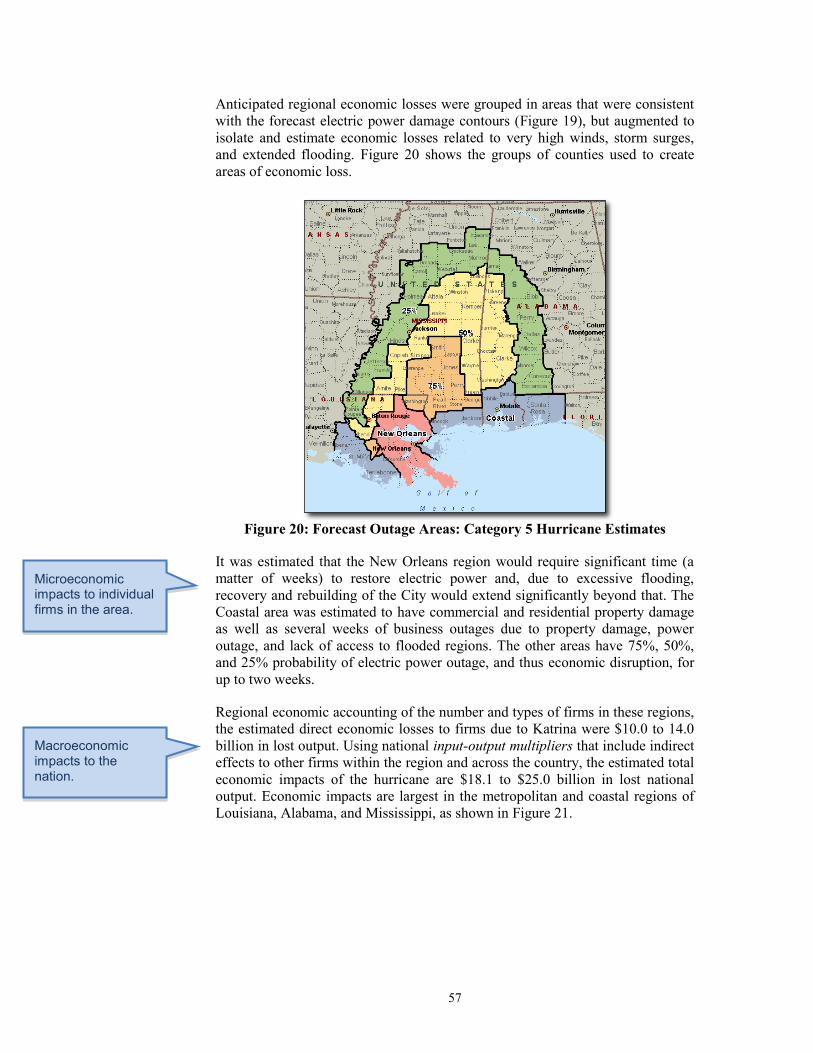
57

Anticipated regional economic losses were grouped in areas that were consistent with the forecast electric power damage contours (Figure 19), but augmented to isolate and estimate economic losses related to very high winds, storm surges, and extended flooding. Figure 20 shows the groups of counties used to create areas of economic loss.

Figure 20: Forecast Outage Areas: Category 5 Hurricane Estimates

It was estimated that the New Orleans region would require significant time (a matter of weeks) to restore electric power and, due to excessive flooding, recovery and rebuilding of the City would extend significantly beyond that. The Coastal area was estimated to have commercial and residential property damage as well as several weeks of business outages due to property damage, power outage, and lack of access to flooded regions. The other areas have 75%, 50%, and 25% probability of electric power outage, and thus economic disruption, for up to two weeks.

Regional economic accounting of the number and types of firms in these regions, the estimated direct economic losses to firms due to Katrina were $10.0 to 14.0 billion in lost output. Using national input-output multipliers that include indirect effects to other firms within the region and across the country, the estimated total economic impacts of the hurricane are $18.1 to $25.0 billion in lost national output. Economic impacts are largest in the metropolitan and coastal regions of Louisiana, Alabama, and Mississippi, as shown in Figure 21.

Microeconomic impacts to individual firms in the area.

Macroeconomic impacts to the nation.

58

Figure 21: Lost GDP, by County: Category 5 Katrina Hurricane

Estimates

As shown in Figure 22, Louisiana bears the brunt of the hurricane’s direct economic impact (and is thus the largest source of indirect impacts). A larger number of Mississippi businesses are affected, however, but for a shorter period of time than those in Louisiana. The industry with the largest economic impact across all states was assumed to be the oil and gas industry, due to the concentration of production, transportation, and refining and processing facilities on the Gulf Coast.

Macroeconomic impacts, by county in affected area.

59

Figure 22: Direct and Total Economic Impacts, by Directly Impacted State:

Category 5 Hurricane Katrina Estimates

Post-Hurricane Analysis

Once Katrina hit land and was recognized to generate significant short-term and long-term economic impacts, both to the affected region and the entire nation, more detailed economic tools and analysis were used. Specifically, NISAC used it is 51-region, 70-industry dynamic econometric model, REMI, to estimate multi-year, multi-region impacts caused by at least six substantive hurricane-related changes to the U.S. economy.

Table 5. Factors Influencing Hurricane Katrina Impacts

Factor

Breaching of the levee and subsequent flooding of New Orleans Longer economic downturn due to electric power outage and flooding Relocation of the residents of New Orleans and other damage areas Protracted changes in household spending Significant expenditures on reconstruction activities Higher energy prices caused by damage to the Gulf Coast chemical industry

4.1 Regional and National Macroeconomic Impacts

National Impacts

Our simulations indicate that Hurricane Katrina will cause national GDP to decline by $32 billion (0.4%) in the first year after the hurricane, $42 billion (0.3%) in year 2, and $12 billion (0.1%) in year 3. National employment will decline by 216,000 in 2005, 250,000 in 2006, and return to baseline levels by 2007. These changes are caused primarily by strong increases in regional

Macroeconomic impacts, direct & indirect, by state

Macroeconomic impacts to the nation.

60

spending by inhabitants of the three affected states on housing/construction, consumer goods, and other regional industries that supply to these sectors, and declines in spending on national durable goods (e.g., automobiles) as result of a loss of confidence by inhabitants of the three affected states about their near-term finances.

State Impacts

Louisiana, while experiencing a wide range of impacts including loss of life, dislocation of its population, and general anxiety and uncertainty that comes from very large natural disasters, receives a very large infusion of federal emergency dollars ($50 billion was recently approved) and in-kind help; this infusion fuels hyper-normal investment and spending in construction, medical, and a wide range of consumer-related industries, thereby generating thousands of jobs and new regional income.

When considering all of these economic additions and subtractions to the Louisiana economy, our simulations estimate that Louisiana GDP will increase by $27 billion (22.4%) in 2005, $33 billion (26.7%) in 2006, and return approximately to baseline in 2007. For similar reasons, Mississippi state GDP increases by $8 billion (12.3%) in 2005, $10 billion (15.7%) in 2006, and returns to baseline by 2007. Alabama GDP increases by $13 billion (10.5%) in 2005, $17 billion (13.6%) in 2006, and returns approximately to baseline in 2007.

Figure 23 displays the change in 2005 GDP, by state. The majority of U.S. states experience minor levels of economic downturn, due largely to increased energy prices. Energy prices increase the costs of transportation, manufacturing, construction, housing, and other key industries, decreasing significantly the purchasing power of residents and businesses and thereby protracting recovery. For example, national nominal personal income in 2005 declines by $5 billion, but real personal income in 2005 declines by $75 billion, owing to increased prices that reduce the purchasing power of each income dollar. Regionally, California experiences the largest decline in GDP in dollar terms, but due the size of the state, experiences a relatively small percent decline in output.

Macroeconomic impacts, direct & indirect, by state

61

Figure 23: Changes in State GDP: 2005

Industry Impacts

By industry, manufacturing sectors are hard hit: for example, national vehicle and parts manufacturing declines by $8 billion (2.0%) in 2005 and $9 billion (2.4%) in 2006, due largely to the uncertainty consumers in LA/MS/AL have about their future finances.76 In response to reconstruction efforts, housing consumption expenditures increase by $5 billion (0.4%) in 2005, $4 billion (0.4%) in 2006, and $2 billion (0.2) in 2007, reflecting the local multiplier impact of construction industries and other reconstruction-related activities.

Comparison with other Estimates of Macroeconomic Impacts

Given the importance of economic impact estimation to DHS, FEMA, Louisiana state government, and other institutions, there have been a number of economic impacts listed. Table 6 compares a number of impact measures from these reports.

Table 6: Comparison of Macroeconomic Estimates

Measure NISAC CBO Global Insight

Lost Output (GDP) 0.4% .5 to 1% .5 - 1% Lost Employment (2005) 216,000 400,000 200,000 Insurance Costs $50 Billion* $30 Billion $35 Billion Change Inflation 1.0% - 0.8%

*NISAC/LANL estimate. Insurance industry estimates of $60 billion insured losses approximate this estimate.

76 This result is consistent with results of other studies in which consumers, experiencing a lack of confidence about their future, delay large-item durable purchases.

Macroeconomic impacts, by economic sector.

62

All of these agencies have stressed that these are approximate, initial estimates based on limited data and observations. The CBO and Global Insight (GI) both agree that the impact on GDP could be between a half and a full percentage point decline, while our estimate is a 0.4% decline. NISAC and GI are close with their estimates of employment loss, while the CBO estimates a greater loss in employment, but acknowledges that estimates range from 150,000 to 500,000. The CBO report does not mention inflationary effects the hurricane may have, however comments have been given by individuals at the Federal Reserve Bank of Chicago, Pennsylvania and Cleveland, in which they all concur that inflation will increase in the short term, but expect the increases to be transient. Specific estimates were not provided; however, GI estimates that inflation will increase to just under 4% as a result of Katrina.

Each factor listed in Table 5 has different, often counterbalancing effects on the other factors; some discussion of these factors helps articulate the overall, net impact.

Loss of Regional Production

LA, MS, and AL lose economic output, decreasing state income and spending in the region and across the nation. In the years that follow, this output is increasingly compensated for by expanded output in other states, which increase their capital investment in response to this new output. Unemployed workers find jobs in and migrate to the compensating parts of the country, or find jobs in other sectors.

Increases in Energy Prices

Increases in energy costs are felt by most sectors in all states, as their production costs (labor, capital, and fuel) increase, requiring increases in their sales prices and subsequently reducing sales and profits. Consumer spending declines, as the purchasing power of income declines. U.S. prices increase as compared to the rest of the world thereby reducing the value of the dollar abroad, exacerbating the already negative balance of trade.

Impacts of Restoration Activities

Funded by insurance dollars and federal and state aid, reconstruction of the damage area will cause significant increases in construction, construction employment, and across-the-board economic activity that result from this increase. This level of increase, however, will cause increases in construction material and labor costs, and propagate these price increases across other sectors of the regional economy.

Impacts of Relocation

The damage from Katrina has forced the evacuation and ultimately the relocation of hundreds of thousands of residents of Louisiana, Mississippi, and Alabama. As shown in Figure 22 and Figure 23, the majority of the estimated 500,000 evacuees have been relocated in Texas, Arkansas, relatively unaffected regions of Louisiana (e.g., Baton Rouge), and adjacent states. Evacuating these residents

Macroeconomic estimates of regional redistribution of output and employment.

Macroeconomic estimates of sectoral redistribution of output and consumer spending.

Macroeconomic estimates of regional relocation of labor supply.

63

from the impacted regions will reduce the labor force in the region and thereby put upward pressure on wages there. However, since the jobs themselves are gone, there is little effect to the outage region, other than the loss of demand that would help revive businesses in the outage region. Destination cities and states will experience a large increase in population (e.g., Baton Rouge has doubled in size), thereby increasing local demand for and spending on housing, food, and other consumer goods, thereby putting upward prices on these goods. Relocation will also increase the labor supply to generally low-wage jobs, putting significant downward pressure on wage rates. These effects will likely be of relatively short duration as evacuees return to their jobs and homes during the expanding recovery period.

4.2 Commodities Exported from and Imported to the Affected Region

Figure 24: Chemical Facilities in Hurricane Damage Area

Table 7 lists the top five classes of commodities exported from the affected regions of Louisiana, Mississippi, and Alabama. Chemical facilities in the damaged region are shown in Figure 7. Chemicals

shipments make up 43% of rail shipments out of the region; disruptions to the chemicals industry will likely reduce demands on local rail freight needs. Mail is 50% of all air shipments out of the

region; likewise, in the short term the reduction in economic activity will significantly reduce demand for air transport. Highway

transport-based exports from the region are evenly distributed among the top 5 commodities. The set of imported commodities (

Microeconomic impacts to individual firms in the area.

64

Table 8) are almost identical to the exported commodities, but the rankings are slightly different.

Table 7: Commodities Exported from Impacted Region: Hurricane Katrina

Transport Mode / Commodity Rank Tons per Month %

Rail Transport Chemicals 1 2,467,561 43% Lumber 2 872,315 15% Pulp/Paper 3 723,505 13% Petroleum 4 394,677 7% General freight 5 312,159 5% Highway Transport General freight 1 7,045,174 17% Petroleum/Coal 2 6,129,538 15% Lumber 3 5,878,191 14% Chemicals 4 4,939,471 12% Minerals 5 3,424,886 8% Air Transport Mail 1 3,517 50% Specialty chemicals 2 881 13% Electrical components 3 727 10% Machine parts 4 648 9% Transportation parts 5 562 8% Waterway Transport Petroleum/Coal 1 6,037,393 35% Chemicals 2 2,533,404 15% Coal 3 1,761,405 10% Agricultural 4 1,593,262 9% Petroleum Crude 5 1,202,800 7%

Macroeconomic impacts to regional commodity flows.

65

Table 8: Commodities Imported from Impacted Region: Hurricane Katrina

Transport Mode / Commodity Rank Tons per Month %

Rail Transport Coal 1 942,479 18% Chemicals 2 894,842 17% Agricultural products 3 705,560 13% Lumber 4 542,784 10% Minerals 5 484,420 9% Highway Transport Intermodal Transfers 1 6,515,194 18% Lumber 2 4,999,529 14% Minerals 3 4,444,934 12% Concrete/Clays 4 3,721,614 10% Food and Kindred 5 3,609,936 10% Air Transport Mail 1 7,611 56% General Freight 2 1,661 12% Electrical components 3 1,278 9% Specialty Chemicals 4 795 6% Machine parts 5 515 4% Waterway Transport Agricultural 1 5,324,880 29% Petroleum Coal 2 3,825,890 21% Coal 3 1,934,694 11% Minerals 4 1,839,620 10% Food and Kindred 5 1,440,172 8%

The macroeconomic simulations indicate that the trade balance of commodities that flow to and from the impacted region could change significantly, putting in question the capacity of the transportation infrastructure to accommodate these changes. For example, the three-state region cannot self-supply manufactured goods necessary for reconstruction, putting upward pressure on the highway transportation sector (e.g., there may not be enough drivers and trucks).

4.3 Chemical Industry Supply Chain Impacts

Katrina caused significant damages to the petroleum industry in the Gulf, a major supplier of crude oil, refined petroleum products, and natural gas as feedstock to the petrochemical industry. The resulting daily loss of chemical production in Louisiana, Mississippi, and Alabama ranges between $46 million and $122

Macroeconomic impacts to regional commodity flows.

Macroeconomic impacts to chemical sector.

66

million77 of lost chemical production. Assuming a 4-week production disruption, the economic impacts are $1.1 billion to $5.1 billion of lost output.

Based on detailed analysis of the chemical facilities in the region and their damages, Table 9 lists the impacted industries and their loss in daily production (by NAICS code; Table 10 describes these industries). In aggregate, these industries in the impacted region generate $66.7 B of sales, or 20% of national sales.

77 Used Benchmark Input-Output Direct Requirements coefficients for 6 digit NAICS codes to determine distribution of these chemicals to other industries. In addition used the 2002 Census value (sales) per 6 digit NAICS.

67

Table 9: Affected Chemical Production

Chemical NAICS Code

National Prod.

Loss (%) Chemical NAICS Code

National Prod.

Loss (%)

Benzene 324110 9 Ethylene Glycol 325199 37 Ethylene 324110 8 Ethylene Oxide 325199 36 Styrene 324110 31 Isopropyl Alcohol 325199 0 Toluene 324110 9 Methyl Chloride 325199 10 Toluene Diisocyanate 324110 23 Methylene Chloride 325199 20 Alpha Olefins 325110 37 Monopropylene Glycol 325199 20 Paraffins 325110 0 n-Butanol 325199 24 Acetylene 325120 51 Perchloroethylene 325199 34 Fluorocarbons 325120 37 Phosgene 325199 34 Liquid Hydrogen 325120 35 Trichloroehtylene 325199 0 Caustic Soda 325181 14 Triethylene Glycol 325199 48 Chlorine 325181 13 Tripropylene Glycol 325199 21 Carbon Black 325182 6 Ammonia Phosphates 325211 22 Calcium Chloride 325188 13 Ethanolamines 325211 39 Hydrofluoric Acid 325188 61 Polychloroprene 325211 34 Phosphorus Trichloride 325188 64 Polyethylene – HD 325211 5 Methyl Ethyl Ketone (MEK) 325191 43 Polyvinyl Chloride 325211 22 Aniline 325192 73 Vinyl Chloride 325211 15 Methylene Diphenyl Diisocyanate (MDI) 325192 57 1,4 Butanediol 325212 37 Nitobenzene 325192 75 Butadiene 325212 11 Phthalic Anhydride 325192 0 Butyl rubber 325212 0 Acrylamide 325199 42 EP rubber 325212 34 Chloroform 325199 20 SB Rubber 325212 14 Diethylene Glycol 325199 35 Ammonia 325311 16 Dipropylene Glycol 325199 21 Urea 325311 26 Ethylene Dichloride 325199 19

68

Table 10: NAICS Codes Definitions

NAICS Code NAICS Description

35120 Industrial Gas Manufacturing 325181 Alkalis and Chlorine Manufacturing 325182 Carbon Black Manufacturing 325188 Other Inorganic Chemical Manufacturing

325190* Basic Organic Chemical Manufacturing 325211 Plastics and Resins

*includes 325191, 325192, and 325199. The chemical production in the impacted region is highly interdependent: these six industries are required for production of most manufactured goods in the US, including most of these six chemicals themselves. Based on detailed analysis of the national use-by-commodity tables,78 Table 11 lists that the top eight industries that will likely experience losses of input materials.

Table 11: Top Industries Impacted by Damage to Chemical Industry

Industry NAICS Code

Asphalt manufacturing 324121 Asphalt coatings/shingle manufacturing 324122 Plastics and resin manufacturing 325211 Synthetic rubber manufacturing 325212 Printing inks and coating 325910 Paint manufacturing 325510 Fertilizer manufacturing 325312 Dye and pigment manufacturing 325130

4.4 National Chlorine Supply Chain

Given that a large fraction of the bulk chlorine production is disrupted by the hurricane, there are significant disruptions to both the bulk chlorine market in the short run and the downstream, bottled chlorine market in the medium run. Rail transportation adjusts greatly, while truck transport adjustment is minimal. Economic markets adjust to make up for the change in level and spatial distribution of production. As simulated, there are occasional national demand flashovers, where firms buy trans-nationally to maintain sufficient chlorine at end-use locations. In total, it takes an estimated 8 weeks after the end of the disruption for the value chain to return to baseline, normal conditions.

Regional Economic Markets

78 Source: U.S. Department of Commerce, Bureau of Economic Analysis, Benchmark Input-Output Tables, http://www.bea.gov/bea/dn2/ i-o_benchmark.htm, September 12, 2005.

Macroeconomic indirect impacts caused by losses in the chemical sector.

69

As illustrated by Figure 25, during normal conditions the bulk chlorine producers in the Northeast serve the Northeast, Central-east, and Northwest while the Gulf Cost producers serve the Southeast and Southwest. During disruption conditions, however, the bulk chlorine markets must make significant adjustments: the Northeast market expands to include more of the Central-east, the undisrupted Gulf Coast producers expand their Southeast market into the Central-east as well.

The bottled chlorine producers are spatially distributed across the country and serve markets well in one to three local states, as shown in Figure 26. Due to the shortages in bulk chlorine, some bottlers cannot purchase bulk chlorine and their markets disappear in the short run: the bottler markets in Nevada, Colorado, Arizona, and New Mexico no longer exist, and their customers are served by California, Washington, Utah, and Texas bottlers.

Mesoeconomic impacts to regional chlorine markets.

70

Baseline Conditions (Day 100)

Disruption Conditions (Day 175)

Figure 25. Bulk Chlorine Market: Baseline and Disruption Conditions

71

Baseline Conditions (Day 100)

Disruption Conditions (Day 175)

Figure 26. Bottled Chlorine Market: Baseline and Disruption Conditions

72

Baseline Conditions (Day 100)

Disruption Conditions (Day 175)

Figure 27. Transportation Use, Chlorine Value Chain: Baseline/Disruption

Regional Transportation Usage

As illustrated in Figure 27, the normal use of rail and truck transportation is spatially consistent with the market use shown in Figure 25 and Figure 26: rail transport (in blue) moves from the North-central part of the country to the Northeast and Northwest portions of the country, while the Gulf Coast production serves the Southeast, Central, and Southwest. Given the spatial distribution of chlorine bottlers across the country, the truck transport (in red) makes local, roughly circular “spider” distributions of shipments.

During the disruption, the Gulf Coast rail shipments are fewer and circumvent the disrupted area; the Gulf Coast shipments extend up northward into the Central-east, and the Northeast rail shipments extend downward to the same area.

73

The truck shipments east of the Mississippi are relatively unchanged while those Central bottlers (west of the Mississippi) now have decidedly westward shipment flows (to customers in Colorado, Arizona, and New Mexico, which lost their local bottlers).

Regional Production and Desired and Completed Purchases

Bulk Chlorine

As illustrated by Figure 28 (where the diameter of the columns in the figure are the amount of production), the distribution of bulk chlorine production is in the Gulf Coast and a significant fraction of it is in the path of the hurricane. During the disruption, the lost production is made up by addition production in Texas and Northeast locations (the light-blue rail lines in the figure can also be used to see where there changes in production are), but there is relatively little excess aggregate.

Comparing the upper and lower panels in Figure 29, which shows desired and completed purchases, we see that the significant purchases made by Gulf Coast firms are lost during disruption, shifting some of this demand northward and away from the West.

Bottled Chlorine

Figure 30 shows the distribution of production for bottled chlorine, during normal conditions and disruption. The two panels in the figure are very similar, with the noticeable exception of increased ordering by a Nevada bottler who increases supply to California, a state that is relatively remote and therefore is distant to most markets and must increase shipments and purchases to weather the disruption.

Finally, Figure 31 shows that the baseline and disrupted distributions of purchases are essentially identical; consumers of bottled chlorine are able to get supply during the disruption (as we see below, the bottled chlorine market does go through some significant adjustments during recovery).

74

Baseline Conditions (Day 100)

Disruption Conditions (Day 175)

Figure 28. Bulk Chlorine Production: Relative Production Rates (as diameter)

75

He

Baseline Conditions (Day 100)

Disruption Conditions (Day 175) Figure 29. Bulk Chlorine Demand (as diameter) and Shipments

(as height): Baseline/Disruption

76

Baseline Conditions (Day 100)

Disruption Conditions (Day 175)

Figure 30. Bottled Chlorine Production (as diameter)

77

Baseline Conditions (Day 100)

Disruption Conditions (Day 175) Figure 31. Bottled Chlorine Demand (as diameter) & Shipments

(as height): Baseline/Disruption

Aggregate Measures

Starting at the top panel (“Unmet Demand”) in Figure 32, we see that unmet demand for bulk chlorine increases by an estimated 50 percent during then disruption and then returns to normal levels about one week into recovery. Bottled chlorine, on the other hand, remains relatively unchanged.

In the second panel (“In-Transit Inventories”), bulk chlorine shipments increase over the disruption, as firms have to ship bulk over longer distances to meet customer demand. Bottled chlorine experiences very large increases in these

78

shipments, as California must make more purchases farther east to meet its water supplier demand.

The average shipping distance for bulk and bottled chlorine increases slightly over the disruption period and returns to normal in about one month. The bottled chlorine market has four noticeable peaks during the recovery period, as some end-users (most notably in California) have to make long distance shipments during four points of national shortage, to maintain sufficient on-site inventories. Finally, GDP decreases by an estimated 30 percent, due largely to the loss of bulk chlorine production capacity, and then returns to normal in about two weeks.

Summary of Chlorine Value Chain

First, the 25-percent loss of bulk chlorine production capacity sets into motion a chain of events that impact both the downstream purchase of bulk and bottled chlorine and impact particular regions of the country. Full recovery from this chain of events takes over two months.

Second, bulk chlorine production shifts to Texas, Alabama, and New York, and the bulk chlorine markets adjust to the new spatial distribution of bulk chlorine producers and users. The notable spatial “losers” in this rationalization of bulk chlorine are the states of Colorado, Arizona, and New Mexico, who are far from the chlorine production in the Gulf Coast and East; the bottlers in these states are unable to get bulk chlorine, causing the bottlers in surrounding states to expand their markets into these states.

Third, the end-users of bottled chlorine are largely unaffected, other than having to ship more chlorine over the disruption period due to larger shipping distances and having to make long distance shipments at four points during recovery.

Fourth, the rail and truck transport of chlorine during the disruptions changes mostly due to changes in market structure and less so due to the change in transportation system. Finally, there is an 30-percent loss of GDP during the disruption, but most end-users of chlorine, most notably water purification plants, are able to maintain on-site inventories throughout the disruption and recovery.

79

Unmet Demand (lbs)

In-Transit Inventories (lbs)

Average Shipping Distance (miles)

Chlorine-related GDP ($)

Figure 32. Macroeconomic Measures: Chlorine Value Chain

4.4.1 Small Businesses and Insured Losses

Most regional economies are composed largely of small businesses. Because of the lack of management resources or know-now, these firms are acutely vulnerable to economic losses and outright failure of their business. Using statistics from analytical studies of previous hurricanes, Table 12 lists the estimated number of small firms (those with less than 100 employees) that are likely to be impacted economically in particular forms by Katrina; Figure 33 shows that the majority of the small firms

Microeconomic direct impacts to small businesses in the affected area.

80

impacted (as measured by the number expected to lose electric power) are located on the Gulf Coast and in the New Orleans metropolitan area, that is, in the direct path of the strongest part of the hurricane.

Table 12: Estimated Number of Impacted Small Businesses (< 100 Employees)

Small Firms Only

Total # firms in impacted counties

Total # of small firms

# expected to lose electric

power

# with physical damage

# that never re-open

# that close after two years

2,064,000 261,000 199,000 120,000 86,000 58,000

Figure 33: Number of Affected Firms with < 100 Employees, by County

The estimates in Table 12 are based on the following data: in a study of the impacts to small businesses of Hurricane Floyd,79 it was estimated that more than 65% of the North Carolina businesses impacted in some form by Hurricane Floyd were “small” businesses, employing fewer than 100 people. Of these, 60% reported physical damage from the hurricane. The Institute for Home Business and Safety has found that “of all businesses that close down following a disaster, more than 43% never reopen, and an additional 29% close permanently within two years.”

79 Institute for Business & Home Safety, accessed at http://www.ibhs.org/publications/ on September 14, 2005.

Microeconomic impacts to small businesses in the affected area.

81

Because of their more limited access to capital, small businesses find it difficult to recover from short-term market disruptions. Survey data also show that less than one in six small businesses carry business interruption insurance and most did not carry flood insurance. Data suggests that the impacts to small businesses of Katrina will be much worse than of Hurricane Floyd, which damaged a predominantly rural and agricultural area and caused commercial economic losses in excess of $6 billion, impacting commercial property, agricultural crops, and business revenues; the area damaged by Katrina is both rural and metropolitan, with employment in fishing, tourism, oil field servicing, and many other economic sectors that are typically dominated by small business. Furthermore, the combination of extensive regional flooding and the probable lack of flood insurance on the part of many small businesses are likely to result in many small business failures. Because small business accounts for a large percentage of local employment, these business failures will contribute significantly to prolonged unemployment. To help mitigate losses, the Small Business Administration (SBA) and Federal Emergency Management Agency (FEMA) have programs to assist small business recovery. SBA deploys disaster assistance teams to begin the process of damage assessment and disaster loan application process for businesses and individuals. Disaster loans for business cover physical losses and economic injury from closures and lost business for up to $1.5 million per business. Loans can be arranged for periods up to 30 years at 4% interest.

Microeconomic impacts to small businesses in the affected area.

5. Summary and Conclusions

5.1 Summary

Economists at Sandia National Laboratories have conducted for the U.S. Department of Homeland Security well over 100 detailed economic impact analyses, for a wide range man-made and natural disruptive events. To complete these, the economists have used a wide range of data sources, models, and software tools, each of which follows a particular economic analysis discipline.

For the purposes of this report, we have grouped those disciplines as either (1) microeconomic, (2) macroeconomic, or (3) mesoeconomic, the last of which provides insights to infrastructure-related economic impacts in ways that the first two have difficulty providing. Each of these disciplines has a different set of units of analysis, different underlying economic theories, and different estimates of economic impact. When used together, NISAC economists provide a rich, comprehensive, and multi-model perspective to the economic impacts of DHS-related disruptive events.

The advantages of this multi-theory, multi-model approach are evident in the example analysis provided herein: estimates of impact include the numbers and types of businesses directly impacted by a disruptive event; the ability of households to relocate and find new jobs; changes in regional market activity and associated regional economic demand, inventories, and shipments; and changes in regional and sectoral output (GDP), employment, and income.

5.2 Conclusions

While the economic theories, models, and analytical capabilities described herein provide a rich environment for understanding and estimating economic impacts, it is only a first attempt. Many additional scenarios of interest have not yet been analyzed, many of the CIKRs have not been covered, and the complete set of important economic impacts are not being estimated yet. To do this, additional techniques and underlying research will be needed.

83

References

Bockarjova, M., Streenge, A.E., and van der Veen, A. 2004. “Structural economic effects of large-scale inundation: a simulation of the Krimpen dike breakage” in: Flooding in Europe: Challenges and Developments in Flood Risk Management: in series Advances in Natural and Technological Hazards Research. Summer 2004.

Brown, T.J. 2009. “Dependency Indicators,” Wiley Handbook of Science and Technology for Homeland Security, New York, NY: John C. Wiley and Sons.

Carlson, R., Cooperstock, L., Loose, V.W., and Ehlen, M.A. An Approach to Estimating Higher-Order Economic Impacts of CBRNE Acts of Terrorism with Application to an Anthrax Attack on the Washington, DC Metropolitan Area (OUO). Sandia National Laboratories SAND Report Number 2007-2470. April 2007.

Carlson, R.E., Ehlen, M.A., Loose, V.W., Pless, D.J., Stamber, K.L., Starks, S.J., and Vargas, V.N. “Rules of Thumb” for Rapid Economic Impact Assessment of Natural and Man-Made Disruptive Events. Sandia National Laboratory SAND Report. December 2008.

Chang, S., Stough, R.R., and Kocornik-Mina, A. 2006. “Estimating the economic consequences of terrorist disruptions in the national capital region: an application of input-output analysis.” Journal of Homeland Security and Emergency Management. Vol 3:3, 2006.

Cho, S., Gordon, P., Moore, J.E., Richardson, H., Shinozuka, M., and Chang, S. 2001. “Integrating Transportation Network and Regional Economic Models to Estimate the costs of A Large Urban Earthquake,” Journal of Regional Science, 41(1): 39-65.

Clower, T. 2007. “Economic applications in disaster research, mitigation, and planning. In McEntire, D., Disciplines, Disasters and Emergency Management: The Convergence and Divergence of Concepts, Issues and Trends in the Research Literature. Springfield, IL: Charles C. Thomas. 2007.

Cooperstock, L., Ehlen, M.A., and Loose, V.W. 2006. “REAcct 1.0: an Initial Methodology for Estimating and Reporting Economic Impacts.” Sandia National Laboratories white paper. October 2006.

Dopfer, K., Foster, J., Potts, J. 2004. “Micro-meso-macro,” Journal of Evolutionary Economics, v. 14, pp. 263-269.

Downes, P.S. and Belasich, D.K. 2005. “NISAC Agent-Based Laboratory of Economics (N-ABLE™): Supply Chain Transportation Agent, Architecture and Design Document.” Manuscript. October 2005.

84

Downes, P.S., Ehlen, M.A., Loose, V.W., Scholand, A.J., Belasich, D.K. 2005. Estimating the Economic Impacts of Infrastructure Disruptions to the U. S. Chlorine Supply Chain: Simulations using the NISAC Agent-Based Laboratory for Economics (N-ABLETM ) Sandia National Laboratories SAND Report Number SAND2005-2031. March 2005.

Dun & Bradstreet, Inc. 2010. Accessed at http://www.dnb.com on January 5, 2010.

Ehlen, M. A., “Search Costs and Market Stability: The Importance of Firm Learning on Equilibrium Price Dispersion,” Sandia National Laboratories # 2004-6213 J, July 2004.

Ehlen, M.A., and Glass, R.J. (2003) “Growth and Defection in Hierarchical, Synergistic Networks,” Proceedings from 2003 SFI Complex Systems Summer School, Santa Fe Institute, Santa Fe, NM, 2003.

Ehlen, M.A., Belasich, D.K., Downes, P.S. 2006. Modeling the Economic Impacts of Increased Border Security on Domestic Firms: Simulations using the NISAC Agent-Based Laboratory for Economics (N-ABLETM ). Sandia National Laboratories SAND Report Number SAND 2006-3794. June 2006.

Ehlen, M.A. and Scholand, A.J. 2005.“Modeling Interdependencies between Power and Economic Sectors using the N-ABLETM Agent-Based Model.” Proceedings of the IEEE Conference on Power Systems, San Francisco, July, 2005.

Ehlen, M.A., Scholand, A.J., Stamber, K.L. 2004. “The Effects of Residential Real-Time Pricing Contracts on Transco Loads, Pricing, and Profitability: Simulations using the N-ABLETM Agent-Based Model. Energy Economics. 13 January 2004.

Eidson, E.D. and Ehlen, M.A. 2005. NISAC Agent-Based Laboratory for Economics (N-ABLETM): Overview of Agent and Simulation Architectures, Sandia National Laboratories SAND Report Number SAND2005-0263.

Ellebracht, L., Loose, V.W., Ehlen, M.A., and Carlson, R. 2007. An Approach to Estimating Higher-Order Economic Impacts of CBRNE Acts of Terrorism. Sandia National Laboratory SAND Report Number SAND2002007-2471. April 2007.

Forrester, J.W. 1961. Industrial Dynamics, Boston, MA: MIT Press.

Gordon, P., Kim, S., Moore, J.E., Park, J., and Richardson, H.W. 2005. “The Economic Impacts of a Terrorist Attack on the U. S. Commercial Aviation System.” University of Southern California, accessed at http://www.usc.edu/dept/create/events/2005_01_31/Gordon.pdf on March 30, 2006.

Gordon, P., et al. 2005. “The economic impact of a terrorist attack on the twin ports of Los Angeles-Long Beach”. The Economic Impacts of Terrorist Attacks. H. W. Richardson, Peter Gordon, and James E. Moore II, eds. Northampton, MA. Edward Elgar Publishers.

85

Haimes, Y.Y., Horowitz, B.M., Lambert, J.H. , Santos, J., Crowther, K., and Lian, C. 2005. “Inoperability Input-Output Model for Interdependent Infrastructure Sectors. II: Case Studies.” Journal of Infrastructure Systems, vol. 11: pp. 80 -92.

Haimes, Y.Y. and Jiang, P. 2001. “Leontief-Based Model of Risk in Complex Interconnected Infrastructures.” ASCE Journal of Infrastructure Systems: 7(1):1-12.

Institute for Business & Home Safety. 2005. Accessed at http://www.ibhs.org/publications/ on September 14, 2005.

Linebarger, J.M., Scholand, A.J., and Ehlen, M.A. 2006. Proceedings of the 39th Hawaii International Conference on System Sciences - 2006, 0-7695-2507-5/06 (C) 2006 IEEE.

Loose, V.W. 2006. “NISAC Agent-Based Laboratory of Economics™ (N-ABLE™): Bank Agent Architecture and Design Document.” Spring 2006. Manuscript.

Jones, D.A., Hollingsworth, M.A., Lawton, C.R., Ehlen, M.A., Davis, J.A., Talso, D.W., Nozick, L.K., Turnquist, M.A., Loose, V.W. 2003. Impact Analysis of Potential Disruptions to Major Railroad Bridges in the U.S. Sandia National Laboratories Report, August 18, 2003.

Leontief, W.W. Input-Output Economics. 2nd ed., New York: Oxford University Press, 1986.

Microsoft Corporation. 2010. “MapPoint,” accessed at http://www.microsoft.com/mappoint/en-us/default.aspx on January 5, 2010.

Minnesota IMPLAN Group, Inc. 1999. IMPLAN Professional, Version 2.0, Social Accounting and Impact Analysis Software: User's Guide, Analysis Guide, Data Guide. Stillwater, MN.

Moore, J.E., Little, R., Cho, S., and Lee, S. 2005. “Using Regional Economic Models to Estimate the costs of Infrastructure Failures: The cost of a Limited Interruption in Electric Power in The Los Angeles Region.” A Keston Institute for Infrastructure Research Brief, accessed at http://www.usc.edu/schools/sppd/lusk/keston/pdf/powerfailure.pdf on March 30, 2006.

National Geospatial-Intelligence Agency Homeland Security Infrastructure Program (HSIP) Gold 2005, http://www.defenselink.mil/policy/sections/policy_offices/hd/assets/downloads/dcip/DCIP_Geospatial_Data_Strategy.pdf

Oak Ridge National Laboratory, Center for Transportation Analyses. 2006. “Intermodal Transportation Network,” accessed at http://cta.ornl.gov/cta/ on April 19, 2006.

Transportation Network,” accessed at http://cta.ornl.gov/cta/ on April 19, 2006.Okuyama, Y. 2003. “Modeling spatial economic impacts of disasters: IO Approaches,” in: Proc.

86

Workshop In Search of Common Methodology on Damage Estimation, Delft, the Netherlands, May 2003.

Rinaldi, S., Peerenboom, J., and Kelly, T. 2001. “Identifying, Understanding and Analyzing Critical Infrastructure Interdependencies,” IEEE Control System Magazine, 21:11-25.

Rose, A.Z. 2005. “Tracing Infrastructure Interdependencies through Economic Interdependencies.” Unpublished paper available accessed at http://www.cpac.missouri.edu/library/johnsontg/agec442/inputoutput/Inputoutput.html on March 30, 2006.

Rose, A.Z. 2006. Regional Models and Data to Analyze Disaster Mitigation and Resilience, Center for Risk and Economic Analysis of Terrorism Events (CREATE): University of Southern California.

Rose, A.Z., Benavides, J., Chang, S., Szczesniak, P., and Lim, D. 1997. “The Regional Economic Impact of an Earthquake: Direct and Indirect Effects of Electricity Lifeline Disruptions.” Journal of Regional Science, 37:437-58.

Rose, A.Z., and Benavides, J. 1998. “Regional Economic Impacts” in M. Shinozuka et al (eds.) Engineering and Socioeconomic Impacts of Earthquakes: An Analysis of Electricity Lifeline Disruption in the New Madrid Area, MCEER, Buffalo, 95-123.

Rose, A.Z. and Miernyck, W. 1989. “Input-Output Analysis: The First Fifty Years.” Economic Systems Research, 1:2, 1989.

Roy, J.R., Hewings, and August, G. 2005. “Regional Input-Output with Endogenous Internal and External Network Flows” REAL 05-T-9. Accessed at http://www2.uiuc.edu/unit/real/d-paper/05-t-9.pdf on March 30, 2006.

Regional Economic Models, Inc. Policy Insight, 433 West Street, Amherst, MA 01002, 2009.

Scholand, A.J., Linebarger, J.M., and Ehlen, M.A. 2005. Proceedings of the 2005 International ACM SiGGROUP Conference on Supporting Group Work (GROUP 2005) 6-9 November 2005, Sanibel Island, Florida, pp. 444-445.

Sprigg Jr., J.A. and Ehlen, M.A. 2007. “Comparative dynamics in an overlapping-generations model: the effects of quasi-rational discrete choice on finding and maintaining Nash equilibrium.” Computational Economics, Springer Science and Business Media.

SRI Consulting. “World Petrochemicals,” accessed at http://www.sriconsulting.com/WP/Public/ProgramContents.html on January 29, 2010.

SRI International. Chemical Economics Handbook, accessed at http://library.dialog.com/bluesheets/htmla/bl0359.html on January 29, 2010.

87

SRI Consulting, Directory of Chemical Producers (DCP), accessed at http://www.sriconsulting.com/DCP/Public/index.html on January 29, 2010.

Stearman, J.D., 2000, Business Dynamics: Systems Thinking and Modeling for a Complex World, Boston, MA: Irwin McGraw-Hill.

U.S. Bureau of the Census. United States Census 2000, accessed at http://www.census.gov/ on January 29, 2010.

U.S. Bureau of the Census, “County Business Patterns.” Accessed at http://www.census.gov/epcd/cbp/view/cbpview.html on August 10, 2009.

U.S. Bureau of the Census, “Regional Input-Output Multipliers II (RIMS II).” Accessed at http://www.bea.gov/bea/regional/rims on August 10, 2009.

U.S. Bureau of Economic Analysis, “Gross-Domestic-Product-(GDP)-by-Industry Data.” Accessed at http://www.bea.gov/industry/gdpbyind_data.htm on August 10, 2009.

U.S. Department of Commerce, Bureau of Economic Analysis, Benchmark Input-Output Tables, http://www.bea.gov/bea/dn2/ i-o_benchmark.htm, September 12, 2005.

U.S. Department of Commerce, Bureau of Economic Analysis. 2010. “Regional Multipliers from the Regional Input-Output Modeling System (RIMS II): A Brief Description,” accessed at https://www.bea.gov/regional/rims/brfdesc.cfm on January 4, 2010.

U.S. Bureau of Labor Statistics. “Employment, Hours, and Earnings from the Current Employment Statistics survey (National).” Accessed at http://www.bls.gov/ces/home.htm on January 29, 2010.

U.S. Department of Homeland Security, National Infrastructure Simulation & Analysis Center (NISAC). 2003. Economic and Public Health and Safety Impacts of Disruptions in Chlorine Transport (OUO). 8 August 2003.

U.S. Department of Homeland Security, National Infrastructure Simulation & Analysis Center (NISAC). 2004. “Toxic Inhalation Hazard (TIH) Industrial Impacts Analysis: Assessing the Impacts of Changes in Toxic Inhalation Hazard Transportation Policy.” Report. March 9, 2004.

U.S. Department of Homeland Security, National Infrastructure Simulation & Analysis Center (NISAC). 2005. Estimating the Regional and National Economic Impacts of Possible Government Actions in Response to a MANPAD Threat (OUO). August 1, 2005.

U.S. Department of Homeland Security, National Infrastructure Simulation & Analysis Center (NISAC). 2005. Comments and Analysis: Review Draft: Scenario for a Magnitude 6.7 Earthquake on the Seattle Fault. A Project Funded by the Earthquake Engineering Research Institute and the Washington Emergency Management Division January 7, 2005.

88

U.S. Department of Homeland Security, National Infrastructure Simulation & Analysis Center (NISAC). 2005. An Agent Model of Agricultural Commodity Trade: Developing Financial Market Capability within the NISAC Agent-Based Laboratory for Economics (N-ABLETM). 7 November 2005.

U.S. Department of Homeland Security, National Infrastructure Simulation and Analysis Center (NISAC). 2007. A Post-Katrina Comparative Economic Analysis of the Chemicals, Food, and Goodyear Value Chains. February 2007.

U.S. Department of Homeland Security, National Infrastructure Simulation & Analysis Center (NISAC). 2007. Economic Modeling for the Analysis of Pandemic Influenza: Supplement to the National Population and Infrastructure Impacts of Pandemic Influenza Report. 15 October 2007.

U.S. Department of Homeland Security, National Infrastructure Simulation & Analysis Center (NISAC). 2007. Impact of Pandemic Influenza-Induced Labor Shortages on the Food Production/Distribution System: Supplement to the National Population and Infrastructure Impacts of Pandemic Influenza Report. 15 October 2007.

U.S. Department of Homeland Security, National Infrastructure Simulation & Analysis Center (NISAC). 2008. 2008 NISAC New Madrid Seismic Zone Study Scenario Analysis of Earthquake Impacts to Infrastructures and the Economy. February 6, 2009. OUO.

U.S. Department of Homeland Security, National Infrastructure Simulation & Analysis Center. (NISAC) 2009. 2009 H1N1 Influenza Study: Impacts on the United States Population and Economy. August 2009.

U.S. Department of Homeland Security, Chemical Industry Project: Capability Report 2007, National Infrastructure Simulation and Analysis Center report, November 27, 2007, pp. 15-20.

U.S. Geological Survey, Geographic Names Information System (GNIS), U. S. Board on Geographic Names, accessed at http://geonames.usgs.gov/ on January 29, 2010.

Vargas, V.N., and Scholand, A.J. 2005. “Improving Agent Behavior with Human Experiments: Mimicking Human Pricing Decisions under Limited Information in Competitive Commodity Markets.” Presentation. 11 November 2005.

Vugrin, E.D., Aamir, M.S., Downes, P.S., Ehlen, M.A., Loose, V.W., Vargas, V.V., and Warren, D.E. 2009. A Framework for Assessing the Economic Criticality of Chemical Facilities, Sandia National Laboratories Report, Albuquerque, NM (OUO). March 12, 2009.

Vugrin, E.D., Warren, D.E., Ehlen, M.A., and Camphouse, R.C. 2009. “A Framework for Assessing the Resilience of Infrastructure and Economic Systems,” submitted to Sustainable Infrastructure Systems: Simulation, Imaging, and Intelligent Engineering, Kasthurirangan Gopalakrishnan and Srinivas Peeta, eds., Springer-Verlag, Inc.

89

West, Guy R., “Notes On Some Common Misconceptions in Input-Output Impact Methodology” University of Queensland, Department of Economics. Accessed at http://eprint.uq.edu.au/view/person/West,_Guy_R..Html on January 29, 2010.

90

Appendix A - N-ABLE™ Software Classes

5.1 AgentLib Software Classes

The NISAC Agent-Based Laboratory for Economics™ (N-ABLE™) is an Agent-Based Model (ABM) designed to model economic value chains and their use of the nation’s critical infrastructure, particularly during man-made and natural disasters. Previous versions of N-ABLE™ have been described elsewhere.80 A current N-ABLE™ simulation is series of analytical steps, with accompanying software programs that prepare and verify the input data, execute the simulation, and process and display the output data.

The primary component is the execution engine – the part that performs the modeling step itself. This engine is built on top of a C++ framework called AgentLib, developed at Sandia National Laboratories, that provides the software services necessary to run generic ABMs, that is, not just N-ABLE™ economic simulations. As shown in Figure 34, these services include reading the input file, performing the simulation, and writing the output file. Other N-ABLE™ software maintains the databases, creates the input files, processes the output file to database, and integrates the overall set of functions. This section focuses on the software design of AgentLib.

Figure 34. N-ABLE™ Suite of Software Functions

8080 For examples, see Eidson, E.D., and Ehlen, M.A., NISAC Agent-Based Laboratory for Economics (N-

ABLE): Overview of Agent and Simulation Architectures, Sandia National Laboratories SAND2005-0263,

February 2005; and Schoenwald, D., Barton, D., and Ehlen, M.A. “An Agent-Based Simulation Laboratory for

Economics and Infrastructure Interdependency,” Proceedings of the 2004 American Control Conference, Vol. 2, pp.

1295-1300, June 2004.

Input File

Data-bases

Simulation Engine

AgentLib Object Classes

N-ABLE™ Object Classes

Output File

Client

91

AgentLib is an ongoing computer science research project, with continual improvements being made towards the goal of being able to run models composed of one billion software agents. It started as a project in the late 1990s to replace the time-slicing simulation engine81 of the Sandia Aspen program82 (written in the C programming language) with a discrete-event engine83 (written in the C++ programming language). In the discrete-event based revision, agents drive themselves by scheduling events for themselves and for other agents on a global calendar. Given the success of that project, the N-ABLE™ ABM model was built on this discrete-event engine and over time, the design evolved into what is now AgentLib. The current design runs on a variety of UNIX platforms, from personal computers (such as Linux desktops and Apple OS X workstations) to massively parallel machines (such as those available at Sandia National Laboratories).

The AgentLib framework provides mechanisms to perform many of the support tasks needed to run an ABM: it provides the ObjGen (object generator) system to specify input file requirements and to then perform the mechanics of reading the input file. It provides the SnapshotRegistrations system to register parts of each agent for regular “snapshots” or output of the agent’s data, and to take the snapshots, which are the primary output from the engine. It provides base classes for the Agents and Events. It provides an object serialization mechanism, called the Transfer system, to exchange the Events and Agents between parallel processes. Finally, it provides the logic that performs the Event-execution loop.

To support these primary tasks, AgentLib also provides additional packages that can be used independently of AgentLib. For example, it includes

an XML processor for reading the input file, an Archive package for gathering the various output files into one file, a data-compression package for reducing the size of the output data, an iostreams-based MPI wrapper for easier parallel implementation, random number generators for improved random number quality, a backtrace utility for debugging, and other packages.

81 “Time slicing” here means a design that divides every simulated day into a fixed number of “slices.” A day starts with a “task” slice or phase where Agents do their daily tasks, including sending messages to other Agents. Then, the remaining slices are used to respond to messages (and respond to the responses, and so on). All time slices must be performed, even if it turns out there is nothing to do in a given slice. Thus, a major limitation of this approach is that we must know a priori the number of slices needed to complete all the message-responses, which in turn leads to a conservative overestimate, and by implication, wasted computation time. 82 For more information on Aspen, see “Aspen’s Micro-simulation Economic Model,” http://www.cs.sandia.gov/tech_reports/rjpryor/index.html (accessed on January 25, 2010). 83 A discrete-event design drives the simulation by keeping an ordered calendar of notable simulation “Events.” In such designs, the simulation clock advances by jumping to the next Event on the Calendar. Such designs are more difficult to parallelize than a time-slicing approach.

92

Almost all of these packages have been developed in-house, despite the current availability of other options. For example, the custom XML processor was written in 2001, when an extensible data processor was needed and XML was promising and new but without suitable publicly available C++ XML processors.

This section describes discusses the overall design goals of AgentLib, gives background on the factors that drove many of the software design decisions, describes the execution engine, and then the input and output subsystems.

5.1.1 Software Goals

A major advantage of agent-based modeling (ABM) is that it provides a conceptual framework for decomposing a large and complex modeling system into sub-systems (agents in this case) that are easier to model directly. By combining many relatively simple agents into a large model, more complex phenomena can be modeled, that is, a complex model emerges from the combination of simpler agent models. In a similar vein, to model extremely complex phenomena, agents can be made somewhat more sophisticated and larger in number. These two steps result in a model that is very computationally intensive, where a single run (such as a model of the national economy over a year) might take days, weeks, or even months of computer time to complete.

To address these time and size issues, AgentLib takes advantage of parallel computing84 approaches, which reduce the time taken to perform a single run, or alternatively, allow for larger, more complex models to run in the same amount of time. Although the performance of single-core (e.g., Intel Pentium) machines has increased dramatically over the last few decades, the pace of those performance increases has slowed. For that reason, and others, multi-core85 and multiprocessor86 machines have become increasingly available and inexpensive, and it is now economical to build “desktop” parallel machines. These and other factors influenced the decision to increase the performance of our agent-based models through parallel computing.

To run on parallel machines, though, the program has to be designed to coordinate concurrent simulation steps across many processes. Furthermore, it needs to be able to generate the same model behaviors and the same results as does a serial version87 of an

84 Parallel computing is the use of more than one CPU concurrently to perform a computation. The term encompasses a variety of hardware platforms including multi-core, multi-processor, and massively parallel computers (which can include thousands of CPUs). The term is usually distinguished from distributed computing in which very large problems (like protein folding or SETI, the search for extraterrestrial life) are chopped up into smaller sub-problems that are then distributed to and solved by millions of individual computers over a widely dispersed geographical network like the Internet. 85 Multi-core microprocessors are those that have more than one computational core within the same chip. Each individual core can simultaneously execute separate programs – in effect, a parallel computer on a single chip. 86 Multi-processor computers have more than one physical microprocessor in the “same machine” – that is, the microprocessors share many hardware components, including memory, disks, and typically can communicate with one another by accessing the shared resources, instead of requiring communication through some sort of network. 87 Serial means not-parallel, or more generally, running with or on only one CPU.

93

AgentLib ABM (i.e., one that runs on a single process), but in much less time and with many more agents. (AgentLib ABMs can run in serial, thereby providing a baseline for conducting verification and validation of model behavior in large ABMs.) AgentLib is designed such that future projects can build ABMs that automatically take advantage of parallel hardware where available. Model builders should be able to follow some straightforward rules and thereby exploit particular hardware’s capabilities -- that is, by following the rules, model builders should not need conditional logic to do one thing in the serial version and another in the parallel version.

5.1.2 Modeling Framework

Fundamentally, AgentLib is a conceptual framework on which ABMs like N-ABLE™ are built – that is, these ABMs extend classes made available by the AgentLib library to implement model-specific behavior. Specifically, Agents are implemented by deriving from the AgentLib class named, naturally enough, “Agent.” (Throughout this chapter we will denote actual AgentLib classes with proper, capital-letter names, e.g., the AgentLib “Agent” class, and generic ABM concepts with indefinite, lower-case nouns, e.g., an ABM “agent.”) Similarly, the events that AgentLib Agents schedule are derived from the class named “Event.”

AgentLib gives model designers a small toolbox of base classes to build on; each base class provides a specific concept that can be extended by the designer to implement the necessary ABM and parallel-computing functionality.

Conceptually, an AgentLib-based ABM is a collection of Agents that implement their own behavior by scheduling Tasks and communicate with other Agents by sending Messages (Figure 35). Tasks and Messages are the only kinds of Events that Agents may schedule in the Event Calendar. (There are other kinds of Events in the model, but they exist to help the engine control the execution of the model – they do not implement specific Agent behaviors.)

Figure 35. AgentLib Agents Scheduling an Event on Event Calendar

Model

The Model base class provides the most visible interface for interacting with the Model as a whole. It conceptually “owns” all of the Agents, the Event Calendar, the parallel synchronization logic, and so forth, although those features are implemented in their own classes. A derived ABM, such as N-ABLE, derives from the Model class and that derived class serves as the basis of the Model framework for the derived ABM.

94

Agent, AgentComponent, and BBoards

All agents in an AgentLib-based ABM are derived from the Agent class. An Agent can represent a very small entity, such as a bacterium, or it can represent large complex organizations like a Government. This level of detail is determined by the particular ABM’s requirements. In design terms, one important explicit purpose of the Agent class is to create a recipient of Events.

To better design large, complex Agents, however, there is still a need to design Agents in terms of smaller components, that is, to better compartmentalize functions of our agents. For example, to implement a “DepartmentStore” Agent (one based on the AgentLib Agent), one component could handle the Electronics department, another component could handle the Clothing department, and so on. Indeed, we could customize a DepartmentStore by changing the set of departments a store might have: a DepartmentStore Agent in a large city might have more departments than one in a small town.88

In previous versions of AgentLib, these smaller components are effectively miniature agents (they scheduled their own tasks and messages), but they have to operate within the context of their owning or enclosing Agent. The owning Agents ended up introducing their own complex “routing” systems to figure out which component should get the Event that was targeted to the Agent as a whole. To address this component-agent problem, the AgentComponent class was introduced to remove the complex “agent within an agent” AgentLib routing schemes. Hence, an AgentComponent is a part of an Agent that can have its own independent Events. A model designer can now combine the Agent and AgentComponent classes in a straightforward fashion – that is, he can design an Agent at an appropriate conceptual level, and implement sub-agents in the form of AgentComponents (Figure 36).

Figure 36. AgentComponents within the AgentLib Agent

Agents (and by extension, AgentComponents) must obey certain design rules in order to be valid members of an AgentLib ABM. First, they can change their internal states only when an Event belonging to the Agent is executed. Second, they can interact with other Agents only through the indirect mechanism of scheduling Events – that is, they can only

88 This design logic follows directly from object-oriented programming, where a “store” could have a collection of “departments,” where each specific department inherits general department characteristics from a general department class. These software classes maintain either “has a” relationships (the store “has” departments) or “is a” relationships (the electronics department “is a” department), thereby providing clean, explicit overall software structures.

95

send Messages to other Agents (and not somehow reach out and touch those other Agents). These rules ensure Agents do not make any assumptions about the physical locations of other Agents during runtime, so we are free to move the Agents around the various parallel-computing processes.

One implication of these design rules is that Agents cannot call member functions89 in other Agents (because the called-upon Agent may not be in the same operating system process – if it’s not in the same process, there is no means for calling a member function90). However, a common situation is that we need to make runtime data (such as a list of all participants in an economic market) available to many Agents – in effect, we want to post the data on a bulletin board for all agents to see. In those cases, it is inconvenient and inefficient to distribute the information by requiring each individual Agent to send a Message to the owner of the data, and have the owner send back a copy of (potentially megabytes of) data.

Therefore, for efficiency, we have special kinds of Agents called BBoards (for “bulletin boards”), shown in Figure 37, that have read-only member functions (that is, ones that cannot be changed by an inquiring Agent) that provide access to their internal data members. BBoard Agents are still required to obey the other design rules for Agents (i.e., the can change internal state only in response to Messages, and interact with other non-BBoard Agents by sending Messages).

Figure 37. AgentLib BBoard

However, to ensure the public member functions of BBoards are available in every process, the BBoards are copied to every process in the simulation; that is, a copy of each BBoard resides on every simulation process and must be synchronized with all the copies (Figure 38). If there are P processes in a simulation, there are P copies of the BBoards, and if there are N BBoard Events, the execution engine will execute those N Events P times. BBoards are a design convenience for Model builders, but their Events represent “serialization” points in the parallel model and therefore they limit the parallel speedup possible in models.

89 In software terms, member functions are functions within the Agent designed to run some aspect of that particular agent. 90 To make a direct call to an Agent’s member function, the calling Agent would need to be able to get the C++ pointer to the memory location of the called-upon Agent, something that cannot be done simply in parallel computing.

96

Figure 38. Synchronizing BBoards Across Processes

Message and Task

All Agent behaviors are implemented in the form of Tasks and Messages. A Task is an Event that an Agent schedules to start an action – for example, to get up in the morning and take its first action of the day. A Message is an Event that one Agent “sends” to another Agent. The distinction between Tasks and Messages is arbitrary –Message Events are the only Events required to implement an AgentLib Model, since an Agent can send a Message to itself (and delay the delivery until the desired time). However, a Task Event typically needs less space to store, and is easier to reason about, so it is provided as a tool for model designers.

An Example AgentLib-based ABM: CoffeeLand

Consider a model of a network of coffee shops in a city with a large number of coffee drinkers. The shops receive drinkers as customers and provide coffee as a service. The drinkers in turn develop preferences for particular shops based on the quality of service received. Unhappy drinkers redirect their patronage to other shops.

The model builder starts identifying the AgentLib Agents in the Model: Shops and Drinkers (where the capitalized words represents specific objects in the model). Although Drinkers are individuals and Shops are firms with several employees, each represents a self-contained entity. Next, the model builder needs to model how Drinkers find Shops. For this model, assume that the builder is not interested in modeling the mechanics of how real-world coffee drinkers discover new real-world shops, such as advertizing or the cognitive state of Drinkers (“I love/hate Starbucks™, so I will always/never go there!”), or other social interactions where drinkers discover their

97

“snootiness” factor is improved or degraded by patronizing specific shops. This particular modeler creates a large directory of Shops and Drinkers can choose from the directory. For this, the modeler uses a BBoard to hold the directory: the “WorldBBS” (for World Bulletin Board System), which contains a directory with an entry for every coffee Shop in the model.

Given our three kinds of Agents (Shops, Drinkers, and WorldBBS), the modeler allows them to interact in the following way:

1. Shops make themselves known to the WorldBBS; 2. Drinkers select a Shop to visit from their preferred lists, or choose new Shops

from the WorldBBS directory; 3. Drinkers visit a Shop (by requesting service); 4. Shops provide service to Drinker; and 5. Drinkers adjust their preferred-Shop lists and schedule their next visit.

We implement these behaviors by designing Tasks and Messages (Figure 39):

1. When first created in the simulation, Shops send the “AddMeToDirectory” Message to the WorldBBS and Drinkers schedule their first “Visit” Task. The WorldBBS receives the “AddMeToDirectory” Messages and builds its directory.

2. When executed, each Drinker’s “Visit” Task chooses a Shop from the preferred list, or failing that, from the WorldBBS.

3. Having chosen a Shop, each Drinker then sends a “ServicePlease” Message to its chosen Shop.

4. Each Shop that receives a “ServicePlease” Message decides how long the service should take, waits that long, and then sends a “ServiceComplete” Messages to the visiting Drinkers.

5. Drinkers receive the “ServiceComplete” Messages and adjust their preferred Shops lists. Drinkers then schedule their next “Visit” Tasks, which then repeats steps 2 through 5.

The model continues to repeat steps 2 through 5 until the predetermined simulation stop time is reached.

Figure 39. CoffeeLand Example

98

This simple CoffeeLand example demonstrates how a designer can implement an AgentLib ABM using discrete AgentLib Events. The Events themselves can involve complicated logic – for example, the work of maintaining preferred lists and selecting new Shops can become very complex, especially if the modeler includes geography and cognitive state – so a relatively simple interaction involving a few exchanged Messages can represent significant computational work. A model involving thousands of Shops and millions of Drinkers can then require a lot of computer time to complete and produce a lot of output results.

5.1.3 Execution Engine

The design of the AgentLib execution engine reflects two major desirable properties: first, the engine needs to be able to run in either serial or parallel mode, where the parallel mode can take advantage of massively parallel architectures. Second, the engine needs to produce the same results regardless of whether it is running in serial or parallel mode. The size of the largest target N-ABLE™ ABM (a billion AgentLib Agents) requires a program that runs on massively parallel or distributed platforms. To do this, it uses MPI91 (Message Passing Interface), a relatively standard communications library design.

To produce the same results for serial and parallel versions means that the engine must be deterministic. That is, the results produced must depend only on the input file – the input “determines” the output. A naively or poorly designed parallel program might inadvertently depend on external factors like the OS scheduling, or on clock drift between distributed machines and as a consequence, the simulation results would likely change based on factors that are beyond the program’s control. A robust parallel ABM design must eliminate these types of problems.

The AgentLib framework starts with a fairly straightforward requirement: an Agent may change only its own internal state and to do so, it may only use information from the triggering Event itself (or from BBoards). The only opportunity an Agent has to change its internal state is when it executes an Event belonging to it. If it only uses information from the Event, the Agent itself is self-contained (if we regard the Event as becoming part of the Agent itself). Therefore the simulation can move Agents arbitrarily to any of the simulation’s processes, whether they are in a serial simulation, a parallel simulation with 4 processes, a parallel simulation with 8 processes, or so on.

An Agent proceeds through a sequence of internal states simply by executing the corresponding sequence of its Events. If the sequence particular to any specific Agent is preserved regardless of the simulation environment characteristics, the simulation can interleave the execution of many such sequences for many Agents and the Agents will all proceed consistently through their corresponding sequence of internal states. As illustrated in Figure 40, if Events in these independent sequences have the same timestamp, the simulation can execute them in parallel. Parallel speedup then comes from having large numbers of Events with the same timestamp.

91 “Message Passing Interface Forum,” accessed at http://www.mpi-forum.org/ on January 25, 2010.

99

Figure 40. Scheduling Parallel Events Across Agents

The parallel-event execution engine thus becomes a system for tracking these independent sequences and moving newly scheduled Events to the correct parallel processes. The first step for tracking the sequence of Events is to include additional information so that the simulation can always sort a random collection of them into the correct and repeatable sequences. The simulation includes information so that it can “shuffle” the Events; that way, different random-number-generator seeds will inject variability into the simulation results. This information uses the following AgentLib constructs:

AgentID. Each Agent has an AgentID that is its unique identifier, which allows the simulation engine to find the Agent in the model and to uniquely identify it in the simulation output. Event SerialNumber. After the initial set of Agents and Events are generated from the Input file, new Events can only be scheduled as a consequence of an Event execution. An Event always belongs to an Agent, so if we have each Agent keep a serial number for the Events that it schedules, we can always uniquely identify every Event with a label consisting of the ordered pair {SourceAgentID, SerialNumber}. Timestamp and RandomNumber. Even though each Event has a unique label, to sort a sequence of Events each Event must have a timestamp; and to perform the shuffling, we add a random number.

The resulting label set is the tuple {Timestamp, RandomNumber, SerialNumber, SourceAgentID}. By sequentially sorting by this tuple (i.e., first by Timestamp, then by RandomNumber, and so on), every Event has only one place where it can possibly be placed in the global, parallel processes-wide sequence of Events.

Parenthetically, the global sequence can also be thought of as the order in which the serial version of the same simulation would execute the Events. The parallel version, then, can

100

execute the per-Agent sequences concurrently and obtain a parallel speed-up while still producing the same numerical results as the serial version.92

Random Number Generators

A particular challenge to parallel computing is setting up a random number generator that ensures the pseudorandom sequences used by the Agents are the same for a given random number seed, but are sufficiently independent to allow for the benefits of parallel computing. For example, synchronizing a global random generator would result in a severe degradation in simulation performance. One solution would be to give every Agent its own random number generator, in which case there would not be any need to synchronize any generator. However, that gives rise to another problem – seeding all of the generators.

Many language-support libraries supply random number generators in the form of linear-congruental generators, or LCGs. These sorts of generators have very good performance and produce pseudorandom sequences with good spectral properties – that is, the pseudorandom numbers “look” random, even though the sequence is entirely determined by a mathematical formula. Further, LCGs don’t require very much memory to store their state, making them excellent time-space tradeoffs. However, a single generator will produce only one pseudorandom sequence, albeit usually with a very long period, or the subsequence length before it starts repeating itself. The periods are often made arbitrarily long (on modern CPUs, they can run full-bore generating numbers for years before they run through their period).

If every Agent has the same LCG (specifically, the same mathematical formula), then each Agent’s generator will be a subsequence of the single sequence generated by the LCG. However, if each Agent’s generator is “seeded” in such a way that the Agents’ subsequences are uniformly distributed over the entire period, and if the period is very long, then the subsequences are unlikely to collide with one another – and each Agent generator can be treated as if it were independent from the other generators. With this logic, we can give each Agent a LCG instead of a more expensive generator (like a Lagged Fibonacci generator, were every seed can provably generate independent sequences, but at a heavy cost in terms of memory and CPU usage).

The problem is then in seeding the generators. It’s too expensive to supply seeds for every Agent in the input file; however, the same kind of generator can’t be used to seed the Agent generators – that would guarantee that the Agent sequences to overlap (the first number generated by Agent A would be the seed used for Agent B’s generator, the second number generated by Agent A would be the first number generated by Agent B, 92 A point of clarification on what is meant by “the same numerical results”: it would unnecessarily burden the parallel implementation to produce byte-for-byte identical serial and parallel output files – that would come at a severe performance cost. Instead, the Agents to “do the same thing” in the serial and parallel versions, while AgentLib is itself free to do things that only appear to change the results. For example, if AgentLib moves Agents around (to perform dynamic load balancing, which is typically non-deterministic), then the output file might have records in a different order from run to run. The order could be forced to be the same in every run, but that would be very expensive (in terms of performance). As another example, the parallel version should take much less time than the serial version to get otherwise-equivalent results.

101

which would be the seed for Agent C’s generator, and so on). As the solution, AgentLib uses two different kinds of random number generators. It uses a combined LCG to get a generator with a very long period and uses that generator for the Agents. Then, it uses a Lagged Fibonacci generator to seed the Agent generators, thus ensuring those generators are uniformly distributed over the entire LCG period.93

AgentLib uses reference implementations for the LCG and Lagged-Fibonacci generators from Knuth.94

Storage, Transfer, and Serialization

A major task in the parallel engine is moving Events from one parallel process to another. Since Events are C++ objects, the engine must package them (specifically, serialize them) so that they can be moved. Unlike the Java programming language, C++ has no built-in mechanism for serializing objects, and while MPI itself does have extensive and complex facilities to package objects and move them with some degree of automation, it is inadequate for our needs --for example, MPI does not support polymorphism and other features used by our Event classes. Ultimately, it is ideal for AgentLib to provide its own package for serializing objects

Maintaining C++ serialization functions, however, can be a real programming chore; they can be a major source of errors that are often very difficult to track down. Furthermore, many serialization packages require two functions for every class – one to write objects of that type (“serializing” them), and another to read them back into memory (the complementary “de-serializing” function). Keeping those functions in synch with one another can be another programming chore.

To address these programming difficulties, AgentLib has a “reflection” package that allows each class to “reflect” on itself and learns the names and types of its members, and then uses C++ template meta-programming95 to generate serialization and de-serialization functions. To make a class serializable, all we have to do is supply the “reflection” and a special trivial constructor. Maintaining the serialization property of the class then devolves to maintaining the class’s reflection. The reflection system is implemented with extensive use of C++ preprocessor macros and C++ template meta-programming. The

93 If it is required later that Agents have truly independent sequences, we can simply switch the Agent generators to the Lagged Fibonacci generator and adopt some other seeding strategy. 94 Knuth, Donald E. The Art of Computer Programming, Volume 2, Third Edition (Seminumerical Algorithms), 1998. We use the LCG generator described in equation 3.3.4-(38), and the Lagged Fibonacci Generator described by the recurrence relation. We use the seeding algorithm for the Lagged Fibonacci generator described in section 3.6. [Note that there is an erratum for the initialization function prior to the 9th printing; our version was initially sourced from the 7th printing, and we have since made the corrections.] 95 Metaprogramming is the use of C++ templates to force the compiler to “write” part of the program. It turns out that the C++ designers made the template system so powerful it is effectively a separate programming language. Thus, we can write metaprograms, or programs that program themselves. Here we use metaprogramming to tell the compiler how to write serialization functions for us – that is, by reading the “reflections,” it can generate code to serialize each reflected member.

102

result of a class reflection is a complex template type with a long template parameter list – basically a list of all the members of the reflected class.

The serialization package implements functions for the standard C++ built-in types, including char, int, float, and polymorphic pointers. To generate a serialization function for a reflected type, the system takes the reflection (the list of members) and then walks the list, generating a function call to the corresponding serialization function for each member. The resulting amalgamation is the serialization function for the reflected class.

Unfortunately, the C++ template meta-programming technique is somewhat abstruse, or complex and difficult to understand, which makes the code difficult to maintain. Since the technique also requires compiler support for some of C++’s more obscure language features, the code can also be somewhat brittle when porting to new platforms. However, in its current form, it is well supported by Intel’s compiler and the ubiquitous GNU GCC compiler collection, and is the best fit for AgentLib’s needs.

MPI Streams

The serialization or transfer functions write to C++ streams; to use the serialization scheme with MPI, it must write to a stream but still have MPI perform the underlying mechanics of moving bytes between parallel processes.

The AgentLib solution is to use the MpiStreams package, which presents a stream interface but uses MPI to transfer data a buffer at a time. To use MpiStreams, the sending process constructs an oMpiStream (an output stream, based on a C++ ostream) and the receiving process constructs a iMpiStream (an input stream, or istream). Then, what is written by C++ into the oMpiStream at one end is read from the iMpiStream by C++ at the other end. Sending an object between processes is as simple as opening MpiStreams between the two processes, then serializing the object into the oMpiStream and de-serializing it from the iMpiStream.

Different MPI implementations have different performance characteristics, depending on the design of the library, the hardware on which the library runs and innumerable other factors. Some implementations perform better when using very large buffers, while other implementations favor smaller buffers. On some machines, an implementation can “fire and forget” a buffer of data, but in others it has to “handhold” the buffer until it arrives safely at the destination. All of these details can be hidden away in the MpiStream package, since it can vary the sizes of the buffers, the number of pending buffers kept, and so on. By encapsulating the details in MpiStream, AgentLib can better adapt to the hardware and MPI implementation than if it had hardcoded MPI calls directly in the simulation code.

Sequencer, Exchange

Being able to “sequence” the events properly (so that the results of serial and parallel execution are the same) and being able to move Events between processes are only part of the parallel-execution challenge. A potentially significant performance bottleneck for parallel simulations is the step of sending Events to their destination Agents, which

103

requires exchanging Events between processes; this is called the parallel-computing communication phase. It is possible that this phase could take so much time to move Events between processes that any performance gain achieved from parallel execution of Events would be lost. As a result, significant work has been done to the AgentLib exchange algorithms to get acceptable performance. Unfortunately, there is no “perfect” algorithm, so AgentLib provides different choices of algorithms at runtime, so that modelers can to tune performance to the specific machine running the simulation.

There is also a time-space tradeoff in choosing an exchange algorithm. Some need to know in which process an Agent is located; if it knows where an Agent is located, it can shorten the path that Events must travel before they arrive at their final destination. However, if knowing where an Agent is located requires a lookup table with a billion Agent entries, too much of the hardware’s resources may be needed just to manage that information. It is not necessary to have a lookup table if the exchange algorithm can infer each Agent’s location based on some attribute about the Agent, such as its AgentID; but in those cases, flexibility in doing load balancing (discussed in the next section) is lost. Ultimately, if the Event-exchanger has that knowledge, the modeler can usually pick a faster Event exchange algorithm.

AgentLib implements an exchange algorithm by organizing processes by different topologies. Its intent is to balance two goals: (1) to reduce the number of communications that must occur (since each communication is expensive), and (2) to reduce the number of steps needed to complete the entire Event exchange. Furthermore, having a single process to buffer all of the Events before it can proceed to the next step of the exchange would lead to poor overall performance, if not cause the program to overflow its memory and crash.

As illustrated in Figure 41, AgentLib could implement the exchange as a “ring” topology, where, say, Process 1 sends its non-local Events to Process 2; Process 2 sends it to Process 3, and so on until the Process N sends its non-local Events to Process 1. In that design, an Event would just travel along until it arrives in the correct process. The ring design, however, requires 2N communication steps (N being the number of processes) to complete a single exchange round. Some simulations that use this exchange may result in severe degradation of performance as N increases.

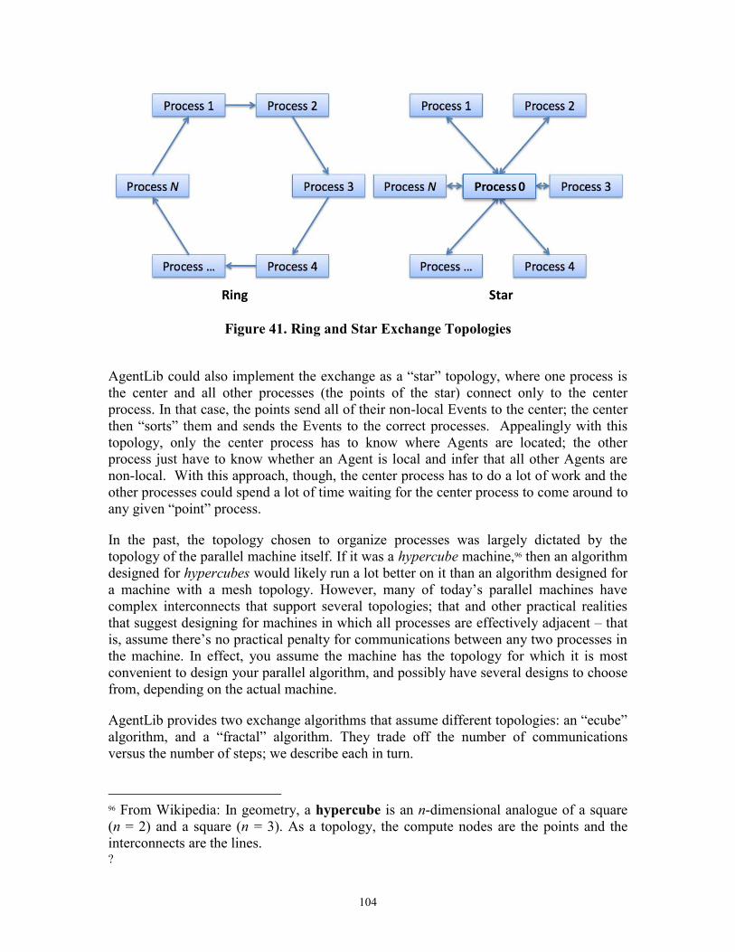
104

Ring Star

Figure 41. Ring and Star Exchange Topologies

AgentLib could also implement the exchange as a “star” topology, where one process is the center and all other processes (the points of the star) connect only to the center process. In that case, the points send all of their non-local Events to the center; the center then “sorts” them and sends the Events to the correct processes. Appealingly with this topology, only the center process has to know where Agents are located; the other process just have to know whether an Agent is local and infer that all other Agents are non-local. With this approach, though, the center process has to do a lot of work and the other processes could spend a lot of time waiting for the center process to come around to any given “point” process.

In the past, the topology chosen to organize processes was largely dictated by the topology of the parallel machine itself. If it was a hypercube machine,96 then an algorithm designed for hypercubes would likely run a lot better on it than an algorithm designed for a machine with a mesh topology. However, many of today’s parallel machines have complex interconnects that support several topologies; that and other practical realities that suggest designing for machines in which all processes are effectively adjacent – that is, assume there’s no practical penalty for communications between any two processes in the machine. In effect, you assume the machine has the topology for which it is most convenient to design your parallel algorithm, and possibly have several designs to choose from, depending on the actual machine.

AgentLib provides two exchange algorithms that assume different topologies: an “ecube” algorithm, and a “fractal” algorithm. They trade off the number of communications versus the number of steps; we describe each in turn.

96 From Wikipedia: In geometry, a hypercube is an n-dimensional analogue of a square (n = 2) and a square (n = 3). As a topology, the compute nodes are the points and the interconnects are the lines. ?

Process 0

105

Every AgentLib-based simulation process has a rank, or identifying number, where the first process has rank 0, the second process has rank 1, and so on, where the Nth process has rank (N-1). Each algorithm requires a number of “communications” (however the number of actual MPI operations, or number of buffers sent, is determined by the buffering strategy employed by the MpiStreams), but in no case is it fewer than the number described.

The ecube exchange algorithm requires the number of processes, N, in a parallel job be a power of two, i.e., 2, 4, 8, 16, and so on. Each process has log2(N) communication peers; the exchange is performed in 2log2(N) steps, and requires Nlog2(N) communications. The ecube algorithm is particularly well suited for hypercube machines, it can be used on symmetric multi-core machines, or on massively parallel machines with InfiniBand interconnects. The goal is to minimize the number of steps needed to complete the exchange, where all communications in a given step can be performed simultaneously. However, the number of communications is not minimized. If, for some reason, the hardware cannot perform the communications simultaneously, other algorithms that have fewer communications should perform better.

The “fractal” exchange algorithm builds a recursive tree topology; the root process has log2(N) children, where the first child has at most one child of its own, the second child has at most two, and the kth child has at most 2k. This approach makes routing Events easier than for trees with k-degree nodes. Further, this approach can be used with any number of processes (not just a power of two, as with the ecube algorithm). This algorithm requires at most 2(N-1) communications and at most 2ceil(log2(N)) steps to complete an exchange round. However, relatively few of the communications can take place simultaneously, and some of the communications can potentially be much larger than the others (which leaves some of the processes idle for extended periods). On the other hand, the algorithm allows some nodes to “prune” some of its children in exchange rounds, eliminating them from one or more synchronization points. Our conjecture is that on some machines (or for some number of processes) the number of communications has a more significant impact on performance than the number of steps needed to complete the round, and on those machines the fractal algorithm will perform better than the ecube algorithm.

Load Balancing

Once a satisfactory exchange algorithm has been selected, a secondary concern for performance is to ensure all processes have the “right” amount of work so that no process spends much of its time waiting for other processes to finish and start communicating. There are two general approaches for distributing load: statically and dynamically. A static approach distributes the load at program startup, based on some heuristic rule. A dynamic approach allows the load to be transferred between processes based on factors detected at runtime.

The only real technique available for dynamically balancing loads is to move Agents from heavily loaded processes to less-busy processes. AgentLib already has a mechanism in place to move Agents, specifically by using the serialization system described earlier.

106

The real challenge is then to determine which Agents to move. First, Agents that “communicate” a lot with each other (in a modeling sense) should to migrate to the same processes so that their in-model communications do not require inter-process communication, that is, they do not require serialization, , and de-serialization. Second, processes with “too much” work should offload agents to processes with “not enough” work.

However, gathering such knowledge can be expensive. Discovering that two Agents “communicate” a lot can be resource intensive and perhaps much more expensive than justified by the time saved. Measuring the load an Agent puts on the system is also challenging; the hardware clock (using portable code) when used for timing may have only millisecond precision. But modern CPUs can execute millions of instructions in a millisecond – which is much more work than most Agents might perform in any round. Further, using the portable mechanism for timing usually involves a system call, which slows the program down. Another option is to use non-portable mechanisms for timing, but that incurs its own costs when we need to port to a new machine.

In any case, the only way to determine if a load-balancing scheme yields a net improvement is to perform simulation experiments. Since alternative exchange algorithms are still under development and there are still not a comprehensive set of performance tabulations, the full task of dynamic load balancing is planned for the near future.

The current load-balancing technique is a static approach: we distribute Agents “round robin” to all processes as they are created. This technique ensures that each process has roughly the same number of Agents, and the same “kinds” of Agents. Most Agents are of the same kind – for example, an N-ABLE™ of the food sector97 has many more Household Agents than it has, say, SuperMarket Agents. Each Household does pretty much the same amount of work, so distributing them round robin is very reasonable. The other Agents that perform significantly more work are also distributed in a round-robin fashion, which effectively distributes their work as well.

5.1.4 Simulation Input

The input file is an XML document that contains all of the input data needed to construct, execute, and otherwise control how the model executes. The bulk of the file consists of Agent definitions – almost every Agent must be specified and configured from data found in the input file. Despite the full specification and configuration done in the input file, all of the “behavior” of the Agents – for example, the mechanics of the Shipping Agent moving packages on the rail network – is built into the simulation engine. The behavior could instead be specified as “scripts” inside the input file; however, that would incur a severe performance penalty and has other severe drawbacks. Since the input file is XML, we have mechanisms that specify how the XML is laid out and other mechanisms to read the XML and turn it into Agents in memory. 97 Ehlen, M.A., Bernard, M.L, and Scholand, A.J. “Cognitive Modeling of Household Economic Behaviors,”

Proceedings of the Second International Workshop on Social Computing, Behavioral Modeling, and Prediction, Phoenix, AZ,

2009.

107

XML Processor

The XML processor is one of the earliest components in the AgentLib suite of software. Although today there are many excellent C++ XML processors to choose from, at the time there weren’t many acceptable C++ XML processors, so one was written and is now an excellent processor.98

The XML processor is a minimal (but W3C-recommendation-compliant) “XML version 1.0” non-validating processor; specifically, it does not support any additional W3C recommendations (such as XML namespaces) or other additions to the basic XML specification. As a result, the AgentLib XML processor very fast and modelers can still use a family of XML tools to generate or manipulate the input file and read it into our program with excellent performance. (For example, the N-ABLE™ XML input files themselves are generated using Java and the JAXB API.99)

Object Generator

The ObjGen System (or “Object Generator”) is used to create the Agents (which are C++ objects) and all of their members (which are also objects). The system provides a mechanism for objects (or more accurately, their corresponding C++ classes) to specify the data that should appear in the input file, to read that data from the file, and then to interpret the data and use it to create an instance of the object.

A class creates an ObjGen for itself by implementing two functions of the ObjGen template (which is parameterized by the class). First, the class provides the “specification” function to specify the data that appears in the input file, and a “generate” function that uses the data to generate a single instance of the object. The rest of the ObjGen template implements the remaining code needed to connect the specification function to the generate function.

Ultimately, the ObjGen system becomes aware of all the classes that can be generated from an input file. The ObjGen system is then used to produce an XML schema file, which describes the format of acceptable XML input files. The format is entirely markup – all specified data is structured using XML elements where attributes of those elements have the numeric, string, or Boolean inputs. The “root” ObjGen, though, is expected to be an instance of the Model class. The Model class specifies its own data (such as the random number generator seed, the model stop time, the snapshot frequency, etc.); then it specifies a section where data for Agents should appear. Each “specification” point is structured with more XML elements; those structuring elements have the class name so that the ObjGen system can call the appropriate generate function. Once the XML schema is written, it can be used by other tools to generate input files. For example, a typical N-ABLE™ input file is created in Java, using a set of classes created by JAXB code using the schema generated by the ObjGen.

98 Since that time, other markup languages with smaller file sizes and simpler implementations have been developed, such as YAML and JSON. 99 “Java Architecture for XML Binding (JAXB),” accessed at http://java.sun.com/developer/technicalArticles/WebServices/jaxb/ on January 15, 2010.

108

However the input file is constructed, it is passed to the ObjGen system. The ObjGen system reads the structuring element that names the model type, such as an N-ABLE™ EconomicAgent, MasterShipper, or list of SupportedCommodities. The ObjGen system then calls the model’s generate function, then continues to read the input file, passing in each data item as the generate function requests them. When it comes to the Agent section, it detects the structuring element that identifies the type of Agent specified at that point. Then it calls the generate function for that type of Agent; that function receives input and generates the corresponding Agent. This process continues until the entire file has been read and all the Agents have been generated.

After the input has been read and all corresponding objects generated, the simulation engine starts the execution phase described earlier. The execution phase is interleaved with output stages, which are described next.

5.1.5 Simulation Output

The output from the model is a collection of files, which are all packaged into a single archive file. The archive includes a copy of the input file, a file containing all the messages produced by the model as it ran, some “type information” files to help the postprocessor process the data, some files containing version information for the various components of the simulation engine, and the primary output data, or “snapshot” data files, specifically, one file for each time step that was captured by the Snapshot system.

Snapshot Registration

An Agent may have many member variables, but usually only a few are interesting for preservation in the output. With the reflection system (discussed above), it is fairly easy to devise a Snapshot scheme that preserves the entire state of Agents to the output file. However, that leads to enormous output files and significantly increases the time needed to post-process the output data. To avoid all that, AgentLib has a “SnapshotRegistration” scheme that allows the modeler to register member variables for publication in the output. Registered members can be either data variables or functions that can examine the state of the Agent and compute a summary value.

When a member is registered, it is registered with a label (often the name of the member); that name is preserved in the output and is ultimately visible to analysts and other consumers of the output. The registration also contains an unusual C++ construct known as a pointer-to-member, which allows us to take an instance of an Agent and obtain a “real” pointer to the member inside that specific instance. With this design, we call the registration function once (for each Agent type) when the program starts up; then all other operations needed to produce the output file are centralized into the Snapshot system.

109

When asked to snapshot an Agent, AgentLib looks up the registration for that type of Agent, resolves the pointers-to-members into real pointers inside that specific Agent, then snapshots the members by following the real pointers.100

Deflate Streams

AgentLib output files are generally large. To reduce the disk space required to store the files and to reduce the time it takes to back them up, to send them over the network, and to otherwise manipulate them, AgentLib works with the data in compressed form. Furthermore, it is undesirable to have the data on disk or in a temporary location in an uncompressed form. Hence, AgentLib uses “Deflate Streams” (or DeflateStrms in the C++ code), to work with the data as a stream of bytes. Writing uncompressed to an oDeflateStrm will automatically compress the data a buffer at a time before writing to the final destination. Similarly, reading data from an iDeflateStream automatically decompresses the incoming data a buffer at a time. These DeflateStrms are somewhat unusual in that they can be used to generate a compressed file in parallel: the technique generates compressed “feeder” streams in parallel (which is the “expensive” part), then concatenates them into a final gzip101 file. If the source or target for the data is slow, this approach improves performance perceptibly, since the slow medium serves up more data in one chunk than it would if it served up the uncompressed data.

Archive

In earlier versions of the engine, the primary output file was an XML document with various sections to store data; for example, the input file was gzip-ped and encoded Base64,102 and then included in the “Input” section of the XML document. A similar mechanism was used to store the version information, while the snapshot data itself was stored as XML text. Over time, as the models grew larger, the output XML files grew to be very large – gigabytes when uncompressed – and processing the file proved to be a major bottleneck, even using the very fast AgentLib XML processor.

To overcome this “shoehorning” of various data types, AgentLib now splits the data into separate files in their “natural” format but still bundles the whole collection into a single file, since it is generally easier to manipulate a single file than a whole collection of separate files. There are two commonly available archive file formats: the standard UNIX tar format, and the relatively open but proprietary Windows-oriented ZIP format. Over the years, those archive formats have built up many new features while still maintaining

100 An alternate design could be to distribute the logic that writes the output file among the Agents (through a virtual function, for example). Such designs would effectively require all classes to be derived from a common base class, something like “SnapshottableObject,” which seems unwieldy. 101 The gzip file format is a standard UNIX compressed file format, described in Deutch, P., Aladdin Enterprises, 1996, “RFC1952 - GZIP file format specification version 4.3,” accessed at http://www.faqs.org/rfcs/rfc1952.html on January 22, 2010. 102 To be able to send binary data through systems designed for text (such as the Internet email system, or, our example here, in XML files), you must first encode the binary data as text. One relatively standard way of doing that is to use base64 encoding, described in Deutch, P., Aladdin Enterprises, 1996, “RFC1952 - GZIP file format specification version 4.3,” accessed at http://www.faqs.org/rfcs/rfc1952.html on January 22, 2010.

110

backward-compatibility with earlier versions of their respective formats. For example, both formats have been enhanced to support 64-bit-sized files and to store other file-system information; the ZIP format has been revised many times to support various compression and encryption technologies, many of which have been obsolete for decades. Both formats offer 64-bit extensions, but they do so in a roundabout way – the ZIP approach is particularly convoluted.

Both formats have their weaknesses: for example the open-source ZIP library is large, complex (because of all the encryption code), and ultimately a chore to program with and maintain. The tar file format isn’t randomly accessible. Both formats are overkill for our purposes; AgentLib only needs to aggregate files so that they can be delivered to the post-processing program.

Thus, AgentLib has its own simple, custom Archive format. Using its own format allows it to avoid the features and complexities of the other formats, and implementing it took less time than it would have taken to incorporate the ZIP library into the AgentLib suite of programs. Files stored in the Archive are automatically compressed using DeflateStrms. Similarly, reading a file from the Archive (using the interface code we supply) causes the files to be automatically decompressed as they are read.

Versioning Information

Because the N-ABLE™ ABM is under constant development, it is important to be able to recover previous versions of engine used to generate a particular output file and as a result, modelers need a way to encode versioning information into the output file. AgentLib queries the Subversion103 source-code tracking repository for the versions of the files that were included into the Engine. (Analysts will most likely be using the “production” version of the engine as opposed to the “development” version, so this information is sufficient to recover the Engine.104) All of the versioning information is stored into the Archive with identifiable names.

Further, AgentLib gathers Subversion version numbers of the repository as a whole and uses it as a shorthand method of identifying the version of the program.

Type Information File

Part of the reason the old XML output files took so long to process was that there is so much redundant information in the structure of the XML data. For example, every Agent’s registered name was repeated in every Snapshot taken for every Agent that is

103 Subversion is a version control software package. It is used to keep a repository of program sources and other files, including the current and previous versions; to share those files between different people, merging their changes into a final version, handling conflicts as appropriate. See “subversion.tigris.org,” accessed at http://subversion.tigris.org/ on January 25, 2010. 104 However, if the analyst is using the development version, then the version information is likely to be stale and it won’t be possible to recover the Engine. If we require the ability to recover a development engine, we can address the issue by storing “diffs” or patch files that can be applied to a base production version in order to recover the changes that ultimately went into the development engine. Also, if it turns out we often need to recover the Engine, we can create scripts to automate the work.

111

snapshotted. Indeed, it was not unusual to see a reduction of 95% or more when zip- or tar-compressing the output file, which implies that at least that much of the information in the file was redundant. (Text files generally compress very well anyway, but it can be surprising to see a 100-megabyte file reduce to a 5-megabyte compressed file.)

The current AgentLib approach reduces file sizes and improves output performance by reducing the amount of redundant data in the files. This is done primarily by extracting the structure of the data and storing it in a “type information” file. This file is a small XML document that describes the structure of every type known to Snapshot system; it also stores the names of the types and the names of the members of each data structure. To the point, this information appears only once in the Archive file.

Snapshot/Timestep Data Files

The primary output of the Engine is “snapshots” of the Agents (and only the Agents) in the model. At regular intervals (for example, every day at midnight in simulation time), the Snapshot system visits every Agent in the Model and asks it to “pose” for a snapshot. If an Agent is willing to pose, the system then captures the state of the Agent (i.e., snapshots it) and stores the snapshot to the output file.

The state of an Agent is expressed entirely in the state of its member variables. Those member variables may in turn be complex data types – so the Snapshot system recursively visits those members to capture the state of each of the member’s member variables – and so on. This recursive visitation yields the structure of the data, but in a flattened format and without annotations. The full structure information is tied to the type of the Agent and the types of its member variables – and so the structure information is stored in the Type Information files described earlier. The Archive only needs to store a type identifier (a single byte) in order to be able to recover the rest of the data for that type from the data file.

The snapshot data is stored as string, but “prepended” with the one-byte binary type identifiers. Our choice of type identifier (just one byte) limits the number of snapshot-able types to 255, but that’s a very large number of types to have in a program. The result is nominally a binary file, albeit one that does not need to be concerned about byte-order (typically an issue with binary files), and one that isn’t really condensed. But, the information has much less redundancy than the XML version, so it takes less time to write – and compressing the data files is beneficial, but is not quite so (embarrassingly) effective as the previous XML-based Archive file.

The Snapshot system itself also runs in parallel, with each process generating a compressed fragment of the data file and then the overall system incorporating the fragments into the final file stored inside the Archive. As a result, the parallel snapshot is a significant source of speedup in the parallel version of the Engine.

112

Post-processing

Once the output Archive is written, it is given over to the post-processing program. The postprocessor reads the Type Information file and constructs a MySQL105 database with tables modeled on the type structure – the member names in the types correspond to the columns. Then, the postprocessor fills the database using data extracted from the timestep data files. Once the database tables are fully populated, the N-ABLE™ Java-based client and other tools are used to visualize the simulation results.

5.1.6 Some Conclusions

As a framework, AgentLib constrains the design of client models like N-ABLE™: if implemented using AgentLib, the model must be a discrete-event model, it must derive all of its Agents from the base class in AgentLib, those Agents must implement their behavior in the form of Events, and so on.

By constraining the design of Agents and Events, it is possible to reason about what Agents can do in the particular model. That reasoning allows the modeler to design safe serial- and parallel-computing versions, and to devise testing apparatuses that ensure the engine is performing properly. For example, the modeler can account for Events to ensure they are all scheduled properly and executed, can verify the input is read correctly, that the output files are well formed, and can compare the results of the serial engine with those of the parallel engine -- if they match, we can conclude the parallel engine with its serialization code, Event-exchange algorithms, and load-balancing logic is working properly (though not necessarily optimally).

However, all of these factors are independent of the model itself – if the tests pass, they say nothing about whether the model is valid. That responsibility is deferred to the model’s designers; it is they who must say that an Agent’s behavior in response to a series of Events is a valid model of real-world behavior. Then, satisfied with the validity of their model, they must verify that the model produces the behavior they have designed.

In summary, if a model can validly be implemented as an Agent-based discrete-event model, and if millions or billions of Agents are desired, then AgentLib goes a long way in helping implement the model as a scalable program that runs on commodity PC hardware all the way up to massively parallel systems.

5.2 N-ABLE™ Library of Economics Classes

N-ABLE™ is built on top of the AgentLib agent-based discrete-event simulation library. N-ABLE™ contains two types of agents. The main type of agent is the economic agent. An economic agent represents a firm that buys and sells commodities. A simulation contains many of these agents. The second type of agent is the shipping agent. The shipping agent models the transportation of packages between agents. Both economic agents and the shipping agent have sub-pieces that are agent components. The buyers and sellers of the economic agent are agent components, and the shipping components of the shipping agent are agent components. Markets, the shipping bulletin board, and social 105 MySQL is a relational database product. See http://www.mysql.com/.

113

networks are bulletin boards. Figure 42 shows the inheritance of N-ABLE™ classes from AgentLib classes.

Figure 42. Relationship of AgentLib and N-ABLE™ Classes

5.2.1 Economic Agents

The main type of agent in N-ABLE™ is an economic agent. An economic agent represents a single firm in a simulation. A firm represents a player in the economic simulation that can buy and consume commodities, produce and sell commodities, or a combination of the two. An economic agent is composed of multiple pieces that perform different functions. The pieces are buyers, sellers, productions, a warehouse, and an

114

accountant. The agent may have some or all of these components depending on its function. Figure 43 shows a typical economic agent.

Figure 43. N-ABLE™ EconomicAgent

An economic agent must have at least one production. The production defines the main role of the agent. An agent can be a source producer, a sink consumer, or a consumer-producer. Source producers consume no commodities; they only produce them. They form the beginning of a supply chain. Figure 44 shows a source producer. Sink consumers produce no commodities; they only consume them. They form the end of a supply chain. Figure 45 shows a sink consumer. Consumer-producers both consume and produce commodities; they form the middle of a supply chain. Most agents in a simulation are usually consumer-producers. Figure 43 shows a consumer-producer. Each production contains a recipe that specifies the input commodities the production uses to make its output commodity.

Figure 44. Source Producer Economic Agent

The buyers purchase the input commodities that the economic agent needs to fulfill its productions. The sellers sell the output commodities produced by the agent’s productions.

115

To buy and sell commodities, an economic agent must belong to a market. A market is a place where sellers advertise their commodities and buyers look to find a seller. Economic agents belong to markets through their buyers and sellers which each belong to a single market. Agents can buy and sell in different markets by having multiple buyers and sellers that belong to different markets. Each agent can only have one buyer of a particular commodity, but it can have multiple sellers of its single output commodity. Usually an agent has only one seller in a particular market, however.

Figure 45. Sink Consumer Economic Agent

Each economic agent contains a single warehouse that holds the agent’s entire stock of its various input and output commodities. Each agent also has a single accountant. The accountant handles the agent’s finances including all payments and receipts of money. Economic agents can belong to social networks which allow them to communicate outside the normal buyer-seller process.

Each economic agent is given a location, which is a latitude and longitude pair. Each agent also belongs to a shipping region. Shipping regions are geographical groupings of agents that are used to estimate shipping costs between two agents. Shipping regions are assigned locations, which become the representative location for that shipping region. Shipping cost estimations use the agent’s shipping region location instead of the agent’s actual location. Inside the US we use counties for shipping regions and county centroids as their representative locations. Outside the US we give each country a single shipping region.

5.2.2 Buyers

A buyer is responsible for purchasing a single commodity, and it belongs to a region. The union of the buyer’s commodity and region determine the market that the buyer belongs to. Each day the buyer determines how much it needs to buy for the day, chooses a seller, and places orders. A buyer also has a list of shipping modes that it can use. N-ABLE™ currently has one type of buyer, the firm buyer as shown in Figure 46.

Figure 46. Buyer, Seller, and Market Classes

116

To avoid having to search the entire market every time a buyer looks for a seller, the buyers keep a preferred sellers list. This list is a subset of the market that has the sellers that best meet the buyer’s criteria for a seller. Currently, the buyers’ criterian is the cheapest total per item cost which is the sum of the commodity cost and the transportation cost. The buyer gets the commodity cost for each seller from the market; it gets the shipping cost from the shipping bulletin board. The user specifies a maximum price that the buyer will pay per item. Sellers that exceed the maximum per item cost will not be put onto the preferred sellers list. There can be multiple shipping modes available between a buyer and a seller. Each buyer and seller lists which modes it can use. The modes a buyer chooses from for a transaction are the modes that both the buyer and seller have in common. Currently, the buyer always chooses the cheapest available shipping mode for each seller. In the future buyers could also select shipping modes based on distance or delivery time.

The first day of the simulation, the buyer considers every seller in its market and puts the sellers with the lowest total per item cost on its preferred sellers list. The size of the preferred sellers list changes throughout the simulation, but the user sets the initial size of the preferred sellers list and a max size the list can grow to. The user also specifies the drop days, which is the number of days a seller will remain on the list without being ordered from before it is removed from the list.

At the beginning of each day, the buyer reviews its preferred sellers list. Any sellers that have been on the list for at least drop days without being ordered from are removed. The buyer updates the total per item cost for each of the sellers remaining on the list. If the preferred sellers list is empty when the buyer is choosing a seller or if the buyer can’t find a seller on the list that can meet its desired order amount, the buyer will search the market for a seller that is not already on the list. If a seller is available, the buyer will use that seller and add it to the preferred sellers list.

When the buyer queries the shipping bulletin board for a seller, it receives a trio of estimates: distance, time of delivery, and per item shipping cost. The buyer could use any combination of these values to choose a seller off its preferred list, but it currently considers only cost. In the future, it might be advantageous for a buyer to also consider how quickly it can get a package from a seller when choosing from whom to buy. The buyers do keep track of the delivery time estimate, however. It is used when the buyer determines when pending orders will arrive.

For sellers that are on the preferred list, the buyer keeps a history of how much shipping has cost in the past from those sellers. The cost history is based on actual cost of shipping that is returned to the buyer when it receives an order from a seller. The history is calculated using the linear combination

previousShippingCostHistory + (1) returnedCost

117

where =.75. The history is mode independent, so previous shipping costs are added into the history ignoring the modes that were traveled. Thus, the history is a blend of the cost of all modes that have been used to ship from that seller.

The shipping cost for sellers that are not on the preferred list is the shipping cost returned from the shipping bulletin board. For sellers that are on the preferred list, the shipping cost is calculated using the linear combination

shippingCostHistory + (1) shippingBBCost where again =.75. The two ’s associated with the shipping cost history are both hard coded.

The buyer keeps track of the market share of each seller on its preferred list. The market share is the ratio of the number of times the buyer has ordered from this seller to the number of total orders the buyer has made. To choose a seller, the buyer converts the market share into a normalized probability distribution. The buyer uses the distribution to randomly pick a seller from the list to consider. Then the buyer randomly selects another seller from the list to consider. The buyer continues to look at new sellers on the list until the expected benefit of continued searching is less than the search cost. The buyer then chooses the seller with the cheapest cost from those it looked at. More details are given by Ehlen106 and Carlson and McAfee107.

Each day, the buyer determines its daily need of its commodity. It keeps a historical average of its daily need and calculates todays need using the linear combination

needReportedByEconomicAgent + (1) historicalNeed where =.17. The buyer attempts to keep enough of its input commodity in stock to be able to meet the daily need for today plus several days in the future. The number of days the buyer considers is called the look ahead days. Each buyer looks at the current inventory level of his commodity, the amount he expects to receive from pending shipments in the next look ahead days, and the daily need over the next look ahead days. He sets his purchase goal to an amount that will ensure he can meet the daily need each day for the next look ahead days.

5.2.3 Sellers

A seller is responsible for selling a single commodity, and it belongs to a single region. The union of the seller’s commodity and region determine the market that the seller belongs to. N-ABLE™ currently has one type of seller, the firm seller as shown in Figure 46.

106 M. A. Ehlen. Bank Competition: The Effect of Market Share and Price Dispersion on Price Levels. Cornell University, Ithaca, NY, 1996. 107 J. A. Carlson and R. P. McAfee. Discrete equilibrium price dispersion. Journal of Political Economy, 91(3):480 – 493, 1983.

118

At the beginning of each day, the sellers determine their price, and they advertise to their market. The information sent to the market includes the commodity price, seller’s shipping region, seller’s shipping modes, and chunk size. The user must specify a chunk size for each seller. A seller will only sell their commodity in increments of their chunk size. For example, there’s a seller with a chunk size of 4. A buyer wants to buy 6 items, but it can only order 4 or 8 items from the seller.

The method the seller uses to determine its price has been designed such that it can be easily modifiable by the user. The seller uses the adaptive behavior engine (ABE), which is essentially a set of pluggable brains to determine how it sets its price. By default N-ABLE™ uses a learning classifier system (LCS), but the user is free to write a new behavior engine and swap it in if they desire. The LCS detects pertinent events in its environment, makes decisions based on its experience of how to respond to those events, and builds up its experience over time allowing it to make better decisions.

5.2.4 Ordering Process

Figure 47 shows the ordering process. At the beginning of the simulation and after every shutdown or recovery, the master shipper sends shipping cost estimates to the shipping bulletin board. The rest of the process happens every day. At the beginning of each day, all the sellers advertise to the market their price, shipping region, shipping modes, and chunk size. The buyers then query the market and the shipping bulletin board to update the information on their preferred sellers lists. Each buyer chooses a seller off his preferred list. If the seller is too expensive, the buyer doesn’t order now and schedules to try again later. The buyer orders as much of his desired amount as he can afford. If his desired amount is not a multiple of the chosen seller’s chunk size, the buyer ceils his order amount up to the next multiple of the seller’s chunk size. The buyer places the order with the seller. When the seller receives the order, it fills as much of the order as it can based on the commodity it has available in its warehouse. The seller responds to the buyer to let it know how much of the order was filled. If the seller filled any of the order, it packages up the shipment and sends it to the master shipper for delivery.

119

Figure 47. Flow of Ordering Process

When the buyer receives the order response, he makes a note of the order. If the order didn’t completely fill the buyer’s desire, then the buyer will choose another seller and attempt to order again after a specified waiting period. The buyer will continue attempting to order until its desire is fulfilled, it has contacted every seller in the market, or the end of the business day has been reached.

The package travels on its desired shipping mode until it reaches its destination at which time the master shipper delivers the package to the buyer notifying it of the actual shipping cost. When the buyer receives the package, he updates his historical average of how much it costs to purchase from a seller with the actual cost information, and he updates his look ahead days as an average of the previous value and the delivery time of the just received package. He also notifies his accountant to pay for the shipment. The accountant pays the seller for the commodity cost and pays the shipper for the shipping cost. As the shipper doesn’t keep track of money currently, it just ignores the payments. The buyer also updates the information it keeps on the seller such as the cost history and delivery time history.

5.2.5 Warehouse

The warehouse stores one or more commodities for an economic agent. The warehouse temporarily stores both inputs that the agent purchases and outputs that the agent produces for sale. The user specifies the initial stock, a minimum amount, and a maximum amount for each commodity that the warehouse will store in the input file. The minimum amount represents the lowest stock level of a commodity that an agent wants to keep on hand. The maximum amount represents the maximum amount of a commodity that the agent has space to store.

The warehouse provides the storage cost for each commodity it stores and the average cost per item to purchase / produce each commodity it stores. The warehouse provides

120

the ability to reserve amounts without actually taking them out of the warehouse. The reserved amount can be later taken out or released. An agent reserves amounts when beginning negotiations for a contract of sale to make sure they are still available when the contract is made. The warehouse keeps track of the salable amount for each commodity, which is the amount in stock minus any reserved amounts and the minimum. The warehouse enforces the reserved, minimum, and maximum amounts “softly,” that is it enforces them only through reporting those amounts when the user asks and when reporting the salable amount. The user must be conscious to not break the constraints.

5.2.6 Accountant

When a buyer and a seller agree on a purchase, they initiate a contract. Each economic agent has a single accountant that keeps track of all the contracts and the agent’s financial data. The accountant records purchase and sale contracts when the agent initiates them. It keeps track of a contract until the relevant package has been delivered and the contract is closed. The accountant also makes and receives all of a firm’s payments. When a buyer receives a shipment, it notifies its accountant who sends payment to the seller’s accountant. The accountant keeps track of the firm’s total production, its total sales in quantities and dollars, its revenues and costs, and its GDP. It also knows the current solvency status of the economic agent.

5.2.7 Regions and Markets

Buyers and sellers belong to regions. A region represents a logical grouping of buyers and sellers that is not necessarily geographical. Regions are created using lazy evaluation. They contain markets which each sell a single commodity. Each region can only contain one market for a particular commodity. The purpose of regions is to provide a way for the user to group buyers and sellers when creating complex input files. In the real world, some markets may be regional, and a single national commodity market may not be appropriate.

Markets in N-ABLE™ are bulletin boards so that their state is the same across all processors. Markets are created using lazy evaluation, so they only exist in a simulation when they are actually used. Figure 48 shows an example simulation that has 3 commodities and 3 regions. There are 4 economic agents in the simulation that create 4 markets. Markets that exist are highlighted in gray. Those that don’t exist are white. N-ABLE™ currently has one type of market, the FirmMarket as shown in Figure 46.

121

Figure 48. Market Example

5.2.8 Productions

A production takes commodities as inputs and transforms them into an output. Each production is controlled by a production manager. The economic agent contains one or more production managers which each contain one or more productions. The production manager decides the daily production target while the production determines how the output is made. Each production has a recipe that specifies the inputs required to make the output. A recipe can have zero or more inputs, but it must have exactly one output. Figure 49 shows a typical production manager and production recipe.

Figure 49. N-ABLE™ Production Manager Classes

A source producer agent has one or more productions that each take no inputs and produce a single output. A sink consumer agent has one or more productions that takes one or more inputs and produces an output of utility that measures if the production

122

consumed the desired amount. A consumer-producer has one or more productions that each take one or more inputs and produce a single output.

Each day at midnight, the economic agent has each production manager review what was produced and what was sold the previous day and historically. Using this information along with the current inventory levels of the output commodity, the production manager decides how much to produce the following day and sets the target production amount. The economic agent then evaluates how much of each input is required to produce the desired production amounts and informs the buyers how much of each input is required for the next day. The buyer determines how much he needs to buy and sets his goals.

Each production has a daily distribution of how the day’s production is divided up over the 24 hour period. If no distribution is given, the default is a uniform distribution over the 24 hour period. The distribution is expected to be normalized. If it isn’t, the code normalizes it. Each hour the production produces the quantity of output specified by the hour’s distribution value times its target production amount and consumes the appropriate amount of input as specified by the recipe.

N-ABLE™ has two main types of productions as shown in Figure 50: firm production and the consumer. The firm production represents a standard production that takes zero or more inputs to produce an output. This type of production is utilized by source producers and consumer-producers. The firm production has the ability to enforce idle periods on the production, where the production stops producing or produces at a small constant daily rate. It also allows a user to set a maximum production rate. The consumer models an endpoint in a supply chain that consumes commodities without producing them but instead producing utility. This type of production is utilized by a sink consumer.

Figure 50. Production, Production Manager, and Social Network Classes in N-

ABLE™

N-ABLE™ has four types of production managers as shown in Figure 50: the inventory based firm production manager and the distribution firm production manager, which are used with firm production, and the consumption manager and the distribution consumption manager, which are used with the consumer. The inventory based firm production manager sets the production target to attempt to keep a set level of inventory. The consumption manager sets the production target of utility to 1 plus or minus a small random amount. The two distribution production managers set the production target based on a yearly distribution given in the define file. The inventory based and

123

distribution firm production managers can have multiple productions but only one production per commodity type. The consumption and distribution consumption managers can only have one production.

5.2.9 Social Networks

In some models it might be beneficial for agents to share information outside the normal buying-selling process. For instance, some large companies set the production targets of multiple production firms from a home office or a model might need to capture the word of mouth effect during an epidemic or other event. N-ABLE™ provides social networks to allow the sharing of this information. A social network is a bulletin board that collects information from the agents in its network. The social network can then process the results and respond back to some or all of the agents in its network. The user specifies which social networks, if any, each agent in the simulation belongs to. N-ABLE™ currently has one type of social network, the economic data reporter as shown in Figure 50. The economic data reporter is described in the next section.

5.2.10 Data Output and the Economic Data Reporter

N-ABLE™ writes output using snapshots. A snapshot is a summary of the state of an agent in the simulation. During a simulation a snapshot is taken every simulation day at midnight where the state of every agent in the simulation is outputted to a file. The snapshot output is what the client uses to visualize the simulation results. For simulations with large numbers of agents, N-ABLE™ can produce vast amounts of output.

In some circumstances a user may only care about the results for a few key firms in the simulation. The snapshotting of the non-key firms slows down the simulation and produces a large amount of information which the user must then wade through. To alleviate this, N-ABLE™ provides a mechanism that allows a user to turn or off the snapshotting of each agent in a simulation individually.

In other circumstances a user may want summary statistics. For this situation N-ABLE™ provides the economic data reporter. The economic data reporter is a social network that collects data from each of the firms in its group and calculates summary statistics for the entire group. The simulation snapshots the summary data of each economic data reporter that exists. The user specifies which economic data reporter group, if any, each agent in the simulation belongs to. If the user needs only the summary statistics, he can turn off the snapshotting of the firms. This is the way NISAC typically uses the economic data reporter.

5.2.11 Shipping Cost

Shipping costs in N-ABLE™ rely upon the concept of a shipping unit. A shipping unit represents a grouping of a commodity that is standardized across all commodities. The grouping, for example, can be a standardized shipping container or a ton. The user specifies the number of items for each commodity that fit in the standardized unit. Notice that this requires data available for commodities for the number of items that fit in the chosen unit. Using the number of items that fit in a unit allows different commodities to have different numbers of items for the same shipping cost as happens in reality. For

124

example, 30 large screen TVs or 2,000 pairs of shoes might make up a ton, and it might cost the same to ship a ton regardless of if it is a ton of TVs or a ton of shoes.

The shipping cost has two components: the distance cost and the infrastructure cost. The distance cost is a dollar per unit-mile cost that captures the part of the shipping cost that is dependent on how far the shipment travels. The infrastructure cost is a dollar per unit cost that captures initial cost required to utilize a speciÞc shipping mode. Whether the shipment travels a short distance or a long distance, there is a part of the shipping cost that is constant. It is the cost to utilize the infrastructure of a particular shipping mode. This is what the infrastructure cost represents. Each shipping component specifies a per unit distance cost, D, and a per unit infrastructure cost, I, that are shared by all commodities that use that infrastructure.

To calculate the total cost for a shipment, the infrastructure and distance costs are first converted to per-item costs. Let d be the distance traveled and u be the items per unit. The per-item distance cost, DI, is

DI= Ddu .

Calculating the per-item infrastructure cost is a little more complicated. Whether a unit is completely full or almost empty, a certain cost is required to use the unit, its infrastructure cost. This argument is based on the fact that in most cases a unit will represent a shipping container which costs a certain amount to use regardless if it’s full or not. Therefore, the per-item infrastructure cost when shipping partial units should be more costly. Whole units use the infrastructure cost directly. Partial units use a modified infrastructure cost that is increased based on its percentage of a whole unit.

Each shipment is divided into whole items, W, and fractional items, F. Whole items are the items that make up whole units. Fractional items are what’s left over after the finding the number of whole items. The fraction, f, is the percentage of a unit the fractional unit makes. The infrastructure cost for a fractional unit is multiplied by the modifier, m, which is determined according to the following scale.

m=

1.00.75f1.1 0.5 f<0.751.20.25f< 0.51.3 0.0 f<0.25

Let q refer to the quantity of items in a shipment, where q=W+F. The per-item infrastructure cost, II, is

II= (W+Fm)

q Iu.

The total item cost, TI, is

125

TI=DI+II. The total cost, T, represents the entire shipping cost of a single shipment, and it is given by

T=qTI= qDd

u +(W+Fm) Iu=CD+CI,

where CD and CI are the part of the total cost due to distance cost and infrastructure cost, respectively.

Notice that only the distance and quantity are independent variables. The rest of them are either constants set at the beginning of a simulation or dependent on distance or quantity. Thus, cost functions are of the form

cost f (d, q).

5.2.12 Locations

Each economic agent in N-ABLE™ is assigned a location by the user, where a location is coordinates given in latitude and longitude. Locations are also assigned to the vertices in transportation networks. The locations allow us to display agents and transportation networks on a globe in the client, and they allow us to perform geospatial operations such as the distance between two locations or the nearest neighbor search.

We calculate the distance between two locations by finding the great circle distance between the two coordinates sets. A great-circle distance is the shortest distance between any two points on the surface of a sphere, in this case the earth, measured along a path on the surface of the sphere. Note that we are assuming the earth is a perfect sphere for distance calculations.

The nearest neighbor search can be defined as given a set of points P in the continuous space S and a point qS, find the point in P that is nearest to q. N-ABLE™ uses the nearest neighbor search to find the vertex on a transportation network that is closest to an agent. The agents and the graphs are both embedded in the Euclidean space of the earth, and the agents are generally not located in the exact place that a vertex is. Thus a translation needs to be made from agents to the nearest transportation vertex.

126

Figure 51. Translating economic agents to networks

Figure 51 shows how the translation from agents to transportation vertices is made. The figure contains two transportation networks, one shown with blue vertices and the other with green vertices. There are two economic agents, each shown as a pink square. Agent a is closest to vertex x from the blue network and closest to vertex y from the green network. Agent b is closest to vertex w from the blue network and closest to vertex z from the green network. These vertices would be the starting points for the agents on the networks.

The nearest neighbor search is implemented using a 3D kd-tree108 which gives an expected constant computation time in most cases vs. the O(n) time of a linear search. We based our implementation of a kd-tree on the implementation given by Freidman, Bentley, and Finkel109. Several variants of 2D and 3D kd-trees as well as several variants of 2D and 3D grid partitioners were tried but the 3D kd-tree performed best.

5.2.13 Transportation Modeling

N-ABLE™ models the transfer of goods from one firm to another using a modular shipping framework that supports multiple types of shippers. The shipping framework consists of the master shipper, shipping components, shipping networks, and the shipping bulletin board. The master shipper encapsulates and serves as the interface between the shipping components and the rest of the simulation. All communication between senders / recipients and the shipping components is made by the master shipper. A shipping component represents a specific shipping mode such as truck or rail. A shipping network is a graph describing a particular infrastructure system such as the US interstate highway system. The shipping bulletin board provides estimates of shipping cost, time, and distance to the senders and recipients.

Currently, there are two types of shipping components implemented: diffusion shippers and network shippers. A diffusion shipper uses the straight-line distance between a sender and a recipient to determine shipping distance, time, and cost. A network shipper contains a graph representing a shipping infrastructure. It uses a shortest path algorithm to determine how to get from sender to recipient. The shipping distances, times, and costs 108 J. L. Bentley. Multidimensional binary search trees used for associative searching. Communications of the ACM, 18(9):509–517, 1975. 109 J. H. Freidman, J. L. Bentley, and R. A. Finkel. An algorithm for finding best matches in logarithmic expected time. ACM Transactions on Mathematical Software, 3(3):209–226, 1977.

127

are calculated using the shortest path. If a new type of shipper is needed, the framework has been designed so that adding another type of shipping component is possible.

The master shipper has the ability to impose infrastructure outages to the transportation networks which allows N-ABLE™ to simulate how the delivery of goods under adverse transportation conditions would affect an industry. For instance we could model how the closing of certain bridges or the closing of a large coastal area due to a hurricane would affect a specific industry through the disruption of its supply chain.

The source for our networks is the Center for Transportation Analysis at Oak Ridge National Laboratory. The center has an intermodal network developed by Bruce Peterson110 and Frank Southworth111 that consists of truck, rail, and water routes.

Master Shipper

The master shipper is the controlling agent for transportation modeling. It contains all of the shipping components that perform the actual transportation modeling and the graphs used by the network shipping components. A firm sends a package to another firm by sending a ship message to the master shipper containing the package information and the shipping mode. The master shipper routes the message to the appropriate shipping component, and the component ships the package. The master shipper also gathers and sends distance and cost estimates for shipping to the shipping bulletin board.

The master shipper contains the graphs used by the network shipping components. Locating the graphs in the master shipper instead of the network shipping components allows multiple shipping components to use the same graph without duplicating it. The master shipper also contains the shutdowns and recoveries that impose infrastructure outages and recoveries on the graphs.

Figure 52. Master Shipper

110 B. E. Peterson, “Cfs multi-modal network documentation,” accessed at http://cta.ornl.gov/transnet/Cnetdoc.ZIP on February 1, 2010. 111 Southworth, F., and Peterson, B.E., Intermodal and international freight network modeling, Transportation Research Part C: Emerging Technologies, 8C:147–166, 2000.

128

Figure 52 shows an example master shipper with two graphs, four network shippers and one diffusion shipper. Graph 1 has three sub-graphs, and graph 2 has one sub-graph. Network shippers 1, 2, and 3 have views of graph 1, and network shipper 4 has a view of graph 2. Diffusion shipper 1 is not associated with a graph.

Shutdowns and Recoveries

A shutdown represents a suspension of a set of edges. It has a beginning time, when the shutdown occurs, and an ending time, when the recovery occurs. A vertex can be suspended as well, but only indirectly. Vertices are automatically suspended when all of their incident edges are suspended. When one of its incident edges is later unsuspended, the vertex is unsuspended.

Edges that are suspended cannot be traveled on, and the shortest path algorithms ignore suspended edges. Thus, shutdowns allow an analyst to capture traffic redirection and mode shifting due to problems with the underlying infrastructure. Shutdowns are defined in the define file. They can be overlapping which means that one shutdown can start before another has ended. Two shutdowns can even suspend the same edges. If two overlapping shutdowns suspend an edge, the edge will be suspended until both recoveries have happened.

Shipping Components

When the master shipper receives a shipment message, it routes the shipment to the appropriate shipping component. When a package is shipped, it is delayed for a specified amount of time called the ship delay before the package begins traveling. The ship delay is also applied at the end of each trip. In most cases with shipments, a package spends some time at both the sender and recipient ends traveling locally, waiting in a local distribution center, or being loaded / unloaded. The delay is intended to represent these times that aren’t spent traveling directly to the destination. There are two types of shipping components as shown in Figure 53, the diffusion shipping component and the network shipping component.

Figure 53. Shipping component classes

Diffusion Shipping Component

The diffusion shipping component is a simple straight-line distance based shipper. It uses the straight-line distance between the locations of the sender and recipients as the path the package will travel. Note that as the locations are on a globe, the straight-line distance is a great circle distance. When a package is given to a diffusion shipping component, the

129

component calculates the distance, delivery time, and shipping cost. The delivery time is twice the shipping delay plus the trip time. The component immediately schedules a message to be sent to the recipient at the delivery time to inform the recipient that the package has arrived along with the distance, delivery time, and shipping cost.

The user assigns a ship delay, shipping speed, infrastructure cost, and distance cost to each diffusion component in the input file. The diffusion shipper does not have the ability to implement shutdowns or recoveries. Thus, it can’t be used to model transportation disruptions.

Network Shipping Component

The network shipper transports packages along an underlying network infrastructure. The shipper transports a package along the shortest path between its source and destination, where the metric for the determining the shortest path is edge impedance, which is described below. The actual movement of the package along the transportation infrastructure is captured, and this data is provided to the client which uses it to show traffic patterns on the infrastructure. The ability to suspend (shutdown) or un-suspend (recover) parts of the transportation network to simulate damage to or obstructions in the network is provided. The graph implementation also supports sub-graphs which allows one to have a single large multimodal graph along with providing access to the individual modal pieces. A network component is associated with a single graph and any combination of that graph’s sub-graphs.

The vertices in the graphs are given coordinates via latitude and longitude. The edges connect vertices and are directed. Edges have certain properties. Impedance represents the cost required to traverse an edge, and it is the weight metric used by the shortest path algorithms. Each edge also has a speed which represents how fast a package can travel unrestricted on an edge. Ambient traffic represents the background traffic on the edge, and it influences the speed at which a package travels on an edge.

Package States

Packages in the network shipper are in one of three states: distribution center, traveling, or waiting. Packages in the distribution center state have been shipped but are waiting for the ship delay to pass. Packages in this state have not yet calculated a path to their destination. The shortest path is calculated when the package is moved to the traveling state. Packages in the traveling state are currently traveling on their shortest path to their destination. Packages in the waiting state should be traveling but can’t because their path has been blocked by a disruption. Figure 54 shows how packages move from one state to another. The blue ovals represent the network shipper states.

130

Figure 54. States of a Package

When a package is shipped, it is placed in the distribution center state. After the shipping delay has passed, a package is moved from the distribution center state. If a path exists to the destination, the package is moved to the traveling state. If no path exists due to a disruption, the package is moved to the waiting state. When a package in the traveling state reaches its destination, the package is delivered. When a package in the traveling state encounters a suspended edge, it is moved to the waiting state. After a package has been in the waiting state for 2 hours, it tries to find a new path. If one exists the package changes to the traveling state; otherwise, it remains in the waiting state until a recovery occurs. When a recovery occurs, all packages try to continue on their path. If it is possible, the packages move to the traveling state. Otherwise, they remain in the waiting state. If a package has no path, the shipper calculates a path for the package and moves it to the traveling state.

Normal Package Travel When a package is shipped via a network shipper, it is delayed by the shipping delay. Once the delay has passed, the shipper finds the nearest transportation vertices to the seller and the buyer. These nearest vertices serve as the starting and ending points for the package’s path. The shipper calculates the shortest path for the package between the vertices nearest the seller and buyer, and the package is sent on its way. When the package reaches its destination vertex, it is again delayed by the shipping delay. Once the delay has passed, the buyer is sent a message that the package has arrived.

The network shipper records the traffic along each edge every day and reports this information in the output. The client uses this information to visualize daily traffic patterns which allows an analyst to quickly determine how traffic is affected by an event. The edge traffic counts are reset at midnight. Recording the daily edge traffic information requires that the network shipper actually travel a package along every edge in its path.

As long as no shutdown is in effect, a package can be safely traveled to the next critical time. The next critical time is the sooner of the next midnight or the beginning of the next shutdown. A package must stop traveling for shutdowns because an edge in its path might be affected by the shutdown. When the shipper moves a package along its path, it takes into account the maximum speed of the edges and the ambient traffic on the edges. Packages are moved along multiple edges until the next critical time. If a package reaches

131

the end of its path before the next critical time, it is delivered immediately subject to the shipping delay. When the package is delivered, the shipper reports the actual distance the package traveled and the travel time to the recipient. The shipper also reports the incurred shipping cost as a per item cost.

Shipping Cost The per unit distance and infrastructure costs for a package shipped on a network shipping component must be calculated for each shipment as the package can travel over sub-graphs that have different per unit distance and infrastructure costs. To find the infrastructure and distance costs, the network shipper calculates a weighted average of the values of the sub-graphs traveled on by the package where each sub-graph’s values are weighted based on the sum of the distance of their edges the package traveled on. Let S be the set of the shipper’s sub-graphs that the package traveled on, and let mi be the number of edges traveled by the package on sub-graph i. Let lij be the length of the ith edge traveled on in the jth mode. The distance traveled by the package is

d= iS

j=0

mi lij

The distance cost of the shipment is

D= iS

j=0

mi Dilij

The infrastructure cost of the shipment is

I=

iS

j=0

mi Iilij

d

The shipper plugs these distance and infrastructure costs into the formulas given in Section 5.2.11 to get the total per item shipping cost that it gives to the package recipient.

Package Travel during a Shutdown Packages that are in transit when a shutdown happens do not know about the shutdown until they arrive at a suspended edge. Packages that have not yet started traveling know about shutdowns when they happen, and they are given a path that bypasses the suspended edges if one exists. A shutdown is modeled as occurring at the beginning of an edge. Thus, if a package is anywhere on an edge except for the beginning vertex when the disruption occurs, it is not effected by that edge being suspended.

132

When a package reaches a suspended edge, it will wait at the beginning of the edge for up to two hours for the edge to become unsuspended. If the edge is unsuspended before the two hours is up, the package continues on its journey. If the two hours expire, the package calculates a new shortest path and begins traveling on the new path.

When a package that is waiting on a suspended edge has waited two hours but it can’t find a new shortest path because it is blocked by suspended edges, it will continue to wait where it is until it can calculate a new shortest path. The package will only attempt to find a new path when a recovery occurs. If a package has not yet started traveling and no path exists due to suspended edges, then the package will wait to travel until a path opens up. The package will only attempt to find a new path when a recovery occurs.

Graph Views Network shippers have “views” of the large graph. A view represents a set of the sub-graphs. This allows us to mix and match the subpieces of the large graph to create multiple transportation mode combinations without requiring a separate whole graph for each combination. For example, we use a version of the ORNL CTA intermodal graph that has six sub-graphs: truck, rail, water, truck-rail connections, truck-water connections, and rail-water connections. We can create a network shipper with a view of any combination of truck, rail, and water by specifying which sub-graphs are in its view. Each view is required to be strongly connected. Most of the graph algorithms take a parameter that limits them to operating on a combination of sub-graphs. Thus, when a network shipper finds the shortest path between two buyers and sellers, it considers only the sub-graphs that make up its view.

Calculating Edge Speed We get the posted speeds for the truck edges from the ORNL network data. The posted speed for all rail edges is set to 45 mph, and the posted speed for all water edges is set to 15 mph.

For trucks, the speed a package can travel on a road is inversely proportional to the amount of traffic on the road. The traffic can be divided into the part generated by the simulation and the ambient traffic, the background traffic on the road not generated by the simulation. We make the assumption that the amount of traffic generated by the simulation is inconsequential compared to the ambient traffic and consider only the ambient traffic when determining speed. N-ABLE™ models traffic in hour increments.

Each edge is given a posted speed, Vp, and a daily ambient traffic value, Ta, in the input file. We divide the daily ambient traffic into hourly values using an hourly distribution extrapolated from Exhibit 8-6 in the Highway Capacity Manual.112 The maximum hourly capacity of an edge is set as 2000.113 Let D(h) be the current hourly distribution value. The demand on an edge, L, which is expressed as a percentage of the maximum capacity, is

112 Transportation Research Board, Highway Capacity Manual, National Research Council 2000, Washington D.C., 2000. 113 Ibid.

133

L= TaD(h)2000 .

Let U[a,b] represent choosing a random value from a uniform distribution between a and b. We calculate the effective speed, Vf, of a package traveling on an edge as Vf=mVp, where m is defined as

m=

U[0.75;1.0] L0.65U[0.66;0.75]0.65L0.85U[0.5;0.66] 0.85L<1.0

U[0;0.5] L1.0

Ambient traffic is not really an issue for the rail and water networks, but they use the same logic to calculate edge speed as the truck network. We set the ambient traffic for all rail and water edges to 1. This causes L to always be less than 0.65 and consequently the speed for rail and water edges is set to between 0.75Vp and Vp. This sets their speed to near full posted speed but with some random slowdown included.

Intermediary Locations and Modes Some commodities may always travel through a certain city regardless of where the sender or recipient are located. For instance, many chemicals imports must pass through Houston as their entry point into the United States. Intermediary locations and modes allow an analyst to model these situations.

An intermediary location represents a location that all packages given to the network shipper will pass through. An intermediary mode represents a mode that a segment of the journey will use. The modes must be sub-graphs that belong to the shipper. To handle the case of chemical imports where some must pass through Houston and some can enter at any location, two network shippers would be defined. The first would be the one defining Houston as an intermediary location and would handle all the packages that must be routed through Houston. The second would not define any intermediary locations and would handle all the remaining traffic.

For n intermediary locations, there must be n+1 intermediary modes. An intermediary location is translated into the closest vertex on the transportation network in either of the two modes on either side of the location. The sender is translated into the closest vertex in the first intermediary mode while the recipient is translated into the closest vertex in the last mode.

As an example, consider a shipper that has the intermediary locations (a,b) and the intermediary modes (A,B,C). Let s and r represent the closest vertices to the sender and the recipient, respectively. Let x and y represent the closest vertices to a and b,

134

respectively. The vertex s is from mode A while r is from mode C. The vertex x is from either mode A or B while y is from either mode B or C. A package would travel from s to x on mode A, from x to y on mode B, and from y to r on mode C. In mathematical terms, the path of the package would be

s

A⇝ x

B⇝ y

C⇝ r

Optimizing the Network Shipper Most of the computation time used by the network shipper occurs in two areas: traveling packages and calculating shortest paths. Traveling packages involves the shipper setting tasks for itself to move the packages at the appropriate time. Since the packages can only move to the next critical time, this could require a number of messages that would overload the event system. The shipper has been designed to schedule as few task as possible. Tasks are scheduled once per timestep that an action needs to occur instead of a separate task for each package.

The network shipper performs a large number of shortest path computations which are somewhat expensive. To reduce the number of paths calculated, the shipper uses two techniques. First, the shipper groups together shortest path queries that have the same source vertex and makes a single call to the graph package for the group. This allows the graph package to potentially optimize the query. Second, the shipper keeps a cache of previously computed paths and pulls paths from the cache when possible. Newly encountered paths are always added to the cache. To reduce memory usage, the packages keep pointers into the path cache instead of storing the paths directly. To keep the cache from getting too large, paths are deleted from the cache when they have been unused for five days. Whenever a shutdown or recovery occurs, the cache is flushed completely. This is required because the graph has changed state and the previously calculated shortest paths may have become invalid.

Graphs

The graph implementation in N-ABLE™ is a directed multigraph that supports sub-graphs. Negative edge weights are prohibited. The graph provides algorithms to find shortest paths, find shortest path distances, determine strong connectedness, and find the nearest vertex to a given latitude and longitude. Edges can be suspended, and suspended edges are ignored by the algorithms. The algorithms also take a parameter indicating which of the sub-graphs to operate on, which allows the algorithm to be executed on the subset of the entire graph that represents a network shipper’s view of the graph.

The graphs in N-ABLE™ are really composite graphs, that is graphs composed of a combination of separate graphs linked together. This is how transportation infrastructures work. For instance, the road and railroad infrastructures are separate networks, but they are connected at certain places. A commodity being transported may spend part of its trip on the railroad network and part on the road network.

135

The composite graphs are implemented using sub-graphs. Each graph is divided into sub-graphs where the union of the sub-graphs equals the entire graph. Dividing the graph into sub-graphs allows multiple network shippers to have different views of the graph. For instance if you have a graph that contains two modes of transportation, you could have one network shipper that utilizes only the first mode while a second network shipper utilizes the union of both modes. Thus, only one copy of the graph needs to be kept for multiple uses. A sub-graph may be a full fledged graph or it may represent a connection between two other graphs. A graph that contains two modes will have three sub-graphs. Two are the modes of transportation, while the third is the link between the two sub-graphs. The link may consist of edges that connect vertices from two different modes, or it may be something more complex with its own internal vertices and edges.

The graphs in N-ABLE™ are directed. Edges can be unidirectional or bidirectional, where a bidirectional edge represents two directed edges. The graphs are given names. Each sub-graph is given a name, and it includes the edges and vertices of the graph that belong to it. An edge or a vertex can only occur in a single sub-graph. A graph’s edges and vertices are the union of the edges and vertices of its sub-graphs. Each vertex is given a name and a location. Each edge is given a name, a starting vertex, and an ending vertex. An edge also has a length (miles), an impedance, a maximum speed (mph), and an average ambient traffic.

Shortest Path A shortest path algorithm finds the path between two vertices in a graph that is “shortest” based on some metric. The most common metric is edge length. Edges in N-ABLE™ graphs have lengths, but we use a different metric for the shortest path. That metric is impedance. We inherited the use of the impedance metric from the ORNL graphs. The impedance edge attribute in the ORNL truck graph is set to be the number of minutes it takes a truck to travel the edge. This value takes into account the speed limit of the road. The impedance attribute for edges in the ORNL rail and water graphs and the intermodal connections have been set such that the flow of traffic across the intermodal graph follows the expected traffic flow across the networks. The flow will switch modes as would be expected in the real world.

The graph package provides point-to-point shortest path (P2P), single source shortest path (SSSP), and single target shortest path (STSP) algorithms. P2P computations, which find the shortest distance between two vertices, are performed using the ALT algorithm114,115. SSSP and STSP computations are performed using the appropriate version of Dijkstra’s algorithm116. An SSSP algorithm finds the shortest distance from a single vertex to every other vertex in the graph. An STSP algorithm finds the shortest distance 114 A. V. Goldberg and C. Harrelson. Computing the shortest path: A* search meets graph theory. In SODA ’05: Proceedings of the sixteenth annual ACM-SIAM symposium on Discrete algorithms, pp. 156–165, Philadelphia, PA, USA, 2005. Society for Industrial and Applied Mathematics. 115 A. V. Goldberg and R. F. Werneck. Computing point-to-point shortest paths from external memory. In ALENEX ’05: Proceedings of the Seventh Workshop on Algorithm Engineering and Experiments. Society for Industrial and Applied Mathematics, 2005. 116 E. W. Dijkstra. A note on two problems in connexion with graphs. Numerische Mathematik, 1:269–271, 1959.

136

from every vertex in the graph to a single vertex. The choice of the ALT and Dijkstra algorithms was made after the testing of numerous shortest path algorithms on the ORNL graphs. A future paper describes the process in more detail. Internally, the SSSP and STSP algorithms are used to create landmarks for the ALT algorithm. Shortest path queries to the graph are performed using a combination of P2P and SSSP algorithms.

The graph package provides algorithms that find a shortest path between a single source and target or the shortest paths between a single source and multiple targets or the shortest paths between multiple sources and a single target. It also provides algorithms that find the shortest path distance between sources and targets and algorithms that find the k nearest vertices to a source vertex based on shortest path distance. When a call is made to an algorithm that returns multiple shortest paths from a single source, the graph package decides whether to use separate P2P queries for each path or a single SSSP query for the group. The P2P algorithm is faster than the SSSP algorithm, but there is a break even point where k P2P calculations with the same source are more expensive than a single SSSP calculation. Currently, the break even point is around 10.

The shortest path algorithms in the package all use a priority queue to hold the vertices that are to be examined next. The speed of this priority queue is one of the most important factors affecting the speed of the algorithms. Several data structures were studied for implementing the priority queue including STL maps, Fibonacci heaps117, and a bucketing scheme. However, pairing heaps118,119 provided the best performance. A pairing heap performs a lot of allocations and deallocations of small homogeneous chunks of memory. Thus, a pool allocator was used to improve the memory allocation performance of the pairing heap.

Strong Connectedness We require all states of each graph to be strongly connected, which means that from each vertex in the graph there exists a path to every other vertex in the graph. A graph changes state whenever a shutdown or recovery occurs because edges and vertices are suspended and unsuspended. We also require all states of all network shippers’ views of graphs to be strongly connected. At the beginning of the simulation, we enforce that the graphs are strongly connected by testing all states of the graph. We also test all states of all network shippers’ views of graphs. The graph package provides the ability to test a graph or any combination of sub-graphs for strong connectedness using the algorithm given by Cormen et al120.

117 M. L. Fredman and R. E. Tarjan. Fibonacci heaps and their uses in improved network optimization algorithms. Journal of the ACM, 34(3):596–615, 1987. 118 M. L. Fredman, R. Sedgewick, D. D. Sleator, and R. E. Tarjan. The pairing heap: A new form of self-adjusting heap. Algorithmica, 1(1):111–129, 1986. 119 J. T. Stasko and J. S. Vitter. Pairing heaps: experiments and analysis. Communications of the ACM, 30(3):234–249, 1987. 120 T. H. Cormen, C. E. Leiserson, R. L. Rivest, and C. Stein. Introduction to algorithms. MIT Press, Cambridge, MA, USA, second edition, 2001.

137

Shipping Bulletin Board

The shipping bulletin board keeps the information necessary to give an estimate of delivery time, cost, and distance for sending a package between any two shipping regions. The shipping bulletin board needs five pieces of information for each shipping component in order to make the calculations: infrastructure cost, distance cost, shipping delay, shipping speed, and distances between all pairs of shipping regions. The shipping delay is a time delay that is set to both the beginning and ending of the packages travel time that represents the time for the pickup and processing or processing and end delivery of the package.

For diffusion shipping components, the user sets the infrastructure cost, distance cost, shipping delay, and shipping speed at the component level in the input file. Each component passes these values to the shipping bulletin board at the beginning of the simulation, and they remain constant throughout the simulation. The distance between two shipping regions is calculated on the fly as a straight-line distance on the earth using great circle distance.

For network shipping components, the user sets the shipping delay at the component level in the input file, but the infrastructure and distance costs are set at the sub-graph level. Additionally, a separate shipping speed is set for each edge in the graph. Obtaining a single value for the shipping delay is straightforward, but the rest of the parameters must use some sort of average. For the infrastructure and distance costs, we calculate a weighted average of the values of all the sub-graphs in the component’s graph where each sub-graph’s values are weighted based on the sum distance of their active edges. For the shipping speed, we calculate a weighted average of the shipping speed of all the active edges in all the sub-graphs weighted on the length of each edge.

For distances between shipping regions, a network shipping component calculates the shortest path between every pair of shipping regions. For n shipping regions, the simulation performs n single-source shortest path calculations. Even though the graphs are directed, we assume that the distance from shipping region a to b is the same as the reverse distance and calculate the distance in only one direction. Reverse distances should be the same as forward distances in most cases on our networks, and when they are different, the difference should be minimal. This allows us to only store the upper triangular part of the nn distance matrix and cuts storage cost in half to n2/2n values.

Each network shipping component passes these values to the shipping bulletin board at the beginning of the simulation. Whenever a graph associated with a network shipping component experiences a shutdown or a recovery, the component recalculates all the values and resends them to the shipping bulletin board. Note that while the shipping delay for a network shipping component remains constant throughout the simulation, the values for the infrastructure cost, distance cost, shipping speed, and distances between all pairs of shipping regions change whenever a shutdown or recovery occurs.

Having the shipping bulletin board gives us several things. First, the buyers can quickly and cheaply get estimates for shipping cost, time, and distance for the sellers they are considering without having to query the master shipper and have it make a calculation for

138

each query. Sending a request to a local bulletin board is cheaper than sending a message to a potentially remote agent, and for network shipping components the calculation of the cost, time, and distance is very expensive. The values are estimates because they are calculated between the buyer’s and seller’s shipping regions representative locations instead of the actual locations of the buyer and seller.

Second, the shipping cost also lets the buyers know if a transportation path exists between themselves and a seller. If there is not a path between the representative locations of two shipping regions, then the master shipper reports a shipping cost between the two shipping regions so exorbitant that no buyer will consider a seller who isn’t reachable. Of course, it is possible for a path to not exist between the two shipping regions but a path to exist between the buyer and seller and vice versa. However, this method works well in practice.

For diffusion shipping components, the bulletin board shipping cost and time values are exact, not an estimate, because the ‘path’ and distance a package travels can’t change between the estimate and the actual shipment. For network shipping components, they are an estimate for several reasons. First, the shipping speed, infrastructure cost, and distance cost are average values for the component. The actual values depend on the exact path taken. Second, the distance given is between the representative locations of the shipping regions of the agents, not the agents’ actual locations. Third, even if the exact distance were given, the distance could change because the package could be rerouted while traveling due to a shutdown.

5.2.14 Converting the ORNL CTA Graphs for Use in N-ABLE™

We had to modify the CTA intermodal network a little to meet our needs. We started by extracting separate truck, rail, and water networks from CTA’s intermodal network. For the truck network, we extracted all the edges and vertices of the truck portion of CTA’s intermodal network. To meet N-ABLE™’s requirement that graphs be strongly connected, we removed pieces that were on islands (including the Hawaiian and Aleutian islands) and a few other pieces that were disconnected from the original graph. For a few of the unidirectional edges, we added the complimentary edge going in the opposite direction. The result was a strongly connected graph that represented the major roads in the continental US (including mainland Alaska), Canada, and Mexico.

The process for extracting the rail network was almost the same. We extracted all the edges and vertices of the rail portion of CTA’s intermodal network. The ORNL network stores separate graphs for each rail company, which are connected by interline edges. To make the graph strongly connected, we removed a few edges and vertices, and we added the reverse edge for a few of the unidirectional edges.

The process for the water network was similar, but there was an additional step. The ORNL network stored three separate water graphs: ocean routes, Great Lakes routes, and all other North American inland water routes. There is some overlap between the three graphs. We wanted a single water network, so we connected the three graphs together

139

into one large water graph, eliminating the overlapping pieces. Some scrubbing of the data was then necessary to make the resulting graph strongly connected.

The connecting edges that link the truck, rail, and water networks were created from the terminals that ORNL used to connect the modes in their intermodal network. Oak Ridge uses three edges (access link, terminal link, access link) and two vertices (terminal gates) to represent a terminal connection between modes. The terminal link and the two terminal gates represent a terminal facility, and an access link represents the connections between the individual modal graphs and the terminal facility. This scheme allowed them a lot of flexibility. For our purposes the extra flexibility is not needed, so we use a single edge, called a terminal edge, to represent a terminal connection. The length of the new terminal edge is the sum of the lengths of its three edge sub-pieces. The impedance of the new terminal connection is the sum of the impedances of its three edge sub-pieces.

Figure 55 shows the version of the CTA network used in N-ABLE™. It consists of three large sub-graphs (truck, rail, and water) shown in blue and three smaller connecting sub-graphs shown in green. The connecting graphs consist of only edges that have one vertex in one of the large sub-graphs and one in another.

Figure 55. N-ABLE™ Implementation of CTA Intermodal Network

The terminal links in the ORNL graph restrict traffic flow by commodity. A terminal link can be designated for a particular commodity, be designated for container traffic, or be completely open. We decided to use only the terminal links that are designated as container traffic or open. This was a suggestion from Bruce Peterson as a valid way to pick a subset of terminals to be used when commodity type is not important. Finding the speed for each edge is relatively straightforward. Speeds are given in mph. For truck edges in the ORNL intermodal network, impedance represents the number of minutes required to travel the edge. The speed for a truck edge is computed by length / impedance 60. For rail edges a speed of 45 mph was assigned, and a speed of 15 mph was assigned to water edges. Like truck edges, impedance for terminal edges

140

roughly represents the number of minutes spent in the terminal. The speed for a terminal edges is thus similarly computed by length / impedance60. As terminal edges are usually quite short and impedance for terminal edges is usually quite high to account for the large amount of time required to switch transportation modes, the speed for terminal edges is usually quite small.

Finding the ambient traffic for truck edges requires a bit more thought. The US Department of Transportation publishes data for the average daily traffic per lane for individual states, the District of Columbia, Puerto Rico, and the nation as a whole in Table HM-62 of their Highway Statistics publication121. The version of the data available when the N-ABLE™ networks were created is from Highway Statistics 2005. Data is given for the following categories: rural interstates, other rural principal arterials, urban interstates, other urban freeways and expressways, and other urban principal arterials. The ORNL truck network includes data that allowed us to categorize the edges appropriately to assign the average daily traffic data to each edge as ambient traffic. In the average daily traffic data, some of the states had traffic values that weren’t reported. In these cases, we set the ambient traffic value in the matrix to the Other Principal Arterial value for that state in the same rural / urban class. For the District of Columbia, there are no reported rural values. We set both rural values to be the value of the corresponding Other Principal Arterials class. In situations where there is any ambiguity in the amount of traffic on an edge, we have to make a choice to assign an ambient traffic to that edge. The choices we made lean toward making an edge have less ambient traffic. We don’t currently have traffic data for Canada or Mexico. As a temporary measure, we assign the average values for the entire US to the edges from Mexico and Canada.

For rail, water, and terminal edges, ambient traffic is not applicable, so the ambient traffic values for these edges were set to 1 to indicate there was no ambient traffic.

121 United States Department of Transportation, Federal Highway Administration, “Highway statistics series,” accessed at http://www.fhwa.dot.gov/policy/ohpi/hss/index.cfm on January 25, 2010.