Economies of Scale: The Case of REITs

Brent W. Ambrose Professor of Finance and Director

Center for Real Estate Studies Gatton College of Business and Economics

University of Kentucky Lexington, KY 40506

(859) 257-7726 ambrose@uky.edu

and

Anthony Pennington-Cross

Director of Research Research Institute for Housing America 1919 Pennsylvania Ave, NW, Suite 700

Washington, DC 20006-3428 (202) 557-2839

July 14, 2000 Contact Author: Brent W. Ambrose Professor of Finance and Director Center for Real Estate Studies Gatton College of Business and Economics University of Kentucky Lexington, KY 40507-0034 (859) 257-7726 ambrose@uky.edu We thank David Brown, Paul Childs, Brad Jordan, David Ling, Peter Linneman, Steve Ott, and the anonymous reviewers for their helpful comments and suggestions. This research is supported by the Real Estate Research Institute (RERI).

Economies of Scale: The Case of REITs

ABSTRACT

Significant controversy exists surrounding the hypothesis of consolidation in the real estate industry. Central to the debate is whether REITs can generate economies of scale through asset growth. To date, empirical evidence is limited. For example, Ambrose, Ehrlich, Hughes, and Wachter (2000) find indirect evidence for scale economies but the effect dissipates over time. This finding appears to contradict Bers and Springer (1998) who find that REIT general and administrative (G&A) expenses exhibit substantial economies of scale. G&A, however, is a relatively small part of total expenses with the cost of capital being the primary expense in a capital-intensive industry. This study builds on previous empirical work by focusing on the cost of capital.

1

Economies of Scale: The Case of REITs

1. INTRODUCTION

Whether real estate investment trusts (REITs) will continue to consolidate though

mergers and acquisitions, portfolio acquisitions, or new development is the subject of

considerable debate. Two opposing views have emerged regarding the future of REIT

consolidation. The first view, advocated by Linneman (1997) and Scherrer (1995), is that the

real estate industry will continue to consolidate over the next quarter century. The primary

motivation given for this potential massive consolidation is the existence of economies of scale.

For example, Zell (1997) makes the case that larger REITs have higher earnings growth

potential, which translates into lower costs of capital. This view is consistent with research in

other industries indicating that larger firms have significant economies of scale. For example,

Hansen and Torregrosa (1992) note that larger firms experience lower underwriting spreads

suggesting economies of scale in underwriting costs. Furthermore, Eckbo (1992) finds that

horizontal consolidation within industries produces efficiencies implying that economies of scale

exist with increasing size.

In contrast, Vogel (1997) suggested that REIT growth was not related to the better

operating efficiency of larger companies, but instead resulted from a series of external events

such as changes in the regulatory environment, changes in tax laws, and growth in institutional

investment. As a result, Vogel does not see continued consolidation as a forgone conclusion. In

one of the few empirical studies of REIT consolidation, Campbell, Ghosh and Sirmans (1998)

confirm that REIT mergers have increased during the 1990s. Yet, they also note the absence of

hostile takeovers and that most mergers have produced either negative or comparably low

2

returns. This implies that the nature of REIT ownership structures may prevent significant

consolidation.

Theoretical work by Goodman (1998) posits that greater REIT liquidity and growth

expectations have lowered investor required rates of return and thus have increased firm values.

These expectations of growth come from a variety of sources, many of which could be transitory

as indicated by Vogel (1997). Nevertheless, for substantial consolidation to occur, bigger REITs

must be better REITs, with better REITs having lower per unit output costs and higher returns.

In one of the few tests of this theory, Ambrose, et al (2000) find indirect evidence that

REITs outperform the average income-producing real estate firm in terms of net operating

income (NOI) growth, but the effect dissipates by the year 1997. In an earlier study, Bers and

Springer (1998) find evidence of scale economies in the reduction of general and administrative

(G&A) expenses. Capozza and Seguin (1998) also examine the impact of G&A expenses and

show that the market penalizes REITs that increase property-level G&A expenses. This penalty

implies that large REITs will outperform small REITs to the extent that they are able to achieve

scale economies at the property level. G&A expenses, however, are a relatively small part of

total expenses (between 7% and 16% of total costs in the sample) implying limited long-run

consolidation potential resulting from G&A expense control. More recently, Capozza and

Seguin (1999) report results that are inconsistent with economies of scale in G&A expenses.

Their analysis suggests that G&A is invariant to firm size. Anderson, Lewis, and Springer

(2000) provide a thorough review of the literature regarding economies of scale in real estate.

As in other capital-intensive industries, the primary expense that limits growth

opportunities for REITs is capital. Firms with the lowest cost of capital have a long-run

competitive advantage over other firms. Although studies (Archer and Faerber, 1966) have

3

documented capital-raising economies in other industries as early as the 1960's, to date no study

has adequately estimated the scale economies associated with capital costs for REITs. In an

earlier attempt, Bers and Springer (1998) relate REIT size, as proxied by book value of total

assets, to costs and find small diseconomies of scale associated with interest expenses.1 Thus,

their results cast doubt on whether significant economies of scale will result from consolidation.

Unfortunately, their analysis does not fully address the issue of whether scale economies exist

with respect to capital since their model only included one capital cost component (interest

expense), which may explain why some of their results are counterintuitive. In contrast,

Capozza and Seguin (1999) find a weak negative relationship between interest expense and asset

size implying potential economies of scale.

This study extends previous empirical work and provides evidence of the nature and

extent of REIT economies of scale using a flexible variant of the Cobb-Douglas production

function. Our analysis focuses on the most important determinate of REIT size, capital cost, as

the primary input into the REIT production function while also incorporating property level and

corporate overhead inputs.

2. METHODOLOGY

We view REITs as firms engaged in the production of real estate space, earning income

by leasing this space. REITs use capital, general corporate functions, and property level

expenditures as production inputs to acquire real assets for lease. We estimate the REIT

production structure as a means of determining whether REITs experience scale economies.

Scale economies describe the condition where costs increase at a slower rate than corresponding

1 Using similar methodology, Bers and Springer (1997) show that the degree of REIT leverage impacts the

4

increases in product output. Firms seeking to operate at scale efficiency will increase outputs to

the minimum point on their U-shaped average cost curve. In competitive markets, firms operate

at the minimum efficient scale. The production function transforms inputs such as capital (K),

administrative (Z) functions, property level expenditures (R), and property capital expenses (E)

into outputs (Q) according to:

( ERZKfQ ,,,= )

) ]

. (1.)

From (1), a weakly separable cost function can be derived:

(2.) ([ QQppppFCC ERZK ;,,,,=

where C is cost, F is a functional form, pK represents the price of capital, pZ is the price of

corporate overhead, pR is the price of property level expenses (including labor), pE is the price of

capital expenditures required to maintain the property, and the cost function is assumed to be

homothetic.2 Given that the cost function is derived from the production function, we can use it

to answer questions regarding production characteristics such as economies of scale.

To provide a flexible functional form for (1), we employ a Cobb-Douglas type

production function

. (3.) REZk REZKQ ββββα 0=

Profit maximizing firms will maximize output Q for a given cost level C (or, alternatively

minimize costs for a given output). The Lagrangean for the maximization of (3) is

( )xCREZK REZk '0 p−+=Λ λα ββββ (4.)

where p is the vector of factor prices for K, Z, E, and R, and x represents the matrix of factor

inputs [K, Z, E, R]. The necessary conditions for maximizing (4) are

magnitude of the estimated scale economies.

5

0=−=∂Λ∂

ii

i

i

pxQ

xλ

β,

and

0' =−=∂Λ∂ xC pλ

.

For each input factor, we calculate its share of total costs as

i

iii

ii

xp

xpβ=

∑=

4

1

. (5.)

Thus, we can specify the full regression model as

(6.) 4,,1,

lnlnlnlnlnlnln 43212

210

K=+=++++++=

isppppQQC

iii

REZK

εβββββααα

where and .∑=

=4

1

1i

iβ ∑=

=4

1

1i

is 3

Since (6) approximates the true cost function, we calculate the mean values of all

variables as the point of approximation. Thus, each variable is divided by its mean before taking

logarithms. As a result, the model coefficients reflect the elasticities at the point of

approximation. The cost function can be estimated by itself or it can be estimated in the full dual

system with the factor share equations. We estimate the system of equations using Zellner’s

Seemingly Unrelated Regressions (SUR) technique and drop one of the share equations to

prevent singularity.

Overall scale economies (OSE) are estimated as

2 We follow the setup typically used in studies of the banking industry (see Kim (1991),Noulas, Ray, and Miller(1990), Hunter, Timme, and Yang (1990), and Gropper (1991)). 3 See Greene (1997). Following Nerlove (1963), we include the quadratic output term to account for the classical U-shaped average cost curve. Further, we follow Christensen and Greene (1976) and estimate (6) as a system of equations.

6

[ ]QQCOSE ln2

1

lnln

121 αα +=

∂∂= . (7.)

The OSE indicates whether scale economies are present when outputs are held constant. This

measure of economies of scale is also often referred to as ray scale economies. If OSE is greater

than one, then costs increase at a proportionally slower rate than output and there is evidence of

economies of scale (i.e. increasing returns to scale). This would indicate that consolidation is

likely in the industry as firms have production incentives to increase their size to capitalize on

economies of scale. In contrast, if OSE is less than one, then there are diseconomies of scale

implying an incentive to shed assets to become more efficient. Finally, an OSE equal to one

implies constant returns to scale implying that firms are operating at minimum cost.4 We

calculate OSEs for different REIT asset sizes to test the hypothesis that larger REITs have

economies of scale advantages over smaller REITs.

3. REIT OUTPUT

To this point, we have not explicitly defined REIT output (Q). Most empirical studies of

scale economies have focused on industries with readily identifiable and quantifiable outputs.

For example, economist have studied scale economies in industries such as the brewing industry

where the output is quantified as barrels or gallons of beer (Tremblay and Tremblay, 1988), the

steel industry where output is gross tonnage of steel produced (McCraw and Reinhardt, 1989),

the electrical utility industry where output is measured in kilowatts-hours (Christensen and

Greene, 1976), the banking industry where output is measured in terms of asset dollars (Noulas,

Ray, and Miller, 1990, and Mullineaux, 1978), or the railroad (Caves, Christensen, and Swanson,

1981), shipping (Jansson and Shneerson, 1978), and airline industries (Borenstein, 1991, and Kin

7

and Singal, 1993) where output is measured in terms of freight-ton or passengers miles hauled, to

name just a few. The overriding feature across these industries is that the firms produce

essentially a homogenous product with readily identifiable input factors necessary for

production. REITs, however, invest in real estate assets and derive profits through leasing space

in these assets. Unfortunately, real estate is not homogenous creating difficulties in quantifying

firm output. At a minimum, real estate differs by product type, by location, and by quality. As a

result, we examine REIT scale economies by separately considering several alternative output

measures.

First, we examine output measured as total assets. This measure has the advantage of

value-weighting real estate investments. Firms that invest in high cost areas may have less total

space than firms investing in low cost areas, but by including capital as an input we can test

whether REITs effectively spread capital costs across their asset base. Unfortunately, total assets

are recorded as book value, which may be a poor measure due to the temporal differences in

when assets are acquired or developed.

As a second output measure, we test economies of scale in total revenue production.5

Total revenue meets one of the requirements for output in that it is a consistent measure of REIT

size and it does include valuation of location, quality, and product type. Larger REITs are able

to produce more revenue either by having larger numbers of properties or by having properties

located in markets commanding premium rents. But, total revenue is the price of the output

multiplied by the quantity of the output. Therefore, by definition total revenue is not output.

Total revenue as a measure of output confuses output prices for output quantities. Unfortunately,

4 The variance of OSE is calculated as: ( ) ( ) ( )∑∑∑ +=

i jji

ii CovVarOSE ααα ,2Var .

5 We thank the editor and reviewers for suggesting this output measure.

8

it is impossible for us to completely separate price and quantity due to lack of information about

the output.

The third output measure is total physical size or total square feet available for lease.

This output measure most closely resembles the physical output measures in other industries

(gallons of beer produced, number of passenger miles flown, etc.). Using square footage of

property is similar to viewing REITs as a manufacturing firm whose income and profitability are

directly related to the amount of product it can produce (lease). Unfortunately, this measure

does not reflect the significant geographic value differences in real assets (e.g. the price per

square foot of space in New York is significantly greater than the price per square foot of space

in Cleveland), the quality of the real asset, or the product type. Yet REIT market values and

hence capital costs reflect their investment decisions. A REIT that is less profitable but has a

more square feet than a smaller, more profitable REIT will have higher capital costs.

Furthermore, we estimate the other factor input prices relative to total revenue, which does not

necessarily correlate with physical size. It is important to recognize that the argument for scale

economies is that larger REITs are able to spread their input costs over a wider asset base.

Therefore, scale economies are most effectively estimated when output measurement is not

biased by variations across time or space.

4. DATA

REITs are a relatively simple corporate structure where the primary inputs determining

the amount of output are the cost of capital, property level expenses (including capital

expenditures), and general corporate overhead. REITs produce additional output by either

purchasing or, in some cases, developing additional buildings. The ability of REITs to increase

9

their production is directly related to their ability to access capital markets, which impacts their

cost of capital.

REIT inputs (capital, G&A expenses, property level expenses, and property capital

expenditures), and output (total assets, total revenue, or total square feet) are obtained from the

SNL REIT DataSource for 1994 through 1998.6 Recognizing that the primary input that

determines a REIT’s expansion potential is capital, we estimate each REIT’s capital cost (input

price) as the weighted average cost of capital (WACC). REIT WACC’s are estimated as

WACC k

D

TC k

P

TC k

S

TC d p s= ⎛ ⎝ ⎜

⎞ ⎠ + ⎛

⎝ ⎜ ⎞ ⎠ + ⎛

⎝ ⎜ ⎞⎠

(5)

where kd, kp, and ks represent the cost of debt (D), preferred stock (P), and common stock (S),

respectively, and TC is the total market capitalization (TC = D+P+S). The cost of debt and

preferred stock are estimated as the ratio of total interest cost to book value of debt (D) and

preferred dividends to book value of preferred stock (P), respectively, and are obtained from the

SNL REIT DataSource. Common stock (S) is the REIT’s market capitalization, which includes

any operating units if applicable.7

Significant controversy exists surrounding the estimation of REIT cost of equity. 8 For

example, given the relatively short period many REITs have traded publicly, obtaining sufficient

returns data to calculate stable betas is problematic. Furthermore, many studies that have

estimated REIT betas report periods of negative betas underscoring the problem of using short

6 SNL Datasource provided by SNL Securities is a comprehensive database tracking financial information on 206 equity, mortgage, and hybrid REITs. 7 Operating units for UPREITs are convertible to common stock. 8 Maris and Elayan (1990) estimated REIT average cost of capital as net cash flow divided by total market capitalization (debt plus equity), where net cash flow is the sum of net income, interest expense, and depreciation. This method produced slightly lower WACC estimates than equation (5), however, the empirical economy of scale estimates are not materially different. Thus, we present the results using the traditional definition of the weighted average cost of capital (see Copeland and Weston, 1988).

10

time horizons in estimation. Thus, we estimate REIT cost of equity using a version of the

dividend growth model

( ) gSDIVks += (8)

where DIV represents the total dividends declared, S is the REIT’s market capitalization

(including operating units, if any), and g is the projected growth rate. To proxy for the projected

growth rate, we average the year-to-year FFO growth rate for the previous two years, averaged

over all REITs.9

Estimating the input prices for corporate and property level expenditures is not

straightforward. Market observable prices for units of corporate overhead or capital

expenditures do not exist and thus we make several assumptions to price these items. For

example, when using total assets or total square feet as outputs we estimate the input price for

corporate G&A expenses by dividing total G&A expenditures by total revenue. Thus, REITs

that expand their revenue while containing overhead costs are able to effectively purchase G&A

at lower prices. We also estimate the input price for property operating expenses by dividing

total property level operating expenses by total revenue. Similarly, we estimate the input price

for capital expenses by dividing total capital expenditures by total revenue. However, when

output is measured using total revenue, we estimate the input prices for G&A, property

expenses, and capital expenditures by dividing by gross property value. Thus, REITs that

expand their property asset base while containing overhead costs, property expenses, and capital

expenditures are able to effectively purchase these goods and services at lower prices.

Complete financial data necessary are available for a cross section of 125 publicly traded

equity REITs in 1994, 134 REITs in 1995, 143 REITs in 1996, 164 REITs in 1997, and 175

11

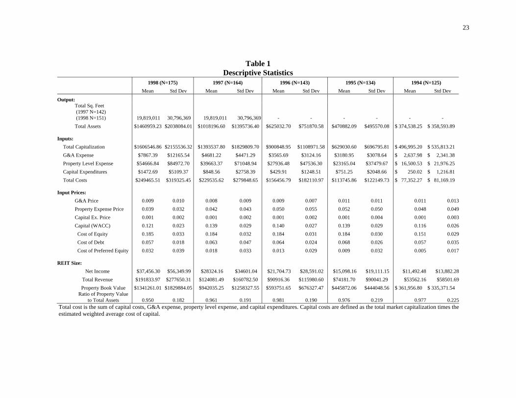
REITs in 1998. Table 1 provides the descriptive statistics for variables needed to estimate

equations 2-4. Capital costs are defined as the product of the price of capital (WACC) and the

amount of capital (total market capitalization). Thus, total costs are the sum of capital costs,

G&A expenses, property operating expenses, and capital expenditures.

We follow Gropper (1991) and estimate the system separately for each year. Thus we are

able to examine whether the growth in the REIT market during the 1990s had an impact on or

resulted from REITs capitalizing on economies of scale. An alternative to using separate cross-

sectional estimations to check for shifts in production technology is to pool the annual data and

include a time trend variable as a proxy for changing technology. Unfortunately, pooling REIT

data across these years raises a number of econometric issues that lead one to question the results

from this method.10 Thus, we report the yearly cross-sectional OSEs.

Table 1 reports the descriptive statistics for the sample. Consistent with the growth in the

REIT market between 1994 and 1998, we see that average REIT output (total revenue) increased

258 percent (from $54 million to $192 million) in nominal terms while average total market

capitalization increased 223 percent (from $497 million to $1,607 million).11 Average REIT net

income increased over 225 percent in nominal terms between 1994 and 1998.

We proxy REIT size using total assets and total property value (at book value) and find a

similar growth trend with average total assets increasing 290 percent in nominal terms over the

sample period (from $374 million to $1,461 million).12 Given that REITs are in the real estate

9 For example, the FFO growth rate for 1998 is found by averaging the FFO growth rates for 1996 and 1997 for all REITs. 10 These issues include sample stability (not all REITs have data for all years) and the impact of inflation. 11 Total revenue increased 225 percent in real terms while market capitalization increased 195 percent in real terms between 1994 and 1998. 12 In real terms, total assets increased 257 percent.

12

business, it is not surprising that property is the primary REIT asset (averaging 97 percent of

total assets).

Table 1 also reports the descriptive statistics for REIT input prices. It is surprising to see

that during this period of significant REIT growth in assets, capitalization, and revenue, REIT

cost of capital remained relatively constant. We note that the average weighted average cost of

capital fluctuated between 11.6 percent in 1994 and 14 percent in 1996. With the exception of

1994, our estimate of the REIT cost of equity showed little variation and averaged 18.4 percent

for the 1995 to 1998 period. Consistent with the overall downward trend in interest rates during

this period, we find that the cost of debt also declined from 6.8 percent in 1995 to 5.7 percent in

1998. Offsetting this trend, the cost of preferred equity experienced a slight increase between

1994 and 1997 with a significant increase in 1998 to 3.2 percent.

5. EMPIRICAL RESULTS

5.1 Output Measured as Total Assets

Table 2 reports the parameter estimates and asymptotic t ratios using outputs as total

assets. We note that across all years, the output coefficients (α1) are positive and statistically

significant, implying positive cost elasticities. As expected, the positive coefficients imply that

as total assets increase, total costs also increase.

Examining the input factor prices, we find positive and highly significant coefficients.

Again, as expected, this suggests that total costs increase with increases in input prices. Given

that access to capital is the primary determinant of REIT expansion capability, it is not surprising

that the parameter for the cost of capital (WACC) is significantly larger than the other input

parameters.

13

Table 3 reports the SUR estimates of the overall scale economies for total assets. We

estimate the OSE’s over a range of REIT asset size categories by dividing the yearly samples

into quartiles and calculate the OSEs at the output means for each size category. By estimating

the model separately for each year, we are able to compare the REIT cost functions across time.

The t-statistics test the hypothesis that OSE is unity, implying constant returns to scale. For the

full sample across all years (1995-1998), we cannot reject the null hypothesis of constant returns

to scale. The implication is that REITs are operating at the minimum cost and that there is no

advantage to either increasing or decreasing in size.

5.2 Output Measured as Total Revenue

Table 4 reports the parameter estimates and asymptotic t ratios with output measured as

total revenue. As with total assets, we note that across all years, the output coefficients (α1) are

positive and statistically significant, implying positive cost elasticities. As expected, the positive

coefficients imply that as total revenues increase, total costs also increase. However, we are

unable to reject the null hypothesis that the output parameter coefficients (α1) are different from

1.0. This indicates that costs increase at the same rate as total revenue. Although, for 1998 we

find the quadratic output coefficient is also positive and significant indicating that costs increase

at an increasing rate as output expands.

Examining the input factor prices, we find positive and highly significant coefficients.

Again, as expected, this suggests that total costs increase with increases in input prices.

However, the input parameter coefficients are significantly less than unity implying that total

costs increase at a lower rate for a given increase in input prices. Given that access to capital is

the primary determinant of REIT expansion capability, it is not surprising that the parameter for

the cost of capital (WACC) is significantly larger than the other input parameters.

14

Table 5 reports the SUR estimates of the overall scale economies. Again, the t-statistics

test the hypothesis that OSE is unity, implying constant returns to scale. For the full sample

across all years (1995-1998), we cannot reject the null hypothesis of constant returns to scale.

An interesting pattern emerges in Table 5 for the various REIT size categories. First,

with the exception of the smallest size category in 1995 and 1996, the estimated OSEs indicate

constant returns to scale in REITs across the larger size categories for all years. For the first

quartile size category in 1994, 1997 and 1998, the estimated OSEs are significantly greater than

1.0 implying increasing returns to scale. The finding of constant returns to scale for most REIT

size categories suggests that in revenue output, REITs from 1995 to 1998 did not demonstrate

the ability to generate significant economies or diseconomies of scale in revenue. Given the

limited time period and the overall lack of statistical significance, it is with caution that we

observe a general pattern. The smallest REITs appear to maintain increasing economies of scale

while the largest REITs (third and fourth quartiles) appear to be trending toward decreasing

returns to scale. This implies that pressure may exist for smaller REITs to become larger to take

advantage of these efficiencies while larger REITs appear to be at the appropriate size to

capitalize on their scale economies.

5.3 Output Measured as Total Square Feet for Lease

As noted above, focusing on total asset size (book value) may distort the analysis of scale

economies since book values of assets do not represent the actual physical output being

produced. Thus in tables 6 and 7, we focus on output measured as total square feet of space

available for lease. Unfortunately, SNL Datasource does not maintain historical property size

records and thus we were only able to collect total square feet owned by REITs for 1997 and

15

1998. Furthermore, not all REITs report their aggregate square footage available for lease and

thus our sample sizes are reduced to 142 firms in 1997 and 151 firms in 1998.

Examining the parameter estimates (Table 6), we again find positive and significant

coefficients for both output (Q) and input factor prices. The positive parameter estimates for

output and the quadratic output term suggests that total costs increase at an increasing rate as

total size increases. However, we find that the output parameter (α1) is significantly less than

unity implying that total costs do not increase at the same rate as physical size. As with total

assets, we find the input parameter coefficient are significantly less than one and we also note

that the parameter coefficients on capital are larger than the other input parameters confirming

that capital cost is the primary input factor for REITs. This finding is consistent with previous

studies that indicate that G&A and property operating expenses are a relatively minor factor in

determining REIT profitability.

Turning to the SUR estimates of overall scale economies (OSE) in Table 7, we find

dramatic evidence of REITs having increasing returns to scale. All the OSE estimates are

significantly greater than 1, which is consistent with increasing returns to scale. Although it is

difficult to extrapolate from two-years of data, the 1998 OSE estimates are smaller than 1997

estimates, which is consistent with REITs increasing their size in order to capitalize on

economies of scale. Since the OSE estimates for 1998 were still greater than one, this suggests

that further consolidation in the REIT industry is necessary for REITs to fully realize economies

of scale.

Examining the OSE estimates for each size quartile, we find that the smaller REITs

exhibit the largest increasing returns to scale. This suggests that smaller REITs have the most to

gain from growth in their portfolios. Although the OSE estimates are smaller, the results also

16

indicate that the largest REITs are also operating in the region of increasing returns to scale.

Again, this implies that even the largest REITs may be able to increase their size to capitalize on

efficiencies in scale economies.

To put these results into perspective, we calculate the impact on total costs of a 50 and

100 basis point increase in the WACC over the respective quartile mean WACC for the 1998

sample. For the sample average, a 50 basis point increase corresponds to a 5.6% increase in the

weighted average cost of capital that translates into a 2.5% increase in total costs. The 100 basis

point increase corresponds to an 11.3% increase in WACC that translates into a 4.1% increase in

total costs. For the average REIT in the smallest quartile, a 100 basis point increase in WACC

(10.5% increase) produces a 2.7% increase in total costs while a similar 100 basis point increase

in capital costs for the average REIT in the largest quartile (a 13.3% increase) produces a 6.7%

increase in total costs. The same relationship holds for a 50 basis point increase in WACC.

Our finding of large-scale economies for REITs is consistent with research in other

industries on scale economies and firm size. For example, Gropper (1991) found that scale

economies in the banking industry have increased following deregulation and that further

technological developments in the banking industry may lead to significant scale economies for

larger banks. In studies of mergers and acquisitions in the 1980s, Ambrose and Megginson

(1992) and Berkovitch and Narayanan (1991) report that as firm size and scale economies

increase, firms face a lower threat of takeover. This suggests that smaller firms without

significant economies of scale face a higher takeover threat implying that consolidation will

occur as larger firms acquire smaller firms. Thus, the finding of significant scale economies in

REITs with respect to capital costs is consistent with Linneman’s (1997) hypothesis that real

17

estate is similar to other capital intensive industries (e.g. steel, railroads, airlines, and brewing,

etc.) and that consolidation will continue.

5.4 A Graphical Comparison of Average Costs Curves

The existence of economies of scale simply tells us whether the average cost curve is

upward sloping (decreasing returns), downward sloping (increasing returns), or flat (constant

returns). Therefore, any examination of economies of scale should at least provide a graphical

representation of the average cost curve. The previous sections estimated cost functions using

three different measures of output – assets, revenue, and square feet. Unfortunately, none of

these measures perfectly identify actual output. For instance, the square feet measure cannot

capture quality differences and revenue cannot separate price from quantity. Even the asset

measure may be inaccurate because it is based on book values not actual market valuations.

We estimate average cost curves using the 1998 SUR parameter estimates for each output

type (see tables 2, 4, and 6). Input prices are evaluated at their mean and the output measure is

varied. This calculation provides us with the total cost for each output level. Estimated total cost

is then divided by output to calculate the average cost. The curves in Figure 1 represent

‘simulated’ average cost curves for each output measure while holding input prices constant. To

aid in the comparison, output and average cost are normalized at their means.

The square feet and asset size measures produce classic looking downward sloping

average cost curves as REITs grow from small firms to medium sized firms. But the cost curves

never turn back up. This implies that our estimates of the cost curve indicate that marginal costs

are still below average costs and that REITs have not reached the minimum efficient scale or the

bottom of the average cost curve. While there may be many potential explanations for this

anomaly, it is likely caused by the lack of precision in our estimates. Lastly, the results that use

18

total revenue as the output measure show the opposite result. REITs face decreasing returns as

the average cost curve is always upward sloping. This strengthens our view that revenue is not

an appropriate measure of REIT output and confuses output prices for output quantities.

6. CONCLUSIONS

The empirical results presented here are mixed. The choice of output measure has a

direct impact on the conclusions drawn regarding the future for REIT consolidation. When scale

economies are estimated with output measured as either total assets or total revenue, we find that

REITs generally appear to be operating at constant returns to scale. Since constant returns to

scale imply that firms are operating at or near their minimum cost function, this implies that

there are no efficiency gains from increasing in size. However, with output measured as the size

of physical assets (square feet for lease), we find significant evidence that REITs have

increasing returns to scale. This would indicate that consolidation of REITs may continue, as

REITs appear to be able to increase size in terms of square foot output without costs dramatically

by becoming larger. This finding is consistent with research showing that scale economies exist

in other capital sensitive industries (such as banking).

These mixed results point out than when examining scale economies in real estate, a note

of caution is in order. As Ambrose, Highfield, and Linneman (2000) discuss, given the relatively

small and similar size of most REITs and the recentness of their integration, the statistical

technology available to measure economies of scale is not sufficiently precise to fully capture

variations across firms. Market dynamics further complicate the analysis. For example, as

leading firms merge, their competitors respond, making it difficult to capture the effect of scale

19

economies cross sectionally.13 Thus, traditional research relying on accounting data reported at

discrete intervals is subject to specification errors that bias the analysis toward statistically

insignificant findings of scale economies. As a result, the definitive answer to the question of

whether scale economies exist in REITs must await the collection of more data across various

aspects of the business cycle.

13 The recent merger activity and consolidation discussions in the airline industry are an example of this effect. The announcement of United Airlines intention of buying USAirways prompted American Airlines and Delta Airlines to begin discussions of a possible merger in response.

20

REFERENCES Ambrose, Brent W., Steven Ehrlich, and Susan Wachter, “REIT Economies of Scale: Fact of Fiction?” Journal of Real Estate Finance and Economics, 20:2 (2000) 213-224. Ambrose, Brent W., Michael J. Highfield, and Peter Linneman, “Economies of Scale” The Wharton Real Estate Review, (Forthcoming). Ambrose, Brent W., and William L. Megginson. “The Role of Asset Structure, Ownership Structure, and Takeover Defenses in Determining Acquisition Likelihood.” Journal of Financial and Quantitative Analysis 27:4 (1992), 575-589. Anderson, Randy I., Danielle Lewis, and Thomas M. Springer, “Operating Efficiencies in Real Estate: A Critical Review of the Literature”, Journal of Real Estate Literature 8:1 (2000), 3-20. Archer, S. H. and L.G. Faerber. “Firm Size and the Cost of Externally Secured Capital”, Journal of Finance, 21:2 (1966), 69-83. Berkovitch, Elazar and M.P. Narayanan. “Competition and the Medium of Exchange in Takeovers.” Review of Financial Studies 3:2 (1991), 153-174. Bers, Martina, and Thomas M. Springer, “Economies of Scale for Real Estate Investment Trusts,” Journal of Real Estate Research 14:3 (1997), 275-290. Bers, Martina, and Thomas M. Springer, “Sources of Scale Economies for REITs”, Real Estate Finance, 14(4) (1998), 47-56. Borenstein, Severin. “The Dominant-Firm Advantage in Multiproduct Industries: Evidence from the US Airlines” The Quarterly Journal of Economics 106:4 (1991), 1237-1266. Campbell, Robert D., Chinmoy Ghosh, and C.F. Sirmans. “The Great REIT Consolidation: Fact or Fancy?” Real Estate Finance 15:2 (1998), 45-54. Capozza, Dennis, and Paul Seguin. “Managerial Style and Firm Value.” Real Estate Economics, 26:1 (1998), 131-150. Capozza, Dennis, and Paul Seguin. “Focus, Transparency and Value: The REIT Evidence.” Real Estate Economics, 27:4 (1999), 587-620. Caves, Douglas W., Laurtis R. Christensen, and Joseph A. Swanson. “Productivity Growth, Scale Economies, and Capacity Utilization in U.S. Railroads, 1955-74.” The American Economic Review 31:1 (1981) 994-1002. Christensen, L.R., and W.H. Greene, “Economies of Scale in US Electric Power Generation,” Journal of Political Economy 84 (1976) 655-676.

21

Copeland, Thomas E. and J. Fred Weston, Financial Theory and Corporate Policy 3rd Ed., (Reading, MA: Addison-Wesley Publishing Company, 1988). Eckbo, B. Espen. “Mergers and the Value of Antitrust Deterrence.” Journal of Finance, 47:3 (1992), 1005-1029. Goodman, Jack, “Making Sense of Real Estate Consolidation”, Real Estate Finance, (Spring 1998). Greene, William H. Econometric Analysis, 3rd Edition (Upper Saddle River, NJ: Prentice Hall, 1997). Gropper, “An Empirical Investigation of Changes in Scale Economies for the Commercial Banking Firm, 1979-1986”, Journal of Money, Credit, and Banking, 23(4) (1991), 718-727. Hansen, Robert S. and Paul Torregrosa. “Underwriter Compensation and Corporate Monitoring.” Journal of Finance, 47:4 (1992), 1537-1555. Hunter, William, Stephen Timme, and Won Keun Yang, “An Examination of Cost Subadditivity and Multiproduct Production in Large U.S. Banks”, Journal of Money, Credit, and Banking, 22(4) (1990), 504-525. Jansson, Jan Owen, and Dan Shneerson, “Economies of Scale of General Cargo Ships”, The Review of Economics and Statistics, 60:2 (1978) 287-293. Kim, Moshe, “Scale Economies in Banking: A Methodological Note”, Journal of Money, Credit, and Banking, 17(1) (1991), 96-102. Kin, E. Han and Vijay Singal. “Mergers and Market Power: Evidence from the Airline Industry” The American Economic Review 83:3 (1993) 549-569. Linneman, Peter, “Forces Changing the Real Estate Industry Forever”, Wharton Real Estate Review, (Spring 1997), 1-12. Maris, Brian A., and Fayez A. Elayan, “Capital Structure and the Cost of Capital for Untaxed Firms: The Case of REITS,” Real Estate Economics (formally AREUEA) 18:1 (1990), 22-39. McCraw, Thomas K. and Forest Reinhardt, “Losing to Win: US Steel’s Pricing, Investment Decisions, and Market Share, 1901-1938” The Journal of Economic History 49:3 (1989), 593-619. Mullineaux, D. “Economies of Scale and Organizational Efficiency in Banking: A Profit Function Approach” Journal of Finance 33 (1978) 259-279. Nerlove, M. “Returns to Scale in Electricity Supply,” in Measurement in Economics, ed. C.F. Christ et al. (Stanford, CA: Stanford University Press, 1963), 167-198.

22

Noulas, Athanasios, Subhash Ray, and Stephen Miller, “Returns to Scale and Input Substitution”, Journal of Money, Credit, and Banking, 22(1) (1990), 94-108. Scherrer, P.S., “The Consolidation of REITs Through Mergers and Acquisitions”, Real Estate Review, (Spring 1995), 23-26. Tremblay, Victor J. and Carol Horton Tremblay. “The Determinants of Horizontal Acquisitions: Evidence from the US Brewing Industry.” Journal of Industrial Economics 37:1 (1988), 21-45. Vogel, John Jr., “Why the New Conventional Wisdom About REITs Is Wrong”, Real Estate Finance, (Summer 1997), 7-12. Zell, Samuel. “Liquid Real Estate.” Wharton Real Estate Review 1:2 (Fall 1997), 40-45.

23

Table 1 Descriptive Statistics

1998 (N=175) 1997 (N=164) 1996 (N=143) 1995 (N=134) 1994 (N=125) Mean Std Dev Mean Std Dev Mean Std Dev Mean Std Dev Mean Std Dev

Output:

Total Sq. Feet (1997 N=142) (1998 N=151) 19,819,011 30,796,369 19,819,011 30,796,369 - - - - - -

Total Assets $1460959.23 $2038084.01 $1018196.60 $1395736.40 $625032.70 $751870.58 $470882.09 $495570.08 $ 374,538.25 $ 358,593.89 Inputs:

Total Capitalization $1606546.86 $2155536.32 $1393537.80 $1829809.70 $900848.95 $1108971.58 $629030.60 $696795.81 $ 496,995.20 $ 535,813.21 G&A Expense $7867.39 $12165.54 $4681.22 $4471.29 $3565.69 $3124.16 $3180.95 $3078.64 $ 2,637.98 $ 2,341.38 Property Level Expense $54666.84 $84972.70 $39663.37 $71048.94 $27936.48 $47536.30 $23165.04 $37479.67 $ 16,500.53 $ 21,976.25 Capital Expenditures $1472.69 $5109.37 $848.56 $2758.39 $429.91 $1248.51 $751.25 $2048.66 $ 250.02 $ 1,216.81 Total Costs $249465.51 $319325.45 $229535.62 $279848.65 $156456.79 $182110.97 $113745.86 $122149.73 $ 77,352.27 $ 81,169.19 Input Prices:

G&A Price 0.009 0.010 0.008 0.009 0.009 0.007 0.011 0.011 0.011 0.013 Property Expense Price 0.039 0.032 0.042 0.043 0.050 0.055 0.052 0.050 0.048 0.049 Capital Ex. Price 0.001 0.002 0.001 0.002 0.001 0.002 0.001 0.004 0.001 0.003 Capital (WACC) 0.121 0.023 0.139 0.029 0.140 0.027 0.139 0.029 0.116 0.026 Cost of Equity 0.185 0.033 0.184 0.032 0.184 0.031 0.184 0.030 0.151 0.029 Cost of Debt 0.057 0.018 0.063 0.047 0.064 0.024 0.068 0.026 0.057 0.035 Cost of Preferred Equity 0.032 0.039 0.018 0.033 0.013 0.029 0.009 0.032 0.005 0.017 REIT Size:

Net Income $37,456.30 $56,349.99 $28324.16 $34601.04 $21,704.73 $28,591.02 $15,098.16 $19,111.15 $11,492.48 $13,882.28 Total Revenue $191833.97 $277650.31 $124081.49 $160782.50 $90916.36 $115980.60 $74181.70 $90041.29 $53562.16 $58501.69 Property Book Value $1341261.01 $1829884.05 $942035.25 $1258327.55 $593751.65 $676327.47 $445872.06 $444048.56 $ 361,956.80 $ 335,371.54

Ratio of Property Value

to Total Assets 0.950 0.182 0.961 0.191 0.981 0.190 0.976 0.219 0.977 0.225Total cost is the sum of capital costs, G&A expense, property level expense, and capital expenditures. Capital costs are defined as the total market capitalization times the estimated weighted average cost of capital.

24

Table 2 Seemingly Unrelated Regression (SUR) Parameter Estimates – Output = Total Assets

Parameters Variable 1994 1995 1996 1997 1998 α0 Intercept 0.121*** 0.113*** 0.122*** 0.199*** 0.252***

(2.73)

(2.82) (3.11) (3.88) (5.86)

α1

ln (Q) 1.054*** 1.027*** 1.012*** 0.977*** 0.968***

(19.47) (22.20) (23.50) (19.09) (24.49)

α2

ln (Q)2 0.001 0.003 -0.005 0.014 0.001

(0.06) (0.15) (-0.30) (0.95) (0.06)

β1

ln (pK) 0.760*** 0.803*** 0.821*** 0.759*** 0.713***

(58.64) (72.37) (77.68) (64.69) (64.19)

β2

ln (pZ) 0.042*** 0.031*** 0.030*** 0.037*** 0.054***

(13.31) (9.96) (13.47) (8.11) (9.40)

β3

ln (pE) 0.177*** 0.142*** 0.127*** 0.172*** 0.205***

(12.23) (11.17) (10.11) (11.78) (16.18)

β4

ln (pR) 0.022 0.024 0.022 0.032 0.028

Note: Numbers in parentheses are asymptotic t statistics. ***- significant at the 1% level. β4 = 1-β1-β2-β3. Q is output (total assets), pK is the price of capital, pZ is the price corporate overhead, pE is the price of capital expenditures necessary to maintain the property, pR is the price of property level expenses, including labor.

25

Table 3 Scale Economy Estimates

Output = Total Assets Quartile 1994 1995 1996 1997 1998

All 0.950 0.976 0.983 1.04 1.034 (-0.69)

(-0.39) (-0.30) (0.70) (0.70)

First 0.953 0.985 0.968 1.10 1.036

(-0.64) (-0.25) (-0.58) (1.63) (0.75)

Second 0.950 0.977 0.982 1.05 1.034 (-0.69) (-0.38) (-0.32) (0.79) (0.70)

Third 0.948 0.974 0.988 1.03 1.033 (-0.70) (-0.43) (-0.21) (0.45) (0.68)

Fourth 0.947 0.970 0.995 1.00 1.032 (-0.73) (-0.50) (-0.08) (0.01) (0.65)

*** - significantly different at the 1% level. ** - significantly different at the 5% level. * - significantly different at the 10% level.

26

Table 4 Seemingly Unrelated Regression (SUR) Parameter Estimates – Output = Total Revenue

Parameters Variable 1994 1995 1996 1997 1998α0 Intercept 0.291*** 0.250*** 0.227*** 0.286*** 0.278***

(4.30)

(3.15) (3.23) (3.75) (4.23)

α1

ln (Q) 0.944*** 0.884*** 0.955*** 0.956*** 1.010***

(13.10) (10.34) (12.84) (12.40) (16.80)

α2

ln (Q)2 0.026 -0.030 0.003 0.022 0.049***

(1.07) (-0.85) (0.10) (0.78) (3.24)

β1

ln (pK) 0.747*** 0.790*** 0.811*** 0.751*** 0.704***

(54.71) (66.55) (72.84) (62.26) (61.07)

β2

ln (pZ) 0.027*** 0.022*** 0.021*** 0.029*** 0.045***

(3.28) (3.13) (4.08) (4.23) (6.39)

β3

ln (pE) 0.170*** 0.138*** 0.118*** 0.160*** 0.194***

(8.76) (7.04) (6.19) (8.38) (11.07)

β4

ln (pR) 0.056 0.050 0.050 0.061 0.056

Note: Numbers in parentheses are asymptotic t statistics. ***- significant at the 1% level. β4 = 1-β1-β2-β3. Q is output (total revenue), pK is the price of

capital, pZ is the price corporate overhead, pE is the price of capital expenditures necessary to maintain the property, pR is the price of property level expenses,

including labor.

27

Table 5 Scale Economy Estimates Output = Total Revenue

Quartile 1994 1995 1996 1997 1998All 1.094 1.087 1.051 1.080 1.068

(1.05)

(0.72) (0.51) (0.89) (0.94)

First 1.210*** 0.981 1.062 1.174** 1.321***

(2.35) (-0.16) (0.61) (1.94) (4.45)

Second 1.097 1.075 1.052 1.089 1.092 (1.08) (0.62) (0.51) (1.00) (1.28)

Third 1.062 1.130 1.048 1.054 1.011 (0.69) (1.07) (0.48) (0.61) (0.15)

Fourth 1.021 1.187* 1.043 1.013 0.920 (0.23) (1.54) (0.43) (0.15) (-1.11)*** - significantly different at the 1% level. ** - significantly different at the 5% level. * - significantly different at the 10% level.

28

Table 6

Seemingly Unrelated Regression (SUR) Parameter Estimates – Output = Total Square Feet For Lease

Parameters Variable 1997 1998α0 Intercept -0.164 -0.091 (-1.28)

(-0.72)

α1

ln (Q) 0.593*** 0.697***

(5.59) (6.72)

α2

ln (Q)2 0.081*** 0.092***

(3.63) (4.11)

β1

ln (pK) 0.740*** 0.689***

(62.88) (61.26)

β2

ln (pZ) 0.028** 0.041***

(2.03) (3.11)

β3

ln (pE) 0.200*** 0.239***

(9.05) (11.17)

β4

ln (pR) 0.032 0.031

Note: Numbers in parentheses are asymptotic t statistics. ***- significant at the 1% level. β4 = 1-β1-β2-β3. Q is output (total square feet for lease), pK is the price of capital, pZ is the price corporate overhead, pE is the price of capital expenditures necessary to maintain the property, pR is the price of property level expenses, including labor.

29

Table 7 Scale Economy Estimates

Output = Total Square Feet For Lease

Quartile 1997 1998All 2.333*** 2.014***

(10.63)

(8.27)

First 5.241*** 4.453***

(33.83) (28.17)

Second 2.458*** 2.260***

(11.63) (10.28)

Third 2.193*** 1.824***

(9.52) (6.73)

Fourth 1.499*** 1.285***

(3.98) (2.32)Note: Numbers in parentheses are asymptotic t statistics. ***- significant at the 1% level.

30

Figure 1- Average Costs Curves

0.6

0.8

1.0

1.2

1.4

1.6

1.8

0.0 0.5 1.0 1.5 2.0 2.5 3.0 3.5Output (Assets, Revenue, or Square Feet)

Ave

rage

Cos

t ($'

s pe

r uni

t of o

utpu

t

Output-Assets

Output-Revenue

Output-Square Feet

Average cost and output is normalized at the mean to aid comparison of each measure. Output-Assets indicates that total assets are the measure of output. Output-Revenue and Output-Square Feet also indicate that outputs are measured by total revenue and total square feet for lease respectively. Curves are estimated by evaluating input prices at their means and varying output from the minimum size up to 2 standard deviations above the mean.