econs 305 - general equilibrium part 1

EconS 305 - General Equilibrium Part 1

Eric Dunaway

Washington State University

[email protected]

October 15, 2015

Eric Dunaway (WSU) EconS 305 - Lecture 21 October 15, 2015 1 / 48

Introduction

We�re at the last step in �guring out how markets work.

Up until now, we�ve always let prices be exogenous, or determinedoutside of the model.

In General Equilibrium, we look at how prices are determined withinthe model as consumers trade with one another.


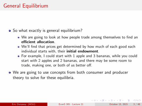
General Equilibrium

So what exactly is general equilibrium?

We are going to look at how people trade among themselves to �nd ane¢ cient allocation.We�ll �nd that prices get determined by how much of each good eachindividual starts with, their initial endowment.For example, I could start with 1 apple and 3 bananas, while you couldstart with 2 apples and 2 bananas, and there may be some room totrade, making one, or both of us better o¤.

We are going to use concepts from both consumer and producertheory to solve for these equilibria.


General Equilibrium

A note:

For the purpose of quizzes or exams, I will expect everyone to be ableto solve these problems graphically, not mathematically.

That being said, if I �nd a way to simplify the problems for everyone, Imight sneak an easy one in (we�ll go over it in that case).

We will cover the full solutions mathematically, however.


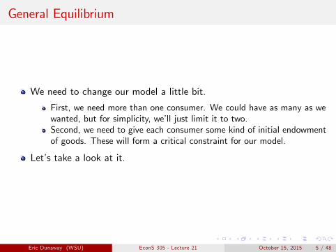
General Equilibrium

We need to change our model a little bit.

First, we need more than one consumer. We could have as many as wewanted, but for simplicity, we�ll just limit it to two.Second, we need to give each consumer some kind of initial endowmentof goods. These will form a critical constraint for our model.

Let�s take a look at it.


General Equilibrium

Consider two individuals (A and B) that both like to consume pizza(good x) and beer (good z). Assume that we know their utilityfunctions (we�ll specify them later).

We�ll say that consumer A is endowed with 1 unit of pizza and 5 unitsof beer, while consumer B is endowed with 7 units of pizza and 3units of beer. We can write this mathematically as

eA = (1, 5) eB = (7, 3)

Let�s look at each consumer graphically.


General Equilibrium

xA

zA

0

8

8


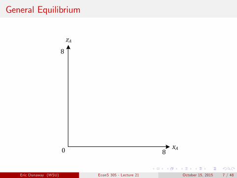
General Equilibrium

xA

zA

0

8

81

5eA


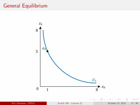
General Equilibrium

xA

zA

0

8

81

5eA

UA


General Equilibrium

xB

zB

0

8

8


General Equilibrium

xA

zA

0

8

87

3 eB


General Equilibrium

0

8

87

3 eB

xB

zB

UB


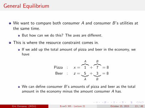
General Equilibrium

We want to compare both consumer A and consumer B�s utilities atthe same time.

But how can we do this? The axes are di¤erent.

This is where the resource constraint comes in.

If we add up the total amount of pizza and beer in the economy, wehave

Pizza : x =

Az}|{1 +

Bz}|{7 = 8

Beer : z = 5|{z}A

+ 3|{z}B

= 8

We can de�ne consumer B�s amounts of pizza and beer as the totalamount in the economy minus the amount consumer A has.


General Equilibrium

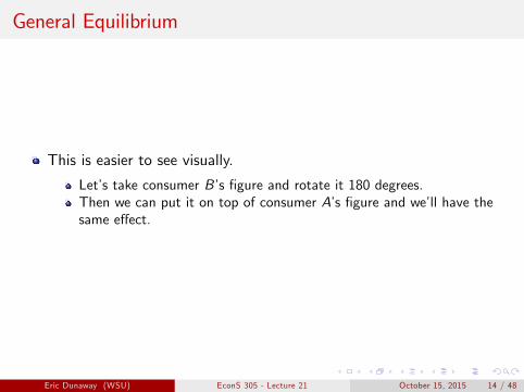
This is easier to see visually.

Let�s take consumer B�s �gure and rotate it 180 degrees.Then we can put it on top of consumer A�s �gure and we�ll have thesame e¤ect.


General Equilibrium

0

8

87

3 eB

xB

zB

UB


General Equilibrium

0

8

8 7

3eB

xB

zB

UB


General Equilibrium

xA

zA

0 1

5eA

UA

0

8

8 7

3eB

xB

zB

UB


Edgeworth Box

This is known as the Edgeworth Box.

E¤ectively, there are two sets of axes, but they are uni�ed due to theresource constraint.The length and width of the box are exactly the total amount of eachgood (8 each in this case).Notice that the endowment points align perfectly. This is nocoincidence.

The edgeworth box shows us how any allocation a¤ects bothconsumers.

Let�s look at a few alternate allocations.


Edgeworth Box

xA

zA

0 1

5e

UA

0

8

8 7

3

xB

zB

UB


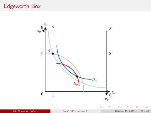
Edgeworth Box

Notice that in the �rst two examples, either consumer A or consumerB was at a lower utility level.

Picking an allocation in those regions helped one consumer, but hurtthe other.

The third allocation, however, improved the utility of both consumersA and B.

It would actually be bene�cial for them to trade to get to thisallocation.In fact, any allocation that lies above both of the original utility curveswould be an improvement for both consumers.


Edgeworth Box

xA

zA

0 1

5e

UA

0

8

8 7

3

xB

zB

UB

Allocations thatare better for

both consumers


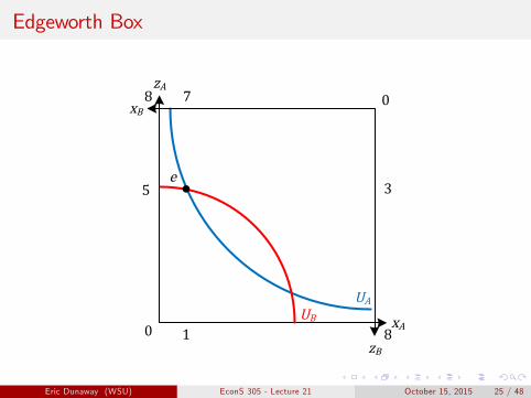
Edgeworth Box

Obviously, our solution will lie somewhere where both consumers arebetter o¤ than their original allocation.

Otherwise, why would they trade?

There are, however, numerous possible allocations that are better forboth consumers, so which one will they agree upon in equilibrium?

Well, we can actually rule some more allocations out �rst.


Edgeworth Box

xA

zA

0 1

5e

UA

0

8

8 7

3

xB

zB

UB


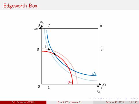
Edgeworth Box

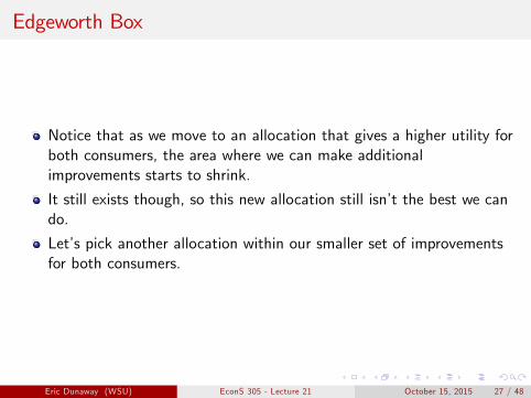
Notice that as we move to an allocation that gives a higher utility forboth consumers, the area where we can make additionalimprovements starts to shrink.

It still exists though, so this new allocation still isn�t the best we cando.

Let�s pick another allocation within our smaller set of improvementsfor both consumers.


Edgeworth Box

xA

zA

0 1

5e

UA

0

8

8 7

3

xB

zB

UB


Edgeworth Box

Here, the utility curves for consumers A and B are tangent to eachother (they only intersect exactly at the allocation point).

The area where we can �nd additional improvements is now zero. Thismeans that neither consumer can do any better without hurting theother consumer.We call this Pareto e¢ ciency.

Before we call this an equilibrium allocation, however, I have to pointout that there are several possible Pareto e¢ cient allocations in thisedgeworth box.


Pareto E¢ ciency

xA

zA

0 1

5e

UA

0

8

8 7

3

xB

zB

UB


Pareto E¢ ciency

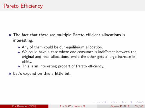
The fact that there are multiple Pareto e¢ cient allocations isinteresting.

Any of them could be our equilibrium allocation.We could have a case where one consumer is indi¤erent between theoriginal and �nal allocations, while the other gets a large increase inutility.This is an interesting propert of Pareto e¢ ciency.

Let�s expand on this a little bit.


Pareto E¢ ciency

In the real world, economists like to apply Pareto e¢ ciency to theirpolicy recommendations.

If we can �nd some policy that makes even one person better o¤without hurting anyone else, of course it�s a good idea.But the fact that there are so many di¤erent allocations that arePareto e¢ cient makes it hard to pick the "fair" allocation.In fact, if I had all of the wealth in the United States and everyone elsehad nothing, that would actually be Pareto e¢ cient.


Pareto E¢ ciency

If we can calculate all of the possible Pareto e¢ cient allocations, theywill form a line.

We call this the contract curve.Let�s see it on our �gure.


Pareto E¢ ciency

xA

zA

0 1

5e

UA

0

8

8 7

3

xB

zB

UB

Contract Curve


Pareto E¢ ciency

Our equilibrium allocation will lay on the contract curve.

Remember that it will also be at least as good as the original utilitylevels for both consumers.

How can we �gure out the contract curve?

Let�s use a couple of tricks from consumer theory.


Contract Curve

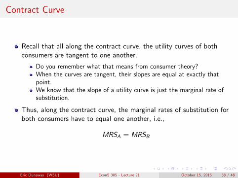
Recall that all along the contract curve, the utility curves of bothconsumers are tangent to one another.

Do you remember what that means from consumer theory?When the curves are tangent, their slopes are equal at exactly thatpoint.We know that the slope of a utility curve is just the marginal rate ofsubstitution.

Thus, along the contract curve, the marginal rates of substitution forboth consumers have to equal one another, i.e.,

MRSA = MRSB


Contract Curve

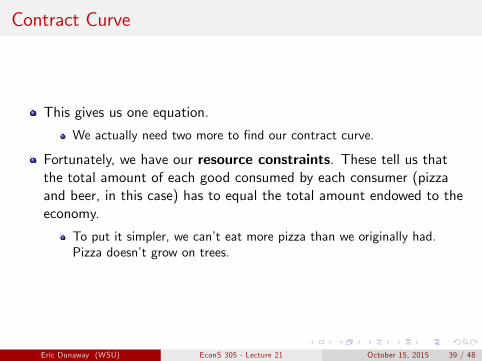
This gives us one equation.

We actually need two more to �nd our contract curve.

Fortunately, we have our resource constraints. These tell us thatthe total amount of each good consumed by each consumer (pizzaand beer, in this case) has to equal the total amount endowed to theeconomy.

To put it simpler, we can�t eat more pizza than we originally had.Pizza doesn�t grow on trees.


Contract Curve

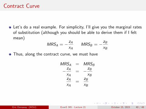
Let�s do a real example. For simplicity, I�ll give you the marginal ratesof substitution (although you should be able to derive them if I feltmean)

MRSA = �zAxA

MRSB = �zBxB

Thus, along the contract curve, we must have

MRSA = MRSB

� zAxA

= � zBxB

zAxA

=zBxB


Contract Curve

Next, we need our resource constraints. Recall that our initialendowments were

eA = (1, 5) eB = (7, 3)

or, Consumer A was endowed with 1 unit of pizza and 5 units of beer,while Consumer B was endowed with 7 units of pizza and 3 units ofbeer.

The amount of pizza we give to each consumer in equilibrium has toequal the original endowment.

Consumer A�sEquilibrium Pizzaz}|{

xA +

Consumer B�sEquilibrium Pizzaz}|{

xB =

Consumer A�sEndowed Pizzaz}|{

1 +

Consumer B�sEndowed Pizzaz}|{

7

xA + xB = 8


Contract Curve

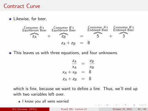
Likewise, for beer,

Consumer A�sEquilibrium Beerz}|{

zA +

Consumer B�sEquilibrium Beerz}|{

zB =

Consumer A�sEndowed Beerz}|{

5 +

Consumer B�sEndowed Beerz}|{

3

zA + zB = 8

This leaves us with three equations, and four unknowns.

zAxA

=zBxB

xA + xB = 8

zA + zB = 8

which is �ne, because we want to de�ne a line. Thus, we�ll end upwith two variables left over.

I know you all were worried


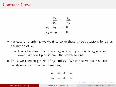
Contract Curve

zAxA

=zBxB

xA + xB = 8

zA + zB = 8

For ease of graphing, we want to solve these three equations for zA asa function of xA.

This is because of our �gure. zA is on our y -axis while xA is on ourx-axis. We could pick several other combinations.

Thus, we need to get rid of zB and xB . We can solve our resourceconstraints for those two variables,

xB = 8� xAzB = 8� zA


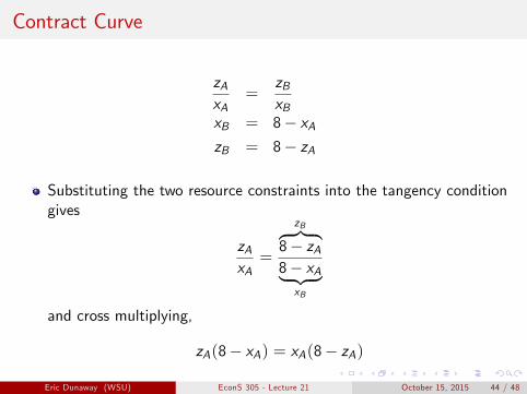
Contract Curve

zAxA

=zBxB

xB = 8� xAzB = 8� zA

Substituting the two resource constraints into the tangency conditiongives

zAxA=

zBz }| {8� zA8� xA| {z }xB

and cross multiplying,

zA(8� xA) = xA(8� zA)


Contract Curve

zA(8� xA) = xA(8� zA)

We can distribute both sides, getting rid of the parenthesis,

8zA � xAzA = 8xA � xAzA

and the xAzA term on both sides cancels out, leaving

8zA = 8xA

Lastly, we divide both sides by 8 and we obtain our contract curve.

zA = xA


Contract Curve

zA = xA

This contract curve tells us that for an allocation to be Paretoe¢ cient, consumer A must consume pizza and beer in equal amounts.

Sounds pretty reasonable.

We also know that our equilibrium allocation will lay somewhere onthis line.

The question is where?That has to do with the initial allocation, which we�ll talk about onMonday.


Summary

We can model the utilities of two consumers at once using anEdgeworth Box.

An allocation where no consumer can be made better o¤ withouthurting the other consumer is called Pareto e¢ cient.

All Pareto e¢ cient allocations are located on the contract curve.


Preview of Monday

We will solve for our equilibrium allocation.

We will also complicate the model a bit, adding the producer�s side.


econs 305 - general equilibrium part 1

Documents