edem 2.6 theory reference guide · edem 2.6 reference guide 4 getting started the information in...

EDEM 2.6 Theory Reference Guide

EDEM 2.6 Reference Guide

2

Copyrights and Trademarks

Copyright © 2014 DEM Solutions. All rights reserved. Information in this document is subject to change without notice. The software described in this document is furnished under a license agreement or nondisclosure agreement. The software may be used or copied only in accordance with the terms of those agreements. No part of this publication may be reproduced, stored in a retrieval system, or transmitted in any form or any means electronic or mechanical, including photocopying and recording for any purpose other than the purchaser’s personal use without the written permission of DEM Solutions. DEM Solutions 49 Queen Street Edinburgh EH2 3NH UK

www.dem-solutions.com

EDEM incorporates CADfix translation technology. CADfix is owned, supplied by and Copyright©

TranscenData Europe Limited, 2007. All Rights Reserved. This software is based in part on the work of the Independent JPEG Group. EDEM uses the Mersenne Twister random number generator, Copyright

© 1997 - 2002, Makoto Matsumoto and Takuji Nishimura, All rights reserved.

EDEM includes CGNS (CFD General Notation System) software. See the Online Help for full copyright notice.

EDEM

®, EDEM Creator

®, EDEM Simulator

®, EDEM Analyst

® and Particle Factory

® are registered

trademarks of DEM Solutions. EDEM Field Data CouplingTM

, EDEM CFD Coupling InterfaceTM

and EDEM Multibody Dynamics Coupling Interface

TM are Trademarks of DEM Solutions. All other

brands or product names are the property of the respective owners.


3

Contents GETTING STARTED ................................................................................................................................... 4

CONTACT MODEL THEORY ....................................................................................................................... 5

HERTZ-MINDLIN (NO SLIP) ................................................................................................................................ 5 Relative Wear.......................................................................................................................................... 7

HERTZ-MINDLIN (NO SLIP) WITH RVD ROLLING FRICTION ....................................................................................... 7 HERTZ-MINDLIN WITH ARCHARD WEAR ............................................................................................................... 8 HERTZ-MINDLIN WITH BONDING ........................................................................................................................ 9 HERTZ-MINDLIN WITH HEAT CONDUCTION ......................................................................................................... 10

Temperature Update ............................................................................................................................ 10 HERTZ-MINDLIN WITH JKR COHESION ............................................................................................................... 10 LINEAR COHESION .......................................................................................................................................... 12 HYSTERETIC SPRING ........................................................................................................................................ 13 MOVING PLANE ............................................................................................................................................. 15 LINEAR SPRING .............................................................................................................................................. 15

PARTICLE BODY FORCES ......................................................................................................................... 17

REFERENCES ........................................................................................................................................... 18

INDEX ..................................................................................................................................................... 19


4

Getting Started

The information in this guide is intended to supplement the discussion in the EDEM 2.6 User Guide and explains the theory and research behind the following:

Contact Models

Particle Body Forces

This guide also contains a Reference section for additional background information.


5

Contact Model Theory

This section explains the contact models available in EDEM 2.6. For additional information about each model’s parameters and the instructions on how to use a model, see the EDEM 2.6 User Guide. A contact model describes how elements behave when they come into contact with each other. EDEM includes the following integrated contact models:

Hertz-Mindlin (no slip)

Hertz-Mindlin (no slip) with RVD Rolling Friction

Hertz-Mindlin with Archard Wear

Hertz-Mindlin with Bonding

Hertz-Mindlin with Heat Conduction

Hertz-Mindlin with JKR Cohesion

Linear Cohesion

Linear Spring

Hysteretic Spring

Moving Plane (Conveyor)

Example simulations that use these contact models are in the examples folder.

You can also create your own user-defined models: EDEM is supplied with sample source files you can modify and compile to create additional plug-in contact models. Refer to the EDEM Programming Guide for more details.

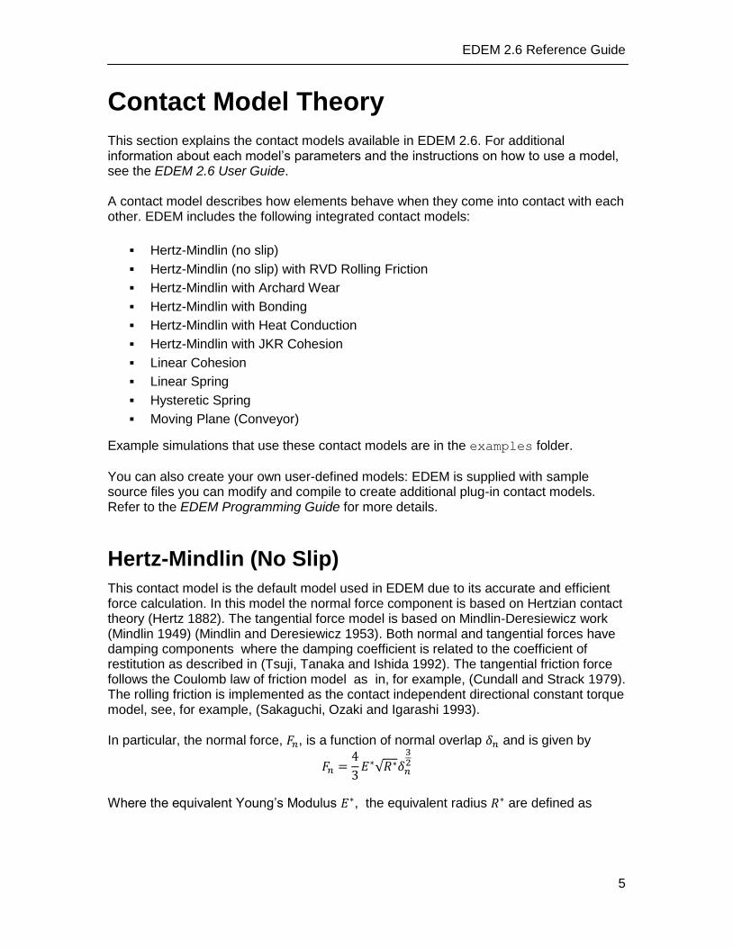
Hertz-Mindlin (No Slip)

This contact model is the default model used in EDEM due to its accurate and efficient force calculation. In this model the normal force component is based on Hertzian contact theory (Hertz 1882). The tangential force model is based on Mindlin-Deresiewicz work (Mindlin 1949) (Mindlin and Deresiewicz 1953). Both normal and tangential forces have damping components where the damping coefficient is related to the coefficient of restitution as described in (Tsuji, Tanaka and Ishida 1992). The tangential friction force follows the Coulomb law of friction model as in, for example, (Cundall and Strack 1979). The rolling friction is implemented as the contact independent directional constant torque model, see, for example, (Sakaguchi, Ozaki and Igarashi 1993).

In particular, the normal force, , is a function of normal overlap and is given by

Where the equivalent Young’s Modulus , the equivalent radius are defined as


6

with , , , and , , being the Young’s Modulus, Poisson ratio and Radius of

each sphere in contact. Additionally there is a damping force, , given by

rel

nn

d

n vmSF *

6

52

Where

is the equivalent mass,

is the normal component of the

relative velocity and and (the normal stiffness) are given by

22ln

ln

e

e

nn RES **2

With the coefficient of restitution. The tangential force, , depends on the tangential

overlap and the tangential stiffness .

ttt SF

with

nt RGS **8

Here is the equivalent shear modulus. Additionally, tangential damping is given by:

rel

tt

d

t vmSF *

6

52

where

is the relative tangential velocity. The tangential force is limited by Coulomb

friction where is the coefficient of static friction.

For simulations in which rolling friction is important, this is accounted for by applying a torque to the contacting surfaces.

iinri RF

with the coefficient of rolling friction, the distance of the contact point from the

center of mass and , the unit angular velocity vector of the object at the contact point.


7

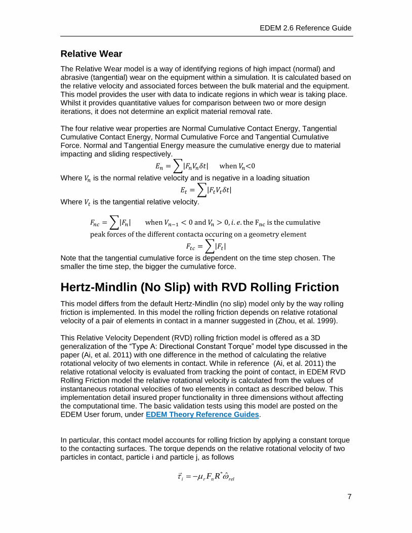
Relative Wear

The Relative Wear model is a way of identifying regions of high impact (normal) and abrasive (tangential) wear on the equipment within a simulation. It is calculated based on the relative velocity and associated forces between the bulk material and the equipment. This model provides the user with data to indicate regions in which wear is taking place. Whilst it provides quantitative values for comparison between two or more design iterations, it does not determine an explicit material removal rate. The four relative wear properties are Normal Cumulative Contact Energy, Tangential Cumulative Contact Energy, Normal Cumulative Force and Tangential Cumulative Force. Normal and Tangential Energy measure the cumulative energy due to material impacting and sliding respectively.

Where is the normal relative velocity and is negative in a loading situation

Where is the tangential relative velocity.

Note that the tangential cumulative force is dependent on the time step chosen. The smaller the time step, the bigger the cumulative force.

Hertz-Mindlin (No Slip) with RVD Rolling Friction

This model differs from the default Hertz-Mindlin (no slip) model only by the way rolling friction is implemented. In this model the rolling friction depends on relative rotational velocity of a pair of elements in contact in a manner suggested in (Zhou, et al. 1999). This Relative Velocity Dependent (RVD) rolling friction model is offered as a 3D generalization of the “Type A: Directional Constant Torque” model type discussed in the paper (Ai, et al. 2011) with one difference in the method of calculating the relative rotational velocity of two elements in contact. While in reference (Ai, et al. 2011) the relative rotational velocity is evaluated from tracking the point of contact, in EDEM RVD Rolling Friction model the relative rotational velocity is calculated from the values of instantaneous rotational velocities of two elements in contact as described below. This implementation detail insured proper functionality in three dimensions without affecting the computational time. The basic validation tests using this model are posted on the EDEM User forum, under EDEM Theory Reference Guides. In particular, this contact model accounts for rolling friction by applying a constant torque to the contacting surfaces. The torque depends on the relative rotational velocity of two particles in contact, particle i and particle j, as follows

relnri RF ˆ*

http://www.dem-solutions.com/forum/viewforum.php?f=17


8

ij

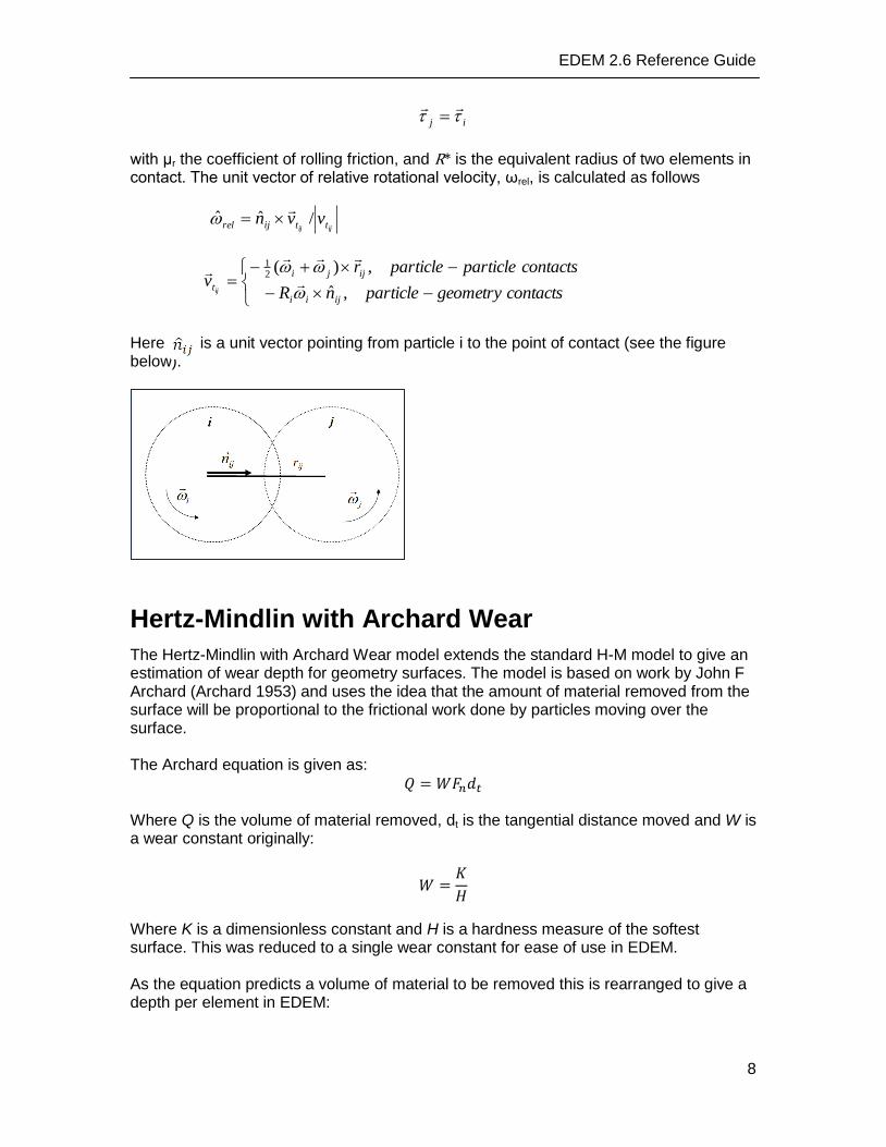
with μr the coefficient of rolling friction, and R* is the equivalent radius of two elements in contact. The unit vector of relative rotational velocity, ωrel, is calculated as follows

Here is a unit vector pointing from particle i to the point of contact (see the figure below).

Hertz-Mindlin with Archard Wear

The Hertz-Mindlin with Archard Wear model extends the standard H-M model to give an estimation of wear depth for geometry surfaces. The model is based on work by John F Archard (Archard 1953) and uses the idea that the amount of material removed from the surface will be proportional to the frictional work done by particles moving over the surface. The Archard equation is given as:

Where Q is the volume of material removed, dt is the tangential distance moved and W is a wear constant originally:

Where K is a dimensionless constant and H is a hardness measure of the softest surface. This was reduced to a single wear constant for ease of use in EDEM. As the equation predicts a volume of material to be removed this is rearranged to give a depth per element in EDEM:

ijij ttijrel vvn /ˆˆ

contactsgeometryparticlenR

contactsparticleparticlerv

ijii

ijji

tij ,ˆ

,)(21


9

Hertz-Mindlin with Bonding

The Hertz-Mindlin with Bonding contact model can be used to bond particles with a finite-sized “glue” bond. This bond can resist tangential and normal movement up to a maximum normal and tangential shear stress, at which point the bond breaks. Thereafter the particles interact as hard spheres. This model is based on work of Potyondy and Cundall (Potyondy and Cundall 2004). This model is particularly useful in modeling concrete and rock structures.

Particles are bonded at the bond formation time tBOND. Before this time, the particles interact through the standard Hertz-Mindlin contact model. After bonding, the forces (Fn,t)/torques (Tn,t) on the particle are set to zero and are adjusted incrementally every timestep according to:

tJ

SM

tJSM

tASvF

tASvF

ntt

tnn

ttt

nnn

2

where:

4

2

2

1B

B

RJ

RA

RB is the radius of the “glue”, Sn,t are the normal and shear stiffness respectively and δt

is the timestep. vn,t are the normal and tangential velocities of the particles and ωn,t the

normal and tangential angular velocities.

The bond is broken when the normal and tangential shear stresses exceed some pre-defined value:

B

nt

B

tn

RJ

M

A

F

RJ

M

A

F

max

max

2

These bond forces/torques are in addition to the standard Hertz-Mindlin forces. Since the bonds involved in this model can act when the particles are no longer physically in contact, the contact radius should be set to higher than the actual radius of the spheres. This model may only be used between particles.


10

Hertz-Mindlin with Heat Conduction

For dilute phase simulations, convective heat transfer is dominant and conductions between the particles or wall can be neglected. However, for dense phase, contacts between particles are significant such that conductive heat transfer must be taken into account. A single phase DEM simulation on heat transfer in granular flow in rotating vessels provides a simple approach in modeling inter-particle heat transfer. This model is based on the work of Chaudhuri (Chaudhuri, Muzzio and Tomassone 2006). The heat flux between the particles is defined as:

2121 ppcpp ThQ

where the contact area is incorporated in the heat transfer coefficient hc and is given by:

3/1

*

*

21

21

4

34

E

rF

kk

kkh N

pp

pp

c

where FN is the normal force, r* the geometric mean of the particles radii from the Hertz’s elastic contact theory and E* is the effective Young’s modulus for the two particles. The bracketed term on the RHS of the equation models the contact area between particles. This contact model must be used along with the Temperature Update body force model.

Temperature Update

This body force model must be used in combination with the Hertz-Mindlin with Heat Conduction model to ensure the function of the heat conduction algorithm as described in (Chaudhuri, Muzzio and Tomassone 2006). After all the heat fluxes have been calculated, the temperature change over time of each particle is updated explicitly using:

h ea tPp Qdt

dTCm

where mp, CP and T are the mass, specific heat capacity and temperature of the particle material type. The RHS denotes the sum of convective and conductive heat fluxes.

Hertz-Mindlin with JKR Cohesion

Hertz-Mindlin with JKR (Johnson-Kendall-Roberts) Cohesion is a cohesion contact model that accounts for the influence of Van der Waals forces within the contact zone and allows the user to model strongly adhesive systems, such as dry powders or wet materials. In this model, the implementation of normal elastic contact force is based on the Johnson-Kendall-Roberts theory reported in (Johnson, Kendal and Roberts 1971).


11

Hertz-Mindlin with JKR Cohesion uses the same calculations as the Hertz-Mindlin (no slip) contact model for the following types of force:

Tangential elastic force

Normal dissipation force

Tangential dissipation force

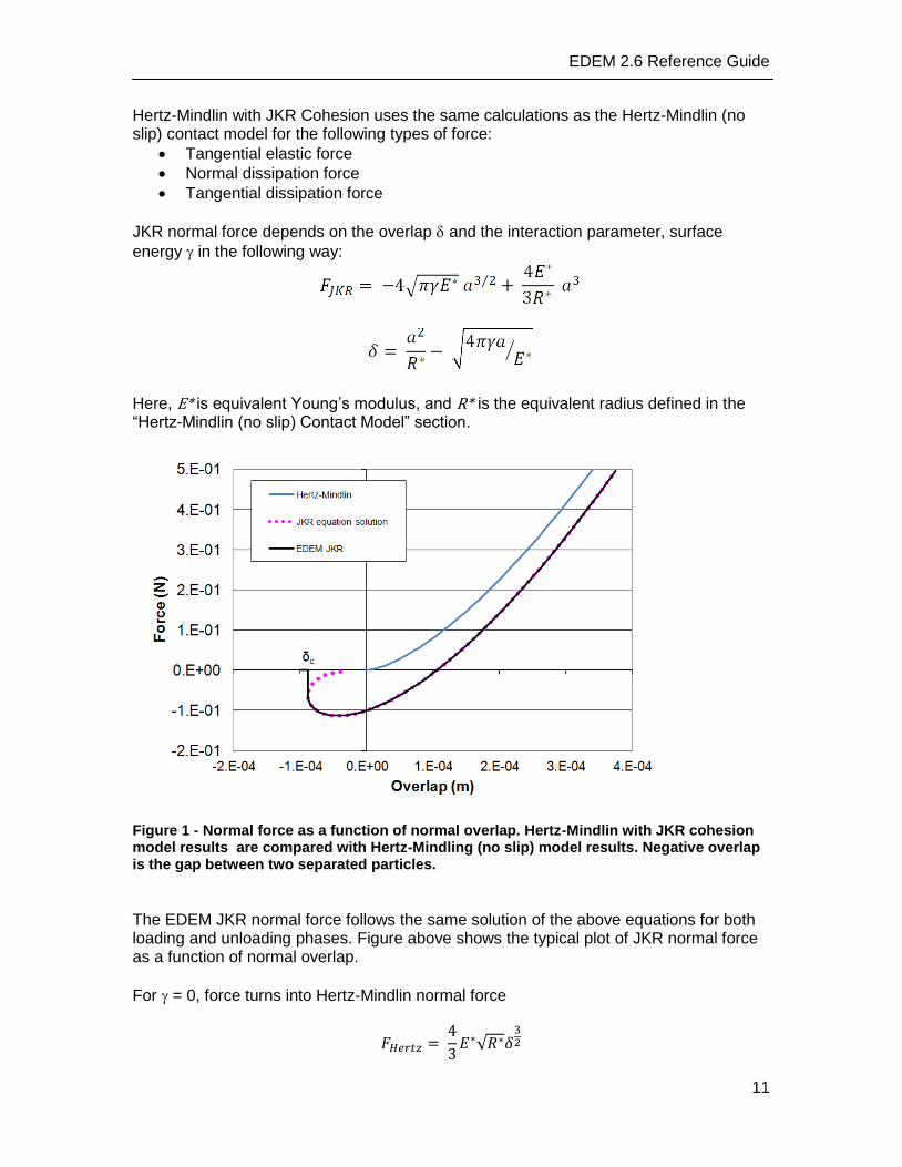
JKR normal force depends on the overlap and the interaction parameter, surface

energy in the following way:

Here, E* is equivalent Young’s modulus, and R* is the equivalent radius defined in the “Hertz-Mindlin (no slip) Contact Model” section.

Figure 1 - Normal force as a function of normal overlap. Hertz-Mindlin with JKR cohesion model results are compared with Hertz-Mindling (no slip) model results. Negative overlap is the gap between two separated particles.

The EDEM JKR normal force follows the same solution of the above equations for both loading and unloading phases. Figure above shows the typical plot of JKR normal force as a function of normal overlap.

For = 0, force turns into Hertz-Mindlin normal force


12

This model provides attractive cohesion forces even if the particles are not in physical contact. The maximum gap between particles with non-zero force is given by

*

2

*

4

R

a

E

a ccc

For δ< δc the model returns zero force. The maximum value of the cohesion force occurs when particles are not in physical contact and the separation gap is less than δc . The value of maximum cohesion force, called pull-out force, is given by

Friction force calculation is different than in the Hertz-Mindlin (no slip) contact model in that it depends on the positive repulsive part of JKR normal force. As a result, the EDEM JKR friction model provides higher friction force when cohesion component of the contact force is higher. The importance and advantages of this friction force model correction in the presence of strong cohesive forces was noted and illustrated in, for example, (Baran, et al. 2009), (Gilabert, Roux and Castellanos 2007). Example validation tests using EDEM JKR models can be also found on the EDEM User forum, under EDEM Theory Reference Guides. Although this model was designed for fine, dry particles, it can be used to model wet particles. The force needed to separate two particles depends on the liquid surface

tension and wetting angle

Equating the above force to JKR max force

allows JKR surface

energy parameter estimation if EDEM particle size is not scaled.

Linear Cohesion

This cohesion model modifies Hertz-Mindlin contact by adding a normal cohesion force.1 This force takes the form:

F = kA

1 The Linear Cohesion model was first introduced by the DEM Solutions engineering and

development team and is used successfully in commercial application projects to model the flow of sticky particles.

31

*

2*

)]([2

143

2

9

E

R

ca



13

where A is the contact area and k is a cohesion energy density with units Jm-3. This

force is added to the traditional Hertz-Mindlin normal force.

No additional tangential force is added in this model, however the magnitude of the non-cohesive normal force is increased beyond Hertz-Mindlin and therefore a stronger frictional force can be withstood before slippage.

Hysteretic Spring

The Hysteretic Spring contact model allows plastic deformation behaviors to be included in the contact mechanics equations, resulting in particles behaving in an elastic manner up to a predefined stress. Once this stress is exceeded, the particles behave as though undergoing plastic deformation. The result is that large overlaps are achievable without excessive forces acting upon them, thus representing a compressible material. Hysteretic Spring normal force calculation is based on the Walton-Braun theory described in the following references (Walton and Braun 1986), (Walton and Braun 1986).

Figure above shows a schematic of the Hysteretic Spring contact model force displacement relationship. Note that the unloading force goes to zero before the displacement recovers to the initial contacting point. The quantity δ0 represents the residual ‘overlap’ that remains because of the plastic deformation (i.e., flattening) in the contact region. The exact location of each old contact spot is not ‘remembered,’ so that particles become like new undeformed spheres once they separate. Subsequent contacts will load along a new loading path with slope, K1. Any reloading before separation follows the slope K2 until the original loading curve K1 is reached, whereupon the lower slope is followed until unloading occurs. In particular, the normal force, FN, is given by:


14

)(unloadingfor 0

)(reloadingunloading/for )(

))((loadingfor

0

002

0211

n

n

nn

nnn

K

KKK

F

where K1 and K2 are the loading and unloading stiffness respectively, δn, is normal overlap and δ0 is the residual overlap. Loading stiffness, K1, is related to the yield strength of each material participating in contact, Y1 and Y2, as follows (Walton O. , 2006):

),min(5 21

*

1 YYRK

Here R* is the equivalent radius of the two particles participating in the contact. The following expression for coefficient of restitution

2

1

K

Ke

allows for the determination of K2 from K1 (Walton O. , 2006). Residual overlap is updated every timestep according to the following rule:

)(unloadingfor

)(reloadingunloading/for

))((loadingfor )1(

0

00

021

2

1

0

nn

n

nnn KKK

K

The main energy dissipation mechanism is due to spring stiffness difference between loading and unloading phases. The need for additional velocity dependent dissipation mechanism to suppress possible un-damped low amplitude oscillations was suggested in (Walton O. , 2006). In EDEM Hysteretic Spring model this mechanism was implemented similar to linear spring normal damping force scaled by dimensionless user set parameter ‘Damping Factor’, bn, as follows:

rel

nn

d

n v

e

kmbF

2

*

ln1

4

Here k is either K1 or K2. The rest of the variables and factors in the above expression are explained in the Linear Spring contact model section. Since EDEM Hysteretic Spring model for normal force can be considered as extension of linear spring model for normal force it makes sense use tangential components of linear spring model for tangential forces. In particular, more general form of linear spring elastic


15

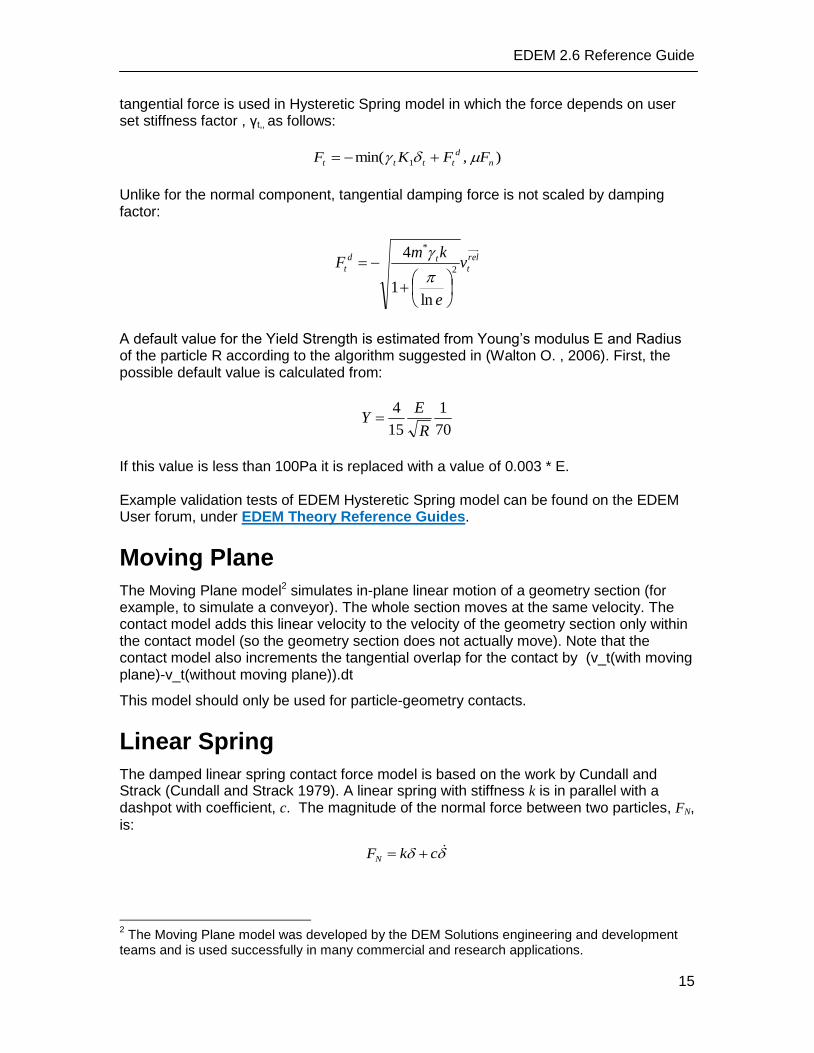
tangential force is used in Hysteretic Spring model in which the force depends on user set stiffness factor , γt,, as follows:

),min( 1 n

d

tttt FFKF

Unlike for the normal component, tangential damping force is not scaled by damping factor:

rel

ttd

t v

e

kmF

2

*

ln1

4

A default value for the Yield Strength is estimated from Young’s modulus E and Radius of the particle R according to the algorithm suggested in (Walton O. , 2006). First, the possible default value is calculated from:

70

1

15

4

R

EY

If this value is less than 100Pa it is replaced with a value of 0.003 * E. Example validation tests of EDEM Hysteretic Spring model can be found on the EDEM User forum, under EDEM Theory Reference Guides.

Moving Plane

The Moving Plane model2 simulates in-plane linear motion of a geometry section (for example, to simulate a conveyor). The whole section moves at the same velocity. The contact model adds this linear velocity to the velocity of the geometry section only within the contact model (so the geometry section does not actually move). Note that the contact model also increments the tangential overlap for the contact by (v_t(with moving plane)-v_t(without moving plane)).dt

This model should only be used for particle-geometry contacts.

Linear Spring

The damped linear spring contact force model is based on the work by Cundall and Strack (Cundall and Strack 1979). A linear spring with stiffness k is in parallel with a dashpot with coefficient, c. The magnitude of the normal force between two particles, FN,

is:

ckFN

2 The Moving Plane model was developed by the DEM Solutions engineering and development

teams and is used successfully in many commercial and research applications.



16

where k is the linear spring stiffness, c is the dashpot coefficient, δ is the overlap, and

is the overlap velocity. Similar force can be applied to the tangential direction.

The spring stiffness and the dashpot coefficient are the parameters in this model and it is a common practice to estimate the spring stiffness and calculate the dashpot coefficient based on this stiffness. The simulation timestep is then estimated based on the spring stiffness.

The spring constant and dashpot coefficient can be calculated based on a combination of material properties and kinematic constraints. One common method is obtained by equating the maximum strain energy in a purely Hertzian contact (Ehertzian) with the maximum strain energy of the existing contact (Emax). This gives:

5

1

*2

1*

2**2

1*

16

15

15

16

ER

VmERk

where the equivalent mass , the equivalent radius and the equivalent Young’s

modulus were defined earlier. V is the typical impact velocity.

For two identical spherical particles with masses of 7.63e-03 kg, radius of 9 mm and Young’s modulus of 2.6e+08, colliding at a velocity of 3 m/s, k ≈ 2.0e+05 N/m.

The impact velocity in an EDEM simulation can usually be taken as a characteristic velocity in the simulation. You can base this velocity as the maximum velocity in the simulation, for example, for a blending operation with the blender operating at Ω rad/s, the characteristic velocity is equal to r Ω m/s, where r is the radius of the blender. The dashpot coefficient is related to the coefficient of restitution as:

2

*

ln1

4

e

kmc

where is the coefficient of restitution. Note that remains constant with the impact speed (assuming other model parameters are constant).

The tangential stiffness is usually estimated as a ratio of the normal spring stiffness (Cundall and Strack 1979). EDEM has the tangential stiffness equal to the normal stiffness.

The dashpot coefficient is calculated using the tangential stiffness in the equation above. The tangential force is computed via:

where kt and ct are the tangential spring and dashpot coefficient, μ is the coefficient of

friction.

The simulation timestep is usually a small percent of the contact duration of the particles. The contact duration for a linear spring model is obtained using the normal stiffness as:


17

where and is the coefficient of restitution.

For = 0.5 we have a contact time of 0.00043 sec. The simulation time step must be less than this value for better integration of the particle states. We recommend you have a value of about 5-10 % of this contact time for accurate results. The details of the soft-particle contact model are relatively unimportant due to the fact that a lumped parameter approach which neglects the details of the contact force (e.g. a coefficient of restitution) is sufficient to describe the collision dynamics.

Note that you can increase the simulation timestep and then try to fix a stiffness that will not allow for excessive overlap. However, since the stiffness and timestep are not based on physical laws, the accuracy of the results is not guaranteed: you might obtain a qualitative similarity but not a quantitative one. We recommend to calculate the stiffness based on the material properties and fix the timestep in EDEM.

There is no general consensus on what is the best contact model. The linear spring model is simpler than Hertz-Mindlin due to less computational overhead. However, in both the models the contact force is discontinuous at the first and last point of contact, and energy dissipation is poor in systems with small relative velocities.

For the same stiffness, we obtain a larger force for the same time step in a Hertz-Mindlin model in comparison with the linear spring. Hence a larger time step can be used with a linear spring contact model.

Particle Body Forces

A particle body force can be set to act upon particles when a specified condition is met; for example, when they are in certain position, or are traveling at a specified velocity. EDEM includes the following integrated particle body forces:

Temperature Update (see page 10)

Example simulations that use these particle body forces are in the examples folder.

You can also create your own user-defined forces: EDEM is supplied with sample source files you can modify and compile to create additional plug-in forces. Refer to the EDEM Programming Guide for more details.


18

References

Ai, Jun, Jian-Fei Chen, J. Michael Rotter, and Jin Y Ooi. "Assessment of rolling resistance models in discrete element simulations." Powder Technology 206 (2011): 269-282. Baran, Oleh, Alfred DeGennaro, Enrique Rame, and Allen Wilkinson. "DEM Simulation of a Schulze Ring Shear Tester." Proceedings of the 6th International Conference on Micromechanics of Granular Media. 2009. 409-412. Chaudhuri, Bodhisattwa, Fernando J. Muzzio, and M. Silvina Tomassone. "Modeling of heat transfer in granular flow in rotating vessels." Chemical Engineering Science 61 (2006): 6348-6360. Cundall, P. A., and O. D. Strack. "A discrete numberical model for granular assemblies." (Geotechnique) 29 (1979): 47-65. Gilabert, F. A., J. -N. Roux, and A. Castellanos. "Computer simulation of model cohesive powders: Influence of assembling procedure." Phys. Rev. E 75 (2007): 011303. Hertz, H. "On the contact of elastic solids." J. reine und angewandte Mathematik 92 (1882): 156-171. Johnson, K. L., K. Kendal, and A. D. Roberts. "Surface energy and the contact of elastic solids." Proc. R. Soc. Lond. A 324 (1971): 301-313. Mindlin, R. D. "Compliance of elastic bodies in contact." Journal of Applied Mechanics 16 (1949): 259-268. Mindlin, R. D., and H. Deresiewicz. "Elastic spheres in contact under varying oblique forces." ASME, September 1953: 327-344. Potyondy, D. O., and P. A. Cundall. "A bonded-particle model for rock." Journal of Rock Mechanics and Minimg Sciences 41 (2004): 1329-1364. Sakaguchi, E., E. Ozaki, and T. Igarashi. "Plugging of the flow of granular materials during the discharge from a silo." Int. J. Mod. Phys. B 7 (1993): 1949-1963. Tsuji, Y., T. Tanaka, and T. Ishida. "Lagrangian numerical simulation of plug flow of cohesionless particles in a horizontal pipe." Powder Technology 71 (1992): 239-250. Walton, O R, and R. L. Braun. "Viscosity and Temperature Calculations for Assemblies of Inelastic Frictional Disks." J. Rheology 30, no. 5 (1986): 949-980. Walton, O. R., and R. L. Braun. "Stress calculations for Assemblies of Inelastic Spheres in Uniform Shear." Acta Mechanica 63 (1986): 73-86. Walton, Otis. (Linearized) Elastic-Plastic contact model. Company report, DEM Solutions, 2006. Zhou, Y. C., B. D. Wright, R. Y Yang, B. H. Xu, and A. B Yu. "Rolling friction in the dynamic simulation of sandpile formation." 269 (1999): 536-553.


19

Index

Alpha value ........................................ 11 Cohesion ............................................ 13 Contact Model ........ 5, 7, 8, 9, 10, 11, 13 Contact Model Theory .......................... 5 Conveyor ............................................ 13 Custom Particle Body Forces ............. 16 Custom Particle Properties ................... 4 Heat Conduction .................................. 9 Hertz-Mindlin ........................................ 5

Hertz-Mindlin (no slip) with RVD Rolling Friction .............................................. 7

Hertz-Mindlin with Bonding ................... 8 Hertz-Mindlin with Heat Conduction ..... 9 Hertz-Mindlin with JKR Cohesion ....... 10 Hysteretic Spring ................................ 11 Linear Spring ...................................... 13 Moving Plane Contact Model .............. 13 Particle Body Force ............................ 16 User Defined Particle Attributes ........... 4

edem 2.6 theory reference guide · edem 2.6 reference guide 4 getting started the information in...

Documents