edge detection - stanford...

Digital Image Processing: Bernd Girod, © 2013 Stanford University -- Edge Detection 1

Edge detection

Gradient-based edge operators Prewitt Sobel Roberts

Laplacian zero-crossings Canny edge detector Hough transform for detection of straight lines Circle Hough Transform


Gradient-based edge detection

Idea (continous-space): local gradient magnitude indicates edge strength

Digital image:

use finite differences to approximate derivatives

Edge templates


Practical edge detectors

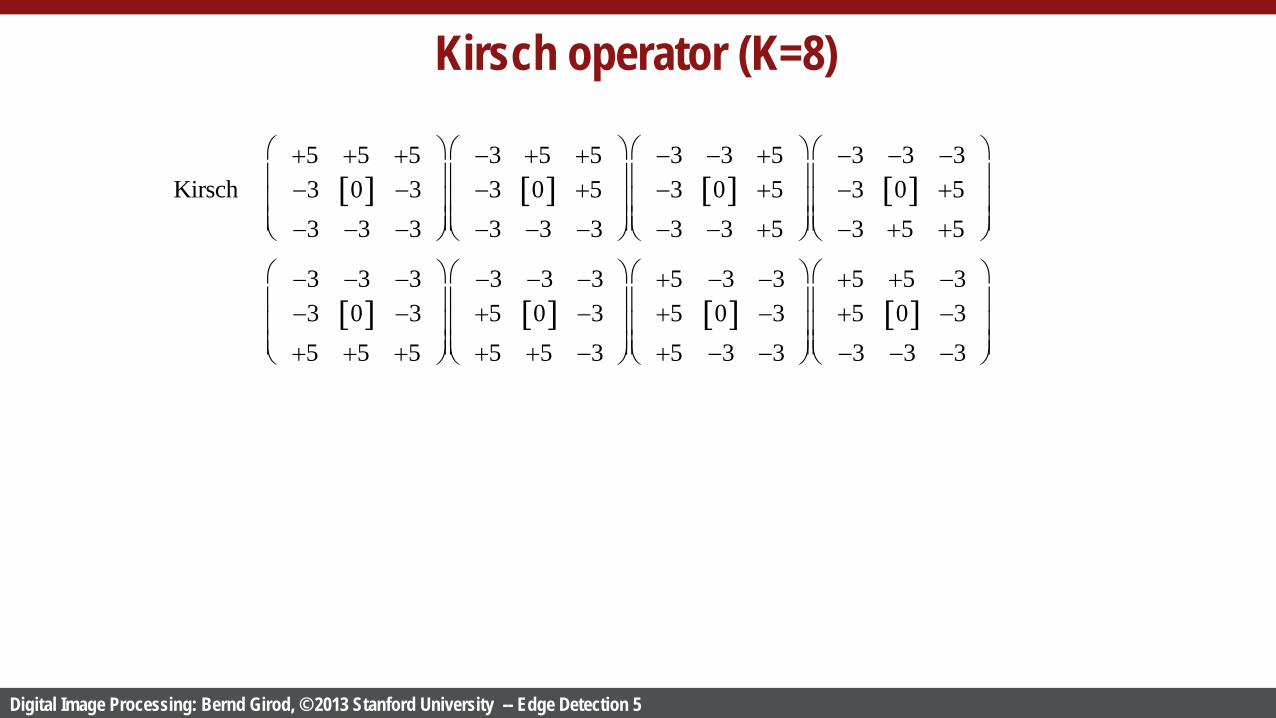
Edges can have any orientation Typical edge detection scheme uses K=2 edge templates Some use K>2

s x, y[ ]

e1 x, y

e2 x, y

eK x, y

Combination,e.g.,

ek x, y 2

k∑

or

Maxk ek x, y

edge magnitude

(edge orientation)

M x, y

α x, y


Gradient filters (K=2)

Prewitt−1 0 1−1 0[ ] 1−1 0 1

−1 −1 −10 0[ ] 01 1 1

Sobel−1 0 1−2 0[ ] 2−1 0 1

−1 −2 −10 0[ ] 01 2 1

Roberts 0[ ] 1−1 0

1[ ] 00 −1

Central

Difference

0 0 0−1 0[ ] 10 0 0

0 −1 00 0[ ] 00 1 0


Kirsch operator (K=8)

Kirsch +5 +5 +5−3 0[ ] −3−3 −3 −3

−3 +5 +5−3 0[ ] +5−3 −3 −3

−3 −3 +5−3 0[ ] +5−3 −3 +5

−3 −3 −3−3 0[ ] +5−3 +5 +5

−3 −3 −3−3 0[ ] −3+5 +5 +5

−3 −3 −3+5 0[ ] −3+5 +5 −3

+5 −3 −3+5 0[ ] −3+5 −3 −3

+5 +5 −3+5 0[ ] −3−3 −3 −3


Prewitt operator example

−1 0 1−1 0[ ] 1−1 0 1

−1 −1 −10 0[ ] 01 1 1

Magnitude of image filtered with

(log display)


(log display)

Original 1024x710

http://www.stanford.edu/class/ee368/Handouts/Lectures/Examples/11-Edge-Detection/


Prewitt operator example (cont.)

Sum of squared horizontal and

vertical gradients (log display)

threshold = 900 threshold = 4500 threshold = 7200



Sobel operator example

Sum of squared horizontal and

vertical gradients (log display)




Roberts operator example

Original 1024x710





Roberts operator example (cont.)

Sum of squared diagonal gradients

(log display)




Edge orientation Central

Difference

0 0 0−1 0[ ] 10 0 0

0 −1 00 0[ ] 00 1 0

Gradient scatter plot

x-component

y-co

mpo

nent

x-component

y-co

mpo

nent

Roberts

0[ ] 1−1 0

1[ ] 00 −1


Edge orientation

Sobel

−1 0 1−2 0[ ] 2−1 0 1

−1 −2 −10 0[ ] 01 2 1

Prewitt

−1 0 1−1 0[ ] 1−1 0 1

−1 −1 −10 0[ ] 01 1 1

x-component y-

com

pone

nt

x-component

y-co

mpo

nent



Edge orientation

5x5 “consistent” gradient operator

[Ando, 2000]

x-component

y-co

mpo

nent



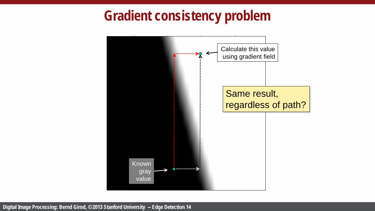
Gradient consistency problem

Known gray

value

Calculate this value using gradient field

Same result, regardless of path?


Laplacian operator

Detect edges by considering second derivative

Isotropic (rotationally invariant) operator Zero-crossings mark edge location

Edge profile f(x)

Detect zero crossing

f ’(x) f”(x)


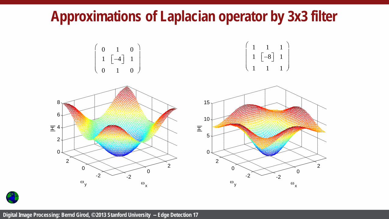
Approximations of Laplacian operator by 3x3 filter

0 1 01 −4 1

0 1 0

1 1 11 −8 1

1 1 1

-20

2

-20

2

0

2

4

6

8

ωxωy

|H|

-20

2

-20

2

0

5

10

15

ωxωy

|H|



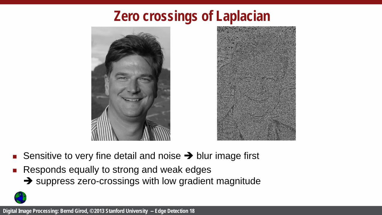
Zero crossings of Laplacian

Sensitive to very fine detail and noise blur image first Responds equally to strong and weak edges suppress zero-crossings with low gradient magnitude



Laplacian of Gaussian

Filtering of image with Gaussian and Laplacian operators can be combined into convolution with Laplacian of Gaussian (LoG) operator

LoG x, y( )= − 1πσ 4 1− x2 + y2

2σ 2

e−

x2+ y2

2σ 2

2σ =

-4-2

02

4

-4

-2

0

2

4-0.1

-0.08

-0.06

-0.04

-0.02

0

0.02

XY



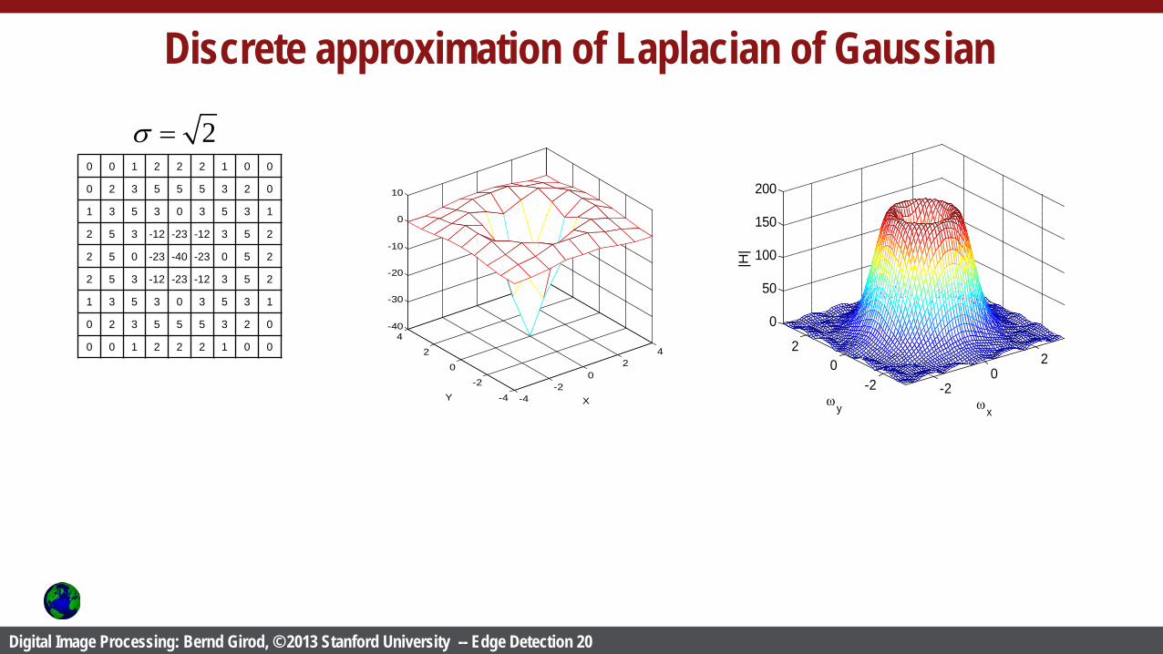
Discrete approximation of Laplacian of Gaussian

2σ =

-20

2

-20

2

0

50

100

150

200

ωxωy

|H|

0 0 1 2 2 2 1 0 0

0 2 3 5 5 5 3 2 0

1 3 5 3 0 3 5 3 1

2 5 3 -12 -23 -12 3 5 2

2 5 0 -23 -40 -23 0 5 2

2 5 3 -12 -23 -12 3 5 2

1 3 5 3 0 3 5 3 1

0 2 3 5 5 5 3 2 0

0 0 1 2 2 2 1 0 0

-4-2

02

4

-4

-2

0

2

4-40

-30

-20

-10

0

10

XY



Zero crossings of LoG

2 2σ = 4 2σ = 8 2σ =2σ =



Zero crossings of LoG – gradient-based threshold

2 2σ = 4 2σ = 8 2σ =2σ =



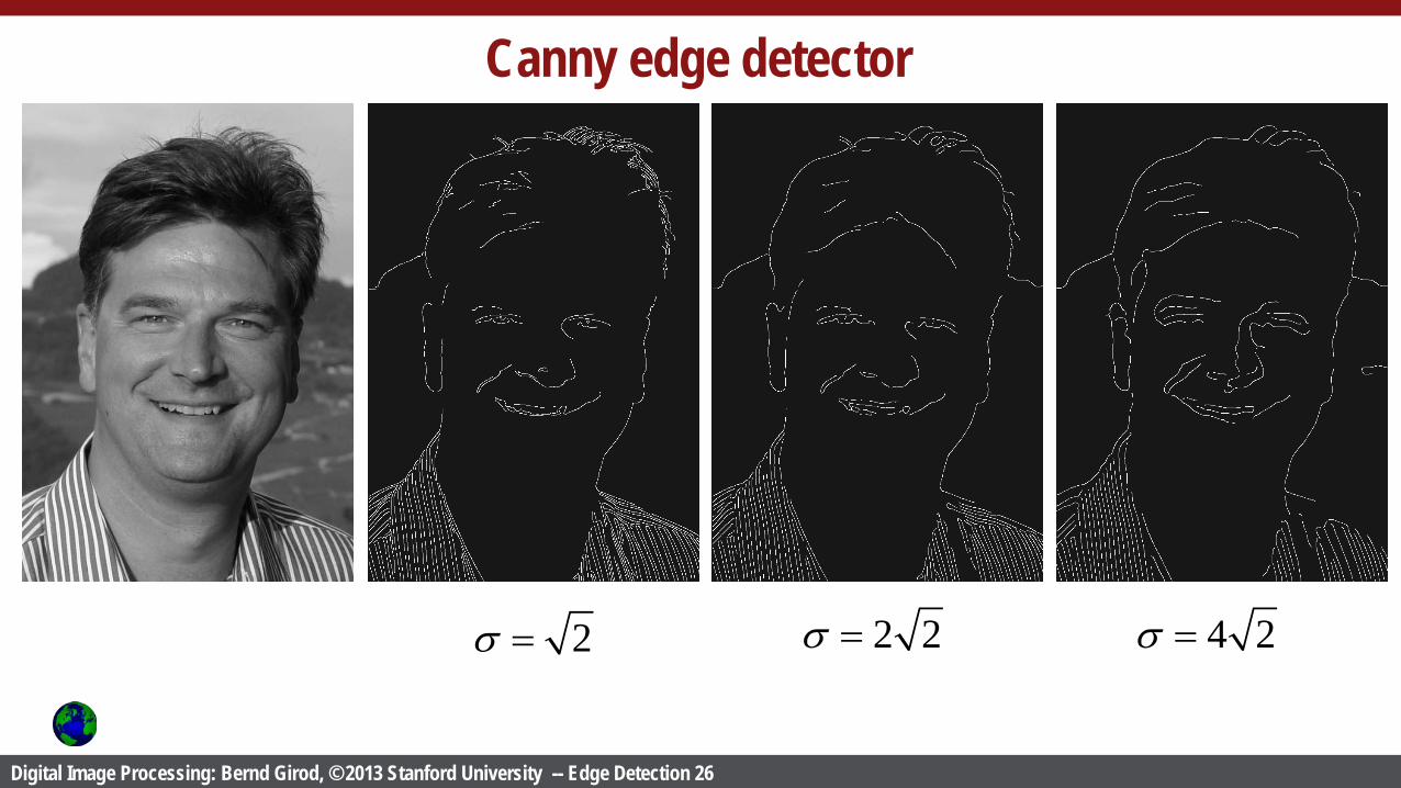
Canny edge detector

1. Smooth image with a Gaussian filter 2. Approximate gradient magnitude and angle (use Sobel, Prewitt . . .)

3. Apply nonmaxima suppression to gradient magnitude 4. Double thresholding to detect strong and weak edge pixels 5. Reject weak edge pixels not connected with strong edge pixels

[Canny, IEEE Trans. PAMI, 1986]

M x, y ≈

∂ f∂x

2

+∂ f∂y

2

α x, y ≈ tan−1 ∂ f

∂y∂ f∂x


Canny nonmaxima suppression

Quantize edge normal to one of four directions: horizontal, -45o, vertical, +45o

If M[x,y] is smaller than either of its neighbors in edge normal direction suppress; else keep.



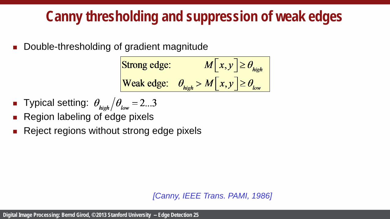
Canny thresholding and suppression of weak edges

Double-thresholding of gradient magnitude

Typical setting: Region labeling of edge pixels Reject regions without strong edge pixels



Canny edge detector

2σ = 2 2σ = 4 2σ =



Hough transform

Problem: fit a straight line (or curve) to a set of edge pixels Hough transform (1962): generalized template matching technique Consider detection of straight lines y = mx + c

x

y

m

c

edge pixel


Hough transform (cont.)

Subdivide (m,c) plane into discrete “bins,” initialize all bin counts by 0 Draw a line in the parameter space [m,c] for each edge pixel [x,y] and increment

bin counts along line. Detect peak(s) in [m,c] plane

x

y

m

c

detect peak


Hough transform (cont.)

Alternative parameterization avoids infinite-slope problem

Similar to Radon transform

π2 xcosθ + ysinθ = ρ

x

y

ρ

θedge pixel

ρ

π−

−π2 θ


Hough transform example

Original image

200 400 600 800

100

200

300

400

500

600

700

800




200 400 600 800

100

200

300

400

500

600

700

800

Original image




Paper (3264x2448)

Global thresholding

-50 0 50

-4000

-2000

0

2000

4000 0

500

1000

1500

θ

ρ

De-skewed Paper

-81.8 deg

-50 0 50

-4000

-2000

0

2000

4000 0

500

1000

1500

-81.8 deg



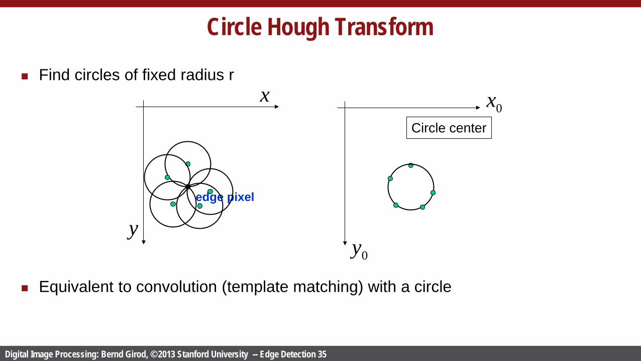
Circle Hough Transform

Find circles of fixed radius r

Equivalent to convolution (template matching) with a circle

x

y

0x

edge pixel

0y

Circle center


Circle Hough Transform for unknown radius

3-d Hough transform for parameters 2-d Hough transform aided by edge orientation “spokes” in parameter space

x

y

0x

edge pixel

0y

Circle center

x0 , y0 ,r( )


Example: circle detection by Hough transform

Original coins image

Prewitt edge detection Detected circles


edge detection - stanford...

Documents