edge detection - upcampilho/pdi/notes/edgedetection.pdf · image processing applications edge...
TRANSCRIPT

Image Processing Applications Edge Detection (by A.Campilho) 1
Edge Detection
Part 1• Introduction• Local Edge Operators
– Gradient of image intensity
– Robert, Sobel and Prewitt operators
– Second Derivative Operators
– Laplacian of Gaussian
Part 2• Marr-Hildreth Edge Detector
• Multiscale Processing
• Canny Edge Detector
• Edge Detection Performance
Outline
References:D. Huttenlocher, “Edge Detection” (http://www.cs.wisc.edu/~cs766-1/readings/edge-detection-huttenlocher.ps)R. Gonzalez, R. Woods, “Digital Image Processing”, Addison Wesley, 1993.D. Marr, E. Hildreth, “Theory of Edge detection”, Proc. R. Soc. Lond., B. 207, 187-217, 1980.

Image Processing Applications Edge Detection (by A.Campilho) 2
Initial considerationsEdges are significant local intensity changes in the image and are important features to analyse an image. They are important clues to separate regions within an object or to identify changes in illumination or colour. They are an important feature in the early vision stages in the human eye.There are many different geometric and optical physical properties in the scene that can originate an edge in an image.Geometric:• Object boundary: eg a discontinuity in depth and/or surface colour or texture• Surface boundary: eg a discontinuity in surface orientation and/or colour or texture• Occlusion boundary: eg a discontinuity in depth and/or surface colour or textureOptical:• Specularity: eg direct reflection of light, such as a polished metallic surface• Shadows: from other objects or part of the same object• Interreflections: from other objects or part sof the same object• Surface markings, texture or colour changes
Edge DetectionIntroduction
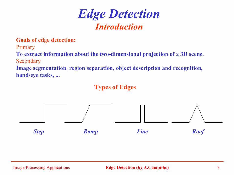
Image Processing Applications Edge Detection (by A.Campilho) 3
Edge DetectionIntroduction
Goals of edge detection:PrimaryTo extract information about the two-dimensional projection of a 3D scene.SecondaryImage segmentation, region separation, object description and recognition, hand/eye tasks, ...
Types of Edges
Step Ramp Line Roof

Image Processing Applications Edge Detection (by A.Campilho) 4
Edge DetectionIntroductionTypes of Edges
RoofRamp
Line
0
50
100
150
200
0 60 120 180 240
0
60
120
180
240
0 75 150 225 300
0
64
128
192
256
0 64 128 192 256
0
64
128
192
256
0 64 128 192 256

Image Processing Applications Edge Detection (by A.Campilho) 5
Edge DetectionIntroduction
DefinitionsEdge point : Point in an image with coordinates [i, j] at the location of a significant local intensity change in the image.Edge fragment : a small line segment about the size of a pixel, or as a point with an orientation attribute. The term edge is commonly used either for edge points or edge fragments. Edge detector : Algorithm that produces a set of edges (edge points or edge fragments) from an image. Some edge detectors can also produce a direction that is the predominant tangent direction of the arc that passes through the pixel.Contour: List of edges of the mathematical curve that models the list of edges.Edge linking: Process of form an ordered list of edges from an unordered list.Edge following: Process of searching the edge image (image with pixels labeled as edge) to determine contours.

Image Processing Applications Edge Detection (by A.Campilho) 6
Edge DetectionLocal Edge Operators
Edge detection is essential the operation of detecting intensity variations. 1st and 2nd derivative operators give the information of this intensity changes. For instance, the first derivative of a step edge has a maximum located of the position of the edge.
The gradient of the image intensity is the vector: [ ] tyx
t
GGyf
xff ,, =
∂∂
∂∂
=∇
x
yyx G
GGGG 122 tan−=+= θThe magnitude and direction of the gradient are:
Is common practice to approximate by absolute values: ||||max(|||| yxyx GGGorGGG +≈+≈
Numerical approximations:
],1[],[
],[]1,[
jifjifG
jifjifG
y
x
+−≈
−+≈
The corresponding convolution masks are:
−
≈−≈11
]11[ yx GG

Image Processing Applications Edge Detection (by A.Campilho) 7
Edge DetectionLocal Edge Operators
When computing an approximation to the gradient, it is important the both directional derivatives produce a result at the same location. The unidimensional approximations, produce a result at different position. For this reason, square kernels are preferred, as:
−−
≈
−−
≈1111
1111
yx GG Location of the estimate
Main steps for Edge detection
• Filtering: gradient operators are very sensitive to noise. It is important to improve the signal to noise ratio, by filtering previously the image. However, there is a trade-off between edge strength and noise reduction.• Enhancement: To emphasize pixels with a significant change in local intensity, using a gradient operator.• Detection: Label the edge points. Thresholding the gradient magnitude is a common technique.• Localization: The location of the edge can be estimated with subpixel resolution.

Image Processing Applications Edge Detection (by A.Campilho) 8
Edge DetectionLocal Edge Operators
−≈
−
≈0110
1001
yx GG
Roberts Operator
−−−≈
−−−
≈121000121
101202101
yx GG
Sobel Operator
−−−≈
−−−
≈111000111
101101101
yx GG
Prewitt Operator

Image Processing Applications Edge Detection (by A.Campilho) 9
Edge DetectionLocal Edge Operators
Sobel Operator
0
50
100
150
200
0 4 8 12 160
60
120
180
240
0 4 8 12 160
64
128
192
256
0 4 8 12 16
Detection
Input Edge Enhancement Detection
The result from the Sobel operator is thresholded to obtain the map of edge pixels. A simple threshold gives rise to discontinuities and several pixels wide. A better approach would be to find only the points with local maxima in gradient values.
But the local maxima of the gradient is the zero crossing in the second derivative.To find the zero crossing of the second derivative of image intensity is another approach for edge detection.

Image Processing Applications Edge Detection (by A.Campilho) 10
Laplacian operatorSmooth edge 1st derivative 2nd derivative
The Laplacian is the 2-D equivalent of the second derivative
Smooth edge Maximum of 1st derivative Zero-crossing of the 2nd derivative
2
2
2
22
yf
xff
∂∂
+∂∂
=∇
1D numerical approximations:
],[)]1,[2]2,[)],[]1,[()]1,[]2,[(
],[]1,[)],[]1,[(2
2
jifjifjifjifjifjifjif
jifx
jifx
jifjifx
Gxx
fx
++−+=−+−+−+=
=∂∂
−+∂∂
=−+∂∂
=∂∂
=∂∂
ji
j+1 j+2
ior j j+1j-1
]1,[)],[2]1,[2
2−+−+=
∂∂ jifjifjif
xf
010141010
2 −=∇2D numerical approximations:
i
j

Image Processing Applications Edge Detection (by A.Campilho) 11
Edge DetectionMarr and Hildreth Edge Detector
The derivative operators presented so far are not very useful because they are very sensitive to noise. To filter the noise before enhancement, Marr and Hildreth proposed a Gaussian Filter, combined with the Laplacian for edge detection. Is is the Laplacian of Gaussian (LoG). The fundamental characteristics of LoG edge detector are:
• The smooth filter is Gaussian, in order to remove high frequency noise.• The enhancement step is the Laplacian.• The detection criteria is the presence of the zero crossing in the 2nd derivative, combined with a corresponding large peak in the 1st derivative. Here, only the zero crossings whose corresponding 1st derivative is above a specified threshold are considered.• The edge location can be estimated using sub-pixel resolution by interpolation.

Image Processing Applications Edge Detection (by A.Campilho) 12
Edge DetectionMarr and Hildreth Edge Detector
The different phases of the LoG filter (or the Mexican hat operator) is illustrated below. The final result can be obtained either by first convolving with the Gaussian filter, and compute the Laplacian, or convolve directly with Laplacian of the Gaussian filter (kernels in the next slide). The LoG filter can be approximated by a difference of two Gaussians (DoG).
Gaussian Filter
1st Derivative
2nd Derivative
Edge Input Output
LoG FilterMexican hat operator
2
22
2)(
4
2222
22
2),(
)],((*),([)],((*),([),(
σ
σσ
yx
eyxyxg
yxfyxgyxfyxgyxh+
−
−+=∇
∇=∇=

Image Processing Applications Edge Detection (by A.Campilho) 13
Edge DetectionScale space
0 0 0 0 0 0 -1 -1 -1 -1 -1 0 0 0 0 00 0 0 0 -1 -1 -1 -1 -1 -1 -1 -1 -1 0 0 00 0 -1 -1 -1 -2 -3 -3 -3 -3 -3 -2 -1 -1 -1 00 0 -1 -1 -2 -3 -3 -3 -3 -3 -3 -3 -2 -1 -1 00 -1 -1 -2 -3 -3 -3 -2 -3 -2 -3 -3 -3 -2 -1 -10 -1 -2 -3 -3 -3 0 2 4 2 0 -3 -3 -3 -2 -1-1 -1 -3 -3 -3 0 4 10 12 10 4 0 -3 -3 -3 -1-1 -1 -3 -3 -2 2 10 18 21 18 10 2 -2 -3 -3 -1-1 -1 -3 -3 -3 4 12 21 24 21 12 4 -3 -3 -3 -1-1 -1 -3 -3 -2 2 10 18 21 18 10 2 -2 -3 -3 -1-1 -1 -3 -3 -3 0 4 10 12 10 4 0 -3 -3 -3 -10 -1 -2 -3 -3 -3 0 2 4 2 0 -3 -3 -3 -2 -10 -1 -1 -2 -3 -3 -3 -2 -3 -2 -3 -3 -3 -2 -1 -10 -1 -1 -2 -3 -3 -3 -2 -3 -2 -3 -3 -3 -2 -1 -10 0 -1 -1 -1 -2 -3 -3 -3 -3 -3 -2 -1 -1 -1 00 0 0 0 -1 -1 -1 -1 -1 -1 -1 -1 -1 0 0 0
0 0 -1 0 00 -1 -2 -1 0-1 -2 16 -2 -10 -1 -2 -1 00 0 -1 0 0
5 x 5 LoG filter
17 x 17 LoG filter
Scale (σ)

Image Processing Applications Edge Detection (by A.Campilho) 14
Edge DetectionScale Space
Original Image
Zero CrossingsLoG Filter Scale (σ)

Image Processing Applications Edge Detection (by A.Campilho) 15
Edge DetectionScale Space
The Gaussian filter removes noise but at the same time smooths the edges and other sharp intensity discontinuities within the images. The amount of blurring depends on the standard deviation. A larger σ corresponds to better noise filtering but the edge blurring increases. As a consequence, there is a trade-off between noise removal (better for larger σ, eg large kernels), and edge enhancement (better for smaller σ, eg small kernels). On the other hand, small filters result in too many noise points and large filters tend to dislocate the edges.
One approach, followed by Marr and Hildreth is to analyse the behavior of edges at different scales of filtering. To combine the information from different scales, the authors assume spatial coincidence:
“If a zero-crossing segment is present in a set of independent ∇2G channels (scales) over a continuous range of sizes and the segment has the same position and orientation in each channel, then the set of such zero crossing segments may be taken to indicate the presence of an intensity change in the image that is due to single physical phenomenon (a change in reflectance, illumination, dept or surface orientation”.
Other authors stated other assumptions
•Zero crossings connected at adjacent scales correspond to the same event, eg no new zeo crossing are introduced as σ increases.• The location of a zero crossing in the Gaussian filtered image tends to its true location as σ → 0.

Image Processing Applications Edge Detection (by A.Campilho) 16
Edge DetectionCanny Edge Detector
Convolution
Non-MaximumSupression
Thresholding
f(i,j)
m(i,j)
n(i,j)t(i,j)
∂∂
∂∂
=
∂∂
+
∂∂
=
∂∂
∂∂
=∇
xf
yf
ji
yf
xfjim
yf
xff
s
s
ss
tss
s
arctan),(
),(
,
22
θ
),(),,(),( jifjiGjif s ∗= σ
GaussianFilter
Gradientf(i,j)
Convolutionm(i,j)
θ(i,j)
fs(i,j)
θ(i,j)
The non-maximum suppression thins the ridges of gradient magnitude m(i,j) by suppressing all values along the line of the gradient that are not peak values of ridge.
The image is gaussian filtered followed by gradient and orientation computation
The n(i,j) is finally thresholded in order to reduce the number of false edge segments.
Smoothing Enhancement Detection

Image Processing Applications Edge Detection (by A.Campilho) 17
Edge DetectionCanny Edge Detector. Gaussian Filtering
f(i,j)
Convolutionm(i,j)
θ(i,j)
fs(i,j)Gaussian
FilterGradient
σ = 1 σ = 2 σ = 3
[ ] [ ]( )
∗=∗∗=∗=
n
nvhs
a
aa
jifaaajGjifiGjifjiGjifM
L 2
1
21 *),(),(),(),(),(),,(),( σσσ
Kernels (h1) [ 4 60 272 450 27 2 60 4 ] [ 4 19 60 146 272 397 450
397 272 146 60 19 4 ][ 1 4 12 29 60 112 185 272 360 425 450
425 360 272 185 112 60 29 12 4 1 ]

Image Processing Applications Edge Detection (by A.Campilho) 18
Canny Edge DetectionGradient , non-maximum supression and thesholding
∂∂
∂∂
=
∂∂
+
∂∂
=
xf
yf
jiyf
xfjim
s
s
ss arctan),(),(22
θStep 1: magnitude and orientation computation
Step 2: Partition of angle orientations
00
1
1
2
23
3)),((sec),( jitorji θϑ =
Step 3: At each pixel DO:
n(i,j) = m(i,j);
IF m(i,j) ≤ the neighbors along the gradient sector
THEN n(i,j)=0;
Step 4: Double Thresholding:
Create two thresholded images t1(i,j) and t2(i,j), using two thresholds T1 and T2, with T1 ≈ 0,4 T2.
This double threshold method allow to add weaker edges (those above T1) if they are neighbors of stronger edges (those above T2). So the threshold image is formed by t2(i,j) including some of the edges in t1(i,j)
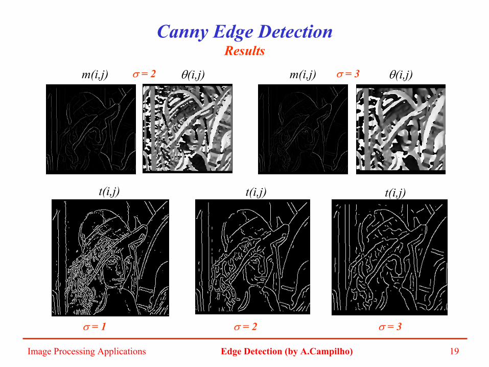
Image Processing Applications Edge Detection (by A.Campilho) 19
Canny Edge DetectionResults
σ = 1 σ = 2 σ = 3
σ = 2 σ = 3m(i,j) θ(i,j) m(i,j) θ(i,j)
t(i,j) t(i,j) t(i,j)

Image Processing Applications Edge Detection (by A.Campilho) 20
Edge Detector Performance
Criteria for evaluating the performance of edge detectors:• Probability of false edges• Probability of missing edges• Error in estimation of the edge angle• Mean square distance of the edge estimate from the true edge• Tolerance to distorted edges and other features such as cornersand junctions.
Figure of merit (W. Pratt)
∑= +
=AI
i iA dIIFM
12
1 11
),max(1
αIA - Image with the detected edgesI1 - Image with the ideal edgesd - distance between the actual and the ideal edgesa - design constant to penalize displaced edges.
For evaluating the performance we may generate images with knownedge locations and then use FM. It is a common practice to evaluate the performance for synthetic images by introducing noise, and plot FM against the signal to noise ratio, to evaluate the degradation in the performance.