EDGE-FRIENDLY DISTRIBUTED PCA

By

BINGQING XIANG

A thesis submitted to the

School of Graduate Studies

Rutgers, The State University of New Jersey

In partial fulfillment of the requirements

For the degree of

Master of Science

Graduate Program in Electrical and Computer Engineering

Written under the direction of

Waheed U. Bajwa

And approved by

New Brunswick, New Jersey

May, 2020

c© 2020

Bingqing Xiang

ALL RIGHTS RESERVED

ABSTRACT OF THE THESIS

Edge-Friendly Distributed PCA

By Bingqing Xiang

Thesis Director: Waheed U. Bajwa

Big, distributed data create a bottleneck for storage and computation in machine learn-

ing. Principal Component Analysis (PCA) is a dimensionality reduction tool to resolve

the issue. This thesis considers how to estimate the principal subspace in a loosely

connected network for data in a distributed setting. The goal for PCA is to extract the

essential structure of the dataset. The traditional PCA requires a data center to ag-

gregate all data samples and proceed with calculation. However, in real-world settings,

where memory, storage, and communication constraints are an issue, it is sometimes

impossible to gather all the data in one place. The intuitive approach is to compute the

PCA in a decentralized manner. The focus of this thesis is to find a lower-dimensional

representation of the distributed data with the well-known orthogonal iteration algo-

rithm. The proposed distributed PCA algorithm estimates the subspace representation

from sample covariance matrices in a decentralized network while preserving the privacy

of the local data.

ii

Acknowledgements

First, I would like to thank my advisor Waheed U. Bajwa, who offered me important

guidance throughout my thesis. He introduced a lot of great ideas and scientific tools

that would take me years to figure out myself. Without his persistence support and

help, the idea of this project and experiments would not flesh out.

I also wish to show my gratitude to Arpita Gang, Zhixiong Yang, Haroon Raja,

Batoul Taki, Rishshabh Dixit, and Asad Lodhi. I am lucky to be a member of this

lovely lab. Everyone has a profound belief in my work, encourages me, and helps me

while I face bottlenecks conducting this study.

I would like to pay my regards to members of my thesis committee: Professor Bo

Yuan and Professor Yuqian Zhang, for offering their time and guidance while reading

this thesis and attending my thesis defense.

iii

Table of Contents

Abstract . . . . . . . . . . . . . . . . . . . . . . . . . . . . . . . . . . . . . . . . ii

Acknowledgements . . . . . . . . . . . . . . . . . . . . . . . . . . . . . . . . . iii

List of Tables . . . . . . . . . . . . . . . . . . . . . . . . . . . . . . . . . . . . . vi

List of Figures . . . . . . . . . . . . . . . . . . . . . . . . . . . . . . . . . . . . vii

1. Introduction . . . . . . . . . . . . . . . . . . . . . . . . . . . . . . . . . . . 1

1.1. Our Contributions . . . . . . . . . . . . . . . . . . . . . . . . . . . . . . 2

1.2. Relationship to Previous Work . . . . . . . . . . . . . . . . . . . . . . . 3

1.3. Thesis Structure . . . . . . . . . . . . . . . . . . . . . . . . . . . . . . . 4

2. Problem Formulation and Algorithms . . . . . . . . . . . . . . . . . . . 5

2.1. Centralized Orthogonal Iteration . . . . . . . . . . . . . . . . . . . . . . 5

2.2. Decentralized PCA . . . . . . . . . . . . . . . . . . . . . . . . . . . . . . 6

2.2.1. The Types of Data Partitions . . . . . . . . . . . . . . . . . . . . 6

2.2.2. Averaging Consensus Algorithm . . . . . . . . . . . . . . . . . . 7

2.2.3. Column-wise Distributed Orthogonal Iteration . . . . . . . . . . 8

2.2.4. Convergence Analysis for C-DOT and CA-DOT . . . . . . . . . 10

2.2.5. Row-wise Distributed Orthogonal Iteration . . . . . . . . . . . . 22

2.2.6. Row-wise Distributed QR decomposition . . . . . . . . . . . . . . 23

3. Experimental Results . . . . . . . . . . . . . . . . . . . . . . . . . . . . . . 25

3.1. Tools and Platform for Numerical Experiments . . . . . . . . . . . . . . 25

3.1.1. Programming Language . . . . . . . . . . . . . . . . . . . . . . . 26

3.1.2. Datasets . . . . . . . . . . . . . . . . . . . . . . . . . . . . . . . . 26

iv

3.1.3. Computing Platform . . . . . . . . . . . . . . . . . . . . . . . . . 27

3.2. Experiments Using Synthetic Data . . . . . . . . . . . . . . . . . . . . . 27

3.3. Experiments Using Real-World Data . . . . . . . . . . . . . . . . . . . . 34

4. Conclusion and Future Work . . . . . . . . . . . . . . . . . . . . . . . . . 40

References . . . . . . . . . . . . . . . . . . . . . . . . . . . . . . . . . . . . . . . 41

v

List of Tables

3.1. Synthetic Experiment 1: Parameters for C-DOT algorithm . . . . . . . 28

3.2. Synthetic Experiment 2: Parameters for CA-DOT with different eigengaps 30

3.3. Synthetic Experiment 3: Parameters for CA-DOT with different p for

Erdos–Renyi topology . . . . . . . . . . . . . . . . . . . . . . . . . . . . 31

3.4. Synthetic Experiment 4: Parameters for ring topology . . . . . . . . . . 32

3.5. Synthetic Experiment 5: Parameters for star topology . . . . . . . . . . 32

3.6. Synthetic Experiment 6: Parameters for CA-DOT with different values

of r. . . . . . . . . . . . . . . . . . . . . . . . . . . . . . . . . . . . . . . 33

3.7. Synthetic Experiment 7: Straggler effect with Erdos–Renyi graphs . . . 33

3.8. Parameters for MNIST experiments . . . . . . . . . . . . . . . . . . . . 36

3.9. Parameters for CIFAR-10 experiments . . . . . . . . . . . . . . . . . . . 37

3.10. Parameters for LFW experiments . . . . . . . . . . . . . . . . . . . . . . 37

3.11. Parameters for ImageNet experiments . . . . . . . . . . . . . . . . . . . 38

vi

List of Figures

1.1. Various network graph topologies considered in this thesis. . . . . . . . . 2

2.1. Types of data partitions considered in this thesis. . . . . . . . . . . . . . 7

3.1. Representative images from MNIST. . . . . . . . . . . . . . . . . . . . . 26

3.2. Representative images from CIFAR-10. . . . . . . . . . . . . . . . . . . . 26

3.3. Representative images from LFW. . . . . . . . . . . . . . . . . . . . . . 27

3.4. Representative images from ImageNet. . . . . . . . . . . . . . . . . . . . 27

3.5. Results for C-DOT corresponding to the parameters in Table 3.1. . . . . 29

3.6. Results for CA-DOT with different eigengaps. . . . . . . . . . . . . . . . 30

3.7. Erdos–Renyi topologies with different p. . . . . . . . . . . . . . . . . . . 31

3.8. Results for CA-DOT with different p for Erdos–Renyi graphs. . . . . . . 31

3.9. Results of CA-DOT for ring and star topologies. . . . . . . . . . . . . . 32

3.10. Results of CA-DOT with different values of r. . . . . . . . . . . . . . . . 34

3.11. Results for RDOT algorithm with synthetic data. . . . . . . . . . . . . . 35

3.12. Results for CA-DOT algorithm with MNIST dataset corresponding to

parameters in Table 3.8. . . . . . . . . . . . . . . . . . . . . . . . . . . . 36

3.13. Results for CA-DOT algorithm with CIFAR-10 dataset corresponding to

parameters in Table 3.9. . . . . . . . . . . . . . . . . . . . . . . . . . . . 37

3.14. Results for CA-DOT algorithm with LFW dataset corresponding to pa-

rameters in Table 3.10. . . . . . . . . . . . . . . . . . . . . . . . . . . . . 38

3.15. Results for CA-DOT algorithm with ImageNet dataset corresponding to

parameters in Table 3.11. . . . . . . . . . . . . . . . . . . . . . . . . . . 39

vii

1

Chapter 1

Introduction

Modern data tend to be big and distributed. As the volume of data enlarges, it is

hard to fit extensive data on a single machine. The intuitive solution is to distribute

data among a connected network with multiple processors. Distributed systems and

distributed computing [1] are already widely used in our daily life; for example, online

banking, search engine, and online gaming. In this thesis we develop a distributed

dimensionality reduction [2] algorithm to extract low-dimensional and useful informa-

tion from high-dimensional and distributed data. The Principal Component Analysis

(PCA) [3] calculates the low-dimensional subspace of a high-dimensional dataset. The

predominant application of PCA is dimensionality reduction, which filters out the hid-

den noise and redundant information in the observed data. PCA is considered an

unsupervised learning machine learning technique. In the learning (training) process,

computers need to learn without labels and target values. In a machine learning pipeline

for supervised learning, PCA algorithms often appear in the preprocessing stage to re-

duce the dimensions of the training data.

The goal in this thesis is to compute PCA for data distributed among a connected

network. This thesis considers two cases for the data distribution: column-wise parti-

tion and row-wise partition. Column-wise separated data indicate that each site stores

some samples with all attributes. In contrast, for the row-wise partition, each site con-

tains a portion of attributes for all data points. The proposed algorithm, Column-wise

Distributed Orthogonal Iteration (C-DOT) algorithm, calculates the PCA for column-

wise distributed data in a decentralized manner. The distributed solution bypasses the

scalability problem of a single machine. Another benefit of decentralized computing is

2

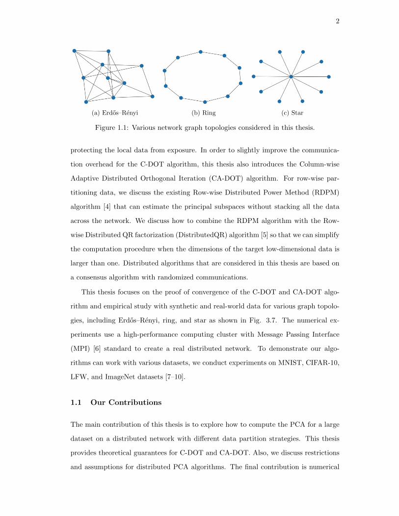
(a) Erdos–Renyi (b) Ring (c) Star

Figure 1.1: Various network graph topologies considered in this thesis.

protecting the local data from exposure. In order to slightly improve the communica-

tion overhead for the C-DOT algorithm, this thesis also introduces the Column-wise

Adaptive Distributed Orthogonal Iteration (CA-DOT) algorithm. For row-wise par-

titioning data, we discuss the existing Row-wise Distributed Power Method (RDPM)

algorithm [4] that can estimate the principal subspaces without stacking all the data

across the network. We discuss how to combine the RDPM algorithm with the Row-

wise Distributed QR factorization (DistributedQR) algorithm [5] so that we can simplify

the computation procedure when the dimensions of the target low-dimensional data is

larger than one. Distributed algorithms that are considered in this thesis are based on

a consensus algorithm with randomized communications.

This thesis focuses on the proof of convergence of the C-DOT and CA-DOT algo-

rithm and empirical study with synthetic and real-world data for various graph topolo-

gies, including Erdos–Renyi, ring, and star as shown in Fig. 3.7. The numerical ex-

periments use a high-performance computing cluster with Message Passing Interface

(MPI) [6] standard to create a real distributed network. To demonstrate our algo-

rithms can work with various datasets, we conduct experiments on MNIST, CIFAR-10,

LFW, and ImageNet datasets [7–10].

1.1 Our Contributions

The main contribution of this thesis is to explore how to compute the PCA for a large

dataset on a distributed network with different data partition strategies. This thesis

provides theoretical guarantees for C-DOT and CA-DOT. Also, we discuss restrictions

and assumptions for distributed PCA algorithms. The final contribution is numerical

3

experiments on both synthetic and real-world data using MPI protocol with a high-

performance computer cluster to form a real distributed network. Furthermore, we

run tests on different datasets with a different number of dimensions, the number of

samples, the chosen rank r, eigengaps, and a variety of graph topologies, including

Erdos–Renyi, ring, and star. Within those experiments, we observe the hidden rela-

tionship between the parameters and the performance of the algorithms. We plot the

error curves corresponding to the number of communications rounds to inspect the

trade-off between communication cost and accuracy. We conclude that the runtime

of experiments has a positive association with the size of the underlying network, the

number of communications rounds, and the connection densities of the network.

1.2 Relationship to Previous Work

The Orthogonal Iteration (OI) [11] is one of the foundations for decentralized orthog-

onal iteration algorithms, which provides a centralized algorithm to learn the lower-

dimensional subspaces from high-dimensional data. Column-wise distributed power

method (CDPM) [12] is a particular case for column-wise distributed orthogonal itera-

tion since CDPM estimates the eigenvector corresponding to the maximum eigenvalue

for the covariance matrix of the high-dimensional data. This thesis expands the idea of

CDPM to find the top-r dimensional subspaces by introducing C-DOT and CA-DOT. A

similar situation applies for the RDPM, which is well developed in [4]. RDPM provides

the method to compute r-th eigenvector by repeating RDPM for r times. To avoid the

repetition over RDPM, we combine the RDPM with the orthogonal iteration algorithm

by applying a Distributed QR factorization (DistributedQR) algorithm [5] to achieve

the orthonormalization task after each iteration of RDPM. Decentralized Orthogonal

Iteration (DecentralizedOI) [13] is explicitly targeting to estimate the r principal eigen-

vectors for the row-separated symmetric weight adjacency matrix of the underlying

network graph. The key to all the distributed algorithms above is a distributed consen-

sus algorithm. Averaging Consensus (AC) [14] allows each site to synchronize a sum

or average of some locally calculated values by sending and receiving values from its

neighbors in an edge system.

4

1.3 Thesis Structure

Chapter 1 describes the motivations, applications, and objectives for this thesis and

introduces the contributions and related work. Chapter 2 describes the orthogonal iter-

ation algorithms for centralized and decentralized networks. This chapter also provides

the algorithmic formulation for different data partitions. Furthermore, this chapter

offers a convergence analysis of C-DOT and CA-DOT algorithms. Chapter 3 acknowl-

edges the programming language, hardware, tools, and datasets applied for the numeri-

cal experiments, and presents the experiments and simulations results for the algorithms

purposed in Chapter 2. Chapter 4 draws some conclusions and discusses future work.

5

Chapter 2

Problem Formulation and Algorithms

The goal of this thesis is to develop a distributed PCA algorithm to reduce the feature

dimension of the matrix A ∈ Rd×n to r, where r is a chosen integer and 1 ≤ r ≤ d. The

row dimensions of A represents the feature dimension, and the column dimensions of A

serves as the sample dimension. The covariance matrix of A is defined as M = E[(A−

E[A])(A − E[A])T ]. We assume matrix A is zero mean, which means the expectation

value E[A] = 0, where 0 ∈ Rd×r denotes a matrix of all zeros. For a zero-mean matrix

A, the covariance matrix M = E[AAT ], and the sample covariance M = 1nAA

T . The

objective function of centralized PCA can be formulated as

Q = argminQc∈Rd×r:QT

c Qc=I

f(Qc) :=∥∥(I −QcQTc )M

∥∥2F

(2.1)

where Qc ∈ Rd×r, and I indicates the identity matrix. This problem can be solved by

applying the famous orthogonal iteration algorithm [11].

2.1 Centralized Orthogonal Iteration

Centralized Orthogonal Iteration (OI) [11] is an iterative method used to compute

the normalized low-dimensional subspace from high-dimensional data with a random

initialization. The sample covariance matrix of the zero-mean matrix A ∈ Rd×n is a

symmetric d × d matrix M = AAT with eigenvalues |λ1| ≥ . . . |λr| > |λr+1| ≥ . . . |λd|,

where r is a chosen integer and 1 ≤ r ≤ d. The output of OI is Qc ∈ Rd×r. Suppose Q

is the top-r eigenvectors of symmetric matrix M . When r = 1, the orthogonal iteration

is equivalent to the power method [11], computing the dominant eigenvector of M .

One of the solutions to distributed orthogonal iterations is to gather all the data in

one place and solve the problem using the centralized orthogonal iteration algorithm.

6

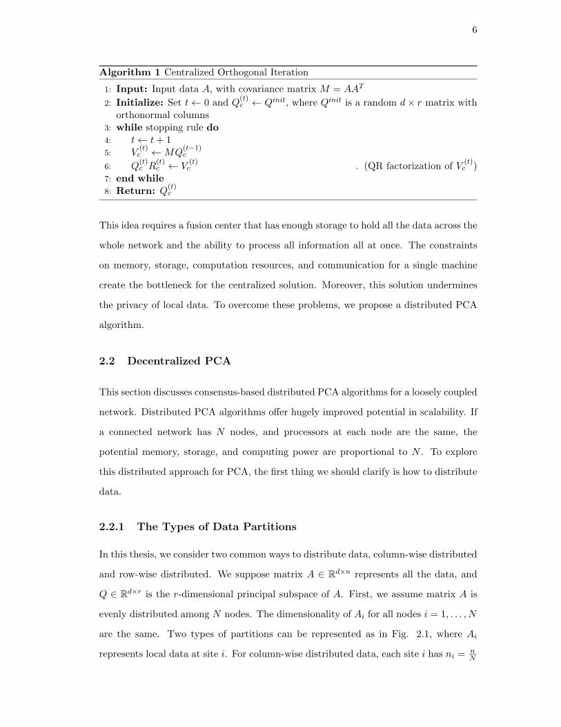
Algorithm 1 Centralized Orthogonal Iteration

1: Input: Input data A, with covariance matrix M = AAT

2: Initialize: Set t← 0 and Q(t)c ← Qinit, where Qinit is a random d× r matrix with

orthonormal columns3: while stopping rule do4: t← t+ 15: V

(t)c ←MQ

(t−1)c

6: Q(t)c R

(t)c ← V

(t)c . (QR factorization of V

(t)c )

7: end while8: Return: Q

(t)c

This idea requires a fusion center that has enough storage to hold all the data across the

whole network and the ability to process all information all at once. The constraints

on memory, storage, computation resources, and communication for a single machine

create the bottleneck for the centralized solution. Moreover, this solution undermines

the privacy of local data. To overcome these problems, we propose a distributed PCA

algorithm.

2.2 Decentralized PCA

This section discusses consensus-based distributed PCA algorithms for a loosely coupled

network. Distributed PCA algorithms offer hugely improved potential in scalability. If

a connected network has N nodes, and processors at each node are the same, the

potential memory, storage, and computing power are proportional to N . To explore

this distributed approach for PCA, the first thing we should clarify is how to distribute

data.

2.2.1 The Types of Data Partitions

In this thesis, we consider two common ways to distribute data, column-wise distributed

and row-wise distributed. We suppose matrix A ∈ Rd×n represents all the data, and

Q ∈ Rd×r is the r-dimensional principal subspace of A. First, we assume matrix A is

evenly distributed among N nodes. The dimensionality of Ai for all nodes i = 1, . . . , N

are the same. Two types of partitions can be represented as in Fig. 2.1, where Ai

represents local data at site i. For column-wise distributed data, each site i has ni = nN

7

observations of d dimensional zero-mean random vectors as shown in Fig. 2.1a, where

Ai ∈ Rd×ni . The objective function of column-wise distributed PCA can be formulated

as

Q = argminQcol,Qcol,iNi=1∈Rd×r

N∑i=1

[fi(Qcol,i) :=

∥∥(I −Qcol,iQTcol,i)Mi

∥∥2F

](2.2)

subject to Qcol = Qcol,1 . . . = Qcol,N , QTcolQcol = QTcol,iQcol,i = I.

Row-wise distributed data often works with sensor networks. Each node i collects

di = dN dimensional measurements for n observations, and Ai ∈ Rdi×n. The goal of

row-wise distributed PCA is to find the r-dimensional subspace Qrow,i corresponding

for each sensor i. The objective function of row-wise distributed PCA can be formulated

as

Q = argminQrow,Qrow,iNi=1∈Rdi×r

N∑i=1

[fi(Qrow,i) :=

∥∥(I −Qrow,iQTrow,i)Mi

∥∥2F

](2.3)

subject to Qrow = [Qrow,1, . . . , Qrow,N ]T , QTrowQrow = I.

(a) Column-wise Distributed Data (b) Row-wise Distributed Data

Figure 2.1: Types of data partitions considered in this thesis.

2.2.2 Averaging Consensus Algorithm

A critical component of distributed PCA is the Averaging Consensus (AC) algorithm.

Our representation of a distributed network is an undirected graph G = (N ; E) con-

sisting of a set of nodes N = 1, 2, . . . , N and a set of edges E . For each edge in G,

(i, j) ∈ E . For each node i, we record its neighbors in sets of nodes Ni = j|(i, j) ∈ E.

The weight matrix W , a doubly-stochastic matrix, corresponds to the graph topology

G = (N ; E). Rows and columns ofW sum to 1, which means∑

iwi,j =∑

j wi,j = 1. The

8

design of the weight matrix W in this thesis corresponds to the local-degree weights [14]

from the Metropolis–Hastings algorithm [15]. The mixing time of a Markov chain as-

sociated with W is τmix.

Each node holds an initial value Z(0)i and the goal of AC is to calculate 1

N

∑Ni=1 Z

(0)i

with finite number of iterations. At iteration tc, node i calculates Z(tc)i through ex-

changing value with its neighbors. If we apply AC for tc iterations as tc → ∞, the

result converges to 1N

∑Ni=1 Z

(0)i .

Algorithm 2 Averaging Consensus Algorithm

1: Input: Matrix Z(0)i at node i, where i ∈ 1, . . . , N and weight matrix W

2: Initialize Consensus: Set tc ← 03: while stopping rule do

4: t(t)c ← t

(t)c + 1

5: Z(tc)i ←

∑j∈Ni

wi,jZ(tc−1)j

6: end while7: Return: Z

(tc)i

2.2.3 Column-wise Distributed Orthogonal Iteration

The fundamental idea of the C-DOT is based on centralized orthogonal iteration [11].

A distributed connected network with N sites contain heterogeneous data. At each

site i the covariance matrix of the local data is a symmetric d× d matrix Mi = AiATi .

Eigenvalues of covariance matrix M =∑N

i=1Mi satisfy |λ1| ≥ . . . |λr| > |λr+1| ≥ . . . ≥

|λd|. We consider r as a chosen integer satisfying 1 ≤ r ≤ d, denoting the dimension of

the principal subspace Q, where Q is a subspace consisting of the top-r eigenvectors of

symmetric matrix M .

The goal of C-DOT is to compute Q without exchanging raw data between inter-

connected sites. We define Qtcol,i as the estimation of Q from t iterations of C-DOT at

site i. The initial estimations of Q at all sites are Q(0)col,i = Qinit, where Qinit ∈ Rd×r

with orthonormal columns. Each node executes t distributed orthogonal iterations. For

every iteration, each site computes MiQt−1col,i, where Qt−1col,i refer to the estimation of Q

after t− 1 distributed orthogonal iterations at node i. Then, we apply tc iterations of

consensus averaging [14] to approximate 1N

∑Ni=1MiQ

t−1col,i. The result from AC at each

9

site is V tcol,i. At the end, each site i has an updated estimation of Q. We obtain Qtcol,i

from applying the QR decomposition (QR) to V tcol,i, where Qtcol,i, R

tcol,i = QR(V t

col,i).

For AC in every C-DOT iteration, we initialize Z(0)i = MiQ

t−1col,i at node i, where

i ∈ 1, . . . N. At iteration tc, each node i receives messages from node j and when

(i, j) ∈ E , the message from node j is multiplied with the corresponding weight wi,j .

At tthc iteration of AC, we have Z(tc)i =

∑j∈Ni

wi,jZ(tc−1)j . This can also be expressed

as Z(tc)i =

∑j∈Ni

wtci,jZ(0)j , where wtci,j is the i, j entry of the matrix W tc , which is

the result of the weight matrix W multiplied with itself for tc times. As tc → ∞,

Z(∞)i = 1

N

∑Nj=1MjQ

t−1col,j . In practice tc cannot be ∞. Therefore, we assume for

each column-wise distributed orthogonal iteration, we apply a total of Tc number of

AC, and fix Tc as a constant number. When we apply To iterations of C-DOT, we have

V tcol,i =

Z(Tc)i

[WTce1]i=∑N

i=jMjQt−1col,j+E tc,i, where E tc,i is the consensus error at tth iteration.

Algorithm 3 Column-wise Distributed Orthogonal Iteration

1: Input: Matrix Ai at node i, where i ∈ 1, . . . , N with covariance matrix Mi, andthe weight matrix W corresponds to an undirected connected graph G

2: Initialize: Set t ← 0 and Qtcol,i ← Qinit, i = 1, 2, . . . , N , where Qinit is a randomd× r matrix, with orthonormal columns

3: while stopping rule do4: t← t+ 15: Initialize Consensus: Set tc ← 0, Z

(tc)i ←MiQ

t−1col,i, i = 1, 2, . . . , N

6: while stopping rule do7: tc ← tc + 18: Z

(tc)i ←

∑j∈Ni

wi,jZ(tc−1)j

9: end while

10: V tcol,i ←

Z(tc)i

[W tce1]i

11: Qtcol,iRtcol,i ← QR factorization(V

(t)col,i)

12: end while13: Return: Qtcol,i

There are two loops in the C-DOT algorithm. The outer loop is the orthogonal itera-

tion, and the inner loop is the averaging consensus. The OI algorithm converges to Q at

an exponential rate. Therefore, the tolerance of the error within a consensus averaging

procedure after t iterations is lower than after t − 1 iteration. To improve the con-

vergence speed, and reduce the number of AC iterations, we propose the Column-wise

Adaptive Distributed Orthogonal Iteration (CA-DOT) algorithm, which is an adaptive

10

version of C-DOT. For CA-DOT, we define Tc = [Tc,1, Tc,2, . . . , Tc,To ], where Tc is a

sequence of number. At tth iteration of CA-DOT, we employ Tc,t averaging consensus

at each site. The algorithm flow for C-DOT and CA-DOT are congruent.

2.2.4 Convergence Analysis for C-DOT and CA-DOT

We focus on the convergence behavior of C-DOT and CA-DOT algorithms in this

section. There are two procedures introducing error into Algorithm 3: orthogonal

iteration and averaging consensus. To summarize the convergence behavior of C-DOT

and CA-DOT, Theorem 1 and Theorem 2 are provided below.

Theorem 1. Suppose M is a symmetric matrix, where M =∑N

i=1Mi. Let Mi be

the covariance matrix for zero-mean local data Ai, and define α :=∑N

i=1‖Mi‖2 and

γ :=√∑N

i=1‖Mi‖22. Eigenvalues of M are λ1, λ2, . . . , λd such that |λ1| ≥ . . . ≥ |λr| >

|λr+1| ≥ . . . |λd|. The r-dimensional principal subspace of M is represented by Q.

Consider PQ as the projection of M onto Q, and PQ′ denote the projection of M onto the

space spanned by the subspace computed after To iterations of Column-wise Decentralized

Orthogonal Iteration (C-DOT). Assume OI and C-DOT are all initialized to Q(0)c =

Q(0)col,i = Qinit,where Qinit is a random d × r matrix, with orthonormal columns. From

centralized orthogonal iteration, define K(to)c := V

(to)T

c V(to)c = R

(to)T

c R(to)c , where R

(to)c is

the Cholesky decomposition of K(to)c , and V

(to)c = MQ

(to)c . Let β = max

to=1...To

∥∥∥R−1(to)c

∥∥∥2.

The weight matrix W corresponds to the underlying graph topology G, and τmix denotes

the mixing time of a Markov chain associated with the weight matrix W . If θ ∈ [0, π/2],

the initialization of Qinit satisfies

cos (θ) = minu∈Q,v∈Qinit

∣∣uT v∣∣‖u‖2‖v‖2

> 0. (2.4)

Each C-DOT iteration runs for a fixed number of consensus iterations Tc. As long

as Tc = Ω(Toτmix log (3

√rαβ) + Toτmix log (ε−1) + τmix log

(γ√Nrα

)), where ε ∈ (0, 1),

we have that

∀i,∥∥QQT −Qcol,iQTcol,i∥∥2 ≤ c

∣∣∣∣λr+1

λr

∣∣∣∣To + 3εTo (2.5)

where c is a positive numerical constant.

11

Theorem 2. Suppose M is a symmetric matrix, where M =∑N

i=1Mi. Let Mi be

the covariance matrix for zero-mean local data Ai, and define α :=∑N

i=1‖Mi‖2 and

γ :=√∑N

i=1‖Mi‖22. Eigenvalues of M are λ1, λ2, . . . , λd such that |λ1| ≥ . . . ≥ |λr| >

|λr+1| ≥ . . . |λd|. The r-dimensional principal subspace of M is represented by Q. Con-

sider PQ as the projection of M onto Q, and PQ′ denote the projection of M onto

the space spanned by the subspace computed after To iterations of Column-wise Adap-

tive Decentralized Orthogonal Iteration (CA-DOT). Assume OI and CA-DOT are all

initialized to Q(0)c = Q

(0)col,i = Qinit,where Qinit is a random d × r matrix, with or-

thonormal columns. From centralized orthogonal iteration, define K(to)c := V

(to)T

c V(to)c =

R(to)T

c R(to)c , where R

(to)c is the Cholesky decomposition of K

(to)c , and V

(to)c = MQ

(to)c .

Let β = maxto=1...To

∥∥∥R−1(to)c

∥∥∥2. The weight matrix W corresponds to the underlying graph

topology G, and τmix denotes the mixing time of a Markov chain associated with the

weight matrix W . If θ ∈ [0, π/2], the initialization of Qinit satisfies

cos (θ) = minu∈Q,v∈Qinit

∣∣uT v∣∣‖u‖2‖v‖2

> 0. (2.6)

At the tth iteration, CA-DOT algorithm runs averaging consensus for Tc,t times. As long

as Tc,t = Ω(tτmix log (3

√rαβ) + Toτmix log (ε−1) + τmix log

(To

γ√Nrα

))for all t ≤ To ,

where ε ∈ (0, 1), we have that

∀i,∥∥QQT −Qcol,iQTcol,i∥∥2 ≤ c

∣∣∣∣λr+1

λr

∣∣∣∣To + 2εTo (2.7)

where c is a positive numerical constant.

Theorem 1 and Theorem 2 provided theoretical guarantees for C-DOT and CA-

DOT algorithm, respectively, which indicate that Qcol,it→ ±Q ∀i at an exponential

rate. The first term on the right side of (2.5) and (2.7) is as a result of errors in OI,

and the second term is due to errors in AC. Lemma 4 helps us proof Theorem 1, and

Lemma 5 helps us proof Theorem 2. The proof of Lemma 4 and Lemma 5 are based

on Theorem 3 [13] which provided the theoretical guarantee for averaging consensus of

matrices.

Theorem 3. [13] Define Z(Tc)i ∈ Rd×r as the matrix at site i after Tc consensus itera-

tions for i ∈ 1, . . . , N, where the initial value at each site i is Z(0)i . Let Z =

∑Ni=1 Z

(0)i ,

12

and define Z ′ =∑N

i=1

∣∣∣Z(0)i

∣∣∣, where the (j, k) entry of Z ′ is the sum of absolute values

of Z(0)i (j, k) at all nodes i. For any δ > 0, and Tc = O(τmix log δ−1), the approximation

error of averaging consensus is

∥∥∥∥ Z(Tc)i

[WTce1]i− Z

∥∥∥∥F

≤ δ‖Z ′‖F , ∀i.

Lemma 4. Suppose to + 1 < To and let Qc be the output of centralized orthogonal

iteration after to iterations. Consider Qcol,i as the output of C-DOT after to iterations

at site i. Let Q′c and Q′col,i denote the result from OI and C-DOT after to+1 orthogonal

iterations. For C-DOT, we fix ε ∈ (0, 1), and define δ := αγ√NrεTo(

13√rαβ

)4To. We

assume

∀i, ‖Qc −Qcol,i‖F +δγ√Nr

α≤ 1

2α2β3√r(2α

√r + δγ

√Nr)

(2.8)

and

Tc = O(τmix log δ−1). (2.9)

We have that

∀i,∥∥Q′c −Q′col,i∥∥F ≤ (3αβ

√r)4

(maxi‖Qc −Qcol,i‖F +

δγ√Nr

α

). (2.10)

Lemma 5. Suppose to + 1 < To and let Qc be the output of centralized orthogonal

iteration after to orthogonal iterations. Consider Qcol,i as the output of CA-DOT

after to iterations at site i. Let Q′c and Q′col,i denote the result from OI and CA-

DOT after to + 1 orthogonal iterations. For CA-DOT, we fix ε ∈ (0, 1), and define

δ := αToγ√NrεTo(

13√rαβ

)4to. We assume

∀i, ‖Qc −Qcol,i‖F +δγ√Nr

α≤ 1

2α2β3√r(2α

√r + δγ

√Nr)

(2.11)

and

Tc,to = O(τmix log δ−1), ∀to. (2.12)

We have that

∀i,∥∥Q′c −Q′col,i∥∥F ≤ (3αβ

√r)4

(maxi‖Qc −Qcol,i‖F +

δγ√Nr

α

). (2.13)

The proof of Lemma 4 and Lemma 5 are mostly identical. Therefore, the following

proof applies to both Lemma 4 and Lemma 5, unless otherwise specified.

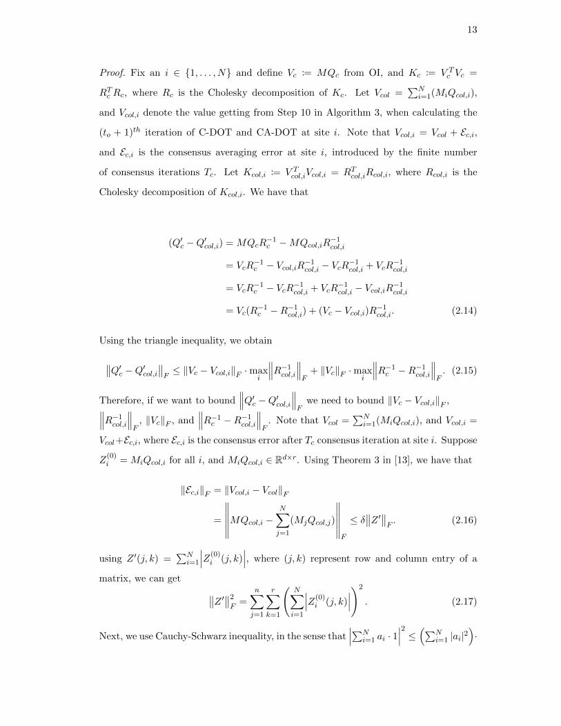
13

Proof. Fix an i ∈ 1, . . . , N and define Vc := MQc from OI, and Kc := V Tc Vc =

RTc Rc, where Rc is the Cholesky decomposition of Kc. Let Vcol =∑N

i=1(MiQcol,i),

and Vcol,i denote the value getting from Step 10 in Algorithm 3, when calculating the

(to + 1)th iteration of C-DOT and CA-DOT at site i. Note that Vcol,i = Vcol + Ec,i,

and Ec,i is the consensus averaging error at site i, introduced by the finite number

of consensus iterations Tc. Let Kcol,i := V Tcol,iVcol,i = RTcol,iRcol,i, where Rcol,i is the

Cholesky decomposition of Kcol,i. We have that

(Q′c −Q′col,i) = MQcR−1c −MQcol,iR

−1col,i

= VcR−1c − Vcol,iR−1col,i − VcR

−1col,i + VcR

−1col,i

= VcR−1c − VcR−1col,i + VcR

−1col,i − Vcol,iR

−1col,i

= Vc(R−1c −R−1col,i) + (Vc − Vcol,i)R−1col,i. (2.14)

Using the triangle inequality, we obtain

∥∥Q′c −Q′col,i∥∥F ≤ ‖Vc − Vcol,i‖F ·maxi

∥∥∥R−1col,i∥∥∥F

+ ‖Vc‖F ·maxi

∥∥∥R−1c −R−1col,i∥∥∥F

. (2.15)

Therefore, if we want to bound∥∥∥Q′c −Q′col,i∥∥∥

Fwe need to bound ‖Vc − Vcol,i‖F ,∥∥∥R−1col,i∥∥∥

F, ‖Vc‖F , and

∥∥∥R−1c −R−1col,i∥∥∥F

. Note that Vcol =∑N

i=1(MiQcol,i), and Vcol,i =

Vcol+Ec,i, where Ec,i is the consensus error after Tc consensus iteration at site i. Suppose

Z(0)i = MiQcol,i for all i, and MiQcol,i ∈ Rd×r. Using Theorem 3 in [13], we have that

‖Ec,i‖F = ‖Vcol,i − Vcol‖F

=

∥∥∥∥∥∥MQcol,i −N∑j=1

(MjQcol,j)

∥∥∥∥∥∥F

≤ δ∥∥Z ′∥∥

F. (2.16)

using Z ′(j, k) =∑N

i=1

∣∣∣Z(0)i (j, k)

∣∣∣, where (j, k) represent row and column entry of a

matrix, we can get ∥∥Z ′∥∥2F

=n∑j=1

r∑k=1

(N∑i=1

∣∣∣Z(0)i (j, k)

∣∣∣)2

. (2.17)

Next, we use Cauchy-Schwarz inequality, in the sense that∣∣∣∑N

i=1 ai · 1∣∣∣2 ≤ (∑N

i=1 |ai|2)·

14

N , to obtain

∥∥Z ′∥∥2F≤ N

n∑j=1

r∑k=1

N∑i=1

∣∣∣Z(0)i (j, k)

∣∣∣2= N

N∑i=1

∥∥∥Z(0)i

∥∥∥2F

= NN∑i=1

(‖MiQcol,i‖2F ). (2.18)

Then we apply matrix norm properties, where ‖AB‖F ≤ ‖A‖2‖B‖F , and ‖AB‖2F ≤

‖A‖22‖B‖2F , and note that Qcol,i are orthonormal matrices with rank r. We have

∥∥Z ′∥∥2F≤ N

N∑i=1

(‖Mi‖22 · ‖Qcol,i‖

2F

)≤ N

(N∑i=1

‖Mi‖22

)· r

≤ Nγ2r. (2.19)

Therefore, we can get ∥∥Z ′∥∥F≤ γ√Nr, (2.20)

and from (2.16) and (2.20) we have that

‖Ec,i‖F ≤ δγ√Nr. (2.21)

Equation (2.21) and Vcol,i = Vcol+Ec,i give us tools to bound ‖Vc − Vcol,i‖F , ‖Vc‖F , and

‖Vcol,i‖F . Note that

Vc − Vcol,i = Vc − (Vcol + Ec,i)

= Vc − Vcol − Ec,i

= MQc −N∑i=1

MiQcol,i − Ec,i

=N∑i=1

Mi(Qc −Qcol,i)− Ec,i. (2.22)

15

Therefore, we have

‖Vc − Vcol,i‖F ≤N∑i=1

‖Mi(Qc −Qcol,i)‖F + ‖Ec,i‖F

≤N∑i=1

‖Mi‖2‖Qc −Qcol,i‖F + δγ√Nr

≤ αmaxi‖Qc −Qcol,i‖F + δγ

√Nr. (2.23)

We are able to bound ‖Vc‖F as follows, where

‖Vc‖F = ‖MQc‖F

≤ ‖M‖2‖Qc‖F

=

∥∥∥∥∥N∑i=1

Mi

∥∥∥∥∥2

‖Qc‖F

≤N∑i=1

‖Mi‖2‖Qc‖F

≤ α√r. (2.24)

Due to the fact from (2.21), we can bound ‖Vcol,i‖F , where

Vcol,i = Vcol + Ec,i

=

N∑i=1

(MiQcol,i) + Ec,i. (2.25)

Note that

‖Vcol,i‖F ≤

∥∥∥∥∥N∑i=1

(MiQcol,i)

∥∥∥∥∥F

+ δγ√Nr

≤N∑i=1

‖MiQcol,i‖F + δγ√Nr

≤N∑i=1

‖Mi‖2√r + δγ

√Nr

≤ α√r + δγ

√Nr.e (2.26)

Next step is to bound∥∥∥R−1col,i∥∥∥

Fand

∥∥∥R−1c −R−1col,i∥∥∥F

. Define Kc := V Tc Vc = RTc Rc,

and Kcol,i := V Tcol,iVcol,i = RTcol,iRcol,i, where Rc and Rcol,i are Cholesky decompositions

16

of Kc and Kcol,i, respectively. We have that Q′c = VcR−1c , and Q′col,i = Vcol,iR

−1col,i. We

obtain Rc = Q′T

c Vc and Rcol,i = Q′T

col,iVcol,i. We have that

Kc −Kcol,i = RTc Rc −RTcol,iRcol,i = V Tc Vc − V T

col,iVcol,i

= V Tc Vc − V T

col,iVcol,i + V Tcol,iVc − V T

col,iVc

= V Tc Vc − V T

col,iVc + V Tcol,iVc − V T

col,iVcol,i. (2.27)

Therefore, we have

‖Kc −Kcol,i‖F ≤ ‖Vc‖F ‖Vc − Vcol,i‖F + ‖Vcol,i‖F ‖Vc − Vcol,i‖F

≤ (‖Vc‖F + ‖Vcol,i‖F )‖Vc − Vcol,i‖F

≤(α√r + α

√r + δγ

√Nr)(

αmaxi‖Qc −Qcol,i‖F + δγ

√Nr

)=(

2α√r + δγ

√Nr)(

αmaxi‖Qc −Qcol,i‖F + δγ

√Nr

)= α2

(2√r +

δγ√Nr

α

)(maxi‖Qc −Qcol,i‖F +

δγ√Nr

α

). (2.28)

We apply a theorem by Stewart [16], which states that if Kc = RTc Rc, and Kcol,i =

RTcol,iRcol,i are Cholesky factorization of symmetric matrices, we have ‖Rc −Rcol,i‖F ≤∥∥K−1c ∥∥2‖Rc‖2‖Kcol,i −Kc‖F . Therefore,

‖Rc −Rcol,i‖F ≤∥∥K−1c ∥∥2‖Rc‖2‖Kcol,i −Kc‖F

=∥∥R−1c ∥∥22‖Rc‖2‖Kcol,i −Kc‖F . (2.29)

The Cholesky decomposition of symmetric matrices Kc and Kcol,i are non-singular

matrices Rc, and Rcol,i. For non-singular matrices Rc, and Rcol,i, we apply a theorem

by Wedin [17]. Then we have∥∥∥R−1c −R−1col,i∥∥∥2≤ 1 +

√5

2‖Rc −Rcol,i‖2 max

∥∥R−1c ∥∥22,∥∥∥R−1col,i∥∥∥22

≤ 1 +√

5

2max

∥∥R−1c ∥∥22, ∥∥∥R−1col,i∥∥∥22∥∥R−1c ∥∥22‖Rc‖2‖Kcol,i −Kc‖F .

(2.30)

Note that Vc = Q′cRc , hence ‖Vc‖2 = ‖Rc‖2, and β = maxto=1,...,To

∥∥∥R−1(to)c

∥∥∥2, and we have

17

that∥∥∥R−1c −R−1col,i∥∥∥2≤ 1 +

√5

2max

∥∥R−1c ∥∥22, ∥∥∥R−1col,i∥∥∥22β2α√rα2

(2√r +

δγ√Nr

α

)

×

(maxi‖Qc −Qcol,i‖F +

δγ√Nr

α

)

≤ 1 +√

5

2max

β2,∥∥∥R−1col,i∥∥∥2

2

α3β2

√r

(2√r +

δγ√Nr

α

)

×

(maxi‖Qc −Qcol,i‖F +

δγ√Nr

α

). (2.31)

Hence all we need to bound is∥∥∥R−1col,i∥∥∥

2. We now apply the perturbation bound for

singular values of a matrix [18], where σr(Rc)− σr(Rcol,i) ≤ ‖Rc −Rcol,i‖2. Note that

σr(Rc) represents the rth singular value of matrix Rc. As σr(Rc) =∥∥R−1c ∥∥−12

and

σr(Rcol,i) =∥∥∥R−1col,i∥∥∥−1

2, we obtain that

∥∥R−1c ∥∥−12−∥∥∥R−1col,i∥∥∥−1

2≤ ‖Rc −Rcol,i‖2∥∥R−1c ∥∥−12≤∥∥∥R−1col,i∥∥∥−1

2+∥∥R−1c ∥∥22‖Rc‖2‖Kcol,i −Kc‖F∥∥R−1c ∥∥−12

≤∥∥∥R−1col,i∥∥∥−1

2+ α3β2

√r

(2√r +

δγ√Nr

α

)

×

(maxi‖Qc −Qcol,i‖F +

δγ√Nr

α

). (2.32)

Then we apply our assumption for (2.32), where ‖Qc −Qcol,i‖F+ δγ√Nrα ≤ 1

2α2β3√r(2α

√r+δγ

√Nr)

,

to obtain ∥∥R−1c ∥∥−12≤∥∥∥R−1col,i∥∥∥−1

2+

1

2β. (2.33)

From our definition for β, we have that β−1 ≤∥∥R−1c ∥∥−12

. We can get∥∥∥R−1col,i∥∥∥−12

+1

2β≥ β−1∥∥∥R−1col,i∥∥∥−1

2≥ 1

2β∥∥∥R−1col,i∥∥∥2≤ 2β. (2.34)

18

Then we can plug in the bound for∥∥∥R−1col,i∥∥∥

2into (2.31). We have that

∥∥∥R−1c −R−1col,i∥∥∥2≤ 1 +

√5

2max

β2,∥∥∥R−1col,i∥∥∥2

2

α3β2

√r

(2√r +

δγ√Nr

α

)

×

(maxi‖Qc −Qcol,i‖F +

δγ√Nr

α

)

≤ 1 +√

5

2max

β2, (2β)2

α3β2

√r

(2√r +

δγ√Nr

α

)

×

(maxi‖Qc −Qcol,i‖F +

δγ√Nr

α

)

≤ 1 +√

5

24β2α3β2

√r

(2√r +

δγ√Nr

α

)

×

(maxi‖Qc −Qcol,i‖F +

δγ√Nr

α

)

≤ 2(

1 +√

5)α3β4

√r

(2√r +

δγ√Nr

α

)

×

(maxi‖Qc −Qcol,i‖F +

δγ√Nr

α

). (2.35)

Up until now we have bounded all terms in (2.15). Apply ‖X‖F ≤√r‖X‖2 to (2.15),

where r is rank of matrix X , we obtain

∥∥Q′c −Q′col,i∥∥F ≤ √r‖Vc − Vcol,i‖F ·maxi

∥∥∥R−1col,i∥∥∥2

+√r‖Vc‖F ·max

i

∥∥∥R−1c −R−1col,i∥∥∥2.

(2.36)

19

Plugging in bounds for ‖Vc − Vcol,i‖F ,∥∥∥R−1col,i∥∥∥

F, ‖Vc‖F , and

∥∥∥R−1c −R−1col,i∥∥∥F

, we have

∥∥Q′c −Q′col,i∥∥F ≤ 2αβ√r

(maxi‖Qc −Qcol,i‖F +

δγ√Nr

α

)

+ 2(

1 +√

5)αrα3β4

√r

(2√r +

δγ√Nr

α

)

×

(maxi‖Qc −Qcol,i‖F +

δγ√Nr

α

)

= 2αβ√r

(maxi‖Qc −Qcol,i‖F +

δγ√Nr

α

)

+ 2(

1 +√

5)α4β4r

32

(2√r +

δγ√Nr

α

)

×

(maxi‖Qc −Qcol,i‖F +

δγ√Nr

α

)

=

2αβ√r + 4(1 +

√5)α4β4r2 + 2

(1 +√

5)α4β4r

32δγ√Nr

α

×

(maxi‖Qc −Qcol,i‖F +

δγ√Nr

α

). (2.37)

For orthonormal matrix Q′c, we have that 1 = ‖Q′c‖2 =∥∥MQCR

−1c

∥∥2≤ ‖M‖2

∥∥R−1c ∥∥2 ≤∑Ni=1‖Mi‖2

∥∥R−1c ∥∥2 ≤ αβ. Therefore α4β4 ≥ αβ ≥ 1, and δγ√Nrα ≤ 1. For C-DOT

algorithm, define δ = αγ√NrεTo( 1

3αβ√r)4To , where δγ

√Nrα = εTo( 1

3αβ√r)4To ≤ ( ε3)4To ≤ 1.

For CA-DOT algorithm, define δ = αToγ√NrεTo( 1

3αβ√r)4to , where δγ

√Nrα = εTo

To( 13αβ√r)4to ≤

(13)4to ≤ 1. Therefore, we obtain

∥∥Q′c −Q′col,i∥∥F ≤ (3αβ√r)4(

maxi‖Qc −Qcol,i‖F +

δγ√Nr

α

). (2.38)

This completes the proofs of Lemma 4 and 5.

Proof. Theorem 1 and 2.

∀i,∥∥QQT −Qcol,iQTcol,i∥∥2 ≤ ∥∥QQT −QcQTc ∥∥2 +

∥∥QcQTc −Qcol,iQTcol,i∥∥2. (2.39)

The first term comes from the centralized orthogonal iteration, where∥∥QQT −QcQTc ∥∥2 ≤

c∣∣∣λr+1

r

∣∣∣t as discussed in [11], and c is some constant. For the second term in (2.39), we

20

have ∥∥QcQTc −Qcol,iQTcol,i∥∥2 ≤ ∥∥QcQTc −Qcol,iQTcol,i∥∥FQcQ

Tc −Qcol,iQTcol,i = QcQ

Tc −Qcol,iQTcol,i +QcQ

Tcol,i −QcQTcol,i∥∥QcQTc −Qcol,iQTcol,i∥∥F ≤ (‖Qc‖2 +

∥∥Q(col,i)

∥∥2

)‖Qc −Qcol,i‖F∥∥QcQTc −Qcol,iQTcol,i∥∥F ≤ 2‖Qc −Qcol,i‖F . (2.40)

For iterations to+1 < To, the results from Lemma 4 and Lemma 5 always hold. Starting

from to = 0, we initialize OI, C-DOT and CA-DOT with same value Qinit = Q(0)c =

Q(0)col,i, and

∥∥∥Q(0)c −Q(0)

col,i

∥∥∥F

= 0. Therefore, we have∥∥∥Q(0)

c −Q(0)col,i

∥∥∥F

+ δγ√Nrα = δγ

√Nrα ,

and applying Lemma 4 and mathematical induction for C-DOT, we have that

∥∥∥Q(to)c −Q(to)

col,i

∥∥∥F

+δγ√Nr

α≤ δγ

√Nr

α

to∑j=0

(3αβ√r)4j

∥∥∥Q(to)c −Q(to)

col,i

∥∥∥F≤ δγ

√Nr

α

to∑j=0

(3αβ√r)4j . (2.41)

Note that (3αβ√r)4 > 3, and 1

(3αβ√r)4

< 13 . Then we have 1 − 1

(3αβ√r)4

> 1 − 13 = 2

3 ,

and (3αβ√r)4

(3αβ√r)4−1 <

32 . Applying geometric series, we obtain

to∑j=0

(3αβ√r)4j =

(3αβ√r)4(to+1) − 1

(3αβ√r)4 − 1

≤ (3αβ√r)4to

(3αβ√r)4

(3αβ√r)4 − 1

≤ 3

2(3αβ

√r)4to . (2.42)

Plug (2.42) into (2.41), we have∥∥∥Q(to)c −Q(to)

col,i

∥∥∥F≤ 3

2

δγ√Nr

α(3αβ

√r)4to . (2.43)

Plug in δγ√Nrα = εTo

(1

3αβ√r

)4Tointo (2.43). As to < To and 3αβ

√r > 3, we have

∥∥∥Q(to)c −Q(to)

col,i

∥∥∥F≤ 3

2εTo(

1

3αβ√r

)4To

(3αβ√r)4to

≤ 3

2εTo

(3αβ√r)4to

(3αβ√r)4To

≤ 3

2εTo . (2.44)

21

From (2.40), we have

∥∥QcQTc −Qcol,iQTcol,i∥∥F ≤ 2‖Qc −Qcol,i‖F ≤ 3εTo . (2.45)

By combining the results, we have completed the proof of Theorem 1, where

∥∥QQT −Qcol,iQTcol,i∥∥2 ≤ c∣∣∣∣λr+1

λr

∣∣∣∣To + 3εTo . (2.46)

For CA-DOT, we apply Lemma 5 and mathematical induction for CA-DOT to∥∥∥Q(0)

c −Q(0)col,i

∥∥∥F

+

δ(0)γ√Nr

α = δ(0)γ√Nr

α . As δ(to) is a defined value for ttho iteration for the outer loop of

the CA-DOT algorithm, we have that

∥∥∥Q(To)c −Q(To)

col,i

∥∥∥F

+δ(To)γ

√Nr

α≤ γ√Nr

α

To∑j=0

(3αβ√r)4jδ(j). (2.47)

Plugging in δ(j) into (2.47), where δ(j) := αToγ√NrεTo(

13√rαβ

)4j, and ε ∈ (0, 1), we

obtain

γ√Nr

α

To∑j=0

(3αβ√r)4j

δ(j) =

To∑i=0

(3αβ√r)4j εTo

To

(1

3√rαβ

)4j

=εTo

To

To∑i=0

1

=(To + 1)

ToεTo

≤ εTo . (2.48)

Thus, we obtain ∥∥∥Q(To)c −Q(To)

col,i

∥∥∥F≤ εTo , (2.49)

and from (2.40), we have

∥∥QcQTc −Qcol,iQTcol,i∥∥F ≤ 2‖Qc −Qcol,i‖F ≤ 2εTo . (2.50)

By combining the results, we have completed the proof of Theorem 2, where∥∥∥QQT −Q(col,i)QT(col,i)

∥∥∥2≤ c

∣∣∣∣λr+1

λr

∣∣∣∣To + 2εTo . (2.51)

22

2.2.5 Row-wise Distributed Orthogonal Iteration

Suppose zero-mean data A ∈ Rd×n is row-wise distributed within an undirected loosely

connected network. Each site i holds local data Ai ∈ Rdi×n matrix, where i ∈

1, . . . , N, d =∑N

i=1 di and di = dN . Matrix A has eigenvalues |λ1| ≥ . . . |λr| >

|λr+1| ≥ . . . |λd|. Define the eigengap :=∣∣∣λr+1

λr

∣∣∣, and eigengap < 1. The output of Row-

wise Distributed Orthogonal Iteration (RDOT) [4,5] is the top-r dimensional principal

subspace Q. Let r be a chosen integer for the dimension of the output Q ∈ Rd×r.

The estimation of Q is Qrow =[Qtrow,1, . . . , Q

trow,N

]T, where Qtrow,i ∈ Rdi×r is the

estimation for the i-th block of Q corresponding to node i. Row-wise distributed power

method [4] is a special case for RDOT, where the row-wise distributed power method is

trying to compute the first principal component. The procedure of computing the r-th

eigenvector with PDPM is provided in [4], where we need r iterations of PDPM that

require an increasing number of projections to make sure top-r eigenspace has orthonor-

mal columns. In this thesis, a small improvement has been done for the computation

of the top-r eigenspace. RDOT uses the Row-wise Distributed QR decomposition (Dis-

tributedQR) [5] to perform QR factorization of V trow,i within each outer loop of the

RDOT algorithm.

Algorithm 4 Row-wise Distributed Orthogonal Iteration

1: Input: Local data, Ai at node i, where i ∈ 1, . . . , N, and weight matrix W2: Initialize: Set t← 0 and Qtrow,i ← Qinit, where Qinit is a random initialized di× r

matrix, with orthonormal columns3: while stopping rule do4: t← t+ 15: Initialize Consensus: Set tc ← 0, Z

(tc)i ← ATi Q

t−1row,i, i = 1, 2, . . . , N

6: while stopping rule do7: tc ← tc + 18: Z

(tc)i ←

∑j∈Ni

wi,jZ(tc−1)j

9: end while

10: V trow,i ← N

mAiZ

(tc)i

[W tce1]i

11: Qtrow,iRtrow,i ← Distributed QR(V t

row,i)12: end while13: Return: Qtrow,i

RDOT algorithm find the estimate of Q when A is row-wise distributed. The con-

vergence analysis and numerical experiments of RDOT will be one of the focus of future

23

work. The number of operations of Z(tc)i ← ATi ×Q

t−1row,i is O(ndir), where Z

(tc)i ∈ Rn×r,

which means when number of observations n is large, the computation cost and the stor-

age cost are expensive for all node i. Therefore, RDOT does not work well with data

that has large number of samples. In the future we want distributed PCA algorithms

to work with big data A that has both large d and large n.

2.2.6 Row-wise Distributed QR decomposition

One of the key steps of RDOT is to orthonormalize V trow = [V t

row,1, . . . , Vtrow,N ]T in each

RDOT iteration as shown in step 11 in Algorithm 4, since V trow is row-wise distributed

across the network. Luckily, a modified Gram-Schmidt Row-wise Distributed QR de-

composition algorithm (DistributedQR) [5] provides the solution for this problem. At

tth iteration of RDOT, let Vrow,i = V trow,i. Define V = [Vrow,1, . . . , Vrow,N ]T , where

V ∈ Rd×r and 1 ≤ r ≤ d. Suppose we want to find the QR factorization of the thin

matrix V = QR. The goal is to calculate a Q ∈ Rd×r with orthonormal columns,

and R ∈ Rr×r is an upper triangular matrix. The m, j entry of matrix Vrow,i can be

represented as Vrow,i(m, j).

Algorithm 5 Row-wise Distributed QR factorization

1: Input: Matrix V ∈ Rd×r is row-wise distributed among N nodes, local data Vrow,iat node i, i ∈ 1, . . . , N , each node stores di consecutive rows of V, and a weightmatrix W

2: for j=1 to r do3: (in node i)4: xi ←

∑dim=1 Vrow,i(m, j)

2

5: si ← AC(x,W ) . (Averaging Consensus of x across all node i)6: Ri(j, j)←

√si

7: Qi(:, j)← Vi(:, j)/Ri(j, j)8: if i 6= j delete Ri(j, j)9: for k = j + 1 to r do

10: x′i ←∑di

m=1Qi(m, j)Vi(m, k)11: Ri(j, k)← AC(x′,W ) . (Averaging Consensus of x′ across all node i)12: Vi(:, k)← Vi(:, k)−Qi(:, j)Ri(j, k)13: if i 6= k delete Ri(j, k)14: end for15: end for16: Return: Qi

24

The convergence behavior of DistributedQR is evaluated in [5], which ensures the re-

liability and scalability of the algorithm. Each iteration of RDOT in Algorithm 4 we can

use DistributedQR to orthonormalize V trow, whereQtrow,iR

trow,i ← Distributed QR(V t

row,i)

and Qtrow = [Qtrow,1, . . . , Qtrow,N ]T is the estimate of Q after t iterations of RDOT.

25

Chapter 3

Experimental Results

The numerical experiments in this chapter demonstrate the convergence behavior of

C-DOT and CA-DOT algorithms to validate the theoretical results in Section 2.2.4. In

this chapter, each table records the experiment parameters corresponding to a result

figure. The corresponding network topology is an undirected connected network with

N sites. If not specified, the network topology is an Erdos–Renyi random graph with

a connection density p. To achieve consensus averaging, we design the weight matrix

W by using the local-degree weights method mentioned in [14]. The upper bound for

the averaging consensus iteration is 50, unless otherwise specified. The columns labeled

“P2P” in all tables stand for the average number of point-to-point communications [19]

per node for an experiment, while the default number of iterations for C-DOT or CA-

DOT is 200 and (K) represents a 1000 number of P2P communications. Furthermore,

the P2P value for the central site and peripheral sites are marked separately for a star

network. The number of communication iterations indicates the cumulative number of

consensus iterations at each site. The eigengap∣∣∣λr+1

λr

∣∣∣ corresponds to the eigenvalues of

of the centralized data A. The true low-rank principal subspace Q ∈ Rd×r is calculated

by the build-in SVD function in Python 3, and the average error in the experiments is

defined as 1N

∑Ni=1

∥∥∥QQT −Qcol,iQTcol,i∥∥∥2.

3.1 Tools and Platform for Numerical Experiments

In this section, we acknowledge the tools and platforms that have been used in the

numerical experiments of this thesis.

26

3.1.1 Programming Language

In this thesis, all the experiments and simulations are implemented in the programming

language Python 3.

3.1.2 Datasets

This section provides a brief introduction to the implemented real-world experiment

datasets in this thesis.

The MNIST [7] is a database of handwritten digits. MNIST contains 50,000 gray-

scale training samples. Every sample consists of a 28× 28 pixels image.

Figure 3.1: Representative images from MNIST.

The Canadian Institute For Advanced Research 10 (CIFAR-10) [8] dataset consists

of 50,000 samples of training data in 10 classes. Our thesis extracts the red channel

of each 32 × 32 pixel color image because of the limitations of the feasibility of our

computing resources.

Figure 3.2: Representative images from CIFAR-10.

Labeled Faces in the Wild (LFW) [9] face database is mainly a public benchmark for

face recognition, consisting of gray-scale images of a number of people’s faces in different

poses, distinct angles, and various light conditions. The number of training samples of

LFW total is 13, 233, and the dimensionality of a single image is 2914 = 62× 47.

27

Figure 3.3: Representative images from LFW.

ImageNet [10] is an important visual database that contains 14 million color im-

ages over more than 20,000 categories. The dimension of the images is inconsistent.

Therefore, we reshape the images in the ImageNet database into a uniformed dimension

1024 = 32× 32 and extract information from the red channel of those images to make

sure the data fit on our computing platform.

Figure 3.4: Representative images from ImageNet.

3.1.3 Computing Platform

Amarel Cluster [20] is a High-Performance-Computer (HPC) provided by the Office of

Advanced Research Computing (OARC) at Rutgers University. Amarel allows us to

use the Message Passing Interface (MPI) [6] in a large connected network.

3.2 Experiments Using Synthetic Data

For synthetic input data, each site i has ni = 500 local samples in R20, where d =

20. Samples are randomly generated from the Gaussian distribution with different

covariances. When the network size N = 10 or N = 20, we use 20 Monte-Carlo

simulations for all experiments with synthetic data.

The first set of experiments investigates the convergence behavior of the C-DOT

algorithm. Furthermore, these experiments analyze the influence of different values of

28

Table 3.1: Synthetic Experiment 1: Parameters for C-DOT algorithm

N Erdos–Renyi: p r Eigengap Consensus Itr Tc P2P (K)

10 0.5 5 0.7 10 9.3220 18.6450 46.6

20 0.25 5 0.7 10 9.920 19.850 49.5

100 0.05 5 0.7 10 1120 2250 55

consensus iterations Tc for different sizes of the networks. The simulation results in

Fig. 3.5 correspond to experiment parameters in Table 3.1. The average error hits a

floor as the number of C-DOT iteration t increases. Furthermore, as the number of

consensus iteration increases in each C-DOT iteration, the error floor decreases, and

a small number of inner loop Tc can lead to faster convergence, regardless of the size

of the network. The number of point-to-point communications grows as Tc increases,

which shows that there is a trade-off between P2P cost and a lower error floor.

In the second set of experiments, we compare the performance of CA-DOT with

different number of consensus iterations and different eigengaps=∣∣∣λr+1

λr

∣∣∣. The ex-

periment parameters are listed in Table 3.2. The number of consensus iterations is

Tc = [Tc,1, . . . , Tc,To ], a sequence of integers, where To is the total number of outer loop

iterations. Define Tc,t = min(T incc × t + T initc , Tmaxc ) at t-th iteration. Note that Tmaxc

is the maximum number of consensus iterations, T initc is the initial value for Tc, and

T incc is the rate of increase of the number of consensus iterations as t increases. The C-

DOT algorithm can be represented as a particular case of CA-DOT, where Tc = Tmaxc .

From the results given in Fig. 3.6, we can conclude that the error floor is determined

by Tmaxc . With the same Tmaxc , the speed of convergence is influenced by T incc and

T initc . If we choose an appropriate value for T incc , Tmaxc and T initc , we can minimize the

communication cost and increase the speed of convergence. Besides, as the eigengaps

get close to 0, the required communication cost decreases. As the eigengaps are getting

close to 1, the convergence speed becomes slower for C-DOT and CA-DOT algorithms.

29

(a) N = 10 (b) N = 20

(c) N = 100

Figure 3.5: Results for C-DOT corresponding to the parameters in Table 3.1.

As the first term in (2.5) and (2.7) show, as the eigengaps get close to 1, the slower

the∣∣∣λr+1

λr

∣∣∣t term goes to 0. In contrast, as the eigengaps get close to 0, the faster the∣∣∣λr+1

λr

∣∣∣t term goes to 0.

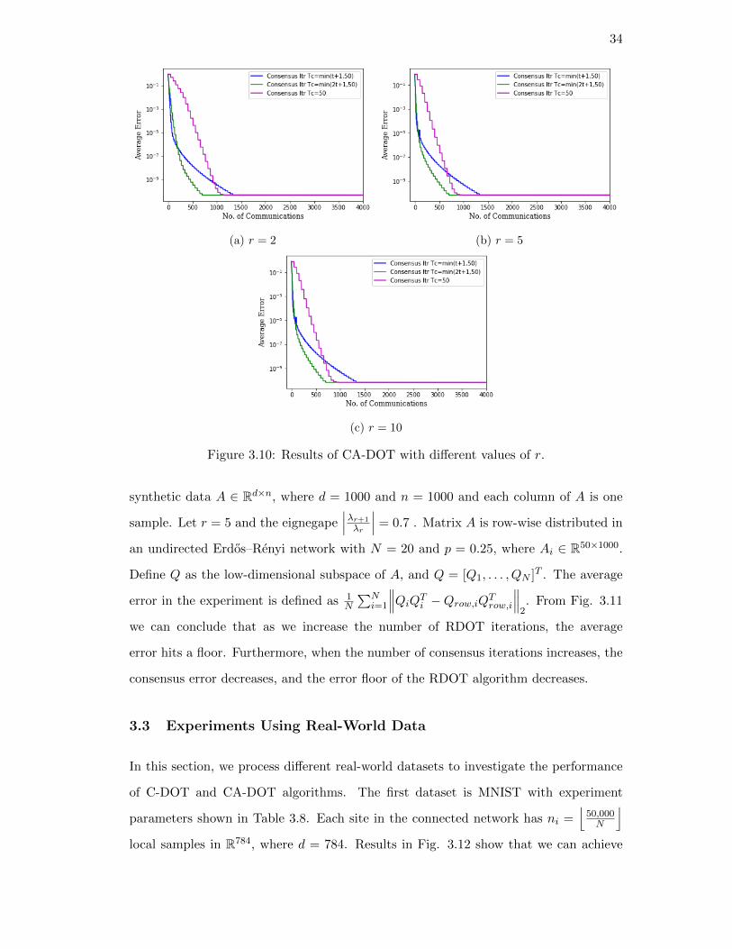
The third set of experiments investigates the convergence behavior of the CA-DOT

algorithm with different values of p for Erdos–Renyi graphs. From the P2P column in

Table 3.3, we can conclude that the number of point-to-point connections increases as

p increases. The value p represents the connection density of an Erdos–Renyi graph.

See Fig. 3.7a when p is close to 1; in this case, we call the network a dense network.

In contrast, in Fig. 3.7c as p gets close to 0, we call the network a sparse network.

Moreover, different p can lead to different mixing time τmix for the corresponding weight

matrix W for the underlying network, which can also affect the error floor as indicated

in Theorem 1 and Theorem 2. Results in Fig. 3.8c show that a sparse network can

lead to slow convergence. Therefore, for a sparse network we want to increase values

for T incc , T initc , Tmaxc and To to achieve faster convergence.

30

Table 3.2: Synthetic Experiment 2: Parameters for CA-DOT with different eigengaps

N Erdos–Renyi: p r Eigengap Consensus Itr Tc P2P (K)

20 0.25 5 0.3 d0.5t+ 1e 34.88t+ 1 40.542t+ 1 43.3150 46.2

20 0.25 5 0.7 d0.5t+ 1e 37.37t+ 1 43.442t+ 1 46.4150 49.5

20 0.25 5 0.9 d0.5t+ 1e 36.47t+ 1 42.382t+ 1 52.2850 48.3

(a) Eigengap = 0.3 (b) Eigengap = 0.7

(c) Eigengap = 0.9

Figure 3.6: Results for CA-DOT with different eigengaps.

31

(a) p = 0.5 (b) p = 0.25 (c) p = 0.1

Figure 3.7: Erdos–Renyi topologies with different p.

Table 3.3: Synthetic Experiment 3: Parameters for CA-DOT with different p forErdos–Renyi topology

N Erdos–Renyi: p r Eigengap Consensus Itr Tc P2P (K)

20 0.5 5 0.7 2t+ 1 90.6650 96.7

20 0.25 5 0.7 2t+ 1 46.4150 49.5

20 0.1 5 0.7 2t+ 1 22.9750 24.5min(5t+ 1, 200) 88.05

(a) p = 0.5 (b) p = 0.25

(c) p = 0.1

Figure 3.8: Results for CA-DOT with different p for Erdos–Renyi graphs.

32

Table 3.4: Synthetic Experiment 4: Parameters for ring topology

N r Eigengap Consensus Itr P2P (K)

20 5 0.7 2t+ 1 18.7550 20min(5t+ 1, 200) 71.88

Table 3.5: Synthetic Experiment 5: Parameters for star topology

N r Eigengap Consensus Itr Center node P2P (K) Edge node P2P (K)

20 5 0.7 2t+ 1 178.13 9.3850 190 10min(2t+ 1, 100) 332.5 17.5min(5t+ 1, 100) 360.43 18.97100 380 20

Experiment 4 and experiment 5 investigates the performance of our algorithms on

the ring and star topologies. The experimental parameters map to Table 3.4 and Table

3.5. The results for ring topology in Fig. 3.9 show that CA-DOT does not perform well

since ring topology is a periodic Markov chain [21] that cannot converge to a steady-

state distribution. The steady-state distribution exists if the Markov chain with finite

number of states is aperiodic and irreducible. Therefore, τmix →∞ for ring topologies.

Experiment 5 investigates performance on the star topology. In Table 3.5, the amount

of point-to-point communication at the center site is equal to the sum of all edge sites,

which creates a bottleneck effect at the central node that can lead to slow convergence

rate for our algorithm. In practice, for a star topology we want increased values for

T incc , T initc , Tmaxc and To for faster convergence.

(a) Ring topology (b) Star topology

Figure 3.9: Results of CA-DOT for ring and star topologies.

33

Table 3.6: Synthetic Experiment 6: Parameters for CA-DOT with different values of r.

N Erdos–Renyi: p r Eigengap Consensus Itr P2P (K)

20 0.25 2 0.7 t+ 1 44.052t+ 1 47.0650 50.2

20 0.25 5 0.7 t+ 1 43.442t+ 1 46.4150 49.5

20 0.25 10 0.7 t+ 1 41.722t+ 1 44.5850 47.55

Table 3.7: Synthetic Experiment 7: Straggler effect with Erdos–Renyi graphs

N p r Eigengap Cons Itr Wall-clock time (s) P2P (K) Straggler

10 0.5 5 0.7 2t+ 1 101.33 45 Enabled2t+ 1 5.18 4550 108.56 48 Enabled50 19.5 48

20 0.25 5 0.7 2t+ 1 98.5 47.81 Enabled2t+ 1 5.08 47.8150 105.59 51 Enabled50 5.74 51

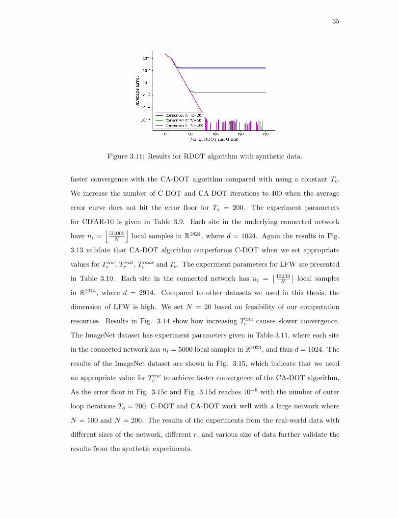
In Table 3.6, we provide the experimental parameters for different values of r. Re-

sults in Fig. 3.10 indicate that C-DOT and CA-DOT perform well with different r,

since the average error reaches 10−9. In practice, the value of r should be chosen based

on the amount of information we want to extract from the original data.

The straggler effect delays the job completion for distributed algorithms when there

is a slow node in the distributed network. In experiment 6 when we enable the straggler

effect for CA-DOT algorithm, we set a 0.01 second delay at a randomly selected site i,

at the time this site is sending information to it’s neighbors. The impact of a straggler

node on C-DOT and CA-DOT algorithms shows in Table 3.7. The wall-clock time of

experiments in Table 3.7 indicates that a slow site can potentially slow down the job

completion for the entire network. To speed up C-DOT and CA-DOT algorithms, we

need to adapt the algorithms to overcome the straggler effect, which is one of the main

focus for our future work.

Results in Fig. 3.11 show the convergence behavior of the RDOT algorithm with

34

(a) r = 2 (b) r = 5

(c) r = 10

Figure 3.10: Results of CA-DOT with different values of r.

synthetic data A ∈ Rd×n, where d = 1000 and n = 1000 and each column of A is one

sample. Let r = 5 and the eignegape∣∣∣λr+1

λr

∣∣∣ = 0.7 . Matrix A is row-wise distributed in

an undirected Erdos–Renyi network with N = 20 and p = 0.25, where Ai ∈ R50×1000.

Define Q as the low-dimensional subspace of A, and Q = [Q1, . . . , QN ]T . The average

error in the experiment is defined as 1N

∑Ni=1

∥∥∥QiQTi −Qrow,iQTrow,i∥∥∥2. From Fig. 3.11

we can conclude that as we increase the number of RDOT iterations, the average

error hits a floor. Furthermore, when the number of consensus iterations increases, the

consensus error decreases, and the error floor of the RDOT algorithm decreases.

3.3 Experiments Using Real-World Data

In this section, we process different real-world datasets to investigate the performance

of C-DOT and CA-DOT algorithms. The first dataset is MNIST with experiment

parameters shown in Table 3.8. Each site in the connected network has ni =⌊50,000N

⌋local samples in R784, where d = 784. Results in Fig. 3.12 show that we can achieve

35

Figure 3.11: Results for RDOT algorithm with synthetic data.

faster convergence with the CA-DOT algorithm compared with using a constant Tc.

We increase the number of C-DOT and CA-DOT iterations to 400 when the average

error curve does not hit the error floor for To = 200. The experiment parameters

for CIFAR-10 is given in Table 3.9. Each site in the underlying connected network

have ni =⌊50,000N

⌋local samples in R1024, where d = 1024. Again the results in Fig.

3.13 validate that CA-DOT algorithm outperforms C-DOT when we set appropriate

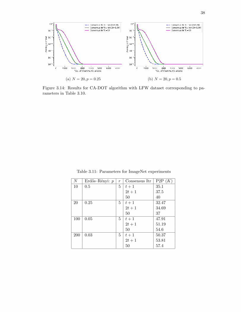
values for T incc , T initc , Tmaxc and To. The experiment parameters for LFW are presented

in Table 3.10. Each site in the connected network has ni =⌊13233N

⌋local samples

in R2914, where d = 2914. Compared to other datasets we used in this thesis, the

dimension of LFW is high. We set N = 20 based on feasibility of our computation

resources. Results in Fig. 3.14 show how increasing T incc causes slower convergence.

The ImageNet dataset has experiment parameters given in Table 3.11, where each site

in the connected network has ni = 5000 local samples in R1024, and thus d = 1024. The

results of the ImageNet dataset are shown in Fig. 3.15, which indicate that we need

an appropriate value for T incc to achieve faster convergence of the CA-DOT algorithm.

As the error floor in Fig. 3.15c and Fig. 3.15d reaches 10−8 with the number of outer

loop iterations To = 200, C-DOT and CA-DOT work well with a large network where

N = 100 and N = 200. The results of the experiments from the real-world data with

different sizes of the network, different r, and various size of data further validate the

results from the synthetic experiments.

36

Table 3.8: Parameters for MNIST experiments

N Erdos–Renyi: p r To Consensus Itr P2P (K)

20 0.25 5 400 t+ 1 82.612t+ 1 85.2550 88

20 0.25 10 400 t+ 1 82.612t+ 1 85.2550 88

100 0.05 5 200 t+ 1 43.882t+ 1 46.87550 50

(a) N = 20, r = 5 (b) N = 20, r = 10

(c) N = 100, r = 5

Figure 3.12: Results for CA-DOT algorithm with MNIST dataset corresponding toparameters in Table 3.8.

37

Table 3.9: Parameters for CIFAR-10 experiments

N Erdos–Renyi: p r To Consensus Itr P2P (K)

20 0.25 5 400 t+ 1 76.982t+ 1 79.4450 82

20 0.25 7 400 t+ 1 76.982t+ 1 79.4450 82

100 0.05 7 400 t+ 1 44.42t+ 1 98.450 101.12

(a) N = 20, r = 5 (b) N = 20, r = 7

(c) N = 100, r = 7

Figure 3.13: Results for CA-DOT algorithm with CIFAR-10 dataset corresponding toparameters in Table 3.9.

Table 3.10: Parameters for LFW experiments

N Erdos–Renyi: p r Consensus Itr P2P (K)

20 0.25 7 t+ 1 42.122t+ 1 4550 48

20 0.5 7 t+ 1 82.492t+ 1 88.1350 94

38

(a) N = 20, p = 0.25 (b) N = 20, p = 0.5

Figure 3.14: Results for CA-DOT algorithm with LFW dataset corresponding to pa-rameters in Table 3.10.

Table 3.11: Parameters for ImageNet experiments

N Erdos–Renyi: p r Consensus Itr P2P (K)

10 0.5 5 t+ 1 35.12t+ 1 37.550 40

20 0.25 5 t+ 1 32.472t+ 1 34.6950 37

100 0.05 5 t+ 1 47.912t+ 1 51.1950 54.6

200 0.03 5 t+ 1 50.372t+ 1 53.8150 57.4

39

(a) N = 10 (b) N = 20

(c) N = 100 (d) N = 200

Figure 3.15: Results for CA-DOT algorithm with ImageNet dataset corresponding toparameters in Table 3.11.

40

Chapter 4

Conclusion and Future Work

In this thesis, we presented a solution for column-wise distributed PCA with an arbi-

trary connected aperiodic underlying network topology. This thesis provides theoretical

guarantees for C-DOT and CA-DOT algorithms when we perform enough number of

averaging consensus iterations. The algorithms offer hugely improved potential in scal-

ability. Furthermore, this thesis presents results of experiments on synthetic data, and

MNIST, CIFAR-10, LFW, and ImageNet datasets. The real-world datasets demon-

strate the performance of C-DOT and CA-DOT.

In the future, we want to provide theoretical guarantees for RDOT and adapt the

algorithm to minimize the communication cost. Moreover, the next step is to develop

a block-wise distributed PCA that works with massive data and can be deployed in

real-world applications, where each site can only store some observations and partic-

ular dimensions of the dataset. Furthermore, we want to design straggler handling

techniques to overcome the straggler effect. We can also apply optimal weight for a

star network for rapid convergence. Then, we can deploy C-DOT and CA-DOT in

real-world machine learning applications. Last but not the least, we want to compare

C-DOT and CA-DOT algorithms with other column-wise distributed PCA algorithms.

41

References

[1] A. S. Tanenbaum and M. Van Steen, “Distributed systems principles andparadigms. 2002,” Cited in, p. 326.

[2] S. T. Roweis and L. K. Saul, “Nonlinear dimensionality reduction by locally linearembedding,” science, vol. 290, no. 5500, pp. 2323–2326, 2000.

[3] H. Hotelling, “Analysis of a complex of statistical variables into principal compo-nents.,” Journal of educational psychology, vol. 24, no. 6, p. 417, 1933.

[4] A. Scaglione, R. Pagliari, and H. Krim, “The decentralized estimation of the samplecovariance,” in 2008 42nd Asilomar Conference on Signals, Systems and Comput-ers, pp. 1722–1726, IEEE, 2008.

[5] H. Strakova, W. N. Gansterer, and T. Zemen, “Distributed QR factorization basedon randomized algorithms,” in International Conference on Parallel Processing andApplied Mathematics, pp. 235–244, Springer, 2011.

[6] D. W. Walker, “Standards for message-passing in a distributed memory environ-ment,” tech. rep., Oak Ridge National Lab., TN (United States), 1992.

[7] L. Deng, “The mnist database of handwritten digit images for machine learn-ing research [best of the web],” IEEE Signal Processing Magazine, vol. 29, no. 6,pp. 141–142, 2012.

[8] A. Krizhevsky, V. Nair, and G. Hinton, “The cifar-10 dataset,” online: http://www.cs. toronto. edu/kriz/cifar. html, vol. 55, 2014.

[9] G. B. Huang, M. Mattar, T. Berg, and E. Learned-Miller, “Labeled faces in thewild: A database forstudying face recognition in unconstrained environments,”2008.

[10] J. Deng, W. Dong, R. Socher, L.-J. Li, K. Li, and L. Fei-Fei, “Imagenet: A large-scale hierarchical image database,” in 2009 IEEE conference on computer visionand pattern recognition, pp. 248–255, IEEE, 2009.

[11] C. F. Van Loan and G. H. Golub, Matrix computations. Johns Hopkins UniversityPress, 1983.

[12] H. Raja and W. U. Bajwa, “Cloud k-svd: A collaborative dictionary learningalgorithm for big, distributed data,” IEEE Transactions on Signal Processing,vol. 64, no. 1, pp. 173–188, 2015.

[13] D. Kempe and F. McSherry, “A decentralized algorithm for spectral analysis,”Journal of Computer and System Sciences, vol. 74, no. 1, pp. 70–83, 2008.

42

[14] L. Xiao and S. Boyd, “Fast linear iterations for distributed averaging,” Systems &Control Letters, vol. 53, no. 1, pp. 65–78, 2004.

[15] W. K. Hastings, “Monte carlo sampling methods using markov chains and theirapplications,” 1970.

[16] G. Stewart, “On the perturbation of LU and Cholesky factors,” IMA Journal ofNumerical Analysis, vol. 17, no. 1, pp. 1–6, 1997.

[17] P.-A. Wedin, “Perturbation theory for pseudo-inverses,” BIT Numerical Mathe-matics, vol. 13, no. 2, pp. 217–232, 1973.

[18] G. W. Stewart, “Perturbation theory for the singular value decomposition,” tech.rep., 1998.

[19] S. D. Mattaway, G. W. Hutton, and C. B. Strickland, “Point-to-point computernetwork communication utility utilizing dynamically assigned network protocoladdresses,” Oct. 10 2000. US Patent 6,131,121.

[20] J. B. Von Oehsen, “Rutgers university. office of advanced research computing,”online: http://oarc.rutgers.edu, 2015.

[21] P. A. Gagniuc, Markov chains: from theory to implementation and experimenta-tion. John Wiley & Sons, 2017.