editorial - kaznu.kz · editorial the most significant scientific achievements are attained through...
TRANSCRIPT

Editorial The most significant scientific achievements are attained through joint efforts of different
sciences, mathematics and physics among them. Therefore publication of Journal, which is showing results of current investigations in the field of mathematics and physics, will allow widely exhibiting scientific problems, tasks and discoveries.
One of the basic goals of the Journal is to promote extensive exchange information between the scientists of all over the world. We suggest publishing original papers and materials of Mathematical and Physical Conferences (after selection) hold in different countries and Republic of Kazakhstan.
Creation of special International Journal of mathematics and physics is of great importance because a great amount of scientists to publish their articles and it will help to wide the geography of future operations. We will be glad to publish also the papers of scientists from other continents.
The Journal will publish experimental and theoretical investigations on mathematics, physical technology and physics. Among the subject emphasized are: modern problems of Calculus Mathematics, Algebra and Mathematical Analysis, Differential Equations and Mechanics, Informatics and Mathematical Modeling, Calculus of Approximations and Program Systems, Astronomy and Space Research, Theoretical Physics and Plasma Physics, Chemical Physics and Radio Physics, Thermo physics, Nuclear Physics, Nanotechnology.
The journal is issued on the base of al-Farabi Kazakh National University. Leading scientists from different countries of the world agreed to be members of the editorial board of the journal. The list of Editorial board is attached.
The Journal will be published 4times a year by al-Farabi Kazakh National University. We hope to receive papers from the many laboratories which are interested in the application of the scientific principles of mathematics and physics and are carrying out research on the subject, whether it is in relation to production new materials or technology problems.

International Journal of mathematics and physics 1 (2010) 1-9
*Corresponding author: E-mail: [email protected] © 2010 al-Farabi Kazakh National University Printed in Kazakhstan
Convergence of the Homotopy Perturbation Method
For Nonlinear Integral and Integro-Differential Equations
Mohamed M. Mousa
Department of Basic Science, Benha Higher Institute of Technology, Benha University, 13512, Egypt Al-Farabi Kazakh National University, 39/47 Masanchi, 050012, Almaty, Kazakhstan
Abstract
In this paper, Basic idea of the Homotopy Perturbation Method (HPM) is introduced, a theory of convergence of HPM for a class of nonlinear Volterra integral equations is proved and a theory for estimation solution error is proved as well. The HPM convergence theory is confirmed and the efficiency of the HPM is investigated by applying the method for solving some nonlinear integral and integro-differential equations.
Introduction
In recent years a lot of attention has been drawn to study of the homotopy perturbation method (HPM) to investigate various scientific models. The HPM, based on series approximation, is one among the newly developed analytical methods for strongly nonlinear problems and has been proven successful in solving a wide class of differential equations [2–8]. The method provides the solution in a rapidly convergent series with components that can be simply computed. The HPM is useful for obtaining both closed form explicit solutions and numerical approximations of linear or nonlinear differential equations and integral equations and it is of great interest to applied science, engineering, physics, biology, etc. Many authors investigated the HPM theory of convergence by solving some problems and showing that the HPM series solution convergent to the exact solution by its shape not by proving a theory. But in this paper, a theory of convergence of the HPM for a class of nonlinear Volterra integral equations has been generally proved. A theory for estimation the error of HPM series solution is proved as well. From the obtained numerical results of the considered examples of nonlinear integral and integro-differential equations, it is clear that the HPM provides remarkable accuracy for the obtained approximate solutions when compared to exact solutions.
Basic idea of the homotopy perturbation
method Consider the following nonlinear differential
equation [2–8]: ( ) ( ) ( ) 0, ,L u N u g Ω+ − = ∈r r (1)
with the boundary conditions of ( ), 0, ,B u u n Γ∂ ∂ = ∈r (2)
where L and N are linear and nonlinear differential operators, respectively, B a boundary operator, g (r) a known analytical function and Γ is the boundary of the domain Ω.
By the homotopy technique, we construct a homotopy V(r,p): Ω×[0,1]→ which satisfies:
( ) ( ) ( )( ) ( ) ( )
, 1
0,
[0,1], ,
H v p p L v
p L v N v g
p Ω
= − ⎡ ⎤⎣ ⎦+ + − =⎡ ⎤⎣ ⎦
∈ ∈
r
r
(3)
where p∈[0,1] is an embedding parameter.
According to the HPM, we can first use the embedding parameter p as a “small parameter”, and assume that the solution of Eq. (3) can be written as a power series in p:
20 1 2 ....v v p v p v= + + + (4)
Setting p=1, results in the solution of Eq. (1):
( )1
0
lim .npn
u v v∞
→=
= = ∑ r (5)
2 International Journal of mathematics and physics 1 (2010) 1-9
International Journal of mathematics and physics 1(2010) 1-9
The components of the series solution (5) can be
easily obtained by solving the system of equations resulted from substituting Eq. (4) into Eq. (3) and comparing the terms with identical powers of p.
Let’s denote the m+1-term approximate solution Sm by
( )0
m
m nn
u S v=
=∑ r . (6)
Convergence for a class of nonlinear
integral equations
Before proceeding to prove a theory of convergence of the HPM to a class of nonlinear Volterra integral equations of the second kind, we will propose a new formulation for the HPM to simplify proving the theory.
According to the HPM, we can reconstruct the homotopy equation (3) as follows,
( ) ( ) ( ) ( ), ,H v p L v p N v g= + =⎡ ⎤⎣ ⎦ r (7)
If 0
nn
n
v p v∞
=
= ∑ where =1|pu v= , then we will
prove that the homotopy equation (7) can be written as
( )
( ) ( )
0
00
,
,..., ,
nn
n
nn n
n
H v p L p v
p p D v v g
∞
=
∞
=
=⎛ ⎞⎜ ⎟⎝ ⎠
⎡ ⎤+ =⎢ ⎥⎣ ⎦
∑
∑ r (8)
where , 0,1,2,...nD n = are decomposed
polynomials of nonlinear operator N(v), i.e.
( ) ( )00
,..., ,nn n
n
N v p D v v∞
=
= ∑ moreover the
decomposed polynomials nD can be constructed from the following formula,
( )00 0
1,..., ,!
0,1,2,...
n nk
n n knk p
D v v N p vn p
n= =
⎡ ⎤∂ ⎛ ⎞= ⎢ ⎥⎜ ⎟∂ ⎝ ⎠⎣ ⎦
=
∑ (9)
Theorem 1. Suppose N(v) is a nonlinear
functional operator and 0
kk
kv p v
∞
=
=∑ , then we have
(i)
( )00 0
0 0
,
n nk
kn nkp p
n nk
knk p
N v N p vp p
N p vp
∞
== =
= =
⎡ ⎤⎡ ⎤∂ ∂ ⎛ ⎞= ⎢ ⎥⎢ ⎥ ⎜ ⎟∂ ∂ ⎝ ⎠⎣ ⎦ ⎣ ⎦
⎡ ⎤∂ ⎛ ⎞= ⎢ ⎥⎜ ⎟∂ ⎝ ⎠⎣ ⎦
∑
∑
(ii) ( ) ( )00
,..., ,nn n
n
N v p D v v∞
=
= ∑
where
( )00 0
1,..., ,!
0,1,2,...
n nk
n n knk p
D v v N p vn p
n= =
⎡ ⎤∂ ⎛ ⎞= ⎢ ⎥⎜ ⎟∂ ⎝ ⎠⎣ ⎦=
∑ .
Proof.
(i) Since 0 0 1
,n
k k kk k k
k k k nv p v p v p v
∞ ∞
= = = +
= = +∑ ∑ ∑
So, we have such result as following
( )00 0
0 1 0
0 0
.
n nk
kn nkp p
n nk k
k knk k n p
n nk
knk p
N v F p vp p
N p v p vp
N p vp
∞
== =
∞
= = + =
= =
⎡ ⎤⎡ ⎤∂ ∂ ⎛ ⎞= ⎢ ⎥⎢ ⎥ ⎜ ⎟∂ ∂ ⎝ ⎠⎣ ⎦ ⎣ ⎦
⎡ ⎤∂ ⎛ ⎞= +⎢ ⎥⎜ ⎟∂ ⎝ ⎠⎣ ⎦
⎡ ⎤∂ ⎛ ⎞= ⎢ ⎥⎜ ⎟∂ ⎝ ⎠⎣ ⎦
∑
∑ ∑
∑
(ii) According to Maclaurin expansion of N(v)
with respect to p, we have
( )0 0
0 0
22
20 0
0 0
11!
1 ...2!
1 ...!
kk
k p
kk
k p
kk
k p
nk n
knk p
N v N p v
N p v pp
N p v pp
N p v pn p
∞
= =
∞
= =
∞
= =
∞
= =
⎡ ⎤⎛ ⎞= ⎢ ⎥⎜ ⎟⎝ ⎠⎣ ⎦
⎧ ⎫⎡ ⎤∂ ⎛ ⎞⎪ ⎪+ ⎨ ⎬⎢ ⎥⎜ ⎟∂ ⎝ ⎠⎣ ⎦⎪ ⎪⎩ ⎭⎧ ⎫⎡ ⎤∂ ⎛ ⎞⎪ ⎪+ +⎨ ⎬⎢ ⎥⎜ ⎟∂ ⎝ ⎠⎣ ⎦⎪ ⎪⎩ ⎭⎧ ⎫⎡ ⎤∂ ⎛ ⎞⎪ ⎪+ +⎨ ⎬⎢ ⎥⎜ ⎟∂ ⎝ ⎠⎣ ⎦⎪ ⎪⎩ ⎭
∑
∑
∑
∑
Mohamed M. Mousa 3
International Journal of mathematics and physics 1(2010) 1-9
According to (i)
( ) ( )0 0
1
0 0
2 22
20 0
0 0
11!
1 ...2!
1 ...,!
p
kk
k p
kk
k p
n nk n
knk p
N v N v
N p v pp
N p v pp
N p v pn p
=
= =
= =
= =
= ⎡ ⎤⎣ ⎦
⎧ ⎫⎡ ⎤∂ ⎛ ⎞⎪ ⎪+ ⎨ ⎬⎢ ⎥⎜ ⎟∂ ⎝ ⎠⎣ ⎦⎪ ⎪⎩ ⎭⎧ ⎫⎡ ⎤∂ ⎛ ⎞⎪ ⎪+ +⎨ ⎬⎢ ⎥⎜ ⎟∂ ⎝ ⎠⎣ ⎦⎪ ⎪⎩ ⎭⎧ ⎫⎡ ⎤∂ ⎛ ⎞⎪ ⎪+ +⎨ ⎬⎢ ⎥⎜ ⎟∂ ⎝ ⎠⎣ ⎦⎪ ⎪⎩ ⎭
∑
∑
∑
Therefore,
( ) ( )00
,..., ,nn n
n
N v p D v v∞
=
= ∑
where
( )00 0
1,..., ,!
0,1,2,...
n nk
n n knk p
D v v N p vn p
n= =
⎡ ⎤∂ ⎛ ⎞= ⎢ ⎥⎜ ⎟∂ ⎝ ⎠⎣ ⎦=
∑
. The proof is complete. From Theorem 1, it is clear that the homotopy
equation (8) is correct one. Applying the inverse operator 1L − to both sides
of equation (8) and using the given condition we obtain
( ) ( )( )
( )
20 1 2
20 0 1 0 1 13
2 0 1 2
1
...
,
, , ...
,
v pv p v
pD v p D v vL
p D v v v
L g
−
−
+ + +
⎡ ⎤++ ⎢ ⎥
+ +⎢ ⎥⎣ ⎦= ⎡ ⎤⎣ ⎦r
(10)
Then the components 0 1 2, , ,...,v v v can be
determined recursively by comparing coefficients of terms with identical powers of p as the following relation
( )0 0
11 0 1,..., , 1,2,3, ....k k k
v
v L D v v k
ϕ−
− −
=⎧⎪⎨ =− =⎡ ⎤⎪ ⎣ ⎦⎩
(11)
where the zero component 0ϕ represents the
terms arising from applying the inverse operator
1L − to the source term g and from using the auxiliary (initial/boundary) conditions. We can obtain n+1-components truncated series solution
nS of Eq. (1) as
=10 0
| .n n
in i p i
i iS p v v
= =
= =∑ ∑ (12)
The recurrence relation (11) is an equivalent to
the homotopy equation (8). To prove the convergence of the series solution
in (12) for the nonlinear Volterra integral equations of the second kind
( ) ( ) ( ) ( )( )0
, d ,t
t
u t g t k t f uτ τ τ= + ∫ (13)
where g(t) is assumed to be bounded
[ ]0 ,t J t T∀ ∈ = and ( ), k t Mτ ≤ 0 t t Tτ∀ ≤ ≤ ≤
and the nonlinear term f (u) is Lipschitz continuous with ( ) ( )f u f w− P u w≤ − , we express the
nonlinear operator N(u) in (1) as a nonlinear function f (u). In this case, 1L L I−= = is the identity operator and according to (9) the nonlinear function f (u) can be represent as
( ) ( )00
,..., ,n nn
f u D v v∞
=
=∑ (14)
where
( )00 0
1,..., ,!
0,1,2,....
n nk
n n knk p
D v v f p vn p
n= =
⎡ ⎤∂ ⎛ ⎞= ⎢ ⎥⎜ ⎟∂ ⎝ ⎠⎣ ⎦=
∑ (15)
Hence from (12) and (14), we can write
( ) ( )00
,..., ,n
n i ii
f S D v v=
=∑ (16)
where the partial sum is ( )0
n
n ii
S v t=
= ∑ .
Solving to the nonlinear Volterra integral
equation (13) using the recursive relation (11) with

4 HPM for Integral and Integro-Differential Equations
International Journal of mathematics and physics 1(2010) 1-9
1L L I−= = and ( ) ( )g g t=r yields
( )0
,ii
u t v∞
=
=∑ (17)
where
( ) ( )
( ) ( ) ( )0
0
1 0 1, ,..., d ,
1,2,3, ....
t
i i it
v t g t
v t k t D v v
i
τ τ− −
=⎧⎪⎪ =⎨⎪⎪ =⎩
∫ (18)
Theorem 2. The series solution (17) of problem
(13) using the HPM converges if 0 1α≤ < and
1maxt J
v∀ ∈
< ∞ , where ( )0PM T tα = − .
Proof. Denote as [ ]( ), .C J∞
the Banach
space of all continuous functions on J with the norm ( ) ( )max
t Jf t f t
∞ ∀ ∈= . Define the sequence
of partial sums nS ; let nS and mS be arbitrary partial sums with n m≥ . We are going to prove that nS is a Cauchy sequence in this Banach space:
maxn m n mt J
S S S S∀ ∈
− = −
( ) ( )
( )
0
0
11 1
1
max max , d
max , d .
tn n
i it J t Ji m i m t
t n
it J i mt
v t k t D
k t D
τ τ
τ τ
−∀ ∈ ∀ ∈= + = +
−
∀ ∈=
= =
=
∑ ∑ ∫
∑∫
From (14) we have ( ) ( )1
1 1
n
i n mi m
D f S f S−
− −=
= −∑ ,
therefore
( ) ( ) ( )
( ) ( ) ( )
0
0
1 1
1 1
1 1
max , d
max , d
.
n m
t
n mt Jt
t
n mt Jt
n m
S S
k t f S f S
k t f S f S
S S
τ τ
τ τ
α
− −∀ ∈
− −∀ ∈
− −
−
= −⎡ ⎤⎣ ⎦
≤ −
≤ −
∫
∫
Let n = m+1; then
1 1
21 2 1 0... .
m m m m
mm m
S S S S
S S S S
α
α α+ −
− −
− ≤ −
≤ − ≤ ≤ −
From the triangle inequality we have
( )
( )
1 2 1
3 2 1
1 2 11 0
2 11
1
...
...
1 ...
1 .1
n m m m m m
m m n n
m m m n
m n m
n mm
S S S S S S
S S S S
S S
v t
v t
α α α α
α α α α
ααα
+ + +
+ + −
+ + −
− −
−
− ≤ − + −
+ − + + −
⎡ ⎤≤ + + + + −⎣ ⎦⎡ ⎤= + + + +⎣ ⎦⎛ ⎞−
= ⎜ ⎟−⎝ ⎠
Since 0 1α≤ < we have ( )1 1n mα −− ≤ ; then
( )1max .1
m
n m t JS S v tα
α ∀ ∈− ≤
− (19)
But ( ) ( ) ( )( )0
1 0, dt
t
v t k t f vτ τ τ= < ∞∫ (since
( ),k t τ and ( ) ( )0v gτ τ= are bounded); so, as
, n m →∞ , then 0n mS S− → . We conclude
that nS is a Cauchy sequence in [ ]C J , so the series in (17) converges and the proof is complete.
Error estimation Theorem 3. The maximum absolute truncation
error of the series solution (17) of the problem (13) is estimated to be
( ) ( ) ( )( )( )
1
0
max ,1
max .
mm
it J i
t J
Ku t v tL
K f x t
αα
+
∀ ∈=
∀ ∈
− ≤−
=
∑.
Proof. From the inequality (19) in Theorem 2,
we have
( )1max .1
m
n m t JS S v tα
α ∀ ∈− ≤
−
Mohamed M. Mousa 5
International Journal of mathematics and physics 1(2010) 1-9
as n →∞ , then ( )nS u t→ and
( ) ( ) ( )( )1 0 0max maxt J t J
v t T t M f v t∀ ∈ ∀ ∈
≤ − , so
( ) ( ) ( )( )1
max .1
m
m t Ju t S f x t
Lα
α
+
∀ ∈− ≤
−
Finally, the maximum absolute truncation error
in the interval J is
( ) ( ) ( )1
0max .
1
mm
it J i
Ku t v tL
αα
+
∀ ∈=
− ≤−∑
This completes the proof. Extension to nonlinear integro-differential
equations For the nonlinear integro-differential equations
in the following form
( ) ( ) ( ) ( )( )
( )0
, d ,
, 0,
t
t
Lu t g t k t f u
B u du dn
τ τ τ= +
=
∫ (20)
where L is a linear differential operator, we can
extend Theorem 2 to prove that the series solution (17) using the recursive formula
( ) ( ) ( )
( ) ( ) ( )0
10 0
11 0 1
,
, ,..., d ,
1,2,3, ....
t
i i it
v t L g t x
v t L k t D v v
i
ϕ
τ τ
−
−− −
⎧ = +⎡ ⎤⎣ ⎦⎪⎪ ⎡ ⎤⎪ = ⎢ ⎥⎨
⎢ ⎥⎪ ⎣ ⎦⎪ =⎪⎩
∫ (21)
convergence to the exact solution ( )u t of Eq.
(20) if exists, where 0ϕ represents the term arising from using the auxiliary (initial /boundary) conditions ( ),B u du dn . This because the integral
operator 1L− is the bounded operator, i.e. [ ]
1L u Q u− ≤ , where Q < ∞ . Applications. Integral equations In order to verify the conclusions of Theorems 2
and 3 consider the following numerical example [9]
( ) ( )
( ) ( )
2 4 6
2
0
1 300 315 520
1 , 0 1,150
t
u t t t t
t u d tτ τ τ
= + + +
− − ≤ ≤∫
with exact solution ( ) ( )215 1u t t= + .
For this example ( ) 2f u u= . Thus, for example
the first six decomposed polynomials , 0,5nD n =
of ( )f u using the formula (15) are computed as follows
2
0 0
1 0 1
22 1 0 2
3 1 2 0 3
24 2 1 3 0 4
5 2 3 1 4 0 5
,2 ,
2 ,2 2 ,
2 2 ,2 2 2 .
D vD v v
D v v vD v v v v
D v v v v vD v v v v v v
=
=
= +
= +
= + +
= + +
According to the decomposed polynomials
using the formula (15) and the iterative formula
(18) with ( ) ( )2 4 61 300 315 5 ,20
g t t t t= + + +
( ) ( )1,150
tk t τ τ= − − and ( ) 2f u u= (local
Lipschitz continuous function), we can calculate any m+1-term approximate solution
( )0
m
m ii
S v t=
= ∑ .
For this example, we solved for vm until m =
20. Here,
2 4 6
81
10
[0,1] [0,
2
1]
1
3 21 13634 80 24000
1 131896 1080000
179
max max
1.0705200
3 ,0
t t
t t
tv
t
t
t
∀ ∈ ∀ ∈
⎛ ⎞+ +⎜ ⎟⎜ ⎟⎜ ⎟= − + +⎜ ⎟⎜ ⎟⎜ ⎟+⎜ ⎟⎝ ⎠
= < ∞
and 385641
400K = . According to Theorem 2, It's
6 HPM for Integral and Integro-Differential Equations
International Journal of mathematics and physics 1(2010) 1-9
clear that ( )mS u t→ as m →∞ because
0 1α≤ < and 1[0,1]maxt
v∀ ∈
< ∞ .
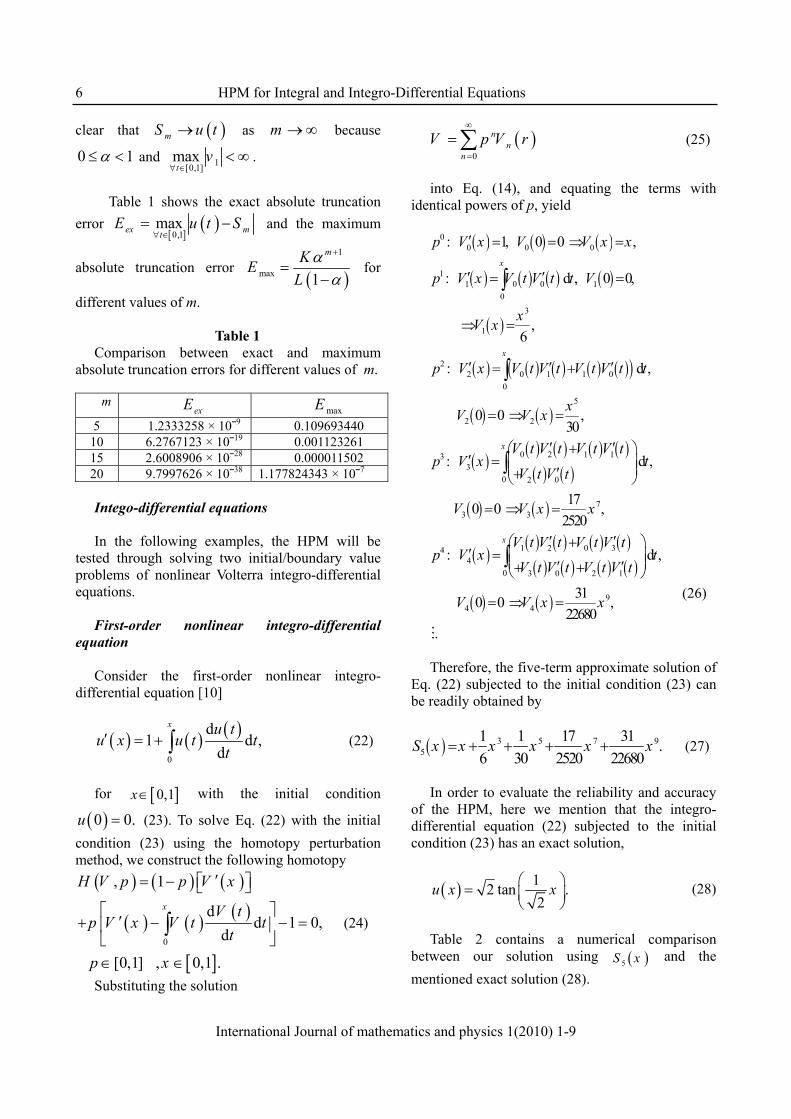
Table 1 shows the exact absolute truncation
error [ ]
( )0,1
maxex mtE u t S
∀ ∈= − and the maximum
absolute truncation error ( )
1
max 1
mKEL
αα
+
=−
for
different values of m.
Table 1 Comparison between exact and maximum
absolute truncation errors for different values of m.
m exE maxE
5 1.2333258 × 10¯9 0.109693440 10 6.2767123 × 10¯19 0.001123261 15 2.6008906 × 10¯28 0.000011502 20 9.7997626 × 10¯38 1.177824343 × 10¯7 Intego-differential equations
In the following examples, the HPM will be
tested through solving two initial/boundary value problems of nonlinear Volterra integro-differential equations.
First-order nonlinear integro-differential
equation Consider the first-order nonlinear integro-
differential equation [10]
( ) ( ) ( )0
d1 d ,
d
x u tu x u t t
t′ = + ∫ (22)
for [ ]0,1x∈ with the initial condition
( )0 0.u = (23). To solve Eq. (22) with the initial condition (23) using the homotopy perturbation method, we construct the following homotopy
( ) ( ) ( )
( ) ( ) ( )
[ ]0
, 1
dd 1 0,
d
[0,1] , 0,1 .
x
H V p p V x
V tp V x V t t
t
p x
′= − ⎡ ⎤⎣ ⎦⎡ ⎤
′+ − − =⎢ ⎥⎣ ⎦∈ ∈
∫ (24)
Substituting the solution
( )0
nn
n
V p V r∞
=
=∑ (25)
into Eq. (14), and equating the terms with
identical powers of p, yield
( ) ( ) ( )
( ) ( ) ( ) ( )
( )
( ) ( ) ( ) ( ) ( )( )
( ) ( )
( )( ) ( ) ( ) ( )( ) ( )
00 0 0
11 0 0 1
03
1
22 0 1 1 0
05
2 2
0 2 1 133
0 2 0
3
: 1, 0 0 ,
: d , 0 0,
,6
: d ,
0 0 ,30
: d ,
x
x
x
p V x V V x x
p V x V t V t t V
xV x
p V x V t V t V t V t t
xV V x
V t V t V t V tp V x t
V t V t
V
′ = = ⇒ =
′ ′= =
⇒ =
′ ′ ′= +
= ⇒ =
′ ′+⎛ ⎞′ = ⎜ ⎟⎜ ⎟′+⎝ ⎠
∫
∫
∫
( ) ( )
( )( ) ( ) ( ) ( )( ) ( ) ( ) ( )
( ) ( )
73
1 2 0 344
0 3 0 2 1
94 4
170 0 ,2520
: d ,
31 0 0 ,22680
.
x
V x x
V t V t V t V tp V x t
V t V t V t V t
V V x x
= ⇒ =
′ ′+⎛ ⎞′ = ⎜ ⎟⎜ ⎟′ ′+ +⎝ ⎠
= ⇒ =
∫
M
(26)
Therefore, the five-term approximate solution of
Eq. (22) subjected to the initial condition (23) can be readily obtained by
( ) 3 5 7 95
1 1 17 31 .6 30 2520 22680
S x x x x x x= + + + + (27)
In order to evaluate the reliability and accuracy
of the HPM, here we mention that the integro-differential equation (22) subjected to the initial condition (23) has an exact solution,
( ) 12 tan .2
u x x⎛ ⎞= ⎜ ⎟⎝ ⎠
(28)
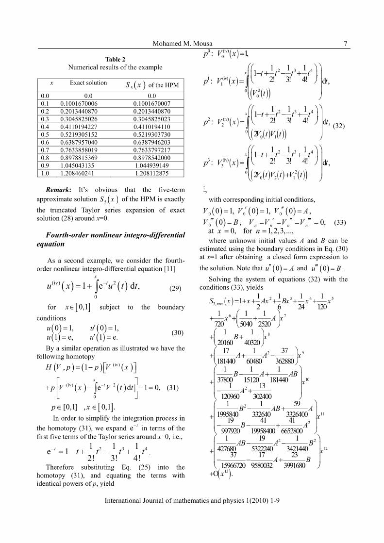
Table 2 contains a numerical comparison
between our solution using ( )5S x and the mentioned exact solution (28).
Mohamed M. Mousa 7
International Journal of mathematics and physics 1(2010) 1-9
Table 2
Numerical results of the example
x Exact solution ( )5S x of the HPM
0.0 0.0 0.0 0.1 0.1001670006 0.1001670007 0.2 0.2013440870 0.2013440870 0.3 0.3045825026 0.3045825023 0.4 0.4110194227 0.4110194110 0.5 0.5219305152 0.5219303730 0.6 0.6387957040 0.6387946203 0.7 0.7633858019 0.7633797217 0.8 0.8978815369 0.8978542000 0.9 1.045043135 1.044939149 1.0 1.208460241 1.208112875
Remark: It’s obvious that the five-term
approximate solution ( )5S x of the HPM is exactly the truncated Taylor series expansion of exact solution (28) around x=0.
Fourth-order nonlinear integro-differential equation
As a second example, we consider the fourth-
order nonlinear integro-differential equation [11]
( ) ( )(iv) 2
0
1 e d ,x
tu x u t t−= + ∫ (29)
for [ ]0,1x∈ subject to the boundary conditions
( ) ( )( ) ( )0 1, 0 1,1 e, 1 e.
u uu u
′= =′= = (30)
By a similar operation as illustrated we have the following homotopy
( ) ( ) ( )
( ) ( )
[ ]
(iv)
(iv) 2
0
, 1
e d 1 0,
[0,1] , 0,1 .
xt
H V p p V x
p V x V t t
p x
−
⎡ ⎤= − ⎣ ⎦⎡ ⎤
+ − − =⎢ ⎥⎣ ⎦∈ ∈
∫ (31)
In order to simplify the integration process in the homotopy (31), we expand e t− in terms of the first five terms of the Taylor series around x=0, i.e.,
2 3 41 1 1e 12! 3! 4!
t t t t t− = − + − + .
Therefore substituting Eq. (25) into the homotopy (31), and equating the terms with identical powers of p, yield
( )
( )( )( )
( )( ) ( )( )
( )( ) ( ) ( )( )
0 (iv)0
2 3 4
1 (iv)1
200
2 3 42 (iv)
20
0 1
2 3 4
3 (iv)3
20 2 1
: 1,
1 1 11 .2! 3! 4!: d ,
1 1 11 .2! 3! 4!: d ,
2
1 1 11 .2! 3! 4!:
2
x
x
p V x
t t t tp V x t
V t
t t t tp V x t
V t V t
t t t tp V x
V t V t V t
=
⎛ ⎞⎛ ⎞− + − +⎜ ⎟⎜ ⎟⎝ ⎠= ⎜ ⎟⎜ ⎟⎝ ⎠⎛ ⎞⎛ ⎞− + − +⎜ ⎟⎜ ⎟⎝ ⎠= ⎜ ⎟⎜ ⎟⎝ ⎠⎛⎛ ⎞− + − +⎜ ⎟⎜⎝ ⎠=
+⎝
∫
∫
0
d ,
,
x
t⎞⎟
⎜ ⎟⎜ ⎟
⎠
∫
M
(32)
with corresponding initial conditions,
( ) ( ) ( )( )
0 0 0
0
0 1, 0 1, 0 ,0 , 0,
at 0, for 1, 2,3,...,n n n n
V V V AV B V V V V
x n
′ ′′= = =′′′ ′ ′′ ′′′= = = = =
= = (33)
where unknown initial values A and B can be estimated using the boundary conditions in Eq. (30) at x=1 after obtaining a closed form expression to the solution. Note that ( )0u A′′ = and ( )0u B′′′ = .
Solving the system of equations (32) with the conditions (33), yields
( ) 2 3 4 5
6 7
8
2 9
10
3,
2
.
2
1 1 1 112 6 24 120
1 1 1 720 5040 2520
1 120160 40320
17 1 37181440 60480 362880
1 1 137800 15120 181440
1 13120960 302400
1 11995840 33
trun x Ax Bx x x
x A x
B x
A A x
B A ABx
B
x
A
S + + + + +
⎛ ⎞+ + +⎜ ⎟⎝ ⎠
⎛ ⎞+ +⎜ ⎟⎝ ⎠⎛ ⎞+ + −⎜ ⎟⎝ ⎠⎛ ⎞− +⎜ ⎟+⎜ ⎟− +⎜ ⎟
⎠
−+
=
⎝
( )
11
2
2 2
12
13
592640 3326400
19 41 41997920 19958400 66528001 19 1
427680 5322240 342144037 17 23
15966720 95800O
32 399 0.
168
AB Ax
B A
AB A Bx
A B
x
⎛ ⎞+⎜ ⎟⎜ ⎟− − +⎜ ⎟⎝ ⎠⎛ ⎞− −⎜ ⎟+⎜ ⎟− − +⎜ ⎟⎝ ⎠+

8 HPM for Integral and Integro-Differential Equations
International Journal of mathematics and physics 1(2010) 1-9
Note that the previous solution is a truncated
formula of the three-term approximate solution ( )3 0 1 2S x V V V= + + . It is interesting to point out that the
approximants , 1, 2,...kS k = serve as approximate solutions of increasing accuracy as k →∞ . It is natural that the accuracy can be enhanced dramatically by evaluating more components, and consequently more approximants. The approximants must therefore satisfy the boundary conditions. By imposing the boundary conditions (30) at x=1 in the full formula of 3S and solving for A and B, we obtain the following and only real solution as an estimation of A and B
1.003793260, 0.9858875713.A B= = (34)
Substituting Eq. (34) into the full formula of 3S
yields an approximate series solution to the problem. The results of the three-term approximate solution 3S are shown in Table 3. In order to evaluate the reliability and accuracy of the HPM, here we mention that the integro-differential equation (29) subjected to the boundary conditions (30) has an exact solution,
( ) e .xu x = (35) Table 3 contains a numerical comparison
between our solution using ( )3S x of the HPM and the mentioned exact solution (35).
Table 3 Numerical results of the example
x Exact solution ( )3S x of the HPM
0.0 1.0 1.0 0.1 1.105171 1.105187 0.2 1.221403 1.221458 0.3 1.349859 1.349964 0.4 1.491825 1.491975 0.5 1.648721 1.648900 0.6 1.822119 1.822301 0.7 2.013753 2.013907 0.8 2.225541 2.225641 0.9 2.459603 2.459639 1.0 2.718282 2.718285
Conclusion
In this paper, the homotopy perturbation method
has been applied to solve nonlinear Volterra integral and integro-differential equations. Numerical results have been presented to show the efficiency of the HPM. From the numerical results it’s clear that the methods provide high accuracy for solving such equations. The convergence theory of the HPM for nonlinear Volterra integral equations has been proved. A clear conclusion can be draw from the numerical results, shown in Tables 1, 2 and 3, that the HPM provides with highly accurate numerical solutions for integral and integro-differential equations as convergent series' with components that are elegantly computed.
References
1. He J.H., Homotopy perturbation technique,
Comput. Methods Appl. Mech. Eng. 178: 257 (1999).
2. He J.H, Application of homotopy perturbation method to nonlinear wave equations, Chaos Solitons and Fractals 26: 695 (2005).
3. Mousa M.M., and Ragab S.F., Application of the homotopy perturbation method to linear and nonlinear schrödinger equations, Z.Naturforsch, J. of Physical Sciences, 63a: 140 (2008).
4. He J.H., An elementary introduction to the homotopy perturbation method, Computers & Mathematics with Applications, 57: 410 (2009).
5. Mousa M.M., and Kaltayev A., Homotopy Perturbation Padé Technique for Constructing Approximate and Exact Solutions of Boussinesq Equations, Applied Mathematical Sciences, 3(22): 1061 (2009).
6. Mousa M.M., and Kaltayev A., Application of the homotopy perturbation method to a magneto-elastico-viscous fluid along a semi-infinite plate, International Journal of Nonlinear Sciences and Numerical Simulation, 10(9): 1113 (2009)
7. Mousa M.M., and Kaltayev A., Application of He’s homotopy perturbation method for solving fractional Fokker–Planck equations, Zeitschrift für Naturforschung A., Journal of Physical Science), 64a: 788 (2009).
8. Yusufoğlu E., Improved homotopy perturbation method for solving Fredholm type integro differential equations, Chaos, Solitons and Fractals 41: 28 (2009).

Mohamed M. Mousa 9
International Journal of mathematics and physics 1(2010) 1-9
9. Andrei D. Polyanin, Alexander V., Handbook
of integral equations, CRC Press, New York, 1998.
10. Avudainayagam A. and Vani C., Wavelet-Galerkin method for integro-differential
equations, Appl. Math. Comput. 32: 247 (2000) 11. Wazwaz A.-M., A reliable algorithm for
solving boundary value problems for higher-order integro-differential equations, Appl. Math. Comput. 118: 327 (2001).
Gfxnghmhjm vgbnjgh

International Journal of mathematics and physics 1 (2010) 10-16
*Corresponding author: E-mail: [email protected] © 2010 al-Farabi Kazakh National University Printed in Kazakhstan
Simulation of Two Phase Filtration in Reservoir with
High Permeable Channel
Assilbekov B.K. Kazakh National University named Al-Farabi, Almaty, Kazakhstan,
Abstract In this work radial drilling technology is modeled and investigated. Distributions of saturation and
pressure for different time are received. Watering of wells with radial channels is estimated.
Introduction
Problems of oil recovery completeness and wells permeability increasing are one of the first priority problems in increasing of recovery profitability and rational using of natural resources of oil deposits especially with low filtration capacitive properties of collectors. Reducing of irretrievable losses in deposits gains in main importance at emaciated deposits which had been exploited long time. Methods of highly remunerative oil production with maximal possible hydrocarbon excavation rate should be based on mutual coupling of closed hydrodynamic system, which consist on following units: oil seam – extracting well – recovery and preparation system – system of seam pressure maintenance (SPM) – injection well – oil seam. At this time development of new methods and technology for oil recovery growth is a base for improvement efficiency of hydrodynamic system work.
One of the modern ways to increase oil recovery is a radial drilling technology. At radial drilling channels with high permeability are constructed for oil recovery from high thickness reservoir with low filtration capacitive properties. Radial drilling is a method of horizontal high permeability channel creation on basis of using modified technology of flexible pump-compressor pipe [1]. Lateral holes with diameter 50mm are drilled at distance 150m from borehole under high pressure. Radial holes could be drilled at several levels.
Advantages of radial drilling technology [1]: increasing of well production and
recoverable reserves of low production wells; allow to make directed well treatment for
example by acid and etc.; improvement of water supply rates in
injection wells;
allow multilayer using in zones with big seam thickness;
decelerate process of bottom water coning. Investigation of bottom water influence in
bottom hole zone is of important practical interest. This problem is known at oil deposits exploitation by vertical and horizontal wells [2-7].
In present paper motion of bottom water in a low conductivity reservoir with high permeable channel is investigated, i.e. how and how fast bottom water reaches to high permeable collector depending on capability of seam and reservoir fluids. Elaboration of mathematical model of fluid filtration in the layer with high-permeability channel and calculations presents practical meaning for definition of radial drilling efficiency and estimation of flow rate to high permeable channel.
Filtration of fluid in reservoir could be described with a model of cracked-porous medium by representing channel with high permeability as a crack [8]. However for this model it is necessary to solve system of filtration equations in crack and porous block with satisfaction of conjugate condition on medium‘s division boundary [8]. Problem formulation and solution is complicated for this model in case of two phase fluid filtration.
Approach based on conception of interpenetrating continuums is simpler [9, 10]. In this case two phase fluid filtration in porous block with high permeable channel is described from a uniform position.
Mathematical model
As it shown above in practice kickoff of
horizontal lateral borehole is made by drilling hole with diameter 0.05m and length till 150m. Direct simulation of lateral borehole is possible by 3D modeling and required good computer resources.
Simulation of Two Phase Filtration in Reservoir 11
International Journal of mathematics and physics 1 (2010) 10-16
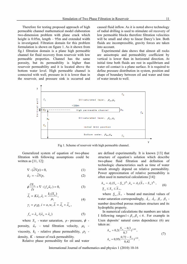
Therefore for testing proposed approach of high
permeable channel mathematical model elaboration two-dimension problem with plane crack which height is 0.05m, length – 95m and extended width is investigated. Filtration domain for this problem formulation is shown on figure 1. As it shown from fig.1 filtration domain is a plane high permeable channel for fluid recovery from reservoir with low permeable properties. Channel has the same porosity, but its permeability is higher than reservoir permeability and it is located above the bottom water level. High permeable channel is connected with well, pressure in it is lower than in the reservoir, and pressure sink is occurred and
caused fluid inflow. As it is noted above technology of radial drilling is used to stimulate oil recovery of low permeable blocks therefore filtration velocities will be small and obey to linear Darcy’s law. Both fluids are incompressible, gravity forces are taken into account.
Experimental data shows that almost all rocks are anisotropic and permeability coefficient by vertical is lower than in horizontal direction. At initial time both fluids are rest in equilibrium and water oil contact is a plane surface. It is required to define pressure distribution in system, position and shape of boundary between oil and water and time of water inrush to well.
Fig 1. Scheme of reservoir with high permeable channel.
Generalized system of equation of two-phase
filtration with following assumptions could be written as [11, 12]:
,0)~( =∇⋅∇ pλ (1)
,~ puT ∇−= λr
(2)
,0)( =⋅∇+∂∂
Tww uft
S rφ (3)
,~~~,,,
,)(,~
woii
i
wiiii
woig
SkK
λλλργ
μλλλ
+===
== (4)
)/( owwwf λλλ += (5)
where wS - water saturation, p - pressure, φ - porosity, Tur - total filtration velocity, iμ - viscosity, ik - relative phase permeability, iρ - density, K - tensor of rock permeability.
Relative phase permeability for oil and water
are defined experimentally. It is known [13] that structure of equation’s solution which describe two-phase fluid filtration and definition of technologic characteristics such as time of water inrush strongly depend on relative permeability. Power approximation of relative permeability is often used in numerical calculations [14]:
,
,)(,)( 212o1w
www
wwww
SSS
SSAkSSAk
≤≤
−=−= ββ
(6)
where ww SS , - bound and maximal values of water saturation correspondingly, 1À , 2À , 1β , 2β - number described porous medium structure and its hydrophilic property.
In numerical calculations the numbers are taken I following ranges 4,1 21 << ββ . For example in Uzen deposits’ natural cores dependence (6) are taken as:
.)42,0
72,0(95,0
,)7,0
3,0(2,0
95,1o
85,2w
w
w
Sk
Sk
−=
−=
(7)

12 Assilbekov B.K.
International Journal of mathematics and physics 1 (2010) 10-16
Boundary condition for pressure: at roof and bottom – no cross-flow condition, at well – well production or pressure constancy (bottom hole pressure), far away from well – pressure constancy (contour pressure); and for saturation: on bottom – constancy, in another parts – zero normal derivative.
System of equations (1)-(3) is solved with following initial and boundary conditions:
⎪⎩
⎪⎨⎧
≤<≤≤
=hzhïðèS
hzïðèSzyS
ww
www ,
0,)0,,( , (8)
,whzw SSw=
= (9)
0=∂∂
=Ly
w
yS
, (10)
,,0
ohz
wz z
pzp γγ −=
∂∂
−=∂∂
==
(11)
⎪⎪
⎩
⎪⎪
⎨
⎧
=∂∂
=∇
=
+
−=∫
otherwiseyp
wellinqdzp
y
rh
rhy
d
d
,0
,~
0
0
0
0
λ, (12)
0pp Ly ==
, (13)
Thereby generalized equation system (1)-(5) with
initial and boundary condition (8)-(13) is used to describe two immiscible fluids filtration in porous seam with high permeable channel. Proposed common approach allows constructing efficient numerical algorithm with automatic satisfaction of conjugate condition at medium interface.
Numerical methods
For numerical implementation of equation’s system (1)-(11) computational grid which allow to visual demonstrate each cell as volume’s element are taken [15, 16]. Pressure equation (1) is solved by implicit method of alternating directions [17]. Saturation is calculated by explicit upstream scheme. Distribution the pressure field is calculated from equation (1) by known initial pressure. The velocity field is obtained from equation (2) using defined pressure fields, saturation distribution is obtained from equation (3).
Calculation of water coning process in bottom hole zone of vertical well are led for mathematical model of two phase fluid filtration and numerical method approbation. Calculations are led for comparison with similar results of other authors [5]. However direct maintenance of all regime parameters (structural, seam, hydrodynamic, thermal) and reservoir fluids and rock properties in calculations are impossible because of shortage of published data in paper [5].
Pressure, saturation and velocity fields at different time have been obtained. Comparison of numerical results by definition of water saturation distribution with data from paper [5] is shown in figure 2. Results are obtained for seven variants of empirical dependences of relative permeability, i.e. power of 1β , 2β in dependence (6) were varied in calculations.
where h - thickness of layer, wh - thickness of water-saturated layer, ww SS , - upper and lower
limit of water saturation, 02r - height of high permeable channel, q - rate of liquid picked up at
section 0=y (in well), dh - position of high permeable channel in vertical section, L - length of oil reservoir.

12 Assilbekov B.K.
International Journal of mathematics and physics 1 (2010) 10-16
Fig. 2. Comparison of numerical results with similar data: upper – author’s calculation, lower – data’s from [5].
It is shown that qualitative coincidence is obvious from figure 2. Quantitative difference is explained by
disagreement of regime’s parameters and conditions [5].
Results and discussions Investigation of mathematical model and method of two phase filtration solution of mixable liquids is carried out
in [6, 7]. The influence of seam and reservoir fluids characteristics on oil recovery process at deposits exploited by horizontal and inclined wells are studied there numerically.
Seam anisotropy is important geologic characteristic which has big influence on deposit’s exploitation. Influence of seam anisotropy rate on oil recovery dynamic at deposit exploitation by vertical well is considered in paper [6]. Effects of anisotropy ratio on horizontal well watering are studied in [7]. Values of vertical permeability to horizontal one [6, 7] are varied in the range from 0.01 to 1.0. Analysis of results [6, 7] shows that increasing of seam anisotropy rate lead to growth of oil recovery and reduction of well watering.
Influence of seam anisotropy rate on exploitation parameters is studied by proposed model and comparison of calculation results with known ones are led. This problem is described interaction between ground water motion and oil recovery from sandstones and has big practical meaning in connection with ubiquitous spreading of groundwater near oil-saturated rock.
Calculation are led for following seam size: length of oil reservoir – 100m, thickness – 30m, length of high permeable collector – 95m, height – 0.05m. Following parameters of seam and formation fluid have big influence on bottom water moving: 1−= hvvh kkk - anisotropy ratio.
Calculation results for different values of anisotropy rate vhk
with the values of seam and
collector permeability =chk 50, well production q =
10m3/day, mobility ratio =μ 0.07 in all cases are shown at fig. 3-7. Watering is an important integral characteristic of process (watering is water portion in extracted fluid at 0=y section). Influence of seam anisotropy rate on watering is shown at figure 3.
Fig 3. Influence of anisotropy rate on watering.
It is shown from figure 3 that with reducing of
seam anisotropy ratio bottom water moves quickly to high permeability collector and have bad influence to oil recovery. Water breaks to high
Time, days
Wat
er C
ut, f
ract
ion
13
14 Assilbekov B.K.
International Journal of mathematics and physics 1 (2010) 10-16
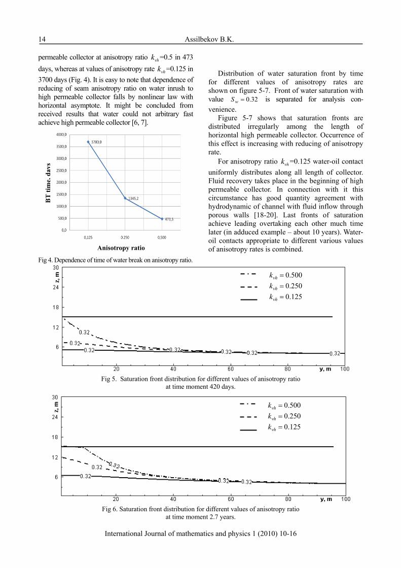
permeable collector at anisotropy ratio vhk =0.5 in 473 days, whereas at values of anisotropy rate vhk =0.125 in 3700 days (Fig. 4). It is easy to note that dependence of reducing of seam anisotropy ratio on water inrush to high permeable collector falls by nonlinear law with horizontal asymptote. It might be concluded from received results that water could not arbitrary fast achieve high permeable collector [6, 7].
Fig 4. Dependence of time of water break on anisotropy ratio.
Distribution of water saturation front by time
for different values of anisotropy rates are shown on figure 5-7. Front of water saturation with value 32.0=wS is separated for analysis con- venience.
Figure 5-7 shows that saturation fronts are distributed irregularly among the length of horizontal high permeable collector. Occurrence of this effect is increasing with reducing of anisotropy rate.
For anisotropy ratio vhk =0.125 water-oil contact uniformly distributes along all length of collector. Fluid recovery takes place in the beginning of high permeable collector. In connection with it this circumstance has good quantity agreement with hydrodynamic of channel with fluid inflow through porous walls [18-20]. Last fronts of saturation achieve leading overtaking each other much time later (in adduced example – about 10 years). Water-oil contacts appropriate to different various values of anisotropy rates is combined.
Fig 5. Saturation front distribution for different values of anisotropy ratio
at time moment 420 days.
Fig 6. Saturation front distribution for different values of anisotropy ratio
at time moment 2.7 years.
Anisotropy ratio
BT
time,
day
s
500.0=vhk250.0=vhk125.0=vhk
500.0=vhk250.0=vhk125.0=vhk

Simulation of Two Phase Filtration in Reservoir 15
International Journal of mathematics and physics 1 (2010) 10-16
Fig 7. Saturation front distribution for different values of anisotropy ratio
at time moment 10.2 years.
Conclusions
Thereby water front with saturation value 32.0=S
moving for three vhk
values by time
shows that reducing of anisotropy rate results in quicker watering of high permeable collector. It is also notably from watering dependence on time of
water breakthrough for different vhk
values. Saturation front had reached high permeable collector the faster at low values of seam anisotropy rate. Physically it could be easy explained.
Reducing of anisotropy rate caused increasing
of vertical seam permeability therefore water-oil surface front faster reach high permeable collector. For example at anisotropy rate vhk =0.5 time of water inrush is equal to 473 days, whereas at vhk =0.125 time of water inrush is equal to 3700 days. It is to be noted that dependence of time of water breakthrough on seam anisotropy rate is nonlinear with horizontal asymptote. Well watering is changed similarly, i.e. well watering is increasing as seam anisotropy reduces. The influence of seam anisotropy rate on well exploitation characteristics could be seen from following result: at value vhk =0.5 watering of production achieves 75% whereas at vhk =0.125 watering is raised to 40% in 7000 days.
References
1. http://www.radialdrilling.com/technology.htm. 2. Letkeman J.P., Ridings R.L. A Numerical
Coning Model, Soc. Petrol. Eng. Journal, 9(4): 418(1970).
3. Spivak A., Coats K.H. Numerical Simulation of Coning Using Implicit Production Terms,Trans. SPE of AIME, 249:257(1970), (SPEJ)
4. Inikori S.O. Numerical Study of Water Coning Control with Downhole Water Sink (DWS) Well Completions in Vertical and Horizontal Wells, PhD Dissertation, Louisiana State University, 2002, 227p.
5. Hernandez J.C. Oil Bypassing by Water Invasion to Wells: Mechanisms And Remediation. Ph.D. Dissertation in the Department of Petroleum Engineering, 2007, 217p.
6. Oghena А. Quantification of uncertainties associated with reservoir performance simulation. Ph.D. Dissertation in petroleum engineering. Texas Technical University, 2007, 225p.
7. Ali Abbas H. A parametric study of water-coning in horizontal wells. In partial fulfillment of the requirements for the Degree of Master of Science in Petroleum Engineering, 1994, 226p.
8. Barenblat G.I., Entov V.М., Ryzhik V.М. Theory of oil and gas flows in natural layer. M.: Nedra, 1984, 210 (In Russian)
9. Rakhmatullin H.А. Hydrodynamic basics of interpenetrating flows of incompressibility medium, Applied Mathematics and Mechanics. 2:184 (1956)(In Russian)
10. Nigmatullin R.I. Dynamics of multiphase medium. М.: Nauka. 1987.(In Russian)
11. Aziz K., Settari A. Petroleum reservoir simulation. М.: Nedra, 1982, 416p.
500.0=vhk250.0=vhk125.0=vhk
16 Assilbekov B.K.
International Journal of mathematics and physics 1 (2010) 10-16
12. Assilbekov B., Zhapbasbayev U.К., Оgai
Е.К. Investigation of water coning in oil-saturated layer. Scientific-Technical Journal of Oil and Gas. Almaty. 5(47):49(2008) (In Russian)
13. Konovalov А.N. Problems of filtration of incompressibility multiphase flows. Novosibirsk. Nauka, 1988, 165 (In Russian)
14. Alishayev М.G., Rosenderg М.D., Teslyuk Е.V. Nonisothermal filtration on oil exploitation. М.: Nedra, 1985, 271p. (In Russian)
15. Rouch P. Computational hydrodynamics: Trans. from eng. М.: Mir, 1980, 616 p.
16. Belocerkovsky О.М. Numerical modeling in mechanics of continuum media. М.: Nauka, 1984, 519p. (In Russian)
17. Chung T.J. Computational Fluid Dynamics:
Cambridge University Press, 2002, 787p. 18. Meerovich I.G., Muchnik G.F. Hydrodynamics
of reservoir system. М.: Nauka, 1986, 274p. (In Russian)
19. Nazarov А.S., Dilman V.V., Sergeev S.P. Experimental investigation of turbulent flows of incompressibility fluids in channels with permeable wall. Theoretical basis of chemical technology. 15(4):561(1981) (In Russian)
20. Idelchik I.Е. Aerodynamics of technological apparatus: feed and pipe-bend and distribution of flows by cross section of apparatus. М.: Mashinostroenie. 1983, 351p. (In Russian).
HKDFUDK CFHXFDGJD

International Journal of mathematics and physics 1 (2010) 17-27
*Corresponding author: E-mail: [email protected] © 2010 al-Farabi Kazakh National University Printed in Kazakhstan
Optimal Control of the Nonlinear Parabolic Equations without
Differentiability of the Control-State Mapping
Simon Serovajsky al-Faraby Kazakh National University, Mechanics and Mathematics Faculty,
Masanchi st. 39/47, Almaty, Kazakhstan, 500012
Abstract We consider the optimal control problem for the system described by nonlinear parabolic equation. The
control is distributed, boundary and initial. The observation is distributed, boundary and final. The control-state mapping is not Gataux differentiable in general case. This property embarrasses the direct using of the standard optimization methods, in particular, the searching of the minimizing functional derivative. However, this dependence is extended differentiable. This result is sufficient for the obtaining the necessary conditions of optimality.
Introduction
Problem Statement
The qualitative and numeric optimization methods require as a rule the differentiability of the minimizing functionals. The direct calculation of its derivatives uses the differentiation of the control-state mapping. The substantiation of this property for nonlinear infinite dimensional systems is a nontrivial problem. Moreover, control-state mapping is often not differentiable. This difficulty can arise without any nonsmooth terms in the functional and the state operator. Therefore the well-known methods of nonsmooth analysis using subgradient, Clarke derivative, etc. (see for example, [1], [2]) or smooth approximation methods (see for example, [3]) are not applicable in this case.
We consider the optimal control problem for systems described by nonlinear parabolic equations. Such problems are well known (see for example, [3] – [14]). However those results use additional limitations in order to guarantee of the existence of the corresponding derivatives. The control-state mapping for our system is not Gataux differentiable if the dimension of the set and the parameter of the nonlinearity are large enough. Therefore the known optimization methods are not applicable in this case. However the optimal control problem is solvable without any restrictions. We have analyzed this problem for the general case using the extended operator derivative. It was applied earlier for nonlinear stationary systems (see [15], [16]).
Let Ω be an opened bounded set from Rn with a smooth boundary Г, 0,T > (0, ),Q T= Ω×
(0, ).TΣ = Γ× We consider the equation
0, 1
, ( , )n
ij Q Qi j i j
y ya a y y y f v x t Qt x x
ρ
=
⎛ ⎞∂ ∂ ∂− + + = + ∈⎜ ⎟⎜ ⎟∂ ∂ ∂⎝ ⎠∑ (1)
with boundary conditions
, ( , ) ,y f v x tν Σ Σ∂
= + ∈Σ∂
(2)
( ,0) , .y x f v xΩ Ω= + ∈Ω (3)
Here the parameter of nonlinearity ρ is positive.
The coefficients of the equation satisfy the inclusions 1( ),ija C∈ Ω 0 ( )a C∈ Ω and the inequalities
2
0, 1
( ) R , ( ) , ,n
nij i j
i j
a x a x xξ ξ α ξ ξ α=
≥ ∀ ∈ ≥ ∈Ω∑
where 0.α > Besides we suppose, that 2 ( ),Sf L S∈ ,S ∈Λ where , , .QΛ = Σ Ω The
conormal derivative is determined by the standard equality
, 1cos( , ),
n
ij ji j j
y ya n xxν =
∂ ∂=∂ ∂∑
where cos( , )jn x is the corresponding cosine of the exterior normal direction n to the surface Г. The point *( , )v v vΩ= with * ( , )Qv v vΣ= is a
control. It is included in the space 2* ( ),V V L= × Ω where 2 2* ( ) ( )V L Q L= × Σ . We determine the spaces
1
1 ( ),X H= Ω 2 ,( )qX L= Ω 1 2 ,X X X= ∩
18 Optimal Control of the Nonlinear Parabolic Equations
International Journal of mathematics and physics 1(2010) 17-27
1 2 1 ,(0, ; )W L T X= 2 2 ,(0, ; )qW L T X=
1 2 ,W W W∩=
, ,Y W Wϕ ϕ ϕ′ ′= ∈ ∈
where 2,q ρ= + / .tϕ ϕ′ = ∂ ∂ Let the linear continuous operator 1 1 1:A X X ′→ and the bilinear continuous form Ψ on 1X be determined by the equality
1 0 1, 1
, ( , ) , . n
iji j j i
A a a d Xx xϕ λϕ λ ϕ λ ϕλ ϕ λ
=Ω
⎛ ⎞∂ ∂= Ψ = + Ω ∀ ∈⎜ ⎟⎜ ⎟∂ ∂⎝ ⎠
∑∫
Here ,μ λ is the value of the linear
continuous functional μ in the point λ. Let operator 2 2 2:A X X ′→ be determined by the formula
2 2.A Xρϕ ϕ ϕ ϕ= ∀ ∈
We determine also the operator :A X X ′→ by
1 2.A A A= + Let the point 1*f W ′∈ satisfies the equality
10
*( ), ( ) . T
f t t dt f dQ f d Wλ λ λ λΣΣ
= + Σ ∀ ∈∫ ∫ ∫
The linear continuous operator 1*:B V W ′→ is determined by the equality
10
( ), ( ) . T
Bv t t dt v dQ v d Wλ λ λ λΣΣ
= + Σ ∀ ∈∫ ∫ ∫
It is obvious that the boundary problem (1) – (3) can be transformed into the evolutional equation
* *( ) ( ) ( ) ( ), (0, )y t Ay t Bv t f t t T′ + = + ∈ (4)
with the initial condition 0 0(0)y f v= + , (5) where ( )y t is a function ( , )y y x t= with a fixed value of t. Here the operator А is continuous and satisfies the inequality
11 21* 2* 1 2
,q
XA A A c Xϕ ϕ ϕ ϕ ϕ ϕ−
′≤ + ≤ + ∀ ∈
where s
ϕ and *s
ϕ are the norms of the
spaces sX and ,sX ′ 1, 2.s =
Besides, the following inequality is true
( )20
, 1
2
1 2
,
( ) ( ) ( ) ( )
, .
n
i ji j i j
q
A A
a a d x d xx x
X
ρ ρ
ϕ ψ ϕ ψ
ϕ ψ ϕ ψ ϕ ψ ϕ ϕ ψ ψ ϕ ψ
ϕ ψ ϕ ψ ϕ ψα
= ΩΩ
− − =
⎡ ⎤∂ − ∂ −= + − + − −⎢ ⎥
∂ ∂⎢ ⎥⎣ ⎦
− + − ∀ ∈
≥
≥
∑∫ ∫
So this operator is monotone. We have also
2 20 1 2
, 1
, . n
q qij
i j i j
A a a d d Xx xϕ ϕϕ ϕ ϕ ϕ ϕ ϕ ϕα
=Ω Ω
⎛ ⎞∂ ∂= + Ω+ Ω + ∀ ∈⎜ ⎟⎜ ⎟∂ ∂⎝ ⎠
≥∑∫ ∫
Then we get
2
1 2
1 2
, .
q
X
AX
α ϕ ϕϕ ϕϕ
ϕ ϕ ϕ
+∈
+≥ ∀
Let .
Xϕ →∞ Then the norm of ϕ in one of
the composite of the space Х at least converges to infinity. So we obtain
1, .
XAϕ ϕ ϕ − →∞
Therefore the operator А is coercitive. So we
conclude that the boundary problem (1) – (3) has

Simon Serovajsky 19
International Journal of mathematics and physics 1(2010) 17-27
the unique solution [ ]y y v= from the space Y for all v V∈ by the monotone operators’ theory (see [17], Capture 2, Theorem 1.2). Besides, the
mapping [ ] :y V Y⋅ → is weak continuous. We determine the cost functional
( )22( ) ( ) [ ] ,
2 2S S
S S SS S S
I v v dS y v y dSχ θ γ∈Λ
⎡ ⎤= + −⎢ ⎥
⎣ ⎦∑ ∫ ∫
where 0,Sχ > 0,Sθ ≥ 2 ( )S L Sy ∈ , Q
γ is the unit
operator, γΣ is the trace operator of the function
determined on the set Q to the surface Σ, and γΩ
characterizes the value of this function for 0.t = Let SU be a nonempty convex closed subset of the space 2 ( ),L S S ∈Λ , and .QU U U UΣ Ω= × × We have the following optimal control problem: (Р) Minimize ( )I v for all .v U∈
The operators S
γ are continuous according the
trace theorem and continuity of the inclusion of the state functional is weak lower semicontinuous according the weak continuity of the mapping
[ ] :y V Y⋅ → . Then the problem (Р) is solvable (see for
example, [2], Capture II, Proposition 1.2).
Differentiation of the control-state mapping
The necessary condition for the optimality for Gataux differentiable functional I in the point u on the convex set U is the variational inequality (see for example, [19], Capture 1, Theorem 1.3)
( ), 0 .I u v u v U′ − ≥ ∀ ∈ (6)
The direct finding of the functional derivative for the problem (Р) requires the differentiability of the mapping [ ] :y V Y⋅ → at this point. However
we have the following proposition. Theorem 1. The mapping [ ] :y V Y⋅ → is not
Gataux differentiable for enough large values of ρ and n.
Proof. Let у be a continuous function on the closure of Q including the space 2,1( )H Q of functions, which are the elements of 2 ( )L Q with first time derivative and all second order special derivatives. Then the left side of the corresponding equality (1) includes in the space 2 ( )L Q . Let function Qv satisfies (1) with chosen function у. It is obvious that the conormal derivative of у on the surface Σ is a point of 2 ( ),L Σ and the value of у for
0t = is the element of the space 2 ( ).L Ω We determine the functions vΣ and vΩ , which satisfy the equalities (2) and (3) for this function у. Then
( ), ,Qv v v vΣ Ω= is included in the space V, besides
[ ].y y v= We suppose now that the mapping [ ] :y V Y⋅ →
is Gataux differentiable in the indicated point v. Then there exists a linear continuous operator
: ,D V Y→ such as ( ) /y y Dhσ σ− → in Y if 0σ → for all ( , , )Qh h h h VΣ Ω= ∈ , where
[ ].y y v hσ σ= + Using equality (1) for the control v and v hσ+ we get the equality
0, 1
( ) ( ) ( ) , ( , )n
i j Qi j i j
y y y ya a y y y y y y h x t Qt x x
σ σσ σ σ
ρ ρ σ=
⎡ ⎤∂ − ∂ −∂− + − + − = ∈⎢ ⎥
∂ ∂ ∂⎢ ⎥⎣ ⎦∑
We have the following convergence by the
supposition of the control-state mapping differentiability
( )1 y y Dht t
σ
σ∂ − ∂
→∂ ∂
in ,W ′
( )1ij ij
i j i j
y y Dha ax x x x
σ
σ⎡ ⎤ ⎛ ⎞∂ −∂ ∂ ∂
→ ⎜ ⎟⎢ ⎥ ⎜ ⎟∂ ∂ ∂ ∂⎢ ⎥⎣ ⎦ ⎝ ⎠ in 1W ′ .
Let us determine the superposition L of the
operator 1 : ( ) ( ),q qL L Q L Q′→ such as 1L y y yρ= ,
and the mapping [ ] :y V Y⋅ → . The first operator is

20 Optimal Control of the Nonlinear Parabolic Equations
International Journal of mathematics and physics 1(2010) 17-27
obviously Frechet differentiable, and the second one is Gataux differentiable by Gataux differentiability of the control-state mapping. Then the operator L is Gataux differentiable by
Compodite Function Theorem, besides
( )1( ) [ ] .L v L y v Dh′ ′= Therefore we get the
following convergence in the norm of ( )qL Q′
0 0
( )lim lim ( 1) .y y y yL v h Lv y Dhρσ σ
σ σ
ρ ρσ ρσ σ→ →
−+ −= = +
So we divide the previous equality into number σ. We obtain after the passing to a limit
0, 1
( 1) , ( , ) .n
ij Qi j i j
Dh Dha a Dh y Dh h x t Qt x x
ρρ=
⎛ ⎞∂ ∂ ∂− + + + = ∈⎜ ⎟⎜ ⎟∂ ∂ ∂⎝ ⎠∑
The following equalities are obtained similarly by the boundary conditions (2) and (3)
, ( , ) ,Dh h x tν Σ
∂= ∈Σ
∂ ( ,0) , .Dh x h xΩ= ∈Ω
Hence the boundary problem
0, 1
( 1) , ( , ) ,n
ij Qi j i j
z za a z y z h x t Qt x x
ρρ=
⎛ ⎞∂ ∂ ∂− + + + = ∈⎜ ⎟⎜ ⎟∂ ∂ ∂⎝ ⎠∑ (7)
, ( , ) ,z h x tν Σ∂
= ∈Σ∂
(8)
( ,0) ,z x h xΩ= ∈Ω (9)
has the solution z Dh= from the space Y for all
h V∈ . Its uniqueness is obvious. Let's choose the parameters ρ and n so large,
that the embedding 2,1( ) ( )qH Q L Q⊂ is broken.
Then there will be a point 0z from the set 2,1( ) \ ( ).qH Q L Q
We determine ( )0 0 0 0, ,Qh h h hΣ Ω= from V such as
0 0
0 0 00
, 1( 1) , ( , ) ,
n
Q iji j i j
z zh a a z y z x t Qt x x
ρρ=
⎛ ⎞∂ ∂ ∂= − + + + ∈⎜ ⎟⎜ ⎟∂ ∂ ∂⎝ ⎠
∑
00 , ( , ) ,zh x t
νΣ∂
= ∈Σ∂
0 0 ( ,0), .h z x xΩ = ∈Ω
Then the solution z of the boundary problem (7)
– (9) coincides with 0z for 0h h= . So it is not included in the space ( ).qL Q Yet we stated earlier,
that the solution of this problem is included in the space Y, which is the subset of ( ).qL Q This contradiction completes the proof.
The last result prohibits directly obtaining the necessary conditions of optimality such as (6). It rules out the use of the known methods for the optimal control problems described by the nonlinear parabolic equations (see in particular, [3] – [14]). Therefore the values of the parameter of nonlinearity and the dimension of the set were limited for overcoming the mentioned difficulty in the cited results (see for example, [3], Chapter IV, Theorem 2.6; [7], Chapter 1, Theorem 3.2; [12], Chapter 2, Theorem 8.1).
However, our optimal control problem has the solution for all values of these parameters. Therefore we would like to analyze this problem without any additional restrictions. Of course, those difficulties can be overcome by using better V spaces for the control variables, such that the state becomes an element of ( )L Q∞ (see for example, [20] for the elliptic case). But if we improve properties of the control, we will constrict the class of solvable problems. We must particularly improve properties of the absolute terms in the equation and the boundary conditions and to raise the regularity of the set. Besides, our state functional becomes not
Simon Serovajsky 21
International Journal of mathematics and physics 1(2010) 17-27
coercive. However this property was used for the proof of the existence of the optimal control. So we must raise the regularity of the state functional. Besides, we prefer to solve our problem with the most natural spaces for a given equation. It is the corollary from most simple a priory estimates.
Thus the problem statement without the changed control space is wider and more natural. We will analyze it by means of a property, which can be interpreted as the special form of differentiability.
Definition (see [15], [16]). Let L be an operator from V into Y, and there
exists the linear topologic spaces V0, Y0, V∗, Y∗ with continuous embeddings
0 0* *, V V V Y Y Y⊂ ⊂ ⊂ ⊂ , and the linear continuous operator D : V0 → Y0 such as
( )L v h Lv Dhσ
σ+ − → in Y∗
for all h∈V∗ if σ→0. Let’s name our operator
(V0,Y0;V∗,Y∗)-extended differentiable in the point .v V∈
It is obvious that the (V,Y;V,Y)-extended derivative is equal to the usual Gataux one. We shall prove that the mapping [ ] :y V Y⋅ → for the problem (1) – (3) is extended differentiable in the arbitrary point v V∈ for all values of ρ and n. We determine the space
/ 20 1 2, [ ] .( )W W y v L Qρϕ ϕ ϕ= ∈ ∈
It is a Hilbert space with the scalar product
( ) ( ) ( )0 1 2
/ 2 / 2
( ), , ( 1) [ ] , [ ] .W W L Q
y v y vρ ρϕ λ θ ϕ λ ρ ϕ λ= + +
Its conjugate space is
0 1 2/ 2 .[ ] , ( )W W Ly v Qρ ϕ λ ϕλ′ ′= ∈ ∈+
Let’s determine also the space
0 0 0| , .Y W Wϕ ϕ ϕ′ ′= ∈ ∈
Theorem 2. The mapping [ ] :y V Y⋅ → for the
boundary problem (1) – (3) has the ( )0 1, ; ,V Y V W -
extended derivative D in the arbitrary point ,v V∈ such as
( )
( ) ( )
0
0 20
*
* *
( ), ( ) , ( )
, [ ](0) ( ), [ ]( ) , ( , ) ( ) ,
T
T
t Dh t dt Dh T
h p Bh t p t dt v V W L
μ μ
μ μ μ μ μ
Ω
Ω Ω
+ =
′= + ∀ ∈ = ∈ × Ω
∫
∫ (10)
where [ ]p μ is the solution of the problem
1*
*[ ]( ) [ ]( ) ( 1) [ ]( ) [ ]( ) ( ), (0, ),p t A p t y v t p t t t Tρμ μ ρ μ μ′− + + + = ∈ (11)
[ ]( )p Tμ μΩ= . (12)
Besides, we have the convergence
[ ] [ ]S SS
y v h y v Dhγ σ γ γσ
+ −→ in 2 ( ),L S S ∈Λ
(13)
for all h V∈ , if 0σ → .
Proof. Let *( , ) ( , , )Qh h h h h hΩ Σ Ω= ≡ be an arbitrary point of the space V, and σ is some number. Then the function [ ] [ ]y v h y vση σ= + − satisfies the equalities
1 2 *( ) ( ) ( ) ( ), (0, ),t A t A t Bh t t Tσ σ σ ση η η σ′ + + = ∈
(14)
0(0) hση σ= , (15)

22 Optimal Control of the Nonlinear Parabolic Equations
International Journal of mathematics and physics 1(2010) 17-27
where
( )22 ,( ) ( 1) [ ] [ ] [ ]A g y v y v h y vσ σ
ρη η ρ ε σ η= ≡ + + + −
[0,1].ε ∈
Let’s determine the space
1 2, .( )W W Lg Qσ σϕ ϕϕ= ∈ ∈
It is Hilbert space with the scalar product
( ) ( ) ( )1 2 ( ), , , .W W L Qg g
σ σ σϕ λ α ϕ λ ϕ λ= +
Its conjugate space is determined by
1 2 ., ( )W W Lg Qσ σϕ λ ϕλ′ ′= ∈ ∈+
We determine also the space
| , .Y W Wσ σ σϕ ϕ ϕ′ ′= ∈ ∈
It coincides with the space 0Y for 0σ = . It is obviously, that the inclusion 1 1A Wση ′∈
and the equality 2A gσ σ ση ϕ= are true, where gσ σϕ η= is a point of the space 2 ( )L Q . Hence
the derivative
1 2 *A A Bhσ σ σ ση η η σ′ = − − + ,
described by the equality (14), includes to the space Wσ′ . Then we obtain the equality
[ ]
( ) ( )
20
0 *0
( ), ( ) ( ), ( ) ,
( ), ( ) , (0) ( ), ( )
( ) ( ) ( )T
T
t t t t A dt
T T h Bh t t dt Y
t t tσ σ σ
σ σ
σλ η η λ η λ
η λ σ λ σ λ λ
′− +Ψ + +
+ = + ∀ ∈
∫
∫ (16)
by (14) and (15) according Green formula and
the integration by parts. Here ( , )ϕ ψ is the scalar product of 2 ( )L Ω .
We consider the following Cauchy problem for the linear evolution equation
*( ) ( ) ( ) ( ), (0, ),p t L t p t t t Tσ μ′− + = ∈ (17)
( ) ,p T μΩ= (18)
where the linear continuous operator ( )L tσ is
determined by
*1 2( ) ( ).L t A A tσ σ= +
We obtain the problem (11), (12) for 0σ = . We have the inequality
( )
*1 2
0 0 0
22 22
1
( ) ( ), ( ) ( ), ( ) ( ) ( ), ( )
.
T T T
n
i iQ QW
L t p t p t dt A p t p t dt A t p t p t dt
p p dQ g p dQ px σ
σ σ
σα=
= + ≥
⎡ ⎤⎛ ⎞∂⎢ ⎥≥ + + =⎜ ⎟∂⎢ ⎥⎝ ⎠⎣ ⎦
∫ ∫ ∫
∑∫ ∫ (19)
Then we obtain that the problem (17), (18) is
uniquely solvable in the space Yσ for all values ,h V∈ number σ, and pair *( , )μ μ μΩ= from the
space 2 ( )W Lσ′ × Ω according to the standard linear evolution equations theory in the Hilbert spaces (see for example, [19], Capture 3, Theorem 1.2). Let’s denote this solution as [ ].pσ μ It depends also from h of course. Therefore, the subsequent
propositions will be true for all .h V∈ However, we are mainly interested in its value at 0σ = which satisfies to (11), (12). As [ ]pσ μ does not depend on h, we will not use h in the indication of the solution of the problem (17), (18) for short.
Let [ ]pσλ μ= in the equality (16). Then
( ) ( )1 10
0 0* *( ), ( ) ( ), , [ ](0) ( ), [ ]( ) .
T T
t t dt T h p Bh t p t dtσ σ σ σμ σ η σ η μ μ μ− −Ω+ = +∫ ∫ (20)

Simon Serovajsky 23
International Journal of mathematics and physics 1(2010) 17-27
We will show, that the limit form of the equality
(20) is (10) if 0σ → . We obtain the following equality
2 2
2 2
0 0*( ) ( )
1 1[ ](0) ( ) [ ]( ), [ ]( ) ( ), [ ]( )2 2
T T
L Lp L t p t p t dt t p t dtσ σ σ σ σμ μ μ μ μ μΩΩ Ω+ = +∫ ∫
by (17), (18). Then we get
1 2 2 11
2 11
2 2 2
22 2
*( ) ( )
*( )
1[ ] [ ] [ ]2
1 1 [ ]2 2 2
L Q L WW
L WW
Wp g p p
p
σ σ σ σ
σ
α μ μ μ μ μ
αμ μ μα
Ω
Ω
Ω ′
Ω ′
+ ≤ + ≤
≤ + +
for 1* Xμ ′∈ , according to the inequality (19).
Hence we obtain the estimates
1sup [ ] 1 1/ ,
MWpσ
μμ α
∈≤ +
2 ( )sup [ ] 1 1/ ,M
L Qg pσ σμ
μ α∈
≤ +
where
( ) 1 2 .1( )M W Lμ μ= ∈ =′× Ω
If 0σ → then [ ] [ ]y v h y vσ+ → in Y for all h V∈ by the weak continuity of the mapping
[ ] :y V Y⋅ → . So the set [ ]y v hσ+ is bounded
in Y, and in ( )qL Q consequently. Then gσ is
bounded in 2 / ( ).qL Qρ Using the Hölder inequality we get an estimation
22 /
2( ) ( )( )
sup ( ) [ ] sup [ ] .qqM M
L Q L QL Qg p g g p c
ρσ σ σ σ σ
μ μμ μ
′∈ ∈≤ ≤
Here and further с will be the different constant
which is not depend on σ. Then by (17) we obtain
1 11
*2 1 *( )[ ] [ ] [ ] ,
q WWL QPp A p A pσ σ σ σμ μ μ μ′ ′′
′ ≤ + +
where 1 1 ' ( ).qP W L Q′= + Hence we obtain the
boundedness of [ ]pσ μ′ in space 1P uniformly
with respect to Mμ∈ according the existing estimates. Then the set [ ]pσ μ is bounded in the space
1 1, P W Pϕ ϕ ϕ′= ∈ ∈
uniformly with respect to Mμ∈ . Using Banach – Alaoglu Theorem we get the
convergence [ ]p rσ μ → weakly in Р uniformly with respect to Mμ∈ after the extraction a subsequence. So we obtain [ ] [ ]y v h y vσ+ → and
[ ]p rσ μ → strongly in 2 ( )L Q and a.e. on Q according the compactness of the embedding of the spaces Y and P into 2 ( )L Q (see [17], Capture 1, Theorem 5.1). Then 2( ) [ ] ( 1) [ ]g p y v rρ
σ σ μ ρ→ +
a.e. on Q uniformly with respect to Mμ∈ . By the
uniform boundedness of 2( ) [ ]g pσ σ μ in space
' ( )qL Q we obtain (see [17], Capture 1, Lemma 1.3) that the last convergence is true also in the weak topology of ' ( ).qL Q After the passing to the limit in
the problem (17), (18) for [ ]p pσ μ= and 0σ → we get [ ].r p μ=
Using the existing estimates we obtain
sup [ ] .W
Mp c
σσ
μμ
∈≤
Then sup [ ]
WM
p cσ
σμ
μ′
∈′ ≤
by equality(16). Hence we get
sup [ ] .Y
Mp c
σσ
μμ
∈≤
So the set [ ](0)pσ μ is bounded in 2 ( )L Ω
uniformly with respect to Mμ∈ according the continuous embedding of Yσ into 2(0, ; ( ))C T L Ω .
24 Optimal Control of the Nonlinear Parabolic Equations
International Journal of mathematics and physics 1(2010) 17-27
Using the early results we obtain [ ](0) [ ](0)p pσ μ μ→ weakly in 2 ( )L Ω
uniformly with respect to .Mμ∈ We consider at first the equality (10) for
0μΩ = . It determines a some linear continuous
operator 1:D V W→ for * 1Wμ ′∈ . Then
*1
*[ ] [ ] [ ] [ ]sup ,
MW
y v h y v y v h y vDh Dh σμ
σ σ μσ σ∈
+ − + −− = − ≤ Π
using (20), where
( )* *
*0
sup , [ ](0) [ ](0) sup ( ), [ ]( ) [ ]( ) ,T
M Mh p p Bh t p t p t dtσ σ σ
μ μμ μ μ μΩ
∈ ∈Π = − + −∫
1* * * *( ,0) , 1 .M Wμ μ μ′= ∈ =
We have already obtained that [ ] [ ]p pσ μ μ→
weakly in Р and [ ](0) [ ](0)p pσ μ μ→ weakly in
2 ( )L Ω uniformly with respect to Mμ∈ , if 0σ → . Hence we obtain the convergence
[ ] [ ]y v h y v Dhσ
σ+ −
→ in 1W
using the embedding *M M⊂ and the last
inequality. We consider now the system (14), (15) as the
problem with respect to the function / .ση σ It is similarly to the conjugate system (17), (18). Then we can repeat the previous arguments for obtaining a priori estimate of its solution in the space Yσ . Hence we obtain the convergence /ση σ η→ weakly in Р if 0σ → . We pass to a limit in the equalities (14), (15) after the division into σ as the same transformations with the problem (17), (18). So η is a solution of the system
1 *( ) ( ) ( 1) [ ]( ) ( ) ( ), (0, ),t A t y v t t Bh t t Tρη η ρ η′ + + + = ∈
0(0) ,hη =
which is equal to the boundary problem (7) – (9). The obtained earlier problem (11), (12) is conjugated to the last system. The estimates of the solution of the problem (14), (15) are true for
0.σ = Then we obtain the inclusion 0.Yη∈ We have known already that / Dhση σ → in 1W . Hence ,Dhη = and 0.Dh Y∈ We obtain also the
inclusion 2( ) ( )Dh T L∈ Ω according the continuity of the embedding of the space Р into
2(0, ; ( )).C T L Ω So the equality (10) is true for the all values of μΩ .
Now it is sufficient to prove the convergence of (13). It has already proven for S Q= . We determine * 0μ = in the equalities (10), (20). We get
2 ( )
[ ]( ) [ ]( ) [ ]( ) [ ]( )( ) sup ( ), ,ML
y v h T y v T y v h T y v TDh T Dh T σμ
σ σ μσ σΩ∈Ω
+ − + −⎛ ⎞− = − ≤ Π⎜ ⎟⎝ ⎠
Where
2(0, ) ( ), 1 .M Lμ μ μΩ Ω Ω Ω= ∈ Ω =
Thus we obtain the condition (13) for .S = Ω with using of the embedding M MΩ ⊂ and repeating of the earlier arguments.
By the trace theorem we have the inclusion 2 ( ).Dh Lγ Σ ∈ Σ We determine now 0μΩ = in the
equalities (10), (20). The point *μ will choose by
00
*( ), ( ) ,T
t t dt d Yμ ϕ μ γ ϕ ϕΣ ΣΣ
= Σ ∀ ∈∫ ∫
where 2 ( ).LμΣ ∈ Σ Then we get

Simon Serovajsky 25
International Journal of mathematics and physics 1(2010) 17-27
2 ( )
[ ] [ ] [ ] [ ]sup .ML
y u h y u y v h y vDh Dh d σμ
γ σ γ γ σ γγ γ μσ σΣ
Σ Σ Σ ΣΣ Σ
∈Σ Σ
+ − + −⎧ ⎫− = − Σ ≤ Π⎨ ⎬⎩ ⎭∫
Here, the set MΣ consists of the such pair
*( ,0)μ , as the first element is determined early with the norm, which is equal to 1. We obtain the condition (13) for S = Σ after the passing to limit. The theorem is proven.
Thus, the control-state mapping is extended differentiable without any limitations on the parameter of nonlinearity and the dimension of set. It is true even without Gataux differentiability (see Theorem 1). The similar results were obtained in [15], [16] for the nonlinear elliptic equations. In particular this dependence is Gataux differentiable for the small values of those parameters; yet it will be broken for its enough large values. For hence, the properties of its solution change with jump: we have the differentiability for the some parameters, and we lose it for other parameters. However, the extended differentiation theory gives the more exact result, because we have always the extended differentiability. Yet the spaces including in the extended derivative determination, depend on these
parameters. Its difference to the initial function spaces augments with augmenting of the parameter of nonlinearity and the dimension of the set. In addition, we note, that all four spaces including in the extended derivative determination are not equal to the spaces of the state functions and controls in the stationary case. Necessary conditions of optimality
Now it is not difficult to obtain the differentiability of the minimizing functional.
Theorem 3. The functional I for the Problem (P) has Gataux derivative in the arbitrary point ,u U∈ such as
( )( ), .S S S S
S S
I u h u p h dSχ γ∈Λ
′ = +∑ ∫ (21)
Here p is the solution of the boundary problem
( )0, 1
( 1) [ ] [ ] , ( , ) ,n
ji Q Q Qi j i j
p pa a p y u p y u y x t Qt x x
ρρ θ γ=
⎛ ⎞∂ ∂ ∂− − + + + = − ∈⎜ ⎟⎜ ⎟∂ ∂ ∂⎝ ⎠
∑ (22)
( )* [ ] , ( , ) ,p y u y x tθ γν Σ Σ Σ∂
= − ∈Σ∂
(23)
( ) ( , ) [ ] , ,p x T y u y xθ γΩ Ω Ω= − ∈Ω (24)
where
*, 1
cos( , ).n
ji ji j j
p pa n xxν =
∂ ∂=
∂ ∂∑
Proof. We obtain the equality
( )( ), S S S SS S
I u h u h Dh dSχ γ∈Λ
= +∑ ∫
using Theorem 2. Then the desirable result is the
corollary from the conditions (10) – (12) for v u= with
( )[ ] ,y u yμ θ γΩ Ω Ω Ω= −
and the point *μ such as
( ) ( ) 00
*( ), ( ) [ ] [ ] .T
Q Q Q QQ
t t dt y u y dQ y u y d Yμ ϕ θ γ γ ϕ θ γ γ ϕ ϕΣ Σ Σ ΣΣ
= − + − Σ ∀ ∈∫ ∫ ∫
It is important that the differentiability of the
minimizing function is obtained in the usual sense although the control-state mapping is only extended differentiable in the general case.
We have the following necessary conditions of
optimality. Theorem 4. The solution ( ), ,Qu u u uΣ Ω= of the
problem (Р) satisfies to the variational inequalities
( )( ) 0 , .S S S S S S SS
u p v u dS v U Sχ γ+ − ≥ ∀ ∈ ∈Λ∫ (25)

26 Optimal Control of the Nonlinear Parabolic Equations
International Journal of mathematics and physics 1(2010) 17-27
Proof. We substitute the value of the functional
derivative from the equality (21) in the condition (6). So we obtain the inequality
( )( ) 0 ( , , ) .S S S S S QS S
u p v u dS v v v v Uχ γ Σ Ω∈Λ
+ − ≥ ∀ = ∈∑ ∫
We determine S Sv u= for two arbitrary set S.
Using the independence of the all components of the set U, we obtain the variational inequalities system (25). The theorem is proven.
Thus the necessary conditions of optimality consist of the state equations (1) – (3) for v u= , the conjugate boundary problem (22) – (24) and the variational inequalities (25). Theorem 4 can be proven with using of the well-known optimization methods for the nonlinear parabolic equations (see [3] – [14]), in case if the parameter of the nonlinearity ρ and the dimension of the set n are enough small and the control-state mapping is not Gataux differentiable. However, these results are not applicable in the general case by Theorem 1. It is important that the necessary conditions of optimality are obtained without any additional restrictions, i.e. for the all cases, when our problem is solvable.
We note also that we consider in view of uniform positions the problem with distributed, boundary and initial control, and distributed, boundary and final observation. The power-mode nonlinear function can be replaced by an arbitrary continuous coercitive monotone function with limited velocity of its increasing. The minimizing functional could be not only quadratic, yet the arbitrary weak lower semicontinuous integral which is differentiable with respect to the state and the control separately. If we have any additional integral constraints such as equalities and inequalities, we will obtain the necessary conditions of optimality with using the mentioned results and infinite dimensional Lagrange principle (see for example, [12]). If we have the problem with pointwise state constraints, we will use extra the penalty method (see for example, [9]). The extended differentiation theory is applicable also for other equations. In particular it was used for the optimal control systems of the nonlinear elliptic equations in [15], [16].
References
1. Clarke F. H., Optimization and Nonsmooth Analysis, John Wiley and Sons, New York, 1983.
2. Ekeland I. and Temam R., Convex Analysis and Variational Problems, North-Holland Publish. Comp., Amsterdam – Oxford; American Elsevier Publish. Comp., Inc., New York, 1976.
3. Neittaanmaki P. and D. Tiba, Optimal Control of Nonlinear Parabolic Systems, Theory, Algorithms, and Applications, Marcel Dekker, New York, 1994.
4. Wolfersdorf L., Optimal control for processing governed by mildly nonlinear equations of parabolic type, Z. Angew. Math. Mech., 56:531 (1976); 57:11 (1977).
5. Sokolowsky J., On optimal control of parabolic systems, Lect. Not. Comp. Sci., 1:623 (1976).
6. Seidman T. and H. X. Zhou, Existence and uniqueness of optimal control for a parabolic equations quasilinear, SIAM J. Contr. Optim., 20(6):749 (1982).
7. Lions J. L., Contrôle de Systèmes Distribués Singuliers, Gauthier-Villars, Paris, 1983.
8. Tröltzsch, F., Optimality Conditions for Parabolic Control Problems and Applications, Teubner Texte, Leipzig, 1984.
9. Barbu, V., Analysis and Control of Nonlinear Infinite Dimensional Systems, Academic Press, Boston, 1993.
10. Ahmed, N. U. and Xiang X. Nonlinear boundary control of semilinear partial systems, SIAM J. Contr. Optim., 34(2):473 (1996).
11. Raymond J. P. and H. Zidani, "Pontryagin's principle for state-constrained control problems governed by parabolic equations with unbounded controls, SIAM J. Contr. Optim., 36(6):1853(1998).
12. Fursikov A. V., Optimal Control of Distributed Systems. Theory and Applications, Amer. Math. Soc., Providence , 1999.
13. Voisie, M. D. First-order necessary conditions of optimality for strongly monotone nonlinear control problems, J. Optim. Theory Appl., 116(2): 421(2003).
14. Lei, L. and G. Wang, Optimal control of semilinear parabolic equations with k-approximate periodic solutions, SIAM J. Contr. Optim., 46(5):1754 (2007).
15. Serovajsky, S. Ya., Calculation of functional gradients and extended differentiation of operators, J. Inverse Ill-Posed Probl., 13(4):383 (2005).
16. Serovajsky, S. Ya., Optimization and Differentiation, Vol. 1, Print-S, Almaty (2006).

Simon Serovajsky 27
International Journal of mathematics and physics 1(2010) 17-27
17. Lions, J. L., Quelques Méthods de Résolution
des Problèmes aux Limites Non Linéaires, Dunod, Gauthier-Villars, Paris, 1969.
18. Gajewski, H., K. Gröger and K. Zacharias, Nichtlineare Operatorgleichungen und Operatordifferentiagleichungen, Academie Verlag, Berlin, 1974.
19. Lions, J. L., Contrôle optimal de systèmes
gouvernés par des équations aux Dérivées Partielles, Dunod, Gauthier-Villars, Paris, 1968.
20. Casas, E., F. Tröltzsch and A.Unger, Second order sufficient optimality conditions for some state-constrainted control problems of semilinear elliptic equations, SIAM J. Contr. Optim., 38(5):1369 (2000).
GHLJGKLO FJYUGKUY
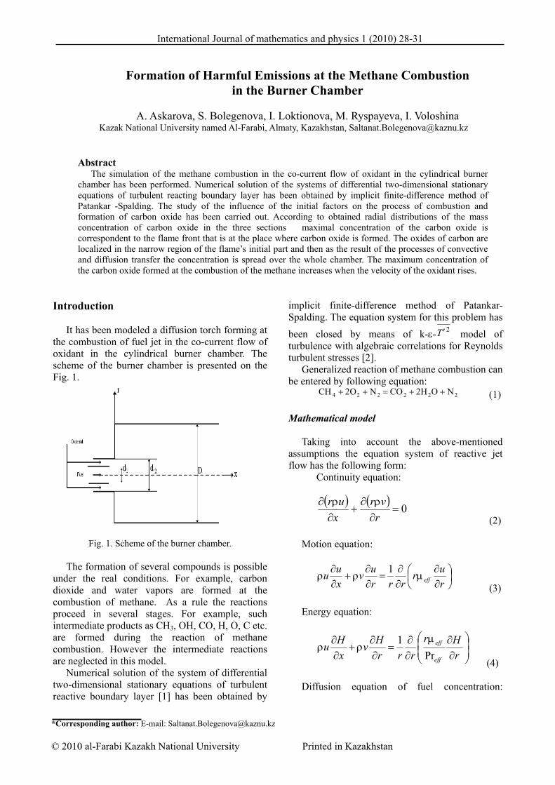
International Journal of mathematics and physics 1 (2010) 28-31
*Corresponding author: E-mail: [email protected] © 2010 al-Farabi Kazakh National University Printed in Kazakhstan
Formation of Harmful Emissions at the Methane Combustion
in the Burner Chamber
A. Askarova, S. Bolegenova, I. Loktionova, M. Ryspayeva, I. Voloshina Kazak National University named Al-Farabi, Almaty, Kazakhstan, [email protected]
Abstract
The simulation of the methane combustion in the co-current flow of oxidant in the cylindrical burner chamber has been performed. Numerical solution of the systems of differential two-dimensional stationary equations of turbulent reacting boundary layer has been obtained by implicit finite-difference method of Patankar -Spalding. The study of the influence of the initial factors on the process of combustion and formation of carbon oxide has been carried out. According to obtained radial distributions of the mass concentration of carbon oxide in the three sections maximal concentration of the carbon oxide is correspondent to the flame front that is at the place where carbon oxide is formed. The oxides of carbon are localized in the narrow region of the flame’s initial part and then as the result of the processes of convective and diffusion transfer the concentration is spread over the whole chamber. The maximum concentration of the carbon oxide formed at the combustion of the methane increases when the velocity of the oxidant rises.
Introduction
It has been modeled a diffusion torch forming at the combustion of fuel jet in the co-current flow of oxidant in the cylindrical burner chamber. The scheme of the burner chamber is presented on the Fig. 1.
Fig. 1. Scheme of the burner chamber.
The formation of several compounds is possible
under the real conditions. For example, carbon dioxide and water vapors are formed at the combustion of methane. As a rule the reactions proceed in several stages. For example, such intermediate products as СН3, ОН, СО, Н, О, С etc. are formed during the reaction of methane combustion. However the intermediate reactions are neglected in this model.
Numerical solution of the system of differential two-dimensional stationary equations of turbulent reactive boundary layer [1] has been obtained by
implicit finite-difference method of Patankar-Spalding. The equation system for this problem has
been closed by means of k-ε- 2Т ′ model of turbulence with algebraic correlations for Reynolds turbulent stresses [2].
Generalized reaction of methane combustion can be entered by following equation: СН О N CO H O N4 2 2 2 2 22 2+ + = + + (1)
Mathematical model
Taking into account the above-mentioned assumptions the equation system of reactive jet flow has the following form:
Continuity equation: ( ) ( ) 0=
∂ρ∂
+∂ρ∂
rvr
xur
(2)
Motion equation:
⎟⎠⎞
⎜⎝⎛
∂∂
μ∂∂
=∂∂
ρ+∂∂
ρrur
rrruv
xuu eff
1
(3)
Energy equation:
⎟⎟⎠
⎞⎜⎜⎝
⎛
∂∂μ
∂∂
=∂∂
ρ+∂∂
ρrHr
rrrHv
xHu
eff
eff
Pr1
(4)
Diffusion equation of fuel concentration:

Methane Combustion 29
International Journal of mathematics and physics 1(2010) 28-31
ω−⎟⎟⎠
⎞⎜⎜⎝
⎛
∂∂μ
∂∂
=∂∂
ρ+∂∂
ρrc
Scr
rrrcv
xcu
eff
eff 111 1
(5)
Transport equations for Burke-Shuman variables:
4,3,2,~1~~
=⎟⎟⎠
⎞⎜⎜⎝
⎛
∂∂μ
∂∂
=∂∂
ρ+∂∂
ρ irc
Scr
rrrcv
xcu i
eff
effii
(6)
Here u, v are longitudinal and transverse components of the averaged velocity, T is a temperature, H=cpT+Qc1 is the enthalpy, с1 is the concentration of methane, с2 is the concentration of oxygen, с3 is the concentration of carbon dioxide, с4 is the concentration of water vapors, с5 is the concentration of nitrogen.
ω is calculated by the following formula:
RTE
ecck−
= βαω 210
Boundary conditions for the equations (1-2) are introduced in the following way:
х=0: 0<y<d1: 01uu = ; c1=c10;
10ii cc~ σ= ; 10010 QcTcH p += d1<y<d2: u u= 02; c1=0;
0ii cc~ = ; 020 TcH p= d2<y<D: u = 0; c1=0;
0ii cc~ = ; 030 TcH p=
0<y< D: 2010 uk α= ;
ε α0 20
0
32
=kL ;
203
20 TT α=′
x≥ 0, y=0:
rk
rc~
rc
rH
ru i1 =
∂∂
=∂∂
=∂∂
=∂∂
=∂∂
0
rT
rrk 2
=∂′∂
=∂∂ε
=∂∂
=
x≥ 0, y=D: u = v = k = 0, T=Tw=const,
0r
Trr
c~
rc
rH 2
i1 =∂′∂
=∂∂ε
=∂∂
=∂∂
=∂∂
For this problem the initial conditions have been
concretized in the following way.
Numerical experiment
The initial speed of methane is u01 = 20.3 m/s, the oxygen initial speed has been varied over the range: 2.8 m/s ≤ u02 c≤ 8.8 m/s. D is the diameter of the duct channel, d1 is the diameter of the nozzle the fuel goes through, d2 is the diameter of the nozzle fuel and oxidant go through together.
The initial temperature value is T01 = 540 K, the temperature of oxidant is T02 = 344 K and the temperature of the duct inner surface is Tw = 300 K.
The initial oxygen concentration in the mixture has been set equal to the content of oxygen in the air c20=0.232. The initial concentration of methane is c10=0.74. It has been considered that the reaction products are absent in the initial section of the duct, that is:с с30 40 0= = . According to the correlation (5) the initial concentration of nitrogen is:
c5=1-0.232-0.058=0.71.
Results and discussion
It has been achieved the satisfactorily agreement with the experimental data on the distribution of the axial temperature given in [3]. The computational experiments of the investigation of the influence of the initial parameters on the combustion process have been conducted.
Figure 2 represents the radial distributions of mass concentration of carbon dioxide in three sections. Two sections are taken in the body of flame and the third one corresponds to the completion of the combustion region. Maximum concentration of carbon dioxide corresponds to the flame front where it is formed in the result of the chemical reaction. At the beginning of the torch it is localized in the narrow region (lines 1, 2) and then it spreads over the whole width of the chamber (line 3) in the result of the process of convective and diffusion transfer.
Figure 3 demonstrates the influence of the velocity of the oxidant co-current flow on the axial distribution of the temperature. Velocity ratio
fu
ox
uum =
is varied over the range 0.13 ≤ m ≤ 0.43.

30 A. Askarova et al.
International Journal of mathematics and physics 1(2010) 28-31
Fig. 2. Radial distribution of concentration of carbon dioxide in different sections of the burner chamber: 1- x = 0.1 m; 2 – х = 0.4 m; 3 – х = 1.6 m.
Fig. 3. The change of temperature along the axis of the burner chamber: 1 – m = 0.13; 2 – m = 0.29; 3 – m = 0.43.
Fig.4. The influence of the oxidant initial velocity on the formation of carbon dioxide: 1 – m = 0.13, 2 – m = 0.29, 3 – m = 0.43.
Fig. 5. Radial distributions of the average velocity and of the kinetic turbulent energy in different sections: 1 – x=0.099m, 2 – x=0.374 m, 3 – x=1.584 m, dot line – u, solid line – k
Fig.6. The influence of the initial fuel concentration on the temperature change along the axis of the torch: 1 – c1 =0.58, 2 - c2 =0.74, 3 – c3 =0.88
Fig.7. The influence of the initial fuel concentration on the formation of the carbon oxide: 1 – c1 =0.58, 2 - c2 =0.74, 3 – c3 =0.88.
As the fuel is in excess and the oxidant is in
deficiency in the gas mixture, than the oxygen concentration in the co-current flow is regarded as a factor limiting the speed of combustion. Therefore the amount of incoming oxygen increases at the rise of the velocity of the air co-current flow and this leads to the increase of the combustion reaction speed, and consequently, to the increase of the temperature and length of the torch.
Figure 4 is a confirmation to this conclusion and it shows the change of concentration of carbon dioxide along the axial of the torch. It follows from this picture that the maximum concentration of carbon dioxide formed at the combustion raises at the increase of the oxidant speed.
Figure 5 shows the distributions of the kinetic turbulent energy and of the averaged velocity in three sections (x=0.099 m; x=0.374 m; x=1.584 m). Kinetic turbulent energy changes in the non-monotonous way and it has several maximums (lines 1, 2) in the core of the torch. These results are explained by the fact that according to the applied turbulence model the generation of the kinetic energy is proportional to a square gradient of the averaged velocity and that fact corresponds to the experimental data. Also it can be seen in the figure 5 that the maximums of kinetic turbulent energy are placed in the field of the maximal change of the average velocity and that field is the place where the jets are mixed.

Methane Combustion 31
International Journal of mathematics and physics 1(2010) 28-31
The influence of the initial fuel concentration on the temperature and on the formation of carbon oxide is represented in figures 6 and 7. Initial methane concentration has been changed in the range from 0.58 to 0.88 that corresponds to the excess of the fuel. As it has been mentioned above the velocity of the combustion is determined by the lack component and that is why the change of the of fuel concentration in the mentioned ranges do not influence substantially on the results of the experiment. Indeed the figures 6 and 7 confirm this conclusion.
Conclusion
Numerical solution of the systems of differential
two-dimensional stationary equations of turbulent reacting boundary layer has been obtained by implicit finite-difference method of Patankar -Spalding. The study of the influence of the initial factors on the process of combustion and formation of carbon oxide has been carried out.
According to radial distributions of the mass concentration of carbon oxide in the three sections maximal concentration of the carbon oxide is correspondent to the flame front that is at the place where carbon oxide is formed. The oxides of carbon are localized in the narrow region of the flame’s initial part and then as the result of the processes of convective and diffusion transfer the concentration is spread over the whole chamber. The maximum concentration of the carbon oxide formed at the combustion of the methane increases when the velocity of the oxidant rises.
Thus the distributions of the fields of temperature, concentration of the carbon oxide gas and kinetic turbulent energy along the whole burner chamber have been obtained.
The computational experiments on the study of the influence of the initial parameters on the combustion process have been performed and on the basis of the obtained results one can conclude:
Kinetic turbulent energy changes in non-monotonous way and in the field of combustion has several maximums which correspond to the fields of the maximal gradients of the average velocity.
When we have the lack oxidant, so velocity increases and the co-flow air leads to the increasing of the rate of the combustion reaction. Therefore this increases the temperature and the length of the torch.
At the excess of the fuel the change of its concentration practically do not influence on the process of combustion.
Acknowledgements
This work has been made with financial support
Scientific Research Institute of Experimental and Theoretical Physics in the framework of the project «Research of dispersion and evolution of the droplets at the turbulent combustion of liquid fuels» (Ф.0508)
References 1. P. Libbi, F. Wiilams. (ed.) Turbulentnye
techeniya reagiruyuschih gazov, Мoscow, Mir, 1983. 325 p.
2. Rodi V. Modeli turbulentnosti okruzhayu-schie sredy. Metody rascheta turbulentnyh techeniy, Moscow, Mir, 1984. 322 p.
3. Aslanyan G.S., Maykov I.L., Chislennoe modelirovanie turbulentnogo goreniya gazoobraznogo topliva v osesimmetrichnyh kamerah, J. Physika goreniya i vzryva 34: 18 (1998).
ZSBHTADH DXZHRTJHYH
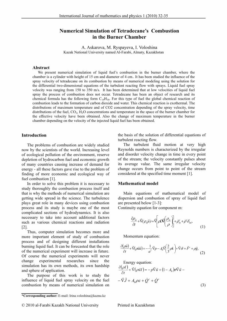
International Journal of mathematics and physics 1 (2010) 32-35
*Corresponding author: E-mail: [email protected]
© 2010 al-Farabi Kazakh National University Printed in Kazakhstan
Numerical Simulation of Tetradecane’s Combustion
in the Burner Chamber
A. Askarova, M. Ryspayeva, I. Voloshina Kazak National University named Al-Farabi, Almaty, Kazakhstan
Abstract We present numerical simulation of liquid fuel’s combustion in the burner chamber, where the
chamber is a cylinder with height of 15 cm and diameter of 4 cm.. It has been studied the influence of the spray velocity of tetradecane on its combustion by means of numerical modeling using the solution for the differential two-dimensional equations of the turbulent reacting flow with sprays. Liquid fuel spray velocity was ranging from 150 to 350 m/s. It has been determined that at low velocities of liquid fuel spray the process of combustion does not occur. Tetradecane has been an object of research and its chemical formula has the following form С14Н30. For this type of fuel the global chemical reaction of combustion leads to the formation of carbon dioxide and water. This chemical reaction is exothermal. The distributions of maximum temperature and of CO2 concentration depending of the spray velocity, time distributions of the fuel, CO2, H2O concentrations and temperature in the space of the burner chamber for the effective velocity have been obtained. Also the change of maximum temperature in the burner chamber depending on the velocity of the injected liquid fuel has been obtained.
Introduction
The problems of combustion are widely studied now by the scientists of the world. Increasing level of ecological pollution of the environment, reserve depletion of hydrocarbon fuel and economic growth of many countries causing increase of demand for energy - all these factors gave rise to the problem of finding of more economic and ecological way of fuel combustion [1].
In order to solve this problem it is necessary to study thoroughly the combustion process itself and that is why the methods of numerical simulation are getting wide spread in the science. The turbulence plays great role in many devices using combustion process and its study is maybe one of the most complicated sections of hydrodynamics. It is also necessary to take into account additional factors such as various chemical reactions and radiation [2].
Thus, computer simulation becomes more and more important element of study of combustion process and of designing different installations burning liquid fuel. It can be forecasted that the role of the numerical experiment will increase in future. Of course the numerical experiments will never change experimental researches since the simulation has its own methods, its own hardship and sphere of application.
The purpose of this work is to study the influence of liquid fuel spray velocity on the fuel combustion by means of numerical simulation on
the basis of the solution of differential equations of turbulent reacting flow.
The turbulent fluid motion at very high Reynolds numbers is characterized by the irregular and disorder velocity change in time in every point of the stream; the velocity constantly pulses about its average value. The same irregular velocity change occurs from point to point of the stream considered at the specified time moment [1].
Mathematical model
Main equations of mathematical model of
dispersion and combustion of spray of liquid fuel are presented below [1-3]: Continuity equation for component m:
,D)u(
t 1msc
mm
mm δρρ
ρρ
ρρρ
&&rrrr
++⎥⎦
⎤⎢⎣
⎡⎟⎟⎠
⎞⎜⎜⎝
⎛∇∇=∇+
∂∂
(1)
Momentum equation:
( ) ( ) ,
321
02 gFkApa
uutu s rrrrrrrrrr
ρσρρρ++∇+⎟
⎠⎞
⎜⎝⎛∇−∇−=∇+
∂∂
(2)
Energy equation: ( ) ( ) ( ) uAupIu
tI rrrrrr
−∇−+∇−=∇+∂
∂ σρρ01
sc QQAJ &&
rr+++∇− ρε0
(3)
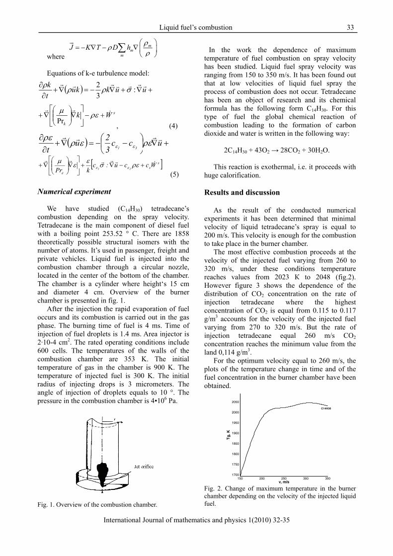
Liquid fuel’s combustion 33
International Journal of mathematics and physics 1(2010) 32-35
where m
mm
J K T D h ρρρ
⎛ ⎞= − ∇ − ∇⎜ ⎟
⎝ ⎠∑
ur
Equations of k-е turbulence model:
( ) uukkutk rrrvrrr
+∇+∇−=∇+∂∂ σρρρ :
32
s
k
Wk &rr
+−⎥⎦
⎤⎢⎣
⎡∇⎟⎟⎠
⎞⎜⎜⎝
⎛∇+ ρεμ
Pr, (4)
( ) ucc32u
t 31
vrrr+∇⎟
⎠⎞
⎜⎝⎛ −−=∇+
∂∂ ρεερρε
εε
[ ]s
sWccu:ckPr 21
&rrrrr+−∇+⎥
⎦
⎤⎢⎣
⎡∇⎟⎟⎠
⎞⎜⎜⎝
⎛∇+ ρεσεεμ
εεε (5)
Numerical experiment
We have studied (C14H30) tetradecane’s
combustion depending on the spray velocity. Tetradecane is the main component of diesel fuel with a boiling point 253.52 ° C. There are 1858 theoretically possible structural isomers with the number of atoms. It’s used in passenger, freight and private vehicles. Liquid fuel is injected into the combustion chamber through a circular nozzle, located in the center of the bottom of the chamber. The chamber is a cylinder where height‘s 15 cm and diameter 4 cm. Overview of the burner chamber is presented in fig. 1.
After the injection the rapid evaporation of fuel occurs and its combustion is carried out in the gas phase. The burning time of fuel is 4 ms. Time of injection of fuel droplets is 1.4 ms. Area injector is 2·10-4 cm2. The rated operating conditions include 600 cells. The temperatures of the walls of the combustion chamber are 353 K. The initial temperature of gas in the chamber is 900 K. The temperature of injected fuel is 300 K. The initial radius of injecting drops is 3 micrometers. The angle of injection of droplets equals to 10 °. The pressure in the combustion chamber is 4•106 Pa.
Fig. 1. Overview of the combustion chamber.
In the work the dependence of maximum
temperature of fuel combustion on spray velocity has been studied. Liquid fuel spray velocity was ranging from 150 to 350 m/s. It has been found out that at low velocities of liquid fuel spray the process of combustion does not occur. Tetradecane has been an object of research and its chemical formula has the following form С14Н30. For this type of fuel the global chemical reaction of combustion leading to the formation of carbon dioxide and water is written in the following way:
2С14Н30 + 43О2 → 28СО2 + 30Н2О.
This reaction is exothermal, i.e. it proceeds with huge calorification.
Results and discussion
As the result of the conducted numerical
experiments it has been determined that minimal velocity of liquid tetradecane’s spray is equal to 200 m/s. This velocity is enough for the combustion to take place in the burner chamber.
The most effective combustion proceeds at the velocity of the injected fuel varying from 260 to 320 m/s, under these conditions temperature reaches values from 2023 К to 2048 (fig.2). However figure 3 shows the dependence of the distribution of CO2 concentration on the rate of injection tetradecane where the highest concentration of CO2 is equal from 0.115 to 0.117 g/m3 accounts for the velocity of the injected fuel varying from 270 to 320 m/s. But the rate of injection tetradecane equal 260 m/s CO2 concentration reaches the minimum value from the land 0,114 g/m3.
For the optimum velocity equal to 260 m/s, the plots of the temperature change in time and of the fuel concentration in the burner chamber have been obtained.
150 200 250 300 350v, m/s
1700
1750
1800
1850
1900
1950
2000
2050
Tg,K
C14H30
Fig. 2. Change of maximum temperature in the burner chamber depending on the velocity of the injected liquid fuel.

34 A. Askarova et al.
International Journal of mathematics and physics 1(2010) 32-35
150 200 250 300 350v, m/s
0.085
0.09
0.095
0.1
0.105
0.11
0.115
0.12
CO
2,g/
m3
C14H30
Fig. 3. The dependence of the distribution of CO2 concentration on the rate of injection tetradecane.
Figure 4 shows the distribution of the temperature in the space of the burner chamber for the velocity of spray equal to 260 m/s at different times: 1.1 ms, 1.8 ms, 3 ms, 4 ms correspondingly. At the final time moment the temperature reaches 2023 К and it can be seen that the temperature torch fills up almost all of the space of the chamber.
0 2R , c m
0
2
4
6
8
Z,c
m
0 2R , cm
0
2
4
6
8
а) b)
0 2R , cm
0
2
4
6
8
0 2 4R, cm
0
2
4
6
8 T2022.621887.851753.071618.31483.521348.751213.971079.2944.425809.65674.875540.1405.325270.55135.775
C14H30
c) d) Fig. 4. The temperature distribution in the combustion chamber during combustion of tetradecane at various time moments: a) 1.1 ms, b) 1.8 ms; c) 3 ms, d) 4 ms for the velocity of the spray 260 m/s.
The distribution of the fuel concentration is
presented in fig. 5 for the same time moments as for the temperature and for the spray velocity 260 m/s. At the initial moment the concentration of fuel has minimal value and then increases because of the fuel injection in the chamber.
0 2R , c m
0
2
4
6
8
Z,c
m
0 2R , cm
0
2
4
6
8
а) b)
0 2R , c m
0
2
4
6
8
0 2 4R , cm
0
2
4
6
8
Fuel0.1867120.1742650.1618170.149370.1369220.1244750.1120270.099580.08713250.0746850.06223750.049790.03734250.0248950.0124475
C14H 30
c) d) Fig.5. The distribution of fuel vapor concentration in the burner chamber at different time moments: a) 1.1 ms, b) 1.8 ms; c) 3 ms, d) 4 ms for the velocity of the spray 260 m/s.
0 2R, cm
0
2
4
6
8
Z,c
m
0.0228375
0.00
7612
5
0 2R, cm
0
2
4
6
8
Z,c
m
0 .0685125
0.01
5225
0.03045
0.045675
0 2 4R,cm
0
2
4
6
8
Z,c
m
0.083737
5
0.015225
0.114187
0.09
135
0.0685125
0.0609
CO20.1141870.1065750.09896250.091350.08373750.0761250.06851250.06090.05328750.0456750.03806250.030450.02283750.0152250.0076125
C14H30
a) b) c) Fig.6. The distribution of CO2 in the combustion chamber during combustion of tetradecane at various time moments: a) 1.8 ms, b) 3 ms, c) 4 ms for the velocity of the spray 260 m/s.

Liquid fuel’s combustion 35
International Journal of mathematics and physics 1(2010) 32-35
0 2R, cm
0
1
2
3
4
5
6
7
8
Z,c
m
0.01001620.000224061
0 2R, cm
0
2
4
6
8
0.0297433
0.0330481
0.02
6438
50.
0132
193
0.0330481
0.02
9743
3
0.01
3219
3
0 2 4R,cm
0
2
4
6
8
0.0495722
0.0396578
0.029743
3
0.01321
93
H2O0.04957220.04626740.04296260.03965780.03635290.03304810.02974330.02643850.02313370.01982890.01652410.01321930.009914440.006609630.00330481
C14H30
a) b) c) Fig. 7. The distribution of concentration of H2O in the combustion chamber at time moments: a) 1.8 ms, b) 3 ms, c) 4 ms for the velocity of the spray 260 m/s.
The fuel quickly vaporizes, the vapors are mixed
with the oxidant and the mixture ignites and burns down for 4 ms. At the final moment the fuel concentration equals zero. Figures 6-7 represent the dynamics of the distribution of reaction products concentration on time for the spray velocity 260 m/s.
Conclusion
In this work the influence of the spray velocity
of liquid tetradecane has been studied. The distributions of maximum temperature and of CO2
concentration depending of the spray velocity, time distributions of the fuel, CO2, H2O concentrations and temperature in the space of the burner chamber for the effective velocity have been obtained. Also the change of maximum temperature in the burner chamber depending on the velocity of the injected liquid fuel has been obtained.
Acknowledgements
This work has been made with financial support
of Scientific Research Institute of Experimental and Theoretical Physics in the framework of the project «Research of dispersion and evolution of the droplets at the turbulent combustion of liquid fuels» (Ф.0508)
References
1. Amsden, A.A., O'Rourke, P.J., Butler, T.D.
KIVA-II: A computer program for chemically reactive flows with sprays, Los Alamos. 1989, p. 160.
2. Askarova, A.S., Ryspayeva, M.Zh., Voloshina, I.E. Vliyanie massy na modelirovanie processa goreniya vpryska zhidkogo topliva. Vestnik KazNU, seriya phizicheskaya. 1:5 (2007).
3. Askarova, A.S., Gorokhovski, М.А., Loktionova, I.V. Ryspayeva, M.Zh. Gorenie zhidkih topliv v kamere sgoraniya. Izvestiya NAN RK, 3:6 (2006).
SAgtsyty shdytijt

International Journal of mathematics and physics 1 (2010) 36-38
*Corresponding author: E-mail: [email protected] © 2010 al-Farabi Kazakh National University Printed in Kazakhstan
Computer Modeling of Radiation Effects in Graphene
A. M. Ilyin1, G. W. Beall2, I. A. Tsyganov1, Y. A. Daineko1
1Physical Department of Kazakh National University, 96a Tole-bi str., Almaty, Kazakhstan, e-mail: [email protected]
2Center of Nanophase Research, Texas State University, Department of Chemistry and Biochemistry, 601 University Drive, San Marcos, Texas, USA, e-mail: [email protected]
Abstract:
Radiation effects in graphene have been simulated and energetic and structural properties of stable defects were investigated. Several types of defects, involving a single carbon atom and a dumbbell absorbed at graphene sheet surface and a dumbbell configuration at a vacancy created by radiation knocking out a carbon atom, were calculated. The calculations also included the effect of vacancy structural relaxation. The transition from metallic to semiconducting state caused by the vacancy-like defect in graphene was observed.
Introduction
It is well known, that thanks to its unique mechanical and electronic properties [1] graphene can be used in many types of sensors and devices in many application areas. It can also be predicted, that in the future there will be many new applications in which graphene-based devices will be subjected to irradiation with neutrons or ions, for example, in space exploration. Moreover, radiation defects can be produced directly under the electron beam in the process of observation of graphene-based devices in transmission electron microscopes. Therefore, investigations of properties of graphene with radiation defects in its structure are of great interest [2-4].
It is not yet clear which kinds of stable atomic defects exist in graphene structure and it is quite difficult to observe such defects directly. Obviously, it is very difficult and in many cases impossible, to observe and characterize individual defects experimentally because of their atomic dimensions. In this situation computer simulation of growth and radiation defects in graphene nanostructures is of great importance [5-6]. Displaced atoms that have been adsorbed on the surface or linked with vacancies, caused by the displacement of atoms from the structure being the most common types of single radiation defects in nanostructures [7].
Our goal in this paper was determining the most stable defect configurations and estimating the energetic and structure features of some types of radiation defects in a small graphene sheet. The calculations were performed utilizing molecular dynamics (MD) and well known extended Hűckel (EH) method.
Results and discussion A graphene sheet for MD simulation of single-
and diatomic defects on the undamaged structure was built of 78 atoms. Van der Waals interaction between adsorbed atoms and graphene was described by LJ potential in the usual form [8].
Presented in Figure 1 is one of investigated defect configurations which is actually a single carbon atom, adsorbed on the surface of the undamaged graphene sheet .
Fig.1. Configuration of a single adsorbed atom on a graphene (N=78) structure.
Fig. 2. Configuration of a dumbbell defect on a graphene (N=78) structure.
Figure 2 presents a configuration of a more complicated, two-atom defect which is like a dumbbell with a symmetrical configuration of the atoms normal to the graphene sheet.
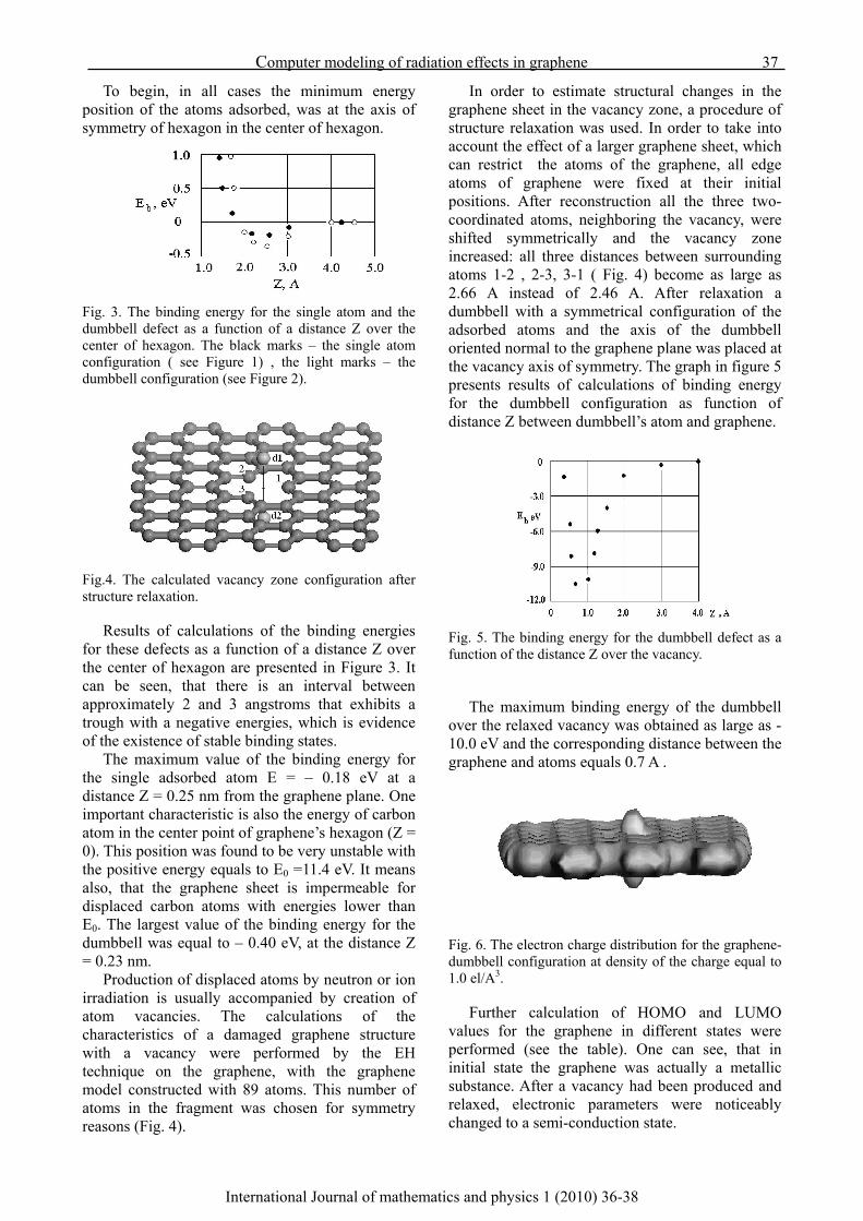
Computer modeling of radiation effects in graphene 37
International Journal of mathematics and physics 1 (2010) 36-38
To begin, in all cases the minimum energy position of the atoms adsorbed, was at the axis of symmetry of hexagon in the center of hexagon.
Fig. 3. The binding energy for the single atom and the dumbbell defect as a function of a distance Z over the center of hexagon. The black marks – the single atom configuration ( see Figure 1) , the light marks – the dumbbell configuration (see Figure 2).
Fig.4. The calculated vacancy zone configuration after structure relaxation.
Results of calculations of the binding energies for these defects as a function of a distance Z over the center of hexagon are presented in Figure 3. It can be seen, that there is an interval between approximately 2 and 3 angstroms that exhibits a trough with a negative energies, which is evidence of the existence of stable binding states.
The maximum value of the binding energy for the single adsorbed atom E = – 0.18 eV at a distance Z = 0.25 nm from the graphene plane. One important characteristic is also the energy of carbon atom in the center point of graphene’s hexagon (Z = 0). This position was found to be very unstable with the positive energy equals to E0 =11.4 eV. It means also, that the graphene sheet is impermeable for displaced carbon atoms with energies lower than E0. The largest value of the binding energy for the dumbbell was equal to – 0.40 eV, at the distance Z = 0.23 nm.
Production of displaced atoms by neutron or ion irradiation is usually accompanied by creation of atom vacancies. The calculations of the characteristics of a damaged graphene structure with a vacancy were performed by the EH technique on the graphene, with the graphene model constructed with 89 atoms. This number of atoms in the fragment was chosen for symmetry reasons (Fig. 4).
In order to estimate structural changes in the graphene sheet in the vacancy zone, a procedure of structure relaxation was used. In order to take into account the effect of a larger graphene sheet, which can restrict the atoms of the graphene, all edge atoms of graphene were fixed at their initial positions. After reconstruction all the three two-coordinated atoms, neighboring the vacancy, were shifted symmetrically and the vacancy zone increased: all three distances between surrounding atoms 1-2 , 2-3, 3-1 ( Fig. 4) become as large as 2.66 A instead of 2.46 A. After relaxation a dumbbell with a symmetrical configuration of the adsorbed atoms and the axis of the dumbbell oriented normal to the graphene plane was placed at the vacancy axis of symmetry. The graph in figure 5 presents results of calculations of binding energy for the dumbbell configuration as function of distance Z between dumbbell’s atom and graphene.
Fig. 5. The binding energy for the dumbbell defect as a function of the distance Z over the vacancy.
The maximum binding energy of the dumbbell
over the relaxed vacancy was obtained as large as -10.0 eV and the corresponding distance between the graphene and atoms equals 0.7 A .
Fig. 6. The electron charge distribution for the graphene-dumbbell configuration at density of the charge equal to 1.0 el/A3.
Further calculation of HOMO and LUMO values for the graphene in different states were performed (see the table). One can see, that in initial state the graphene was actually a metallic substance. After a vacancy had been produced and relaxed, electronic parameters were noticeably changed to a semi-conduction state.

38 M. Ilyin at. al.
International Journal of mathematics and physics 1 (2010) 36-38
Table 1 Effect of the radiation defect on HOMO LUMO characteristics of graphene
state HOMO, eV LUMO, eV initial -7.620 -7.615 vacancy,
after relaxation -7.382 -7.180
The large value of the binding energy for the
dumbbell defect and the electron charge distribution (see Fig. 6) obviously demonstrate, that there is significant interaction between the dumbbell and a graphene, as well as between atoms of the dumbbell itself.
The calculations were made also for bilayer graphene fragment, in the usual graphite-like configuration, presented in figure 7. The coupled atom pair which was removed by creating the vacancy pair is marked by black. The interstitial C-atom , knocked from the structure was placed between graphene layers. After that relaxation procedure was used to obtain a minimum of the total energy of the defect volume. The edge atoms of graphenes were fixed in order accounting the size effect. One can see from figure 8 that after relaxation center parts of graphenes significantly entered into the gap, so that distances between atoms 1-2 and 3-4 turned out equal nearly 1.43 A. Obviously, it is the main cause of rising two additional bonds between graphenes.
Fig.7. Graphene bilayer used for building complex interior defect.
Fig.8. The total defect configuration of bonding radiation defects in bilayer grapheme.
Fig. 9. The distribution of the electron charge (the density equals 1.4 el / A3).
In figure 8 one can see the essential approach of
atoms 1-2 and 3-4 facilitating the rising two additional bonds. The distribution of the electron charge presented in Figure 9 proves existing of three covalent bonds between graphene layers. The total binding energy for this complex defect configuration was calculated as large as -11.3 eV.
Conclusion
Some stable radiation defect configurations, involving single adsorbed atom, the dumbbell like defect of displaced atoms and a vacancy-like defect, associated with a dumbbell of adsorbed atoms as well as complex interior defect in bilayer graphene were simulated. The binding energy, structure, and some electron characteristics of defects have been determined. There is significant interaction between atoms of the dumbbell pair and also between adsorbed single atoms and graphene. It was shown that the vacancy defect caused by displacement of atoms from the structure converts the graphene from metallic to semiconducting with a small band gap. The secondary additional fast bonds accompanying to primary interstitial bridge-like one for bilayer graphene were observed.
References 1. Stauber, T., Peres, N.M.R., and Guinea, F., Phys.
Rev. B76, 2007, 205423. 2. Hashimoto, A., Suenaga, K., Gloter, A., Urita,
K., & Iijima, S., Nature 430, 2004, 870-873. 3. Jian-Hao Chen, Cullen, W.G., Jang, C., Fuhrer,
M.S., and Williams, E.D., Phys. Rev. Lett. , 102, 2009, 236805.
4. Teweldebrhan, D., and Balandin, A.A., Appl.Phys.Lett., 94, 2009, 013101-3.
5. Gun-Do Lee, Wang, C.Z., et al. Phys.Rev.,B 74, 2006, 245411.
6. Tachikava, H., and Kawabata, H., J. Phys. Chem. C, 2009, 113(18) 7603-7609
7. Ilyin, A.M., Daineko, E.A., and Beall, G.W., Physica E, 42, 2009, pp.67-69.
8. Maruyama, S., Kimura, T., ASME International Mechanical Engineering Congress and Exhibit, Orlando, November 5-11, 2000.

International Journal of mathematics and physics 1 (2010) 39-41
*Corresponding author: E-mail: [email protected] 2010 al-Farabi Kazakh National University Printed in Kazakhstan
Computer Modeling of Bridge–Like Radiation Defects in The Carbon
Nano-Structures
A. M. Ilyin1, G. W. Beall2, I. A. Tsyganov1, Y. A. Daineko1 1Physical Department of Kazakh National University, 96a Tole-bi str., Almaty, Kazakhstan,
e-mail: [email protected] 2Center of Nanophase Research, Texas State University, Department of Chemistry and Biochemistry, 601
University Drive, San Marcos, Texas, USA, e-mail: [email protected] Abstract
The paper presents results of computer simulation and study of a special type of radiation induced defects, which can be produced in carbon nanostructures. Some stable configurations of bridge-like defects, in carbon nanotubes were constructed and investigated. A new type of possible stable defects, which can arise between opened ends of MWNT is presented. The binding energy and structure characteristics of the defects have been determined utilizing well known semiempirical extended Hűckel techniques.
Introduction
It is well known, that single-walled carbon nanotubes (SWNT) and multi-walled carbon nanotubes (MWNT) can be used in production of new composite materials. These composites can be based on metal, ceramic or polymer matrices filled with carbon nanotubes as elements of reinforcement. Many of the good physical and electrical properties can be exploited by incorporating the nanotubes into some form of the matrix material [1-5]. Obviously the main goal of using nanotubes in making composites is using their extremely high mechanical properties in combination with low density. The same is true of the very high electrical conductivity of especially the SWNT where normally insulating polymers can be rendered conducting with very low weight percent of the nanotubes. This situation unfortunately is not true of the very high thermal conductivity of the carbon nanotubes. Composites produced from carbon nanotubes only yield thermal conductivities following the rule of mixtures. One of the important and unfortunately poorly understood factor is being a way of bonding of a matrix with carbon nanostructures. It should be taking into account that the sp2 electron structure often results in very low binding energy between CNT’s surface and atoms of many elements.
This results in poor interfacial bonding of the nanotubes or nanostructures fragments that can slide in the matrix, or relatively to each other under stressed condition. It results in decreasing the part of CNT’s surface, transferring stress between matrix and reinforcement elements under stressed
state of the composite. This therefore limits rather severely the amount of ultimate strength present in the nanotubes that can effectively be transferred to the matrix. It is reasonable to suppose that defects in such structures might improve situation by linking nanoelements to each other allowing them to act as cross-links which will increase the stiffness of the composite. In general, investigations of radiation effects in carbon nanostructures are of great interest at present [6,7]. However, it is not yet well understood which kinds of stable atomic complex defects exist in carbon structures and it is not easy to observe such defects directly and in some cases to make interpretation of measurements [8]. In this situation computer simulation of radiation defects in carbon nanostructures becomes of great im- portance [9-11].
It is posited, that some types of radiation defects can act as a route to additional chemical bonds, promoting the strengthening of composite materials consisting of high concentration of carbon nanostructures. In this paper we consider results of simulation and investigation of structural and energetic properties of some possible configurations of defects, which can be produced by fast particles irradiation of a nanocomposite, involving carbon nanostructures. The calculations were performed utilizing well known semiempirical atomic basis extended Hűckel method.
Simulation and calculations
Further we consider different types of possible radiation defects in carbon nanostructures rising
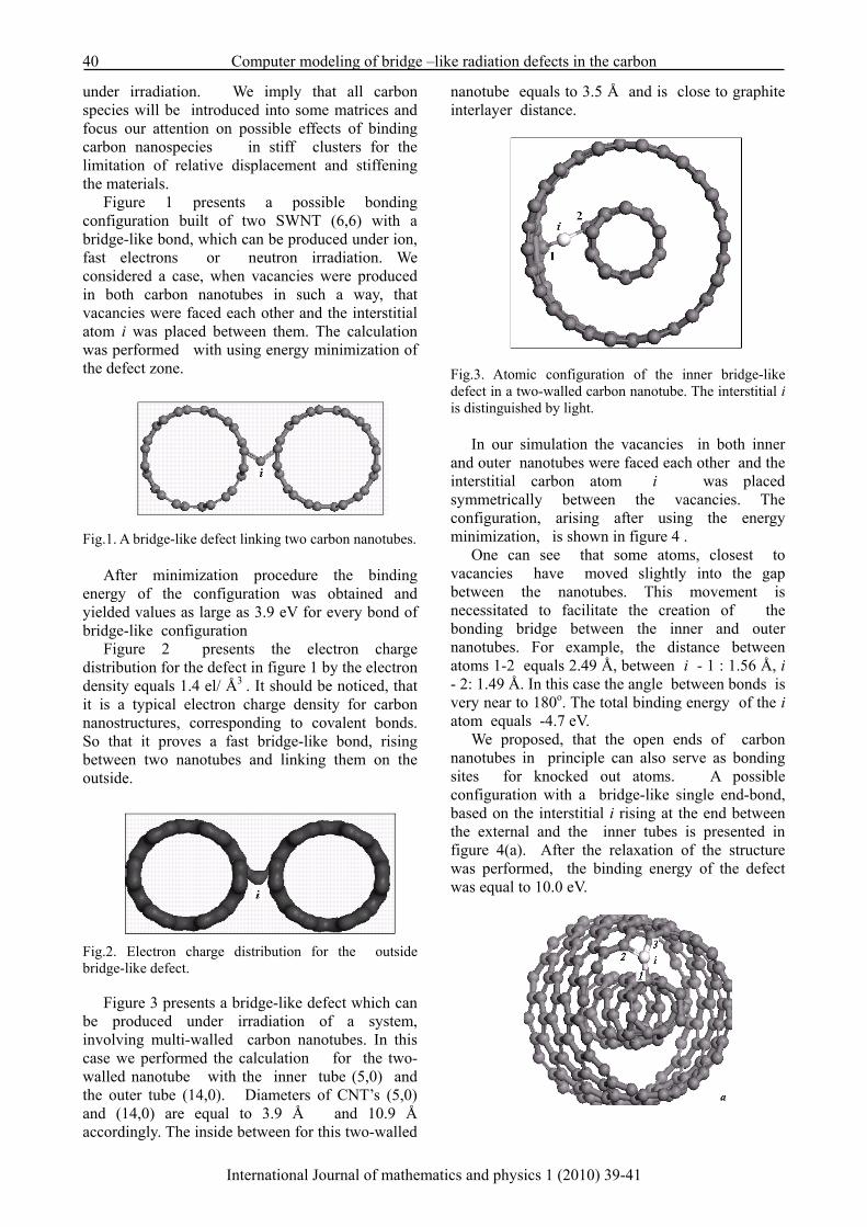
40 Computer modeling of bridge –like radiation defects in the carbon
International Journal of mathematics and physics 1 (2010) 39-41
under irradiation. We imply that all carbon species will be introduced into some matrices and focus our attention on possible effects of binding carbon nanospecies in stiff clusters for the limitation of relative displacement and stiffening the materials.
Figure 1 presents a possible bonding configuration built of two SWNT (6,6) with a bridge-like bond, which can be produced under ion, fast electrons or neutron irradiation. We considered a case, when vacancies were produced in both carbon nanotubes in such a way, that vacancies were faced each other and the interstitial atom i was placed between them. The calculation was performed with using energy minimization of the defect zone.
Fig.1. A bridge-like defect linking two carbon nanotubes.
After minimization procedure the binding
energy of the configuration was obtained and yielded values as large as 3.9 eV for every bond of bridge-like configuration
Figure 2 presents the electron charge distribution for the defect in figure 1 by the electron density equals 1.4 el/ Å3 . It should be noticed, that it is a typical electron charge density for carbon nanostructures, corresponding to covalent bonds. So that it proves a fast bridge-like bond, rising between two nanotubes and linking them on the outside.
Fig.2. Electron charge distribution for the outside bridge-like defect.
Figure 3 presents a bridge-like defect which can be produced under irradiation of a system, involving multi-walled carbon nanotubes. In this case we performed the calculation for the two-walled nanotube with the inner tube (5,0) and the outer tube (14,0). Diameters of CNT’s (5,0) and (14,0) are equal to 3.9 Å and 10.9 Å accordingly. The inside between for this two-walled
nanotube equals to 3.5 Å and is close to graphite interlayer distance.
Fig.3. Atomic configuration of the inner bridge-like defect in a two-walled carbon nanotube. The interstitial i is distinguished by light.
In our simulation the vacancies in both inner
and outer nanotubes were faced each other and the interstitial carbon atom i was placed symmetrically between the vacancies. The configuration, arising after using the energy minimization, is shown in figure 4 .
One can see that some atoms, closest to vacancies have moved slightly into the gap between the nanotubes. This movement is necessitated to facilitate the creation of the bonding bridge between the inner and outer nanotubes. For example, the distance between atoms 1-2 equals 2.49 Å, between i - 1 : 1.56 Å, i - 2: 1.49 Å. In this case the angle between bonds is very near to 180o. The total binding energy of the i atom equals -4.7 eV.
We proposed, that the open ends of carbon nanotubes in principle can also serve as bonding sites for knocked out atoms. A possible configuration with a bridge-like single end-bond, based on the interstitial i rising at the end between the external and the inner tubes is presented in figure 4(a). After the relaxation of the structure was performed, the binding energy of the defect was equal to 10.0 eV.

M. Ilyin at. al. 41
International Journal of mathematics and physics 1 (2010) 39-41
Fig. 4. A possible atomic configurations of bridge-like defects between the ends of a two-walled carbon nanotube (5,0) / (14,0). The interstitials i are distinguished by light. (a) lengths of the bonds: i-1: 1.31 Å ; i-2, i-3 : 1.41 Å.
More complicated configuration is presented in
figure 4(b). This unusual nanotubular object involves 5 bridge-like end-bonds between the external and inner tubes. Such defect results not only in bonding, but also in closing the end gap of two-walled carbon nanotubes. View of the atomic configuration of the complex bridge-like defects in a two-walled carbon nanotube. Lengths of bonds: i – 1: 1.30 Å , i – 2, i – 3 : 1.39 Å. Distances between interstitial atoms vary approximately from 3.5 to 4.1 Å .
Fig.5. The lateral view of the deformed and closed end of the two-walled nanotube presented in Figure 4(b).
One can see the essential deformation of the end
field by bonding and closing it with bridge-like defects.
Conclusion
Some possible types of stable bridge-like radiation defects, which can originate under fast particles irradiation in typical carbon nanostructures were simulated. Results of calculation illustrate possible linked configurations for SWNT, MWNT. The binding energy and structure characteristics of defects have been determined. A new type of defect configuration based on bridge-like bonds between ends of MWNT is presented. Radiation production of such types of defects can be useful for application in materials science, particularly in R&D of new materials with using the carbon nanostructures as reinforcement elements, for stiffening the nanostructures.
References 1. Harris, P.J.F., Intern. Mater. Rev., 49(1): 31
(2004) 2. Ajayan, P.M., Schadler, L.S. , Giannaris, C., &
Rubio ,A. , Adv. Mater. 12:750 (2000). 3. Hu, Y., Shenderova, O.A., Hu, Z. , Padgett,
C.W., & Brenner, D.W., Rep. Prog. Phys. 69:1847(2006).
4. Laha, T., Liu, Y. and Agarwal, A., J. of Nanoscience and Nanotechnology, 7:1(2007).
5. Hashimoto, A., Suenaga, K., Gloter, A., Urita, K. & Iijima, S., Nature 430:870 (2004).
6. Krasheninnikov, A. V. , Nordland, K., Sirvio, M., Salonen, E.,and Keinonen, J. Phys.Rev. B.63:2454052001(2001).
7. Krasheninnikov, A. V. & Banhart F., Nat. Mater. 6: 723 (2007).
8. Teweldebrhan,D. and Balandin, A.A., Appl. Phys. Lett., 94:013101 (2009).
9. Ilyin, A.M., Daineko, E.A., and Beall, G.W., Physica E, 42:67 (2009).
10. Futa, M.G., and Kelires,. P.C., Appl. Phys.Lett. 86:191916 (2005).
11. Yazyev, O.V., Tavernelli, I., Rothlisberger, U. & Helm, L., Phys. Rev. B 75:115418 (2007).
Drtjyutkui fdfthjftuiyg
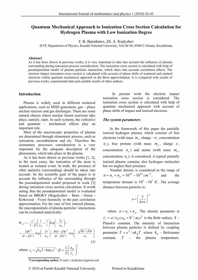
International Journal of mathematics and physics 1 (2010) 42-45
*Corresponding author: E-mail: [email protected]
© 2010 al-Farabi Kazakh National University Printed in Kazakhstan
Quantum Mechanical Approach to Ionization Cross Section Calculation for
Hydrogen Plasma with Low Ionization Degree
F. B. Baimbetov, Zh. A. Kudyshev IETP, Department of Physics, Kazakh National University, Tole Bi 96, 050012 Almaty, Kazakhstan.
Abstract As it has been shown in previous works, it is very important to take into account the influence of plasma surrounding during ionization process consideration. The ionization cross section is calculated with help of pseudopotential model of plasma particles interaction, which takes into account correlation effects. The electron impact ionization cross section is calculated with account of phase shifts of scattered and emitted electrons within quantum mechanical approach in the Born approximation. It is compared with results of previous works, experimental data and suitable results of other authors.
Introduction
Plasma is widely used in different technical applications, such as MHD generators, gas – phase nuclear reactors and gas discharges. There are some natural objects where nuclear fusion reactions take place, namely, stars. In such systems, the collective and quantum – mechanical effects play an important role.
Most of the macroscopic properties of plasma are determined through elementary process, such as ionization, recombination and etc. Therefore the elementary processes consideration is a very important for the adequate description of the phenomena, which take place in the plasma.
As it has been shown in previous works [1, 2], in the most cases, the ionization of the atom is treated as isolated event. In truth, the presence of other particles (surrounding) should be taken into account. So the scientific goal of the paper is to account the influence of the surrounding through the pseoudopotential model proposed in work [3] during ionization cross section calculation. It worth noting that the pseudopotential model is evaluated based on BBGKY (Bogolyubov - Born - Green - Kirkwood - Yvon) hierarchy in the pair correlation approximation. For the case of low ionized plasma, the macropotentials of plasma particles’ interactions can be evaluated analytically:
(1)
where 28/ enTkr eBn π= ;
2
21
⎟⎟⎠
⎞⎜⎜⎝
⎛=
n
B
ra
β
In present work the electron impact ionization cross section is considered. The ionization cross section is calculated with help of quantum mechanical approach with account of phase shifts of impact and ionized electrons.
The system parameters
In the framework of this paper the partially ionized hydrogen plasma, which consists of free electrons (with mass em , charge e− , concentration
en ), free protons (with mass pm , charge e ,
concentration pn ) and atoms (with mass nm ,
concentration nn ), is considered. A typical partially ionized plasma contains also hydrogen molecules but we neglect their presence.
Number density is considered in the range of 32420 1010 −−=+= cmnnn pe , and the
temperature domain is K73 1010 − . The average distance between particles is:
1/33
4a
nπ⎛ ⎞= ⎜ ⎟⎝ ⎠
where pe nnn += . The density parameter is
Bs aar /= ( 2 2/B ea m e= h is the Bohr radius), h - Planck's constant. The intensity of interaction between plasma particles is defined by coupling parameter Take B/2=Γ where Bk - Boltzmann constant, T - the plasma temperature.
⎟⎟
⎠
⎞
⎜⎜
⎝
⎛ +−
−−
−⎟⎟⎠
⎞⎜⎜⎝
⎛−
−+
+⎟⎟⎠
⎞⎜⎜⎝
⎛−⎟⎟
⎠
⎞⎜⎜⎝
⎛+
−−=Φ
BB
BBen
ar
Expre
arExp
re
arExp
rae
)()()(
)(β
βββ
ββ
β
12132
12
2111
2
2
2
2
2
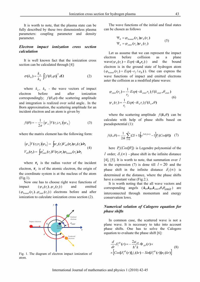
Ionization cross section for hydrogen plasma 43
International Journal of mathematics and physics 1 (2010) 42-45
It is worth to note, that the plasma state can be
fully described by these two dimensionless plasma parameters: coupling parameter and density parameter. Electron impact ionization cross section calculation
It is well known fact that the ionization cross
section can be calculated through [4]:
∫ Ω= dfkk
k n 2
00 ),()( ϕθσ (2)
where nk , 0k - the wave vectors of impact
electron before and after ionization correspondingly; ),( ϕθf -the scattering amplitude and integration is realized over solid angle.. In the Born approximation, the scattering amplitude for an incident electron and an atom is given by
02121 ψψπ
θ );()( rrVf n−= (3)
where the matrix element has the following form:
22220
1001021
rrrr
rr
11
11
drVrV
drVrrrV
boundemitn
nnn
∫∫
=
=
)();()()(
)()()();(
* ϕϕ
ψψψψ (4)
where 1r is the radius vector of the incident
electron, 2r is of the atomic electron, the origin of the coordinate system is at the nucleus of the atom (Fig.1).
Now one has to choose right wave functions of impact ( )( 10 rψ , )( 1rnψ ) and emitted ( )( 2rboundϕ , )( 2remitϕ ) electrons before and after ionization to calculate ionization cross section (2).
emitθ
θ
rθ
y
x
Emitted electron
Scattered electron
Bound electron
Impact electron
Fig. 1. The diagram of electron impact ionization of atom.
The wave functions of the initial and final states
can be chosen as follows
)()()()(
12
1020
rrrr
nemitn
bound
ψϕψϕ
=Ψ
=Ψ (5)
Let us assume that we can represent the impact
electron before collision as a plane wave( )()( 10 rkiExpr −=10ψ ) and the bound electron is in the ground state of hydrogen atom ( )/()( Bbound arExpr 22 −=ϕ ). One can express the wave functions of impact and emitted electrons aster the collision as a modified plane waves:
),()()(
),()()(
θψ
θϕ
nnn
emitemitemitemit
kfrikExpr
r
kfrikExpr
r
11
1
22
2
1
1
−=
−=
(6)
where the scattering amplitude ),( θkf can be
calculate with help of phase shifts based on pseudopotential (1):
[ ]∑∞
=
∞ −+=0
2 11221
ll
i CosPelik
kf l ])[()(),( )( θθ δ (7)
here ])[( θCosPl is Legendre polynomial of the
l order; )(∞lδ - phase shift in the infinite distance [4], [5]. It is worth to note, that summation over l in the expression (7) is done till 20=l and the phase shift in the infinite distance )(∞lδ is determined at the distance, where the phase shifts have a constant value (Fig.2.).
It is worth noting that the all wave vectors and corresponding angels ( emitn emit θθ ,,,, kkk0 ) are interconnected through momentum and energy conservation lows. Numerical solution of Calogero equation for phase shifts
In common case, the scattered wave is not a
plane wave. It is necessary to take into account phase shifts. One has to solve the Calogero equation to evaluate the phase shift [6]:
[ ])()]([)()]([
)()(
krnrSinkrjrCos
rk
rdrd
labll
abl
ababab
l
δδ
μδ
−×
×Φ−= 2
2h (8)
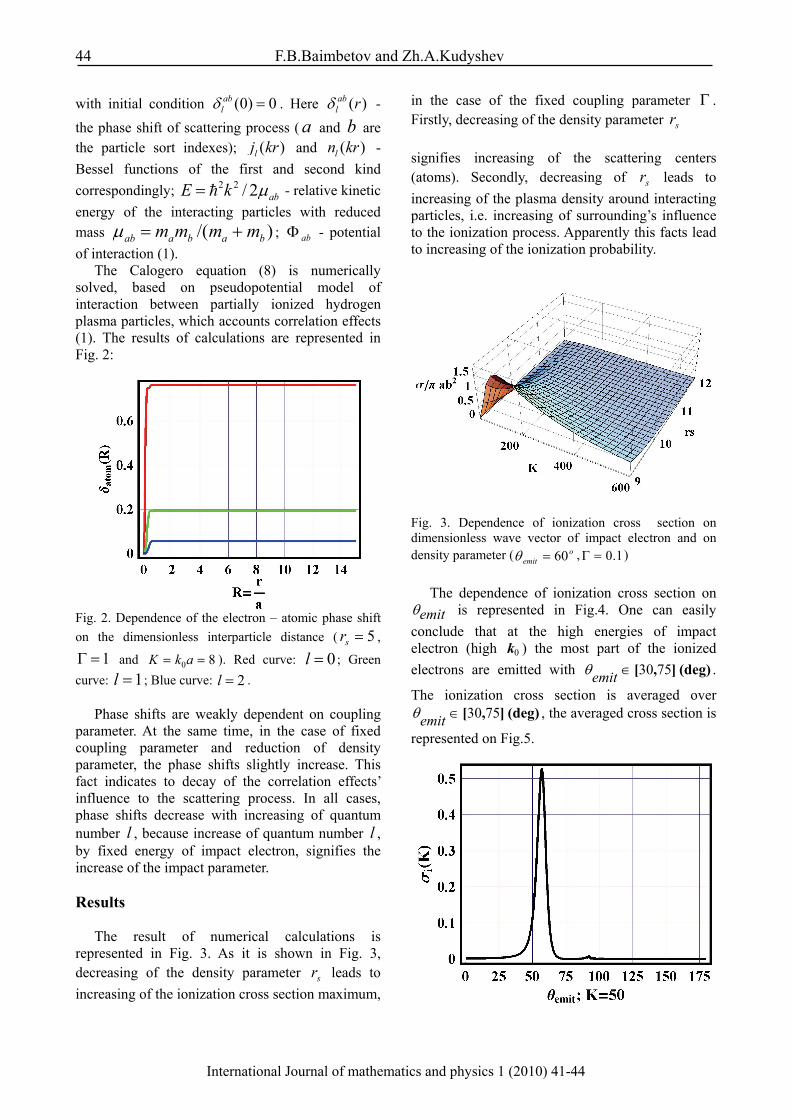
44 F.B.Baimbetov and Zh.A.Kudyshev
International Journal of mathematics and physics 1 (2010) 41-44
with initial condition (0) 0ab
lδ = . Here ( )abl rδ -
the phase shift of scattering process ( a and b are the particle sort indexes); ( )lj kr and ( )ln kr - Bessel functions of the first and second kind correspondingly; 2 2 / 2 abE k μ= h - relative kinetic energy of the interacting particles with reduced mass /( )ab a b a bm m m mμ = + ; abΦ - potential of interaction (1).
The Calogero equation (8) is numerically solved, based on pseudopotential model of interaction between partially ionized hydrogen plasma particles, which accounts correlation effects (1). The results of calculations are represented in Fig. 2:
Fig. 2. Dependence of the electron – atomic phase shift on the dimensionless interparticle distance ( 5=sr ,
1=Γ and 80 == akK ). Red curve: 0l = ; Green curve: 1l = ; Blue curve: 2l = .
Phase shifts are weakly dependent on coupling
parameter. At the same time, in the case of fixed coupling parameter and reduction of density parameter, the phase shifts slightly increase. This fact indicates to decay of the correlation effects’ influence to the scattering process. In all cases, phase shifts decrease with increasing of quantum number l , because increase of quantum number l , by fixed energy of impact electron, signifies the increase of the impact parameter. Results
The result of numerical calculations is represented in Fig. 3. As it is shown in Fig. 3, decreasing of the density parameter sr leads to increasing of the ionization cross section maximum,
in the case of the fixed coupling parameter Γ . Firstly, decreasing of the density parameter sr
signifies increasing of the scattering centers (atoms). Secondly, decreasing of sr leads to increasing of the plasma density around interacting particles, i.e. increasing of surrounding’s influence to the ionization process. Apparently this facts lead to increasing of the ionization probability.
Fig. 3. Dependence of ionization cross section on dimensionless wave vector of impact electron and on density parameter ( o
emit 60=θ , 1.0=Γ )
The dependence of ionization cross section on emitθ is represented in Fig.4. One can easily
conclude that at the high energies of impact electron (high 0k ) the most part of the ionized electrons are emitted with (deg)],[ 7530∈emitθ .
The ionization cross section is averaged over (deg)],[ 7530∈emitθ , the averaged cross section is
represented on Fig.5.
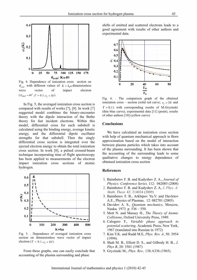
Ionization cross section for hydrogen plasma 45
International Journal of mathematics and physics 1 (2010) 42-45
Fig. 4. Dependence of ionization cross section on
emitθ with different values of akK 0= dimensionless wave vector of impact electron ( o
emit 60=θ , 1.0=Γ , 10=Sr ).
In Fig. 5, the averaged ionization cross section is compared with results of works [7], [8]. In work [7] suggested model combines the binary-encounter theory with the dipole interaction of the Bethe theory for fast incident electrons. Within this model, differential cross for each subshell is calculated using the binding energy, average kinetic energy, and the differential dipole oscillator strengths for that subshell. Then the singly differential cross section is integrated over the ejected electron energy to obtain the total ionization cross section. In work [8], a pulsed crossed-beam technique incorporating time of flight spectroscopy has been applied to measurements of the electron impact ionization cross sections of atomic hydrogen.
Fig. 5. . Dependence of averaged ionization cross section on dimensionless wave vector of impact electron ( 1.0=Γ , 10=Sr ).
From these graphs, one can easily conclude that accounting of the plasma surrounding and phase
shifts of emitted and scattered electrons leads to a good agreement with results of other authors and experimental data.
Fig. 6. . The comparison graph of the obtained ionization cross – section (solid red curve; 10=Sr and
1.0=Γ ) with corresponding results of M.Gryzinski (thin blue curve), experimental data [11] (point), results of other authors [10] (yellow curve) Conclusions
We have calculated an ionization cross section with help of quantum mechanical approach in Born approximation based on the model of interaction between plasma particles which takes into account of the plasma surrounding. It has been shown that the accounting of the surrounding leads to some qualitative changes to energy dependence of obtained ionization cross section
References
1. Baimbetov F. B. and Kudyshev Z. A., Journal of
Physics: Conference Series, 112: 042085 (2008) 2. Baimbetov F. B. and Kudyshev Z. A, J. Phys. A:
Math. Theor. 42: 214034 (2009) 3. Baimbetov F. B., Arkhipov Yu.V. and Davletov
A.E., Physics of Plasmas, 12: 082701 (2005). 4. Davidov A. S., Quantum mechanics, Moscow,
Nauka. 1973. p. 536 – 550. 5. Mott N. and Massey H., The Theory of Atomic
Collisions, Oxford University Press, 1949. 6. Calogero F., Variable phase approach to
potential scattering, Academic Press, New York, 1967 (translated into Russian in 1972)
7. Kim Y.K. and Rudd M.E, Phys. Rev. A, 50: 3954 (1994).
8. Shah M. B., Elliott D. S., and Gilbody H. B., J. Phys B, 20: 3501 (1987)
9. Gryzinski M., Phys. Rev., 138:A336 (1965).

International Journal of mathematics and physics 1 (2010) 46-51
*Corresponding author: E-mail: [email protected]
© 2010 al-Farabi Kazakh National University Printed in Kazakhstan
Some Peculiarities in the Formation of Amorphous and Nanostructure
Composite Thin Films by Sol-Gel Technology
N. Korobova1, O. Issaikina2, T. Fedorenko2 1Kazak National University named Al-Farabi, Almaty, Kazakhstan, [email protected]
2National Engineering Academy Republic of Kazakhstan Abstract
The development of new improved type of dielectric materials on the conception of multiphase structure has been carried out in this paper. Metal alkoxide solutions were used for application of thin films by electrophoretic deposition technique. We succeeded in preparation of amorphous and composite dielectric films from Al alkoxides. Specific features of the preparation technique were considered. Microstructure of the films was examined as well as their dielectric properties. TEM analyses reveals that films deposited from aging sols and heat-treated at temperatures as low as 400 °C contain small whiskers of δ-Al2O3. The alteration in crystallization behavior of Al2O3 whiskers was discussed in terms of aging starting sols before electrophoretic deposition. Mullite ultra-dispersion uniform powder preparation has been discussed.
Introduction
The alkoxide-based sol-gel process is one of the most promising methods for synthesizing ceramic powders and, especially, films at relatively low-temperatures. Sol-gel process has many advantages, such as easy composition control and fabrication of large area thin films, film homogeneity, low cost, and a simple fabrication cycle [1-3]. Therefore, it could be practical to make use of sol-gel technique to prepare thin films of desired properties.
The study of alumina/semiconductor or alumina/metal systems are very important for the realization of MOS or MOM (metal–oxide–semiconductor/metal) structures for sensor system, because their quality depends strongly on the quality of the insulating layers and the interface insulator/semiconductor or metal. Al2O3 is a technologically important material due to its excellent dielectric properties, good adhesion to many surfaces, thermal and chemical stability. These properties make Al2O3 attractive in microelectronics and thin film device industry as an insulator, ion barrier, and protective coating [4].
Usually, the metal alkoxides used in synthesizing dielectrics are very unstable, because of the high electropositive nature of the metal atoms. Methoxyethanol has been widely used as a solvent and stabilizer for preparing precursors, due to its chelating properties and low viscosity, but it is very toxic and hazardous solvent. Also many works reported that a controlled atmosphere (argon or nitrogen) must be used to synthesize oxides [2-4]. However, for industrial applications, ease of
operation also should be considered. For the present work, a series of Al2O3 films was prepared in air by sol-gel method without using some alkoxide stabilizer, which reduces the reactivity of the metal alkoxides. The choice of precursors can affect the chemical-reaction kinetics, microstructures and properties of the product, so in this paper we compared the crystallization behavior of Al2O3 films derived from the same precursors, stressing the influence of experiment conditions and where it was possible to obtain the uniform amorphous or composite (amorphous matrix with alumina whiskers) dielectric films. Dense oxide films were prepared by electrophoretic deposition method (EPD), and the electrical properties of the sintered dielectric films were measured and reported.
Experimental Procedure
a) Alumina film preparation. Sol was
synthesized using aluminum iso-propoxide and ethanol, which were commercially obtained and used without further purification and 0,5-1 h under vigorous stirring to obtain translucent, homogeneous, stable sol. This step was performed at room temperature and in a CO2 – free atmosphere. The stainless steel substrate was cleaned with ethanol-acetone solution in an ultrasonic bath for 20 min, washed with distilled water and then dried before used. Thin films of Al2O3 were manufactured on a stainless steel substrate by electrophoretic deposition process from prepared alcohol sol. We try to keep attention to the sol aging time- that is the time passed from

Some Peculiarities in the Formation of Amorphous and Nanostructure Composite 47
International Journal of mathematics and physics 1 (2010) 46-51
its preparation to the moment of utilization. In the work [5] we have considered the influence of aging sol on the morphology and structure of sol particles and also the sol-gel chemistry of Al(iso-C3H7O)3 in various alcohols. The deposition always occurred at the cathode with a constant electric field of 200-300 V/cm for a time period of 0,5-2 min. The thickness of a deposited gel layer was usually in the range of 1-3 μm. Precise thickness depended upon deposition conditions (voltage and time) and the nature of the sol (aging time, particle size, concentration). For comparing oxide films were coated on stainless steel substrate by the dip coating process using the same sols at a substrate drawing speed of 0.4 mm/s. Gel layers were dried and calcined at 350-400 0C in air for 20 min. The morphologies of the surfaces of the films were observed with scanning electron microscope (SEM). Detailed thermal analysis was conducted, and the relation between the preparation conditions and phase-forming process was described here. XRD spectra were recorded using Cu Kα radiation. For the electrical characterization of Al2O3 films, aluminum top electrodes were applied onto the surface of the films using a shadow masking-sputtering method. The electrical properties of the obtained thin films were evaluated and compared with Al2O3 films prepared by dip coating.
b) Mullite film preparation. Some specific comments necessary to underline about mullite film preparation. Alumina particles dispersed in a solution of pH <9 have a positive electrostatic charge (Fig.1a), silica particles dispersed in a solution of pH >2 have a negative electrostatic charge (Fig.1b), so mixed colloidal dispersion of alumna and silica may hetero-coagulate through mutual attraction by electrostatic forces to form a dispersion of composite particles (Fig.1c).
(a)
(b)
( c )
Fig.1. TEM micrographs of complex particles during electrophoretic deposition. (a) Alumina particles dispersed in a solution with pH <9, (b) silica particles dispersed in a solution with pH >2; (c) mixed colloidal dispersion of alumina and silica, x 10000000. (Alumina particles were covered with 1 or 2 layers of silica particles).
Results and discussion
The amorphous or nanocrystalline powder, as
observed by TEM, consists of weakly bonded, well- faceted particles (Fig.2a-c). The change in shape and crystallinity degree of the particles during sol preparation could be related closely to the aging of aluminium hydroxides. Studies based upon electron microscopy show that fresh sol consists of amorphous hydroxide (2a); 2-3 h aging sol has pseudoboehmite phase, more than 3h sol contains mixture of boehmite and scattered small crystals of bayerite (2b). After 24 h of aging bayerite becomes the predominant phase (Fig.2c).
(a)
(b)
(c )
Fig. 2. Electron micrographs and diffraction patterns of hydrated sol particle with different aging time: around 1h, (b) 4 h, (c) 24 h; x10000000.
48 N. Korobova et al.
International Journal of mathematics and physics 1 (2010) 46-51
The TGA and DTG data, measured in dry air and in inert atmosphere (argon) are shown in Fig.3(a-b).
(a)
(b)
Fig.3. TG/DTG for electrophoretic electrode gel in (a) dry air (10 0C/min), (b) in argon (10 0C/min).
The electrophoretic electrode gel decomposition occurs in four steps centered at 80, 190, 340 and 455 0C in air and in inert atmosphere seems to comprise six steps centered at 70, 200, 330, 420, 590 and 910 0C, respectively. The second step is very broad, seems to comprise of two maxima indicating several overlapping processes are taking place, and also occurs in inert atmosphere. The last two steps are not seen in inert atmosphere at the exact same temperatures, which leads to the conclusion that atmospheric O2 plays a role in these steps.
The weight loss in the temperature 80 and 190 0C is attributed to the loss of absorbed water and combustible organic residual alkoxy groups. Around 340 0C, the third step takes place in the decomposition pathway of the electrode gel.
The fragments and compounds detected are H2O, CO, CO2. These fragments prove that there still exist organic compounds, which are combusted or undergo dehydration at 340 0C. The final step may be around 455 0C for CO2 and H2O. The recommended temperature of electrophoresis deposits was 350 0C in the air and it was depended only with the tenso-resistive properties of stainless steel substrates and good dielectric properties of prepared films. Later we investigated the influence of heat-treatment conditions on the dielectric properties (Table 1).
Table 1 Influence of heat-treatment conditions on the dielectric
properties of amorphous Al2O3 films
It is worth noting that the oxygen annealing
leads to significant reduction of carbon concentration, which can increase during electrophoresis in the open cell. This is attributed to the reaction of carbon residue with injected O2 and desorption as CO or CO2 from films during post-annealing. It was found, that heat-treatment in the air atmosphere is a key and essential step in the Al2O3 film preparation processing.
XRD and TEM patterns had shown that ~350-nm thick Al2O3 film was amorphous deposited at 350 C from fresh sols and no crystalline peak is observed after 650 C post-annealing for 30 min. However, the TEM analysis gives evidence for the formation of δ-Al2O3 whiskers embedded in an amorphous matrix of the films deposited at temperatures as low as 400 °C from “old” sols (Fig.4).
(a)
(b)
Surro-unded mediu
m
Tem-perature, 0C
Thickness, nm
Capa-city, pF
Dielectric break-down
strength, MV/cm
% of yield
H2O vapor
300 350 400
350 375 390
740 720 685
2.50 4.60 5.30
72 74 67
Air
300 350 400
320 410 350
760 747 714
2.72 5.70 7.1
70 76 65
Argon 300 350 400
375 400 360
690 775 725
2.53 3.50 5.30
53 61 55
Some Peculiarities in the Formation of Amorphous and Nanostructure Composite 49
International Journal of mathematics and physics 1 (2010) 46-51
(c )
(d)
Fig.4. TEM micrographs of composite films with different shape of whickers, which depended from age sol: (a) from 3 h sol; (b) from 5 h sol; (c-d) from 8-10 h sol; (e) after 24 h sol, x10000000.
(a)
(б)
(c)
Fig.5. AFM surface morphology of amorphous alumina film (a) and composite film, (b) prepared by EPD and crystalline Al2O3 film on stainless steel substrate by dip coating method (c).
Table 2 Comparing of dielectric properties of Al2O3 films
prepared on stainless steel substrate by electrophoresis and by the dip coating process at room temperature
Series of experim
ents
Loss factor, tan δ
(frequency =0,1 MHz)
Resis-tance, Ohm
(U=30В)
Dielec-tric
break-down
strength, MV/cm
Adhe-sion, 10-6
N/m2
View on the film surface
А Dip
coating (fresh sol)
0,02 0,04
1,5 109
7,5 108
3,2 2,9
2,10 2,30
Porous, rough
surface
В Dip
coating (9h sol)
0,02 0,02
-
-
-
-
1,90 2,10
Porous, broken pieces of film
С EPD (fresh sol)
0,008 0,006 0,005
6 1011
1,2 1012
1,3 1012
5,3 5,4 5,8
2,62 2,60 2,56
Uniform,
smoothest,
non-porous
D EPD
(9h sol)
0,009 0,010 0,008
1,7 1010 1,5 1010 2,3 1010
3,0 2,9 3,8
2,40 2,45 2,60
Uniform,
smoothest,
non-porous
Micrographs of breakdown voltage of
amorphous and composite Al2O3 films were shown in Fig. 6(a-b).
(a)
(b)
Fig.6. Micrographs of breakdown voltage of amorphous (a), composite Al2O3 films (b).
50 N. Korobova et al.
International Journal of mathematics and physics 1 (2010) 46-51
The study of temperature dependence was concluded, that the breakdown voltage of room temperature film was >5 MV/cm and this value decreased with the increasing temperature for amorphous films. It was about 2.3 MV/cm at 400 and 500 0C.
EPD method is based on the principle that ceramic powders suspended in a liquid vehicle attain a surface charge. The charged particles will move under the influence of an electric field and deposit on an electrode. In general, the use of EPD for ceramic forming offers certain advantages such as short deposition time, and the ability to form a wide variety of shapes [6-7]. Transition metal alkoxides are very reactive and experience hydrolysis and condensation rapidly when electrophoretic deposition was carried out in air. The water content of the solution affects critically the rate of hydrolysis relative to condensation. The hydrolysis and polycondensation of metal alkoxide precursors yield an initial formation of “fractal” clusters, which upon reaching a critical size begin to form a continuous network or skeleton via cluster-cluster aggregation (Fig.7) near the cathode-substrate.
Numerous researchers [5, 7-9] have studied the preparation of alumina thin films via the sol-gel method using Al(OR)3 alkoxides. Aluminium isopropoxide exhibits high rates of hydrolysis and polycondensation and tends to precipitate into condensed particles when combined with water. Yoldas [9] has pointed out that acid and a critical amount of water are important for obtaining a transparent alumina sol for homogeneous coatings. We propose that during EPD sol particles reacted very quickly with air moisture and have been modified by acid, which produced near the electrode (cathode) space by electrochemical reaction:
C2H5OH → CH3-COH → CH3-COOH (acetic
acid) So, we focused attention on the chemical
processes, which take place, including the following: (1) hydrolysis and peptization; (2) the influence of anionic groups on the formation of either amorphous polymer nuclei or crystalline nuclei of gels. It was found that chemical and structural make-up of the hydroxide formed by the hydrolysis of the aluminium alkoxides is more flexible and depends largely on the prevailing conditions during the hydrolysis and sol-gel transformation.
A remarkable feature of Al2O3 –SiO2 coatings is their good resistance against thermal shock due to the porous state of the coated layer with a
consequently low Young's modulus. There have been investigations on such thermal barrier coatings, applied to aircraft gas turbine components [4].
(a)
(b)
Fig.7.Schematic representation of gel chain formation (a-b) by the fractal aggregation (a); and electrophoretic gel chain formation near cathode (b)
However, the existence of many pores with a
bimodal distribution and a laminar structure in the coating reduces coating strength and oxidation protection of the base metals [5].In order to counteract these problems, there have been many efforts to obtain dense coatings by controlling particle size and morphology of the deposited materials [4]. The aim of the present study was also to survey the effects of the age treatment on ceramic coating of Al2O3 - SiO2 on the metal substrate, (AISI type 304 stainless steel). These effects were characterized by phase identification, Vickers hardness measurement, and tensile test for fresh and aged sols.
Adhesion strength was evaluated by a tensile adhesion test using a testing machine at a cross head speed of 0.5 mm/min. Before measurements, the specimens were filled with acrylic resin in a vacuum dryer and cured at 150 oC for 1 h to prevent adhesive penetration. After removing the protruded acrylic resin, the specimens were fixed with tensile jigs using epoxy adhesives and then cured at 150 oC for 2 h. The tensile strength of the epoxy adhesive was only 60-70 MPa, so strengths more than those values could not be estimated by this method. Microstructures of surfaces, cross-sections, and fracture surfaces were observed using optical microscopy and scanning electron microscopy (SEM). Element distribution (Al2O3 - SiO2) near the interface between the layer and the substrate was analyzer by using an electron probe microanalyses.

Some Peculiarities in the Formation of Amorphous and Nanostructure Composite 51
International Journal of mathematics and physics 1 (2010) 46-51
Alumina starting particles consisted mainly of amorphous phase and of small amount of γ-Al2O3 when we used fresh sols (up to 3 hours). Using 5 hour-aged sols (η-Al2O3 - SiO2) films were mainly obtained with a little amount of γ-Al2O3 (Fig.8a-b).
Distinction between η-Al2O3 and γ-Al2O3 was examined by the presence of splitting in the (400) and (440) reflections for γ-Al2O3. It was found that in case of Al2O3 - SiO2 films prepared by sol-gel method from metal alkoxides, Vickers hardness and tensile strength were remarkably improved, from 2 MPa to 5.3 MPa for Al2O3 - SiO2 films and from 3 MPa to > 6 MPa for composite alumina films, respectively.
(a)
(b)
Fig.8. Surface morphology of (Al2O3 - SiO2) film prepared by EPD (a) using fresh sols (~3h), and (Al2O3 - SiO2) film (b) using aged sols (>5h) on stainless steel substrate.
Conclusion
Our study reveals that, through electrophoretic
process using Al(iso-OPr)3, and TEOS it is possible to obtain films containing amorphous or crystalline alumina at temperatures as low as ~400 °C. Amorphous Al2O3 films were fabricated on
stainless steel substrates by electrophoresis as a candidate for the dielectric layer in sensor devices. The best dielectric breakdown strength > 5.0 MV/cm has been obtained from the 0,5-1,0 h prepared sols. It is clearly established that the aging effect plays a vital role in crystallization and leads to the composite films with δ Al2O3 whickers. Electrophoretic deposition offers a new approach for coating oxides on the conducting substrates. Acknowledgements
This work has been made with financial support
Scientific Research Institute of Experimental and Theoretical Physics in the framework of the project «Structure process investigations of common and composite functional films » (Ф.0508).
References
1. Schroeder H. Oxide layers deposited from
organic solutions. Physics of thin films./Ed. Hass G., Thun R.V., Acad. Press. New York – London, 1969, p.87-96.
2. Buchanan R.C. Ceramic materials for Electronics. Marcel Dekker, New York, 2006, 318p.
3. Brinker, C.J., Scherer, G.W. Sol-gel Science. Academic Press, San Diego, 2008, p.1
4. Korobova N., Soh Deawha, Chu Sunnam, Symp. KIEEME, Korea, 1998, pp. 477-480.
5. Korobova N., Metal alkoxides as source materials in the sol-gel technique. Book1 Aluminum silicate sol-gel materials: ceramics and thin films. Almaty, 1997, 110p.
6. Korobova N., Puzikova D., Mischenko D., Timoshenkov S., Intern. Conf. of Maritime Information and Communication Science (ICKIMICS 2009) , June 24-25, 2009. Manila, Philippines. 2(1):10, 2009.
7. Korobova N. IX Intern. Conf. on the Structure of Non-crystalline Materials, July 11-15 2004, NY USA, 32481.
8. Korobova N., Sarsembinov Sh., Il’in A. X Intern. Conf. on The Structure of Non-Crystalline Materials, NCM10, Sept.18-22, 2006, Praha, pp.222
9. Yoldas B.E. J.Appl.Chem. Biotechnol. 23: 803 (1973).
Djghikhol dfjhikgjk

International Journal of mathematics and physics 1 (2010) 52-54
*Corresponding author: E-mail: [email protected] © 2010 al-Farabi Kazakh National University Printed in Kazakhstan
Entropy –metrical Characteristics
of Solar Radio Signals and Variable Stars Brightness Curves
Z. Zhanabayev, N. Alimgazinova, A. Naurzbayeva, A. Beisebayeva Kazak National University named al-Farabi, Almaty, Kazakhstan, [email protected]
Abstract
Information-entropic and generalized metrical characteristics of solar radio signals and variable stars brightness curves have been determined. It was shown that the new suggested method provides the possibility of quantitative classification of various types of astrophysical signals.
Introduction
In the works [1-3] it was shown that solar radio bursts features are structured-ness, non-linearity and chaotic character of time series which represent them. For this reason use of methods of dynamic chaos theory is the only way to analyze these radio bursts adequately to their physical nature. In this paper a new method of quantitative classification of solar radio bursts signals on the basis of information-entropic analysis is suggested. This method are also applied to establish regularities of variable stars brightness curves.
Methods Criteria of self-similarity and self-affinity
Defining information via an event probability P in the equation
I= - ln P, (1)
and taking information I as determining variable we can write the following expressions [4, 5]:
),()(,)()( IpIfedIIfIPI
I === ∫∞
−
∫∞
−
−+==I
IeIdIIIfIS )1()()( (2)
where f(I) is density of probability distribution
function of information and S(I) is information entropy.
Let us define fixed points f(I) and S(I) as
,11 Ie I =−
567.01 =I ;
222)1( IeI I =+ − , 806.01 =I . (3)
These fixed points are single and stable, at the same time they are limits of infinite maps, which at any information initial values, correspond to (1):
iI
i eI .11,1
−+ = ,
...2,1,0,)1( 21,21,2 =+= −++ ieII I
ii (4)
Interpretation of numbers 1 2I , I can be
different. Number 1I is the value of self-similar normalized information, i.e. information is equal to probability density of its realization. By definition information is born when symmetry is violated (appearance of heterogeneity) and behavior of a process is probabilistic. Therefore, self-similarity of information indicates to self-affinity of a process or an object.
Informational entropy IeIIS −+= )1()( is an average value of information as a function of probability density Ie− . Therefore number 2I is the criterion of self-similarity of a structurally homogeneous chaotic system. Let us call briefly number I1 the self-affinity criterion and I2 the self-similarity criterion. Self-affinity (local property) manifests itself at crude resolution, when a physical quantity measurement scale is comparable with the system’s characteristic quantities. Self-similarity appears at rather high resolution.
Let us find a criterion for transition from self-similarity to self-affinity. The condition for the fixed point of entropy (the equation for I2) is converted into the equation for I1 when 12 <<I . In an intermediate case when 1202 ≤= II ,
212 Ie I −≈− (the worst approximation), we have
,0120220 =−+ II 20 0.618I = . (5)
Similarly, 110 101 ,Ie I I− ≈ − = 10 0.5.I =

Entropy-metrical characteristics of solar radio signals 53
International Journal of mathematics and physics 1 (2010) 52-54
It is known from the dynamic chaos theory that if ratio of modulation frequency to systems natural
frequency reaches I20, so a qualitative change in the nature of motion (transformation of quasiperiodic
to chaotic motion) can occur. Thus, numbers I1, I2 extend applicability of Fibonacci number I20 which is a “golden section” of dynamic measure (the ”worst” irrational number in terms of approximation to rational numbers) for the description of self-affinity and self-similarity of probabilistic (stochastic and chaotic) phenomena.
Self-affinity and self-similarity are demonstration of scale invariance which is the main property of self-organizing process and appearance of order in chaos. Entropy decreases at self-organization and its value for a structural equilibrium, homogeneous system normalized to unity belongs to [I1, I2] range.
Heterogeneity, structural nonequilibrium state of a system can be taken into account by use of the Tsallis statistics [6]. The principle of the method is the use for the canonical Gibbs distribution the function
11
1 ))1(1(][exp −− −−=− q
q xqx , 10 ≤< q , (6)
which turns into a common exponent at value of
heterogeneity parameter 1→q . Via function (6) the maps (4) can be written as
( )( )( ) ( )12,11,1 11 −−
+ −−= qqii IqI
( )( ) ( ) ( )( ) ( )
⎟⎟⎠
⎞⎜⎜⎝
⎛−−−−−
−= −−
+1
,211
,21,2 111111
1 qqi
qii Iq
qIq
qI
, ;,00 ∞=I ,...2,1,0=i (7)
At 1→q 1,1 +iI tends to 1I from below
( 11,1 II i ≤+ ), and 1,2 +iI tends to 2I from above ( 21,2 II i ≤+ ) (fig.1). At growth of heterogeneity (which is external disturbance) entropy decreases in a self-affine system and increases in a self-similar system.
In fig. 1 the classification of chaotic systems (in terms which we suggest) based on self-affinity and self-similarity criteria is shown.
Via empirical values we can find chaotic signals entropy by use of multifractal spectral function [7]:
1 2( ( 1)) qf q D S Ia == = = = , (8)
where q is multifractal moment degree, α(q) is
fractal dimension of a cell (a structure with the minimal scale δ), f(α(q)) is fractal dimension of a set of cells characterized by α(q), Dq is an generalized multifractal dimension. Let us note that
entropy normalization remains a problem when entropy is calculated via Shenon formula directly.
Fig. 1. Entropy evolution with respect to iteration number. Processes: I −noise-shaped (normalized entropy
] ]2 ,1mS S I∈ ), II − self-similar
[ ]20 2,mS S I I∈ , III − self- affine ] ]1 20,mS S I I∈ , IV −
self-organized [ ] *1 2, ,mS S I I i i∈ ≥ area of
mS S stability, V − heterogeneous ] ]10 1,mS S I I∈ .
Generalized metric characteristic Let us consider a change of entropy
(topological parameter) depending on a pure metrical characteristic. Hölder integral inequality for two arbitrary functions ( ) ( ),i jx t x t can be given as an equality via some coefficient which can be called the generalized metric characteristic [5]:
.111,
11
,, =+
⎟⎠
⎞⎜⎝
⎛⎟⎠⎞
⎜⎝⎛
=qpxx
xxK
ji
qqj
ppi
qpjxix (9)
Formula (9) follows from the existence of
metric parameters of the range xi(t), xj (t). This formula is true for integral and fractional values of p, q. 2p q= = values correspond to topological dimension of the Euclidean surface. We can use p = D > 1, where D is the fractal dimension of the xi(t) curve which can be self-similar or self-affine within certain measurement scale intervals. If xi = x, xj = 1, p
= q = 2 we have 2,2 2 /xK x x= i. e.
signal form factor used in radio physics. If we take xi = x(t), xj = t, we will get characteristic of signal’s affinity and heterogeneity ,
,p qx tK . This
value can also be used as a signal/noise ratio in

54 Z. Zhanabayev et al
International Journal of mathematics and physics 1 (2010) 52-54
dynamic chaos, affinity measure, nonequilibrium measure, complexity measure etc. Therefore hereinafter we shall take iteration step i equal to
,,i j
p qx xK .
It is necessary to note that qpxx ji
K ,, quantity
identifies signals more accurately than conventional statistical parameters, such as dispersion, correlation function etc.
Conclusion
In the present work we have shown that
quantitative description of regularities of dynamic chaos can be given by use of the dependence of metric-topological characteristic (i.e. informational entropy for self-similar and self-affine states) on purely metrical characteristic
,,
p qx tK . By use of this dependence for signals with
different nature we can classify them by quantitative criteria of stochasticity, self-similarity, self-affinity, self-organization, heterogeneity, so, we have a possibility to make up a conclusion about physical nature of examined processes.
Fig. 3. Entropy-metrical diagram of variable stars brightness curves
References 1. Kurths, J. & Schwarz, U. Space Sci. Rev.,
68:171 (1994). 2. Veronig, A., Messerotti, M., Hanslmeir, A.
& Rucker. H. O. CESRA Workshop on Coronal Explosive Events (Metsaehovi Publications on Radio Science) HUT-MET-27, 66, 1998.
3. Veronig, A., Messerotti, M., Hanslmeir, A. A&A, 357:337 (2000).
4. Zhanabayev, Z. Rep.Nat.Acad of Science RK, 5:14 (1996).
5. Zhanabayev, Z.& Grevtseva, T. , Physica B, 391(1): 12 (2007).
6. Aringazin, A.& Mazhitov, M., Physica A., 325:409 (2003).
7. Feder, J. Fractals, New York and London, Premium Press, 1988.
8. http://www.ngdc.noaa.gov/stp/SOLAR/ftpsolarradio.html (National Geophysical Data Center)
9. Zheleznyakov, V., Radio emission of the Sun and the planets, Pergamon Press, Oxford, 1970.
10. Wild, J.P.& Smerd, S.F., Ann. Rev. Astron. and Astrophys., 10: 159 (1972).
11. http://www.astronet.ru/variable star