edpf: a real-time parameter-free edge segment detector

EDPF: A REAL-TIME PARAMETER-FREE EDGE SEGMENT

DETECTOR WITH A FALSE DETECTION CONTROL

CUNEYT AKINLAR* and CIHAN TOPAL†

Computer Engineering Department

Anadolu University, Eskisehir, Turkey*[email protected]†[email protected]

Received 10 June 2011

Accepted 22 September 2011Published 14 May 2012

Wepropose a real-time, parameter-free edge/edge segmentdetectionalgorithmbasedonournovel

edge/edge segment detector, the edge drawing (ED) algorithm; hence the name edge drawing

parameter free (EDPF). EDPFworks by running EDwith ED's parameters set at their extremes.This produces all edge segments in a given image with numerous false detections. The detected

edge segments are then validated by an \a contrario" validation step due to the Helmholtz

principle, which eliminates invalid detections leaving only \meaningful" edge segments.

Keywords : Parameter-free edge detection; edge/edge segment detection; boundary/contour

detection; edge segment validation; Helmholtz principle; real-time imaging.

1. Introduction

Edge detection is a very basic and important problem in image processing,

and various edge detection algorithms have been proposed in the

literature.3,6,8,12,20,21,26,30,37,40,41,46,48,49,51�53,56,57,59,63 Many computer vision and

image processing applications start by detecting edges in a given image, and use the

edge map for further higher level processing such as line segment

extraction,1,11,13,15,18,22,23,27,29,31,34,36,62 shape coding and detection,16,24,28,33,38,54,58

recognition,19 registration,7,61 and many others. The success of the rest of the

application depends on the quality of the produced edge map, which is de¯ned to

consist of perfectly contiguous, well-localized, nonjittered and one-pixel wide edge

segments.4,5,17,25,32,47,55 The speed of edge detection algorithm is also important

especially for real-time applications.

All edge detection algorithms have many parameters that must be set by the user.

Choosing the right values for the parameters of an edge detector is not an easy job.

Usually, the user is required to choose di®erent sets of parameters for di®erent types

of images, which is a heavy burden on the user. Furthermore, traditional edge

International Journal of Pattern Recognitionand Arti¯cial Intelligence

Vol. 26, No. 1 (2012) 1255002 (22 pages)

#.c World Scienti¯c Publishing Company

DOI: 10.1142/S0218001412550026

1255002-1

Int.

J. P

att.

Rec

ogn.

Art

if. I

ntel

l. 20

12.2

6. D

ownl

oade

d fr

om w

ww

.wor

ldsc

ient

ific

.com

by A

NA

DO

LU

UN

IVE

RSI

TY

on

02/2

0/18

. For

per

sona

l use

onl

y.

http://dx.doi.org/10.1142/S0218001412550026

detectors approach the problem of edge detection as ¯nding the discontinuities in the

contrast of an image and return all such discontinuities as edge elements (edgels)

without regard to whether the returned edgels are in fact on the boundary of a

perceptually meaningful structure. This means that if a uniform white noise image is

fed into a traditional edge detector, many of the pixels are returned as edgels; but in

fact there is no perceptually meaningful structure in a white noise image according to

the Gestalt school of perception.9,10

Ideally, one would like to have an edge detector that runs fast (real-time if possible),

requires no parameter-tuning and returns only perceptually \meaningful" edge seg-

ments. To satisfy these requirements, Desolneux,Moisan andMorel (DMM)8made use

of the computational Gestalt theory, and proposed a parameter-free edge detection

algorithm. Their idea is to compute all the pieces of all level lines of an image and pick

only the \meaningful" pieces. A piece of a level line or an edge segment is de¯ned to be

\meaningful" if the norm of the gradient along the edge segment is high compared to

the distribution of the gradient over the entire image.8�10,40 Although DMM's algor-

ithm is parameter-free and returns only the perceptually \meaningful" edge segments,

it not only takes a very long time to execute, but it also leads to over-representation of

the edge segments, i.e. multiple edge detections around an edge area.40

Despite the problems associated with DMM's parameter-free edge detector, their

edge segment validation mechanism due to the Helmholtz principle is very practical,

and can be used for validation of edge segments detected by any edge segment

detection algorithm.8 In this paper, we make use of this edge segment validation

method, and propose a real-time, parameter-free edge/edge segment detector based

on our recently-proposed, novel edge/edge segment detector, the edge drawing (ED)

algorithm;12,57 hence the name edge drawing parameter free (EDPF). EDPF works

by running ED with ED's parameters set at their extremes. This produces all edge

segments in a given image with numerous false detections. The detected edge seg-

ments are then validated by the \a contrario" validation step due to the Helmholtz

principle,8�10,40 which eliminates invalid detections leaving only \meaningful " edge

segments. We believe that EDPF is a major step forward in the quest for a real-time,

parameter-free edge segment detector.

The rest of the paper is organized as follows: Sec. 2 describes step-by-step how ED

processes an image to produce the ¯nal edgemap. Section 3 discusses the edge segment

validation mechanism due to the Helmholtz principle. Section 4 talks about realizing

EDPF by running ED with ED's parameters set at their extremes. Section 5 analyzes

the performance of EDPF from di®erent perspectives, and Sec. 6 concludes the paper.

2. Edge/Edge Segment Detection by ED

ED is our recently-proposed, novel, real-time edge/edge segment detection algor-

ithm.12,57 What makes ED stand out from the existing edge detectors, e.g. Canny,6 is

the following: While the other edge detectors give out a binary edge image as output,

where the detected edge pixels are usually independent, disjoint, discontinuous

C. Akinlar & C. Topal

1255002-2

Int.

J. P

att.

Rec

ogn.

Art

if. I

ntel

l. 20

12.2

6. D

ownl

oade

d fr

om w

ww

.wor

ldsc

ient

ific

.com

by A

NA

DO

LU

UN

IVE

RSI

TY

on

02/2

0/18

. For

per

sona

l use

onl

y.

entities; ED produces a set of edge segments, which are clean, contiguous, connected

chains of edge pixels. Thus, while the outputs of other edge detectors require further

processing to generate potential object boundaries, which may not even be possible or

result in inaccuracies; ED not only produces perfectly connected object boundaries by

default, but it also achieves this in blazing speed compared to other edge detector.12,57

ED works on grayscale images, and performs edge segment detection in four steps:

(1) The image is ¯rst passed through a ¯lter, e.g. Gauss, to suppress noise and

smooth out the image. Our experiments have shown that a 5� 5 Gaussian ¯lter

with a � ¼ 1 makes ED produce the best results. Therefore in all experiments

presented in this paper, we assume that the input image is ¯rst smoothed with

this smoothing kernel.

(2) The next step is to compute the gradient magnitude and direction at each pixel

of the smoothed image. Any of the known gradient operators, e.g. Prewitt,46

Sobel,52 Scharr,51 etc., can be used at this step. The computed gradient map is

usually thresholded to eliminate nonedge areas. This is achieved by a \gradient

threshold " as in all gradient-based edge detectors, e.g. Canny low threshold.6

The remaining pixels constitude what is called the \edge areas." The ¯nal edge

map will be a subset of the pixels within the edge areas.

(3) In the third step, we compute a set of pixels, called the anchors, which are

pixels with a very high probability of being edge elements (edgels). The anchors

correspond to pixels where the gradient operator produces maximal values, i.e.,

the peaks of the gradient map. In the current version of ED, this step is im-

plemented by nonmaximal suppresion as in Canny.6 It should be noted that in

traditional nonmaximal suppression employed by Canny, a pixel is considered

to be an edgel candidate if its gradient value is bigger than both of its neighbors

in the pixel's gradient direction. However, ED considers a pixel to be an anchor

if its gradient value is bigger than both of its neighbors in the pixel's gradient

direction by a certain threshold, called the \anchor threshold ".12,57 This is just

to choose more stable anchors to start the linking process.

(4) In the fourth and ¯nal step, ED connects the anchors computed in the third

step by drawing edges between them; hence the name Edge Drawing (ED). The

whole process is similar to children's dot-to-dot boundary completion puzzles,

where a child is given a dotted boundary of an object, and he/she is asked to

complete the boundary by connecting the dots. Starting from an anchor (dot),

ED makes use of the neighboring pixels' gradient magnitudes and directions,

and walks to the next anchor by going over the gradient maximas. If you

visualize the gradient map as a mountain in 3D, this is very much like walking

over the mountain top from one peak to the other.12,57

Looking at the steps taken by ED, we see that the ¯rst three steps are very similar

to traditional gradient-based edge detectors such as Canny. But at the fourth step,

ED follows a very unorthodox approach: While traditional edge detectors follow a

A Real-Time Parameter-Free Edge Segment Detector with a False Detection Control

1255002-3

Int.

J. P

att.

Rec

ogn.

Art

if. I

ntel

l. 20

12.2

6. D

ownl

oade

d fr

om w

ww

.wor

ldsc

ient

ific

.com

by A

NA

DO

LU

UN

IVE

RSI

TY

on

02/2

0/18

. For

per

sona

l use

onl

y.

reactive approach and work by eliminating candidate edgels computed in the third

step using such technqiues as hysterisis, edge thinning, etc., ED follows a proactive

approach and works by drawing edges between successive anchors. This allows ED to

obtain the edges in edge segment form, each consisting of 1-pixel wide, contiguous,

connected chain of pixels.

Figure 1 shows ED in action on a 512� 512 pixels grayscale Lena image. Figure 1(b)

shows the thresholded gradient map, i.e. the edge areas. Final edge map produced by

ED would be a subset of pixels from this map. Figure 1(c) shows a set of anchors

obtained by nonmaximal supression. Clearly, the anchors depict the boundaries of the

objects in the image clearly visible to a human observer. The ¯nal edge map, shown in

Fig. 1(d), is obtained by linking the anchors (see Refs. 12 and 57 for a detailed

description of how ED links the anchors to obtain the ¯nal edge map).

(a) (b)

(c) (d)

Fig. 1. (a) The grayscale Lena image, (b) thresholded gradient map, (c) anchors and (d) ¯nal edge map.Prewitt operator was used to obtain the gradient map. A gradient threshold of 24 and an anchor threshold

of 5 were used to obtain the thresholded gradient map and anchors. The ¯nal edge map was obtained by

ED's smart routing algorithm.12,57


1255002-4

Int.

J. P

att.

Rec

ogn.

Art

if. I

ntel

l. 20

12.2

6. D

ownl

oade

d fr

om w

ww

.wor

ldsc

ient

ific

.com

by A

NA

DO

LU

UN

IVE

RSI

TY

on

02/2

0/18

. For

per

sona

l use

onl

y.

As mentioned before, ED not only produces a binary edge map similar to

other edge detectors, but it also produces a set of edge segments, each consisting of a

linear chain of pixels. Obtaining the edge map as a set of edge segments is very

important as this facilitates further processing without any extra e®ort. Various

post-processing alternatives include edge segment validation,8,40 line segment

detection,1,11,13,15,18,22,23,27,29,31,34,36,62 shape coding and detection,16,24,28,33,38,54,58

recognition,19 registration,7,61 among many others. Edge segment validation is

especially important as it lets all nonmeaningful segments getting eliminated leaving

only \meaningful" edge segments. The next section describes how this can be done

using the Helmholtz principle.

3. Edge Segment Validation by the Helmholtz Principle

According to the computational Gestalt theory9,10 and due to a perception principle

by Helmholtz, a geometric structure (grouping or Gestalt) is perceptually

\meaningful " if its expectation by chance is very small in a random situation. This is

an \a contrario" approach, where the objects are detected as outliers of the back-

ground model. As shown by Desolneux, Moisan and Morel (DMM),8 a suitable

background model is the one in which all pixels (thus the gradient angles/values) are

independent. DMM show that the simplest such background model is the \Gaussian

white noise." This means that no meaningful structure is perceptible in a random

white noise image, and any large deviation from a white noise image should be

perceptible provided this large deviation corresponds to an a priori ¯xed list of

geometric structures, i.e. lines, curves, etc.11,22,23,36

Using the above principles, DMM8 proposed an edge detection and validation

algorithm. Their idea is to look for all level lines of an image, and select \meaningful "

ones by comparing the gradient of each piece to the distribution of the gradients over

the entire image. This algorithm lends itself to a parameter-free edge detector. But

the proposed edge detector is very slow (which makes it unsuitable especially for real-

time applications) and it has the problem of over-representation or edge replication;

that is, every edge is detected multiple times in slightly di®erent positions.40 Despite

the problems associated with DMM's parameter-free edge detector, the proposed

edge validation method is very practical, and can be used to validate any edge

segment for \meaningfulness." In the following, we ¯rst describe DMM's edge seg-

ment validation algorithm, and then show how it can be utilized to e±ciently vali-

date edge segments detected by EDPF.

Let A be a discrete image of N �N pixels, I: A ! f0; . . . ; 255g be the image's

gray-scale values, and g: A ! ½0;þ1� be the norm of its gradient (called the contrast

hereafter) computed via ¯nite di®erences. De¯ne H to be the empirical cumulative

distribution of the gradient norm \g" on the image as follows8,10,40:

Hð�Þ ¼ 1

M#fx 2 AjgðxÞ � �g;


1255002-5

Int.

J. P

att.

Rec

ogn.

Art

if. I

ntel

l. 20

12.2

6. D

ownl

oade

d fr

om w

ww

.wor

ldsc

ient

ific

.com

by A

NA

DO

LU

UN

IVE

RSI

TY

on

02/2

0/18

. For

per

sona

l use

onl

y.

where M is the total number of pixels where contrast 6¼ 0. For an edge segment Si

with length li, the number of connected pieces P of Si is li � ðli � 1Þ=2. We then have

the total number of connected pieces of all edge segments Np de¯ned as

Np ¼Xi

liðli � 1Þ2

:

Consider a connected piece P of a segment with length l, counted in independent

points at Nyquist distance, i.e. 2. Let � be the minimum contrast of the points

x1;x2; . . . ;xl of P. Then the number of false alarms (NFA) of this event (edge seg-

ment) is de¯ned as NFAðPÞ ¼ Np �Hð�Þ l.8,10,40 P is called "-meaningful if

NFAðPÞ � ". Intiutively, NFA de¯nes the number of false events (segment detec-

tions) under a reasonable noise model. This means that the expectation of the

number of segments output by the algorithm when run on a white noise image is � ".

For all practical purposes, Ref. 8 suggests setting " to 1, which would mean 1 false

alarm (detection) for the image.

With these de¯nitions, we validate an edge segment S detected by ED as

follows8,40:

I. For each connected piece P of S do:(a) Let � be the minimum contrast on P and l its length.

(b) Compute NFAðPÞ ¼ Np �Hð�Þ l.(c) If NFAðPÞ � ", then P is valid.

(d) else P is invalid.

II. Output the valid pieces P of S, and discard others.

Notice that step I(b) of the algorithm computes a positive real number for each

piece P of a segment S. This quantity is a score of how meaningful the piece is: The

closer to zero, the better; that is, pieces with smaller NFA values are more mean-

ingful than those with bigger NFA values. It is worth noting the following two

lemmas8: (1) For two segments having equal length, the one with the bigger mini-

mum contrast is more meaningful. Since 0 � Hð�Þ � 1 and Hð�Þ is a descreasing

function, Hð�Þ is smaller for bigger contrast values. Therefore, the proof easily fol-

lows from the de¯nition of NFA. (2) For two segments having the same minimum

contrast, the longer one is more meaningful. Since 0 � Hð�Þ � 1, the proof easily

follows from the de¯nition of NFA. We can also add the following corrolary to the

second Lemma: If a segment S of length l with minimum contrast � is invalid, i.e.

NFAðSÞ > 1, then no piece P of S containing the pixel with the minimum contrast

can be valid. This easily follows from the second Lemma as follows: Since any piece P

of S would be shorter than S, and any piece P containing the pixel having the

minimum contrast would have the same Hð�Þ as S, NFAðPÞ � NFAðSÞ; therefore Pis less meaningful. If S is invalid, then so is P.


1255002-6

Int.

J. P

att.

Rec

ogn.

Art

if. I

ntel

l. 20

12.2

6. D

ownl

oade

d fr

om w

ww

.wor

ldsc

ient

ific

.com

by A

NA

DO

LU

UN

IVE

RSI

TY

on

02/2

0/18

. For

per

sona

l use

onl

y.

Computing the NFA for each piece P of a segment S would not only take a lot of

computational time, but it is also unnecessary due to Lemma 2 and its corollary.

Therefore, we use the following recursive algorithm to validate an edge segment S of

length l consisting of pixels x1;x2; . . . ;xl.

Symbols used in the algorithm:

S: Segment to be validated

l: Length of the segment in pixels

H: Cumulative gradient distribution function on the image

�: The minimum gradient value on S

ValidateSegment(S, l)fI. Compute NFAðSÞ ¼ Np �Hð�Þ lI. if (NFAðSÞ � 1) then return true; // valid segment

II. Let 1 � k � l be the pixel having the minimum contrast

III. Let P1 ¼ x1;x2; . . . ;xk�1 and P2 ¼ xkþ1;xkþ2; . . . ;x1

IV. ValidateSegment(P1, k�1);

V. ValidateSegment(P2, l� k);

g // end-ValidateSegment

The above recursive algorithm runs in linear time to e±ciently validate an edge

segment. So, after ED computes all edge segments, we simply compute Np, total

number of connected pieces of all edge segments, and H, the cumulative gradient

distribution function. We then call ValidateSegment algorithm for each segment.

The invalid (meaningless) pieces of segments are then discarded, and the valid

(meaningful) pieces retained.

4. Edge Drawing Parameter Free

To make ED a parameter-free (EDPF) edge detector, we run ED with its parameters

set at their extremes. This generates all edge segments in a given image with nu-

merous false detections. We then feed all returned edge segments into the edge

segment validation algorithm described in Sec. 3, and eliminate all false edge segment

detections; thus, returning only the meaningful edge segments as de¯ned by the

Helmholtz principle.8�10,40

ED has two user-set thresholds: (1) Gradient threshold and (2) anchor threshold.

Gradient threshold is used to eliminate nonedge pixels; that is, pixels where an

edgel cannot be located (refer to Fig. 1(b)). These are pixels where the gradient

operator produces small values and correspond to °at zones in the image. Nonedge

areas must be eliminated from contention after the gradient computation in step 2 of

the algorithm.


1255002-7

Int.

J. P

att.

Rec

ogn.

Art

if. I

ntel

l. 20

12.2

6. D

ownl

oade

d fr

om w

ww

.wor

ldsc

ient

ific

.com

by A

NA

DO

LU

UN

IVE

RSI

TY

on

02/2

0/18

. For

per

sona

l use

onl

y.

The correct value for the Gradient threshold is a tricky question. One idea would

be to set Gradient threshold to 0 and leave all pixels as potential edgel candidates.

This is not correct due to image quantization errors.22,23,36 Assuming a quantization

noise of \n," what we observe is the image i 0 ¼ iþ n. Since gradient computation is

performed over the observed image i, we get gradði 0Þ ¼ gradðiÞ þ gradðnÞ. Thus, ifthe gradient value of a pixel is smaller than or equal to gradðnÞ, then we can assume

that the gradient change at the pixel is due to quantization error and eliminate this

pixel from among the potential edgel candidates.

The value of gradðnÞ depends on the gradient operator used to compute the

image's gradient map. Consider the Prewitt operator46 computing the gradient at a

pixel P as follows:

gxðP Þ ¼�1 0 1

�1 0 1

�1 0 1

24

35 � P ;

gyðP Þ ¼�1 �1 �1

0 0 0

1 1 1

24

35 � P ;

gradðP Þ ¼ ffiffiffiffiffiffiffiffiffiffiffiffiffiffiffiffiffiffiffiffiffiffiffiffiffiffiffiffiffiffiffiffiffiffigxðP Þ2 þ gyðP Þ2p

:

Since the maximum quantization error between two pixels occurs when the pixel pair

have quantization errors of�1 and 1, respectively,23 the maximum gradient value due

to quantization error in the x direction gxðnÞ � P would be equal to 2þ 2þ 2 ¼ 6.

Similarly, gyðnÞ � P would be equal to 6. Then, gradðnÞ � P ¼ ffiffiffiffiffiffiffiffiffiffiffiffiffiffiffiffi62 þ 62

p ¼ 8:48.

Therefore, when the Prewitt operator (default for EDPF) is used to compute the

gradient map, we set the gradient threshold to 8.48 and eliminate all pixels whose

gradient values are smaller than this threshold. For other gradient operators, e.g.

Sobel,52 Scharr,51 Gradient threshold can be computed similarly.

Anchor threshold is used in selection of the anchors. Recall from Sec. 2 that ED

performs nonmaximal supression with a threshold to compute the anchors. If the

gradient value of a pixel within the edge areas is bigger than both of its neighbors by

\Anchor threshold" in the pixel's gradient direction, then the pixel is assumed to be

anchor. With EDPF, we do not want to miss any anchors. So, we set Anchor

threshold to 0, and perform traditional nonmaximal suppression. Thus, all maximas

of the gradient map are selected as anchors.

After the computation of the anchors, we sort the anchors with respect to their

gradient values, and start the edge linking process with the anchor having the

maximum gradient value from among the remaining anchors. We perform anchor

sorting by \counting sort " since the maximum gradient value is a small ¯xed value.

The reason to start anchor linking with the anchor having the maximum gradient

value is based on the observation that the NFA values for segments consisting of

pixels with big gradient values will be closer to zero; that is, such segments will be

more meaningful. So, our goal is to extract such segments during early stages of edge


1255002-8

Int.

J. P

att.

Rec

ogn.

Art

if. I

ntel

l. 20

12.2

6. D

ownl

oade

d fr

om w

ww

.wor

ldsc

ient

ific

.com

by A

NA

DO

LU

UN

IVE

RSI

TY

on

02/2

0/18

. For

per

sona

l use

onl

y.

segment extraction. As the major edge segments are extracted from the image, the

remaining segments will be short and consist of weak pixels, i.e. pixels having small

gradient values. We can then expect these weak segments to get eliminated during

validation. Thus, we will end up with long meaningful segments at the end.

5. Experiments

We analyze EDPF's performance in six steps. In Sec. 5.1, we compare and contrast

EDPF's edge segments before and after edge segment validation. In Sec. 5.2, we

compare the quality of EDPF's edge maps to that of the famous Canny6 edge

detector, and also compare their running time performance. In Sec. 5.3, we look at

the e®ects of di®erent gradient operators on EDPF's ¯nal edge map. In Sec. 5.4, we

analyze EDPF's performance on noisy images. In Sec. 5.5, EDPF's performance as a

boundary or contour detector is analyzed, and the results are compared with several

state of the art boundary/contour detection algorithms both visually and quanti-

tatively using F-measure60 as a yardstick. Finally, in Sec. 5.6, line segment extraction

from EDPF's edge segments are discussed, and the extracted line segments are

compared with the state of the art line segment detector (LSD) by Grompone von

Gioi.22,23,36

5.1. Edge maps produced by EDPF

As discussed in Sec. 4, EDPF works by running ED with all ED's parameters set at

their extremes. This generates many edge segments with numerous false detections,

which are eliminated during segment validation leaving only the meaningful segments.

Figure 2 shows the edge maps produced by EDPF for four di®erent images.

Prewitt gradient operator is used to obtain the edge maps. Figure 2(b) shows the

detected edge segments before the validation is employed. These edge maps contain

many edge segments with numerous false detections. Figure 2(c) shows the ¯nal edge

maps after validation. Clearly, the ¯nal results contain seemingly all (as observed by

a human) edge segments. The eliminated edge segments are beyond the mean-

ingfulness limit as de¯ned by the Helmholtz principle. To see more results produced

by EDPF, the reader may perform additional tests at EDPF's web site.14

5.2. EDPF versus OpenCV Canny

In this section, our goal is to compare the edge maps produced by EDPF to that of

the famous Canny edge detector, which has been shown to produce the best results in

many situations5,17 and is generally accepted to be the de-facto edge detection

algorithm for many computer vision and image processing applications. Among

various implementations of Canny's edge detector, we selected OpenCV implemen-

tation42 for two reasons: First, a standard implementation frees the reader from any

suspicion about potential implementation discrepancies as anyone can download

OpenCV freely. Second, and more importantly, OpenCV implementation of Canny is


1255002-9

Int.

J. P

att.

Rec

ogn.

Art

if. I

ntel

l. 20

12.2

6. D

ownl

oade

d fr

om w

ww

.wor

ldsc

ient

ific

.com

by A

NA

DO

LU

UN

IVE

RSI

TY

on

02/2

0/18

. For

per

sona

l use

onl

y.

(a) (b) (c)

Fig. 2. (a) Original images (512� 512), (b) EDPF's edge maps before edge segment validation and (c)EDPF's ¯nal edge maps after edge segment validation. Prewitt gradient operator is used to obtain the edge

maps. Notice how clean and complete the edge maps are.


1255002-10

Int.

J. P

att.

Rec

ogn.

Art

if. I

ntel

l. 20

12.2

6. D

ownl

oade

d fr

om w

ww

.wor

ldsc

ient

ific

.com

by A

NA

DO

LU

UN

IVE

RSI

TY

on

02/2

0/18

. For

per

sona

l use

onl

y.

the only edge detector that can match our algorithm in terms of speed and real-time

applicability.

Figure 3 shows the edge maps produced by OpenCV Canny and EDPF for four

di®erent images. The ¯rst three rows show natural images. It is clear from EDPF's

results that EDPF extracts all perceptually visible boundaries in all images and achieves

this in blazing real-time speed. Notice that EDPF's edge segments are of very high

quality consisting of 1-pixel wide, contiguous chain of pixels. Comparing EDPF's edge

maps to that of OpenCVCanny, we see that OpenCVCanny's results not only consist of

many noisy notch-like structures, but they also contain some missing parts circled in the

edge maps. Speci¯cally, the vertical line in the Lena image, and the curb in the Street

image are not detected by OpenCVCanny. These are low contrast areas and are ¯ltered

out during gradient thresholding in the case of OpenCV Canny.We can reduce Canny's

thresholds to detect these areas, but that would cause more invalid detections in other

parts of the images, and the quality of Canny's edge maps would get worse.

The last row in Fig. 3 shows a Gaussian white noise image and its edge maps.

According to the Gestalt perception theory, no meaningful structure is visible in this

image. But notice that OpenCV Canny's edge map contains a lot of meaningless

edgels. However, EDPF's edge map contains no detections at all consistent with the

theory. Notice that EDPF eliminates many noise-like detections around anisotropic

structures such as tree leaves, grass, carpet, °u®y parts of Lena's hat, etc.

As for the running time performance of EDPF and OpenCV Canny, we see that

OpenCV Canny is faster than EDPF; however, EDPF still runs real-time for all

images in Fig. 3. Speci¯cally, EDPF takes only 16ms for the Lena image, 11ms for

the Street image, 17ms for the Boy&Girl image and 32ms for the white noise image.

All and all, EDPF runs only two times slower than OpenCV Canny.

Notice that EDPF's results are returned as a set of edge segments, each consisting

of a linear, contiguous chain of pixels. The number of edge segments returned by

EDPF for each image in Fig. 3 is given under EDPF's edge maps. These linear chains

are readily available for further higher-level processing. In Sec. 5.6, we will use these

edge segments to extract line segments, which are important for applications such as

stereo matching, image compression, registration, etc.

5.3. The e®ects of the gradient operator on EDPF's edge segments

As we stated in Sec. 2, EDPF is independent of the gradient operator and can run

with a gradient map computed by any of the well-known gradient operators, i.e.

Prewitt, Sobel, Scharr. In this section, our goal is to show the performance of EDPF

under di®erent gradient operators.

Figure 4 shows EDPF's edge maps with Prewitt, Sobel and Scharr gradient

operators for four di®erent images. As seen from the results, EDPF produces all

perceptually visible structures in all images, and the results are almost identical for

di®erent gradient operators. Since the computation of the Prewitt operator is the

fastest, we use Prewitt as the default gradient operator for EDPF.


1255002-11

Int.

J. P

att.

Rec

ogn.

Art

if. I

ntel

l. 20

12.2

6. D

ownl

oade

d fr

om w

ww

.wor

ldsc

ient

ific

.com

by A

NA

DO

LU

UN

IVE

RSI

TY

on

02/2

0/18

. For

per

sona

l use

onl

y.

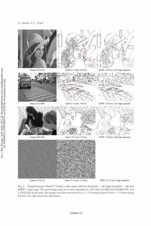
Image (512x512) OpenCV Canny: 8.40 ms EDPF: 16.75 ms, 214 edge segments

Image (512x384) OpenCV Canny: 6.90 ms EDPF: 11.65 ms, 201 edges egments

Image (600x450) Open CV Canny: 9.51ms EDPF: 17.69 ms, 284 edge segments

Image (512x512) Open CV Canny: 13.62ms EDPF: 32.12 ms, 0 edge segments

Fig. 3. Original images; OpenCV Canny's edge maps with low threshold ¼ 30, high threshold ¼ 60; andEDPF's edge maps. The processing times have been obtained in a PC with 2.2GHz Intel E4500 CPU and

2 GB RAM. In all cases, the images were ¯rst smoothed by a 5� 5 Gaussian kernel with � ¼ 1 before being

fed into the edge detection algorithms.


1255002-12

Int.

J. P

att.

Rec

ogn.

Art

if. I

ntel

l. 20

12.2

6. D

ownl

oade

d fr

om w

ww

.wor

ldsc

ient

ific

.com

by A

NA

DO

LU

UN

IVE

RSI

TY

on

02/2

0/18

. For

per

sona

l use

onl

y.

5.4. EDPF's performance on noisy images

Noisy images are very tough cases for typical edge detectors. Since the noise causes

many discontinuities in an image, a typical edge detector produces many invalid

edgel detections. To evaluate the performance of EDPF on noisy images, we have

taken an image, added increasing amounts of Gaussian white noise to the image and

fed the resulting noisy images to EDPF and OpenCV Canny.

Figure 5 shows the edge maps produced by OpenCV Canny and EDPF for an

image containing a house as the amount of noise in the image is increased. Speci¯-

cally, the image in the ¯rst row contains no noise; the images in the second, third and

fourth rows contain 5%, 10% and 15% Gaussian white noise, respectively. In no noise

and low noise cases (rows one and two), both OpenCV Canny and EDPF produce

high-quality edge maps. But in high noise cases (rows three and four), OpenCV

Canny produces almost completely garbage edge maps, but EDPF is able to

(a) (b) (c) (d)

Fig. 4. (a) Original images. (b)�(d) EDPF's edge maps with Prewitt, Sobel and Scharr gradient oper-

ators, respectively.


1255002-13

Int.

J. P

att.

Rec

ogn.

Art

if. I

ntel

l. 20

12.2

6. D

ownl

oade

d fr

om w

ww

.wor

ldsc

ient

ific

.com

by A

NA

DO

LU

UN

IVE

RSI

TY

on

02/2

0/18

. For

per

sona

l use

onl

y.

(a) (b) (c)

Fig. 5. (a) Original image. First row — no noise; second, third and fourth rows — 5%, 10% and 15%

Gaussian white noise added, respectively, (b) OpenCV Canny's edge maps with low threshold ¼ 30, highthreshold ¼ 60 and (c) EDPF's edge maps.


1255002-14

Int.

J. P

att.

Rec

ogn.

Art

if. I

ntel

l. 20

12.2

6. D

ownl

oade

d fr

om w

ww

.wor

ldsc

ient

ific

.com

by A

NA

DO

LU

UN

IVE

RSI

TY

on

02/2

0/18

. For

per

sona

l use

onl

y.

eliminate noisy parts of the image and return the general structure of the house,

albeit by missing some parts such as the long roof line on the left. The reason for

EDPF missing some valid boundaries in high noise cases has to do with ED's anchor

linking step.12,57 Recall from Sec. 2 that ED works by computing a set of stable

anchors and linking these anchors by a smart routing algorithm. The linking step

makes use of pixel's gradient magnitudes and directions. In low noise cases, Gaussian

smoothing is able to take care of the noise so that the gradient magnitudes and

directions are not adversely a®ected. However, in high noise cases, the noise on the

boundary of an object (such as the roof line on the left) diverts the anchor linking

direction towards noisy parts of the image. This causes short, noisy edge segment

formations, which get eliminated during segment validation. Despite such potential

boundary misses in high noise images, EDPF is still able to detect many of the

meaningful boundaries of the objects in the given images as seen from EDPF's edge

map results. It is also important to note that EDPF may miss some valid boundaries,

but it never returns meaningless edge segment formations (as de¯ned by the

Helmholtz principle) no matter how much noise is present in the image.

5.5. EDPF as a boundary/contour detector

EDPF can be used as a boundary/contour detector for image segmentation.2,39,43�45,60

In this section, we quantitatively evaluate the quality of the edge maps produced by

EDPF, and compare them to a few state of the art boundary/contour detection

algorithms. For the purposes of evaluation, we will use the RUG database,50 which

contains 40 natural images and their hand-drawn ground-truth segmentation data.

Figure 6 shows six images from the RUG database50 and each row in Fig. 6

corresponds to boundaries/contours detected by a di®erent algorithm. The second

row shows the hand-drawn ground-truth segmentation data. The third row shows

the contours detected by EDPF, the fourth row shows the contours detected edge

detection and image segmentation system (EDISON),39 and the ¯fth row shows the

contours detected by adaptive pseudo dilation (APD)43 algorithm. The results for

the ground-truth data, EDISON and APD were taken from APD's Web site.50 We

stress that EDPF is a general purpose edge/edge segment detection algorithm;

whereas both EDISON and APDF are speci¯cally tailored towards boundary/con-

tour detection and image segmentation. Comparing EDPF's contours to ground-

truth data we observe that EDPF seems to detect most of the contours present in the

ground-truth data, but EDPF also detects some super°uous contours especially

around anisotropic structures in the background such as grass, trees and clouds.

EDISON, although speci¯cally designed for image contour detection and image

segmentation problems, does not seem to perform any better than EDPF. APD

seems to produce cleaner contours, but at the expense of missing some details in the

images.

To quantitatively compare the performance of EDPF, EDISON and APD on the

RUG database, we use the famous F -measure metric.2,43,60 Let DC be the set of


1255002-15

Int.

J. P

att.

Rec

ogn.

Art

if. I

ntel

l. 20

12.2

6. D

ownl

oade

d fr

om w

ww

.wor

ldsc

ient

ific

.com

by A

NA

DO

LU

UN

IVE

RSI

TY

on

02/2

0/18

. For

per

sona

l use

onl

y.

contour pixels detected by an algorithm, and GT be the set of pixels in the ground-

truth data. De¯ne precision (P ) and recall (R) as follows:

R ¼ cardfDC \GTgcardfGTg ; P ¼ cardfDC \GTg

cardfDCg :

F -measure, de¯ned as the harmonic mean of P and R; F ¼ 2PR=ðP þRÞ, measures

the performance of a boundary detection algorithm: The bigger the value of

F -measure, the better the algorithm is in detecting the boundaries compared to

hand-drawn ground-truth segmentation data.

Table 1 shows the Recall, Precision and F -measure averages for 40 images in the

RUG database for EDPF,14 EDISON39 and APD [59].43 According to F -measure

metric, APD has the best performance while EDPF and EDISON have the same

performance. The ¯ndings are consistent with the visual tests shown in Fig. 6: EDPF

Fig. 6. Six test images (¯rst row), ground truth contours (second row), contours detected with EDPF

(third row), contours detected with edge detection and image segmentation system (EDISON) (fourth

row)39 and contours detected with adaptive pseudo dilation (APD) (¯fth row).43


1255002-16

Int.

J. P

att.

Rec

ogn.

Art

if. I

ntel

l. 20

12.2

6. D

ownl

oade

d fr

om w

ww

.wor

ldsc

ient

ific

.com

by A

NA

DO

LU

UN

IVE

RSI

TY

on

02/2

0/18

. For

per

sona

l use

onl

y.

and EDISON detect most of the contours present in the ground-truth data (high

recall), but also detect many super°uous contours (low precision). APD on the other

hand produces much cleaner boundaries (high precision), but misses on many of the

contours (low recall). We would like to stress that although EDPF is a general

purpose edge/edge segment detection algorithm and is parameter-free, its perform-

ance is not worse than EDISON, which is a boundary/contour detection algorithm

speci¯cally tailored towards image segmentation problems. Given that EDPF has

high recall rate, EDPF's edge segments can further be processed after initial detec-

tion, and many super°uous detections found in the background can be eliminated.

Such post-processing would increase the precision rate of EDPF and result in a much

higher F -measure ratio. Tailoring EDPF towards such speci¯c image segmentation

problems is out of the scope of this paper, and is left as future work.

5.6. Line segment detection from EDPF's edge segments

As we stated in Sec. 5.2, EDPF returns its output both as a binary edge map similar

to traditional edge detection algorithms, and also as a set of edge segments, each

comprised of a linear, contiguous chain of pixels. In this section, we show how to

make use of EDPF's edge segments to extract all line segments in a given image in an

e±cient manner. We also compare our results to the fastest line segment extraction

algorithm in the literature; the LSD by Grompone von Gioi et al.22,23,36

Figure 7 shows ¯ve natural images (column one) and EDPF's edge segments for

each image (column two). To extract line segments from EDPF's edge segments, we

simply walk over the linear chain of pixels making up an edge segment and ¯t a line

segment to these pixels using the standard least squares line ¯tting algorithm.35 A

line segment is extended for as long as the line ¯t error stays within a certain

threshold, e.g. 1 pixel error. When the error exceeds this threshold, we output a line

segment and recursively use the rest of the edge segment pixels to extract more line

segments. This process continues until all edge segments are processed (see Refs. 1

and 13 for more details on line segment extraction from a given edge segment).

The third column in Fig. 7 shows the line segments extracted from EDPF's edge

segments. The numbers under each image shows the total number of extracted line

segments and the total running time for the entire process. This running time

includes the time for edge segment detection by EDPF, line segment extraction from

EDPF's edge segments, and line segment validation due to the Helmholtz prin-

ciple.11,22,23,36 We see from the results that not only EDPF's line segments are very

Table 1. Recall, Precision and F -measure averages for 40 images in the

RUG database for EDPF,14 EDISON39 and APD.43

Algorithm Recall average Precision average F -measure average

EDPF 0.75 0.30 0.41EDISON39 0.74 0.30 0.41

APD43 0.46 0.70 0.54


1255002-17

Int.

J. P

att.

Rec

ogn.

Art

if. I

ntel

l. 20

12.2

6. D

ownl

oade

d fr

om w

ww

.wor

ldsc

ient

ific

.com

by A

NA

DO

LU

UN

IVE

RSI

TY

on

02/2

0/18

. For

per

sona

l use

onl

y.

Image (400x400) EDPF: 173 Edge Segments EDPF: 151 lines, 15.41 ms LSD: 171 lines, 75.50 ms





Fig. 7. Original images (column one), EDPF's edge segments (column two), line segments extracted from

EDPF's edge segments (column three) and LSD's line segments (column four). The processing times have

been obtained in a PC with 2.2GHz Intel E4500 CPU and 2 GB RAM.


1255002-18

Int.

J. P

att.

Rec

ogn.

Art

if. I

ntel

l. 20

12.2

6. D

ownl

oade

d fr

om w

ww

.wor

ldsc

ient

ific

.com

by A

NA

DO

LU

UN

IVE

RSI

TY

on

02/2

0/18

. For

per

sona

l use

onl

y.

well localized, but also the total running time is very low. Speci¯cally, all line seg-

ment detections can be performed in real time.

The last column in Fig. 7 shows the line segments detected by the famous LSD by

Grompone von Gioi et al.22,23,36 LSD works by growing line support regions by

combining pixels having similar gradient orientations. Region growing continues

until the error exceeds a certain threshold, at which point the line support region is

validated using the Helmholtz principle and a line segment is output if validated.

LSD is known to be the fastest line segment detection algorithm in the literature, and

produces no false detections.

Comparing EDPF's line segments to those of LSD, we see that not only EDPF's

line segments are better than LSD's but EDPF's line segment extraction algorithm

runs up to seven times faster than LSD. Pay particular attention to the last row in

Fig. 7, which is the noisy house image. For this image, EDPF detects many long line

segments; whereas LSD is not able to detect many of the visible line segments in the

image. Note that neither EDPF nor LSD has any false detections because both

validate their line segments with a validation algorithm due to the Helmholtz

principle (see Refs. 22, 23 and 36 for details on line segment validation due to the

Helmholtz principle). We conclude that line segment extraction from EDPF's edge

segments is a huge improvement from the current state of the art line segment

extraction algorithms and would be very suitable for the next generation computer

vision algorithms. We stress that this is all made possible by EDPF's clean, con-

tiguous, well-localized edge segments.

6. Conclusion

We present a real-time, parameter-free edge/edge segment detection algorithm based

on our novel edge/edge segment detector, the edge drawing (ED) algorithm; hence

the name edge drawing parameter free (EDPF). The edge segments produced by

EDPF are of high-quality consisting of clean, contiguous, well-localized, one-pixel

wide edges. The edge segments are also \meaningful" as de¯ned by the Helmholtz

principle; that is, they are guaranteed to reside on the boundaries of perceptually

visible Gestalt structures. Experiments on many di®erent images and many more

that the reader may perform online14 show that EDPF produces good results with

many di®erent sets of images. We believe that EDPF is a major step forward in the

quest for a parameter-free edge/edge segment detector, and would be very suitable

for the next generation real-time computer vision and image processing applications.

References

1. C. Akinlar and C. Topal, EDLines: Realtime line segment detection by edge drawing(ED), IEEE Int. Conf. Image Processing (ICIP) (2011).

2. P. Arbela�ez, M. Maire, C. Fowlkes and J. Malik, Contour detection and hierarchicalimage segmentation, IEEE Trans. Patt. Anal. Mach. Intell. 33(5) (2011) 898�916.

3. F. Bergholm, Edge focusing, IEEE Trans. Patt. Anal. Mach. Intell. 9(6) (1987) 726�741.


1255002-19

Int.

J. P

att.

Rec

ogn.

Art

if. I

ntel

l. 20

12.2

6. D

ownl

oade

d fr

om w

ww

.wor

ldsc

ient

ific

.com

by A

NA

DO

LU

UN

IVE

RSI

TY

on

02/2

0/18

. For

per

sona

l use

onl

y.

4. K. Bowyer, C. Kranenburg and S. Dougherty, Edge detector evaluation using empiricalROC curves, Comput. Vis. Image Understand. 84(1) (2001) 77�103.

5. D. J. Bryant and D. W. Bouldin, Evaluation of edge operators using relative andabsolute grading, Int. Conf. Pattern Recognition and Image Processing, Chicago (1979),pp. 138�145.

6. J. Canny, A computational approach to edge detection, IEEE Trans. Patt. Anal. Mach.Intell. 8(6) (1986) 679�698.

7. X. Dai and S. Khorram, A feature-based image registration algorithm using improvedchain-code representation combined with invariant moments, IEEE Trans. Geosci.Remote Sens. 37(5) (1999) 2351�2362.

8. A. Desolneux, L. Moisan and J. M. Morel, Edge detection by Helmholtz principle,J. Math. Imag. Vis. 14(3) (2001) 271�284.

9. A. Desolneux, L. Moisan and J. M. Morel, From Gestalt Theory to Image Analysis: AProbobilistic Approach (Springer, 2008).

10. A. Desolneux, L. Moisan and J. M. Morel, Gestalt theory and computer vision, Seeing,Thinking and Knowing (Kluwer Academic Publishers, 2004), pp. 71�101.

11. A. Desolneux, L. Moisan and J. M. Morel, Meaningful alignments, Int. J. Comput. Vis.40(1) (2000) 7�23.

12. Edge Drawing Web Site, http://ceng.anadolu.edu.tr/CV/EdgeDrawing.13. EDLines Web Site, http://ceng.anadolu.edu.tr/cv/EDLines.14. EDPF Web Site, http://ceng.anadolu.edu.tr/CV/EDPF.15. A. Etemadi, Robust segmentation of edge data, Int. Conf. Image Processing and Its

Applications (1992), pp. 311�314.16. V. Ferrari, L. Fevrier, F. Jurie and C. Schmid, Groups of adjacent contour segments for

object detection, IEEE Trans. Patt. Anal. Mach. Intell. 30(1) (2008) 36�51.17. J. R. Fram and E. S. Deutsch, On the quantitative evaluation of edge detection schemes

and their comparison with human performance, IEEE Trans. Comput. 24(6) (1975)616�628.

18. H. Freeman, Computer processing of line drawing images, Comput. Surv. 6 (1974) 57�98.19. Y. Gao and M. K. H. Leung, Face recognition using line edge map, IEEE Trans. Patt.

Anal. Mach. Intell. 24(6) (2002) 764�779.20. M. Gokmen and C. C. Li, Edge detection and surface reconstruction using re¯ned

regularization, IEEE Trans. Patt. Anal. Mach. Intell. 15(5) (1993) 492�498.21. P. H. Gregson, Using angular dispersion of gradient direction for detecting edge ribbons,

IEEE Trans. Patt. Anal. Mach. Intell. 15 (1993) 682�696.22. R. Grompone von Gioi, J. Jakubowicz, J. M. Morel and G. Randall, LSD: A line segment,

Technical report, Centre de Mathematiques et de leurs Applications (CMLA), EcoleNormale Superieure de Cachan (ENS-CACHAN) (2008).

23. R. Grompone von Gioi, J. Jakubowicz, J. M. Morel and G. Randall, LSD: A fast linesegment detector with a false detection control, IEEE Trans. Patt. Anal. Mach. Intell.32(4) (2010) 722�732.

24. L. Gupta and M. D. Srinath, Contour sequence moments for the classi¯cation of closedplanar shapes, Patt. Recogn. 20(3) (1987) 267�272.

25. M. D. Heath, S. Sarkar, T. Sanocki and K. W. Bowyer, A robust visual method forassessing the relative performance of edge-detection algorithms, IEEE Trans. Patt. Anal.Mach. Intell. 19 (1997) 1338�1359.

26. W. E. Higgins and C. Hsu, Edge detection using 2D local structure information, Patt.Recogn. 27(2) (1994) 277�294.

27. P. Hough, Method and means for recognizing complex patterns, US Patent 306954(1962).


1255002-20

Int.

J. P

att.

Rec

ogn.

Art

if. I

ntel

l. 20

12.2

6. D

ownl

oade

d fr

om w

ww

.wor

ldsc

ient

ific

.com

by A

NA

DO

LU

UN

IVE

RSI

TY

on

02/2

0/18

. For

per

sona

l use

onl

y.

28. J. Iivarinen, M. Peura, J. Särelä and A. Visa, Comparison of combined shape descriptorsfor irregular objects, Proc. Eight British Machine Vision Conf., UK (1997).

29. J. Illingworth and J. Kittler, A survey of the Hough transform, Comput. Vis., Graph.,Image Process. 44(1) (1988) 87�116.

30. L. A. Iverson and S. W. Zucker, Logical/linear operators for image curves, IEEE Trans.Patt. Anal. Mach. Intell. 17(10) (1995) 982�996.

31. W. J. Kang, X. Ding, J. Cui and L. Ao, Fast straight-line extraction algorithm based onimproved Hough transform, Opto-Electron. Eng. 34(3) (2007) 105�108.

32. T. Kanungo, M. Y. Jaisimha, J. Palmer and R. M. Haralick, A methodology for quan-titative performance evaluation of detection algorithms, IEEE Trans. Image Process.4(12) (1995) 1667�1674.

33. S. Kiranyaz, M. Ferreira and M. Gabbouj, A generic shape/texture descriptor overmultiscale edge ¯eld: 2-D walking ant histogram, IEEE Trans. Image Process. 17(3)(2008) 377.

34. N. Kiryati, Y. Eldar and A. M. Bruchstein, Probabilistic Hough transform, Patt. Recogn.24 (1991) 303�316.

35. Least Squares Line Fitting, http://en.wikipedia.org/wiki/Least Squares.36. LSD: A Line Segment Detector Web Site, http://www.ipol.im/pub/algo/gjmr

line segment detector.37. D. C. Marr and E. Hildreth, Theory of edge detection, Proc. Roy. Soc. Lond. B

207(1167) (1980) 187�217.38. S. Marshall, Review of shape coding techniques, Image Vis. Comput. 7(4) (1989)

281�294.39. P. Meer and B. Georgescu, Edge detection with embedded con¯dence, IEEE Trans. Patt.

Anal. Mach. Intell. 23(12) (2001) 1351�1365.40. E. Meinhardt-Llopis, Edge detection by selection of pieces of level lines, Proc. Int. Conf.

Image Processing (ICIP) (2008), pp. 613�616.41. V. S. Nalwa and T. O. Binford, On detecting edges, IEEE Trans. Patt. Anal. Mach. Intell.

8(6) (1986) 699�714.42. OpenCV 2.1, http://opencv.willowgarage.com.43. G. Papari and N. Petkov, Adaptive pseudo dilation for gestalt edge grouping and contour

detection, IEEE Trans. Image Process. 17(10) (2008) 1950�1962.44. G. Papari and N. Petkov, Edge and line oriented contour detection: State of the art,

Image Vis. Comput. 29 (2011) 79�103.45. G. Papari, P. Campisi, N. Petkov and A. Neri, A biologically motivated multiresolution

approach to contour detection, EURASIP J. Adv. Signal Process. 2007 (2007) 71828.46. J. M. S. Prewitt, Object enhancement and extraction, Picture Processing and Psycho-

pictorics, eds. B. Lipkin and A. Rosenfeld (Academic Press, 1970).47. V. Ramesh and R. M. Haralick, Performance characterization of edge detectors, Proc.

SPIE, Applications of Arti¯cial Intelligence X: Machine Vision and Robotics, Vol. 1708(1992), pp. 252�266.

48. K. R. Rao and J. Ben-Arie, Optimal edge detection using expansion matching and res-toration, IEEE Trans. Patt. Anal. Mach. Intell. 16(12) (1994) 1169�1182.

49. C. A. Rothwell, J. L. Mundy, W. Ho®man and V. D. Nguyen, Driving vision by topology,Int. Symp. Computer Vision, Coral Gables, November 1995, pp. 395�400.

50. RUG database, http://www.cs.rug.nl/�imaging/APD/rug/rug.html.51. H. Scharr, Optimal operators in digital image processing, Ph.D. thesis, Heidelberg

University (2000).52. I. Sobel and G. Feldman, A 3� 3 isotropic gradient operator for image processing, Pattern

Classi¯cation and Scene Analysis (John Wiley and Sons, 1973), pp. 271�272.


1255002-21

Int.

J. P

att.

Rec

ogn.

Art

if. I

ntel

l. 20

12.2

6. D

ownl

oade

d fr

om w

ww

.wor

ldsc

ient

ific

.com

by A

NA

DO

LU

UN

IVE

RSI

TY

on

02/2

0/18

. For

per

sona

l use

onl

y.

53. V. Srinivasan, Edge detection using neural networks, Patt. Recogn. 27(12) (1994)1653�1662.

54. J. S. Stahl and S. Wang, Edge grouping combining boundary and region information,IEEE Trans. Image Process. 16(10) (2007) 2590.

55. R. N. Strickland and D. K. Cheng, Adaptable edge quality metric, Opt. Eng. 32(5) (1993)944�951.

56. P. J. Tadrous, A simple and sensitive method for directed edge detection, Patt. Recogn.28(10) (1995) 1575�1586.

57. C. Topal, C. Akınlar and Y. Genç, Edge drawing: A heuristic approach to robust real-time edge detection, Proc. Patt. Recognition (ICPR) (2010), pp. 2424�2427.

58. F. van der Heijden, Edge and line feature extraction based on covariance models, IEEETrans. Patt. Anal. Mach. Intell. 17(1) (1995) 16.

59. F. van der Heijden, Edge and line feature extraction based on covariance models, IEEETrans. Patt. Anal. Mach. Intell. 17(1) (1995) 16�33.

60. S. Wang, F. Ge and T. Liu, Evaluating edge detection through boundary detection,EURASIP J. Appl. Signal Process. 2006 (2006) 1�15.

61. M. Xia and B. Liu, Image registration by super-curves, IEEE Trans. Image Process.13(5) (2004) 720.

62. L. Xu, E. Oja and P. Kultanen, A new curve detection method: Randomized HoughTransform (RHT), Patt. Recogn. Lett. 11(5) (1990) 331�338.

63. D. Ziou and S. Tabbone, A multiscale edge detector, Patt. Recogn. 26(9) (1993)1305�1314.

CuneytAkinlar receivedhis B.Sc. degree in Com-puter Engineering fromBilkent University in 1994;M.Sc. andPh.D. degrees inComputer Science fromthe University of Mary-land, College Park in 1997and 2001, respectively. Heis currently an AssistantProfessor in Anadolu Uni-

versity, Computer Engineering Department (AU-CENG). Before joining AU-CENG, he worked atPanasonic Technologies, Princeton, NJ, and Sie-mens Corporate Research, Princeton, NJ as stu-dent intern and research scientist between 1999and 2003.

His current research interests include real-time image processing and computer visionalgorithms, high-performance computing, storagesystems and computer networks.

Cihan Topal receivedhis B.Sc. degree in Elec-trical Engineering andM.S. degree in ComputerEngineering, both fromAnadolu University, in2005 and 2008, respect-ively. He worked as astudent intern at SiemensCorporate Research,Princeton, New Jersey.

He is currently working at Anadolu UniversityComputer Engineering Department, Turkey,torwards his Ph.D. degree. His research interestsare in the area of image processing and computervision applications, and pattern recognition.


1255002-22

Int.

J. P

att.

Rec

ogn.

Art

if. I

ntel

l. 20

12.2

6. D

ownl

oade

d fr

om w

ww

.wor

ldsc

ient

ific

.com

by A

NA

DO

LU

UN

IVE

RSI

TY

on

02/2

0/18

. For

per

sona

l use

onl

y.

edpf: a real-time parameter-free edge segment detector

Documents