education and the timing of births: evidence from a ... · education and the timing of births:...

Education and the Timing of Births:

Evidence from a Natural Experiment in Italy

Margherita Fort

Dipartimento di Scienze Statistiche Università degli Studi di Padova

and European Centre for Analysis in the Social Sciences, ISER

ISER Working Paper 2005-20

Institute for Social and Economic Research The Institute for Social and Economic Research (ISER) specialises in the production and analysis of longitudinal data. ISER incorporates the following centres: • ESRC Research Centre on Micro-social Change. Established in 1989 to identify, explain, model

and forecast social change in Britain at the individual and household level, the Centre specialises in research using longitudinal data.

• ESRC UK Longitudinal Studies Centre. A national resource centre for promoting longitudinal

research and for the design, management and support of longitudinal surveys. It was established by the ESRC as independent centre in 1999. It has responsibility for the British Household Panel Survey (BHPS).

• European Centre for Analysis in the Social Sciences. ECASS is an interdisciplinary research

centre which hosts major research programmes and helps researchers from the EU gain access to longitudinal data and cross-national datasets from all over Europe.

The British Household Panel Survey is one of the main instruments for measuring social change in Britain. The BHPS comprises a nationally representative sample of around 9,000 households and over 16,000 individuals who are reinterviewed each year. The questionnaire includes a constant core of items accompanied by a variable component in order to provide for the collection of initial conditions data and to allow for the subsequent inclusion of emerging research and policy concerns. Among the main projects in ISER’s research programme are: the labour market and the division of domestic responsibilities; changes in families and households; modelling households’ labour force behaviour; wealth, well-being and socio-economic structure; resource distribution in the household; and modelling techniques and survey methodology. BHPS data provide the academic community, policymakers and private sector with a unique national resource and allow for comparative research with similar studies in Europe, the United States and Canada. BHPS data are available from the UK Data Archive at the University of Essex http://www.data-archive.ac.uk Further information about the BHPS and other longitudinal surveys can be obtained by telephoning +44 (0) 1206 873543. The support of both the Economic and Social Research Council (ESRC) and the University of Essex is gratefully acknowledged. The work reported in this paper is part of the scientific programme of the Institute for Social and Economic Research.

Acknowledgement: This version of the paper, based on my PhD thesis at the University of Padova, has been developed during my research visit (ECASS visiting fellowship) to the Institute of Social and Economic Research (October 2005), whose hospitality is gratefully acknowledged. I would like to thank my PhD supervisor Enrico Rettore, for his useful comments and insights, and Erich Battistin and Massimiliano Bratti for their constructive and detailed comments. I am grateful to Marco Francesconi and John Ermisch for useful discussions. This paper has also benefited from comments and suggestions of partecipants in seminars at the University of Padova, LABORatorio Revelli (Torino) and at the Institute of Social and Economic Research (Colchester). Financial support from MIUR to the project ``Evaluating the effects of labour market polices and incentives to firms and welfare policies: methodological issues and case studies'' is gratefully acknowledged. The usual disclaimer applies.

Readers wishing to cite this document are asked to use the following form of words:

Fort, Margherita (October 2005) ‘Education and the Timing of Births: Evidence from a Natural Experiment in Italy’, ISER Working Paper 2005-20. Colchester: University of Essex.

For an on-line version of this working paper and others in the series, please visit the Institute’s website at: http://www.iser.essex.ac.uk/pubs/workpaps/

Institute for Social and Economic Research University of Essex Wivenhoe Park Colchester Essex CO4 3SQ UK Telephone: +44 (0) 1206 872957 Fax: +44 (0) 1206 873151 E-mail: [email protected] Website: http://www.iser.essex.ac.uk

© October 2005 All rights reserved. No part of this publication may be reproduced, stored in a retrieval system or transmitted, in any form, or by any means, mechanical, photocopying, recording or otherwise, without the prior permission of the Communications Manager, Institute for Social and Economic Research.

ABSTRACT

This paper assesses the causal effects of education on the timing of first births allowing for heterogeneity in the effects across individuals while controlling for self-selection of women into education. Identification relies on exogenous variation in schooling induced by a mandatory school reform rolled out nationwide in Italy in the early 1960s. Findings based on Census data (Italy, 1981) suggest that a large fraction of the women affected by the reform postpones the time of the first birth but catches up with this fertility delay before turning 26. There is some indication that the fertility return to schooling of these women is substantially different from the one of the average individual in the population. Keywords : Causal Effects Identification, Education, Local Average Treatment Effects, Motherhood Decisions, Regression Discontinuity Design. JEL codes: J10, J13, I2.

1

NON-TECHNICAL SUMMARY

This paper aims at assessing the causal effects of education on the timing of births in Italy by exploiting a school reform rolled out in the early 1960s, which increased the compulsory schooling age by three years (from 11 to 14). Italy was in the early 1990s one of the first countries to attain and sustain the lowest-low fertility levels. Besides, the Italian schooling system has undergone lots of changes since 1859, particularly as far as compulsory schooling is concerned; notably, the last increase of compulsory schooling age was planned in 1999. Thus, addressing the question of how fertility responds to exogenous variation in education might prove useful for planning effective policies aimed at contrasting the decreasing trends in fertility. In the last decades, several European countries have experienced both a decline in fertility and motherhood postponement: Sleebos (2003) underlined that several OECD governments are considering or have already introduced specific measures aimed at countering these trends in fertility. Besides, also teenage childbearing attracts some politic interest, due to its association with a range of disadvantages, both for the mother and for children: on average, across 13 countries of the European Union, women who give birth as a teenager are twice as likely of living in poverty. At the same time, also the education level of individuals has recently been (and is currently) on the agenda of policy makers in most countries: in the period 1950-1970 many European countries carried out major educational reforms aimed at increasing compulsory schooling, at unifying curricula, at delaying or abolishing the selection of more able students into separate schools and the central role of education in achieving the European Union strategic goal has also been recently stressed during the 2005 summit in Bruxelles. Do family friendly policies, policies aimed at reducing teenage childbearing and policies aimed at increasing average schooling achievement pursue compatible goals? Besides, do these policies affect any woman in the same way? A number of studies report negative association between schooling achievements and completed fertility in most countries. According to the model developed by Mullin and Wang (2002), women with greater ability face larger loss in earnings from having children and thus delay childbearing. Moreover, higher ability women are more sensitive to changes in the utility children provide once born. Ellwood et al. (2004) find some evidence that the lifetime costs of childrearing are particularly high for skilled women and are reduced by delaying childbearing. To assess if policies aimed at increasing average schooling achievement and policies aimed at reconciling motherhood and work pursue intrinsically contrasting goals, further knowledge has to be achieved on the causal effects of education on fertility. Indeed, the direct comparison between women with different qualification level does not generally identify the causal effects of education on fertility, since women with preferences for larger number of children are likely to invest less in human capital and have their children earlier. Besides, giving insights on the variability of the fertility returns on education across women might be relevant for targeting policies to specific subgroups of individuals. In this paper, evidence supporting the role of education in determining the timing of first births is provided. The identification strategy exploits the fact that women born just after year 1949 were affected by the increase in compulsory schooling imposed by a reform rolled out nationwide in Italy in the early 1960s, whereas women born just before year 1949 were not. Compared to women born before 1949, women of the cohorts 1950-1952 have substantially lower likelihood to experience childbearing for the first time by the ages 19, 20, 21, whereas they have a higher likelihood to bear their first child by the age 23. No evidence is found of a causal effect of education on the probability of bearing the first child by older ages (24, 25, and 26).

2

On prior grounds it sounds credible that women born in subsequent cohort are essentially exchangeable, so that these results are essentially as good as comparisons based on randomization. However, over the 1970s women position in the society, in Italy, went trough major changes, driven also by the newly introduced law on divorce (1970), the decrease in the threshold age at which a person becomes of age (1975), the law on abortion (1978) and the availability of oral contraceptives. The internal validity of the research design is extensively discussed, explicitly considering also these factors: evidence based on the data at hand suggests that the 1963 reform represents a valid instrument, which helps to correctly identify the causal effect of education on the timing of first births for the sub-population of women affected by the reform. The estimates provided apply only to women who were affected by the 1963 reform on compulsory schooling, i.e. to 3%-6% of the population. Besides, findings suggest heterogeneity of the effects across individuals and that the fertility return to schooling of women affected by the reform is likely to be substantially different from the one of the average woman in the population. Generalizing this effect to a wider set of individuals requires typically to rely on stronger conditions than those who guarantee local identification. Nonetheless, the sub-population of women affected by the reform might be per se an interesting sub-population, if, for example, the women affected by compulsory schooling laws happen to be those at the highest risk of teenage childbearing.

1 Introduction and Motivation of the Paper

This paper aims at assessing the causal effects of education on the timingof first births in Italy by exploiting a school reform rolled out in the early1960s, which increased the compulsory schooling age by three years (from11 to 14).Italy was in the early 1990s one of the first countries to attain and sustainthe lowest-low fertility levels1(Kohler and Billari and Ortega [44]). Besides,the Italian schooling system has undergone lots of changes since 1859, par-ticularly as far as compulsory schooling is concerned (see Genovesi [35]);notably, the last increase of compulsory schooling age was planned in 1999.Thus, addressing the question of how fertility responds to exogenous varia-tion in education might prove useful for planning effective policies aimed atcontrasting the decreasing trends in fertility.In the last decades, several European countries have experienced both de-cline in fertility and motherhood postponement (Gustafsson [36]): Sleebos[56] underlined that several OECD governments are considering or havealready introduced specific measures aimed at countering these trends infertility.Besides, also teenage childbearing attracts some politic interest, due to itsassociation with a range of disadvantages, both for the mother2 and for chil-dren3: on average, across 13 countries of the European Union, women whogive birth as a teenager are twice as likely of living in poverty (UNICEF[59]).At the same time, also the education level of individuals has recently been(and is currently) on the agenda of policy makers in most countries4: in theperiod 1950-1970 many European countries carried out major educationalreforms aimed at increasing compulsory schooling, at unifying curricula,at delaying or abolishing the selection of more able students into separateschools (Leschinsky and Mayer [48]).

Do family friendly policies, policies aimed at reducing teenage childbearingand policies aimed at increasing average schooling achievement pursue com-

1Total fertility rate at or below 1.3.2For instance: dropping out school, being unemployed or low paid, live in poor housing

conditions, live on welfare.3For instance: being a victim of neglect or abuse, becoming involved in crime, achieving

lower qualification, abusing drug or alcohol.4The Millennium Development Goals include “achieve universal primary education”

(goal 2) and “eliminate gender disparity in primary and secondary education, preferablyby 2005, and in all levels of education no later than 2015” (target 4) (UN MillenniumProject 2005 [1]). The central role of education in achieving the European Union strategicgoal (“become the most competitive and dynamic knowledge-based economy in the worldcapable of sustainable economic growth with more and better jobs and greater socialcohesion”) has also been recently stressed during the 2005 summit in Bruxelles (EuropeanUnion [26])

1

patible goals? Besides, do these policies affect any woman in the same way?A number of studies report negative association between schooling achieve-ment and completed fertility in most countries: among others, Nicoletti andTanturri[50], examining data on 10 European countries, found that higherlevel of education generally lead to both postponement of motherhood andto a reduction of the probability of the first birth event.According to the model developed by Mullin and Wang[49], women withgreater ability face larger loss in earnings from having children and thusdelay childbearing. Moreover, higher ability women are more sensitive tochanges in the “childrearing preference”5. Ellwood et al. [33] find some evi-dence that the lifetime costs of childrearing are particularly high for skilledwomen and are reduced by delaying childbearing. Costs of childbearingfor high skilled women seem to increase with time. Conversely, low skilledwomen seem to face a one-time loss.

To assess if policies aimed at increasing average schooling achievementand policies aimed at reconciling motherhood and work pursue intrinsicallycontrasting goals, further knowledge has to be achieved on the causal effects

of education on fertility. Indeed, the direct comparison between women withdifferent qualification level does not generally identify the causal effects ofeducation on fertility, since women with preferences for larger number ofchildren are likely to invest less in human capital. Besides, giving insightson the variability of the fertility returns on education across women mightbe relevant for targeting policies to specific subgroups of individuals.

Thus, the main focus of this paper is to address the question of howfertility responds to exogenous variations in education in Italy, allowingfor heterogeneity in the effects across individuals while controlling for self-selection of women into education. Since the analysis is not restricted tomarital fertility and it considers a cohort measure of fertility instead than aperiod one, it can be profitably combined with previous work by Bratti[17]widening the knowledge on the determinants of the recent trends in fertilityin Italy. Moreover, it presents an identification strategy that can be eas-ily used for the same purpose in other countries, thus setting the bases forfuture beneficial cross-country comparisons, which might support the gener-alizability of the results. The same identification strategy has already beenused to investigate the links between female labour force participation andmarital fertility (among others, Angrist and Evans [4] and Schultz [54]) buthas not yet been used to deal directly with the links between education andfertility.

The remainder of the paper is organized as follows: section 2 discusses

5That is the utility children provide once born.

2

the predictions of economic models of fertility choices, with particular atten-tion to the potential role of parents educational achievement in determiningthe timing of births. Besides, section 2 reviews empirical findings of previ-ous studies on the relationship between parent’s educational achievement onthe timing of births. Section 3 presents in greater detail the identificationand the estimation strategy, as well as the data used. Section 4 discussesthe main findings and section 5 provides arguments supporting the internalvalidity of the estimates. Section 6 concludes.

2 Education & Tempo Fertility: Theoretical Mod-els and Empirical Evidence

This section, firstly, discusses how variation in prices, wages and incomecould affect the optimal age at motherhood according to the various dy-namic models developed in the literature6, highlighting the potential roleof parents education in determining the timing of births. Then, it presentsempirical evidence found in previous studies on the relationship betweenparent’s educational achievement and tempo fertility.

Some of the crucial ideas of the work by Becker[6] are relevant also forthe dynamic modelling of fertility: (i) the idea that household membersspecialize in market or home activities according to their comparative ad-vantages and also allocate investments according to these, (ii) the conceptof “children’s quality” (future earning ability and life expectancy of the off-spring) and the implications of the interaction between number of childrenand children’s quality.Becker argued that men and women have different comparative advantagesin their contribution to childrearing: women, who devote much time in effort-intensive activities like child rearing, would economize the use of energy inthe workplace, seeking more convenient and less energy-intensive jobs; asa consequence, women with children might reduce their time in the labourforce and their investments in market human capital, leading to a furtherdecline in the opportunity for working. Indeed, most economic models offertility behaviour consider husband’s and wife’s contribution to childrearingin an asymmetric way7, asserting that only wife’s time is spent in housing

6Economic models for fertility behaviour can be divided into two main classes: static(one period lifetime) and dynamic (multiple periods lifetime) models of fertility behaviour.Static models focus on the determinants of completed fertility (Becker [6], Easterlin [32],Leibenstein [47]), whereas, dynamic models are mainly concerned in explaining the timingand spacing of births and help in the understanding of completed family size as it resultsfrom the sequence of births (Butz and Ward[19], Cigno [24], Cigno and Ermisch [25],Happel et al. [40], Gustafsson [36]).

7Willis[pp. 380][60] asserts that even sexual activity is “a matter of choice of thewoman”.

3

responsibility and that the demand for children is more sensitive to changesin wife’s wage than to household income changes. The last statement fol-lows from the reversal of the quantity-quality ordering for price and incomeelasticities8. The husband’s income is usually assumed exogenous.Butz and Ward[19] considered the options for intertemporal substitutionof births and the role of future expectations, adding an additional choicevariable (the timing of fertility) to the previous set (quantity and quality ofchildren and allocation of wife’s time between work and household responsi-bilities): a wage increase in the current period will induce a substitution ofbirths toward the future, while a wage increase in the future will lower therelative price of a current birth, which might lead to an increase in currentfertility. These effects operate in addition to the usual income and priceeffects given by the static fertility theory.Gustafsson [36] highlights the role of three factors in determining the opti-mal age at motherhood: (i) the value parents attribute to their offspring:parents with positive time preference have an incentive to have their childrenearly in life, in order to enjoy them longer; (ii) how the mother’s costs ofchildbearing evolve over her lifetime; (iii) the structure of capital markets.In the case of perfectly imperfect capital markets, the optimal age at moth-erhood results from the comparison between the marginal loss of incomedue to depreciation of the woman’s human capital and the marginal utilityof income in terms of consumption: the model presented by Happel et al.[40] suggests that households have an incentive to postpone births until amoment when the cost of child can be offset by man’s higher earnings.In the case of perfect capital markets, the timing of births depends on theopportunity cost of children, i.e. the opportunity cost of mother’s time, andhusband’s income lifetime path plays no role, since it is assumed that man’slabour market career is not affected by birth timing. Besides, the cost ofmother’s time is affected by: (i) the amount of woman’s accumulated hu-man capital at the beginning of the planning period;(ii) the rate at whichwoman’s job skills decay with no participation in the labour market; (iii) theslope of woman’s age earning curve; (iv) the profile of human capital invest-ments; (v) the length of time spent not participating in the labour market.Most models predict that increases in these factors give an incentive to thepostponement of motherhood (Gustafsson [36]). Conversely, according toCigno [23], if the rate of women human capital depreciation does not varywith the ability level, women with higher education will have their childrenin the earlier part of their marriage, whereas women with low ability willspread births more evenly over their married life. Nonetheless, Cigno andErmisch [25] highlighted that this tendency might be offset by the fact thatwomen with greater human capital have also steeper earnings profiles which

8Becker and Lewis[7] conclude that the observed price elasticity of quantity exceed thatof quality and, conversely, the observed elasticity of quality exceed that of quantity.

4

might induce them to delay parenthood.

According to the model developed by Mullin and Wang [49], women withgreater ability face larger loss in earnings from having children and thusdelay childbearing. Moreover, higher ability women are more sensitive tochanges in the “childrearing preference”9. Ellwood et al. [33] find some evi-dence that the lifetime costs of childrearing are particularly high for skilledwomen and are reduced by delaying childbearing. The authors suggest thatthe period specific costs of childrearing result from the present value of thepay lost and the subsequent reduced-pay spell due to rearing a child in aspecific period and the difference between the without-child and with-childwage growth rates. If the earning profile flattens in the period after thewoman has a child, early births might be particularly costly in a careerwhen age-earnings profiles are steep. Since the profiles of more educatedwomen are steeper on average, “it would seem plausible that the gains towaiting would be greater for this group” (Ellwood et al. [33, p. 4]).The dynamic model proposed by Blackburn et al. [9] suggests that individ-uals who prefer an early child birth are less likely to invest in human capital.

In most models, education is regarded as a “modernization variable”which affects both demand and supply for children: Janowitz [43] distin-guished direct effects of education on fertility, consisting in the influencethrough widening a woman’s horizons and increasing contraceptive knowl-edge, and indirect effects, consisting in the influence through market pro-ductivity or labour force participation and age at marriage. Other authors(Blossfeld and De Rose [11], Kohler et al. [55]) highlighted the importanceof distinguishing between the level of educational investments and the en-rolment status itself.The leading idea is that education level might affect marginal market wageof the woman and her earning profile, thus changing the opportunity costof children and inducing modification in the demand for children.The supply of children could be affected by changes in education achievementas well: enhancement of average education might alter fertility behaviouraccruing knowledge and more efficient use of contraceptive methods10.Greater schooling achievement has also consequences for marriage and di-vorce, making the division of labour between wife and husband less straight-forward and making therefore less efficient to marry. Gustafsson and Worku[37] find that “higher education of one of the spouses, the duration in ed-ucation and unfavourable labour market conditions delay couple formation(and first birth)” in Britain and Sweden.

9That is the utility children provide once born.10Schultz and Rosenzweig [51] found evidence suggesting that couples with higher educa-

tion level have a wider knowledge of contraceptive methods and use them more efficiently.

5

Women usually wait with children until after they have finished educationalcareers because of: (i) the incompatibility of education and childbearing; (ii)the increased risk of not completing education due to a birth and the highopportunity cost of failing to complete education; (iii) the high life cyclecosts of delaying completed education and delaying the entrance into thelabour market, especially in high developed countries with high returns tohuman capital; (iv) the desire to establish oneself in career after completingeducation and before having a child; (v) social norms that discourage child-bearing while human or couples are still in education (Blossfeld et al. [11],[12], [13]).Changes in the husband’s schooling achievement are not expected to stronglyaffect completed fertility and the timing and spacing of children. Nonethe-less, the educational attainment of the wife is not an exogenous variablewith respect to her husband’s wage rate, education, or tastes for children:mate selection and allocation of both spouse’s time between the market andnon-market activities are decisions that are intimately related to price andincome variables as well as underlying tastes, which might be driven partlyalso by education.

In short, most dynamic models of fertility behaviour predict the post-ponement of motherhood as a consequence of enhanced schooling achieve-ment. Husband’s education is not expected to exert great effects, even if itplays a role shifting family budget constraint and contributing to the allo-cation of parents’ time between market and non-market activities.

There are a number of issues involved in the analysis of the relationshipbetween education and fertility decisions. Firstly, fertility is a multidimen-sional phenomenon: earlier empirical work on the determinants of fertilityfocused on completed fertility, whereas recently the determinants of the tim-ing and spacing of births have been investigated11 . Secondly, measures offertility have been traditionally referred to women because of the lesser roleof men in child rearing. However, recent changes in the appearance of thefamily in most European countries, might cast doubts on the adequacy ofthis approach12. In addition to this, measures of fertility differ accordingto the reference calendar time (period or cohort) on which they are built:fertility might be analysed from a period perspective (births in a given timeperiod) or from a cohort perspective (births to a group of women born withina particular time period). If the processes determining individual’s fertilitybehaviour are stationary, than period and cohort measures of fertility matchexactly. The two sets of measures differ when changes in fertility behaviour

11In addition, one could also consider desired fertility, that is the number of children awoman would have, had she been able to achieve the exact quantity she wanted.

12Recently, Willis[60] discusses the economics of fatherhood.

6

occur (for instance due to effects of a war or because of changes in laws oras a result of a recession, and so on). Observed changes in quantum fer-tility based on period measure are misleading, since they do not take intoaccount that younger cohorts might later catch up. Thirdly, as previouslyhighlighted in this section, the channels through which the effect of educa-tion might take place are numerous (Janowitz [43]) and, lastly, the effect ofeducation on fertility might be heterogeneous across women with differentability, skill levels (Blackburn et al. [9], Ellwood et al. [33], Mullin andWang [49]), family background .

Estimating the magnitude of the causal effect of education achievementon fertility is a non-trivial challenge. The major issue is the typical prob-lem of econometric identification. Generally variation in income and pricesrecorded in the data may not correspond to an exogenous variation becauseof unobserved heterogeneity: woman with preferences for larger number ofchildren are likely to spend more time not engaged in the labour force andthe less time spent working lowers the returns on human capital accumula-tion and thus her investments (in human capital); women with preferencesfor earlier births are less likely to invest in education (Blackburn et al. [9]).As a consequence, the direct comparison of the fertility behaviour of womenwith different education level is likely to lead to biased estimates of the im-pact of education on fertility.

Lots of empirical studies have documented positive association betweeneducation and fertility postponement.Blossfeld and Huinink [12], Blossfeld and Jaenichen [13] and Blossfeld and DeRose [11] distinguish two distinct roles of education in determining women’sfertility decisions: on the one hand, the role of human capital accumu-lation (i.e., the specific level of qualification acquired) and, on the otherhand, the role of educational enrolment itself. Using longitudinal data andevent-history analysis methods, the authors document a delaying effect ofeducation on the timing of first marriage and entry into motherhood com-mon both in Germany (Blossfeld and Jaenichen [13]) and in Italy (Blossfeldand De Rose [11]). However, Blossfeld and Huinink [12] and Blossfeld andJaenichen [13] include in their model a number of controls for the unobservedheterogeneity among individuals (mainly social background variables, suchas father’s social class, number of siblings and type of residence at age 15)whereas Blossfeld and de Rose [11] do not take endogeneity of schoolingdecisions into account.Nicoletti and Tanturri [50] consider the determinants of the motherhoodpostponement in 10 European countries13 and find that higher levels of ed-

13Belgium, Denmark, France, Germany, Greece, Ireland, Italy, Portugal, Spain, UnitedKingdom.

7

ucation generally lead to both the postponement of parenthood and thereduction of the probability of the first birth event. According to their find-ings, an early completion of education and an early entry into the labourmarket are associated with early entry into motherhood in all Europeancountries.However, as pointed out in the previous section, the identification and es-timation of the causal effect of education on fertility requires either to beable to control for factors driving women’s preferences over children andwork (and thus human capital investments and accumulation) or to assigneducation level randomly to individuals, so that it would not be correlatedwith personal or social factors.Bloemen and Kalwij [10], in their analysis of the timing of births and labourmarket transitions of women in the Netherlands, show that unobserved het-erogeneity is empirically important. Their findings suggest that women withhigher preference for work over children have significantly higher employ-ment rates at all ages, delay births and have a significant lower level ofcompleted fertility. Moreover, their results show that an increase in theyears of schooling of a woman causes her to schedule births later in life butit does not significantly affect her completed fertility.Bratti[17], in his study on labour force participation and marital fertility inItaly, controls for unobserved heterogeneity including in his model a widerange of background variables, such as father’s and mother’s education, jobqualification and branch of activity. Using survey data (1993 Survey onHouseholds Income and Wealth, Bank of Italy), he finds that the probabil-ity of giving birth for women with primary and lower secondary educationdecreases monotonically with age, whereas women with upper secondary andtertiary education levels tend to postpone fertility. It should be highlightedthat Bratti’s measure of marital fertility is a period measure of maritalfertility, i.e. it measures marital fertility of the hypothetical cohort withage-specific marital fertility rates observed in a given year.Skirbekk, Kohler and Prskawetz[55] use the exogenous variation in schoolgraduation resulting from differences in birth month to estimate the effect of“duration of education” or “age at graduation” on the timing of births andmarriage in Sweden. Using data from the Swedish registration system, theyfind that the difference of eleven months in the age at graduation impliesa delay of almost 5 months in the age at first birth, event which generallyoccurs almost 8-10 years after graduation14.

14In addition to this, the authors note that, at relatively young childbearing ages, thosewho were born in the first half of the year (that is, those who were the oldest in theirclass) have a lower risk of having a first child than those who were born in the second halfof the year. However, this pattern reverses at older ages. The same results hold also asregards the timing of second-order births and the timing of marriage. The authors suggestthat this pattern might result from the fact that women tend to synchronize the timingof births and marriage with women in their school cohorts, rather than with women of a

8

The results by Bratti [17] apply to women with “mean taste for children andwork”. This characterization is sensible when the effect is constant acrossdifferent levels of (unobserved) tastes for children and work (and humancapital accumulation) or , equivalently, when an increase in schooling hassimilar effects on the fertility behaviour of observationally identical women.In this case, education and tastes do not interact in shaping the women’sbehaviour: both factors have an independent contribution. Nevertheless,education might interact with tastes in a non-trivial way, inducing a moreintricate change in the timing and in the distribution of births.

This paper focuses on the total effect of education on fertility and noattempt is made to disentangle direct and indirect effects. Sticking to thetraditional approach, fertility is defined referring only to women status andleaving men contributions to fertility decisions aside. The identificationstrategy employed allows both to control for endogeneity in the selection ofindividuals into education and to allow for heterogeneity in the effects acrossindividuals. Finally, effects on one dimension of the phenomenon (tempo)are considered, due to limitations of the availability of data on completedfertility.

3 Empirical Analysis

As the discussion in the previous section highlighted, the identification andestimation of the causal effects of education on fertility requires either tobe able to control for unobserved heterogeneity in the individuals decisionsas regards education and fertility or to assign education level randomly to in-dividuals, so that it would not be correlated with personal or social factors.Holding some regularity conditions, the “natural experiment approach”15

guarantees the identification of causal effects for a sub-population , theso called compliers (Angrist, Imbens and Rubin [5], Imbens and Rubin[42], Abadie, Angrist and Imbens [2]). The compliers represent the sub-population of individuals whose treatment status can be influenced by theinstrument. This identification strategy is grounded on mild non parametricrestrictions and does not fully spell out the underlying theoretical relation-ships among outcome and the “cause”.

This section firstly introduces the framework for causal inference andpresents the causal parameters of interest, highlighting the crucial assump-tions for identification characterizing the research design exploited. Then,

similar age.15See Rosenzweig and Wolpin [52] for a critical review of recent studies in different areas

of enquiry which used this approach.

9

it gives a description of the data used.

3.1 Identification of the Causal Parameters of Interest

Economic models of fertility behaviour suggest that tempo fertility (Y ) candescribed as a general function of inputs, some of which are choice variablesof the mother (X) and some of which are concomitants (W ), i.e. factors af-fecting fertility decisions which are not determined by the mother: X mightinclude whether a mother is enrolled in school, whether she works, the ex-tent to which she seeks parental care, whether she lives with a man and thecharacteristics of the man she lives with; W might include mother’s geneticability to conceive and give birth to a child, the woman’s parents charac-teristics. The choice variables X can be affected by the schooling level (E)and concomitants (W ), whereas the concomitants may not and the schoolinglevel might itself be included in X. This can be formalized as: Y = f(X,W )and X = g(E,W ) and this formalization leads to the following gradient of

fertility in schooling:∂Y

∂E=

∂f

∂X

′

∂g

∂E.

The effect of education on fertility is a reduced form parameter summarizingthe impact of schooling on behaviour ∂g

∂Eand the impact of behaviour on

fertility ∂f∂X

.In this application, the outcome of interest Y represents woman’s age ather first child’s birth (measure of tempo fertility). Di is a dummy variablerepresenting the treatment (namely, “more schooling”): it takes the value 1if individual i has a high qualification and the value 0 otherwise. Di

Potential outcomes (Rubin [53], Holland [41]) are defined, for all the indi-viduals in the population regardless their actual treatment status, as follows:

Y 1

iis the mother’s age at first birth i if she would be exposed to the treat-ment, i.e. if she would get a high qualification;

Y 0

iis the mother’s age at first birth i if she would not be exposed to thetreatment, i.e. if she would get a low qualification.

For each individual i, one observes Yi = Y 1

i Di + Y 0

i

(1−Di

)and Di: since,

for each individual i, Di can either take the value 0 or 1 but not both, oneobserves Y 1

i on individuals with high education level and Y 0

i for individualswith low education level. The observed outcome is factual and the not-observed outcome is referred as counterfactual (Rubin [53], Holland [41]).The individual specific causal effect is defined as Y 1

i − Y 0

i ≡ βi and is in-trinsically not observable. The fact that usually one is not interested in thespecific sample units but, conversely, in making inference on the behaviourof units under the influence of the treatment generally sustains the shift fromindividual causal effects to average effects. Indeed, one is usually interestedin the following causal parameters:

10

• the average treatment effect ATE = E[Y 1

i −Y 0

i ] = E[Y 1

i ]−E[Y 0

i ]

• the average treatment on the treated effectATTE = E[Y 1

i − Y 0

i |Di = 1]

• the effect of treatment on quantile q (QTE)

QTEq = F−1

Y 1 (q) − F−1

Y 0 (q),∀q ∈ [0, 1]

where F−1

X (q) =min{x ∈ X : FX(x) ≥ q}, X is the set of values ofthe random variable X and FX is its cumulative distribution function.This definition of QTE is consistent with the general model of treat-ment response proposed by Lehmann [46] and definitions by Doksum[31].The quantile treatment effect represents the change in the responsefunction required to stay on the qth conditional quantile function (hor-izontal distance between the distribution functions FY 1 and FY 0).

If the treatment effect is homogeneous, the average treatment effect repre-sents the treatment effect for a randomly chosen individual in the popula-tion. Otherwise, it represents the average of the different effects over thewhole population. Since quantile treatment effects might differ at differentvalues of q, ideally, one can test the hypothesis of heterogeneity of the im-pact comparing quantile treatment effects at different quantiles: dissimilarquantile treatment effects at different quantiles q suggest heterogeneity ofthe treatment effect.The average treatment effect ATE is the average of all possible quantiletreatment effects. Thus, when the treatment affects only the location of thedistribution, QTE and ATE correspond exactly; conversely, the two differwhen the potential outcomes distribution differ by scale or by location andscale.

Average causal effects and quantile treatment effects of education (Di) onfertility (Yi) cannot be directly identified from the comparison of E[Y 0

i ] andE[Y 1

i ] or F−1

Y 1 (q) F−1

Y 0 (q) in the observed data, unless D was randomly as-signed to individuals, eventually conditioning on a set of covariates. Indeed,in observational studies, D is generally not randomly assigned to individu-als and individuals with different values of Di are likely to be systematicallydifferent as regards both their socie-economic status and their fertility Yi:variation in D might actually reflect endowments such as parental resourcesand time preferences which are likely to affect women decisions but are notobserved by the analysts.

In this application, identification of the causal effect of education on fer-tility relies on a regression discontinuity design (Trochim [58], Thistlethwaite

11

and Campbell [57]), exploiting a mandatory schooling reform rolled out na-tionwide in Italy in 196316. The 1963 reform (N.1859 Act December 31,1962) prescribed the unification of the previous junior high school (scuola

media and scuola di avviamento professionale) in a single compulsory juniorhigh school (scuola media). Until 1963, individuals basically completed pri-mary school (5 years); from 1963 onwards, it was effectively compulsory toattend at least 8 years of schooling, which were common for all individuals,regardless their preferences for high education courses or vocational train-ing. According to the new law in force, individuals should attend school atleast until junior high school (scuola media) graduation. Individuals whohad been in school for at least 8 years at the time of their 14th birthday wereallowed to drop out. Basically, due to the new law, individuals born after1949 were compelled to attend 3 more years schooling. Since assignment tothe treatment (“more schooling”) was fully determined by the individuals’date of birth (S), it can be argued that it was random. The individuals’date of birth is observed by the analyst.

Let s be the threshold date of birth from which the increase in com-pulsory schooling started to be effective: a discontinuity in the conditionaldistribution of D given S around s is expected, due to the effect of the 1963reform. On the other hand, the conditional distribution of any predeter-mined characteristic W given S is expected to be smooth around s and itis assumed that the 1963 reform did not exert any direct effect on women’sfertility decisions. If this is so, a discontinuity in the conditional distribu-tion of D given S would map directly into a discontinuity in the conditionaldistribution of Y given S, provided schooling achievement (the treatmentD) causally affects fertility decisions (Y ). Moreover, the discontinuity in thedistribution of Y will be proportional to the average causal effect of educa-tion on fertility in the same way the reduced form effect in an instrumentalvariable setting is proportional to the structural parameter (Hahn, Toddand Van der Klaauw [39]).Compliance with the reform was not perfect (Brandolini and Cipollone[16]):some individuals born after 1949, i.e. assigned to the treatment, did notreach high qualification level (compulsory schooling) and some individualsborn before 1949, i.e. not assigned to the treatment, attended 8 years ofschooling even if not compelled to. Due to the imperfect compliance withthe assignment to the treatment, this identification strategy does not leadto the identification of the average treatment on the treated effect unlessthe causal effect of education on fertility is homogeneous in the population.In the case of heterogeneous effect, instead, it identifies the average causaleffect of education on fertility for those individuals persuaded to obtainadditional education by virtue of the reform (compliers), that is the local

16For an overview on recent changes in the Italian schooling system, see Genovesi [35].

12

average treatment effect, LATE (Angrist, Imbens and Rubin[5]). Indeed,the reform does not affect the educational attainment of individuals whowould achieve a high qualification whether compelled or not (always takers)and individuals who would not achieve high qualification whether compelledor not (never takers) and it is assumed that there are no individuals whowould not attain high qualification if compelled but would attain high qual-ification if not compelled (defiers).

To sum up, the research design guarantees the identification of the causaleffect17 of education (the treatment D, namely “more schooling”) on thefertility index Y around the threshold s for the subpopulation of compliers

provided that: (i) the average effect of the 1963 reform on schooling achieve-ment is not null around the threshold ; (ii) individuals close to the thresholds are similar as regards potential outcomes; (iii) there are no individualswho do exactly the opposite of their assignment.Note that the result on identification does not rely on a parametric specifica-tion of the relationship between Yi and Di, neither it relies on the assumptionof homogeneity of the treatment effect across individuals. To allow for het-erogeneous effects over the distribution of Yi, the attention will be devotedto quantile treatment effects. Quantile treatment effect can be easily ob-tained from the potential outcomes’ marginal distributions. Indeed, Imbensand Rubin [42] showed that, under the LATE identifying assumptions18,the compliers’ potential outcomes’ distributions F C

.1 (y) ≡ Prob[Y 1

i ≤ y|C]and F C

.0 (y) ≡ Prob[Y 0

i ≤ y|C] can be written as a weighted average of ob-served distribution by treatment status and assignment to the treatment.Similarly, in the regression discontinuity design framework, it can be easilyshown that the following holds:

FC.1 (y, s) =

(φa + φc)

φcF11(y, s) −

φa

φcF01(y, s) (1)

FC.0 (y, s) =

(φn + φc)

φcF10(y, s) −

φn

φcF00(y, s) (2)

where F.1C and F.0C denote the potential outcomes distributions amongcompliers; Fzd(y, s) denote the distribution of Y conditional on S = s,D = d and Z = z; Zi is a dummy variable which describes the assignmentto the treatment: it takes the value 1 if the individual i is assigned tothe treatment, i.e. she is born after the first year since the 1963 reform

17See Hahn, Todd and Van der Klaauw[39] for a formal discussion on identification andestimation of treatment effects in a regression-discontinuity design.

18Namely, stable unit treatment value assumption, the exclusion restriction, the strictmonotonicity and the random assignment assumption. See Angrist, Imbens and Rubin [5]for an extensive discussion.

13

started to be effective, and 0 otherwise19; φa, φn, φc represent the populationproportions of always takers, never takers and compliers, respectively.The four distribution Fzd(y, s), d ∈ {0, 1}, z ∈ {0, 1}, can be identified fromthe observed data (Y,D, S, Z), as well as the proportions φa, φn, φc since:

1 − E[Di|Si = s, Z = 1] = φn (3)

E[Di|Si = s, Z = 0] = φa (4)

1 = φn + φc + φa (5)

As a consequence, also the potential outcomes’ distributions F C.1 (y, s) and

FC.0 (y, s) for compliers (and thus quantile treatment effects for compliers)

can be identified.It can be shown (Imbens and Rubin [42]) that F01 ≡ F AT

.1 and F10 ≡ F .0NT ,where F AT

.1 denotes the distribution of Y 1 among always takers and F .0NT

denotes the distribution of Y 0 among never takers.Moreover, note that the proportion of compliers corresponds exactly withthe (first stage) effect of the reform on education20.Finally, it is easy to show that:

FC.1 (y, s) − F C

.0 (y, s) =F1.(y, s) − F0.(y, s)

φc(s)(6)

where:• F1.(y, s) ≡ Prob[Yi ≤ y|Si = s, Zi = 1]• F0.(y, s) ≡ Prob[Yi ≤ y|Si = s, Zi = 0]• φc(s) is the proportion of compliers at s.Equation (6) represents the causal effect of education at s on F (y) for com-

pliers. F1.(y, s) − F0.(y, s) is the intention-to-treat effect, i.e. the differencein the outcome F (y) by the instrument Z, regardless actual treatment sta-tus, that is regardless the observed value of D.

The identification strategy employed enables to control for the unob-served heterogeneity in decision to entry into motherhood and educationalchoices on the basis of random assignment but it is valid only for the subpop-ulation of compliers at s. Notably, it does not require additional assumptionsto retrieve quantile treatment effects.

3.2 Data and Related Issues

Implementation of the identification strategy outlined in the previous sectionhinges on the estimation of a set of conditional expectations and conditionaldistributions; in particular, one seeks to estimate: (i) E[Di|Si, Zi] in order

19Thus, Zi = 1 if Si ≥ s and Zi = 0 if Si < s, where Si represents the year of birth ofindividual i and s is the threshold year since the 1963 reform started to be effective.

20That is φc = E[Di|Si = s, Z = 1] − E[Di|Si = s, Z = 0].

14

to ascertain the size of the discontinuity in woman’s schooling achievementresulting from the compliance with the 1963 reform on mandatory school-ing in Italy; (ii) Prob[Yi < y|Si, Zi] in order to identify treatment effects ofeducation on the distribution of mother’s age at first birth Yi up to a scale.To estimate these conditional expectations one can either use parametric ornon parametric techniques.The econometric literature has emphasized the use of local polynomial tech-niques to estimate conditional expectations in the regression discontinuitydesign (see Hahn and Van der Klaauw [38] and Hahn, Todd and Van derKlaauw [39]). However, for relatively well-behaved conditional expectations,estimates based on local polynomials differ little from those based on globalpolynomials. Moreover, local polynomial techniques are not necessarily themost appropriate when extrapolation is concerned, as it is the case in thisapplication. Therefore, conditional expectations of the fertility index Yand the treatment variable D by parsimonious global polynomial methods:more precisely, each conditional expectation will be smoothed by meansof a polynomial in S and Z ≡ 1(S ≥ s) of appropriate degree of smooth-ness. Sensitivity of the parametric results to different smoothing techniques,specifically to the choice of the degree of smoothness, is checked and docu-mented.An additional issue one has to face with the empirical analysis, is fixing s, i.e.the threshold from which the 1963 reform started to be effective: accordingto Brandolini and Cipollone [16, pp. 12], people potentially affected by the1963 reform on mandatory schooling are those who in 1963 were less than 15years old and without middle school degree, those who were between 6 and14 years old in 1963, that is those born between 1949-1956; instead, Flabbi[34, pp. 13] claimed that the reform starts “to be effective on people bornafter the 1950”. The empirical strategy followed to get the first stage effectestimates (see section 4.1) addresses this quandary in a very simple way.The main drawback of the using the 1963 reform as instrument is that itaffects the schooling attainment of a relatively small subpopulation, namelythose born in 1949-1952. Containing records on millions of individuals, theCensus data can be used to create sizeable cohort’s samples, even for rela-tively small target population groups such as women born in a specific yearand with specific educational levels21. However, a disadvantage of usingCensus data compared to survey data is that Census do not usually collectinformation on a wide set of variables and are not readily available. Indeed,information from the Census data is not appropriate to examine the com-pleted fertility of the cohorts of interests, namely 1938-1956: women of thosecohorts were actually still too young in 1981 to infer their completed fertility

21Survey data provide relatively few individuals in each cohort and, therefore, offer lesspowerful means to the analysis of the causal relationship between education and fertilityin settings such the one considered in this application.

15

from the number of children they already have had at the time of the inter-view. Therefore, the analysis is limited on the causal effects of education ontempo fertility.

3.2.1 12th Census: the 2% Sample

The data used come from the 2% random sample drawn from 12th Censusdata for preliminary analysis (see ISTAT[29]). On the whole, data provideinformation on 1,118,570 individuals, 372,102 households.The data contain single records for each individual in each household withinformation on his/her characteristics22. These informations allowed to linkindividuals in the same household and to match own-children to motherswithin the household.Data have been distributed by the National Institute of Statistic without thehousehold identifying code, therefore an algorithm has been implemented tolink individuals in the same household. The algorithm exploited the factthat data are ordered. To assess the success of the algorithm in locatingindividuals in households, characteristics of the resulting household sampleand characteristics of the household sample constructed by ISTAT on thesame data (see ISTAT[29]) have been compared. Results of the linkage aresatisfactory (see Table 1).The sample of analysis is restricted to individuals with Italian citizenship23

born between 1938 and 1956, that is to 285,129 individuals (142,051 malesand 143,078 females). The sample has been then further restricted to con-sider only individuals with Italian citizenship living in households with allItalian members.Data on potential and factual mothers of cohorts 1938-1956 are extractedconsidering all the women of these cohorts within each household with allItalian members, which leaves with a sample of 142,386 women.Children are considered own-children of the woman who is either the house-hold head or the wife of the household head of the household in whichchildren live at the time of the 1981 Census Interview (October 25, 1981).Once children are matched to mothers, the calculation of mothers’ age atbirth of each children living in the household is straightforward, since infor-mation on the date of birth of each household member is available. Then,mother’s age at birth of the oldest child (remaining at home) is considered,and referred as mother’s age at first birth. Only records of women for whomage at first birth resulted greater than 15 years where considered, whichleaves with a final sample of 141,311 women.The empirical procedure used to matched children and mothers has two

22Date of birth, age, gender, education (highest level achieved by the time of the 1981Census interview), labour market status, marital status, region of residence, citizenship,the individual’s relationship to the householder.

231,114,503 individuals, 99.6% of the original sample.

16

Table 1: Households Characteristics. Italy. 2% Sample of the 12th CensusData.

HH’s by Number of Members HH’s by Age of the Reference PersonN ISTAT[29] tables Linked Sample Age ISTAT[29] tables Linked Sample

1 66,421 66,421 20-24 2,618 2,6182 88,440 88,442 25-29 13,684 13,6843 82,035 82,033 30-34 27,236 27,2364 79,781 79,780 35-39 28,711 28,7115 35,471 35,471 40-44 32,658 32,6586 12,483 12,484 45-49 30,911 30,911

> 7 7,471 7,471 50-54 28,985 28,98555-59 23,255 23,255

HH’s by Marital Status of the Reference Person HH’s by Number of Children Aged less than 6Mar. Status ISTAT[29] tables Linked Sample N ISTAT[29] tables Linked Sample

Single 33,517 33,517 None 305,665 305,665Married 273,219 273,219 1 52,206 52,206Widowed 56,916 56,916 2 13,028 13,028Leg. Sep. 6,113 6,113 >=3 1,203 1,203Divorced 2,307 2,308

drawbacks. Firstly, one is only able to calculate mother’s age at birth ofchildren still leaving in the parental home at the time of the interview. Thisentails that the age at first birth assigned to mothers might be upward bi-ased, the bias being more serious for women of the older cohorts. Secondly,one is only able to assign children to women who have already left parentalhome, i.e. women who are either living on their own, regardless maritalstatus, or are living with their husband at the time of the Census interview.The first point risen brings to question the adequacy of the data to describethe timing of fertility of the older cohorts. However, it is not likely to affectthe identification of the causal effect of education on the timing of births.Indeed, the causal effect of education on fertility is correctly identified pro-vided that children born to women of the cohorts 1948-1952 are still livingin the parental home at the time of the Census interview. Since mean ageat first birth of women of these cohorts is nearly 25 (ISTAT[30, Table 2, pp.82]) and Italian adolescents tend to leave parental home late24, this is likelyto hold in practice.

Mothers and children might be mismatched when the natural mother of

24The median age at which individuals born between 1966-1975 leave the parental homeis 26.2 years for females, 24.9 years for males; for males born between 1956-1965 is 26.7,whereas for females of the same cohorts is 23.6 (Billari[8, Tab. 3.8, pp. 96]).

17

each child is not the household head or the wife of the household head: thismight happen when a woman rears her child in her parents’ home or whenthe woman has divorced and re-married and lives with the children of the“new” husband. Lastly, children and mothers might be mismatched if thechildren living in the household have been adopted. The number of house-holds in which there is a woman aged between 20 and 50 who is neither thewife of the household head nor the household head and there are individualsin the household aged less than 18 who are not children of the householdhead is roughly 4,351, nearly 1% of all the households. So, in the worst case,the proportion of households in which the empirical strategy exploited tomatch mothers and children might have lead to wrongly assign children tomothers would not exceed 1%.

Mother’s age at first birth is right-censored, since one can only observebirths occurred up to the date of the interview. Actually, in 1981, womenof the cohorts 1938-1956 are aged between 25 and 43 and they have not yetcompleted their fertile lifespan. The extent of censoring of distribution ofage at first birth varies by cohort with the older cohorts being less affected,ranging from nearly 16% for the cohorts 1938-1945 to a maximum of 54%for the cohort of women born in 1956. The extent of censoring for thoseborn between 1946 and 1952 ranges between 19% and 35%.

4 Main Findings

The results are presented in two steps. Firstly, the impact of the 1963 reformon education is presented. The reform exerted an effect on the qualificationlevel of women who in 1963 had just completed primary school, namelythose of the cohorts 1949-1952, increasing the proportion of women of thosecohorts who achieved junior high school degree. The influence was larger forwomen who were younger at the time the reform was introduced: the effectranges between 0.01 and 0.06. Thus, for some fraction of individuals, beingborn just after the reform on mandatory schooling was introduced leadsthem to obtain more schooling than they otherwise would have. Estimatesare robust to the choice of smoothing technique and to the choice of thedegree of smoothness.Secondly, the causal effects on maternal education on fertility decisions areconsidered. Findings based on Census data suggest that, a large fraction ofthe women affected by the reform tend to postpone the time of first birth butcatch up the fertility delay before turning 26. There is some indication thatthe fertility returns on education among these women might be substantiallydifferent from the one of the average individual in the population: comparedwith women who do not comply with the reform, the compliers tend to havetheir first child earlier in the absence of the treatment and later in the

18

presence of the treatment.

4.1 The (First Stage) Effect of the 1963 Mandatory SchoolReform on Education

In this section, firstly, the measure of education exploited in this applicationis discussed and, secondly, the size of the effect of the 1963 mandatory schoolreform on education is assessed.

The Census data provide information only on the highest educationallevel achieved by the time of the Census interview. In principle, the 1963reform could have affected the whole distribution of women’s educationallevel. However, individuals affected by the 1963 reform are the peculiarsubpopulation of those individuals who would not have completed juniorhigh school if not compelled. This suggests that the 1963 reform has even-tually increased only the proportion of women achieving exactly junior highschool degree, correspondingly reducing the proportion of individuals withprimary school degree, but leaving the rest of the distribution unchanged.Thus, the binary variable describing treatment status, Di, is defined as fol-lows: it takes the value 1 if individual i has exactly junior high school degreeand 0 otherwise. The analysis is limited to women with at most junior highschool degree25.

A descriptive analysis, not reported here for brevity, suggests to fixs = 1952, as the threshold year from which the 1963 reform started to beeffective. However, the 1963 Reform was effective also for individuals borna few years before, namely in 1949, 1950 and 1951. Therefore, contrast-ing directly the proportion of individuals with high qualification level in thecohorts around s might give biased estimates of the effect of the 1963 reform.

The empirical strategy followed to get estimates of E[Di|Si = s] helps toaddress this quandary: firstly, the evolution of the series E[Di|Si] over timeis smoothed using a polynomial of appropriate degree of smoothness; sec-ondly, the information on the qualification level of individuals born up tothe year 194826 is exploited to get estimates of E[Di|Si = s, Z = 0], s =1949, 1950, 1951, 1952 and, similarly, the information on the qualificationlevel of individuals born after the year 1948 is exploited to get estimates ofE[Di|Si = s, Z = 1], s =1949, 1950, 1951, 1952.

25The analysis has also been carried out using data of the whole sample of potentialand factual mothers and defining treated individuals those women with at least juniorhigh school qualification at the time of the 1981 Census interview. The first stage effectestimates obtained on this wider sample have the same magnitude of those presented inTable 2 and lead to consistent inferential conclusions. These estimates, not reported herefor brevity, are available from the author upon request.

26No one born before the year 1948 could have been affected by the 1963 reform.

19

Figure 1: First Stage Effect of the 1963 Reform on Women’s SchoolingAchievement. 2% Sample of the 12th Census Data. Potential and factual

mothers (i.e. women with Italian citizenship living in households with allItalian members whose age at first birth was either censored or greater than15 years).

Effect on the Proportion of Women with Effect on the Proportion of Women withexactly Junior High School Degree exactly High School Degree

1940 1945 1950 1955

0.2

0.3

0.4

0.5

Italy, Women, D=1(Degree=jhs)

Data: Census 1981Cohort

P(D

=1|

coho

rt)

Fitted,smpl<=1948,LPMFitted,smpl<=1948,LOGITPredicted1,smpl<=1948,LPMPredicted1,smpl<=1948,LOGITC.I. Bounds Predicted1,LPMFitted2,smpl>1948,LPMFitted2,smpl>1948,LOGITC.I. Bounds fitted2,LPM

1940 1945 1950 1955

0.10

0.15

0.20

0.25

0.30

0.35

Italy, Women, D=1(Degree=hs)


P(D

=1|

coho

rt)

Fitted, LPMFitted,LOGITC.I. Bounds Fitted,LPM

The motivation to consider this particular set of values of s is twofold: firstly,it is interesting to explore whether the 1963 reform had had different effectsdepending on the time elapsed since primary school completion: individualsborn in 1952 were exactly 11 years old in 1963, that is they just completedprimary school at the time the 1963 reform started to be effective, whereasindividuals of younger cohorts were still attending primary school at thetime the reform has been introduced and individuals of older cohorts (thoseborn between 1949 and 1951) (should have) completed primary educationyears before. Secondly, extrapolation becomes less plausible once one movesfurther from the threshold year s = 1949 .Table 2 reports estimates of the proportion of compliers 27 φc(s) computedat different values of s for different degrees of the smoothness. The preferredspecification28 is written using bold characters.The hypothesis that the effect is null (H0 : φc(s) = 0 vs H1 : φc(s) 6= 0 ) istested using standard results on testing linear hypothesis in linear modelsand p-values corresponding to the test are reported in Table 2.

27Recall that the estimates of the effect of the 1963 reform on education (D) correspondexactly to estimates of the proportion of compliers.

28Different specifications have been tested using standard test statistics for linear modelsand the more parsimonious model which adequately describes the data has been selected.

20

Table 2: First Stage Effect of the 1963 Reform on the proportion of Womenwho achieved exactly Junior High School Degree (P (just)) by the time of the12th Census Interview. 2% Sample 12th Census Data. Sample of potential

and factual mothers (i.e. women with Italian citizenship living in householdswith all Italian members whose age at first birth was either censored orgreater than 15 years) with at most Junior High School Degree.

Overall Sample Size: 128,086. Average Cohort Sample Size: 5,569

Smoothing Technique: Linear Probability Model

s = 1949 s = 1950mod1 mod2 mod3 mod1 mod2 mod3

�

φc(s) 0.02 0.02 0.01 0.03 0.03 0.03test 5.08 1.48 0.42 16.11 16.58 3.54p-value 0.04 0.24 0.53 0.00 0.00 0.08


�

φc(s) 0.05 0.05 0.05 0.06 0.07 0.06test 31.36 37.36 5.56 47.15 53.56 6.02p-value 0.00 0.00 0.04 0.00 0.00 0.03

Smoothing Technique: Logit Model


�

φc(s) 0.01 0.01 0.01 0.02 0.02 0.03test∗ 5.83 0.65 1.26 17.26 15.68 8.21p-value 0.02 0.42 0.26 0.00 0.00 0.01


�

φc(s) 0.04 0.04 0.05 0.05 0.05 0.07test∗ 32.45 38.00 12.29 47.73 54.40 13.14p-value 0.00 0.00 0.00 0.00 0.00 0.00

mod1 linear trend on 1938-1948 cohorts, linear trend on 1948-1956 cohorts; mod2 linear

trend on 1938-1948 cohorts, quadratic trend on 1948-1956 cohorts; mod3 quadratic trend

on 1938-1948, quadratic trend on 1948-1956 cohorts. Estimates under the preferred spec-

ification are reported using bold characters. The hypothesis tested by test∗ is a necessary

and sufficient condition for the null hypothesis H0 : φc(s) = 0 vs H1 : φc(s) 6= 0.

21

Table 3: Effect of the 1963 reform on the proportion of Women who achievedexactly High School Degree (P (hs)) by the time of the 12th Census Interview.2% Sample of the 12th Census data. Sample of potential and factual mothers(i.e. women living in households with all Italian members whose age at firstbirth was either censored or greater than 15 years) with at most High SchoolDegree.


Smoothing Technique: Linear Probability Model

s = 1949 s = 1950mod.a mod.b mod.c mod.a mod.b mod.c

�

φc(s) 0.01 0.00 0.00 0.03 0.01 0.00test∗ 4.47 0.20 0.13 23.00 1.57 0.13p-value 0.05 0.66 0.90 0.00 0.23 0.90


�

φc(s) 0.04 0.02 0.00 0.05 0.03 0.00test∗ 46.04 2.53 0.13 66.95 2.86 0.13p-value 0.00 0.14 0.90 0.00 0.11 0.90

Smoothing Technique: Logit Model


�

φc(s) 0.01 0.00 0.01 0.02 0.01 0.01test∗ 2.65 0.11 1.50 0.85 14.06 1.50p-value 0.1 0.74 0.13 0.36 0.00 0.13


�

φc(s) 0.03 0.01 0.01 0.04 0.02 0.01test∗ 26.86 1.14 1.50 36.09 1.03 1.50p-value 0.00 0.29 0.13 0.00 0.31 0.13

mod.a linear trend on 1938-1948 cohorts, quadratic trend on 1948-1956 cohorts; mod.b

quadratic trend on 1938-1948 cohorts, quadratic trend on 1948-1956 cohorts; mod.c com-

mon quadratic trend on 1938-1948 and on 1948-1956 cohorts. Estimates under the pre-

ferred specification are reported using bold characters. The hypothesis tested by test∗ is a

necessary and sufficient condition for the null hypothesis H0 : φc(s) = 0 vs H1 : φc(s) 6= 0.

22

Figures reported in Table 2 suggest that the proportion of compliers φc(s)increases as one moves s closer to 1952, regardless the specific smoothingtechnique employed and the degree of smoothness used. The observed pat-tern in the magnitude of the proportion of compliers is consistent with thefollowing story: women who were 14 at the time of the 1963 reform, i.e.most of those born in year 1949, did not go back to school to accomplishtheir obligations, whereas some women, for who the time elapsed betweenthe completion of primary school and the year 1963 (in which the reform hasbeen in force) was smaller, did, so that the reform exerted a larger influenceon these second group of women.A similar exercise has been performed to check if there has been any effectof the reform on the proportion of women who achieved high school qualifi-cation. The inspection of figures in Table 3 and the graph in the right-handpanel of Figure 1 suggest that there is no effect of the 1963 reform on theproportion of women who achieve high school degree.

4.2 The Effect of Education on the Timing of Births

The analysis carried out in the previous section suggests that the 1963 re-form lead to nearly 6% increase in the proportion of individuals who achievejunior high school qualification. This section examines the effects of the1963 reform on the timing of births and provides insights on the magnitudeof the causal effects of education on fertility.

Graphs in Figure 2 depict the cohort pattern in F (y) at the ages y ∈ [18, 26]for the sample of potential and factual mothers with at most junior highschool degree. Each graph shows a marked increasing trend29. This counter-intuitive tendency is due to the fact that graphs actually represent the prob-ability that a woman of a specific cohort bore by the age y the oldest childwho is still living with her at the time of the Census interview, who is notnecessarily the first child ever born to that woman. This “mismatch” leadsto assign to older cohorts’ women a value of age at first birth which is higherthan the true one. As previously highlighted (section 3.2), the arising biasdoes not affect the result on local identification of the causal effect of edu-cation on the timing of births for compliers at s, s =1949, 1950, 1951, 1952,provided children born to women of the cohorts close to s, that is 1948-1952,are still living in the parental home at the time of the interview.

If additional schooling reduces the incidence of first births by the age y, onewould expect a decrease in the likelihood of experiencing first birth by agey for women born in the cohorts 1949-1952. The graphs in Figure 2 provide

29The same pattern is observed considering the sample of all potential and factual moth-ers. Graphs, not reported for brevity, are available from the author upon request.

23

Figure 2: Effect of the 1963 reform on F (y) = Prob[Yi ≤ y] at distinct valuesof y, Y Woman’s Age at First Birth. 2% Sample of the 12th Census data.Sample of potential and factual mothers (i.e. women living in householdswith all Italian members whose age at first birth was either censored orgreater than 15 years) with at most Junior High School Degree.

F(y) at y=18 F(y) at y=19 F(y) at y=20

1940 1945 1950 1955

0.00

0.02

0.04

0.06

0.08

Italy, 12th Census data (1981)

Sample of potential and factual mothers with at most JHS degreeCohort

F(y

) at

y=

18, Y

Age

at 1

st B

irth Fitted,smpl<=1948,LPM

Fitted,smpl<=1948,LOGITPredicted1,smpl<=1948,LPMPredicted1,smpl<=1948,LOGITC.I. Bounds Predicted1,LPMFitted2,smpl>1948,LPMFitted2,smpl>1948,LOGITC.I. Bounds fitted2,LPM

1940 1945 1950 1955

0.05

0.10

0.15



F(y

) at

y=

19, Y

Age

at 1

st B

irth


1940 1945 1950 1955

0.05

0.10

0.15

0.20

0.25



F(y

) at

y=

20, Y

Age

at 1

st B

irth



1940 1945 1950 1955

0.10

0.15

0.20

0.25

0.30

0.35



F(y

) at

y=

21, Y

Age

at 1

st B

irth


1940 1945 1950 1955

0.15

0.20

0.25

0.30

0.35

0.40

0.45



F(y

) at

y=

22, Y

Age

at 1

st B

irth


1940 1945 1950 1955

0.25

0.30

0.35

0.40

0.45



F(y

) at

y=

23, Y

Age

at 1

st B

irth



1940 1945 1950 1955

0.35

0.40

0.45

0.50

0.55



F(y

) at

y=

24, Y

Age

at 1

st B

irth


1940 1945 1950 1955

0.45

0.50

0.55

0.60



F(y

) at

y=

25, Y

Age

at 1

st B

irth


1940 1945 1950 1955

0.50

0.55

0.60

0.65

0.70

0.75



F(y

) at

y=

26, Y

Age

at 1

st B

irth


24

descriptive evidence supporting this prediction. Point estimates30 of the dis-continuity (intention-to-treat effects) based on the sample of potential andfactual mothers with at most junior high school degree, not reported herefor brevity, suggest that women born between 1950 and 1952 have a reducedlikelihood of nearly 3% of bearing their first child by the age y =19, 20, 21.There is some evidence of a positive effect of the reform on the probabilityof bearing the first child by the age y =23 and 24, whereas estimates of theeffects at older ages, namely ages 25 and 26, are not statistically distinctfrom zero. The results are broadly robust with respect to the choice of theparametric smoothing technique31.Intention-to-treat effects seem rather stable over the different cohorts ofwomen affected by the 1963 reform, i.e. across different values of s.In short, the evidence points toward the conclusion that the 1963 reform leadto: (i) increased education (nearly 6% increase in the proportion of individ-uals who achieve Junior High School qualification), (ii) reduced likelihood(nearly 3%) of giving births by younger ages (19, 20, 21), (iii) negligibleeffects of giving births at older ages (25, 26). There is some indication thatwomen delay early first births, then anticipate first births around age 23, 24and then catch up with the fertility delay before turning 26.Nonetheless, a reduced form analysis does not provide insights on the mag-nitude of the causal effects of education on fertility. To address this, theWald estimator (see equation (6)) is computed: these estimates, reportedin Table 4, are simply the ratio of the reduced-form estimates (intention-to-treat effect estimates to first-stage effect estimate). Standard errors arecalculated using the delta method32.Estimates suggest that a large fraction of the women affected by the re-form postpone the transition to motherhood due to the higher qualificationachieved.However, education causes a delay in the transition to motherhood only forthose women who, in the absence of the treatment, would have had theirfirst child by young ages, namely by the age y =19, 20, 21. There is someevidence that these women then (by the age y = 23, 24) anticipate first

30Estimates were computed following the same empirical strategy exploited to get thefirst stage effect estimates. Sensitivity of the estimates to the degree of smoothness hasbeen explored: inferential conclusions are generally robust to choice of the degree of thesmoothing polynomial. Estimates have been computed only at the values of s at whichthe first stage effect of the 1963 reform was significantly different from zero according totests performed at 1%significance level.

31The same analysis has been carried out using the whole sample of potential andfactual mothers and defining treated individuals those women with at least junior highschool degree. Estimates of the intention-to-treat effects, not reported here for brevitybut available from the author upon request, do not differ from those based on the sampleof potential and factual mothers with at most junior high school degree.

32Results based on data of the whole sample of potential and factual mothers, notreported for brevity but available from the author upon request, are broadly consistentwith those presented in Table 4.

25

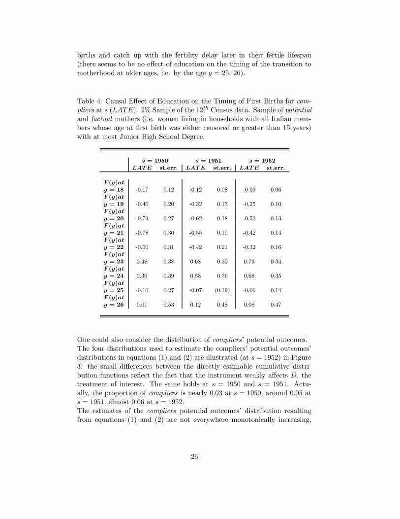
births and catch up with the fertility delay later in their fertile lifespan(there seems to be no effect of education on the timing of the transition tomotherhood at older ages, i.e. by the age y = 25, 26).

Table 4: Causal Effect of Education on the Timing of First Births for com-

pliers at s (LATE). 2% Sample of the 12th Census data. Sample of potential

and factual mothers (i.e. women living in households with all Italian mem-bers whose age at first birth was either censored or greater than 15 years)with at most Junior High School Degree.

s = 1950 s = 1951 s = 1952LATE st.err. LATE st.err. LATE st.err.

F (y)at

y = 18 -0.17 0.12 -0.12 0.08 -0.09 0.06F (y)at

y = 19 -0.46 0.20 -0.32 0.13 -0.25 0.10F (y)at

y = 20 -0.79 0.27 -0.62 0.18 -0.52 0.13F (y)at

y = 21 -0.78 0.30 -0.55 0.19 -0.42 0.14F (y)at

y = 22 -0.60 0.31 -0.42 0.21 -0.32 0.16F (y)at

y = 23 0.48 0.38 0.68 0.35 0.79 0.34F (y)at

y = 24 0.36 0.39 0.58 0.36 0.68 0.35F (y)at

y = 25 -0.10 0.27 -0.07 (0.19) -0.06 0.14F (y)at

y = 26 0.01 0.53 0.12 0.48 0.08 0.47

One could also consider the distribution of compliers’ potential outcomes.The four distributions used to estimate the compliers’ potential outcomes’distributions in equations (1) and (2) are illustrated (at s = 1952) in Figure3: the small differences between the directly estimable cumulative distri-bution functions reflect the fact that the instrument weakly affects D, thetreatment of interest. The same holds at s = 1950 and s = 1951. Actu-ally, the proportion of compliers is nearly 0.03 at s = 1950, around 0.05 ats = 1951, almost 0.06 at s = 1952.The estimates of the compliers potential outcomes’ distribution resultingfrom equations (1) and (2) are not everywhere monotonically increasing,

26

Figure 3: Distribution of Woman’s Age at First Birth, by Instrument andTreatment Status. 2% Sample of the 12th Census data. Sample of all po-

tential and factual mothers (i.e. women living in households with all Italianmembers) whose age at first birth was either censored or greater than 15years) with at most Junior High School Degree.

18 20 22 24 26

0.1

0.2

0.3

0.4

0.5

0.6

0.7

Italy at s=1952

Age at 1st Birth

Cdf

s by

Ass

ignm

ent t

o th

e T

reat

men

t, N

ot T

reat

ed

F00, Never Taker & CompliersF10, Never Takers

18 20 22 24 260.

10.

20.

30.

40.

50.

6

Italy at s=1952

Age at 1st Birth

Cdf

s by

Ass

igne

men

t to

the

Tre

atm

ent,

Tre

ated

F11, Always Takers & CompliersF01, Always Takers

neither nonnegative (see graphs33 on the left in Figure 4). Imbens andRubin[42] firstly highlighted this drawback: the unrestricted estimates ofthe compliers’ potential outcomes density functions they considered in theirapplication were not everywhere nonnegative. The authors underlined thatthe non-negativity of density functions might result from sampling variationas well as from violations of the assumptions. In this application, as it willbecome clearer after the discussion on the internal validity of the researchdesign (section 5), the main reason driving the non-monotonicity of the un-restricted estimates of the compliers’ cumulative distribution functions issample variation.Imbens and Rubin[42] considered alternative estimators and found that anaive estimator of the density functions, obtained simply imposing non neg-ativity, performs essentially as estimators based on the maximum likelihood.They also noted that , even naive correction, can change inference consid-erably.The alternative estimator considered for the compliers’ cumulative distribu-

33For the sake of conciseness, only graphs referring to the case s = 1952 are reported.Graphs referring to the case s = 1950 and s = 1951 show a similar pattern. Theseadditional graphs are available upon request from the author.

27

Figure 4: Compliers’ Distribution of Y 1 (Age at First Birth if women achieveHigh Qualification (Junior High School Degree)) and Y 0 (Age at First Birthif women achieve Low Qualification (less than Junior High School Degree)).2% Sample of the 12th Census data. Sample of all potential and factual

mothers (i.e. women living in households with all Italian members) whoseage at first birth was either censored or greater than 15 years) with at mostJunior High School Degree.

Compliers’ Distribution of Y 1

Unrestricted Estimates Revised Estimates

18 20 22 24 26

0.0

0.2

0.4

0.6

Italy,at s=1952

Age at 1st Birth

F1.

c(y)

,F11

(y),

F01

(y)

Fc.1, CompliersF01, Always TakersF11, Always Takers & Compliers

18 20 22 24 26

0.0

0.1

0.2

0.3

0.4

0.5

0.6

0.7

Italy at s=1952

(with correction)Age at 1st Birth

F1.

c(y)

,F11

(y),

F01

(y)

Fc.1 CompliersF01, Always TakersF11, Always Takers & Compliers

Compliers’ Distribution of Y 0

Unrestricted Estimates Revised Estimates

18 20 22 24 26

0.0

0.2

0.4

0.6

Italy at s=1952

Age at 1st Birth

F0.

c(y)

,F00

(y),

F10

(y)

Fc.0 Compliers F00, Never Takers & CompliersF10, Never Takers

18 20 22 24 26

0.1

0.2

0.3

0.4

0.5

0.6

0.7

Italy at s=1952

(with correction)Age at 1st Birth

F0.

c(y)

,F00

(y),

F10

(y)

Fc.0 CompliersF00, Never Takers & CompliersF10, Never Takers

28

tion functions is the the following naive estimator:

FC.1 (y, s)

∗

= max(

0, F C.1 (y, s), FC

.1 (y − 1, s)∗),

FC.0 (y, s)

∗

= max(

0, F C.0 (y, s), FC

.0 (y − 1, s)∗)

Unrestricted and “revised” estimates are presented on the left-hand panelin Figure 5.As it is clear from the inspection of the graphs in Figure 5, “revised” es-timates of the cumulative distribution functions of compliers are not ableto reproduce the reversal of the local average treatment effect observed atthe age 23 at s = 1950, that is when the proportion of compliers is lowest(φc = 0.03). Instead, the reversal is correctly reproduced as the proportionof compliers increases, i.e. at s = 1951 (φc = 0.05), s = 1952 (φc = 0.06).

Pointwise estimates of the vertical distance between the “revised” estimates

of compliers’ potential outcome distribution functions, i.e. FC.1 (y, s)

∗

−

FC.0 (y, s)

∗

, are presented in Table 5, together with the corresponding un-

restricted estimates34, i.e. FC.1 (y, s)− FC

.0 (y, s), and estimates of the propor-

tions of always takers (φa) and never takers (φn).Revised and unrestricted estimates of the causal effect of education on theproportion of women who raise their first child by the ages 18 − 22 arebroadly consistent. Both revised and unrestricted estimates show a reversalin the effect at y = 23. However, revised estimates suggest that the effectat older ages is stable and much smaller than the one the correspondingunrestricted estimate depict.

34These estimates might slightly differ from estimates already reported in Table 4 be-cause of sample variation: unrestricted estimates in Table 4 are computed contrastingpointwise estimates of the two cumulative distribution function by assignment to thetreatment Z and re-weighting these difference by the proportion of compliers (see equa-tion (6)), whereas calculations of the unrestricted estimates reported in Table 5 are mademoving from the weighted average of the pointwise estimates of four cumulative distribu-tion functions, that is the cumulative distribution functions of the outcome by treatmentand assignment to the treatment (see equations (1) and (2)). Unrestricted estimates ofTable 4 and 5 are broadly consistent.

29

Table 5: Causal Effect of Education on the Timing of First Births for com-

pliers at s (LATE). “Revised” and Unrestricted Estimates. Summary. 2%Sample of the 12th Census data. Sample of all potential and factual mothers(i.e. women living in households with all Italian members) whose age at firstbirth was either censored or greater than 15 years) with at most Junior HighSchool Degree.

s = 1950 s = 1951 s = 1952�

φa

�

φn

�

φa

�

φn

�

φa

�

φn

0.335 0.630 0.348 0.602 0.361 0.573F (y)at unr. rev. unr. rev. unr. rev.

y = 18 -0.14 -0.08 -0.12 -0.08 -0.10 -0.08

y = 19 -0.40 -0.29 -0.31 -0.24 -0.25 -0.21

y = 20 -0.69 -0.64 -0.51 -0.51 -0.41 -0.41

y = 21 -0.85 -0.74 -0.64 -0.59 -0.52 -0.49

y = 22 -0.39 -0.48 -0.32 -0.35 -0.28 -0.28

y = 23 0.44 -0.19 0.66 0.08 0.47 0.08

y = 24 0.33 -0.16 0.58 0.14 0.41 0.14

y = 25 -0.19 -0.16 -0.18 0.14 -0.18 0.09

y = 26 -0.02 -0.16 -0.10 0.14 0.04 0.09

Revised estimates (rev.) are computed as F C.1

(y, s)∗

− F C.0

(y, s)∗

, where F C.1

(·, s)∗

,

F C.0

(·, s)∗

represent the “revised” estimates of the compliers’ potential outcome distri-

bution functions. Unrestricted estimates are obtained as F C.1

(y, s) − F C.0

(y, s), F C.1

(·, s),

F C.0

(·, s) represent the unrestricted estimates of the compliers’ potential outcome distri-

bution functions. These estimates might differ a little from those presented in Table 4

because of sample variation.

30

Graphs in Figure 4 depict the cumulative distribution functions of Y 1 andY 0 for the sub-population of compliers and for the non-compliers (always

takers and never takers).

The cumulative distribution function of Y 1, i.e. the mother’s age at firstbirth if she would achieve high qualification, for compliers and always tak-

ers (see for instance graphs in Figure 4) exhibits striking differences: in thepresence of the treatment, the proportion of compliers who bear their firstchild by young ages (18-21) is smaller than the proportion of always takers

who bears their first child by the same age. However, between y = 22 andy = 24 the relationship reverses. This is consistent with the fact that, inthe presence of the treatment compliers postpone the first birth event withrespect to always takers. The gap between the compliers’ and always takers’cumulative distribution functions of Y 1 over the interval y ∈ [18, 21] reducesas the proportion of compliers increases whereas the gap between the twodistribution function over the interval [22, 24] rises slightly.

The differences between the cumulative distribution function of Y 0, i.e. themother’s age at first birth if she would achieve low qualification for compliers

and never takers (see for instance graphs in Figure 4) are noticeable, withthe compliers distribution being relatively steeper over almost the wholesupport y ∈ [18, 26]; thus, in the absence of the treatment, compliers seemsto have their first child by younger ages than never takers. The gap be-tween the compliers’ and never takers’ cumulative distribution functions ofY 0 over the support [18, 26] slightly reduces as the proportion of compliers

increases, reversing its sign at higher values of y, namely y = 25, y = 26, ats = 1951, s = 1952.

On the whole, it seems that, at all points35 s (s = 1950, s = 1951, s = 1952),in the presence of the treatment, the potential outcome distribution of com-

pliers gets closer to the potential outcome distribution of always takers, aty = 25, y = 26. Similarly, in the absence of the treatment, the potentialoutcome distribution of compliers gets closer to the potential outcome dis-tribution of never takers, at y = 25, y = 26.Empirical quantiles of the compliers’ potential outcomes’ distributions havebeen computed, moving from the “revised” estimates: due to censoring inthe observed distribution by treatment and assignment to the treatment,higher quantiles of the compliers’ potential outcomes’ distribution cannotbe identified. Some of the identifiable quantiles, namely the first six deciles,and corresponding quantile treatment effects for the subpopulation of com-

pliers are reported in Table 6: figures suggest heterogeneity of the impact

35Additional graphs show the same pattern observed at s=1952 and are not reportedfor brevity. However, they are available upon request from the author.

31

of education over the distribution of births.

Table 6: Quantile Treatment Effect of Education on the Timing of FirstBirths for compliers at s (IV − QTE), selected quantiles q. 2% Sampleof the 12th Census data. Sample of all potential and factual mothers (i.e.women living in households with all Italian members) whose age at firstbirth was either censored or greater than 15 years)with at most Junior HighSchool Degree.

quantile q q.1 q.0 q.1 − q.0 q.1 q.0 q.1 − q.0 q.1 q.0 q.1 − q.0(Y 1) (Y 0) (Y 1) (Y 0) (Y 1) (Y 0)

s = 1950 s = 1951 s = 1952q = 0.1 22 19 3 22 19 3 22 19 3q = 0.2 22 19 3 22 19 3 22 19 3q = 0.3 23 20 3 23 20 3 23 20 3q = 0.4 23 20 3 23 20 3 23 20 3q = 0.5 23 20 3 23 20 3 23 21 2q = 0.6 - 20 - 23 21 2 23 25 -2

The empirical evidence provided suggests that education causes a postpone-ment in the transition to motherhood only to women who, in the absence ofthe treatment (i.e., “more schooling”), would have had their first child byyoung ages. These women are likely those who, in the absence of the treat-ment, face a lower opportunity cost of children and are therefore less likelyto participate in the labour market. A rise in the achieved education, byincreasing their current market wage36, increases the probability that theyparticipate in the labour market and rises the opportunity cost of children.Thus, women end up delaying early childrearing. As a consequence, thenumber of women who bear their first child by the age 19, 20, 21 and 22years decreases. However, they later anticipate first births and catch up thefertility delay before turning 26: indeed, the number of women who expe-rience motherhood by the age 23 or 24 increases as schooling achievementincreases and there seems to be no effect of the education on the proportionof women who experience motherhood by older ages, namely by the age 25,26.

36Brandolini and Cipollone [16] exploited the 1963 reform as instrument to assess thereturns on education for women in Italy. Their estimate of the average return on educationfor women over the years 1992 and 1997 ranges from 7% to 10%.

32

Figure 5: Compliers’ Potential Outcomes’ Cumulative Distributions func-tions, quantile and quantile treatment effects. 2% Sample of the 12th Cen-sus data. Sample of all potential and factual mothers (i.e. women livingin households with all Italian members) whose age at first birth was eithercensored or greater than 15 years)with at most Junior High School Degree.

18 20 22 24 26

0.0

0.2

0.4

0.6

Italy, at s=1950

Age at 1st Birth

F0.

c(y)

,F00

(y),

F10

(y),

F1.

c(y)

,F11

(y),

F01

(y)

Fc.1 Compliers (revised)Fc.1 Compliers (unrestr.)Fc.0 Compliers (revised)Fc.0 Compliers (unres)

0.1 0.2 0.3 0.4 0.5 0.6 0.7

1921

23

Quantiles’ Estimates (smooth=regr.)

Quantile

Mot

her’s

Age

at 1

st B

irth

Quantiles of Compliers’ Cdf of Y.0Quantiles of Complier Cdf of Y.1

0.1 0.2 0.3 0.4 0.5 0.6 0.72.

03.

04.

0

Quantile Treatment Effects for Compliers at s=1950

Quantile

Diff

eren

ce (

year

s)

18 20 22 24 26

0.0

0.2

0.4

0.6

Italy, at s=1951

Age at 1st Birth

F0.

c(y)

,F00

(y),

F10

(y),

F1.

c(y)

,F11

(y),

F01

(y)


0.1 0.2 0.3 0.4 0.5 0.6 0.7

2024


Quantile

Mot

her’s

Age

at 1

st B

irth

Quantiles of Compliers’ Cdf of Y.0Quantiles of Complier Cdf of Y.1

0.1 0.2 0.3 0.4 0.5 0.6 0.7

2.0

2.4

2.8


Quantile

Diff

eren

ce (

year

s)

18 20 22 24 26

0.0

0.2

0.4

0.6

Italy, at s=1952

Age at 1st Birth

F0.

c(y)

,F00

(y),

F10

(y),

F1.

c(y)

,F11

(y),

F01

(y)


0.1 0.2 0.3 0.4 0.5 0.6 0.7

1620

24


Quantile

Mot

her’s

Age

at 1

st B

irth

Quantiles of Compliers’ Fc.0Quantiles of Compliers’ Fc.1

0.1 0.2 0.3 0.4 0.5 0.6 0.7

−2

02


Quantile

Diff

eren

ce (

year

s)

33

Results, however, hold only for compliers and findings suggest heterogeneityof the effects across individuals: compared to always takers, under the effectof the treatment, compliers tend to have their first child later in their fertilelifespan, whereas, in the absence of the treatment, compliers tend to havetheir first child earlier compared to never takers. This discussion suggeststhat the fertility return to schooling of women affected by the reform is likelyto be substantially different from the one of the average woman in the popu-lation. The identification strategy exploited in this application is capturingonly the average marginal effect for women affected by the 1963 reform.Generalizing this effect to a wider set of individuals requires typically re-lying on stronger conditions than those who guarantee local identification.Angrist [3] proposed a set of assumptions which allow to link average treat-ment effect and local average treatment effect. In further research, attemptswill be made to link these results more closely to a theoretical frameworkso that the generalization of the effect from compliers to a wider sets ofindividuals can be easily pursued.

An important issue remains unresolved: the internal validity of the researchdesign, which is a precondition for the interpretation of the results. Thisissue is extensively discussed in the next section. Evidence is provided sup-porting the identifying assumption that, local to the cohorts of women bornin the years when the reform started to be effective, the precise timing ofmotherhood is effectively random, giving credence to the causal effects esti-mates discussed so far.

5 The Internal Validity of the Research Design: A

Discussion

In this section evidence is provided to ensure that the research design ex-ploited manipulates only maternal education, so that results have a causalinterpretation.Most of the crucial assumptions for identification (local continuity at s, ex-clusion restriction, stable unit treatment value assumption and local mono-tonicity) are intrinsically not testable.This comment applies in particular to the local monotonicity condition.Violation of the monotonicity assumption might lead to severe consequencesin this application, since the instrument (the 1963 reform) weakly affects thetreatment status (Angrist, Imbens and Rubin[5]). Nonetheless, the assump-tion of no defiers seems rather plausible since it basically requires that: (i)each woman born in years 1949-1952 got at least as much schooling as shewould have in the absence of the 1963 reform on compulsory schooling and(ii) each woman born in 1948 got at most as much schooling as she wouldhave if the 1963 reform has been in place one year before.

34

The small amount of compliers supports the stable unit treatment value as-sumption: hardly the behaviour of 6% of the whole population might haveinduced spill over effects.

Finally, a case can be made on the violation of the local continuity assump-tion: if the same cohorts of women affected by the 1963 reform have alsobeen affected by other treatments, the identification strategy proposed toidentify the causal effect of education on fertility is no longer valid, evenfor the small sub-population of compliers. The assumption of local conti-nuity requires that any variable determined prior to the assignment to thetreatment is independent of treatment status. Thus, the local continuityassumption can be tested examining if any pre-treatment variable W hasa smooth conditional distribution (given S) around s (Lee[45]). Similarly,one would expect that the fertility behaviour of women not affected by the1963 reform changes smoothly over cohorts. To test the validity of the lo-cal continuity assumption, fertility of women of the cohorts 1938-1956 whoachieved high school qualification will be considered. Since these womenhave not been affected by the 1963 reform (see the right-hand panel of Fig-ure 1 and Table 3), one would expect that the fertility behaviour of thesewomen changes smoothly over cohorts. This prediction has been checkedconsidering the proportion of women with high school qualification who hadtheir first child37 by the age y, by cohort, F (y|s), where y ∈ [20, 26] denotesthe woman’s age at first birth and s ∈ [1938, 1956] denotes the cohort towhich women belong. The small number of events occurred38 does not al-low to get precise estimates and forced to consider ages not younger thany = 20. Notwithstanding this caution, the precision of the estimates remainsquite low. On the whole, even slightly different parametric specification ofthe smoothing polynomial lead to conclude that the differences at s =1949,1950, 1951, 1952 are negligible, as one can see from the figures in Table7 and the graphs in Figure 6. As already mentioned, since estimates arefar from being precise, this result might not be conclusive, nonetheless itprovides some evidence supporting the validity of the local independenceassumption.

37The discussion of the previous section applies: the age considered is the age at theoldest child still living in the parental home at the time of the interview.

38Events are births occurred to women with high school qualification belonging anycohort between 1938-1956.

35

Figure 6: F (y) = Prob[Yi ≤ y], Y Woman’s Age at First Birth at distinctvalues of y. Italy. 2% Sample of the 12th Census Data. Sample of Womenwith High School Degree.

F(y) at y=20 F(y) at y=21

1940 1945 1950 1955

0.01

0.02

0.03

0.04

0.05

Italy


F(y

) at

y=

20, Y

Age

at 1

st B

irth


1940 1945 1950 19550.

020.

040.

060.

080.

100.

12

Italy

Data: Census 1981, Sample of Women with HS DegreeCohort

F(y

) at

y=

21, Y

Age

at 1

st B

irth



1940 1945 1950 1955

0.06

0.08

0.10

0.12

0.14

0.16

Italy


F(y

) at

y=

22, Y

Age

at 1

st B

irth


1940 1945 1950 1955

0.10

0.12

0.14

0.16

0.18

0.20

0.22

Italy


F(y

) at

y=

23, Y

Age

at 1

st B

irth



1940 1945 1950 1955

0.20

0.25

0.30

0.35

Italy


F(y

) at

y=

24, Y

Age

at 1

st B

irth


1940 1945 1950 1955

0.25

0.30

0.35

0.40

0.45

Italy


F(y

) at

y=

25, Y

Age

at 1

st B

irth


36

Table 7: Effect of the Assignment to the Treatment (Z) on the Proportionof Women with High School Degree who bear their First Child by the Agey, F (y, s) = Prob[Yi ≤ y|S = s], Y Woman’s Age at First Birth. Italy(Prob[Yi ≤ y]−). 2% Sample of the 12th Census Data. Sample of potential

and factual mothers (i.e. women living in households with all Italian mem-bers whose age at first birth was either censored or greater than 15 years)with High School Degree.


Smoothing Technique: Linear Probability Modely 20 21 22 23 24 25 26

1949effect -0.01 -0.01 0.01 0.02 0.02 0.02 0.01test 1.75 -0.66 1.32 1.10 2.76 1.87 0.07p-value 0.10 0.52 0.21 0.29 0.12 0.19 0.80

1950effect -0.01 -0.01 0.01 0.02 0.01 0.00 0.01test 1.75 -0.66 1.32 1.10 0.59 0.04 0.16p-value 0.10 0.52 0.21 0.29 0.45 0.89 0.70

1951effect -0.01 -0.01 0.01 0.02 0.00 -0.02 0.00test 1.75 -0.66 1.32 1.10 0.02 0.89 0.00p-value 0.10 0.52 0.21 0.29 0.89 0.36 0.96

1952effect -0.01 -0.01 0.01 0.02 -0.02 -0.04 -0.02test 1.75 -0.66 1.32 1.10 0.96 3.88 0.83p-value 0.10 0.52 0.21 0.29 0.34 0.07 0.38

Smoothing Technique: Logit Modely 20 21 22 23 24 25 26

1949effect -0.01 -0.02 0.00 -0.01 0.01 0.00 0.00test∗ 6.62 6.24 0.26 0.43 0.16 0.05 0.03p-value 0.01 0.01 0.61 0.51 0.69 0.83 0.86

1950effect -0.01 -0.01 0.00 0.00 0.01 0.00 0.00test∗ 3.24 3.10 0.04 0.14 0.24 0.01 0.06p-value 0.07 0.08 0.84 0.71 0.62 0.94 0.80

1951effect -0.01 -0.01 0.01 0.00 0.01 -0.01 0.00test∗ -0.93 -1.19 0.30 0.13 0.01 0.61 0.02p-value 0.34 0.27 0.58 0.71 0.92 0.44 0.88

1952effect 0.00 -0.01 0.01 -0.01 -0.01 -0.03 -0.02test∗ 0.21 -0.67 0.25 0.40 0.29 2.95 1.52p-value 0.65 0.41 0.62 0.53 0.59 0.09 0.22

Estimates and standard errors under the preferred specification of the general tendency

in the series Fs(y) = Prob[Yi ≤ y|Si = s]. The hypothesis tested by test∗ is a necessary

and sufficient condition for the effect to be null.

37

One can claim that over the 1970s women position in the society, inItaly, went trough major changes, driven also by the newly introduced lawon divorce (1970), the decrease in the threshold age at which a person be-comes of age (1975), the law on abortion (1978) and the availability of oralcontraceptives. Had these changes differently affected women born beforeand after 1949, the validity of the identification strategy exploited in thisstudy could be questioned. Note that for the result on identification to bevalid, one does not need that none of these changes have affected the womenbehaviour, nor to maintain that they have not occurred, but just that theyaffected women around 1949 in a similar way. In particular, it is crucial thatthe discontinuity in the series Fs(y)39 (as a function of s) is fully attributableto the effect of the 1963 reform and it is not driven by the mentioned inno-vations.If the introduction of any of these innovations affected fertility, one wouldobserve a discontinuity in the series Fs(y) (as a function of s) at the points corresponding to the cohort who has firstly been affected. Note that theposition of the discontinuity is expected to differ at different values of s.The main features of these innovations are presented below and argumentssuggesting that the discontinuity observed around s = 1949 has not beendue to their impact are discussed.

Law N. 898, December 1, 1970 on divorce: the newly introduced lawallowed to men and women who experience a legal separation to re-marry. Before 1970, in Italy, marriage was considered an indissolu-ble bond. The 1970 law might have affected the decision to marryand to have children40. However, , in the last decades, Italy has notexperienced the massive increase in the number of divorces which isapparent in some other European countries and the family structurehas not yet substantially changed: still nowadays the most commonmodel of living together is marriage and divorce and cohabitation arenot widespread practice (see Castiglioni[20], De Sandre et al.[28],[27]).It seems that the link between country-specific cultural factors andthe family structure is strong and slowly evolving over time.The fertility behaviour (between the age 18 and 26) of women bornbetween 1944 and 195241 might, in principle, have been affected by thelaw N. 898. Women of the cohort 1944 were 26 years old in 1970; thusif the law exerted any effect on their fertility behaviour, one would ob-serve a discontinuity examining the graph of Fs(y) at y = 26 in Figure2. However, the series seems to evolve smoothly over cohorts around

39Fs(y) denotes proportion of women of the cohort s who bear their first child by theage y.

40In Italy, the rate of out of wedlock births is extremely low. Thus, one can claim thatthe decision to marry might also have consequences on fertility decisions.

41Younger cohorts were less than 18 at the time the law N. 898 has been introduced.

38

the points s = 1944, s = 1945. Similarly, there seems to be no evidencesupporting the presence of a discontinuity at s = 1945 as one exam-ines the graph of Fs(y) at y = 25, or the presence of a discontinuity ats = 1946 in the graph of Fs(y) at y = 24. As one examines the graph ofFs(y) at y = 23 the observed series seems to evolve smoothly betweenat s = 1947, s = 1948; similarly, as one considers Fs(y) at y = 20, theseries seems to evenly increase between s = 1950 and s = 1951. Atyounger ages, the pattern of the series is more “noisy”, therefore noattempt is made to include also those graphs in the analysis. On thewhole, it seems that basically the law N. 898 did not exert effects onthe individuals fertility behaviour of such magnitude that it could bemeaningful in explaining the discontinuity which has been attributedto the effect of the 1963 reform on fertility.

Law N. 39, March 8,1975 : due to the law N. 39 , individuals becomeof age at the age 18, whereas until 1975 the threshold age was 21.Thus, from 1975 onwards, individuals could vote and become legallyresponsible for themselves 3 years before what stated the older law.Cazzola[22, pp. 313] suggests that the age at which individuals becomeof age is strongly linked to the age at which individuals experience theirfirst sexual intercourse, since individuals generally feel it is appropriateto experience sexual intercourse (an “adult matter”) since that age inparticular.Individuals who might have been affected by the decrease in the thresh-old age, and thus might have anticipate their first sexual intercourse,are mainly individuals who turned 18 around 1975, that is individ-uals born around 1957. However, women belonging to the cohorts1948-1956 were already of age at the time this change occurred, there-fore it is claimed the decrease in the threshold age did not affect thebehaviour of any of them.

Law N. 194, May 22, 1978 & Availability of the Pill : the newly in-troduced law N. 194 legalized abortion in Italy42. By virtue of thelaw any woman can request an abortion within the first 90 days ofpregnancy43. The request for abortion might be connected to moth-ers’ health (both physical and mental) or children’ health (includ-ing the possibility of malformation), to the specific circumstances inwhich conception was brought about and/or it might be groundedon the woman specific economic or social conditions (lack of means).After the introduction of the Law N. 194, Italy firstly experiencedan increase in the number of induced abortions (1980-1984), caused

42In 1981, a referendum to abrogate the law was held and almost 70% of the populationvoted against the abrogation.

43After this period, in cases when the continuation of the pregnancy would seriouslyendanger the woman’s health, an abortion is still possible.

39

both by the progressive improvement of the statistics (Buratta andBoccuzzo[18]) and the replacement of some illegal abortion by legal op-eration; then, the number of abortions steady and consistently declineduntil 1995, remaining rather stable around 138,000-140,000 in the fol-lowing years. Boccuzzo and Loghi[14] and Boccuzzo and Buratta[18]underlined similarities between Italy and the other European countrieswhere the abortion has been legalized: almost all countries experienceda shift from a regime where abortion was mainly requested by mar-ried women (just after the legalization) to a regime where abortion ismainly requested by women who are not married. It is claimed thatthe legalization of abortion in Italy has not significantly changed theopinion of individuals towards abortion as a practical mean of fertilitycontrol, but it has eventually44 succeeded in reducing the number ofillegal abortions: women still continue to consider carefully this oppor-tunity and request abortion mainly when the pregnancy is expectedto endanger the woman’s health45. Indeed, the issue on abortion isconnected to a number of ethical and cultural issues and debate onthe topic is still not concluded after almost thirty years the law hasbeen in force.Cazzola[21, pp. 442] pointed out that favourable opinions on abor-tion seems to be associated with higher socio-economic conditions andhigher qualifications and with favourable opinion on consensual unionsas well.

The contraceptive pill was developed in 1956 by the American Dr. Gre-gory Goodwin Pincus and it was introduced in the U.S. in 1960 and in1961 in Europe. Oral contraceptives have been firstly available in Italyin 1965. However, both the use of contraceptives and the circulating ofinformation on contraceptives were forbidden in Italy (art. 553 Codice

Penale) until 197846. Between 1965 and 1978, the availability of thepill was highly restricted: it was considered a drug, not an effectivecontraceptive method. Then, the Law N. 194 officially repealed thenorm together with those which used to forbid abortion. Although theproportion of women who uses oral contraceptives has been increasing,still, in 2000 less than 20% of the Italian women between 15 and 44years old uses the pill as current contraceptive method, placing Italy

44The assessment of the impact of the Law deserve a specific analysis which is notattempted here.

45Cazzola [21], using survey data on fertility in Italy, shows that, in 1995, women basi-cally agree to abortion in cases when the pregnancy would seriously endanger the woman’sheatlh but generally do not have a favourable opinion on abortion when it is used to avoidunexpected pregnancies.

46Actually, already in 1971 the Constitutional Court stated that the norm was notconstitutionally lawful (Act March 24, 1971 n. 49).

40

among the European countries with the lowest levels of oral contra-ceptives’ use (France, Spain, United Kingdom).Contrasting data of two distinct survey on fertility behaviour held inItaly in 1979 and 1995, Bonarini[15] presented evidence of a markedchange in the characteristics of the contraceptive methods used, con-sistent with a shift from the less to the more effective means of con-traception: the rate of use of coitus interruptus decreased from 51% in1979 to 17% in 1995, whereas the rate of use of the pill increased from14% to 21% between the same years and the rate of use of IUD (IntraUterine Device) almost doubled (3% in 1979, 7% in 1995). Nonethe-less, the overall rate of contraceptive use remained quite stable betweenthe two surveys and in 1995 the use of natural methods of contracep-tion widespread among young women (33%). Bonarini[15, pp. 404]also highlighted that the non-use of contraception, as well as the rateof use of less effective means of contraception, decreases as educationlevel increases.

The fertility behaviour of women of the cohorts 1952-1956 might inprinciple have been affected by the law N. 194 and the availabilityof oral contraceptives. A discontinuity in the series Fs(y) at y = 25at s = 1953 or in the series Fs(y) at y = 24 at s = 1954 or in theseries Fs(y) at y = 23 at s = 1955 might be related to the effect ofthe law N. 194. The data at hand, however, do not provide evidencesuggesting that such a discontinuity exists or that it might have beenthe main factor driving the discontinuity observed in the series Fs(y)around s = 1948, s = 1949.

To sum up, the arguments provided suggests that the 1963 reform representa valid instrument, which helps to correctly identify the causal effect ofeducation on the timing of first births for compliers.

6 Concluding Remarks

In this paper, evidence supporting the role of education in determining thetiming of first births has been provided. Evidence is based on the com-parison of the likelihood that a woman bears her first child by a given agebetween women born around 1949. The identification strategy exploits thefact that women born just after year 1949 were affected by the increase incompulsory schooling introduced by a reform rolled out nationwide in Italyin the early 1960s, whereas women born just before year 1949 were not.Compared to women born before 1949, women of the cohorts 1950-1952have substantially lower likelihood to experience childbearing for the firsttime by the ages y=19, 20, 21, whereas they have a higher likelihood to bear

41

their first child by the age y = 23. No evidence is found of a causal effect ofeducation on the probability of bearing the first child at older ages ( by theage y = 24, 25, 26).These results are essentially as good as comparisons based on randomizationprovided that confounders show a smooth cohort pattern. On prior groundsit sounds credible that women born in subsequent cohort are essentially ex-changeable. However, over the 1970s women position in the society, in Italy,went trough major changes, driven also by the newly introduced law on di-vorce (1970), the decrease in the threshold age at which a person becomes ofage (1975), the law on abortion (1978) and the availability of oral contracep-tives. The internal validity of the research design is extensively discussed,explicitly considering also these factors: evidence based on the data at handsuggests that the 1963 reform represent a valid instrument, which helps tocorrectly identify the causal effect of education on the timing of first birthfor compliers.The estimates provided apply only to women who were affected by the 1963reform on compulsory schooling, i.e. to 3%-6% of the population. Besides,findings suggest heterogeneity of the effects across individuals: under theeffect of the treatment, compliers tend to have their first child later in theirfertile lifespan compared to always takers, whereas, in the absence of thetreatment, compliers tend to have their first child earlier compared to never

takers. This discussion suggests that the fertility returns to schooling of thewomen affected by the reform are likely to be substantially different fromthe one of the average woman in the population.Generalizing this effect to a wider set of individuals requires typically to relyon stronger conditions than those who guarantee local identification. In fur-ther research, attempts will be made to link these results more closely to atheoretical framework so that the generalization of the effect from compliers

to a wider sets of individuals can be easily pursued.Since new mandatory schooling laws have been introduced in many countriesin the last decades, the identification strategy employed in this study canbe easily replicated in other countries. This would represent an intriguingway to generalize results to a wider population.Nonetheless, the subpopulation of compliers might be per se and interestingsub-population, if, for example, the women affected by compulsory school-ing laws happen to be those at the highest risk of teenage childbearing. Ithas long been emphasized the role of education in reducing rates of teenagepregnancy: the results presented here further support this evidence for Italy.

Another caution in interpreting these results should be mentioned: whetherchanges in education produce similar effects regardless of the level at whichadditional education is obtained has not yet been assessed and, similarly,neither which level of female schooling has the greatest or the smallest effecton fertility. Thus, it would be interesting to explore the effects of increase in

42

education at higher educational level using the same approach. In principle,this would be possible for Italy, where a reform of the higher education sys-tem (university) has been implemented in year 2000 (Decreto Ministeriale

N. 509/99).

Finally, findings are consistent with previous results by Bloemen andKalwij [10] for the Netherlands, whereas they are not fully consistent withprevious findings by Bratti [17]. This might be for mainly three reasons:firstly, Bratti focuses on marital fertility, whereas this application does notrestrict the analysis to married women; secondly Bratti considers a periodmeasure of fertility, conversely here the analysis is based on cohort measuresof fertility; lastly, Bratti [17] considers the effects of education on the prob-ability of a birth event 47, whereas here the analysis is focused on the timingof first birth.

References

[1] UN Millennium Project 2005. Investing in Development: A PracticalPlan to Achieve the Millennium Development Goals. Overview. Avail-able from http://www.unmillenniumproject.org/documents/MainReportComplete-lowres.pdf, 2005. Edited,Designed and Produced by Communications DevelopmentInc., Washington, D.C.

[2] A. Abadie, J. Angrist, and G. Imbens. Instrumental Variables Estimates of theEffect of Subsidized Training on the Quantiles of Trainee Earnings. Econometrica,70(1):91–117, 2002.

[3] J. Angrist. Treatment Effect Heterogeneity in Theory and Practice. The Economic

Journal, 114:C52–C83, March 2004. Issue 494.

[4] J.D. Angrist and W. Evans. Children and Their Parents Labour Supply: Evidencefrom Exogenous Variation in Family Size. American Economic Review, 88(3):450–477, 1998.

[5] J.D. Angrist, G.W. Imbens, and D.B. Rubin. Identification of Causal Effects UsingInstrumental Variables. Journal of the American Statistical Association, 91(434):444–455, June 1996. with discussion.

[6] G.S. Becker. A Treatise on the Family. Cambridge, Harvard University, 1991.

[7] G.S. Becker and H.G. Lewis. On the Interaction Between the Quantity and Qualityof Children. The Journal of Political Economy, 81(2):S279–S288, March-April 1973.Part 2: New Economic Approaches to Family.

[8] F. Billari. L’Analisi delle Biografie e la Transizione allo Stato Adulto, volume 7 ofRicerche. Coop. Libraria Editrice Universita di Padova, CLEUP, May 2000.

[9] M. L. Blackburn, D. E. Bloom, and D. Neumark. Fertility Timing, Wages and HumanCapital. Journal of Population Economics, 6(1):1–30, 1993.

47“We consider a birth event to be the presence in the family of a child aged more thanone and less then two years old.” Bratti [17, pp.537]

43

[10] H. Bloemen and A. S. Kalwij. Female Labor Market Transition and the Timingof Births: a Simultaneous Analysis of the Effects of Schooling. Labour Economics,8:593–620, 2001.

[11] H.P. Blossfeld and A. De Rose. Educational Expansion and Changes in Entry intoMarriage and Motherhood. the Experience of Italian Women. Genus, 48:73–89, 1992.

[12] H.P. Blossfeld and J. Huinink. Human Capital Investments or Norms of Role Tran-sition? How Women’s Schooling and Career Affect the Process of Family Formation.The American Journal of Sociology, 97(1):143–168, July 1991.

[13] H.P. Blossfeld and U. Jaenichen. Educational Expansion and Changes in Women’sEntry into Marriage and Motherhood in the Federal Republic of Germany. Journal

of the Marriage and the Family, 54(2):302–315, May 1992.

[14] G. Boccuzzo and M. Loghi. Potenzialita e Limiti dell’Indagine Inf-2 in tema diAbortivita Volontaria. In A. Pinelli P. De Sandre and A. Santini, editors, Nuzialita

e Fecondita in Trasformazione: Percorsi e Fattori del Cambiamento, pages 147–162.Il Mulino, Bologna, 1999.

[15] F. Bonarini. L’Uso della Contraccezione in Italia: dalla Retrospezione del 1979 aquella del 1995-96. In A. Pinelli P. De Sandre and A. Santini, editors, Nuzialita e

Fecondita in Trasformazione: Percorsi e Fattori del Cambiamento, pages 395–411. IlMulino, Bologna, 1999.

[16] A. Brandolini and P. Cipollone. Return to Education in Italy 1992-1997. Bank ofItaly, Research Dept., September 2002.

[17] M. Bratti. Labour Force Participation and Marital Fertility of Italian Women: TheRole of Education. Journal of Population Economics, 16(3):525–554, August 2003.

[18] V. Buratta and G. Boccuzzo. Evolution and Epidemiology of Induced Abortion inItaly. Journal of Modern Italian Studies, 6(1):1–18, 2001.

[19] W.P. Butz and M.P. Ward. Completed Fertility and Its Timing. The Journal of

Political Economy, 88(5):917–940, October 1980.

[20] M. Castiglioni. Analisi Differenziale della Nuzialit. In A. Pinelli P. De Sandre andA. Santini, editors, Nuzialita e Fecondita in Trasformazione: Percorsi e Fattori del

Cambiamento, pages 347–363. Il Mulino, Bologna, 1999.

[21] A. Cazzola. Le Opinioni sull’Interruzione Volontaria di Gravidanza. In A. PinelliP. De Sandre and A. Santini, editors, Nuzialita e Fecondita in Trasformazione: Per-

corsi e Fattori del Cambiamento, pages 427–443. Il Mulino, Bologna, 1999.

[22] A. Cazzola. L’Ingresso nella Sessualita Adulta. In A. Pinelli P. De Sandre andA. Santini, editors, Nuzialita e Fecondita in Trasformazione: Percorsi e Fattori del

Cambiamento, pages 311–326. Il Mulino, Bologna, 1999.

[23] A. Cigno. Human Capital and the Time-Profile of Human Fertility. Economics

Letters, 13:385–392, 1983.

[24] A. Cigno. The Economics of the Family. Oxford University Press, New York, 1991.

[25] A. Cigno and J. Ermisch. A Microeconomic Analysis of the Timing of Births. Euro-

pean Economic Review, 33:737–760, 1989.

44

[26] European Union Council. Presidency Conclusions and Annexes. Presidency Conclu-sions and Annexes, Summit Bruxelles, June 2005, 2005.

[27] P. De Sandre. La Formazione di Nuove Famiglie. In M. Barbagli and C. Saraceno,editors, Lo Stato delle Famiglie in Italia. Il Mulino, Bologna, 1997.

[28] P. De Sandre, F Ongaro, R. Rettaroli, and S. Salvini. Matrimonio e Figli tra Rinvio

e Rinuncia, volume CCCXC of Studi e Ricerche. Il Mulino - Bologna, 1997.

[29] Istituto Nazionale di Statistica (ISTAT). Dati sulle Caratteristiche Strutturali dellaPopolazione e delle Abitazioni: Campione al 2% dei Fogli di Famiglia, Dati Provvi-sori, XXII Censimento Generale della Popolazione. Technical report, ISTAT, 1983.

[30] Istituto Nazionale di Statistica (ISTAT). La Fecondita nelle Regioni Italiane: Analisiper Coorti, anni 1952-1993. Collana: Informazioni 35, ISTAT, 1997.

[31] K. Doksum. Empirical Probability Plots and Statistical Inference for Nonlinear Mod-els in the Two-Sample Case. The Annals of Statistics, 2:267–277, 1974.

[32] R.A. Easterlin. An Economic Framework for Fertility Analysis. Studies in Family

Planning, 6(3):54–63, March 1975.

[33] D. Ellwood, Ty Wilde, and L. Batchelder. The Mommy Track Divides:The impact of Childbearing on Wages of Women of Differing Skill Lev-els. Working Paper, Russell Sage Foundation, March 2004. Available athttp://www.russellsage.org/publications/workingpapers/mommytrack/document.

[34] L. Flabbi. Returns to Schooling in Italy OLS, IV and Gender Differences. WorkingPaper 1,1999, Universita Bocconi, 1999. Serie di Econometria ed Economia Applicata.

[35] G. Genovesi. Storia della Scuola Italiana dal Settecento ad oggi, volume Fare scuolaof Manuali Laterza;204. Laterza, Roma, 3rd edition, 2004.

[36] S. Gustafsson. Optimal Age at Motherhood. Theoretical and Empirical Consider-ations on the Postponement of Maternity in Europe. In K.F. Zimmermann andM. Vogler, editors, Family, Household and Work, pages 345–367. Springer-VerlangBerlin Heidelberg, 2003. Population Economics Series.

[37] S. Gustafsson and S. Worku. Assortative Mating by Education and Postponementof Couple Formation and First Birth in Britain and Sweden. Review of Economics

of the Household, 3(1), March 2005.

[38] J. Hahn, P. Todd, and W. Van der Klaauw. Evaluating the Effect of an Antidiscrim-inatory Law Using a Regression-Discontinuity Design. Working Paper Series 7131,National Bureau of Economic Research, NBER, May 1999.

[39] J. Hahn, P. Todd, and W. Van der Klaauw. Identification and Estimation of Treat-ment Effects with a Regression Discontinuity Design. Econometrica, 69(1):201–209,January 2001. Notes and Comments.

[40] S.K. Happel, J.K. Hill, and S.A Low. An Economic Analysis of the Timing of Child-birth. Population Studies, 38(2):299–311, June 1984.

[41] P.W. Holland. Statistics and Causal Inference. Journal of the American Statistical

Association, 81(396):946–970, 1986. With discussion.

[42] G.W. Imbens and D.B. Rubin. Estimating the Outcome Distribution for Compliersin Instrumental Variables Models. Review of Economic Studies, 64:555–574, 1997.

45

[43] B. S. Janowitz. An Analysis of the Impact of Education on Family Size. Demography,13(2):189–198, May 1976.

[44] H.P. Kohler, F.C. Billari, and J. A. Ortega. The Emergence of Lowest-Low Fertilityin Europe During the 1990s. Population and Development Review, 28(4):641–680,2002.

[45] D.S. Lee. Randomized Experiments from Non-Random Selection in the U.S. HouseElections. January 2005.

[46] E.L Lehmann. Nonparametrics: Statistical Methods Based on Ranks. San Francisco,CA: Holdenday, 1974.

[47] H. Leibenstein. The Economic Theory of Fertility Decline. The Quarterly Journal

of Economics, 89(1):1–31, February 1975.

[48] A. Leschinsky and K.U. Mayer, editors. The Comprehensive School Experiment Re-

visited: Evidence from Western Europe. Frankfurt am Main: Verlang Peter Lang,1990.

[49] C.H. Mullin and P. Wang. The Timing of Childbearing Among HeterogeneousWomen in Dynamic General Equilibrium. Working Paper 9231, National Bureauof Economic Research, Available at http://www.nber.org/papers/w9231, October2002.

[50] C. Nicoletti and L. Tanturri. Differences in Delaying Motherhood Across Eu-ropean Countries: Empirical Evidence from the ECHP. Working Paper 2005-4, Institute of Social and Economic Research, November 2005. Available athttp://www.iser.ac.uk/pubs/workpaps.

[51] M.R. Rosenzweig and T.P. Schultz. Schooling, Information and Nonmarket Pro-ductivity: Contraceptive Use and Its Effectiveness. International Economic Review,30(2):457–477, May 1989.

[52] M.R. Rosenzweig and K.I. Wolpin. Natural “Natural Experiments” in Economics.Journal of Economic Literature, 38:827–874, December 2000.

[53] D.B Rubin. Estimating Causal Effects of Treatments in Randomized and Nonran-domized Studies. Journal of Educational Psycology, 66:688–701, 1974.

[54] T.P. Schultz. Changing World Prices, Women’s Wages, and the Fertility Transition:Sweden, 1860-1910. The Journal of Political Economy, 93(6):1126–1154, December1985.

[55] V. Skirbekk, H.-P. Kohler, and A. Prskawetz. Birth-Month, School Graduation andthe Timing of Births and Marriage. Demography, 41(3):547–568, 2004.

[56] J.E. Sleebos. Low Fertility Rates in OECD Countries: Facts and Policy Responses.Social, Employment and Migration Working Papers 15, OECD, 2003.

[57] D.L. Thistlethwaite and D.T. Campbell. Regression Discontinuity Analysis: an Al-ternative to the Ex Post Facto Experiment. Journal of Educational Psychology,51(6):309–317, 1960.

[58] W. Trochim. Research Design for Program Evaluation: the Regression-Discontinuity

Approach. Beverly Hills, Sage Publications, 1984.

46

[59] UNICEF. A League Table of Teenage Births in Rich Nations. Innocenti ReportCard 3, UNICEF Innocenti Research Centre, Florence, July 2001.

[60] R.J. Willis. The Economics of Fatherhood. The American Economic Review,90(2):378–382, May 2000. Papers and Proceedings of the One Hundred TwelfthAnnual Meeting of the American Economic Association.

47

education and the timing of births: evidence from a ... · education and the timing of births:...

Documents