Educational Corruption and Growth

Philip ShawUniversity of Connecticut

November 12, 2007

Job Market Paper

Abstract

Educational corruption is a worldwide phenomenon yet its impacton economic growth is unclear. In this paper we formulate a macroe-conomic model to explore the impact educational corruption may haveon growth, educational attainment, and the education wage premium.We find that our model can produce a negative relationship betweeneconomic growth and educational corruption as well as a positive re-lationship between the education wage premium and educational cor-ruption. We find empirical support for these relationships in a cross-section of countries. In addition to this fact, our model also producesa negative relationship between the level of educational attainmentand educational corruption as found in the data. To add to a recentline of literature on social status and its implications for growth, weshow that attaching status to education can be growth enhancing incountries that experience low to medium levels of educational cor-ruption but growth reducing in countries that experience high levelsof educational corruption. We also show that borrowing constraintscan exacerbate the impact educational corruption has on economicgrowth, the wage premium, and educational attainment rates.

JEL codes: I2, O41, D73Keywords: Educational Corruption, Growth, Conditional Moment Test

1

1 Introduction

Educational corruption is a worldwide phenomenon yet its impact on eco-nomic growth is not clear. Problematic levels of educational corruption havebeen reported in China, Colombia, Russia, Georgia, New Zealand, Nigeria,Thailand, Afghanistan, and Kenya to name only a few.1 Various types of ed-ucational corruption have been reported including, but not limited, bribingfor entrance, bribing to pass exams, and paying for degrees. MacWilliams(2002) describes one instance where a professor of a Georgian school actuallydistributed a price list for various types of bribes to his students.

The first step to exploring educational corruption is defining it. Followingthe literature on corruption, Heyneman (2004) defines educational corruptionas: “the abuse of authority for personal as well as material gain.” Educa-tional corruption is not solely for material gain because it also includes gainsfrom personal advancement such as an increase in social status. Studentsmay use bribing as a way of avoiding the selection mechanisms or qualitymeasures in place to distinguish themselves from their fellow students withthe expectations of some current or future gain.

Rumyantseva (2005) goes further in defining educational corruption byexplaining what the author refers to as the “taxonomy” of educational cor-ruption. She finds that two main types of educational corruption exist. Onetype involves students directly, which has the potential to impact students’values, opportunities, and beliefs. The other type of educational corruptiondoes not directly involve students but indirectly affects the outcome of stu-dents. An example of this type might be a school administrator embezzlingfunds from an educational institution which reduces the resources availableto students. We focus on the prior and more specifically we focus on bribingfor entrance.

In Shaw (2007), I find that approximately 56% of Ukrainian studentsbribed to enter their educational institution. Of those surveyed, womenwere approximately 6% more likely to have given a bribe than men. Thosestudents who bribed on their final exams in high school were 16% more likelyto bribe for entrance into college. As reported by Rumyantseva (2004b),a World Bank study revealed that in Kazakhstan, 69% percent of thosestudents who bribed did so for entry into universities while 10% bribed to

1For a review of cases of educational corruption around the world, see Rumyantseva(2004a).

2

obtain better grades. Although studies like Shaw (2007) and Rumyantseva(2004b) shed some light as to the frequency and the potential determinantsof educational corruption, they do not give us any idea as to the potentialimpact educational corruption has on economic growth, nor do they provideus with an analytical framework for studying corruption in education. It istherefore the goal of this paper to provide that framework thus allowing usto say something about the economic impacts of educational corruption.

Educational corruption allows students to bypass quality and selectionmetrics that are normally in place within educational institutions. Qual-ity of education is important because it determines the quality of the laborforce and therefore has impacts on productivity and innovation for a coun-try. Hanushek and Kim (1995) explore the importance of the quality of laborforce and its impacts on economic growth and find a positive and significantrelationship with economic growth for a cross-section of countries. Usinginternational test scores to obtain a quality index, they find a one standarddeviation in measured cognitive skills translates into a one percent differencein the average growth rate. Their results are robust to model specificationand lead to increased precision in the prediction of average growth rates forthe sample used. Their results present evidence to support the importantrelationship between educational quality and economic performance. Edu-cational corruption may deteriorate the quality of education thus inhibitingeconomic growth.

Fershtman, Murphy, and Weiss (1996) explore the relationship betweensocial status, education, and economic growth and find that while social sta-tus plays an important role in the allocation of talent; its role may lead todecreased economic performance. Professions carrying high levels of statustend to draw people of all types of ability. Talent may be misallocated be-cause people with high wealth levels have access to “high quality” institutionsor specialized training that allows them to be employed in high status posi-tions regardless of their ability. Furthermore, if those high-wealth individualsare of low-ability, then there may be a negative impact on economic growthif those high status industries are growth enhancing. The optimal allocationof talent would be allocating the high-ability individuals to growth enhanc-ing industries regardless of their wealth. Schools have the ability to achievethis if they are operating effectively. It is important to note that we do notstate that the misallocation of talent does not occur in countries withouteducational corruption, only that this process is accelerated in countries thatdo have corruption in education. Thus educational corruption inhibits ed-

3

ucational establishments’ ability to act as a filter thus allowing high-wealthlow-ability students to enter institutions that have better connections to po-sitions of high status. The results of Fershtman et al. (1996) reveal anotherpath in which educational corruption is detrimental to economic performance.

Heyneman (2004) supports the argument that educational corruption de-stroys the selection method that can be created by educational establish-ments. Klitgaard (1986) stresses the importance of basing selection intoeducational institutions based on ability and discusses the impact of properselection mechanisms on both efficiency and equity in educational outcomes.It therefore easy to see how bribing into educational institutions can workto reduce the importance of ability in the admissions process. Pinera andSelowsky (1981) attempt to quantify the impacts of the misallocation of tal-ent on economic performance finding that developing countries could improvetheir per capita gross national product by five percentage points if they wereto base their leadership upon merit as opposed to gender or social status.

The purpose of this paper is to provide a theoretical framework to studythe effects educational corruption has on economic growth, educational at-tainment, and the education wage premium. Building on the frameworkdeveloped by Fershtman et al. (1996), we develop an overlapping generationsmodel with borrowing constraints explicitly modeling educational corruption.Educational corruption is introduced into the model by allowing agents toincrease their entrance probabilities through bribing. We show that educa-tional corruption has a negative impact on economic growth and increasesthe educational wage premium. Given the presence of educational corruption,higher importance of social status may be growth enhancing in low corrup-tion countries, while the opposite effect is found for highly corrupt countries.Model implications are shown to match empirical evidence obtained by uti-lizing Transparency Internationals Corruption Perceptions Index. We alsoshow that growth rates can be improved by relaxing borrowing constraints,even for countries with a high degree of educational corruption.

The remainder of the paper is structured as follows. In Section 2 we de-velop and overlapping generations model of educational corruption. Section3 describes the simulation exercise and its results. We conduct an empiricalverification of model implications in Section 4. Section 5 concludes.

4

2 Model

Here we formulate an overlapping generations model of educational corrup-tion. Our economy is populated by a continuum of households of mass 1,and a representative firm. The intuition and setup of the model is similarto Fershtman et al. (1996). In their mode, they assume agents can chooseto go to school or not. If an agent decides to go to school, he automaticallyget in. In our model, agents do not know with certainty if they will join theeducated work force but instead they face a probability. Households not onlygive up wage earnings by going to school, but they also can bribe in order toincrease their chance of entering an education institution.

2.1 Households

Agents are assumed to live for two periods and are heterogenous in twodimensions – innate ability, µ, and asset holdings (wealth), a. Thus, wedenote the distribution of agents by the density function f(µ, a). We assumethat the distribution of agents is time invariant such that each new generationis born identically distributed in terms of their asset holdings and innateability.2 When agents are born, they choose to go to school or not. If anagent decides not to go to school, he or she immediately joins the labor forceand becomes a laborer (l) earning the market wage wlt for that period. Wefurther assume that if they decide not to go to school, they remain laborersfor the remainder of their life. If an agent decides to go to school they facea probability π(m) of getting in and becoming a manager (m) in the secondperiod of their life. If they become a manager, they will receive a wage ofwmt+1µ. Therefore agents who become managers get paid the market wageas well as an ability premium. The way we model educational corruptionis to allow students to bribe zt which increases their probability of entryinto school. Thus agents who decide to go to school face the probability1 − π(m) of not getting in and becoming a laborer in the second period oftheir life. If an agent does not get into school he/she receives a wage ofwlt+1 in the second period of life. Agents choose over current consumptionct, future consumption ct+1, and asset holdings at+1. The return on assets isdefined endogenously as rt+1. It is also assumed that agents receive status

2It would be interesting to investigate the endogenous distribution of young agents, butthis complicates the model and requires one to make an assumption about the evolutionof ability across generations.

5

from their respective occupations which we denote as Sst+1 for s ∈ [m, l]. If anagent decides to not go to school he or she faces the following maximizationproblem:

U(ct, ct+1) = maxat+1,ct,ct+1

ln(ct) + ln(ct+1) + ln(Slt+1) (1)

subject to

ct + at+1 ≤ wlt + rta (2)

ct+1 ≤ rt+1at+1 + wlt+1 (3)

amin ≤ at+1 (4)

Equation 2 is the budget constraint of the first period and Equation 3 is thesecond period budget constraint. Equation 4 denotes a borrowing constraint.An agent who decides to attempt to go to school must choose the following:at+1, ct, zt, and cst+1 where s ∈ [m, l]. Thus an agent who attempts to attendschool must choose over future contingent claims to consumption in additionto time t variables because his or her future is not known with certainty.Therefore the maximization problem facing the agent who attempts schoolingis as follows:

U(ct, cst+1) = max

at+1,ct,zt,cst+1

Etln(ct) +∑s

[ln(cst+1) + ln(Sst+1)]π(s) (5)

subject to

ct + at+1 + zt ≤ rta (6)

cmt+1 ≤ rt+1at+1 + wmt+1µ w.prob. π(m) (7)

clt+1 ≤ rt+1at+1 + wlt+1 w.prob. 1− π(m) (8)

amin ≤ at+1 (9)

zt ≤ zmax (10)

Equation 6 denotes first period constraint and Equations 7 and 8 denotesecond period constraints conditional on the entrance to the educational in-stitution. A key assumption of the model is the fact that attempting schoolcomes with a fixed cost of foregone labor wages in addition to an extra ex-penditure in the form of a bribe. This cost will be taken into considerationwhen agents decide to attempt schooling or not. Agent simply compare the

6

indirect utility associated with both maximization problems and choose overthe one that yields the highest level of utility. We also introduce borrow-ing constraints through the variable amin so that we can see how the lackof financial markets impact equilibrium outcomes. An agent who attemptsschooling will also be bound above by the perceived maximum bribe in theeconomy which we denote as zmax. We make this assumption for two reasons:1) it ensures that our probability function is a proper probability functionand 2) we believe that when bribes are offered it is not the amount of thebribe that matters, but instead it is the size of the bribe relative to the max-imum bribe offered. Note that although each agent takes zmax as given, it isendogenously determined. A more detailed discussion of this can be foundin the next section of the paper.

Another variable that we introduce into our model is social status. Aspointed out by Fershtman and Weiss (1993) social status plays an importantrole in the allocation of individuals across different occupations. The authorspoint out that people don’t only consider the wages of a particular occupationwhen making choices but they also consider the level of social status that isattached to a particular profession. In their paper they introduce a two-sector general equilibrium model with production in which social status isdefined to be a function of the average wage and average level of skill withina particular occupation. Agents in their model can give up current periodwage income to obtain education and become skilled workers. They showthat agents with higher non-wage incomes are more likely to sacrifice currentperiod wage income to obtain higher social status. The authors also showthat economies with a higher emphasis on social status will have a lowerlevel of aggregate output and also experience higher levels of wage inequalitybetween skilled and unskilled workers. In later work by Fershtman et al.(1996), they explore the impact of social status on economic growth. Theyshow that if that social status can have a negative effect on economic growthif their is a “crowding out” effect in the sense that the low ability high non-wage income agents replace the high ability low non-wage income in themarket for managers.

In light of these recent findings we consider social status to play an impor-tant role in the choice to educate and can therefore impact the determinationof equilibrium wages and growth. Given this finding we will include it in ourformulation of the model. Following Fershtman et al. (1996) closely we as-sume that status is measured in terms of the relative average ability of theprofession. An educated worker receives the following level of social status:

7

Smt+1 =

(µmµl

)δwhere

µm =

∫ ∫Ψt+1,m

µf(µ, a)dµda∫ ∫Ψt+1,m

f(µ, a)dµda

and

µl =

∫ ∫Υt+1,l

µf(µ, a)dµda+∫ ∫

Θt+1,lµf(µ, a)dµda∫ ∫

Υt+1,lf(µ, a)dµda+

∫ ∫Θt+1,l

f(µ, a)dµda

Social status of uneducated is Slt+1 =(µlµm

)δ. We denote the set of agents

that attempted schooling in time t and were successful as Ψt+1,m. Let Θt,l

denote the set of agents who did not attempt schooling and went directly intothe workforce in time t. ∆t,l is the set of agents that attempted schoolingbut were not successful. Therefore the set of “old” laborers at time t + 1 isdefined by Υt+1,l = Θt,l∪∆t,l. Θt+1,l is the set of young agents who choose tonot attempt schooling at time t+1. Thus the set of all time t+1 laborers canbe defined by Ψt+1,l = Υt+1,l ∪Θt+1,l. Finally denote the entire set of youngagents at time t + 1 as Γt+1. The parameter δ represents the importance ofsocial status as found in Fershtman et al. (1996).

An interesting feature of social status as pointed out by Fershtman et al.(1996) is the fact that it has a public good characteristic because each agentof a given profession shares the same level of social status. It is often difficultto observe the individual ability of each agent of a profession thus the bestmeasure of a person’s ability is the average ability of his/her cohort.

2.2 The Probability of Entry

If agents face a probability of becoming educated and thus becoming a man-ager, a natural question is what should determine the probability? It seemsthat reasonable place to start is to assume that any agents probability ofbecoming a manager should be a function of ability (µ) and the amountthey bribe (zt). We investigate several ways these two variables can influ-ence the probability of entry. The first probability function we propose is thefollowing:

P1 : π(m) = p(µ, zt) = (µ− 1)γ + (1− γ)

(ztzmax

)α(11)

8

where γ ∈ [0, 1], α ∈ (0, 1) and µ ∈ [1, 2]. Therefore the probability that anagent becomes a manager is a convex combination of ability and the ratioof an agent’s bribe to that of the maximum bribe in the economy which wedenote as zmax. The function P1 has a few desirable features including thefact that this function is a true probability function. To see this evaluate theprobability at the maximum values for µ and zt which gives us p(2, zmax) = 1ensuring that p(µ, zt) ∈ [0, 1]. Furthermore notice as γ → 1 the probability ofentrance is solely a function of an agent’s ability but when γ → 0 the agentsprobability of entry is only a function of the amount he or she bribes relativeto the maximum bribe in the economy. This feature will be particulary usefulwhen we examine equilibrium outcomes of the model under the assumptionof no educational corruption (γ = 1), or a maximum level of educationalcorruption (γ = 0).

One problem facing our analysis is the fact that we cannot know in ad-vance what the probability function should look like. To estimate such afunction from the data we would need to observe the amount students bribedfor entry as well as their ability, which in itself is historically hard to obtain.Even if we did observe some rough measure of ability and the amount a stu-dent bribed, we would need this data for both students who were successfulin gaining entrance and those who were not successful. To our knowledgethis data set simply does not exist. To address the ambiguity surround-ing the probability function we introduce an alternative specification for theprobability of entrance:

P2 : π(m) = p(µ, zt) = (µ− 1)γ + (1− γ)(µ− 1)

(ztzmax

)α(12)

The first thing to notice about P2 is that when γ → 1 (no ed. corruption)P2 and P1 are equivalent. Notice however that when γ → 0 P1 is only afunction of an agents bribe while for P2 ability still matters even under afully corrupt regime (γ = 0). In other words, functional form P2 allows forinteraction between the bribe and ability.

Another notable difference between P1 and P2 is that for equal valuesof µ, zt, and zmax it is true that P1 ≥ P2 (higher probability of entrance).This relationship will play an important role in explaining the results of themodel.

9

2.3 The Firm

The representative firm employs both types of workers and produces a singleconsumption good according to the following production function:

Yt = At{a[bKθt + (1− b)NM θ

t ]ρθ + (1− a)NLρt}

1ρ (13)

where NLt is the number of uneducated workers, NMt is the efficiency unitsof educated labor, and Kt is the capital stock. A nice feature of this pro-duction technology is the fact that it is very flexible in terms of representingvarious levels of complementarity and substitutability in the three factors ofproduction. Notice that if ρ, θ = 1, then production is represented by perfectsubstitutability, and with ρ, θ = −∞, then production is represented by per-fect complementarity. When ρ, θ = 0, then production is of Cobb-Douglastype.

Another reason to use this type of production technology comes from thefact that there has been a line of literature that has focused on the estimationof the parameters of this function.

The goal of the firm is to maximize each period profits taking factor pricesas given:

maxNLt,NMt,Kt

Yt − wltNLt − wmt NMt −Ktrt

This yields the following factor demand curves:

rt = AρtY1−ρt a[bKθ

t + (1− b)NM θt ]

ρθ−1bKθ−1

t

wlt = AρtY1−ρt (1− α)NLρ−1

t

wmt = AρtY1−ρt a[bKθ

t + (1− b)NM θt ]

ρθ−1(1− b)NM θ−1

t

Notice, that we implicitly assume that labor is hired in efficiency units. Theefficiency of managers depend on their ability, while the efficiency units oflaborers is simply equal to the total number of laborers employed. In otherwords, given the two managers that differ by ability, the one with the higherability will produce more. For laborers it is assumed that their productivityis independent of their ability.

2.4 Learning Technology

We model the evolution of the technological parameter At following Fersht-man and Weiss (1993) where they assume that only the educated can add

10

to the stock of knowledge. When managers attend school they not only gainaccess to the current stock of knowledge, but add to it by utilizing theirability in school and adding to the total stock of knowledge available in thesecond period of their life. Thus technology evolves as follows:

At+1 = (1 + gt+1)At,

where

gt+1 = τ

∫ ∫Ψt+1,m

µf(µ, a)dµda = τNMt+1 and τ > 0.

Thus the growth rate of technological progress at any given time is solely afunction of the aggregate ability of the educated agents.

2.5 Equilibrium

In this section we focus on the characteristics of a stationary rational expec-tations equilibrium. Each period agents form expectations over future wagesand the status of each occupation as well as future interest rates. Given theirexpectations they make their decisions appropriately. In a rational expecta-tions equilibrium the expectations of each agent must be confirmed. Sincethe distribution of characteristics f(µ, a) is invariant over time we only needto find a stationary distribution of laborers and managers. The definition ofa stationary rational expectations equilibrium is as follows:

Definition 1. A rational expectations equilibrium is defined by (i) an in-variant distribution of young agents F (µ, a), (ii) expectations set EtΛt+1 =[EtS

st+1Etw

st+1Etgt+1Etrt+1], (iii) known probability function p(zt, µ), (iv) in-

dividual household decision rules zt, at+1, ct, and (v) contingent consumptioncst+1, s ∈ [m, l] such that:

1) Given the expectations set, individual household consumption rules andcontingent consumption solve the household problem.2) Given the probability function, p(zt, µ), the set of managers and laborersis time invariant: Ψt,m = Ψt+1,m and Ψt,l = Ψt+1,l.3) Expectations are realized so that EtΛt+1 = Λt+1.3) Aggregate consistency conditions hold:

i) NMt =∫ ∫

Ψt,mµf(µ, a)dµda

ii) NLt =∫ ∫

Υt,lf(µ, a)dµ+

∫ ∫Θt,l

f(µ, a)dµda

11

iii) Kt =∫ ∫

Ψt,matf(µ, a)dµda+

∫ ∫Υt,l

atf(µ, a)dµda+∫ ∫

Γtaf(µ, a)dµda

4) {NLt, NMt, Kt} solves the firm’s maximization problem.

3 Simulation

Since there is no closed form solution of the model we have to resort tonumerical methods. The model is solved using the standard algorithm forperfect foresight rational expectations equilibrium.3

3.1 Parametrization

3.1.1 Production function

For the parametrization of the production function we turn to the literature.Duffy, Papageorgiou, and Perez-Sebastian (2004) estimate the equation for apanel of countries using three different forms of nonlinear estimation includ-ing non-linear least squares (NLLS), NLLS with fixed effects (NLLS-FE),and generalize method of moments with fixed effects (GMM-IV). Duffy et al.(2004) results suggest that under Monte Carlo simulations NLLS has the low-est absolute median bias in the estimation of ρ over different Monte Carlospecifications, while GMM-IV produces the lower absolute median bias in theestimation of θ. Duffy et al. (2004) show estimates of between .23861 and1.25 for ρ and for θ they provide estimates ranging from 0.03832 to 0.56737.Krusell, Ohanian, Rıos-Rull, and Violante (2000) and Polgreen and Silos(2005) also focus on the estimation of ρ and θ, however, their specificationsinclude both capital structures and capital equipment, which is not applica-ble to our model specification. Furthermore, they estimate the parameters oftheir model using only U.S. data unlike the 73 country panel used by Duffyet al. (2004). The values we assign for ρ and θ can be found in Table 1.

3.1.2 Distribution of Young

Due to the fact that the distribution of the young agents f(µ, a) is fixed overtime, the results of the model could vary depending upon the how the distri-bution of ability (µ) and assets (a) is defined. If agents born with high levels

3A nice exposition is provided in Heer and Maussner (2005).

12

of wealth are also of high ability, then the impact educational corruption hason growth may be very small as it will be the highest ability agents who willdecide to go to school and pay the highest bribes, because they are also theagents who can afford to take the risky investment in schooling. However, ifwealth and ability are negatively correlated, the impact of educational cor-ruption may be expected to be very large – wealthy lowest ability agents maybe the ones who obtain schooling due to the higher probability of entry. Toaddress this ambiguity we vary the distribution of the young to see how theresults vary across different specifications.

Rather than just guess what the distribution of wealth and ability lookslike at the aggregate we draw on some recent literature for some hints. Arecent study by Zagorsky (2007) shows that while ability is a strong predictorof income, it has no statistical relationship with initial wealth after control-ling for other factors. Zagorsky (2007) reports a simple correlation betweenwealth and ability of only .12 suggesting that if there is any relationship be-tween wealth and ability, it is close to zero, at least for the United States.Because the study was isolated to only the U.S. we still vary the distributionof wealth and ability restricting our analysis to two cases only: one in whichthe correlation between ability and wealth is .85 (Distribution I) and anotherin which the correlation between ability and wealth is zero (Distribution II).

3.1.3 Other parameters

Regarding the parametrization of the production function we draw on theresults of Duffy et al. (2004). Table 1 shows the values assigned for each ofthe respective parameters:

Table 1: ParametrizationProduction Function Free Parametersθ 0.4 δ 0.5ρ 0.5 γ [0,1]a 0.4 α 0.5b 0.5 amin 0

Since it is unclear what values α, γ, and δ should take we try a broadrange of values. More specifically we vary γ over the interval [0, 1] to see how

13

educational corruption, as defined in this model, impacts economic growthas well as the education wage premium and the choice to educate or not.

3.2 Simulation results

In this section we discuss the numerical results for the model. Figures 1-3show the results of the model in terms of the impact varying degrees of edu-cational corruption have on economic growth, the education wage premium,and the proportion of agents who obtain education for both Distribution Iand Distribution II. We also perform simulations for both specifications ofthe entrance probability function.

3.2.1 Correlated Ability and Wealth

Figures 1(a), 2(a), and 3(a) have the results under the assumption that wealthand ability are strongly positively correlated. Notice in Figure 1(a) using thefirst probability function specification P1 the impact on annual growth isvery small when moving from γ = 0 (ability does not matter) to γ = 1 (onlyability matters). This is a stark contrast to the results under the assumptionthat the probability function takes the form presented by P2 which show amonotonically increasing relationship between the annual growth rate and theimportance of ability in the probability of entrance. A highly corrupt country(γ = 0) would experience an annual growth rate of 2.16% versus 2.49% for anuncorrupt educational system (γ = 1). This difference in growth would leadto a 10% difference in the level of GDP per capita between the uncorrupt andcorrupt country after 30 years. Thus the impact educational corruption hason growth can be quite small when wealth and ability are highly correlated.

Figure 2(a) presents the results for the education wage premium as wevary the degree of corruption. Notice that like the growth rates, the educationwage premium is flat across values of γ for P1 suggesting that the degree ofcorruption has no real impact on the wage premium. Once again, this resultis quite different when using P2 for the probability of entrance. The resultsshow a monotonically decreasing relationship between the education wagepremium and γ. For example, when γ = 0 the wage premium is 69.91% ascompared to 43.57% when γ = 1.

The results for the proportion of educated agents are found in Figure3(a). When we use P1 the proportion of educated workers is increasing incorruption, however, the difference at the minimum and maximum values is

14

rather small. For example, when γ = 0 the proportion educated is 19.98%as compared to 19.39% for γ = 1. When using P2 the proportion educatedis increasing in γ. The difference in the proportion educated when γ = 1 ascompared to γ = 0 is 3.71%.

3.2.2 Uncorrelated Ability and Wealth

Figures 1(b), 2(b), and 3(b) have the results under the assumption that thereis no correlation between wealth and ability as suggested by Zagorsky (2007).Figure 1(b) shows that once again depending on which function we use forthe probability on entrance the results can be quite different. Using P2 wefind that as you reduce the degree of corruption in the economy the annualgrowth rate increases monotonically. Also notice that the magnitude of thischange is much larger under Distribution II as compared to Distribution I.The annual growth rate for a very corrupt country (γ = 0) is approximately1.42% as compared to 2.41% for a country with γ = 1. This difference isquite large over a period of 30 years leading to a difference of 34% in levels.For the function P1, growth is decreasing as we move from γ = 0 towardsγ = .7 suggesting that educational corruption can be good for growth ina certain range for γ. However, after γ = .7 corruption is detrimental togrowth.

Figure 2(b) shows the impact educational corruption has on the educationwage premium. For the function P1 the wage premium is increasing for valuesof γ between 0 to .7 but then declines as γ → 1. For P2 wage premium isstrictly decreasing as we decrease the degree of educational corruption. Whenγ = 0 the wage premium is 155% as compared to 51% when γ = 1.

The function P1 produces a U-shaped pattern in the number of educatedagents as we increase γ from 0 to 1 as found in Figure 3(b). This resultcomes from the fact that P1 ≥ P2 as discussed above. It is generally true thatagents with higher ability and higher wealth will tend to choose to go to schoolbecause they have the higher expected payoff from doing so, due to higherprobabilities of entrance and higher expected wages in the future. Agentswith a low ability parameter µ will not choose to try schooling when using P2but will try schooling under P1 when γ = 0 thus the aggregate ability will bedriven up as long as the low ability agents are not replacing the high ability.Given that growth is defined by the aggregate ability of the educated, thiswill increase the growth rate of the economy. Furthermore, as the low abilityhigh wealth agents choose to go to school they drive down the wage premium

15

as they add to the stock of aggregate ability. For medium values of γ, thelow ability high wealth agents will start to drop out as their probability ofentrance declines thus increasing the wage premium and reducing the growthrate. Notice that when we use P2 the number of educated workers increasesmonotonically as γ → 1. Note that when γ = 0 the percent educated isapproximately 9.33% as compared to 18.54% for γ = 1. Thus the percentageof agents who obtain education when ability is the only factor of selection isalmost twice that of a fully corrupt country.

The main results of the paper suggest that the distribution of wealth andability certainly change the size of the effect educational corruption has ongrowth, the wage premium, and the proportion educated, but for the mostpart, leave the trends unaffected.4 This result is particulary true for thefunctional form P2. Comparing across the two types of probability functionswe are left with two very different stories for the impact educational corrup-tion has on growth. In one case educational corruption decreases economicgrowth while it may be growth enhancing in another case. We are thereforeleft with conflicting results. To help clarify we turn to the data to see ifour model can replicate some of the basic facts that we observe about thewage premium, economic growth, and educational attainment and respectiverelationships to educational corruption.

3.2.3 Other Theoretical Implications

In the next section we will establish that function form P2 (allowing forinteraction between ability and bribing) seems to produce results consistentwith the data. Thus here we report more results of the theoretical modelunder the assumption that the probability of entry is fully defined by P25.We can then provide more results from the model as we remove social statusfrom the model and relax the borrowing constraints to see how this impactsthe results of the model. To save on computational time we define what wecall three regimes of educational corruption: no corruption (γ = 1), mediumcorruption (γ = .5), and finally high corruption (γ = 0). Table 3 reproducesthe results of the baseline model with the parameters as laid out in section4. Table 4 only differs from our baseline model because we now allow agents

4Results for a negative correlation between wealth and ability suggest the same pattern.However, the magnitude of the impact corruption has on growth, the wage premium, andproportion educated is much larger depending upon the degree of correlation.

5These results do not differ qualitatively for P1, thus we do not report them here.

16

borrow. Given that agents can borrow against future income, they may beable to bribe more to increase their probability of entry which should have aneffect on the allocation of agents and thus growth. As can be seen from Table3, allowing agents to borrow is growth enhancing across all three regimes.Relaxing the borrowing constraint for a highly corrupt country increases thegrowth rate by .27% annually. It also increases the number of educated from9.3% to 11.4% and drives down the wage premium by 35%. Notice thispattern is true for both non-corrupt and medium corrupt country. Relaxingthe borrowing constraint leads to higher growth for a couple of reasons. Onereason is that in the high to medium corruption countries agents can borrowagainst future earnings and use this to increase the amount of their bribe thusincreasing the probability of entry. This will induce some agents to attemptschooling because they now face a higher probability of becoming a manager.As more people choose to attempt schooling it must be true that at least aportion of them will get into school. Therefore, the aggregate ability of theeducated must go up as long as their isn’t a crowding out effect. Notice thatthis story is consistent with the higher average bribe reported in Table 4.

Up till this point, we have not really discussed what role social statusplays in the choice to educate. In order to explore the link between socialstatus and educational corruption we remove status from the model to seehow it changes the results. Fershtman et al. (1996) show that social status canhave different impacts on economic growth depending upon the productiontechnology used. In their paper Fershtman et al. (1996) show that whenthere is an increase in the importance of social status, growth can decrease iftheir is a “crowding out” effect, meaning that high ability agents are replacedwith low ability agents thus dragging down the aggregate ability and thusreducing growth. Social status can also be good for growth under what theauthors’ refer to as the “dilution effect”. Although an increase in lower abilityagents may drive down the average ability of the educated, it may actuallyincrease the aggregate ability of the educated thus increasing growth. Thusthe impact social status has on growth can be good or bad depending uponwhich type of effect exists in equilibrium. For this paper we would like tobuild on their analysis by investigating how educational corruption and socialstatus interact in equilibrium.

Table 5 and Table 6 show the results with borrowing constraints andreduced borrowing constraints, when we take status out of the model. Noticethat the same trends exist with or without social status in the model. Whatis interesting is the fact that social status can be good or bad depending upon

17

the regime in place. When agents are restricted from borrowing, introducingsocial status is good for medium to no corruption economies but bad for highcorruption countries. Notice that in Table 5 the annual growth rate for a highcorruption economy is 1.48% when there is no social status as compared to1.42% when status is taken into consideration by agents.

4 Empirical verification

In order to relate the implications of the model to the data and to motivatethe choice between the two specifications for the entrance probability, weestimate bivariate relationships between the variables of interest. Thus theseempirical relationships should be treated as indicative only.

4.1 Data

Unfortunately, data on educational corruption is not readily available soempirically measuring the impact educational corruption has on economicgrowth, the education wage premium, and educational attainment is diffi-cult. One potential way of getting around this problem is to find a proxyvariable for educational corruption. One that immediately stands out as apotential candidate is Transparency International’s Corruption PerceptionsIndex (CPI). The CPI uses country experts, business leaders, residents andnon residents to assess the perceived degree of corruption within each coun-try.6 The index is on a scale of 0 to 10 where a score of 10 is associatedwith the lowest level of corruption while a score of 0 is associated with thehighest level of corruption. The CPI has been used in many empirical studiesincluding, but not limited to, Seligson (2002), Habib and Zurawicki (2002),Javorcik (2004), and Smarzynska and Wei (2000).

We take data on the return to education across countries from Psacharopou-los (1993). Psacharopoulos (1993) compiles the data from his own work aswell as various other studies. For annual growth rates we take the datafrom the Penn World Tables (PWT) as found in Heston, Summers, and Aten(2006). We calculate annual growth rates for a period of 30 years. We alsouse tertiary completion rates from the Barro-Lee data set on educational at-tainment as found in Barro and Lee (2000). Given these variables we nowturn to estimation procedure.

6For a complete description of methodology go to http://www.transparency.org/

18

4.2 Estimation

To estimate the relationship between growth, the college wage premium, andtertiary completion rates we turn to nonparametric estimation. The distinctadvantage of using nonparametric estimation is the fact that we don’t needto specify functional form. We can express an estimator for E(y|x) as follows:

mb(xj) =

∑ni=1 Kb(

xj−xib

)yi∑ni=1Kb(

xj−xib

)(14)

where Kb is the kernel function and b is the bandwidth which is chosen usingthe method of cross validation. We can also compare the nonparametricestimate to an alternative parametric model using the H-M stat developed byHardle and Mammen (1993). When using nonparametric estimation we willgenerally take interest in the shape of the functions estimated thus we wouldlike to test the functional form estimated against an alternative specificationincluding testing whether a variable is mean independent of another. Usingthe previous notation we construct the H-M stat as follows:

Tn = nbd/2∫

(mb(xj)− Γb,nmθ(xj))2dxj (15)

As suggested by Hardle and Mammen (1993) we replace the integral withthe sum over the design points obtaining:

Tn = nbd/2N∑j=1

(mb(xj)− Γb,nmθ(xj))2 (16)

where Γb,nmθ =∑ni=1Kb(

xj−xib

)mθ(xi)∑ni=1Kb(

xj−xib

)and mθ(xi) is a parametric estimate for

E(y|x). Hardle and Mammen (1993) show that the asymptotic distribu-tion of Tn is not a good approximation in finite samples so they recommendconstructing the null distribution using the wild bootstrap. We also reportthe SELR statistic from Tripathi and Kitamura (2003) and the H-S statistictaken from Horowitz and Spokoiny (2001).7 As shown by Tripathi and Ki-tamura (2003), all three statistics have different power properties dependingon whether the errors are normal, extreme value, or a mixture of two normal

7The author would like to thank Gautam Tripathi for access to the Gauss code neededto run the SELR test and the H-S stat.

19

distributions. For a sample size of 250, Tripathi and Kitamura (2003) showthat the SELR, H-M, and H-S all have size close to their nominal levels. Itshould be noted that we estimate bivariate regressions to get a rough pictureof what relationship exists between educational corruption and each of thedependent variables listed above. It is acknowledged that these regressionsdo not provide any kind of definitive results. Instead, they simply allow usto capture some basic relationships between corruption and the dependentvariables of interest. With this in mind, we proceed to the results under theassumption that we are dealing with exogenous independent variables.

4.3 Empirical results

Figure 4(a) shows the results for the nonparametric estimate of the condi-tional mean of annual growth on the corruption perceptions index (CPI).Notice that on the same graph we plot the density estimate of the CPI.Towards the tails of the distribution the functional form estimated is notas reliable as towards the center of the distribution thus in the tails weshould place little weight on the curvature of the function. Note that theE(AnnualGrowth|CPI) is upward sloping in the range 1-5.9 for the CPIand then monotonically decreases there after. It seems that corruption hasa negative impact on countries that experience high to medium levels ofcorruption but has a positive impact on growth for countries experiencingmoderate to low levels of corruption.

When we compare this result to the model found in Figure 4(b) we seethat the function P1 produces the exact opposite of what we observe in thedata. However, for the function P2 the model seems to match the data inthe range of 1-5.9 for the CPI. Since it is most likely that the countries thatdo have educational corruption are in this range, our model seems to do adecent job of replicating the relationship between corruption and growth forthe countries that our analysis might be applied to.

Turning to the the wage premium and educational corruption, Figure 5(a)and 5(b) compare the results from our estimation to the results produced bythe model. Once again the probability function P2 produces results thatmatch the data quite well. This is in contrast to the results produced usingthe function P1 which suggests a negative relationship between corruptionand the wage premium over the range 1-5.9 for the CPI. If this were true, weshould see the wage premium rise (fall) as we move to the right (left) alongthe horizontal axis. From Figure 5(a), it is clear that this relationship does

20

not exist in the data. Instead we can see that as the degree of corruptionincreases, so does the wage premium.

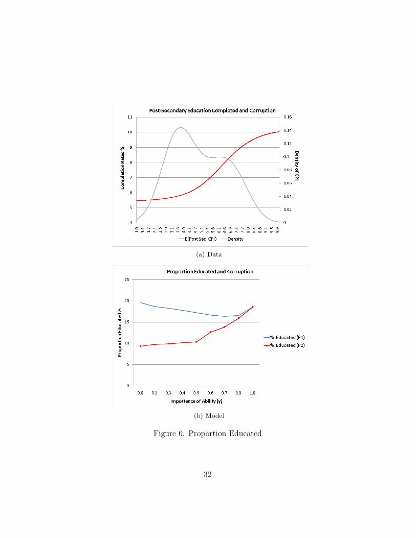
Another nice feature about the probability function P2 is the fact thatit also reproduces the relationship we observe between corruption and pro-portion educated. Notice from Figure 6(a) and 6(b) that the proportioneducated is negatively correlated with corruption. Our model produces ex-actly this result when we assume the probability of becoming educated isdefined by the function P2. When we assume the functional form under P1,the model produces results that are inconsistent with what we observe forour cross-section of countries. Thus there seems to be broad support for ourmodel in the data when we specify the probability of obtaining an educationby the function P2.

Table 5 reports the results for the SELR, H-S, and H-M statistics forvarious null hypotheses regarding three different types of functional formsincluding linear, quadratic, and cubic. We also test whether the mean of eachdependent variable is independent of corruption. Under all three regressionsthe null of mean independence is rejected at the 5% level. In terms of modelspecification, we reject the a linear model for growth using the H-S and H-M statistics but fail to reject quadratic and cubic specification using theSELR and H-M stats. This result suggest that there is a significant degreeof nonlinearity in the relationship between growth and corruption. For thewage premium we can only exclude the quadratic specification and meanindependence. For post secondary completion rates, the model we fail toreject the linear, quadratic, and cubic specifications using the SELR and H-Mstatistic while rejecting the cubic specification when using the H-S statistic.The results therefore offer us little guidance as to the functional form betweenpost secondary completion rates and corruption. The only thing we canconclude is that they are negatively related.

5 Conclusions

Up to this point, the impact of educational corruption on growth has been un-clear. This paper provides an analytical framework for studying the macroe-conomic implications of educational corruption. We develop an overlappinggenerations model of educational corruption and show that educational cor-ruption has a negative impact on economic growth and the level of edu-cational attainment. The driving force behind this result is the fact that

21

high-ability low-wealth individuals face much lower probabilities of entrythan they otherwise would if there was no educational corruption. In thissense a misallocation of talent occurs. Higher income groups, regardless ofthey innate ability, can be expected to enter the educational institution morefrequently which can lead to a lower accumulation of knowledge and slowereconomic growth if the “crowding out” effect is present. It is also shownthat this mechanism increases the wage premium on education. Apart fromincreasing wage premium, this may perpetuate the existence of educationalcorruption. In this sense, educational corruption can be seen as self sustain-ing process.

While education provides higher income, it is also associated with a highersocial status. Given the presence of educational corruption, higher impor-tance of social status may be growth enhancing in low corruption countries,while growth reducing for highly corrupt countries.

If agents are constrained financially and cannot borrow, the distortionscreated by educational corruption are exacerbated. We find that relaxingborrowing constraints is growth enhancing even when educational corruptionis rampant. Thus one policy implication for countries experiencing high levelsof corruption in the educational sector is to institute mechanisms that wouldincrease access to educational credit. The creation of this financial marketleads to increased levels of educational attainment and can serve to offset theimpact educational corruption has on the economy.

Using Transparency International’s Corruption Perceptions Index, weshow that the predictions of the model match up well with what we ob-serve for a cross-section of countries. Using nonparametric estimation, weare able to find hints about the appropriate modeling assumptions of howbribing changes the probability of entry. We find that even in highly corruptcountries, the probability of entry is not solely based on bribes, but rathersome combination of bribes and an agent’s ability.

22

References

Barro, R. J., & Lee, J.-W. (2000). International Data on Educa-tional Attainment Updates and Implications. Nber working papers7911, National Bureau of Economic Research, Inc. available athttp://ideas.repec.org/p/nbr/nberwo/7911.html.

Duffy, J., Papageorgiou, C., & Perez-Sebastian, F. (2004). Capital-Skill Com-plementarity? Evidence from a Panel of Countries. The Review ofEconomics and Statistics, 86 (1), 327–344.

Fershtman, C., Murphy, K. M., & Weiss, Y. (1996). Social Status, Education,and Growth. Journal of Political Economy, 104 (1), 108–32.

Fershtman, C., & Weiss, Y. (1993). Social Status, Culture and EconomicPerformance. Economic Journal, 103 (419), 946–59.

Habib, M., & Zurawicki, L. (2002). Corruption and Foreign Direct Invest-ment. Journal of International Business Studies, 33 (2), 291–307.

Hanushek, E. A., & Kim, D. (1995). Schooling, LaborForce Quality, and Economic Growth.. available athttp://ideas.repec.org/p/nbr/nberwo/5399.html.

Hardle, W. K., & Mammen, E. (1993). Comparing nonparametric versusparametric regression fits. The Annals of Statistics, 21 (4), 1926–1947.

Heer, B., & Maussner, A. (2005). Dynamic General Equilibrium Modeling:Computational Methods and Applications. Springer.

Heston, A., Summers, R., & Aten, B. (2006). Penn World Table Version6.2. Tech. rep., Center for International Comparisons of Production,Income and Prices at the University of Pennsylvania.

Heyneman, S. (2004). Education and Corruption. International Journal ofEducation Development, 24 (6).

Horowitz, J. L., & Spokoiny, V. G. (2001). An Adaptive, Rate-OptimalTest of a Parametric Mean-Regression Model against a NonparametricAlternative. Econometrica, 69 (3), 599–631.

23

Javorcik, B. S. (2004). The composition of foreign direct investment andprotection of intellectual property rights: Evidence from transitioneconomies. European Economic Review, 48 (1), 39–62.

Klitgaard, R. (1986). Elitism and Meritocracy in Developing Countries. Tech.rep., Johns Hopkins University Press.

Krusell, P., Ohanian, L. E., Rıos-Rull, J.-V., & Violante, G. L. (2000).Capital-Skill Complementarity and Inequality: A MacroeconomicAnalysis. Econometrica, 68 (5), 1029–1054.

MacWilliams, B. (2002). In Georgia, Professors Hand Out Price Lists. TheChronicle of Higher Education.

Pinera, S., & Selowsky, M. (1981). The Optimal Ability-Education Mix andthe Misallocation of Resources Within Education. Journal of Develop-ment Economics, 8 (1), 111–131.

Polgreen, L., & Silos, P. (2005). Capital-skill Complementarity and Inequal-ity: A Sensitivity Analysis. Working paper 2005-20, Federal ReserveBank of Atlanta.

Psacharopoulos, G. (1993). Returns to investment in education : a globalupdate. Policy research working paper series 1067, The World Bank.

Rumyantseva, N. L. (2004a). Corruption in Higher Education. Tech. rep..

Rumyantseva, N. L. (2004b). Higher Education in Kazakhstan: The Issue ofCorruption. International Higher Education.

Rumyantseva, N. L. (2005). Taxonomy of Corruption in Higher Education.Peabody Journal of Education, 80 (1), 81–92.

Seligson, M. A. (2002). The Impact of Corruption on Regime Legitimacy: AComparative Study of Four Latin American Countries. The Journal ofPolitics, 64 (2), 408–433.

Shaw, P. (2007). The Determinants of Educational Corruption inHigherEducation: The Case of Ukraine. Tech. rep., Working Paper.

24

Smarzynska, B. K., & Wei, S.-J. (2000). Corruption and Composition ofForeign Direct Investment: Firm-Level Evidence. Nber working papers7969, National Bureau of Economic Research, Inc.

Tripathi, G., & Kitamura, Y. (2003). Testing Conditional Moment Restric-tions. The Annals of Statistics, 31 (6), 2059–2095.

Zagorsky, J. L. (2007). Do You Have to Be Smart to Be Rich? The Impactof IQ on Wealth, Income, and Financial Distress. Intelligence, 35 (5),489–501.

25

Table 2: Results for SELR, H-S, and H-M statistics (5% level)Growth Regression

Null SELR H-S H-MH0: linear No Yes YesH0: quadratic No Yes NoH0: cubic No Yes No

Wage Premium RegressionNull SELR H-S H-MH0: linear No No NoH0: quadratic Yes No YesH0: cubic No No No

Post-Secondary RegressionNull SELR H-S H-MH0: linear No No NoH0: quadratic No No NoH0: cubic No Yes No

26

(a) Distribution I

(b) Distribution II

Figure 1: Annual Growth Rate

27

(a) Distribution I

(b) Distribution II

Figure 2: The Education Wage Premium

28

(a) Distribution I

(b) Distribution II

Figure 3: Proportion Educated

29

(a) Data

(b) Model

Figure 4: Annual Growth Rate

30

(a) Data

(b) Model

Figure 5: The Education Wage Premium

31

(a) Data

(b) Model

Figure 6: Proportion Educated

32

Tab

le3:

Wit

hb

orro

win

gco

nst

rain

tsR

egim

eE

duca

ted

(%)

Annual

Gro

wth

Rat

e(%

)W

age

Pre

miu

m(%

)A

vera

geB

rib

eN

oC

orru

pti

on18

.82.

425

50.8

430.

000

Med

ium

Cor

rupti

on12

.21.

775

110.

878

0.03

9H

igh

Cor

rupti

on9.

31.

423

156.

480

0.06

9

Tab

le4:

Wit

hre

duce

db

orro

win

gco

nst

rain

tsR

egim

eE

duca

ted

(%)

Annual

Gro

wth

Rat

e(%

)W

age

Pre

miu

m(%

)A

vera

geB

rib

eN

oC

orru

pti

on23

.12.

775

25.2

860.

000

Med

ium

Cor

rupti

on17

.32.

297

60.9

430.

051

Hig

hC

orru

pti

on11

.41.

685

121.

023

0.08

7

33

Tab

le5:

Wit

hb

orro

win

gco

nst

rain

tsan

dno

soci

alst

atus

Reg

ime

Educa

ted

(%)

Annual

Gro

wth

Rat

e(%

)W

age

Pre

miu

m(%

)A

vera

geB

rib

eN

oC

orru

pti

on14

.22.

003

87.4

310.

000

Med

ium

Cor

rupti

on10

.81.

595

132.

250

0.02

7H

igh

Cor

rupti

on9.

81.

479

148.

196

0.05

2

Tab

le6:

Wit

hre

duce

db

orro

win

gco

nst

rain

tsan

dno

soci

alst

atus

Reg

ime

Educa

ted

(%)

Annual

Gro

wth

Rat

e(%

)W

age

Pre

miu

m(%

)A

vera

geB

rib

eN

oC

orru

pti

on21

.52.

688

32.3

010.

000

Med

ium

Cor

rupti

on17

.72.

340

57.5

440.

035

Hig

hC

orru

pti

on9.

91.

487

146.

798

0.06

3

34